Pergamon Computers chem. Engng Vol. 21, No. 5, pp. 543-558, 1997

Cop)right © 1996 Elsevier Science Ltd Printed in Great Britain. All rights reserved

PII: S0098-1354(96)00283.9 0098-1354/97 $17.00 +0.00

THE DYNAMIC BEHAVIOUR OF LIQUID-LIQUID AGITATED DISPERSIONS--II. COUPLED HYDRODYNAMICS AND MASS

TRANSFER

L. M. RIBEIRO a, P. E R. REGUEIRAS a, M. M. L. GUIMAR~,ES b, C. M. N. MADUREIRA a and J. J. C.

CRuz-lhrcro ~*

a Faculdade de Engenharia da Universidade do Porto, Portugal

b lnstituto Superior de Engenharia do Porto, Portugal

c Universidade do Minho, Escola de Engenharia, Braga, Portugal

(Received 18 April 1994; revised 24 January 1996)

Abstract--This paper extends the algorithm previously developed by the authors (Ribeiro et al., Comp. Chem. Engng 19, 333, 1995b) to the simulation of the full trivariate (drop volume, age and solute concentration) unsteady-state behaviour of interacting liquid-liquid dispersions, in continuous or batch stirred vessels. The algorithm uses Coulaloglou and Tavlarides (1977) drop interaction model, but it may easily accommodate any alternative models. Both rigid and oscillating drop mass transfer behaviour have been tested. The procedure enables to simulate in detail all relevant aspects of the dynamics of interacting dispersions in mass transfer conditions, namely the gradual approach to steady-state and the response to pulse and step changes in the main process variables. The algorithm's speed is high, allowing to envisage its future application in the control of mass transfer contacting equipment, with only modest computer resources. Copyright © 1996 Elsevier Science Ltd

INTRODUCTION

The general population balance equation (PBE) which

describes the dispersed phase of a liquid-liquid system, in which the individual drop properties define a vector n in a multidimensional phase space, has been introduced

in Part I of this work (Ribeiro et al., 1995b),

~f(n,t)+~---n[d~'.[(n,t)]=B(n,t)-D(n,t). (1)

In Part I, our discussion was restricted to a scalar counterpart of (1), as the goal was the description of the hydrodynamic behaviour (drop volume distribution only) of a homogenous turbulent agitated dispersion (the reader is referred to Part I for details on the treatment of the hydrodynamics). When mass transfer is added to the PBE model, the drops must generally be characterized

by three independent variables, namely, drop size, solute concentration and age. In the present work, we consider a homogeneous (uniform hold-up) perfectly agitated system, in which each drop is represented by three internal variables, namely, volume, r/, concentration, c, and age, ~'. We adopt, as before, the interaction kernels of

Coulaloglou and Tavlarides (1977), and represent,

respectively by g(r}), ~ r / ' ) , h(r/,r/') and A(r/,r/') the breakage frequency, the volume density distribution of the daughter drops, the collision frequency and the

* To whom all correspondence should be addressed FAX: 351-53-604492/604450/616936

coalescence efficiency of drops. Mass transfer during drop motion through the vessel (between two consec- utive interaction events) is accounted for by both the

rigid and the oscillating drop models, as presented by Cruz-Pinto (1979) and Cruz-Pinto et al. (1983).

We first discuss the equations which describe the transient behaviour of the trivariate drop volume- concentration-age distribution and the mathematical technique used to solve them. We then describe the computer code, LLSS (Liquid-Liquid Systems Simula- tion), which implements the solution method, and show that it adequately predicts the performance of turbulent agitated liquid-liquid systems undergoing mass transfer. Finally, the advantages and disadvantages of the present numerical method are discussed, as well as its properties in terms of accuracy and efficiency.

PROBLEM DESCRIPTION AND MATHEMATICAL MODEL

The system under consideration is a perfectly mixed, spatially homogeneous, turbulent dispersion, consisting of two immiscible liquidsma dispersed phase and a continuous phase--in a stirred tank contactor. The continuous phase is supposed to contain a solute which

transfers to the dispersed phase.

We assume that the continuous phase is first delivered into the vessel and the impeller speed adjusted to some required value. Then, the dispersed phase, in the form of an ensemble of droplets with known (generally non- uniform) drop volume distribution, is also fed, according to a set feed volume phase ratio (hold-up). Simultane- ously, the dispersion is withdrawn at a rate that equals

543

544 L. M. RIBEIRO et al.

to a set feed volume phase ratio (hold-up). Simultane- ously, the dispersion is withdrawn at a rate that equals the overall input rate of the two phases. Due to the

assumed perfect mixing, the outlet drop distribution of the drop properties at any instant in time is identical to the distribution inside the vessel at that time. Perfect

mixing also implies a mean residence time of both the continuous and the dispersed phases, which is deter-

mined by the vessel's volume and the dispersion input/ output flow. During this residence time period, the drop internal properties are expected to change discontinu-

ously by breakage, coalescence, feed and exit events, and continuously, due to mass transfer and aging.

To describe drop breakage and coalescence, we again adopt the hydrodynamic model of Coulaloglou and Tavlarides (1977). This model was developed in the absence of mass transfer and assumes that, in addition to being statistically homogeneous, the dispersion has a low dispersed phase hold-up and the drops (assumed

spherical) move around in a locally isotropic turbulent flow field, where Kolmogoroffs energy distribution is assumed valid. It is also assumed that both drop break-

up and coalescence arise as independent binary proc- esses that are functions of drop volume alone. It should be mentioned that, probably, the interaction functions that describe breakage and coalescence should include solute transfer across the interface between the two phases (Jeon and Lee, 1986; Kanel, 1990) and so, should accordingly be expressed not only as functions of drop size but also of drop solute concentration and age. In the present status of our algorithm, any influence of the solute on the interaction rates is limited to its effect on the interfacial tension. On the other hand, however, the introduction of the internal variable age is absolutely necessary because, if mass transfer occurs by diffusion within the drop, the internal solute concentration will not be uniform. The age, defined as the time elapsed since a given drop has assumed its identity in the vessel, is critical in accounting for the drop solute concentration gradients, which are time (age)-dependent.

It is not our purpose here to fully discuss the assumptions made in Coulaloglou and Tavlarides' model. Marangoni instabilities, which would greatly enhance the interaction rates, have been excluded in the present work. The chemical systems used herein (see first paragraph of Application to Unsteady-State Liquid- Liquid Systems) and direction of mass transfer con- sidered (continuous to dispersed), which do not lead to interfacial tension gradients during mass transfer, are consistent with this assumption (Cruz-Pinto, 1979). Coulaloglou and Tavlarides' model has been selected by many recent works, concerning the dynamic behaviour of turbulent agitated liquid-liquid dispersions, with or without mass transfer, yielding results in reasonable agreement with the available experimental data (Bapat et

al., 1983; Hsia and Tavlarides, 1983; Jeon and Lee, 1986; Kanel, 1990; Skelland and Kanel, 1992).

The expressions of the interaction functions for this hydrodynamic model-breakage frequency, volume den- sity distribution of the daughter drops, collision fre- quency and coalescence efficiency (g, /3, h and ,t, respectively)--were given on Part I of this work and are also listed herein, in Appendix A.

When a drop breaks, we assume that the internal mixing is sufficient to ensure uniform and identical concentration in the daughter droplets formed, which should equal the average concentration of the parent

drop at the instant of breakage. Identically, the coales- cence of two drops originates a new born drop with uniform solute concentration, satisfying the solute mass balance.

Equation (1) can now be rewritten considering the specific form of the source and sink terms on the right- hand side. Iffye~d (r/, t) represents the inlet drop volume density distribution, and 0 the mean residence time of

the whole dispersion (and, so, also of the dispersed phase), equation (1) expands to

0 0 0 O-t f( r/'c' r't) + ff~ [[( r/'c' r't)~Tl + Oc [flr/,c,'r,t)lel

0 [f(r/,c,z,t)~r]=2 ~ ~ ~f(r/',c',r',t')g(r/')

x/3(r /Ir / ' )~ ' )~c ' - c)dr/'dc'd'r'

1 + s s f

7 f < ~ '

r/C-r/'C' 17-- r/J

- - , ¥ ' , t ) h ( r / ' , r / - r / ' )Mr/ ' , r / - r/')

I × 6(~')dr/'dc'd'r'dTt'+ ~ feeed(r/,t)6(c - cf~d)

- f(r/,c,7,t)[g(r/)+ ~ ~'~ e ~ f(r/',c','r',t)

×h(r/,r/')A(r/,r/')dr/'dc'd'r'+l-o] (2)

where fir/, c, ~', t) is the instantaneous trivariate drop number density distribution function and 6 the Dirac delta function. While 6(z) resets the age of all entering and new born drops to zero, 6 (c - t)~.~,~) sets the feed concentration of the feed drops to c=ci~d (also zeroing the feed rate of drops of any other solute concentration), and 6 ( c ' - c) just sections the population of drops of

Liquid-liquid agitated dispersions--ll

volume r/born by breakage at c'---c.We will now need to where Sh is the Sherwood number, consider the time evolution of the phase variables. With respect to the variables volume and age, it is accepted Sh= kcp~d that mDAop, t "

~/=0;~r= ! (3) The values for A~ are given by

i.e., drop volume is not influenced by mass transfer and drop age is just a shift in time. Thus, the left hand side of equation (2) becomes

0 0 ~f(r/,c,~',t)+ ~ [f(r/,c,~',t)~]+ f---J(Tl, c,r,t). (4)

The time evolution of the variable c represents the rate of change of the solute concentration in a drop of state (r/, c, r) by mass transfer. It is assumed that mass transfer occurs (from the continuous to the dispersed phase) only during the process of drop motion through the vessel (the time scale associated with drop interactions is small, when compared to that of the quiescence periods). To predict mass transfer, we use both the rigid and the oscillating drop models as proposed by Cruz-Pinto (1979) and Cruz-Pinto et al. (1983), and therein explained in detail. These models adopt the usual overall approach to the problem of mass transfer, and express the transfer performance in terms of a drop size and time-dependent coefficient, Koo. On specifying this coefficient, one can obtain the time evolution of c, by

545

(9)

A,.= A214A~ +Sh(Sh - 2)1 (io)

In the above equations, Dao represents the dispersed phase solute diffusivity, m is the solute distribution coefficient (dispersed/continuous), kc is the continuous phase partial mass transfer coefficient, and the p's represent the phase densities.

The oscillating drop model proposed by Cruz-Pinto et

al. (op. cit.) is a considerably modified version of previous penetration-based oscillating drop models (Rose and Kintner, 1966; Angelo et al., 1966). This modified model assumes that the oscillation frequency of each drop is proportional to the agitation power input per unit drop surface energy. The overall dispersed phase mass transfer coefficient is, in this case, given by

DAoSh' s[Sh'(DAols) 'r2- 11 Koo(d)= Sh,2DAo_ s , (11)

where s (rate of surface renewal) is proportional to the oscillation frequency,

d<c> 6Koo , (c - <c>), (5)

dt d C~pcemd

s= - - (12) 6o-

where <c> and c* are, respectively, the mean concentra- tion of the drop and the equilibrium dispersed phase solute concentration value, and d is the drop diameter. In the rigid drop model, intercirculation within the drop is hindered and its behaviour comparable with that of a stagnant rigid sphere. Concentration profiles are allowed to develop within the drop, until it undergoes an interaction event resulting in complete internal mixing. The corresponding instantaneous overall mass transfer coefficient is thus time (age, ~') or concentration gradient-dependent, and decreases with drop age--Cruz- Pinto (1979)--according to

4DAo ® " [ 2 4DAo~" Koo(d,z)= ~ ,=~ (6) t

Here L is given by,

2 4DAoI" ~ L=6 ;~, a,exp - Ai -- '-~2 ) (7)

and the values A t are the solutions of the equation

A,eot(A i) + (Sh/2 - I ) = 0, (8)

The Sherwood number, Sh', differs from Sh as Sh' =Shl

d. Relative to the oscillating drop model, the computa-

tion time of the rigid drop alternative is higher, since the overall mass transfer coefficient now depends on drop size and age, rather than on drop size alone. In the case of oscillating drops, the study of the system may thus be accomplished just with the bivariate volume-concentra- tion distribution.

As pointed out previously by Cruz-Pinto (1979) and Cruz-Pinto et al. (1983), the mass transfer behaviour of real dispersions may be intermediate between that predicted for rigid drops and that predicted for oscillat- ing drops. Realistic modelling may required accounting for a range of drop behaviour, depending on drop size, between these two limiting cases. However, in many situations the behaviour seems to be adequately described by purely oscillating drops (Korchinsky and Endres, 1993).

To complete the mathematical model, we need to write the initial conditions for equations (2) and (5). We choose

f(r/,c, r,0) = 0;c(0) = 0, (13)

546 L. M. RIBEIRO et al.

i.e., the vessel is initial filled with continuous phase only, and no solute is present in the dispersed phase feed.

THE POPULATION BALANCE EQUATION IN DISCRETE

PHASE SPACE

PBE (2) is a first order non-linear partial integral- differential equation in three dimensional phase space, for which no analytical solution is known. Our numer-

ical approach to solve this equation (2) and the coupled ordinary differential equation (5) is based upon a space- time discretization. We manipulate an equivalent but

approximate system, in which drops can reside only in cell sites, and time is quantized by discrete values, t=O,At, 2At, 3At, etc.. Drops move from cell to cell in

discretized phase-space at each time step. The imple- mented numerical integration scheme involves the explicit calculation of time derivatives, with a first-order backward finite-difference method.

If no interaction events occur in the dispersion, as time progresses, drops just drift smoothly through phase

space without jumping from one point in phase space to another. These gradual and continuous changes are

described by the last three terms of the left hand side of PBE(2). For this convective movement along the respective coordinate axis, to know the fraction of drops

which, at some time t, have coordinates between r/and ~/+Ar/, c and c+dc, and r and z+Az, we need to

consider the number of phase trajectories entering this volume element through its different faces and the number of trajectories which leave from the correspond- ing opposite faces. In the case of PBE (2), only the faces normal to the c axis, at c and c+Ac, and to the z axis, at ~" and ~r+ A~', need to be examined - - see expression (4). As dt=d~', the change in the number of drops within this volume element due to the flux in the 0" direction, is

f( r/,c,z+ A~',t)A~lAc - f( rl, c,~',t)Ar/Ac-- ~ Ar/AcA~', (14)

and, as we adopt At=Az

f( r/,c,r+ A~',t)=f( r/,c,r,t- At), (15)

i.e. drop aging is implemented as a simple shift in time. With respect to the flux along the concentration axis,

as the magnitude of the phase velocity along this axis is known---equation (5)--the corresponding fractional change in the number of drops may be calculated from

3? r/,c + Ac, r,t)e( ~,c, Ac, z,t) A r/A r - y( r/,c, r,t)

x~( ,1,c,r,t)A~A,r=( . Of 0~ ) c( ~,c, r,t) ~c +f(r/,c,r,t)

x A r/AcA~'. (16)

However, because with Coulaloglou and Tavlarides'

model mass transfer doesn't affect drop volume and drop

age, the change in the number of drops due to the convective motion in the c direction is easily calculated from equation (5) with the appropriate mass transfer coefficient, according to rigid or oscillating mass transfer behaviour. Hence, drop mean concentration in each time step is given by

{ 1 1 / c(t)-- ~- ~. dt ] ~ L -d-~ At ] c ( t - At), (17)

for rigid drops, and by

c.,-- - - ) - r

c(t - At), (18)

for oscillating drops, which is the result of integrating equation (5) between t - At and t.The nonzero fight hand

side of PBE (2) reflects the possibility of spontaneous creation and destruction of drops due to breakage, coalescence, feed and exit events. These sudden inter- actions are characteristic of the behaviour of this type of systems and do produce discontinuous jumps in the otherwise smooth phase space trajectories. The numer- ical treatment of equation (2) is thus constrained by this

discrete nature of the interaction phenomena. To over- come this difficulty, when advancing f over a time interval At, these ubiquitous phenomena are artificially displaced to the time step boundaries, where they are collectively handled according to the fight hand side of (2) - - see Appendix B for a detailed presentation. We should emphasize that, during the actual drop inter- actions, no continuous variation in time of phase space variables is supposed to occur.

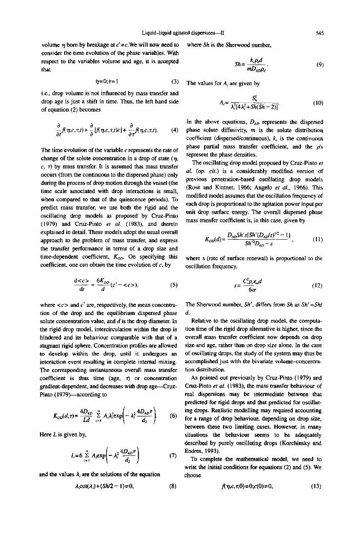
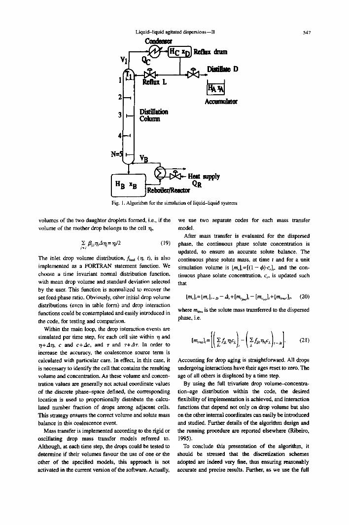
The algorithm developed is sketched in Fig. I. The algorithm is implemented as a FORTRAN 77

code, LLSS (Liquid-Liquid Systems Simulation). The

discrete phase space is defined by the user, in terms of size and number of cells in each coordinate range. The same logarithmic grid of volumes adopted on Part 1 of this work is used, in order to gather enough information about the smaller drops with a reasonably short number of cells (see section Results and Discussion, herein),

with the representative drop volume of each size class taken as the geometric average of it's lower (rh,) and upper (r/,,) bounds, i.e., r/i=(r/~ × r/,) v2. Linear grids are adopted for c and r (A~-= At). Drop interaction functions are defined according to the corresponding expressions (see the Appendix A), and implemented as FORTRAN statement functions.

An appropriate treatment of fl(~lr/') is devised so that when a mother drop of volume r/' undergoes breakage, volume is conserved among the normally-distributed

Liquid-liquid agitated dispersions--II

C ~

¥1 ~ ' ~ llaflnx, dram

5 4 7

4--,I I

1 N=5 2VB

HB j l~lm~et/Rat,it~ Fig. 1. Algorithm for the simulation of liquid-liquid systems

volumes of the two daughter droplets formed, i.e., if the volume of the mother drop belongs to the cell r/i,

jX fly., ~jA Tli= 7//2 (19)

The inlet drop volume distribution, f f~ (r/, t), is also implemented as a FORTRAN statement function. We choose a time invariant normal distribution function, with mean drop volume and standard deviation selected by the user. This function is normalized to recover the set feed phase ratio. Obviously, other initial drop volume

distributions (even in table form) and drop interaction functions could be contemplated and easily introduced in

the code, for testing and comparison. Within the main loop, the drop interaction events are

simulated per time step, for each cell site within r /and r/+AT/, c and c+Ac, and ~" and ~r+A~'. In order to

increase the accuracy, the coalescence source term is calculated with particular care. In effect, in this case, it is necessary to identify the cell that contains the resulting volume and concentration. As these volume and concen- tration values are generally not actual coordinate values of the discrete phase-space defined, the corresponding location is used to proportionally distribute the calcu- lated number fraction of drops among adjacent cells.

This strategy ensures the correct volume and solute mass balance in this coalescence event.

Mass transfer is implemented according to the rigid or oscillating drop mass transfer models referred to. Although, at each time step, the drops could be tested to determine if their volumes favour the use of one or the other of the specified models, this approach is not activated in the current version of the software. Actually,

we use two separate codes for each mass transfer model.

After mass transfer is evaluated for the dispersed phase, the continuous phase solute concentration is updated, to ensure an accurate solute balance. The

continuous phase solute mass, at time t and for a unit simulation volume is [me],=[(1- &).c~],, and the con- tinuous phase solute concentration, c o is updated such that

[me],= [mc],_a,- A,+ [mcij ,-- [me.j,+ [m,,,J,, (20)

where re,ms is the solute mass transferred to the dispersed phase, i.e.

(21)

Accounting for drop aging is straightforward. All drops undergoing interactions have their ages reset to zero. The age of all others is displaced by a time step.

By using the full trivariate drop volume-concentra- tion-age distribution within the code, the desired flexibility of implementation is achieved, and interaction functions that depend not only on drop volume but also on the other internal coordinates can easily be introduced and studied. Further details of the algorithm design and the running procedure are reported elsewhere (Ribeiro, 1995).

To conclude this presentation of the algorithm, it should be stressed that the discretization schemes adopted are indeed very fine, thus ensuring reasonably accurate and precise results. Further, as we use the full

548 L. M. RIBEIRO et al.

dispersed phase property distribution (as opposed to only a small sample of individual drops), the accuracy and the

precision of the predictions are only limited by those of the actual physical and mathematical models and not by the size of the sample, as happens with nearly all Monte- Carlo simulations studies. Of course, this also makes virtually impossible to directly compare the results of

such widely different approaches and algorithms.

APPLICATION T O UNSTEADY-STATE L I Q U I D - L I Q U I D

SYSTEMS

As an application of the schemes discussed above, we describe in this work the trivariate behaviour of a high interfacial tension, low interacting dispersion, in tran-

sient, dynamic conditions. The liquid-liquid system selected is toluene-acetone (solute)-water system, (0"=0.032 J/m-'). Mass transfer is directed from the continuous phase (water) to the dispersed phase (tolu- ene), and the inlet concentration of acetone in the

continuous phase is constant and equal to 20 Kg/m 3. The partition coefficient of the solute from the aqueous to the organic phase is constant and set equal to 0.7. Physical and transport properties for this liquid-liquid system, initial concentration values and inlet drop volume distribution, which are all input requirements for the

numerical code, are listed in Table 1. These values are the same as adopted by Guimar~es (1989) and Guimar- aes et al. (1990), in order to allow comparing the

predicted results, when the steady-state is reached. Several simulations were conducted for different

residence times and agitation power input densities. A range of residence times, between 60 and 600 s, and of agitation power input densities, between 0.05 W/Kg and 0.25 W/Kg, were examined. Full numerical results for these ranges, as well as results for a low interfacial tension, highly interacting system--methylisobutylk- etone-acetone-water system (0"=0.009 j/m'-) are pre-

sented elsewhere (Ribeiro, 1995).

Table I. lnvariant data used in the present work

Variable Value

o" [J.m-2] 0.320 × 10- p# [Kg.m -3] 0.860× 103 p, [Kg.m -3] 0.1 x 104 /x,. [Kg.m- ' . s - '] 0.1 × 10 -2 ~b 0.500X 10 i C~ 0.418× 10 -2 C2 0.558 × 10- C~ 0.165 × 10 -2 C4 [m-"] 0.474 x 1013 C~ 0.300× I0 m 0.700 k~ [m.s -I] 0.200× 10 -~ D~o [m"'s -~] 0.267 × 10 -~ Cco [Kg.m -3] 0.200 x 102 Crx, [kg.m - "*] 0.000 <~,> [m 3] 0.500 x 10 -~ o', [m 3] 0.625 x 10- ")

RESULTS AND DISCUSSION

Results presented herein were computed until t=8 0, where 0= 120 s is the mean residence time. A time step At= 1 s was used for all cases. Drop volumes span the range (10-12 m 3, 10-9 m3). whereas drop solute concen-

trations vary up to 20 Kg/m 3. The phase space dis-

cretized domain consists of a drop volume grid of 12 intervals per decade and a concentration grid of 36 cells. Maximum value of At/ is 0.20 × 10 -9 m 3 and Ac=0.56 Kg/m 3.

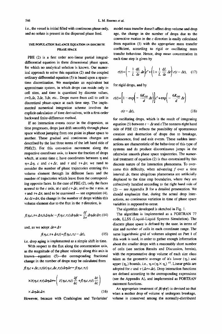
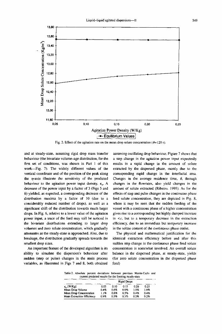
Figure 2 illustrates the behaviour of the mean drop solute concentration with varying agitation rate, for the

rigid mass transfer model. Values are plotted for t=960 s (steady-state). As expected, drop concentration increases with a levelling-off tendency for the higher agitation power input densities, as mass transfer approaches equilibrium. Equilibrium concentration values for each agitation power density examined are also shown for

comparison. Table 2 lists the percent deviations between the

Monte-Carlo (Guimar~es, op. cit.) steady state results and the current predicted results at t= 960 s, for the range of agitation power input densities tested, assuming rigid drops. It may be seen that the present results are in good agreement with those of this earlier study. We should mention that the Monte-Carlo results are means of several runs--cf. Guimar~es (1990)--and that the per- cent deviations between the repeat runs are of the same order of magnitude of those between these two widely

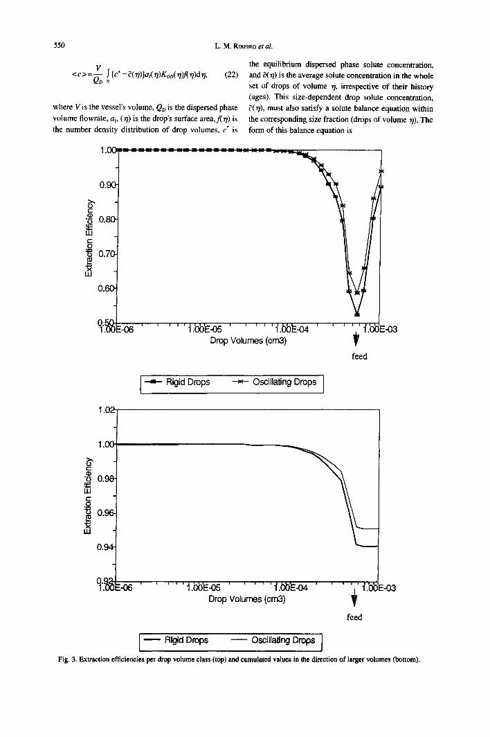
different algorithms. In Fig. 3 (top), the extraction efficiency is plotted for

each drop volume class of the discretized volume range (average over all ages), for both mass transfer models. These values are plotted at steady-state, for an agitation rate of 0.15 W/Kg. The cumulated values, in the direction of larger volumes, are also shown (bottom). As may be clearly recognized, near the average drop volume feed value, where we expect to find, in the outlet stream, drops with properties similar to those of the feed, the extraction efficiencies decrease significantly. As expected, oscillating drops also induce greater extraction efficiencies near the feed, where larger drops prevail.

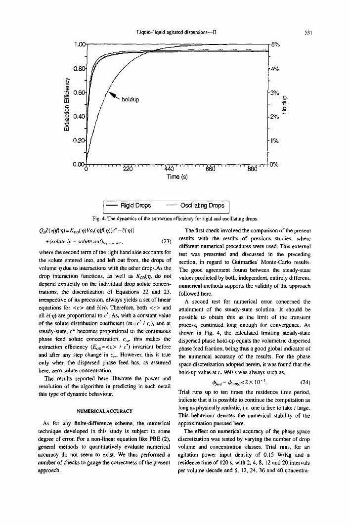
The behaviour of rigid and oscillating drops is also depicted in Fig. 4, where the dynamics of the overall extraction efficiencies is represented along with the calculated bold-up build-up curve. For the operating conditions selected, the extraction efficiencies are nearly steady after three residence time periods.

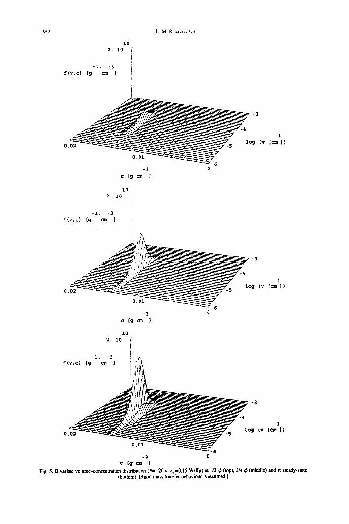
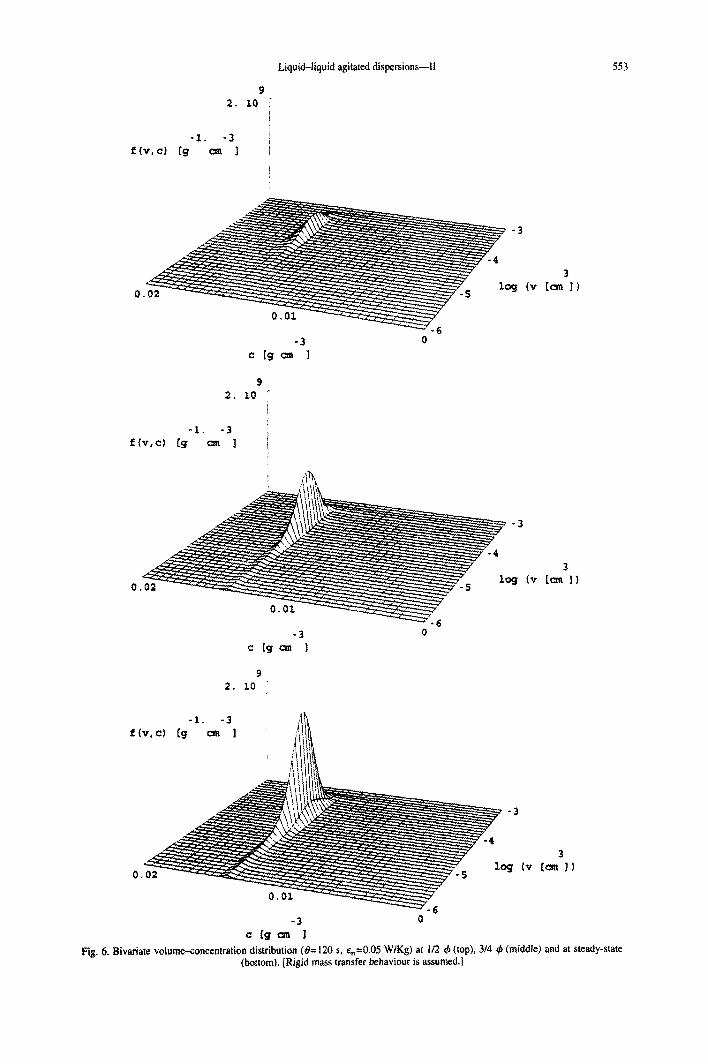
Figures 5 and 6 show a temporal sequence of the bivariate drop volume--concentration density distribu- tion, respectively, for 0= 120 s and e,,=0.15 W/Kg, and for 8=120 s and E,~=0.05 W/Kg. The bivariate drop volume concentration distribution is, in both figures, represented at 83 s (I/2 ~b), 166 s (3/4 &) after start-up,

Liquid-liquid agitated dispersions--II 549

13,80

E

¢..,

0

0

0

13,60

13,40 •

13,20

13,00

12,80

12,60

12,40

12,20

12,00

11,80 0,05

• • •

0,10 0,15 0,20

Agitation Power Density (W/Kg)

[-~- Equilibrium Values I

0,25

Fig. 2. Effect of the agitation rate on the mean drop solute concentration (0= 120 s).

and at steady-state, assuming rigid drop mass transfer behaviour (the bivariate volume-age distribution, for the first set of conditions, was shown in Part 1 of this work--Fig. 7). The widely different values of the vertical coordinate and of the position of the peak along the r/-axis illustrate the sensitivity of the predicted behaviour to the agitation power input density, e,,. A decrease of the power input by a factor of 3 (Figs 5 and

6) yielded, as expected, a corresponding decrease of the distribution maxima by a factor of l0 (due to a considerably reduced number of drops), as well as a significant shift of the distribution towards much larger drops. In Fig. 6, relative to a lower value of the agitation power input, a trace of the feed may still be noticed in the bivariate distributions extending to larger drop volumes and zero solute concentration, which gradually attenuates as the steady-state is approached. Also, due to breakage, the distribution gradually spreads towards the smallest drop sizes.

An important feature of the developed algorithm is its ability to simulate the dispersion's behaviour after

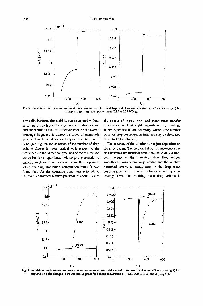
sudden (step or pulse) changes in the main process variables, as illustrated in Figs 7 and 8, both obtained

assuming oscillating drop behaviour. Figure 7 shows that a step change in the agitation power input expectedly results in a rapid change in the amount of solute extracted by the dispersed phase, mostly due to the corresponding rapid change in the interracial area. Changes in the average residence time, 0, through changes in the fiowrates, also yield changes in the amount of solute extracted (Ribeiro, 1995). As for the effects of step and pulse changes in the continuous phase feed solute concentration, they are depicted in Fig. 8, where it may be seen that the sudden feeding of the vessel with a continuous phase of a higher concentration gives rise to a corresponding but highly damped increase in <c, but to a temporary decrease in the extraction efficiency, due to an immediate but temporary increase in the solute content of the continuous phase outlet.

The physical and mathematical justification for the identical extraction efficiency before and after this sudden step change in the continuous phase feed solute concentration is somewhat involved. An overall solute balance in the dispersed phase, at steady-state, yields (for zero solute concentration in the dispersed phase feed)

Table 2. Absolute percent deviations between previous Monte-Carlo and current predicted results for the limiting steady-state

Rigid Drops • m [W/Kg] 0.05 0.10 0.15 0.20 0.25 Mean Drop Volume 0.4% 0.6% 0.0% 1.5% 1,6% Mean Drop Concentration 1. 1% 0.8% 0.5% 0.4% 0,4% Mean Extraction Efficiency 0.9% 0.5% 0.3% 0.2% 0.2%

550 L.M. RIBEIRO et al.

V <c >=-~D ! [c" -~'( rl)]al( rl)Koo( rl)f( rl)d'q, (22)

where V is the vessel's volume, Qo is the dispersed phase volume flowrate, a~, (r/) is the drop's surface area, fir/) is the number density distribution of drop volumes, c* is

the equilibrium dispersed phase solute concentration, and ~'(r/) is the average solute concentration in the whole set of drops of volume r/, irrespective of their history (ages). This size-dependent drop solute concentration, ~(r/), must also satisfy a solute balance equation within the corresponding size fraction (drops of volume r/). The form of this balance equation is

1°0C ~ ' ~

0.9C

8" • ~ 0.8O

~ 0.7(

0.6C

-o3 / Drop Volumes (cm3)

f e e d

[ .-m- Rigid Drops Oscillating Drops I

1.02

8" t - O

73

¢,.

.o

1.0C

0.98

0.9(

O.9z

-06 . . . . . t . b b ' E - 0 5 . . . . . ~ ) ~ '

Drop Volumes (cm3) ' ' ~'l'.b~ =-03

¥

f e e d

I Rigid Drops Oscilla~ng Drops J

Fig. 3. Extraction efficiencies per drop volume class (top) and cumulated values in the direction of larger volumes (bottom).

Liquid-liquid agitated dispersions--II

o >" 0 I I ~ o l d u p t 4 % ~o. 3 %

O.

Time (s)

551

I Rigid Drops Oscillating Drops I Fig. 4. The dynamics of the extraction efficiency for rigid and oscillating drops.

Qo~( 71)f( rl) = Koo( rl) Va,( rl)f( TI)[ c" - ~( ~7) ]

+ (solute in - solute out)hr,ok . . . . . ~., (23)

where the second term of the right hand side accounts for the solute entered into, and left out from, the drops of volume 7/due to interactions with the other drops.As the drop interaction functions, as well as Koo(~l, do not depend explicitly on the individual drop solute concen- trations, the discretization of Equations 22 and 23, irrespective of its precision, always yields a set of linear equations for <c> and ~(r/). Therefore, both <c> and all ?(r/) are proportional to c*. As, with a constant value of the solute distribution coefficient (m=c" / c,.), and at steady-state, c* becomes proportional to the continuous phase feed solute concentration, c,.o, this makes the extraction efficiency (Eoo=<c> / c') invariant before and after any step change in coo. However, this is true only when the dispersed phase feed has, as assumed here, zero solute concentration.

The results reported here illustrate the power and resolution of the algorithm in predicting in such detail this type of dynamic behaviour.

NUMERICAL ACCURACY

As for any finite-difference scheme, the numerical technique developed in this study is subject to some degree of error. For a non-linear equation like PBE (2), general methods to quantitatively evaluate numerical accuracy do not seem to exist. We thus performed a number of checks to gauge the correctness of the present approach.

The first check involved the comparison of the present results with the results of previous studies, where different numerical procedures were used. This external test was presented and discussed in the preceding section, in regard to Guimar~es' Monte-Carlo results. The good agreement found between the steady-state values predicted by both, independent, entirely different, numerical methods supports the validity of the approach followed here.

A second test for numerical error concerned the attainment of the steady-state solution. It should be possible to obtain this as the limit of the transient process, continued long enough for convergence. As shown in Fig. 4, the calculated limiting steady-state dispersed phase hold-up equals the volumetric dispersed phase feed fraction, being thus a good global indicator of the numerical accuracy of the results. For the phase space discretization adopted herein, it was found that the hold-up value at t=960 s was always such as,

~f , , , i - ~b,=960<2 × 10-5. (24)

Trial runs up to ten times the residence time period, indicate that it is possible to continue the computation as long as physically realistic, i.e. one is free to take t large. This behaviour denotes the numerical stability of the approximation pursued here.

The effect on numerical accuracy of the phase space discretization was tested by varying the number of drop volume and concentration classes, Trial runs, for an agitation power input density of 0.15 W/Kg and a residence time of 120 s, with 2, 4, 8, 12 and 20 intervals per volume decade and 6, 12, 24, 36 and 40 concentra-

552 L.M. R1BEIRO et aL

I0 2. 10

-1 . -3 f ( v , c ) [g ca ]

0.02

-3 c [ g e m ]

-3

~ '41 (v

- 6 0

10 2. 10

-1. -3 (v, c) [g ca t i

'.

log (v 0 .02 ~ -~

0.01 ~ 6

-3 0

c [gem ]

3 [ca ])

10 2. 10

- 1 . -3 ( k f (v, c ) [ g cm ] /~t/~

3

0 . 0 2 . l o g (v [,,m 11

0.01

- 6 -3 0

c [ g e m !

Fig. 5. Bivariate volume-concentration distribution (0= 120 s, ~=0.15 W/Kg) at 1/2 ~ (top), 3/4 ~ (middle) and at steady-state (bottom), [Rigid mass transfer behaviour is assumed.]

Liquid-liquid agitated dispersions--lI 553

9 2. 10

-1 . -3 ( v , c ) [ g c,n ]

-3

S -4 3 0.02 log (v [c~ ])

-6 -3 0

c [ g c = ]

9 2. 10

-1. -3 f(v,c) [g c~, ]

q

3 0.02 log (v [cm ])

0.01 -6

0 -3 c [ g c m ]

9 2. l o

-1 . -3 ~l~ f (v, c) , I I I ~ ~ [g c a ] /~

(v [cm ] ) o.o2 o

-3 0 c [ g c m ]

Fig. 6. Bivariate volume-concentration distribution (#= 120 s, ~m=0.05 W/Kg) a~ I/2 4) (~op), 3t4 ~ (middle) and at steady-state (bottom). [Rigid mass transfer bchaviour is assumed.i

554 L.M. R1BEIRO et al.

A ~

13.15

13.1

13.05

13

12.95

12.9

12.85

xlO -3

/ 2do

t,s 4do 600

¢,d

0.94

0.938

0.936

0.934

0.932

0.93

0.928

0.926 2d0 460

t , S

600

Fig. 7. Simulation results (mean drop solute concentration - - left - - and dispersed phase overall extraction efficiency - - right) for a step change in agitation power input (0.15 to 0.25 W/Kg).

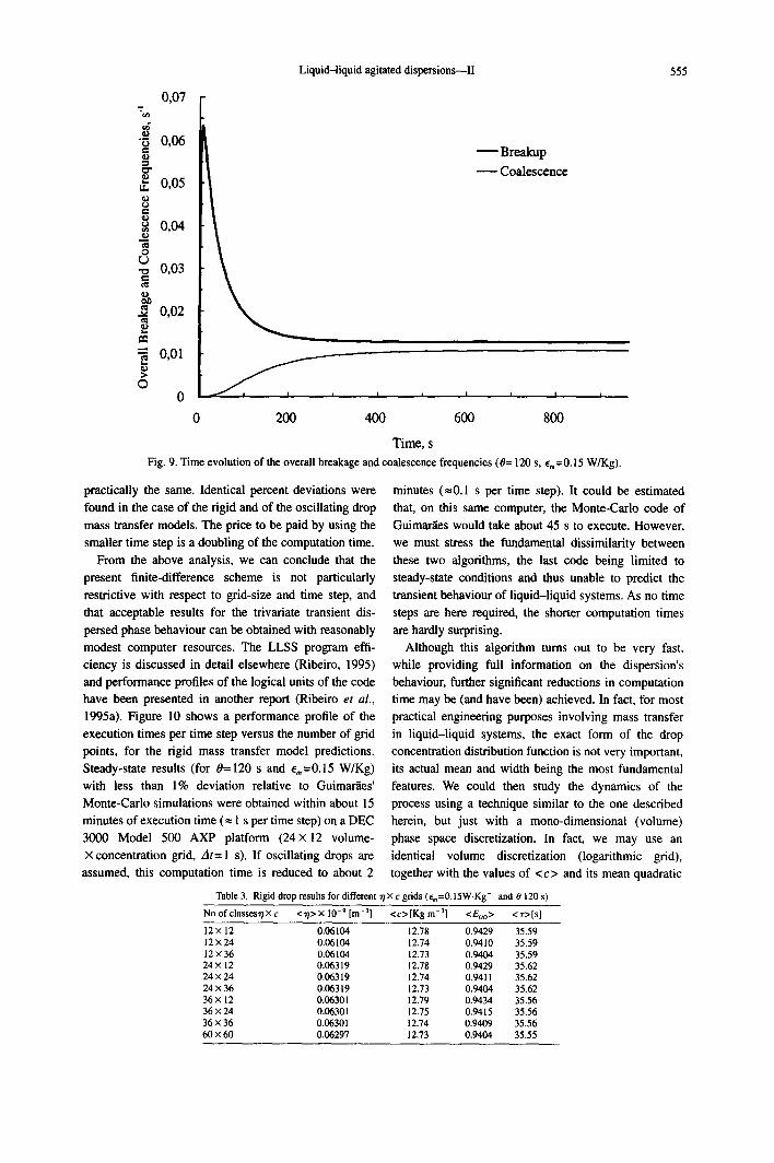
tion cells, indicated that stability can be ensured without resorting to a prohibitively large number of drop volume and concentration classes. However, because the overall

breakage frequency is almost an order of magnitude greater than the coalescence frequency, at least until 3/4~b (see Fig. 9), the selection of the number of drop volume classes is more critical with respect to the differences in the numerical precision of the results, and the option for a logarithmic volume grid is essential to

gather enough information about the smaller drop sizes, while avoiding prohibitive computation times. It was found that, for the operating conditions selected, to maintain a numerical relative precision of about 0.3% in

the results of <r/>, <c> and mean mass transfer efficiencies, at least eight logarithmic drop volume intervals per decade are necessary, whereas the number

of linear drop concentration intervals may be decreased down to 12 (see Table 3).

The accuracy of the solution is not just dependent on the grid-spacing. The predicted drop volume-concentra- tion densities for identical conditions, with only a two- fold increase of the time-step, show that, besides smoothness, results are very similar and the relative numerical errors, at steady-state, in the drop mean concentration and extraction efficiency are approx- imately 0.5%. The resulting mean drop volume is

16.5 xlO

16

15.5

-~ 14.5

v 14

13.5

13

12.5

-3

s" /

/ /

/ /

/

! / / step /

/ l !

460 600

0.93

0.928 _ pulse

0.926 / . ' " ........ t

0.924

0.922

0.92 ep

~ 0.918

0.916

0.914

0.912

0.91~ 200 400 60(

t, s t, s Fig. 8, Simulation results (mean drop solute concentration - - left - - and dispersed phase overall extraction efficiency w fight) for

step and l s pulse changes in the continuous phase feed solute concentration - - Ac~=0.25 co U (t) and Ac~--co 8 (t).

Liquid-liquid agitated dispersions--II 555

0,07

,g

0,06 Breakup

"~ Coalescence ~. 0,05

,~ 0,04

• ~ 0,03 ¢ -

0,02

0,01

> ©

0 200 400 600 800

Time, s

Fig. 9. Time evolution of the overall breakage and coalescence frequencies (0= 120 s, ~m=0.15 W/Kg).

practically the same. Identical percent deviations were

found in the case of the rigid and of the oscillating drop

mass transfer models. The price to be paid by using the

smaller time step is a doubling of the computation time.

From the above analysis, we can conclude that the

present finite-difference scheme is not particularly

restrictive with respect to grid-size and time step, and

that acceptable results for the trivariate transient dis-

persed phase behaviour can be obtained with reasonably

modest computer resources. The LLSS program effi-

ciency is discussed in detail elsewhere (Ribeiro, 1995)

and performance profiles of the logical units of the code have been presented in another report (Ribeiro et al.,

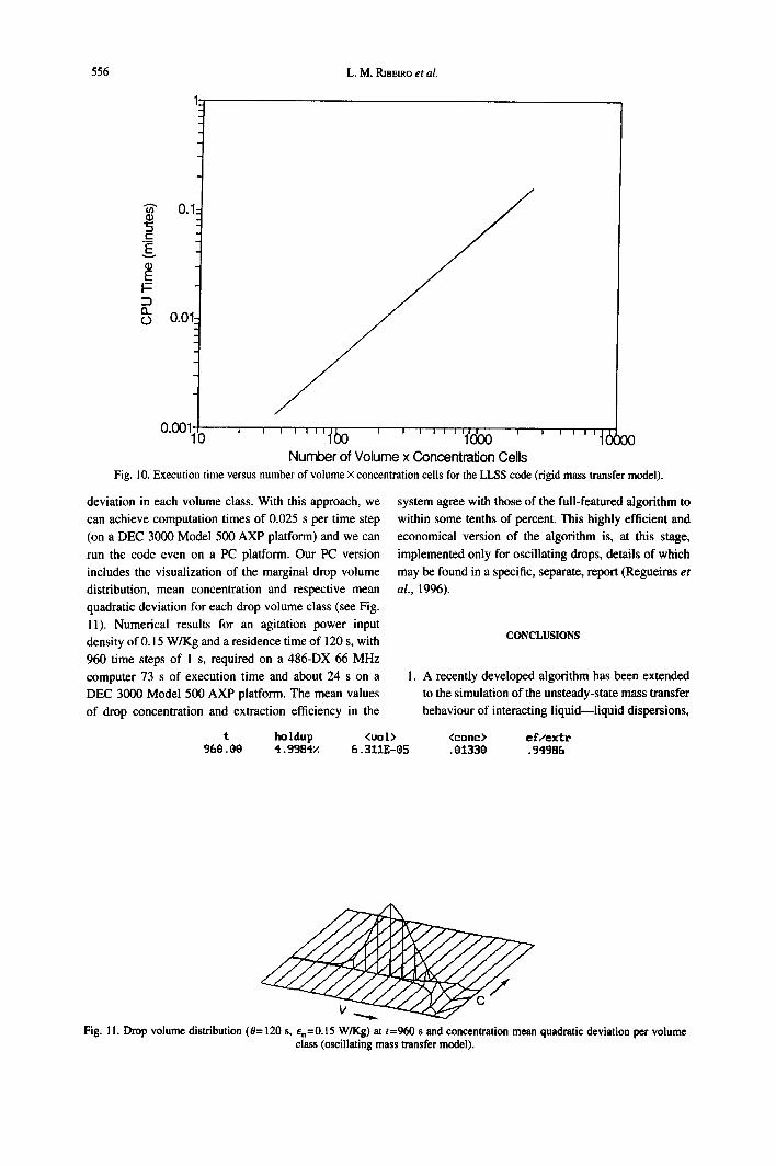
1995a). Figure 10 shows a performance profile of the

execution times per time step versus the number of grid

points, for the rigid mass transfer model predictions.

Steady-state results (for 0=120 s and era=0.15 W/Kg)

with less than 1% deviation relative to Guimar~es'

Monte-Carlo simulations were obtained within about 15

minutes of execution time (~ 1 s per time step) on a DEC

3000 Model 500 AXP platform (24×12 volume°

x concentration grid, At= 1 s). If oscillating drops are

assumed, this computation time is reduced to about 2

Table 3. Rigid drop results for different

minutes (~0.1 s per time step). It could be estimated

that, on this same computer, the Monte-Carlo code of

Guimar,r~es would take about 45 s to execute. However,

we must stress the fundamental dissimilarity between

these two algorithms, the last code being limited to

steady-state conditions and thus unable to predict the

transient behaviour of liquid-liquid systems. As no time

steps are here required, the shorter computation times

are hardly surprising.

Although this algorithm turns out to be very fast,

while providing full information on the dispersion's

behaviour, further significant reductions in computation

time may be (and have been) achieved. In fact, for most

practical engineering purposes involving mass transfer

in liquid-liquid systems, the exact form of the drop

concentration distribution function is not very important,

its actual mean and width being the most fundamental

features. We could then study the dynamics of the

process using a technique similar to the one described

herein, but just with a mono-dimensional (volume)

phase space discretization. In fact, we may use an

identical volume discretization (logarithmic grid),

together with the values of <c> and its mean quadratic

"qX c grids (e,,=0.15W.Kg-i and 0 120 s)

12 x 12 0.06104 12.78 0.9429 35.59 12×24 0.06104 12.74 0.9410 35.59 12 x 36 0.06104 12.73 0.9404 35.59 24 × 12 0.06319 12.78 0.9429 35.62 24×24 0.06319 12.74 0.9411 35.62 24 × 36 0.06319 12.73 0.9404 35.62 36 × 12 0.06301 12.79 0.9434 35.56 36x24 0.06301 12.75 0.9415 35.56 36 × 36 0.06301 12.74 0.9409 35.56 60 × 60 0.06297 12.73 0.9404 35.55

No of classes17 X c <r/>X 10 -9 [m -x] <c>[Kg m -3] <Eoo> <'r> [s I

556 L.M. RIBEIRO et al.

0.1

.

° ~

£

I=

o 0.01-

o . o o l ' ' ' ' ' ' " " l ' r h n ' ' ' )0

Number of Volume x Concentralion Cells Fig. 10. Execution time versus number of volume X concentration cells for the LLSS code (rigid mass transfer model).

deviation in each volume class. With this approach, we

can achieve computation times of 0.025 s per time step

(on a DEC 3000 Model 500 AXP platform) and we can

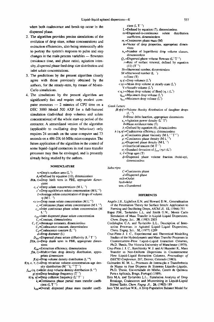
run the code even on a PC platform. Our PC version

includes the visualization of the marginal drop volume

distribution, mean concentration and respective mean

quadratic deviation for each drop volume class (see Fig.

I i). Numerical results for an agitation power input

density of 0.15 W/Kg and a residence time of 120 s, with

960 time steps of 1 s, required on a 486-DX 66 MHz

computer 73 s of execution time and about 24 s on a

DEC 3000 Model 500 AXP platform. The mean values

of drop concentration and extraction efficiency in the

t ho l dup <oo 1 > 960.00 4.9984:<.

system agree with those of the full-featured algorithm to

within some tenths of percent. This highly efficient and

economical version of the algorithm is, at this stage,

implemented only for oscillating drops, details of which

may be found in a specific, separate, report (Regueiras et

al., 1996).

CONCLUSIONS

I. A recently developed algorithm has been extended

to the simulation of the unsteady-state mass transfer

behaviour of interacting liquid--liquid dispersions,

<conc> e f / e x t r 6. 311E-05 .01330 .94986

Fig. 11. Drop volume distribution (0--120 s, ~,~--0.15 W/Kg) at t=960 s and concentration mean quadratic deviation per volume class (oscillating mass transfer model).

Liquid-liquid agitated dispersions--II

when both coalescence and break-up occur in the

dispersed phase.

2. The algorithm provides precise simulations of the

evolution of drop sizes, solute concentrations and

extraction efficiencies, also being intrinsically able

to portray the system's response to pulse and step

changes in the main process variables - - flowrates

(residence time, and phase ratio), agitation inten-

sity, dispersed phase feed drop size distribution and

inlet solute concentrations.

3. The predictions by the present algorithm closely

agree with those previously obtained by the

authors, for the steady-state, by means of Monte-

Carlo simulations.

4. The simulations by the present algorithm are

significantly fast and require only modest com-

puter resources - - 2 minutes of CPU time on a

DEC 3000 Model 500 AXP for a full-featured

simulation (individual drop volumes and solute

concentrations) of the whole start-up period of the

contactor. A streamlined version of the algorithm

(applicable to oscillating drop behaviour) only

requires 24 seconds on the same computer and 73

seconds on a 486-DX 66 MHz microcomputer. The

future application of the algorithm in the control of

some liquid-liquid contactors in real mass transfer

processes may thus be envisaged, and is presently

already being studied by the authors.

NOMENCLATURE

a~=Drop's surface area (L 2) Aj=Defined by equation (10), dimensionless

B(n, t)=Drop birth term in PBE, appropriate dimen- sions

c, c' =Drop solute concentrations (M L-3) c* =Drop equilibrium solute concentration (M L-3) ~=Average solute concentration of drops of volume

77 (M L-3) <c>=Drop mean solute concentration (M L -3)

co=Continuous phase solute concentration (M L-3) coo=Inlet continuous phase solute concentration (M

L -3) Coo=Inlet dispersed phase solute concentration C,----Constant, dimensionless

C) C2=Breakage constants, dimensionless C3---Coalescence constant, dimensionless C4---Coalescence constant (L--') d=Drop diameter (L)

D^D=Dispersed phase solute diffusivity (L 2 T- )) D(n, t)=Drop death term in PBE, appropriate dimen-

sions EoD=Extraction efficiency, dimensionless

f(n, t)=Multiveriate drop density distribution, appro- priate dimensions

flr/)=Drop volume density distribution (L -6) fir/, c, ~', t)=Drop trivariate volume--concentration-age den-

sity distribution (M-) L -3 T- )) ff,,a (7/, t)=Inlet drop volume density distribution (L -~)

g(r/)=Drop breakage frequency (T-~) h(r/, rD=Drop collision frequency (L 3 T- ~)

k~---Continuous phase partial mass transfer coeffi- cient (L T- ~)

koD--Overall dispersed phase mass transfer coeffi-

557

cient (L T- ~) L=Defined by equation (7), dimensionless re=Dispersed-to-continuous solute distribution

coefficient, dimensionless m,.---Continuous phase mass (M) n=Vector of drop properties, appropriate dimen-

sions n,=Number of logarithmic drop volume classes,

dimensionless Qo =Dispersed phase volume flowrate (L 3 T-J)

s=Rate of surface renewal, defined by equation (12) (T-~)

Sh =Sherwood number, dimensionless Sh'=Sherwood number (L ~)

t=Time (T) r/,r/'=Drop volumes (L 3)

< r/>=Mean drop volume at steady-state (L 3) V =Vessel's volume (L 3)

< r/,>=Mean drop volume of freed (r/, t (L 3) r/ma,=Maximum drop volume (L 3) r/,~i,,=Minimum drop volume (L 3)

Greek Letters ,8(r/Ir/')=Volume density distribution of daughter drops

(L -3) ,~=Dirac delta function, appropriate dimensions

e,,,=Agitation power density (L 2 T 3) 0=Mean residence time (T)

A~=Defined by equation (8), dimensionless A (r/,r/') =Coalescence efficiency, dimensionless

#~,=Continuous phase viscosity (M L-~ T-~) p~=Continuous phase density (M L-3) p,j=Dispersed phase density (M L-3) ~r=Interfacial tension (M T- 2) o-, =Standard deviation of ff, e,i (r/,t) (L 3)

r, q=Drop ages (T) q'~=Dispersed phase volume fraction (hold-up),

dimensionless

Subscripts C=Continuous phase d=Dispersed phase

exit =Outlet feed=Inlet trns. =Transferred

REFERENCES

Angelo J.B., Lightfoot E.N. and Howard D.W., Generalization of the Penetration Theory for Surface Strech: Application to Forming and Oscillating Drops, AIChE Jl, 12, (1966) 751

Bapat P.M., Tavlarides L.L. and Smith G.W., Monte Carlo Simulation of Mass Transfer in Liquid-Liquid Dispersions, Chem. Engng. Sci., 38, (1983) 2003

Coulaloglou C.A. and Tavlarides L.L., Description of Inter- action Processes in Agitated Liquid-Liquid Dispersions, Chem. Engng. Sci., 32, (1977) 1289

Cruz-Pinto J. J. C., Experimental and Theoretical Modelling Studies of the Hydrodynamic and Mass Transfer Processes in Countercurrent-Flow Liquid-Liquid Extraction Columns, Ph.D. Thesis, The Victoria University of Manchester (1979).

Cruz-Pinto J. J. C., Korchinsky W. J. and AI Husseini R., Mass Transfer to Non-Uniform Dispersions in Countercurrent Flow Liquid-Liquid Extraction Columns, Proceedings of 1SEC83 Conference, 207, Denver, Colorado (1983).

Guimar~es M. M. L., Processos de Interac~o e Transfer~ncia de Massa na Fase Dispersa de Sistemas Lfquido--Liquido, Ph.D. Thesis, Universidade do Minho, Centro de Qufmica Pura e Aplicada, Braga, Portugal (1989).

Hsia M.A. and Tavlarides L.L., Simulation Analysis of Drop Breakage, Coalescence and Micromixing in Liquid-Liquid Stirred Tanks, Chem. Engng. Jl., 26, (1983) 189

Jeon Y.M. and Lee W.K., A Drop Population Balance Model for

558

Mass Transfer in Liquid-Liquid Dispersion. I. Simulation and Its Results, Ind. Engng. Chem. Fundam., 25, (1986) 293

Kanel J. S., Effects of Some Interracial Phenomena on Mass Transfer in Agitated Liquid-Liquid Dispersions, Ph.D. The- sis, Georgia Institute of Technology (1990).

Korchinsky W. J. and Endres J. C. T., Countercurrent Liquid- Liquid Contacting: Modelling, Parameter Evaluation and Column Operating Conditions, Solvent Extraction in the Process Industries, (ed. D. H. Logsdall and M. J. Slater), Vol. 2, 1159, Elsevier (1993).

Regueiras P. F. R., Ribeiro L. M., Guimar~s M. M. L., Madureira C. M. N. and Croz-Pinto J. J. C., Precise and Fast Computer Simulations of the Dynamic Mass Transfer Behaviour of Liquid-liquid Agitated Contactors, Value adding through solvent extraction (ed. The University of Melbourne) 1031 0996).

Ribeiro L.M., Regueiras P.ER., Guimarr~es M.M.L. and Cruz- Pinto JJ.C., Numerical Simulation of Liquid-Liquid Agi- tated Dispersions on the VAX 6520/VP, Computing Systems in Engng, 6, (1995) 465

Ribeiro L.M., Regueiras P.F.R., Guimar~es M.M.L., Madureira C.M.N. and Cruz-Pinto J.J.C., The Dynamic Behaviour of Liquid-Liquid Agitated Dispersions. I -- The Hydro- dynamics, Computers and Chem. Engng, 19, (1995) 333

Ribeiro L. M., Ph.D. Thesis, Universidade do Minho, Braga Portugal ( 1995 ).

Rose P.M. and Kintuer R.C., Mass Transfer from Large Oscillating Drops, AIChE Jl., 12, (1966) 530

Skelland A.H.P. and Kanel J.S., Simulation of Mass Transfer in a Batch Agitated Liquid-Liquid Dispersion, Ind Engng. Chem. Res., 31, 0992) 908

APPENDIX A

The expressions used for the breakage frequency, the collision frequency and the coalescence efficiency are

h( 'r/, "r/' ) = C3 ~"3( I"/~J3 + ~/~/3)( ~ + ff'bg) '/2 (A.2)

and

L. M. RIBEIRO et al.

(A.3)

To describe the breakage process, it is also necessary to know the average volume distribution resulting from the breakage of a single drop. We have assumed, as Coulaloglou and Tavlarides (1977), binary breakage and an approximately normal daughter- droplets volume distribution, i.e.

4.5(2r/' - 7/)2 ] ~(r/'lr/)= 2.402 exp • (A.4) ,7 .72

APPENDIX B

The following expressions are used to calculate the rate of drop birth and death in each drop volume-concentration class (Jdc).

Rate of Interaction Events Birth by breakage

Birth by coalescence

Entrance

Death by breakage

Death by coalescence

f;~,

Exit

f;J,

Expression

n

2 i~=j.=, fid, giBj.i A 7i

jj 1 ~ ZJ, Z',: 2 i=. i,=~

i':r/j= r / . . r/,

i'~:cj - rl'ci'+ ~1"c'7 ~j

1 bY,.,j o

fJ~j

f., ~ ,~, f.h.h,.,~. i= I F~=

i * : 7 / j =7 / , , - 7/~.

l