Carboxymethylcellulose Acetate Butyrate Water-Dispersions

as Renewable Wood Adhesives

Jesse Loren Paris

Thesis submitted to the faculty of the

Virginia Polytechnic Institute and State University

in partial fulfillment of the requirements for the degree of

Master of Science

In

Forest Products

Charles E. Frazier, Chair

Kevin J. Edgar

Maren Roman

August 5, 2010

Blacksburg, VA

Keywords: Carboxymethylcellulose acetate butyrate, CMCAB, wood adhesives, viscosity, dynamic mechanical analysis, adhesive penetration, mode I fracture testing

Carboxymethylcellulose Acetate Butyrate Water-Dispersions

as Renewable Wood Adhesives

Jesse Loren Paris

ABSTRACT

Two commercial carboxymethylcellulose acetate butyrate (CMCAB) polymers, high and low

molecular weight (MW) forms, were analyzed in this study. High-solids water-borne dispersions

of these polymers were studied as renewable wood adhesives. Neat polymer analyses revealed

that the apart from MW, the CMCAB systems had different acid values, and that the high MW

system was compromised with gel particle contaminants. Formulation of the polymer into water-

dispersions was optimized for this study, and proved the “direct method”, in which all

formulation components were mixed at once in a sealed vessel, was the most efficient

preparation technique. Applying this method, 4 high-solids water dispersions were prepared and

evaluated with viscometry, differential scanning calorimetry, dynamic mechanical analysis, light

and fluorescence microscopy, and mode I fracture testing.

Thermal analyses showed that the polymer glass transition temperature significantly increased

when bonded to wood. CMCAB dispersions produced fairly brittle adhesive-joints; however, it is

believed toughness can likely be improved with further formulation optimization. Lastly,

dispersion viscosity, film formation, adhesive penetration and joint-performance were all

dependent on the formulation solvents, and moreover, these properties appeared to correlate with

each other.

ACKNOWLEDGEMENTS

First, I wish to express my utmost gratitude to my guiding professor and committee chair, Dr.

Charles E. Frazier. Early on in my undergraduate studies, he first encouraged me to consider a

graduate education. Now upon completion of my Master of Science, I have a deep respect and

calling to continue research in the wood-based composites arena. Dr. Frazier taught me self-

confidence and scientific rigor which I plan to carry forward in my future endeavors.

I also want to thank my committee members Dr. Maren Roman and Dr. Kevin Edgar; their

support and unique scientific backgrounds significantly contributed to both my personal

development and to that of this work. I also wish to thank the entire faculty, staff and students of

the Department of Wood Science and Forest Products who guided and worked alongside me for

both my Bachelor and Master degrees. The training and scientific discussions from two

particular professors, Drs. Audrey Zink-Sharp and Scott Renneckar were appreciated and very

important in this work. Additionally, I thank David Jones and Rick Caudill for their training and

friendly conversations, as well. And I offer a very special thanks to my fellow group members in

the wood adhesion group for their invaluable friendship and support.

I wish to thank the Wood-Based Composites Center for funding this project, and the Sustainable

Engineered Materials Institute for providing additional financial support. Also, I thank Eastman

Chemical Company for providing me with the polymer I studied and greatly appreciated

dispersion formulation advice.

Last but not least, I wish to thank my family. Their endless love and encouragement have fueled

my desire to continue my education and expand my horizons.

iii

Table of Contents

 ABSTRACT .................................................................................................................................... ii 

ACKNOWLEDGEMENTS ........................................................................................................... iii 

Table of Contents ........................................................................................................................... iv 

List of Figures .............................................................................................................................. viii 

List of Tables ............................................................................................................................... xiii 

1  Introduction and Literature Review ........................................................................................ 1 

1.1  Introduction ...................................................................................................................... 1 

1.2  Wood Adhesion ................................................................................................................ 2 

1.2.1  History of Wood Adhesives ...................................................................................... 2 

1.2.2  Fundamentals and Mechanisms of Wood Adhesion ................................................. 6 

1.3  Cellulose and Cellulose Derivatives ................................................................................ 9 

1.3.1  Cellulose Structure .................................................................................................. 10 

1.3.2  Cellulose Derivatives .............................................................................................. 12 

1.3.3  Carboxymethylcellulose Acetate Butyrate ............................................................. 17 

1.4  Analytical Techniques .................................................................................................... 25 

1.4.1  Viscosity ................................................................................................................. 25 

iv

1.4.2  Dynamic Mechanical Analysis (DMA) .................................................................. 31 

1.4.3  Adhesive Performance Testing ............................................................................... 34 

1.5  References ...................................................................................................................... 42 

2  Carboxymethylcellulose Acetate Butyrate (CMCAB) Neat Polymer Characterization ....... 52 

2.1  Introduction .................................................................................................................... 52 

2.2  Experimental .................................................................................................................. 54 

2.2.1  Materials ................................................................................................................. 54 

2.2.2  Methods................................................................................................................... 54 

2.3  Results and Discussion ................................................................................................... 58 

2.3.1  Polymer Acid Number ............................................................................................ 58 

2.3.2  Polymer Thermal Properties ................................................................................... 59 

2.3.3  Plasticizer Analysis ................................................................................................. 69 

2.4  Conclusions .................................................................................................................... 71 

2.5  References ...................................................................................................................... 72 

3  CMCAB Dispersion Formulation and Optimization ............................................................ 74 

3.1  Introduction .................................................................................................................... 74 

3.2  Experimental .................................................................................................................. 76 

3.2.1  Materials ................................................................................................................. 76 

3.2.2  Methods................................................................................................................... 77 

3.3  Results and Discussion ................................................................................................... 81 

v

3.3.1  Dispersion Mixing Criteria ..................................................................................... 81 

3.3.2  Dispersion Solvent/Viscosity Relationship ............................................................. 82 

3.3.3  Film Formation Study ............................................................................................. 88 

3.4  Conclusions .................................................................................................................... 90 

3.5  References ...................................................................................................................... 92 

4  CMCAB Dispersion Polymer Thermal Properties ............................................................... 93 

4.1  Introduction .................................................................................................................... 93 

4.2  Experimental .................................................................................................................. 93 

4.2.1  Materials ................................................................................................................. 93 

4.2.2  Methods................................................................................................................... 94 

4.3  Results and Discussion ................................................................................................... 99 

4.3.1  Adhesive Thermal Properties .................................................................................. 99 

4.4  Conclusions .................................................................................................................. 115 

4.5  References .................................................................................................................... 117 

5  CMCAB Adhesive Performance ......................................................................................... 118 

5.1  Introduction .................................................................................................................. 118 

5.2  Experimental ................................................................................................................ 118 

5.2.1  Materials ............................................................................................................... 118 

5.2.2  Methods................................................................................................................. 119 

5.3  Results and Discussion ................................................................................................. 125 

vi

5.3.1  Dispersion Viscosities ........................................................................................... 125 

5.3.2  Adhesive-layer thickness Measurements .............................................................. 128 

5.3.3  Mode I Fracture Performance ............................................................................... 129 

5.3.4  Adhesive Penetration ............................................................................................ 134 

5.4  Conclusions .................................................................................................................. 138 

5.5  References .................................................................................................................... 140 

6  Conclusions and Future Work ............................................................................................ 142 

7  APPENDICES .................................................................................................................... 144 

APPENDIX 1 Solids Content Measurement - TGA ............................................................... 144 

APPENDIX 2 Adhesive-Layer Thickness Measurements ..................................................... 147 

APPENDIX 3 Water-Submersion DMA ................................................................................ 151 

APPENDIX References .......................................................................................................... 155 

vii

List of Figures

Figure 1-1: Contact angle (a) less than 90° representing favorable wetting and (b) greater than

90° representing unfavorable wetting. ............................................................................................ 7 

Figure 1-2: Molecular structure of cellobiose (numbers = carbon atoms on AGUs). .................. 11 

Figure 1-3: Dimer representation of the molecular structure of CMCAB (actual substitution

positions are random). ................................................................................................................... 18 

Figure 1-4: Commercial cellulose mixed ester nomenclature. ..................................................... 19 

Figure 1-5: (a) Diagram of simple shear flow; (b) Variables defining simple shear mechanics

(adapted from Barnes 2000).......................................................................................................... 26 

Figure 1-6: Representative viscosity plot; (a) shear-thinning fluid, (b) Newtonian fluid. ........... 27 

Figure 1-7: Representative CMCAB dilute solution viscosity data collected in this study; [n] =

0.520 dL/g. .................................................................................................................................... 29 

Figure 1-8: Steady-state viscosity geometries; (a) Cone-and-plate, (b) concentric cylinder. ....... 30 

Figure 1-9: Typical torsional DMA scan for a dispersion-cast CMCAB film from this study with

storage modulus (G’), loss modulus (G’’), and tan δ. ................................................................... 33 

Figure 1-10: Fracture Modes: I) opening or cleavage, II) forward shear, and III) transverse shear

of tearing. ...................................................................................................................................... 36 

Figure 1-11: Contoured dual cantilever beam (CDCB) fracture specimen in Mode I. ................. 37 

Figure 1-12: Typical cubed root of compliance (C1/3) versus crack length (a) plot. .................... 40 

Figure 2-1: Representative blank fit (red) and raw specimen data (blue) plots: pH v. titrant

volume and 1st derivative pH v. titrant volume. ............................................................................ 58 

Figure 2-2: Representative TGA responses of CMCAB-High (red) and -Low (blue) powders

showing % weight loss (solid), and the derivative of % weight loss (10°C/min in air). ............ 61 

viii

Figure 2-3: Representative DSC plots for CMCAB-High powder (a) and CMCAB-High film (b).

Heating rate = 10°C/min; cooling = 5°C/min. .............................................................................. 63 

Figure 2-4: Representative second heat DSC plots of CMCAB-High and -Low powders and

films at 10°C/min. ......................................................................................................................... 65 

Figure 2-5: Plot of % strain as a function of oscillation stress used to determine polymer LVR.

Isothermal stress-sweeps conducted on CMCAB-High and -Low films at low as a function of

temperature as indicated. .............................................................................................................. 67 

Figure 2-6: Average DMA curves (n = 3) for CMCAB-High, showing the first heat and

subsequent cool as indicated (3°C/min., 1Hz). ............................................................................. 68 

Figure 2-7: Average DMA (3°C/min., 1 Hz) solution-cast (from THF) film first heat (a) tan δ

curves and (b) Tg values as a function of % CP as indicated; error bars represent ± 1 standard

deviation (n = 3). ........................................................................................................................... 70 

Figure 3-1: CMCAB carboxylic acid neutralization with N,N-dimethylethanolamine. ............... 75 

Figure 3-2: Average peak-hold flow curves as a function of mixing time for CMCAB-High

dispersions (25% solids, 10.9% neutralization) in EGBE:IPA mixed solvents as indicated (n = 2-

3, 500 s-1). ..................................................................................................................................... 82 

Figure 3-3: Average steady-state flow curves (25°C, n = 3) for CMCAB-High dispersions (23%

solids, 10.9% neutralization) using neat and mixed solvents as indicated. .................................. 84 

Figure 3-4: Average peak-hold flow curves (500 s-1, 25°C, n = 4) for CMCAB-Low dispersions

(40% solids, 12% neutralization) using neat and mixed solvents as indicated. ............................ 85 

Figure 3-5: Representative ηred and ηinh as a function of concentration for CMCAB-Low in

EGBE, MPK, and a 50:50 wt% EGBE/MPK mixture as indicated. ............................................. 87 

ix

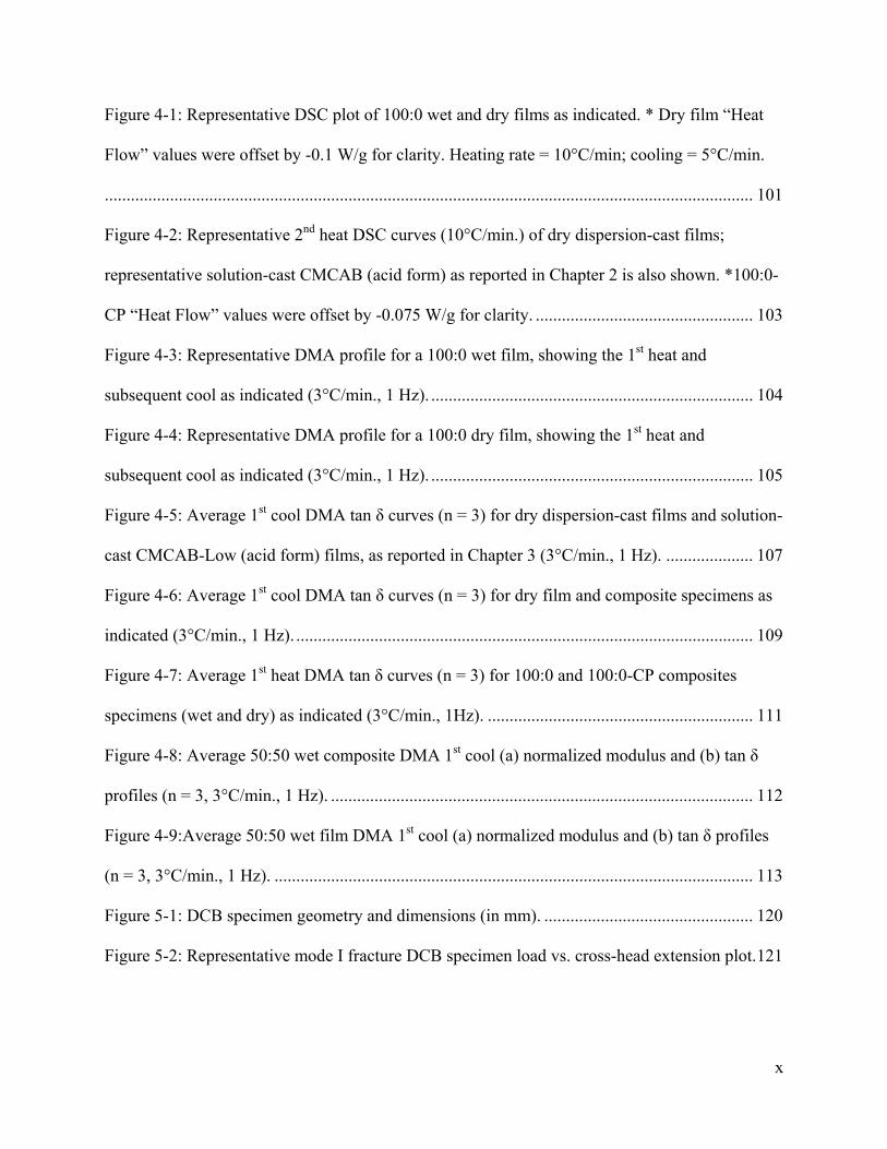
Figure 4-1: Representative DSC plot of 100:0 wet and dry films as indicated. * Dry film “Heat

Flow” values were offset by -0.1 W/g for clarity. Heating rate = 10°C/min; cooling = 5°C/min.

..................................................................................................................................................... 101 

Figure 4-2: Representative 2nd heat DSC curves (10°C/min.) of dry dispersion-cast films;

representative solution-cast CMCAB (acid form) as reported in Chapter 2 is also shown. *100:0-

CP “Heat Flow” values were offset by -0.075 W/g for clarity. .................................................. 103 

Figure 4-3: Representative DMA profile for a 100:0 wet film, showing the 1st heat and

subsequent cool as indicated (3°C/min., 1 Hz). .......................................................................... 104 

Figure 4-4: Representative DMA profile for a 100:0 dry film, showing the 1st heat and

subsequent cool as indicated (3°C/min., 1 Hz). .......................................................................... 105 

Figure 4-5: Average 1st cool DMA tan δ curves (n = 3) for dry dispersion-cast films and solution-

cast CMCAB-Low (acid form) films, as reported in Chapter 3 (3°C/min., 1 Hz). .................... 107 

Figure 4-6: Average 1st cool DMA tan δ curves (n = 3) for dry film and composite specimens as

indicated (3°C/min., 1 Hz). ......................................................................................................... 109 

Figure 4-7: Average 1st heat DMA tan δ curves (n = 3) for 100:0 and 100:0-CP composites

specimens (wet and dry) as indicated (3°C/min., 1Hz). ............................................................. 111 

Figure 4-8: Average 50:50 wet composite DMA 1st cool (a) normalized modulus and (b) tan δ

profiles (n = 3, 3°C/min., 1 Hz). ................................................................................................. 112 

Figure 4-9:Average 50:50 wet film DMA 1st cool (a) normalized modulus and (b) tan δ profiles

(n = 3, 3°C/min., 1 Hz). .............................................................................................................. 113 

Figure 5-1: DCB specimen geometry and dimensions (in mm). ................................................ 120 

Figure 5-2: Representative mode I fracture DCB specimen load vs. cross-head extension plot. 121 

x

Figure 5-3: Representative mode I fracture DCB specimen cubed-root compliance vs. crack

length plot and linear fit (m = 0.345, b = 0.005). ........................................................................ 123 

Figure 5-4: Average dispersion steady-state viscosity v. shear rate flow curves (cone-and-plate,

25°C, n = 3). ................................................................................................................................ 125 

Figure 5-5: Average dispersion (100 g batch specifically for viscosity measurements) steady-

state viscosity v. shear rate flow curves measured with (a) cone-and-plate and (b) concentric

cylinders geometries (25°C, n = 3). ............................................................................................ 127 

Figure 5-6: Average DCB adhesive-layer thicknesses (n = 45); error bars represent ±1 standard

deviation. ..................................................................................................................................... 129 

Figure 5-7: Representative energy v. crack length plot for a DCB specimen (100:0) tested in

mode I cleavage. ......................................................................................................................... 130 

Figure 5-8: Average CMCAB adhesive-joint critical and arrest mode I fracture energies; error

bars represent 1 standard deviation (SYP ~12% MC, 25°C). ..................................................... 131 

Figure 5-9: Average 1st heat DMA tan δ curves (3°C/min., 1Hz, n = 3) for wet 100:0 and 100:0-

CP composites (Chapter 4). ........................................................................................................ 133 

Figure 5-10: Representative earlywood cross-sectional photomicrographs observed with epi-

fluorescence (50X, 0.5% Safranin O stain, filter set 360 nm/400 nm/420 nm); 100 μm scale bars.

..................................................................................................................................................... 135 

Figure 5-11: Average SYP earlywood CMCAB adhesive penetration; error bars indicate ±1

standard deviation. ...................................................................................................................... 136 

Figure 7-1: Representative 100:0 weight and derivative weight curves vs. temperature, as

indicated, measured with High-res TGA (20°C/min in air, sensitivity: 1.0, res.: 3.0). .............. 145 

xi

Figure 7-2 Representative AL dispersion bondline images as indicated (100 X, scale bars = 100

μm). ............................................................................................................................................. 149 

Figure 7-3: Average AL dispersion adhesive-layer thicknesses as indicated (n = 11 - 20); error

bars represent ±1 standard deviation. .......................................................................................... 150 

Figure 7-4: Average 1st cool DMA (a) G' and (b) tan δ curves (n = 3) for dry and water-

submerged CMCAB-High dispersion-cast films (3°C/min., 1Hz). ............................................ 153 

xii

List of Tables

Table 1-1: Typical properties of commercial CMCAB mixed esters. .......................................... 19 

Table 1-2: Properties of chemicals used in CMCAB dispersion formulations. ............................ 24 

Table 2-1: Average ANs for CMCAB-High and -Low ±1 standard deviation; n = number of

observations. ................................................................................................................................. 59 

Table 2-2: Average polymer thermal properties (n = 3) ± 1 standard deviation as measured with

TGA (10°C/min. in air), DSC (20°C/min.), and DMA (3°C/min., 1Hz). ..................................... 60 

Table 3-1: MW, boiling point (bp), and density of chemicals used in dispersion formulations. . 76 

Table 3-2: Average CMCAB-Low intrinsic viscosities, [η], (n = 3) acquired from linear fits of

ηred vs. c plots in EGBE, MPK, and a 50:50 wt% EGBE/MPK mixture ±1 standard deviation. . 88 

Table 3-3: Film formation results for CMCAB-High dispersions (10.9% neutralization) as a

function of solids content and organic solvent component(s). ..................................................... 89 

Table 3-4: Film formation results for CMCAB-Low dispersions (12% neutralization, 45%

continuous phase) as a function of solids content and organic solvent component(s). CC -

coalesced and clear; CT - coalesced and translucent. ................................................................... 90 

Table 4-1: Component masses and wt% used to prepare CMCAB dispersions. .......................... 95 

Table 4-2: Average film and composite (wet and dry) Tgs (CMCAB salt form) and % adhesive in

composite specimens (n = 3 - 6), ±1 standard deviation measured with DSC (20°C/min., 2nd heat)

and DMA (3°C/min., 1 Hz, 1st cool). .......................................................................................... 100 

Table 4-3: Average adhesive film weight loss (n = 3 - 6), ±1 standard deviation, with DSC for

desiccator- and vacuum-oven-dried specimens. ......................................................................... 102 

Table 4-4: Average 50:50 wet composite and film DMA 1st cool normalized modulus and tan δ

data (n = 3, 3°C/min., 1 Hz). ....................................................................................................... 113 

xiii

xiv

Table 4-5: Average first heat Tgs (n = 3) for 100:0 and 100:0-CP composites (wet and dry) as

measured with DMA (3°C/min., 1 Hz). ...................................................................................... 115 

Table 5-1: Average CMCAB adhesive-joint critical and arrest mode I fracture energies, ± 1

standard deviation (SYP ~12% MC, 25°C) ................................................................................ 131 

Table 5-2: Average SYP earlywood CMCAB adhesive penetration ± 1 standard deviation. .... 136 

Table 7-1: Average dispersion % solids ± 1 standard deviation; bonding systems (n = 3) and

additional viscometry systems (n = 2) measured with High-res TGA (20°C/min in air, sensitivity:

1.0, res.: 3.0). .............................................................................................................................. 146 

1 Introduction and Literature Review

1.1 Introduction

When solid wood is broken down into smaller dimensions and reformed into an integral

composite, the use of the timber resource is extended, composite physical properties can be more

consistent by defect randomization, and dimensional stability can be improved (Peshkova and Li

2003). Wood composites have been used by humans for centuries, from early decorative veneers

and furniture manufacturing, to structural products including panels and engineered lumber now

vital to the construction industry. Today, nearly all structural wood composites are manufactured

with non-renewable, synthetic adhesives derived from fossil fuels (Sellers 1985). However, this

was not always the case; early adhesive systems were based on renewable, natural materials. In

today’s society all industries are challenged to be more environmentally conscious and to use

resources in a sustainable manner. For the wood composites industry, already based on a

renewable resource, further environmental stewardship can be realized with the adoption of

adhesive systems derived from natural materials.

Cellulose is the most abundant biopolymer on the planet, and its derivatives have been used for

over a century for films, coatings and plastics technologies. This research investigates the use of

high-solids, water-based dispersions of carboxymethylcellulose acetate butyrate (CMCAB)

mixed esters as renewable wood adhesives. This objective was pursued with various polymer

characterization techniques, the preparation and optimization of CMCAB water dispersions, as

well as adhesive performance evaluations. Analytical techniques employed in this study included

titrations for acid number determination, thermogravimetric analysis, differential scanning

1

calorimetry, dilute-solution and steady-state viscometry, dynamic mechanical analysis, mode I

fracture testing, and light and fluorescence microscopy.

1.2 Wood Adhesion

1.2.1 History of Wood Adhesives

Early humans observed materials that were naturally “sticky” and tried to use them as sealants

and adhesives for tools, furniture, and shelter. Many such natural materials were developed into

commercial adhesive systems for wood-composites industries. Some of these early raw materials

included soy proteins, starch, blood, collagen extracts, milk proteins (caseins), fish skin extracts,

and vegetable proteins (Lambuth 1994).

Of these, soy, blood and casein were the most commercially significant for structural wood

composites before World War II, and utilized water dispersible, cross-linkable proteins for bond

integrity. Protein adhesives were observed to produce very strong bonds, and were mainly used

for plywood applications. However, these systems were not resistant to moisture, mold, fungi, or

enzymatic and bacterial attack, and were thus limited to interior applications (Lambuth 1994;

Pocius 1997; Sellers Jr 1994). In the 1920’s, phenol-formaldehyde (PF) was developed

representing the first truly exterior, thermosetting resin (Lambuth 1994). War efforts fueled the

research to optimize these new synthetic adhesive systems. After WWII the petrochemical

companies invested heavily in adhesive markets, and within a decade virtually phased out all

commercial protein-based adhesives due to the cheaper, seemingly limitless supply of the

synthetic systems (Keimel 1994; Lambuth 1994). Yet, protein adhesives could be easily re-

implemented into commercial plywood production in an emergency or if ever economically

feasible (Lambuth 1994; Sellers 1985).

2

Synthetic adhesive technologies have been expanding rapidly since the end of WWII, and have

allowed for remarkable increases in product types and manufacturing capacities of structural

wood products (Sellers Jr 1994). These systems, however, are getting increased scrutiny with

respect to their non-renewable petrochemical origins. Concern over the availability and costs of

global oil supplies in the future has sparked a re-interest in the development of renewable

materials (Imam et al. 2001; Peshkova and Li 2003). The current challenge is to develop

renewable systems that can compete with synthetic, thermosetting adhesives in both cost and

performance (Yang et al. 2006a).

There have been many recent efforts to address this challenge. Proteins, both plant and animal,

carbohydrates, and natural phenolic compounds have been re-investigated for use as renewable

adhesives due to their abundance, high molecular weight, and high degrees of functional groups

capable of adhesion and cross-linking with high surface energy substrates (Haag et al. 2006;

Olivares et al. 1995; Yang et al. 2006b).

Soy protein has received considerable research as a base raw material for many renewable

adhesive systems; however, the greatest performance results have been observed when used in

combination with synthetics. In 1997, Steele et al. developed a finger jointing adhesive

comprised of soy protein isolate (SPI) and phenol-resorcinol-formaldehyde (PRF) (Steele et al.

1998). Several other studies have shown that soy-flour cross-linked with PF could be used for

bonding plywood, oriented strand board (OSB), and medium density fiber-board panels (MDF)

(Wescott et al. 2006; Yang et al. 2006a; Yang et al. 2006b). One research group at Oregon State

University has focused heavily on soy-based wood adhesives over the past decade (Li et al.

2004; Liu and Li 2007; Schwarzkopf et al. 2009). One system investigated, the Soy/PAE

adhesive (Li et al. 2004), has achieved commercial significance, and is being produced to

3

manufacture hardwood plywood (2005) . However, it too consists of over 40 wt% solids

polyamidoamine-epichlorohydrin (PAE), a synthetic polymer. Additionally, soy is being used

simply as an additive in many synthetic-based adhesives, reducing the amount of petrochemical

resins in their formulations (Sellers Jr 2001).

Animal proteins, specifically blood, are extensively used in synthetic plywood adhesives as foam

promoters and additives, again reducing petrochemical usage (Lambuth 1994; Sellers Jr 2001).

Adhesives based on blood proteins, blood/peanut proteins, and blood/soy proteins in

combination with PF resin solids between 30-50% all met exterior-grade MDF requirements

established by the American National Standards Institute (ANSI) (Yang et al. 2006b).

Polysaccharides represent a very diverse class of carbohydrates; they are generally long chain,

high molecular weight polymers made of repeating 5 or 6 carbon sugar units. Several

polysaccharide-based structural adhesives have been researched over the past decade, though

none have proven commercially significant (designation as “structural” means an adhesive is

used for the manufacture of primary building elements such as plywood or laminated beams; it

also means that the adhesive has passed a rigorous series of certification standards that test

moisture durability, creep resistance, and other performance criteria). Starch is, and has been,

used as a very important adhesive material; however, it generally serves non-structural purposes

in the paper and paperboard industries (Baumann and Conner 1994). More recently, starch was

cross-linked with polyvinyl alcohol (PVOH) and 5-7 wt% latex to yield a moisture resistant

plywood-adhesive that exhibited wood failure levels over 99% determined using ASTM D-906-

64 (Imam et al. 2001). In 2003, chitosan and chitosan-konjac glucomannan mixtures were

investigated as natural-polymer based wood adhesives; the resulting composites showed dry

bond performance comparable to commercial UF resins (Umemura et al. 2003). Chitosan has

4

also been investigated as part of a 3 component system, also containing laccase enzymes and

phenolic compounds, capable of strong, partially water resistant, wood adhesion (Peshkova and

Li 2003). Polysaccharides from microbial organisms have also been tested as wood adhesives

yielding bond shear strengths comparable to commercial polyvinyl acetate (PVA) –based wood

adhesives (Haag et al. 2006).

Lignin, the polyphenolic network-like polymer found in plant cell walls, is one of the most

abundant polymers on earth, second only to cellulose. Spent sulfite liquors (SSL) from industrial

pulping processes produce vast annual quantities of sulphonated lignin byproducts, a majority of

which are burned for fuel; but some are recovered as chemical products (Lewis and Lantzy

1989). SSL has been heavily investigated for use as a renewable adhesive for particleboard,

plywood, and fiberboard, though the lignin structure is simply not as reactive as conventional PF

resins (Pizzi 1994a). Particleboard production with modified SSL adhesives has achieved

“technical” success, but manufacturing costs were higher than for common synthetic systems,

thus SSL adhesives were never commercialized (Lewis and Lantzy 1989). However,

lignosulphates can copolymerize with PF resins, and thus have been used as additives in many

synthetic systems (Olivares et al. 1995). Numerous patents and research articles have described

the use of lignin-PF systems, and commercial success has been seen for many wood panel

products with up to 40% phenol substitution (Doering 1992; Lewis and Lantzy 1989; Olivares et

al. 1995; Pizzi 1994a; Sellers Jr 2001). However, lignin costs have risen to a point where blended

systems are no longer commercially competitive with pure synthetics, and are therefore no

longer used in composite production (Rammon 2010).

5

1.2.2 Fundamentals and Mechanisms of Wood Adhesion

Adhesion has been defined as the state in which two surfaces, or adherends, are held together by

chemical and/or physical forces (Sellers Jr 1994). Sellers explains, though, that the goal of wood

adhesion is not simply to hold the material together, but rather to transfer mechanical loads and

stresses away from the adhesive interface, and into the bulk of the joined materials. This requires

that both adhesive forces (wood/adhesive molecular interactions), and cohesive forces (attractive

forces within the bulk adhesive), must be greater than the strength of the wood (Sellers Jr 1994).

Several theories explaining the mechanisms of adhesion have been presented, each valid

depending on the materials and conditions employed (Schultz and Nardin 1994). The theories of

adsorption, mechanical interlock, covalent bonding, and interpenetrating networks (IPN) are a

few that have been applied to the discussion of wood adhesion.

1.2.2.1 Adsorption Theory

The adsorption theory is generally considered as the most important mechanism of adhesion for

all substrates, including wood. This theory suggests that intermolecular forces (also known as

secondary associations, and van der Waals forces), develop across the interface between

adhesive and adherend (Comyn 2005; Pizzi 1994b). Individually, these intermolecular

interactions are weak, but summed collectively across molecular surfaces within the joint, their

strengths are more than adequate (Comyn 2005).

The distances over which these forces operate are between 0.2-0.3 nm, therefore the adhesive

must achieve intimate contact with the wood surface. This requires the adhesive to be liquid at

some point throughout the bonding process to effectively ‘wet’ the substrate (Sellers Jr 1994).

The term ‘wetting’ refers to the contact of a liquid onto a solid surface, and the extent of wetting

6

is measured by the contact angle as defined in Figure 1-1. The contact angle (Θ) represents a

balance between the solid, liquid, and interfacial energies. Good ‘wetting’ is achieved when Θ is

less than 90 degrees. This occurs when the solid has high surface energy and/or the liquid has

low surface tension (Vick 2002). Surface tension reflects cohesive forces within a liquid, the

intermolecular forces between molecules in a pure liquid (Comyn 2005). When the liquid/solid

attractive forces (adhesive forces) are greater than the liquid cohesive forces, the liquid will wet

the surface. It is generally believed that favorable wetting is required for good adhesion; however

it is also known that favorable wetting is no guarantee for good adhesion. For wood bonding,

favorable wetting is desirable because it promotes adhesive penetration and often prevents the

entrapment of air onto the adhesive layer.

(a) (b)

Figure 1-1: Contact angle (a) less than 90° representing favorable wetting and (b) greater than

90° representing unfavorable wetting.

1.2.2.2 Mechanical Interlocking

Adhesive wetting and penetration is also critical for the mechanical interlocking theory. This

theory suggests that upon solidification, a penetrated adhesive becomes anchored to the substrate

resulting in stronger and tougher joints (Kamke and Lee 2007; Pocius 1997; Schultz and Nardin

1994; Vick 2002). Wood surfaces are naturally porous and contain irregularities from machining

prior to bonding; the solidified adhesive physically interlocks, or keys, with the adherend at these

7

sites on a scale of microns to millimeters. Wood-adhesive penetration has been clearly shown to

improve joint toughness (Ebewele et al. 1986a), however, there is not a direct correlation

between penetration depth and bond performance (Kamke and Lee 2007). It is generally

accepted that penetration should be deep enough to transfer bond stresses away from damaged

surface cells and into sound wood; however, excessive penetration may lead to a ‘starved’

bondline where too-little adhesive remains in the interface (Kamke and Lee 2007; Vick 2002).

Mechanical interlocking is considered necessary for good adhesion, but it is just one of the

contributing factors.

1.2.2.3 Covalent Bonding

Primary chemical bonds, or covalent bonds, between adhesive and wood may contribute to the

wood adhesion mechanism. Covalent bonds are significantly stronger than secondary

associations (Schultz and Nardin 1994); however covalent bonds are unlikely to increase the

measured wood-bond strength (many non-covalent bonding adhesives are already stronger than

wood itself), but they are desirable for improved durability against moisture (Pocius 1997).

While wood contains many and various reactive functional groups, there is little clear evidence

of covalent bonding in wood-adhesive joints (Sellers Jr 1994; Vick 2002). This opportunity for

covalent bonding is especially true for the highly reactive constituents of PF, phenol-resorcinol-

formaldehyde (PRF), resorcinol-formaldehyde (RF), and isocyanate adhesives, which also

happen to be extremely durable systems (Sellers Jr 1994; Vick 2002).

1.2.2.4 Interpenetrating Networks (IPN)

IPN theory suggests that adhesives containing reactive monomers, or very low molecular weight

(MW) constituents, may interpenetrate into the cell wall ‘network’ of wood polymers (Kamke

and Lee 2007). This nano-scale adhesive mechanism has not yet been proven to occur in wood,

8

but is thought to contribute to the high bond strength and durability of low MW systems such as

polymeric methylenebis(phenylisocyanate) (pMDI) (Bao et al. 2003; Frazier and Ni 1998;

Kamke and Lee 2007; Semple et al. 2006).

1.2.2.5 Solidification and Load-resistance

In order for wood-composites to resist mechanical stresses, the liquid adhesive must solidify into

an integral film. For wood adhesives, this can occur by one or a combination of three

mechanisms: solvent evaporation or diffusion, cooling from a molten phase, or polymerization

into chemically cross-linked structures (Vick 2002). Most structural wood-adhesives are

synthetic thermosets; curing of these systems (often with heat) results in a rigid, cross-linked

network incapable of subsequent softening or dissolution (Pocius 1997; Vick 2002). Several

thermosetting adhesives use water as a carrier and polymerize as they dry in an adhesive joint

(Vick 2002); structural polymeric isocyanate adhesives cure by reacting with the water present in

the air and wood (Sellers Jr 1994). Thermoplastic wood adhesives are typically considered non-

structural, and dry and/or cool to form load bearing structures; these systems can soften upon

subsequent heating (Pocius 1997). However, depending on the softening temperature, or glass-

transition temperature (Tg), thermoplastic adhesives may function as either rigid glassy structures

or as compliant flexible materials. The polymer investigated in this research is a water-

dispersible, high Tg, thermoplastic cellulose derivative that will dry into a rigid and glassy

adhesive layer.

1.3 Cellulose and Cellulose Derivatives

When discussing wood-composites, it is worth mentioning that wood itself is a natural bio-

composite material. Wood is mainly comprised of four natural polymers, namely cellulose,

xylans, glucomannans, and lignin (Klemm et al. 2005). Cellulose is the main structural

9

component of wood representing between 40-50% of the dry mass, and is the most abundant,

natural homopolymer (Klemm et al. 2005; Olivares et al. 1995; Osullivan 1997). Early humans

indirectly used cellulose in the form of wood and other plant materials for fuel, fibers, clothing,

paper, and building materials; major developments in chemical and manufacturing technologies

have made cellulose one of our most invaluable natural resources.

1.3.1 Cellulose Structure

Cellulose, (C6H10O5)n, was first isolated and identified in 1838 by the French chemist Anselme

Payen; since then vast research efforts have been directed towards the characterization and

technological manipulation of cellulose (Klemm et al. 2005; Osullivan 1997). Its structure

contains D-glucopyranose units, commonly referred to as anhydroglucose units (AGUs) linked

with β-(1-4) glycosidic bonds, acetal bonds (Heinze et al. 2006). In woody tissue, native

cellulose chains contain roughly 10,000 of these repeat units (Osullivan 1997); however, the

degree of polymerization (DP) observed upon isolation with industrial pulping is far less,

between 300 – 1700 (Heinze et al. 2006; Klemm et al. 2005).

Each AGU contains three free hydroxyl (OH) groups, the primary hydroxyl at carbon atom 6

(C6), and the two secondary hydroxyls at C2 and C3. These hydroxyl groups make cellulose

hydrophilic and chemically reactive (Klemm et al. 2005). Secondary interactions at these sites

promote cellulose alignment and coherence into highly oriented fibrils containing crystalline and

noncrystalline regions (El Seoud and Heinze 2005). Figure 1-2 shows the cellobiose unit, the 2

AGU repeating unit of the cellulose chain (Klemm et al. 2005).

10

O O

OHOOH

OH

O

OHOHOH

OH

OH O

OHOOH

OH

O

OHOH

OH

2n = (DP/2) - 2

13

45

6

Non-reducing end

Reducing end

Figure 1-2: Molecular structure of cellobiose (numbers = carbon atoms on AGUs).

Each cellulose chain has two distinct ends; analogous to a single pyranose unit, the so called

“reducing end” refers to the hemiacetal structure resulting from ring closure at the C1 aldehyde,

and the non-reducing end exhibits the secondary hydroxyl unit at the C4 position (Klemm et al.

2005). The β-(1-4) glycosidic (acetal) linkage is susceptible to acid catalyzed hydrolysis (Heinze

et al. 2006), but is stable in neutral to alkaline solutions. However alkaline conditions will

promote another degradation pathway where the terminal reducing sugar is cleaved, exposing the

successive reducing sugar to the same fate. This degradative progression is referred to as the

peeling reaction (Knill and Kennedy 2003), and while it can cause a serious DP reduction, it is

not as damaging as acid hydrolysis.

The inter-chain associations in the crystalline regions are so great, that cellulose degrades before

melting, and only dissolves in special, highly associative solvent systems (Edgar et al. 2001).

However cellulose derivatization, which converts the hydroxyl groups to esters or ethers for

example, produces cellulosic materials with dramatically different and often very useful

properties. Such cellulose derivatives exhibit characteristics more similar to synthetic polymers,

including solubility in common solvents and melt processability (Edgar et al. 2001; El Seoud and

Heinze 2005). Because the cellulose AGU contains three hydroxyl groups, the extent of

11

derivatization is noted by the degree of substitution (DS); this varies from 0 to 3 according to the

average number of hydroxyl groups that have been derivatized. The physical properties of

cellulose derivatives vary broadly according to the nature of derivatization (the structure of the

resulting substituent), the DS, and also the DP.

1.3.2 Cellulose Derivatives

Cellulose derivatives have been industrially significant for over a century, and represented the

first commercial thermoplastic materials. Today, the commercial use of these cellulosic materials

is extremely broad; they represent a major material resource for thermoplastic films, fibers,

textiles, coatings, food additives, and pharmaceutical technologies. Commercial use of cellulose-

based materials is expected to increase in both breadth and depth as industries look for more

sustainable and environmentally friendly raw materials (Edgar et al. 2001). Cellulose derivatives

are generally categorized as two separate classes, esters and ethers, based on the nature of their

added substituents.

1.3.2.1 Cellulose Esters

Cellulose esters are formed when the free hydroxyls react with acids or acid anhydrides (Balser

et al. 2004). Industrially, cellulose esters are formed in a heterogeneous process where cellulose

fibers are only swollen and not fully dissolved in the reaction medium (Heinze et al. 2006).The

cellulose chains are first activated, or swollen with water or a dilute acid, to break down the

extensive hydrogen bonding network; this allows the derivatizing agent to access previously

hindered hydroxyls along the chains (Steinmeier 2004). Acid derivatizing agents, and a catalyst

such as sulfuric acid, are added to the activated cellulose to start the esterification reaction

(Steinmeier 2004). However, the polymer DP is significantly lowered in these harsh acid

12

conditions, and must be carefully controlled to avoid sacrificing certain product properties

(Bottenbruch and Anders 1996; Heinze et al. 2006).

As mentioned, the DS and the type of substituent, heavily influences the final material

properties. It is also important to achieve uniform derivatization where the DS and substitution

pattern are uniform along the chain length. However, this is difficult to achieve in the

heterogeneous process. Consequently, it is common practice to fully derivatize to a DS of 3. If a

lower DS is desired, then the triester may be subsequently hydrolyzed in a homogeneous solution

to a lower DS with a presumably uniform substitution pattern (Balser et al. 2004; Heinze et al.

2006; Steinmeier 2004).

Cellulose nitrate (CN) was the first cellulose derivative (Barsha 1954), and is still today the most

important, and only industrially produced inorganic cellulose ester. CN’s have been

commercially important materials for propellant and explosive technologies, lacquers,

photographic films, and molded plastics. In fact, Celluloid, a CN product softened with camphor,

is regarded as the first thermoplastic molding compound, and is still used today in many

industries (Balser et al. 2004). CN’s are industrially prepared with mixtures of nitric and sulfuric

acids which leaves residual, unstable sulfuric acid ester groups; once these are removed CN’s

can achieve DS values up to 2.9 (Balser et al. 2004; Barsha 1954; Heinze et al. 2006). This

desulfonation improves the thermal stability of cellulose nitrates, but they are still very

susceptible to photochemical degradation (Balser et al. 2004). This was a major fire hazard for

the early motion-picture industry when the films were made of cellulose nitrates; these were

replaced by the less flammable organic cellulose acetate films (Balser et al. 2004).

13

Cellulose acetate (CA) is by far the most commercially important cellulose derivative, and is

produced as a raw material for many industrial applications (Heinze et al. 2006). CA was first

synthesized in 1865 by heating cellulose in acetic acid under pressure; today it is largely

manufactured with the more reactive acetic acid anhydride and also sulfuric acid catalyst (Balser

et al. 2004). Industrial significance was achieved in 1905 when it was discovered that partial

hydrolysis of the fully acetylated product afforded it solubility in common, inexpensive solvents

(Malm and Hiatt 1954). Common products include a chloroform soluble, cellulose triacetate

(CTA) with a DS range of 2.8 – 2.9, and the acetone soluble cellulose diacetate (CDA) with DS

values 2.4-2.6 (Bottenbruch and Anders 1996; Heinze et al. 2006).

CTA has several material properties that have allowed it to hold significant market share against

synthetic plastics in photographic and cinematographic applications: it is highly moisture

resistant, can form microcrystalline structures with unique birefringence properties, and has a

brittle “easy-to-tear” nature (Sata et al. 2004). Recently, CTA’s have received great attention in

liquid crystal display (LCD) technologies, for use as computer and television screens (Edgar et

al. 2001; Sata et al. 2004).

CDA, more commonly referred to as simply CA, is produced for a much broader application

range. Textile industries use CA yarns spun from fiber acetate for woven fabrics and synthetic

silk products (Law 2004). Cellulose acetates are heavily employed in lacquers, having seen

considerable growth from their first uses in World War I as a lighter, water-resistant, and non-

flammable coating for airplane wings (Edgar et al. 2001). Cellulose acetate has a unique

“signature taste” and when used as a filter tow can remove and retain various undesired

chemicals from smoke; therefore 95% of the world’s cigarettes are produced with a CA filter

(Rustemeyer 2004). CA’s have high glass transitions temperatures (Tg), are melt processable and

14

extrudable, and have good compatibility with plasticizers, and thus are extensively used in

plastic molding applications for fashion accessories, personal protective equipment, packaging,

playing cards, and tool handles (Carollo and Grospietro 2004). Today, much research attention is

given to increase the biodegradability of such CA plastics; it has been shown that CA’s with a

DS of 2.05 maintain mechanical integrity, while affording the potential for rapid biodegradation

(Edgar et al. 2001; Samios et al. 1997).

Cellulose derivatives still containing free hydroxyls, such as CDA, are capable of being further

treated with higher order acid anhydrides to yield mixed esters (Malm and Hiatt 1954). Just like

neat organic cellulose esters, mixed esters can be prepared from virtually any acid under the right

conditions; however, the most commercially important are cellulose acetate propionate (CAP)

and cellulose acetate butyrate (CAB) (Balser et al. 2004). Neat organic esters of cellulose with

propionic or butyric acids are difficult to manufacture and have lower strength and hardness

compared to CA; however, the mixed esters offer many improved properties over all three neat

esters (Balser et al. 2004; Malm and Hiatt 1954). CAP and CAB have gained commercial

importance in several fields, most notably in thermoplastic and coating technologies. Molded

plastics of CAP and CAB are tougher than neat CA’s and require less plasticizer; they also have

better dimensional stability, lower water adsorption, and are easily stabilized for long term

weather resistance (Bottenbruch and Anders 1996; Edgar et al. 2001). Thus, these materials have

found specialty uses in many of the same plastic markets as CA’s. CAB mixed esters are

important in automotive coatings formulations, as they have high compatibility with synthetic

and inorganic materials, improve metal flake orientation, and rapidly increase viscosity during

drying (Bottenbruch and Anders 1996; Edgar et al. 2001). Extensive pharmaceutical research has

15

also been conducted on CAP and CAB polymer matrices for controlled drug-release applications

(Edgar 2007).

1.3.2.2 Cellulose Ethers

The other major class of cellulose derivatives is cellulose ethers. As with cellulose esters,

cellulose etherification should occur using swollen, activated cellulose. However for

etherification, activation is conducted in aqueous alkali (NaOH) which creates swollen alkali

cellulose (Thielking and Schmidt 2006). Cellulose ethers are soluble in a wide range of solvents,

often including water, and the chain length will have a large impact on the solution viscosity. As

previously mentioned, cellulose chain peeling occurs in alkaline media, so during the pre-

etherification swelling process, the DP is carefully controlled by how long the polymer is

allowed to remain in the swelling agent (Savage et al. 1954). The etherifying agent, generally an

alkyl halide or epoxide, is then added to the caustic slurry of alkali cellulose; the ensuing

substitution reaction takes place stoichiometrically as NaOH is consumed according to

Williamson synthesis (Balser et al. 2004; Thielking and Schmidt 2006). Ethers may also be

prepared using simple epoxides which readily react with activated cellulose, where NaOH

simply acts as a catalyst (Balser et al. 2004; Thielking and Schmidt 2006).

In addition to often being water soluble, cellulose ethers are hydrolytically stable and are non-

toxic (Balser et al. 2004; Edgar et al. 2001; Thielking and Schmidt 2006). Thus they have

become particularly important polymers in many diverse fields (Thielking and Schmidt 2006).

Again, as with cellulose esters, the DS and type of substituent are important in determining

material properties.

16

Carboxymethylcellulose (CMC), prepared with sodium chloroacetic acid, is the most

commercially important cellulose ether with annual production over 230 kilo-tons (Savage et al.

1954; Thielking and Schmidt 2006). Commercial CMC’s in the sodium salt form, are available

in DS ranges between 0.2 – 1.5 (Savage et al. 1954; Thielking and Schmidt 2006). In contrast,

the free acid form of CMC is water-insoluble, and has very limited applications (Savage et al.

1954). Initially, CMC products contain residual sodium chloride salt, and sodium glycolate

(Savage et al. 1954). These unpurified CMC’s are used in detergents where they both bind with

soil particles, and prevent re-deposition onto fabrics (Thielking and Schmidt 2006). Similarly,

unpurified CMC’s are used in many industrial oil, water, and natural gas drilling applications

where they bind to rock dust (Balser et al. 2004). CMC purification is conducted with alcohol-

water mixtures that extract the residual byproducts (Savage et al. 1954). Purified products are

used in surface coatings and emulsion paint formulations, as well as for pulp sizing in paper

manufacturing (Thielking and Schmidt 2006). The highest purity CMC’s are used in

pharmaceutical and cosmetic formulations, and as food additives and stabilizers in many

beverages (Thielking and Schmidt 2006).

1.3.3 Carboxymethylcellulose Acetate Butyrate

It is possible to achieve, highly substituted, mixed cellulose derivatives with both ester and ether

functionalities. Due to their high hydrolytic stability, low DS (0.2 to 0.7) carboxyalkyl cellulose

ethers can be further reacted with typical short chain organic acid anhydrides to add either neat

or mixed ester moieties (Allen et al. 1998). Carboxymethylcellulose acetate butyrate (CMCAB)

mixed esters were developed by Eastman Chemical Co., and represent one of the most

commercially important of these mixed ether/ester cellulose derivatives. Figure 1-3 shows the

structure of CMCAB.

17

O O

OOOH

O

O

OOHOH

OH

CH3

O

OH

O

CH3

H

O

n=(DP/2)-2

Figure 1-3: Dimer representation of the molecular structure of CMCAB (actual substitution

positions are random).

CMCAB is insoluble in water, but with partial neutralization of its acid functionality, it can be

stabilized in aqueous dispersions (Lawniczak et al. 2003). CMCAB is, however, soluble in many

organic solvents commonly used in coatings, including a variety of ketones, esters, alcohols, and

glycol ethers (Posey-Dowty et al. 1999). Additionally, CMCAB is a glassy, relatively high

molecular weight (MW) polymer with a high glass transition temperature (Tg) (Posey-Dowty et

al. 1999).

CMCAB is synthesized by esterification of stable, purified, sodium salt CMC’s. These are first

protonated and subsequently re-activated with sulfuric acid to transform them to the free acid

form, CMC-H; the swollen chains are then esterified with acetic and butyric anhydrides (Allen et

al. 1998; Posey-Dowty et al. 1999). As mixed-esterification is occurring in one step, the DS of

each component will be dependent on the proportion of the two acids used. Due to the size

difference between the 2 and 4 carbon chain moieties, a great excess of butyric acid must be used

to achieve a higher DS of butyrate groups than the less sterically hindered acetates. As with

18

conventional esters, these polymers are typically fully derivatized for product uniformity, then

subsequently hydrolyzed back to lower desired DS values (Allen et al. 1998; Posey-Dowty et al.

1999).

Two commercial products, CMCAB-641-0.2 (-Low) and CMCAB-641-0.5 (-High), were

developed and marketed by Eastman as a low and high MW version of this mixed ester; these

polymers are the subject of this study. The product names, described in Figure 1-4, follow typical

cellulose mixed ester nomenclature (Edgar 2007), and their average product properties are

provided in Table 1-1, adapted from Table 1 in Eastman Publication GN-431C (2004).

Figure 1-4: Commercial cellulose mixed ester nomenclature.

Table 1-1: Typical properties of commercial CMCAB mixed esters.

Typical Propertiesa CMCAB Cellulose Ester 641-0.2 641-0.5

Acid number 60.0 60.0 Butyryl Content, wt% 37.0 37.0 Acetyl Content, wt% 6.0 6.0 Hydroxyl Content, wt% 3.0 3.0 Molecular Weight, MWn 22,000 35,000 Glass Transition temperature, °C 137 137 Melting Range, °C 145-160 145-160 Density, g/cc 1.21 1.21

aProperties typical of average lots.

19

DS values for carboxymethyl (CM), acetate (Ac), butyrate (Bu), and OH groups of these

products are 0.33, 0.44, 1.64, and 0.59, respectively (Amim et al. 2009b; Posey-Dowty et al.

2007). With these and the MWs of the various ester moieties (MWCM = MW carboxymethyl),

CMCAB-Low and –High average DP values are calculated using equation 1-1, and roughly

equal 63 and 110, respectively.

1-1

               

These esters have been investigated for use as an amorphous matrix for drug release (Posey-

Dowty et al. 2007); however, the greatest use of CMCAB is in various coating applications.

CMCAB solutions and partially neutralized water-based dispersions may be used as protective

coatings, manmade sizing agents for fiber-boards, or pigment stabilizers and rheological

modifiers in many paint formulations (Obie 2006).

1.3.3.1 CMCAB Waterborne Coatings and Films

In waterborne coatings, rapid solids (and consequently viscosity) increases due to water and

solvent evaporation are important to prevent sagging and dripping. Conventional CAB’s are

highly lipophilic, and aid in this anti-sagging process, but at the cost of good flow and leveling.

Additional additives are used to help promote flow and leveling by lowering the coating’s

surface tension, but this can cause other drying defects such as cratering, mounding, and

pinholing (Posey-Dowty et al. 2002). CMCAB has a unique balance of hydrophilicity from the

CM groups and lipophilicity from its ester moieties; this provides excellent flow and leveling

20

while still preventing sagging in many paint formulations containing CMCAB dispersions

(Lawniczak et al. 2003; Posey-Dowty et al. 2002). CMCAB water-dispersions also keep metallic

flakes in suspension significantly longer than paints with polyurethane thickeners (Posey-Dowty

et al. 2002). Basecoats using CMCAB dispersions are also brighter than their synthetic

competitors due to better metallic flake orientation during drying (Posey-Dowty et al. 2002).

Coatings containing CMCAB effectively wet and adhere to a variety of substrates including

wood, steel, and plastics (Posey-Dowty et al. 1999). CMCAB dispersions can then dry into clear,

tough films with excellent mar and re-dissolve resistance (Obie 2006). The film formation

process for polymer dispersions consists of three basic steps: 1) evaporation of the water and

highly volatile compounds causes a significant increase in solids content; 2) the packing of these

particles becomes more efficient as the film matt is prepared; 3) as interstitial water and/or

solvent diffuse to the surface the particles coalesce into a continuous, physical inter-particle

network (Richey and Burch 2002). There must be effective chain mobility in order for

coalescence to occur. The glass transition temperature (Tg) is the temperature at which

amorphous polymers soften, and achieve viscous, liquid-like mobility (Wiese 2002). Coalescing

agents are generally used to get good film fusion in many applications with high Tg polymers.

Coalescents are essentially volatile plasticizers that lower the effective Tg during drying. These

then diffuse through the film once it is formed, and evaporate from the surface, effectively

raising the Tg (Martens 1980; Richey and Burch 2002). CMCAB has high compatibility with

many coalescents and plasticizers commonly used in coating applications (Obie 2006).

Plasticizers are often used with cellulosic materials to improve their processing, film formation,

and crack resistance by reducing the Tg (Wadey 2001). These are generally less volatile than

coalescents, and are expected to remain in the final product for a significant period of time, if not

21

permanently. Plasticizers are categorized as external and internal, the former of which maintains

its chemical identity and only associates with the base polymer through secondary interactions

(Wadey 2001). External plasticizers will thus migrate in the resulting product and can eventually

diffuse to the surface and leave the material, again allowing the Tg to increase (Wadey 2001).

Common external plasticizers used with cellulosics include phthalate, sebacate, and citrate esters

(Bottenbruch and Anders 1996; Onions 1986; Rahman and Brazel 2004; Wadey 2001). Phthalate

plasticizers have recently received scrutiny regarding their potential toxicity (Rahman and Brazel

2004). Citrates, on the other hand, are growing in popularity as they are non-toxic,

environmentally friendly, and biodegradable (Rahman and Brazel 2004); citrates are commonly

used in the food and medical sectors (Bottenbruch and Anders 1996; Onions 1986). Plasticizers

are generally added to cellulosic materials at quantities between 3 - 38 weight percent (wt%) of

the solids in a formulation, depending on the cellulosic material and desired final product

properties (Bottenbruch and Anders 1996). For instance Posey-Dowty and colleagues used 11 wt

% triethyl citrate as a plasticizer for preparing CMCAB films for drug matrix studies (Posey-

Dowty et al. 2007). Generally speaking, neat esters with smaller substituents, such as CA, have

higher Tgs, roughly 180°C, and therefore require more plasticizer than mixed esters with larger

groups like CMCAB with a Tg between 135-141°C (Amim et al. 2009b; Posey-Dowty et al.

2007). This is a reflection of the chain proximity, the distance between adjacent chain

backbones; chains with smaller, uniform functional groups can approach each other more

closely, achieving closer packing and stronger intermolecular association i.e. they possess a

higher Tg.

22

1.3.3.2 CMCAB Dispersions

CMCAB with DSCM of 0.3 are insoluble in water. However, water solubility is achieved by

neutralizing the carboxylic acid groups to afford salts; intermediate solubility and thus water

dispersability is achieved through partial neutralization (McCreight et al. 2006). Suitable

neutralizing agents are bases, such as amines or ammonia. Aqueous solutions of neutralized

CMCAB tend to have steep solids/viscosity relationships and higher pH values due to the excess

neutralizing base (McCreight et al. 2006). Such solutions are less commonly employed due to

the lower attainable solids content, and potential ester hydrolysis due to the higher pH

(McCreight et al. 2006).

CMCAB water-dispersions are more widely used in coatings formulations, particularly in the

automotive industry, and can be prepared with greater solids contents. An example of one of

these systems is provided as follows (Posey-Dowty et al. 2002):

CMCAB powder (20 g) is dissolved in 30 g ethylene glycol monobutylether (EGBE)

with high-shear mixing. To this solution, 49.73 g of deionized water and 0.27 g of

N,N-dimethylethanolamine (DMEA), the neutralizing agent, are added and again

mixed with high shear. The resulting dispersion appears creamy and has 20% solids

with 15% carboxylic acid neutralization.

The viscosity of these water-dispersions can be controlled by several factors including the MW,

the percent solids, percent neutralization, and the type of formulation solvents. An example of a

lower viscosity mixed solvent formulation is provided (Obie 2006):

CMCAB powder (28 g) is dissolved in a mixture of 10 g EGBE, 20 g methyl propyl

ketone (MPK), and 36 g anhydrous isopropanol (IPA) with high-shear mixing. A

23

common industrial diluent used in solvent free, and high viscosity resins,

CARDURA E-10TM, is employed at 5.6 g. To this solution 94 g of water and 0.4 g

DMEA are added. High-shear mixing again yields a smooth, stable dispersion with

15% solids and 15% acid neutralization.

The diluent in this mixed solvent system also acts as a plasticizer and improves coalescence, for

EGBE, the only solvent with a higher boiling than the polymer Tg, is used in the lowest quantity.

Table 1-2 gives typical properties for the components used in the above formulations.

Table 1-2: Properties of chemicals used in CMCAB dispersion formulations.

Component Boiling Point, bp

(°C)

Denisty (g/mL)

Solvents Ethylene glycol monobutyl ether (EGBE)(a) 169-172.5 0.901Isopropanol (IPA)(a) 81-83 0.785Methyl propyl ketone (MPK)(a) 100-110 0.807

Neutralizing Agent

N,N-Dimethylethanolamine (DMEA)(a) 134-136 0.886

Continuous Media

Deionized Water 100 1

Diluent CARDURA E-10™(b) 251-278 -(a) product properties reported by Sigma-Aldrich® (b) product properties reported by Hexion™ Specialty Chemicals

The amount of amine used in these formulations depends on its MW, the amount of solids, and

the polymer acid number (AN). Equation 1-2 shows how to calculate the amount of amine

necessary for a desired level of neutralization expressed as a decimal percent (Martens 1980).

24

1-2

.  .  

56100

The acid number represents the amount of free carboxylic acid groups on CMCAB, and is

described as the amount of potassium hydroxide (KOH; MW is 56.1 g/mol) in mg, required to

neutralize 1 g of the polymer sample (Obie 2006). CMCAB acid numbers are determined

through standard titration procedures (Obie 2006).

1.4 Analytical Techniques

The ability for high-solids CMCAB water-dispersions to wet, adhere, and dry into integral films

on a variety of substrates (Posey-Dowty et al. 1999) has prompted the question: could these

systems also be effective as renewable wood adhesives? This research attempts to answer this

question. In doing so, numerous analytical techniques have been applied to determine: basic

polymer properties, solution and dispersion characteristics, and adhesive performance. Major

studies included viscosity measurements, dynamic mechanical analysis, and mode-I fracture of

wood adhesive bonds.

1.4.1 Viscosity

As previously mentioned, wood adhesives must be able to flow and wet the substrate. Rheology

is the study of material deformation and flow, and viscosity is defined as resistance to flow

(Barnes 2000). In shear flow, liquid particles slip over or past one another when subjected to a

shear force; Figure 1-5a shows these particles as hypothetical layers. A velocity gradient is

created perpendicular to the force direction, as each layer will flow at a greater velocity than the

one beneath it. This gradient, or the change in velocity over the change in distance is called the

25

shear rate, γ̇ . The force causing the flow multiplied by the area over which it is acting is the

shear stress, σ, as shown in b; shear stress is also commonly referred to as τ (Pocius

1997). The deformation caused by simple shear is γ (Barnes 2000).

Figure 1-5

(a) (b)

Figure 1-5: (a) Diagram of simple shear flow; (b) Variables defining simple shear mechanics

(adapted from Barnes 2000).

Stress has units of Pascals (Pa) and shear rate has units of reciprocal seconds (s-1). The viscosity

of a liquid, η, is the ratio of the shear stress to the shear rate and has units of Pa*s (equation 1-3).

1-3

 Aγ̇E 

Viscosity values are more typically shown in units of centipoises (cP); 1 cP equals 1000 Pa*s, or

1 milipascal second (mPa*s) (Barnes 2000). When the viscosity of a fluid is constant over a

broad range of shear rates it is referred to as Newtonian; non-Newtonian fluids show shear-

dependent viscosities (Pocius 1997). When a fluid’s viscosity decreases with increasing viscosity

it is shear-thinning, also referred to as pseudoplastic flow; this is shown in Figure 1-6 (Barnes

2000).

26

Log v

iscos

ity, η

(mPa

*s)

Log shear rate, γ (s-1)∙

(a)

(b)

Figure 1-6: Representative viscosity plot; (a) shear-thinning fluid, (b) Newtonian fluid.

Polymers in solution or suspension tend to exhibit shear-thinning behavior past some critical

shear rate (γ̇ c) (Clasen and Kulicke 2001; Hiemenz 1984). Above this point, the polymer

particles become oriented, and flow more readily in the direction of the shear-stress (Barnes et al.

1989). The viscosity/shear-rate relationship for polymers, specifically cellulose derivatives is

heavily dependent on the polymer MW, the type and distribution of its substituents, the solution

or continuous phase medium, and the polymer concentration in the system (Clasen and Kulicke

2001). For any given material, its viscosity can also be affected by temperature and pressure, so

these variables are generally controlled in experimentation (Barnes 2000).

Viscosity measurements are important both for polymer characterization and understanding of

adhesive flow. Dilute solution viscosities speak to specific polymer-solvent interactions; whereas

higher concentration flow experiments can describe how the system will perform in a variety of

technological applications, as in pumping transfer or coatings application.

27

1.4.1.1 Dilute-Solution Viscometry

Dilute-solution, or capillary, viscometry is a method commonly used to measure polymer

molecular weights and/or the degree of polymer solvation (polymer/solvent interaction). The

intrinsic viscosity (IV), [η], obtained from these measurements, is a characteristic polymer

property; it represents the polymer’s contribution to a solution’s viscosity for a given solvent and

concentration. This is a direct reflection of the effective particle size (or chain molecular weight),

where larger chains exhibit higher IV values (Teraoka 2002). For any given, random coil

polymer, better solvents uncoil the chains more efficiently, increasing their surface area and the

resulting flow resistance or [η] (Amim et al. 2009a).

These measurements are typically performed using a capillary viscometer in a controlled

temperature bath. Polymer solution flow times are measured as a function of concentration. With

an Ubbelohde-dilution viscometer sub-dilutions can be performed in situ, saving both time and

error associated with separate serial dilutions (Mays and Hadjichristidis 1991).

The viscosity (η) of a liquid flowing through a capillary is defined by Poiseuille’s equation; a

simplified form of which is shown in equation 1-4 (Mays and Hadjichristidis 1991).

1-4

A is a viscometer constant, t is the efflux time measured in seconds, and ρ is the pressure. The

relative viscosity (ηr) is the ratio of polymer solution viscosity, η, to the neat solvent viscosity,

ηo. When the same viscometer is used, ηr is simply the ratio of the two system’s efflux times.

With ηr and the concentration, c, one can calculate both the reduced (ηred) and inherent (ηinh)

viscosities, as shown in equations 1-5 and 1-6 (Mays and Hadjichristidis 1991; Teraoka 2002).

28

1-5

 1

1-6

 ln

Plotting ηred and ηinh versus c for several different concentrations, and extrapolating to zero-

concentration should result in a common Y-intercept; this is the intrinsic viscosity (Mays and

Hadjichristidis 1991; Teraoka 2002). Figure 1-7 shows a representation of this relationship.

0.0 0.1 0.2 0.3 0.4 0.5 0.60.45

0.50

0.55

0.60

0.65

ηred: Y = 0.092X+0.520; R2 = 0.99

ηinh: Y = -0.043X+0.520; R2 = 0.97

η red

/ η i

nh (d

L/g)

Solution Concentration (g/dL)

Figure 1-7: Representative CMCAB dilute solution viscosity data collected in this study; [n] =

0.520 dL/g.

Polymer/solvent interactions are of practical importance and have been studied for decades

(Harding 1997). CMCAB-High was offered in IV ranges between 0.3 – 0.65 dL/g (Edgar et al.

29

2001), and in 2009 Amim and colleagues measured CMCAB-Low IV’s in ethyl acetate and

acetone, both good solvents, as 0.5 and 0.46 dL/g respectively (Amim et al. 2009a).

1.4.1.2 Steady State Viscometry

Non-Newtonian fluids exhibit shear-dependent viscosities; therefore, flow experiments are

generally designed to test these over a broad range of shear rates. Steady state experiments ramp

the shear-rate in a step-wise manner, collecting viscosity values when the equilibrium stress is

reached. Bulk fluid viscosities can be measured in this fashion with a variable shear viscometer

or a rheometer, the latter of which is more versatile and typically has higher torque and

resolution capabilities (Barnes 2000). Two common geometries used with these instruments are

the cone-and-plate and the concentric cylinder, also called the cup-and-bob or Couette

viscometer, and are shown in Figure 1-8 (Rosen 1993). These geometries impose uniform shear

rates, and therefore stresses, throughout the liquid being tested, and are thus ideal for measuring

fluid viscosities (Barnes 2000).

a

b

Figure 1-8: Steady-state viscosity geometries; (a) Cone-and-plate, (b) concentric cylinder.

For the cone-and-plate geometry, the cone is lowered into the liquid to a gap only a few tens of

microns above the plate; this truncation gap is designed to reduce wear on the plate, and it allows

small suspended particles to flow in the fluid (Barnes 2000). An advantage of this method is it

30

requires very small sample volumes. The concentric cylinder method measures the fluid flow in

the gap formed between the cylinders with different radii. This geometry can allow for larger

particles to be suspended in the sample (Barnes 2000).

The viscosity of solutions and suspensions of cellulose derivatives have been extensively studied

(Clasen and Kulicke 2001; Hiemenz 1984), but again, the profiles are highly dependent on the

polymer properties and formulation chemistry. The bulk flow properties of CMCAB solutions

(Posey-Dowty et al. 2002) and dispersions (Lawniczak et al. 2003) have been tested in steady-

state flow; both types of systems exhibited pseudoplastic flow.

1.4.2 Dynamic Mechanical Analysis (DMA)

Just as all liquids have a viscous response to applied stresses, all solid polymers show a

viscoelastic response (Pocius 1997). Dynamic mechanical analysis (DMA) is an analytical

technique used to probe and characterize this viscoelastic response as a function of time,

temperature, and applied stress, σ. When a material is stressed, it undergoes deformation called

strain, γ; the ratio of σ to γ is the material modulus. Young’s Modulus (E) is measured when the

sample is tested in tension; if the sample is stressed and strained in shear the shear modulus (G)

is obtained. DMA measurements provide a complex modulus, E* (or G*), consisting of two

components. The elastic component (E’ or G’) is the storage modulus of the material; this is the

material’s stiffness and represents the energy recovered when the stress is released. The viscous

component is the loss modulus (E’’ or G’’) which describes the energy lost through friction and

molecular motions (Menard 2008). The ratio of the loss to the storage modulus is the tan delta

(tan δ) which identifies energy dissipation maxima where mechanical stimuli are most

effectively absorbed or damped.

31

In a DMA experiment, a sinusoidal, oscillatory stress is applied to a sample; the resulting strain

will also be sinusoidal, but lags behind the impetus stress. This phase lag is a reflection of the

viscoelastic response; perfectly elastic materials would be completely in-phase with the input

stress and viscous materials would be completely out of phase (Menard 2008). A typical stress

versus strain plot shows a lower region where σ is directly proportional to γ; this is the linear

viscoelastic region (LVR). When operating within the LVR, the response frequency is the same

as the input stress ensuring accurate moduli calculation (Lopez-Suevos and Frazier 2005). Also,

points outside the LVR can cause physical changes in the normal polymer packing (Menard

2008).

Several modes of deformation may be tested with various DMA fixtures; however these are

generally categorized as either axial or torsional. Axial experiments produce E* as the stress

mode is generally tensile, flexural, or compressive. G* values are obtained from a torsional

DMA experiment as the sample is subject to shear forces (Menard 2008). Both tests acquire

moduli and tan δ values as a function of time, temperature and frequency. Figure 1-9 shows a

typical DMA scan of a thermoplastic polymer tested in torsion.

32

25 50 75 100 125 150 175105

106

107

108

109

G' G'' M

odul

us (P

a)

Temperature (∠C)

0.0

0.2

0.4

0.6

0.8

Tan δ

Tan

δ

Figure 1-9: Typical torsional DMA scan for a dispersion-cast CMCAB film from this study with

storage modulus (G’), loss modulus (G’’), and tan δ.

Note that the storage modulus exhibits about three decades of stiffness reduction, typical of an

amorphous thermoplast having passed through its glass transition temperature. The temperature

of the corresponding peak in the tan δ curve is often defined as the Tg (Menard 2008); this point

is frequency dependent (Pocius 1997).

The viscoelastic nature of polymeric adhesives heavily influences their strength and performance

(Pocius 1997). DMA experiments have been extensively used to study thermosetting resin cure

kinetics (Kim et al. 1991; Wang et al. 2007) and wood-adhesive/polymer interactions (Hristov

and Vasileva 2003; Liu et al. 2001; Lopez-Suevos et al. 2010; Lopez-Suevos and Frazier 2005,

2006). In 2005, Lopez-Suevos and Frazier developed a torsional parallel-plate DMA method for

testing neat PVA films, and wood-PVA adhesive composite specimens. In their study it was

revealed that the polymer Tg was increased by roughly 5°C when bonded to wood, suggesting

33

strong PVA-wood interactions (Lopez-Suevos and Frazier 2005). Similar Tg increases have been

seen for other thermoplastic polymer/wood composite systems (Hristov and Vasileva 2003; Liu

et al. 2001; Lopez-Suevos and Frazier 2006). The Tg of dry wood occurs at high temperatures

associated with high levels of degradation (Back and Salmén 1982); therefore it is not observed

in dry composite DMA specimens.

1.4.3 Adhesive Performance Testing

Adhesive performance tests are typically of two types: strength-based, and energy-based.

Strength-based tests of adhesively-bonded wood assemblies often stress samples to failure in

shear parallel and/or tension perpendicular to the grain (Vick 2002). However, wood is weakest

in these directions, meaning that wood failure often obscures or even prevents a clear adhesion

measurement. Additionally, the results of these tests provide average stresses at failure; but the

stress distribution is typically non-uniform in these specimens (DeVries and Borgmeier 1994).

An alternative approach is to assess the adhesive-joint performance based on fracture mechanics,

an energy-based approach.

1.4.3.1 Introduction to Fracture Mechanics

The theory of fracture mechanics stems from a basic principle that all materials contain flaws as

micro cracks or discontinuities, and these become sites of stress concentration. The stress around

a crack tip can be described as the stress intensity factor (K); fracture occurs in a material when

K reaches a critical value, Kc, the fracture toughness of a material (Pocius 1997; River 1994).

Assuming the principle of energy conservation, fracture mechanics states that the displacement

energy caused by the impetus stress is balanced against the potential energy in the material, and

the energy required to extend a crack (Gagliano and Frazier 2001). G is the strain energy release

rate (SERR), and at the critical point (Gc) represents the energy released (U) with new addition

34

of crack area (A) within a specimen of width (B), as shown in equation 1-7 (Blackman et al.

1991; Pocius 1997; River et al. 1989).

1-7

∆∆

Gc is another representation of an adhesive-joint’s fracture toughness, and is related to Kc in the

case of plane-strain by equation 1-8 (Ebewele et al. 1980; River 1994).

1-8

  1

E and ν represent the elastic modulus and Poisson’s ratio, respectively, of the adherends in the

joint.

Fracture in materials may be described in terms of one, or a combination, of three different

modes shown in Figure 1-10. In mode I the material is opened in cleavage; mode II stresses the

material in forward shear, and mode III applies the shear force transversely in a tearing fashion

(Bodig and Jayne 1982; Ebewele et al. 1979).

35

Mode I Mode II Mode III

Figure 1-10: Fracture Modes: I) opening or cleavage, II) forward shear, and III) transverse shear

of tearing.

Mode I is generally considered the weakest, and has been used extensively to test adhesive-joints

with metal adherends (2007; Davalos et al. 1997; Ebewele et al. 1979). The failure of an

adhesive-joint opened in cleavage can occur in two different fashions when the critical fracture

energy (GIc) is reached. The crack will either propagate rapidly, resulting in catastrophic failure,

or the material will absorb energy at the crack tip causing crack arrest with an associated arrest

energy (GIa) (Ebewele et al. 1980). Critical and arrest mode I fracture energies are calculated

according to equations 1-9 and 1-10, respectively.

1-9

2

1-10

2

In these equations, B is the specimen width, Pc and Pa are the critical and arrest loads, a is the

length, and C is the specimen compliance.

36

1.4.3.2 Fracture Testing of Wood Adhesive-Joints

The application of fracture testing in adhesion studies has been most commonly applied to metals

and plastics. Its application to wood adhesion was first conducted in 1979 by Koutsky and

colleagues. At the time, it was difficult to simultaneously measure both the load and the crack

length. Therefore, the specimen type employed for these early studies was the contoured dual

cantilever beam (CDCB), which has a linear compliance vs. crack length relationship (Ebewele

et al. 1979; Mijovic and Koutsky 1979); Figure 1-11 shows a representation of the CDCB

geometry.

Figure 1-11: Contoured dual cantilever beam (CDCB) fracture specimen in Mode I.

The linear relationship can be expressed as a geometry-specific constant, m; therefore, GIc

can be calculated for CDCB specimens with equation 1-11 where E is the bending modulus

(Ebewele et al. 1979; Mijovic and Koutsky 1979).

1-11

4

Crack energies measured in this fashion only varied with the critical load Pc (Mijovic and

Koutsky 1979). Additionally, specimens were prepared with low longitudinal grain angles

37

forming a “V” shape spanning the bondline (Figure 1-11); this helped force a propagating crack

to remain in the bondline (Ebewele et al. 1979; Ebewele et al. 1980; Mijovic and Koutsky 1979).

This specimen geometry, however, had several drawbacks. Machining and bonding were

difficult, which resulted in variable bondline thicknesses; furthermore, each contour geometry

required calibration for the appropriate ‘m’ constant. Koutsky and colleagues first alleviated

these difficulties in 1989 by preparing flat DCB specimens of uniform thickness, and

subsequently bonding them to aluminum beams machined with the appropriate contour (River et

al. 1989; Scott et al. 1992). These specimens however, were expensive and time consuming to

prepare for the aluminum had to be chemically etched prior to bonding and cleaned again before

reuse (River and Okkonen 1993). River and Okkonen saw success with similar composite

CDCB’s, only they substituted the expensive aluminum with cheap and disposable OSB (River

and Okkonen 1993); Davalos et al. also achieved good results with this method using laminated

strand lumber (LSL) rather than OSB (Davalos et al. 1997).

During the aforementioned geometry progression, an incredible amount of research data was

attained using Mode-I fracture mechanics to explain inherent wood adhesive-joint

characteristics. These studies analyzed the effects of bondline thickness and wood surface

characteristics, such as grain angle, roughness, age, moisture content (%MC) and thermal

degradation (Ebewele et al. 1979; Ebewele et al. 1980, 1986b; Mijovic and Koutsky 1979).

Research also focused on adhesive characteristics such as resin formulation, reactivity, cure-

time, viscosity, and filler type and amount (Ebewele et al. 1979; Ebewele et al. 1982, 1986a;

River et al. 1989). Additional studies were conducted on the contour shape, and the GIc

dependence on testing rate and temperature (Lim et al. 1994; Lim and Mizumachi 1995; River

38

and Okkonen 1993). This mass of research proved the power of this method for investigating

intrinsic adhesive and adhesive-adherend interfacial properties.

In 2001, Gagliano and Frazier developed a new procedure for testing simple, flat DCB

specimens. With this method, the relationship is no longer linear; however, advancements

in digital technology allowed for a dedicated, magnified video-monitor system to aid in real-time

crack length (a) measurements (Gagliano and Frazier 2001). Additionally, fiber-based adherends

(i.e. wood) tend to have low shear moduli which can lead to rotations and deflections at the crack

tip (Blackman et al. 1991). Therefore, GIc is calculated following a shear-corrected compliance

method as shown in equation 1-12 (Gagliano and Frazier 2001).

1-12

 

(EI)eff is the specimen effective flexural modulus of rigidity, and χ is the shear correction, or

crack length offset factor. These values are obtained from a plot of the cubed root of compliance

versus crack length, as show in Figure 1-12 (Gagliano and Frazier 2001).

39

Figure 1-12: Typical cubed root of compliance (C1/3) versus crack length (a) plot.

(EI)eff and χ are calculated using the slope (m) and intercept (b) values obtained from a linear fit

of the C1/3 v. a plot with equations 1-13 and 1-14 (Gagliano and Frazier 2001).

1-13

 2

3

1-14

This method has proven to be a very powerful technique, and successfully eliminates errors

associated with variable adherend modulus values commonly associated with wood (Gagliano

and Frazier 2001).

40

The application of fracture mechanics to evaluate wood adhesive-joint performance has been

growing in popularity throughout the wood science arena. Developments in testing equipment

have even allowed for mixed-mode failure measurements. A recent study revealed, that the

classic assumption of materials being weakest when stressed in pure Mode I, may not always be

the case. Sing et al. found that a material stressed in a mixture of modes I and II can create SERR

values lower than either pure mode (Singh et al. 2010). With this knowledge, and future

advances in methodology, fracture mechanics can help predict failure conditions representative

of real applications for wood composite materials.

41

1.5 References

2004: CMCAB 641-0.2 and 641-0.5 cellulose esters. Kingsport, TN: Eastman Chemical Company. (2005) Soy-based adhesive being used in hardwood plywood. Forest Products Journal 55, 12-12. ASTM D 3433 - 99 (2007) Standard test method for fracture strength in cleavage of adhesives bonded in metal joints. ASTM International, West Conshohoken, PA. 15.06 Allen, J., M., Wilson, A. K., Lucas, P. L. and Curtis, L. G. 1998: Process for preparing carboxyalkyl cellulose esters. In Office, U. S. P. a. T., editor, United States, 20. Amim, J., Jr., Petri, D. F. S., Maia, F. C. B. and Miranda, P. B. (2009a) Solution behavior and surface properties of carboxymethylcellulose acetate butyrate. Cellulose 16, 773-782. Amim, J., Kawano, Y. and Petri, D. F. S. (2009b) Thin films of carbohydrate based surfactants and carboxymethylcellulose acetate butyrate mixtures: Morphology and thermal behavior. Materials Science & Engineering C-Biomimetic and Supramolecular Systems 29, 420-425. Back, E. L. and Salmén, N. L. (1982) Glass transitions of wood components hold implications for molding and pulping processes. Tappi 65, 107-110. Balser, K., Hoppe, L., Eicher, T., Wandel, M., Astheimer, H.-J., Steinmeier, H. and Allen, J., M. 2004: Cellulose esters. In Bohnet, M., Bellussi, G., Bus, J., Cornils, B., Drauz, K., Greim, H., Herrmann, W., Jackel, K., Karst, U., Kleemann, A., Kreysa, G., Laird, T., Meier, W., Plass, L., Roper, M., Sawamoto, M., Sholtz, J., Schubert-Zsilavecz, M., Sundmacher, K., Ulber, R., Yoda, N., Wietelmann, U. and Zass, E., editors, Ullmann's Encyclopedia of Industrial Chemistry, New York: Wiley. Bao, S. C., Daunch, W. A., Sun, Y. H., Rinaldi, P. L., Marcinko, J. J. and Phanopoulos, C. (2003) Solid state two-dimensional NMR studies of polymeric diphenylmethane diisocyanate (PMDI) reaction in wood. Forest Products Journal 53, 63-71.

42

Barnes, H. A. 2000. A handbook of elementry rheology. The University of Wales Institute of Non-Newtonian Fluid Mechanics, Aberystwyth Barnes, H. A., Hutton, J. F. and Walters, K. 1989. An introduction to rheology. Elsevier : Distributors for the U.S. and Canada, Elsevier Science Pub. Co., Amsterdam ; New York Barsha, J. 1954: Inorganic esters. In Ott, E., Spurlin, H. M. and Grafflin, M. W., editors, Cellulose and Cellulose Derivatives, New York: Interscience Publishers, Inc., 713 - 762. Baumann, M. G. D. and Conner, A. H. 1994: Carbohydrate polymers as adhesives. In Pizzi, A. and Mittal, K. L., editors, Handbook of Adhesive Technology, New York: Marcel Dekker, Inc., xi, 680 p. Blackman, B., Dear, J. P., Kinloch, A. J. and Osiyemi, S. (1991) The calculation of adhesive fracture energies from double-cantilever beam test specimens. Journal of Materials Science Letters 10, 253-256. Bodig, J. and Jayne, B. 1982. Mechanics of wood and wood composites. Van Nostrand Reinhold Company, Inc., New York Bottenbruch, L. and Anders, S. 1996. Engineering thermoplastics : polycarbonates, polyacetals, polyesters, cellulose esters. Hanser Publishers ; Distributed in the USA and Canada by Hanser/Gardner, Munich ; New York Cincinnati Carollo, P. and Grospietro, B. (2004) Plastic materials. Macromolecular Symposia 208, 335-351. Clasen, C. and Kulicke, W. M. (2001) Determination of viscoelastic and rheo-optical material functions of water-soluble cellulose derivatives. Progress in Polymer Science 26, 1839-1919. Comyn, J. 2005: What are adhesives and sealants and how do they work? In Adams, R. D., editor, Adhesive bonding : science, technology and applications, Boca Raton Cambridge: CRC Press ; Woodhead Pub., 23-51.

43

Davalos, J. F., Madabhusi-Raman, P. and Qiao, P. (1997) Characterization of Mode-I fracture of hybrid material interface bonds by contoured DCB specimens. Engineering Fracture Mechanics 58, 173-192. DeVries, K. L. and Borgmeier, P. R. 1994: Testing of Adhesives. In Pizzi, A. and Mittal, K. L., editors, Handbook of adhesive technology, New York: Marcel Dekker, Inc., 65-91. Doering, G., A. 1992: Lignin midified phenol-formaldehyde resins. In Office, U. S. P. a. T., editor, United States: Georgia-Pacific Resins, Inc. Ebewele, R., River, B. and Koutsky, J. (1979) Tapered double cantilever beam fracture tests of phenolic-wood adhesive joints .Part I. Development of specimen geometry - Effects of bondline thickness, wood anisotropy and cure time on fracture energy. Wood and Fiber 11, 197-213. Ebewele, R. O., River, B. H. and Koutsky, J. A. (1980) Tapered double cantilever beam fracture tests of phenolic-wood adhesive joints .part II. Effects of surface-roughness, the nature of surface-roughness, and surface aging on joint fracture energy. Wood and Fiber 12, 40-65. Ebewele, R. O., River, B. H. and Koutsky, J. A. (1982) Relationship between phenolic adhesive chemistry, cure and joint performance .part I. Effects of base resin constitution and hardener on fracture energy and thermal effects during cure. Journal of Adhesion 14, 189-217. Ebewele, R. O., River, B. H. and Koutsky, J. A. (1986a) Relationship between phenolic adhesive chemistry and adhesive joint performance - Effect of filler type on fracture energy. Journal of Applied Polymer Science 31, 2275-2302. Ebewele, R. O., River, B. H. and Koutsky, J. A. (1986b) Wood processing variables and adhesive joint performance. Journal of Applied Polymer Science 32, 2979-2988. Edgar, K. J. (2007) Cellulose esters in drug delivery. Cellulose 14, 49-64. Edgar, K. J., Buchanan, C. M., Debenham, J. S., Rundquist, P. A., Seiler, B. D., Shelton, M. C. and Tindall, D. (2001) Advances in cellulose ester performance and application. Progress in Polymer Science 26, 1605-1688.

44

El Seoud, O. A. and Heinze, T. 2005: Organic esters of cellulose: New perspectives for old polymers. Polysaccharides 1: Structure, Characterization and Use, 103-149. Frazier, C. E. and Ni, J. W. (1998) On the occurrence of network interpenetration in the wood-isocyanate adhesive interphase. International Journal of Adhesion and Adhesives 18, 81-87. Gagliano, J. M. and Frazier, C. E. (2001) Improvements in the fracture cleavage testing of adhesively-bonded wood. Wood and Fiber Science 33, 377-385. Haag, A. P., Geesey, G. G. and Mittleman, M. W. (2006) Bacterially derived wood adhesive. International Journal of Adhesion and Adhesives 26, 177-183. Harding, S. E. (1997) The intrinsic viscosity of biological macromolecules. Progress in measurement, interpretation and application to structure in dilute solution. Progress in Biophysics & Molecular Biology 68, 207-262. Heinze, T., Liebert, T. and Koschella, A. 2006. Esterification of polysaccharides. Springer, Berlin ; New York Hiemenz, P. C. 1984. Polymer chemistry : the basic concepts. M. Dekker, New York Hristov, V. and Vasileva, S. (2003) Dynamic mechanical and thermal properties of modified poly(propylene) wood fiber composites. Macromolecular Materials and Engineering 288, 798-806. Imam, S. H., Gordon, S. H., Mao, L. and Chen, L. (2001) Environmentally friendly wood adhesive from a renewable plant polymer: characteristics and optimization. Polymer Degradation and Stability 73, 529-533. Kamke, F. A. and Lee, J. N. (2007) Adhesive penetration in wood - a review. Wood and Fiber Science 39, 205-220. Keimel, F. A. 1994: Historical Development of Adhesives and Adhesive Bonding. In Pizzi, A. and Mittal, K. L., editors, Handbook of Adhesive Technology, New York: Marcel Dekker, Inc., 3-15.

45

Kim, M. G., Nieh, W. L. S. and Meacham, R. M. (1991) Study of the curing of phenol-formaldehyde resol resins by dynamic mechanical analysis. Ind Eng Chem Res 30, 798-803. Klemm, D., Heublein, B., Fink, H. P. and Bohn, A. (2005) Cellulose: Fascinating biopolymer and sustainable raw material. Angew. Chem.-Int. Edit. 44, 3358-3393. Knill, C. J. and Kennedy, J. F. (2003) Degradation of cellulose under alkaline conditions. Carbohydrate Polymers 51, 281-300. Lambuth, A. L. 1994: Protein adhesives for wood. In Pizzi, A. and Mittal, K. L., editors, Handbook of adhesive technology, New York: M. Dekker, 259-281. Law, R. C. (2004) Cellulose acetate in textile application. Macromolecular Symposia 208, 255-265. Lawniczak, J. E., Posey-Dowty, J. D., Seo, K. S. and Walker, K. 2003: Rheological aspects of carboxymethyl cellulose acetate butyrate (CMCABΤΜ) in waterborne coatings. Paint and Coatings Industry, Troy, MI. Lewis, N., G. and Lantzy, T., R. 1989: Lignin in adhesives: Introduction and historical perspective. In Hemingway, R. W., Conner, A. H. and Branham, S. J., editors, Adhesives from Renewable Resources, Washington, D.C.: American Chemical Society, 13-26. Li, K., Peshkova, S. and Geng, X. (2004) Investigation of soy protein-kymene adhesive systems for wood composites. J. Am. Oil Chem. Soc. 81, 487-491. Lim, W. W., Hatano, Y. and Mizumachi, H. (1994) Fracture-toughness of adhesive joints .1. Relationship between strain-energy release rates in 3 different fracture modes and adhesive strengths. Journal of Applied Polymer Science 52, 967-973. Lim, W. W. and Mizumachi, H. (1995) Fracture-toughness of adhesive joints .2. Temperature and rate dependencies of Mode-I fracture-toughness and adhesive tensile-strength. Journal of Applied Polymer Science 57, 55-61.

46

Liu, Y. and Li, K. (2007) Development and characterization of adhesives from soy protein for bonding wood. International Journal of Adhesion and Adhesives 27, 59-67. Liu, Z. Q., Cunha, A. M., Yi, X. S. and Bernardo, C. A. (2001) Thermal characterizations of wood flour/starch cellulose acetate compounds. Journal of Macromolecular Science-Physics B40, 529-538. Lopez-Suevos, F., Eyholzer, C., Bordeanu, N. and Richter, K. (2010) DMA analysis and wood bonding of PVAc latex reinforced with cellulose nanofibrils. Cellulose 17, 387-398. Lopez-Suevos, F. and Frazier, C. E. (2005) Parallel-plate rheology of latex films bonded to wood. Holzforschung 59, 435-440. Lopez-Suevos, F. and Frazier, C. E. (2006) Fracture cleavage analysis of PVAc latex adhesives: Influence of phenolic additives. Holzforschung 60, 313-317. Malm, C., J. and Hiatt, G., D. . 1954: Organic esters. In Ott, E., Spurlin, H. M., Grafflin, M. W., Bikales, N. M. and Segal, L., editors, Cellulose and cellulose derivatives, New York,: Interscience Publishers, 763-824. Martens, C. R. 1980. Waterborne coatings : emulsion and water-soluble paints. Van Nostrand Reinhold, New York Mays, J. W. and Hadjichristidis, N. 1991: Polymer characterization using dilute solution viscometry. In Barth, H. G. and Mays, J. W., editors, Modern methods of polymer characterization, New York: J. Wiley, x, 561 p. McCreight, K. W., Webster, D. C. and Kemp, L. K. 2006: Aqueous dispersions of carboxylated cellulose esters, and methods of making them. In Office, U. S. P. a. T., editor, United States: Eastman Chemical Company, 33. Menard, K. P. 2008. Dynamic mechanical analysis: a practical introduction. CRC Press, Boca Raton, FL Mijovic, J. S. and Koutsky, J. A. (1979) Effect of wood grain angle on fracture properties and fracture morphology of wood-epoxy joints. Wood Science 11, 164-168.

47

Obie, R. 2006: Use of carboxymethyl cellulose acetate butyrate as a precoat or size for cellulosic man-made fiber boards. United States Patent and Trademark Office, United States: Eastman Chemical Corporation, 1-20. Olivares, M., Aceituno, H., Neiman, G., Rivera, E. and Sellers, T. (1995) Lignin-modified phenolic adhesives for bonding radiata pine plywood. Forest Products Journal 45, 63-67. Onions, A. (1986) Films from water-based colloidal dispersions. Manufacturing Chemist 57, 66-67. Osullivan, A. C. (1997) Cellulose: the structure slowly unravels. Cellulose 4, 173-207. Peshkova, S. and Li, K. (2003) Investigation of chitosan-phenolics systems as wood adhesives. Journal of Biotechnology 102, 199-207. Pizzi, A. 1994a: Natural phenolic adhesives II: Lignin. In Pizzi, A. and Mittal, K. L., editors, Handbook of Adhesive Technology, New York: Marcel Dekker, Inc., 359-368. Pizzi, A. 1994b: Phenolic resin adhesives. In Pizzi, A. and Mittal, K. L., editors, Handbook of Adhesive Technology, New York: Marcel Dekker, Inc., 329-346. Pocius, A. V. 1997. Adhesion and adhesives technology: an introduction. Hanser Publishers; Hanser/Gardner Publications, Munich, New York; Cincinnati, Ohio Posey-Dowty, J. D., Seo, K. S., Walker, K. R. and Wilson, A. K. (2002) Carboxymethylcellulose acetate butyrate in water-based automotive paints. Surface Coatings International Part B-Coatings Transactions 85, 203-208. Posey-Dowty, J. D., Watterson, T. L., Wilson, A. K., Edgar, K. J., Shelton, M. C. and Lingerfelt, L. R. (2007) Zero-order release formulations using a novel cellulose ester. Cellulose 14, 73-83. Posey-Dowty, J. D., Wilson, A. K., Curtis, L. G., Swan, P. M. and Seo, K. S. 1999: Carboxyallkyl cellulose esters for use in aqueous pigment dispersions. United States Patent and Trademark Office, United States: Eastman Chemical Corporation, 1-24.

48

Rahman, M. and Brazel, C. S. (2004) The plasticizer market: an assessment of traditional plasticizers and research trends to meet new challenges. Progress in Polymer Science 29, 1223-1248. Rammon, R., M. 2010: Personal E-mail communication with Frazier, C. E. and Paris, J. L., Blacksburg, VA. Richey, B. and Burch, M. 2002: Applications for decorative and protective coatings. In Urban, D. and Takamura, K., editors, Polymer Dispersions and Their Industrial Applications, Weinheim: Wiley-VCH, 123-161. River, B. H. 1994: Fracture of adhesive-bonded wood joints. In Pizzi, A. and Mittal, K. L., editors, Handbook of Adhesive Technology, New York: Marcel Dekker, Inc., 151- 177. River, B. H. and Okkonen, E. A. (1993) Contoured wood double cantilever beam specimen for adhesive joint fracture tests. Journal of Testing and Evaluation 21, 21-28. River, B. H., Scott, C. T. and Koutsky, J. A. (1989) Adhesive joint fracture-behavior during setting and aging. Forest Products Journal 39, 23-28. Rosen, S. L. 1993. Fundamental principles of polymeric materials. Wiley, New York Rustemeyer, P. (2004) CA filter tow for cigarette filters. Macromolecular Symposia 208, 267-291. Samios, E., Dart, R. K. and Dawkins, J. V. (1997) Preparation, characterization and biodegradation studies on cellulose acetates with varying degrees of substitution. Polymer 38, 3045-3054. Sata, H., Murayama, M. and Shimamoto, S. (2004) Properties and applications of cellulose triacetate film. Macromolecular Symposia 208, 323-333.

49

Savage, A. B., Young, A. E. and Maasberg, A. T. 1954: E. Ethers. In Ott, E., Spurlin, H. M. and Grafflin, M. W., editors, Cellulose and Cellulose Derivatives, Part II, New York: Interscience Publishers, Inc., 505-1055. Schultz, J. and Nardin, M. 1994: Theories and mechanisms of wood adhesion. In Pizzi, A. and Mittal, K. L., editors, Handbook of Adhesive Technology, New York: Marcel Dekker, Inc., 19-33. Schwarzkopf, M., Huang, J. and Li, K. C. (2009) Effects of adhesive application methods on performance of a soy-based adhesive in oriented strandboard. J. Am. Oil Chem. Soc. 86, 1001-1007. Scott, C. T., River, B. H. and Koutsky, J. A. (1992) Fracture testing wood adhesives with composite cantilever beams. Journal of Testing and Evaluation 20, 259-264. Sellers Jr, T. 1994: Adhesives in the wood industry. In Pizzi, A. and Mittal, K. L., editors, Handbook of Adhesive Technology, New York: Marcel Dekker, Inc., 599-614. Sellers Jr, T. (2001) Wood adhesive innovations and application in North America. (cover story). Forest Products Journal 51, 12. Sellers, T. 1985. Plywood and adhesive technology. M. Dekker, New York Semple, K. E., Sackey, E. K., Fakhri, H. R., McConchie, T. and Smith, G. D. (2006) Effect of extended mat open assembly time on properties of OSB bonded with pMDI. Wood and Fiber Science 38, 546-552. Singh, H. K., Chakraborty, A., Frazier, C. E. and Dillard, D. A. (2010) Mixed mode fracture testing of adhesively bonded wood specimens using a dual actuator load frame. Holzforschung 64, 353-361. Steele, P. H., Kreibich, P. E., Steynberg, P. J. and Hemingway, R. W. (1998) Finger jointing green southern yellow pine with a soy-based adhesive. Adhes Age 41, 49-+. Steinmeier, H. (2004) Chemistry of cellulose acetylation. Macromolecular Symposia 208, 49-60.

50

51

Teraoka, I. 2002. Polymer solutions : an introduction to physical properties. Wiley, New York Thielking, H. and Schmidt, M. 2006: Cellulose ethers. In Bohnet, M., Bellussi, G., Bus, J., Cornils, B., Drauz, K., Greim, H., Herrmann, W., Jackel, K., Karst, U., Kleemann, A., Kreysa, G., Laird, T., Meier, W., Plass, L., Roper, M., Sawamoto, M., Sholtz, J., Schubert-Zsilavecz, M., Sundmacher, K., Ulber, R., Yoda, N., Wietelmann, U. and Zass, E., editors, Ullmann's Encyclopedia of Industrial Chemistry: John Wiley & Sons, Inc. Umemura, K., Inoue, A. and Kawai, S. (2003) Development of new natural polymer-based wood adhesives I: dry bond strength and water resistance of konjac glucomannan, chitosan, and their composites. Journal of Wood Science 49, 221-226. Vick, C. B. 2002: Adhesive bonding of wood materials. In (U.S.), F. P. L., editor, Wood Handbook, Wood as an Engineering Material, Ontario: Algrove Publishing Limited, 465. Wadey, B. L. 2001: Plasticizers. In Robert, A. M., editor, Encyclopedia of Physical Science and Technology, New York: Academic Press, 441-456. Wang, J., Laborie, M.-P. G. and Wolcott, M. P. (2007) Application of beam mechanics to sensing the cure development of wood-phenolic joints by dynamic mechanical analysis. Thermochimica Acta 465, 18-24. Wescott, J. M., Frihart, C. R. and Traska, A. E. (2006) High-soy-containing water-durable adhesives. Journal of Adhesion Science and Technology 20, 859-873. Wiese, H. 2002: Characterization of aqueous polymer dispersions. In Urban, D. and Takamura, K., editors, Polymer Dispersions and Their Industrial Applications, Weinheim: Wiley-VCH, 41-73. Yang, I., Kuo, M. and Myers, D. J. (2006a) Bond quality of soy-based phenolic adhesives in southern pine plywood. J. Am. Oil Chem. Soc. 73, 231-237. Yang, I., Kuo, M. L., Myers, D. J. and Pu, A. B. (2006b) Comparison of protein-based adhesive resins for wood composites. Journal of Wood Science 52, 503-508.

2 Carboxymethylcellulose Acetate Butyrate (CMCAB) Neat Polymer

Characterization

2.1 Introduction

Carboxymethylcellulose Acetate Butyrate (CMCAB) mixed esters were developed by Eastman

Chemical Company for use in automotive coatings. These are relatively high molecular weight

(MW) thermoplastic polymers with high glass transition temperatures (Tg). CMCAB is soluble in

a wide range of organic solvents, and capable of being dispersed in water. These water-

dispersions afford CMCAB many benefits over traditional rheological modifiers used in

aqueous-coatings, such as fast dry-to-touch, improved metallic flake orientation, and improved

flow and leveling without compromising sag resistance (Posey-Dowty et al. 2002).

Stable dispersions require neutralization of a portion of the carboxymethyl (CM) functionality

with ammonia or an amine to create ammonium carboxylate salts along the polymer backbone.

These salts promote water interactions that stabilize the dispersion, and the degree of

neutralization controls dispersion properties in addition to the resulting film properties. Too

much neutralization will promote CMCAB water solubility, potentially resulting in impractically

high dispersion/solution viscosity. Too little neutralization may reduce dispersion stability and

negatively impact subsequent film formation. The precise degree of carboxylic acid

neutralization (expressed as the mass of neutralizing amine) is determined by the amine MW, the

polymer acid number (AN), the polymer mass, and the target neutralization expressed as a

decimal percent; this is calculated with equation 2-1.

52

2-1

.  .  

56100

The AN is a reflection of the amount of free acid groups on a polymer, and is expressed as the

amount of potassium hydroxide (KOH) required to neutralize 1 gram of the sample (Obie 2006).

CMCAB water-dispersions can effectively wet, adhere, and dry into integral films on a number

of substrates including steel, plastics, and wood. Film formation and dry film performance are

very closely related to the polymer Tg. To form an integral film during drying, polymer particles

must have sufficient mobility to coalesce with one another; this is a function of the Tg which can

be manipulated by the nature and volatility of the solvents used in dispersion formulation

(Martens 1980; Richey and Burch 2002). Additionally, amorphous glassy polymers, like

CMCAB, may produce strong films, but the toughness is also dependent on the Tg. Films from

high Tg polymers are often brittle, and require plasticizers to improve their performance

(Bottenbruch and Anders 1996; Wadey 2001).

In this research, the feasibility of using CMCAB water-borne dispersions as renewable wood

adhesives was investigated. In this chapter, intrinsic polymer characteristics important to

dispersion, resulting film, and subsequent adhesive properties are presented. Acid numbers, and

polymer thermal properties, namely the degradation and glass transition temperatures, were

measured for two CMCAB samples having different MW. Analytical techniques included acid

number determination, thermogravimetric analysis (TGA), differential scanning calorimetry

(DSC), and dynamic mechanical analysis (DMA). Additionally, the effects of a citrate plasticizer

(CP) on the polymer Tg were observed.

53

2.2 Experimental

2.2.1 Materials

High and low MW CMCAB polymers, CMCAB-641-0.5 (CMCAB-High) and CMCAB-641-0.2

(CMCAB-Low) were kindly provided by Eastman Chemical Co in powder form. Acetone

(HPLC-grade, 99.9% pure), pyridine (A.C.S. grade, ≥99.0% pure), (2) approximately 0.1 normal

sodium hydroxide (NaOH) solutions in water, and Triethyl O-acetylcitrate, hereafter referred to

as CP for citrate plasticizer (≥99% pure) were purchased from Sigma-Aldrich. Ultra-pure, de-

ionized water was obtained with a Millipore Direct-Q 3 filtration system. HPLC grade

tetrahydrofuran (THF) and phosphorous pentoxide (P2O5) were purchased from Fisher Scientific.

2.2.2 Methods

2.2.2.1 Acid Number Determination

CMCAB acid numbers were determined using a standard titration procedure, scaled down from

that described in U.S. patent 7026470 (Obie 2006): stock solutions (400-500 mL) were prepared

with 5 parts (by volume) pyridine and 4 parts acetone in 1000 mL Erlenmeyer flasks. A

volumetric pipette was used to transfer 50 mL of the solvent solution to clean, 250 mL

Erlenmeyer flasks containing magnetic stir bars. To three flasks, a CMCAB specimen (~0.2 g)

was added and allowed to stir for several hours (complete polymer dissolution required about 1

to 3 hours); three flasks remained free of polymer as blanks. Prior to titration, 11.1 mL de-

ionized water was added to each flask (final solution 5:4:2, pyridine: acetone: water, by volume).

Blank and sample solutions were prepared from the same stock solvent solution, and tested on

the same day. These were titrated to the upper pH limit with 0.1 N NaOH using a Brinkmann

54

Bottletop digital burette, while being stirred; real-time pH values were acquired with a Mettlier

Toledo AG pH meter throughout the process.

Polymer acid numbers were calculated with equation 2-2.

2-2

 56.1

.  

A is the volume of NaOH required to reach the endpoint for a sample solution. B is the average

NaOH volume required to titrate blank solutions to the endpoint. N is the precise normality of the

NaOH solution, and Wt. is the mass of CMCAB in mg dissolved in sample A. The endpoint was

defined as the peak in the first derivative pH vs. titrant volume curve.

2.2.2.2 Thermogravimetric Analysis (TGA)

TGA of CMCAB polymer powders were performed with a TA Instruments Q500 TGA.

Specimens, approximately 15-35 mg, were loaded into platinum TGA pans, and ramped from

room temperature to 700°C at 10°C/min. Dry air at 60 ml/min was used as the specimen purge

gas. All tests were performed in triplicate.

2.2.2.3 Solution and Film Preparation

Solutions (10 wt % solids) were prepared by dissolving 4 g of CMCAB-High or -Low in 36 g

THF in 50 mL glass tubes, and mixed overnight with a Vortex Genie II at maximum speed.

Solutions were cast into Teflon molds, covered with foil, and allowed to air dry slowly in a fume

hood at room temperature. After 1 week, the solid films were weighed and placed in a desiccator

with fresh P2O5 under dry nitrogen (N2) gas. Films were weighed daily, and considered dry when

daily weight loss was < 0.1%.

55

2.2.2.4 Differential Scanning Calorimetry (DSC)

Neat CMCAB powders and 3.18 mm (1/8 inch) diameter disks obtained from solution-cast films

were loaded into aluminum Hermetic pans (2-6 mg). Thermal scans were performed using a TA

Instruments Q100 DSC. Dry N2 was used as the purge gas at 50 mL/min. Specimens were

equilibrated at -90°C then ramped with a heat/cool/heat procedure between -90°C and 200°C, at

a heating rate of 10°C/min and a cooling rate of 5°C/min. After testing, specimen weight change

was recorded. All tests were performed in triplicate. Tg values were recorded as the step-change

inflection point from 2nd heat scans.

2.2.2.5 Dynamic Mechanical Analysis (DMA)

8mm diameter disks (300 - 400 μm thick) were obtained from solution-cast films. Specimens

were tested in parallel-plate, dynamic torsion at 1 Hz frequency, using a TA Instruments AR1000

rheometer under dry N2 gas. A 2±1 N compressive normal force held the specimens to prevent

slippage. The linear viscoelastic region (LVR) was determined with 1 specimen from both MW

films prior to testing by running stress-sweeps at 25°C and 160°C. Linear stress/strain plots were

created, and the LVR limit was defined as the highest stress level that maintained the plot’s

correlation coefficient (R2, for the least squares fit) above or equal to 0.99. These LVR

measurements proved that a 0.05% strain setting was suitable for the entire temperature range.

Dynamic thermal scans were conducted as follows: 1) equilibrate 25°C, 2 min, 2) heat to 160°C,

3°C/min, 3) equilibrate 160°C, 2 min, 4) cool to 40°C, 3°C/min. All tests were performed in

triplicate. Tg values were recorded as the peak tan δ temperature from cooling scans prior to

averaging.

56

2.2.2.6 Plasticizer Analysis - DMA

CMCAB-Low solutions (10% solids) were prepared in THF containing CP in quantities from 0

to 10 wt%. Solutions were cast in Teflon molds and dried (air, 1 day; desiccator over P2O5, 7 - 10

days); films were considered dry when daily weight loss was < 0.1%.

DMA specimens (8 mm dia., ~250 - 700 μm thick) excised from cast films were tested in

parallel-plate, dynamic torsion with a TA Instruments AR1000 rheometer (1 Hz, dry N2 gas, 2±1

N normal force). Dynamic thermal scans were conducted as follows: 1) equilibrate 25°C, 2 min,

2) heat to 160°C, 3°C/min, 2000 Pa, 3) equilibrate 160°C, 2 min, 4) cool to 40°C, 3°C/min, 6000

Pa. All tests were performed in triplicate. Tg values were recorded as the temperature of the peak

in the tan δ response from individual 1st heat scans. Subsequently, average DMA response curves

were produced using OriginPro software, version 8.0.63; the “Average Multiple Curves”

function was employed with a tolerance of 1°C and 3°C for tan δ and G’ responses, respectively.

2.2.2.7 Data Analysis

Raw data obtained from TGA and DSC measurements was analyzed using TA Universal

Analysis 2000 version 4.5A. Raw DMA data was analyzed using TA Rheology Advantage Data

Analysis version 5.6.0. All fitting, averaging and statistical analyses were performed using

OriginPro version 8.0.63. Data were analyzed with a two-sample, unequal-variance, t-test for

pairwise comparisons, or a standard one-way ANOVA with a “Bonferroni comparison of means

test” for multiple sample comparisons. All statistical analyses employed a 95% confidence level

(α = 0.05).

57

2.3 Results and Discussion

2.3.1 Polymer Acid Number

As mentioned, CMCAB is water dispersible through the partial neutralization of its carboxylic

acid groups with a suitable amine. Consequently, an accurate acid number determination is

valuable. Typical acid number titration curves are shown in Figure 2-1; also shown are the

derivative curves used to identify endpoints.

 

0.0 0.1 0.2 0.3 0.4 2.0 2.5789

1011121314

0.0 0.1 0.2 0.3 0.4 2.0 2.5

0

20

40

60

pH

Blank Sample

2.35mL

1st D

eriv

ativ

e pH

Volume NaOH (mL)

0.06mL

Figure 2-1: Representative blank fit (red) and raw specimen data (blue) plots: pH v. titrant

volume and 1st derivative pH v. titrant volume.

58

CMCAB-High solutions showed evidence of un-dissolved gel particles; however, these were not

believed to affect the AN measurement. CMCAB-low specimens showed no evidence of gel

particles. Table 2-1 shows the average ANs for CMCAB-High and CMCAB-Low.

Table 2-1: Average ANs for CMCAB-High and -Low ±1 standard deviation; n = number of

observations.

Polymer AN (mg KOH/ g CMCAB) n CMCAB-High 66.05 ±0.70 5 CMCAB-Low 68.29 ±0.57 6

The average ANs of CMCAB-High and CMCAB-Low were 66.05 mg/g and 68.29 mg/g,

respectively. Eastman specifications list both CMCAB polymers (high and low MW) as having

the same acid numbers (60 mg/g). These results show that CMCAB-High and -Low have ANs

higher than the reported values and different from each other (p = 4.8x10-4).

2.3.2 Polymer Thermal Properties

CMCAB powder and film thermal properties were characterized with three different methods;

TGA, DSC, and DMA. The major interest of this research was to identify the polymers’

degradation and glass transition temperatures.

Table 2-2 shows the average results.

59

Table 2-2: Average polymer thermal properties (n = 3) ± 1 standard deviation as measured with

TGA (10°C/min. in air), DSC (20°C/min.), and DMA (3°C/min., 1Hz).

Polymer

Degradation Temp. in air

(°C)

Tg "DSC" (°C)

Tg "DMA" (°C)

CMCAB-High Powder 338.2 ±0.4 141.9 ±0.3 -

CMCAB-Low Powder 341.5 ±1.3 142.6 ±0.1 -

CMCAB-High Film - 141.2 ±0.7 144.0 ±0.7

CMCAB-Low Film - 141.6 ±0.7 145.0 ±0.3

2.3.2.1 TGA

Figure 2-2 shows representative TGA data for CMCAB-High and -Low powders.

60

0 100 200 300 400 500 600 700

100

80

60

40

20

0

Temperature (°C)

Wei

ght L

oss

(%)

CMCAB-High CMCAB-Low

0.00

0.25

0.50

0.75

1.00

1.25

1.50

Der

ivat

ive

Wei

ght L

oss

(%/°C

)

Figure 2-2: Representative TGA responses of CMCAB-High (red) and -Low (blue) powders

showing % weight loss (solid), and the derivative of % weight loss (10°C/min in air).

The initial weight loss between 25°C - 100°C (average 1.91% in CMCAB-High and 1.67% in

CMCAB-Low) is likely due to adsorbed specimen moisture. The next major weight loss initiates

near 200°C, and represents the onset of polymer thermal degradation. This happens to coincide

with the onset of solid wood thermal degradation, occurring between ~160°C and 220°C

depending on moisture content (Havens et al. 1971; Lenth 1999). The large peak in the

derivative curve represents the maximum degradation rate; this is the degradation temperature

reported in Table 2-2. These values (Table 2-2), 338.23 (CMCAB-High) and 341.47 (CMCAB-

Low), are comparable with several previous studies of cellulose, cellulose esters, and CMC’s

61

(Biswal and Singh 2004; de Britto and Assis 2009; Lucena et al. 2003). The 400°C to 500°C

weight loss plateau has also been previously observed for cellulose and its derivatives, and

represents residual char when specimens are tested in air (as in this work) rather than in an inert

environment. This residue, however, does further degrade above 500°C, resulting in ~100%

polymer degradation before 600°C, with no evidence of inorganic ash. Here complete oxidation

is observed, as neat CMC and cellulose powders have shown to maintain residue past 700°C

when tested under dry N2 (Soom et al. 2006; Uskokovic 2008). The results also show that the

low MW polymer degrades at a slightly higher temperature than CMCAB-High (p = 0.04).

2.3.2.2 DSC

Figure 2-3 shows representative DSC thermographs of CMCAB-High powder and film

specimens; CMCAB-Low showed similar DSC thermographs.

62

-50 0 50 100 150 200

-0.4

-0.2

0.0

0.2

-50 0 50 100 150 200

-0.4

-0.2

0.0

0.2H

eat F

low

(W/g

)

Temperature (°C)

ENDO

(a) Powder Form

First Heat First Cool Second Heat

(b) Solution-cast Film

Figure 2-3: Representative DSC plots for CMCAB-High powder (a) and CMCAB-High film (b).

Heating rate = 10°C/min; cooling = 5°C/min.

Regarding the polymer powder, the broad first heat endotherm (40 - 100°C) could be related to

moisture loss (Rodrigues et al. 2005), consistent with the TGA profiles (Figure 2-2); This event

is significantly reduced in THF cast films (bp THF = 66°C), where great care was given to

ensure dryness. Powders were not carefully dried prior to testing and likely contained absorbed

water. At first observation, this would agree with the % weight loss data in

Table 2-2; however between the powders and films there were no significant differences in this

initial weight loss (p = 0.12). The polymer powder first-heat shows a step change near 150°C, as

63

in a glass transition; but this is complicated by a minor, overlapping exotherm (~160°C). That

the Tg occurs near 150°C is confirmed in the subsequent cooling and heating scans. The minor,

complicating exotherm (powder, first heat) may be an inter-chain esterification (crosslinking); or

it could be related to crystallization, but the subsequent cool and heat do not support this

hypothesis- the true origin of this peak is unknown. As mentioned, the large, high-temperature,

step-change in the first cool (~134 - 136°C) and second heat (~141 - 142°C) is the CMCAB glass

transition. Tg values were recorded as the inflection point in this region of the second heat curves

(Table 2-2). Eastman product literature indicates that the CMCAB Tg is about 137°C, in

reasonable agreement with Table 2-2. Figure 2-4 provides a closer look at representative second

heats of powders and their solution-cast films.

64

-50 0 50 100 150

-0.4

-0.2

0.0

0.2

Hea

t Flo

w (W

/g)

Temperature (°C)

CMCAB-High CMCAB-High Film CMCAB-Low CMCAB-Low Film

ENDO

Figure 2-4: Representative second heat DSC plots of CMCAB-High and -Low powders and

films at 10°C/min.

Tg values are not significantly different based on polymer MW, nor whether measured as a

powder or solution-cast film (p = 0.119). These are in direct agreement with those measured for

CMCAB-Low by Amim et al. in 2009. Regarding the second heats, Figure 2-3 and Figure 2-4

both indicate a minor endotherm near 50°C. Careful inspection suggests that a continuous

baseline occurs before and after the endotherm; and no similar signal is observed in cooling

meaning that this is not a glass transition. This minor endotherm appears absent in the thoroughly

dried films, and so is probably related to the large first-heat endotherm discussed above as

65

possible residual moisture. Amim et al. (2009) also observed the very slight endotherm around

50°C in second heat curves; however, no comment was provided as to its origin. Finally, the

DSC traces provide no indication of crystallinity; however the scans were terminated at 200°C

because TGA indicated this temperature was the onset of degradation. Eastman product literature

indicates that CMCAB exhibits melting from 145 to 160°C, contradicting the data here that show

no evidence of crystallinity.

2.3.2.3 DMA

DMA was used as a complimentary technique for identifying the polymer glass transition. Disks,

8 mm in diameter were excised from the CMCAB solution-cast films, and tested in parallel-

plate, torsion mode; prior to thermal scans, the polymer LVR’s were determined. Used to

identify the appropriate strain setting, Figure 2-5 shows typical isothermal stress-sweeps for both

polymers within the samples’ LVR.

66

102 103 1041E-3

0.01

0.1

1

10

100 CMCAB-High 25°C CMCAB-High 160°C CMCAB-Low 25°C CMCAB-Low 160°C 0.05% Strain

Oscillation Stress (Pa)

Stra

in (%

)

Figure 2-5: Plot of % strain as a function of oscillation stress used to determine polymer LVR.

Isothermal stress-sweeps conducted on CMCAB-High and -Low films at low as a function of

temperature as indicated.

For comparative purposes, 0.05% strain was selected as a common setting for DMA thermal

scans. This value was within the upper strain limit for CMCAB-High at low temperature, and it

proved to be appropriate for all specimens and temperatures (Figure 2-5). Figure 2-6 shows

DMA data for CMCAB-High; the response of CMCAB-Low was quite similar.

67

25 50 75 100 125 150 175105

106

107

108

109

CMCAB-High first heat CMCAB-High first cool

G' (

Pa)

Temperature (°C)

0.00

0.25

0.50

0.75

1.00

1.25

1.50

Tan

δ

Figure 2-6: Average DMA curves (n = 3) for CMCAB-High, showing the first heat and

subsequent cool as indicated (3°C/min., 1Hz).

The films had an initial stiffness around 40 megapascals, and then exhibited about two decades

of softening through the glass transition. Prior to softening, a stiffening trend is shown with a

corresponding tan δ signal; this might correspond to the first heat DSC endotherm (~50˚C)

discussed previously. Upon cooling, the material stiffened through nearly four decades of

modulus, considerably stiffer than the first heat response. This was most likely due to a

combination of specimen densification from the compressive normal force or more efficient

polymer packing allowed by the increased mobility. Tgs (Table 2-2) were not statistically

different from each other (p = 0.099), but were higher than those measured with the DSC. This

68

was expected as the DSC is analogous to a very low frequency experiment, and the polymer Tg is

frequency dependent (Pocius 1997). Additionally, DMA and DSC Tgs were measured from first

cool and second heat scans respectively, and these experiments probe different material

properties.

2.3.3 Plasticizer Analysis

The effect of plasticizer content on solution-cast film Tgs was measured; Figure 2-7a shows

average DMA first heat tan δ vs. % CP curves, and Figure 2-7b shows the average Tgs.

69

80 100 120 140 1600.0

0.5

1.0

1.5

0 2 4 6 8 10

120

125

130

135

140 0% 1% 2% 5% 10%

Tan

δ

Temperature (°C)

CP

Tg (°

C)

Plasticizer Content (%)

Figure 2-7: Average DMA (3°C/min., 1 Hz) solution-cast (from THF) film first heat (a) tan δ

curves and (b) Tg values as a function of % CP as indicated; error bars represent ± 1 standard

deviation (n = 3).

Tgs decreased as a function of plasticizer content, although the incremental change became

smaller as the plasticizer content increased; and at 10% CP, the value Tg was still well over

100°C. Additionally, at higher CP contents, a second phase became more evident in the tan δ

profile. Neat cellulose-based thermoplastic materials are generally brittle, and therefore

plasticizers are often included to improve film formation and crack resistance (Wadey 2001).

This particular CP, which is non-toxic and environment friendly, was employed to improve

70

adhesive fracture toughness (Posey-Dowty et al. 2007; Rahman and Brazel 2004); CP effects on

dispersion Tg and adhesive performance will be further discussed in Chapters 4 and 5.

2.4 Conclusions

Characteristic CMCAB polymer properties were successfully determined. CMCAB-Low had a

higher acid value than CMCAB-High, which in turn was higher than the previously reported

value. CMCAB-Low showed major degradation only a few degrees Celsius higher than

CMCAB-High, and both polymers remained stable through the degradation onset range of native

wood. CMCAB-High and -Low solution-cast polymer film Tg values were determined using two

different techniques. Values were not significantly different from each other, nor from the neat

polymer powders. Additionally, Tgs decreased as a function of plasticizer content. These

observations will provide a baseline for comparing the impacts of various treatments (acid

neutralization and wood-adhesive interactions) on CMCAB thermal behavior.

71

2.5 References

Biswal, D. R. and Singh, R. P. (2004) Characterisation of carboxymethyl cellulose and polyacrylamide graft copolymer. Carbohydrate Polymers 57, 379-387. Bottenbruch, L. and Anders, S. 1996. Engineering thermoplastics : polycarbonates, polyacetals, polyesters, cellulose esters. Hanser Publishers ; Distributed in the USA and Canada by Hanser/Gardner, Munich ; New York Cincinnati de Britto, D. and Assis, O. B. G. (2009) Thermal degradation of carboxymethylcellulose in different salty forms. Thermochimica Acta 494, 115-122. Havens, J. A., Welker, J. R. and Sliepcevich, C. M. 1971: Pyrolysis of wood: A thermoanalytical study. In Hilado, C. J., editor, Pyrolysis of polymers, Westport, CT: Technomic 30-42. Lenth, C. 1999: Wood material behavior in severe environments. Wood Science and Forest Products, Blacksburg, VA: Virginia Polytechnic Institute and State University, 129. Lucena, M. d. C. C., V. de Alencar, A. E., Mazzeto, S. E. and Soares, S. d. A. (2003) The effect of additives on the thermal degradation of cellulose acetate. Polymer Degradation and Stability 80, 149-155. Martens, C. R. 1980. Waterborne coatings : emulsion and water-soluble paints. Van Nostrand Reinhold, New York Obie, R. 2006: Use of carboxymethyl cellulose acetate butyrate as a precoat or size for cellulosic man-made fiber boards. United States Patent and Trademark Office, United States: Eastman Chemical Corporation, 1-20. Pocius, A. V. 1997. Adhesion and adhesives technology: an introduction. Hanser Publishers; Hanser/Gardner Publications, Munich, New York; Cincinnati, Ohio

72

73

Posey-Dowty, J. D., Seo, K. S., Walker, K. R. and Wilson, A. K. (2002) Carboxymethylcellulose acetate butyrate in water-based automotive paints. Surface Coatings International Part B-Coatings Transactions 85, 203-208. Posey-Dowty, J. D., Watterson, T. L., Wilson, A. K., Edgar, K. J., Shelton, M. C. and Lingerfelt, L. R. (2007) Zero-order release formulations using a novel cellulose ester. Cellulose 14, 73-83. Rahman, M. and Brazel, C. S. (2004) The plasticizer market: an assessment of traditional plasticizers and research trends to meet new challenges. Progress in Polymer Science 29, 1223-1248. Richey, B. and Burch, M. 2002: Applications for decorative and protective coatings. In Urban, D. and Takamura, K., editors, Polymer Dispersions and Their Industrial Applications, Weinheim: Wiley-VCH, 123-161. Rodrigues, G., da Silva, R. C., Meireles, C. D., da Assuncao, R. M. N. and Otaguro, H. (2005) Water flux through blends from waste materials: Cellulose acetate (from sugar cane bagasse) with polystyrene (from plastic cups). Journal of Applied Polymer Science 96, 516-522. Soom, R. M., Hassan, W. H. W., Top, A. G. M. and Hassan, K. (2006) Thermal properties of oil palm fibre, cellulose and its derivatives. Journal of Oil Palm Research 18, 272-277. Uskokovic, V. (2008) Composites comprising cholesterol and carboxymethyl cellulose. Colloids and Surfaces B: Biointerfaces 61, 250-261. Wadey, B. L. 2001: Plasticizers. In Robert, A. M., editor, Encyclopedia of Physical Science and Technology, New York: Academic Press, 441-456.

3 CMCAB Dispersion Formulation and Optimization

3.1 Introduction

The objective of this research was to investigate the feasibility of using high-solids,

carboxymethylcellulose acetate butyrate (CMCAB) water-based dispersions as renewable wood

adhesives. In the previous chapter, neat polymer properties, namely the degradation temperature,

glass-transition temperature (Tg), and the polymer acid number (AN) were described. CMCAB

dispersions have been used in waterborne automotive coatings (Lawniczak et al. 2003; Posey-

Dowty et al. 2002). These systems were used as rheological modifiers in aqueous paint

formulations, and had relatively low solids-contents; upon addition to the coating, polymer

concentrations became further diluted. As a wood adhesive, it is believed that CMCAB

dispersions will require significantly higher solids contents, such that resulting films would

create an adhesive layer with mechanical integrity.

As mentioned in the literature review, CMCAB is relatively nonpolar; it is insoluble in water and

soluble in organic solvents such as acetone and ethylene glycol monobutyl ether. Water

solubility occurs when the carboxylic acid groups are completely neutralized into their salt

forms. It follows then that water dispersibility is achieved through partial neutralization of the

acid functionality, where ammonia or various organic amines are commonly employed. The

tertiary amine, N,N-dimethylethanolamine is frequently used, and that is the case for most of

this work. Figure 3-1 shows the alkyl ammonium carboxylate salt form of CMCAB, hereafter

referred to as CMCAB salt or the CMCAB salt form.

74

O O

OOOH

O

O

OOHOH

OH

CH3

O

OH

O

CH3

H

O

n=(DP/2)-2

N CH3

CH3

OH

NH+CH3

CH3

OH

O O

OOOH

O

O

OOHOH

OH

CH3

O

O-

O

CH3

H

O

n=(DP/2)-2

Water dispersable alkyl ammonium carboxylate

Figure 3-1: CMCAB carboxylic acid neutralization with N,N-dimethylethanolamine.

CMCAB salt dispersions may be formed by first dissolving CMCAB into an organic solvent,

whereafter the solution is blended into water containing the neutralizing alkyl amine. The

continuous (or water) phase typically represents ~50 wt% of the total formulation (Obie 2006;

Posey-Dowty et al. 2002) with a polymer to organic solvent ratio between 1:1 and 1:4

(McCreight et al. 2006). If such a high water content is maintained, higher solids contents are

achieved at the expense of the organic solvent content.

The organic solvent component is very important in dispersion preparation and film formation.

Different solvents have different degrees of solvating power, or the ability to effectively unravel

and extend the chains; this has a direct influence on the system viscosity. Solvation, also, softens

the polymer particles reducing the effective Tg during drying (Richey and Burch 2002); this

affords polymer chains sufficient mobility to coalesce.

Preparation and properties of high-solids CMCAB adhesives will be significantly different than

typical low-solids dispersions used in aqueous-coatings. In this chapter, different dispersion

formulations and preparation techniques will be characterized and discussed to optimize film

75

formation and adhesive properties. Different mixing methods and criteria, as well as the effects

of different solvents on system viscosity and film formation are presented.

3.2 Experimental

3.2.1 Materials

High and low molecular weight (MW) CMCAB polymers, CMCAB-641-0.5 (CMCAB-High)

and CMCAB-641-0.2 (CMCAB-Low) were kindly provided by Eastman Chemical Co. in

powder form. Ethylene glycol butyl ether (EGBE) (≥99% pure), methyl propyl ketone (MPK)

(≥99% Ultra pure grade), isopropyl alcohol (IPA) (≥99.5% A.C.S. reagent grade) and N,N -

dimethylethanolamine (DMEA) (≥99.5% pure) were purchased from Sigma-Aldrich. Ultra-pure,

de-ionized water was obtained with a Millipore Direct-Q 3 filtration system. Table 3-1 provides

some basic physical properties of the aforementioned solvents.

Table 3-1: MW, boiling point (bp), and density of chemicals used in dispersion formulations.

Component MW (g/Mol)

bp (°C)

Density (g/mL)

EGBEa 118.18 171b 0.901 MPKa 86.13 100-110 0.807 IPAa 60.10 81-83 0.785

DMEAa 89.14 134-136 0.886 Water 18.02 100 1.0

(a) Properties reported by Sigma-Aldrich (b) bp EGBE reported at 743 mmHG

76

3.2.2 Methods

3.2.2.1 Dispersion Mixing Techniques

Two different dispersion preparation techniques were investigated. One involved CMCAB

dissolution in organic solvent followed by blending the CMCAB solution into the water/amine

mixture (hereafter referred to as the “organic dissolution method”), and the other involved the

simultaneous blending of all dispersion components (the “direct method”)

Organic Dissolution Method

A 3-neck, 250 mL round-bottom flask was heated in a 50°C silicon oil bath. An overhead stirrer,

with glass stir-rod and Teflon blade, provided a variable mixing shear-range (50-2000 rpm).

Mixing was conducted under an N2 gas blanket. Organic solvent(s) were introduced and

CMCAB was added incrementally via a powder addition funnel with low shear stirring (~100

rpm). Solutions were mixed until they appeared homogeneous. The water/amine mixture was

added and mixing continued for 1-3 hours at ~900 – 1100 rpm until a homogeneous and milky

white dispersion was obtained.

Direct Method

A suitable container (vial or jar) was chosen and weighed. All liquid components were added,

followed by the polymer; the system was weighed after each addition. The container was sealed

and mixed upright by constant shaking with a Vortex Genie II at maximum speed. During the

course of this study, 2 such vortex mixers were employed. In certain cases, the specimen mass

was near the limit of the mixer and over time it was noted that mixing power appeared to decline.

Consequently, the mixing shear rate was not strictly controlled. However, all dispersions

appeared milky white and smooth; the effects of mixing time are discussed below.

77

Equation 3-1 illustrates how to determine the appropriate amount of neutralizing amine:

3-1

.  .  

56100

where the amine mass (wt. amine) is determined from the amine molecular weight (MW amine),

CMCAB acid number (AN), mass of CMCAB (wt. solids), the desired degree of neutralization

expressed as a decimal percent (neutralization), and 56100 is the MW potassium hydroxide in

mg.

3.2.2.2 Mixing Time Analysis

A series of small-scale (5-12 g), mixed solvent (EGBE and IPA) CMCAB-High dispersions were

prepared with the direct mixing method. Formulations contained 9, 25, 32, and 40 wt% solids,

with EGBE:IPA solvent ratios ranging between 100:0 - 20:80. All systems had 10.9% acid

neutralization with DMEA, and a 50 wt% continuous water phase except for the 40% solids

systems which required a 45% continuous phase (15% organic solvent to form a smooth

dispersion). Viscosity was measured as a function of mixing time for the 25 and 32 wt% solids

systems. Peak-hold flow experiments (500 s-1, 70 s) with aluminum parallel-plate geometry (25

mm, 300 μm gap, 25 °C, n = 2 - 3) were conducted on a TA Instruments AR 1000 rheometer.

Dispersion mixing was considered complete when the viscosity stabilized.

3.2.2.3 Film Formation Analysis

Film formation analyses were conducted in two stages. The first stage employed the CMCAB-

high dispersions described above for the mixing time analysis. Approximately 3 mL of the

CMCAB-High dispersions were applied to clean plate-glass, and they were allowed to dry as

78

described below. The second stage of the film formation study employed dispersions based upon

CMCAB-Low; these were prepared with the direct method using EGBE:MPK solvent mixtures

(100:0, 70:30, 50:50) with solids contents of 35 - 40%, 12% neutralization, and with 45%

continuous phase. Instead of using plate glass, these dispersions were cast into Teflon molds. All

films, CMCAB-High and CMCAB-Low, were air-dried in a fume hood at ~22°C - 24°C. Film

formation was visually inspected as a function of organic solvent and solids content. Film quality

(clarity and coalescence) was qualitatively categorized as coalesced and clear (CC), coalesced

and translucent (CT), coalesced and opaque (CO), and not coalesced (NC).

3.2.2.4 Dispersion Solvent/Viscosity Studies

Two CMCAB-High dispersions (10.9% neutralization, 22.5% solids, 50% continuous phase)

were prepared with the organic dissolution method. One system had a single solvent, EGBE; the

second system had a mixed solvent of 55% IPA, 30% MPK, and 15% EGBE. Similarly, 2

CMCAB-Low dispersions (12% neutralization, 40% solids, 45% continuous phase) were

prepared with the direct method; one contained 100% EGBE, and the other 50:50 EGBE:MPK.

Dispersion viscosities were measured on a TA Instruments AR 1000 rheometer: 1) High MW

with steady-state flow (~0.03 - 1000 s-1) and steel cone-and-plate geometry (40 mm dia., 1:59°,

57 μm gap, 25°C, n = 2 - 3) and a “solvent-trap” cover; 2) Low MW with peak-hold (500 s-1, 70

s) and aluminum parallel-plate geometry (25 mm, 300 μm gap, 25 °C, n = 4).

3.2.2.5 Dilute Solution Viscometry

CMCAB-High and -Low organic solutions (~15 - 20 mL, ~4.5 - 6.5 mg/mL) were prepared in

EGBE and separately in MPK; 3 CMCAB-Low solutions (~6 mg/mL) were prepared in 50:50

wt% EGBE:MPK. Neat solvents were filtered with 0.22 μm-pore syringe filters; the resulting

79

solutions were filtered (1.0 μm-pore glass micro-fiber syringe filter) prior to testing. Viscosity

was measured with Cannon Ubbelohde-dilution capillary viscometers, sizes 25 (MPK and 50:50)

and 100 (EGBE) in a 30±0.1°C circulating water-bath. The initial solution was diluted in situ

such that 6 different concentrations were obtained. The relative viscosity (ηr) is expressed as the

ratio of the solution efflux time to that of the neat solvent. With ηr and each concentration (c) the

reduced (ηred) and inherent (ηinh) viscosities were calculated with equations 3-2 and 3-3.

3-2

 1 

3-3

 ln

ηred and ηinh were plotted as a function of c; linear fits yielded nearly-common Y-intercepts

representing the polymer intrinsic viscosity (IV). Flow times were collected until the standard

deviation was ~ ≤ 1 second; all tests were performed in triplicate.

3.2.2.6 Data Analysis

Raw steady-state and peak-hold viscosity data was acquired with TA Rheology Advantage Data

Analysis version 5.6.0; average flow curves were prepared with OriginPro version 8.0.63 with

the “Average Multiple Curves” function and tolerance values of 0.01 s-1 and 1 s, respectively.

Dilute solution viscometry data was processed in Microsoft Office Excel 2007 and OriginPro.

80

3.3 Results and Discussion

3.3.1 Dispersion Mixing Criteria

The organic dissolution method was first employed and it was quickly discovered that this

method is both laborious and ineffective. Because high solids content dispersions were desired,

the initial organic solvent dissolution was complicated by high viscosities and poor mixing. The

maximum practically achievable dispersion-solids contents were 25%. Additionally, TGA

showed that significant evaporative solvent losses occurred, as also reported by others (Posey-

Dowty 2009; Posey-Dowty et al. 2002).

Eastman researchers kindly suggested the direct mixing method in which all components were

combined and mixed in a closed container that prevented evaporative losses and resulted in high

quality dispersions (Posey-Dowty 2009). Two mixing mechanisms were investigated, one a

rolling mixer which was effective for large samples, and the other a vortex mixer, ideal for

smaller samples. The vortex mixer was selected for this work, and dispersion solids contents of

up to 40% were achieved. The vortex mixer caused one minor problem, and this was elevated

sample temperatures from 30°C to 45°C, caused by mechanical energy. Evaporative losses were

nevertheless minimized and dispersion solids contents were typically within 5% of the target.

As the optimum mixing time was formulation dependent, a series of small-scale EGBE:IPA,

CMCAB-High dispersions was prepared to determine the minimum mixing time that provided

stable viscosities. Figure 3-2 shows typical average flow curves for two systems at the solvent

ratio extremes (25% solids).

81

0 10 20 30 40 50 60 70102

103

0 10 20 30 40 50 60 70102

103

2 Days 3 Days 4 Days 5 Days

Vis

cosi

ty (m

Pa•

s)

Flow time at constant shear rate (s)

100:0

Mixing Time

20:80

Figure 3-2: Average peak-hold flow curves as a function of mixing time for CMCAB-High

dispersions (25% solids, 10.9% neutralization) in EGBE:IPA mixed solvents as indicated (n = 2-

3, 500 s-1).

The mixing time required to achieve a stable dispersion viscosity varied from 3 - 4 days. The

100% EGBE system required 3 days while all others required 4. Therefore a 4 day mixing time

was selected for this study.

3.3.2 Dispersion Solvent/Viscosity Relationship

Figure 3-2 demonstrates that, once stabilized, the final dispersion viscosity was a strong function

of the solvent ratio. This is likely caused by varied solvent/polymer interactions, and it must also

82

be recognized that differential solvation could impact the dispersion particle size. However, a

particle size analysis was not conducted in this study. It was observed that the final viscosity was

directly related to the EGBE concentration. Wood adhesive viscosity plays a critical role in both

wetting and penetration (Kamke and Lee 2007). In many cases, excessive viscosity is a greater

concern because this can impede wood penetration. Early in this study, qualitative observations

suggested that higher EGBE concentrations produced better dispersions having superior film

formation. However, since one goal was to maximize the dispersion solids content, it was

deemed necessary to investigate solvent mixtures that could provide higher solids contents at

lower viscosities. That mixed solvent systems can dramatically reduce dispersion viscosity is

again demonstrated in a steady-state flow curve, Figure 3-3.

83

0.01 0.1 1 10 100 1000102

103

104

105

106

100% EGBE 55% IPA

30% MPK 15% EGBE

Vis

cosi

ty (m

Pa•

s)

Shear Rate (s-1)

Figure 3-3: Average steady-state flow curves (25°C, n = 3) for CMCAB-High dispersions (23%

solids, 10.9% neutralization) using neat and mixed solvents as indicated.

As before, the mixed solvent system provides dispersions with significantly lower viscosities, in

this case roughly 2 decades lower in the low shear range. Both systems exhibit shear-thinning,

but the 100% EGBE dispersion shows an additional extreme shear thinning above 100 s-1.

Similarly, Figure 3-4 shows a mixed solvent system has a lower viscosity than a 100% EGBE

dispersion prepared with CMCAB-Low.

84

0 10 20 30 40 50 60 70

103

104

Time (s)

100% EGBE 50% EGBE

50% MPK

Vis

cosi

ty (m

Pa•

s)

Figure 3-4: Average peak-hold flow curves (500 s-1, 25°C, n = 4) for CMCAB-Low dispersions

(40% solids, 12% neutralization) using neat and mixed solvents as indicated.

Of course dispersion viscosity is but one important parameter; the solvent dependency of film

formation will be discussed later.

EGBE is a good solvent for CMCAB polymers (Obie 2006; Posey-Dowty et al. 2002; Posey-

Dowty et al. 1999); and as mentioned above, dispersion viscosity was directly related to the

EGBE concentration. In light of these observations, dilute solution viscometry was conducted in

an effort to gain insight into solvation effects. The intrinsic viscosity, [η], speaks to the solvating

power of a solvent for a given polymer; better solvents unravel and expand polymer chains,

85

resulting in greater effective surface area and greater resistance to flow (Amim et al. 2009).

Intrinsic viscosity measurements were attempted with neat CMCAB and three solvents, EGBE,

MPK, and IPA. Note that these measurements were conducted with the acid form of CMCAB,

and not the salt form as occurs in the dispersions.

Dilute solution viscometry provided two early observations. One was that IPA is a non-solvent

for CMCAB; the other was that CMCAB-High contained gel particles that prevented complete

dissolution. Consequently, intrinsic viscosity measurements were only conducted with CMCAB-

Low in EGBE, MPK, and a 50:50 mixture thereof. CMCAB-Low formed good solutions and

provided reproducible [η] values. Figure 3-5 shows representative ηred and ηinh vs. c plots for

CMCAB-Low.

86

0.15 0.30 0.45 0.600.40

0.45

0.50

0.55

0.60

0.15 0.30 0.45 0.600.40

0.45

0.50

0.55

0.60

0.15 0.30 0.45 0.600.40

0.45

0.50

0.55

0.60

ηred ηinh

η red

and

ηin

h (d

L/g)

EGBE MPK

Concentration (g/dL)

50:50

Figure 3-5: Representative ηred and ηinh as a function of concentration for CMCAB-Low in

EGBE, MPK, and a 50:50 wt% EGBE/MPK mixture as indicated.

[η] is the zero-concentration intercept for each solution, and it is often determined as the

common intercept from linear fits of the ηred and ηinh vs. c plots. Figure 3-5 reveals that the

inherent viscosity plots suffered from poor linearity. Consequently, intrinsic viscosities were

recorded using only the reduced viscosity plots, all of which had R2 values > 0.9; Table 3-2.

87

Table 3-2: Average CMCAB-Low intrinsic viscosities, [η], (n = 3) acquired from linear fits of

ηred vs. c plots in EGBE, MPK, and a 50:50 wt% EGBE/MPK mixture ±1 standard deviation.

Polymer Solvent [η] (dL/g) CMCAB-Low EGBE 0.41 ±0.01

0.45 MPK ±0.02 0.51 50:50 ±0.01

CMCAB-Low had a higher [η] in MPK than in EGBE, and the highest viscosity was observed in

the 50:50 mixture [These results are similar to 2 other reported, ‘good’ CMCAB-Low solvents,

ethyl acetate and acetone (0.50 ±0.01 and 0.46 ±0.01 dL/g, respectively) (Amim et al. 2009)].

Unfortunately, dilute solution viscometry of the CMCAB acid form provided little or no insight

into solvent effects observed in the dispersions. Dilute solution viscometry of the acid form

showed that the solvent mixture provided the greatest viscosity; whereas in dispersions of the salt

form, the solvent mixtures resulted in the lowest viscosity. Regarding solvent mixture effects in

the dispersions, perhaps EGBE promotes greater viscosity by specific interaction with the

ammonium carboxylate salts. However as mentioned above, the dispersion viscosities might also

reflect particle size effects that were not studied here. In the future, particle size effects should be

studied; and if possible, dilute solution viscometry of the CMCAB salt form should be included.

3.3.3 Film Formation Study

Film formation is invaluable to adhesive performance; a dry adhesive-layer must be able to resist

loads and transfer stresses away from the bondline. CMCAB-High EGBE:IPA dispersions were

prepared with different solids contents and solvent ratios to test film formation; these categorical

results are provided in Table 3-3.

88

Table 3-3: Film formation results for CMCAB-High dispersions (10.9% neutralization) as a

function of solids content and organic solvent component(s).

Solids Content

Solvent Ratio - EGBE:IPA

100:0 80:20 50:50 20:80

9% CC CC CC CT

25% CC - CT NC

32% CT - CO NC

40%* CO CO - -

CC - Coalesced and clear; integral, transparent film CT - Coalesced and translucent; integral film CO - Coalesced and opaque; integral film NC - Not coalesced; brittle, powdery film 40%* required adjustment of continuous phase - 45%

Film quality decreased with decreasing solvent content (rising percent solids) and decreasing %

EGBE. Adhesive film coalescence is of greater importance than clarity; dispersed polymers may

not coalesce if their Tg is greater than the boiling point (bp) of the formulation solvents (Richey

and Burch 2002). Integral films formed even at the highest solids contents for the 100% EGBE

system; the bp of EGBE is 171°C at 743 mmHG, significantly greater than the CMCAB Tg,

141°C (reported in chapter 2). On the other hand, high solids dispersions containing high %IPA

(bp IPA 81-83°C) did not coalesce. Additionally, 40% solids dispersions were unachievable with

EGBE:IPA solvent ratios < 80:20. However, 70:30 and 50:50 EGBE:MPK systems with 40%

solids were achieved with CMCAB-Low; film formation results for these systems are provided

in Table 3-4.

89

Table 3-4: Film formation results for CMCAB-Low dispersions (12% neutralization, 45%

continuous phase) as a function of solids content and organic solvent component(s). CC -

coalesced and clear; CT - coalesced and translucent.

Solids Content

Solvent Ratio - EGBE:MPK 100:0 70:30 50:50

35% CC - - 40% - CT CT

EGBE:MPK systems all formed integral forms at high solids contents.

Because CMCAB-low dispersions provided integral films using either EGBE or EGBE/MPK

mixtures, the three-solvent system was eliminated from further consideration. Furthermore,

CMCAB-High was eliminated because its dispersions appeared inferior (by visual inspection) to

those from CMCAB-Low; this might have been related to the presence of gel particles observed

in CMCAB-High. CMCAB-Low exhibited no sign of gel particles.

3.4 Conclusions

In this chapter, an effective mixing technique was established for future CMCAB dispersions.

With the direct method, all components are added to a container at once; whereupon it is closed

and mixed with continuous shaking. A mixing time of 4 days was determined adequate for

polymer dispersions to stabilize. Dispersion viscosity was heavily influenced by the type of

organic solvent(s) used in preparation; mixed solvent EGBE:IPA and EGBE:MPK dispersions

showed significantly lower viscosities than neat EGBE systems. Intrinsic viscosity

measurements showed that a 50:50 EGBE/MPK mixture solvated free-acid from CMCAB-Low

polymers most efficiently, followed by MPK then EGBE. However, CMCAB dispersions

90

contain the CMCAB-salt form; therefore dispersion viscosities cannot be explained with neat-

polymer/solvent interactions alone.

EGBE:IPA dispersions cast on glass showed a film quality dependence on solvent type and

amount; these systems also failed to provide stable dispersions and integral films at 40% solids.

EGBE:MPK dispersions, on the other hand, produced integral films at 70:30 and 50:50 solvent

ratios with 40% solids.

CMCAB-High polymers contain insoluble particles and proved difficult to work with.

Conversely, CMCAB-Low polymers were easier to work with, and free of insoluble particles;

these were therefore chosen as the main polymer for further CMCAB adhesive investigation.

91

92

3.5 References

Amim, J., Jr., Petri, D. F. S., Maia, F. C. B. and Miranda, P. B. (2009) Solution behavior and surface properties of carboxymethylcellulose acetate butyrate. Cellulose 16, 773-782. Kamke, F. A. and Lee, J. N. (2007) Adhesive penetration in wood - a review. Wood and Fiber Science 39, 205-220. Lawniczak, J. E., Posey-Dowty, J. D., Seo, K. S. and Walker, K. 2003: Rheological aspects of carboxymethyl cellulose acetate butyrate (CMCABΤΜ) in waterborne coatings. Paint and Coatings Industry, Troy, MI. McCreight, K. W., Webster, D. C. and Kemp, L. K. 2006: Aqueous dispersions of carboxylated cellulose esters, and methods of making them. In Office, U. S. P. a. T., editor, United States: Eastman Chemical Company, 33. Obie, R. 2006: Use of carboxymethyl cellulose acetate butyrate as a precoat or size for cellulosic man-made fiber boards. United States Patent and Trademark Office, United States: Eastman Chemical Corporation, 1-20. Posey-Dowty, J. D. 2009: Personal E-mail communication with Frazier, C. E. and Paris, J. L., Blacksburg, VA. Posey-Dowty, J. D., Seo, K. S., Walker, K. R. and Wilson, A. K. (2002) Carboxymethylcellulose acetate butyrate in water-based automotive paints. Surface Coatings International Part B-Coatings Transactions 85, 203-208. Posey-Dowty, J. D., Wilson, A. K., Curtis, L. G., Swan, P. M. and Seo, K. S. 1999: Carboxyallkyl cellulose esters for use in aqueous pigment dispersions. United States Patent and Trademark Office, United States: Eastman Chemical Corporation, 1-24. Richey, B. and Burch, M. 2002: Applications for decorative and protective coatings. In Urban, D. and Takamura, K., editors, Polymer Dispersions and Their Industrial Applications, Weinheim: Wiley-VCH, 123-161.

4 CMCAB Dispersion Polymer Thermal Properties

4.1 Introduction

In Chapter 2, carboxymethylcellulose acetate butyrate (CMCAB) mixed esters were

characterized with respect to acid number and thermal properties. This led to a discussion of

CMCAB water dispersion formulation (Chapter 3); and the direct formulation method was

proven effective and convenient. There it was also discussed that the high molecular weight

CMCAB sample was compromised by the presence of gel particles, and this caused the research

to focus on the low molecular weight CMCAB sample. Having satisfactorily optimized CMCAB

dispersion formulation, this chapter describes the thermal properties of films born from

dispersions destined for adhesion testing (to be described in Chapter 5). The dispersion-born

films described in this chapter were prepared in two different ways; one method employed

simple casting into Teflon molds, and the other involved the excision of bondlines, containing

adhesive layers, from specimens prepared for adhesion testing.

4.2 Experimental

4.2.1 Materials

CMCAB-641-0.2 (CMCAB-Low) was kindly provided by Eastman Chemical Co. Ethylene

glycol butyl ether (EGBE) (≥99% pure), methyl propyl ketone (MPK) (≥99% Ultra pure grade),

N,N - dimethylethanolamine (DMEA) (≥99.5% pure), and triethyl O-acetylcitrate (CP) (≥99%

pure) were purchased from Sigma-Aldrich. HPLC grade tetrahydrofuran (THF) and phosphorous

pentoxide (P2O5) were purchased from Fisher Scientific. Ultra-pure, de-ionized water was

obtained with a Millipore Direct-Q 3 filtration system. Commercial southern yellow pine (Pinus

93

spp.) lumber (sapwood; free of knots and other visible defects) was purchased from a local

building supplier.

4.2.2 Methods

4.2.2.1 Dispersion preparation

CMCAB-Low water-dispersions (200 g, 12% neutralization based on the measured acid value of

68.29 mg/KOH, Chapter 2, 45% continuous phase) were prepared with either EGBE or an

EGBE/MPK mixture using the direct method (described in Chapter 3). An external plasticizer,

CP, was included in one system at 5 wt% of the solids phase. Note that the vortex mixer

employed for dispersion preparation input sufficient mechanical energy to elevate the dispersion

temperatures to ~ 30˚C – 45˚C. Mixed solvent and 100% EGBE systems had target solids

contents of 40% and 35%, respectively; measured values were within 5% of the targets

(according to thermogravimetric analysis as detailed in APPENDIX 1). Dispersions were named

by their EGBE:MPK solvent ratios, and are presented in Table 4-1, along with complete

formulations.

94

Table 4-1: Component masses and wt% used to prepare CMCAB dispersions.

Dispersion Component Mass (g) % wt. 50:50 CMCAB-Low 80 40.00

Water 88.96 44.48 EGBE 15 7.50 MPK 15 7.50

DMEA 1.042 0.52 Total 200 100.00

70:30 CMCAB-Low 80 40.00 Water 88.96 44.48 EGBE 21 10.50 MPK 9 4.50

DMEA 1.042 0.52 Total 200 100.00

100:0 CMCAB-Low 70 35.00 Water 89.09 44.54 EGBE 40 20.00 DMEA 0.912 0.46 Total 200 100.00

100:0-CP CMCAB-Low 70 35.00 Water 89.09 44.54 EGBE 36.5 18.25 DMEA 0.912 0.46

CP 3.5 1.75 Total 200 100.00

4.2.2.2 Specimen preparation

Regarding thermal analysis, two specimen classifications are used in this chapter; “film

specimens” were taken from films cast into Teflon molds, and “composite specimens” were

taken from the bondlines (containing the adhesive-layer) removed from bonded dual cantilever

beams (DCB) that were employed for adhesion testing (described in Chapter 5). Dispersions

were cast into Teflon molds, covered with foil, and allowed to air dry in a fume hood at room

temperature. After 1 week, the solid films were placed in a desiccator with fresh P2O5 under dry

95

nitrogen (N2) gas. Films were weighed daily and considered dry when weight loss was < 0.1%.

Final film thicknesses were ~700 - 1100 μm.

SYP lumber was machined into laminae (238x149x12 mm3, long x tan x rad) with ~3° grain

angle between the bonding surface and the longitudinal axis. These were conditioned to ~12%

moisture content (20°C, 65% relative humidity). Immediately prior to bonding, surfaces were

planed to a final lamina thickness of 10 mm. Laminae were paired such that the radial grain

patterns formed a “V.” The first 30 mm X 149 mm of each lamina (at the loading end) were

coated with paraffin to prevent bonding. Dispersions were applied to one lamina/pair at 269 g/m²

solids (accurate % solids are presented in APPENDIX 1) and spread evenly over the bonding

area. Open assembly times ranged between 1 and 3 minutes; closed assembly times were longer,

as 4 laminae were coldpressed simultaneously (~1 - 10 minutes). Bonds were consolidated at

room temperature with 1.38 MPa (200 psi) for 24 hours.

Bonded laminates were ripped into 20 mm wide DCB specimens for fracture testing (described

in Chapter 5). Of the DCB specimens, five were randomly selected to prepare DMA specimens

from within the DCB bondlines. The bondline was removed with a bandsaw, and each side was

subsequently hand sanded (150 grit) to remove excess wood. The excised bondlines ranged in

total thickness from 250 - 700 μm (accurately measured between the parallel-plates of the

rheometer used for DMA), and the associated adhesive layer thickness ranged from ~50 - 90 μm

(measured from the sides of intact DCB specimens using a stereoscope, as described in Chapter

5). The percent adhesive in these composite DMA specimens was estimated from the average

adhesive-layer thickness divided by the average total bondline thickness (Table 4-2).

96

DMA specimens (8 mm dia.) were removed from films and excised bondlines; DSC specimens

(3.18 mm dia.) were obtained from films. Film and composite specimens were further classified

by residual solvent/water contamination as “wet” or “dry.” Wet film specimens were subjected to

open air and desiccator drying to a weight change of less than 0.1% (described above); wet

composite specimens were taken from DCB specimens that had been equilibrated to ~ 12% MC -

these were subsequently stored in the open atmosphere achieving an estimated MC of ~ 8 - 10%.

Dry film and composite specimens were obtained through vacuum drying (60°C, ≤ 0.3 mmHg,

24 hrs).

4.2.2.3 Differential Scanning Calorimetry (DSC)

Wet and dry film specimens were loaded into aluminum Hermetic pans (~6 - 9 mg). Thermal

scans were performed using a TA Instruments Q100 DSC (dry N2 gas 50 mL/min, n = 3-6).

Specimens were equilibrated at -90°C then ramped with a heat/cool/heat between -90°C and

200°C (heating = 10°C/min and cooling = 5°C/min). After testing, specimen weight change was

recorded. Tg values were recorded as the step-change inflection point from 2nd heat scans.

4.2.2.4 Dynamic Mechanical Analysis (DMA)

Film and composite specimens (wet and dry) were tested in parallel-plate, dynamic torsion using

a TA Instruments AR1000 rheometer (1 Hz, under N2 gas). The linear viscoelastic region (LVR)

was determined by running stress-sweeps on each specimen type at 25°C prior to testing. Linear

stress/strain plots were created, and the LVR limit was defined as the highest stress level that

maintained the plot’s correlation coefficient (R2, for the least squares fit) above or equal to 0.99.

Film specimens were suitably analyzed under strain control, and it was found that a 0.05% strain

setting was effective. Separately, it was determined that stress control was best for composite

97

specimens, and a suitable stress setting was 10,000 Pa and 12,000 Pa for heating and cooling

scans, respectively.

Film and composite specimens were held with 2±1 and 10±1 N normal forces, respectively, to

prevent slippage. Dynamic thermal scans were conducted for film specimens as follows: 1)

equilibrate at 25°C, 2 min, 2) heat to 160°C, 3°C/min, 3) equilibrate at 160°C, 2 min, 4) cool to

40°C, 3°C/min. Composite specimen DMA scans were conducted as follows: 1) equilibrate at

25°C, 2 min, 2) heat to 175°C, 3°C/min, 3) equilibrate at 160°C, 2 min, 4) cool to 40°C,

3°C/min.

Wet 50:50 film and composite specimens were also tested on a TA Instruments AR2000

rheometer (8 mm parallel-plate, N2 gas). Film specimens were first equilibrated at 160°C for

either 2 min. (2±1 N), 10 min. (1±1 N, first 8 min., 2±1N last 2 min.), or 30 min. (1±1 N, first 28

min., 2±1N last 2 min), and then cooled to 80°C (3°C/min.). Composite specimens were

equilibrated at 175°C for either 2 min. (10±1 N), 10 min. (2±1 N, first 8 min.; 10±1N last 2

min.), or 30 min. (2±1 N, first 28 min.; 10±1N last 2 min), and then cooled to 110°C (3°C/min.).

Storage moduli were normalized at the lowest temperature prior to averaging.

All tests were performed in triplicate. The temperature of the tan δ maximum (cooling-mode)

was recorded as the Tg for each specimen. Subsequently, average DMA response curves were

produced using OriginPro software, version 8.0.63; the “Average Multiple Curves” function was

employed with a tolerance of 1°C.

4.2.2.5 Data Analysis

Raw DSC data was analyzed using TA Universal Analysis 2000 version 4.5A. Raw DMA data

was analyzed using TA Rheology Advantage Data Analysis version 5.6.0. All fitting, averaging

98

4.3 Results and Discussion

4.3.1 Adhesive Thermal Properties

Recall that film and composite specimens were prepared from dispersions having 12% acid

neutralization. Consequently, the following is a discussion of the thermal properties of the

associated CMCAB salt forms. DSC and DMA were used to measure thermal properties of film

and composite specimens containing residual solvent/water (wet specimens), and for specimens

having been thoroughly dried (dry specimens). Ordinarily, solvent contaminated specimens

would not be considered for thermal analysis. However in this case, wet specimens could be

analogous to bondline conditions present during adhesion testing (described in Chapter 5).

Table 4-2 provides average Tg values and the percent adhesive in composite specimens.

99

Table 4-2: Average film and composite (wet and dry) Tgs (CMCAB salt form) and % adhesive in

composite specimens (n = 3 - 6), ±1 standard deviation measured with DSC (20°C/min., 2nd heat)

and DMA (3°C/min., 1 Hz, 1st cool).

Sample

Tg "DSC" (°C)

Tg "DMA" (°C)

Tg "DMA" (°C)

Adhesive Layer

(%)

Films Composites CMCAB-Low (Acid Form)

Neat 141.6 ±0.7  145 ±0.3 - 5% CP - ‐  123.7 ±1.9

50:50-wet 131.3 ±0.7 144.2 ±0.7 - - 70:30-wet 128.1 ±2.3 144 ±0.1100:0-wet 122 ±1.9 142.8 ±1.0 157.3 ±1.0 12 ±2.1

100:0-CP-wet 114.9 ±3.8 135.5 ±0.7 151.2 ±1.2 8.8 ±0.650:50-dry 131.3 ±2.7 145 ±0.6 160.9 ±1.5 12.8 ±0.470:30-dry 132.1 ±0.6 146.3 ±1.3 160.6 ±1.2 20.9 ±0.9100:0-dry 131.8 ±1.3 144.4 ±0.8 159.7 ±0.4 10.9 ±2.4

100:0-CP-dry 116.6 ±0.6 139.2 ±0.6 148.1 ±0.6 12.6 ±3.3

4.3.1.1 DSC

Figure 4-1 shows representative 100:0 wet and dry film DSC scans; the other formulations

showed similar thermographs (Table 4-2).

100

-40 0 40 80 120 160-0.6

-0.4

-0.2

0.0

0.2

Hea

t Flo

w (W

/g)

Temperature (°C)

First Heat (Solid - Wet) First Cool (Dashed - Dry*) Second Heat

ENDO

122.0°C

131.8°C

Figure 4-1: Representative DSC plot of 100:0 wet and dry films as indicated. * Dry film “Heat

Flow” values were offset by -0.1 W/g for clarity. Heating rate = 10°C/min; cooling = 5°C/min.

The wet film first heat showed a very weak signal near 50˚C, followed by a double endotherm

from 85˚C to 125˚C; in the dry film, the 50°C signal was even further reduced suggesting it was

caused by solvent contamination, and the double endotherm was shifted up by ~20°C, indicating

it was most likely the result of thermal history. Recall that Eastman product literature indicated a

CMCAB (acid form) melting transition from 145˚C to160˚C, and that no crystallinity evidence

was found, as described in Chapter 3; this was again the case for the CMCAB salt form.

101

Wet film, first cool and second heat scans showed a single Tg, ~115°C and 122°C, respectively.

Average second heat Tgs displayed an increasing trend with decreasing EGBE content (Table

4-2). After testing, wet specimens exhibited ~8 - 12% weight loss, again with a decreasing trend

with decreasing EGBE content, as shown in Table 4-3.

Table 4-3: Average adhesive film weight loss (n = 3 - 6), ±1 standard deviation, with DSC for

desiccator- and vacuum-oven-dried specimens.

Dispersion DSC Specimen Weight Loss (%) Wet Dry

50:50 8.2 ±0.7 6.5 ±0.6 70:30 9.5 ±1.2 6.9 ±1.4 100:0 10.9 ±0.6 7.6 ±3.7

100:0-CP 10.8 ±1.1 7.7 ±1.1

Average second heat Tgs and percentage weight loss are also provided in Table 4-2 and Table

4-3, respectively; Figure 4-2 shows representative second heat scans for dry specimens of each

dispersion.

102

-50 0 50 100 150-0.5

-0.4

-0.3

-0.2

-0.1

0.0H

eat F

low

(W/g

)

Temperature (°C)

CMCAB (Acid Form) 50:50 70:30 100:0 100:0-CP*

ENDO

Figure 4-2: Representative 2nd heat DSC curves (10°C/min.) of dry dispersion-cast films;

representative solution-cast CMCAB (acid form) as reported in Chapter 2 is also shown. *100:0-

CP “Heat Flow” values were offset by -0.075 W/g for clarity.

Dry film Tgs were independent of the dispersion solvent ratio. Surprisingly, Table 4.3 shows that

even thoroughly dried film specimens exhibited a 6 - 7% weight loss during DSC analysis.

Finally, DSC analysis indicated that the CMCAB salt form exhibited a Tg that was about 10˚C

lower than for the acid form of the neat polymer.

4.3.1.2 DMA - Films

A representative DMA profile for a 100:0 wet film is provided in Figure 4-3.

103

25 50 75 100 125 150 175104

105

106

107

108

109

Temperature (°C)

G' (

Pa)

First Heat First Cool

0.0

0.2

0.4

0.6

0.8

1.0

Tan

δ

Figure 4-3: Representative DMA profile for a 100:0 wet film, showing the 1st heat and

subsequent cool as indicated (3°C/min., 1 Hz).

Initially, the film storage modulus was ~40 megapascals, prior to softening nearly 2 decades

through the glass transition. At ~150°C the specimen slightly stiffened, perhaps because of

densification from the compressive normal force; in the subsequent cooling, stiffening occurred

through nearly 4 decades of modulus. The dramatic differences in the heating and cooling

storage modulus curves were, as mentioned, probably related to densification from the clamping

normal force; however other effects may be contributing. Film specimens were rarely perfectly

flat, and so optimal specimen/parallel-plate contact likely occurred only after the first-heating

104

through the glass transition. Wet film first heat tan δ profiles showed two distinct peaks. The first

peak appeared to be related to residual solvent; the intensity of this shoulder declined as the

EGBE content was reduced in the dispersions. The second tan δ peak was associated with the

polymer glass transition. DMA and DSC analysis of wet film specimens suggested that residual

solvent contamination in the adhesion test specimen might be a concern; we will return to this

point in the discussion of composite specimens, below. Figure 4-4 shows a representative 100:0

dry film DMA profile.

25 50 75 100 125 150 175104

105

106

107

108

109

Temperature (°C)

G' (

Pa)

First Heat First Cool

0.0

0.2

0.4

0.6

0.8

1.0

Tan

δ

Figure 4-4: Representative DMA profile for a 100:0 dry film, showing the 1st heat and

subsequent cool as indicated (3°C/min., 1 Hz).

105

It is seen that the attempts to dry the films thoroughly were unsuccessful; “dry” film specimens

still showed the tan δ shoulder that is attributed to residual solvent (review Figure 2-6 to observe

the DMA scan of a THF-cast film that was effectively dried). While incomplete, drying was

sufficiently effective such that first cool tan δ maximum temperatures were independent of the

solvent ratio. Figure 4-5 shows average 1st cool DMA tan δ curves for dry dispersion-cast films,

and average Tg values are provided in Table 4-2. Inspection of Table 4-2 reveals that the citrate

plasticizer impacts the acid and salt forms of the polymer differently; five wt% CP reduces the

acid form Tg by about 21°C, whereas the salt form experiences only a 5°C reduction. Note in

Figure 4-5 that the plasticized specimen exhibits a low temperature tan δ shoulder that resembles

solvent contamination as it occurred for the plasticizer-free specimens. However, be reminded

that Figure 2-7a demonstrates that the plasticizer is associated with a low temperature tan δ

shoulder. In other words, the plasticized specimen in Figure 4-5 exhibits a shoulder born from

residual solvent and plasticizer; and the latter is expected to remain within and near the bondlines

of adhesion test specimens as the CP is less polar and has a far greater bp than EGBE. While

touching on the subject of CMCAB plasticizers, it was discovered that dispersion-cast films

(CMCAB salt form) are dramatically softened by water. APPENDIX 3 describes the water-

submersion DMA of a CMCAB-high dispersion cast film.

106

40 60 80 100 120 140 160

0.0

0.5

1.0

1.5Ta

n δ

CMCAB (Acid Form) 50:50 70:30 100:0 100:0-CP

Temperature (°C)

Figure 4-5: Average 1st cool DMA tan δ curves (n = 3) for dry dispersion-cast films and solution-

cast CMCAB-Low (acid form) films, as reported in Chapter 3 (3°C/min., 1 Hz).

Note that the DMA and DSC data provide conflicting views of the impact of CMCAB carboxylic

acid ionization. Recall that DSC data, Figure 4-2 and Table 4-2, suggested that the salt form

exhibited a Tg that was about 10˚C less than for the acid form. The DMA data, Figure 4-5 and

Table 4-2, indicate that the salt and acid forms exhibited identical Tgs. Consequently, the residual

solvent broadened the DSC transition (where the Tg measurement was taken from the inflection

point of the transition), whereas the DMA was able to resolve the residual solvent effect.

Therefore, and perhaps surprisingly, 12% carboxylic acid neutralization did not alter the

107

CMCAB Tg. However, it is unknown if the dispersion-born films retain all, or some percentage,

of the original carboxylic acid neutralization When bonded to wood, the CMCAB salt form will

certainly experience a diffusion potential that could remove DMEA from the adhesive layer; and

this potential includes an equilibrium with uronic acids present in wood. In other words, it is

possible that bonding and subsequent equilibration with wood could cause some of all of the

CMCAB caroxylates to revert back to the acid form. This topic warrants further investigation.

4.3.1.3 DMA - Composites

Composite specimens (obtained from the bondlines of adhesion test specimens), were also

subjected to vacuum drying at elevated temperature; Figure 4-6 directly compares the first cool

scans of dry composite and film specimens.

108

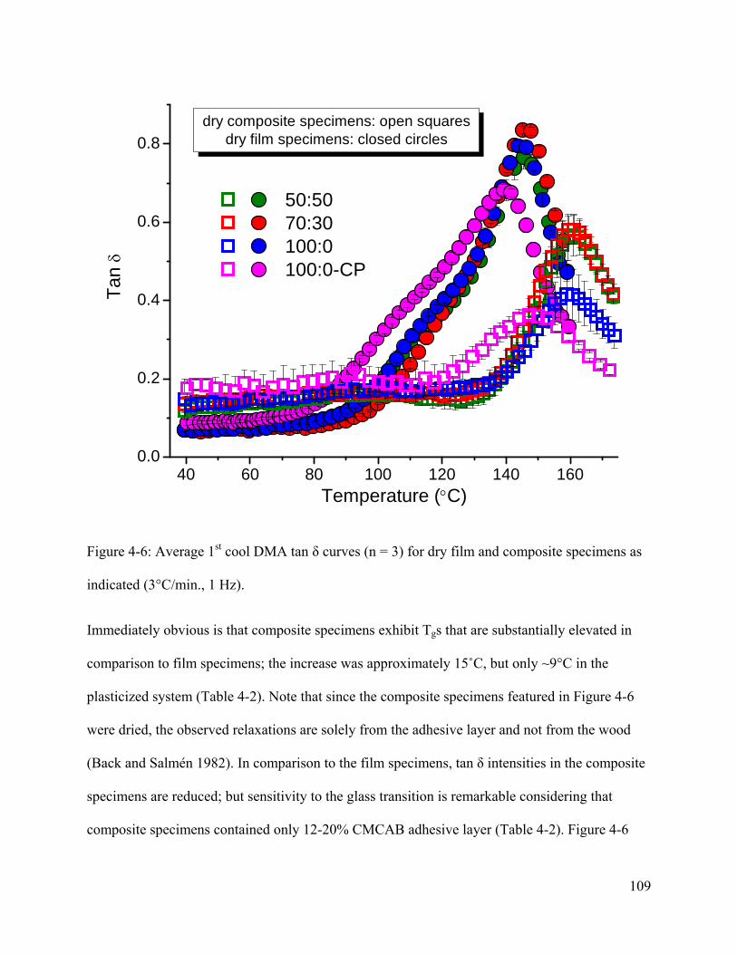
40 60 80 100 120 140 1600.0

0.2

0.4

0.6

0.8

Tan

δ

50:50 70:30 100:0 100:0-CP

Temperature (°C)

dry composite specimens: open squaresdry film specimens: closed circles

Figure 4-6: Average 1st cool DMA tan δ curves (n = 3) for dry film and composite specimens as

indicated (3°C/min., 1 Hz).

Immediately obvious is that composite specimens exhibit Tgs that are substantially elevated in

comparison to film specimens; the increase was approximately 15˚C, but only ~9°C in the

plasticized system (Table 4-2). Note that since the composite specimens featured in Figure 4-6

were dried, the observed relaxations are solely from the adhesive layer and not from the wood

(Back and Salmén 1982). In comparison to the film specimens, tan δ intensities in the composite

specimens are reduced; but sensitivity to the glass transition is remarkable considering that

composite specimens contained only 12-20% CMCAB adhesive layer (Table 4-2). Figure 4-6

109

demonstrates that a significant interaction occurs between CMCAB (salt form) and wood. Other

wood/adhesive systems exhibit similar, but more modest, effects, where wood increases the

adhesive Tg by only about 5 - 7°C (Hristov and Vasileva 2003; Lopez-Suevos and Frazier 2005,

2006). The wood/CMCAB interaction was very significant; a 9 - 15°C Tg increase implies that

the interaction dramatically reduced CMCAB backbone flexibility. When considering wood

/adhesive interactions it helps to define how such effects could occur. The term “interaction”

suggests that direct wood/CMCAB molecular contact occurs such that the entire adhesive layer

is impacted. Consequently, the wood/adhesive interaction might arise through primary and

secondary associations. As will be discussed in Chapter 5, the adhesive-layer thickness in this

work ranged from 40 – 90 microns. It would perhaps be remarkable if nanoscale secondary and

primary interactions could directly influence a bulk phase that is 40 – 90 microns thick.

Certainly, the potential for wood/CMCAB hydrogen bonding is great, and since 12% of the

carboxyl groups may be in the salt form, some potential for ionic interactions also exists. Also

possible is the formation of ester linkages between wood and CMCAB. However, the bonding

process was conducted at room temperature and so conditions for covalent attachment were not

optimized. Aside from these direct effects, a wood/adhesive interaction can also arise from

indirect effects. In the case of the CMCAB dispersion, it is possible that wood significantly

impacts the film formation process. For instance compared to a dispersion cast upon Teflon,

wood absorbency will dramatically accelerate water and solvent loss, and this would influence

particle coalescence and subsequent polymer packing. This point is consistent with the first heat

scans shown in Figure 4-7, where wet and dry composite specimens are compared.

110

25 50 75 100 125 150 175

0.1

0.2

0.3

0.4

0.5

0.6

0.7 T

an δ

100:0 Wet 100:0 Dry 100:0-CP Wet 100:0-CP Dry

Temperature (°C)

Figure 4-7: Average 1st heat DMA tan δ curves (n = 3) for 100:0 and 100:0-CP composites

specimens (wet and dry) as indicated (3°C/min., 1Hz).

Notice that the wet composite specimens exhibit very little or perhaps no residual solvent

(compare to dry film specimens in Figures 4-5 and 4-6). In the first heat, wet composite

specimens (Figure 4-7) exhibited a minor tan δ peak near 70˚C, and this peak was absent in the

corresponding dry specimens. While some residual solvent may have been detected in the wet

composite specimens, it is clear that wood facilitated the removal of solvent from the CMCAB

adhesive layer.

111

Recall though that the Tg’s listed in Table 4-2 and the DMA curves in Figure 4-6 are of first cool

scans where the solvo-thermal history was expected to have been erased from the CMCAB

response. However, specimens were only equilibrated at the high temperature for 2 minutes

which was perhaps too short to allow sufficient relaxation of indirect, wood induced, film

formation effects. Figure 4-8 and Figure 4-9 show average 50:50 wet composite and film

specimen first cool scans, respectively, with 2, 10, and 30 minute high temperature equilibration

times; average modulus and tan δ data are provided in Table 4-4.

120 140 160 180

10-3

10-2

10-1

100

120 140 160 1800.0

0.2

0.4

0.6

0.8

1.0

Nor

mal

ized

Mod

ulus

2 minutes 10 minutes 30 minutes

50:50-wet composite specimens

(b)

Tan

δ

Temperature (°C)

(a)

Figure 4-8: Average 50:50 wet composite DMA 1st cool (a) normalized modulus and (b) tan δ

profiles (n = 3, 3°C/min., 1 Hz).

112

80 100 120 140 160

10-3

10-2

10-1

100

80 100 120 140 1600.0

0.2

0.4

0.6

0.8

1.0G

' (P

a)

Temperature (°C)

2 minutes 10 minutes 30 minutes

50:50-wet film specimens

(a) (b)

Tan

δ

Figure 4-9:Average 50:50 wet film DMA 1st cool (a) normalized modulus and (b) tan δ profiles

(n = 3, 3°C/min., 1 Hz).

Table 4-4: Average 50:50 wet composite and film DMA 1st cool normalized modulus and tan δ

data (n = 3, 3°C/min., 1 Hz).

Sample High Temp.

Equilibration (m)

High Temp. Modulus

(Normalized)

First Cool Tg (°C)

Tg Increase

(°C) Peak Tan δ

50:50 Composite

2 2.6E-02 ±1.0E-02 162.8 ±0.6 - 0.63 ±0.09 10 6.3E-02 ±2.0E-02 164.8 ±0.8 2.0 0.53 ±0.04 30 1.5E-01 ±1.7E-02 168.2 ±0.8 5.4 0.40 ±0.02

50:50 Film

2 5.5E-04 ±1.4E-04 148.5 ±0.9 - 0.86 ±0.02 10 9.6E-04 ±2.1E-04 150.0 ±1.2 1.5 0.73 ±0.07 30 2.8E-03 ±1.2E-03 152.3 ±1.3 3.8 0.65 ±0.02

113

It was evident that with increased equilibration time, CMCAB chain mobility in the composite

specimens became more restricted, as shown by the increased high temperature modulus, the

reduced tan δ peak intensity, and the increased Tg (Figure 4-8 and Table 4-4). This is likely the

result of crosslinking in the bulk adhesive layer and between CMCAB polymers and wood. This

analysis offered little insight into the presence or lack of indirect effects having caused the

CMCAB/wood interaction; however it did offer evidence for direct CMCAB/wood interactions.

Figure 4-9 and Table 4-4 show the same crosslinking effect in film specimens; yet the observed

crosslinking modulus and tan δ effects were slightly greater in the composite specimens (Table

4-9). This further supports the possibility that direct effects contributed to the significant

CMCAB/wood interaction.

The precise nature of the wood/CMCAB interaction still requires further study because it

probably includes effects both from direct molecular interaction and also from the indirect

influence on film formation. Whatever the case may be, the wood/CMCAB interaction was

significant; and this implies that adhesion is favorable.

Additionally, note that wood influenced the plasticizer effect. In Figures 2-7, 4-5 and 4-6,

plasticized film specimens exhibit a clear tan δ shoulder. In contrast, Figure 4-7 shows that the

plasticized domain is not as well resolved; there is instead a single and broad relaxation. It was

also observed that vacuum drying did not affect the 1st heat Tg for the either system as shown in

Table 4-5.

114

Table 4-5: Average first heat Tgs (n = 3) for 100:0 and 100:0-CP composites (wet and dry) as

measured with DMA (3°C/min., 1 Hz).

Sample First Heat Tg (°C)

100:0-Wet 151.1 ±1.3 100:0-Dry 153.4 ±0.4

100:0-CP-Wet 142.8 ±1.1 100:0-CP-Dry 142.2 ±0.2

4.4 Conclusions

The thermal properties of CMCAB dispersion-born specimens were analyzed. Even after

extensive drying, films cast onto Teflon contained residual solvent. This residual solvent

complicated DSC analysis where it appeared that the CMCAB salt form exhibited a lower Tg

than was seen in the acid form. However, the effects of solvent contamination were better

resolved using DMA, and DMA revealed that the CMCAB acid and salt forms exhibited

identical Tgs. Composite specimens were excised directly from the bondlines of adhesion test

specimens. Even though the adhesive layer was a minor proportion of the composite specimens,

the adhesive layer DMA response was very good. DMA of the composite specimens revealed a

significant CMCAB/wood interaction; this was a 9˚C Tg increase in the plasticized specimen,

and a 15˚C Tg increase in unplasticized specimens. The precise nature of the wood/CMCAB

interaction was unknown; however it was found that wood facilitated solvent diffusion away

from the adhesive layer. This implied that the CMCAB/wood interaction involves indirect effects

that could impact particle coalescence and film formation. Additionally, high temperature

crosslinking effects were observed to be greater in composite specimens than in films which

115

suggested that direct effects of primary and secondary interactions also probably contributed to

the observed Tg increase. The observed strength of the CMCAB/wood interaction suggested that

adhesion was favorable in these composite specimens.

116

117

4.5 References

Back, E. L. and Salmén, N. L. (1982) Glass transitions of wood components hold implications for molding and pulping processes. Tappi 65, 107-110. Hristov, V. and Vasileva, S. (2003) Dynamic mechanical and thermal properties of modified poly(propylene) wood fiber composites. Macromolecular Materials and Engineering 288, 798-806. Lopez-Suevos, F. and Frazier, C. E. (2005) Parallel-plate rheology of latex films bonded to wood. Holzforschung 59, 435-440. Lopez-Suevos, F. and Frazier, C. E. (2006) Fracture cleavage analysis of PVAc latex adhesives: Influence of phenolic additives. Holzforschung 60, 313-317.

5 CMCAB Adhesive Performance

5.1 Introduction

Having optimized CMCAB dispersions for high solids content and controllable viscosity, and

after demonstrating a favorable wood/CMCAB interaction, this chapter focuses on adhesion

performance as tested using mode-I fracture. Wood adhesive viscosity impacts penetration and

the resulting adhesive layer thicknesses (Ebewele et al. 1979; Kamke and Lee 2007); in turn,

penetration and adhesive layer thickness play a critical role in adhesive-joint performance

(Ebewele et al. 1979; Ebewele et al. 1986; Kamke and Lee 2007). Consequently, this chapter

attempts to correlate fracture toughness with dispersion viscosity, adhesive-layer thickness, and

also adhesive penetration.

5.2 Experimental

5.2.1 Materials

CMCAB-641-0.2 (CMCAB-Low) was kindly provided by Eastman Chemical Co. Ethylene

glycol butyl ether (EGBE) (≥99% pure), methyl propyl ketone (MPK) (≥99% Ultra pure grade),

N,N - dimethylethanolamine (DMEA) (≥99.5% pure), and triethyl O-acetylcitrate (CP) (≥99%

pure) were purchased from Sigma-Aldrich. Ultra-pure, de-ionized water was obtained with a

Millipore Direct-Q 3 filtration system. Safranin O powder was purchased from Fisher Scientific

and used in solution (0.5 wt% in water) for better adhesive penetration visualization.

118

5.2.2 Methods

5.2.2.1 Dispersion Preparation

In Chapter 4, 200 g CMCAB dispersions 50:50, 70:30, 100:0, and 100:0-CP were prepared with

40% (mixed solvent) and 35% (100% EGBE) target solids contents; these systems were used to

bond laminates from which DCB fracture specimens were obtained. Smaller batches (100 g) of

each formulation were prepared with the same mixing procedure (described in Chapter 4) to be

used for viscosity measurements.

5.2.2.2 Viscometry

5.2.2.2.1 Cone-and-plate

Dispersion viscosities (both the 200 g systems used for bonding and the 100 g systems

specifically for viscometry) were measured with a steel cone-and-plate geometry (~0.6 mL, 40

mm dia., 1:59°, 57 μm gap, 25°C) on a TA Instruments AR 1000 rheometer; shear rates were

ramped from ~0.03 - 1000 s-1 in steady-state flow. A steel “solvent-trap” cover minimized

solvent evaporation. All tests were performed in triplicate.

5.2.2.2.2 Concentric Cylinder

The 100 g dispersion viscosities were also measured with a concentric cylinder geometry (~20 -

21 g, conical rotor: 14 mm radius, 42 mm height; cup: 15 mm radius; gap: 1 mm; 25°C) on a TA

Instruments AR G2 rheometer; shear rates were ramped from ~0.03 - 1000 s-1 with steady-state

flow. All tests were performed in triplicate.

5.2.2.3 Adhesive-layer Thickness Measurements

The term “bondline” is defined as wood on either side of the “adhesive layer”; subsequently, the

“adhesive-layer” is the dispersion film layer not including wood. Bondlines of 5 random DCB

119

specimens were observed under 100 X magnification with a Nikon SMZ1500 stereoscope

equipped with a Nikon DS-Fi1 digital camera. One image was collected from each 1/3 of the

effective fracture test length (DCB length subtracting 50 mm from either end); three equally-

spaced adhesive-layer thickness measurements were taken from each image with NIS-Elements

BR 3.1 image analysis software.

5.2.2.4 Mode I Fracture Testing

DCB specimens, as shown in Figure 5-1, were equilibrated to ~12% moisture content (MC)

(20°C, 65% relative humidity, 14 days). Specimens were removed from the environmental

chamber one-at-a-time, and tested in mode I cleavage, similar to the method described in

Gagliano and Frazier (2001). Immediately prior to testing, loading-pin holes (3.8 mm dia.) were

drilled through each specimen (Figure 5-1). One edge of the bondline was coated with white

typographic correction fluid, and a millimeter scale was attached directly below the bondline to

aid in crack length visualization. A chisel and vise were used to initiate a 50 mm pre-crack, as

measured from the center of the loading-pin holes. DCB free-ends were supported horizontally

prior to loading to minimize joint stress.

1030

Grain angle ≈ 3

5

20

10

Figure 5-1: DCB specimen geometry and dimensions (in mm).

Testing was conducted with TestWorks 4.0 and a screw-driven MTS (Model GL-10) with a 1000

N load cell; a 10 - 12 N pre-load was first applied to each specimen, whereupon the displacement

120

was zeroed. Loading was initiated at 1 mm/min; subsequent cycle’s loading rates were adjusted

such that crack extension occurred within approximately 1 min. For an individual cycle, when

the loading curve went non-linear, the critical load was recorded and cross-head extension was

fixed, allowing the crack to extend and arrest; crack propagation was observed at 10X

magnification with a digital camera and live-feed monitor. After 45 s, the arrest load was

recorded, and the cross-head automatically returned to zero, where upon a subsequent cycle was

began, as shown in Figure 5-2.

0 1 2 3 4 5 6 7 8 9 100

20

40

60

80

100

120

Arrest

Load

(N)

Extension (mm)

Critical

Figure 5-2: Representative mode I fracture DCB specimen load vs. cross-head extension plot.

Data was collected within 50 mm from either end of DCB specimens. Critical and arrest mode I

fracture energies, GIc and GIa, were calculated as follows (Gagliano and Frazier 2001):

121

5-1

 

where Pc is the critical load causing crack initiation (the arrest load, Pa, was used to calculate

GIa), a is the crack length, B is the DCB width, (EI)eff is the effective flexural modulus of rigidity,

and χ is a shear correction factor for low shear-modulus adherends (Blackman et al. 1991). (EI)eff

and χ are calculated from experimental data with equations 5-2 and 5-3:

5-2

 2

3

5-3

where m and b are the slope and intercept, respectively, obtained from a linear fit of the

specimen cubed root of compliance (C1/3) versus crack length plot, as shown in Figure 5-3.

122

0.03 0.06 0.09 0.12 0.15 0.180.02

0.03

0.04

0.05

0.06

Crack Length, a (m)

(Com

plia

nce)

1/3 (m

/N)1/

3 Y = 0.345 X + 0.005R2 = 0.996

Figure 5-3: Representative mode I fracture DCB specimen cubed-root compliance vs. crack

length plot and linear fit (m = 0.345, b = 0.005).

A sensitivity analysis determined that 0.96 was the minimum acceptable linear C1/3 correlation

coefficients (R²) for this study; all adhesive specimens were within this limit. Each DCB

specimen yielded between 10 and 20 cycles, and 10 random DCBs were tested for each adhesive;

average results included all individual cycle energies from each treatment (n = 130 - 173).

5.2.2.5 Adhesive Penetration Analysis

Small composite specimens, (~30x10x10 mm³, long x rad x tan) were excised from the untested

region (last 50 mm) of 5 random DCB specimens per dispersion. Specimens were soaked in

deionized water (~24 hrs, ~25°C); 30 μm thick cross-sectional slices were cut from each

123

specimen with a Sledge Microtome “G.S.L. 1.” Sections were loaded onto microscope slides and

stained with a 0.5% Safranin O solution; after ~1 minute excess stain was washed away with

deionized water. Cover-slips were temporarily secured with small weights, and sections were

allowed to dry on a hot plate (~60 - 90°C, ~12 hours); cover slips were then permanently

mounted with nail varnish.

Adhesive penetration was observed at 50 X magnification using a Zeiss Axioskop epi-

fluorescence microscope with a 100 W HBO lamp; the optical filter set consisted of a 360 nm

excitation filter, 400 nm dichromatic mirror, and a 420 nm emission filter. Earlywood lumen

maximum penetration (MP) was measured with a simple average representing a modified form

of the MP equation described in Sernek et al. (1999):

5-4

MPearlywood∑ yin1n

where yi is the distance from the wood/adhesive layer interface to the furthest edge of adhesive

object i (1 of 5 deepest/image), and n is the total number of measurements. Between 1 and 2

images were collected per section (40 - 50 measurements/adhesive). When no penetration, or

fewer than 5 objects, occurred in an image, zeros were used for yi values.

5.2.2.6 Data Analysis

Raw viscosity data was analyzed using TA Rheology Advantage Data Analysis version 5.6.0.

Critical and arrest fracture loads and slopes were identified with TestWorks 4.0. Adhesive-layer

thickness and penetration were measured using NIS-Elements BR 3.1 image analysis software.

Fracture and penetration data were processed in Microsoft Office Excel 2007. All fitting,

124

averaging and statistical analyses were performed using OriginPro version 8.0.63. Average

viscosity plots were prepared with the “Average Multiple Curves” function and a tolerance of

0.01 s-1. ANOVAs with “Bonferroni comparison of means tests” were employed to determine

mean thickness, toughness, and penetration differences (α = 0.05).

5.3 Results and Discussion

5.3.1 Dispersion Viscosities

Figure 5-4 shows average flow curves for CMCAB dispersions using cone-and-plate geometry.

0.01 0.1 1 10 100 1000100

101

102

103

104

105

106

107

50:50 70:30 100:0 100:0-CP

Vis

cosi

ty (m

Pa•

s)

Shear Rate (1/s)

50:50 and 70:30 - 40% solids100:0 and 100:0-CP - 35% solids

Figure 5-4: Average dispersion steady-state viscosity v. shear rate flow curves (cone-and-plate,

25°C, n = 3).

125

The dispersions are shear-thinning and lower-shear rate viscosities increase with percent EGBE,

even though 100% EGBE systems have lower % solids (APPENDIX 1). This echoes previous

findings that dispersion viscosities increase with the EGBE content (Chapter 3). Past a critical

shear rate (~100 s-1), an extreme shear thinning is observed; this effect is solvent-system

dependent as 100:0 shear-thins to the greatest degree.

A second, smaller-scale (100 g) batch of each dispersion formulation was prepared specifically

for concentric cylinder viscometry. Additionally, a pair-wise cone-and-plate measurement was

conducted for these systems as an appropriate comparison of the same material; Figure 5-5

shows these results. The measured % solids from these additional (viscometry only) systems are

also provided in APPENDIX 1.

126

10-2 10-1 100 101 102 103100

101

102

103

104

105

106

107

10-2 10-1 100 101 102 103100

101

102

103

104

105

106

107

50:50 and 70:30 - 40% solids100:0 and 100:0-CP - 35% solids

Vis

cosi

ty (m

Pa•

s)(a) (b)

50:50 70:30 100:0 100:0-CP

Shear Rate (1/s)

Figure 5-5: Average dispersion (100 g batch specifically for viscosity measurements) steady-

state viscosity v. shear rate flow curves measured with (a) cone-and-plate and (b) concentric

cylinders geometries (25°C, n = 3).

Figure 5-4 and Figure 5-5a are not identical; this indicated variability in the mixing procedure

between batches likely due to a reduction in instrument power and different batch sizes (200 g

vs. 100 g).

The geometry comparison shows flow curves still became steeper past a critical shear rate; this

effect is more severe with the cone-and-plate, and again 100:0 showed it to the greatest degree.

However, the difference between the two methods could be related to viscometer gap-size

127

effects, where the dispersion particle size may exceed the 57 μm gap in the cone and plate

geometry; but this is not a likely concern with the concentric cylinder geometry, having a 1000

μm gap

Wood anatomy will also induce a particle-size/viscosity dependence during consolidation, as

softwood tracheids are only several 10s of microns in diameter (Panshin and De Zeeuw 1980). In

addition, it was observed that dispersion viscosities increased rapidly when applied to wood as

water and solvent diffused into the porous substrate. Therefore, viscosities during bonding may

be more complex than could be described with aforementioned steady state flow experiments; in

other words, the results in Figure 5-4 are not negated by those in Figure 5-5b for possibly

describing the nature of the dispersions during wood bonding.

5.3.2 Adhesive-layer thickness Measurements

A preliminary adhesive-layer thickness analysis described in APPENDIX 2 revealed that 100:0

systems containing 40% solids produced significantly thicker adhesive-layers than 50:50 and

70:30 systems; reducing the 100:0 solids to 35% affectively yielded a bondline of comparable

thickness. This is why the CMCAB dispersions were prepared with their respective target solids

contents (35% and 40%). Figure 5-6 shows the average adhesive-layer thickness results for DCB

adhesion test specimens.

128

0

20

40

60

80

100

120 50:50 and 70:30 - 40% solids100:0 and 100:0-CP - 35% solids

C

B

A

100:0-CP100:070:30

Adhe

sive

-Lay

er T

hick

ness

(μm

)

Adhesive50:50

A

Figure 5-6: Average DCB adhesive-layer thicknesses (n = 45); error bars represent ±1 standard

deviation.

Average adhesive-layer thicknesses were not equal; however, all were of the same order of

magnitude, and so the fracture results were not expected to be complicated by bondline thickness

effects.

5.3.3 Mode I Fracture Performance

Mode I fracture energies were determined for 10 random DCB specimens; Figure 5-7 shows a

representation of the results from a single 100:0 DCB specimen.

129

0.050 0.075 0.100 0.125 0.150 0.1750

50

100

150

200

250 Critical Arrest

Ener

gy (J

/m2 )

Crack Length, a (m)

Figure 5-7: Representative energy v. crack length plot for a DCB specimen (100:0) tested in

mode I cleavage.

As previously mentioned, this test yielded individual cycle energies, independent of crack length,

and CMCAB DCB specimens produced between 10 and 20 cycles with corresponding critical

and arrest energies. Average GIc and GIa values are provided in Table 5-1 and Figure 5-8.

130

Table 5-1: Average CMCAB adhesive-joint critical and arrest mode I fracture energies, ± 1

standard deviation (SYP ~12% MC, 25°C)

Adhesive Critical Energy, GIc (J/m²)

Arrest Energy, GIa (J/m²)

n

50:50 59.2 ±19.2 50.3 ±17.5 165 70:30 61.8 ±17.0 53.1 ±16.3 157 100:0 149.2 ±45.1 127.9 ±36.3 173

100:0-CP 147.8 ±60.3 125.5 ±48.8 130

50:50 70:30 100:0 100:0-CP0

20

40

60

80

100

120

140

160

180

200

n=130n=173

n=157

BB

A

Critical Arrest

Frac

ture

Ene

rgie

s (J

/m2 )

Adhesive System

A

n=165

Figure 5-8: Average CMCAB adhesive-joint critical and arrest mode I fracture energies; error

bars represent 1 standard deviation (SYP ~12% MC, 25°C).

131

Adhesives 50:50 and 70:30 yielded similar, very low fracture toughness’s; the 100:0 system, on

the other hand provided significantly increased GIc and GIa values. Yet, ~150 J/m² is still fairly

brittle, and considered low for typical wood adhesives. Thermosetting phenol-formaldehyde,

urea-formaldehyde, and phenol-resorcinol-formaldehyde resins typically produce critical mode I

fracture energies between 200 and 900 J/m² depending on wood species and the presence of

various additives (Ebewele et al. 1980; Gagliano and Frazier 2001; River 1994); toughened

epoxies and thermoplastic polyvinyl acetate adhesive GIc values can be up to ~1000 - 1500 J/m²

(Lopez-Suevos and Frazier 2006; River 1994).

In this research, the 50:50, 70:30, and 100:0 systems were tested first. Cellulose-based

thermoplastics are often brittle, therefore plasticizers are commonly included to improve crack

resistance and film toughness (Wadey 2001). In Figures 2-7, 4-5 and 4-6, plasticized film

specimens exhibit only a slightly reduced Tg, implying fracture measurements would still be

probing the polymers in their glassy state; however, a clear tan δ shoulder is also observed for

these film specimens. It is known that heterogeneous polymer systems can often complicate the

path of a propagating crack, resulting in increased toughness values (Shin and Jang 1997); this

has been demonstrated for brittle epoxy films using both inorganic nano-particles and separately

using larger phase, high Tg thermoplastic polymers as fillers (Bucknall and Partridge 1983; Deng

et al. 2007; Kim et al. 2008; Shin and Jang 1997). The shoulder present in CP films is analogous

to the thermoplastic polymer additive epoxy-toughening case, where two polymers are present

both with high Tg values (Bucknall and Partridge 1983).

Therefore it was considered that additional toughening might have occurred by this dual-phase

mechanism rather than sub-ambient Tg depression. Yet, when wet-composite specimens obtained

from DCB bondlines were tested, the residual solvent was no longer present due to the more

132

efficient drying process imposed by the wood substrate; Figure 5-9 again shows the affect of 5%

CP on the CMCAB Tg in composite bondlines.

25 50 75 100 125 150 1750.1

0.2

0.3

0.4

0.5

0.6

0.7

0.8

Tan

δ

100:0 100:0-CP

Temperature (°C)

Figure 5-9: Average 1st heat DMA tan δ curves (3°C/min., 1Hz, n = 3) for wet 100:0 and 100:0-

CP composites (Chapter 4).

The CP system had nearly the same tan δ profile as the 100:0 system, with only a slightly

reduced Tg and broader peak. Therefore, it was unfortunate, but not surprising that 5% CP

addition failed to provide additional toughness to the 100:0 system.

133

Triethyl O-acetylcitrate, however, is just one of many plasticizers compatible with CMCAB

polymers (Obie 2006). In addition to plasticizer type and content, dispersions can be formulated

with numerous different solvents, neutralizing amines, degrees of neutralization, and even

different CMCAB polymers (molecular weight and degrees of substitution). Therefore, although

GI values are currently lower than desired, it is believed that future dispersion optimization can

improve CMCAB adhesive-joint performance; initial ~150 J/m² GIc values (Table 5-1 and Figure

5-8) are encouraging for these novel renewable adhesives.

5.3.4 Adhesive Penetration

To help explain GI differences between the mixed solvent and 100% EGBE systems, adhesive

penetration was observed with fluorescence microscopy. Earlywood lumen penetration was

considered in this study; Figure 5-1 shows a representative penetration image for each adhesive.

134

50:50

70:30

100:0

100:0‐CP

(a)

(b)

(c)

(d)

Figure 5-10: Representative earlywood cross-sectional photomicrographs observed with epi-

fluorescence (50X, 0.5% Safranin O stain, filter set 360 nm/400 nm/420 nm); 100 μm scale bars.

Images only show one side of the bondline, as joints failed during section preparation. This

suggested that CMCAB adhesive formulations may also need to be optimized for greater

moisture durability. No official durability study was conducted in this research; however it was

discovered that water-submersion significantly plasticized CMCAB dispersion-cast films

(APPENDIX 3).

Mixed solvent systems had very low, if any, penetration, whereas 100% EGBE systems showed

significant adhesive penetration; Table 5-2 and Figure 5-11 provide the average penetration

results.

135

Table 5-2: Average SYP earlywood CMCAB adhesive penetration ± 1 standard deviation.

Adhesive Penetration (μm) n

50:50 64.2 ±78.83 45 70:30 68.1 ±54.42 45 100:0 255.1 ±151.05 50

100:0-CP 151.3 ±73.37 40

0

50

100

150

200

250

300

350

400

C

B

A

100:0-CP100:070:30

Pene

tratio

n (μ

m)

Adhesive

n=45 n=45

n=50

n=40

50:50

A

Figure 5-11: Average SYP earlywood CMCAB adhesive penetration; error bars indicate ±1

standard deviation.

Mixed solvent systems had the same average penetration depth, which was significantly lower

than the 100% EGBE systems. Previous research has shown that wood-adhesive penetration

136

clearly improves joint toughness (Ebewele et al. 1986); penetration results appeared to directly

correlate with the fracture results for the mixed solvent and 100:0 adhesives (Figure 5-8). The CP

system, on the other hand, did not penetrate as deeply as the 100:0 system (p = 5.7E-5), and yet

the fracture energies of these systems were the same (Table 5-1 and Figure 5-8). Although

penetration is important for wood adhesives, there is not a direct correlation between penetration

depth and bond-performance (Kamke and Lee 2007); it may be then that both the CP and 100:0

systems merely reached some minimum optimal penetration depth. Yet, this phenomenon

deserves further investigation.

Wood-adhesive penetration is impacted by adhesive viscosity and the applied consolidation

pressure during bonding (Kamke and Lee 2007; Sernek et al. 1999); an attempt was made to

correlate the penetration results with the dispersion cone-and-plate viscosity results (Figure 5-4).

As these systems are shear-thinning, such a correlation required identifying the shear rate they

were subject to during consolidation. For a shear-rate (γ̇ ) approximation, the wood cells were

considered as cylinders, and the equation for the shear rate of a fluid flowing through a pipe was

chosen (Darby 2001):

5-5

γ=8νD

Where D is the diameter of the pipe (cell lumen), and ν is the linear fluid viscosity, calculated as:

5-6

ν=V

A*t

137

Where V is the volume of material, A is the area of the pipe, and t is the flow time. Earlywood

cell diameters were directly measured from experimental photomicrographs to be ~50 μm, and

the volume was assumed to be that of a Loblolly Pine (Pinus taeda) tracheid (length = 4.33 mm)

(Panshin and De Zeeuw 1980). With a press closing time between 2 - 3 seconds, a shear rate

between 350 and 230 s-1 was estimated. In this range the 100:0 adhesive had the lowest viscosity

followed by the CP system and then the mixed solvent which had similar viscosities in this shear

range (Figure 5-4). This would appear to clearly explain the differences in penetration depths

between the adhesives. However, the concentric cylinder viscosity results did not show the same

extreme shear-thinning behavior (Figure 5-5b). As previously mentioned; the viscosity

differences between geometries were believed caused by particle size affects, and wood cells,

too, may induce a particle size limit. Therefore, the aforementioned penetration/cone-and-plate

viscosity correlation is not necessarily negated by the concentric cylinder results; merely, the

particle size assumption deserves further investigation.

5.4 Conclusions

Dispersion viscosities were measured with two different techniques. The flow curves differed

depending on the experimental geometry used; however, both techniques showed CMCAB

dispersion viscosities were shear-thinning and dependent on the formulation solvents.

DCB adhesive-layer thicknesses were not equal across all dispersion systems. However, they

were all within the same order of magnitude, and therefore considered adequate for fracture test

comparisons.

Mixed solvent dispersions produced low fracture energies representing a brittle adhesive-joint.

The 100:0 system was significantly tougher than the mixed solvent systems, yet, it too exhibited

138

lower GIc values than typical wood adhesives. Additionally, a system containing 5% triethyl O-

acetylcitrate plasticizer did not increase fracture toughness. However, this is just the beginning of

CMCAB-adhesive studies, and variable formulations may be created to optimize adhesive-joint

toughness values.

Penetration measurements showed the mixed solvent systems did not penetrate deeply, and in

some cases not at all, into the SYP adherends; the 100% EGBE systems on the other hand did

show considerable penetration. The 50:50, 70:30, and 100:0 systems’ penetration and fracture

energies show a direct correlation; however the differences in penetration depths between the

100:0 and 100:0-CP systems did not affect their fracture energies. Additionally, penetration

depths appear to correlate with adhesive cone-and-plate viscosity measurements, yet this

hypothesis requires additional investigation. Lastly, the possible correlations between viscosity,

penetration depth, and fracture toughness are all solvent system dependent.

139

5.5 References Blackman, B., Dear, J. P., Kinloch, A. J. and Osiyemi, S. (1991) The calculation of adhesive fracture energies from double-cantilever beam test specimens. Journal of Materials Science Letters 10, 253-256. Bucknall, C. B. and Partridge, I. K. (1983) Phase separation in epoxy resins containing polyethersulphone. Polymer 24, 639-644. Darby, R. 2001. Chemical engineering fluid mechanics. Marcel Dekker, New York Deng, S. Q., Ye, L. and Friedrich, K. (2007) Fracture behaviours of epoxy nanocomposites with nano-silica at low and elevated temperatures. Journal of Materials Science 42, 2766-2774. Ebewele, R., River, B. and Koutsky, J. (1979) Tapered double cantilever beam fracture tests of phenolic-wood adhesive joints .Part I. Development of specimen geometry - Effects of bondline thickness, wood anisotropy and cure time on fracture energy. Wood and Fiber 11, 197-213. Ebewele, R. O., River, B. H. and Koutsky, J. A. (1980) Tapered double cantilever beam fracture tests of phenolic-wood adhesive joints .part II. Effects of surface-roughness, the nature of surface-roughness, and surface aging on joint fracture energy. Wood and Fiber 12, 40-65. Ebewele, R. O., River, B. H. and Koutsky, J. A. (1986) Relationship between phenolic adhesive chemistry and adhesive joint performance - Effect of filler type on fracture energy. Journal of Applied Polymer Science 31, 2275-2302. Gagliano, J. M. and Frazier, C. E. (2001) Improvements in the fracture cleavage testing of adhesively-bonded wood. Wood and Fiber Science 33, 377-385. Kamke, F. A. and Lee, J. N. (2007) Adhesive penetration in wood - a review. Wood and Fiber Science 39, 205-220. Kim, B. C., Park, S. W. and Lee, D. G. (2008) Fracture toughness of the nano-particle reinforced epoxy composite. Composite Structures 86, 69-77.

140

141

Lopez-Suevos, F. and Frazier, C. E. (2006) Fracture cleavage analysis of PVAc latex adhesives: Influence of phenolic additives. Holzforschung 60, 313-317. Obie, R. 2006: Use of carboxymethyl cellulose acetate butyrate as a precoat or size for cellulosic man-made fiber boards. United States Patent and Trademark Office, United States: Eastman Chemical Corporation, 1-20. Panshin, A. J. and De Zeeuw, C. 1980. Textbook of wood technology : structure, identification, properties, and uses of the commercial woods of the United States and Canada. McGraw-Hill, New York River, B. H. 1994: Fracture of adhesive-bonded wood joints. In Pizzi, A. and Mittal, K. L., editors, Handbook of Adhesive Technology, New York: Marcel Dekker, Inc., 151- 177. Sernek, M., Resnik, J. and Kamke, F. A. (1999) Penetration of liquid urea-formaldehyde adhesive into beech wood. Wood and Fiber Science 31, 41-48. Shin, S. and Jang, J. (1997) Toughness improvement of high-performance epoxy resin using aminated polyetherimide. Journal of Applied Polymer Science 65, 2237-2246. Wadey, B. L. 2001: Plasticizers. In Robert, A. M., editor, Encyclopedia of Physical Science and Technology, New York: Academic Press, 441-456.

6 Conclusions and Future Work

Carboxymethylcellulose acetate butyrate (CMCAB) mixed esters were analyzed in the free acid

form (powders and solution-cast films) and in the water-dispersible salt form (dispersions, films,

and wood-adhesive composite specimens). Analytical testing consisted of standard acid number

determinations, differential scanning calorimetry, dynamic mechanical analysis, viscometry,

mode I fracture testing, and light and fluorescence microscopy. The major conclusions of this

research are summarized as follows:

1. Two commercial CMCAB samples were studied, where the principal difference was

thought to be in molecular weight. However, these samples had different acid numbers,

and more importantly, the high molecular weight sample contained insoluble gel

particles. Consequently, the high molecular weight sample was excluded from detailed

studies of dispersion formulation and adhesion testing.

2. By visual inspection, the low molecular weight CMCAB sample formed good water

dispersions with solids contents up to 40%. The viscosities of these dispersions exhibited

a strong dependence on the organic solvents used in the formulation. Mixtures of MPK

and EGBE provided good dispersions with viscosities that were much lower than for

dispersions using EGBE only.

3. Dilute solution viscometry of CMCAB (acid form) did not provide clear insight into

solvent effects that impacted the dispersion viscosity. This suggested that the CMCAB

salt form exhibited solvation effects that were completely different from the acid form. It

also suggested that dispersion viscosity is probably impacted by complex solvation

effects that alter the dispersion particle size, which was not studied here.

142

4. While the salt form of CMCAB probably impacted solvation effects, it was found that the

presence of the alkyl ammonium salts did not alter the CMCAB glass transition.

5. Residual solvent in dispersion-born films complicated thermal analysis using DSC, but

DMA was able to clarify this complication.

6. Adhesion test specimens were machined such that bondlines were successfully excised

and analyzed using DMA. This revealed a significant wood/CMCAB interaction where

wood caused a large increase in the CMCAB Tg.

7. While DMA showed a strong CMCAB/wood interaction that suggested good adhesion,

mode-I fracture testing revealed that the bondline toughness was relatively low. A citrate

plasticizer (5%) did not improve bondline toughness.

8. Lastly, adhesive viscosity, film formation, penetration, and fracture toughness are

dependent on organic solvent components (type and amount); moreover these properties

show possible correlations to each other.

This project introduced the use of CMCAB water-dispersions as novel renewable wood

adhesives. As mentioned, CMCAB appears to interact strongly with wood, and so potential

exists for its use as a wood adhesive. However and perhaps not surprisingly, CMCAB exhibited

brittle behavior that must be overcome if this system will become a significant wood adhesive.

However, this research represents only the initial steps towards optimization for wood adhesive

application. Additional plasticizers and/or various other toughening mechanisms should be

further investigated. Future research should include a dispersion particle-size analysis and an

investigation of the various polymer salt/solvent interactions to better understand the viscosity

and penetration effects. Also, the potential for wood/CMCAB covalent bonding should be

explored, as well as other methods to incorporate effective crosslinking.

143

7 APPENDICES

APPENDIX 1

Solids Content Measurement - TGA

Introduction

Dispersions prepared in Chapter 4 (200 g systems used for bonding) and Chapter 5 (100 g

systems used for viscometry) had target solids contents of 40% for the mixed solvent systems

and 35% for the pure EGBE systems. This appendix presents actual % solids measured with

thermogravimetric analysis (TGA).

Experimental

Adhesive % solids were determined with a TA Instruments Q500 TGA with high-res. dynamic

mode (20 - 80 mg, ~25°C - 800°C, 20°C/min, sensitivity: 1.0, resolution: 3.0, dry air 60

mL/min). Solids contents were recorded as the weight % value corresponding with a minimum in

the derivative weight % trace; as shown in Figure 7-1. Three replicates were performed for the

200 g dispersions, and two replicates were adequate for the additional viscometry systems. Raw

TGA data was analyzed using TA Universal Analysis 2000 version 4.5A.

144

100 200 300 400 500 600 700

0

20

40

60

80

100W

eigh

t (%

)

Temperature (°C)

Weight

0.0

0.5

1.0

1.5

2.0

Derivative Weight

Der

ivat

ive

Wei

ght (

%/°C

)

Target: 35%Measured: 35.41% (229.1°C)

Figure 7-1: Representative 100:0 weight and derivative weight curves vs. temperature, as

indicated, measured with High-res TGA (20°C/min in air, sensitivity: 1.0, res.: 3.0).

Results

Table 7-1 provides average solids contents for both dispersion batches prepared and used in

Chapter 4 and Chapter 5.

145

Table 7-1: Average dispersion % solids ± 1 standard deviation; bonding systems (n = 3) and

additional viscometry systems (n = 2) measured with High-res TGA (20°C/min in air, sensitivity:

1.0, res.: 3.0).

Dispersion Solids Content (%)

Target Bonding Systems

Additional Viscometry

Systems 50:50 40 42.0 ±0.3 41.5 70:30 40 41.2 ±0.4 41.2 100:0 35 35.5 ±0.5 35.6

100:0-CP 35 36.9 36.0 ±0.2

During mixing, condensation was observed on the inner walls of each container, explaining the

differences between theoretical and actual % solids. Additionally, the boiling point of Triethyl

O-acetylcitrate was ~229°C at 100 mmHg, and was present in the 100:0-CP system at 1.75%

(Table 4-1) explaining the observed increase in % solids over the 100:0 system. These average

solids contents were used in determining adhesive solid spread-rates.

146

APPENDIX 2

Adhesive-Layer Thickness Measurements

Introduction

This appendix addresses adhesive-layer thickness measurements used for CMCAB dispersion

optimization.

Experimental

Materials

CMCAB-641-0.2 (CMCAB-Low) was kindly provided by Eastman Chemical Co. Ethylene

glycol butyl ether (EGBE) (≥99% pure), methyl propyl ketone (MPK) (≥99% Ultra pure grade),

and N,N - dimethylethanolamine (DMEA) (≥99.5% pure) were purchased from Sigma-Aldrich.

Ultra-pure, de-ionized water was obtained with a Millipore Direct-Q 3 filtration system.

Commercial southern yellow pine (Pinus spp.) lumber (sapwood; free of knots and other visible

defects) was purchased from a local building supplier.

Dispersion Preparation

Small-scale dispersions (10 g, 12% DMEA neutralization, 45% continuous phase) were prepared

with either a single solvent, EGBE, or an EGBE:MPK solvent mixture, using the direct method

(described in Chapter 3). Two 100% EGBE systems consisted of 35% and 40% solids; two

mixed solvent systems (EGBE:MPK wt% ratios 50:50 and 70:30) both had 40% solids contents.

Dispersions used in this study are hereafter referred to with the prefix “AL” indicating their use

for “adhesive-layer” thickness measurements.

147

Adhesive-Layer Thickness Measurements

SYP specimens (120x30x10 mm³, long x tan x rad) with ~3° grain angles (as described in

Chapter 4) were prepared and bonded with the AL dispersions (269 g/m, 1.38 MPa, ~25°C, 24

hours). The outer 5 mm along the composite edges were removed and discarded. Side-grain

bondlines were observed under 100 X magnification with a Nikon SMZ1500 stereoscope

equipped with a Nikon DS-Fi1 digital camera. Bondline images (3 - 4 per specimen) were taken

randomly along the specimen lengths; adhesive-layer thicknesses were measured from images

with NIS-Elements BR 3.1 image analysis software (n = 11 - 20).

Results

Figure 7-2 shows representative bondline images for AL dispersions; Figure 7-3 shows the

average AL dispersion adhesive-layer thicknesses.

148

(a) AL 50:50 – 40%

(b) AL 100:0 – 40%

(b) AL 70:30 – 40%

(d) AL 100:0 – 35%

Figure 7-2 Representative AL dispersion bondline images as indicated (100 X, scale bars = 100

μm).

149

0

10

20

30

40

50

60

70

80

90

100

AL 100:0-35%

AL 100:0-40%

AL 70:30-40%

Adh

esiv

e-La

yer T

hick

ness

(μm

)

AL 50:50-40%

Figure 7-3: Average AL dispersion adhesive-layer thicknesses as indicated (n = 11 - 20); error

bars represent ±1 standard deviation.

The 40% solids AL systems were prepared and measured first. The AL 100:0-40% system

yielded an adhesive layer significantly thicker than the other two systems; this was unacceptable

for appropriate fracture toughness comparisons. Consequently, the AL 100:0-35% system was

prepared in an attempt to achieve a comparably-thick adhesive layer (by means of a reduced

viscosity). Indeed, this system did produce a comparable adhesive-layer. This is why the 100%

EGBE dispersions discussed in Chapter 4 and Chapter 5 were prepared with a target 35% solids

compared to 40% for mixed solvent systems.

150

APPENDIX 3

Water-Submersion DMA

Introduction

The thermal stability of CMCAB dispersion-cast films was investigated with water-submersion

DMA, in which the specimen is tested in the parallel-plate torsion while fully immersed in water.

Experimental

Materials

CMCAB-641-0.5 (CMCAB-High) was kindly provided by Eastman Chemical Co in powder

form. Ethylene glycol butyl ether (EGBE) (≥99% pure) and N,N - dimethylethanolamine

(DMEA) (≥99.5% pure) were purchased from Sigma-Aldrich. Ultra-pure, de-ionized water was

obtained with a Millipore Direct-Q 3 filtration system. Phosphorous pentoxide (P2O5) was

purchased from Fisher Scientific.

Specimen Preparation

A CMCAB-High dispersion (15% solids, 100% EGBE, 50% continuous phase, and 10.9%

DMEA neutralization) was prepared with the organic dissolution method (described in Chapter

3). Dispersions were cast into Teflon molds, covered with foil, and allowed to air dry slowly in a

fume hood at room temperature. After 2 weeks, the solid films were placed in a desiccator with

fresh P2O5 under dry nitrogen (N2) gas. Films were weighed daily, and considered dry when

weight loss was < 0.1%. DMA disks (8 mm dia., ~500 - 900 μm thick) were excised from films.

151

Dynamic Mechanical Analysis (DMA) - Dry and Water-Submerged

Specimens were tested in parallel-plate, dynamic torsion using a TA Instruments AR1000

rheometer (1 Hz, N2 gas, 5±1 N, 0.05% strain). Specimens were tested under dry conditions, and

also while submerged in water (n = 3). For dry specimens, dynamic thermal scans were

conducted as follows: 1) equilibrate at 25°C, 2 min, 2) heat to 170°C, 3°C/min, 3) equilibrate at

170°C, 2 min, 4) cool to 25°C, 3°C/min. Water-submersion DMA scans were conducted in the

same manner; however, the maximum temperature was only 95°C to avoid rapid evaporation.

Raw DMA data was analyzed using TA Rheology Advantage Data Analysis version 5.6.0.

Subsequently, average DMA response curves were produced using OriginPro software, version

8.0.63; the “Average Multiple Curves” function was employed with a tolerance of 1°C.

Results

Figure 7-4 shows the average results of this study (cooling mode).

152

50 100 150105

106

107

108

109

50 100 150

0.00

0.25

0.50

0.75

1.00

1.25

Dry Water-submersion

G' (

Pa)

(a) (b)

Temperature (°C)

Tan

δ

Figure 7-4: Average 1st cool DMA (a) G' and (b) tan δ curves (n = 3) for dry and water-

submerged CMCAB-High dispersion-cast films (3°C/min., 1Hz).

Dry films were tested through the entire thermal range, and showed G’ and tan δ profiles similar

to the 100:0 dispersion systems (described in Chapter 4) with a peak tan δ temperature ~131°C.

Water-submerged specimens softened at a significantly reduced temperature. The tan δ profile

did not quite reach a discernable peak in the reduced experimental temperature range; however,

the modulus data clearly showed the plasticization effect.

CMCAB is insoluble in water; however, the partially neutralized salt form stabilizes water-

dispersions. Previous research has shown that coalesced films are resistant to being re-dissolved

153

by water or typical solvents used in aqueous coatings (Obie 2006; Posey-Dowty et al. 2002).

However, this data clearly revealed that films still retain an affinity for, and can be greatly

plasticized by water.

154

155

APPENDIX References

Obie, R. 2006: Use of carboxymethyl cellulose acetate butyrate as a precoat or size for cellulosic man-made fiber boards. United States Patent and Trademark Office, United States: Eastman Chemical Corporation, 1-20. Posey-Dowty, J. D., Seo, K. S., Walker, K. R. and Wilson, A. K. (2002) Carboxymethylcellulose acetate butyrate in water-based automotive paints. Surface Coatings International Part B-Coatings Transactions 85, 203-208.