Mixed Boundary Value Problems for the Helmholtz Equation in a Quadrant

Mixed Boundary Value Problemsfor the Helmholtz Equation in a Quadrant

L. P. Castro, F.-O. Speck and F. S. Teixeira

Dedicated to the memory of Ernst Luneburg

Abstract. The main objective is the study of a class of boundary value prob-lems in weak formulation where two boundary conditions are given on the half-lines bordering the first quadrant that contain impedance data and obliquederivatives. The associated operators are reduced by matricial coupling rela-tions to certain boundary pseudodifferential operators which can be analyzedin detail. Results are: Fredholm criteria, explicit construction of generalizedinverses in Bessel potential spaces, eventually after normalization, and regu-larity results. Particular interest is devoted to the impedance problem and tothe oblique derivative problem, as well.

Mathematics Subject Classification (2000). Primary 35J25; Secondary 30E25,47G30, 45E10, 47A53, 47A20.

Keywords. Boundary value problem, Helmholtz equation, half-line potential,pseudodifferential operator, Fredholm property, normalization, diffraction prob-lem.

1. Introduction

A class of quite basic model problems from diffraction theory gave rise to thepresent studies, see [16] for the physical background, history and early references.

Let Qj , j = 1, 2, 3, 4, denote the four open quadrants in R2 bordered by the

coordinate semi-axes Γ1 = x = (x1, x2) ∈ R2 : x1 ≥ 0 , x2 = 0, etc., that are

numbered counter-clockwise. For open sets Ω ⊂ Rn and s ∈ R, let Hs(Ω) and Hs

Ω

denote the common Bessel potential spaces of Hs = Hs(Rn) elements restricted

This work was supported in part by Centro de Matematica e Aplicacoes of Instituto Supe-

rior Tecnico and Unidade de Investigacao Matematica e Aplicacoes of Universidade de Aveiro,through the Portuguese Science Foundation (FCT–Fundacao para a Ciencia e a Tecnologia),co-financed by the European Community.

2 Castro, Speck and Teixeira

to Ω and supported on Ω, respectively. Our central aim is solving the followingboundary value problem (BVP) for the Helmholtz equation (HE) in Q1.Problem P1(B1, B2). Determine (all weak solutions) u ∈ H1(Q1) (explicitly andin closed analytical form) such that

Au(x) = (∆ + k2)u(x) =

(∂2

∂x21

+∂2

∂x22

+ k2

)u(x) = 0 in Q1

B1u(x) =

(αu+ β

∂u

∂x2+ γ

∂u

∂x1

)(x) = g1(x) on Γ1 (1.1)

B2u(x) =

(α′u+ β′ ∂u

∂x1+ γ′

∂u

∂x2

)(x) = g2(x) on Γ2 .

Herein the following data are given: a complex wave number k with ℑmk >0, constant coefficients α, β, γ, α′, β′, γ′ as fixed parameters and arbitrary gj ∈

H−1/2(Γj), justified later in Proposition 2.1, see Remark 2.2 (b). Note that β andβ′ are the coefficients of the normal derivatives, whilst γ and γ′ are those of thetangential derivatives. In case of a Dirichlet condition, i.e., β = γ = 0, we assumeg1 ∈ H1/2(Γ1).

The impedance problem plays a key role; for convenience it will be denotedby P1(ℑ1,ℑ2) with boundary conditions (BC):

ℑ1u(x) =∂u(x)

∂x2+ ip1u(x) = g1(x) on Γ1

(1.2)

ℑ2u(x) =∂u(x)

∂x1+ ip2u(x) = g2(x) on Γ2

where the imaginary part of pj turns out to be important: (i) ℑmpj > 0: physicallymost reasonable due to positive finite conductance in electromagnetic theory forinstance; (ii) p1 = 0 or/and p2 = 0: Neumann condition(s) allow a much simplersolution [19], [6]; (iii) if both ℑmpj are negative the potential approach has tobe modified in a cumbersome way (in contrast to the mixed case which can besolved like (i) or (ii)). (iv) if pj ∈ R \ 0 for j = 1, 2, the problem needs anotherkind of normalization that is not carried out in this paper as considered to be lessimportant.

The treatment of example (1.2) carries a great part of the hitherto unknownstructure of mixed BVPs (1.1).

For brevity and symmetry reasons we shall write the two BCs of (1.1) in thefollowing form:

αu+0 + βu+

1 + γu+τ = g1 on Γ1

(1.3)α′u+

0 + β′u+1 + γ′u+

τ = g2 on Γ2

where u+0 = T0,Γj

u denotes the trace of u, u+1 = T1,Γj

u the trace of the normalderivative and u+

τ the trace of the tangential derivative, respectively, on the positivebank of Γj .

Mixed Boundary Value Problems for the Helmholtz Equation 3

All considerations will be carried out for BVPs of normal type1 where theso-called pre-symbol σ1 of B1 satisfies

σ1(ξ) = α− βt(ξ) + γϑ(ξ) 6= 0 , ξ ∈ R(1.4)

σ±11 (ξ) = O

(|ξ|

±1)

as |ξ| → ∞ ,

and the pre-symbol σ2 of B2 is supposed to satisfy the same condition with dashed

coefficients. Herein t(ξ) = (ξ2 − k2)1/2

denotes the common branch in C (withvertical cuts from k via ∞ to −k and t(ξ) ∼ ξ at +∞) and ϑ(ξ) = −iξ, ξ ∈ R. Inbrief we write t−1σj ∈ GL∞ = GL∞(R) – the group of invertible L∞ functions –or say that σj is 1-regular. This assumption can be proved to be necessary for theFredholm property in the spaces under consideration (for first order BCs) and itholds in physically relevant cases.

Furthermore we shall study the question of low regularity simultaneously withP1(B1, B2), i.e., looking for u ∈ H1+ǫ(Q1) and assuming gj ∈ H−1/2+ǫ(Γj) whereǫ ∈ [0, 1[, provided order Bj = 1. This will be helpful particularly when the prob-lem is not Fredholm, namely for normalization in the data space. High regularity,due to ǫ ≥ 1, is planned to be studied in a forthcoming paper by a modified rea-soning. In those considerations we speak about the parameter-dependent problemPǫ

1(B1, B2).The explicit analytical solution of P1(B1, B2) is known for the case (j) where

both conditions are Dirichlet or Neumann type [19] and for the case (jj) where onlyone condition is Dirichlet, Neumann, or tangential (β = 0) type and the other onemay be arbitrary in the sense of (1.1) and (1.4) [6]. In particular the impedanceproblem P1(ℑ1,ℑ2) and the oblique derivative problem (α = α′ = 0) were stillopen. Only well-posedness of P1(ℑ1,ℑ2) has been proved in [23] for the case(1.2) (i). The present results are complete in the sense to solve the normal typeproblems P1(B1, B2) for arbitrary complex coefficients in (1.3) and any data in(1.4) by closed analytical formulas as it was carried out for Sommerfeld problems[24], [25], [26].

The present article represents an extension of the paper [6] where we startedworking with coupling relations between (i) the operator associated to Pǫ

1(B1, B2):

Lǫ = (B1, B2)T

: H1+ǫ(Q1) → H−1/2+ǫ(Γ1) ×H−1/2+ǫ(Γ2) , (1.5)

that acts from a subspace H 1+ǫ(Q1) = H 1(Q1) ∩ H1+ǫ(Q1) of weak solutionsof the HE into the corresponding data space, and (ii) certain boundary pseudo-differential operators (generalizing those which result from the single/double layerpotentials). That approach was based on a particular representation formula (interms of Dirichlet/Neumann data) which is now replaced by a new general ansatzin terms of so-called half-line potentials. It enables us to reduce Lǫ by explicit oper-ator matrix identities to (pure) convolution type operators with symmetry (CTOS,for short; see Section 3 and 4). These can be analyzed with respect to their Fred-holm characteristics and explicitly inverted (in the sense of generalized inverses),

1In view of some literature it could be called “piecewise elliptic” [3], [6].


eventually after normalization according to a recent paper of the authors [7]. Theimpedance problem is treated firstly in Section 4 because of technical reasons andits importance as well. The general case (1.1) is outlined in Section 5, and obliquederivative problems with real coefficients are analyzed in Section 6 as a prototypewhere all the principal features and difficulties appear.

2. Basic Notation and Previous Results

Let us recall some known results [28], [11], [6], [7]. Hs(Ω) denotes2 the subspace ofHs(Ω) functionals f that are extensible by zero in Hs, i.e., ℓ0f ∈ S ′(Rn) belongsto Hs, whilst Hs

Ω stands for the Hs distributions supported on Ω, s ∈ R. Let r±denote the restriction operator to R±, in corresponding Bessel potential spaces.We know that for Ω = R±

r±HsΩ = Hs(Ω) = Hs(Ω) iff |s| < 1/2 (2.1)

and the same holds for (special) Lipschitz domains Ω ⊂ Rn [27], e.g., for Ω = Q1.

Furthermore (still for Ω = R±)

r±HsΩ = Hs(Ω) ⊂ Hs(Ω) if |s| = 1/2 (2.2)

6=dense

where the embedding is continuous. The same, except density, holds for s > 1/2.The case of s < −1/2 is less important here, but note that the δ-functional belongsto Hs

± = HsR±

if and only if s < −1/2.

Therefore, the zero extension operator

ℓ0 : Hs(R+) → Hs+ (2.3)

is bounded and invertible by restriction

r+ℓ0 = IHs(R+) , ℓ0r+ = IHs+

iff |s| < 1/2 . (2.4)

As a matter of fact, even and odd extension have wider ranges, precisely

ℓe : Hs(R+) → Hs,e for s ∈

]−

1

2,3

2

[

(2.5)

ℓo : Hs(R+) → Hs,o for s ∈

]−

3

2,1

2

[

where they are invertible by r+ [7, §2]. Here we are using the notation

Hs,e = ϕ ∈ Hs : ϕ = Jϕ , Hs,o = ϕ ∈ Hs : ϕ = −Jϕ (2.6)

with Jϕ(x) = ϕ(−x) for ϕ ∈ Hs, s ≥ 0, and Jϕ(ψ) = ϕ(Jψ) for test functions ψin the case of s < 0, respectively.

2The notation of the “tilde spaces” is not uniform in the existing literature. Sometimes it is usedfor what we call Hs

Ω, see e.g. [8], [28]. The present notation is compatible with the early sources

that can be found in [12].


Note that the even and odd extension operators can be also used for extendingfunctionals from Q1 to the upper half-plane Q12 = intQ1 ∪Q2 or to the right half-plane Q14 ⊂ R

2, respectively, in a similar way.The following result tells us that the mixed Dirichlet/Neumann problem

P1(D,N) is well-posed and explicitly solved in a very simple way.

Proposition 2.1 ([19], [6]). There is a toplinear isomorphism

KDN,Q1: X = H1/2(Γ1) ×H−1/2(Γ2) → H

1(Q1)

u = KDN,Q1(f, g)

T= KD,Q12

ℓef + KN,Q14ℓog

(2.7)KD,Q12

ℓef(x) = F−1ξ 7→x1

exp [−t(ξ)x2]ℓef(ξ) , x ∈ Q12

KN,Q14ℓog(x) = −F

−1ξ 7→x2

exp [−t(ξ)x1] t−1(ξ) ℓog(ξ) , x ∈ Q14

that satisfies

(T0,Γ1, T1,Γ2

)TKDN,Q1

= IX(2.8)

KDN,Q1(T0,Γ1

, T1,Γ2)T

= IH 1(Q1) .

Herein we used the common Fourier transformation F in Hs(R) and vector

transposition (·, ·)T

for the operator format.

Remarks 2.2. (a) The representation formula (2.7) can be employed as a potentialansatz of H 1(Q1) functions to solve other BVPs, see the next results.(b) It justifies the choice of data spaces in the formulation of P1(B1, B2).(c) Formulas (2.8) can be interpreted in the way that the operator L = L0 asso-ciated with the BVP, see (1.5), is (two-sided bounded) invertible by the Poissonoperator (2.7) – a very rare but not unique situation as we shall see in the nexttwo sections.(d) Low regularity is evident: The result holds for solutions u ∈ H 1+ǫ(Q1) anddata (f, g) ∈ Xǫ = H1/2+ǫ(Γ1) ×H−1/2+ǫ(Γ2), if ǫ ∈ [0, 1[, and formally even forǫ ∈ ] − 1, 1[.

Classically speaking: If we put now the ansatz (2.7) into the general BCs ofP1(B1, B2), we obtain a two-by-two system of boundary pseudodifferential equa-tions with a particular structure described by the form of the boundary pseudo-differential operator (BΨDO) T given in the next theorem.

Theorem 2.3 ([6]). The operator L = L0 in (1.5) that is associated with the BVPP1(B1, B2) can be factorized as

L = T (T0,Γ1, T1,Γ2

)T

T = LKDN,Q1: H1/2(Γ1) ×H−1/2(Γ2) → H−1/2(Γ1) ×H−1/2(Γ2)

(2.9)

=

(T1 K1

K2 T2

)=

(r+Aφ1

ℓe C0Aψ1ℓo

C0Aψ2ℓe r+Aφ2

ℓo

)


where we meet convolution operators Aφ = F−1φ·F of order 1 and 0, respectively,with Fourier symbols

φ1 = α− βt+ γϑ , ψ1 = βθ(2.10)

ψ2 = α′ − γ′t , φ2 = −α′t−1 + β′ + γ′θ

(recalling that t(ξ) = (ξ2 − k2)1/2

and ϑ(ξ) = −iξ, for ξ ∈ R), θ = −ϑ/t, and

C0f(x) = (2π)−1∫

R

exp[−t(ξ)x]f(ξ) dξ , x > 0. (2.11)

Remarks 2.4. (a) Due to the last two results, L and T are toplinear equivalent(i.e., they coincide up to composition with boundedly invertible operators) [1],[14, Chapter IV- §1].(b) The operators C0 and Kj were named around the corner operators in [19],since they related data from Γ1 and Γ2, e.g.,

C0ℓe = T0,Γ2

KD,Q12ℓe : H1/2(Γ1) → H1/2(Γ2)

(2.12)K1 = βT1,Γ2

KN,Q12ℓo : H−1/2(Γ1) → H−1/2(Γ2) .

(c) The so-called convolution type operators with symmetry Tj were treated in [7](scalar case), and [5] (matrix case). They have similar properties as Wiener-Hopfoperators in Bessel potential spaces [22]. Some of these properties are outlined inthe appendix.(d) Therefore, all those BVPs could be analyzed in detail for which one of theoperators Kj is zero, i.e., precisely if one of the boundary operators (BOs) isDirichlet, Neumann or tangential type, see (2.10) with β = γ = 0, α′ = γ′ = 0or β = 0, respectively, and think of a possible exchange of the roles of x1 and x2.The results are summarized as follows.

Theorem 2.5 ([6]). Let P1(B1, B2) be of normal type, see (1.1) and (1.4), and theoperator T defined in (2.9) be triangular due to Remark 2.4 (d). The followingcases occur:

(i) Tj are both invertible and so is T .(ii) Tj are both one-sided invertible and Fredholm, thus T is Fredholm.(iii) At least one of the operators Tj is not normally solvable. Then there exists

an ǫ0 > 0 such that the operators T ǫj , Tǫ, that result from (1.5), satisfy (ii)

for ǫ ∈ ]0, ǫ0[.

In all cases, a generalized inverse of T or T ǫ, respectively, can be explicitly repre-sented in terms of factorizations of φj and algebraic composition formulas. More-over, in the last case, T : X → Y can be normalized by choosing a dense subspace≺

Y ⊂ Y with a different topology such that the continuous extension of a generalized

inverse (T ǫ)−

of T ǫ in L (≺

Y ,X) represents a generalized inverse of the normalized

operator≺

T : X →≺

Y .


There are further direct results about the computation of defect numbers andthe description of low regularity in all cases where T is triangular.

The cases that are not covered by the preceding result are BVPs where B1

is such that

• α 6= 0, β 6= 0, γ = 0 – impedance condition• α = 0, β 6= 0, γ 6= 0 – oblique derivative condition• α 6= 0, β 6= 0, γ 6= 0 – “general” BC

and B2 (with dashed coefficients) belongs also to one of these cases. They will beanalyzed in what follows.

3. The Half-line Potential Approach

We propose an ansatz for the weak solutions of the HE, which is more generalthan the DN-representation in (2.7), in order to solve the BVPs P1(B1, B2) thatcould not be treated before, see [6], Theorem 5.7.

Definition 3.1. Let mj ∈ N0, ψj : R → C be measurable functions such that ψjis mj-regular, i.e., t−mjψj ∈ GL∞ and let ℓj : H1/2−mj (R+) → H1/2−mj (R) becontinuous extension operators for j = 1, 2. Then

u(x) = F−1ξ 7→x1

exp[−t(ξ)x2]ψ

−11 (ξ)ℓ1f1(ξ)

(3.1)+F

−1ξ 7→x2

exp[−t(ξ)x1]ψ

−12 (ξ)ℓ2f2(ξ)

with fj ∈ H1/2−mj (R+) and x = (x1, x2) ∈ Q1 is said to be a half-line potential(HLP) in Q1 with density (f1, f2).

We call it strict for H 1(Q1) if (3.1) defines a bijective mapping, written inthe form

K = K1 + K2 = Kψ1,ψ2

(3.2): X = H1/2−m1(R+) ×H1/2−m2(R+) → H

1(Q1)

specifying ℓj when necessary. Keeping in mind low regularity properties: K ǫ :

Xǫ = H1/2−m1+ǫ(R+) × H1/2−m2+ǫ(R+) → H 1+ǫ(Q1), we speak about a strictHLP for H 1+ǫ(Q1) in the corresponding case.

Remarks 3.2. (a) Under the assumptions of Definition 3.1, K is a bounded linearoperator in the setting of (3.2), as well as K ǫ for ǫ ∈ ]− 1, 1[ if ℓj = ℓe, mj = 0 orℓj = ℓo, mj = 1, which follows by elementary estimation.(b) If K is strict, the operator L associated to the BVP (1.1) is toplinear equiv-alent to a BΨDO T = LK that will be analyzed and optimized by the choice ofψ1 and ψ2 later on.(c) As we shall see, in general it is not evident to recognize the strictness of K andit turns out to be convenient to admit non-strict potentials. A similar observationwas recently used by S. E. Mikhailov in the method of reduction by parametrices[20].


(d) We are mainly interested in the case mj = 1 and ℓj = ℓo due to (1.1), but alsomake use of m1 = 0 (for incorporating Dirichlet data) and mj ≥ 2 in the contextof regularity properties and higher order BOs in future work.(e) One can prove that t−mjψj ∈ GL∞ is necessary for the strictness of K (simi-larly to the theory of singular integral operators of normal type [21], [2]).

Proposition 3.3. Let L = (B1, B2)T

be given by (1.1) and K by (3.1) and (3.2).Then the composed operator T = LK has the form:

T =

(r+Aφ11

ℓ1 C0Aφ12ℓ2

C0Aφ21ℓ1 r+Aφ22

ℓ2

): X → Y (3.3)

where Y = H−1/2(R+)2

identifying Γj with R+ and

φ11 = σ1ψ−11 = (α− βt+ γϑ)ψ−1

1 , φ12 = σ1∗ψ−12 = (α+ βϑ− γt)ψ−1

2(3.4)

φ21 = σ2∗ψ−11 = (α′ + β′ϑ− γ′t)ψ−1

1 , φ22 = σ2ψ−12 = (α′ − β′t+ γ′ϑ)ψ−1

2 .

Proof. It is a straightforward computation substituting (3.1) into the BCs.

L =

(B1

B2

)

H1(Q1) −−−−→ Y

K = K1 + K2տ րT =

(T1 K1

K2 T2

)

X

Figure 1. Operator composition T = LK .

In general it is unknown how to analyze the analytical properties (like in-vertibility, Fredholmness, etc.) of (3.3) unless T is upper/lower triangular [6], [7].However (3.3) provides a lot of information about P1(B1, B2) due to the greatvariety of possible choices of ψj , as we shall see. Figure 1 illustrates the operatorcomposition in use.

Lemma 3.4. For any φ ∈ L∞ the operator given by

K(s) = C0Aφℓo : Hs(R+) → Hs(R+)

(3.5)

K(s)f(x1) = (2π)−1∫

R

exp[−t(ξ)x1]φ(ξ)ℓof(ξ) dξ , x1 ∈ R+

is well-defined and bounded if s ∈ ] − 3/2, 1/2[. In this case, K(s) = 0 if and onlyif φ is an even function. Replacing ℓo by ℓe, we have boundedness of K(s) fors ∈ ] − 1/2, 3/2[ being zero if and only if φ is odd.


Proof. K(s) is bounded as a composition of bounded operators ℓo : Hs(R+) →Hs [6], Aφ and C0.

If φ is even, then g = Aφℓof is odd and C0g = 0, since the integrand of

(3.5) is odd for any x1 > 0. If φ is not even (a.e.), there exists an interval Iǫ =]ξ0 − ǫ, ξ0 + ǫ[⊂ R+ where

∫

Iǫ

φ(ξ) dξ −

∫

−Iǫ

φ(ξ) dξ 6= 0 .

Choosing x1 = 1 and ℓof(ξ) = exp[t(ξ)] sgn(ξ) χIǫ∪−Iǫ(ξ) we obtain that K(s)f

does not vanish in a neighborhood of 1. χΓ denotes the characteristic function of aset Γ ⊂ R or R

n. The choice of ℓof is admissible since F ℓo : Hs(R+) → L2,o(R, ts)is surjective (where the exponent notation “o” in the last space refers to the oddfunctions in the corresponding weighted L2 space). The second statement is provedby analogy.

Example 3.5. We can interpret the formulas of Proposition 2.1 in a way that theDN ansatz (2.7) represents the simplest possible HLP that is strict for H 1(Q1)due to (2.8) and, moreover, “reproduces the data”, i.e., T = I in (3.3) and Figure 1,choosing ℓ1 = ℓe, ℓ2 = ℓo, σ1 = 1 = ψ1, σ2 = −t = ψ2. Looking at (3.3) and (3.5)it seems promising to search for more HLPs with the two nice properties (2.8) or,at least, one of them.

Definition 3.6. The HLP defined by (3.1) and (3.2) is said to be reproducing ifthere are BOs B1, B2 such that T = I in (3.3). For given BOs (1.1) we say thatthe BVP P1(B1, B2) admits a reproducing HLP ansatz if T = I for ψj = σj , i.e.,when B1u = f1, B2u = f2 in (3.1).

Note that this definition can be modified if the orders of Bj are different from1, see Remark 3.2 (d). However, for the operators given by (1.1), we introduce thecompanion operators due to B1 and B2:

B1∗u = αu+0 + γu+

1 + βu+τ on Γ2

(3.6)B2∗u = α′u+

0 + γ′u+1 + β′u+

τ on Γ1 ,

respectively, exchanging the coefficients of the normal and tangential derivativeson the other branch of the boundary.

Theorem 3.7. Consider a BVP P1(B1, B2) given by (1.1). Then the followingconditions are equivalent:

(i) The BVP admits a reproducing HLP ansatz (3.1); in this case, ψj coincideswith the pre-symbol σj of Bj.

(ii) The BVP is of normal type and B2 equals (up to a constant factor) thecompanion operator B1∗ due to B1; thus they are companion to each otherand, therefore, compositions of the corresponding trace operator with the same


spacial differential operator:

B1u = T0,Γ1

(αu+ β

∂u

∂x2+ γ

∂u

∂x1

)

(3.7)

B2u = T0,Γ2

(αu+ β

∂u

∂x2+ γ

∂u

∂x1

)· const .

(iii) The pre-symbols of Bj have the form

σ1 = α− βt+ γϑ σ2 = (α− γt+ βϑ) · const (3.8)

and are 1-regular, i.e., t−1σj ∈ GL∞, cf. (1.4).

Proof. (i) implies relations (3.3), (3.4) with T = I, these yield that σ1 = ψ1,σ2 = ψ2 are 1-regular due to the boundedness of the corresponding operators;further σ1∗ψ

−12 and σ2∗ψ

−11 have to be even functions, which leads to (iii) and,

vice versa, (iii) implies (i). (ii) is a reformulation by definition.

So we arrived at the conjecture that the DN ansatz (2.7) is not the only onewith properties (2.8) – being reproducing and strict (for H 1(Q1) and in modi-fication of the present definitions, since the order of the Dirichlet BO is zero).Apparently there is at least a considerable class of reproducing HLPs K ψ,ψ∗ thatcan be used to solve further problems. An important and non-trivial question iswhether K ψ,ψ∗ is strict and, if not, how to overcome the difficulty that not allu ∈ H 1(Q1) are represented by such potentials. Let us start with some naturalconclusions.

Corollary 3.8. Let ψ be the pre-symbol of a BO B on Γ1 (see (1.4)) such thatt−1ψ ∈ GL∞. Then K ψ,ψ∗ is strict for H 1(Q1) if and only if P1(B,B∗) iswell-posed.

Proof. Consider, by analogy of (2.8b) the composed operator K ψ,ψ∗(B,B∗)T

which equals the unity operator in H 1(Q1) if and only if it is bounded and sur-jective, i.e., P1(B,B∗) is well-posed (note also that t−1ψ ∈ GL∞ does not implyt−1ψ∗ ∈ GL∞, cf. (3.8)).

Corollary 3.9. Let P1(B1, B2) be of normal type with BOs of first order. ThenK = K σ1,σ1∗ is a reproducing HLP (and K σ2∗,σ2 as well), provided σ1∗ (or σ2∗,respectively) is 1-regular. Furthermore, the BΨDO corresponding to (3.3) has theform

T =

(T1 K1

0 I

)or T =

(I 0K2 T2

), (3.9)

respectively, where

T1 = r+Aσ1σ−1

2∗

ℓo , K1 = C0Aσ1∗σ−1

2

ℓo

(3.10)T2 = r+Aσ2σ

−1

1∗

ℓo , K2 = C0Aσ2∗σ−1

1

ℓo .

Proof. By inspection.


Definition 3.10 (see also [1]). Two linear operators W1 and W2 (acting betweenBanach spaces) are said to be toplinear equivalent after extension if there existadditional Banach spaces Z1 and Z2, and boundedly invertible linear operators Eand F such that (

W1 00 IZ1

)= E

(W2 00 IZ2

)F . (3.11)

Corollary 3.11. If P1(B1, B2) is of normal type and K σ1,σ1∗ is strict (respectivelyK σ2∗,σ2 with analogue results), then

(i) L = (B1, B2)T

and T2 are toplinear equivalent after extension,(ii) they have isomorphic kernels and cokernels,(iii) they are simultaneously either (1) invertible or (2) only one-sided invertible

and Fredholm or (3) not normally solvable (but easily normalized by help ofthe parameter ǫ, see the appendix).

Proof. All is based on the operator matrix identity

T = (B1, B2)TK =

(I 0K2 T2

)=

(0 II K2

)(T2 00 I

)(0 II 0

)(3.12)

with obvious consequences and on the discussion of scalar CTOS in [6] and [7]outlined in the appendix.

Corollary 3.12. If P1(B1, B1∗) is of normal type and K = K σ1,σ1∗ is not strictfor H 1(Q1), then

H1(Q1) = im K

·+ ker (B1, B1∗)

T(3.13)

is a toplinear decomposition of the weak solutions space.

Proof. Since K is left invertible by K − = (B1, B1∗)T

we can decompose

IH 1(Q1) = K K−·+(I − K K

−). (3.14)

Remark 3.13. Although a projector onto ker (B1, B1∗)T

is known as to be thesecond part in the right-hand side of (3.14) for any P1(B1, B2) of normal type, itis not yet clear how to determine its rank or a basis, in general (see examples inSection 4 and further results in Section 5).

The principle remaining question is: How to “invert” an operator L=(B1, B2)T

that satisfies the relation (3.12) where K is explicitly left invertible and Fredholmand T2 is a CTOS that has one of the properties mentioned in Corollary 3.11 (iii).We prepare the concrete answer by some auxiliary formulas as follows.

Lemma 3.14. Let K ∈ L (X,Z), L ∈ L (Z, Y ) be bounded linear operators inBanach spaces and

T = LK . (3.15)


(i) If T− is a right regularizer of T , i.e., TT− = I − F1 where F1 is compact(or even a finite rank operator or projector), then L− = K T− is a rightregularizer of L.

(ii) If T− is a left regularizer of T and K is Fredholm, then L− = K T− is aleft regularizer of L.

(iii) If K is Fredholm, then L is normally solvable if and only if T is normallysolvable.

Proof. Proposition (i) is evident, by inspection:

L(K T−) = (LK )T− = TT− = I − F1 . (3.16)

(ii) Let T−T = I − F2, K −K = I − F3, K K − = I − F4. Then

S = K−

K T−LK = (I − F3)(I − F2) = I − F5(3.17)

K SK− = I − F6 = (I − F4)K T−L(I − F4) ,

i.e.,

K T−L = I − F7 (3.18)

where Fj are compact (or finite rank operators, respectively).(iii) Since K is Fredholm and K K −K = K , we have a direct (algebraic andtopological) sum

Z = Z1 ⊕ Z0 = im K ⊕ F4Z

where F4 = I − K K − has finite characteristic. (3.15) implies that imT ⊂ imL.A direct algebraic decomposition of imL is given by

imL = LZ1

·+ LZ0 = imT

·+ spany1, . . . , yn (3.19)

where yj is a basis of LZ0. Thus imL and imT are simultaneously closed ornot.

Corollary 3.15. (i) If T has the form of (3.12), we have corresponding conclusions

between properties of L = (B1, B2)T

and T2.(ii) If K is Fredholm, the operators L, T and T2 are simultaneously Fredholm ornot.(iii) The explicit form of F7 in (3.18) is:

F7 = F6 − F4K T−L− K T−LF4 + F4K T−LF4 (3.20)

F6 = F4 + K F5K− = F4 + K (F2 + F3 − F3F2)K

−

= I − K K−

K T−TK−

which simplifies to the following form, if K is bijective, i.e., in the concrete setting(3.2), it is reproducing (F3 = 0) and strict for H 1(Q1) (F4 = 0):

F7 = K F2K− = K K

− − K T−TK− . (3.21)

In the last case, F7 is a projector if F2 is a projector.


For fixed complex parameters p, with ℑmp > 0, from now on we will use thefunction ζp defined by ζp(ξ) = (ξ − p)/(ξ + p), ξ ∈ R (which has winding number1 as in the case p = i).

Knowing the structure of T2 very well, we obtain the following result.

Theorem 3.16. Let P1(B1, B2) be of normal type, L defined by (1.5) (case ǫ = 0),

and K σ1,σ1∗ : H−1/2(R+)2

→ H 1(Q1) be reproducing and strict. Then L isFredholm if and only if

ℜe (2πi)−1∫

R

d log(σ2σ

−11∗

)− 1/4 /∈ Z . (3.22)

In this case, L is left/right invertible by

L− = K T− = K

(I 0

−T−2 K2 T−

2

)

(3.23)

T−2 = r+A

−1σeℓor+A

−1ζκ

iℓor+A

−1σ−ℓo =

r+Aσ−1eℓor+Aζ−κ

i σ−1

−

ℓo , κ ≥ 0

r+Aσ−1e ζ−κ

iℓor+Aσ−1

−

ℓo , κ ≤ 0

where (see the appendix):

σ = σ2σ−11∗ = σ−ζ

κi σe , κ ∈ Z (3.24)

and

Aσ = Aσ−Aζκ

iAσe

: H−1/2 → H2η → H−1/2 (3.25)

is an asymmetric factorization through H2η, 2η ∈ ]−3/2, 1/2[. The integer numberκ and the intermediate space order 2η are given by the splitting

ℜe (2πi)−1∫

R

d log(σ2σ

−11∗

)= κ+ η . (3.26)

Proof. Corollary 3.11 implies that L and T2 are toplinear equivalent after extensionby (3.12) and therefore both are Fredholm or not, respectively. The Fredholmcriterion for T2 is known [7], see the appendix, as well as a representation of ageneralized inverse which is a left/right inverse for κ ≥ 0 or κ ≤ 0, respectively.The formula (3.23) for L− then yields LL−L = L provided T2T

−2 T2 = T2 which

applies in both cases of left or right invertibility.

Corollary 3.17. Under the previous assumptions, the Fredholmness of L impliesthat Lǫ is also Fredholm with the same characteristics

α(Lǫ) = dim kerLǫ = α(L)(3.27)

β(Lǫ) = codim imLǫ = β(L)

as long as η + ǫ ∈ ] − 3/4, 1/4[.


Corollary 3.18. If, under the same assumptions, L is not Fredholm, i.e., (3.22) isviolated, then L is not normally solvable. However

β(L) = codim imL <∞ (3.28)

and, admitting η = −3/4, Lǫ is Fredholm for ǫ ∈ ]0, 1[. The operator L can be imagenormalized and the normalized operator has a left inverse defined by a continuousextension of (Lǫ)

−, ǫ > 0 [22], [7].

4. Explicit Solution of the Impedance Problem

We come back to the BVP (1.1) with particular BO (1.2) that have pre-symbolsof the form

σ1(ξ) = ip1 − t(ξ)(4.1)

σ2(ξ) = ip2 − t(ξ) , ξ ∈ R ,

such that pj 6= 0 and t−1σj ∈ GL∞, j = 1, 2, i.e., the BVP is of normal type. Itwas recognized as an open canonical problem of particular interest in mathematicalphysics [15], [16], [6]. The DN ansatz (2.7) yielded a fully equipped (non-triangular)BΨDO (2.9). With the new HLP ansatz we shall succeed to present a completeand most adequate analytical solution that reflects the various aspects pointedout before. Therefore it can be seen as an important reference problem within theclass P1(B1, B2). A crucial point is that the companion BOs Bj∗ are tangential,i.e.,

σj∗(ξ) = ipj + ϑ(ξ) = ipj − iξ , ξ ∈ R , j = 1, 2 (4.2)

which fact simplifies the computations tremendously.Corollary 3.9 tells us that the HLPs K σ1,σ1∗ and K σ2∗,σ2 are reproduc-

ing. Due to Corollary 3.8 they are strict for H 1(Q1) if and only if P1(B1, B1∗)and P1(B2∗, B2), respectively, are well-posed. This is equivalent to the fact thatℑmp1 > 0 and ℑmp2 > 0, respectively, see Corollary 5.6 in [6]. So, let us firstconsider the case where one of these conditions is satisfied, say:

4.1. Case ℑmp2 > 0

According to the last observation the operator L = (ℑ1,ℑ2)T

: H 1(Q1) →

H−1/2(R+)2

is toplinear equivalent to

T =

(T1 K1

0 I

)(4.3)

where T1 and K1 are given by (3.10):

T1 = r+Aσℓo , K1 = C0Aσ1∗σ

−1

2

ℓo ,(4.4)

σ(ξ) = σ1(ξ)σ−12∗ (ξ) = −i

t(ξ) − ip1

ξ − p2.


One can see that the sign of ℑmp1 does not matter so far. The form of thepre-symbol σ yields already a so-called asymmetric factorization through an inter-mediate space (AFIS) of Aσ [6], [7] (cf. also the appendix), namely:

Aσ = Aσ−1

2∗

Aσ1: H−1/2+ǫ → H−3/2+ǫ → H−1/2+ǫ (4.5)

in the sense of bounded operator composition where ǫ ∈ ]0, 1[, σ1 is an even functionand σ−1

2∗ is “minus type”, i.e., holomorphically extensible into the lower complexhalf-plane. The corresponding factor (invariance) properties imply that

(T ǫ1 )−1

= r+Aσ−1

1

ℓor+Aσ2∗ℓo : H−1/2+ǫ(R+) → H−1/2+ǫ(R+) (4.6)

represents the bounded inverse of the operator T ǫ1 that is restricted to spaces oflow regularity.

The CTOS theory [7] implies that ǫ ∈ ]0, 1[ is also necessary for the invert-ibility of T ǫ1 . So we obtain the first result:

Proposition 4.1. Let pj ∈ C, t−1σj ∈ GL∞, ℑmp1 > 0 or ℑmp2 > 0, and ǫ ≥ 0.Then Pǫ

1(ℑ1,ℑ2) is well-posed if and only if ǫ ∈ ]0, 1[.

Remark 4.2. The condition t−1σj ∈ GL∞ is guaranteed in diffraction theory, e.g.,if pj and k are taken from the first quadrant of the complex plane [17].

Next let us study the explicit solution formulas, i.e., solve the equation

Lu = LK f = Tf = g (4.7)

where T is given by (4.3). We obtain under the assumptions of Proposition 4.1(dropping the ǫ-dependence for short)

u = K f = K T−1g = Kσ2∗,σ2

(T−1

1 −T−11 K1

0 I

)(g1g2

)

= Kσ2∗,σ2

(T−1

1 (g1 −K1g2)g2

)

(4.8)u(x1, x2) = F

−1ξ 7→x1

exp[−t(ξ)x2]σ−12∗ (ξ)Fx1 7→ξℓ

or+Aσ−1

1

ℓor+Aσ2∗ℓog1(x1)

+F−1ξ 7→x2

exp[−t(ξ)x1]σ−12 (ξ)Fx2 7→ξℓ

og2(x2)

where g1 = g1 −K1g2 = g1 − C0Aσ1∗σ−1

2

ℓog2. Further we can omit the first term

ℓor+, since Aσ−1

1

transforms odd functions into odd functions, and replace ℓog1 by

an arbitrary extension of g1 ∈ H−1/2+ǫ(R+) into H−1/2+ǫ(R), commonly denotedby ℓg1 [11], since Aσ2∗

is minus type. Thus we arrive at the explicit solution formula(which can also be verified straightforwardly as to present a solution of P1(ℑ1,ℑ2)in H 1+ǫ(Q1)):


Proposition 4.3. Under the assumptions of Proposition 4.1 the unique solution ofPǫ

1(ℑ1,ℑ2) for ǫ ∈ ]0, 1[ and arbitrary gj ∈ H−1/2+ǫ(R+) , j = 1, 2, is given by

u(x1, x2) = F−1ξ 7→x1

exp[−t(ξ)x2]σ−12∗ (ξ)σ−1

1 (ξ)

Fx1 7→ξℓor+Aσ2∗

ℓ(g1 − C0Aσ1∗σ

−1

2

ℓog2

)(x1) (4.9)

+F−1ξ 7→x2

exp[−t(ξ)x1]σ−12 (ξ)Fx2 7→ξℓ

og2(x2) , (x1, x2) ∈ Q1 .

Remark 4.4. This formula can be used to discuss smoothness and singular behaviorof u near the boundary and near the edge, analogously to considerations in [18].

Regarding the problem in the original H 1 setting (ǫ = 0), it is known fromthe Neumann problem P1(N,N) [6] that a compatibility condition is necessaryfor the solution, namely

g1 + g2 ∈ H−1/2(R+) (4.10)

considering the principal parts of the BOs and using the fact that H1/2(R+) ⊂

H−1/2(R+).Condition (4.10) can be re-discovered here for P1(ℑ1,ℑ2), in a little compli-

cated but systematic way, by so-called minimal normalization of T or T1 in theirimage spaces [22], [7], see the final result in Theorem 4.13 at the end of this section.

4.2. Case ℑmp2 < 0 3

We know already that K σ2∗,σ2 is reproducing, i.e., left invertible:

(ℑ2∗,ℑ2)TK

σ2∗,σ2 = IH−1/2(R+)2 . (4.11)

The formula remains obviously true in Y ǫ = H−1/2+ǫ(R+)2

for ǫ ∈ ] − 1, 1[ asa composition of bounded operators continuously extended or restricted, respec-tively, from Y 0, see (2.5). Fortunately we know more about the auxiliary BO

Lǫa = (ℑ2∗,ℑ2)T

: H1+ǫ → Y ǫ , |ǫ| < 1 (4.12)

from [6], because ℑ2∗ is tangential:

Lemma 4.5. Let P1(ℑ2∗,ℑ2) be of normal type, σ2 = ip2 − t be the pre-symbol ofℑ2, ℑmp2 < 0, and ǫ ∈ ] − 1, 1[. Then Lǫa is Fredholm with characteristics

α (Lǫa) = 1 , β (Lǫa) = 0 . (4.13)

Proof. Clearly, Lǫa is surjective from the observations before. The (strict) DN-ansatz yields a toplinear equivalent BΨDO

T ǫa = LǫaK1,−t=

(T ǫa1 0Kǫa2 T ǫa2

): Xǫ

a = H1/2+ǫ(R+)×H−1/2+ǫ(R+) → Y ǫ (4.14)

where

T ǫa1 = r+Aσ2∗ℓe , T ǫa2 = r+A−σ2t−1ℓo , Kǫ

a2 = C0Aσ2ℓe (4.15)

3and ℑm p1 6= 0 with main interest in ℑm p1 < 0.


cf. [6], Corollary 5.6. By inspection we see that T ǫa2 is invertible by r+A−σ−1

2tℓo

since the Fourier symbol is even and belongs to GL∞. The other CTOS T ǫa1 has a“plus type” pre-symbol that must be factorized (see the appendix):

σ2∗(ξ) = −iξ + ip2 = −i(ξ − p2) = −i(ξ + p2)ξ − p2

ξ + p2= σ−(ξ)ζ−1

−p2(ξ) (4.16)

where wind ζ−p2 = 1 since ℑm (−p2) > 0. The corresponding AFIS

Aσ2∗= Aσ−

Aζ−1

−p2

: H1/2+ǫ → H1/2+ǫ → H−1/2+ǫ (4.17)

yields a right inverse

(T ǫa1)−

= r+Aζ−p2ℓer+Aσ−1

−

ℓ (4.18)

and a projector onto the kernel of T ǫa1

Π = I − (T ǫa1)−T ǫa1 (4.19)

which has characteristic α (T ǫa1) = −wind ζ−1−p2 = 1.

Corollary 4.6. The kernel of T ǫa1 is explicitly given by

kerT ǫa1 = ker r+Aζ−1

−p2

ℓe = spanf0

f0(ξ) = (ξ − p2)−1

(4.20)

f0(x1) = −i exp[−ip2x1] χR+(x1)

so that

kerT ǫa =

µ

(ϕ01

ϕ02

): µ ∈ C

ϕ01 = f0 , ϕ02 = −(T ǫa2)−1Kǫ

a2 ϕ01 = r+Aσ−1

2t ℓo C0Aσ2

ℓe f0

and the kernel of Lǫa consists of the multiples of the function

u0 = u01 + u02 = K1,−t(ϕ01, ϕ02) . (4.21)

The first part has the form

u01(x1, x2) = F−1ξ 7→x1

exp[−t(ξ)x2]ℓef0(ξ)

= (2π)−1∫

R

exp[−iξx1 − t(ξ)x2]1

ξ2 − p22

dξ , xj > 0 .

The next result is a consequence of (4.11), (4.12) and Corollary 3.12 admittingrestricted or extended spaces due to ǫ ∈]0, 1[ or ǫ ∈] − 1, 0[, respectively.

Corollary 4.7. Under the assumptions of Lemma 4.5,

Kǫ = (K σ2∗,σ2)

ǫ: H−1/2+ǫ(R+)

2→ H

1+ǫ(Q1) (4.22)

is Fredholm with characteristics

α(K ǫ) = 0 , β(K ǫ) = 1 (4.23)


and spanu0 represents a complement of im K ǫ.

Next, let us look at the composed operator

T = LK = (ℑ1,ℑ2)TK

σ2∗,σ2 =

(T1 K1

K2 T2

)(4.24)

bearing in mind the ǫ-dependence, T ǫ : Xǫ → Y ǫ, as in (4.12). I.e., we consider theBΨDO of the impedance problem P1(ℑ1,ℑ2) resulting from the (ℑ2∗,ℑ2) dataansatz. Proposition 3.3 gives us the form of the involved operators that appear in(4.24):

T1 = r+Aσ1σ−1

2∗

ℓo , T2 = I(4.25)

K1 = C0Aσ1∗σ−1

2

ℓo , K2 = 0 .

Lemma 4.8. Let P1(ℑ1,ℑ2) be of normal type (i.e., σj = ipj − t are 1-regular,j = 1, 2), let ℑmp2 < 0 (such that σ2∗ = ip2 + ϑ is 1-regular) and ǫ ∈ ] − 1, 1[.Then T ǫ1 is left invertible by

(T ǫ1 )−

= r+Aσ−1eℓor+Aζ−1

−p2

ℓor+Aσ−1

−

ℓ = r+Aσ−1eℓor+Aσ−1

+

ℓo

(4.26)σ−(ξ) = −i(ξ + p2)

−1, σe(ξ) = t(ξ) − ip1 = −σ1(ξ), σ+(ξ) = −i(ξ − p2)

−1

and β(T ǫ1 ) = 1.

Proof. The pre-symbol σ = σ1σ−12∗ of T1 admits the factorization

σ(ξ) =ip1 − t

ip2 − iξ= −i

t− ip1

ξ − p2= −i(ξ + p2)

−1 ξ + p2

ξ − p2(t− ip1)

(4.27)Aσ = Aσ−

Aζ−p2Aσe

: H−1/2+ǫ → H−3/2+ǫ → H−3/2+ǫ → H−1/2+ǫ .

which is an AFIS with κ = 1 (see the appendix), so we can apply formulas (A.11)and (A.12). Moreover, the second term ℓor+ in (4.26) can be omitted, since Aζ−1

−p2

is

minus type, which yields the second formula including a plus type symbol σ+.

Remark 4.9 (The HLP paradox). We have “reduced” the impedance problem (withℑmp2 < 0) to a boundary pseudodifferential equation Tu = g where T is notsurjective but only left invertible (with β(T ) = β(T ǫ1 ) = 1). Could it be that theproblem is well-posed anyway? The answer is yes, since the reduction of L to T1

in (4.24) is not an equivalence (after extension) relation.We have seen already in Proposition 4.1 that this happens if ℑmp1·ℑmp2 < 0

and suppose now that the non-strict HLPs will be useful in general.

Theorem 4.10. Let P1(ℑ1,ℑ2) be of normal type, ℑmpj 6= 0, j = 1, 2, and ǫ ∈[0, 1[. Then Pǫ

1(ℑ1,ℑ2) is well-posed if and only if ǫ 6= 0.

Proof. First we realize that the problem is not well-posed if ǫ = 0, because thecompatibility condition (4.11) is also necessary for the impedance problem. Thiscan be seen from the fact that the sum g1+g2 of the given impedance data belongs

to H−1/2(R+) up to a function in H1/2(R+), which is a subspace of the first one.


It remains to prove the result for both ℑmpj < 0 and ǫ ∈ ]0, 1[. We have, inthe notation of Corollary 4.7, that

T ǫ = LǫK ǫ

where T ǫ and K ǫ are left invertible with one-dimensional defect spaces.This implies that Lǫ is Fredholm with

indLǫ = α(Lǫ) − β(Lǫ) = 0

β(Lǫ) ≤ β(T ǫ) = 1.

I.e., α(Lǫ) = β(Lǫ) = 0 or 1. We have to disprove that the latter can happen. Tothis end consider (dropping ǫ)

L = L(K K− + (I − K K

−)) = TK− + LP1 (4.28)

where K − = (ℑ2∗,ℑ2)T is a left inverse of K and P1 = I−K K − is the projector

along im K onto kerK −, that consists of the multiples of u0 given by (4.21).The first term on the right hand side of (4.28) is an operator in full rank

factorization (known from matrix theory), i.e., T is left invertible, K − right in-vertible. Moreover

α(TK−) = α(K −) = 1 , ker(TK

−) = ker(K −)

β(TK−) = β(T ) = 1 , im (TK

−) = im (T )

Now, there are two possibilities: either (i) LP1 “fills the gap”, i.e., it maps u0

into Y \ imT and L is bijective, or (ii) L maps u0 into imT (including 0) andα(L) = β(L) = 1 according to (4.28). It remains to disprove that the latter canhappen. Thus we like to show that, for u0 given by (4.21),

Lu0 /∈ imT (4.29)

or, equivalently

(I − TT−)Lu0 6= 0 (4.30)

(where T− is the left inverse of T ), for which it suffices to prove that

g0 = (I − T1T−1 )ℑ1u01 6= 0 . (4.31)

where u01 represents the first part of u0, see Corollary 4.6. Written in full we have

g0 = r+Aσ−ζ−p2(I − ℓor+)Aζ−1

−p2σ−1

−

ℓf+(4.32)

f+(x1) = ℑ1u01(x1) = r+Aσ1ℓeϕ01(x1) = r+F

−1ξ 7→x1

ip1 − t(ξ)

ξ2 − p22

6= 0 .

The extension ℓf+ ∈ H−1/2+ǫ does not matter for g0, since ζ−1−p2σ

−1− (ξ) = i(ξ−p2)

is minus type, i.e., annulated by r+ later on in the operator composition.

Choosing the zero extension ψ+ = ℓ0f+ ∈ H−1/2+ǫ+ (recall that ǫ ∈ ]0, 1[), we

arrive at

g0 = r+Aσ−ζ−p2(I − ℓor+)Aζ−1

−p2σ−1

−

ψ+ 6= 0 (4.33)


since (I − ℓor+)Aζ−1

−p2σ−1

−

ψ+ is supported in R− and σ−ζ−p2 is plus type.

Remark 4.11. We like to point out that the operator associated to the impedanceproblem P1(ℑ1,ℑ2) where both ℑmpj < 0, j = 1, 2, cannot be reduced by astrict, reproducing HLP to a triangular BΨDO of the form (3.3). The proof willbe given later in Section 5 (Example 5.7 (a)).

Let us determine the explicit solution formulas in the last case, starting withnon-vanishing ǫ ∈]0, 1[. They are just a modification of (4.9) by incorporation of aone-dimensional operator K0.

Theorem 4.12. Let P1(ℑ1,ℑ2) be of normal type, ℑmp1 6= 0, ℑmp2 < 0, andǫ ∈ ]0, 1[. The unique solution uǫ of Pǫ

1(ℑ1,ℑ2) for arbitrary gj ∈ H−1/2+ǫ(R+)is given by (dropping the parameter ǫ in various terms)

uǫ = Kσ2∗,σ2(f1, f2) + µu0 (4.34)

f = (f1, f2)T

= T−g − µT−Lu0 (4.35)

where

T =

(T1 K1

0 I

), T− =

(T−

1 −T−1 K1

0 I

)(4.36)

as given in Lemma 4.8, u0 is taken from Corollary 4.6 and µ ∈ C such that4

µ(I − TT−

)Lu0 =

(I − TT−

)g . (4.37)

Proof. We know from Theorem 4.10 and Corollary 4.7 that the unique solutioncan be uniquely represented in the form (4.34) where fj ∈ H−1/2+ǫ(R+) andu0 ∈ ker(ℑ2∗,ℑ2)

T . Applying L, we obtain

LKσ2∗,σ2(f1, f2) + µLu0 = g . (4.38)

Now (4.35) results from the application of T− to (4.38) and (4.37) follows fromthe rank 1 projection I − TT− along imT onto kerT−.

4.3. Explicit Solution of P1(ℑ1,ℑ2)

The impedance problem in the genuine setting (ǫ = 0) is not Fredholm, but can benormalized by changing the data space “slightly”, i.e., choosing a suitable densesubspace of Y with a different topology, as described in the appendix.

Theorem 4.13. Let P1(ℑ1,ℑ2) be of normal type and ℑmpj 6= 0. Then the associ-

ated operator L : H 1(Q1) → Y = H−1/2(R+)2

is not normally solvable. However

α(L) = 0 , β(L) = dimY/ imL = 0 . (4.39)

In the case ℑmp2 > 0, the related operators T = LK and T1, see (4.7) etc., havethe same properties. The minimal image normalized operator (which is unique upto equivalent norms in the new image space) of T1, given by (4.25), reads

≺

T 1= RstT1 : H−1/2(R+) → H−1/2(R+) (4.40)

4The parameter µ can be expressed in a complicated way as the value of a linear functionalacting on g.


and is boundedly invertible by

≺

T−11 = Ext (T ǫ1 )

−1: H−1/2(R+) → H−1/2(R+) (4.41)

defined as continuous extension of

(T ǫ1 )−1

= r+Aσ−1

1

ℓor+Aσ2∗ℓo : H−1/2+ǫ(R+) → H−1/2+ǫ(R+) , ǫ ∈ ]0, 1[ . (4.42)

Explicit representations of inverses≺

T−1,≺

L−1 of the corresponding normalized op-erators result from the relations (4.7), (4.8), and the explicit solution of P1(ℑ1,ℑ2)from (4.9).

In the case ℑmp2 < 0, all runs the same up to β(T ) = β(T1) = 1 and themodified solution formulas (4.34)–(4.37).

Proof. The characteristics of the operators L, T , T1 are known from the foregoing.The normalization of T1 = r+Aσℓ

o, where σ = σ1σ−12∗ and ℑmp2 > 0, results from

the AFIS of

Aǫσ = Aǫσ−1

2∗

Aǫσ1: H−1/2+ǫ → H−3/2+ǫ → H−1/2+ǫ (4.43)

for ǫ ∈ ]0, 1[, such that r+ℓo is well-defined and we have common invariance prop-

erties in these spaces:

(Aǫσ)±1ℓor+ = ℓor+(Aǫσ)

±1ℓor+

(4.44)ℓor+

(Aǫσ2∗

)±1= ℓor+

(Aǫσ2∗

)±1ℓor+ .

In the case ǫ = 0, the formal inverse (4.42) is not defined on the full spaceH−1/2(R+) due to the unboundedness of ℓo, see (2.5), but as a bounded operator

from H−1/2(R+) into H−1/2(R+), invertible by≺

T1. The rest of the proof is evident.

Note that (4.35) yields the condition f0 ∈ H1/2(R+) for the density f0 of u0

given in Corollary 4.6 in the case ǫ = 0 such that ℓof0 ∈ H1/2(R) and K0f0 ∈H 1(Q1).

Remark 4.14. The compatibility condition g ∈≺

Y is equivalent to (4.10), which isknown to be necessary from the Neumann problem (considering principal parts)and sufficient by verifying that u ∈ H 1(Q1) in (4.34) for ǫ = 0 under the condition(4.10).

Remark 4.15. It is clear that the present method holds completely for problemsP1(B1,ℑ2) (see (1.1), (1.2)) of normal type with ℑmp2 6= 0. The resulting op-erator T1 has the form (4.25) where σ1 is not even anymore and needs to befactorized (see [6] and the appendix). However, the results can be carried out byanalogy taking into account an additional case: T1 may be Fredholm and rightinvertible.


5. General Boundary Conditions including Oblique Derivatives

Now we tackle the problem P1(B1, B2) where all principal coefficients β, γ, β′

and γ′ do not disappear, still considering normal type problems where σ1, σ2 are1–regular, see (1.4).

The idea of using a reproducing HLP with ψ1 = σ1 = ψ2∗ or ψ2 = σ2 = ψ1∗

leads to the difficulty of analyzing P1(B1, B1∗) or P1(B2∗, B2) where no bound-ary operator is tangential neither of impedance type that are not included in theclasses treated before [6]. I.e., there is no direct way to determine (at least) thecodimension of the image of that kind of potential which we needed for general-izing the previous results. Thus we look for a new type of HLP K that makes Ttriangular in Figure 1 of Proposition 3.3 and can be analyzed in what its mappingproperties are concerned. This will be carried out in detail for a prototype ansatz,referring to analogy in the other cases.

As before, we prefer a strict HLP, however must accept Fredholm K whichnow might be left or right invertible (having a low dimensional kernel) or justFredholm (with α(K ) · β(K ) 6= 0 which we like to avoid). The strategy for thechoice of the HLP is based upon the following lemma:

Lemma 5.1. Formula (3.1) represents a strict HLP for H 1(Q1) (or H 1+ǫ(Q1)) ifand only if for one (and thus for any) well-posed problem P1(B1, B2) the operatorT in (3.3) is boundedly invertible.

Proof. It is clear from Figure 1.

So we can test if an ansatz is strict and modified methods hold for one-sidedinvertible K . On the other hand it is clear how to obtain a triangular BΨDO T :

Lemma 5.2. Let P1(B1, B2) be given by (1.1), where β, γ, β′, γ′ ∈ C \ 0, and K

be a HLP as defined in (3.1). Then the BΨDO T = LK (see (3.3)) is lower/uppertriangular if and only if ψ1 = σ2∗ or ψ2 = σ1∗, respectively (up to constant factors).

Proof. This is an application of Lemma 3.4 noting that the pre-symbols σ1, σ2,σ1∗, σ2∗ are all not even nor odd.

Remark 5.3. Plenty of possible choices result from the two preceding lemmas, butmany lead to the same or analogous conclusions. Choosing the second variant inLemma 5.2, the point is to find a well-posed problem P1(G1, G2) and a symbolψ1, such that

Ttest = (G1, G2)TK

ψ1,σ1∗ (5.1)

is upper/lower triangular. This is easily achieved by

Ttest 1 = (D,N)TK

1,σ1∗ =

(I K1

0 r+A−tσ−1

1∗

ℓo

)

(5.2)

Ttest 2 = (N,D)TK

−t,σ1∗ =

(I K2

0 r+Aσ−1

1∗

ℓo

)


where the form of Kj does not matter. Also tangential or impedance operators arepossible instead of D or N , respectively. Another suitable choice is, e.g.,

Ttest 3 = (B1,D)TK

−t,σ1∗ =

(r+A−σ1t−1ℓo 0

0 r+Aσ−1

1∗

ℓo

)(5.3)

provided P1(B1,D) is well-posed. One finds several variants. However, let us focus(only) the first two, which are not equivalent in general – fortunately. Let us analyzeand compare them:

Lemma 5.4. Let σ1∗ = α+ βϑ− γt be 1–regular, i.e.,

φ1 = −tσ−11∗ =

(γ − β

ϑ

t−α

t

)−1

∈ GL∞ . (5.4)

Then the main terms in the matrices of (5.2), denoted by T1 and T2, satisfy

T1 = r+A−tσ−1

1∗

ℓo = r+At1/2

−

ℓor+Aφ10ℓor+At−1/2ℓo : H−1/2(R+) → H−1/2(R+)

(5.5)φ10 = t

−1/2−

(−tσ−1

1∗

)t1/2 = ζ

−1/4k

(−tσ−1

1∗

),

i.e., the operator T1 is toplinear equivalent to the (lifted) CTOS T10 = r+Aφ10ℓo :

L2(R+) → L2(R+).Further

T2 = r+Aσ−1

1∗

ℓo = r+At−1/2

−

ℓor+Aφ20ℓor+At−1/2ℓo : H−1/2(R+) → H1/2(R+)

(5.6)φ20 = t

1/2− σ−1

1∗ t1/2 = −ζ

1/4k

(−tσ−1

1∗

)= −ζ

1/2k φ10

and T20 = r+Aφ20ℓo : L2(R+) → L2(R+) is toplinear equivalent to T2.

Proof. The formulas are verified straightforwardly due to the fact that the termsℓor+ in the factorizations of Tj may be omitted.

Proposition 5.5. Let σ1∗ = α+βϑ−γt be 1–regular and use the notation as beforein (5.2)–(5.6). Then:

(i) K 1,σ1∗ is strict if and only if

ℜe (2πi)−1∫

R

d log(tσ−1

1∗

)∈

]−

1

2,1

2

[; (5.7)

(ii) K −t,σ1∗ is strict if and only if

ℜe (2πi)−1∫

R

d log(tσ−1

1∗

)∈ ]−1, 0[ . (5.8)

Proof. (i) Lemma 5.4 yields that K 1,σ1∗ is toplinear equivalent after extension toT10. The appendix tells us that the invertibility of S = T10 is equivalent to thefact that its pre-symbol σ = φ10 satisfies (A.3) with κ = 0 and η ∈ ]−3/4, 1/4[,i.e., (5.7) holds. (ii) Analogously, K −t,σ1∗ is toplinear equivalent after extension

to T20 with a different pre-symbol φ20 = −ζ1/2k φ10 given by (5.6), which leads to

(5.8).


Corollary 5.6. For any first order BO B1 of normal type we can find a strict HLPK ψ1,σ1∗ (at least) if

ℜe (2πi)−1∫

R

d log(tσ−1

1∗

)∈

]−1,

1

2

[(5.9)

putting ψ1 = 1 or ψ1 = −t in the corresponding case.

Examples 5.7. (a) Proof of the statement in Remark 4.11: Recall the impedanceproblem with both ℑmpj < 0. If there was a strict HLP that reduces L to anupper triangular T , it necessarily has the form K ψ1,σ1∗ . Now the DN test yieldsthat

Ttest = (D,N)TK

ψ1,σ1∗ =

(r+Aψ−1

1

ℓo C0Aσ−1

1

ℓo

0 r+A−tσ−1

1∗

ℓo

)

is invertible, in particular that r+A−tσ−1

1∗

ℓo is invertible which is not the case as

we can see from (5.7): For ℑmk > 0, ℑmp1 < 0, σ = −tσ−11∗ we obtain

σ(ξ) =−(ξ2 − k2)

1/2

ip1 − iξ= −i

(ξ − k

ξ − p1

)1/2(ξ + k

ξ − p1

)1/2

ℜe (2πi)−1∫

R

d logσ = (2π)−1∫

R

d arg σ = (2π)−1∫

R

d arg

(ξ − k

ξ − p1

)1/2

=1

2.

(b) The graphs of the pre-symbols σ1∗ of oblique derivative operators

B1∗ = β∂

∂x1+ γ

∂

∂x2(5.10)

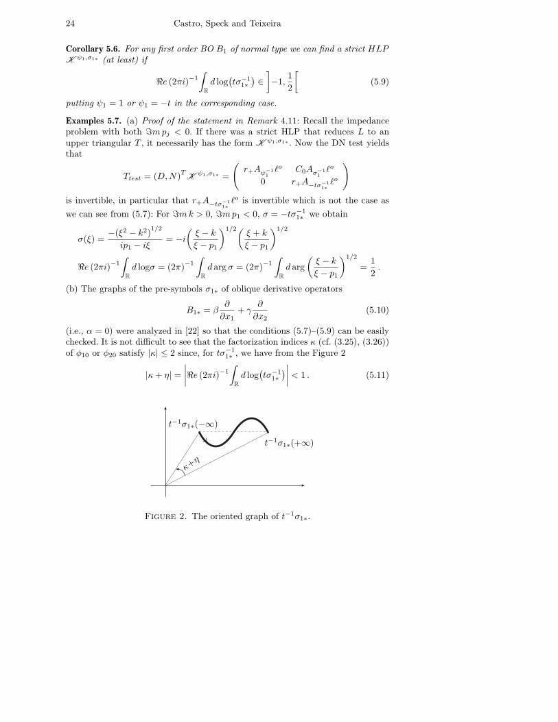
(i.e., α = 0) were analyzed in [22] so that the conditions (5.7)–(5.9) can be easilychecked. It is not difficult to see that the factorization indices κ (cf. (3.25), (3.26))of φ10 or φ20 satisfy |κ| ≤ 2 since, for tσ−1

1∗ , we have from the Figure 2

|κ+ η| =

∣∣∣∣ℜe (2πi)−1∫

R

d log(tσ−1

1∗

)∣∣∣∣ < 1 . (5.11)

t−1σ1∗(+∞)

t−1σ1∗(−∞)

κ+η

Figure 2. The oriented graph of t−1σ1∗.


Another possibility to enlarge the interval (5.9) where one of the standardHLPs is strict is to think about the “low regularity parameter” ǫ introduced in(1.5).

Corollary 5.8. Let B1 be a first order BO of normal type, then we can find anǫ ∈] − 1, 1[ and a HLP

(K ψ1,σ1∗)ǫ: H∓1/2+ǫ(R+) ×H−1/2+ǫ(R+) → H

1+ǫ(Q1) (5.12)

that is bijective if

κ+ η = ℜe (2πi)−1∫

R

d log(tσ−1

1∗

)∈

]−

3

2, 1

[(5.13)

where the ∓ sign in (5.12) corresponds with ψ1 = −t and ǫ ∈]−1, 1[ or with ψ1 = 1and ǫ ∈] − 3/2, 1/2[, respectively.

Proof. Starting with Lǫ from (1.5) we come to the toplinear equivalent after ex-

tension operators (5.5) or (5.6) where φ10 carries a factor ζ−1/4+ǫ/2k and φ20 carries

a factor ζ1/4+ǫ/2k instead of those with ǫ = 0. This gives the wider range of (5.13)

by analogy to the preceding considerations.

Remark 5.9. A pure oblique derivative operator B1 = β ∂∂x2

+ γ ∂∂x1

(α = 0) of

normal type satisfies (5.13) as observed in (5.11).

Due to the overlapping intervals (5.7), (5.8) it is not necessary to work withpotential operators which are not normally solvable. It remains an open questionwhether it is always possible to find a strict HLP of the form (5.1) by the presentideas for any BVP P1(B1, B2) of normal type. However the described methodscover already a wide subclass of physically interesting cases.

Let us see the consequences of a strict ansatz again starting with ǫ = 0 forsimplicity.

Theorem 5.10. Let P1(B1, B2) be of normal type, order Bj = 1, K = K 1,σ1∗ :

H1/2(R+) × H−1/2(R+) → H 1(Q1) be strict, L = (B1, B2)T

: H 1(Q1) →

H−1/2(R+)2

and

T = LK =

(T1 0K T2

)=

(r+Aσ1

ℓe 0C0Aσ2∗

ℓe r+Aσ2σ−1

1∗

ℓo

)(5.14)

: H1/2(R+) ×H−1/2(R+) → H−1/2(R+)2.

Then the following assertions are equivalent:(i) L is normally solvable,(ii) T is normally solvable,(iii) T1 and T2 are normally solvable.In this case, all these operators are Fredholm and T1 and T2 have one-sided inversesgiven by the appendix, especially by (A.11) and its analogue for ℓe. Then, T is alsoFredholm.


Proof. Let L be normally solvable. Hence the image of T1 is closed due to thetriangular form of T and thus Fredholm, see the appendix. This implies that

T ∼

(I 0K T2

)+ F1 (5.15)

are toplinear equivalent operators, where F1 is a finite rank operator. Thus imT2

must be closed and T2 is also Fredholm. Moreover scalar Fredholm CTOS are one-sided invertible. Finally, if T1 and T2 are Fredholm and one-sided invertible, thenT is Fredholm and L as well.

Remark 5.11. If a bounded linear operator in Banach spaces has the form

T =

(T1 0K T2

)(5.16)

and T1 and T2 are (only) one-sided invertible, then T is not necessarily normallysolvable, see the example of Wiener-Hopf operators with oscillating pre-symbolsarising from convolution type operators on finite intervals [4]. In the present con-text, T1 and T2 are also Fredholm and so is T .

Theorem 5.12. In the situation of Theorem 5.10 let T1 be left invertible or T2 beright invertible, i.e., there are generalized inverses T−

j such that

T−1 T1 = I , T2T

−2 T2 = T2 (5.17)

or

T1T−1 T1 = T1 , T2T

−2 = I . (5.18)

Then, for U = −T−2 KT

−1 ,

T− =

(T−

1 0U T−

2

)(5.19)

represents a generalized inverse of T . In particular T− is the inverse of T if T1

and T2 are both invertible.

Proof. A direct computation yields

TT−T =

(T1T

−1 T1 0

KT−1 T1 + T2UT1 + T2T

−2 K T2T

−2 T2

)(5.20)

and insertion of U gives T in both situations. The special case of invertible Tj isnow evident.

Proposition 5.13. In the situation of Theorem 5.10 let T1T−1 = I and T−

2 T2 = I.Then (5.19) represents a two-sided regularizer of the Fredholm operator T .

Proof. With T−1 T1 = I − F1, T2T

−2 = I − F2 we have

TT− =

(I 0

KT−1 − T2T

−2 KT

−1 I − F2

)=

(I 0

F2KT−1 I − F2

)(5.21)


where F2 is a finite rank operator, and similarly

T−T =

(I + F1 0T−

2 KF1 I

). (5.22)

It is obvious how these results can be employed to determine the explicitsolution of P1(B1, B2) in general, under the present assumptions, and for itsvariants (5.2), (5.3) by analogy. In order to avoid the situation of Proposition 5.13where none of the two operators is two-sided invertible, it may help to exchangethe roles of σ1 and σ2 in (5.14) or to search for a different ansatz.

There is a certain stability with respect to the parameter ǫ which we describeonly in the principal case:

Corollary 5.14. Under the assumptions of Theorem 5.12 there exists an interval]ǫ1, ǫ2[, ǫ1 < 0 < ǫ2, such that Lǫ, T ǫ, T ǫj are Fredholm for ǫ ∈]ǫ1, ǫ2[ with Fredholmcharacteristics independent of ǫ.

The operators L, T , Tj and their generalized inverses given before map thecorresponding subspaces into each other (low regularity) for ǫ ∈]0, ǫ2[ and havecontinuous extensions for ǫ ∈]ǫ1, 0[5.

It remains to say something about the case where we cannot find a strictHLP. As a prototype, let us consider again K 1,σ1∗ of (5.2) when it is Fredholmand not invertible, i.e., only one-sided invertible:

Lemma 5.15. The operator Ttest1 in (5.2) is left or right invertible if and only iftσ−1

1∗ ∈ GL∞ and

ℜe (2πi)−1∫

R

d log(tσ−1

1∗

)= κ+ η (5.23)

where η ∈] − 1/2, 1/2[ and κ ∈ N0 or −κ ∈ N0, respectively. In this case,

T−test1 =

(I K1

0 T1

)−

=

(I −K1T

−1

0 T−1

)(5.24)

represents a left/right inverse of Ttest1 if T−1 is a left/right inverse of T1 =

r+A−tσ−1

1∗

ℓo, and we can choose explicitly

T−1 = r+A

−1e ℓor+C

−1ℓor+A−1− ℓo (5.25)

where A−tσ−1

1∗

= A−CAe is an AFIS (see explicitly analytical formulas in the

appendix), C = Aζκi

and we may drop the second/first term ℓor+ in this formula.

Proof. The criteria (5.23) is known from the appendix, see (5.7), the formulas(5.24) and (5.25) are verified straightforwardly.

5The largest interval can be determined as to be the intersection of the two intervals resulting

from the factorization of the lifted pre-symbols of σ1 and σ2σ−1

1∗due to the appendix taking into

account the possible changes of the parameter s in (A.10) (cf. Section 6 for the class of obliquederivative problems).


Theorem 5.16. Let P1(B1, B2) be of normal type, β, γ, β′, γ′ ∈ C \ 0, Ttest1 =

(D,N)TK 1,σ1∗ be left invertible (cf. (5.2) and Lemma 5.15). As before put

L = (B1, B2)T

: H1(Q1) → H−1/2(R+)

2= Y

K = K1,σ1∗ : X = H1/2(R+) ×H−1/2(R+) → H

1(Q1) (5.26)

T = LK : X → Y

as given in (5.14). Then

(i) either both T and L are not normally solvable or both are Fredholm;(ii) if T− is a left/right regularizer of T , then L− = K T−is a left/right regular-

izer of L (and all are two-sided regularizers);(iii) in this case

α(T ) ≤ α(L) ≤ α(T ) + β(K )

β(T ) − β(K ) ≤ β(L) ≤ β(T ) (5.27)

β(K ) = α(K −) if K−

K = I .

Particularly, if T is right invertible then L is also right invertible, and, if Tis left invertible then α(L) ≤ β(K );

(iv) in the other case ( imT and imL are not closed), the formulas (5.27) holdwith β(T ), β(L) exchanged by β(T ) = dimY/ imT and β(L) = dimY/ imL,respectively.

Proof. (i) is a consequence of Theorem 5.10 noting that K is Fredholm if Ttest1is left invertible according to Lemma 5.15.

(ii) follows from Lemma 3.14.(iii) is generally true for Fredholm operators which satisfy the relations T =

LK , K −K = I and the additional assumptions, respectively.(iv) can be seen by analogy to Corollary 3.18.

Let us outline the explicit solution of P1(B1, B2) under the assumptions ofTheorem 5.16 in the Fredholm case (characterized by Lemma 5.15). One can tryto determine a generalized inverse L− of L (till now we have only the regularizerL− = K T− but not LL−L = L). However it seems most convenient for practicalpurposes to proceed as follows.

Our HLP K yields a unique decomposition of any u ∈ H 1(Q1) by

u = K f + u0 = K K−u+ (I − K K

−)u (5.28)

where K − is the left inverse of K given by

K− = T−

test1(D,N)T

(5.29)

and T−test1 is the left inverse of Ttest1 obtained in (5.24) by AFIS. I.e., we search

for f = K −u ∈ im K − = H 1(Q1) and u0 ∈ ker K − such that

Lu = Tf + Lu0 = g . (5.30)


Note that ker K − is finite dimensional and explicitly determined by the analysisof (5.29).

Now there are two cases: (i) either

imT ∩ L ker K− = 0 (5.31)

or (ii) there exist linear independent h1, . . . , hm in this intersection (explicitlycalculable by Lemma 5.15 etc., by determining the form of u0 ∈ kerK − andsolving TT−Lu0 = Lu0).

In the simpler case (i) of (5.31), a necessary and sufficient solvability conditionfor the equation (5.30) as well as the form of the solution, if existing, can bedetermined by means of linear algebra as follows. Since

imL = imT ⊕ L ker K− (5.32)

equation (5.30) decomposes by the ansatz (5.28) into the system of two indepen-dent equations

LK f = Tf = g1 ∈ imT(5.33)

Lu0 = g0 = g − g1 ∈ L ker K− .

Evidently, the resulting solvability condition reads

g − TT−g ∈ L ker K− , (5.34)

because Tf = g1 is solvable for g1 = TT−g ∈ imT , and can be verified ordisproved analytically. If it holds, the general solution of Lu = g is obviously givenby

u = K(T−g + v

)+ u0 (5.35)

where T−g = T−TT−g = T−g1 = f is a particular solution of Tf = g1, since T−

is a reflexive generalized inverse due to factorization theory, v = (I − T−T )v isan arbitrary element in the kernel of T , and u0 is obtained from the finite systemLu0 = g0 (see Section 6 for a special case).

In the second case (ii) where (5.31) differs from the zero space, we can followthe same strategy noting that now the kernel of L may contain additional termsdue to the appearance of h1, . . . , hm in (5.31) that can be determined by algebraicmeans computing the intersection of spanh1, . . . , hm and L ker K −. However,the solvability condition (5.34) remains the same and (5.35) may be replaced by

u = K(T−g + v

)+ u0 +

∑cjuj (5.36)

where uj ∈ ker K − such that Luj ∈ imT and u0 belongs to a complementof spanuj in ker K −. The exact numbers α(L) and β(L) in general are stillunknown but can be determined in concrete cases, cf. Section 6. So we have proved:

Corollary 5.17. Under the assumptions of Theorem 5.16, in the Fredholm case,P1(B1, B2) is solvable if and only if (5.34) is satisfied. Then the general solutionis given by (5.35) where u0 ∈ kerK −, which is a linear combination of H 1(Q1)elements determined from (5.29) with coefficients provided by Lu0 = g0.


The final case, where the HLP is not left but right invertible, is similar andeven simpler. We refine ourselves to resuming some central results.

Corollary 5.18. Under the assumptions of Theorem 5.16, up to Ttest1 being rightinstead of left invertible, i.e., K K − = I instead of K −K = I, we obtain theresults (i) and (ii) as before. (iii) is replaced by

α(T ) − α(K ) ≤ α(L) ≤ α(T )(5.37)

β(L) = β(T ) .

Particularly, if T is left invertible, then L is left invertible, T−T = I implies thatL− = K T− is a left inverse of L. If T is right invertible, then L− = K T− is aright regularizer (but K T− is not necessarily a right inverse of L).

(iv) holds by analogy, referring to (5.28).

Note that we have here L = TK − beside of T = LK and therefore easierconclusions from imL = imT , particularly the solvability condition

TT−g = g (5.38)

for the solution of Lu = g. Furthermore any u ∈ H 1(Q1) can be represented bythe HLP K , however not uniquely in general:

u = K f(5.39)

f = f1 + f0 = K−

K f + (I − K−

K )f

where f1 ∈ im K − is unique and f0 ∈ kerK arbitrary. So we get:

Corollary 5.19. Under the assumptions of Corollary 5.18, in the Fredholm case,P1(B1, B2) is solvable if and only if (5.29) is satisfied where T− is known froman AFIS. Then the general solution is given by

u = K f1(5.40)

f1 = T−g + f2

where f2 ∈ kerT (and this representation is only unique up to elements f0 ∈ker K ∩ kerT ).

6. Oblique Derivative Problems with Real Coefficients

As an example we treat the class of BVPs (1.1) where α = α′ = 0 and β, γ, β′, γ′ ∈R, as illustrated in Figure 3, which is of particular interest from the physical pointof view.

Again we abbreviate L = (B1, B2)T,

σ1 = −βt+ γϑ , σ1∗ = −γt+ βϑ(6.1)

σ2 = −β′t+ γ′ϑ , σ2∗ = −γ′t+ β′ϑ

Mixed Boundary Value Problems for the Helmholtz Equation 31PSfrag

Q1

Γ1

Γ2

(γ, β)–direction

(β′, γ′)–direction

β ∂u∂x2

+ γ ∂u∂x1

= g1

β′ ∂u∂x1

+ γ′ ∂u∂x2= g2

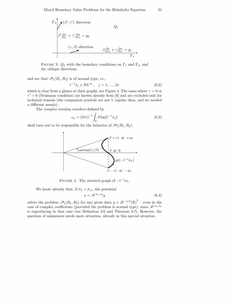
Figure 3. Q1 with the boundary conditions on Γ1 and Γ2, andthe oblique directions.

and see that P1(B1, B2) is of normal type, i.e.,

t−1σj ∈ GL∞ , j = 1, . . . , 2∗ (6.2)

which is clear from a glance at their graphs, see Figure 4. The cases where γ = 0 orγ′ = 0 (Neumann condition) are known already from [6] and are excluded only fortechnical reasons (the companion symbols are not 1–regular then, and we neededa different ansatz).

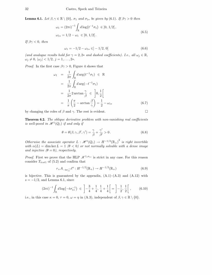
The complex winding numbers defined by

ωj = (2πi)−1∫

R

d log(t−1σj

)(6.3)

shall turn out to be responsible for the behavior of P1(B1, B2).

arctan(γ/β)

β + iγ at +∞

β − iγ at −∞

β at 0

gr(−t−1σ1)

Figure 4. The oriented graph of −t−1σ1.

We know already that, if σ2 = σ1∗, the potential

u = Kσ1,σ2g (6.4)

solves the problem P1(B1, B2) for any given data g ∈ H−1/2(R)2

– even in thecase of complex coefficients (provided the problem is normal type), since K σ1,σ2

is reproducing in that case (see Definition 3.6 and Theorem 3.7). However, thequestion of uniqueness needs more attention, already in this special situation.


Lemma 6.1. Let β, γ ∈ R \ 0, σ1 and σ1∗ be given by (6.1). If βγ > 0 then

ω1 = (2πi)−1∫

R

d log(t−1σ1

)∈ ]0, 1/2[ ,

(6.5)ω1∗ = 1/2 − ω1 ∈ ]0, 1/2[ .

If βγ < 0, then

ω1 = −1/2 − ω1∗ ∈] − 1/2, 0[ (6.6)

(and analogue results hold for γ = 2, 2∗ and dashed coefficients). I.e., all ωj ∈ R,ωj 6= 0, |ωj | < 1/2, j = 1, . . . , 2∗.

Proof. In the first case βγ > 0, Figure 4 shows that

ω1 =1

2π

∫

R

d arg(t−1σ1) ∈ R

=1

2π

∫

R

d arg(−t−1σ1)

=1

2π2 arctan

γ

β∈

]0,

1

2

[

=1

π

(π

2− arctan

β

γ

)=

1

2− ω1∗ (6.7)

by changing the roles of β and γ. The rest is evident.

Theorem 6.2. The oblique derivative problem with non-vanishing real coefficientsis well-posed in H 1(Q1) if and only if

θ = θ(β, γ, β′, γ′) =γ

β+γ′

β′> 0 . (6.8)

Otherwise the associate operator L : H 1(Q1) → H−1/2(R+)2

is right invertiblewith α(L) = dim kerL = 1 (θ < 0) or not normally solvable with a dense imageand injective (θ = 0), respectively.

Proof. First we prove that the HLP K 1,σ1∗ is strict in any case. For this reasonconsider Ttest1 of (5.2) and confirm that

r+A−tσ−1

1∗

ℓo : H−1/2(R+) → H−1/2(R+) (6.9)

is bijective. This is guaranteed by the appendix, (A.1)–(A.3) and (A.12) withs = −1/2, and Lemma 6.1, since

(2πi)−1∫

R

d log(−tσ−1

1∗

)∈

]−

3

4+

1

4,

1

4+

1

4

[=

]−

1

2,

1

2

[, (6.10)

i.e., in this case κ = 0, τ = 0, ω = η in (A.3), independent of β, γ ∈ R \ 0.


Hence the invertibility of L = (B1, B2)T

: H 1(Q1) → H−1/2(R+)2

is equiv-alent to the invertibility of the operator

T = LK1,σ1∗ =

(T11 0K T22

)=

(r+Aσ1

ℓe 0C0Aσ2∗

ℓe r+Aσ2σ−1

1∗

ℓo

)(6.11)

: H1/2(R+) ×H−1/2(R+) → H−1/2(R+)2

according to Theorem 5.10 and we have to study the main diagonal elements Tjj(the notation is chosen to avoid confusion with formerly used Tj).

By analogy to Lemma 5.4 (lifting) we have the operator toplinear equivalence

T11 = r+Aσ1ℓe ∼ r+Aσ10

ℓe : L2(R+) → L2(R+)

σ10 = t−1/2− σ1t

−1/2 = ζ−1/4k t−1σ1 (6.12)

ω10 = −1

4+ ω1 ∈

]− 1

4 ,14

[if βγ > 0

]− 3

4 ,−14

[if βγ < 0

according to Lemma 6.1 and Figure 4 (and ω10 = −1/4 in the exceptional caseγ = 0 of the Neumann condition).

Furthermore the operator

T22 = r+Aσ2σ−1

1∗

ℓo : H−1/2(R+) → H−1/2(R+) (6.13)

has an (unlifted) pre-symbol σ22 = σ2σ−11∗ with complex winding number

ω22 = (2πi)−1∫

R

d log(σ2σ

−11∗

)

= (2πi)−1∫

R

d log(t−1σ2

)− (2πi)

−1∫

R

d log(t−1σ1∗

)

= ω2 − ω1∗ =

ω1 + ω2 −

12 if βγ > 0

ω1 + ω2 + 12 if βγ < 0

(6.14)

due to Lemma 6.1.Now let us study the three cases corresponding to the sign of θ:

Case θ > 0. We can assume γ/β > 0 (otherwise exchange the roles of B1 and B2).Thus we have

ω10 ∈

]−

1

4,1

4

[⊂

]−

1

4,3

4

[, (6.15)

i.e., it belongs to the parameter range where T11 is invertible (see the appendix,case ℓe). Furthermore (6.8) yields

1

π

(arctan

γ

β+ arctan

γ′

β′

)> 0

ω1 + ω2 > 0 (6.16)

ω22 = ω1 + ω2 −1

2∈

]−

1

2,1

2

[


according to Figure 4, (6.14) and Lemma 6.1, i.e., ω22 belongs exactly to theparameter range where T22 is invertible (for s = −1/2).Case θ < 0. We can assume γ/β < 0 (otherwise exchange the roles of B1 and B2).(6.12) implies

ω10 ∈

]−

3

4,−

1

4

[, (6.17)

i.e., ω10 = −1+η where η ∈]1/4, 3/4[⊂]−1/4, 3/4[ and T11 is right invertible withα(T11) = dim kerT11 = 1. It remains to show that T22 is invertible anyway for Tin (6.11) having the same characteristics as T11, cf. Theorem 5.12. Analogously to(6.16) we conclude

ω1 + ω2 < 0(6.18)

ω22 = ω1 + ω2 +1

2∈

]−

1

2,1

2

[

with the help of the last line of (6.14) and Lemma 6.1, i.e., it belongs also to theparameter range where T22 is invertible (for s = −1/2).Case θ = 0. Let γ/β > 0 and γ′/β′ = −γ/β < 0. Again T11 is invertible (see thecase θ > 0), ω1 + ω2 = 0 due to (6.16) and ω22 = −1/2, see (6.14). Thus wehave the case ω22 = η22 = −1/2 with κ = τ = 0 in (A.3) for σ = σ2σ

−11∗ and the

conclusions of the statement.

Remark 6.3. There is a nice geometrical interpretation of the well-posedness condi-tion (6.8). Letting β > 0 and β′ > 0 without loss of generality (otherwise multiplythe BC by −1), we can say: Either the vectors v = (γ, β), v′ = (β′, γ′) of directionof the oblique derivatives are both pointing into the interior of Q1 (γ > 0 andγ′ > 0), or one is not, but the other one points into Q1 and is “more flat”, i.e.,nearer to the axis direction, i.e., the tangential component is relatively longer.

Remark 6.4. It is possible to include the case γ′ = 0 (or γ = 0 by symmetry) inthe statement of Theorem 6.2, i.e., in this case one of the BCs is Neumann type.Obviously, γ′ = 0 does not effect the strictness of K 1,σ1∗ nor the other conclusionsof the proof of Theorem 6.2 (ω2 = 0). However this result can also be obtained from[6]. Further, the case of parallel directions (σ1 = σ2∗) mentioned in the context of(6.4) really splits into the two cases θ > 0 and θ < 0 corresponding to a well-posedproblem and a solvable problem with one-dimensional kernel, respectively.

Let us think about the explicit solution to the oblique derivative problem inclosed analytical form, namely by the help of an AFIS of Aσ2σ

−1

1∗

and of At−1σ1as

well. Fortunately our HLP K 1,σ1∗ is strict for any choice of β, γ ∈ R \ 06, see(6.11), but there are three cases of different nature corresponding with the sign ofθ. However, the results are extremely transparent: We have just to “invert” thetwo scalar operators Tjj of (6.11) in a sense.

6It is strict also for β = 0 and γ 6= 0 which is a joke.


Lemma 6.5. Let β, γ, β′, γ′ ∈ R \ 0, the pre-symbols σ1, . . . , σ2∗ be given by(6.1) and T22 = r+Aσ22

ℓo : H−1/2(R+) → H−1/2(R+) be defined by (6.13) withσ22 = σ2σ

−11∗ . Then T22 is boundedly invertible if and only if

θ =γ

β+γ′

β′6= 0 (6.19)

and the inverse reads

T−122 = r+Aσ−1

22eℓor+Aσ−1

22−

ℓo (6.20)

where Aσ22= Aσ22−

Aσ22eis an AFIS according to the appendix with κ = 0. If θ =

0, T22 is not normally solvable (and will be considered later in propositions 6.12–6.14).

Proof. We collect and assemble the formulas. In the case θ > 0 we know from(6.16) that the complex winding number ω22 of σ22 is real and belongs to theinterval ] − 1/2, 1/2[. The appendix yields for σ = σ22 and s = −1/2 that κ = 0,τ = 0, η = ω22 and

s+ 2η = −1

2+ 2ω22 ∈

]−

3

2,1

2

[(6.21)

such that (A.10) is satisfied. Factorizing

σ22 = σ22−σ22e (6.22)

as σ in (A.4)–(A.8) we obtain an AFIS of Aσ22and the inverse (6.20).

The case θ < 0 leads to ω22 ∈] − 1/2, 1/2[ as well, see (6.18), and we receivethe same formulas as before. The case θ = 0 corresponds with ω22 = −1/2 ands+ 2η = −1/2 + 2ω22 = −3/2 discussed subsequent to (A.10).

Lemma 6.6. Let β, γ ∈ R \ 0, i.e., σ1 and σ1∗ as given by (6.1) are 1–regular.Then T11 = r+Aσ1

ℓe : H1/2(R+) → H−1/2(R+) is right invertible by

T−11 = r+Aσ−1

11eℓer+Aζ−κ

iℓer+Aσ−1

11−

ℓe (6.23)

where

κ =

0 if βγ > 0

−1 if βγ < 0(6.24)

and the factors σ11e, σ11− are given in the proof. Moreover the formula (6.23)simplifies to

T−111 = r+Aσ−1

11eℓer+Aσ−1

11−

ℓe (6.25)

if (and only if) βγ > 0, representing the inverse of T11.

Proof. In both cases, due to the sign of βγ, we obtain an AFIS (case ℓe) of the(lifted) operator

Aσ10= Aσ10−

CAσ10e(6.26)


from the appendix formulas (A.4)–(A.8) putting σ = σ10 = σ10−ζκi σ10e, because

the complex winding number of σ10 satisfies

ω10 = κ+ η (6.27)

with κ given by (6.24) and η ∈] − 1/4, 3/4[ according to (6.12) and the splittingin (6.17), respectively. Due to the lifting in (6.12), T11 and T10 = r+Aσ10

ℓe arerelated by

T11 = r+At1/2

−

ℓeT10r+At1/2ℓe . (6.28)

Hence, the right inverse

T−10 = r+Aσ−1

10eℓer+Aζ−κ

iℓer+Aσ−1

10−

ℓe (6.29)

of T10 yields (6.23) with

σ11e = t1/2σ10e , σ11− = t1/2− σ10− (6.30)

and (6.25) is an obvious consequence of κ = 0.

Theorem 6.7. Let β, γ, β′, γ′ ∈ R \ 0, θ = β/γ + β′/γ′, T be defined by (6.11)and

T− =

(T−

11 0−T−1

22 KT−11 T−1

22

)(6.31)

where T−11 and T−1

22 are given by (6.23) and (6.20), respectively.

(i) If θ > 0 let βγ > 0 (without loss of generality). The unique solution of the

oblique derivative problem (in H 1(Q1) for arbitrary g ∈ H−1/2(R+)2) is

given by

u = K1,σ1∗f

(6.32)f = T−g .

Here T−11 and T−1

22 are the inverses of T11 and T22 due formula (6.23) or(6.25) and (6.20) inserted into (6.31).

(ii) If θ < 0 let βγ < 0 (without loss of generality). The oblique derivative problem

is solvable (in H 1(Q1) for arbitrary g ∈ H−1/2(R+)2) and the solutions are

given by

u = K1,σ1∗f

f = T−g + µf0 , µ ∈ C

(6.33)f0 =

(f01f02

)=

(f01

−T−122 Kf01

)

f01 = r+F−1(σ−1

10et−5/2

)

where σ10e is the factor found in (6.26).


Proof. In the first case, the problem is uniquely solvable according to Theorem 6.2and the solution is given by (6.32) due to the first part of its proof until (6.11).Both Tjj are invertible with inverses given by Lemma 6.5 and Lemma 6.6.

In the second case, u is also represented by the strict HLP K 1,σ1∗ andthe density f is obtained from Tf = g where T is right invertible with a one-dimensional kernel, spanf0 say, where

Tf0 =

(T11 0K T22

)(f01f02

)= 0 (6.34)

leads to the representation in terms of f01 since T22 is invertible by (6.20). Theequation T11f01 = 0 is equivalent to each of the following conditions resulting from(6.26)–(6.28):

T10r+At1/2ℓef01 = 0

r+Aζ−1

iℓer+Aσ10et1/2ℓef01 = 0 (6.35)

r+Aσ10et1/2ℓef01 = µ r+F−1t−2

which implies the representation of f01 in (6.33).

Remark 6.8. All factors mentioned before can be directly expressed in terms ofexplicit analytical formulas of the appendix. Particularly, in the present case,

σ10 = t−1/2− σ1t

−1/2 = t−3/4− t

−1/4+ σ1 = σ10−ζ

−1i σ10e (6.36)

due to κ = −1, where (put σ = σ10 in (A.4)–(A.8))

σ10e = ζiσ−110−σ10

σ10− = t2η− ψ10− = t2η− expP− log

(ψ10ψ

−110

)(6.37)

ψ10 = σ−110 (+∞) ζ−ω10

i σ10

and ω10 = η − 1 with η ∈] − 1/4, 3/4[. If κ = 0 (case θ > 0), we have ω10 = η andthe factors ζ−1

i in (6.36) and ζi in (6.37) have to be omitted.

In what concerns the representation of T−122 (continuing Lemma 6.5) it is even

simpler to factor the pre-symbol

σ22 = σ22−σ22e (6.38)

according to s = −1/2, κ = 0, η = ω22, cf. (6.21), where

σ22− = ts+2η− ψ22− = t

2η−1/2− exp

P− log

(ψ22ψ

−122

)

(6.39)ψ22 = σ−1

22 (+∞) ζ−ω22

i σ22

with η − 1/4 ∈] − 3/4, 1/4[.

Before thinking about the critical case (θ = 0), it is useful to discuss lowregularity of the solutions (for θ 6= 0). Again we start considering T ǫ11 and T ǫ22


separately, as restrictions (cf. (1.5)) or continuous extensions, respectively, writing

T ǫ11 = RstT11 : H1/2+ǫ(R+) → H−1/2+ǫ(R+) , ǫ ∈]0, 1[(6.40)

T ǫ11 = ExtT11 : H1/2+ǫ(R+) → H−1/2+ǫ(R+) , ǫ ∈] − 1, 0[

and T ǫ22 analogously with domain H−1/2+ǫ due to the even/odd extension operatorin (6.12) and (6.13), respectively.

It is possible to determine exactly the parameter ranges of ǫ in terms of thenumbers ω1 and ω2 rather than regarding the existence result of Corollary 5.14.However, we carry it out only for the case where θ > 0, referring to analogy forθ < 0.

Proposition 6.9. Under the assumptions of Theorem 6.7, (i), i.e., θ > 0, βγ > 0,ω1 > 0 and ω1 + ω2 > 0, the following operators are invertible

T ǫ11 : H1/2+ǫ(R+) → H−1/2+ǫ(R+) iff ǫ ∈] − ω1, 1 − ω1[

T ǫ22 : H−1/2+ǫ(R+) → H−1/2+ǫ(R+) iff ǫ ∈] − (ω1 + ω2), 1 − (ω1 + ω2)[ (6.41)

T ǫ : H1/2+ǫ(R+) ×H−1/2+ǫ(R+) → H−1/2+ǫ(R+)2

if ǫ ∈] − ω1, 1 − (ω1 + ω2)[

where ω1 + ω2 < 1.

Proof. From Lemma 6.6 and formulas (6.12), (6.15) we have that T11 is invertibleif and only if

ω10 = ω1 −1

4∈

]−

1

4,1

4

[(6.42)

belongs to ] − 1/4, 3/4[. Therefore, the restricted/extended operator is invertibleif and only if

ǫ <3

4−

(ω1 −

1

4

)and ǫ > −

1

4−

(ω1 −

1

4

)(6.43)

which proves the first result. Similarly, T22 is invertible if and only if (6.16) issatisfied which gives the second result. Thus, if both conditions are fulfilled thenT ǫ is also invertible due to its form (6.11) and (6.31). Lemma 6.1 yields ω1 +ω2 <1.

Remark 6.10. It is also sufficient to assume ǫ ∈] − ω2, 1 − (ω1 + ω2)[ for T ǫ to beinvertible instead of the last condition in Proposition 6.9, due to the symmetryargument.

Corollary 6.11 (low regularity of the solution). Under the assumption of Proposi-tion 6.9, the weak solution u of the oblique derivative problem belongs to H1+ǫ(Q1)

provided g ∈ H−1/2+ǫ(R+)2

and ǫ < 1 − (ω1 + ω2) where ωj ∈]0, 1/2[, see (6.7).

Now let us consider the critical case where

θ =γ

β+γ′

β′= 0 (6.44)


which corresponds with directions of the two oblique derivatives that are orthogo-

nal to each other. We know from Theorem 6.2 that L : H 1(Q1) → H−1/2(R+)2

isnot normally solvable, but injective with a dense image. Thus L can be normalizedby restriction of its image space

≺

L= RstL : H1(Q1) →

≺

Y = imL (6.45)

with the norm induced by imL. This idea implies a “natural compatibility condi-tion” for the data g = (g1, g2) to make the oblique derivative problem well-posed,the analogue of (4.10) known from the Neumann problem. We like to derive thisnecessary and sufficient condition.

First we normalize L by a simultaneous positive ǫ–shift in the orders of allspaces:

Proposition 6.12. Let β, γ, β′, γ′ ∈ R \ 0, βγ > 0, θ = 0 and ǫ ∈]0, 1[. Then

Lǫ = Rst (B1, B2)T

: H1+ǫ(Q1) → H−1/2+ǫ(R+)

2(6.46)

is boundedly invertible.

Proof. First we recall that the restricted/extended operator

(D,N)T

: H1+ǫ(Q1) → H1/2+ǫ(R+) ×H−1/2+ǫ(R+) (6.47)

is invertible for |ǫ| < 1, see Proposition 2.1 and (2.5). Therefore, Remark 5.3implies that the HLP

(K

1,σ1∗)ǫ

: H1/2+ǫ(R+) ×H−1/2+ǫ(R+) → H1+ǫ(Q1) (6.48)

is toplinear equivalent to the modified operator T ǫtest1 in (5.2). We know from (6.9)–(6.10) that (6.48) is strict for ǫ = 0 since −ω1∗ ∈]− 1/2, 1/2[. Replacing s = −1/2by s = −1/2 + ǫ we find that this HLP is strict if and only if ω1 − 1/2 + ǫ/2 =−ω1∗ + ǫ/2 ∈] − 1/2, 1/2[, i.e., if and only if

ǫ

2∈] − ω1, 1 − ω1[ , (6.49)

an ǫ–interval of length 2, indeed, as in (6.47).Modifying (6.12) for T ǫ11 we find that ωǫ10 = −1/4 + ǫ/2 + ω1 ∈] − 1/4 +

ǫ/2, 1/4 + ǫ/2[ and that T ǫ11 is invertible if and only if ωǫ10 ∈] − 1/4, 3/4[, see theℓe variant of (A.3) for s = 0. This is also equivalent to (6.49).

Generalizing T ǫ22 in (6.13) for ǫ > 0 we get invertibility for ωǫ22 = ω2 − ω1∗ +ǫ/2 ∈]−1/2, 1/2[ where ω2−ω1∗ = ω1 +ω2−1/2 = −1/2, since βγ > 0 and θ = 0,i.e., simply ǫ/2 ∈]0, 1[.

The intersection with (6.49) yields that Lǫ ∼ T ǫ is boundedly invertible forǫ ∈ ]0, 2(1 − ω1)[ where ω1 ∈]0, 1/2[ due to Lemma 6.1.

Remark 6.13. The ǫ–intervals where T ǫjj , j = 1, 2, are bijective, have both length 2.In the present situation, their intersection has length more than 1. However, thatresult depends on the ansatz, and the determination of the maximal ǫ–intervalwhere Lǫ is invertible remains open.


Now let us determine the “natural compatibility conditions” mentioned inthe context of (6.45).

Proposition 6.14. Under the assumptions of Proposition 6.12 the image normal-ization of L (for ǫ = 0) reads

≺

L= Rst (B1, B2)T

: H1(Q1) →

≺

Y (6.50)

where≺

Y ⊂ H−1/2(R+)2

(6.51)

is a dense subspace characterized by the compatibility condition

g2 −KT−111 g1 ∈ H−1/2(R+) (6.52)

for (g1, g2) ∈≺

Y . Herein, T−111 is given by T−

11 in Lemma 6.6 with κ = 0 (regarding

ǫ ∈ [0, 1[).≺

L is boundedly invertible in that space setting and the oblique derivative

problem is well-posed for data given in≺

Y .

Proof. Considering the family of boundedly invertible operators

T ǫ = Rst

(T11 0K T22

): H1/2+ǫ(R+) ×H−1/2+ǫ(R+) → H−1/2+ǫ(R+)

2(6.53)

for ǫ ∈]0, 1[, we know that T ǫ11 is invertible for ǫ ∈ [0, 1[ and T ǫ22 for ǫ ∈]0, 1[ beinginjective for ǫ = 0 with dense image in H−1/2(R+) and given by the appendix:

≺

Y 22 = imT22 = r+Aλ−s−iτ−1/2

−

ℓor+H−1/2+ = r+H

−1/2+ = H−1/2(R+) (6.54)

since s = −1/2, τ = 0, i.e., −s− iτ − 1/2 = 0. Thus, the necessary and sufficientcondition (6.52) for the solvability of Tf = g results from (6.54) and

(T11 0K T22

)f = g =

(g1g2

)

Kf1 + T22f2 = g2 (6.55)

T22f2 = g2 −KT−111 g1 ∈

≺

Y 22 .

The consequences for L are evident.

Appendix A.

Here is a brief outline of the constructive (generalized) inversion of a scalar CTOSunder special assumptions that are most convenient for the present purpose [7]. Ageneralization to matrix CTOS can be found in [5] and more constructive methodsare planned to be published in near future combining results from [9], [10] and [13].

The central case is

S = r+Aσℓo : Hs(R+) → Hs(R+) (A.1)


(or ℓe instead of ℓo, respectively) where

σ ∈ GCν(R) , ν ∈]0, 1[(A.2)

s ∈] − 3/2, 1/2[ (or ] − 1/2, 3/2[ respectively)

which yields that S is a composition of bounded linear operators and Aσ : Hs →Hs is bijective.

Defining

ω = (2πi)−1∫

R

d logσ = κ+ η + iτ (A.3)

where κ ∈ Z, η ∈ [−3/4 − s/2, 1/4 − s/2[ (or η ∈ [−1/4 − s/2, 3/4 − s/2[,respectively), and τ ∈ R, one can write

σ = σ(+∞) ζωi ψ (A.4)

with ψ ∈ GCν(R), ψ(∞) = 1 and7

ζi(ξ) =λ−(ξ)

λ+(ξ)=ξ − i

ξ + i, ξ ∈ R . (A.5)

We put ψ(ξ) = ψ(−ξ) for ξ ∈ R and factorize

ψ = ψ−ψe (A.6)

into an even function ψe ∈ GCν(R) and a minus type function ψ− ∈ GCν(R) by

ψ− = expP− log

(ψψ−1

)(A.7)

where P− = (I − SR)/2 is the Hilbert projector.Now define

σ− = λ2(η+iτ)− ψ−

(A.8)σe = ζ−κi σ−1

− σ

where σe turns out to be even [7] and consider the factorization

Aσ = Aσ−CAσe

: Hs → Hs+2η → Hs+2η → Hs (A.9)

with C = F−1ζκi · F and

s+ 2η ∈

[−

3

2,1

2

[(or s+ 2η ∈

[−

1

2,3

2

[, respectively). (A.10)

(A.9) was named an asymmetric factorization through an intermediate space (AFIS)in [7], [6] and has the following properties:

If s + 2η 6= −3/2, i.e., s + 2η ∈] − 3/2, 1/2[ (or s + 2η ∈] − 1/2, 3/2[), thecomposed operator (replace ℓo by ℓe in the alternative case):

S− = r+A−1σeℓor+C

−1ℓor+A−1σ−ℓ : Hs(R+) → Hs(R+) (A.11)

7Instead of λ±(ξ) one can use t±(ξ) = ξ ± k, ξ ∈ R, since ℑm k > 0.


represents a composition of bounded linear operators and a one-sided (left/right)inverse of S (if κ ≥ 0 or κ ≤ 0, respectively, and the second/first term ℓor+ in(A.11) can be omitted). In this case S is Fredholm with

α(S) = dim kerS = max0,−κ(A.12)

β(S) = dimHs/ imS = max0, κ

and projectors I−S−S onto the kernel and SS− onto the image of S are obtainedin the standard way, as an advantage of considering all operators as to be boundedin suitable (Sobolev) spaces. κ is referred to as the factorization index and directlygiven by

κ = Int

(ℜe ω +

3

4+s

2

)= sup

z ∈ Z : z ≤ ℜe ω +

3

4+s

2

(A.13)

(replace 3/4 by 1/4 in the ℓe case).If s + 2η = −3/2 (or −1/2, respectively), the operator S is not normally

solvable. It can be easily normalized by a simultaneous change of s in the twospaces of (A.1), e.g., replacing s by s+ ǫ, ǫ 6= 0, such that s+ ǫ ∈] − 3/2, 1/2[ (ors+ ǫ ∈] − 1/2, 3/2[, respectively) and applying the previous result with the sameformulas (A.12) if ǫ > 0.

However, S can also be normalized by only changing the image space, namelyreplacing it by a dense subspace [7, Theorem 5.4]

≺

Hs(R+) = r+Aλ−s−iτ−1/2

−

H−1/2+ (A.14)

with the norm induced by H−1/2+ . Then, a one sided inverse of the normalized

operator≺

S is obtained by continuous extension of the one-sided inverse of theprevious operator in Hs+ǫ(R+) where ǫ > 0, in brief

(≺

S)−

= ExtS(s+ǫ) :≺

Hs (R+) → Hs(R+) . (A.15)

A dual method for domain normalization is described in [22] in the contextof Wiener-Hopf operators which is not carried out here for CTOS. Both are calledminimal (image/domain) normalization of S and unique up to norm equivalence.

There are various consequences, e.g., for operators of the form (A.1) acting

between different spaces, S : Hr(R+) → Hs(R+) where ts−rσ ∈ GCν(R) whichare toplinear equivalent to so-called lifted operators on L2(R+) (i.e., (A.1) with

s = 0). Choosing λ(ξ) = (ξ2 + 1)1/2

or, alternatively, λ(ξ) = t(ξ) = (ξ2 − k2)1/2

,we have

S = r+Aλ−s−

ℓS0r+Aλrℓo

S0 = r+Aσ0ℓo : L2(R+) → L2(R+) (A.16)

σ0 = λs−σλ−r

provided r ∈]− 3/2, 1/2[ (or r ∈]− 1/2, 3/2[ if we replace ℓo by ℓe), such that theextension operator is left invertible by r+.


References

[1] H. Bart and V. E. Tsekanovskii, Matricial coupling and equivalence after extension,Oper. Theory Adv. Appl. 59 (1992), 143–160.

[2] A. Bottcher and B. Silbermann, Analysis of Toeplitz Operators, Springer-Verlag,Berlin, 1990.

[3] L. P. Castro, R. Duduchava and F.-O. Speck, Localization and minimal normalizationof some basic mixed boundary value problems. In: Factorization, Singular Operatorsand Related Problems (S. Samko, A. Lebre and A. F. dos Santos, eds.), pp. 73–100.Kluwer Acad. Publ., Dordrecht, 2003.

[4] L. P. Castro and F.-O. Speck, Relations between convolution type operators on inter-vals and on the half-line, Integral Equations Operator Theory 37 (2000), 169–207.

[5] L. P. Castro and F.-O. Speck, Inversion of matrix convolution type operators withsymmetry, Port. Math. (N.S.) 62 (2005), 193–216.

[6] L. P. Castro, F.-O. Speck and F. S. Teixeira, On a class of wedge diffraction problemsposted by Erhard Meister, Oper. Theory Adv. Appl. 147 (2004), 211–238.

[7] L. P. Castro, F.-O. Speck and F. S. Teixeira, A direct approach to convolution typeoperators with symmetry, Math. Nachr. 269-270 (2004), 73–85.

[8] R. Duduchava, Integral Equations in Convolution with Discontinuous Presymbols,Singular Integral Equations with Fixed Singularities, and their Applications to SomeProblems of Mechanics, Teubner Verlagsgesellschaft, Leipzig, 1979.

[9] T. Ehrhardt, Invertibility theory for Toeplitz plus Hankel operators and singularintegral operators with flip, J. Funct. Anal. 208 (2004), 64–106.

[10] T. Ehrhardt and F.-O. Speck, Transformation techniques towards the factorizationof non-rational 2×2 matrix functions, Linear Algebra Appl. 353 (2002), 53–90.

[11] G. I. Eskin, Boundary Value Problems for Elliptic Pseudodifferential Equations,Translations of Mathematical Monographs 52, AMS, Providence, R.I., 1981.

[12] P. Grisvard, Elliptic Problems in Nonsmooth Domains, Monographs and Studies inMathematics 24, Pitman (Advanced Publishing Program), Boston, 1985.

[13] I. Gohberg, M. A. Kaashoek and I. M. Spitkovsky, An overview of matrix factoriza-tion theory and operator applications, Oper. Theory Adv. Appl. 141 (2003), 1–102.

[14] S. Lang, Real and Functional Analysis, 3rd ed., Grad. Texts in Math. 142, Springer-Verlag, New York, 1993.

[15] E. Luneburg and R. A. Hurd, On the diffraction problem of a half-plane with differentface impedances, Can. J. Phys. 62 (1984), 853–860.

[16] E. Meister, Some solved and unsolved canonical problems of diffraction theory, Lec-ture Notes in Math. 1285 (1987), 320–336.

[17] E. Meister and F.-O. Speck, Diffraction problems with impedance conditions, Appl.Anal. 22 (1986), 193–211.

[18] E. Meister and F.-O. Speck, Modern Wiener-Hopf methods in diffraction theory,Pitman Res. Notes Math. Ser. 216 (1989), 130–171.

[19] E. Meister, F. Penzel, F.-O. Speck and F. S. Teixeira, Some interior and exteriorboundary value problems for the Helmholtz equation in a quadrant, Proc. Roy. Soc.Edinburgh Sect. A 123 (1993), 275–294.


[20] S. E. Mikhailov, Analysis of united boundary-domain integro-differential and integralequations for a mixed BVP with variable coefficient, Preprint CMS/MAT/2004/11,Glasgow Caledonian University (2004), 26 p.

[21] S. G. Mikhlin and S. Prossdorf, Singular Integral Operators, Springer-Verlag, Berlin,1986.

[22] A. Moura Santos, F.-O. Speck and F. S. Teixeira, Minimal normalization of Wiener-Hopf operators in spaces of Bessel potentials, J. Math. Anal. Appl. 225 (1998), 501–531.

[23] F. Penzel and F. S. Teixeira, The Helmholtz equation in a quadrant with Robin’sconditions, Math. Methods Appl. Sci. 22 (1999), 201–216.

[24] A. F. dos Santos, A. B. Lebre and F. S. Teixeira, The diffraction problem for ahalf-plane with different face impedances revisited, J. Math. Anal. Appl. 140 (1989),485–509.

[25] F.-O. Speck, Sommerfeld diffraction problems with first and second kind boundaryconditions, SIAM J. Math. Anal. 20 (1989), 396–407.

[26] F.-O. Speck, R. A. Hurd and E. Meister, Sommerfeld diffraction problems with thirdkind boundary conditions, SIAM J. Math. Anal. 20 (1989), 589–607.

[27] E. M. Stein, Singular Integrals and Differentiability Properties of Functions, Prince-ton University Press, Princeton, 1970.

[28] H. Triebel, Interpolation Theory, Function Spaces, Differential Operators, North-Holland, Amsterdam, 1978.

L. P. CastroDepartment of MathematicsUniversity of Aveiro3810–193 AveiroPortugale-mail: [email protected]

F.-O. SpeckDepartment of MathematicsI.S.T., Technical University of Lisbon1049–001 LisbonPortugale-mail: [email protected]

F. S. TeixeiraDepartment of MathematicsI.S.T., Technical University of Lisbon1049–001 LisbonPortugale-mail: [email protected]

Mixed Boundary Value Problems for the Helmholtz Equation in a Quadrant

Documents

Transcript of Mixed Boundary Value Problems for the Helmholtz Equation in a Quadrant