Minimizing Latency and Data MemoryRequirement for Real-time Chain-Structured

Synchronous DataflowHuiXue ZHAO 4, Laurent GEORGE2'4, Serge MIDONNET3, St'phan TASSART', Ivan BOURMEYSTER'

{hui.zhao, stephan.tassart, ivan.bourmeyster}(st.com, lgeorge(oieee.org, serge.midonnetc&luniv-mlv.fr

'ST Microelectronics - CSD/MMSU/AudioInnovation29, Boulevard Romain Rolland

75014 Paris France3 IGM - Universite de Mamne la Vallee,5 bd Descartes - Champs sur Mamne

77454 Mamne La Vallee - France

Abstract-This paper considers the problem of schedulingreal-time applications composed by a SDF (synchronousdataflow) chain. SDF has been wildly used in DSP (DigitalSignal Processor) design environments over the past ten years.We study a SDF which is characterized by a source task, a chainofprocessing tasks and a sink task. The source, processing andsink tasks are executed in three different processors. Source andsink tasks are periodic real-time tasks. Processing tasks processtokens (data blocks) from the source node down to the sink node.Each task has an input and an output buffer filled with tokens.This model is typically used in embedded mlltimediaapplications. We propose, in this paper, a scheduling algorithmwhich optimizes latency of the application and requires smallbuffer sizes. We show how to compute the latency of a SDFchain and how to fix the dimension ofbuffers. We then validateour results onto a multimedia system simulator of the STNomadik*Rplatform.

I. IntroductionWe consider a synchronous dataflow (SDF) scheduling

problem characterized by:* A source task: it produces the tokens (data block) and

passes them to its successor task. It can be a hard diskor a hardware machine which regularly takes samplesfrom a multimedia source (sound, video or image). If itis a hardware machine, we refer to an MSPsource(Multimedia Signal Processor). An MSPsource is aperiodic real time task with a deadline constraint equalto its period. The data is periodically available withMSPsource for its successor while it is alwaysavailable with hard disk.

* A sink task: the sink task consumes the tokens from itspredecessor task. It can be a hard disk or a hardwaremachine which regularly consumes data. In the case ofa hardware machine, we refer to an MSPsink. AnMSPsink is a periodic real time task with a deadlineequals to its period.

2LACSC,ECE53 rue de Grenelle75007 Paris-France

4 LISSI - Universite Paris 12,120 rue Paul Armangot,

94400 Vitry -France

* Buffers: they are used to store tokens passing betweenthe tasks. Each task has an input and an output buffer.The input buffer of a task is also the output buffer of itsuccessor task.

* Processing tasks: they form a chain of transform tasksthat processes tokens from the source task down to thesink task. They are all executed in the same,independent processor. A processing task can be firedwhen it has enough tokens in its input buffer andenough room for output tokens in its output buffer.

In such a SDF model, three processors are involved:one for source task, a second one for sink task, and a lastone for all processing tasks. This type of SDF is used inembedded systems, and is found especially in devicesrunning multimedia applications like mobile phones,multimedia players, etc.

This paper focuses on the following three problems:* The sink task starting time determination. For a given

SDF characterized as above, the sink task starting timeis the relative time after firing the first source taskinsuring that all further periodic sink firings will bevalid (token available). In the case where source andsink tasks are started simultaneously, this problem isequivalent to an initial sink task input buffer sizedetermination.

* The end to end response time: it is the traveling time ofthe tokens from the source task to the sink taskthroughout the system. We define the latency of thetask chain as the end to end response time for theminimum (earlier) possible sink task starting time.

* Buffers dimensioning: the size of each buffer along thechain needs to be determined. These sizes depend onthe schedule algorithm. In general, construction of abuffer-optimal SDF topological sort is NP-hard [5].

1-4244-0840-7/07/$20.00 02007 IEEE. 293

Various scheduling algorithms and techniques havebeen developed for different SDF applications. [2] presentsthe classical SDF scheduling algorithm that fires tasks in ademand-driven way, as soon as possible after they becomefireable. A similar approach has been developed inSystemC for heterogeneous system modelling in [4]. Theyare not totally fitting our case because they don't considerthat source and sink tasks can be fired periodically withdeadline constraints. [3] has developed the DLC (Dynamicloop count) single appearance scheduling algorithm. Itgenerates a looped single appearance scheduling in such away that each task appears only once in the schedule. [2, 5]have developed algorithms for code and memoryminimization for certain types of SDF graphs based on thesingle appearance scheduling technique. These singleappearance scheduling algorithms are geared towardsminimizing buffer requirements for software synthesiswhile they can generate a great end to end response time ofthe task graph.

This paper is organized as follows. We first defineconcepts and notations in section 2. We describe our SDFmodelling in detail. We define a valid P-schedule whichoptimizes application latency and buffer sizes along thechain. In section 3, we show how to compute for such a P-schedule: the end to end response time, the latency of thechain and the sink task starting time. Then we show how todetermine all buffer sizes along the chain. Schedulingconditions are determined as well. In section 4, we analyseand compare results obtained on a simulator that weimplemented to reproduce a P-scheduled behaviour for agiven system. Finally, we conclude.

II. Model and NotationsWe consider in this paper a chain of tasks indexed by

increasing order where:

* zi: a task in chain. i cf1, n] where z1 represents thesource task and cn represents the sink task

* Ci: the execution duration of zi* Ti: the period of task-i. if ri is a source or a sink

task.* Si: the necessary number of tokens taken from the

input buffer consumed by zi at each activation.The source task consumes 0 token

* F,: the number oftokens produced by z, in its outputbuffer at each activation. The sink taskproduces0 token

* L: latency of the chain. It must be less than orequal to the given latency ofthe real application.It is not necessary to minimize but a low latencyis preferred to a high latency.

We consider in this paper non-preemptive tasks. Weanalyse the MSPsource to MSPsink case because it is themost constraint one. For example hard disk to MSPsink orMSPsource to hard disk case (hard disk task having noperiodical real time behaviour) can easily be derived fromthe MSPsource to MSPsink case.

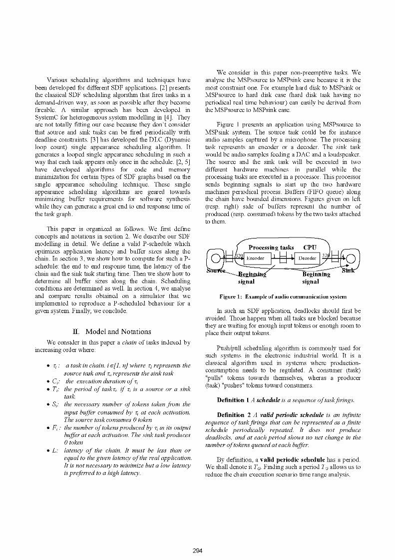
Figure 1 presents an application using MSPsource toMSPsink system. The source task could be for instanceaudio samples captured by a microphone. The processingtask represents an encoder or a decoder. The sink taskwould be audio samples feeding a DAC and a loudspeaker.The source and the sink task will be executed in twodifferent hardware machines in parallel while theprocessing tasks are executed in a processor. This processorsends beginning signals to start up the two hardwaremachines periodical process. Buffers (FIFO queue) alongthe chain have bounded dimensions. Figures given on left(resp. right) side of buffers represent the number ofproduced (resp. consumed) tokens by the two tasks attachedto them.

signal signal

Figure 1: Example of audio communication system

In such an SDF application, deadlocks should first beavoided. Those happen when all tasks are blocked becausethey are waiting for enough input tokens or enough room toplace their output tokens.

Push/pull scheduling algorithm is commonly used forsuch systems in the electronic industrial world. It is aclassical algorithm used in systems where production-consumption needs to be regulated. A consumer (task)"pulls" tokens towards themselves, wheras a producer(task) "pushes" tokens toward consumers.

Definition 1 A schedule is a sequence oftaskfirings.

Definition 2 A valid periodic schedule is an infinitesequence of taskfirings that can be represented as a finiteschedule periodically repeated. It does not producedeadlocks, and at each period shows no net change in thenumber oftokens queued at each buffer.

By definition, a valid periodic schedule has a period.We shall denote it TG. Finding such a period TG allows us toreduce the chain execution scenario time range analysis.

294

Assumption 1 A processing task can be fired as soonas it has enough tokens in its input buffer.

Assumption 2 Task's priorities in the chain follow anincreasing order (a task zi has a higherpriority than a taskij if i j).

Assumption 3 At source task beginning signal, allbuffers in the chain are empty (initial conditions).

For a given chain, many valid periodic schedules exist.Once a scheduling technique is defined, then buffer sizescan be set so as to avoid deadlocks. Scheduling conditionscan be identified, sink task starting time and latency can bedetermined as well.

Definition 3 A P-schedule is a validperiodic schedulewhere the Push scheduling algorithm is usedfor schedulingthe tasks.

Definition 4 A valid P-schedule is a P-schedule forwhich assumptions 1&2&3 are valid.

A valid P-schedule is a sequence of task firings. In itsdefinition there are no data specific temporal constraints.However in the model we study, temporal constraints doexist as source and sink tasks are producing / consumingtokens on a periodic basis. Obviously input token presencein the chain is constrained in time by source task. Also, asink task may execute later than the purely P-schedulebased time (i.e. sink is a hard disk). Execution would bedelayed to the next sink period. However we shall see thatthe chain latency remains unchanged, as it is defined for theminimum sink task starting time. The only consequence ison the sink task input buffer dimension. We will explainthis in detail later.

Lemma 1: There is a unique valid P-schedule for thechain.

Proof: Consider at any time any two tasks in the chain.There are three cases: (i) none are ready (w.r.t. their firingconditions), none are scheduled; (ii) only one is ready andis scheduled; (iii) both are ready. In this case, task priorityis used for scheduling. Combining the three cases, theexecution order is unique. For a given chain, valid P-schedule leads to a unique scheduling sequence. P

Lemma 2: The valid P-schedule leads to minimumbuffer sizes and a minimum latency ofthe chain.

Proof: With the assumption 1, tokens are producedand consumed as soon as possible. And with theassumption 1& 2, the tokens follow the fastest way until thesink task. This leads to a minimum buffer size need to storetokens, as entering tokens are exit out of the system as soonas possible. a

Later, we will prove that a chain empty at init withminimum buffer sizes between each processing tasks andusing a push scheduling algorithm does not necessarilyleads to the valid P-scheduling (conditions are notsufficient). Though, the valid P-schedule does belong to theset of P-schedules empty at init with a minimum buffer sizebetween each processing tasks.

Finally, we define:* qi: the number ofactivations of zi in theperiod TG.In the MSPsource to MSPsink case, T1 and T11 respect

the following relationship: q1Tj = q1T1= TG. This meansthat the source task token production time and the sink tasktoken consumption time are the same. Note that within TGperiod, the number of token entering and exiting the systemare not necessarily identical.

III. ResolutionsIn this section, we first show how to compute the end

to end response time of a chain for a valid P-schedule, todetermine its latency and to find sink task starting time. Weuse the same principle of [8, 9] which present how tocompute the end to end response of any task in a set of taskchains. Then we show how to determine the buffer sizes inthe chain. A simulator is developed to compute directly thelatency and all buffer sizes on the chain. We will alsoillustrate with an example that valid P-schedule algorithmleads to optimized latency and minimum buffer sizes.

A. Determination oflatency ofthe chainIn this section, we show how to find the latency of the

chain. For this purpose, we need first to find each task'sactivation number within the period TG. We then determinea valid P-schedule. These steps will be illustrated using anexample.

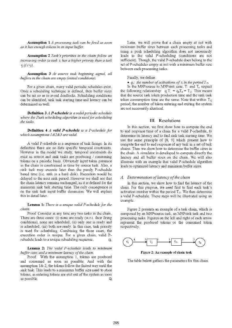
Figure 2 presents an example of a task chain, which iscomposed by an MSPsource task, an MSPsink task and twoprocessing tasks. Figures on the left and right of each arrowrepresent the produced tokens or the consumed tokenrespectively.

4 3 1 1 2 3 Q

Figure 2: An example of chain task

The table below gathers the parameters for this chain.

295

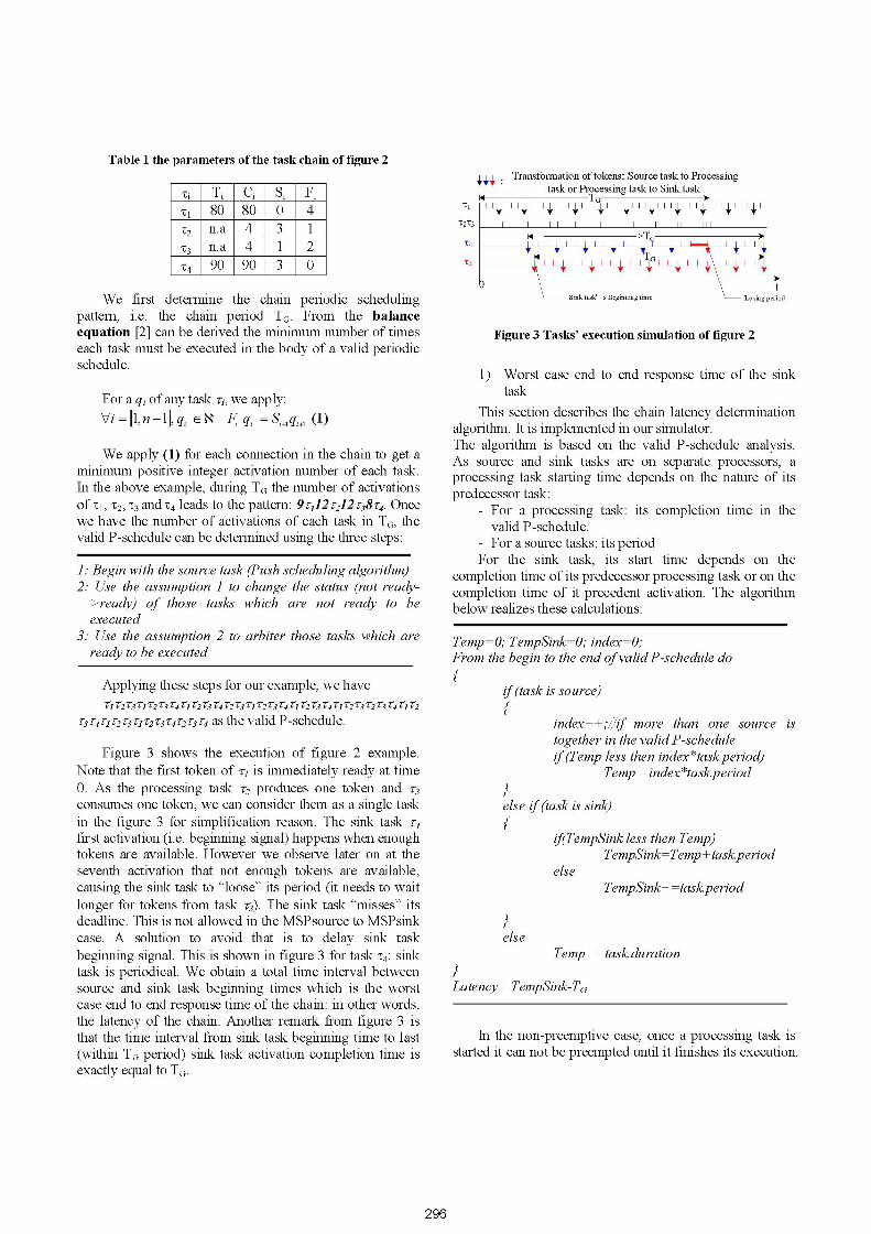
Table 1 the parameters of the task chain of figure 2

T1 C. S. F.Ti|Ti Ci i |Ft1 80 80 0 4C2 n.a 4 3 1C3 n.a 4 1 2C4 90 90 3 0

We first determine the chain periodic schedulingpattern, i.e. the chain period TG. From the balanceequation [2] can be derived the minimum number of timeseach task must be executed in the body of a valid periodicschedule.

For a qi of any task ri, we apply:Vi = [1,n-1], q, E N F qi = S.,q, (1)

We apply (1) for each connection in the chain to get aminimum positive integer activation number of each task.In the above example, during TG the number of activationsof t1, t2, t3 and t4 leads to the pattern: 9r112r212r38r4. Oncewe have the number of activations of each task in TG, thevalid P-schedule can be determined using the three steps:

1: Begin with the source task (Push scheduling algorithm)2: Use the assumption 1 to change the status (not ready-

>ready) of those tasks which are not ready to beexecuted

3: Use the assumption 2 to arbiter those tasks which areready to be executed

Applying these steps for our example, we haveTl T2T3Tl T2 T3 T4Tl T2T3 T4T2 T3 Ti T2T3T4Tl T2 T3 4T4 T2 T3 T2 T3 4T4 T2

T3T4TJT2T3TJT2T3T4T2T3T4 as the valid P-schedule.

Figure 3 shows the execution of figure 2 example.Note that the first token of r- is immediately ready at time0. As the processing task i2 produces one token and i3consumes one token, we can consider them as a single taskin the figure 3 for simplification reason. The sink task r4first activation (i.e. beginning signal) happens when enoughtokens are available. However we observe later on at theseventh activation that not enough tokens are available,causing the sink task to "loose" its period (it needs to waitlonger for tokens from task T3). The sink task "misses" itsdeadline. This is not allowed in the MSPsource to MSPsinkcase. A solution to avoid that is to delay sink taskbeginning signal. This is shown in figure 3 for task t4: sinktask is periodical. We obtain a total time interval betweensource and sink task beginning times which is the worstcase end to end response time of the chain: in other words,the latency of the chain. Another remark from figure 3 isthat the time interval from sink task beginning time to last(within TG period) sink task activation completion time isexactly equal to TG.

Transfornation of tokens: Source task to Processingtask or Processing task to Sink task

<4 TG---Ti

T2T3 n] n] m n] n] m n]nT m

T4.>TG

< ~ TG

0 t\ Losing period

Figure 3 Tasks' execution simulation of figure 2

1) Worst case end to end response time of the sinktask

This section describes the chain latency determinationalgorithm. It is implemented in our simulator.The algorithm is based on the valid P-schedule analysis.As source and sink tasks are on separate processors, aprocessing task starting time depends on the nature of itspredecessor task:

- For a processing task: its completion time in thevalid P-schedule.

- For a source tasks: its periodFor the sink task, its start time depends on the

completion time of its predecessor processing task or on thecompletion time of it precedent activation. The algorithmbelow realizes these calculations:

Temp=O; TempSink=O; index=O;From the begin to the end ofvalid P-schedule do{

if (task is source){

index+ +;/if more than one source istogether in the valid P-scheduleif(Temp less then index*task.period)

Temp= index*task.period

else if (task is sink){

if(TempSink less then Temp)TempSink=Temp +task.period

elseTempSink+ =task.period

elseTemp+ =task. duration

Latency =TempSink-TG

In the non-preemptive case, once a processing task isstarted it can not be preempted until it finishes its execution.

296

\Sink task' s Beginning time

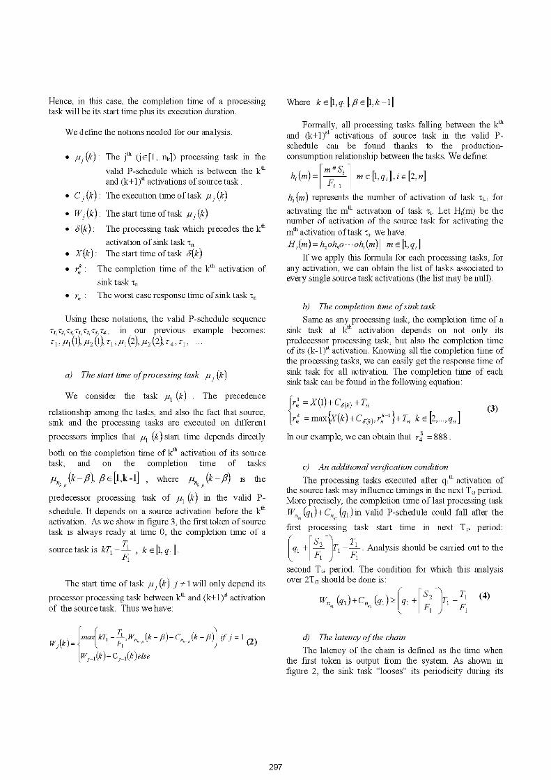
Hence, in this case, the completion time of a processingtask will be its start time plus its execution duration.

We define the notions needed for our analysis.

* plu(k): The jth (j E [1, nk]) processing task in the

valid P-schedule which is between the kthand (k+1)st activations of source task

* Cj (k) The execution time of task pj (k)*Wj (k) The start time of task uj (k)* 8(k): The processing task which precedes the kth

activation of sink task t11* X(k): Thestarttimeoftask 8(k)

*1rk. The completion time of the kth activation ofsink task t11

* rn The worst case response time of sink taskc1

Using these notations, the valid P-schedule sequence'C,T2, T3,iCl,T2, T3 'r4... in our previous example becomes:

iPi(1) 2 (1), -C ,(2),2 (2), 4~ j~

a) The start time ofprocessing task p, (k)

We consider the task ,u1 (k) The precedence

relationship among the tasks, and also the fact that source,sink and the processing tasks are executed on differentprocessors implies that ,u1 (k) start time depends directly

both on the completion time of kth activation of its sourcetask, and on the completion time of tasks

(nk(k--,), ,E6[1,k-1] , where ,unk (k -,8) is the

predecessor processing task of ,u1 (k) in the valid P-schedule. It depends on a source activation before the kthactivation. As we show in figure 3, the first token of sourcetask is always ready at time 0, the completion time of a

source task is kT1 - k E [1, q1]F1 i

The start time of task pj (k) j . 1 will only depend its

processor processing task between kth and (k+1 )t activationof the source task. Thus we have:

w)maxKkTl I ,WI (k ji)+Cn (k I) ifj=(2)wa-1 (k) + Ci (k) else

Where k E [1, q11/3E [1, k -1]

Formally, all processing tasks falling between the kthand (k+1 )st activations of source task in the valid P-schedule can be found thanks to the production-consumption relationship between the tasks. We define:

h(m= mil m [1,qi],i c[2,n]

hi (m) represents the number of activation of task ti-1 foractivating the mth activation of task ci. Let Hi(m) be thenumber of activation of the source task for activating themt activation of task ci. we have:Hi (m) = h2oh3o ...ohi(m) m E [1,qi]

If we apply this formula for each processing tasks, forany activation, we can obtain the list of tasks associated toevery single source task activations (the list may be null).

b) The completion time ofsink taskSame as any processing task, the completion time of a

sink task at kth activation depends on not only itspredecessor processing task, but also the completion timeof its (k- 1f)t activation. Knowing all the completion time ofthe processing tasks, we can easily get the response time ofsink task for all activation. The completion time of eachsink task can be found in the following equation:

{rI = X(1) + C5(k) + Tn

r = max{X(k)+C(k),rk }+TfT k E [2,...,q,](3)

In our example, we can obtain that r4 = 888.

c) An additional verification conditionThe processing tasks executed after ql th activation of

the source task may influence timings in the next TG period.More precisely, the completion time of last processing taskWn,, (ql) + Cn,, (ql) in valid P-schedule could fall after the

first processing task start time in next TG period:

(q +K2 } JT1 - Analysis should be carried out to the

second TG period. The condition for which this analysisover 2TG should be done is:

T1F,

(4)

d) The latency ofthe chainThe latency of the chain is defined as the time when

the first token is output from the system. As shown infigure 2, the sink task "looses" its periodicity during its

297

(ql)+C,, (ql)> q, +s' T,Wn,l F,

execution in the first TG period. To avoid this, the sink taskbeginning signal shall be delayed. Knowing the period ofthe chain and the last completion time of the sink task, thelatency L can be obtained by the equation:

IL = TG ifWl (ql ) + Cn, (q, ) < (q , FT

1

L= 2qr - 2TG else ()

In our example, L= 168. L is also the earliest sinkbeginning signal time after source beginning signal. Inother word, if the source machine starts at time 0, then thesink machine should be started at 168 unit of time.

B Determination ofinitial buffer sizeThe following theorem is used to compute the

minimum buffer size:

Theorem 1-f]] : Given an SDF edge e, the lowerbound on the amount ofmemory required by any scheduleon the edge e is given by a+b-c. Where a is the number oftoken produced at edge e, b is the number of tokenconsumed at edge e, c = gcd(a,b). gcd denotes the greatestcommon divisor.

It is interesting to know whereas push schedulingalgorithm in the condition of minimum buffer size settingsgenerates the same sequence of tasks as the valid P-schedule. The following example shows it is not. Considera chain with tasks B, C and D where B and C areprocessing tasks and D is the sink task. Suppose theproduced and/or consumed tokens number is 1 for everytask. Suppose that at time t task C is just finished and B isready again. Two choices are possible: processing eithertask B or task D. We see that the schedule is not uniqueunder these conditions. Note also that resulting chainlatency will also be different.

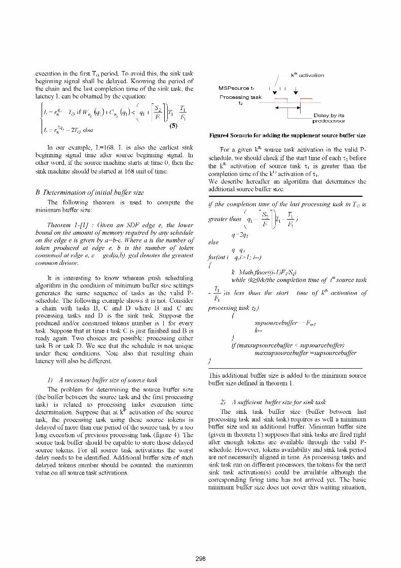
1) A necessary buffer size ofsource taskThe problem for determining the source buffer size

(the buffer between the source task and the first processingtask) is related to processing tasks execution timedetermination. Suppose that at kth activation of the sourcetask, the processing task using these source tokens isdelayed of more than one period of the source task by a toolong execution of previous processing task (figure 4). Thesource task buffer should be capable to store those delayedsource tokens. For all source task activations the worstdelay needs to be identified. Additional buffer size of suchdelayed tokens number should be counted: the maximumvalue on all source task activations.

MSPsource t1

Processing taslt2

Kth activation

Delay by itspredecessor

Figure4 Scenario for adding the supplement source buffer size

For a given kth source task activation in the valid P-schedule, we should check if the start time of each t2 beforethe kth activation of source task c1 is greater than thecompletion time of the kth activation of tI.We describe hereafter an algorithm that determines theadditional source buffer size.

if (the completion time of the last processing task in TG is

greater than q, +l)T,1 1

q=2qelse

q=qlfor(int i= q,i> 1; i--){

k=Math.floor((i-])Fi S2)while (k>O&(the completion time of ithsource task

))is less than the start time of kh activation ofF1processing task m2)

{supsourcebuffer+=Fnk--

if (maxsupsourcebuffer < supsourcebuffer)maxsupsourcebuffer =supsourcebuffer

This additional buffer size is added to the minimum sourcebuffer size defined in theorem 1.

2) A sufficient buffer sizefor sink taskThe sink task buffer size (buffer between last

processing task and sink task) requires as well a minimumbuffer size and an additional buffer. Minimum buffer size(given in theorem 1) supposes that sink tasks are fired rightafter enough tokens are available through the valid P-schedule. However, tokens availability and sink task periodare not necessarily aligned in time. As processing tasks andsink task run on different processors, the tokens for the nextsink task activation(s) could be available although thecorresponding firing time has not amved yet. The basicminimum buffer size does not cover this waiting situation,

298

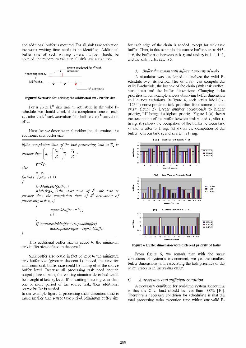
and additional buffer is required. For all sink task activationthe worst waiting time needs to be identified. Additionalbuffer size of such waiting tokens number should becounted: the maximum value on all sink task activations.

tokens produced for kth sinkactivation

Processing task tn.

MSPsink tn

kth activation

Figure5 Scenario for adding the additional sink buffer size

For a given kth sink task m, activation in the valid P-schedule, we should check if the completion time of eachm-1 after the kth sink activation falls before the kth activationofTn.

Hereafter we describe an algorithm that determines theadditional sink buffer size.

if(the completion time of the last processing task in TG is

greater then (qi +F 2 ]T )

q =2qnelse

q qnfor(inti=],i<q; i++){

k Math.ciel(S Fn-)while(k<qn 1&the start time of ith sink task is

greater then the completion time of kth activation ofprocessing task cn-1)

{supsinkbuffer+=Fk++

If(maxsupsinkbuffer < supsinkbuffer)maxsupsinkbuffer =supsinkbuffer

This additional buffer size is added to the minimumsink buffer size defined in theorem 1.

Sink buffer size could in fact be kept to the minimumsink buffer size (given in theorem 1). Indeed, the need foradditional sink buffer size could be managed at the sourcebuffer level. Because all processing task need enoughoutput place to start, the waiting situation described couldbe brought at task r2 level. If its waiting time is greater thanone or more period of the source task, then additionalsource buffer is needed.In our example figure 2, processing tasks execution time ismuch smaller than source task period. Minimum buffer size

for each edge of the chain is needed, except for sink taskbuffer. Thus, in this example, the source buffer size is: 4+3-1=6, the buffer size between task -c and task i3 is: 1+1-1=1,and the sink buffer size is 5.

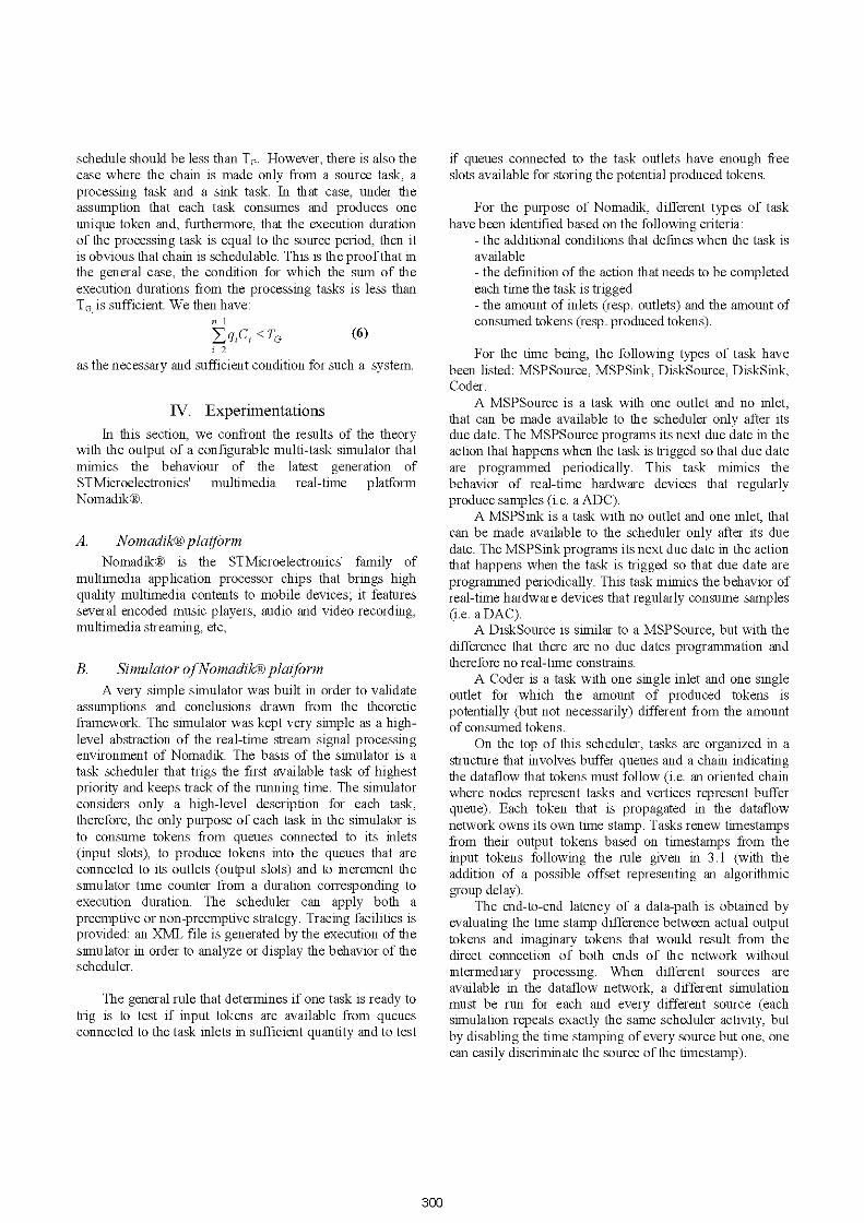
3) Buffer dimension with differentpriority oftasksA simulator was developed to analyze the valid P-

schedule over its period. The simulator can compute thevalid P-schedule, the latency of the chain (sink task earlieststart time) and the buffer dimensions. Changing taskspriorities in our example allows observing buffer dimensionand latency variations. In figure 4, each series label (ex:"1234") corresponds to task priorities from source to sink(w.r.t. figure 2). Larger number corresponds to higherpriority, "4" being the highest priority. Figure 4 (a) showsthe occupation of the buffer between task t1 and tC2 after t1firing. (b) shows the occupation of the buffer between tasktC2 and tC3 after t2 firing. (c) shows the occupation of thebuffer between task tC3 and tC4 after tC3 firing.

( a ) aurffer of tsk 1 -2

1 2 3 4 5 e 7 a 9 10 11 1

nunFiirino

(c-) bu ff-er o>f tias--k 2-3

Figure 6 Buffer dimension with different priority of tasks

From figure 6, we remark that with the sameconditions of system's environment, we get the smallestbuffer dimensions with associating the task priorities of thechain graph in an increasimg order.

C A necessary and sufficient conditionA necessary condition for real-time system scheduling

is that the CPU load should be less than 100% [10].Therefore a necessary condition for scheduling is that thetotal processing tasks execution time within our valid P-

299

5

3-

2-

1

0

_ 3_ 1 324E3 1 432

2 3 4 5 6

numFiring8 9

(k>) k uffiar o)f tas-%k 3

5

3

2

1

0

E3 1 234

M 1324

a3 1432

2-5

2

1-5

1

0-5

0

E3 1234m 1324E3 1432

1 2 3 4 5 6 7 8 9 10 11 12

numFiring

schedule should be less than TG. However, there is also thecase where the chain is made only from a source task, aprocessing task and a sink task. In that case, under theassumption that each task consumes and produces oneunique token and, furthermore, that the execution durationof the processing task is equal to the source period, then itis obvious that chain is schedulable. This is the proof that inthe general case, the condition for which the sum of theexecution durations from the processing tasks is less thanTG is sufficient. We then have:

n-l

qiCi <TGi=2

(6)

as the necessary and sufficient condition for such a system.

IV. ExperimentationsIn this section, we confront the results of the theory

with the output of a configurable multi-task simulator thatmimics the behaviour of the latest generation ofSTMicroelectronics' multimedia real-time platformNomadik .

A. NomadikRplatformNomadik R is the STMicroelectronics' family of

multimedia application processor chips that brings highquality multimedia contents to mobile devices; it featuresseveral encoded music players, audio and video recording,multimedia streaming, etc,

B. Simulator ofNomadik1 platformA very simple simulator was built in order to validate

assumptions and conclusions drawn from the theoreticframework. The simulator was kept very simple as a high-level abstraction of the real-time stream signal processingenvironment of Nomadik. The basis of the simulator is atask scheduler that trigs the first available task of highestpriority and keeps track of the running time. The simulatorconsiders only a high-level description for each task,therefore, the only purpose of each task in the simulator isto consume tokens from queues connected to its inlets(input slots), to produce tokens into the queues that areconnected to its outlets (output slots) and to increment thesimulator time counter from a duration corresponding toexecution duration. The scheduler can apply both apreemptive or non-preemptive strategy. Tracing facilities isprovided: an XML file is generated by the execution of thesimulator in order to analyze or display the behavior of thescheduler.

The general rule that determines if one task is ready totrig is to test if input tokens are available from queuesconnected to the task inlets in sufficient quantity and to test

if queues connected to the task outlets have enough freeslots available for storing the potential produced tokens.

For the purpose of Nomadik, different types of taskhave been identified based on the following criteria:

- the additional conditions that defines when the task isavailable- the definition of the action that needs to be completedeach time the task is trigged- the amount of inlets (resp. outlets) and the amount ofconsumed tokens (resp. produced tokens).

For the time being, the following types of task havebeen listed: MSPSource, MSPSink, DiskSource, DiskSink,Coder.

A MSPSource is a task with one outlet and no inlet,that can be made available to the scheduler only after itsdue date. The MSPSource programs its next due date in theaction that happens when the task is trigged so that due dateare programmed periodically. This task mimics thebehavior of real-time hardware devices that regularlyproduce samples (i.e. a ADC).

A MSPSink is a task with no outlet and one inlet, thatcan be made available to the scheduler only after its duedate. The MSPSink programs its next due date in the actionthat happens when the task is trigged so that due date areprogrammed periodically. This task mimics the behavior ofreal-time hardware devices that regularly consume samples(i.e. aDAC).

A DiskSource is similar to a MSPSource, but with thedifference that there are no due dates programmation andtherefore no real-time constrains.

A Coder is a task with one single inlet and one singleoutlet for which the amount of produced tokens ispotentially (but not necessarily) different from the amountof consumed tokens.

On the top of this scheduler, tasks are organized in astructure that involves buffer queues and a chain indicatingthe dataflow that tokens must follow (i.e. an oriented chainwhere nodes represent tasks and vertices represent bufferqueue). Each token that is propagated in the dataflownetwork owns its own time stamp. Tasks renew timestampsfrom their output tokens based on timestamps from theinput tokens following the rule given in 3.1 (with theaddition of a possible offset representing an algorithmicgroup delay).

The end-to-end latency of a data-path is obtained byevaluating the time stamp difference between actual outputtokens and imaginary tokens that would result from thedirect connection of both ends of the network withoutintermediary processing. When different sources areavailable in the dataflow network, a different simulationmust be run for each and every different source (eachsimulation repeats exactly the same scheduler activity, butby disabling the time stamping of every source but one, onecan easily discriminate the source of the timestamp).

300

The API of the simulator offers utilities in order to:- instantiate and configure every necessary tasks- build the dataflow chain,- configure every queue.Once the tasked are instantiated and configured, the

dataflow chain built and queues configured, the simulatorrepeats the scheduling activities until the counter trackingrunning time reach a given limit, while tracing everyactivities (task name, trig date, queue modification,overflow or loss of real-time, token end-to-end latencyetc.). The result of the file trace can be used for post-mortem analysis or visualization.

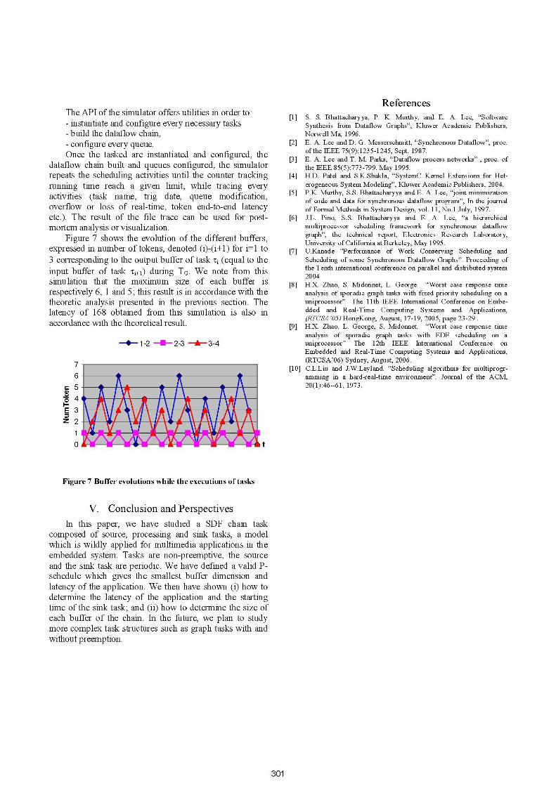
Figure 7 shows the evolution of the different buffers,expressed in number of tokens, denoted (i)-(i+1) for i=1 to3 corresponding to the output buffer of task ti (equal to theinput buffer of task i+,) during TG. We note from thissimulation that the maximum size of each buffer isrespectively 6, 1 and 5; this result is in accordance with thetheoretic analysis presented in the previous section. Thelatency of 168 obtained from this simulation is also inaccordance with the theoretical result.

1-2 2-3 3-4

a

0

Ez

7

6543210

References[1] S. S. Bhattacharyya, P. K. Murthy, and E. A. Lee, "Software

Synthesis from Dataflow Graphs", Kluwer Academic Publishers,Norwell Ma, 1996.

[2] E. A. Lee and D. G. Messerschmitt, "Synchronous Dataflow", proc.of the IEEE 75(9):1235-1245, Sept, 1987.

[3] E. A. Lee and T. M. Parks, "Dataflow process networks", proc. ofthe IEEE 85(5):773-799, May 1995.

[4] H.D. Patel and S.K.Shukla, "SystemC Kernel Extensions for Het-erogeneous System Modeling", Kluwer Academic Publishers, 2004.

[5] P.K. Murthy, S.S. Bhattacharyya and E. A. Lee, "joint minimizationof code and data for synchronous dataflow program", In the journalof Formal Methods in System Design, vol. 1 1, No.1 July, 1997.

[6] J.L. Pino, S.S. Bhattacharyya and E. A. Lee, "a hierarchicalmultiprocessor scheduling framework for synchronous dataflowgraph", the technical report, Electronics Research Laboratory,University of California at Berkeley, May 1995.

[7] U.Kanade "Performance of Work Conserving Scheduling andScheduling of some Synchronous Dataflow Graphs". Proceeding ofthe Tenth international conference on parallel and distributed system2004

[8] H.X. Zhao, S. Midonnet, L. George. "Worst case response timeanalysis of sporadic graph tasks with fixed priority scheduling on auniprocessor" The 11th IEEE International Conference on Embe-dded and Real-Time Computing Systems and Applications,(RTCSA '05) HongKong, August, 17-19, 2005, page 23-29.

[9] H.X. Zhao, L. George, S. Midonnet. "Worst case response timeanalysis of sporadic graph tasks with EDF scheduling on auniprocessor" The 12th IEEE International Conference onEmbedded and Real-Time Computing Systems and Applications,(RTCSA'06) Sydney, August, 2006.

[10] C.L.Liu and J.W.Layland. "Scheduling algorithms for multiprogr-amming in a hard-real-time environment". Journal of the ACM,20(1):46--61, 1973.

t

Figure 7 Buffer evolutions while the executions of tasks

V. Conclusion and PerspectivesIn this paper, we have studied a SDF chain task

composed of source, processing and sink tasks, a modelwhich is wildly applied for multimedia applications in theembedded system. Tasks are non-preemptive, the sourceand the sink task are periodic. We have defined a valid P-schedule which gives the smallest buffer dimension andlatency of the application. We then have shown (i) how todetermine the latency of the application and the startingtime of the sink task; and (ii) how to determine the size ofeach buffer of the chain. In the future, we plan to studymore complex task structures such as graph tasks with andwithout preemption.

301