programa presidencial contra cultivos ilicitos - CORPONARIÑO
TESIS DOCTORAL
MINERÍA DE DATOS EN EL ANÁLISIS DE LAS FIRMAS DE CULTIVOS
AGRÍCOLAS
PHD THESIS
DATA MINING IN THE ANALYSIS OF CROP SIGNATURES
FERNANDO RODRÍGUEZ MORENO
2013
DEPARTAMENTO DE
EXPRESIÓN GRÁFICA


TESIS DOCTORAL
MINERÍA DE DATOS EN EL ANÁLISIS DE LAS FIRMAS DE CULTIVOS
AGRÍCOLAS
PHD THESIS
DATA MINING IN THE ANALYSIS OF CROP SIGNATURES
FERNANDO RODRÍGUEZ MORENO
2013
DEPARTAMENTO DE
EXPRESIÓN GRÁFICA
CONFORMIDAD DEL DIRECTOR
FDO: ÁNGEL MANUEL FELICÍSIMO PÉREZ


El doctor Don Ángel Manuel Felicísimo Pérez informa que: La memoria titulada Minería de datos en el análisis de las firmas de cultivos agrícolas, que presenta Fernando Rodríguez Moreno, Licenciado en Ciencias Ambientales, para optar al grado de Doctor, ha sido realizada en el Departamento de Expresión Gráfica de la Universidad de Extremadura, bajo mi dirección y reuniendo todas las condiciones exigidas a los trabajos de tesis doctoral.
Badajoz, Febrero de 2013.
Fdo.: Ángel Manuel Felicísimo Pérez


“The scientist is free, and must be free to ask any question, to doubt
any assertion, to seek for any evidence, to correct any errors."
J. Robert Oppenheimer AGRADECIMIENTOS A mis padres, a mi director de tesis, a mi… no es fácil escribir este apartado siendo justo porque el camino ha sido largo y duro. En ocasiones la ayuda era premeditada, en otras resultó fruto del azar, a veces surgió en el momento y lugar menos esperado, otras fue fruto de algún desencuentro. Esta tesis es el resultado de una estupenda partida de billar. Hoy contemplo satisfecho el buen trabajo y quiero darle las gracias a todos aquellos que me dedicaron tiempo porque todos ellos participaron en esa partida de billar, todos ellos me han traído aquí, por eso, muchas gracias. ACKNOWLEDGEMENTS To my parents, my supervisor, my ... not easy to write this section being fair because the road has been long and hard. Sometimes the help was premeditated, in other was haphazard, sometimes emerged when and where least expected, others were the result of a misunderstanding. This thesis is the result of a great game of pool. Today I look satisfied the good work and I want to thank everyone who spent time with me because they all participated in the game of pool, all of them have brought me here, so, thank you very much.


A mis padres


F. Rodríguez Moreno Tabla de contenidos / Table of contents I
Tabla de contenidos / Table of contents
INTRODUCCIÓN / INTRODUCTION ............................................................................................................................. 1
NECESIDADES DEL AGRICULTOR / FARMERS' NEEDS ...................................................................................................................... 1
SOLUCIONES ACTUALES / CURRENT SOLUTIONS ........................................................................................................................... 2
PROBLEMAS ACTUALES / CURRENT PROBLEMS............................................................................................................................. 3
PROPÓSITO DE ESTA TESIS / PURPOSE OF THIS THESIS .................................................................................................................... 4
ESTRUCTURA Y CONTENIDO DE LA TESIS / STRUCTURE AND CONTENT OF THE THESIS ............................................................................ 5
Índices espectrales de vegetación / Spectral vegetation indices ................................................................................. 5
Garantías exigidas en el estudio / Guarantees required in the study .......................................................................... 5
Técnicas de reducción de dimensiones / Techniques for dimensionality reduction ..................................................... 6
Árboles de decisiones / Decision trees ......................................................................................................................... 7
Interpretación espacial de los parámetros de la planta / Spatial interpretation of plant parameters ....................... 8
Lo que se obtendrá con la lectura de esta tesis / What you get by reading this thesis ............................................... 9
REFERENCIAS / REFERENCES .................................................................................................................................................. 10
EVALUATING SPECTRAL VEGETATION INDICES FOR A PRACTICAL ESTIMATION OF NITROGEN CONCENTRATION IN
DUAL PURPOSE (FORAGE AND GRAIN) TRITICALE ..................................................................................................... 13
CITATION ........................................................................................................................................................................... 13
DOWNLOAD LINK ................................................................................................................................................................. 13
HEADER ............................................................................................................................................................................. 13
ABSTRACT .......................................................................................................................................................................... 13
RESUMEN .......................................................................................................................................................................... 14
INTRODUCTION ................................................................................................................................................................... 15
MATERIAL AND METHODS ..................................................................................................................................................... 15
RESULTS AND DISCUSSION ..................................................................................................................................................... 18
REFERENCES ....................................................................................................................................................................... 20
PCA VERSUS ICA FOR THE REDUCTION OF DIMENSIONS OF THE SPECTRAL SIGNATURES IN THE SEARCH FOR AN INDEX
FOR THE CONCENTRATION OF NITROGEN IN PLANT ................................................................................................. 23
CITATION ........................................................................................................................................................................... 23
DOWNLOAD LINK ................................................................................................................................................................. 23
HEADER ............................................................................................................................................................................. 23
ABSTRACT .......................................................................................................................................................................... 23
RESUMEN .......................................................................................................................................................................... 24
INTRODUCTION ................................................................................................................................................................... 25
MATERIAL AND METHODS ..................................................................................................................................................... 26
RESULTS AND DISCUSSION ..................................................................................................................................................... 30
ACKNOWLEDGEMENTS ......................................................................................................................................................... 34
REFERENCES ....................................................................................................................................................................... 34
A DECISION TREE FOR NITROGEN APPLICATION BASED ON A LOW COST RADIOMETRY ............................................ 37
CITATION ........................................................................................................................................................................... 37
DOWNLOAD LINK ................................................................................................................................................................. 37
HEADER ............................................................................................................................................................................. 37
ABSTRACT .......................................................................................................................................................................... 37

F. Rodríguez Moreno Tabla de contenidos / Table of contents II
INTRODUCTION ................................................................................................................................................................... 38
MATERIAL AND METHODS ..................................................................................................................................................... 40
RESULTS ............................................................................................................................................................................ 44
DISCUSSION ....................................................................................................................................................................... 49
ACKNOWLEDGEMENTS ......................................................................................................................................................... 50
REFERENCES ....................................................................................................................................................................... 51
SPATIAL INTERPRETATION OF PLANT PARAMETERS IN PRECISION AGRICULTURE WITH WINTER WHEAT .................. 55
CITATION ........................................................................................................................................................................... 55
DOWNLOAD LINK ................................................................................................................................................................. 55
HEADER ............................................................................................................................................................................. 55
ABSTRACT .......................................................................................................................................................................... 55
INTRODUCTION ................................................................................................................................................................... 56
MATERIALS AND METHODS .................................................................................................................................................... 58
Field experiments and data collection ....................................................................................................................... 58
Data analysis .............................................................................................................................................................. 59
Evaluation .................................................................................................................................................................. 63
RESULTS AND DISCUSSION ..................................................................................................................................................... 65
Field Pachty ................................................................................................................................................................ 65
Field Haj ..................................................................................................................................................................... 69
CONCLUSIONS ..................................................................................................................................................................... 74
ACKNOWLEDGEMENT ........................................................................................................................................................... 75
REFERENCES ....................................................................................................................................................................... 75
RESULTADOS Y DISCUSIÓN / RESULTS AND DISCUSSION .......................................................................................... 83
ESTIMACIÓN DEL ESTADO NUTRICIONAL DEL CULTIVO MEDIANTE RADIOMETRÍA / ESTIMATION OF NUTRITIONAL STATUS OF THE CROP BY
RADIOMETRY ...................................................................................................................................................................... 83
DIAGNÓSTICO AGRONÓMICO MEDIANTE INTERPRETACIÓN ESPACIAL DE LOS PARÁMETROS DE LA PLANTA / DIAGNOSIS AGRONOMIC BY SPATIAL
INTERPRETATION OF PLANT PARAMETERS .................................................................................................................................. 90
NOVEDADES INTRODUCIDAS / INNOVATIONS INTRODUCED .......................................................................................................... 93
LÍNEAS DE TRABAJO FUTURAS / FUTURE RESEARCH ..................................................................................................................... 94
REFERENCIAS / REFERENCES .................................................................................................................................................. 95
CONCLUSIONES / CONCLUSIONS .............................................................................................................................. 97

F. Rodríguez Moreno Introducción / Introduction 1 de 97
Introducción / Introduction
Necesidades del agricultor / Farmers' needs
Los agricultores son cada día más conscientes de la necesidad de aplicar el tratamiento agronómico
específico que precisa el cultivo de tal forma que el rendimiento de los insumos sea máximo y el
desarrollo sostenible (Barker and Pilbeam 2007; Jones 1998; Marschner 1995; Mengel and Kirkby
2001). De esta forma se obtiene el máximo beneficio hoy y se garantiza la rentabilidad de la actividad
agrícola en el futuro.
En la consecución de esta meta la agricultura de precisión juega un papel determinante. La
agricultura de precisión pone a disposición del agricultor la última tecnología (Srinivasan 2006;
Stafford 1997), gracias a la cual es posible cartografiar de forma precisa, rápida y barata el campo y
aplicar un tratamiento diferencial ajustado a las necesidades específicas de cada una de las unidades
tierra que lo componen.
La correcta delimitación de las unidades tierra así como el certero diagnóstico agronómico de las
mismas se puede conseguir aunando conocimientos agronómicos y técnicas de minería de datos,
evidenciarlo es el propósito de esta tesis. Este binomio está fuera del alcance de muchos agricultores
por lo que es necesario desarrollar metodologías de muestreo/análisis más sencillas y tratar de
desarrollar sistemas de apoyo a la decisión, de forma que el agricultor pueda encontrar las respuestas
que necesita con la ayuda de su consultor agrícola y del laboratorio.
Farmers are increasingly aware of the need for specific agronomic treatment, the required for the
crop such that the input performance is maximized and the development is sustainable (Barker and
Pilbeam 2007; Jones 1998; Marschner 1995; Mengel and Kirkby 2001). Thus the farmer gets the
maximum benefit today and ensures the profitability of the farm in the future.
Precision agriculture plays a key role in achieving that goal. Precision agriculture offers to the farmer
the latest technology (Srinivasan 2006; Stafford 1997), thanks to which it is possible to map accurately,
quickly and cheaply the field and apply differential treatment adjusted to the specific needs of each of
the land units
Proper delineation of land units and its correct agronomic diagnosis can be obtained by combining
agricultural knowledge and data mining, the purpose of this thesis is to prove it. This binomial is
beyond the reach of many farmers so it is necessary to develop methodologies for a simple sampling /
analysis and try to develop a decision support system, so the farmer can find the answers with the help
of his agricultural consultant and laboratory.

F. Rodríguez Moreno Introducción / Introduction 2 de 97
Soluciones actuales / Current solutions
Gracias a numerosos estudios agronómicos se han conseguido identificar los rangos de
concentraciones y las relaciones entre las concentraciones de los nutrientes adecuadas para la mayoría
de los cultivos (Marschner 1995; Rengel 1998; Reuter et al. 1998). Rangos de suficiencia y relaciones
que pueden emplearse como referencia en la elaboración de los planes de fertilización, de esta forma es
más probable que el agricultor alcance altos y sostenibles rendimientos del cultivo.
El procedimiento tradicional para la obtención de las concentraciones de los nutrientes en la planta
son los análisis foliares. Su obtención requiere trabajo de campo (muestreo) y de laboratorio (análisis),
es por tanto costosa en tiempo y recursos. Si es necesaria una estimación rápida y barata, entonces la
solución son las medidas de la reflectancia espectral del cultivo (medidas proximales o remotas). Son
muchos los trabajos científicos que han demostrado el potencial de la radiometría para estimar la
concentración de los diferentes nutrientes en la planta (Bannari et al. 2007; Cammarano et al. 2011; De
Assis Carvalho Pinto et al. 2007; Gnyp et al. 2009; Goel et al. 2003; Gómez-Casero et al. 2007).
Hoy existen numerosos dispositivos comerciales (Abdelhamid et al. 2003; Arregui et al. 2006;
Castelli and Contillo 2009; Graeff et al. 2009), muchos de ellos sencillos dispositivos de mano
programados con intuitivas interfaces de usuario, que ofrecen estimaciones del nivel de los nutrientes
en la planta obtenidas a partir de las lecturas que el agricultor puede obtener en unos pocos minutos de
muestreo en campo.
It has been possible to identify the ranges of concentrations and relations between the
concentrations of nutrients suitable for most crops thanks to numerous agronomic studies (Marschner
1995; Rengel 1998; Reuter et al. 1998). Sufficiency ranges and relationships that can be used as a
reference to calculate the fertilization plan, so it is more likely that farmers achieve high and sustainable
crop yields.
The traditional procedure for obtaining the concentrations of nutrients in the plant is leaf analysis.
Its obtaining requires fieldwork (sampling) and laboratory (analysis), it is therefore costly in time and
resources. Whether a rapid and inexpensive estimation is necessary, then the solution is spectral
reflectance measurements of the crop (proximal or remote measurements). Many scientific studies
have shown the potential of radiometry to estimate the concentration of different nutrients in the plant
(Bannari et al. 2007; Cammarano et al. 2011; De Assis Carvalho Pinto et al. 2007; Gnyp et al. 2009; Goel
et al. 2003; Gómez-Casero et al. 2007).
Today there are numerous commercial devices (Abdelhamid et al. 2003; Arregui et al. 2006; Castelli
and Contillo 2009; Graeff et al. 2009), many of them simple handheld devices programmed with
intuitive user interfaces, which provide estimates of the level of nutrients in the plant derived from the
readings that the farmer can get in a few minutes of field sampling.
F. Rodríguez Moreno Introducción / Introduction 3 de 97
Problemas actuales / Current problems
Los anteriormente comentados rangos de suficiencia para las concentraciones de los nutrientes son
específicos del cultivo e incluso del cultivar, además requieren el muestreo de una parte determinada
de la planta en un estado fenológico concreto (Marschner 1995; Rengel 1998). Otro problema de los
rangos de suficiencia es que sólo han sido validados en unas determinadas condiciones, las de los
ensayos en las que fueron determinados, las cuales no pueden abarcar todas las combinaciones posibles
de desarrollo del cultivo (Alves Mourão Filho 2005; Camacho et al. 2012; Jeong et al. 2009; Stalenga
2007). El caso de las metodologías que emplean relaciones entre nutrientes es diferente, son más
generalizables en el espacio y tiempo, aunque las limitaciones anteriores no ha desaparecido (Agbangba
et al. 2011; Amundson and Koehler 1987; Dagbénonbakin et al. 2010).
Las firmas espectrales del cultivo, procedentes de medidas proximales o remotas, se transforman en
estimaciones de los niveles de los nutrientes en la planta mediante modelos que poseen una baja
capacidad de generalización espacio-temporal. Esto reduce su efectividad en explotaciones agrícolas
reales (Heege et al. 2008; Li et al. 2010), relegando al binomio agronomía-radiometría a los grandes
campos dónde resulta imbatible en la actualidad. En esos escenarios una pequeña mejora por unidad de
superficie supone un gran incremento en los beneficios, es por ello que hasta pueden llegar a disponer
de un panel de expertos que realicen estudios de calibración.
Si no mejora la efectividad y capacidad de generalización de los modelos que relacionan las firmas
espectrales (reflectancia) del cultivo y las concentraciones de nutrientes en la planta, el aumento del
rendimiento del cultivo y de la sostenibilidad posibles gracias a la agricultura de precisión
(radiometría), no llegará a todas las explotaciones agrícolas.
The previously mentioned sufficiency ranges for concentrations of nutrients are crop specific and
even of the cultivar. It also requires the sampling of a particular part of the plant in a particular
phenological stage (Marschner 1995; Rengel 1998). Another problem, the sufficiency ranges have been
validated in certain conditions, the conditions of the trials in which they were determined, which
cannot cover all possible combinations of crop development (Alves Mourão Filho 2005; Camacho et al.
2012; Jeong et al. 2009; Stalenga 2007). The case of the methodologies use relationships between
nutrients is different; it is more generalizable over space and time, although the above limitations are
not gone (Agbangba et al. 2011; Amundson and Koehler 1987; Dagbénonbakin et al. 2010).
The crop spectral signatures, from proximal or remote measures, are transformed into estimates of
the levels of nutrients in the plant using models that have low space-time generalization ability. This
reduces its effectiveness in real farms (Heege et al. 2008; Li et al. 2010), relegating the binomial
agronomy-radiometry to large areas where it is currently unbeatable. In these scenarios a small
improvement per unit area is a large increase in profits, which is why they may even have a panel of
experts to carry out calibration studies.
If the effectiveness and generalizability of the models do not improve, the increase in crop yield and
sustainability possible thanks to precision agriculture will not reach all farms.

F. Rodríguez Moreno Introducción / Introduction 4 de 97
Propósito de esta tesis / Purpose of this thesis
El propósito de esta tesis es realizar dos aportaciones significativas en el campo de la agricultura de
precisión. Ambas aportaciones persiguen el mismo objetivo, aumentar la eficacia y reducir los costes de
los diagnósticos agronómicos integrales. En caso de conseguirlo aumentaría el número de explotaciones
agrícolas que pueden apostar por la agricultura de precisión. Esa resultaría ser la opción más rentable
tanto para el presente como para el futuro.
Una explicación simplificada del proceso de diagnóstico agronómico sería adquisición de
información relevante del cultivo e interpretación de la misma, los dos procesos a los que esta tesis
dirige la atención. Se pretende mejorar la efectividad y capacidad de generalización de los modelos que
estiman el estado nutricional de la planta a partir de medidas espectrales. También se trata de
incorporar las técnicas geomáticas desarrolladas en las últimas décadas (GPS, GIS,…) a las metodologías
clásicas para la interpretación de los niveles de los nutrientes en la planta. El objetivo es desarrollar una
metodología para el diagnóstico agronómico de los campos, sería un proceso lógico deductivo que
trabaja con evidencias obtenidas en el mismo campo. No serían precisos estudios previos y por tanto
estaría a disposición de cualquier agricultor independientemente del área geográfica o cultivo.
The purpose of this thesis is to make two significant contributions in the field of precision
agriculture. Both contributions have the same objective, to increase efficiency and reduce the costs of
comprehensive agronomic diagnosis. In case of achieving the objectives, this would increase the
number of farms that can go for precision agriculture. It would be the most profitable option for the
present and the future.
A simplified explanation of the process for the agronomic diagnostic would be the acquisition of
relevant information of the crop and interpretation of the same, the two processes to which this thesis
directs the attention. It is intended to improve the effectiveness and generalizability of models that
estimate the nutritional status of the plant from spectral measurements. On the other hand tries to
incorporate the techniques developed in the last decades (GPS, GIS ...) to the classical methods for the
interpretation of the levels of nutrients in the plant. The purpose is to develop a methodology to make
agronomic diagnosis; it would be a deductive process that works with evidence obtained in the same
field. No previous studies would be needed and therefore it would be available to all farmers, regardless
of geographic area or crop.
F. Rodríguez Moreno Introducción / Introduction 5 de 97
Estructura y contenido de la tesis / Structure and content of the thesis
Índices espectrales de vegetación / Spectral vegetation indices
La tesis comienza evaluando el verdadero potencial de los 21 índices espectrales de vegetación
(radiometría) más ampliamente usados para estimar la concentración de un nutriente, el nitrógeno, en
planta (Blackburn 2007; Panda et al. 2010; Raymond Hunt et al. 2011; Schellberg et al. 2008). Prueba
realizada en unas condiciones que simulan una explotación agrícola real (amplio rango de condiciones
de desarrollo). Es preciso conocer si los índices espectrales de vegetación son una solución en la
práctica, si empleándolos es posible obtener estimaciones correctas, rápidas y baratas del estado
nutricional del cultivo. En caso afirmativo habría que dirigir los esfuerzos a proyectos de demostración
con los que animar la transferencia de la tecnología a los agricultores.
The thesis begins by evaluating the true potential of 21 spectral vegetation indices (radiometry), the
most widely used indices to estimate the concentration of a nutrient, the nitrogen, in plant (Blackburn
2007; Panda et al. 2010; Raymond Hunt et al. 2011; Schellberg et al. 2008). Testing conducted under
conditions that simulate real farms (wide range of growing conditions). It is necessary to know if
spectral vegetation indices are a practical solution, if it is possible to obtain correct, fast and cheap
estimates of the crop nutritional status. If so efforts should be directed to demonstration projects which
encourage the transfer of technology to the farmers.
Garantías exigidas en el estudio / Guarantees required in the study
En esta tesis se dedica un apartado especial al procedimiento de evaluación de los resultados.
Confundir una relación descriptiva con una predictiva conduciría al desarrollo de un modelo cuyas
recomendaciones no tendrían ningún valor, lo que haría que los objetivos de la tesis fueran
inalcanzables. Para obtener evaluaciones realistas se toman 4 medidas, una ya comentada,
experimentar en un amplio rango de condiciones de desarrollo. La segunda medida consiste en forzar al
modelo que ha de relacionar el índice espectral de vegetación y la concentración de nutriente a que sea
válido durante todo el período durante el cual sería posible actuar para corregir una potencial
deficiencia (novedad). La tercera medida es el uso de la validación cruzada en la evaluación de las
relaciones y la cuarta medida es el empleo en el ensayo del cultivo que presenta mayores dificultades
para el desarrollo de modelos radiométricos, el triticale de doble propósito.
Verato es el cultivar del triticale (X Triticosecale Wittmack) que soporta el pastoreo del ganado
durante su desarrollo sin arruinar la cosecha final. Esta peculiaridad dificulta la consecución del
objetivo, el desarrollo de un modelo radiométrico eficaz y generalizable, al no poder confiar en el
verdor como estimador de la concentración de nitrógeno (después del pastoreo el cultivo amarillea
debido a un desajuste entre crecimiento y síntesis de clorofila, no por déficit de nitrógeno). Eso obliga a

F. Rodríguez Moreno Introducción / Introduction 6 de 97
la búsqueda de rasgos espectrales más directamente relacionados con la concentración de nitrógeno,
los cuales respondan correctamente incluso en condiciones complicadas.
Gracias a estas medidas se pretende determinar el umbral mínimo de eficacia de la metodología, se
aumentan las garantías de poder predictivo del modelo y se reducen costes de implementación,
facilitando así la transferencia de los resultados a explotaciones agrícolas reales.
This thesis has a special section to describe the procedure of evaluating the results. Mistaking a
descriptive relationship with a predictive relationship leads to the development of a model whose
recommendations would have no value; in that case the objectives of the thesis would be unreachable.
For realistic assessments four measures were taken, the first has already been mentioned,
experimentation in wide range of growing conditions. The second measure consists in forcing the
model (the model that has to relate spectral vegetation index and nutrient concentration) to be valid in
the period during which one could act to correct a potential shortcoming (new). The third measure is
the use of cross-validation in the evaluation of relationships and the fourth measure is employment in
the test of a crop that presents superior difficulties for the development of radiometric models, the dual
purpose triticale.
Verato is the cultivar of triticale (X Triticosecale Wittmack) that supports livestock grazing during its
development without ruining the final harvest. This peculiarity makes difficult to achieve the objective,
the development of an effective and generalizable radiometric model, because with that crop the green
of the plant is not a good estimator of the nitrogen concentration (after grazing the crop yellowing due
to a mismatch between growth and chlorophyll synthesis, no nitrogen deficiency). That requires finding
spectral features directly related to the concentration of nitrogen, which respond correctly even in
difficult conditions.
Thanks to these measures the minimum threshold of effectiveness of the methodology could be
determined; they increase the guarantees of predictive power and reduce implementation costs, thus
facilitating the transfer of results to the real farms.
Técnicas de reducción de dimensiones / Techniques for dimensionality reduction
En el mismo escenario y con los mismos datos y procedimiento de evaluación se estudia si las dos
técnicas de reducción de dimensiones más potentes, Análisis de componentes principales (PCA) (Shlens
2005) y Análisis de componentes independientes (ICA) (Hyvärinen and Oja 2000), son adecuadas para
el procesamiento de los datos obtenidos en el muestreo hiperespectral del cultivo (firma espectral
completa). Si las técnicas son efectivas entonces concentrarán la información relativa al estado
nutricional del cultivo en una decena de nuevas componentes, con las que sería fácil desarrollar
modelos de regresión con los que estimar eficazmente la concentración de nitrógeno en planta.
Un resultado positivo en el estudio con las técnicas de reducción de dimensiones difícilmente sería
un resultado transferible, esto es así dado el coste del espectroradiómetro necesario para obtener la
firma espectral. El objetivo de este estudio es dar un paso intermedio, comprobar que aún con todas las

F. Rodríguez Moreno Introducción / Introduction 7 de 97
garantías exigidas es posible desarrollar un modelo efectivo con capacidad de generalización en el
espacio y tiempo (dentro de la misma campaña).
In the same scenario and with the same data and evaluation procedure, it was studied whether the
two techniques for dimensionality reduction more powerful, Principal component analysis (PCA)
(Shlens 2005) and Independent Component Analysis (ICA) (Hyvärinen and Oja 2000), are suitable for
processing the data obtained in the hyperspectral sampling of the crop (spectral signature). If the
techniques are effective then they will concentrate the information about the nutritional status of the
crop in a dozen new components, with which it would be easy to develop regression models to
effectively estimate the nitrogen concentration.
A positive result in the study with the techniques for dimensionality reduction would hardly be a
transferable result; this is because the cost of the spectroradiometer, the device needed to obtain the
spectral signature. The objective of this study is to reach an intermediate goal, verifying that even with
all the guarantees required, it is possible to develop an effective model with generalization ability in
space and time (within the same campaign).
Árboles de decisiones / Decision trees
La última etapa en esta línea de investigación es la evaluación de la capacidad de los árboles de
decisión (Gehrke 2006; Loh 2011; Ruß and Brenning 2010) para estimar la concentración de nitrógeno
en planta, empleando para ello la reflectancia de la planta en unas pocas longitudes de onda. Esta
investigación se realiza en las mismas condiciones que el estudio con las técnicas de reducción de
dimensiones.
Los árboles de decisión evaluados no emplearán más de tres longitudes de onda (reflectancia), de
esta forma no será necesaria la participación de un caro espectroradiómetro de campo para realizar la
estimación del estado nutricional del cultivo, superando el problema que tiene el trabajo con las
técnicas de reducción de dimensiones.
No todo cambio en la concentración de nitrógeno en la planta tiene un efecto sensible en la misma,
existiendo por tanto cierta incertidumbre en el cálculo del plan de fertilización. En consecuencia
estimar la concentración de nitrógeno en planta sin una precisión de varios decimales, tal y como
consigue el laboratorio, no tiene efectos significativos en la gestión agrícola.
Hacer que la salida del árbol de decisión sea un nivel para la concentración de nitrógeno en lugar de
un valor concreto puede suponer una mejora en su efectividad. Esto sería así si el algoritmo de
clasificación, puntos de ruptura naturales (Jenks 1967), agrupa de tal forma que resulte más fácil
encontrar rasgos espectrales distintivos para cada nivel, lo que facilitaría la tarea a los árboles de
decisión.

F. Rodríguez Moreno Introducción / Introduction 8 de 97
The last step in this research is the evaluation of the capacity of decision trees (Gehrke 2006; Loh
2011; Ruß and Brenning 2010) to estimate the nitrogen concentration in plants, using for it the
reflectance of the plant at a few wavelengths. This research is carried out in the same conditions as the
study with the techniques for dimensionality reduction.
Decision trees include up to three wavelengths (reflectance), so it will not be necessary to have an
expensive field spectroradiometer for estimating the nutritional status of the crop, overcoming the
problem of the work with the techniques for dimensionality reduction.
Not every change in the nitrogen concentration has a significant effect on the plant, so there is some
uncertainty in the calculation of the fertilization plan. Estimating the plant nitrogen concentration
without a precision of several decimal places (as the lab gets) has not significant effects on farm
management.
Making the output of the decision tree is a level for the nitrogen concentration instead of a specific
value can mean an improvement in the effectiveness of the decision tree. This would be so if the
classification algorithm, Jenks natural breaks (Jenks 1967), groups such a way that it is easier to find
distinctive spectral features for each level, which would facilitate the task of the decision trees.
Interpretación espacial de los parámetros de la planta / Spatial interpretation of plant
parameters
En la otra línea de estudio, el diagnóstico agronómico de los campos conocida la concentración de los
nutrientes y otros parámetros (altura, verdor,…) de las plantas, se expondrán los trabajos con dos
explotaciones agrícolas ubicada en centro Europa (Chequia), sembradas de trigo de invierno.
Lo primero es la identificación de un índice de barata, fácil y rápida determinación que permita una
correcta estimación del desarrollo de las plantas. Ese índice puede suministrar valiosa información al
servicio de la gestión agrícola y una referencia válida con la que comparar, mediante regresiones no
lineales y validaciones cruzadas, las concentraciones de los nutrientes en la búsqueda de una relación
con significación estadística fruto de un vínculo causa-efecto que pueda ser empleado en la toma de
decisiones.
Dada la dificultad de trabajar con pequeños conjuntos de datos, se evaluará el uso de los factores
espaciales (funciones de superficie y variables topográficas) para:
Verificar la relación espacial entre las muestras obtenidas en el mismo campo.
Realizar una validación espacial de las relaciones encontradas entre el índice de desarrollo del
cultivo y los nutrientes.
Identificar factores limitantes no-nutrientes (textura, orientación,…).
Interpolar los datos obtenidos en el muestreo a todo el campo. Esto último es muy importante
dado que es posible efectuar el diagnóstico apoyándose en un muestreo de bajo coste del campo y
por ello la geoestadística no es una alternativa de garantía por las dificultades para obtener un
variograma fiable (Oliver 2010).

F. Rodríguez Moreno Introducción / Introduction 9 de 97
The other line of study is the agronomic diagnosis of fields known the nutrient concentration and
other plant parameters (height, green ...). Works in two farms located in Central Europe (Czech
Republic) and sown with winter wheat will be discussed.
The first is the identification of an index with cheap, easy and quick determination, which allows a
correct estimation of the development of the plants. This index can provide valuable information at the
service of the agricultural management and a valid reference with which to compare, using nonlinear
regressions and cross-validations, the concentrations of nutrients in the search for a relationship
(statistically significant), result of a cause and effect relationship that can be used in decision-making.
Given the difficulty of working with small data sets, it will evaluate the use of spatial factors (surface
functions and topographic variables) to:
Check the spatial relationship between the samples obtained in the same field.
Perform a spatial validation of the relationships found between the crop development index and
the nutrients.
Identify non-nutrient limiting factors (texture, orientation ...).
Interpolate to the entire field the data obtained in the sampling. It is very important since it is
possible to make the diagnosis relying on a low-cost sampling. Geostatistics is not an alternative
with guarantees by the difficulties of obtaining a reliable variogram with a low-cost sampling
(Oliver 2010).
Lo que se obtendrá con la lectura de esta tesis / What you get by reading this thesis
Con el índice de desarrollo del cultivo, los estudios de relación (índice de desarrollo del cultivo y
nutrientes) y los análisis basados en los factores espaciales se compondría un sistema integral para el
diagnóstico agronómico de campos que no precisaría de estudios previos, que podría ser implementado
con los datos obtenidos en un muestreo de bajo coste del campo y que podría identificar factores
limitante de toda naturaleza, no sólo déficit de nutrientes. Siendo lo mejor de todo que el diagnostico
estaría siempre respaldado por evidencias estadísticas obtenidas en el mismo campo.
Con el estudio radiométrico del triticale se pretende determinar la efectividad real de los índices
espectrales de vegetación y comprobar si en esas condiciones (amplio rango de condiciones de
desarrollo y amplio intervalo fenológico) la minería de datos (técnicas de reducción de dimensiones,
árboles de decisión y algoritmos de clasificación) puede mejorar los resultados de los anteriores. Como
todo ello está referido al triticale de doble propósito, los valores obtenidos podrían determinar el
umbral mínimo de eficiencia de la radiometría apoyada por la minería de datos al servicio de la
agricultura de precisión.
The crop development index (CDI), the analysis based on spatial factors and the studies of the
relationship between CDI-nutrients would compose a comprehensive system for agronomic diagnosing
of fields that does not require previous studies. It could be implemented with data from a low-cost
sampling of the field and it would identify limiting factors of all kinds, not only nutrient deficit. Being

F. Rodríguez Moreno Introducción / Introduction 10 de 97
the best of everything that the diagnosis would always be supported for statistical evidence obtained in
the same field.
The radiometric study about triticale seeks to determine the real effectiveness of spectral vegetation
indices and check whether in these conditions, a wide range of development conditions and phenology,
the data mining (techniques for dimensionality reduction, decision trees and classification algorithms)
can improve outcomes thereof. As all this is based on the study with the dual purpose triticale, the
values obtained could determine the minimum level of efficiency of the radiometry and data mining at
the service of the precision agriculture.
Referencias / References
Abdelhamid, M., Horiuchi, T. & Oba, S. (2003). Evaluation of the SPAD value in faba bean (Vicia faba L.) leaves in relation to different fertilizer applications. Plant Production Science, 6(3), 185-189, doi:10.1626/pps.6.185.
Agbangba, E. C., Olodo, G. P., Dagbenonbakin, G. D., Kindomihou, V., Akpo, L. E. & Sokpon, N. (2011). Preliminary DRIS model parameterization to access pineapple variety 'Perola' nutrient status in Benin (West Africa). African Journal of Agricultural Research, 6(27), 5841-5847, doi:10.5897/ajar11.889.
Alves Mourão Filho, F. D. A. (2005). DRIS and sufficient range approaches in nutritional diagnosis of "Valencia" sweet orange on three rootstocks. Journal of Plant Nutrition, 28(4), 691-705, doi:10.1081/pln-200052645.
Amundson, R. & Koehler, F. (1987). Utilization of DRIS for diagnosis of nutrient deficiencies in winter wheat. Agronomy Journal, 79(3), 472-476.
Arregui, L. M., Lasa, B., Lafarga, A., Irañeta, I., Baroja, E. & Quemada, M. (2006). Evaluation of chlorophyll meters as tools for N fertilization in winter wheat under humid Mediterranean conditions. European Journal of Agronomy, 24(2), 140-148, doi:10.1016/j.eja.2005.05.005.
Bannari, A., Khurshid, K. S., Staenz, K. & Schwarz, J. W. (2007). A comparison of hyperspectral chlorophyll indices for wheat crop chlorophyll content estimation using laboratory reflectance measurements. IEEE Transactions on Geoscience and Remote Sensing, 45(10), 3063-3074, doi:10.1109/tgrs.2007.897429.
Barker, A. V. & Pilbeam, D. J. (2007). Handbook of plant nutrition: CRC press. Blackburn, G. A. (2007). Hyperspectral remote sensing of plant pigments. Journal of Experimental
Botany, 58(4), 855-867, doi:10.1093/jxb/erl123. Camacho, M. A., da Silveira, M. V., Camargo, R. A. & Natale, W. (2012). Normal nutrient ranges by the
CHM, DRIS and CND methods and critical level by method of the reduced normal distribution for orange-pera. Revista Brasileira de Ciencia do Solo, 36(1), 193-200, doi:10.1590/s0100-06832012000100020.
Cammarano, D., Fitzgerald, G., Basso, B., Chen, D., Grace, P. & O'Leary, G. (2011). Remote estimation of chlorophyll on two wheat cultivars in two rainfed environments. Crop and Pasture Science, 62(4), 269-275, doi:10.1071/cp10100.
Castelli, F. & Contillo, R. (2009). Using a chlorophyll meter to evaluate the nitrogen leaf content in flue-cured tobacco (Nicotiana tabacum L.). Italian Journal of Agronomy, 4(2), 3-11.
Dagbénonbakin, G., Agbangba, C., Glèlè Kakaï, R. & Goldbach, H. (2010). Preliminary diagnosis of the nutrient status of cotton (Gossypium hirsutum L) in Benin (West Africa). Bulletin de la Recherche Agricole du Bénin, 67, 32-44.
De Assis Carvalho Pinto, F., Da Silva Junior, M. C., De Queiroz, D. M. & Vieira, L. B. (2007). Pasture nitrogen status identification using a balloon remote sensing plataform. Minneapolis, MN: American Society of Agricultural and Biological Engineers.

F. Rodríguez Moreno Introducción / Introduction 11 de 97
Gehrke, J. (2006). Classification and regression trees. In J. Wong (Ed.), Encyclopedia of data warehousing and mining (Vol. 1, pp. 141): Information Science Publishing.
Gnyp, M. L., Fei, L., Miao, Y., Koppe, W., Jia, L., Chen, X. et al. (2009). Hyperspactral data analysis of nitrogen fertilization effects on winter wheat using spectrometer in North China Plain. CORD Conference Proceedings, 1-4, doi:10.1109/WHISPERS.2009.5289007.
Goel, P. K., Prasher, S. O., Landry, J. A., Patel, R. M., Viau, A. A. & Miller, J. R. (2003). Estimation of crop biophysical parameters through airborne and field hyperspectral remote sensing. Transactions of the American Society of Agricultural Engineers, 46(4), 1235-1246.
Gómez-Casero, M. T., López-Granados, F., Peña-Barragán, J. M., Jurado-Expósito, M., García-Torres, L. & Fernández-Escobar, R. (2007). Assessing nitrogen and potassium deficiencies in olive orchards through discriminant analysis of hyperspectral data. Journal of the American Society for Horticultural Science, 132(5), 611-618.
Graeff, S., Claupein, W., Pfenning, J. & Liebig, H. P. (2009). Evaluation of different active and passive sensor systems to adapt N fertilizer applications in broccoli (Brassica oleracea convar. botrytis var. italica). Acta Horticulturae, 824, 133-140.
Heege, H. J., Reusch, S. & Thiessen, E. (2008). Prospects and results for optical systems for site-specific on-the-go control of nitrogen-top-dressing in Germany. Precision Agriculture, 9(3), 115-131, doi:10.1007/s11119-008-9055-3.
Hyvärinen, A. & Oja, E. (2000). Independent component analysis: Algorithms and applications. Neural networks, 13(4-5), 411-430.
Jenks, G. F. (1967). The data model concept in statistical mapping. International Yearbook of Cartography, 7, 186-190.
Jeong, K. Y., Whipker, B., McCall, I. & Frantz, J. (2009). Gerbera leaf tissue nutrient sufficiency ranges by chronological age. Acta Horticulturae, 843, 183-190.
Jones, J. B. (1998). Plant nutrition manual: CRC. Li, F., Miao, Y., Hennig, S. D., Gnyp, M. L., Chen, X., Jia, L. et al. (2010). Evaluating hyperspectral vegetation
indices for estimating nitrogen concentration of winter wheat at different growth stages. Precision Agriculture, 11(4), 335-357, doi:10.1007/s11119-010-9165-6.
Loh, W. Y. (2011). Classification and regression trees. Wiley Interdisciplinary Reviews: Data Mining and Knowledge Discovery, 1(1), 14-23.
Marschner, H. (1995). Mineral nutrition of higher plants: Academic Press. Mengel, K. & Kirkby, E. A. (2001). Principles of Plant Nutrition: Kluwer Academic Publishers. Oliver, A. (2010). Geostatistical applications for precision agriculture: Springer. Panda, S. S., Hoogenboom, G. & Paz, J. O. (2010). Remote sensing and geospatial technological
applications for site-specific management of fruit and nut crops: A review. Remote Sensing, 2(8), 1973-1997, doi:10.3390/rs2081973.
Raymond Hunt, E., Daughtry, C. S. T., Eitel, J. U. H. & Long, D. S. (2011). Remote sensing leaf chlorophyll content using a visible band index. Agronomy Journal, 103(4), 1090-1099, doi:10.2134/agronj2010.0395.
Rengel, Z. (1998). Nutrient use in crop production: CRC. Reuter, D., Robinson, B., Mader, P. & Tlustos, P. (1998). Plant Analysis: An Interpretation Manual.
Biologia Plantarum, 41(2), 317-317. Ruß, G. & Brenning, A. (2010). Data mining in precision agriculture: Management of spatial information.
In E. Hüllermeier, R. Kruse & F. Hoffmann (Eds.), IPMU'10 Proceedings of the Computational intelligence for knowledge-based systems design and 13th international conference on Information processing and management of uncertainty (Vol. 6178, pp. 350-359, Lecture Notes in Computer Science). Dortmund: Springer Berlin / Heidelberg.
Schellberg, J., Hill, M. J., Gerhards, R., Rothmund, M. & Braun, M. (2008). Precision agriculture on grassland: Applications, perspectives and constraints. European Journal of Agronomy, 29(2-3), 59-71, doi:10.1016/j.eja.2008.05.005.
Shlens, J. (2005). A tutorial on principal component analysis: Systems Neurobiology Laboratory, University of California at San Diego.
Srinivasan, A. (2006). Handbook of precision agriculture: Principles and applications: Taylor & Francis. Stafford, J. V. (1997). Precision Agriculture '97: Spatial variability in soil and crop: BIOS Scientific Pub.

F. Rodríguez Moreno Introducción / Introduction 12 de 97
Stalenga, J. (2007). Applicability of different indices to evaluate nutrient status of winter wheat in the organic system. Journal of Plant Nutrition, 30(3), 351-365, doi:10.1080/01904160601171207.

F. Rodríguez Moreno Artículo Nº1 / Article # 1 13 de 97
Evaluating spectral vegetation indices for a practical estimation of nitrogen
concentration in dual purpose (forage and grain) triticale
Citation Rodriguez-Moreno, F., & Llera-Cid, F. (2011a). Evaluating spectral vegetation indices for a practical estimation of nitrogen concentration in dual purpose (forage and grain) triticale. Spanish Journal of Agricultural Research, 9(3), 681-686, doi:10.5424/sjar/20110903-265-10.
Download link
http://revistas.inia.es/index.php/sjar/article/download/2013/1511
https://dl.dropbox.com/u/72234534/001.pdf
Header
F. Rodriguez-Moreno* and F. Llera-Cid
Centro de Investigación "La Orden-Valdesequera". Junta de Extremadura. Finca "La Orden". Ctra. N-V.
Km. 372. 06187 Guadajira. Badajoz. Spain.
*E-mail: [email protected] | Phone: +34 924014071.
Short title: Practical estimation of nitrogen concentration in triticale by spectral vegetation indices
Topic: Agricultural engineering
Received: 19-07-10
1 figure, 3 tables
Abstract
There is an ample literature on spectral indices as estimators of the crop's chlorophyll concentration,
and, by extension, of the nitrogen concentration. In this line, the suitability of 21 of these indices was
evaluated as nitrogen concentration indicators for the dual purpose (fodder and grain) triticale (X
Triticosecale Wittmack). The interval of interest was the one in that it would be possible to intervene to
correct the deficiency of nitrogen (defined according to practical criteria); one peculiarity of this study
is that it only develops a model for that period; more developments complicate the profitability,
because the annual stability is not guaranteed and calibration studies are expensive. The results
showed that, although there are significant correlations between the greenness indices and the crop's
nitrogen concentration, for none of the spectral indices the relationship can reach acceptable values
that encourage their use in the new techniques of precision agriculture of low cost. One solution for

F. Rodríguez Moreno Artículo Nº1 / Article # 1 14 de 97
improving the effectiveness and reduce costs could be to use the information contained in the spectral
signature beyond what is easily explicable by biochemistry and biophysics, in other words, using data
mining in the search for new spectral indices directly related to the concentration of nitrogen in plant
and stable throughout crop development. At present, the squared correlation coefficient (R²) of the best
fits reach 0.5 for the later phenological stages, this mark is reduced to 0.3 with an approach of low cost.
Additional key words: cereals; leaf reflectance; nutritional status; precision agriculture;
radiometry; remote sensing
Resumen
Evaluación de índices de vegetación espectrales para la estimación de la concentración de
nitrógeno en triticale de doble aptitud (forraje y grano)
Existe una extensa literatura que describe el potencial de los índices espectrales como indicadores
de la concentración de clorofila en el cultivo y, por extensión, de la concentración de nitrógeno. En esta
línea se encuentra este trabajo, donde se evalúa la idoneidad de los 21 índices espectrales más usados
para realizar estimaciones en triticale (X Triticosecale Wittmack) de doble propósito (forraje-grano). El
intervalo fenológico de interés se define siguiendo criterios prácticos, es aquel durante el cual se puede
actuar para corregir una deficiencia de nitrógeno. Una peculiaridad es que sólo se desarrolla un modelo
para todo ese periodo; más desarrollos complicarían la rentabilidad, ya que la estabilidad de los
modelos no está garantizada y las calibraciones son costosas. Los resultados mostraron que, aunque
existe correlación significativa entre los índices de verdor y la concentración de nitrógeno, para
ninguno de los índices espectrales la relación alcanza valores que animen a su uso en las metodologías
de bajo coste. Para mejorar la efectividad y reducir costes se podría usar la información contenida en la
firma espectral más allá de lo que es fácilmente explicable por la bioquímica-biofísica, en otras palabras,
usar la minería de datos en la búsqueda de índices espectrales directamente relacionados con la
concentración de nitrógeno y estables a lo largo del desarrollo del cultivo. El coeficiente de correlación
al cuadrado (R²) del mejor de los ajustes existentes alcanza un valor de 0,5 para los últimos estadios
fenológicos, marca que se reduce a 0,3 al emplear una metodología de bajo coste.
Palabras clave adicionales: agricultura de precisión; cereales; estado nutricional; radiometría;
reflectancia de la hoja; teledetección
Abbreviations used: aR² (adjusted correlation coefficient); NDVI (normalized difference vegetation
index); p-value (statistical significance); R² (correlation coefficient); RMSE (square root of the mean
square error)
F. Rodríguez Moreno Artículo Nº1 / Article # 1 15 de 97
Introduction
Reflectance measurements can be used to obtain the values of the most widely used spectral indices
(reviewed in Ustin et al., 2004) as indicators of chlorophyll concentration. These indices, together with
the canopy radiative transfer models, allow one to estimate the state of the vegetation from satellite and
aerial images. Our ultimate goal is to make this approach a reality in agriculture and the action plan
begins with identifying the most appropriate spectral index and estimating the magnitude of its
relationship with nitrogen concentration. This study assesses the potential of the methodology in easily
reproducible conditions on farms. The immediate objective is to determine if the spectral indices keep
the effectiveness reported by other authors when implementation costs are reduced (only a model for
relating reflectance and nutritional status by campaigning on a stage with high variability), which is
necessary to facilitate the transfer.
Some of the spectral indices commonly used as indicators of chlorophyll concentrations include
corrections for the effect of the soil on the measurements of the canopy reflectance (Huete, 1988;
Rondeaux et al., 1996; Zarco-Tejada et al., 2004), unnecessary precautions in this study because it
works with reflectance measurements of the leaf.
This work is in line with that described by Heege et al. (2008). They related the measurements of
greenness, obtained by sensors mounted on farm equipment, with the dose of nitrogen fertilizer. They
used fluorescence and reflectance measurements, in the case of reflectance; they tested the
determination of the red-edge inflexion point both numerically and empirically.
The work of Li et al. (2010), although similar to this one, differs in that in this study is limited to one
the number of models that relate the spectral index and the nitrogen concentration in the plant
throughout the development, instead of looking for relationships for specific growth stages, that is what
has been done so far because the plant changes during its development (Marschner, 1995; Azcón-Bieto
and Talón, 2003) complicate another approach.
With the dual purpose triticale, one has the possibility of allowing livestock to graze more than once
without ruining the harvest. After each grazing by livestock the plant has to regenerate the above-
ground part and with it the ability to synthesize chlorophyll, but the below-ground part is unaffected so
that the plant's nitrogen absorbing capacity remains intact. The result is an imbalance in the first weeks
after each cutting which is manifest in a yellowing of the plant. This is not a symptom of nitrogen
deficiency, since there has been neither a decrease in the concentration of this element nor an
interruption in plant growth. This characteristic is a major additional obstacle to the transference of
radiometric technology to the dual purpose triticale case.
Material and methods
As part of a study at the "La Orden-Valdesequera" Research Centre aimed at determining the optimal
combination of seeding density, number of grazing and doses of nitrogenous fertilizers for growing
triticale (X Triticosecale Wittmack), the reflectance of the leaves throughout the growth of the crop was
measured.
F. Rodríguez Moreno Artículo Nº1 / Article # 1 16 de 97
The experimental design was a split-split-plot with four replicates. The first factor was the seeding
density (400, 500 and 600 plants m-2), the second the number of times the crop was cut to simulate
grazing (0, 1 and 2 grazing by livestock) and the third the dose of nitrogenous fertilizer (0, 75 and 125
kg ha-1). Each factor had three levels, so that there were 108 experimental plots in total, each of 30 m².
The leaf reflectance measurements were made at 80, 117, 132, and 164 days after seeding (campaign
2009). Together with these measurements, crop samples were taken and sent to the laboratory for the
determination of the concentration of total nitrogen by the Kjeldahl method.
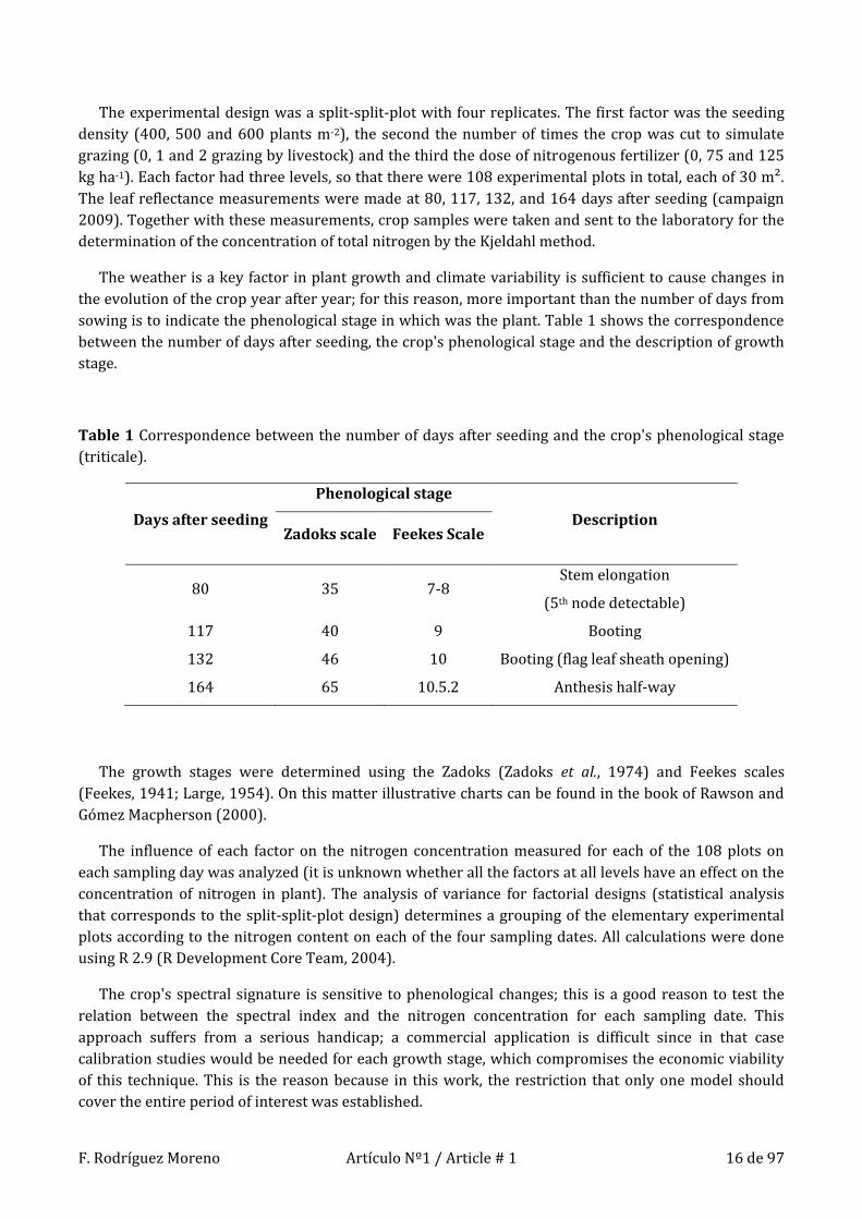
The weather is a key factor in plant growth and climate variability is sufficient to cause changes in
the evolution of the crop year after year; for this reason, more important than the number of days from
sowing is to indicate the phenological stage in which was the plant. Table 1 shows the correspondence
between the number of days after seeding, the crop's phenological stage and the description of growth
stage.
Table 1 Correspondence between the number of days after seeding and the crop's phenological stage
(triticale).
Days after seeding
Phenological stage
Description Zadoks scale Feekes Scale
80 35 7-8 Stem elongation
(5th node detectable)
117 40 9 Booting
132 46 10 Booting (flag leaf sheath opening)
164 65 10.5.2 Anthesis half-way
The growth stages were determined using the Zadoks (Zadoks et al., 1974) and Feekes scales
(Feekes, 1941; Large, 1954). On this matter illustrative charts can be found in the book of Rawson and
Gómez Macpherson (2000).
The influence of each factor on the nitrogen concentration measured for each of the 108 plots on
each sampling day was analyzed (it is unknown whether all the factors at all levels have an effect on the
concentration of nitrogen in plant). The analysis of variance for factorial designs (statistical analysis
that corresponds to the split-split-plot design) determines a grouping of the elementary experimental
plots according to the nitrogen content on each of the four sampling dates. All calculations were done
using R 2.9 (R Development Core Team, 2004).
The crop's spectral signature is sensitive to phenological changes; this is a good reason to test the
relation between the spectral index and the nitrogen concentration for each sampling date. This
approach suffers from a serious handicap; a commercial application is difficult since in that case
calibration studies would be needed for each growth stage, which compromises the economic viability
of this technique. This is the reason because in this work, the restriction that only one model should
cover the entire period of interest was established.

F. Rodríguez Moreno Artículo Nº1 / Article # 1 17 de 97
On each sampling date, 20 leaves at random were collected in each of the 108 elementary plots. Ten
estimates of the reflectance (each averaging 50 readings) were made of these samples, using the ASD
FieldSpec 3 spectroradiometer for this. This device has a spectral range of 350–2500 nm, a sampling
interval of 1.4 nm for the range 350–1000 nm and 2 nm for the range 1000–2500 nm, and a spectral
resolution of 3 nm at 700 nm and 10 nm from 1400 nm to 2100 nm. Readings were performed using a
plant probe plus leaf clip. The light source of the plant probe is a halogen bulb with a colour
temperature of 2901±10 K.
For each of the different groups of elementary plots defined according to their concentration of
nitrogen on each sampling date, the mean reflectance was calculated by averaging the readings taken in
their respective elementary plots. The average spectral signature for each of the groups identified
during the growth of the crop was then used to determine the value of each of the selected spectral
indices given in Table 2.
The relationship between the different spectral indices and the nitrogen concentrations was
evaluated by calculating the correlation coefficient squared (R2), the adjusted squared correlation
coefficient (aR2), the square root of the mean square error (RMSE) and the statistical significance (p-
value) of the model (analysis of the variance explained as against the residual). Figure 1 is a flowchart
that summarizes the whole process.
Figure 1 Flow chart that summarizes the experiment design and data processing methods.

F. Rodríguez Moreno Artículo Nº1 / Article # 1 18 de 97
Table 2 Spectral indexes related to the content in chlorophyll used
Spectral index Formulation1 Author
Green NDVI2 (R780-R550)/(R780+R550) Gitelson and Merzlyak
(1996)
Green reflectance R550 Biochemical deduction
Logarithm of reciprocal
reflectance
log(1/R737) Yoder and Pettigrew-
Crosby (1995)
Modified chlorophyll absorption
in reflectance index
[(R700 - R670) – 0.2 * (R700 -
R550)]*(R700/R670)
Daughtry et al. (2000)
Modified red-edge normalized
difference vegetation index
(R750-R705)/(R750+R705-
2*R445)
Sims and Gamon (2002)
Modified red-edge ratio (R750-R445)/(R705-R445) Sims and Gamon (2002)
Near infrared reflection R800 Biochemical deduction
Normalized difference
vegetation index
(R800-R670)/(R800+R670) Deering (1978)
Pigment specific normalized
difference a
(R800-R675)/(R800+R675) Blackburn (1998)
Pigment specific normalized
difference b
(R800-R650)/(R800+R650) Blackburn (1998)
Pigment specific simple ratio a R800/R675 Sims and Gamon (2002)
Pigment specific simple ratio b R800/R650 Sims and Gamon (2002)
Ratio analysis of reflectance
spectra a
R675/R700 Blackburn (1999)
Ratio analysis of reflectance
spectra b
R675/(R650*R700) Blackburn (1999)
Ratio of near infrared to green R800/R550 Biochemical deduction
Ratio of near infrared to red R800/R670 Biochemical deduction
Reciprocal reflectance 1/R700 Gitelson et al. (1999)
Red edge inflect point (700+40)*{[(R670+R780)/2]-
R700}/(R740-R700)
Guyot et al. (1988)
Red reflectance R670 Biochemical deduction
Red-edge NDVI (R750-R705)/(R750+R705) Sims and Gamon (2002)
Zarco-Tejada & Miller R750/R710 Zarco-Tejada et al. (2001) 1 R+number: reflectance at number nm. 2NDVI: normalized difference vegetation index.
Results and discussion
Table 3 shows that all the models, except the one developed for the modified chlorophyll absorption
in reflectance index, explained a significant portion of the variance of the plant's nitrogen concentration,
but in none of the cases the magnitude of the relationship was enough for developing a profitable
methodology. The highest R2 was 0.31, and corresponded to the green reflectance index.

F. Rodríguez Moreno Artículo Nº1 / Article # 1 19 de 97
This study determines the reduction in the effectiveness if one tries to estimate the concentration of
nitrogen in the plant by a low-cost approach. The reduction is 38% (the value of R² is reduced from 0.5
to 0.31), a significant reduction received with a positive evaluation because of the complexity involved
in developing a single model for different phenological stages and the enormous handicap which entails
the double duality of the crop. It is understood that this reduction in effectiveness is the highest
possible and that's not enough to discard the approach of a precision agriculture of low cost, at least
remains to evaluate the potential of data mining in the exploitation of the information contained in
spectral signature.
Table 3 Goodness of the fit between spectral indices and the concentration of nitrogen.
Spectral index R2 Adjusted
R2
p-values
for model
RMSE1
Green NDVI2 0.235 0.233 0.000 0.691 Green reflectance 0.315 0.314 0.000 0.653
Logarithm of reciprocal reflectance 0.179 0.177 0.000 0.715
Modified chlorophyll absorption in reflectance
index
0.008 0.006 0.065 0.786
Modified red-edge normalized difference
vegetation index
0.058 0.056 0.000 0.766
Modified red-edge ratio 0.047 0.045 0.000 0.771
Near infrared reflection 0.122 0.120 0.000 0.740
Normalized difference vegetation index 0.139 0.137 0.000 0.732
Pigment specific normalized difference a 0.123 0.121 0.000 0.739
Pigment specific normalized difference b 0.231 0.229 0.000 0.692
Pigment specific simple ratio a 0.115 0.113 0.000 0.743
Pigment specific simple ratio b 0.208 0.206 0.000 0.703
Ratio analysis of reflectance spectra a 0.027 0.025 0.001 0.779
Ratio analysis of reflectance spectra b 0.252 0.250 0.000 0.683
Ratio of near infrared to green 0.213 0.211 0.000 0.700
Ratio of near infrared to red 0.131 0.128 0.000 0.736
Reciprocal reflectance 0.226 0.224 0.000 0.695
Red edge inflect point 0.032 0.030 0.000 0.777
Red reflectance 0.173 0.171 0.000 0.718
Red-edge NDVI 0.156 0.154 0.000 0.725
Zarco-Tejada & Miller 0.134 0.132 0.000 0.735 1 RMSE: square root of the mean square error. 2NDVI: normalized difference vegetation index.
The spectral signature of a leaf is extremely sensitive to the conditions affecting the leaf itself and to
the conditions under which the measurements are made. These conditions vary considerably
throughout the period during which it would be possible to act to correct a possible nitrogen deficiency
in the crop, for this reason the models were specific to a growth stage, something that complicates the
profitability and thus the transfer of technology, this study explores this field and its conclusion
suggests that the cost of using a single model is not as high as could be expected.
In light of the results, exactly of the results of F test and associated p-value for significance of the
model, one can say that the independent variables, spectral indices, are important in explaining the
observed variation in dependent variable, concentration of nitrogen in plant. These indices have a
F. Rodríguez Moreno Artículo Nº1 / Article # 1 20 de 97
biochemical and biophysical basis, the existence of that relationship was expected, different is the
magnitude of it, so small that makes one think about the weakness of using non-specific index for the
concentration of nitrogen in plant.
It is confirmed that, in cultivating dual purpose triticale, calculations based solely on a greenness
measurement, such as the green reflectance index (the index which gave the best correlation in this
study), would lead to obtaining erroneous estimates of the nitrogen concentration.
The single model developed for the entire period of interest – from stem elongation (when tillering
has ended) through booting and heading to flowering – gave lower correlations between the vegetation
spectral indices and the crop's nitrogen concentration than those reported in similar studies in which
different phenological intervals were modeled separately (Heege et al., 2008; Li et al., 2010). In
particular, the value of R² was reduced by about 40%, from 0.5 for the final growth stages (Li et al.,
2010) to the value of 0.3 for the entire period of crop growth.
The techniques of precision agriculture have to reach to the cultivation of the dual purpose triticale.
Since nitrogen's role in a plant is not restricted to be a component of chlorophyll and the spectral
signature of the leaf is function of its composition and configuration, it has to be possible to derive new
spectral indices which estimate nitrogen concentrations based on other variables besides of the
greenness of the plant.
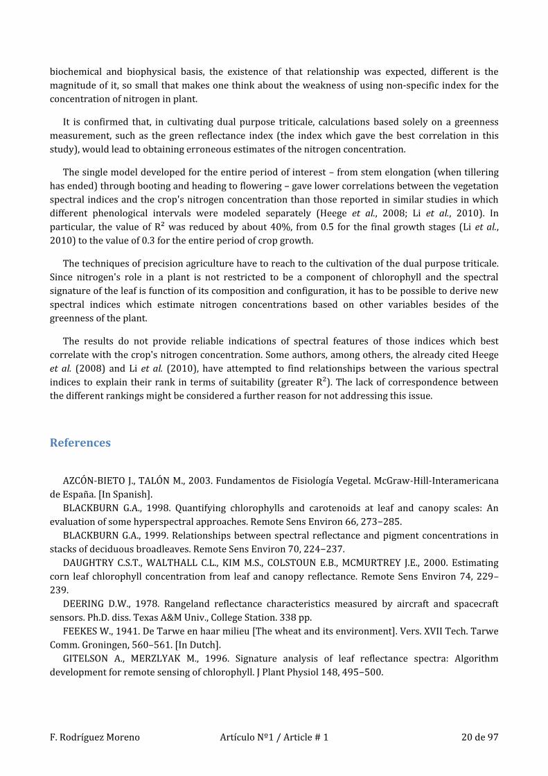
The results do not provide reliable indications of spectral features of those indices which best
correlate with the crop's nitrogen concentration. Some authors, among others, the already cited Heege
et al. (2008) and Li et al. (2010), have attempted to find relationships between the various spectral
indices to explain their rank in terms of suitability (greater R²). The lack of correspondence between
the different rankings might be considered a further reason for not addressing this issue.
References
AZCÓN-BIETO J., TALÓN M., 2003. Fundamentos de Fisiología Vegetal. McGraw-Hill-Interamericana
de España. [In Spanish].
BLACKBURN G.A., 1998. Quantifying chlorophylls and carotenoids at leaf and canopy scales: An
evaluation of some hyperspectral approaches. Remote Sens Environ 66, 273−285.
BLACKBURN G.A., 1999. Relationships between spectral reflectance and pigment concentrations in
stacks of deciduous broadleaves. Remote Sens Environ 70, 224−237.
DAUGHTRY C.S.T., WALTHALL C.L., KIM M.S., COLSTOUN E.B., MCMURTREY J.E., 2000. Estimating
corn leaf chlorophyll concentration from leaf and canopy reflectance. Remote Sens Environ 74, 229–
239.
DEERING D.W., 1978. Rangeland reflectance characteristics measured by aircraft and spacecraft
sensors. Ph.D. diss. Texas A&M Univ., College Station. 338 pp.
FEEKES W., 1941. De Tarwe en haar milieu [The wheat and its environment]. Vers. XVII Tech. Tarwe
Comm. Groningen, 560–561. [In Dutch].
GITELSON A., MERZLYAK M., 1996. Signature analysis of leaf reflectance spectra: Algorithm
development for remote sensing of chlorophyll. J Plant Physiol 148, 495−500.

F. Rodríguez Moreno Artículo Nº1 / Article # 1 21 de 97
GITELSON A.A., BUSCHMANN C., LICHTENTHALER H.K., 1999. The chlorophyll fluorescence ratio
R735/F700 as an accurate measure of the chlorophyll content in plants. Remote Sens Environ 69,
296−302.
GUYOT G., BARET F., MAJOR D.J., 1988. High spectral resolution: determination of spectral shifts
between the red and infrared. Int Arch Photogram Remote Sens 11, 750–760.
HEEGE H.J., REUSCH S., THIESSEN E., 2008. Prospects and results for optical systems for site-specific
on-the-go control of nitrogen-top-dressing in Germany. Precis Agric 9, 115–131.
HUETE A.R., 1988. A soil-adjusted vegetation index (SAVI), Remote Sens Environ 25, 295-309.
LARGE E.G., 1954. Growth stages in cereals: Illustration of the Feeke's scale. Plant Pathol 3, 128-129.
LI F., MIAO Y., HENNIG S., GNYP M., CHEN X., JIA L., BARETH G., 2010. Evaluating hyperspectral
vegetation indices for estimating nitrogen concentration of winter wheat at different growth stages.
Precis Agric 11, 335-357.
MARSCHNER H., 1995. Mineral nutrition of higher plants, 2nd Ed. Academic Press.
R DEVELOPMENT CORE TEAM, 2004. R: a language and environment for statistical computing.
Foundation for Statistical Computing, Vienna. Available in http://www.R-project.org. [1 May, 2010].
RAWSON H.M., GÓMEZ MACPHERSON H., 2000. Irrigated wheat. FAO, Roma.
RONDEAUX G., STEVEN M., BARET F., 1996. Optimization of soil-adjusted vegetation indices. Remote
Sens Environ 55, 95–107.
SIMS D.A., GAMON J.A., 2002. Relationships between leaf pigment content and spectral reflectance
across a wide range of species, leaf structures, and developmental stages. Remote Sens Environ 81,
337−354.
USTIN S.L., JACQUEMOUD S., ZARCO-TEJADA P., ASNER G., 2004. Remote sensing of environmental
processes: State of the science and new directions. In: Manual of remote sensing, vol. 4. (Ustin S.L., vol.
ed.). Remote sensing for natural resource management and environmental monitoring. ASPRS. John
Wiley and Sons, NY. pp. 679–730.
YODER B.J., PETTIGREW-CROSBY R.E., 1995. Predicting nitrogen and chlorophyll content and
concentrations from reflectance spectra (400–2500 nm) at leaf and canopy scales. Remote Sens Environ
53, 199−211.
ZADOKS J.C., CHANG T.T., KONZAK C.F., 1974. A decimal code for the growth stages of cereals. Weed
Res 14, 415-421.
ZARCO-TEJADA P.J., MILLER J., NOLAND T.L., MOHAMMED G.H., SAMPSON P.H., 2001. Scaling-up and
model inversion methods with narrowband optical indices for chlorophyll content estimation in closed
forest canopies with hyperspectral data. IEEE T Geosci Remote Sens 39, 1491–1507.
ZARCO-TEJADA P.J., MILLER J.R., MORALES A., BERJON A., AGUERA J., 2004. Hyperspectral indices
and model simulation for chlorophyll estimation in open-canopy tree crops. Remote Sens Environ 90,
463–476.

F. Rodríguez Moreno Artículo Nº1 / Article # 1 22 de 97

F. Rodríguez Moreno Artículo Nº2 / Article # 2 23 de 97
PCA versus ICA for the reduction of dimensions of the spectral signatures in
the search for an index for the concentration of nitrogen in plant
Citation Rodriguez-Moreno, F., & Llera-Cid, F. (2011b). PCA versus ICA for the reduction of dimensions of the spectral signatures in the search of an index for the concentration of nitrogen in plant. Spanish Journal of Agricultural Research, 9(4), 1168-1175, doi:10.5424/sjar/20110904-093-11.
Download link
http://revistas.inia.es/index.php/sjar/article/download/2366/1563
https://dl.dropbox.com/u/72234534/002.pdf
Header
F. Rodriguez-Moreno* and F. Llera-Cid
Centro de Investigación "La Orden-Valdesequera". Junta de Extremadura. Finca "La Orden". Ctra. N-V.
Km. 372. 06187 Guadajira. Badajoz. Spain.
*Corresponding author: [email protected] | Phone: +34 924014071.
Short title: Estimation of the nitrogen nutritional status by spectral analysis with PCA and ICA
Topic: Agricultural engineering
Received: 22-02-11
2 figures, 3 tables
Abstract
The vegetation spectral indices have been widely used as estimators of the nutritional status of the
crops. This study has evaluated if it is possible to improve the effectiveness of these indices to estimate
the nitrogen concentration using dimension reduction techniques to process the spectral signatures. It
has also demanded that the model is valid in a wide range of growing conditions and phenological
stages, thus increasing the predictive power guarantee and reducing the implementation effort. This
work has been done using an agronomic trial with dual purpose triticale (X Triticosecale Wittmack)
whose design included plots with different planting densities, number of grazing and fertilizer doses.
The spectral signatures of the leaves were recorded with the ASD-FieldSpec 3 spectroradiometer and
the nitrogen concentrations were determined by Kjeldahl method. The factors with effect on nitrogen
concentration were identified by the analysis of variance and pairwise comparisons and, then, the mean

F. Rodríguez Moreno Artículo Nº2 / Article # 2 24 de 97
spectral signature was calculated for each of the groups formed. The dimensional reduction was
performed with both PCA and ICA. The analysis of the relationships between components and nitrogen
concentration showed that only the components obtained with PCA generated a significant model
(p=0.00) with a R2=0.68. The best spectral vegetation index in this test, the reflectance in green,
obtained a R2=0.31. Although further confirmation is needed, this study shows that the PCA may be a
viable alternative to spectral vegetation indices.
Additional key words: cereals; dual purpose triticale; independent component analysis; leaf;
precision agriculture; principal component analysis; radiometry
Resumen
PCA versus ICA para la reducción de dimensiones de las firmas espectrales en la búsqueda de
un índice para la concentración de nitrógeno en planta
Los índices espectrales de vegetación han sido ampliamente usados como estimadores del estado
nutricional de los cultivos. En este estudio se ha evaluado si es posible mejorar la eficacia de esos
índices para estimar la concentración de nitrógeno empleando técnicas de reducción de dimensiones
para procesar las firmas espectrales. Además se ha exigido que el modelo sea válido en un amplio rango
de condiciones de desarrollo y estados fenológicos, aumentando así las garantías de poder predictivo y
reduciendo el esfuerzo de implementación. Se realizó un ensayo agronómico con triticale de doble
aptitud (X Triticosecale Wittmack), en cuyo diseño se incluyeron parcelas con diferentes densidades de
siembra, aprovechamientos y fertilización. La firma espectral de las hojas se registró con el
espectroradiómetro ASD-FieldSpec 3 y la concentración de nitrógeno se determinó mediante el método
Kjeldahl. Los factores con efecto en la concentración de nitrógeno fueron identificados mediante el
análisis de la varianza y tests de comparación de medias; posteriormente se calculó la firma espectral
media para cada uno de los grupos. La reducción de dimensiones se realizó tanto con PCA como con
ICA. El análisis de las relaciones entre componentes y concentración de nitrógeno mostró que sólo las
componentes obtenidas con PCA generaron un modelo significativo (p=0,00) con un R2=0,68. El mejor
índice espectral de vegetación en esta prueba, la reflectancia en verde, obtuvo un R2=0,31. Aunque es
necesaria una mayor confirmación, en este trabajo se muestra que el PCA puede ser una alternativa
válida a los índices espectrales de vegetación.
Palabras claves adicionales: agricultura de precisión; análisis de componentes independientes;
análisis de componentes principales; cereales; hoja; radiometría; triticale de doble aptitud
Abbreviations used: Adj R2 (adjusted correlation coefficient); ICA (independent component
analysis); MSE (mean square error); NDVI (normalized difference vegetation index); PCA (principal

F. Rodríguez Moreno Artículo Nº2 / Article # 2 25 de 97
component analysis); RMSE (square root of the mean square error); SNR (signal to noise ratio); SWIR
(shortwave Infrared); VNIR (visible and near-infrared)
Introduction
The demand of nitrogen by the crop throughout its development is well known (Alaru et al., 2004)
and both the excessive and the deficit have a negative impact on production, operating costs and
environmental conservation.
The technology available today can get huge volumes of information at a reasonable cost; the
challenge is the correct interpretation of that information (Moran et al., 1997). Reflectance
measurements can be used to obtain the values of the most widely used spectral indices (Guyot et al.,
1988; Yoder and Pettigrew-Crosby, 1995; Gitelson and Merzlyak, 1996; Blackburn, 1998; Gitelson et al.,
1999; Daughtry et al., 2000; Ustin et al., 2004) as indicators of chlorophyll concentration. The suitability
of these indices to estimate the concentration of nitrogen in plants is limited; Li et al. (2010) showed
that the predictive power of these indices can reach a R2=0.5 for certain growth stages. Heege et al.
(2008) reached higher values, but they linked the spectral signature with a dose of fertilizer applied and
not with the nutritional status of the plant.
The work of Li et al. (2010) revealed one of the challenges to overcome, the poor spatial and
temporal generalization of the models developed. Another difficulty was evidenced in the work of
Rodriguez-Moreno and Llera-Cid (2011); the tests are conducted under conditions difficult to
reproduce in real farms. In a real farm, for example, there isn´t a panel of experts dedicated to calibrate
the methodology, so the tasks of identifying acceptable cuts in the procedure and finding out the true
effectiveness of the methodology are left to farmers.
In this context, only in the large farms (large areas) can bet strong for these new technologies,
because the small improvements per unit area represent a significant increase in production and
benefits, which compensated for the salary of specialist staff and equipment costs required for
implementation. This is a sad reality as precision agriculture, besides trying to maximize profits, also
seeks sustainability and protecting the environment (Moran et al., 1997).
Studies, some of them six years old (Waheed et al., 2006), have shown the high potential of
radiometry and artificial intelligence in the field of precision agriculture, this work is in that line. The
purpose of this study is to present a methodology which improves, in easily reproducible conditions on
farms; the effectiveness of the methodologies based on the classical vegetation spectral indices and also
offers greater guarantees of space-time generalization.
With the dual purpose triticale (X Triticosecale Wittmack), the crop used in this study, there is the
possibility of letting livestock grazing on more than one occasion without ruining the final harvest. The
plant after each grazing has to regenerate the above-ground part and with it the ability to synthesize
chlorophyll, but the below-ground part is unaffected so that the plant's nitrogen absorbing capacity
remains intact. The result is an imbalance in the first weeks after each cut, which is manifested by a
yellowing of the plant. This is not a symptom of nitrogen deficiency, since there has been neither a
decrease in the concentration of this element nor an interruption in plant growth.

F. Rodríguez Moreno Artículo Nº2 / Article # 2 26 de 97
The loss of greenness is not always related to a nutritional deficiency, this peculiarity, entailed by the
crop chosen for the study, requires that the radiometric model is based on spectral features different
from those used in many of the vegetation spectral indices such as the index of the reflectance in green.
These new spectral features have to be more closely related to the concentration of nitrogen because
they respond correctly under conditions in which the classical indices err.
There is no competition between old and new spectral features, it is a necessity dictated by the crop,
when developing models for other cereals without the dual purpose both features can be integrated and
thus obtain better levels of effectiveness.
One way to increase the guarantees of predictive power is limiting the number of models, only one
model will be developed for the entire period during which it would be possible to correct the
shortcoming nitrogen in the crop. The changes in the plant during its development (Marschner, 1995;
Azcón-Bieto and Talón, 2003) complicate the development of generic models, but if that development is
possible, then the model would provide greater guarantees, the Occam's razor is applicable. In addition,
a unique development would reduce the participation of specialists in the implementation, which would
reduce costs and would facilitate transfer of technology.
The huge volume of data obtained in a hyperspectral sampling is very complex to analyze and its
processing has a high computational cost. For contexts such as these were devised dimension reduction
techniques, which filter the noise, identify redundancies and reveal the structure hidden. The most
widely used dimensional reduction techniques are principal component analysis (PCA) (Rao, 1964) and
independent component analysis (ICA) (Hyvärinen and Oja, 2000). This study will examine whether the
components identified by these techniques contain the information necessary to estimate, by a linear
regression model and under the conditions described above, the nitrogen concentration in the plants.
The anticipated results would be evidences to support three hypotheses, the existence of features in
the spectral signatures closely related to nitrogen concentration, the ability to develop models valid for
a wide phenological range and the appropriateness of the dimension reduction techniques to process of
the spectral signatures preserving the information on the nutritional status.
Material and methods
As part of a study at the "La Orden-Valdesequera" Research Centre (Badajoz, Spain) in order to
determine the optimal combination of factors for the cultivation of the triticale, the reflectance of the
leaves, at different stages of crop development, were measured.
The experimental design used was a split-split-plot with four replicates. The first factor was seeding
density (400, 500 and 600 plants m-2), the second the number of times the crop was cut to simulate
grazing (0, 1 and 2 grazing), and the third the dose of nitrogenous fertilizer (0, 75 and 125 kg ha-1). Each
factor had three levels, so that there were 108 experimental plots in total, each of 30 m². The leaf
reflectance measurements were made at 80, 117, 132, and 164 days after seeding. Together with these
measurements, crop samples were taken, which were sent to the laboratory for the determination of
the concentration of total nitrogen by the Kjeldahl method. The correspondence between the number of
days after seeding and the crop's phenological stage, along with his description, is presented in the
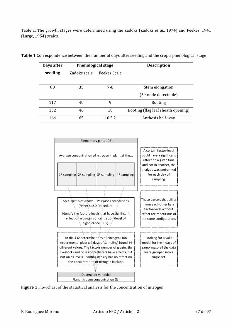
F. Rodríguez Moreno Artículo Nº2 / Article # 2 27 de 97
Table 1. The growth stages were determined using the Zadoks (Zadoks et al., 1974) and Feekes, 1941
(Large, 1954) scales.
Table 1 Correspondence between the number of days after seeding and the crop's phenological stage
Days after
seeding
Phenological stage Description
Zadoks scale Feekes Scale
80 35 7-8 Stem elongation
(5th node detectable)
117 40 9 Booting
132 46 10 Booting (flag leaf sheath opening)
164 65 10.5.2 Anthesis half-way
Figure 1 Flowchart of the statistical analysis for the concentration of nitrogen
1º sampling 2º sampling 3º sampling 4º sampling
Looking for a valid
model for the 4 days of
sampling,so all the data
were grouped into a
single set.
In the 432 determinations of nitrogen (108
experimental plots x 4 days of sampling) found 14
different values. The factors number of grazing (by
livestock) and doses of fertilizers have effects, but
not on all levels. Planting density has no effect on
the concentration of nitrogen in plant.
Dependent variable:
Plant nitrogen concentration (%)
Elementary plots 108
Average concentration of nitrogen in plant at the...
A certain factor-level
could have a significant
effect on a given time
and not in another, the
analysis was performed
for each day of
sampling.
Those parcels that differ
from each other by a
factor-level without
effect are repetitions of
the same configuration.
Split-split-plot Anova + Pairwise Comparisons
(Fisher´s LSD Procedure)
Identify the factors-levels that have significant
effect on nitrogen concentration (level of
significance 0.05).

F. Rodríguez Moreno Artículo Nº2 / Article # 2 28 de 97
Principal component analysis (PCA) Independent component analysis (ICA)
The criteria that guides the transformation is improving
the signal-to-noise ratio. The new base should be a
linear combination of the original.
The information contained in each of the new
components is statistically independent
Number of components: The smallest set that explains
95% of the variance.
A good estimation of the number of independent
components is the optimal number of principal
components (ONPC), number determined in the PCA.
Seven ICA were done, the numbers of independent
components were: ONPC, ONPC+1, ONPC+2, ONPC+3,
ONPC-1, ONPC-2, ONPC-3
Independent variable: Independent variable:
Principal components Independent components (7 dataset)
a1 * Component1 + … + an * Componentn + b
Relationship evaluated by the correlation coefficient squared, the adjusted squared correlation coefficient, the square root of the
mean square error and the statistical significance of the model.
Dependent variable:
Plant nitrogen
concentration (%)
Calculation of linear regression: [Nitrogen concentration] =
Spectral signatures 432 (108 plots × 4 sampling days)
Calculation of the spectral signatures representative of each nitrogen concentration, averaging all signatures obtained on plots with
the same concentration.
In accordance with the experimental design, the influence of each factor on the nitrogen
concentration measured for each of the 108 plots on each sampling day was analyzed (it is unknown
whether all the factors at all levels have an effect on the concentration of nitrogen). The split-split-plot
analysis of variance (ANOVA) and the pairwise comparisons, Fisher's LSD Procedure, determined a
grouping of the plots according to the nitrogen concentration (p=0.05). Figure 2 is a flowchart
explaining this analysis. This and the rest of calculations were done using R 2.9 (R Development Core
Team, 2004).
Figure 2 Flowchart of the analysis of spectral signatures
On each sampling date, 20 leaves at random were collected in each of the 108 elementary plots. Ten
estimates of the reflectance (each averaging 50 readings) were made of these samples, using the ASD
FieldSpec 3 spectroradiometer for this. This device has a spectral range of 350–2500 nm, a sampling
interval (the spacing between sample points in the spectrum) of 1.4 nm for the range 350–1000 nm and
2 nm for the range 1000–2500 nm, and a spectral resolution (the full-width-half-maximum of the
instrument response to a monochromatic source) of 3 nm at 700 nm and 10 nm from 1400 nm to 2100
nm. Readings were performed using a plant probe plus leaf clip. The light source of the plant probe is a
halogen bulb with a colour temperature of 2901±10 K.

F. Rodríguez Moreno Artículo Nº2 / Article # 2 29 de 97
The reflectances for the wavelengths in which the transition between the spectroradiometer sensors
(VNIR - SWIR1 and SWIR1 - SWIR2) occur were removed of the spectral signatures, regions where
instrumental errors could be found.
For each of the different groups of elementary plots, formed according to their nitrogen
concentration on each sampling date, the mean reflectance was calculated by averaging the readings
taken in their respective plots. As the number of models has been limited to one, from this point all the
pairs of nitrogen concentration - spectral signatures come together in one set, regardless of the date of
sampling, since the model had to provide a correct estimate for all of them without knowing that
information.
The dimension reduction techniques filter the noise, identify redundancies and reveal the structure
hidden. There are different strategies; each employs different assumptions about the original
components and the mixing process, mathematical assumptions that may not fit perfectly with the data
set. This is the reason why two techniques, with statements so distant, have been tested.
The principal component analysis (PCA) searches for a new base, linear combination (this restriction
simplifies the search) of the original base (in which the data were collected), that best expresses the
data. For the PCA, the dynamics of interest is the one with better signal-to-noise ratio (SNR); this is the
search criteria of the new base. Reducing the number of dimensions is got by eliminating noise and
redundancy (Rao, 1964).
The independent component analysis (ICA) is the other technique that was tested. This dimension
reduction technique seeks that the information contained in the new components is statistically
independent (Hyvärinen and Oja, 2000). The ICA has been proved successful in many cases in which the
PCA fails (Ozdogana, 2010).
The PCA returns as many components as inputs. In this study it was identified the smallest group of
new components necessary to explain, at least, the 95% of the total variance, excluding other
components; this is the way in which dimensional reduction was achieved. The ICA is different; one
must indicate the number of independent components to generate. In this study the number of principal
components (PCA) employed has been used as an estimation of the number of independent
components (ICA) needed, performing several tests around that number.
It has built a linear regression model for each of the different sets of components generated (PCA
and ICA) with nitrogen concentration (%). The goodness of fit of each model was evaluated by
calculating the correlation coefficient squared (R2), the adjusted squared correlation coefficient (adjR2),
the square root of the mean square error (RMSE) and the statistical significance (p-value) of the model
(analysis of the variance). Figure 3 is a flowchart that summarizes the whole process.
The score to improve is 0.31, the value of R2 obtained by the green reflectance index, which is the
highest correlation found between the nitrogen concentration and the classical spectral indices.
Calculation obtained with the same dataset that this study and performing the evaluation under the
same conditions. The list of spectral indices analyzed in the comparative and other details of the study
is in Rodriguez-Moreno and Llera-Cid (2011).

F. Rodríguez Moreno Artículo Nº2 / Article # 2 30 de 97
Results and discussion
The split-split-plot ANOVA (Table 2) and the pairwise comparisons (Fisher's LSD procedure)
identified the factors with effect on nitrogen concentration (Level of significance in all tests of 0.05).
Table 2 Results of the split-split-plot ANOVA, factors with effect on nitrogen concentration
Factor (simple or
interaction)
Sampling
1st 2nd 3rd 4th
Phenological stage
Stem
elongation
Booting Booting (flag leaf
sheath opening)
Anthesis
half-way
Seeding density
Number of cuts * *
Dose of nitrogenous fertilizer * * *
Seeding density -
Number of cuts
Seeding density - Dose of
nitrogenous fertilizer
Number of cuts - Dose of
nitrogenous fertilizer
*
Seeding density -
Number of cuts - Dose of
nitrogenous fertilizer
*: effect on nitrogen concentration at the level of significance of 0.05.
It was observed that the factor seeding density had no effect at any time, the levels may not be
appropriate or perhaps the effects were felt later.
The effect of the factor number of grazing was not analyzed in the first dataset, since the first cut was
made after this sampling. In the dataset of the second and third sampling, with two levels (0 and 1 cut),
it was determined that the factor number of grazing had effect on the concentration of nitrogen. The
analysis of the fourth dataset, the first with three levels since the second cut was made after the third
sampling, revealed that the three levels of the factor number of grazing had significant effect on plant
nitrogen concentration.
The factor dose of fertilizer had effect on the concentration of nitrogen in all the datasets, but only in
the fourth dataset the levels 75 and 125 kg ha-1 had different effects. The fact that the effects of the two

F. Rodríguez Moreno Artículo Nº2 / Article # 2 31 de 97
higher doses of fertilizers do not differ is natural. The triticale takes the nitrogen from the soil along its
development, but most absorption occurs in a developmental stage later than the dates on which the
samplings were done (Lance et al., 2007).
Those plots that differed only by a factor or level without effect were repetitions, so the
representative value for the concentration of nitrogen and the spectral signature were obtained by
averaging the data from plots with the same configuration. The 14 different nitrogen concentrations
recorded in the 108 plots and the four days of sampling were: 1.02, 1.19, 1.22, 1.31, 1.36, 1.42, 1.52,
1.54, 1.64, 1.95, 2.32, 2.74, 3.14 and 3.40 percentage of nitrogen.
Cumulative variance explained by the first 10 components obtained using PCA reached 99.5% of the
total variance. This percentage was considered sufficient, so only the first 10 components were taken
into account in developing the linear regression.
Unable to make the same test to determine the appropriate number of components for the ICA, it
was chosen to calculate 7 linear regressions (using 7 to 13 components). If the 99.5% of the variance of
the reflectance could be explained with only 10 components in the case of PCA, ICA had to need
something similar.
It has built a linear regression for each of the different sets of components generated (PCA and ICA)
with nitrogen concentration (%). The goodness of fit of each model (Table 3) was evaluated by
calculating the R2, the adj R2, the RMSE and the p-value of the model.
The best fit, R2=0.68, was reached in the linear regression with the components of the PCA. That
result showed that the spectral signatures of crops meet the suppositions on the PCA is based (linearity
in the change of base, higher variance means greater importance of the variable in the dynamics and
that the principal components are orthonormal).
The winner model is presented in the Table 4. Except the fourth and ninth components, the rest
were included in the model (Level of significance of 0.05). The eighth component is the one that gets the
highest coefficient, but the seventh, the tenth and the second are close, so one cannot conclude that the
concentration of nitrogen can be identified with a particular component, one must use the derived
model.
This study provides evidences that data mining is an effective technique for analyzing the spectral
signatures in the search for estimators of the nutritional status of the crop.
This work shows that the changes in the crop throughout its development are not sufficient to
prevent the development of a single model. This means that the implementation of this methodology
would require, at most, a calibration study per crop campaign. At this point it is worth recalling the high
variability in the experimental plots in terms of growing conditions, which means that the effort to
adjust the model could be valid for a large area.

F. Rodríguez Moreno Artículo Nº2 / Article # 2 32 de 97
Table 3 Goodness of all linear regressions made between the sets of components (PCA and ICA) and the
nitrogen concentration (percentage of nitrogen)
Technique Number of
components
Significance of the model
(p-value) R2 Adj R2 MSE RMSE
ICA 7 0.19 0.02 0.01 0.62 0.79
8 0.61 0.02 0.00 0.62 0.79
9 0.12 0.03 0.01 0.62 0.78
10 0.42 0.02 0.00 0.62 0.79
11 0.48 0.03 0.00 0.62 0.79
12 0.18 0.04 0.01 0.62 0.79
13 0.33 0.03 0.00 0.62 0.79
PCA 10 0.00 0.68 0.67 0.20 0.45
Adj R2: adjusted correlation coefficient. ICA: independent component analysis. MSE: mean square error.
PCA: principal component analysis. R²: correlation coefficient. RMSE: square root of the mean square
error.
Table 4. Linear regression built with the components obtained with the PCA and the nitrogen
concentration (percentage of nitrogen)
Coefficients p-value
Constant 2.236 0.000
Component Nº1 -0.013 0.000
Component Nº2 -0.020 0.000
Component Nº3 0.008 0.000
Component Nº4 -0.001 0.551
Component Nº5 0.009 0.001
Component Nº6 -0.012 0.001
Component Nº7 0.028 0.000
Component Nº8 -0.053 0.000
Component Nº9 0.003 0.742
Component Nº10 0.027 0.028
In an evaluation, under the same conditions and with the same dataset, of the potential of spectral
indices of vegetation to estimate the concentration of nitrogen in plant was determined that the best
index was the reflectance in green, which reached an R2=0.31 (Rodriguez-Moreno and Llera-Cid, 2011).
The results of this study placed the strategy with the PCA over the spectral indices such as NDVI. This is
not surprising because it is not the first work that improves their effectiveness. An example is the result
obtained by Waheed et al. (2006), which was able to develop a decision tree with a classification hit rate

F. Rodríguez Moreno Artículo Nº2 / Article # 2 33 de 97
above 90% in a similar experiment. The models developed by Waheed et al. (2006), with more than 5
years old, have been unable to replace the spectral indices of vegetation; the NDVI keeps its hegemony
in the scientific and commercial uses.
The NDVI needs to be determined the reflectance at two wavelengths, the methodology presented in
this article needs to be applied the complete hyperspectral signature. More information improves the
estimates, but to overcome the NDVI, the simplicity and cost effectiveness are as important as the
effectiveness.
The complexity of the new methodology could be reduced by identifying the wavelengths with
greater weight in the components built into the model and developing with them a model that, instead
of estimating the concentration of nitrogen, estimates if the plant is deficient in nitrogen. In that case
one would only need to know the reflectance in a few wavelengths and the data processing would be
easier.
Competing with the NDVI in terms of profitability would be possible with more studies supporting
the greater effectiveness of this method in all scenarios and that is a valid methodology for large areas
that only requires a calibration study per crop campaign. While both aspects do not improve, simplicity
and profitability, the methodology presented will not end the hegemony of the spectral indices of
vegetation.
Li et al. (2010) presented the model with more predictive power; in his development the spectral
indices of vegetation and the brute force search were tested, by the difficulties of the brute force search
one can say that the methodology presented in this article has a similar complexity. The models
developed by Li et al. (2010) are specific for certain phenological stages and his best model reaches an
R2=0.5, this work achieves a small improvement, R2=0.68, with a valid model for the whole period
during which it could act to correct the deficiency in the crop.
It is very likely that this study has determined the lower threshold of efficacy, the dual purpose
triticale supports the grazing by livestock throughout its development without ruining the final harvest;
this makes it a special crop with additional difficulties for the development of radiometric models
(details given in the introduction). It is hoped that the models developed for other cereals can get
higher scores, but studies are needed to quantify it.
Developing this model has required the processing of over nine million data. In the case of
developing a similar model with data taken in various scenarios (other locations, different weather,
varieties, etc.) the data volume will grow exponentially, making it impossible to process, even for
supercomputing centers. Proving that dimensional reduction techniques are effective is the first step
required to initiate such studies.
The progress made has the limitation of requiring the spectral signatures of the leaves; an on-going
investigation is going to determine if the model could be adjusted to operate with measures of
vegetation canopy reflectance.

F. Rodríguez Moreno Artículo Nº2 / Article # 2 34 de 97
Acknowledgements
To Ángel M. Felicísimo (Department of Graphic Expression, University of Extremadura) for his help
in the wording and editing of this work.
To Vojtěch Lukas (Department of Agrosystems and Bioclimatology, Mendel University) for his help
in the planning and debugging of this research.
To Verónica Cruz Sobrado and Angélica Mª Rivera Martín (Research Center "The Order-
Valdesequera", Government of Extremadura) for their management of the agronomic trial.
References
ALARU M., MØLLER B., HANSEN Å., 2004. Triticale yield formation and quality influenced by
different N fertilisation regimes. Agron Res 2(1), 3-12.
AZCÓN-BIETO J., TALÓN M., 2003. Fundamentos de Fisiología Vegetal. McGraw-Hill-Interamericana
de España. [In Spanish].
BLACKBURN G.A., 1998. Quantifying chlorophylls and carotenoids at leaf and canopy scales: An
evaluation of some hyperspectral approaches. Remote Sens Environ 66, 273−285.
DAUGHTRY C.S.T., WALTHALL C.L., KIM M.S., COLSTOUN E.B., MCMURTREY J.E., 2000. Estimating
corn leaf chlorophyll concentration from leaf and canopy reflectance. Remote Sens Environ 74, 229–
239.
FEEKES W., 1941. De Tarwe en haar milieu [The wheat and its environment]. Vers. XVII Tech. Tarwe
Comm. Groningen, 560–561. [In Dutch].
GITELSON A., MERZLYAK M., 1996. Signature analysis of leaf reflectance spectra: algorithm
development for remote sensing of chlorophyll. J Plant Physiol 148, 495−500.
GITELSON A.A., BUSCHMANN C., LICHTENTHALER H.K., 1999. The chlorophyll fluorescence ratio
R735/F700 as an accurate measure of the chlorophyll content in plants. Remote Sens Environ 69,
296−302.
GUYOT G., BARET F., MAJOR D.J., 1988. High spectral resolution: determination of spectral shifts
between the red and infrared. Int Arch Photogram Remote Sens 11, 750–760.
HEEGE H.J., REUSCH S., THIESSEN E., 2008. Prospects and results for optical systems for site-specific
on-the-go control of nitrogen-top-dressing in Germany. Precis Agric 9, 115–131.
HYVÄRINEN A., OJA E., 2000. Independent component analysis: algorithms and applications.
Neuralnetworks 13(4-5), 411-430.
LANCE R.G., CARASELLA D.N., DOUGLAS L.K., 2007. Winter Triticale response to nitrogen
fertilization when grown after corn or soybean. Agron J 99, 49–58.
LARGE E.G., 1954. Growth stages in cereals: illustration of the Feeke's scale. Plant Pathol 3, 128-129.
LI F., MIAO Y., HENNIG S., GNYP M., CHEN X., JIA L., BARETH G., 2010. Evaluating hyperspectral
vegetation indices for estimating nitrogen concentration of winter wheat at different growth stages.
Precis Agric 11, 335-357.
MARSCHNER H., 1995. Mineral nutrition of higher plants, 2nd Ed. Academic Press.
MORAN M., INOUE Y., BARNES E.M., 1997. Opportunities and limitations for image-based remote
sensing in precision crop management. Remote Sens Environ 61, 319-346.

F. Rodríguez Moreno Artículo Nº2 / Article # 2 35 de 97
OZDOGANA M., 2010. The spatial distribution of crop types from MODIS data: temporal unmixing
using independent component analysis. Remote Sens Environ 114(6), 1190-1204.
R DEVELOPMENT CORE TEAM, 2004. R: a language and environment for statistical computing.
Foundation for Statistical Computing, Vienna. Available in http://www.R-project.org. [1 May, 2010].
RAO C.R., 1964. The use and interpretation of principal component analysis in applied research.
Sankhya Ser A 26, 329 -358.
RODRÍGUEZ-MORENO F., LLERA-CID F., 2011. Evaluating spectral vegetation indices for a practical
estimation of nitrogen concentration in dual purpose (forage and grain) triticale. Span J Agric Res 9(3),
681-686.
USTIN S.L., JACQUEMOUD S., ZARCO-TEJADA P., ASNER G., 2004. Remote sensing of environmental
processes: State of the science and new directions. In: Manual of remote sensing, vol. 4. (Ustin S.L., vol.
ed.). Remote sensing for natural resource management and environmental monitoring. ASPRS. John
Wiley and Sons, NY. pp. 679–730.
WAHEED T., BONNELL R.B., PRASHER S.O., PAULET E., 2006. Measuring performance in precision
agriculture: cart―a decision tree approach. Agr Water Manage 84(1-2), 173-185.
YODER B.J., PETTIGREW-CROSBY R.E., 1995. Predicting nitrogen and chlorophyll content and
concentrations from reflectance spectra (400–2500 nm) at leaf and canopy scales. Remote Sens Environ
53, 199−211.
ZADOKS J.C., CHANG T.T., KONZAK C.F., 1974. A decimal code for the growth stages of cereals. Weed
Res 14, 415-421.

F. Rodríguez Moreno Artículo Nº2 / Article # 2 36 de 97

F. Rodríguez Moreno Artículo Nº3 / Article # 3 37 de 97
A decision tree for nitrogen application based on a low cost radiometry
Citation Rodriguez-Moreno, F., & Llera-Cid, F. (2012). A decision tree for nitrogen application based on a low cost radiometry. Precision Agriculture, 1-15, doi:10.1007/s11119-012-9272-7.
Download link
http://www.springerlink.com/content/cjvr6rm4j116324r/
https://dl.dropbox.com/u/72234534/003.pdf
Header
F. Rodriguez-Moreno ∙ F. Llera-Cid
Centro de Investigación "La Orden-Valdesequera". Junta de Extremadura. Finca "La Orden". Ctra. N-V.
Km. 372. 06187 Guadajira. Badajoz. Spain.
*Corresponding author: [email protected]
Phone: +34 924014071 | Fax: +34 924014001
Abstract
Fertilizer recommendations based on radiometry require studies to calibrate the relationships to
scenario conditions; otherwise the effectiveness may be reduced. The objective of this study was to
develop a decision tree to detect nitrogen deficiency with efficiency comparable to the analysis of the
full spectral signature, with simplicity similar to a spectral index and valid over a wide range of
development conditions and phenological stages. An agronomic trial with a dual purpose triticale (X
Triticosecale Wittmack) was used in this study having different planting densities, number of grazing
events (regeneration from defoliation) and nitrogen fertilization. At different phenological stages, the
spectral signatures of leaves were recorded with an ASD-FieldSpec 3 spectroradiometer and the
nitrogen concentrations were determined by the Kjeldahl method. Agronomic factors that affect the N
concentration were identified using ANOVA; subsequently PCA was carried out on the set of spectral
signatures representative of the groups formed according to nitrogen concentration. Linear regression
was used to evaluate the relationship between the principal components and plant nitrogen
concentration. Wavelengths with greater significance were used to construct a decision tree. The
resulting decision tree defined for nitrogen using the Jenks Natural Breaks method had a success rate of
68.3%. The best spectral index had a R2 = 0.31 while the estimate using the full spectral signature

F. Rodríguez Moreno Artículo Nº3 / Article # 3 38 de 97
reached a R2 = 0.68. Although further testing is needed, this work shows the approach was able to
successfully categorize nitrogen deficiency.
Keywords: Cereals - Classification algorithms - Leaf reflectance - Principal component analysis -
Spectral vegetation indices
Abbreviations used: Adj R2 (adjusted determination coefficient); ANOVA (analysis of variance);
MSE (mean square error); NDVI (normalized difference vegetation index); PCA (principal component
analysis); p-value (statistical significance); R² (coefficient of determination); RMSE (root mean square
error); SNR (signal to noise ratio); SWIR (shortwave infrared); VNIR (visible and near-infrared)
Introduction
Models that relate spectral measurements with fertilizer rate need to be calibrated to scenario
conditions to achieve the best fertilizer recommendations (Wood et al. 2003; Tian et al. 2009; Tian et
al. 2011; Zhu et al. 2008; Y. Li et al. 2006). Interest in improving the efficiency and capacity of these
relationships (generalization over space and time) is because they offer an immediate improvement in
sustainability and profitability (Bongiovanni and Lowenberg-Deboer 2004).
Technologies for variable-rate nutrient applications based on prepared maps are commercially
available. If such maps are appropriate, each land unit will receive the most appropriate treatment
according to its characteristics (Llorens et al. 2010; Zhang et al. 2010), and frequently accompanied by a
reduction of inputs and an increase in both production and quality. The nitrogen (N) demand of crops
as they develop is well documented, as are the adverse effects that excessive and deficit nutrition have
on production, operating costs and environmental conservation (Alaru et al. 2003; Gibson et al. 2007).
Technologies available today can generate huge volumes of information at a reasonable cost; the
challenge is the correct interpretation of this information (Moran et al. 1997). Reflectance
measurements can be used to obtain the values of the most widely used spectral indices (Vrindts et al.
2003; Dorigo et al. 2007; Broge and Leblanc 2001; Broge and Mortensen 2002; Li et al. 2008; Li et al.
2010) as indicators of chlorophyll concentration. The suitability of these spectral indices to estimate
plant N concentration is limited as sometimes demonstrated under on-farm conditions (Li et al. 2010;
Li et al. 2008). As such, there is need for calibration studies under scenario conditions (Wood et al.
2003; Yoder and Pettigrew-Crosby 1995; Zhu et al. 2008). The profitability of this approach is not high,
but sensible (Auernhammer 2001; Robertson et al. 2007; Schellberg et al. 2008; Schroers et al. 2010).
This increase in profitability combined with the simplicity of implementation has made spectral
vegetation indices the approach of choice in scientific and commercial applications.
The alternative to spectral vegetation indices is the analysis of spectral signatures using data-mining
techniques. The effectiveness can be superior, but the resulting models have a lower capacity to
generalize space-time relationships and are more difficult and costly to implement (Li et al. 2010;
Waheed et al. 2006; Goel et al. 2003; Rumpf et al. 2010; Ruß and Brenning 2010; Shao et al. 2009).

F. Rodríguez Moreno Artículo Nº3 / Article # 3 39 de 97
The available radiometric models are not ideal (Li et al. 2010; Waheed et al. 2006; Zhou et al. 2008;
Yao et al. 2010). Improvements in both effectiveness and ability to generalize over space and time are
desirable. Implementing these improvements is the goal of this research. The proposed methodology
should be simple and require the lowest possible participation of specialists because any deployment
cost will complicate the viability for precision agriculture.
Changes in plants during the growing season (Marschner 1995; Taiz and Zeiger 1991) complicate
the development of general models, but if that development were possible, the resulting model would
provide greater guarantees of predictive power. Moreover, it would reduce participation of specialists
in the implementation phase, which would reduce costs and facilitate the transfer of technology.
The spectral signatures of the crop, coming from experimental plots with different planting
densities, number of grazing events, N rates and growth stages are a set of data with more than nine
million values. The analysis of such a data set is complex and computationally expensive, therefore PCA
(Esbensen and Geladi 2009) was used. This dimension reduction technique reveals the hidden structure
and eliminates redundant information and noise. This technique is suitable for this type of study
because it simplifies the study of the relationship between the spectral signature and N concentration
(Bajwa et al. 2004; Chen et al. 2009; Leon et al. 2003).
Linear regression was used to evaluate the relationship between the measured components and
plant N concentration. Wavelengths with greater significance were used to construct a decision tree.
The expected response of the decision tree is the indication if additional N fertilizer is required by
the crop; therefore, the target variable with which the decision tree had to be trained is the reclassified
N concentration (adequate or inadequate level). There are four key crop development stages when it
comes to sample collection. Each is associated with an optimal N concentration difference (Alaru et al.
2003) and thus the groups/levels used in the decision tree have been defined accordingly.
The Jenks Natural Breaks Classification method (Jenks 1967) has been used for reclassification. This
algorithm groups all recorded N concentrations so that the variance within each group is minimal and
the variance between groups is maximal. This algorithm was considered appropriate for this study
because the treatments induce N concentrations that are distributed into natural groups (Jenks 1967)
focused on the optimum for each phenological stage.
A decision tree is a nonparametric model in the form of a dichotomous key developed through a
complex iterative algorithm. Its goal is to identify, from a training data set, the key features that allow
predicting an attribute for a subject with a known probability of success. It is a technique that is
included within the field of artificial intelligence and data mining. The recommendations of Breiman
(1984) have been followed in the development of the decision tree.
Verato is the cultivar of dual purpose triticale (X Triticosecale Wittmack) used in this study. It
supports the grazing of sheep, goats and pigs, which ends when livestock eat all the grass or when the
crop reaches Zadoks 31 grow stage (Zadoks et al. 1974). In the case of early termination, it would be
possible to have a second grazing (number of grazing events); even then this cultivar would provide a
good harvest of grain. Plants regenerate the above-ground ability to synthesize chlorophyll after each
grazing event, but the below-ground part is unaffected, so the N absorbing capacity remains intact. The
result is a nutrient imbalance in the first weeks after each cut, which is manifested by a yellowing of the
plant. This is not a symptom of N deficiency, since there has not been an interruption of plant growth; it
is a quick restart that barely delays the physiological maturity date. The consequence is that the loss of

F. Rodríguez Moreno Artículo Nº3 / Article # 3 40 de 97
greenness is not always associated with a nutrient deficiency. As such, different spectral features are
required than are typically used with more conventional vegetation indices, such as those that involve
green reflectance. Any additional spectral features would hopefully capture aspects of the cereal
cropping system that are not embedded within classical vegetation indices.
The objective of this research was to develop an innovative and effective spectral model for dual
purpose triticale that characterizes the N status of the cropping system and thereby indicates the need
for additional N fertilizer. Achievement of this goal would include developing data-mining protocols to
identify and evaluate spectral features that are closely related to plant N concentration.
Material and methods
This work is a part of a study at the "La Orden-Valdesequera" Research Center (Badajoz, Spain) to
determine the optimal combination of factors for the cultivation of a dual purpose triticale (X
Triticosecale Wittmack, cultivar Verato).
Verato is a new winter triticale (X Triticosecale Wittmack) cultivar released in 2007 by the "La
Orden-Valdesequera" Research Center. This cultivar of triticale continues to grow over the winter, has
delayed bolting dates and reaches physiological maturity quite late. It shows better adaptation to cold
areas, especially where soil fertility is lacking. This cultivar is very tall and in some cases it could have
problems with lodging. It has high resistance against powdery mildew fungus (Blumeria graminis f.sp.
Hordei), but unfortunately, it shows susceptibility to brown rust fungus (Puccinia recondita f.sp. Tritici),
which influences the performance in areas where it is most common. It has an excellent tillering
capability which affects yields that are usually low. It is a dual purpose cultivar (grain and fodder),
mainly for its high ability for regrowth and tillering.
Spectral reflectance measurements were made using an ASD FieldSpec 3 spectroradiometer
(Analytical Spectral. Devices, Boulder, CO, USA). This device has a spectral range of 350–2500 nm, a
sampling interval (the spacing between sample points in the spectrum) of 1.4 nm over the range of
350–1000 nm and 2 nm from 1000–2500 nm, and a spectral resolution (the full-width-half-maximum
of the instrument response to a monochromatic source) of 3 nm at 700 nm and 10 nm from 1400- 2100
nm. Readings were performed using a plant probe with a leaf clip. The light source of the plant probe
was a halogen bulb with a colour temperature of 2901±10 K.
Crop samples were analyzed in the laboratory of the Research Center according to internationally
accepted protocols. All calculations and statistical analyses were conducted using the software R 2.9 (R-
Development_Core_Team 2008).
A split-split-plot design of experiment with four replicates was used. The first factor was plant
density (400, 500 and 600 plants m-2); the second factor was the number of cuts to simulate grazing (0,
1 and 2 cuts); and the third factor was N rate (0, 75 and 125 kg ha-1). Each of the 108 experimental plots
had an area of 30 m².
Plant sampling in 2011 was done 80, 117, 132 and 164 days after sowing. On each sampling date,
random leaves were collected in each of the 108 plots. The leaves in the top quartile of plant height
were taken, leaves with the highest influence on measures of vegetation canopy reflectance; the reason
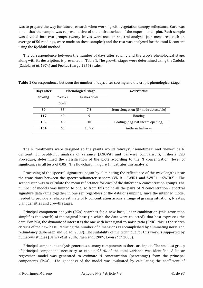
F. Rodríguez Moreno Artículo Nº3 / Article # 3 41 de 97
was to prepare the way for future research when working with vegetation canopy reflectance. Care was
taken that the sample was representative of the entire surface of the experimental plot. Each sample
was divided into two groups, twenty leaves were used in spectral analysis (ten measures, each an
average of 50 readings, were made on these samples) and the rest was analyzed for the total N content
using the Kjeldahl method.
The correspondence between the number of days after sowing and the crop's phenological stage,
along with its description, is presented in Table 1. The growth stages were determined using the Zadoks
(Zadoks et al. 1974) and Feekes (Large 1954) scales.
Table 1 Correspondence between the number of days after sowing and the crop's phenological stage
Days after
sowing
Phenological stage Description
Zadoks
Scale
Feekes Scale
80 35 7-8 Stem elongation (5th node detectable)
117 40 9 Booting
132 46 10 Booting (flag leaf sheath opening)
164 65 10.5.2 Anthesis half-way
The N treatments were designed so the plants would “always”, “sometimes” and “never” be N
deficient. Split-split-plot analysis of variance (ANOVA) and pairwise comparisons, Fisher's LSD
Procedure, determined the classification of the plots according to the N concentration (level of
significance in all tests of 0.05). The flowchart in Figure 1 illustrates this analysis.
Processing of the spectral signatures began by eliminating the reflectance of the wavelengths near
the transitions between the spectroradiometer sensors (VNIR - SWIR1 and SWIR1 - SWIR2). The
second step was to calculate the mean reflectance for each of the different N concentration groups. The
number of models was limited to one, so from this point all the pairs of N concentration - spectral
signature data came together in one set, regardless of the date of sampling, since the intended model
needed to provide a reliable estimate of N concentration across a range of grazing situations, N rates,
plant densities and growth stages.
Principal component analysis (PCA) searches for a new base, linear combination (this restriction
simplifies the search) of the original base (in which the data were collected), that best expresses the
data. For PCA, the dynamic of interest is the one with best signal-to-noise ratio (SNR); this is the search
criteria of the new base. Reducing the number of dimensions is accomplished by eliminating noise and
redundancy (Esbensen and Geladi 2009). The suitability of the technique for this work is supported by
numerous studies (Bajwa et al. 2004; Chen et al. 2009; Leon et al. 2003).
Principal component analysis generates as many components as there are inputs. The smallest group
of principal components necessary to explain 95 % of the total variance was identified. A linear
regression model was generated to estimate N concentration (percentage) from the principal
components (PCA). The goodness of the model was evaluated by calculating the coefficient of

F. Rodríguez Moreno Artículo Nº3 / Article # 3 42 de 97
determination (R2), the adjusted coefficient of determination (adjR2), the root mean square error
(RMSE) and the statistical significance (p-value) of the model (analysis of the variance).
Figure 1 Flowchart of the statistical analysis of nitrogen concentration
This linear regression model was developed for a previous study (Rodriguez-Moreno and Llera-Cid
2011b). In that work this model was the final result, it is a significant model with a high coefficient of
determination. In this work, it has been used as a method to identify the components that are
significantly related to N concentration.
There are two PCA outputs, a set of principal components and a transformation matrix that projects
the original data onto the new basis. The linear combinations that generated components significantly
related to N concentration were extracted from the matrix to identify the two wavelengths having the
greatest weight in each component. Treatments in this study ranged from N deficient to excessive,
which encompasses optimal N concentration values for each sampling time during grazing and growth
stage before maturity (Alaru et al. 2003).
Elementary plots (108)
Average plant nitrogen (N) concentration at
the...
A certain factor-level
could have a
significant effect on a
given time and not in
another, the analysis
was performed for
each day of sampling.
1º
sampling
2º
sampling
3º
sampling
4º
sampling
Those parcels that
differ from each
other by a factor-
level without effect
are repetitions of the
same configuration.
Split-split-plot Anova + Pairwise Comparisons
(Fisher´s LSD Procedure)
Identify factors-levels that have significant
effect on N concentration (level of significance
0.05).
Fourteen different values for the N
concentration were found in the four hundred
thirty-two determinations (108 experimental
plots x 4 days of sampling). Number of
grazing events and fertilizer rate had effects,
but not in all levels and times. Seeding
density had no effect on plant N
concentration.
Looking for a valid
model for the 4 days
of sampling, so all
data were grouped
into a single set.
Dependent variable:
Plant N concentration (%)

F. Rodríguez Moreno Artículo Nº3 / Article # 3 43 de 97
The Jenks Natural Breaks Classification method (Jenks 1967) was used to classify N concentrations
recorded during the four days of sampling. This algorithm minimizes the total sum of squared
deviations by adjusting the thresholds for the different groups. Figure 2 illustrates the iterative process.
Figure 2 Flowchart of the algorithm to implement Jenks Natural Breaks
The recommendations of Breiman (1984) were followed in development of the decision tree. The
decision tree classification algorithm was chosen because it was appropriate for the output variable.
Gini's diversity index was applied as the split criterion. The weight of all observations was the same and
the minimum number of observations that an impure node required before dividing was 10. All
variables were considered in each division process. Once the decision tree reached its maximum size,
the tree was pruned; the objective was to eliminate insignificant nodes of the training data set. This
pruning minimizes the over-fitting problem and maximizes the predictive power of the model. Cross-
validation was used in the evaluation of the decision tree; it allows obtaining a correct estimation of the
predictive ability.
The decision tree needs to compete in simplicity with spectral vegetation indices that use reflectance
values at two or three wavelengths for the calculation. For this reason, development of the decision tree
was limited to a maximum of three wavelengths. The resulting decision tree has a combination of two
or three elements (wavelengths) that are sensitive to plant N concentration. It should be recognized
that the algorithm used to create the decision does not guarantee choosing the optimal set of input
variables. Further, algorithms with a larger number of inputs variables may perform better. Figure 3
shows a flowchart that summarizes all the steps of the methodology.
This iterative process ends when improvement in TSSD
falls below a threshold level. While optimization is not
assured, the process can be repeated by changing the
thresholds and comparing the TSSD values.
The mean values for each initial class
are calculated and the sum of squared
deviations of class members from the
mean values is computed. The total
sum of squared deviations (TSSD) is
recorded.deviations (TSSD) is kept.
One selects the attribute, x, to be
classified and specifies the number of
classes required, k.
Jenks Natural Breaks
A set of (k‑1) random or uniform
values are generated in the range
[min(x),max(x)]. They are used as
initial class boundaries.
Individual values in each class are
assigned to adjacent classes by
adjusting the class boundaries to
check that the TSSD can be reduced.The goal is that the within-class
variance is as small as possible and
between-class variance is as large as
possible.
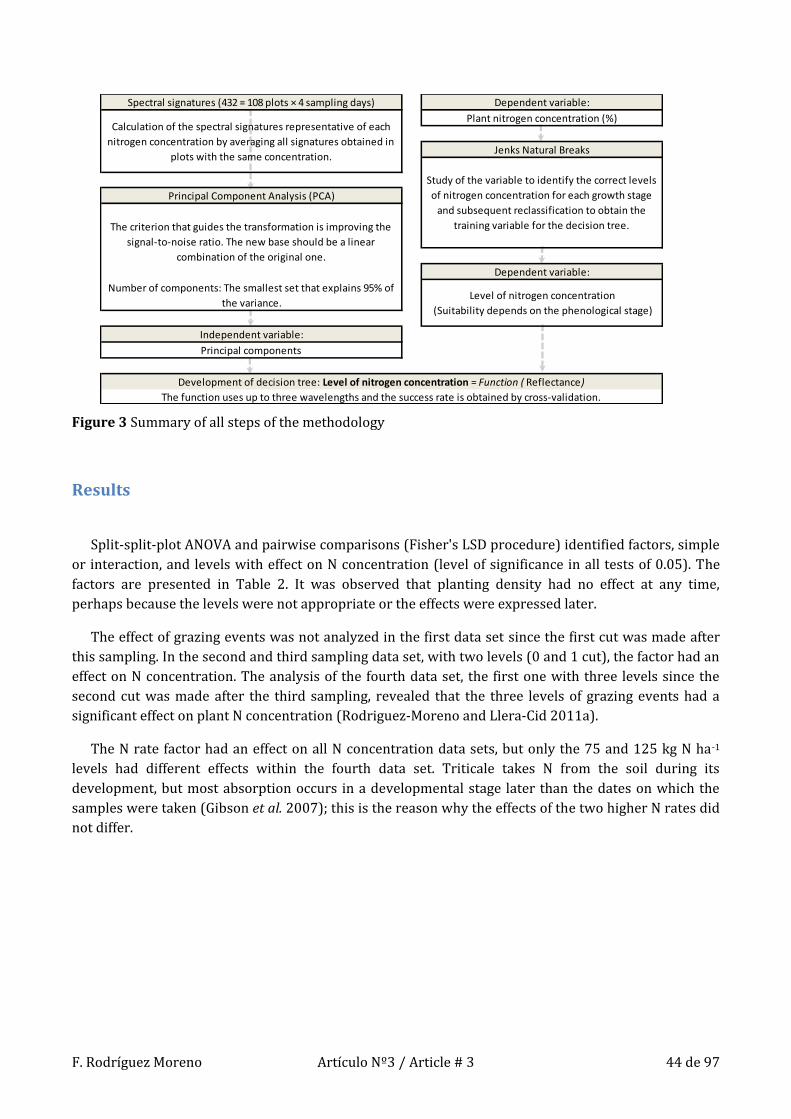
F. Rodríguez Moreno Artículo Nº3 / Article # 3 44 de 97
Figure 3 Summary of all steps of the methodology
Results
Split-split-plot ANOVA and pairwise comparisons (Fisher's LSD procedure) identified factors, simple
or interaction, and levels with effect on N concentration (level of significance in all tests of 0.05). The
factors are presented in Table 2. It was observed that planting density had no effect at any time,
perhaps because the levels were not appropriate or the effects were expressed later.
The effect of grazing events was not analyzed in the first data set since the first cut was made after
this sampling. In the second and third sampling data set, with two levels (0 and 1 cut), the factor had an
effect on N concentration. The analysis of the fourth data set, the first one with three levels since the
second cut was made after the third sampling, revealed that the three levels of grazing events had a
significant effect on plant N concentration (Rodriguez-Moreno and Llera-Cid 2011a).
The N rate factor had an effect on all N concentration data sets, but only the 75 and 125 kg N ha-1
levels had different effects within the fourth data set. Triticale takes N from the soil during its
development, but most absorption occurs in a developmental stage later than the dates on which the
samples were taken (Gibson et al. 2007); this is the reason why the effects of the two higher N rates did
not differ.
Plant nitrogen concentration (%)
Jenks Natural Breaks
Dependent variable:
Study of the variable to identify the correct levels
of nitrogen concentration for each growth stage
and subsequent reclassification to obtain the
training variable for the decision tree.
Independent variable:
Principal components
The function uses up to three wavelengths and the success rate is obtained by cross-validation.
Development of decision tree: Level of nitrogen concentration = Function ( Reflectance)
Level of nitrogen concentration
(Suitability depends on the phenological stage)
Spectral signatures (432 = 108 plots × 4 sampling days)
Principal Component Analysis (PCA)
The criterion that guides the transformation is improving the
signal-to-noise ratio. The new base should be a linear
combination of the original one.
Number of components: The smallest set that explains 95% of
the variance.
Calculation of the spectral signatures representative of each
nitrogen concentration by averaging all signatures obtained in
plots with the same concentration.
Dependent variable:
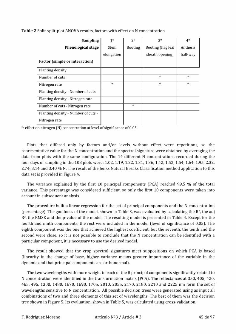
F. Rodríguez Moreno Artículo Nº3 / Article # 3 45 de 97
Table 2 Split-split-plot ANOVA results, factors with effect on N concentration
Sampling 1º 2º 3º 4º
Phenological stage Stem
elongation
Booting Booting (flag leaf
sheath opening)
Anthesis
half-way
Factor (simple or interaction)
Planting density
Number of cuts * *
Nitrogen rate * * *
Planting density - Number of cuts
Planting density - Nitrogen rate
Number of cuts - Nitrogen rate *
Planting density - Number of cuts -
Nitrogen rate
*: effect on nitrogen (N) concentration at level of significance of 0.05.
Plots that differed only by factors and/or levels without effect were repetitions, so the
representative value for the N concentration and the spectral signature were obtained by averaging the
data from plots with the same configuration. The 14 different N concentrations recorded during the
four days of sampling in the 108 plots were: 1.02, 1.19, 1.22, 1.31, 1.36, 1.42, 1.52, 1.54, 1.64, 1.95, 2.32,
2.74, 3.14 and 3.40 % N. The result of the Jenks Natural Breaks Classification method application to this
data set is provided in Figure 4.
The variance explained by the first 10 principal components (PCA) reached 99.5 % of the total
variance. This percentage was considered sufficient, so only the first 10 components were taken into
account in subsequent analysis.
The procedure built a linear regression for the set of principal components and the N concentration
(percentage). The goodness of the model, shown in Table 3, was evaluated by calculating the R2, the adj
R2, the RMSE and the p-value of the model. The resulting model is presented in Table 4. Except for the
fourth and ninth components, the rest were included in the model (level of significance of 0.05). The
eighth component was the one that achieved the highest coefficient, but the seventh, the tenth and the
second were close, so it is not possible to conclude that the N concentration can be identified with a
particular component, it is necessary to use the derived model.
The result showed that the crop spectral signatures meet suppositions on which PCA is based
(linearity in the change of base, higher variance means greater importance of the variable in the
dynamic and that principal components are orthonormal).
The two wavelengths with more weight in each of the 8 principal components significantly related to
N concentration were identified in the transformation matrix (PCA). The reflectances at 350, 405, 420,
465, 495, 1300, 1480, 1670, 1690, 1705, 2010, 2055, 2170, 2180, 2210 and 2225 nm form the set of
wavelengths sensitive to N concentration. All possible decision trees were generated using as input all
combinations of two and three elements of this set of wavelengths. The best of them was the decision
tree shown in Figure 5. Its evaluation, shown in Table 5, was calculated using cross-validation.
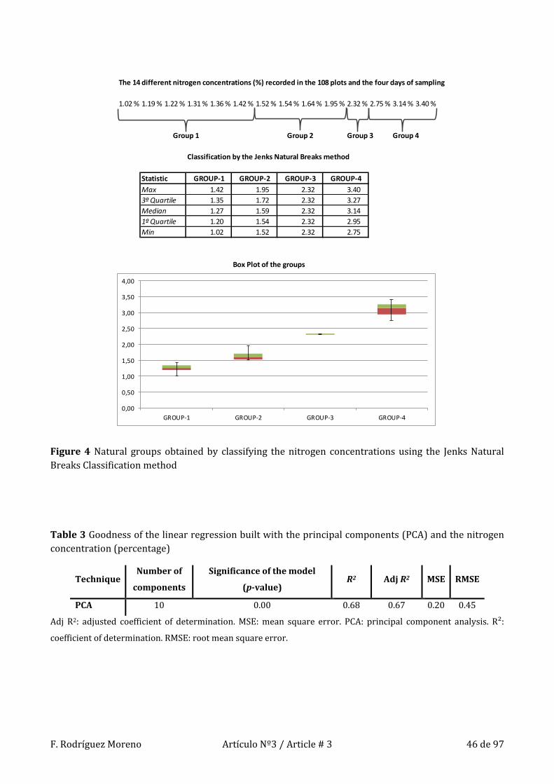
F. Rodríguez Moreno Artículo Nº3 / Article # 3 46 de 97
Figure 4 Natural groups obtained by classifying the nitrogen concentrations using the Jenks Natural
Breaks Classification method
Table 3 Goodness of the linear regression built with the principal components (PCA) and the nitrogen
concentration (percentage)
Technique Number of
components
Significance of the model
(p-value) R2 Adj R2 MSE RMSE
PCA 10 0.00 0.68 0.67 0.20 0.45
Adj R2: adjusted coefficient of determination. MSE: mean square error. PCA: principal component analysis. R²:
coefficient of determination. RMSE: root mean square error.
The 14 different nitrogen concentrations (%) recorded in the 108 plots and the four days of sampling
1.02 % 1.19 % 1.22 % 1.31 % 1.36 % 1.42 % 1.52 % 1.54 % 1.64 % 1.95 % 2.32 % 2.75 % 3.14 % 3.40 %
Group 3 Group 4
Classification by the Jenks Natural Breaks method
1.42 1.95 2.32 3.40
1.35 1.72 2.32 3.27
1.27 1.59 2.32 3.14
1.20 1.54 2.32 2.95
1.02 1.52 2.32 2.75
Box Plot of the groups
Group 1 Group 2
Statistic
Max
3º Quartile
Median
1º Quartile
Min
GROUP-1 GROUP-2 GROUP-3 GROUP-4
0,00
0,50
1,00
1,50
2,00
2,50
3,00
3,50
4,00
GROUP-1 GROUP-2 GROUP-3 GROUP-4

F. Rodríguez Moreno Artículo Nº3 / Article # 3 47 de 97
Table 4 Linear regression built with the principal components and the N concentration (percentage)
Coefficients p-value
Constant 2.236 0.000
Component Nº1 -0.013 0.000
Component Nº2 -0.020 0.000
Component Nº3 0.008 0.000
Component Nº4 -0.001 0.551
Component Nº5 0.009 0.001
Component Nº6 -0.012 0.001
Component Nº7 0.028 0.000
Component Nº8 -0.053 0.000
Component Nº9 0.003 0.742
Component Nº10 0.027 0.028
The resulting decision tree needs only the reflectance at 350, 1670 and 2170 nm to reach a success
rate (average of all groups) of 66.2 %. The number of cases in each of the four groups defined was not
the same. If the success rate for the model was calculated using a weighted average by the percentage of
cases in each group, then the model had a success rate of 68.3 %.
Table 5 Success rate of the decision tree
Group 1 2 3 4
Success rate 71.7 % 55.0 % 65.6 % 72.4 %
Success rate (simple
average)
66.2 %
Group 1 2 3 4
Weight of
each group
27.8 % 13.9 % 22.2 % 36.1 %
Success rate
(average weighted by the
percentage of cases in each group)
68.3 %

F. Rodríguez Moreno Artículo Nº3 / Article # 3 48 de 97
Figure 5 Decision tree for the nitrogen concentration created using reflectance at three wavelengths
None of the wavelengths traditionally used in the estimation of nitrogen (Rodriguez-Moreno and
Llera-Cid 2011a) has been included in the decision tree. This can be explained by the cultivar used in
the study, the dual purpose triticale, where the greenness of the plant is not always a good estimator of
N concentration. The reflectance at 350 nm has been associated with the photosynthetic activity (Ray et
al. 2007; Ren et al. 2006) and the reflectance at short-wavelength infrared (1670 and 2170 nm) is
related to water stress (L. Zhang et al. 2012; Wang et al. 2010), which sometimes is related to the N
concentration (Zhao et al. 2004). These references indicate what could be the main biological meaning
of the wavelengths used.
The result of PCA showed that 95 % of the information contained in the spectral signature could be
expressed with only 10 principal components. Reflectance values at different wavelengths are not
independent of each other and therefore it is not always easy to describe a pure biological reason for
the identified wavebands. Others have shown that the wavelengths used in the decision tree are directly
related to the N concentration at different phenological stages (Li et al. 2010; Koppe et al. 2010).
The potential for spectral vegetation indices to estimate plant N concentration was evaluated. The
test, based on the same data from the agronomic trial with triticale, determined that the best spectral
index involved green reflectance, which reached a R2=0.31 (Rodriguez-Moreno and Llera-Cid 2011a). In
this work, the proposed strategy performed better than spectral indices, such as NDVI. This has not
been the first experience where the effectiveness of spectral vegetation indices has been surpassed. An
example is the result obtained by Waheed et al. (2006), who were able to develop a decision tree with a
classification success rate above 90 % in a similar experiment.
The linear regression built with the goal to identify the principal components sensitive to N
concentration, Tables 3 and 4, had a R2 of 0.68, which could resemble a success rate of 82.5 %. That
value is slightly below the success rate achieved by Waheed et al. (2006). Major differences were
expected for the peculiarities of a dual purpose triticale for having developed a model for a wider range
of phenological stages and for the measures taken to increase the guarantees of predictive power.
350 1670 2170
NO EXIT TO Group 4
YES
NO EXIT TO Group 1
YES
NO EXIT TO Group 4
YES
NO EXIT TO Group 2
YES
EXIT TO Group 3
Involved wavelengths (nm)
If ( Reflectance [1670 nm] < 0.48 )
If ( Reflectance [2170 nm] < 0.20 )
If ( Reflectance [350 nm] < 0.08 )
If ( Reflectance [2170 nm] < 0.26 )
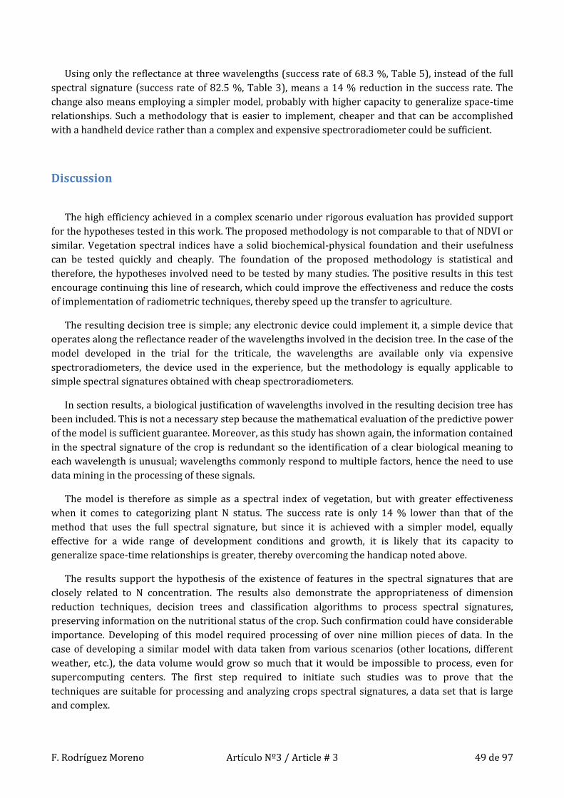
F. Rodríguez Moreno Artículo Nº3 / Article # 3 49 de 97
Using only the reflectance at three wavelengths (success rate of 68.3 %, Table 5), instead of the full
spectral signature (success rate of 82.5 %, Table 3), means a 14 % reduction in the success rate. The
change also means employing a simpler model, probably with higher capacity to generalize space-time
relationships. Such a methodology that is easier to implement, cheaper and that can be accomplished
with a handheld device rather than a complex and expensive spectroradiometer could be sufficient.
Discussion
The high efficiency achieved in a complex scenario under rigorous evaluation has provided support
for the hypotheses tested in this work. The proposed methodology is not comparable to that of NDVI or
similar. Vegetation spectral indices have a solid biochemical-physical foundation and their usefulness
can be tested quickly and cheaply. The foundation of the proposed methodology is statistical and
therefore, the hypotheses involved need to be tested by many studies. The positive results in this test
encourage continuing this line of research, which could improve the effectiveness and reduce the costs
of implementation of radiometric techniques, thereby speed up the transfer to agriculture.
The resulting decision tree is simple; any electronic device could implement it, a simple device that
operates along the reflectance reader of the wavelengths involved in the decision tree. In the case of the
model developed in the trial for the triticale, the wavelengths are available only via expensive
spectroradiometers, the device used in the experience, but the methodology is equally applicable to
simple spectral signatures obtained with cheap spectroradiometers.
In section results, a biological justification of wavelengths involved in the resulting decision tree has
been included. This is not a necessary step because the mathematical evaluation of the predictive power
of the model is sufficient guarantee. Moreover, as this study has shown again, the information contained
in the spectral signature of the crop is redundant so the identification of a clear biological meaning to
each wavelength is unusual; wavelengths commonly respond to multiple factors, hence the need to use
data mining in the processing of these signals.
The model is therefore as simple as a spectral index of vegetation, but with greater effectiveness
when it comes to categorizing plant N status. The success rate is only 14 % lower than that of the
method that uses the full spectral signature, but since it is achieved with a simpler model, equally
effective for a wide range of development conditions and growth, it is likely that its capacity to
generalize space-time relationships is greater, thereby overcoming the handicap noted above.
The results support the hypothesis of the existence of features in the spectral signatures that are
closely related to N concentration. The results also demonstrate the appropriateness of dimension
reduction techniques, decision trees and classification algorithms to process spectral signatures,
preserving information on the nutritional status of the crop. Such confirmation could have considerable
importance. Developing of this model required processing of over nine million pieces of data. In the
case of developing a similar model with data taken from various scenarios (other locations, different
weather, etc.), the data volume would grow so much that it would be impossible to process, even for
supercomputing centers. The first step required to initiate such studies was to prove that the
techniques are suitable for processing and analyzing crops spectral signatures, a data set that is large
and complex.

F. Rodríguez Moreno Artículo Nº3 / Article # 3 50 de 97
A question that remains is the magnitude of the calibration necessary to use the resulting model in
another scenario with the same success. The implementation of this methodology would require, at
most, a calibration study per crop season. At this point, it is worth recalling the high variability in the
experimental plots in terms of growing conditions, which means that the effort to adjust the model
could be valid for a large area. Perhaps it is possible to design simple experiments to estimate the
calibration parameters of the model, experiments that farmers could perform.
The resulting model is ready to operate in a wide range of conditions, but its effectiveness is
unknown. Fortunately, it is a challenge that is faced with a large arsenal of modeling and analysis
techniques (derivative of the reflectance with respect to the wavelength or the time, neural networks,
genetic algorithms, multivariate adaptive regression splines, etc.). These techniques have already
demonstrated their enormous potential to solve problems of similar nature. The result obtained in this
work has been evaluated as satisfactory; this is the reason why these techniques, more powerful in
some ways, but also more complex, have not been employed.
It is very likely that this study has determined the lowest threshold of efficacy for a dual purpose
triticale that supports the grazing of livestock during its development, without ruining the final harvest;
this makes it a special crop with additional difficulties for the development of radiometric models
(details given in the introduction). It is expected that models developed for other cereals without a dual
purpose can achieve greater effectiveness. This increase would be achieved by the combination of
spectral vegetation indices and models developed using the proposed methodology. This needs to be
proven and quantified, therefore further studies are needed.
The resulting model requires direct-contact radiometric measurements of plant leaves. The next step
is to determine whether, with measures of vegetation canopy reflectance, it is possible to reproduce the
results. If that were achieved, then it would be appropriate to experiment with a high-efficiency system
in real-time for the identification of the plant N requirements.
Competing with vegetation spectral indices, NDVI or similar, in terms of profitability would be
possible with more studies supporting the greater effectiveness of the models obtained using this
methodology. This study has shown that there are models valid for large areas because they respond
satisfactorily even for crops under different growth conditions and they only require a calibration study
per crop season because the model can be valid for a wide range of phonological stages. While it is not
satisfactorily resolved, the presented methodology will not end with the hegemony of vegetation
spectral indices, although the resulting models have achieved higher efficacies in scientific works.
Acknowledgements
The authors would like to thank the staff of Mendel University, Czech Republic, Soňa Valtýniová and
Vojtěch; University of Extremadura, Spain, Ángel M. Felicísimo; J.S. Schepers for their help.

F. Rodríguez Moreno Artículo Nº3 / Article # 3 51 de 97
References
Alaru, M., Laur, Ü., & Jaama, E. (2003). Influence of nitrogen and weather conditions on the grain
quality of winter triticale (Vol. 1, Vol. 1). Tartu, ESTONIE: Estonian Agricultural University.
Auernhammer, H. (2001). Precision farming -- the environmental challenge. Computers and
Electronics in Agriculture, 30(1-3), 31-43, doi:10.1016/s0168-1699(00)00153-8.
Bajwa, S. G., Bajcsy, P., Groves, P., & Tian, L. F. (2004). Hyperspectral image data mining for band
selection in agricultural applications. Transactions of the ASAE, 47(3), 895-907.
Bongiovanni, R., & Lowenberg-Deboer, J. (2004). Precision agriculture and sustainability. Precision
Agriculture, 5(4), 359-387, doi:10.1023/B:PRAG.0000040806.39604.aa.
Breiman, L. (1984). Classification and regression trees (The Wadsworth statistics/probability
series). Belmont, Calif.: Wadsworth International Group.
Broge, N. H., & Leblanc, E. (2001). Comparing prediction power and stability of broadband and
hyperspectral vegetation indices for estimation of green leaf area index and canopy chlorophyll density.
Remote Sensing of Environment, 76(2), 156-172, doi:10.1016/s0034-4257(00)00197-8.
Broge, N. H., & Mortensen, J. V. (2002). Deriving green crop area index and canopy chlorophyll
density of winter wheat from spectral reflectance data. Remote Sensing of Environment, 81(1), 45-57,
doi:10.1016/s0034-4257(01)00332-7.
Chen, Y. H., Jiang, J. B., Huang, W. J., & Wang, Y. Y. (2009). Comparison of principal component
analysis with VI-empirical approach for estimating severity of yellow rust of winter wheat. Guang Pu
Xue Yu Guang Pu Fen Xi, 29(8), 2161-2165.
Dorigo, W. A., Zurita-Milla, R., de Wit, A. J. W., Brazile, J., Singh, R., & Schaepman, M. E. (2007). A
review on reflective remote sensing and data assimilation techniques for enhanced agroecosystem
modeling. International Journal of Applied Earth Observation and Geoinformation, 9(2), 165-193,
doi:10.1016/j.jag.2006.05.003.
Esbensen, K. H., & Geladi, P. (2009). Principal component analysis: concept, geometrical
interpretation, mathematical background, algorithms, history, practice. In D. B. Stephen, Rom, x00E,
Tauler, & W. Beata (Eds.), Comprehensive Chemometrics (pp. 211-226). Oxford: Elsevier.
Gibson, L. R., Nance, C. D., & Karlen, D. L. (2007). Winter triticale response to nitrogen fertilization
when grown after corn or soybean (Vol. 99, Vol. 1). Madison, WI, ETATS-UNIS: American Society of
Agronomy.
Goel, P. K., Prasher, S. O., Patel, R. M., Landry, J. A., Bonnell, R. B., & Viau, A. A. (2003). Classification of
hyperspectral data by decision trees and artificial neural networks to identify weed stress and nitrogen
status of corn. Computers and Electronics in Agriculture, 39(2), 67-93.
Jenks, G. F. The data model concept in statistical mapping. In K. Frenzel (Ed.), International Yearbook
of Cartography, 1967 (Vol. 7, pp. 186): Rand McNally & Co. doi:citeulike-article-id:8241517.
Koppe, W., Li, F., Gnyp, M. L., Miao, Y., Jia, L., Chen, X., et al. (2010). Evaluating multispectral and
hyperspectral satellite remote sensing data for estimating winter wheat growth parameters at regional
scale in the North China plain. Photogrammetrie, Fernerkundung, Geoinformation, 2010(3), 167-178,
doi:10.1127/1432-8364/2010/0047.
Large, E. C. (1954). Growth stages in cereals illustration of the Feekes scale. Plant Pathology, 3(4),
128-129, doi:10.1111/j.1365-3059.1954.tb00716.x.
Leon, C. T., Shaw, D. R., Cox, M. S., Abshire, M. J., Ward, B., Wardlaw, M. C., et al. (2003). Utility of
remote sensing in predicting crop and soil characteristics. Precision Agriculture, 4(4), 359-384,
doi:10.1023/a:1026387830942.

F. Rodríguez Moreno Artículo Nº3 / Article # 3 52 de 97
Li, F., Gnyp, M. L., Jia, L., Miao, Y., Yu, Z., Koppe, W., et al. (2008). Estimating N status of winter wheat
using a handheld spectrometer in the North China Plain. Field Crops Research, 106(1), 77-85,
doi:10.1016/j.fcr.2007.11.001.
Li, F., Miao, Y., Hennig, S., Gnyp, M., Chen, X., Jia, L., et al. (2010). Evaluating hyperspectral vegetation
indices for estimating nitrogen concentration of winter wheat at different growth stages. Precision
Agriculture, 11(4), 335-357, doi:10.1007/s11119-010-9165-6.
Li, Y., Zhu, Y., Dai, T., Tian, Y., & Cao, W. (2006). Quantitative relationships between leaf area index
and canopy reflectance spectra of wheat. Ying Yong Sheng Tai Xue Bao, 17(8), 1443-1447.
Llorens, J., Gil, E., Llop, J., & Escolà, A. (2010). Variable rate dosing in precision viticulture: Use of
electronic devices to improve application efficiency. Crop Protection, 29(3), 239-248,
doi:10.1016/j.cropro.2009.12.022.
Marschner, H. (1995). In Mineral Nutrition of Higher Plants (Second Edition). London: Academic
Press.
Moran, M. S., Inoue, Y., & Barnes, E. M. (1997). Opportunities and limitations for image-based remote
sensing in precision crop management. Remote Sensing of Environment, 61(3), 319-346,
doi:10.1016/s0034-4257(97)00045-x.
R-Development_Core_Team. (2008). R: A Language and Environment for Statistical Computing.
Vienna: Foundation for Statistical Computing.
Ray, S. S., Jain, N., Miglani, A., Singh, J. P., Singh, A. K., Panigrahy, S., et al. (2007. Defining optimum
narrow bands and bandwidths for agricultural applications. In Hyderabad, 2007 (Vol. 4, pp. 2458-2467,
58th International Astronautical Congress 2007).
Ren, J., Chen, Z., Tang, H., & Shi, R. (2006). Regional yield estimation for winter wheat based on net
primary production model. Nongye Gongcheng Xuebao/Transactions of the Chinese Society of
Agricultural Engineering, 22(5), 111-117.
Robertson, M., Isbister, B., Maling, I., Oliver, Y., Wong, M., Adams, M., et al. (2007). Opportunities and
constraints for managing within-field spatial variability in Western Australian grain production. Field
Crops Research, 104(1-3), 60-67, doi:10.1016/j.fcr.2006.12.013.
Rodriguez-Moreno, F., & Llera-Cid, F. (2011a). Evaluating spectral vegetation indices for a practical
estimation of nitrogen concentration in dual purpose (forage and grain) triticale. Spanish Journal of
Agricultural Research, 9(3), 681-686, doi:10.5424/2013.
Rodriguez-Moreno, F., & Llera-Cid, F. (2011b). PCA versus ICA for the reduction of dimensions of the
spectral signatures in the search for an index for the concentration of nitrogen in plant. Spanish Journal
of Agricultural Research, 9(3).
Rumpf, T., Mahlein, A. K., Steiner, U., Oerke, E. C., Dehne, H. W., & Plümer, L. (2010). Early detection
and classification of plant diseases with support vector machines based on hyperspectral reflectance.
Computers and Electronics in Agriculture, 74(1), 91-99, doi:10.1016/j.compag.2010.06.009.
Ruß, G., & Brenning, A. (2010). Data Mining in Precision Agriculture: Management of spatial
information. In E. Hüllermeier, R. Kruse, & F. Hoffmann (Eds.), Computational Intelligence for
Knowledge-Based Systems Design (Vol. 6178, pp. 350-359, Lecture Notes in Computer Science):
Springer Berlin / Heidelberg.
Schellberg, J., Hill, M. J., Gerhards, R., Rothmund, M., & Braun, M. (2008). Precision agriculture on
grassland: Applications, perspectives and constraints. European Journal of Agronomy, 29(2-3), 59-71,
doi:10.1016/j.eja.2008.05.005.
Schroers, J. O., Gerhards, R., & Kunisch, M. (2010). Economic evaluation of precision crop protection
measures. In E. C. Oerke, R. Gerhards, G. Menz, & R. A. Sikora (Eds.), Precision Crop Protection - the
Challenge and Use of Heterogeneity (pp. 417-426): Springer Netherlands.

F. Rodríguez Moreno Artículo Nº3 / Article # 3 53 de 97
Shao, Y., Zhao, C., Bao, Y., & He, Y. (2009). Quantification of nitrogen status in rice by least squares
support vector machines and reflectance spectroscopy. Food and Bioprocess Technology, 1-8,
doi:10.1007/s11947-009-0267-y.
Taiz, L., & Zeiger, E. (1991). Plant physiology: Benjamin/Cummings Pub. Co.
Tian, Y. C., Yang, J., Yao, X., Zhu, Y., & Cao, W. X. (2009). Quantitative relationships between hyper-
spectral vegetation indices and leaf area index of rice. Ying Yong Sheng Tai Xue Bao, 20(7), 1685-1690.
Tian, Y. C., Yao, X., Yang, J., Cao, W. X., Hannaway, D. B., & Zhu, Y. (2011). Assessing newly developed
and published vegetation indices for estimating rice leaf nitrogen concentration with ground- and
space-based hyperspectral reflectance. Field Crops Research, 120(2), 299-310,
doi:10.1016/j.fcr.2010.11.002.
Vrindts, E., Reyniers, M., Darius, P., De baerdemaeker, J., Gilot, M., Sadaoui, Y., et al. (2003). Analysis
of soil and crop properties for precision agriculture for winter wheat. Biosystems Engineering, 85(2),
141-152, doi:10.1016/s1537-5110(03)00040-0.
Waheed, T., Bonnell, R. B., Prasher, S. O., & Paulet, E. (2006). Measuring performance in precision
agriculture: CART--A decision tree approach. Agricultural Water Management, 84(1-2), 173-185,
doi:10.1016/j.agwat.2005.12.003.
Wang, Y. Y., Li, G. C., Zhang, L. J., & Fan, J. L. (2010). Retrieval of leaf water content of winter wheat
from canopy hyperspectral data using partial least square regression. Guang Pu Xue Yu Guang Pu Fen
Xi/Spectroscopy and Spectral Analysis, 30(4), 1070-1074, doi:10.3964/j.issn.1000-0593(2010)04-
1070-05.
Wood, G. A., Taylor, J. C., & Godwin, R. J. (2003). Calibration methodology for mapping within-field
crop variability using remote sensing. Biosystems Engineering, 84(4), 409-423, doi:10.1016/s1537-
5110(02)00281-7.
Yao, X., Zhu, Y., Tian, Y., Feng, W., & Cao, W. (2010). Exploring hyperspectral bands and estimation
indices for leaf nitrogen accumulation in wheat. International Journal of Applied Earth Observation and
Geoinformation, 12(2), 89-100, doi:10.1016/j.jag.2009.11.008.
Yoder, B. J., & Pettigrew-Crosby, R. E. (1995). Predicting nitrogen and chlorophyll content and
concentrations from reflectance spectra (400-2500 nm) at leaf and canopy scales. Remote Sensing of
Environment, 53(3), 199-211, doi:10.1016/0034-4257(95)00135-n.
Zadoks, J. C., Chang, T. T., & Konzak, C. F. (1974). A decimal code for the growth stages of cereals.
Weed research, 14(6), 415-421, doi:10.1111/j.1365-3180.1974.tb01084.x.
Zhang, L., Zhou, Z., Zhang, G., Meng, Y., Chen, B., & Wang, Y. (2012). Monitoring the leaf water content
and specific leaf weight of cotton (Gossypium hirsutum L.) in saline soil using leaf spectral reflectance.
European Journal of Agronomy, 41, 103-117, doi:10.1016/j.eja.2012.04.003.
Zhang, X., Shi, L., Jia, X., Seielstad, G., & Helgason, C. (2010). Zone mapping application for precision-
farming: a decision support tool for variable rate application. Precision Agriculture, 11(2), 103-114,
doi:10.1007/s11119-009-9130-4.
Zhao, C., Liu, L., Wang, J., Huang, W., Song, X., Li, C., et al. Methods and application of remote sensing
to forecast wheat grain quality. In Anchorage, AK, 2004 (Vol. 6, pp. 4008-4010, 2004 IEEE International
Geoscience and Remote Sensing Symposium Proceedings: Science for Society: Exploring and Managing
a Changing Planet. IGARSS 2004)
Zhou, D. Q., Tian, Y. C., Yao, X., Zhu, Y., & Cao, W. X. (2008). Quantitative relationships between leaf
total nitrogen concentration and canopy reflectance spectra of rice. Ying Yong Sheng Tai Xue Bao, 19(2),
337-344.
Zhu, Y., Yao, X., Tian, Y., Liu, X., & Cao, W. (2008). Analysis of common canopy vegetation indices for
indicating leaf nitrogen accumulations in wheat and rice. International Journal of Applied Earth
Observation and Geoinformation, 10(1), 1-10, doi:10.1016/j.jag.2007.02.006.

F. Rodríguez Moreno Artículo Nº3 / Article # 3 54 de 97

F. Rodríguez Moreno Artículo Nº4 / Article # 4 55 de 97
Spatial interpretation of plant parameters in precision agriculture with
winter wheat
Citation Precision Agriculture, yet unpublished.
Download link
Not available.
Header
F. Rodriguez-Moreno1, V. Lukas2, L. Neudert2, T. Dryšlová2
1Centro de Investigación ‘‘La Orden-Valdesequera’’, Gobierno de Extremadura. Finca ‘‘La Orden’’, Ctra.
N-V. Km. 372, 06187 Guadajira, Badajoz, Spain.
e-mail: [email protected] ; [email protected]
2Mendel University in Brno, Department of Agrosystems and Bioclimatology, Zemedelska 1, 613 00
Brno, Czech Republic
Abstract
This paper presents a methodology for the spatial interpretation of plant parameters, which is used
to diagnose the status of winter wheat. The crop monitoring took place in the Czech Republic in 2010 in
two fields using uniform crop management (52 and 38ha). The survey was carried out at BBCH30
phenological stage using a regular sampling grid with 150m distance between points (27 and 18points).
The plant height and chlorophyll concentration (Yara N-Tester) were recorded and plant samples were
taken to analyze the nutrients concentrations (N, P, K, Mg, Ca and S). A crop development index was
developed from plant height and N-Tester values and compared with the results of plant analysis in
order to determine the relationships, which were validated through spatial analysis. It may indicate the
nutrients which limit plant grow at that stage. As a next step, the crop development index was
compared with yield data to evaluate the success and stability in identifying the limiting factors. The
method revealed that the limiting factors in the first field were potassium, calcium and nitrogen (in that
order), nutrients significantly related to soil, climatology (surface functions) and relief. In the second
field, the crop development index was not associated with any nutrient, but it was related to the
topography (slope and moisture). Furthermore, it is found that in both cases the diagnoses were
consistent with the DRIS diagnoses. The results show that if leaf analyses are complemented with the

F. Rodríguez Moreno Artículo Nº4 / Article # 4 56 de 97
characterization of crop development, it is possible to obtain successful diagnosis using statistical and
spatial analysis.
Keywords: Cereals / Crop development (biomass and crop vigor) / Diagnosis and Recommendation
Integrated System (DRIS) / Plant nutrition / Site specific crop management / Spatial analysis
Abbreviations used: DRIS (Diagnosis and Recommendation Integrated System); CDI (Crop
development index); p-value ( Statistical significance); R2 (Determination coefficient); RMSE (Root mean
square error); SF (Spatial factors);
Introduction
Diagnosis of the nutritional status of a crop identifies the treatment necessary to correct potential
deficiencies and allows the crop to develop properly without input wastage (Barker and Pilbeam 2007;
J. B. Jones 1998; Marschner 1995; Mengel and Kirkby 2001). Today, with the rise of precision
agriculture it is necessary to repeat the diagnostic procedure in each land unit (Srinivasan 2006;
Stafford 2007). This is why indirect methods which offer a rapid assessment of a crop’s nutritional
status are sought, and why they rely upon the spatial relationship between samples to interpolate the
results (Oliver 2010).
As a result of agronomic trials, it has been possible to determine sufficiency ranges for the different
nutrients of most crops (Marschner 1995; Rengel 1998; Reuter et al. 1998). Using other agronomic
studies, faster but with a greater demand for computational requirements and statistical knowledge, it
has been able to identify the relationships (ratios) between nutrients that characterize the plants of a
particular crop which offer the best yield (Bailey et al. 1997a; Bailey et al. 1997b; Bailey et al. 2000;
Beaufils 1973). Recent advances in this topic correspond to the identification of spectral features
related to the nutritional status of the crop, resulting in the development of handsets that after a few
minutes of reading in the field provide fertilizer recommendations (N-Tester of YARA International
ASA, Germany).
Agronomic studies leading to the identification of rules for the interpretation of leaf analysis have a
particular configuration (Alves Mourão Filho 2005; Jeong et al. 2009; Krug et al. 2010; Partelli et al.
2007; Soltanpour et al. 1995). It is not possible to experiment with all feasible configurations of crop
development, which means that outside of that range of tested conditions, in real complex conditions,
the adequacy of those rules of interpretation is unknown.
Although agricultural practices and crop development correspond with one of the cases for which a
given set of interpretation rules were developed, the assessment of nutritional status will not be
available at all times. The methodologies that work with sufficiency ranges identify the phenological
stage of the crop on which to carry out the sampling and the plant part to be analyzed to proceed to
diagnose (Marschner 1995; Rengel 1998). The methodologies that use nutrient ratios were presented
as being more robust in this section, but experimentation has shown that the sensitivity, although
lower, continues (Agbangba et al. 2011; Amundson and Koehler 1987; R. Beverly 1987; R. B. Beverly

F. Rodríguez Moreno Artículo Nº4 / Article # 4 57 de 97
1991; M. E. Sumner 1977). Indirect methods are calibrated by means of some of the methodology
described above. So, these methods inherit the same problems (Arregui et al. 2006; Liu et al. 2003), to
which it has to add the errors inherent in using an indirect measurement instead of a leaf analysis.
The interpretation of a set of leaf analysis from a given field should not be done individually because
they are not independent samples. It is the reason why geostatistics can be used successfully in their
extrapolation (Gholizadeh et al. 2009; Qian et al. 2009; Vieira and Gonzalez 2003). Studying the
variability (differential development) of the crop at the field (Cao et al. 2012; Guo et al. 2010) might
come to understand the causes. After deducting the diagnosis, the corrective treatment is obtained by
combining agronomy, technology and economics.
A methodology that studies the spatial variability of the crop has to start by defining an index to
quantify the crop development. In this study that index is defined as the product of the reading of N-
Tester and the plant height in centimeters. Both are simple measurements related to a large number of
determining factors in the development of cereals such as chlorophyll content (Jhanji and Sekhon
2011), the phenological stage (Escobar-Gutiérrez and Combe 2012), health status (Byamukama et al.
2012), water stress (S. Ma et al. 2012; Niu et al. 2007), salt stress (L. Zhang et al. 2012), competitive
stress (Yenish and Young 2004) and productivity (Ivanova and Tsenov 2011).
The variance recorded by the crop development index (CDI) has to be caused by some factor. For
example, the concentration of potassium is not right across the field. If that were to be the case, the
study of the relationship between CDI and potassium concentration by regression and cross-validation
(Draper and Smith 1981; Witten et al. 2011) would reveal a significant relationship whereby the
potassium explains a certain percentage of the CDI variance . By reversing the process, one develops a
diagnostic method for identifying the limiting factor for crop growth. However, it has to be accepted
that the relationship with statistical significance implies a causal relationship that can be used
successfully in agricultural management, a hypothesis shared by all the traditional methods.
Spatial variability in the concentration of nutrients, the CDI (in the above example, potassium
deficiency explaining the CDI should, in turn, be explained by means of a gradient in the soil properties
…) and the crop yield are the result of the interaction between soils, climate, topography, anthropogenic
activities and health incidents (Blandino et al. 2012; Fiez et al. 1994; Halvorson and Doll 1991;
Kravchenko and Bullock 2000; L. P. Li et al. 2012; Miller et al. 1988; Patil et al. 2010; Sharma-Poudyal
and Chen 2011; Wiik and Ewaldz 2009). The soil and climate may be unknown, but their effects can be
successfully represented by the use of surface functions (Irmak et al. 2010; Jiang et al. 2010; L. Ma and
Zuo 2012; Shi et al. 2012; C. C. Yang et al. 2004; Zandi et al. 2011). The effects of the relief have to be a
function of topographic variables (elevation, slope, aspect, curvature and flow accumulation) (Fraisse et
al. 2001; Pachepsky et al. 2001; Persson et al. 2005), which can be derived from a digital elevation
model obtained through a simple differential GPS (DGPS). If agricultural management is uniform or
known, only a health problem of the crop in its early stages, due to the spatial-temporal randomness of
its occurrence (de Carvalho Alves et al. 2009; Demon et al. 2011; Jewell et al. 2009; B. Li et al. 2011;
Meentemeyer et al. 2008; Plantegenest et al. 2007), would exceed the modeling capacity of the group
formed by surface functions and topographic variables, known in this work as spatial factors (SF).
Studies have taken place in which strategies close to these have been tested successfully (Akramkhanov
et al. 2011; McBratney et al. 2003; Moore et al. 1993; Odeha et al. 1994; Park et al. 2001).
There are two reasons to study whether the concentrations of nutrients, the CDI and the crop yield
are related to spatial factors. Firstly, it serves as a check on the diagnosis because if a nutrient is

F. Rodríguez Moreno Artículo Nº4 / Article # 4 58 de 97
identified as limiting but it is not related to spatial factors, it would have to be considered a problem
with the data or a lack of spatial relationship between samples. Secondly, these relationships with the
spatial factors allow the interpolation of the variables and, thereby, obtain variable application maps
and crop yield maps for the entire field. Both results are very important because of the small numbers
of samples needed for the implementation of this methodology. In a small data set, the results are
sensitive to outliers and the interpolation is limited using geostatistics because the number and
distribution of data does not allow identifying of a reliable variogram (Oliver 2010).
The aim of this study was to improve the interpretation of leaf analysis, complementing the
traditional diagnostic with a spatial interpretation of plant parameters (SIOPP), which could provide
own evidence for each scenario of the factor that is acting as limiting for the crop development. This can
improve agricultural management, rationalize inputs, increase crop yield, reduce environmental impact
and improve the profitability of farms, probably through the implementation of the new methodology in
system decision support.
Materials and methods
Field experiments and data collection
The data used in this study were obtained from an experiment carried out in two fields in the South
Moravian region of the Czech Republic: The field Pachty (48° 59’ N, 16° 38’ E) with an area of 52.5 ha is
located on a plain (elevation 176 – 182 m) with an average annual temperature of 9.2 °C, precipitation
of 483 mm per year and a predominant soil type described as chernozem. The field Haj (49° 15’ N,
17°06’ E) has an area of 37.8 ha and is located in hilly terrain (elevation 280 – 342 m) with a haplic
luvisol soil type, average annual temperature of 9.25 °C and precipitation of 542 mm per year. In 2010,
both locations were planted with winter wheat (fore-crop: sunflower at Pachty, spring barley at Haj)
and the crop management was uniform within each field.
In BBCH 30 growth stage (Zadoks et al. 1974), plant samples were taken for analysis of nutrients in
dry matter (content of N, P, K, Ca, Mg and S) according to the methodology valid in the Czech Republic
(Zbíral 2005). Simultaneously with plant sampling, chlorophyll concentration using an N-Tester (YARA
International ASA, Germany) and the height of plants were measured, they are plant parameters used in
this study. The survey was done in a regular grid of 150 x 150 m (27 samples in Pachty, 18 in Haj)
within a circle of 5 m of diameter at each sampling point (Figure 1).
To get information about the final production at both locations, yield sampling was carried out with
the same point grid two weeks before harvest. Spikes were cut from an area of 0.2 m2 at two places
within a circle of 5 m of diameter at each point of the 150 m sampling grid. The spikes were threshed in
lab and yield was estimated as t. ha-1.
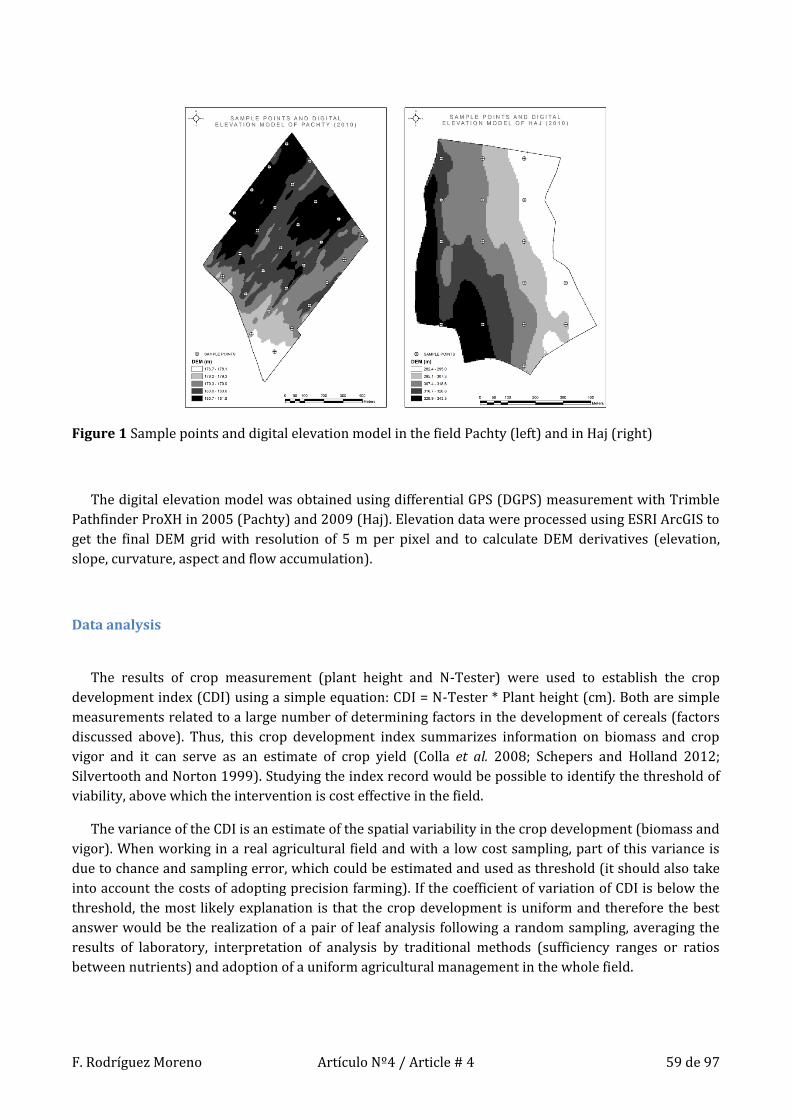
F. Rodríguez Moreno Artículo Nº4 / Article # 4 59 de 97
Figure 1 Sample points and digital elevation model in the field Pachty (left) and in Haj (right)
The digital elevation model was obtained using differential GPS (DGPS) measurement with Trimble
Pathfinder ProXH in 2005 (Pachty) and 2009 (Haj). Elevation data were processed using ESRI ArcGIS to
get the final DEM grid with resolution of 5 m per pixel and to calculate DEM derivatives (elevation,
slope, curvature, aspect and flow accumulation).
Data analysis
The results of crop measurement (plant height and N-Tester) were used to establish the crop
development index (CDI) using a simple equation: CDI = N-Tester * Plant height (cm). Both are simple
measurements related to a large number of determining factors in the development of cereals (factors
discussed above). Thus, this crop development index summarizes information on biomass and crop
vigor and it can serve as an estimate of crop yield (Colla et al. 2008; Schepers and Holland 2012;
Silvertooth and Norton 1999). Studying the index record would be possible to identify the threshold of
viability, above which the intervention is cost effective in the field.
The variance of the CDI is an estimate of the spatial variability in the crop development (biomass and
vigor). When working in a real agricultural field and with a low cost sampling, part of this variance is
due to chance and sampling error, which could be estimated and used as threshold (it should also take
into account the costs of adopting precision farming). If the coefficient of variation of CDI is below the
threshold, the most likely explanation is that the crop development is uniform and therefore the best
answer would be the realization of a pair of leaf analysis following a random sampling, averaging the
results of laboratory, interpretation of analysis by traditional methods (sufficiency ranges or ratios
between nutrients) and adoption of a uniform agricultural management in the whole field.

F. Rodríguez Moreno Artículo Nº4 / Article # 4 60 de 97
In case of rejecting the hypothesis of uniform crop development, it should be studied the
relationship between CDI and spatial factors (SF). The SF (surface functions and topographic variables)
represent the gradients in meteorology / climatology, soil and topography, which should be the natural
cause of the spatial variability of CDI in the two fields (indications for other scenarios provided above).
If the CDI was not related to the SF, the hypothesis of spatial relationship between samples would
have to be rejected and therefore it would be necessary to use the advanced techniques to delineate
site-specific management units (Aimrun et al. 2011; Buttafuoco et al. 2010; Corwin and Lesch 2010;
Guastaferro et al. 2010; Ortega and Santibáñez 2007; X. Zhang et al. 2010). This means using of the
methods of precision agriculture such as the remote sensing, crop maps, electrical conductivity of soil,
etc.
If the crop development was deficient and/or uniform or if there was not spatial relationship
between samples, in any of the cases, the profitability of sampling and leaf analysis would be negative.
This new methodology incorporates the above steps because they represent only a small additional
effort and provide valuable information that helps to deduce the correct diagnosis. The improvements
do not end here; reached the point where is evident the need for foliar analysis, the study of the CDI
map helps determine the number and location of samples (the CDI map for the entire field is obtained
using the model with the SF).
The fourth stage is the study of the correlation between the CDI and the concentration of each
nutrient. This is studied independently by calculating the corresponding p-value and coefficient of
determination (R2). Cross-validation was used for better assessment of the significance and magnitude
of the relationships, the goal is to identify relations with predictive capacity (Antoniadou and Wallach
2000; Guisan and Zimmermann 2000; Muñoz and Felicísimo 2004; Steyerberg et al. 2001). The result of
cross-validation is sensitive to the grouping because of the small number of samples (27 samples in
Pachty, 18 in Haj), therefore 20 different random groupings were defined and the cross-validation was
repeated for each of them (Cheng et al. 2010; Das et al. 2008; K. Yang et al. 2011). The result was the
average of all evaluations. All calculations and statistical analyses were conducted using the software
Matlab 2009b.
Exploring the regression model relating the CDI and a given nutrient can discover three important
characteristics:
It is possible to determine whether the nutrient is excessive (negative relationship with the CDI)
or deficient (positive relationship).
Comparing the coefficient of determination obtained by the different nutrients, it is possible to
establish the order of importance, from the most important (which is responsible for the greatest
variance in the CDI) to the least important.
Knowing the cost of each fertilizer and studying the type of response between nutrient and CDI
(linear, cubic, exponential ...), it is possible to determine whether that nutrient would get the
largest increase in crop yield at lower cost.
If two or more nutrients are identified as limiting (significantly related to CDI), there is the
possibility that their effects are related because the problem of one of them induces the problem in the
other. In that case, the set of interrelated nutrients would present a high correlation and therefore it
could be detected by evaluating the significance (p-value) and strength (R2) of the relationship between
nutrients by cross-validation, the same process as described above. If two or more nutrients are linked
by a relationship of cause and effect, one would have to identify which of those nutrients explains more

F. Rodríguez Moreno Artículo Nº4 / Article # 4 61 de 97
Crop development(biomass and vigor)
Nutrient concentration
Imagine twenty-four samples with two errors (below), one due to an unrepresentative sample and the other to a laboratory error, both lead to overestimate the concentration of the nutrient.
There is a significant relationship with a high coefficient of determination (left). How could one know that this result is skewed by outliers?
Statistical procedures, such as Cook's distance, would warn of two points with great weight in the regression. Working with small dataset that will happen often and not always indicate outliers but insufficient sampling
Spatial analysis can solve the problem. In the example, the set of points would adjust well to a plane (below), this is because 92% of the data is correct and practically constant. If attention is directed to the suspect data one would see that they have larger errors than the rest and that if the relationship was reevaluated by cross validation the coefficient of determination would fall significantly.
The lack of spatial coherence is the argument for rejecting the relationship between crop growth and nutrient.
Diagnosis of outliers using spatial analysis
Crop development(biomass and vigor)
Nutrient concentration
Errors
ErrorsCrop development gradually increases from left to right and
the nutrient concentration is constant in the field (error free)
variance of the CDI and consult agronomic text to confirm that a problem with that nutrient may induce
problems with the other nutrients involved.
In the fifth stage, the models that relate the concentrations of nutrients (those identified as limiting)
with spatial factors have to be developed (as with the CDI). In both fields, there has been a uniform
agricultural management and no health problem has been reported. In this scenario, if the crop
development is not uniform (CDI is not close to constant), both the CDI as those nutrients responsible
for its variability (limiting factors) have to be modeled as a function of spatial factors. If this
requirement is not fulfilled, the diagnosis had to be rejected. The number of data involved is small and
therefore sensitivity to outliers is very high.
Errors in sampling or analysis may alter the regression model between the nutrient and the SF,
occasionally improving the goodness of fit and thus giving rise to a false identification as limiting. The
same errors that very likely deteriorate the spatial structure of the data, which is why this fifth step
serves as a check and has a capital importance. This procedure is inspired by the work of authors who
have verified the spatial structure of the results obtained in different locations to evaluate the method
used in the analysis (Basso et al. 2001; Grohs et al. 2009; G. Jones et al. 2010a, 2010b, 2010c). An
illustrative figure of this diagnosis of outliers using spatial analysis is shown in Figure 2 and a flowchart
summarizing the above is shown in Figure 3.
Figure 2 Explanation of how spatial analysis can help in identifying outliers
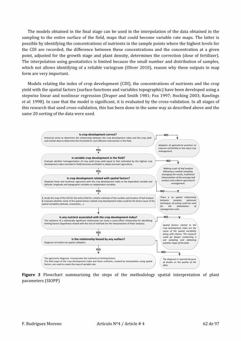
F. Rodríguez Moreno Artículo Nº4 / Article # 4 62 de 97
Is crop development correct?Historical series to determine the relationship between the crop development index and the crop yield and market data to determine the threshold for cost-effective intervention in the field.
Adoption of agricultural practices to improve soil fertility or low input crop management.
Is variable crop development in the field?Evaluate whether homogenization of crop yield (crop yield equal to that estimated by the highest crop development index recorded in field) becomes profitable to adopt precision agriculture.
Making a pair of leaf analysis following a random sampling,
averaging the results, traditional interpretation of the average leaf analysis and uniform agricultural
management.
Is crop development related with spatial factors?Stepwise linear and nonlinear regression with the crop development index as the dependent variable and latitude, longitude and topographic variables as independent variables.
NO
NO
YES
YES
Is any nutrient associated with the crop development index?The existence of a statistically significant relationship can mean a cause-effect relationship for identifying limiting factors (hypothesis shared with the rest of methods for the interpretation of foliar analysis).
There is no spatial relationship between samples, advanced techniques of zoning could be used for the delimitation of management units.
1. Study the map of the CDI for the entire field for a better estimate of the number and location of leaf analysis.2. Evaluate whether some of the spatial factors related crop development index could be the direct cause of the spatial variability (altitude, orientation,...).
YES NO
Spatial factors related to the crop development index are the cause of the spatial variability along with chance. The research could go deeper conducting a soil sampling and obtaining weather maps of the field.
Is the relationship biased by any outliers?Diagnosis of outliers by spatial validation.
The diagnosis is rejected because of doubts on the quality of the data.
The agronomic diagnosis incorporates the nutrients as limiting factors.The field maps of the crop development index and these nutrients, created by interpolation using spatial factors, are used to create the map of variable rate.
YES
YES
NO
NO
The models obtained in the final stage can be used in the interpolation of the data obtained in the
sampling to the entire surface of the field, maps that could become variable rate maps. The latter is
possible by identifying the concentrations of nutrients in the sample points where the highest levels for
the CDI are recorded, the difference between these concentrations and the concentration at a given
point, adjusted for the growth stage and plant density, determines the correction (dose of fertilizer).
The interpolation using geostatistics is limited because the small number and distribution of samples,
which not allows identifying of a reliable variogram (Oliver 2010), reason why these outputs in map
form are very important.
Models relating the index of crop development (CDI), the concentrations of nutrients and the crop
yield with the spatial factors (surface functions and variables topographic) have been developed using a
stepwise linear and nonlinear regression (Draper and Smith 1981; Fox 1997; Hocking 2003; Rawlings
et al. 1998). In case that the model is significant, it is evaluated by the cross-validation. In all stages of
this research that used cross-validation, this has been done in the same way as described above and the
same 20 sorting of the data were used.
Figure 3 Flowchart summarizing the steps of the methodology spatial interpretation of plant
parameters (SIOPP)
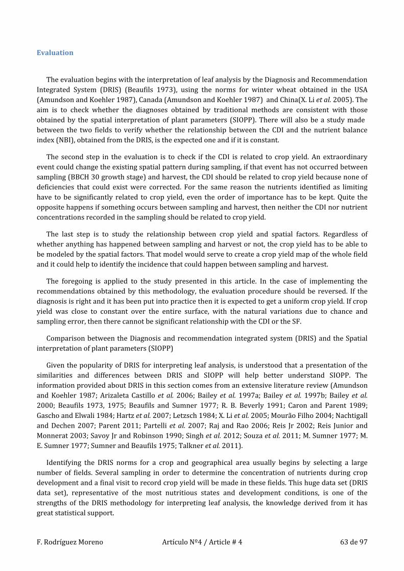
F. Rodríguez Moreno Artículo Nº4 / Article # 4 63 de 97
Evaluation
The evaluation begins with the interpretation of leaf analysis by the Diagnosis and Recommendation
Integrated System (DRIS) (Beaufils 1973), using the norms for winter wheat obtained in the USA
(Amundson and Koehler 1987), Canada (Amundson and Koehler 1987) and China(X. Li et al. 2005). The
aim is to check whether the diagnoses obtained by traditional methods are consistent with those
obtained by the spatial interpretation of plant parameters (SIOPP). There will also be a study made
between the two fields to verify whether the relationship between the CDI and the nutrient balance
index (NBI), obtained from the DRIS, is the expected one and if it is constant.
The second step in the evaluation is to check if the CDI is related to crop yield. An extraordinary
event could change the existing spatial pattern during sampling, if that event has not occurred between
sampling (BBCH 30 growth stage) and harvest, the CDI should be related to crop yield because none of
deficiencies that could exist were corrected. For the same reason the nutrients identified as limiting
have to be significantly related to crop yield, even the order of importance has to be kept. Quite the
opposite happens if something occurs between sampling and harvest, then neither the CDI nor nutrient
concentrations recorded in the sampling should be related to crop yield.
The last step is to study the relationship between crop yield and spatial factors. Regardless of
whether anything has happened between sampling and harvest or not, the crop yield has to be able to
be modeled by the spatial factors. That model would serve to create a crop yield map of the whole field
and it could help to identify the incidence that could happen between sampling and harvest.
The foregoing is applied to the study presented in this article. In the case of implementing the
recommendations obtained by this methodology, the evaluation procedure should be reversed. If the
diagnosis is right and it has been put into practice then it is expected to get a uniform crop yield. If crop
yield was close to constant over the entire surface, with the natural variations due to chance and
sampling error, then there cannot be significant relationship with the CDI or the SF.
Comparison between the Diagnosis and recommendation integrated system (DRIS) and the Spatial
interpretation of plant parameters (SIOPP)
Given the popularity of DRIS for interpreting leaf analysis, is understood that a presentation of the
similarities and differences between DRIS and SIOPP will help better understand SIOPP. The
information provided about DRIS in this section comes from an extensive literature review (Amundson
and Koehler 1987; Arizaleta Castillo et al. 2006; Bailey et al. 1997a; Bailey et al. 1997b; Bailey et al.
2000; Beaufils 1973, 1975; Beaufils and Sumner 1977; R. B. Beverly 1991; Caron and Parent 1989;
Gascho and Elwali 1984; Hartz et al. 2007; Letzsch 1984; X. Li et al. 2005; Mourão Filho 2004; Nachtigall
and Dechen 2007; Parent 2011; Partelli et al. 2007; Raj and Rao 2006; Reis Jr 2002; Reis Junior and
Monnerat 2003; Savoy Jr and Robinson 1990; Singh et al. 2012; Souza et al. 2011; M. Sumner 1977; M.
E. Sumner 1977; Sumner and Beaufils 1975; Talkner et al. 2011).
Identifying the DRIS norms for a crop and geographical area usually begins by selecting a large
number of fields. Several sampling in order to determine the concentration of nutrients during crop
development and a final visit to record crop yield will be made in these fields. This huge data set (DRIS
data set), representative of the most nutritious states and development conditions, is one of the
strengths of the DRIS methodology for interpreting leaf analysis, the knowledge derived from it has
great statistical support.

F. Rodríguez Moreno Artículo Nº4 / Article # 4 64 de 97
In the case of the spatial interpretation of plant parameters (SIOPP) is not necessary a study to
identify the set of norms of interpretation, it only needs a small data set collected in the field that has to
be diagnosed (the methodology is available to any crop as long as its CDI has been identified, which has
been proved simple and is independent of the geographical area). The purpose is the agronomic
diagnosis of that field; the recommendations will not be generalized to other field, so that the greater or
lesser variance that is captured in this field is all that is needed. It will be analyzed to try to determine
the factor or factors responsible for the spatial variability in the crop development (biomass and crop
vigor).
DRIS dataset is processed through a combination of brute force (calculation of all possible ratios
between the concentrations of nutrients, sometimes restricted to those pairs whose evolution during
crop development follow the same trend) and statistics (each of these ratios between nutrients is
evaluated using statistical tests to check for statistical significance that supports the use of this ratio to
distinguish the crops with high and low yield).
That analysis method is not suitable for processing the data set obtained in a field because of the
lower volume of data and variance. Since samples are not independent because they would come from
the same field (it is unlikely that agronomic parameters vary randomly at small scale in a field), is
possible to use regression models (linear and nonlinear), tests of statistical significance (ANOVA) and
cross validation to identify the factor or factors responsible for the gradient in the crop development
(biomass and crop vigor) registered in the field.
There is a common point of great importance between the two methodologies. The statistical
methods used are different but the result is the same, identifying a statistically significant relationship
between a factor (nutrient or other) and the crop development / yield. Both methods rely on that
statistical relationship corresponds to a cause - effect relationship and therefore the crop yield can
increase if one acts on the factor.
SIOPP uses an index of crop development (biomass and vigor) as reference instead of crop yield. This
is the result of a necessity since SIOPP does not use information from a previous study and it has to
provide a diagnosis at the time of sampling, when the crop yield is not available. The advantages of
using an index of crop development are as follows:
The agronomic diagnoses will not be influenced by events that might occur between sampling and
harvest.
Before spending resources on leaf sampling, it is possible to obtain a diagnosis which determines:
If the expected crop yield makes cost effective the intervention in the field.
If the crop is uniformly developed and therefore the best answer would be to adopt a uniform
agricultural management.
If there is spatial relationship between the samples, because otherwise advanced techniques of
zoning for the delimitation of management units would be need.
The CDI map for the field helps estimate the number and location of leaf samples, avoiding
wasting resources.
Another difference between DRIS and SIOPP is the use of spatial factors (SF), it would be possible to
study its incorporation into the DRIS but where the SF are essential and they give maximum benefit is
in SIOPP. Thanks to them, five following objectives can be achieved:

F. Rodríguez Moreno Artículo Nº4 / Article # 4 65 de 97
Study of spatial patterns.
Diagnosis of outliers.
Data interpolation.
Help in identifying non-nutrient limiting factors.
Support for the study of events that break the relationship between the crop development index
and crop yield.
Results and discussion
Field Pachty
The coefficient of variation of the different nutrients ranges from 10 to 20% (Table 1), reason for
determining the crop does not have a uniform development. This judgment is reinforced by knowing
the coefficients of variation of N-Tester and crop height and it is confirmed by observing the variance in
crop yield.
Table 1 Statistical summary of the plant parameters for the field Pachty
Pachty N (%) P (%) K (%) Mg (%) Ca (%) S (%) N-Tester Height (cm) CDI Yield (t.ha-1)
Mean 3.654 0.349 3.347 0.106 0.276 0.202 441.00 28.822 12795 7.963
St.dev. 0.382 0.055 0.350 0.020 0.052 0.021 52.637 3.900 2702 1.562
Kurtosis 1.287 -0.934 0.307 0.062 -0.685 0.687 -0.658 -0.300 -0.677 -0.611
Skewness 0.957 0.340 0.514 0.798 0.128 0.203 -0.268 0.420 0.048 0.544
Minimum 3.12 0.27 2.78 0.08 0.20 0.16 336.00 21.30 7796 5.60
Maximum 4.75 0.45 4.24 0.15 0.38 0.26 517.00 37.00 17786 11.06
CV (%) 10.45 15.70 10.46 19.10 18.84 10.36 11.94 13.53 21.12 19.62
n= 27 27 27 27 27 27 27 27 27 27
The convenience of using CDI in place of the reading of N-Tester or plant height was supported by
the literature and it is confirmed by checking that the variance of the product is far superior to the
individual variances, the CDI collects more information on crop.
The crop development is satisfactory because the readings of the N-Tester and the crop height are
within the normal range for that growth stage determined by the historical data of the crop. The second
requirement for the implementation of the methodology is that crop growth is not uniform, also
satisfied given the coefficient of variation of CDI, about 21%. The third requirement is the existence of a
significant relationship between the CDI and SF, which would confirm the spatial structure of the CDI
and the causal role of SF. The coefficient of determination obtained proves the hypothesis, the
requirement are meets.
The regression model between CDI and SF shows complicated interactions between surface
functions and topographic variables, which results in a complex spatial pattern shown in Figure 4 (left).
This map suggests increasing the number of samples in the field compared to that used in the

F. Rodríguez Moreno Artículo Nº4 / Article # 4 66 de 97
characterization of CDI and it provides indications of where they should be taken. In this experiment
the number and location (regular grid) were kept. The result of this decision can be seen in the Table 2,
the quality of the maps obtained for the nutrients and the crop yield are low, the suggestion was
appropriate.
All requirements are met so it is possible to carry out a spatial interpretation of plant parameters
(SIOPP), the results of the next step, the study of the relationship between CDI and nutrients, together
with other studies, are shown in Table 2.
Table 2 Coefficients of determination among plant analysis results, CDI index, yield and spatial factors
for the field Pachty obtained by cross-validation
Pachty N (%) P (%) K (%) Mg (%) Ca (%) S (%) CDI Yield (t.ha-1)
Yield 0.307** 0.033 0.552** 0.277** 0.428** 0.320** 0.515** 1
CDI 0.159* 0.132 0.490** 0.123 0.311** 0.126 1 0.515**
Spatial factors 0.270* 0.485** 0.170* 0.274** 0.309** 0.376** 0.563** 0.168
The subscript numbers correspond to the coefficients of determination in the regression; they were not significant
and therefore not proceeded to the cross-validation.
The concentrations of potassium, calcium and nitrogen are positively related to the crop
development index; these are the nutrients that could be acting as limiting (Table 2). The correlations
between them are shown in Table 3. All of them are significant but none reached a high value, the
expected value for two nutrients linked by a relationship of the type inductor-induced. In winter wheat
this relationship exists between nitrogen and sulfur (Järvan et al. 2012; Rasmussen 1996; Rasmussen
and Douglas Jr 1992), having found between these nutrients a significant relationship with a coefficient
of determination of 0.64.
Table 3 Coefficients of determination among nutrients significantly related to CDI obtained by cross-
validation
leaf_N leaf_K 0.24*
leaf_N leaf_Ca 0.28**
leaf_K leaf_Ca 0.22*
The K, Ca and N, in that order by percentage of variance explained of the CDI, are confirmed as
limiting factors after checking that their concentrations are significantly related to spatial factors (Table
2). The results obtained indicate that the priority action to improve crop develop would be a variable-
rate fertilizer application to correct the most likely limiting factor, potassium deficiency. It would also
recommend correcting the deficiencies of calcium and nitrogen. Each nutrient has its own variable-rate
application map derived from the interpolation to the entire surface of the CDI and the nutrient, using
for this purpose the spatial factors. The concentration of the nutrient in the reference points, those in
which the CDI reaches the highest values, is the level that the nutrient has to reach across the field, the

F. Rodríguez Moreno Artículo Nº4 / Article # 4 67 de 97
difference is calculated and corrected by phenological stage and crop density, the result is the fertilizer
dose to be applied.
It is important to differentiate between the diagnosis and corrective treatment. With the same
diagnosis the treatment varies depending on whether it wants to improve crop yield in the campaign or
to find an efficient system. The results obtained by comparing the crop development index with
nutrients (the identification of calcium as limiting) and the study of the maps of distribution of
nutrients (Figure 4) warn about a problem with soil pH, so a correct treatment for potassium and
nitrogen will force the plant development through the use of fertilizers (which will require the use of
larger amounts of input each year). The alternative is to direct efforts to reach an efficient and
sustainable soil (L-Baeckström et al. 2006; Miao et al. 2011; Míša and Křen 2001; Wienhold and
Halvorson 1998).
Usually it chooses the first alternative, which explains why foliar analysis is a tool used in special
cases where the crop yield in a given field has fallen to a point that investment in inputs is not
profitable. In the diagnosis of this problem is where the methodologies for the interpretation of leaf
analysis play a decisive role. Having an alternative to the sufficiency ranges and relationships between
nutrients (DRIS and similar), which incorporates new techniques developed in recent decades (GPS, GIS
...), will increase the chances of success.
The nutritional balance index (NBI) with China norms reaches a 22.95, with USA and Canada norms
the value stands at about 52 (Table 4). There is agreement between the DRIS diagnoses and the CDI to
identify the existence of a severe nutritional imbalance in the development of the crop. Then the DRIS
index for each nutrient will be studied to identify those responsible for the nutritional imbalance.
Table 4 Statistical summary of nutritional balance index (NBI), DRIS norms from USA, Canada and
China for the Pachty field
Pachty NBI (USA) NBI (Canada) NBI (China)
Mean 51.837 51.928 22.949
St.dev. 9.196 13.140 13.315
Kurtosis -0.701 -0.058 -0.476
Skewness 0.461 0.728 0.672
Minimum 36.94 32.22 4.83
Maximum 71.67 84.05 52.82
CV (%) 17.74 25.30 58.02
n= 27 27 27
Each set of DRIS norms points to a different nutrient as limiting (Table 5). This lack of consensus
highlights the need to obtain a set of DRIS norms specific for this scenario and prevent from identifying
an incompatibility between DRIS and spatial interpretation of plant parameters (SIOPP).
Phosphorus is identified as limiting, with different severity, for the three sets of DRIS norms. That
nutrient limitation was not identified as limiting by the methodology of spatial interpretation of plant
parameters. Figure 4 (left) shows the crop reaches maximum levels of development in areas where the

F. Rodríguez Moreno Artículo Nº4 / Article # 4 68 de 97
concentration of P has minimum values. Given this evidence with statistical significance obtained in the
data set of interest and the fact that crop yield is not significantly related to P (Table 2), the more
plausible explanation is that the identification of P as a limiting factor is an error of the sets of DRIS
norms used.
The rest of the DRIS diagnostic coincides with what is deduced by analyzing spatial. Potassium and
nitrogen are limiting factors and the sulfur is not a problem in the two sets of DRIS norms, USA and
Canada, where it is included in the calculations.
Table 5 Summary statistics of DRIS indices for nutrients with the norm from USA, Canada and China for
Pachty
DRIS norms from USA CANADA CHINA
DRIS indices for N K P S N K P S N K P
Mean 13,848 9,072 8,729 20,189 5,419 15,765 8,294 22,341 10,319 3,987 8,642
St.dev. 3,325 3,648 2,450 3,583 4,191 6,434 3,887 5,609 5,230 2,396 5,981
Kurtosis -1,449 -0,426 -1,446 -0,252 -1,515 -0,494 -1,354 -0,317 0,325 -0,060 -1,171
Skewness 0,148 0,696 0,372 -0,011 0,054 0,625 0,219 -0,332 0,854 0,663 0,432
Minimum 8,726 3,344 5,402 13,290 -1,245 5,139 1,984 10,312 1,940 -0,004 1,155
Maximum 19,661 17,622 12,511 27,350 11,661 30,606 14,885 31,551 23,395 9,658 19,766
CV (%) 24,014 40,208 28,074 17,749 77,334 40,809 46,862 25,104 50,678 60,104 69,202
n= 27 27 27 27 27 27 27 27 27 27 27
Percentage of cases
Position after
ascending sort
USA CANADA CHINA
N K P S N K P S N K P
1º 0.00 7.41 81.48 11.11 100.00 0.00 0.00 0.00 0.00 29.63 70.37
2º 55.56 37.04 7.41 0.00 0.00 0.00 70.37 29.63 88.89 11.11 0.00
3º 44.44 55.56 0.00 0.00 0.00 92.59 7.41 0.00 11.11 59.26 29.63
4º 0.00 0.00 11.11 88.89 0.00 7.41 22.22 70.37
Differential treatment was not applied so only if there had been some incidence from sampling to
harvest, it could happen that crop development index was not related to crop yield. The coefficient of
determination between development index and crop yield reached 0.51 (significant result evaluated by
cross-validation), the hypothesis regarding the incidence was rejected and therefore the concentrations
at BBCH 30 growth stage of the nutrients identified as limiting factors also have to be significantly
related to crop yield and keep the order of importance (order by percentage of variance explained of
the CDI). The coefficient of determination between the crop yield and potassium is 0.55, with calcium
had 0.43 and with nitrogen 0.31 (Table 2).
In the field Pachty has been possible to deduce a successful agronomic diagnosis without the need of
any prior study and without relying on the ability to generalize of a set of norms of interpretation
obtained in another geographic area and / or with another crop.

F. Rodríguez Moreno Artículo Nº4 / Article # 4 69 de 97
Figure 4 Interpolations based on spatial factors of the CDI (left) and of the concentration of P (right) in
Pachty
Field Haj
The coefficient of variation for the different nutrients ranged between 3 and 8%, in that order of
magnitude is unlikely that the crop was developing very heterogeneous (Table 6). This hypothesis is
strengthened by knowing the coefficient of variation of the reading of N-Tester and the height of the
crop, about half that recorded in Pachty, and it is confirmed by knowing the crop yield. The coefficient
of variation of crop yield is situated 3 percentage points above the CDI; this is not an important
variation but it reaches a magnitude more difficult to explain by random that the variability of CDI.
The convenience of using CDI in place of the reading of N-Tester or the height of the plant is again
supported by checking that the variance of the product is higher than the variances of the factors, the
CDI provides more information on the crop (Table 6).
Both the N-Tester readings and crop heights are within normal for that growth stage determined by
the historical data. The crop development is satisfactory but the second requirement of the
methodology, a heterogeneous development of the crop, only partially meets. The coefficient of
variation of the CDI is about 10%, it is a low value in trials of this nature and it could be caused by noise
or random. The doubt is solved by knowing that there is a significant relationship between the CDI and
SF reaching a determination coefficient of 0.53. This means that there is spatial relationship between
the samples and only 47% of the small variance cannot be explained by the SF, percentage of variance
that can be caused by noise or random.

F. Rodríguez Moreno Artículo Nº4 / Article # 4 70 de 97
Table 6 Summary statistics of the plant parameters for field Haj
Haj N (%) P (%) K (%) Mg (%) Ca (%) S (%) N-Tester Height (cm) CDI Yield (t.ha-1)
Mean 5.000 0.492 3.641 0.112 0.488 0.328 584.78 29.428 17214 9.827
St.dev. 0.155 0.034 0.208 0.005 0.033 0.029 29.389 2.242 1632 1.232
Kurtosis 0.188 0.086 0.281 -0.436 -0.694 3.653 0.180 1.445 0.417 -0.094
Skewness -0.688 -0.656 -0.454 -0.655 0.063 1.163 0.628 -0.001 0.176 0.764
Minimum 4.68 0.42 3.16 0.10 0.43 0.28 537.00 24.40 13786 7.97
Maximum 5.24 0.54 3.95 0.12 0.55 0.41 646.00 34.50 20528 12.32
CV (%) 3.09 6.94 5.71 4.73 6.84 8.86 5.03 7.62 9.48 12.54
n= 18 18 18 18 18 18 18 18 18 18
The relationship between the CDI and SF is supported mainly by a simple surface function, a
decreasing gradient from southeast to northwest (Figure 5 left). In the next stage it will examine
whether that gradient corresponds to some nutrient, but first is the sampling for leaf analysis. As in the
field Pachty, the sampling for determination of CDI and foliar sampling is coincident, but unlike what
happened in the field Pachty, in the field Haj the spatial pattern is simple (Figure 5 left) so the number
and location of samples (regular grid) is correct and therefore the interpolations will have higher
quality (the sampling could have been even smaller).
The requirements are fulfilled and therefore the results of the next stage of the methodology, the
study of the relationship between CDI and nutrients, together with other studies, are presented in Table
7.
Table 7 Coefficients of determination among plant analysis results, CDI index, yield and spatial factors
for field Pachty obtained by cross-validation
Haj N (%) P (%) K (%) Mg (%) Ca (%) S (%) CDI Yield (t.ha-1)
Yield 0.008 0.006 0.002 0.002 0.000 0.116 0.092 1
CDI 0.000 0.068 0.099 0.156 0.088 0.020 1 0.092
Spatial factors 0.455** 0.179 0.352* 0.246 0.288* 0.538** 0.527** 0.758**
The subscript numbers correspond to the coefficients of determination in the regression; they were not significant
and therefore not proceeded to the cross-validation.
None of the nutrient is significantly related to CDI and therefore there are no cross-correlations to
study. There is not a large spatial variability of nutrients and therefore this result is not surprising, the
question is whether the small spatial variability captured by the CDI is due to a gradient in soil
properties, a gradient in moisture, etc. With the information available is not possible to identify the
cause, the research could go deeper conducting a soil sampling and obtaining weather maps of the field.
This information is not necessary for the purpose of this study, the facts are conclusive. None nutrient is
identified as the cause of the low variability in the CDI and the crop is developing well and almost
homogeneous. It is not possible to adjust the fertilizer plan in order to homogenize the crop yield.
Under these circumstances the recommendation is to apply a generous and uniform fertilization.
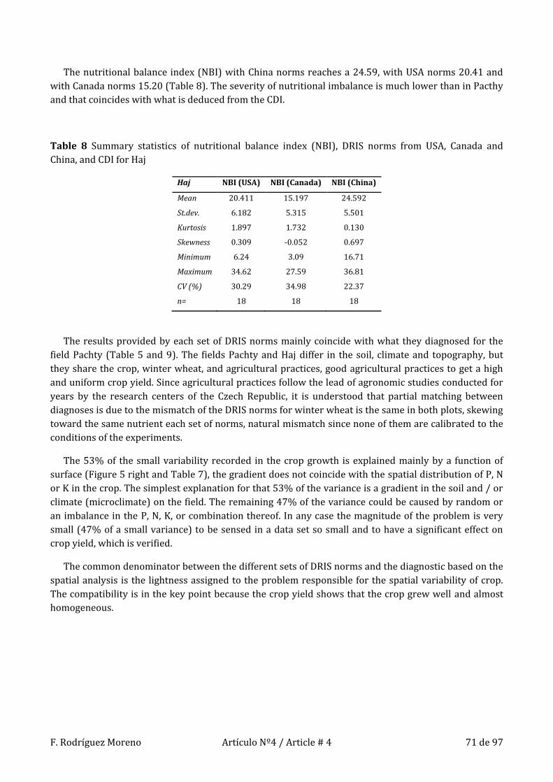
F. Rodríguez Moreno Artículo Nº4 / Article # 4 71 de 97
The nutritional balance index (NBI) with China norms reaches a 24.59, with USA norms 20.41 and
with Canada norms 15.20 (Table 8). The severity of nutritional imbalance is much lower than in Pacthy
and that coincides with what is deduced from the CDI.
Table 8 Summary statistics of nutritional balance index (NBI), DRIS norms from USA, Canada and
China, and CDI for Haj
Haj NBI (USA) NBI (Canada) NBI (China)
Mean 20.411 15.197 24.592
St.dev. 6.182 5.315 5.501
Kurtosis 1.897 1.732 0.130
Skewness 0.309 -0.052 0.697
Minimum 6.24 3.09 16.71
Maximum 34.62 27.59 36.81
CV (%) 30.29 34.98 22.37
n= 18 18 18
The results provided by each set of DRIS norms mainly coincide with what they diagnosed for the
field Pachty (Table 5 and 9). The fields Pachty and Haj differ in the soil, climate and topography, but
they share the crop, winter wheat, and agricultural practices, good agricultural practices to get a high
and uniform crop yield. Since agricultural practices follow the lead of agronomic studies conducted for
years by the research centers of the Czech Republic, it is understood that partial matching between
diagnoses is due to the mismatch of the DRIS norms for winter wheat is the same in both plots, skewing
toward the same nutrient each set of norms, natural mismatch since none of them are calibrated to the
conditions of the experiments.
The 53% of the small variability recorded in the crop growth is explained mainly by a function of
surface (Figure 5 right and Table 7), the gradient does not coincide with the spatial distribution of P, N
or K in the crop. The simplest explanation for that 53% of the variance is a gradient in the soil and / or
climate (microclimate) on the field. The remaining 47% of the variance could be caused by random or
an imbalance in the P, N, K, or combination thereof. In any case the magnitude of the problem is very
small (47% of a small variance) to be sensed in a data set so small and to have a significant effect on
crop yield, which is verified.
The common denominator between the different sets of DRIS norms and the diagnostic based on the
spatial analysis is the lightness assigned to the problem responsible for the spatial variability of crop.
The compatibility is in the key point because the crop yield shows that the crop grew well and almost
homogeneous.
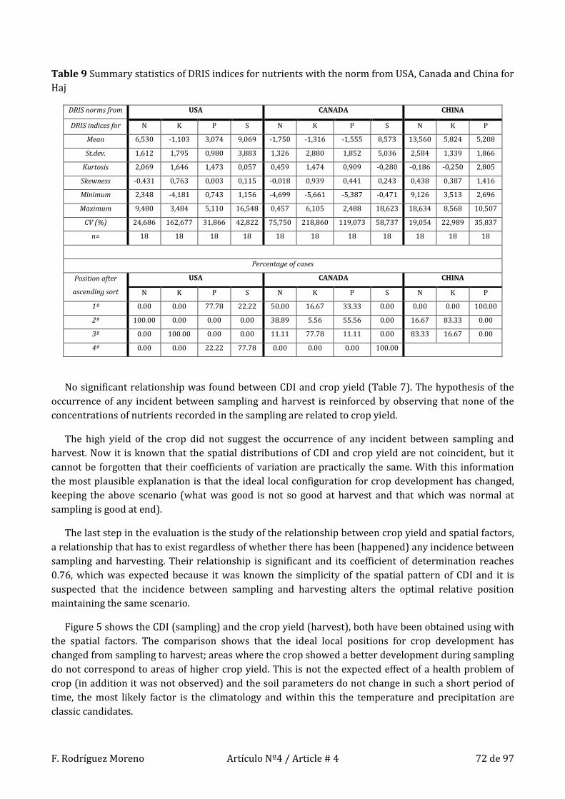
F. Rodríguez Moreno Artículo Nº4 / Article # 4 72 de 97
Table 9 Summary statistics of DRIS indices for nutrients with the norm from USA, Canada and China for
Haj
DRIS norms from USA CANADA CHINA
DRIS indices for N K P S N K P S N K P
Mean 6,530 -1,103 3,074 9,069 -1,750 -1,316 -1,555 8,573 13,560 5,824 5,208
St.dev. 1,612 1,795 0,980 3,883 1,326 2,880 1,852 5,036 2,584 1,339 1,866
Kurtosis 2,069 1,646 1,473 0,057 0,459 1,474 0,909 -0,280 -0,186 -0,250 2,805
Skewness -0,431 0,763 0,003 0,115 -0,018 0,939 0,441 0,243 0,438 0,387 1,416
Minimum 2,348 -4,181 0,743 1,156 -4,699 -5,661 -5,387 -0,471 9,126 3,513 2,696
Maximum 9,480 3,484 5,110 16,548 0,457 6,105 2,488 18,623 18,634 8,568 10,507
CV (%) 24,686 162,677 31,866 42,822 75,750 218,860 119,073 58,737 19,054 22,989 35,837
n= 18 18 18 18 18 18 18 18 18 18 18
Percentage of cases
Position after
ascending sort
USA CANADA CHINA
N K P S N K P S N K P
1º 0.00 0.00 77.78 22.22 50.00 16.67 33.33 0.00 0.00 0.00 100.00
2º 100.00 0.00 0.00 0.00 38.89 5.56 55.56 0.00 16.67 83.33 0.00
3º 0.00 100.00 0.00 0.00 11.11 77.78 11.11 0.00 83.33 16.67 0.00
4º 0.00 0.00 22.22 77.78 0.00 0.00 0.00 100.00
No significant relationship was found between CDI and crop yield (Table 7). The hypothesis of the
occurrence of any incident between sampling and harvest is reinforced by observing that none of the
concentrations of nutrients recorded in the sampling are related to crop yield.
The high yield of the crop did not suggest the occurrence of any incident between sampling and
harvest. Now it is known that the spatial distributions of CDI and crop yield are not coincident, but it
cannot be forgotten that their coefficients of variation are practically the same. With this information
the most plausible explanation is that the ideal local configuration for crop development has changed,
keeping the above scenario (what was good is not so good at harvest and that which was normal at
sampling is good at end).
The last step in the evaluation is the study of the relationship between crop yield and spatial factors,
a relationship that has to exist regardless of whether there has been (happened) any incidence between
sampling and harvesting. Their relationship is significant and its coefficient of determination reaches
0.76, which was expected because it was known the simplicity of the spatial pattern of CDI and it is
suspected that the incidence between sampling and harvesting alters the optimal relative position
maintaining the same scenario.
Figure 5 shows the CDI (sampling) and the crop yield (harvest), both have been obtained using with
the spatial factors. The comparison shows that the ideal local positions for crop development has
changed from sampling to harvest; areas where the crop showed a better development during sampling
do not correspond to areas of higher crop yield. This is not the expected effect of a health problem of
crop (in addition it was not observed) and the soil parameters do not change in such a short period of
time, the most likely factor is the climatology and within this the temperature and precipitation are
classic candidates.

F. Rodríguez Moreno Artículo Nº4 / Article # 4 73 de 97
Figure 5 Interpolations based on spatial factors of the CDI (left) and the crop yield (right) in Haj
A period with an abnormal temperature could affect to the crop yield, even it could negate the
relationship between CDI and crop yield, but it is not expected that it can change the ideal relative
positions for the crop development. The other candidate is the precipitation. Up to sampling the crops
was better developed in low areas, an intense precipitation in conjunction with a specific edaphology
could change the ideal relative positions for crop development, making the upper and middle zones
more suitable than the low, wherein the amount of water may be excessive.
From May to July the precipitation in 2010 was 228 liters per square meter higher than the average
precipitation for that period, data obtained from the meteorological stations of the university and the
meteorological service of the Czech Republic. This is an objective evidence to accept that in 2010 an
incident happened between sampling and harvest, explaining the lack of relationship between the CDI
and crop yield. Given this conclusion, a leveling of the land or improvement in the drainage would be
advisable. It would homogenize crop yield and would decrease the effects of heavy precipitation. This
finding proves that the verification phase of diagnosis can also provide valuable advice to farmers. This
is another improvement that SIOPP incorporates, which helps to carry out integral agronomic
diagnosis.
The spatial interpretation of plant parameters begins by identifying the variability in the crop
development, then examines whether there is any robust statistical evidence that points to any of the
factors as the cause of that variability in the field. The success of the diagnosis can be evaluated by the
farmer with the data of the harvest, but this is not part of the methodology, it is a mechanism of
evaluation. Sometimes it leads to the research of the incidence that annulled the relationship between
CDI and crop yield. In this work it was necessary to carry out this research to show the success of the
diagnoses obtained by SIOPP.
The argument that led to the identification of the precipitation (a campaign with abnormally high
precipitation) as the cause of the incidence was not enough, that's why it was necessary to verify it by

F. Rodríguez Moreno Artículo Nº4 / Article # 4 74 de 97
studying weather and climate data. The identification of the incidence is an independent research and
not always it will be easy to know what might be behind.
Conclusions
The identification of a simple crop development index (biomass and crop vigor) for winter wheat
closely related to crop yield, even with uncertainties about its best formulation, improves agricultural
management of fields because it enables the inclusion in the decision making process of an estimation
of the crop yield (cost-effective intervention) and a measure of the spatial variability in the crop
development (suitability of the use of precision agriculture and need for leaf sampling and analysis).
Also provides a reference for the interpretation of leaf analysis which is not affected by events
occurring between sampling and harvest the crop. Despite what might have been feared at first instant,
the CDI is not biased towards a given nutrient or factor.
Using a stepwise linear and nonlinear regression, cross-validations and spatial checks has been
possible to identify statistically significant relationships between crop development and factors
(nutrient or other) with causal involvement. They can be used in agricultural management to improve
crop yield. It has been possible to adapt the statistical procedures that support the other methodologies
for interpreting leaf analysis to the data set obtained in a field, thus the diagnoses are supported by
statistical evidence obtained in the same field (it does not require previous studies). This has been
made possible by the inclusion in the analysis of spatial relationship between samples taken in the same
field. The use of GPS, GIS and other tools of precision agriculture were not available at the time of
development of the methodology for the interpretation of leaf analysis based on sufficiency ranges or
relationships between nutrients. In this article is presented the natural evolution of those
methodologies, although certain aspects have been modified to make them complementary.
The use of spatial factors (SF), surface functions and topographic variables, has allowed an effective
evaluation of the spatial structure of the data and the identification of the factors (nutrient or other
nature) affecting crop development. SF have also served for interpolation of the data obtained in
sampling, which is very important when working with low-cost methodology , since the data do not
allow identification of a reliable variogram and therefore geostatistics is not an alternative in this
scenario. The cross-validation with repetitions and the aforementioned spatial verification are the other
techniques that have been proven effective when working with small datasets (low-cost methodology).
Analyzing the relationship between the crop development index and the factor identified as limiting
is possible to determine whether:
The factor is acting as limiting by excess (negative relationship) or deficit (positive).
The relative severity of the limitation (coefficient of determination).
The response type (linear, exponential …) that show the crop acting on the factor (function type).
This information together with the concentration of the nutrient in the points where the crop
reaches its peak (maximum CDI) allows the development of an optimal fertilization plan.
The results presented in this article are important evidence for the spatial interpretation of plant
parameters. Although further studies are needed to improve the formulation of the CDI and other

F. Rodríguez Moreno Artículo Nº4 / Article # 4 75 de 97
issues, from these pages are encouraged to increase minimally the sampling with the characterization
of crop development and implement this methodology. It would be a convenient complement to the use
of DRIS for the interpretation of leaf analysis, especially when the norms employed have not been
specifically developed for the scenario (geographic area-crop).
The fundamentals of this approach are agronomy, statistics and spatial analysis. Probably too
complex for many large agricultural fields where the binomial agronomy - remote sensing are giving
great results. But because of the weaknesses of that binomial, those fields will have problems with the
crop yield over time, moment in which leaf analysis may be the solution. If there alternative
methodologies for the interpretation of the analysis, it will increase the chances of achieving a correct
diagnosis.
This low cost methodology could be the first step in the adoption of precision agriculture by farmers
(where the binomial agronomy and remote sensing is not profitable). Although statistical analyzes are
complex, they are all implemented in software for statistical and spatial analysis, so its implementation
would be in the scope of the soil laboratory or agronomic consultant.
Acknowledgement
This study was supported by research project NAZV QI111A133 "Improvement of cereal variety
potential realization using temporal and spatial analysis of stand spectral characteristic" and research
plan No. MSM6215648905 “Biological and technological aspects of sustainability of controlled
ecosystems and their adaptability to climate change".
Thank J.S. Schepers for your enormous patience, surpassed only by your knowledge. Without your
help this would have been impossible.
References
Agbangba, E. C., Olodo, G. P., Dagbenonbakin, G. D., Kindomihou, V., Akpo, L. E., & Sokpon, N. (2011).
Preliminary DRIS model parameterization to access pineapple variety 'Perola' nutrient status in Benin
(West Africa). African Journal of Agricultural Research, 6(27), 5841-5847, doi:10.5897/ajar11.889.
Aimrun, W., Amin, M. S. M., & Nouri, H. (2011). Paddy field zone characterization using apparent
electrical conductivity for rice precision farming. International Journal of Agricultural Research, 6(1),
10-28, doi:10.3923/ijar.2011.10.28.
Akramkhanov, A., Martius, C., Park, S. J., & Hendrickx, J. M. H. (2011). Environmental factors of spatial
distribution of soil salinity on flat irrigated terrain. Geoderma, 163(1-2), 55-62,
doi:10.1016/j.geoderma.2011.04.001.
Alves Mourão Filho, F. D. A. (2005). DRIS and sufficient range approaches in nutritional diagnosis of
"Valencia" sweet orange on three rootstocks. Journal of Plant Nutrition, 28(4), 691-705,
doi:10.1081/pln-200052645.
Amundson, R., & Koehler, F. (1987). Utilization of DRIS for diagnosis of nutrient deficiencies in
winter wheat. Agronomy Journal, 79(3), 472-476.

F. Rodríguez Moreno Artículo Nº4 / Article # 4 76 de 97
Antoniadou, T., & Wallach, D. (2000). Evaluating decision rules for nitrogen fertilization. Biometrics,
56(2), 420-426.
Arizaleta Castillo, M., Rodríguez, V., & Rodríguez, O. (2006). DRIS norms and indexs for coffee
nutritional evaluation. Acta Cientifica Venezolana, 57(2), 59-65.
Arregui, L. M., Lasa, B., Lafarga, A., Irañeta, I., Baroja, E., & Quemada, M. (2006). Evaluation of
chlorophyll meters as tools for N fertilization in winter wheat under humid Mediterranean conditions.
European Journal of Agronomy, 24(2), 140-148, doi:10.1016/j.eja.2005.05.005.
Bailey, J. S., Beattie, J. A. M., & Kilpatrick, D. J. (1997a). The diagnosis and recommendation integrated
system (DRIS) for diagnosing the nutrient status of grassland swards: I. Model establishment. Plant and
Soil, 197(1), 127-135, doi:10.1023/a:1004236521744.
Bailey, J. S., Cushnahan, A., & Beattie, J. A. M. (1997b). The diagnosis and recommendation integrated
system (DRIS) for diagnosing the nutrient status of grassland swards: II. Model calibration and
validation. Plant and Soil, 197(1), 137-147, doi:10.1023/a:1004288505814.
Bailey, J. S., Dils, R. A., Foy, R. H., & Patterson, D. (2000). The diagnosis and recommendation
integrated system (DRIS) for diagnosing the nutrient status of grassland swards: III Practical
applications. Plant and Soil, 222(1-2), 255-262, doi:10.1023/A:1004827206618.
Barker, A. V., & Pilbeam, D. J. (2007). Handbook of plant nutrition: CRC press.
Basso, B., Ritchie, J. T., Pierce, F. J., Braga, R. P., & Jones, J. W. (2001). Spatial validation of crop models
for precision agriculture. Agricultural Systems, 68(2), 97-112, doi:10.1016/s0308-521x(00)00063-9.
Beaufils, E. R. (1973). Diagnosis and recommendation integrated system (DRIS). Soil science bulletin,
1, 1-132.
Beaufils, E. R. (1975). Calibration of soil and treatment yield/quality factors. Ilustration of how the
proposed diagnosis and recommendation integrated system (DRIS) is applied. Proceedings of the 6th
Congress on Soil Science Society of South Africa, 69-90.
Beaufils, E. R., & Sumner, M. E. (1977). Effect of time of sampling on the diagnosis of the N, P, K, Ca,
and Mg requirements of sugarcane by the DRIS approach. Proceedings of The South African Sugar
Technologists' Association, 62-67.
Beverly, R. (1987). Comparison of DRIS and alternative nutrient diagnostic methods for soybean.
Journal of Plant Nutrition, 10(8), 901-920.
Beverly, R. B. (1991). A practical guide to the Diagnosis and Recommendation Integrated System
(DRIS): Cornell University.
Blandino, M., Haidukowski, M., Pascale, M., Plizzari, L., Scudellari, D., & Reyneri, A. (2012). Integrated
strategies for the control of Fusarium head blight and deoxynivalenol contamination in winter wheat.
Field Crops Research, 133, 139-149, doi:10.1016/j.fcr.2012.04.004.
Buttafuoco, G., Castrignanò, A., Colecchia, A. S., & Ricca, N. (2010). Delineation of management zones
using soil properties and a multivariate geostatistical approach. Italian Journal of Agronomy, 5(4), 323-
332.
Byamukama, E., Tatineni, S., Hein, G. L., Graybosch, R. A., Baenziger, P. S., French, R., et al. (2012).
Effects of single and double infections of winter wheat by Triticum mosaic virus and Wheat streak
mosaic virus on yield determinants. Plant Disease, 96(6), 859-864, doi:http://dx.doi.org/10.1094/PDIS-
11-11-0957-RE.
Cao, Q., Cui, Z., Chen, X., Khosla, R., Dao, T. H., & Miao, Y. (2012). Quantifying spatial variability of
indigenous nitrogen supply for precision nitrogen management in small scale farming. Precision
Agriculture, 13(1), 45-61, doi:10.1007/s11119-011-9244-3.
Caron, J., & Parent, L. (1989). Derivation and assessment of DRIS norms for greenhouse tomatoes.
Canadian Journal of Plant Science, 69(3), 1027-1035.

F. Rodríguez Moreno Artículo Nº4 / Article # 4 77 de 97
Colla, G., Rouphael, Y., Cardarelli, M., Temperini, O., Rea, E., Salerno, A., et al. (2008). Influence of
grafting on yield and fruit quality of pepper (Capsicum annuum L.) grown under greenhouse conditions.
In D. I. Leskovar (Ed.), (Vol. 782, pp. 359-363).
Corwin, D., & Lesch, S. (2010). Delineating site-specific management units with proximal sensors.
Geostatistical Applications for Precision Agriculture, 139-165.
Cheng, F., Yu, J., & Xiong, H. (2010). Facial expression recognition in JAFFE dataset based on Gaussian
process classification. IEEE Transactions on Neural Networks, 21(10), 1685-1690,
doi:10.1109/tnn.2010.2064176.
Das, S. K., Chen, S., Deasy, J. O., Zhou, S., Yin, F. F., & Marks, L. B. Decision fusion of machine learning
models to predict radiotherapyinduced lung pneumonitis. In 7th International Conference on Machine
Learning and Applications, ICMLA 2008, San Diego, CA, 2008 (pp. 545-550)
de Carvalho Alves, M., Silva, F. M., Pozza, E. A., & Oliveira, M. S. (2009). Modeling spatial variability
and pattern of rust and brown eye spot in coffee agroecosystem. Journal of Pest Science, 82(2), 137-148,
doi:10.1007/s10340-008-0232-y.
Demon, I., Cunniffe, N. J., Marchant, B. P., Gilligan, C. A., & Van Den Bosch, F. (2011). Spatial sampling
to detect an invasive pathogen outside of an eradication zone. Phytopathology, 101(6), 725-731,
doi:10.1094/phyto-05-09-0120.
Draper, N. R., & Smith, H. (1981). Applied regression analysis (Vol. 1): Wiley.
Escobar-Gutiérrez, A. J., & Combe, L. (2012). Senescence in field-grown maize: From flowering to
harvest. Field Crops Research, 134, 47-58, doi:10.1016/j.fcr.2012.04.013.
Fiez, T. E., Miller, B. C., & Pan, W. L. (1994). Winter wheat yield and grain protein across varied
landscape positions. Agronomy Journal, 86(6), 1026-1032.
Fox, J. (1997). Applied regression analysis, linear models, and related methods: Sage Publications,
Inc.
Fraisse, C. W., Sudduth, K. A., & Kitchen, N. R. (2001). Delineation of site-specific management zones
by unsupervised classification of topographic attributes and soil electrical conductivity. Transactions of
the American Society of Agricultural Engineers, 44(1), 155-166.
Gascho, G., & Elwali, A. (1984). Soil testing, foliar analysis, and DRIS as guides for sugarcane
fertilization. Agronomy Journal, 76(3), 466-470.
Gholizadeh, A., Amin, M. S. M., Anuar, A. R., & Aimrun, W. (2009). Evaluation of leaf total nitrogen
content for nitrogen management in a Malaysian paddy field by using soil plant analysis development
chlorophyll meter. American Journal of Agricultural and Biological Science, 4(4), 278-282,
doi:10.3844/ajabssp.2009.278.282.
Grohs, D. S., Bredemeier, C., Mundstock, C. M., & Poletto, N. (2009). Model for yield potential
estimation in wheat and barley using the GreenSeeker sensor. Engenharia Agrícola, 29(1), 101-112,
doi:10.1590/s0100-69162009000100011.
Guastaferro, F., Castrignanò, A., de Benedetto, D., Sollitto, D., Troccoli, A., & Cafarelli, B. (2010). A
comparison of different algorithms for the delineation of management zones. Precision Agriculture,
11(6), 600-620, doi:10.1007/s11119-010-9183-4.
Guisan, A., & Zimmermann, N. E. (2000). Predictive habitat distribution models in ecology. Ecological
Modelling, 135(2–3), 147-186, doi:10.1016/s0304-3800(00)00354-9.
Guo, J., Chen, L., Wang, X., Chen, T., Ma, W., Meng, Z., et al. (2010). The effect of precision variable
fertilization on wheat based on prescription map. Sensor Letters, 8(1), 173-177,
doi:10.1166/s1.2010.1222.
Halvorson, G. A., & Doll, E. C. (1991). Topographic effects on spring wheat yields and water use. Soil
Science Society of America Journal, 55(6), 1680-1685.

F. Rodríguez Moreno Artículo Nº4 / Article # 4 78 de 97
Hartz, T. K., Johnstone, P. R., Williams, E., & Smith, R. F. (2007). Establishing lettuce leaf nutrient
optimum ranges through DRIS analysis. HortScience, 42(1), 143-146.
Hocking, R. R. (2003). Methods and applications of linear models: regression and the analysis of
variance (Wiley Series in Probability and Statistics, Vol. 427): John Wiley and Sons.
Irmak, A., Ranade, P. K., Marx, D., Irmak, S., Hubbard, K. G., Meyer, G., et al. (2010). Spatial
interpolation of climate variables in Nebraska. Transactions of the ASABE, 53(6), 1759-1771.
Ivanova, A., & Tsenov, N. (2011). Winter wheat productivity under favorable and drought
environments. I. an overall effect. Bulgarian Journal of Agricultural Science, 17(6), 777-781.
Järvan, M., Edesi, L., & Adamson, A. (2012). Effect of sulphur fertilization on grain yield and yield
components of winter wheat. Acta Agriculturae Scandinavica Section B: Soil and Plant Science, 62(5),
401-409, doi:10.1080/09064710.2011.630677.
Jeong, K. Y., Whipker, B., McCall, I., & Frantz, J. (2009). Gerbera leaf tissue nutrient sufficiency ranges
by chronological age. Acta Horticulturae, 843, 183-190.
Jewell, C. P., Keeling, M. J., & Roberts, G. O. (2009). Predicting undetected infections during the 2007
foot-and-mouth disease outbreak. Journal of the Royal Society Interface, 6(41), 1145-1151,
doi:10.1098/rsif.2008.0433.
Jhanji, S., & Sekhon, N. K. (2011). Chlorophyll meter (SPAD-502), an effective and reliable tool for
estimating chlorophyll content-How? National Academy Science Letters, 34(11-12), 407-412.
Jiang, X. J., Liu, X. J., Huang, F., Jiang, H. Y., Cao, W. X., & Zhu, Y. (2010). Comparison of spatial
interpolation methods for daily meteorological elements. Chinese Journal of Applied Ecology, 21(3),
624-630.
Jones, G., Gée, C., Villette, S., & Truchetet, F. A crop field modeling to simulate agronomic images. In
4th International Symposium on Communications, Control, and Signal Processing, ISCCSP-2010,
Limassol, 2010a
Jones, G., Gée, C., Villette, S., & Truchetet, F. (2010b). Validation of a crop field modeling to simulate
agronomic images. Optics Express, 18(10), 10694-10703, doi:10.1364/oe.18.010694.
Jones, G., Gée, C., Villette, S., & Truchetet, F. Validation of a virtual agronomic image modeling. In 2nd
International Conference on Image Processing Theory, Tools and Applications, IPTA 2010, Paris, 2010c
(pp. 517-520)
Jones, J. B. (1998). Plant nutrition manual: CRC.
Kravchenko, A. N., & Bullock, D. G. (2000). Correlation of corn and soybean grain yield with
topography and soil properties. Agronomy Journal, 92(1), 75-83.
Krug, B. A., Whipker, B. E., McCall, I., & Cleveland, B. (2010). Geranium leaf tissue nutrient sufficiency
ranges by chronological age. Journal of Plant Nutrition, 33(3), 339-350,
doi:10.1080/01904160903470398.
L-Baeckström, G., Hanell, U., & Svensson, G. (2006). Nitrogen use efficiency in an 11-year study of
conventional and organic wheat cultivation. Communications in Soil Science and Plant Analysis, 37(3-
4), 417-449, doi:10.1080/00103620500449302.
Letzsch, W. S. (1984). Standardized diagnosis and recommendation integrated system (DRIS) data
banks. Communications in Soil Science & Plant Analysis, 15(7), 841-848.
Li, B., Sanderlin, R. S., Melanson, R. A., & Yu, Q. (2011). Spatio-temporal analysis of a plant disease in a
non-uniform crop: A Monte Carlo approach. Journal of Applied Statistics, 38(1), 175-182,
doi:10.1080/02664760903301150.
Li, L. P., Liu, Y. Y., Luo, S. G., & Peng, X. L. (2012). Effects of nitrogen management on the yield of
winter wheat in cold area of northeastern China. Journal of Integrative Agriculture, 11(6), 1020-1025,
doi:10.1016/s2095-3119(12)60094-x.

F. Rodríguez Moreno Artículo Nº4 / Article # 4 79 de 97
Li, X., Li, Y., Liu, J., & Zhang, Z. (2005). Application DRIS on winter wheat fertilization in Guanzhong
area. Plant Nutrition and Fertilizer Science, 11(2), 174-178.
Liu, X., Ju, X., Zhang, F., & Chen, X. (2003). Nitrogen recommendation for winter wheat using Nmin
test and rapid plant tests in North China Plain. Communications in Soil Science and Plant Analysis,
34(17-18), 2539-2551, doi:10.1081/css-120024785.
Ma, L., & Zuo, C. (2012). A comparison of spatial interpolation models for mapping rainfall erosivity
on China mainland. 1st International Conference on Energy and Environmental Protection, ICEEP 2012
(Vol. 518-523, pp. 4489-4495). Hohhot.
Ma, S., Zhang, X., Duan, A., Yang, S., & Sun, J. (2012). Regulated deficit irrigation effect of winter wheat
under different fertilization treatments. Transactions of the chinese society of agricultural engineering,
28(6), 139-143, doi:10.3969/j.issn.1002-6819.2012.06.023.
Marschner, H. (1995). Mineral nutrition of higher plants: Academic Press.
McBratney, A. B., Mendonça Santos, M. L., & Minasny, B. (2003). On digital soil mapping. Geoderma,
117(1-2), 3-52, doi:10.1016/s0016-7061(03)00223-4.
Meentemeyer, R. K., Anacker, B. L., Mark, W., & Rizzo, D. M. (2008). Early detection of emerging forest
disease using dispersal estimation and ecological niche modeling. Ecological Applications, 18(2), 377-
390, doi:10.1890/07-1150.1.
Mengel, K., & Kirkby, E. A. (2001). Principles of Plant Nutrition: Kluwer Academic Publishers.
Miao, Y., Stewart, B. A., & Zhang, F. (2011). Long-term experiments for sustainable nutrient
management in China. A review. Agronomy for Sustainable Development, 31(2), 397-414,
doi:10.1051/agro/2010034.
Miller, M. P., Singer, M. J., & Nielsen, D. R. (1988). Spatial variability of wheat yield and soil properties
on complex hills. Soil Science Society of America Journal, 52(4), 1133-1141.
Míša, P., & Křen, J. (2001). Measurement of sustainability of model arable farming systems. Rostlinna
Vyroba, 47(7), 301-308.
Moore, I. D., Gessler, P. E., Nielsen, G. A., & Peterson, G. A. (1993). Soil attribute prediction using
terrain analysis. Soil Science Society of America Journal, 57(2), 443-452.
Mourão Filho, F. A. A. (2004). DRIS: Concepts and applications on nutritional diagnosis in fruit crops.
Scientia Agricola, 61(5), 550-560.
Muñoz, J., & Felicísimo, A. M. (2004). Comparison of statistical methods commonly used in predictive
modelling. Journal of Vegetation Science, 15(2), 285-292.
Nachtigall, G. R., & Dechen, A. R. (2007). Testing and validation of DRIS for apple tree. Scientia
Agricola, 64(3), 288-294.
Niu, G., Rodriguez, D. S., Rodriguez, L., & Mackay, W. (2007). Effect of water stress on growth and
flower yield of big bend bluebonnet. HortTechnology, 17(4), 557-560.
Odeha, I. O. A., McBratney, A. B., & Chittleborough, D. J. (1994). Spatial prediction of soil properties
from landform attributes derived from a digital elevation model. Geoderma, 63(3-4), 197-214.
Oliver, A. (2010). Geostatistical applications for precision agriculture: Springer.
Ortega, R. A., & Santibáñez, O. A. (2007). Determination of management zones in corn (Zea mays L.)
based on soil fertility. Computers and Electronics in Agriculture, 58(1), 49-59,
doi:10.1016/j.compag.2006.12.011.
Pachepsky, Y. A., Timlin, D. J., & Rawls, W. J. (2001). Soil water retention as related to topographic
variables. Soil Science Society of America Journal, 65(6), 1787-1795.
Parent, L. E. (2011). Diagnosis of the nutrient compositional space of fruit crops. Revista Brasileira
de Fruticultura, 33(1), 321-334, doi:10.1590/s0100-29452011000100041.

F. Rodríguez Moreno Artículo Nº4 / Article # 4 80 de 97
Park, S. J., McSweeney, K. K., & Lowery, B. B. (2001). Identification of the spatial distribution of soils
using a process-based terrain characterization. Geoderma, 103(3-4), 249-272, doi:10.1016/s0016-
7061(01)00042-8.
Partelli, F. L., Vieira, H. D., De Carvalho, V. B., & Filho, F. D. A. A. M. (2007). Diagnosis and
recommendation integrated system norms, sufficiency range, and nutritional evaluation of Arabian
coffee in two sampling periods. Journal of Plant Nutrition, 30(10), 1651-1667,
doi:10.1080/01904160701615525.
Patil, R. H., Laegdsmand, M., Olesen, J. E., & Porter, J. R. (2010). Growth and yield response of winter
wheat to soil warming and rainfall patterns. Journal of Agricultural Science, 148(5), 553-566,
doi:10.1017/s0021859610000419.
Persson, A., Pilesjö, P., & Eklundh, L. (2005). Spatial influence of topographical factors on yield of
potato (Solanum tuberosum L.) in central Sweden. Precision Agriculture, 6(4), 341-357,
doi:10.1007/s11119-005-2323-6.
Plantegenest, M., Le May, C., & Fabre, F. (2007). Landscape epidemiology of plant diseases. Journal of
the Royal Society Interface, 4(16), 963-972, doi:10.1098/rsif.2007.1114.
Qian, Z., Shen, G., Liu, C., Xu, J., & Sarris, A. Applications of regression kriging and GIS in detecting the
variation in leaf nitrogen and phosphorus of spruce in Europe. In 2009 WRI World Congress on
Computer Science and Information Engineering, CSIE 2009, Los Angeles, CA, 2009 (Vol. 2, pp. 336-340)
Raj, G., & Rao, A. (2006). Identification of yield-limiting nutrients in mango through dris indices.
Communications in Soil Science and Plant Analysis, 37(11-12), 1761-1774,
doi:10.1080/00103620600710587.
Rasmussen, P. E. (1996). Effect of nitrogen, sulfur, and phosphorus sufficiency on nutrient content in
white winter wheat. Communications in Soil Science and Plant Analysis, 27(3-4), 585-596.
Rasmussen, P. E., & Douglas Jr, C. L. (1992). The influence of tillage and cropping-intensity on cereal
response to nitrogen, sulfur, and phosphorus. Fertilizer Research, 31(1), 15-19,
doi:10.1007/bf01064223.
Rawlings, J. O., Pantula, S. G., & Dickey, D. A. (1998). Applied regression analysis: A research tool:
Springer.
Reis Jr, R. D. A. (2002). DRIS norms universality in the corn crop. Communications in Soil Science and
Plant Analysis, 33(5-6), 711-735, doi:10.1081/css-120003061.
Reis Junior, R. A., & Monnerat, P. H. (2003). Norms establishment of the Diagnosis and
Recommendation Integrated System (DRIS) for nutritional diagnosis of sugarcane. Pesquisa
Agropecuaria Brasileira, 38(2), 277-282.
Rengel, Z. (1998). Nutrient use in crop production: CRC.
Reuter, D., Robinson, B., Mader, P., & Tlustos, P. (1998). Plant Analysis: An Interpretation Manual.
Biologia Plantarum, 41(2), 317-317.
Savoy Jr, H. J., & Robinson, D. L. (1990). A survey of plant analysis interpretations and applications in
the United States. Communications in Soil Science & Plant Analysis, 21(9-10), 811-830.
Schepers, J. S., & Holland, K. H. (2012). Evidence of dependence between crop vigor and yield.
Precision Agriculture, 13(2), 276-284, doi:10.1007/s11119-012-9258-5.
Sharma-Poudyal, D., & Chen, X. M. (2011). Models for predicting potential yield loss of wheat caused
by stripe rust in the U.S. Pacific Northwest. Phytopathology, 101(5), 544-554, doi:10.1094/phyto-08-
10-0215.
Shi, W., Liu, J., Du, Z., & Yue, T. (2012). Development of a surface modeling method for mapping soil
properties. Journal of Geographical Sciences, 22(4), 752-760, doi:10.1007/s11442-012-0960-z.
Silvertooth, J. C., & Norton, E. R. (1999). Environmental considerations for cotton fertilization.
Proceedings of the 1999 Beltwide Cotton Conference, January, 1999, Orlando, Florida, USA, 29-31.

F. Rodríguez Moreno Artículo Nº4 / Article # 4 81 de 97
Singh, D., Singh, K., Hundal, H. S., & Sekhon, K. S. (2012). Diagnosis and recommendation integrated
system (DRIS) for evaluating nutrient status of cotton (Gossipium hirsutum). Journal of Plant Nutrition,
35(2), 192-202, doi:10.1080/01904167.2012.636122.
Soltanpour, P. N., Malakouti, M. J., & Ronaghi, A. (1995). Comparison of diagnosis and
recommendation integrated system and nutrient sufficiency range for corn. Soil Science Society of
America Journal, 59(1), 133-139.
Souza, R. F., Leandro, W. M., da Silva, N. B., da Cunha, P. C. R., & Ximenes, P. A. (2011). Nutritional
diagnosis for cotton under savannah by using the dris and sufficiency ranges methods. Pesquisa
Agropecuaria Tropical, 41(2), 220-228.
Srinivasan, A. (2006). Handbook of precision agriculture: Principles and applications: Taylor &
Francis.
Stafford, J. V. (2007). Precision Agriculture '07: Wageningen Academic Publishers.
Steyerberg, E. W., Harrell Jr, F. E., Borsboom, G. J. J. M., Eijkemans, M. J. C., Vergouwe, Y., & Habbema, J.
D. F. (2001). Internal validation of predictive models: Efficiency of some procedures for logistic
regression analysis. Journal of Clinical Epidemiology, 54(8), 774-781, doi:10.1016/s0895-
4356(01)00341-9.
Sumner, M. (1977). Use of the DRIS system in foliar diagnosis of crops at high yield levels.
Communications in Soil Science & Plant Analysis, 8(3), 251-268.
Sumner, M. E. (1977). Application of Beaufils' diagnostic indices to maize data published in the
literature irrespective of age and conditions. Plant and Soil, 46(2), 359-369, doi:10.1007/bf00010092.
Sumner, M. E., & Beaufils, E. R. (1975). Diagnosis of the NPK requirements of sugarcane plant age and
season using Beaufils' system (DRIS): Preliminary observations. Proceedings of The South African Sugar
Technologists' Association, 137-141.
Talkner, U., Meiwes, K. J., Mindrup, M., & Nagel, R. V. (2011). Evaluating the nutritional status of a
spruce forest: The potential of DRIS (Diagnosis and Recommendation Integrated System): M. & H.
Schaper.
Vieira, S. R., & Gonzalez, A. P. (2003). Analysis of the spatial variability of crop yield and soil
properties in small agricultural plots. Bragantia, 62(1), 127-138.
Wienhold, B. J., & Halvorson, A. D. (1998). Cropping system influences on several soil quality
attributes in the northern Great Plains. Journal of Soil and Water Conservation, 53(3), 254-258.
Wiik, L., & Ewaldz, T. (2009). Impact of temperature and precipitation on yield and plant diseases of
winter wheat in southern Sweden 1983-2007. Crop Protection, 28(11), 952-962,
doi:10.1016/j.cropro.2009.05.002.
Witten, I. H., Frank, E., & Hall, M. A. (2011). Data mining: Practical machine learning tools and
techniques: Elsevier.
Yang, C. C., Prasher, S. O., Lacroix, R., & Kim, S. H. (2004). Application of Multivariate Adaptive
Regression Spline (MARS) to simulate soil temperature. Transactions of the American Society of
Agricultural Engineers, 47(3), 881-887.
Yang, K., Wang, H., Dai, G., Hu, S., Zhang, Y., & Xu, J. Determining the repeat number of cross-
validation. In 4th International Conference on Biomedical Engineering and Informatics, BMEI 2011,
Shanghai, 2011 (Vol. 3, pp. 1706-1710)
Yenish, J. P., & Young, F. L. (2004). Winter wheat competition against jointed goatgrass (Aegilops
cylindrica) as influenced by wheat plant height, seeding rate, and seed size. Weed Science, 52(6), 996-
1001, doi:10.1614/ws-04-006r.
Zadoks, J. C., Chang, T. T., & Konzak, C. F. (1974). A decimal code for the growth stages of cereals.
Weed Research, 14(6), 415-421, doi:10.1111/j.1365-3180.1974.tb01084.x.

F. Rodríguez Moreno Artículo Nº4 / Article # 4 82 de 97
Zandi, S., Ghobakhlou, A., & Sallis, P. Evaluation of spatial interpolation techniques for mapping soil
pH. In 19th International Congress on Modelling and Simulation - Sustaining Our Future:
Understanding and Living with Uncertainty, MODSIM2011, Perth, WA, 2011 (pp. 1153-1159)
Zbíral, J. (2005). Plant analysis: Integrated work procedures. Brno: ÚKZÚZ (Central Institute for
Supervising and Testing in Agriculture).
Zhang, L., Zhou, Z., Zhang, G., Meng, Y., Chen, B., & Wang, Y. (2012). Monitoring the leaf water content
and specific leaf weight of cotton (Gossypium hirsutum L.) in saline soil using leaf spectral reflectance.
European Journal of Agronomy, 41, 103-117, doi:10.1016/j.eja.2012.04.003.
Zhang, X., Shi, L., Jia, X., Seielstad, G., & Helgason, C. (2010). Zone mapping application for precision-
farming: A decision support tool for variable rate application. Precision Agriculture, 11(2), 103-114,
doi:10.1007/s11119-009-9130-4.

F. Rodríguez Moreno Resultados y discusión / Results and discussion 83 de 97
Resultados y discusión / Results and discussion
Estimación del estado nutricional del cultivo mediante radiometría /
Estimation of nutritional status of the crop by radiometry
Veintiún índices espectrales de vegetación fueron evaluados, los 5 índices que alcanzaron los
mejores coeficientes de determinación con la concentración de nitrógeno se muestran en la Tabla R1a.
Tabla R1a Los cinco mejores índices espectrales de vegetación en el estudio
Índice espectral Formulación1 Autor R2 RMSE
Green reflectance R550 Deducción bioquímica 0.315*** 0.653 Ratio analysis of reflectance spectra b
R675/(R650*R700) (Blackburn 1999) 0.252*** 0.683
Green NDVI (R780-R550)/(R780+R550)
(Gitelson and Merzlyak 1996) 0.235*** 0.691
Pigment specific normalized difference b
(R800-R650)/(R800+R650)
(Blackburn 1998) 0.231*** 0.692
Reciprocal reflectance 1/R700 (Gitelson et al. 1999) 0.226*** 0.695 1Formulación: Reflectancia a N (número) nm. R2: Coeficiente de determinación indicando el nivel de
significación, todos con alfa igual a 0.001 (***). RMSE: Raíz cuadrada del error cuadrático medio.
El índice reflectancia en el verde alcanza un coeficiente de determinación de 0.315 y la raíz cuadrada
del error cuadrático medio se sitúa en 0.653, lo cual supone el 27% del rango registrado por la
concentración de nitrógeno en las 108 parcelas elementales y las 4 jornadas de muestreo. Con esa
efectividad la mejora en la gestión agrícola sería sensible pero pequeña y por tanto no será una solución
rentable para pequeñas y medianas explotaciones agrícolas.
Otros autores han realizado evaluaciones semejantes, en ellas se ha estimado que el coeficiente de
determinación real (capacidad predictiva) que pueden alcanzar los modelos basados en índices
espectrales se sitúa alrededor de 0.5 (Li et al. 2010a). La diferencia con esos estudios no pueden ser las
condiciones de desarrollo del cultivo puesto que en todos se ha trabajado con un amplio rango para las
mismas.
La peculiaridad del cultivo empleado en el estudio, el triticale de doble propósito, podría haber sido
la causa de la reducción en la efectividad. El pastoreo del ganado obliga a un rebrote del cultivo y
durante un tiempo se produce un desajuste entre desarrollo de la planta y síntesis de clorofila, ello se
traduce en un amarillamiento que no alerta de la escasez de nitrógeno. En este contexto en el que el
verdor de la planta no es siempre un indicador fiable del nivel de clorofila y dado que muchos índices
espectrales de vegetación se apoyan en él (Feng et al. 2008), era previsible una reducción en la
efectividad. El hecho de que el índice reflectancia en el verde alcance el mejor resultado prueba que los
efectos del amarillamiento desaparecen rápidamente y que el doble propósito del cultivo no es la causa
probable de la disminución registrada en la efectividad.

F. Rodríguez Moreno Resultados y discusión / Results and discussion 84 de 97
La otra diferencia con los estudios anteriormente citados es el hecho de haber desarrollado un único
modelo para un amplio rango fenológico. Los resultados obtenidos sugieren que esta es la causa de la
disminución en la efectividad, lo cual está respaldado por los estudios que alertaban de la pequeña
capacidad de generalización espacio temporal de los modelos (Li et al. 2010a).
En la Figura R1a se proporciona una descripción de las longitudes de onda empleadas en los 5
mejores índices espectrales de vegetación. No es posible identificar una región del espectro que esté
asociada con el éxito de los índices, eso abre la puerta a una exploración en la búsqueda de rasgos
espectrales que puedan aunar esfuerzos para desarrollar modelos efectivos y generalizables, los
modelos que se necesitan para que esta tecnología sea rentable en todas las explotaciones agrícolas.
Figura R1a Diagrama ilustrando las longitudes de onda empleadas por los mejores índices espectrales
de vegetación en el estudio
La firma hiperespectral del cultivo registrada durante el muestreo tiene un rango espectral de 350–
2500 nm, un intervalo de muestreo (la separación entre dos puntos muestreados en el espectro) de 1.4
nm en el rango 350–1000 nm y 2 nm en el rango 1000–2500 nm, y una resolución espectral (el ancho
total a la mitad de la altura de la respuesta del instrumento ante una fuente monocromática) de 3 nm a
700 nm y 10 nm en el rango 1400- 2100 nm.
Explorar este conjunto de datos mediante regresión múltiple no es posible por problemas de
colinealidad. La Figura R2a muestra la reflectancia típica de la vegetación en función de la longitud de
onda. La continuidad que se puede apreciar en la firma espectral evidencia que las reflectancias en las
distintas longitudes de onda no son variables independientes. Sólo con que una de ellas fuese
combinación lineal de las otras, el modelo de regresión sería irresoluble porque la matriz X'X sería
singular (su determinante sería cero y no se podría invertir). En un experimento con datos reales la
colinealidad perfecta es altamente improbable, pero es indiscutible que en los datos existe la llamada
casi-colinealidad, dicho de otro modo, que algunas variables son "casi" combinación lineal de otra u
otras. Esto se verificó comprobando que algunos coeficientes de correlación simple y múltiple entre las
variables independientes están cercanos a 1, aunque no alcancen dicho valor.

F. Rodríguez Moreno Resultados y discusión / Results and discussion 85 de 97
Al existir casi-colinealidad en los datos la matriz X'X es casi-singular y su determinante no es cero
pero es muy pequeño. Para invertir una matriz hay que dividir por su determinante y con un
determinante pequeño la estimación de los coeficientes presentará problemas de precisión y será
inestable. Además, como las varianzas (sus matrices) de los estimadores es proporcional a X'X, en
presencia de colinealidad los errores estándar de los coeficientes serán grandes. La respuesta natural a
este problema es el uso de las técnicas de reducción de dimensiones, las cuales fueron ideadas para
trabajar en este contexto. A continuación se presentan los resultados obtenidos al aplicar el Análisis de
componentes principales (PCA) (Shlens 2005) y el Análisis de componentes independientes (ICA)
(Hyvärinen and Oja 2000).
Las diez primeras componentes principales obtenidas mediante el PCA concentran el 99.5% de la
varianza total, lo cual es una confirmación del severo problema de colinealidad en los datos. Las
reflectancias en las distintas longitudes de onda no son independientes entre sí y por tanto no es
probable la existencia de una relación exclusiva entre la reflectancia en una región del espectro y un
parámetro del cultivo. Una pequeña alteración de la planta podría llegar a afectar a una gran parte del
espectro, esto puede explicar por qué se han identificado diferentes índices espectrales con los mismos
parámetros del cultivo y por qué las evaluaciones de los mismos índices espectrales en otras
condiciones no reproducen los resultados (Akiyama et al. 1996; Feng et al. 2008; Li et al. 2010a; Li et al.
2010b; Ustin et al. 2009; Zhu et al. 2006; Zhu et al. 2008; Zillmann et al. 2006).
Figura R2a Firma espectral de la vegetación
Aún con ese primer resultado existe la posibilidad, aunque remota, de que el PCA haya perdido la
información relativa al estado nutricional debido a un incumplimiento de alguna de sus suposiciones.
Esto queda rechazado al comprobar que existe una relación significativa entre 8 de las componentes

F. Rodríguez Moreno Resultados y discusión / Results and discussion 86 de 97
principales y la concentración de nitrógeno en planta, alcanzando un coeficiente de determinación de
0.68.
Al haberse incluido en el modelo de regresión 8 componentes principales, ha de rechazarse el que
hubiera sido el resultado deseado, la identificación de la deficiencia de nitrógeno con una determinada
componente principal. En ese caso el estudio de la relación causa-efecto hubiera sido más sencillo y sólo
se precisaría una parte de la firma espectral del cultivo para la estimación del estado nutricional. Dado
el grado de conexión que existe entre las reflectancias en las diferentes longitudes de onda es natural
que se haya necesitado una combinación de componentes para estimar un parámetro de la planta.
El buen resultado obtenido con el PCA hacía augurar un mal resultado con el ICA por los diferentes
planteamientos que cada uno defiende. Los resultados confirmaron el pronóstico, el modelo entre las
10 componentes independientes y la concentración de nitrógeno en planta no resultó significativo
(nivel de significación igual a 0.05) y el coeficiente de determinación se quedó en 0.02.
El resultado alcanzado mediante el procesamiento con el PCA de la firma espectral del cultivo
supone una mejora respecto a los estudios realizados por otros autores (Heege et al. 2008; Li et al.
2010a; Li et al. 2010b), pero dado el alto coste del espectroradiómetro necesario para su
implementación, el empleo de esta metodología está limitado a las grandes explotaciones agrícolas,
donde la adquisición del equipo resultaría rentable.
Ahora que se conoce que es posible desarrollar modelos eficaces y generalizables en el espacio y en
el tiempo, es momento de reducir su complejidad. Se probó con una combinación de árboles de decisión
y fuerza bruta, lo cual condujo al desarrollo de un árbol de decisión que con sólo conocer la reflectancia
del cultivo en 3 longitudes de onda (350, 1670 and 2170 nm), es capaz de estimar el nivel del nitrógeno
en planta con una efectividad del 68%, resultado obtenido empleando validación cruzada.
Ninguna de las longitudes de onda tradicionalmente empleadas en la estimación de la concentración
de nitrógeno en planta ha sido incluida en el árbol de decisión. La reflectancia a 350 nm ha sido
vinculada con la actividad fotosintética (Ray et al. 2007; Ren et al. 2006) y la reflectancia en el infrarrojo
de longitud de onda corta (1670 y 2170 nm) está relacionada con el estrés hídrico (X. Wang et al. 2010;
Y. Y. Wang et al. 2010; Zhang et al. 2012), lo cual en ocasiones ha estado relacionado con la
concentración de nitrógeno (X. Wang et al. 2010; Y. Y. Wang et al. 2010; Zhang et al. 2012). Lo anterior
son indicaciones de los que podrían ser los significados biológicos de las longitudes de onda empleadas
en el árbol de decisión, aunque solo es una explicación puesto que existen otros estudios que mostraron
que esas regiones del espectro están directamente relacionadas con la concentración de nitrógeno en
planta en diferentes estados fenológicos (Koppe et al. 2010; Li et al. 2010a).
Esta justificación biológica de las longitudes de onda implicadas en el árbol de decisión no es un paso
estrictamente necesario porque la evaluación matemática del poder predictivo del árbol de decisión es
garantía suficiente. La información contenida en la firma espectral del cultivo es redundante y por tanto
la identificación de un significado biológico para cada longitud de onda es difícil. Lo normal es que la
reflectancia en una determinada longitud de onda responda a múltiples factores, de ahí la necesidad de
emplear la minería de datos para procesar estas señales.
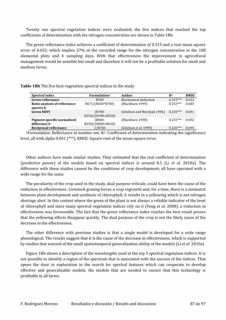
F. Rodríguez Moreno Resultados y discusión / Results and discussion 87 de 97
Twenty one spectral vegetation indices were evaluated; the five indices that reached the top
coefficients of determination with the nitrogen concentration are shown in Table 1Rb.
The green reflectance index achieves a coefficient of determination of 0.315 and a root mean square
error of 0.653, which implies 27% of the recorded range for the nitrogen concentration in the 108
elemental plots and 4 sampling days. With that effectiveness the improvement in agricultural
management would be sensible but small and therefore it will not be a profitable solution for small and
medium farms.
Table 1Rb The five best vegetation spectral indices in the study.
Spectral index Formulation1 Author R2 RMSE
Green reflectance R550 Biochemical deduction 0.315*** 0.653 Ratio analysis of reflectance spectra b
R675/(R650*R700) (Blackburn 1999) 0.252*** 0.683
Green NDVI (R780-R550)/(R780+R550)
(Gitelson and Merzlyak 1996) 0.235*** 0.691
Pigment specific normalized difference b
(R800-R650)/(R800+R650)
(Blackburn 1998) 0.231*** 0.692
Reciprocal reflectance 1/R700 (Gitelson et al. 1999) 0.226*** 0.695 1Formulation: Reflectance at number nm. R2: Coefficient of determination indicating the significance
level, all with alpha 0.001 (***). RMSE: Square root of the mean square error.
Other authors have made similar studies. They estimated that the real coefficient of determination
(predictive power) of the models based on spectral indices is around 0.5 (Li et al. 2010a). The
difference with these studies cannot be the conditions of crop development; all have operated with a
wide range for the same.
The peculiarity of the crop used in the study, dual purpose triticale, could have been the cause of the
reduction in effectiveness. Livestock grazing forces a crop regrowth and, for a time, there is a mismatch
between plant development and synthesis of chlorophyll, it results in a yellowing which is not nitrogen
shortage alert. In this context where the green of the plant is not always a reliable indicator of the level
of chlorophyll and since many spectral vegetation indices rely on it (Feng et al. 2008), a reduction in
effectiveness was foreseeable. The fact that the green reflectance index reaches the best result proves
that the yellowing effects disappear quickly. The dual purpose of the crop is not the likely cause of the
decrease in the effectiveness.
The other difference with previous studies is that a single model is developed for a wide range
phenological. The results suggest that it is the cause of the decrease in effectiveness, which is supported
by studies that warned of the small spatiotemporal generalization ability of the models (Li et al. 2010a).
Figure 1Rb shows a description of the wavelengths used in the top 5 spectral vegetation indices. It is
not possible to identify a region of the spectrum that is associated with the success of the indices. That
opens the door to exploration in the search for spectral features which can cooperate to develop
effective and generalizable models, the models that are needed to ensure that this technology is
profitable in all farms.

F. Rodríguez Moreno Resultados y discusión / Results and discussion 88 de 97
Figure 1Rb Diagram illustrating the wavelengths used for the best vegetation spectral indices in the
study
The hyperspectral signature of the crop recorded during sampling has a spectral range of 350–2500
nm, a sampling interval (the spacing between sample points in the spectrum) of 1.4 nm over the range
of 350–1000 nm and 2 nm from 1000–2500 nm, and a spectral resolution (the full-width-half-
maximum of the instrument response to a monochromatic source) of 3 nm at 700 nm and 10 nm from
1400- 2100 nm.
Exploring this dataset by multiple regression is not possible because collinearity problems. Figure
2Rb shows typical reflectance of vegetation as a function of wavelength. The continuity in the spectral
signature proves that the reflectances at different wavelengths are not independent variables. If one of
them was a linear combination of the other, the system of equations would be unsolvable because the
matrix X'X would be singular (its determinant would be zero and it could not be reversed). In an
experiment with real data the perfect collinearity is highly unlikely, but it is indubitable that in the data
there is the called quasi-collinearity, in other words, some variables are "almost" linear combination of
other. This was verified by checking the correlation coefficients (simple and multiple) between the
independent variables, several are close to 1, but they do not reach that value.
There is quasi-collinearity in the data and therefore the matrix X'X is almost-singular and its
determinant is not zero but is very small. A matrix is inverted dividing the matrix by its determinant
and with a small determinant the estimation of the coefficients presents problems of accuracy and is
unstable. Moreover, as the variances (their matrices) of the estimators are proportional to X'X, in the
presence of collinearity the standard errors of the coefficients will be large. The natural response to this
problem is the use of techniques for dimensionality reduction, which were designed to work in this
context. The results of applying the Principal component analysis (PCA) (Shlens 2005) and the
Independent component analysis (ICA) (Hyvärinen and Oja 2000) are presented below.
The first ten principal components obtained by PCA concentrate the 99.5% of the total variance,
which is a confirmation of the severe problem of collinearity in the data. The reflectances in the
different wavelengths are not independent of each other and therefore it is unlikely that there is a
unique relationship between the reflectance in a region of the spectrum and a plant parameter. A small
alteration might alter much of the spectrum of the plant; this may explain why different spectral indices

F. Rodríguez Moreno Resultados y discusión / Results and discussion 89 de 97
have been identified with the same crop parameters and why assessments of the same spectral indices
in other conditions do not reproduce the same results (Akiyama et al. 1996; Feng et al. 2008; Li et al.
2010a; Li et al. 2010b; Ustin et al. 2009; Zhu et al. 2006; Zhu et al. 2008; Zillmann et al. 2006).
Figure 2Rb Vegetation spectral signature
Even with this first result there is a possibility, however remote, that the PCA has lost the
information on the nutritional status due to the breach of any assumption. This was rejected after
checking that there is a significant relationship between 8 principal components and the plant nitrogen
concentration, relationship with a coefficient of determination of 0.68.
The regression model includes 8 principal components. The desired result, the existence of a
relationship between a single principal component and the nitrogen deficiency, has to be rejected. If
that had been the case, the study would have been simpler and it would require only a portion of the
crop spectral signature for the estimation of the nutritional status. Given the degree of connection
between the reflectances at the different wavelengths, it is natural requiring a combination of
components to estimate a plant parameter.
The good results obtained with the PCA portended a poor outcome with the ICA; this is due to the
different approaches that each defends. The results confirmed the prognosis, the model built with the
10 independent components and the plant nitrogen concentration was not significant (at the level of
significance of 0.05) and the coefficient of determination remained at 0.02.
The result achieved by processing the spectral signatures of the crop by the PCA is an improvement
on the studies of other authors (Heege et al. 2008; Li et al. 2010a; Li et al. 2010b), but given the high
cost of the spectroradiometer necessary for its implementation, the use of this methodology is limited
to large farms where the acquisition of the equipment would be profitable.

F. Rodríguez Moreno Resultados y discusión / Results and discussion 90 de 97
It is known that it is possible to develop effective and generalizable (space and time) models, now it
is time to reduce their complexity. A combination of decision trees and brute strength was tested, which
led to the development of a decision tree that just knowing the crop reflectance in three wavelengths
(350, 1670 and 2170 nm) is able to estimate the level of nitrogen in plant with an effectiveness of 68%,
a result obtained using cross-validation.
None of the wavelengths traditionally used in the estimation of nitrogen has been included in the
decision tree. The reflectance at 350 nm has been associated with the photosynthetic activity (Ray et al.
2007; Ren et al. 2006) and the reflectance at short-wavelength infrared (1670 and 2170 nm) is related
to water stress (X. Wang et al. 2010; Y. Y. Wang et al. 2010; Zhang et al. 2012), which sometimes is
related to the nitrogen concentration (Zhao et al. 2004). These references indicate what could be the
main biological meaning of the wavelengths used. Others authors have shown that the wavelengths
used in the decision tree are directly related to the nitrogen concentration at different phenological
stages (Koppe et al. 2010; Li et al. 2010a).
This biological justification of the wavelengths involved in the resulting decision tree is not a step
strictly necessary, the mathematical evaluation of the predictive power of the model is sufficient
guarantee. The information contained in the crop spectral signature is redundant and therefore the
identification of a clear biological meaning for each wavelength is unusual; wavelengths commonly
respond to multiple factors, hence the need to use data mining in the processing of these signals.
Diagnóstico agronómico mediante interpretación espacial de los parámetros de
la planta / Diagnosis agronomic by spatial interpretation of plant parameters
Los resultados anteriores son una evidencia de que sería posible estimar eficazmente el nivel de los
nutrientes en la planta de forma rápida y barata. Este avance por sí sólo no supondrá una gran ayuda
para los agricultores puesto que falta una metodología para la interpretación eficaz de los niveles de los
nutrientes en la planta.
Es posible realizar una detallada estimación (mediante radiometría, análisis foliares u otros
métodos) del nivel de nutrientes en un campo agrícola y que eso no se traduzca en un aumento del
rendimiento del cultivo. Esto podría suceder por diferentes motivos:
1. Porque sea un mal año en el que la mejor opción sea optar por una gestión agrícola de mínimos,
cancelando el muestreo del cultivo porque no sería rentable. Es preciso poder estimar esta
circunstancia en tiempo de muestreo.
2. Porque no exista estructura espacial en el cultivo, es decir, que los puntos de muestreo no sean
buenos estimadores de su vecindad y por tanto los errores por la interpolación a toda la
superficie arruinen la potencial mejora. Esto debiera ser investigado antes de emplear recursos
en el muestreo del cultivo. Podría ser necesario el empleo de técnicas de delimitación de zonas de
gestión.
3. Porque las normas para la interpretación de los niveles de nutrientes (rangos de suficiencia o
relaciones entre nutrientes) no sean específicas del cultivo – área geográfica y por tanto no sean
eficaces. Diferentes trabajos mostraron la limitada capacidad de generalización.

F. Rodríguez Moreno Resultados y discusión / Results and discussion 91 de 97
4. Porque suceda algún evento entre el muestreo del cultivo y la cosecha, el cual afecte
negativamente al rendimiento del cultivo. En ese caso ese evento debiera ser identificado para
aumentar el conocimiento y ser capaces de evitarlo en el futuro.
Los resultados mostrados en el cuarto artículo que compone esta tesis responden a todas las
cuestiones anteriores.
El índice de desarrollo del cultivo (CDI) mostró recabar más información sobre el estado del cultivo
que la altura o el NTester de forma independiente, resultó ser un buen estimador de la variabilidad
espacial del cultivo en ambos campos y en el campo Pacthy fue buen estimador del rendimiento del
cultivo. El CDI no fue buen estimador de la producción en Haj porque entre el muestreo y la cosecha
llovieron 228mm por encima de la media, incidencia que alteró el desarrollo del cultivo, conocido esto
se evidenció que el CDI es un eficaz estimador del rendimiento del cultivo, pudiendo llegar a
determinarse umbrales de viabilidad para el mismo. Si el cultivo no alcanza ese mínimo en el momento
del muestreo la intervención en el campo no es rentable, lo que responde al primer punto de los
mencionados anteriormente.
Para comprobar la estructura espacial se estudió la relación entre el CDI y los factores espaciales
(funciones de superficie y variables topográficas), encargados de representar los factores que podrían
causar la variabilidad espacial. En ambos campos se comprobó que existía una estructura espacial,
dejando al azar y al error de muestreo aproximadamente el 5% de toda la varianza registrada por el
CDI. Sólo con eso se responde al segundo punto, pero este procedimiento aporta más, estudiando la
variabilidad espacial del CDI en la parcela se puede estimar el número y ubicación de muestras foliares
necesarias, lo cual optimizaría el muestro y reduciría su coste.
Comprobado que el desarrollo del cultivo es correcto y que existe una estructura espacial se procede
al muestreo foliar. En este punto se podrían emplear rangos de suficiencia o relaciones entre nutrientes
para su interpretación. Para tratar de superar el tercer punto y dado que el CDI es un buen estimador
del rendimiento del cultivo, se optó por estudiar la relación entre el CDI y los diferentes nutrientes,
identificando como limitantes aquellos que expliquen parte de la varianza del CDI. Eso significa confiar
en que una relación estadística implique una relación causal, por ello es necesario tomar muchas
precauciones en ese estudio para obtener un resultado válido. Ese es un punto en común con las otras
metodologías para la interpretación de análisis foliares, las cuales han demostrado que no es una
debilidad. Una nueva prueba de ello son los resultados obtenidos en ambos campos. En Pacthy se
identifica el K, el Ca y el N como deficientes, lo cual es coincidente con lo deducido en el muestreo del
suelo y compatible con el diagnóstico DRIS. En el Haj no se identificaron factores limitantes, lo cual
volvió a ser coincidente con lo diagnosticado por otros métodos y explica el alto y uniforme
rendimiento del cultivo.
Si al llegar la cosecha se realiza un nuevo muestreo, entonces es posible comprobar si existe relación
entre el CDI y el rendimiento del cultivo, si no existe esa relación entonces la hipótesis será la de la
ocurrencia de alguna incidencia entre el muestreo y la cosecha, la cual podría llegar a identificarse
analizando el mapa del CDI y del rendimiento del cultivo de todo el campo obtenido mediante los
factores espaciales.
Como se ha comentado anteriormente, en el campo Haj ocurrió una incidencia entre muestreo y
cosecha. El alto rendimiento del cultivo coincidía con la alta estimación del mismo obtenida mediante el
CDI, pero sus patrones espaciales no coincidían. Comparando los mapas del CDI y del rendimiento del
cultivo se observó que las posiciones ideales relativas habían cambiado desde el muestreo a la cosecha

F. Rodríguez Moreno Resultados y discusión / Results and discussion 92 de 97
de tal forma que hizo sospechar de una precipitación inusualmente intensa, se consultó el registro
meteorológico y se confirmó la incidencia.
The above results are evidence that would be possible to estimate the level of nutrients in the plant
quickly, accurately and cheaply. This development alone will not be a great help to the farmers because
of the lack of a methodology for efficient interpretation of the levels of nutrients in the plant.
It is possible to make a detailed estimate of the level of nutrients in an agricultural field (radiometry,
leaf analysis or other methods) and that this does not imply an improvement in the crop yield. That
could happen for several reasons:
1. Because it is a bad year in which the best option is to opt for an agricultural management of
minimum cost. The crop sampling has to be canceled because it would not be profitable. It is
necessary to estimate this circumstance at the time of sampling.
2. Because there is not spatial structure in the crop development. The sampling points are not good
estimators of their neighborhood and therefore the recommendations in unsampled points
(interpolations) would be wrong, ruining the potential improvement. This should be investigated
before wasting resources on a crop sampling. It could be necessary to use zoning techniques to
delineate areas of management.
3. Because the rules for the interpretation of the levels of nutrients (sufficiency ranges or
relationships between nutrients) are not specific of the crop - geographical area and therefore
they are not effective. Different studies showed the limited generalizability.
4. Because some event occurs between the sampling of the crop and the harvest, which adversely
affects the crop yield. In that case the event should be identified to increase the knowledge and be
able to avoid it in the future.
The results shown in the fourth article included in this thesis answer all the above questions.
The crop development index (CDI) showed gather more information about the state of the crop than
the height or the Nester independently. It turned out to be a good estimator of the spatial variability of
the crop in both fields and in the field Pacthy it was good estimator of crop yield. The CDI was not good
estimator of production in Haj because between sampling and harvest rained 228mm above the mean,
incident that affected the development of the crop. Known this it became clear that the CDI is an
efficient estimator of crop yield. Viability thresholds that determine when the intervention in the field is
cost-effective could be identified, which responds to the first point of the above.
The relationship between the CDI and the spatial factors (surface functions and topographic
variables) was studied to check the spatial structure, responsible for representing the factors that could
cause the spatial variability. Spatial structure was found in the two fields, attributing to chance and
sampling error only the 5% of the variance recorded by CDI. That answers the second point, but this
procedure provides more. The number and location of necessary samples can be estimated studying the
spatial variability of the CDI in the field, it would optimize the sampling and reduce its cost.
Only if the crop development is correct and there is a spatial structure, leaf sampling is carried out.
At this point one could use sufficiency ranges or relationships between nutrients for its interpretation,
but in order to overcome the third point and since the CDI is a good estimator of crop yield, we decided

F. Rodríguez Moreno Resultados y discusión / Results and discussion 93 de 97
to study the relationship between the CDI and the different nutrients, identifying as limiting to those
that explain part of the variance of the CDI. That means trusting that a statistical relationship implies a
causal relationship. It is necessary to take great care in this study to obtain a valid result. That is a point
in common with the other methodologies for interpreting leaf analysis, which have shown that it is a
valid hypothesis. New proofs of it are the results in both fields. It identifies the K, Ca and N as deficient
in Pacthy, which is coincident with the inferred from the soil sampling and supported by DRIS. In Haj
the limiting factors were not identified, which was again coincident with other methods and it explains
the high and uniform crop yield.
If at harvest a new sampling is carried out, then it is possible to check the correlation between the
CDI and the crop yield. If there is not relationship, then the hypothesis would be the occurrence of any
incident between sampling and harvest, which could be identified by analyzing the map of CDI and crop
yield obtained by spatial factors.
As mentioned above, in the field Haj an incidence occurred between sampling and harvest. The high
crop yield coincided with the high estimate obtained by the CDI, but their spatial patterns differed.
Comparing CDI maps and crop yield was observed that the ideal positions (relative) had changed from
sampling to harvest. This made us suspicious of precipitation; an unusually intense precipitation could
explain the observed. The meteorological record was consulted and the incident was confirmed.
Novedades introducidas / Innovations introduced
Estudio radiométrico:
El empleo de una combinación de técnicas de la minería de datos rigurosamente evaluadas
mediante repeticiones de la validación cruzada.
La búsqueda de modelos con mayor capacidad de generalización. Pese a los evidentes cambios
durante el desarrollo del cultivo, se buscaron rasgos espectrales relacionados estrecha y
firmemente con el nivel de nitrógeno en planta, los cuales fueron encontrados.
Diagnóstico agronómico:
La definición de un índice de desarrollo del cultivo que sirve para estimar el rendimiento del
cultivo, como referencia con la que comparar las concentraciones de los nutrientes, etc.
El estudio de la variabilidad espacial para determinar la conveniencia de adoptar la agricultura de
precisión, la necesidad de emplear técnicas avanzadas para la delimitación de zonas de gestión,
etc.
La realización de un diagnóstico agronómico basado en evidencias obtenidas en el mismo campo
y su evaluación al final de la campaña.
…

F. Rodríguez Moreno Resultados y discusión / Results and discussion 94 de 97
Radiometric research:
The use of a combination of data mining techniques rigorously evaluated by cross validation.
The search for models with higher generalization ability. Despite the obvious changes during the
crop development, we sought spectral features closely and firmly related to the level of nitrogen
in plant.
Agronomic diagnosis:
The definition of a crop development index used to estimate the crop yield. It also serves as a
reference with which to compare the concentrations of nutrients, etc.
The study of the spatial variability to determine the advisability of adopting precision agriculture,
the need to employ advanced techniques for the delimitation of the agricultural management
zones, etc.
Performing an agronomic diagnosis based on evidence obtained in the same field and its
assessment at the end of the campaign.
…
Líneas de trabajo futuras / Future research
Estudio radiométrico:
Identificar la magnitud de la calibración necesaria para ajustar los modelos radiométricos a las
condiciones específicas de cada campaña. Determinar si las longitudes de onda son válidas y sólo
hay que modificar los umbrales del árbol de decisión.
Tratar de reproducir los resultados obtenidos en el estudio radiométrico empleando medidas de
la reflectancia del dosel de vegetación en lugar de la firma espectral de las hojas. Ello supondría
un logro rápidamente transferible al sector. Si eso es posible entonces se puede desarrollar un
sistema montado en maquinaría agrícola que en tiempo real estime el estado nutricional del
cultivo. Dada la agilidad del sistema podría barrer grandes superficies en poco tiempo, esto haría
rentable la inversión en agricultura de precisión.
Diagnóstico agronómico:
Explorar nuevas formulaciones del índice de desarrollo del cultivo (CDI). Determinar si medidas
radiométricas y/o descriptores del patrón de desarrollo colonial del cultivo pueden mejorar la
eficacia del CDI.
Comprobar la idoneidad del CDI para diferentes cultivares (trigo de invierno) y otros cereales,
incluso para otros cultivos.
Realizar estudios que determinen umbrales para la media y la desviación del CDI, los cuales
ayuden en la toma de decisiones del agricultor.
Comprobar si las interpolaciones empleando los factores espaciales pueden mejorar incluyendo
imágenes remotas de toda la parcela.

F. Rodríguez Moreno Resultados y discusión / Results and discussion 95 de 97
Continuar con los ensayos de la metodología, tratando de buscar los escenarios más complejos,
para determinar su potencial.
Radiometric research:
Identifying the magnitude of the necessary calibration to adjust the radiometric models to the
specific conditions of each campaign. Determine if the wavelengths are valid and it just needs to
modify the thresholds of the decision tree.
Trying to reproduce the results obtained in the study using canopy reflectance instead of the
spectral signature of the leaves. It could mean an achievement quickly transferable to the farms. If
that is possible then one can develop a system mounted on farm machinery that in real time
estimates the nutritional status of the crop. Given the agility of the system, it could sweep large
areas in a short time. This would make profitable the investment in precision agriculture.
Agronomic diagnosis:
Explore new formulations of the crop development index (CDI). Determine whether radiometric
measurements and / or the pattern of colonial development can improve the efficiency of the CDI.
Check the suitability of the CDI for different cultivars (winter wheat) and other cereals, even for
other crops.
Studies to determine thresholds for the mean and the standard deviation of the CDI, which help in
the decision making of the farmer.
Check if interpolations using spatial factors along with remote images can achieve better results.
Continue testing the methodology, trying to look for the more complex scenarios, to determine its
potential.
Referencias / References
Akiyama, T., Inoue, Y., Shibayama, M., Awaya, Y. & Tanaka, N. (1996). Monitoring and predicting crop growth and analysing agricultural ecosystems by remote sensing. Agricultural and Food Science in Finland, 5(3), 367-376.
Blackburn, G. A. (1998). Quantifying chlorophylls and carotenoids at leaf and canopy scales: An evaluation of some hyperspectral approaches. Remote Sensing of Environment, 66(3), 273-285, doi:10.1016/s0034-4257(98)00059-5.
Blackburn, G. A. (1999). Relationships between spectral reflectance and pigment concentrations in stacks of deciduous broadleaves. Remote Sensing of Environment, 70(2), 224-237, doi:10.1016/s0034-4257(99)00048-6.
Feng, W., Yao, X., Zhu, Y., Tian, Y. C. & Cao, W. X. (2008). Monitoring leaf nitrogen status with hyperspectral reflectance in wheat. European Journal of Agronomy, 28(3), 394-404, doi:10.1016/j.eja.2007.11.005.
Gitelson, A. A., Buschmann, C. & Lichtenthaler, H. K. (1999). The chlorophyll fluorescence ratio F735/F700 as an accurate measure of the chlorophyll content in plants. Remote Sensing of Environment, 69(3), 296-302, doi:10.1016/s0034-4257(99)00023-1.
Gitelson, A. A. & Merzlyak, M. N. (1996). Signature analysis of leaf reflectance spectra: Algorithm development for remote sensing of chlorophyll. Journal of Plant Physiology, 148(3-4), 494-500.

F. Rodríguez Moreno Resultados y discusión / Results and discussion 96 de 97
Heege, H. J., Reusch, S. & Thiessen, E. (2008). Prospects and results for optical systems for site-specific on-the-go control of nitrogen-top-dressing in Germany. Precision Agriculture, 9(3), 115-131, doi:10.1007/s11119-008-9055-3.
Hyvärinen, A. & Oja, E. (2000). Independent component analysis: Algorithms and applications. Neural networks, 13(4-5), 411-430.
Koppe, W., Li, F., Gnyp, M. L., Miao, Y., Jia, L., Chen, X. et al. (2010). Evaluating multispectral and hyperspectral satellite remote sensing data for estimating winter wheat growth parameters at regional scale in the North China plain. Photogrammetrie, Fernerkundung, Geoinformation, 2010(3), 167-178, doi:10.1127/1432-8364/2010/0047.
Li, F., Miao, Y., Hennig, S. D., Gnyp, M. L., Chen, X., Jia, L. et al. (2010a). Evaluating hyperspectral vegetation indices for estimating nitrogen concentration of winter wheat at different growth stages. Precision Agriculture, 11(4), 335-357, doi:10.1007/s11119-010-9165-6.
Li, F., Zhang, H., Jia, L., Bareth, G., Miao, Y. & Chen, X. (2010b). Estimating winter wheat biomass and nitrogen status using an active crop sensor. Intelligent Automation and Soft Computing, 16(6), 1221-1230.
Ray, S. S., Jain, N., Miglani, A., Singh, J. P., Singh, A. K., Panigrahy, S. et al. (2007). Defining optimum narrow bands and bandwidths for agricultural applications. 58th International Astronautical Congress (Vol. 4, pp. 2458-2467). Hyderabad.
Ren, J., Chen, Z., Tang, H. & Shi, R. (2006). Regional yield estimation for winter wheat based on net primary production model. Transactions of the chinese society of agricultural engineering, 22(5), 111-117.
Shlens, J. (2005). A tutorial on principal component analysis: Systems Neurobiology Laboratory, University of California at San Diego.
Ustin, S. L., Gitelson, A. A., Jacquemoud, S., Schaepman, M., Asner, G. P., Gamon, J. A. et al. (2009). Retrieval of foliar information about plant pigment systems from high resolution spectroscopy. Remote Sensing of Environment, 113(1), S67-S77, doi:10.1016/j.rse.2008.10.019.
Wang, X., Guo, N., Zhao, C., Zhang, K. & Zhang, H. (2010). Hyperspectral reflectance characteristics for spring wheat in different drought intimidate. Paper presented at the 18th International Conference on Geoinformatics, Beijing, June 18-20
Wang, Y. Y., Li, G. C., Zhang, L. J. & Fan, J. L. (2010). Retrieval of leaf water content of winter wheat from canopy hyperspectral data using partial least square regression. Spectroscopy and Spectral Analysis, 30(4), 1070-1074, doi:10.3964/j.issn.1000-0593(2010)04-1070-05.
Zhang, L., Zhou, Z., Zhang, G., Meng, Y., Chen, B. & Wang, Y. (2012). Monitoring the leaf water content and specific leaf weight of cotton (Gossypium hirsutum L.) in saline soil using leaf spectral reflectance. European Journal of Agronomy, 41, 103-117, doi:10.1016/j.eja.2012.04.003.
Zhao, C., Liu, L., Wang, J., Huang, W., Song, X., Li, C. et al. (2004). Methods and application of remote sensing to forecast wheat grain quality. Paper presented at the Geoscience and Remote Sensing Symposium (IGARSS '04), Anchorage, AK, 20-24 Sept. 2004
Zhu, Y., Li, Y., Feng, W., Tian, Y., Yao, X. & Cao, W. (2006). Monitoring leaf nitrogen in wheat using canopy reflectance spectra. Canadian Journal of Plant Science, 86(4), 1037-1046.
Zhu, Y., Yao, X., Tian, Y., Liu, X. & Cao, W. (2008). Analysis of common canopy vegetation indices for indicating leaf nitrogen accumulations in wheat and rice. International Journal of Applied Earth Observation and Geoinformation, 10(1), 1-10, doi:10.1016/j.jag.2007.02.006.
Zillmann, E., Graeff, S., Link, J., Batchelor, W. D. & Claupein, W. (2006). Assessment of cereal nitrogen requirements derived by optical on-the-go sensors on heterogeneous soils. Agronomy Journal, 98(3), 682-690, doi:10.2134/agronj2005.0253.

F. Rodríguez Moreno Conclusiones / Conclusions 97 de 97
Conclusiones / Conclusions
En la firma espectral del cultivo existen rasgos relacionados con el nivel de nitrógeno en planta, los
cuales permanecen estables durante un amplio intervalo fenológico.
Aún en un amplio rango de condiciones de desarrollo, es posible desarrollar modelos radiométricos
eficaces, pero se desconoce si han de ser calibrados cada campaña y si sería posible ajustarlos para
operar con medidas de reflectancia del dosel de vegetación.
La metodología SIOPP ha probado ser eficaz realizando el diagnóstico agronómico de dos
explotaciones agrícolas reales en las que los problemas eran complejos. Con las evidencias disponibles
y dado el bajo coste añadido que implica su implementación, ya se considera una alternativa al uso de
rangos de suficiencia o relaciones entre nutrientes para la interpretación de los análisis foliares.
Cuando no existan zonas en el campo con un buen desarrollo del cultivo, zonas de referencia, SIOPP
no podrá realizar el diagnóstico. Las condiciones de desarrollo del cultivo han de estar alejadas del
óptimo, esa primera corrección, obvia revisando un tratado de agronomía, es un requisito de la
metodología en casos extremos.
En caso de existir severa heterogeneidad (márgenes abruptos) o si hay que diagnosticar
plantaciones con centenares de hectáreas de extensión, SIOPP puede presentar problemas ante la
debilidad de modelar barreras y/o infinidad de gradientes. En ese caso sería necesario realizar un
estudio previo para la delimitación de las zonas de gestión, esta es una de las líneas de trabajo futuras.
There are features in the spectral signature of the crop related to plant nitrogen (N) content, which
remain stable over a wide range of phenological stages.
Even in a wide range of development conditions, it is possible to develop effective radiometric
models, but it is unknown if they have to be calibrated in each campaign and whether it would be
possible to adjust them to operate with measures of vegetation canopy reflectance.
The spatial interpretation of plant parameters (SIOPP) has proven to be effective for the agronomic
diagnosis of two real farms where the problems were complex. With the available evidence and given
the low added cost involved in its implementation, it is considered as an alternative to using sufficiency
ranges and relationships between nutrients for interpreting leaf analysis.
When there are not areas in the field with a good crop development, reference areas, SIOPP cannot
make the diagnosis. The conditions for crop development should be away from the optimum. That first
correction, which has to be obvious after reviewing any textbook of agronomy, is a requirement of the
methodology in extreme cases.
In case of severe heterogeneity (abrupt margins) or if it has to diagnose plantations with hundreds
of hectares, SIOPP can present problems because of the difficulty of modeling steep barriers and / or
countless gradients. In that case it would be necessary to carry out a study for the definition of areas of
management; this is one of the future lines of work.

Copyright © 2022 FDOKUMEN