Microwave Properties of Carbon Powders - -ORCA
177
Microwave Properties of Carbon Powders A thesis submitted in fulfilment of the requirement for the degree of Doctor of Philosophy By Fatma Shkal School of Engineering - Cardiff University UK -2018
-
Upload
khangminh22 -
Category
Documents
-
view
2 -
download
0
Transcript of Microwave Properties of Carbon Powders - -ORCA
Microwave Properties
of Carbon Powders
A thesis submitted in fulfilment of the requirement for the degree of
Doctor of Philosophy
By
Fatma Shkal
School of Engineering - Cardiff University
UK -2018
II
DECLARATION AND STATEMENTS
DECLARATION
This work has not previously been accepted in substance for any degree and is not
concurrently submitted in candidature for any degree.
Signed …………………….…... (candidate) Date……….……….
STATEMENT 1
This thesis is being submitted in partial fulfilment of the requirements for the degree of
Doctor of Philosophy (PhD).
Signed …………………….…. (Candidate) Date……….……….
STATEMENT 2
This thesis is the result of my own independent work/investigation, except where
otherwise stated. Other sources are acknowledged by explicit references.
Signed …………………….… (candidate) Date……….……….
STATEMENT 3
I hereby give consent for my thesis, if accepted, to be available for photocopying and
inter-library loan, and for the title and summary to be made available to outside
organisations.
Signed …………………….…. (candidate) Date……….……….
III
ABSTRACT
Microwave techniques have been used in many applications due to the simplicity of the
associated construction and use. They provide several advantages in contrast with
traditional methods, including fast (almost instantaneous) measurements and their non-
destructive nature, at least at low microwave power levels. Moreover, microwave methods
provide an accurate and sensitive measurements of dielectric properties of carbon powders
(in sp2 form) due to their strong interactions with microwave electric fields.
The contributions to the state-of-the-art provided by the work presented in this thesis
are novel applications of the microwave cavity and coaxial probe methods to
differentiate between the types of carbon materials of industrial relevance by
characterization of their dielectric properties. Measurements are typically carried out
between 10 MHz to 10 GHz for the coaxial probe method, and between 2.5 GHz to 10
GHz for the cavity method, also as a function of temperature up to 150 0C.
The results of this thesis show that microwave methods are sufficient to differentiate
carbons materials by measuring the complex permittivity under different conditions.
The industrial relevance arises from being able to identify different types of carbons in
two groups: one for blast furnace dust, which is crucial to quantify the utilization of coal
injected in the furnace and determine the efficiency of coal injection; the other for
activated carbons, which are highly porous structures used for applications such as
carbon dioxide capture in fossil fuel combustion
Dielectric properties of different carbons (quantified by their complex permittivities)
shown in this thesis are measured in-situ as frequency-dependent and temperature-
dependent quantities and are different for different types of carbonaceous materials in
the two groups of powders. Hence, the impact of this work is the realisation of simple and
easy to use test methods that are robust enough to be applied in an industrial setting.
IV
ACKNOWLEDGEMENTS
First and foremost, I thank the Almighty Allah for showering his infinite bounties and grace
upon me to complete my Ph.D. study.
I would like to offer my most sincere thanks to my supervisor, Professor Adrian Porch for
the opportunity to work with such an exciting field. I am grateful for his counsel and he
has my lasting admiration. I must also thank him for all suggestions, explanations, and
improvements in the writing of this thesis.
My thanks go to Doctor Julian Steer at the Cardiff School of Engineering for his assistance
in providing the blast furnace dust samples. I must also thank him for all his suggestions,
explanations.
My thanks go to Doctor Susana Garcia Lopez and her team at Heriot Watt School of
Engineering & Physical Sciences for their assistance in providing the activated carbon
samples.
My thanks go to Duncan Muir at the Cardiff School of Earth and Ocean Sciences for his
assistance in the SEM characterizations.
I acknowledge the financial support of Libyan government. Thank you also to my friends
and colleagues whose enlightening conversations has informed and enthused me throughout
my studies.
This research would not be possible without the help of many people. I wish to express my
gratitude to them all for their contributions. Many thanks to the technicians in the
electrical/electronic workshop, mechanical workshop, and the IT group in the School of
Engineering for their help and cooperation.
This work would not have been possible without the love and patience from my friend
Mabrouka and my cousin Noor and her husband Masoud, whose unfaltering support and
encouragement have been invaluable.
Finally, and not least, I would like to give my deepest thanks to my parents and family for
supporting me spiritually throughout my studies.
V
PUBLICATIONS
1. Fatma Shkal, Susana Garcia Lopez, Daniel Slocombe, Adrian Porch,
“Microwave Characterization of Activated Carbons.” Journal of Computer and
Communications, 2017. 6(01): p. 112
2. Céline Shepherd, Emina Hadzifejzovic , Fatma Shkal, Kerstin Jurkschat,
Jonathan Moghal, Emily M. Parker, Montree Sawangphruk, Daniel R.
Slocombe, John S. Foord, Mark G. Moloney., “New Routes to Functionalize
Carbon Black for Polypropylene Nanocomposites”. Langmuir, 2016. 2016.
32(31): p. 7917-7928.
3. Fatma Shkal, Julian Steer, Adrian Porch, “Microwave Techniques to
Differentiate the Types of Carbon.” accepted to the Eurpean Conference on
Feul and Enrgy research and its Applications (12th ECCRIA).

VI
TABLE OF CONTENTS
Table of Contents
DECLARATION AND STATEMENTS ................................................................... II
ABSTRACT ................................................................................................................ III
ACKNOWLEDGEMENTS ....................................................................................... IV
TABLE OF CONTENTS ........................................................................................... VI
LIST OF FIGURES ................................................................................................... XI
LIST OF TABLES .................................................................................................. XIX
LIST OF ABBREVIATIONS ................................................................................. XX
Chapter 1 Introduction and Thesis Summary ........................................................... 1
1.1 Project Aims .................................................................................................... 1
1.2 Thesis Outline .................................................................................................. 2
1.3 Main original contributions ............................................................................. 3
Chapter 2 Literature Survey ...................................................................................... 4
2.1 Activated Carbons ........................................................................................... 4
2.1.1 Types of activated carbon ........................................................................ 5
2.1.2 Applications of activated carbons ............................................................ 6
2.1.3 Production of activated carbon ................................................................ 7
2.1.4 Structure of activated carbons .................................................................. 8
2.1.5 Microwave characterization of activated carbons .................................. 10
2.1.6 Regeneration of activated carbons ......................................................... 12
2.1.7 Advantages of microwave regeneration ................................................. 13
2.2 Blast furnace dust .......................................................................................... 14
VII
2.2.1 Synthesis and characterization of blast furnace dust.............................. 15
2.2.2 Microwave characterization of carbons in blast furnace dust ................ 16
2.3 The surface chemistry of activated carbon .................................................... 18
2.4 Bonding in carbon ......................................................................................... 21
2.4.1 Sp3 Hybridization ................................................................................... 21
2.4.2 Sp2 Hybridization ................................................................................... 22
2.5 Microwave measurement techniques ............................................................ 24
2.5.1 Non-resonant techniques ........................................................................ 24
2.5.2 Resonance techniques ............................................................................ 32
2.6 Microwave techniques for this research ........................................................ 39
Chapter 3 Modelling, Design and Methods ............................................................ 41
3.1 Introduction ................................................................................................... 41
3.2 Dielectric theory ............................................................................................ 41
3.2.1 Space charge polarization ...................................................................... 42
3.2.2 Polarization by dipole alignment ........................................................... 42
3.2.3 Ionic polarization ................................................................................... 43
3.2.4 Quantification of polarization and depolarization effects ...................... 43
3.2.5 Penetration Depth ................................................................................... 45
3.2.6 Effect of electronic conductivity on microwave loss ............................. 46
3.2.7 Dielectric Relaxation .............................................................................. 47
3.3 Fundamentals of cylindrical cavities ............................................................. 48
3.3.1 Mode chart ............................................................................................. 50

VIII
3.3.2 Quality factor ......................................................................................... 51
3.3.3 Coupling of cavity resonators (excitation) ............................................. 52
3.3.4 Network analyser and scattering parameters.......................................... 55
3.3.5 Equivalent circuits of cavity resonators ................................................. 56
3.4 Cavity perturbation theory ............................................................................. 57
3.5 Modelling and design of the cylindrical cavity resonator ............................. 61
3.6 Fundamentals of the coaxial probe technique ............................................... 62
3.7 Modelling and design of coaxial probe ......................................................... 65
3.8 Errors and calibration .................................................................................... 66
3.8.1 Network analyser calibration ................................................................. 67
3.8.2 Cavity measurement system calibration................................................. 67
3.8.3 Coaxial probe measurement calibration ................................................. 67
Chapter 4 Microwave cavity for dielectric characterization ................................... 69
4.1 Introduction ................................................................................................... 69
4.2 Measurement system ..................................................................................... 69
4.3 Materials ........................................................................................................ 73
4.4 Dielectric properties measurements of activated carbons ............................. 75
4.5 Dielectric properties of carbons in blast furnace dust ................................... 77
4.6 Conclusions ................................................................................................... 79
Chapter 5 Frequency-dependent dielectric properties ............................................ 81
5.1 Multiple modes cavity system ....................................................................... 81
5.2 Open-ended coaxial probe system ................................................................. 85
5.3 Dielectric properties of powdered activated carbons .................................... 86
IX
5.4 Dielectric properties of carbon mixed with silicone rubber .......................... 92
5.4.1 Dielectric properties of activated carbon composites ............................ 93
5.4.2 Dielectric properties of carbons contained in blast furnace dust ........... 97
5.5 Conclusion ................................................................................................... 103
Chapter 6 Temperature-Dependent Dielectric Properties ..................................... 104
6.1 Measurement system ................................................................................... 104
6.2 Materials ...................................................................................................... 108
6.3 Temperature-dependent dielectric properties of activated carbon .............. 109
6.3.1 Scanning Electron Microscopy (SEM) ................................................ 116
6.4 Temperature-dependent dielectric properties of BFD ................................. 119
6.5 Cavity system for dielectric measurements of saturated AC ...................... 124
6.6 Conclusion ................................................................................................... 128
Chapter 7 Conclusion and future work ................................................................. 130
7.1 Literature Survey: ........................................................................................ 130
7.2 Analysis: Microwave Systems Principles ................................................... 130
7.3 Experiments ................................................................................................. 130
7.4 Characterization of activated carbon materials ........................................... 131
7.5 Characterization of types of carbon contained in BFD ............................... 131
7.6 Further Work ............................................................................................... 132
7.6.1 Microwave regeneration of saturated activated carbons ...................... 132
7.6.2 Electric fields distribution .................................................................... 133
7.6.3 Microwave excitation system ............................................................... 134
APPENDIX A Durometer Conversion Chart ........................................................ 137
X
APPENDIX B Published paper 1 .......................................................................... 138
XI
LIST OF FIGURES
Figure 2-1 Types of activated carbons[13] .................................................................... 6
Figure 2-2 Production of activated carbon ..................................................................... 7
Figure 2-3 Three-dimensional and two-dimensional structures of activated carbon. [20]
........................................................................................................................................ 9
Figure 2-4 Complex permittivities of activated carbon from coconut shell. ε׳ and ε׳׳
values increase monotonically with temperature from 23ºC to 188.5ºC [21] ............. 11
Figure 2-5 Comparison between microwave and conventional heating desorption of
carbon dioxide at 70˚C and 130˚C [8] ........................................................................ 12
Figure 2-6 Adsorptive capacities of phenol after various cycles of regeneration in
electric furnace (EF) and microwave (MW) furnaces. horizontal axis show the samples
of AC, labelled as CiRi where Ci the cycles of saturation and Ri the number of
regenerations [11]......................................................................................................... 14
Figure 2-7 Frequency dependency of relative complex permittivity (εr’ and εr") for the
graphite and carbon black samples: (a) AT-No.5, (b) artificial graphite, (c) pure carbon,
and (d) carbon black.[22] ............................................................................................. 17
Figure 2-8 surface chemistry of carbon black [38] ...................................................... 18
Figure 2-9 Nitrogen and oxygen surface groups on carbon. [40] ................................... 20
Figure 2-10 some possible surface groups[41] ............................................................ 20
Figure 2-11 sp3 -hybrid orbital [42] ............................................................................. 22
Figure 2-12 the crystal structure of diamond, whose bonds are fully sp3 hybridized [43]
...................................................................................................................................... 22
Figure 2-13 sp3 -hybrid orbital.[42] ............................................................................ 23
Figure 2-14 Crystal structure of graphite. .................................................................... 24
Figure 2-15 Measurement using transmission/reflection method with a waveguide.[50]
...................................................................................................................................... 26
Figure 2-16 Dependency of dielectric permittivity on the frequency and filler amount
for composites based on NBR [51] .............................................................................. 27
XII
Figure 2-17 Dependency of dielectric permittivity on the frequency and filler amount
for composites based on NR [51] ................................................................................. 27
Figure 2-18 Schematic of the measuring procedure using an open-ended coaxial probe
[54] ............................................................................................................................... 29
Figure 2-19 Schematic diagram of measurement system for the free space method using
a pair of lens antennas .................................................................................................. 31
Figure 2-20 Variations of the dielectric permittivity with frequency for coals: (a) real
part, (b) imaginary part of bituminous coal samples, (c) real part and (d) imaginary part
of anthracite coal samples[58] ..................................................................................... 32
Figure 2-21 Dielectric properties of hay vs. temperature under nitrogen environment at
915 MHz and 2450 MHz with initial density of 0.76 ± 0.05 g/cc; (a) relative dielectric
constant and (b) relative loss factor.[67] ...................................................................... 35
Figure 2-22 Schematic diagram of a split dielectric resonator fixture [70] ................. 36
Figure 2-23 Microstrip and ring resonator .................................................................. 37
Figure 2-24 Schematic of DSRR microfluidic sensor[76] ........................................... 38
Figure 2-25𝑆21 of the sensor using a quartz tube: simulated results by COMSOL
Multiphysics Software (dotted lines) and measured results (solid lines and symbols)
[77] ............................................................................................................................... 38
Figure 2-26 𝑆21 of the sensor using PFA tube: simulated results by COMSOL
Multiphysics Software (dotted lines) and measured results (solid lines and symbols)
[77] ............................................................................................................................... 39
Figure 3-1 the polarisation of a dielectric material when placed in a uniform electric
field. ............................................................................................................................. 42
Figure 3-2 Dielectric constant and loss dispersion of dielectric materials against
frequency[79] ............................................................................................................... 43
Figure 3-3 The depolarization effects in dielectric cylindrical shape. (a) Cylindrical
sample in parallel, non-depolarising configuration, and (b) Cylindrical sample in
perpendicular, depolarising configuration. .................................................................. 44
Figure 3-4 Debye and Cole-Cole Diagrams [90] ......................................................... 48
Figure 3-5 Resonant mode chart for a cylindrical cavity [2] ....................................... 51
XIII
Figure 3-6 The coupling probe [93] ............................................................................. 52
Figure 3-7 The coupling loop [93] .............................................................................. 53
Figure 3-8 Aperture coupling, electric and magnetic [93] ......................................... 53
Figure 3-9 A series resonant circuit coupled to a feedline [2] ..................................... 54
Figure 3-10 Two port network ..................................................................................... 56
Figure 3-11 series and parallel RLC equivalent circuits of resonator[2] .................... 56
Figure 3-12 A dielectric material, in the form of a thin rod, measured using a cylindrical
host cavity resonator [64] ............................................................................................. 58
Figure 3-13 a resonant cavity perturbed by a changing in the permittivity or permeability
of the materials in the cavity. (a) Original cavity. (b) Perturbed cavity [2] ............... 58
Figure 3-14 Typical S21 spectra, for the empty cavity and with the load (sample).[99]
...................................................................................................................................... 60
Figure 3-15 Cavity system set-up. .............................................................................. 61
Figure 3-16 COMSOL Simulation of some TM modes. Electric and magnetic field
distributions. ................................................................................................................. 62
Figure 3-17 Open-circuit coaxial line sample measurement configuration [102] ....... 63
Figure 3-18 Equivalent circuit of an open-ended coaxial probe .................................. 64
Figure 3-19 Square flange coaxial flat probe. The flange improves the performance of
the probe because the flange model more closely represents the model of an infinite
ground plane. ................................................................................................................ 65
Figure 3-20 COMSOL model of the coaxial probe. Electric field distribution, the active
sample region of the probe is at the tip of the probe where the E-field evanescently
disperses into the air atmosphere, the colours are for illustrative purpose only (red is
being high) ................................................................................................................... 66
Figure 4-1 COMSOL simulation of the cylindrical cavity resonator TM010, showing the
electric ((a)) and (c)) and magnetic ((b) and (d)) field distribution. ............................ 70
Figure 4-2 COMSOL simulation of the resonant traces of the TM010 mode when empty
and when sample-loaded. Insertion the sample reduces the resonant frequency from
2.4925GHz to 2.3875GHz and increases the bandwidth from 1.2MHz to 6.33MHz,
dependent on the complex permittivity of the sample. ................................................ 71

XIV
Figure 4-3 Photographs of the experiment set-up for cavity perturbation measurement.
...................................................................................................................................... 72
Figure 4-4 the resonant traces of the TM010 mode when clean quartz tube and tube with
finger prints loaded to the cavity. The finger prints have negligible affects............... 73
Figure 4-5 Grinding the granular activated carbon to powder ..................................... 75
Figure 4-6 Dielectric constant of activated carbon samples. The typical standard error
is ±0.02, which in most cases is too small to observe. ................................................. 76
Figure 4-7 Dielectric loss factor of activated carbon samples. The typical standard error
is ±0.0027, which in most cases is too small to observe. ............................................. 77
Figure 4-8 Dielectric constant of different carbon samples. The typical standard error is
±0.03, which in most cases is too small to observe. .................................................... 78
Figure 4-9 Dielectric loss factor of different carbon samples. The typical standard error
is ±0.03, which in most cases is too small to observe. ................................................. 78
Figure 4-10 Dielectric constant of lab-made carbon samples. The typical standard error
is ±0.01, which in most cases is too small to observe. ................................................. 79
Figure 4-11 Dielectric loss factor of lab-made carbon samples. The typical standard
error is ±0.024, which in most cases is too small to observe. ...................................... 79
Figure 5-1 Real components of complex permittivity of different types of carbons ... 83
Figure 5-2 Imaginary components of complex permittivity of different types of carbons
...................................................................................................................................... 83
Figure 5-3 Real components of complex permittivity of different types of coals ....... 84
Figure 5-4 Imaginary components of complex permittivity of different types of coals
...................................................................................................................................... 84
Figure 5-5 Real components of complex permittivity of lab-made samples ............... 85
Figure 5-6 Imaginary components of complex permittivity of lab-made samples ...... 85
Figure 5-7 coaxial probe and sample fixture. Sample is placed on the top of the probe,
while S11 is measured using a PNA network analyser and controlled by a LabVIEW
program.[43]................................................................................................................. 86
Figure 5-8 real component of the complex permittivity of powdered activated carbon
(Norit GCN3070) for 10 independent measurements .................................................. 88
XV
Figure 5-9 imaginary component of the complex permittivity of powdered activated
carbon (Norit GCN3070) for 10 independent measurements ...................................... 88
Figure 5-10 Real component of complex permittivity of Char 80% for 10 independent
measurements ............................................................................................................... 89
Figure 5-11 Imaginary component of complex permittivity of Char 80% for 10
independent measurements .......................................................................................... 89
Figure 5-12 Real component of the complex permittivity of Coke 80% for 10
independent measurements .......................................................................................... 90
Figure 5-13 Imaginary component of the complex permittivity of Coke 80% for 10
independent measurements .......................................................................................... 90
Figure 5-14 Real component of the complex permittivity of Coal 80% for 10
independent measurements .......................................................................................... 91
Figure 5-15 Imaginary components of the complex permittivity of Coal 80% for 10
independent measurements .......................................................................................... 91
Figure 5-16 Real components of complex permittivity of Silicone rubber for 5 samples.
...................................................................................................................................... 94
Figure 5-17 Imaginary components of complex permittivity of Silicone rubber for 5
samples. ........................................................................................................................ 94
Figure 5-18 Real component of complex permittivity of 4:1 for 5 samples ................ 95
Figure 5-19 Real and imaginary component of complex permittivity of 4:1 for 5 samples
...................................................................................................................................... 95
Figure 5-20 Real component of complex permittivity of 8:1 for 5 samples ................ 96
Figure 5-21 Imaginary component of complex permittivity of 8:1 for 5 samples ....... 96
Figure 5-22 Real component of complex permittivity ................................................. 97
Figure 5-23 Imaginary component of complex permittivity ........................................ 97
Figure 5-24 Real components of complex permittivity of coke for 10 independent
measurements ............................................................................................................... 99
Figure 5-25 Imaginary components of complex permittivity of coke for 10 independent
measurements ............................................................................................................... 99
XVI
Figure 5-26 Real component of complex permittivity of coal 3 for 10 independent
measurements ............................................................................................................. 100
Figure 5-27 Imaginary component of complex permittivity of coal 3 for 10 independent
measurements ............................................................................................................. 100
Figure 5-28 Real component of complex permittivity of coal 5 for 10 independent
measurements ............................................................................................................. 101
Figure 5-29Imaginary component of complex permittivity of coal 5 for 10 independent
measurements ............................................................................................................. 101
Figure 5-30 Real components of complex permittivity for three different types of carbon
samples ....................................................................................................................... 102
Figure 5-31 Imaginary components of complex permittivity for three different types of
carbon samples ........................................................................................................... 102
Figure 6-1 Distributions of electric (top) and magnetic (bottom) fields of the nodal mode
TM210 at 5.33 GHz ...................................................................................................... 106
Figure 6-2 Distributions of the electric (top) and magnetic (bottom) fields of the nodal
mode TM310 at 6.61 GHz .......................................................................................... 106
Figure 6-3 Photograph of the bench-top experimental assembly for cavity
measurements. The cavity is put inside a computer-controlled oven and connected to a
network analyser under control of a LabVIEW program. .......................................... 108
Figure 6-4 Real component of complex permittivity vs. temperature of CN ............ 110
Figure 6-5 Imaginary component of complex permittivity vs. temperature of CN ... 111
Figure 6-6 Real component of complex permittivity vs. temperature of CN800 ...... 111
Figure 6-7 Imaginary component of complex permittivity vs. temperature of CN800
.................................................................................................................................... 112
Figure 6-8 Real component of complex permittivity vs. temperature of CNO300 ... 112
Figure 6-9 Imaginary component of complex permittivity vs. temperature of CNO300
.................................................................................................................................... 113
Figure 6-10 Photograph of the ejected materials after first heating cycle ................. 113
Figure 6-11 Real component of complex permittivity vs. temperature of CN .......... 114
Figure 6-12 Imaginary component of complex permittivity vs. temperature of CN . 115
XVII
Figure 6-13 Real component of complex permittivity vs. temperature of CN800 .... 116
Figure 6-14 Imaginary component of complex permittivity vs. temperature of CN800
.................................................................................................................................... 116
Figure 6-15 SEM photograph of activated carbon samples before heating, the scale is
shown at 200µm and 60µm. ....................................................................................... 117
Figure 6-16 SEM photograph of activated carbon samples after heating, the scale is
shown at 200µm and 60µm. ....................................................................................... 118
Figure 6-17 Thermogravimetric analysis of activated carbon samples ..................... 119
Figure 6-18 Real component of complex permittivity vs. temperature of coke ........ 120
Figure 6-19 Imaginary component of complex permittivity vs. temperature of coke 120
Figure 6-20 Real component of complex permittivity vs. temperature of coal 3 ...... 121
Figure 6-21 Imaginary component of complex permittivity vs. temperature of coal 3
.................................................................................................................................... 122
Figure 6-22 Real component of complex permittivity vs. temperature of coal 5 ...... 122
Figure 6-23 Imaginary component of complex permittivity vs. temperature of coal 5
.................................................................................................................................... 123
Figure 6-24 Real component of complex permittivity vs. temperature ..................... 123
Figure 6-25 Imaginary component of complex permittivity vs. temperature ............ 124
Figure 6-26 Real component of complex permittivity of AC sample saturated with water
.................................................................................................................................... 126
Figure 6-27 Imaginary component of complex permittivity of AC sample saturated with
water ........................................................................................................................... 126
Figure 6-28 Real component of complex permittivity of AC sample saturated with CO2
.................................................................................................................................... 127
Figure 6-29 Imaginary component of complex permittivity of AC sample saturated with
CO2 ............................................................................................................................. 127
Figure 7-1 the large aluminium cylindrical cavity resonator. .................................... 133
Figure 7-2 Electric field distribution of a 900MHz cavity operating in the TM010 mode
.................................................................................................................................... 134
XVIII
Figure 7-3 Schematic of the whole microwaving system using the large cavity ....... 134
Figure 7-4 System set up ready for measurement ...................................................... 135

XIX
LIST OF TABLES
Table 2-1 dielectric properties of coals at different frequencies, all at 600C [36] ....... 17
Table 3-1 values of penetration depth for some dielectric materials ........................... 45
Table 3-2 Values of 𝑝𝑛𝑚 ............................................................................................... 50
Table 3-3 Values of 𝑝𝑛𝑚′ ............................................................................................ 50
Table 3-4 Summary of formulae for Series and Parallel Resonators [2] ..................... 56
Table 4-1 Group 1 carbon materials. ........................................................................... 74
Table 4-2 Group 2 carbon materials. ........................................................................... 74
Table 4-3 Lab-made samples ....................................................................................... 74
Table 5-1 Resonant frequencies (in GHz) of the various TM modes used here. ......... 82
Table 6-1 Ultimate analysis of the activated carbon samples[113, 114] ................... 109
Table 6-2 Properties of coal samples ......................................................................... 109
XX
LIST OF ABBREVIATIONS
AC = Activated Carbon
BFD = Blast Furnace Dust
ISM = Industrial, Scientific and Medical frequency
IUPAC = International Union of Pure and Applied Chemistry
MUT = Materials Under Test
PSA= Pressure Swing Adsorption
SEM = Scanning Electron Microscopy
TGA = Thermogravimetric Analyser/Analysis
TSA= Temperature Swing Adsorption

1
Chapter 1 Introduction and Thesis Summary
It is important to develop reliable test methods in characterization of carbon materials
to replacing and improving the existing technologies. Microwave resonators can
provide very accurate characterization of carbon materials due to the sensitivity of
carbonaceous materials to the microwave electric field component. However,
resonators provide the measurements at the discrete set of resonant frequencies, but a
broadband coaxial probe has the ability to provide the measurements over a range of
frequencies, although with a much lower sensitivity.
This thesis focuses on microwave techniques used in the characterization of different
types of carbons. The original contributions are proposed to provide new test methods
to quantify and differentiate between these carbonaceous materials.
Microwave cavity perturbation has been used to characterise and differentiate two
groups of carbonaceous materials. The first group is activated carbons, produced from
different precursors and different treatments such as ammoxidation and ammonia heat
treatment. The other group is of carbons in blast furnace dust, such as coke, coal or
partially burnt chars.
The broadband coaxial probe was also used to determine the frequency-dependent
permittivity for both groups over range of frequencies from 10 MHz to above 10 GHz.
In addition, the cylindrical cavity at 2.5 GHz was used for the measurement of the
temperature-dependent dielectric properties of both groups of carbon materials, to
investigate their microwave complex permittivity as functions of temperature.
1.1 Project Aims
The aims of this project were to develop and use microwave systems that could be
used to differentiate the types of carbon materials. Cylindrical cavity resonators (at
the ISM frequency of approximately 2.5 GHz) and coaxial probes were used for
dielectric property investigation of the carbon samples and used to differentiate them.
The main sets of experiments were as follows:
Microwave techniques to measure the dielectric properties of different carbon
materials.
2
Frequency-dependent dielectric properties of carbon materials.
Temperature-dependent dielectric properties of carbon materials.
1.2 Thesis Outline
The thesis is composed of the following chapters:
Chapter 1 - Introduction and Thesis Summary
This chapter presents a general introduction, the main project aims, and the thesis
outline.
Chapter 2 – Literature Survey
This chapter gives a background on the carbon materials studied in this thesis, their
properties, and presents a literature survey on the use of microwave techniques for
measuring the dielectric properties of materials, with focusing on carbonaceous
materials. Some examples from the literature related to microwave cavities and other
microwave measurement techniques are presented for selected applications.
Chapter 3 - Modelling, Design and Methods
This chapter presents a review of the theory of microwave techniques, the design of
the microwave systems used in this research and the simulation of both types of
microwave applicators that have been used for the dielectric property measurements.
This includes the design fundamentals and simulation of the cylindrical cavity
resonator and coaxial probe.
Chapter 4 - Microwave cavity for dielectric characterization
Measurement of complex permittivity of different types of activated carbons, produced
from different precursors, using the microwave cavity system are presented.
Additionally, the main different forms of carbon contained in blast furnace dust (BFD)
are also presented. The results show the effectiveness of the microwave cavity
technique as a simple method to characterise and differentiate between activated
carbons and the main components in BFD using dielectric properties only, without the
need for more sophisticated materials analysis.
3
Chapter 5 - Frequency-dependent dielectric properties
This chapter presents the results of using a multimode cavity and open-ended coaxial
probe for frequency-dependent dielectric characterisation of carbon materials. The
microwave cavity excited in different TM modes was used for complex permittivity
measurements at the discrete set of resonant frequencies. The open ended coaxial
probe technique was also used to investigate dielectric properties of different types of
carbon over a wider range of frequencies from 10MHz to 20GHz, to support the spot
2.5 GHz results presented in Chapter 4.
Chapter 6 - Temperature-dependent dielectric properties
The microwave cavity perturbation method was used for the temperature-dependent
dielectric characterisation of carbons. The whole cavity system (plus sample) was
placed inside a controlled laboratory oven to change the ambient temperature. This
was to study the absorption/desorption of species from activated carbon (in particular),
such as moisture.
Chapter 7 - Conclusions and future work
The main conclusions of the work are summarized in this chapter and some
recommendations are presented for future work.
1.3 Main original contributions
The main contributions presented in this thesis are summarised as:
• New use of the microwave cavity and coaxial probe methods to characterize
the dielectric properties of activated carbon samples.
• First demonstration of microwave methods to differentiate the main
components of blast furnace dust.
• First in-situ dielectric characterization of activated carbons as a function to
temperature to study the absorption/desorption processes.
4
Chapter 2 Literature Survey
The historical development of microwave engineering in the latter half of the 20th
century has led to the introduction of many new methods which can be applied in
numerous industrial and biological applications. Most traditional microwave/RF
applications are in communication systems such as wireless and radar systems, but
now also in medical and environment applications [1, 2].
This chapter presents the most common microwave techniques, relevant for the
characterization and applications of carbonaceous materials. Activated carbons and
other different forms of carbons contained in blast furnace dust will be the focus of
this thesis. Activated carbon materials, their applications, production, and the
regeneration of activated carbon will be introduced in Section 2.1. Section 2.2 reviews
blast furnace dust. Chemical aspects of carbon will be outlined in Sections 2.3 and
2.4. Finally, the chapter concludes with Section 2.5, comprising a review of
microwave measurement techniques and the associated advantages/disadvantages of
each technique.
2.1 Activated Carbons
“Activated carbon” is a generic terminology referred to carbonaceous materials of very
large surface area and highly porous microstructures. In general, the activated carbon
samples have pore volumes of about 0.2ml/g, and the surface area is approximately in
the range 400 - 2000 m2/g; subsequently, they have inherently low densities, which is
less than 0.4 g/cm3 [3-5].
Activated carbon (AC) materials can be generally manufactured from different organic
materials, such as biomass, coal, wood, sawdust, coconut shell, peach or apricot stones
and waste materials, after which the activation process is carried out. The activation
process can be physical or chemical. In physical activation, a char is exposed to steam,
CO2, or air at high temperatures. In chemical activation, some activating elements are
introduced during the carbonization process, such as zinc chloride (ZnCl2), phosphoric
acid (H3PO4), potassium hydroxide (KOH). The mixture of the chemical agents and
the AC is heated at temperatures ranging from 340ºC to 780ºC. Adding these
chemicals to AC provides products with high porosity. The advantages of chemical
5
activation are the higher production volumes, lower temperature of activation, less
activation time and higher development of porosity; among the disadvantages are the
high costs of the activating agents and the need to perform an additional washing stage
to remove the chemical agent [6, 7].
Activated carbon materials have many industrial applications, especially in the
purification of gases and water technologies, but they have limited adsorption capacity.
Therefore, it is preferable to regenerate any exhausted activated carbon instead of
disposing of it, to minimize the cost of production of fresh material. Moreover,
materials regeneration will reduce the hazards of pollutants on the environment which
result from increased waste. The world-wide necessity to capture and store carbon
dioxide from, for example, the combustion of fossil fuels in particular, has increased
greatly in the last few years [8-10].
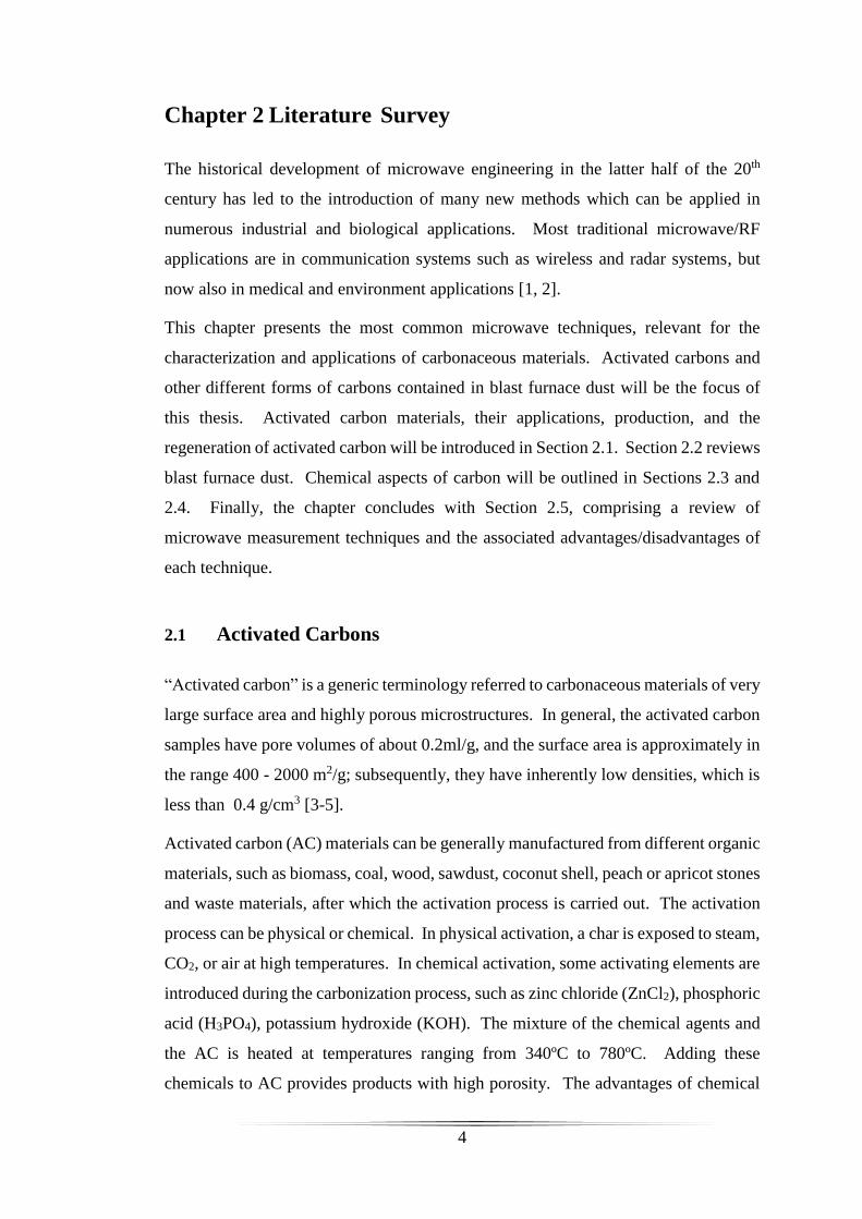
2.1.1 Types of activated carbon
There are many types of activated carbon materials available commercially, in both
granular and powdered forms, and are used for water purification by surface adsorption
of the dissolved organics and contaminant species from water and wastewaters due to
their highly porous structure. Granular activated carbon has a typical average particle
size (“diameter”) of about 0.2 mm, and can be manufactured from hard organic starting
materials such as almond and coconut shell. Powdered activated carbon can be easily
obtained from the granular form by grinding. Fibres and activated carbon cloths are
other different forms of activated carbon, which can be woven to form a flexible, thin
“fabric.” Figure 2.1 illustrates these different forms of activated carbons [11-13].

6
Figure 2-1 Types of activated carbons[13]
2.1.2 Applications of activated carbons
As already mentioned, activated carbon has many industrial and chemical applications.
It is used in capture and storage technologies such as storage carbon dioxide. It is also
used to determine and remove volatile organic pollutants. For example, activated
carbon used to purify water from the liquid phase pollutants.
The different size of pores in AC should be considered for the specific application, as
the AC adsorbs molecules from both liquid and gaseous phases, which depends on
their surface area, their shape, pore size, and surface chemical characteristics. These
properties specify the quality of AC and are directly the result of the nature of
precursors and the type of the production method and the temperature of production.
In adsorption from the gas phase, mainly microporous carbon is used, whereas
mesoporous carbon is applied in liquid phase processes. Applications of mesoporous
activated carbons include: drinking water purification, waste-water treatment,
sweetener decolourization, food, and chemical processing. On the other hand,
microporous carbons are used for solvent recovery, gasoline emission control,
cigarette filters and for industrial emission gas treatment [7, 8, 14, 15].

7
2.1.3 Production of activated carbon
Activated carbon materials are produced from different organic materials such as
coconut and almond shell, biomass, and waste materials. The manufacturing methods
can be divided into two main processes: carbonization and activation [6]. Figure 2-2
shows the typical life cycle of activated carbons.
Figure 2-2 Production of activated carbon
2.1.3.1 Carbonization
In this process, the raw materials are treated under elevated temperatures to reduce the
volatile content in the raw materials in order to convert it to a suitable form for
activation.
After the carbonization stage, most of the non-carbon elements such as hydrogen and
oxygen are first removed in gaseous form by pyrolytic decomposition of the raw
material and the released atoms of elementary carbon are grouped into organized
crystallographic formation known as elementary graphitic crystallites.
Carbonization of biomass material starts above 170ºC and it is almost completed
around 500ºC- 600ºC. The rate of pyrolysis is considerably affected by the moisture
content of the starting material. Additional important factors are uniform heating of
the furnace and the temperature of carbonization, which must not be very high.
Carbonization
Activation
Saturation
Regeneration
8
In the simple carbonization product, the common arrangement of the crystallites is
irregular, so that free gaps remain between them. However, as a result of deposition
and decomposition of tarry materials, these gaps are filled (or at least blocked) by
disorganized (amorphous) carbon. The resulting carbonized product has small
adsorption capacity. Apparently, at least for carbonization at lower temperatures, part
of the formed tar remains in the pores between the crystallites and on their surface.
Such carbonized materials can then be partially activated by removing the tarry
products by heating them in a stream of an inert gas, or by extracting them with a
suitable solvent, or by a chemical reaction [16].
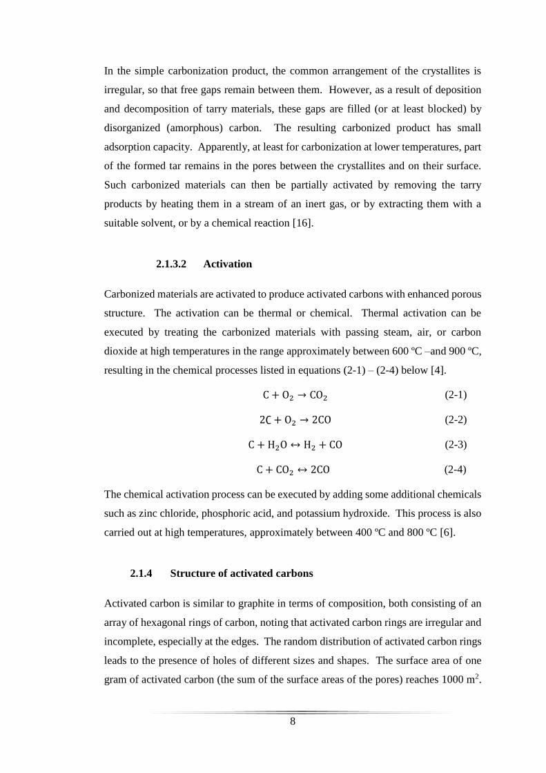
2.1.3.2 Activation
Carbonized materials are activated to produce activated carbons with enhanced porous
structure. The activation can be thermal or chemical. Thermal activation can be
executed by treating the carbonized materials with passing steam, air, or carbon
dioxide at high temperatures in the range approximately between 600 ºC –and 900 ºC,
resulting in the chemical processes listed in equations (2-1) – (2-4) below [4].
C + O2 → CO2 (2-1)
2∁ + O2 → 2CO (2-2)
C + H2O ↔ H2 + CO (2-3)
C + CO2 ↔ 2CO (2-4)
The chemical activation process can be executed by adding some additional chemicals
such as zinc chloride, phosphoric acid, and potassium hydroxide. This process is also
carried out at high temperatures, approximately between 400 ºC and 800 ºC [6].
2.1.4 Structure of activated carbons
Activated carbon is similar to graphite in terms of composition, both consisting of an
array of hexagonal rings of carbon, noting that activated carbon rings are irregular and
incomplete, especially at the edges. The random distribution of activated carbon rings
leads to the presence of holes of different sizes and shapes. The surface area of one
gram of activated carbon (the sum of the surface areas of the pores) reaches 1000 m2.

9
In addition, the absence of activated carbon rings at the edges leads to the presence of
certain atomic groups on the surface, which in turn determines the chemical nature of
the AC surface (acidic, base, neutral). It is noted that the nature of raw material used
in the preparation of AC, as well as the activation method, are the most important
factors affecting the type and quantity of surface groups [16].
Micro-crystallites of AC are formed during carbonization of the raw materials, then
free valence electrons are produced during the activation process; these electrons are
very reactive. Additionally, the formation of interior vacancies in the microcrystalline
structures can be affected by the presence of impurities and process conditions. The
only difference between the graphite structure and that of AC is that the latter is the
harder of the two [17].
The porous structure of AC can contain some of different non-homogeneous atoms
such as oxygen and hydrogen. Some AC materials can also contain different amounts
of minerals (sometimes denoted as ash content). The AC composition depends on the
nature of the raw material used as the precursor. The porous structure of AC is
considered as the main physical property that characterizes them. This is formed by
pores of different sizes which as shown in Figure 2-3 which, according to IUPAC
recommendations [18], can be classified into three major groups:
• Micropores with a pore width of less than 2 nm.
• Mesopores with widths from 2 to 50 nm.
• Macropores with a pore width larger than 50 nm [13, 19].
Figure 2-3 Three-dimensional and two-dimensional structures of activated carbon [20]

10
2.1.5 Microwave characterization of activated carbons
Most carbonaceous materials have a common characteristic of being highly absorbing
of microwave energy, mostly as a result of their interaction with the microwave electric
field, and so can be quantified and characterized by their dielectric properties. This
absorption of microwave energy will result in intense, volumetric heating of the
samples if the microwave electric field (i.e. microwave power) is high [7, 14].
The relative permittivity of the material r is used to quantify a material’s response (via
its polarization) to an applied electric field. At microwave frequencies this is
considered a complex quantity; its real part 휀𝑟′ is related to the material polarization
(i.e. stored energy), whilst its imaginary part 휀′𝑟′ is related to energy loss. Their ratio
tan=휀𝑟′′/휀𝑟
′ is known as the material’s loss tangent and is the usual figure of merit
used to compare the power dissipation between different dielectric materials at
microwave frequencies. Therefore, it is necessary to measure the complex permittivity
of any material to quantify its interaction with a microwave electric field, especially
its ability to be heated by microwaves [6, 14, 21].
A number of studies attempted to measure the complex permittivity of AC at
microwave frequencies [14, 21-27]. The AC samples were produced from coconut
shell and were investigated using broadband measurements over a frequency range
between 0.2 to 26 GHz at different temperatures. The samples were prepared as fine
powders with particle size from 710 µm to 1500µm. They were heated at 180˚C for
72 hours to ensure that there was no absorption of additional chemical species, such
as water. These studies concluded that most AC materials have a susceptibility to
being heated by microwave radiation in the range of frequencies between 0.9 and 6
GHz, which is allowed by their high values of loss tangent. This frequency range
includes the main industrial, scientific, and medical microwave ranges (at about 0.9,
2.45 and 5.7 GHz). It was also concluded, unsurprisingly, that the complex
permittivity of AC materials depended on the frequency and temperature [14].
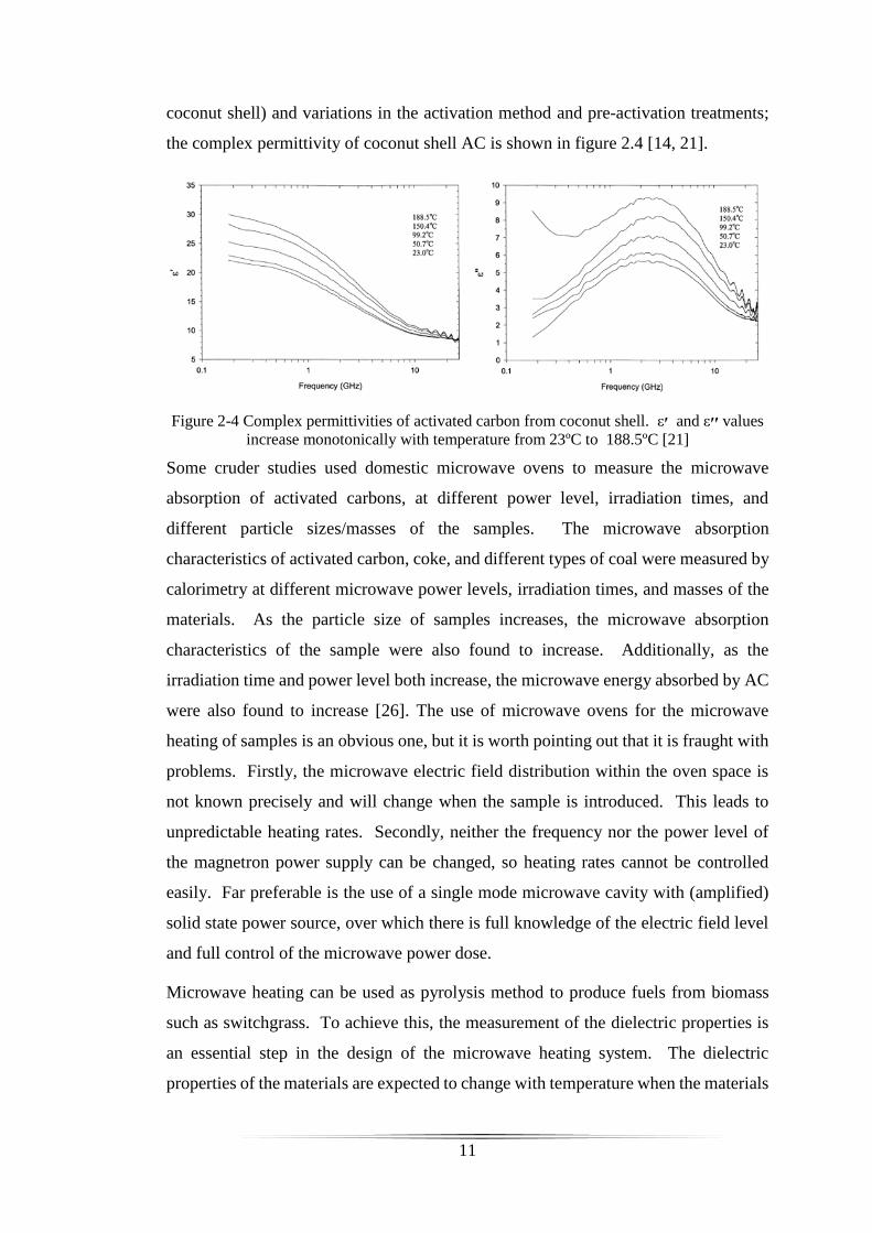
Permittivities of three AC samples of different origin were measured using a coaxial
dielectric probe over the frequency range from 0.2 to 26 GHz at temperature range
between 22ºC and 190 ºC. There were obeserved differences in permittivity of AC
samples owing to the variations in the carbonaceous raw material (i.e. peat, coal, and
11
coconut shell) and variations in the activation method and pre-activation treatments;
the complex permittivity of coconut shell AC is shown in figure 2.4 [14, 21].
Figure 2-4 Complex permittivities of activated carbon from coconut shell. ε׳ and ε׳׳ values
increase monotonically with temperature from 23ºC to 188.5ºC [21]
Some cruder studies used domestic microwave ovens to measure the microwave
absorption of activated carbons, at different power level, irradiation times, and
different particle sizes/masses of the samples. The microwave absorption
characteristics of activated carbon, coke, and different types of coal were measured by
calorimetry at different microwave power levels, irradiation times, and masses of the
materials. As the particle size of samples increases, the microwave absorption
characteristics of the sample were also found to increase. Additionally, as the
irradiation time and power level both increase, the microwave energy absorbed by AC
were also found to increase [26]. The use of microwave ovens for the microwave
heating of samples is an obvious one, but it is worth pointing out that it is fraught with
problems. Firstly, the microwave electric field distribution within the oven space is
not known precisely and will change when the sample is introduced. This leads to
unpredictable heating rates. Secondly, neither the frequency nor the power level of
the magnetron power supply can be changed, so heating rates cannot be controlled
easily. Far preferable is the use of a single mode microwave cavity with (amplified)
solid state power source, over which there is full knowledge of the electric field level
and full control of the microwave power dose.
Microwave heating can be used as pyrolysis method to produce fuels from biomass
such as switchgrass. To achieve this, the measurement of the dielectric properties is
an essential step in the design of the microwave heating system. The dielectric
properties of the materials are expected to change with temperature when the materials

12
are heated by microwaves, therefore, it is important to investigate this effect. Many
factors can vary the dielectric properties during pyrolysis process, such as the existence
of water, the decomposition of volatile material, the change in weight and density, and
the transformation process of biomass into carbonaceous material. It has been found
that there was a decrease in the permittivity through the drying and pyrolysis processes,
as might be expected owing to the high permittivity of water (of both its real and
imaginary parts). However, the permittivity sharply increased in char region; the
transformation of phase to carbonaceous char could be the main reason behind this
sudden rise in dielectric properties [27].
2.1.6 Regeneration of activated carbons
Microwave heating technology has been utilized for the regeneration of AC in recent
years. For example, microwave heating was used to release CO2 from AC materials
at two different temperatures (70˚C and 130˚C), and the results were compared with
conventional methods, in which a commercial tubular oven was used. The materials
used in this study were commercially-available AC which was produced from coconut
shell. The study concluded that the microwave heating offers the fastest rate of
releasing CO2 from samples, at a rate 3-4 times faster when compared with
conventional oven heating, as shown in Figure 2-5 [8].
Figure 2-5 Comparison between microwave and conventional heating desorption of carbon
dioxide at 70˚C and 130˚C [8]
In these experiments, an electrical oven and a single mode microwave cavity
(operating at 2.45GHz) were used to regenerate AC which was saturated by phenol, at
850 ºC. The study concluded that, when comparing microwave heating with

13
conventional heating, the regeneration process time was 9 times shorter, taking only 4
minutes compared to 37 minutes when a conventional oven was used. Moreover, the
porous structure of regenerated AC was efficiently preserved [11].
2.1.7 Advantages of microwave regeneration
Using microwave heating to recycle exhausted AC has many benefits, including the
ability to be repeated multiple times and its speed of regeneration compared to
traditional methods; hence, it is more efficient than traditional approaches in that it
uses less total energy. Moreover, microwave methods have been demonstrated to
retain the original porous structure of the starting AC material, actually with an
apparent increase in total surface area when using microwave heating to regenerate the
AC. Ania et al. [10] concluded that mesoporosity of the AC samples which were
treated using microwaves were about 20% larger than the samples treated in an electric
furnace. Meanwhile, microporosity was found to become higher in AC samples
treated with microwaves. This result occurs mainly when treatment is carried out
under an inert N2 atmosphere, whilst providing an oxidizing atmosphere during the
treatment gives rise to an increase of mesoporosity, due to partial gasification of the
activated carbon [11]. Additionally, the adsorption performance and capacity of
materials has been found to be improved when using microwave heating compared to
conventional methods [8, 11, 14, 19, 28-30]. Figure 2-6 shows a comparison of the
adsorption capacity of AC and the regenerated samples when saturated with phenol,
between microwave and conventional electric furnace recycling to compare the effect
of the different heating mechanisms on the adsorptive capacities of the regenerated AC
[11].

14
Figure 2-6 Adsorptive capacities of phenol after various cycles of regeneration in electric
furnace (EF) and microwave (MW) furnaces. horizontal axis show the samples of AC,
labelled as CiRi where Ci the cycles of saturation and Ri the number of regenerations [11]
2.2 Blast furnace dust
Carbonaceous materials found in blast furnace dust can be categorized into three types:
namely, char, coke, and coal, but the predictable quantity of coal is low. Both char
and soot result from very rapid pyrolysis of coal [31].
Coke, which is a high-carbon product, is usually produced by destructive distillation
of coal, coke has a simple composition, consisting mainly of carbon with some mineral
materials and small amounts of hydrogen, sulphur and oxygen [32]. On the other hand,
coke has a very complex structure, with a different size of pores and wall and shapes
as well as cracks. The coke walls consist of different textures which have various
microscopic properties and vary in optical anisotropy depending on the rank and type
of coal in the coal mix used [33].
One of the usual processes in modern blast furnace ironmaking is the injection of
powdery coal. The main purpose of this is to reduce the consumption of coke (per ton)
during hot metal production, which is usually referred to as coke rate. The monitoring
of the combustion of injected coal is not possible as the process occurs within an
extremely hot and completely closed environment. Currently, the level of combustion
of the injected, pulverised coal can be obtained from indirect analysis of the particles
loaded in the top gap of the furnace, and from the dust collected at the end of the

15
process. The combustion efficiency characteristic of the furnace can be demonstrated
by the quantification of the types and amounts of the different carbon materials in the
blast furnace dust (BFD), especially for materials resulting from pulverised coal
injection. However, such quantification is a major challenge, as the origin and the type
of the resulting carbon materials cannot be identified using a chemical analysis of
carbon. Although, BFD has high levels of carbonaceous material resulting from
loaded coke, distinguishing between the carbonaceous materials produced from loaded
coke and combustion remainders is not simple because both have the same chemical
characteristics. In addition, detection of small amounts of pulverised coal injection
residues in BFD is very challenging because BFD also contains a large amount of non-
carbonaceous materials, such as iron ore. Thermogravimetric analysis (TGA) can be
adapted for the quantitative analysis of BFD to differentiate the different types of
carbon [31, 34] , but realistic alternatives are scarce.
For these reasons, in this research, microwave techniques were proposed for a simpler,
more practical differentiation of carbonaceous materials in blast furnace dust based on
their dielectric property measurement. The simplicity of this method also means that
it could be deployed in-situ at the combustion site.
2.2.1 Synthesis and characterization of blast furnace dust
Blast furnace dust is one of the most important solid industrial wastes and it contains
many key components. Carbon is the most common component contained with high
concentration. Such carbonaceous materials are prospective materials for recycling as
fuels or agents for thermochemical transformation or mineralogy.
To transfer carbonaceous materials in BFD into waste gas, they are gasified and the
two major resultant gases - methane and hydrogen – are collected to be used as fuels.
The main factors affecting the efficiency of the combustion and gasification processes
are the physical and chemical properties of the carbons contained in the BFD.
Therefore, differentiation of types of BFD carbons is necessary for their recycling as
fuels or reducing agents. Existing typical techniques for differentiation include:
• Chemical analysis methods: the carbonaceous materials contained unused coal,
char, and coke.

16
• X-ray diffraction techniques, in combination with chemical analysis, as a
standard procedure to identify and differentiate the char and coke structures.
• Raman spectroscopy, which is used to determine the proportion of char and
coke and the degree of graphitization for carbonaceous materials.[35]
2.2.2 Microwave characterization of carbons in blast furnace dust
A number of studies show the potential of the use of microwaves as a non-invasive
tool to differentiate types of carbons [14, 21, 22, 25, 26]. Microwave complex
permittivity, which contains information about both the polarization and absorption
characteristics, of different types of carbon can be measured and used to distinguish
between coke and other types of coal, which could also contain different quantities of
carbon, moisture, volatile materials and ash. Different carbonaceous materials have
been shown to yield significant differences in their microwave absorption, with coke
being the best absorber [26].
Published results have demonstrated the variations of the microwave complex
permittivities of different types of carbons with different properties and chemical
compositions, with measurements carried out in the range of X-band frequencies (8.2
to 12.4 GHz) and more generally in the frequency range between 1 and 10 GHz. It has
been found that the permittivity values of coals are considerably smaller than for
graphite and carbon black. As shown in Figure 2-7, the complex permittivity of three
graphite (AT-No.5, artificial graphite and pure carbon) and one carbon black samples
were measured. The real part 휀𝑟′ was found to decrease with increasing frequency,
limiting to a close to constant value above 6.5 GHz. The imaginary (i.e. loss) 휀𝑟′′
values also decrease with increasing frequency in the similar way as the 휀𝑟′ values [22].
Marland et al. [33] attempted to use microwave cylindrical cavity resonator for
dielectric permittivity measurements of UK coals with different coal rank and different
minerals contents at three frequencies (0.165, 1.413 and 2.216GHz). They concluded
that the permittivities of coals decrease with coal rank and depend (as one would
expect) on the moisture and mineral contents; they also change with both temperature
and frequency. The results summarized in Table 2-1. The dielectric properties of coals

17
can change with frequency, decrease with increasing frequencies to and approach a
constant value above 6.5 GHz. as shown in Figure 2-7 [36].
Figure 2-7 Frequency dependency of relative complex permittivity (εr’ and εr") for the
graphite and carbon black samples: (a) AT-No.5, (b) artificial graphite, (c) pure carbon, and
(d) carbon black [22]
Table 2-1 dielectric properties of coals at different frequencies, all at 600C [36]
coal 0.615 GHZ 1.413 GHZ 2.216 GHZ
휀𝑟′ 휀𝑟
′′ 휀𝑟′ 휀𝑟
′′ 휀𝑟′ 휀𝑟
′′
F-1 2.91 0.6130 2.89 0.1433 2.93 0.1657
F-2 2.47 0.0443 2.46 0.0402 2.49 0.0539
F-3 2.30 0.0543 2.31 0.0534 2.34 0.0818
F-4 2.80 0.1951 2.75 0.1810 2.77 0.2087
F-5 2.40 0.1380 2.34 0.1317 2.32 0.1389
F-6 2.88 0.191 2.84 0.1489 2.86 0.1564
F-7 2.50 0.1150 2.45 0.1188 2.45 0.1252
F-8 3.63 0.3792 2.52 0.3191 3.51 0.3153
P-1 2.94 0.2161 2.84 0.1893 2.87 0.1848
P-2 1.62 0.0873 1.61 0.0772 1.62 0.0772
P-3 2.89 0.1929 2.80 0.1768 2.84 0.1684
P-4 2.27 0.0740 2.24 0.0560 2.28 0.0658
P-5 2.66 0.1401 2.65 0.1186 2.69 0.1274
P-6 2.42 0.1623 2.39 0.0803 2.44 0.0914
P-7 2.62 0.1055 2.55 0.0783 2.58 0.0906

18
2.3 The surface chemistry of activated carbon
Activated carbon is an effective adsorbent for the removal of dissolved organic
substances from waters and wastewaters. The physicochemical nature of the surface
of carbon is an important factor in the adsorption process and should be considered in
selection or preparation of carbons for specific applications. The surface of any
activated carbon is comprised in part of residual electron- and ion exchange functional
groups, connected by electron-conducting bond systems. The nature of these
functional groups is determined to a large extent by the method of activation, as well
as by the type of raw material from which the carbon is prepared. With the existence
of electron- and ion-exchange groups at the surface of carbon, it is reasonable to expect
that electrolytes in solution may interact with the carbon to influence its behaviour as
an adsorbent. In fact, such interactions could considerably affect the overall adsorption
process under certain conditions, possibly effecting changes in the process which may
be put to good advantage to achieve higher efficiency or enhanced effectiveness for
the removal of pollutants [37].
Although there is little direct information available on the structure of activated
carbon, much can be derived from existing data on the structure of carbon black. Very
little chemical difference exists between these two substances, and the only apparent
physical difference is that the carbon black has much less internal surface area [37].
Figure 2-8 surface chemistry of carbon black [38]

19
The surface chemistry of carbon plays an important role because of its high reactivity.
In the field of carbonaceous materials, the surface chemistry usually refers to the
chemical nature and properties of their surface (being made up of unpaired electrons)
and of the type, quantity, and bonding of various heteroatoms, especially oxygen.
These are bonded to the carbon skeleton and form the same surface functional groups
as those typically found in aromatic compounds. Such groups may be acidic groups
(i.e. carboxyls, lactones, and phenols) and basic groups (i.e. pyrones, chromenes,
ethers, and carbonyls). Also, the delocalized p-electrons of carbon’s basal planes are
basic sites. Moreover, activated carbon has reducing ability due to oxygen functional
groups such as phenolic, lactone, carbonyl, and quinone [39].
The behaviour of carbonaceous materials in catalysis depends on their surface properties,
which in turn are determined by their structure. The structure of the porous carbons used
in catalysis is graphitic; thus, there are unsaturated carbon atoms at the edges of the
graphene layers and in basal plane defects that can easily react with oxygen, water, or
nitrogen compounds, originating in surface groups such as those represented schematically
in Figure 2-9. These groups can be used to anchor catalysts or catalyst precursors, or for
subsequent functionalization; in addition, they may be active sites for specific catalytic
reactions.

20
Figure 2-9 Nitrogen and oxygen surface groups on carbon. [40]
Among the oxygenated groups, carboxylic acids and anhydrides, lactones, lactols, and
phenols, are acidic, while carbonyl and ether groups are neutral or may form basic
structures (quinone, chromene, and pyrone groups). The nitrogen groups include pyridine
(N-6), pyrrole, or pyridone (N-5), and oxidised nitrogen (NX) at the edges, and quaternary
nitrogen (N-Q) incorporated into the graphene structure. The nitrogen atoms provide
additional electrons, inducing surface basicity and enhanced catalytic activity in oxidation
reactions. The acidic surface properties are caused by the presence of carboxyl groups
(also in the form of their cyclic anhydrides), lactones, or lactols as shown in Figure
2-10, and hydroxyl groups of phenolic character [40, 41].
Figure 2-10 some possible surface groups [41]

21
2.4 Bonding in carbon
Molecular bonding behaviour has a large influence on the structure of a material and
its chemical and physical properties. Carbon atoms bond themselves are not in form
of identical molecular orbitals, they actually are in form of hybridized orbitals. In the
following sections, the term hybridization is explained in this context and the influence
on the properties is described using the examples of graphite and diamond. Pure
carbon has many allotropes with markedly different crystal structures which reveal
also very different material properties, originating from the particular type of bonding
between carbon atoms.
The normal bonding behaviour of molecular orbitals involves the bonding of the same
kind of orbital. Two s-orbitals or two similar p-orbitals bind together in an antibonding
and bonding way, depending on the sign of the orbital. Carbon atoms form bonds by
the mixing (i.e. hybridization) of different orbitals, namely s- and p-orbitals. Also a
mixture of s-, p- and d-orbitals is possible, but is less important for combining carbon
orbitals only [42]. In the next section, the resulting sp3 and sp2 hybridization will be
explained in detail.
2.4.1 Sp3 Hybridization
A carbon atom contains six electrons which occupy the following electron
configuration: (1s) 2 (2s) 2 (2p) 2. In the ground state there are two unpaired electrons
in the outer shell, so that one could assume the ability to bind only two additional
molecules. Because of the small energy difference between the 2s- and the 2p-states,
it is easily possible to excite one electron from the 2s state into the 2p-state. In the
presence of an external perturbation, such as a nearby atom such as hydrogen, the
energy difference is overcome. This results in a mixed state formed out of one s-orbital
and three p-orbitals (namely px, py and pz). Four new hybrid orbitals are formed. The
direction of the orbitals and also the centre of mass are determined by the specific
contributions of the p-orbitals and the s-orbital. A combination of the hybrid orbitals
produces a tetrahedral assembly with the centre of masses in the corners shown in
Figure 2-11. This is called sp3 hybridization, and accounts for the highly symmetric
bonding found in the diamond form of carbon, which accounts for many of its
remarkable material properties (e.g. hardness, strength, and stiffness).

22
Figure 2-11 sp3 -hybrid orbital [42]
The characteristic angle between the hybrid orbitals in the sp3 -configuration is 109.5º.
Assembling many different sp3 - hybridized carbon atoms within a single crystal, one
achieves the typical diamond structure as shown in Figure 2-12. The unique properties
of diamond are now even more understandable. Due to the three-dimensional sp3 –
structure, the binding strength between neighbouring carbon atoms is equal for each
atom and very strong. Diamond has a wide bandgap of about 5 eV and so its electrical
conductivity is very low (it can be considered to be almost an ideal dielectric material);
as a consequence, its microwave absorption is also very low (it has a very small loss
tangent at microwave frequencies). Furthermore, the transparent appearance of
diamond is associated with the wide bandgap, so that electrons cannot be excited out
of the valence band into the conduction band with wavelengths in the optical range.
Figure 2-12 the crystal structure of diamond, whose bonds are fully sp3 hybridized [43]
2.4.2 Sp2 Hybridization
Sp2 Hybridization is the combination of one s-orbitals with only two p- orbitals,
namely px and py. They contribute to form a planar assembly, as shown in Figure 2-13,
with a characteristic angle of 120º between the hybrid orbitals, thus forming a so-called

23
σ-bond. The additional pz-orbital is perpendicular to the sp2 hybrid orbitals and forms
a so-called π-bond.
Figure 2-13 sp3 -hybrid orbital [42]
A typical example of a sp2 hybridized crystal structure is graphite, shown in Figure
2-14. It consists of parallel carbon layers. Within a single layer, the planar sp2 hybrid
orbitals align themselves as in Figure 2-8 to form a structure with strong binding.
Between the layers the π-orbitals give rise to weak Van-der-Waals forces, allowing the
layers to slide over each other. As a result, graphite is very soft and is thus used in
pencils. Conversely, a single layer (known as graphene) is the stiffest material known.
The band structure of graphite is such that it can be described as a semimetal. The
connection of valence and conduction bands allows easy electron excitation into the
conduction band, independent of the wavelength, so that graphite is a very good
electrical conductor over a broad range of frequencies and is optically opaque.

24
Figure 2-14 Crystal structure of graphite.
2.5 Microwave measurement techniques
Over the past three decades, measurements of dielectric properties of materials using
microwave techniques has received much attention. This has been especially so for
the non- destructive characterisation of materials used in passive device applications,
including sensors.
Microwave measurement techniques are generally divided into two main categories,
resonant and non-resonant methods. The measurement methods used for dielectric
measurement in this work are cavity resonator and coaxial probe methods, which will
be described in more detail below.
2.5.1 Non-resonant techniques
Transmission/Reflection techniques are used for measurements of the real part of the
complex permittivity of both high and low loss materials over a broad range of

25
frequencies. However, these methods do not have adequate resolution to measure the
imaginary part of the permittivity, and so have limited use for materials with low loss
tangents. The transmission/ reflection techniques have two basic types. One method
depends on measuring the complex S-parameters S11 and S21 (i.e. voltage reflection
and transmission coefficients, respectively), which are then used to calculate the
dielectric property via a suitable inversion process; this is called a distributed
impedance technique and is used for frequencies typically above about 0.1 GHz). The
other method (typically used for frequencies less than about 0.1 GHz) is a lumped
impedance technique which is based on circuit theory, which essentially involves the
direct measurement of capacitance. Both of these methods require precise knowledge
of the electric field and its uniformity in the vicinity of the sample under test; indeed,
the inversion analysis is simplified by assuming the electric field is uniform within the
sample, an approximation which is valid for a suitable design of sample test fixture
[44-46].
2.5.1.1 Transmission line method (Waveguide)
In this method, a specified length of sample is filled inside an enclosed section of
transmission line prior to measuring the reflected and transmitted signals. In spite of
this method being more accurate than the coaxial probe reflectance method (more of
which below), it has a narrower range of frequencies (especially when using
waveguide fixtures). Furthermore, the sample preparation is more difficult, since the
sample should fit within the fixture tightly, with no gaps which would form material
boundaries between the materials and hence affect the electric field component normal
to these boundaries [47, 48].
A microwave network analyser (purchased from major microwave instrument
suppliers such as Keysight and Rohde & Schwarz) can be used to measure the S-
parameters to obtain permittivity (and, indeed, permeability when magnetic) of the
sample filling the transmission line test fixture.
In this T/R technique waveguides are often used at higher frequencies (e.g. above 10
GHz) and coaxial lines are preferable at lower frequencies. Waveguide test fixtures
can be rectangular or circular waveguides and the mode of transmission depends on
the aspect ratio of the test structure [49]. In practice, rectangular waveguide operating

26
in the TE01 mode is most common, since for circular waveguide the dominant TE11
mode is degenerate (comprising in practice of two orthogonal modes propagating at
the same frequency).
Figure 2-15 Measurement using transmission/reflection method with a waveguide [50]
A coaxial line has been presented in [51] as a tool for microwave permittivity
measurements of two elastomeric matrixes differing in their chemical nature.
According to the study, it has been found that the interface polarization, relaxation
processes, and the distribution of absorption active filler can be affected by the type of
matrices, and are reflected in the permittivity values measured [51].
Figure 2-16 and Figure 2-17 show the dielectric constant (εr) of nitrile butadiene rubber
(NBR) and natural rubber (NR) based composites as a function of frequency and filler
amount. As the frequency and amount of filler increased, the values of the dielectric
constant increased. For both matrices, the effect is more noticeable at higher filler
amounts. The overall values of the dielectric constant of NBR based composites are
higher than those for NR based ones. The main reason of this behaviour is in the

27
polarity of the two matrixes (the nitrile matrix is very polar while the natural rubber is
non-polar) [51].
Figure 2-16 Dependency of dielectric permittivity on the frequency and filler amount for
composites based on NBR [51]
Figure 2-17 Dependency of dielectric permittivity on the frequency and filler amount for
composites based on NR [51]

28
2.5.1.2 Coaxial probe method
The coaxial probe method is basically an adaption of the transmission line method in
that only reflected signals from the sample are measured. The sample is simply fixed
at the open circuit termination of the cable. For this reason, an electric field interacts
with the sample so that the method is only suitable for dielectric property measurement
(and not for simultaneous magnetic property measurement).
In this method, the flat surface of a solid sample is in contact with the tip of the coaxial
probe, or the coaxial probe is dipped into a liquid sample; it is very important to ensure
that there is no gap between the probe tip and the sample, as this is difficult to model
in the inversion analysis to extract complex permittivity, and so the method works best
for flat, homogeneous samples. The method is easy in that no special machining of
the sample is needed, other than the presentation of a flat surface, and can be used over
a very broad band of frequencies (typically 100 MHz–110 GHz, the upper frequency
dependent on the diameter of the coaxial aperture at the open circuit end of the probe).
As previously mentioned, the method has limited accuracy, especially for low loss
materials. The coaxial probe used in the experiments in this thesis was specially
adapted from a miniature connector (in this case, a K-connector) to increase the
bandwidth of operation. The probe and its analysis are discussed in more detail in
Chapter 3.
In the case of solid sample measurements, the coaxial probe with a flat flange is
preferable for use, to make the resulting inversion analysis to calculate complex
permittivity easier. In the case of liquid and semi-solid samples, such as biological
and food materials, flange-free open-ended coaxial line probes have been used for
broadband measurements of permittivity but require careful calibration [47]. The error
related to the coaxial probe measurement method is related to the density of the
sample, the contact between the sample and the end of the probe, and the conductivity
between the particles in the case of the powder samples. This method is not suitable
in the case of granular samples, owing to the random nature of the contacts between
the grains, especially if they are of size which is comparable to the characteristic fall-
off of electric field from the end of the probe [47].
The open ended coaxial probe has been used for the last 40 years or so. One of the
[52] first reports in the literature is by Stuchly and Stuchly in 1982, who used it to

29
measure the dielectric properties of biological materials [50, 52]. Over the years the
method has been improved involving refined geometries, inversion procedures, and
experimental calibration. The calibration reference planes for the coaxial probe are
established using well known reference materials using Short-Open-Load (SOL)
techniques [47, 49]. SOL calibration is based on shorts, opens, and loads as calibration
standards, with each component behaviour being specified in advance using data or
models. As the behaviours of all standards are well known, measuring them with the
network analyser provides the opportunity to define all of the error terms. The load
behaviour mainly determines the directivity terms. Together, the short and open
mainly determine source match and reflection tracking [53].
The coaxial probe has electrical field lines both inside the probe and a fringing field
which spills out at the end. The probe is basically an open-ended coaxial line
consisting of a centre conductor surrounded by a dielectric material and an outer
conductor. A schematic of the measurement set-up is shown in Figure 2-18.
Figure 2-18 Schematic of the measuring procedure using an open-ended coaxial probe [54]
The open-ended coaxial probe has been used for dielectric measurement of oil palm
shell and oil palm shell char in the frequency ranging between 0.5 and 20GHz at room
temperature for the elemental identification of biomass. The dielectric properties of
oil palm shell and oil palm shell char are found to be largely dependent upon the
microwave frequency. This would be a suggest using microwaves for thermal

30
treatment of biomass, as an efficient, fast and volumetric method of heating to convert
biomass to bio oil and other products [55, 56].
2.5.1.3 Free space method
In this method, two antennas (a transmitter and receiver) antennas are used to measure
the phase shift of a signal with and without a sample placed in the line-of-sight path.
The sample is usually in sheet-form, and the electric field of the transmitted signal is
oriented parallel to the sample, to make the inversion analysis simple and to negate the
need for depolarisation factors. The sample does not require any special preparation,
other than its careful orientation and it should be of sheet like nature; thus the method
is convenient, especially for high temperature measurements since the sample is
isolated from the test fixtures, and for inhomogeneous dielectric materials since there
is no requirement for special sample preparation.
Additionally, this technique may be preferable for continuous monitoring and control
in industrial applications. For example, moisture content determination and density
measurement can be carried out using free space methods and the measurement of
permittivity can be achieved accurately over a broadband of frequencies by this
technique [47, 49]. Figure 2-19 shows a typical configuration of a free-space
measurement setup. The system consists of a vector network analyser, antennas,
cables, and computer software to collect S parameters and invert them into complex
permittivity values. The antennas are usually horn-type and are fed with a TE01
waveguide, giving electric field polarisation in the flat plane of the sample. Whilst the
method is inherently broad-band, the bandwidth is limited to a specific waveguide
band by the use of waveguide antennas.
As mentioned, this method assumes that a uniform plane wave is normally incident on
the flat surface of a homogenous material, and that the planar sample has infinite extent
laterally [47, 57], thus neglecting any diffraction effects at the edges of the sample.
To obtain accurate results some other factors should be taken in account: namely, the
type of radiating elements, the design of the sample holder, the sample geometry
(especially thickness and its uniformity) and the sample location between the two
radiating elements. This method is contactless, non-destructive, and is appropriate for
high frequency measurements; it is also possible to use low frequencies although this

31
is limited by practical sample size, owing to the large size of the antennas required [48,
50].
Figure 2-19 Schematic diagram of measurement system for the free space method using a
pair of lens antennas
The dielectric properties of two types of Chinese coals have been measured using the
free space method in the low-terahertz (THz) frequency range between 75 GHz to 110
GHz [58]. the two types of coals are bituminous and anthracite. They have different
properties. Bituminous coals have lower fixed carbon and higher volatile matter than
anthracite. They are also having different physical properties, Bituminous coal
appears shiny and smooth, but it actually has layers. Whilst, Anthracite coal is a hard,
brittle, and black lustrous coal, often referred to as hard coal, containing a high
percentage of fixed carbon and a low percentage of volatile matter. It is found that the
dielectric properties for both coals (bituminous and anthracite) decrease considerably
with increasing frequency, as shown in Figure 2-20. The anthracite coals exhibit higher
real and imaginary permittivity values compared with bituminous coals. The
imaginary part of the permittivity of the coal samples exhibits a more significantly
decreasing trend in the frequency range from 90 GHz to 110 GHz compared with
frequencies below 90 GHz. It is also notable that dielectric properties of some coal
samples depends on the moisture content For example, in Figure 2-20(a), dielectric
constant of sample E is much higher than sample C owing to their relative moisture
contents he moisture contents (9.45% for E, compared with 2.47% for C). However,

32
the differences in dielectric properties of other bituminous samples is not clear because
of the uncertainty in their moisture contents [58].
Figure 2-20 Variations of the dielectric permittivity with frequency for coals: (a) real
part, (b) imaginary part of bituminous coal samples, (c) real part and (d) imaginary part of
anthracite coal samples [58]
2.5.2 Resonance techniques
Resonance techniques typically have greater utility in measuring low loss materials.
This is owing to the ability to measure very small changes in resonance bandwidth (or,
equivalently, quality factor Q) associated with the presence of a sample. Since for
dielectric property measurement the sample is immersed in the electric field of the
cavity, there is no issue with sample contact (as with the coaxial probe), though one
has to take care about the orientation of the electric field relative to the sample [59].
Resonant techniques can use one microwave port, but generally 2-port measurements
of the S-parameters are performed.
Though similar in principle to the free space R/T method, measurements of dielectric
properties of materials by resonant methods are more accurate than these reflection/
transmission methods, especially for dielectric loss. A disadvantage is that

33
measurement can only be accomplished at the (discrete) resonant frequencies allowed
by the resonances of the host system, whereas in the transmission/ reflection methods
the measurements can be obtained over a range of frequencies, though in practice this
range is not that broad owing to the restrictions imposed by the waveguide band used
[44-46].
2.5.2.1 Cavity Resonators
Microwave cavity resonators are used in many applications in the heating and drying
of materials in industrial applications, such as the paper and food industries [44, 60] .
The main advantages of using microwaves instead of traditional processes of heating
is that microwave heating (via its electric field in most instances of water-containing
materials) is fast, volumetric (as the penetration depth can be very large, from cm to
m scales) and can be designed to be highly efficient [60, 61].
Waveguide-type resonators (usually called “cavity” resonators) are more superior to
circuit-type (i.e. lumped element) resonators since their quality factor can reach several
thousands, compared to a few hundred at most for circuits; the main reason for this is
the higher operational frequency of cavity resonators, coupled with the fact that the
electromagnetic fields are distributed over a larger volume (strictly, a higher volume
to surface area ratio), both of which lead to higher Q. For this reason, lumped element
resonators are not suitable for some applications such as spectroscopy and accurate
tuning applications [62].
Microwave cavities will be used in this thesis to measure the complex relative
permittivity of carbon samples. In this process, cavity perturbation analysis is used to
calculate the complex permittivity from measurements of the resonant frequency shift
and the change of quality factor on inserting the samples into the electric field of the
cavity resonator[44, 63]. Perturbation theory and analysis will be discussed in detail in
Chapter 3. The accuracy of the results of cavity resonator measurements depends on
several factors. The most important is the quality factor, a high value of which is
needed for measurements of dielectric loss, especially for low loss and/or small
volume samples [64].
Levcheva et al. [65], presented a new method of using a cylindrical host cavity in its
TE011 mode, proposed to measure complex permittivity of different states of low loss

34
dielectric materials: foams, layers, and thin sheets. When the resonator was filled with
foam materials, exact solutions for resonator’s fields were used for calculations. In
the case of thin disk specimen, which is placed centrally in the resonator, the
perturbation method was used to extract its complex permittivity [65].
In [66] a cylindrical cavity resonator was used to measure the dielectric constant and
loss tangent of five different types of biomass generated from the Malaysian
agricultural industry (oil palm shell, empty fruit bunch, rice husk, and coconut shell)
and wood (sawdust) based industry. The measurements were made at the frequencies
of 397 MHz, 912 MHz, 1429 MHz, 1948 MHz, 2466 MHz, and 2986 MHz using a
cavity perturbation method in the temperature range between room temperature up to
around 700 °C. This study could be the basis of design and simulate a microwave
biomass processing system with selective frequency for large scale application [66].
Microwave cavity resonators were used to investigate the microwave dielectric
properties of switchgrass and hay during the process of simultaneous heating. The
relative dielectric constant, loss factor, and tangent loss of the hay were measured at
915 and 2450 MHz frequencies from room temperature to around 700 0C and under
nitrogen (N2) environment, as shown in Figure 2-21. The heating process can be
divided into three different phases, namely drying, pyrolysis, and char region. The
dielectric permittivity decreased during the drying and pyrolysis stages, but increased
dramatically in the char region, indicating the strong microwave absorption capability
of the char. This could be due to the transformation of biomass material into
carbonaceous material, continuous change in weight and density, or the release of
moisture and volatile matter. Hence, the dielectric properties tend to change with
temperature and material characteristics. Models can also be developed for the
dielectric properties that can be helpful to design and simulate microwave systems for
biofuel and bio-product applications [67].

35
Figure 2-21 Dielectric properties of hay vs. temperature under nitrogen environment at 915
MHz and 2450 MHz with initial density of 0.76 ± 0.05 g/cc; (a) relative dielectric constant
and (b) relative loss factor [67]
Microwave cavity resonators were used to investigate the dielectric properties of corn
stover (i.e. the remains of stalks, leaves, and cobs after the corn harvest) during its
thermal decomposition. The results confirm that the ability of corn stover to absorb
microwaves is poor in in the pyrolysis stage but high in the char stage [27, 67, 68].
Cavity resonators were also used to measure the dielectric properties of oil shale at
2470 and 912 MHz to investigate effects of organic content, temperature, and moisture
content on the microwave heating efficiency. [69] One of the factors that limits the use
of microwave heating as a convenient technology for the extraction of organic material
from oil shales is an insufficient means of obtaining accurate dielectric property data
[69].
2.5.2.2 Dielectric Resonators
A dielectric resonator (DR) is constructed of cylindrical or rectangular shape and is
made up of low loss and dielectric material surrounded by a metallic cavity, which
preserves a high Q (as much as 100000 at room temperature and frequencies below 5
GHz). Dielectric constant, Q factor, and temperature coefficient of the resonant
frequency are the most significant properties of materials for DRs. In general, DRs
are smaller, lower in cost and weight compared with an air-spaced cavity of the same
resonant frequency made wholly from aluminium or copper. Microwaves can easily
be coupled into the resonator by installing probe antennas or small loops through the

36
walls of the outer metal shield. Dielectric resonators can be utilized for dielectric
property measurements as for air-spaced rectangular or cylindrical cavity resonators,
with a suitably designed sampled space (e.g. a gap between two dielectrics, or an axial
hole) [2]. Dielectric resonators have become common resonant components of
microwave filters and oscillators owing to their compact size and low loss (i.e. high
Q) [2].
The split-post dielectric resonator (SPDR) has now become a well-established
technique for measurements of the dielectric properties of low loss dielectric materials,
thin films and wide bandgap semiconductors that are difficult to measure by other
techniques. It is a highly accurate method for measuring the complex permittivity. The
SPDR technique was used to measure complex permittivity of single crystal standard
reference dielectric materials in frequency range 1.4–5.5 GHz to compare the results
with well-known dielectric properties previously measured by other techniques [70].
The results show that split post resonators can be used to measure permittivity with
uncertainty about 0.3%. The SPDR has also been used for measurements of the
complex permittivity of dielectric and ferrite laminar specimens at a frequency range
1-12 GHz. Single crystals quartz was used as the standard reference material since it
has an accurately determined permittivity and very low dielectric losses to assess the
SPDR for the uncertainty of permittivity; this study demonstrates well the use of the
SPDR for accurate and convenient measurements of dielectric properties at
frequencies 20-25 GHz [70-72]. The geometry for the split dielectric resonators is
shown in Figure 2-22, showing clearly the sample space.
Figure 2-22 Schematic diagram of a split dielectric resonator fixture [70]

37
2.5.2.3 Microstrip Ring Resonator
There are many microwave circuits that use microstrip ring resonators, such as filters,
oscillators, mixers, couplers and antennas. Their attractiveness is due to their compact
and planar design, and also compatibility with integrated circuit technology.
Microstrip ring resonator structure can be used more to measure dielectric constant
and loss factor of materials (especially thin films or flat substrates) at broadband
frequencies using their harmonics, rather than using many different ring resonators
individually. A microstrip ring resonator consists of printed microstrip on a solid
substrate, as shown in Figure 2-23 [73-75]. Such resonators have been very useful for
accurate measurements of the complex permittivities of liquids in a microfluidic
environment, for “lab-on-chip” applications.
Figure 2-23 Microstrip and ring resonator
Dielectric properties of some common liquids (such as hexane, chloroform, methanol,
ethanol, and water) have been measured using a new double split-ring resonator
(DSRR) with two gaps, which is shown in Figure 2-24. The samples were filled inside
two types of tubes (quartz and PFA tubes). Perturbation theory was used to extract the
dielectric properties of samples from the shift in resonant frequency and change in the
quality factor [76, 77].

38
Figure 2-24 Schematic of DSRR microfluidic sensor [76]
resonator sensitivity is limited at high permittivity by the effects of depolarization, but
for low permittivity gives very accurate results for small changes in the permittivity of
liquids. From Figure 2-25 and Figure 2-26 it is clear that water caused the largest
resonant frequency shift, while the minimum shift was caused by hexane, which is
consistent with their known dielectric properties [76, 77].
Figure 2-25|𝑆21| of the sensor using a quartz tube: simulated results by COMSOL
Multiphysics Software (dotted lines) and measured results (solid lines and symbols) [77]
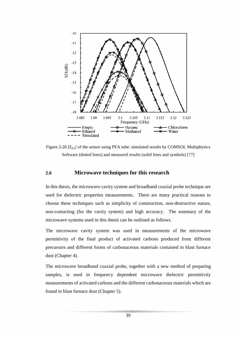
39
Figure 2-26 |𝑆21| of the sensor using PFA tube: simulated results by COMSOL Multiphysics
Software (dotted lines) and measured results (solid lines and symbols) [77]
2.6 Microwave techniques for this research
In this thesis, the microwave cavity system and broadband coaxial probe technique are
used for dielectric properties measurements. There are many practical reasons to
choose these techniques such as simplicity of construction, non-destructive nature,
non-contacting (for the cavity system) and high accuracy. The summary of the
microwave systems used in this thesis can be outlined as follows.
The microwave cavity system was used in measurements of the microwave
permittivity of the final product of activated carbons produced from different
precursors and different forms of carbonaceous materials contained in blast furnace
dust (Chapter 4).
The microwave broadband coaxial probe, together with a new method of preparing
samples, is used in frequency dependent microwave dielectric permittivity
measurements of activated carbons and the different carbonaceous materials which are
found in blast furnace dust (Chapter 5).

40
The microwave cavity system has been incorporated into an oven, with procedures to
calibrate temperature errors, and is thus used in temperature dependent microwave
dielectric permittivity measurements of activated carbons and blast furnace dust
(Chapter 6).
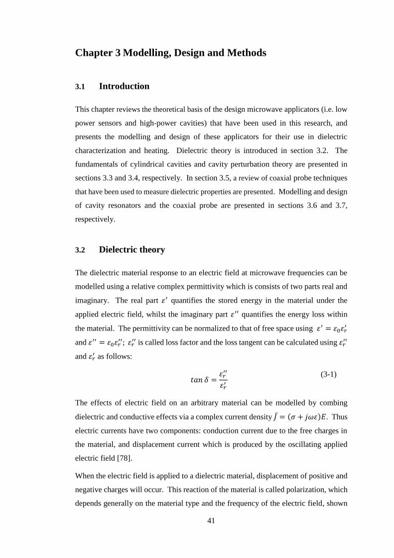
41
Chapter 3 Modelling, Design and Methods
3.1 Introduction
This chapter reviews the theoretical basis of the design microwave applicators (i.e. low
power sensors and high-power cavities) that have been used in this research, and
presents the modelling and design of these applicators for their use in dielectric
characterization and heating. Dielectric theory is introduced in section 3.2. The
fundamentals of cylindrical cavities and cavity perturbation theory are presented in
sections 3.3 and 3.4, respectively. In section 3.5, a review of coaxial probe techniques
that have been used to measure dielectric properties are presented. Modelling and design
of cavity resonators and the coaxial probe are presented in sections 3.6 and 3.7,
respectively.
3.2 Dielectric theory
The dielectric material response to an electric field at microwave frequencies can be
modelled using a relative complex permittivity which is consists of two parts real and
imaginary. The real part 휀′ quantifies the stored energy in the material under the
applied electric field, whilst the imaginary part 휀′′ quantifies the energy loss within
the material. The permittivity can be normalized to that of free space using 휀′ = 휀0휀𝑟′
and 휀′′ = 휀0휀𝑟′′; 휀𝑟
′′ is called loss factor and the loss tangent can be calculated using 휀𝑟′′
and 휀𝑟′ as follows:
𝑡𝑎𝑛 𝛿 =
휀𝑟′′
휀𝑟′
(3-1)
The effects of electric field on an arbitrary material can be modelled by combing
dielectric and conductive effects via a complex current density 𝐽 = (𝜎 + 𝑗𝜔휀)𝐸. Thus
electric currents have two components: conduction current due to the free charges in
the material, and displacement current which is produced by the oscillating applied
electric field [78].
When the electric field is applied to a dielectric material, displacement of positive and
negative charges will occur. This reaction of the material is called polarization, which
depends generally on the material type and the frequency of the electric field, shown
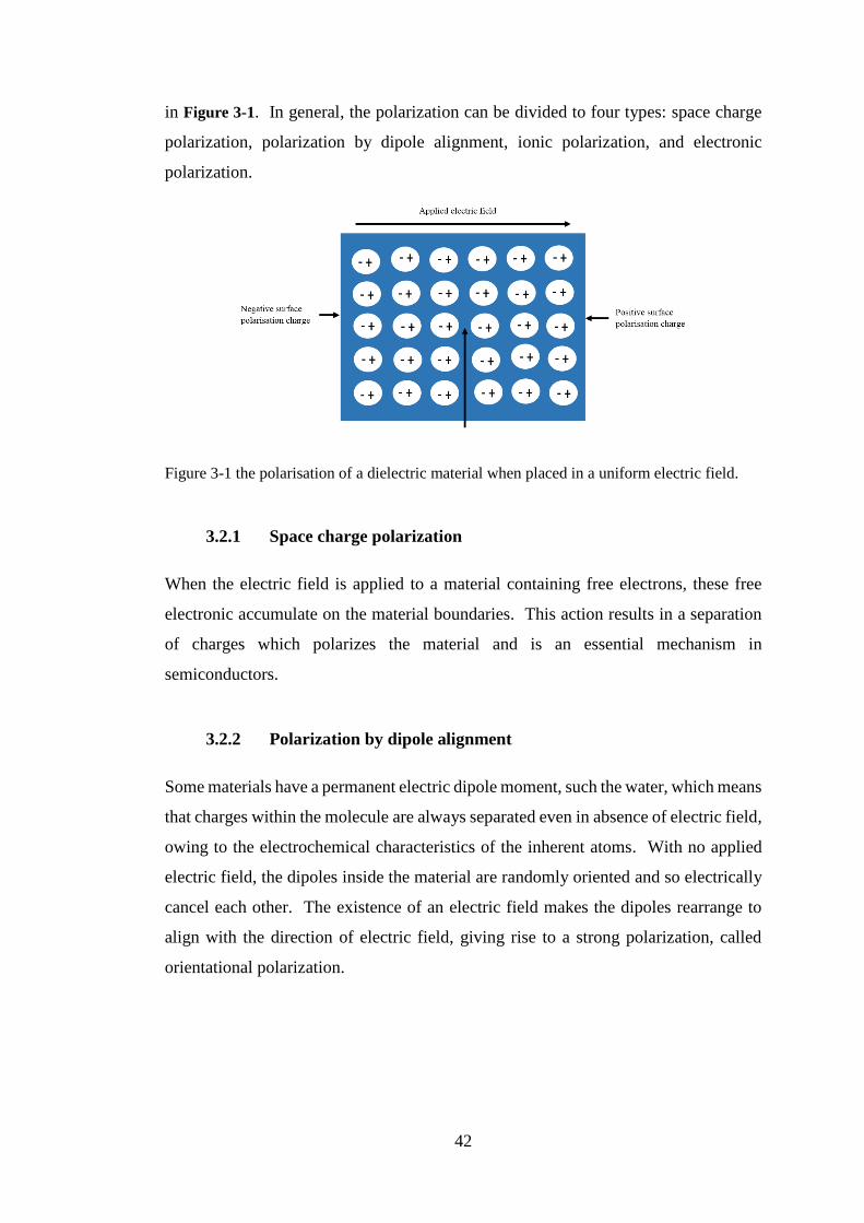
42
in Figure 3-1. In general, the polarization can be divided to four types: space charge
polarization, polarization by dipole alignment, ionic polarization, and electronic
polarization.
Figure 3-1 the polarisation of a dielectric material when placed in a uniform electric field.
3.2.1 Space charge polarization
When the electric field is applied to a material containing free electrons, these free
electronic accumulate on the material boundaries. This action results in a separation
of charges which polarizes the material and is an essential mechanism in
semiconductors.
3.2.2 Polarization by dipole alignment
Some materials have a permanent electric dipole moment, such the water, which means
that charges within the molecule are always separated even in absence of electric field,
owing to the electrochemical characteristics of the inherent atoms. With no applied
electric field, the dipoles inside the material are randomly oriented and so electrically
cancel each other. The existence of an electric field makes the dipoles rearrange to
align with the direction of electric field, giving rise to a strong polarization, called
orientational polarization.
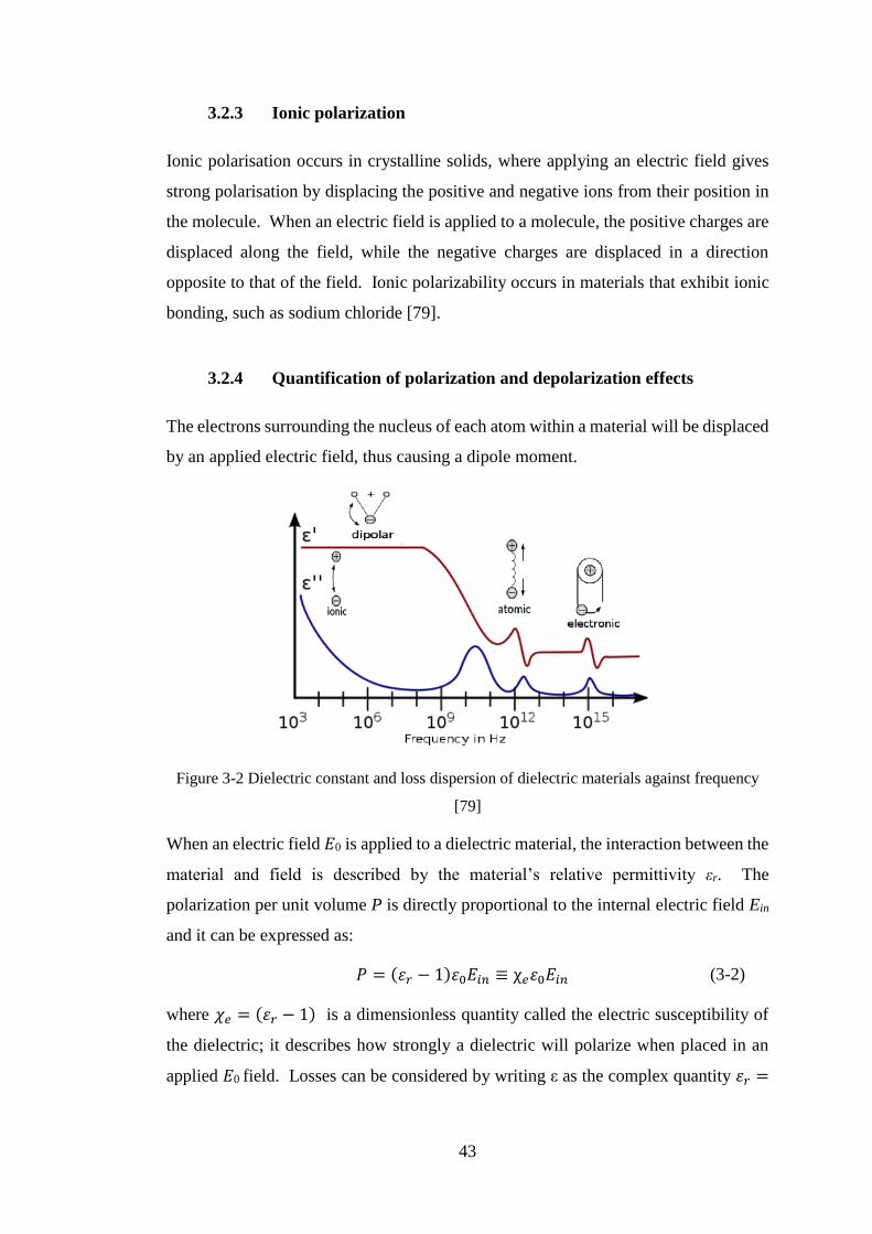
43
3.2.3 Ionic polarization
Ionic polarisation occurs in crystalline solids, where applying an electric field gives
strong polarisation by displacing the positive and negative ions from their position in
the molecule. When an electric field is applied to a molecule, the positive charges are
displaced along the field, while the negative charges are displaced in a direction
opposite to that of the field. Ionic polarizability occurs in materials that exhibit ionic
bonding, such as sodium chloride [79].
3.2.4 Quantification of polarization and depolarization effects
The electrons surrounding the nucleus of each atom within a material will be displaced
by an applied electric field, thus causing a dipole moment.
Figure 3-2 Dielectric constant and loss dispersion of dielectric materials against frequency
[79]
When an electric field 𝐸0 is applied to a dielectric material, the interaction between the
material and field is described by the material’s relative permittivity εr. The
polarization per unit volume P is directly proportional to the internal electric field Ein
and it can be expressed as:
𝑃 = (휀𝑟 − 1)휀0𝐸𝑖𝑛 ≡ χ𝑒휀0𝐸𝑖𝑛 (3-2)
where 𝜒𝑒 = (휀𝑟 − 1) is a dimensionless quantity called the electric susceptibility of
the dielectric; it describes how strongly a dielectric will polarize when placed in an
applied 𝐸0 field. Losses can be considered by writing ε as the complex quantity 휀𝑟 =
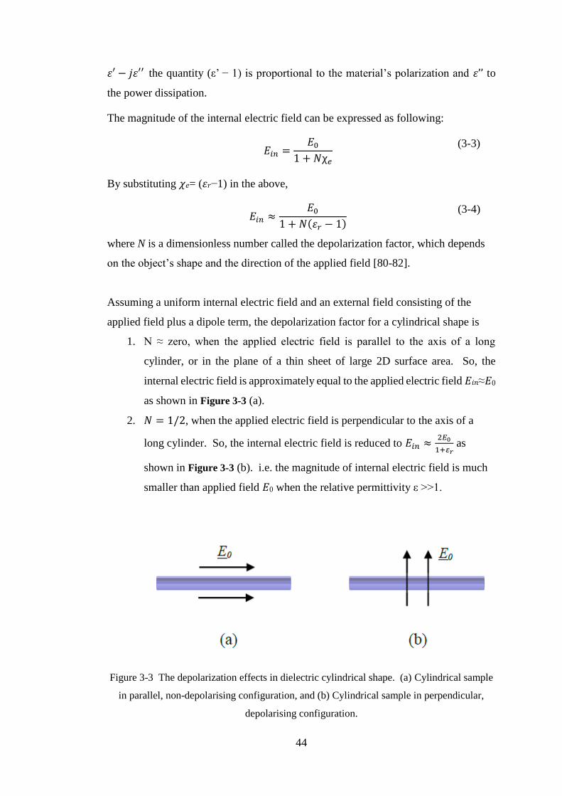
44
휀′ − 𝑗휀′′ the quantity (ε’ − 1) is proportional to the material’s polarization and 휀’’ to
the power dissipation.
The magnitude of the internal electric field can be expressed as following:
𝐸𝑖𝑛 =
𝐸0
1 + 𝑁χ𝑒
(3-3)
By substituting 𝜒𝑒= (휀𝑟−1) in the above,
𝐸𝑖𝑛 ≈
𝐸0
1 + 𝑁(휀𝑟 − 1)
(3-4)
where N is a dimensionless number called the depolarization factor, which depends
on the object’s shape and the direction of the applied field [80-82].
Assuming a uniform internal electric field and an external field consisting of the
applied field plus a dipole term, the depolarization factor for a cylindrical shape is
1. N ≈ zero, when the applied electric field is parallel to the axis of a long
cylinder, or in the plane of a thin sheet of large 2D surface area. So, the
internal electric field is approximately equal to the applied electric field 𝐸𝑖𝑛≈𝐸0
as shown in Figure 3-3 (a).
2. 𝑁 = 1/2, when the applied electric field is perpendicular to the axis of a
long cylinder. So, the internal electric field is reduced to 𝐸𝑖𝑛 ≈2𝐸0
1+𝜀𝑟 as
shown in Figure 3-3 (b). i.e. the magnitude of internal electric field is much
smaller than applied field 𝐸0 when the relative permittivity ε >>1.
Figure 3-3 The depolarization effects in dielectric cylindrical shape. (a) Cylindrical sample
in parallel, non-depolarising configuration, and (b) Cylindrical sample in perpendicular,
depolarising configuration.

45
Therefore, it is desirable to apply and electric field E along the long dimension of the
material sample in applications that require the maximum internal electric field inside
the material. Only in these instances is there maximum polarisation, and so maximum
interaction between the applied electric field and the sample [83].
3.2.5 Penetration Depth
The penetration depth, 𝐷𝑝, the depth to which the field penetrates to 1/e ≈ 37% of its
surface value, is a measure of the depth of microwave penetration in a dielectric
material. It is mathematically defined as[84]:
𝐷𝜌 =𝜆0
2𝜋(2휀′)1
2⁄[1 + (
휀′′
휀′)
2
]
12⁄
− 1
−12⁄
(3-5)
where 𝜆 is the free space wavelength of incident radiation. From (3-5), the penetration
depth increases with an increase in the wavelength or a decrease in the frequency. The
penetration depth is also approximately inversely proportional to the values of 휀′ and
휀′′.
Due to the short wavelength of microwaves (of the order of centimetres), they
penetrate quite deeply within non-metals, so keeping the resonator perturbation
principle preserved. Accordingly, the volumetric material properties can be deduced,
e.g. moisture content, since microwaves are not restricted to the surface of the tested
material [84-86]. Table 3-1 shows the relative permittivity (real part) of selected
materials and the field penetration depth at a frequency of 3 GHz
Table 3-1 values of penetration depth for some dielectric materials
Material T [ºC] 𝜺𝒓 Dp [m]
Water 25 76.7 0.023
Ice -12 3.20 19.77
Polystyrene 25 2.55 60.42
Teflon 22 2.10 146.44
Table salt 25 2.26 32.62
Fused quartz 25 3.78 246.91
46
Taking the opposite extreme of a weakly conducting dielectric, the skin depth δ of a
good conductor is expressed as
𝛿 = √2
𝜔𝜇𝜎= √
2𝜌
𝜔𝜇
(3-6)
where 𝜇 is the permeability of the material in H/m, 𝜇=𝜇0𝜇𝑟, σ is the conductivity in S/m
and ρ is the resistivity in Ωm. The skin depth according to (3-7) is a function of three
variables; conductivity (or resistivity), permeability, and frequency of operation. Since
𝜇𝑟≈1 for most metals, the skin depth can be re-written as:
𝛿 = √2
𝜔𝜇0𝜎= √
2𝜌
𝜔𝜇0
(3-7)
At microwave frequencies, the skin depth for good conductors is extremely small
(around 1μm), and so a very thin coating of a good conductor such as gold or silver is
necessary to realize low-loss microwave components [2, 87].
3.2.6 Effect of electronic conductivity on microwave loss
Conductivity introduces an energy loss mechanism owing to the scattering of mobile
charges in an applied electric field. This introduces a characteristic term in the imaginary
permittivity which is inversely proportional to frequency and directly proportional to the
conductivity, as shown in (3-8).
휀 = 휀′ − 𝑗휀′′ (3-8)
휀′′ = 휀𝑑′′ + 휀𝜎
′′ = 휀𝑑′′ +
𝜎
휀0𝜔 (3-9)
The subscripts d and s stand for contributions due to the lattice of a material and
electronic conduction, respectively. At low frequencies, ε is dominated by the
influence of conductivity, while the variation of permittivity in the microwave range
is mainly caused by lattice (dipolar) relaxation effects. At microwave frequencies,
dipolar polarization is dominant at lower frequencies while electronic and atomic
polarizations are dominant at higher frequencies. For electrolytes, the latter is related
to the ionic concentration of solutions (i.e. their conductivity) which is also then
inversely dependent on frequency.

47
3.2.7 Dielectric Relaxation
Relaxation of a dielectric is a phenomenon that normally happens immediately after
removing the applied electric field, the charges take a finite time to return to their
natural positions. The time which is taken by material’s charges to return to their
normal order is called the relaxation time [60, 88].
There are different relaxation models for dielectrics, such as that of Debye, leading to
the Cole-Cole equations [80]. Debye’s theory shows the relation between complex
permittivity and relaxation time, namely, as the relaxation time increases, the
permittivity decreases. Debye’s equation can be expressed as follows:
휀 = 휀′ − 𝑗휀′′ = 휀∞ +휀𝑠 − 휀∞
1 + 𝑗𝜔𝜏 (3-10)
Therefore, the real and imaginary parts can be separated as follows:
휀′ = 휀∞ +
휀𝑠 − 휀∞
1 + 𝑗(𝜔𝜏)2 , 휀′′ =
(휀𝑠 − 휀∞)𝜔𝜏
1 + 𝑗(𝜔𝜏)2
(3-11)
where 휀∞ is the permittivity at high frequency (infinity), 휀𝑠 is the permittivity at low
frequency (static), 𝜔 is the angular frequency and 𝜏 is the relaxation time (a constant).
Practically, liquids and solids tend to have more extended distributions for permittivity
than the Debye equation shows because of the different origins of the relaxation
phenomenon, and also given the fact that the materials might have a relaxation
spectrum. This can be demonstrated mathematically by adding the empirical exponent
parameter α to the Debye equation, as in the following form [60, 89].
휀 = 휀∞ +휀𝑠 − 휀∞
1 + (𝑗𝜔𝜏)1−𝛼 (3-12)
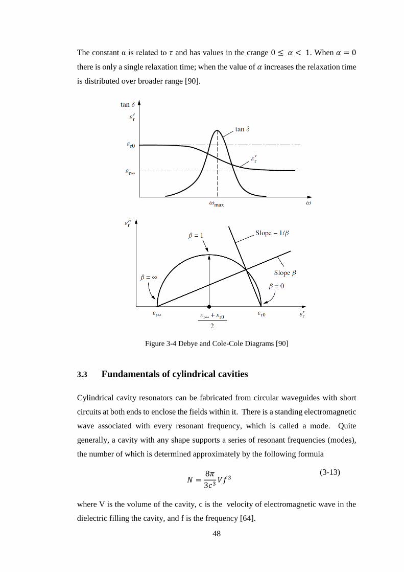
48
The constant α is related to 𝜏 and has values in the crange 0 ≤ 𝛼 < 1. When 𝛼 = 0
there is only a single relaxation time; when the value of 𝛼 increases the relaxation time
is distributed over broader range [90].
Figure 3-4 Debye and Cole-Cole Diagrams [90]
3.3 Fundamentals of cylindrical cavities
Cylindrical cavity resonators can be fabricated from circular waveguides with short
circuits at both ends to enclose the fields within it. There is a standing electromagnetic
wave associated with every resonant frequency, which is called a mode. Quite
generally, a cavity with any shape supports a series of resonant frequencies (modes),
the number of which is determined approximately by the following formula
𝑁 =
8𝜋
3𝑐3𝑉𝑓3
(3-13)
where V is the volume of the cavity, c is the velocity of electromagnetic wave in the
dielectric filling the cavity, and f is the frequency [64].
49
Resonant modes occur when the electric and magnetic fields form standing waves,
with resonant frequencies which depend on the internal dimensions of the cavity and
dielectric properties of the material contained within the cavity. The transverse electric
(TE) and transverse magnetic (TM) are the two types of modes which exist in a cavity
with only metal walls.
The TE modes in cylindrical cavity of radius (a) and length (d) and the propagation
constant of the 𝑇𝐸𝑛𝑚𝑙 mode can be expressed as:
𝐸𝑡 = 𝐸(𝜌, ϕ)(𝐴+𝑒−𝑗𝛽𝑛𝑚𝑧 + 𝐴−𝑒+𝑗𝛽𝑛𝑚𝑧)𝑒𝑗𝜔𝑡 (3-14)
𝛽𝑛𝑚 = √𝑘2 − (𝑝𝑛𝑚
′
𝑎)
2
(3-15)
where 𝑘 = 𝜔√𝜇𝜖. Applying the field boundary conditions (𝐸𝑡 = 0 at 𝑧 = 0 and 𝑑)
leads to the conditions 𝐴+ = −𝐴− and 𝐴+𝑠𝑖𝑛𝛽𝑛𝑚𝑑 = 𝑙𝜋, for 𝑙=0, 1, 2, 3 . . . where 𝑙
is the integer number of half-guide wavelengths along the cavity length. The resonant
frequency of the 𝑇𝐸𝑛𝑚𝑙 mode can be written as in equation(3-16) [2].
𝑓𝑛𝑚𝑙 =𝑐
2𝜋√𝜇𝑟휀𝑟
√(𝑝𝑛𝑚
′
𝑎)
2
+ (𝑙𝜋
𝑑)
2
(3-16)
The propagation constant and resonant frequency of the 𝑇𝑀𝑛𝑚𝑙 mode is [2]
𝛽𝑛𝑚 = √𝑘2 − (𝑝𝑛𝑚
𝑎)
2
(3-17)
𝑓𝑛𝑚𝑙 =𝑐
2𝜋√𝜇𝑟휀𝑟
√(𝑝𝑛𝑚
𝑎)
2
+ (𝑙𝜋
𝑑)
2
(3-18)
The parameters introduced in these equations are as follows:
𝑓𝑛𝑚ℓ is the operation frequency of the cylindrical cavity resonator.
𝑐 is the speed of light in vacuum, i.e. 3×10⁸ m/s
𝜇𝑟 is the relative permeability of the material inside the cylindrical cavity resonator
휀𝑟 is the relative permittivity of the material inside the cylindrical cavity resonator
The values of 𝑝𝑛𝑚 and 𝑝’𝑛m are listed below in Table 3-2 and Table 3.3 respectively [2].
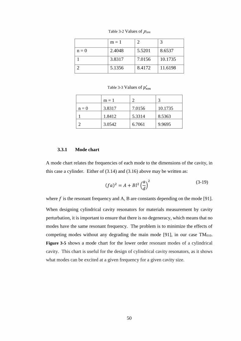
50
Table 3-2 Values of 𝑝𝑛𝑚
m = 1 2 3
n = 0 2.4048 5.5201 8.6537
1 3.8317 7.0156 10.1735
2 5.1356 8.4172 11.6198
Table 3-3 Values of 𝑝𝑛𝑚′
m = 1 2 3
n = 0 3.8317 7.0156 10.1735
1 1.8412 5.3314 8.5363
2 3.0542 6.7061 9.9695
3.3.1 Mode chart
A mode chart relates the frequencies of each mode to the dimensions of the cavity, in
this case a cylinder. Either of (3.14) and (3.16) above may be written as:
(𝑓𝑎)2 = 𝐴 + 𝐵𝑙2 (
𝑎
𝑑)
2
(3-19)
where 𝑓 is the resonant frequency and A, B are constants depending on the mode [91].
When designing cylindrical cavity resonators for materials measurement by cavity
perturbation, it is important to ensure that there is no degeneracy, which means that no
modes have the same resonant frequency. The problem is to minimize the effects of
competing modes without any degrading the main mode [91], in our case TM010.
Figure 3-5 shows a mode chart for the lower order resonant modes of a cylindrical
cavity. This chart is useful for the design of cylindrical cavity resonators, as it shows
what modes can be excited at a given frequency for a given cavity size.

51
Figure 3-5 Resonant mode chart for a cylindrical cavity [2]
3.3.2 Quality factor
The quality factor is the ratio of the stored energy and the energy losses per cycle in
the metal walls of the cavity, which is defined as
𝑄 =
2𝜋𝑓 (𝑒𝑛𝑒𝑟𝑔𝑦 𝑠𝑡𝑜𝑟𝑒𝑑 𝑖𝑛 𝑡ℎ𝑒 𝑐𝑎𝑣𝑖𝑡𝑦)
𝑝𝑜𝑤𝑒𝑟 𝑙𝑜𝑠𝑡= 𝜔0
𝑢
𝑝𝑙𝑜𝑠𝑠
(3-20)
Q represents the quality factor without any load (external circuits), ω0 is the angular
resonant frequency. When a cavity resonator is connected to external circuits, which
have their own effective quality factor 𝑄𝑒𝑥𝑡 since the coupling effectively causes a
leakage (i.e. loss) of energy, the total, measured quality factor 𝑄𝑡 becomes as in (3-21).
1
𝑄𝑡=
1
𝑄+
1
𝑄𝑒𝑥𝑡 and 𝑄𝑡 =
𝑓0
∆𝑓
(3-21)
where 𝑓0 is the centre frequency, ∆𝑓 is the shift of resonant frequency.
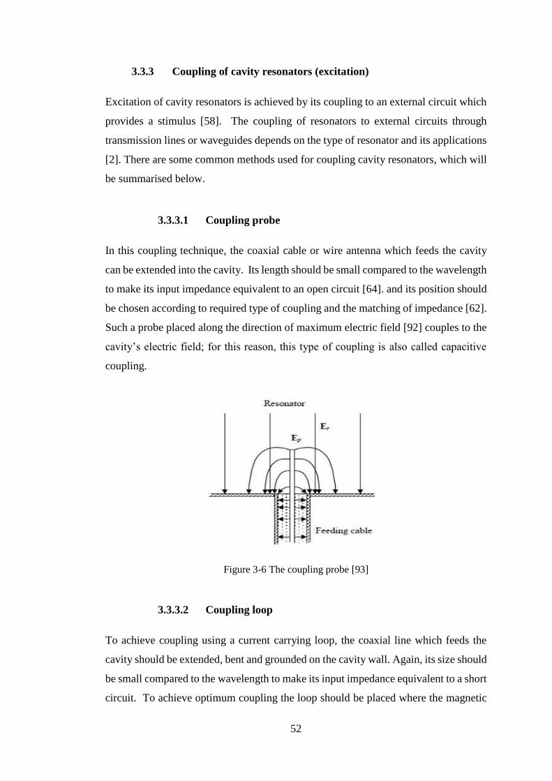
52
3.3.3 Coupling of cavity resonators (excitation)
Excitation of cavity resonators is achieved by its coupling to an external circuit which
provides a stimulus [58]. The coupling of resonators to external circuits through
transmission lines or waveguides depends on the type of resonator and its applications
[2]. There are some common methods used for coupling cavity resonators, which will
be summarised below.
3.3.3.1 Coupling probe
In this coupling technique, the coaxial cable or wire antenna which feeds the cavity
can be extended into the cavity. Its length should be small compared to the wavelength
to make its input impedance equivalent to an open circuit [64]. and its position should
be chosen according to required type of coupling and the matching of impedance [62].
Such a probe placed along the direction of maximum electric field [92] couples to the
cavity’s electric field; for this reason, this type of coupling is also called capacitive
coupling.
Figure 3-6 The coupling probe [93]
3.3.3.2 Coupling loop
To achieve coupling using a current carrying loop, the coaxial line which feeds the
cavity should be extended, bent and grounded on the cavity wall. Again, its size should
be small compared to the wavelength to make its input impedance equivalent to a short
circuit. To achieve optimum coupling the loop should be placed where the magnetic
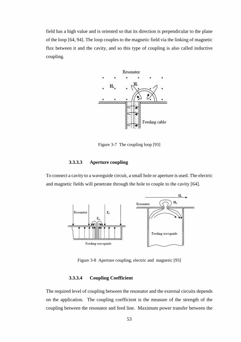
53
field has a high value and is oriented so that its direction is perpendicular to the plane
of the loop [64, 94]. The loop couples to the magnetic field via the linking of magnetic
flux between it and the cavity, and so this type of coupling is also called inductive
coupling.
Figure 3-7 The coupling loop [93]
3.3.3.3 Aperture coupling
To connect a cavity to a waveguide circuit, a small hole or aperture is used. The electric
and magnetic fields will penetrate through the hole to couple to the cavity [64].
Figure 3-8 Aperture coupling, electric and magnetic [93]
3.3.3.4 Coupling Coefficient
The required level of coupling between the resonator and the external circuits depends
on the application. The coupling coefficient is the measure of the strength of the
coupling between the resonator and feed line. Maximum power transfer between the
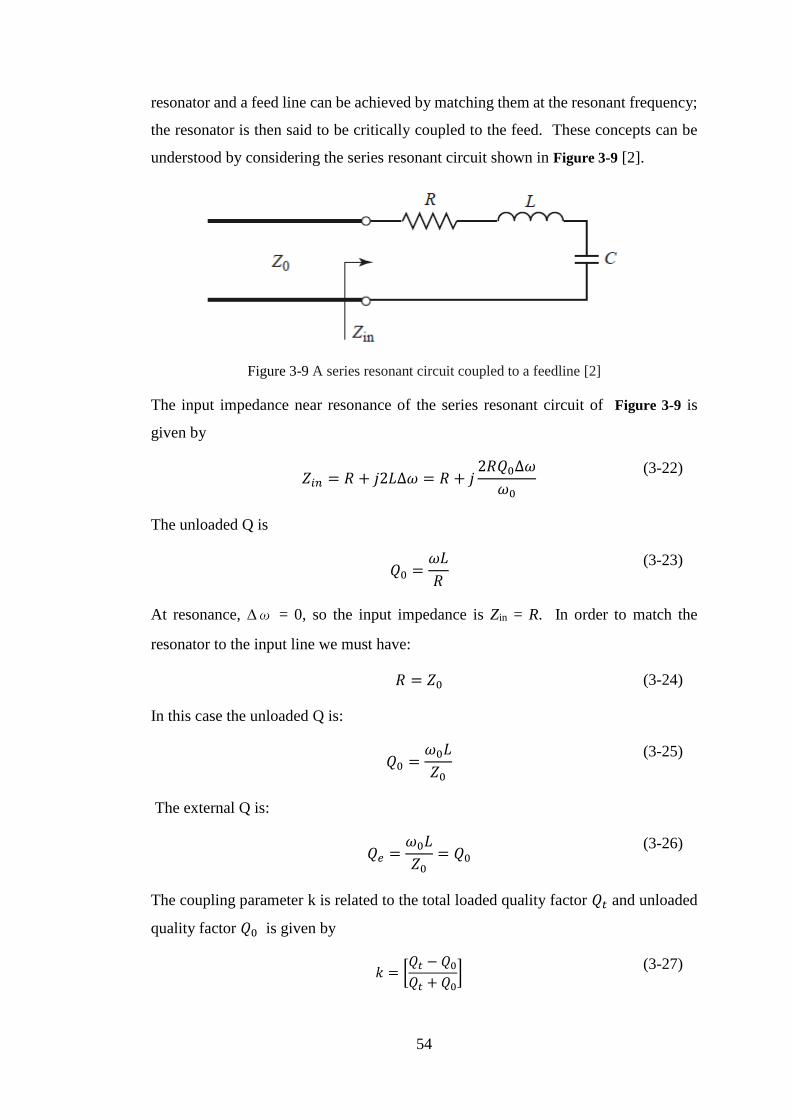
54
resonator and a feed line can be achieved by matching them at the resonant frequency;
the resonator is then said to be critically coupled to the feed. These concepts can be
understood by considering the series resonant circuit shown in Figure 3-9 [2].
Figure 3-9 A series resonant circuit coupled to a feedline [2]
The input impedance near resonance of the series resonant circuit of Figure 3-9 is
given by
𝑍𝑖𝑛 = 𝑅 + 𝑗2𝐿∆𝜔 = 𝑅 + 𝑗
2𝑅𝑄0∆𝜔
𝜔0
(3-22)
The unloaded Q is
𝑄0 =
𝜔𝐿
𝑅
(3-23)
At resonance, ∆ω = 0, so the input impedance is Zin = R. In order to match the
resonator to the input line we must have:
𝑅 = 𝑍0 (3-24)
In this case the unloaded Q is:
𝑄0 =
𝜔0𝐿
𝑍0
(3-25)
The external Q is:
𝑄𝑒 =
𝜔0𝐿
𝑍0= 𝑄0
(3-26)
The coupling parameter k is related to the total loaded quality factor 𝑄𝑡 and unloaded
quality factor 𝑄0 is given by
𝑘 = [
𝑄𝑡 − 𝑄0
𝑄𝑡 + 𝑄0]
(3-27)

55
The higher the value of loaded Q, the lower the value of the coupling parameter. The
coupling coefficient g is defined to be
𝑔 =
𝑄0
𝑄𝑒𝑥𝑡
(3-28)
Both the coupling parameter k and coupling coefficient g should be low to obtain
higher loaded quality factor [95]. In the following discussion we will refer to the
coupling coefficient g (rather than k).
There are three cases of coupling levels, which are:
• Under coupling when 𝑔 < 1
• Critically coupling 𝑔 = 1 (resonator is matched to its input line)
• Over coupling 𝑔 < 1
3.3.4 Network analyser and scattering parameters
Scattering parameters can be measured using a network analyser at different
frequencies. A network analyser mainly consists of a source, used to generate a known
signal, and receiver used to determine changes to this signal caused by the material-
under-test. They are capable of measuring transmitted (S21) and reflected (S11) signals,
expressed as voltage transmission or reflection coefficients. Equations defining the
full set of four scattering parameters of a two port network (e.g. a two port cavity) are
expressed in (3-29) to (3-32).
𝑠11(𝑓𝑜𝑟𝑤𝑎𝑟𝑑 ) =𝑟𝑒𝑓𝑙𝑒𝑐𝑡𝑒𝑑
𝑖𝑛𝑐𝑖𝑑𝑒𝑛𝑡=
𝑏1
𝑎1𝑎2=0 (3-29)
𝑠21(𝑓𝑜𝑟𝑤𝑎𝑟𝑑 ) =𝑡𝑟𝑎𝑛𝑠𝑚𝑖𝑡𝑡𝑒𝑑
𝑖𝑛𝑐𝑖𝑑𝑒𝑛𝑡=
𝑏2
𝑎1𝑎2=0 (3-30)
𝑠22(𝑟𝑒𝑣𝑒𝑟𝑠𝑒 ) =𝑟𝑒𝑓𝑙𝑒𝑐𝑡𝑒𝑑
𝑖𝑛𝑐𝑖𝑑𝑒𝑛𝑡=
𝑏2
𝑎2𝑎1=0 (3-31)
𝑠12(𝑟𝑒𝑣𝑒𝑟𝑠𝑒) =𝑡𝑟𝑎𝑛𝑚𝑖𝑡𝑡𝑒𝑑
𝑖𝑛𝑐𝑖𝑑𝑒𝑛𝑡=
𝑏1
𝑎2𝑎1=0 (3-32)
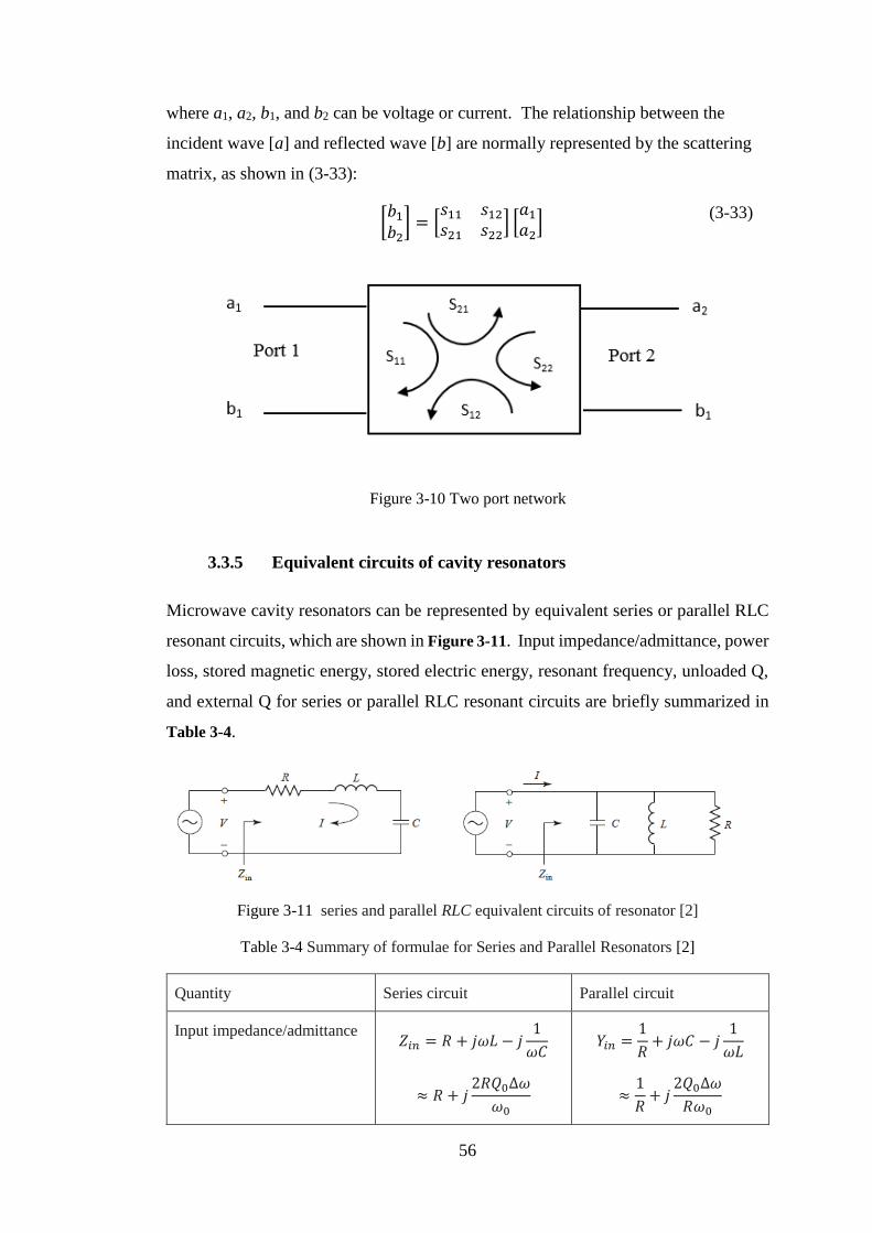
56
where a1, a2, b1, and b2 can be voltage or current. The relationship between the
incident wave [a] and reflected wave [b] are normally represented by the scattering
matrix, as shown in (3-33):
[𝑏1
𝑏2] = [
𝑠11 𝑠12
𝑠21 𝑠22] [
𝑎1
𝑎2]
(3-33)
Figure 3-10 Two port network
3.3.5 Equivalent circuits of cavity resonators
Microwave cavity resonators can be represented by equivalent series or parallel RLC
resonant circuits, which are shown in Figure 3-11. Input impedance/admittance, power
loss, stored magnetic energy, stored electric energy, resonant frequency, unloaded Q,
and external Q for series or parallel RLC resonant circuits are briefly summarized in
Table 3-4.
Figure 3-11 series and parallel RLC equivalent circuits of resonator [2]
Table 3-4 Summary of formulae for Series and Parallel Resonators [2]
Quantity Series circuit Parallel circuit
Input impedance/admittance 𝑍𝑖𝑛 = 𝑅 + 𝑗𝜔𝐿 − 𝑗
1
𝜔𝐶
≈ 𝑅 + 𝑗2𝑅𝑄0∆𝜔
𝜔0
𝑌𝑖𝑛 =1
𝑅+ 𝑗𝜔𝐶 − 𝑗
1
𝜔𝐿
≈1
𝑅+ 𝑗
2𝑄0∆𝜔
𝑅𝜔0
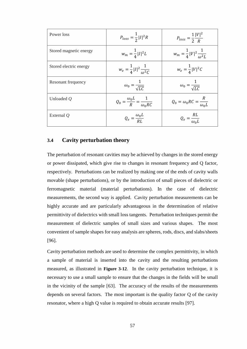
57
Power loss 𝑃𝑙𝑜𝑠𝑠 =
1
2|𝐼|2𝑅 𝑃𝑙𝑜𝑠𝑠 =
1
2
|𝑉|2
𝑅
Stored magnetic energy 𝑤𝑚 =
1
4|𝐼|2𝐿 𝑤𝑚 =
1
4|𝑉|2
1
𝜔2𝐿
Stored electric energy 𝑤𝑒 =
1
4|𝐼|2
1
𝜔2𝐶 𝑤𝑒 =
1
4|𝑉|2𝐶
Resonant frequency 𝜔0 =
1
√𝐿𝐶 𝜔0 =
1
√𝐿𝐶
Unloaded Q 𝑄0 =
𝜔0𝐿
𝑅=
1
𝜔0𝑅𝐶 𝑄0 = 𝜔0𝑅𝐶 =
𝑅
𝜔0𝐿
External Q 𝑄𝑒 =
𝜔0𝐿
𝑅𝐿 𝑄𝑒 =
𝑅𝐿
𝜔0𝐿
3.4 Cavity perturbation theory
The perturbation of resonant cavities may be achieved by changes in the stored energy
or power dissipated, which give rise to changes in resonant frequency and Q factor,
respectively. Perturbations can be realized by making one of the ends of cavity walls
movable (shape perturbations), or by the introduction of small pieces of dielectric or
ferromagnetic material (material perturbations). In the case of dielectric
measurements, the second way is applied. Cavity perturbation measurements can be
highly accurate and are particularly advantageous in the determination of relative
permittivity of dielectrics with small loss tangents. Perturbation techniques permit the
measurement of dielectric samples of small sizes and various shapes. The most
convenient of sample shapes for easy analysis are spheres, rods, discs, and slabs/sheets
[96].
Cavity perturbation methods are used to determine the complex permittivity, in which
a sample of material is inserted into the cavity and the resulting perturbations
measured, as illustrated in Figure 3-12. In the cavity perturbation technique, it is
necessary to use a small sample to ensure that the changes in the fields will be small
in the vicinity of the sample [63]. The accuracy of the results of the measurements
depends on several factors. The most important is the quality factor Q of the cavity
resonator, where a high Q value is required to obtain accurate results [97].

58
Figure 3-12 A dielectric material, in the form of a thin rod, measured using a cylindrical host
cavity resonator [64]
The cavity’s material perturbations are considered as a means of measuring material
properties by analysis of the shift in the (complex) resonant frequency when the
dielectric material sample is inserted into the cavity [2, 64].
Figure 3-13 a resonant cavity perturbed by a changing in the permittivity or permeability of
the materials in the cavity. (a) Original cavity. (b) Perturbed cavity [2]
We assume that the material inside the cavity resonator has permittivity ε and
permeability µ. The subscript “0” is used to denote the resonant frequency and EM
fields of the cavity before the perturbation. Maxwell’s time-dependent equations can
then be written as
𝛻 × 𝐸0 = −𝑗𝜔0𝜇𝐻0
(3-34)
𝛻 × 𝐻0 = 𝑗𝜔0𝜖𝐸0
(3-35)
𝛻 × E = −𝑗𝜔(𝜇 + ∆𝜇)H (3-36)
𝛻 × H = 𝑗𝜔(𝜖 + ∆𝜖)E (3-37)
where ∆𝜖 and ∆𝜇 are the changes in permittivity and permeability [98].

59
We next take the scalar product of the conjugate of (3-34) with , and the scalar
product of (3-35) with 𝐸0∗ . Subtracting the results and using the vector identity
𝛻. ( × ) = . 𝛻 × − 𝐴. 𝛻 × gives
𝛻 ∙ (𝐸0∗ × ) = 𝑗𝜔0𝜇 ∙ 𝐻0
∗ − 𝑗𝜔(𝜖 + ∆𝜖)𝐸0∗ ∙ (3-38)
Repeating the same procedures on (3-35) and (3-36), we obtain (3-39)
𝛻 ∙ ( × 𝐻0∗ ) = −𝑗𝜔0(𝜇 + ∆𝜇)𝐻0
∗ . − 𝑗𝜔0𝐸0∗ ∙ (3-39)
By adding (3-38) and (3-39), integrating over the volume 𝑉0, and applying the
divergence theorem we get
∫𝑣0
𝛻 ∙ (𝐸0∗ × + × 𝐻0
∗ )𝑑𝑣 = ∫𝑠0
(𝐸0∗ × + × 𝐻0
∗ ). 𝑑𝑠
= 𝑗∫𝑣0
[𝜔0𝜖 − 𝜔(𝜖 + ∆𝜖)]𝐸0∗ . + [𝜔0𝜇 − 𝜔(𝜇∆𝜇)]𝐻0
∗ . 𝑑𝑣
(3-40)
As long as × = 0, the integrals over the cavity surfaces give zero, hence.
𝜔 − 𝜔0
𝜔=
−∭ (∆𝜖. 𝐸0∗ + ∆𝜇. 𝐻0
∗ )𝑑𝑣
∭ (𝜖. 𝐸0∗ + 𝜇. 𝐻0
∗ )𝑑𝑣
(3-41)
Assuming ∆𝜖 and ∆𝜇 are very small, E and H can be approximated by 𝐸0 and 𝐻0
; i.e.
the unperturbed fields. Thus
𝜔 − 𝜔0
𝜔0=
−∭ (∆𝜖|0|2 + ∆𝜇|0|2)𝑑𝑣
∭ (𝜖|0|2 + 𝜇|0|2)𝑑𝑣
(3-42)
From equation (3-12) and (3-18), it is clear that the resonant frequency will reduce in
proportion to increases in ε and µ. Equation (3-42) determines the change in centre
frequency of a resonator when a sample is inserted inside it.
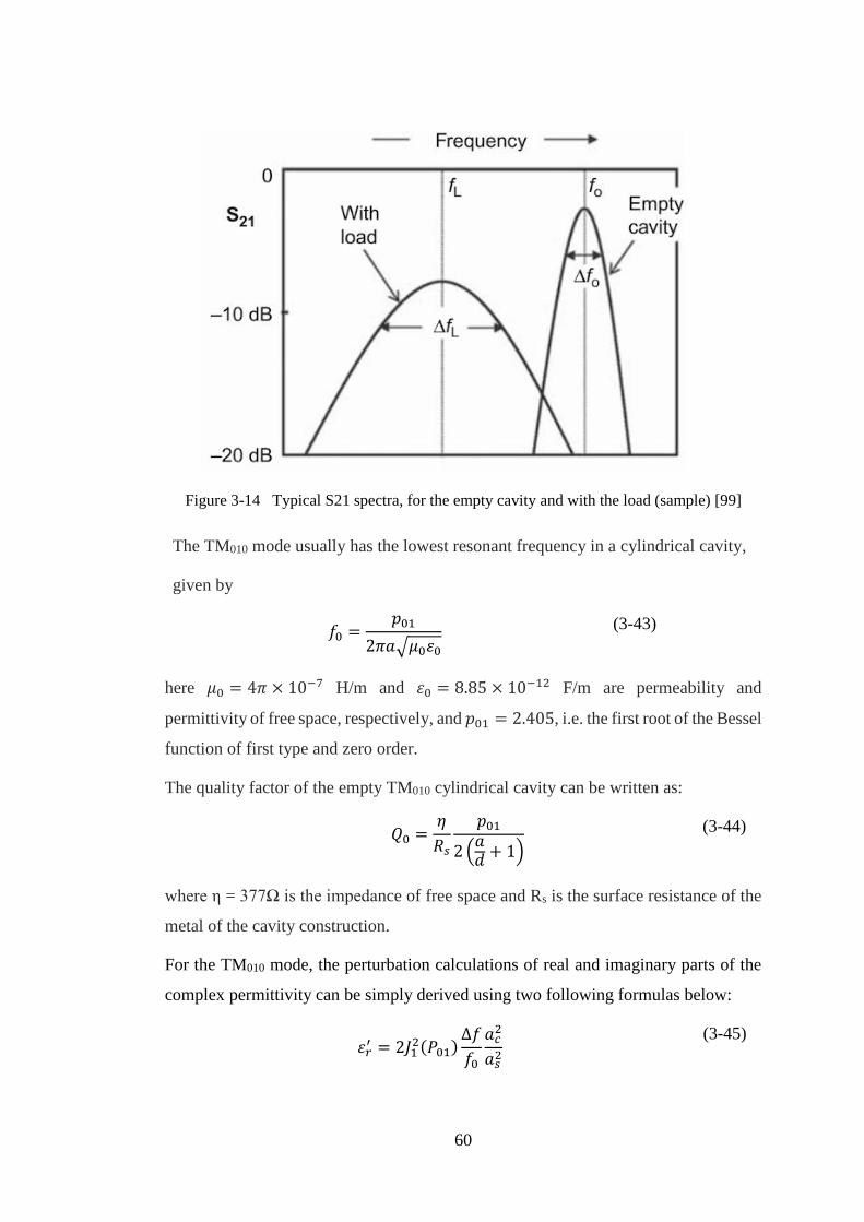
60
Figure 3-14 Typical S21 spectra, for the empty cavity and with the load (sample) [99]
The TM010 mode usually has the lowest resonant frequency in a cylindrical cavity,
given by
𝑓0 =𝑝01
2𝜋𝑎√𝜇0휀0
(3-43)
here 𝜇0 = 4𝜋 × 10−7 H/m and 휀0 = 8.85 × 10⁻¹² F/m are permeability and
permittivity of free space, respectively, and 𝑝01 = 2.405, i.e. the first root of the Bessel
function of first type and zero order.
The quality factor of the empty TM010 cylindrical cavity can be written as:
𝑄0 =𝜂
𝑅𝑠
𝑝01
2 (𝑎𝑑
+ 1) (3-44)
where η = 377Ω is the impedance of free space and Rs is the surface resistance of the
metal of the cavity construction.
For the TM010 mode, the perturbation calculations of real and imaginary parts of the
complex permittivity can be simply derived using two following formulas below:
휀𝑟
′ = 2𝐽12(𝑃01)
∆𝑓
𝑓0
𝑎𝑐2
𝑎𝑠2
(3-45)
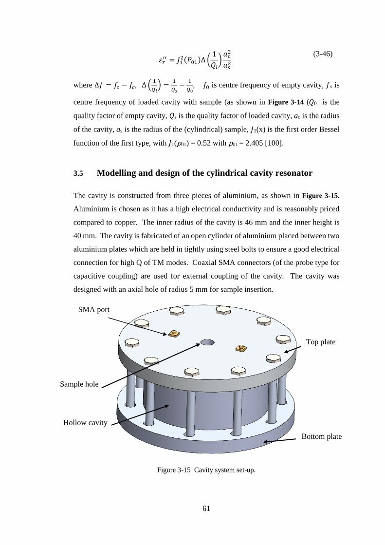
61
휀𝑟
′′ = 𝐽12(𝑃01)∆ (
1
𝑄𝑙)
𝑎𝑐2
𝑎𝑠2
(3-46)
where ∆𝑓 = 𝑓𝑐 − 𝑓𝑐, ∆ (1
𝑄𝑙) =
1
𝑄𝑠−
1
𝑄0, 𝑓0 is centre frequency of empty cavity, 𝑓s is
centre frequency of loaded cavity with sample (as shown in Figure 3-14 )𝑄0 is the
quality factor of empty cavity, 𝑄s is the quality factor of loaded cavity, ac is the radius
of the cavity, as is the radius of the (cylindrical) sample, 𝐽1(x) is the first order Bessel
function of the first type, with 𝐽1(p01) = 0.52 with p01 = 2.405 [100].
3.5 Modelling and design of the cylindrical cavity resonator
The cavity is constructed from three pieces of aluminium, as shown in Figure 3-15.
Aluminium is chosen as it has a high electrical conductivity and is reasonably priced
compared to copper. The inner radius of the cavity is 46 mm and the inner height is
40 mm. The cavity is fabricated of an open cylinder of aluminium placed between two
aluminium plates which are held in tightly using steel bolts to ensure a good electrical
connection for high Q of TM modes. Coaxial SMA connectors (of the probe type for
capacitive coupling) are used for external coupling of the cavity. The cavity was
designed with an axial hole of radius 5 mm for sample insertion.
Figure 3-15 Cavity system set-up.
SMA port
Sample hole
Hollow cavity
Top plate
Bottom plate
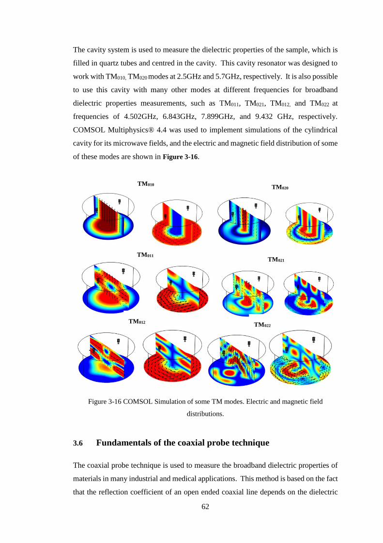
62
The cavity system is used to measure the dielectric properties of the sample, which is
filled in quartz tubes and centred in the cavity. This cavity resonator was designed to
work with TM010, TM020 modes at 2.5GHz and 5.7GHz, respectively. It is also possible
to use this cavity with many other modes at different frequencies for broadband
dielectric properties measurements, such as TM011, TM021, TM012, and TM022 at
frequencies of 4.502GHz, 6.843GHz, 7.899GHz, and 9.432 GHz, respectively.
COMSOL Multiphysics® 4.4 was used to implement simulations of the cylindrical
cavity for its microwave fields, and the electric and magnetic field distribution of some
of these modes are shown in Figure 3-16.
Figure 3-16 COMSOL Simulation of some TM modes. Electric and magnetic field
distributions.
3.6 Fundamentals of the coaxial probe technique
The coaxial probe technique is used to measure the broadband dielectric properties of
materials in many industrial and medical applications. This method is based on the fact
that the reflection coefficient of an open ended coaxial line depends on the dielectric
TM010
TM022
TM012
TM020
TM021
TM011
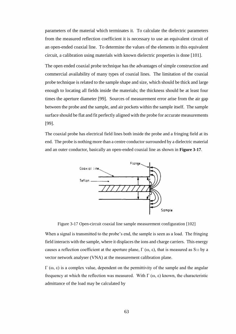
63
parameters of the material which terminates it. To calculate the dielectric parameters
from the measured reflection coefficient it is necessary to use an equivalent circuit of
an open-ended coaxial line. To determine the values of the elements in this equivalent
circuit, a calibration using materials with known dielectric properties is done [101].
The open ended coaxial probe technique has the advantages of simple construction and
commercial availability of many types of coaxial lines. The limitation of the coaxial
probe technique is related to the sample shape and size, which should be thick and large
enough to locating all fields inside the materials; the thickness should be at least four
times the aperture diameter [99]. Sources of measurement error arise from the air gap
between the probe and the sample, and air pockets within the sample itself. The sample
surface should be flat and fit perfectly aligned with the probe for accurate measurements
[99].
The coaxial probe has electrical field lines both inside the probe and a fringing field at its
end. The probe is nothing more than a centre conductor surrounded by a dielectric material
and an outer conductor, basically an open-ended coaxial line as shown in Figure 3-17.
Figure 3-17 Open-circuit coaxial line sample measurement configuration [102]
When a signal is transmitted to the probe’s end, the sample is seen as a load. The fringing
field interacts with the sample, where it displaces the ions and charge carriers. This energy
causes a reflection coefficient at the aperture plane, Γ (ω, ε), that is measured as S11 by a
vector network analyser (VNA) at the measurement calibration plane.
Γ (ω, ε) is a complex value, dependent on the permittivity of the sample and the angular
frequency at which the reflection was measured. With Γ (ω, ε) known, the characteristic
admittance of the load may be calculated by

64
𝑌𝐿(𝜔, 휀) = 𝑌0
1 − Γ(𝜔, 휀)
1 + Γ(𝜔, 휀)
(3-47)
where Y0 is the probe’s characteristic admittance. With YL(ω,ε) calculated, complex
permittivity may be found from (3-47) by using an appropriate inversion process
𝑌𝐿(𝜔, 휀) = 𝑗𝜔𝐶1 + 𝑗𝐴𝜔3휀2 + 𝐵𝜔4휀2.5 (3-48)
where A and B are constants dependent on the dimensions of the aperture.
The complex permittivity of the samples can be extracted using a capacitive model
which is shown in Figure 3-18. The complex permittivity can be calculated from
measured reflected coefficient S11 from the reflected signal using (3-50).
Figure 3-18 Equivalent circuit of an open-ended coaxial probe
When a dielectric sample with complex relative permittivity is connected to the probe,
the equivalent capacitance will be changed and therefore the complex reflection
coefficient at the measurement plane (measured by the network analyser) is given by
(3-49).
𝑠11
∗ = 𝑠11𝑒𝑗𝜃 =1 + 𝑗𝜔𝑍0(휀𝑟𝐶0 + 𝐶𝑓)
1 − 𝑗𝜔𝑍0(휀𝑟𝐶0 + 𝐶𝑓)
(3-49)
where Z0 is the characteristic impedance of the coaxial line (here 50Ω), C0 is the
capacitance of the probe terminated in free space, Cf is the fringing capacitance, ω is
the angular frequency, θ is the phase associated with the electrical length of the coaxial
probe and ε is the complex permittivity of the sample. The complex relative
permittivity can be derived using (3-50).
휀𝑟 =
1 − 𝑆11∗
𝑗𝜔𝑧0𝐶0(1 + 𝑆11∗ )
𝐶𝑓
𝐶0
(3-50)
The two unknown capacitances can be calculated by measuring material with known
permittivity, such as water [103-106].

65
3.7 Modelling and design of coaxial probe
The microwave broadband coaxial probe is designed for dielectric measurements over
the low to high GHz region. It operates by measuring reflected scattering parameters
when the sample is attached to the open ended of coaxial probe, where the
electromagnetic fields (here, specifically the electric field) interact with the material
under test. Complex permittivity can be accurately measured using open-ended
coaxial probes by adding a finite conductor flange at the probe’s aperture. This can be
used for a more accurate formulation for extracting permittivity from the
measurements [107].
Measurement of complex permittivity by using a probe with a flange significantly
improves the performance of the probe in contrast with measurement using probe
without a flange, since the standard coaxial aperture models require a flange
(mathematically, a conducting, infinite half plane).
The aperture of the probe used in this research has an active region which has an outer
diameter of 1.6 mm with an inner conductor with a diameter of 0.3 mm, as shown in
Figure 3-19. The simulation results of a COMSOL model of the coaxial probe used in
this research.
Figure 3-19 Square flange coaxial flat probe. The flange improves the performance of the
probe because the flange model more closely represents the model of an infinite ground
plane.

66
Figure 3-20 COMSOL model of the coaxial probe. Electric field distribution, the active
sample region of the probe is at the tip of the probe where the E-field evanescently disperses
into the air atmosphere, the colours are for illustrative purpose only (red is being high)
3.8 Errors and calibration
There are three types of errors, namely systematic, drift and random errors. Systematic
errors are those such as frequency response, directivity, and load match, and are the
resultant of deficiencies in the measurement devices and most of them are invariant
with time. Systematic errors can be determined and mostly eliminated through a
calibration process, and mathematically removed during the measurement procedures.
Drift errors are due to the changing the ambient or experimental conditions and require
a stable environment in terms of temperature and humidity to be eliminated.
Random errors are unpredictable and can be caused by the internal noise of the
instrument, connectors, adapters, and cables. Such errors can be minimized by making
repeatable measurements and calculating the average values.

67
3.8.1 Network analyser calibration
It is important to calibrate the network analyser before any measurements to minimize
the systematic measurement uncertainty referred to above. A mathematical technique
called vector error correction can be used to provide very accurate measurements. This
method depends on measuring known electrical standards to quantify the errors and
their effects can be mathematically removed from the following measurements.
3.8.2 Cavity measurement system calibration
The systematic errors in the cavity measurements are due to different reasons. Firstly,
the existence of the sample hole in the cavity can add some errors to the measurements
due to the distortion in the fields inside the cavity; this will have an impact on the
resonant frequency, which introduce an error into the measured dielectric properties
of the MUT. The error produced by the sample hole can be analytically corrected.
Secondly, changing the ambient conditions in terms of temperature and humidity can
also affect the measurements, but these can be minimized by working in stable
environment [108].
The most important cause of errors in cavity measurement is sample preparation,
which overwhelms any error associated with the accuracy of measuring the frequency
shift and quality factor. Sample preparation errors can be minimised by trying to
prepare several samples identically and performing a suitable statistical analysis on the
end results.
3.8.3 Coaxial probe measurement calibration
The calibration of the network analyser for coaxial probe measurements is a very
important step to obtain an accurate measurement and minimize the imperfections of
network analyser. Full one port calibration was done by the standard Agilent 85052D
calibration kit using the SOLT technique to the plane of the SMA connector. It is
simple and can be done once for every set of measurements. Moreover, it can be done
for a broad range of frequencies.
In the SOLT technique, the behaviours of all standard are known, and the error can be
defined by measuring the standards with network analyser. The load behaviour largely

68
sets the directivity terms. Together, the short and open largely determine source match
and reflection tracking.
Shorts can be defined by an S-parameter file or a model consisting of a transmission
line length and a frequency-dependent inductance.
Opens can be defined by an S-parameter file or a model consisting of a transmission
line length and a frequency-dependent capacitance.
Loads can be defined by an S-parameter file or a model consisting of a transmission
line length, a shunt capacitance, a resistance, and a series inductance.

69
Chapter 4 Microwave cavity for dielectric characterization
4.1 Introduction
Arising from the need to differentiate the types of carbons, a microwave cavity system
was used as a test method to characterise different types of carbons by measuring the
dielectric complex permittivity. This chapter focuses on dielectric property
measurements of two different groups of carbons, namely, activated carbons and
carbonaceous materials contained in blast furnace dust. Significant dielectric contrasts
between various samples have been measured in both groups.
The technique is based on measuring changes in the resonant frequency and quality
factor of the cavity before and after the sample under test is inserted inside the cavity
using a vector network analyser, as described in detail theoretically in Chapter 3.
The microwave cavity perturbation method was used to measure the dielectric
properties of six different types of activated carbons, to assess the effects of the
production technique on their dielectric properties, and the effects of impregnation
with some adsorbates such as Ammonia (NH3). The different types of carbons
contained in blast furnace dust, namely coke, coal or partially burnt char, have been
characterized also. The differentiation of these types of carbons in blast furnace dust
is important to quantify the utilization of coal injected in the furnace and to determine
the efficiency of coal injection.
4.2 Measurement system
The experimental implementation of the dielectric complex permittivity measurement
system is described in this section. A cylindrical cavity is connected to a Keysight
PNA N5232A network analyser system to measure the voltage transmission
coefficient, S21, in the frequency domain, and to record the change in centre frequency
and quality factor when the sample inserted inside the cavity.
The material under test is inserted vertically through an axial hole (of diameter 5 mm),
since the electric field is at a maximum along the axis in the TM010 mode. The cavity
has an internal radius of 46 mm and length 40 mm, giving a resonant frequency of the

70
empty cavity in the TM010 mode of approximately 2.5 GHz, reducing to around 2.45
GHz when filled with sample (i.e. within the relevant ISM band). The length is chosen
to be not so short as to reduce the quality factor Q too much, but not too long as to
allow the mode TE111 to interfere with the TM010 mode. The measured Q of the empty
cavity in the TM010 mode is around 8000. This is lower than the “book value” of
around 12000 for aluminium since aluminium alloy is used in the fabrication, and
imperfections in the surface (such as roughness and dislocations) will increase the
surface resistance, hence reducing Q. The measured value of 8000 is deemed
acceptable for cavity perturbation. Therefore, on insertion of an axial sample, the
centre frequency will be shifted downwards, and the quality factor will reduced for the
TM010 mode, as explained in section 3.4.
Figure 4-1 shows the COMSOL simulation results for the electric (E) and the magnetic
(H) fields, showing a 3D view in (a) and (b), side view in (c) and (d), for the mode
TM010. The operating resonant frequency is 2.498 GHz for the dimensions listed
above.
Figure 4-1 COMSOL simulation of the cylindrical cavity resonator TM010, showing the
electric ((a)) and (c)) and magnetic ((b) and (d)) field distribution.
(a)
(d) (c)
(b)

71
Figure 4-2 presents the COMOSL simulation S21 for the cylindrical cavity resonator
before and after a filled tube inserted is inside the cavity (the outer diameter of the tube
is 2 mm and inner diameter is 1.2 mm and is filled with water, 휀𝑟 = 78).
Figure 4-2 COMSOL simulation of the resonant traces of the TM010 mode when empty and
when sample-loaded. Insertion the sample reduces the resonant frequency from 2.4925GHz
to 2.3875GHz and increases the bandwidth from 1.2MHz to 6.33MHz, dependent on the
complex permittivity of the sample.
The real and imaginary values of the complex permittivity can be extracted from the
change in both resonant frequency and quality factor using the equations (4-1) and
(4-2). These are derived from the cavity perturbation equations (3-45) and (3-46) for
a sample along the axis of the cavity, with its length placed parallel to the electric field
(as for the TM010 mode) [100].
휀′ − 1 = (
𝑓0 − 𝑓𝑠
𝑓0) (
2𝑉𝑒𝑓𝑓
𝑉𝑠)
(4-1)
휀′′ = ∆ (
1
𝑄) (
𝑉𝑒𝑓𝑓
𝑉𝑠)
(4-2)

72
where 𝑓0 and 𝑓𝑠 are the resonant frequencies without and with sample, respectively,
𝑉𝑠 is the sample volume within the cavity and 𝑉𝑒𝑓𝑓 is the effective cavity volume. This
latter quantity is the effective space filled by the electric field energy, and for the TM010
mode can be shown to be about 26.9% of the cylinder volume [100].
A photograph of the microwave cavity system and its supporting/auxiliary systems,
based on the information from the literature review, is seen in Figure 4-3.
For all of the experiments, powdered samples were filled in quartz tubes with inner
and outer diameter of 2.0 mm and 2.4 mm, respectively. The TM010 mode at 2.498GHz
was used, with the sample tube centred in the cavity using open SMA connector, as
shown in Figure 4-3. Error introduced due to the finger prints on the quartz tube while
loading the samples investigated by measuring clean empty tube and tube with lots of
finger prints on. That is shown in Figure 4-4. It is clear that, the finger prints on the
tube is negligible.
Figure 4-3 Photographs of the experiment set-up for cavity perturbation measurement.
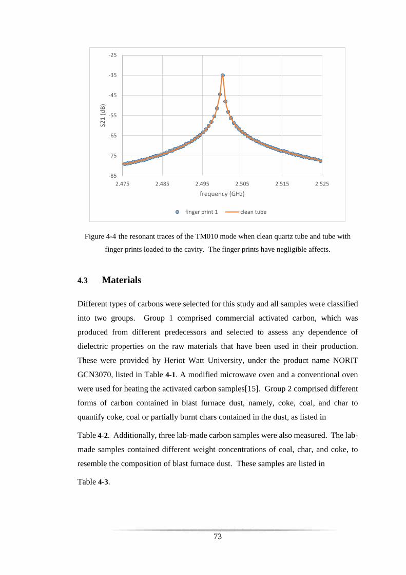
73
Figure 4-4 the resonant traces of the TM010 mode when clean quartz tube and tube with
finger prints loaded to the cavity. The finger prints have negligible affects.
4.3 Materials
Different types of carbons were selected for this study and all samples were classified
into two groups. Group 1 comprised commercial activated carbon, which was
produced from different predecessors and selected to assess any dependence of
dielectric properties on the raw materials that have been used in their production.
These were provided by Heriot Watt University, under the product name NORIT
GCN3070, listed in Table 4-1. A modified microwave oven and a conventional oven
were used for heating the activated carbon samples[15]. Group 2 comprised different
forms of carbon contained in blast furnace dust, namely, coke, coal, and char to
quantify coke, coal or partially burnt chars contained in the dust, as listed in
Table 4-2. Additionally, three lab-made carbon samples were also measured. The lab-
made samples contained different weight concentrations of coal, char, and coke, to
resemble the composition of blast furnace dust. These samples are listed in
Table 4-3.
-85
-75
-65
-55
-45
-35
-25
2.475 2.485 2.495 2.505 2.515 2.525
S21
(d
B)
frequency (GHz)
finger print 1 clean tube
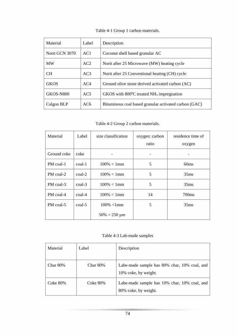
74
Table 4-1 Group 1 carbon materials.
Material Label Description
Norit GCN 3070 AC1 Coconut shell based granular AC
MW AC2 Norit after 25 Microwave (MW) heating cycle
CH AC3 Norit after 25 Conventional heating (CH) cycle
GKOS AC4 Ground olive stone derived activated carbon (AC)
GKOS-N800 AC5 GKOS with 8000C treated NH3 impregnation
Calgon BLP AC6 Bituminous coal based granular activated carbon (GAC)
Table 4-2 Group 2 carbon materials.
Material Label size classification oxygen: carbon
ratio
residence time of
oxygen
Ground coke coke - - -
PM coal-1 coal-1 100% < 1mm 5 60ms
PM coal-2 coal-2 100% < 1mm 5 35ms
PM coal-3 coal-3 100% < 1mm 5 35ms
PM coal-4 coal-4 100% < 1mm 14 700ms
PM coal-5 coal-5 100% <1mm
50% > 250 µm
5 35ms
Table 4-3 Lab-made samples
Material Label Description
Char 80% Char 80% Labe-made sample has 80% char, 10% coal, and
10% coke, by weight.
Coke 80% Coke 80% Labe-made sample has 10% char, 10% coal, and
80% coke, by weight.
75
Coal 80% Coal 80% Labe-made sample has 10% char, 80% coal, and
10% coke, by weight.
The Group 1 samples of activated carbon were formed from different particle sizes. They
were crushed using a mortar and pestle, and then sieved by 63µ Lab sieve to be
approximately 60µm size, as illustrated schematically in Figure 4-5.
Figure 4-5 Grinding the granular activated carbon to powder
The sample powders were poured into quartz tubes (outer and inner diameters of 2.4
mm and 2.0 mm respectively) and left to settle on a vibrating stage for 10 minutes.
Quartz was chosen as a tube material as it has very low dielectric loss and thus minimal
effect on the unloaded centre frequency and bandwidth. To minimise the errors,
multiple samples are prepared in the same way and measured using the cavity.
4.4 Dielectric properties measurements of activated carbons
The real and imaginary parts of the complex permittivity are shown in Figure 4-6 and
Figure 4-7, which illustrate the average values of the measurements of complex
permittivity of Group 1 activated carbon samples. The dielectric properties of activated
carbons have been presented in the 3rd International Conference on Microwave and
Terahertz Technology (ICMTT 2018) [109].
The same measurements were repeated at least 10 times for each sample, so that mean
values (and standard deviation of the mean) can be estimated reliably for each sample.
Figure 4-6 shows that the dielectric constant (i.e. real values of the complex
permittivity) of the samples for all activated carbons are significantly different. The
small errors are associated with the small differences in sample volumes each time a

76
powder sample is loaded into the cavity (since they are powders, with random packing
nature, and all tubes have a volume size distribution giving an error of about 2%).
It is clear that the sample AC6, which is produced from bituminous coal, has the
highest values of real permittivity, around 14.14. Samples AC1, AC2 and AC3 are the
same activated carbon which is produced from coconut shell, samples AC2 and AC3
are treated with microwave and conventional heating, respectively; both have values
of real permittivity that are approximately similar to AC1. The dielectric constant of
AC5, which was produced from ground olive stone with 800ºC and treated with NH3
impregnation, is approximately double that of the real permittivity of AC4, derived
from ground olive stone.
Figure 4-7 show the dielectric loss factor (i.e. imaginary value of the complex
permittivity) of all activated carbon samples. It is clear that the values are again
significantly different. The sample AC6, again, has the highest value of 9.57. Samples
AC1, AC2 and AC3 have slightly different values. The dielectric loss factor of AC5,
produced from ground olive stone with 800ºC treated NH3 impregnation, is
approximately double the dielectric loss factor of AC4, derived from ground olive
stone.
Figure 4-6 Dielectric constant of activated carbon samples. The typical standard error is
±0.02, which in most cases is too small to observe.
5.89
4.62 4.503.61
8.36
14.14
0
2
4
6
8
10
12
14
16
AC1 AC2 AC3 AC4 AC5 AC6
Die
lect
ric
const
ant

77
Figure 4-7 Dielectric loss factor of activated carbon samples. The typical standard error is
±0.0027, which in most cases is too small to observe.
4.5 Dielectric properties of carbons in blast furnace dust
The real and imaginary parts of the complex permittivity of different types of carbon
are shown in Figure 4-8 and Figure 4-9, respectively. The average values of the
measurements of complex permittivity of Group 2, comprising different forms of
carbon contained in blast furnace dust, are illustrated. These figures show that the
dielectric constant and loss factor of all samples are different and depend on the coal
type.
Figure 4-8 and Figure 4-9 clearly show that the coke has highest values of dielectric
constant and dielectric loss factor. The dielectric constant and loss factor of Coal-3 is
at least 2.5 times that of other types of coals.
The real and imaginary parts of the complex permittivity of the three lab–made blast
furnace samples are shown in Figure 4-10 and Figure 4-11. From these it is clear that
the samples containing the highest weight concentration of coke and char have higher
complex permittivity than the sample with highest weight concentration of coal.
0.84 0.71 0.490.12
0.53
9.57
0
2
4
6
8
10
12
AC1 AC2 AC3 AC4 AC5 AC6
Loss
fac
tor
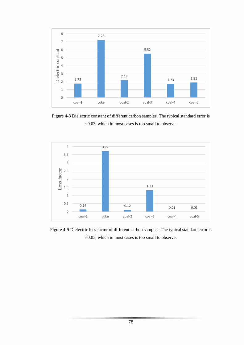
78
Figure 4-8 Dielectric constant of different carbon samples. The typical standard error is
±0.03, which in most cases is too small to observe.
Figure 4-9 Dielectric loss factor of different carbon samples. The typical standard error is
±0.03, which in most cases is too small to observe.
1.78
7.25
2.19
5.52
1.73 1.91
0
1
2
3
4
5
6
7
8
coal-1 coke coal-2 coal-3 coal-4 coal-5
Die
lect
ric
con
stan
t
0.14
3.72
0.12
1.33
0.01 0.010
0.5
1
1.5
2
2.5
3
3.5
4
coal-1 coke coal-2 coal-3 coal-4 coal-5
Loss
fac
tor

79
Figure 4-10 Dielectric constant of lab-made carbon samples. The typical standard error is
±0.01, which in most cases is too small to observe.
Figure 4-11 Dielectric loss factor of lab-made carbon samples. The typical standard error is
±0.024, which in most cases is too small to observe.
4.6 Conclusions
This chapter has presented the principles of cavity perturbation applied to
measurements of the complex permittivity of different types of carbon materials at
frequency of around 2.5 GHz using a cylindrical host cavity operating in its TM010
mode.
11.2811.80
2.93
0
2
4
6
8
10
12
14
char 80% coke80% coal80%
Die
lect
ric
con
stan
t
5.82
18.08
0.060
2
4
6
8
10
12
14
16
18
20
char 80% coke80% coal80%
loss
fac
tor
80
It can be concluded that the dielectric properties of activated carbons change
depending on the raw materials that have been used in their production; for example,
AC6, which was produced from bituminous coal, has the highest dielectric constant
and loss factor, at values of 14.1 and 9.6, respectively. It is also noticed that the both
AC2 and AC3 samples, which were pre-heated using conventional heating and
microwave heating, respectively, have approximately the same complex permittivities.
In addition, the different types of carbons contained in blast furnace dust have different
dielectric properties, where the coke and coal-3 have highest dielectric constants at
approximately 7.25 and 5.5, respectively. They also have the highest dielectric loss
factors at 3.7 and 1.3, respectively. As coke is generally made by heating coal in the
absence of air, the loss of the volatile components and restructuring of the carbon may
increase. As a consequence of that the conductivity increases due to increasing
electron mobility. As temperatures continue to increase the mobility of electrons and
level of free charge per unit volume increases.
For the lab-made blast furnace dust, the samples contained different weight
contribution of coke, coal, and char. The sample that contained the highest amount of
coke had highest dielectric constant and loss factor, at approximately 11.8 and 18.07,
respectively.
The importance of these measurements and the variant dielectric properties of carbon
samples would mean that microwave cavity technique can be simply used to
differentiate activated carbons and carbons contained in blast furnace dust. This is a
completely new way of assessing this complex material and could open up an
important on-site diagnostic for all industrial applications involving blast furnaces.
81
Chapter 5 Frequency-dependent dielectric properties
A microwave cavity offers several TM modes which can be used for complex
permittivity measurements over a range of frequencies, from 2.5 GHz up to about 10
GHz, which may provide more complete information than results at the single TM010
resonant frequency (around 2.5 GHz for the measurements presented here). Using a
microwave cavity system to measure the frequency-dependent complex permittivity
of different types of carbons is both practical and simple, at least in terms of the
preparation the samples. Moreover, due to its high sensitivity, it is more accurate
compared to other techniques.
An open-ended coaxial probe technique was also used to investigate dielectric
properties of different types of carbon over a much wider range of frequencies, from
10 MHz to 20 GHz. Although the coaxial probe is broadband, it has lower accuracy
compared with the cavity method, especially for loss measurements. It is also prone
to large error, so coaxial measurements need to be repeated many times to assess such
errors; this is especially so for inhomogeneous samples.
This chapter focuses on the frequency-dependent dielectric properties measurements
of two different groups of carbons. Activated carbons and carbonaceous materials
contained in BFD (blast furnace dust), i.e. Groups 1 and 2, respectively, identified in
Chapter 4. Significant contrasts between various samples have been measured in both
groups.
5.1 Multiple modes cavity system
Microwave complex permittivity can be measured over a range of frequencies using a
cavity (the same cavity used in the previous chapter) by exciting multiple TM modes
which have frequencies calculated using (3-18) and listed in Table 5-1. The samples
were mixed with silica to minimize the effects of the inter-grain conductivity between
the particles of the powder, so that the intrinsic loss properties are characterised. It
should be noted that, by definition, all of these TM modes provide an electric field
parallel to an axial sample.
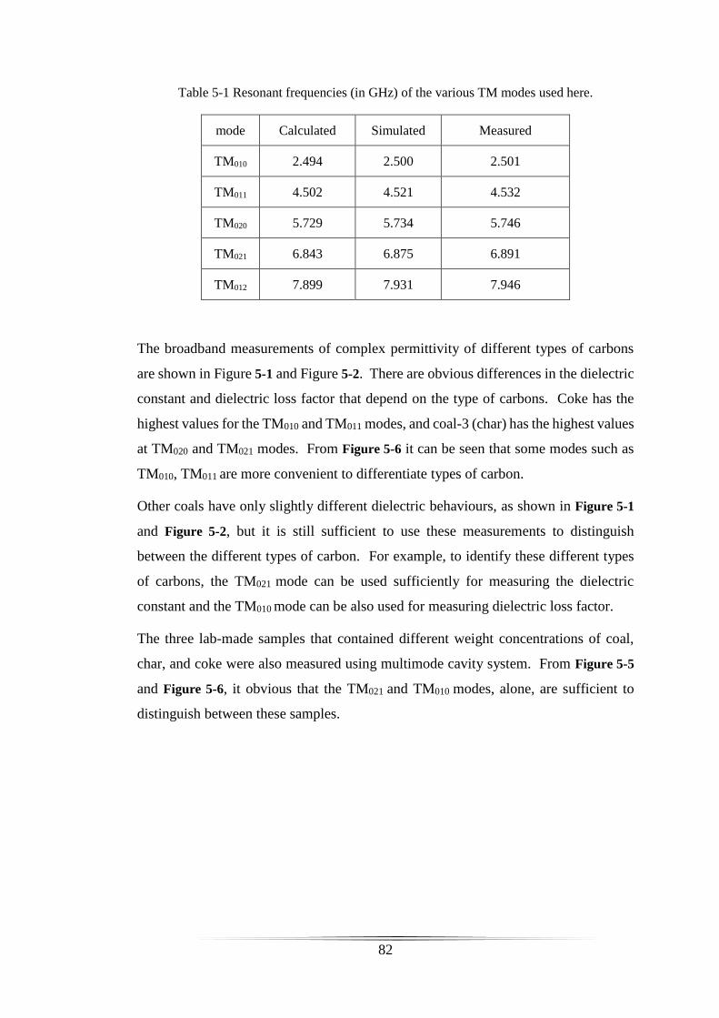
82
Table 5-1 Resonant frequencies (in GHz) of the various TM modes used here.
mode Calculated Simulated Measured
TM010 2.494 2.500 2.501
TM011 4.502 4.521 4.532
TM020 5.729 5.734 5.746
TM021 6.843 6.875 6.891
TM012 7.899 7.931 7.946
The broadband measurements of complex permittivity of different types of carbons
are shown in Figure 5-1 and Figure 5-2. There are obvious differences in the dielectric
constant and dielectric loss factor that depend on the type of carbons. Coke has the
highest values for the TM010 and TM011 modes, and coal-3 (char) has the highest values
at TM020 and TM021 modes. From Figure 5-6 it can be seen that some modes such as
TM010, TM011 are more convenient to differentiate types of carbon.
Other coals have only slightly different dielectric behaviours, as shown in Figure 5-1
and Figure 5-2, but it is still sufficient to use these measurements to distinguish
between the different types of carbon. For example, to identify these different types
of carbons, the TM021 mode can be used sufficiently for measuring the dielectric
constant and the TM010 mode can be also used for measuring dielectric loss factor.
The three lab-made samples that contained different weight concentrations of coal,
char, and coke were also measured using multimode cavity system. From Figure 5-5
and Figure 5-6, it obvious that the TM021 and TM010 modes, alone, are sufficient to
distinguish between these samples.
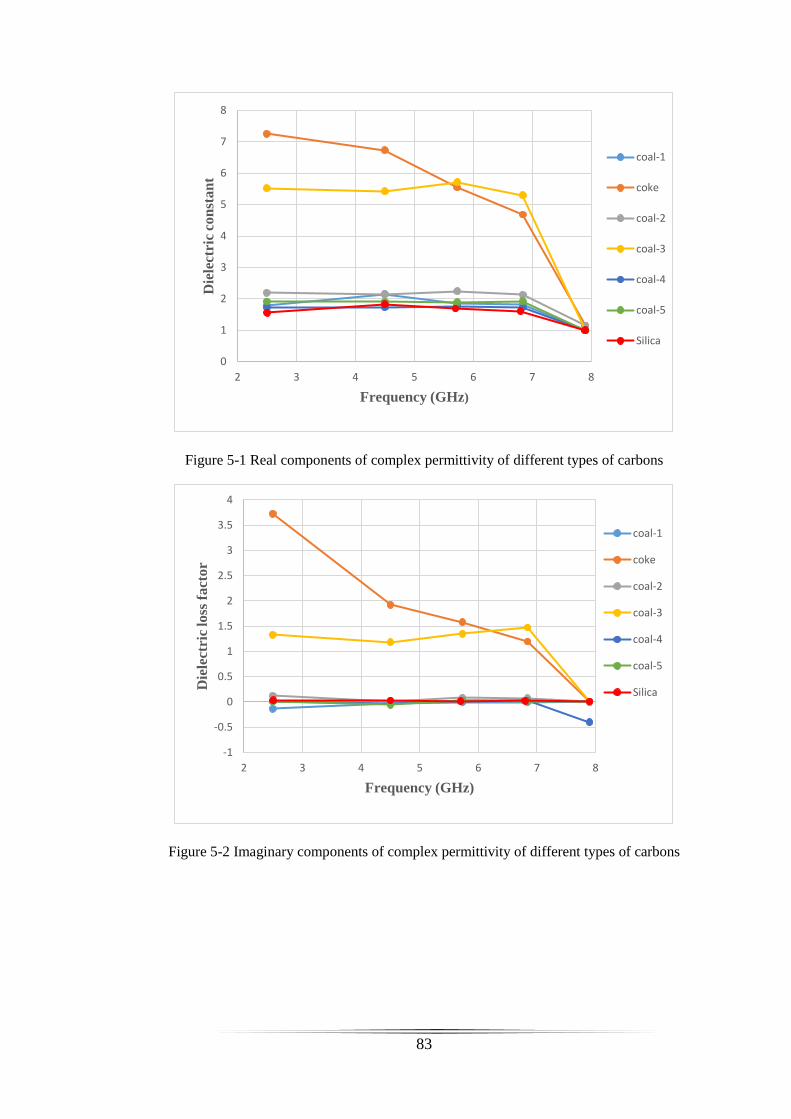
83
Figure 5-1 Real components of complex permittivity of different types of carbons
Figure 5-2 Imaginary components of complex permittivity of different types of carbons
0
1
2
3
4
5
6
7
8
2 3 4 5 6 7 8
Die
lect
ric
con
sta
nt
Frequency (GHz)
coal-1
coke
coal-2
coal-3
coal-4
coal-5
Silica
-1
-0.5
0
0.5
1
1.5
2
2.5
3
3.5
4
2 3 4 5 6 7 8
Die
lect
ric
loss
fact
or
Frequency (GHz)
coal-1
coke
coal-2
coal-3
coal-4
coal-5
Silica

84
Figure 5-3 Real components of complex permittivity of different types of coals
Figure 5-4 Imaginary components of complex permittivity of different types of coals
0
0.5
1
1.5
2
2.5
2 3 4 5 6 7 8
Die
lect
ric
con
sta
nt
Frequency (GHz)
coal-1 coal-2 coal-4 coal-5
-1
-0.8
-0.6
-0.4
-0.2
0
0.2
2 3 4 5 6 7 8
loss
fact
or
Frequency (GHz)
coal-1 coal-2 coal-4 coal-5

85
Figure 5-5 Real components of complex permittivity of lab-made samples
Figure 5-6 Imaginary components of complex permittivity of lab-made samples
5.2 Open-ended coaxial probe system
The coaxial probe technique is used to measure the dielectric properties of material
over a broad, continuous range of frequencies. The samples were in granular from,
0
5
10
15
20
25
30
35
40
2 3 4 5 6 7
Die
lect
ric
con
sta
nt
Frequency (GHz)
char80%
coke80%
coal80%
-5
0
5
10
15
20
2 3 4 5 6 7
Die
lect
ric
loss
fact
or
Frequency (GHz)
char80%
coke80%
coal80%

86
being activated carbon which was produced from coconut shell provided by Heriot
Watt University (the product name is NORIT GCN3070). The samples were
introduced to the probe in two different forms. Firstly, the measurements started with
powdered samples. Secondly, the powdered samples were mixed with silicone rubber
in different mixing ratios. The powders were formed by grinding the sample using a
mortar and pestle, followed by sieving using a 63µ Lab sieve to approximately 60µm
size.
The samples were pressed onto the top of the coaxial probe using the system shown in
Figure 5-7 to ensure that there is good contact between the sample and probe.
Figure 5-7 coaxial probe and sample fixture. Sample is placed on the top of the probe, while
S11 is measured using a PNA network analyser and controlled by a LabVIEW program [43]
The measurements were carried out using coaxial flat probe with square flange which
was connected to the Agilent PNA-L vector network analyser, after a standard short-
open-load calibration process done using an Agilent 85052D calibration Kit.
5.3 Dielectric properties of powdered activated carbons
It was found during the analysis of the resulting data that the data values varied
considerably over the fifty sets of measurement of activated carbon and ten sets of
measurement of three lab-made carbon samples (containing different weight
concentration of coal, char and coke). These differences have a likely origin in the
random electrical contacts that occur between the powder grains, which cause
connective paths which also could affect the capacitance (and hence “dielectric
constant”) at these high frequencies. The array of contacts is different each time the
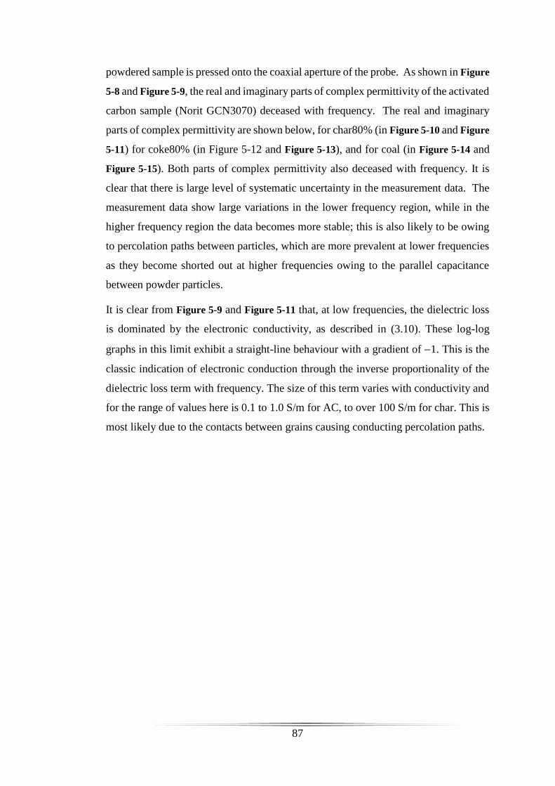
87
powdered sample is pressed onto the coaxial aperture of the probe. As shown in Figure
5-8 and Figure 5-9, the real and imaginary parts of complex permittivity of the activated
carbon sample (Norit GCN3070) deceased with frequency. The real and imaginary
parts of complex permittivity are shown below, for char80% (in Figure 5-10 and Figure
5-11) for coke80% (in Figure 5-12 and Figure 5-13), and for coal (in Figure 5-14 and
Figure 5-15). Both parts of complex permittivity also deceased with frequency. It is
clear that there is large level of systematic uncertainty in the measurement data. The
measurement data show large variations in the lower frequency region, while in the
higher frequency region the data becomes more stable; this is also likely to be owing
to percolation paths between particles, which are more prevalent at lower frequencies
as they become shorted out at higher frequencies owing to the parallel capacitance
between powder particles.
It is clear from Figure 5-9 and Figure 5-11 that, at low frequencies, the dielectric loss
is dominated by the electronic conductivity, as described in (3.10). These log-log
graphs in this limit exhibit a straight-line behaviour with a gradient of 1. This is the
classic indication of electronic conduction through the inverse proportionality of the
dielectric loss term with frequency. The size of this term varies with conductivity and
for the range of values here is 0.1 to 1.0 S/m for AC, to over 100 S/m for char. This is
most likely due to the contacts between grains causing conducting percolation paths.

88
Figure 5-8 real component of the complex permittivity of powdered activated carbon (Norit
GCN3070) for 10 independent measurements
Figure 5-9 imaginary component of the complex permittivity of powdered activated carbon
(Norit GCN3070) for 10 independent measurements
From Figure 5-8 and Figure 5-9 and the negative slope with increasing frequency
emerges in both real and imaginary parts, this decrease in loss with frequency is
because of either free electron conductivity or space-charge polarisation, both of which
are mechanisms related to conduction. Free electron conductivity appears in the losses
1
10
100
1000
2.50E+06 5.00E+07 1.00E+09 2.00E+10
Die
lect
ric
con
sta
nt
Frequency (Hz)
1
10
100
1000
10000
2.50E+06 5.00E+07 1.00E+09 2.00E+10
Loss
fact
or
Frequency (Hz)

89
with a 1/f dependence. Space-charge polarisation appears in both the real and
imaginary parts of permittivity. This mechanism can therefore be identified by a
decrease in both the real and imaginary parts as frequency increases
Figure 5-10 Real component of complex permittivity of Char 80% for 10 independent
measurements
Figure 5-11 Imaginary component of complex permittivity of Char 80% for 10 independent
measurements
-2000
0
2000
4000
6000
8000
10000
12000
2.00E+06 4.00E+07 8.00E+08 1.60E+10
Die
lect
ric
con
sta
nt
Frequency (Hz)
1
10
100
1000
10000
100000
1000000
2.00E+06 4.00E+07 8.00E+08 1.60E+10
Loss
fact
or
Frequency (Hz)
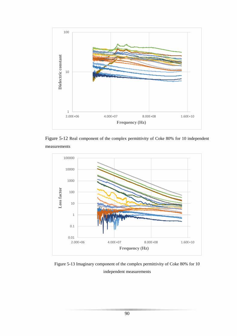
90
Figure 5-12 Real component of the complex permittivity of Coke 80% for 10 independent
measurements
Figure 5-13 Imaginary component of the complex permittivity of Coke 80% for 10
independent measurements
1
10
100
2.00E+06 4.00E+07 8.00E+08 1.60E+10
Die
lect
ric
con
sta
nt
Frequency (Hz)
0.01
0.1
1
10
100
1000
10000
100000
2.00E+06 4.00E+07 8.00E+08 1.60E+10
Loss
fact
or
Frequency (Hz)

91
Figure 5-14 Real component of the complex permittivity of Coal 80% for 10 independent
measurements
Figure 5-15 Imaginary components of the complex permittivity of Coal 80% for 10
independent measurements
0
1
2
3
4
5
6
7
8
9
2.00E+06 4.00E+07 8.00E+08 1.60E+10
Die
lect
ric
con
sta
nt
Frequency (Hz)
-4
-3
-2
-1
0
1
2
3
2.00E+06 4.00E+07 8.00E+08 1.60E+10
Loss
fact
or
Frequency (Hz)
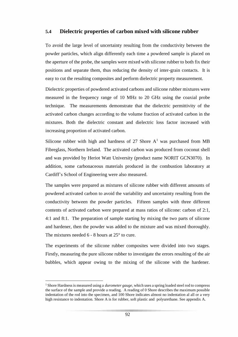
92
5.4 Dielectric properties of carbon mixed with silicone rubber
To avoid the large level of uncertainty resulting from the conductivity between the
powder particles, which align differently each time a powdered sample is placed on
the aperture of the probe, the samples were mixed with silicone rubber to both fix their
positions and separate them, thus reducing the density of inter-grain contacts. It is
easy to cut the resulting composites and perform dielectric property measurement.
Dielectric properties of powdered activated carbons and silicone rubber mixtures were
measured in the frequency range of 10 MHz to 20 GHz using the coaxial probe
technique. The measurements demonstrate that the dielectric permittivity of the
activated carbon changes according to the volume fraction of activated carbon in the
mixtures. Both the dielectric constant and dielectric loss factor increased with
increasing proportion of activated carbon.
Silicone rubber with high and hardness of 27 Shore A1 was purchased from MB
Fibreglass, Northern Ireland. The activated carbon was produced from coconut shell
and was provided by Heriot Watt University (product name NORIT GCN3070). In
addition, some carbonaceous materials produced in the combustion laboratory at
Cardiff’s School of Engineering were also measured.
The samples were prepared as mixtures of silicone rubber with different amounts of
powdered activated carbon to avoid the variability and uncertainty resulting from the
conductivity between the powder particles. Fifteen samples with three different
contents of activated carbon were prepared at mass ratios of silicone: carbon of 2:1,
4:1 and 8:1. The preparation of sample starting by mixing the two parts of silicone
and hardener, then the powder was added to the mixture and was mixed thoroughly.
The mixtures needed 6 - 8 hours at 25° to cure.
The experiments of the silicone rubber composites were divided into two stages.
Firstly, measuring the pure silicone rubber to investigate the errors resulting of the air
bubbles, which appear owing to the mixing of the silicone with the hardener.
1 Shore Hardness is measured using a durometer gauge, which uses a spring loaded steel rod to compress
the surface of the sample and provide a reading. A reading of 0 Shore describes the maximum possible
indentation of the rod into the specimen, and 100 Shore indicates almost no indentation al all or a very
high resistance to indentation. Shore A is for rubber, soft plastic and polyurethane. See appendix A.
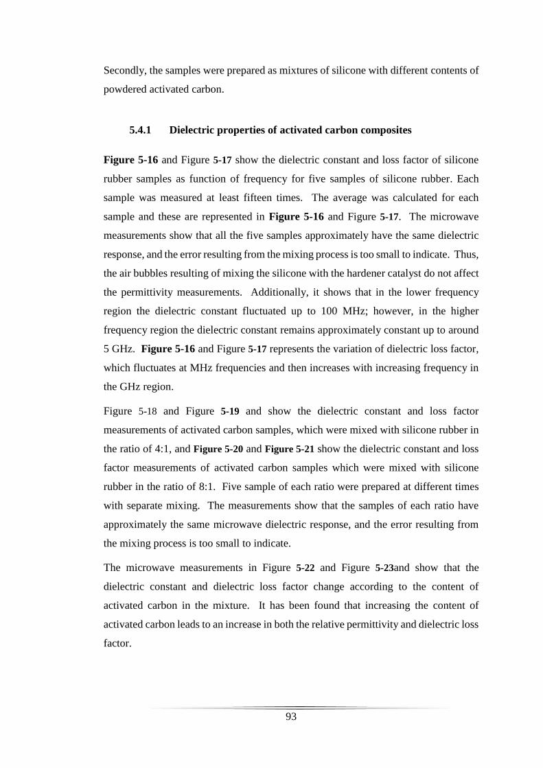
93
Secondly, the samples were prepared as mixtures of silicone with different contents of
powdered activated carbon.
5.4.1 Dielectric properties of activated carbon composites
Figure 5-16 and Figure 5-17 show the dielectric constant and loss factor of silicone
rubber samples as function of frequency for five samples of silicone rubber. Each
sample was measured at least fifteen times. The average was calculated for each
sample and these are represented in Figure 5-16 and Figure 5-17. The microwave
measurements show that all the five samples approximately have the same dielectric
response, and the error resulting from the mixing process is too small to indicate. Thus,
the air bubbles resulting of mixing the silicone with the hardener catalyst do not affect
the permittivity measurements. Additionally, it shows that in the lower frequency
region the dielectric constant fluctuated up to 100 MHz; however, in the higher
frequency region the dielectric constant remains approximately constant up to around
5 GHz. Figure 5-16 and Figure 5-17 represents the variation of dielectric loss factor,
which fluctuates at MHz frequencies and then increases with increasing frequency in
the GHz region.
Figure 5-18 and Figure 5-19 and show the dielectric constant and loss factor
measurements of activated carbon samples, which were mixed with silicone rubber in
the ratio of 4:1, and Figure 5-20 and Figure 5-21 show the dielectric constant and loss
factor measurements of activated carbon samples which were mixed with silicone
rubber in the ratio of 8:1. Five sample of each ratio were prepared at different times
with separate mixing. The measurements show that the samples of each ratio have
approximately the same microwave dielectric response, and the error resulting from
the mixing process is too small to indicate.
The microwave measurements in Figure 5-22 and Figure 5-23and show that the
dielectric constant and dielectric loss factor change according to the content of
activated carbon in the mixture. It has been found that increasing the content of
activated carbon leads to an increase in both the relative permittivity and dielectric loss
factor.

94
Figure 5-16 Real components of complex permittivity of Silicone rubber for 5 samples.
Figure 5-17 Imaginary components of complex permittivity of Silicone rubber for 5 samples.
3
3.1
3.2
3.3
3.4
3.5
3.6
3.7
3.8
3.9
4
5.00E+06 5.00E+07 5.00E+08 5.00E+09 5.00E+10
die
lect
ric
con
sta
nt
Frequency (Hz)
-0.5
0
0.5
3.00E+06 3.00E+07 3.00E+08 3.00E+09 3.00E+10
loss
fact
or
Frequency (Hz)

95
Figure 5-18 Real component of complex permittivity of 4:1 for 5 samples
Figure 5-19 Real and imaginary component of complex permittivity of 4:1 for 5 samples
2.5
3
3.5
4
4.5
5
5.5
6
6.5
3.00E+06 3.00E+07 3.00E+08 3.00E+09 3.00E+10
die
lect
ric
con
sta
nt
Frequency (Hz)
-3
-2
-1
0
1
2
3
3.00E+06 3.00E+07 3.00E+08 3.00E+09 3.00E+10
loss
fact
or
Frequency (Hz)
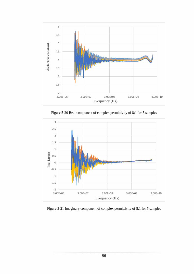
96
Figure 5-20 Real component of complex permittivity of 8:1 for 5 samples
Figure 5-21 Imaginary component of complex permittivity of 8:1 for 5 samples
2
2.5
3
3.5
4
4.5
5
5.5
6
3.00E+06 3.00E+07 3.00E+08 3.00E+09 3.00E+10
die
lect
ric
con
sta
nt
Frequency (Hz)
-2
-1.5
-1
-0.5
0
0.5
1
1.5
2
2.5
3
3.00E+06 3.00E+07 3.00E+08 3.00E+09 3.00E+10
loss
fact
or
Frequency (Hz)
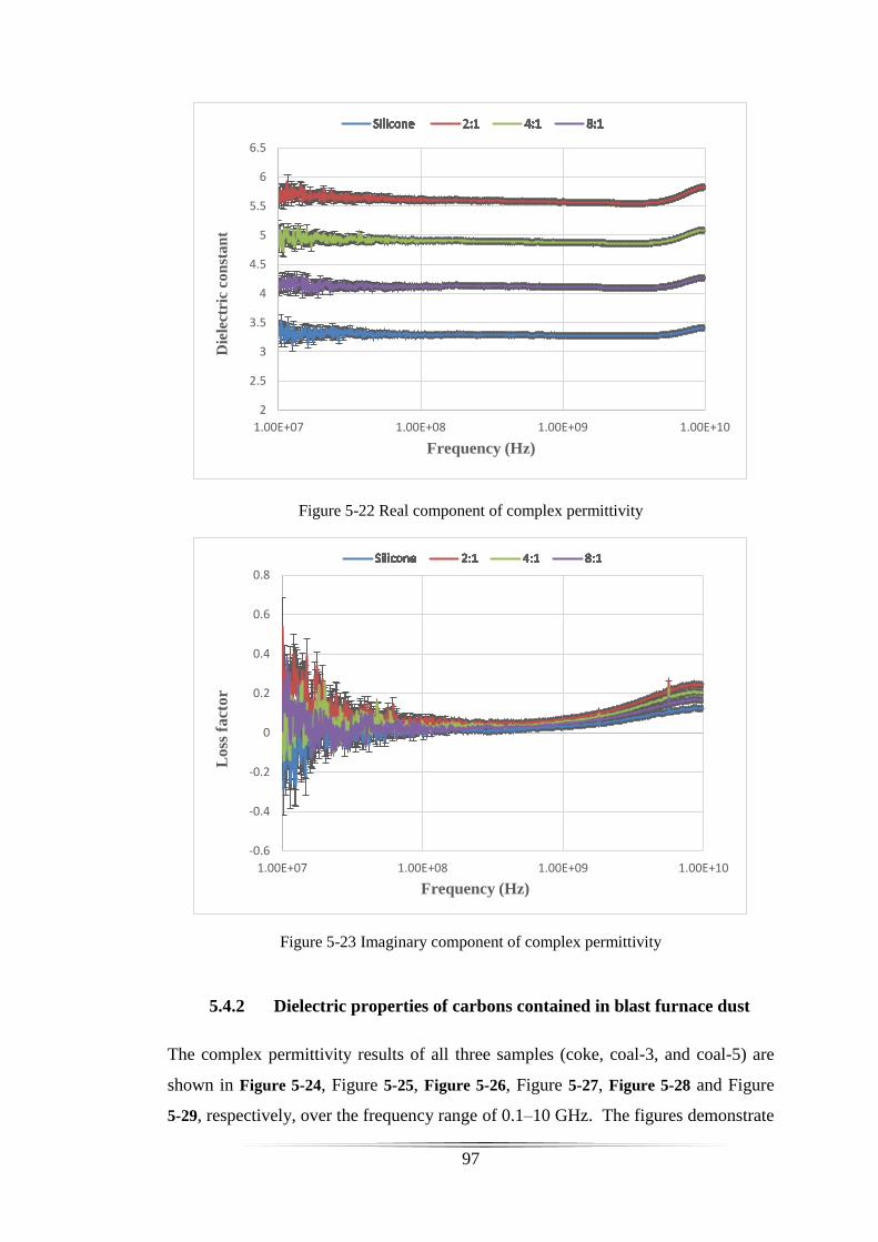
97
Figure 5-22 Real component of complex permittivity
Figure 5-23 Imaginary component of complex permittivity
5.4.2 Dielectric properties of carbons contained in blast furnace dust
The complex permittivity results of all three samples (coke, coal-3, and coal-5) are
shown in Figure 5-24, Figure 5-25, Figure 5-26, Figure 5-27, Figure 5-28 and Figure
5-29, respectively, over the frequency range of 0.1–10 GHz. The figures demonstrate
2
2.5
3
3.5
4
4.5
5
5.5
6
6.5
1.00E+07 1.00E+08 1.00E+09 1.00E+10
Die
lect
ric
con
sta
nt
Frequency (Hz)
-0.6
-0.4
-0.2
0
0.2
0.4
0.6
0.8
1.00E+07 1.00E+08 1.00E+09 1.00E+10
Loss
fact
or
Frequency (Hz)
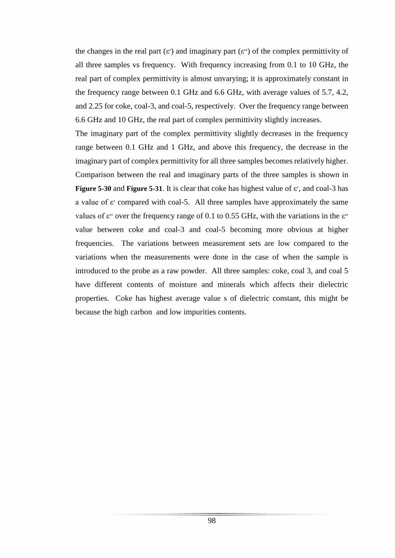
98
the changes in the real part (ε׳) and imaginary part (ε׳׳) of the complex permittivity of
all three samples vs frequency. With frequency increasing from 0.1 to 10 GHz, the
real part of complex permittivity is almost unvarying; it is approximately constant in
the frequency range between 0.1 GHz and 6.6 GHz, with average values of 5.7, 4.2,
and 2.25 for coke, coal-3, and coal-5, respectively. Over the frequency range between
6.6 GHz and 10 GHz, the real part of complex permittivity slightly increases.
The imaginary part of the complex permittivity slightly decreases in the frequency
range between 0.1 GHz and 1 GHz, and above this frequency, the decrease in the
imaginary part of complex permittivity for all three samples becomes relatively higher.
Comparison between the real and imaginary parts of the three samples is shown in
Figure 5-30 and Figure 5-31. It is clear that coke has highest value of ε׳, and coal-3 has
a value of ε׳ compared with coal-5. All three samples have approximately the same
values of ε׳׳ over the frequency range of 0.1 to 0.55 GHz, with the variations in the ε׳׳
value between coke and coal-3 and coal-5 becoming more obvious at higher
frequencies. The variations between measurement sets are low compared to the
variations when the measurements were done in the case of when the sample is
introduced to the probe as a raw powder. All three samples: coke, coal 3, and coal 5
have different contents of moisture and minerals which affects their dielectric
properties. Coke has highest average value s of dielectric constant, this might be
because the high carbon and low impurities contents.
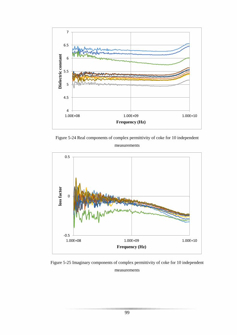
99
Figure 5-24 Real components of complex permittivity of coke for 10 independent
measurements
Figure 5-25 Imaginary components of complex permittivity of coke for 10 independent
measurements
4
4.5
5
5.5
6
6.5
7
1.00E+08 1.00E+09 1.00E+10
Die
lect
ric
con
sta
nt
Frequency (Hz)
-0.5
0
0.5
1.00E+08 1.00E+09 1.00E+10
loss
fact
or
Frequency (Hz)
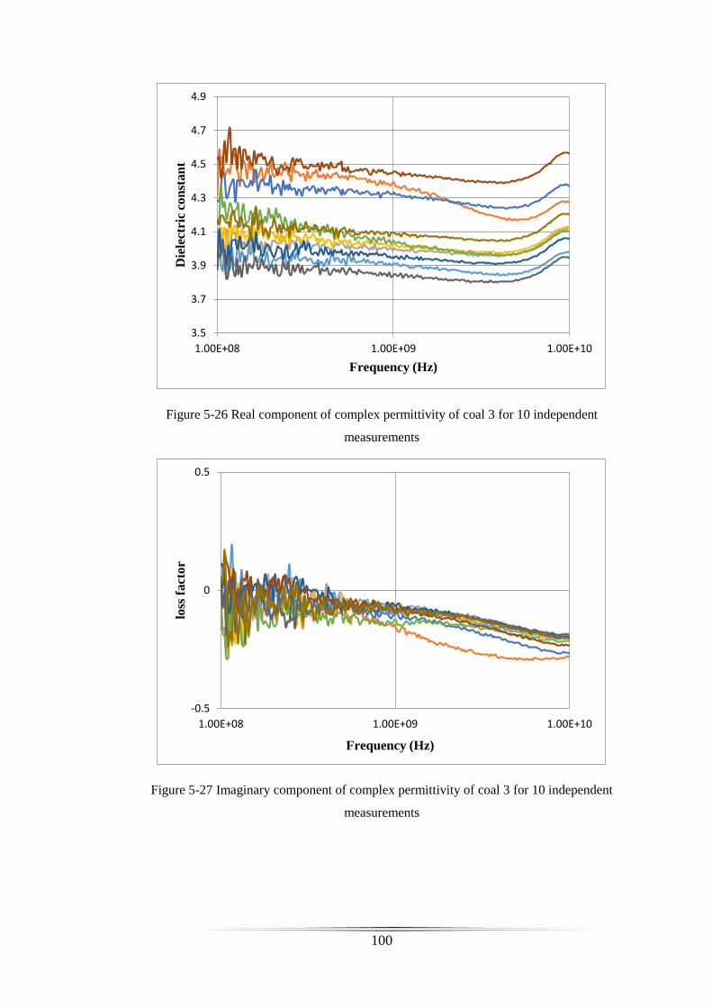
100
Figure 5-26 Real component of complex permittivity of coal 3 for 10 independent
measurements
Figure 5-27 Imaginary component of complex permittivity of coal 3 for 10 independent
measurements
3.5
3.7
3.9
4.1
4.3
4.5
4.7
4.9
1.00E+08 1.00E+09 1.00E+10
Die
lect
ric
con
sta
nt
Frequency (Hz)
-0.5
0
0.5
1.00E+08 1.00E+09 1.00E+10
loss
fact
or
Frequency (Hz)

101
Figure 5-28 Real component of complex permittivity of coal 5 for 10 independent
measurements
Figure 5-29Imaginary component of complex permittivity of coal 5 for 10 independent
measurements
1.8
1.9
2
2.1
2.2
2.3
2.4
2.5
2.6
2.7
2.8
1.00E+08 1.00E+09 1.00E+10
Die
lect
ric
con
sta
nt
Frequency (Hz)
-0.5
0
0.5
1.00E+08 1.00E+09 1.00E+10
loss
fact
or
Frequency (Hz)
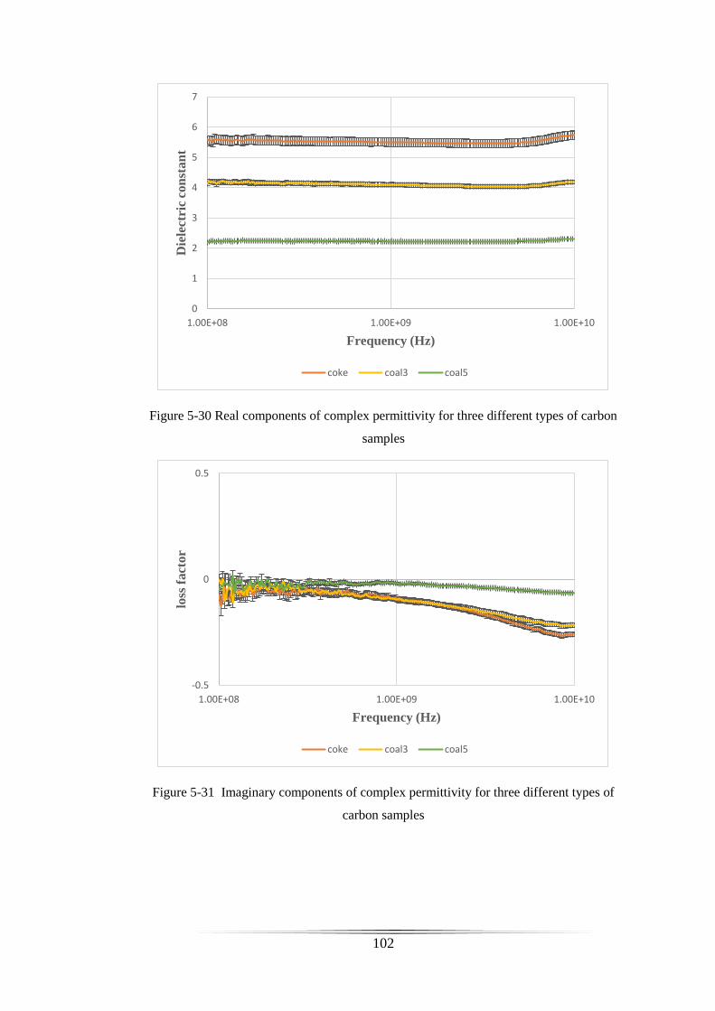
102
Figure 5-30 Real components of complex permittivity for three different types of carbon
samples
Figure 5-31 Imaginary components of complex permittivity for three different types of
carbon samples
0
1
2
3
4
5
6
7
1.00E+08 1.00E+09 1.00E+10
Die
lect
ric
con
sta
nt
Frequency (Hz)
coke coal3 coal5
-0.5
0
0.5
1.00E+08 1.00E+09 1.00E+10
loss
fact
or
Frequency (Hz)
coke coal3 coal5
103
5.5 Conclusion
The microwave dielectric properties of activated carbon/ silicone rubber mixtures were
investigated over the frequency range 10 MHz to 20 GHz using a coaxial probe with
increasing content of activated carbon within a silicone host.
The preparation methods of samples by dispersion of AC in silicone rubber have a
strong impact on the properties of the resulting samples, at a same activated carbon
loading, considerable improvement in the dielectric measurement with regard to the
error. Mixing powders with silicone rubber decrease finite conductivity between the
grains.
The results showed increases in dielectric constant and dielectric loss with increasing
mass fraction of activated carbon in the sample. The results also show that the
dielectric constant of all samples highly fluctuated in the region of frequencies between
10 MHz to 100 MHz this can be related to the phase change, whereas above 100 MHz
it becomes approximately constant.
The same procedures and techniques were used for measuring the dielectric properties
of three different types of carbonaceous materials contained in blast furnace dust over
the frequency range 10 MHz to 10 GHz. The results show that the dielectric properties
of the samples are influenced with increasing frequency, especially in the higher GHz
region. The dielectric constant increase and the losses decrease with increasing
frequency.
This study shows that multimode microwave cavity system can be used to estimate the
microwave dielectric properties of carbon materials contained in BFD in the 2 to 10
GHz range. Some modes are more satisfied to differentiate these types of coal and
coke, such as TM010 . In general, dielectric properties of the samples decrease as the
frequency increased.
In conclusion, it is has been demonstrated that both the multimode cavity and open-
ended coaxial probe methods are appropriate to be used as test methods for identifying
and differentiating the different types of carbons based on the frequency dependence
of their dielectric properties. The broadband coaxial technique is shown to be repeatable
and accurate and a clear frequency dependence occurs for both real and imaginary parts
of permittivity.
104
Chapter 6 Temperature-Dependent Dielectric Properties
Owing to their application in, for example, carbon dioxide capture, it is necessary to
characterise the dielectric properties of activated carbon over a variable temperature
range, typically to around 1500C. Measuring temperature-dependent dielectric
properties of activated carbons may be advantageous in the thermal treatment of
activated carbons and in the thermal regeneration of saturated activated carbon.
In blast furnace dust (BFD), the dielectric properties of different types of carbon need
to be characterised as a function of temperature to allow the real time monitoring of
complex permittivity to differentiate the types of carbon. This is important to quantify
the utilization of coal injected in the furnace and to determine the efficiency of coal
injection.
The temperature dependent properties of two groups of carbon materials, activated
carbons and the three different coal-based constituents contained in BFD, were
measured using the TM010 microwave cavity technique at frequency of 2.498 GHz in
the temperature range 30 0C to 150 0C.
6.1 Measurement system
In this chapter, the cavity perturbation technique is used for temperature dependent
dielectric properties measurements. In this technique, which is detailed in Chapter 3,
a sample of material is inserted (via a quartz sample tube) into the cavity and the
resulting perturbations are measured.
A change in the ambient temperature of the cavity will cause a change in the resonant
frequency, due to the thermal expansion of the cavity which causes change in the
cavity dimensions, radius (a) and height (d). The thermal expansion coefficient α of
the aluminium metal making up the cavity can be used to describe these changes.
Therefore, the assumption that the volume of the cavity is fixed is not valid in the case
of changing temperature. The perturbation equations (3-46) and (3-47) are valid in the
case of the sample size being small compared to the cavity size. Therefore, any change
in the cavity size due to temperature variation must be included in the calculations.
This imposes systematic errors on the real part of the permittivity, in particular, as
changes in frequency due to cavity dimension changes may be wrongly interpreted as
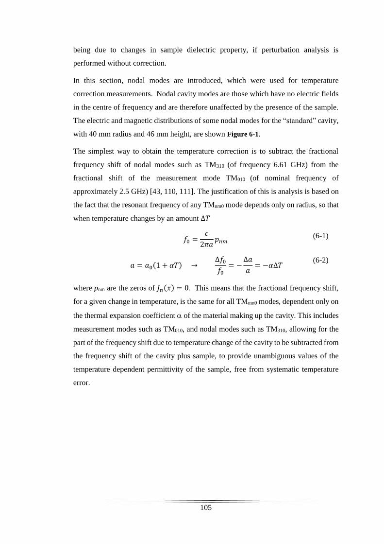
105
being due to changes in sample dielectric property, if perturbation analysis is
performed without correction.
In this section, nodal modes are introduced, which were used for temperature
correction measurements. Nodal cavity modes are those which have no electric fields
in the centre of frequency and are therefore unaffected by the presence of the sample.
The electric and magnetic distributions of some nodal modes for the “standard” cavity,
with 40 mm radius and 46 mm height, are shown Figure 6-1.
The simplest way to obtain the temperature correction is to subtract the fractional
frequency shift of nodal modes such as TM310 (of frequency 6.61 GHz) from the
fractional shift of the measurement mode TM010 (of nominal frequency of
approximately 2.5 GHz) [43, 110, 111]. The justification of this is analysis is based on
the fact that the resonant frequency of any TMnm0 mode depends only on radius, so that
when temperature changes by an amount ∆𝑇
𝑓0 =𝑐
2𝜋𝑎𝑝𝑛𝑚 (6-1)
𝑎 = 𝑎0(1 + 𝛼𝑇) →
∆𝑓0
𝑓0= −
∆𝑎
𝑎= −𝛼∆𝑇
(6-2)
where pnm are the zeros of 𝐽𝑛(𝑥) = 0. This means that the fractional frequency shift,
for a given change in temperature, is the same for all TMmn0 modes, dependent only on
the thermal expansion coefficient of the material making up the cavity. This includes
measurement modes such as TM010, and nodal modes such as TM310, allowing for the
part of the frequency shift due to temperature change of the cavity to be subtracted from
the frequency shift of the cavity plus sample, to provide unambiguous values of the
temperature dependent permittivity of the sample, free from systematic temperature
error.
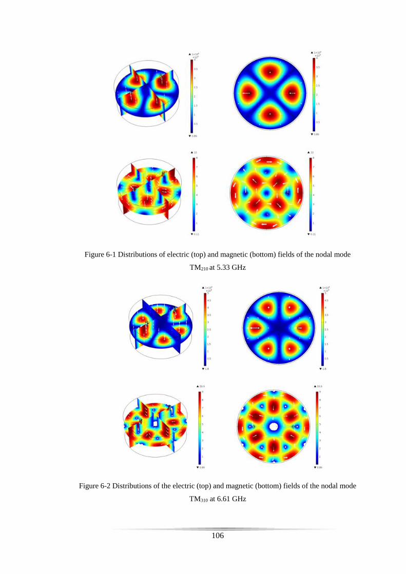
106
Figure 6-1 Distributions of electric (top) and magnetic (bottom) fields of the nodal mode
TM210 at 5.33 GHz
Figure 6-2 Distributions of the electric (top) and magnetic (bottom) fields of the nodal mode
TM310 at 6.61 GHz
107
Thus, the simplest way to obtain the temperature correction using a nodal mode is to
subtract the fractional frequency shift of the nodal mode (such as TM210 and TM310)
from the measurement mode TM010 [43, 110, 112].
This process is shown quantitatively below, where the subscript “u” denotes the
fractional frequency shift with temperature of the unperturbed cavity. Through cavity
perturbation, the change in permittivity with respect to a reference temperature can be
expressed as following:
∆𝑓𝑠(𝑇)
𝑓𝑠(0)= [
∆𝑓010,𝑠(𝑇)
𝑓010,𝑠(0)−
∆𝑓𝑚10,𝑠(𝑇)
𝑓𝑚10,𝑠(0)]
− [∆𝑓010,𝑢(𝑇)
𝑓010,𝑢(0)−
∆𝑓𝑚10,𝑢(𝑇)
𝑓𝑚10,𝑢(0)]
(6-3)
휀1(𝑇) ≃ −2 [
𝑓𝑠(𝑇) − 𝑓0(0)
𝑓0(0)]
𝑉𝑐
𝑉𝑠𝐺𝑛𝑚𝑝 + 1
(6-4)
휀2(𝑇) ≃ −2 [
1
𝑄𝑠(𝑇)−
1
𝑄0(0)]
𝑉𝑐
𝑉𝑠𝐺𝑛𝑚𝑝
(6-5)
The nodal mode TM310 is used for temperature correction in the experiments presented
here as it is not perturbed by a sample placed along its axis; both electric and magnetic
fields are zero in this location. In the case of the use of the standard cavity with radius
of 40 mm and height of 46 mm, TM310 occurs at resonant frequent of 6.61 GHz (since
p31 = 6.380). Applying (6-4) and (6-5) to calculate the corrected temperature dependent
dielectric constant and loss factor.
For the temperature dependent experiments the cavity (loaded with a sample) was
placed inside a Memmert UF30 laboratory oven, as shown in Figure 6-3. The change
in the resonant frequency and bandwidth were recorded using a custom LabVIEW
program. Temperature was measured using resistance temperature detector PT100
RTDs provided by Omega, interfaced to a National Instruments C-DAQ. At each
temperature, the magnitude of the voltage transmission coefficient S21 was measured
in the frequency domain with a PNA-L network analyser N5232A to obtain the
resonant frequency and quality factor Q.
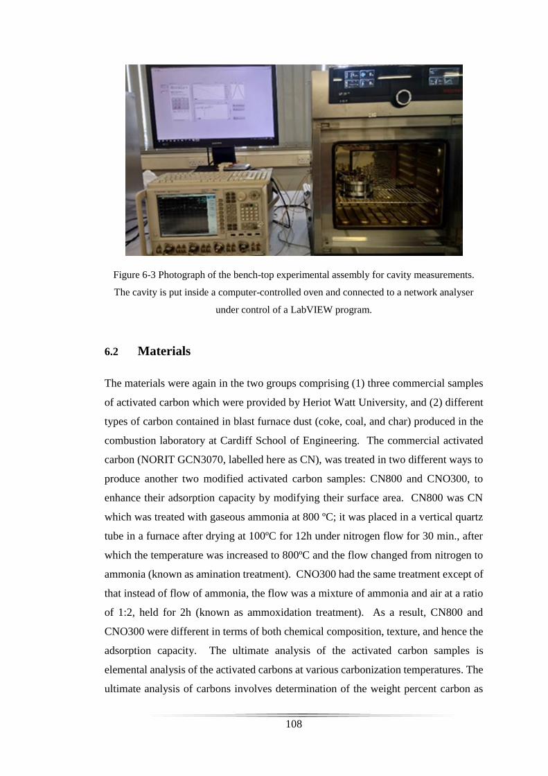
108
Figure 6-3 Photograph of the bench-top experimental assembly for cavity measurements.
The cavity is put inside a computer-controlled oven and connected to a network analyser
under control of a LabVIEW program.
6.2 Materials
The materials were again in the two groups comprising (1) three commercial samples
of activated carbon which were provided by Heriot Watt University, and (2) different
types of carbon contained in blast furnace dust (coke, coal, and char) produced in the
combustion laboratory at Cardiff School of Engineering. The commercial activated
carbon (NORIT GCN3070, labelled here as CN), was treated in two different ways to
produce another two modified activated carbon samples: CN800 and CNO300, to
enhance their adsorption capacity by modifying their surface area. CN800 was CN
which was treated with gaseous ammonia at 800 ºC; it was placed in a vertical quartz
tube in a furnace after drying at 100ºC for 12h under nitrogen flow for 30 min., after
which the temperature was increased to 800ºC and the flow changed from nitrogen to
ammonia (known as amination treatment). CNO300 had the same treatment except of
that instead of flow of ammonia, the flow was a mixture of ammonia and air at a ratio
of 1:2, held for 2h (known as ammoxidation treatment). As a result, CN800 and
CNO300 were different in terms of both chemical composition, texture, and hence the
adsorption capacity. The ultimate analysis of the activated carbon samples is
elemental analysis of the activated carbons at various carbonization temperatures. The
ultimate analysis of carbons involves determination of the weight percent carbon as
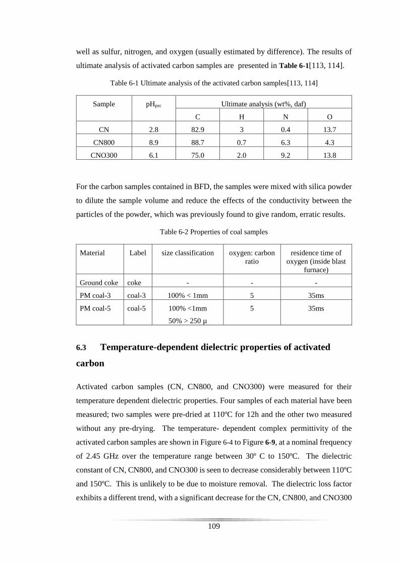
109
well as sulfur, nitrogen, and oxygen (usually estimated by difference). The results of
ultimate analysis of activated carbon samples are presented in Table 6-1[113, 114].
Table 6-1 Ultimate analysis of the activated carbon samples[113, 114]
Sample pHpzc Ultimate analysis (wt%, daf)
C H N O
CN 2.8 82.9 3 0.4 13.7
CN800 8.9 88.7 0.7 6.3 4.3
CNO300 6.1 75.0 2.0 9.2 13.8
For the carbon samples contained in BFD, the samples were mixed with silica powder
to dilute the sample volume and reduce the effects of the conductivity between the
particles of the powder, which was previously found to give random, erratic results.
Table 6-2 Properties of coal samples
Material Label size classification oxygen: carbon
ratio
residence time of
oxygen (inside blast
furnace)
Ground coke coke - - -
PM coal-3 coal-3 100% < 1mm 5 35ms
PM coal-5 coal-5 100% <1mm
50% > 250 µ
5 35ms
6.3 Temperature-dependent dielectric properties of activated
carbon
Activated carbon samples (CN, CN800, and CNO300) were measured for their
temperature dependent dielectric properties. Four samples of each material have been
measured; two samples were pre-dried at 110ºC for 12h and the other two measured
without any pre-drying. The temperature- dependent complex permittivity of the
activated carbon samples are shown in Figure 6-4 to Figure 6-9, at a nominal frequency
of 2.45 GHz over the temperature range between 30º C to 150ºC. The dielectric
constant of CN, CN800, and CNO300 is seen to decrease considerably between 110ºC
and 150ºC. This is unlikely to be due to moisture removal. The dielectric loss factor
exhibits a different trend, with a significant decrease for the CN, CN800, and CNO300
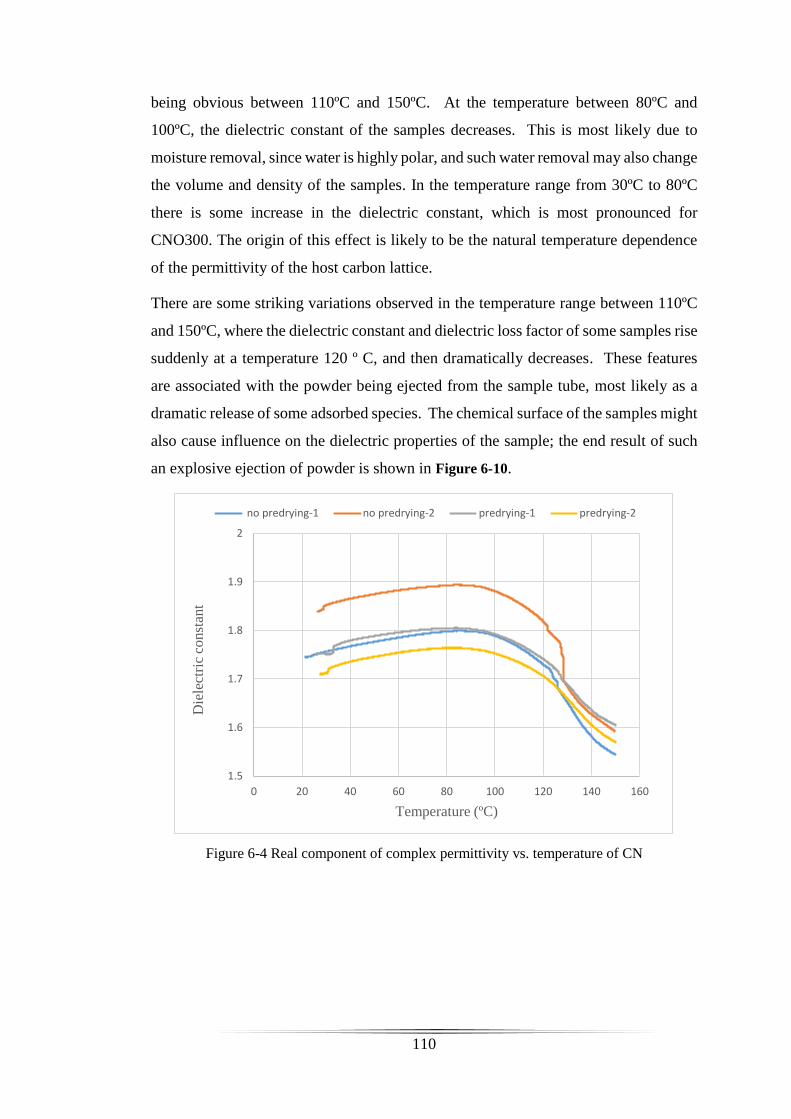
110
being obvious between 110ºC and 150ºC. At the temperature between 80ºC and
100ºC, the dielectric constant of the samples decreases. This is most likely due to
moisture removal, since water is highly polar, and such water removal may also change
the volume and density of the samples. In the temperature range from 30ºC to 80ºC
there is some increase in the dielectric constant, which is most pronounced for
CNO300. The origin of this effect is likely to be the natural temperature dependence
of the permittivity of the host carbon lattice.
There are some striking variations observed in the temperature range between 110ºC
and 150ºC, where the dielectric constant and dielectric loss factor of some samples rise
suddenly at a temperature 120 º C, and then dramatically decreases. These features
are associated with the powder being ejected from the sample tube, most likely as a
dramatic release of some adsorbed species. The chemical surface of the samples might
also cause influence on the dielectric properties of the sample; the end result of such
an explosive ejection of powder is shown in Figure 6-10.
Figure 6-4 Real component of complex permittivity vs. temperature of CN
1.5
1.6
1.7
1.8
1.9
2
0 20 40 60 80 100 120 140 160
Die
lect
ric
const
ant
Temperature (ºC)
no predrying-1 no predrying-2 predrying-1 predrying-2

111
Figure 6-5 Imaginary component of complex permittivity vs. temperature of CN
Figure 6-6 Real component of complex permittivity vs. temperature of CN800
0.04
0.05
0.06
0.07
0.08
0.09
0.1
0 20 40 60 80 100 120 140 160
loss
fac
tor
Temperature (ºC)
no predrying-1 no predrying-2 predrying-1 predrying-2
2.5
3
3.5
4
4.5
5
5.5
0 20 40 60 80 100 120 140 160
Die
lect
ric
const
ant
Temperature (ºC)
no predrying-1 no predrying-2 predrying-1 predrying-2
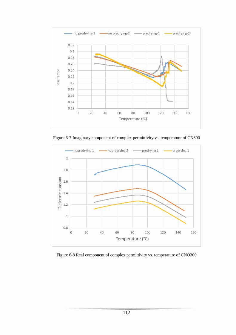
112
Figure 6-7 Imaginary component of complex permittivity vs. temperature of CN800
Figure 6-8 Real component of complex permittivity vs. temperature of CNO300
0.12
0.14
0.16
0.18
0.2
0.22
0.24
0.26
0.28
0.3
0.32
0 20 40 60 80 100 120 140 160
loss
fac
tor
Temperature (ºC)
no predrying-1 no predrying-2 predrying-1 predrying-2
0.8
1
1.2
1.4
1.6
1.8
2
0 20 40 60 80 100 120 140 160
Die
lect
ric
const
ant
Temperature (ºC)
nopredrying 1 nopredrying 2 predrying 1 predrying 1
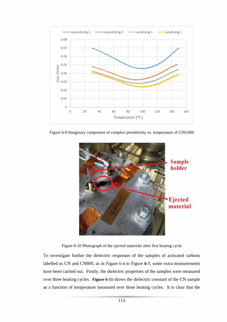
113
Figure 6-9 Imaginary component of complex permittivity vs. temperature of CNO300
Figure 6-10 Photograph of the ejected materials after first heating cycle
To investigate further the dielectric responses of the samples of activated carbons
labelled as CN and CN800, as in Figure 6-4 to Figure 6-7, some extra measurements
have been carried out. Firstly, the dielectric properties of the samples were measured
over three heating cycles. Figure 6-11 shows the dielectric constant of the CN sample
as a function of temperature measured over three heating cycles. It is clear that the
0
0.01
0.02
0.03
0.04
0.05
0.06
0.07
0.08
0 20 40 60 80 100 120 140 160
loss
fac
tor
Temperature (ºC)
nopredrying 1 nopredrying 2 predrying 1 predrying 1
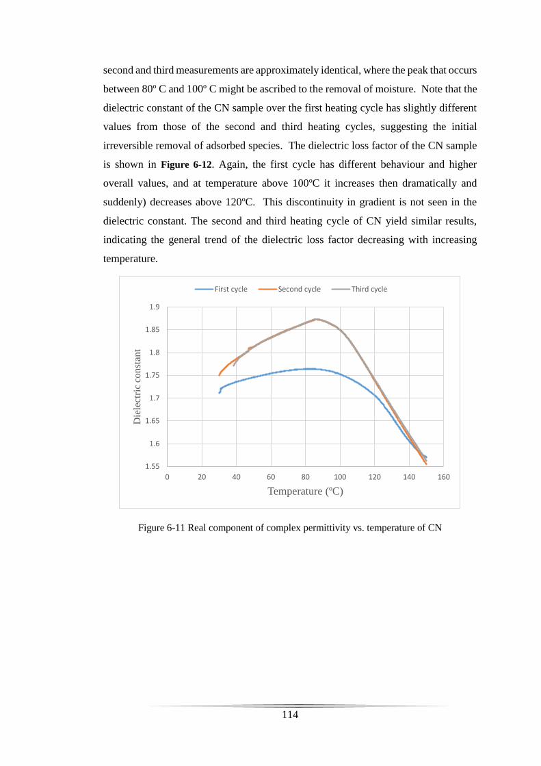
114
second and third measurements are approximately identical, where the peak that occurs
between 80º C and 100º C might be ascribed to the removal of moisture. Note that the
dielectric constant of the CN sample over the first heating cycle has slightly different
values from those of the second and third heating cycles, suggesting the initial
irreversible removal of adsorbed species. The dielectric loss factor of the CN sample
is shown in Figure 6-12. Again, the first cycle has different behaviour and higher
overall values, and at temperature above 100ºC it increases then dramatically and
suddenly) decreases above 120ºC. This discontinuity in gradient is not seen in the
dielectric constant. The second and third heating cycle of CN yield similar results,
indicating the general trend of the dielectric loss factor decreasing with increasing
temperature.
Figure 6-11 Real component of complex permittivity vs. temperature of CN
1.55
1.6
1.65
1.7
1.75
1.8
1.85
1.9
0 20 40 60 80 100 120 140 160
Die
lect
ric
const
ant
Temperature (ºC)
First cycle Second cycle Third cycle

115
Figure 6-12 Imaginary component of complex permittivity vs. temperature of CN
Real and imaginary parts of measured complex permittivity of the CN800 sample are
shown in Figure 6-13 and Figure 6-14, respectively. For dielectric constant, the values
peak between 80º C and 100º C for the first and second heating cycles, similar to the
CN sample, while during the first heating cycle the dielectric constant slightly
increases up to 120ºC, above which it dramatically decreases. The dielectric loss factor
of the CN800 sample exhibits different behaviour and higher values through the first
heating cycle, and above a temperature of 120ºC it dramatically increases before
decreased above 130ºC. The second and third heating cycles of the CN sample show
that the dielectric loss factor gradually decreases with increasing temperature.
0.06
0.065
0.07
0.075
0.08
0.085
0 20 40 60 80 100 120 140 160
loss
fac
tor
Temperature (ºC)
First cycle Second cycle Third cycle
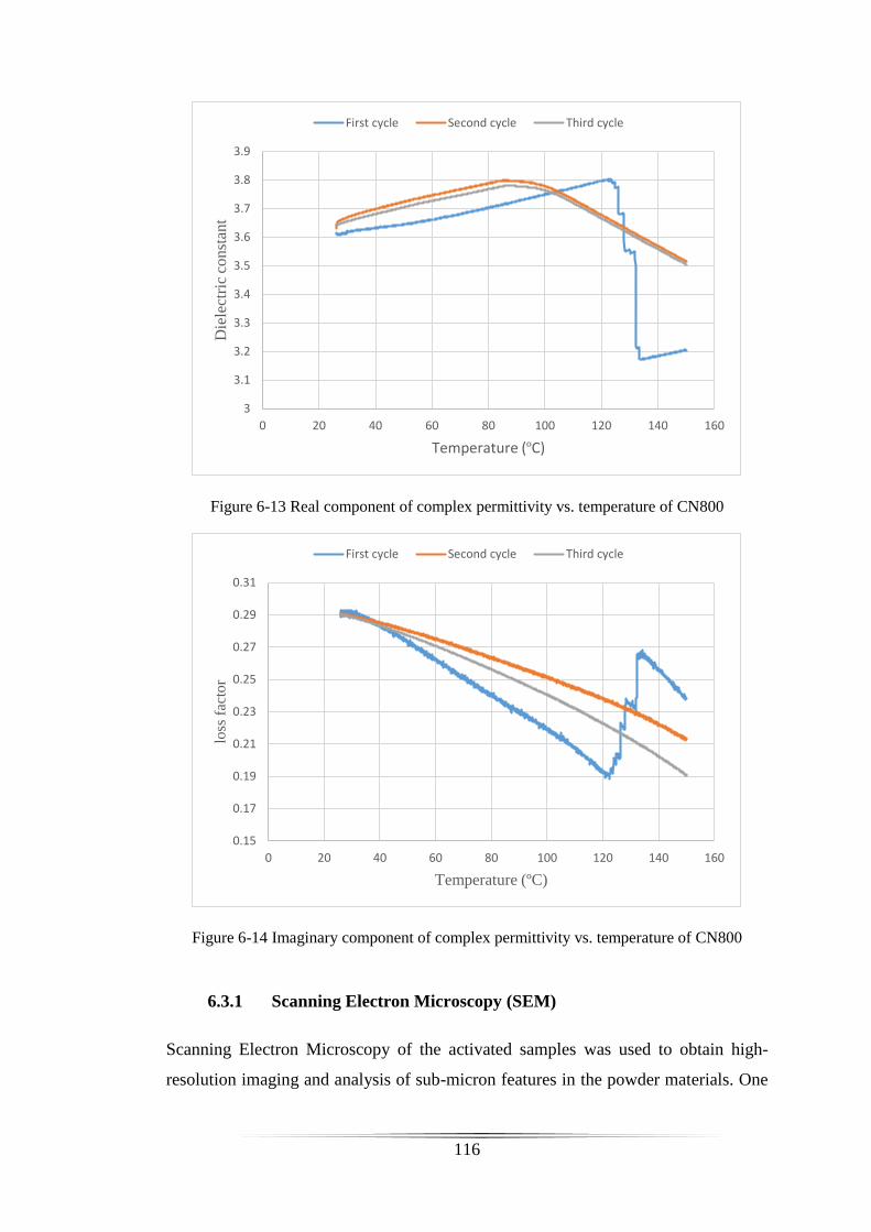
116
Figure 6-13 Real component of complex permittivity vs. temperature of CN800
Figure 6-14 Imaginary component of complex permittivity vs. temperature of CN800
6.3.1 Scanning Electron Microscopy (SEM)
Scanning Electron Microscopy of the activated samples was used to obtain high-
resolution imaging and analysis of sub-micron features in the powder materials. One
3
3.1
3.2
3.3
3.4
3.5
3.6
3.7
3.8
3.9
0 20 40 60 80 100 120 140 160
Die
lect
ric
con
stan
t
Temperature (ºC)
First cycle Second cycle Third cycle
0.15
0.17
0.19
0.21
0.23
0.25
0.27
0.29
0.31
0 20 40 60 80 100 120 140 160
loss
fac
tor
Temperature (ºC)
First cycle Second cycle Third cycle
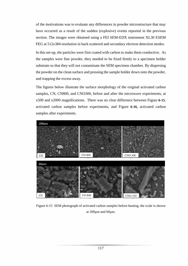
117
of the motivations was to evaluate any differences in powder microstructure that may
have occurred as a result of the sudden (explosive) events reported in the previous
section. The images were obtained using a FEI SEM-EDX instrument XL30 ESEM
FEG at 512x384 resolution in back scattered and secondary electron detection modes.
In this set-up, the particles were first coated with carbon to make them conductive. As
the samples were fine powder, they needed to be fixed firmly to a specimen holder
substrate so that they will not contaminate the SEM specimen chamber. By dispersing
the powder on the clean surface and pressing the sample holder down onto the powder,
and trapping the excess away.
The figures below illustrate the surface morphology of the original activated carbon
samples, CN, CN800, and CNO300, before and after the microwave experiments, at
x500 and x2000 magnifications. There was no clear difference between Figure 6-15,
activated carbon samples before experiments, and Figure 6-16, activated carbon
samples after experiments.
Figure 6-15 SEM photograph of activated carbon samples before heating, the scale is shown
at 200µm and 60µm.
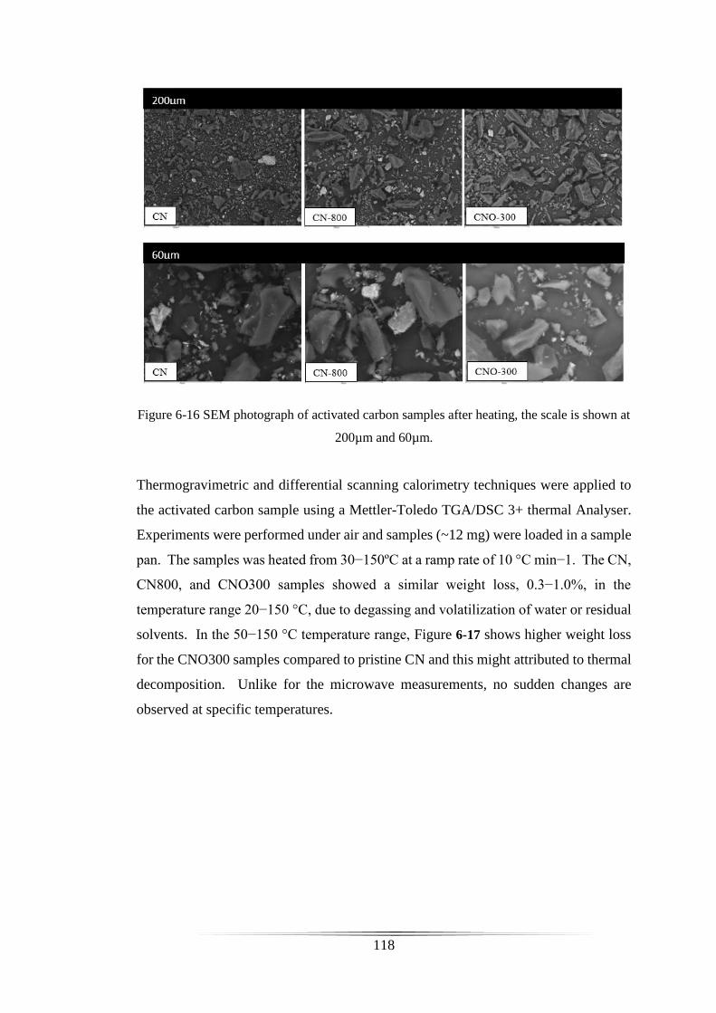
118
Figure 6-16 SEM photograph of activated carbon samples after heating, the scale is shown at
200µm and 60µm.
Thermogravimetric and differential scanning calorimetry techniques were applied to
the activated carbon sample using a Mettler-Toledo TGA/DSC 3+ thermal Analyser.
Experiments were performed under air and samples (~12 mg) were loaded in a sample
pan. The samples was heated from 30−150ºC at a ramp rate of 10 °C min−1. The CN,
CN800, and CNO300 samples showed a similar weight loss, 0.3−1.0%, in the
temperature range 20−150 °C, due to degassing and volatilization of water or residual
solvents. In the 50−150 °C temperature range, Figure 6-17 shows higher weight loss
for the CNO300 samples compared to pristine CN and this might attributed to thermal
decomposition. Unlike for the microwave measurements, no sudden changes are
observed at specific temperatures.
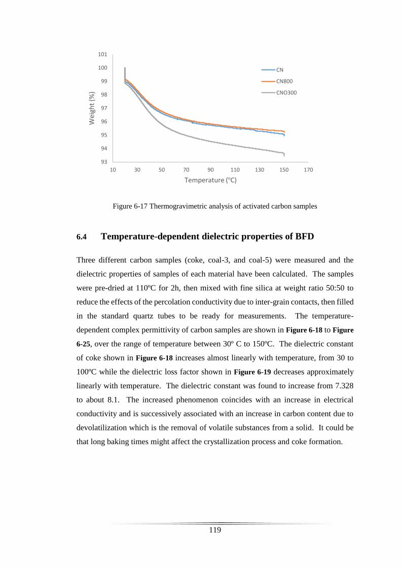
119
Figure 6-17 Thermogravimetric analysis of activated carbon samples
6.4 Temperature-dependent dielectric properties of BFD
Three different carbon samples (coke, coal-3, and coal-5) were measured and the
dielectric properties of samples of each material have been calculated. The samples
were pre-dried at 110ºC for 2h, then mixed with fine silica at weight ratio 50:50 to
reduce the effects of the percolation conductivity due to inter-grain contacts, then filled
in the standard quartz tubes to be ready for measurements. The temperature-
dependent complex permittivity of carbon samples are shown in Figure 6-18 to Figure
6-25, over the range of temperature between 30º C to 150ºC. The dielectric constant
of coke shown in Figure 6-18 increases almost linearly with temperature, from 30 to
100ºC while the dielectric loss factor shown in Figure 6-19 decreases approximately
linearly with temperature. The dielectric constant was found to increase from 7.328
to about 8.1. The increased phenomenon coincides with an increase in electrical
conductivity and is successively associated with an increase in carbon content due to
devolatilization which is the removal of volatile substances from a solid. It could be
that long baking times might affect the crystallization process and coke formation.
93
94
95
96
97
98
99
100
101
10 30 50 70 90 110 130 150 170
We
igh
t (%
)
Temperature (ºC)
CN
CN800
CNO300
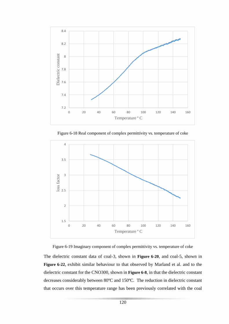
120
Figure 6-18 Real component of complex permittivity vs. temperature of coke
Figure 6-19 Imaginary component of complex permittivity vs. temperature of coke
The dielectric constant data of coal-3, shown in Figure 6-20, and coal-5, shown in
Figure 6-22, exhibit similar behaviour to that observed by Marland et al. and to the
dielectric constant for the CNO300, shown in Figure 6-8, in that the dielectric constant
decreases considerably between 80ºC and 150ºC. The reduction in dielectric constant
that occurs over this temperature range has been previously correlated with the coal
7.2
7.4
7.6
7.8
8
8.2
8.4
0 20 40 60 80 100 120 140 160
Die
lect
ric
con
stan
t
Temperature º C
1.5
2
2.5
3
3.5
4
0 20 40 60 80 100 120 140 160
loss
fac
tor
Temperature º C
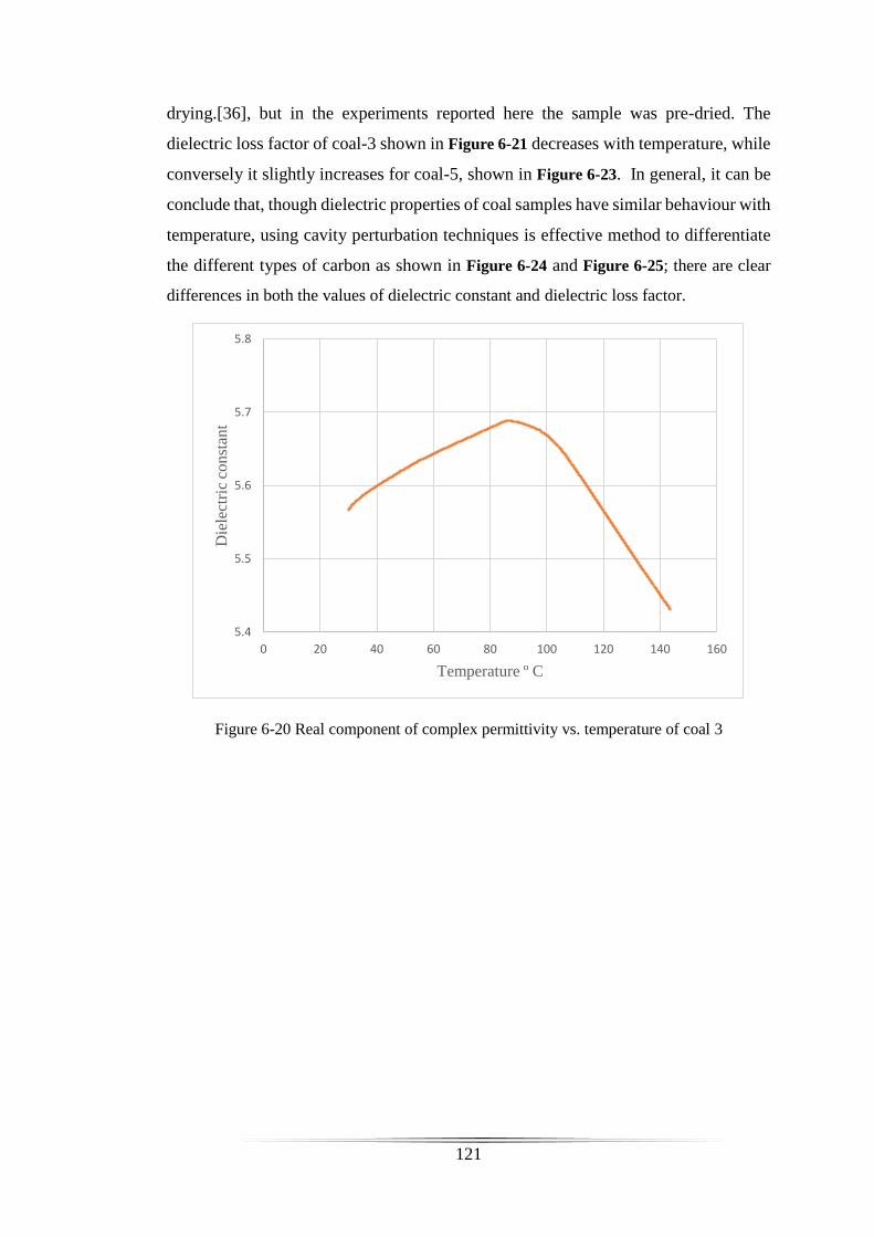
121
drying.[36], but in the experiments reported here the sample was pre-dried. The
dielectric loss factor of coal-3 shown in Figure 6-21 decreases with temperature, while
conversely it slightly increases for coal-5, shown in Figure 6-23. In general, it can be
conclude that, though dielectric properties of coal samples have similar behaviour with
temperature, using cavity perturbation techniques is effective method to differentiate
the different types of carbon as shown in Figure 6-24 and Figure 6-25; there are clear
differences in both the values of dielectric constant and dielectric loss factor.
Figure 6-20 Real component of complex permittivity vs. temperature of coal 3
5.4
5.5
5.6
5.7
5.8
0 20 40 60 80 100 120 140 160
Die
lect
ric
con
stan
t
Temperature º C

122
Figure 6-21 Imaginary component of complex permittivity vs. temperature of coal 3
Figure 6-22 Real component of complex permittivity vs. temperature of coal 5
1.315
1.317
1.319
1.321
1.323
1.325
1.327
0 20 40 60 80 100 120 140 160
loss
fac
tor
Temperature º C
1.7
1.8
1.9
2
2.1
0 20 40 60 80 100 120 140 160
Die
lect
ric
const
ant
Temperature º C
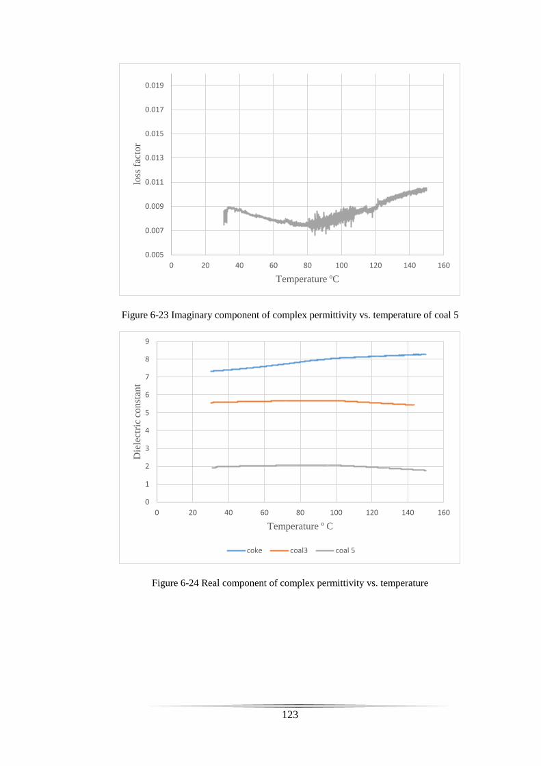
123
Figure 6-23 Imaginary component of complex permittivity vs. temperature of coal 5
Figure 6-24 Real component of complex permittivity vs. temperature
0.005
0.007
0.009
0.011
0.013
0.015
0.017
0.019
0 20 40 60 80 100 120 140 160
loss
fac
tor
Temperature ºC
0
1
2
3
4
5
6
7
8
9
0 20 40 60 80 100 120 140 160
Die
lect
ric
const
ant
Temperature º C
coke coal3 coal 5
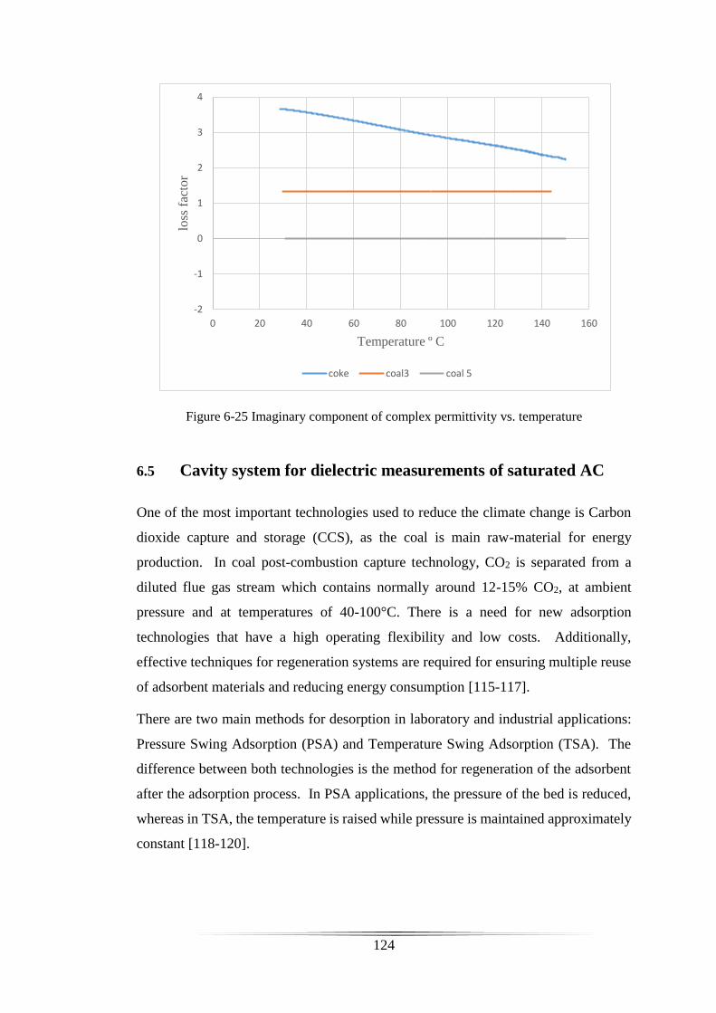
124
Figure 6-25 Imaginary component of complex permittivity vs. temperature
6.5 Cavity system for dielectric measurements of saturated AC
One of the most important technologies used to reduce the climate change is Carbon
dioxide capture and storage (CCS), as the coal is main raw-material for energy
production. In coal post-combustion capture technology, CO2 is separated from a
diluted flue gas stream which contains normally around 12-15% CO2, at ambient
pressure and at temperatures of 40-100°C. There is a need for new adsorption
technologies that have a high operating flexibility and low costs. Additionally,
effective techniques for regeneration systems are required for ensuring multiple reuse
of adsorbent materials and reducing energy consumption [115-117].
There are two main methods for desorption in laboratory and industrial applications:
Pressure Swing Adsorption (PSA) and Temperature Swing Adsorption (TSA). The
difference between both technologies is the method for regeneration of the adsorbent
after the adsorption process. In PSA applications, the pressure of the bed is reduced,
whereas in TSA, the temperature is raised while pressure is maintained approximately
constant [118-120].
-2
-1
0
1
2
3
4
0 20 40 60 80 100 120 140 160
loss
fac
tor
Temperature º C
coke coal3 coal 5

125
Activated carbons are one class of carbonaceous adsorbents that use CO2 capture, due
to their wide availability, low cost, high thermal stability and low sensitivity to
moisture [118, 119, 121].
In these experiments, activated carbon in the form of granular manufactured by Cabot
Corporation was used. The size of the particles of AC was around 210-595µm, and
the surface area was 1513.9 m²/g and pore diameter about 1.2 nm [15]; particles were
dried in a lab oven at 110 °C for 12 h and stored in a desiccator before using in the
relevant experiments.
The same granular AC samples were crushed as previously into fine powders (section
4.3). The adsorption of water vapour was done in a very simple way by putting the
sample close to boiling water for ten minutes, then performing the microwave
characterization using the same cavity system and laboratory oven. Experiments were
conducted using the same system as illustrated in Figure 6-3. The complex
permittivity of the water-saturated samples were measured over the temperature range
of 30ºC -150ºC, and the results are illustrated in Figure 6-26 and Figure 6-27. The
dielectric constant decreases considerably between 80ºC and 150ºC, correlated to the
expected drying of the sample. The associated dielectric loss factor of the water-
saturated, granular AC is shown in Figure 6-27 and this also decreases with
temperature.
To attempt to saturate the AC samples with carbon dioxide, granular activated carbon
(GCN3070) was filled in quartz tubes, with glass wool frits used at both ends of the
quartz tube to support the AC samples. First, 5g samples of granular AC were dried
in the laboratory oven at 110ºC for 2 hours. Next, a CO2 stream was passed through
the sample at room temperature and atmospheric pressure for 1 hour, at a flow rate of
1 litre/min. Two granular AC samples were measured using cavity resonator system
using the TM010 mode at 2.498GHz.

126
Figure 6-26 Real component of complex permittivity of AC sample saturated with water
Figure 6-27 Imaginary component of complex permittivity of AC sample saturated with
water
Figure 6.28 and Figure 6-29 show the time-dependent dielectric constant and dielectric
loss factor of two granular AC carbon samples. The changes in dielectric constant and
loss factor of both samples are small, implying little desorption of CO2 at room
temperature, even for the highly porous structure of AC.
3.75
3.8
3.85
3.9
3.95
4
4.05
0 20 40 60 80 100 120 140 160
Die
lect
ric
con
stan
t
Temperature ºC
0
0.2
0.4
0.6
0.8
1
0 20 40 60 80 100 120 140 160
loss
fac
tor
Temperature º C
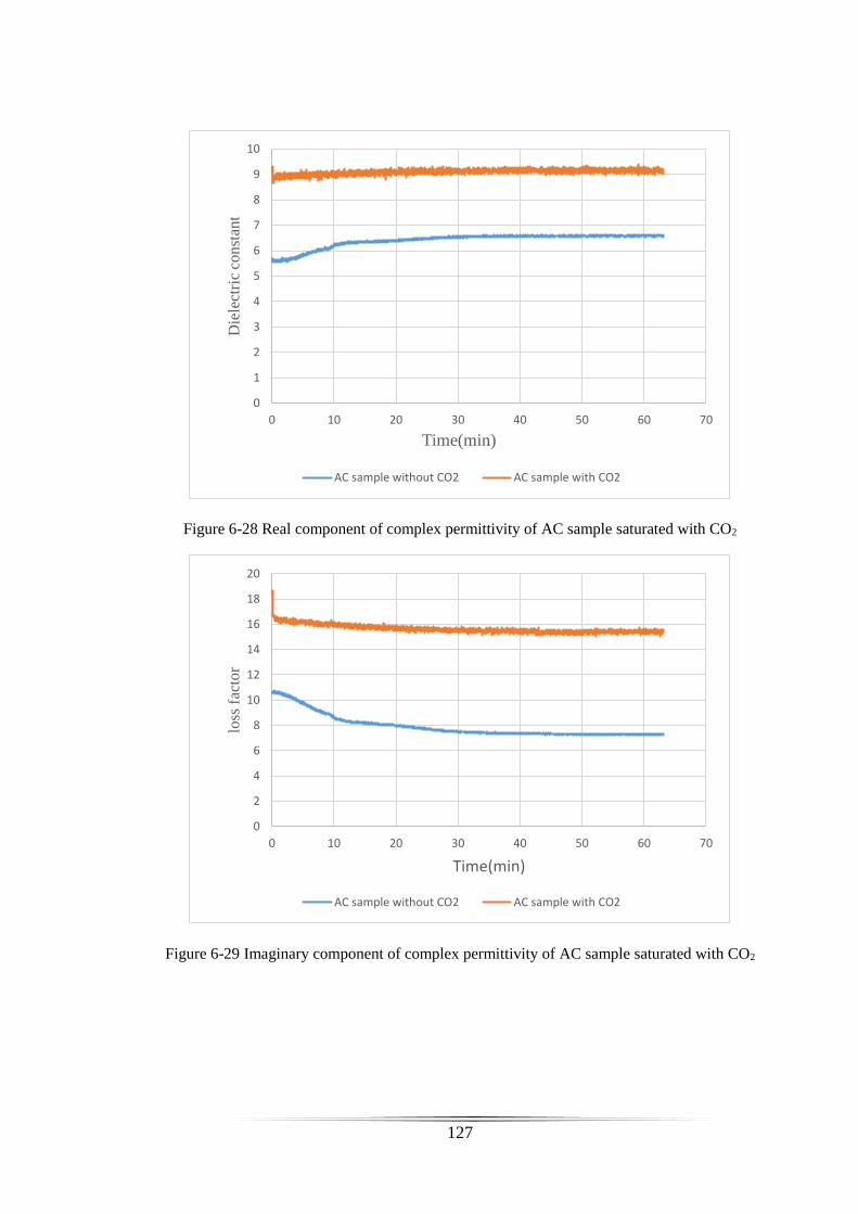
127
Figure 6-28 Real component of complex permittivity of AC sample saturated with CO2
Figure 6-29 Imaginary component of complex permittivity of AC sample saturated with CO2
0
1
2
3
4
5
6
7
8
9
10
0 10 20 30 40 50 60 70
Die
lect
ric
con
stan
t
Time(min)
AC sample without CO2 AC sample with CO2
0
2
4
6
8
10
12
14
16
18
20
0 10 20 30 40 50 60 70
loss
fac
tor
Time(min)
AC sample without CO2 AC sample with CO2
128
6.6 Conclusion
In this chapter the potential for the use of microwave cavity techniques for the
measurement of the temperature-dependent dielectric properties of activated carbons
and carbonaceous materials contained in BFD at microwave frequencies are presented.
The TM310 mode was used as a nodal mode for temperature correction of the TM010
measurements. The dielectric properties of both groups of carbons were measured
within the temperature range between 30ºC and 150ºC. Measurements were recorded
using a LabVIEW program. The measurements show that the dielectric constant
variations with temperature for most samples exhibit a significant decrease between
80ºC and 150ºC, except for the coke sample, whose dielectric constant increases with
temperature. This decrease in the dielectric constant might be related to the drying of
the samples, as moisture removal would decrease both dielectric constant and loss
factor.
The measurements of activated carbons have high practical relevance in the use of
cavity perturbation as a means of characterising the dielectric properties prior to (or
simultaneous with) the use of microwave heating in order to regeneration exhausted
activated carbon. Additionally, the results demonstrate the potential for this technique
to differentiate the carbonaceous materials contained in BFD at different temperatures
in order to combine the microwave system with blast furnace to allowing the real-time
monitoring of complex permittivity of coal, char, and coke in BFD.
Finally, it is worth noting that the sudden change in dielectric properties of activated
carbons when undergoing microwave characterisation, associated with explosive
ejection of the powder samples, is not seen in the BFD materials. This uniqueness to
activated samples, with their large surface areas and porous nature, is currently
unexplained, but has been observed for the first time in this thesis. It is worth noting
that this effect only occurs when microwaves are applied. Similar experiments on the
same samples heating to the same temperatures with just the oven (and no microwaves
applied) show no such ejection. This is consistent with the lack of changes observed
in the thermogravimetric data of Figure 6-20. The microwave power levels for the
cavity perturbation experiments here are very low, at 0 dBm (i.e. 1 mW rms). For them
to have such a dramatic effect implies an extreme microwave coupling to an explosive
phenomenon which may have important consequences for the use of microwaves in
the regeneration of such samples when used, for example, in carbon dioxide capture.

129

130
Chapter 7 Conclusion and future work
This chapter summarises the main conclusions, discusses the relevant challenges that
have been faced during the research, and finally provides suggestions for future work
and possible improvements that can be implemented. This thesis has focused on using
microwave techniques in characterizing and differentiating types of carbons. In this
respect, two groups of carbonaceous materials have been characterized.
7.1 Literature Survey:
Chapter 2 gives a survey of the properties and applications of activated carbon
materials, blast carbon materials contained in furnace dust. The initial proposal of this
research is to design and build microwave cavity system and broadband coaxial probe
applicator to measure dielectric properties of these materials, in order to characterize
and differentiate these materials over range of frequencies and under temperature
range between 30ºC and 150ºC.
7.2 Analysis: Microwave Systems Principles
Chapter 3 gives an explanation on the microwave cavity system and how they work.
The relevant equations for the microwave cavity perturbation method are presented,
with an original expression for the theoretical bandwidth for TM modes. A variety of
different modes with different frequencies have been identified for measuring the
frequency dependent dielectric properties. A circuit model is also presented which is
important for understanding how to take measurements. Additionally, Principles and
design of the coaxial probe system are presented, with details of the chosen model
which used to extract complex permittivity from the measured data.
7.3 Experiments
Chapter 4 The microwave cavity system in this chapter has been shown to have high
measurement accuracy for both carbon groups. Even when the samples are from the

131
same materials treated differently such as samples AC2 and AC3, the system are
capable of differentiate the samples.
Chapter 5 This study shows that multi-mode microwave cavity can be used to
estimate the microwave dielectric properties of carbons contained in BFD at the
discrete set of resonant frequencies in the 2 to 10 GHz range. TM modes were used.
Moreover, broadband measurements of dielectric properties of both carbon groups
were presented and the results show that both the multimode cavity and open-ended
coaxial probe methods are appropriate to be used as test methods for identifying and
differentiating the different types of carbons based on the frequency dependence of
their dielectric properties.
Chapter 6 gives an explanation of how to use microwave cavity resonator to measure
the temperature dependent dielectric properties of samples. A procedure for the
correction of systematic temperature fluctuations using higher order cylindrical modes
is detailed. Analytically, the temperature dependent resonant frequency and
bandwidth of all modes are linked, respectively, through the thermal expansion
coefficient and the coefficient of resistivity. In practice, offsets in these coefficients
exist across the modes. The relationship between each of the modes, however, is
constant and thus this procedure should only be used to remove systematic fluctuations
in the conducted experiment.
7.4 Characterization of activated carbon materials
The dielectric complex permittivity of activated carbons has been measured using both
microwave cavity and coaxial probe techniques to represent and quantify the
differences between different AC materials that have been produced from different
precursors and had different treatments.
7.5 Characterization of types of carbon contained in BFD
Microwave cavity and coaxial probe techniques have been used for measuring the
dielectric complex permittivity of carbonaceous materials contained in BFD. This
characterization of these materials is required to differentiate the different forms of
carbonaceous materials from the raw materials coke and coal. The differentiation of

132
these types of carbons in the blast furnace dust is important to quantify the utilization
of coal injected in the furnace and determine the efficiency of coal injection.
7.6 Further Work
In this research, attempts have been made to comprehensive characterization of
different types of carbons by measuring the change in complex permittivity with
frequency and temperature. With regard to the activated carbon materials, more
microwave heating experiments are suggested to regenerate or recycle the loaded
activated carbons.
7.6.1 Microwave regeneration of saturated activated carbons
In order to try to develop microwave system to regeneration of activated carbons, a
cylindrical cavity at lower centre frequency has already been designed using
COMSOL Multiphysics software shown in Figure 7-1. The cavity is designed to have
its TM010 mode at a frequency of 900 MHz and TM010 mode, so the cavity’s inner
radius should be 128 mm. A mode chart is used to choose an appropriate length of
cavity based on the ratio (2𝑎𝑑⁄ )
2
to ensure that there is no interference between the
TM010 mode and TE111; this results in the cavity’s inner height being chosen to be 200
mm. It should be noted that 900 MHz is an ISM frequency, at which there are a number
of cost-effective power amplifiers for generation of high microwave powers up to 1
kW. The larger cavity volume permits larger sample volumes, in this case up to a few
cm3, depending on the loss factor of the samples.
The cavity is constructed from three parts: cavity body, the bottom lid and the side
piece to place the coupling connector. Aluminium is chosen for the cavity’s metal,
since it is easy to machine, cheap and has low mass compared with copper, even though
the Q factor is only sacrificed by about 25%.

133
Figure 7-1 the large aluminium cylindrical cavity resonator.
The coupling loop is designed on the middle of the side of cylindrical metal wall, and
it is shown in Figure 7-1. The radius of coupling loop in the simulations is 5 mm and
the radius of the coupling loop in the practice is 25 mm. There are two types of
coupling used; SMA connectors at the top of the cavity allow cavity perturbations in
the usual way, to study dielectric properties of a sample; the side-wall N connector
allows high power to be pumped into the cavity, so that in principle samples can be
simultaneously heated and characterized.
7.6.2 Electric fields distribution
Figure 7-2 shows the electric field distribution for the TM010 mode in this large
cylindrical cavity, including the 5 cm diameter sample hole which acts as a microwave
choke. These are calculated and plotted using COMSOL software. The intensity of
electric field decreases from the cavity centre to the boundary walls, where it is reduced
to zero.

134
Figure 7-2 Electric field distribution of a 900MHz cavity operating in the TM010 mode
7.6.3 Microwave excitation system
A high power system was designed to deliver high power microwave at both
frequencies of 2.45 GHz and 900 MHz, for both small and large cavities used in this
thesis. Figure 7.3 illustrates a circuit diagram of the system. It consists of a microwave
generator which provides an rms output at a power level of 1mW to the input of the
high power amplifier for cavity excitation. The system set up for experiments is shown
in Figure 7-3 and Figure 7-4.
Figure 7-3 Schematic of the whole microwaving system using the large cavity
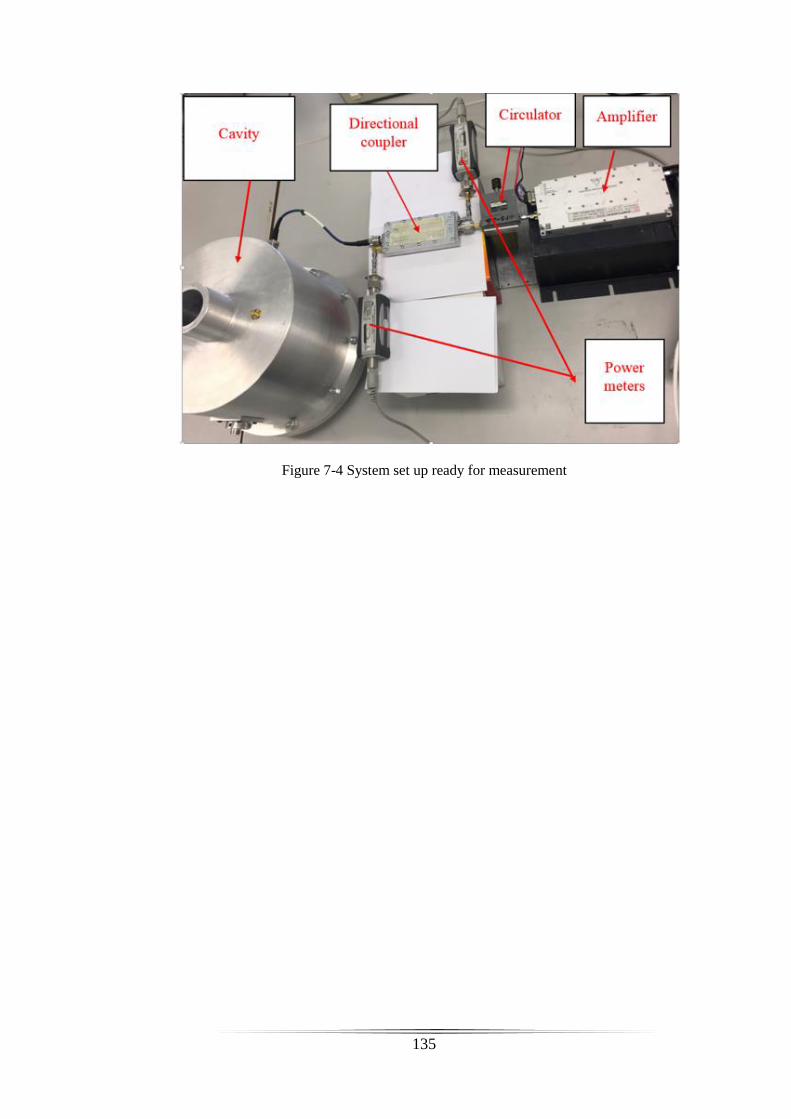
135
Figure 7-4 System set up ready for measurement

136
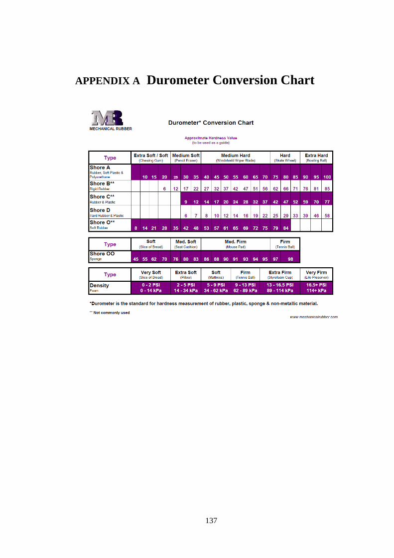
137
APPENDIX A Durometer Conversion Chart
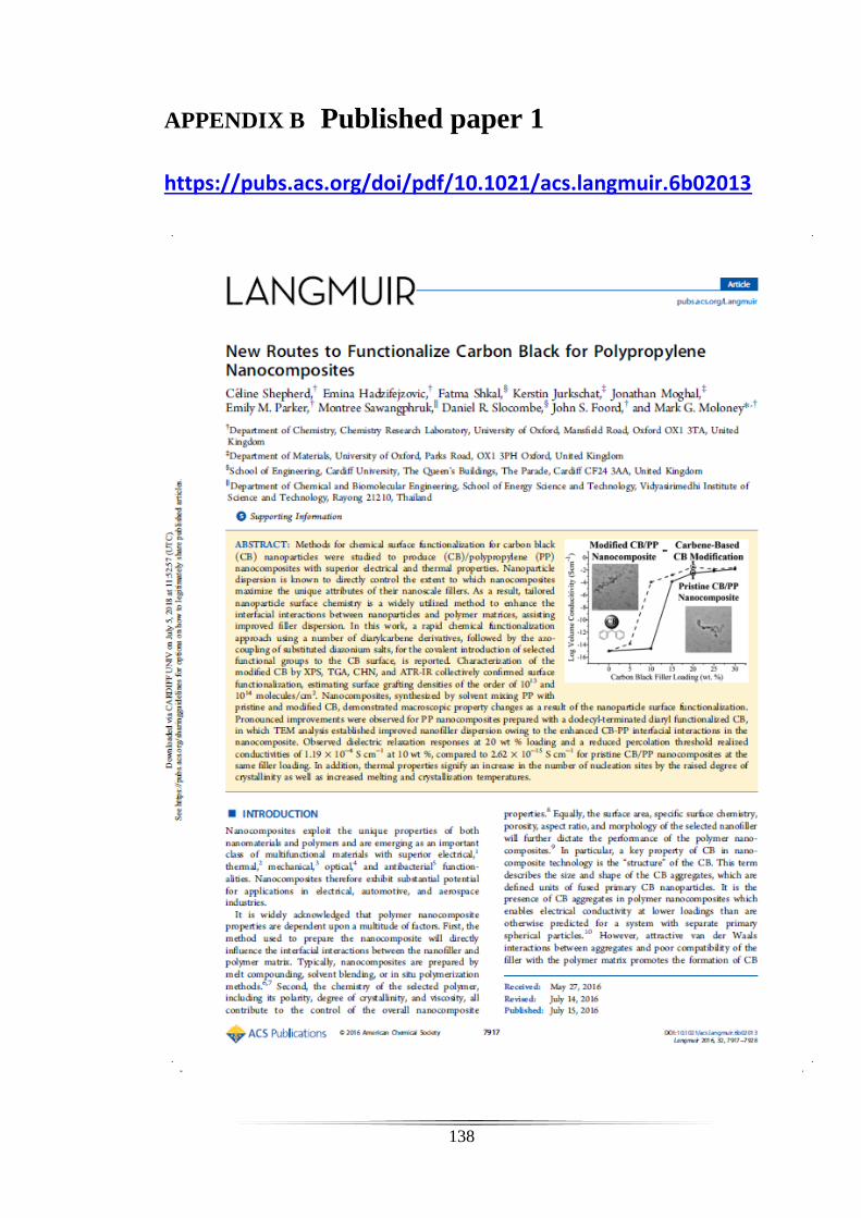
138
APPENDIX B Published paper 1
https://pubs.acs.org/doi/pdf/10.1021/acs.langmuir.6b02013
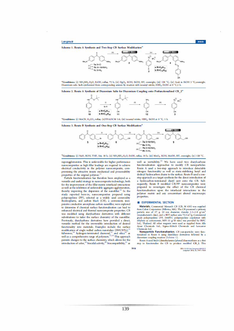
139
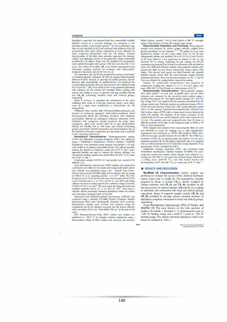
140
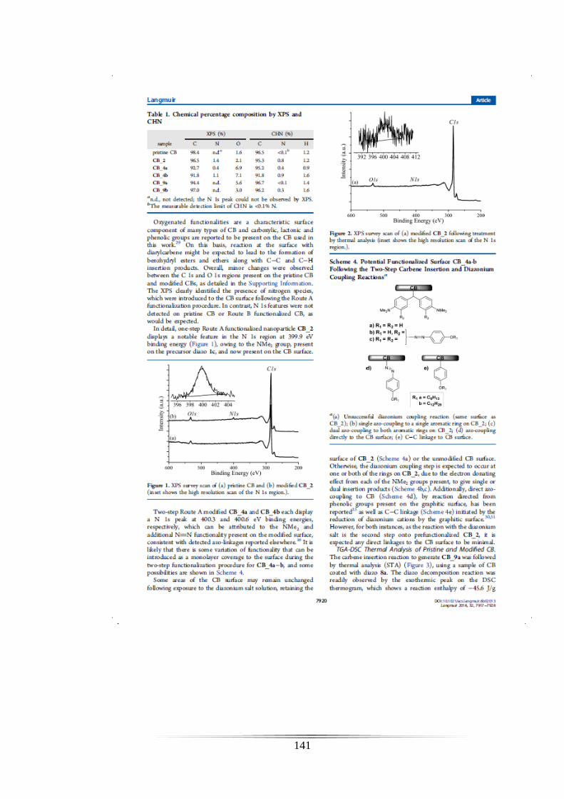
141
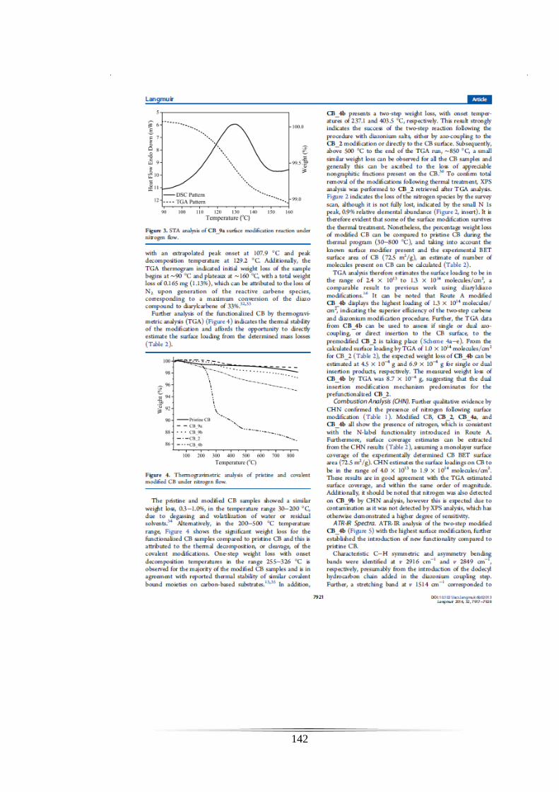
142

143

144

145

146

147

148

149

150

151
References
1. Prapuchanay, E., N. Puangngernmak, and S. Chalermwisutkul. A single mode cylindrical microwave cavity for heating applications of liquid material. in Electrical Engineering/Electronics, Computer, Telecommunications and Information Technology (ECTI-CON), 2012 9th International Conference on. 2012. IEEE.
2. Pozar, D.M., Microwave engineering. 4th ed. ed. 2012: Hoboken, N.J. : Wiley. 3. McDougall, G., The physical nature and manufacture of activated carbon. Journal of
the South African institute of mining and metallurgy, 1991. 91(4): p. 109-120. 4. Al-Qodah, Z. and R. Shawabkah, Production and characterization of granular activated
carbon from activated sludge. Brazilian Journal of Chemical Engineering, 2009. 26(1): p. 127-136.
5. Stewart, M.L. and J. Stencel, Treatment of Activated Carbons for Densification. PREPRINTS OF PAPERS-AMERICAN CHEMICAL SOCIETY DIVISION FUEL CHEMISTRY, 1993. 38: p. 408-408.
6. Menéndez, J., et al., Microwave heating processes involving carbon materials. Fuel Processing Technology, 2010. 91(1): p. 1-8.
7. Dias, J.M., et al., Waste materials for activated carbon preparation and its use in aqueous-phase treatment: a review. Journal of Environmental Management, 2007. 85(4): p. 833-846.
8. Chronopoulos, T., et al., CO 2 desorption via microwave heating for post-combustion carbon capture. Microporous and Mesoporous Materials, 2014. 197: p. 288-290.
9. Ania, C., et al., Effect of microwave and conventional regeneration on the microporous and mesoporous network and on the adsorptive capacity of activated carbons. Microporous and Mesoporous Materials, 2005. 85(1): p. 7-15.
10. Hesas, R.H., et al., Preparation and characterization of activated carbon from apple waste by microwave-assisted phosphoric acid activation: application in methylene blue adsorption. BioResources, 2013. 8(2): p. 2950-2966.
11. Ania, C., et al., Microwave-induced regeneration of activated carbons polluted with phenol. A comparison with conventional thermal regeneration. Carbon, 2004. 42(7): p. 1383-1387.
12. Qiu, Y. and M. Hawley. Composite material processing in a single mode cavity with variable frequency microwaves. in 12th International Conference on Composite Materials. Paris, France. 1999.
13. Menendez-Diaz, J. and I. Martin-Gullon, Types of carbon adsorbents and their production. Interface Science and Technology, 2006. 7: p. 1-47.
14. Atwater, J. and R. Wheeler Jr, Microwave permittivity and dielectric relaxation of a high surface area activated carbon. Applied Physics A, 2004. 79(1): p. 125-129.
15. Chronopoulos, T., et al., CO2 desorption via microwave heating for post-combustion carbon capture. Microporous and Mesoporous Materials, 2014. 197: p. 288-290.
16. YAĞŞİ, N.U., Production and Characterization of Activated Carbon from Apricot Stones, in The Department of Chemical Engineering. 2004, The Middle East Technical University. p. 114.
17. Harris, P.J., Z. Liu, and K. Suenaga, Imaging the atomic structure of activated carbon. Journal of Physics: Condensed Matter, 2008. 20(36): p. 362201.
18. Rouquerol, J., et al., Recommendations for the characterization of porous solids (Technical Report). Pure and Applied Chemistry, 1994. 66(8): p. 1739-1758.

152
19. Warhurst, A.M., G.L. McConnachie, and S.J. Pollard, Characterisation and applications of activated carbon produced from Moringa oleifera seed husks by single-step steam pyrolysis. Water Research, 1997. 31(4): p. 759-766.
20. White, R.J., et al., Tuneable porous carbonaceous materials from renewable resources. Chemical Society Reviews, 2009. 38(12): p. 3401-3418.
21. Atwater, J.E. and R.R. Wheeler, Complex permittivities and dielectric relaxation of granular activated carbons at microwave frequencies between 0.2 and 26 GHz. Carbon, 2003. 41(9): p. 1801-1807.
22. Hotta, M., et al., Complex permittivity of graphite, carbon black and coal powders in the ranges of X-band frequencies (8.2 to 12.4 GHz) and between 1 and 10 GHz. ISIJ international, 2011. 51(11): p. 1766-1772.
23. Yang, Y., et al., Characterizing Adsorption Performance of Granular Activated Carbon with Permittivity. Materials, 2017. 10(3): p. 269.
24. Al-Sehemi, A.G., et al., Effect of Activated Carbons on the Dielectric and Microwave Properties of Natural Rubber Based Composites. Materials Research, 2017. 20(5): p. 1211-1220.
25. Ab Jabal, S.N., Y.B. Seok, and W.F. Hoon, Carbon composition, surface porosities and dielectric properties of coconut shell powder and coconut shell activated carbon composites. Journal of Engineering and Applied Sciences 2016. 11(6).
26. He, C.L., et al., Calorimetry Study of Microwave Absorption of Some Solid Materials. Journal of Microwave Power and Electromagnetic Energy, 2013. 47(4): p. 251-261.
27. Motasemi, F., et al., Microwave dielectric characterization of switchgrass for bioenergy and biofuel. Fuel, 2014. 124: p. 151-157.
28. Omorogie, M.O., J.O. Babalola, and E.I. Unuabonah, Regeneration strategies for spent solid matrices used in adsorption of organic pollutants from surface water: a critical review. Desalination and Water Treatment, 2016. 57(2): p. 518-544.
29. Ania, C.O., et al., Microwave-assisted regeneration of activated carbons loaded with pharmaceuticals. Water Res, 2007. 41(15): p. 3299-306.
30. Bradshaw, S., E.V. Wyk, and J.d. Swardt, Preliminary economic assessment of microwave regeneration of activated carbon for the carbon in pulp process. Journal of microwave power and electromagnetic energy, 1997. 32(3): p. 131-144.
31. Ng, K., et al., Carbon type differentiation technique for diagnosing pulverised coal injection efficiency. Ironmaking & Steelmaking, 2016. 43(3): p. 214-219.
32. Gray, R. and K. Devanney, Coke carbon forms: microscopic classification and industrial applications. International Journal of Coal Geology, 1986. 6(3): p. 277-297.
33. Lundgren, M., Blast furnace coke properties and the influence on off-gas dust. 2010, Luleå tekniska universitet.
34. Geerdes, M., R. Chaigneau, and I. Kurunov, Modern Blast Furnace Ironmaking: An Introduction (2015). 2015: Ios Press.
35. Zhong, Y., et al., Structural Characterization of Carbon in Blast Furnace Flue Dust and Its Reactivity in Combustion. Energy & Fuels, 2017. 31(8): p. 8415-8422.
36. Marland, S., A. Merchant, and N. Rowson, Dielectric properties of coal. Fuel, 2001. 80(13): p. 1839-1849.
37. Snoeyink, V.L. and W.J. Weber, The surface chemistry of active carbon; a discussion of structure and surface functional groups. Environmental Science & Technology, 1967. 1(3): p. 228-234.
38. Leblanc, J.L., Rubber–filler interactions and rheological properties in filled compounds. Progress in polymer science, 2002. 27(4): p. 627-687.
39. Barroso-Bogeat, A., et al., Activated carbon surface chemistry: Changes upon impregnation with Al (III), Fe (III) and Zn (II)-metal oxide catalyst precursors from NO3− aqueous solutions. Arabian Journal of Chemistry, 2016.

153
40. Figueiredo, J.L., Functionalization of porous carbons for catalytic applications. Journal of Materials Chemistry A, 2013. 1(33): p. 9351-9364.
41. Boehm, H.P., Surface oxides on carbon and their analysis: a critical assessment. Carbon, 2002. 40(2): p. 145-149.
42. Peschel, G., Carbon-carbon bonds: hybridization. Obtained online from: http://www. physik. fu-berlin. de/einrichtungen/ag/ag-reich/lehre/Archiv/ss2011/docs/Gina_Peschel-Handout. pdf, published on, 2011. 5(5).
43. Cuenca, J.A., Characterisation of powders using microwave cavity perturbation. PhD thesis, Cardiff University, 2015.
44. Sheen, J., Comparisons of microwave dielectric property measurements by transmission/reflection techniques and resonance techniques. Measurement Science and Technology, 2009. 20(4): p. 042001.
45. Krupka, J., Frequency domain complex permittivity measurements at microwave frequencies. Measurement Science and Technology, 2006. 17(6): p. R55.
46. Singh, D.P., et al., Microwave cavity technique to study the dielectric response in 4′-n-Heptyl-4-biphenyl nematic liquid crystal at 20.900 GHz and 29.867 GHz. Measurement, 2011. 44(4): p. 605-610.
47. Jha, S.N., et al., Measurement techniques and application of electrical properties for nondestructive quality evaluation of foods—a review. Journal of food science and technology, 2011. 48(4): p. 387-411.
48. Note, A.A., Agilent Basics of Measuring the Dielectric Properties of Materials. Agilent Literature Number, 2006.
49. Saeed, K., et al., Planar microwave sensors for complex permittivity characterization of materials and their applications, in Applied Measurement Systems. 2012, InTech.
50. Venkatesh, M. and G. Raghavan, An overview of dielectric properties measuring techniques. Canadian biosystems engineering, 2005. 47(7): p. 15-30.
51. Al-Hartomy, O.A., et al., Effect of matrix chemical nature on the properties of composites for microwave absorbers. Polymer-Plastics Technology and Engineering, 2013. 52(11): p. 1113-1121.
52. Stuchly, M., Dielectric properties of biological substances-Tabulated. J. Microwave Power, 1997. 15(1): p. 39-43.
53. Rytting, D., Network analyzer error models and calibration methods. White Paper, September, 1998.
54. Reinecke, T., et al., Open-ended coaxial probe for the quantification of edema in human brain tissue. Sensors and Actuators B: Chemical, 2014. 204: p. 763-769.
55. Salema, A.A., et al., Dielectric properties and microwave heating of oil palm biomass and biochar. Industrial Crops and Products, 2013. 50: p. 366-374.
56. Tripathi, M., et al., Effect of microwave frequency on dielectric properties of oil palm shell (OPS) and OPS char synthesized by microwave pyrolysis of OPS. Journal of Analytical and Applied Pyrolysis, 2015. 112: p. 306-312.
57. Tereshchenko, O., F.J.K. Buesink, and F.B.J. Leferink. An overview of the techniques for measuring the dielectric properties of materials. in General Assembly and Scientific Symposium, 2011 XXXth URSI. 2011. IEEE.
58. Fan, W., et al., Dielectric properties of coals in the low-terahertz frequency region. Fuel, 2015. 162: p. 294-304.
59. Sklavounos AH, Barker NS. Liquid-permittivity measurements using a rigorously modeled overmoded cavity resonator. IEEE Transactions on Microwave Theory and Techniques. 2014 Jun;62(6):1363-72.
60. Thuery J. Microwaves: industrial, scientific, and medical applications. Artech House on Demand; 1992.

154
61. Orfanidis, A.P., G.A. Kyriacou, and J.N. Sahalos, Numerical analysis of cylindrical cavities used for microwave heating, employing the mode matching technique. PIERS Online, 2007. 3(8): p. 1228-1231.
62. Kashyap, R.S., Waveguide resonators. Term paper report, Dept. of Electrical Engineering, Indian Institute of Technology, Bombay..
63. Che, W., et al. Permittivity measurement of biological materials with improved microwave cavity perturbation technique. in Microwave Conference, 2008. EuMC 2008. 38th European. 2008. IEEE.
64. Li, X. and Jiang, Y., 2010. Design of a Cylindrical Cavity Resonator for Measurements of Electrical Properties of Dielectric Materials.
65. Levcheva, V. and S. Ivanov, Application of TE011 mode cylindrical resonator for complex permittivity estimation of dielectric materials. Bulg. J. Phys, 2005. 32(2): p. 147-158.
66. Salema, A.A., et al., Microwave dielectric properties of Malaysian palm oil and agricultural industrial biomass and biochar during pyrolysis process. Fuel Processing Technology, 2017. 166: p. 164-173.
67. Motasemi, F., A.A. Salema, and M.T. Afzal, Dielectric characterization of corn stover for microwave processing technology. Fuel Processing Technology, 2015. 131: p. 370-375.
68. Motasemi, F., M.T. Afzal, and A.A. Salema, Microwave dielectric characterization of hay during pyrolysis. Industrial Crops and Products, 2014. 61: p. 492-498.
69. Al-Harahsheh, M., et al., Dielectric properties of Jordanian oil shales. Fuel Processing Technology, 2009. 90(10): p. 1259-1264.
70. Krupka, J., et al., Uncertainty of complex permittivity measurements by split-post dielectric resonator technique. Journal of the European Ceramic Society, 2001. 21(15): p. 2673-2676.
71. Chen, F., et al., Effect of Cavity Dimensions on TE01δ Mode Resonance in Split-Post Dielectric Resonator Techniques. Journal of Electromagnetic Analysis and Applications, 2012. 4(09): p. 358.
72. Givot, B., J. Krupka, and K. Derzakowski. Split-post dielectric resonator for complex permittivity measurements at 20-25 GHz. in Microwaves, Radar and Wireless Communications, 2002. MIKON-2002. 14th International Conference on. 2002. IEEE.
73. Semouchkina E, Cao W, Mittra R. Modeling of microwave ring resonators using the finite‐difference time‐domain method (FDTD). microwave and optical technology letters. 2000 Mar 20;24(6):392-6..
74. Heinola, J.-M., et al., Investigation of Using the Harmonics of a Microstrip Ring Resonator Structure on Determination of Dielectric Properties.
75. Waldron, I.J., Ring Resonator Method for Dielectric Permittivity Measurements of Foams. 2006, Worcester Polytechnic Institute.
76. Abduljabar, A.A., Compact microwave microfluidic sensors and applicator. 2016, Cardiff University.
77. Abduljabar, A.A., et al., Novel microwave microfluidic sensor using a microstrip split-ring resonator. IEEE Transactions on Microwave Theory and Techniques, 2014. 62(3): p. 679-688.
78. Sklavounos, A.H. and N.S. Barker, Liquid-Permittivity Measurements Using a Rigorously Modeled Overmoded Cavity Resonator. Ieee Transactions on Microwave Theory and Techniques, 2014. 62(6): p. 1363-1372.
79. Banerjee, G., Electrical and electronics engineering materials. 2014: PHI Learning Pvt. Ltd.
80. Vander Vorst, A., A. Rosen, and Y. Kotsuka, RF/microwave interaction with biological tissues. Vol. 181. 2006: John Wiley & Sons.

155
81. Von Hippel, A.R. and A.S. Labounsky, Dielectric Materials and Applications. 1995: Artech House.
82. Ulaby, F.T. and U. Ravaioli, Fundamentals of Applied Electromagnetics, 7/E. 2015: Pearson Education.
83. Klein, O., et al., Microwave cavity perturbation technique: part I: principles. International Journal of Infrared and Millimeter Waves, 1993. 14(12): p. 2423-2457.
84. Metaxas, A.a. and R.J. Meredith, Industrial microwave heating. IEEE Power Engineering Vol. 1. 1983, London, UK: Peter Peregrinus.
85. Meredith, R.J., Engineers' handbook of industrial microwave heating. IEEE Power 1998, London, UK: Iet.
86. Nowak, D., The Impact of Microwave Penetration Depth on the Process of Heating the Moulding Sand with Sodium Silicate. Archives of Foundry Engineering, 2017. 17(4): p. 115-118.
87. Orfanidis, S.J., Electromagnetic waves and antennas. 2002: Rutgers University New Brunswick, NJ.
88. Grant, E.H., R. Sheppard, and G. South, Dielectric behaviour of biological molecules in solution. Monographs on physical biochemistry. 1978, Oxford: Clarendon Press.
89. Polar molecules. By P. Debye, Ph.D., Pp. 172. New York: Chemical Catalog Co., Inc., 1929. Journal of the Society of Chemical Industry, 1929. 48(43): p. 1036-1037.
90. Chen, L.-F., et al., Microwave electronics: measurement and materials characterization. 2004: John Wiley & Sons.
91. Wilson, I., C. Schramm, and J. Kinzer, High Q resonant cavities for microwave testing. Bell System Technical Journal, 1946. 25(3): p. 408-434.
92. Donovan, S., et al., Microwave cavity perturbation technique: Part II: Experimental scheme. International Journal of Infrared and Millimeter Waves, 1993. 14(12): p. 2459-2487.
93. Nyfors, E.G., Cylindrical microwave resonator sensors for measuring materials under flow. 2000: Helsinki University of Technology.
94. Gardiol, F.E., Introduction to microwaves. 1984: Dedham, Mass. : Artech House. 95. Raveendranath, U., S.B. Kumar, and K.T. Mathew, Improved loaded quality factor of
cavity resonators with cross iris coupling. Iete Technical Review, 1999. 16(5-6): p. 481-485.
96. Balmus, S., et al., The cavity perturbation method for the measurement of the relative dielectric permitivity in the microwave range. Journal of optoelectronics and advanced materials, 2006. 8(3): p. 971.
97. Li, X. and Y. Jiang, Design of a Cylindrical Cavity Resonator for Measurements of Electrical Properties of Dielectric Materials. 2010, University of Gävle: Sweden.
98. Waldron, R., Perturbation theory of resonant cavities. Proceedings of the IEE-Part C: Monographs, 1960. 107(12): p. 272-274.
99. Mehdizadeh, M., Microwave/RF applicators and probes: for material heating, sensing, and plasma generation. 2015: William Andrew.
100. Li, S., C. Akyel, and R.G. Bosisio, Precise Calculations and Measurements on the Complex Dielectric Constant of Lossy Materials Using TM/sub 010/Cavity Perturbation Techniques. IEEE Transactions on Microwave Theory and Techniques, 1981. 29(10): p. 1041-1048.
101. Zajíček, R., J. Vrba, and K. Novotný, Evaluation of a Reflection Method on an Open-Ended Coaxial Line and its Use in Dielectric Measurements. Acta Polytechnica, 2006. 46(5).
102. Grant, J., et al., In vivo dielectric properties of human skin from 50 MHz to 2.0 GHz. Physics in Medicine & Biology, 1988. 33(5): p. 607.

156
103. Cuenca, J.A., et al., Investigating the broadband microwave absorption of nanodiamond impurities. IEEE Transactions on Microwave Theory and Techniques, 2015. 63(12): p. 4110-4118.
104. Porch, A., et al., Microwave treatment in oil refining. Applied Petrochemical Research, 2012. 2(1-2): p. 37-44.
105. Stuchly, M.A. and S.S. Stuchly, Equivalent circuit of an open-ended coaxial line in a lossy dielectric. IEEE Transactions on instrumentation and Measurement, 1982. 1001(2): p. 116-119.
106. Gabriel, C., T. Chan, and E. Grant, Admittance models for open ended coaxial probes and their place in dielectric spectroscopy. Physics in medicine and biology, 1994. 39(12): p. 2183.
107. Zheng, H. and C.E. Smith, Permittivity measurements using a short open-ended coaxial line probe. IEEE Microwave and Guided Wave Letters, 1991. 1(11): p. 337-339.
108. Bussey, H. and A. Estin, Errors in dielectric measurements due to a sample insertion hole in a cavity. IRE Transactions on microwave Theory and Techniques, 1960. 8(6): p. 650-653.
109. Shkal, F., et al., Microwave Characterization of Activated Carbons. Journal of Computer and Communications, 2017. 6(01): p. 112.
110. Slocombe, D., The electrical properties of transparent conducting oxide composites, PhD thesis, Cardiff University, 2012.
111. Cuenca, J.A., D.R. Slocombe, and A. Porch, Temperature Correction for Cylindrical Cavity Perturbation Measurements. IEEE Transactions on Microwave Theory and Techniques, 2017. 65(6): p. 2153-2161.
112. Cuenca, J.A., D.R. Slocombe, and A. Porch, Temperature Correction for Cylindrical Cavity Perturbation Measurements.
113. Plaza, M.G., et al., Ammoxidation of carbon materials for CO2 capture. Applied Surface Science, 2010. 256(22): p. 6843-6849.
114. Pevida, C., et al., Surface modification of activated carbons for CO2 capture. Applied Surface Science, 2008. 254(22): p. 7165-7172.
115. Council, W., World energy resources, 2013 survey: summary. Report. World Energy Council, 2013.
116. Wang, M., et al., Post-combustion CO2 capture with chemical absorption: a state-of-the-art review. Chemical Engineering Research and Design, 2011. 89(9): p. 1609-1624.
117. Balsamo, M., et al., CO2 adsorption onto synthetic activated carbon: Kinetic, thermodynamic and regeneration studies. Separation and Purification Technology, 2013. 116: p. 214-221.
118. Chronopoulos, T., et al., Utilisation of microwave energy for CO2 desorption in post-combustion carbon capture using solid sorbents. Energy Procedia, 2014. 63: p. 2109-2115.
119. Plaza, M.G., et al., Post-combustion CO2 capture with a commercial activated carbon: comparison of different regeneration strategies. Chemical Engineering Journal, 2010. 163(1-2): p. 41-47.
120. Chronopoulos, T., CO2 desorption via microwave heating for post-combustion carbon capture. Microporous and Mesoporous Materials, 2014(197): p. 288–290.
121. Yu, C.-H., C.-H. Huang, and C.-S. Tan, A review of CO2 capture by absorption and adsorption. Aerosol Air Qual. Res, 2012. 12(5): p. 745-769.