
2017Al-hwayzeeMHAPhD.pdf - ORCA - Cardiff University
326
-
Upload
khangminh22 -
Category
Documents
-
view
0 -
download
0
Transcript of 2017Al-hwayzeeMHAPhD.pdf - ORCA - Cardiff University

Design and Development of Gasification
Processes in Fluidised Bed Chemical
Reactor Engineering
Thesis Submitted to Cardiff University in Fulfilment of the
Requirements for the Degree of Doctor of Philosophy in Chemical
Engineering-Reactor Design
By
Mohammed Hussein Ahmed Al-hwayzee
B.Sc. Chemical Eng. & M.Sc. Chemical Eng.
School of Engineering - Cardiff University
Cardiff, Wales, United Kingdom
September 2016

III
DECLARATION
This work has not previously been accepted in substance for any degree and is not
concurrently submitted in candidature for any degree.
Signed …………………….…... (Mohammed H. A. Al-hwayzee) Date 30/09/2016
STATEMENT 1
This thesis is being submitted in partial fulfilment of the requirements for the degree of
Doctor of Philosophy (PhD).
Signed …………………….…. (Mohammed H. A. Al-hwayzee) Date 30/09/2016
STATEMENT 2
This thesis is the result of my own independent work/investigation, except where
otherwise stated. Other sources are acknowledged by explicit references.
Signed …………………….… (Mohammed H. A. Al-hwayzee) Date 30/09/2016
STATEMENT 3
I hereby give consent for my thesis, if accepted, to be available for photocopying and
inter-library loan, and for the title and summary to be made available to outside
organisations.
Signed …………………….…. (Mohammed H. A. Al-hwayzee) Date 30/09/2016

IV
ABSTRACT
This thesis focuses on studying and investigation the effects of the hydrodynamic and
operating parameters in the air-biomass gasification in a bubbling fluidised bed gasifier
under low temperature (<800oC) conditions and evaluating the potential of the
gasification of two solid biomass waste materials, Iraqi date palm wastes and sawdust
pinewood. These parameters are air flowrate, particle size of the sand bed material,
biomass particle size, static bed height, air equivalence ratio, bed temperature, number
of holes in distributor plates and biomass fuel type.
A design study was conducted to provide preliminary data for designing and
constructing a large lab-scale fluidised bed column, diameter D=8.3cm, for cold and hot
fluidisation experiments. Cold fluidisation experiments were conducted to provide the
fluidisation behaviour data for the sand, biomass and their mixture.
The design and cold fluidisation results have shown a compatible finding in the
following: 1) the design parameter Umf has shown that, it increases as sand particle size
increases. 2) It was not affected by static bed height. In addition, cold fluidisation results
show that: sand has a high fluidisation quality compared to pure biomass and sand-
biomass mixture and there is no effect of the bed static height on the Umf.
In general, the studied parameters on the air-biomass gasification performance have
shown that: 1) air flowrate has a considerable effect, 2) as sand and biomass particle
size increases a weakened gasification was achieved. 3) The static height effect has been
observed due to the location of the biomass feeding position thereby affecting reactant
residence time. 4) For equivalence ratio range (0.2-0.4) the lowest value provided
optimum gas composition and LHV values, whereas the highest value ER= 0.43
provided highest (CCE), CGE) and (GY). 5) No significant effect was seen for bed
temperature between 360 to 465oC. 6) A considerable effect has been shown for the
distributor plate configuration.
Finally, the results has shown that SPWB has potential compared to IDPWB for energy
generation. However, additional simulation, optimization and experimental studies on
the bubbling fluidised biomass gasification for a broad range of operating and
hydrodynamic parameters are hereby suggested.

V
DEDICATION
To my Imam Al Hujjah Ibnu Alhassen (ajtf)
I am your soldier
To my parents ……
To my wife ….. my love
To my lovely daughters…..
Safa, Amenah, Nusk and Gherked
To my brothers and Sisters

VI
ACKNOWLEDGEMENTS
Foremost, I would like to praise and thank my GOD (ALLAH) for helping me to
complete this thesis.
I would like to extend my thanks to the Iraqi Government-Ministry of Higher Education
and Scientific Research, in particular Kerbala University for granting the opportunity
to study and complete the PhD. Thanks for the staff of the Iraqi cultural attaché in
London for their help during my stay in the UK.
The words are not sufficient to express my gratefulness and deepest thanks to my
supervisor, Dr. Richard Marsh for his continuous supervision, positive discussions,
important ideas through this research work and his various support along my study.
Again I repeat my grate thank for him.
I would like also to thank the staff of School of Engineering and the staff of the
Mechanical Engineering Work Shop. Special thanks for Mr Malcolm Seaborne and
other technical staff for their technical supports during experimentation. My thanks for
Dr. Julian Steer for his help and support.
I must also thank Mr Hussein, the director of the project of the Organic Fertilizer
Preparation and Mushroom Cultivation - Karbala City-Iraq and other staff for their help
for providing my research an Iraqi date palm wastes biomass material IDPWB.
I wish also to thank all the staff of the Research Office, Finance Office and the IT staff
in School of Engineering for their help during my study period.
I would like to present my thanks for the staff of the Cardiff University Student Support
for their helps and advice.
I am greatly indebted to my devoted wife. My gratefulness for her love, care, encourage,
support, patience in best and worse conditions. My, thanks to my lovely daughters Safa,
Amenah, Nusk and Gherked who have suffered the most during my absence in their
most needed times. My apology for them.
Finally, my deepest thanks and gratitude to my big family, brothers, sisters and my
relatives for their helps, supports and prayers.

VII
TABLE OF CONTENTS
Contents
DECLARATION ....................................................................................................... III
ABSTRACT ................................................................................................................ IV
DEDICATION ............................................................................................................. V
ACKNOWLEDGEMENTS ....................................................................................... VI
TABLE OF CONTENTS ......................................................................................... VII
Chapter 1 ...................................................................................................................... 1
1.1 Background ..................................................................................................... 2
1.2 Gasification and biomass gasification ............................................................. 4
1.3 Fluidised Bed Reactors .................................................................................... 7
1.4 Energy in Iraq .................................................................................................. 7
1.5 Iraqi Biomass Energy-Date Palm Wastes ....................................................... 8
1.6 Motivation and Aims ..................................................................................... 11
1.7 Research Hypothesis ..................................................................................... 11
1.8 Layout of the thesis structure ........................................................................ 12
Chapter 2 .................................................................................................................... 14
2.1 Introduction ................................................................................................... 15
2.2 Biomass Gasification Reactions .................................................................... 15
2.2.1 Water-gas reaction (R2.7) ...................................................................... 17

VIII
2.2.2 Boudouard reaction (R2.13) ................................................................... 17
2.2.3 Water-gas shift reaction (R2.8) .............................................................. 17
2.2.4 Methanation reaction (R2.12) ................................................................ 17
2.2.5 Steam methane reforming reaction (R2.9) ............................................. 17
2.3 Key factors affecting the gasification process ............................................... 18
2.3.1 Gasifier design ....................................................................................... 18
2.4 Gasification of biomass in the bubbling fluidised bed gasifiers BFBGs ...... 23
2.4.1 Factors affecting biomass gasification process in bubbling fluidised bed
gasifiers …………………………………………………………………………24
2.4.2 Hydrodynamic factors ............................................................................ 31
2.5 Fluidisation phenomena and fluidised bed .................................................... 35
2.5.1 Fluidised bed column ............................................................................. 36
2.5.2 Solid particles classification: ................................................................. 37
2.5.3 Types of fluidisations (fluidisation regimes) ......................................... 37
2.5.4 Minimum fluidization velocity and pressure drop ................................. 40
2.5.5 Biomass fluidisation ............................................................................... 44
2.5.6 Parameters affect minimum fluidisation velocity .................................. 47
2.6 Summary ....................................................................................................... 52
Chapter 3 .................................................................................................................... 54

IX
3.1 Introduction ................................................................................................... 55
3.2 Geometry and hydrodynamic design of the bubbling fluidised bed gasifier. 56
3.2.1 Theoretical model of bubbling fluidising bed reactor ............................ 56
3.2.2 Design equations for the reaction bed section........................................ 57
3.2.3 Freeboard Section................................................................................... 64
3.2.4 Distributor plate and air box section ...................................................... 65
3.3 Rig and gasifier operating flexibility ............................................................. 68
3.3.1 Design procedure and design steps ........................................................ 69
3.3.2 Design Results ........................................................................................ 72
3.3.3 Summary of the flexible design and geometry parameters of the gasifier
76
3.4 Summary ....................................................................................................... 79
Chapter 4 .................................................................................................................... 80
4.1 Introduction ................................................................................................... 81
4.2 Characterization of quartz sand material ....................................................... 81
4.2.1 Sand material preparation ...................................................................... 81
4.3 Characterisation of biomass materials ........................................................... 87
4.3.1 Sample preparation................................................................................. 87
4.3.2 The composition analysis of biomass solid fuels ................................... 93

X
4.4 Cold rig prepared materials ......................................................................... 101
4.4.1 Fluidised bed cold column (transparent pipe) ...................................... 101
4.4.2 Air flow-box pipe section..................................................................... 103
4.4.3 Stainless steel flanges ........................................................................... 104
4.4.4 Perforated Distributor Plate ................................................................. 104
4.4.5 Air flow measurements ........................................................................ 105
4.4.6 Air pressure regulator control .............................................................. 106
4.4.7 Pressure drop device (Manometer) ...................................................... 106
4.5 Hot rig prepared materials ........................................................................... 107
4.5.1 The pipe of fluidised bed reaction section ........................................... 107
4.5.2 Freeboard pipe section- second part ..................................................... 108
4.6 Summary ..................................................................................................... 109
Chapter 5 .................................................................................................................. 110
5.1 Introduction ................................................................................................. 111
5.2 Cold experiment rig hardware ..................................................................... 111
5.2.1 Feed air pressure regulator ................................................................... 112
5.2.2 Rotameters............................................................................................ 113
5.2.3 Bubbling fluidised bed column ............................................................ 113

XI
5.2.4 Cold rig sundry equipment ................................................................... 113
5.3 Cold rig process procedure .......................................................................... 115
5.3.1 Preparation procedure .......................................................................... 115
5.3.2 Operation procedures ........................................................................... 116
5.4 Cold-rig experimental data measurements .................................................. 118
5.4.1 Pressure drop across distributer plate and bed column ........................ 118
5.4.2 Measuring of superficial velocity of air flow through bed column ..... 118
5.4.3 Minimum fluidisation conditions finding from measuring parameters 119
5.4.4 Measuring of bed height at minimum fluidisation conditions ............. 120
5.5 Hot-Rig testing parameters and experimental plan design .......................... 120
5.6 Equipment of hot (gasification) experiment-test rig ................................... 124
5.6.1 Bubbling fluidised bed reactor BFBR (gasifier) .................................. 127
5.6.2 High temperature gasifier electric heater ............................................. 128
5.6.3 Biomass screw feeder ........................................................................... 129
5.6.4 Screw feeder-cooling system ............................................................... 130
5.6.5 Producer gas particulate filtration ........................................................ 131
5.6.6 Tar capturing system ............................................................................ 131
5.6.7 Producer gas analyser unit ................................................................... 132

XII
5.7 Hot-rig bubbling fluidised bed gasification process procedures ................. 133
5.7.1 Commissioning and preparation procedures ........................................ 133
5.7.2 Vertical temperature distribution a long fluidised bed gasifier ............ 134
5.7.3 Commissioning of biomass gasification experiments .......................... 135
5.7.4 Preparation procedures of gasification hot-rig ..................................... 135
5.7.5 Operating procedure of gasification hot-rig ......................................... 138
5.8 Hot-Rig experimental data measurements and calculations ........................ 140
5.8.1 Temperatures ........................................................................................ 140
5.8.2 Minimum fluidisation conditions at high temperature ......................... 140
5.8.3 Required time for gasification experiment ........................................... 141
5.8.4 Biomass mass flow rate settings .......................................................... 141
5.8.5 Measuring of producer gas composition .............................................. 143
5.8.6 Gasification Performance Parameters Calculations ............................. 144
5.9 Summary ..................................................................................................... 146
Chapter 6 .................................................................................................................. 147
6.1 Introduction ................................................................................................. 148
6.2 Hydrodynamic results for cold experiments................................................ 148
6.2.1 Distributor plate pressure drop-air velocity profile .............................. 148

XIII
6.2.2 Air fluidisation behaviour for a single bed material ............................ 150
6.2.3 Pressure drop-air velocity for air-sand system at minimum fluidisation
conditions ........................................................................................................... 159
6.2.4 Pressure drop and air velocity for air-(biomass-sand mixture) system at
minimum fluidisation conditions ....................................................................... 164
6.3 Summary ..................................................................................................... 173
Chapter 7 .................................................................................................................. 174
7.1 Introduction ................................................................................................. 175
7.2 Hot rig experiments -biomass air gasification results ................................. 175
7.2.1 Gasifier temperature distribution for gasifier preparation ................... 175
7.2.2 Vertical temperature distribution along the fluidised bed gasifier ....... 177
7.2.3 Results of minimum fluidisation conditions at high temperature ........ 181
7.2.4 Performance of the biomass bubbling fluidised bed gasifier ............... 182
7.2.5 Material balance ................................................................................... 237
7.3 Summary ..................................................................................................... 242
Chapter 8 .................................................................................................................. 244
8.1 Conclusions ................................................................................................. 245
8.1.1 Design Study ........................................................................................ 245
8.1.2 Cold fluidisation experimental tests ..................................................... 246

XIV
8.1.3 Air-biomass gasification experimental tests ........................................ 247
8.2 Recommendations for Future work ............................................................. 250
Chapter 9 .................................................................................................................. 252
APPENDIX A ........................................................................................................... 264
A.1 Design steps calculation .............................................................................. 265
A.2 The geometry drawing of the gasifier components (sections): ................... 268
A.2.1 Gases Outlet Top Section – No (1) ...................................................... 269
A.2.2 Free-board section – Part I-No (2) ....................................................... 269
A.2.3 Free-board section – Part II No (3) ...................................................... 270
A.2.4 Fluidisation reaction section – No (4) .................................................. 271
A.2.5 Distributor plate section – No (5) ........................................................ 271
A.2.6 Air box (plenum) section – No (6) ....................................................... 272
APPENDIX B ........................................................................................................... 275
APPENDIX C ........................................................................................................... 282
APPENDIX D ........................................................................................................... 286
D.1 Comparison of three materials, sand, SPWB and IDPWB ............................. 287
D.2 Air fluidization behaviour for sand–biomass mixture bed .............................. 290
D.2.1 Experiment of: 2cm SPWB (1180-1500) µm / 8.3cm sand (500-600) µm
............................................................................................................................ 290
D.2.2 Experiment of: 2cm SPWB (500-600) µm / 8.3cm sand (500-600) µm .. 292

XV
D.2.3 Experiment of: 8.3cm SPWB (1180-1500) µm/ 8.3 cm and (500-600) µm
............................................................................................................................ 295
D.2.4 Experiment of 8.3cm SPWB (500-600) µm/ 8.3 cm and (500-600) µm . 297
APPENDIX E ........................................................................................................... 299
E.1 Gas analysis test .......................................................................................... 300
E.2 Total mass and carbon balances for all experimental tests.......................... 301
E.2.1 Air flow rate experimental tests group ................................................. 301
E.2.2 Sand particle size experimental tests group ......................................... 302
E.2.3 Biomass particle size experimental tests group ................................... 303
E.2.4 Static bed height experimental tests group........................................... 304
E.2.5 Equivalence ratio experimental tests group ......................................... 305
E.2.6 Bed temperature T2 experimental tests group ..................................... 306
E.2.7 Holes number of distributor plate experimental tests group ................ 307

XVI
LIST OF ABBREVIATIONS
BFB = Bubbling Fluidised Bed BFBG = Bubbling Fluidised Bed Gasifier BFBR = Bubbling Fluidised Bed Reactor BSI = British Standard International CC = Carbon Conversion
CCE
= Carbon Conversion Efficiency % CGE = Cold-Gas Efficiency % CFB = Circulating Fluidised Bed
CFBC = Circulating Fluidised Bed Combustor CFBG = Circulating Fluidised Bed Gasifier CFBR = Circulating Fluidised Bed Reactor CH4 = Methane gas CO = Mono carbon oxide CO2 = Di-carbon oxide db = Dry basis condition
DCFB = Dual Circulating Fluidised Bed EFB = Empty Fruit Branch ER = Equivalence Ratio
FCFB = Fast Circulating Fluidised Bed Ga = Galileo number
GSR = Gasifier Solid Residue GY = Gas yield Nm3db/kg feed H2 = Hydrogen gas
H2O = Water HHV = High Heating Value MJ/Nm3db ICE
= Internal Combustion Engine IDPWB = Iraqi date palm waste biomass
LHV = Low Heating Value MJ/Nm3db MAFR = Mass Air Fuel Ratio
(MAFR)actual = Actual Mass Air Fuel Ratio (MAFR)stoichio = Stoichiometric Mass Air Fuel Ratio
N2 = Nitrogen gas O2 = Oxygen gas
PGC = Producer Gas Composition R1-R16 = Reaction Number
S/B = Steam to biomass ratio SPWB = Sawdust pinewood biomass
T = Temperature TGA = Thermo Gravimetric Analysis TWH = Tera Watt-hour
XVII
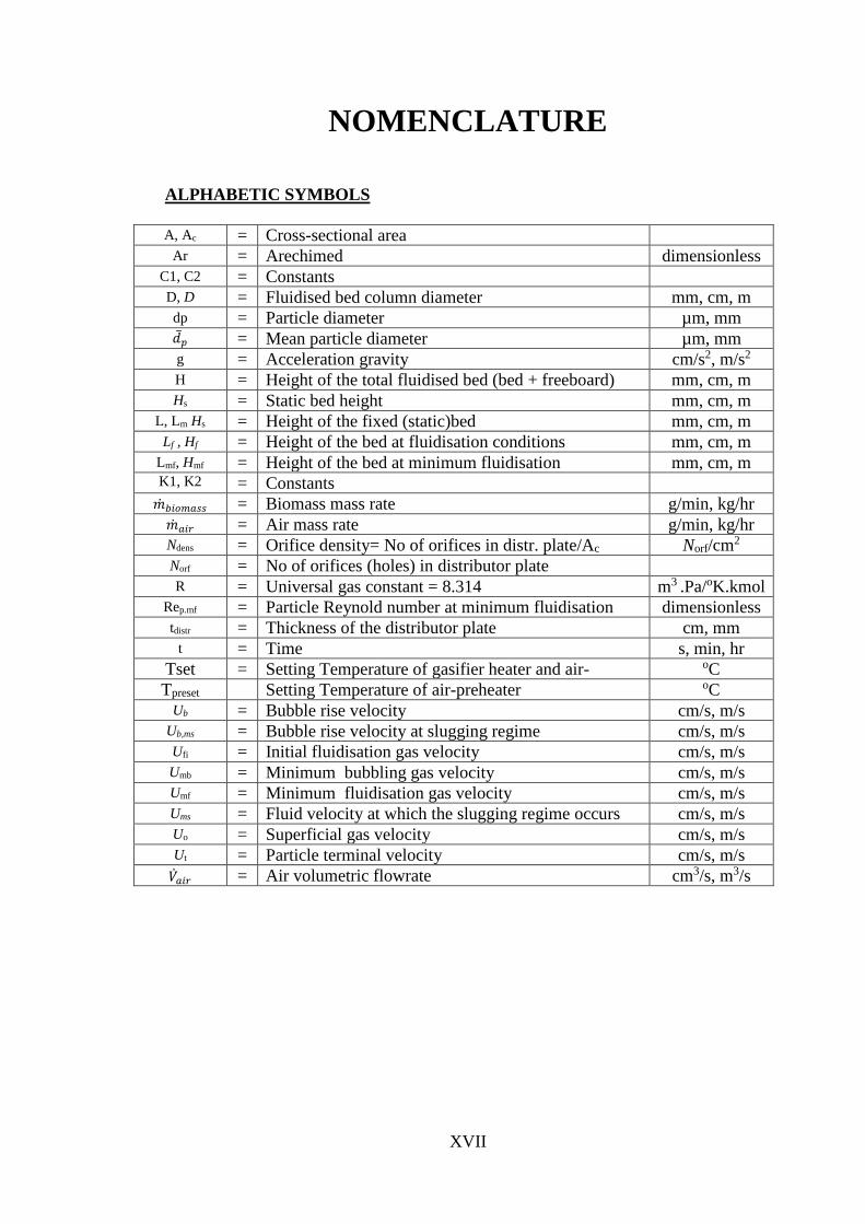
NOMENCLATURE
ALPHABETIC SYMBOLS
A, Ac = Cross-sectional area
Ar = Arechimed dimensionless C1, C2 = Constants D, D = Fluidised bed column diameter mm, cm, m dp = Particle diameter µm, mm �̅�𝑝 = Mean particle diameter µm, mm g = Acceleration gravity cm/s2, m/s2 H = Height of the total fluidised bed (bed + freeboard) mm, cm, m Hs = Static bed height mm, cm, m
L, Lm Hs = Height of the fixed (static)bed mm, cm, m Lf , Hf = Height of the bed at fluidisation conditions mm, cm, m
Lmf, Hmf = Height of the bed at minimum fluidisation mm, cm, m K1, K2
= Constants
�̇�𝑏𝑖𝑜𝑚𝑎𝑠𝑠 = Biomass mass rate g/min, kg/hr
�̇�𝑎𝑖𝑟 = Air mass rate g/min, kg/hr Ndens = Orifice density= No of orifices in distr. plate/Ac
Norf/cm2 Norf = No of orifices (holes) in distributor plate R = Universal gas constant = 8.314 m3 .Pa/oK.kmol
Rep.mf = Particle Reynold number at minimum fluidisation
mmmmmmmmminimumffffffluidisation
dimensionless tdistr = Thickness of the distributor plate cm, mm
t = Time s, min, hr
Tset = Setting Temperature of gasifier heater and air-
preheater
oC
Tpreset Setting Temperature of air-preheater oC Ub = Bubble rise velocity cm/s, m/s
Ub,ms = Bubble rise velocity at slugging regime cm/s, m/s Ufi = Initial fluidisation gas velocity cm/s, m/s Umb = Minimum bubbling gas velocity cm/s, m/s Umf = Minimum fluidisation gas velocity cm/s, m/s Ums = Fluid velocity at which the slugging regime occurs cm/s, m/s Uo = Superficial gas velocity cm/s, m/s Ut = Particle terminal velocity cm/s, m/s
�̇�𝑎𝑖𝑟 = Air volumetric flowrate cm3/s, m3/s

XVIII
GREEK SYMBOLS
α = Volume of the wake per volume of bubbles dimensionless δ = Fraction of the total bed occupied by the bubbles dimensionless
ΔPbed = Pressure drop across the bed mbar ΔPdistr = Pressure drop across the distributor plate mbar ε, εs = Voidage of the static bed dimensionless εmf = Voidage of the bed at minimum fluidisation dimensionless εf = Voidage of the bed at fluidisation conditions dimensionless µ = Fluid dynamic viscosity Kg/m.s ρf = Density of fluid g/cm3, kg/m3 ρg = Density of gas g/cm3, kg/m3
ρs, ρp = Density of solid particle g/cm3, kg/m3 ρb = Bulk density of the solid material g/cm3, kg/m3 ϕs = Particle sphericity dimensionless

1
Chapter 1
Introduction

Chapter 1: Introduction
2
1.1 Background
The expansion of human activity since the Industrial Revolution has increased for fossil
type energy sources, especially petroleum derivatives due to their easy transport and
storage. Given that fossil resources have been formed over millions of years, it is not
possible to replenish its reserves especially if compared to the current of consumption
rate, so this type of energy is considered non-renewable. Recent crises have included
fuel prices, depletion of this fuel in the near future, problems of the pollution of the
environment and rising surface temperatures, known as global warming. All the above
have been causing great concern for humanity and promoting many countries in the
world represented by developed countries to move to reduce these environmental
problems. This has included prioritisation of renewable and environmentally clean
energy sources to protect the planet and to avoid possible human catastrophe. Although
many of these countries possess fossil fuel energy such as oil, natural gas and coal, the
impacts of climate change should be mitigated including the use of renewables. These
renewable energy sources include solar energy, wind energy, hydro energy,
underground thermal energy and biomass. Bioenergy includes bio-ethanol alcohol
(biofuels) which can be produced from the fermentation of sugars, starches and other
plants, biodiesel which can be produced from vegetable oil (such as soybeans) and
biogas which can be produced from plants, sewage waste, as well as wood and cellulosic
material combustion as a source of thermal energy.(Demirel 2012)
Global studies generally indicate that the countries of the world are generally moving
towards the use of renewable energy, particularly biomass energy, which has nowadays
become a strong alternative and considered a new effective source of energy. As stated
in the International Energy Agency report in 2009, bioenergy accounted about 68.6%
of the total primary energy consumption in the renewable energy domain and this, in
turn, accounted for about 9% of the total primary energy overall amenities. This means
that biomass formed 6.2 % of that total as shown in Figure 1.1(Eea 2011) , while in
2012, this percentage became about 10% (International Energy Agengy 2014)

Chapter 1: Introduction
3
Figure 1. 1 Total primary energy consumption by energy source in 2009, EU-27 (Eea 2011)
The study provided by the International Energy Agency on the entire global
consumption for the use of biomass energy in the production of electric stated that the
global energy consumption in 2009 was 290 TWh, equivalent to 1.5% of world
electricity production. In addition, according to the study forecasts this percentage will
increase each year slightly until it expected to be 7.5% in 2050, which correspond 3100
TWh (Eisentraut and Brown 2012).
As mentioned above, climate change is one of the largest environmental risks. It has
occurred as a result of increase greenhouse gas emissions since the beginning of the
Industrial Revolution. These emission gases are mostly composed of water vapour,
carbon dioxide, methane, nitrous oxide, ozone, which play a major role in the Earth's
surface heating. One of the advantages uses of biomass fuels that they do not lead to an
increase in the greenhouse gases, where plants absorb carbon dioxide in the atmosphere
by photosynthesis and when they are burned so they come out the same amount that has
been absorbed (Demirel 2012)(Basu 2010). This is called carbon cycle as shown in
Figure 1.2. Therefore, the cultivation of plants leads to the closure of the carbon cycle,
and hence there is no increase in carbon dioxide levels in the environment.

Chapter 1: Introduction
4
Figure 1. 2 The carbon cycle (http://thefrogpad.weebly.com/general-ecology.html,” n.d.)
The stored chemical energy in biomass material can be released as heat by combustion.
Biomass can also be converted to producer gases by gasification, partial oxidation, or
by pyrolysis with no oxidation. These producer gases can be used as fuel for energy
generation and for the creation of new chemical compounds for example in Ficher-
Tropsch synthesis. There are three thermal-chemical conversion process mainly,
combustion, gasification and pyrolysis processes.
1.2 Gasification and biomass gasification
Gasification technology is a thermo-chemical process that can convert biomass fuels
such as crop residues, sewage sludge and municipal wastes into a fuel gas which could
be utilised for applications including electricity generation, heating and chemical
products. The gasification process is a partial oxidation reaction, which can convert a
solid biomass fuel to a gaseous fuel using an air-fuel ratio less than 1 at specific
conditions of temperature and pressure. Many chemical reactions occur at high
temperature and at specific equivalence ratio, air fuel ratio, throughout this process
leading to the final desired product (Christopher Higman 2003).
Biomass gasification process can be categorised in three processing steps: upstream
processing step, (which includes biomass reduction size, drying and preparation of
gasifying agents), gasification process step, and downstream process step, (which
includes producer gas clean-up and reforming and gas utilisation). (Kumar et al. 2009).

Chapter 1: Introduction
5
The process step of the biomass gasification is the heart of the process. It includes
thermal-chemical conversion of biomass fuel to an energy rich combustible gaseous
product in controlled conditions using different gasifying agents such as air, O2-air, O2,
air and/or steam and air and/or CO2. Unlike the combustion process where biomass
oxidation is completed in one-step, the biomass fuel in the gasification process
undergoes a series of physical transformation process and chemical reactions within the
gasifier. These processes are shown in Figure 1.3-a and b:
Drying: Where the moisture content of the solid biomass fuel evaporates, leaving
dry biomass and releasing steam which may contribute in later chemical reactions.
Pyrolysis: This occurs when the solid biomass is exposed to elevated temperature
in the gasifier. Volatile materials are released by the pyrolysis process, which
precedes the gasification process, at low temperature (350-700oC) as initial biomass
conversion. This step includes devolatization of volatile materials and thermal
breakdown of weaker chemical bonds of larger hydrocarbon molecules in solid
biomass. The low temperature volatile vapours consist of gaseous species mainly
hydrogen and methane, large condensable molecules (phenol and acids) called
primary tars, which are characterised by oxygenated compounds that give the
primary tar its high reactivity, and a solid chars (a material containing mainly coal
and ash). In the presence of a gasifying agent and a relatively high temperature
environment (700-850 oC), secondary gas-phase reactions including (cracking,
reforming, combustion, and CO shift) of primary tars are initiated producing
combustible gases and secondary tars (phenolic and olefins). At higher
temperatures (850-1000oC), tertiary conversion of secondary tars to poly aromatic
hydrocarbons (PAHs) also occur and soot formation is observed (Morf et al.
2002)(Piriou 2009).
Combustion: Within the gasification environment some of the char and of the
volatile products combust partially with a limited amount of oxygen to produce
CO2, CO, H2O and the required heat to sustain the gasification reactions.
Gasification: where char residues, pyrolysis tars (primary, secondary and tertiary
tars) and pyrolysis gases are partially oxidised at high temperature (600-1500oC)
using the required gasifying agents to produce a producer gas mainly hydrogen
(H2), carbon monoxide (CO), carbon dioxide (CO2), methane (CH4) and traces of
ethane and propane. Also, char and tar are the result of incomplete reaction of
biomass (Chhiti and Kemiha 2013) .

Chapter 1: Introduction
6
a) Process sequence for gasification of biomass solid fuel (P. Basu2010)
(Christopher Higman 2003)
b) Schematic representation of three thermochemical process (Redrawn)-(Arena
2012), (Gómez-barea et al. 2011).
Figure 1. 3 Schematic of biomass gasification process (a and b)
As mentioned above, during the gasification step different thermal process are taking
place. In addition, depending on operating conditions, several exothermic and
endothermic chemical reactions take place in the gasifier. Due to the reversibility of the
gasification reactions, the direction of the reaction and its conversion require a
knowledge in thermodynamic and reaction kinetics. The thermodynamic equilibrium of
the gasification reactions imposes a high effect on the thermal efficiency and the
producer gas composition.

Chapter 1: Introduction
7
1.3 Fluidised Bed Reactors
Chemical reactors are used in chemical processes to convert raw materials to new
product materials at specific conditions, such as temperature, reactants concentration
and pressure. There are different types, configurations and designs of reactors
depending on the nature of the process and the factors affecting the process efficiency.
One class of these reactors is the fluidised bed reactor, which is used in gas-solid
reactions especially in a process involving a thermo-chemical conversion process. In
the last ten years, fluidised bed reactor technologies have generated research interest in
biomass gasification processes because of advantages in temperature uniformity and
control, excellent fuel flexibility and high heat and mass transfer rates (Alauddin et al.
2010)(Siedlecki et al. 2011).
Basically, fluidised bed is a packed bed through which fluid flows at such a high
velocity that the bed is loosened and the particle-fluid mixture behaves as though it is a
fluid. Thus, when a bed of particles is fluidised, the entire bed can be transported like a
fluid, if desired. This phenomenon has been utilised to obtain excellent contact of the
solid and fluid and the solid and wall due to a vigorous agitation. This condition means
that nearly uniform temperatures through the bed, high heat and mass transfers and high
reaction rates (for process with chemical reaction) can be maintained. For these reasons
thermochemical processes such as solid biomass and coal gasification, combustion and
pyrolysis have been carried out using fluidised bed reactors (Basu 2006) (Christopher
Higman 2003).
In the case of a fluidized bed gasifier the fuel, solid fuel biomass or coal, is gasified in
a bed of small particles (inert or catalytic bed material or both) fluidized by a suitable
gasification medium gas. There are two principal types of fluidised bed gasifier;
bubbling fluidised bed and circulating fluidised bed, which are presented in Chapter 2
in details.
1.4 Energy in Iraq
Energy resources in Iraq mainly rely on fossil fuels including predominantly oil,
followed by natural gas. Iraq is the world's third-largest oil exporter. Iraq ranked fifth
and thirteenth in the sequence of the world's oil and natural gas reserves, respectively.
Sources of energy available from fossil fuels are considered the mainstay of the Iraqi
economy where the export of oil is currently constituted 95% of state revenue. At the

Chapter 1: Introduction
8
moment, all sectors such as electricity, industry, transport, buildings rely mostly on
fossil energy sources mainly oil.
According to the central scenario presented by the International Energy Agency on
energy in Iraq as shown in Figure 1.4, 90% of Iraqi electricity comes from fossil energy
sources, oil and gas. The remaining 10% is from renewable energy i.e. hydropower
represented a contribution of 5 TWh and will contribute 5% in 2035, while for solar
energy the scenario considered that this energy would contribute 50MW in 2035. With
regard to wind and biomass energies, the scenario reported that the wind speed in Iraq
is relatively low, and the resources of biomass material are moderate so the scenario
and within the study period this was not considered on a large scale.
Figure 1. 4 Primary energy demand by fuel in Iraq, in million ton oil equivalent (International
Energy Agency 2012)
So according to this scenario, the contribution of renewables will be small compared to
the fossil fuels oil and natural gas. Given the high carbon emissions from Iraqi’s
industries, the desire of the main sectors to decrease their dependency on fossil fuels
and to make use of renewable energy resources, many official research centres have
been recently established in Iraqi ministries to upgrade the Iraqi contribution in
renewable energies. These ministries are the ministry of electricity, ministry of industry
and minerals and ministry of higher education and scientific research.
1.5 Iraqi Biomass Energy-Date Palm Wastes
The wastes and residues of plants and other agricultural products can be considered as
biomass resources. The date palm wastes are one of these biomass wastes. Since Iraq is
the original palm frontrunners and is one of the Arabic countries in the production of

Chapter 1: Introduction
9
dates, it is logical that Iraq should take serious steps towards bio-energy sources from
date palm trees.
Iraq has suitable climate conditions for this tree cultivation. Palm trees are usually tall
(tall stem), with no branches, and enormous leaves, or fronds, at their tops as shown in
Figure (1.5). Date palms can be grown on large tracts of land and vast stretches of
middle to the south of Iraq.
Figure 1. 5 Single date palm tree showing its stem, leaves (fronds).
Statistical studies indicate that Iraq possesses large numbers of date palm trees. A study
published by Dr. Abdul-Basit Auda, (Anon 2011c) reported that Iraq has a wide
production of these tree approximately 16 million trees and are distributed in many Iraqi
states as shown in Figure 1.6 (Anon 2011c). Also, the date palm tree of old trees can be
short-lived to about 100 years and more (Ali 2010).
Figure 1. 6 Production of Iraqi date palm trees by states in Iraq in1998 (Anon 2011c)

Chapter 1: Introduction
10
Studies reported that the single one date palm tree like any tree need to be cleaned and
pruned once a year, leaving significant amounts of wastes, approximately 25-50 kg per
tree. These wastes are; dry leaves, leaf bases, fibres generated as a result of the growth,
as well as parts bearing the fruit (date) of the palm, which is called raceme, as shown
in the images below, Figure 1.7 (AHMED F. ZABAR 2012). In Iraq, in the past, the dry
waste of these residues is not considered to have significant economic value. They were
destroyed by burning or utilising as fuel in cooking operations and some local
industries. Sometimes their stems was used in house roofs building. All these above
factors enhance the sustainability of using these Iraqi date palm wastes.
Figure 1. 7 Waste materials of Iraqi date palm trees
In recent years, the Iraqi government represented by Ministry of Agriculture has tried
to take advantage of these wastes and residues as much as possible for using as an
organic fertiliser. Some of the research centres have been established for this purpose.
These centres currently cover only a small percentage of these wastes compared to the
large quantities of such waste.
It can be concluded that these Iraqi date palm residues can be preliminary considered as
one of the varieties of the biomass solid fuel which can be utilised to obtain a clean
gaseous fuel in Iraq which can be used in many fields and applications, thereafter it will
be one of those major biomass renewable energy sources. In order to see the feasibility

Chapter 1: Introduction
11
of these residues in biomass gasification, these residues were chosen as one feedstock
material in this study.
1.6 Motivation and Aims
The design and development of low-carbon gasification processes are still at immature
stages. There is still a lot of basic scientific information lacking in the technical
literature. This study will be concerned with the investigation of fluidization parameters
on biomass gasification in order to produce fundamental data for the enhanced
understanding of fluidised bed gasifier design. The principal aims of this study are:
1) To provide a basic database for air bubbling fluidised bed biomass gasification.
2) To design and develop an air fluidised bed gasifier.
3) To study the effect of the bubbling fluidised bed hydrodynamic parameters on
the gasifier performance.
4) To evaluate the feasibility of the Iraqi date palm residues as a biomass feedstock
in biomass gasification and hence will contribute to support renewable
bioenergy in Iraq.
5) To evaluate the gasifier performance at low gasification temperature.
1.7 Research Hypothesis
The drive to increase renewable energy production and displace the use of fossil fuels
has caused an increase in interest in biomass gasification. The performance of the
biomass gasification reactors to obtain high quality syngas still needs further
development and modification. The fluidised bed reactor, especially the bubbling
fluidised bed reactor, is one of these reactors that should be studied for improvement in
terms of operating method and energy consumption. This study aimed to deal the
following research hypotheses:
(a) Designing, building and constructing a hot air bubbling fluidised bed gasifier close
to a pilot plant scale, rather than lab-scale, to give a practical indication for
industrial gasifier performance.
(b) Studying the hydrodynamic parameters of the bubbling fluidised bed gasifier in
isothermal conditions i.e. as a cold fluidised bed to provide primary data for
fluidised operation under hot gasifying condition.
(c) Using Iraqi date palm biomass wastes comparing to sawdust pinewood material,
which is an abundant biomass material in UK and its high chemical specifications

Chapter 1: Introduction
12
enhance its potential using in gasification processes as a feedstock biomass
material. This will give a reliable indication to use the Iraqi date palm wastes as a
biomass material source for renewable energy generation in Iraq.
(d) Whether the number of holes in perforated distributor plate, expressed as a
distributor open area, has any effect on the bed hydrodynamic and consequently on
the gasifier performance.
1.8 Layout of the thesis structure
The following Chapters have structured the thesis:
Chapter 1: In this chapter, the general overview on the energy conservation and climate
change are highlighted. Energy resources are discussed, and alternative approaches to
reducing sources contributing to the climate change are presented. The aims of the
current research, hypotheses and thesis structure are also described.
Chapter 2: In this chapter, the overview on the biomass gasification is provided.
Factors affecting gasification process, gasifier performance and syngas quality are
discussed in detail. The development of the fluidised bed reactor from coal feedstock to
biomass is highlighted. In addition, Factors affecting minimum fluidisation velocity are
discussed as well.
Chapter 3: This chapter presents the theoretical design of the experimental rig
especially the fluidised bed gasifier, air box section, distributor plate section and reactor
bed and freeboard sections. Design equations and steps of design calculations for these
sections are also presented.
Chapter 4: In this chapter, the materials and methods of characterisation that were
performed on the biomass materials, pine wood sawdust and Iraqi date palm residues,
and quartz sand are described. In addition, all equipment and accessories for cold and
hot rigs are presented.
Chapter 5: This chapter details the experimental layout and describes procedures that were
used during the fluidised bed hydrodynamics and biomass gasification. The parameters of
interest and operating conditions for all experimental tests are explained in detail
Chapter 6: This chapter displays and discusses the experimental results obtained from
this study from cold fluidisation rig. Fluidised bed hydrodynamic under different
experimental tests are discussed.

Chapter 1: Introduction
13
Chapter 7: This chapter displays and discusses the experimental results obtained from
this study from biomass gasification hot rig. Gasification product gas composition and
gasifier performance for different operating and hydrodynamic parameters under
different experimental tests are discussed.
Chapter 8: In this chapter, the findings from experimental undertaken in this study are
concluded. The recommendations for future work in the field of fluidised bed biomass
gasification to improve the gasifier performance and syngas composition and heating
value are highlighted and proposed.

Chapter 2
Theory and Literature Review

Chapter 2: Theory and Literature Review
15
2.1 Introduction
In this chapter, a biomass gasification system and its expected reactions (around 10-14
reactions) are described and reviewed. Gasifier design, an important factor that affects
the gasification process, is presented in Section 2.3.1, where the main type of the
fluidised bed gasifiers is reviewed. Due to their interest in this study, definition,
characterisations and drawbacks of two common types of fluidised bed gasifier,
bubbling and circulating, are offered in some detail. In Section 2.4, the gasification of
biomass in fluidised bed reactor is presented and in Section 2.4.1 the factors that
noticeably affect the fluidised bed gasifier performance for biomass gasification such
as biomass feedstoke type, operating temperature, gasifying agents, equivalence ratio,
and bed material are highlighted and explained. Also, the hydrodynamic factors of
bubbling fluidization that affect the biomass gasification process are also highlighted
and reviewed in Section 2.4.2. To be more acquainted with the fluidisation
phenomenon, the classification of four groups for solid particles and the types of
fluidization regimes are defined in Sections 2.5.2 and 2.5.3, respectively. The important
design parameter, minimum fluidisation velocity Umf is identified and highlighted in
Section 2.5.4. Furthermore, the methodology of the experimental measuring and
theoretical estimation of Umf velocity is presented in detail. Also, the fluidisation of
single biomass and binary mixtures are explained in Section 2.5.5. Finally, Section 2.5.6
reviews the factors that affect the design parameter Umf.
2.2 Biomass Gasification Reactions
As mentioned in Chapter 1- Section 1.2 during the gasification step several chemical
reactions occur among the hydrocarbons in the fuel (mainly char), steam, carbon
dioxide, oxygen, and hydrogen in the gasifier, in addition to chemical reactions among
the released gases. Table 2.1 presents typical reactions for biomass gasification process.
This table shows the reaction number of each reaction, the chemical equation, the heat
of reaction, which indicates reaction type, exothermic or endothermic, and the name of
reaction. The understanding of the gasification physical processes and chemical
reactions are essential in the gasification process design and operation

Chapter 2: Theory and Literature Review
16
Table 2. 1 Main reactions in heterogeneous and homogeneous phase during the solid biomass
gasification process (Arena 2012)
Reaction
No
Reaction classification and equation Heat of
Reaction
MJ/kmol
Reaction Name
R2.1
Biomass Pyrolysis
Biomass Char+ Tar + H2O + Light gas
(CO+CO2+CH4+H2+ O2 + N2+ …)
>0
Biomass devolatilisation
R2.2
R2.3
R2.4
R2.5
R2.6
Oxidation Reactions
C+ ½ O2 CO
CO + ½ O2 CO2
C + O2 CO2
H2 + ½ O2 H2O
CnHm + n/2 O2 nCO + m/2H2
-111
-283
-394
-242
Exothermic
Carbon partial oxidation
Carbon monoxide oxidation
Carbon oxidation
Hydrogen oxidation
CnHm partial oxidation
R2.7
R2.8
R2.9
R2.10
Gasification reactions involving steam
C + H2O CO + H2
CO + H2O CO2 + H2
CH4 + H2O CO + 3H2
CnHm + nH2O nCO + (n + m/2)H2
+131
-41
+206
Endothermic
Water-gas reaction
Water- gas shift reaction
Steam methane reforming
Steam reforming
R2.11
R2.12
Gasification reaction involving Hydrogen
C + 2H2 CH4
CO + 3H2 CH4 + H2O
-75
-227
Hydrogen gasification
Methanation
R2.13
R2.14
Gasification reaction involving carbon dioxide
C + CO2 2CO
CnHm + nCO2 n 2nCO + m/2 H2
+172
Endothermic
Boudouard reaction
Dry reforming
R2.15
R2.16
Decomposition reaction of tars and hydrocarbons
pCxHy qCnHm + rH2
CnHm nC + m/2H2
Endothermic
Endothermic
Dehydrogenation
Carbonization
Note that CxHy represents tars and CnHm represents hydrocarbon with a smaller number of carbon atoms.
The chemical reactions of gasification can proceed to different extents depending on
the gasification conditions of temperature, pressure, and the feedstock type. The most
significant gasification reactions are:
Chapter 2: Theory and Literature Review
17
2.2.1 Water-gas reaction (R2.7)
This is a heterogeneous (gas-solid), reversible and an endothermic reaction. Due to its
products CO and H2 gases, it is considered a principal gasification reaction. According
to their equilibrium graphs, it is not so extensively affected by temperature as the
Bouduard reaction, especially above 800oC.
2.2.2 Boudouard reaction (R2.13)
This is a heterogeneous (gas-solid), reversible reaction and highly endothermic reaction.
In this reaction CO gas is produced by reacting CO2 gas with char at high temperature
and low pressure, at least 700oC in atmospheric pressure. At one atmosphere, its
equilibrium graph shows that above 700oC, CO gas concentration increases
significantly when the temperature increases. The rate of this reaction is insignificant
below 1000oK (Basu 2010).
2.2.3 Water-gas shift reaction (R2.8)
This is a homogeneous (gas-gas), reversible and low exothermic reaction. This reaction
is used to adjust H2 to CO ratios in producer gas or syngas for many end products or to
set the H2 gas volume % to meet the downstream process requirements (Basu 2010).
This reaction can operate with different catalysts between 205oC and 482oC (Laboratory
2016).
2.2.4 Methanation reaction (R2.12)
This is a homogeneous (gas-gas), reversible and a highly exothermic reaction. However,
it is preferred at low temperature and high pressure. Due to its higher heating value
comparing with CO or H2, CH4 is the desired gas in combustion process applications.
2.2.5 Steam methane reforming reaction (R2.9)
This is a homogeneous (gas-gas), reversible and a highly endothermic reaction. It
progresses very slowly and requires relatively low temperature and catalyst. To occur
and due to its enthalpy, this reaction requires a high amount of energy. It is a limited
reaction due to the low concentration of CH4 in the gasifier.

Chapter 2: Theory and Literature Review
18
2.3 Key factors affecting the gasification process
There are many factors that affect the gasification process, producer gas quality (
composition, production of H2, CO, CO2 and CH4, free tar content and heating value)
and the performance of gasification ( represented by gas yield, carbon conversion
efficiency, and total heating value efficiency). Generally, these factors are reactor
design, origin feedstock of fuel, operating conditions such as equivalence ratio,
temperature, pressure and gasifying agent (medium). In addition, for each type of
gasifier design, there are additional factors that affect the gasification process and
reactor performance.
2.3.1 Gasifier design
Reactor design is crucial for gasification efficiency, composition and heating value of
the product gas, and also for tar formation. Practically, according to the gas-solid
contact method, three main categories of gasifier used for biomass gasification are
(Basu 2010)(Siedlecki et al. 2011):
I- Fixed-Bed (Moving-Bed) Gasifiers.
- Updraft
- Downdraft
- Crossdraft
II- Entrained flow gasifiers.
III- Fluidised Bed Gasifiers:
- Bubbling fluidized bed gasifier (BFBG).
- Circulating fluidized bed gasifier (CFBG).
Despite the fact that these gasifiers apply analogous principles for biomass fuel
conversion, but their operations and performances are different.
2.3.1.1 Fluidised bed gasifiers:
As mentioned in Chapter 1-Section 1.3, fluidised bed reactors can be used for
thermochemical gas-solid reaction processes. For a fluidized bed gasifier the fuel, solid
fuel biomass or coal, is gasified in a bed of small particles (inert or catalytic bed material
or both) and fluidized by a suitable gasification medium gas (Basu 2010). There are two
principal types of fluidised bed gasifier.
Chapter 2: Theory and Literature Review
19
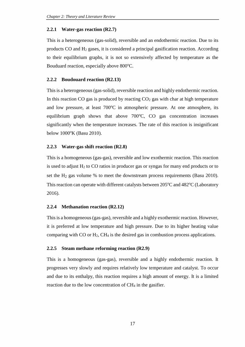
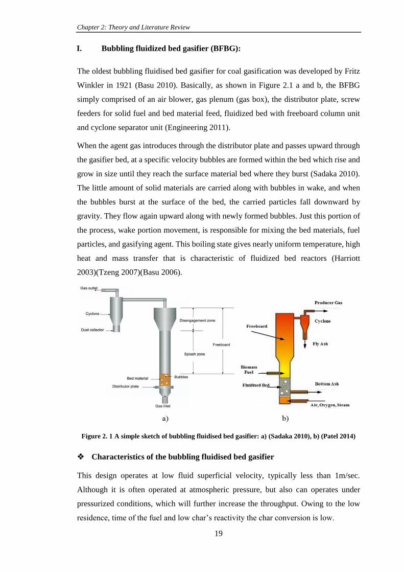
I. Bubbling fluidized bed gasifier (BFBG):
The oldest bubbling fluidised bed gasifier for coal gasification was developed by Fritz
Winkler in 1921 (Basu 2010). Basically, as shown in Figure 2.1 a and b, the BFBG
simply comprised of an air blower, gas plenum (gas box), the distributor plate, screw
feeders for solid fuel and bed material feed, fluidized bed with freeboard column unit
and cyclone separator unit (Engineering 2011).
When the agent gas introduces through the distributor plate and passes upward through
the gasifier bed, at a specific velocity bubbles are formed within the bed which rise and
grow in size until they reach the surface material bed where they burst (Sadaka 2010).
The little amount of solid materials are carried along with bubbles in wake, and when
the bubbles burst at the surface of the bed, the carried particles fall downward by
gravity. They flow again upward along with newly formed bubbles. Just this portion of
the process, wake portion movement, is responsible for mixing the bed materials, fuel
particles, and gasifying agent. This boiling state gives nearly uniform temperature, high
heat and mass transfer that is characteristic of fluidized bed reactors (Harriott
2003)(Tzeng 2007)(Basu 2006).
Figure 2. 1 A simple sketch of bubbling fluidised bed gasifier: a) (Sadaka 2010), b) (Patel 2014)
Characteristics of the bubbling fluidised bed gasifier
This design operates at low fluid superficial velocity, typically less than 1m/sec.
Although it is often operated at atmospheric pressure, but also can operates under
pressurized conditions, which will further increase the throughput. Owing to the low
residence, time of the fuel and low char’s reactivity the char conversion is low.

Chapter 2: Theory and Literature Review
20
The uniform temperature distribution, high mixing and high heat and mass transfer are
applicable throughout the gasifier. Carbon with some fine bed material and ash are
entrained in the gas product, trapped, and separated out in a cyclone. BFBG has high
flexibility and suitability for the gasification of solid biomass fuel regarding both
particle size and different types of materials. This design results in lower cost and less
maintenance. It is suitable for scaling up. (Gautam 2010)(Tzeng 2007) (Ciferno and
Marano 2002)(Brown 2006).(Siedlecki et al. 2011)(Puig-Arnavat et al. 2010).
Drawbacks of the bubbling fluidised bed gasifier
Particulates elutriate as the product gas increases the solid load in the cyclone and filter.
The issue of the weakness of the interaction and mixing of the species when the
conversion of the char is low due to the low residence time of the fuel, the slow
reactivity of the char and un-recycled trapped solid materials.
At higher temperatures above 900-950oC and when the biomass fuels have a high
content of ash, potential ash melting will occur causing stickiness of particles leading
to the agglomeration phenomena causing bed de-fluidization and thereby the gasifier.
(Cirad 2009) (Puig-Arnavat et al. 2010) (Siedlecki et al. 2011).
II. Circulating fluidized bed gasifier (CFBG):
Simple (classical) circulating fluidized bed
This general circulating fluidized bed abbreviated as CFB, has been used as a common
term since the 1970s and for gas-solid process applications CFB technology dates back
to the 1960s (Yang 2003). This gasifier type works at a high superficial gas velocity
beyond bubbling and turbulent fluidization regimes. It is also known as fast fluidization
under certain conditions (see Section 2.5.3.5). At this critical point, known as the
transition boundary velocity, the bed particle entrainment occurs. This is called a
transport or transition velocity. Beyond this point, the bed fluidisation cannot be
continued without entrained solids recycling. The typical gas velocity range is 2-12
m/sec and particle rate flux range is 10-1000 kg/m2.sec, so that there is not an interface
distinguishing between a dense bed and a dilute region above. By this point, a CFB is
differentiated from a bubbling fluidized bed BFB (Siedlecki et al. 2011)(Yang 2003)
(Ciferno and Marano 2002)(Klein 2002).

Chapter 2: Theory and Literature Review
21
Figure 2.2 shows a schematic diagram of CFBG gasifier. As a result of gas high-velocity
the entrained solid particles will separate, re-circulate and return back to the reactor
through an external particle flow system, which usually consists of one or more
cyclones, a standpipe and a valve or seal (Yang 2003) (Ciferno and Marano 2002)
Figure 2. 2 Classical circulating fluidized bed gasifier-direct heating: a) Lurji Gasifier
(Christopher Higman 2003), b) Classical type (Siedlecki et al. 2011)
There are two types of circulating fluidized bed (Siedlecki et al. 2011) (Christopher
Higman 2003):
Fast circulating fluidized bed FICFB (Indirectly Heated Unit):
Sometimes is called Dual or Twin Circulating Fluidized Bed Reactor DCFB. The
operation of this gasifier is based in which the gasifier vessel is divided into two distinct
fluidization; reactors, which are operated at two different gas velocities as shown in
Figure 2.3, one of them is a bubbling fluidized gasifier BFBG, where usually the steam
is an agent gas while the other reactor (combustor) is a simple circulating fluidized bed
combustor CFBC, usually air is an agent gas. Some of its features are available in (Puig-
Arnavat et al. 2010). The design aimed to avoid mixing of gasification products with
those from the combustion in order to obtain high purity hydrogen. In the combustor
heat generated, due to char combustion raises the bed material temperature. After
leaving combustor, it is captured by a cyclone and then recirculated into the BFBG to
supply the required heat for char gasification endothermic reactions using steam as an
agent gas (Siedlecki et al. 2011) (Brown 2006)(Christopher Higman 2003).

Chapter 2: Theory and Literature Review
22
Figure 2. 3 Twin (dual) fluidized bed gasifier (Basu 2010)
Characteristics of the circulating fluidised bed gasifier:
If height of the bed is significantly high, then long and controllable residence time of
particles can be achieved. It can be operated at pressurized conditions. Also at higher
velocities, typically 2-12 m/sec leading to higher velocities of the recirculation and
violent gas-solid contact and mixing. This will give high heat and mass transfers and
reaction rates which causing higher overall carbon conversion. This is suitable for large-
scale systems and has very good scale-up potential. Its ability and flexibility to gasifying
different types and particle sizes of feedstocks with different compositions and moisture
content, especially biomass and wastes, of which the size, shape, and fluidizing
characteristics, are harder to control than coal. The energy throughput per unit cross-
sectional area of gasifier is higher than for BFBG.
Drawbacks of circulating fluidising bed:
The reactor height significantly increases their cost. The process control mechanism is
more complex in comparison to its BFB counterpart. As with BFB, because the ash
content and temperature limitation, bed agglomeration is a possibility. As a result of
long circulation loop, gradients of temperature occur in the solid flow axis direction.

Chapter 2: Theory and Literature Review
23
Tar conversion is still not high, but it is little higher than BFBG gasifier. (Sadaka 2010)
(Tzeng 2007) (Siedlecki et al. 2011)(Klein 2002)(Ciferno and Marano 2002) (Yang
2003).
2.4 Gasification of biomass in the bubbling fluidised bed gasifiers
BFBGs
As mentioned in previous sections fluidised bed gasifiers enhance the gasification
reaction rate and conversion efficiencies (mainly carbon and thermal efficiency) due to
high heat and mass transfer, excellent mixing and high contact of gas-solid fuel. In
addition, the use of the bed material as a medium of heat transfer and catalyst, will
highly contribute to tar reduction and improve the producer gas quality. These
specifications encourage researchers to use the bubbling fluidised bed gasifier for
biomass gasification studies.
Jeremiáš et al., 2009) evaluated the effect of the addition of the gasifying agent CO2 to
the main gasifying agent steam in bubbling fluidised bed gasifier and various bed
materials on the performance of allothermal gasifier.(Lv et al. 2004) developed a small
scale bubbling fluidised bed gasifier to study the effects of pine sawdust biomass
gasification parameters. They investigated the effects of gasifier temperature,
equivalence ratio, steam-biomass ratio, pine sawdust particle size on the gasifier
performance represented by gas composition, producer gas LHV and carbon
conversion. To show the potential of implementing air-bubbling fluidised bed gasifiers
in rural electrification projects for biomass agricultural wastes, a wood chips biomass
gasification in a large size of BFBG was performed by (Lim and Alimuddin 2008). They
monitored the gasifier performance in terms of its thermal output. In their review paper,
(Alauddin et al. 2010) presented 27 various research paper, for the dated period between
1995 and 2009, which were conducted in gasification of lignocellulosic biomass,
(agricultural residues, herbaceous crops , forestry residues, waste paper and other
wastes (municipal and industrial), etc.) in bubbling fluidised bed gasifier for renewable
energy development. These data were presented as a table in four fields for each
research paper: system configuration and operation parameters, investigated
parameters, optimum obtained results and reference. In their conclusion, they stated that
researchers confirmed that fluidised bed gasifiers have a great potential to perform the
gasification of this type of biomass. In recent years, the investigators and studies have
been conducted and investigated in lignocellulosic biomass gasification for renewable

Chapter 2: Theory and Literature Review
24
energy development specifically by fluidised bed gasifiers such as: (Lahijani and Zainal
2011) investigated the gasification of palm empty fruit bunch (EFB) biomass in a pilot
scale air-blown bubbling fluidised bed to examine the ability of EFB biomass for
renewable energy uses. Their results show the potential of their biomass for bioenergy
production factories. Similarly (Kim et al. 2013) investigated the efficiency of the
production of a gas fuel for a syngas-engine power supply from woody solid fuel
biomass using a gasification technology by air-blown bubbling fluidised bed gasifier.
They found that the caloric value of the producer gas (above 4.7 MJ/Nm3) was satisfied
for syngas engines. (Tilay et al. 2014) carried out various experiments in non-catalytic
biomass gasification for syngas production using two types of the gasifire, lab-scale
fixed-bed and pilot-scale bubbling fluidised bed. The feedstock biomass was called
canola meal, which is one of by- product of solvent extraction of canola oil industry in
Canada. They studied the effect of various gasification parameters, mainly temperature,
equivalence ratio ER and three different gasifying agents steam, O2, and CO2, on the
gasifier performance. From their experimental results for both gasifiers, they found that
canola biomass could be considered as one of the potential sources for syngas
production. In addition, those results show the ability to use the data for further
processes design and canola gasification scale-up at industrial applications.
2.4.1 Factors affecting biomass gasification process in bubbling fluidised bed
gasifiers
In general, design and operation of any gasifier entail a high comprehension of the effect
of biomass feedstock types and operation parameters, and hydrodynamic parameters for
fluidised bed gasifiers, on the performance index of the gasification system. The main
task of most biomass gasification research is to better these indices by improving the
producer gas composition, gain a significant gas lower heating value LHV, lowering tar
content and promoting the cold gas efficiency, gas yield and carbon efficiency
(Alauddin et al. 2010). It should be noticed that for any gasification process the
maximum value of those indices could not be achieved together at the same time.
2.4.1.1 Biomass feedstock
Biomass feedstock flexibility is one factor that plays a key role in the gasifier design
and performance. The physical and chemical properties of biomass feedstock are
important in establishing operating conditions of, specifically bubbling fluidised bed

Chapter 2: Theory and Literature Review
25
gasifiers. Chemical properties can be known according to any standard methods using
analysis tools, mainly proximate analyses, heating value LHV and. ultimate analyses
These analyses are detailed in Chapter 4-Section, 4.3.2.1, 4.3.2.2 and 4.3.2.3,
respectively. These analyses can also be used to carry out calculations related to the
process design and performance (Christopher Higman 2003). Figure 2.4 shows the
general formula of those analyses (Siedlecki et al. 2011).
Figure 2. 4 General composition and main chemical elements in typical solid biomass fuels
(Siedlecki et al. 2011)
In addition, the Figure shows the basis on which the analysis is based on such as dry
ash-free basis (daf), dry basis (db) and as received basis (ar). These bases are critical
to the state for any analysis. (Legonda 2012) established a standard analysis of solid
biomass fuel as shown in Table 2.2.
Table 2. 2 Typical proximate, ultimate and trace element analysis of biomass (Legonda 2012)

Chapter 2: Theory and Literature Review
26
Volatile matter content is a measure of the reactivity of the solid fuel, where reactivity
is a measure of chemical activity of substances and a tendency of material to undergo a
chemical reaction. Therefore, a solid biomass, which has higher volatile material
content are more reactive and can be easily converted into gas with a low amount of
char-producing. Also, this biomass char is highly porous, and this property can increase
the rate of gasification. Although a biomass which has a high content of volatile matter
can be gasified easier, but at the same time, its producer gas has a high tar yield which
is a problem in biomass gasification process downstream and producer gas quality
making its removal difficult not easy (Basu 2006)(Basu 2010).
Moisture content: It is an important physical property of a given biomass solid fuel
which highly affects the design and operation of the gasifier. Moisture content in
biomass varies in the interval 3-63% (Vassilev et al. 2010). Most the steam reactions in
gasification processes are endothermic as shown in reactions R2.7, R2.9 and R2.10,
Table 2.1 except reaction R8, which is an exothermic reaction. For high moisture
content of solid biomass fuel, a significant amount of heat is required for moisture
evaporation comparing with a small amount of heat which can be obtained by
exothermic reaction heat R2.8, -41MJ/kmol. This will reduce the thermal energy inside
the gasifier. Thereafter, this can hinder the endothermic reactions resulting in a low
quality of producer gas, its low heating value LHV and composition (Basu 2010)
(Kirsanovs et al. 2014). Also, this may increase methane composition and lower
hydrogen content due to exothermic hydrogen gasification reaction R2.11. This reaction
occurs because of the production of H2 in the presence of CO by water-gas shift reaction
(R2.8) due to high moisture content (Kirsanovs et al. 2014) (Radwan 2012). High
moisture content, above 30%, causes ignition difficulties. In addition, it reduces the
temperature achieved in the oxidation zone resulting in incomplete cracking of
hydrocarbons which are released by pyrolysis reactions (Kirsanovs et al. 2014)
(Radwan 2012). This will increase the percentage of undesired materials, e.g. tar
products downstream. Many researchers studied the effect of moisture for several
biomass solid fuels on the low heating value of biomass fuel itself (Marsh et al. 2008)
and (Molino et al. 2015). They found that low heating value of each fuel proportion
inversely with the moisture content.
On the other hand, some moisture content in the feedstock is desirable because it can
contribute in enhancing steam reforming reactions, R2.9 and R2.10, and char
gasification, R2.7, at higher temperature. Also, for syngas composition adjusting, steam

Chapter 2: Theory and Literature Review
27
with a required value of steam-fuel ratio or as gasifying agent is widely used in
industrial gasification applications (Vassilev et al. 2010).
Ash content: It is another important issue especially in bubbling fluidized bed gasifiers,
which affects the practical operation of the gasifier. It does not effect on the producer
gas composition directly. Chemically, ash content is an inorganic solid material, which
is mainly composed of metal oxides and some of their salts. Ash content can be
measured by proximate analysis for biomass (Siedlecki et al. 2011) and (Basu 2006).
The issues and negative effects of the ash content lies in the following: 1) a high amount
of ash will reduce the heating value of the solid fuel. 2) When the ash contains a high
amount of alkali oxides and salts, which are promoted in the existence of chlorine and
especially with high silica content in bed material forming eutectic materials (sticky
compounds) of low melting points about 770oC for alkali-silicates (K2O-SiO2), whereas
it is lower for K2O-CaO-SiO2. These materials lead to agglomeration phenomena
especially in high temperature bubbling fluidized bed gasifiers causing a bed material
defluidisation and therefore gasifier shutdown (Siedlecki et al. 2011)(Radwan 2012).
Recently research has been conducted to study the effect of lignocellulosic biomass
composition (as a feedstock) on the performance of gasification and pyrolysis process.
(Hlavsová et al. 2016) evaluated the effect of the composition of nine herbaceous plants
on the products (gases, liquids and solid char) distribution from pyrolysis using a fixed
bed reactor. They found that product distribution were affected by chemical and
biochemical composition of biomass fuel, liquid, and char secondary reactions. (Lv et
al. 2010) investigated the effect of six types of natural biomass and acid-washed
biomass, represented by their three compositions, cellulose, lignin and AAEM species
(Alkali and Alkaline Earth Metals), on gasification and pyrolysis properties using a
TGA analyzer and fixed bed reactor. They concluded that interaction between AAEM-
cellulose-lignin is responsible on the activity of biomass gasification. Also, they
observed that the pyrolysis rate was higher when the cellulose content was raised.
Whereas the pyrolysis rate for biomass with higher lignin content became slower. In
their research paper, (Barmina et al. 2013) stated that when various lignocellulosic
biomass are used for fuel gas production, detailed experimental research is needed to
evaluate the influence of the differences in their chemical and elemental composition
on gasification and combustion processes.

Chapter 2: Theory and Literature Review
28
2.4.1.2 Air gasification agent (medium)
Many gasifying agents have been used in the gasification process. These agents are
typically air, oxygen, steam, CO2, H2, and combination of them in required ratio. The
gasification product gas can be classified according to its lower heating value (LHV).
The value of LHV of the producer gas depends on the type of gasifying agent employed
as illustrated in Table 2.3 (Cirad 2009) (Radwan 2012).
Table 2. 3 Classifications of producer gas according to lower heating value (Cirad 2009)
LHV level LHV, MJ/Nm3 Gasifying agent
Low 4 – 6 using air and air/steam
Medium 12 – 18 using O2/ steam
High 40 using H2
The main oxidation reactions during the biomass gasification process using air as
gasifying agent, as a source of oxygen, are R2.2 to R2.6 have been shown in Table 2.1.
Lee, Kim, & Song, (2002) revealed in their experimental study, air/steam gasification
of an Australian bituminous coal in a fluidised bed, that with increasing air/coal ratio
(1.6 – 3.2) at 850oC, carbon conversion and gas yield, were increased from 0.3 to 0.42
and 0.25 to 0.425Nm3/kg, respectively, whereas the calorific value (LHV) decreased
from 2.7MJ/kg to 1.6MJ/kg. In addition, the composition of product gas was
significantly affected by increasing the air/coal ratio; H2 varied from 9.5% to 5.5%, CO
from 5.9% to 4.5%, CH4 from 2% to 1.4%, while CO2 increased from 7.0% to 8.9%.
(Devi et al. 2002) showed in their review that the effect of the gasifying agent on the
product gas composition, especially tar formation, depends on the equivalence ratio.
The review reported that the product gas composition by (vol. %) produced from air
gasification in the fluidised bed at 800oC and at ER= 0.35, was CO= 14%, H2= 10%,
CO2= 15%. The tar content decreased considerably with increasing ER to values
typically of 2 g /Nm3 being obtained. (Narvaez et al. 1996) reported that the gasification
of pine sawdust with air at 800oC and with the ER raise to 0.45 gives tar content of
about 2-7 g/Nm3. ER strongly influences the product gas quality and is more significant
at higher temperatures. Moreover, 30% of the tar concentration was decreased when ER
increased from 0.22 to 0.32 at 700oC. The decrease was mainly attributed to the
conversion of phenol. Most of the phenol can be converted at values of ER= 0.27 and
700oC.

Chapter 2: Theory and Literature Review
29
(Siedlecki et al. 2011) confirmed in their review that the effect of ER on the main output
parameters such as tar yield, cold gas efficiency (CGE), carbon conversion (CC), and
the reactor temperature (T) take the trends illustrated in Figure 2.5 As can be seen the
trends are similar to those previously reported. The Figure shows that increase an ER
leads to increase oxygen, which leads to increase combustion of the char and product
gas and thereby leads to increase the carbon conversion and reactor temperature. This
means the yield of the combustible producer gases and thereby the cold gas efficiency
will decrease. Finally, as ER increases the yield of the tar will decrease due to tar
cracking and oxidation reactions.
Figure 2. 5 Effect of the variation of ER on the main process parameters (Siedlecki et al. 2011)
2.4.1.3 Temperature
Temperature is an essential parameter in the gasification process. Due to the thermal-
chemical reactions, temperature plays an important role in accelerating the rate of the
endothermic and exothermic reaction of gasification process, tar cracking and char
conversion. Its effects revealed in producer gas quality, gas yield and low heating value
LHV.
For biomass fluidized bed gasification, the temperature range lies between nearly 650oC
and 950oC. The effect of the temperature parameter on gasification performance
depends on various factors mainly: 1) the type of gasifying agent, 2) Equivalence ratio,
which in turn depends on the method of the source of the heat supply, externally or
internally, where for internal heating ER will affect temperature, whereas for external
heating the controlling temperature is not affected by ER. 3) Biomass fuel moisture
content. 4) The heat loss from the system. (Gautam 2010) (Siedlecki et al. 2011).
(Cao et al. 2006) investigated experimentally the performance of a proposed tar-free
biomass gasification process conducted by a lab-scale air-sawdust biomass fluidized

Chapter 2: Theory and Literature Review
30
bed gasifier under autothermic conditions. They studied the effect of temperature
variations at the top (freeboard) and the bottom (dense) regions of gasifier on the tar
reduction in producer gas. Regarding tar reduction, they observed when the bottom
temperature was at 651oC and the top temperature increased firstly to 750oC, to 854oC,
to 898oC and finally to 934oC, the tar content in producer gas was 1227mg/Nm3,
21mg/Nm3, 15.98mg/Nm3 and 12.34mg/Nm3, respectively. On the other hand, there
was no improvement in the tar reduction when top temperature increased to 850oC.
They found that at the optimum temperatures, upper region was 860oC and bottom
region was 750oC the carbon conversion efficiency and cold gas efficiency could reach
above 87.1% and 56.9%, respectively. In air-polypropylene gasification in bubbling
fluidized bed reactor, (Xiao et al. 2007) studied the effect of operating parameters, ER
(i.e. temperature effect), static bed height, and fluidisation velocity on gas composition,
producer gas LHV, and product yield (gas, tar and char) distribution. They found a
strong effect of ER ranging from 0.2-0.45 (i.e. temp (approximately) = 700oC – 900oC)
at U/Umin= 3.0 and Hs=200mm on the product gas distribution. When ER increased the
gas yield increased from 76.1 to 94.4 wt %, whereas tar decreased dramatically and
reached to 0.5 wt% at ER= 0.4. In addition, the char yield decreased from 15.9 to 5.0
wt %. This effect of ER on gas, tar and char yield was attributed to the temperature
effect and this in turn attributed to primary pyrolysis at high bed temperature, higher
secondary cracking temperature which led to tar cracking reactions. In addition, a higher
gasification temperature promoted the endothermic char gasification reactions mainly
Boudouard and water - gas shift, R2.13 and R2.8, respectively, Table 2.1. When ER
(also temperature) increased (for the same range), HHV was decreased significantly
from 11.35 to 5.17 MJ/Nm3, whereas the composition of CO2 increased significantly,
from 7.0 to 16 vol %. This was due to the combustion reactions. For CO and H2 their
content trend initially increased with ER and then decreased. For the former it increased
dramatically from 20% to 22.5 at ER=0.25 and then decreased dramatically to 14.5 %
at 0.45, whereas for the latter increased gradually from 4.5 % to 5.5 % at ER=0.35 then
decreased gradually to 4.5 % at ER=0.45. CH4 decreased slightly from 6 % to 4 %. A
similar investigation was conducted by (Ghani A.K. et al. 2009) for air gasification of
two biomass agricultural wastes (coconut shell and palm kernel shell) by a lab-scale
bubbling fluidized bed to study the potential of those biomass for hydrogen production.
For the temperature effect, they found that for two biomass, gas yield and low heating

Chapter 2: Theory and Literature Review
31
value increased as temperature increased. The same effect was obtained for CO and H2
composition, whereas opposite effect was obtained for CH4 composition.
2.4.1.4 Equivalence Ratio, ER
Equivalence ratio is an important factor in biomass gasification, where it is directly
related to air or O2 amount and flowrates, biomass feeding amount and gasifier
temperature. This parameter, sometimes called “ air ratio or air factor” and, sometimes
is represented by the symbol λ (Lambda) (Siedlecki et al. 2011). It is a dimensionless
factor that relates the actual and the stoichiometric amounts of the reactants of the
thermal conversion process. This relation has been described and defined by Equation
3.25 in Chapter 3. ER value specifies the type of the thermal process. ER=0.0 refers to
pyrolysis process, 0.0 < ER< 1.0 to gasification process and ER > 1.0 to combustion
process. ER is highly related to the reactor temperature. When ER increases (i.e. amount
of oxygen increases and vice versa or the amount of fuel reduces and vice versa). This
oxygen increase will permit to combust the product gas and char, thereby reactor
temperature will increase and subsequently will affect the product gas quality and
process performance (Xiao et al. 2007)(Ghani A.K. et al. 2009)(Basu 2010)(Siedlecki
et al. 2011). These affects have been shown in Figure 2.5. According to producer gas
specifications needed and uses especially in fluidized bed gasifiers to achieve optimum
conditions, the typical values of ER vary from 0.2 to 0.4. The selected range of ER value
for most air or oxygen biomass fluidized bed gasification studies lies in this range
(Siedlecki et al. 2011) (Basu 2006)(Basu 2010)(Makwana et al. 2015). For ER values
less than 0.18, gasification process will approach pyrolysis (i.e. low reaction
temperature and higher tar content in producer gas), whereas for ER >0.45 a low quality
of producer gas will produce (Makwana et al. 2015)(Basu 2010)(Basu 2006)(Alauddin
et al. 2010).
2.4.2 Hydrodynamic factors
2.4.2.1 Static bed height
The effect of bed height for air-polypropylene gasification on the performance of the
bubbling fluidized bed gasifier was investigated by (Xiao et al. 2007). For a fixed values
of ER=0.3 and the ratio of air superficial velocity to minimum fluidisation velocity
Uo/Umf = 3.0, the effect of three values of static bed height 100, 200, 300 mm were
studied. They showed this effect was not significant on the gas composition. CO and

Chapter 2: Theory and Literature Review
32
CO2 reached maximum values for bed height of 200mm, whereas H2 remained almost
constant. CH4 and heavier hydrocarbons dropped slightly with the increase of bed
height. The higher heating value fell steadily as bed height increased. They attributed
this to the decrease of hydrocarbon because of the bed height increase the residence
time increase, where at high temperature zone the cracking reactions of hydrocarbon
were enhanced. On gas yield there was no significant effect. (Ghani A.K. et al. 2009)
studied the effect of bed static height from 15cm to 35cm (with 5cm increment) at fixed
fluidization velocity ratio and ER for two biomass materials -air gasification in a
fluidized bed gasifier. They concluded that static bed height does not affect significantly
the gasification process. They showed that increasing the bed height would increase the
residence time of gases and the reactions of hydrocarbon cracking especially in the high
temperature dense bed. On the other hand, too high bed height gave an unfavorable
effect because of large bubble formation (slug fluidisation). Their results showed
generally a significant increase when bed height increased from 15cm to 30cm, whereas
this decreased from 30cm to 35cm.
2.4.2.2 Gasifying agent (fluid) velocity
For the same study of (Xiao et al. 2007), the effect of air superficial velocity (expressed
in Uo/Umf ratio from 2 to 4) on the gas composition at fixed ER and bed height values
was studied. As fluidization velocity increased CO, H2 and CnHm gases decreased
whereas CH4 was slightly increased and CO2 dramatically increased. This was
attributed to the high quantity of air available, which leads to rapid exothermic and
combustion reactions, hence a higher amount of CO2 in the producer gas. Increasing
fluidisation velocity decreased the gas yield. For the same study mentioned in bed
height effect, Section-2.4.2.1(Ghani A.K. et al. 2009), the effect of three fluidisation
velocity ratios 2.2, 2.8, and 3.33 was investigated. The trend of gas LHV for two
biomasses decreased dramatically as velocity ratio increased. A similar trend was found
for gas yield for coconut shell biomass, while an opposite trend was found for palm
kernel shell biomass. For producer gas composition, increasing the ratio caused a
decreasing trend for CO and H2 components, whilst an increasing trend for CO2 and
CH4 gases. Most of studies have discussed the effect of air flowrate its equivalence ratio
relationship. According to its definition, ER is considered from the measuring of the air
(or oxygen) flowrate (Kumar et al. 2009). There has been no any research studies taken
on the effect of agent gas, in a fluidized bed gasifier, on gasification performance with

Chapter 2: Theory and Literature Review
33
hydrodynamic aspects. What should be taken into account is that gas flow rate must be
more than the minimum fluidisation flowrate conditions. (Kumar et al. 2009) reported
that increasing air flowrate leads to an increase in temperature and in turn higher
biomass fuel conversion and quality of producer gas, which is a positive effect. This air
increase will lead to increasing in the combustion reactions, which in turn decreases the
heating value of the producer gas. For this reason, the ER value has a limited range
(from 0.2 to 0.45). Also higher air flowrate affect biomass conversion due to its short
residence time. The effect of ER has been discussed in the previous section. It should
be noted that in the above studies for fluidisation flow effect, they kept ER values
constant by altering the biomass flow rate when airflow increased or decreased.
2.4.2.3 Biomass particle size
Many researchers studied the effect of biomass particle size on the gasification process
in fluidized bed reactors. In their experimental study on biomass air-steam fluidisation
gasification, (Lv et al. 2004) explored the effect of biomass (pine sawdust) particle size,
their average size 0.75, 0.53, 0.38, 0.25mm, on gasification performance, gas yield, gas
LHV, carbon conversion efficiency and gas composition at specific operating
conditions. Their results showed that all performance parameters increased as particle
size decreased. They attributed that CH4, CO, and C2H4 were more influenced by
smaller particle than larger particles, except CO2 produced less. They concluded that
for biomass producer gas quality and yield the small particles were more preferable than
large size. They explained that reaction kinetics is a controlling step for pyrolysis
process when smaller particle sizes are used, whereas gas diffusion is a controlling step
when large particles are used due to the diffusion of the product gas. In their study,
(Ghani A.K. et al. 2009) confirmed this fact when they studied the particle size effects
in air gasification of three types of agricultural residues for H2 production. They proved
that H2 composition and its yield decreased when biomass particle size increased from
0.1mm to 5mm. For air fluidisation gasification of empty fruit bunch for H2-rich
production, (Mohammed et al. 2011) found that smaller biomass particle size produced
more CH4 and CO and less CO2, while for H2 its composition remained approximately
constant for particle sizes <0.3mm and 0.3-0.5mm then decreased dramatically for
particle size 0.5-1mm. This is agrees with above study (Lv et al. 2004). In addition,
LHV and total yield of the producer gas increased as biomass particle size decreased,
while char and tar yield decreased. They attributed these findings to the increase of

Chapter 2: Theory and Literature Review
34
temperature gradient inside the large particles causing a lower temperature than the
surface. Finally, they concluded that the smallest size gave maximum producer gas
yield, while the second range, 0.3-0.5mm gave highest LHV and optimum gas
composition of producer gas.
From their experimental study on H2 - rich producer gas by steam gasification of
biomass in a research-scale fluidized bed, (Fremaux et al. 2015) investigated the effect
of three particle sizes. These sizes are 0.5-1 mm (small), 1-2.5 mm (medium) and 2.5-
5 mm (large) of wood residue biomass on H2 yield and tar content in producer gas at
temperature=900oC and at different S/B ratio(by wt), varied from 0.5 to 1. They found
that small size improved H2 yield and clearly at high S/B ratios (0.8-1). They cited two
reasons. The first one related to decreasing heat transfer resistance with decreasing
particle size and the second one due to diffusion limitations of volatile materials formed.
Moreover, (Mohd Salleh et al. 2015) investigated the influence of the bio-char particle
size of EFB (empty fruit bunch) biomass material, in the range ≥ 0.2mm and ≤ 2mm,
on carbon conversion and producer gas; yield, composition and high heating value in
an air-blown fluidized bed gasifier at 800oC. Their results indicated that when particle
sizes decreased the H2 and CO compositions, producer gas yield, high heating value and
carbon conversion increased and a slight increase in CH4. In their meta-study in biomass
gasification conversion process, (Nguyen et al. 2015) emphasized that this process is
highly affected by shapes and size of biomass feedstock particles. They cited a study,
which observed that when the biomass particle size decreased the composition of H2
plus CO and H2/CO ratio increased.
2.4.2.4 Fluidised bed material
Fluidized bed reactors usually use a bed material capable of performing the fluidization
process. The main tasks of any bed material used in any thermo-chemical reaction, such
as gasification, are:
During the gasification process, the bed material should remain inert with reactant
materials at the process conditions.
It can operate at high temperature. Furthermore, it has a high specific heat capacity
and can store heat, which can be used to gasify the biomass fuel to drive the
endothermic reactions.
The material can transfer heat between the particles itself and biomass solid-fuel
particles. By this method large temperature peaks will be avoided, also a uniform

Chapter 2: Theory and Literature Review
35
temperature distribution in the reactor can be achieved (Siedlecki et al.
2011)(Christopher Higman 2003)(Harriott 2003)(Daizo and Levenspiel 1991).
Inert and natural silica sand material is considered as a bed material, which has been
used in the fluidized bed gasification process. Since the mid- 1980s, interest in the
subject of catalysis for biomass gasification has grown because of the need to produce
a high quality producer gas from the biomass gasification process to increase its
economic feasibility (David Sutton, Brian Kellehr 2001). Beside the above tasks, the
catalysts employed in this process have an important effect on gasification process,
mainly:
1- Catalytic activity on some of the gasification reactions. This effect is mostly
desirable to increase the rate of tar conversion, enhance the product gas quality and
reduce methane concentration. All these effects lead to improve the gasifier
performance.
2- Interaction with the fuel constituents at a certain temperatures results in a change
of physical properties. For this case the other important problem that can be
observed is agglomeration, which is an undesirable phenomenon leading to de-
fluidization (Siedlecki et al. 2011).
Because of these influences, the choice of the bed material is considered an important
parameter in the gasifier design. This requires special bed material characteristics and
properties, such as (Siedlecki et al. 2011) (David Sutton, Brian Kellehr 2001):
The main materials which can be potentially used as catalytically active materials either
as in-bed additives or even bed materials in fluidised bed gasifier are: Dolomites (Ca
Mg(CO3)2), limestone (calcites) (CaCO3), magnesites (MgCO3) and olivine
((Mg+2,Fe+2)2SiO4)(Siedlecki et al. 2011).
2.5 Fluidisation phenomena and fluidised bed
When a fluid flows upward through a packed bed of solid particles, at a specific velocity
the drag force of the fluid holds the particles medium and a continuous motion of solids
particles is formed producing a loosened suspension bed. This bed is called a fluidised
bed. It behaves like a fluid, which can flow through pipes and valves. These phenomena
can be used in wide applications to obtain high mixing and agitation of the fluid-solid
particles, which produces an excellent contact between the solids and the solids itself,
the fluid and the column wall. A uniform temperature distribution throughout the
reactor, a high mass and heat transfer and its ability to operate in a continuous state are

Chapter 2: Theory and Literature Review
36
the main advantages which make fluidised bed reactors one of the widely used in
industrial applications. Many applications can be applied by this phenomenon for
physical and chemical processes. For the former such as: water moving through sand
bed, water-zeolite ion exchange, drying and cooling of powders in food,
pharmaceuticals and polymer industries, granulation and pneumatic transport of
powder. For the latter; such as chemical reactors for coal or biomass gasification or
combustion or pyrolysis, chlorination processes, catalytic cracking and catalyst
regeneration, etc. Most industrial applications of fluidization include gas-solids system
(Subramanian 2004) (Halvorsen 2010) (Basu 2006) (J.S.M.Botterill 1975).
2.5.1 Fluidised bed column
As shown in Figure 2.6, most of fluidised bed columns consist of the following
components;1) gas plenum (gas inbox), which is a chamber where the gas enters the
bed; 2) distributor plate which is used to hold the solid particles and to pass and
distribute the gas uniformly through the bed; 3) the bed region with a specific height of
solid particles; and 4) the freeboard region to collect the particles which have been
escaped from the bed region. In fluidised bed reactors, bed and freeboard regions are
reaction regions. More details will be found in next chapters.
Figure 2. 6 Schematic of fluidised bed column (Teaters et al. 2014)

Chapter 2: Theory and Literature Review
37
2.5.2 Solid particles classification:
According to Geldart's classification, there are four solid particle materials, which are
classified according to its fluidization properties based on particle density and mean
particle size (Geldart 1973) (Daizo and Levenspiel 1991), (Cocco et al. 2014):
Type A particles:
Are describe as aeratable particles. Density is less than about 1400kg/m3 and mean
diameter between 30 and 100 µm. In this type, the bubbles form and appear at velocity
larger than the minimum fluidisation velocity, i.e. Umb > Umf. Fluid Cracking Catalysts
FCC particles is one material of this type of particles.
Type B particles:
Sometimes these are called sand-like or bubbly particles. Density is in the range
between 1400-4000 kg/m3 and having a mean diameter in the range 40 to 500-600µm.
In this type the bubbles appear and form at the fluidisation point at once, Umb = Umf.
Due to their easy fluidisation, they have wide range of use in industrial applications.
Glass beads and coarse silica sand materials are examples of this type particle.
Type C Particles:
These are very fine and cohesive particles. Their mean diameter are less than 30 µm.
Due to their high inter-particle force, these very fine solids are difficult to fluidize
(Harriott 2003). Materials of this type particle are starch, talc, fly ash, and flour.
Type D particles:
Sometimes they called a spoutable group. This type has very large solid particles greater
than 1000 µm and spouted beds may be formed. Some of roasting metal ores, wheat,
and coffee beans are classified in this type particle.
Furthermore, a Geldart chart can be used to specify the type of fluidised material
depending on three fluidisation parameters: particle density of bed material ρp, fluid
density ρf or ρg , and mean particle size of bed material dp, which can apply only for air
at ambient temperature and pressure (Ommen and Ellis 2010).
2.5.3 Types of fluidisations (fluidisation regimes)
Depending on fluid velocity and the type and size of the solid particles as well as bed
volume there are various types of fluidization behavior that can be clarified as shown

Chapter 2: Theory and Literature Review
38
below. As shown in Figure 2.7-a, a fixed (packed) bed, when a fluid flows upward
through a bed of solid particles at very low velocity, the bed is fixed and there is no any
movement of particles because the fluid does not have enough velocity (force) to move
the particles. In this case, the fluid just percolates through the porous areas between
fixed particles. However, this bed is governed by the Ergun equation (2.1) (see Section
2.5.4.1), as superficial fluid velocity increases the pressure drop across the bed increases
as well.
2.5.3.1 Incipient fluidization (minimum fluidisation):
As the fluid velocity increases then the bed reaches conditions at which the bed particles
start to move and behave as a fluid (or look like possessing liquid properties). At this
point, the weight of particles is enough to be supported and counterbalanced by the drag
forces, which are exerted by the fluid flow. At this condition the bed is considered to be
fluidised as shown in Figure 2.7-b and the fluid velocity is called the minimum
fluidisation velocity (Umf) (J.S.M.Botterill 1975)(Harriott 2003)(Sethupathy and E.
Natarajan (Institute for Energy Studies, Anna University 2012). More details of gas
fluidisation for this point are available in Section 2.5.4.
2.5.3.2 Quiescent state (Particulate fluidisation, or homogeneous):
Quiescent fluidisation is the condition of the bed that lies between the incipient
fluidization and bubbles appearance (bubble fluidization). This condition gives a
uniform diffusion of particles within the fluid and a uniform expansion of the bed. It
only occurs for gas systems over a narrow range of gas velocities between minimum
velocity fluidization and minimum velocity of bubbling, when a quiescent state is in the
bed (J.S.M.Botterill 1975)(Harriott 2003). This type of fluidization is very clear for
type A particles as shown in Figure 2.7- d. Figure 2.7-c shows the smooth fluidisation
which is especially related to liquid-solid systems when the liquid velocity is above the
minimum fluidisation.
2.5.3.3 Bubbling fluidization (aggregative or heterogeneous fluidisation):
This refers to the condition of the bed, which occurs at the point of bubbles appearing
after the quiescent condition. This condition occurs when the gas velocity increases
beyond the minimum bubbling velocity, for group A, and directly beyond of the
minimum fluidization velocity for group B and group D, respectively. Within this type
of fluidization two types of slugging fluidisation conditions can appear when the bed

Chapter 2: Theory and Literature Review
39
height to bed diameter ratio is greater than about 2 (narrow column diameter) as shown
in Figure 2.7-e and f. However, the bubbles coalesce into larger ones and when their
diameter become approximately 2/3 of the bed diameter, the bed introduces slugging
conditions. This bubbling fluidisation regime is one of the most applied in gas-solid
systems (J.S.M.Botterill 1975)(Harriott 2003) (Yang 2003).
2.5.3.4 Turbulent Fluidization:
When the fluidisation velocity is further increased much larger than minimum
fluidisation velocity (Umf) or minimum fluidization bubbling velocity (Umb), a turbulent
bed regime will be reached, which is a highly expanded and densely active (Siedlecki
et al. 2011). It lies between bubbling and fast fluidisation regimes. In this regime, the
bed line surface is hidden, and the different sizes and shapes of solids clusters and gas
gaps in turbulent motion can be observed as shown in Figure 2.7g.
2.5.3.5 Fast and Pneumatic Fluidisation:
With a further increase in fluidisation velocity larger than the turbulent fluidisation
velocity, the bed material will exhibit to the fast fluidisation and pneumatic transport
fluidisation, depending on velocity. Sometimes called a dilute or lean phase fluidisation.
It will be spread along the total height of the bed where the solids are in random motion
and are held out of the bed with the gas as depicts in Figure 2.7-h. All the above (for all
types of fluidisation) can be referred to sources (J.S.M.Botterill 1975) (Daizo and
Levenspiel 1991)(Harriott 2003) (Yang 2003)(Cocco et al. 2014).

Chapter 2: Theory and Literature Review
40
Figure 2. 7 Schematic of various types of fluidisation regimes (Daizo and Levenspiel 1991)
2.5.4 Minimum fluidization velocity and pressure drop
Consider a column of solid particles at any height handled by a porous distributor as
shown in Figure 2.6. When any fluid passes and flows through this fixed (packed) bed
at low velocity, there is no movement observed and the particles stay in close contact,
here the weight of the particles is larger than buoyancy forces and drag forces due to
the fluid superficial velocity Uo. Later as the velocity gradually increases the pressure
drop across the bed will increase until particles begin to move and this means the
pressure drop is equal to the gravity force of the particles and fluid bed per unit cross-
sectional area of the bed, as shown in Figures 2.8 and 2.9. Further increase in flow
results in unbalanced forces across the bed and the bed becomes fluidize, where the
pressure drop reaches to a maximum value ∆Pmax due to a small drag force, which is
needed to overcome the particles frictional forces for rearranging themselves. After this
rearrangement, the pressure decreases to its balance forces point. At this point, the
pressure drop stays constant for any increase in velocity. The velocity at this fluidization
point is called the minimum fluidization velocity (Umf), which represents the transition
point between fixed bed and bubbling fluidisation regimes (Daizo and Levenspiel
1991)(Yang 2003)(University of Florida 2015).
Increasing Fluid Velocity

Chapter 2: Theory and Literature Review
41
Figure 2. 8 Schematic diagram of pressure drop-gas velocity for solid particles bed (Daizo and
Levenspiel 1991)
Overall, the minimum fluidisation velocity Umf is considered an important design
parameter in fluidised bed systems, which is very important for characterizing the
hydrodynamics of such systems. The value of this parameter can be found by using
theoretical or experimental approaches.
2.5.4.1 Theoretical calculations
The theoretical pressure drop-velocity relationship for a height of fixed bed of
uniformly sized solid particles, prior the point of fluidisation, is governed by the Ergun
Equation which is defined by Equation (2.1) (Daizo and Levenspiel 1991)(Yang 2003).
∆𝑃 𝐿⁄ = [150𝜇𝑈𝑜 (1−𝜀)
2
( ∅𝑠 𝑑𝑝 )2𝜀3
] + [1.75 𝑈𝑜2 (1− 𝜀)𝜌𝑓
(∅𝑠 𝑑𝑝)𝜀3] (2.1)
Equation 2.1 can apply for any dimensional consistency units.
To calculate the minimum fluidisation velocity Umf, velocity at which the force of the
net weight (net gravitational force) of the bed and the upward force (drag force) exerted
by the fluid are balanced. Where:
The drag force of the fluid (upward force) = pressure drop across the bed × cross-
sectional area of the bed =
= ∆𝑃𝐴 (2.2)
The net weight of the particles = net gravitational force of the particles =
= 𝐴𝐿𝑚𝑓𝑔(1 − 휀𝑚𝑓)(𝜌𝑝 − 𝜌𝑓) (2.3)
As shown above at the bed fluidisation point (minimum fluidisation), a point of the
balancing force, Equation 2.2 equal Equation 2.3, then
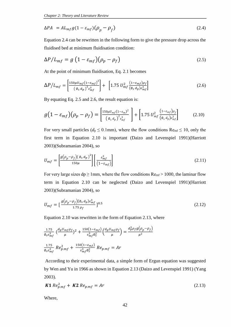
Chapter 2: Theory and Literature Review
42
∆𝑃𝐴 = 𝐴𝐿𝑚𝑓𝑔(1 − 휀𝑚𝑓)(𝜌𝑝−𝜌𝑓) (2.4)
Equation 2.4 can be rewritten in the following form to give the pressure drop across the
fluidised bed at minimum fluidisation condition:
∆𝑃 𝐿𝑚𝑓⁄ = 𝑔 (1 − 휀𝑚𝑓)(𝜌𝑝 − 𝜌𝑓) (2.5)
At the point of minimum fluidisation, Eq. 2.1 becomes
∆𝑃 𝐿𝑚𝑓⁄ = [150𝜇𝑈𝑚𝑓(1−𝜀𝑚𝑓)
2
( ∅𝑠 𝑑𝑝 )2𝜀𝑚𝑓3
] + [1.75 𝑈𝑚𝑓2 (1−𝜀𝑚𝑓)𝜌𝑓
(∅𝑠 𝑑𝑝)𝜀𝑚𝑓3 ] (2.6)
By equating Eq. 2.5 and 2.6, the result equation is:
𝑔(1 − 휀𝑚𝑓)(𝜌𝑝 − 𝜌𝑓) = [150𝜇𝑈𝑚𝑓(1−휀𝑚)
2
( ∅𝑠 𝑑𝑝 )2휀𝑚𝑓3
] + [1.75 𝑈𝑚𝑓2
(1−휀𝑚𝑓)𝜌𝑓
(∅𝑠 𝑑𝑝)휀𝑚𝑓3 ] (2.10)
For very small particles (dp ≤ 0.1mm), where the flow conditions Remf ≤ 10, only the
first term in Equation 2.10 is important (Daizo and Levenspiel 1991)(Harriott
2003)(Subramanian 2004), so
𝑈𝑚𝑓 = [𝑔(𝜌𝑝−𝜌𝑓)( ∅𝑠 𝑑𝑝 )
2
150𝜇] [
𝜀𝑚𝑓3
(1−휀𝑚𝑓)] (2.11)
For very large sizes dp ≥ 1mm, where the flow conditions Remf > 1000, the laminar flow
term in Equation 2.10 can be neglected (Daizo and Levenspiel 1991)(Harriott
2003)(Subramanian 2004), so
𝑈𝑚𝑓 = [ 𝑔(𝜌𝑝−𝜌𝑓)(∅𝑠 𝑑𝑝)𝜀𝑚𝑓
3
1.75 𝜌𝑓 ]0.5 (2.12)
Equation 2.10 was rewritten in the form of Equation 2.13, where
1.75
∅𝑠𝜀𝑚𝑓3 (
𝑑𝑝𝑈𝑚𝑓𝜌𝑓
𝜇)2 +
150(1−𝜀𝑚𝑓)
𝜀𝑚𝑓3 ∅𝑠
2 (𝑑𝑝𝑈𝑚𝑓𝜌𝑓
𝜇) =
𝑑𝑝3𝜌𝑓𝑔(𝜌𝑝−𝜌𝑓)
𝜇2
1.75
∅𝑠𝜀𝑚𝑓3 𝑅𝑒𝑝.𝑚𝑓
2 + 150(1−𝜀𝑚𝑓)
𝜀𝑚𝑓3 ∅𝑠
2 𝑅𝑒𝑝.𝑚𝑓 = 𝐴𝑟
According to their experimental data, a simple form of Ergun equation was suggested
by Wen and Yu in 1966 as shown in Equation 2.13 (Daizo and Levenspiel 1991) (Yang
2003).
𝑲𝟏 𝑅𝑒𝑝.𝑚𝑓2 + 𝑲𝟐 𝑅𝑒𝑝.𝑚𝑓 = 𝐴𝑟 (2.13)
Where,

Chapter 2: Theory and Literature Review
43
𝑅𝑒𝑝.𝑚𝑓 = (𝑑𝑝𝑈𝑚𝑓𝜌𝑓
𝜇) , is defined as the particle Reynold number
𝐴𝑟 = 𝑑𝑝3𝜌𝑓𝑔(𝜌𝑝−𝜌𝑓)
𝜇2 , is defined as Archimedes number, a
dimensionless group. Sometimes called Galileo number Ga.
𝑲𝟏 = 1.75
∅𝑠𝜀𝑚𝑓3 , 𝑲𝟐 =
150(1−𝜀𝑚𝑓)
𝜀𝑚𝑓3 ∅𝑠
2 are constants, depend on the void of
the bed at minimum fluidisation 휀𝑚𝑓 and sphericity ∅𝑠 of the bed
particle.
Equation 2.13 is a quadratic equation, which can be solved for Rep.mf. Finally,
Umf can be obtained. For most practical applications, Equation 2.13 was
solved and rearranged in term of Reynold number in the following form.
𝑅𝑒𝑝.𝑚𝑓 = (𝑑𝑝𝑈𝑚𝑓𝜌𝑓
𝜇) = [𝑪𝟏
𝟐 + 𝑪𝟐 𝐴𝑟]0.5 − 𝑪𝟏 (2.14)
Where: C1= K2/2K1 and C2= 1/K2 are constants, which can obtained
empirically when both parameters ɛmf and/or ϕs are not available. These
constants are available in many published papers for many investigators
(Daizo and Levenspiel 1991)(Yang 2003)(Jiliang et al. 2013).
2.5.4.2 Experimental determination
As explained above the transition point between the fixed bed regime and fluidised bed
regime has been used practically to determine the minimum fluidisation velocity for
gas-solid systems. Experimentally, for any gas-solid particle system the pressure drop-
gas superficial velocity diagram can be built. As shown in Figure 2.9 below, for the
fixed bed region when the low gas velocity increases the pressure drop across the bed
increases linearly until the bed at point A is ready to start to expand and fluidise. A
further slight increase of velocity the pressure drop reaches its maximum point (B) and
then reduces to point C, a point at which the forces are balanced and pressure drop
remains nearly constant for any increase in gas velocity as shown in line CD. The next
step is the reversing of process (from fluidisation to defluidisation) by decreasing the
gas velocity steadily. The pressure drop in fixed bed region for defluidisation path (EF)
is less than fluidisation path due to the particle loosing arrangement. The intersection
point E of extended DC line and extended FE line will represent the minimum

Chapter 2: Theory and Literature Review
44
fluidisation velocity. In most literature the intersection point A of line DC and
increasing velocity line in fixed bed represents the initial fluidisation velocity Umf,i and
point C represents the complete fluidisation velocity Umf,c (Subramanian
2004)(University of Florida 2015). Most research used this pressure drop profile
method for determining mainly the minimum fluidisation velocity Umf for a specified
fluidisation system (Badday et al. 2014) (Chok et al. 2010)(Chok 2009) (Subramani et
al. 2007)(Patil et al. 2005)(Hilal et al. 2001)(Gauthier et al. 1999).
Figure 2. 9 Pressure drop-gas superficial velocity fluidisation diagram (redrawn) (University of
Florida 2015)
2.5.5 Biomass fluidisation
Due to their extreme nature, high content of cellulose, hemicellulose and lignin
composition and a wide range in physical characterizations (mainly irregular size, shape
and density) biomass is considered anisotropic material, which gives it a clear difference
in their mechanical property in various directions (Guo et al. 2012). Thereby, these
properties have made the characterization of fluidisation of biomass materials,
especially agricultural and forest residues (lignocellulosic biomass), is not predictable
easily (Cui and Grace 2007)(Escudero and Heindel 2011)(Oliveira et al. 2013)(Shao et
al. 2013). The hydrodynamic fluidisation of various types of biomass particles has been
investigated by many researchers focusing on; the fluidisation characteristics of
biomass particles as a single material, improving their fluidisation characterization by
mixing them with a fluidisable second solid (inert) material like sand, alumina, calcite,
etc, (Karmakar et al. 2013)(Zhang et al. 2011). Moreover, this parameter also needs to
study the effects of related parameters on it such as: biomass particle size, density,
biomass weight percent in the bed mixture and the degree of the mixture mixing and

Chapter 2: Theory and Literature Review
45
segregation due to the high difference in the densities, particle size and composition of
two materials of the mixture.
2.5.5.1 Fluidisation of a single biomass material
For characterising of fluidization of single biomass materials, many studies have been
conducted. In their experiments (Aznar et al. 1992) showed that agricultural and forest
biomass materials such as sawdust, straw and ground thistle cannot be fluidised unless
using a second fluidising solid material.
Fluidisation characteristics such as particle size, bulk density and fluidising velocity for
various Malaysian biomass residues ( rise husk, sawdust, peanut shell, coconut shell
and palm fibre) and coal and bottom ash were experimentally obtained by (Abdullah et
al. 2003). These experiments were conducted using an air-cold flow-fluidising column.
They classified sawdust, coconut shell, coal and bottom ash were classified in Geldart’s
B particle size, whereas rice husk and palm fibre type D and A respectively. They
concluded that type B group has good fluidising behaviour, while group D and A have
a weak behaviour.
(Zhong et al. 2008) carried out their fluidisation experiments on both, single biomass
materials and binary mixture with three inert fluidisation medium materials, silica sand,
alumina oxide and continental flood basalt (CFB) cinder. Their biomass materials were
five, three of them were approximate sphere particles (wood chip ρp=564kg/ m3, millet
ρp= n.a, and mung beans ρp= 1640kg/ m3), whereas the others were long thin particles
(cotton stalk ρp = 365 kg/m3 and corn stalk ρp =274 kg/m3). They measured the
minimum fluidisation for each material using a similar procedure that was followed by
(Rao and Bheemarasetti 2001). The value of Umf was measured using a descending gas
flow curve from the complete fluidised state. For two long thin biomasses, they found
that these materials could not be fluidised when the particle aspect ratio was over a
certain value. They attributed to their particles nature for bridging and relaxing each
other and this affected their fluidisation negatively. While the fluidisation for single
biomass for approximate spherical particles was not presented.
In their study, (Chok et al. 2010) considered that palm shell biomass wastes fall in
Geldart D group. They reported that this material is difficult to fluidise as a single
material. To facilitate fluidisation, it should be mixed with another fluidisable material
like sand.
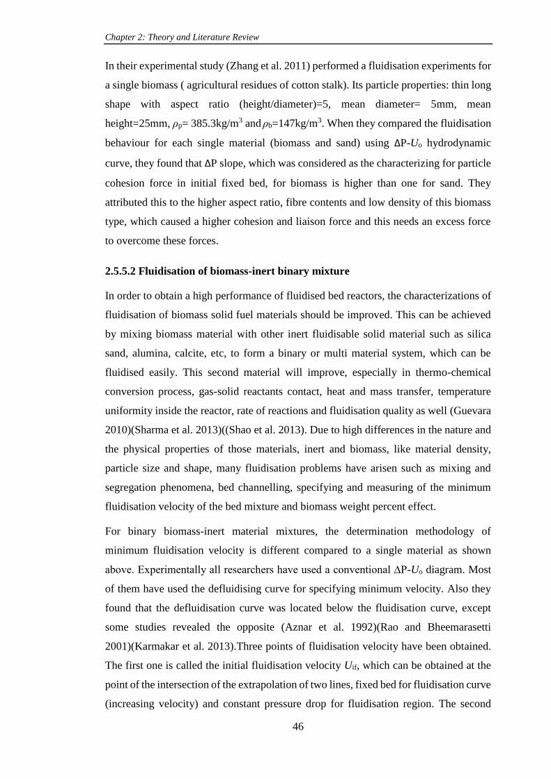
Chapter 2: Theory and Literature Review
46
In their experimental study (Zhang et al. 2011) performed a fluidisation experiments for
a single biomass ( agricultural residues of cotton stalk). Its particle properties: thin long
shape with aspect ratio (height/diameter)=5, mean diameter= 5mm, mean
height=25mm, ρp= 385.3kg/m3 and ρb=147kg/m3. When they compared the fluidisation
behaviour for each single material (biomass and sand) using ∆P-Uo hydrodynamic
curve, they found that ∆P slope, which was considered as the characterizing for particle
cohesion force in initial fixed bed, for biomass is higher than one for sand. They
attributed this to the higher aspect ratio, fibre contents and low density of this biomass
type, which caused a higher cohesion and liaison force and this needs an excess force
to overcome these forces.
2.5.5.2 Fluidisation of biomass-inert binary mixture
In order to obtain a high performance of fluidised bed reactors, the characterizations of
fluidisation of biomass solid fuel materials should be improved. This can be achieved
by mixing biomass material with other inert fluidisable solid material such as silica
sand, alumina, calcite, etc, to form a binary or multi material system, which can be
fluidised easily. This second material will improve, especially in thermo-chemical
conversion process, gas-solid reactants contact, heat and mass transfer, temperature
uniformity inside the reactor, rate of reactions and fluidisation quality as well (Guevara
2010)(Sharma et al. 2013)((Shao et al. 2013). Due to high differences in the nature and
the physical properties of those materials, inert and biomass, like material density,
particle size and shape, many fluidisation problems have arisen such as mixing and
segregation phenomena, bed channelling, specifying and measuring of the minimum
fluidisation velocity of the bed mixture and biomass weight percent effect.
For binary biomass-inert material mixtures, the determination methodology of
minimum fluidisation velocity is different compared to a single material as shown
above. Experimentally all researchers have used a conventional ∆P-Uo diagram. Most
of them have used the defluidising curve for specifying minimum velocity. Also they
found that the defluidisation curve was located below the fluidisation curve, except
some studies revealed the opposite (Aznar et al. 1992)(Rao and Bheemarasetti
2001)(Karmakar et al. 2013).Three points of fluidisation velocity have been obtained.
The first one is called the initial fluidisation velocity Uif, which can be obtained at the
point of the intersection of the extrapolation of two lines, fixed bed for fluidisation curve
(increasing velocity) and constant pressure drop for fluidisation region. The second

Chapter 2: Theory and Literature Review
47
velocity is called the minimum fluidisation velocity Umf, which can be specified at the
point of the intersection of the extrapolation of two lines, fixed bed for defluidisation
curve and constant pressure drop at fluidisation condition. The third velocity is called a
complete fluidisation velocity Ucf, which was specified when the first conversion of
constant pressure drop line for defluidisation curve to fixed bed conditions and vice
versa or, by observation, when entire bed materials are moved (Aznar et al. 1992).
Figure 2.10 illustrates all these velocities for various studies. Many researchers used
these three velocity values to evaluate the fluidisation quality of the system. They said
that whenever the interval distance between Uif and Ucf is small the fluidisation quality
is good (Sampaio 2013). This interval sometimes called segregation interval (Ucf-Uif).
In most previous studies, Umf velocity was taken as minimum fluidisation velocity as a
design parameter.
Figure 2. 10 Schematic of pressure-superficial velocity curve for biomass-inert binary mixtures
showing three types of minimum fluidisation velocities (Sampaio 2013)
Experimentally, investigators confirmed in their studies the using of the above
procedure of the determining of the minimum fluidising velocity (using decreasing
velocity) for biomass-inert mixtures. They are, such as (Qiaoqun et al. 2005),
(Formisani et al. 2008), (Zhang et al. 2011), (Oliveira et al. 2013), (Sharma et al. 2013),
(Sampaio 2013), (Kumoro et al. 2014), etc, whereas (Clarke et al. 2005) used the
intersection point of fluidisation (increasing velocity) curve, not the defluidisation
curve.
2.5.6 Parameters affect minimum fluidisation velocity
In fluidisation systems, either for single bed or for binary biomass-inert mixtures, many
parameters affect the values of the design parameter minimum fluidisation velocity.

Chapter 2: Theory and Literature Review
48
2.5.6.1 Particle size of the bed material
For four different particle size ranges between 125 and 500µm of single sand
(ρs=2700kg/m3), (Aznar et al. 1992) showed that both velocities Umf and Ucf increased
as sand particle size increased
(Badday et al. 2014)investigated the effect of particle size on minimum fluidisation
velocity Umf. They used three particle sizes of sand bed material 301µm, 454µm, 560µm
using 0.1 ID of fluidisation column. They found out that Umf increased as particle size
increased. Similar finding was obtained by (Qiaoqun et al. 2005) for sand material only.
(Chok 2009) found in their study for compartmented fluidised bed gasifier (gasifier and
combustor compartments) that both velocities Umf and Ucf for sand material for both
compartments increased as mean particle size 𝑑𝑝 increased (196, 272, 341, 395µm).
(Dora et al. 2013) studied the fluidisation characteristics of four ternary mixtures for
three different particle sizes of single dolomite solid material in a conical column bed.
One aspect of their study, the effect of bed static height Hs (10cm, 12.5cm, 15cm and
17.5cm), cone angle (4.61, 5.13, 7.47 and 11.2), average particle size for each ternary
mixture (1.29mm, 1.2mm, 1.125mm and 1.106mm) on pressure drop ∆Pmf and
superficial velocity Umf at minimum fluidisation conditions were discussed. For average
particle size effect they found that for a cone angle of 7.47 and initial static bed height
= 10cm, ∆Pmf and Umf increased as the particle size increased.
2.5.6.2 Height of static bed
The effect of the static bed height Hs of the sand–sawdust biomass binary mixture on
minimum fluidisation velocity was studied by(Aznar et al. 1992). For different ratio of
Hs/D (bed height to column diameter), they observed there was no effect of the bed
height on Umf or Ucf. The minimum fluidisation velocity was conducted by (Marque
2002) for 2D rectangular fluidised bed column (1× 0.2 × 0.012 m). For different static
bed heights (8, 16, 20, 40, 60 cm) and glass beads particle size range (250-400µm), they
showed that static bed height had a significant effect on minimum fluidisation velocity
Umf, where Umf increased as Hs increased. For conical tapered fluidised bed (Sau et al.
2007) experimentally showed that the static bed height Hs had no effect on the Umf. For
the effect of static height (or biomass bed) on the minimum fluidisation velocity, (Jena
et al. 2008) and (Escudero and Heindel 2011) concluded that there was no any change
in Umf value when the static bed height was changed. In their experimental study on the
flow behaviour of a mixture of four different biomass material, which differed in their

Chapter 2: Theory and Literature Review
49
particle shape, size and density, with sand as fluidisation medium, (Shao et al. 2013)
showed that for multi composition mixture there was no clear effect of the static bed
height Hs on the minimum fluidisation velocity when increased from 100mm to 200mm.
As mentioned in previous section for (Dora et al. 2013) study, they showed that for this
type of bed column and for a specific cone angle and average particle size of ternary
mixture, ∆Pmf and Umf increased as the initial static bed height Hs increased. This finding
is contrary to the previous study (Sau et al. 2007) above, which used a conical bed, and
the conventional bed columns which have been presented above.
2.5.6.3 Percentage of biomass in biomass-solid binary mixture
For different volume percentage of pine sawdust biomass-sand (ρs=2700kg/m3)
mixture, for four different sand particle sizes, (Aznar et al. 1992) studied the effect of
biomass concentration on both fluidisation velocities Umf and Ucf. They found out that
a linear increase of both velocities up to nearly 50 % as biomass content increased for
four sand sizes. In addition, they showed that the mixture could not be fluidised when
the sawdust biomass percentage reached 75-80%. In (Rao and Bheemarasetti 2001)
study one aspect of their results shows the effect of the biomass mass percent for three
types of agricultural residues, rise husk, sawdust and groundnut shell, for three biomass
mass percent, 0%, 2%, 5% and 15%, on the minimum fluidisation velocity of biomass-
sand binary mixture. It can be seen that Umf of the mixture increased linearly as biomass
percent increased for a range between 0 % and 5 %. Whereas this increased
exponentially for a range between 5% and 15%. A similar effect was obtained by
(Karmakar et al. 2013) for three biomass types rise husk, bagasse and sawdust for four
weight percent 2%, 5%, 10% and 15%.
Also, (Qiaoqun et al. 2005) observed that as mass fraction of rise husk increased (from
0% to approximately 10.5%) the measured Umf increased linearly. (Clarke et al. 2005)
showed that for a specific size of glass sphere and sawdust moisture content, as the mass
fraction of sawdust increased the Umf of the mixture increased. Also for (Zhong et al.
2008) and (Chok et al. 2010) studies, which have been presented in previous section, a
similar finding was found for their biomass materials.
For their fluidisation of biomass material, sweet sorghum bagasse, tobacco residues and
soybean hulls, in sand binary mixtures, (Oliveira et al. 2013) found out, for three
biomass percent 5%, 10% and 15%, that for biomass material-sand mixture Umf

Chapter 2: Theory and Literature Review
50
decreased slightly as biomass percent increased, whereas for the other two materials,
Umf increased as the biomass percent increased.
(Sharma et al. 2013) used a cold-flow column to study the effect of the mixture
composition of the reactor bed, gasifier solid residues GSR, switchgrass fuel biomass
and inert silica sand material, on fluidisation behaviour. Their mixture composition
ranged from 0.17 to 5 % (as wt %) of the sand amount for switchgrass, for their binary
mixture, and from 5.0 to 35 % of the switchgrass amount for GSR material, for their
tertiary mixture. ∆P-Uo graphical method, as described before, was used to determine
Umf experimentally. They found that minimum fluidisation velocity for a mixture of
sand and GSR was decreased dramatically when GSR increased from 5% to 35 %. In
contrast, for a tertiary mixture the minimum velocity was increased as mass fraction of
two materials, switchgrass and GSR, increased from 0.17% to 3% and from 5% to 35
%, respectively. Using the effective properties of tertiary mixture the determining of
Umf from selected correlations from previous work did not agree well with the
experimental values for all mixture composition. Finally, they concluded that bed
mixture of 5% weight of switchgrass caused a segregation and bed channelization,
whereas up to 3% weight percent the bed fluidisation was sustained.
2.5.6.4 Elevated temperature
As mentioned before, the fluidised bed has been widely used in thermo-chemical
conversion processes (combustion, gasification and pyrolysis). These process are
working at a high temperature reached to 900-1000oC in fluidised bed gasifiers. This
high temperature affects the physical properties of the fluidisation medium, thereby
affecting the fluidisation behaviour which is mainly represented by minimum
fluidisation velocity design parameter (Lettieri and Macrì 2016). (R. R. Pattipati 1981)
experimentally investigated the effect of the temperature on the minimum fluidisation
velocity Umf. It was conducted for sand material (for small particle < 2mm and for
particles > 2mm) in fluidised bed using hot air as fluidised medium. They found that
for small particles (240, 462 and 1310µm) Umf decreased with temperature (from 18 to
900oC), whereas for large particles (3376µm) Umf increased. In their experimental study
(Subramani et al. 2007) determined the Umf at a wide range of temperature from 25oC
to 700oC for four bed materials type Geldart B ( ilmenite, sand, limestone, and quartz
magnetite) for various small particle sizes ( 128, 134, 163, and 200 µm) using air as a
fluidising medium. Each value of Umf was determined at steady required temperature.

Chapter 2: Theory and Literature Review
51
Their experimental data, which was presented graphically, showed that as the
temperature increased Umf decreased for all materials and particle sizes, which agrees
with the finding results of (R. R. Pattipati 1981) for small particle sizes. In addition, it
was noticed that the trends of Umf took a considerable decrease for temperature ranged
approximately from 298oK to 600oK, while this decreasing took place steadily for
temperature above 600oK. For particle size, Umf still increased with particle sizes of bed
material without any effect of high temperature on particle size. For two bed materials,
quartz sand ( ρs= 2750 kg/m3) and bottom ash (ρs= 2500 kg/m3) with average particle
diameter =0.5mm, and for temperature range from 30oC to 600oC, the experimental
results of fluidisation study obtained by (Jiliang et al. 2013) showed similar effect of
temperature on Umf that has been presented above. Similar result of temperature effects
on Umf was obtained by (Seo et al. 2014). They used a silica sand material with different
mean particle size (𝑑𝑝̅̅ ̅ = 135, 210, 270, and 385µm) for temperature ranged from 25 to
800oC. From their results, they confirmed that at high temperature (400-800oC) for
small particle sizes (𝑑𝑝̅̅ ̅ = 135, 210, and 270 µm) Umf became constant, whereas a
considerable decrease for (𝑑𝑝̅̅ ̅ = 385 µm). Recently, (Lettieri and Macrì 2016) reviewed
most experimental and theoretical studies related to the temperature effects on
fluidisation parameters, mainly minimum fluidisation velocity.
2.5.6.5 Distributor plate performance
The performance of fluidised bed reactors is strongly affected by the fluidisation
quality. Design of the gas distributor plate plays an important role in the fluidisation
quality to achieve the aims. There are various types of distributor plate (grates) designs.
These plates can be classified into three groups: 1) plate-type distributor, which consists
of two types, porous plate and perforated plate, 2) Nozzle (Tuyere) -type or bubble cap-
type, 3) Sparge pipe-type. This study focus on the perforated plate design because of its
simple manufacturing, cheap, suitable for pilot plant and laboratory researches (Basu
2006), (Yang 2003), (Daizo and Levenspiel 1991).
(Bauer et al. 1981) studied the effect of distributor design on the performance of the
fluidised bed reactor by using the fraction of unreacted ozone as a performance
parameter. They found that porous plate provided a better conversion than perforated
plate distributor.

Chapter 2: Theory and Literature Review
52
For studying the effects of distributor plate on the minimum fluidisation velocity Umf
(Hilal et al. 2001) used four different type of distributors. Three of them were perforated
plates with hole diameter 0.794mm for each, hole pitch were (12, 9, 7mm), and percent
of free (open) area ( 0.34, 0.61, 1.17 %), respectively, whereas the fourth one was a
porous plastic with thickness of 1.71cm and permeability of 12.35 Darcy. They found
that as the pitch hole decreased, Umf increased. The highest value of Umf value was for
porous plate. In the fluidised bed dryer (Jangam et al. 2009) studied experimentally and
via modelling the effect of the percentage open area (from 10% to 50%) and orifice
diameter of 2mm thick metal perforated distributor plate on the maldistribution function
in percent, a criteria which was used for distributor plates comparison. A lower value
indicates a better air distribution (uniformity of airflow) across the cross-section of the
bed. They found that this maldistribution function decreased when the open area
decreased and became near zero when low values of open area were used,
approximately 10%-20%. For orifice diameter effect, they showed that the air
uniformity reduced when the orifice diameter increased. For their experimental study
on fluidisation of bagasse biomass-sand mixtures (Augusta et al. 2011) showed that
there were no changes in the value of the minimum fluidisation velocity Umf when the
orifice diameter of the tuyere gas distributor changed. (Ghaly et al. 2015) studied the
configuration effect (shape and conical angle) of the distributor plate on the pressure
drop in a bubbling fluidised bed reactor. They classified the fluidisation quality
according to pressure drop fluctuations, which can be observed in gas-fluidised bed.
Good fluidisation gives moderate fluctuations, while large fluctuations may denote
slugging, and no fluctuations denote strong channelling in the bed. Therefore, a
distributor plate should be designed to give moderate pressure fluctuations.
2.6 Summary
The combined effects of the operating and hydrodynamic parameters on the gasification
process, generally, and on the bubbling fluidised bed gasifier performance, particularly,
have been reviewed. The biomass gasification by the airflow bubbling fluidised bed
gasifier has been highlighted. The method of the determination of the minimum
fluidisation velocity has been described, analytically using the theoretical equations and
experimentally using the ∆P-Umf hydrodynamic curve. The factors, which affect this
velocity have been presented.
Overall, from this review it can be concluded and suggested that:
Chapter 2: Theory and Literature Review
53
a) Air gas can be utilized as gasifying agent (fluidisation medium) for biomass
gasification. Biomass gasification using air-flow bubbling fluidised bed gasifier can
be achieved at a range from 350oC to 900oC. Also, between 0.2 and 0.6 the
equivalence ratio can be used.
b) According to the literature studies the inert material silica sand, which is belong to
Geldart type B, can be used as a high quality fluidised bed material for single material
or for biomass binary mixtures at high temperature gasification process. The range
of particle size is ranged from 100µm to 600µm.
c) Due to a shortage data in agricultural biomass gasification by air fluidising bed
gasifier, and gasifier performance, the operating and hydrodynamic factors that
affect the design and performance of the gasifier have been researched.
d) The effect of the number of distributor plate holes on the fluidised bed gasifier
performance has not been found in literature. This research is also studied this effect.

Chapter 3
Design and Development of the Rig

Chapter 3: Design and Development of the Rig
55
3.1 Introduction
In order to study, experimentation, the performance and the conversion rates of the
gasification process for solid biomass fuels in bubbling fluidised bed gasifier, a new
lab-scale rig for this gasifier was designed and built. The designing and building of the
rig specified the main and secondary rig components, which contributed to the study.
In this chapter, firstly the whole structure of the rig has been identified by specifying
those main and secondary components. Determining the size of the rig depends mainly
on determining the size of the reactor itself. It is a gasifier whose is the focus of this
study.
The study has required the gasifier to be in a size that is easy to control its operation
and at the same time has enough research flexibility. This flexibility will allow for
appropriate ranges of design parameters, which are needed to study their effects on the
gasifier performance whether for this current or for subsequent studies in this field.
The design method, which is followed in this study, differs from the design methods,
which are usually followed in the design of the chemical engineering unit operations.
In these methods, the capacity of production or the mass flow rate of any feed material
with other given data is firstly specified. Then the calculations of the mass and energy
balances will be performed. Finally the needed design parameters and thereby the size
of the unit will be obtained. Whereas, in this study the size of the gasifier is firstly
specified by selecting a suitable and desire value of the gasifier diameter. Based on the
diameter selection the other design parameters have been calculated and their required
ranges specified. These ranges can specify the size of the main secondary components
of the rig, like biomass screw feeder, air flowrate rotameter, air pre-heater and electrical
high temperature heater in addition to the height of the gasifier itself. All these design
parameter ranges give enough gasifier flexibility to study the effects of these design
parameters.

Chapter 3: Design and Development of the Rig
56
3.2 Geometry and hydrodynamic design of the bubbling fluidised
bed gasifier
3.2.1 Theoretical model of bubbling fluidising bed reactor
In this study, the two-phase model of Kuni-Levenspiel (1969) has been used to represent
the behavior of the gas-solid bubbling fluidised bed reactor. It gives a good
representation of the experimental data for this system. For this model the two phases
are an emulsion phase, often called the dense phase, and a bubble phase, also can be
called a lean phase as shown in Figure (3.1) (Daizo and Levenspiel 1991) (Ommen and
Ellis 2010).
Figure 3. 1 Sketch of the two–phase model in the bubbling fluidised bed (Ommen and Ellis 2010)
The bubble phase consists of a bubble, which contains a very small amount of solid
particles. As shown in Figure 3.2 it is not spherical but it has a nearly hemispherical top
and a pushed in the bottom. Each bubble has what is called wake that contains a
significant amount of solids. This wake, with its solids can be pulled when the bubble
is rise. A cloud region which separates the bubble and the emulsion phases is created
when a gas from a rising bubble is penetrated for a short distance into the surrounding
emulsion phase(Newton 1969) (Daizo and Levenspiel 1991) (Yang 2003).

Chapter 3: Design and Development of the Rig
57
Figure 3. 2 Sketch of the bubble, wake, cloud and emulsion (Newton 1969)
In this model, there are several concepts and definitions, mainly as following (Newton
1969)(Daizo and Levenspiel 1991)(Yang 2003):
The fraction of the total bed occupied by the bubbles without wakes, 𝛿.
The volume of the wake per volume of bubbles, 𝛼.
The fraction of the total bed occupied by the wakes, 𝛼𝛿.
The fraction of the total bed that occupied by the emulsion phase including clouds,
(1 − 𝛿 − 𝛼𝛿).
3.2.2 Design equations for the reaction bed section
For bubbling fluidised bed reactor a two-phase model, bubble and emulsion phases, will
be used for this type of fluidising regime. There are a number of design equations govern
this regime and this model.
3.2.2.1 Calculation of the minimum fluidization velocity, Umf:
As mentioned in Chapter 2-Section 2.5.4.1, minimum fluidization velocity Umf is an
important parameter in fluidised bed reactor design. It can be calculated using Equation
(2.11) or a quadratic Eurgn equation with the form shown in Equation (3.1). For fine
particles, the constants C1=33.7 and C2= 0.0408, which were recommended by Wen
and Yu (Daizo and Levenspiel 1991).
𝑅𝑒𝑝.𝑚𝑓 = (𝑑𝑝𝑈𝑚𝑓𝜌𝑓
𝜇) = [𝑪𝟏
𝟐 + 𝑪𝟐 𝐴𝑟]0.5 − 𝑪𝟏 (3.1)
Equation (3.2) was used to calculate the bed void fraction at the minimum fluidization
conditions ɛmf (Newton 1969) (Daizo and Levenspiel 1991):
휀𝑚𝑓 = 0.586 ∅𝑠−0.72 [
𝜇2
ɳ 𝑑𝑝3 𝜌𝑔
]0.024
[𝜌𝑔
𝜌𝑠]0.021
(3.2)

Chapter 3: Design and Development of the Rig
58
∅𝑠 = 𝑃𝑎𝑟𝑡𝑖𝑐𝑙𝑒 𝑠ℎ𝑒𝑟𝑒𝑐𝑖𝑡𝑦 =𝑠𝑢𝑟𝑓𝑎𝑐𝑒 𝑎𝑟𝑒𝑎 𝑜𝑓 𝑎 𝑠𝑝ℎ𝑒𝑟𝑖𝑐𝑎𝑙 𝑝𝑎𝑟𝑡𝑖𝑐𝑙𝑒
𝑎𝑐𝑡𝑢𝑎𝑙𝑙𝑦 𝑠𝑢𝑟𝑓𝑎𝑐𝑒 𝑎𝑟𝑒𝑎 𝑜𝑓 𝑡ℎ𝑒 𝑝𝑎𝑟𝑡𝑖𝑐𝑙𝑒=
𝐴𝑠
𝐴𝑝 (3.3a)
∅𝑠 =𝜋[(6𝑉𝑝/𝜋)
1/3]2
𝐴𝑝= 𝜋[6𝑉𝑝/𝜋]
2/3
𝐴𝑝 (3.3b)
Where:
𝑉𝑝: Volume of a spherical particle
𝑉𝑝 =𝜋𝑑𝑝
3
6 (3.4)
𝑑𝑝 = �̅�𝑝 =1
∑𝑓𝑖𝑑𝑝𝑖
= 𝑡ℎ𝑒 𝑚𝑒𝑎𝑛 𝑝𝑎𝑟𝑡𝑖𝑐𝑙𝑒 𝑠𝑖𝑧𝑒 (3.5)
𝑓𝑖 is the fraction of particles with diameter 𝑑𝑝𝑖.
3.2.2.2 Calculation of the particle terminal velocity, Ut
Terminal velocity is a free fall velocity of the particle. For design purpose, it is
considered a maximum superficial velocity (velocity of the agent fluid) in the bubbling
fluidised bed. By this limitation superficial velocity must be above Umf and below Ut.
Based on Reynold numbers of the particles, two relation- ships of terminal velocity are
presented by Kuni-Levenspiel (Newton 1969)(Basu 2006).
𝑈𝑡 =𝜂𝑑𝑝
2
18𝜇 for ReUt < 0.4 (3.6a)
𝑈𝑡 = [1.78∗10−2𝜂2
𝜌𝑔𝜇]1/3 𝑑𝑝 for 0.4 < ReUt < 500 (3.6b)
3.2.2.3 Calculation of the slugging velocity, Ums
Slugging velocity is a fluid velocity at which the slugging regime occurs. It can be
expressed by the bubble rise velocity Ub,ms, where below the value of this velocity
slugging shall not take place (Newton 1969) (Daizo and Levenspiel 1991) (Basu 2006).
The bubble rise velocity can be expressed by an equation below.
𝑈𝑏,𝑚𝑠 = 𝑈𝑚𝑓 + 0.07 (𝑔𝐷)1/2 (3.7)
(Daizo and Levenspiel 1991) concluded that when the fluidising velocity (superficial
velocity of fluidisation) is more than Ub,ms slugging would be the main regime.

Chapter 3: Design and Development of the Rig
59
3.2.2.4 Calculation of the superficial velocity, Uo
Uo calculation can be suggested according to the conditions
𝑈𝑚𝑓 < 𝑈𝑜 < 𝑈𝑡 and 𝑈𝑚𝑓 < 𝑈𝑜 < 𝑈𝑏,𝑚𝑠
The condition at which the slugs are formed when the maximum stable bubble size
dbmax, which is calculated by Equation (3.10), is greater than 0.6 times the diameter of
the bed D, the permitted maximum bubble size 𝑑𝑏𝑚𝑎𝑥,𝑝 (Daizo and Levenspiel 1991)
(Yang 2003), i.e.
𝑑𝑏𝑚𝑎𝑥,𝑝 = 0.6 𝐷 (3.8)
In other reference, 𝑑𝑏𝑚𝑎𝑥,𝑝 =2
3 𝐷 (3.9)
In other word, dbmax should not exceed 0.6D or 2/3 D; otherwise, the suggested Uo must
be changed.
3.2.2.5 Calculation of the maximum bubble-size, dbmax
For the estimation of the bubble size at any superficial velocity it is important and useful
to know if the fluidised bed provide the slugging phenomena or not by comparing the
estimated value to the bed diameter according to Equation (3.10).
𝑑𝑏𝑚 = 𝑑𝑏𝑚𝑎𝑥 = 0.652[ 𝐴𝑐 (𝑈𝑜 − 𝑈𝑚𝑓)]0.4, in cm (3.10)
Where Ac = cross-sectional area of the fluidised bed reactor.
Uo - Umf = excess fluidizing velocity
3.2.2.6 Calculation of the bed height, H
According to Baeyens & Geldert analysis (Yang 2003), there are three separate zones
in a deep bed operating with an excess velocity Uo - Umf as illustrated in Figure (3.3)
Figure 3. 3 Stages of the slug regime establishment

Chapter 3: Design and Development of the Rig
60
The minimum bed height for stable slugging can be calculated by equation (3.11).
𝐻𝐿,𝑚𝑖𝑛 = 60 𝐷0.175 , D in cm (3.11)
The maximum bed height below which the bed will be freely bubbling can be calculated
from equation (3.12).
𝐻𝑓𝑏,𝑚𝑎𝑥 =(𝐷−2.51𝐷0.2)
0.13𝐷0.47 , D in cm (3.12)
The slugging regime can be avoided by operating within zone (1) with freely bubbling
bed. Most of the literatures (Daizo and Levenspiel 1991) (Yang 2003) (Basu 2006)
stated that to avoid the slugging regime, especially in the lab-scale and pilot plant
reactors, the ratio of the bed height to the bed diameter must not exceed 2.
i.e.
𝐻𝑠
𝐷 ≤ 2 (3.13a)
It means that
Hs,max = 2D (3.13b)
H/D ratio sometimes called aspect ratio. For this design study, Equation (3.13b) was
recommended to use for Hs specifying.
3.2.2.7 Calculation of the bubble size db, at any height h of the bed at any time.
Bubble diameter sometimes called a mean bubble size or an equivalent volume diameter
of a bubble. (Daizo and Levenspiel 1991) (Yang 2003) (Basu 2006) mentioned that for
Geldart B and D solids, Mori & Wen suggested a correlation for bubble size at any
height h in the bed as in equation (3.14).
𝑑𝑏𝑚− 𝑑𝑏
𝑑𝑏𝑚− 𝑑𝑏𝑜= 𝑒−0.3ℎ 𝐷⁄
Or
𝑑𝑏 = 𝑑𝑏𝑚 − (𝑑𝑏𝑚 − 𝑑𝑏𝑜) × 𝑒−0.3ℎ 𝐷⁄ (3.14)
Where:
dbm = 𝑑𝑏𝑚𝑎𝑥 = The maximum size of bubble, Eq.(3.10).
dbo = The initial bubble size formed near the bottom of the bed at the plate distributor.
Equation (3.14) can be applied within the following conditions

Chapter 3: Design and Development of the Rig
61
𝐻/𝐷 ≤ 1.3
60𝜇𝑚 ≤ 𝑑𝑝 ≤ 450𝜇𝑚
0.5 𝑐𝑚 𝑠𝑒𝑐⁄ ≤ 𝑈𝑚𝑓 ≤ 20 𝑐𝑚 𝑠𝑒𝑐⁄
𝑈𝑜 − 𝑈𝑚𝑓 ≤ 48 𝑐𝑚 𝑠𝑒𝑐⁄
For beds with diameter between 7 and 30 cm, Equation (3.14) approximately has good
accuracy (Newton 1969).
dbo can be estimated depending on the type of the distributor plate, dbo in cm:
For porous plates (Newton 1969)(Daizo and Levenspiel 1991) (Yang 2003) (Basu
2006)
𝑑𝑏𝑜 = 0.00376 (𝑈𝑜 − 𝑈𝑚𝑓)2 (3.15a)
For perforated plate
𝑑𝑏𝑜 = 0.347[𝐴𝑐(𝑈𝑜 − 𝑈𝑚𝑓) 𝑛𝑑]⁄0.4
(3.15b)
Where, nd is the number of the holes.
3.2.2.8 Calculation of the bubble rise velocity, Ub
It can be calculated from Equation (3.16) (Daizo and Levenspiel 1991) (Basu 2006).
𝑈𝑏 = ( 𝑈𝑂 − 𝑈𝑚𝑓 ) + 0.71 ( 𝑔𝑑𝑏)0.5 (3.16)
All terms are defined in previous steps.
3.2.2.9 Calculation of the fraction of bed in bubble phase, 𝜹
This represents a volume fraction of the total bed occupied by the bubbles that does not
include the wake. It can be calculated from Equation (3.17).
𝛿 =𝑈𝑜− 𝑈𝑚𝑓
𝑈𝑏− (𝑈𝑚𝑓×(1+𝛼)) (3.17)
𝛼 is the volume of wake per volume of bubble. It's value vary between 0.25-1, with
typical values close to 0.4 (Newton 1969) (Yang 2003) .
Notes 1: The bed material fraction in the wakes is (𝛼𝛿).
2: The bed fraction in emulsion phase (not including bubble wakes)
=1 − 𝛿 − 𝛼𝛿. (3.18)

Chapter 3: Design and Development of the Rig
62
3: For fast bubbles or when𝑈𝑏 > 5𝑈𝑚𝑓 휀𝑚𝑓⁄ , clouds are thin and (Daizo &
Levenspiel, 1991).
𝛿 = 𝑈𝑜− 𝑈𝑚𝑓
𝑈𝑏−𝑈𝑚𝑓 (3.19)
4: In highly bubbling beds where, 𝑈𝑜 ≫ 𝑈𝑚𝑓, the approximation of 𝛿 is(Daizo
and Levenspiel 1991) :
𝛿 =𝑈𝑜
𝑈𝑏 (3.20)
3.2.2.10 Calculation of the mass solid in the bed, Ws
The mass balance for the bed solids gives (Newton 1969),
𝑊𝑠 = 𝜌𝑠𝐴𝑐𝐻𝑠 (1 − 휀𝑠) (3.21)
= 𝜌𝑠𝐴𝑐 𝐻 (1 − 휀)
= 𝜌𝑠𝐴𝑐𝐻𝑓 (1 − 휀𝑓)
= 𝜌𝑠𝐴𝑐𝐻𝑚𝑓(1 − 휀𝑚𝑓)
Where, 𝜌𝑠 = a particle density of the solid bed material.
𝐴𝑐 = cross-sectional area of the bed reactor.
𝐻𝑠 = height of the bed settled before particles start to lift (static bed height).
𝐻𝑓 = height of the bed at any time.
휀𝑠 = porosity (void fraction) of the settled (fixed or static) bed.
For Geldert B and D solids bed, (Daizo and Levenspiel 1991) gave an equation
represents 휀𝑓 , 휀𝑚𝑓 𝑎𝑛𝑑 𝛿 relation,
(1 − 휀𝑓) = (1 − 𝛿)(1 − 휀𝑚𝑓) (3.22)
From equation (3.22) 휀𝑓 can be calculated
휀𝑓 = 1 − [(1 − 𝛿)(1 − 휀𝑚𝑓)] (3.23)
From equation (3.21) and equation (3.22), the mass of the solid bed can also be
calculated:
𝑊𝑠 = 𝜌𝑠𝐴𝑐𝐻𝑓(1 − 𝛿)(1 − 휀𝑚𝑓) (3.24)
All parameters in equation (3.24) can be given or calculated as shown in previous steps.

Chapter 3: Design and Development of the Rig
63
3.2.2.11 Calculations of the feed biomass flow rate:
The feed mass rate of biomass can be calculated from the supplied air flowrate and
suggested gasification equivalence ratio, ER, where:
𝑬𝑹 =[𝒎𝒂𝒔𝒔 𝒂𝒊𝒓 𝒇𝒖𝒆𝒍 𝒓𝒂𝒕𝒊𝒐, 𝑴𝑨𝑭𝑹]𝒂𝒄𝒕𝒖𝒂𝒍
[𝒎𝒂𝒔𝒔 𝒂𝒊𝒓 𝒇𝒖𝒆𝒍 𝒓𝒂𝒕𝒊𝒐, 𝑴𝑨𝑭𝑹]𝒔𝒕𝒐𝒊𝒄𝒉𝒊𝒐𝒎𝒆𝒕𝒓𝒊𝒄 (3.25)
The actual mass air fuel ratio is a ratio of the actual air mass rate �̇�𝑎𝑖𝑟, to the actual
biomass mass rate �̇�𝑏𝑖𝑜𝑚𝑎𝑠𝑠. However these actual values can be experimentally
specified and calculated and observed from the measurement devices in the rig. Also
for design purposes, they can be theoretically calculated from above equation (3.25).
Thereafter the feed mass rate of biomass can be calculated by
[ 𝑚𝑎𝑠𝑠 𝑎𝑖𝑟 𝑓𝑢𝑒𝑙 𝑟𝑎𝑖𝑜 ]𝑎𝑐𝑡𝑢𝑎𝑙 = 𝐸𝑅 × [𝑚𝑎𝑠𝑠 𝑎𝑖𝑟 𝑓𝑢𝑒𝑙 𝑟𝑎𝑡𝑖𝑜]𝑠𝑡𝑜𝑖𝑐ℎ𝑖𝑜
[𝑀𝐴𝐹𝑅]𝑎𝑐𝑡𝑢𝑎𝑙 = 𝐸𝑅 × [𝑀𝐴𝐹𝑅]𝑠𝑡𝑜𝑖𝑐ℎ𝑖𝑜 (3.26)
The value of the equivalence ratio ER can be suggested. For the air gasification system
the stoichiometric value of the mass air fuel ratio, depending on the composition of the
solid biomass, can be approximately estimated from the Equation (3.27) (PETRO
2007).
[𝑀𝐴𝐹𝑅]𝑠𝑡𝑜𝑖𝑐ℎ𝑖𝑜 = 8.89 × [%𝐶 + 0.375 ×%𝑆] + 26.5 × %𝐻 − 3.3 × %𝑂 (3.27)
Where: %C, %S, %H and %O are the carbon, sulfur, hydrogen, and oxygen composition
percent in solid biomass fuel. These percent can be obtained from the ultimate analysis
of the fuel.
Finally, the actual (required) feed mass rate of the fuel biomass can be calculated by
equation (3.28):
�̇�𝑏𝑖𝑜𝑚𝑎𝑠𝑠 = [�̇�𝑎𝑖𝑟] [ 𝑀𝐴𝐹𝑅]𝑎𝑐𝑡𝑢𝑎𝑙⁄ (3.28)
From the density of the air at a specific temperature and pressure, conditions at which
the air volumetric flow rate is specified or measured, which can be calculated from the
superficial velocity Uo of the air and bed cross-sectional area Ac as shown in equation
(3.30), the air mass flow-rate will be calculated.
𝑎𝑖𝑟 𝑚𝑎𝑠𝑠 𝑓𝑙𝑜𝑤𝑟𝑎𝑡𝑒
= [𝑣𝑜𝑙𝑢𝑚𝑒𝑡𝑟𝑖𝑐 𝑓𝑙𝑜𝑤𝑟𝑎𝑡𝑒]
× [𝑎𝑖𝑟 𝑑𝑒𝑛𝑠𝑖𝑡𝑦 𝑎𝑡 𝑠𝑝𝑒𝑐𝑖𝑓𝑖𝑐 𝑡𝑒𝑚𝑝𝑒𝑟𝑎𝑡𝑢𝑟𝑒 𝑎𝑛𝑑 𝑝𝑟𝑒𝑠𝑠𝑢𝑟𝑒]
∴ �̇�𝑎𝑖𝑟 = �̇�𝑎𝑖𝑟 ∗ 𝜌𝑎𝑖𝑟 𝑎𝑡 ambient cond. (3.29)

Chapter 3: Design and Development of the Rig
64
Where
�̇�𝑎𝑖𝑟 = ( 𝑈𝑜)(𝐴𝑐) (3.30)
3.2.3 Freeboard Section
Freeboard is defined as the height of the column section, as a part of the fluidised bed
column, between the surface of the bed phase (dense phase) and the outlet of the gas. It
is called the freeboard height Hfb. However, the design of this section is important to
give a chance to the solid materials to return to the bed section. In addition, it gives
additional time to complete some chemical reactions like tar materials in gasification
process. For design consideration, the location of the exit gas should be above the
Transport Disengaging Height TDH, a height at which the flux of the solids material
and its size distribution are approximately constant. Figure (3.4) shows these
definitions. Note play, when Hfb is greater than TDH the carryover of solids will be
reduced and vice versa. This will directly affected the duty of the solid separator
equipment. In addition, for the thermal conversion the carryover of the unburned solid
carbon will be minimized when Hfb > TDH. In addition, this height will give additional
residence time for the chemical reactions.
Figure 3. 4 Schematic of freeboard zones in bubbling fluidised bed (Basu 2006)
3.2.3.1 Estimation of TDH and total height of the gasifier
Many empirical correlations can be used to estimate the TDH. Three correlations have
been used in this design to calculate TDH.
1. Froud correlation (Yang 2003).
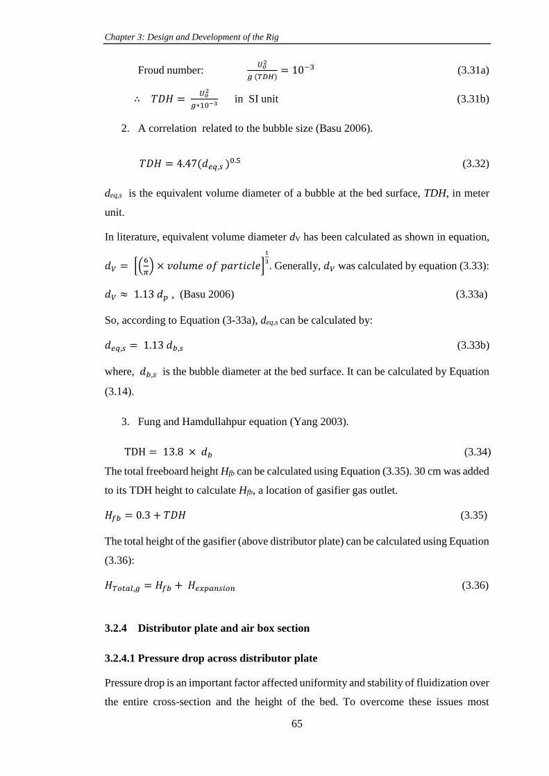
Chapter 3: Design and Development of the Rig
65
Froud number: 𝑈𝑜2
𝑔 (𝑇𝐷𝐻)= 10−3 (3.31a)
∴ 𝑇𝐷𝐻 = 𝑈𝑜2
𝑔∗10−3 in SI unit (3.31b)
2. A correlation related to the bubble size (Basu 2006).
𝑇𝐷𝐻 = 4.47(𝑑𝑒𝑞,𝑠 )0.5 (3.32)
deq,s is the equivalent volume diameter of a bubble at the bed surface, TDH, in meter
unit.
In literature, equivalent volume diameter dV has been calculated as shown in equation,
𝑑𝑉 = [(6
𝜋) × 𝑣𝑜𝑙𝑢𝑚𝑒 𝑜𝑓 𝑝𝑎𝑟𝑡𝑖𝑐𝑙𝑒]
1
3. Generally, 𝑑𝑉 was calculated by equation (3.33):
𝑑𝑉 ≈ 1.13 𝑑𝑝 , (Basu 2006) (3.33a)
So, according to Equation (3-33a), deq,s can be calculated by:
𝑑𝑒𝑞,𝑠 = 1.13 𝑑𝑏,𝑠 (3.33b)
where, 𝑑𝑏,𝑠 is the bubble diameter at the bed surface. It can be calculated by Equation
(3.14).
3. Fung and Hamdullahpur equation (Yang 2003).
TDH = 13.8 × 𝑑𝑏 (3.34)
The total freeboard height Hfb can be calculated using Equation (3.35). 30 cm was added
to its TDH height to calculate Hfb, a location of gasifier gas outlet.
𝐻𝑓𝑏 = 0.3 + 𝑇𝐷𝐻 (3.35)
The total height of the gasifier (above distributor plate) can be calculated using Equation
(3.36):
𝐻𝑇𝑜𝑡𝑎𝑙,𝑔 = 𝐻𝑓𝑏 + 𝐻𝑒𝑥𝑝𝑎𝑛𝑠𝑖𝑜𝑛 (3.36)
3.2.4 Distributor plate and air box section
3.2.4.1 Pressure drop across distributor plate
Pressure drop is an important factor affected uniformity and stability of fluidization over
the entire cross-section and the height of the bed. To overcome these issues most

Chapter 3: Design and Development of the Rig
66
practical designs of bubbling beds keep the distributor pressure drop within 15%-30%
of the bed pressure drop (Yang 2003) (Basu 2006),
For design calculation, pressure drop across distributor plate can be calculated using
Equation (3.38) (Yang 2003),
∆𝑃𝑑𝑖𝑠 = 0.3 × ∆𝑃𝑏𝑒𝑑 (3.38)
∆𝑃𝑏𝑒𝑑 Can be calculated from equation (3.39) (Basu 2006),
∆𝑃𝑏𝑒𝑑 = 𝜌𝑃(1 − 휀𝑓)𝐻𝑓𝑔 = 𝜌𝑃(1 − 휀𝑚𝑓)𝐻𝑚𝑓𝑔 (3.39)
For superficial velocities up to 5 m/sec and for group (A) particles, 휀𝑓 can be
approximately calculated,
휀𝑓 =𝑈𝑓+1
𝑈𝑓+2 (3.40)
For a rough estimation of void 휀𝑓, Equation (3.40) can be used for other bubbling beds
like B group particles (Basu 2006).
The total pressure drop across distributor plate and bed material can be calculated using
Equation (3.41),
∆𝑃𝑇𝑜𝑡𝑎𝑙 = ∆𝑃𝑑𝑖𝑠 + ∆𝑃𝑏𝑒𝑑 (3.41)
3.2.4.2 Gas velocity at orifice, 𝑼𝒐𝒓𝒇
𝑈𝑜𝑟𝑓 is related to ∆𝑃𝑑𝑖𝑠 according to equation (3.42) (Yang 2003)(Basu 2006),
𝑈𝑜𝑟𝑓 = 𝐶𝑑[2 ∆𝑃𝑑𝑖𝑠𝑡
𝜌𝑔,𝑜𝑟𝑓]0.5 (3.42)
𝐶𝑑, is the discharge coefficient and its value range is 0.5-0.8. For thick plate and
(𝑡 𝑑𝑜𝑟𝑓)⁄ > 0.09, 𝐶𝑑 can be calculated from equation (3.43) (Basu 2006),
𝐶𝑑 = 0.82(𝑡𝑑𝑖𝑠𝑡𝑟 𝑑𝑜𝑟𝑓)⁄ 0.13 (3.43)
3.2.4.3 Number of distributor plate orifices (holes), Norf
For any number of orifices of distributor plate, Norf, which its diameter is dorf, orifice
velocity Uorf and superficial velocity Uf =Uo may be related by making a gas mass
balance,
[Total gas mass inside the orifice] orifice = [total mass of the gas in the bed above plate]bed
= [total mass of the gas in the air-box under plate] air-box

Chapter 3: Design and Development of the Rig
67
[𝑁𝑜𝑟𝑓(𝜋
4 𝑑𝑜𝑟𝑓
2 )(𝑈𝑜𝑟𝑓)(𝜌𝑔,𝑜𝑟𝑓)]𝑜𝑟𝑖𝑓𝑖𝑐𝑒=[(𝜋
4 𝐷2)(𝑈𝑓)(𝜌𝑔)]𝑏𝑒𝑑 (3.44)
∴ 𝑁𝑜𝑟𝑓 = (𝐷
𝑑𝑜𝑟𝑓)2 (
𝜌𝑔
𝜌𝑔,𝑜𝑟𝑓) (
𝑈𝑓
𝑈𝑜𝑟𝑓) (3.44a)
The number of the holes per unit area can be calculated by equation (3.45)
𝑁𝑑𝑒𝑛 =𝑁𝑜𝑟𝑓
𝐴𝑐 (3.45)
3.2.4.4 Orifices layout
The density of the holes, Nden, the number of the orifices per unit area of the distributor
plate, depends on the orifices arrangement on the plate and the orifices pitch, the
distance between holes center. There are two main orifices arrangement (Yang
2003)(Basu 2006),
1- Equidistance triangular layout
For this arrangement,
𝑁𝑑𝑒𝑛 =2
√3
1
𝑃𝑝𝑖𝑡𝑐ℎ2 (3.46a)
Or
𝑃𝑝𝑖𝑡𝑐ℎ = √2
√3
1
𝑁𝑑𝑒𝑛 (3.46b)
2- Square Pitch Layout
For this arrangement,
𝑁𝑑𝑒𝑛 = 1
𝑃2 (3.47a)
P
dorf
f

Chapter 3: Design and Development of the Rig
68
Or
𝑃𝑝𝑖𝑡𝑐ℎ =1
√𝑁𝑑𝑒𝑛 (3.47b)
Triangle hole layout was chosen for perforated distributor design for this study because
of its more holes per unit area, the equidistance of the pitch for all orifices in the grid
and the stagnant zones are less(Yang 2003).
3.2.4.5 Air box (plenum) design
The plenum section is the room that directly located below the distributor plate. Its task
is to disperse the gas uniformly under the plate. Through survey research relevant most
of the researchers(Yang 2003)(Basu 2006) have not pointed to any design calculations
or to the design equations related to air box design through which pushes gas to
fluidisation reactor across the distribution plate. (Yang 2003) showed in brief various
design configurations and their specifications. (Basu 2006) said that as a result of the
air flow there is an additional resistance, i.e. pressure drop. It is called rearrangement
resistance ∆𝑃𝑟.
3.3 Rig and gasifier operating flexibility
The gasifier, which is the focus of this study, is the heart of the rig. This gasifier was
needed to design and construct to have flexible design specifications. Thereafter
allowing the manipulation and the change of the values of the parameters and factors
whose have a direct and indirect impact on the performance and efficiency of the
reactor. This will give sufficient flexibility for the researcher to study and search most
and a wide range of the variables affecting the gasification process in the bubbling
fluidised bed gasifiers.
P
dorf

Chapter 3: Design and Development of the Rig
69
3.3.1 Design procedure and design steps
According to the hydrodynamic relations, which govern the design of the bubbling
fluidised bed reactor, a simple Matlab program was built for this purpose and is
presented in Appendix B. According to the required feeding data, presented in Table
3.1, the program was processed. The design procedure and steps are presented in
Appendix A. A logarithmic chart for this design procedure is shown in Figure 3.5.
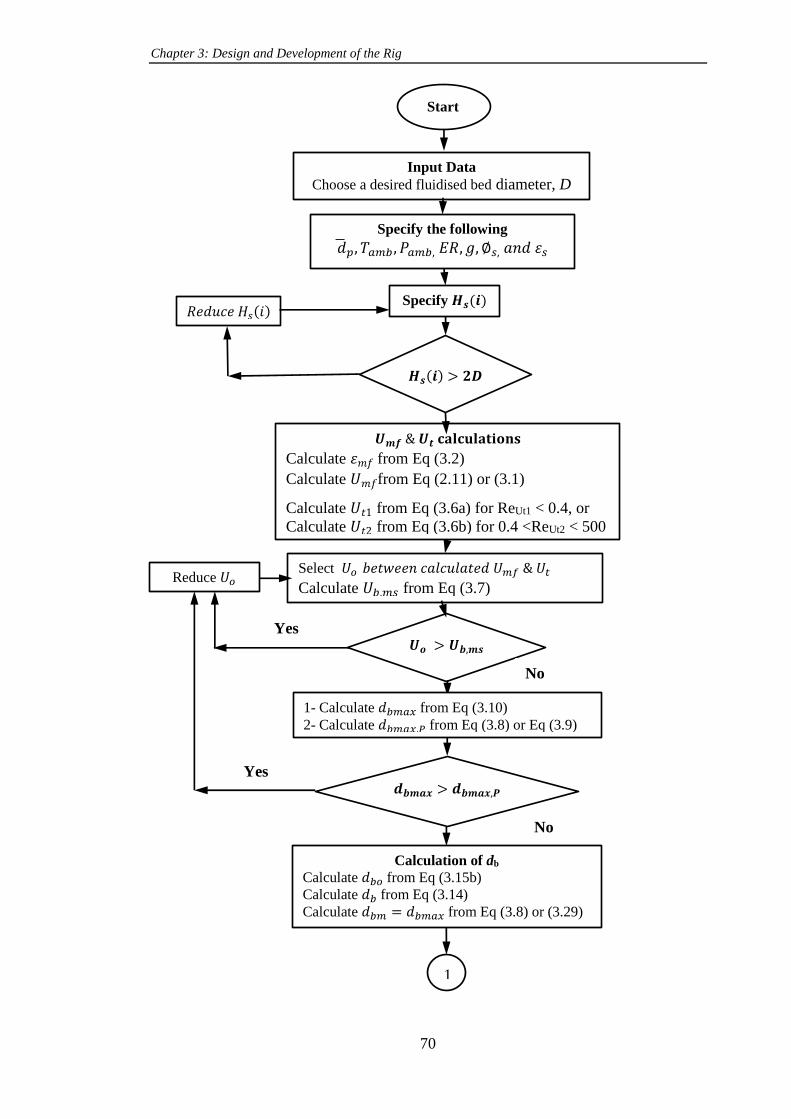
Chapter 3: Design and Development of the Rig
70
Input Data
Choose a desired fluidised bed diameter, D
Specify the following
𝑑 𝑝, 𝑇𝑎𝑚𝑏 , 𝑃𝑎𝑚𝑏, 𝐸𝑅, 𝑔, ∅𝑠, 𝑎𝑛𝑑 휀𝑠
Specify 𝑯𝒔(𝒊)
𝑼𝒎𝒇 & 𝑼𝒕 𝐜𝐚𝐥𝐜𝐮𝐥𝐚𝐭𝐢𝐨𝐧𝐬
Calculate 휀𝑚𝑓 from Eq (3.2)
Calculate 𝑈𝑚𝑓from Eq (2.11) or (3.1)
Calculate 𝑈𝑡1 from Eq (3.6a) for ReUt1 < 0.4, or
Calculate 𝑈𝑡2 from Eq (3.6b) for 0.4 <ReUt2 < 500
𝑅𝑒𝑑𝑢𝑐𝑒 𝐻𝑠(𝑖)
𝑯𝒔(𝒊) > 𝟐𝑫
Select 𝑈𝑜 𝑏𝑒𝑡𝑤𝑒𝑒𝑛 𝑐𝑎𝑙𝑐𝑢𝑙𝑎𝑡𝑒𝑑 𝑈𝑚𝑓 & 𝑈𝑡
Calculate 𝑈𝑏,𝑚𝑠 from Eq (3.7)
𝑼𝒐 > 𝑼𝒃,𝒎𝒔
Reduce 𝑈𝑜
Start
Calculation of db
Calculate 𝑑𝑏𝑜 from Eq (3.15b)
Calculate 𝑑𝑏 from Eq (3.14)
Calculate 𝑑𝑏𝑚 = 𝑑𝑏𝑚𝑎𝑥 from Eq (3.8) or (3.29)
1
1- Calculate 𝑑𝑏𝑚𝑎𝑥 from Eq (3.10)
2- Calculate 𝑑𝑏𝑚𝑎𝑥,𝑃 from Eq (3.8) or Eq (3.9)
𝒅𝒃𝒎𝒂𝒙 > 𝒅𝒃𝒎𝒂𝒙,𝑷
Yes
Yes
No
No

Chapter 3: Design and Development of the Rig
71
Figure 3. 5 Logarithm layout of the gasifier design
Calculate 𝑀𝐴𝐹𝑅𝑠𝑡𝑜𝑖𝑐ℎ𝑖𝑜 from Eq (3.27)
Calculate 𝑀𝐴𝐹𝑅𝑎𝑐𝑡𝑢𝑎𝑙 from Eq (3.26)
Calculate �̇�𝑎𝑖𝑟 from Eq (3.30)
Calculate �̇�𝑎𝑖𝑟 from Eq (3.29)
Calculate �̇�𝑏𝑖𝑜𝑚𝑎𝑠𝑠 from Eq (3.28)
End
Calculation of TDH
From Eq (3.31b) or Eq (3.32) or Eq (3.34)
Calculation of Ws and Hexp
Calculation of 𝜹
1-Calculate 𝑈𝑏 from Eq (3.16)
2-Calculate 𝛿 from Eq (3.17)
1
Specify dorf and tdis
Calculate
Norf, Nden, Ppitch
From Eqs (3.44a), (3.45) and (3.46b),
respectively
Distributor Design Steps
Calculate ɛf from Eq (3.40) or (3.23)
Calculate ∆Pbed from Eq (3.39)
Calculate ∆Pdis from Eq (3.38)
Calculate ∆PTotal from Eq (3.41)
Calculate Cd from Eq (3.43)
Calculation of the Total gasifier Height,
HTotal,g From Eq (3.36)
Biomass Feed Mass Flowrate Calculation
Input ER and biomass fuel Ultimate Analysis:
%C, %H, %O, %S, %N

Chapter 3: Design and Development of the Rig
72
3.3.2 Design Results
Basically, the size of the reactor can be specified by determining the diameter. Also, the
size of many accessories of the gasifier rig and material quantities, reactant and bed
materials, will be affected by the gasifier size, which should be taken into consideration
as well. Therefore, the diameter should be firstly specified. It was needed to be as large
lab-scale as possible to study the gasifier performance as if it was a pilot plant size to
be closer to the industrial performance. Firstly, 15cm reactor diameter was
recommended. A Matlab design calculation program was run out. The first results
showed that 15cm diameter gave a large size indication through the biomass feeding
quantity, which was considered a control parameter for gasifier sizing. Therefore, three
sizes, 15cmm, 11.5cm, 8.3cm were selected to compare their results to choose the
suitable one. According to the input feeding data as shown in Table 3.1, the results were
obtained as follows:
Table 3. 1 Feeding data for gasifier design program for three-selected diameter
Program Feeding (Input) Data Specifications and Values
1- Bed Material Solid silica sand particles
2- Gas Agent Air
2- Solid Fuel Sawdust Pinewood biomass
3- Bed material Particle Size
1-(300-425)µm dp=0.0396cm, 2-(425-500)µm
dp= 0.0478cm, 3-(500-600) dp=0.0546cm
4- Bed Material Static Height Hs, cm 1) 0.5D, 2) 1D, 3) 1.5D, 4) 2D, 5) 3D
5- Operating Temperature, oC Ambient Temperature= 20oC
6- Operating Pressure, atm 1 atm
8- Superficial Air Velocity Uo, cm/sec
From Umf (as minimum value) for 5-6 iteration
with step =5cm/sec.
9- Sand particle sphericity ɸs and sand
static porosity ɛs
0.75 and ɛs can be calculated by particle and bulk
density.
10- Equivalence Ratio ER = 0.2 minimum and = 0.6 maximum
11- Ultimate Analysis of sawdust biomass
fuel
Provided in Chapter 4

Chapter 3: Design and Development of the Rig
73
3.3.2.1 Biomass feed mass flowrate:
From the design results, the mass flow rate of biomass feeding fuel, Fedbio in kg/hr,
was calculated as a minimum value and maximum value for each selected diameter,
8.3cm, 11.5cm and 15cm as shown in Table 3.2 and Figure 3.6. These minimum and
maximum values were calculated according to minimum fluidising air velocity Umf, for
the smallest particle size and maximum ER=0.6, and maximum air velocity, for largest
particle size, and minimum ER=0.2, respectively.
Table 3. 2 Minimum and maximum values of feeding biomass mass flowrate for three selected
values of gasifier diameter.
D, cm Feedbio (min), kg/hr Feedbio (max), kg/hr
8.3 0.22 2.46
11.5 0.42 4.72
15 0.72 8.04
Figure 3. 6 Minimum and maximum values of feeding biomass mass flowrate for three selected
values of gasifier diameter.
From the results, it can be seen that the minimum biomass mass flowrates, 0.22kg/hr
and 2.46 kg/hr are belong to the diameter 8.3cm. For this diameter, these quantities can
be easily provided comparing to other diameters 11.5cm and 15cm.

Chapter 3: Design and Development of the Rig
74
3.3.2.2 Number of orifices (holes) of distributor plate:
From the results of the design calculations, it can be seen that the minimum and
maximum values of the number of holes of the distributor plate Norf was affected by air
superficial velocity, static height of the bed and bed material particle size. For the case
of D=8.3cm and for bed particle size (500-600), Figure 3.7 shows that number of holes
increases when the air velocity increases, whereas it decreases as the bed static height
increases. For other particle sizes, the effect shows similar behaviour. The results show
that there is no effect of ER. The same behaviour was obtained for other diameters.
Figure 3. 7 Effect of superficial air velocity and static bed height on the number of holes for
gasifier diameter D=8.3cm, for bed particle size (500-600) µm
The summary of the results of minimum and maximum values of number of holes for
three diameters, for three particle sizes, for five different static height and for different
velocities are presented in Figure 3.8.
Figure 3. 8 Effect of gasifier diameter on the number of distributor hole. Minimum and
maximum values were selected for each diameter.

Chapter 3: Design and Development of the Rig
75
3.3.2.3 Total height of the gasifier above the distributor plate
The total height of the gasifier HTotal for D= 8.3cm was calculated in meter unit. This
height was calculated for three different equations of TDH. As shown in Table 3.3 the
minimum value was taken at smallest gasifier diameter, 0.5D and at minimum
fluidisation air velocity Umf, whereas the maximum values was taken at 3D and at latest
value of air velocity Uo with step= 5cm/sec. According to Equation (3.31b), the design
calculations showed that HTotal varied only as Uo varied. Whereas for other two
equations HTotal varied with superficial velocity and significantly with static height and
there is no effect of particle size. From the Table, it can be seen that the values of HTotal,
whose were calculated by Equations of TDH (3.34) and (3.32) are more satisfied and
suitable for the lab-scale gasifier.
Table 3. 3 Minimum and maximum values of total height of gasifier for three different TDH
equations for D=8.3cm
Particle Size,
µm (500-600) (425-500) (300-425)
TDH Eq. HTotalmin,
m
HTotal
max, m
HTotalmin,
m
HTotalmax,
m
HTotal min,
m
HTotal max,
m
(3.34) 0.47 1.54 0.47 1.54 0.47 1.54
(3.31b) 5.9 34.8 3.9 29.4 2.2 23.9
(3.32) 0.47 2 0.47 2 0.47 2
3.3.2.4 Effect of the static bed height and diameter of the gasifier diameter on the
minimum fluidisation air velocity
Design calculations showed that the variation of the static bed height Hs and gasifier
diameter D were not affected the minimum fluidisation air velocity for all three selected
particle size of the bed material. From the Figure 3.9a and b, it can be seen that for a
specific bed particle size when the gasifier diameter or static bed height increases the
design parameter Umf stay constant. This is due to the all-theoretical and empirical
equations of Umf calculation have not any effect of Hs and D.

Chapter 3: Design and Development of the Rig
76
a) b)
Figure 3. 9 Effect of a) gasifier diameter D and b) static bed height Hs on the minimum
fluidisation air velocity Umf
3.3.3 Summary of the flexible design and geometry parameters of the gasifier
3.3.3.1 Summary of the main design parameters
According to the required feeding data, which are shown in Table 3.1, and design
results, the range values, minimum and maximum, of the main flexible design
parameters are summarized in Table 3.4.
Table 3. 4 Recommended flexible values of design parameters for gasifier diameter D=8.3cm
Parameters Recommended flexible Range
Minimum value Maximum value
1- Gasifier diameter, D 8.3cm 8.3cm
2- Biomass feed mass rate, Fedbio 0.22 kg/hr 2.46 kg/hr
3- Fluidising agent (Air) flow rate Umf of (300-425)
µm
3-5×Umf of (500-
600)µm
4- Gasification Reaction Temp, T2. * 350oC 900oC
5- Reaction Equivalence Ratio, ER * 0.2 0.6
6- Static bed height, Hs ** 0.5D 2.5D
7- Bed Material Particle Size *** (300-425)µm (500-600)µm
8- Total height of the gasifier 0.47m 2m
9- No of holes of distributor plate ≈ 10 ≈ 100 and more * Suggested values according to gasification operating conditions.
** Suggested range for design purposes.
*** Suggested ranges according to the supply sand and Geldert B Type.
3.3.3.2 Summary of the geometry and dimension of the gasifier parts
To implement gasifier height and geometry flexibility, a gasifier should be divided into
many sections, as columns. According to the sections design, as shown above, the
suggested assembled gasifier unit is shown in Figure 3.10 below. Each section should

Chapter 3: Design and Development of the Rig
77
be had two flanges, upper and lower. These flanges help the researcher to join the
required sections as required. These sections are, starting from the bottom of the gasifier
as follows:
3.3.3.2.1 Air box (plenum) section
This section has a fixed height 30cm and one upper flange. Its bottom is directly
connected to the air supply pipe. This pipe introduce at the center inside the box section
for 20cm. There is 10cm between the open top end of the air supply pipe and distributor
plate. There is a 2.54cm hole diameter at the center of the air-box bottom to collect the
falling materials from the bed through distributor plate. Its geometry drawing and
specifications are presented in section A.2.6 in Appendix A.
3.3.3.2.2 Distributor plate (grate) section
This section is a circular thick metal plate. It has the same outside diameter of the
flanges. It contains a number of orifices (holes), 1.5mm recommended diameter, with a
triangle holes layout. These holes are located within the inside cross-sectional area of
the reactor column to distribute the gas into the bed. Also it contains a same number
and size of the flange holes, 10 mm diameter, which are located in similar distribution
of flange holes. These holes are located outside diameter of the column (pipe) section.
Its geometry drawing and specifications are presented in Section A.2.5 in Appendix A.
3.3.3.2.3 Fluidised bed reaction section
The height of this section depends on the results of the design calculations of the
expansion height of the bed solid material during fluidisation process. Any excess
height for this section can be considered as a part of the freeboard height section. This
section has an upper and bottom flanges which can join from the bottom flange to
plenum and distributor plate sections. In addition, it includes 2-3 holes. Two of them
are used for biomass and bed material feeding point and the third for waste material
outlet point. Its geometry drawing and specifications are presented in Section A.2.4 in
Appendix A.
3.3.3.2.4 Freeboard section
It is a flexible section. This section may consist of one to three different height pieces
depending on the study investigation. Each of them consist two upper and lower flanges.
In addition, for design and research consideration the diameter of this freeboard section

Chapter 3: Design and Development of the Rig
78
can be changed. It includes holes for producer gas outlet, for gas analyzer sample and
for measuring instruments. Its geometry drawing and specifications are presented in
Sections A.2.2 and A.2.3.
3.3.3.2.5 Gas outlet top section
It is an optional section. Its geometry drawing and specifications are presented in
Sections A.2.1.
Figure 3. 10 Schematic of the suggested of the assembled air bubbling fluidised bed gasifier

Chapter 3: Design and Development of the Rig
79
3.4 Summary
In this chapter, a design study and calculations have been conducted for a biomass
bubbling fluidised bed gasifier. The size of the gasifier reactor was suggested to be lab
and pilot scale and to be more flexible and representative of an industrial process for
research purposes.
Hydrodynamic and geometry design equations for a bubbling fluidised bed reactor were
outlined. A Matlab code was built for this purpose. Three values of reactor diameters
were selected to specify the optimum values for this study. One of the design results
was the biomass mass feeding rate, which gives an indication of the size of the reactor
and the required quantities of the biomass for each experiment. By using these design
results, the reactor diameter was specified.
In addition, the design results have shown the effect of the particle size of the bed
material, the static bed height and the number of holes in the distributor plate as a
function of minimum fluidisation velocity. These design effects will thus form a
preliminary database for the fluidisation hydrodynamics in the cold and hot conditions.
Furthermore, according to these results the manufacturing and construction of the parts
of the gasifier unit were conducted.
Chapter 4
Materials and Methods for
Characterization
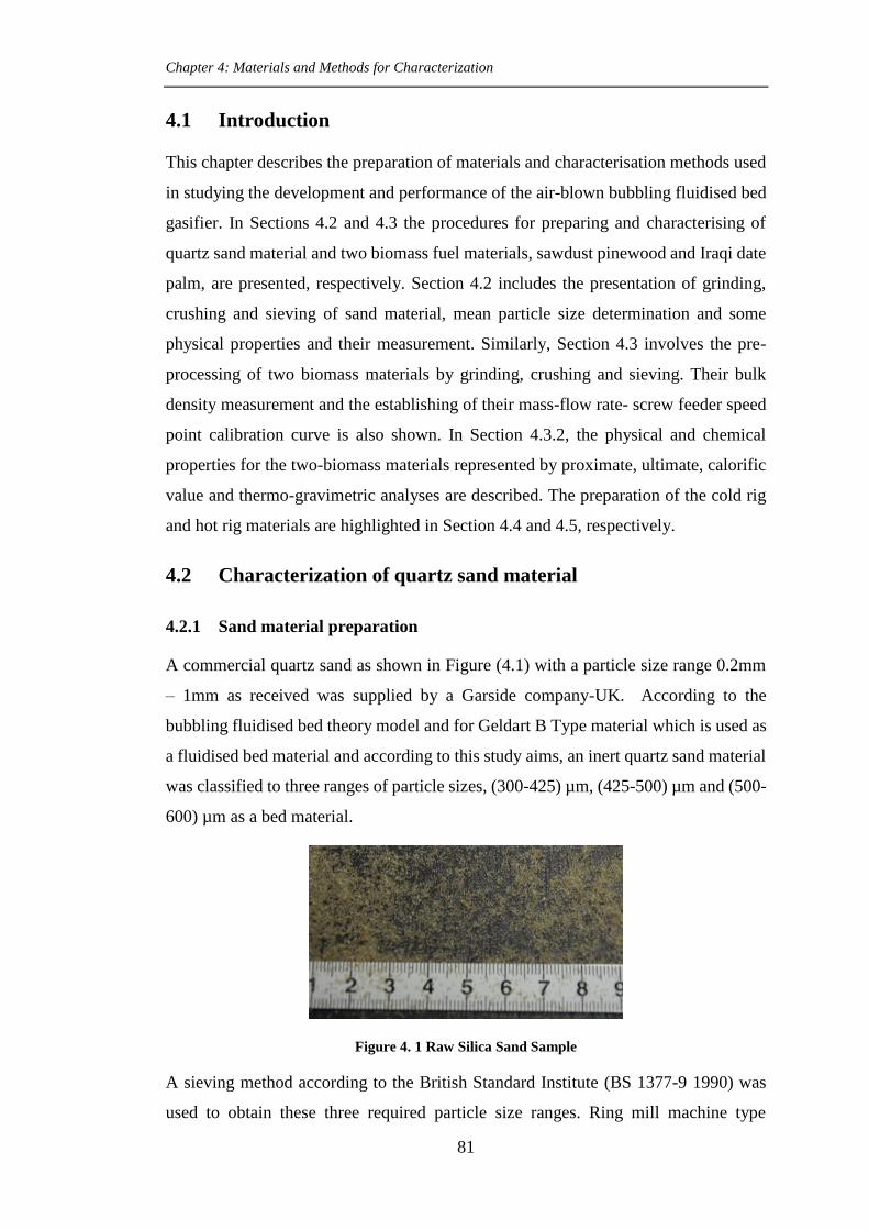
Chapter 4: Materials and Methods for Characterization
81
4.1 Introduction
This chapter describes the preparation of materials and characterisation methods used
in studying the development and performance of the air-blown bubbling fluidised bed
gasifier. In Sections 4.2 and 4.3 the procedures for preparing and characterising of
quartz sand material and two biomass fuel materials, sawdust pinewood and Iraqi date
palm, are presented, respectively. Section 4.2 includes the presentation of grinding,
crushing and sieving of sand material, mean particle size determination and some
physical properties and their measurement. Similarly, Section 4.3 involves the pre-
processing of two biomass materials by grinding, crushing and sieving. Their bulk
density measurement and the establishing of their mass-flow rate- screw feeder speed
point calibration curve is also shown. In Section 4.3.2, the physical and chemical
properties for the two-biomass materials represented by proximate, ultimate, calorific
value and thermo-gravimetric analyses are described. The preparation of the cold rig
and hot rig materials are highlighted in Section 4.4 and 4.5, respectively.
4.2 Characterization of quartz sand material
4.2.1 Sand material preparation
A commercial quartz sand as shown in Figure (4.1) with a particle size range 0.2mm
– 1mm as received was supplied by a Garside company-UK. According to the
bubbling fluidised bed theory model and for Geldart B Type material which is used as
a fluidised bed material and according to this study aims, an inert quartz sand material
was classified to three ranges of particle sizes, (300-425) µm, (425-500) µm and (500-
600) µm as a bed material.
Figure 4. 1 Raw Silica Sand Sample
A sieving method according to the British Standard Institute (BS 1377-9 1990) was
used to obtain these three required particle size ranges. Ring mill machine type

Chapter 4: Materials and Methods for Characterization
82
Labtech-Essa, (model No 100100-Australia) as shown in Figure (4.2) was used to
reduce the sand particle size to get enough quantities of these sand particle size ranges.
This sand was mainly used in cold fluidised rig mode for hydrodynamic studying and
in hot fluidised rig (gasifier) mode for biomass gasification as an inert bed material.
Figure 4. 2 Sand grinding and crushing machine
4.2.1.1 Mean particle diameter
As shown in Chapter 3 particle size diameter of bed material has been considered an
important factor in fluidised bed design calculations. The available standard apparatus
of sieving analysis just give a range of particle size measurement such as: (300-425)
µm, (425-500) µm, (500-600) µm and etc. They do not give a specific mean value as
needed. For this reason each range of above particle size of sand material, a Malvern
particle size analysis was done using a Malvern apparatus – Model – Mastersizer-3000.
It measures particles from 10nm up to 3.5mm. The principle of the measuring of the
particle size distribution in Mastersizer-3000 depends mainly on the laser diffraction
technique. In this technique, a laser beam passes through a dispersed particulate sample
and the angular variation in intensity of the scattered light is measured. The light is
scattered at small angles, relative to the laser beam, by large particles. Whereas it is
scattered at large angles by small particles. By using the Mie theory of light scattering,
this angular scattering data is then analysed to calculate the size of the particles. This
size is then reported as a volume equivalent sphere diameter.

Chapter 4: Materials and Methods for Characterization
83
The Mastersizer is comprised of the main following: Optical unit, one or more
dispersion units, a measurement cell and computer( Mastersizer application software)
(Malvern Instruments n.d.) and (Malvern Instruments 2015).
From the Malvern analysis results, as shown in Appendix (C), a mean particle diameter
for each range was calculated using Equation (4.1)(Basu 2006).
𝒅 𝒑 =𝟏
∑𝒙𝒊𝒅𝒑𝒊
𝒏𝒊=𝟏
(4.1)
�̅�𝑝 =Mean particle diameter.
𝑥𝑖 = Fraction of particle size (i).
𝑑𝑝𝑖 = Diameter of particle size (i).
The calculation procedure was started from the results of the sand Malvern analysis.
As shown in Figure (4.3), for example, it is the result of the sand range (500-600) µm,
which is available in appendix (C). There are two data columns one for particle size
diameter in µm and the second is for its volume percent, which are boarded by a red
line box as shown in Figure (4.3) below. These are represented by dpi and xi in Eq
(4.2), respectively. Then by applying Eq (4.1) the mean particle size for this range of
sand, 𝑑𝑝̅̅ ̅ , will be obtained.
Figure 4. 3 Image of the Malvern analysis results for sand particle size range (500-600) µm

Chapter 4: Materials and Methods for Characterization
84
Equation (4-1) is one of a common method that is used in fluidised bed design for
mean particle size calculation of bed material. The results of the mean particle size of
the three selected ranges are shown in Table (4.1).
Table 4. 1 Mean particle size for three sand particle size ranges
4.2.1.2 Particle density
Particle density is a physical property of powdered and granular material. It is defined
as the mass of particles of material divided to its volume excluding open pores and
closed pores. A supplier company gave this density for supplied sand. As shown in the
design equations in Chapter 3 this property is considered an important design
parameter in hydrodynamic fluidised bed studies.
4.2.1.3 Bulk density
Bulk density is a physical property of powdered and granular material. It is defined as
an apparent powder density, which is the mass of a powder divided by its apparent
volume. The bulk density of silica sand material was measured by following the British
Standard Institute procedure BS EN 1377-9: 1990 (BS 1377-9 1990). As defined, the
bulk density can be affected by many factors, such as, particle size, a procedure that
follows to measure it and external conditions such as vibration and compaction which
should be avoided. Bulk density was used to specify the height of a bed material inside
the column with a specific diameter, where the bed height is a design parameter that
affected the gasifier performance. Practically, it is difficult to achieve the same bulk
density procedure as followed by BSI for material inside the column because of the
long height of the pouring distance due to the long height of the column of the rig
experiment compared to a required procedure in BSI. Also, bulk density is used to
calculate the bed porosity by applying Equation (4.2)

Chapter 4: Materials and Methods for Characterization
85
4.2.1.4 Porosity
Porosity is a property of granular and powdered materials. It is defined as a volume
fraction of voids between particles of a specific volume of the material. It can be
directly related to bulk and particle density as shown in Equation (4.2),
𝑝𝑜𝑟𝑜𝑠𝑖𝑡𝑦 = 휀 = 1 −𝐵𝑢𝑙𝑘 𝐷𝑒𝑛𝑠𝑖𝑡𝑦, 𝜌𝑏
𝑃𝑎𝑟𝑡𝑖𝑐𝑙𝑒 𝐷𝑒𝑛𝑠𝑖𝑡𝑦, 𝜌𝑝 (4.2)
4.2.1.5 Sand bulk density measurement
According to BS 1337-9:1990 (BS 1377-9 1990) the sand bulk density (as received)
was measured for several ranges of sand particle sizes: (220-300) µm, (300-425) µm,
(425-500) µm, (500-600) µm and (600-850) µm by using a sand bulk density
apparatus, which is shown in Figure (4.4). The apparatus consists of two pieces: 1) a
long cylinder with cone called a pouring cylinder, it is shown in Figure 4.4(a), and 2)
a short cylinder with edge at its top, called calibrating container, it is shown in Figure
4.4(b). The internal diameter and height of the calibrating cylinder was measured to
calculate its volume (V) in kg/m3. Its weight (as empty) was measured in kg, (m1). A
quantity of a specific range of particle size of the sand was prepared. The shutter on
the pouring cylinder must be closed prior to fill it with the sand. Thereafter it was
placed on a flat surface of a wide area of a known weight of a clean glass plate. Then
the shutter should be opened to allow sand to run out. When no further flow of sand
takes place inside the cylinder the shutter must be closed and the pouring cylinder
should be carefully removed. The glass plate and the sand (that had filled the cone of
the pouring cylinder) were weighted together. The mass of the sand was calculated.
This measurement was repeated three times. Let this mass be (m2). Finally, after it has
been refilled with sand and its shutter has been kept closed the pouring cylinder was
directly placed and fitted on the top of the calibrating cylindrical container and all were
placed on the glass plate to be sure that all sand was weighed. The shutter was opened
to allow the sand run out to fill both, the calibrating cylinder and the cone space until
there is no further sound of passing sand throughout takes place in the cylinder. Then
the shutter should be closed and subsequently the upper part should be carefully lifted
and removed. Afterwards the glass base, calibrating cylinder and sand cone all were
together weighed, let their mass be (m3). Finally the bulk density of the required sand
was determined by simple calculations. The net mass of the sand inside the calibrating
cylinder m4, in kg will be,

Chapter 4: Materials and Methods for Characterization
86
𝑚4 = 𝑚3 − 𝑚2 − 𝑚1 −𝑚𝑎𝑠𝑠 𝑜𝑓 𝑔𝑙𝑎𝑠𝑠𝑒𝑑 𝑝𝑙𝑎𝑡𝑒 (4.3)
Then the bulk density of the sand will be,
𝑆𝑎𝑛𝑑 𝐵𝑢𝑙𝑘 𝐷𝑛𝑠𝑖𝑡𝑦,𝑘𝑔
𝑚3
= 𝑚𝑎𝑠𝑠 𝑜𝑓 𝑡ℎ𝑒 𝑠𝑎𝑛𝑑 𝑖𝑛𝑠𝑖𝑑𝑒 𝑡ℎ𝑒 𝑐𝑎𝑙𝑖𝑏𝑟𝑎𝑡𝑖𝑛𝑔 𝑐𝑦𝑙𝑖𝑛𝑑𝑒𝑟, 𝑘𝑔
𝑉𝑜𝑙𝑢𝑚𝑒 𝑜𝑓 𝑐𝑎𝑙𝑖𝑏𝑟𝑎𝑡𝑖𝑛𝑔 𝑐𝑦𝑙𝑖𝑛𝑑𝑒𝑟, 𝑚3
= 𝑚4
𝑉 (4.4)
Figure 4. 4 Sand bulk density apparatus: a) Upper piece called pouring cylinder with cone, b)
Lower piece called calibrating cylindrical container
The results of sand bulk density for all particle size ranges are shown in Table (4.2).
Shutter

Chapter 4: Materials and Methods for Characterization
87
Table 4. 2 Values of the sand bulk density for each range of sand particle size
4.3 Characterisation of biomass materials
4.3.1 Sample preparation
4.3.1.1 Iraqi date palms wastes biomass (IDPWB) material
As shown in Chapter 1 – Section 1.4, it can be concluded that these Iraqi date palm
residues can be preliminary considered as one of the varieties of biomass solid fuel
which can be used to obtain a clean gaseous fuel and thereafter it will be one of those
major biomass renewable energy sources. Therefore, these residues were chosen as
one raw material in this study. An Iraqi research centre directory called Project of
Organic Fertilizer Preparation and Mushroom Cultivation Directory / Karbala City–
Iraq, which belongs to the Iraqi Ministry of Agriculture, supplied this biomass. It was
supplied as ground of complete frond with particle size (as length) ranged from 3 to
8cm and from 3 to 6mm (as diameter) as shown in Figure (4.5).
Figure 4. 5A first stage of cutting and grinding of a whole frond of Iraqi date palm (8mm as
received)
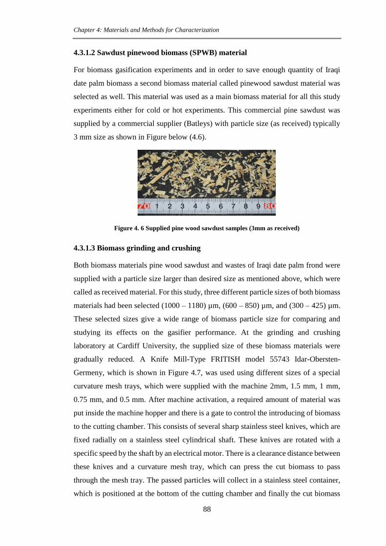
Chapter 4: Materials and Methods for Characterization
88
4.3.1.2 Sawdust pinewood biomass (SPWB) material
For biomass gasification experiments and in order to save enough quantity of Iraqi
date palm biomass a second biomass material called pinewood sawdust material was
selected as well. This material was used as a main biomass material for all this study
experiments either for cold or hot experiments. This commercial pine sawdust was
supplied by a commercial supplier (Batleys) with particle size (as received) typically
3 mm size as shown in Figure below (4.6).
Figure 4. 6 Supplied pine wood sawdust samples (3mm as received)
4.3.1.3 Biomass grinding and crushing
Both biomass materials pine wood sawdust and wastes of Iraqi date palm frond were
supplied with a particle size larger than desired size as mentioned above, which were
called as received material. For this study, three different particle sizes of both biomass
materials had been selected (1000 – 1180) µm, (600 – 850) µm, and (300 – 425) µm.
These selected sizes give a wide range of biomass particle size for comparing and
studying its effects on the gasifier performance. At the grinding and crushing
laboratory at Cardiff University, the supplied size of these biomass materials were
gradually reduced. A Knife Mill-Type FRITISH model 55743 Idar-Obersten-
Germeny, which is shown in Figure 4.7, was used using different sizes of a special
curvature mesh trays, which were supplied with the machine 2mm, 1.5 mm, 1 mm,
0.75 mm, and 0.5 mm. After machine activation, a required amount of material was
put inside the machine hopper and there is a gate to control the introducing of biomass
to the cutting chamber. This consists of several sharp stainless steel knives, which are
fixed radially on a stainless steel cylindrical shaft. These knives are rotated with a
specific speed by the shaft by an electrical motor. There is a clearance distance between
these knives and a curvature mesh tray, which can press the cut biomass to pass
through the mesh tray. The passed particles will collect in a stainless steel container,
which is positioned at the bottom of the cutting chamber and finally the cut biomass

Chapter 4: Materials and Methods for Characterization
89
were packed into a suitable bag to be ready for the sieving step. To get a required
particle size as mentioned above four sizes of curved mesh trays 2mm, 1.5mm, 1mm
and 0.5mm were used to be a first step of sieving stage for the particle size needed.
Following this, the samples were stored in sealed bags.
Figure 4. 7 Grinding and crushing machine for biomass materials
4.3.1.4 Sieving of biomass material
According to the required biomass particle size for this study ground biomass materials
for a certain mesh size was sieved to a desired size using standard sieving trays
available in the soil laboratory. The sieving analysis procedure was followed according
to BSI(Anon 2011b) . The sieve apertures 0.300 mm, 425mm, 500mm, 600 mm, 0.85
mm, 1.18 mm, and 1.5mm were employed in this study. However, for this study the
required biomass particle size are in the ranges (1000-1180) µm, (600 – 850) µm, (300
-425) µm. As shown in Figures 4.8 and 4.9, the shape of the particles of both two
biomass materials takes a longitudinal shape (not spherical) with aspect ratio greater
than 1, assuming cylindrical particle shape. Because of the nature of the biomass
material and the non-spherical particle shape (needle shape especially for these large
particle size ranges), the available Malvern apparatus cannot correctly measures the
mean diameter for each selected range of the particles. In addition, because all the
selected ranges are the minimum range of the available sieve the mean diameter cannot
be calculated by the sieving analysis method.

Chapter 4: Materials and Methods for Characterization
90
300-425 µm (b) 425 – 600 µm (c) 1000-1180 µm
Figure 4. 8 Particle size ranges of Iraqi date palm grinding fronds samples
(a) 300-425 µm (b) 425 – 600 µm (c) 1000-1180 µm
Figure 4. 9 Particle size ranges of sawdust pinewood grinding fronds samples.
4.3.1.5 Biomass bulk density measurement
In this study, biomass bulk density is considered an important parameter for fluidised
bed hydrodynamic calculations. It was measured as received according to BS EN
15103:2009 (British Standards Institution (BSI) 2010). A hollow cylindrical
measuring container within required measurement specifications and within accepted
height-diameter ratio, 1.25 to 1.5, was prepared and weighed. The schematic of the
apparatus is shown in Figure 4.10 below.

Chapter 4: Materials and Methods for Characterization
91
Figure 4. 10 Schematic of the apparatus of the biomass bulk density
For both biomass type, pinewood sawdust and Iraqi date palm, and for three required
particle size for both biomass type (300-425) µm, (600-825) µm and (1000-1180) µm,
the bulk density (as received) was calculated according to the following equation:
𝐵𝐷𝑎𝑟 (𝑎𝑡 𝑀𝑎𝑟) =(𝑚2−𝑚1)
𝑉 (4.5)
Where: 𝐵𝐷𝑎𝑟 Bulk density as received in kg/m3
𝐵𝐷𝑑 Bulk density of the sample mass on dry basis in kg/m3
𝑀𝑎𝑟 The moisture content, as received, as percentage by mass
𝑚1 The mass of the empty container in kg
𝑚2 The mass of the filled container in kg
𝑉 The net volume of the measuring container in m3
The biomass bulk density on dry basis (Dd) can be calculated by Eq. (4.6)
𝐷𝑑 = 𝐷𝑎𝑟 ∗ (100− 𝑀𝑎𝑟)
100 (4.6)
The measuring results of biomass bulk densities, as received, for three particle size
ranges for both biomass types are shown in Table (4.3).
Table 4. 3 Bulk density values (as received) for both biomass materials for each particle size
range

Chapter 4: Materials and Methods for Characterization
92
4.3.1.6 Biomass screw feeder: calibration of biomass mass flow rate
For DDSR-20 model, where details are shown in Section 4.4.6, a calibration curve of
biomass mass flow rate-screw feeder speed setting for two types biomass materials
were obtained. These calibration curves can be used to find the speed setting point of
the screw feeder apparatus that corresponded to a certain value of required biomass
mass flow rate. The biomass mass flow rate value contributes mainly in equivalence
ratio calculation, which is an important parameter in the gasification process. The
procedure of calibration was conducted as follows: Prior to calibration, some required
materials and tools were prepared such as: a medium size of cylindrical metal container
to collect the outlet biomass from screw feeder, stop watch to measure the time
required for a biomass mass at a certain speed point, accurate balance to weigh the
collected biomass and enough quantity of a particular particle size for both types of
biomass materials. The calibration procedure is as follows: 1) Suitable quantity of
biomass was poured in the screw feeder hopper. It should be a small quantity especially
at low speed to avoid stopping of the drive motor due to the biomass quantity. 2)
Switch on the screw feeder apparatus to run the motor to allow a biomass to fill the
clearance spaces inside the arm, a pipe of the twin- screw rod feeder, which are driven
by the electric motor, to ensure a correct measuring of time. 3) An empty cylindrical
container, which was previously weighed let it be m1, was directly placed underneath
the outlet of the screw pipe to ensure that all biomass particles were collected inside.
4) For the first starting of the calibration process the speed point setting was firstly set
at each 0.5 increment, where the speed setting scale is divided up to 10 increment,
starting from 0 to 10. 5). From the screw feeder control panel the screw feeder motor
was switched on and at the same time, the stopwatch was immediately run. 6) For 1
minute running time the drive motor was switched off, let this time be t1 in min. 7) The
container with collected biomass were weighted, let it be m2 in gm. 8) The above
procedure was repeated for next speed increment of, 0.5, 1, 1.5, 2, 2.5, 3,……….., 9.5,
10. Finally, the mass flow rate for both biomass materials were calculated as following:
𝐵𝑖𝑜𝑚𝑎𝑠𝑠 𝑚𝑎𝑠𝑠 𝑓𝑙𝑜𝑤 𝑟𝑎𝑡𝑒 𝑖𝑛 𝑔𝑚 𝑚𝑖𝑛⁄ = 𝑚𝑏𝑖𝑜̇ = 𝑚2− 𝑚1
𝑡1 (4.7)
These values were drawn to obtain a standard calibration curve for each biomass
material as shown in Figure (4.11a & b). From these calibration curves at required
biomass mass flow rate the screw feeder speed can be set.
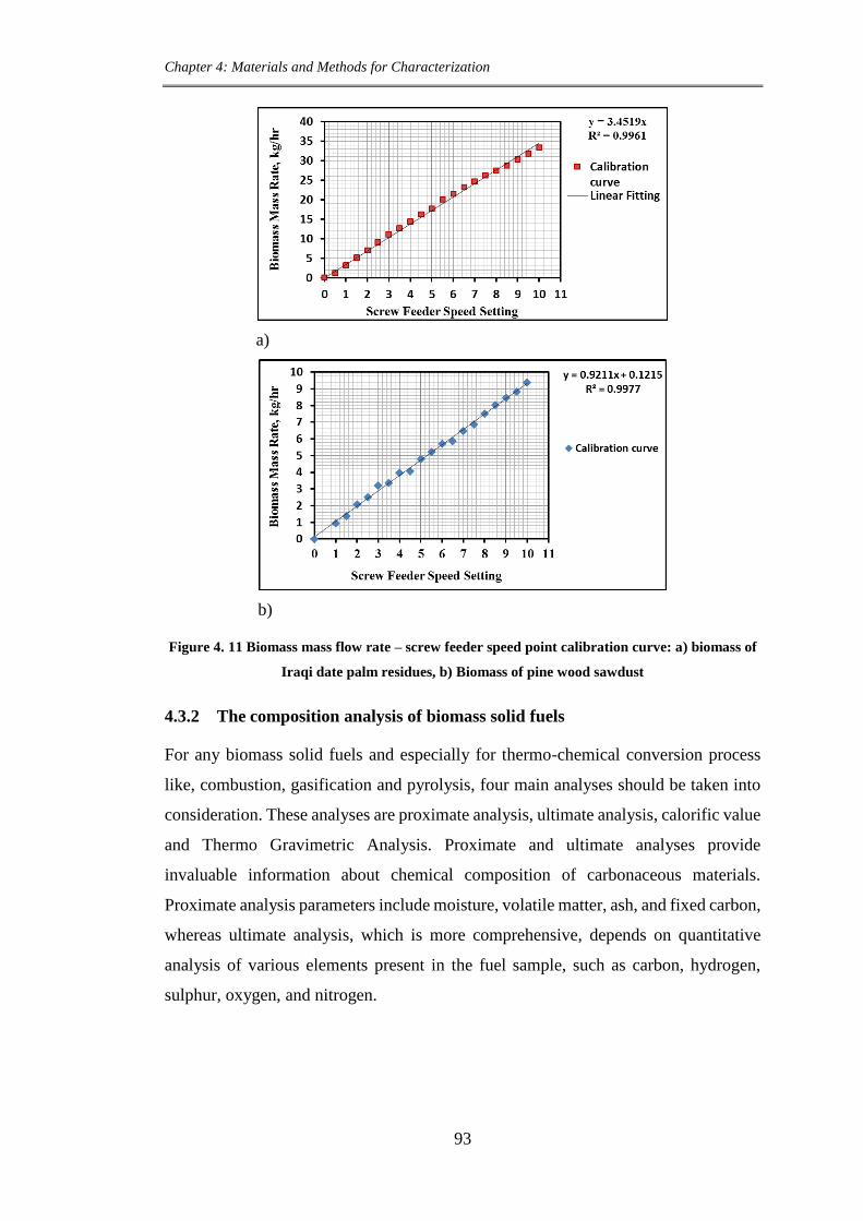
Chapter 4: Materials and Methods for Characterization
93
a)
b)
Figure 4. 11 Biomass mass flow rate – screw feeder speed point calibration curve: a) biomass of
Iraqi date palm residues, b) Biomass of pine wood sawdust
4.3.2 The composition analysis of biomass solid fuels
For any biomass solid fuels and especially for thermo-chemical conversion process
like, combustion, gasification and pyrolysis, four main analyses should be taken into
consideration. These analyses are proximate analysis, ultimate analysis, calorific value
and Thermo Gravimetric Analysis. Proximate and ultimate analyses provide
invaluable information about chemical composition of carbonaceous materials.
Proximate analysis parameters include moisture, volatile matter, ash, and fixed carbon,
whereas ultimate analysis, which is more comprehensive, depends on quantitative
analysis of various elements present in the fuel sample, such as carbon, hydrogen,
sulphur, oxygen, and nitrogen.

Chapter 4: Materials and Methods for Characterization
94
4.3.2.1 Proximate analysis
In this analysis, contents of moisture, volatile material, ashes and fixed carbon are
determined which represent the properties of a specific fuel material. These properties
are important to assess the characteristics of any fuel during thermo - chemical
conversion processes and thereby their effects on reactor design. The methods used to
estimate these contents were explained as shown below:
4.3.2.1.1 Moisture content
The moisture content in the biomass was determined according BSI (En 14774-1
2009). The analysis was conducted in triplicate to monitor the repeatability between
the test samples. Three ceramic dishes with lids were pre-conditioned, to remove
moisture, by heating at 105oC for 2 hours in a drying oven and then cooled to room
temperature in a desiccator. After cooling, the dishes and their lids were weighed to
nearest 0.1 mg. After weighing the dishes, a minimum fuel sample of 1 g was weighed
to nearest 0.1 mg and spread evenly over the respective dishes and heated in the drying
oven at 105oC for 2 hours. Before removing the samples from the oven, the lids were
replaced and the assemblies transferred to the desiccator for cooling to room
temperature. The moisture content (MC) expressed in percentage was calculated
according to Equation (4.8).
𝑀𝐶 % = [ 𝑚2−𝑚3
𝑚2− 𝑚1 ] ∗ 100 (4.8)
Where:
𝑚1 = The mass of the empty ceramic dish and lid.
𝑚2 = The mass of the ceramic dish and lid and biomass fuel before heating.
𝑚3 = The mass of the ceramic dish, lid and residue after heating.
4.3.2.1.2 Ash content
Ash content is the measure of mass of the inorganic matter left after ignition of a fuel
under BSI (Technical committee CEN/TC 2005). The analysis was carried out in
triplicate to monitor the repeatability between the test samples. Prior to combustion of
the fuel samples, three empty ceramic dishes were preconditioned in the muffle
furnace to remove volatile matter by heating to 550oC for 2 hours. After conditioning,
the dishes were cooled to room temperature in a desiccator and weighed.

Chapter 4: Materials and Methods for Characterization
95
Approximately 1 g of dried solid biomass fuel sample weighed to the nearest 0.1 mg
was spread over each dish and then heated in the furnace at 550oC for 2 hours to ensure
complete combustion. The dishes with residues were then transferred to the desiccator,
cooled to room temperature and weighed. The ash content (AC) on dry basis was
calculated using Equation (4.9).
𝐴𝐶 % = [ 𝑚2−𝑚3
𝑚2− 𝑚1 ] ∗ 100 ∗
100
100−𝑀𝐶 (4.9)
Where:
𝑚1 = Mass of the empty ceramic dish and lid.
𝑚2 = Mass of the ceramic dish and lid and biomass fuel before heating.
𝑚2 = Mass of the ceramic dish and lid and biomass fuel after heating.
MC = Mass fraction of the moisture of the general analysis of the solid biomass sample
on wet basis, as percent.
4.3.2.1.3 Volatile matter content
Volatile matter expresses the mass of the material loss, deducting that due to moisture,
when a test sample is subjected to heat in the absence of air under specific conditions.
Volatile matter normally consists of various hydrocarbons, which affect burning
characteristics of the solid carbonaceous fuel such as biomass. In this study, the
volatile matter was determined according to BSI (CEN (European Comitte for
Standardisation) 2009) standard procedure. Three fused silica crucibles with lids were
preconditioned to remove volatiles by heating at 900oC for seven minutes and then
were cooled to room temperature in the desiccator. When cool, the crucibles with lids
were weighed to the nearest 0.1 mg. Minimum sample of 1 g was spread evenly over
the respective crucibles and then heated in a muffle furnace at 900oC for 7 min. After
this time, the crucibles with residue were cooled in desiccator to room temperature and
then were weighed. The net weight loss of the material was determined by subtracting
the loss due to moisture content. The volatile matter (VM) content on dry basis was
calculated using Equation (4.10). The analysis was carried out in triplicate to monitor
the repeatability between the test samples.
𝑉𝑀 % = [ 𝑚2−𝑚3
𝑚2− 𝑚1 ] ∗ 100 − 𝑀𝑤 ∗
100
100−𝑀𝑎𝑑 (4.10)
Where:
𝑚1 = The mass of the empty ceramic dish and lid.
𝑚2 = The mass of the ceramic dish and lid and biomass fuel before heating.

Chapter 4: Materials and Methods for Characterization
96
𝑚3 = The mass of the ceramic dish, lid and residue after heating.
𝑀𝑤 = The mass fraction of moisture in the solid biomass sample as a percentage.
𝑀𝑎𝑑= The mass fraction of moisture of the general analysis sample on wet basis
(ad means as analysed) as a percentage = MC.
4.3.2.1.4 Fixed carbon content
Fixed carbon (FC) is the solid of combustible residue that remains after any heated,
gasified or pyrolysed, solid or liquid fuel, where all the volatile matters are released
and ash is excluded. The fixed-carbon content of any solid fuel is determined by
difference by deducting the percentages of moisture, volatile matters, and ash from a
solid biomass sample as shown in Equation (4.11). Since gas-solid combustion
reactions are slower than gas-gas reactions, a high fixed-carbon content indicates that
the coal will require high temperature and long time to react. So that increased fixed
carbon content in the feedstock can reduce the rate of the fuel conversion in the gasifier
reactor.
𝐹𝐶 % = 100 − [𝑀𝑜𝑖𝑠𝑡𝑢𝑟𝑒 𝑐𝑜𝑛𝑡𝑒𝑛𝑡 % − 𝑉𝑜𝑙𝑡𝑖𝑙𝑒 𝑚𝑎𝑡𝑡𝑒𝑟 % − 𝐴𝑠ℎ 𝑐𝑜𝑛𝑡𝑒𝑛𝑡 %]
(4.11)
4.3.2.2 Calorific value
Caloric value is the most important characteristic of any fuel, gas, liquid and solid. It
is the amount of energy in MJ generated from combustion of a unit mass in (kg for
solid fuel) or volume in (m3 for liquid and Nm3 for gas fuel) of fuel by oxygen.
Calorific value is expressed as a gross (Higher) calorific value (HHV) or lower
calorific value (LHV). The former gives the total energy released when water in the
combustion products is in liquid state and the latter, vapour. The principle of the work
of the bomb calorimeter basically depends on the heat of the combustion that is created
by a sample of a solid fuel which is burned under an oxygen rich atmosphere in a
closed pressure vessel called (bomb) under controlled conditions. This vessel is
surrounded by water jacket, which absorbs the energy released by the sample
combustion and the resulting temperature change within the absorbing medium is
observed. Thereby the heat of combustion is then calculated.
In this work, a computerised bomb calorimeter, Parr 6100, Figure (4-12) from Parr
Instrument Company was used to determine the gross heating value of the biomass
feedstock according to BSI (BS DD CEN/TS 14918 2005) standard procedure. Prior

Chapter 4: Materials and Methods for Characterization
97
to analysis, three certified benzoic acid pellets calibrated the bomb calorimeter. After
calibration was completed, 1 g of biomass material was analysed in the bomb by
following the procedure steps according to the operation manual of 6100 Parr
instrument (Parr instrument company n.d.). The test will automatically proceed
through the following steps: Pre-period cycle, Fire the sample and Post-period cycle.
Once the calorimeter analysing is finished with the post-period cycle the results will
print out on the printer or display on the touch screen. This analysis was done in
triplicate to monitor the repeatability between the fuel samples. The net calorific value
was determined by using Equation (4.12) specified in (Aenor, 2005).
𝑞𝑤𝑣,𝑛𝑒𝑡,𝑚 = { 𝑞𝑣,𝑔𝑟,𝑑 − 206𝑊𝐻,𝑑 } ∗ ( 1 − 0.01𝑀𝑇) − 23.05𝑀𝑇 (4.12)
Where 𝑞𝑣,𝑔𝑟,𝑑 = Gross calorific value at constant volume in J/g.
𝑊𝐻,𝑑 = Hydrogen content (wt %), of the moisture-free (dry) fuel, respectively.
𝑀𝑇 = The total moisture content (wt %).
Figure 4. 12 Bomb calorimeter, Parr 6100
4.3.2.3 Ultimate analysis
Determination of the elemental composition of a fuel is called an ultimate analysis. It
depends on quantitative analysis of various elements present in the fuel sample. Most
commonly, carbon, hydrogen, nitrogen, sulphur and oxygen (CHNSO) are measured
in a particular fuel through complete combustion. These elements are important in
calculating the chemical formula of the solid or liquid fuel and determining an
appropriate stoichiometric air or O2-fuel ratio for the combustion or gasification
process as well. Additionally, any catalyst activity depends on the concentration of
poisoning elements in the feed an example of which is sulphur. In this study, the same
type of the sawdust pinewood biomass SPWB, which was used by previous PhD study,

Chapter 4: Materials and Methods for Characterization
98
was also used. The ultimate analysis for this biomass was taken from it(Legonda
2012). For checking test, the carbon and sulphur composition for this material were
reanalysed in (LECO) analyser model SC-144DR, which is shown in Figure 4.13. It is
a software-controlled instrument designed to determine the carbon and sulphur
content. This analyser principally works on the flow of the combustion gases through
the two infrared detection cells. One cell is carbon IR to measure the concentration of
CO2 gas and the second cell is sulphur cell to measure the concentration of SO2 gas.
The instrument converts these concentrations to percentage value using an equation
pre-set in the software(LECO 2008). For Iraqi date palm biomass IDPWB material,
Minton Treharne & Davies LTD Company, UK, did the ultimate analysis.
Figure 4. 13 LECO Carbon-Sulfure analyser, model SC-144DR
The results of proximate, ultimate and calorific analyses of two biomass materials,
pinewood biomass and Iraqi date palm wastes biomass materials are presented in Table
4.4. Carbon content of char + sand mixture, a residues solid materials after each
biomass gasification experiment, was measured according to BSI – BS EN 15104:
2011 (Anon 2011a) using LECO analyser.

Chapter 4: Materials and Methods for Characterization
99
Table 4. 4 Proximate and ultimate analyses for sawdust pinewood and Iraqi date palm wastes
biomass materials as received (ar) basis
4.3.2.4 Thermo gravimetric analysis (TGA)
Thermogravimetry is a standard method to analyse organic, inorganic and synthetic
materials. This analysis includes heating a weighted test sample on a highly sensitive
microbalance, which is exposed to a controlled temperature system in a controlled
environment according to BS EN ISO 11358:1997 (British Standards Institution (BSI)
2014). The TGA analysis for the two-biomass materials was conducted using a Mettler
Toledo TGA Series, model-TGA/DSC 3+ as shown in Figure 4.14. In this study, 11mg
of each biomass was weighed by a precision balance to the nearest 0.01mg and heated
from 35oCto 900oC. Two test were performed, first by air and the second by N2 at a
flowrate of 50ml/min and heating rate 10oC/min. Mass loss with temperature profiles
were recorded for each second using STARe Thermal Analysis software.

Chapter 4: Materials and Methods for Characterization
100
Figure 4. 14 Thermogravimetric analyser (Mettler Toledo TGA Series, TGA/DSC 3+)
A thermogavimetric analysis of two biomass materials, SPWB and IDPWB using air
and N2 were conducted. Their thermal behaviours are presented in Figure 4.15 (a) and
(b), respectively. From the two Figures, it can be seen that there are three distinct
phases. The first mass loss phase is due to moisture evaporation at a temperature less
than 105oC followed by a large mass loss of volatile materials between 200-375oC,.
The third phase of mass loss of volatiles takes place between 350oC and 425oC when
air was used and between 375oC and 880oC when N2 was used. Furthermore, for this
phase the increase of mass loss was sharply for the former and slightly for the later. In
addition, for both biomass the trend of air and N2 within the first and second phase are
identical whereas for the third phase N2 and air are approximately diverged at 400oC.
Also, it can be seen that the mass loss for SPWB is larger than IDPWB for both gases.
Overall, it can be concluded that for gasification process, which locates between
pyrolysis and combustion, these two biomass can be gasified between 350 and 900o C
a) SPWB

Chapter 4: Materials and Methods for Characterization
101
b) IDPWB
Figure 4.15 Thermogravimetric behaviour of the two-biomass materials using air and N2: a) For
SPWB and b) For IDPWB
4.4 Cold rig prepared materials
In order to study the hydrodynamic design parameters of the bubbling fluidised bed
reactor experimentally a cold rig fluidised bed was built, constructed and assembled
as shown in Figure 4.16 and also presented in Chapter 5.
Figure 4.16 Assembled cold rig for fluidised bed column
The prepared materials, which were used in cold rig, are as follow:
4.4.1 Fluidised bed cold column (transparent pipe)
For cold rig experiments, a transparency acrylic pipe was used. As shown in Figure
4.17 (a) and (b), two models of pipe were used as a fluidised bed column to perform

Chapter 4: Materials and Methods for Characterization
102
the cold rig hydrodynamic experiments. The first model (a) is a conventional case,
which was mainly used for all experiments Whereas the second model (b) was
assembled with the intake point hole of the screw feeder by a small unit, which was
fixed directly on the outside of the acrylic pipe at a point 4.2cm above the distributer
plate. This was to show the movement and dispersion of biomass particles inside bed
material when the feeding point is located at the position near the distributer plate or
within the bed height area. This model exactly represents the actual case for a hot rig
gasification experiments. The former model was drilled with several holes for pressure
negative side tube tapping. In addition, one side of this pipe was tightly introduced
inside a plastic flange, which has a same specification of metal flange, until both edges
pipe and bottom flange surface were levelled. The second end of this pipe was left free.
Then this assembled plastic pipe-flange unit was tied with the distributor plate and air-
box pipe section by flanges with metal screws to compose the fluidised bed cold rig.
For the second model the plastic pipe was joined with a metal flange for both ends by
a metal screw rod, thereafter this assembled pipe will be ready to join directly with the
distributor plate and air flow-box pipe section. The dimensions of this acrylic pipe:
height does not exceed 1m length to give a good using flexibility of bed height and
expansion height through fluidisation experiments. Its internal diameter and thickness
are the same for metal type, 83mm and 3mm, respectively. Two metric measuring
rulers were putted down on the external pipe wall. They were used to measure the bed
material height at static bed and during fluidisation conditions for various air flowrates.

Chapter 4: Materials and Methods for Characterization
103
Figure 4. 17 Acrylic transparent column for fluidised bed cold rig, (a) a conventional column,
(b) a column assembled with the intake unit of screw feeder, c) screw feeder intake unit.
4.4.2 Air flow-box pipe section
According to the design steps (chapter 3) and dimension, the air box was manufactured
with the same specifications of the reactor pipe section. This type of pipe was supplied
by CG Rees Supplier Company-UK with the following specification, 316L stainless
steel, nominal pipe size 3” for 10S Schedule (outside diameter 88.9 mm, inside
diameter 82.8 mm and 3.05 mm thickness). For the section of the air box 300mm of
this pipe type was used. Its open upper side was welded with 6 mm thickness of the
standard flange and the bottom side was welded with a concave shape of stainless steel
material. This bottom side was drilled with two holes. One of them was connected to
the 300mm length of 1” diameter of stainless steel pipe to collect and evacuate the bed
and residue solid material (char and ash) of gasification process which may drop down
through the perforated plate into the air-box. The other end of this pipe is plugged
during gasification test. The second hole was used to introduce a 200mm length and
1” diameter stainless steel air flow pipe inside the air box pipe with slight curvature to
take a coaxial centre with the air box pipe to allow oxidant gas flow towards the
distributor plate. 100 mm length was left free between the top end of the introduced
pipe and the upper side of the air box pipe to ensure a good dispersion of air across the
distributer plate and subsequently across the fluidised bed material column. This air
box section is shown in Figure 4.18 below. For the same purpose, this air box was
employed for both cold rig and hot rig experiments. 100mm below the upper open end
of air-box pipe a hole was drilled across the pipe wall for positive pressure side taping
for gas flow pressure drop measuring across the distributor plate and bed material.
1500 mm length of a stainless steel 1” pipe was used to join the feed source of
compressed air supply to the air-box section pipe via inlet gas flow pipe as shown in
Figure 4.1. This pipe will give a steady air flow through the air box. For the hot rig
this pipe was introduced inside the air preheater furnace for air heating.

Chapter 4: Materials and Methods for Characterization
104
Figure 4. 18 Air-Box section pipe for both cold and hot rig.
4.4.3 Stainless steel flanges
10 open flanges of 6mm thickness, 169 mm external diameter and 89 mm internal
diameter (for open side which is equal to the external diameter of the all gasifier pipe-
sections) as shown in Figure 4.19 were provided. These flanges were made of 316L
stainless steel metal and supplied by Cross Engineering Swansea LTD Company-UK.
These flanges were mainly used for gasifier pipe sections connection, where they were
welded with the all ends of pipe sections. These welding pipe section-flange can be
joined each other throughout the holes of flange by screws to build the completely cold
rig fluidised bed column or gasifier column in the hot rig.
Figure 4.19 Stainless steel type-316L flange
4.4.4 Perforated Distributor Plate
Cross Engineering Swansea LTD Company-UK provided a number of 6mm thickness
circular solid 316L stainless steel metal plates. These plates have the same flange

Chapter 4: Materials and Methods for Characterization
105
specifications in, metal type, external diameter, number of joining holes and their
diameter and position as the rig flanges. These plates were used as a perforated
distributor plates to distribute the fluidising gas uniformly through the bed material.
According to design calculations and for studying the hydrodynamic effects of the
distributor plates open area on the gasifier performance, four plates were prepared by
drilling them with 1.5mm diameter holes for different number of holes 19, 55, 85,169,
which represent three different open area. As explained in Chapter 3 these holes were
arranged with a triangular shape for a specific pitch and located within the inner cross-
sectional area of the gasifier pipe, 83mm inside diameter. For each plate, the lengths
of pitch, which represents the distance between any two neighbour centre points of the
holes are 19, 11.78 9.8 and 5.94mm, respectively. Therefore, the subsequent open area
for each distributor plate is, 33.6, 97.1, 150, and 298mm2, respectively. All distributor
plates were signed with a specific formula, which was taken the form, dor1.5mm-N19-
P19, dor1.5mm–N55-P11.78, dor1.5mm-N85-P9.8 and dor1.5mm-N169-P5.94,
respectively, as shown in Figure 4.20.
Figure 4. 20 Perfórate distributor plate: a) dor1.5mm-N169-P5.94, b) dor1.5mm-N85-P9.8, c)
dor1.5mm-N55-P11.75, d) dor1.5mm-N19-P19. The formula symbols dor-N-P represent dor the
hole diameter in mm, N the number of holes and P the pitch distance in mm, respectively.
4.4.5 Air flow measurements
In order to measure a wide range and an accurate gas flow rate inside the fluidised bed
column, two measurement apparatus rotameters were used. One of them (small scale)
was used for air volumetric flow rates ranging from 0.0 to 50 litre/min whereas the
second (medium scale) and was used for air flow rates ranged from 30 litre/min to 300
litre/min. These two flow meters were connected in such a way that can read separately
as it was needed.

Chapter 4: Materials and Methods for Characterization
106
4.4.6 Air pressure regulator control
For prevention and safety, an air pressure regulator was directly installed after air
intake point to maintain and control the pressure inside flowmeters within accepted
safety limitations. In addition, this regulator can be used to supply enough pressure to
be capable of setting a required airflow rates especially at high-required airflow rates.
This regulator is equipped with a control valve, to regulate air pressure thereafter its
flow rate, and pressure gauge, in bar and psi units, to read air pressure as shown in
Figure (4.16).
4.4.7 Pressure drop device (Manometer)
As shown in Figure (4.21) a digital manometer, model-P200 H, for pressure drop
measurement, which Digitron Company made, had been used. This device measured
the pressure difference between two points across perforated distributer plate plus
fluidised bed column in mbar units and a pressure drop across distributer plate only.
The first point (positive point,) is directly located 100mm underneath the perforated
distributer plate in the air-box pipe section and this will join to the positive point (red
tube) of the manometer. The second point (negative point), represented by multi
points, is located in the fluidised bed transparency column above the distributor plate
and this will join to the negative point of the manometer. The manometer operates
with 3.5-volt battery. The maximum operating temperature is 50oC.
Figure 4. 21 Digital manometer

Chapter 4: Materials and Methods for Characterization
107
4.5 Hot rig prepared materials
4.5.1 The pipe of fluidised bed reaction section
1000mm of 316L stainless steel pipe with the same nominal size of air box pipe
section, as mentioned in Section 4.4.2 was prepared. Two flanges were welded at the
bottom and upper ends of the pipe as shown in Figure 4.22. The former is used to
connect together with the assembled air box section pipe and distributer perforated
plate via the air box flange. The latter flange is used to connect with any additional
required part of free board section. For high temperature conditions a gasket insulated
material 5 mm thickness was used between each pair of flanges and between the
distributor plate and flanges. This reaction section includes three zones, bed material
zone (250-300mm length), splash zone (50-100mm length), and the rest covers the
freeboard zone. Four tapping holes for thermocouples starting from the bottom base
above distributer plate at 45 mm, 445 mm, 845 mm and 1245 mm to read the
temperature at the centre of the inside pipe, T2, T1, T3 and T7, respectively. Additional
two holes were used for product gas analyser sample stream at place near
thermocouple point of T3 and T4. Another 1”diameter hole is used for pouring a
fluidised bed material through a small piece of 1” diameter pipe, which was welded to
the main pipe surface. This hole is approximately located at 850 mm from the
perforated plate. Two large holes were drilled at the bottom of the pipe. The first one
takes the same shape as the front view shape of the arm of the biomass screw feeder.
The shape and dimension of front section of this hole is shown in Figure 4.23 (a) and
(b). This hole is used as a feeding point for biomass solid fuel material and the centre
of this hole is located at 42 mm above the distributer plate. To install and hold a
biomass screw feeder arm at this hole, a unit constructed from steel was welded to the
outer surface wall of the gasifier pipe reaction section at the position of the biomass
feeding hole. This unit was made from steel for the gasifier pipe for the hot rig and
from transparent acrylic for the cold rig as explained in section 4.4.1. The last hole, 1”
diameter, was made as near as possible the upper surface of the distributor plate. At
this hole, one end of a short piece, 50 mm of 1” diameter stainless steel pipe was
welded to the reaction section pipe wall of the gasifier, whereas a suitable screw nut
can plug the second end. This hole enables the operator to remove and evacuate the

Chapter 4: Materials and Methods for Characterization
108
bed material, sand, and all the solid gasification products, ash and char, at the end of
each gasification experiment using a vacuum cleaner.
Figure 4.22 Pipe reaction section
Figure 4. 23 Dimension of the biomass house - hold unit feeding hole: a) For longitudinal
measure and b) For width measure
4.5.2 Freeboard pipe section- second part
A 300 and 700 mm length of the same pipe specifications of previous sections was
prepared to construct the second part of freeboard reactions section. This pipe is a
complementary section to the first part free board, which was included in the pipe of
the bed reaction section. Similarly, these freeboard pipe sections were also welded
with two flanges at the upper and bottom pipe ends as shown in Figure 4.22. The
former end was opened to the atmosphere to the extraction ventilation system and the
latter end was connected to the upper flange end of the bed reactions pipe section. Two
holes were drilled in this section first one for product gas analysing, 100mm below the
upper pipe end and the second hole for thermocouple installing at a position 1245 mm
above distributor plate to measure T7.

Chapter 4: Materials and Methods for Characterization
109
4.6 Summary
This chapter has shown the materials and methods used in characterising the bed
material sand and two solid fuel biomasses, sawdust pinewood SPWB and Iraqi date
palm IDPWB. According to a range of standard methods, these materials were
characterised. Grinding machines were used for sand and biomass size reduction. In
addition, their bulk densities were also measured. To calculate the mean particle size
of the sand material for each range, a Malvern analyser was used.
Characterization of two biomass fuels involved proximate and ultimate analysis as
well as thermogavimetric analysis. Ultimate analysis was useful for the fuels to
quantify the combusting elements and then determine MAFR at stoichiometric
conditions and thereby the equivalence ratio. Proximate analysis was used to quantify
the reaction characteristics of the biomasses. In addition, thermogravimetric analysis
was used to show the weight loss of the fuel material at specific working conditions as
a function of temperature and time. Finally, a total carbon analyser was used to
measure the carbon content of biomass fuel and char + sand mixture, i.e. the residue
of biomass gasification fluidised bed.
To construct the cold and hot rigs the materials and components of each rig were
prepared such as the air-box section, distributor plates, flanges, transparent pipe for
the cold fluidising column and stainless steel pipe for the reactor and freeboard
sections of the hot rig.

Chapter 5
Cold and Hot Rig: Construction,
Hydrodynamic and Gasification
Experiment Set-Up

Chapter 5: Cold and Hot Rig: Construction, Hydrodynamic and Gasification Experiment Set-Up
111
5.1 Introduction
This chapter describes the building and construction of the experimental-rig for both,
cold and hot operation. In Sections 5.2 and 5.6, all equipment and instruments used
during cold and hot (gasification experiments) rigs are presented and described. In
Sections 5.3 and 5.7 the procedures for preparation and operation for two rigs, cold
and hot are outlined in details, respectively. Moreover, safety steps are highlighted,
especially for gasification trials because of its hazardous products. Commissioning
trials to test the temperature distribution limitations along the gasifier and
commissioning trials for biomass gasification by bubbling fluidised bed are detailed
in Sections 5.7.1 and 5.7.3, respectively. For gasification trials, testing parameters and
experiments plan design in tables and flow chart form are presented in Section 5.5.
Sections 5.4 and 5.8 highlight the experimental data measurements for specific
parameters in cold and hot rigs, respectively. Procedures in measuring and
determining the design parameters and gasifier performance are included in these
sections.
5.2 Cold experiment rig hardware
A schematic layout and the experimental test of the cold rig fluidised bed used in this
study are shown in Figure 5.1 and Figure 5.2, respectively. The rig mainly consists of
an air pressure regulator, two rotameters, to feed a required air flow rate to the fluidised
bed column. The digital manometer was used to measure the pressure drop across the
fluidised bed column. The cold rig also included standard fittings to give connection
between components using either 316 stainless steel pipes or PVC tubes.

Chapter 5: Cold and Hot Rig: Construction, Hydrodynamic and Gasification Experiment Set-Up
112
Figure 5. 1 Schematic layout of cold rig fluidised bed column
Figure 5. 2 Experimental test cold-rig for hydrodynamic bubbling fluidisation studies
5.2.1 Feed air pressure regulator
Compressed air was supplied by a pipeline to the laboratory where the cold rig was
installed. This air was used as a gas phase for the hydrodynamic experiments in the
cold rig and as a gasifying agent for hot rig air gasification experiments. To avoid

Chapter 5: Cold and Hot Rig: Construction, Hydrodynamic and Gasification Experiment Set-Up
113
rotameter damage due to high pressure of air supply and to control air flowrate within
the required limitation, an air pressure regulator was used. This regulator also provided
a wide range for air velocity measurement by decreasing or increasing the air pressure.
5.2.2 Rotameters
To cover a wide range of a required air flow rate to obtain a hydrodynamic curve of
the bubbling fluidised bed system of this study, two rotameters were used to control
and measure a specific air flow rate which was supplied to the fluidised column. One
rotameter is a large scale, Platon Glass Flowmeter NGX series, model GTF 3ASS and
was supplied by RM&C company UK. Its flow rate-operating limit ranged between 30
and 300 l/min at ± 1.25 accuracy of full scale with scale length 100mm nominal. For
flow, controlling a fine needle valve was provided on the flowmeter inlet. The other
rotameter was a small scale and its operating limit ranges from 0 to 50 l/min at ± 1.25
accuracy of full scale with 2 l/min of its sub-graduated scale.
5.2.3 Bubbling fluidised bed column
The fluidised bed column is the main part in cold-rig set-up. It consisted of air-flow
box pipe section, distributor plate and transparent pipe. These components were
described in detail in Chapter 4 Section 4.4. The assembly layout of the column is
shown in Figure 5.3.
Figure 5. 3 Cold-rig: fluidised bed column assembly
5.2.4 Cold rig sundry equipment
In cold rig setting-up, various accessories and materials were used involving:

Chapter 5: Cold and Hot Rig: Construction, Hydrodynamic and Gasification Experiment Set-Up
114
Pipes and fitting: A 1 inch diameter stainless steel pipe type 316 with fittings
were used to transfer the supplied air to the air-box section, for connecting
between the rotameters group and fluidised column unit.
PVC tubes: Various diameters (6mm & 9mm) of un-reinforced PVC tube was
used for rig components connections. They were a connection from air pressure
regulator to rotameters group, from rotameters to stainless steel pipe to transfer
air to the air-box section via stainless steel pipe and for manometer connections
to fluidised bed unit to measure the pressure difference between any required two
points across the column unit.
Metric scale ruler: This ruler was attached to the external surface of the
transparent pipe, for two sides of the pipe, taking the upper surface of the
distributor plate as a zero level. These rulers were used as a mean to measure the
bed height in centimetres for static Hs, minimum fluidisation Hmf and expansion
Hexp conditions.
Standard measuring container: From the same specification of the transparent
pipe, which was used for fluidised column, a short piece, 30cm height, was formed
as a cylindrical measuring unit scale. A metric scale ruler ranged between 0 and
30 cm was attached to the wall and the cylinder base was considered as zero level.
This measuring container was used to measure a required static height Hs and its
corresponding weight and a bulk density for any required experiment. Due to the
difficulty of the obtaining a direct accurate measurement for the static height of a
bed material inside fluidised bed column due to inability to obtain a uniform bed
surface level, this container was initially used to measure the static height of any
bed material and thereafter to calculate its bulk density or porosity.
Video camera: A Canon type video camera was used to film each cold fluidised
bed experiment as movie files and images. These movie files help to study
visually, as required, the hydrodynamic behaviour of the bed for one bed material
such as sand and a mixture of two different materials such as sand and biomass
materials for different biomass weight percent before and after fluidisation limits
as shown in this study. These movies can be directly used or converted to images.
They can be used to estimate the bubble size at different static bed height at
different air superficial velocities at different bed particle size, bubble velocity,
and to measure the expansion height of the bed Hexp.

Chapter 5: Cold and Hot Rig: Construction, Hydrodynamic and Gasification Experiment Set-Up
115
Digital manometer: This was used to measure the pressure drop between any
two points in the bubbling fluidized bed column. Its specification was mentioned
in section 4.4.7.
5.3 Cold rig process procedure
According to the cold rig set-up described in Section 5.2, the hydrodynamic behaviour
experiments of the bubbling fluidised bed for bed materials, sand and biomass, were
performed. The obtained data were employed as a baseline data in the biomass
bubbling fluidised bed gasification experiments. The preparation and operating
procedure for these hydrodynamic experiments are presented in the two next sections,
respectively.
5.3.1 Preparation procedure
For the cold-rig set up the preparation procedures were as follows:
(a) It should be ensured that all rig components and measuring instruments were
securely installed and fixed. According to the risk assessment all required safety
tools were prepared and supplied as well. Also the lab extraction system was
checked for sufficient ventilation.
(b) It should be ensured that compressed air was supplied to the laboratory, and the
manometer and its batteries worked correctly.
(c) Prior to starting any experiment, it should be ensured that the control valves of
compressed air and rotameters were closed.
(d) For a required range of particle size for a selected static bed height, a bed material,
sand or biomass or their mixture, was prepared.
(e) Prior to its using, the empty measuring cylinder container was weighed. A bed
material for a selected static bed height filled it. After levelling the bed surface
inside the container the height was read. Then the filled measuring container was
weighed.
(f) The net weight of the bed material was calculated by difference. Usually, the bed
static height was taken in term of bed static height to bed column inside diameter
ratio, Hs/D, such as: 0.5D, D, 1.5D, 2D, 2.5D.

Chapter 5: Cold and Hot Rig: Construction, Hydrodynamic and Gasification Experiment Set-Up
116
5.3.2 Operation procedures
The experimental procedures for the operation of the cold-rig for the hydrodynamic
studying of the bubbling fluidised bed were as follows:
5.3.2.1 Measuring of pressure drop across distributor plate only
The following steps were conducted to measure the pressure drop across the distributor
plate only for each specific air flowrate. This pressure drop was symbolized by ∆𝑃𝑑𝑖𝑠𝑡.
(a) The positive and negative points of the manometer were connected to tapping
points underneath the distributer plate and above it, respectively. The manometer
was switched on, where its reading was zero at zero air flowrate.
(b) Prior to opening the rotameter valve, the main intake valve of compressed air was
opened. For small air flowrate, from 0-30 l/min, a small rotameter was used.
(c) Starting from 10 l/min a rotameter control valve was opened. At the same time
the air pressure at 1 bar or more, not exceeding than 3 bars, was regulated.
(d) At this flow rate and after air flow steadying, the manometer was read.
(e) For a new flow rate, usually the flow rate step is 10 l/min, the above steps, from
(c) to (e) were repeated. The pressure drop values across the distributor plate for
each air flow rates from (0)- to (140) l/min were taken.
(f) For four required perforated distributor plates, the steps from (a) to (e) were
repeated to measure their pressure drop at a specific flow rate.
5.3.2.2 Procedure of establishing of the hydrodynamic curve of the bubbling
fluidised bed for a specific bed material
Experimentally, to measure, estimate and calculate the main hydrodynamic design
parameters, mainly air-agent velocity at minimum fluidisation conditions for any
fluidised bed material system, an experimental hydrodynamic curve was built and
developed. For each perforated distributor plate, the procedure steps are as follows:
I. Measuring a pressure drop across distributor plate plus bed material
together ∆𝑷𝒅𝒊𝒔𝒕+𝒃𝒆𝒅.
a) According to steps (a-f) in Section 5.3.1, a prepared bed material was poured from
the open top end of fluidised bed column. The bed was levelled to permit
measurement the static height Hs of the bed in correct way.

Chapter 5: Cold and Hot Rig: Construction, Hydrodynamic and Gasification Experiment Set-Up
117
b) For increasing air flowrate the same procedure steps (a – e) in Section 5.3.2.1 was
followed. Note that the measuring values of pressure drop in this step represented
the pressure drop value across distributor plate plus bed material together at a
specific air-agent flow rate. It was symbolized by, ∆𝑃𝑑𝑖𝑠𝑡+𝑏𝑒𝑑.
c) In this step, the value of pressure drop across distributor plate plus bed material
was re-measured for each specific air flowrate in the decreasing direction. It
means that the starting flow rate for decreasing direction was the last flow rate in
increasing direction. At each step of specific air flowrate value the total pressure
drop was measured.
d) At zero value of air flowrate the bed height inside column was read. This
represents the bed height at minimum fluidisation conditions, Hmf.
e) Each experiment, for each air flowrate was recorded by a video camera especially
for all increasing values of air flowrates to show and watch the hydrodynamic
behaviour of the fluidised bed. The top view of cross-sectional area, for each
increasing value of flow rate, and the height bed Hmf were also recorded.
II. Establishing of the hydrodynamic curve
a) A net value of pressure drop across the bed material for the increasing air flow
rate case and the decreasing case were calculated by subtracting the pressure drop
across distributor plate ∆𝑃𝑑𝑖𝑠𝑡 from the total pressure drop across distributer plate
plus bed material, ∆ 𝑃𝑑𝑖𝑠𝑡+𝑏𝑒𝑑 , i.e.
(∆𝑃𝑏𝑒𝑑 )𝑖𝑛𝑐 = (∆𝑃𝑑𝑖𝑠𝑡+𝑏𝑒𝑑)𝑖𝑛𝑐 − ∆𝑃𝑑𝑖𝑠𝑡 (5.1)
(∆𝑃𝑏𝑒𝑑 )𝑑𝑒𝑐 = (∆𝑃𝑑𝑖𝑠𝑡+𝑏𝑒𝑑)𝑑𝑒𝑐 − ∆𝑃𝑑𝑖𝑠𝑡 (5.2)
b) For measuring values of bed pressure drop at a specific air-agent flow rate, for
both increasing flow rate case and decreasing case, hydrodynamic curves for a
specific bed material for both cases were established. The details will be shown
in Section 5.4.3.
III. A required experiment repetition
a) To study the effect of static bed height on the minimum fluidisation velocity for
one particle size range and bed material and on the fluidisation regime nature, the
experiment steps in Section 5.3.2.2, I a-e and II a-b, were repeated for different
static bed height, 0.5D, D, 1.5D, 2D and 2.5D.

Chapter 5: Cold and Hot Rig: Construction, Hydrodynamic and Gasification Experiment Set-Up
118
b) The experiment steps in Section 5.3.2.2, I a-e and II a-b, were repeated for a
mixture of sand bed material and pine wood sawdust material as follows, 2.1cm
biomass/ 8.3cmsand, 4.15cm biomass/ 8.3cm sand and 8.3cm biomass/ 8.3cm
sand, respectively. These height ratios were converted to the biomass weight
percent, 2.68 %, 5.22 %, and 9.93%, respectively.
c) The experiment steps in Section 5.3.2.2, I a-e and II a-b, were separately repeated
for pine wood and Iraqi date palm biomass materials to show the fluidisation
hydrodynamic behaviour of each.
5.4 Cold-rig experimental data measurements
5.4.1 Pressure drop across distributer plate and bed column
As illustrated in Section 5.3.2.1 the pressure drop across distributer plate only and the
combined pressure drop across the distributer plate and bed material column were
measured. Then the net pressure drop across bed material column was calculated for
increasing and decreasing cases as shown in Equations (5.1) and (5.2) in Section
5.3.2.2-II-a.
These pressure drop measurements are essential for hydrodynamic curve establishing
where pressure drop across the bed column ∆𝑃𝑏𝑒𝑑 represents the Y-axis of the curve.
This pressure drop parameter was calculated for sand material alone for three ranges
of sand particle sizes, for different static bed height for each range of sand particle
size, for biomass material alone and for different biomass and sand mixtures. The
measurements of all these pressure drops were conducted for increasing and
decreasing air flowrate cases, separately. All these measurements were conducted
using a digital manometer in mbar pressure units.
5.4.2 Measuring of superficial velocity of air flow through bed column
The second important coordinate, X-axis, for hydrodynamic curve development is the
superficial air velocity or flow rate for a specific column diameter. As mentioned in
Section (5.2.2), this parameter was measured using an air rotameter instrument and for
velocity measurement. To create this curve, the pressure drop for each flowrate was
measured for two flowrate paths. The first path was an ascending flowrate, which
started from zero to any flowrate above 100l/min. whereas the second path was a
descending flowrate starting from the last flowrate, where the ascending path ended,

Chapter 5: Cold and Hot Rig: Construction, Hydrodynamic and Gasification Experiment Set-Up
119
to the zero flowrate. These two paths formed a hysteresis curve as shown in Figure 5.4
in next Section.
5.4.3 Minimum fluidisation conditions finding from measuring parameters
The two parameters, pressure drop of the bed column and superficial air velocity or
flow rate represent the axes-coordinates for the hydrodynamic curve, Y-axis for the
former and X-axis for the latter. From the measured data of the two axes, the
hydrodynamic curve was developed as shown in Figure (5.4).
Fixed Bed Regiem
Air Superficial Velocity or Air Flowrate X-axis
Umin,f
Minimum fluidisation Conditions, Velocity or
Flowrate
Bed
Pre
ssu
re D
rop
, Y-a
xis
Constant ∆P= W/A at Minimum Fluidisation Conditions
Bubbling Fludisation regiem
Ascending Curve
Descending Curve
Figure 5. 4 Hydrodynamic curve of bubbling fluidised bed system
In this study, a hydrodynamic curve was used to find minimum fluidisation air velocity
or flow rate. The pressure drop at minimum fluidisation conditions can also be found.
As displayed in Figure 5.4, the pressure drop was directly increased with increasing
gas flow rate in fixed bed regime area. When the bed reached the fluidisation
conditions, this pressure drop was constant with any further increasing gas flow rate.
To specify the value of the minimum air velocity or flowrate the following steps were
followed:
a) For the bubbling fluidised system, the hydrodynamic curves for ascending and
descending cases were drawn as presented in the Figure above. The former case
is represented by a solid black curve whereas the latter is represented by a solid
red curve.

Chapter 5: Cold and Hot Rig: Construction, Hydrodynamic and Gasification Experiment Set-Up
120
b) In the fluidisation region, the straight line of constant pressure drop was extended
toward Y-axis to intersect this axis. The green dashed line represented this
extended line.
c) Similarly, the descending line (red line) in the fixed bed region was extended
toward the top. This extended line was also represented by green dashed line.
d) From the intersection point of those extension lines, which were generated in
above steps (b) and (c), a new dashed line was extended toward the X-axis. From
this new intersection point (at X-axis), the air velocity or flow rate was read,
which was represented the minimum fluidisation of air velocity Umin,f or flow rate.
This procedure was used to find a minimum fluidisation conditions for a bed materials,
sand and sand-biomass mixture with a specific biomass weight percent.
5.4.4 Measuring of bed height at minimum fluidisation conditions
After the completing the fluidisation experiment for ascending and descending gas
flow measurements, i.e. mean at zero gas flow rate, the new static height of bed
material was measured in using the two rulers, which were fixed on the external wall
of the transparent fluidised bed column. The average of two rules reading was taken.
This bed height is a result of bed expansion at minimum fluidisation conditions due to
fluidisation phenomena and is called a minimum fluidisation bed height Hmin,f. This
parameter was used to calculate hydrodynamic design parameters by using theoretical
or empirical equations as shown for, example, in Chapter 3- Section 3.2.2.10.
5.5 Hot-Rig testing parameters and experimental plan design
According to the aim and objectives of this study, the experimental plan for the
biomass gasification by the bubbling fluidised bed gasifier was designed. This design
was achieved depending on the main design parameters, hydrodynamic and operating
parameters of the process, which affected the gasifier performance. According to the
literature review in Chapter 2, these parameters were specified and selected. To study
each parameter effects experimentally, three values for each parameter were specified
a minimum number to satisfy the comparison of parameter effects. The selected
parameters and their values are presented in Table 5.1. This table shows seven
parameters and their corresponding values.

Chapter 5: Cold and Hot Rig: Construction, Hydrodynamic and Gasification Experiment Set-Up
121
Table 5. 1 Fluidised bed gasification parameters and their selected values
According to the number of the parameters and number of their values, the experiment
plan was designed. The experiments were classified into seven groups and each group
represented the values of one parameter related to the other parameters to form one
experiment for each value of specified parameter. These groups and the experiment
parameter relationships were explained by each group flow chart as shown in Figures
5.5 and 5.6. For example, to study the effect of the sand bed material particle size,
three experiments were conducted for three particle size values at the same operating
conditions and values of the other six parameters as shown in Group I flow chart in
Figure 5.5.

Chapter 5: Cold and Hot Rig: Construction, Hydrodynamic and Gasification Experiment Set-Up
122
Figure 5. 5 Experiment flow chart for Groups I, II, III and IV
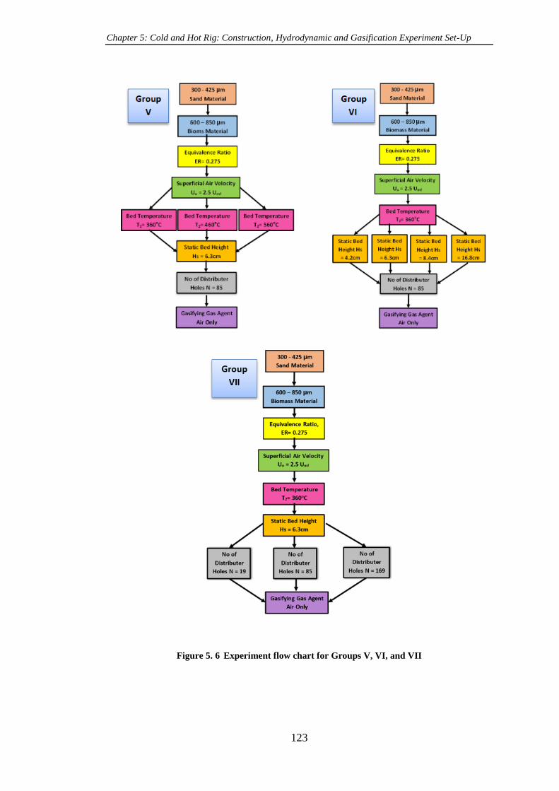
Chapter 5: Cold and Hot Rig: Construction, Hydrodynamic and Gasification Experiment Set-Up
123
Figure 5. 6 Experiment flow chart for Groups V, VI, and VII

Chapter 5: Cold and Hot Rig: Construction, Hydrodynamic and Gasification Experiment Set-Up
124
5.6 Equipment of hot (gasification) experiment-test rig
The schematic layout and the experimental test rig of bubbling fluidised bed gasifier
used in this study are shown in Figure 5.7 and Figure 5.8, respectively. The rig
consisted of an air regulator, two-air feeding rotameters group, an air preheater
furnace, a bubbling fluidised bed gasifier, (which in turn consists of an air box section
and perforated distributor plate. Also, it consisted a reaction bed and freeboard
sections), an electrical gasifier heater and its control panel, a biomass screw feeder
system and its water cooling system and nitrogen gas supply system. In addition, a
producer gas filter, a tar capturing system, a vacuum pump and a gas analyser system,
These rig components comprised of standard 316 stainless steel pipes, PVC pipes and
their fittings to give connection between components using 316 stainless steel pipes.
The digital manometer was used to measure the pressure drop across the fluidised bed
column. High temperature theromocouples, Type-K, were used to measure
temperature where they were needed.

Figure 5. 7 Schematic layout of the biomass bubbling fluidised bed
gasification trials set-up
1-C
om
pre
ssed
air
str
eam
, 2
- N
2 g
as b
ott
le,
3-
Wat
er c
hil
ler,
4-
Chil
ler
coil
hea
t ex
chan
ger
, 5
- W
ater
pan
, 6
- W
ater
pum
p,
7-
Cupper
wat
er
coil
hea
t ex
chan
ger
, 8
- A
ir p
ress
ure
reg
ula
tor,
9-
Scr
ew f
eed
er a
rm, 10
- N
2 g
as r
ota
met
er, 11
- A
ir r
ota
met
er, 12
- B
iom
ass
scre
w f
eed
er, 13
-
Furn
ace
hea
ter,
14
- B
ub
bli
ng f
luid
ised
bed
gas
ifie
r, 1
5-P
roduce
gas
fil
ter,
16
- S
and
-char
dis
char
ge
stre
am,
17
- Im
pin
ger
bo
ttle
s se
t w
ith
isopro
pan
ol
solv
ent,
18
- F
reez
er r
oom
, 19
- S
ilic
a gel
bott
les
set,
20
-Vac
uu
me
pum
p, 21
- P
roduce
gas
rota
met
er, 22
- C
ontr
ol
val
ve,
23
- G
as
anal
yse
r d
evic
e, 2
4-
Com
pute
r unit
, 25
- C
han
ge
val
ve,
26
- A
ir p
rehea
ter
furn
ace,
27
- D
istr
ibuto
r pla
te.

Chapter 5: Cold and hot rig construction, and hydrodynamic and gasification experiment set up
126
Figure 5. 8 Experimental test hot rig for biomass bubbling fluidised bed gasification studies.

Chapter 5: Cold and hot rig construction, and hydrodynamic and gasification experiment set up
127
A tubular furnace Type MTF 12/38B as shown in Figure (5.9) was used to heat the
supply air from the ambient temperature to a required reaction temperature to enhance
the gasification reactions. Carbolite Company-UK manufactured this furnace. Its
specifications are, 220-240 Volts, 50-60 Hz, 1500 Watts, 6.3 Amps maximum, and
1200oC maximum allowed temperature. An in-built control panel was provided to set
and control the temperature inside the furnace.
Figure 5. 9 Air Preheater Tubular Furnace, Type-MTF 12/38B
5.6.1 Bubbling fluidised bed reactor BFBR (gasifier)
In the same way as mentioned in Section 5.2, this hot test rig consists of a main part
of the gasification process called gasifier. It composed of the following main
components: air flow-box section, perforated distributor plate, fluidised bed section
and freeboard section. The design details of each section are available in Chapter 3-
Section (3.3.3.2) and Appendix A. The manufacturing of each section is available in
Chapter 4 Section 4.4.2, 4.4.4, 4.5.1 and 4.5.2, respectively. These four sections were
all assembled by joining their flanges together using stainless steel bolts to form the
intended gasifier. The schematic layout of the assembled gasifier is shown in Figure
5.10. Thermal gasket material, 5mm thickness, was used between each two sections as
a thermal insulator to avoid any air or/and gas leakage along the gasifier flanges and
to avoid any thermal adhesion that may take place between two metal surfaces due to
high surface temperature exposure. For heat saving and for thermal safety, the whole
gasifier and the connecting stainless steel pipe between the air preheater outlet and
air-box inlet were wrapped with 50 mm thickness of a high quality glass wool insulator
blanket material and aluminium foil.

Chapter 5: Cold and hot rig construction, and hydrodynamic and gasification experiment set up
128
Figure 5. 10 Schematic layout of biomass bubbling fluidised bed gasifier illustrating
thermocouples distribution along it and produce gas analysing streams
5.6.2 High temperature gasifier electric heater
Ceramic fibre electric-heater was used to heat the main rig section of the gasifier,
mainly the fluidised bed and freeboard reactions section, which included part of the
freeboard section, to gain the appropriate and required temperature for gasification
reactions. Watlow Company-UK supplied this product. A semi-cylindrical unit – Type
1 with full vestibule was selected for this purpose as shown in Figure 5.11 (a) and (b).
Two halves of this heater were needed to enfold the full external surface area of the
reaction section pipe with dimensions of, D= 89mm, L= 737mm, E=64mm. The

Chapter 5: Cold and hot rig construction, and hydrodynamic and gasification experiment set up
129
electrical rating for each half are, Volts= 240, Power= 2500 watts, and surface
loading= 2.1 W/cm2. These ceramic heaters operate at a maximum temperature up to
1204oC and exclusively use radiant heat transfer mode providing a high temperature
performance. The supplied heater is suitable for use up to 1093oC (WATLOW 2013).
These two heaters were controlled using a PID temperature controller panel.
a) b)
Figure 5. 11 Type1- full vestibule ceramic fibre electric heater: a) schematic of a half with its
dimensions, b) Image of two halves
5.6.3 Biomass screw feeder
DDSR-20 model of stainless steel biomass screw feeder was used as a biomass feeding
driver. This biomass feeder was manufactured by Braender Technology and supplied
by Genesis Process Solution Ltd-UK. This model was designed for feeding biomass
bulk solids. It composes of the components shown in Figure (5.12). The biomass
material can be poured in the hopper of the device and driven into the twin-screw
feeder by an electric drive motor. The filling of the screw trough was improved by a
trough agitator, which is rotated in combination above the twin-screw feeder, and all
were driven via a spur gear unit by the motor. A separate drive controller unit FC-B1
was provided with the feeder. This controller was used to control: the main power
supply by a main switch, the speed of screw feeder by speed potentiometer regulator
to set a desired speed from 0.0 -100% and finally to control the starting and stopping
of the operation by using an operating switch. This feeder can give a maximum design
mass flow rate 24 kg/hr.

Chapter 5: Cold and hot rig construction, and hydrodynamic and gasification experiment set up
130
a) b)
Figure 5. 12 DDSR –20 biomass screw feeder: (a) Complete screw feeder unit: 1-Hopper lid 2-
Hopper 3- Drive motor 4- Spur gear unit 5- Agitator trough 6- Screw feeder base 7- Twin-
screw arm, (b) Power supply and drive controller unit
For this feeder, a calibration curve for a specific biomass mass flow rate can be
obtained. It was shown in Section 4.3.1.6.
5.6.4 Screw feeder-cooling system
To prevent biomass pyrolysis inside the arm of the screw feeder at the gasifier fuel
feeding point due to higher temperature during gasification experiments, a water
cooling system was installed. The cooling system consisted of a basin filled with water,
a water chiller, which has an external cooling coil submerged in water basin for water
cooling, a copper coil which was wrapped along the screw feeder arm to cool the
biomass fuel, and a water pump to circulate a cool water from the water basin to copper
coil then again to a water basin. The cooling temperature provided by this system
depends mainly on the temperature of the fluidised bed section T2, shown in Figure
5.10. The temperature of biomass at the gasifier feeding point was measured by a K-
type thermocouple. The thermocouple was installed on the external surface of screw
arm, which was away 50mm from gasifier feeding point. An-inert environment was
provided, to prevent biomass combustion inside screw feeder, using N2 gas. 0.3-0.4

Chapter 5: Cold and hot rig construction, and hydrodynamic and gasification experiment set up
131
l/min of N2 gas was fed inside the hopper of biomass screw feeder through a small-
scale N2 gas rotameter.
5.6.5 Producer gas particulate filtration
The producer gas from the rig holds many impurities such as fine particles of sand,
char, unreacted biomass and traces of condensed tar vapours. These contaminants have
a detrimental effects on the downstream equipment and instruments causing deposition
in this rig, i.e. the vacuum pump and the GC gas analyser, which is highly sensitive to
these contaminants. In order to obtain a high purity producer gas for GC gas analyser
purposes these impurities must be removed as a first step for purification. Therefore,
a filter paper medium was used for this purpose. A GA55 grade, circular, 47mm
diameter and 0.6 µm pore Whatman glass fibre filter paper type was used for this
purpose. After each experiment, the filter was cleaned from the tar and other impurities
using an isopropanol solvent. A new filter paper was replaced.
5.6.6 Tar capturing system
A schematic diagram of the tar capturing system is shown in Figure 5.13. It was
designed with the same principle design as used in the tar sampling, which was
designed according to the standard method for biomass gasification–Tar and particles
in product gases - sampling and analysing tar from gasification processes by BSI-
CEN/TS 15439:2006 (Energy research Centre of the Netherlands 2004). The main
purpose of using a tar capturing system was to remove all condensable compounds
from producer gas to avoid any damage in downstream devices due to tar compounds
condensation and deposits. The system consisted mainly of an assembly frame of four
positions for fixing standard dreschel bottles MF 29/3/250 as shown in Figure 5.8( real
image of assembly from lab). These four bottles were connected in series and were
filled with 100 ml of isopropanol solvent (99.8 %) from Fisher Scientific. This solvent
was used for tar compounds screening. Each bottle position has inner tubes, which
were made from 316 stainless steel pipe ϕ 6 x 145 x 1mm. A freezer (BEKO, ZA630W)
rated 50 W and minimum temperature of -15oC was used to accommodate the impinger
bottles assembly to achieve solvent cooling. The inlet pipe from the outlet filter from
the gasifier was connected to the first bottle inner tube through a hole on a top side of
the freezer. The outlet of the fourth bottle train was connected to silica gel bottle train.

Chapter 5: Cold and hot rig construction, and hydrodynamic and gasification experiment set up
132
Silica gel was used to ensure that water vapour in the gas stream was completely
removed and any other impurities may available in the gas stream as well.
Figure 5. 13 Schematic diagram of the tar capturing system: 1-4 are impinger bottles, each 100
ml of isopropanol, in the freezer at (-15oC). Silica gel bottles 5 and 6 were kept at 20-25oC
5.6.7 Producer gas analyser unit
After cleaning and tar capturing, producer gas was sent to gas analyser unit. This unit
consisted of, a vacuum pump, a small-scale rotameter, one bottle of silica gel and gas
analyser. The vacuum pump was necessary to supply enough flow of producer gas to
overcome the pressure drop from the filtration and tar capturing system. A small-scale
rotameter, ml/min scale, was used to control the producer gas flow rate within flow
rate limitations of the gas analyser, not more than 1 ml/min. A silica gel bottle was
installed directly before the analyser to ensure a high purity of producer gas. Finally,
the gas analyser type (X-STREAM X2GP - EMERSON) as shown in Figure (5.14)
was used to analysis a biomass gasification producer gas. The new X-STREAM gas
analysers can measure up to five different gas components using any combination of
the following analysing techniques: IR = non-dispersive infrared analysis, UV =
ultraviolet analysis, pO2 = paramagnetic oxygen analysis, eO2 = electrochemical
oxygen analysis, TC = thermal conductivity analysis (Emerson Process Management
2012).
Due to the high sensitivity of gas analyser against any impurities, the producer gas
must be free from them. This analyser was capable of analysing into CO, CO2, CH4,
Freezer

Chapter 5: Cold and hot rig construction, and hydrodynamic and gasification experiment set up
133
H2 and O2. It has five channels, one for each above-mentioned gases. These channels
must be firstly purged by N2 gas and calibrated by a standard mixture of gases: 15%
CO, 15%CO2, 15% H2, and 5.0 % CH4 where the difference was N2. This analyser has
inlet and outlet streams for producer gas. The output gas stream was directly exhausted
to the extraction system. These data provided a volume percent composition for each
gas mentioned above as a function of time in seconds.
Figure 5. 14 X-STREAM X2GP-EMERSON gas analyser
5.7 Hot-rig bubbling fluidised bed gasification process procedures
5.7.1 Commissioning and preparation procedures
After completing the first stage (without insulation, tar capturing unit, biomass feeding
screw feeder and its cooling system) of the gasifier structure, gasifier commissioning
temperature setting tests were needed. This was for testing and understanding the
performance of the gasifier electric heater and the temperature distribution along
gasifier sections at equilibrium conditions for cases of with and without air preheater,
airflow, bed material. The temperature distributions were specified according to the
thermocouples points that were distributed and fixed along gasifier as shown in Figure
5.10. These tests helped to specify the minimum and maximum limits of the
temperatures of the gasification reaction section at fluidised bed reactions zone and
freeboard gas reactions zone as well at thermally steady state conditions. Firstly, the
top section (reaction section) of the gasifier was tested. It was operated with electrical
heaters only without pipe reactor insulation and without bed material silica sand and
without airflow. This was performed for several electrical heater setting temperatures
Tset=T1, 500oC, 700oC, 800oC, 900oC and 1000oC. Unfortunately, the results show
Gas Inlet Gas Outlet

Chapter 5: Cold and hot rig construction, and hydrodynamic and gasification experiment set up
134
that the required range of temperature at the gasifier reaction section cannot be
obtained. To improve these results all active exposed surfaces of the gasifire were well
insulated. Also a quantity of 8.3 cm height of a 300-425 µm particle size of bed
material silica sand was used and poured inside the reactor. The tests were repeated
for several heater-setting temperatures T1 between 500oC and 1000oC. All tests were
let to achieve equilibrium conditions. The results are displayed in Figure 7.1, which
shows the values of the temperature T2, the temperature at bed reaction zone, 4.15 cm
above distributor plate at biomass feeding point as a function of time. The final
equilibrium values of T2 corresponding to setting temperatures T1: 500oC, 700oC,
800oC, 900oC and 1000oC are shown in Table 7.1
Additional sets of electrical heater setting temperatures, 400oC, 600oC, 750oC and
825oC were selected to obtain the equilibrium temperature value T2 (when T2 in
gasifier reaches steady state). These temperatures are shown in Table 7.1
Tests were conducted to see the possibility of making T2 to be a setting temperature
Tset instead of Tset=T1. This was because; theoretically it was best to put T2, a
required bed reaction temperature, as a Tset. However, particularly it was found that
the point of the heater at T1 still behaved as supply temperature, by the electrical
heater, and this led to rise the temperature T1 more rapidly than new setting
temperature T2 and was expected to go to overload conditions of the upper limit of the
heater temperature supply (1200oC).
5.7.2 Vertical temperature distribution a long fluidised bed gasifier
Experiments at specific conditions, for various particle sizes of silica sand bed
material, 300-425µm, 425-500µm and 500-600µm , for a range of gasifier setting
temperature (gasifier electrical heater setting temperature) without preheater and with
preheater and for different air flow rate were conducted. There are two main aims for
these experiments: first to gain a database for axial temperature distributions along
the gasifier and its limits. This enables the researcher to observe and specify a desired
gasification reaction temperature according to the setting conditions. The second aim
is to study the hydrodynamic behaviour of the fluidised bed reactor mainly the
minimum fluidisation velocity, an important design parameter, at high temperature
conditions. However, 600oC, 750oC and 900oC of gasifier setting temperatures
Tset=T1 without air preheating were chosen as a first set experiments for gasifier

Chapter 5: Cold and hot rig construction, and hydrodynamic and gasification experiment set up
135
operating with air flow rate ranged from 10 l/min to 100-140 l/min. The results are
presented and discussed in Chapter 7-Section 7.2.2 and shown in Figure 7.3 (a-a-), (b-
b-) and (c-c-).
The second set of experiments for setting temperature Tset=T1=950oC, 900oC and
825oC with air preheating, using tubular furnace setting temperature at Tpreset= 750oC,
were also conducted. They are shown in Figure 7.4 (a-a-), (b-b-), (c-c-), respectively.
The third set of experiments for setting temperature Tset=T1=825oC and 900oC with
air preheating, using tubular furnace setting temperature at Tpreset= 900oC, were also
conducted as shown in Figure 7.5 a-a- and b-b-. For temperature points, their positions
are shown in Figure (5.10) T4, T2, T1, T3 and T7 at gasifier temperature measuring
points, -10cm, 4cm, 44cm, 84cm and 124cm, respectively, their equilibrium
temperature results were obtained for two groups where mentioned above. The results
presented and discussed in Chapter 7, Figure 7.5
The last comparison of the bed temperature T2 levelling, a temperature at 4.15cm point
above distributor plate, for three experiments is shown in Chapter 7-Figure 7.6. Each
of them had a setting temperature Tset=T1=900oC and Tpreset= 900oC, 750oC, 0.0oC as
well.
5.7.3 Commissioning of biomass gasification experiments
These experiments were conducted according to hydrodynamic and gasifier
temperature distribution results, and considered as a preliminary test for preparing the
gasifier for next study of complete rig experiments. Pine wood sawdust as biomass
solid fuel, quartz sand as bed material and air as gasifying gas agent were used for
these tests. For a specific range of the particle size of the sand material a superficial
velocity of airflow, expressed as volumetric flow rate in l/min, according to its
minimum fluidisation velocity, was specified. Then at a specific gasification
equivalence ratio and air flowrate, a mass flow rate of biomass was calculated.
Subsequently, from the sawdust biomass screw feeder calibration curve the mass flow
rate of biomass was specified.
5.7.4 Preparation procedures of gasification hot-rig
After completing gasifier temperature setting and commissioning and after joining all
gasification hot-rig secondary units and accessories, at this step the rig was considered

Chapter 5: Cold and hot rig construction, and hydrodynamic and gasification experiment set up
136
ready to conduct the required gasification experiments. Prior to any experimental
operation, a number of preparation steps should be followed.
I. Safety preparation
Prior to start any gasification experiments the following safety and security steps were
performed:
The lab extraction system for gasification product gas ventilating was checked to
ensure its operation readiness.
Lab gas detector alarm and personal gas monitor was tested to be ready at any
time.
Trip hazard, hot equipment signs and required protective equipment (PPE) were
prepared to avoid any harm.
Electrical circuits for all electrical component of the rig were checked to be ready
in operation.
Any flammable material such as biomass fuel and isopropanol liquid solvent were
deported outside the rig area.
II. Experiment preparation procedures
The preparation procedures for the experiment set-up were as follows:
a) According to fluidised bed biomass gasification process and plan of experiments,
specific required materials were prepared such as: A specified particle size range
of the sand bed material for a specific static bed height was weighted. This sand
particle size let to know the value of the cold minimum air fluidization flow rate,
which was obtained from the cold-rig experiments. Also a specific particle size
range of the biomass solid fuel was weighed. This weight of biomass was
calculated according to the required biomass mass flow rate for a required time of
gasification process for each experiment. The biomass mass flow rate was
calculated according to a selected value of each air flowrate and equivalence ratio
(by mass). Prior to use this experiment, it was dried up to 105-110oC for 2 hours
using a dryer oven.
b) Availability of N2 gas and supplying compressed air were checked and prepared.
c) The biomass screw feeder was tested for driving a consistent flow of the biomass
particles especially at low biomass flow rates, which correspond to low values of
screw feeder speed point. These speed points need a low quantity of biomass in
the hopper to reduce the weight load limits of biomass during low screw speeds.

Chapter 5: Cold and hot rig construction, and hydrodynamic and gasification experiment set up
137
This will ensure the driving of screw feeder motor and then the smooth flow of
biomass inside gasifier.
d) The function of the water cooling system for screw feeder cooling was checked.
The water pump was checked for supplying a suitable water flow rate. The
function of chiller and its coil were also checked. This was operated after gasifier
heating up. A K-Type thermocouple was used to monitor the temperature near
biomass feeding point.
e) Due to tar compounds precipitation and blockage, especially between gasifier
outlet point of producer gas for analysing and a vacuum pump suction point, a
connection gas pipe lines, type PVC, were replaced by a new pipes, whereas the
stainless steel pipes were cleaned. Then for gas pipelines leakage checking, a
purging with air at 15 l/min for 30 minutes was used, which was appropriate to
produce sufficient pressure to detect any leaks.
f) The tar capturing system was preconditioned by cleaning the 250 ml dreschel
bottles using, firstly an isopropanol solvent and secondly a laboratory liquid
detergent and then dried at 115oC for 2-3 hours to remove any impurities.
g) To confirm that the tar-capturing unit was properly functioning, the fridge was
turned on for 24 hours to achieve an effective cooling environment, approximately
-10oC. This was monitored using a K type thermocouple.
h) The function of the vacuum pump was verified by using the producer gas
rotameter, which was placed before the gas analyser.
i) The electrical heater of the gasifier was tested for the setting temperature at point
T1 inside gasifier column. This temperature was set at 900oC and the temperature
rise observed through the controller. All temperature measurement points T4, T3
and T7 distributed along gasifier were observed. External K-Type thermocouples
for these points were connected to the thermometer, whilst T1 and T2 points were
connected to the electrical heater controller panel. The air preheater tubular
furnace was tested for the required temperature of the inlet air to the gasifier T4.
Its controller monitored the temperature inside the preheater furnace, whereas the
air outlet temperature at the preheater furnace end was monitored by a K-Type
thermocouple. The setting temperature of the preheater was 900oC or 750oC.
j) Prior to producer gas analysis, the five channels of the gas analyser were purged
using N2 gas. Then a standard gas mixture calibrated these channels.
Chapter 5: Cold and hot rig construction, and hydrodynamic and gasification experiment set up
138
5.7.5 Operating procedure of gasification hot-rig
The thorough experimental procedures conducted for the running of the gasification
hot-rig were as follows:
1) Prior to any test, the gasifier furnace was switched on and the temperature along
the gasifier was observed. Similarly, if it was operating, the air preheater tubular
furnace was also switched on.
2) A specified weighed amount of the sand bed material (for a specified particle size
range and static bed height) was poured inside the gasifier through a hole located
at the top of the gasifier.
3) During the gasifier furnace activation, the preheating period took 3-4 hours, the
first and second dreschel bottles in the tar-capturing unit were each filled by 100
ml of isopropanol measured at room temperature. The third and fourth bottles
were left empty. Finally, the whole unit was assembled.
4) While the setting temperature inside the gasifier at point T1 reached (250oC), the
extraction system in the laboratory was run to take out undesirable gases
(combustible and toxic gases) which may be present.
5) During gasifier furnace activation, the gas analyser was purged by N2 gas and
calibrated by a standard gas. This purging and calibration procedure was
undertaken once per day for all experiments.
6) When the bed temperature at point T2 in the gasifier reached a required reaction
temperature, the control valve of the air rotameter was opened to supply a required
air flowrate in l/min (within fluidisation conditions). This air flowrate depends
mainly on the minimum fluidisation flow rate value for sand material which in
turn depends on a selected sand particle size range. At this step, adjustable
balancing between a required air flowrate and a required gasification temperature
T2 was needed to keep the operating parameters at their required specified values
for each experiment.
7) During step (6) the required dried biomass (for a specific particle size range) was
poured inside the screw feeder hopper. At this time the N2 gas rotameter control
valve was opened up to 0.3-0.4l/min to prevent biomass pyrolysis inside the screw
feeder. This required biomass was specified according to its mass flow rate
calculations. The biomass mass flow rate was calculated at a specific gasification
equivalence ratio and at a selected air gasifying agent flow rate. From this mass

Chapter 5: Cold and hot rig construction, and hydrodynamic and gasification experiment set up
139
flow rate and for a specified experiment time, the required biomass mass for any
experiment was allocated. The procedure of the biomass mass flow rate
calculations will be shown in Section 5.8.4.
8) For a calculated biomass mass flow rate value, the corresponding speed point
value of the biomass screw feeder was determined using biomass-speed point
calibration curve, which was prepared as shown in Chapter 4. This speed point
was adjusted using a speed point regulator in the screw feeder controller.
9) The vacuum pump in the gas analyser system was switched on to supply enough
producer gas flow rate (not exceed 1 ml/min) to the gas analyser. A rotameter
control valve was opened to supply this flow rate.
10) A compatible gas analysis online software was prepared using a personal
computer. This software was used to record the gases analysing data at time=0.0
i.e. the moment of the gasification reaction experiment starting.
11) When the gasifier reached the required operating temperature, the biomass screw
feeder was switched on. The required experiment time (in minutes) was specified
according to the weight of the prepared biomass, as explained in step 7. From the
commissioning tests, it was seen that the biomass feeding time, which was
required to achieve equilibrium conditions was less than 2 min. So most of the
experiments were conducted for 5min.
12) After the experiment reached its specified time, the gasification reaction was
stopped by switching off the biomass screw feeder and electrical heater. The
airflow was also closed. Finally, the vacuum pump in gas analyser system was
switched off, the producer gas rotameter was closed and the data analysing
software were stopped after 15 min from the experiment starting.
13) At this step, the air flow was replaced by inert N2 gas to prevent char reactions as
much as possible for accurate calculation of carbon conversion with respect to its
reaction time period. N2 gas flow rate was maintained at a minimum flow rate for
fluidisation conditions to ensure a perfect inert environment for all the bed (sand
+ char) and to cool a gasifier as quickly as possible.

Chapter 5: Cold and hot rig construction, and hydrodynamic and gasification experiment set up
140
5.8 Hot-Rig experimental data measurements and calculations
5.8.1 Temperatures
As shown in Chapter 2-Section 2.5.1.3 operating temperature is an important factor in
the biomass gasification process. Gasifier performance and gasification process
efficiency are highly affected by the operating temperature where the temperature
inside the gasifier affects the producer gas composition. At bed section, the bed
measurement temperature T2 controls the biomass gasification reaction rates, whilst
in the gasifier freeboard section the temperatures T1, T3 and T7 control the tar cracking
reaction rates. Also, in case of the using the preheater furnace, the inlet air temperature
to the gasifier affected the temperature distribution along the gasifier. Moreover, the
tar capturing process needs low temperatures to prevent isopropanol solvent
evaporation and to improve the tar solution in the solvent. As a result of gasification
exothermic and endothermic reactions, the fluctuation of bed temperature T2
throughout the gasification experiment as a function of time was also recorded. Finally,
at the inlet biomass feeding point a low temperature environment below 150oC was
needed to prevent biomass pyrolysis, which affects the gasifier performance.
Therefore, measuring these temperatures was significant in controlling the overall
gasification process.
As mentioned in Sections 5.5.1 and 5.5.2, these temperatures were measured using K-
Type thermocouple and were observed using a multichannel digital thermometer and
a built-in thermometer for both: gasifier furnace control panel and air preheater
furnace.
5.8.2 Minimum fluidisation conditions at high temperature
Due to the variation of air density with temperature, tests were conducted to measure
the minimum fluidisation conditions (especially minimum fluidisation air flowrate) at
elevated temperature conditions. In the same manner, which was followed to find the
minimum fluidisation conditions for air - sand material system at cold conditions, the
airflow rate at minimum fluidisation conditions at elevated temperature was found.
Firstly, the tests were conducted for sand particle size range (300-425) µm for three
gasifier furnace setting temperature T1, 600oC, 750oC and 900oC, where these
temperatures gave a corresponding bed temperature T2, 70oC, 95oC and 400oC,

Chapter 5: Cold and hot rig construction, and hydrodynamic and gasification experiment set up
141
respectively. The obtained values of minimum fluidisation air flowrate are displayed
and discussed Chapter 7 in Table 7.2 and Figure 7.7.
5.8.3 Required time for gasification experiment
For continuous of biomass gasification process experiments, the required time was
considered an important parameter because it indicated that the point at which the
gasification reactions reached equilibrium (steady state) conditions. The steady
conditions mean that the composition of the gasification producer gas does not change
with time. For three times, 2.5 min, 5 min and 10 min, biomass gasification
experiments were conducted at the same conditions: air flowrate, equivalence ratio,
bed temperature T2, biomass mass flow rate and sand material particle size. The testing
results were indicated that the required time to reach the equilibrium conditions was
2.5min. According to these results and depending on biomass amount availability,
most of the continuous gasification experiments were performed for a 5 min period
time. For biomass gasification experiments, a stopwatch was used to measure a
required time of the process. At the same time, the online gas analyser results provided
the change of the compositions of a producer gas with time (in seconds) during
gasification experiments interval. This time-gas composition data was helpful to
measure and specify the following: 1) starting point of reaction equilibrium conditions,
2) the starting point of the decline of the gas composition at the end time of the
experiment and 3) the time that was required to reach the equilibrium point.
5.8.4 Biomass mass flow rate settings
As discussed in Chapter 2, for gas-solid reactions the gasification process depends
mainly on two essential reactants, gasifying agent gas and solid fuel material. The
reaction quantities of these two reactants are related by equivalence ratio. The
gasification process operates within incomplete combustion conditions, which means
that the required quantity of oxygen is always less than its stoichiometric quantity
(partial oxidation). To achieve these conditions the actual air-fuel ratio must be less
than the stoichiometric air-fuel ratio. As mentioned above these two ratios are related
by ER where the value of this ratio depends on the process type. For gasification
process, the fuel was definitely considered as excess reactant whilst the oxidant was
the limiting reactant.

Chapter 5: Cold and hot rig construction, and hydrodynamic and gasification experiment set up
142
5.8.4.1 Equivalence ratio, biomass feeding rate and air mass flow rate setting
As shown in Equation (3.25), ER relates the mass flow rate of both reactant materials,
air and biomass fuel, in actual and stoichiometric conditions. The main objective is the
specifying and setting the required biomass feeding mass flowrate for a specific air
flowrate and required equivalence ratio. This biomass air mass flowrate can be
calculated as shown in Chapter 3 Equation (3- 25) to Equation (3.30)
Usually, the stoichiometric quantities of air and biomass can be calculated from the
chemical reaction equation for complete combustion for all quantity of each
combustible element in the fuel as illustrated in Table 5.2. The formal quantity was
calculated by summing the required O2 for each element, using the ultimate analysis
of biomass fuel, subtracting the latent oxygen in the biomass fuel.
Table 5. 2 Quantities of O2 required for stoichiometric calculation for biomass fuel
From the net O2 required mass, the required air mass can be calculated using O2 weight
percent in air, 0.232, whereas N2 weight percent=0.7547)(Basu 2010). For this purpose
a general equation for any biomass fuel was developed, by this study, to determine the
stoichiometric mass air fuel ratio (MAFR)stoichio as shown in Equation (5.4).
(𝑀𝐴𝐹𝑅)𝑠𝑡𝑜𝑖𝑐ℎ𝑖𝑜 = [2.664×𝐶 𝑤𝑡% + 7.937×𝐻 𝑤𝑡% − 𝑂 𝑤𝑡% + 0.998×𝑆 𝑤%]
0.232×[𝐶 𝑤𝑡%+𝐻 𝑤𝑡%+𝑂 𝑤𝑡%+𝑆 𝑤%+𝑁 𝑤𝑡%] (5.4)
Where: C wt%, H wt%, O wt%, S w%, N wt%, represent the weight percent of the
elements C, H, O, S, and N, respectively, in the ultimate analysis of the biomass fuel.
By applying Equation (5.4) and from ultimate analysis for each biomass, the
stoichiometric mass air fuel ratio (MAFR)stoichio for each biomass, SPWB and IDPWB
are 6.2 and 6.352, respectively.
Equation 3.25 was considered a first step for biomass mass rate determination and this
led to determining the corresponding screw feeder speed point. The steps of the
biomass fuel mass flow rate calculations have been detailed in Chapter 3. These steps
were arranged and summarized as a flow chart as shown in Figure 5.15.
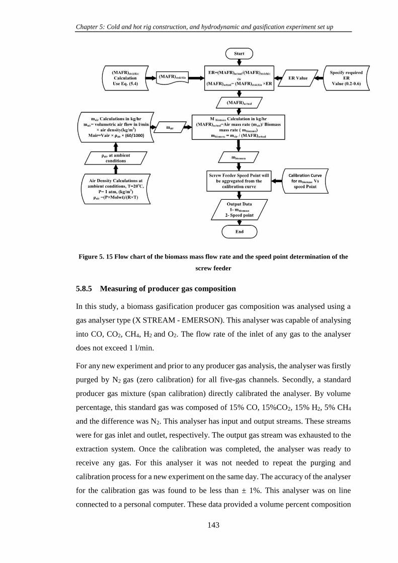
Chapter 5: Cold and hot rig construction, and hydrodynamic and gasification experiment set up
143
Figure 5. 15 Flow chart of the biomass mass flow rate and the speed point determination of the
screw feeder
5.8.5 Measuring of producer gas composition
In this study, a biomass gasification producer gas composition was analysed using a
gas analyser type (X STREAM - EMERSON). This analyser was capable of analysing
into CO, CO2, CH4, H2 and O2. The flow rate of the inlet of any gas to the analyser
does not exceed 1 l/min.
For any new experiment and prior to any producer gas analysis, the analyser was firstly
purged by N2 gas (zero calibration) for all five-gas channels. Secondly, a standard
producer gas mixture (span calibration) directly calibrated the analyser. By volume
percentage, this standard gas was composed of 15% CO, 15%CO2, 15% H2, 5% CH4
and the difference was N2. This analyser has input and output streams. These streams
were for gas inlet and outlet, respectively. The output gas stream was exhausted to the
extraction system. Once the calibration was completed, the analyser was ready to
receive any gas. For this analyser it was not needed to repeat the purging and
calibration process for a new experiment on the same day. The accuracy of the analyser
for the calibration gas was found to be less than ± 1%. This analyser was on line
connected to a personal computer. These data provided a volume percent composition

Chapter 5: Cold and hot rig construction, and hydrodynamic and gasification experiment set up
144
for five producer gas components, which have been mentioned above as a function of
time in seconds.
5.8.6 Gasification Performance Parameters Calculations
5.8.6.1 Producer gas Yield (GY)
Due to the inactivity of N2 at gasification conditions, Producer Gas (P.G.) yield in
Nm3/hr can be estimated making use N2 mass balance for gasifier system as shown in
Chapter 7 Figure 7.37. For total N2 mass balance,
𝑀𝑎𝑠𝑠 𝑟𝑎𝑡𝑒 𝑜𝑓 𝑡𝑜𝑡𝑎𝑙 𝑖𝑛𝑝𝑢𝑡 𝑁2 = 𝑀𝑎𝑠𝑠 𝑟𝑎𝑡𝑒 𝑜𝑓 𝑡𝑜𝑡𝑎𝑙 𝑜𝑢𝑡𝑝𝑢𝑡 𝑁2
𝑀𝑎𝑠𝑠 𝑟𝑎𝑡𝑒 𝑜𝑓 𝑡𝑜𝑡𝑎𝑙 𝑖𝑛𝑝𝑢𝑡 𝑁2
= 𝑀𝑎𝑠𝑠 𝑟𝑎𝑡𝑒 𝑜𝑓 𝑁2 𝑖𝑛 𝑎𝑖𝑟 + 𝑀𝑎𝑠𝑠 𝑟𝑎𝑡𝑒 𝑜𝑓 𝑁2 𝑖𝑛 𝑏𝑖𝑜𝑚𝑎𝑠𝑠 𝑓𝑢𝑒𝑙
𝑀𝑎𝑠𝑠 𝑟𝑎𝑡𝑒 𝑜𝑓 𝑁2 𝑖𝑛 𝑎𝑖𝑟 = 𝑤𝑡% 𝑜𝑓 𝑁2 𝑖𝑛 𝑎𝑖𝑟 × 𝑚𝑎𝑠𝑠 𝑟𝑎𝑡𝑒 𝑜𝑓 𝑓𝑒𝑒𝑑𝑖𝑛𝑔 𝑎𝑖𝑟 �̇�𝑎𝑖𝑟
𝑀𝑎𝑠𝑠 𝑟𝑎𝑡𝑒 𝑜𝑓 𝑁2 𝑖𝑛 𝑓𝑢𝑒𝑙
= 𝑤𝑡% 𝑜𝑓 𝑁2 𝑖𝑛 𝑓𝑢𝑒𝑙 × 𝑚𝑎𝑠𝑠 𝑟𝑎𝑡𝑒 𝑜𝑓 𝑓𝑒𝑒𝑑𝑖𝑛𝑔 𝑓𝑢𝑒𝑙 �̇�𝑏𝑖𝑜𝑚𝑎𝑠𝑠
The total moles of N2 in producer gas P.G. can be calculated using its molecular
weight, 28 using Equation (5.5)
𝑇𝑜𝑡𝑎𝑙 𝑚𝑜𝑙𝑒𝑠 𝑜𝑓 𝑁2 𝑖𝑛 𝑃. 𝐺. = 𝑇𝑜𝑡𝑎𝑙 𝑜𝑢𝑡𝑝𝑢𝑡 𝑚𝑎𝑠𝑠 𝑟𝑎𝑡𝑒 𝑜𝑓 𝑁2 28⁄ (5.5)
Then, the total moles rate of P.G. can be calculated, making use total moles of N2 in
P.G. using Equation (5.6).
𝑀𝑜𝑙𝑒𝑠 𝑟𝑎𝑡𝑒 𝑜𝑓 𝑃. 𝐺. = 𝑇𝑜𝑡𝑎𝑙 𝑚𝑜𝑙𝑒 𝑟𝑎𝑡𝑒 𝑜𝑓 𝑁2 𝑖𝑛 𝑃.𝐺
𝑣𝑜𝑙% 𝑜𝑓 𝑁2 𝑖𝑛 𝑃.𝐺. 100⁄ (5.6)
Volume parentage of N2 in P.G. was estimated using Equation (5.7) by the difference
of the producer gases, which were analysed. These gases are CO, CO2, CH4, H2, and
O2 in volume percentage.
𝑉𝑜𝑙% 𝑜𝑓 𝑁2 𝑖𝑛 𝑃. 𝐺. = 100 − 𝑣𝑜𝑙% 𝑜𝑓( 𝐶𝑂 + 𝐶𝑂2 + 𝐶𝐻4 + 𝐻2 + 𝑂2) (5.7)
It can be noticed that for ideal gas, the volume percent and mole percent are equal. The
volumetric flowrate of producer gas in Nm3/hr can be calculated making use that for
ideal gas at standard conditions, 273.15oK and 101.325 kPa, each 1 kgmol of the gas
occupied 22.4 Nm3. Therefore, the producer gas in volumetric flowrate, for example
Nm3/hr, at ambient conditions can be calculated using Equation (5.8).

Chapter 5: Cold and hot rig construction, and hydrodynamic and gasification experiment set up
145
𝑃. 𝐺. 𝑣𝑜𝑙𝑢𝑚𝑒𝑡𝑟𝑖𝑐 𝑓𝑙𝑜𝑤𝑟𝑎𝑡𝑒 = 𝑚𝑜𝑙𝑒𝑠 𝑟𝑎𝑡𝑒 𝑜𝑓 𝑃. 𝐺. × 22.4 (5.8)
Finally, the gas yield GY of producer gas per unit mass of biomass feeding fuel, for
example in Nm3/kg of feed biomass can be calculated using Equation (5.9).
𝐺𝑌 𝑖𝑛, (𝑁𝑚3 𝑘𝑔 𝑓𝑒𝑒𝑑 𝑓𝑢𝑒𝑙) = 𝑣𝑜𝑙𝑢𝑚𝑒𝑡𝑟𝑖𝑐 𝑓𝑙𝑜𝑤𝑟𝑎𝑡𝑒 𝑜𝑓 𝑃.𝐺 𝑖𝑛 (𝑁𝑚3 ℎ𝑟)⁄
𝑚𝑎𝑠𝑠 𝑟𝑎𝑡𝑒 𝑜𝑓 𝑓𝑒𝑒𝑑 𝑓𝑢𝑒𝑙 𝑖𝑛(�̇�𝑏𝑖𝑜𝑚𝑎𝑠𝑠 ℎ𝑟)⁄⁄ (5.9)
5.8.6.2 Carbon conversion efficiency (CCE)
This Efficiency can be estimated making use the yield of producer gas in (kgmol/kg
biomass feed) and the composition of three gases in producer gas, which are hold
carbon atom C mainly, CO, CO2 and CH4 as follows (Basu 2006).
𝑇𝑜𝑡𝑎𝑙 𝑚𝑜𝑙𝑒𝑠 𝑜𝑓 𝑜𝑢𝑡𝑝𝑢𝑡 𝐶 𝑖𝑛 𝑃. 𝐺. 𝑝𝑒𝑟 𝑢𝑛𝑖𝑡 𝑚𝑎𝑠𝑠 𝑜𝑓 𝑓𝑒𝑒𝑑 𝑏𝑖𝑜𝑚𝑎𝑠𝑠 =
[𝐶𝑂%+𝐶𝑂2%+ 𝐶𝐻4%
100] × [
𝑇𝑜𝑡𝑎𝑙 𝑚𝑜𝑙𝑒 𝑟𝑎𝑡𝑒𝑠 𝑜𝑓 𝑃.𝐺
𝑀𝑎𝑠𝑠 𝑟𝑎𝑡𝑒 𝑜𝑓 𝑏𝑖𝑜𝑚𝑎𝑠𝑠 𝑓𝑒𝑒𝑑]
(5.10)
𝑇𝑜𝑡𝑎𝑙 𝑚𝑎𝑠𝑠 𝑜𝑓 𝐶 𝑖𝑛 𝑃. 𝐺. 𝑝𝑒𝑟 𝑢𝑛𝑖𝑡 𝑚𝑎𝑠𝑠 𝑜𝑓 𝑓𝑒𝑒𝑑 𝑏𝑖𝑜𝑚𝑎𝑠𝑠 =
[𝑇𝑜𝑡𝑎𝑙 𝑚𝑜𝑙𝑒𝑠 𝑜𝑓 𝐶 𝑖𝑛 𝑃. 𝐺. 𝑝𝑒𝑟 𝑢𝑛𝑖𝑡 𝑚𝑎𝑠𝑠 𝑜𝑓 𝑓𝑒𝑒𝑑 𝑏𝑖𝑜𝑚𝑎𝑠𝑠] × 12 (5.11)
The mass rate of input carbon to the gasifier can be calculated from the weight percent
of carbon C in the biomass fuel, Ultimate analysis, and the mass rate of the biomass
feeding, using Equation (5.12).
𝑇𝑜𝑡𝑎𝑙 𝑖𝑛𝑝𝑢𝑡 𝑚𝑎𝑠𝑠 𝑟𝑎𝑡𝑒 𝑜𝑓 𝐶 = [𝑤𝑡% 𝑜𝑓 𝐶 𝑖𝑛 𝑓𝑒𝑒𝑑 𝑏𝑖𝑜𝑚𝑎𝑠𝑠
100] ×
[𝐵𝑖𝑜𝑚𝑎𝑠𝑠 𝑓𝑒𝑒𝑑 𝑚𝑎𝑠𝑠 𝑟𝑎𝑡𝑒] (5.12)
Finally, CCE can be calculated using Equation (5.13).
𝐶𝐶𝐸% = [𝑇𝑜𝑡𝑎𝑙 𝑜𝑢𝑡𝑝𝑢𝑡 𝑜𝑓 𝐶 𝑚𝑎𝑠𝑠 𝑟𝑎𝑡𝑒 𝑖𝑛 𝑃.𝐺
𝑇𝑜𝑡𝑎𝑙 𝑖𝑛𝑝𝑢𝑡 𝑜𝑓 𝐶 𝑚𝑎𝑠𝑠 𝑟𝑎𝑡𝑒 𝑖𝑛 𝑓𝑒𝑒𝑑] =
[𝑇𝑜𝑡𝑎𝑙 𝑜𝑢𝑡𝑝𝑢𝑡 𝑜𝑓 𝐶 𝑚𝑎𝑠𝑠 𝑝𝑒𝑟 𝑚𝑎𝑠𝑠 𝑜𝑓𝑓𝑒𝑒𝑑 𝑏𝑖𝑜𝑚𝑎𝑠𝑠
𝑇𝑜𝑡𝑎𝑙 𝐼𝑛𝑝𝑢𝑡 𝑜𝑓 𝐶 𝑚𝑎𝑠𝑠 𝑝𝑒𝑟 𝑚𝑎𝑠𝑠𝑜𝑓 𝑓𝑒𝑒𝑑 𝑏𝑖𝑜𝑚𝑎𝑠𝑠] (5.13)
5.8.6.3 LHV of producer gas
The LHV of producer gas in MJ/Nm3 can be calculated as follows (Basu 2006).
𝑃. 𝐺. 𝐿𝐻𝑉 = [𝐶𝑂 ℎ𝑒𝑎𝑡 𝑜𝑓 𝑐𝑜𝑚𝑏 ×𝐶𝑂%
100] + [𝐶𝐻4 ℎ𝑒𝑎𝑡 𝑜𝑓 𝑐𝑜𝑚𝑏 ×
𝐶𝐻4%
100 ] +
[𝐻2 ℎ𝑒𝑎𝑡 𝑜𝑓 𝑐𝑜𝑚𝑏 ×𝐻2 %
100 ] (5.14)

Chapter 5: Cold and hot rig construction, and hydrodynamic and gasification experiment set up
146
The heat of combustion of the gases CO, CH4 and H2 are 11.97, 33.95, and 10.22
MJ/Nm3, respectively (Legonda 2012), (Basu 2006).
From producer gas yield in, Nm3/kg fuel feed, the output LHV of producer gas in
MJ/kg fuel feed can be calculated using Equation (5.15).
𝑃. 𝐺. 𝐿𝐻𝑉 𝑖𝑛 (𝑀𝐽
𝑁𝑚3) = [𝑃. 𝐺. 𝐿𝐻𝑉 𝑖𝑛 (𝑀𝐽
𝑘𝑔 𝑓𝑢𝑒𝑙 𝑓𝑒𝑒𝑑)] / [𝑃. 𝐺. 𝑌𝑖𝑒𝑙𝑑 𝑖𝑛 (
𝑁𝑚3
𝑘𝑔 𝑓𝑢𝑒𝑙 𝑓𝑒𝑒𝑑)]
(5.15)
5.8.6.4 Cold-Gas Efficiency CGE
Cold –gas efficiency can be calculated using Equation (5.16) (Basu 2006).
𝐶𝐺𝐸% = [𝐿𝐻𝑉 𝑜𝑓 𝑃.𝐺.(𝑜𝑢𝑡𝑝𝑢𝑡)
𝐿𝐻𝑉 𝑜𝑓 𝑓𝑢𝑒𝑙 𝑓𝑒𝑒𝑑 (𝐼𝑛𝑝𝑢𝑡)] × 100 (5.16)
5.9 Summary
In this chapter, the experimental approach used and data measured during biomass
cold fluidisation and gasification trials is presented. .For each rig the components and
procedure of preparation and operation are described. In addition, the experimental
data measured for both rigs are presented.
For the cold rig, the visual observation of the fluidisation phenomenon for sand,
biomass and their mixtures was recorded. Also, the procedure of the establishing of
the hydrodynamic curve, ΔP-Uo curve, was derived. This curve has been used to
determine the minimum fluidisation velocity for each set of conditions such as particle
size for sand bed material, static bed height and mass percent for biomass - sand
mixtures.
For the hot rig, the design of the biomass gasification experimental tests was prepared.
This was useful to study the effect of the hydrodynamic and operating parameters on
the performance of the bubbling fluidised bed gasifier. Seven groups of experimental
tests were established and each group had three or four experiments. Finally, the
experimental data measurements such as temperatures, air flowrates, producer gas
composition and the weight of the char + sand mixture residue are presented.
Furthermore, the procedure of the calculation of the performance parameters such as,
ER, CCE, LHV and CGE are presented.

Chapter 6
Results and Discussion for Cold
Hydrodynamic Fluidisation
Experiments
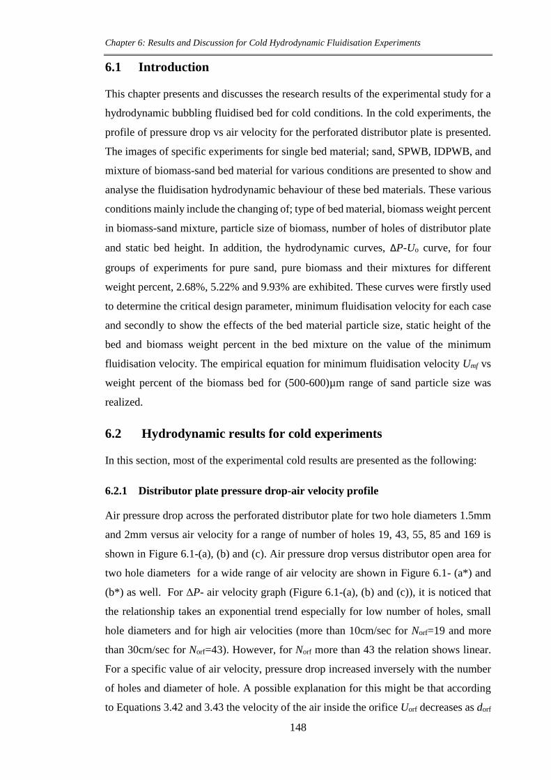
Chapter 6: Results and Discussion for Cold Hydrodynamic Fluidisation Experiments
148
6.1 Introduction
This chapter presents and discusses the research results of the experimental study for a
hydrodynamic bubbling fluidised bed for cold conditions. In the cold experiments, the
profile of pressure drop vs air velocity for the perforated distributor plate is presented.
The images of specific experiments for single bed material; sand, SPWB, IDPWB, and
mixture of biomass-sand bed material for various conditions are presented to show and
analyse the fluidisation hydrodynamic behaviour of these bed materials. These various
conditions mainly include the changing of; type of bed material, biomass weight percent
in biomass-sand mixture, particle size of biomass, number of holes of distributor plate
and static bed height. In addition, the hydrodynamic curves, ∆P-Uo curve, for four
groups of experiments for pure sand, pure biomass and their mixtures for different
weight percent, 2.68%, 5.22% and 9.93% are exhibited. These curves were firstly used
to determine the critical design parameter, minimum fluidisation velocity for each case
and secondly to show the effects of the bed material particle size, static height of the
bed and biomass weight percent in the bed mixture on the value of the minimum
fluidisation velocity. The empirical equation for minimum fluidisation velocity Umf vs
weight percent of the biomass bed for (500-600)µm range of sand particle size was
realized.
6.2 Hydrodynamic results for cold experiments
In this section, most of the experimental cold results are presented as the following:
6.2.1 Distributor plate pressure drop-air velocity profile
Air pressure drop across the perforated distributor plate for two hole diameters 1.5mm
and 2mm versus air velocity for a range of number of holes 19, 43, 55, 85 and 169 is
shown in Figure 6.1-(a), (b) and (c). Air pressure drop versus distributor open area for
two hole diameters for a wide range of air velocity are shown in Figure 6.1- (a*) and
(b*) as well. For ΔP- air velocity graph (Figure 6.1-(a), (b) and (c)), it is noticed that
the relationship takes an exponential trend especially for low number of holes, small
hole diameters and for high air velocities (more than 10cm/sec for Norf=19 and more
than 30cm/sec for Norf=43). However, for Norf more than 43 the relation shows linear.
For a specific value of air velocity, pressure drop increased inversely with the number
of holes and diameter of hole. A possible explanation for this might be that according
to Equations 3.42 and 3.43 the velocity of the air inside the orifice Uorf decreases as dorf

Chapter 6: Results and Discussion for Cold Hydrodynamic Fluidisation Experiments
149
increases. As shown in Equation 3.42, the effect of Uorf on ΔPdist is more effective
compared to dorf effect. In addition, from Equation 3.44-a, it can be seen that as the
number of holes increase the velocity Uorf increases and thereby ΔPdist decreases.
From the Figure 6.1-(a*) and (b*), it can be shown that at specific air velocity ΔPdist
decreases as the distributor open area increases. For dorf=1.5mm, Figure 6.1-(a*) shows
a sharp decrease of pressure drop from 0.36 to 0.76cm2, whereas for dorf=2mm, as
shown in Figure 6.1-(b*) the decrease was gradual. In addition, the Figure shows for
specific open area the pressure drop decreased as air velocity decreased. High air
velocities more than 18.1cm/sec shows show sharp increase in pressure drop for
dorf=1.5mm and a gradual increase for dorf=2mm. In addition, it can be seen that for both
hole diameter and for all velocities the pressure drop across distributor plate is than 10
mbar for Norf more than 43 holes. A possible explanation for this might be, first as has
explained in above paragraph and second that the large open area has a low resistance
against the air and subsequently low-pressure drop across the plate.
For this finding, it can be concluded that at specific air velocity the pressure drop across
the perforated plate decreases as the available cross sectional area of the holes increases.
In addition, for a specific open area (number of holes Norf) the pressure drop increases
as air velocity increases.
Chapter 6: Results and Discussion for Cold Hydrodynamic Fluidisation Experiments
150
a) a*)
b) b*)
c)
Figure 6. 1 Pressure drop-air velocity profile and distributor open area across distributor plate:
a) 1.5mm-hole diameter, a*) 1.5mm-open area, b) 2mm-hole diameter, b*) 2mm-open area, c) two
holes diameter, 1.5mm and 2mm.
6.2.2 Air fluidisation behaviour for a single bed material
6.2.2.1 Air-sand fluidisation system (300-425) µm
An experimental fluidisation behaviour of an air-sand system as a single bed mateial is
shown in Figure 6.2. In this experiment, a sand of particle size (300-425) µm, static
Chapter 6: Results and Discussion for Cold Hydrodynamic Fluidisation Experiments
151
height of the sand bed column Hs =8.3cm and distributor type 1.5mm-N85-P9 is taken
an example to show the sand fluidisation behaviour. Figure 6.2 displays the sequnce of
images of the experiment for a sequence of air velocity increase, from 0.0 l/min= 0.0
cm/sec to air flowrate 110 l/min = 33.9 cm/sec. According to the sequence, the images
show that the bed remained fixed and stagnant for air flowrates from 0.0 l/min to 30
l/min. Any appearance of air bubbles was not observed. For this range of velocity the
bed can be described as a fixed bed. At 40 l/min the image shows the bubbles
appearance. Small bubbles revealed at the bottom and became larger during their transit
upwards through the sand bed and finally they burst at the top of the bed surface. At
this low velocity the motion of the bubbles were comparatively slow. The practical
experience told that fluidisation started between 30 l/min and 35 l/min. This was
confirmed by the hydrodynamic curve, ∆P-Uo curve, which was established and used
for minimum fluidisation velocity determination as shown in Figure 6.5-c. From this
curve, the value of this velocity for this range of particle size was approximetly 35 l/min
(10.875cm/sec) as shown in the Figure 6.2 and Figure 6.5-c and this value is compatible
with the observed value. As velocity increased the following bed changes were
observed: the fluidisation of the bed became more clear, the bubble rising velocity and
their size were increased, due to their coalesance, also the expansion of bed height
became greater. Also at high velocities the bed became more violent, the bubbles burst
strongly at the top of the bed surface causing greater mixing, increasing the bursting
region above the bed and the bed pressure drop became more variable. Overall, it can
be concluded and confirmed that this sand material, as a single material for 300-425 µm
particle size range, was fluidised naturally and smoothly and can be classified as a
Gldert B group (Yang 2003),(Daizo and Levenspiel 1991). The similar behaviour was
also experimentally observed for other two sand particle sizes of this study, 425-500
µm and 500-600 µm for all conditions which were used in all experiments.

Chapter 6: Results and Discussion for Cold Hydrodynamic Fluidisation Experiments
152
Uo= 0.0 l/min Uo= 10 l/min Uo= 20 l/min Uo= 30 l/min
Uo= 40 l/min Uo= 50 l/min Uo= 60 l/min Uo= 70 l/min
Uo= 80 l/min Uo= 90 l/min Uo= 100 l/min Uo= 110 l/min
Figure 6. 2 Images of fluidisation behavior for air-sand system, (300-425)µm, for air flowrates
from 0.0 to 110 l/min

Chapter 6: Results and Discussion for Cold Hydrodynamic Fluidisation Experiments
153
6.2.2.2 Air- biomass fluidisation system
I. Sawdust pinewood biomass SPWB
The results of the experiment of fluidization for air-(300-425) µm pure sawdust
pinewood biomass system for a wide range of air flowrate, from 0 l/min to 120 l/min
was observed to show its fluidization behavior as a single material. observed
hydrodynamic behavior are presented as images, for each air flowrate, in Figure 6.3.
For each flowrate, a number of images for different sides of the bed column were taken
to show the bed behavior clearly and in detail. At air flowrates from 0.0 l/min to 30
l/min, the images show that the top bed surface is not level, is irregular and rough. At
these velocities there were no effects of air velocity on the bed fluidization, e.g. air
bubbles, bed expansion and bed shape. From the image at 40-50 l/min velocities and
from experimental observation, clear changes in bed strength and shape along the bed
column were seen. Cracks, bridges (arching) and caves creation, bed expansion, air
channeling along the bed which led to form holes at the top of the bed surface are the
evidence of these changes. From the images of the sawdust bed at air velocities 60 to
120 l/min it can be seen as air velocity increases the number and size of the cracks,
bridges, cavities and air channel diameter inside the bed were increased, causing bed
expansion at some regions of the bed, bed attritions at the top surface edges in other
regions. This also, creates a number of different sized holes at the top of the bed surface
and projects biomass particles from the top surface above the bed as shown in Figure
6.3. These effects continuously changed the shape of the bed irregularly and randomly.
These phenomena can be attributed to the structure and physical properties of this type
of biomass materials especially wood and agricultural residues. The low particle
density, irregular shape, high particle aspect ratio, moisture content, high cohesion,
friction, inter-particle forces between biomass particles themselves and high
electrostatic actions represent main characteristics of this type of material. All these
characteristics contribute directly to bridging, arching, cluster formation, and particle
interlocking during the fluidization process, causing material defluidisation. According
to experimental observation, to prevent such bridging, clustering and channeling in
biomass fluidization, a high drag force is needed to overcome these forces. Thereafter
a high gas flowrate is needed. Due to high flowrate and low biomass particle density,
the particles will project easily and conveyed outside the fluidized column resulting in
significant mass loss. However, it can be concluded that these types of biomass material,

Chapter 6: Results and Discussion for Cold Hydrodynamic Fluidisation Experiments
154
which hold these properties cannot obey fluidization laws, thereafter they cannot be
fluidized easily as a single material.

Chapter 6: Results and Discussion for Cold Hydrodynamic Fluidisation Experiments
155
Uo= 0.0 – 30 l/min
Uo= 40 - 50 l/min
Uo= 60 l/min
Uo= 70 l/min
Bed Arching
and Bridging
Channelling
and Collapse

Chapter 6: Results and Discussion for Cold Hydrodynamic Fluidisation Experiments
156
Uo= 80 l/min
Uo= 90 l/min Uo= 100 l/min
Uo= 110 l/min Uo= 120 l/min
Bed Arching
and Bridging
Channelling
and Collapse

Chapter 6: Results and Discussion for Cold Hydrodynamic Fluidisation Experiments
157
Uo=0.0 l/min at descending velocity, for Hmf measurement
Figure 6. 3 Images of fluidisation behavior for air- SPWB system for air flowrates from 0.0 to 120
l/min.
II. Iraqi date palm waste biomass, IDPWB (300-425)µm
An experiment for the fluidization of air - (300-425) µm pure Iraqi date palm biomass
(IDPWB) for a wide range of air flowrates, from 0.0 l/min to 90 l/min was conducted
to show its fluidization behavior as a single material. The results of the observed
hydrodynamic behavior are presented as images for each air flowrate in Figure 6.4.
From experimental observations and as shown in the images, it was noticed that IDPWB
particles, as a single material, behave similarly to air-fluidization behavior of sawdust
material for all velocities. The first appearance of air bubbles was observed between 40
l/min and 50 l/min. All un-fluidization phenomenon, which were shown in sawdust
fluidization experiments, such as: particles agglomeration, bridging or arching, caves,
air channels and holes, and biomass projection occurred with IDPWB as well. However,
this un-fluidisation ability of this material can also be attributed to the material physical
characteristics, which are similar to sawdust biomass properties. Finally, it can be
concluded that this biomass material, IDPWB, with such properties cannot obey the
fluidization laws thereafter they cannot be fluidized easily as a single material.
Therefore, IDPWB and SPWB materials, which were used in this study, were
considered as a one type of biomass material for the hydrodynamic fluidization study.
The other observed results are presented and discussed in Appendix D.

Chapter 6: Results and Discussion for Cold Hydrodynamic Fluidisation Experiments
158
Uo= 0.0 l/min Uo= 10 l/min
Uo= 20 l/min Uo= 30 l/min
Uo=40 l/min Uo=50 l/min
Uo= 60 l/min Uo=70 l/min
Bed Arching
and Bridging
Bed Arching
and Bridging

Chapter 6: Results and Discussion for Cold Hydrodynamic Fluidisation Experiments
159
Uo= 80 l/min Uo= 90 l/min
Uo= 0.0 l/min, at descending velocity for Hmf measurement
Figure 6. 4 Images of fluidisation behavior for air- IDPWB system for air flowrates from 0.0 to 90
l/min.
6.2.3 Pressure drop-air velocity for air-sand system at minimum fluidisation
conditions
In order to determine the governing phenomenon, minimum fluidisation air velocity Umf
, for the air-sand fluidised bed system, the hydrodynamic curves were established for
each range of particle size of sand material (500-600)µm, (425-500)µm and (300-
425)µm for two cases, ascending (fluidising) and descending (defluidising) air velocity
Uo, as shown in Figure 6.5 a, b and c, respectively. The procedure of this curve
establishment has been presented in Chapter 5-section 5.4.3. For each particle size range
the experiment was repeated for three static heights of bed material Hs: 8.3cm, 16.6cm
and 20.75cm, which was represented in terms of internal column (pipe) diameter D, 2D
and 2.5D, respectively, to show the effect of the static bed height on the bed fluidisation
behaviour as displayed in Figure 6.6 a, b and c, respectively. The hydrodynamic curve
represents the relationship between the pressure drop of the airflow across the fluidised
bed material and the air superficial velocity flowing through a bed. This curve can be
drawn for ascending (fluidisation) and descending (defluidisation) air flowrate. As
Channelling
and Collapse

Chapter 6: Results and Discussion for Cold Hydrodynamic Fluidisation Experiments
160
shown in the Figure 6.5, the trend of the relation is approximately similar for all cases.
For a specific static bed, height at a fixed bed region and for ascending case the pressure
drop is linearly proportional to airflow, where it rises considerably, until reaching a
point at which the pressure drop across the bed stays evenly constant for any additional
flow increase. This condition can also include forces required to overcome wall friction,
bed compaction and adhesive forces between bed and distributor (Rhodes 2008)(Yang
2003)(Daizo and Levenspiel 1991). At the constant pressure drop point the forces which
are exerted on the bed material are balanced and all bed particles are upheld and
supported by the upwards air flow stream. The air drag force and the gravitational force
on the mass of the bed represent these forces. Thereby the pressure drop is
approximately equal to the weight of the bed material divided by cross sectional area of
the bed W/A (Yang 2003)(Daizo and Levenspiel 1991). For a descending case
(decreasing air flowrate), it can be seen that the pressure drop is constant until it reaches
a fixed bed region (below fluidisation point). After that, the pressure drop decreases
significantly as airflow decreases. For the same flow rate, the pressure drop for the
descending case is mostly less than for the ascending case. This is due to the formation
of a loose fixed bed due to the particles settling. A typical sketch of this curve has been
shown in Figure 5.4, Chapter 5 – Section 5.4.3. For this reason the minimum fluidisation
velocity is taken as the intersection of the constant pressure drop horizontal line with
the straight line of fixed bed ∆P- Uo line for defluidisation case (Daizo and Levenspiel
1991). In addition, From Figures 6.5 (a) and (b) and (c) and 6.6 (a), (b) and c, it can be
shown that the bed pressure drop increased with increasing static bed height Hs for three
particle size ranges, respectively. This is because, that for constant diameter more drag
force is required to fluidise more bed mass, (to overcome the resistance forces). The
pressure drop values are around (32-33)mbar, (25-26)mbar and (12-13)mbar for the
static bed height Hs 2.5D=20.75cm, 2D=16.6cm and 1D=8.3cm, respectively, for all
three particle size ranges as shown in clear in Figure 6.6 as well. In addition, it can be
noticed that for a specific height the pressure drop at fluidisation conditions is not
affected by sand particle size.

Chapter 6: Results and Discussion for Cold Hydrodynamic Fluidisation Experiments
161
a)
b)
c)
Figure 6. 5 Hydrodynamic curve for air-quartz sand system for bubbling fluidised bed: a) for
500-600µm, b) for 425-500µm, c) for 300-425µm of quartz sand

Chapter 6: Results and Discussion for Cold Hydrodynamic Fluidisation Experiments
162
a)
b)
c)
Figure 6. 6 Hydrodynamic curve for air-quartz sand system for bubbling fluidised bed: a) for Hs=
8.3cm, b) for Hs= 16.6cm, c) for Hs= 20.75cm of sand bed
As mentioned before the main purpose of the ∆P-Uo plot is to determine the governing
parameter in a gas-solid fluidised bed system, the velocity of the air at minimum
fluidisation conditions. Because of the difficulty of specifying and determining this
parameter by experimentation, the plotting of this curve is considered a successful
method for determining the minimum velocity. A common procedure for determining
this velocity has been included in Chapter 5-section 5.4.2. The values of the minimum
fluidisation air velocity for air-sand cold system for three particle size ranges, 300-425,
425-500 and 500-600 µm are: 10.875cm/sec, 18.665cm/sec and 23cm/sec as shown in

Chapter 6: Results and Discussion for Cold Hydrodynamic Fluidisation Experiments
163
Figure 6.7. In this study for fluidised column inside diameter (gasifier inside diameter)
ID=8.3cm, the corresponding values in (litre/min) units are 35.29, 60.56, 74.63,
respectively. From Figures 6.5, 6.6 and 6.7, it can be seen that the velocity at minimum
fluidisation conditions are increased gradually as the particle size of the bed material
increases. This can be explained by the Eurgan equation, where the gas velocity
equation at the minimum fluidisation conditions shows a proportional relationship with
particle size, either for Reynold number Re < 20 or for Re >1000. However, the particle
diameter has a significant effect on the minimum velocity for the former relationship
comparing to the later relationship (Daizo and Levenspiel 1991)(Yang 2003).
Physically, at the point of the minimum fluidisation the frictional force between particle
and fluid just counterbalances the weight of particles. These forces will increase when
the particle diameter increases. This means that it needs more force, and then it needs
high air (gas) flowrate to overcome the particles weight to achieve the minimum
fluidisation point.
On the other hand, it can be noticed that for a specific bed material particle size and for
a specific column diameter this velocity is approximately constant as the height of the
static bed Hs increases. This finding corroborates with the literatures (Karnik et al. 2013)
(Escudero and Heindel 2011),(Gunn and Hilal 1997)(Shao et al. 2013). Also in all
theoretical and empirical equations of minimum velocity in the literature review, the
bed static height effects have not included. Additionally this can be attributed to
frictional forces, as stated above; there is no change in these forces between the particle
and the fluid, which could be a result of the bed compacting due to the static height
increasing. Umf is therefore constant for the selected static bed height, although the
pressure drop will increase as the static bed increases because of the bed mass
increasing.

Chapter 6: Results and Discussion for Cold Hydrodynamic Fluidisation Experiments
164
Figure 6. 7 Values of the minimum air fluidisation velocity for air-sand system for three particle
size ranges of sand (300-425) µm, (425-500) µm and (500-600) µm
6.2.4 Pressure drop and air velocity for air-(biomass-sand mixture) system at
minimum fluidisation conditions
6.2.4.1 For single biomass material system
For a single biomass material (in this study was SPWB) for particle size ranges (300-
425) µm and (1180-1500)µm for static bed height Hs= 8.3 cm, efforts were conducted
to fluidise this material as shown in Figure 6.8 (a) and (b), respectively. It can be noticed
that in the fixed bed region both system behave sand material, where the bed pressure
drop increases as the air superficial velocity increases until reaching the maximum
point of ∆P. Normally this point gives an indication that the system will fluidise and
then the pressure drop will take a constant trend. However, it can be seen that this
biomass deviates from normal fluidised bed behaviour. As shown in Figure 6.8-a, the
pressure drop for the ascending case after the fluidisation point fluctuates widely and
the trend is downward while in Figure 6.8-b the pressure drop after a peak point takes
the opposite behaviour. In addition, it was observed that for the same biomass, the
hydrodynamic curve, especially after peak point, took a different trend for ascending
and descending cases. This abnormal fluidisation behaviour can be attributed to the
biomass material physical properties; cohesion and mechanical forces between their
particles (Miccio et al. 2013) and (Miccio et al. 2011). In addition, low particle density
which cannot be classified as Geldart B material, it’s irregular particle shape with high
aspect ratio (length/width) and high electrostatic charges between particles and the
plastic wall. Therefore, from these results it can be inferred that a single biomass
material cannot be easily fluidised. This infer is supported by (Rao and Bheemarasetti
2001), (Qiaoqun et al. 2005), (Zhong et al., 2008), (Karmakar, et al., 2013) and (Kumoro

Chapter 6: Results and Discussion for Cold Hydrodynamic Fluidisation Experiments
165
et al., 2014). This finding is in good agreement with previous works (Zhang et al.,
2011).
a)
b)
Figure 6. 8 Hydrodynamic curve for air - sawdust pinewood biomass SPWB system for bubbling
fluidised bed: a) for Hs= 8.3cm and dp between 300 and 425µm and b) for Hs= 8.3cm and dp
between 1180µm and 1500µm
6.2.4.2 For sand-biomass mixture materials system
According to the results in the previous section and as stated in the literature review
(Chapter 2), the fluidisation characteristics of the agricultural and forest residues of the
biomass solid fuels can be improved. In this study, the fuel biomass materials are SPWB
and IDPWB. This improvement can be achieved by mixing with an inert fluidised
material, Geldert B group, such as sand to obtain the required fluidisation hydrodynamic
characteristics of the bed. For biomass (SPWB)-sand fluidisation experiments, their
condition data and results are presented as groups as shown in Table 6.1: group I, group
II, group III and group IV. In addition, their hydrodynamic curves, for each group, are
presented in Figure 6.9.

Chapter 6: Results and Discussion for Cold Hydrodynamic Fluidisation Experiments
166
Table 6. 1 Cold fluidisation experiments for group of pinewood sawdust biomass-sand mixture: information and results.
Experiments, Group I (continue Table 6.1)
Distributor No of
Open
Area Biomass Sand Height Ratio Biomass
Hs as
observed Umf Hmf ∆P- Uo Curve
Plate Type holes cm2 P.S. (µm)
P.S.[mean]
(µm)
Bio, cm/ Sand,
cm wt %
in column,
cm cm/sec cm In Figure
dor-1.5mm-N85-P9 85 1.501 1180-1500
500-600
[545.92] 2.07/8.3 2.68 28 9.5 Fig 6.9, G I-a
dor-1.5mm-N55-
P10.5 55 0.971 1180-1500
500-600
[545.92] 2.07/8.3 2.68 8.95 27.5 9.5 Fig 6.9, G I-b
dor-1.5mm-N19-
P19.19 19 0.336 1180-1500
500-600
[545.92] 2.07/8.3 2.68 - - - Fig 6.9, G I-c
Experiments, Group II (continue Table 6.1)
Distributor No of
Open
Area Biomass Sand Height Ratio Biomass
Hs as
observed Umf Hmf ∆ P- Uo curve
Plate Type holes cm2 P.S. (µm)
P.S.[mean]
(µm)
Bio, cm/ Sand,
cm wt %
in column,
cm cm/sec cm In Figure
dor-1.5mm-N85-P9 85 1.501 1180-1500
500-600
[545.92] 4.15/8.3 5.22 10.25 32 9.5 Fig 6.9, G II-a
dor-1.5mm-N55-
P10.5 55 0.971 1180-1500
500-600
[545.92] 4.15/8.3 5.22 11.65 31.5 9.5 Fig 6.9, G II-b
dor-1.5mm-N19-
P19.19 19 0.336 1180-1500
500-600
[545.92] 4.15/8.3 5.22 10.3 - - Fig 6.9, G II-c

Chapter 6: Results and Discussion for Cold Hydrodynamic Fluidisation Experiments
167
Experiments, Group III (continue Table 6.1)
Distributor No of
Open
Area Biomass Sand Height Ratio Biomass
Hs as
observed Umf Hmf ∆ P- Uo curve
Plate Type holes cm2 P.S. (µm)
P.S.[mean]
(µm)
Bio, cm/ Sand,
cm wt %
in column,
cm cm/sec cm In Figure
dor-1.5mm-N85-P9 85 1.501 1180-1500
500-600
[545.92] 8.3/8.3 9.93 12.9 43 15.5 Fig 6.9, G III-a
dor-1.5mm-N55-
P10.5 55 0.971 1180-1500
500-600
[545.92] 8.3/8.3 9.93 13.4 43.5 16 Fig 6.9, G III-b
dor-1.5mm-N19-
P19.19 19 0.336 1180-1500
500-600
[545.92] 8.3/8.3 9.93 13.3 - 16.1 Fig 6.9, G III-c
Experiments, Group IV (continue Table 6.1)
Distributor No of
Open
Area Biomass Sand Height Ratio Biomass
Hs as
observed Umf Hmf ∆ P- Uo curve
Plate Type holes cm2 P.S.(µm)
P.S.[mean]
(µm)
Bio, cm/ Sand,
cm wt %
in column
cm cm/sec cm In Figure
dor-1.5mm-N85-P9 85 1.501 500-600
500-600
[545.92] 10/12.45 8.85 18.4 37 22 Fig 6.9, G IV-a
dor-1.5mm-N55-
P10.5 55 0.971 500-600
500-600
[545.92] 10/12.45 8.85 18.4 36 17.5 Fig 6.9, G IV-b
dor-1.5mm-N19-
P19.19 19 0.336 500-600
500-600
[545.92] 10/12.45 8.85 19 - 17.7 Fig 6.9, G IV-c

Chapter 6: Results and Discussion for Cold Hydrodynamic Fluidisation Experiments
168
Group I
a) b) c)
Group II
a) b) c)
Figure 6. 9 Hydrodynamic curve for sawdust pinewood biomass SPWB - sand mixture fluidisation system for experiments Group I, Group II, Group III, Group IV

Chapter 6: Results and Discussion for Cold Hydrodynamic Fluidisation Experiments
169
Group III
a) b) c)
Group IV
a) b) c)
Figure 6.9 (continue)

Chapter 6: Results and Discussion for Cold Hydrodynamic Fluidisation Experiments
170
Table 6.1 shows the selected experiments, which were conducted with specific
conditions to test the fluidisation behaviour of the biomass-sand mixture. Parameters
that may affect this behaviour were taken into consideration. These parameters are:
number of holes of a distributor plate (distributor plate open area), biomass-sand
mixtures represented by a ratio of biomass height to sand height and biomass weight %.
All these parameters and their values are represented in the columns in Table 6.1. In
addition, the other columns are the static height of the bed Hs, minimum fluidisation
velocity, bed height at minimum fluidisation Hmf and the last column gives the figure
number for ∆P- Uo, hydrodynamic curve, for each experiment.
From the values above the value of the minimum fluidisation velocity for each weight
percent of the biomass in the mixture for each group, as shown in-group tables in Table
6.1, was obtained. The same procedure steps for obtaining the minimum velocity from
hydrodynamic curve for a single material, which presented in Chapter 5, Section 5.4.2
were followed. The values of the static and minimum fluidisation heights for each
experiment were obtained from the transparent column by direct observation. From
Figure 6.9 the hydrodynamic curve for air velocity of ascending and descending cases
for all groups are shown. These figures can be discussed throughout the following
points:
∆P-Uo curves for ascending air velocity
In general, for all experiment conditions, which are shown in Table 6.1, the trend of
the curve for ascending case at fixed bed region is similar. ∆P across the bed column
is increased linearly as air velocity increases, until reaching a point at which the bed
pressure drop becomes constant as the velocity increases. At this point, the bed
introduces its fluidisation region. For most experiments it can be seen that a peak
point of pressure drop appears and after that the bed pressure drop fall linearly and
then level off reaching the balance of the forces exerted on the bed, at which the bed
pressure drop start to be constant as velocity increases (refer to the discussion
presented in section 6.2.4). Except for experiments which used a distributor plate of
N=19, there was not a clear constant pressure drop line. This means that it is difficult
to reach the forces balance point for all increases in velocity as shown in Figure 6.9
in Group I-c, Group II-c, Group III-c and Group IV-c. These phenomena can be
attributed to two reasons. The first is due to the existence of some cohesion and

Chapter 6: Results and Discussion for Cold Hydrodynamic Fluidisation Experiments
171
friction forces between bed particles, mainly in bed mixture of significantly different
particle densities. The second reason is due to the distributor plate hole number. It
can be seen that the bed, which used a low open area plate type, low number of hole,
follows this behaviour clearly. However, these plates have also a high-pressure drop,
as shown in section 6.2.1, so it need a high-pressure drop to overcome this resistance
compared to the high open area plates. The figures of the experiments of the
distributor plate type dor-1.5mm-N19-P19.9 show these effects compare to the other
plate types dor-1.5mm-N55-P11.75 and dor-1.5mm-N85-P9. In addition, from the
figures of this plate, it can be seen that the pressure drop after the peak point drops
sharply and fluctuate at high velocities. Therefore, these plate types could not give
accepted bed fluidisation behaviour and it was difficult to estimate the minimum
fluidisation velocity from their hydrodynamic curves. In contrast, the figures for all
experiments, which used distributor plate type dor-1.5mm-N55-P11.75 and dor-
1.5mm-N85-P9 show a normal behaviour.
∆P-Uo curves for descending air velocity
For descending airflow cases, generally when air velocity decreased the bed pressure
drop stayed constant until it reached the fixed bed region and then decreased linearly
until zero velocity. From Figure 6.9, for all Groups, it can be seen that the separation
distance between the ascending curve and descending curve increases as the biomass
weight percent in the bed mixture increased and the curves tend to a single linear
trend, at high biomass concentrations, 9.93%. This can be attributed to the inter-
particle forces between bed particles. These forces increase as the biomass weight
percent is increased (Karmakar et al. 2013). During fluidisation and because of its
low density compared to sand material, most of the biomass segregated from the sand
and escaped to the top bed surface. At this point, the bed behaved as if it was sand
only, then the bed will lose most of the inter-particle forces caused by biomass
particles and behave as a different cycle. Consequently, according to the estimation
procedure of the minimum fluidisation velocity, Umf will be high for this high
biomass weight percent. Tables 6.1 and Figure 6.10 show Umf increases as biomass
weight percent is increased. The Umf values for 0 %, 2.68 %, 5.22 % and 9.93 %
biomass –sand mixture are 23, 28, 32 and 43cm/sec, respectively.
The values of the minimum fluidisation velocity, which were obtained for the
experiments that used a distributor plate type dor-1.5mm-N85-P9 were adopted. This is

Chapter 6: Results and Discussion for Cold Hydrodynamic Fluidisation Experiments
172
due to their smoothing hydrodynamic curves compared to the other plate types. Their
experimental values are summarised and presented in Figure 6.10.
The Figure shows that the design parameter, minimum fluidisation velocity increased
gradually as biomass weight percent increase. For sawdust biomass weight percent from
0% to 10%, this trend agrees with that obtained by (Rao and Bheemarasetti 2001) and
(Karmakar et al. 2013).
Figure 6. 10 Pinewood sawdust biomass wt % -air minimum fluidisation velocity relationship
Theoretically, for the same conditions, which have been used in biomass-(500-600) µm
sand mixtures, it was assumed that the other ranges of sand particle size (425-500 and
(300-425µm) behave the same behaviour and take the same trend line. Figure (6.11)
shows their trend lines.
Figure 6. 11 Pinewood sawdust biomass wt % -air minimum fluidisation velocity relationship for
three ranges of sand particle size

Chapter 6: Results and Discussion for Cold Hydrodynamic Fluidisation Experiments
173
6.3 Summary
This chapter has shown the results of the hydrodynamic fluidisation experiments for
cold rig. The image results of the fluidisation behaviour for three materials, sand,
SPWB, IDPWB and sand has discussed. These results has explained that the sand has a
good fluidisation behaviour whereas the two biomass have shown a weakened
behaviour. The results have shown that the fluidisation of the biomass can improved by
mixing it with the inert material sand with a small mass percent. Furthermore, for sand
material the hydrodynamic curve has established, while for biomass has not achieved.
For pure sand material and for sand-biomass mixtures, the measurement of the
minimum fluidisation velocity has observed and estimated from the hydrodynamic
curve. The results have shown that minimum velocity affected by the sand particle size.
It has increased as particle size increased, but it has not affected by the static bed height.
In addition, the minimum fluidisation velocity has affected considerably by biomass
mass percent. It increased as the mass percent increased.
The obtained results of the values of this design parameter will use as a preliminary
design data for biomass gasification experiments.

Chapter 7
Results and Discussion of Biomass
Gasification

Chapter 7: Results and discussion of Biomass Gasification
175
7.1 Introduction
In this chapter the results of the experimental study of the two biomass, SPWB and
IDPWB, under air gasification in the bubbling fluidised bed reactor are presented and
discussed. The results of the setting and bed temperature relationship and the
temperature distribution for the experiment conditions along the empty gasifier are also
presented and discussed. The gas analysis results of the two biomasses feedstocks are
provided to evaluate the performance of the bubbling fluidised bed gasifier. Seven
operating and design parameters that affect the gasifier performance are researched and
discussed. These seven parameters are: air flowrate, particle size of the sand bed
material, particle size of the biomass fuel feedstock material, static bed height, air
Equivalence Ratio, bed temperature and number of holes (orifice) in the distributor
plate. The effects of these parameters are discussed through the performance
parameters: producer gas composition (PGC), carbon conversion efficiency (CCE),
cold gas efficiency (CGE), lower heating value (LHV) of the producer gas, producer
gas yield (GY) and producer gases ratios.
7.2 Hot rig experiments -biomass air gasification results
7.2.1 Gasifier temperature distribution for gasifier preparation
As shown in Chapter 5- Section 5.7.1 (commissioning and preparation procedures) for
temperature distribution along the gasifier, especially for bed temperature T2, Figure
7.1 shows the results of temperature T2 based on each set point temperature Tset=T1.
The operating conditions were for 8.3 cm static bed height and 300-425µm particle size
of sand bed material. There was no air flowing through the bed and no preheating. It
can be seen that for a specific set point temperature Tset=T1, T2 increased with time.
At the first, T2 increases dramatically, then after 300min the trend will approximately
be levelled off which considered a thermal equilibrium state for a specific set point
temperature.

Chapter 7: Results and discussion of Biomass Gasification
176
Figure 7. 1 Experimental results of a gasifier temperature at bed section at T=T2, 4.15cm above
the distributor plate, for different setting temperature Tset=T1 of the electric heater using 8.3cm
static bed height of 300-425 µm of sand bed material and no air flow (no preheated air)
Also, a group of experiments for various setting temperature were conducted. The
corresponding T2 was taken directly at steady state (thermal equilibrium) conditions.
All set point temperature Tset=T1 and their corresponding T2 are listed in Table 7.1.
Table 7. 1 Experimental values of bed temperature, T2 for each set point temperature, Tset=T1
for present fluidised bed gasifier study at specific conditions
Tsett=T1 oC T bed= T2 oC Comments
400 151 *
500 215 **
600 293 *
700 361 **
750 410 *
800 452 **
825 485 *
900 551 **
1000 640 **
* T2 was directly recorded from experiment test at steady state (thermal equilibrium) conditions
** T2 was extracted from Figure 7.1 at steady state (thermal equilibrium) conditions
As shown in Chapter 5- Section 5.7.1 the data in Table 7.1 were plotted and fitted as
shown in Figure 7.2. A power fitting empirical equation was obtained with R2 =0.9994.
𝑇2 = 0.0114 ∗ ( 𝑇𝑠𝑒𝑡 )1.5845 (7.1)

Chapter 7: Results and discussion of Biomass Gasification
177
Figure 7. 2 Empirical correlation for bed temperature, Tbed=T2 and setting temperature, Tset
=T1 for fluidised bed gasifier (for gasifier of this study) for zero air flowrate
Equation 7.1 can be used to predict the temperature at the bed zone T2 in gasifier for
any specific setting temperature Tset. From the Figure, it can be inferred that the highest
bed temperatures T2, which can be obtained for a maximum allowable stetting
temperature 1000oC and 900oC, are approximately 640oC and 551oC, respectively for
zero air flowrate. For safety purposes and to avoid the electrical heater damage, it was
recommended to operate at 900-950oC as a maximum setting temperature for the
gasifier electrical heater.
7.2.2 Vertical temperature distribution along the fluidised bed gasifier
The details of the temperature distribution along the fluidised bed gasifier during
fluidisation process of (300-425) µm, Hs=8.3cm of sand bed material for several air
flowrates and their results have been presented in Chapter 5-Section 5.7.2. This section
highlights the optimum conditions of the gasifier setting temperature that should be
followed for subsequent biomass gasification experiments. The Figures below 7.3, 7.4
and 7.5 consist of three sets of Figures. Each set displays two Figures, the (left hand
side), shows the measured temperature variation, at each position along gasifier T4, T2,
T1, T3 and T7 with air flowrates, while (right hand side) shows the temperature
distribution along specific gasifire positions, -10cm, 4cm, 44cm, 84cm and 124cm,
respectively for each air flow rate. For the left hand side figure of each set conditions a,
b and c as shown in Figures 7.3, 7.4 and 7.5, it can be observed that the temperature
T1=Tset stayed constant as air flowrate increased. This because it was a temperature
controlling at 600oC, 750oC and 900oC, respectively and all temperatures below it (T4
and T2) and above it (T3 and T7) are less than T1. T3 and T7 increase dramatically
with air flowrate increase initially time then temperatures gradually decrease especially

Chapter 7: Results and discussion of Biomass Gasification
178
at high velocities. On the contrary T4 and T2 decrease at initially and then levelled off
at approximately 40 l/min. For T2, its trend draws attention where it reaches to a
minimum temperature at 30 l/min for T1= 600oC and 750oC and at 10 l/min for
T1=900oC and then it increases steadily and then levelled off at 40 l/min. This
phenomenon can be attributed to the fluidisation of bed material, which led to increase
the bed void and consequently cause a reduction in temperature for a short time. This
phenomenon was also repeated for all setting conditions as shown in Figures 7.3, 7.4
and 7.5. Figures 7.3, 7.4 and 7.5 show the temperature distribution along a specific
gasifier position for each air flowrate for each setting conditions. It can be seen that the
maximum temperature inside the gasifier represents a set point temperature T1=Tset at
position= 44cm, from distributor plate level, for any value of air flowrate. The heat
transfers from the point T1 to the top and bottom gasifier regions because of temperature
gradient. By comparing the three Figures 7.3, 7.4 and 7.5, it can be noticed, in general,
that conditions with the air preheater give a best temperature distribution results,
especially for T2, a temperature at bed region at biomass fuel feeding point.
Unfortunately, the set point temperature conditions with air preheater were excluded
because of the repetition damages of the air preheater. For the temperature setting
conditions without air preheater, as shown in Figure 7.3 and summary Figure 7.6, it can
be seen that the highest temperature at T2 point =340-350oC can be gained at Tset=T1=
900oC compared to T2 temperature =100-120oC and 180-200oC at Tset=T1 600oC and
750oC, respectively. For these reasons Tset=T1=900oC was adopted for all biomass
gasification experiments. The temperature values T2, which can be obtained by any set
point temperature of the gasifier heater, were directly affected according to selected
parameters: air flowrates, gasification equivalence ratio, particle size and static height
of bed material.

Chapter 7: Results and discussion of Biomass Gasification
179
Figure 7. 3 Temperature distribution along gasifier, T4, T2, T1=Tset, T3, T7, without preheater:
(a) and (a-) at Tset=T1=600oC, (b) and (b-) at Tset=T1=750oC, (c) and (c-) at Tset=T1=900oC

Chapter 7: Results and discussion of Biomass Gasification
180
Figure 7. 4 Temperatures distribution along gasifier, T4, T2, T1=Tset, T3, T7, with air preheater:
(a) and (a-) at Tset=T1=950oC, Tpreset=750oC, (b) and (b-) at Tset=T1=900oC, Tpreset=750oC, (c)
and (c-) at Tset=T1=825oC and Tpreset=750oC

Chapter 7: Results and discussion of Biomass Gasification
181
Figure 7. 5 Temperatures distribution along gasifier T4, T2, T1=Tset, T3, T7, with air preheater:
(a) and (a-) at Tset=T1=900oC, Tpreset=900oC, (b) and (b-) at Tset =T1=825oC and Tpreset=900oC
Figure 7. 6 Temperature trends for T2 for Tset=T1=900oC, 750oC and 600oC without preheater
7.2.3 Results of minimum fluidisation conditions at high temperature
In Chapter 5-Section 5.8.2, an experimental procedure of the determination of the
minimum fluidisation velocity for sand-air system at elevated temperature has been
presented. The results obtained from the experiments, for air-sand system, sand particle
size (300-425) µm, Hs=8.3cm and gasifier diameter ID=8.3cm, are presented in Table
7.2 and Figure 7.7. The results show that air flowrate at minimum fluidisation
conditions decreased significantly as temperature increase. This decrease is less
significant at (20-100)oC, whereas at 400oC the decrease is more significant. This
phenomena could be attributed to the fact that as temperature increases the fixed bed

Chapter 7: Results and discussion of Biomass Gasification
182
voidage increases due to increase of the bed inter-particle forces (Van der Waals forces)
with temperature (Formisani et al. 1998). These results broadly agree with the findings
of other studies with a slight difference in trend at the low temperatures (20-100)oC
(Formisani et al. 1998), (Subramani et al. 2007) and (Jiliang et al. 2013).
Table 7. 2 Experimental data of minimum fluidisation air flow at elevated temperature for air-
sand system, sand particle size (300-425) µm, Hs=8.3cm and gasifier diameter ID=8.3cm
Figure 7. 7 Effect of bed temperature on the minimum fluidisation air flow rate for air-sand
system, sand particle size (300-425)µm, Hs=8.3cm and gasifier diameter ID=8.3cm
An empirical equation was obtained for these experiment data conditions as shown in
Equation 7.2. These data were fitted for temperature range (20-400) oC by polynomial
2nd degree function with regression value R2= 0.9994.
𝑌 = 35.705 − 0.0168 𝑋 − 5 ∗ 10−5 ∗ 𝑋2 (7.2)
Where Y represents air flowrate at minimum fluidisation conditions and X represents a
bed temperature T2 in oC.
7.2.4 Performance of the biomass bubbling fluidised bed gasifier
This study set out with the aim of assessing experimentally the effects of the gasification
operating and hydrodynamic parameters on the performance of the biomass bubbling
fluidised bed gasifier within a low gasification temperature conditions. These

Chapter 7: Results and discussion of Biomass Gasification
183
gasification parameters are the gasifying agent (medium) flowrate, the sand bed
material particle size, the biomass fuel particle size, the static height of bed material,
the gasification equivalence ratio the bed temperature and the number of holes of the
distributor plate. Whereas gasifier performance is mainly understood through the
following concepts: The Producer Gas Composition (PGC), the Fuel Carbon
Conversion Efficiency (CCE), the Gas yield (GY), the Cold Gas Efficiency (CGE) and
the producer gas Lower Heating Value (LHV).
7.2.4.1 Gasification test for steady state producer gas composition
A few tests were conducted to evaluate and determine the steady state producer gas
composition, also to determine the minimum required time for the continuous biomass
feeding for gasification experiments to achieve the steady state objective. Continuous
gasification experiments for 5 and 10 minutes were conducted for this purpose. Prior to
start the experiment, for each test the gasifier was prepared at a specific temperature
and the air was fed through the bed at a required flow rate. At starting time t=0, the gas
analyzer was turned on to analyze initially the air composition for 30 sec. At this time
the screw feeder was turned on to feed a quantity of biomass (according to a specific
ER) for 5 minutes (300 sec for first test) and 10 minutes (600 sec for second test). For
both tests, the same conditions of biomass gasification were used. For two tests, the
screw feeder was turned off and air flow was closed at the end of the 330 sec and 630
sec period, respectively.
Their results are shown in Figures 7.8a and b, respectively. It is apparent from the
figures that no appearance for all producer gases, except O2 gas, in the period time
between 30 sec and approximately 100-110sec. As a result of the gasification reactions,
at this time (100-110 sec) O2 gas composition declined suddenly whereas CO, CO2, H2
and CH4 were released and rose gradually (for a few seconds) then they rose sharply.
For most experiments, at any specific time the composition of producer gases took a
descending trend, CO> CO2 > H2 > CH4. Also from the Figures, a and b, it can be shown
that at the end of 330 sec and 630 sec when the gasification process (reaction) was
stopped, all producer gases were reduced significantly. In addition, for both tests it can
be seen that gases took their composition steady approximately around180-220 sec. Due
to the location of the gas analyzer, it was seen that there was a delay time , giving a
delay in the analysis time of around (100-120) sec. This case was confirmed by
conducting a test for a standard gas mixture where its composition (in volume %) was

Chapter 7: Results and discussion of Biomass Gasification
184
CO=0.1 %, CO2= 1 % and O2= 1 % and the rest is N2. The results are shown in Figure
E.1 (a) and (b) in Appendix E-Section E.1. It can be seen that analyzing results revealed
a similar behaviour comparing to the results of previous tests for all aspects: feeding
starting time, analyzing delay time, time of gases appearance, steady state time of gas
composition, etc.
Figure 7. 8 A tested experiments for biomass producer gas composition: a) For 5 minutes biomass
feeding time and b) For 10 minutes biomass feeding time
Finally, it can be concluded as follows that: there was an analyzing delay time of 70-90
sec starting from the commencement of biomass feeding. This is due to the distance
there was a period time to reach a steady state gas composition, the real reading of
producer gas composition was taken at the period time between steady state starting
time and biomass feeding stop time taking into account the analyzing delay time. At

Chapter 7: Results and discussion of Biomass Gasification
185
this steady state period time, the average composition for each producer gas was taken
and realized in the performance calculations.
7.2.4.2 Effect of gasifying agent (Air) flowrate
Table 7. 3 Operating conditions for air flowrate parameter experimental tests
a) For SPWB
Operating Parameters Air Flowrate, l/min (kg/hr) at 20oC
44 (3.18) 66 (4.77) 88 (6.36)
1- Equivalence Ratio ER 0.42 0.42 0.42
2- Reaction Bed Temperature T2, oC 360 360 360
3- Bed Material (Sand) Particle Size, µm 300-425 300-425 300-425
4- Biomass solid Fuel Particle Size, µm 600-850 600-850 600-850
5- Static Bed Height Hs, cm 6.225 6.225 6.225
6- Mass Rate of biomass Feeding, kg/hr 1.21 1.82 2.42
7- (MAFR)stoichiometric For SPWB 6.2 6.2 6.2
8- Air superficial velocity Uo, cm/sec 13.56 20.34 27.12
b) For IDPWB
Operating Parameters Air Flowrate, l/min (kg/hr) at 20oC
44 (3.18) 66 (4.77) 88 (6.36)
1- Equivalence Ratio ER 0.381 0.381 0.381
2- Reaction Bed Temperature T2, oC 360 360 360
3- Bed Material (Sand) Particle Size, µm 300-425 300-425 300-425
4- Biomass solid Fuel Particle Size, µm 600-850 600-850 600-850
5- Static Bed Height Hs, cm 6.225 6.225 6.225
6- Mass Rate of biomass Feeding, kg/hr 1.32 1.97 2.63
7- (MAFR)stoichiometric For IDPWB 6.352 6.352 6.352
8- Air superficial velocity Uo, cm/sec 13.56 20.34 27.12
(a) Producer gas composition (PGC) for two biomass materials
According to the operating conditions which have been shown in Table 7.3(a) and (b),
Figure 7.9 (a) and (b) presents the effect of air flowrate on the producer gas composition
for two biomass feedstock materials, SPWB and IDPWB, respectively. The effect of
this parameter was taken under constant ER, where the air flow increased to achieve a
constant value of equivalence ratio. For both biomass it can be seen that as flowrate
increased the CO composition increased gradually whereas CO2, H2 and CH4
composition decreased gradually, except CH4 which stayed constant for the former
biomass. These CO and CO2 findings disagreed with the findings published by Almeida
et al. (2016) for olive bagasse gasification, Muazu et al. (2015) and Xiao et al. (2007)
for polypropylene gasification, where CO decreased and CO2 increased. . But, for CO2
the finding agreed with the results published by Ramin Radmanesh, Jamal Chaouki
(2006) for both ER 0.25 and 0.35. For this study, the increase in CO composition can

Chapter 7: Results and discussion of Biomass Gasification
186
be attributed to the increase of O2 gas as air flowrate increased and consequently the
exothermic partial oxidation reactions of carbon R2.3 and high hydrocarbon (CnHm)
R2.6 will occur under low bed temperature and high freeboard temperature and partial
oxidation atmosphere. These reactions can be considered as dominant reactions for CO
production compared to the complete combustion reaction for CO2 production. Also
according to the R2.6 the partial oxidation of the hydrocarbon compounds including
light hydrocarbon such as CH4 leading to consume them and produce CO and H2 gases,
especially in the freeboard section due to the high temperature at 900oC. In contrast, the
exothermic reaction R2.5 (hydrogen oxidation) maybe enhanced by the air increase at
partial oxidation conditions consuming H2 gas. Furthermore, the shorter residence time,
due to increasing air flowrate, leads to a smaller release of volatile matter(Sadaka et al.
2002) ,(Xiao et al. 2007), and (Almeida et al. 2016). The above analysis explains why
CO increased while H2 and CH4 decreased as air flowrate increased. At the same time
the slight reduction of CO2 can be attributed to its consumption in the freeboard section
by the endothermic dry reforming reaction of high hydrocarbon compound R2.14 and
the Boudouard reaction R2.13 due to escaping char in the freeboard due to higher
velocity(Maglinao et al. 2015).
Furthermore, variations in the air flowrate have an effect on the bed hydrodynamics,
which take place mainly by affecting bubble size and velocity thereby the bubble area
fraction, residence time of the gas phase and biomass particles. When the air flowrate
is increased the bed will expand, thus making the emulsion phase of the bed more
porous, providing more O2 and increasing the bubble size and velocity. This gives more
mixing and higher heat and mass transfer rates leading to higher rate of partial oxidation
reactions in bed section (Das and Datta 2014) (Ramin Radmanesh, Jamal Chaouki 2006)
. On the other hand, for constant ER the flowrate increase will require more biomass
causing an increase in minimum fluidisation velocity and thereby decrease the gas flow
in the bubble creating a smaller bubble size and velocity and hence a uniform bubble
distribution improving fluidisation quality (as explained in Chapter 6) (Fotovat et al.
2015). These fluidisation conditions will keep the bed in partial oxidation environments
(because of the constant ER) and a quiet fluidisation behaviour (due to the rise of the
biomass mass fraction in the bed) compared to the low air flowrates (which need low
biomass mass fraction). The partial oxidation environment does not sufficiently
increase the bed temperature to enhance the exothermic, endothermic and cracking
reactions in the bed. On the other hand, the residence time at low air flowrates is higher

Chapter 7: Results and discussion of Biomass Gasification
187
than high air flowrates, which gives greater chemical contact time. Thereby these
hydrodynamic conditions resulted in reduction in composition of H2, CO2 and CH4 in
producer gas as air flowrate increased. As shown in Figure 7.9 (a) and (b) it can be also
observed that the combustible gases produced from IDPWB were lower than SPWB
whereas CO2 was higher, which affect the LHV of the producer gas. In addition, the
observed high percent of CH4 and H2 might be related to the tar cracking in the initial
region of the gasifier freeboard section promoted by high temperature at 900oC.
a) SPWB
b) IDPWB
Figure 7. 9 Effect of air flowrate on producer gas composition (PGC): a) For SPWB biomass
material, b) For IDPWB biomass material
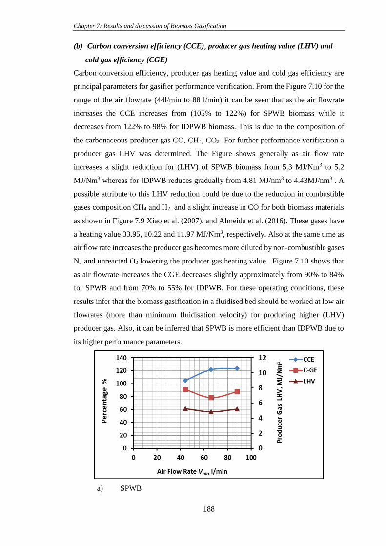
Chapter 7: Results and discussion of Biomass Gasification
188
(b) Carbon conversion efficiency (CCE), producer gas heating value (LHV) and
cold gas efficiency (CGE)
Carbon conversion efficiency, producer gas heating value and cold gas efficiency are
principal parameters for gasifier performance verification. From the Figure 7.10 for the
range of the air flowrate (44l/min to 88 l/min) it can be seen that as the air flowrate
increases the CCE increases from (105% to 122%) for SPWB biomass while it
decreases from 122% to 98% for IDPWB biomass. This is due to the composition of
the carbonaceous producer gas CO, CH4, CO2 For further performance verification a
producer gas LHV was determined. The Figure shows generally as air flow rate
increases a slight reduction for (LHV) of SPWB biomass from 5.3 MJ/Nm3 to 5.2
MJ/Nm3 whereas for IDPWB reduces gradually from 4.81 MJ/nm3 to 4.43MJ/nm3 . A
possible attribute to this LHV reduction could be due to the reduction in combustible
gases composition CH4 and H2 and a slight increase in CO for both biomass materials
as shown in Figure 7.9 Xiao et al. (2007), and Almeida et al. (2016). These gases have
a heating value 33.95, 10.22 and 11.97 MJ/Nm3, respectively. Also at the same time as
air flow rate increases the producer gas becomes more diluted by non-combustible gases
N2 and unreacted O2 lowering the producer gas heating value. Figure 7.10 shows that
as air flowrate increases the CGE decreases slightly approximately from 90% to 84%
for SPWB and from 70% to 55% for IDPWB. For these operating conditions, these
results infer that the biomass gasification in a fluidised bed should be worked at low air
flowrates (more than minimum fluidisation velocity) for producing higher (LHV)
producer gas. Also, it can be inferred that SPWB is more efficient than IDPWB due to
its higher performance parameters.
a) SPWB

Chapter 7: Results and discussion of Biomass Gasification
189
b) IDPWB
Figure 7. 10 Effect of air flowrate on performance parameters: a) for SPWB biomass material
and b) For IDPWB biomass material
(c) Producer gases yield (GY)
Figure 7.11 (a) and (b) highlights the effect of the air flowrate (air velocity) bed material
on the gases yield for two biomass materials. It can be seen that for SPWB, the total gas
yield was slightly decreased from 3.32 to 3.2Nm3/kg feed db, while for IDPWB as
shown in Figure (b) the total gas yield was slightly decreased from 2.82 to 2.48Nm3/kg
feed db. For SPWB, the gas yield for each individual gas: N2 stayed constant at
1.59Nm3/kg feed db, CO2 was slightly increased from 0.32 to 0.37 and then decreased
to 0.28nm3/kg feed db, CO increased a little from 0.71 to 0.72, CH4 approximately
stayed constant at 0.14Nm3/kg feed db, H2 decreased slightly 0.41 to o.35 Nm3/kg feed
db and O2 decreased from 0.15 to 0.09 and then increased to 0.15Nm3/kg feed db. For
IDPWB the gas yield of the individual gases: N2 stays constant at 1.46 nm3/kg feed db,
CO an CO2 CH4, H2, and O2 decreased slightly from 0.39 to 0.38, from 0.4 to 0.31, from
0.15 to 0.1, from 0.26 to 0.6 and from 0.12 to 0.06 Nm3/kg feed db, respectively. It can
be concluded that a higher gas yield can be obtained at low air flowrate 44l/min. In
comparison with, SPWB produced higher gas yield than IDPWB. This finding is agreed
with the finding published by (Xiao et al. 2007) for polypropylene air gasification. The
yield of the producer gas in (wt/wt pp) was slightly decreased as fluidisation velocity
increased. At ER=0.3 and Uo/Umf=3.0, the gas yield was between 2.79 and 2.88 Nm3/kg
feed db.

Chapter 7: Results and discussion of Biomass Gasification
190
a) SPWB
b) IDPWB
Figure 7. 11 Effect of air flowrate on gas yield: a) For SPWB biomass material and b) For
IDPWB biomass material
(d) Gases ratios
Figure 7.12 (a) and (b) presents the effect of air flowrate on the gases ratios in producer
gas for both biomass feedstock materials. These ratios can consider as a mean for
expressing and assessing the producer gas quality. From the Figure 7.12, it can be seen
that the general trends of ratios for both biomass are similar. CO/CO2 ratio increased
from 2.18 to 2.54 for SPWB and from 0.98 to 1.2 for IDPWB as air flowrate increased.
The ratios 2.54 and 1.2 were maximum ratio that were achieved by both biomass at the
highest air flowrate. These high ratios confirm the gasification reactions due to partial

Chapter 7: Results and discussion of Biomass Gasification
191
oxidation and low CO2 producing compared to CO. The high difference in this ratio
between two biomass refers to the occurrence of combustion reactions for IDPWB
(which was also confirmed by H2/CO2, 0.64 to 0.51 along the flow rate interval)
compared to SPWB (which has H2/CO2, 1.26 to 1.24). For IDPWB, H2/CO2 and
CH4/CO2 ratios indicate to less amount of H2 and CH4 compared to CO2. The H2/CO
ratio is an important ratio to specify the syngas quality. From the Figure 7.12 it can be
seen that this ratio is less than 1.0 and decreases (from 0.58 to 0.49 for SPWB and from
0.66 to 0.42 for IDPWB) as air flowrate increases for both biomass. From these results,
it is possible to conclude that the water-gas shift reaction was not active due to
insufficient quantities of H2O. Thus, for increasing H2 gas in producer gas a specific
amount of steam or a moist biomass or moist air should be introduced. It can be
concluded that according to syngas utilization a low air flowrate is preferred to produce
high H2.
a) SPWB

Chapter 7: Results and discussion of Biomass Gasification
192
b) IDPWB
Figure 7. 12 Effect of air flowrate on producer gases ratios: a) For SPWB biomass material and
b) For IDPWB biomass material
7.2.4.3 Effect of particle size of sand bed material
Table 7. 4 Operating conditions for sand bed material particle size parameter experimental tests:
a) For SPWB
Operating Parameters Bed Material (Sand) Particle Size, µm
300-425 425-500 500-600
1- Air Flowrate l/min (kg/hr) 44 (3.18) 75 (5.45) 95 (6.72)
2- Reaction Bed Temperature T2, oC 360 360 360
3- Equivalence Ratio ER 0.43 0.43 0.43
4- Biomass solid Fuel Particle Size, µm 600-850 600-850 600-850
5- Static Bed Height Hs, cm 6.225 6.225 6.225
6- Mass Rate of biomass Feeding, kg/hr 1.2 2.05 2.6
7- (MAFR)stoichiometric For SPWB 6.2 6.2 6.2
8- Air superficial velocity Uo, cm/sec 13.56 23.11 29.28
b) For IDPWB
Operating Parameters Bed Material (Sand) Particle Size, µm
300-425 425-500 500-600
1- Air Flowrate l/min (kg/hr) 44 (3.18) 75 (5.45) 95 (6.72)
2- Reaction Bed Temperature T2, oC 360 360 360
3- Equivalence Ratio ER 0.381 0.381 0.381
4- Biomass solid Fuel Particle Size, µm 600-850 600-850 600-850
5- Static Bed Height Hs, cm 6.225 6.225 6.225
6- Mass Rate of biomass Feeding, kg/hr 1.32 2.26 2.78
7- (MAFR)stoichiometric For IDPWB 6.352 6.352 6.352
8- Air superficial velocity Uo, cm/sec 13.56 23.11 29.28
Chapter 7: Results and discussion of Biomass Gasification
193
(a) Producer gas composition (PGC) for two biomass materials
According to the operating conditions which have been shown in Table 7.4(a) and (b),
Figure 7.13 (a) and (b) presents the effect of the particle size of the sand bed material
on the producer gas composition for two biomass materials for constant operating
conditions. It can be seen, in general, that the trend of the effect of sand particle size for
both biomass for all gases are similar. As particle size increases from 300-425µm to
(500-600) µm CO composition increases slightly from 21.3% to 23.2% for SPWB and
from 11% to 12.5% for IDPWB. Whereas, for CO2, CH4 and H2 their composition
decrease slightly from (9.8% to 8.8%), (4.4%to 4%) and (12.3% to 11.9%),
respectively, for SPWB and from (6.5% to 5%), (10.2% to 10 %) and (5% to 3%),
respectively for IDPWB. In addition, it can be shown that SPWB provided higher
producer gas quality than IDPWB and the latter was more affected by bed particle size
than former. This can be due to the high difference in chemical and physical properties
between two biomass materials as shown in Table 4.4. The slight effect of the sand bed
particle size on the producer gas quality can be attributed to firstly, the sand is un-
catalytically active (inert) material which does not play any chemical conversion role
in enhancement for tar conversion and producer gas quality so for this case there is no
clear effect of particle size. Secondly, from the hydrodynamic aspect when the particle
size increases the minimum fluidisation velocity Umf of the air increases as explained in
(Chapter 6). For a specific air superficial velocity Uo, Uo=1.25Umf was taken for each
experiment. As shown in Chapter 6-Section 6.2.3, for 300-425µm sand particle size
Umf= 10.875cm/sec= 35.3l/min and for Uo=1.25Umf, Uo = 44l/min. Therefore, for the
particle size 425-500µm and 500-600µm, which has Umf =18.665cm/sec= 60.6l/min and
Umf-=23cm/sec = 74.6l/min and their Uo will be 75.75l/min and 93.25l/min,
respectively. This means that for the last two particle size more air is required than for
300-425µm, 1.72 Uo = 75.75l/min and 2.12Uo = 93,25l/min, respectively. This will give
the same effect of the increasing air flowrate as shown in previous section. However, at
the same time this air increase needs an increase in the biomass feeding mass flowrate
to keep ER constant. This biomass increase (41.9%) for 425-500µm and 52.8% for 500-
600µm will lead to an increase in the mass fraction of biomass in the bed and thereby
increases the minimum fluidisation velocity of the bed mixture. These hydrodynamic
changes will weaken the bed fluidisation behaviour as particle size increases and finally,
will weaken gasifier performance.

Chapter 7: Results and discussion of Biomass Gasification
194
The function of the bed material is to hold heat between fuel particles and provide a
high transfer capacity. This high transfer capacity ensures sufficiently high heating rates
and homogeneous temperature distribution and therefore good control of flue gas or
producer gas composition (Folkeson 2014). Due to their high surface area, small bed
particles size can give a high heat and mass transfer and high contact between bed and
biomass particles leading to high rate of reactions. (Kern et al. 2013) attributed the
highest H2 content in producer gas, in addition to the steam effect, to the increase of the
catalytic activity of the fine olivine particles 370µm due to their increased specific
surface area compared to the coarse particles of 510µm diameter. In addition, they
concluded that the significant effect of the particle size on the tar content could not be
found.
Koppatz et al. (2012) reported in their research that there was no common agreement in
the literature where the principal properties, which control the bubbling fluidised bed
characterization such as bubble size, bubble rise velocity and bed expansion, are to be
considered independent of the mean particle size or not. They concluded that general
gas composition (main gaseous components) was found to be broadly independent of
the bed particle size. This agrees with the results for SPWB but disagrees for IDPWB.
This disagreement might be due to their irregular needle shape, which has a higher
aspect ratio than SPWB particles.
a) SPWB

Chapter 7: Results and discussion of Biomass Gasification
195
b) IDPWB
Figure 7. 13 Effect of particle size of sand bed on producer gas composition (PGC): a) For SPWB
biomass material and b) For IDPWB biomass material
(b) Carbon conversion efficiency (CCE), cold-gas efficiency (CGE), and producer
gas heating value (LHV)
Figure 7.14 (a) and (b) shows the effect of the particle size of sand bed material on the
performance parameters CCE, CGE and LHV for two biomass materials. It can be seen
that for SPWB there is no effect of particle size, whereas for IDPWB the parameters
decline moderately as particle size increases. For SPWB the performance parameters
CGE and LHV were approximately levelled off at 109% and 6.2MJ/Nm3db,
respectively, whereas CCE was slightly increased from128 to 131%. For IDPWB the
relation is different where CCE, CGE and LHV are declined, approximately from (83%
to 75%), (48% to 36%) and (3.65 to 3.04 MJ/Nm3 db), respectively as the sand particle
size increases. Comparatively, gasification with SPWB gives high performance than
IDPWB. Using small particle size of the bed is preferable for producing high LHV gas,
high CGE and CCE for IDPWB. However, it is a little different for SPWB.

Chapter 7: Results and discussion of Biomass Gasification
196
a) SPWB
b) IDPWB
Figure 7. 14 Effect of particle size of sand bed on CCE, CGE and LHV performance parameters:
a) For SPWB biomass material and b) For IDPWB biomass material
(c) Producer gas yield (GY)
Figure 7.15 (a) and (b) highlights the effect of the particle size of the sand bed material
on the gases yield for two biomass materials. It can be seen that for SPWB, the total gas
yield was stayed constant on 3.3 Nm3/kg feed db as sand particle size was increased;
while for IDPWB, the total gas yield was decreased moderately from 2.5 to 2.25Nm3/kg
feed db. For SPWB the gas yield for most individual gas stay constant. CO showed
highest gas yield compared to H2, CO2, CH4 and O2. For IDPWB, the individual gases,
except N2, CO2 and CO, slightly increased along the range of the sand particle size. In
comparison with, SPWB produced higher CO and H2 gas yield than IDPWB. The small

Chapter 7: Results and discussion of Biomass Gasification
197
effect of particle size on gasifier performance and gas yield especially for SWPB can
be attributed to the constancy of the ER for the three ranges of sand particle size.
Although the larger particle size needs more air flowrate for fluidisation, but due to the
constant ER, its effect is decreased. Hydro-dynamically, it was thought that these
particle sizes were approximately convergent. Consequently, this was resulted in a
similar hydrodynamic behaviour.
a) SPWB
b) IDPWB
Figure 7. 15 Effect of particle size of sand bed on gases yield (GY): a) For SPWB biomass
material and b) For IDPWB biomass material.
(d) Gases Ratios
Figure 7.16 (a) and (b) highlights the effect of the particle size of the sand bed material
on the gases ratio for two biomass materials. It can be shown that SPWB implemented

Chapter 7: Results and discussion of Biomass Gasification
198
high CO/CO2 and H2/CO2 ratios in comparing with IDPWB, whereas the other ratios
are less than 0.6 for both biomass. For both biomass, the general trend of the CO/CO2
ratio increases gradually from 2.3 to 2.65 for SPWB and slightly increases from 1.05 to
1.15 for IDPWB as particle size increases. This ratio gives an indication that CO amount
is more than CO2 especially for large particle size. Due to the partial oxidation
environment and low residence time, due to the air flowrate increase due to the particle
size increase, these resulted in producing high CO and reducing H2 and CO2. For SPWB,
the H2/CO ratio decreased slightly from 0.65 to 0.5, CH4/CO2 increased slightly from
0.4 to 0.45 and CH4/CO stays constant at 0.2. For IDPWB. H2/CO decreased from 0.6
to 0.5, CH4/CO2 and CH4/CO decreased a little from 4.5 to 3.0. The result confirms
that IDPWB produced low CO and H2 gas in comparing with SPWB. The bed particle
size, (300-425)µm revealed a best H2/CO2 and H2/CO ratios for SPWB and IDPWB
producer gas.
a) SPWB

Chapter 7: Results and discussion of Biomass Gasification
199
b) IDPWB
Figure 7. 16 Effect of particle size of the sand bed on gases ratio: a) For SPWB biomass material
and b) For IDPWB biomass material
7.2.4.4 Effect of the biomass fuel particle size
Table 7. 5 Operating conditions for biomass fuel particle size parameter experimental tests
a) For SPWB
Operating Parameters Biomass Solid Fuel Particle Size, µm
300-425 600-850 1000-1180
1- Air Flowrate l/min (kg/hr) 30 (2.17) 30 (2.17) 30 (2.17)
2- Reaction Bed Temperature T2, oC 360 360 360
3- Bed Material (Sand) Particle Size, µm 300-425 300-425 300-425
4- Equivalence Ratio ER 0.55 0.55 0.55
5- Static Bed Height Hs, cm 6.225 6.225 6.225
6- Mass Rate of biomass Feeding, kg/hr 0.641 0.641 0.641
7- (MAFR)stoichiometric For SPWB 6.2 6.2 6.2
8- Air superficial velocity Uo, cm/sec 9.25 9.25 9.25
b) For IDPWB
Operating Parameters Biomass solid Fuel Particle Size, µm
300-425 600-850 1000-1180
1- Air Flowrate l/min (kg/hr) 44 (3.18) 44 (3.18) 44 (3.18)
2- Reaction Bed Temperature T2, oC 360 360 360
3- Bed Material (Sand) Particle Size, µm 300-425 300-425 300-425
4- Equivalence Ratio ER 0.381 0.381 0.381
5- Static Bed Height Hs, cm 6.225 6.225 6.225
6- Mass Rate of biomass Feeding, kg/hr 1.315 1.315 1.315
7- (MAFR)stoichiometric For IDPWB 6.352 6.352 6.352
8- Air superficial velocity Uo, cm/sec 13.56 13.56 13.56

Chapter 7: Results and discussion of Biomass Gasification
200
(a) Producer gas composition (PGC) for two biomass materials
According to the operating conditions, which have been shown in Table 7.5 (a) and (b),
the results of the effect of the biomass particle size on the producer gas composition for
two biomass materials SPWB and IDPWB are presented in Figure 7.17 (a) and (b),
respectively. Three particle size ranges were used 300-425µm, 600-850µm and 1000-
1180µm. Generally, it can be seen that the average trend of the effect of the biomass
particle size for both biomass for most gases (CO, H2, CH4 and O2) are similar except
CO2 for SPWB, which has an opposite trend. The average trend of the composition of
the gases decreased as particle size increased: For SPWB, the gases CO from 16.5% to
14%, H2 from 13% to 9%, CH4 from 3% to 2.5% decreased, whereas CO2 increased
from 6% to 10%. For IDPWB the gases decreased gradually: for CO from 14.5% to
7.7%, H2 from 9% to 5% CO2 from 12.5% to 9.8%, CH4 from 5% to 3.5%. For the both
biomass materials, the Figure shows that the smaller particle size produced more CO,
H2, and CH4 and, less CO2 for SPWB and more for IDPWB, than the larger particles.
Three explanations may possible to interpret this particle size effect. 1) The smaller
particles have faster heating rate due to their larger surface area than large size. 2) For
smaller particle size the main control step in the pyrolysis process is reaction kinetics,
while for larger particle size the gas diffusion step is controlled because of the product
gas generated inside the particle is not easy to diffuse out (Lv et al. 2004) (Dr. Sami
Sadaka, P.E. n.d.) and (Feng et al. 2011). 3). Depending on fluidisation conditions, it
might be due to the low weight of small particles, most of them were segregated quickly
to the bed surface and entrained to the freeboard section, which was kept at high
temperature 900oC at gasifier position 44cm. In addition, the pyrolysis process is
dominated by a heat transfer process, so both particle size and shape affect the
conversion time significantly, especially for large size particles (Lu et al. 2010). These
conditions lead to high pyrolysis and gasification reactions producing high quality
gases. (Mohammed et al. 2011) attributed this effect to the greater temperature gradient
inside the particle for large particles than small particles at a given time leading to an
increase in the char and decrease in gases. It can be concluded that SPWB produced
higher CO, and H2 gases than IDPWB for this study range of biomass particle size,
whereas for CH4, the latter produced higher. Also According to this gasifier design
study and for this range of particle size the result reveals that the smaller size is more
favorable for high quality producer gas production.

Chapter 7: Results and discussion of Biomass Gasification
201
a) SPWB
b) IDPWB
Figure 7. 17 Effect of particle size of biomass fuel on producer gas composition (PGC): a) For
SPWB biomass material and b) For IDPWB biomass material
(b) Carbon conversion efficiency (CCE), cold-gas efficiency (CGE), and producer
gas heating value (LHV)
Figure 7.18(a) and (b) shows the effect of the biomass particle size on the performance
parameters CCE, CGE and LHV for two biomass materials. According to the
composition results in previous section for SPWB, it can be said that those performance
parameters increased significantly to the maximum value and decreased to the minimum
value as biomass particle size increased. They increased: CCE from 109% to 177%,
CGE from 89.48% to 136% and LHV from 4.26 to 5.53MJ/Nm3 db as particle size
increased from No 1 to No 2, respectively. Then they decreased to 100%, 65% and
3.44MJ/Nm3 as particle size increased to No 3, respectively. For IDPWB the parameters
declined significantly as particle size increased: CCE from 116% to 62%, CGE from
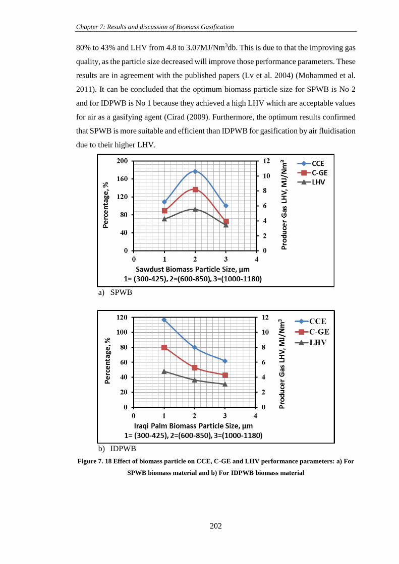
Chapter 7: Results and discussion of Biomass Gasification
202
80% to 43% and LHV from 4.8 to 3.07MJ/Nm3db. This is due to that the improving gas
quality, as the particle size decreased will improve those performance parameters. These
results are in agreement with the published papers (Lv et al. 2004) (Mohammed et al.
2011). It can be concluded that the optimum biomass particle size for SPWB is No 2
and for IDPWB is No 1 because they achieved a high LHV which are acceptable values
for air as a gasifying agent (Cirad (2009). Furthermore, the optimum results confirmed
that SPWB is more suitable and efficient than IDPWB for gasification by air fluidisation
due to their higher LHV.
a) SPWB
b) IDPWB
Figure 7. 18 Effect of biomass particle on CCE, C-GE and LHV performance parameters: a) For
SPWB biomass material and b) For IDPWB biomass material

Chapter 7: Results and discussion of Biomass Gasification
203
c) Producer gas yield (GY)
Figure 7.19 (a) and (b) highlights the effect of the particle size of the biomass fuel on
the gas yield for two biomass materials. Similarly, to gas composition it can be seen
that for SPWB, the general average trend of the gas yield decrease as biomass particle
increase, except for CO2 yield there is a slight increase from 0.1 to 0.2 Nm3/kg feed db
and N2 stayed constant on 2.0 Nm3/kg feed db. For total gas yield, the decrease was
from 3.9 to 3.6Nm3/kg feed, while for the rest gases the decrease was CO from 0.65 to
0.49, CH4 from 0.11 to 0.09, H2 from 0.5 to 0.32 and O2 from 0.36 to 0.25Nm3/kg feed
db. For IDPWB the general trend for all gases is moderately decreased except N2, which
stayed constant at 1.63Nm3/kg feed db and O2 from 0.22 to 0.35Nm3/kg feed db. The
total gas yield decreased moderately from 3.2 to 2.7Nm3/kg feed, whereas the rest gases
decreased slightly: CO from 0.46 to 0.21, CO2 from 0.41 to 0.26, CH4 from 0.2 to 0.1,
H2 from 0.29 to 0.14. Again, the gas yield gives a good indication for gasifier
performance. It can be confirmed that the smaller biomass particles produce higher gas
yield than larger particles per each kg of biomass. In addition, the SPWB biomass fuel
is more efficient than IDPWB due to its higher elemental composition.
a) SPWB

Chapter 7: Results and discussion of Biomass Gasification
204
b) IDPWB
Figure 7. 19 Effect of particle size of biomass feedstock on gases yield: a) for SPWB biomass
material and b) for IDPWB biomass material
(d) Gases Ratios
Figure 7.20 (a) and (b) highlights the effect of the particle size of the biomass feedstock
on the gas ratio for two biomass materials. It can be shown that as particle size increased
CO/CO2 and H2/CO2 ratios decreased dramatically from 2.6 to 1.4 and from 2 to 0.9,
respectively for SPWB and from 1.13 to 0.83 and from 0.7 to 0.53, respectively for
IDPWB. H2/CO and CH4/CO2 ratios decreased slightly from 0.75 to 0.68 and from 0.45
to 0.27, respectively for SPWB whereas, CH4/CO ratio remained constant on 0.15. For
IDPWB H2/CO and CH4/CO increased a little from 0.62 to 0.66 and from 0.44 to 0.46,
respectively, while CH4/CO2 decreased a little from 0.48 to 0.38. These ratios give an
indication of the heterogeneous and homogenous reactions that may occur inside the
bed and freeboard sections. From the values of CO/CO2, H2/CO2 for both biomass at
smaller particle size indicates that the exothermic partial oxidation reactions, R2-R6,
are dominant because these reactions are related to the particle itself and thereby the
rate of devolatilisation rate, for higher hydrocarbon yield. Furthermore, H2/CO and
CH4/CO ratios indicate the contributions of the exothermic reactions, water gas shift R8
and Methanation R12. The shortage of the H2 gas may be due to the Methanation
reaction because it consumes three times the amount of H2 compared to CO. It can be
inferred that SPWB produced more CO rich syngas than IDPWB, especially at smaller
particle size. In addition, the observed high CO/CO2, H2/CO2 and CH4/CO2 ratios

Chapter 7: Results and discussion of Biomass Gasification
205
emphasizes the partial oxidation existence for both biomass, especially for smaller
particle size.
a) SPWB
b) IDPWB
Figure 7. 20 Effect of particle size of the biomass feedstock on gases ratio: a) for SPWB biomass
material and b) for IDPWB biomass material.

Chapter 7: Results and discussion of Biomass Gasification
206
7.2.4.5 Effect of the bed static height Hs
Table 7. 6 Operating conditions for static bed height parameter experimental tests:
a) For SPWB
Operating Parameters Static Bed Height Hs, cm
4.15=0.5D 6.225=0.75D 8.3=1D
1- Air Flowrate l/min (kg/hr) 44 (3.18) 44 (3.18) 44 (3.18)
2- Reaction Bed Temperature T2, oC 360 360 360
3- Bed Material (Sand) Particle Size, µm 300-425 300-425 300-425
4- Biomass solid Fuel Particle Size, µm 600-850 600-850 600-850
5- Equivalence Ratio ER 0.42 0.42 0.42
6- Mass Rate of biomass Feeding, kg/hr 1.192 1.192 1.192
7- (MAFR)stoichiometric For SPWB 6.2 6.2 6.2
8- Air superficial velocity Uo, cm/sec 13.56 13.56 13.56
b) For IDPWB
Operating Parameters Static Bed Height Hs, cm
4.15=0.5D 6.225=0.75D 8.3=1D
1- Air Flowrate l/min (kg/hr) 44 (3.18) 44 (3.18) 44 (3.18)
2- Reaction Bed Temperature T2, oC 360 360 360
3- Bed Material (Sand) Particle Size, µm 300-425 300-425 300-425
4- Biomass solid Fuel Particle Size, µm 600-850 600-850 600-850
5- Equivalence Ratio ER 0.381 0.381 0.381
6- Mass Rate of biomass Feeding, kg/hr 1.315 1.315 1.315
7- (MAFR)stoichiometric For IDPWB 6.352 6.352 6.352
8- Air superficial velocity Uo, cm/sec 13.56 13.56 13.56
(a) Producer gas composition (PGC) for two biomass materials
According to the operating conditions, which have been shown in Table 7.6 (a) and (b),
Figure 7.21 (a) and (b) presents the influence of the static bed height on the producer
gas composition for two biomass SPWB and IDPWB, respectively. Three static bed
height Hs were used: 4.15cm, 6.225cm and 8.3cm, which correspond to Hs/D ratio: 0.5,
0.75 and 1, respectively, where D is the bed diameter=8.3cm. From Figure 7.21 (a) and
(b) for SPWB, it can be seen that the effect on producer gas composition was as follows:
the trends of production CO, H2 and CH4 are similar. Their lowest composition was at
Hs = 4.15cm, whereas the highest was at Hs = 6.225cm. CO2 stayed constant along Hs
range. In addition, the sequence of the gas composition is CO> H2> CO2> CH4 for all
Hs range. For IDPWB the trend of the gases is different, CO decreased steadily while
H2 increased steadily along Hs range. Whereas CO2 and CH4 stayed constant. The
sequence of the gases at Hs = 4.15cm is CO> CO2> H2 >CH4, whereas at Hs = 8.3cm
the sequence is CO2> CO> H2 > CH4.

Chapter 7: Results and discussion of Biomass Gasification
207
There are several possible explanation for these results. The observed low value of the
gas composition of CO, H2, CH4 and O2 at the bed height 4.15cm for both biomass
materials compared to other heights, except CO for IDPWB was higher, might be
attributed to the biomass feeding position. For this bed height, 0.5D= 4.15cm, the
biomass feeding was on-bed, the biomass was fed directly on the bed surface, unlike
other two heights where the feeding was in-bed, 2.075cm under the bed surface for the
bed height 0.75D=6.225cm and under 4.15cm for the bed height 1D=8.3cm. In both
cases, the feeding position was at 0.5D= 4.15cm above distributor plate. In-bed feeding
gives an actual fluidisation and thereby results in robust mixing and sufficient contact
of the biomass with bed particles enhancing the devolatization, gasification tar cracking
and reforming reactions and therefore increasing the conversion efficiency (Wilk et al.
2013) (Rapagnà et al. 2008).
For CO2 gas this constant concentration for both biomass materials might be attributed
to the abundant availability of O2 at the bottom of the bed height due to a small size
and low rise velocity of bubbles (Ross et al. 2007). In addition, the diffusion of the
oxygen from the bubbles , especially at the higher bed position is low (Basu 2006), so
it might be the same amount of CO2 was produced due to the combustion reactions R2.3
and R2,4. The bed height also affects the residence time of the produced gases in the
dense bed, where for a specific fluidisation flowrate a longer residence time could be
achieved by increasing the bed height, which subsequently enhances the cracking
reactions of tar and hydrocarbons (Xiao et al. 2007).
For H2 gas, the bed length 0.75D and 1D improved H2 production comparing to 0.5D
bed length. This might be due to the feeding position, where for the later length there
was no residence time for reactions inside the bed due to direct biomass feeding to the
bed surface. At the same time the thermal cracking of the tar was not effective at this
bed height to produce enough hydrogen (Sudipta 2013). For the 1D bed height,
although it has longer residence time than 0.75D length, there is no high difference in
composition of H2. This is might be due to the negative bubble effects at higher bed
heights. In addition, it could be said that there was no high difference in the residence
time of the two lengths, 0.75D and 1D. For CH4 gas for both biomass, there was a small
effect of the bed height, especially at 0.75D and 1D heights. The low value of CH4 at
0.5D height it might be attributed to the position of the feeding point position, as has
been explained above, where there was a poor hydrogen gasification reaction R11 due
to a lower amount of H2 and carbon. In addition, it can be observed that production of

Chapter 7: Results and discussion of Biomass Gasification
208
CH4 from IDPWB was higher than SPWB. This it might be due to the difference in their
physical and chemical properties. For O2 gas it can be seen a high consuming at 0.5D
height for IDPWB. This might be due to high partial oxidation of exothermic reactions
as shown in high CO production.
In overall, for this range of bed height the results show that the effect of the bed height
on producer gas composition is not highly significant.
a) SPWB
b) IDPWB
Figure 7. 21 Effect of the bed static height Hs on the producer gas composition (PGC): a) for
SPWB biomass material and b) for IDPWB biomass material
(b) Carbon conversion efficiency, cold-gas efficiency, and producer gas heating value
Figure 7.22 (a) and (b) provides the effect of the static bed height Hs on the performance
parameters for two biomass SPWB and IDPWB, respectively. It can be observed that
the performance parameters CCE, LHV and CGE increased from 112% to 148%, 4.71

Chapter 7: Results and discussion of Biomass Gasification
209
to 5.76 MJ/Nm3 db and 81% to 114% for SPWB, while from 142% to 147%, 5.24 to
5.42MJ/Nm3 db and 84% to 91% for IDPWB as bed height increased from 0.5D to
0.75D, respectively. For bed height increasing from 0.75D to 1D the results show
decreasing in CCE, LHV and CGE to 130%, 5.29MJ/Nm3 db, respectively and 100%
for SPWB, while to 134%, 4.97MJ/Nm3 db and 82% for IDPWB, respectively.
These results might be possibly explained that the observed increasing and decreasing
of these performance parameters along the three bed heights can be linked to the
increasing and decreasing of CO, CO2, H2 and CH4 concentration in producer gas, as
revealed in Figure 7.21-(a) and (b), as discussed in previous section. As has been shown
in the calculation procedure for CCE, LHV and CGE in Chapter 5-Section 5.8.6, the
gases CO, CO2, and CH4 represent the carbon conversion in producer gas, whereas the
gases CO, H2 and CH4 represent the chemical energy conversion, LHV and CGE, where
each of them has a specific heating value. Therefore, from the Figure, it can be found
that for SPWP, in all cases, the performance parameters for two bed heights 0.75D and
1D were higher than for 0.5D. This might be due to the position of the feeding point,
which for 0.5D the feeding was on–bed, whereas for the others was in-bed. This
difference mainly affected the residence time and bed hydrodynamic behaviour.
However, for the other bed heights the difference may be mainly affected by the bed
hydrodynamic conditions due to the creation of larger volume bubbles in the higher bed
height. The larger bubble size produce a faster bubble velocity and a less gas-solid
contact time (Van Den Enden and Lora 2004) and (Xiao et al. 2007). At the same time
the maximum values of those three performance parameters was obtained at 0.75D. The
same finding was also obtained for IDPWB, 0.75D height has a maximum values, but
the two heights, 0.5D and 1D, were in competition.

Chapter 7: Results and discussion of Biomass Gasification
210
a) SPWB
b) IDPWB
Figure 7. 22 Effect of the bed static height Hs on CCE, CGE and LHV performance parameters:
a) for SPWB biomass material and b) for IDPWB biomass material
(c) Gases Ratios
Figure 7.23 (a) and (b) provides the effect of the bed height on the gases ratio for two
biomass materials. It can be shown that SPWB implemented maximum CO/CO2, 2.3,
at 0.75D bed height and decreased to 2.1 at 1D. H2/CO2 was increased from 1.25 at
0.5D and approximately levelled off at ratio=1.5 at 0.75D and 1D. H2/CO increased
slightly along the bed height from 0.62 to 0.7. A slight increase for CH4/CO2 ratio from
0.3 to 0.4 at 0.75D and then a little decrease to 0.35 at 1D was observed. CH4/CO
remained constant at 0.18 along the bed height. For IDPWB Figure (b) shows mostly
low gas ratio, less than one. CO/CO2 ratio decreased gradually along the range of bed

Chapter 7: Results and discussion of Biomass Gasification
211
height from 1.7 to 0.9, H2/CO increased gradually from 0.5 to 0.8, H2/CO2 increased
slightly from 0.55 at 0.5D and then levelled off at 0.7 and CH4/CO and CH4/CO2 ratios
show approximately identical and constant trend along the bed height range at 0.2. The
possible explanation for these results can be linked to the composition distribution for
the gases CO, CO2, H2 and CH4, which has been explained in Section 7.2.4.5-(a). A
further observation that can be obtained from the Figure is higher CO/CO2 and H2/CO2
ratios for SPWB than IDPWB, whereas for H2/CO ratio was approximately the same.
Overall, for this range of bed height it can be concluded that there is no high significant
effect, especially at 0.75D and 1D due to their position feeding point under bed surface.
The ratio of H2/CO is differently affected by the operating parameters in the gasification
processes. In order to this, the ratio of H2/CO has been selected as a benchmark of
efficiency to evaluate the purpose of applying produced syngas in methanol synthesis
process. In addition, the ratio of CO/CO2 is selected as a scale to measure the efficiency
of the process and to contemplate the competition of the gasification/combustion,
(Ravaghi-ardebili et al. 2014).
a) SPWB

Chapter 7: Results and discussion of Biomass Gasification
212
b) IDPWB
Figure 7. 23 Effect of the bed static height Hs on the gas ratio: a) for SPWB biomass material and
b) for IDPWB biomass material.
(d) Producer gas yield (GY)
Figure 7.24 (a) and (b) highlights the effect of the static bed height on the gases yield
for two biomass materials. It can be observed that for SPWB, the total gas yield was
increased significantly from 3.18 to 3.8Nm3/kg feed db as bed height increased from
0.5D to 0.75D and then decreased moderately to 3.7Nm3/kg feed db at 1D bed height.
For IDPWB the total gas yield was increased slightly from 2.9 to 3.1Nm3/kg feed db as
bed height increased from 0.5D to 0.75D and then approximately levelled off at
3Nm3/kg feed db at 1D bed height. Furthermore, the gas yield observation for each gas
along the three bed heights was as follows: For SPWB, the maximum yield was for
CO= 0.84 at 0.75D, H2= 0.6 at 0.75D, CH4=0.16, CO2 and N2 approximately stayed
constant on 0.35 and 1.59Nm3/kg feed db along bed height interval, respectively. For
IDPWB the gas yield for each gas was; CO and CO2 approximately stayed constant
at=0.47, H2 and O2 increased slightly from 0.26 to 0.34 and from 0.05 to 0.13,
respectively, CH4 approximately stayed constant at 0.2 Nm3/kg feed db and N2 stayed
constant on 1.46Nm3/kg feed db.
As discussed before the yield results completely depend on the producer gas
composition. In general, from the Figures (a) and (b) it can be seen that SPWB achieved
gases yield higher than IDPWB. This can be linked to the higher gas composition as has
shown in Figure 7.21 (a) and (b) and discussed in Section 7.2.4.5-(a).

Chapter 7: Results and discussion of Biomass Gasification
213
a) SPWB
b) IDPWB
Figure 7. 24 Effect of static bed height Hs on gases yield (GY): a) for SPWB biomass material and
b) for IDPWB biomass material

Chapter 7: Results and discussion of Biomass Gasification
214
7.2.4.6 Effect of the equivalence ratio
Table 7. 7 Operating conditions for equivalence ratio parameter experimental tests
a) For SPWB
Operating Parameters Equivalence Ratio ER
0.2 0.31 0.5 0.55
1- Air Flowrate l/min (kg/hr) 30 (2.17) 30 (2.17) 30 (2.17) 30 (2.17)
2- Reaction Bed Temperature T2, oC 360 360 360 360
3- Bed Material (Sand) Particle Size, µm 300-425 300-425 300-425 300-425
4- Biomass solid Fuel Particle Size, µm 600-850 600-850 600-850 600-850
5- Static Bed Height Hs, cm 6.225 6.225 6.225 6.225
6- Mass Rate of biomass Feeding, kg/hr 1.74 1.14 0.7 0.64
7- (MAFR)stoichiometric For SPWB 6.2 6.2 6.2 6.2
8- Air superficial velocity Uo, cm/sec 9.25 9.25 9.25 9.25
b) For IDPWB
Operating Parameters Equivalence Ratio ER
0.2 0.277 0.381 0.45
1- Air Flowrate l/min (kg/hr) 44 (3.18) 44 (3.18) 44 (3.18) 44 (3.18)
2- Reaction Bed Temperature T2, oC 360 360 360 360
3- Bed Material (Sand) Particle Size, µm 300-425 300-425 300-425 300-425
4- Biomass solid Fuel Particle Size, µm 600-850 600-850 600-850 600-850
5- Static Bed Height Hs, cm 6.225 6.225 6.225 6.225
6- Mass Rate of biomass Feeding, kg/hr 2.5 1.81 1.32 1.11
7- (MAFR)stoichiometric For IDPWB 6.352 6.352 6.352 6.352
8- Air superficial velocity Uo, cm/sec 13.56 13.56 13.56 13.56
(a) Producer Gas Composition for Two Biomass Materials
According to the operating conditions which have been shown in Table 7.7 (a) and (b),
the results of the effect of ER on the producer gas composition is revealed in Figure
7.25-(a) and (b) for both biomass feedstock SPWB and IDPWB, respectively. ER was
changed by changing biomass feed rate at a fixed air flowrate. For SPWB it can be seen
that as ER increased in the interval of from 0.2 to 0.31 all producer gases, CO, H2, CO2
and CH4 were decreases from 22% to 18%, 16% to 12%, 8.8 to 7% and 5.8% to 3.5%,
respectively. Thereafter, as ER increased in the interval of from 0.31 to 0.55 the gases
increased to 22.5%, 16.7%, 10.8% and 4.4% respectively, whereas O2 increased from
7.2% to 9.8% and then decreased to 3.5%.
For IDPWB the trend of the producer gas composition in ER interval (0.31-0.55) is
different compared to SPWB. It can be seen that as ER increased in the interval (0.2 to
0.277) CO, CO2, H2 and CH4 were decreased from 16.5% to 13.5%, 14.7% to 12.8%,
9.6% to 8.2% and 7.7 to 6.1%, respectively, whereas O2 remained constant at 6.6%. For
Chapter 7: Results and discussion of Biomass Gasification
215
increase ER in interval (0.227 to 0.38), the gases were constant, respectively, while O2
decreased to 5.6%. For the last interval (0.38 to 0.45) as ER increased the gases
decreased again from 12.9% to 11.2%, 13.3% to 12.3%, 8.5% to 7.1% and 6.1 to 4.8%,
respectively, while O2 increased a little to 6.2%. For this biomass, the trend of the results
are agree with the results of Hg et al. (2016) for sawdust and pigeon pea biomass air
gasification for ER interval (0.35 to 0.61) for the former and (0.38 to 0.68) for the latter.
In addition, for ER range (0.21 to 0.32), which was studied for the same principle of
this study by changing fuel and keeping constant airflow rate, at 770oC. The results of
the researchers (Lahijani and Zainal 2011) are in agreement with this study results for
the producer gas composition for both biomass material except the CO2 trend, which
increased for all their ER ranges.
There are several explanations for these results. The high gas concentration for both
biomass materials at ER= 0.2 compared to others ER, especially for IDPWB, might be
attributed to the high amount of biomass fuel feeding for this ER. However, it can be
expected that a high amount of volatile matter might be released inside the bed, reaction
R2.1, and with partial oxidation environment exothermic homogenous reactions occur
producing a high amount of the CO and H2 compared to CO2 and CH4, according to
reactions R2.1, R2.2-R2.6. Also within these conditions, the water gas shift reaction
R2.8 occurs due to H2O releasing by R2.5. Furthermore, the high temperature, up to
900oC in the freeboard, and long residence time inside the freeboard section are high
enough for tar and high hydrocarbon thermal cracking and homogenous gas reactions,
secondary tar reactions, which are indicated by the increase in levels of CO, H2 and CH4
(Sudipta 2013) and (W.A.W.K. Ghani1, 2*, R.A. Moghadam1, M.A.M. Salleh1, 2
2012). The gas concentrations, which were released by SPWB, were higher than
IPDWB. This is may be because of the high volatile matter of the former biomass as
shown in Table 4.4. In addition, the air flowrate, which was used for SPWB was lower
than air flowrate for IDPWB, 30l/min for the former and 44l/min for the latter. This low
flowrate increased the residence time in the bed and freeboard sections. Also the
difference in the chemical composition of each component of lignocellulosic (cellulose,
hemicelluloses and lignin) biomass might affect the devolatilisation rates (Chhiti and
Kemiha 2013).
For SPWB, the amount of produced CO2 was much less than H2 and CO for all
investigated ER values. This may be attributed to the dry reforming endothermic
reactions of high hydrocarbons, R2.14, in the freeboard section resulting in high

Chapter 7: Results and discussion of Biomass Gasification
216
amounts of CO and H2 and reduction of CO2. Also, the endothermic Boudouard reaction
R2.13 could be expected to enhance in the freeboard section due to the conditions and
the availability of the entrained porous char in freeboard (Feng et al. 2011). This
condition may also available for IDPWB. This due to the two exothermic reactions
Methanation R2.12 and hydrogen gasification R2.11 producing CH4 and the
endothermic tar decomposition reaction that might be occurred in freeboard section
(Ghani A.K. et al. 2009). This can be confirmed by the high concentration of CH4 in
producer gas for this ER value 0.2. Furthermore, it can be observed that CH4
approximately stayed constant at ER interval (0.31-0.55) for SPWB. It can be attributed
to the balance of CH4 consumption, R2.10, and its generation, whereas for IDPWB CH4
continuously declined at ER interval (0.227-0.45). Likewise, for this biomass the
decreasing of biomass feeding along the ER interval may have a high contribution in
the decrease of the producer gas composition due to their low volatile matter compared
to SPWB.
On the hydrodynamic aspect, for these observed results, it can be interpreted that,
according to the ER calculation method, ER was increased as biomass fuel decreased
and thereby the mass fraction of the biomass was decreased. As shown in chapter 6,
biomass fraction in the bed mixture affect the fluidisation quality, where the bubble
phase characteristics affect the particle mixing and segregation in the fluidised bed
reactor and thereby affects the performance of the biomass gasifier (Fotovat et al. 2015).
Increasing biomass mass fraction is driving to create more homogenous distribution of
small bubbles across the bed cross –section leading to improve fluidisation quality and
thereby improving gasification performance (Fotovat et al. 2013). According to their
fluidisability, the low performance of IDPWB compared to SPWB might be attributed
to the higher irregularity in shape and higher aspect ratios of IDPWB particles (refer to
Chapter 6).

Chapter 7: Results and discussion of Biomass Gasification
217
a) SPWB
b) IDPWB
Figure 7. 25 Effect of the air ER on the producer gas composition (PGC): a) For SPWB biomass
material and b) For IDPWB biomass material
(b) Carbon conversion efficiency, cold-gas efficiency, and producer gas heating
value
The effect of the air ER on the performance parameters for two biomass SPWB and
IDPWB is provided in Figure 7.26 (a) and (b), respectively. For SPWB, it can be
observed that the performance parameters CCE, CGE and LHV were slightly decreased:
from 74% to 72%, 60% to 55.7% and 6.2 to 4.6 MJ/Nm3 db, respectively, as ER
increased from 0.2 to 0.31. Whereas, for ER interval (0.31 to 0.55) the performance
parameters increased significantly to, 199%, 149%, respectively, except LHV which

Chapter 7: Results and discussion of Biomass Gasification
218
increased slightly to 5.9MJ/Nm3db. This increasing can be linked to the increase in
combustible gases CO, H2 and CH4, in this ER interval, as shown in Figure 7.25-(a).
For IDPWB, as shown in Figure 7.25-(b), in general the average trend was similar
compared to SPWB for ER range from 0.2 to 0.381. It can be observed that the
performance parameters CCE, CGE and LHV slightly decreased: from 83.9% to 82.1%,
52.6% to 50.2% and 5.6 to 4.5 MJ/Nm3 db, respectively, as ER increased from 0.2 to
0.277. Whereas CCE and CGE increased gradually to 110.7% and 67.5%, respectively
and LHV stayed constant as ER increased to 0.381. Finally, all parameters decreased
gradually to 104.8%, 60% and 3.7 MJ/Nm3, respectively as ER increased to 0.43.
As discussed before, for both biomass materials CCE is a result of carbon conversion,
mainly to CO, CO2 and CH4. Hence, it was affected significantly by their composition
in the producer gas as shown in previous section. For heating value LHV and CGE, it
can be observed that the heating value is highly affected by the composition of the
combustible gases, mainly CO, H2 and CH4.
Finally, it can be seen that for the ER range (from 0.2 to 0.43) the gasifier performance
is approximately similar for both feed stock biomass materials SPWB and IDPWB.
a) SPWB

Chapter 7: Results and discussion of Biomass Gasification
219
b) IDPWB
Figure 7. 26 Effect of the ER on the CCE, CGE and LHV performance parameters: a) For SPWB
biomass material and b) For IDPWB biomass material
(c) Gases ratios
Figure 7.27-(a) and (b) provides the effect of ER on the gases ratio for two biomass
materials. It can be shown that for SPWB as ER increased, for its entire interval, the
ratios CO/CO2, H2/CO2 and CH4/CO2 decreased gradually from 2.5 to 2.1, 1.8 to 1.5
and 0.7 to 0.4, respectively. This can be attributed to high partial oxidation atmosphere
at low ER and high oxidation at high ER values leading to rise in CO2 concentration.
H2/CO ratio revealed approximately constant value= 0.7 at ER interval 0.2-0.5 and
increased a little to 0.74 at ER= 0.55. CH4/CO approximately stayed constant at ER=0.2.
For IDPWB Figure 7.26 (b) shows mostly low, gas ratio, less than one. CO/CO2 ratio
decreased gradually from 1.12 to 0.9 along the interval of ER (0.2-0.45), whereas ER
did not affect the rest ratios in the interval (0.2-0.38), but they decreased slightly for ER
interval (0.38-0.45). This indicates that oxidation reactions are to some extent active at
higher ER due to the availability of O2 compared to the feed fuel(Mohammed et al.
2011).
Overall, it can be concluded that SPWB provided higher CO/CO2 and H2/CO2 and a
slightly higher H2/CO ratio than IDPWB. Furthermore, ratios indicated that the
producer gas is rich in combustible gases at low equivalence ratio than high ER.

Chapter 7: Results and discussion of Biomass Gasification
220
a) SPWB
b) IDPWB
Figure 7. 27 Effect of the air ER on the gas ratio: a) For SPWB biomass material and b) For
IDPWB biomass material
(d) Producer gas yield (GY)
Figure 7.28-(a) and (b) displays the effect of the Equivalence Ratio ER on the gases
yield for two biomass materials. It can be observed that for SPWB, the total gas yield
increased exponentially from 1.85 to 4.86Nm3/kg feed db as ER increased from 0.2 to
0.55. For IDPWB the total gas yield increased gradually from 1.7 to 2.95Nm3/kg feed
db. This finding is in agreement with the previous finding published by(Ramin
Radmanesh, Jamal Chaouki 2006) and the results reported by(Lahijani and Zainal

Chapter 7: Results and discussion of Biomass Gasification
221
2011). In addition, for both biomass N2 gas yield increased linearly as ER increased
along the range. For SPWB, it increased from 0.75 to 2.04Nm3/kg feed db where for
IDPWB increased from0.77 to 1.73Nm3/kg feed db. This is due to, as it has been shown
in Chapter 5-Section 5.8.6, that mass of input N2 was equal to mass of output. In
addition, for this ER interval and for constant air flowrate the biomass mass rate must
decrease as ER increased to achieve a required ER. Therefore, the net result of N2 yield
in Nm3/kg feed db led to increase as ER increased.
Furthermore, the gas yield observation for each individual gas along the ER range was
as follows. For SPWB, as shown in Figure 7.28-(a), in general, there was a gradual
increase for CO from 0.41 to 1.1, H2 from 0.3 to 0.8 and CO2 from 0.16 to 0.52, CH4
from 0.11 to 0.22Nm3/kg feed db along ER range (from 0.2 to 0.55). For IDPWB, as
shown in Figure 7.28-(b), in general a slight and an identical increase for CO, CO2, H2
and CH4 from 0.28 to 0.33, 0.25 to 0.36, 0.16 to 0.21Nm3/kg feed db, respectively, along
ER range (from 0.2 to 0.43).
For these observed results it can be interpreted that the increase in gas yield GY can be
linked to the resultant of the producer gas composition results, as shown in previous
section, and to the calculations of the moles of N2 gas in producer gas for each kg fuel
feed, which decreased as ER increased.
a) SPWB

Chapter 7: Results and discussion of Biomass Gasification
222
b) IDPWB
Figure 7. 28 Effect of the equivalence ratio ER on gas yield (GY): a) for SPWB biomass material
and b) for IDPWB biomass material
7.2.4.7 Effect of the Bed Temperature T2
Table 7. 8 Operating conditions for bed temperature T2 parameter experimental tests:
a) For SPWB
Operating Parameters Bed Temperature T2, oC
360 465
1- Air Flowrate l/min 44 (3.18) 44 (3.18)
2- Equivalence Ratio ER 0.43 0.43
3- Bed Material (Sand) Particle Size, µm 300-425 300-425
4- Biomass solid Fuel Particle Size, µm 600-850 600-850
5- Static Bed Height Hs, cm 6.225 6.225
6- Mass Rate of biomass Feeding, kg/hr 1.192 1.192
7- (MAFR)stoichiometric For SPWB 6.2 6.2
8- Air superficial velocity Uo, cm/sec 13.56 13.56
b) For SPWB
Operating Parameters Bed Temperature T2, oC
360 465
1- Air Flowrate l/min (kg/hr) 44 (3.18) 44 (3.18)
2- Equivalence Ratio ER 0.381 0.381
3- Bed Material (Sand) Particle Size, µm 300-425 300-425
4- Biomass solid Fuel Particle Size, µm 600-850 600-850
5- Static Bed Height Hs, cm 6.225 6.225
6- Mass Rate of biomass Feeding, kg/hr 1.315 1.315
7- (MAFR)stoichiometric For IDPWB 6.352 6.352
8- Air superficial velocity Uo, cm/sec 13.56 13.56
Chapter 7: Results and discussion of Biomass Gasification
223
(a) Producer gas composition for two biomass materials
According to the operating conditions, which have been shown in Table 7.8-(a) and (b),
Figure 7.29-(a) and (b) presents the effect of the bed temperature T2 on the producer
gas composition for two biomass materials for constant operating conditions. From the
Figure, the results revealed that for both biomass the trend of this effect for all gases are
similar, except O2 gas, and CH4 for SPWB only. The Figure 7.28 (a) shows that as the
bed temperature increased from 360oC to 465oC the gases CO, H2, CO2 increased
steadily from 22.5 to 23.8, 2 to 17, 10 to 11 vol %, respectively, whereas CH4 remained
constant at 4% and O2 decreased slightly from 5 to 4 vol%. For IDPWB, Figure 7.28
(b) shows the gases CO, CO2, H2 and CH4 increased steadily from 13.8% to 15.2%,
from 14% to 15.78%, from 9.13% to 10.92%, and from 6.5% to 7.12%, respectively,
whereas O2 decreased from 4.54% to 3.97%. From the observed results it can be
interpreted that there are three main factors which might play a role in producer gas
composition.
The first factor is the bed temperature T2, which was low in this study. However,
according to TGA analysis as shown in TGA Figure 4.15-Chapter 4 this temperature
could enhance the release of the most of the volatile matter, which is a comparatively
fast process. In addition, it can enhance the exothermic oxidation reaction, mainly
partial oxidation with air gasification agent resulting in releasing higher amounts of CO
than CO2 and heat depending on the ER value (Gómez-barea et al. 2011).
The second factor is related to the bed hydrodynamics i.e. the fluidisation quality. The
fuel particle position and the residence time, air flow rate, formation of the bubbles
(their size and velocity), fuel particle size, and the heat homogeneity in the bed all affect
the volatile and char mixing and then reaction with the surrounding gas by secondary
reactions. On the other hand for the experiment operating conditions the low mass
percent of the biomass, 2.68% at the end of 5 min feeding, inside the bed was not
affected the minimum fluidisation velocity value and thereby not affected the
fluidisation quality.
The third factor is the secondary conversion of tar and high hydrocarbons by thermal
cracking under high temperature conditions. For this study this reaction can be expected
due to high freeboard temperature T1=900oC and enough residence time resulting in
high quality of producer gas represented by high composition of combustible gases CO,
H2 and CH4. High yield of H2 gas could occur at thermal cracking and low equivalence

Chapter 7: Results and discussion of Biomass Gasification
224
ratio conditions according to endothermic reactions R2.15 and R2.16 (Skoulou et al.
2008). In addition, endothermic reaction R2.14 confirm CO2 reaction with tar and
hydrocarbon, specifically in freeboard section, producing additional amount of H2 and
CO. CH4 production is possibly due to the exothermic Methanation reaction R2.12 and
tar cracking R2.15 in freeboard section Gómez-Barea & Leckner (2010). The
heterogeneous gasification reactions, mainly char reaction Bouduard R2.13 and water
gas R2.7 , inside the bed could occur due to low temperature inside the bed and their
slow endothermic reactions (Basu 2006) (Gómez-barea et al. 2011). Overall, it can be
concluded that the temperature either bed or freeboard has a significant effect on the
producer gas quality, especially with a high bed fluidisation quality due to a heat
homogeneity and uniform temperature distribution.
a) SPWB

Chapter 7: Results and discussion of Biomass Gasification
225
b) IDPWB
Figure 7. 29 Effect of the bed temperature T2 on the producer gas composition: a) for SPWB
biomass material and b) for IDPWB biomass material
(b) Carbon conversion efficiency, cold-gas efficiency, and producer gas heating
value
The effect of the bed temperature T2 on the performance parameters for two biomass
SPWB and IDPWB is indicated in Figure 7.30-(a) and (b), respectively. It can be
observed that the performance parameters CCE, LHV and CGE were increased
positively as T2 increased from 360oC to 465oC, except CCE for SPWB, which
decreased slightly from 148% to 145%, due to CH4 decreased. As discussed before,
CCE is a result of carbon conversion to CO, CO2 and CH4. Hence, it was affected
significantly by their composition in the producer gas as shown in previous section. For
heating value and CGE, it can be observed that for SPWB the LHV and CGE increased
steadily from 5.66 to 6MJ/Nm3db and from 107% to 125%, respectively. This higher
heating value is due to the high composition of the combustible gases CO, H2 and CH4.
This producer gas can be classified within a medium LHV level, according to the
classification has been shown in Table 2.4, which is suitable for further utilization in
internal combustion engines (ICE), turbines for power production and for the chemical
formation of methanol and methane (Skoulou et al. 2008).
For IDPWB the producer gas CCE, LHV and CGE increased steadily from 122.3% t0
145.8 %, from 4.8 to 5.4MJ/Nm3 db and from 75% to 90%, respectively.
Finally, it can be seen that the higher gasifier performance can be achieved by using
SPWB as a fuel feedstock biomass compared to IDPWB.

Chapter 7: Results and discussion of Biomass Gasification
226
a) SPWB
b) IDPWB
Figure 7. 30 Effect of the bed temperature T2 on CCE, CGE and LHV performance parameters:
a) for SPWB biomass material and b) for IDPWB biomass material
(c) Gases ratios
Figure 7.31-(a) and (b) provides the effect of bed temperature T2 on the gas ratio for
two biomass materials. It can be shown that for both biomass materials, SPWB and
IDPWB, the results revealed that there was no significant effect of this range of
temperature on the gas ratio, in volume ratio or mole ratio, CO/CO2, H2/CO2, CH4/CO2,
H2/CO and CH4/CO. The value of these ratios are linked to the composition of gases in
the producer gas as shown in Section (7.2.4.7-a). However, SPWB shows higher
CO/CO2 and H2/CO2 than IDPWB’s ratios, approximately 2.5 and 1.5 for the former
and 1.0 and 0.6 for the latter, whereas H2/CO and CH4/CO2 are approximately similar,
around 0.6 and 0.4, respectively. H2/CO ratio is an important ratio, which can be used

Chapter 7: Results and discussion of Biomass Gasification
227
to specify the producer gas quality and its uses. For this range of bed temperature, it can
be seen that there is no significant effect on these ratios.
a) SPWP
b) IDPWB
Figure 7. 31 Effect of the bed temperature T2 on the gases ratio: a) for SPWB biomass material
and b) for IDPWB biomass material
(d) Producer gases yield(GY)
Figure 7.32 (a) and (b) highlights the effect of the bed temperature on the gas yield for
two biomass materials. It can be observed that for SPWB, the total gas yield was
increased steadily from 3.7 to 4.2Nm3/kg feed db as bed temperature increased from
360oC to 465oC. For IDPWB the total gas yield was increased slightly from 2.8 to
3.1Nm3/kg feed db. Furthermore, the gas yield observation for each individual gas along
the bed temperature range was as follows: For SPWB, a slight increase for CO from

Chapter 7: Results and discussion of Biomass Gasification
228
0.84 to 1.0, H2 from 0.55 to 0.7 and CO2 from 0.35 to 0.4, whereas N2 and CH4
approximately stayed constant on 1.6 and 0.15, respectively. For IDPWB, a slight and
identical increase for CO and CO2 from 0.38 to 0.45, H2 and CH4 increased slightly
from 0.25 to 0.32 and from 0.15 to 0.2, respectively and N2 stayed constant on 1.4. All
units are in Nm3/kg feed db. It can be concluded that there is no significant effect of bed
temperature on the total producer gas yield and for individual gases for both biomass.
Furthermore, SPWB produced higher total producer gas yield than IDPWB. There is
possible explanation for these results. The observed increase in total gas yield and
individual gas yield can be strongly linked to the change in each gas composition as has
been discussed above. Due to a slight difference in the producer gas composition and
then gas yield due to a low bed temperatures, so the same difference was revealed due
to the thermal cracking of gas-phase hydrocarbon (secondary reactions) in the high
temperature freeboard section T1=Tset=900oC Cao et al. (2006), Mohammed et al.
(2011).
a) SPWB

Chapter 7: Results and discussion of Biomass Gasification
229
b) IDPWB
Figure 7. 32 Effect of the bed temperature T2 on gas yield (GY): a) for SPWB biomass material
and b) for IDPWB biomass material
7.2.4.8 Effect of the number of holes of the distributor plate
Table 7. 9 Operating conditions for holes number of distributor plate parameter experimental
tests
a) For SPWB
Operating Parameters Holes No of Distributor Plate, Norf
19 85 169
1- Air Flowrate l/min (kg/hr) 44 (3.18) 44 (3.18) 44 (3.18)
2- Reaction Bed Temperature T2, oC 360 360 360
3- Bed Material (Sand) Particle Size, µm 300-425 300-425 300-425
4- Biomass solid Fuel Particle Size, µm 600-850 600-850 600-850
5- Equivalence Ratio ER 0.42 0.42 0.42
6- Mass Rate of biomass Feeding, kg/hr 1.192 1.192 1.192
7- (MAFR)stoichiometric For SPWB 6.2 6.2 6.2
8- Air superficial velocity Uo, cm/sec 13.56 13.56 13.56
b) For IDPWB
Operating Parameters Holes No of Distributor Plate, Norf
19 85 169
1- Air Flowrate l/min (kg/hr) 44 (3.18) 44 (3.18) 44 (3.18)
2- Reaction Bed Temperature T2, oC 360 360 360
3- Bed Material (Sand) Particle Size, µm 300-425 300-425 300-425
4- Biomass solid Fuel Particle Size, µm 600-850 600-850 600-850
5- Equivalence Ratio ER 0.42 0.42 0.42
6- Mass Rate of biomass Feeding, kg/hr 1.192 1.192 1.192
7- (MAFR)stoichiometric For IDPWB 6.352 6.352 6.352
8- Air superficial velocity Uo, cm/sec 13.56 13.56 13.56

Chapter 7: Results and discussion of Biomass Gasification
230
(a) Producer gas composition for two biomass materials
According to the operating conditions, which have been shown in Table 7.9-(a) and (b),
Figure 7.33 (a) and (b) presents the influence of the number of holes Norf of the
distributor plate on the producer gas composition for two biomass materials. The
operating conditions of this effect for both biomass SPWB and IDPWB are presented
in Table 7.9 (a) and (b), respectively. The configurations used were 19, 85 and 169
holes, which equate to the open area 0.3, 1.5 and 3cm2, respectively. From Figure 7.32-
(a) and (b), for both biomass, it can be seen that the effect on producer gas composition
was as follows: CO initially increased from 15% to 22.8%, when the Norf increased from
19 to 85 and then decreased to 12.6% at Norf =169. While for IDPWB it decreased
steadily from 12.5% at 19 Norf to 11.2% at 85 and then to 8.2% at Norf =169. H2 had a
similar trend but lower than the CO trend. It increased slightly from 13.5% to 15.3% for
the first period (19 to 85) and then decreased to 10.2% at 169, whereas for IDPWB H2
decreased slightly from 10% to 5.7%. For CO2 a trend was obtained for SPWB material
similar to CO. It increased from 5.9% to 9.8% and then decreased to 6.6%, while for
IDPWB the trend was similar to CO2 for SPWB. It increased from 4.5% to 12.3% and
then decreased to 6.3%. Finally, CH4 decreased very slightly for SPWB from 5.3% to
4.1% along the Norf range, whereas for IDPWB CH4 increased from 4.1% to 4.5% for
(19 - 85 Norf range) and then approximately stayed constant at 4.6% for (85-169 Norf
range). Furthermore, it can be seen that SPWB produced higher gas concentration than
IDPWB except CH4 gas was approximately the same. This is possibly, as shown in
Table 4.4, due to the higher characteristics, higher chemical composition (Ultimate and
Proximate analysis), of the former material than latter. So for SPWB the maximum
producing value for CO, CO2, and H2 was attained at Norf =85, whereas for CH4 at Norf
=19. For IDPWB the maximum value for CO2 and CH4 was attained at Norf =85, while
for CO and H2 at Norf =19. In all cases, for both biomass materials it can be seen that the
distributor Norf =19 had a better effect than Norf =169.
According to the experiment operating conditions and according to this discrepancy in
the behaviour of the distributor effect on the gasification results especially for the two-
biomass materials, SPWB and IDPWB. Norf =85 was found the optimum distributor
plate for the former biomass material and Norf =19 the optimum for the latter. The
possible explanations for these results can be attributed to: the high chemical and
physical characteristics of SPWB compared to IDPWB especially the shape of their
particles. The latter has a high needle shape, high particle aspect ratio and inter-particle

Chapter 7: Results and discussion of Biomass Gasification
231
force, which leads to a high cohesion between particles and then a weak associated
hydrodynamic behaviour with bed material. Finally, this leads to a weak uniform
temperature distribution and low rate of mass and heat transfer and reaction rates. So,
because of the high pressure drop due to a low number of orifices the distributor plate
of Norf =19 can provide a sufficient pressure driving force to ensure a high solid
fluidisation and then attained the homogenous flow structure (Dong et al. 2009). On the
other hand the distributor plate of Norf =85 has a low pressure drop but because of the
large number of holes will generate large number of small bubbles, the air would be
distributed more effectively (Dong et al. 2009) and increase the air residence time in the
bed (Yang 2003). However, for Norf =169 the matter is different, where it provided a
lowest effect. It can be interpreted that the bubbles coalescence phenomena is more
clear for high holes number (more than Norf =85). This high holes number produces a
large number of the convergent bubbles due to the small hole pitch. This converge leads
to coalesce the bubbles fast and gradually producing larger and larger bubbles along the
bed. Finally, these large bubbles will possibly contribute a weak contact between the
reactants leading to a low reaction rates. These results lead to infer that there is a limited
number of holes should not be exceeded. In addition, the bubble size is an important
variable, which affects the fluidised bed gasifier performance through its influence on
the hydrodynamic parameters. From Chapter 3- Equation (3.15-b) for the perforated
plate the initial bubble diameter dbo increased when the number of orifices Norf
decreased and then the bubble region area decreased with increasing Norf as shown in
Equation (3.17) and confirmed by (Dong et al. 2009).
All these hydrodynamic effects because of the distributor plate design will affect
significantly the gasification producer gas composition quality and the gasifier
performance. Although the importance of the distributor plate in the design of fluidised
bed gasifier, but any published research in studying the effect of the distributor plate
holes number on the gasifier performance has not been found.
Overall, for this range of the distributor plate holes number the results show that Norf=85
has a significant effect on SPWB gasification producer gas composition, whereas for
IDPWB is Norf =19, especially for CO and H2. In addition, there is an optimum and
limited number of distributor holes.

Chapter 7: Results and discussion of Biomass Gasification
232
.
a) SPWB
b) IDPWB
Figure 7. 33 Effect of the number of holes of the distributor plate Norf on the producer gas
composition: a) for SPWB biomass material and b) for IDPWB biomass material.
(b) Carbon conversion efficiency, cold-gas efficiency, and producer gas heating value
Figure 7.34-(a) and (b) provides the effect of the number of holes of the distributor plate
on the performance parameters for two biomass SPWB and IDPWB, respectively. It
can be observed that along the range of Norf = (19-85) the performance parameters CCE,
LHV and CGE for SPWB were increased from 87% to 150.1%, 5.0 to 5.8 MJ/Nm3db
and from 82% to 116.2%, while for the second range (85-169), they decreased to 64.7%,
4.0 MJ/Nm3db and 54.5%, respectively. For IDPWB, only CCE increased from 75.3%
to 104.8% in the first range and then decreased to 59.8% at Norf =169. Whereas LHV

Chapter 7: Results and discussion of Biomass Gasification
233
and CGE decreased steadily, for the whole range (19-85-169), from 4.0 to 3.1MJ/nm3db
and from 60 % to 42.6%, respectively.
Furthermore, it can be seen that for IDPWB the maximum value of CCE achieved at
85, while for LHV and CGE at 19. For SPWB, the maximum value for three
performance parameters was achieved at Norf = 85.
These results might be possibly explained that the observed increasing and decreasing
of these performance parameters along the three Norf values can be linked to the
composition of CO, CO2, H2 and CH4 in the producer gas, as revealed in Figure 7.32 (a)
and (b). This is due to the gases, which hold carbon atom, CO, CO2, and CH4 represent
the carbon conversion CCE in producer gas, whereas the gases CO, H2 and CH4
represent the chemical energy conversion, LHV and CGE.
It can be concluded that for SPWB-air gasification the attained results of the heating
value of the producer gas, LHV= 5.76 MJ/Nm3 db at Norf = 85, proved the potential of
this biomass to generate energy. In contrast, for IDPWB the attained results, LHV=4.0
MJ/Nm3 db at Norf = 19, proved the potential of this biomass.
a) SPWB
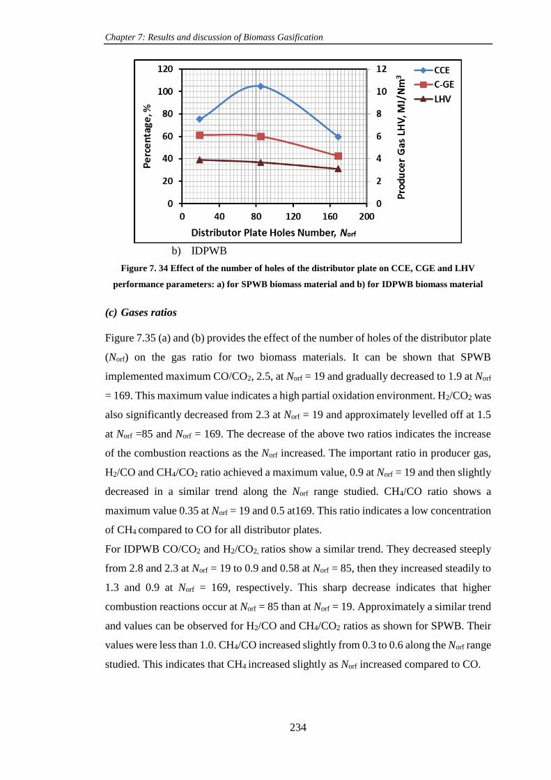
Chapter 7: Results and discussion of Biomass Gasification
234
b) IDPWB
Figure 7. 34 Effect of the number of holes of the distributor plate on CCE, CGE and LHV
performance parameters: a) for SPWB biomass material and b) for IDPWB biomass material
(c) Gases ratios
Figure 7.35 (a) and (b) provides the effect of the number of holes of the distributor plate
(Norf) on the gas ratio for two biomass materials. It can be shown that SPWB
implemented maximum CO/CO2, 2.5, at Norf = 19 and gradually decreased to 1.9 at Norf
= 169. This maximum value indicates a high partial oxidation environment. H2/CO2 was
also significantly decreased from 2.3 at Norf = 19 and approximately levelled off at 1.5
at Norf =85 and Norf = 169. The decrease of the above two ratios indicates the increase
of the combustion reactions as the Norf increased. The important ratio in producer gas,
H2/CO and CH4/CO2 ratio achieved a maximum value, 0.9 at Norf = 19 and then slightly
decreased in a similar trend along the Norf range studied. CH4/CO ratio shows a
maximum value 0.35 at Norf = 19 and 0.5 at169. This ratio indicates a low concentration
of CH4 compared to CO for all distributor plates.
For IDPWB CO/CO2 and H2/CO2, ratios show a similar trend. They decreased steeply
from 2.8 and 2.3 at Norf = 19 to 0.9 and 0.58 at Norf = 85, then they increased steadily to
1.3 and 0.9 at Norf = 169, respectively. This sharp decrease indicates that higher
combustion reactions occur at Norf = 85 than at Norf = 19. Approximately a similar trend
and values can be observed for H2/CO and CH4/CO2 ratios as shown for SPWB. Their
values were less than 1.0. CH4/CO increased slightly from 0.3 to 0.6 along the Norf range
studied. This indicates that CH4 increased slightly as Norf increased compared to CO.

Chapter 7: Results and discussion of Biomass Gasification
235
a) SPWB
b) IDPWB
Figure 7. 35 Effect of the number of holes of the distributor plate on the gases ratio: a) for SPWB
biomass material and b) for IDPWB biomass material
(d) Producer gas yield (GY)
Figure 7.36-(a) and (b) highlights the effect of the number of the holes of the distributor
plate on the gas yield for two biomass materials. It can be observed that for SPWB, the
total gas yield attained a maximum value, 3.75 Nm3/kg feed db, at Norf = 85 and the
minimum value was 2.55 Nm3/kg feed db at Norf = 169. Similarly for individual gases
CO, H2, CO2 and CH4 the maximum yield was attained at Norf = 85. Their values took a
descending sequence as follows: 0.9, 0.6, 0.4 and 0.2 Nm3/kg feed db, respectively,
whereas N2 stayed constant, 1.6Nm3/kg feed db.

Chapter 7: Results and discussion of Biomass Gasification
236
For IDPWB the maximum value was 3.0Nm3/kg feed db at Norf = 85 and the minimum
value was 2.5Nm3/kg feed db at Norf = 169. Whereas for the individual gases their yield
attained very low values except N2, which attained a constant yield value, 1.7Nm3/kg
feed db, for all three-distributor plates. The maximum yield values for CO and H2 were
0.4 and 0.3 nm3/kg feed db, respectively at Norf = 19, while for CO2 and CH4 were 0.4
and 0.2Nm3/kg feed db, respectively at Norf = 85.
As discussed in Section 7.2.4.8-(a), the yield results completely depend on the producer
gas composition. In general, from the Figure7.36-(a) and (b) it can be seen that SPWB
achieved gas yield higher than IDPWB for total producer gas and individual gases. This
can be linked to the higher producer gas compositions for SPWB as shown in Figure
7.34 (a) compared to producer gas composition for IDPWB as shown in Figure 7.34 (b).
Furthermore the best total gas yield that can be achieved for both, SPWB and IDPWB
was at distributor plate, Norf = 85.
a) SPWB

Chapter 7: Results and discussion of Biomass Gasification
237
b) IDPWB
Figure 7. 36 Effect of the number of holes of the distributor plate on gases yield: a) for SPWB
biomass material and b) for IDPWB biomass material
7.2.5 Material balance
A material balance and carbon species mass balance in the gasification system were
undertaken to observe the conversion of biomass material, SPWB and IDPWB, into
producer gas as well as the other products as illustrated in Figure 7.37. As described in
Chapter 5 reactant materials, biomass fuel and air were fed to the fluidised bed gasifier.
The inert material, sand, was used as fluidised bed material. The products were
classified as producer gas, tar, traces of particulates and char + sand mixture. The
producer gas was represented mainly CO, CO2, CH4, H2 and O2, which their
composition were measured in volume percent, whereas N2 was calculated by
difference. Char in the char-sand mixture represented the unburnt carbon. Tar and
particulates represented a condensable volatile material and a fine particles, sand and
char, respectively.
For this study the output product streams, producer gas and char only were considered
making the total and carbon mass balances of the gasification system. The boundary of
this system was laid out using a dashed line as shown in Figure 7.37.

Chapter 7: Results and discussion of Biomass Gasification
238
Figure 7. 37 Schematic of the block diagram of the biomass gasification system mass balance
For steady state conditions, the total mass balance in the fluidised bed gasification
system was calculated using Equation 7.3a.
𝑇𝑜𝑡𝑎𝑙 𝐼𝑛𝑝𝑢𝑡 𝑀𝑎𝑠𝑠 = 𝑇𝑜𝑡𝑎𝑙 𝑂𝑢𝑡𝑝𝑢𝑡 𝑀𝑎𝑠𝑠 (7.3)
[(�̇�)𝑎𝑖𝑟 + (�̇�)𝑏𝑖𝑜.𝑓𝑢𝑒𝑙 ]𝐼𝑛𝑝𝑢𝑡= [(�̇�)𝑝.𝑔𝑎𝑠 + (�̇�)𝑐ℎ𝑎𝑟]𝑂𝑢𝑡𝑝𝑢𝑡
(7.3a)
The mass of the input biomass fuel, input inert sand (m)sand and output char + sand
(m)char + sand mixture were weighed using a laboratory scale balance. The mass rate of air
and producer gas were calculated according to Equation 7.4 and Equation 7.8,
respectively. All the streams were calculated in mass rate unit, g/min, except the sand
in g. Therefore, 1 min as the basis of the calculations was taken. The duration of the
experiment time (t) was 5 min. Steady state conditions were assumed
(�̇�)𝑎𝑖𝑟 = 𝑉𝑎𝑖𝑟 × 𝜌𝑎𝑖𝑟 × 1000 (7.4)
Where 𝑉𝑎𝑖𝑟 and 𝜌𝑎𝑖𝑟 are the input air flowrate (l/min) and air density (1.2 g/cm3 at
ambient temperature). Producer gas mass rate (�̇�)𝑝.𝑔𝑎𝑠 can be calculated as follows:
Using Equation (5.9) in Chapter 5, the individual gas yield of each gas was determined
using Equation (7.5).
𝑌𝑖 = 𝑌𝑃.𝐺𝑎𝑠 × 𝑥𝑖 (7.5)

Chapter 7: Results and discussion of Biomass Gasification
239
Where 𝑌𝑖, 𝑌𝑃.𝐺𝑎𝑠, 𝑥𝑖 are the individual gas yield in (Nm3/kg fuel feed), yield of producer
gas in (Nm3/ kg fuel feed) and mole fraction of individual gas (i), respectively. This unit
of (i) gas yield converted to (m) i in [mass of (i) gas/ mass feed fuel] unit using Equation
(7.6).
𝑚𝑖 = 𝑦𝑖 × (𝑀𝑤𝑡)𝑖/22.4 (7.6)
∴ (𝑚)̇ 𝑖 = 𝑚𝑖 ∗ (𝑚)̇ 𝑏𝑖𝑜.𝑓𝑢𝑒𝑙 (7.7)
∴ (𝑚)̇ 𝑝.𝑔𝑎𝑠 = ∑(𝑚)̇ 𝑖 (7.8)
Where (𝑀𝑤𝑡)𝑖 , (𝑚)̇ 𝑖 are molecular weight of gas (i) and the mass rate of gas (i) in
(g/min), respectively.
Carbon mass balance was performed to observe the conversion of biomass fuel
materials, SPWB and IDPWB, to gases and char. Only both biomass fuels were
considered as a principal source of the carbon in the input streams. For this study in the
output, producer gas and char + sand streams were considered the main source of
carbon. According to the mass balance, Equation (7.1), carbon balance was determined
using Equation (7.9).
(𝐶)̇ 𝑏𝑖𝑜.𝑓𝑢𝑒𝑙 = (𝐶)̇ 𝑃.𝑔𝑎𝑠 + (𝐶)̇ 𝑐ℎ𝑎𝑟+𝑠𝑎𝑛𝑑 (7.9)
Where (𝐶)̇ 𝑏𝑖𝑜.𝑓𝑢𝑒𝑙, (𝐶)̇ 𝑃.𝑔𝑎𝑠, 𝑎𝑛𝑑 (𝐶)̇ 𝑐ℎ𝑎𝑟+𝑠𝑎𝑛𝑑 are the carbon mass rate (g/min) in
biomass feed fuel, producer gas and char + sand streams, respectively. These carbon
mass rates were determined using Equation (7.10), (7.12) and (7.13), respectively.
(𝐶)̇ 𝑏𝑖𝑜.𝑓𝑢𝑒𝑙 = (𝐶𝐶)𝑏𝑖𝑜.𝑓𝑢𝑒𝑙 × (𝑚)̇ 𝑏𝑖𝑜.𝑓𝑢𝑒𝑙 (7.10)
Where (𝐶𝐶)𝑏𝑖𝑜.𝑓𝑢𝑒𝑙 is the carbon mass fraction in biomass feed fuel, using biomass
ultimate analysis as shown in Table 4.1.
(𝐶)̇ 𝑖 = 𝐶𝑖 × (𝑚)̇ 𝑏𝑖𝑜.𝑓𝑢𝑒𝑙 = [𝑦𝑖 × 12/22.4] × (𝑚)̇ 𝑏𝑖𝑜.𝑓𝑢𝑒𝑙 (7.11)
(𝐶)̇ 𝑃.𝑔𝑎𝑠 = ∑(𝐶)̇ 𝑖 (7.12)
Where (𝐶)̇ 𝑖, 𝐶𝑖 are the carbon mass rate and carbon mass of the carbonaceous gas (i),
respectively.
(𝐶)̇ 𝑐ℎ𝑎𝑟+𝑠𝑎𝑛𝑑 = (𝐶𝐶)𝑐ℎ𝑎𝑟+𝑠𝑎𝑛𝑑 × (𝑚)𝑐ℎ𝑎𝑟+𝑠𝑎𝑛𝑑/𝑡 (7.13)
Where (𝐶𝐶)𝑐ℎ𝑎𝑟+𝑠𝑎𝑛𝑑 𝑎𝑛𝑑 (𝑚)𝑐ℎ𝑎𝑟+𝑠𝑎𝑛𝑑the carbon mass fraction and mass of char +
sand mixture stream, respectively.
Equation 7.14 was used to determine the comparison of the total and carbon mass
balance parameters between input and output streams.

Chapter 7: Results and discussion of Biomass Gasification
240
% 𝐸𝑟𝑟𝑜𝑟 = [𝐼𝑛𝑝𝑢𝑡 𝑚𝑎𝑠𝑠−𝑂𝑢𝑡𝑝𝑢𝑡 𝑚𝑎𝑠𝑠
𝐼𝑛𝑝𝑢𝑡 𝑚𝑎𝑠𝑠] × 100 (7.14)
For each parameter, whose effect has been discussed in Section 7.2.4.2 – 7.2.4.8, the
results of the measured and calculated quantities for each experiment for each stream in
the total and carbon mass balances are outlined in tables. The data in these tables are
presented to show the trend of the each parameter group on the gasification mass
balance streams. These tables and figures are shown in Appendix E
The total and carbon mass balances data of the experiment group of the air flowrate
parameter for the two biomass materials, SPWB and IDPWB was selected as an
example. These data are outlined in Table 7.10 (a) and (b) and Figure 7.38 (a) and (b).
From the table it can be seen that for SPWB for three air flowrates the total mass of the
output streams were 80.3, 121.9 and 164.7g/min, which is more than the total mass input
streams 73.2, 109.7, and 146.3g/min leading to -9.7, -11.1 and -12.6 % error,
respectively. This result will interpreted in the proceeding. IDPWB showed an opposite
trend except for 44 l/min, which showed a similar trend to SPWB. For carbon mass
balance for SPWB the total balance between input and output streams for three air flow
rates were at -59.8, -86.5 and -60.7 % error, respectively, whereas for IDPWB were at
-60.8, -14.1 and -12.7, respectively. These higher output carbon mass was due to the
high output carbon mass in producer gas which was higher than the total input carbon
mass itself. These results will be explained in the next paragraphs.
In Figure 7.38 it can be seen that the total mass input (Biomass fuel + Air) and carbon
(carbon input) lines were taken as a reference lines for total mass and carbon balances.
Each line can be used to observe the output streams of the total and carbon mass
deviations. Furthermore, when the output mass lines follows a downward trend, it
indicates that the output mass is less than the input mass and gives positive (+ve) percent
error and vice versa. From the Figure 7.38, for both biomass, it can be seen that as the
air flowrate increased from 44 to 88 l/min all streams were increased except the char
stream of IDPWB was slightly decreased. Furthermore, for SPWB the total output mass
of producer gas and char was greater than the total mass input, whereas for IDPWB was
lesser. For both biomass the deviation (% error) increased as air flowrate increased. For
carbon balance, it can be seen that the total mass of the output carbon was exceeded the
total input carbon. This excess for SPWB was higher than IDPWB.

Chapter 7: Results and discussion of Biomass Gasification
241
The negative deviation either for total mass balance or carbon balance might be
attributed to the following reasons: 1). the biomass screw feeder supplied more biomass
quantity than the measured. 2) There were quantities of char residues and soot product
from previous experiments that available inside gasifier at the freeboard section. Due to
a high temperature and oxidation atmosphere in this section gasification and combustion
reactions possibly occurred. These materials in turn led to increase the amount of carbon
in producer gas causing high carbon conversion efficiency CCE and cold gas efficiency
CGE. 3) The error that may result by the gas analyzer was excluded because it was
calibrated for each experiment. 4) The heterogeneity of the residue mixture (char +
sand) due to their high-density difference caused no precision carbon content
measurement and leading to inaccurate mass balances.
Table 7. 10 Total and carbon mass balances for air flowrate experiments: a) for SPWB and b) for
IDPWB
a) SPWB
Air flow,
l/min Stream
Total mass balance, g/min Carbon mass balance, g/min
Input Output % Error Input Output % Error
44 Biomass Fuel
Air
Producer Gas
Char + Sand
20.17
52.98
-
-
-
-
77.75
2.52
-
-
-
-
9.96
-
-
-
-
-
12.66
3.26
-
-
-
-
Total 73.15 80.27 -9.74 9.96 15.92 -59.84
66 Biomass Fuel
Air
Producer Gas
Char + Sand
30.26
79.47
-
-
-
-
113.16
8.71
-
-
-
-
14.95
-
-
-
-
-
18.19
9.69
-
-
-
-
Total 109.73 121.87 -11.07 14.95 27.88 -86.52
88 Biomass Fuel
Air
Producer Gas
Char+Sand
40.36
105.96
-
-
-
-
152.79
11.93
-
-
-
-
19.94
-
-
-
-
-
24.61
7.44
-
-
-
-
Total 146.32 164.72 -12.57 19.94 32.05 -60.73
b) IDPWB
Air flow,
l/min Stream
Total mass balance, g/min Carbon mass balance, g/min
Input Output % Error Input Output % Error
44 Biomass Fuel
Air
Producer Gas
Char+Sand
21.92
52.98
-
-
-
-
75.26
3.36
-
-
-
-
9.34
-
-
-
-
-
11.42
3.60
-
-
-
-
Total 74.90 78.62 -4.96 9.34 15.02 -60.81
66 Biomass Fuel
Air
Producer Gas
Char+Sand
32.87
79.47
-
-
-
-
104.09
2.98
-
-
-
-
14.00
-
-
-
-
-
14.91
0.97
-
-
-
-
Total 112.34 107.08 -4.69 14.00 15.98 -14.14
88 Biomass Fuel
Air
Producer Gas
Char+Sand
43.84
105.96
-
-
-
-
135.45
2.45
-
-
-
-
18.67
-
-
-
-
-
18.61
2.43
-
-
-
-
Total 149.80 137.90 -7.95 18.67 21.04 -12.68

Chapter 7: Results and discussion of Biomass Gasification
242
a) SPWB
b) IDPWB
Figure 7. 38 Total and carbon mass balances for air flowrate experiments: a) for SPWB and b)
for IDPWB
7.3 Summary
This chapter has shown the results of the possibility of the gasification of the two-
biomass materials, SPWB and IDPWB, by using an air-blown bubbling fluidised bed
gasifier. The results and the effect of the operating and hydrodynamic parameters has
been presented and discussed in detail. The air flowrate parameter has shown a negative
effect on the performance parameter, especially for IDPWB feedstock, and H2 gas
decreased as flow increased. In addition, it has shown that a high LHV can be produced
at low air velocities. The smaller sand particle size has shown a slightly effect higher

Chapter 7: Results and discussion of Biomass Gasification
243
than the others on producer gas composition and performance parameter for SPWB,
whereas the effect was higher for IDPWB feedstock. In addition, a smaller biomass
particle size has shown a more favorable quality producer gas production and upgrade
performance parameters. Furthermore, the effects of the static bed height have shown a
fluctuating effect on the performance parameters whereas the maximum values at the
medium height 0.75D has been concluded. In general, different effects of ER parameter
has been detected on the gasification of two biomass feedstocks. This chapter has also
shown the positive effect of the bed temperature on all the produced combustible gases
composition, in addition to performance parameter. The effect of the number of the
holes of the distributor plate has been discussed and it has shown a different effect
depending on the biomass type. Finally, the total and carbon mass balance in the
biomass gasification system has been conducted to observe the balancing of input and
output streams.

Chapter 8
Conclusions and Recommendations for
Future Work

Chapter 8: Conclusions and Recommendations for Future Work
245
8.1 Conclusions
This study is concerned with the investigation of the effect of the hydrodynamic
fluidization parameters and operating conditions on the performance of the
gasification of the solid biomass fuels in a bubbling fluidised bed reactor. This
involved a preliminary design and cold experimental hydrodynamic studies to provide
design data for gasification processes.
The main conclusions that found in this research study are summarised and classified
into three major groups: a design study, cold fluidisation experimental tests, and
biomass gasification experimental trials.
8.1.1 Design Study
The design study has shown an important part of this research for predicting and
providing an elementary design data for constructing both cold fluidization and
biomass gasification rigs and for conducting their experimental tests as well. From the
results of the design study, the following findings have been concluded:
According to the available facilities the suitable size, represented by the gasifier
diameter, of the bubbling fluidised bed gasifier has been specified. For this study,
8.3cm the internal diameter of the gasifier column has been selected.
The design parameter, minimum fluidization velocity Umf, was highly affected by
the particle size of the bed material. This, in turn, specified the minimum
requirement of air flowrate, an agent gas for fluidization. These quantities of the
air have helped to specify the required quantity of biomass fuel for gasification at
a selected equivalence ratio.
It has indicated that the minimum fluidization velocity was not affected by the
static height of the bed material Hs.
The number of distributor plate holes, Norf affected the air flowrate. It means that
for each specific flow rate, there is a specific number of holes. Furthermore, this
has a direct effect on the hydrodynamic behaviour of the fluidised bed reactor
represented by the pressure drop across the plate and the number of the generated
bubbles. For the cold fluidisation experimental tests, Norf =19, 55 and 85 were used,
whereas, for the gasification tests, Norf =19, 85 and 169 have been used.

Chapter 8: Conclusions and Recommendations for Future Work
246
Finally, from the design results, this design model can predict the gasifier size and
some of required hardware, such as biomass screw feeder and air rotameters
specifications.
8.1.2 Cold fluidisation experimental tests
The experimental tests on the hydrodynamics of the fluidization of inert sand material,
SPWB and IDPWB biomass materials and biomass-inert mixtures have been
conducted to study fluidisation material behaviours and to determine the minimum
fluidization velocity for each single and mixed materials according to the geometry
design results.
The cold experimental tests has shown the following conclusions over the ranges tested
within the thesis:
Fluidization behaviour, bed material or solid fuel reactant, has depended on the
type and physical characteristics of the material. By observing the fluidization
behaviour the findings have shown that sand bed material has a perfect fluidization
ability leading to establishing a smooth hydrodynamic curve (ΔP-Uo), whereas the
observed fluidization behaviour of each biomass, SPWB and IDPWB, which are
the biomass materials in this study, have shown a weak fluidization behaviour
causing an unclear hydrodynamic curve. The indication of this weak fluidization
was observed during the formation of the bridging, clustering and channelling
features inside the biomass bed column. This was due to their physical
characteristics: low particle density, irregular shape, and high particle aspect ratio,
moisture content and high inter-particular forces between biomass particles.
The minimum fluidization velocity for sand bed material Umf has been found from
the hydrodynamic curve (ΔP-Uo). Furthermore, it has concluded that Umf was
affected by the sand particle size. For three ranges of particle size of the sand
material, (300-425) µm, (425-500) µm and (500-600) µm were 10.875, 18.665
and 23 cm/sec, respectively.
The three static bed heights Hs, 0.5D=4.15, 0.75D= 6.225 and 1D=8.3cm, have no
significant effect on the minimum fluidization velocity Umf.
In order to upgrade their fluidization behaviour, biomass material has been
blended with the sand material in a specific weight percent. The finding has shown

Chapter 8: Conclusions and Recommendations for Future Work
247
that the minimum fluidization velocity can be estimated by their established
hydrodynamic curve. In addition, it has been found that when the mass percent
increased the Umf has gradually increased.
8.1.3 Air-biomass gasification experimental tests
Experimental tests for air-biomass gasification in the bubbling fluidised bed gasifier
have been conducted. The effect of fluidization hydrodynamics and operating
conditions parameters on the performance have been investigated. The conclusion can
be outlined as follows:
Uniform axial temperature distribution along the fluidised bed gasifier has not
been achieved. This was because that the electric heater element has one
temperature set point, which provided a maximum allowable temperature 1020oC
at the position 44 cm above the distributor plate. Practically 900oC as the set
temperature has been used for all experimental tests. Experiments had shown
551oC, a bed temperature T2 that can be achieved when the gasifier was filled
with an 8.3cm static bed height of (300-425) µm particle size of sand material
with zero airflows. The best temperature distribution at equilibrium conditions for
airflow range (30-100l/min and more) has been obtained at the set-point
temperature 900oC and bed temperature T2 at 340-360oC. It is likely that uniform
conditions do not occur in real systems, and this result shows that temperature
distribution is an important operational consideration.
For 5 min and more, this biomass feeding time has approximately shown stable
conditions of producer gas composition, CO, CO2, CH4, H2 and O2.
Effect of air flowrate parameter: This parameter has shown a significant effect
on the producer gas composition and performance parameters (CCE), (CGE),
(LHV) and gas yield (Y) at constant equivalence ratio, i.e. the feed rate of feeding
biomass increases as air flowrate increases. It has been shown that the trends of
the producer gases composition for two biomass, SPWB and IDPWB were
similar. H2, CO2 and CH4 decreased as air flowrate increased whereas CO
increased. SPWB has produced higher H2 and CO and lower CO2 and CH4 than
IDPWB. A low air flowrate of 44 l/min has shown a significant effect providing
a highest (CCE), (CGE), (LHV), gas yield (GY) and gas composition for IDPWB.

Chapter 8: Conclusions and Recommendations for Future Work
248
Within this range of air flowrates, an LHV of producer gas for both biomass has
been achieved between 4.0 and 5.3MJ/Nm3db.
This factor is mainly related to the hydrodynamic fluidization parameters such as
bubble size and velocity, which are linked to the bubble fraction in the bed, and
the residence time of the gas and biomass particles. In addition, as the air flowrate
increase, the biomass mass fraction in the bed increase and thereby the minimum
fluidization velocity increase.
Effect of particle size of san bed material: The effect of this factor has shown that
as sand particle size increased the hydrodynamic changes will weaken the
gasification performance. These hydrodynamic changes were due to the variations
in the values of the minimum fluidization velocity due to the various ranges of
sand particle size.
For SPWB it has been shown that there was no a considerable effect of the sand
particle size on the producer gas composition and gasifier performance parameters
(CCE), (CGE), (LHV) and (GY), which agrees with published results. While for
IDPWB it has been shown that the low range of sand particle size (300-425) µm
provided higher performance parameters (CCE), (CGE), (LHV) and (GY) than
the other ranges, (425-500) µm and (500-600) µm which provided a similar effect.
SPWB has provided 6MJ/Nm3db (LHV) of producer gas, which is higher than
IDPWB.
Effect of the biomass particle size: This parameter has shown a significant effect
on the producer gas composition and performance parameters for both biomass
SPWB and IDPWB. In general, the best effect has been achieved by the smallest
biomass particle size (300-425) µm due to their high reaction surface area. Three
possible reason can be given and confirmed due to this finding, 1) The smaller
particles have a faster heating rate, where in the pyrolysis process the control step
for smaller particles is reaction kinetics. 2) Whereas for larger is the gas diffusion
step. 3) Due to the segregation phenomena of the biomass particles which is faster
for small particles than large particles due to the low weight of the former
particles.
Effect of the static bed height Hs: For this study, according to the experiment
operating conditions and due to the position of the temperature set point it has
been shown that the bed temperature T2 decreased as the bed height increased
thereby affecting the gasifier performance. Furthermore, the position of the

Chapter 8: Conclusions and Recommendations for Future Work
249
biomass feeding point has also affected the gasifier performance. For this range
of the three selected bed heights, the static height 6.23cm has shown the best
results for both biomass materials, in particular on the performance parameters.
This height has achieved two important points, a suitable residence time larger
than Hs=4.15cm and lesser than Hs=8.3cm, the feeding point was located within
the bed height (in bed feeding point) providing a better mixing and contact of
reactants than the on-bed feeding point.
Effect of equivalence ratio ER: The results have shown that equivalence ratio has
a significant effect on the biomass gasification performance. For the range (0.2-
0.45) of ER for both biomass materials, SPWB and IDPWB it has been shown
that at lowest value of ER=0.2 the highest gas compositions, LHV, have been
obtained, whereas the highest values of the (CCE), (CGE), and total and individual
gas yield have been achieved at ER=0.45. In addition, it has been shown that the
total producer gas yield increases significantly as ER increases due to the rise of
the gas yield of each individual gas in the producer gas. Furthermore, in this study
the fluidization hydrodynamic has shown a significant effect on the ER effects.
This was because of the increase of ER was at constant air flowrate, and decrease
biomass mass rate is leading to decreasing in biomass mass fraction inside the
bed.
Effect of the bed temperature T2: The results of this factor have shown that the
low bed temperature 360oC and 465oC had a considerable effect on the gasifier
performance producing a high producer gas composition, (CCE), (CGE), (LHV)
and gas yield (GY). SPWB has shown higher results for these producer gas and
performance parameters than IDPWB. Furthermore, it has been illustrated that the
increase of the bed temperature T2 from 360 to 465oC does not provide a
significant difference in the results.
Effect of the number of holes of the distributor plate Norf: The results of the
consequences of this parameter Norf has revealed that this has a significant effect
on the biomass gasification performance. The results have also shown there is a
disagreement in its effect on each biomass results. For this range of Norf it has
proved that the Norf= 85 is the optimum distributor plate for SPWB, whereas Norf=
19 is the optimum for IDPWB.

Chapter 8: Conclusions and Recommendations for Future Work
250
For all factors effects, the results have appeared that SPWB has higher gasification
potential in fluidised bed reactor than IDPWB.
For all factors, the results have shown the highest composition of CO and H2 in
producer gas and the former is greater than the later.
8.2 Recommendations for Future work
The following are the number of possible future studies that can be done within this
study:
A simulation based preliminary design study should be performed for biomass
gasification research using a high-performance software such as FLUENT.
Increase the biomass feeding time, minimum 1/2 hour, to show the maximum
equilibrium bed temperature without external heating.
Modify and improve the performance of the air biomass bubbling fluidised
gasifier for optimum gasification conditions with optimisation studies within a
broad range of studied parameters or factors (more than 5 points for each factor)
to obtain a wider range of gasification conditions.
To enhance biomass gasification performance and conversion further research
work can be conducted under high-temperature conditions in the bed and
freeboard sections. This will require multi-temperature set points, particularly in
the bed and freeboard sections.
For a correct material balance for an air-biomass gasification process, an accurate
instrument for all input and output streams to their mass rate or volumetric flow
rate are needed. For example, the tar measurement, measurement of the total
producer gas mass rate and measurement of accumulated particulates, which
accompanied producer gas quantification.
The research study should be conducted to examine the effect of the catalyst
materials on the biomass gasification in the bubbling fluidised bed gasifier. This
catalyst material can be used with the sand material for a different mass percent
or alone according to the physical properties and the potential of the catalyst. In
addition, a research study can be conducted to investigate the effect of other gas
agents such as CO2, steam, H2, etc…or a mixture of them with air.

Chapter 8: Conclusions and Recommendations for Future Work
251
For the same conditions of this study, a research study under pyrolysis conditions
using N2 gas as an agent gas for fluidization and for pyrolysis environment
conditions can be recommended, i.e. varying the hydrodynamic conditions
independently of ER and vice versa.
To obtain more specific and precise biomass gasification results, high quality
instruments with computer control are needed.

References

References
253
Abdullah, M.Z., Husain, Z. and Pong, S.L.Y. 2003. Analysis of cold test results for
various biomass fuels. Biomass and Bioenergy 24, pp. 487–494.
AHMED F. ZABAR, A.B. 2012. Cultivation of date palm in Iraq. A nnales
Universitatis Mariae Curie-Sklodowska L U B L IN – P O L O N IA XXII(1), pp. 39–
53.
Alauddin, Z., Lahijani, P., Mohammadi, M. and Mohamed, A. 2010. Gasification of
lignocellulosic biomass in fluidized beds for renewable energy development: A
review. Renewable and Sustainable Energy Reviews 14(9), pp. 2852–2862.
Ali, H.G. 2010. Development of date palm Cultivation and its Role in Sustainability
of Agriculture in Oman. IV International Date Palm Conference, Abu Dhabi, United
Arab Emirate IV(882), pp. 29–35.
Almeida, A.F., Vieira, M.S., Ribeiro, A.M., Pereira, I.M. and Neto, M.P. 2016. Effect
of Air/Biomass Ratio on the Gasification of Olive Bagasse Particles. International
Journal of Environmental Science and Development 7(4), pp. 269–272.
Anon 2011a. BSI Standards Publication Solid biofuels — Determination of total
content of carbon , hydrogen and nitrogen — Instrumental methods.
Anon 2011b. BSI Standards Publication Solid recovered fuels — Methods for the
preparation of the test sample from the laboratory sample.
Anon 2011c. Date Palm Cultivation in Iraq. www.iraqi-datepalm.net.
Anon No Titlehttp://thefrogpad.weebly.com/general-ecology.html [Online].
Arena, U. 2012. Process and technological aspects of municipal solid waste
gasification. A review. Waste Management 32(4), pp. 625–639.
Augusta, A., Pécora, B., Vinicius, M., Geris, A., Harold, J. and Arnao, S. 2011.
Experimental Study of Gas Distributors for Fluidized Beds Containing Sand-Bagasse
Mixtures.
Aznar, M.P., Gracia-Gorria, F.A. and Corella, J. 1992. Minimum and maximum
velocities for fluidization for mixtures of agricultural and forest residues with a second
fluidized solid. I. Preliminary data and results with sand-sawdust mixtures.
International Chemical Engineering 32(1), pp. 95–102.
Badday, B.A., Gupta, A. V., Beddai, A.A. and Naik, M.T. 2014. Experimental Study
on the Bed Voidage and Minimum Fluidization Velocity of Gas-Solid Fluidization
under Different Conditions. International jornal of Mechanical Engineering 2(7), pp.
22–26.
Barmina, I., Lickrastina, A., Valdmanis, R., Zake, M., Arshanitsa, A., Solodovnik, V.
and Telysheva, G. 2013. Effects of Biomass composition variations on gasification
and combustion characteristics. Engineering for rural development, pp. 382–387.

References
254
Basu, P. 2006. Combustion and Gasification fluidised Beds.
Basu, P. 2010. Biomass Gasification and Pyrolysis-Practical Design and Theory.
Elsevier Ink.
Bauer, W., Werther, J. and Emig, G. 1981. Influence of gas distributor design on the
performance of fluidized bed reactor. Ger. Chem. Eng 4, pp. 291–298.
British Standards Institution (BSI) 2010. Solid biofuels. Determination of bulk density.
(BS EN 15103:2009).
British Standards Institution (BSI) 2014. Plastics — Thermogravimetry (TG) of
polymers — Part 1: General principles. Bs En Iso 11358-1:2014.
Brown, J. 2006. Biomass Gasification : Fast Internal Circulating Fluidised Bed
Gasifier Characterisation and Comparison. Fuel 89(2), pp. 384–391.
BS 1377-9 1990. Soils for civil engineering purposes.
BS DD CEN/TS 14918 2005. Solid biofuels - Method for the determination of calorific
value.
Cao, Y., Wang, Y., Riley, J.T. and Pan, W.-P. 2006. A novel biomass air gasification
process for producing tar-free higher heating value fuel gas. Fuel Processing
Technology 87(4), pp. 343–353.
CEN (European Comitte for Standardisation) 2009. EN 15148:2009 Solid biofuels -
Determination of the content of volatile matter.
Chhiti, Y. and Kemiha, M. 2013. Thermal Conversion of Biomass , Pyrolysis and
Gasification : A Review. The International Journal of Engineering And Siences (IJES)
2(3), pp. 75–85. Available at: www.theijes.com.
Chok, V.S. 2009. Effect of Particle and Bed Diameter on Characteristic Velocities in
Compartmented Fluidized Bed Gasifier. 09.
Chok, V.S., Gorin, a and Chua, H.B. 2010. Minimum and Complete Fluidization
Velocity for Sand-Palm Shell Mixtures , Part I : Fluidization Behavior and
Characteristic Velocities Department of Chemical Engineering , University
Technology PETRONAS , School of Engineering and Science , Department of . 7(6),
pp. 763–772.
Christopher Higman, M. van der B. 2003. Gasification. Elsevier Ltd.
Ciferno, J.P. and Marano, J.J. 2002. Benchmarking biomass gasification technologies
for fuels, chemicals and hydrogen production. US Department of Energy. National
Energy (June), p. 58.
Cirad, B.P. 2009. Catalytic Biomass Gasification Process in Fluidized bed Reactor
Dottorato di Ricerca in Ingegneria Chimica. Thesis (January).

References
255
Clarke, K.L., Pugsley, T. and Hill, G. a. 2005. Fluidization of moist sawdust in binary
particle systems in a gas-solid fluidized bed. Chemical Engineering Science 60(24),
pp. 6909–6918.
Cocco, R., Karri, S.B.R. and Knowlton, T. 2014. Introduction to fluidization.
Chemical Engineering Progress 110(11), pp. 21–29.
Cui, H. and Grace, J.R. 2007. Fluidization of biomass particles: A review of
experimental multiphase flow aspects. Chemical Engineering Science 62(1-2), pp. 45–
55.
Daizo, K. and Levenspiel, O. 1991. Fluidization engineering.
Das, B. and Datta, A. 2014. Effects of Fluidizing Gas Flow Rate and Reactor Diameter
on the Hydrodynamics of a Bubbling Fluidized Bed Gasifier.
David Sutton, Brian Kellehr, J.R.H.R. 2001. Review of literature on catalysts for
biomass gasification. Fuel Processing Technology 73, pp. 155–173.
Demirel, Y. 2012. Energy: Production, Conversion, Storage, Conservation, and
Coupling.
Devi, L., Ptasinski, K.J. and Janssen, F.J.J.G. 2002. A review of the primary measures
for tar elimination in biomass gasification processes. Biomass and Bioenergy 24(2),
pp. 125–140.
Dong, S., Cao, C., Si, C. and Guo, Q. 2009. Effect of perforated ratios of distributor
on the fluidization characteristics in a gas-solid fluidized bed. Industrial and
Engineering Chemistry Research 48(1), pp. 517–527.
Dora, D.T.K., Panda, S.R., Mohanty, Y.K. and Roy, G.K. 2013. Hydrodynamics of
gas-solid fluidization of a homogeneous ternary mixture in a conical bed: Prediction
of bed expansion and bed fluctuation ratios. Particuology 11(6), pp. 681–688.
Dr. Sami Sadaka, P.E., P.E. 1. Gasification. Center for Sustainable Environmental
Technologies , Iowa State University (1521 West F. Ave, Nivada, IA 50201).
Eea 2011. Total primary energy consumption by energy source in 2008, EU-27.
Eisentraut, A. and Brown, A. 2012. Technology Roadmap Bioenergy for Heat and
Power. Technology Roadmaps (2), pp. 1–41.
Emerson Process Management 2012. X-Stream Gas Analyzers, Instruction Manual.
En 14774-1 2009. Solid biofuels - Determination of moisture content - Oven dry
method - Part 1: Total moisture - Reference method. , pp. 1–8.
Van Den Enden, P.J. and Lora, E.S. 2004. Design approach for a biomass fed fluidized
bed gasifier using the simulation software CSFB. Biomass and Bioenergy 26(3), pp.
281–287.

References
256
Energy research Centre of the Netherlands 2004. Biomass gasification - Tar and
particles in product gases - Sampling and analysis. 2, p. 41.
Engineering, C. 2011. The effect of parameters on the performance of a Fluidized bed
reactor and Gasifier The effect of parameters on the performance of a Fluidized bed
reactor and Gasifier. (209).
Escudero, D. and Heindel, T.J. 2011. Bed height and material density effects on
fluidized bed hydrodynamics. Chemical Engineering Science 66(16), pp. 3648–3655.
Feng, Y., Xiao, B., Klaus, G., Gong, C. and Jingbo, W. 2011. Influence of Particle
Size and Temperature on Gasification Performance in Externally Heated Gasifier.
Smart Grid and Renewable Energy 02(03), pp. 177–183.
Folkeson, B. 2014. Propensity of various bed materials used in fluidized beds to retain
ash-forming elements from biomass fuels.
Formisani, B., Girimonte, R. and Longo, T. 2008. The fluidization process of binary
mixtures of solids: Development of the approach based on the fluidization velocity
interval. Powder Technology 185(2), pp. 97–108.
Formisani, B., Girimonte, R. and Mancuso, L. 1998. Analysis of the fluidization
process of particle beds at high temperature. Chemical Engineering Science 53(5), pp.
951–961.
Fotovat, F., Abbasi, A., Spiteri, R.J., de Lasa, H. and Chaouki, J. 2015. A CPFD model
for a bubbly biomass-sand fluidized bed. Powder Technology 275, pp. 39–50.
Fotovat, F., Chaouki, J. and Bergthorson, J. 2013. The effect of biomass particles on
the gas distribution and dilute phase characteristics of sand-biomass mixtures fluidized
in the bubbling regime. Chemical Engineering Science 102, pp. 129–138.
Fremaux, S., Beheshti, S.-M., Ghassemi, H. and Shahsavan-Markadeh, R. 2015. An
experimental study on hydrogen-rich gas production via steam gasification of biomass
in a research-scale fluidized bed. Energy Conversion and Management 91, pp. 427–
432.
Gautam, G. 2010. Parametric Study of a Commercial-Scale Biomass Downdraft
Gasifier: Experiments and Equilibrium Modeling.
Gauthier, D., Zerguerras, S. and Flamant, G. 1999. Influence of the particle size
distribution of powders on the velocities of minimum and complete fluidization.
Chemical Engineering Journal 74(3), pp. 181–196.
Geldart, D. 1973. Types of gas fluidization. Powder Technology 7(5), pp. 285–292.
Ghaly, a., Ergudenler, A. and Ramakrishnan, V. 2015. Effect of Distributor Plate
Configuration on Pressure Drop in a Bubbling Fluidized Bed Reactor. Advances in
Research 3(3), pp. 251–268. Available at:
http://www.sciencedomain.org/abstract.php?iid=755&id=31&aid=6538.

References
257
Ghani A.K., Moghadam R.A., Salleh M.A. and Alias A.B. 2009. Air Gasification of
Agricultural Waste in Fluidized Bed Gasifier: Hydrogen Production Performance.
Energies 2, pp. 258–268.
Gómez-Barea, a. and Leckner, B. 2010. Modeling of biomass gasification in fluidized
bed. Progress in Energy and Combustion Science 36(4), pp. 444–509.
Gómez-barea, A., Leckner, B. and Ollero, P. 2011. Methods to improve the
performance of fluidized bed biomass gasifiers. Energy Conversion, pp. 1–12.
Guevara, D.E. 2010. Bed height and material density effects on fluidized bed
hydrodynamics. MSc thesis, Iowa state university, USA.
Gunn, D.J. and Hilal, N. 1997. The expansion of gas-fluidised beds in bubbling
fluidisation. Chemical Engineering Science 52(16), pp. 2811–2822.
Guo, Q., Chen, X. and Liu, H. 2012. Experimental research on shape and size
distribution of biomass particle. Fuel 94, pp. 551–555.
Halvorsen, B. 2010. Applications. , p. 16.
Harriott, P. 2003. Chemical Reactor Design.
Hilal, N., Ghannam, M.T. and Anabtawi, M.Z. 2001. Effect of Bed Diameter,
Distributor and Inserts on Minimum Fluidization Velocity. Chemical Engineering &
Technology 24(2), pp. 161–165.
Hlavsová, A., Corsaro, A., Raclavská, H., Vallová, S. and Juchelková, D. 2016. The
effect of feedstock composition and taxonomy on the products distribution from
pyrolysis of nine herbaceous plants. Fuel Processing Technology 144, pp. 27–36.
International Energy Agency 2012. Iraq Energy Outlook. , pp. 1–142.
International Energy Agengy 2014. 2014 Key World Energy STATISTICS.
J.S.M.Botterill 1975. Fluid-bed heat transfer, J. London: Acadimic Press INC.LTD.
Jangam, S. V., Mujumdar, A.S. and Thorat, B.N. 2009. Design of an Efficient Gas
Distribution System for a Fluidized Bed Dryer. Drying Technology 27(11), pp. 1217–
1228.
Jena, H.M., Roy, G.K. and Biswal, K.C. 2008. Studies on pressure drop and minimum
fluidization velocity of gas-solid fluidization of homogeneous well-mixed ternary
mixtures in un-promoted and promoted square bed. Chemical Engineering Journal
145(1), pp. 16–24.
Jeremiáš, M., Pohořelý, M., Vosecký, M., Skoblia, S., Kameníková, P., Svoboda, K.
and Punčochář, M. 2009. Experimental Study of Fluidized-Bed Biomass Gasification
with CO 2 + H 2 O Mixtures on Limestone and Silica Sand. IEC Gasification
conference publication.
References
258
Jiliang, M., Xiaoping, C. and Daoyin, L. 2013. Minimum fluidization velocity of
particles with wide size distribution at high temperatures. Powder Technology 235, pp.
271–278.
Karmakar, M.K., Haldar, S. and Chatterjee, P.K. 2013. STUDIES ON
FLUIDIZATION BEHAVIOUR OF SAND AND BIOMASS MIXTURES.
International Journal of Engineering Technology and Advanced Engineering
3(Special Issue).
Karnik, A., Rangarajan, A. and Tandon, M. 2013. Numerical Investigation of the
Effect of Bed Height and Coefficient of Restitution on the Minimum Fluidization
Velocity of a Cylindrical Fluidized Bed . (December), pp. 1–5.
Kern, S., Pfeifer, C. and Hofbauer, H. 2013. Gasification of lignite in a dual fluidized
bed gasifier - Influence of bed material particle size and the amount of steam. Fuel
Processing Technology 111, pp. 1–13.
Kim, Y.D., Yang, C.W., Kim, B.J., Kim, K.S., Lee, J.W., Moon, J.H., Yang, W., Yu,
T.U. and Lee, U. Do 2013. Air-blown gasification of woody biomass in a bubbling
fluidized bed gasifier. Applied Energy 112, pp. 414–420.
Kirsanovs, V., Žandeckis, A., Blumberga, D. and Veidenbergs, I. 2014. The influence
of process temperature , equivalence ratio and fuel moisture content on gasification
process : A review. 2(JUNE).
Klein, A. 2002. Gasification: an alternative process for energy recovery and disposal
of municipal solid wastes. New York (May), pp. 1–50.
Koppatz, S., Schmid, J.C., Pfeifer, C. and Hofbauer, H. 2012. The E ff ect of Bed
Particle Inventories with Di ff erent Particle Sizes in a Dual Fluidized Bed Pilot Plant
for Biomass Steam Gasi fi cation.
Kumar, A., Jones, D.D. and Hanna, M. a. 2009. Thermochemical Biomass
Gasification: A Review of the Current Status of the Technology. Energies 2(3), pp.
556–581.
Kumoro, A., Nasution, D., Cifriadi, A. and Falaah, A. 2014. A New Correlation For
The Prediction of Minimum Fluidization of Sand And Irregularly Shape Biomass
Mixtures In A Bubbling Fluidized Bed. 9(23), pp. 21561–21573.
Laboratory, N.E.T. (NETL) 2016. -systems/gasification/gasifipedia/water-gas-shift
[Online].
Lahijani, P. and Zainal, Z.A. 2011. Gasification of palm empty fruit bunch in a
bubbling fluidized bed: A performance and agglomeration study. Bioresource
Technology 102(2), pp. 2068–2076.
LECO, C. 2008. SC-144DR Sulfur / Carbon Determinator Specification Sheet. 5/08-
REV8(209-134-001), pp. 0–1.

References
259
Lee, W.-J., Kim, S.-D. and Song, B.-H. 2002. Steam gasification of an australian
bituminous coal in a fluidized bed. Korean Journal of Chemical Engineering 19(6),
pp. 1091–1096.
Legonda, I.A. 2012. Biomass gasification using a horizontal entrained-flow gasifier
and catalytic processing of the product gas.
Lettieri, P. and Macrì, D. 2016. Effect of Process Conditions on Fluidization. KONA
Powder and Particle Journal (October), pp. 1–24.
Lim, M.T. and Alimuddin, Z. 2008. Bubbling fluidized bed biomass gasification—
Performance, process findings and energy analysis. Renewable Energy 33(10), pp.
2339–2343.
Lu, H., Ip, E., Scott, J., Foster, P., Vickers, M. and Baxter, L.L. 2010. Effects of
particle shape and size on devolatilization of biomass particle. Fuel 89(5), pp. 1156–
1168.
Lv, D., Xu, M., Liu, X., Zhan, Z., Li, Z. and Yao, H. 2010. Effect of cellulose, lignin,
alkali and alkaline earth metallic species on biomass pyrolysis and gasification. Fuel
Processing Technology 91(8), pp. 903–909.
Lv, P.., Xiong, Z.., Chang, J., Wu, C.., Chen, Y. and Zhu, J.. 2004. An experimental
study on biomass air–steam gasification in a fluidized bed. Bioresource Technology
95(1), pp. 95–101.
Maglinao, A.L., Capareda, S.C. and Nam, H. 2015. Fluidized bed gasification of high
tonnage sorghum, cotton gin trash and beef cattle manure: Evaluation of synthesis gas
production. Energy Conversion and Management 105, pp. 578–587.
Makwana, J.P., Joshi, A.K., Athawale, G., Singh, D. and Mohanty, P. 2015. Air
gasification of rice husk in bubbling fluidized bed reactor with bed heating by
conventional charcoal. Bioresource technology 178, pp. 45–52.
Makwana, J.P., Joshi, A.K., Patel, N.R. and Patel, D. 2016. Effect of Equivalence
Ratio on Performance of Fluidized Bed Gasifier Run With Sized Biomass.
International journal of mechanical , aerospace, indusrtial, mechatronic and
manufacturing engineering 10(6), pp. 974–978.
Malvern Instruments 2015. Mastersizer 3000 user manual. November(MAN0474-07-
EN-00).
Malvern Instruments Mastersizer 3000-Smarter Particle Sizing, Malvern-Material
relationships.
Marque, J.J.P. 2002. Minimum fluidization velocities for gasÁ solid 2D beds
Guadalupe Ramos Caicedo *, Mo. Chemical Engineering and Processing 41, pp. 761–
764.

References
260
Marsh, R., Steer, J.M., Fesenko, E., Cleary, V., Rahman, A., Griffiths, A.J. and
Williams, K.P. 2008. Biomass and waste co-firing in large-scale combustion systems.
Proceedings of the ICE-Energy (August), pp. 115–126. Available at:
http://orca.cf.ac.uk/7933/.
Miccio, F., Barletta, D. and Poletto, M. 2013. Flow properties and arching behavior of
biomass particulate solids. Powder Technology 235, pp. 312–321.
Miccio, F., Silvestri, N., Barletta, D. and Poletto, M. 2011. Characterization of Woody
Biomass Flowability. Chemical engineering transactions 24, pp. 643–648.
Mohammed, M. a. a., Salmiaton, A., Wan Azlina, W. a. K.G., Mohammad Amran,
M.S. and Fakhru’l-Razi, A. 2011. Air gasification of empty fruit bunch for hydrogen-
rich gas production in a fluidized-bed reactor. Energy Conversion and Management
52(2), pp. 1555–1561.
Mohd Salleh, M. a., Nsamba, H.K., Yusuf, H.M., Idris, A. and Ghani, W. a. W.A.K.
2015. Effect of Equivalence Ratio and Particle Size on EFB Char Gasification. Energy
Sources, Part A: Recovery, Utilization, and Environmental Effects 37(15), pp. 1647–
1662.
Molino, A., Chianese, S. and Musmarra, D. 2015. Biomass gasification technology:
The state of the art overview. Journal of Energy Chemistry 000, pp. 1–16.
Morf, P., Hasler, P. and Nussbaumer, T. 2002. Mechanisms and kinetics of
homogeneous secondary reactions of tar from continuous pyrolysis of wood chips.
Fuel 81(7), pp. 843–853.
Muazu, R.I., Borrion, A.L. and Stegemann, J. a 2015. Fluidised Bed Gasification of
Multiple Agricultural Biomass Derived Briquettes. 9(5), pp. 610–616.
Narvaez, I., Orıo, A., Aznar, M.P. and Corella, J. 1996. Biomass Gasification with Air
in an Atmospheric Bubbling Fluidized Bed . Effect of Six Operational Variables on
the Quality of. Ind. Eng. Chem. Res. 35(95), pp. 2110–2120.
Newton, H.W. 1969. R12.3 Fluidized-Bed Reactors 1. Symposium A Quarterly
Journal In Modern Foreign Literatures 168, pp. 1–44.
Nguyen, M., Duddy, G. and Karam, C. 2015. PAM Review.
Oliveira, T.J.P., Cardoso, C.R. and Ata??de, C.H. 2013. Bubbling fluidization of
biomass and sand binary mixtures: Minimum fluidization velocity and particle
segregation. Chemical Engineering and Processing: Process Intensification 72, pp.
113–121.
Ommen, J.R. Van and Ellis, N. 2010. Fluidization Gas-Solid Fluidized Bed.
Parr instrument company 6100 Calorimeter Operation.
References
261
Patel, N. 2014. http://www.slideshare.net/nmpatel92/hot-producer-gas-cleaning-
system [Online].
Patil, K., Bower, T., Bellmer, D. and Huhnke, R. 2005. Fluidization Characteristics of
Sand and Chopped Switchgrass- Sand Mixtures. Agricultural Engineering
International: the CIGR Ejournal VII, pp. 1–9.
PETRO, J.J.R. j. d. M. and S.L. 2007. Basic design of a fluidized bed gasifier for rice
husk on a pilot scale. Latin American Applied Research 37, pp. 299–306.
Piriou, B. 2009. Catalytic Biomass Gasification Process in Fluidized bed Reactor
Dottorato di Ricerca in Ingegneria Chimica.
Puig-Arnavat, M., Bruno, J.C. and Coronas, A. 2010. Review and analysis of biomass
gasification models. Renewable and Sustainable Energy Reviews 14(9), pp. 2841–
2851.
Qiaoqun, S., Huilin, L., Wentie, L., Yurong, H., Lidan, Y. and Gidaspow, D. 2005.
Simulation and experiment of segregating/mixing of rice husk-sand mixture in a
bubbling fluidized bed. Fuel 84(14-15), p. 1739.
R. R. Pattipati, C.Y.W. 1981. Minimum Fluidization Velocity at High Temperatures.
Ind. Eng. Chem. Process Des. Dev. 20, pp. 705–707.
Radwan, A.M. 2012. An overview on gasification of biomass for production of
hydrogen rich gas. Der Chemica Sinica 3(2), pp. 323–335.
Ramin Radmanesh, Jamal Chaouki, and C.G. 2006. Biomass Gasification in a
Bubbling Fluidized Bed Reactor: Experiments and Modeling. AICHE 52(12), pp. 405–
410.
Rao, T.R. and Bheemarasetti, J.V.R. 2001. Minimum fluidization velocities of
mixtures of biomass and sands. Energy 26(6), pp. 633–644. Available at:
http://linkinghub.elsevier.com/retrieve/pii/S0360544201000147\npapers3://publicati
on/doi/10.1016/S0360-5442(01)00014-7.
Rapagnà, S., Mazziotti, G. and Rapagna, S. 2008. Devolatilization of wood particles
in a hot fluidized bed : Product yields and conversion rates Product yields and
conversion rates. (December).
Ravaghi-ardebili, Z., Manenti, F., Pirola, C. and Soares, F. 2014. Influence of the
Effective Parameters on H 2 : CO Ratio of Syngas at Low-Temperature Gasification.
37, pp. 253–258.
Rhodes, M. 2008. Introduction to Particle Technology: Second Edition.
Ross, D., Noda, R., Horio, M., Kosminski, A., Ashman, P. and Mullinger, P. 2007.
Axial gas profiles in a bubbling fluidised bed biomass gasifier. 86, pp. 1417–1429.

References
262
Sadaka, S. 2010. Gasification, producer gas and syngas. Agriculture and Natural
Resources.
Sadaka, S.S., Ghaly, a. E. and Sabbah, M. a. 2002. Two phase biomass air-steam
gasification model for fluidized bed reactors: Part II - Model sensitivity. Biomass and
Bioenergy 22(6), pp. 463–477.
Sampaio, D.P. 2013. Effect of the Geometry of a Gas Distributor ( Tuyere Type ) on
Fluidization of a Binary Mixture Biomass-Sand. 22nd International Congress of
Mechanical Engineering (COBEM 2013) (Cobem), pp. 6439–6448.
Sau, D.C., Mohanty, S. and Biswal, K.C. 2007. Minimum fluidization velocities and
maximum bed pressure drops for gas–solid tapered fluidized beds. Chemical
Engineering Journal 132(1-3), pp. 151–157.
Seo, M.W., Goo, J.H., Kim, S.D., Lee, J.G., Guahk, Y.T., Rho, N.S., Koo, G.H., Lee,
D.Y., Cho, W.C. and Song, B.H. 2014. The transition velocities in a dual circulating
fluidized bed reactor with variation of temperatures. Powder Technology 264, pp. 583–
591.
Sethupathy, S.B. (Velammal E.C. and E. Natarajan (Institute for Energy Studies, Anna
University, C. 2012. Hydrodynamic study on gasification of biomass in a fluidized bed
gasifier. International Journal of Engineering Science and Technology 4(01), pp. 316–
323.
Shao, Y., Ren, B., Jin, B., Zhong, W., Hu, H., Chen, X. and Sha, C. 2013. Experimental
flow behaviors of irregular particles with silica sand in solid waste fluidized bed.
Powder Technology 234, pp. 67–75.
Sharma, A.M., Kumar, A., Patil, K.N. and Huhnke, R.L. 2013. Fluidization
characteristics of a mixture of gasifier solid residues, switchgrass and inert material.
Powder Technology 235, pp. 661–668.
Siedlecki, M., de Jong, W. and Verkooijen, A.H.M. 2011. Fluidized bed gasification
as a mature and reliable technology for the production of bio-syngas and applied in the
production of liquid transportation fuels-a review. Energies 4(3), pp. 389–434.
Skoulou, V., Koufodimos, G., Samaras, Z. and Zabaniotou, A. 2008. Low temperature
gasification of olive kernels in a 5-kW fluidized bed reactor for H2-rich producer gas.
International Journal of Hydrogen Energy 33(22), pp. 6515–6524.
Subramani, H.J., Mothivel Balaiyya, M.B. and Miranda, L.R. 2007. Minimum
fluidization velocity at elevated temperatures for Geldart’s group-B powders.
Experimental Thermal and Fluid Science 32(1), pp. 166–173.
Subramanian, R. 2004. Flow through Packed Beds and Fluidized Beds. …
University,[cited February 2007], http://www. …, pp. 1–6. Available at:
http://web2.clarkson.edu/projects/subramanian/ch301/notes/packfluidbed.pdf.

References
263
Sudipta, R.M.& S.G.& 2013. Cracking of tar by steam reforming and hydrogenation.
, pp. 103–111.
Teaters, L.C., Tech, V., Battaglia, F. and Tech, V. 2014. On the Computational
Modeling of Unfluidized and Fluidized Bed Dynamics. Journal of Fluids Engineering
136(October 2014), pp. 1–7.
Technical committee CEN/TC 2005. Solid biofuels - Determination of ash content.
Management, pp. 1–140.
Tilay, A., Azargohar, R., Gerspacher, R., Dalai, A. and Kozinski, J. 2014. Gasification
of Canola Meal and Factors Affecting Gasification Process. BioEnergy Research, pp.
1–13.
Tzeng, L.M. 2007. Characterization of a Bubbling Fluidized Bed Biomass Gasifier.
University of Florida 2015. Fluidization: A Unit Operation in Chemical Engineering.
(March 13 2015), pp. 1–13. Available at: http://www.che.ufl.edu/unit-ops-
lab/experiments/FB/FB-manual.pdf.
Vassilev, S. V., Baxter, D., Andersen, L.K. and Vassileva, C.G. 2010. An overview of
the chemical composition of biomass. Fuel 89(5), pp. 913–933.
W.A.W.K. Ghani1, 2*, R.A. Moghadam1, M.A.M. Salleh1, 2, A.T. 2012. Gasification
Performance of Rice Husk in Fluidized Bed Reactor: A Hydrogen-Rich Production.
Journal of Energy & Environment 4(1), pp. 7–11.
WATLOW 2013. Ceramic Fiber Heaters.
Wilk, V., Schmid, J.C. and Hofbauer, H. 2013. Influence of fuel feeding positions on
gasification in dual fluidized bed gasifiers. Biomass and Bioenergy 54, pp. 46–58.
Xiao, R., Jin, B., Zhou, H., Zhong, Z. and Zhang, M. 2007. Air gasification of
polypropylene plastic waste in fluidized bed gasifier. Energy Conversion and
Management 48(3), pp. 778–786.
Yang, W. 2003. Handbook of fluidization and fluid-particle systems. CRC press.
Zhang, Y., Zhong, W. and Jin, B. 2011. Experimental and Theoretical Study on
Fluidization of Stalk-Shaped Biomass Particle in a Fluidized Bed. International
Journal of Chemical Reactor Engineering 9, pp. 1–23.
Zhong, W., Jin, B., Zhang, Y., Wang, X. and Xiao, R. 2008. Fluidization of biomass
particles in a gas-solid fluidized bed. Energy and Fuels 22(6), pp. 4170–4176.

APPENDIX A
Gasifier Design Procedure and Steps

Appendix A: Gasifier design procedure and steps
265
A.1 Design steps calculation
To show the procedure and algorithm of the fluidized bed gasifier design, the following
steps were built and performed:
Step 1: Given input data:
The following data should be given as an input data to calculate the design parameters
in the next steps:
1- Inside diameter of the fluidised bed reaction section in cm, D. This value can be
given as desired, but at the same time will limit the gasifier size.
2- Diameter of the selected particle size of the solid bed material in cm, dp.
3- The value of the ambient temperature in℃, Tamb.
4- The value of the atmospheric pressure in Pascal unit, Pamb.
5- A selected value of the equivalence ratio from applicable range for solid biomass
gasification, ER.
6- Viscosity and density of the gasifying gas at required temperature and pressure in
𝒈𝒎 𝒄𝒎. 𝒔⁄ , 𝝁𝒇 and 𝒈𝒎 𝒄𝒎𝟑⁄ , 𝝆𝒇, respectively. These two physical properties can
be calculated for air from equations (A.1) and (A.2).
𝝁𝒇 =1.458 ×10⁻⁶𝑇1.5
(𝑇+110.4) (A.1)
Where, T is air temperature in oK
𝝆𝒇 =𝑃 ×𝑀𝑜𝑙𝑤𝑡
𝑅 ×𝑇 (A.2)
For P= Pressure in Pascal unit, T= absolute temperature in oK, the value and units of
universal gas constant R is 8.314 (m3) (Pa) (K-1) (mol-1)
7- Gravitation accélération 𝒈, 𝒄𝒎 𝒔𝟐 ⁄ .
8- Particle density of the solid bed material in 𝒈𝒎 𝒄𝒎𝟑⁄ , 𝝆𝒔.
9- Sphericity of the solid bed particles in dimensionless units, ∅𝒔.
10- Void fraction (porosity) of the solid bed material in dimensionless units, 𝜺𝒔.
Porosity can be calculated from equation (A.3) or may be given.
Porosity = 𝜺𝒔 = 1 − 𝑏𝑢𝑙𝑘 𝑑𝑒𝑛𝑠𝑖𝑡𝑦
𝑝𝑎𝑟𝑡𝑖𝑐𝑙𝑒 𝑑𝑒𝑛𝑠𝑖𝑡𝑦 (A.3)
Step 2: Selection of static bed height, Hs

Appendix A: Gasifier design procedure and steps
266
In this step a several values of the height of the static bed Hs is selected as desired and
required by putting it in a loop with a certain step.
Step 3:
1- From Equation (3-2), the porosity of the solid bed material at minimum fluidisation
conditions 𝜺𝒎𝒇 is calculated.
2- From Equation (3-1) the gas velocity at minimum fluidisation conditions Umf was
calculated.
3- The terminal velocity of the solid particle Ut, which represents a maximum value of
the superficial gas velocity, is calculated either by equation (3.6a) for Ut1 if Reynold
number at this velocity ReUt1 is less than 0.4 or by Equation (3.6b) for Ut2 if Reynold
number at this velocity ReUt2 is greater than 0.4 and less than 500.
4- The minimum slugging velocity Ub,ms is calculated from Equation (3.7).
Step 4: Selection of superficial gas velocity, Uo.
After Step 3 the superficial gas velocity Uo value can be suggested and selected from
the range
𝑼𝒎𝒇 < 𝑼𝒐 < 𝑼𝒕 , 𝑎𝑛𝑑
𝑼𝒎𝒇 < 𝑼𝒐 < 𝑼𝒎𝒔 ,
To see the effect of the gas velocity value on many design parameters, several Uo values
were selected by making a loop with a certain step starting from Umf as initial value up
to Ums velocity or any value within the required range as a final value. In this loop many
values of the gas superficial velocity will be obtained within one value of the static
height Hs in the main loop as shown in step 3. Five values of the static height were
selected in terms of the static height to diameter Hs /D ratios, 0.5D, 1D, 1.5D, 2D and
3D, respectively.
Step 5: Calculation of the fraction of the solid bed in bubble phase, 𝜹:
This parameter can be calculated by the following parameters:
1- From equation (3.16) bubble rise velocity Ub can be calculated.
2- To calculate Ub it is required to calculate the bubble diameter at a certain height of
fluidised bed db from equation (3.14).
3- From equation (3.10), (3.15b) and (3.13b), dbm, dbo and Hmax should be calculated,
respectively to calculate dbo.
4- Eventually, 𝜹 can be calculated from Equation (3.17).
Step 6: Calculations of the height of the expansion bed:

Appendix A: Gasifier design procedure and steps
267
The expansion height of the solid bed material, Hexp and its height at the minimum
fluidisation conditions, Hmf can be calculated from Equations (3.21) and (3.22).
Step 7: Calculation the mass of the solid bed material, Ws for a certain static
height Hs.
This mass can be calculated from either Equation (3.21) or Equation (3.24).
Step 8: Calculations of the TDH and the total height of the gasifier, Htotal.
From Equations (3.31b) or (3.32) or (3.34) the total disengaging height TDH can be
calculated. From Equation (3.36) the total height of the gasifier above distributor plate
can be calculated.
Step 9: Calculations of the design parameters of the distributor plate.
1- From Equation (3.39), the pressure drop across the bed can be calculated, ∆𝑃𝑏𝑒𝑑
in 𝑁 𝑚2⁄ .
2- The pressure drop across the plate∆𝑃𝑑𝑖𝑡𝑟 can be calculated from Equation (3.38).
3- The total pressure drop across the gasifier column can be calculated by Equation
(3.41).
4- 1.5mm diameter of the orifice (hole) of the perforated distributor plate dorf was
recommended to select (Basu 2006) to avoid the falling of the solid particles inside
the air-box. Also, 6mm was recommended as a thickness of the distributor plate, tdist
to avoid the material defects at high temperature.
5- The drag coefficient of the gas flow through the holes Cd was calculated from
Equation (3.43).
6- The gas velocity through the orifice Uorf was calculated by Equation (3.42).
7- From the above design parameters the number of the orifices (holes), Norf, can be
calculated from Equation (3.44a).
8- The number of the holes per unit cross-sectional area of the distributor plate, which
is called orifice or hole density Nden, is calculated by Equation (3.45).
9- The triangular layout of the holes distribution is recommended and the pitch Ppitch
of this layout is calculated by Equation (3.46b).
Step 10: Gasification equivalence ratio selecting , ER, and solid biomass mass
flow-rate �̇�𝒃𝒊𝒐 calculations:
1- The required value of the gasification equivalence ratio ER should be selected
from a recommended range, usually between 0.2 and 0.55.

Appendix A: Gasifier design procedure and steps
268
2- From the ultimate analysis of the solid biomass material the stoichiometric air fuel
ratio, [MAFR]stoichio can be estimated by Equation (3.27).
3- The actual air fuel ratio, [MAFR]actual was calculated from Equation (3.26).
4- The air gas volumetric flow rate �̇�𝑎𝑖𝑟 was calculated from Equation (3.30).
5- At the ambient temperature and pressure and for ideal gas the air mass flowrate
�̇�𝑎𝑖𝑟 was calculated from the Equation (3.29).
6- From actual air-fuel ratio [MAFR]actual and air mass flow-rate �̇�𝑎𝑖𝑟 the solid
biomass mass flowrate �̇�𝑏𝑖𝑜𝑚𝑎𝑠𝑠 was calculated from Equation (3.28).
A.2 The geometry drawing of the gasifier components (sections):
According to the design results and gasification process requirements, the suggested
design and geometry drawing specifications of the gasifier components were prepared.
The schematic of the whole rig, geometry and detail specifications for each component
are shown in the next sections. The whole rig of the assembled fluidised bed gasifier has
been shown in Figure 3.6. All components (Sections) are titled and pointed by giving a
number for each one and were specified and drawn in details as shown below. The
gasifier pipe, flange specifications are as follows:
Gasifier pipe:
Pipe material: Stainless-Steel type 316L.
Pipe nominal size: 3
Inside Pipe Diameter: 82.8mm.
Outside pipe diameter: 88.9mm.
Pipe thickness: 3.05mm.
Flange:
Flange Type: Open-Flat Face Flange
Flange material: Stainless-Steel type-316L.
Flange outside diameter: 170mm.
Flange inside diameter: ≈ 90mm.
No. of Flange holes: 6.
Diameter of the hole: 10mm.
Flange thickness: 6mm.

Appendix A: Gasifier design procedure and steps
269
The geometric shape and specifications of each section of the gasifier are shown as
follows:
A.2.1 Gases Outlet Top Section – No (1)
The geometric shape of this section is shown in Figure (A.1). The specifications of this
section are shown in details as follows:
Gasifier pipe specifications: As shown in Section A.2 - gasifier pipe.
Flange specifications: As shown in Section A.2 - Flange.
No of flanges: 1
Connection pipe specification: Stainless-Steel
Outlet vertical pipe length: 50mm.
Outlet horizontal pipe length: 200mm.
Figure A. 1 Geometry of the gas out let-top section.
A.2.2 Free-board section – Part I-No (2)
The geometric shape of this section is shown in figure (A.2). The specifications of this
section are shown in details as follows:
Gasifier pipe specifications: As shown in Section A.2, gasifier pipe.
Flange specifications: As shown in Section A.2, Flange.
No of flanges: 2.
Pipe length: 700mm.

Appendix A: Gasifier design procedure and steps
270
Figure A. 2 Geometry of the free-board section – Part I
A.2.3 Free-board section – Part II No (3)
The geometric shape of this section is shown in figure (A.3). The specifications of this
section are shown in details as follows:
Gasifier pipe specifications: As shown in Section A.2, gasifier pipe.
Flange specifications: As shown in Section A.2, Flange.
No of flanges: 2
Pipe length: 1000mm.
Figure A. 3 Geometry of the free-board section – Part II

Appendix A: Gasifier design procedure and steps
271
A.2.4 Fluidisation reaction section – No (4)
The geometric shape of this section is shown in Figure (A.4). The specifications of this
section are shown in details as follows:
Gasifier pipe specifications: As shown in Section A.2, gasifier pipe.
Flange specifications: As shown in Section A.2, Flange.
No of flanges: 2
Pipe length: 325mm.
There are 3 holes in the pipe:
- Bed material feeding-250mm length from porous plate distributor surface.
- Biomass material feeding - 40mm length from plate distributor surface.
- Solid material outlet (sand + char) – at plate distributor level.
Figure A. 4 Geometry of the fluidized bed section.
A.2.5 Distributor plate section – No (5)
The geometric shape of this section is shown in figure (A.5). The specifications of this
section are shown in details as follows:
Material of the plate: Similar to flange specifications
No. of the orifices (holes) for air distribution: depend on the superficial velocity
values (calculated).
Diameter of the orifice (hole): 1.5mm or 2mm.

Appendix A: Gasifier design procedure and steps
272
The holes of the distributor plate lie within inside pipe diameter border: 83mm.
Holes arrangement: Triangular
Pitch length: depends on the number of the holes (calculated).
Figure A. 5 Geometry of the distributor plate section.
A.2.6 Air box (plenum) section – No (6)
The geometric shape of this section is shown in Figure (A.6). The specifications of this
section are shown in details as follows:
Gasifier pipe specifications: As shown in Section A.2, gasifier pipe.
Flange specifications: As shown in Section A.2, Flange.
No. of flanges: 2, top only.
Pipe length: 300mm.
Inlet air pipe length: 300mm.
Inside diameter of the air supply pipe: 25.4mm.
Thickness of the air pipe: 2mm.
Length of the solid waste pipe: 150mm.
Inside diameter of the solid waste pipe: 11mm.
Thickness of the solid waste pipe: 0.5mm.

Appendix A: Gasifier design procedure and steps
273
Figure A. 6 Geometry of the air box (plenum) section
The geometric shape of the assembled of the whole bubbling fluidised bed gasifier is
shown in Figure A.7 as shown below:

Appendix A: Gasifier design procedure and steps
274
Longitudinal
Section
Figure A. 7 Geometry of the assembled fluidized bed gasifier

APPENDIX B
Matlab Program for Design of the
Bubbling Fluidised Bed

Appendix B: Matlab Program for Design of the bubbling Fluidised bed
276
% Design programme For Bubbling Fluidised Bed Reactor clear all; clc; display (' enter the values of the required parameters') % dp = input( ' enter the value of particle diameter,in ( cm ) dp
=') % TR = input( ' enter the value of reaction temperature TR =') % PR = input( ' enter the value of the reactor pressure PR =') % ER = input( ' enter the value of the equivalence ratio ER =') % VR = input( ' enter the value of the gas volumetric flow rate VR
=') % g = input( ' enter the value of the gravitational acceleration in
(cm/s2)g=') % mg = input( ' enter the value of the viscosity of the gasifying
fluid in (g/cm.s) mg =') % pc = input( ' enter the value of the density of the solid
catalyst particles in (g/cm3) pc =') % pg = input( ' enter the value of the density of the gas in
(g/cm3) pg =') % SPH= input( ' enter the value of the spherity of the particles
SPH =') % D = input( ' Enter the value of the column rector bed diameter in
cm D= ') TC=20 TK=273.15+TC P1=101.325*10^3 dp=0.0396; g=980; mg=1.458*((TK^1.5)/(TK+110.4))/(10^5) pc=2.65; pg=(P1/((287.058)*TK))/1000 target=pg SPH=0.78; D=8.3; Es=0.42;
for i=1:1:5 j=1 Hs= input(' Hs= ') target(j,i)=Hs
display ( ' Umf and Ut calculations ') display ( ' 1- calculation of the epsilon at the minimum
fluidisation condition Emf= '); Emf = 0.586*(SPH^(-0.72))*((mg^2/(pg*g*(pc-
pg)*dp^3))^(0.029))*((pg/pc)^(0.021)) j=j+1 target(j,i)= Emf display (' 2- calculation of the minimum fluidization velocity in
(cm/s) Umf = ') Umf1=((( SPH *dp)^2)*(g*(pc-pg))*(Emf^3))/(150*mg*(1-Emf)) j=j+1 target(j,i)=Umf1 Ar=(pg*g*(pc-pg)*(dp)^3)/(mg^2) j=j+1 target(j,i)=Ar Remf=(((33.7)^2+(0.0408*Ar))^0.5)-33.7 j=j+1 target(j,i)=Remf Umf=(Remf*mg)/(pg*dp)
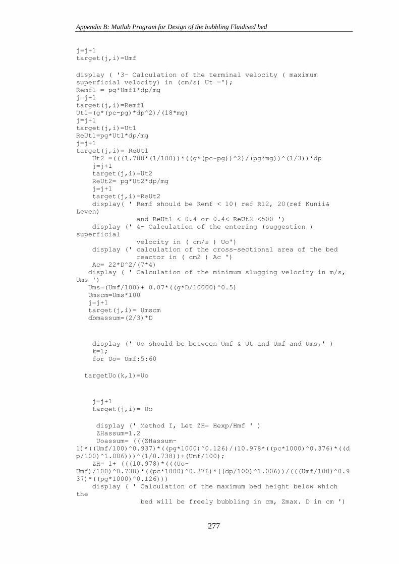
Appendix B: Matlab Program for Design of the bubbling Fluidised bed
277
j=j+1 target(j,i)=Umf
display ( '3- Calculation of the terminal velocity ( maximum
superficial velocity) in (cm/s) Ut ='); Remf1 = pg*Umf1*dp/mg j=j+1 target(j,i)=Remf1 Ut1=(g*(pc-pg)*dp^2)/(18*mg) j=j+1 target(j,i)=Ut1 ReUt1=pg*Ut1*dp/mg j=j+1 target(j,i)= ReUt1 Ut2 =(((1.788*(1/100))*((g*(pc-pg))^2)/(pg*mg))^(1/3))*dp j=j+1 target(j,i)=Ut2 ReUt2= pg*Ut2*dp/mg j=j+1 target(j,i)=ReUt2 display( ' Remf should be Remf < 10( ref R12, 20(ref Kunii&
Leven)
and ReUt1 < 0.4 or 0.4< ReUt2 <500 ') display (' 4- Calculation of the entering (suggestion )
superficial
velocity in ( cm/s ) Uo') display (' calculation of the cross-sectional area of the bed
reactor in ( cm2 ) Ac ') Ac= 22*D^2/(7*4) display ( ' Calculation of the minimum slugging velocity in m/s,
Ums ') Ums=(Umf/100)+ 0.07*((g*D/10000)^0.5) Umscm=Ums*100 j=j+1 target(j,i)= Umscm dbmassum=(2/3)*D
display (' Uo should be between Umf & Ut and Umf and Ums,' ) k=1; for Uo= Umf:5:60
targetUo(k,1)=Uo
j=j+1 target(j,i)= Uo
display (' Method I, Let ZH= Hexp/Hmf ' ) ZHassum=1.2 Uoassum= (((ZHassum-
1)*((Umf/100)^0.937)*((pg*1000)^0.126)/(10.978*((pc*1000)^0.376)*((d
p/100)^1.006)))^(1/0.738))+(Umf/100); ZH= 1+ (((10.978)*(((Uo-
Umf)/100)^0.738)*((pc*1000)^0.376)*((dp/100)^1.006))/(((Umf/100)^0.9
37)*((pg*1000)^0.126))) display ( ' Calculation of the maximum bed height below which
the
bed will be freely bubbling in cm, Zmax. D in cm ')

Appendix B: Matlab Program for Design of the bubbling Fluidised bed
278
Zmax=((D- 2.51*(D^0.2))/(0.13*(D^0.47))) ZmaxR=Zmax/D Hmax=2*D j=j+1 target(j,i)=Hmax Zs = 60*(D^0.175) ZsR=Zs/D
display (' 5- calculation of the bubble velocity Ub in ( cm/s ),
Ub= ') dbo=0.347*[Ac*(Uo-Umf)/Norf]^0.4 j=j+1 target(j,i)=dbo dbm= 0.652*(Ac*(Uo-Umf))^0.4 j=j+1 target(j,i)=dbm targetUo(k,i+1)=target(j,i) Dbmax= (2/3)*D
db= dbm-(dbm-dbo)*exp(-0.3*Hs/(2*D)) j=j+1 target(j,i)=db display (' 6- calculation of the fraction of bed in bubble phase
S') Ub= Uo-Umf+(0.71)*(g*db)^0.5 j=j+1 target(j,i)=Ub a=0.255 S= (Uo-Umf)/(( Ub- Umf)*(1+a)) j=j+1 target(j,i) =S Rexpstatic=(1-Es)/((1-S)*(1-Emf)) j=j+1 target(j,i) =Rexpstatic Hexp1=Rexpstatic*Hs j=j+1 target(j,i)=Hexp1
Rexpmf=1/(1-S) j=j+1 target(j,i) =Rexpmf Hmf=Hs*(1-Es)/(1-Emf) j=j+1 target(j,i)=Hmf Hexp2=(Rexpmf)*Hmf j=j+1 target(j,i) =Hexp2 display ( ' 7- calculation the mass of the solid bed material
Ws, in
grams ') Ws= Hs* Ac* (1-Es)*pc Ws2=Hexp1*Ac*(1-S)*(1-Emf)*pc j=j+1 target(j,i)= Ws2 display ( ' Design of the Freeboard Section ' ) display ( ' Calculation of the TDH in m ') TDH0=13.8*db/100 j=j+1 target(j,i)=TDH0 Uom=Uo/100
Appendix B: Matlab Program for Design of the bubbling Fluidised bed
279
gm=g/100 TDH1= (Uom^2*1000)/gm j=j+1 target(j,i)=TDH1 dbs= dbm-(dbm-dbo)*exp(-0.3*Hs/D) dbsmeter= 1.13*dbs/100 TDH2= (4.47)*(dbsmeter^0.5) j=j+1 target(j,i)=TDH2 display ( ' Calculation of volumetric flowrate, Vo, in cm3/s ') Volmetric=Ac*Uo j=j+1 target(j,i)=Volmetric TDH3= (D^( 1-(0.115)*Uo-0.587))*(4.46*Volmetric) TDH3= TDH3/100 j=j+1 target(j,i)=TDH3 display ( ' Calculation of the total height of the Reactor in
meter,
Htotl ') Hmaxm=Hmax/100 Htotal0= TDH0+Hmaxm+0.3 j=j+1 target (j,i)=Htotal0 Htotal1= TDH1+Hmaxm+0.3 j=j+1 target (j,i)=Htotal1 Htotal2= TDH2+Hmaxm+0.3 j=j+1 target(j,i)=Htotal2 Htotal3= TDH3+Hmaxm+0.3
display ( ' Distributor Design Steps ') display ( ' Calculation of the BED pressure drop, DPBED in N/m2
') display (' let Epsexp= (1-E)') Epsexp=((1-S)*(1-Emf));
DPBED= Epsexp*Hexp1*0.01*(g*0.01)*(pc*1000) j=j+1 target(j,i)=DPBED DPBED2= Epsexp*Hexp1*0.01*(g*0.01)*(pc-pg)*1000 display ( ' Calculation of the DISTRIBUTOR pressure drop, DPDIST
in
N/m2 ') DPDIST= 0.3*DPBED j=j+1 target(j,i)=DPDIST DPtotal=DPBED+DPDIST j=j+1 target(j,i)=DPtotal display ( ' Let CD = 0.8 ') display ( ' Select diameter of the orifice (hole) in distribute
plate value in m, dor ') display ( ' Select of the orifice (hole) in distribute plate
value
in m, dor ') display ( ' enter the value of dor, dor = ') dor=0.0015 display ( ' Select thickness of the porous distributor plate
value

Appendix B: Matlab Program for Design of the bubbling Fluidised bed
280
in m, ThickPD ') display ( ' enter the value of ThickPD, ThickPD= ') display ( ' ratio of ThickPD/dor should be > 0.09') ThickPD=0.006 CD=0.82*((ThickPD/dor)^0.13) j=j+1 target (j,i)=CD display ( ' Calculation of the velocity through the orifice in
m/s,
Uor. pgor density of the gas at orifice in kg/m3 ') pgor=pg*1000 Uor=CD*((2*DPDIST/pgor)^0.5) j=j+1 target (j,i)=Uor display ( ' calculate N the number of orifice in the plate and
NPm2
the number per unit area m2') N= ((D/ (100*dor))^2)* (pg*1000/pgor)*(Uo/(100*Uor)) j=j+1 target(j,i)=N
NPm2= 4*10000*N/((22/7)*(D^2)) j=j+1 target(j,i) =NPm2 display (' This is the number of holes in the plate at assomed
dor
You can assume another and another') display (' From assumed CD & dor one can calculate the thickness
of
the plate distributor in ( m ), ThickPD'); ThickPD= dor*(CD/0.82)^(1/0.13) j=j+1 target(j,i)=ThickPD display (' You can compare this thickness value to that which
can be
obtained by Fig 4,Handbook of fluidization, p.160 '); display (' Calculate the pitch distant in ( m ), PITCH, for
triangular layout '); PITCH = (2/((3^(0.5))*NPm2))^0.5 j=j+1 target(j,i)=PITCH display (' Calculations of the actual compressor power
consumption
in kW ') Pexit=101.325*10^3 P2=(DPtotal+ Pexit) Q2=Volmetric/1000000 Gama=1.4 Eff=0.85 Powerid= (Gama/(Gama-1))*P2*Q2*(1-(P1/P2)^((Gama-1)/Gama)) Poweract=Powerid/Eff j=j+1 target(j,i)=Poweract TCi=20 TC1=273.15+TCi T2comp=TC1+((TC1/Eff)*(((P2/P1)^((Gama-1)/Gama))-1)) j=j+1 target(j,i)=T2comp
plot (targetUo(:,2),targetUo(:,1))

Appendix B: Matlab Program for Design of the bubbling Fluidised bed
281
plot (targetUo(:,2),targetUo(:,1)) % plot (N,Uo)
% for t=1:j; % target1(1,t)=target(1,t); % end % target1 % end display ( ' Equvalence Ratio and Mass Flowrate of The Biomass
Calculations ' ); ER=0.2 display( ' From the Ultimate Analysis of The Biomass Entere the
following '); C = 49.4 Su = 0.02 H = 5.9 N2gas=0 O = 40.68 RStoic = 8.89*(C+0.375*Su)+26.5*(H)-3.3*O RACTU = ER* RStoic
AirV = Uo*Ac/(10^6) TR=20+273.15 Airkg = (P1)*AirV*29/((8.3145)*TK) FedBios = Airkg/(RACTU) FedBioh = FedBios*60 j=j+1 target(j,i)=FedBioh k=k+1 end
end

APPENDIX C
Analysis of Particle Size Distribution
for Three Sand Ranges (500-600), (425-
500) and (300-425) µm, respectively

Appendix C: Analysis of Particle Size Distribution for Three sand Ranges (500-600), (425-500) and
(300-425) µm, respectively
283
Figure C. 1 Image of the Malvern analysis results for sand particle size range (500-600) µm

Appendix C: Analysis of Particle Size Distribution for Three sand Ranges (500-600), (425-500) and
(300-425) µm, respectively
284
Figure C. 2 Image of the Malvern analysis results for sand particle size range (425-500) µm.

Appendix C: Analysis of Particle Size Distribution for Three sand Ranges (500-600), (425-500) and
(300-425) µm, respectively
285
Figure C. 3 Image of the Malvern analysis results for sand particle size range (300-425) µm

APPENDIX D
Results and Discussion of the Rest
Results of Chapter 6

Appendix D: Results and discussion of the rest results of Chapter 6
287
D.1 Comparison of three materials, sand, SPWB and IDPWB
Figure D.1 shows photographically a comparison of the behaviour of air fluidisation
for three single materials, sand, SPWB and IDPWB for each air flowrate from 10 l/min
to 120 l/min. For each flowrate, three images for those three materials were arranged
starting from the left-hand side, respectively. This image comparison can be used to
show the differences of three materials in their fluidisation behaviour. As discussed in
previous sections, the biomass materials SPWB and IDPWB have a poor fluidisation
ability compared to sand material. This is because of the high density of sand material,
which classify them within the Geldert B group. This group can be easily fluidised. In
contrast, because of their low density, these two biomass materials are not classified
within Geldert B group. It means that are not easily fluidised.
Uo=10 l/min
Uo= 20 l/min

Appendix D: Results and discussion of the rest results of Chapter 6
288
Uo- 30 L/min
Uo= 40 l/min

Appendix D: Results and discussion of the rest results of Chapter 6
289
Uo= 50 l/min
Uo= 60 l/min
Uo= 70 l/min

Appendix D: Results and discussion of the rest results of Chapter 6
290
Uo= 80 l/min
Uo= 90 l/min
Figure D. 1 Images for air fluidisation behavior comparison of three single materials, sand,
IDPWB and SPWB for descending velocities from 0.0 to 110 l/min
D.2 Air fluidization behaviour for sand–biomass mixture bed
D.2.1 Experiment of: 2cm SPWB (1180-1500) µm / 8.3cm sand (500-600) µm
Figure D.2 shows the image sequence of the bed fluidization behavior for the mixture
of 2.075cm sawdust biomass (1180-1500) µm/8.3cm sand (500-600) µm. This ratio
was 2.69% weight percent of SPWB biomass in the mixture. At zero to 50 l/min of air
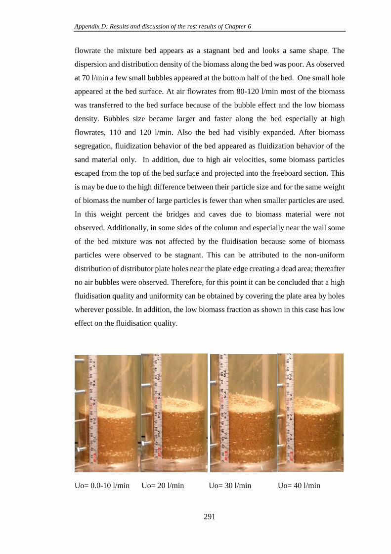
Appendix D: Results and discussion of the rest results of Chapter 6
291
flowrate the mixture bed appears as a stagnant bed and looks a same shape. The
dispersion and distribution density of the biomass along the bed was poor. As observed
at 70 l/min a few small bubbles appeared at the bottom half of the bed. One small hole
appeared at the bed surface. At air flowrates from 80-120 l/min most of the biomass
was transferred to the bed surface because of the bubble effect and the low biomass
density. Bubbles size became larger and faster along the bed especially at high
flowrates, 110 and 120 l/min. Also the bed had visibly expanded. After biomass
segregation, fluidization behavior of the bed appeared as fluidization behavior of the
sand material only. In addition, due to high air velocities, some biomass particles
escaped from the top of the bed surface and projected into the freeboard section. This
is may be due to the high difference between their particle size and for the same weight
of biomass the number of large particles is fewer than when smaller particles are used.
In this weight percent the bridges and caves due to biomass material were not
observed. Additionally, in some sides of the column and especially near the wall some
of the bed mixture was not affected by the fluidisation because some of biomass
particles were observed to be stagnant. This can be attributed to the non-uniform
distribution of distributor plate holes near the plate edge creating a dead area; thereafter
no air bubbles were observed. Therefore, for this point it can be concluded that a high
fluidisation quality and uniformity can be obtained by covering the plate area by holes
wherever possible. In addition, the low biomass fraction as shown in this case has low
effect on the fluidisation quality.
Uo= 0.0-10 l/min Uo= 20 l/min Uo= 30 l/min Uo= 40 l/min

Appendix D: Results and discussion of the rest results of Chapter 6
292
Uo= 50 l/min Uo= 60 l/min Uo= 70 l/min Uo= 80 l/min
Uo= 100 l/min Uo= 110 l/min Uo= 120 l/min
Figure D. 2 Images of the cold fluidization of 2 cm SPWB (1180-1500) µm/ 8.3cm Sand (500-600)
µm mixture
D.2.2 Experiment of: 2cm SPWB (500-600) µm / 8.3cm sand (500-600) µm
The cold hydrodynamic fluidization experiment was conducted for 2.68 weight
percent of sawdust biomass (500-600) µm-sand (500-600) µm mixture to show the
effect of biomass particle size on the hydrodynamics of fluidization and compared to
the previous experiment. This mixture was represented by a height ratio of 2 cm
biomass to 8.3 cm sand. Materials were mixed well and poured in the plastic fluidized
column. The bed mixture took the shape as shown in Figure D.3 (image 1 for 0.0
l/min). It shows that this biomass particle size (white color) was approximately

Appendix D: Results and discussion of the rest results of Chapter 6
293
distributed and dispersed more homogenous and dense along the bed comparing to
previous large particle size. Some of them assembled at the top of the bed surface. It
can be also seen that there was not any changes in the shape of the bed column when
the air velocity increased from 0 l/min to 60 l/min. At 70 l/min= 21.57cm/sec small air
bubbles were seen. They moved upward slowly and burst slightly at the top bed surface
as shown in the image. These small bubbles created small holes at the bed surface,
confirming that air channels were formed. The image of 80 l/min=24.66 cm/sec shows
that the bubbles became more clear and faster than before along the bed. The
distribution of biomass particles were changed along the bed, segregated and pushed
upward and jammed at the bed surface. A slight expansion of the bed was observed.
As shown in the images for air flowrates from 90 l/min to 120 l/min and by experiment
observation the bubbles gradually became more clear, larger and faster. Due to high
velocity, air bubbles action and their low density comparing to the sand, most of the
biomass particles went up faster to the top bed surface. Because of the bubble burst
intensity at the surface, some of the biomass particles were pushed to the freeboard
and a quantity of them stayed projected into the freeboard according to the force
balance theory. Systematically as velocity increased, the bed became more fluidized
and behaved as if a sand material only. These phenomena were more clearly at high
velocities, 110 l/min and 120 l/min, than previous velocities as shown in images of
Figure D.3. From these observations, it can be concluded that for low biomass
concentration in biomass-sand mixtures the bed fluidization behavior is more close to
the single sand material behavior. However, this behavior gives a good fluidization
quality and homogeneity. Comparing to (1180-1500)µm biomass particle size, (500-
600) µm was dispersed and distributed more effectively and densely along the bed. In
addition, for the same biomass mass percent mixture, the fluidisation of bed mixture
was not highly affected by biomass particle size.

Appendix D: Results and discussion of the rest results of Chapter 6
294
Uo= 0-40 l/min Uo= 50 l/min Uo= 60 l/min Uo= 70 l/min
Uo= 80 l/min Uo= 90 l/min Uo= 100 l/min Uo= 110 l/min
Uo= 110 l/min Uo=120 l/min Uo=120 l/min
Figure D. 3 Images of the cold fluidization of 2.07cm SPWB (500-600) µm/ 8.3cm Sand (500-600)
µm mixture

Appendix D: Results and discussion of the rest results of Chapter 6
295
D.2.3 Experiment of: 8.3cm SPWB (1180-1500) µm/ 8.3 cm and (500-600) µm
Figure D.4 shows the sequence of the bed fluidization behavior for the mixture of
8.3cm sawdust biomass (1180-1500) µm/ 8.3 sand (500-600) µm. This ratio was 9.93
weight percent of SPWB. The bed materials were well mixed and poured in the
column. The bed took the shape as shown in Figure D.4 (image 1 for 0.0 l/min). In
addition, the density of the biomass distribution is approximately uniform. This is
because of high biomass weight percent, 9.93 %, comparing to 2.69% for the same
height 8.3cm of sand. As shown in Figure D.4 (image 1 &2) for air velocities from 0
l/min to 60 l/min there was not any changes in bed shape, neither for biomass
distribution nor for bed height. No any bubbles were observed at these velocities. At
70 l/min airflow rate, bubbles could not be observed clearly, but a small hole was
observed at the bed surface. This hole indicates that a few numbers of bubbles were
available creating a small diameter of air channel along the bed. At 80 l/min air
flowrate, a few bubbles appeared at the bottom of the bed at one side of the bed surface.
At 100 l/min of air, the bubbles were increased along the bed and caused cracking in
the side bed surface. Due to a bed expansion, the top surface of the bed became more
level. As the air flowrate increased up to 150 l/min, as shown in Figure D.4 (images
for 110-150l/min) the cracking of the bed, bed bridges and cavities inside the bed and
bed expansion were increased and became larger. In addition, biomass particles were
slowly transferred and segregated upward and accumulated at the top bed surface.
Overall, for this biomass weight percent at these high velocities such as 150 l/min, a
clear fluidization behavior compared to single-sand material cannot be observed.
There was no violent fluidization and mixing in the bed, no bubble bursting at the top
bed surface and then no clear and fast transfer of biomass particles to the freeboard
section. It can be noticed for a short period of time many changes in the bed body may
occur due to bridges, and channels breaks. Approximately, 17.5 cm average bed height
was recorded at 150 l/min air flowrate.
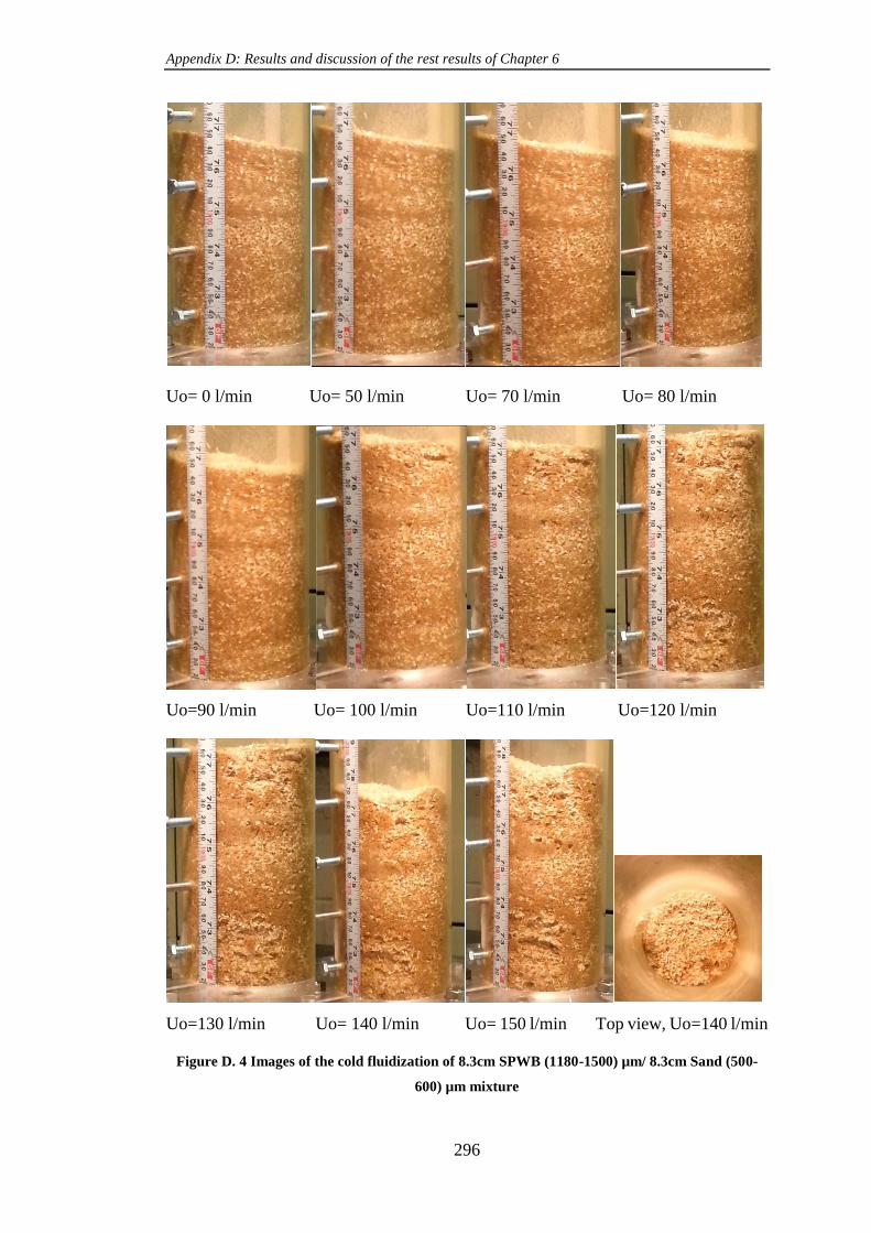
Appendix D: Results and discussion of the rest results of Chapter 6
296
Uo= 0 l/min Uo= 50 l/min Uo= 70 l/min Uo= 80 l/min
Uo=90 l/min Uo= 100 l/min Uo=110 l/min Uo=120 l/min
Uo=130 l/min Uo= 140 l/min Uo= 150 l/min Top view, Uo=140 l/min
Figure D. 4 Images of the cold fluidization of 8.3cm SPWB (1180-1500) µm/ 8.3cm Sand (500-
600) µm mixture

Appendix D: Results and discussion of the rest results of Chapter 6
297
D.2.4 Experiment of 8.3cm SPWB (500-600) µm/ 8.3 cm and (500-600) µm
Figure D.5 shows the sequence of the bed fluidization behavior for the mixture of
8.3cm SPWB (500-600) µm/ 8.3cm Sand (500-600) µm. This ratio is equivalent to
9.93 weight percent of sawdust biomass. The bed materials were well mixed then
poured in the column. The bed took the shape as shown in Figure D.5 - image 1 for
zero l/min. The biomass distribution is approximately looking more dens comparing
to previous bed of large biomass particle size (1180-1500) µm for the same weight
percent. In addition, it is more dense compared to the previous bed of the same biomass
particle size (500-600) µm for less biomass weight percent, 2.68%. For the former,
this is because of the same biomass weight percent the number of small particles is
larger than large particles, thereafter for the same unit area the number of small
particles size was considerably occupied comparing to large particles. For the latter,
because of the high biomass weight percent, 9.93 %, compared to 2.68% has a high
dispersion and distribution density. In addition, the biomass distribution is looking
more clear and uniform along the bed.
In this experiment, the hydrodynamic fluidization behavior and the bed changes
because of air velocity increase are considerably similar to the bed behavior of the
mixture shown in Figure D.3. Comparing to the previous experiment, the biomass
dispersion along the bed appeared more dense and clear. This is because of the small
biomass particle range (500-600) µm compared to biomass size in previous
experiment, 1180-1500 µm. The fluidization bubbles were observed at 80 l/min. So,
for this experiment the same conclusions as shown in previous experiment can be
obtained.
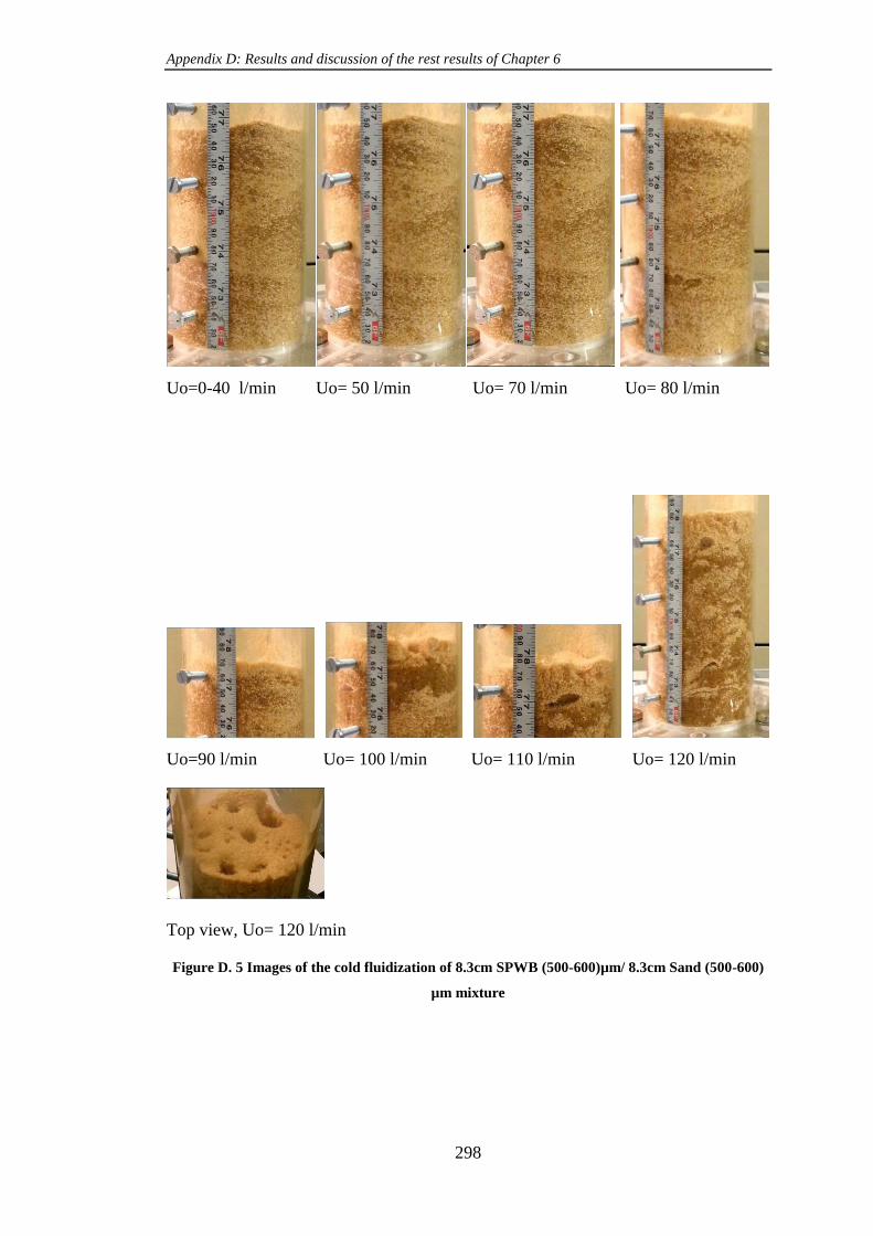
Appendix D: Results and discussion of the rest results of Chapter 6
298
Uo=0-40 l/min Uo= 50 l/min Uo= 70 l/min Uo= 80 l/min
Uo=90 l/min Uo= 100 l/min Uo= 110 l/min Uo= 120 l/min
Top view, Uo= 120 l/min
Figure D. 5 Images of the cold fluidization of 8.3cm SPWB (500-600)µm/ 8.3cm Sand (500-600)
µm mixture

APPENDIX E
Total Mass and Carbon Balances for
All Experimental Tests

Appendix E: Total mass and carbon balances for all experimental tests
300
E.1 Gas analysis test
a)
b)
Figure E. 1 Composition-time analyzing behaviour for standard gas mixture CO2= 1%, O2= 1%
and CO= 0.1%: a) for normal scale and b) for enlargement scale

Appendix E: Total mass and carbon balances for all experimental tests
301
E.2 Total mass and carbon balances for all experimental tests
E.2.1 Air flow rate experimental tests group
Table E. 1 Total and carbon mass balances for air flowrate experiments: a) for SPWB and b)
for IDPWB
a) SPWB
Air flow,
l/min Stream
Total mass balance, g/min Carbon mass balance, g/min
Input Output % Error Input Output % Error
44 Biomass Fuel
Air
Producer Gas
Char+Sand
20.17
52.98
-
-
-
-
77.75
2.52
-
-
-
-
9.96
-
-
-
-
-
12.66
3.26
-
-
-
-
Total 73.15 80.27 -9.74 9.96 15.92 -59.84
66 Biomass Fuel
Air
Producer Gas
Char+Sand
30.26
79.47
-
-
-
-
113.16
8.71
-
-
-
-
14.95
-
-
-
-
-
18.19
9.69
-
-
-
-
Total 109.73 121.87 -11.07 14.95 27.88 -86.52
88 Biomass Fuel
Air
Producer Gas
Char+Sand
40.36
105.96
-
-
-
-
152.79
11.93
-
-
-
-
19.94
-
-
-
-
-
24.61
7.44
-
-
-
-
Total 164.33 164.72 -12.57 19.94 32.05 -60.73
b) IDPWB Air flow,
l/min Stream
Total mass balance, g/min Carbon mass balance, g/min
Input Output % Error Input Output % Error
44 Biomass Fuel
Air
Producer Gas
Char+Sand
21.92
52.98
-
-
-
-
75.26
3.36
-
-
-
-
9.34
-
-
-
-
-
11.42
3.60
-
-
-
-
Total 74.90 78.62 -4.96 9.34 15.02 -60.81
66 Biomass Fuel
Air
Producer Gas
Char+Sand
32.87
79.47
-
-
-
-
104.09
2.98
-
-
-
-
14.00
-
-
-
-
-
14.91
0.97
-
-
-
-
Total 112.34 107.08 -4.69 14.00 15.98 -14.14
88 Biomass Fuel
Air
Producer Gas
Char+Sand
43.84
105.96
-
-
-
-
135.45
2.45
-
-
-
-
18.67
-
-
-
-
-
18.61
2.43
-
-
-
-
Total 149.80 137.90 -7.95 18.67 21.04 -12.68

Appendix E: Total mass and carbon balances for all experimental tests
302
a) SPWB b) IDPWB
Figure E. 2 Total and carbon mass balances for air flowrate experiments: a) for SPWB and b)
for IDPWB
E.2.2 Sand particle size experimental tests group
Table E. 2 Total and carbon mass balances for sand particle size experiments: a) for SPWB and
b) for IDPWB
a) SPWB Sand
P.S, µm Stream
Total mass balance, g/min Carbon mass balance, g/min
Input Output %Error Input Output %Error
(300-425) Biomass Fuel
Air
Producer Gas
Char+Sand
19.86
52.98
-
-
-
-
77.64
3.63
-
-
-
-
9.81
-
-
-
-
-
12.64
0.82
-
-
-
- Total 72.84 81.27 -11.57 9.81
13.46 -37.20
(425-500) Biomass Fuel
Air
Producer Gas
Char+Sand
34.21
90.31
-
-
-
-
132.45
6.01
-
-
-
-
16.90
-
-
-
-
-
21.60
4.99
-
-
-
-
Total 124.52 138.47 -11.20 16.90 26.59 -57.31
(500-600) Biomass Fuel
Air
Producer Gas
Char+Sand
43.34
114.39
-
-
-
-
168.15
4.01
-
-
-
-
21.60
-
-
-
-
-
28.06
4.66
-
-
-
-
Total 157.73 172.16 -9.15 21.60 32.72 -52.83
b) IDPWB Sand
P.S, µm Stream
Total mass balance, g/min Carbon mass balance, g/min
Input Output %Error Input Output %Error
(300-425) Biomass Fuel
Air
Producer Gas
Char+Sand
21.92
52.98
-
-
-
-
68.07
3.36
-
-
-
-
9.34
-
-
-
-
-
6.24
3.61
-
-
-
-
Total 74.90 71.43 4.63 9.34
9.85 -5.45
(425-500) Biomass Fuel
Air
Producer Gas
Char+Sand
37.61
90.91
-
-
-
-
108.33
3.72
-
-
-
-
16.02
-
-
-
-
-
10.71
0.00
-
-
-
-
Total 128.52 112.05 12.82 16.02 10.71 33.14
(500-600) Biomass Fuel
Air
Producer Gas
Char+Sand
46.36
112.06
-
-
-
-
131.25
2.45
-
-
-
-
19.75
-
-
-
-
-
14.76
0.00
-
-
-
- Total 158.41 133.70 15.60 19.75 14.76 25.25

Appendix E: Total mass and carbon balances for all experimental tests
303
a) SPWB b) IDPWB
Figure E. 3 Total and carbon mass balances for sand particle size experiments: a) for SPWB
and b) for IDPWB
E.2.3 Biomass particle size experimental tests group
Table E. 3 Total and carbon mass balances for biomass particle size experiments: a) for SPWB
and b) for IDPWB
a) SPWB Biomass
P.S, µm Stream
Total mass balance, g/min Carbon mass balance, g/min
Input Output %Error Input Output %Error
(300-425) Biomass Fuel
Air
Producer Gas
Char+Sand
10.68
36.12
-
-
-
-
47.96
2.13
-
-
-
-
5.28
-
-
-
-
-
5.76
0.89
-
-
-
-
Total 46.80 53.71 -14.76 5.28 6.65 -25.98
(600-850) Biomass Fuel
Air
Producer Gas
Char+Sand
10.68
36.12
-
-
-
-
55.45
3.15
-
-
-
-
5.28
-
-
-
-
-
9.34
1.89
-
-
-
-
Total 46.80 64.80 -38.43 5.28 11.23 -112.82
(1000-
1180)
Biomass Fuel
Air
Producer Gas
Char+Sand
10.68
36.12
-
-
-
-
45.79
5.98
-
-
-
-
5.28
-
-
-
-
-
5.28
3.13
-
-
-
-
Total 46.80 51.07 -9.11 5.28 8.41 -59.43
b) IDPWB Biomass
P.S, µm Stream
Total mass balance, g/min Carbon mass balance, g/min
Input Output %Error Input Output %Error
(300-425) Biomass Fuel
Air
Producer Gas
Char+Sand
21.92
52.98
-
-
-
-
85.51
1.32
-
-
-
-
9.34
-
-
-
-
-
12.66
6.61
-
-
-
-
Total 74.90 86.82 -15.92 9.34
19.27 -106.33
(600-850) Biomass Fuel
Air
Producer Gas
Char+Sand
21.92
52.98
-
-
-
-
75.84
3.56
-
-
-
-
9.34
-
-
-
-
-
8.66
3.61
-
-
-
-
Total 74.90 79.40 -6.03 9.34 12.27 -31.37
(1000-
1180)
Biomass Fuel
Air
Producer Gas
Char+Sand
21.92
52.98
-
-
-
-
74.29
4.48
-
-
-
-
9.34
-
-
-
-
-
6.70
5.39
-
-
-
- Total 74.90 78.77 -5.16 9.34 12.09 -29.51

Appendix E: Total mass and carbon balances for all experimental tests
304
a) SPWB b) IDPWB
Figure E. 4 Total and carbon mass balances for biomass particle size experiments: a) for SPWB
and b) for IDPWB
E.2.4 Static bed height experimental tests group
Table E. 4 Total and carbon mass balances for static bed height experiments: a) for SPWB and
b) for IDPWB
a) SPWB Hs, cm Stream Total mass balance, g/min Carbon mass balance, g/min
Input Output %Error Input Output %Error
4.15 Biomass Fuel
Air
Producer Gas
Char+Sand
20.17
52.98
-
-
-
-
74.86
2.27
-
-
-
-
9.96
-
-
-
-
-
11.22
3.64
-
-
-
-
Total 73.15 77.13 -5.44 9.96
14.86 -49.17
6.225 Biomass Fuel
Air
Producer Gas
Char+Sand
20.17
52.98
-
-
-
-
82.13
3.64
-
-
-
-
9.96
-
-
-
-
-
14.73
0.82
-
-
-
-
Total 73.15 85.77 -17.25 9.96 15.55 -56.11
8.3 Biomass Fuel
Air
Producer Gas
Char+Sand
20.17
52.98
-
-
-
-
80.04
2.59
-
-
-
-
9.96
-
-
-
-
-
12.91
1.76
-
-
-
-
Total 73.15 82,63 -12.96 9.96 14.67 -47.25
b) IDPWB Hs, cm Stream Total mass balance, g/min Carbon mass balance, g/min
Input Output %Error Input Output %Error
4.15 Biomass Fuel
Air
Producer Gas
Char+Sand
21.92
52.98
-
-
-
-
77.76
0.90
-
-
-
-
9.34
-
-
-
-
-
13.3
0.00
-
-
-
-
Total 74.90 78.66 -5.02 9.34
13.3
-42.48
6.225 Biomass Fuel
Air
Producer Gas
Char+Sand
37.61
90.91
-
-
-
-
80.67
3.36
-
-
-
-
16.02
-
-
-
-
-
13.71
3.61
-
-
-
-
Total 128.52 84.03 -12.18 16.02 17.32 -85.46
8.3 Biomass Fuel
Air
Producer Gas
Char+Sand
46.36
112.06
-
-
-
-
78.88
1.34
-
-
-
-
19.75
-
-
-
-
-
12.47
6.36
-
-
-
-
Total 158.41 80.22 -7.10 19.75 18.83 -101.65
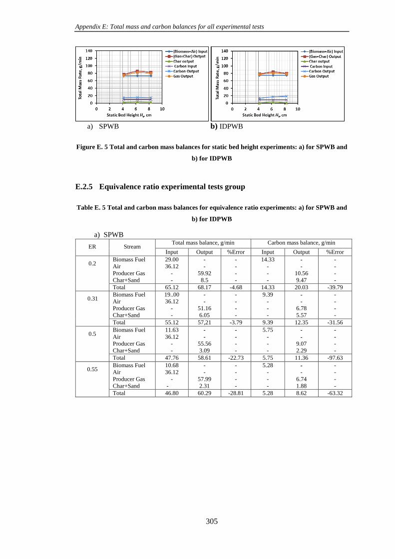
Appendix E: Total mass and carbon balances for all experimental tests
305
a) SPWB b) IDPWB
Figure E. 5 Total and carbon mass balances for static bed height experiments: a) for SPWB and
b) for IDPWB
E.2.5 Equivalence ratio experimental tests group
Table E. 5 Total and carbon mass balances for equivalence ratio experiments: a) for SPWB and
b) for IDPWB
a) SPWB
ER Stream Total mass balance, g/min Carbon mass balance, g/min
Input Output %Error Input Output %Error
0.2 Biomass Fuel
Air
Producer Gas
Char+Sand
29.00
36.12
-
-
-
-
59.92
8.5
-
-
-
-
14.33
-
-
-
-
-
10.56
9.47
-
-
-
-
Total 65.12 68.17 -4.68 14.33 20.03 -39.79
0.31 Biomass Fuel
Air
Producer Gas
Char+Sand
19..00
36.12
-
-
-
-
51.16
6.05
-
-
-
-
9.39
-
-
-
-
-
6.78
5.57
-
-
-
-
Total 55.12 57,21 -3.79 9.39 12.35 -31.56
0.5 Biomass Fuel
Air
Producer Gas
Char+Sand
11.63
36.12
-
-
-
-
55.56
3.09
-
-
-
-
5.75
-
-
-
-
-
9.07
2.29
-
-
-
-
Total 47.76 58.61 -22.73 5.75 11.36 -97.63
0.55 Biomass Fuel
Air
Producer Gas
Char+Sand
10.68
36.12
-
-
-
-
57.99
2.31
-
-
-
-
5.28
-
-
-
-
-
6.74
1.88
-
-
-
-
Total 46.80 60.29 -28.81 5.28 8.62 -63.32

Appendix E: Total mass and carbon balances for all experimental tests
306
b) IDPWB
ER Stream Total mass balance, g/min Carbon mass balance, g/min
Input Output %Error Input Output %Error
0.2 Biomass Fuel
Air
Producer Gas
Char+Sand
41.71
52.98
-
-
-
-
86.73
15.10
-
-
-
-
17.77
-
-
-
-
-
14.90
6.58
-
-
-
-
Total 94.69 101.83 -7.54 17.77
21.48
-20.88
0.277 Biomass Fuel
Air
Producer Gas
Char+Sand
30.14
52.98
-
-
-
-
74.33
8.28
-
-
-
-
12.84
-
-
-
-
-
10.54
5.09
-
-
-
-
Total 82.61 82.61 0.62 12.84 15.63 -21.74
0.381 Biomass Fuel
Air
Producer Gas
Char+Sand
21.14
52.98
-
-
-
-
73.05
3.56
-
-
-
-
9.34
-
-
-
-
-
10.34
3.61
-
-
-
-
Total 76.61 76.61 -2.28 9.34
13.95 -49.39
0.45 Biomass Fuel
Air
Producer Gas
Char+Sand
18.55
52.98
-
-
-
-
67.96
0.97
-
-
-
7.90
-
-
-
-
-
8.79
2.88
-
-
-
Total 71.53 68.93 3.63 7.90
11.67 -47.72
a) SPWB b) IDPWB
Figure E. 6 Total and carbon mass balances for equivalence ratio experiments: a) for SPWB
and b) for IDPWB
E.2.6 Bed temperature T2 experimental tests group
Table E. 6 Total and carbon mass balances for bed temperature T2 experiments: a) for SPWB
and b) for IDPWB
a) SPWB
T2, oC Stream Total mass balance, g/min Carbon mass balance, g/min
Input Output %Error Input Output %Error
360 Biomass Fuel
Air
Producer Gas
Char+Sand
19.86
52.98
-
-
-
-
83.38
3.63
-
-
-
-
9.91
-
-
-
-
-
14.40
0.82
-
-
-
- Total 72.84 87.01 -19.45 9.91
15.22 -53.54
465 Biomass Fuel
Air
Producer Gas
Char+Sand
19.86
52.98
-
-
-
-
88.95
1.30
-
-
-
-
9.91
--
-
-
-
-
-
13.76
0.55
-
-
-
-
Total 72.84 90.25 -23.90 9.91 14.31 -44.42

Appendix E: Total mass and carbon balances for all experimental tests
307
b) IDPWB T2, oC Stream Total mass balance, g/min Carbon mass balance, g/min
Input Output %Error Input Output %Error
360 Biomass Fuel
Air
Producer Gas
Char+Sand
21.92
52.98
-
-
-
-
75.26
3.36
-
-
-
-
9.34
-
-
--
-
-
-
11.42
3.61
-
-
-
-
Total 74.90 78.62 -4.96 9.34 15.03
-60.93
465 Biomass Fuel
Air
Producer Gas
Char+Sand
21.92
52.98
-
-
-
-
82.03
3.386
-
-
-
-
9.34
-
-
-
-
-
13.89
2.77
-
-
-
-
Total 74.90 85.41 -14.04 9.34 16.67 -78.50
a) SPWB b) IDPWB
Figure E. 7 Total and carbon mass balances for bed temperature T2 experiments: a) for SPWB
and b) for IDPWB
E.2.7 Holes number of distributor plate experimental tests group
Table E. 7 Total and carbon mass balances for distributor holes number experiments: a) for
SPWB and b) for IDPWB
a) SPWB Norf Stream Total mass balance, g/min Carbon mass balance, g/min
Input Output %Error Input Output %Error
19 Biomass Fuel
Air
Producer Gas
Char+Sand
19.87
52.98
-
-
-
-
68.71
5.8
-
-
-
-
9.81
-
-
-
-
-
8.54
6.96
-
-
-
-
Total 72.85 74.51 -2.28 9.81
15.5 -60
85 Biomass Fuel
Air
Producer Gas
Char+Sand
19.87
52.98
-
-
-
-
84.14
3.66
-
-
-
-
9.81
-
-
-
-
-
14.4
1.19
-
-
-
-
Total 72.85 87.80 -20.52 9.81 15.93 -62.31
169 Biomass Fuel
Air
Producer Gas
Char+Sand
19.87
52.98
-
-
-
-
58.97
3.33
-
-
-
-
9.81
-
-
-
-
-
6.35
4.1
-
-
-
-
Total 72.85 62.3 -14.48 9.81 10.45 -6.45

Appendix E: Total mass and carbon balances for all experimental tests
308
b) IDPWB
Norf Stream Total mass balance, g/min Carbon mass balance, g/min
Input Output %Error Input Output %Error
19 Biomass Fuel
Air
Producer Gas
Char+Sand
18.55
52.98
-
-
-
-
61.31
6.84
-
-
-
-
7.9
-
-
-
-
-
5.95
3.99
-
-
-
-
Total 71.53 68.15 4.73 7.9 9.94 -25.83
85 Biomass Fuel
Air
Producer Gas
Char+Sand
18.55
52.98
-
-
-
-
67.96
3.33
-
-
-
-
7.9
-
-
-
-
-
8.79
2.9
-
-
-
-
Total 71.53 71.29 0.34 7.9 11.69 -48.01
169 Biomass Fuel
Air
Producer Gas
Char+Sand
18.55
52.98
-
-
-
-
56.19
1.95
-
-
-
-
7.9
-
-
-
-
-
7.9
2.81
-
-
-
-
Total 71.53 62.3 18.71 7.9 10.71 -35.62
a) SPWB b) IDPWB
Figure E. 8 Total and carbon mass balances for distributor holes number experiments: a) for
SPWB and b) for IDPWB