1

MICROSCOPIC TRAFFIC SIMULATION: MODELS AND APPLICATION Tomer Toledo Massachusetts Institute of Technology, Center for Transportation and Logistics, 77 Massachusetts Ave., NE20-208, Cambridge MA, 02139, USA, Tel: (617) 252-1123, Fax: (617) 252-1130, Email: toledo@mit.edu Haris Koutsopoulos Northeastern University, Department of Civil and Environmental Engineering, 437 Snell Engineering Center, Boston MA 02115,USA, Tel: (617) 373-4635, Fax: (617) 373-4419, Email: haris@coe.neu.edu Moshe Ben-Akiva Massachusetts Institute of Technology, Department of Civil and Environmental Engineering, 77 Massachusetts Ave., 1-181, Cambridge MA, 02139, USA, Tel: (617) 253-5324, Fax: (617) 253-0082, Email: mba@mit.edu Mithilesh Jha Jacobs Civil Inc., 222 South Riverside Plaza, Chicago IL, 60606, USA Tel: (312) 612-6043, Fax: (312) 655-9706, Email: mithilesh.jha@jacobs.com ABSTRACT Microscopic traffic simulation is an important tool for traffic analysis, particularly in the presence of intelligent transportation systems (ITS). In this paper we describe the main components of a microscopic traffic simulation model and illustrate the discussion with examples drawn from our experience with a microscopic traffic simulation tool, MITSIMLab. With respect to the use of simulation models in practical applications we discuss issues related to their calibration and validation. We demonstrate this part with a case study of applying MITSIMLab in Stockholm, Sweden. INTRODUCTION Traffic congestion is a major problem in urban areas. It has a significant adverse economic impact through deterioration of mobility, safety and air quality. A recent study (FHWA 2001) estimated that 32% of the daily travel in major U.S. urban areas in 1997 occurred under congested traffic conditions. The annual cost of lost time and excess fuel consumption during congestion was estimated at $72 billion, which represents a 300% increase from 1982. Schrank and Lomax (2001) estimated that 1,800 new freeway lane-miles and 2,500 new urban street lane-miles would have been required in the U.S.

2

in order to keep congestion from increasing from 1998 to 1999. The budgets required for such infrastructure investments far exceed available resources. Moreover, in many urban areas, land scarcity and environmental constraints would limit construction of new roads or expansion of existing ones even if funds were available. As a result, the importance of better management of the road network to efficiently utilize existing capacity is increasing. In recent years, a large array of traffic management schemes have been proposed and implemented. Methods and algorithms proposed for traffic management need to be calibrated and tested. In most cases, only limited, if any, field tests are feasible because of prohibitively high costs and lack of public acceptance. Furthermore, the usefulness of such field studies is deterred by the inability to fully control the conditions under which they are performed. Hence, tools to perform such evaluations in a laboratory environment are needed. Intelligent Transportation Systems (ITS) applications, such as dynamic traffic management and route guidance, have emerged as important tools for traffic management. These applications involve information dissemination from a traffic management center to drivers and deployment of management and control schemes. The impact of information and control strategies on traffic flow can be realistically modeled only through the response of individual drivers to the information. For example, evaluation of different incident response strategies that utilize lane use signs requires modeling of drivers’ response to the signs and a plausible model of their lane changing behavior. Microscopic simulation models, which analyze traffic phenomena through explicit and detailed representation of the behavior of individual drivers, have been widely used to that end by both researchers and practitioners. The detailed level of behavior modeling in microscopic simulation models is particularly critical when disaggregate relations between vehicles are more important than aggregate traffic flow characteristics. An example is the study of safety impacts, for which headway distributions, frequency of emergency braking and the number and locations of lane changes may provide better indication of the impact on safety of different geometric design plans than aggregate measures such as average speed, flow and density. The purpose of this paper is to describe the main components of a microscopic traffic simulation model and discuss calibration and validation of these tools to practical applications. We illustrate the discussion with examples drawn from our experience using the microscopic traffic simulator MITSIMLab (Yang and Koutsopoulos 1996, Yang et al 2000). OVERALL STRUCTURE While the software implementation may vary significantly, three main components are common to most existing microscopic traffic simulation tools: 1. Traffic flow model (vehicle-mover) 2. Traffic management system representation 3. Output and graphical interfaces In MITSIMLab these components are implemented as separate modules, which exchange information with each other according to the paradigm outlined in Figure 1. Within the microscopic traffic simulator (MITSIM) module, the movements of individual vehicles are represented via detailed travel and driving behavior models. Traffic flow characteristics emerge from the individual behaviors. Vehicles traveling in the network activate surveillance devices (e.g. loop

3

detectors, video-sensors). The information gathered by the surveillance system is transferred to the traffic management simulator (TMS), which represents the traffic control and routing logic under evaluation. This information is used to determine traffic control settings and route guidance. The control and routing strategies generated by the traffic management module determine the states of traffic control and route guidance devices. In turn, drivers respond to the various traffic controls and guidance while interacting with each other. Output from the simulation can be obtained both in the form of numerical data and via the graphical user interface (GUI), which is used for both debugging purposes and demonstration of traffic impacts through vehicle animation.

Traffic ManagementSimulator (TMS)

Microscopic TrafficSimulator (MITSIM)

Traffic Control andRouting Devices

Traffic SurveillanceSystem

Graphical UserInterface (GUI)

Figure 1. Elements of MITSIMLab and their Interactions

In the next sections we describe some of the important elements and models within the simulation framework. TRAFFIC FLOW MODELING In microscopic simulation, traffic flow is captured by detailed modeling of the behavior of individual vehicles, including representation of travel demand and behavior (e.g. route choice models) and driving behavior (e.g. speed/acceleration, lane changing and gap acceptance models). Simulated traffic patterns emerge from the collective travel and driving decisions made by the simulated drivers. Hence, the realism of the simulator depends on the richness and fidelity of these models and therefore development of sound behavior models and rigorous calibration and validation of these models are critically important to any application of the simulation tool. Travel demand Travel demand is most commonly represented in microscopic traffic simulation tools by time-dependent origin to destination (OD) tables. During a simulation run, individual vehicles are generated based on the demand rates specified in these tables. An alternative specification of the demand utilizes generation rates at the origins and turning fractions at intersections. The advantage of this approach is that it uses data that is directly measurable in the field. This approach is suitable for simulation of traffic corridors, which do not allow for route choices. However, in more complex networks, it may lead to significant over-estimation of traffic flows caused by vehicles circulating around the network. Moreover, since simulated vehicles do not have defined destinations, route choice behavior may not be modeled realistically and therefore, for example, the impact of advanced traveler information systems (ATIS) may not be captured.

4

To illustrate this problem, consider the network shown in Figure 2. Suppose that the true demand is for 50 trips for each of the following OD pairs: 1→3, 1→6, 4→3, 4→6 and that only the simple paths (1-2-3, 1-2-5-6, 4-5-2-3 and 4-5-6, respectively) are used. Based on field observations, the following generation rates and turning fractions would be defined: • 100 vehicles generated at nodes 1 and 4. • At node 2: 50% turning to node 3, 50% turning to node 5. • At node 5: 50% turning to node 2, 50% turning to node 6.

1 52 6

43 Figure 2. Network illustrating travel demand representations

Table 1 summarizes the expected number of vehicles (rounded to the nearest integer) that originate at node 1 and follow various routes until they leave the network according to a simulation model that uses the above generation rates and turning percentages. On average, 25% of these vehicles cycle in the network causing overestimation of congestion in the network. Furthermore, the overestimation of congestion increases with the dimension of the network since the probability that a vehicle would leave the network decreases further. The result for vehicles originating at node 4 is similar.

Route Expected number of vehicles 1-2-3 50 1-2-5-6 25 1-2-5-2-3 13 1-2-5-2-5-6 6 1-2-5-2-5-2-3 3 1-2-5-2-5-2-5-6 2 1-2-5-2-5-2-5-2-3 1

Table 1. The expected number of vehicles following various routes in the network

In MITSIMLab time-dependent OD tables are used to input travel demand. OD tables may be defined for time intervals of varying duration. They may also be defined for up to 15 different user-defined vehicle types (e.g. cars, trucks, buses, SUVs) or generated vehicles may be randomly assigned a vehicle type based on an input fleet mix. Vehicle tables may also be used to specify the demand, replacing or complementing OD tables. Vehicle tables are lists of vehicles to be generated with pre-specified origins, destinations, departure times and optionally vehicle types and paths. Routing behavior The paths drivers follow in the network are determined by route choice models, which may be either path-based or link-based. Path-based models assume that drivers select between alternative routes to their destinations based on the attributes of the entire path. Link-based models assume that drivers only select the next link to travel on at each decision point. The main disadvantage of path-based models is that they require enumeration of all used paths, which may be prohibitively expensive in

5

large networks. In contrast, link-based models do not require path enumeration but represent myopic behavior that may lead to unrealistic choices, such as a vehicle traveling on the freeway, taking an off-ramp and immediately after that an on-ramp back to the freeway. Moreover, link-based route choice may result in cyclic paths. The explicit path choice set defined for path-based models can easily exclude such paths. MITSIMLab supports both route choice models. The path-based model utilizes a path-size logit model (Ramming 2002), which accounts for overlap between paths. The path choice set is specified by the user for each OD pair. Choice probabilities for the various paths are given by:

( ) ( )( )( )( )

( )( )

exp ln exp|

expexp lnnn

in in in inn

jn jnjn jnj Cj C

V PS PS VP i C

PS VV PS∈∈

+= =

+ ∑∑ (1)

inV and inPS are the systematic utility and the size of path i to driver n, respectively. nC is the path

choice set for driver n. The systematic utilities inV depend on perceived path travel times, which are calculated as the sum of perceived travel times on links that comprise the path. Drivers may perceive freeway travel times differently from travel times on urban streets. A freeway bias coefficient captures this behavior:

i

ai

a a

TTTTβ∈Γ

= ∑ (2)

iTT and aTT are the travel times on path i and link a, respectively. iΓ is the set of links in path i. aβ is a link-type variable defined by:

1

freeway

a if link a is freeway

otherwiseββ

=

(3)

( 1)freewayβ ≥ is a constant that captures drivers' preference to freeway travel. The path-size term adjusts the path utility to account for overlapping links in alternative paths. It is bounded 0 1inPS< ≤ . Its value is 1 if the path does not overlap with other paths and decreases with the level of overlap. A number of path-size formulations have been proposed in the literature (see Ramming 2002 for a review). The formulation of Bekhor et al (2001) is adopted in MITSIMLab:

1

i

n

ain

a iiaj

j C j

lPSLLL

γ

γ δ∈Γ

∈

=

∑

∑

(4)

al and iL are the lengths of link a and path i, respectively. ajδ are elements of the link-path incidence matrix, i.e., 1ajδ = if path j includes link a and 0 otherwise.

The link-based model uses a multinomial logit formulation:

( ) ( )( )

exp|

expsn

lnsn

knk L

VP l L

V∈

=∑

(5)

lnV is the systematic utility, to driver n, of selecting link l as the next link. snL is the set of links (emanating from node s) that driver n may choose as the next link. Systematic utilities inV depend on the perceived travel time on link l, the perceived travel time on the shortest path from the downstream node of link l to the destination, and a freeway diversion dummy

6

variable, which penalizes exiting a freeway (i.e. drivers traveling on a freeway and choosing a non-freeway next link). The effect of traveler guidance and information on route choices may be captured in both the path-based and the link-based route choice models through link travel time tables that are updated according to the specifications of the guidance system. Drivers with no access to information use habitual link travel time tables, which represent prevailing traffic conditions. Drivers who have access to information (e.g. pre-trip, in-vehicle technologies and variable message signs) use updated link travel time tables, which incorporate real-time traffic conditions. In the path-based model route choices are reevaluated whenever new information is received. Drivers' preference to keep their previously assigned habitual paths is captured by diversion dummy variables, which penalize switching from the driver's habitual route. Driving behavior Traffic dynamics in micro-simulation tools is the emergent result of a set of driving behavior models, which determine the speed/acceleration and lane changes performed by vehicles under various conditions. Acceleration models include free-flow, car following and emergency behaviors. Lane changing behavior is most often classified as either mandatory (MLC) or discretionary (DLC). MLC applies when the vehicle must change lanes, for example, to follow the path or to avoid a blocked lane. DLC applies when the driver perceives that traffic conditions are better in other lanes. In most cases acceleration and lane changing behaviors are modeled separately. The core model implemented in MITSIMLab is an integrated driving behavior model, which captures both lane changing and acceleration behaviors and accounts for inter-dependencies and correlations between these behaviors. The structure of the integrated model is shown in Figure 3. The model hypothesizes four levels of decision-making: target lane, gap acceptance, target gap and acceleration. This decision process is latent. The target lane and target gap choices are both unobservable. Only the driver's actions (lane changes and accelerations) are observed. Latent choices are shown as ovals in Figure 3. Observed choices are shown as rectangles. At the highest level the driver chooses a target lane. The target lane is the lane the driver perceives as best to be in. A utility maximization model is used to explain the target lane choice. Lane utilities integrate mandatory and discretionary lane changing considerations into a single model, and thus capture trade-offs between these considerations. Important variables that affect the target lane choice are the distance to the point where a the vehicle must be in a specific lane and the number of lane changes required to be in that lane, densities and speeds of the vehicles in the neighborhood of the subject, presence of heavy vehicles and tailgating behavior. In the case that either the right lane or the left lane are chosen, the driver evaluates the adjacent gap in the target lane and decides whether this gap can be used to execute the lane change or not. If the gap is accepted the lane change is immediately executed. Gap acceptance decisions are based on comparing the available lead and lag space gaps, defined by the clear spacing between the subject and the intended leader and lag vehicles, respectively, with the corresponding critical gaps, which are the minimum acceptable gaps. Critical gaps are functions of explanatory variables, such as the relative speeds of the subject with respect to the lead and lag vehicles. In order to accept the gap and execute the lane change both the lead gap and the lag gap must be acceptable. If the adjacent gap is rejected, the driver chooses a target gap in the target lane traffic. The target gap will be used to perform the desired lane change. In the current implementation the target gap choice

7

set includes three alternatives, defined by their locations relative to the subject vehicle: the adjacent gap, the forward gap and the backward gap. The target gap choice is based on the lengths of the candidate gaps, relative speeds of the vehicles involved and the distance from the subject vehicle to an ideal position relative to the target gap, which would allow the driver to execute the lane change.

RightLeft

Forward

Acc. Acc.Acc.

Current

Acc.

Forward

Acc.Acc. Acc.

...

TargetLane

TargetGap

Acceleration

Gapacceptance

ChangeRight

ChangeLeft

NoChange

NoChange

Adjacent

Acc.

Backward Backward

Acc.

Adjacent

Figure 3. Structure of the integrated driving behavior model

For each one of the situations described above, a corresponding acceleration behavior is defined. Vehicles that choose to stay in their current lanes would, depending on the time headway from the front vehicle (leader), either follow their leader or accelerate to attain their desired speeds. A similar behavior also applies for vehicles that are executing a lane change, but with respect to their leader in the new lane. The acceleration of vehicles that have chosen a target gap is determined such that to facilitate the execution of the desired lane change using the target gap (i.e. the driver tries to position the vehicle in a way that will increase the probability that the target gap will be acceptable). This acceleration may also be constrained by car following considerations, since the lane change is not immediate. In addition to this core model, behaviors in several other situations are represented in the simulation. For example, the acceleration model also represents emergency braking, response to signals and signs and accounts for vehicle capabilities and driver aggressiveness. The lane changing model also represents priority and non-priority merging behaviors and yielding and forced merging behaviors. TRAFFIC MANAGEMENT SYSTEM REPRESENTATION Accurate representation of the traffic management system is important to ensure the realism of simulation results, and is particularly essential when the simulation tool is used to evaluate the performance of various traffic control and guidance systems, which require support for a wide range of traffic control and route guidance systems, such as ramp control, freeway mainline control (e.g., lane control signs, variable speed limit signs, portal signals at tunnel entrances), intersection control, variable message signs and in-vehicle route guidance.

8

The traffic management simulator (TMS) module in MITSIMLab has a generic structure that can represent different designs of such systems with logic at varying levels of sophistication, from isolated pre-timed signals to real-time predictive systems. Figure 4 outlines the structure of TMS. Control strategies and routing information are generated using either reactive or proactive approaches. The reactive approach consists of pre-determined control laws that depend only on the current network state. In the proactive approach, the system predicts future traffic conditions and optimizes traffic control and routing strategies based on these predicted conditions. In this case, the generation of control and routing strategies is an iterative process. Given a proposed strategy, traffic conditions on the network are predicted and the performance of the candidate strategy is evaluated. If the strategy is found to be satisfactory, it is implemented; if additional strategies need to be tested, another generation-prediction iteration is performed.

TMS

Network StateEstimation

Control & RoutingGeneration

Network StatePrediction

Surveillance SensorData

Traffic Controls &Route Guidance

Traffic Simulator(MITSIM)

Figure 4. Structure of the traffic management simulator (TMS)

The most widely used traffic management tool is traffic signal control at intersections. TMS supports modeling of intersection controls through three types of controllers: pre-timed, actuated and a generic controller. The logic for the pre-timed and actuated controllers, which are simpler to implement, require pre-specified phase plans and phase orders. In some cases, such as for pre-timed or four-phase actuated controllers, these types can simulate the control logic exactly. In other cases, they may be used to approximate more advanced control logic such as dual-ring controllers or European controllers in which phasing is not necessarily explicit. The generic controller (Davol 2001) addresses the limitations of the two controllers and allows the simulation of a wide range of advanced control strategies. Instead of requiring each phase to be specified explicitly, the generic logic allows each movement (signal group) to be controlled independently, thus providing full flexibility in the control logic. This logic is specified by means of detailed conditions that must be met before a signal indication changes, such as time, detector states, other signal states, and other controller states. By specifying these conditions, any logic can be modeled. For example, specifying only time constraints simulates a pre-timed controller. Constraints with respect to detector states add vehicle actuation, while constraints as to other signal states allow the specification of complementary or conflicting movements. Conditions on other controller states allow coordinated and area-wide adaptive control, which is necessary for the simulation of advanced control systems. Figure 5 summarizes the logic of the generic controller. The controller iterates through all the signal groups. For each signal group, it evaluates the logic conditions and determines whether the group’s signal state should be updated. Because the group states may be inter-dependent,

9

with the state of one group as an input to the logic of another group, this evaluation step must be iterative. Therefore, when the states of all the signal groups have been determined, the controller again cycles through the groups to check if the new states cause more signal groups to change. This process is repeated until the states of all signal groups are stable, at which point the controller displays the updated states of the traffic signals in TMS. This process is repeated each time step, typically 0.1 seconds of simulation time.

Initialize controller

Read input parametersSet signals to initial states

For all signal groups:

Display updatedsignal states

Set new state

Evaluateconditions

Any statechanges ?

Yes

No

Advancesimulation clock

Figure 5. Logic of the generic controller

OUTPUT AND GRAPHICAL INTERFACE Simulation tools are used to study complex systems, and therefore generate extensive sets of outputs. While very useful, this wealth of information can make it difficult to gain insights and analyze the system based only on the numerical outputs. To that end, most micro-simulation tools offer extensive graphical user interfaces (GUI). These interfaces are used for both debugging purposes and demonstration of traffic impacts through vehicle animation. Figure 6 shows examples of the MITSIMLab GUI. The figure on the left illustrates a high level view of the network. Links are color coded to demonstrate congestion levels. The figure on the right focuses on the details of the operations of a complex interchange.

Figure 6. Example of the graphical user interface

10

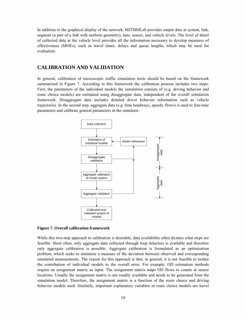
In addition to the graphical display of the network, MITSIMLab provides output data at system, link, segment (a part of a link with uniform geometry), lane, sensor, and vehicle levels. The level of detail of collected data at the vehicle level provides all the information necessary to develop measures of effectiveness (MOEs), such as travel times, delays and queue lengths, which may be used for evaluation. CALIBRATION AND VALIDATION In general, calibration of microscopic traffic simulation tools should be based on the framework summarized in Figure 7. According to this framework the calibration process includes two steps: First, the parameters of the individual models the simulation consists of (e.g. driving behavior and route choice models) are estimated using disaggregate data, independent of the overall simulation framework. Disaggregate data includes detailed driver behavior information such as vehicle trajectories. In the second step, aggregate data (e.g. time headways, speeds, flows) is used to fine-tune parameters and calibrate general parameters in the simulator.

Estimation ofindividual models

Data collection

Aggregate calibrationof model system

Disaggregatevalidation

Model refinement

Dis

aggr

egat

eda

taA

ggre

gate

data

Aggregate validation

Calibrated andvalidated system of

models

Figure 7. Overall calibration framework

While this two-step approach to calibration is desirable, data availability often dictates what steps are feasible. Most often, only aggregate data collected through loop detectors is available and therefore only aggregate calibration is possible. Aggregate calibration is formulated as an optimization problem, which seeks to minimize a measure of the deviation between observed and corresponding simulated measurements. The reason for this approach is that, in general, it is not feasible to isolate the contribution of individual models to the overall error. For example, OD estimation methods require an assignment matrix as input. The assignment matrix maps OD flows to counts at sensor locations. Usually the assignment matrix is not readily available and needs to be generated from the simulation model. Therefore, the assignment matrix is a function of the route choice and driving behavior models used. Similarly, important explanatory variables in route choice models are travel

11

times, which are flow-dependent. Simulated flows are a function of the OD flows, driving behavior and the route choice model itself. Hence, the following optimization problem, which simultaneously calibrates the parameters of interest (OD flows, route choice and driving behavior parameters) may be formulated:

( )( )

, ,min ,

. . , ,

arg min

obs sim

OD

sim

obs

X

f M M

s t M g OD

OD AX Y

β θ

β θ=

= −

(6)

β , θ and OD are the vectors of parameters to be calibrated: driving behavior, route choice and OD flows, respectively. obsM and simM are vectors of observed and simulated traffic measurements, respectively. ( )g ⋅ represents the simulation process. obsY are observed traffic counts at sensor locations. A is the assignment matrix. The above problem is very difficult to solve exactly. The OD constraint, for example, is a fixed-point problem, which is a hard problem in its own merit (Cascetta and Postorino 2001). Hence, we propose the iterative heuristic approach outlined in Figure 8. This approach accounts for interactions between driving behavior, OD flows and route choice behavior by iteratively calibrating driving behavior parameters and travel behavior elements. At each step the corresponding sets of parameters is calibrated, while the other parameters remain fixed to their previous values. Calibration of the route choice model requires a set of reasonable paths for each OD and expected link travel times used as explanatory variables in the model. OD estimation requires generation of an assignment matrix. Hence, the travel behavior calibration step is also iterative: based on the existing OD flows, parameters of the route choice model are calibrated. The calibrated route choice model is used to generate an assignment matrix, and perform OD estimation. The new OD flows are used to re-calibrate route choice parameters and so on.

Calibration ofdriving behavior

parameters

Calibration ofroute choiceparameters

O-D estimation

Path choiceset generation

Initial drivingbehavior

Calibration

Convergence

Calibrated trafficsimulation model

No

Yes

Habitualtravel times

Figure 8. Methodology for aggregate calibration of micro-simulation models.

12

In summary the proposed calibration process proceeds as follows: Step 1. Initialize parameters, 0β , 0θ and 0OD . Step 2. Estimate OD and calibrate route choice parameters assuming fixed driving behavior

parameters. Step 3. Calibrate driving behavior parameters assuming the OD matrix and route choice parameters

estimated in Step 2. Step 4. Update habitual travel times using the OD matrix, route choice and driving behavior

parameters estimated in Steps 2 and 3. Step 5. Check for convergence: If convergence, terminate.

Else, continue to step 2. Case study We now describe in more detail the application of the procedure described above to a case study in Stockholm, Sweden. The case study network is a mixed urban-freeway network in the Brunnsviken area, north of the Stockholm CBD, shown in Figure 9. The E4 corridor, on the west side of the network is the main freeway connecting the northern suburbs to the CBD. The east side of the network is a parallel arterial. These routes experience heavy southbound congestion during the AM peak period.

MCS sensors

Loop detectors

1 2

E4

E18 MCS sensors

1

2

3

Passage points

Loop detectors

4

5

6

7B

A D

C

Queue Measurement

(a) May 1999 (b) May 2000

Figure 9. The case study network and measurement locations.

AM peak period traffic data from May 1999 was collected for calibration. Similar data was collected a year later, during May 2000, for validation. Sensor and other measurement locations for May 1999 and May 2000 are also shown in Figure 9. Sensor data was available from the Motorway Control System (MCS) and additional loop detectors. The validation data also included measurements of point-to-point travel times by probe vehicles. The probe vehicles also recorded queue lengths. Additional queue measurements were obtained from aerial photographs. A static AM peak OD flows matrix, previously developed for planning studies, was available for OD estimation. Additional information about vehicle mix by type (i.e. autos, buses, trucks etc.) and lane use privilege (i.e.

13

permission to use bus lanes) was used to set corresponding input data for the simulation model. The type assigned to a simulated vehicle affects its physical properties (length and width) and performance capabilities (e.g. maximum speed, maximum acceleration and deceleration). The importance of lane use privileges in this application stems from the extensive bus lanes system in place. Only buses and taxis are allowed to use these lanes. The autos category was further split into two separate groups: high-performance and low-performance vehicles. Vehicles in these groups have different capabilities in terms of their maximum acceleration, deceleration and speeds. Initial parameter calibration Driving behavior parameters The various parameters of the driving behavior models, with the exception of the desired speed parameters, were calibrated using the above procedure. The parameters of the distribution of desired speeds were estimated independently from speed data. The desired speed is the speed that the driver would choose in the absence of any restrictions imposed by other vehicles or by traffic control devices. This speed is affected by the geometry of the section and by driver characteristics. In MITSIMLab, the desired speed distribution is defined relative to the speed limit. This distribution was inferred from the speeds of unconstrained vehicles, which were defined as those vehicles that crossed the sensor stations at times when the flow rate was less than 600 veh/hr/lane. This threshold corresponds to the Highway Capacity Manual (HCM 2000) level of service A. An analysis of the sensitivity of the desired speed distribution with respect to the flow threshold was performed. Desired speed distributions were also developed assuming flow thresholds of 300 and 200 veh/hr/lane. The results were not significantly different from the one obtained for 600 veh/hr/lane. A small sub-network of the Brunnsviken network was used to obtain initial values for other driving behavior parameters. Important considerations that led to adopting this approach were: 1. The calibration process is more manageable when performed on a sub-network. 2. The sub-network was chosen such that available sensor data can be used to generate accurate OD

flows at 1 min. intervals. Moreover, for each OD pair in the sub-network only one path exists. Therefore most of the errors generated by OD estimation and route choice modeling were eliminated.

Figure 10. Location and details of the calibration sub-network.

14

The sub-network and sensor locations within it are shown in Figure 10. This sub-network was chosen for several reasons including: 1. Minimal downstream effects – the location is far from possible spillbacks from the bottlenecks in

the network that may affect the behavior but are not represented in the MITSIMLab sub-network model.

2. Representation of different behaviors – The sub-network contains on- and off-ramps, allowing capturing mandatory and discretionary lane changing and merging behavior, which are likely to be important behaviors in this case study.

Since sensor counts were used to extract OD information for the sub-network, the calibration objective function was to minimize the square deviations of simulated sensor speeds from the observed ones:

2

1 1min ( )

T Nsim obs

nt ntt n

V Vβ = =

−∑∑ (7)

obsntV and sim

ntV are the observed and simulated speeds, respectively, measured at sensor n during time period t. N and T are the number of sensors and time periods, respectively. Path choice set generation The path-based route choice model requires a set of alternative paths for each OD pair in the network. The following procedure was used to generate these sets: 1. Generation of a comprehensive path set – A comprehensive path choice set was generated using

the link-based route choice model. 2. Unreasonable path elimination - The link-based route choice tends to generate a large number of

paths. Unreasonable paths (e.g. paths using off-ramp and on-ramp immediately after that) were eliminated.

The path choice set may depend on traffic conditions, in which case the process should be repeated as OD flows and the parameters of the route choice model evolve to ensure that all reasonable paths are captured. The structure of the Brunnsviken network facilitates the generation of the path set, since only one or two reasonable paths exist for each OD pair. Therefore, the path generation exercise was preformed only once. Overall Calibration OD estimation The OD estimation problem is often formulated as a generalized least squares (GLS) problem. The GLS formulation minimizes the deviations between estimated and observed sensor counts while also minimizing the deviation between the estimated OD flows and seed OD flows (Cascetta et al 1993). The corresponding optimization problem is:

( ) ( ) ( ) ( )1 1

0min

T TH H H H

XAX Y W AX Y X X V X X− −

≥− − + − − (8)

X and HX are vectors of estimated and historical (seed) OD flows, respectively. HY are the historical (observed) sensor counts. A is the assignment matrix, which maps OD flows to sensor counts. W and V are the variance-covariance matrices of the sensor counts and OD flows, respectively. However, in the problem discussed in this paper, the assignment matrix is not known. Hence, we propose the following iterative process: First, the simulation is run, using the calibrated parameters

15

and a set of seed OD flows to generate an assignment matrix. This assignment matrix is in turn used for OD estimation. Due to congestion effects, the assignment matrix generated from the seed OD may be inconsistent with the estimated OD. Therefore, the OD estimation process must be iterative. The Brunnsviken network includes a large number of OD pairs and sensor locations, which made OD estimation computationally intensive. To overcome this limitation, a sequential estimation technique (Cascetta et al 1993), which exploits the sparse structure of the assignment matrix was employed. The sequential estimation process is as follows: The seed OD is taken as fixed for the first time period. An assignment matrix is generated and used to estimate the effect of the first period demand on sensor counts in subsequent periods. The demand in the second period is then estimated, based on the observed counts less the estimated contribution from OD flows in the first time period. The assignment matrix is used to estimate the effect of second period demand on subsequent periods. This process is continued until OD flows are estimated for all periods of interest. Route Choice Parameter Given the OD flows, path choice sets and habitual travel times, parameters of the route choice model were calibrated to match the split between the two sensors marked 1 and 2 in Figure 9a. These points were selected because the structure of the network ensures that all vehicles with a choice of paths pass exactly one of them. Splits rather than counts were used in order to reduce errors from inaccuracies in the scale of the OD matrix, especially at early stages of the estimation process. Driving behavior parameters While the initial calibration of driving models included a wide range of parameters, during this step only a limited set of parameters was calibrated. Sensitivity analysis indicated that the calibration could focus on the scale parameters of the various models. Scale parameters are the sensitivity constants in the acceleration models and alternative specific constants in the lane changing models. Hence, given OD flows and route choice parameters, scale parameters of the acceleration and lane changing models were calibrated using the formulation given in Equation (7), now applied to the entire network. Habitual travel times The route choice model uses habitual path travel times as explanatory variables. Calibration of the model parameters requires knowledge of these travel times. While planning studies can be used to provide initial values, further refinement is necessary to capture the time-dependent nature of travel times and improve the accuracy of the models. Therefore, an iterative day-to-day perception updating model was used to improve initial travel times estimates obtained from planning studies. At each iteration of this process, representing a day, habitual travel times were updated as follows:

( )1 1k k k k kit it itTT tt TTλ λ+ = + − (9)

kitTT and k

ittt are the habitual and experienced travel times on link i, time period t on day k, respectively. kλ is a weight parameter ( 0 1kλ< < ).

16

Validation Results Three types of measurements were used to validate the calibrated MITSIMLab model: traffic flows, travel times and queue lengths by comparing simulated measurements with the corresponding observed measurements. OD flows were estimated from the May 2000 traffic counts and the previously calibrated model parameters. Traffic flows Observed and simulated traffic flows at key sensor locations were compared using two hours of AM peak data at 15 min. intervals. The results are presented in Figure 11. Two measures of goodness-of-fit were used to quantify the relationship between observed and simulated measurements: The root mean square normalized error (RMSNE), which quantifies the total percentage error of the simulator and the mean normalized error (MNE), which indicates the existence of consistent under- or over-prediction in the simulated measurements. These measures are calculated by:

2

1

1 sim obsNn n

obsn n

m mRMSNEN m=

−=

∑ (10)

1

1 sim obsNn n

obsn n

m mMNEN m=

−= ∑ (11)

obsnm and sim

nm are the observed and simulated measurements, respectively. N is the number of measurement points (over time in this case). RMSNE for the different locations range from 5% to 17%. MNE values range from –12% to 14%. In general, simulated flows correspond well to the measurements and accurately capture temporal patterns. Note that sensor flows were used to estimate the OD flows. Hence, the results emphasize the importance of OD estimation. Travel times Point-to-point travel times measured by the probe vehicles were compared against average simulated travel times. Only few probe vehicle observations were available. Therefore, mean observed travel times could not be accurately estimated. Instead, Figure 12 compares average simulated travel times and individual probe vehicle observations. The figure also shows travel times values corresponding to the average ±2 standard deviations of the simulated travel time. Assuming that simulated travel times follow a normal distribution, these values define an interval containing 95% of simulated travel times. 80 out of the 120 (67%) probe vehicle observations are within these intervals. Simulated travel times match the observed ones very in sections A-B, B-C and D-C, which are relatively uncongested during the AM peak period. Sections C-D, C-B and B-A are heavily congested, as indicated by the shapes of the travel time curves. These shapes are rather well replicated, although the simulation underestimates travel times. The largest incomparability between observed and simulated measurements is in sections A-D and D-A. These are short and congested sections dominated by traffic signals and roundabouts. Some of the error in these sections may be attributed to inconsistencies in the traffic counts in this area (e.g. entry flows to an intersection do not match exit flows) that led to poor OD estimation and to imperfections in the representation of traffic control (e.g. pedestrian and bicycle signals) in the simulation tool.

17

T ra ff ic F low s: 1 W es tbound

0

2 00

4 00

6 00

8 00

10 00

12 00

14 00

16 00

6:4 5 7:00 7 :15 7 :3 0 7 :4 5 8:0 0 8:1 5 8 :30 8 :4 5

O b serv e d

M ITS IM L ab

T ra f f ic F lo w s : 1 E a s tb o u n d

0

2 0 0

4 0 0

6 0 0

8 0 0

1 0 0 0

1 2 0 0

1 4 0 0

1 6 0 0

6 :4 5 7 :00 7 :1 5 7 :3 0 7 :4 5 8 :0 0 8 :1 5 8 :3 0 8 :4 5

O b s e rv ed

M IT S IM Lab

T ra f f ic F lo w s : 2 S o u th b o u n d

0

2 0 0

4 0 0

6 0 0

8 0 0

1 0 0 0

1 2 0 0

1 4 0 0

1 6 0 0

6 :4 5 7 :0 0 7 :1 5 7 :3 0 7 :4 5 8 :0 0 8 :1 5 8 :3 0 8 :4 5

O b served

M IT S IM L a b

T ra f f ic F lo w s : 3 N o r th b o u n d

0

2 0 0

4 0 0

6 0 0

8 0 0

1 0 0 0

1 2 0 0

1 4 0 0

1 6 0 0

6 :4 5 7 :0 0 7 :1 5 7 :3 0 7 :4 5 8 :0 0 8 :1 5 8 :3 0 8 :4 5

O b s erv e d

M IT S IM L ab

T ra f f ic F lo w s : 4 W e s tb o u n d

0

2 0 0

4 0 0

6 0 0

8 0 0

1 0 0 0

1 2 0 0

1 4 0 0

1 6 0 0

6 :4 5 7 :0 0 7 :1 5 7 :3 0 7 :4 5 8 :0 0 8 :1 5 8 :3 0 8 :4 5

O b s erv e d

M IT S IM L ab

T ra f f ic F lo w s : 4 E a s tb o u n d

0

2 0 0

4 0 0

6 0 0

8 0 0

1 0 0 0

1 2 0 0

1 4 0 0

1 6 0 0

6 :4 5 7 :0 0 7 :1 5 7 :3 0 7 :4 5 8 :0 0 8 :1 5 8 :3 0 8 :4 5

O b s erv e d

M IT S IM L ab

T ra f f ic F lo w s : 5 W e s tb o u n d

0

2 0 0

4 0 0

6 0 0

8 0 0

1 0 0 0

1 2 0 0

1 4 0 0

1 6 0 0

6 :4 5 7 :00 7 :1 5 7 :3 0 7 :4 5 8 :0 0 8 :1 5 8 :3 0 8 :45

O bs erved

M IT S IM L ab

T ra f f ic F lo w s : 5 E a s tb o u n d

0

2 0 0

4 0 0

6 0 0

8 0 0

1 0 0 0

1 2 0 0

1 4 0 0

1 6 0 0

6 :4 5 7 :00 7 :1 5 7 :3 0 7 :4 5 8 :0 0 8 :1 5 8 :3 0 8 :4 5

O b s erv ed

M IT S IM Lab

T ra f f ic F lo w s : 6 N o rth b o u n d

0

2 0 0

4 0 0

6 0 0

8 0 0

1 0 0 0

1 2 0 0

1 4 0 0

1 6 0 0

6 :4 5 7 :0 0 7 :1 5 7 :3 0 7 :4 5 8 :0 0 8 :1 5 8 :3 0 8 :4 5

O b s e rve d

M IT S IM L a b

T ra ff ic F lo w s : 6 S o u th b o u n d

0

2 0 0

4 0 0

6 0 0

8 0 0

1 0 0 0

1 2 0 0

1 4 0 0

1 6 0 0

6 :45 7 :0 0 7 :1 5 7 :30 7 :4 5 8 :0 0 8 :15 8 :3 0 8 :4 5

O b s e rved

M IT S IM L ab

T ra f fic F lo w s : 7 S o u th b o u n d

0

2 0 0

4 0 0

6 0 0

8 0 0

1 0 0 0

1 2 0 0

1 4 0 0

1 6 0 0

6 :4 5 7 :0 0 7 :1 5 7 :3 0 7 :4 5 8 :0 0 8 :1 5 8 :3 0 8 :45

O b s erv ed

M IT S IM L ab

T ra f f ic F lo w s : 7 N o rth b o u n d

0

2 00

4 00

6 00

8 00

1 0 00

1 2 00

1 4 00

1 6 00

6 :4 5 7 :00 7 :1 5 7 :3 0 7 :45 8 :0 0 8 :1 5 8 :3 0 8 :45

O b s erv ed

M IT S IM L ab

Figure 11. Comparison of observed and simulated flows at sensor locations.

18

Travel Times: A to B

0.00

50.00

100.00

150.00

200.00

250.00tr

avel

tim

e (s

)7:00 7:15 7:30 7:45 8:00 8:15 8:30 8:45 9:00

Mean - 2*SDMeanMean + 2*SDMeasurements

Travel Times: B to A

0.00100.00200.00300.00400.00500.00600.00700.00800.00900.00

trav

el ti

me

(s)

7:00 7:15 7:30 7:45 8:00 8:15 8:30 8:45 9:00

Mean - 2*SDMeanMean + 2*SDMeasurements

Travel Times: B to C

0.00

50.00

100.00

150.00

200.00

250.00

300.00

350.00

trav

el ti

me

(s)

7:00 7:15 7:30 7:45 8:00 8:15 8:30 8:45 9:00

Mean - 2*SDMeanMean + 2*SDMeasurements

Travel Times: C to B

0.00100.00200.00300.00400.00500.00600.00700.00800.00900.00

trav

el ti

me

(s)

7:00 7:15 7:30 7:45 8:00 8:15 8:30 8:45 9:00

Mean - 2*SDMeanMean + 2*SDMeasurements

Travel Times: C to D

0.00200.00400.00600.00800.00

1000.001200.001400.001600.001800.002000.00

trav

el ti

me

(s)

7:00 7:15 7:30 7:45 8:00 8:15 8:30 8:45 9:00

Mean - 2*SDMeanMean + 2*SDMeasurements

Travel Times: D to C

0.0050.00

100.00150.00200.00250.00300.00350.00400.00

trav

el ti

me

(s)

7:00 7:15 7:30 7:45 8:00 8:15 8:30 8:45 9:00

Mean - 2*SDMeanMean + 2*SDMeasurements

Travel Times: D to A

0.00

50.00

100.00

150.00

200.00

250.00

trav

el ti

me

(s)

7:00 7:15 7:30 7:45 8:00 8:15 8:30 8:45 9:00

Mean - 2*SDMeanMean + 2*SDMeasurements

Travel Times: A to D

0.0050.00

100.00150.00200.00250.00300.00350.00400.00450.00

trav

el ti

me

(s)

7:00 7:15 7:30 7:45 8:00 8:15 8:30 8:45 9:00

Mean - 2*SDMeanMean + 2*SDMeasurements

Figure 12. Comparison of observed and simulated point-to-point travel times.

19

Queue lengths Simulated queue lengths were compared against those measured by the probe vehicles and from aerial photos. Both queues, shown in Figure 13, are very significant. At their peak they may interlock and grow beyond the Northern boundary of the network. They are well represented in the simulation both in terms of magnitude and time of occurrence. However, the number of observations is very limited, which forbids rigor statistical analysis of the results.

Queue Lengths at D

0300600900

120015001800210024002700

7:26 7:33 7:40 7:48 7:55 8:02 8:09 8:16 8:24 8:31Time

Que

ue L

engt

h (m

)

MITSIMLab Aerial Photos Probe Vehicles

Queue Lengths at B

0

200

400

600

800

1000

1200

1400

1600

7:26 7:33 7:40 7:48 7:55 8:02 8:09 8:16 8:24 8:3Time

Que

ue L

engt

h (m

)MITSIMLab Aerial Photos Probe Vehicles

Figure 13. Comparison of observed and simulated queue lengths.

CONCLUSION Microscopic traffic simulation is an important tool for traffic analysis, particularly in the presence of intelligent transportation systems (ITS). Microscopic traffic simulators analyze traffic phenomena through detailed representation of the behaviors of individual vehicles/drivers. Rigorous calibration and validation of these models are essential to the fidelity of micro-simulation tools. REFERENCES Bekhor S., Ben-Akiva M. and Ramming M.S. (2001) Route choice: choice set generation and

probabilistic choice models, In Preprints of the Triennial Symposium on Transportation Analysis, TRISTAN IV, Sao Miguel, Azores Islands, Portugal, vol. 3, pp. 459-464.

Cascetta E., Inaudi D. and Marquis G. (1993) Dynamic Estimators of Origin-Destination Matrices Using Traffic Counts, Transportation Science, 27, pp. 363-373.

Cascetta E. and Postorino M.N. (2001) Fixed Point Approaches to the Estimation of O/D Matrices Using Traffic Counts on Congested Networks, Transportation Science, 35, pp. 134 –147.

Davol A.P. (2001) Modeling of traffic signal control and transit signal priority strategies in a microscopic simulation laboratory, Master Thesis, Department of Civil and Environmental Engineering, Massachusetts Institute of Technology, Cambridge, MA.

Dial R.B. (1971) A probabilistic multipath traffic assignment model which obviates the need for path enumeration, Transportation Research, 5, pp. 83-111.

FHWA (2001) Managing our congested streets and highways, publication No. FHWA-OP-01-018, Federal Highway Administration, US Department of Transportation, Washington DC.

HCM (2000) Highway Capacity Manual, Special Report 209, Transportation Research Board, National Research Council, Washington DC.

20

Schrank D. and T. Lomax (2001) The 2001 urban mobility report, Texas Transportation Institute Research Report, May 2001.

Ramming M.S. (2002) Network knowledge and route choice, PhD dissertation, Department of Civil and Environmental Engineering, Massachusetts Institute of Technology, Cambridge, MA.

Yang, Q. and Koutsopoulos H.N. (1996). A microscopic traffic simulator for evaluation of dynamic traffic management systems, Transportation Research, 4C, pp. 113-129.

Yang, Q., Koutsopoulos H.N. and Ben-Akiva M.E. (2000). A Simulation Laboratory for Evaluating Dynamic Traffic Management Systems, Transportation Research Record, 1710, pp. 122-130.