Economics Letters 45 (1994) 103-111

016%1765/94/$07.00 0 1994 Elsevier Science B.V. All rights reserved

103

A microscopic model of the stock market

Cycles, booms, and crashes

Moshe Levy Racah Institute of Physics, Hebrew University, Jerusalem, Israel

Haim Levy* School of Business, Hebrew University, Jerusalem, Israel University of Florida, Gainesville, FL 32611, USA

Sorin Solomon Racah Institute of Physics, Hebrew University, Jerusalem, Israel

Received 25 August 1993

Accepted 8 November 1993

Abstract

We present a model of the stock market based on the behavior of individual investors. Simulations exhibit rich

phenomena which include cycles, booms, and crashes. Low dividend yield and more homogeneous market participants are shown to induce crashes.

JEL classification: GlO

1. Introduction

For many years, researchers believed that total returns followed a random walk. In his recent article, Samuelson (1991, p. 181) asserts:

The dogma that total returns of common stocks are a random walk through time is being questioned in favor of the

hypothesis that, in the long periods of investing, epochs of high total returns tend to be followed by epochs of low, and vice versa.

In our model, a microscopic element is an individual investor. We assume that each investor acts to maximize his expected utility. Since out model is non-linear and does not yield to an analytical analysis, we studied it mainly by means of simulation. We shall concentrate on three aspects of stock market behavior: cycles, booms, and crashes.

The fact that the existing linear model has limited explanatory power where cycles, booms, and

* Corresponding author.

SSDI 0165-1765(93)00383-Y

104 M. Levy et al. i Economics Letrers 45 (lYY4) 103-111

crashes are concerned is well known [see Peters (1991) and Samuelson (1991)]. Gennotte and Leland (1990) show that when investors do not face the same information, crashes may occur.

We show in this paper that the market suffers from discontinuity; hence, crashes and booms exist, even when all investors face the same information (historical returns) and the decision- makers have some investor’s specific factors. [In Peter’s terms, this can be the human qualitative factor; see Peters (1991).] F or a modest magnitude of the individual’s specific factor, crashes, booms, and market discontinuity are predicted. However, when this investor’s specific factor increases in magnitude, the market becomes more heterogeneous and, consequently, smooth with only mild crashes and booms.

2. The model

Our market consists of two investment options: a stock (or the index of stocks) and a bond. The bond is a riskless asset, while the stock is risky. The stock serves as a proxy to the Standard & Poor index. The extension from one risky asset to many risky assets is straightforward.

The bond is a riskless investment yielding a constant return at the end of each period. We denote this riskless rate of return by R. The firm earns income ? and distributes a fixed dividend D. ’

In making the optimal diversification between the risk and the riskless asset, one should consider the ex-ante returns. However, since these returns are generally not available, we assume that the ex-post distribution of returns is employed as an estimate of the ex-ante distribution.

We keep track of the last 10 rates of returns of the stock. This we call the stock’s History: H(l), H(2), . , H(10). In the model, we assume that the investor believes each of the last 10 History elements H(j) has an equal probability of 1 /lO of occurring in the next period. (Altering the number of remembered Histories and changing the assumption of equal probability does not materially affect the results.)

Each investor has to decide how to divide his money between the two investment options. We start with a model where all investors have the same utility function, and we take this function to be log W, W being the wealth. However, we introduce heterogeneity in the decision-making (see below) which is similar in its effect to having different preferences across investors.

Each investor decides how many shares he wishes to hold at any given price by maximizing his expected utility. Suppose investor i holds N,,(i) shares at the price of P, per share and has a total wealth (including his bonds) of W,(i). Also suppose that each investor has stored in his memory some initial History, History 0, which consists of a set of 10 numbers H(j), j = 1,2, . . . , 10. If the price of the share were now set to a hypothetical price P, , how many shares should investor i hold in order to maximize his expected utility?

The new P, will change the ith investors wealth to

[recall that there is a capital gain (loss) on the N, shares held]. Given the price P,, and the resulting wealth W,,, the investor chooses the investment proportion X(i) to be invested in the risky asset, where X(i) maximizes the expected utility as given by

’ Obviously, if there are cycles in ?. it may induce cycles in the stock price. Also, if the market predicts a future drastic

decline in ?, it may cause a crash. We claim that even if all ? are identically and independently distributed over time, we still predict booms and crashes in the stock market.

M. Levy et al. I Economics Letters 45 (1994) 103-111 10.5

EU[X(i)] = (I/IO),$i log[(l -X(i))W,(i)(l + R) + X(i)W,(i)(l + H(j))] ,

where the first term in the square brackets is the contribution of the bond to the wealth and the second term is the stock’s contribution.

The optimum investment proportion at stage 1, X,(i), is a function of the History of the rates of return on the stock H(l), . . . , H( lo), and the riskless return R.

The stock price and the investor’s wealth are determined simultaneously. The optimum proportion of investment in the risky asset, X,(i), determines the number of shares, N,,(i), the investor wishes to hold at price P,:

The number of shares investor i wishes to hold as a function of the price of the share is his personal demand curve. Summing the demands of all investors gives us the aggregate demand curve. Since the total number of shares in the market, denoted by N, is fixed, the collective demand curve sets the new price of the shares P,.

After the first trade, the wealth of each investor has changed to WO+:

w,,+(i) = W,(i) + M)(P, - P,) )

when the subscript ‘+’ indicates an instant after the trade takes place. The number of shares held by investor i after the trade is

N,(i) = X,G)Wl. = X,(~)W&) + N”(E’)(p, - PO)1

p 1 PI

Now a period of no trading follows; at the end of this period, dividends and interest are received.

The new price, P,, adds a new element to the History of the stock. The most recent return will be

P, - PO + D H(ll)= p .

0

We now update the History by adding H(ll) and shifting backwards: H(ll) becomes the new H(lO). H(lO) becomes H(9), etc. H(1) is eliminated from the History. By this process we revise the History every period. Employing such a procedure, one can analyze the stock market fluctuations over time.

The model described so far is deterministic. In more realistic situations, investors are influenced by factors other than the cold rational utility maximization [see Peters (1991)]. We take into account all the unknown psychological factors and any other differences among investors by adding a random variable to the optimal proportion of investment. To be more specific, we replace X(i) with X(i) when

2; = X(i) + e(i)

where e(i) is drawn at random from a normal distribution with standard deviation V. We should emphasize that while X(i) was the same for all investors, X(i) is not because e(i) is drawn

106 M. Levy et al. I Economics Letters 4.5 (1994) 10.3-111

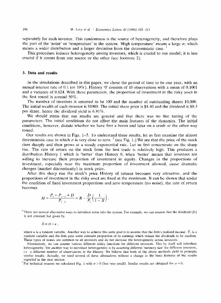
separately for each investor. This randomness is the source of heterogeneity, and therefore plays the part of the ‘noise’ or ‘temperature’ in the system. ‘High temperature’ means a large (T, which means a wider distribution and a larger deviation from the deterministic case. 2

This procedure induces heterogeneity among investors, which is crucial to our model; it is less crucial if it comes from one source or the other (see footnote 2).

3. Data and results

In the simulations described in this paper, we chose the period of time to be one year, with an annual interest rate of 0.1 (or 10%). History ‘0’ consists of 10 observations with a mean of 0.1001 and a variance of 0.024. With these parameters, the proportion of investment in the risky asset in the first round is around 50%.

The number of investors is assumed to be 100 and the number of outstanding shares 10,000. The initial wealth of each investor is $1000. The initial share price is $4.40 and the dividend is $0.3 per share, hence the dividend yield is 6.81%.

We should stress that our results are general and that there was no fine tuning of the parameters. The initial conditions do not affect the main features of the dynamics. The initial conditions, however, dictate whether we have first a boom and later on a crash or the other way round.

Our results are shown in Figs. 1-5. To understand these results, let us first examine the almost deterministic case in which (T is very close to zero. ’ (see Fig. 1.) We see that the price of the stock rises sharply and then grows at a steady exponential rate. Let us first concentrate on the sharp rise. The rate of return on the stock from the first trade is relatively high. This produces a distribution History 1 which is ‘better’ than History 0, when ‘better’ means that investors are willing to increase their proportion of investment in equity. Changes in the proportions of investment, especially near the maximum proportion of investment allowed, cause dramatic changes (market discontinuity) in stock price.

After this sharp rise the stock’s price History of returns becomes very attractive, and the proportions of investment in the risky asset are fixed at the maximum. It can be shown that under the condition of fixed investment proportions and zero temperature (no noise), the rate of return becomes

H= P,-P,_,+D

P I-1

’ There are several alternative ways to introduce noise into the system. For example, we can assume that the dividend (D)

is not constant but given by

where E is a random variable. Another way to achieve this same goal is to assume that the firm’s realized income, ?, is a random variable and the firm pays some constant proportion of its earnings which induce the dividends to be random.

These types of noises are common to all investors and do not increase the heterogeneity across investors. Alternatively, we can assume various different utility functions for different investors. This by itself will introduce

heterogeneity. Yet another way to introduce heterogeneity is by assuming different ‘memory size’ for different investors, i.e. a different number of observations in the History. We believe that both of the above methods yield in principle

similar results. Actually, we tried several of these alternatives without a change in the basic features of the results

reported in the next section. ‘For technical reasons we calculated Fig. 1 with a>0 (but very small). Similar results are obtained for D =O.

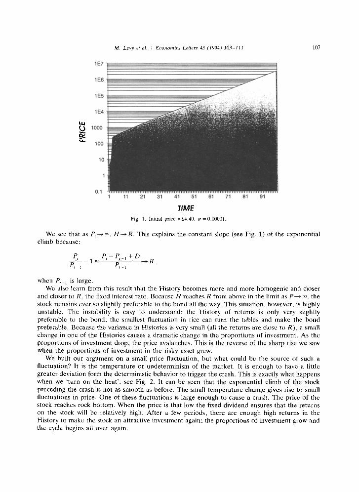
M. Levy et al. i Economics Lefters 45 (1994) 103-Ill 107

lE7

lE5

lE4

g lo*

Q 100

0.1 1 11 21 31 41 51 61 71 61 91

TIME Fig. 1. Initial price = $4.40, CT = 0.00001.

We see that as P,* 00, H-+ R. This explains the constant slope (see Fig. 1) of the exponential climb because:

P I--l_

P, - P,_l + D P P +-R,

t-1 c-1

when Pt_, is large. We also learn from this result that the History becomes more and more homogenic and closer

and closer to R, the fixed interest rate. Because H reaches R from above in the limit as P-00, the stock remains ever so slightly preferable to the bond all the way. This situation, however, is highly unstable. The instability is easy to understand: the History of returns is only very slightly preferable to the bond, the smallest fluctuation in rice can turn the tables and make the bond preferable. Because the variance in Histories is very small (all the returns are close to R), a small change in one of the Histories causes a dramatic change in the proportions of investment. As the proportions of investment drop, the price avalanches. This is the reverse of the sharp rise we saw when the proportions of investment in the risky asset grew.

We built our argument on a small price fluctuation, but what could be the source of such a fluctuation? It is the temperature or undeterminism of the market. It is enough to have a little greater deviation form the deterministic behavior to trigger the crash. This is exactly what happens when we ‘turn on the heat’, see Fig. 2. It can be seen that the exponential climb of the stock preceding the crash is not as smooth as before. The small temperature change gives rise to small fluctuations in price. One of these fluctuations is large enough to cause a crash. The price of the stock reaches rock bottom. When the price is that low the fixed dividend ensures that the returns on the stock will be relatively high. After a few periods, there are enough high returns in the History to make the stock an attractive investment again; the proportions of investment grow and the cycle begins all over again.

108

lE7

lE6

lE5

lE4

g 'OOiJ

fL 100

10

1

0.1 1 11 21 31 41 51 61 71 81 91

TIME Fig. 2. Initial price = $4.40, (T = 0.01.

How do the dynamics depend on the initial conditions? Maybe the crashes and cycles appear only when the price starts on the way up? In Fig. 3 can be seen a similar run with the exception that the initial price was set at $4.60. Because the initial price is higher, the contribution of D to

lE5

lE4

1000

s 100

10

1

0.1 1 11 21 31 41 51 61 71 81 91

TIME Fig. 3. Initial price = $4.60. (r = 0.01.

M. Levy et al. I Economics Letters 45 (1994) 103-111 109

lE5

lE4

1 11 21 31 41 51 61 71 61 91

T/ME

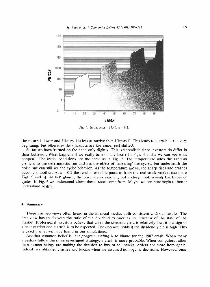
Fig. 4. Initial price = $4.40, CT = 0.2

the return is lower and History 1 is less attractive than History@. This leads to a crash at the very beginning, but otherwise the dynamics are the same, just shifted.

So far we have ‘turned on the heat’ only slightly. This is unrealistic since investors do differ in their behavior. What happens if we really turn on the heat? In Figs. 4 and 5 we can see what happens. The initial conditions are the same as in Fig. 2. The temperature adds the random element to the deterministic run and has the effect of ‘smearing’ the cycles, but underneath the noise one can still see the cyclic behavior. As the temperature grows, the sharp rises and crashes become smoother. At u = 0.2 the results resemble patterns from the real stock market (compare Figs. 5 and 6). At first glance, the price seems random, but a closer look reveals the traces of cycles. In Fig. 6 we understand where these traces come from. Maybe we can now begin to better understand reality.

4. Summary

There are two views often heard in the financial media, both consistent with our results. The first view has to do with the ratio of the dividend to price as an indicator of the state of the market. Professional investors believe that when the dividend yield is relatively low, it is a sign of a bear market and a crash is to be expected. The opposite holds if the dividend yield is high. This is exactly what we have found in our simulations.

Another common belief is that program trading is to blame for the 1987 crash. When many investors follow the same investment strategy, a crash is more probable. When computers rather than human beings are making the decision to buy or sell stocks, orders are more homogenic. Indeed, we obtained crashes and booms when we assumed homogenic decisions. However, once

110 M. Levy et al. I Economics Letters 45 (1994) 103-111

lE5

lE4

10

1

0.1 1 11 21 31 41 51 61 71 81 91

TIME Fig. 5. Initial price = $4.40, rr = 0.8.

lE4

1000

100

10

1

0.1 1 9is -i936. 1956 1966 1976 1966

YEAR END Fig. 6. Common stocks in the U.S. capital markets. 1926-1991

we ‘turned on the heat’ and created heterogeneous decision-making, the cycles became milder and the crashes much smaller. The higher the temperature, the lower the probability of a crash.

It is encouraging to discover such rich phenomena arising from such a simple model. It is even more encouraging that these phenomena seem to fit reality so nicely.

M. Levy et al. I Economics Letters 45 (1994) 103-111 111

References

Gennote, G. and H. Leland, 1990, Market liquidity, hedging, and crashes, American Economic Review 80, no. 5, 999-1021.

Peters, E.E., 1991, Chaos and order in the capital markets. A new view of cycles, prices and market volatility (Wiley, New York).

Samuelson, P.A., 1991, Long-run risk tolerance when equity returns are mean regressing: Pseudo-paradoxes and

vindication of business-man’s risk, in: W.C. Brainard, W.D. Nordhaus and H.W. Watts, eds., Money, macroeconomics,

and economic policy. Essays in honor of James Tobin (MIT Press, Cambridge, MA).