Microgrid management withweather-based forecasting of

energy generation, consumptionand prices.

Jonathan Dumas

Supervisor: Prof. Bertrand Cornélusse

Faculty of Applied SciencesDepartment of Computer Science and Electrical Engineering

Liège University

This version of the manuscript is pending the approval of the jury.This dissertation is submitted for the degree of

Doctor of Philosophy

Montefiore research unit November 2021

Jury members

Prof. Quentin Louveaux (President) University of Liège, Belgium.Prof. Bertrand Cornélusse (Supervisor) University of Liège, Belgium.Prof. Gilles Louppe University of Liège, Belgium.Prof. Pierre Pinson Technical University of Denmark, Denmark.Prof. Ricardo Bessa INESC TEC, Portugal.Prof. Simone Paoletti University of Siena, Italy.

“ Nothing is impossible, just do it and let’s see. ”— A true coconut-shaker

“There are admirable potentialities in every humanbeing. Believe in your strength and your youth.

Learn to repeat endlessly to yourself: It all dependson me. ”

— André Gide

“In vino veritas. ”— Pliny the Elder, 23–79 A.D.

Declaration

I hereby declare that except where specific reference is made to the work of others, thecontents of this dissertation are original and have not been submitted in whole or in partfor consideration for any other degree or qualification in this or any other university.This dissertation is my own work and contains nothing which is the outcome of workdone in collaboration with others, except as specified in the text and Acknowledgements.

Jonathan DumasNovember 2021

Acknowledgements

Throughout the writing of this dissertation, I have received a great deal of supportand assistance.

FamilyI would like to acknowledge my family, and especially Perrine and my daughter Lily.I could not have achieved this thesis without their emotional and material support.They always have been there for me. Perrine saved me much time taking care of ourbeloved daughter, she did, in fact, the most challenging part of the job. In myopinion, it is simple to work, especially in a research environment. It is much harderto raise a child. In addition, I could not have been so implied, without her support, innon-profit organizations to help make energy transition to a carbon-free economy: theShifters Belgium1, the working group on the sustainability of the ReD2 (an associationaiming to gather the Ph.D. candidates from the University of Liège), the climate3 anddigital collages4, and the ClimActes 2021 summer school5.

SupervisorI express my gratitude to my supervisor Prof. Bertrand Cornélusse, whose expertisewas invaluable in formulating the research questions and methodology. Bertrand issignificantly implicated in designing exciting lectures for bachelor and master students.He is also committed to supervising his Ph.D. students despite its busy agenda. Pro-fessors are supposed to be supermen or superwomen: teach, teach and teach, then,being at the front end of the research, and of course, implicated in the University andFaculty challenges. However, they have as everybody 24 hours per day :). He madeit possible to work with the Sienna group and encouraged me throughout the past

1https://theshiftproject.org/equipe/#benevoles2https://www.facebook.com/reduliege/3https://climatefresk.org/4https://digitalcollage.org/5http://climactes.org/

x

three years. We have had helpful discussions on technical topics like optimization andmachine learning and friendly talks on many other questions. Your insightful feedbackpushed me to sharpen my thinking and brought my work to a higher level. We hadthe opportunity to spend an excellent stay at the first microgrids summer school atBelfort in 2019. He also provided the funds for three summer schools: microgridssummer school at Belfort [2019], sustainable ICT summer school at Catholic Universityof Louvain [2020], and ClimActes at Liège University [2021]. He provided the fundsfor attending several conferences: 16th European Energy Market Conference (EEM2019), XXI Power Systems Computation Conference (PSCC 2020), 16th InternationalConference on Probabilistic Methods Applied to Power Systems (PMAPS 2020), 14thIEEE PowerTech (PowerTech 2021). Finally, the two stays at Sienna University in2019 and 2020 (just before the lockdown of the covid-19 crisis).

Thesis committeeI am grateful to Prof. Simone Paoletti, Prof. Quentin Louveaux, and Xavier Fettweis,research associate FNRS, for being part of the thesis committee, their support, andvaluable guidance throughout this thesis and the discussions about optimization andweather forecasting. In addition, Xavier Fettweis taught how to use the MAR regionalclimate model. I want to thank all three of you for your regular support and theopportunities to further my research.

Thesis juryI am deeply honored by this jury. Each one of the members is profoundly remarkablein his field and inspired my research during this thesis. I could not have dreamt of abetter jury and hope to be at the level expected. In addition, I sincerely thank thejury members for devoting themselves to reading this manuscript and all the relatedadministrative duties.

Liège University Applied Science Faculty colleaguesI thank my colleagues and friends of the Applied Science Faculty for their supportand for the exciting discussions we had together during the last three years: especiallySelmane Dakir, Antonio Sutera, Antoine Wehenkel, Laurine Duchesne, Pascal Leroy,Adrien Bolland, Raphael Fonteneau, Sylvain Quoilin, Gaulthier Gain, Ioannis Noukas,Miguel Manuel de Villena, and all the others that I did not mention. I also thankGilles Louppe, associate professor at Liège University, for the quality of his course"INFO8010 - Deep Learning". Gilles Louppe is very involved in designing exciting

xi

courses. I enjoyed the lectures that I followed in Spring 2021 at the end of this thesis.I wish I had attended them at the beginning of my thesis to understand better thedeep learning topic that I learned from scratch.

Coconut-shakers group and ReDI thank my beloved friends of the coconut-shakers group: Antoine Dubois, FrançoisRigo, Thibaut Theate, Gilles Corman, and Adrien Corman. We have worked togetherintensively to propose actions and ideas at the Applied Science Faculty to make tinychanges about the climate change issue. There is still a massive gap between rhetoricand actions. Nevertheless, we keep on believing that one-day things will change! I alsothank the active members of the ReD: Kathleen Jacquerie, Chloe Stevenne, ColineGrégoire, and all the others that I did not mention.

Sienna University colleaguesI appreciated working with Prof. Simone Paoletti, Prof. Antonello Giannitrapani, andProf. Antonio Vicino from Sienna University. It was terrific to work with them atSienna University, and we have had enjoyable moments. They are devoted to their work,and they know how to make a good working relationship. They helped to understandstochastic programming better and to develop exciting research directions.

Master studentsI thank all the master students who did incredible work on various topics such asforecasting, optimization during their master thesis, especially during the covid-19crisis. It was a great pleasure to work with them: Audrey Lempereur [2020-AppliedScience Faculty], Clement Liu [2020-Ecole Polytechnique], Jean Cyrus de Gourcuff[2021-Ecole Polytechnique], Colin Cointe [2021-Mines ParisTech], Damien Lanaspeze[2021-Mines ParisTech], Benjamin Delvoye [2021-Applied Science Faculty], and GabrielGuerra Martin [2021-Polytechnic University of Catalonia].

Liège University Applied Science Faculty staffI sincerely thank the shadow workers of the Applied Science Faculty: the cleaningworkers (thank you Patricia!), the administrative staff (Eric Vangenechten), and allthe others that I did not mention. I also thank the academic staff of the AppliedScience Faculty: Eric Delhez (for the discussions on sustainability even if I think can dobetter!), Angélique Leonard, Dominique Toye, and all the others that I did not mention.

xii

Liège University human resource staffI thank all the human resource staff. We are so fortunate at the University of Liègeto have free and very high-quality training courses on various topics such as self-development, negotiation, teamwork. In particular, I appreciate the training courses ofJean Yves Girin. He is incredible, and he helped me improve my human skills (butthere is still much work to do). I can only encourage all the academics (includingprofessors), administrative staff, Ph.D. candidates, and researchers to attend thesetraining courses. I was the only man and the only one from the Applied Science Facultymost of the time. Does that mean that the ’men’ do not need these training coursesabout human skills?

Liège University IFRESI thank the IFRES for the pedagogical training that we attend as teaching assistants.We are lucky that Liège University provides these training courses.

P. PinsonI thank professor Prof. Pierre Pinson from the Technical University of Denmark.His work has been a great inspiration during this thesis. In addition, he is open todiscussion and sharing all material from his courses. In particular, I used a lot of thecourse materials "Renewables in Electricity Markets" to design the forecasting lessonsthat I taught in the course "ELEN0445 Microgrids" at the University of Liège duringthe years 2018, 2019, 2020, and 2021.

Summer schoolsMicrogrids Belfort 2019 summer school. I thank all the members of the microgridsBelfort 2019 summer school, and especially Robin Roche. It was the first summerschool on microgrids, and we learned a lot in an enjoyable working environment. TheTyphoon Hil team did a great job presenting its tools and organize the challenge.

Sustainable ICT 2020 summer school. I also thank the members of the SustainableICT 2020 summer school that took place at the Catholic University of Louvain (UCL).It was an excellent summer school with very skilled researchers and Ph.D. candidates.There is at UCL a group of Ph.D. candidates (Thibault Pirson, Gregoire Lebrun, andmany others) and professors (Jean-Pierre Raskin, Hervé Jeanmart, David Bol) verymotivated to address the sustainability challenges. It is a great source of inspiration.

xiii

ClimACTES 2021 summer school. I am grateful to all the members of the ClimACTES2021 summer school that took place at Liège University. This event was outstandingwhere we have faced the challenges of climate change and the urgent need to reducethe emission of greenhouse gases drastically. The first week was dedicated to lessonsfrom professors from several universities about these challenges. Then, we worked inthe second week to develop projects to achieve ambitious targets to help to decarbonizethe economy. I was part of the education team, and I learned from students and peoplefrom various backgrounds. It was one of the richest experiences in my life. PhilippeGilson, that founded ClimACTES, is a great source of inspiration. The work of all theClimACTES volunteers was incredible. They dedicated two entire years to build thissummer school. I can only say congratulations!

ReviewersI would like to thank all the reviewers of the papers submitted to conferences andjournals. They helped me to improve the work proposed and to get out of my comfortzone.

Liège UniversityFinally, I thank the University of Liège. Indeed, they financed me as a teachingassistant during these two last years and provided me with a nice working environment.

Abstract

“Do. Or do not. There is no try.”— Yoda

Climate ChangeThe decade 2009-2019 was particularly intense in rhetoric about efforts to tackle theclimate crisis, such as the 2015 United Nations Climate Change Conference, COP 21.However, the carbon dioxide emissions at the world scale increased constantly from29.7 (GtCO2) in 2009 to 34.2 in 2019. The current gap between rhetoric and realityon emissions was and is still huge. The Intergovernmental Panel on Climate Changeproposed different mitigation strategies to achieve the net emissions reductions thatwould be required to follow a pathway that limits global warming to 1.5°C withno or limited overshoot. There are still pathways to reach net-zero by 2050. Severalreports propose detailed scenarios and strategies to achieve these targets. They remainnarrow and highly challenging, requiring all stakeholders, governments, businesses,investors, and citizens to take action this year and every year after so that the goaldoes not slip out of reach. In most of these trajectories, electrification and an increasedshare of renewables are some of the key pillars. The transition towards a carbon-freesociety goes through an inevitable increase in the share of renewable genera-tion in the energy mix and a drastic decrease in the total consumption of fossil fuels.

Thesis topicIn contrast to conventional power plants, renewable energy is subject to uncertainty.Most of the generation technologies based on renewable sources are non-dispatchable,and their production is stochastic and complex to predict in advance. A high shareof renewables is challenging for power systems that have been designed and sized fordispatchable units. Therefore, this thesis studies the integration of renewables in powersystems by investigating forecasting and decision-making tools.

Since variable generation and electricity demand both fluctuate, they must beforecast ahead of time to inform real-time electricity scheduling and longer-term system

xvi

planning. Better short-term forecasts enable system operators to reduce reliance onpolluting standby plants and proactively manage increasing amounts of variable sources.Better long-term forecasts help system operators and investors to decide where andwhen to build variable plants. In this context, probabilistic forecasts, which aim atmodeling the distribution of all possible future realizations, have become a vital toolto equip decision-makers, hopefully leading to better decisions in energy applications.

When balancing electricity systems, system operators use scheduling and dispatchto determine how much power every controllable generator should produce. Thisprocess is slow and complex, governed by NP-hard optimization problems such asunit commitment and optimal power flow. Scheduling becomes even more complexas electricity systems include more storage, variable generators, and flexible demand.Thus, scheduling must improve significantly, allowing operators to rely on variablesources to manage systems. Therefore, stochastic or robust optimization strategieshave been developed along with decomposition techniques to make the optimizationproblems tractable and efficient.

Thesis contentThese two challenges raise two central research questions studied in this thesis: (1)How to produce reliable probabilistic renewable generation forecasts, consumption,and electricity prices? (2) How to make decisions with uncertainty using probabilisticforecasts to improve scheduling? The thesis perimeter is the energy management of"small" systems such as microgrids at a residential scale on a day-ahead basis. Themanuscript is divided into two main parts to propose directions to address both researchquestions: (1) a forecasting part; (2) a planning and control part.

Thesis first partThe forecasting part presents several techniques and strategies to produce and evaluateprobabilistic forecasts. We provide the forecasting basics by introducing the differenttypes of forecasts to characterize the behavior of stochastic variables, such as renewablegeneration, and the tools to assess the different types of forecasts. An example offorecast quality evaluation is given by assessing PV and electrical consumption pointforecasts computed by standard deep-learning models such as recurrent neural net-works. Then, the following Chapters investigate the quantile forecasts, scenarios, anddensity forecasts on several case studies. First, more advanced deep-learning modelssuch as the encoder-decoder architecture produce PV quantile forecasts. Second, adensity forecast-based approach computes probabilistic forecasts of imbalance prices

xvii

on the Belgian case. Finally, a recent class of deep generative models, normalizingflows, generates renewable production and electrical consumption scenarios. Usingan energy retailer case study, this technique is extensively compared to state-of-the-art generative models, the variational autoencoders and generative adversarial networks.

Thesis second partThe planning and control part proposes approaches and methodologies based on opti-mization for decision-making under uncertainty using probabilistic forecasts on severalcase studies. We introduce the basics of decision-making under uncertainty usingoptimization strategies: stochastic programming and robust optimization. Then, weinvestigate these strategies in several case studies in the following Chapters. First, wepropose a value function-based approach to propagate information from operationalplanning to real-time optimization in a deterministic framework. Second, three Chap-ters focus on the energy management of a grid-connected renewable generation plantcoupled with a battery energy storage device in the capacity firming market. Thisframework promotes renewable power generation facilities in small non-interconnectedgrids. The day-ahead planning of the system uses either a stochastic or a robustapproach. Furthermore, a sizing methodology of the system is proposed. Finally, weconsider the day-ahead market scheduling of an energy retailer to evaluate the forecastvalue of the deep learning generative models introduced in the forecasting part.

PerspectivesWe propose four primary research future directions. (1) Forecasting techniques ofthe future. The development of new machine learning models that take advantageof the underlying physical process opens a new way of research. For instance, newforecasting techniques that take advantage of the power system characteristics, suchas the graphical normalizing flows capable of learning the power network structure,could be applied to hierarchical forecasting. (2) Machine learning for optimization.Models that simplify optimization planning problems by learning a sub-optimal space.For instance, a deep learning model can partially learn the sizing space to provide afast and efficient tool. A neural network can also emulate the behavior of a physicssolver that solves electricity differential equations to compute electricity flow in powergrids. Furthermore, such proxies could evaluate if a given operation planning decisionwould lead to acceptable trajectories where the reliability criterion is met in real-time. (3) Modelling and simulation of energy systems. New flexible and open-sourceoptimization modeling tools are required to capture the growing complexity of such

xviii

future energy systems. To this end, in the past few years, several open-source modelsfor the strategic energy planning of urban and regional energy systems have beendeveloped. EnergyScope TD and E4CLIM are two of them where we think it may berelevant to implement and test the forecasting techniques and scheduling strategiesdeveloped in this thesis. (4) Psychology and machine learning. Achieving sustainabilitygoals requires as much the use of relevant technology as psychology. Therefore, one ofthe main challenges is not designing relevant technological tools but changing how weconsume and behave in our society. Thus, machine learning and psychology could helpto identify appropriate behaviors to reduce carbon footprint. Then, inform individuals,and provide constructive opportunities by modeling individual behavior.

Table of contents

Foreword 1

1 General introduction 91.1 Context and motivations . . . . . . . . . . . . . . . . . . . . . . . . . . 91.2 Classification of forecasting studies . . . . . . . . . . . . . . . . . . . . 131.3 Content and contributions . . . . . . . . . . . . . . . . . . . . . . . . . 14

I Forecasting 21

Part I general nomenclature 25

2 Forecasting background 272.1 Point forecast . . . . . . . . . . . . . . . . . . . . . . . . . . . . . . . . 292.2 Probabilistic forecasts . . . . . . . . . . . . . . . . . . . . . . . . . . . 30

2.2.1 Quantiles . . . . . . . . . . . . . . . . . . . . . . . . . . . . . . 302.2.2 Prediction intervals . . . . . . . . . . . . . . . . . . . . . . . . . 312.2.3 Scenarios . . . . . . . . . . . . . . . . . . . . . . . . . . . . . . 322.2.4 Density forecasts . . . . . . . . . . . . . . . . . . . . . . . . . . 32

2.3 Model-based formulation . . . . . . . . . . . . . . . . . . . . . . . . . . 322.4 Model training . . . . . . . . . . . . . . . . . . . . . . . . . . . . . . . 33

2.4.1 Regression with supervised learning . . . . . . . . . . . . . . . . 332.4.2 Empirical risk minimization . . . . . . . . . . . . . . . . . . . . 342.4.3 The "double descent" curve . . . . . . . . . . . . . . . . . . . . . 362.4.4 Training methodology . . . . . . . . . . . . . . . . . . . . . . . 372.4.5 Learning, validation, and testing sets . . . . . . . . . . . . . . . 372.4.6 k-fold cross-validation . . . . . . . . . . . . . . . . . . . . . . . 38

2.5 Conclusions . . . . . . . . . . . . . . . . . . . . . . . . . . . . . . . . . 38

xx Table of contents

3 Forecast evaluation 413.1 Metrics for point forecasts . . . . . . . . . . . . . . . . . . . . . . . . . 433.2 Metrics for probabilistic forecasts . . . . . . . . . . . . . . . . . . . . . 44

3.2.1 Calibration . . . . . . . . . . . . . . . . . . . . . . . . . . . . . 443.2.2 Univariate skill scores . . . . . . . . . . . . . . . . . . . . . . . . 453.2.3 Multivariate skill scores . . . . . . . . . . . . . . . . . . . . . . 47

3.3 Point forecasting evaluation example . . . . . . . . . . . . . . . . . . . 493.3.1 Formulation . . . . . . . . . . . . . . . . . . . . . . . . . . . . . 493.3.2 Forecasting models . . . . . . . . . . . . . . . . . . . . . . . . . 503.3.3 Results . . . . . . . . . . . . . . . . . . . . . . . . . . . . . . . . 51

3.4 Conclusions . . . . . . . . . . . . . . . . . . . . . . . . . . . . . . . . . 53

4 Quantile forecasting 554.1 Formulation . . . . . . . . . . . . . . . . . . . . . . . . . . . . . . . . . 584.2 Related work . . . . . . . . . . . . . . . . . . . . . . . . . . . . . . . . 594.3 Forecasting models . . . . . . . . . . . . . . . . . . . . . . . . . . . . . 59

4.3.1 Gradient boosting regression (GBR) . . . . . . . . . . . . . . . 594.3.2 Multi-layer perceptron (MLP) . . . . . . . . . . . . . . . . . . . 604.3.3 Encoder-decoder (ED) . . . . . . . . . . . . . . . . . . . . . . . 60

4.4 The ULiège case study . . . . . . . . . . . . . . . . . . . . . . . . . . . 614.4.1 Case study description . . . . . . . . . . . . . . . . . . . . . . . 614.4.2 Numerical settings . . . . . . . . . . . . . . . . . . . . . . . . . 624.4.3 Day-ahead results . . . . . . . . . . . . . . . . . . . . . . . . . . 634.4.4 Intraday results . . . . . . . . . . . . . . . . . . . . . . . . . . . 644.4.5 Conclusions . . . . . . . . . . . . . . . . . . . . . . . . . . . . . 68

4.5 Comparison with generative models . . . . . . . . . . . . . . . . . . . . 684.6 Conclusions . . . . . . . . . . . . . . . . . . . . . . . . . . . . . . . . . 70

5 Density forecasting of imbalance prices 715.1 Related work . . . . . . . . . . . . . . . . . . . . . . . . . . . . . . . . 735.2 Formulation . . . . . . . . . . . . . . . . . . . . . . . . . . . . . . . . . 74

5.2.1 Net regulation volume forecasting . . . . . . . . . . . . . . . . . 745.2.2 Imbalance price forecasting . . . . . . . . . . . . . . . . . . . . . 75

5.3 Case study . . . . . . . . . . . . . . . . . . . . . . . . . . . . . . . . . . 775.4 Results . . . . . . . . . . . . . . . . . . . . . . . . . . . . . . . . . . . . 785.5 Conclusions . . . . . . . . . . . . . . . . . . . . . . . . . . . . . . . . . 815.6 Appendix: balancing mechanisms . . . . . . . . . . . . . . . . . . . . . 83

Table of contents xxi

5.6.1 Balancing mechanisms . . . . . . . . . . . . . . . . . . . . . . . 835.6.2 Belgium balancing mechanisms . . . . . . . . . . . . . . . . . . 845.6.3 Additional results . . . . . . . . . . . . . . . . . . . . . . . . . . 84

6 Scenarios 876.1 Introduction . . . . . . . . . . . . . . . . . . . . . . . . . . . . . . . . . 90

6.1.1 Related work . . . . . . . . . . . . . . . . . . . . . . . . . . . . 916.1.2 Research gaps and scientific contributions . . . . . . . . . . . . 936.1.3 Applicability of the generative models . . . . . . . . . . . . . . . 976.1.4 Organization . . . . . . . . . . . . . . . . . . . . . . . . . . . . 97

6.2 Background . . . . . . . . . . . . . . . . . . . . . . . . . . . . . . . . . 986.2.1 Multi-output forecasts using a generative model . . . . . . . . . 986.2.2 Deep generative models . . . . . . . . . . . . . . . . . . . . . . 986.2.3 Theoretical comparison . . . . . . . . . . . . . . . . . . . . . . . 105

6.3 Quality assessment . . . . . . . . . . . . . . . . . . . . . . . . . . . . . 1066.3.1 Classifier-based metric . . . . . . . . . . . . . . . . . . . . . . . 1076.3.2 Correlation matrix between scenarios . . . . . . . . . . . . . . . 1096.3.3 Diebold-Mariano test . . . . . . . . . . . . . . . . . . . . . . . . 109

6.4 Case study . . . . . . . . . . . . . . . . . . . . . . . . . . . . . . . . . . 1116.4.1 Implementation details . . . . . . . . . . . . . . . . . . . . . . . 1116.4.2 Hyper-parameters . . . . . . . . . . . . . . . . . . . . . . . . . . 114

6.5 Quality results . . . . . . . . . . . . . . . . . . . . . . . . . . . . . . . 1176.5.1 Wind track . . . . . . . . . . . . . . . . . . . . . . . . . . . . . 1176.5.2 All tracks . . . . . . . . . . . . . . . . . . . . . . . . . . . . . . 118

6.6 Conclusions and perspectives . . . . . . . . . . . . . . . . . . . . . . . . 1256.7 Appendix: Table 6.1 justifications . . . . . . . . . . . . . . . . . . . . . 1266.8 Appendix: background . . . . . . . . . . . . . . . . . . . . . . . . . . . 127

6.8.1 NFs . . . . . . . . . . . . . . . . . . . . . . . . . . . . . . . . . 1276.8.2 VAEs . . . . . . . . . . . . . . . . . . . . . . . . . . . . . . . . 1286.8.3 GANs . . . . . . . . . . . . . . . . . . . . . . . . . . . . . . . . 130

7 Part I conclusions 133

II Planning and control 135

8 Decision-making background 1398.1 Linear programming . . . . . . . . . . . . . . . . . . . . . . . . . . . . 141

xxii Table of contents

8.1.1 Formulation of a linear programming problem . . . . . . . . . . 1418.1.2 Duality in linear programming . . . . . . . . . . . . . . . . . . . 141

8.2 Stochastic optimization . . . . . . . . . . . . . . . . . . . . . . . . . . . 1428.3 Robust optimization . . . . . . . . . . . . . . . . . . . . . . . . . . . . 144

8.3.1 Benders-dual cutting plane algorithm . . . . . . . . . . . . . . . 1458.3.2 Column and constraints generation algorithm . . . . . . . . . . 146

8.4 Conclusions . . . . . . . . . . . . . . . . . . . . . . . . . . . . . . . . . 147

9 Coordination of the planner and controller 1499.1 Notation . . . . . . . . . . . . . . . . . . . . . . . . . . . . . . . . . . . 1539.2 Problem statement . . . . . . . . . . . . . . . . . . . . . . . . . . . . . 155

9.2.1 Assumptions . . . . . . . . . . . . . . . . . . . . . . . . . . . . . 1559.2.2 Formulation . . . . . . . . . . . . . . . . . . . . . . . . . . . . . 155

9.3 Proposed method . . . . . . . . . . . . . . . . . . . . . . . . . . . . . . 1569.3.1 Computing the cost-to-go function . . . . . . . . . . . . . . . . 1579.3.2 OPP formulation . . . . . . . . . . . . . . . . . . . . . . . . . . 1589.3.3 OP constraints . . . . . . . . . . . . . . . . . . . . . . . . . . . 1599.3.4 RTP formulation . . . . . . . . . . . . . . . . . . . . . . . . . . 1609.3.5 RTO constraints . . . . . . . . . . . . . . . . . . . . . . . . . . 161

9.4 Test description . . . . . . . . . . . . . . . . . . . . . . . . . . . . . . . 1619.5 Numerical results . . . . . . . . . . . . . . . . . . . . . . . . . . . . . . 163

9.5.1 No symmetric reserve . . . . . . . . . . . . . . . . . . . . . . . . 1639.5.2 Results with symmetric reserve . . . . . . . . . . . . . . . . . . 165

9.6 Conclusions . . . . . . . . . . . . . . . . . . . . . . . . . . . . . . . . . 166

10 Capacity firming using a stochastic approach 16910.1 Notation . . . . . . . . . . . . . . . . . . . . . . . . . . . . . . . . . . . 172

10.1.1 Sets and indices . . . . . . . . . . . . . . . . . . . . . . . . . . . 17210.1.2 Parameters . . . . . . . . . . . . . . . . . . . . . . . . . . . . . 17310.1.3 Variables . . . . . . . . . . . . . . . . . . . . . . . . . . . . . . . 174

10.2 The Capacity Firming Framework . . . . . . . . . . . . . . . . . . . . . 17410.2.1 Day-ahead engagement . . . . . . . . . . . . . . . . . . . . . . . 17510.2.2 Real-time control . . . . . . . . . . . . . . . . . . . . . . . . . . 175

10.3 Problem formulation . . . . . . . . . . . . . . . . . . . . . . . . . . . . 17610.3.1 Deterministic approach . . . . . . . . . . . . . . . . . . . . . . . 17610.3.2 Deterministic approach with perfect forecasts . . . . . . . . . . 17810.3.3 Stochastic approach . . . . . . . . . . . . . . . . . . . . . . . . . 179

Table of contents xxiii

10.3.4 Evaluation methodology . . . . . . . . . . . . . . . . . . . . . . 17910.4 MiRIS microgrid case study . . . . . . . . . . . . . . . . . . . . . . . . 180

10.4.1 Results for unbiased PV scenarios with fixed variance . . . . . . 18210.4.2 BESS capacity sensitivity analysis . . . . . . . . . . . . . . . . . 184

10.5 Conclusions and perspectives . . . . . . . . . . . . . . . . . . . . . . . . 18710.6 Appendix: PV scenario generation . . . . . . . . . . . . . . . . . . . . 187

11 Capacity firming sizing 19111.1 Problem statement . . . . . . . . . . . . . . . . . . . . . . . . . . . . . 194

11.1.1 Stochastic approach . . . . . . . . . . . . . . . . . . . . . . . . . 19511.1.2 Deterministic approach . . . . . . . . . . . . . . . . . . . . . . . 19611.1.3 Oracle controller . . . . . . . . . . . . . . . . . . . . . . . . . . 196

11.2 Forecasting methodology . . . . . . . . . . . . . . . . . . . . . . . . . . 19611.2.1 Gaussian copula-based PV scenarios . . . . . . . . . . . . . . . 19711.2.2 PV point forecast parametric model . . . . . . . . . . . . . . . . 19711.2.3 PV scenarios . . . . . . . . . . . . . . . . . . . . . . . . . . . . 198

11.3 Sizing study . . . . . . . . . . . . . . . . . . . . . . . . . . . . . . . . . 19811.3.1 Problem statement and assumptions . . . . . . . . . . . . . . . 19811.3.2 Levelized cost of energy (LCOE) . . . . . . . . . . . . . . . . . 20011.3.3 Case study description . . . . . . . . . . . . . . . . . . . . . . . 20111.3.4 Sizing parameters . . . . . . . . . . . . . . . . . . . . . . . . . . 20211.3.5 Sizing results . . . . . . . . . . . . . . . . . . . . . . . . . . . . 202

11.4 Conclusions and perspectives . . . . . . . . . . . . . . . . . . . . . . . . 204

12 Capacity firming using a robust approach 20712.1 Problem formulation . . . . . . . . . . . . . . . . . . . . . . . . . . . . 212

12.1.1 Deterministic planner formulation . . . . . . . . . . . . . . . . . 21312.1.2 Robust planner formulation . . . . . . . . . . . . . . . . . . . . 21312.1.3 Second-stage planner transformation . . . . . . . . . . . . . . . 21512.1.4 Controller formulation . . . . . . . . . . . . . . . . . . . . . . . 217

12.2 Solution methodology . . . . . . . . . . . . . . . . . . . . . . . . . . . . 21712.2.1 Convergence warm start . . . . . . . . . . . . . . . . . . . . . . 21812.2.2 Algorithm convergence . . . . . . . . . . . . . . . . . . . . . . . 21812.2.3 Benders-dual cutting plane algorithm . . . . . . . . . . . . . . . 21912.2.4 Column and constraints generation algorithm . . . . . . . . . . 221

12.3 Case Study . . . . . . . . . . . . . . . . . . . . . . . . . . . . . . . . . 22212.3.1 Numerical settings . . . . . . . . . . . . . . . . . . . . . . . . . 223

xxiv Table of contents

12.3.2 Constant risk-averse parameters strategy . . . . . . . . . . . . . 22312.3.3 Dynamic risk-averse parameters strategy . . . . . . . . . . . . . 22512.3.4 BD convergence warm start improvement . . . . . . . . . . . . . 22812.3.5 BD and CCG comparison . . . . . . . . . . . . . . . . . . . . . 229

12.4 Conclusion . . . . . . . . . . . . . . . . . . . . . . . . . . . . . . . . . . 230

13 Energy retailer 23113.1 Notation . . . . . . . . . . . . . . . . . . . . . . . . . . . . . . . . . . . 23313.2 Problem formulation . . . . . . . . . . . . . . . . . . . . . . . . . . . . 234

13.2.1 Stochastic planner . . . . . . . . . . . . . . . . . . . . . . . . . 23413.2.2 Dispatching . . . . . . . . . . . . . . . . . . . . . . . . . . . . . 236

13.3 Value results . . . . . . . . . . . . . . . . . . . . . . . . . . . . . . . . . 23713.3.1 Results summary . . . . . . . . . . . . . . . . . . . . . . . . . . 239

13.4 Conclusions . . . . . . . . . . . . . . . . . . . . . . . . . . . . . . . . . 23913.5 Appendix: Table 13.2 justifications . . . . . . . . . . . . . . . . . . . . 241

14 Part II conclusions 243

15 General conclusions and perspectives 24515.1 Summary . . . . . . . . . . . . . . . . . . . . . . . . . . . . . . . . . . 24515.2 Future directions . . . . . . . . . . . . . . . . . . . . . . . . . . . . . . 248

15.2.1 Forecasting techniques of the future . . . . . . . . . . . . . . . . 24815.2.2 Machine learning for optimization . . . . . . . . . . . . . . . . . 24815.2.3 Modelling and simulation of energy systems . . . . . . . . . . . 25015.2.4 Machine learning and psychology . . . . . . . . . . . . . . . . . 251

References 253

Foreword

“The greatest glory in living lies not in neverfalling, but in rising every time we fall.”

— Nelson Mandela

“Adults keep saying we owe it to the youngpeople, to give them hope, but I don’t wantyour hope. I don’t want you to be hopeful. Iwant you to panic. I want you to feel the fearI feel every day. I want you to act. I want youto act as you would in a crisis. I want you toact as if the house is on fire, because it is.”

— Greta Thunberg

Climate ChangeThe Intergovernmental Panel on Climate Change (IPCC) set the global net anthro-pogenic CO2 emission trajectories and targets, depicted in Figure 1, to limit climatechange [6]. It is a summary for policymakers (SPM) that presents the key findings ofthe special report published in 20186, based on the assessment of the available scientific,technical and socio-economic literature relevant to Global Warming of 1.5°C and forthe comparison between Global Warming of 1.5°C and 2°C above pre-industrial levels.The SPM presents the emission scenarios consistent with 1.5°C Global Warming:

’In model pathways with no or limited overshoot of 1.5°C, global netanthropogenic CO2 emissions decline by about 45% from 2010 levels by 2030

6The IPCC released in August 2021 the AR6 SPM [42]. It presents key findings of the WorkingGroup I contribution to the IPCC’s Sixth Assessment Report (AR6) on the physical science basis ofclimate change. It is a must to read for every decision-maker, professor, researcher, or person thatwants to understand the challenges at stake.

2 Table of contents

(40–60% interquartile range), reaching net-zero around 2050 (2045–2055interquartile range).’ [6][C.1]7

Fig. 1 IPCC global net anthropogenic CO2 emission pathways and targets. Credits: [6,Figure SPM.3a].

The IPCC proposes different mitigation strategies to achieve the net emissions reduc-tions required to follow a pathway to limit Global Warming to 1.5°C with no or limitedovershoot. These strategies require a tremendous amount of effort from all countries.

7https://www.ipcc.ch/sr15/chapter/spm/

Table of contents 3

’Pathways limiting Global Warming to 1.5°C with no or limited overshootwould require rapid and far-reaching transitions in energy, land, urban andinfrastructure (including transport and buildings), and industrial systems(high confidence). These systems transitions are unprecedented in termsof scale, but not necessarily in terms of speed, and imply deep emissionsreductions in all sectors, a wide portfolio of mitigation options and asignificant upscaling of investments in those options (medium confidence).’[6][C.2]7

Trajectories to achieve IPCC targetsSeveral reports propose pathways and strategies to achieve these targets. The Interna-tional Energy Agency (IEA8) presents a comprehensive study of how to transition to anet-zero energy system by 2050 in the special report ’Net-zero by 2050: A roadmap forthe global energy system’ [3]. It is consistent with limiting the global temperature riseto 1.5 °C without a temperature overshoot (with a 50 % probability). The Net-ZeroEmissions by 2050 Scenario (NZE) shows what is needed for the global energy sectorto achieve net-zero CO2 emissions by 2050:

’In the NZE, global energy-related and industrial process CO2 emissions fallby nearly 40% between 2020 and 2030 and to net-zero in 2050. Universalaccess to sustainable energy is achieved by 2030. There is a 75% reductionin methane emissions from fossil fuel use by 2030. These changes take placewhile the global economy more than doubles through to 2050 and the globalpopulation increases by 2 billion.’ [3, Chapter 2: Summary]

The key pillars of decarbonization of the global energy system proposed are (1)energy efficiency, (2) behavioral changes, (3) electrification, (4) renewables, (5)hydrogen and hydrogen-based fuels, (6) bioenergy, and (7) carbon capture, utilization,and storage.

First, concerning electrification, the direct use of low-emissions electricity in placeof fossil fuels is one of the most significant drivers of emissions reductions in the NZE,accounting for around 20% of the total reduction achieved by 2050. The share of theelectricity in the final consumption increases from 20% in 2020 to 49% in 2050. Itconcerns the sectors of the industry, transport, and buildings. Second, concerningrenewables:

’At a global level, renewable energy technologies are the key to reducingemissions from electricity supply. Hydropower has been a leading low-

8https://www.iea.org/

4 Table of contents

emission source for many decades, but it is mainly the expansion of wind andsolar that triples renewables generation by 2030 and increases it more thaneightfold by 2050 in the NZE. The share of renewables in total electricitygeneration globally increases from 29% in 2020 to over 60% in 2030 and tonearly 90% in 2050. To achieve this, annual capacity additions of wind andsolar between 2020 and 2050 are five-times higher than the average over thelast three years. Dispatchable renewables are critical to maintain electricitysecurity, together with other low-carbon generation, energy storage androbust electricity networks. In the NZE, the main dispatchable renewablesglobally in 2050 are hydropower (12% of generation), bioenergy (5%),concentrating solar power (2%) and geothermal (1%).’ [3, Section 2.4.5]

The IEA report is not the ground truth but has the merit to propose guidelinesand directions. There are many other reports and organizations that present strategiesand scenarios to achieve the IPCC targets. For instance, The Shift Project (TSP) isa European think tank9 advocating the shift to a post-carbon economy. It proposesguidelines and information on energy transition in Europe. The take-home message isthat there are still pathways to reach net-zero by 2050. They remain narrowand challenging, requiring all stakeholders, governments, businesses, investors, andcitizens to take action this year and every year after so that the goal does not slip outof reach.

Gap between rhetoric and realityHowever, the current gap between rhetoric and reality on emissions is stillhuge:

’We are approaching a decisive moment for international efforts to tacklethe climate crisis – a great challenge of our times. The number of countriesthat have pledged to reach net-zero emissions by mid-century or soon aftercontinues to grow, but so do global greenhouse gas emissions. This gapbetween rhetoric and action needs to close if we are to have a fighting chanceof reaching net-zero by 2050 and limiting the rise in global temperatures to1.5 °C.’ [3, Foreword]

Figure 2 illustrates humorously this gap. The UNEP Emissions Gap Report providesevery year a review of the difference between the greenhouse emissions forecast in2030 and where they should be to avoid the worst impacts of climate change. Figure

9https://theshiftproject.org/en/home/

Table of contents 5

Fig. 2 Climate change fake news. Credits: Xavier Gorce.

3 depicts the global GHG emissions under different scenarios and the emissions gapin 2030. 2009-2019 was particularly intense in rhetoric tackling the climate crisis likethe 2015 United Nations Climate Change Conference, COP 21. However, the carbondioxide emissions at the world scale constantly rose from 29.7 (GtCO2) in 2009 to 34.2in 2019 [118]10. In the meantime, the primary energy consumption increased from 134000 TWh to 162 000. In 2019, the primary energy consumption by fuel was composedof oil 53 600 (33.1%), coal 39 300 (24.2%), natural gas 43 900 (27.0%), nuclear energy6 900 (4.3%), hydro-electricity 10 500 (6%), and renewables 8 100 (5%), as depicted inFigure 4. The share of renewables in the energy mix progressed and reached 5% in2019 (a record). However, the total consumption of fossil fuels such as oil, coal, andnatural gas also rose. Oil continues to hold the largest share of the energy mix, coal isthe second-largest fuel, and natural gas grew to a record share of 24.2%.

The Covid-19 pandemic has delivered a shock to the world economy. It resulted inan unprecedented 5.8% decline in CO2 emissions in 2020. The IPCC targets for 2050require a reduction of 5% each year from 2020 to 2050. However, the IEA data showsthat global energy-related CO2 emissions have started to climb again since December2020. Nevertheless, there is still hope, and every action to decrease the CO2 emissionsto gain a reduction of 0.1°C is a winning!

10https://www.bp.com/content/dam/bp/business-sites/en/global/corporate/pdfs/energy-economics/statistical-review/bp-stats-review-2020-full-report.pdf

6 Table of contents

Fig. 3 Global GHG emissions under different scenarios and the emissions gap in 2030(median and 10-th to 90-th percentile range; based on the pre-COVID-19 currentpolicies scenario). Credits: [130, Figure ES.5].

Table of contents 7

Fig. 4 World consumption of primary energy (left) and shares of global primary energy(right) from 1994 to 2020. Credits: BP’s Statistical Review of World Energy 2020[118].

Chapter 1

General introduction

OverviewThis chapter introduces the context, motivations, content, and contributions ofthe thesis. Two main parts compose the manuscript: (1) forecasting; (2) planningand control. Finally, it lists the publications.

“Life has no meaning a priori... It is up toyou to give it a meaning, and value is nothingbut the meaning that you choose.”

— Jean-Paul Sartre

1.1 Context and motivations

Statement 1. Let suppose a utopian world where the current gap between rhetoricand reality on GHG emissions has been drastically decreasing to limit Climate Changeand achieve the ambitious targets prescribed by the IPCC.

Therefore, according to the IPCC targets, the transition to a carbon-free societygoes through an inevitable increase in the renewable generation’s share in the energymix and a drastic decrease in the total consumption of fossil fuels.

Statement 2. This thesis does not debate or study whether and where renewablesshould be implemented.

Renewables have pros and cons and are not carbon-free. We take the scenariosproposed by organizations such as the IPCC or IEA that evaluate the relevance of aparticular type of renewable energy in the energy transition pathways. In addition,

10 General introduction

the development of variable renewable energies systems results from and producesmany interactions between several actors such as citizens, electricity networks, markets,and ecosystems [109]. This thesis does not discuss energy transformations’ politicaland social aspects and focuses on integrating renewable energies into an existinginterconnected system.

Statement 3. This thesis studies the integration of renewables in power systems byinvestigating forecasting and decision-making tools based on machine learning.

In contrast to conventional power plants, renewable energy is subject to uncertainty.Generation technologies based on renewable sources, with the notable exception ofhydro and biomass, are non-dispatchable, i.e., their output cannot or can only partlybe controlled at the will of the producer. Their production is stochastic [124] andtherefore, hard to forecast. A high share of renewables is challenging for power systemsthat have been designed and sized for dispatchable units [168]. Variable renewableenergies depend on meteorological conditions and thus pose challenges to the electricitysystem’s adequacy when conventional capacities are reduced. Therefore, it is necessaryto redefine the flexible power system features [90].

Machine learning can contribute on all fronts by informing the research, deployment,and operation of electricity system technologies. High leverage contributions in powersystems include [151]: accelerating the development of clean energy technologies,improving demand and clean energy forecasts, improving electricity system optimizationand management, and enhancing system monitoring. This thesis focuses on twoleverages: (1) the supply and demand forecast; (2) the electricity system optimizationand management.

Since variable generation and electricity demand both fluctuate, they must beforecast ahead of time to inform real-time electricity scheduling and longer-term systemplanning. Better short-term forecasts enable system operators to reduce reliance onpolluting standby plants and proactively manage increasing amounts of variable sources.Better long-term forecasts help system operators and investors to decide where andwhen to build variable plants. Forecasts need to become more accurate, span multiplehorizons in time and space, and better quantify uncertainty to support these use cases.In this context, probabilistic forecasts [69], which aim at modeling the distribution of allpossible future realizations, have become an important tool to equip decision-makers,hopefully leading to better decisions in energy applications [124, 85, 87].

When balancing electricity systems, system operators use scheduling and dispatchto determine how much power every controllable generator should produce. Thisprocess is slow and complex, governed by NP-hard optimization problems [151] such

1.1 Context and motivations 11

as unit commitment and optimal power flow that must be coordinated across multipletime scales, from sub-second to days ahead. Scheduling becomes even more complexas electricity systems include more storage, variable generators, and flexible demand.Indeed, operators manage even more system components while simultaneously solvingscheduling problems more quickly to account for real-time variations in electricityproduction. Thus, scheduling must improve significantly, allowing operators to rely onvariable sources to manage systems.

Therefore, the two main research questions are:

1. How to produce reliable probabilistic forecasts of renewable generation, consump-tion, and electricity prices?

2. How to make decisions with uncertainty using probabilistic forecasts to improvescheduling?

Modeling tools for energy systems differ in terms of their temporal and spatial res-olutions, level of technical details, simulation horizons. In particular, two classes ofmodels can be distinguished depending on their focus: (1) system operation and (2)system design [35]. [114, Chapter 1] depicts both of these classes.

In the first class, the operational models of energy systems generally optimize asingle sector’s operation, such as the electricity sector, and do not consider investmentcosts. They describe the constraints of the studied system with a high level of accuracyand can model rapid variations in renewable energy production, forecast errors, orreserve markets. The energy system must be controlled at any time, which requires anexcellent technical resolution of the components and accounts for the risks of failure.The system must decide how the load is shared between the different units below thehour at a short time horizon. Solving this problem involves accurately representingproduction units, such as the power ramps up or load constraints. Therefore, models willdecide which units must be committed to optimally dispatching the load or generatingshortly (hours - days).

In the second class, the long-term planning models generate scenarios for an energysystem’s long-term evolution. They include investments, optimize the system designover multiple years, and have a lower technical resolution of operational constraints.With a horizon of one year, new units can be built in existing sites or former unitsmodernized. With a longer horizon, the overall system can be changed. When thehorizon is long enough to neglect the existing system, the models can then optimizethe future design of the energy system from scratch and assess the impact of differentlong-term policies on the design of the system.

12 General introduction

Each model class is essential and answers different needs to tackle the energytransition and help integrate renewable energies. This thesis addresses the first class ofmodels. An example of a thesis investigating the second one is Limpens [114].

Statement 4. This thesis considers the energy management of "small" systems suchas microgrids at a residential scale on a day-ahead basis.

Indeed, the development of microgrids provides an effective way to integrate re-newable energy sources and exploit the available flexibility in a decentralized manner.Microgrids are small electrical networks composed of decentralized energy resourcesand loads controlled locally. They can be operated either interconnected or in islandedmode. Figure 1.1 depicts a microgrid composed of PV generation, diesel generator(Genset), storage systems, load, and an energy management system (EMS). Energystorage is a crucial component for the stable and safe operation of a microgrid. Storagedevices can compensate for the variability of the renewable energy sources and theload to balance the system. The reader is referred to Zia et al. [191] that proposesa comparative and critical analysis on decision-making strategies and their solutionmethods for microgrid energy management systems.

Fig. 1.1 Microgrid scheme. Credits: ELEN0445 Microgrids course https://github.com/bcornelusse/ELEN0445-microgrids, Liège University.

Statement 5. This thesis considers the energy management of grid-connected micro-grids on a day-ahead basis.

Therefore, we are interested in producing reliable day-ahead probabilistic forecastsof renewable generation, consumption, and electricity prices1 for a microgrid composed

1This thesis considers only the imbalance prices in the Belgian case study.

1.2 Classification of forecasting studies 13

of PV or wind generation and electrical consumption. However, in some specific cases,this perimeter is not strictly respected. For instance, the sizing of a grid-connectedPV plant with a battery energy storage system is studied in the specific framework ofcapacity firming or the day-ahead planning of an energy retailer.

1.2 Classification of forecasting studies

One of the first works of this thesis was to conduct a literature review of forecastingstudies. The forecasting literature is vast and composed of thousands of papers,even when selecting a particular field such as load or PV forecasting. Therefore, aclassification into two dimensions of load forecasting studies is proposed by Dumas andCornélusse [48] to decide which forecasting tools to use in which case. The approach canbe extended to electricity prices, PV, or wind power forecasting. This classification aimsto provide a synthetic view of the relevant forecasting techniques and methodologiesby forecasting problem. This methodology is illustrated by reviewing several papersand summarizing the leading techniques and methodologies’ fundamental principles.

The classification process relies on two parameters that define a forecasting prob-lem: a temporal couple with the forecasting horizon and the resolution and a loadcouple with the system size and the load resolution. Each article is classified withkey information about the dataset used and the forecasting tools implemented: theforecasting techniques (probabilistic or deterministic) and methodologies, the datacleansing techniques, and the error metrics. The process to select the articles reviewedwas conducted into two steps. First, a set of load forecasting studies was built basedon relevant load forecasting reviews and forecasting competitions. The second stepconsisted of selecting the most relevant studies of this set based on the followingcriteria: the quality of the description of the forecasting techniques and methodologiesimplemented, the description of the results and the contributions. For the sake ofclarity, this manuscript does not detail this study. It can be read in two passes.

1. The first one identifies the forecasting problem of interest to select the corre-sponding class into one of the four classification tables. Each one references allthe articles classified across a forecasting horizon. They provide a synthetic viewof the forecasting tools used by articles addressing similar forecasting problems.Then, a second level composed of four Tables summarizes key information aboutthe forecasting tools and the results of these studies.

14 General introduction

2. The second pass consists of reading the key principles of the main techniquesand methodologies of interest and the reviews of the articles.

1.3 Content and contributions

The manuscript is divided into two main parts: Part I forecasting; Part II planning andcontrol. Figure 1.2 depicts the thesis skeleton. Part I provides the forecasting tools andmetrics required to produce and evaluate reliable point and probabilistic forecasts tobe used as input of decision-making models in Part II. The latter proposes approachesand methodologies based on optimization for decision-making under uncertainty usingprobabilistic forecasts on several case studies.

Forecaster Planner Controller

Day-ahead decision-making

Probabilistic forecasts

Scenarios

Quantiles

Density forecasts

- Deep learning generative models

- Gaussian copula

Quantile regression:- Neural networks- Gradient boosting

- Gaussian processes- Statistical approach

Stochastic planner

Robust planner

Quality evaluation

Decomposition technique:- Benders-type cutting

plane- Column and

constraints generation

Value evaluation

Intraday decision-making

Coordination of planner and controller

Value function

Probabilistic metrics: univariate and multivariate

- capacity firming- energy retailer

- microgrid

Par t I Par t II

Fig. 1.2 Thesis skeleton.

1.3 Content and contributions 15

Part I content and contributions

The content and main contributions of the forecasting part are:

• Chapter 2 introduces different types of forecasts to characterize the behavior ofstochastic variables, such as renewable generation, electrical consumption, andelectricity prices.

• Chapter 3 provides the tools to assess the different types of forecasts. Forpredictions in any form, one must differentiate between their quality and theirvalue. This Chapter focus on forecast quality. Part II addresses the forecast value.An example of forecast quality assessment is conducted on PV and electricalconsumption point forecasts. They are computed using common deep-learningmodels such as recurrent neural networks and used as inputs of day-aheadplanning in Chapter 9.

References: The point forecast quality evaluation is an extract of JonathanDumas, Selmane Dakir, Clément Liu, and Bertrand Cornélusse. Coordination ofoperational planning and real-time optimization in microgrids. Electric PowerSystems Research, 190:106634, 2021. URL https://arxiv.org/abs/2106.02374.

• Chapter 4 investigates PV quantiles forecasts using deep-learning models such asthe encoder-decoder architecture. Then, Chapter 12 uses the PV intraday pointand quantiles forecasts as inputs of a robust optimization planner.

References: This chapter is an adapted version of Jonathan Dumas, ColinCointe, Xavier Fettweis, and Bertrand Cornélusse. Deep learning-based multi-output quantile forecasting of pv generation. In 2021 IEEE Madrid PowerTech,pages 1–6, 2021. doi: 10.1109/PowerTech46648.2021.9494976. URL https://arxiv.org/abs/2106.01271.

• Chapter 5 proposes imbalance prices density forecasts with a particular focus onthe Belgian case. A two-step density forecast-based approach computes the netregulation volume state transition probabilities to infer the imbalance prices.

References: This chapter is an adapted version of Jonathan Dumas, IoannisBoukas, Miguel Manuel de Villena, Sébastien Mathieu, and Bertrand Cornélusse.Probabilistic forecasting of imbalance prices in the belgian context. In 2019 16thInternational Conference on the European Energy Market (EEM), pages 1–7.IEEE, 2019. URL https://arxiv.org/abs/2106.07361.

16 General introduction

• Chapter 6 studies the generation of scenarios for renewable production andelectrical consumption by implementing a recent class of deep generative models,normalizing flows. It provides a fair comparison of the quality and value of thistechnique with the state-of-the-art deep learning generative models, VariationalAutoEncoders, and Generative Adversarial Networks. Chapter 13 assesses theforecast value.

References: This chapter is an adapted version of Jonathan Dumas, AntoineWehenkel, Damien Lanaspeze, Bertrand Cornélusse, and Antonio Sutera. Adeep generative model for probabilistic energy forecasting in power systems:normalizing flows. Applied Energy, 305:117871, 2022. ISSN 0306-2619. doi:https://doi.org/10.1016/j.apenergy.2021.117871. URL https://arxiv.org/abs/2106.09370.

• Finally, Chapter 7 draws the general conclusions and perspectives of Part I.

Part II content and contributions

The content and main contributions of the planning and control part are:

• Chapter 8 introduces different types of optimization strategies for decision-making under uncertainty: stochastic and robust optimization. Then, it presentssuccinctly two decomposition methods to address the two-stage robust non-linearoptimization problem: the Benders dual-cutting plane and the column andconstraints generation algorithms.

• Chapter 9 presents a value function-based approach as a way to propagateinformation from operational planning to real-time optimization.

References: This chapter is an adapted version of Jonathan Dumas, SelmaneDakir, Clément Liu, and Bertrand Cornélusse. Coordination of operationalplanning and real-time optimization in microgrids. Electric Power SystemsResearch, 190:106634, 2021. URL https://arxiv.org/abs/2106.02374.

• Chapter 10 addresses the energy management, using a stochastic approach, of agrid-connected renewable generation plant coupled with a battery energy storagedevice in the capacity firming market. This framework has been designed topromote renewable power generation facilities in small non-interconnected grids.

References: This chapter is an adapted version of Jonathan Dumas, BertrandCornélusse, Antonello Giannitrapani, Simone Paoletti, and Antonio Vicino.

1.3 Content and contributions 17

Stochastic and deterministic formulations for capacity firming nominations. In2020 International Conference on Probabilistic Methods Applied to Power Systems(PMAPS), pages 1–7. IEEE, 2020. URL https://arxiv.org/abs/2106.02425.

• Chapter 11 extends Chapter 10 and proposes a sizing methodology of the system.

References: This chapter is an adapted version of Jonathan Dumas, BertrandCornélusse, Xavier Fettweis, Antonello Giannitrapani, Simone Paoletti, andAntonio Vicino. Probabilistic forecasting for sizing in the capacity firmingframework. In 2021 IEEE Madrid PowerTech, pages 1–6, 2021. doi: 10.1109/PowerTech46648.2021.9494947. URL https://arxiv.org/abs/2106.02323.

• Chapter 12 extends Chapter 10 and investigates the day-ahead planning usingrobust optimization.Python code: https://github.com/jonathandumas/capacity-firming-ro

References: This chapter is an adapted version of Jonathan Dumas, ColinCointe, Antoine Wehenkel, Antonio Sutera, Xavier Fettweis, and Bertrand Cor-nelusse. A probabilistic forecast-driven strategy for a risk-aware participation inthe capacity firming market. IEEE Transactions on Sustainable Energy, pages 1–1,2021. doi: 10.1109/TSTE.2021.3117594. URL https://arxiv.org/abs/2105.13801.

• Chapter 13, is the extension of Chapter 6, and presents the forecast valueevaluation of the deep learning generative models by considering the day-aheadmarket scheduling of electricity aggregators, such as energy retailers or generationcompanies.Python code: https://github.com/jonathandumas/generative-models

References: This chapter is an adapted version of Jonathan Dumas, AntoineWehenkel, Damien Lanaspeze, Bertrand Cornélusse, and Antonio Sutera. Adeep generative model for probabilistic energy forecasting in power systems:normalizing flows. Applied Energy, 305:117871, 2022. ISSN 0306-2619. doi:https://doi.org/10.1016/j.apenergy.2021.117871. URL https://arxiv.org/abs/2106.09370.

• Finally, Chapter 14 draws the general conclusions and perspectives of Part II.

18 General introduction

Publications

The thesis is mainly based on the following studies, all available in open-access onarXiv, listed in chronological order:

• Jonathan Dumas and Bertrand Cornélusse. Classification of load forecasting stud-ies by forecasting problem to select load forecasting techniques and methodologies,2020. URL https://arxiv.org/abs/1901.05052

• Jonathan Dumas, Ioannis Boukas, Miguel Manuel de Villena, Sébastien Mathieu,and Bertrand Cornélusse. Probabilistic forecasting of imbalance prices in thebelgian context. In 2019 16th International Conference on the European EnergyMarket (EEM), pages 1–7. IEEE, 2019. URL https://arxiv.org/abs/2106.07361

• Jonathan Dumas, Selmane Dakir, Clément Liu, and Bertrand Cornélusse. Coordi-nation of operational planning and real-time optimization in microgrids. ElectricPower Systems Research, 190:106634, 2021. URL https://arxiv.org/abs/2106.02374

• Jonathan Dumas, Bertrand Cornélusse, Antonello Giannitrapani, Simone Paoletti,and Antonio Vicino. Stochastic and deterministic formulations for capacity firmingnominations. In 2020 International Conference on Probabilistic Methods Appliedto Power Systems (PMAPS), pages 1–7. IEEE, 2020. URL https://arxiv.org/abs/2106.02425

• Jonathan Dumas, Colin Cointe, Xavier Fettweis, and Bertrand Cornélusse. Deeplearning-based multi-output quantile forecasting of pv generation. In 2021 IEEEMadrid PowerTech, pages 1–6, 2021. doi: 10.1109/PowerTech46648.2021.9494976.URL https://arxiv.org/abs/2106.01271

• Jonathan Dumas, Bertrand Cornélusse, Xavier Fettweis, Antonello Giannitrapani,Simone Paoletti, and Antonio Vicino. Probabilistic forecasting for sizing in thecapacity firming framework. In 2021 IEEE Madrid PowerTech, pages 1–6, 2021.doi: 10.1109/PowerTech46648.2021.9494947. URL https://arxiv.org/abs/2106.02323

• Jonathan Dumas, Colin Cointe, Antoine Wehenkel, Antonio Sutera, XavierFettweis, and Bertrand Cornelusse. A probabilistic forecast-driven strategy fora risk-aware participation in the capacity firming market. IEEE Transactionson Sustainable Energy, pages 1–1, 2021. doi: 10.1109/TSTE.2021.3117594. URLhttps://arxiv.org/abs/2105.13801

1.3 Content and contributions 19

• Jonathan Dumas, Antoine Wehenkel, Damien Lanaspeze, Bertrand Cornélusse,and Antonio Sutera. A deep generative model for probabilistic energy forecastingin power systems: normalizing flows. Applied Energy, 305:117871, 2022. ISSN0306-2619. doi: https://doi.org/10.1016/j.apenergy.2021.117871. URL https://arxiv.org/abs/2106.09370.

Part I

Forecasting

23

OverviewPart I presents the forecasting techniques and metrics required to produce andevaluate reliable point and probabilistic forecasts to be used as input of decision-making models in Part II. Then, it investigates the various types of forecastsin several case studies: point forecasts, quantile forecasts, prediction intervals,density forecasts, and scenarios.

“I never think of the future — it comes soonenough.”

— Albert Einstein

“We have two classes of forecasters: Thosewho don’t know — and those who don’t knowthey don’t know.”

— John Kenneth Galbraith

Figure 1.3 illustrates the organization of Part I, which can be read in two passesdepending on the forecasting knowledge. First, a forecasting practitioner may identifythe forecasting type of interest and select the corresponding Chapter. For instance,Chapter 6 studies the scenarios of renewable generation and electrical consumption.Second, a forecasting entrant should be interested in reading Chapters 2 and 3 toacquire the forecasting basics. Then, the following Chapters are the application of eachtype of forecast on case studies.

24

ScenariosQuantiles

Normalizing flowsVariational autoencodersGenerative adversarial networks

Gaussian processesStatistical approach

Quality evaluationForecasting basics

Point forecasting

Density forecasts

Chapt er 2

Chapt er 4 Chapt er 6Chapt er 5

Training

Metrics for point and probabilistic forecasts

Chapt er 3

Neural networksGradient boosting

Quantiles Density forecasts Scenarios

Point forecast evaluation

Fig. 1.3 Part I skeleton.

Part I general nomenclature

AcronymsName DescriptionPDF Probability Density Function.CDF Cumulative Distribution Function.(N)MAE (Normalized) mean absolute error.(N)RMSE (Normalized) root mean square error.CRPS Continuous ranked probability score.IS Interval score.ES Energy score.VS Variogram score.DM Diebold-Mariano.RNN Recurrent Neural Network.LSTM Long Short-Term Memory.BLSTM Bidirectional LSTM.GBR Gradient boosting regression.MLP Multi-layer perceptron.ED Encoder-decoder.NFs Normalizing Flows.GANs Generative adversarial Networks.VAEs Variational AutoEncoders.

Variables and parametersName Range DescriptionX Continuous random variable.X Continuous multivariate random variable.x ∈ R Realization of the random variable X.

26

x ∈ RT Realization of the multivariate random variable X.x ∈ R Point forecast of x.x ∈ RT Multi-output point forecast of x.x(q) ∈ R Quantile forecast of x.x(q) ∈ RT Multi-output quantile forecast of x.I(α) ∈ R2 Prediction interval with a coverage rate of (1 − α).I(α) ∈ R2T Multi-output prediction interval with a coverage rate of (1 − α).xi ∈ R Scenario i of x.xi ∈ RT Scenario i of x.ϵ ∈ R Point forecast error.ξ ∈ 0, 1 Indicator variable.ξ ∈ R+ Empirical level.

SymbolsName Descriptiongθ Forecasting model with parameters θ.E Expectation.f Probability Density Function.F Cumulative Distribution Function.f Density forecast of the pdf.F Density forecast of the cdf.ρ Pinball loss function.

Sets and indicesName Descriptiont Time index.k Forecasting lead time index.T Forecasting horizon.q Quantile index.ω Scenario index.#Ω Number of scenarios.T Set of time periods, T = 1, 2, . . . , T.Ω Set of scenarios, Ω = 1, 2, . . . , #Ω.D Information set.

Chapter 2

Forecasting background

OverviewThis chapter introduces the main concepts in forecasting as a background forthe work developed in the following chapters of this manuscript. It presents thevarious types of forecasts: point forecasts, quantile forecasts, prediction intervals,density forecasts, and scenarios. In addition, it provides some knowledge on howto train a forecasting model.General textbooks [124, 83, 184, 75] provide further information for the interestedreader. Two courses on this topic also provide interesting material: (1) "Renew-ables in Electricity Markets"a given by professor Pierre Pinson at the TechnicalUniversity of Denmark. It covers some basics of electricity markets, the impact ofrenewables on markets, participation of renewable energy producers in electricitymarkets, and renewable energy analytics (mainly forecasting); (2) "INFO8010 -Deep Learning"b, ULiège, Spring 2021, given by associate professor Gilles Louppeat Liège University. It covers the foundations and the landscape of deep learning.

ahttp://pierrepinson.com/index.php/teaching/bhttps://github.com/glouppe/info8010-deep-learning

“If life were predictable it would cease to belife, and be without flavor. ”

— Eleanor Roosevelt

28 Forecasting background

ScenariosQuantiles

Normalizing flowsVariational autoencodersGenerative adversarial networks

Gaussian processesStatistical approach

Quality evaluationForecasting basics

Point forecasting

Density forecasts

Chapt er 2

Chapt er 4 Chapt er 6Chapt er 5

Training

Metrics for point and probabilistic forecasts

Chapt er 3

Neural networksGradient boosting

Quantiles Density forecasts Scenarios

Point forecast evaluation

Fig. 2.1 Chapter 2 position in Part I.

2.1 Point forecast 29

Following Morales et al. [124] power generation from renewable energy sources, suchas wind and solar, are referred to as stochastic power generation in this thesis. Electricalconsumption and electricity prices are also modeled as stochastic variables. Predictionsof renewable energy generation, consumption, and electricity prices can be obtainedand presented differently. The choice of a particular kind of forecast depends on theprocess characteristics of interest to the decision-maker and the type of operationalproblem. The various types of forecasts and their presentation are introduced in thefollowing, starting from the most common point forecasts and building up towards themore advanced products that are probabilistic forecasts and scenarios.

This Chapter is organized as follows. Section 2.1 introduces the point forecasts.Section 2.2 presents the various types of probabilistic forecasts. Section 2.3 proposes anabstract formulation of a model-based forecaster. Section 2.4 provides some knowledgeon how to train a forecasting model. Finally, conclusions are drawn in Section 2.5.

2.1 Point forecast

Let xt ∈ R be the variable of interest, e.g., renewable energy generation, consumption,or electricity prices, measured at time t, which corresponds to a realization of therandom variable Xt.

Definition 2.1.1 (A model-based forecast). [124, Chapter 2] A (model-based) forecastxt+k|t ∈ R is an estimate of some of the characteristics of the stochastic process Xt+k

issued at time t for time t + k given a model gθ, with parameters θ and the informationset D gathering all data and knowledge about the processes of interest up to time t,such as weather forecasts, historical observations, calendars variables, etc.

In the above definition, k is the lead time, sometimes also referred to as forecasthorizon. The ’hat’ symbol expresses that xt+k|t is an estimate only. It models thepresence of uncertainty both in our knowledge of the process and inherent to theprocess itself. The forecast for time t + k is conditional on our knowledge of stochasticprocess up to time t, including the data used as input to the forecasting process andthe models identified and parameters estimated. Therefore, a forecaster somewhatmakes the crucial assumption that the future will be like the past.

Forecasts are series of consecutive values xt+k|t, k = k1, . . . , kT , that is, for regularlyspaced lead times up to the forecast length T . That regular spacing ∆t is called thetemporal resolution of the forecasts. For instance, when one talks of day-ahead forecastswith an hourly resolution, forecasts consist of a series gathering predicted power valuesfor each of the following 24 hours of the next day.

30 Forecasting background

Definition 2.1.2 (Point forecast). [124, Chapter 2] A point forecast xt+k|t ∈ R is asingle-valued issued at time t for t + k, and corresponds to the conditional expectationof Xt+k

xt+k|t := E[Xt+k|t|gθ, D], (2.1)

given gθ, and the information set D.

A forecast in the form of a conditional expectation translates to acknowledging thepresence of uncertainty, even though it is not quantified and communicated.

Definition 2.1.3 (Multi-output point forecast). A multi-output point forecast com-puted at t for t + k1 to t + kT is the vector

xt :=[xt+k1|t, . . . , xt+kT |t]⊺ ∈ RT . (2.2)

Depending on the problem formulation, it can be computed directly as a vector oras an aggregate of single output forecasts.

2.2 Probabilistic forecasts

In contrast to point predictions, probabilistic forecasts aim at providing decision-makers with the full information about potential future outcomes. Let ft and Ft bethe probability density function (PDF) and related cumulative distribution function(CDF) of Xt, respectively.

Definition 2.2.1 (Probabilistic forecast). [124, Chapter 2] A probabilistic forecastissued at time t for time t + k consists of a prediction of the PDF (or equivalently, theCDF) of Xt+k, or of some summary features.

Various types of probabilistic forecasts have been developed: quantile, predictionintervals, scenarios, and density forecasts.

2.2.1 Quantiles

Definition 2.2.2 (Quantile forecast). [124, Chapter 2] A quantile forecast x(q)t+k|t ∈ R

with nominal level q is an estimate, issued at time t for time t + k of the quantile x(q)t+k|t

for the random variable Xt+k|t

P [Xt+k|t ≤ x(q)t+k|t|gθ, D] = q, (2.3)

2.2 Probabilistic forecasts 31

given gθ, and the information set D. Or equivalently x(q)t+k|t = F −1

t+k|t(q), with F theestimated cumulative distribution function of the continuous random variable X.

By issuing a quantile forecast x(q)t+k|t, the forecaster tells at time t that there is

a probability q that xt+k will be less than x(q)t+k|t at time t + k. Quantile forecasts

are of interest for several operational problems. For instance, the optimal day-aheadbidding of wind or PV generation uses quantile forecasts whose nominal level is asimple function of day-ahead and balancing market prices [23]. Furthermore, quantileforecasts also define prediction intervals that can be used for robust optimization.

Definition 2.2.3 (Multi-output quantile forecast). A multi-output quantile forecast oflength T with nominal level q computed at t for t + k1 to t + kT is the vector

x(q)t :=[x(q)

t+k1|t, . . . , x(q)t+kT |t]

⊺ ∈ RT . (2.4)

2.2.2 Prediction intervals

Quantile forecasts give probabilistic information in the form of a threshold levelassociated with a probability. Even though they may be of direct use for severaloperational problems, they cannot provide forecast users with a feeling about the levelof forecast uncertainty for the coming period. For that purpose, prediction intervalsdefine the range of values within which the observation is expected to be with a certainprobability, i.e., its nominal coverage rate [144].

Definition 2.2.4 (Prediction interval). [124, Chapter 2] A prediction interval I(α)t+k|t ∈

R2 issued at t for t + k, defines a range of potential values for Xt+k, for a certain levelof probability (1 − α), α ∈ [0, 1]. Its nominal coverage rate is

P [Xt+k ∈ I(α)t+k|t|gθ, D] = 1 − α. (2.5)

Definition 2.2.5 (Central prediction interval). [124, Chapter 2] A central predictioninterval consists of centering the prediction interval on the median where there is thesame probability of risk below and above the median. A central prediction intervalwith a coverage rate of (1 − α) is estimated by using the quantiles q = (α/2) andq = (1 − α/2). Its nominal coverage rate is

I(α)t+k|t = [x(q=α/2)

t+k|t , x(q=1−α/2)t+k|t ]. (2.6)

For instance, central prediction interval with a nominal coverage rate of 90%, i.e.,(1 − α) = 0.9, are defined by quantile forecasts with nominal levels of 5 and 95%.

32 Forecasting background

Definition 2.2.6 (Multi-output central prediction interval). A multi-output centralprediction interval with a coverage rate of (1 − α) computed at t for t + k1 to t + kT isthe vector

I(α)t+k|t = [I(α)

t+k1|t, . . . , I(α)t+kT |t]

⊺ ∈ R2T . (2.7)

2.2.3 Scenarios

Let us introduce the multivariate random variable

Xt := Xt+k, k = k1, . . . , kT , (2.8)

which gathers the random variables characterizing the stochastic power generationprocess for the T following lead times. Hence, it covers their marginal densities as wellas their interdependence structure.

Definition 2.2.7 (Scenarios). Scenarios issued at time t and for a set of T successivelead times, i.e., with k = k1, . . . , kT consist of a set of M time trajectories

xit := [xi

t+k1|t, . . . , xit+kT |t]⊺ ∈ RT i = 1, . . . , M. (2.9)

The resulting time trajectories comprise scenarios like those commonly used instochastic programming.

2.2.4 Density forecasts

All the various types of predictions presented in the above, i.e., point, quantile, andinterval forecasts, are only partly describing the complete information about the futureof X at every lead time. Density forecasts would give this whole information for eachpoint of time in the future.

Definition 2.2.8 (Density forecast). [124, Chapter 2] A density forecasts ft+k|t (Ft+k|t)issued at time t for t+k, is a complete description of the pdf (or cdf) of Xt+k conditionalon a given model gθ, and the information set D.

2.3 Model-based formulation

Let assume the information set D := xt, ctNt=1 is composed of N independent and

identically distributed samples from the joint distribution p(x, c) of two continuousvariables X and C. X is the variable of interest, e.g., renewable energy generation,

2.4 Model training 33

consumption, or electricity prices, and C is the context, e.g., the weather forecasts,calendar variables, or exogenous variables. Generically, any prediction of a randomvariable X issued at time t, being point or probabilistic forecast is a linear or nonlinearfunction of D. The goal of Part I is to generate multi-output context-based forecasts xthat are distributed under p(x|c).

Definition 2.3.1 (Multi-output model-based forecasts). A multi-output model-basedforecasts of length T computed by gθ at t for t + k1 to t + kT is the vector

xt ∼gθ(x<t, ct) ∈ RT , (2.10)

given the context ct, and observations x<t = [x1, . . . , xt−1]⊺ up to time t.

Its purpose is to generate synthetic but realistic data xt whose distribution is asclose as possible to the unknown data distribution p(x|c). When considering pointforecasts, quantile forecasts, and scenarios, xt is defined by (2.2), (2.4), and (2.9),respectively. This abstract formulation is used in Section 3.3 and Chapters 4 and 6where the forecasting models and the related inputs including the context are specified.

2.4 Model training

This section provides the basics of supervised learning that is used in Part I to trainthe forecasting models gθ. It relies mainly on Lecture 1 of INFO8010 - Deep Learning1,ULiège, Spring 2021, from associate professor Gilles Louppe [119] at Liège University.The interested reader may found interesting materials in Duchesne [47, Chapter 3]and Sutera [162, Chapter 2]. They introduce the different types of machine learningproblems, describe their characteristics, and the procedure to apply supervised learning.

2.4.1 Regression with supervised learning

Consider the unknown joint probability distribution p(x, c) of two continuous variablesX, e.g., renewable energy generation, and C, e.g., the weather forecasts, introduced inthe previous Section. Let assume some training data D = xt, ctN

t=1 composed of N

independent and identically distributed samples.Supervised learning is usually concerned with the two following inference problems:

classification and regression. Classification consists of identifying a decision boundary1https://github.com/glouppe/info8010-deep-learning

34 Forecasting background

between objects of distinct classes. Regression aims at estimating relationships among(usually continuous) variables. In this thesis, we focus on regression.

Definition 2.4.1 (Regression). Given xt, ct ∈ D, for t = 1, . . . , N we would like toestimate for any new c

E[X = x|C = c]. (2.11)

For instance, let assume gθ is parameterized with a neural network where thelast layer does not contain any final activation. If we make the assumption thatp(x, c) ∼ N (x; µ = gθ(x|c); σ2 = 1), we can perform maximum likelihood estimationto estimate the model’s parameters θ that is equivalent to minimize the negative loglikelihood

arg maxθ

p(D|θ) ∼ arg minθ

− log∏

xt,ct∈Dp(x = xt|ct, θ) (2.12a)

= arg minθ

−∑

xt,ct∈Dlog p(x = xt|ct, θ) (2.12b)

= arg minθ

−∑

xt,ct∈Dlog

(1√2π

exp(

− 12∥xt − gθ(xt|ct)∥2

))(2.12c)

∼ arg minθ

∑xt,ct∈D

∥xt − gθ(xt|ct)∥2, (2.12d)

which recovers the common squared error loss L(x, x ∼ gθ(x|c)) = ∥x − x∥2 that willbe used in Section 3.3 for point forecasting.

2.4.2 Empirical risk minimization

Consider a function gθ produced by a learning algorithm. The predictions of thisfunction can be evaluated through a loss L : RT × RT → R, such that L(x, x ∼gθ(x|c)) ≥ 0 measures how close the prediction x from x is. For instance, in pointforecasting L is the mean squared error or the pinball loss for quantile forecasting.

The key idea of the model training relies on the empirical risk minimization. Let Gdenote the hypothesis space, i.e. the set of all functions gθ than can be produced bythe chosen learning algorithm.

2.4 Model training 35

Definition 2.4.2 (Empirical risk minimization). [169] We are looking for a functiongθ with a small expected risk

R(gθ) = Ex,c∼p(x,c)

[L(x, x ∼ gθ(x|c)], (2.13)

also called the generalization error.

Therefore, for a given data generating distribution p(x, c) and for a given hypothesisspace G, the optimal model is

g⋆θ = arg min

gθ∈GR(gθ). (2.14)

However, since p(x, c) is unknown, the expected risk cannot be evaluated and theoptimal model cannot be determined. Nevertheless, if we have some training dataD = xt, ctN

t=1 composed of N independent and identically distributed samples, wecan compute an estimate that is the empirical risk [169] (or training error)

R(gθ, D) = 1N

∑xt,ct∈D

L(xt, xt ∼ gθ(xt|ct). (2.15)

This estimator is unbiased and can be used for finding a good enough approximationof g⋆

θ , resulting in the empirical risk minimization principle

g⋆θ,D = arg min

gθ∈GR(gθ, D). (2.16)

Note: most machine learning algorithms, including neural networks, implement em-pirical risk minimization. Under regularity assumptions, empirical risk minimizersconverge: limN→∞ g⋆

θ,D → g⋆θ .

The capacity of a hypothesis space induced by a learning algorithm intuitivelyrepresents the ability to find a suitable model gθ ∈ G for any function, regardless ofits complexity. In practice, capacity can be controlled through hyper-parameters θ

of the learning algorithm. Then, the goal is to adjust the capacity of the hypothesisspace G such that the expected risk of the empirical risk minimizer gets as low aspossible. To this end, it is essential to understand the concept of the bias-variancetrade-off [64]. First, reducing the capacity makes g⋆

θ,D fit the data less on average,which increases the bias term (under-fitting). Second, increasing the capacity makesg⋆

θ,D vary a lot with the training data, which increases the variance term (over-fitting).Therefore, the bias-variance trade-off implies that a model should balance under-fitting

36 Forecasting background

and over-fitting: rich enough to express underlying structure in data, simple enough toavoid fitting spurious patterns. It is summarized in the classical U-shaped risk curve[9], shown in Figure 2.2.

Risk

Training risk

Test risk

Capacity of Hsweet spot

under-fitting over-fitting

Fig. 2.2 The classical U-shaped risk curve arising from the bias-variance trade-off.Curves for training risk (dashed line) and test risk (solid line). Note: H on the Figureis G. Credits: [9].

2.4.3 The "double descent" curve

In the past few years, several studies have raised questions about the mathematicalfoundations of machine learning and their relevance to practitioners. Indeed, verycomplex machine learning models such as neural networks are trained to exactly fitthe data. Classically, following the concept of bias-variance trade-off, these modelsshould be considered over-fit. However, they often obtain high accuracy on test data.It is illustrated by Figure 2.3 from Belkin et al. [9] that discuss empirical evidence forthe double descent curve. This study demonstrated that the capacity of the function

Risk

Training risk

Test risk

Capacity of H

under-parameterized

“modern”interpolating regime

interpolation threshold

over-parameterized

“classical”regime

Fig. 2.3 The double descent risk curve, which incorporates the U-shaped risk curve (i.e.,the "classical" regime) together with the observed behavior from using high capacityfunction classes (i.e., the "modern" interpolating regime), separated by the interpolationthreshold. Credits: [9].

class does not necessarily reflect how well the predictor matches the inductive bias

2.4 Model training 37

appropriate for the problem at hand. By training models on a range of real-worlddatasets and synthetic data, the inductive bias that seems appropriate is the regularityor smoothness of a function as measured by a specific function space norm. Then, byconsidering larger function classes, which include more candidate predictors compatiblewith the data, the training allowed to determine interpolating functions with smallernorms and are thus "simpler". Therefore, increasing function class capacity improvesthe performance of classifiers. This connection investigated by Belkin et al. [9] betweenthe performance and the structure of machine learning models delineates the limitsof classical analyses. It has implications for both the theory and practice of machinelearning.

2.4.4 Training methodology

In practice, one has a finite dataset of input-output pairs D and no further informa-tion about the joint probability distribution p(x, c). Then, the model is selected byminimizing the empirical risk (2.15) over the dataset. Therefore, it is typically stronglybiased in an optimistic way and is a bad estimate of the generalization error, alsocalled the testing error. A "good" model should predict well data independent fromthe dataset used for training but drawn from the same distribution.

2.4.5 Learning, validation, and testing sets

A good practice in machine learning is to use a dedicated part of the dataset as anindependent testing set that is not used to train the models but only to estimate thegeneralization error. Ideally, the dataset D is divided randomly into three parts, asdepicted in Figure 2.4.

1. The models are trained on the learning set.

2. The validation set is used: (1) to evaluate the generalization error of the trainedmodels to select among several learning algorithms the one more suited to thestudied problem; (2) to optimize some algorithm’s hyper-parameters θ and toavoid over-fitting.

3. Finally, the testing set is kept until the end of the process. It allows assessingthe performance of the selected model on independent data.

A common rule is to build the training set as large as possible to obtain good predictorswhile keeping enough samples in the validation and testing sets to correctly conductthe hyper-parameters selection and estimate the generalization error properly.

38 Forecasting background

Fig. 2.4 Proper evaluation protocols. Credits: Francois Fleuret, EE559 Deep Learning,EPFL https://fleuret.org/dlc/.

2.4.6 k-fold cross-validation

When the dataset is composed of only a few months of data, dividing it into threeparts can lead to a too "small" learning set to learn good predictors regarding boththe empirical risk and the generalization error. In this case, the k-fold cross-validationmethodology allows evaluating the generalization error of the algorithm correctly [83].

It consists of dividing the dataset into k-folds. Then, the model is trained on k − 1folds, and one fold is left out to evaluate the testing error. In total, the model is trainedk times with k pairs of learning and testing sets. The generalization error is estimatedby averaging the k errors computed on k testing sets. This procedure is adopted inChapters 4 and 5 where the dataset is composed of only a few months. Figure 2.5depicts a 5-folds cross-validation.

However, k-fold cross-validation may suffer from high variability, which can beresponsible for bad choices in model selection and erratic behavior in the estimatedexpected prediction error. A study conducted by Bengio and Grandvalet [13] demon-strated there is no unbiased estimator of the variance of k-fold cross-validation. There-fore, the assessment of the significance of observed differences in cross-validation scoresshould be treated with caution.

2.5 Conclusions

This Chapter introduces the forecasting basics with the various types of forecasts,starting from the most common point forecasts and building up towards the moreadvanced probabilistic products: quantiles, prediction intervals, scenarios, and densityforecasts. It also provides some basics on how to train and evaluate a forecasting modelproperly. The next Chapter presents the methodologies to evaluate the quality of thesevarious types of forecasts.

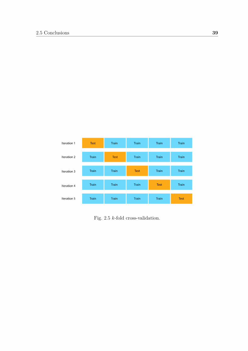
2.5 Conclusions 39

Fig. 2.5 k-fold cross-validation.

Chapter 3

Forecast evaluation

OverviewThis chapter introduces the main concepts in forecasting evaluation as a back-ground for the work developed in the following chapters of this manuscript.General textbooks such as [124] provide further information to the interestedreader. In addition, the course "Renewables in Electricity Markets"a given byprofessor Pierre Pinson at the Technical University of Denmark proposes valuablematerials on this topic.

ahttp://pierrepinson.com/index.php/teaching/

“Everything that can be counted does notnecessarily count; everything that countscannot necessarily be counted.”

— Albert Einstein

42 Forecast evaluation

ScenariosQuantiles

Normalizing flowsVariational autoencodersGenerative adversarial networks

Gaussian processesStatistical approach

Quality evaluationForecasting basics

Point forecasting

Density forecasts

Chapt er 2

Chapt er 4 Chapt er 6Chapt er 5

Training

Metrics for point and probabilistic forecasts

Chapt er 3

Neural networksGradient boosting

Quantiles Density forecasts Scenarios

Point forecast evaluation

Fig. 3.1 Chapter 3 position in Part I.

3.1 Metrics for point forecasts 43

For predictions in any form, one must differentiate between their quality and theirvalue [124]. The forecast quality corresponds to the ability of the forecasts to genuinelyinform of future events by mimicking the characteristics of the processes involved.The forecast value, studied in Part II, relates to the benefits of using forecasts indecision-making, such as participation in the electricity market. Consequently, forecastquality is independent of the current operational problem while not forecast value.Intuitively, it is relevant to evaluate the forecast quality before using the predictions asinput to operational problems. Even if a good quality does not necessarily imply agood forecast value, the quality assessment provides interesting information about themodel at hand.

This Chapter adopts the general framework of Morales et al. [124] to provide thebasics required to appraise the quality of predictions. It is organized as follows. Sections3.1 and 3.2 introduce the metrics for point and probabilistic forecasting, respectively.Finally, conclusions are drawn in Section 3.4.

3.1 Metrics for point forecasts

The base quantity for evaluating point forecasts of a continuous random variable is theforecast error.

Definition 3.1.1 (Forecast error). [124, Chapter 2] The forecast error ϵt+k|t is thedifference between observed and predicted values

ϵt+k|t := xt+k|t − xt+k|t. (3.1)

Note that the forecast error may be normalized so that verification results can becomparable for different time series. If so, normalization is most commonly performedby the nominal capacity of the site of interest. The first error criterion that may becomputed is the bias of the forecasts, which corresponds to the systematic part of theforecast error. It may be corrected in a straightforward manner using simple statisticalmodels.

Definition 3.1.2 (Bias). [124, Chapter 2] The bias is the mean of all errors over theevaluation period of length N , considered indifferently. For lead time k, it is

bias(k) := 1N

N∑t=1

ϵt+k|t. (3.2)

44 Forecast evaluation

This summary measure does not tell much about the quality of point forecastsbut only about a systematic error that should be corrected. Therefore, for a betterappraisal of the forecasts, it is advised to use scores such as the mean absolute androot mean square errors.

Definition 3.1.3 (Mean absolute error). [124, Chapter 2] The mean absolute error(MAE) is defined as the average of the absolute forecast errors over an evaluation setof length N

MAE(k) := 1N

N∑t=1

|ϵt+k|t|. (3.3)

Definition 3.1.4 (Root mean square error). [124, Chapter 2] The root mean squareerror (RMSE) is defined as the square root of the sum of squared errors over anevaluation of length N

RMSE(k) :=

√√√√ 1N

N∑t=1

(ϵt+k|t)2. (3.4)

All the above error criteria are independent of the length of the evaluation set. Thenominal capacity of the renewable energy site of interest can be used to normalizethem, and then they are referred to Nbias, NRMSE, and NMAE.

3.2 Metrics for probabilistic forecasts

3.2.1 Calibration

The first requirement of probabilistic forecasts is to consistently inform about theprobability of events. It leads to the concept of probabilistic calibration, also referredto as reliability. The assessment of probabilistic calibration only informs about a formof bias of probabilistic forecasts. A frequentist approach, based on an evaluation set ofsufficient length, can be performed by assessing the reliability of each of the definingquantile forecasts using the indicator variable.

Definition 3.2.1 (Indicator variable). [124, Chapter 2] The indicator variable ξqt,k, for

a given quantile forecast x(q)t+k|t and corresponding realization xt+k is

ξqt,k := 1xt+k<x

(q)t+k|t =

1 xt+k < x(q)t+k|t

0 xt+k ≥ x(q)t+k|t

. (3.5)

3.2 Metrics for probabilistic forecasts 45

ξqt,k is a binary variable indicating if the quantile forecasts cover, or not, the

measurements. The empirical level of quantile forecasts can be defined, estimated, andeventually compared with their nominal one by using this indicator variable.

Definition 3.2.2 (Empirical level). [124, Chapter 2] The empirical level ξqt,k, for a

nominal level q and lead time k, is obtained by calculating the mean of the ξqt,kN

t=1

time-series over an evaluation set of length N

ξqt,k := 1

N

N∑t=1

ξqt,k. (3.6)

The difference between nominal and empirical levels of quantile forecasts is to beseen as a probabilistic bias. Then, probabilistic calibration may be appraised visuallyby using reliability diagrams plotting empirical vs. nominal levels of the quantilesdefining density forecasts.

3.2.2 Univariate skill scores

Perfectly calibrated probabilistic forecasts do not guarantee that the forecasts are "good".For instance, they may not discriminate among situations with various uncertaintylevels, while these aspects are crucial in decision-making. The overall quality ofprobabilistic forecasts may be assessed based on skill scores. First, we consider theunivariate skill score that can only assess the quality of the forecasts with respect totheir marginals (time period). Second, we focus on the multivariate skill score thatcan directly assess multivariate scenarios.

Continuous ranked probability score

The continuous ranked probability score (CRPS) [70] is a univariate scoring rule thatpenalizes the lack of resolution of the predictive distributions as well as biased forecasts.It is negatively oriented, i.e., the lower, the better, and for deterministic forecasts, itturns out to be the mean absolute error (MAE). Thus, it can be directly comparedto the MAE criterion used for point forecasts since the CRPS is its generalizationin a probabilistic forecasting framework. The CRPS is used to compare the skill ofpredictive marginals for each component of the random variable of interest. In ourcase, for the twenty-four time periods of the day.

46 Forecast evaluation

Definition 3.2.3 (CRPS-integral). [70] The CRPS for predictive densities Ft+k|t andcorresponding measurement xt+k|t, is calculated over an evaluation set of length N

CRPS(k) := 1N

N∑t=1

∫x′

[Ft+k|t(x′) − 1x′>xt+k|t]2dx′. (3.7)

However, it is not easy to estimate the integral form of the CRPS defined by (3.7).

Definition 3.2.4 (CRPS-energy). [70] Gneiting and Raftery [70] propose a formulationcalled the energy form of the CRPS since it is just the one-dimensional case of theenergy score, defined in negative orientation as follows

CRPS(P, xt+k|t) =EP [|X − xt+k|t|] − 12EP [|X − X ′|], (3.8)

where X and X’ are independent random variables with distribution P and finite firstmoment, and EP is the expectation according to the probabilistic distribution P.

The CRPS can be computed for quantile forecasts and scenarios. Let xit+k|tM

i=1

be the set of M scenarios generated at time t for lead time k. The estimator of (3.8)proposed by Zamo and Naveau [181], over an evaluation set of length N for lead timek, is

CRPS(k) = 1N

[N∑

t=1

1M

M∑i=1

|xit+k|t − xt+k| − 1

2M2

M∑i,j=1

|xit+k|t − xj

t+k|t|]. (3.9)

Let x(q)t+k|t

Qq=1 be the set of Q quantiles generated at time t for lead time k. (3.8) is

over an evaluation set of length N for lead time k

CRPS(k) = 1N

[N∑

t=1

1Q

Q∑q=1

|x(q)t+k|t − xt+k| − 1

2Q2

Q∑q,q′=1

|x(q)t+k|t − x

(q′)t+k|t|

]. (3.10)

Quantile score

The quantile score (QS), also known as the pinball loss, is complementary to theCRPS. It permits obtaining detailed information about the forecast quality at specificprobability levels, i.e., over-forecasting or under-forecasting, and particularly thoserelated to the tails of the predictive distribution [112]. It is negatively oriented andassigns asymmetric weights to negative and positive errors for each quantile.

3.2 Metrics for probabilistic forecasts 47

Definition 3.2.5 (Pinball loss). The pinball loss function for a given quantile q is

ρq(x, x) := max(1 − q)(x − x), q(x − x)

. (3.11)

Definition 3.2.6 (Quantile score). The quantile score, over an evaluation set of lengthN for lead time k, is

QS(k) := 1N

N∑t=1

1Q

Q∑q=1

ρq(x(q)t+k|t, xt+k). (3.12)

The quantile score, over an evaluation set of length N for a given quantile q over alllead times k, is

QS(q) := 1N

N∑t=1

1T

kT∑k=k1

ρq(x(q)t+k|t, xt+k). (3.13)

Interval score

The interval score (IS) [70] assesses the quality of central prediction interval forecastsspecifically. It rewards narrow prediction intervals. It penalizes the forecasts where theobservation is outside the interval thanks to the penalty term that depends on α

Definition 3.2.7 (IS). The interval score, for a central prediction interval with acoverage rate of (1 − α), over an evaluation set of length N and for lead time k is

IS(k) = 1N

N∑t=1

(x(1−α/2)t+k|t − x

(α/2)t+k|t) + 2

α(x(α/2)

t+k|t − xt+k)1xt+k≤x(α/2)t+k|t

+ 2α

(xt+k − x(1−α/2)t+k|t )1xt+k≥x

(1−α/2)t+k|t . (3.14)

Note: the skill scores can be normalized by the total installed capacity for arenewable generation plant.

3.2.3 Multivariate skill scores

Energy score

The energy score (ES) is the most commonly used scoring rule when a finite number oftrajectories represents distributions. It is a multivariate generalization of the CRPSand has been formulated and introduced by Gneiting and Raftery [70]. The ES isproper and negatively oriented, i.e., a lower score represents a better forecast. TheES is used as a multivariate scoring rule by Golestaneh et al. [72] to investigate and

48 Forecast evaluation

analyze the spatio-temporal dependency of PV generations. They emphasize the ESpros and cons. It is capable of evaluating forecasts relying on marginals with correctvariances but biased means. Unfortunately, its ability to detect incorrectly specifiedcorrelations between the components of the multivariate quantity is somewhat limited.

Definition 3.2.8 (Energy score). Gneiting and Raftery [70] introduced a generalizationof the continuous ranked probability score defined in negative orientation as follows

ES(P, x) =EP ∥X − x∥ − 12EP ∥X − X ′∥, (3.15)

where and X and X’ are independent random variables with distribution P and finitefirst moment, EP is the expectation according to the probabilistic distribution P, and∥ · ∥ the Euclidean norm.

The ES is computed following Gneiting et al. [71] over an evaluation set of lengthN as follows

ES = 1N

M∑t=1

[1

M

M∑i=1

∥xit − xt∥ − 1

2M2

M∑i,j=1

∥xit − xj

t ∥]. (3.16)

Note: when we consider the marginals of x, it is easy to recognize that (3.16) is theCRPS.

Variogram score

An alternative class of proper scoring rules based on the geostatistical concept ofvariograms is proposed by Scheuerer and Hamill [157]. They study the sensitivityof these variogram-based scoring rules to inaccurate predicted means, variances, andcorrelations. The results indicate that these scores are distinctly more discrimina-tive concerning the correlation structure. Thus, the Variogram score (VS) capturescorrelations between multivariate components in contrast to the Energy score.

Definition 3.2.9 (Variogram score). For a given day t of the testing set and a T -variate observation xt ∈ RT , the Variogram score metric of order γ is formally definedas

VSt =T∑

k,k′wkk′

(|xt,k − xt,k′ |γ − EP |xt,k − xt,k′|γ

)2

, (3.17)

where xt,k and xt,k′ are the k-th and k′-th components of the random vector xt

distributed according to P for which the γ-th absolute moment exists, and wkk′ are

3.3 Point forecasting evaluation example 49

non-negative weights. Given a set of M scenarios xitM

i=1 for this given day t, theforecast variogram EP |xt,k − xt,k′|γ can be approximated ∀k, k′ = 1, · · · , T by

EP |xt,k − xt,k′ |γ ≈ 1M

M∑i=1

|xit,k − xi

t,k′ |γ. (3.18)

Then, the VS is averaged over the testing set of length N

VS = 1N

N∑t=1

VSt. (3.19)

In this thesis, we evaluate the Variogram score with equal weights across all hours of theday wkk′ = 1 and using a γ of 0.5, which for most cases provides a good discriminatingability as reported in Scheuerer and Hamill [157].

3.3 Point forecasting evaluation example

This section proposes an example of point forecasting quality evaluation. It is basedon an extract of Dumas et al. [54]. In addition, it introduces multi-output weather-based point forecasting by defining the problem formulation and implementation on areal-case study to compute PV and electrical consumption forecasts. They are used bya day-ahead deterministic planner presented in Chapter 9. Note: PV intraday pointforecast will also be considered in this thesis using an encoder-decoder architecturedeveloped in Dumas et al. [51]. Chapter 4 details the approach and the results.

3.3.1 Formulation

Point forecasting corresponds to the conditional expectation of the stochastic processfor every lead time (2.1). This definition is linked to the so-called loss function L(x, x).Loss functions assign a penalty to forecast errors as a proxy of the cost of these errorsfor those making decisions based on such forecasts. There exist various types of lossfunctions, such as the mean squared error or the pinball loss. A special relevant caseof a loss function to compute point forecasts is the mean squared error

L2(x, x) = (x − x)2. (3.20)

At the time t a point forecast xt+k|t for time t + k is the value of the process suchthat it minimizes the expected loss for the forecast user for all potential realizations of

50 Forecast evaluation

the process, given our state of knowledge at that time. Therefore, when consideringmulti-output point forecasts of length T the estimation of the model parameters isperformed by solving

θ⋆ = arg minθ

1N

N∑t=1

∥xt − xt∥22, (3.21a)

xt ∼gθ(x<t, ct), (3.21b)

given the information set D of length N , and ∥·∥2 the Euclidean norm.

3.3.2 Forecasting models

Two standard forecasting techniques are implemented to forecast the PV productionand the consumption, with a dedicated model per variable of interest. The first modeluses a Recurrent Neural Network (RNN) of the Keras Python library [33]. The RNNis a Long Short Term Memory (LSTM) with one hidden layer composed of 2 × n + 1neurons with n the number of input features. The second model is a Gradient BoostingRegressor (GBR) of the Scikit-learn Python library [140]. They both use past valuesof the PV production and consumption, and the weather forecasts provided by theLaboratory of Climatology of the Liège University, based on the MAR regional climatemodel [59]. It is an atmosphere model designed for meteorological and climatic research,used for a wide range of applications, from km-scale process studies to continental-scalemulti-decade simulations. The study Dumas et al. [54] focuses on the real-time controlof microgrids based on planning that requires a forecast horizon of a few hours up to afew days. Both models are trained by solving (3.21a) that becomes

xt ∼gθ(x<t, ct), (3.22a)x<t =[xt, ..., xt−k4 ], (3.22b)

ct =[cit+k1|t, ..., ci

t+kT |t], (3.22c)

with xt the variable to forecast, i.e, PV, consumption, and ci the forecast of theith weather variable, e.g., direct solar irradiance, wind speed, air temperature. Inthe case study considered, the point forecasts are computed each quarter for thesubsequent T = 96 periods with a resolution ∆t = 15 minutes. The forecasting processis implemented by using a rolling forecast methodology where the learning set isupdated every six hours, with a fixed size limited to the week preceding the forecasts,to maintain a reasonable computation time.

3.3 Point forecasting evaluation example 51

05:0006:00

07:0008:00

09:0010:00

11:0012:00

13:0014:00

15:0016:00

17:0018:00

19:0020:00

21:0022:00

23:0000:00

01:0002:00

03:0004:00

05:0006:00

07:000100200300400500600700800900

1000

kW

PVRNNGBR

Fig. 3.2 PV point forecasts on June 12, 2019 computed at 06h00 UTC. The PVobservations are in black.

3.3.3 Results

Figure 3.2 illustrates the PV point forecasts of the RNN and GBR models comparedto the observations (black) on a particular day of the testing set. It is interesting topoint out the sudden drop in the PV production around 10 a.m. that the models donot accurately forecast.

The point forecasts are evaluated each quarter over the entire forecasting horizon, thenext 96 periods, using the Normalized Mean Absolute Error (NMAE), the NormalizedRoot Mean Squared Error (NRMSE), and the Normalized Energy Measurement Error(NEME). The normalizing coefficients for both the NMAE and NRMSE are the meanof the absolute values of the PV and consumption over all the simulation data set. TheNEME is the NMAE of the energy summed over the entire forecasting horizon. Figures3.3 and 3.4 provide the scores for both GBR and LSTM models for each quarter, plainlines, and the average over the entire simulation dataset, dashed lines. On average,the LSTM model yields slightly smaller average NMAE, NRMSE, and NEME values.However, the differences are not significant, and the forecast value (see Chapter 9)needs to be evaluated to decide which model is the best.

52 Forecast evaluation

05-2005-21

05-2205-23

05-2405-25

05-2605-27

05-2805-29

05-3005-31

06-0106-02

06-0306-04

06-0506-06

06-0706-08

06-0906-10

06-1106-12

06-1306-14

06-1506-160

20406080

100120140160180200

%

NMAENRMSENEME

NMAE meanNRMSE meanNEME mean

05-2005-21

05-2205-23

05-2405-25

05-2605-27

05-2805-29

05-3005-31

06-0106-02

06-0306-04

06-0506-06

06-0706-08

06-0906-10

06-1106-12

06-1306-14

06-1506-160

20406080

100120140160180200

%

NMAENRMSENEME

NMAE meanNRMSE meanNEME mean

Fig. 3.3 PV forecast scores, GBR (top) and LSTM (bottom).

05-2005-21

05-2205-23

05-2405-25

05-2605-27

05-2805-29

05-3005-31

06-0106-02

06-0306-04

06-0506-06

06-0706-08

06-0906-10

06-1106-12

06-1306-14

06-1506-160

20

40

60

80

%

NMAENRMSENEME

NMAE meanNRMSE meanNEME mean

05-2005-21

05-2205-23

05-2405-25

05-2605-27

05-2805-29

05-3005-31

06-0106-02

06-0306-04

06-0506-06

06-0706-08

06-0906-10

06-1106-12

06-1306-14

06-1506-160

20

40

60

80

%

NMAENRMSENEME

NMAE meanNRMSE meanNEME mean

Fig. 3.4 Consumption forecast scores, GBR (top) and LSTM (bottom).

3.4 Conclusions 53

3.4 Conclusions

This Chapter provides the basics of forecast verification to acquire background knowl-edge on forecast quality that corresponds to the ability of the forecasts to genuinelyinform of future events by mimicking the characteristics of the processes involved. Incontrast, the forecast value, investigated in Part II, relates to the interests of usingforecasts in decision-making, such as participation in the electricity market. However,it is intuitively expected that higher-quality forecasts will yield better policies anddecisions. Therefore, quality evaluation is complementary to value evaluation andprovides an insight into forecasting model skills. The Chapter illustrates the evaluationmethodology with a multi-output point forecasting model and an implementation of areal-case study using two standard techniques. The weather-based forecasting modelsare trained to compute quarterly day-ahead PV and electrical consumption pointforecasts. Then, the quality is assessed by computing point forecasts metrics. In thefollowing Chapters, the quality metrics are used to evaluate the various probabilisticforecasts on several case studies.

56 Quantile forecasting

Chapter 4

Quantile forecasting

OverviewOverall, the Chapter contributions can be summarized as follows.

1. A deep learning-based multi-output quantile architecture computes predic-tion intervals of PV generation on a day-ahead and intraday basis. Thegoal is to implement an improved probabilistic intraday forecaster, theencoder-decoder, to benefit from the last PV generation observations. Thisarchitecture is compared to a feed-forward neural network.

2. The weather forecasts are used to directly take into account the impact ofthe weather forecast updates generated every six hours.

3. A proper assessment of the quantile forecasts is conducted by using a k-foldcross-validation methodology and probabilistic metrics. It allows computingaverage scores over several testing sets and mitigating the dependency ofthe results to specific days of the dataset.

4. Finally, a comparison of deep learning quantile regression models is con-ducted with quantiles derived from deep learning generative models.

References: This chapter is an adapted version of the following publications:

Jonathan Dumas, Colin Cointe, Xavier Fettweis, and Bertrand Cornélusse. Deeplearning-based multi-output quantile forecasting of pv generation. In 2021 IEEEMadrid PowerTech, pages 1–6, 2021. doi: 10.1109/PowerTech46648.2021.9494976.URL https://arxiv.org/abs/2106.01271.

Jonathan Dumas, Antoine Wehenkel, Damien Lanaspeze, Bertrand Cornélusse,and Antonio Sutera. A deep generative model for probabilistic energy forecastingin power systems: normalizing flows. Applied Energy, 305:117871, 2022. ISSN0306-2619. doi: https://doi.org/10.1016/j.apenergy.2021.117871. URL https://arxiv.org/abs/2106.09370.

57

“Prediction is very difficult, especially if it’sabout the future.”

— Niels Bohr

ScenariosQuantiles

Normalizing flowsVariational autoencodersGenerative adversarial networks

Gaussian processesStatistical approach

Quality evaluationForecasting basics

Point forecasting

Density forecasts

Chapt er 2

Chapt er 4 Chapt er 6Chapt er 5

Training

Metrics for point and probabilistic forecasts

Chapt er 3

Neural networksGradient boosting

Quantiles Density forecasts Scenarios

Point forecast evaluation

Fig. 4.1 Chapter 4 position in Part I.

58 Quantile forecasting

This Chapter focuses on quantile forecasts that provide probabilistic informationabout future renewable power generation, in the form of a threshold level associatedwith a probability. This approach is investigated in Dumas et al. [51] with probabilisticPV forecasters that exploit recent breakthroughs in the field of data science by usingadvanced deep learning structures, such as the encoder-decoder architecture [27]. It isimplemented to compute day-ahead and intraday multi-output PV quantiles forecasts,to efficiently capture the correlation between time periods, and to be used as input ofa robust optimization model. For instance, to address the energy management systemof a grid-connected renewable generation plant coupled with a battery energy storagedevice detailed in Dumas et al. [52] and Chapter 12. The case study is composedof PV production monitored on-site at the University of Liège (ULiège), Belgium.The weather forecasts from the MAR climate regional model [59] provided by theLaboratory of Climatology are used as inputs of the deep learning models.

The remainder of this Chapter is organized as follows. Section 4.1 presents thenon-parametric quantile forecasting framework. Section 4.2 provides the related work.Section 4.3 details the forecasting techniques. Section 4.4 describes the case studyand presents the results. Section 4.5 proposes a comparison of the quantile regressionmodels with quantiles derived from deep learning generative models. Finally, Section4.6 summarizes the main findings and highlights ideas for further work.

4.1 Formulation

Quantile regression [106] is one of the most famous non-parametric approach. It doesnot assume the shape of the predictive distributions. It can be implemented withvarious types of forecasting techniques, e.g., neural networks, linear regression, gradientboosting, or any other regression techniques. The estimation of the model parametersθ to compute multi-output quantile forecasts of length T is performed by minimizingthe pinball loss (3.11) over all lead times

θ⋆ = arg minθ

1N

N∑t=1

1Q

Q∑q=1

kT∑k=k1

ρq(x(q)t+k, xt+k), (4.1)

x(q)t ∼gθ(x<t, ct), (4.2)

given the information set D of length N , and a set of Q quantiles.

4.2 Related work 59

4.2 Related work

The literature on quantile forecasting is broad. We present a few papers that havegained our attention in quantile PV probabilistic forecasting. At the Global EnergyForecasting Competition 2014 [85] solar forecasts are expressed in the form of 99quantiles with various nominal proportions between zero and one. The models areevaluated by using the pinball loss function. This study summarizes the recent researchprogress on probabilistic energy forecasting at that time, and this competition made itpossible to develop innovative techniques. A systematic framework for generating PVprobabilistic forecasts is developed by Golestaneh et al. [73]. A non-parametric densityforecasting method based on Extreme Learning Machine is adopted to avoid restrictiveassumptions on the shape of the forecast densities. A combination of bidirectionalRecurrent Neural Networks (RNNs) with Long Short-Term Memory (LSTM), calledBidirectional LSTM (BLSTM), is proposed by Toubeau et al. [166]. It has the benefitsof both long-range memory and bidirectional processing. The BLSTM is trained byminimizing the quantile loss to compute quantile forecasts of aggregated load, windand PV generation, and electricity prices on a day-ahead basis. Finally, an innovativearchitecture, referred to as encoder-decoder (ED), is developed by Bottieau et al.[27] to generate reliable predictions of the future system imbalance used for robustoptimization.

4.3 Forecasting models

This Section presents the forecasting techniques implemented to compute multi-outputpoint and quantile forecasts of PV generation.

4.3.1 Gradient boosting regression (GBR)

Gradient boosting builds an additive model in a forward stage-wise fashion [83]. Itallows for the optimization of arbitrary differentiable loss functions. In each stage, aregression tree is fit on the negative gradient of the given loss function. The gradientboosting regressor (GBR) from the Scikit-learn [140] Python library is trained byminimizing the quantile loss. The learning rate is set to 10−2, the max depth to 5, andthe number of estimators to 500. There is a GBR model trained per quantile as thislibrary does not handle a single model for several quantiles.

60 Quantile forecasting

4.3.2 Multi-layer perceptron (MLP)

A description of the most widely used "vanilla" neural network, the multi-layer perceptron(MLP), is provided by [83]. A MLP with a single hidden layer is considered for theday-ahead forecasts and as the benchmark for the intraday forecasts. Note, MLPswith two and three hidden layers did not provide any significant improvement on thecase study considered. The activation function is the Rectified Linear Unit (ReLU).The number of neurons of the hidden layer is ninput + (noutput − ninput)/2, with ninput

and noutput the number of neurons of the input and output layers, respectively. Thelearning rate is set to 10−2 and the number of epoch to 500 with a batch size of 8. Itis implemented using the PyTorch Python library [139].

4.3.3 Encoder-decoder (ED)

Several technical information about recent advances in neural networks is provided byToubeau et al. [166], Bottieau et al. [27]. In particular, recurrent neural networks haveshown a high potential in processing and predicting complex time series with multi-scaledynamics. However, RNNs are known to struggle in accessing time dependencies morethan a few time steps long due to the vanishing gradient problem. Indeed, back-propagated errors during the training stage either fades or blows up over time. LongShort-Term Memory and Gated Recurrent Units networks tackle this problem by usinginternal memory cells [27]. A neural network composed of a LSTM and feed-forwardlayers, referred to as LSTM in the rest of the Chapter, is implemented for the day-aheadand intraday forecasts. The number of LSTM units is ninput + (noutput − ninput)/3, andthe number of neurons of the feed-forward layer ninput + 2 × (noutput − ninput)/3.

An innovative architecture referred to as encoder-decoder [27], is composed of twodifferent networks and has recently shown promising results for translation tasks andspeech recognition applications and imbalance price forecasting. The encoder-decoder,depicted in Figure 4.2, processes features from the past, such as past PV observations,to extract the relevant historical information that is contained into a reduced vectorof fixed dimensions, based on the last hidden state. Then, the decoder processes thisrepresentation along with the known future information such as weather forecasts. Aversion of the encoder-decoder architecture (ED-1) is implemented with a LSTM as theencoder and a MLP as the decoder. In a second version (ED-2), the decoder is a LSTMfollowed by an additional feed-forward layer. Both versions of the encoder-decoderare used as intraday forecasters. In ED-1, the encoder has 2 × ninput units with ninput

the number of neurons of the encoder input layer, features from the past. Then, the

4.4 The ULiège case study 61

Encoder

Past information

Weather forecasts

Decoder

Forecasts

LSTM

LSTM/MLP

Fig. 4.2 Encoder-decoder architecture.

encoder output is merged with the weather forecasts becoming the decoder input layerthat has noutput/2 neurons. In ED-2, the decoder has the same number of cells as theencoder, and the feed-forward layer is composed of noutput/2 neurons. The LSTM,ED-1, and ED-2 models are implemented using the TensorFlow Python library [1].The activation functions are the ReLU. The learning rate is set to 10−3, the number ofepoch to 500 with a batch size of 64 for the three models.

A sensitivity analysis has been conducted to select the hyperparameters: numberof hidden layers, neurons, epochs, and learning rate. Overall, increasing the number ofhidden layers and neurons increases the model complexity. It can enhance the accuracy,but only up to a limited number of layers and neurons due to overfitting issues. Inaddition, the hyperparameter solution is closely related to the size of the historicaldatabase [166]. A deep learning model with more significant hidden layers and neuronsrequires a large amount of data to estimate the parameters accurately. In the casestudy considered, there are only 157 days of data with a 15 minutes resolution. Thus,we decided to restrict the number of layers and neurons to select a smaller model thatperforms better with the available information.

4.4 The ULiège case study

4.4.1 Case study description

The ULiège case study is composed of a PV generation plant with an installed capacityof 466.4 kW. The PV generation has been monitored on a minute basis for 157 days.The data is resampled to 15 minutes. The set of quantiles is q = 10%, . . . , 90% forboth the day-ahead and intraday forecasts. Numerical experiments are performed on

62 Quantile forecasting

an Intel Core i7-8700 3.20 GHz based computer with 12 physical CPU cores and 32 GBof RAM running on Ubuntu 18.04 LTS.

4.4.2 Numerical settings

The MAR regional climate model [59] provided by the Laboratory of Climatology ofthe Liège University is forced by GFS (Global Forecast System) to compute weatherforecasts on a six hours basis, four-time gates per day at 00:00, 06:00, 12:00, and18:00 with a 10-day horizon and a 15 minutes resolution. The solar irradiance and airtemperature at 2 meters are normalized by a standard scaler and used as inputs to theforecasting models.

A k-fold cross-validation strategy computes average scores over several testing setsto mitigate the dependency of the results to specific days of the dataset. The dataset isdivided into k parts of equal length, and there are k possible testing sets 1 ≤ i ≤ k. Fora given testing set i, the models are trained over the k − 1 parts of the dataset. Elevenpairs of fixed lengths of 142 and 15 days are built. One pair is used to conduct thehyperparameters sensitivity analysis, and the ten others for testing where the scoresare averaged. The Mean Absolute Error and Root Mean Squared Error are introducedto evaluate the point forecasts. The MAE, RMSE, CRPS, and IS are normalized bythe PV total installed capacity with NMAE and NRMSE the normalized MAE andRMSE.

The day-ahead models, MLP, LSTM, and GBR compute forecasts at noon for thenext day. Four intraday time gates are considered at 00:00, 06:00, 12:00, and 18:00.The intraday forecasts of time gate 00:00 are computed by the day-ahead models usingonly the weather forecasts. Then, the following three intraday forecasts are computedby intraday models where the MLP, ED-1, and ED-2 models use the weather forecastsand the last three hours of PV generation.

The day-ahead and the first intraday predictions are delivered for the 96 quartersof the next day from 00:00 to 23:45 indexed by time steps 0 ≤ k ≤ 95. The predictionhorizons span from 12 to 36 hours, for the day-ahead gate 12:00, and 0 to 24 hours, forthe intraday gate 00:00. The prediction horizon is cropped to 11 ≤ k ≤ 80 because thePV generation is always 0 for time steps 0 ≤ k ≤ 10 and 81 ≤ k ≤ 95 on the ULiègecase study. The next three intraday predictions are performed for the 72, 48, and 24next quarters of the day corresponding to the gates 06:00, 12:00, and 18:00. Therefore,the prediction horizons span from 0 to 18 hours, 0 to 12 hours, and 0 to 6 hours. Theintraday forecasting time periods are 24 ≤ k ≤ 80, 48 ≤ k ≤ 80, and 72 ≤ k ≤ 80.

4.4 The ULiège case study 63

Table 4.1 compares the mean and the standard deviation of the computation timesover the ten learning sets to train the point and quantile forecast models1.

day-ahead MLP LSTM GBRpoint 5.3 (0.1) 23.7 (0.3) 3.4 (0.1)quantile 7.6 (0.2) 69.0 (0.6) 44.6 (0.4)intraday MLP ED-1 ED-2point 5.0 (0.1) 5.2 (0.1) 17.2 (0.2)quantile 17.9 (0.2) 6.4 (0.2) 18.0 (0.3)

Table 4.1 Training computation time (s).

4.4.3 Day-ahead results

Figure 4.3a compares the NMAE (plain lines), NRMSE (dashed lines), and Figure 4.3bthe CRPS per lead time k of the day-ahead models of gate 12:00. Table 4.2 providesthe mean and standard deviation of the NMAE, NRMSE, and CRPS. The LSTMachieved the best results for both point and quantile forecasts. Figures 4.5a, 4.5c, and4.5e compare the MLP, LSTM, and GBR day-ahead quantile and point forecasts (blackline named dad 12) of gate 12:00 on August 2, 2020 with the observation in red. Onecan see that the predicted intervals of the LSTM model better encompass the actualrealizations of uncertainties than the MLP and GBR.

Score Gate MLP LSTM GBR

NMAE 12 8.2 (1.2) 7.6 (1.5) 9.2 (0.9)24 7.9 (1.2) 7.7 (1.6) 9.0 (0.8)

NRMSE 12 10.2 (1.4) 9.2 (1.6) 11.2 (0.9)24 9.7 (1.2) 9.4 (1.8) 10.9 (0.8)

CRPS 12 6.2 (1.1) 4.4 (0.2) 6.4 (0.7)24 6.2 (1.0) 4.4 (0.2) 6.3 (0.6)

Table 4.2 The NMAE, NRMSE, CRPS of day-ahead models are averaged over allperiods. The best-performing model for each score and gate is written in bold.

1The day-ahead and intraday LSTM training times are identicals for both point and quantileforecasts as they only take the weather forecasts as inputs.

64 Quantile forecasting

10 20 30 40 50 60 70 800

5

10

15

20

25

%

MLPLSTMGBR

(a) NMAE (plain) and NRMSE (dashed).

10 20 30 40 50 60 70 8002468

101214

%

MLPLSTMGBR

(b) CRPS.

Fig. 4.3 NMAE, NRMSE, and CRPS of the day-ahead models per lead time k.

4.4.4 Intraday results

Table 4.3 provides the averaged NMAE, NRMSE, and CRPS per gate of intradaymodels. The LSTM achieved the best NMAE and NRMSE for the 06:00 gate, and theED-1 achieved the best NMAE and NRMSE for the noon gate and the best CRPS forboth gates. Figure 4.4 compares the CRPS per lead time k of the intraday models. TheED-1 benefits from the last PV generation observations. Indeed, some CRPS valuesfor both 06:00 and 12:00 gates are below the ones of 00:00 gate. Table 4.4 providesthe interval score of intraday models for 80%, 60%, 40%, and 20% width of centralintervals. The ED-1 model achieved the best results except for the prediction intervalwidth of 80%, where it is ED-2 and LSTM for the 06:00 and 12:00 gates, respectively.Overall, The LSTM achieved close results to the ED-1. Figures 4.5b, 4.5d, and 4.5fcompare the ED-1, LSTM, and ED-2 intraday quantile and point forecasts (black linenamed intra 6) of 06:00 gate on August 2, 2020 with the observation in red. Generally,one can see that the predicted intervals of ED-1 and LSTM models better encompassthe actual realizations of uncertainties than ED-2.

4.4 The ULiège case study 65

Score Gate MLP ED-1 ED-2 LSTM

NMAE 6 8.9 (1.0) 8.5 (1.4) 9.4 (1.0 ) 7.6 (1.5)12 6.7 (1.4) 6.4 (1.3 ) 7.1 (1.1) 7.2 (1.1)

NRMSE 6 10.9 (0.9) 10.3 (1.3) 11.3 (1.1) 7.7 (1.6)12 8.7 (1.3) 7.8 (1.2) 8.5 (1.2) 9.4 (1.8)

CRPS 6 8.1 (0.7) 5.9 (0.9) 6.6 (0.7) 6.2 (0.7)12 5.8 (1.2) 4.5 (0.7) 5.6 (1.8) 4.7 (0.5)

Table 4.3 The NMAE, NRMSE, CRPS of intraday models are averaged over all periods.The best-performing model for each score and gate is written in bold.

Width Gate MLP ED-1 ED-2 LSTM

80% 6 24.4 (2.9) 14.9 (4.0) 13.9 (4.9) 19.3 (4.2)12 17.4 (3.5) 10.6 (1.8) 11.6 (10.1) 9.6 (2.0)

60% 6 37.6 (3.2) 29.9 (5.0) 32.2 (4.2) 30.7 (4.6)12 27.2 (4.3) 22.4 (4.2) 27.5 (10.8) 22.6 (3.1)

40% 6 58.0 (4.5) 50.1 (6.5) 57.2 (6.0) 51.6 (5.8)12 42.4 (6.9) 37.7 (5.9) 48.1 (16.8) 39.2 (4.9)

20% 6 111.8 (8.4) 97.1 (11.7) 112.1 (10.3) 99.5 (10.4)12 81.5 (13.8) 72.7 (10.0) 94.8 (32.1) 76.5 (8.0)

Table 4.4 The interval score of intraday models is averaged over all periods. Thebest-performing model for each score and gate is written in bold.

66 Quantile forecasting

10 20 30 40 50 60 70 800.02.55.07.5

10.012.515.017.520.0

%

00:0006:0012:0018:00

(a) ED-1.

10 20 30 40 50 60 70 800.02.55.07.5

10.012.515.017.520.0

%

00:0006:0012:0018:00

(b) ED-2.

10 20 30 40 50 60 70 800.02.55.07.5

10.012.515.017.520.0

%00:0006:0012:0018:00

(c) MLP.

10 20 30 40 50 60 70 800.02.55.07.5

10.012.515.017.520.0

%

00:0006:0012:0018:00

(d) LSTM.

Fig. 4.4 CRPS of intraday models per lead time k.

4.4 The ULiège case study 67

10 20 30 40 50 60 70 800

100

200

300

400

500

kW

q1 = 0.1qQ = 0.9Pmdad 12

(a) MLP day-ahead.

30 40 50 60 70 800

100

200

300

400

500

kW

q1 = 0.1qQ = 0.9Pmintra 6

(b) ED-1 intraday.

10 20 30 40 50 60 70 800

100

200

300

400

500

kW

q1 = 0.1qQ = 0.9Pmdad 12

(c) LSTM day-ahead.

30 40 50 60 70 800

100

200

300

400

500

kW

q1 = 0.1qQ = 0.9Pmintra 6

(d) LSTM intraday.

10 20 30 40 50 60 70 800

100

200

300

400

500

kW

q1 = 0.1qQ = 0.9Pmdad 12

(e) GBR day-ahead.

30 40 50 60 70 800

100

200

300

400

500

kW

q1 = 0.1qQ = 0.9Pmintra 6

(f) ED-2 intraday.

Fig. 4.5 Quantiles vs. point forecasts of day-ahead models of gate 12:00 (left), andintraday models of gate 06:00 (right) on August 2, 2020, the observations are in red.

68 Quantile forecasting

4.4.5 Conclusions

An encoder-decoder architecture is implemented on the intraday scale to produceaccurate forecasts. It efficiently captures the contextual information composed of pastPV observations and future weather forecasts while capturing the temporal dependencybetween forecasting periods over the entire forecasting horizon. The models are com-pared by using a k-fold cross-validation methodology and quality metrics on a real casestudy composed of the PV generation of the parking rooftops of the Liège University.The best day-ahead model for point and quantile forecasts is a neural network composedof a LSTM cell and an additional feed-forward layer. Then, the encoder-architecturecomposed of a LSTM-MLP yields accurate and calibrated forecast distributions learnedfrom the historical dataset compared to the MLP and LSTM-LSTM models for theintraday point and quantile forecasts. However, the LSTM produced similar results.

Several extensions are under investigation. First, using a larger dataset of at leastone full year to consider the entire PV seasonality. Second, developing a PV scenarioapproach based on the encoder-decoder architecture.

4.5 Comparison with generative models

This Section proposes a quality evaluation of the normalizing flows (NFs) and LSTMPV quantiles, used in Chapter 12 for robust optimization, using the quantile score, thereliability diagram, and the continuous ranked probability score. Indeed, the two-phaseengagement control of the capacity firming framework requires day-ahead and intradaytop-quality forecasts. The more accurate the forecasts, the better the planning andthe control. To this end, the Normalizing Flows technique computes quantile day-ahead forecasts compared to a common alternative technique using a Long Short-TermMemory neural network. The controller requires intraday point forecasts computedby an encoder-decoder architecture. NFs are investigated in Section 6.2 of Chapter 6.Both NFs and LSTM models use as input the weather forecasts of the MAR climateregional model provided by the Laboratory of Climatology of the Liège University [59].The NFs model generates day-ahead scenarios, and the quantiles are derived. TheLSTM model computes the quantiles directly and is trained by minimizing the quantileloss. The set of PV quantiles considered for the assessment is q = 10%, . . . , 90%.

4.5 Comparison with generative models 69

In this study, the class of Affine Autoregressive flows is implemented2. A five-stepAffine Autoregressive flow is trained by maximum likelihood estimation with 500 epochsand a learning rate of 10−4. The LSTM learning rate is 10−3, the number of epoch to500 with a batch size of 64. Figure 4.6 provides the results for these quality metrics

10 20 30 40 50 60 70 80 90%

1.00

1.25

1.50

1.75

2.00

%

(a) QS(q).

10 20 30 40 50 60 70 80 90q

102030405060708090

%

NFLSTM

(b) Reliability diagram.

0 20 40 60 80lead time

0

2

4

6

8

10

%

(c) CRPS(k).

Fig. 4.6 Quantile forecast quality evaluation of LSTM v.s NFs models.

computed over the entire dataset normalized by the total installed capacity. The NFsmodel outperforms the LSTM model with average values of 1.49% and 2.80% vs. 1.69%and 3.15% for the QS and CRPS, respectively. The NFs quantiles are also more reliable,as indicated by the reliability diagram. These results motivate the use of the NFs asthey outperform common deep learning approaches such as LSTM models.

2https://github.com/AWehenkel/Normalizing-Flows [176]

70 Quantile forecasting

4.6 Conclusions

This Chapter proposes a formulation of the quantile forecasts problem using deep learn-ing models trained by quantile regression to compute multi-output PV quantiles. Theforecast quality is evaluated on a real case study composed of the PV generation of theparking rooftops of the Liège University. In addition, these quantile regression modelsare compared to PV quantiles derived from deep learning generative models, whichwill be investigated in detail in Chapter 6. In terms of forecast quality, the generativemodels outperform on this case study the quantile regression models. However, it doesnot mean they are better in terms of forecast value which will be assessed in Chapter12 where a robust planner uses the PV quantiles in the form of prediction intervals.

Chapter 5

Density forecasting of imbalanceprices

OverviewThe contributions of this Chapter are two-fold.

1. A novel two-step probabilistic approach (TSPA) is proposed for forecastingthe Belgium imbalance prices. The TSPA uses a direct forecasting strategy[163]. It consists of forecasting an imbalance price for each quarter of thehorizon independently from the others, requiring a model per quarter.

2. It sets a reference for other studies as this subject is rarely addressed.

References: This chapter is an adapted version of the following publication:

Jonathan Dumas, Ioannis Boukas, Miguel Manuel de Villena, Sébastien Mathieu,and Bertrand Cornélusse. Probabilistic forecasting of imbalance prices in thebelgian context. In 2019 16th International Conference on the European EnergyMarket (EEM), pages 1–7. IEEE, 2019. URL https://arxiv.org/abs/2106.07361.

“If you don’t know where you’re going anyroad will do.”

— Lewis Carroll

72 Density forecasting of imbalance prices

ScenariosQuantiles

Normalizing flowsVariational autoencodersGenerative adversarial networks

Gaussian processesStatistical approach

Quality evaluationForecasting basics

Point forecasting

Density forecasts

Chapt er 2

Chapt er 4 Chapt er 6Chapt er 5

Training

Metrics for point and probabilistic forecasts

Chapt er 3

Neural networksGradient boosting

Quantiles Density forecasts Scenarios

Point forecast evaluation

Fig. 5.1 Chapter 5 position in Part I.

5.1 Related work 73

This Chapter presents the probabilistic forecasting of imbalance prices methodologydeveloped in Dumas et al. [49]. A novel two-step probabilistic approach is proposed,with a particular focus on the Belgian case. The first step consists of computing thenet regulation volume (NRV) state transition probabilities. It is modeled as a matrixestimated using historical data. This matrix is then used to infer the imbalance prices.Indeed, the NRV can be related to the level of reserves activated, and the correspondingmarginal prices for each activation level are published by the Belgian TransmissionSystem Operator (TSO) one day before electricity delivery. The model is compared to:(1) a multi-layer perceptron, implemented in a deterministic setting; (2) the widelyused probabilistic technique, the Gaussian Processes (GP).

This Chapter is organized as follows. Section 5.1 details the related work. Section 5.2introduces the novel two-step probabilistic approach formulation and the assumptionsmade. Section 5.3 describes the numerical tests on the Belgian case. Section 5.4 reportsthe results. Conclusions are drawn in Section 5.5. Appendix 5.5 lists the acronyms,parameters, and forecasted or computed variables. Finally, Annex 5.6 provides a shortreminder of the imbalance market and the Belgian balancing mechanisms.

5.1 Related work

The progressive, large-scale integration of renewable energy sources has altered elec-tricity market behavior and increased the electricity price volatility over the last fewyears [41, 77, 99]. In this context, imbalance price forecasting is an essential tool thestrategic participation in short-term energy markets. Several studies take into accountthe imbalance prices as penalties for deviation from the bids to compute the optimalbidding strategy [67, 143, 23, 25]. However, these penalties are known only a posteriori.A forecast indicating the imbalance prices and the system position, short or long, withan interval to inform about the range of potential outcomes is a powerful tool fordecision making. Probabilistic forecasting usually outperforms deterministic modelswhen used with the appropriate bidding strategies [143]. Whereas the literature onday-ahead electricity forecast models is extensive, studies about balancing marketprices forecast have received less attention. We recommend three papers related tothis topic. First, a statistical description of imbalance prices for shortage and sur-plus is presented by Saint-Drenan [154]. Second, a combination of classical and datamining techniques to forecast the system imbalance volume is addressed by Garciaand Kirschen [62]. Finally, a review and benchmark of time series-based methods forbalancing market price forecasting are proposed by Klæboe et al. [104]. One-hour and

74 Density forecasting of imbalance prices

NRV transition matrices

estimation

NRV Historical

data

ARC table

Imbalance prices

forecast

Assumptions

Learning phase

Operationnal forecaster

Fig. 5.2 Two-step probabilistic approach (TSPA) imbalance price forecasting process.

one-day-ahead forecasts are considered for state determination, balancing volume, andprice forecasting on the Nord Pool price zone NO2 in Norway.

5.2 Formulation

This study focuses on the intraday market time scale that requires a forecasting horizonfrom a few minutes to a few hours with a resolution ∆t. The day-ahead time scalerequires forecasts of the imbalance prices from 12 to 36 hours, which is not realistic atthis stage. The input data are the imbalance price history, the NRV, and the marginalprices for activation published by the TSO. The probabilistic approach consists offorecasting the imbalance prices in two steps: computing the NRV state transitionprobabilities, then forecasting the imbalance prices, as depicted in Figure 5.2. It ismotivated by the ELIA imbalance price mechanisms detailed in Appendix 5.6.

5.2.1 Net regulation volume forecasting

Let consider the T forecasting horizons k1 = ∆t, . . . , kT = T∆t with ∆t the marketperiod, 15 minutes for Belgium. The NRV historical data is discretized into N bins, vi,centered around vi,1/2. Note: this discretization has been determined after a statisticalstudy of the NRV distribution. The T NRV transition matrices (v)t+k|t, of dimensionsN × N , from a known state at time t to a future state at time t + k are estimated by

5.2 Formulation 75

Fig. 5.3 NRV transition matrix from t to t + 15 min (left) and t + 60 min (right).

using the NRV historical data, and referred to as (v)t+k|t. They are composed of thefollowing conditional probabilities ∀k = k1, . . . , kT

pijt+k|t = Pr[v(t + k) ∈ vj | v(t) ∈ vi], i, j ∈ J1; NK2, (5.1)

with v(t) the measured NRV at time t, and ∑Nj=1 pij

t+k|t = 1 ∀i ∈ J1; NK. The conditionalprobabilities (5.1) are estimated statistically over the learning set (LS) ∀k = k1, . . . , kT

pijt+k|t =

∑t∈LS 1v(t+k)∈vj | v(t)∈vi∑

t∈LS 1v(t)∈vi, i, j ∈ J1; NK2. (5.2)

Figure 5.3 illustrates the matrices (v)t+k1|t and (v)t+k4|t with 2017 as learning set. Theestimated mean vm

t+k|t and standard deviation vstdt+k|t of the NRV at time t for t + k are

calculated as followsvm

t+k|t =N∑

j=1pij

t+k|tvj,1/2

vstdt+k|t =

√√√√√ N∑j=1

pijt+k|t(vj,1/2 − vm

t+k|t)2,

(5.3)

with i such as v(t) ∈ vi.

5.2.2 Imbalance price forecasting

The NRV can be related to the level of reserves activated and the corresponding marginalprices for each activation level, published by the TSO one day before electricity delivery.We thus first forecast the NRV and its spread among the Gross Upward regulationVolume (GUV) and Gross Downward regulation Volume (GDV). Then, we forecast

76 Density forecasting of imbalance prices

the reserve products activated (contracted or not) to select the most probable MIPand MDP into the ARC table. Finally, the mean and the standard deviation of theimbalance price forecast are derived.

However, the ARC table contains only the contracted reserve products. Most of thetime, the first activated reserve products come from the non contracted InternationalGrid Control Cooperation platform (IGCC-/+), the contracted secondary reserve(R2-/+) and the non contracted regulation reserves (Bids-/+)1. For instance, considera quarter of an hour with an NRV of 150 MW, spread into 170 MW of GUV and 20MW of GDV. Suppose ELIA activated 80 MW of IGCC+ and 90 MW of R2+. Then,the MIP is given in the marginal activation price of R2+ in the ARC table at the range[0, 100] MW. Suppose that ELIA has activated 20 MW of IGCC+, 20 MW of R2 +,and 130 MW of Bids+. Then, the MIP is given in the marginal activation price ofBids+. However, this is not a contracted reserve, and its price is not in the ARC table.Then, it is more complicated to predict the MIP and consequently the imbalance prices.Therefore, we introduce several simplifying assumptions justified by a statistical studyon the 2017 ELIA imbalance data.

Assumption 1. The NRV is entirely spread into the GUV if the NRV is positive orGDV if the NRV is negative.

The mean and standard deviation of the GUV and GDV are 109 ± 82 MW vs. 17 ± 27MW when the NRV is positive, while it is 13±20 MW vs. 110±73 MW when the NRVis negative. This assumption enables to select directly in the ARC table the marginalprice for activation corresponding to the range of activation equal to the NRV, minusIGCC.

Assumption 2. We do not consider the Bids reserve product. Thus, we assume theNRV spreads over the IGCC and reserve products of the ARC table.

The percentage of Bids reserve product, positive or negative, activated over each quarterof 2017 is 11.5%.

Assumption 3. The level of activated IGCC reserve product is modeled by a functionh of the NRV.

h assigns for a given value of NRV a range of activation p into the ARC table. cpt is the

ARC marginal price at t and for the activation range p, with p ∈ J1; P K. If h(v) falls1More information about the reserve products is available at http://www.elia.be.

5.3 Case study 77

into the activation range p, then cpt (h(v)) is equal to cp

t . Due to the 2017 statisticaldistribution of the IGCC versus the NRV, h is defined as follows

h(x) =

x if |x| ≤ 100,

x − 100 if x > 100,

x + 100 if x < 100.

(5.4)

The mean and standard deviation (MW) of the IGCC+ and IGCC- are

17 ± 25 & 23 ± 24 if |NRV | ≤ 100,

50 ± 48 & 5 ± 15 if NRV > 100,

2 ± 10 & 67 ± 47 if NRV < 100.

Generally, ELIA first tries to activate the IGCC product to balance the system.However, when the system imbalance is too high other reserve products are required.

Assumption 4. The positive imbalance price is equal to the negative one.

The positive and negative imbalance means prices are 42.23 and 43.04 e/MWh.They are different 30.38% of the time, but the NMAE and NRMSE are 0.02 and 0.06%.Indeed, the positive and negative prices differ only by a small correction parameter ifthe system imbalance is greater than 140 MW, cf. Appendix 5.6.2.

Under these assumptions, the estimated mean πmt+k|t and standard deviation πstd

t+k|t

of the imbalance prices at time t for t + k are calculated as follows

πmt+k|t =

N∑j=1

pijt+k|tc

t+kj (h(vj,1/2))

πstdt+k|t =

√√√√√ N∑j=1

pijt+k|t(c

t+kj

(h(vj,1/2)) − πm

t+k|t

)2,

(5.5)

with i such as v(t) ∈ vi. Finally, on a quarterly basis a forecast is issued at time t and

composed of a set of T couples π>t :=

(πmt+k|t, πstd

t+k|t)kT

k=k1

.

5.3 Case study

This approach is compared to a widely used probabilistic technique, the GaussianProcesses, and a "classic" deterministic technique, a Multi-Layer Perceptron (MLP).Both techniques are implemented using the Scikit-learn Python library [140]. The

78 Density forecasting of imbalance prices

2018-012017-12

2018-012018-01

2018-122018-11

2018-012017

LS VS

2018-022017 -> 2018-01

2018-122017 -> 2018-11

TSPA & MLP GP

VS

VS

LS

LS

LS VS

LS VS

LS VS

Fig. 5.4 Rolling forecast strategy.

GP uses Matérn, constant and white noise kernels. The MLP has one hidden layercomposed of 2 × n + 1 neurons with n input features. The dataset comprises the 2017and 2018 historical Belgium imbalance price and NRV, available on Elia’s website.Both the MLP and GP models forecast the imbalance prices based on the previoustwenty-four hours of NRV and imbalance prices, representing a total of 2 × 96 inputfeatures. The MLP uses a Multi-Input Multi-Output (MIMO) strategy, and the GP aDirect strategy [163]2. The Direct strategy consists of training a model gk per marketperiod

πt+k|t = gk(πt, . . . , πt−kT, vt, . . . , vt−kT

), ∀k = k1, . . . , kT , (5.6)

and the forecast is composed of the T predicted values computed by the T modelsgk. In contrast, the MIMO strategy consists of training only one model g to directlycompute the T values of the variable of interest

[πt+k1|t, . . . , πt+kT |t]⊺ = g(πt, . . . , πt−kT, vt, . . . , vt−kT

). (5.7)

For both MIMO and Direct strategies, the forecast is computed quarterly and composedof T values. The forecasting process uses a rolling forecast strategy where the trainingset is updated every month, depicted in Figure 5.4. Its size increases by one monthfor both the MLP and TSPA techniques, with the initial training set being 2017.However, it is limited to the month preceding the forecast for the GP technique tomaintain a reasonable computation time. The validation set is 2018, where each monthis forecasted by a model trained on a different learning set.

5.4 Results

The probabilistic forecasts are evaluated using the Pinball Loss Function (PLF) andthe Continuous Ranked Probability Score. They are compared to the deterministic

2GP regression with multiple outputs is non-trivial and still a field of active research [172, 117].

5.4 Results 79

k Technique NMAE NRMSE PLF CRPS

15 minMLP 52.74 84.37 - -GP 61.33 98.59 16.48 32.64TSPA 61.91 101.24 16.07 31.84

60 minMLP 61.85 97.26 - -GP 62.13 101.14 16.09 31.87TSPA 66.47 105.43 15.22 30.15

360 minMLP 72.64 112.90 - -GP 72.61 114.56 14.79 29.29TSPA 73.35 114.2 14.2 28.12

Table 5.1 Average scores over all lead times k. The best-performing model for eachlead time is written in bold.

metrics with the Normalized Mean Absolute Error (NMAE), and the Normalized RootMean Squared Error (NRMSE) of the mean predicted imbalance prices. The scoresNMAE(k), NRMSE(k), PLF(k), and CRPS(k) for a lead time k are computed overthe entire validation set. The normalizing coefficient for both the NMAE and NRMSEis 55.02 €/MWh, the mean absolute value of the imbalance prices over 2018.

The forecaster computes the mean and standard deviation of the imbalance pricesper market period. Then, a Gaussian distribution generates samples, and the percentiles1, . . . , 99 are derived. They are used to compute the PLF. The CRPS is computed usingthe crps_gaussian function of the Python properscoring3 library. Table 5.1 presents theaverage scores over all lead times k for the horizons of 15, 60 and 360 minutes. Figure5.5a provides the average scores over all lead times k for each forecasting horizon, andFigure 5.5b depicts the score per lead time k for the forecasting horizon of 360 minutes.

Two days, depicted in Figure 5.6, from the validation set are selected to illustratethe results. On January 8, 2019, the ELIA system was short on average, leadingto a high NRV and imbalance prices. On January 10, 2019, the ELIA system wasalternatively short and long leading to fluctuating NRV and imbalance prices. The 15minutes horizon forecasts are depicted in Figure 5.7, where only the last forecastedvalue for each quarter is shown. The 60 and 360 minutes horizon forecasts are depictedin Figure 5.8 in Appendix 5.6.3. On January 8, 2019 the GP provides better results on

3https://pypi.org/project/properscoring/

80 Density forecasting of imbalance prices

15 60 120 180 240 300 3600102030405060708090

100110120130140150

MLP NMAETSPA NMAEGP NMAE

MLP NRMSETSPA NRMSEGP NRMSE

TSPA PLFGP PLF

GP CRPSTSPA CRPS

(a) Average scores over all lead times k foreach forecasting horizon.

15 60 120 180 240 300 3600102030405060708090

100110120130140150

MLP NMAETSPA NMAEGP NMAE

MLP NRMSETSPA NRMSEGP NRMSE

TSPA PLFGP PLF

GP CRPSTSPA CRPS

(b) Score per lead time k for the forecastinghorizon of 360 minutes.

Fig. 5.5 Scores.

0 1 2 3 4 5 6 7 8 9 10 11 12 13 14 15 16 17 18 19 20 21 22 23200100

0100200300400500600700800

MW

08 01 201810 01 2018

Fig. 5.6 ELIA NRV on January 8, 2019 (blue) and January 10, 2019 (orange).

average as it accurately follows the actual prices. On January 10, 2019, there is no clearwinner. Other figures are reported in Appendix 5.6.3 for other forecasting horizons.The MLP provides the best NMAE and NRMSE, except for the horizon of 360 minutes,and the TSPA the best CRPS and PLF scores for the three forecasting horizonsconsidered. However, to select the best forecasting model, it would be necessary tomeasure the accuracy of the global bidding chain composed of the forecasting anddecision-making modules.

01-08 00 01-08 03 01-08 06 01-08 09 01-08 12 01-08 15 01-08 18 01-08 21 01-09 00

0

100

200

400

500

600

/MWh

MLPmean TSPAmean GPsolution-/+ std TSPA-/+ std GP

(a) January 8, 201901-10 00 01-10 03 01-10 06 01-10 09 01-10 12 01-10 15 01-10 18 01-10 21 01-11 0040

20

0

20

40

60

80

100

120

/MWh

MLPmean TSPAmean GPsolution-/+ std TSPA-/+ std GP

(b) January 10, 2019

Fig. 5.7 MLP, GP and TSPA 15 minutes horizon forecasts.

5.5 Conclusions 81

5.5 Conclusions

This study addressed the problem of forecasting the imbalance prices in a probabilisticframework. The novel two-step probabilistic approach consists of computing the netregulation volume state transition probabilities. Then, it infers the imbalance pricefrom the ELIA ARC table and computes a probabilistic forecast. It is compared to theMLP and GP techniques in the Belgium case. The results indicate it outperforms themusing probabilistic metrics, but it is less accurate at predicting the precise imbalanceprices.

Learning models could improve this novel probabilistic approach in three directions:(1) To avoid making our simplifying assumptions. (2) By adding input features todescribe the market situation better. (3) Extending the approach to implement thewhole bidding strategy chain would allow determining which approach is the best.

82 Density forecasting of imbalance prices

Appendix: notation

AcronymsARC Available Regulation CapacityBRP Balancing Responsible PartyGP Gaussian ProcessesGDV Gross Downward regulation VolumeGUV Gross Upward regulation VolumeIGCC International Grid Control CooperationMDP Marginal price for Downward Regulationmetric NMAE, NRMSE, PLF, CRPSMIMO Multi-Input Multi-OutputMIP Marginal price for Upward RegulationNRV Net Regulation VolumeR2 Secondary reserve, upwards or downwardsTSO Transmission System OperatorTSPA Two-Step Probabilistic Approach

ParametersSymbol Description Unitπ+, π− Positive/Negative imbalance price e/MWhα1, α2 ELIA parameters for π+ and π− e/MWhcp

t ARC marginal price at t and for activation range p e/MWhv(t) NRV measured at time t MWvi NRV bin i MWvi,1/2 Center of NRV bin i MW(v)t+k|t NRV transition matrix from t to t + k -pij

t+k|t NRV conditional probabilities at t for t + k -

Forecasted or computed variablesSymbol Description Unitπm

t+k|t Predicted mean imbalance price at t for t + k e/MWhπstd

t+k|t Standard deviation of πmt+k|t at t for t + k e/MWh

π>t Set

(πmt+k|t, πstd

t+k|t)kT

k=k1

e/MWh

5.6 Appendix: balancing mechanisms 83

vmt+k|t Predicted mean NRV at t for t + k MW

vstdt+k|t Standard deviation of vm

t+k|t at t for t + k MW(v)t+k|t Estimated NRV transition matrix from t to t + k -

(v)>t Set

(v)t+k|t

kT

k=k1

-

pijt+k|t Estimated NRV conditional probability at t for t + k -

5.6 Appendix: balancing mechanisms

5.6.1 Balancing mechanisms

A balancing mechanism aims to balance a given geographical area and control sud-den imbalances between injection and off-take. Generally, this mechanism relies onexchanges with neighboring TSOs, the responsible balance parties, and the usageof reserve capacities. Each party that desires to inject or off-take to the grid mustbe managed by a Balancing Responsible Party (BRP). The BRP is responsible forbalancing all off-takes and injections within its customer’s portfolio. The TSO appliesan imbalance tariff when it identifies an imbalance between total physical injections,imports, and purchases on the one hand and total off-takes, exports, and sales on theother. When the BRPs cannot balance their customer’s portfolios, the TSO activatesreserves to balance the control area. These reserves are mainly from conventionalpower plants, which can be quickly activated upward or downward to cover real-timesystem imbalances. The main types of reserve are the Frequency Containment Reserve(FCR), the Automatic Frequency Restoration Reserve (aFRR), the Manual FrequencyRestoration Reserve (mFRR), and the Replacement Reserve (RR)4. The activationof these reserves results from a merit order representing the activation cost of reservecapacity. If the system faces a power shortage, the TSO activates upward reserves thatresult in a positive marginal price on the reserve market. Then, the TSO pays theBalancing Service Provider. The cost of this activation is transferred to the BRPs.BRPs facing short positions are reinforcing the system imbalance. They must paythe marginal price to the TSO. BRPs facing long positions are restoring the systemimbalance. They receive the marginal price from the TSO. This mechanism incentivesmarket players to maintain their portfolios in balance, as well as to reduce the netsystem imbalance.

4https://www.entsoe.eu/

84 Density forecasting of imbalance prices

5.6.2 Belgium balancing mechanisms

This section describes the ELIA imbalance price mechanisms and the data publicationpart of the TSPA inputs. On a 15 minutes basis, the NRV is defined as the sum of theGUV and GDV. The Gross Upward Volume (GUV) is the sum of the volumes of allupward regulations. The Gross Downward Volume (GDV) is the sum of the volumesof all downward regulations. If the NRV is positive, the highest price of all upwardactivated products, the Marginal price for Upward Regulation (MIP), is applied for theimbalance price calculation. If the NRV is negative, the lowest price of all downwardactivated products, the Marginal price for Downward Regulation (MDP), is applied.The definitions of the positive π+ and negative π− imbalance prices are provided inTable 5.2. The correction parameters α1 and α2 are zero when the system imbalance islower than 140 MW and proportional to it when greater than 140 MW.

The MIP and MDP prices are in the third Available Regulation Capacity (ARC)table most of the time. The ARC publication considers the applicable merit order,i.e., the order in which Elia must activate the reserve products. Then, the volumesare ranked by activation price (cheapest first). The marginal price is the highest pricefor every extra MW upward volume and the lowest for every extra MW downwardvolume. The ARC table, showing the activation price of the contracted reserves peractivation range of 100 MW, displays the estimated activation price considering acertain NRV. For a given quarter-hour t there are P marginal prices for activationcp

t , p ∈ J1; P K, each one of them related to the activation range p. P is equal to 22with 11 negatives ranges and 11 positives ranges. The first activation range, p = 1,corresponds to the interval [−∞, −1000] MW, the second one to [−1000, −900], ...,[−100, 0], [0, 100] up to [1000, +∞]. The data of day D are published on D − 1 at 6pm based on the nomination of day-ahead and intraday programs and bids submittedby the concerned parties. The values of each quarter-hour of the day are refreshedquarterly. Therefore, the published values are an estimation. However, they are likelyto include the MIP and MDP prices. At the condition to determine the NRV and itsspread between the GUV and GDV. The TSPA takes as input the third ARC table todetermine the most probable MIP and MDP prices.

5.6.3 Additional results

5.6 Appendix: balancing mechanisms 85

BRP perimeter NRV < 0 NRV > 0> 0 π+ = MDP − α1 π+ = MIP

< 0 π− = MDP π− = MIP + α2

Table 5.2 Elia imbalance prices.

01-08 00 01-08 03 01-08 06 01-08 09 01-08 12 01-08 15 01-08 18 01-08 21 01-09 00100

0

100

200

300

400

500

600

/MWh

MLPmean TSPAmean GPsolution-/+ std TSPA-/+ std GP

(a) January 8, 201901-08 00 01-08 03 01-08 06 01-08 09 01-08 12 01-08 15 01-08 18 01-08 21 01-09 00

0

100

200

300

400

500

/MWh

MLPmean TSPAmean GPsolution-/+ std TSPA-/+ std GP

(b) January 8, 2019

01-10 00 01-10 03 01-10 06 01-10 09 01-10 12 01-10 15 01-10 18 01-10 21 01-11 00

0

50

100

150

200

250

/MWh

MLPmean TSPAmean GPsolution-/+ std TSPA-/+ std GP

(c) January 10, 201901-10 00 01-10 03 01-10 06 01-10 09 01-10 12 01-10 15 01-10 18 01-10 21 01-11 00

25

0

25

50

75

100

125

150

/MWh

MLPmean TSPAmean GPsolution-/+ std TSPA-/+ std GP

(d) January 10, 2019

Fig. 5.8 MLP, GP and TSPA 60 (left) and 360 (right) minutes horizon forecasts.

01-08 12 01-08 13 01-08 14 01-08 15 01-08 16 01-08 17 01-08 18

0

100

200

300

400

500

/MWh

MLPmean TSPAmean GPsolution-/+ std TSPA-/+ std GP

(a) January 8, 201901-10 12 01-10 13 01-10 14 01-10 15 01-10 16 01-10 17 01-10 1840

20

0

20

40

60

80

100

120

/MWh

MLPmean TSPAmean GPsolution-/+ std TSPA-/+ std GP

(b) January 10, 2019

Fig. 5.9 MLP, GP and TSPA forecasts, 12h00 UTC, with an horizon of 360 minutes.

88 Scenarios

Chapter 6

Scenarios

OverviewThe main contributions of this Chapter are three-fold:

1. We present to the power systems community a recent class of deep learninggenerative models: the Normalizing Flows (NFs). Then, we provide afair comparison of this technique with the state-of-the-art deep learninggenerative models, Generative Adversarial Networks (GANs) and Varia-tional AutoEncoders (VAEs). It uses the open data of the Global EnergyForecasting Competition 2014 (GEFcom 2014) [86]. To the best of ourknowledge, it is the first study that extensively compares NFs, GANs, andVAEs on several datasets, PV generation, wind generation, and load with aproper assessment of the quality and value based on complementary metrics,and an easily reproducible case study;

2. We implement conditional generative models to compute improved weather-based PV, wind power, and load scenarios. In contrast to most of theprevious studies that focused mainly on past observations;

3. Overall, we demonstrate that NFs are more accurate in quality and value,providing further evidence for deep learning practitioners to implement thisapproach in more advanced power system applications.

This study provides open-access to the Python code: https://github.com/jonathandumas/generative-models.References: This chapter is an adapted version of the following publication:

Jonathan Dumas, Antoine Wehenkel, Damien Lanaspeze, Bertrand Cornélusse,and Antonio Sutera. A deep generative model for probabilistic energy forecastingin power systems: normalizing flows. Applied Energy, 305:117871, 2022. ISSN0306-2619. doi: https://doi.org/10.1016/j.apenergy.2021.117871. URL https://arxiv.org/abs/2106.09370.

89

“I won’t say ’See you tomorrow’ because thatwould be like predicting the future, and I’mpretty sure I can’t do that.”

— Ludwig Wittgenstein

ScenariosQuantiles

Normalizing flowsVariational autoencodersGenerative adversarial networks

Gaussian processesStatistical approach

Quality evaluationForecasting basics

Point forecasting

Density forecasts

Chapt er 2

Chapt er 4 Chapt er 6Chapt er 5

Training

Metrics for point and probabilistic forecasts

Chapt er 3

Neural networksGradient boosting

Quantiles Density forecasts Scenarios

Point forecast evaluation

Fig. 6.1 Chapter 6 position in Part I.

90 Scenarios

6.1 Introduction

This Chapter focuses on scenario generation, a popular probabilistic forecasting methodto capture the uncertainty of load, photovoltaic (PV) generation, and wind generation.It consists of producing sequences of possible load or power generation realizations forone or more locations.

Forecasting methodologies can typically be classified into two groups: statisticaland machine learning models. On the one hand, statistical approaches are moreinterpretable than machine learning techniques, sometimes referred to as black-boxmodels. On the other hand, they are generally more robust, user-friendly, and successfulin addressing the non-linearity in the data than statistical techniques. We provide inthe following a few examples of statistical approaches. More references can be found inKhoshrou and Pauwels [100] and Mashlakov et al. [121].

Multiple linear regression models [173] and autoregressive integrated moving average[40] are among the most fundamental and widely-used models. The latter generatesspatiotemporal scenarios with given power generation profiles at each renewables gener-ation site [123]. These models mostly learn a relationship between several explanatoryvariables and a dependent target variable. However, they require some expert knowl-edge to formulate the relevant interaction between different variables. Therefore, theperformance of such models is only satisfactory if the dependent variables are wellformulated based on explanatory variables. Another class of statistical approachesconsists of using simple parametric distributions, e.g., the Weibull distribution forwind speed [97], or the beta distribution for solar irradiance [98] to model the densityassociated with the generative process. In this line, the (Gaussian) copula method hasbeen widely used to model the spatial and temporal characteristics of wind [145] andPV generation [185]. For instance, the problem of generating probabilistic forecasts forthe aggregated power of a set of renewable power plants harvesting different energysources is addressed by Camal et al. [29].

Overall, these approaches usually make statistical assumptions increasing the diffi-culty to model the underlying stochastic process. The generated scenarios approximatethe future uncertainty but cannot correctly describe all the salient features in thepower output from renewable energy sources. Deep learning is one of the newest trendsin artificial intelligence and machine learning to tackle the limitations of statisticalmethods with promising results across various application domains.

6.1 Introduction 91

6.1.1 Related work

Recurrent neural networks (RNNs) are among the most famous deep learning techniquesadopted in energy forecasting applications. A novel pooling-based deep recurrentneural network is proposed by Shi et al. [158] in the field of short-term household loadforecasting. It outperforms statistical approaches such as autoregressive integratedmoving average and classical RNN. A tailored forecasting tool, named encoder-decoder,is implemented in Dumas et al. [51] to compute intraday multi-output PV quantilesforecasts. Guidelines and best practices are developed by Hewamalage et al. [84]for forecasting practitioners on an extensive empirical study with an open-sourcesoftware framework of existing RNN architectures. In the continuity, Toubeau et al.[166] implemented a bidirectional long short-term memory (BLSTM) architecture. Itis trained using quantile regression and combined with a copula-based approach togenerate scenarios. A scenario-based stochastic optimization case study compares thisapproach to other models regarding forecast quality and value. Finally, Salinas et al.[155] trained an autoregressive recurrent neural network on several real-world datasets.It produces accurate probabilistic forecasts with little or no hyper-parameter tuning.

Deep generative modeling is a class of techniques that trains deep neural networksto model the distribution of the observations. In recent years, there has been agrowing interest in this field made possible by the appearance of large open-accessdatasets and breakthroughs in both general deep learning architectures and generativemodels. Several approaches exist such as energy-based models, variational autoencoders,generative adversarial networks, autoregressive models, normalizing flows, and numeroushybrid strategies. They all make trade-offs in terms of computation time, diversity, andarchitectural restrictions. We recommend two papers to get a broader knowledge of thisfield. (1) The comprehensive overview of generative modeling trends conducted by Bond-Taylor et al. [24]. It presents generative models to forecasting practitioners under asingle cohesive statistical framework. (2) The thorough comparison of normalizing flows,variational autoencoders, and generative adversarial networks provided by Ruthottoand Haber [152]. It describes the advantages and disadvantages of each approach usingnumerical experiments in the field of computer vision. In the following, we focus onthe applications of generative models in power systems.

In contrast to statistical approaches, deep generative models such as VariationalAutoEncoders (VAEs) [102] and Generative Adversarial Networks (GANs) [74] directlylearn a generative process of the data. They have demonstrated their effectivenessin many applications to compute accurate probabilistic forecasts, including powersystem applications. They both make probabilistic forecasts in the form of Monte Carlo

92 Scenarios

samples that can be used to compute consistent quantile estimates for all sub-ranges inthe prediction horizon. Thus, they cannot suffer from the issue raised by Ordiano et al.[133] on the non-differentiable quantile loss function. Note: the generative models suchas GANs and VAEs allow directly generating scenarios of the variable of interest. Incontrast with methods that first compute weather scenarios to generate probabilisticforecasts such as implemented by Sun et al. [161] and Khoshrou and Pauwels [100]. AVAE composed of a succession of convolutional and feed-forward layers is proposedby Zhanga et al. [187] to capture the spatial-temporal complementary and fluctuantcharacteristics of wind and PV power with high model accuracy and low computationalcomplexity. Both single and multi-output PV forecasts using a VAE are compared byDairi et al. [37] to several deep learning methods such as LSTM, BLSTM, convolutionalLSTM networks, and stacked autoencoders. The VAE consistently outperformed theother methods. A GAN is used by Chen et al. [31] to produce a set of wind powerscenarios that represent possible future behaviors based only on historical observationsand point forecasts. This method has a better performance compared to GaussianCopula. A Bayesian GAN is introduced by Chen et al. [30] to generate wind andsolar scenarios, and a progressive growing of GANs is designed by Yuan et al. [180]to propose a novel scenario forecasting method. In a different application, a GAN isimplemented for building occupancy modeling without prior assumptions [32]. Finally,a conditional version of the GAN using several labels representing some characteristicsof the demand is introduced by Lan et al. [110] to output power load data consideringdemand response programs.

Improved versions of GANs and VAEs have also been studied in the context ofenergy forecasting. The Wasserstein GAN enforces the Lipschitz continuity through agradient penalty term (WGAN-GP), as the original GANs are challenging to train andsuffer from mode collapse and over-fitting. Several studies applied this improved versionin power systems: (1) a method using unsupervised labeling and conditional WGAN-GP models the uncertainties and variation in wind power [186]; (2) a WGAN-GPmodels both the uncertainties and the variations of the load [175]; (3) Jiang et al. [93]implemented scenario generation tasks both for a single site and for multiple correlatedsites without any changes to the model structure. Concerning VAEs, they sufferfrom inherent shortcomings, such as the difficulties of tuning the hyper-parameters orgeneralizing a specific generative model structure to other databases. An improvedVAE is proposed by Qi et al. [147] with the implementation of a β hyper-parameterinto the VAE objective function to balance the two parts of the loss. This improvedVAE is used to generate PV and power scenarios from historical values.

6.1 Introduction 93

However, most of these studies did not benefit from conditional information suchas weather forecasts to generate improved PV power, wind power, and load scenarios.In addition, to the best of our knowledge, only Ge et al. [63] compared NFs to thesetechniques for the generation of daily load profiles. Nevertheless, the comparison onlyconsiders quality metrics, and the models do not incorporate weather forecasts.

6.1.2 Research gaps and scientific contributions

This study investigates the implementation of Normalizing Flows [149, NFs] in powersystem applications. NFs define a new class of probabilistic generative models. Theyhave gained increasing interest from the deep learning community in recent years. ANF learns a sequence of transformations, a flow, from a density known analytically,e.g., a Normal distribution, to a complex target distribution. In contrast to other deepgenerative models, NFs can directly be trained by maximum likelihood estimation.They have proven to be an effective way to model complex data distributions withneural networks in many domains. First, speech synthesis [132]. Second, fundamentalphysics to increase the speed of gravitational wave inference by several orders ofmagnitude [78] or for sampling Boltzmann distributions of lattice field theories [4].Finally, in the capacity firming framework by Dumas et al. [52].

This present work goes several steps further than Ge et al. [63] that demonstratedthe competitiveness of NFs regarding GANs and VAEs for generating daily load profiles.First, we study the conditional version of these models to demonstrate that they canhandle additional contextual information such as weather forecasts or geographicallocations. Second, we extensively compare the model’s performances both in termsof forecast value and quality. The forecast quality corresponds to the ability of theforecasts to genuinely inform of future events by mimicking the characteristics of theprocesses involved. The forecast value relates to the benefits of using forecasts indecision-making, such as participation in the electricity market. Third, we considerPV and wind generations in addition to load profiles. Finally, in contrast to the affineNFs used in their work, we rely on monotonic transformations, which are universaldensity approximators [88].

Given that Normalizing Flows are rarely used in the power systems communitydespite their potential, our main aim is to present this recent deep learning techniqueand demonstrate its interest and competitiveness with state-of-the-art generativemodels such as GANs and VAEs on a simple and easily reproducible case study. Theresearch gaps motivating this study are three-fold:

94 Scenarios

1. To the best of our knowledge, only Ge et al. [63] compared NFs to GANs andVAEs for the generation of daily load profiles. Nevertheless, the comparison isonly based on quality metrics, and the models do not take into account weatherforecasts;

2. Most of the studies that propose or compare forecasting techniques only considerthe forecast quality such as Ge et al. [63], Sun et al. [161], and Mashlakov et al.[121];

3. The conditional versions of the models are not always addressed, such as inGe et al. [63]. However, weather forecasts are essential for computing accurateprobabilistic forecasts.

With these research gaps in mind, the main contributions of this Chapter are three-fold:

1. We provide a fair comparison both in terms of quality and value with the state-of-the-art deep learning generative models, GANs and VAEs, using the opendata of the Global Energy Forecasting Competition 2014 (GEFcom 2014) [86].To the best of our knowledge, it is the first study that extensively compares theNFs, GANs, and VAEs on several datasets, PV generation, wind generation, andload with a proper assessment of the quality and value based on complementarymetrics, and an easily reproducible case study;

2. We implement conditional generative models to compute improved weather-basedPV, wind power, and load scenarios. In contrast to most of the previous studiesthat focused mainly on past observations;

3. Overall, we demonstrate that NFs are more accurate in quality and value, provid-ing further evidence for deep learning practitioners to implement this approachin more advanced power system applications.

In addition to these contributions, this study also provides open-access to thePython code1 to help the community to reproduce the experiments. Figure 6.2 providesthe framework of the proposed method and Table 6.1 presents a comparison of thepresent study to three state-of-the-art papers using deep learning generative models togenerate scenarios.

1https://github.com/jonathandumas/generative-models

6.1 Introduction 95

Criteria [175] [147] [63] studyGAN ×

VAE ×

NF × ×

Number of models 4 1 3 3PV × ×

Wind power × ×

Load ∼

Weather-based × ×

Quality assessment

Quality metrics 5 3 5 8Value assessment × ×

Open dataset ∼ ×

Value replicability - ∼ -

Open-access code × × ×

Table 6.1 Comparison of the study’s contributions to three state-of-the-art studiesusing deep generative models.: criteria fully satisfied, ∼: criteria partially satisfied, ×: criteria not satisfied,?: no information, -: not applicable. GAN: a GAN model is implemented; VAE: aVAE model is implemented; NF: a NF model is implemented; PV: PV scenarios aregenerated; Wind power: wind power scenarios are generated; Load: load scenariosare generated; Weather-based: the model generates weather-based scenarios; Qualityassessment: a quality evaluation is conducted: Quality metrics: number of qualitymetrics considered; Value assessment: a value evaluation is considered with a casestudy; Open dataset: the data used for the quality and value evaluations are inopen-access; Value replicability: the case study considered for the value evaluation iseasily reproducible; Open-access code: the code used to conduct the experiments is inopen-access. Note: the justifications are provided in Appendix 6.7.

96 Scenarios

NFsGEFcom 2014

Qualit y

Day-ahead bidding of an energy retailer

8 complementary metrics

Introduction of Norm alizing Flows (NFs) in power systems.

Extensive and fair comparison with:

VAEs

GANs

- Generative Adversarial Networks (GANs)

- Variational AutoEncoders (VAEs)

Open dat aset :

- PV

- wind power

- load

NFs are

overall more

accurate.

- Training

- Scenarios generation

- stochastic optimization

- scenarios evaluation

Result s

Met hodology

Value

Fig. 6.2 The framework of the study.The Chapter’s primary purpose is to present and demonstrate the potential of NFs inpower systems. A fair comparison is conducted both in terms of quality and value withthe state-of-the-art deep learning generative models, GANs and VAEs, using the opendata of the Global Energy Forecasting Competition 2014 [86]. The PV, wind power,and load datasets are used to assess the models. The quality evaluation is conductedby using eight complementary metrics, and the value assessment by considering theday-ahead bidding of an energy retailer using stochastic optimization. Overall, NFstend to be more accurate both in terms of quality and value and are competitive withGANs and VAEs.

6.1 Introduction 97

6.1.3 Applicability of the generative models

Probabilistic forecasting of PV, wind generation, electrical consumption, and electricityprices plays a vital role in renewable integration and power system operations. Thedeep learning generative models presented in this Chapter can be integrated intopractical engineering applications. We present a non-exhaustive list of five applicationsin the following. (1) The forecasting module of an energy management system (EMS)[159]. Indeed, EMSs are used by several energy market players to operate variouspower systems such as a single renewable plant, a grid-connected or off-grid microgridcomposed of several generations, consumption, and storage devices. An EMS iscomposed of several key modules: monitoring, forecasting, planning, control, etc.The forecasting module aims to provide the most accurate forecast of the variableof interest to be used as inputs of the planning and control modules. (2) Stochasticunit commitment models that employ scenarios to model the uncertainty of weather-dependent renewables. For instance, the optimal day-ahead scheduling and dispatch ofa system composed of renewable plants, generators, and electrical demand are addressedby Camal et al. [29]. (3) Ancillary services market participation. A virtual power plantaggregating wind, PV, and small hydropower plants is studied by Camal et al. [29] tooptimally bid on a day-ahead basis the energy and automatic frequency restorationreserve. (4) More generally, generative models can be used to compute scenarios forany variable of interest, e.g., energy prices, renewable generation, loads, water inflowof hydro reservoirs, as long as data are available. (5) Finally, quantiles can be derivedfrom scenarios and used in robust optimization models such as in the capacity firmingframework [52].

6.1.4 Organization

The remainder of this Chapter is organized as follows. Section 6.2 presents thegenerative models implemented: NFs, GANs, and VAEs. Section 6.3 provides thequality and assessment methodology. Section 6.5 details empirical results on theGEFcom 2014 dataset, and Section 6.6 summarizes the main findings and highlightsideas for further work. Chapter 13 in Part II provides the forecast value assessment.Appendix 6.7 presents the justifications of Table 6.1, and Appendix 6.8 providesadditional information on the generative models.

98 Scenarios

6.2 Background

This section formally introduces the conditional version of NFs, GANs, and VAEsimplemented in this study. We assume the reader is familiar with the neural network’sbasics. However, for further information, Goodfellow et al. [76], Zhang et al. [184]provide a comprehensive introduction to modern deep learning approaches.

6.2.1 Multi-output forecasts using a generative model

Let us consider some dataset D = xi, ciNi=1 of N independent and identically dis-

tributed samples from the joint distribution p(x, c) of two continuous variables X

and C. X being the wind generation, PV generation, or load, and C the weatherforecasts. They are both composed of T periods per day, with xi := [xi

1, . . . , xiT ]⊺ ∈ RT

and ci := [ci1, . . . , ci

T ]⊺ ∈ RT . The goal of this work is to generate multi-outputweather-based scenarios x ∈ RT that are distributed under p(x|c).

A generative model is a probabilistic model pθ(·), with parameters θ, that can beused as a generator of the data. Its purpose is to generate synthetic but realistic datax ∼ pθ(x|c) whose distribution is as close as possible to the unknown data distributionp(x|c). In our application, it computes on a day-ahead basis a set of M scenarios atday d − 1 for day d

xid :=

[xi

d,1, . . . , xid,T

]⊺∈ RT i = 1, . . . , M. (6.1)

For the sake of clarity, we omit the indexes d and i when referring to a scenario x inthe following.

6.2.2 Deep generative models

Figure 6.3 provides a high-level comparison of three categories of generative modelsconsidered in this Chapter: Normalizing Flows, Generative Adversarial Networks, andVariational AutoEncoders.

Normalizing flows

A normalizing flow is defined as a sequence of invertible transformations fk : RT → RT ,k = 1, . . . , K, composed together to create an expressive invertible mapping fθ :=f1 . . . fK : RT → RT . This composed function can be used to perform densityestimation, using fθ to map a sample x ∈ RT onto a latent vector z ∈ RT equipped

6.2 Background 99

NFs

VAEs

GANs

Log-likelihood

maximization

Flow Inverse

Min-max

problem

Discr im inat orFake /

real ?

Generat or

Encoder Decoder

Variational lower

bound

maximization

Fig. 6.3 High-level comparison of three categories of generative models consideredin this Chapter: normalizing flows, generative adversarial networks, and variationalautoencoders.All models are conditional as they use the weather forecasts c to generate scenarios xof the distribution of interest x: PV generation, wind power, load. Normalizing flowsallow exact likelihood calculation. In contrast to generative adversarial networks andvariational autoencoders, they explicitly learn the data distribution and provide directaccess to the exact likelihood of the model’s parameters. The inverse of the flow isused to generate scenarios. The training of generative adversarial networks relies on amin-max problem where the generator and the discriminator parameters are jointlyoptimized. The generator is used to compute the scenarios. Variational autoencodersindirectly optimize the log-likelihood of the data by maximizing the variational lowerbound. The decoder computes the scenarios. Note: Section 6.2.3 provides a theoreticalcomparison of these models.

100 Scenarios

with a known and tractable probability density function pz, e.g., a Normal distribution.The transformation fθ implicitly defines a density pθ(x) that is given by the change ofvariables

pθ(x) = pz(fθ(x))| det Jfθ(x)|, (6.2)

where Jfθis the Jacobian of fθ regarding x. The model is trained by maximizing the

log-likelihood ∑Ni=1 log pθ(xi, ci) of the model’s parameters θ given the dataset D. For

simplicity let us assume a single-step flow fθ to drop the index k for the rest of thediscussion.

In general, fθ can take any form as long as it defines a bijection. However, acommon solution to make the Jacobian computation tractable in (6.2) consists ofimplementing an autoregressive transformation [103], i.e., such that fθ can be rewrittenas a vector of scalar bijections f i

fθ(x) := [f 1(x1; h1), . . . , fT (xT ; hT )]⊺, (6.3a)hi := hi(x<i; φi) 2 ≤ i ≤ T, (6.3b)

x<i := [x1, . . . , xi−1]⊺ 2 ≤ i ≤ T, (6.3c)h1 ∈ R, (6.3d)

where f i(·; hi) : R → R is partially parameterized by an autoregressive conditionerhi(·; φi) : Ri−1 → R|hi| with parameters φi, and θ the union of all parameters φi.

There is a large choice of transformers f i: affine, non-affine, integration-based,etc. This work implements an integration-based transformer by using the class ofUnconstrained Monotonic Neural Networks (UMNN) [176]. It is a universal densityapproximator of continuous random variables when combined with autoregressivefunctions. The UMNN consists of a neural network architecture that enables learningarbitrary monotonic functions. It is achieved by parameterizing the bijection f i asfollows

f i(xi; hi) =∫ xi

0τ i(xi, hi)dt + βi(hi), (6.4)

where τ i(·; hi) : R|hi|+1 → R+ is the integrand neural network with a strictly positivescalar output, hi ∈ R|hi| an embedding made by the conditioner, and βi(·) : R|hi| → R aneural network with a scalar output. The forward evaluation of f i requires solving theintegral (6.4) and is efficiently approximated numerically by using the Clenshaw-Curtis

6.2 Background 101

quadrature. The pseudo-code of the forward and backward passes is provided byWehenkel and Louppe [176].

Papamakarios et al. [136]’s Masked Autoregressive Network (MAF) is implementedto simultaneously parameterize the T autoregressive embeddings hi of the flow (6.3).Then, the change of variables formula applied to the UMMN-MAF transformationresults in the following log-density when considering weather forecasts

log pθ(x, c) = log pz(fθ(x, c))| det Jfθ(x, c)|, (6.5a)

= log pz(fθ(x, c)) +T∑

i=1log τ i

(xi, hi(x<i), c

), (6.5b)

that can be computed exactly and efficiently with a single forward pass. The UMNN-MAF approach implemented is referred to as NF in the rest of the Chapter. Figure 6.4depicts the process of conditional normalizing flows with a three-step NF for PVgeneration. Note: Appendix 6.8.1 provides additional information on NFs.

PV

generation

weather

forecasts

weather

forecastsPV scenarios

Norm alizing Flow

Scenar ios generat ion

Fig. 6.4 The process of conditional normalizing flows is illustrated with a three-stepNF for PV generation.The model fθ is trained by maximizing the log-likelihood of the model’s parameters θgiven a dataset composed of PV observations and weather forecasts. Recall fθ defines abijection between the variable of interest x, PV generation, and a Normal distributionz. Then, the PV scenarios x are generated by using the inverse of fθ that takes asinputs samples from the Normal distribution z and the weather forecasts c.

102 Scenarios

Variational autoencoders

A VAE is a deep latent variable model composed of an encoder and a decoder whichare jointly trained to maximize a lower bound on the likelihood. The encoder qφ(·) :RT × R|c| → Rd approximates the intractable posterior p(z|x, c), and the decoderpθ(·) : Rd × R|c| → RT the likelihood p(x|z, c) with z ∈ Rd. Maximum likelihood isintractable as it would require marginalizing with respect to all possible realizations ofthe latent variables z. Kingma and Welling [102] addressed this issue by maximizingthe variational lower bound Lθ,φ(x, c) as follows

log pθ(x|c) =KL[qφ(z|x, c)||p(z|x, c)] + Lθ,φ(x, c), (6.6a)≥Lθ,φ(x, c), (6.6b)

Lθ,φ(x, c) :=Eqφ(z|x,c)

[log p(z)pθ(x|z, c)

qφ(z|x, c)

], (6.6c)

as the Kullback-Leibler (KL) divergence [141] is non-negative. Appendix 6.8.2 detailshow to compute the gradients of Lθ,φ(x, c), and its exact expression for the implementedVAE composed of fully connected neural networks for both the encoder and decoder.Figure 6.5 depicts the process of a conditional variational autoencoder for PV generation.

Generative adversarial networks

GANs are a class of deep generative models proposed by Goodfellow et al. [74] wherethe key idea is the adversarial training of two neural networks, the generator andthe discriminator, during which the generator learns iteratively to produce realisticscenarios until they cannot be distinguished anymore by the discriminator from realdata. The generator gθ(·) : Rd × R|c| → RT maps a latent vector z ∈ Rd equippedwith a known and tractable prior probability density function p(z), e.g., a Normaldistribution, onto a sample x ∈ RT , and is trained to fool the discriminator. Thediscriminator dϕ(·) : RT × R|c| → [0, 1] is a classifier trained to distinguish betweentrue samples x and generated samples x. Goodfellow et al. [74] demonstrated thatsolving the following min-max problem

θ⋆ = arg minθ

maxϕ

V (ϕ, θ), (6.7)

where V (ϕ, θ) is the value function, recovers the data generating distribution if gθ(·)and dϕ(·) are given enough capacity. The state-of-the-art conditional Wasserstein GAN

6.2 Background 103

Encoder

PV

generation

weather

forecasts

Decoder

PV scenarios

reparameterization

trick

weather

forecasts

Var iat ional Aut oEncoder

Scenar ios generat ion

Decoder

PV scenarios

weather

forecasts

Fig. 6.5 The process of the conditional variational autoencoder is illustrated for PVgeneration.The VAE is trained by maximizing the variational lower bound given a dataset composedof PV observations and weather forecasts. The encoder qφ maps the variable of interestx to a latent space z. The decoder pθ generates the PV scenarios x by taking as inputssamples z from the latent space and the weather forecasts c.

with gradient penalty (WGAN-GP) proposed by Gulrajani et al. [79] is implementedwith V (ϕ, θ) defined as

V (ϕ, θ) = −(Ex[dϕ(x|c)] − E

x[dϕ(x|c)] + λGP

), (6.8a)

GP =Ex

[(∥∇xdϕ(x|c)∥2 − 1

)2], (6.8b)

where x is implicitly defined by sampling convex combinations between the data andthe generator distributions x = ρx + (1 − ρ)x with ρ ∼ U(0, 1). The WGAN-GPconstrains the gradient norm of the discriminator’s output with respect to its input toenforce the 1-Lipschitz conditions. This strategy differs from the weight clipping ofWGAN that sometimes generates only poor samples or fails to converge. Appendix6.8.3 details the successive improvements from the original GAN to the WGAN andthe final WGAN-GP implemented, referred to as GAN in the rest of the Chapter.Figure 6.6 depicts the process of a conditional generative adversarial network for PVgeneration.

104 Scenarios

weather

forecasts

Generat ive Adversar ial Net work

Generat or

PV scenarios

Discr im inat or

PV generationweather forecasts

Fake /

real ?

Scenar ios generat ion

weather

forecasts

Generat or

PV scenarios

Fig. 6.6 The process of the conditional generative adversarial network is illustrated forPV generation.The GAN is trained by solving a min-max problem given a dataset composed of PVobservations x and weather forecasts. The generator gθ computes PV scenarios x bytaking as inputs samples from the Normal distribution z and the weather forecasts c,and the decoder dϕ tries to distinguishes true data from scenarios.

6.2 Background 105

6.2.3 Theoretical comparison

Normalizing flows are a generative model that allows exact likelihood calculation. Theyare efficiently parallelizable and offer a valuable latent space for downstream tasks. Incontrast to GANs and VAEs, NFs explicitly learn the data distribution and providedirect access to the exact likelihood of the model’s parameters, hence offering a soundand direct way to optimize the network parameters [177]. However, NFs suffer fromdrawbacks [24]. One disadvantage of requiring transformations to be invertible is thatthe input dimension must be equal to the output dimension, making the model difficultto train or inefficient. Each transformation must be sufficiently expressive while beingeasily invertible to compute the Jacobian determinant efficiently. The first issue isalso raised by Ruthotto and Haber [152] where ensuring sufficient similarity of thedistribution of interest and the latent distribution is of high importance to obtainmeaningful and relevant samples. However, in our numerical simulations, we did notencounter this problem. Concerning the second issue, the UMNN-MAF transformationprovides an expressive and effective way of computing the Jacobian.

VAEs indirectly optimize the log-likelihood of the data by maximizing the variationallower bound. The advantage of VAEs over NFs is their ability to handle non-invertiblegenerators and the arbitrary dimension of the latent space. However, it has beenobserved that when applied to complex datasets such as natural images, VAEs samplestend to be unrealistic. There is evidence that the limited approximation of the trueposterior, with a common choice being a normally distributed prior with diagonalcovariance, is the root cause [190]. This statement comes from the field of computervision. However, it may explain the shape of the scenarios observed in our numericalexperiments in Section 6.5.

The training of GANs relies on a min-max problem where the generator and thediscriminator are jointly optimized. Therefore, it does not rely on estimates of thelikelihood or latent variable. The adversarial nature of GANs makes them notoriouslydifficult to train due to the saddle point problem [7]. Another drawback is the modecollapsing, where one network stays in bad local minima, and only a small subset of thedata distribution is learned. Several improvements have been designed to address theseissues, such as the Wasserstein GAN with gradient penalty. Thus, GANs models arewidely used in computer vision and power systems. However, most GAN approachesrequire cumbersome hyperparameter tuning to achieve similar results to VAEs or NFs.In our numerical simulations, the GAN is highly sensitive to hyperparameter variations,which is consistent with [152].

106 Scenarios

Each method has its advantages and drawbacks and makes trade-offs in termsof computing time, hyper-parameter tuning, architecture complexity, etc. Therefore,the choice of a particular method is dependent on the user criteria and the datasetconsidered. In addition, the challenges of power systems are different from computervision. Therefore, the limitations established in the computer vision literature such asBond-Taylor et al. [24] and Ruthotto and Haber [152] must be addressed with caution.Therefore, we encourage the energy forecasting practitioners to test and compare thesemethods in power systems applications.

6.3 Quality assessment

For predictions in any form, one must differentiate between their quality and their value[124]. Forecast quality corresponds to the ability of the forecasts to genuinely informof future events by mimicking the characteristics of the processes involved. Forecastvalue relates, instead, to the benefits from using forecasts in a decision-making process,such as participation in the electricity market. The forecast value is assessed in Part IIChapter 13 by considering the day-ahead market scheduling of electricity aggregators,such as energy retailers or generation companies.

Evaluating and comparing generative models remains a challenging task. Severalmeasures have been introduced with the emergence of new models, particularly in thefield of computer vision. However, there is no consensus or guidelines as to whichmetric best captures the strengths and limitations of models. Generative models needto be evaluated directly to the application they are intended for [165]. Indeed, goodperformance to one criterion does not imply good performance to the other criteria.Several studies propose metrics and make attempts to determine the pros and cons. Weselected two that provide helpful information. (1) 24 quantitative and five qualitativemeasures for evaluating generative models are reviewed and compared by Borji [26] witha particular emphasis on GAN-derived models. (2) several representative sample-basedevaluation metrics for GANs are investigated by Huang et al. [89] where the kernelMaximum Mean Discrepancy (MMD) and the 1-Nearest-Neighbour (1-NN) two-sampletest seem to satisfy most of the desirable properties. The key message is to combineseveral complementary metrics to assess the generative models. Some of the metricsproposed are related to image generation and cannot directly be transposed to energyforecasting.

Therefore, we used eight complementary quality metrics to conduct a relevantquality analysis inspired by the energy forecasting and computer vision fields. They

6.3 Quality assessment 107

can be divided into four groups: (1) the univariate metrics composed of the continuousranked probability score, the quantile score, and the reliability diagram. They can onlyassess the quality of the scenarios with respect to their marginals; (2) the multivariatemetrics are composed of the energy and the variogram scores. They can directly assessmultivariate scenarios; (3) the specific metrics composed of a classifier-based metricand the correlation matrix between scenarios for a given context; (4) the Diebold andMariano statistical test. The univariate and multivariate metrics are already definedin Chapter 3. Therefore, only the specific metrics and statistical test are introduced inthis Section.

6.3.1 Classifier-based metric

Modern binary classifiers can be easily turned into robust two-sample tests where thegoal is to assess whether two samples are drawn from the same distribution [113]. Inother words, it aims at assessing whether a generated scenario can be distinguishedfrom an observation. To this end, the generator is evaluated on a held-out testingset that is split into a testing-train and testing-test subsets. The testing-train set isused to train a classifier, which tries to distinguish generated scenarios from the actualdistribution. Then, the final score is computed as the performance of this classifier onthe testing-test set.

In principle, any binary classifier can be adopted for computing classifier two-sample tests (C2ST). A variation of this evaluation methodology is proposed by Huanget al. [89] and is known as the 1-Nearest Neighbor (NN) classifier. The advantageof using 1-NN over other classifiers is that it requires no special training and littlehyper-parameter tuning. This process is conducted as follows. Given two sets ofobservations Sr and generated Sg samples with the same size, i.e., |Sr| = |Sg|, it ispossible to compute the leave-one-out (LOO) accuracy of a 1-NN classifier trained onSr and Sg with positive labels for Sr and negative labels for Sg. The LOO accuracy canvary from 0 % to 100 %. The 1-NN classifier should yield a 50 % LOO accuracy when|Sr| = |Sg| is large. This is achieved when the two distributions match. Indeed, thelevel 50 % happens when a label is randomly assigned to a generated scenario. It meansthe classifier is not capable of discriminating generated scenarios from observations.If the generative model over-fits Sg to Sr, i.e., Sg = Sr, and the accuracy would be0 %. On the contrary, if it generates widely different samples than observations, theperformance should be 100 %. Therefore, the closer the LOO accuracy is to 1, thehigher the degree of under-fitting of the model. The closer the LOO accuracy is to0, the higher the degree of over-fitting of the model. The C2ST approach using LOO

108 Scenarios

with 1-NN is adopted by Qi et al. [147] to assess the PV and wind power scenarios ofa β VAE.

However, this approach has several limitations. First, it uses the testing set to trainthe classifier during the LOO. Second, the 1-NN is very sensitive to outliers as it simplychose the closest neighbor based on distance criteria. This behavior is amplified whencombined with the LOO where the testing-test set is composed of only one sample.Third, the euclidian distance cannot deal with a context such as weather forecasts.Therefore, we cannot use a conditional version of the 1-NN using weather forecasts toclassify weather-based renewable generation and the observations. Fourth, C2ST withLOO cannot provide ROC curve but only accuracy scores. An essential point aboutROC graphs is that they measure the ability of a classifier to produce good relativeinstance scores. In our case, we are interested in discriminating the generated scenariosfrom the observations, and the ROC provides more information than the accuracymetric to achieve this goal. A standard method to reduce ROC performance to asingle scalar value representing expected performance is to calculate the area underthe ROC curve, abbreviated AUC. The AUC has an important statistical property: itis equivalent to the probability that the classifier will rank a randomly chosen positiveinstance higher than a randomly chosen negative instance [58].

To deal with these issues, we decided to modify this classifier-based evaluation byconducting the C2ST as follows: (1) the scenarios generated on the learning set areused to train the classifier using the C2ST. Therefore, the classifier uses the entiretesting set and can compute ROC; (2) the classifier is an Extra-Trees classifier thatcan deal with context such as weather forecasts.

More formally, for a given generative model g, the following steps are conducted:

1. Initialization step: the generative model g has been trained on the LS andhas generated M weather-based scenarios per day of both the LS and TS:xi

LSMi=1 := ∪d∈LSxi

dMi=1 and xi

TSMi=1 := ∪d∈TSxi

dMi=1. For the sake of clarity

the index g is omitted, but both of these sets are dependent on model g.

2. M pairs of learning and testing sets are built with an equal proportion of

generated scenarios and observations: DiLS :=

xi

LS, 0 ∪ xiLS, 1

and Di

TS =xi

TS, 0 ∪ xiTS, 1

. Note: |Di

LS| = 2|LS| and |DiTS| = 2|TS|.

3. For each pair of learning and testing sets DiLS, Di

TSMi=1 a classifier di

g is trainedand makes predictions.

6.3 Quality assessment 109

4. The ROCig curves and corresponding AUCi

g are computed for i = 1, · · · , M .

This classifier-based methodology is conducted for all models g, and the results arecompared. Figure 6.7 depicts the overall approach. The classifiers di

g are all Extra-Treesclassifier made of 1000 unconstrained trees with the hyper-parameters "max_depth"set to "None", and “n_estimators" to 1 000.

NFs VAEsGANs

1. Generate M scenarios per

day of both the LS & TS

2. Build M pairs of LS & TS for

a conditional classifier

3. M classifiers per model

classifier 1

ROC & AUC 1

classifier M.......

ROC & AUC M

Com pare t he m odels

.......

Fig. 6.7 Classifier-based metric methodology.Each generative model generates M scenarios per day of the learning and testing sets.They are used to build M pairs of learning and testing sets for a conditional classifierby including an equal proportion of observations and weather forecasts. M conditionalclassifiers, per model, are trained and make predictions. The M ROC and AUC arecomputed per model, and the results are compared.

6.3.2 Correlation matrix between scenarios

The second specific metric consists of computing the correlation matrix between thescenarios generated for given weather forecasts. Formally, let xiM

i=1 be the set of M

scenarios generated for a given day of the testing set. It is a matrix (M × 24) whereeach row is a scenario. Then, the Pearson’s correlation coefficients are computed intoa correlation matrix (24 × 24). This metric indicates the variety of scenario shapes.

6.3.3 Diebold-Mariano test

Using relevant metrics to assess the forecast quality is essential. However, it isalso necessary to analyze whether any difference in accuracy is statistically significant.

110 Scenarios

Indeed, when different models have almost identical values in the selected error measures,it is not easy to draw statistically significant conclusions on the outperformance of theforecasts of one model by those of another. The Diebold-Mariano (DM) test [43] isprobably the most commonly used statistical testing tool to evaluate the significanceof differences in forecasting accuracy. It is model-free, i.e., it compares the forecastsof models, and not models themselves. The DM test is used in this study to assessthe CRPS, QS, ES, and VS metrics. The CRPS and QS are univariate scores, and avalue of CRPS and QS is computed per marginal (time period of the day). Therefore,the multivariate variant of the DM test is implemented following Ziel and Weron [192],where only one statistic for each pair of models is computed based on the 24-dimensionalvector of errors for each day.

For a given day d of the testing set, let ϵd ∈ R be the error computed by an arbitraryforecast loss function of the observation and scenarios. The test consists of computingthe difference between the errors of the pair of models g and h over the testing set

∆(g, h)d = ϵgd − ϵh

d , ∀d ∈ TS, (6.9)

and to perform an asymptotic z-test for the null hypothesis that the expected forecasterror is equal and the mean of differential loss series is zero E[∆(g, h)d] = 0. It meansthere is no statistically significant difference in the accuracy of the two competingforecasts. The statistic of the test is deduced from the asymptotically standard normaldistribution as follows

DM(g, h) =√

#TS µ

σ, (6.10)

with #TS the number of days of the testing set, µ and σ the sample mean and thestandard deviation of ∆(g, h). Under the assumption of covariance stationarity of theloss differential series ∆(g, h)d, the DM statistic is asymptotically standard normal.The lower the p-value, i.e., the closer it is to zero, the more the observed data isinconsistent with the null hypothesis: E[∆(g, h)d] < 0 the forecasts of the model h aremore accurate than those of model g. If the p-value is less than the commonly acceptedlevel of 5 %, the null hypothesis is typically rejected. It means that the forecasts ofmodel g are significantly more accurate than those of model h.

When considering the ES or VS scores, there is a value per day of the testingset ESd or VSd. In this case, ϵd = ESd or ϵd = VSd. However, when considering theCRPS or QS, there is a value per marginal and per day of the testing set CRPSd,k orQSd,k. A solution consists of computing 24 independent tests, one for each hour ofthe day. Then, to compare the models based on the number of hours for which the

6.4 Case study 111

predictions of one model are significantly better than those of another. Another wayconsists of a multivariate variant of the DM-test with the test performed jointly forall hours using the multivariate loss differential series. In this case, for a given day d,ϵg

d = [ϵgd,1, . . . , ϵg

d,24]⊺, ϵhd = [ϵh

d,1, . . . , ϵhd,24]⊺ are the vectors of errors for a given metric of

models g and h, respectively. Then the multivariate loss differential series

∆(g, h)d = ∥ϵgd∥1 − ∥ϵh

d∥1, (6.11)

defines the differences of errors using the ∥ · ∥1 norm. Then, the p-value of two-sidedDM tests is computed for each model pair as described above. The univariate versionof the test has the advantage of providing a more profound analysis as it indicateswhich forecast is significantly better for which hour of the day. The multivariateversion enables a better representation of the results as it summarizes the comparisonin a single p-value, which can be conveniently visualized using heat maps arrangedas chessboards. In this study, we decided to adopt the multivariate DM-test for theCRPS and QS.

6.4 Case study

The quality and value evaluations of the models are conducted on the load, wind,and PV tracks of the open-access GEFCom 2014 dataset [86], composed of one, ten,and three zones, respectively. See Chapter 13 for the value evaluation and the energyretailer problem statement. Figure 6.8 depicts the methodology to assess both thequality and value of the GAN, VAE and NF models implemented in this study.

6.4.1 Implementation details

By appropriate normalization, we standardize the weather forecasts to have a zeromean and unit variance. Table 6.2 provides a summary of the implementation detailsdescribed in what follows. For the sake of proper model training and evaluation, thedataset is divided into three parts per track considered: learning, validation, andtesting sets. The learning set (LS) is used to fit the models, the validation set (VS) toselect the optimal hyper-parameters, and the testing set (TS) to assess the forecastquality and value. The number of samples (#), expressed in days, of the VS and TS, is50 · nz, with nz the number of zones of the track considered. The 50 days are selectedrandomly from the dataset, and the learning set is composed of the remaining partwith D · nz samples, where D is provided for each track in Table 6.2. The NF, VAE,

112 Scenarios

NFs VAEsGANs

GEFcom 2014

LS := Learning set

VS := Validation set

TS := Testing set

LS VS TS

Training

Hyper-parameters

8 m et r ics:

- Quantile score

- Continuous ranked

probability score

- Reliability diagram

- Energy score

- Variogram score

- Classifier-based metric

- Scenarios correlations

- Diebold-Mariano test

Day-ahead bidding of an

energy ret ailer :

- Portfolio composed of PV,

wind power, load, and

storage device

- Stochastic optimization

based on scenarios

- Day-ahead planning

- Dispatching

- Profit computation

Models com par ison :

- quality metrics

- profits

Qualit y Value

- PV

- wind power

- load

Open dat aset s:

scenarios

Fig. 6.8 Methodology to assess the quality and value of the GAN, VAE, and NF modelsimplemented in this study.The PV, wind power, and load datasets of the open-access Global Energy ForecastingCompetition 2014 are divided into three parts: learning, validation, and testing sets.The learning set is used to train the models, the validation set to select the optimalhyper-parameters, and the testing set to conduct the numerical experiments. Thequality and value of the models are assessed by using the scenarios generated on thetesting set. The quality evaluation consists of eight complementary metrics. The valueassessment uses the simple and easily reproducible case study of the day-ahead biddingof an energy retailer. The energy retailer portfolio is composed of PV, wind powergeneration, load, and a storage system device. The retailer bids on the day-aheadmarket by computing a planning based on stochastic optimization. The dispatch iscomputed by using the observations of the PV generation, wind power, and load. Then,the profits are evaluated and compared.

6.4 Case study 113

and GAN use the weather forecasts as inputs to generate on a day-ahead basis M

scenarios x ∈ RT .

Wind track

The zonal u10, u100 and meridional v10, v100 wind components at 10 and 100 metersare selected, and six features are derived following the formulas provided by Landryet al. [111] to compute the wind speed ws10, ws100, energy we10, we100 and directionwd10, wd100 at 10 and 100 meters

ws =√

u + v, (6.12a)

we =12ws3, (6.12b)

wd =180π

arctan(u, v). (6.12c)

For each generative model, the wind zone is taken into account with one hot-encodingvariable Z1, . . . , Z10, and the wind feature input vector for a given day d is

cwindd =[u10

d , u100d , v10

d , v100d , ws10

d , ws100d ,

we10d , we100

d , wd10d , wd100

d , Z1, . . . , Z10], (6.13)

of dimension nf · T + nz = 10 · 24 + 10.

PV track

The solar irradiation I, the air temperature T, and the relative humidity rh are selected,and two features are derived by computing I2 and IT. For each generative model, thePV zone is taken into account with one hot-encoding variable Z1, Z2, Z3, and the PVfeature input vector for a given day d is

cPVd =[Id, Td, rhd, I2

d, ITd, Z1, Z2, Z3], (6.14)

of dimension nf · T + nz. For practical reasons, the periods where the PV generation isalways 0, across all zones and days, are removed, and the final dimension of the inputfeature vector is nf · T + nz = 5 · 16 + 3.

114 Scenarios

Load track

The 25 weather station temperature w1, . . . , w25 forecasts are used. There is only onezone, and the load feature input vector for a given day d is

cloadd =[w1, . . . , w25], (6.15)

of dimension nf · T = 25 · 24.

Wind PV LoadT periods 24 16 24nz zones 10 3 —nf features 10 5 25cd dimension nf · T + nz nf · T + nz nf · T

# LS (days) 631 · nz 720 · nz 1999# VS/TS (days) 50 · nz 50 · nz 50

Table 6.2 Dataset and implementation details.Each dataset is divided into three parts: learning, validation, and testing sets. Thenumber of samples (#) is expressed in days and is set to 50 days for the validation andtesting sets. T is the number of periods per day considered, nz the number of zonesof the dataset, nf the number of weather variables used, and cd is the dimension ofthe conditional vector for a given day that includes the weather forecasts and the onehot-encoding variables when there are several zones. Note: the days of the learning,validation, and testing sets are selected randomly.

6.4.2 Hyper-parameters

Table 6.3 provides the hyper-parameters of the NF, VAE, and GAN implemented.The Adam optimizer [101] is used to train the generative models with a batch sizeof 10% of the learning set. The NF implemented is a one-step monotonic normalizerusing the UMNN-MAF2. The embedding size |hi| is set to 40, and the embeddingneural network is composed of l layers of n neurons (l × n). The same integrandneural network τ i(·) ∀i = 1, . . . , T is used and composed of 3 layers of |hi| neurons(3 × 40). Both the encoder and decoder of the VAE are feed-forward neural networks(l × n), ReLU activation functions for the hidden layers, and no activation function for

2https://github.com/AWehenkel/Normalizing-Flows

6.4 Case study 115

Wind PV Load

(a)

Embedding Net 4 × 300 4 × 300 4 × 300Embedding size 40 40 40Integrand Net 3 × 40 3 × 40 3 × 40Weight decay 5.10−4 5.10−4 5.10−4

Learning rate 10−4 5.10−4 10−4

(b)

Latent dimension 20 40 5E/D Net 1 × 200 2 × 200 1 × 500Weight decay 10−3.4 10−3.5 10−4

Learning rate 10−3.4 10−3.3 10−3.9

(c)

Latent dimension 64 64 256G/D Net 2 × 256 3 × 256 2 × 1024Weight decay 10−4 10−4 10−4

Learning rate 2.10−4 2.10−4 2.10−4

Table 6.3 (a) NF, (b) VAE, and (c) GAN hyper-parameters.The hyper-parameters selection is performed on the validation set using the Pythonlibrary Weights & Biases [21]. This library is an experiment tracking tool for machinelearning, making it easier to track experiments. The GAN model was the most time-consuming during this process, followed by the VAE and NF. Indeed, the GAN ishighly sensitive to hyper-parameter modifications making it challenging to identify arelevant set of values. In contrast, the NF achieved satisfactory results, both in termsof scenarios shapes and quality, by testing only a few sets of hyper-parameter values.

116 Scenarios

Generat orDiscr im inat or

256 256

256256

Fake / real ?

or

Decoder

200

20 20

200

Encoder

Var iat ional aut oencoder Generat ive adversar ial net work

300 300

300300

300

300

300

300

GeneratorFlow

Norm alizing f low

Fig. 6.9 Variational autoencoder, generative adversarial network, and normalizing flowstructures implemented for the wind dataset.VAE: both the encoder and decoder are feed-forward neural networks composed of onehidden layer with 200 neurons. Increasing the number of layers did not improve theresults for this dataset. The latent space dimension is 20.GAN: both the discriminator and generator are feed-forward neural networks composedof two hidden layers with 256 neurons. The latent space dimension is 64.NF: a single-step monotonic normalizing flow is implemented with a feed-forward neuralnetwork composed of four hidden layers with 300 neurons. The latent space dimension is40. Note: For clarity, the integrand network is not included but is a feed-forward neuralnetwork composed of three hidden layers with 40 neurons. Increasing the number ofsteps of the normalizing flow did not improve the results. The monotonic transformationis complex enough to capture the stochasticity of the variable of interest. However,when considering affine autoregressive normalizing flows, the number of steps shouldbe generally higher. Numerical experiments indicated that a five-step autoregressiveflow was required to achieve similar results for this dataset. Note: the results are notreported in this study for the sake of clarity

the output layer. Both the generator and discriminator of the GAN are feed-forwardneural networks (l × n). The activation functions of the hidden layers of the generator(discriminator) are ReLU (Leaky ReLU). The activation function of the discriminatoroutput layer is ReLU, and there is no activation function for the generator outputlayer. The generator is trained once after the discriminator is trained five times tostabilize the training process, and the gradient penalty coefficient λ in (6.7) is set to10 as suggested by Gulrajani et al. [79].

Figure 6.9 illustrates the VAE, GAN, and NF structures implemented for the winddataset where the number of weather variables selected and the number of zones is 10,and 10, respectively. Recall, c := weather forecasts, x := scenarios x := wind powerobservations, z := latent space variable, ϵ := Normal variable (only for the VAE).

6.5 Quality results 117

6.5 Quality results

First, a thorough comparison of the models is conducted on the wind track. Second,all tracks are considered for the sake of clarity. Note that the model ranking slightlydiffers depending on the track.

6.5.1 Wind track

In addition to the generative models, a naive approach is designed (RAND). Thescenarios of the learning, validation and testing sets are sampled randomly from thelearning, validation, and testing sets, respectively. Intuitively, it boils down to assumethat past observations are repeated. These scenarios are realistic but may not becompatible with the context. Each model generates a set of 100 scenarios for eachday of the testing set. And the metrics are computed. Figure 6.10 compares the QS,reliability diagram, and CRPS of the wind (markers), PV (plain), and load (dashed)tracks. Overall, for the wind track in terms of CRPS, QS, and reliability diagrams, theVAE achieves slightly better scores, followed by the NF and the GAN. The ES and VSmultivariate scores confirm this trend with 54.82 and 18.87 for the VAE vs 56.71 and18.54 for the NF, respectively.

Figure 6.13 provides the results of the DM tests for these metrics. The heat mapindicates the range of the p-values. The closer they are to zero, dark green, the moresignificant the difference between the scores of two models for a given metric. Thestatistical threshold is five %, but the scale color is capped at ten % for a betterexposition of the relevant results. For instance, when considering the DM test for theRAND CRPS, all the columns of the RAND row are in dark green, indicating that theRAND scenarios are always significantly outperformed by the other models. TheseDM tests confirm that the VAE outperforms the NF for the wind track consideringthese metrics. Then, the NF is only outperformed by the VAE and the GAN by boththe VAE and NF. These results are consistent with the classifier-based metric depictedin Figure 6.11a, where the VAE is the best to mislead the classifier followed by the NF,and GAN.

The left part of Figure 6.12 provides 50 scenarios, (a) NF, (c) GAN and (e) VAE,generated for a given day selected randomly from the testing set. Notice how the shapeof the NF’s scenarios differs significantly from the GAN and VAE as they tend to bemore variable with no identifiable trend. In contrast, the VAE and GAN scenariosseem to differ mainly in nominal power but have similar shapes. This behavior is evenmore pronounced for the GAN, where the scenarios rarely crossed over the periods.

118 Scenarios

For instance, there is a gap in generation around periods 17 and 18 where all theGAN’s scenarios follow this trend. These observations are confirmed by computingthe corresponding time correlation matrices, depicted by the right part of Figure 6.12demonstrating there is no correlation between NF’s scenarios. On the contrary, theVAE and GAN correlation matrices tend to be similar with a time correlation of thescenarios over a few periods, with more correlated periods when considering the GAN.This difference in the scenario’s shape is striking and not necessarily captured bymetrics such as the CRPS, QS, or even the classifier-based metric and is also observedon the PV and load tracks, as explained in the next paragraph.

NFwind

VAEPV

GANload

0 20 40 60 80 100q

0

2

4

6

%

(a) Quantile score.

0 20 40 60 80 100q

0

20

40

60

80

100

%

(b) Reliability diagram.

1 6 12 18 24Hour

0

2

4

6

8

10

%

(c) CRPS.

Fig. 6.10 Quality standard metrics comparison on the wind (markers), PV (plain), andload (dashed) tracks.Quantile score (a): the lower and the more symmetrical, the better. Note: the quantilescore has been averaged over the marginals (the 24 time periods of the day). Reliabilitydiagram (b): the closer to the diagonal, the better. Continuous ranked probabilityscore per marginal (c): the lower, the better. NF outperforms the VAE and GAN forboth the PV and load tracks and is slightly outperformed by the VAE on the windtrack. Note: all models tend to have more difficulties forecasting the wind power thatseems less predictable than the PV generation or the load.

6.5.2 All tracks

Table 6.4 provides the averaged quality scores. The CRPS is averaged over the 24 timeperiods CRPS. The QS over the 99 percentiles QS. The MAE-r is the mean absoluteerror between the reliability curve and the diagonal, and AUC is the mean of the 50AUC. Overall, for the PV and load tracks in CRPS, QS, reliability diagrams, AUC,ES, and VS, the NF outperforms the VAE and GAN and is slightly outperformedby the VAE on the wind track. On the load track, the VAE outperforms the GAN.

6.5 Quality results 119

NF VAE GAN RAND

Wind

CRPS 9.07 8.80 9.79 16.92QS 4.58 4.45 4.95 8.55MAE-r 2.83 2.67 6.82 1.01AUC 0.935 0.877 0.972 0.918ES 56.71 54.82 60.52 96.15VS 18.54 17.87 19.87 23.21

PV

CRPS 2.35 2.60 2.61 4.92QS 1.19 1.31 1.32 2.48MAE-r 2.66 9.04 4.94 3.94AUC 0.950 0.969 0.997 0.947ES 23.08 24.65 24.15 41.53VS 4.68 5.02 4.88 13.40

Load

CRPS 1.51 2.74 3.01 6.74QS 0.76 1.39 1.52 3.40MAE-r 7.70 13.97 9.99 0.88AUC 0.823 0.847 0.999 0.944ES 9.17 15.11 17.96 38.08VS 1.63 1.66 3.81 7.28

Table 6.4 Averaged quality scores per dataset.The best performing deep learning generative model for each track is written in bold.The CRPS, QS, MAE-r, and ES are expressed in %. Overall, for both the PV and loadtracks, the NF outperforms the VAE and GAN and slightly outperforms the VAE onthe wind track.

120 Scenarios

0.0 0.2 0.4 0.6 0.8 1.0False Positive Rate

0.0

0.2

0.4

0.6

0.8

1.0

True

Pos

itive

Rat

e

(a) ROC Wind.

0.0 0.2 0.4 0.6 0.8 1.0False Positive Rate

0.0

0.2

0.4

0.6

0.8

1.0

True

Pos

itive

Rat

e(b) ROC PV.

0.0 0.2 0.4 0.6 0.8 1.0False Positive Rate

0.0

0.2

0.4

0.6

0.8

1.0

True

Pos

itive

Rat

e

(c) ROC load.

Fig. 6.11 Wind, PV, and load tracks classifier-based metric.Wind: the VAE (orange) is the best to mislead the classifier, followed by the NF(blue) and GAN (green). PV and load: the NF (blue) is the best to fake the classifier,followed by the VAE (orange) and the GAN (green). Note: there are 50 ROC curvesdepicted for each model, each corresponding to a scenario generated used as input ofthe classifier. It allows taking into account the variability of the scenarios to avoidhaving results dependent on a particular scenario.

However, the VAE and GAN achieved similar results on the PV track, and the GANperformed better in terms of ES and VS. These results are confirmed by the DM testsdepicted in Figure 6.13. The classifier-based metric results for both the load and PVtracks, provided by Figure 6.11, confirm this trend where the NF is the best to trickthe classifier followed by the VAE and GAN.

Similar to the wind track, the shape of the scenarios differs significantly betweenthe NF and the other models for both the load and PV tracks as indicated by Figure6.14. Note: the load track scenarios are highly correlated for both the VAE and GAN.Finally, Figure 6.15 provides the average of the correlation matrices over all days ofthe testing set for each dataset. The trend depicted above is confirmed. This differencebetween the NF and the other generative model may be explicated by the design ofthe methods. The NF explicitly learns the probability density function (PDF) of themulti-dimensional random variable considered. Thus, the NF scenarios are generatedaccording to the learned PDF producing multiple shapes of scenarios. In contrast, thegenerator of the GAN is trained to fool the discriminator, and it may find a shapeparticularly efficient leading to a set of similar scenarios. Concerning the VAE, it isless obvious. However, by design, the decoder is trained to generate scenarios from thelatent space assumed to follow a Gaussian distribution that may lead to less variability.

6.5 Quality results 121

scenarios 10 % 50 % 90 % obs

0 5 10 15 20 250.0

0.2

0.4

0.6

0.8

1.0

(a) NF.

0.4

0.2

0.0

0.2

0.4

0.6

0.8

1.0

(b) NF.

0 5 10 15 20 250.0

0.2

0.4

0.6

0.8

1.0

(c) GAN.

0.4

0.2

0.0

0.2

0.4

0.6

0.8

1.0

(d) GAN.

0 5 10 15 20 250.0

0.2

0.4

0.6

0.8

1.0

(e) VAE.

0.4

0.2

0.0

0.2

0.4

0.6

0.8

1.0

(f) VAE.

Fig. 6.12 Wind power scenarios shape comparison and analysis.Left part (a) NF, (c) GAN, and (e) VAE: 50 wind power scenarios (grey) of a randomlyselected day of the testing set along with the ten % (blue), 50 % (black), and 90 %(green) quantiles, and the observations (red). Right part (b) NF, (d) GAN, and (f)VAE: the corresponding Pearson time correlation matrices of these scenarios with theperiods as rows and columns. The NF tends to exhibit no time correlation betweenscenarios. In contrast, the VAE and GAN tend to be partially time-correlated over afew periods.

122 Scenarios

NF VAE GAN RAND

NFVA

EGA

NRA

ND

0

2

4

6

8

10

(a) Wind CRPS DM.

NF VAE GAN RANDNF

VAE

GAN

RAND

0

2

4

6

8

10

(b) PV CRPS DM.

NF VAE GAN RAND

NFVA

EGA

NRA

ND

0

2

4

6

8

10

(c) Load CRPS DM.

NF VAE GAN RAND

NFVA

EGA

NRA

ND

0

2

4

6

8

10

(d) Wind QS DM.

NF VAE GAN RAND

NFVA

EGA

NRA

ND

0

2

4

6

8

10

(e) PV QS DM.

NF VAE GAN RAND

NFVA

EGA

NRA

ND

0

2

4

6

8

10

(f) Load QS DM.

NF VAE GAN RAND

NFVA

EGA

NRA

ND

0

2

4

6

8

10

(g) Wind ES DM.

NF VAE GAN RAND

NFVA

EGA

NRA

ND

0

2

4

6

8

10

(h) PV ES DM.

NF VAE GAN RAND

NFVA

EGA

NRA

ND

0

2

4

6

8

10

(i) Load ES DM.

NF VAE GAN RAND

NFVA

EGA

NRA

ND

0

2

4

6

8

10

(j) Wind VS DM.

NF VAE GAN RAND

NFVA

EGA

NRA

ND

0

2

4

6

8

10

(k) PV VS DM.

NF VAE GAN RAND

NFVA

EGA

NRA

ND

0

2

4

6

8

10

(l) Load VS DM.

Fig. 6.13 Wind, PV and load tracks Diebold-Mariano tests.Wind track: the DM tests of the CRPS, QS, ES, and VS confirm that the VAEoutperforms the NF for these metrics. PV and load tracks: the NF outperforms theVAE and GAN for all metrics. Note: the GAN outperforms the VAE for both the ESand VS for the PV track. However, the VAE outperforms the GAN on this dataset forboth the CRPS and QS.

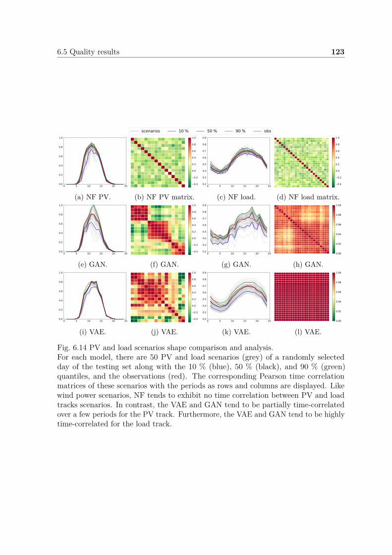
6.5 Quality results 123

scenarios 10 % 50 % 90 % obs

0 5 10 15 20 250.0

0.2

0.4

0.6

0.8

1.0

(a) NF PV.

0.4

0.2

0.0

0.2

0.4

0.6

0.8

1.0

(b) NF PV matrix.0 5 10 15 20 250.2

0.3

0.4

0.5

0.6

0.7

0.8

0.9

(c) NF load.

0.4

0.2

0.0

0.2

0.4

0.6

0.8

1.0

(d) NF load matrix.

0 5 10 15 20 250.0

0.2

0.4

0.6

0.8

1.0

(e) GAN.

0.4

0.2

0.0

0.2

0.4

0.6

0.8

1.0

(f) GAN.0 5 10 15 20 250.2

0.3

0.4

0.5

0.6

0.7

0.8

0.9

(g) GAN.0.90

0.92

0.94

0.96

0.98

1.00

(h) GAN.

0 5 10 15 20 250.0

0.2

0.4

0.6

0.8

1.0

(i) VAE.

0.4

0.2

0.0

0.2

0.4

0.6

0.8

1.0

(j) VAE.0 5 10 15 20 250.2

0.3

0.4

0.5

0.6

0.7

0.8

0.9

(k) VAE.0.90

0.92

0.94

0.96

0.98

1.00

(l) VAE.

Fig. 6.14 PV and load scenarios shape comparison and analysis.For each model, there are 50 PV and load scenarios (grey) of a randomly selectedday of the testing set along with the 10 % (blue), 50 % (black), and 90 % (green)quantiles, and the observations (red). The corresponding Pearson time correlationmatrices of these scenarios with the periods as rows and columns are displayed. Likewind power scenarios, NF tends to exhibit no time correlation between PV and loadtracks scenarios. In contrast, the VAE and GAN tend to be partially time-correlatedover a few periods for the PV track. Furthermore, the VAE and GAN tend to be highlytime-correlated for the load track.

124 Scenarios

0.4

0.2

0.0

0.2

0.4

0.6

0.8

1.0

(a) Wind-NF.

0.4

0.2

0.0

0.2

0.4

0.6

0.8

1.0

(b) PV-NF.

0.4

0.2

0.0

0.2

0.4

0.6

0.8

1.0

(c) NF-load.

0.4

0.2

0.0

0.2

0.4

0.6

0.8

1.0

(d) Wind-GAN.

0.4

0.2

0.0

0.2

0.4

0.6

0.8

1.0

(e) PV-GAN.

0.90

0.92

0.94

0.96

0.98

1.00

(f) GAN-load.

0.4

0.2

0.0

0.2

0.4

0.6

0.8

1.0

(g) Wind-VAE.

0.4

0.2

0.0

0.2

0.4

0.6

0.8

1.0

(h) PV-VAE.

0.990

0.992

0.994

0.996

0.998

1.000

(i) VAE-load.

Fig. 6.15 Average of the correlation matrices over the testing set for the three datasets.Left: wind power; center: PV; right:load. The trend in terms of time correlationis observed on each day of the testing set for all tracks. The NF scenarios are notcorrelated. In contrast, the VAE and GAN scenarios tend to be time-correlated over afew periods. In particular, the VAE generates highly time-correlated scenarios for theload dataset.

6.6 Conclusions and perspectives 125

6.6 Conclusions and perspectives

This Chapter proposed a fair and thorough comparison of NFs with the state-of-the-artdeep learning generative models, GANs and VAEs, both in quality and value. Thenumerical experiments employ the open data of the Global Energy Forecasting Competi-tion 2014. The generative models use the conditional information to compute improvedweather-based PV, wind power, and load scenarios. This Chapter demonstrated thatNFs can challenge GANs and VAEs as they are, overall, more accurate both in termsof quality and value (see Chapter 13). In addition, they can be used effectively bynon-expert deep learning practitioners. In addition, NFs have several advantages overmore traditional deep learning approaches that should motivate their introduction intopower system applications:

1. NFs directly learn the stochastic multivariate distribution of the underlyingprocess by maximizing the likelihood. Therefore, in contrast to VAEs and GANs,NFs provide access to the exact likelihood of the model’s parameters, henceoffering a sound and direct way to optimize the network parameters [177]. Itmay open a new range of advanced applications benefiting from this advantage.For instance, to transfer scenarios from one location to another based on theknowledge of the probability density function. A second application is theimportance sampling for stochastic optimization based on a scenario approach.Indeed, NFs provide the likelihood of each generated scenario, making it possibleto filter relevant scenarios in stochastic optimization.

2. In our opinion, NFs are easier to use by non-expert deep learning practitionersonce the libraries are available, as they are more reliable and robust in termsof hyper-parameters selection. GANs and VAEs are particularly sensitive tothe latent space dimension, the structure of the neural networks, the learningrate, etc. GANs convergence, by design, is unstable, and for a given set ofhyper-parameters, the scenario’s quality may differ completely. In contrast, itwas easier to retrieve relevant NFs hyper-parameters by manually testing a fewsets of values, satisfying training convergence, and quality results.

Nevertheless, their usage as a base component of the machine learning toolbox is stilllimited compared to GANs or VAEs.

126 Scenarios

6.7 Appendix: Table 6.1 justifications

Wang et al. [175] use a Wasserstein GAN with gradient penalty to model both theuncertainties and the variations of the load. First, point forecasting is conducted, andthe corresponding residuals are derived. Then, the GAN generates residual scenariosconditional on the day type, temperatures, and historical loads. The GAN model iscompared with the same version without gradient penalty and two quantile regressionmodels: random forest and gradient boosting regression tree. The quality evaluation isconducted on open load datasets from the Independent System Operator-New England3

with five metrics: (1) the continuous ranked probability score; (2) the quantile score;(3) the Winkler score; (4) reliability diagrams; (5) Q-Q plots. Note: the forecast valueis not assessed.

Qi et al. [147] propose a concentrating solar power (CSP) configuration method todetermine the CSP capacity in multi-energy power systems. The configuration modelconsiders the uncertainty by scenario analysis. A β VAE generates the scenarios. Itis an improved version of the original VAE However, it does not consider weatherforecasts, and the model is trained only by using historical observations. The qualityevaluation is conducted on two wind farms and six PV plants using three metrics. (1)The leave-one-out accuracy of the 1-nearest neighbor classifier. (2) The comparisonof the frequency distributions of the actual data and the generated scenarios. (3)Comparing the spatial and temporal correlations of the actual data and the scenariosby computing Pearson correlation coefficients. The value is assessed by consideringthe case study of the CSP configuration model, where the β VAE is used to generatePV, wind power, and load scenarios. However, the VAE is not compared to anothergenerative model for both the quality and value evaluations. Note: the dataset doesnot seem to be in open-access. Finally, the value evaluation case study is not trivialdue to the mathematical formulation that requires a certain level of knowledge of thesystem. Thus, the replicability criterion is partially satisfied.

Ge et al. [63] compared NFs to VAEs and GANs for the generation of daily loadprofiles. The models do not take into account weather forecasts but only historicalobservations. However, an example is given to illustrate the principle of generatingconditional daily load profiles by using three groups: light load, medium load, andheavy load. The quality evaluation uses five indicators. Four to assess the temporal

3https://www.iso-ne.com/

6.8 Appendix: background 127

correlation: (1) probability density function; (2) autocorrelation function; (3) loadduration curve; (4) a wave rate is defined to evaluate the volatility of the daily loadprofile. Furthermore, one additional for the spatial correlation: (5) Pearson correlationcoefficient is used to measure the spatial correlation among multiple daily load profiles.The simulations use the open-access London smart meter and Spanish transmissionservice operator datasets of Kaggle. The forecast value is not assessed.

6.8 Appendix: background

6.8.1 NFs

NF computation

Evaluating the likelihood of a distribution modeled by a normalizing flow requires com-puting (6.2), i.e., the normalizing direction, as well as its log-determinant. Increasingthe number of sub-flows by K of the transformation results in only O(K) growth inthe computational complexity as the log-determinant of Jfθ

can be expressed as

log | det Jfθ(x)| = log

∣∣∣∣∣K∏

k=1det Jfk,θ

(x)∣∣∣∣∣, (6.16a)

=K∑

k=1log | det Jfk,θ

(x)|. (6.16b)

However, with no further assumption on fθ, the computational complexity of the log-determinant is O(K ·T 3), which can be intractable for large T . Therefore, the efficiencyof these operations is essential during training, where the likelihood is repeatedlycomputed. There are many possible implementations of NFs detailed by Papamakarioset al. [137], Kobyzev et al. [105] to address this issue.

Autoregressive flow

The Jacobian of the autoregressive transformation fθ defined by (6.3) is lower triangular,and its log-absolute-determinant is

log | det Jfθ(x)| = log

T∏i=1

∣∣∣∣∣∂f i

∂xi

(xi; hi)∣∣∣∣∣, (6.17a)

=T∑

i=1log

∣∣∣∣∣∂f i

∂xi

(xi; hi)∣∣∣∣∣, (6.17b)

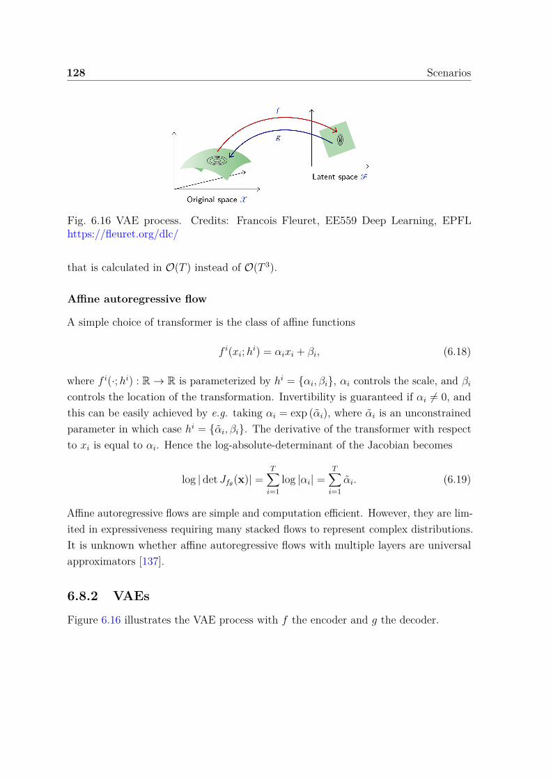
128 Scenarios

Fig. 6.16 VAE process. Credits: Francois Fleuret, EE559 Deep Learning, EPFLhttps://fleuret.org/dlc/

that is calculated in O(T ) instead of O(T 3).

Affine autoregressive flow

A simple choice of transformer is the class of affine functions

f i(xi; hi) = αixi + βi, (6.18)

where f i(·; hi) : R → R is parameterized by hi = αi, βi, αi controls the scale, and βi

controls the location of the transformation. Invertibility is guaranteed if αi = 0, andthis can be easily achieved by e.g. taking αi = exp (αi), where αi is an unconstrainedparameter in which case hi = αi, βi. The derivative of the transformer with respectto xi is equal to αi. Hence the log-absolute-determinant of the Jacobian becomes

log | det Jfθ(x)| =

T∑i=1

log |αi| =T∑

i=1αi. (6.19)

Affine autoregressive flows are simple and computation efficient. However, they are lim-ited in expressiveness requiring many stacked flows to represent complex distributions.It is unknown whether affine autoregressive flows with multiple layers are universalapproximators [137].

6.8.2 VAEs

Figure 6.16 illustrates the VAE process with f the encoder and g the decoder.

6.8 Appendix: background 129

Gradients computation

By using (6.6) Lθ,φ is decomposed in two parts

Lθ,φ(x, c) = Eqφ(z|x,c)

[log pθ(x|z, c)] − KL[qφ(z|x, c)||p(z)]. (6.20)

∇θLθ,φ is estimated with the usual Monte Carlo gradient estimator. However, theestimation of ∇φLθ,φ requires the reparameterization trick proposed by Kingma andWelling [102], where the random variable z is re-expressed as a deterministic variable

z =gφ(ϵ, x), (6.21)

with ϵ an auxiliary variable with independent marginal pϵ, and gφ(·) some vector-valuedfunction parameterized by φ. Then, the first right hand side of (6.20) becomes

Eqφ(z|x,c)

[log pθ(x|z, c)] = Ep(ϵ)

[log pθ(x|gφ(ϵ, x), c)]. (6.22)

∇φLθ,φ is now estimated with Monte Carlo integration.

Conditional VAE implemented

Following Kingma and Welling [102], we implemented Gaussian multi-layer perceptrons(MLPs) for both the encoder NNφ and decoder NNθ. In this case, p(z) is a centeredisotropic multivariate Gaussian, pθ(x|z, c) and qφ(x|z, c) are both multivariate Gaussianwith a diagonal covariance and parameters µθ, σθ and µφ, σφ, respectively. Note thatthere is no restriction on the encoder and decoder architectures, and they could aswell be arbitrarily complex convolutional networks. Under these assumptions, theconditional VAE implemented is

p(z) = N (z; 0, I), (6.23a)pθ(x|z, c) = N (x; µθ, σ2

θI), (6.23b)qφ(z|x, c) = N (z; µφ, σ2

φI), (6.23c)µθ, log σ2

θ = NNθ(x, c), (6.23d)µφ, log σ2

φ = NNφ(z, c). (6.23e)

130 Scenarios

Then, by using the valid reparameterization trick proposed by Kingma and Welling[102]

ϵ ∼N (0, I), (6.24a)z :=µφ + σφϵ, (6.24b)

Lθ,φ is computed and differentiated without estimation using the expressions

KL[qφ(z|x, c)||p(z)] = − 12

d∑j=1

(1 + log σ2φ,j − µ2

φ,j − σ2φ,j), (6.25a)

Ep(ϵ)

[log pθ(x|z, c)] ≈ − 12

∥∥∥∥x − µθ

σθ

∥∥∥∥2, (6.25b)

with d the dimensionality of z.

6.8.3 GANs

GAN

The original GAN value function V (ϕ, θ) proposed by Goodfellow et al. [74] is

V (ϕ, θ) =Ex[log dϕ(x|c)] + E

x[log(1 − dϕ(x|c))]︸ ︷︷ ︸

:=−Ld

, (6.26a)

Lg := − Ex[log(1 − dϕ(x|c))], (6.26b)

where Ld is the cross-entropy, and Lg the probability the discriminator wrongly classifiesthe samples.

WGAN

The divergences which GANs typically minimize are responsible for their training insta-bilities for reasons investigated theoretically by Arjovsky and Bottou [7]. Arjovsky et al.[8] proposed instead using the Earth mover distance, also known as the Wasserstein-1distance

W1(p, q) = infγ∈Π(p,q)

E(x,y)∼γ[∥x − y∥], (6.27)

where Π(p, q) denotes the set of all joint distributions γ(x, y) whose marginals arerespectively p and q, γ(x, y) indicates how much mass must be transported from x

6.8 Appendix: background 131

to y in order to transform the distribution p into q, ∥·∥ is the L1 norm, and ∥x − y∥represents the cost of moving a unit of mass from x to y. However, the infimum in (6.27)is intractable. Therefore, Arjovsky et al. [8] used the Kantorovich-Rubinstein duality[170] to propose the Wasserstein GAN (WGAN) by solving the min-max problem

θ⋆ = arg minθ

maxϕ∈W

Ex[dϕ(x|c)] − E

x[dϕ(x|c)], (6.28)

where W = ϕ : ∥dϕ(·)∥L ≤ 1 is the 1-Lipschitz space, and the classifier dϕ(·) :RT × R|c| → [0, 1] is replaced by a critic function dϕ(·) : RT × R|c| → R. However, theweight clipping used to enforce dϕ 1-Lipschitzness can lead sometimes the WGAN togenerate only poor samples or failure to converge [79]. Therefore, we implemented theWGAN-GP to tackle this issue.

Chapter 7

Part I conclusions

“If you’re lonely when you’re alone, you’re inbad company.”

— Jean-Paul Sartre

Part I presents the forecasting tools and metrics required to produce and evaluatereliable point and probabilistic forecasts used as input of decision-making models. Theforecasts take various forms: point forecasts, quantiles, prediction intervals, densityforecasts, and scenarios. An example of forecast quality evaluation is given withstandard deep learning models such as recurrent neural networks that compute PVand electrical consumption point forecasts on a real case study. Then, several casestudies are used to assess the forecast quality of probabilistic forecasts.

• Deep learning models such as the encoder-decoder architecture and recurrentneural networks compute PV quantile forecasts. These models are trainedby quantile regression. The forecast quality is evaluated on a real case studycomposed of the PV generation of the parking rooftops of the Liège University.The quantile regression models are compared to quantiles derived from deeplearning generative models. In terms of forecast quality, the latter modelsoutperform, in this case, the quantile regression models. The forecast valueis assessed in Part II where the quantile forecasts are used as input of robustoptimization planners in the form of prediction intervals.

• A density forecast-based approach produces probabilistic forecasts of imbalanceprices, focusing on the Belgian case. The two-step probabilistic approach com-putes the net regulation volume state transition probabilities. Then, it infers theimbalance price. A numerical comparison of this approach to standard forecasting

134 Part I conclusions

techniques is performed on the Belgium case. The proposed model outperformsother approaches on probabilistic error metrics but is less accurate at predictingthe imbalance prices. Deep learning models could improve this probabilisticapproach to avoid simplifying assumptions and adding input features to describethe market situation better.

• Finally, a recent class of deep learning generative models, the normalizing flows,is investigated. A fair and thorough comparison is conducted with the state-of-the-art deep learning generative models, generative adversarial networks andvariational autoencoders. The experiments employ the open data of the GlobalEnergy Forecasting Competition 2014. The models use the conditional informa-tion to compute improved weather-based PV, wind power, and load scenarios.The results demonstrate that normalizing flows can challenge generative adversar-ial networks and variational autoencoders. Indeed, they are overall more accurateboth in terms of quality and value (see Chapter 13). Furthermore, they can beused effectively by non-expert deep learning practitioners.

Part II

Planning and control

137

OverviewPart II presents the decision-making tools under uncertainty required to addressthe day-ahead planning of a microgrid. It investigates several approaches: deter-ministic planning using linear programming based on point forecasts, stochasticprogramming using scenarios, and robust optimization using quantile forecasts.Several case studies are considered: a grid-connected microgrid using a valuefunction approach to propagate the information from planning to real-time opti-mization, a grid-connected microgrid in the capacity firming framework, and anenergy retailer on the day-ahead market. The case studies use the forecastingtechniques studied in Part II.

“The straight line, a respectable opticalillusion which ruins many a man.”

— Victor Hugo

Figure 7.1 illustrates the organization of the second part. It addresses the energymanagement of a grid-connected microgrid by using the forecasting techniques studiedin Part I. Chapter 8 provides the optimization basics. Chapter 9 proposes a valuefunction-based approach as a way to propagate information from operational planningto real-time optimization. Chapters 10, 11, and 12 propose stochastic, sizing, androbust approaches to address the energy management of a grid-connected renewablegeneration plant coupled with a battery energy storage device in the capacity firmingmarket, respectively. The capacity firming framework has been designed for isolatedmarkets, such as the Overseas France islands. Chapter 13 is the extension of Chapter6. It investigates the forecast value assessment of the deep generative models byconsidering an energy retailer portfolio on the day-ahead market. Finally, Chapter 14draws the conclusions of Part II.

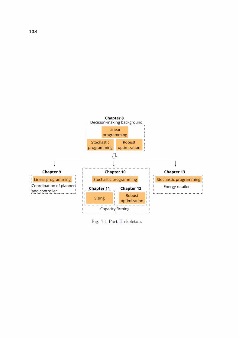
138

Coordination of planner and controller

Decision-making backgroundChapt er 8

Chapt er 10 Chapt er 13

Stochastic programming

Robust optimization

Chapt er 12

Capacity firming

Energy retailer

Chapt er 9

Linear programming

Chapt er 11

Linear programming Stochastic programming

Robust optimization

Sizing

Stochastic programming

Fig. 7.1 Part II skeleton.

Chapter 8

Decision-making background

OverviewThis Chapter introduces some basics of linear programming and optimizationmethodologies to address uncertainty in decision-making used to formulate theproblems considered in Part II.The interested reader is referred to more general textbooks for further information[124, 16, 22] and the lectures of the courses "Renewables in Electricity Markets"a

and "Advanced Optimization and Game Theory for Energy Systems"b given byprofessor Pierre Pinson and associate professor Jalal Kazempour, respectively, atthe Technical University of Denmark.

ahttp://pierrepinson.com/index.php/teaching/bhttps://www.jalalkazempour.com/teaching

“Nothing is more difficult, and therefore moreprecious, than to be able to decide.”

— Napoleon Bonaparte

140 Decision-making background

Coordination of planner and controller

Decision-making backgroundChapt er 8

Chapt er 10 Chapt er 13

Stochastic programming

Robust optimization

Chapt er 12

Capacity firming

Energy retailer

Chapt er 9

Linear programming

Chapt er 11

Linear programming Stochastic programming

Robust optimization

Sizing

Stochastic programming

Fig. 8.1 Chapter 8 position in Part II.

8.1 Linear programming 141

Section 8.1 introduces the mathematical formulation of a linear optimization prob-lem. Sections 8.2 and 8.3 present the mathematical formulations of a linear optimizationproblem when considering uncertainty in the parameters of the problem. First, by con-sidering a stochastic programming approach. Second, by using a robust methodology.

8.1 Linear programming

8.1.1 Formulation of a linear programming problem

The most straightforward instance of an optimization problem is a linear programmingproblem.

Definition 8.1.1 (Linear programming). Linear programming (LP) minimizes a linearcost function subject to linear equality and inequality constraints.

In a LP problem, we are given a cost vector c ∈ Rn and we seek to minimize alinear cost function c⊺x over all n-dimensional vectors x ∈ Rn subject to a set oflinear equality and inequality constraints. Suppose that there is a total of m suchconstraints and let b ∈ Rm and A be the m × n matrix. The constraints can beexpressed compactly in the form Ax ≥ b.

Definition 8.1.2 (LP in standard form). [16, Chapter 1] A linear programmingproblem of the form

minx

c⊺x (8.1)

s.t. Ax = b,

x ≥ 0,

is said to be in the standard form.

LP problems model a wide variety of real-world problems, such as day-aheadplanning of a microgrid.

8.1.2 Duality in linear programming

Duality theory deals with the relation between a LP problem, called the primal, andanother LP problem, called the dual. It uncovers the deeper structure of a LP problemand is a powerful tool that has various applications. The duality theory is motivatedby the Lagrange multiplier method, where a price variable is associated with each

142 Decision-making background

constraint. It explores prices under which the presence or absence of the constraintsdoes not affect the optimal cost. Then, the correct prices can be found by solving anew LP problem, called the original’s dual [16].

Definition 8.1.3 (Dual of a LP problem). [16, Chapter 4] Given a primal problem inthe standard form (8.1), its dual is defined as

maxp

p⊺b (8.2)

s.t. p⊺A ≤ c⊺,

x ≥ 0,

with p the price vector of the same dimension as b.

Note that the dual of the dual problem is the primal problem. The strong dualitytheorem is the central result of linear programming duality.

’If a linear programming problem has an optimal solution so does its dual,and the respective optimal costs are equal.’ [16, Chapter 4, Theorem 4.4]

8.2 Stochastic optimization

Most decision-making problems are subject to uncertainty due to the intrinsic stochas-ticity of natural events conditioning our choices, e.g., the weather, or, more generally,to the inaccurate knowledge of input information. Therefore, decision-makers areinterested in methods and tools that provide solutions less sensitive to environmentalinfluences or inaccurate data while simultaneously reducing cost, increasing profit, orimproving reliability [124, Appendix C].

Let consider a LP in the standard form (8.1). If parameters A, b, and c areperfectly known, solution algorithms for linear optimization problems, e.g., the simplexmethod, can be used to find the best value of the decision variable vector x.

However, suppose some of these parameters are contingent on the realization ξ(ω)of a particular random vector ξ. In that case, determining the optimal solution to theproblem (8.1) may become further challenging. First, the issue of how to guaranteethe feasibility of decision vector x becomes remarkably more involved when optimizingunder uncertainty because A and b are not completely known in advance. Second, theissue of how to guarantee the optimally of decision vector x is at stake because c is notcompletely known in advance. Finally, the LP problem (8.1) needs to be recast so that

8.2 Stochastic optimization 143

solution algorithms for linear programming problems can be used to obtain the optimalvalue of decision vector x taking into account the uncertainty of the parameters.

Stochastic programming provides the concepts and tools required to deal withthe implications of having uncertain data in an optimization problem for decisionmaking to address the three issues previously stated. It assumes that an accurateprobabilistic description of the random variable is assumed available, under the formof the probability distributions or densities. In the following, we consider stochasticprogramming with recourse where the set of decisions is divided into two groups:(1) decisions have to be taken before the realization of uncertain parameters. Thesedecisions are known as first-stage, x, or here-and-now decisions and do not dependon the realization of the random parameters; (2) decisions can be taken after therealization of uncertain parameters. These decisions are called second-stage, y(x, ω), orrecourse decisions and are dependent on each plausible value of the random parameters.Note: the term recourse points to the fact that second-stage decisions enable thedecision-maker to adapt to the actual outcomes of the random events.

Definition 8.2.1 (Two-stage program with fixed recourse). [22, Chapter 2] A classicaltwo-stage stochastic linear program with fixed recourse is

minx

c⊺x + Eξ[Q(x, ξ(ω))] (8.3)

s.t. Ax = b,

x ≥ 0,

with

Q(x, ξ(ω)) = miny

q(ω)⊺y (8.4)

s.t. Wy = h(ω) − T (ω)x, ∀ω ∈ Ωy ≥ 0, ∀ω ∈ Ω

the second-stage value function.

Note: the uncertainty involved in problem (8.3) and (8.4) is assumed to be properlyrepresented by means of a finite set Ω of scenarios ω, with a probability αω such that∑

ω∈ω αω = 1.

144 Decision-making background

Definition 8.2.2 (Deterministic equivalent problem). [22, Chapter 2] The determin-istic equivalent problem of the stochastic programming problem (8.3)-(8.4) is

minx,y

c⊺x +∑ω∈ω

αωq(ω)⊺y (8.5)

s.t. Ax = b,

Wy = h(ω) − T(ω)x, ∀ω ∈ Ωx ≥ 0,

y ≥ 0, ∀ω ∈ Ω

and can be directly processed by off-the-shelf optimization software for linear programs.

8.3 Robust optimization

Robust optimization considers optimization problems with uncertain parameters notmodeled using probability distributions but with uncertainty sets. A robust optimiza-tion strategy investigates a solution to an optimization problem that is feasible for anyrealization of the uncertain parameters within the uncertainty set and optimal for theworst-case realization of these uncertain parameters [124, Appendix D].

Definition 8.3.1 (Two-stage robust optimization with fixed recourse). The generalform of two-stage robust optimization formulation is

minx

c⊺x + maxu∈U

miny∈Ω(x,u)

q⊺y (8.6)

s.t. Ax = b,

x ≥ 0,

with U the uncertainty set and

Ω(x, u) = y ≥ 0 : Wy = h − Tx − Mu. (8.7)

The objective of the problem (8.6) is to make the best decisions represented byvariable vector x for the worst realization of parameters in vector u and considering therecourse decisions described by variable vector y. If the right-hand-side problem, the y-problem, is convex, it can be replaced by its dual and merged with the middle u-problemrendering it a conventional single-level maximization problem. Overall, the resultingproblem is a min-max problem that in some cases can be solved using decomposition

8.3 Robust optimization 145

such as the Benders-dual cutting plane method [18] or column-and-constraint genera-tion algorithm [183]. Both the Benders-dual method and the column-and-constraintgeneration procedure are implemented in a master sub-problem framework.

8.3.1 Benders-dual cutting plane algorithm

The key idea of the Benders-dual cutting plane (BD) algorithm is to gradually constructthe value function of the first-stage decisions using dual solutions of the second-stagedecision problems.

Consider the case where the second-stage decision problem is a linear programming(LP) problem in x. We first take the relatively complete recourse assumption thatthis LP is feasible for any given x and u. Let p be its dual variables. Then, weobtain its dual problem, which is a maximization problem and can be merged withthe maximization over u. As a result, we have the following dispatch problem, whichyields the sub-problem (SP) in the BD algorithm.

Definition 8.3.2 (BD sub-problem).

R(x) = maxu,p

(h − Tx − Mu)⊺p (8.8)

s.t. W⊺p ≥ q,

u ∈ U .

Note: that the resulting problem in (8.8) is a bilinear optimization problem. Severalapproaches have been developed to address this issue and depend on the case study.

Suppose, we have an oracle that can solve (8.8) for a given first stage variable x.Then, the optimal solution is (p⋆, u⋆), and a cutting plane in the form of

θ ≥ (h − Tx − Mu⋆)⊺p⋆ (8.9)

can be generated, and included in the master problem (MP).

Definition 8.3.3 (BD master problem). At iteration k of the BD master problem is

minx,θ

c⊺x + θ (8.10)

s.t. Ax = b,

θ ≥ (h − Tx − Mu⋆l )⊺p⋆

l ∀l ≤ k (8.11)x ≥ 0, θ ∈ R,

146 Decision-making background

which can compute an optimal first stage solution x⋆k.

The MP and SP provide the lower and upper bounds with c⊺x⋆k + θ⋆

k and R(x⋆k−1),

respectively, at iteration k. When considering the relatively complete recourse assump-tion, [183, 18, 14] demonstrated the BD algorithm converges to the optimal solution ofthe two-stage robust optimization problem. The lower and upper bounds converge in afinite number of steps by iteratively introducing cutting planes (8.9) and computing theMP (8.10). Note: if the SP is a MILP, this result is not straightforward. It is the casein the capacity firming problem studied in Chapter 12 where this issue is addressed.

8.3.2 Column and constraints generation algorithm

The column and constraints generation (CCG) algorithm does not create constraintsusing dual solutions of the second-stage decision problem. It dynamically generatesconstraints with recourse decision variables in the primal space for an identified scenario.Let assume the uncertainty set U is a finite discrete set with U = u1, . . . , uN andy1, . . . , yN are the corresponding recourse decision variables. Then, the 2-stage RO(8.6) can be reformulated as follows

minx,θ

c⊺x + θ (8.12)

s.t. Ax = b, (8.13)θ ≥ q⊺yl ∀l ≤ N (8.14)Wyl = h − Tx − Mul ∀l ≤ N (8.15)x ≥ 0, yl ≥ 0 ∀l ≤ N, θ ∈ R. (8.16)

Thus, it reduces to solve an equivalent, probably large-scale, MILP, which is very closeto a 2-stage stochastic programming model if the probability distribution over U isknown. When the uncertainty set is large or is a polyhedron, enumerating all thepossible uncertain scenarios in U is not feasible. Constraints (8.14) indicate that not allscenarios, and their corresponding variables and constraints, are necessary for definingthe optimal value x⋆ of the 2-stage RO. It is likely that a few relevant scenarios, asmall subset of the uncertainty set, play a significant role in the formulation. Therefore,the key idea of the CCG procedure is to generate recourse decision variables for thesignificant scenarios.

Definition 8.3.4 (CCG sub-problem). Similar to the BD method, the CCG algorithmuses a master sub-problem framework. Let assume an oracle can solve the dispatch

8.4 Conclusions 147

problem for a given first-stage x

Q(x) = maxu∈U

miny∈Ω(x,u)

q⊺y. (8.17)

Then, the optimal solution u⋆ can be derived to build constraints and variables in themaster problem.

Definition 8.3.5 (CCG master problem). At iteration k of the CCG master problemis

minx,θ

c⊺x + θ (8.18)

s.t. Ax = b, (8.19)θ ≥ q⊺yl ∀l ≤ k (8.20)Wyl = h − Tx − Mu⋆,l ∀l ≤ k (8.21)x ≥ 0, yl ≥ 0 ∀l ≤ k, θ ∈ R, (8.22)

which can compute an optimal first stage solution x⋆k.

Similar to BD, the MP and SP provide the lower and upper bounds with c⊺x⋆k + θ⋆

k

and Q(x⋆k−1), respectively, at iteration k.

8.4 Conclusions

This Chapter introduces the basics of linear programming and approaches to handleuncertainty in the parameters with the stochastic programming and robust approach.Depending on the application, each approach has its pros and cons. When consideringstochastic programming, the number of scenarios needed to describe the most plausibleoutcomes of the uncertain parameters may be huge, leading to large-scale optimizationproblems that may become difficult to solve or intractable. In this case, a robustapproach provides an alternative and compact manner to describe uncertain parameters.However, the robust counterpart optimization problem may be challenging to solve andrequires a decomposition technique such as a Benders-dual cutting plane or columnand constraints generation algorithm that is not trivial to implement numerically.

150 Coordination of the planner and controller

Chapter 9

Coordination of the planner andcontroller

OverviewThis Chapter presents a two-layer approach with a value function to propagateinformation from operational planning to real-time optimization. The valuefunction-based approach shares some similarities with the coordination schemeproposed in Kumar et al. [108], which is based on stochastic dual dynamicprogramming. This study brings new contributions:

1. The approach is tested by accounting for forecasting errors and high-resolution data monitored on-site corresponding to a "real-life" case.

2. The value function approach allows to deal with indeterminacy issues.When there are several optimal solutions to the upper-level problem, thisis accounted for in the lower level part, and a bias term can be added tofavor one type of behavior over another, e.g., charge early.

3. This methodology is fully compatible with the energy markets as it candeal with imbalance, reserve, and dynamic selling/purchasing prices.

This study reports results on an industrial microgrid capable of on/off-gridoperation. Generation and consumption forecasts are based on weather forecastsobtained with the MAR model [59].References: This chapter is an adapted version of the following publication:

Jonathan Dumas, Selmane Dakir, Clément Liu, and Bertrand Cornélusse. Coordi-nation of operational planning and real-time optimization in microgrids. ElectricPower Systems Research, 190:106634, 2021. URL https://arxiv.org/abs/2106.02374.

151

“When making a decision of minorimportance, I have always found itadvantageous to consider all the pros and cons.In vital matters, however, such as the choiceof a mate or a profession, the decision shouldcome from the unconscious, from somewherewithin ourselves. In the important decisions ofpersonal life, we should be governed, I think,by the deep inner needs of our nature.”

— Sigmund Freud

Coordination of planner and controller

Decision-making backgroundChapt er 8

Chapt er 10 Chapt er 13

Stochastic programming

Robust optimization

Chapt er 12

Capacity firming

Energy retailer

Chapt er 9

Linear programming

Chapt er 11

Linear programming Stochastic programming

Robust optimization

Sizing

Stochastic programming

Fig. 9.1 Chapter 9 position in Part II.

152 Coordination of the planner and controller

The hierarchical microgrid control levels divide a global microgrid control problemin time and space [134]. Control levels range from distributed device level controllersthat run at a high frequency to centralized controllers optimizing market integrationthat run much less frequently. For computation time reasons, centralized controllersare often subdivided into two levels. Operational planning controllers that optimizedecisions over a time horizon of one or several days but with a market period resolution,e.g., 15 minutes. Real-time optimization controllers that deal with actions within thecurrent market period. The coordination of these two levels is paramount to achievingthe safest and most profitable operational management of microgrids. Microgridcontrol and management can be achieved in several ways. Control techniques andthe principles of energy-storage systems are summarized in Palizban et al. [134]. Aclassification of microgrid control strategies into primary, secondary, and tertiary levelsis done in Olivares et al. [131]. The two-level approach has been intensively studied.A double-layer coordinated control approach, consisting of the scheduling layer andthe dispatch layer, is adopted in Jiang et al. [94]. The schedule layer provides aneconomical operation scheme, including state and power of controllable units basedon the look-ahead multi-step optimization. In contrast, the dispatch layer follows thescheduling layer by considering power flow and voltage limits. A two-stage dispatchstrategy for grid-connected systems is discussed in Wu et al. [179], where the first stagedeals with the day-ahead schedule, optimizing capital and operational cost. At thesame time, the lower level handles the rescheduling of the units for few hours ahead witha time resolution of 15 min. A two-stage control strategy for a PV BESS-ICE (InternalCombustion Engine) microgrid is implemented in Sachs and Sawodny [153]. DiscreteDynamic Programming is used in the first layer, while the second layer problem isposed as a Boundary Value Problem. An approach with a high-level deterministicoptimizer running at a slow timescale, 15 min, coupled to a low-level stochasticcontroller running at a higher frequency, 1 min, is studied in Cominesi et al. [36]. Atwo-layer predictive energy management system for microgrids with hybrid energystorage systems consisting of batteries and supercapacitors is considered in Ju et al. [96].This approach incorporates the degradation costs of the hybrid energy storage systems.A practical Energy Management System for isolated microgrid which considers theoperational constraints of Distributed Energy Resources, active-reactive power balance,unbalanced system configuration, and loading, and voltage-dependent loads is studiedin Solanki et al. [160]. A two-layer mixed-integer linear programming predictive controlstrategy was implemented and tested in simulation and experimentally in Polimeni et al.[146]. Finally, Moretti et al. [125] implemented a two-layer predictive management

9.1 Notation 153

strategy for an off-grid hybrid microgrid featuring controllable and non-controllablegeneration units and a storage system.

It is organized as follows. Section 9.1 summarizes the notation. Section 9.2formulates the problem in an abstract manner. Section 9.3 introduces the novel two-level value function-based approach and the assumptions made. Section 9.4 describesthe numerical tests. Section 9.5 reports the results. Conclusions are drawn in Section9.6. The methodology used for forecasting is reported in Section 3.3 of Chapter 3.

9.1 Notation

Sets and indicesName Descriptiond Device index.t, t′ RTO and OP time periods indexes.τ(t) Beginning of the next market period at time t.Ti(t) Set of RTO time periods = t, t + ∆t, ..., t + Ti.T m

a (t) Set of OP time periods = τ(t), τ(t) + ∆τ, ..., τ(t + Ta).Ta, Tl Time durations, with Ta ≪ Tl

Dk Set of non-flexible loads (k = nfl), sheddable loads (k = she), steerablegenerators (k = ste), non-steerable generators (k = nst), storagedevices (k = sto).

ParametersName Description Unit∆t Time delta between t and the market period. minutes∆τ Market period. minutesηcha, ηdis Charge and discharge efficiencies. %P , P Maximum charging and discharging powers. kWCnfl

d,t Non-flexible power consumption. kWCshe

d,t Flexible power consumption. kWSinit

d,t Initial state of charge of battery d. kWhph Maximum peak over the last twelve months. kWπp Yearly peak power cost. e/kWπs

OP Unitary revenue for providing reserve. e/kW

154 Coordination of the planner and controller

πsRT O Unitary RTO symmetric reserve penalty. e/kW

πkd,t Cost of load shedding (k = she), generating energy (k = ste),

curtailing generation (k = nst).e/kWh

γstod,t Fee to use the battery d. e/kWh

πet , πi

t Energy prices of export and import. e/kWhπi

d, πin Energy prices of day and night imports. e/kWh

Icap, Ecap Maximum import and export limits. kWPVp, Cp PV and consumption capacities. kWSp Storage capacity. kWhS, S Maximum and minimum battery capacities. kWh

Forecasted or computed variablesName Description Unitat Action at t. -am

t Purely market related actions. -ad

t Set-points to the devices of the microgrid -ak

d,t Fraction of load shed (k = she), generation activated (k =ste), generation curtailed (k = nst) ([0, 1]).

-

achad,t , adis

d,t Fraction of the maximum charging and discharging powersused for battery d ([0, 1]).

-

egrit , igri

t Energy export and import. kWhδpt′ OP peak difference between peak at t′ and ph. kWδpτ(t−∆τ),τ(t) RTO peak difference between peak at τ(t) and ph. kWsT SO

t TSO symmetric reserve signal (0; 1). -rsym Symmetric reserve. kW∆rsym Reserve difference between OP and RTO. kWrs+

d,t′ , rs−d,t′ Upward and downward reserves of power available and pro-

vided by storage device d.kW

sd,t State of charge of battery d. kWhst Microgrid state at time t. -sm

t Information related to the current market position. -sd

t State of the devices. -vt The cost-to-go function. keω Forecast of a random vector ω. -

9.2 Problem statement 155

X Average of a variable X. kWXmax, Xmin Maximum and minimum of X. kWXstd Standard deviation of X. kWcE, cp, ct Energy, peak and total costs. ke∆p Peak increment. kWItot, Etot Total import and export. MWh

9.2 Problem statement

A global microgrid control problem can be defined, for a given microgrid design andconfiguration, as operating a microgrid safely and in an economically efficient manner,by harvesting as much renewable energy as possible, operating the grid efficiently,optimizing the service to the demand side, and optimizing other side goals. We refinethis definition below and start by making a few assumptions.

9.2.1 Assumptions

In this study, the control optimizes economic criteria, which are only related to activepower. All devices areconnected to the same electrical bus, which can be connected ordisconnected from a public grid permanently or dynamically. Device-level controllersoffer an interface to communicate their operating point and constraints, e.g., maximumcharge power as a function of the current state, and implement control decisions toreach power set-points. Fast load-frequency control, islanding management, as well asreactive power control are not in scope. The microgrid is a price taker in energy andreserve markets.

9.2.2 Formulation

Abstractly, a microgrid optimization problem can be formulated as follows

mina

∑t∈Tl

c(at, st, ωt) (9.1a)

s.t. ∀t ∈ Tl, st+∆t = f(at, st, ωt, ∆t), (9.1b)st ∈ St. (9.1c)

A controller has to return a set of actions at = (amt , ad

t ) at any time t over the life ofthe microgrid (Tl). Actions should be taken as frequently as possible to cope with theeconomic impact of the variability of the demand and generation sides, but not too

156 Coordination of the planner and controller

often to let transients vanish, e.g., every few seconds. The time delta between actionat and the next action taken is denoted by ∆t, and is not necessarily constant. Someof these actions are purely market-related am

t , while other actions are communicated asset-points to the devices of the microgrid ad

t . The state st = (smt , sd

t ) of the microgridat time t is thus also made of two parts. (1) sd

t represents the state of the devices,such as a storage system or a flexible load. (2) sm

t gathers information related tothe current market position, such as the nominated net position of the microgridover the next market periods. The cost function c gathers all the economic criteriaconsidered. The transition function f describes the physical and net position evolutionof the system. At time instants t ∈ ∆τ, 2∆τ, . . ., with ∆τ the market period, somecosts are incurred based on the value of some state variables, which are then reset forthe following market period. This problem is challenging to solve since the system’sevolution is uncertain, actions have long-term consequences, and are both discrete andcontinuous. Furthermore, although functions f and c are assumed time-invariant, theyare generally non-convex and parameterized with stochastic variables ωt.

9.3 Proposed method

In practice, solving the microgrid optimization problem above amounts, at every timet, to forecasting the stochastic variables ωTl(t), then solving the problem1

a⋆Tl(t) = arg min

∑t′∈Tl(t)

c(at′ , st′ , ωt′) (9.2a)

s.t. ∀t′ ∈ Tl(t), st′+∆t′ = f(at′ , st′ , ωt′ , ∆t′), (9.2b)st′ ∈ S ′

t, (9.2c)

and applying a⋆t (potentially changing am,⋆

t at some specific moments only). Forecastsare valid only for a relatively near future, and optimizing over a long time would beincompatible with the real-time operation. Thus, this problem is approximated bycropping the lookahead horizon to Ta(t) ⊂ Tl(t). However, market decisions must berefreshed much less frequently than set-points. We thus propose to further decomposethe problem in an operational planning problem (OPP) for T m

a (t) that computes1Which is here expressed as a deterministic problem for simplicity but should be treated as a

stochastic problem in practice.

9.3 Proposed method 157

Forecasting Operational planning

Real-time optimization

Fig. 9.2 Hierarchical control procedure illustration.

market decisions

am,⋆T m

a (t) = arg min∑

t′∈T ma (t)

cm(amt′ , st′ , ωt′) (9.3a)

s.t. ∀t′ ∈ T ma (t), st′+∆τ = fm(am

t′ , st′ , ωt′ , ∆τ) (9.3b)st′ ∈ St′ , (9.3c)

and a real-time problem (RTP) that computes set-points for time t

ad,⋆t = arg min cd(ad

t , st, ωt) + vτ(t)(sτ(t)) (9.4a)s.t. sτ(t) = fd(ad

t , st, ωt, τ(t) − t) (9.4b)sτ(t) ∈ Sτ(t), (9.4c)

with c(at, st, wt) = cm(amt , st, wt) + cd(ad

t , st, ωt). The function vt is the cost-to-go as afunction of the system’s state at the end of the ongoing market period. It regularizesdecisions of RTP to account for the longer-term evolution of the system. We detailhereunder how we obtain vt. An overview of the approach is depicted in Figure 9.2.

9.3.1 Computing the cost-to-go function

The function vt represents the optimal value of (9.3) as a function of the initial statesτ(t) of this problem. If we make the assumption that (9.3) is modeled as a linearprogram, the function vτ(t) is thus convex and piecewise linear. Every evaluation of(9.3) with the additional constraint2

sτ(t) = s′ ⊥ µ (9.5)2The ⊥ µ notation means that µ is the dual variable of the constraint.

158 Coordination of the planner and controller

yields the value vτ(t)(s′) and a supporting inequality (a cut)

vτ(t)(s) ≥ vτ(t)(s′) + µT s. (9.6)

The algorithm to approximate vτ(t)(s′) works as follows:

1. estimate the domain of vτ(t), i.e., the range of states reachable at time τ(t) andthe most probable state that will be reached s⋆

τ(t);

2. evaluate vτ(t)(s⋆τ(t)) and the associated µ⋆;

3. repeat step 2 for other state values until all regions of vτ(t) are explored.

Note: that if the state is of dimension one and (9.3) is a linear program, simplex basisvalidity information can be used to determine for which part of the domain of vτ(t) thecurrent cut is tight, else a methodology such as proposed in Bemporad et al. [10] canbe used.

9.3.2 OPP formulation

The OPP objective function implemented for the case study is

JOPT m

a (t) =∑

t′∈T ma (t)

(COP

t′ + DOPt′

)(9.7)

with Operational Planner (OP) the name of this planer. T ma (t) is composed of 96

values with ∆τ = 15 minutes and Ta = 24 hours. COPt′ models the immediate costs

and DOPt′ the delayed costs at t′. COP

t′ takes into account different revenues and costsrelated to energy flows: the costs of shed demand, steered and non steered generation,the revenues from selling energy to the grid, the costs of purchasing energy from thegrid and the costs for using storage

COPt′ =

∑t′∈T m

a (t)

( ∑d∈Dshe

∆τπshed,t′Cshe

d,t′ashed,t′ +

∑d∈Dste

∆τπsted,t′P ste

d,t′asted,t′ +

∑d∈Dnst

∆τπnstd,t′P nst

d,t′ anstd,t′

+∑

d∈Dsto

∆τγstod [P dηcha

d achad,t′ + P d

ηdisd

adisd,t′ ] − πe

t′egrit′ + πi

t′igrit′

). (9.8)

DOPt′ is composed of the peak cost and symmetric reserve revenue

DOPt′ = πpδpt′ − πs

OP rsymt′ , (9.9)

9.3 Proposed method 159

δpt′ is the peak difference between the previous maximum historic peak ph and thecurrent peak within the market period t′. rsym

t′ is the symmetric reserve provided tothe grid within the current market period t′.

9.3.3 OP constraints

The first set of constraints defines bounds on state and action variables, ∀t′ ∈ T ma (t)

akd,t′ ≤ 1 ∀d ∈ Dk, ∀k ∈ ste, she, nst (9.10a)

achad,t′ ≤ 1 ∀d ∈ Dsto (9.10b)

adisd,t′ ≤ 1 ∀d ∈ Dsto (9.10c)

Sd ≤ sd,t′ ≤ Sd ∀d ∈ Dsto. (9.10d)

The energy flows are constrained, ∀t′ ∈ T ma (t), by

(egrit′ − igri

t′ )/∆τ −∑

d∈Dnst(1 − anst)P nst

d,t′ +∑

d∈Dsteaste

d,t′P sted,t′

+∑

d∈Dnfl

Cnfld,t′ +

∑d∈Dshe

(1 − ashed,t′)Cshe

d,t′ +∑

d∈Dsto

(P dacha

d,t′ − P dadisd,t′

)= 0 (9.11a)

(egrit′ − igri

t′ )/∆τ ≤ Ecapt′ (9.11b)

(igrit′ − egri

t′ )/∆τ ≤ Icapt′ . (9.11c)

The dynamics of the state of charge are, ∀d ∈ Dsto

sd,1 − ∆τ(P dηchad acha

d,1 − P d

ηdisd

adisd,1) = Sinit

d (9.12a)

sd,t′ − sd,t′−∆τ − ∆τ(P dηchad acha

d,t′ − P d

ηdisd

adisd,t′) = 0, ∀t′ ∈ T m

a (t) (9.12b)

sd,τ(t+Ta) = Sendd . (9.12c)

The set of constraints related to the peak power ∀t′ ∈ T ma (t)

(igrit′ − egri

t′ )/∆τ ≤ pt′ (9.13a)−δpt′ ≤ 0 (9.13b)−δpt′ ≤ −(pt′ − ph). (9.13c)

160 Coordination of the planner and controller

The last constraints define symmetric reserve ∀t′ ∈ T ma (t)

rs+d,t′ ≤ (sd,t′ − Sd) ηdis

d

∆τ∀d ∈ Dsto (9.14a)

rs+d,t′ ≤ P d(1 − adis

d,t′) ∀d ∈ Dsto (9.14b)

rs−d,t′ ≤

(Sd − sd,t′

)ηcha

d ∆τ∀d ∈ Dsto (9.14c)

rs−d,t′ ≤ P d(1 − acha

d,t′) ∀d ∈ Dsto (9.14d)rsym, OP ≤

∑d∈Dsto

rs+d,t′ +

∑d∈Dste

P sted,t′(1 − aste

d,t′) +∑

d∈DnstP nst

d,t′ (1 − anst) (9.14e)

+∑

d∈Dshe

Cshed,t′(1 − ashe

d,t′)

rsym, OP ≤∑

d∈Dsto

rs−d,t′ +

∑d∈Dste

P sted,t′aste

d,t′ +∑

d∈DnstP nst

d,t′ anst +∑

d∈Dshe

Cshed,t′ashe

d,t′ . (9.14f)

9.3.4 RTP formulation

The RTP objective function implemented for the case study is

JRT Ot = CRT O

t + DRT Ot + vτ(t)(sτ(t)) (9.15)

with Real-Time Optimizer (RTO) the name of this controller. CRT Ot models the

immediate costs, DRT Ot the delayed costs and vτ(t)(sτ(t)) the cost-to-go function of the

state of the system at time t within a current market period. CRT Ot is the same as

COPt′ by replacing t′ by t, ∆τ by ∆t and considering only one period of time t. DRT O

t

is composed of the peak cost and symmetric reserve penalty costs

DRT Ot = πpδpτ(t−∆τ),τ(t) + sT SO

t πsRT O∆rsym, (9.16)

δpτ(t−∆τ),τ(t) is the peak difference between the previous maximum historic peak ph

and the current peak within the market period computed by RTO. The difference withOP relies on its computation as at t the market period is not finished. Thus, the peakwithin this market period is made of two parts. (1) The peak from the beginning ofthe market period to t. (2) The peak from the actions taken from t to the end of themarket period. ∆rsym is the difference between the symmetric reserve computed byOP and the current reserve within the market period computed by RTO. sT SO

t is thereserve activation signal to activate the tertiary symmetric reserve. It is set by theTSO, 0 if activated, else 1. The activation occurs at the beginning of the followingmarket period.

9.4 Test description 161

9.3.5 RTO constraints

The set of constraints that defines the bounds on state and action variables and theenergy flows are the same as the OP (9.10) and (9.11) by replacing t′ by t, ∆τ by∆t and considering only one period of time t. The following constraint describes thedynamics of the state of charge ∀d ∈ Dsto and ∀t ∈ Ti(t)

sd,τ(t) − ∆t(P dηchad acha

d,t − P d

ηdisd

adisd,t) = Sinit

d,t . (9.17)

The set of constraints related to the peak power ∀t ∈ Ti(t)

(igrit − egri

t )/∆t ≤ pt,τ(t) (9.18a)−δpτ(t) ≤ 0 (9.18b)−δpτ(t) ≤ −(pτ(t−∆τ),τ(t) − ph) (9.18c)

pτ(t−∆τ),τ(t) = βpτ(t−∆τ),t + (1 − β)pt,τ(t) (9.18d)

with β = 1 − ∆t/∆τ . The last set of constraints defining the symmetric reserve are thesame as the OP (9.14) by replacing t′ by t, rsym, OP by rsym, RTO and adding ∀t ∈ Ti(t)

− ∆rsym ≤ 0 (9.19a)− ∆rsym ≤ −(rsym, OP − rsym, RTO). (9.19b)

9.4 Test description

Our case study is the MiRIS microgrid located at the John Cockerill Group’s inter-national headquarters in Seraing, Belgium3. It is composed of PV, several energystorage devices, and a non-sheddable load. The load and PV data we use come fromon-site monitoring. All data, including the weather forecasts, are available on theKaggle platform4. The case study consists of comparing RTO-OP to a Rule-BasedController (RBC) for three configurations of the installed PV capacity, cf. Table 9.1.The RBC prioritizes the use of PV production for the supply of electrical demand. Ifthe microgrid is facing a long position, it charges the battery. Furthermore, if thisone is fully charged, it exports to the main grid. If the microgrid is facing a shortposition, it prioritizes using the battery to supply the demand. Moreover, if this one

3https://johncockerill.com/fr/energy/stockage-denergie/4https://www.kaggle.com/jonathandumas/liege-microgrid-open-data

162 Coordination of the planner and controller

is fully discharged, it imports from the main grid. This controller does not take intoaccount any future information, e.g., PV, consumption forecasts, energy prices, ormarket information such as the peak of the symmetric reserve. Case 3 results from asizing study that defined the optimal device sizes given the PV and consumption data.The sizing methodology used is described in Dakir and Cornélusse [38].

Figure 9.3 shows the PV & consumption data over the simulation period: fromMay 20, 2019 to June 16, 2019. The selling price πe is constant, and the purchasingprice is composed of a day πi

d and night prices πin. Day prices apply from 5 a.m. to 8

p.m. (UTC) during the weekdays, and night prices apply from 8 p.m. to 5 a.m. duringweekdays and the entire weekend. The peak mechanism is taken into account witha constant peak price πp and an initial maximum historic peak ph. Storage systemsare initially fully charged. The PV and consumption data have a 1-second resolution,meaning the RTO could compute its optimization problem each five to ten seconds inoperational mode. CPLEX 12.9 is used to solve all the optimization problems on anIntel Core i7-8700 3.20 GHz-based computer with 12 threads and 32 GB of RAM. Theaverage computation time per optimization problem composed of the OP and RTO isa few seconds. However, to maintain a reasonable simulation time, RTO is called everyminute. The dataset is composed of 28 days with an average computation time oftwo hours to solve 1440 optimization problems per day, with a one-minute resolution,leading to two days for the entire dataset. The OP computes a quarterly planningcorresponding to the Belgian market period. The computation time of the RTO on aregular computer is around a few seconds and the OP around twenty seconds. In total,the simulation computation time is up to a few hours. The OP computes quarterlyplanning based on PV and consumption twenty-four ahead forecasts. The weather-based forecast methodology is described in detail in Section 3.3 of Chapter 3. Two"classic" deterministic techniques are implemented, a Recurrent Neural Network (RNN)with the Keras Python library [33] and a Gradient Boosting Regression (GBR) withthe Scikit-learn Python library [140]. These models use as input the weather forecastsprovided by the Laboratory of Climatology of the Liège University, based on the MARregional climate model [59]. It is an atmosphere model designed for meteorologicaland climatic research, used for a wide range of applications, from km-scale processstudies to continental-scale multi-decade simulations. To estimate the impact of the PVand consumption forecast errors on the controllers, the simulation is performed withthe OP having access to the PV and consumption future values (RTO-OP⋆). Then,the simulation is performed with the symmetric reserve mechanisms to cope with the

9.5 Numerical results 163

Case PVp PV PVmax PVmin PVstd

1 400 61 256 0 722 875 133 561 0 1573 1750 267 1122 0 314Case Cp C Cmax Cmin Cstd

1 - 3 1000 153 390 68 72Case Sp S, S P , P ηcha, ηdis Sinit

1 - 3 1350 1350, 0 1350, 1350 0.95, 0.95 100Case ph, πp Icap Ecap πi

d, πin πe

1 - 3 150, 40 1500 1500 0.2, 0.12 0.035Table 9.1 Case studies parameters and data statistics.

05-2005-21

05-2205-23

05-2405-25

05-2605-27

05-2805-29

05-3005-31

06-0106-02

06-0306-04

06-0506-06

06-0706-08

06-0906-10

06-1106-12

06-1306-14

06-1506-16

0

200

400

600

800

1000

1200

kW

CPV 3PV 2PV 1

00:0001:00

02:0003:00

04:0005:00

06:0007:00

08:0009:00

10:0011:00

12:0013:00

14:0015:00

16:0017:00

18:0019:00

20:0021:00

22:0023:00

0

200

400

600

800

1000

1200

kW

CPV 3PV 2PV 1

Fig. 9.3 Top: PV & consumption simulation data. Bottom: zoom on June 12, 2019.

forecast errors. A constant symmetric reserve price πsOP for the OP and a penalty

reserve πsRT O for the RTO are set to 20 (e/ kW).

9.5 Numerical results

9.5.1 No symmetric reserve

Table 9.2 provides the simulation results without taking into account the symmetricreserve. The smaller the PV installed capacity, the higher the peak and energy costs.The RTO-OP⋆ provides the minimal peak cost, whereas the RBC provides the minimalenergy cost on all cases. However, RTO-OP⋆ achieves the minimal total cost, composed

164 Coordination of the planner and controller

Case 1 cE cp ct ∆p Itot Etot

RBC 10.13 6.68 16.81 167 61 0RTO-OPRNN 10.37 3.62 13.99 91 64 1RTO-OPGBR 10.25 5.27 15.53 132 63 1RTO-OP⋆ 10.24 0.99 11.23 25 64 1Case 2 cE cp ct ∆p Itot Etot

RBC 3.19 4.85 8.04 121 22 7RTO-OPRNN 4.78 2.87 7.65 72 31 15RTO-OPGBR 4.30 4.90 9.2 123 28 13RTO-OP⋆ 4.06 0 4.06 0 26 10Case 3 cE cp ct ∆p Itot Etot

RBC -2.13 4.12 1.99 105 3 77RTO-OPRNN -1.66 4.12 2.46 105 7 80RTO-OPGBR -1.67 4.23 2.56 106 7 81RTO-OP⋆ -1.90 0 0 0 5 79

Table 9.2 Results without symmetric reserve.

of the energy and peak costs. This simulation illustrates the impact of the forecastson the RTO-OP behavior. The RNN forecaster provides the best results, but theRTO-OPRNN is still a long way to manage the peak as RTO-OP⋆ due to the forecastingerrors. The peak cost strongly penalizes the benefits as it applies to the entire yearahead once it has been reached.

In case 3, all the controllers except RTO-OP⋆ reached the maximum peak onJune 12, 2019 around 10:30 a.m. as shown on Figure 9.4. Figure 9.3 shows a suddendrop in the PV production around 10 a.m. that is not accurately forecasted by the RNNand GBR forecasters as shown in Figure 3.2. This prediction leads to the non-accurateplanning of OP. Thus, the RTO cannot anticipate this drop and has to import energyto balance the microgrid at the last minute. Figure 9.5 shows the controllers behavioron June 12, 2019 where the peak is reached. In case 2, all controllers reached the samepeak as in case 3 except RTO-OPRNN that reached a smaller one on June 5, 2019.The forecast’s accuracy explains this behavior as in case 3. Finally, in case 1, eachcontroller reached a different peak. The smallest one is achieved by the RTO-OP⋆,followed by the RTO-OPRNN . These cases show that the RTO-OP controller optimizes

9.5 Numerical results 165

05-2005-21

05-2205-23

05-2405-25

05-2605-27

05-2805-29

05-3005-31

06-0106-02

06-0306-04

06-0506-06

06-0706-08

06-0906-10

06-1106-12

06-1306-14

06-1506-160

1234567

k

RTO OPRTO OPRNN

RTO OPGBR

RBC

05-2005-21

05-2205-23

05-2405-25

05-2605-27

05-2805-29

05-3005-31

06-0106-02

06-0306-04

06-0506-06

06-0706-08

06-0906-10

06-1106-12

06-1306-14

06-1506-160

1234567

k

RTO OPRTO OPRNN

RTO OPGBR

RBC

05-2005-21

05-2205-23

05-2405-25

05-2605-27

05-2805-29

05-3005-31

06-0106-02

06-0306-04

06-0506-06

06-0706-08

06-0906-10

06-1106-12

06-1306-14

06-1506-160

1234567

k

RTO OPRTO OPRNN

RTO OPGBR

RBC

Fig. 9.4 Case 1 (top), 2 (middle), 3 (bottom) cumulative peak costs.

PV-storage usage and thus requires less installed PV capacity for a given demandlevel. This result was expected as the peak management is not achieved by the RBCand becomes critical when the PV production is smaller than the consumption. Thissimulation also demonstrates the forecast accuracy impact on the RTO-OP behavior.

9.5.2 Results with symmetric reserve

Table 9.3 provides the simulation results by taking into account the symmetric reserve.Figure 9.6 depicts on case 3 the behavior differences between RTO-OPRNN without andwith symmetric reserve. Figures 9.7 and 9.8 show the SOC and peaks costs evolution ofcase 2 & 1. The controller tends to maintain a storage level that allows RTO-OPRNN

to better cope with forecast errors. Indeed for case 3, there is no more peak reachedby RTO-OPRNN , only 1 kW for case 2, and it has been almost divided by two for case1. However, this behavior tends to increase the energy cost if the PV production islarge compared to the consumption, such as in case 3. Indeed, the controller will tendto store more energy in the battery instead of exporting it. RTO-OP⋆ did not performbetter with the symmetric reserve. The symmetric reserve competes with the peakmanagement, and the RTO-OP⋆ tends not to discharge the battery entirely even if itis required to avoid a peak. In case 2, the peak is reached on June 12, 2019 around08:00. The controller could have avoided it by totally discharging the battery but did

166 Coordination of the planner and controller

00:0001:00

02:0003:00

04:0005:00

06:0007:00

08:0009:00

10:0011:00

12:0013:00

14:0015:00

16:0017:00

18:0019:00

20:0021:00

22:0023:000

102030405060708090

100

SOC

%RTO OPRTO OPRNN

RTO OPGBR

RBC

00:0001:00

02:0003:00

04:0005:00

06:0007:00

08:0009:00

10:0011:00

12:0013:00

14:0015:00

16:0017:00

18:0019:00

20:0021:00

22:0023:00

2000

200400600800

100012001400

kW

RTO OPRTO OPRNN

RTO OPGBR

RBC

Fig. 9.5 Case 3 SOC (top) and net export power (bottom) on June 12, 2019.

05-2005-21

05-2205-23

05-2405-25

05-2605-27

05-2805-29

05-3005-31

06-0106-02

06-0306-04

06-0506-06

06-0706-08

06-0906-10

06-1106-12

06-1306-14

06-1506-160

102030405060708090

100

SOC

%

RTO OPRNN s = 0RTO OPRNN s = 20

Fig. 9.6 Case 3 SOC comparison for RTO-OPRNN with and without symmetric reserve.

not maintain the reserve level. It is the same behavior in case 1, where the peak couldhave been limited if all the battery was discharged. There is an economic trade-off tomanage the peak and the reserve simultaneously. It depends on the valorization or noton the market of the symmetric reserve. The reserve can also be valorized internallyto cope with non or complex forecastable events. Such as a sudden drop in export orimport limits due to loss of equipment or grid congestion.

9.6 Conclusions

A two-level value function-based approach is proposed as a solution method for amulti-resolution microgrid optimization problem. The value function computed bythe operational planner based on PV and consumption forecasts allows coping withthe forecasting uncertainties. The real-time controller solves an entire optimizationproblem, including the future information propagated by the value function. Thisapproach is tested on the MiRIS microgrid case study with PV and consumption data

9.6 Conclusions 167

Case 1 cE cp ct ∆p Itot Etot

RTO-OPRNN 10.50 2.12 12.62 53 65 3RTO-OP⋆ 10.47 2.75 13.22 69 65 2Case 2 cE cp ct ∆p Itot Etot

RTO-OPRNN 5.33 0.04 5.37 1 41 27RTO-OP⋆ 4.78 0.99 5.77 25 35 20Case 3 cE cp ct ∆p Itot Etot

RTO-OPRNN -0.04 0 -0.04 0 24 99RTO-OP⋆ -0.15 0 -0.15 0 23.2 98

Table 9.3 Results with symmetric reserve.

monitored on-site. The results demonstrate the efficiency of this method to managethe peak in comparison with a Rule-Based Controller. This test case is completelyreproducible as all the data used are open, PV, consumption monitored, and forecasted,including the weather forecasts. The proposed method can be extended in threeways. First, a stochastic formulation of the operational planning problem to cope withprobabilistic forecasts. Second, adding the balancing market mechanisms. Finally,considering a community composed of several entities inside the microgrid.

168 Coordination of the planner and controller

05-2005-21

05-2205-23

05-2405-25

05-2605-27

05-2805-29

05-3005-31

06-0106-02

06-0306-04

06-0506-06

06-0706-08

06-0906-10

06-1106-12

06-1306-14

06-1506-160

1

2

3k

RTO OPRNN

RTO OP

05-2005-21

05-2205-23

05-2405-25

05-2605-27

05-2805-29

05-3005-31

06-0106-02

06-0306-04

06-0506-06

06-0706-08

06-0906-10

06-1106-12

06-1306-14

06-1506-160

1

2

3

k

RTO OPRNN

RTO OP

Fig. 9.7 Case 1 (top) and 2 (bottom) cumulative peak costs.

05-2005-21

05-2205-23

05-2405-25

05-2605-27

05-2805-29

05-3005-31

06-0106-02

06-0306-04

06-0506-06

06-0706-08

06-0906-10

06-1106-12

06-1306-14

06-1506-160

102030405060708090

100

SOC

%

RTO OPRNN

RTO OP

05-2005-21

05-2205-23

05-2405-25

05-2605-27

05-2805-29

05-3005-31

06-0106-02

06-0306-04

06-0506-06

06-0706-08

06-0906-10

06-1106-12

06-1306-14

06-1506-160

102030405060708090

100

SOC

%

RTO OPRNN

RTO OP

Fig. 9.8 Case 1 (top) and 2 (bottom) SOC.

Chapter 10

Capacity firming using a stochasticapproach

OverviewThis Chapter proposes a stochastic approach to address the energy managementof a grid-connected renewable generation plant coupled with a battery energystorage device in the capacity firming market. Both deterministic and stochasticapproaches result in optimization problems formulated as quadratic problemswith linear constraints. The considered case study is a real microgrid with PVproduction monitored on-site.References: This chapter is an adapted version of the following publication:

Jonathan Dumas, Bertrand Cornélusse, Antonello Giannitrapani, Simone Paoletti,and Antonio Vicino. Stochastic and deterministic formulations for capacity firmingnominations. In 2020 International Conference on Probabilistic Methods Appliedto Power Systems (PMAPS), pages 1–7. IEEE, 2020. URL https://arxiv.org/abs/2106.02425.

“We are our choices.”— Jean-Paul Sartre

170 Capacity firming using a stochastic approach

Coordination of planner and controller

Decision-making backgroundChapt er 8

Chapt er 10 Chapt er 13

Stochastic programming

Robust optimization

Chapt er 12

Capacity firming

Energy retailer

Chapt er 9

Linear programming

Chapt er 11

Linear programming Stochastic programming

Robust optimization

Sizing

Stochastic programming

Fig. 10.1 Chapter 10 position in Part II.

171

The capacity firming framework is mainly designed for isolated markets, such asthe Overseas France islands. For instance, the French Energy Regulatory Commission(CRE) publishes capacity firming tenders and specifications. The system considered isa grid-connected renewable energy power plant, e.g., photovoltaic or wind-based, witha battery energy storage system (BESS) for firming the renewable generation. At thetendering stage, offers are selected on the electricity selling price. Then, the successfultenderer builds its plant and sells the electricity exported to the grid at the contractedselling price, but according to a well-defined daily engagement and penalization schemespecified in the tender specifications. The electricity injected in or withdrawn fromthe grid must be nominated the day-ahead, and engagements must satisfy rampingpower constraints. The remuneration is calculated a posteriori by multiplying therealized exports by the contracted selling price minus a penalty. The deviations of therealized exports from the engagements are penalized through a function specified inthe tender. A peak option can be activated in the contract for a significant selling priceincrease during a short period defined a priori. Therefore, the BESS must shift therenewable generation during peak hours to maximize revenue and manage renewableenergy uncertainty.

The problem of modeling a two-phase engagement/control with an approach dealingwith uncertainty in the context of the CRE capacity framework is still an open issue.This framework has received less attention in the literature than more traditionalenergy markets such as day-ahead and intraday markets of European countries.

The optimal day-ahead bidding strategies of a plant composed of only a productiondevice have been addressed in, e.g., Pinson et al. [143], Bitar et al. [23], Giannitrapaniet al. [65, 66]. The optimal offer turns out to be a suitable percentile of the PV/windpower cumulative distribution function. Under the assumption of time-invariant powergeneration statistics, the cumulative distribution functions can be estimated fromhistorical data of the power generated by the plant. This assumption is not alwaysjustified, especially for PV power generation. In Giannitrapani et al. [66], the authorsinvestigate two approaches to properly take into account the effects of seasonal variationand non-stationary nature of PV power generation in the estimation of PV powerstatistics. However, incorporating energy storage in the framework is still an openproblem, and the literature provides several approaches and methodologies to thisend. An optimal power management mechanism for a grid-connected PV system withstorage is implemented in [150] using Dynamic Programming (DP) and is comparedwith simple ruled-based management. The sizing and control of an energy storagesystem to mitigate wind power uncertainty is addressed by Haessig [80], Haessig et al.

172 Capacity firming using a stochastic approach

[81, 82] using stochastic dynamic programming (SDP). The framework is similar tothe CRE PV capacity firming tender with a wind farm operator committed on aday-ahead basis to a production engagement. Finally, three distinct optimizationstrategies, mixed-integer quadratic programming, simulation-based genetic algorithm,and expert-based heuristic, are empirically compared by N’Goran et al. [128] in theCRE framework.

This study addresses the energy management of a grid-connected PV plant andBESS. This topic is studied within the capacity firming specifications of the CRE, inline with the tender AO-CRE-ZNI 2019 published on July 12, 2019, using the MiRISmicrogrid case study. The capacity firming problem can be decomposed into two steps.The first step consists of computing the day-ahead nominations. The second stepconsists of computing the renominations and the set-points in real-time to minimizethe energy and ramp power deviations from nominations. This study focuses on thefirst step and proposes both a stochastic and a deterministic formulation. The maingoal of this study is to validate the stochastic approach by using an ideal predictorproviding unbiased PV scenarios. Thus, the BESS efficiencies are perfect, and thedegradation is not taken into account for the sake of simplicity. Different levels ofprediction accuracy are evaluated. Then, the results are compared with those of thedeterministic formulation, assuming perfect forecasts returned by an oracle. Bothdeterministic and stochastic approaches result in optimization problems formulatedas quadratic problems with linear constraints. The considered case study is a realmicrogrid with PV production monitored on-site.

The study is organized as follows. Section 10.1 provides the notation that is alsoused for Chapters 11 and 12. Section 10.2 describes the capacity firming framework.Section 10.3 proposes the deterministic and stochastic formulations of the nominationprocess. Section 10.4 introduces the MiRIS microgrid case study and presents theresults. Conclusions are drawn in Section 10.5. Appendix 10.6 describes the methodol-ogy to generate the set of unbiased PV scenarios.

10.1 Notation

10.1.1 Sets and indices

Name Description

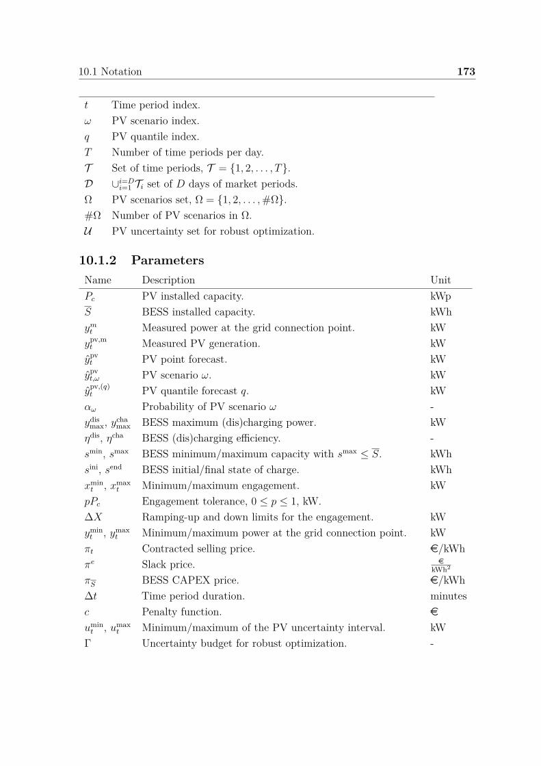
10.1 Notation 173

t Time period index.ω PV scenario index.q PV quantile index.T Number of time periods per day.T Set of time periods, T = 1, 2, . . . , T.D ∪i=D

i=1 Ti set of D days of market periods.Ω PV scenarios set, Ω = 1, 2, . . . , #Ω.#Ω Number of PV scenarios in Ω.U PV uncertainty set for robust optimization.

10.1.2 ParametersName Description UnitPc PV installed capacity. kWpS BESS installed capacity. kWhym

t Measured power at the grid connection point. kWypv,m

t Measured PV generation. kWypv

t PV point forecast. kWypv

t,ω PV scenario ω. kWy

pv,(q)t PV quantile forecast q. kW

αω Probability of PV scenario ω -ydis

max, ychamax BESS maximum (dis)charging power. kW

ηdis, ηcha BESS (dis)charging efficiency. -smin, smax BESS minimum/maximum capacity with smax ≤ S. kWhsini, send BESS initial/final state of charge. kWhxmin

t , xmaxt Minimum/maximum engagement. kW

pPc Engagement tolerance, 0 ≤ p ≤ 1, kW.∆X Ramping-up and down limits for the engagement. kWymin

t , ymaxt Minimum/maximum power at the grid connection point. kW

πt Contracted selling price. e/kWhπe Slack price. e

kWh2

πS BESS CAPEX price. e/kWh∆t Time period duration. minutesc Penalty function. e

umint , umax

t Minimum/maximum of the PV uncertainty interval. kWΓ Uncertainty budget for robust optimization. -

174 Capacity firming using a stochastic approach

dq, dΓ Uncertainty and budget depths for robust optimization. %M−

t , M+t Big-M’s values for robust optimization. -

10.1.3 Variables

For the sake of clarity the subscript ω is omitted.Name Range Description Unitxt [xmin

t , xmaxt ] Engagement. kW

yt [ymint , ymax

t ] Net power at the grid connection point. kWypv

t [0, ypvt ] PV generation. kW

ychat [0, ycha

max] BESS charging power. kWydis

t [0, ydismax] BESS discharging power. kW

yst [smin, smax] BESS state of charge. kWh

d−t , d+

t R+ Short/long deviation. kWyb

t 0, 1 BESS binary variable. -zt 0, 1 PV uncertainty set binary variable for robust optimization. -αt [M−

t , M+t ] Variables to linearize ztϕ

ypv

t for robust optimization. -

Dual variables, and corresponding constraints

Dual variables of constraints are indicated with brackets [·].Name Range Descriptionϕcha

t , ϕdist R− Maximum storage (dis)charging.

ϕsmint , ϕsmax

t R− Minimum/maximum storage capacity.ϕy

t R Net power balance.ϕymin

t , ϕymax

t R− Minimum/maximum net power.ϕsini

t , ϕsendt R− Initial/final state of charge.

ϕst R− BESS dynamics.

ϕd−t , ϕd+

t R− Under/overproduction.ϕypv

t R− Renewable generation.

10.2 The Capacity Firming Framework

The capacity firming framework can be decomposed into a day-ahead engagementprocess, Section 10.2.1, and a real-time control process, Section 10.2.2. Each day isdiscretized in T periods of duration ∆t. In the sequel, the period duration is the samefor day-ahead engagement and the real-time control, t is used as a period index, andT is the set of periods in a day.

10.2 The Capacity Firming Framework 175

Forecaster Planner

Dead line

Market Periods

Fig. 10.2 Day-ahead nomination process.

10.2.1 Day-ahead engagement

Each day, the operator of the renewable generation plant is asked to provide thegeneration profile to be followed the next day to the grid operator, based on renewablegeneration forecasts. More formally, a planner computes on a day-ahead basis, beforea deadline, a vector of engagements composed of T values [x1, . . . , xT ]⊺. Figure10.2 illustrates the day-ahead nomination process. The grid operator accepts theengagements if they satisfy the constraints

|xt − xt−1| ≤ ∆X, ∀t ∈ T \ 1 (10.1a)−xt ≤ −xmin

t , ∀t ∈ T (10.1b)xt ≤ xmax

t , ∀t ∈ T , (10.1c)

with ∆X a ramping power constraint, a fraction of the total installed capacity Pc

determined at the tendering stage and imposed by the grid operator.

10.2.2 Real-time control

Then, in real-time, a receding-horizon controller computes at each period the generationlevel and the charge or discharge set-points from t to T , based on forecasts of renewablegeneration and the engagements. Only the set-points of the first period are applied tothe system. The remuneration is calculated ex-post based on the realized power ym

t

at the grid coupling point. For a given control period, the net remuneration rt of theplant is the gross revenue ∆tπty

mt minus a penalty c(xt, ym

t ), with πt the contractedselling price set at the tendering stage

rt = ∆tπtymt − c(xt, ym

t ), ∀t ∈ T . (10.2)

The penalty function c depends on the specifications of the tender. For the sake ofsimplicity for the rest of this Chapter, c is assumed to be symmetric, convex, and

176 Capacity firming using a stochastic approach

quadratic piecewise-linear

c(xt, ymt ) = πe(∆t)2

(max

(0, |xt − ym

t | − pPc

))2

(10.3)

with 0 ≤ p ≤ 1, and πe is a slack price (e/kWh2).

10.3 Problem formulation

The problem statement follows the abstract formulation defined in Chapter 9 wherea global microgrid control problem can be defined as operating a microgrid safelyand in an economically efficient manner. In the capacity firming context, a two-stageapproach is considered with a planner and a controller. A quadratic formulation withlinear constraints models the CRE non-convex penalty. In this study, the planner andcontroller optimize economic criteria, which are only related to active power. Theancillary or grid services are not in the scope of the capacity firming specifications.The BESS degradation is not taken into account. The planner and controller horizonsare cropped to twenty-four hours.

Deterministic (D) and stochastic (S) formulations of the day-ahead nominationproblem are compared. The deterministic formulation is used as a reference to validatethe stochastic approach by considering perfect knowledge of the future (D⋆). In thisChapter, both approaches consider only exports to the grid1. The optimization variablesand the parameters are defined in Section 10.1.

10.3.1 Deterministic approach

The objective function JD to minimize is the opposite of the net revenue

JD(xt, yt) =∑t∈T

−πt∆tyt + πe(∆t)2[(d−t )2 + (d+

t )2]. (10.4)

1The imports from the grid are allowed only under specific conditions into the contract.

10.3 Problem formulation 177

The deterministic formulation is the following Mixed-Integer Quadratic Program(MIQP)

minxt∈X ,yt∈Ω(xt,ypv

t )JD(xt, yt)

X =xt : (10.6)

(10.5)

Ω(xt, ypvt ) =

yt : (10.7) − (10.11)

,

where X and Ω(xt, ypvt ) are the sets of feasible engagements xt and dispatch solutions yt

for a fixed engagement xt and renewable generation point forecast ypvt . The optimization

variables of (10.5) are the engagement variables xt, the dispatch variables yt (the netpower at the grid connection point), ydis

t (BESS discharging power), ychat (BESS

charging power), st (BESS state of charge), ybt (BESS binary variables), ypv

t (renewablegeneration), and d−

t , d+t (deviation variables) (cf. the notation Section 10.1). From

(10.1), the engagement constraints are

xt − xt−1 ≤ ∆X, ∀t ∈ T \ 1 (10.6a)xt−1 − xt ≤ ∆X, ∀t ∈ T \ 1 (10.6b)

−xt ≤ −xmint , ∀t ∈ T (10.6c)

xt ≤ xmaxt , ∀t ∈ T . (10.6d)

The ramping constraint on x1 is deactivated to decouple consecutive days of simulation.In reality, the updated value of the last engagement of the previous day would be takento satisfy the constraint. The set of constraints that bound ycha

t , ydist , and ys

t variablesare ∀t ∈ T

ychat ≤ yb

t ychamax [ϕcha

t ] (10.7a)ydis

t ≤ (1 − ybt )ydis

max [ϕdist ] (10.7b)

−st ≤ −smin [ϕsmin

t ] (10.7c)st ≤ smax, [ϕsmax

t ] (10.7d)

where ybt are binary variables that prevent the simultaneous charge and discharge of

the BESS. The power balance equation and the constraints on the net power at the

178 Capacity firming using a stochastic approach

grid connection point are ∀t ∈ T

yt = ypvt + (ydis

t − ychat ) [ϕy

t ] (10.8a)

−yt ≤ −ymin [ϕymin

t ] (10.8b)yt ≤ ymax. [ϕymax

t ] (10.8c)

The dynamics of the BESS state of charge are

s1 − sini = ∆t(ηchaycha1 − ydis

1ηdis ) [ϕsini ] (10.9a)

st − st−1 = ∆t(ηchaychat − ydis

t

ηdis ), ∀t ∈ T \ 1 [ϕst ] (10.9b)

sT = send = sini, [ϕsend ] (10.9c)

where the parameters send and sini are introduced to decouple consecutive days ofsimulation. In reality, sini would be the updated value of the last measured state ofcharge of the previous day. The variables d−

t , d+t are defined ∀t ∈ T to model the

penalty

−d−t ≤

(yt − (xt − pPc)

)[ϕd−

t ] (10.10a)

−d+t ≤

((xt + pPc) − yt

), [ϕd+

t ] (10.10b)

with 0 ≤ p ≤ 1. Finally, the PV generation is bounded ∀t ∈ T by the point forecastypv

t

ypvt ≤ ypv

t . [ϕypv

t ] (10.11)

10.3.2 Deterministic approach with perfect forecasts

With perfect forecasts, (10.5) becomes

minxt∈X ,yt∈Ω(xt,ypv

t =ypv,mt )

JD⋆(xt, yt), (10.12)

with ypvt = ypv,m

t ∀t ∈ T in (10.11).

10.3 Problem formulation 179

10.3.3 Stochastic approach

In the stochastic formulation, the objective is given by

JS = E[∑

t∈T−πt∆tyt + c(xt, yt)

](10.13)

where the expectation is taken with respect to ypvt . Using a scenario-based approach,

(10.13) is approximated by

JS ≈∑ω∈Ω

αω

∑t∈T

[− πt∆tyt,ω + πe(∆t)2

((d−

t,ω)2 + (d+t,ω)2

)], (10.14)

with αω the probability of scenario ω ∈ Ω, and ∑ω∈Ω αω = 1. Then, the problem to

solve becomes

minxt∈X ,yt,ω∈Ω(xt,ypv

t,ω)JS(xt, yt,ω). (10.15)

All the optimization variables but xt are now defined ∀ω ∈ Ω.

10.3.4 Evaluation methodology

The second step of capacity firming, i.e., computing the set-points in real-time, isrequired to assess the quality of the nomination process. However, since this studyfocuses on the computation of day-ahead engagements, we simulate the second stepwith an ideal real-time controller2 once the engagements are fixed. The methodologyto assess the engagements consists of solving

Jeval =∑t∈T

−πtxt + c(xt, yt) (10.16)

s.t (10.7)-(10.11) with ypvt = ypv,m

t in (10.11) and given engagements xt previouslycomputed by the planner S. The optimization variables of (10.16) are yt, d−

t , d+t , ypv

t ,ycha

t , ydist , and st. The optimal value of Jeval

S is compared with the optimal value of JD⋆

in (10.12).2Using a real-time controller with intraday forecasts is required to assess the planner-controller.

However, this study focus only on the nomination step.

180 Capacity firming using a stochastic approach

01Feb

2019

0203040506070809101112131415161718192021222324252627280

200

400

600

800

1000

kW

PV

Fig. 10.3 MiRIS February 2019 PV production.

10.4 MiRIS microgrid case study

The MiRIS3 microgrid case study, located at the John Cockerill Group’s internationalheadquarters in Seraing, Belgium, is composed of a PV production plant, a BESS, anda load. For the need of this study, only historical data of PV generation are required.The BESS capacity S is 1000 kWh, smax = S, and the total PV installed capacity Pc is2000 kWp. The market period duration ∆t is 15 minutes. The simulation dataset D isthe month of February 2019. Figure 10.3 illustrates the MiRIS PV production andTable 10.1 provides some key statistics. Table 10.2 defines the indicators used in thissection. It is of paramount importance to notice that the results of this case study

Pc ypv,m ypv,mstd ypv,m

max ypv,m%,max ypv,m

tot

2000 104.6 202.4 988.1 49.4 70.3Table 10.1 MiRIS February 2019 dataset statistics.

are only valid for this dataset and cannot be extrapolated over an entire year withoutcaution. CPLEX4 12.9 is used to solve all the optimization problems, on an Intel Corei7-8700 3.20 GHz based computer with 12 threads and 32 GB of RAM. Tables 10.3and 10.4 provide the case study and BESS parameters.

3https://johncockerill.com/fr/energy/stockage-denergie/4https://www.ibm.com/products/ilog-cplex-optimization-studio

10.4 MiRIS microgrid case study 181

Name Description Unitypv,m Averaged PV generation. kWypv,m

std PV generation standard deviation. kWypv,m

max Maximum PV generation. kWypv,m

tot Total PV energy produced. MWhypv,m

%,max ypv,mmax divided by the total installed PV capacity Pc. %

tCPU Averaged computation time per optimization problem. s[X]D Total of a variable Xt:

∑t∈D Xt. X unit

[ypv]D Total PV generation. MWhypv

% PV generation ratio: [ypv]D[ypv,m]D . %

ycha% BESS charge ratio: [ycha]D

[ypv]D . %ycha

max% Percentage of days of the dataset where the BESS achieved itsmaximum storage capacity.

%

y% Export ratio: [y]D[x]D . %

Rmax Maximum achievable revenue: π[ypv,m]D. keRe Gross revenue: π[y]D. kere Maximum achievable revenue ratio: Re

Rmax. %

Ce Quadratic penalty: [c]D. keRn,e Net revenue with quadratic penalty: Re − Ce. ke

Table 10.2 Comparison indicators.

182 Capacity firming using a stochastic approach

π πe ∆t ∆X xmax ymax p

0.045 0.0045 15 10 2000 2000 5%Table 10.3 Case study parameters.

smax smin ychamax ydis

max ηcha ηdis sini send

1000 0 1000 1000 1 1 0 0Table 10.4 BESS parameters.

10.4.1 Results for unbiased PV scenarios with fixed variance

A set of unbiased PV scenarios is generated for several values of the standard deviationσ of the prediction error. Table 10.5 shows the considered values of σ, expressed as afraction of the actual PV generation. Moreover, Table 10.5 reports the cardinality ofthe generated scenario sets. Table 10.6 compares the average computation time peroptimization problem between planners S and D⋆. Note, The optimization problemof planner S with #Ω = 1 has the same number of variables and constraints as theplanner D⋆. The computation time is compatible with a day-ahead process even with100 scenarios, as it takes on average 7 seconds to compute the nominations for theday-ahead. Table 10.7 and Figure 10.4 provide the results of the ratio indicators,respectively, for the planners D⋆ and S.

For all indicators, the results of both planners are almost equal with the smallervalue of σ and the highest value of #Ω, as expected. On average, the curtailment of PVgeneration equals 5%. The maximum y% value is achieved with σ = 3.5% because thenominations are more conservative when the variance increases, leading to a smallerratio. On average, 30% (27%) of the production, for planner D⋆ (S), is stored in theBESS over the entire dataset. S% is equal to 17.9% (17.9%5) for the planner D⋆ (S),meaning the BESS reached its maximum storage level 5 days out of the 28 days of thedataset. In fact, during sunny days, the BESS is fully charged. A larger BESS capacityshould decrease the curtailment and improve the gross revenue. Note: it is a winter

5The value is the same for the #Ω and σ values considered.

σ 3.5% 7% 10.5% 14%#Ω 5 10 50 100

Table 10.5 Scenario generation parameters.

10.4 MiRIS microgrid case study 183

#Ω 1 5 10 50 100# variables 769 3 457 6 817 33 697 67 297# constraints 1 248 5 092 9 897 48 337 96 387tCPU S - 0.3 0.8 3 7tCPU D⋆ 0.1 - - - -

Table 10.6 Averaged computation times.

[ypv]D ypv% ycha

% ychamax% y%

66.7 94.9 29.6 17.9 76.2Table 10.7 Planner D⋆ ratio indicators.

month where the maximum generated PV power reached only half of the installed PVcapacity. During a summer month, the maximum production should reach at least80% of the total installed capacity on sunny days. Thus, with a storage capacity of 1MWh, the curtailment is expected to be higher during sunny summer days.

Table 10.8 and Figure 10.5 provide the results of the revenue indicators for theplanners D⋆ and S, respectively. It should be noted that in this case, Rn,e = −Jeval

S .The smallest value of the objective function is achieved by the planner D⋆. It is followedclosely by the planner S, even for the highest value of σ. This result demonstrates thevalidity of the approach when exploiting an unbiased stochastic predictor.

In terms of net revenue, both planners achieved 93.7% of Rmax ≈ 3.16 ke, whichresults in a loss of 6.3%. Most of this loss is due to the curtailment of PV generation.For both planners, the net revenue increases with the generation.

3.5 7 10.5 14

5

10

50

100

94.9 94.7 94.6 94.4

94.9 94.8 94.7 94.4

94.9 94.8 94.6 94.3

94.9 94.7 94.6 94.3 94.4

94.5

94.6

94.7

94.8

%

(a) ypv% .

3.5 7 10.5 14

5

10

50

100

87.8 86.8 86.5 86.7

90.9 89.3 88.2 89.1

94.9 89.9 90.2 92.7

95.5 89.9 90.9 92.3 88.0

90.0

92.0

94.0

%

(b) y%.

Fig. 10.4 Planner S ratio indicator with #Ω = 5, 10, 50, 100, σ = 3.5, 7, 10.5, 14%.

184 Capacity firming using a stochastic approach

Re re Ce Rn,e JevalD⋆

3.0 94.9 0.04 2.96 -2.96Table 10.8 Planner D⋆ revenue indicators.

3.5 7 10.5 14

5

10

50

100

3.00 3.00 2.99 2.98

3.00 3.00 2.99 2.99

3.00 3.00 2.99 2.98

3.00 3.00 2.99 2.98 2.98

2.99

3.00

3.00

k

(a) Re.

3.5 7 10.5 14

5

10

50

100

2.96 2.96 2.95 2.95

2.96 2.96 2.96 2.95

2.96 2.96 2.95 2.95

2.96 2.96 2.95 2.95 2.95

2.95

2.95

2.95

2.96

2.96

k

(b) Rn,e = −JevalS .

Fig. 10.5 Planner S revenue indicators with #Ω = 5, 10, 50, 100, σ = 3.5, 7, 10.5, 14%.

For sunny days, the difference between the nominations and the exports is higherthan the tolerance just before the production occurs, between 5 and 8 am. Indeed,the planner tends to maximize the revenue by maximizing the exports. However,the ramping power constraints (10.6) impose a maximum difference between twoconsecutive nominations. To maximize the net revenue over the entire day, the plannercomputes nominations that are not achievable at the beginning of the day to maximizethe exports during the day. This results in a penalty between 5 and 8 am.

10.4.2 BESS capacity sensitivity analysis

The goal is to conduct a sensitivity analysis on the BESS capacity S to determine itsmarginal value and the optimal BESS size S

⋆ for a given CAPEX πS. The efficienciesare still assumed to be unitary. sini and send are set to 0 kWh. Table 10.9 provides theother BESS parameters for the five cases. The scenarios are generated using #Ω = 100,and σ = 3.5, 7, 10.5, 14%. A new indicator, expressed in ke, is defined to quantify thegain provided by the BESS over fifteen years

∆Rn,ei = 15 × 12 × (Rn,e

i − Rn,e5 ) ∀i ∈ 1, 2, 3, 4. (10.17)

It is a lower bound of the total gain as it relies on the results of a winter month. Asummer month should provide higher revenue. Table 10.10 provide the planner D⋆

10.4 MiRIS microgrid case study 185

Case S [kWh] smin [kWh] ychamax [kW] ydis

max [kW]1 2000 0 2000 20002 1000 0 1000 10003 500 0 500 5004 250 0 250 2505 0 0 0 0

Table 10.9 BESS parameters.

indicators. The results demonstrate the interest in using a BESS to optimize thebidding. The larger the BESS is, the lower the curtailment is. Thus, the net revenueincreases with the BESS capacity. The maximum achievable revenue is reached witha storage capacity of 2 MWh. However, the larger the BESS is, the smaller ∆Rn,e

increases. It means the marginal benefit decreases with the increase of BESS capacity.A trade-off should be found between the BESS capacity and its CAPEX. Figure 10.6aprovides ∆Rn,e and its quadratic interpolation in comparison with two BESS pricesπS = 0.1 and 0.228 ke/kWh. The value of the derivative [d∆Rn,e

dS]S=0 provides the

maximum CAPEX that provides a profitable BESS. Then, the optimal storage capacityS

⋆ for a given CAPEX is provided solving [d∆Rn,e

dS]S = πS. For instance, with a CAPEX

of 0.1 ke/kWh, S⋆ is approximately 350 kWh. Figure 10.6b provides the values of

∆Rn,e − πSS with a quadratic interpolation.Figure 10.7 provides the planner S revenue indicators. The results are still almost

identical for all indicators for the smallest value of σ and very close with the highestone, as expected.

0 250 500 1000 2000kWh

020406080

100120140

k0.1 Sinterpolation0.228 S

Rn, e

(a) Variation of the net revenue.

0 250 500 1000 2000kWh

60

40

20

0

20

k

interpolationRn, e 0.1 S

S = 350 kWh

(b) Optimal BESS.

Fig. 10.6 Optimal BESS for a given CAPEX price.

186 Capacity firming using a stochastic approach

Case [ypv]D ypv% ycha

% ychamax% y%

1 70.3 100 45.6 17.9 77.72 66.7 94.9 29.6 17.9 76.23 63.6 90.5 17.3 39.3 76.44 61.7 87.7 11.1 46.4 75.25 56.0 79.6 - - 70.4

Case Re Ce Rn,e JevalD⋆ ∆Rn,e

1 3.16 0.01 3.15 -3.15 1282 3.0 0.04 2.96 -2.96 943 2.86 0.04 2.84 -2.84 724 2.77 0.06 2.71 -2.71 495 2.52 0.08 2.44 -2.44 0

Table 10.10 Planner D⋆ ratio and revenue indicators BESS capacity sensitivity analysis.

3.5 7 10.5 14

0

250

500

1000

2000

2.52 2.51 2.51 2.49

2.77 2.77 2.76 2.75

2.86 2.86 2.86 2.85

3.00 3.00 2.99 2.98

3.16 3.16 3.16 3.162.50

2.60

2.70

2.80

2.90

3.00

3.10

k

(a) Re.

3.5 7 10.5 14

0

250

500

1000

2000

2.43 2.43 2.43 2.43

2.72 2.72 2.71 2.71

2.82 2.82 2.82 2.82

2.96 2.96 2.95 2.95

3.15 3.15 3.15 3.152.60

2.80

3.00

k

(b) Rn,e = −JevalS .

Fig. 10.7 Planner S revenue indicators BESS capacity sensitivity analysis with #Ω = 100,σ = 3.5, 7, 10.5, 14%.

10.5 Conclusions and perspectives 187

10.5 Conclusions and perspectives

This Chapter addresses the energy management of a grid-connected PV plant coupledwith a BESS within the capacity firming framework. The method is composed of twosteps: computing the day-ahead nominations, then computing the renominations andthe set-points in real-time to minimize the energy and ramp power deviations fromnominations. This study investigates the first step by comparing a stochastic and adeterministic formulation. The main goal is to validate the stochastic approach byusing an ideal predictor providing unbiased PV scenarios.

The results of the stochastic planner are comparable with those of the deterministicplanner, even when the prediction error variance is non-negligible. Finally, the BESScapacity sensitivity analysis results demonstrate the advantage of using a BESS tooptimize the bidding day-ahead strategy. However, a trade-off must be found betweenthe marginal gain provided by the BESS and its investment and operational costs.

Several extensions of this work are under investigation. The first is to assess theplanner’s behavior better using a full year of data. Then, the next challenge is to usea more realistic methodology to generate PV generation scenarios. Several scenariogeneration approaches could be investigated, based on a point forecast model suchas the PVUSA model [46, 19, 20], combined with Gaussian copula [135, 142, 72].Alternatively, using the deep generative models introduced in Chapter 6. Anotherchallenge is to consider the non-convex penalty function specified by the CRE into theobjective. Finally, the last challenge is to investigate the second step of the capacityfirming problem, for instance, by adapting the approach implemented in Dumas et al.[54].

10.6 Appendix: PV scenario generation

This Annex describes the methodology to generate the set of unbiased PV scenarios.The goal is to define an ideal unbiased predictor with a fixed variance over all lead times.In this section, let t be the current time index, k be the lead time of the prediction,K be the maximum lead time of the prediction, yt+k be the true value of the signaly at time t + k, and yt+k|t be the value of yt+k predicted at time t. The forecasts arecomputed at 4 pm (nominations deadline) for the day-ahead. With a market periodduration of fifteen minutes, K is equal to 128. The PV forecasts are needed for leadtimes from k = 33 (00:00 to 00:15 am) to k = K = 128 (11:45 to 12:00 pm). Then,

188 Capacity firming using a stochastic approach

yt+k|t and yt+k are assumed to be related by

yt+k|t = yt+k(1 + ϵk). (10.18)

The error term ϵk is generated by the moving-average model [28, Chapter 3]

ϵ1 = η1 (10.19a)

ϵk = ηk +k−1∑i=1

αiηk−i ∀k ∈ 2, ..., K (10.19b)

with αiK−1i=1 scalar coefficients, ηkK

k=1 independent and identically distributed se-quences of random variables from a normal distribution N (0, σ). Thus, the variance ofthe error term is

Var(ϵ1) = σ2 (10.20a)

Var(ϵk) =(1 +

k−1∑i=1

α2i

)σ2 ∀k ∈ 2, ..., K. (10.20b)

It is possible to simulate with this model an increase of the prediction error variancewith the lead time k by choosing

αi = pi ∀i ∈ 1, ..., K − 1. (10.21)

(10.20a) becomes, ∀k ∈ 1, ..., K

Var(ϵk) = σ2Aϵk(10.22)

with Aϵkdefined ∀k ∈ 1, ..., K by

Aϵk=

k−1∑i=0

(p2)i = 1 − (p2)k

1 − p2 . (10.23)

Then, with 0 ≤ p < 1, it is possible to make the prediction error variance independentof the lead time as it increases. Indeed:

limk→∞

Aϵk= A∞ = 1

1 − p2 . (10.24)

10.6 Appendix: PV scenario generation 189

For instance, with p = 0.9 and K = 128, for k ≥ 33, Aϵk≈ A∞ that is approximately

5.26. Thus, ∀k ∈ 33, ..., K

Var(ϵk) ≈ 5.26σ2. (10.25)

Finally, the σ value to set a maximum ϵmax with a high probability of 0.997, corre-sponding to a three standard deviation confidence interval from a normal distribution,is found by imposing ϵmax = 3

√Var(ϵK):

σ ≈ ϵmax

3√

A∞, (10.26)

with ϵmax = 0.25, 0.50, 0.75, 1.0, σ = 3.5, 7, 10.5, 14%.

192 Capacity firming sizing

Chapter 11

Capacity firming sizing

OverviewThis Chapter proposes an approach to size a grid-connected renewable generationplant coupled with a battery energy storage device in the capacity firming market.The main novelties in the CRE capacity framework context are three-fold.

1. First, a MIQP formulation is proposed to address the planning stage of thetwo-phase engagement control that is compatible with a scenario approachto approximate the Mixed-Integer Non-Linear Programming problem gen-erated by the CRE non-convex penalty function. It is compared to thedeterministic formulation using perfect knowledge of the future and PVpoint forecasts on empirical data from the PV production monitored on-siteat the Liège University (ULiège), Belgium.

2. Second, a transparent and easily reproducible Gaussian copula methodologyis implemented to generate PV scenarios based on the parametric PVUSAmodel using a regional climate model.

3. Finally, the sizing of the system is addressed by a grid search to approximatethe optimal sizing for a given selling price using both the deterministic andstochastic approaches.

References: This chapter is an adapted version of the following publication:

Jonathan Dumas, Bertrand Cornélusse, Xavier Fettweis, Antonello Giannitrapani,Simone Paoletti, and Antonio Vicino. Probabilistic forecasting for sizing in thecapacity firming framework. In 2021 IEEE Madrid PowerTech, pages 1–6, 2021.doi: 10.1109/PowerTech46648.2021.9494947. URL https://arxiv.org/abs/2106.02323.

193

“Each player must accept the cards life dealshim or her: but once they are in hand, he orshe alone must decide how to play the cards inorder to win the game.”

— Voltaire

Coordination of planner and controller

Decision-making backgroundChapt er 8

Chapt er 10 Chapt er 13

Stochastic programming

Robust optimization

Chapt er 12

Capacity firming

Energy retailer

Chapt er 9

Linear programming

Chapt er 11

Linear programming Stochastic programming

Robust optimization

Sizing

Stochastic programming

Fig. 11.1 Chapter 11 position in Part II.

194 Capacity firming sizing

The sizing has only been investigated by Haessig [80] in a similar context but witha wind farm. The main thread motivating the contribution of this Chapter is to extendChapter 10 to address the sizing of a grid-connected PV plant and a BESS subject togrid constraints in this context. However, the sizing problem is difficult due to thistwo-phase engagement control with a day-ahead nomination and an intraday controlto minimize deviations from the planning. A single sizing optimization problem wouldresult in a non-linear bilevel optimization problem with an upper level, the sizingpart, and a lower level, the two-phase engagement control. Thus, a grid search isconducted to approximate the optimal sizing for a given selling price using both thedeterministic and stochastic approaches. In the two-phase engagement control, the PVuncertainty is considered at the planning stage by considering a stochastic approachthat uses PV scenarios generated by a Gaussian copula methodology. The plannerdetermines the engagement profile on a day-ahead basis given a selling price profile,the PV scenarios, and the system’s current state, including the battery state of charge.Then, the engagement plan is sent to the grid operator and to the controller thatcomputes every 15 minutes the production, i.e., injection or withdrawal, and set-points,e.g., BESS charge or discharge, until the end of the day. The optimization problemsare formulated as Mixed-Integer Quadratic Problems (MIQP) with linear constraints.

The remainder of this Chapter is organized as follows. Section 11.1 defines theproblem statement. Section 11.2 provides the PVUSA parametric point forecast model,and the Gaussian Copula approach to generate PV scenarios. Section 11.3 investigatesthe system sizing using both the deterministic and stochastic MIQP approaches. Finally,Section 11.4 summarizes the main findings and highlights ideas for further work. Note,the capacity firming process is described in Section 10.2 of Chapter 10.

11.1 Problem statement

In this Chapter, the problem formulation is almost strictly identical to Chapter 10.The only difference lies in the definition (10.2) of the penalty c. The penalty defined inthe CRE specifications of the tender AO-CRE-ZNI 2019 published on July 12, 2019is adopted to conduct the sizing. The optimization variables and the parameters aredefined in Section 10.1.

11.1 Problem statement 195

11.1.1 Stochastic approach

A stochastic planner with a MIQP formulation and linear constraints is implementedusing a scenario-based approach. The planner computes on a day-ahead basis theengagement plan xt, ∀t ∈ T to be sent to the grid. The problem formulation is givenby (10.15), where only short deviations are considered with the penalty defined in theCRE specifications of the tender AO-CRE-ZNI 2019 published on July 12, 2019. Incompact form, the optimization problem is

min∑ω∈Ω

αω

∑t∈T

[− ∆tπtyt,ω + ∆tπt

Pc

d−t,ω

(d−

t,ω + 4pPc

)]s.t.: (11.1a)

xt − xt−1 ≤ ∆Xt, ∀t ∈ T \ 1 (11.1b)xt−1 − xt ≤ ∆Xt, ∀t ∈ T \ 1 (11.1c)

xt ≤ xmaxt , ∀t ∈ T (11.1d)

−xt ≤ −xmint , ∀t ∈ T (11.1e)

−d−t,ω ≤ yt,ω − (xt − pPc), ∀t ∈ T (11.1f)

yt,ω ≤ (xt + pPc), ∀t ∈ T (11.1g)ypv

t,ω ≤ ypvt,ω, ∀t ∈ T (11.1h)

ychat,ω ≤ yb

t,ωychamax, ∀t ∈ T (11.1i)

ydist,ω ≤ (1 − yb

t,ω)ydismax, ∀t ∈ T (11.1j)

−st,ω ≤ −smin, ∀t ∈ T (11.1k)st,ω ≤ smax, ∀t ∈ T (11.1l)yt,ω = ypv

t,ω + ydist,ω − ycha

t,ω , ∀t ∈ T (11.1m)yt,ω ≤ ymax

t , ∀t ∈ T (11.1n)−yt,ω ≤ −ymin

t , ∀t ∈ T (11.1o)

s1,ω − sini = ∆t(ηchaycha1,ω −

ydis1,ω

ηdis ) (11.1p)

st,ω − st−1,ω = ∆t(ηchaychat,ω −

ydist,ω

ηdis ), ∀t ∈ T \ 1 (11.1q)

sT,ω = send = sini. (11.1r)

The optimization variables are xt (engagement at the coupling point), yt,ω (net powerat the coupling point), ∀ω ∈ Ω, d−

t,ω (underproduction), ypvt,ω (PV generation), yb

t,ω

(BESS binary variable), ychat,ω (BESS charging power), ydis

t,ω (BESS discharging power),and st,ω (BESS state of charge) (cf. the notation Section 10.1). The engagement

196 Capacity firming sizing

constraints are (11.1b)-(11.1e), where the ramping constraint on x1 is deactivated todecouple consecutive days of simulation. The CRE non-convex piecewise quadraticpenalty function is modeled by the constraints (11.1f) ∀ω ∈ Ω, that defines the variablesd−

t,ω ∈ R+ to model the quadratic penalty for underproduction, and (11.1g) ∀ω ∈ Ωforbidding overproduction that is non-optimal as curtailment is allowed [128]. The setof constraints that bound ypv

t,ω, ychat,ω , ydis

t,ω, and st,ω variables are (11.1h)-(11.1l) ∀ω ∈ Ωwhere ypv

t,ω are PV scenarios, and ybt,ω are binary variables that prevent the BESS

from charging and discharging simultaneously. The power balance equation and theproduction constraints are (11.1m) and (11.1n)-(11.1o) ∀ω ∈ Ω. The dynamics of theBESS state of charge is provided by constraints (11.1p)-(11.1r) ∀ω ∈ Ω. Note, theparameters send and sini are introduced to decouple consecutive days of simulation.

11.1.2 Deterministic approach

The deterministic (D) formulation of the planner is a specific case of the stochasticformulation by considering only one scenario where ypv

t,ω become ypvt , PV point forecasts.

The deterministic formulation with perfect forecasts (D⋆) is D with ypvt = ypv,m

t ∀t ∈ T .For both the deterministic planners D and D⋆, the optimization variables are xt, yt,d−

t , ypvt , bt, ycha

t , ydist , and st.

11.1.3 Oracle controller

The oracle controller is an ideal real-time controller that assumes perfect knowledgeof the future by using as inputs the engagement profile to compute the set-points,maximize the revenues and minimize the deviations from the engagements. The oraclecontroller is D⋆ where the engagements are parameters.

11.2 Forecasting methodology

The Gaussian copula approach has been widely used to generate wind and PV scenariosin power systems [145, 72]. However, to the best of our knowledge, there is almost noguidance available on which copula family can describe correlated variations in PVgeneration [72], hence the Gaussian copula family is selected instead of copulas likeArchimedean or Elliptical.

11.2 Forecasting methodology 197

11.2.1 Gaussian copula-based PV scenarios

In this section, let t be the current time index, k be the lead time of the prediction,Z = Z1, ..., ZT a multivariate random variable, FZk

(·), k = 1, ..., T the marginalcumulative distribution functions, and RZ the correlation matrix. The goal is togenerate samples of Z. The Gaussian copula methodology consists of generatinga trajectory u = [u1, . . . , uT ] from the multivariate Normal distribution N (0, RZ).Then, to transform each entry uk through the standard normal cumulative distributionfunction ϕ(·): uk = ϕ(uk), k = 1, ..., T , and finally, to apply to each entry uk theinverse marginal cumulative distribution function of Zk: zk = F −1

Zk(uk), k = 1, ..., T . In

our case, Z is defined as the error between the PV measurement x and the PV pointforecast ypv

Zk = ypv,mt+k − ypv

t+k|t k = 1, ..., T. (11.2)

FZk(·) and RZ are estimated from the data, and following the methodology described

above, a PV scenario i at time t is generated for time t + k

ypv,(i)t+k|t = ypv

t+k|t + zik k = 1, ..., T. (11.3)

The PV point forecasts ypvt+k|t are computed by using the PVUSA model presented in

the following Section.

11.2.2 PV point forecast parametric model

A PV plant can be modeled using the well-known PVUSA parametric model [46],which expresses the instantaneous generated power as a function of irradiance and airtemperature

ypv,mt = aIt + bI2

t + cItTt, (11.4)

where ypv,mt , It and Tt are the generated power, irradiance and air temperature at time

t, respectively, and a > 0, b < 0, c < 0 are the PVUSA model parameters. Theseparameters are estimated following the algorithm of Bianchini et al. [19] that efficientlyexploits only the power generation measurements and the theoretical clear-sky irradianceand is characterized by lightweight computational effort. The same implementationof the algorithm is used with a sliding window of 12 hours. The parameters reachedthe steady-state values in 50 days on the Uliège case study, described in the following

198 Capacity firming sizing

Section, with

[a, b, c]⊺ = [0.573, −7.68 · 10−5, −1.86 · 10−3]⊺. (11.5)

The weather hindcasts from the MAR regional climate model [59], provided by theLaboratory of Climatology of the Liège University, are used as inputs of the parametricPVUSA model. The ERA51 reanalysis database forces the MAR regional climate toproduce weather hindcasts. Finally, the PV point forecasts are computed

ypvt+k|t = aIt+k|t + bI2

t+k|t + cIt+k|tTt+k|t, ∀k = k1, . . . , kT , (11.6)

and use as inputs to generate PV scenarios following the Gaussian copula approach.

11.2.3 PV scenarios

The Uliège case study is composed of a PV generation plant with an installed capacityof 466.4 kWp. The simulation dataset is composed of August 2019 to December 2019,151 days in total, with a total production of 141.3 MWh. The Uliège PV generation ismonitored on a minute basis and is resampled to 15 minutes. The set of PV scenariosis generated using the Gaussian copula approach based on the PVUSA point forecasts.Figure 11.2 illustrates a set of 5 PV scenarios on four days of the dataset. The PVscenarios are used as input of a stochastic optimization problem.

11.3 Sizing study

The goal is to determine the optimal sizing of the BESS and PV for a given sellingprice and its related net revenue over the lifetime project to bid at the tendering stageoptimally.

11.3.1 Problem statement and assumptions

The ratio rS = SPc

, BESS maximum capacity over the PV installed capacity, isintroduced to model several BESS and PV system configurations. The total exports,imports, deviation costs, number of charging and discharging cycles for several rS andselling prices are computed. Based on the BESS and PV CapEx (Capital Expenditure)

1The fifth-generation European Centre for Medium-Range Weather Forecasts atmospheric reanalysisof the global climate.

11.3 Sizing study 199

00:00 05:00 10:00 15:00 20:000

100

200

300

400kW

Pm

P

(a) August 22, 2019.

00:00 05:00 10:00 15:00 20:000

100

200

300

400

kW

Pm

P

(b) August 10, 2019.

00:00 05:00 10:00 15:00 20:000

100

200

300

400

kW

Pm

P

(c) September 30, 2019.

00:00 05:00 10:00 15:00 20:000

100

200

300

400

kW

Pm

P

(d) December 10, 2019.

Fig. 11.2 5 PV scenarios (gray), PVUSA point forecats (red), and PV measurements(black).

I and OpEx (Operational Expenditure) O&M, the LCOE (Levelized Cost Of Energy)is calculated

LCOE = CRF · I + O&M + W + CE , (11.7)

with CRF the Capital Recovery Factor (or Annuity Factor), and E, W, C, the annualexport, withdrawal, and deviation costs, respectively. Then, the net revenue over thelifetime project is defined as the annual gross revenue R divided by the annual exportto the grid minus the LCOE

net(π, rS) := R

E− LCOE. (11.8)

The higher the net revenue, the more profitable the system. Section 11.3.2 detailsthe LCOE definition and the assumptions to establish (11.7) and (11.8). Finally, the

200 Capacity firming sizing

optimal sizing for a given selling price is provided by

r⋆S(π) = arg max

rS

∈RS

net(π, rS), (11.9)

with RS the sizing space, and the sizing approach is depicted in Figure (11.3).

Dead l ine

Forecaster

Planner Controller

PVBESS

Two-phase engagement control Sizing grid search

Fig. 11.3 Sizing approach.

11.3.2 Levelized cost of energy (LCOE)

The LCOE (e/ MWh) is "the unique break-even cost price where discounted revenues,price times quantities, are equal to the discounted net expenses"2. It means the LCOEis the lower bound of the selling price to be profitable over the lifetime of the projectand is defined as

n∑t=0

Et · LCOE(1 + i)t

=n∑

t=0

Expensest

(1 + i)t, (11.10)

with i (%) the discount rate, n (years) the lifetime of the project, and Et (MWh) theannual energy at year t. The lifetime expenses comprise investment costs I that arethe upfront investment (or CapEx) (e/kW for PV and e/kWh for BESS), operationand maintenance cost (or OpEx) O&M (e/kW for PV and e/kWh for BESS), theannual cost of the energy withdrawn from the grid W (e), and the annual deviationcost penalty C (e)

LCOE =∑n

t=0It+O&Mt+Wt+Ct

(1+i)t∑nt=0

Et

(1+i)t

. (11.11)

2Annex II Metrics & Methodology of the AR5 IPCC report.

11.3 Sizing study 201

We assume the annual cost of the energy Et (Wt) exported (withdrawn), the annualOpEx O&Mt, and the annual deviation cost Ct are constant during the lifetime of theproject: E, W, C and O&M ∀t > 0. The investment costs I are the sum of all capitalexpenditures needed to make the investment fully operational discounted to t = 0.Thus, It = 0 ∀t > 0 and I0 = I. Finally, the system is operational at year t = 1: E0 = 0,O&M0 = 0, W0 = 0, and C0 = 0. (11.11) becomes

LCOE =I + (O&M + W + C)∑n

t=11

(1+i)t

E∑nt=1

1(1+i)t

, (11.12)

that is re-written

LCOE = CRF · I + O&M + W + CE , (11.13)

with CRF = (∑nt=1

1(1+i)t )−1 = i

1−(1+i)−n . The gross revenue is the energy exportedto the grid that is remunerated at the selling price. The annual gross revenue R isassumed to be constant over the project lifetime. Then, the LCOE can be comparedto R divided by the annual export E to assess the financial viability of the project bycalculating (11.8).

11.3.3 Case study description

The ULiège case study comprises a PV generation plant with an installed capacity Pc of466.4 kW. The period from August 2019 to December 2019, 151 days in total, composesthe dataset. The PV generation is monitored on a minute basis and resampled to 15minutes.

The simulation parameters of the planners and the oracle controller are identical.The planning and controlling periods are ∆t = 15 minutes. The peak hours arebetween 7 pm and 9 pm (UTC+0). The specifications of the tender AO-CRE-ZNI 2019published on July 12, 2019 define the ramping power constraint on the engagements∆X = 7.5%Pc (15%Pc) during off-peak (peak) hours. The lower bound on theengagement is xmin

t = −5%Pc (xmint = 20%Pc) during off-peak (peak) hours. The lower

bound on the production is ymint = −5%Pc (ymin

t = 15%Pc) during off-peak (peak)hours. The upper bounds on the engagement and production are xmax

t = ymaxt = Pc.

Finally, the engagement deadband is 5% of Pc.

202 Capacity firming sizing

The Python Pyomo3 5.6.7 library is used to implement the algorithms in Python 3.7.IBM ILOG CPLEX Optimization Studio4 12.9 is used to solve all the mixed-integerquadratic optimization problems. Numerical experiments are performed on an IntelCore i7-8700 3.20 GHz based computer with 12 threads and 32 GB of RAM runningon Ubuntu5 18.04 LTS. The average computation time per optimization problem ofthe S planner with #Ω = 20 scenarios is 3 (s) for an optimization problem with 15 000variables and 22 000 constraints.

11.3.4 Sizing parameters

The BESS and PV CAPEX are 300 e/kWh and 700 e/kW, the BESS and PV OPEXare 1% of the CAPEX, the project lifetime is 20 years, and the weighted average cost ofcapital is 5%. The BESS lifetime in terms of complete charging and discharging cyclesis 3 000. The BESS is assumed to be capable of fully charging or discharging in one hourycha

max = ydismax = smax/1, with charging and discharging efficiencies ηcha = ηdis = 0.95.

Each simulation day is independent with a discharged battery at the first and lastperiod to its minimum capacity sini = send = 10%smax. The BESS minimum (smin) andmaximum (smax) capacities are 10% and 90% of the total BESS storage capacity S. Thesizing space is a grid composed of 56 values with RS = 0.5, 0.75, 1, 1.25, 1.5, 1.75, 2and P = 50, 100, 150, 200, 250, 300, 350, 400.

11.3.5 Sizing results

The D⋆, D, and SΩ=20 planners are used with the oracle controller over the simulationdataset. E, W, C, and the number of complete charging and discharging cycles arecalculated by extrapolating the 151 days to one year. Figure 11.4 provides the gridsearch sizing results for the three planners. For a given selling price, the net is maximalwhen rS = 0.5. When rS increases, the BESS is more and more used to withdraw andexport during peak hours. It leads to an increase in the number of charging/dischargingcycles that implies an increase of the number of BESS required during the projectlifetime and consequently an increase of the BESS CAPEX. As the BESS CAPEXmainly drives the LCOE, R

Eis not capable of compensating the LCOE increase resulting

in a net decrease. The number of charging and discharging cycles is approximately the3www.http://www.pyomo.org/4https://www.ibm.com/products/ilog-cplex-optimization-studio5https://ubuntu.com

11.3 Sizing study 203

same for both the D and S planners, independently of the selling price, and rises from4 700 with rS = 0.5 to 13 000 with rS = 2.

The differences between D⋆, D, and S planners are minor. D⋆ tends to overestimatethe net by underestimating the LCOE (underestimating the deviation, BESS CAPEX,and withdrawal costs) and overestimating R

E. However, the minimal selling price to

be profitable with rS = 0.5, is approximately 80 e/ MWh for all planners as shownby Figure 11.4. Then, the higher the selling price, the higher the net. In the CREspecifications, the best tender is mainly selected based on the selling price criterion. Atrade-off should be reached between the net and the selling price to be selected.

0.6 0.8 1.0 1.2 1.4 1.6 1.8 2.0r

50

100

150

200

250

300

350

400-1

80.0

-150

.0

-120.0

-90.0-60.0-30.0

0.030.0

60.090.0

120.0150.0180.0210.0240.0270.0

300.0

(a) D⋆-oracle.

0.6 0.8 1.0 1.2 1.4 1.6 1.8 2.0r

50

100

150

200

250

300

350

400

-180

.0

-150

.0

-120.0

-90.0-60.0-30.0

0.0

30.060.0

90.0120.0150.0180.0

210.0240.0

270.0

(b) D-oracle.

0.6 0.8 1.0 1.2 1.4 1.6 1.8 2.0r

50

100

150

200

250

300

350

400

-180

.0

-150

.0

-120.0-90

.0-60.0-30.0

0.0

30.060.090.0

120.0150.0180.0

210.0240.0

270.0

(c) S20-oracle.

50 100

150

200

250

300

350

400

50

0

50

100

150

200

250

300

350DDS = 20

(d) net(π, r⋆S

= 0.5).

Fig. 11.4 Sizing results: net(π, rS) (e/ MWh).

This sizing study seems to indicate that it is not very sensitive to the controlpolicy, i.e, deterministic with perfect knowledge, deterministic with point forecasts,

204 Capacity firming sizing

and stochastic with scenarios. However, it may be dangerous not considering theuncertainty at the sizing stage and could lead to overestimating the system performanceand underestimating the sizing. Indeed, the two-phase engagement control net revenuesare similar between planners explaining the minor differences in terms of sizing. Twomain limitations could explain this result. First, large deviations (15-20%) fromthe engagement plan at the control step occur rarely. Indeed, the oracle controllermay compensate for inadequate planning and limits the deviations. A more realisticcontroller with point forecasts should be considered. Second, when such deviationsoccur, they are usually within the tolerance where there is no penalty. Furthermore,when the deviations are outside, the penalty is relatively small in comparison with thegross revenue. A sensitivity analysis of the numerical settings of the CRE specificationsshould be performed.

11.4 Conclusions and perspectives

The key idea of this Chapter is to propose a methodology to size the PV and BESSin the context of the capacity firming framework. Indeed, the two-phase engagementcontrol cannot easily be modeled as a single sizing optimization problem. Such anapproach would result in a non-linear bilevel optimization problem challenging to solvewith an upper level, the sizing part, and a lower level, the two-phase engagementcontrol. The two-phase engagement control is decomposed into two steps: computingthe day-ahead engagements, then recomputing the set-points in real-time to minimizethe deviations from the engagements. The CRE non-convex penalty function is modeledby a threshold-quadratic penalty that is compatible with a scenario approach. Thestochastic formulation using a scenario approach is compared to the deterministicformulation. The PV scenarios are generated using a Gaussian copula methodologyand PV point forecasts computed with the PVUSA model. The minimal selling priceto be profitable, on this dataset, in the context of the capacity firming framework isapproximately 80 e/ MWh with a BESS having a maximal capacity, fully charged ordischarged in one hour, of half the total PV installed power. The sizing study indicatesthat it is not very sensitive to the control policy. The differences are minor between thedeterministic with perfect knowledge (or point forecasts) and stochastic with scenariosstrategies. However, further investigations are required to implement a more realisticcontroller that uses intraday point forecasts and conduct a sensitivity analysis on thesimulation parameters.

Several extensions are under investigation.

11.4 Conclusions and perspectives 205

• A PV generation methodology that is less dependent on the PV point forecastsand considers the PV power’s error dependency should be implemented.

• PV scenarios clustering and reduction techniques could be considered to selectrelevant PV scenarios and improve the stochastic planner results.

• A sizing formulation as a single optimization problem with the PV and BESScapacities as variables. It allows to compute the optimum directly and avoiddoing a grid search. However, this formulation is not trivial due to the specifictwo-phase engagement control of the capacity firming framework.

• Finally, the BESS aging process could be modeled in the sizing study. A datasetwith at least a full year of data should be considered to consider the PV seasonalityfully.

208 Capacity firming using a robust approach

Chapter 12

Capacity firming using a robustapproach

OverviewThis Chapter proposes a robust approach to address the energy managementof a grid-connected renewable generation plant coupled with a battery energystorage device in the capacity firming market. It is an extension of Chapter 10by considering another optimization formulation to handle the PV uncertainty.The main contributions are two-fold:

1. The core contribution is applying the robust optimization framework to thecapacity firming market in a tractable manner thanks to a Benders decom-position of the optimization problem and a warm start of the algorithm. Inaddition, a dynamic risk-averse parameters selection taking advantage ofthe quantile forecast distribution is proposed.

2. The secondary contribution is the use of the Normalizing Flows, which is anew advanced forecasting technique, to provide the uncertainty estimationin the form of PV quantiles for the robust planner. To the best of ourknowledge, it is the first study to use NFs in a power system application.

References: This chapter is an adapted version of the following publication:

Jonathan Dumas, Colin Cointe, Antoine Wehenkel, Antonio Sutera, Xavier Fet-tweis, and Bertrand Cornelusse. A probabilistic forecast-driven strategy for arisk-aware participation in the capacity firming market. IEEE Transactions onSustainable Energy, pages 1–1, 2021. doi: 10.1109/TSTE.2021.3117594. URLhttps://arxiv.org/abs/2105.13801.

209

“You have to start with the truth. The truthis the only way that we can get anywhere.Because any decision-making that is basedupon lies or ignorance can’t lead to a goodconclusion.”

— Julian Assange

Coordination of planner and controller

Decision-making backgroundChapt er 8

Chapt er 10 Chapt er 13

Stochastic programming

Robust optimization

Chapt er 12

Capacity firming

Energy retailer

Chapt er 9

Linear programming

Chapt er 11

Linear programming Stochastic programming

Robust optimization

Sizing

Stochastic programming

Fig. 12.1 Chapter 12 position in Part II.

210 Capacity firming using a robust approach

There are several approaches to deal with renewable energy uncertainty. Oneway is to consider a two-stage stochastic programming approach [22]. It has alreadybeen applied to the capacity firming framework [53, 127, 80, 138]. The generationuncertainty is captured by a set of scenarios modeling possible realizations of thepower output. However, this approach has three drawbacks. First, the problem sizeand computational requirement increase with the number of scenarios, and a largenumber of scenarios are often required to ensure the good quality of the solution.Second, the accuracy of the algorithm is sensitive to the scenario generation technique.Finally, it may be challenging to identify an accurate probability distribution of theuncertainty. Another option is to consider robust optimization (RO) [11, 17], appliedto unit commitment by [18, 95], and in the capacity firming setting [127]. RO accountsfor the worst generation trajectory to hedge the power output uncertainty, wherethe uncertainty model is deterministic and set-based. Indeed, the RO approach putsthe random problem parameters in a predetermined uncertainty set containing theworst-case scenario. It has two main advantages [18]: (1) it only requires moderateinformation about the underlying uncertainty, such as the mean and the range ofthe uncertain data; (2) it constructs an optimal solution that immunizes against allrealizations of the uncertain data within a deterministic uncertainty set. Therefore,RO is consistent with the risk-averse fashion way to operate power systems. However,the RO version of a tractable optimization problem may not itself be tractable, andsome care must be taken in choosing the uncertainty set to ensure that tractability ispreserved.

Traditionally, a two-stage RO model is implemented for the unit commitmentproblem in the presence of uncertainty. However, it is challenging to compute and oftenNP-hard. Two classes of cutting plane strategies have been developed to overcomethe computational burden. The Benders-dual cutting plane (BD) algorithms are themost used and seek to derive exact solutions in the line of Benders’ decomposition [12]method. They decompose the overall problem into a master problem involving thefirst-stage commitment decisions at the outer level and a sub-problem associated withthe second-stage dispatch actions at the inner level. Then, they gradually constructthe value function of the first-stage decisions using dual solutions of the second-stagedecision problems [18, 95]. In contrast, the column-and-constraint generation (CCG)procedure, introduced by [189, 183] does not create constraints using dual solutionsof the second-stage decision problem. Instead, it dynamically generates constraintswith recourse decision variables in the primal space for an identified scenario. Thegenerated variables and constraints in the CCG procedure are similar to those in the

211

Robust Planner

Controller

PV

BESS

Day-ahead PV quantiles

Normalizing Flows vs. LSTM

Intraday PV point forecasts

Day-ahead planning

Benders dual cutting plane or column and constraints generation algorithm

Encoder-decoder

Dynamic risk-averse strategy

profit evaluation

Fig. 12.2 Forecast-driven robust optimization strategy.

deterministic equivalent of a two-stage stochastic programming model. The BD andCCG algorithms have not been compared in the capacity firming framework to thebest of our knowledge.

This Chapter proposes a reliable and computationally tractable probabilisticforecast-driven robust optimization strategy. It can use either a BD or CGG al-gorithm in the capacity firming framework, depicted in Figure 12.2. Our work goesseveral steps further than [127]. The main contributions of this Chapter are three-fold:

1. The core contribution is applying the robust optimization framework to thecapacity firming market in a tractable manner by using a Benders decomposition.The non-linear robust optimization problem is solved both using the Benders-dualcutting plane and the column-and-constraint generation algorithms. To the bestof our knowledge, it is the first time that a comparison of these algorithms isperformed in the capacity firming framework. In addition, the convergence of theBD algorithm is improved with a warm-start procedure. It consists of buildingan initial set of cuts based on renewable generation trajectories assumed to beclose to the worst-case scenario. The results of both the CCG and BD two-stageRO planners are compared to the deterministic planner using perfect knowledgeof the future, the nominal point forecasts, i.e., the baseline to outperform, andthe quantiles (a conservative approach). The case study is the photovoltaic (PV)generation monitored on-site at the University of Liège (ULiège), Belgium.

2. Second, a dynamic risk-averse parameters selection taking advantage of thequantile forecast distribution is investigated and compared to a strategy withfixed risk-averse parameters.

3. Finally, the normalizing flows (NFs) is implemented. A new class of probabilisticgenerative models has gained increasing interest from the deep learning commu-nity in recent years. NFs are used to compute day-ahead quantiles of renewable

212 Capacity firming using a robust approach

generation for the robust planner. Then, an encoder-decoder architecture fore-casting model [27] computes the intraday point forecasts for the controller. Tothe best of our knowledge, it is the first study to use NFs in a power systemapplication.

In addition to these contributions, this study also provides open access to thePython code1 to help the community to reproduce the experiments. The rest of thisChapter is organized as follows. Section 12.1 provides the mathematical formulationsof the robust and deterministic planners. Section 12.2 develops the Benders-dualcutting plane algorithm. The case study and computational results are presented inSection 12.3. Finally, Section 12.4 concludes this study and draws some perspectives offuture works. Note, the capacity firming process is described in Section 10.2 of Chapter10, and Section 4.5 in Chapter 4 introduces the forecasting techniques and proposes aquality evaluation.

12.1 Problem formulation

For the sake of simplicity in this Chapter, the penalty c defined in (10.2) is assumed tobe symmetric, convex, and piecewise-linear

c(xt, ymt ) = π∆tβ

(max

(0, |xt − ym

t | − pPc

)), (12.1)

with β a penalty factor. Note, in this Chapter, both the import and export areconsidered in contrast to Chapter 10. A two-stage robust optimization formulationis built to deal with the engagement for the uncertain renewable generation that ismodeled with an uncertainty set. The deterministic and robust formulations of theplanner are presented in Sections 12.1.1 and 12.1.2. The robust optimization problemwith recourse has the general form of a min-max-min optimization problem. Theuncertainty set is defined by quantiles forecasts and a budget of uncertainty Γ. Section12.1.3 uses the dual of the inner problem to formulate a min-max optimization problem.Finally, Section 12.1.4 presents the formulation of the controller. The optimizationvariables and the parameters are defined in Section 10.1.

1https://github.com/jonathandumas/capacity-firming-ro

12.1 Problem formulation 213

12.1.1 Deterministic planner formulation

The deterministic formulation of the planner is provided in Section 10.3 of Chapter10. The only difference lies in the definition of the penalty c that is assumed tobe symmetric, convex, and piecewise-linear instead of a quadratic penalty in (10.5).Therefore, in this Chapter, the objective function J of the deterministic planner tominimize is

J(xt, yt

)=∑t∈T

πt∆t[−yt + β(d−t + d+

t )]. (12.2)

The deterministic formulation is the following Mixed-Integer Linear Program (MILP)

minxt∈X ,yt∈Ω(xt,ypv

t )J(xt, yt)

X =xt : (10.6)

(12.3)

Ω(xt, ypvt ) =

yt : (10.7) − (10.11)

where X and Ω(xt, ypv

t ) are the sets of feasible engagements xt and dispatch solutionsyt, respectively. The optimization variables of (12.3) are the engagement variablesxt, the dispatch variables yt (the net power at the grid connection point), ydis

t (BESSdischarging power), ycha

t (BESS charging power), st (BESS state of charge), ybt (BESS

binary variables), ypvt (renewable generation), and d−

t , d+t (deviation variables) (cf. the

notation Section 10.1).

12.1.2 Robust planner formulation

The uncertain renewable generation ypvt of (10.11) is assumed to be within an interval

U = [umint , umax

t ] that can be obtained based on the historical data or an interval forecastcomposed of quantiles. In the following ypv

t is replaced by ut in (10.11). The proposedtwo-stage robust formulation of the capacity firming problem consists of minimizingthe objective function over the worst renewable generation trajectory

maxut∈U

[min

xt∈X , yt∈Ω(xt,ut)J(xt, yt

)], (12.4)

that is equivalent to

minxt∈X

[maxut∈U

minyt∈Ω(xt,ut)

J(xt, yt

)]. (12.5)

214 Capacity firming using a robust approach

The worst-case dispatch cost has a max-min form, where

minyt∈Ω(xt,ut)

J(xt, yt

)determines the economic dispatch cost for a fixed engagement and a renewable genera-tion trajectory, which is then maximized over the uncertainty set U .

In the capacity firming framework, where curtailment is allowed, the uncertaintyinterval consists only in downward deviations [umin, y

pv,(0.5)t ], with y

pv,(0.5)t the PV 50%

quantile forecast.

Demonstration 1. Let consider U1 = [umint , y

pv,(0.5)t ], U2 = [ypv,(0.5)

t , umax], u1t ∈ U1,

u2t ∈ U2, y1

t ∈ Ω1 = Ω(xt, u1t ∈ U1), and y2

t ∈ Ω2 = Ω(xt, u2t ∈ U2). Then, for a given

engagement xt

maxut∈U

minyt∈Ω(xt,ut)

J(xt, yt

)= max

[maxu1

t ∈U1min

y1t ∈Ω1

J(xt, y1

t

), max

u2t ∈U2

miny2

t ∈Ω2J(xt, y2

t

)]. (12.6)

The only difference between Ω1 and Ω2 is provided by (10.11) where ypvt,1 ≤ u1

t andypv

t,2 ≤ u2t . By definition of the uncertainty sets u1

t ≤ u2t ∀t ∈ T , and it is straightforward

that ypvt,1 ≤ u2

t . In addition, the variables y1t satisfy all the other constraints of Ω2 ∀t ∈ T .

Therefore, y1t ∈ Ω2 ∀t ∈ T , and Ω1 ⊆ Ω2. Thus, for a given engagement xt, ∀u1 ∈ U1,

and ∀u2 ∈ U2

miny2

t ∈Ω2J(xt, y2

t ) = J⋆2 ≤ min

y1t ∈Ω1

J(xt, y1t ) = J⋆

1 . (12.7)

Finally, max[J⋆2 , J⋆

1 ] = J⋆1 . It means the worst-case is in Ω1 that corresponds to U1.

In addition, the worst generation trajectories, in robust unit commitment problems,are achieved when the uncertain renewable generation ut reaches the lower or upperbounds of the uncertainty set [189, Proposition 2]. Thus, the uncertainty set at t iscomposed of two values and ut ∈ umin; y

pv,(0.5)t .

Following [18, 95], to adjust the degree of conservatism, a budget of uncertainty Γtaking integer values between 0 and 95 is employed to restrict the number of periodsthat allow ut to be far away from its nominal value, i.e., deviations are substantial.Therefore, the uncertainty set of renewable generation U is defined as follows

U =

ut ∈ RT :∑t∈T

zt ≤ Γ, zt ∈ 0; 1, ut = ypv,(0.5)t − ztu

mint ∀t ∈ T

, (12.8)

12.1 Problem formulation 215

where umint = y

pv,(0.5)t − y

pv,(q)t , with 0 ≤ q ≤ 0.5. When Γ = 0, the uncertainty set

U = ypv,(0.5)t is a singleton, corresponding to the nominal deterministic case. As Γ

increases the size of U enlarges. This means that a larger total deviation from theexpected renewable generation is considered, so that the resulting robust solutions aremore conservative and the system is protected against a higher degree of uncertainty.When Γ = T , U spans the entire hypercube defined by the intervals for each ut.

12.1.3 Second-stage planner transformation

The robust formulation (12.5) consists of solving a min-max-min problem, which cannotbe solved directly by a commercial software such as CPLEX or GUROBI. A scenario-based approach, e.g., enumerating all possible outcomes of ut that could lead to theworst-case scenario for the problem, results in at least 2Γ possible trajectories2. Thus,to deal with the huge size of the problem a Benders type decomposition algorithm isimplemented.

Constraints (10.7a)-(10.7b) make the dispatch problem a MILP, for which a dualformulation cannot be derived. In view of this, following [95], the constraints (10.7a)-(10.7b) are relaxed (the convergence of the relaxed dispatch problem is discussedin Section 12.2.2). Then, by applying standard tools of duality theory in linearprogramming, the constraints and the objective function of the dual of the dispatchproblem are derived. The dual of the feasible set Ω(xt, ut), with (10.7a)-(10.7b) relaxed,provides the dual variables ϕt and the following objective

G(xt, ut, ϕt

)=∑t∈T

[ϕcha

t ychamax + ϕdis

t ydismax − ϕsmin

t smin + ϕsmax

t smax − ϕymin

t ymin + ϕymax

t ymax

+ ϕsinisini + ϕsend

send − ϕd−

t (xt − pPc) + ϕd+

t (xt + pPc) + ϕypv

t ut

].

(12.9)

Then, the dual of the dispatch problem minyt∈Ω(xt,ut) J(xt, yt

)is

maxϕt∈Φ

G(xt, ut, ϕt

)(12.10)

Φ =(12.11a) − (12.11k)

,

2There are n =∑Γ

k=0(96

k

)possible trajectories where n is within the interval [2Γ, 296] as (1 + 1)Γ =∑Γ

k=0(Γ

k

)and (1 + 1)96 =

∑96k=0

(96k

)by using the binomial formula.

216 Capacity firming using a robust approach

with the set of constraints Φ defined by

ϕyt − ϕymin

t + ϕymax

t − ϕd−

t + ϕd+

t = − πt∆t, ∀t ∈ T [yt] (12.11a)−ϕd−

t ≤βπt∆t, ∀t ∈ T [d−t ] (12.11b)

−ϕd+

t ≤βπt∆t, ∀t ∈ T [d+t ] (12.11c)

ϕdis1 − ϕy

1 + ϕsini ∆t

ηdis ≤0 [ydis1 ] (12.11d)

ϕdist − ϕy

t + ϕst

∆t

ηdis ≤0, ∀t ∈ T \ 1 [ydist ] (12.11e)

ϕcha1 + ϕy

1 − ϕsiniηcha∆t ≤0 [ycha

1 ] (12.11f)ϕcha

t + ϕyt − ϕs

tηcha∆t ≤0, ∀t ∈ T \ 1 [ycha

t ] (12.11g)−ϕsmin

1 + ϕsmax

1 + ϕsini − ϕs2 ≤0 [s1] (12.11h)

−ϕsmin

t + ϕsmax

t + ϕst−1 − ϕs

t ≤0, ∀t ∈ T \ 1, 2, T [st] (12.11i)−ϕsmin

T + ϕsmax

T + ϕsend + ϕsT ≤0 [sT ] (12.11j)

−ϕyt + ϕypv

t ≤0, ∀t ∈ T [ypvt ]. (12.11k)

Definition 12.1.1 (Sub-Problem). As a result, the worst-case dispatch problemmaxut∈U

[minyt∈Ω(xt,ut) J

(xt, yt

)]is equivalent to the following problem, which yields

the sub-problem (SP) in the Benders-dual cutting plane and column-and-constraintgeneration algorithms

SP : R(xt) = maxut∈U , ϕt∈Φ

G(xt, ut, ϕt

). (12.12)

Overall, (12.5) becomes a min-max problem

minxt∈X

[max

ut∈U , ϕt∈ΦG(xt, ut, ϕt

)], (12.13)

that can be solved using a Benders decomposition technique such as BD or CCG,between a master problem, that is linear, and a sub-problem, that is bilinear, sinceIndeed, G has the following bilinear terms ϕypv

t ut = ϕypv

t p(0.5)t −ϕypv

t ztumint . It is possible

to linearize the products of the binary and continuous variables ztϕypv

t of G by using astandard integer algebra trick [156] with the following constraints ∀t ∈ T

−M−t zt ≤ αt ≤ M+

t zt (12.14a)−M−

t (1 − zt) ≤ ϕypv

t − αt ≤ M+t (1 − zt), (12.14b)

12.2 Solution methodology 217

where M±t are the big-M’s values of ϕypv

t and αt is an auxiliary continuous variable. Thedefinition of the uncertainty set (12.8) with binary variables, based on [189, Proposition2], is essential to linearize G.

12.1.4 Controller formulation

last measured values, and renewable generation intraday point forecasts. It computesat each period t the set-points from t to the last period T of the day. The formulationis the following MILP

minyt∈Ω(xt,ypv

t )J(xt, yt

). (12.15)

12.2 Solution methodology

Following the methodology described by Bertsimas et al. [18], Jiang et al. [95], a two-level algorithm can be used to solve the min-max (12.5) problem with a Benders-dualcutting plane algorithm.

Definition 12.2.1 (Master Problem). The following master problem (MP) is solvediteratively by adding new constraints to cut off the infeasible or non-optimal solutionsand is defined at iteration j by

MP : minxt∈X , θ

θ (12.16a)

θ ≥ G(xt, αt,l, ϕt,l

), ∀l ≤ j optimality cuts (12.16b)

G(xt, αt,k, ϕt,k

)≤ 0, ∀k ≤ j, feasibility cuts (12.16c)

where constraints (12.16b) represent the optimality cuts, generated by retrieving theoptimal values αt,l, ϕt,l of the SP (12.12), while constraints (12.16c) represent thefeasibility cuts, generated by retrieving the extreme rays αt,k, ϕt,k of (12.12), and θ isthe optimal value of the second-stage problem.

The MP can compute an optimal solution at iteration j (xt,j, θj). Note, that R(xt,j)provides an upper bound and θj+1 provides a lower bound to the optimal value of(12.5). Therefore, by iteratively introducing cutting planes (12.16b and (12.16c) fromthe SP and computing MP (12.16), lower and upper bounds will converge and anoptimal solution of (12.5) can be obtained.

218 Capacity firming using a robust approach

12.2.1 Convergence warm start

A four-dimension taxonomy of algorithmic enhancements and acceleration strategiesis proposed by [148]: solution generation, solution procedure, decomposition strategy,cut generation. The solution generation is the method used to set trial values forthe SP. The quality of these solutions impacts the number of iterations, as the SPuses them to generate cuts and bounds. The standard strategy is to solve the MPwithout modification. However, heuristics can be used as a warm-start strategy togenerate an initial set of tight cuts to strengthen the MP. A simple heuristic is proposedby [116] to generate feasible solutions and a set of good initial cuts. Computationalevidence demonstrated the efficiency of this approach in terms of solution quality andtime. Therefore, we designed the following warm-start method to improve the Bendersconvergence by building an initial set of cuts θi1≤i≤I for the master problem (12.16).It consists of sampling renewable generation trajectories that are assumed to be closeto the worst trajectory of U . Let t1 and tf be the time periods corresponding to thefirst and last non null PV 50% quantile forecast values. If m = tf − (t1 + Γ − 1) > 0,m trajectories are sampled. The mth sampled trajectory is built by setting the Γvalues of the PV 50% quantile forecast to the umin

t lower bound for time periodst1 + (m − 1) ≤ t ≤ t1 + Γ − 1 + (m − 1). An additional trajectory is built by settingthe Γ maximum values of the PV 50% quantile forecast to umin

t lower bound. Then,for each sampled trajectory ut,i, the MILP formulation (12.3) is used to compute therelated engagement plan xt,i. Finally, the cut θi is built by solving (12.12) where theuncertainty set is a singleton U = ut,i, and the engagement plan is xt,i to retrievethe optimal values with (12.16b)

θi = G(xt,i, αt,i, ϕt,i

), i = 1 . . . I.

12.2.2 Algorithm convergence

First3, we make the relatively complete recourse assumption that the SP is feasiblefor any engagement plan xt and generation trajectory ut. This assumption is validin the capacity firming framework where curtailment is allowed. If the system facesunderproduction where xt is large, the generation is 0, and the BESS discharged,penalties are applied. If it encounters overproduction where xt is close to 0, thegeneration is large, and the BESS is charged, the excess of generation is curtailed. In

3The comments of this subsection apply to the BD and CCG algorithms.

12.2 Solution methodology 219

both cases, there is always a feasible dispatch. Notice, when the relatively completerecourse assumption does not hold, [14] propose an extension of the CCG algorithm.

Second, the convergence of the relaxed SP is checked at each iteration of thealgorithm by ensuring there is no simultaneous charge and discharge. However, such asituation should not occur because, in case of overproduction, the excess of generationcan be curtailed. Simultaneous charging and discharging could indeed be an equivalentsolution to dissipate the excess energy. That solution can be avoided in practice byadding a minor penalty for using the storage system. However, we never observedsimultaneous charge and discharge over the hundreds of simulations carried out. Thus,it is not required to implement an extension of the BD or CCG algorithm that handlesa linear two-stage robust optimization model with a mixed-integer recourse problemsuch as proposed by [188].

Finally, the overall convergence of the algorithm toward the optimal solution ischecked. Indeed, depending on the big-M’s values, the algorithm may converge byreducing the gap between the MP and SP. However, it does not ensure an optimalsolution. Therefore, once the convergence between the MP and SP is reached atiteration j = J , the objective of the MP at J is compared to the objective of theMILP formulation (12.3) using the worst-case generation trajectory u⋆,J

t as parameters.If the absolute gap |MILP J − MP J | is higher than a convergence threshold ϵ, theconvergence is not reached. Then, larger big-M’s values are set, and the algorithm isrestarted until convergence, or a stopping criterion is reached.

12.2.3 Benders-dual cutting plane algorithm

The Benders-dual cutting plane algorithm consists of solving (12.13) without constraints[(10.7a)-(10.7b)] following the procedure previously described, and to obtain a day-ahead robust schedule xt,J at the last iteration J .

Definition 12.2.2 (Benders-dual cutting plane algorithm). The initialization stepconsists of setting the initial big-M’s values M−

t = 1 and M+t = 0 ∀t ∈ T , the

time limit resolution of the sub-problem (12.12) to 10 s, and the threshold con-vergence ϵ to 0.5 e. Let MP j, SP j, be the MP and SP objective values at it-eration j, the lower and upper bounds, respectively, and MILP J the MILP ob-jective value using the worst renewable generation trajectory u⋆,J

t at iteration J .

Initialization.Warm-start: build the initial set of cuts θi1≤i≤I .

220 Capacity firming using a robust approach

while |MILP J − MP J2 | > ϵ and M−

t < 500 doInitialize j = 0, solve the MP (12.16) and retrieve xt,0.while the 10 last |MP j − SP j| are not < ϵ do

Solve the SP (12.12) with xt,j as parameters:if the SP is unbounded then

Retrieve the extreme rays αt,k, ϕt,k, 0 ≤ k ≤ j.Add the k-th feasibility cut: G

(xt,j, αt,k, ϕt,k

)≤ 0.

elseRetrieve the optimal values αt,l, ϕt,l, 0 ≤ l ≤ j.Add the l-th optimality cut: θ ≥ G

(xt,j, αt,l, ϕt,l

).

Update the upper bound SP j = R(xt,j).SP check: no simultaneous charge and discharge.

end ifSolve the MP (12.16): get the optimal values θj, xt,j.Update the lower bound MP j = θj and j = j + 1.

end whilej = J : convergence between the SP and MP is reached. Check convergence withMILP: get u⋆,J

t from SP J and compute MILP J (12.3).if |MILP J − MP J | > ϵ then

if M−t ≤ 50 then

Update big-M’s values M−t = 10 + M−

t ∀t ∈ T .else

Update big-M’s values M−t = 100 + M−

t ∀t ∈ T .end ifReset j to 0 and restart algorithm with a new MP .

end ifend whileRetrieve the final xt,J engagement.

12.2 Solution methodology 221

12.2.4 Column and constraints generation algorithm

We implemented the column and constraints generation procedure proposed by [189,183]. The following master problem (MP2) is solved at iteration j

minxt∈X , θ, ys

t 0≤s≤j

θ (12.17a)

θ ≥ J(xt, ys

t

), s = 0 . . . j (12.17b)

yst ∈ Ω(xt, u⋆,s

t ), s = 0 . . . j, (12.17c)

where constraints (12.17b) and (12.17c) serve as optimality and feasibility, respectively.ys

t 0≤s≤j are the new variables added to the MP2, and u⋆,st represent the worst

PV trajectory computed by the SP at iteration 0 ≤ s ≤ j. Note: in our CCGimplementation, we solve the SP with the same approach as the SP of the BDalgorithm.

Definition 12.2.3 (Column and constraints generation algorithm). The initializationstep is identical to BD, and the CCG algorithm implemented is similar to BD. Note:there is a maximum of 50 iterations between the SP and the MP2 before checkingthe convergence with the MILP. If the criterion is not reached, the big-M’s values areincreased. Indeed, at each iteration j the yj

t variables are added to the MP2. In our case,it represents approximately 1 000 new variables at each iteration. With 50 iterations,the MP2 is a MILP with approximately 50 000 variables which begins to be hard to solvewithin a reasonable amount of time.

Initialization.while |MILP J − MP J

2 | > ϵ and M−t < 500 do

Initialize j = 0, solve the MP2 (12.17) and retrieve xt,0.while the two last |MP j

2 − SP j| are not < ϵ and j < 50 doSolve the SP (12.12) with xt,j as parameters:Create variables yj

t in MP2.Retrieve u⋆,j

t from the SP.Add the feasibility cut to the MP2: yj

t ∈ Ω(xt, u⋆,jt ).

if the SP is bounded thenAdd the optimality cut: θ ≥ J

(xt, yj

t

).

Update the upper bound: SP j = R(xt,j).SP check: no simultaneous charge and discharge.

end ifSolve the MP2 (12.17): get the optimal values θj, xt,j.

222 Capacity firming using a robust approach

Update the lower bound: MP j2 = θj and j = j + 1.

end whilej = J : convergence between the SP and MP is reached. Check convergence withMILP: get u⋆,J

t from SP J and compute MILP J (12.3).if |MILP J − MP J

2 | > ϵ thenif M−

t ≤ 50 thenUpdate big-M’s values M−

t = 10 + M−t ∀t ∈ T .

elseUpdate big-M’s values M−

t = 100 + M−t ∀t ∈ T .

end ifReset j to 0 and restart algorithm with a new MP2.

end ifend whileRetrieve the final xt,J engagement.

12.3 Case Study

The BD and CCG algorithms are compared on the ULiège case study. It comprises aPV generation plant with an installed capacity Pc = 466.4 kWp. The PV generation ismonitored on a minute basis, and the data are resampled to 15 minutes. The datasetcontains 350 days from August 2019 to November 2020, missing data during March2020. The NFs approach is compared to a widely used neural architecture, referredto as Long Short-Term Memory (LSTM). In total, eight versions of the planner areconsidered. Four RO versions: BD-LSTM, BD-NF, CCG-LSTM, and CCG-LSTM.Four deterministic versions: the oracle that uses perfect knowledge of the future, abenchmark that uses PV nominal point forecasts, and two versions using NFs andLSTM PV quantiles. The set of PV quantiles is Q = q = 10%, . . . , 50%. Thecontroller uses PV intraday point forecasts and the day-ahead engagements computedby the planners to compute the set-points and the profits. They are normalized by theprofit obtained with the oracle planner and expressed in %.

Section 12.3.1 presents the numerical settings. Section 12.3.2 provides the resultsof the sensitivity analysis for several risk-averse pairs [umin

t = ypv,(q)t , Γ], with q =

10, . . . , 40%, and Γ = 12, 24, 36, 48. Section 12.3.3 investigates a dynamic risk-averseparameter selection. Section 12.3.4 presents the improvement in terms of computationtime provided by the initial set of cuts. Finally, Section 12.3.5 compares the BD andCCG algorithms.

12.3 Case Study 223

12.3.1 Numerical settings

The testing set is composed of thirty days randomly selected from the dataset. Thesimulation parameters of the planners and the controller are identical. The planningand controlling periods duration are ∆t = 15 minutes. The peak hours are set between7 pm and 9 pm (UTC+0). The ramping power constraint on the engagements are∆Xt = 7.5%Pc (15%Pc) during off-peak (peak) hours. The lower bounds on theengagement xmin and the net power ymin are set to 0 kW. The upper bound on theengagement xmax and the net power ymax are set to Pc. Finally, the engagementtolerance is pPc = 1%Pc, and the penalty factor β = 5. The BESS minimum smin andmaximum smax capacity are 0 kWh and 466.4 kWh, respectively. It is assumed to becapable of fully charging or discharging in one hour ydis

max = ychamax = smax/1 with charging

and discharging efficiencies ηcha = ηdis = 95%. Each simulation day is independentwith a fully discharged battery at the first and last period sini = send = 0 kWh. ThePython Gurobi library is used to implement the algorithms in Python 3.7, and Gurobi4

9.0.2 to solve all the optimization problems. Numerical experiments are performed onan Intel Core i7-8700 3.20 GHz based computer with 12 threads and 32 GB of RAMrunning on Ubuntu 18.04 LTS.

Figures 12.3a and 12.3b illustrate the LSTM and NFs PV quantile forecasts,observation, and nominal point forecasts on September 14, 2019. Figures 12.3c and12.3d provide the engagement plan (x) and the BESS state of charge (s) computedwith the RO planner, the deterministic planner with the nominal point forecasts, andthe perfect knowledge of the future.

12.3.2 Constant risk-averse parameters strategy

The risk-averse parameters of the RO approach [ypv,(q)t , Γ] are constant over the dataset.

One way to identify the optimal pair is to perform a sensitivity analysis [174]. Figure12.4 provides the normalized profits of the BD-RO, CCG-RO, and deterministicplanners using PV quantiles, left with LSTM and right with NFs, and nominal pointforecasts. The RO and deterministic planners outperform by a large margin thebaseline. The latter, the deterministic planner with nominal point forecasts, cannotdeal with PV uncertainty and achieved only 53.3 %. Then, the planners using NFsquantiles significantly outperform the planners with LSTM quantiles. Overall, the CCGalgorithm achieved better results for almost all pairs of risk-averse parameters. Thehighest profits achieved by the CCG-NF, BD-NF and NF-deterministic planners are 73.8

4https://www.gurobi.com/

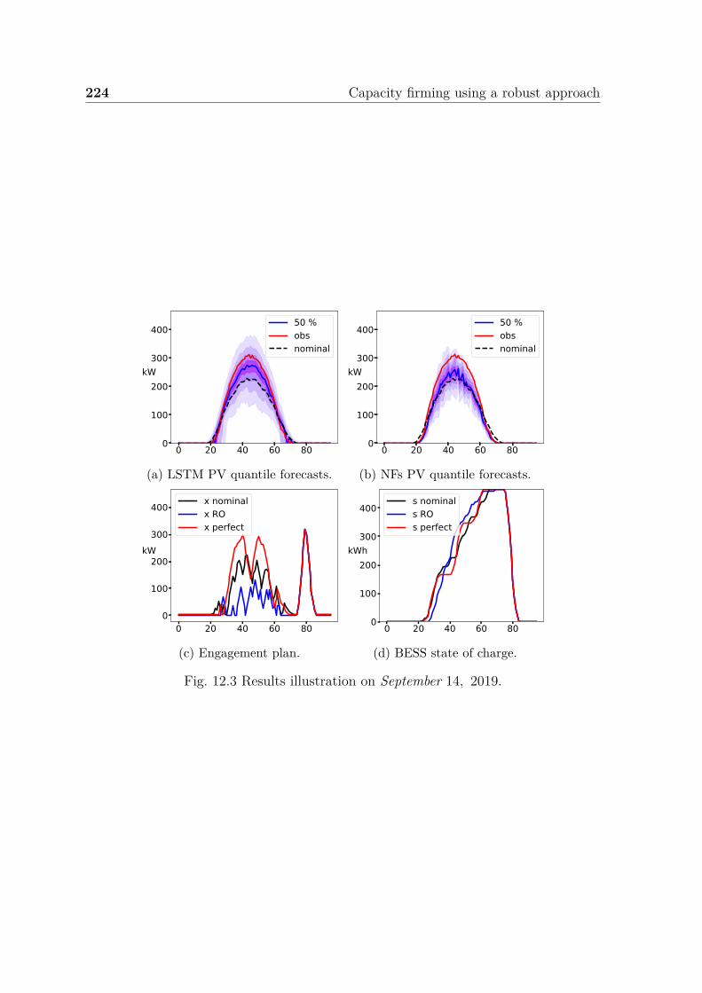
224 Capacity firming using a robust approach

0 20 40 60 800

100

200

300

400

kW

50 %obsnominal

(a) LSTM PV quantile forecasts.

0 20 40 60 800

100

200

300

400

kW

50 %obsnominal

(b) NFs PV quantile forecasts.

0 20 40 60 800

100

200

300

400

kW

x nominalx ROx perfect

(c) Engagement plan.

0 20 40 60 800

100

200

300

400

kWh

s nominals ROs perfect

(d) BESS state of charge.

Fig. 12.3 Results illustration on September 14, 2019.

12.3 Case Study 225

12 24 36 48 /

10

20

30

40

q62.5 65.5 65.0 61.8 64.6

56.0 63.8 63.1 62.8 66.2

52.1 56.9 58.4 60.4 63.3

44.8 49.3 52.2 53.2 54.1

Nominal = 53.3 %

50

55

60

65

70

75

%

(a) BD-LSTM.

12 24 36 48 /

10

20

30

40

q68.8 70.9 63.2 61.6 63.0

69.3 70.3 72.5 72.6 71.9

65.8 67.6 71.2 68.9 74.1

62.2 64.8 67.1 65.6 67.2

Nominal = 53.3 %

50

55

60

65

70

75

%

(b) BD-NF.

12 24 36 48 /

10

20

30

40

q62.5 64.8 65.9 64.9 64.6

55.7 63.2 65.4 66.2 66.2

50.7 57.1 62.2 61.1 63.3

44.1 47.6 49.3 53.7 54.1

Nominal = 53.3 %

50

55

60

65

70

75%

(c) CCG-LSTM.

12 24 36 48 /

10

20

30

40

q72.1 72.9 67.5 64.2 63.0

71.7 73.8 72.8 72.8 71.9

65.0 70.3 71.9 72.4 74.1

64.0 65.8 65.1 66.0 67.2

Nominal = 53.3 %

50

55

60

65

70

75

%

(d) CCG-NF.

Fig. 12.4 Results with constant risk-averse parameters. Normalized profit (%) of theBD and CCG RO planners ([Γ, q]), deterministic ([/, q]) planner, and the referencethat is the deterministic planner with point-forecasts (Nominal). Left part: LSTMquantiles, right part: NF quantiles.

%, 72.6 % and 74.1 %, respectively, with the risk-averse parameters [q = 20%, Γ = 24],[q = 20%, Γ = 48], and the quantile 30 %. It should be possible to improve theRO results by tuning the risk-averse parameters [ypv,(q)

t , Γ]. However, these resultsemphasize the interest in considering a deterministic planner with the relevant PVquantile as point forecasts, which are easy to implement, fast to compute (a fewseconds), and less prone to convergence issues than the RO approach.

12.3.3 Dynamic risk-averse parameters strategy

In this section, the risk-averse parameters [umint , Γ] of the RO approach are dynamically

set based on the day-ahead quantile forecasts distribution, and umint is not necessarily

equal to the same quantile ypv,(q)t ∀t ∈ T . The motivation of this strategy is to assume

226 Capacity firming using a robust approach

that the sharper the quantile forecast distribution around the median is, the lessrisk-averse the RO approach should be.

Two parameters are designed to this end: (1) the PV uncertainty set max depthdq to control umin

t ; (2) the budget depth dΓ to control Γ. dq is a percentage of thedistance between the median and the 10% quantile d50−10, and dΓ is a percentage ofthe total installed capacity Pc. Then, two rules are designed to dynamically set therisk-averse parameters [umin

t , Γ] for each day of the dataset. For a given day, and theset of time periods where the PV median is non null, the distances between the PVmedian and the PV quantiles 20, 30, and 40% are computed: d50−20, d50−30, d50−40.umin

t is dynamically set at each time period t as follows

umint =

ypv,(0.1)t if d

50−20/30/40t > dqd

50−10t

ypv,(0.2)t if d

50−20/30t > dqd

50−10t

ypv,(0.3)t if d50−20

t > dqd50−10t

ypv,(0.4)t otherwise

. (12.18)

For a given day, the budget of uncertainty Γ is dynamically set based on the followingrule

Γ = #t : d50−10t > dΓPc. (12.19)

Figure 12.5 provides the normalized profits of the CCG-RO, BD-RO, and determin-istic planners for several pairs [dΓ, dq] using both the LSTM and NF quantiles. Theplanners achieved better results when using the NF quantiles. Overall, the results areimproved compared to fixed risk-averse parameters for all the planners. The highestprofits achieved by the CCG-NF, BD-NF and NF-deterministic planners are 75.0 %,72.6 % and 75.0 %, respectively, with [dΓ, dq] = [10, 30], [dΓ, dq] = [10, 5], and dq = 50%.

12.3 Case Study 227

5 10 20 /d

5

10

20

30

50

dq63.6 65.8 63.8 65.2

63.2 67.2 63.3 66.7

64.2 64.5 59.7 65.8

64.9 64.5 58.3 64.1

58.3 59.9 53.0 61.550

55

60

65

70

75

%

(a) BD-LSTM.

5 10 20 /d

5

10

20

30

50

dq63.4 72.6 65.7 63.0

64.1 71.6 65.7 62.7

69.9 70.8 64.0 71.6

70.7 72.3 65.0 71.3

71.6 69.0 62.7 75.050

55

60

65

70

75

%

(b) BD-NF.

5 10 20 /d

5

10

20

30

50

dq67.3 69.8 62.1 65.2

69.0 69.9 62.4 66.7

66.4 66.6 56.7 65.8

63.5 64.0 53.2 64.1

60.3 58.8 52.0 61.550

55

60

65

70

75

%

(c) CCG-LSTM.

5 10 20 /d

5

10

20

30

50

dq66.6 72.7 65.9 63.0

66.3 73.0 66.2 62.7

71.0 73.6 65.8 71.6

74.7 75.0 62.8 71.3

72.6 71.0 60.9 75.050

55

60

65

70

75

%

(d) CCG-NF.

Fig. 12.5 Results with dynamic risk-averse parameters. Normalized profit (%) of theBD and CCG RO planners ([dΓ, dq]), and deterministic ([/, dq]) planner. Left part:LSTM quantiles, right part: NF quantiles.

228 Capacity firming using a robust approach

0 20 40 60 80 100 120 140 160iteration j

186

184

182

180

178

176

174

172

170 MP j

SP jMILP J ±MILP J

0 10 20 30 40iteration j

186

184

182

180

178

176

174

172

170

MP j

SP jMILP J ±MILP J

Fig. 12.6 Benders convergence without (left) and with (right) an initial set of cuts onSeptember 14, 2019.

θi1≤i≤I tav t50% tmin tmax ttot

False 3.5 2.0 < 0.1 34.1 105.4True 2.0 0.7 < 0.1 30.4 61.3

Table 12.1 Computation times (min) statistics.

12.3.4 BD convergence warm start improvement

Overall, the warm-start procedure of the BD algorithm improves the convergenceby reducing the number of iterations and allows to reach more frequently optimalsolution. In addition, it reduces the number of times the big-M’s values need to beincreased before reaching the final convergence criterion with the MILP. It is illustratedby considering the dynamic risk-averse parameters strategy with [dΓ, dq] = [10, 10].Figure 12.6 illustrates the reduction of the total number of iteration J required toconverge below the threshold ϵ, on a specific day of the dataset. It is divided by 3.6from 159 to 44. The computation time is divided by 4.1 from 7.4 min to 1.8 min. Table12.1 provides the computation times (min) statistics over the entire dataset with andwithout warm start. The averaged tav and total ttot computation times are drasticallyreduced when using the warm-start.

12.3 Case Study 229

Algorithm RO-type t 1% Jmax

BD-NF static 85.2 (151.9) 0.0 72.6CCG-NF static 7.5 (6.0) 1.9 73.8BD-NF dynamic 102.3 (107.3) 0.0 72.6CCG-NF dynamic 9.2 (5.5) 4.2 75.0

Table 12.2 BD vs CCG statistics.t (s) is the averaged computation time per day with the standard deviation in thebracket. 1% (%) is the % of instances that did not terminate with optimality. t and 1%are computed over all days of the testing set and for all pair of constant (dynamic) risk-averse parameters [umin

t , Γ] ([dΓ, dq]). Jmax (%) is the best-normalized profit achievedusing the NF quantiles over all risk-averse parameters.

12.3.5 BD and CCG comparison

Table 12.2 provides a comparison of the BD and CCG algorithms when using NFquantiles for both the static and dynamic robust optimization strategies. Overall,the CCG algorithm converges in 5-10 iterations instead of 50-100 for BD. Therefore,the CCG computes the day-ahead planning in approximately 10 seconds, ten timesfaster than BD. This observation is consistent with [183] that demonstrated the CCGalgorithm converges faster than BD. Let n be the number of extreme points of theuncertainty set P and m of the space Φ defined by constraint (12.11). The BDalgorithm computes an optimal solution in O(nm) iterations, and the CCG procedurein O(n) iterations [183]. Note: the BD algorithm is still competitive in an operationalframework as it takes on average 1-2 minutes to compute the day-ahead planning.However, we observed that the CCG does not always converge to an optimal solution(see Section 12.2.2), which never happened with the BD algorithm. Fortunately, thesecases amount to only a few % of the total instances. Overall, the CCG algorithmachieved better results than the BD for almost all the risk-averse parameters. Finally, inour opinion, both algorithms require the same amount of knowledge to be implemented.Indeed, the only difference is the MP as the SP are solved identically.

230 Capacity firming using a robust approach

12.4 Conclusion

The core contribution of this study is to address the two-phase engagement/controlproblem in the context of capacity firming. A secondary contribution is to use a recentdeep learning technique, Normalizing Flows, to compute PV quantiles. It is comparedto a typical neural architecture, referred to as Long Short-Term Memory. We developedan integrated forecast-driven strategy modeled as a min-max-min robust optimizationproblem with recourse that is solved using a Benders decomposition procedure. Twomain cutting plane algorithms used to address the two-stage RO unit commitmentproblems are compared: the Benders-dual cutting plane and the column-and-constraintgeneration algorithms. The convergence is checked by ensuring a gap below a thresholdbetween the final objective and the corresponding deterministic, objective value. Arisk-averse parameter assessment selects the optimal robust parameters and the optimalconservative quantile for the deterministic planner. Both the NF-based and LSTM-based planners outperformed the deterministic planner with nominal point PV forecasts.The NF model outperforms the LSTM in forecast value as the planner using the NFquantiles achieved higher profit than the planner with LSTM quantiles. Finally, adynamic risk-averse parameter selection strategy is built by taking advantage of the PVquantile forecast distribution and provides further improvements. The CCG procedureconverges ten times faster than the BD algorithm in this case study and achieves betterresults. However, it does not always converge to an optimal solution.

Overall, the RO approach for both the BD and CCG algorithms allows findinga trade-off between conservative and risk-seeking policies by selecting the optimalrobust optimization parameters, leading to improved economic benefits compared tothe baseline. Therefore, offering a probabilistic guarantee for the robust solution.However, the deterministic planner with the relevant PV quantile achieved interestingresults. It emphasizes the interest to consider a well-calibrated deterministic approach.Indeed, it is easy to implement, computationally tractable for large-scale problems,and less prone to convergence issues. Note: this approach can be used in any othercase study. It only requires a few months of data, renewable generation, and weatherforecasts to train the forecasting models to compute reliable forecasts for the planner.

Several extensions are under investigation: (1) a stochastic formulation of the plan-ner with improved PV scenarios based on Gaussian copula methodology or generatedby a state-of-the-art deep learning technique such as Normalizing Flows, Generative Ad-versarial Networks or Variational AutoEncoders; (2) an improved dynamic risk-averseparameter selection strategy based on a machine learning tool capable of better-takingadvantage of the PV quantiles distribution.

Chapter 13

Energy retailer

OverviewThis Chapter investigates the forecast value assessment of the deep generativemodels studied in Chapter 6. The reader is referred to Chapter 6 for the context,primary contributions, the NFs, GANs, and VAEs background, and the descriptionof the Global Energy Forecasting Competition 2014 (GEFcom 2014) case study.References: This chapter is an adapted version of the following publication:

Jonathan Dumas, Antoine Wehenkel, Damien Lanaspeze, Bertrand Cornélusse,and Antonio Sutera. A deep generative model for probabilistic energy forecastingin power systems: normalizing flows. Applied Energy, 305:117871, 2022. ISSN0306-2619. doi: https://doi.org/10.1016/j.apenergy.2021.117871. URL https://arxiv.org/abs/2106.09370.

“Be willing to make decisions. That’s themost important quality in a good leader.”

— George S. Patton

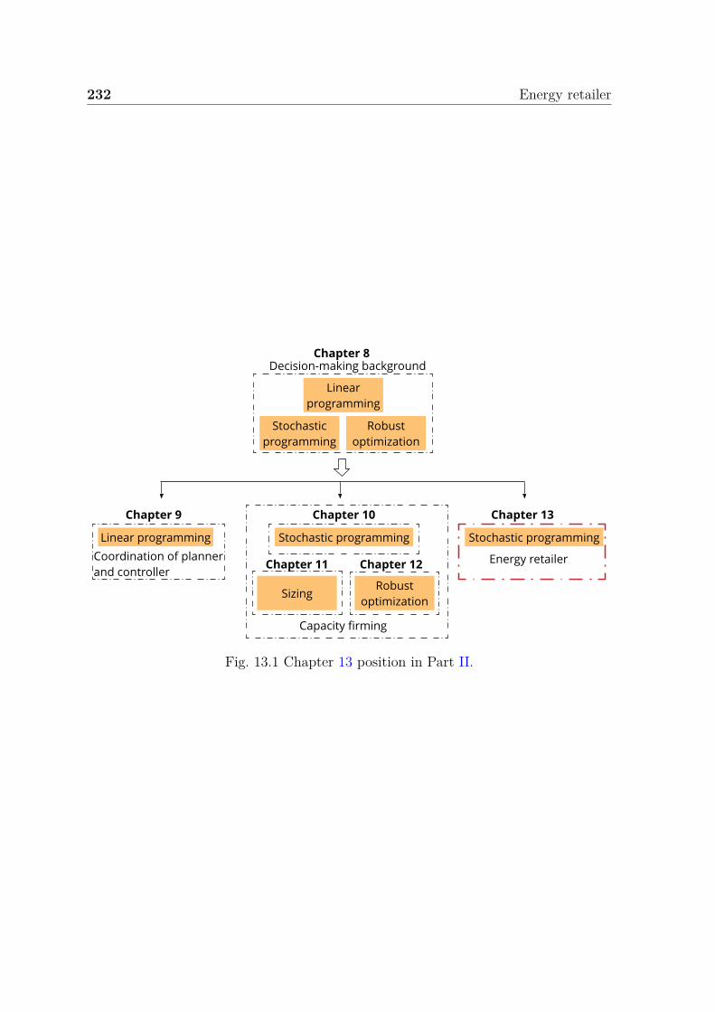
232 Energy retailer

Coordination of planner and controller

Decision-making backgroundChapt er 8

Chapt er 10 Chapt er 13

Stochastic programming

Robust optimization

Chapt er 12

Capacity firming

Energy retailer

Chapt er 9

Linear programming

Chapt er 11

Linear programming Stochastic programming

Robust optimization

Sizing

Stochastic programming

Fig. 13.1 Chapter 13 position in Part II.

13.1 Notation 233

A model that yields lower errors in terms of forecast quality may not always pointto a more effective model for forecast practitioners [87]. To this end, similarly toToubeau et al. [166], the forecast value is assessed by considering the day-ahead marketscheduling of electricity aggregators, such as energy retailers or generation companies.The energy retailer aims to balance its portfolio on an hourly basis to avoid financialpenalties in case of imbalance by exchanging the surplus or deficit of energy in theday-ahead electricity market. The energy retailer may have a battery energy storagesystem (BESS) to manage its portfolio and minimize imports from the main grid whenday-ahead prices are prohibitive.

Section 13.2 introduces the notations used in this Chapter. Section 13.2 presentsthe formulation of the energy retailer case study. Section 13.3 details empirical valueresults on the GEFcom 2014 dataset, and Section 13.4 summarizes the main findingsand highlights ideas for further work.

13.1 Notation

Sets and indicesName Descriptiont Time period index.ω Scenario index.T Number of time periods per day.#Ω Number of scenarios.T Set of time periods, T = 1, 2, . . . , T.Ω Set of scenarios, Ω = 1, 2, . . . , #Ω.

ParametersName Description Unitemin

t , emaxt Minimum/maximum day-ahead bid. MWh

ymint , ymax

t Minimum/maximum retailer net position. MWhydis

max, ychamax BESS maximum (dis)charging power. MW

ηdis, ηcha BESS (dis)charging efficiency. -smin, smax BESS minimum/maximum capacity. MWhsini, send BESS initial/final state of charge. MWhπt Day-ahead price. e/MWh

234 Energy retailer

qt, λt Negative/positive imbalance price. e/MWh∆t Duration of a time period. hour

Variables

For the sake of clarity the subscript ω is omitted.Name Range Description Unitet [emin

t , emaxt ] Day-ahead bid. MWh

yt [ymint , ymax

t ] Retailer net position. MWhypv

t [0, 1] PV generation. MWyw

t [0, 1] Wind generation. MWyl

t [0, 1] Load. MWycha

t [0, ychamax] Charging power. MW

ydist [0, ydis

max] Discharging power. MWst [smin, smax] BESS state of charge. MWhd−

t , d+t R+ Short/long deviation. MWh

ybt 0, 1 BESS binary variable. -

13.2 Problem formulation

Let et [MWh] be the net energy retailer position on the day-ahead market during thet-th hour of the day, modeled as a first stage variable. Let yt [MWh] be the realized netenergy retailer position during the t-th hour of the day, which is modeled as a secondstage variable due to the stochastic processes of the PV generation, wind generation,and load. Let πt [e/ MWh] the clearing price in the spot day-ahead market for thet-th hour of the day, qt ex-post settlement price for negative imbalance yt < et, and λt

ex-post settlement price for positive imbalance yt > et. The energy retailer is assumedto be a price taker in the day-ahead market. It is motivated by the individual energyretailer capacity being negligible relative to the whole market. The forward settlementprice πt is assumed to be fixed and known. As imbalance prices tend to exhibit volatilityand are difficult to forecast, they are modeled as random variables, with expectationsdenoted by qt = E[qt] and λt = E[λt]. They are assumed to be independent randomvariables from the energy retailer portfolio.

13.2.1 Stochastic planner

A stochastic planner with a linear programming formulation and linear constraintsis implemented using a scenario-based approach. The planner computes the day-

13.2 Problem formulation 235

ahead bids et that cannot be modified in the future when the uncertainty is resolved.The second stage corresponds to the dispatch decisions yt,ω in scenario ω that aims atavoiding portfolio imbalances modeled by a cost function f c. The second-stage decisionsare therefore scenario-dependent and can be adjusted according to the realization ofthe stochastic parameters. The stochastic planner objective to maximize is

JS = E[∑

t∈Tπtet + f c(et, yt,ω)

], (13.1)

where the expectation is taken with respect to the random variables, the PV generation,wind generation, and load. Using a scenario-based approach, (13.1) is approximated by

JS ≈∑ω∈Ω

αω

∑t∈T

[πtet + f c(et, yt,ω)

], (13.2)

with αω the probability of scenario ω ∈ Ω, and ∑ω∈Ω αω = 1. The mixed-integer linearprogramming (MILP) optimization problem to solve is

maxet∈X ,yt,ω∈Y(et)

∑ω∈Ω

αω

∑t∈T

[πtet − qtd

−t,ω − λtd

+t,ω

], (13.3a)

X =

et : et ∈ [emint , emax

t ]

, (13.3b)

Y(et) =

yt,ω : (13.4a) − (13.4m)

. (13.3c)

The optimization variables are et, day-ahead bid of the net position, ∀ω ∈ Ω, yt,ω,retailer net position in scenario ω, d−

t,ω, short deviation, d+t,ω, long deviation, ypv

t,ω, PVgeneration, yw

t,ω, wind generation, ychat,ω , battery energy storage system (BESS) charging

power, ydist,ω, BESS discharging power, st,ω, BESS state of charge, and yb

t,ω a binaryvariable to prevent from charging and discharging simultaneously. The imbalancepenalty is modeled by the constraints (13.4a)-(13.4b) ∀ω ∈ Ω, that define the shortand long deviations variables d−

t,ω, d+t,ω ∈ R+. The energy balance is provided by (13.4c)

∀ω ∈ Ω. The set of constraints that bound ypvt,ω and yw

t,ω variables are (13.4d)-(13.4e)∀ω ∈ Ω where ypv

t,ω and ywt,ω are PV and wind generation scenarios. The load is assumed

to be non-flexible and is a parameter (13.4f) ∀ω ∈ Ω where ylt,ω are load scenarios.

The BESS constraints are provided by (13.4g)-(13.4j), and the BESS dynamics by

236 Energy retailer

(13.4k)-(13.4m) ∀ω ∈ Ω.

−d−t,ω ≤ −(et − yt,ω), ∀t ∈ T (13.4a)

−d+t,ω ≤ −(yt,ω − et), ∀t ∈ T (13.4b)

yt,ω

∆t= ypv

t,ω + ywt,ω − yl

t,ω + ydist,ω − ycha

t,ω , ∀t ∈ T (13.4c)

ypvt,ω ≤ ypv

t,ω, ∀t ∈ T (13.4d)yw

t,ω ≤ ywt,ω, ∀t ∈ T (13.4e)

ylt,ω = yl

t,ω, ∀t ∈ T (13.4f)ycha

t,ω ≤ ybt,ωycha

max, ∀t ∈ T (13.4g)ydis

t,ω ≤ (1 − ybt,ω)ydis

max, ∀t ∈ T (13.4h)−st,ω ≤ −smin, ∀t ∈ T (13.4i)

st,ω ≤ smax, ∀t ∈ T (13.4j)s1,ω − sini

∆t= ηchaycha

1,ω −ydis

1,ω

ηdis , (13.4k)

st,ω − st−1,ω

∆t= ηchaycha

t,ω −ydis

t,ω

ηdis , ∀t ∈ T \ 1 (13.4l)

sT,ω = send = sini. (13.4m)

Notice that if λt < 0, the surplus quantity is remunerated with a non-negative price.In practice, such a scenario could be avoided provided that the energy retailer hascurtailment capabilities, and (qt, λt) are strictly positive in our case study. Thedeterministic formulation with perfect forecasts, the oracle (O), is a specific case ofthe stochastic formulation by considering only one scenario where ypv

t,ω, ywt,ω, and yl

t,ω

become the actual values of PV, wind, and load ∀t ∈ T . The optimization variablesare et, yt, d−

t , d+t , ypv

t , and ywt , ycha

t , ydist , st, and yb

t .

13.2.2 Dispatching

Once the bids et have been computed by the planner, the dispatching consists ofcomputing the second stage variables given observations of the PV, wind power, andload. The dispatch formulation is a specific case of the stochastic formulation with et

as parameter and by considering only one scenario where ypvt,ω, yw

t,ω, and ylt,ω become

the actual values of PV, wind, and load ∀t ∈ T . The optimization variables are yt, d−t ,

d+t , ypv

t , and ywt , ycha

t , ydist , st, and yb

t .

13.3 Value results 237

0 5 10 15 20

0.50

0.25

0.00

0.25

0.50

0.75

1.00

35

40

45

50

55

60

65

/MW

h

PV Wind Load net t

Fig. 13.2 Energy retailer case study: illustration of the observations on a random dayof the testing set.The energy retailer portfolio comprises PV generation, wind power, load, and storagedevice. The PV, wind power, and load scenarios from the testing set are used as inputsof the stochastic day-ahead planner to compute the optimal bids. The net is the powerbalance of the energy retailer portfolio. The day-ahead prices πt are obtained from theBelgian day-ahead market on February 6, 2020.

13.3 Value results

The energy retailer portfolio comprises wind power, PV generation, load, and a batteryenergy storage device. The 50 days of the testing set are used and combined withthe 30 possible PV and wind generation zones (three PV zones and ten wind farms),resulting in 1 500 independent simulated days. A two-step approach is employed toevaluate the forecast value:

• First, for each generative model and the 1 500 days simulated, the two-stagestochastic planner computes the day-ahead bids of the energy retailer portfoliousing the PV, wind power, and load scenarios. After solving the optimization,the day-ahead decisions are recorded.

• Then, a real-time dispatch is carried out using the PV, wind power, and loadobservations, with the day-ahead decisions as parameters.

This two-step methodology is applied to evaluate the three generative models, namelythe NF, GAN, and VAE. Figure 13.2 illustrates an arbitrary random day of the testingset with the first zone for both the PV and wind. πt [e/ MWh] is the day-ahead priceson February 6, 2020 of the Belgian day-ahead market used for the 1 500 days simulated.The negative qt and positive λt imbalance prices are set to 2 × πt, ∀t ∈ T . The retaileraims to balance the net power, the red curve in Figure 13.2, by importing/exportingfrom/to the main grid. Usually, the net is positive (negative) at noon (evening) when

238 Energy retailer

the PV generation is maximal (minimal), and the load is minimal (maximal). As theday-ahead spot price is often maximal during the evening load peak, the retailer seeksto save power during the day by charging the battery to decrease the import duringthe evening. Therefore, the more accurate the PV, wind generation, and load scenariosare, the better is the day-ahead planning.

The battery minimum smin and maximum smax capacities are 0 and 1, respectively. Itis assumed to be capable of fully (dis)charging in two hours with ydis

max = ychamax = smax/2,

and the (dis)charging efficiencies are ηdis = ηcha = 95%. Each simulation day isindependent with a fully discharged battery at the first and last period of each daysini = send = 0. The 1 500 stochastic optimization problems are solved with 50 PV,wind generation, and load scenarios. The python Gurobi library is used to implementthe algorithms in Python 3.7, and Gurobi1 9.0.2 is used to solve the optimizationproblems. Numerical experiments are performed on an Intel Core i7-8700 3.20 GHzbased computer with 12 threads and 32 GB of RAM running on Ubuntu 18.04 LTS.

The net profit, that is, the profit minus penalty, is computed for the 1 500 daysof the simulation and aggregated in the first row of Table 13.1. The ranking of eachmodel is computed for the 1 500 days. The cumulative ranking is expressed in termsof percentage in Table 13.1. NF outperformed both the GAN and VAE with a totalnet profit of 107 ke. There is still room for improvement as the oracle, which hasperfect future knowledge, achieved 300 ke. NF, ranked first 39.0% during the 1 500simulation days and achieved the first and second ranks 69.6%. Overall, in terms of

NF VAE GANNet profit (ke) 107 97 931 (%) 39.0 31.8 29.21 & 2 (%) 69.6 68.3 62.11 & 2 & 3 (%) 100 100 100

Table 13.1 Total net profit (ke) and cumulative ranking (%).Using the NF PV, wind power, and load scenarios, the stochastic planner achieved thehighest net profit with 107 ke, ranked first 39.0 %, second 30.6 %, and third 30.4 %over 1 500 days of simulation. The second-best model, the VAE, achieved a net profitof 97 ke, ranked first 31.8 %, second 36,5 %, and third 31.7 %.

forecast value, the NF outperforms the VAE and GAN. However, this case study is"simple," and stochastic optimization relies mainly on the quality of the average of

1https://www.gurobi.com/

13.4 Conclusions 239

the scenarios. Therefore, one may consider taking advantage of the particularitiesof a specific method by considering more advanced case studies. In particular, thespecificity of the NFs to provide direct access to the probability density function maybe of great interest in specific applications. It is left for future investigations as moreadvanced case studies would prevent a fair comparison between models.

13.3.1 Results summary

Table 13.2 summarizes the main results of this study by comparing the VAE, GAN, andNF implemented through easily comparable star ratings. The rating for each criterionis determined using the following rules - 1 star: third rank, 2 stars: second rank, and3 stars: first rank. Specifically, training speed is assessed based on reported totaltraining times for each dataset: PV generation, wind power, and load; sample speed isbased on reported total generating times for each dataset; quality is evaluated with themetrics considered; value is based on the case study of the day-ahead bidding of theenergy retailer; the hyper-parameters search is assessed by the number of configurationstested before reaching satisfactory and stable results over the validation set; the hyper-parameters sensitivity is evaluated by the impact on the quality metric of deviationsfrom the optimal the hyper-parameter values found during the hyper-parameter search;the implementation-friendly criterion is appraised regarding the complexity of thetechnique and the amount of knowledge required to implement it.

13.4 Conclusions

This Chapter proposed a fair and thorough comparison of NFs with the state-of-the-artdeep learning generative models, GANs and VAEs, in terms of value. The experimentsare performed using the open data of the Global Energy Forecasting Competition2014. The generative models use the conditional information to compute improvedweather-based PV, wind power, and load scenarios. This study demonstrated that NFsare capable of challenging GANs and VAEs. They are overall more accurate both interms of quality (see Chapter 6) and value and can be used effectively by non-expertdeep learning practitioners. Note, Section 6.6 in Chapter 6 presents the NFs advantagesover more traditional deep learning approaches that should motivate their introductioninto power system applications.

240 Energy retailer

Criteria VAE GAN NFTrain speed ⋆⋆⋆ ⋆⋆⋆ ⋆⋆⋆

Sample speed ⋆⋆⋆ ⋆⋆⋆ ⋆⋆⋆

Quality ⋆⋆⋆ ⋆⋆⋆ ⋆⋆⋆

Value ⋆⋆⋆ ⋆⋆⋆ ⋆⋆⋆

Hp search ⋆⋆⋆ ⋆⋆⋆ ⋆⋆⋆

Hp sensibility ⋆⋆⋆ ⋆⋆⋆ ⋆⋆⋆

Implementation ⋆⋆⋆ ⋆⋆⋆ ⋆⋆⋆

Table 13.2 Comparison between the deep generative models.The rating for each criterion is determined using the following rules - 1 star: thirdrank, 2 stars: second rank, and 3 stars: first rank. Train speed: training computationtime; Sample speed: scenario generation computation time; Quality: forecast qualitybased on the eight complementary metrics considered; Value: forecast value based onthe day-ahead energy retailer case study; Hp search: assess the difficulty to identifyrelevant hyper-parameters; Hp sensibility: assess the sensitivity of the model to agiven set of hyper-parameters (the more stars, the more robust to hyper-parametermodifications); Implementation: assess the difficulty to implement the model (themore stars, the more implementation-friendly). Note: the justifications are provided inAppendix 13.5.

13.5 Appendix: Table 13.2 justifications 241

13.5 Appendix: Table 13.2 justifications

The VAE is the fastest to train, with a recorded computation time of 7 seconds onaverage per dataset. The training time of the GAN is approximately three times longer,with an average computation time of 20 seconds per dataset. Finally, the NF is theslowest, with an average training time of 4 minutes. This ranking is preserved with theVAE the fastest concerning the sample speed, followed by the GAN and NF models.The VAE and the GAN generate the samples over the testing sets, 5 000 in total, in lessthan a second. However, the NF considered takes a few minutes. In contrast, the affineautoregressive version of the NF is much faster to train and generate samples. Note:even a training time of a few hours is compatible with day-ahead planning applications.In addition, once the model is trained, it is not necessarily required to retrain it everyday.

The quality and value assessments have already been discussed in Sections 6.5 and13.3. Overall, the NF outperforms both the VAE and GAN models.

Concerning the hyper-parameters search and sensibility, the NF tends to be themost straightforward model to calibrate. Compared with the VAE and GAN, we foundrelevant hyper-parameter values by testing only a few combinations. In addition, theNF is robust to hyper-parameter modifications. In contrast, the GAN is the mostsensitive. Variations of the hyper-parameters may result in very poor scenarios bothin terms of quality and shape. Even for a fixed set of hyper-parameters values, twoseparate training may not converge towards the same results illustrating the GANtraining instabilities. The VAE is more accessible to train than the GAN but is alsosensitive to hyper-parameters values. However, it is less evident than the GAN.

Finally, we discuss the implementation-friendly criterion of the models. Note:this discussion is only valid for the models implemented in this study. There existvarious architectures of GANs, VAEs, and NFs with simple and complex versions.In our opinion, the VAE is the effortless model to implement as the encoder anddecoder are both simple feed-forward neural networks. The only difficulty lies in thereparameterization trick that should be carefully addressed. The GAN is a bit moredifficult to deploy due to the gradient penalty to handle but is similar to the VAE withboth the discriminator and the generator that are feed-forward neural networks. TheNF is the most challenging model to implement from scratch because the UMNN-MAFapproach requires an additional integrand network. An affine autoregressive NF iseasier to implement. However, it may be less capable of modeling the stochasticityof the variable of interest. However, forecasting practitioners do not necessarily have

242 Energy retailer

to implement generative models from scratch and can use numerous existing Pythonlibraries.

Chapter 14

Part II conclusions

“Everything has been figured out, except howto live.”

— Jean-Paul Sartre

Part II presents several approaches to address the energy management of a grid-connected microgrid. It proposes handling the renewable generation uncertaintyby considering deterministic, stochastic, and robust approaches that rely on pointforecasts, scenarios, and quantiles forecasts. Several numerical experiments evaluatethese approaches.

• The MiRIS microgrid located at the John Cockerill Group’s international head-quarters in Seraing, Belgium, assesses a value function-based approach to prop-agate information from operational planning to real-time optimization. Thismethodology relies on point forecasts of PV and electrical demand to conductthe deterministic optimization. The results demonstrate the efficiency of thismethod to manage the peak in comparison with a Rule-Based Controller.

• The MiRIS case study is also employed in the capacity firming market. It allowsstudying a stochastic approach to address the energy management of a grid-connected renewable generation plant coupled with a battery energy storagedevice. The results of the stochastic planner are comparable with those of thedeterministic planner, even when the prediction error variance is non-negligible.However, further investigations are required to use a more realistic methodologyto generate PV scenarios and a realistic controller.

• A sizing study is performed using the capacity firming framework in a differentcase: the ULiège case study. The results indicate that the approach is not

244 Part II conclusions

very sensitive to the control policy. The difference between the deterministicwith perfect knowledge (or point forecasts) and stochastic with scenarios isminor. However, further investigations are required to implement a more realisticcontroller that uses intraday point forecasts and conduct a sensitivity analysis onthe simulation parameters.

• A robust day-ahead planner is compared to its deterministic counterpart usingthe ULiège case study in the capacity firming framework. Overall, it allowsfinding a trade-off between conservative and risk-seeking policies by selecting theoptimal robust optimization parameters, leading to improved economic benefitscompared to the baseline.

• Finally, a stochastic approach deals with the optimal bidding of an energy retailerportfolio on the day-ahead market to assess the value of a recent class of deeplearning generative models, the normalizing flows. The numerical experimentsuse the open-access data of the Global Energy Forecasting Competition 2014.The results demonstrate that normalizing flows can challenge Variational AutoEn-coders and Generative Adversarial Networks. They are overall more accurateboth in terms of quality (see Chapter 6) and value and can be used effectively bynon-expert deep learning practitioners.

Chapter 15

General conclusions andperspectives

OverviewThis chapter concludes the thesis and identifies four potential research directionsin both forecasting and planning for microgrids. (1) Forecasting techniques of thefuture with the development of new machine learning models that take advantageof the underlying physical process. (2) Machine learning for optimization withmodels that simplify optimization planning problems by learning a sub-optimalspace. (3) Modelling and simulation of energy systems by applying forecastingand decomposition techniques investigated in this thesis into open-source code.(4) Machine learning and psychology where models could identify appropriatebehaviors to reduce carbon footprint. Then, inform individuals, and provideconstructive opportunities by modeling individual behavior.

“Words are loaded pistols.”— Jean-Paul Sartre

15.1 Summary

The IPCC report ’AR5 Climate Change 2014: Mitigation of Climate Change’1, statesthat electrical systems are responsible for about a quarter of human-caused greenhousegas emissions each year. According to the IPCC, the transition to a carbon-free society

1https://www.ipcc.ch/report/ar5/wg3/

246 General conclusions and perspectives

goes through an inevitable increase in the renewable generation’s share in the energymix and a drastic decrease in the total consumption of fossil fuels. However, a high shareof renewables is challenging for power systems that have been designed and sized fordispatchable units. In addition, a major challenge is to implement these changes acrossall countries and contexts, as electricity systems are everywhere. Machine learningcan contribute on all fronts by informing the research, deployment, and operation ofelectricity system technologies. High leverage contributions in power systems include[151]: accelerating the development of clean energy technologies, improving demandand clean energy forecasts, improving electricity system optimization and management,and enhancing system monitoring. This thesis focuses on two leverages: (1) the supplyand demand forecast; (2) the electricity system optimization and management.

Since variable generation and electricity demand both fluctuate, they must beforecast ahead of time to inform real-time electricity scheduling and longer-term systemplanning. Better short-term forecasts enable system operators to reduce reliance onpolluting standby plants and proactively manage increasing amounts of variable sources.Better long-term forecasts help system operators and investors to decide where andwhen to build variable plants. Forecasts need to become more accurate, span multiplehorizons in time and space, and better quantify uncertainty to support these use cases.Therefore, probabilistic forecasts have become a vital tool to equip decision-makers,hopefully leading to better decisions in energy applications.

When balancing electricity systems, system operators use scheduling and dispatchto determine how much power every controllable generator should produce. Thisprocess is slow and complex, governed by NP-hard optimization problems [151] suchas unit commitment and optimal power flow that must be coordinated across multipletime scales, from sub-second to days ahead. Scheduling becomes even more complexas electricity systems include more storage, variable generators, and flexible demand.Indeed, operators manage even more system components while simultaneously solvingscheduling problems more quickly to account for real-time variations in electricityproduction. Thus, scheduling must improve significantly, allowing operators to rely onvariable sources to manage systems.

These two challenges raise the following two central research questions:

• How to produce reliable probabilistic forecasts of renewable generation, consump-tion, and electricity prices?

• How to make decisions with uncertainty using probabilistic forecasts to improvescheduling?

15.1 Summary 247

This thesis studies the day-ahead management of a microgrid system and investigatesboth questions into two parts.

Part I investigates forecasting techniques and quality metrics required to produceand evaluate point and probabilistic forecasts. Then, Part II use them as inputof decision-making models. Chapters 2 and 3 present the forecasting basics. Theyintroduce the different types of forecasts to characterize the behavior of stochasticvariables, such as renewable generation or electrical consumption, and the assessmentprocedures. An example of forecast quality evaluation is provided by employingstandard deep-learning models such as recurrent neural networks to compute PV andelectrical consumption point forecasts. The following Chapters of Part I study thepoint forecasts, quantile forecasts, scenarios, and density forecasts. Chapter 4 proposesto implement deep-learning models such as the encoder-decoder architecture to producePV quantile forecasts. Then, a day-ahead robust optimization planner uses theseforecasts in the form of prediction intervals in the second part of this thesis. Chapter5 presents a density forecast-based approach to compute probabilistic forecasting ofimbalance prices with a particular focus on the Belgian case. Finally, Chapter 6analyzes the scenarios of renewable generation and electrical consumption of a newclass of deep learning generative models, the normalizing flows. Relevant metricsassess the forecast quality. A thorough comparison is performed with the variationalautoencoders and generative adversarial networks models.

Part II presents several approaches and methodologies based on optimization fordecision-making under uncertainty. It employs the forecasts computed in the first partof the thesis. Chapter 8 introduces the different types of optimization strategies fordecision making under uncertainty. Chapter 9 presents a value function-based approachas a way to propagate information from operational planning to real-time optimizationin a deterministic framework. Chapters 10, 11, and 12 consider a grid-connectedrenewable generation plant coupled with a battery energy storage device in the capacityfirming market. This framework has been designed to promote renewable powergeneration facilities in small non-interconnected grids. First, a stochastic optimizationstrategy is adopted for the day-ahead planner. Second, a sizing study of the system isconducted to evaluate the impact of the planning strategy: stochastic or deterministic.Finally, a robust day-ahead planner is considered to optimize the results regardingrisk-aversion of the decision-maker. Finally, Chapter 13 is the extension of Chapter 6.It presents the forecast value of the deep learning generative models by considering theday-ahead market scheduling of an energy retailer. It is an easily reproducible casestudy designed to promote the normalizing flows in power system applications.

248 General conclusions and perspectives

15.2 Future directions

We propose four primary research future directions.

15.2.1 Forecasting techniques of the future

Nowadays, the renewable energy forecasting field is highly active and dynamic. Hence,new forecasting methods will likely be proposed and used in operational problemsrelated to power system applications in the coming years. The type of forecasts to beused as input to operational problems will depend upon the problem’s nature and theformulation of the corresponding optimization problem. Machine learning algorithmsof the future will need to incorporate domain-specific insights. For instance, the study[151] defines exciting research directions. We propose in the following several researchdirections. First, it is well known that the weather fundamentally drives both variablegeneration and electricity demand. Thus, machine learning algorithms should drawfrom climate modeling, weather forecasting innovations, and hybrid physics-plus-MLmodeling techniques [171, 39]. Second, machine learning models could be designedto directly optimize system goals [45, 56]. An example is given by Donti et al. [45].They use a deep neural network to produce demand forecasts that optimize electricityscheduling costs rather than forecast accuracy. Third, better understanding the value ofimproved forecasts is an interesting challenge. In this line, the benefits of specific solarforecast improvements in a region of the United States are described by Martinez-Anidoet al. [120]. Finally, studying techniques that take advantage of the power systemcharacteristics, such as graphical neural networks [177, 44]. They are capable of learningthe power network structure and could provide successful contributions to hierarchicalforecasting. Indeed, probabilistic graphical models reduce to Bayesian networks witha pre-defined topology and a learnable density at each node [177]. From this newperspective, the graphical normalizing flow provides a promising way to inject domainknowledge into normalizing flows while preserving Bayesian networks’ interpretabilityand the representation capacity of normalizing flows. In this line, a graphical model isused to detect faults in rooftop solar panels [91]. This paper proposes Solar-Clique, adata-driven approach that can flag anomalies in power generation with high accuracy.

15.2.2 Machine learning for optimization

There is a broad consensus in the power system community that the uncertain natureof renewable energy sources like wind and solar is likely to induce significant changes in

15.2 Future directions 249

the paradigms of power systems management [124]. The electricity market results fromtraditional practices, such as unit commitment or economic dispatch, designed given ageneration mix mainly formed by dispatchable plants. Therefore, they are now to bereexamined so that stochastic producers can compete on equal terms. For instance, thecapacity firming market is a new design conceived to promote renewable generation inisolated markets. The type of decision-making tools to deal with these new marketdesigns and systems, such as microgrids, depends upon the nature of the problem itself.These tools have been studied intensively, and new methods will likely be proposed andused in power system applications. In particular, machine learning for optimization isnowadays a hot topic. It learns partially or totally the sizing space to provide a fastand efficient sizing tool. It also simplifies optimization planning problems by learning asub-optimal space. This approach has already been investigated in a few applications.For instance:

• Machine learning can be used to approximate or simplify existing optimizationproblems [15, 182], and to find good starting points for optimization [92].

• Dynamic scheduling [57] and safe reinforcement learning can also be used tobalance the electric grid in real-time.

• Misyris et al. [122] propose a framework for physics-informed neural networksin power system applications. In this line, Fioretto et al. [60] present a deeplearning approach to the optimal power flows. The learning model exploits theinformation available in the similar states of the system and a dual Lagrangianmethod to satisfy the physical and engineering constraints present in the optimalpower flows.

• Donon et al. [44] propose a neural network architecture that emulates the behav-ior of a physics solver that solves electricity differential equations to computeelectricity flow in power grids. It uses proxies based on graph neural networks.

• Tsaousoglou et al. [167] consider an economic dispatch problem for a communityof distributed energy resources, where energy management decisions are madeonline and under uncertainty. The economic dispatch problem is a multi-agentMarkov Decision Process. The difficulties lie in the curse of dimensionality andin guaranteeing the satisfaction of constraints under uncertainty. A novel methodthat combines duality and deep learning tackles these challenges.

250 General conclusions and perspectives

15.2.3 Modelling and simulation of energy systems

As already previously stated, the transition towards more sustainable fossil-free energysystems requires a high penetration of renewables, such as wind and solar. These newenergy resources and technologies will lead to profound structural changes in energysystems, such as an increasing need for storage and drastic electrification of the heatingand mobility sectors. Therefore, new flexible and open-source optimization modelingtools are required to capture the growing complexity of such future energy systems.To this end, in the past few years, several open-source models for the strategic energyplanning of urban and regional energy systems have been developed. A list of suchmodels is depicted in [115]. We select and present two2 of them where we think it maybe relevant to implement and test the forecasting techniques and scheduling strategiesdeveloped in this thesis.

First, EnergyScope TD [115] is a novel open-source model for the strategic energyplanning of urban and regional energy systems. EnergyScope TD optimizes an entireenergy system’s investment and operating strategy, including electricity, heating, andmobility. Its hourly resolution, using typical days, makes the model suitable forintegrating intermittent renewables, and its concise mathematical formulation andcomputational efficiency are appropriate for uncertainty applications. A new researchdirection could be integrating multi-criterion optimization to consider the carbonfootprint, the land use, the energy return on investment, and the cost could be anexciting and challenging research direction [126]. Solving such a complex optimizationproblem may require decomposition techniques such as the ones investigated in thisthesis.

Second, E4CLIM [164] is open-source Python software integrating flexibility needsfrom variable renewable energies in the development of regional energy mixes. Itaims at evaluating and optimizing energy deployment strategies with higher sharesof variable renewable energies. It also assesses the impact of new technologies andclimate variability and allows conducting sensitivity studies. The E4CLIM’s potentialwas already illustrated at the country scale with an optimal recommissioning study ofthe 2015 Italian PV-wind mix. A new research direction could be to adapt and developE4CLIM at the infra-regional scale and consider the electrical grid constraints. It mayimply solving complex optimization problems requiring state-of-the-art decompositiontechniques.

2In both cases, machine learning investigation for optimization may be an interesting researchdirection to simplify and improve the models.

15.2 Future directions 251

15.2.4 Machine learning and psychology

This last research direction goes off the beaten tracks. In my opinion, achievingsustainability goals requires as much the use of relevant technology as psychology.Therefore, one of the main challenges is not designing relevant technological tools butchanging how we consume and behave in our society. In other words, technology willnot save us. Nevertheless, it is the way we use technology that could help us to meetthe sustainability targets. Therefore, it requires research in transdisciplinary fieldsto design collaborative solutions and guidances towards this goal. Psychology is acomprehensive tool to study and understand why there is a gap between rhetoric andactions. An increase in psychological research on climate change has been conductedsince the last decade [34]. We select and provide three useful references among thevast literature on this topic to the interested reader. Seven categories of psychologicalbarriers or dragons of inaction are studied by Gifford [68] where five strategies areproposed to help overcome them. A discussion is proposed by Nielsen et al. [129] toconsider how further research can make an even more significant difference in limitingClimate Change. Finally, Abrahamse and Steg [2] analyze the effect of social influence.Social influence refers to how our behavior is affected by what other people do orthink. This study compares the effectiveness of different social influence approaches tosustainability using a meta-analysis. It also presents what remains to be investigatedabout the mechanisms linking social influence to behavior change.

This topic raises several exciting research questions. (1) How can we considerpsychology and human behavior when designing deep learning algorithms or decision-making tools? (2) How can we use algorithms to influence behavior towards sustainablegoals? (3) How can we design new tools and propose relevant climate change solutionswithout leading to a rebound effect? (4) Do we need high-tech solutions to make asignificant shift? Or is it more a matter of behavior and psychology? What is theoptimal trade-off?

Some actions can meaningfully reduce each person’s carbon footprint and, if widelyadopted, could significantly mitigate global emissions [178]. Machine learning couldhelp identify those behaviors, inform individuals, and provide constructive opportunitiesby modeling individual behavior [151].

First, by understanding how is composed our carbon footprint. Indeed, as individu-als, we may lack the data and knowledge to know which decisions are most impactfulregarding the carbon footprint. Therefore, machine learning can help determine anindividual’s carbon footprint based on their behavior and personal and householddata. For instance, a natural language processing model can identify the products

252 General conclusions and perspectives

we purchased from a bill or a type of transportation from email. The algorithm canalso monitor household electricity and gas consumption or the food we eat. Then,making it possible to predict the associated emissions and help consumers who wish toidentify which behaviors result in the highest emissions. In addition, such a machinelearning model could use counterfactual reasoning to demonstrate to consumers howmuch their emissions would be reduced for each behavior they changed. Therefore,such information can empower people to understand how they can best help mitigateclimate change through behavior change.

Second, by facilitating behavior change. Indeed, machine learning can model andcluster individuals based on their climate knowledge, preferences, demographics, andconsumption characteristics [61]. Thus, it predicts who will be most responsive tonew technologies and sustainable behavior change. For instance, such techniques haveimproved the enrollment rate of customers in an energy savings program by 2-3x[5]. It can also make the effects of climate change more tangible for consumers andhelp motivate those who wish to act. In this line, Konstantakopoulos et al. [107] hasproposed gamification through deep learning to allow further individuals to exploretheir energy usage.

References

[1] Martín Abadi, Ashish Agarwal, Paul Barham, Eugene Brevdo, Zhifeng Chen,Craig Citro, Greg S. Corrado, Andy Davis, Jeffrey Dean, Matthieu Devin,Sanjay Ghemawat, Ian Goodfellow, Andrew Harp, Geoffrey Irving, MichaelIsard, Yangqing Jia, Rafal Jozefowicz, Lukasz Kaiser, Manjunath Kudlur, JoshLevenberg, Dandelion Mané, Rajat Monga, Sherry Moore, Derek Murray, ChrisOlah, Mike Schuster, Jonathon Shlens, Benoit Steiner, Ilya Sutskever, KunalTalwar, Paul Tucker, Vincent Vanhoucke, Vijay Vasudevan, Fernanda Viégas,Oriol Vinyals, Pete Warden, Martin Wattenberg, Martin Wicke, Yuan Yu, andXiaoqiang Zheng. TensorFlow: Large-scale machine learning on heterogeneoussystems, 2015. URL https://www.tensorflow.org/. Software available fromtensorflow.org.

[2] Wokje Abrahamse and Linda Steg. Social influence approaches to encourageresource conservation: A meta-analysis. Global environmental change, 23(6):1773–1785, 2013.

[3] International Energy Agency. Net zero by 2050: A roadmap for the global energysystem. Technical report, International Energy Agency, 2021.

[4] Michael S. Albergo, Denis Boyda, Daniel C. Hackett, Gurtej Kanwar, KyleCranmer, Sébastien Racanière, Danilo Jimenez Rezende, and Phiala E. Shanahan.Introduction to normalizing flows for lattice field theory, 2021.

[5] Adrian Albert and Mehdi Maasoumy. Predictive segmentation of energy con-sumers. Applied energy, 177:435–448, 2016.

[6] Myles Allen, Mustafa Babiker, Yang Chen, and Heleen C. de Coninck. Ipccsr15: Summary for policymakers. Technical report, Intergovernmental Panel onClimate Change, October 2018. Drafting Authors: Myles Allen (UK), MustafaBabiker (Sudan), Yang Chen (China), Heleen de Coninck (Netherlands/EU),Sarah Connors (UK), Renée van Diemen (Netherlands), Opha Pauline Dube(Botswana), Kristie L. Ebi (USA), Francois Engelbrecht (South Africa), MarionFerrat (UK/France), James Ford (UK/Canada), Piers Forster (UK), SabineFuss (Germany), Tania Guillén Bolaños (Germany/Nicaragua), Jordan Harold(UK), Ove Hoegh-Guldberg (Australia), Jean-Charles Hourcade (France), DanielHuppmann (Austria), Daniela Jacob (Germany), Kejun Jiang (China), TomGabriel Johansen (Norway), Mikiko Kainuma (Japan), Kiane de Kleijne (Nether-lands/EU), Elmar Kriegler (Germany), Debora Ley (Guatemala/Mexico), DianaLiverman (USA), Natalie Mahowald (USA), Valérie Masson-Delmotte (France),J. B. Robin Matthews (UK), Richard Millar (UK), Katja Mintenbeck (Germany),

254 References

Angela Morelli (Norway/Italy), Wilfran Moufouma-Okia (France/Congo), LuisMundaca (Sweden/Chile), Maike Nicolai (Germany), Chukwumerije Okereke(UK/Nigeria), Minal Pathak (India), Antony Payne (UK), Roz Pidcock (UK),Anna Pirani (Italy), Elvira Poloczanska (UK/Australia), HansOtto Pörtner (Ger-many), Aromar Revi (India), Keywan Riahi (Austria), Debra C. Roberts (SouthAfrica), Joeri Rogelj (Austria/Belgium), Joyashree Roy (India), Sonia I. Senevi-ratne (Switzerland), Priyadarshi R. Shukla (India), James Skea (UK), RaphaelSlade (UK), Drew Shindell (USA), Chandni Singh (India), William Solecki(USA), Linda Steg (Netherlands), Michael Taylor (Jamaica), Petra Tschakert(Australia/Austria), Henri Waisman (France), Rachel Warren (UK), PanmaoZhai (China), Kirsten Zickfeld (Canada).

[7] Martin Arjovsky and Léon Bottou. Towards principled methods for traininggenerative adversarial networks, 2017.

[8] Martin Arjovsky, Soumith Chintala, and Léon Bottou. Wasserstein generativeadversarial networks. In International conference on machine learning, pages214–223. PMLR, 2017.

[9] Mikhail Belkin, Daniel Hsu, Siyuan Ma, and Soumik Mandal. Reconciling modernmachine-learning practice and the classical bias–variance trade-off. Proceedingsof the National Academy of Sciences, 116(32):15849–15854, 2019.

[10] Alberto Bemporad, Andrea Garulli, Simone Paoletti, and Antonio Vicino. Agreedy approach to identification of piecewise affine models. In InternationalWorkshop on Hybrid Systems: Computation and Control, pages 97–112. Springer,2003.

[11] Aharon Ben-Tal, Laurent El Ghaoui, and Arkadi Nemirovski. Robust optimization,volume 28. Princeton University Press, 2009.

[12] Jacques F Benders. Partitioning procedures for solving mixed-variables program-ming problems. Numerische mathematik, 4(1):238–252, 1962.

[13] Yoshua Bengio and Yves Grandvalet. No unbiased estimator of the variance ofk-fold cross-validation. Journal of machine learning research, 5(Sep):1089–1105,2004.

[14] Dimitris Bertsimas and Shimrit Shtern. A scalable algorithm for two-stageadaptive linear optimization, 2018.

[15] Dimitris Bertsimas and Bartolomeo Stellato. Online mixed-integer optimizationin milliseconds, 2021.

[16] Dimitris Bertsimas and John N Tsitsiklis. Introduction to linear optimization,volume 6. Athena Scientific Belmont, MA, 1997.

[17] Dimitris Bertsimas, David B Brown, and Constantine Caramanis. Theory andapplications of robust optimization. SIAM review, 53(3):464–501, 2011.

References 255

[18] Dimitris Bertsimas, Eugene Litvinov, Xu Andy Sun, Jinye Zhao, and TongxinZheng. Adaptive robust optimization for the security constrained unit commit-ment problem. IEEE transactions on power systems, 28(1):52–63, 2012.

[19] Gianni Bianchini, Simone Paoletti, Antonio Vicino, Franco Corti, and FedericoNebiacolombo. Model estimation of photovoltaic power generation using partialinformation. In IEEE PES ISGT Europe 2013, pages 1–5. IEEE, 2013.

[20] Gianni Bianchini, Daniele Pepe, and Antonio Vicino. Estimation of photovoltaicgeneration forecasting models using limited information. Automatica, 113:108688,2020.

[21] Lukas Biewald. Experiment tracking with weights and biases, 2020. URLhttps://www.wandb.com/. Software available from wandb.com.

[22] John R Birge and Francois Louveaux. Introduction to stochastic programming.Springer Science & Business Media, 2011.

[23] Eilyan Y Bitar, Ram Rajagopal, Pramod P Khargonekar, Kameshwar Poolla,and Pravin Varaiya. Bringing wind energy to market. IEEE Transactions onPower Systems, 27(3):1225–1235, 2012.

[24] Sam Bond-Taylor, Adam Leach, Yang Long, and Chris G. Willcocks. Deepgenerative modelling: A comparative review of vaes, gans, normalizing flows,energy-based and autoregressive models, 2021.

[25] Trine Krogh Boomsma, Nina Juul, and Stein-Erik Fleten. Bidding in sequentialelectricity markets: The nordic case. European Journal of Operational Research,238(3):797–809, 2014.

[26] Ali Borji. Pros and cons of gan evaluation measures. Computer Vision and ImageUnderstanding, 179:41–65, 2019.

[27] Jérémie Bottieau, Louis Hubert, Zacharie De Grève, François Vallée, and Jean-François Toubeau. Very-short-term probabilistic forecasting for a risk-awareparticipation in the single price imbalance settlement. IEEE Transactions onPower Systems, 35(2):1218–1230, 2019.

[28] George EP Box, Gwilym M Jenkins, Gregory C Reinsel, and Greta M Ljung.Time series analysis: forecasting and control. John Wiley & Sons, 2015.

[29] Simon Camal, Fei Teng, Andrea Michiorri, Georges Kariniotakis, and L Badesa.Scenario generation of aggregated wind, photovoltaics and small hydro productionfor power systems applications. Applied Energy, 242:1396–1406, 2019.

[30] Yize Chen, Pan Li, and Baosen Zhang. Bayesian renewables scenario generationvia deep generative networks. In 2018 52nd Annual Conference on InformationSciences and Systems (CISS), pages 1–6. IEEE, 2018.

[31] Yize Chen, Yishen Wang, Daniel Kirschen, and Baosen Zhang. Model-freerenewable scenario generation using generative adversarial networks. IEEETransactions on Power Systems, 33(3):3265–3275, 2018.

256 References

[32] Zhenghua Chen and Chaoyang Jiang. Building occupancy modeling using gener-ative adversarial network. Energy and Buildings, 174:372–379, 2018.

[33] François Chollet et al. Keras. https://keras.io, 2015.

[34] Susan Clayton and Christie Manning. Psychology and climate change: Humanperceptions, impacts, and responses. Academic Press, 2018.

[35] Seán Collins, John Paul Deane, Kris Poncelet, Evangelos Panos, Robert CPietzcker, Erik Delarue, and Brian Pádraig Ó Gallachóir. Integrating shortterm variations of the power system into integrated energy system models: Amethodological review. Renewable and Sustainable Energy Reviews, 76:839–856,2017.

[36] Stefano Raimondi Cominesi, Marcello Farina, Luca Giulioni, Bruno Picasso, andRiccardo Scattolini. A two-layer stochastic model predictive control scheme formicrogrids. IEEE Transactions on Control Systems Technology, 26(1):1–13, 2017.

[37] Abdelkader Dairi, Fouzi Harrou, Ying Sun, and Sofiane Khadraoui. Short-termforecasting of photovoltaic solar power production using variational auto-encoderdriven deep learning approach. Applied Sciences, 10(23):8400, 2020.

[38] Selmane Dakir and Bertrand Cornélusse. Combining optimization and simulationfor microgrid sizing. In 2021 IEEE Madrid PowerTech, pages 1–6, 2021. doi:10.1109/PowerTech46648.2021.9494788.

[39] Utpal Kumar Das, Kok Soon Tey, Mehdi Seyedmahmoudian, Saad Mekhilef,Moh Yamani Idna Idris, Willem Van Deventer, Bend Horan, and Alex Stojcevski.Forecasting of photovoltaic power generation and model optimization: A review.Renewable and Sustainable Energy Reviews, 81:912–928, 2018.

[40] Jan G De Gooijer and Rob J Hyndman. 25 years of time series forecasting.International journal of forecasting, 22(3):443–473, 2006.

[41] Kristof De Vos. Negative wholesale electricity prices in the german, french andbelgian day-ahead, intra-day and real-time markets. The Electricity Journal, 28(4):36–50, 2015.

[42] Masson Delmotte, P. Zhai V., A. Pirani, S. L. Connors, C. Péan, S. Berger,N. Caud, Y. Chen, L. Goldfarb, M. I. Gomis, M. Huang, K. Leitzell, E. Lonnoy,J. B. R. Matthews, T. K. Maycock, T. Waterfield, O. Yelekçi, R. Yu, and B. Zhou(eds.). IPCC, 2021: Summary for Policymakers. In: Climate Change 2021: ThePhysical Science Basis. Contribution of Working Group I to the Sixth AssessmentReport of the Intergovernmental Panel on Climate Change. Cambridge UniversityPress, 2021.

[43] Francis X Diebold and Robert S Mariano. Comparing predictive accuracy. Journalof Business & economic statistics, 20(1):134–144, 2002.

[44] Balthazar Donon, Benjamin Donnot, Isabelle Guyon, and Antoine Marot. Graphneural solver for power systems. In 2019 International Joint Conference onNeural Networks (IJCNN), pages 1–8. IEEE, 2019.

References 257

[45] Priya L. Donti, Brandon Amos, and J. Zico Kolter. Task-based end-to-end modellearning in stochastic optimization, 2019.

[46] RN Dows and EJ Gough. Pvusa procurement, acceptance, and rating practicesfor photovoltaic power plants. Technical report, Pacific Gas and Electric Co.,San Ramon, CA (United States). Dept. of Research and Development, 1995.

[47] Laurine Duchesne. Machine Learning of Proxies for Power Systems ReliabilityManagement in Operation Planning. PhD thesis, Université de Liège, Liège,Belgique, 2021.

[48] Jonathan Dumas and Bertrand Cornélusse. Classification of load forecasting stud-ies by forecasting problem to select load forecasting techniques and methodologies,2020. URL https://arxiv.org/abs/1901.05052.

[49] Jonathan Dumas, Ioannis Boukas, Miguel Manuel de Villena, Sébastien Mathieu,and Bertrand Cornélusse. Probabilistic forecasting of imbalance prices in thebelgian context. In 2019 16th International Conference on the European EnergyMarket (EEM), pages 1–7. IEEE, 2019. URL https://arxiv.org/abs/2106.07361.

[50] Jonathan Dumas, Bertrand Cornélusse, Antonello Giannitrapani, Simone Paoletti,and Antonio Vicino. Stochastic and deterministic formulations for capacity firmingnominations. In 2020 International Conference on Probabilistic Methods Appliedto Power Systems (PMAPS), pages 1–7. IEEE, 2020. URL https://arxiv.org/abs/2106.02425.

[51] Jonathan Dumas, Colin Cointe, Xavier Fettweis, and Bertrand Cornélusse. Deeplearning-based multi-output quantile forecasting of pv generation. In 2021 IEEEMadrid PowerTech, pages 1–6, 2021. doi: 10.1109/PowerTech46648.2021.9494976.URL https://arxiv.org/abs/2106.01271.

[52] Jonathan Dumas, Colin Cointe, Antoine Wehenkel, Antonio Sutera, XavierFettweis, and Bertrand Cornelusse. A probabilistic forecast-driven strategy for arisk-aware participation in the capacity firming market. IEEE Transactions onSustainable Energy, pages 1–1, 2021. doi: 10.1109/TSTE.2021.3117594. URLhttps://arxiv.org/abs/2105.13801.

[53] Jonathan Dumas, Bertrand Cornélusse, Xavier Fettweis, Antonello Giannitrapani,Simone Paoletti, and Antonio Vicino. Probabilistic forecasting for sizing in thecapacity firming framework. In 2021 IEEE Madrid PowerTech, pages 1–6, 2021.doi: 10.1109/PowerTech46648.2021.9494947. URL https://arxiv.org/abs/2106.02323.

[54] Jonathan Dumas, Selmane Dakir, Clément Liu, and Bertrand Cornélusse. Coordi-nation of operational planning and real-time optimization in microgrids. ElectricPower Systems Research, 190:106634, 2021. URL https://arxiv.org/abs/2106.02374.

[55] Jonathan Dumas, Antoine Wehenkel, Damien Lanaspeze, Bertrand Cornélusse,and Antonio Sutera. A deep generative model for probabilistic energy forecastingin power systems: normalizing flows. Applied Energy, 305:117871, 2022. ISSN

258 References

0306-2619. doi: https://doi.org/10.1016/j.apenergy.2021.117871. URL https://arxiv.org/abs/2106.09370.

[56] Adam N Elmachtoub and Paul Grigas. Smart “predict, then optimize”. Manage-ment Science, 2021.

[57] Andreas Essl, André Ortner, Reinhard Haas, and Peter Hettegger. Machinelearning analysis for a flexibility energy approach towards renewable energyintegration with dynamic forecasting of electricity balancing power. In 201714th International Conference on the European Energy Market (EEM), pages 1–6.IEEE, 2017.

[58] Tom Fawcett. Roc graphs: Notes and practical considerations for researchers.Machine learning, 31(1):1–38, 2004.

[59] Xavier Fettweis, Jason Box, Cécile Agosta, Charles Amory, Christoph Kittel,Charlotte Lang, Dirk van As, Horst Machguth, and Hubert Gallée. Reconstruc-tions of the 1900–2015 greenland ice sheet surface mass balance using the regionalclimate MAR model. Cryosphere (The), 11:1015–1033, 2017.

[60] Ferdinando Fioretto, Terrence W.K. Mak, and Pascal Van Hentenryck. Predictingac optimal power flows: Combining deep learning and lagrangian dual methods.Proceedings of the AAAI Conference on Artificial Intelligence, 34(01):630–637,Apr. 2020. doi: 10.1609/aaai.v34i01.5403.

[61] Elizabeth Gabe-Thomas, Ian Walker, Bas Verplanken, and Gavin Shaddick.Householders’ mental models of domestic energy consumption: using a sort-and-cluster method to identify shared concepts of appliance similarity. PloS one, 11(7):e0158949, 2016.

[62] Maria P Garcia and Daniel S Kirschen. Forecasting system imbalance volumesin competitive electricity markets. IEEE Transactions on Power Systems, 21(1):240–248, 2006.

[63] Leijiao Ge, Wenlong Liao, Shouxiang Wang, Birgitte Bak-Jensen, and Jayakrish-nan Radhakrishna Pillai. Modeling daily load profiles of distribution networkfor scenario generation using flow-based generative network. IEEE Access, 8:77587–77597, 2020.

[64] Stuart Geman, Elie Bienenstock, and René Doursat. Neural networks and thebias/variance dilemma. Neural computation, 4(1):1–58, 1992.

[65] Antonio Giannitrapani, Simone Paoletti, Antonio Vicino, and Donato Zarrilli.Bidding strategies for renewable energy generation with non stationary statistics.IFAC Proceedings Volumes, 47(3):10784–10789, 2014.

[66] Antonio Giannitrapani, Simone Paoletti, Antonio Vicino, and Donato Zarrilli.Bidding wind energy exploiting wind speed forecasts. IEEE Transactions onPower Systems, 31(4):2647–2656, 2015.

References 259

[67] Antonio Giannitrapani, Simone Paoletti, Antonio Vicino, and Donato Zarrilli.Bidding wind energy exploiting wind speed forecasts. IEEE Transactions onPower Systems, 31(4):2647–2656, 2016.

[68] Robert Gifford. The dragons of inaction: psychological barriers that limit climatechange mitigation and adaptation. American psychologist, 66(4):290, 2011.

[69] Tilmann Gneiting and Matthias Katzfuss. Probabilistic forecasting. AnnualReview of Statistics and Its Application, 1:125–151, 2014.

[70] Tilmann Gneiting and Adrian E Raftery. Strictly proper scoring rules, prediction,and estimation. Journal of the American statistical Association, 102(477):359–378,2007.

[71] Tilmann Gneiting, Larissa I Stanberry, Eric P Grimit, Leonhard Held, andNicholas A Johnson. Assessing probabilistic forecasts of multivariate quantities,with an application to ensemble predictions of surface winds. Test, 17(2):211–235,2008.

[72] Faranak Golestaneh, Hoay Beng Gooi, and Pierre Pinson. Generation andevaluation of space–time trajectories of photovoltaic power. Applied Energy, 176:80–91, 2016.

[73] Faranak Golestaneh, Pierre Pinson, and Hoay Beng Gooi. Very short-termnonparametric probabilistic forecasting of renewable energy generation—withapplication to solar energy. IEEE Transactions on Power Systems, 31(5):3850–3863, 2016.

[74] Ian Goodfellow, Jean Pouget-Abadie, Mehdi Mirza, Bing Xu, David Warde-Farley,Sherjil Ozair, Aaron Courville, and Yoshua Bengio. Generative adversarial nets.Advances in neural information processing systems, 27, 2014.

[75] Ian Goodfellow, Yoshua Bengio, and Aaron Courville. Deep Learning. MIT Press,2016. http://www.deeplearningbook.org.

[76] Ian Goodfellow, Yoshua Bengio, and Aaron Courville. Deep learning. MIT press,2016.

[77] Richard Green and Nicholas Vasilakos. Market behaviour with large amounts ofintermittent generation. Energy Policy, 38(7):3211–3220, 2010.

[78] Stephen R Green and Jonathan Gair. Complete parameter inference for gw150914using deep learning. Machine Learning: Science and Technology, 2(3):03LT01,2021.

[79] Ishaan Gulrajani, Faruk Ahmed, Martin Arjovsky, Vincent Dumoulin, and AaronCourville. Improved training of wasserstein gans, 2017.

[80] Pierre Haessig. Dimensionnement et gestion d’un stockage d’énergie pourl’atténuation des incertitudes de production éolienne. PhD thesis, Cachan, Ecolenormale supérieure, 2014.

260 References

[81] Pierre Haessig, Bernard Multon, Hamid Ben Ahmed, Stéphane Lascaud, and Li-onel Jamy. Aging-aware nas battery model in a stochastic wind-storage simulationframework. In 2013 IEEE Grenoble Conference, pages 1–6. IEEE, 2013.

[82] Pierre Haessig, Bernard Multon, Hamid Ben Ahmed, Stéphane Lascaud, and Pas-cal Bondon. Energy storage sizing for wind power: impact of the autocorrelationof day-ahead forecast errors. Wind Energy, 18(1):43–57, 2015.

[83] Trevor Hastie, Robert Tibshirani, and Jerome Friedman. The elements ofstatistical learning: data mining, inference, and prediction. Springer Science &Business Media, 2009.

[84] Hansika Hewamalage, Christoph Bergmeir, and Kasun Bandara. Recurrentneural networks for time series forecasting: Current status and future directions.International Journal of Forecasting, 37(1):388–427, 2020.

[85] Tao Hong and Shu Fan. Probabilistic electric load forecasting: A tutorial review.International Journal of Forecasting, 32(3):914–938, 2016.

[86] Tao Hong, Pierre Pinson, Shu Fan, Hamidreza Zareipour, Alberto Troccoli, andRob J. Hyndman. Probabilistic energy forecasting: Global energy forecastingcompetition 2014 and beyond. International Journal of Forecasting, 32(3):896–913, 2016. ISSN 0169-2070. doi: https://doi.org/10.1016/j.ijforecast.2016.02.001.

[87] Tao Hong, Pierre Pinson, Yi Wang, Rafał Weron, Dazhi Yang, and HamidrezaZareipour. Energy forecasting: A review and outlook. IEEE Open Access Journalof Power and Energy, 7:376–388, 2020. doi: 10.1109/OAJPE.2020.3029979.

[88] Chin-Wei Huang, David Krueger, Alexandre Lacoste, and Aaron Courville. Neuralautoregressive flows. In International Conference on Machine Learning, pages2078–2087. PMLR, 2018.

[89] Gao Huang, Yang Yuan, Qiantong Xu, Chuan Guo, Yu Sun, Felix Wu, and KilianWeinberger. An empirical study on evaluation metrics of generative adversarialnetworks, 2018.

[90] Semich Impram, Secil Varbak Nese, and Bülent Oral. Challenges of renewableenergy penetration on power system flexibility: A survey. Energy Strategy Reviews,31:100539, 2020.

[91] Srinivasan Iyengar, Stephen Lee, Daniel Sheldon, and Prashant Shenoy. Solar-clique: Detecting anomalies in residential solar arrays. In Proceedings of the 1stACM SIGCAS Conference on Computing and Sustainable Societies, pages 1–10,2018.

[92] Mahdi Jamei, Letif Mones, Alex Robson, Lyndon White, James Requeima, andCozmin Ududec. Meta-optimization of optimal power flow. In ICML Workshop,Climate Change: How Can AI Help, 2019.

[93] Congmei Jiang, Yongfang Mao, Yi Chai, and Mingbiao Yu. Day-ahead renewablescenario forecasts based on generative adversarial networks. International Journalof Energy Research, 45(5):7572–7587, 2021.

References 261

[94] Quanyuan Jiang, Meidong Xue, and Guangchao Geng. Energy management ofmicrogrid in grid-connected and stand-alone modes. IEEE transactions on powersystems, 28(3):3380–3389, 2013.

[95] Ruiwei Jiang, Jianhui Wang, and Yongpei Guan. Robust unit commitment withwind power and pumped storage hydro. IEEE Transactions on Power Systems,27(2):800–810, 2011.

[96] Chengquan Ju, Peng Wang, Lalit Goel, and Yan Xu. A two-layer energy manage-ment system for microgrids with hybrid energy storage considering degradationcosts. IEEE Transactions on Smart Grid, 9(6):6047–6057, 2017.

[97] Sami H Karaki, Bassel A Salim, and Riad B Chedid. Probabilistic model of a two-site wind energy conversion system. IEEE Transactions on Energy Conversion,17(4):530–536, 2002.

[98] SH Karaki, RB Chedid, and R Ramadan. Probabilistic performance assessmentof autonomous solar-wind energy conversion systems. IEEE Transactions onenergy conversion, 14(3):766–772, 1999.

[99] Janina C Ketterer. The impact of wind power generation on the electricity pricein germany. Energy Economics, 44:270–280, 2014.

[100] Abdolrahman Khoshrou and Eric J Pauwels. Short-term scenario-based proba-bilistic load forecasting: A data-driven approach. Applied Energy, 238:1258–1268,2019.

[101] Diederik P. Kingma and Jimmy Ba. Adam: A method for stochastic optimization,2017.

[102] Diederik P Kingma and Max Welling. Auto-encoding variational bayes, 2014.

[103] Durk P Kingma, Tim Salimans, Rafal Jozefowicz, Xi Chen, Ilya Sutskever, andMax Welling. Improved variational inference with inverse autoregressive flow. InD. Lee, M. Sugiyama, U. Luxburg, I. Guyon, and R. Garnett, editors, Advancesin Neural Information Processing Systems, volume 29. Curran Associates, Inc.,2016.

[104] Gro Klæboe, Anders Lund Eriksrud, and Stein-Erik Fleten. Benchmarking timeseries based forecasting models for electricity balancing market prices. EnergySystems, 6(1):43–61, 2015.

[105] Ivan Kobyzev, Simon Prince, and Marcus Brubaker. Normalizing flows: Anintroduction and review of current methods. IEEE Transactions on PatternAnalysis and Machine Intelligence, 2020.

[106] Roger Koenker and Gilbert Bassett Jr. Regression quantiles. Econometrica:journal of the Econometric Society, pages 33–50, 1978.

[107] Ioannis C Konstantakopoulos, Andrew R Barkan, Shiying He, Tanya Veeravalli,Huihan Liu, and Costas Spanos. A deep learning and gamification approach to im-proving human-building interaction and energy efficiency in smart infrastructure.Applied energy, 237:810–821, 2019.

262 References

[108] Ranjeet Kumar, Michael J Wenzel, Matthew J Ellis, Mohammad N ElBsat,Kirk H Drees, and Victor M Zavala. A stochastic dual dynamic programmingframework for multiscale mpc. IFAC-PapersOnLine, 51(20):493–498, 2018.

[109] Olivier Labussière and Alain Nadaï. Energy transitions: a socio-technical inquiry.Springer, 2018.

[110] Jian Lan, Qinglai Guo, and Hongbin Sun. Demand side data generating basedon conditional generative adversarial networks. Energy Procedia, 152:1188–1193,2018.

[111] Mark Landry, Thomas P Erlinger, David Patschke, and Craig Varrichio. Proba-bilistic gradient boosting machines for gefcom2014 wind forecasting. InternationalJournal of Forecasting, 32(3):1061–1066, 2016.

[112] Philippe Lauret, Mathieu David, and Pierre Pinson. Verification of solar irradianceprobabilistic forecasts. Solar Energy, 194:254–271, 2019.

[113] Erich L Lehmann and Joseph P Romano. Testing statistical hypotheses. SpringerScience & Business Media, 2006.

[114] Gauthier Limpens. Generating energy transition pathways: application to Belgium.PhD thesis, UCL-Université Catholique de Louvain, 2021.

[115] Gauthier Limpens, Stefano Moret, Hervé Jeanmart, and Francois Maréchal.Energyscope td: A novel open-source model for regional energy systems. AppliedEnergy, 255:113729, 2019.

[116] Hui Lin and Halit Üster. Exact and heuristic algorithms for data-gatheringcluster-based wireless sensor network design problem. IEEE/ACM transactionson networking, 22(3):903–916, 2013.

[117] Haitao Liu, Jianfei Cai, and Yew-Soon Ong. Remarks on multi-output gaussianprocess regression. Knowledge-Based Systems, 144:102–121, 2018.

[118] B Looney. Statistical review of world energy, 2020, 2020.

[119] Gilles Louppe. Understanding random forests: From theory to practice. PhDthesis, Université de Liège, Liège, Belgique, 2014.

[120] Carlo Brancucci Martinez-Anido, Benjamin Botor, Anthony R Florita, CarolineDraxl, Siyuan Lu, Hendrik F Hamann, and Bri-Mathias Hodge. The value ofday-ahead solar power forecasting improvement. Solar Energy, 129:192–203,2016.

[121] Aleksei Mashlakov, Toni Kuronen, Lasse Lensu, Arto Kaarna, and Samuli Honka-puro. Assessing the performance of deep learning models for multivariate proba-bilistic energy forecasting. Applied Energy, 285:116405, 2021.

[122] George S Misyris, Andreas Venzke, and Spyros Chatzivasileiadis. Physics-informedneural networks for power systems. In 2020 IEEE Power & Energy Society GeneralMeeting (PESGM), pages 1–5. IEEE, 2020.

References 263

[123] Juan M Morales, Roberto Minguez, and Antonio J Conejo. A methodology togenerate statistically dependent wind speed scenarios. Applied Energy, 87(3):843–855, 2010.

[124] Juan M Morales, Antonio J Conejo, Henrik Madsen, Pierre Pinson, and MarcoZugno. Integrating renewables in electricity markets: operational problems, volume205. Springer Science & Business Media, 2013.

[125] L Moretti, S Polimeni, L Meraldi, P Raboni, S Leva, and G Manzolini. Assessingthe impact of a two-layer predictive dispatch algorithm on design and operationof off-grid hybrid microgrids. Renewable Energy, 143:1439–1453, 2019.

[126] Bastien Muyldermans and Gauthier. Nève. Multi-criteria optimisation of anenergy system and application to the belgian case. Master’s thesis, CatholicUniversity of Louvain, 2021.

[127] Arnold N’Goran. Contrôle optimal et gestion énergétique d’une station d’énergieautonome par optimisation robuste. PhD thesis, Université Paris sciences etlettres, 2020.

[128] Arnold N’Goran, Bruno Daugrois, Marc Lotteau, and Sophie Demassey. Optimalengagement and operation of a grid-connected pv/battery system. In 2019 IEEEPES Innovative Smart Grid Technologies Europe (ISGT-Europe), pages 1–5.IEEE, 2019.

[129] Kristian S Nielsen, Susan Clayton, Paul C Stern, Thomas Dietz, Stuart Cap-stick, and Lorraine Whitmarsh. How psychology can help limit climate change.American Psychologist, 76(1):130, 2021.

[130] Anne Olhoff and John M. Christensen, editors. Emissions Gap Re-port 2020. UNEP DTU Partnership, 2020. URL https://www.unep.org/emissions-gap-report-2020.

[131] Daniel E Olivares, Ali Mehrizi-Sani, Amir H Etemadi, Claudio A Cañizares,Reza Iravani, Mehrdad Kazerani, Amir H Hajimiragha, Oriol Gomis-Bellmunt,Maryam Saeedifard, Rodrigo Palma-Behnke, et al. Trends in microgrid control.IEEE Transactions on smart grid, 5(4):1905–1919, 2014.

[132] Aaron Oord, Yazhe Li, Igor Babuschkin, Karen Simonyan, Oriol Vinyals, KorayKavukcuoglu, George Driessche, Edward Lockhart, Luis Cobo, Florian Stimberg,et al. Parallel wavenet: Fast high-fidelity speech synthesis. In Internationalconference on machine learning, pages 3918–3926. PMLR, 2018.

[133] Jorge Ángel González Ordiano, Lutz Gröll, Ralf Mikut, and Veit Hagenmeyer.Probabilistic energy forecasting using the nearest neighbors quantile filter andquantile regression. International Journal of Forecasting, 36(2):310–323, 2020.

[134] Omid Palizban, Kimmo Kauhaniemi, and Josep M Guerrero. Microgrids in activenetwork management part i: Hierarchical control, energy storage, virtual powerplants, and market participation. Renewable and Sustainable Energy Reviews,36:428–439, 2014.

264 References

[135] George Papaefthymiou and Dorota Kurowicka. Using copulas for modelingstochastic dependence in power system uncertainty analysis. IEEE Transactionson Power Systems, 24(1):40–49, 2008.

[136] George Papamakarios, Theo Pavlakou, and Iain Murray. Masked autoregressiveflow for density estimation. In Advances in Neural Information ProcessingSystems, pages 2338–2347, 2017.

[137] George Papamakarios, Eric Nalisnick, Danilo Jimenez Rezende, Shakir Mohamed,and Balaji Lakshminarayanan. Normalizing flows for probabilistic modeling andinference. Journal of Machine Learning Research, 22(57):1–64, 2021.

[138] Alessandra Parisio, Evangelos Rikos, and Luigi Glielmo. Stochastic model pre-dictive control for economic/environmental operation management of microgrids:An experimental case study. Journal of Process Control, 43:24–37, 2016.

[139] Adam Paszke, Sam Gross, Soumith Chintala, Gregory Chanan, Edward Yang,Zachary DeVito, Zeming Lin, Alban Desmaison, Luca Antiga, and Adam Lerer.Automatic differentiation in pytorch. In NIPS-W, 2017.

[140] Fabian Pedregosa, Gaël Varoquaux, Alexandre Gramfort, Vincent Michel,Bertrand Thirion, Olivier Grisel, Mathieu Blondel, Peter Prettenhofer, RonWeiss, Vincent Dubourg, et al. Scikit-learn: Machine learning in python. theJournal of machine Learning research, 12:2825–2830, 2011.

[141] Fernando Pérez-Cruz. Kullback-leibler divergence estimation of continuousdistributions. In 2008 IEEE international symposium on information theory,pages 1666–1670. IEEE, 2008.

[142] Pierre Pinson and Robin Girard. Evaluating the quality of scenarios of short-termwind power generation. Applied Energy, 96:12–20, 2012.

[143] Pierre Pinson, Christophe Chevallier, and George N Kariniotakis. Tradingwind generation from short-term probabilistic forecasts of wind power. IEEETransactions on Power Systems, 22(3):1148–1156, 2007.

[144] Pierre Pinson, Henrik Aa Nielsen, Jan K Møller, Henrik Madsen, and George NKariniotakis. Non-parametric probabilistic forecasts of wind power: requiredproperties and evaluation. Wind Energy: An International Journal for Progressand Applications in Wind Power Conversion Technology, 10(6):497–516, 2007.

[145] Pierre Pinson, Henrik Madsen, Henrik Aa Nielsen, George Papaefthymiou, andBernd Klöckl. From probabilistic forecasts to statistical scenarios of short-termwind power production. Wind Energy: An International Journal for Progressand Applications in Wind Power Conversion Technology, 12(1):51–62, 2009.

[146] S. Polimeni, L. Moretti, G. Manzolini, S. Leva, L. Meraldi, and P. Raboni.Numerical and experimental testing of predictive ems algorithms for pv-bessresidential microgrid. In 2019 IEEE Milan PowerTech, pages 1–6, 2019. doi:10.1109/PTC.2019.8810548.

References 265

[147] Yuchen Qi, Wei Hu, Yu Dong, Yue Fan, Ling Dong, and Ming Xiao. Optimalconfiguration of concentrating solar power in multienergy power systems with animproved variational autoencoder. Applied Energy, 274:115124, 2020.

[148] Ragheb Rahmaniani, Teodor Gabriel Crainic, Michel Gendreau, and Walter Rei.The benders decomposition algorithm: A literature review. European Journal ofOperational Research, 259(3):801–817, 2017.

[149] Danilo Rezende and Shakir Mohamed. Variational inference with normalizingflows. In International Conference on Machine Learning, pages 1530–1538. PMLR,2015.

[150] Yann Riffonneau, Seddik Bacha, Franck Barruel, and Stephane Ploix. Optimalpower flow management for grid connected pv systems with batteries. IEEETransactions on sustainable energy, 2(3):309–320, 2011.

[151] David Rolnick, Priya L. Donti, Lynn H. Kaack, Kelly Kochanski, AlexandreLacoste, Kris Sankaran, Andrew Slavin Ross, Nikola Milojevic-Dupont, NatashaJaques, Anna Waldman-Brown, Alexandra Luccioni, Tegan Maharaj, Evan D.Sherwin, S. Karthik Mukkavilli, Konrad P. Kording, Carla Gomes, Andrew Y.Ng, Demis Hassabis, John C. Platt, Felix Creutzig, Jennifer Chayes, and YoshuaBengio. Tackling climate change with machine learning, 2019.

[152] Lars Ruthotto and Eldad Haber. An introduction to deep generative modeling.GAMM-Mitteilungen, page e202100008, 2021.

[153] Julia Sachs and Oliver Sawodny. A two-stage model predictive control strategyfor economic diesel-pv-battery island microgrid operation in rural areas. IEEETransactions on Sustainable Energy, 7(3):903–913, 2016.

[154] Yves-Marie Saint-Drenan. Wind power predictions analysis. part 1. tennetimbalance price system. development of a model for tennet imbalance price.Technical report, Energy research Centre of the Netherlands ECN, 2002.

[155] David Salinas, Valentin Flunkert, Jan Gasthaus, and Tim Januschowski. Deepar:Probabilistic forecasting with autoregressive recurrent networks. InternationalJournal of Forecasting, 36(3):1181–1191, 2020.

[156] Iacopo Savelli, Bertrand Cornélusse, Antonio Giannitrapani, Simone Paoletti,and Antonio Vicino. A new approach to electricity market clearing with uniformpurchase price and curtailable block orders. Applied energy, 226:618–630, 2018.

[157] Michael Scheuerer and Thomas M Hamill. Variogram-based proper scoring rulesfor probabilistic forecasts of multivariate quantities. Monthly Weather Review,143(4):1321–1334, 2015.

[158] Heng Shi, Minghao Xu, and Ran Li. Deep learning for household load fore-casting—a novel pooling deep rnn. IEEE Transactions on Smart Grid, 9(5):5271–5280, 2017.

266 References

[159] Jéssica Alice A Silva, Juan Camilo López, Nataly Bañol Arias, Marcos J Rider,and Luiz CP da Silva. An optimal stochastic energy management system forresilient microgrids. Applied Energy, 300:117435, 2021.

[160] Bharatkumar V Solanki, Claudio A Cañizares, and Kankar Bhattacharya. Prac-tical energy management systems for isolated microgrids. IEEE Transactions onSmart Grid, 2018.

[161] Mucun Sun, Cong Feng, and Jie Zhang. Probabilistic solar power forecastingbased on weather scenario generation. Applied Energy, 266:114823, 2020.

[162] Antonio Sutera. Importance measures derived from random forests: characterisa-tion and extension. PhD thesis, Université de Liège, Liège, Belgique, 2021.

[163] Souhaib Ben Taieb, Gianluca Bontempi, Amir F Atiya, and Antti Sorjamaa. Areview and comparison of strategies for multi-step ahead time series forecastingbased on the nn5 forecasting competition. Expert systems with applications, 39(8):7067–7083, 2012.

[164] Alexis Tantet, Marc Stéfanon, Philippe Drobinski, Jordi Badosa, Silvia Concettini,Anna Cretì, Claudia D’ambrosio, Dimitri Thomopulos, and Peter Tankov. E4clim1.0: The energy for a climate integrated model: Description and application toitaly. Energies, 12(22):4299, 2019.

[165] Lucas Theis, Aäron van den Oord, and Matthias Bethge. A note on the evaluationof generative models, 2016.

[166] Jean-François Toubeau, Jérémie Bottieau, François Vallée, and Zacharie De Grève.Deep learning-based multivariate probabilistic forecasting for short-term schedul-ing in power markets. IEEE Transactions on Power Systems, 34(2):1203–1215,2018.

[167] Georgios Tsaousoglou, Katerina Mitropoulou, Konstantinos Steriotis, Nikolaos GPaterakis, Pierre Pinson, and Emmanouel Varvarigos. Managing distributedflexibility under uncertainty by combining deep learning with duality. IEEETransactions on Sustainable Energy, 2021.

[168] Falko Ueckerdt, Robert Brecha, and Gunnar Luderer. Analyzing major challengesof wind and solar variability in power systems. Renewable energy, 81:1–10, 2015.

[169] Vladimir Vapnik. Principles of risk minimization for learning theory. In Advancesin neural information processing systems, pages 831–838, 1992.

[170] Cédric Villani. Optimal transport: old and new, volume 338. Springer Science &Business Media, 2008.

[171] Cyril Voyant, Gilles Notton, Soteris Kalogirou, Marie-Laure Nivet, ChristophePaoli, Fabrice Motte, and Alexis Fouilloy. Machine learning methods for solarradiation forecasting: A review. Renewable Energy, 105:569–582, 2017.

[172] Bo Wang and Tao Chen. Gaussian process regression with multiple responsevariables. Chemometrics and Intelligent Laboratory Systems, 142:159–165, 2015.

References 267

[173] Pu Wang, Bidong Liu, and Tao Hong. Electric load forecasting with recencyeffect: A big data approach. International Journal of Forecasting, 32(3):585–597,2016.

[174] Ran Wang, Ping Wang, and Gaoxi Xiao. A robust optimization approach forenergy generation scheduling in microgrids. Energy Conversion and Management,106:597–607, 2015.

[175] Yi Wang, Gabriela Hug, Zijie Liu, and Ning Zhang. Modeling load forecast uncer-tainty using generative adversarial networks. Electric Power Systems Research,189:106732, 2020.

[176] Antoine Wehenkel and Gilles Louppe. Unconstrained monotonic neural networks.In Advances in Neural Information Processing Systems, pages 1545–1555, 2019.

[177] Antoine Wehenkel and Gilles Louppe. Graphical normalizing flows. In Interna-tional Conference on Artificial Intelligence and Statistics, pages 37–45. PMLR,2021.

[178] Katie Williamson, Aven Satre-Meloy, Katie Velasco, and Kevin Green. Climatechange needs behavior change: Making the case for behavioral solutions to reduceglobal warming. Rare: Arlington, VA, USA, 2018.

[179] Xiong Wu, Xiuli Wang, and Chong Qu. A hierarchical framework for generationscheduling of microgrids. IEEE Transactions on Power Delivery, 29(6):2448–2457,2014.

[180] Ran Yuan, Bo Wang, Zhixin Mao, and Junzo Watada. Multi-objective windpower scenario forecasting based on pg-gan. Energy, page 120379, 2021.

[181] Michaël Zamo and Philippe Naveau. Estimation of the continuous rankedprobability score with limited information and applications to ensemble weatherforecasts. Mathematical Geosciences, 50(2):209–234, 2018.

[182] Ahmed S Zamzam and Kyri Baker. Learning optimal solutions for extremely fastac optimal power flow. In 2020 IEEE International Conference on Communica-tions, Control, and Computing Technologies for Smart Grids (SmartGridComm),pages 1–6. IEEE, 2020.

[183] Bo Zeng and Long Zhao. Solving two-stage robust optimization problems usinga column-and-constraint generation method. Operations Research Letters, 41(5):457–461, 2013.

[184] Aston Zhang, Zachary C. Lipton, Mu Li, and Alexander J. Smola. Dive intodeep learning, 2021.

[185] Hongxuan Zhang, Zongxiang Lu, Wei Hu, Yiting Wang, Ling Dong, and JietanZhang. Coordinated optimal operation of hydro–wind–solar integrated systems.Applied Energy, 242:883–896, 2019.

268 References

[186] Yufan Zhang, Qian Ai, Fei Xiao, Ran Hao, and Tianguang Lu. Typical windpower scenario generation for multiple wind farms using conditional improvedwasserstein generative adversarial network. International Journal of ElectricalPower & Energy Systems, 114:105388, 2020.

[187] Hongxuan Zhanga, Wei Hua, Rui Yub, Maolin Tangb, and Lijie Dingc. Optimizedoperation of cascade reservoirs considering complementary characteristics betweenwind and photovoltaic based on variational auto-encoder. In MATEC Web ofConferences, volume 246, page 01077. EDP Sciences, 2018.

[188] Long Zhao and Bo Zeng. An exact algorithm for two-stage robust optimizationwith mixed integer recourse problems. submitted, available on Optimization-Online. org, 2012.

[189] Long Zhao and Bo Zeng. Robust unit commitment problem with demand responseand wind energy. In 2012 IEEE power and energy society general meeting, pages1–8. IEEE, 2012.

[190] Shengjia Zhao, Jiaming Song, and Stefano Ermon. Towards deeper understandingof variational autoencoding models, 2017.

[191] Muhammad Fahad Zia, Elhoussin Elbouchikhi, and Mohamed Benbouzid. Mi-crogrids energy management systems: A critical review on methods, solutions,and prospects. Applied energy, 222:1033–1055, 2018.

[192] Florian Ziel and Rafał Weron. Day-ahead electricity price forecasting with high-dimensional structures: Univariate vs. multivariate modeling frameworks. EnergyEconomics, 70:396–420, 2018.