Genomic Association Screening Methodology for High - ORBi

Genomic Association Screening Methodology for High-

Dimensional and Complex Data Structures

Detecting n-Order Interactions

Jestinah M. Mahachie John

Promotor: Prof. Dr. Dr. Kristel Van Steen

Liege, 2012

University of Liege

Faculty of Applied Sciences

Department of Electrical Engineering and Computer Science

Genomic Association Screening Methodology for High-

Dimensional and Complex Data Structures

Detecting n-Order Interactions

Jestinah M. Mahachie John

Promotor: Prof. Dr. Dr. Kristel Van Steen

Chair : Prof. Dr. Louis Wehenkel

Internal Jury : Prof. Dr. Rodolphe Sepulchre

Prof. Dr. Pierre Geurts

External Jury : Prof. Dr. Marylyn D. Ritchie

Prof. Dr. Florence Demenais

Prof. Dr. Núria Malats

Liege, 2012

Thesis submitted in fulfilment of the requirements for the degree of Doctor in Electrical

Engineering and Computer Science

Copyright © 2012, Jestinah M. Mahachie John and Kristel Van Steen [email protected], [email protected]

ALL RIGHTS RESERVED. Any unauthorized reprint or use of this material is prohibited. No

part of this thesis may be reproduced or transmitted in any form or by any means, electronic

or mechanical, including photocopying, recording, or by any information storage and

retrieval system without express written permission from the authors.

Cover picture: Science 327, 425 (2010)

iii

To the love of my life, Genesis Chevure

To the first fruit of my womb and currently the only one, Takunda Chevure

iv

Acknowledgements

Everything has a beginning, everything comes to an end!

The road to my PhD began in October 2008 and involves input from several people to whom

I am indebted. Walking through this journey of 4 years alone would not have been possible.

My sincere thanks go to my promotor, Prof. Dr. Dr. Kristel Van Steen for guiding and

mentoring me in all the work which led to this PhD. Thank you very much for encouraging

me to think deeper and to be more productive in research. I am very grateful and fortunate to

have you as my mentor. There were tough moments when I felt I missed it but you gave me

countless valuable advice and always led me back on track.

I gratefully acknowledge my colleagues in the STATGEN Lab at Montefiore Institute,

François Van Lishout, Elena Gusareva, Baerbel Maus, Kyrylo Bessonov and Tom Cattaert

(who left the lab earlier this year). Guys you made my stay at Montefiore enjoyable. I cherish

all productive team meetings we had, sometimes coupled with Easter eggs, cookies and

birthday cakes. Your contribution in having this PhD a success is greatly appreciated.

To the secretaries and IT personnel, thank you all for accommodating an English speaking

lady like me. You always tried your best to help me out. You never gave up with me though

sometimes it took longer to understand each other. Diane Zander, words only are not enough

to thank you for filling in and processing my note de dèbours during my first 2 years.

Prof. Louis Wehenkel and Prof. Rodolphe Sepulchre, if it was not because of your good

hearts, this PhD would not have been finished. When funds for my studies were nowhere, you

respectively chipped in with BIOMAGNET funds to pay me for 2 years and bought me a

computer to use for my PhD. I am also indebted to the FNRS (Funds for Scientific Research)

which saw me through the last half of my PhD.

I sincerely thank my thesis committee members, Prof. Rodolphe Sepulchre and Prof. Pierre

Geurts for the 4 years they assessed and monitored my thesis progress. To all the jury

members, thank you for agreeing to read the manuscript and to participate in my thesis

defense.

I am grateful for the spiritual nourishment I received during my stay in Belgium. My heartfelt

thanks go to the Same Annointing Ministries in Hasselt and the Redeemed Christian Church

of God in Gent. Pastoress Grace and Pastor Amponsah, Pastor and Pastor (Mrs) Afolabi, may

the word of God you deposited in me continue to grow. Pastoress Grace, I have seen God

v

fulfilling the words (which I remember vividly) you told me when you visited during my first

week in Belgium.

My family in Zimbabwe, though we were not together physically, spiritually you were with

me. I extend my gratitude to my parents, siblings, in-laws and uncle Joe for their prayers and

moral support. To the Zimbabwean community in Belgium, guys you made me miss home

less!

Special mention goes to my love, Genesis and our dear son, Takunda. You are the best people

who gave me company through thick and thin. To my husband, you stayed with the baby

playing both mother and father‘s role when I travelled for conferences or other study related

trips. I remember I first left Takunda with you for 3 nights when he was only 4 months. You

never complained but rather encouraged and motivated me. Even at home when I would

have much work to do for my studies, you always made sure that the baby is ok. My love

Genesis, words are not enough to express my appreciation for your unconditional love.

Takunda my son, you encouraged me from your pregnancy, I never fell sick for the whole 9-

month period. I worked until a day before I gave birth to you. After birth, you would always

stay next to mum while she works. As young as you were, I could see it in you that you knew

mum needed encouragement. Now you are 3 years old, you sing, dance and entertain me and

papa all the time. You are our bundle of joy, we love you!

Above all, I give glory, adoration and honour to the Almighty God!

vi

Summary

We developed a data-mining method, Model-Based Multifactor Dimensionality Reduction

(MB-MDR) to detect epistatic interactions for different types of traits. MB-MDR enables the

fast identification of gene-gene interactions among 1000nds of SNPs, without the need to

make restrictive assumptions about the genetic modes of inheritance. This thesis primarily

focused on applying Model-Based Multifactor Dimensionality Reduction for quantitative

traits, its performance and application to a variety of data problems. We carried out several

simulation studies to evaluate quantitative MB-MDR in terms of power and type I error,

when data are noisy, non-normal or skewed and when important main effects are present.

Firstly, we assessed the performance of MB-MDR in the presence of noisy data. The error

sources considered were missing genotypes, genotyping error, phenotypic mixtures and

genetic heterogeneity. Results from this study showed that MB-MDR is least affected by

presence of small percentages of missing data and genotyping errors but much affected in the

presence of phenotypic mixtures and genetic heterogeneity. This is in line with a similar

study performed for binary traits. Although both Multifactor Dimensionality Reduction

(MDR) and MB-MDR are data reduction techniques with a common basis, their ways of

deriving significant interactions are substantially different. Nevertheless, effects on power of

introducing error sources were quite similar. Irrespective of the trait under consideration,

epistasis screening methodologies such as MB-MDR and MDR mainly suffer from the

presence of phenotypic mixtures and genetic heterogeneity.

Secondly, we extensively addressed the issue of adjusting for lower-order genetic effects

during epistasis screening, using different adjustment strategies for SNPs in the functional

SNP-SNP interaction pair, and/or for additional important SNPs. Since, in this thesis, we

restrict attention to 2-locus interactions only, adjustment for lower-order effects always (and

only) implies adjustment for main genetic effects. Unfortunately most data dimensionality

reduction techniques based on MDR do not explicitly require that lower-order effects are

included in the ‗model‘ when investigating higher-order effects (a prerequisite for most

traditional, especially regression-based, methods). However, epistasis results may be

hampered by the presence of significant lower-order effects. Results from this study showed

hugely increased type I errors when main effects were not taken into account or were not

properly accounted for. We observed that additive coding (the most commonly used coding

in practice) in main effects adjustment does not remove all of the potential main effects that

deviate from additive genetic variance. In addition, also adjusting for main effects prior to

vii

MB-MDR (via a regression framework), whatever coding is adopted, does not control type I

error in all scenarios. From this study, we concluded that correction for lower-order effects

should preferentially be done via codominant coding, to reduce the chance of false positive

epistasis findings. The recommended way of performing an MB-MDR epistasis screening is

to always adjust the analysis for lower-order effects of the SNPs under investigation, ―on-the-

fly‖. This correction avoids overcorrection for other SNPs, which are not part of the

interacting SNP pair under study.

Thirdly, we assessed the cumulative effect of trait deviations from normality and

homoscedasticity on the overall performance of quantitative MB-MDR to detect 2-locus

epistasis signals in the absence of main effects. Although MB-MDR itself is a non-parametric

method, in the sense that no assumptions are made regarding genetic modes of inheritance,

the data reduction part in MB-MDR relies on association tests. In particular, for quantitative

traits, the default MB-MDR way is to use the Student‘s t-test (steps 1 and 2 of MB-MDR).

Also when correcting for lower-order effects during quantitative MB-MDR analysis, we

intrinsically maneuver within a regression framework. Since the Student‘s t-statistic is the

square root of the ANOVA F-statistic. Hence, along these lines, for MB-MDR to give valid

results, ANOVA assumptions have to be met. Therefore, we simulated data from normal and

non-normal distributions, with constant and non-constant variances, and performed

association tests via the student‘s t-test as well as the unequal variance t-test, commonly

known as the Welch‘s t-test. At first somewhat surprising, the results of this study showed

that MB-MDR maintains adequate type I errors, irrespective of data distribution or

association test used. On the other hand, MB-MDR give rise to lower power results for non-

normal data compared to normal data. With respect to the association tests used within MB-

MDR, in most cases, Welch‘s t-test led to lower power compared to student‘s t-test. To

maintain the balance between power and type I error, we concluded that when performing

MB-MDR analysis with quantitative traits, one ideally first rank-transforms traits to

normality and then applies MB-MDR modeling with Student‘s t-test as choice of association

test. Clearly, before embarking on using a method in practice, there is a need to extensively

check the applicability of the method to the data at hand. This is a common practice in

biostatistics, but often a forgotten standard operating procedure in genetic epidemiology, in

particular in GWAI studies.

In addition to the presentation of extensive simulation studies, we also presented some MB-

MDR applications to real-life data problems. These analyses involved MB-MDR analyses on

viii

quantitative as well as binary complex disease traits, primarily in the context of

asthma/allergy and Crohn‘s disease. In two of the presented analyses, MB-MDR confirmed

logistic regression and transmission disequilibrium test (TDT) results. Part of the

aforementioned methodological developments was initiated on the basis of observations of

MB-MDR behavior on real-life data.

Both the practical and theoretical components of this thesis confirm our belief in the potential

of MB-MDR as a promising and versatile tool for the identification of epistatic effects,

irrespective of the design (family-based or unrelated individuals) and irrespective of the

targeted disease trait (binary, continuous, censored, categorical, multivariate). A thorough

characterization of the different faces of MB-MDR this versatility gives rise to is work in

progress.

ix

Résumé

Nous avons développé une méthode d‘exploration de données, à savoir la Réduction de

dimensionnalité multifactorielle basée sur un modèle Model-Based Multifactor

Dimensionality Reduction (MB-MDR) afin d‘identifier des interactions épistatiques pour

différents types de caractères. La méthode MB-MDR permet une identification rapide des

interactions entre gènes parmi 1000 marqueurs ou SNP, sans devoir faire des hypothèses

restrictives concernant les modes de transmission génétique. Cette thèse porte principalement

sur l‘application de la réduction de dimensionnalité multifactorielle basée sur un modèle MB-

MDR aux caractères quantitatifs, leur performance et leur application à une série de

problèmes relatifs aux données. Nous avons mené une série d‘études de simulation en vue

d‘évaluer la MB-MDR quantitative en termes de performance et d‘erreur de type I, dans le

cas où les données sont bruyantes, anormales ou faussées et en présence d‘effets importants

principaux.

Premièrement, nous avons évalué la performance de la MB-MDR en présence de données

bruyantes. Les sources d‘erreur considérées étaient les génotypes manquants, les erreurs de

génotype, les mélanges phénotypiques et l‘hétérogénéité génétique. Les résultats de cette

étude ont démontré que la MB-MDR est influencée dans une moindre mesure en présence

d‘un faible pourcentage de données manquantes et d‘erreurs de génotype. Elle est toutefois

fortement influencée en présence de mélanges phénotypiques et d‘une hétérogénéité

génétique. Ces résultats sont conformes à une étude similaire menée dans le cadre des

caractères binaires. Même si la Réduction de dimensionnalité multifactorielle (MDR) et la

MB-MDR sont des techniques de réduction de données sur base commune, leur mode de

dérivation d‘interactions significatives est substantiellement différent. Toutefois, les

conséquences constatées sur la capacité d‘introduction d‘erreurs sources sont assez similaires.

Indépendamment du caractère en question, les méthodes de détection de l‘épistasie comme la

MB-MDR et MDR sont principalement gênées par la présence de mélanges phénotypiques et

de l‘hétérogénéité génétique.

Deuxièmement, nous avons largement traité du problème que constitue l‘adaptation des effets

génétiques d‘ordre inférieur pendant la détection de l‘épistasie, moyennant l‘utilisation de

différentes stratégies d‘adaptation pour les marqueurs dans la paire interactive SNP-SNP

fonctionnelle et/ou les principaux marqueurs supplémentaires. Comme nous nous sommes

limités dans cette thèse aux interactions à 2 loci, l‘adaptation des effets d‘ordre inférieur

implique toujours (et uniquement) une adaptation des principaux effets génétiques.

x

Malheureusement, la plupart des techniques de réduction de dimensionnalité basées sur la

MDR ne nécessitent pas explicitement la présence d‘effets d‘ordre inférieur dans le

‗modèle‘ lors de l‘étude des effets d‘ordre supérieur (une condition indispensable pour la

plupart des méthodes traditionnelle à base de régression). Cependant, les résultats

épistasiques peuvent être entravés par la présence d‘effets significatifs d‘ordre inférieur. Les

résultats de cette étude ont montré une importante hausse des erreurs de type I lorsque les

principaux effets ne sont pas pris en compte ou correctement comptabilisés. Nous avons

également constaté que le codage additif (le code le plus utilisé en pratique) dans l‘adaptation

des effets principaux n‘annule pas tous les effets principaux potentiels découlant de la

variance génétique additive. Par ailleurs, l‘adaptation des principaux effets précédant la MB-

MDR (sur la base d‘un modèle à régression), peu importe le codage utilisé, ne contrôle pas

l‘erreur de type I dans tous les cas. Dans le cadre de cette étude, nous avons conclu que la

correction des effets d‘ordre inférieur devrait se faire de préférence moyennant le codage

codominant, afin de réduire le risque de résultats épistasiques faussement positifs. Il est

conseillé de réaliser une détection épistasique MB-MDR en adaptant toujours l‘analyse en

fonction des effets d‘ordre inférieur des marqueurs étudiés, ―on-the-fly‖. Cette correction

évite la surcorrection des autres marqueurs, qui ne font pas partie de la paire SNP interactive

étudiée.

Troisièmement, nous avons étudié l‘effet cumulé des déviations de caractère par rapport à la

normalité et à l'homoscédasticité sur l‘ensemble des performances de la MB-MDR afin

d‘identifier l‘épistasie entre 2 loci en l‘absence des principaux effets. Même si la méthode

MB-MDR est une technique non paramétrique, autrement dit aucune hypothèse n‘est faite

concernant les modes de transmission génétique, la réduction des données dans la MB-MDR

dépend de tests d‘association. Plus particulièrement en ce qui concerne les caractères

quantitatifs, la méthode MB-MDR standard à utiliser est le test t de Student (étapes 1 et 2 de

la MB-MDR). Lorsque nous adaptons les effets d‘ordre inférieur pendant l‘analyse MB-MDR

quantitative, nous agissons de manière intrinsèque dans un cadre de régression. Le test t de

Student étant la racine carrée du test f ANOVA, les hypothèses ANOVA doivent dès lors être

rencontrées pour que la MB-MDR donne des résultats valides. C‘est pourquoi, nous avons

simulé des données de distributions normales et anormales, avec des variances constantes et

non constantes et avons réalisé des tests d‘association via le test t et la variance inégale du

test t, mieux connu sous le nom de test de Welch. Il est étonnant de voir à première vue, que

les résultats de cette étude indiquent que la méthode MB-MDR permet des erreurs de type I

xi

appropriées, indépendamment de la distribution des données ou du test d‘association utilisé.

D‘un autre côté, la méthode MB-MDR donne lieu à des résultats moins performants pour les

données anormales en comparaison avec les données normales. Conformément aux tests

d‘association utilisés dans le cadre de la méthode MB-MDR, le test de Welch est le plus

souvent, moins performant que le test t. Afin de garder l‘équilibre entre les performances et

l‘erreur de type I, nous avons conclu que lorsque nous réalisons une analyse MB-MDR avec

des caractères quantitatifs, il convient idéalement de ramener les caractères à la normalité

avant d‘appliquer une MB-MDR avec comme test d‘association, le test t de Student. Il est

évident qu‘il convient de vérifier de manière approfondie, avant d‘utiliser concrètement une

méthode, son applicabilité aux données en question. Il s‘agit là d‘une pratique commune des

biostatistiques et d‘une procédure d‘exploitation standard souvent oubliée dans

l‘épidémiologie génétique, en particulier dans les études GWAI.

En outre de la présentation des vastes études de simulation, nous avons également appliqué la

méthode MB-MDR à certains problèmes de données réels. Ces analyses comprennent des

analyses MB-MDR faites sur des traits de maladie complexe quantitative et binaire,

premièrement dans le cas de l‘asthme/allergie et ensuite dans le cas de la maladie de Crohn.

Dans deux des analyses présentées, la méthode MB-MDR a confirmé les résultats du test de

régression logistique et du TDT. Le chapitre sur les développements méthodologiques

susmentionnés a été initié sur la base d‘observations de la méthode MB-MDR sur des

données réelles.

Les composantes pratiques et théoriques de cette thèse confirment notre foi dans le potentiel

du MB-MDR comme un moyen prometteur et polyvalent dans le cadre de l‘identification des

effets épistatiques, indépendamment du concept (familial ou anonyme) et des traits de la

maladie étudiée (binaires, continus, censurés, catégoriques, multi-varié). Cette polyvalence

qui créé les différentes facettes de la MB-MDR est un travail qui n‘est pas encore achevé.

xii

List of Acronyms

AIC Akaike's information criterion

ANOVA Analysis of variance

CD Crohn's disease

CNV Copy number variation

DNA Deoxyribonucleic acid

FWER Family-wise error rate

GE Genotyping error

GH Genetic heterogeneity

GWA Genome-wide association

GWAI Genome-wide association interaction

HWE Hardy-Weinberg equilibrium

IF Impact factor

LD Linkage disequilibrium

MAF Minor allele frequency

MB-MDR Model-based multifactor dimensionality reduction

MDR Multifactor dimensionality reduction

MG Missing genotype

MR Multiple regression

PM Phenotypic mixture

RNA Ribonucleic acid

SNP Single-nucleotide polymorphism

SR Single regression

ST Student‘s t-test

UC Ulcerative colitis

WT Welch‘s t-test

xiii

Table of Contents

PART 1: INTRODUCTION AND AIMS ................................................................................. 1

Chapter 1: Introduction ...................................................................................................... 2

1.1 Complex Diseases .................................................................................................... 2

1.2 Human Genetic Information .................................................................................... 2

1.2.1 Single Nucleotide Polymorphisms .................................................................... 3

1.2.2 Copy Number Variations .................................................................................. 3

1.2.3 Epigenetics ........................................................................................................ 4

1.3 Quality Control ........................................................................................................ 4

1.3.1 Hardy-Weinberg Equilibrium ........................................................................... 4

1.3.2 Minor Allele Frequency .................................................................................... 4

1.3.3 Genotype Call Rate ........................................................................................... 5

1.4 The Principles of Genetic Association ..................................................................... 5

1.4.1 Candidate Polymorphism Studies ..................................................................... 5

1.4.2 Candidate Gene Studies .................................................................................... 5

1.4.3 Fine Mapping Studies ....................................................................................... 6

1.4.4 Genome-wide Association Studies ................................................................... 6

1.5 Sequencing ............................................................................................................... 6

1.6 Genetic Models in GWA Studies ............................................................................. 7

1.7 From GWA Studies to Genome-wide Association Interaction Studies ................... 8

1.8 Genome-wide Association Interaction (GWAI) Studies ......................................... 9

1.8.1 Biological Epistasis and Statistical Epistasis .................................................. 10

1.8.2 Importance of Epistasis ................................................................................... 11

1.8.3 Statistical methods to detect epistasis ............................................................. 13

1.8.3.1 Model-Based Multifactor Dimensionality Reduction .............................. 21

Chapter 2: Aims and Thesis Organization ....................................................................... 25

2.1 Aims ....................................................................................................................... 25

2.2 Thesis Organization ............................................................................................... 25

References ........................................................................................................................ 26

PART 2: METHODOLOGICAL DEVELOPMENTS ............................................................ 41

Chapter 1 .............................................................................................................................. 42

../AlmostFinal_CombinedDocument_10-10-2012.doc#_Toc337668985



xiv

Model-Based Multifactor Dimensionality Reduction to Detect Epistasis for Quantitative

Traits in the Presence of Error-free and Noisy Data ............................................................ 42

Abstract ............................................................................................................................ 43

1.1 Introduction ................................................................................................................ 44

1.2 Materials and Methods ............................................................................................... 45

1.2.1 Introducing noise ................................................................................................ 45

1.2.2 Adjustment for main effects ................................................................................ 47

1.2.3 Data Simulation .................................................................................................. 47

1.3 Results ........................................................................................................................ 49

1.3.1 The impact of not correcting for lower-order effects .......................................... 49

1.3.2 The impact of appropriately correcting an epistasis analysis for lower-order

effects ........................................................................................................................... 52

1.4 Discussion .................................................................................................................. 56

References ........................................................................................................................ 60

Chapter 2 .............................................................................................................................. 62

Lower-order Effects Adjustment in Quantitative Traits Model-Based Multifactor

Dimensionality Reduction ................................................................................................... 62

Abstract ............................................................................................................................ 63

2.1 Introduction ................................................................................................................ 64


2.2.1 Strategies to adjust for lower-order genetic effects ............................................ 66

2.2.1.1 Main effects screening prior to MB-MDR................................................... 66

2.2.1.2 Main effects adjustment as an integral part of MB-MDR ........................... 67

2.2.2 Data Simulation .................................................................................................. 68

2.3 Results ........................................................................................................................ 70

2.3.1 Familywise error rates and false positive rates ................................................... 70

2.3.2 Empirical power estimates .................................................................................. 76

2.4 Discussion .................................................................................................................. 78

References ........................................................................................................................ 81

Chapter 3 .............................................................................................................................. 83

A Robustness Study of Parametric and Non-parametric Tests in Model-Based Multifactor

Dimensionality Reduction for Epistasis Detection .............................................................. 83

Abstract ............................................................................................................................ 84

3.1 Introduction ................................................................................................................ 85









xv


3.2.1 Analysis method: MB-MDR ............................................................................... 89

3.2.2 Data Simulation .................................................................................................. 90

3.3 Results ........................................................................................................................ 92

3.3.1 Data related ......................................................................................................... 92

3.3.2 Familywise error rates and false positive rates ................................................... 97

3.3.3 Empirical power estimates .................................................................................. 99

3.4 Discussion ................................................................................................................ 103

References ...................................................................................................................... 107

PART 3: PRACTICAL APPLICATIONS............................................................................. 110

Analysis 1........................................................................................................................... 111

Analysis of the High Affinity IgE Receptor Genes Reveals Epistatic Effects of FCER1A

Variants on Eczema Risk ................................................................................................... 111

1.1 Aim of the Analysis ................................................................................................. 112

1.2 Data description ....................................................................................................... 112

1.3 MB-MDR Results and Discussion ........................................................................... 112

Analysis 2........................................................................................................................... 114

Comparison of Genetic Association Strategies in the Presence of Rare Alleles ............... 114




Analysis 3........................................................................................................................... 117

Genetic Variation in the Autophagy Gene ULK1 and Risk of Crohn‘s Disease ............... 117




Analysis 4........................................................................................................................... 120

Crohn‘s Disease Susceptibility Genes Involved in Microbial Sensing, Autophagy and

Endoplasmic reticulum (er) Stress and their Interaction.................................................... 120




References ...................................................................................................................... 122

PART 4: GENERAL DISCUSSION AND FUTURE PERSPECTIVES ............................. 123













xvi

Chapter 1: Discussion .................................................................................................... 124

1.1 General objective ................................................................................................. 124

1.2 General Discussion .............................................................................................. 124

Chapter 2: Future Perspectives ...................................................................................... 128

2.1 Introduction .......................................................................................................... 128

2.2 Linkage Disequilibrium ....................................................................................... 128

2.3 MB-MDR for Multivariate Traits ........................................................................ 129

2.4 Molecular Reclassification of Cases .................................................................... 131

2.5 Population Stratification ...................................................................................... 131

2.6 Multiple Testing in MB-MDR Revisited ............................................................. 132

2.7 Increased Efficiency in Lower-Order Effect Correction ..................................... 133

References ...................................................................................................................... 135

PART 5: CURRICULUM VITAE AND PUBLICATION LIST .......................................... 139

Curriculum Vitae ........................................................................................................... 140

List of Publications as first or contributing author ........................................................ 141

APPENDIX: Supplementary Material ................................................................................... 145



xvii

List of Figures

PART 1

Figure 1. 1 The conceptual relationship between biological and statistical epistasis.. ............ 11

Figure 1. 2 Classification of the methods that detect epistasis. ............................................... 15

Figure 1. 3 Summary of steps involved in implementation of the MDR method. ................... 17

Figure 1. 4 Summary of the steps involved in MB-MDR analysis.. ........................................ 24

PART 2

Figure 1. 1 Empirical power estimates of MB-MDR as the percentage of analyses where the

correct interaction (SNP1 x SNP2) is significant at the 5% level, for error-free and noise-

induced simulation settings. ..................................................................................................... 51


correct interaction (SNP1 x SNP2) is significant at the 5% level, for error-free simulation

settings. .................................................................................................................................... 53


correct interactions (SNP1 x SNP2) and/or (SNP3 x SNP4) are significant at the 5% level, in

the presence GH. ...................................................................................................................... 55

Figure 2. 1 Different approaches to adjust for lower-order effects in MB-MDR epistasis

screening. ................................................................................................................................. 65

Figure 2. 2 False positive percentages of MB-MDR based on additive (A) and co-dominant

(B) correction. .......................................................................................................................... 73

Figure 2. 3 Power to identify SNP1, SNP2, as significant for additive (A) and codominant (B)

correction. ................................................................................................................................ 77

Figure 3. 1 Group comparison test, maintaining adequate Type 1 error control, when group

sizes are unequal. ..................................................................................................................... 88

Figure 3. 2 Density plots for original trait (panel A) and rank transformed traits (panel B) for

one simulated data replicate with epistatic variance, 10%. ..................................................... 93

Figure 3. 3 Qq-plots of squared Student‘s t- test values for association between the multi-

locus genotype combination cell 0-0 versus the pooled remaining multi-locus genotypes, for

normal and chi-squared trait distributions or non-transformed and rank-transformed to normal

data. .......................................................................................................................................... 94

xviii

Figure 3. 4 Qq-plots of MB-MDR step 2 test values (squared Student‘s t), for normal and chi-

squared trait distributions, and non-transformed or rank-transformed to normal data. ........... 95

Figure 3. 5 Qq-plots of squared Student‘s t- test values for association between the multi-

locus genotype combination cell 2-2 versus the pooled remaining multi-locus genotypes, for

normal and chi-squared trait distributions or non-transformed and rank-transformed to normal

data. .......................................................................................................................................... 96

Figure 3. 6 Scatter plot matrices of MB-MDR multiple testing corrected p-values for the

causal SNP pair for a variety of a priori data transformations. .............................................. 102

PART 3

Figure 3.1 The Autophagy Connection.. ................................................................................ 119

xix

List of Tables

PART 1

Table 1.1 A list of MDR related methodological publications since the conception of the

Multifactor Dimensionality Reduction method. ...................................................................... 18

PART 2

Table 1.1 Proportion 22

ggen of the total genetic variance in error-free data that is due to

genetics in the error-prone data, exhibiting either 5% (GE5) or 10% (GE10) genotyping

errors, or 25% (PM25) or 50% (PM50) phenotypic mixture. .................................................. 46

Table 1. 2 Type I error percentages for data generated under the general null hypothesis of no

genetic association in the absence and presence of noise. ....................................................... 49

Table 2. 1 Theoretically derived proportions of the genetic variance due to main effects

(additive and dominance) or epistasis. ..................................................................................... 69

Table 2. 2 Type I error percentages for data generated under the null hypothesis of no genetic

association of the interacting pair. ........................................................................................... 71

Table 2. 3 False positive percentages of MB-MDRadjust involving SNP3 and/or SNP4. ...... 75

Table 3. 1 Type I error rates for data generated under the null hypothesis of no genetic

association. ............................................................................................................................... 98

Table 3. 2 False positive percentages of MB-MDR involving pairs other than the interacting

pair (SNP1, SNP2). .................................................................................................................. 98

Table 3. 3 Power estimates of MB-MDR to detect the correct interacting pair (SNP1, SNP2).

................................................................................................................................................ 101

PART 1

INTRODUCTION AND AIMS

2

Chapter 1: Introduction

1.1 Complex Diseases

Healthy functioning of the immune system is of paramount importance to everyone since it

controls the ability to fend off illness and disease. What really causes disease and why it is

that some people develop cancers while others develop heart attacks or why some people

rather develop debilitating disorders such as arthritic conditions, Crohn‘s disease, Alzheimer

disease, asthma, diabetes, multiple sclerosis, Parkinson disease, osteoporosis, glaucoma,

depression, during their life-time, are easily formulated questions, yet with non-trivial

answers. In contrast to diseases that are driven by a single gene (i.e., monogenic disease), the

aforementioned diseases have a multifactoral genetic underpinning (i.e., polygenic). By

definition, the etiology of complex diseases usually involves a combination of genetic,

environmental, and lifestyle factors, most of which have not yet been identified [1]. This

combination of different gene varieties, possibly having a modifying effect on each other (as

the result of gene-gene interactions) or the potential modifying effect of the surrounding

environment (as the result of gene-environment interactions) may lead to the development or

progression of disease in some individuals but not in others. Complex diseases are indeed

―complex‖ and it leaves no doubt that finding the causal mechanisms of a complex disease

will be a challenge in genetic epidemiology for several years to come [2]. In an attempt to

characterize genetic contributors to (complex) diseases, there exist several tools to collect

genetic data, analyze or process in order to derive useful information from them.

This chapter presents a brief overview of important developments in genetic association

studies that are relevant for the sequel of this thesis. We start by outlying how genetic

information can be captured and summarize commonly used criteria to check data quality. In

Section 1.8, we motivate studying gene-gene interactions and describe the foundations on

which this work is built.

1.2 Human Genetic Information

Individual genomes stored in the sequence of deoxyribonucleic acid (DNA) can differ

greatly, from single-letter changes to complex structural differences over chunks of up to a

million base pairs of genetic code [3, 4]. This genetic code is made up of four chemical

3

nucleotide bases: adenine (A), guanine (G), cytosine (C), and thymine (T). Several sources of

genomic variation in humans exist causing uniqueness from one individual to the other.

1.2.1 Single Nucleotide Polymorphisms

Single nucleotide polymorphism (SNP) refers to a single base pair change that is variable

across the general population at a frequency of at least 1%. Each SNP represents a difference

in a single DNA building block. There are two types of nucleotide base substitutions resulting

in SNPs: 1) a transition substitution which occurs between purines (A, G) or between

pyrimidines (C, T) and 2) a transversion substitution which occurs between a purine and a

pyrimidine. The former constitutes two thirds of all SNPs [5]. A SNP in a coding region may

be referred to as synonymous if the substitution causes no amino acid change to the protein it

produces or as non-synonymous if the substitution results in an alteration of the encoded

amino acid. The different bases, either A, T, C or G, present at a SNP location are known as

alleles. In humans, most SNPs are bi-allelic, indicating there are two possible bases at the

corresponding site within a gene (e.g. A and a). From these SNP bases, three allele

combinations known as genotypes in a population can be observed: the homozygous

wildtype, AA, heterogeneous, Aa and homozygous rare, aa. In this thesis, we will use SNPs

as genetic markers.

1.2.2 Copy Number Variations

While most initial studies of genetic variation concentrated on individual nucleotide

sequences (SNPs), investigators have also found that large-scale changes involving loss or

gain of the DNA sequence occur in many locations throughout the genome. Structural

variations such as insertions, deletions, inversions, duplications, translocations and copy

number variations (CNVs) result in changes in the physical arrangement of genes on

chromosomes. Redon et al. [6] defined a CNV as a DNA segment of one kilobase or larger

that is present at a variable copy number in comparison with a reference genome. During the

past several years, hundreds of new variations in repetitive regions of DNA have been

identified, leading researchers to believe that CNVs are also an important component of

genomic diversity [7, 8].

4

1.2.3 Epigenetics

Epigenetics is another type of genetic variation used to describe heritable features that control

the functioning of genes within an individual cell but do not constitute a physical change in

the corresponding DNA sequency [9]. This type of variation arises from chemical tags that

attach to DNA and affect how it gets read. At some alleles, the epigenetic state of the DNA

and associated phenotype can be inherited transgenerationally [10, 11].

1.3 Quality Control

It is important that prior to any statistical analysis, a quality control step is carried out. This

step is needed to carefully consider and account for potential marker errors that could lead to

false significant association [12]. Essential criteria used for genomic data quality control

involve Hardy-Weinberg equilibrium handling, minor allele frequency checks and genotype

call rate control. For more details about the standard quality control filters for genome-wide

association studies, we refer to the Travemunde Criteria [13, 14]. Our lab is currently

developing a minimal protocol for genome-wide association interaction screening.

1.3.1 Hardy-Weinberg Equilibrium

Hardy-Weinberg equilibrium (HWE) refers to the independence of alleles at a single site

between two homologous chromosomes. Unless specific disturbing influences (e.g. non-

random mating, random genetic drift) are introduced the allele and genotype frequencies

remain constant from generation to generation [15]. HWE is recommended to be checked

only in founders or in controls due to the fact that departures from HWE may arise in

diseased individuals if a genuine association exists between the SNP and the disease [16-20].

SNPs that are out of HWE (after multiple correction) are excluded from further analysis. For

a bi-allelic locus, the de Finetti diagram is extensively used to graphically represent

relationships between genotype frequencies [19, 21]. No consensus exists on the appropriate

threshold for HWE p-values [22].

1.3.2 Minor Allele Frequency

The minor allele frequency (MAF) refers to the frequency of the least common allele at a

variable site. Most genetic association studies are based on the common disease-common

variant (CDCV) hypothesis. With large-scale sequencing, a shift to the common disease-rare

5

variant (CDRV) hypothesis is gradually taking place [23]. In the context of former CDCV

hypothesis, rare SNPs with MAFs less than 5% are often excluded from analysis.

1.3.3 Genotype Call Rate

The (per SNP) genotype call rate refers to proportion of genotypes per marker with non-

missing data (i.e. the proportion of observed genotype counts). It is common practice to

remove markers with a call rate less than 95% [12, 24-26].

1.4 The Principles of Genetic Association

A genetic association refers to statistical relationships in a population between an individual's

genetic information and a phenotype. The genetic association can be either direct or indirect,

depending on whether the allele under investigation directly influences the phenotype or

whether the allele is in linkage disequilibrium (LD) with the disease-predisposing mutation

[27]. LD refers to the non-random association between two alleles at two loci on a

chromosome in a natural breeding population [28]. An important advance towards enabling

efficient genetic association studies was the determination of LD patterns on a genome-wide

scale through the HapMap project [29].

According to Foulkes [9], genetic association studies can be roughly divided into four

categories: candidate polymorphism, candidate gene, fine mapping and whole genome-wide

scans. Two fundamentally different designs are used in genetic association studies: family-

based designs and population designs that use unrelated individuals (see Table 2 of [30] for a

comprehensive list of commonly used designs).

1.4.1 Candidate Polymorphism Studies

Candidate polymorphism studies involve investigations of associations between a marker and

a trait for which there is an a priori hypothesis about functioning. These studies rely on prior

scientific evidence suggesting that the set of SNPs under investigation is relevant to the

disease trait. The goal of these studies is to determine whether a given SNP or a set of SNPs

is functional and has a direct influence on the trait.

1.4.2 Candidate Gene Studies

Unlike candidate polymorphism studies which look at SNPs irrespective of common location

on a gene or not, candidate gene studies involve multiple SNPs within a single gene. The

6

choice of SNPs depends on predefined linkage disequilibrium blocks. The SNPs being

studied in these studies are not necessarily functional. Recall that the underlying criterion

linked to LD is that the SNPs under investigation capture information about the genetic

variability of the gene under consideration, though the SNPs may not serve as the true

disease-causing variants. Currently, candidate gene studies are mainly used to validate

findings from genome-wide association studies as well as further exploring of additional

associations based on clinical variables (see Section 1.4.4).

1.4.3 Fine Mapping Studies

Fine-mapping involves the identification of markers that are very tightly linked to a targeted

gene. These studies aim to determine precisely where on the genome the mutation that causes

the disease is positioned. Within the context of mapping studies, the term quantitative trait

loci (QTL) is used to refer to stretches of DNA containing or linked to the genes that underlie

a quantitative trait.

1.4.4 Genome-wide Association Studies

Like candidate gene approaches, genome-wide association (GWA) studies aim at identifying

associations between genetic markers and a trait. However, GWA studies tend to be less

hypothesis driven and involve characterization of a much larger number of SNPs [9]. The

shift from candidate gene to GWA studies has been made possible through the completion of

the Human Genome Project in 2003 [31] and the International HapMap Project in 2005 [32].

GWA studies have been successful in identifying genetic associations with more than 1600

published GWA studies on SNPs at a genome-wide significance level 8105 p for more

than 280 traits [33, 34].

1.5 Sequencing

Recent advances in sequencing technology has enabled the identification of rare variants

(MAF<5%) [35]. Apart from SNPs, rare variants have been reported to contribute to the

genetic variation of complex diseases as well [36]. Sequencing is the process of reading the

nucleotide bases in a DNA molecule hereby looking at all portions of the genome, not just

those that include instructions for making proteins [37]. Sequencing a person‘s entire genetic

code is known as whole-genome sequencing. Exome sequencing refers to the processing of

sequencing only the coding regions of the genome. The exome makes up about 1% of the

7

genome [38]. Although exome sequencing has recently been shown to expedite disease gene

discovery, it misses non-coding variation and some structural variations [39-44]. As the cost

difference between exome and whole-genome sequencing shrinks, additional methods are

needed to analyze the wealth of information whole-genome sequencing provides [45, 46].

1.6 Genetic Models in GWA Studies

In order to determine the appropriate test for association, a genetic model must first be

specified [47]. One of the important components of a genetic model involves the inheritance

pattern, the transmission of material from parent to offspring. When the transmission

involves genetic material, the inheritance is termed genetic inheritance. There are several

modes of inheritance (genetic and non-genetic) and these can be categorized into three

groups: single gene or Mendelian (genetic conditions caused by a mutation in a single gene

follow predictable patterns of inheritance within families), Multifactorial (inheritance pattern

resulting from an interplay between genetic factors and environmental factors as in complex

diseases) and Mitochondrial (inheritance from the mother's egg) [48]. Mendelian inheritance

can be further categorized into autosomal dominant, autosomal recessive, X-linked dominant,

X-linked recessive. Dominant conditions are expressed in individuals who have just one copy

of the mutant allele whereas recessive conditions are clinically manifest only when an

individual has two copies of the mutant allele. For X-linked inheritance, the gene causing the

trait or the disorder is located on the X chromosome [49].

However, due to the absence of sufficient biological understanding of genetically complex

diseases, the true underlying mode of inheritance is rarely known [50, 51]. Researchers

customarily test several genetic models and choose the most parsimonious model to explain

the data at hand [52, 53]. In other words, the choice is often driven by convention or

convenience. Most used genetic models include, but are not limited to additive, recessive,

dominant, codominant, multiplicative [54]. These models are defined based on another

component of genetic models called the penetrance parameter of the trait allele. Penetrance

parameters specify the relationship between genotype and trait [55]. For a dichotomous trait,

a penetrance parameter is defined for each genotype as the P(trait|genotype). For a

quantitative trait, Y, the penetrance function describes the distribution of the trait conditional

on an individual's genotype, f(Y|genotype).

In population association studies (e.g. case-control studies), the risk of disease is interpreted

differently depending on the genetic model used. Under the codominant model, the risk of

8

disease when having two copies of affected allele is arbitrarily different from having a single

copy. Under the dominant model, a single affected allele increases disease risk whereas under

the recessive model, two copies of the affected allele are required for increased risk. Under

the additive model, having two affected alleles have twice increased risk as compared to

having a single affected allele. Under the multiplicative model, the increased risk of having

two affected alleles is a square of having a single affected allele [56, 57]. The analysis for the

multiplicative model is performed by allele not genotype and requires both case and control

genotypes to be in be in Hardy–Weinberg Equilibrium [58].

In the context of quantitative traits, phenotype variability can be attributed to genetic

variation and environmental variation. The proportion of phenotypic variance that is

attributable to genotypic variance is known as heritability [59]. In quantitative GWA studies,

genetic variance is often further divided into additive and dominance variance. Variance in

phenotype can also result from epistatic effects and hence the variance decomposition can be

extended to multiple loci. For instance, for a two-locus interaction, the epistatic variance

decomposition can be attributed to additive-additive (interactive effect of two alleles, one

from each locus), additive-dominance (interaction effects of three alleles, one from one locus

and two from the other) and dominance-dominance (interactive combinations of four alleles,

two from each locus) [60].

1.7 From GWA Studies to Genome-wide Association Interaction Studies

Hundreds of millions of dollars have been spent on GWA studies and more than 400

susceptibility regions identified but still most of the genetic variance in risk or quantitative

trait for most common diseases remains undiscovered. Genome-wide association studies have

led to the identification of >1 600 loci harboring genetic variants associated with >280

common human diseases and traits [34].

Although great progress in genome-wide association studies has been made, the significant

SNP associations identified by GWA studies account for only a few percent of the genetic

variance, leading many to question where and how we can find the missing heritability. The

proportion of heritability apparently explained by GWA studies has grown (to 20–30% in

some well-studied cases and >50% in a few), but, for most traits, the majority of the

heritability remains unexplained [61]. This has led the field of genetics to be faced with a

dilemma now known as the missing heritability problem [62]. Several possible explanations

of this ―missing heritability‖ have been proposed [23, 35, 36, 63-65]. These include alleles

9

with small effects (small effects virtually eliminates any detectable signal and requires

unfeasibly large sample sizes to allow detection), rare variants (when GWA studies began,

the field was dominated by the simple common disease–common variant hypothesis),

population differences (most genetic variations are associated with the geographical and

historical populations in which the mutations first arose), disease heterogeneity (some

diseases are actually simply collections of symptoms, which may stem from multiple, distinct

genetic causes), copy number variation (see Section 1.2.2), epigenetic inheritance (see

Section 1.2.3), and lastly the focus of this thesis, epistatic interactions (genes associated with

the same disease, compared to genes associated with different diseases, more often tend to

share a protein-protein interaction and a gene ontology biological process).

1.8 Genome-wide Association Interaction (GWAI) Studies

The complexity of genetics of human complex diseases can be largely attributed to epistatic

or gene-gene interactions [66]. The presence of gene-gene interactions is of particular

concern in complex disease genetics because if the effect of one locus is altered or masked by

effects at another locus, power to detect the first locus is likely to be reduced and elucidation

of the combination of independent effects at the two loci will be hindered by their interaction.

If more than two loci are involved, the situation is likely to be further complicated by the

possibility of complex multi-way interactions among some or all of the contributing loci.

The term ‗epistasis‘ was initially used by Bateson [67] to refer to a masking effect whereby a

variant or allele at one locus prevents the variant at another locus from manifesting its effect.

In other words, it refers to a distortion of Mendelian segregation ratios due to one gene

making the effect of another. Few years later, Fisher [68] defined epistasis in a statistical way

in terms of deviations from a model of multiple additive effects with respect to a quantitative

phenotype.

Note that, depending on the scale used to assess these deviations, different definitions for

epistasis are implied. Moreover, the same terminology has been used in different areas with a

totally different meaning. What is meant by epistasis may vary depending on whether

biologists, epidemiologists, statisticians, or human and quantitative geneticists are involved

[69]. This has led in the past to a lot of confusion and uncertainty about how to best approach

the problem of epistasis identification.

10

1.8.1 Biological Epistasis and Statistical Epistasis

Epistasis can be viewed from two major perspectives, biological and statistical, each derived

from and leading to different assumptions and research strategies. The two perspectives have

been reviewed in detail by Moore and Williams [70]. We use this article as an anchor article

for this and the next section to illustrate biological and statistical epistasis.

It should be noted that biological epistasis results from physical interactions among

biomolecules (e.g. DNA, RNA, proteins, enzymes, etc.) within gene regulatory networks and

biochemical pathways and occurs at the cellular level in an individual. On the other hand,

statistical epistasis (in the Fisher sense, extended to non-qualitative traits) occurs at the

population level and is realized when there is inter-individual variation in DNA sequences

(vertical bars, Figure 1.1). Here it is assumed that the relationship between multi-locus

genotypes and phenotypic variation in a population is not predictable based solely on the

actions of the genes considered singly. The existence of biological epistasis may go

undetected at a population level, due to a variety of reasons, including power of the statistical

analysis approach. Hence, under ―optimal‖ conditions, biological variation may be viewed as

sufficient for the statistical detection of epistasis. Biological epistasis can nevertheless occur

in the absence of statistical epistasis when every individual sampled from a population is the

same with respect to their DNA sequence variations and biomolecules (circle, square and

triangle, Figure 1.1). Vice versa, evidence for statistical epistasis may not always be easily

translated into biological epistasis. The key challenge is to develop methodologies that can

bridge or narrow the gap between these two viewpoints. How to do this, is still less clear

[20].

11

Figure 1. 1 The conceptual relationship between biological and statistical epistasis. Source:

Moore and Williams [70].

1.8.2 Importance of Epistasis

The limitations of data collection when considering humans (ideally several 1000nds of

homogeneous samples are obtained to unravel disease-related gene-gene interactions [71-

73]), as well as the inability to perform rigorous genetic experiments on human subjects,

hampers the quest for knowledge about genetic mechanisms operating on human complex

disease traits. The progress in understanding human disease genes owes much to research in

experimental organisms [74-76]. Animal models have greatly improved our understanding of

the cause and progression of human genetic diseases and have proven to be a useful tool for

discovering targets for therapeutic drugs [77].

An important lesson learnt from model organisms is that orthologous genes are ubiquitously

present in living organisms (i.e. there are certain genes that all living organisms from a

common ancestor have because they perform very basic life functions). This knowledge has

been extremely important in human genetics. The function of many identified human disease

genes has been inferred from functional information about its ortholog in model organisms

[78, 79]. Of human genes, 50% are orthologous with yeast. In addition, the near-complete

sequence of the mouse genome reveals that 99% of mouse genes turn out to have analogues

in humans and that most mouse and human ortholog pairs have a high degree of protein

sequence identity with a mean amino acid identity of 78.5% [80]. Since living organisms

12

clearly share some similar biochemical processes, evidence in one organism may give

important clues about functioning and existing processes in another.

Just as model organisms have been instrumental in defining the roles of genes and the

structure of genetic pathways that are important for human disease in GWA studies, they are

equally useful in defining the principles of epistasis or to detect gene-gene interactions.

Moreover, experimental organisms may be even more useful in the context of gene-gene

interactions than for the characterization of the functions of individual genes, because – to

date - the power resulting from genetic tractability (i.e. one can take genes out of an organism

or put genes into it very easily) is often compounded in studies of gene interaction [76]. Mice

is the most genetically tractable of mammalian species [81].

Studies in model organisms have shown that epistatic interactions may occur frequently and

can even involve more than two loci [82, 83]. For instance, novel loci that act through

epistatic pathways have been identified through multidimensional scans of complex traits in

mice [84, 85], Drosophila [86], chicken [83, 87], plants [88, 89] and rats [90, 91]. These

studies suggest that multiple interacting genes can influence complex phenotypes often in the

absence of significant single-locus effects [92]. However, other similar studies have reported

only low levels of epistasis or no epistasis at all, despite being thorough and involving large

sample sizes [91, 93, 94]. This clearly indicates the complexity with which multifactorial

traits are regulated; no single mode of inheritance can be expected to be the rule in all

populations and traits.

A handful of evidences exist for humans. Some of the existing ones have been cited in

Phillips [95]. Examples include diabetes [96], coronary artery disease [97], bipolar effective

disorder [98], and autism [99]. To date, only for some of the reported findings additional

support could be provided by functional analysis, as was the case for multiple sclerosis. Here,

Gregersen et al. [100] found evidence that natural selection might be maintaining linkage

disequilibrium between several different histocompatibility loci (DR2a and DR2b) known to

be associated with multiple sclerosis. A more recent example involves Alzheimer‘s disease

(AD). Combarros et al. [101] replicated an interaction between IL-6 and IL-10 on AD that

was found in their preliminary study in the Rotterdam dataset and had been reported earlier

by Infante et al. [102].

Finally, looking into epistatic interactions might lead to the uncovering of cryptic genetic

variation, hereby enhancing genetic heritability explanation [103-105]. This is turn paves the

13

way to a better understanding of the mechanism of disease-causing genetic variants and of the

role epistasis may play in explaining human variation and human health. In this thesis, we

make the assumption that epistasis is a natural thing to occur but we remark that there are

also complicating factors that make its detection difficult (discussed in the next section).

1.8.3 Statistical methods to detect epistasis

The number of identified epistatic effects in humans (not necessarily replicated!), showing

susceptibility to common complex human diseases, follows a steady growth curve [106, 107],

due to the growing number of toolbox methods and approaches. Most of the developed methods to detect epistasis have not yet been successfully applied in

the context of genome-wide real-life data (success here defined as biologically or clinically

relevant), mainly due to two issues; 1) GWAI methods are computationally intensive and 2) a

large number of samples are needed to be translated into sufficient power to detect epistatic

effects from 100 thousands of SNPs, which are usually not available. In the absence of

efficient computational algorithms or a powerful IT environment, GWAI studies may become

practically infeasible, since the number of possible SNP-SNP interactions grows

exponentially with the number of involved SNPS. One way to deal with the exponential

increase is to pre-select ―interesting‖ regions of the genome, hereby reducing the

computational burden. Typical for large-scale epistasis studies, such as GWAI studies, is that

one has to deal with a ‗small n big p‘ problem, where the number of samples (n) is much

smaller than the number of variables (p) [20, 108], potentially giving rise to curse of

dimensionality problems. The expression curse of dimensionality is due to Bellman [109] and

in statistics it relates to the fact that the convergence of any estimator to the true value of a

smooth function defined on a space of high dimension is very slow. This curse is particularly

a problem when solving the epistasis detection problem within a parametric paradigm, such

as when adopting a regression framework.

Standard (automatic) stepwise procedures that are popular in regression-based model-

building may also miss interactions that occur in the absence of detectable main effects [110].

In addition, regression-based approaches may not be optimal in identifying interactions when

they are applied to rare variants because of the rare variants‘ low frequencies and weak

signals [42, 111]. Hence, more advanced and efficient methods are needed to identify gene–

gene interactions and epistatic patterns of susceptibility.

14

To date, several methods (beyond simple regression approaches) in epistasis screening

methodology have been released [20], and several criteria have been used in an attempt to

make a classification of the available approaches. Some of these criteria are: the strategy is

exploratory in nature or not, modeling is the main aim or testing is, the epistatic effect is

tested indirectly or directly, the approach is parametric or non-parametric, the strategy uses

exhaustive search algorithms or takes a reduced set of input-data, that may be derived from

prior expert knowledge or some filtering approaches. Shang et al. [112] based on Kilpatrick

[113] identified thirty-six methods and classified them into three categories according to their

search strategies. The classifications used as presented in Figure 1.2 are exhaustive search,

stochastic search, and heuristic search.

Despite the fact that Shang et al. [112] classified several methods into a category based on a

general search strategy, issues still remain on how to compare performances of these

methods. Comparing epistatic methods (mainly done via simulation-based power studies)

seems to be comparing ―apples and oranges‖ because the comparison is not a direct

comparison of key characteristics of the methods themselves but of a ―total approach‖. For

instance, BOOST of Wan et al. [114] and AntEpiSeeker of Wang et al. [115] both involve

two-stages testing in order to determine whether the interactive effect of a SNP pair is

significant. BOOST uses a likelihood ratio test in the first stage and a chi-squared test in the

second stage. On the other hand, AntEpiSeeker, a two-stage ant colony optimization

algorithm uses a chi-squared test in the first stage and in the second stage it conducts an

exhaustive search of interactions within the highly suspected SNP sets, and within the

reduced set of SNPs with top ranking trait levels. When data consist of binary observations,

the score statistic is the same as the chi-squared statistic in the Pearson's chi-squared test.

Only when the sample size becomes large, the statistical power of the score test will be

similar to that of the likelihood ratio test. Hence, the question of interest is to know how

methods would compare when making them as alike as possible, in the sense of replacing test

statistics by their (statistically) most optimal counterparts and using the same multiple testing

correction strategy (when the nature of the method allows doing so). This requires adapting

existing methods, methods for which the source code is neither always easily accessible nor

readable.

15

Figure 1. 2 Classification of the methods that detect epistasis.

Legend All methods can be classified into three categories according to their search

strategies, i.e., exhaustive search, stochastic search, and heuristic search. Methods with bold

names are described and evaluated in detail in the Source manuscript. Source: Shang et al.

[112].

16

Among the methods presented in Figure 1.2 is the Multifactor Dimensionality Reduction

(MDR), a non-parametric method of Ritchie et al. [116]. MDR offers an alternative to

traditional statistical methods such as logistic regression. The method is model-free and non-

parametric in the sense that it does not assume any particular genetic model and that it does

not estimate any parameters, respectively. MDR nicely tackles the dimensionality problem

involved in interaction detection for binary traits by pooling multi-locus genotypes into two

groups of risk based on some threshold value. Those cells with a case/control ratio equal to or

above the threshold are labeled as High-risk and the remaining cells as Low-risk. The main

steps of MDR are presented in Figure 1.3.

However, the first versions of the MDR method had some ‗major‘ drawbacks including that

some important interactions could be missed due to pooling too many cells together. For

instance, in the case where there are cases but no controls, the cell is labeled High risk and

when there are controls but no cases, the cell is labeled Low risk. It is only restricted to binary

traits (case-control studies and discordant sib-pairs) with balanced designs (i.e., it strictly

required each individual in the dataset to have observed data for each variable otherwise the

program would crash). The method could not adjust for lower-order effects and confounding

factors. In addition, an MDR analysis could only reveal at most one significant epistasis

model with the selection based on computationally demanding cross-validation and

permutation strategies. For each number of factors under consideration, the best model

selected by MDR is the one with the lowest prediction error and maximum cross-validation

consistency. The 10-fold cross-validation procedure may be repeated a number of times to

reduce the possibility of poor estimates of the prediction error that are due to chance divisions

of the data. In this case, selection criteria are averaged over runs.

The easy-to-use and well-documented MDR software supporting the MDR method and its

initial successes in practice (e.g. [117-120] ), stimulated researchers to look more closely into

dimensionality reduction methodologies as a way to make progress in GWAI studies. The

MDR community was born. MDR open source version is freely available via

www.epistasis.org and http://ritchielab.psu.edu.

Since its conception, about 400 methodological and applied papers have emerged that build

on or use multifactor dimensionality reduction principles. Table 1.1 shows a list of MDR-

related (methodological) papers that were published since the first publication of MDR in

2001, till the time this thesis was submitted. In particular, Table 1.1 provides information

about targeted study design (i.e. whether the method is applied to unrelated or related

17

individuals), the outcome type that the method was applied to, the ability to deal with

population stratification, the ability to handle missingness or requires complete cases

(requiring a priori imputation impute) and whether the method allows for covariates or

confounders adjustment. The last column of Table 1.1 summarizes/discusses the key features

of the variation to the initial MDR method. We remark that although some of the methods

can be extended beyond what has currently been described for the study design, we limited

our categorization to those situations explicitly discussed in the referenced research papers.

While it ‗might not be exhaustive‘, we tried our best to collect all available papers; the

collection was obtained through PubMed searches (www.ncbi.nlm.nih.gov/pubmed: with

―multifactor dimensionality reduction‖ in the abstract or main body of the manuscript) and

the ―epistasis blog‖ (www.epistasis.org). We also appended our own work (published or

submitted papers, papers under construction and presented abstracts).

Figure 1. 3 Summary of steps involved in implementation of the MDR method.

Legend A set of n genetic and/or discrete environmental factors is selected; the n factors and

their possible multifactor classes or cells are represented in n-dimensional space; each

multifactor cell in n-dimensional space is labeled as either ―High-risk‖ or ―Low-risk‖; and the

prediction error of each model is estimated. For each multifactor combination, hypothetical

distributions of cases (left bars in boxes) and of controls (right bars in boxes) are shown.

Source: Ritchie et al. [116].

18

Table 1.1 A list of MDR related methodological publications since the conception of the Multifactor Dimensionality Reduction method by Ritchie et al.[116].

Name Study

design1

outcome

type2

Population

stratification3

Missing

genotypes

allowed4

Covariates

allowed5

Key

references

Extensions to the original method

MDR 1 1 2 4 3 Ritchie et al. 2001 [116]

MDR 1 1 2 3 3 Hahn et al. 2003 [121] handles missing data by defining a new fourth level to be used when missing data is encountered, overcoming

the need to only use complete data for analysis

EMDR 3 1 2 3 3 Mei et al. 2005 [122] provides model selection without cross validation, and use a chi-square statistic as an alternative to prediction error.

MDR-PDT 3,4 1 2 3 3 Martin et al. 2006 [123] handles families of diverse structure, overcoming the restriction of MDR to family data of discordant-sib-pairs

or trios

MDR 1 1 2 3 3 Motsinger et al. 2006 [124] reduces the number of MDR Cross validation intervals from ten to five hence reduced computation time

OR MDR 1 1 2 3 1 Chung et al. 2007 [125] uses the odds ratio as a quantitative measure of disease risk, allowing one to quantify the measure of disease risk for each combination of genotypes. In addition it reduces false positives and negative errors when the ratio of

cases to controls in a cell is equal to the preset threshold

MDR 1 1 2 3 3 Velez et al. 2007 [126] accommodates imbalanced designs and utilizes balanced accuracy instead of accuracy, overcoming restriction to

only balanced designs

GMDR 1,2 1,2 2 3 2 Lou et al. 2007 [127] applicable to both dichotomous and continuous outcomes in population studies and permits adjustment for all

forms of confounding factors, overcoming restriction to only binary traits with no adjustment of confounders

LM MDR 1 1 2 3 3 Lee et al. 2007 [128] estimates frequencies for empty cells from a parsimonious log-linear model, improving the MDR in classifying sparse or empty cells

MDR-Phenomics 3 1 2 3 1 Mei et al. 2007 [129] identifies genetic effects within triad families by integration of phenotypic variables into MDR, hereby controlling for genetic heterogeneity

MDR 1 1 2 3 3 Bush et al. 2008 [130] replaces classification error with different contingency measures to score model quality in order to improve the

ability of MDR to detect gene-gene interactions

PGMDR 3,4 1,2 2 3 2 Lou et al. 2008 [131] accommodates family-based designs of diverse structure instead of only sib-pairs and trios, also accommodating continuous traits

MB-MDR 1 1 2 1 2 Calle et al. 2008a,2008b [132, 133]

R-based method that introduces 3 risk group categories to avoid over pooling of individuals to 2 groups, outputs

more than 1 model, adjusts for confounding factors and uses simulation-based null distribution to test for

multiple testing, performs multiple testing separately for the high-and low-risk groups and averages the

respective corrected p-values to obtain an overall significance, uses logistf to address the issue of parameter

separation

FAM-MDR 4,5 2 2 1 2 Cattaert et al. 2008a, 2010 [134, 135]

extends the MB-MDR to family data with the familial structure is removed via a polygenic model using the GenABLE package and residuals are used as the new traits, adjusts for covariates on polygenic residuals in a

regression step and uses the new residuals at the new traits for FAM-MDR modeling, adopts a permutation

permutation-based strategy for multiple testing

19

MDR 1 1 2 3 3 Motsinger 2008 [136]

uses n-locus permutation test, a separate null distribution is created for each n-level of interaction rather than an

omnibus permutation test where a single null distribution is generated from the best model of each of at least 1000 randomized datasets. The comparison analysis confirmed the need to stick to the omnibus permutation test

since it controls false positives without limiting power.

MDR 1 1 2 3 3 Pattin et al. 2009 [137] tests hypothesis using an extreme value distribution instead of permutation test , overcoming the computational

burden while maintaining power

MB-MDR 1 1 2 1 2 Van Steen et al. 2010a, 2011 [138, 139] C++ based MB-MDR that adopts step-down maxT procedure to adjust for multiple testing instead of a simple

permutation strategy, applied to noisy data on binary outcomes

MB-MDR 2 2 2 1 2 Mahachie John et al. 2010aa, 2011 [140,

141]

extends C++ MB-MDR to noisy data on continuous outcomes with and without adjusting for functional SNPs.

Adjustment of the functional SNPs is performed in a regression based model and the residuals are considered as

new traits for MB-MDR

MB-MDR 2 2 2 1 2 Mahachie John et al. 2010ba, 2012 [142,

143]

extends adjustment of SNPs to non-functional SNPs as well. Different strategies are used to adjust prior to C++ MB-MDR as well as "on the fly adjustment", where the main effects of the interaction pair under investigation

are adjusted for while running MB-MDR

MB-MDR 2 4,5 2 1 3 Savenije et al. 2010a [144]

extends C++ MB-MDR to multiple continuous traits using the Hotelling's T2 test to allocate risk groups. When

the original outcome is discrete, multinomial logistic regression if first applied and residuals are used as new

traits in MB-MDR

MB-MDR 1 1 2 1 2 Cattert et al. 2010a [145] multi-locus genotype cells in C++ MB-MDR are allocated based on ranking procedures (e.g. ranked according to their case to control ratios and apply the Wilcoxon rank-sum test of association between disease status and these

ratios) hereby improving allocation of cells to High- and Low-risk groups and performance of MB-MDR

MB-MDR 1,2 1,2 2 1 2 Urrea et al. 2010 [146] R package for R-based MB-MDR. The package now incorporates continuous outcomes in addition to only binary

as at conception

PWMDR 1 1 2 3 3 He et al. 2010 [147] addresses the issue of sparse and empty cells in higher dimensional contingency table by scoring each pair-wise interaction of the genetic factors involved and combine the scores of all such pair wise interactions

MDR 1 1 2 3 1 Gui et al. 2010 [148] extends MDR to adjustment of only discrete covariates, allows MDR to at least incorporate some confounders

SDR 1 3 2 3 3 Beretta et al. 2010 [149] extends MDR to survival outcomes while estimating individual multi-locus cells survival functions in a non-

parametric way via the Kaplan-Meier method hereby able to handle censored data too.

RMDR 1 1 2 3 3 Gui et al. 2011a [150] extends MDR to 3 categories (High-, Low- and unknown risk- groups) while using the Fisher‘s Exact Test for determining whether specific genotype combinations should be included in the overall MDR. The ―unknown risk

group‖ is excluded when calculating the balanced accuracy of the MDR model.

Surv-MDR 1 3 2 3 2 Gui et al. 2011b [151] extends MDR to survival outcomes. Instead of comparing the case–control ratio of each multi-locus genotype to a fixed threshold T, here log-rank test statistics are used to compare the survival distributions of each multi-locus

genotype combination and its complement

MDR 1 1 2 3 1 Winham et al. 2011 [152] Extends MDR to R software for R friendly users via MDR package

PedGMDR 4 1,2 2 3 2 Chen et al. [153] builts a minimal sufficient statistic approach [154] into the GMDR framework, informative nonfounder generates a pair of statistics for transmitted and pseudo nontransmitted individuals, infers the nontransmitted

genotypes of an individual to construct a control for each offspring, doubling the sample size

20

PedG-MDR II 4 1,2 2 3 2 Chen et al. 2011 [155]

calculates the statistics on the observed sample directly (undoubled), and evaluates their p values by constructing

the empirical reference distributions on the basis of the sufficient statistic on a null distribution, hence theoretically halve the computing burden and memory requirement of PedGMDR

MDR-SP 1 1 1 3 2 Niu et al. 2011 [156]

extends MDR to structured populations, uses an association test that is robust to population stratification, instead

of using the ratio of cases to controls by MDR, to divide the multi-marker genotypes into high- and low risk groups

SVM-based PGMDR 3,4 1,2 2 3 2 Fang et al. 2012 [157] allows detection for the main and interaction effects from multiple genotype combinations in family data while accounting for confounding factors

MB-MDR GWAI Protocol

1,2,3,4,5 1,2,3,4,5 2 1,2 2 Gusareva et al. 2011a [158] GWA epistasis screening to enhance MB-MDR analysis on large-scale data

MB-MDR 2 2 1 1,2 2 Gusareva et al. 2012aa, 2012b [159, 160] extends the MB-MDR to population structure which is removed via a polygenic model using the GenABLE

package and residuals are used as the new traits in MB-MDR

MB-MDR 2 2 2 1,2 2 Van Lishout et al. 2012a [161] MB-MDR software description with details on An Efficient Algorithm to Perform Multiple Testing in Epistasis

Screening

MB-MDR 1 3 2 1,2 2 Van Lishout et al. 2012ba* [162] extends MB-MDR to survival outcomes while using log-rank test to allocate risk groups

Filter-based MDR 1 1 2 3 3 Dai et al. 2012 [163] involves global testing of p-values in conjunction with filtration process performed via ReliefF algorithm

Explanation coding: 1Subject design: 1) case-control, 2) other-unrelateds, 3) trios, 4) nuclear families, 5) extended pedigrees 2Outcome Type: 1) binary, 2) continuous, 3) survival, 4) multivariate, 5) discrete other than binary 3Population Stratification: 1) yes, 2) no 4Missing genotypes allowed: 1) available cases, 2) method procedure deletes missing genotypes and only uses complete cases, 3) other, 4) no 5Covariates allowed: 1) only categorical, 2) all form of covariates including SNP lower order effects, 3) no aPresented abstract a*Abstract to be presented in December 2012

21

1.8.3.1 Model-Based Multifactor Dimensionality Reduction

Within the context of extending the MDR method of Ritchie et al. [116], Calle et al. [132]

developed the Model-Based Multifactor dimensionality reduction (MB-MDR) method,

initially also focusing on dichotomous traits, accommodating confounding factors. The

principal difference between MDR and MB-MDR, applied to binary traits, is that MB-MDR

merges multi-locus genotypes exhibiting some significant evidence of H(igh) or L(ow) risk,

based on association testing, rather than on comparison with a threshold value. In addition,

those multilocus genotypes that either show no evidence of association or have no sufficient

sample size contribute to an additional MB-MDR category, that of ‗no evidence‘. The

introduction of the third category avoids pooling too many multilocus genotype cells together

or forcing either a high risk or low risk label on them. The MB-MDR method, which now

incorporates continuous traits as well, was first made available via an R package mbmdr

[146].

It should be noted that the original MB-MDR method, although overcoming the MDR

weaknesses mentioned in Section 1.8.3, has some major shortcomings. Firstly, it outputs p-

values corrected for multiple testing via a simulation-based null distribution based on minor

allele frequencies (MAFs). This leads to different null distributions for interaction pairs with

different MAF combinations. As a consequence, the multiple testing procedure remains a

cumbersome component. Secondly, Wald test statistics are used to test for associations. The

Wald test is an asymptotic test and it assumes infinite amount of data [164, 165]. This is not

the case when one compares multilocus genotypes, small sample sizes tend to be involved. In

practice, infinite amounts of recorded data are never available. Hence, the Wald test is

unreliable to use with MB-MDR or dimensionality reduction methods in general since it tends

to be biased when data are sparse [166]. Thirdly, two types of null-distribution adjusted p-

values are obtained, one p-value for the H-labeled multilocus genotypes (tested versus the L

risk genotypes) and one p-value for the L-labeled multilocus genotypes (tested versus the H

risk genotypes), say PH and PL respectively. In order to correct for multiple aggregation of

cells, the overall adjusted p-value for the interaction pair under investigation is then computed

as the minimum of PH and PL. To note, the ‗no evidence‘ for risk category is not used when

computing the adjusted p-values which is a drawback since, for data that are already hard to

acquire, not all samples were used in the process. Fourthly, MB-MDR uses R package logistf

[167], Firth's bias reduced logistic regression approach with penalized profile likelihood based

confidence intervals for parameter estimates [168]. The reason for its implementation is to

22

guard against near-to-complete data separation problems leading to parameter estimation

difficulties. However, logistf only targets binary traits with link function logit.

Accommodating other link functions in the binomial family requires the implementation of

package brglm (bias reduction in generalized linear models) [169]. Supported link functions

are logit, probit, cloglog and cauchit. Although brglm is currently implemented only for the

binomial family, the upcoming version is expected to work with all families supported by

generalized linear models [170].

Based on the aforementioned issues related to the first implementation of MB-MDR [132],

our lab decided to shift gears. We kept the ―core features‖ of the method and then used these

as foundations to develop different ―faces‖ of the MB-MDR methodology, hereby addressing

possible complications that emerged from practical applications on the fly. The software

supporting this new viewpoint is also called MB-MDR and was written in C++ [171].

Because of its importance, we summarize again the core features of MB-MDR: 1)

dimensionality reduction via multilocus genotype cell-labeling, allowing for a variety of label

choices, depending on the evidence to enhance or reduce disease risk/mean trait/survival

outcome, 2) association testing-based model selection instead of cross-validation-based model

selection, where association tests are also used to derive the cell labels, 3) flexible multiple

testing correction based on what is known from the ―multiple testing community‖.

In what follows, we explain the different steps involved in MB-MDR analyses in more detail.

For a sufficiently frequent bi-allelic marker, there are 3 theoretically possible genotypes.

Hence, 2 bi-allelic markers give rise to 9 multilocus cells. Each of the 9 multilocus genotype

cells alternatively constitute group 1. The remaining 8 multilocus genotypes constitute group

2. The key MB-MDR steps, translated to analyze quantitative traits, using the default options

of the MB-MDR software, are summarized in Figure 1.4. In MB-MDR step 1, a Student t-test

at significance level 0.1 is used to compare the mean trait values in the 2 aforementioned

groups of multi-locus genotypes. In step 2, the cell-based results of step 1 are used to label

significant cells as H(igh) or L(ow) and non significant ones as ‗no evidence‘, O. The sign of

the Student's t-test statistic is used to distinguish between H and L: a positive (negative) sign

refers to H (L). The result is a dimensionality reduction from a categorical multilocus genetic

explanatory variable with 9 factor levels, to a new categorical explanatory variable with factor

levels (labels) H, L and O. A new association test is subsequently performed to assess the

relation between the newly created construct and the quantitative trait, Y, of interest. In

particular, we consider the maximum of two Student t-tests, one comparing the H-cells versus

23

{L,O}-cells and one comparing the L-cells versus {H,O}-cells. In step 3, the overall

significance is assessed by adopting the permutation-based maxT correction of Westfall and

Young [172] with 999 replicates. This criterion uses all observations for every interaction

under investigation and is independent of the minor allele frequencies. Thus, instead of being

model allele frequency specific as in the original MB-MDR, we make use of permutation data

to generate a reference distribution while maintaining type I control. Part of the computational

concerns related to the aforementioned permutation-based significance assessment of multiple

epistasis hypothesis tests jointly, were elevated by an improved implementation of the

algorithm [171].

The first evaluation of our method was on simulated binary data with and without noise by

Cattaert et al. [139]. It showed that MB-MDR has increased power over MDR to identify

gene–gene interactions for most considered genetic models, even in the presence of error

sources. From a clinical point of view, binary outcomes may be preferred as they facilitate

setting diagnostic criteria for disease and offer a simpler interpretation of common effect

measures from statistical models (such as odds ratios and relative risks). These advantages

come with some information-loss. From a statistical point of view, this loss of information

implies that more human samples may be required to attain prespecified power levels [173].

In addition, since many diseases are not uniquely defined by a binary trait (e.g., there exist

several non-categorical asthma-related phenotypes such as log IgE and sensitization level),

the need to develop a continuous face of MB-MDR emerged. This is the subject of this thesis.

Some of the challenges include dealing with a more refined/detailed phenotype, with potential

outliers and a wide variety of underlying distributions, as well as fully exploiting this potential

wealth of information in the search for gene-gene interactions. We remark that other faces of

MB-MDR exist, which address censored traits, and multivariate traits as well. Their

implementation in the MB-MDR software and their validation is ongoing. Although Figure

1.4 presents a scenario for 2-order interactions using bi-allelic genetic markers, the ―core

features‖ of MB-MDR naturally accommodate higher-order interactions and multi-allelic

markers as well.

24

Figure 1. 4 Summary of the steps involved in MB-MDR analysis. Source: Mahachie John et

al. [141, 143].

25

Chapter 2: Aims and Thesis Organization

2.1 Aims

The main aim of this thesis was to investigate the performance of the MB-MDR methodology

adapted to quantitative traits, to identify the bottlenecks and to develop solutions accordingly.

Validation of new developments was mainly done via simulated data on quantitative traits for

unrelateds, using a variety of 2-locus epistasis models and scenarios‘. Programs to simulate

the data needed for our studies were written in R [174] and can be obtained upon request. In

the validation assessment, special attention was given to power performance and false positive

control properties. In addition to using simulated data, the ability to detect epistasis on real-

life data (binary and quantitative traits) was investigated as well.

All MB-MDR based analyses were carried out with the C++ based MB-MDR software as

introduced in Van Lishout et al. [171] and freely downloadable as an executable file from

http://www.statgen.ulg.ac.be. Throughout this thesis, we will use MB-MDR interchangeably

to indicate the ―method‖ and the ―software‖. Note that both method and C++ based software

differ substantially from the MB-MDR method as developed by Calle et al. [175] (to date,

accommodating both binary and continuous traits) and the associated R package ―mbmdr‖

with its implementation, as outlined in the main introduction section of this thesis.

2.2 Thesis Organization

The work presented in this thesis can be divided into two components: a methodological

development component and a practical application component. Having presented the general

introduction in PART 1, we present the methodological aspects of the thesis in PART 2,

consisting of 3 chapters. In chapter 1, we investigate the power of MB-MDR to detect gene–

gene interactions in the absence or presence of error sources or noise (including genotyping

errors, missing genotypes, phenotypic mixtures and genetic heterogeneity). In Chapter 2, we

assess the performance of different corrective measures for lower-order genetic effects in

MB-MDR epistasis detection. In Chapter 3, we evaluate the cumulative effect of deviations

from normality and homoscedasticity on the overall performance of MB-MDR giving leads

on the importance of adhering to general assumptions related to the implemented tests for

association. We present practical applications in PART 3. In PART 4, we give a general

discussion and future perspectives. Lastly, PART 5 presents a short curriculum vitae and the

list of publications related to the author of this thesis.

26

References

1. Craig J: Complex diseases: Research and applications. Nature Education 2008, 1.

2. Gifford F: Complex genetic causation of human disease: Critiques of and

rationales for heritability and path analysis. Theoretical Medicine and Bioethics

1989, 10.

3. Lindpaintner K: Genetics in drug discovery and development: challenge and

promise of individualizing treatment in common complex diseases. British

Medical Bulletin 1999, 55:471.

4. Adams JU: DNA Sequencing Technologies. Nature Education 2008, 1.

5. Griffiths AJF, William MG, Miller JH, Lewontin RC: Modern Genetic Analysis.

1999.

6. Redon R, Ishikawa S, Fitch KR, Feuk L, Perry GH, Andrews TD, Fiegler H, Shapero

MH, Carson AR, Chen W, et al: Global variation in copy number in the human

genome. Nature 2006, 444:444-454.

7. Clancy S: Copy number variation. Nature Education 2008, 1.

8. Zhang D, Qian Y, Akula N, Alliey-Rodriguez N, Tang J, Gershon ES, Liu C, The

Bipolar Genome S: Accuracy of CNV Detection from GWAS Data. PLoS ONE

2011, 6:e14511.

9. Foulkes AS: Applied Statistical Genetics with R: For Population-based Association

Studies. Springer; 2009.

10. Youngson NA, Whitelaw E: Transgenerational Epigenetic Effects. Annual Review

of Genomics and Human Genetics 2008, 9:233-257.

11. Daxinger L, Whitelaw E: Transgenerational epigenetic inheritance: More

questions than answers. Genome Res 2010, 20: 1623-1628

12. Anderson CA, Pettersson FH, Clarke GM, Cardon LR, Morris AP, Zondervan KT:

Data quality control in genetic case-control association studies. Nat Protoc 2010,

5: 1564-1573.

13. Samani NJ, Erdmann J, Hall AS, Hengstenberg C, Mangino M, Mayer B, Dixon RJ,

Meitinger T, Braund P, Wichmann HE, et al: WTCCC and the Cardiogenics

Consortium. Genome-wide association analysis of coronary artery disease. N Engl

J Med 2007, 357:443-453.

14. Ziegler A: Genome-Wide Association Studies: Quality Control and Population-

Based Measures. Genet Epidemiol 2009, 33:S45-S50.

27

15. Andrews C: The Hardy-Weinberg Principle. Nature Education Knowledge 2010,

1:65.

16. Nielsen DM, Ehm MG, Weir BS: Detecting Marker-Disease Association by Testing

for Hardy-Weinberg Disequilibrium at a Marker Locus. The American Journal of

Human Genetics 1998, 63:1531-1540.

17. Lee W-C: Searching for Disease-Susceptibility Loci by Testing for Hardy-

Weinberg Disequilibrium in a Gene Bank of Affected Individuals. American

Journal of Epidemiology 2003, 158:397-400.

18. Czika W, Weir BS: Properties of the Multiallelic Trend Test. Biometrics 2004,

60:69-74.

19. Ziegler A, König IR: A Statistical Approach to Genetic Epidemiology:2nd Updated.

Willey Blackwell; 2010.

20. Van Steen K: Travelling the world of gene–gene interactions. Briefings in

Bioinformatics 2011.

21. Edwards AWF: Foundations of Mathematical Genetics 2nd Edition. Cambridge

University Press; 2000.

22. Khoury M, Bedrosian S, Gwinn M, Higgins J, Ioannidis J, Little J: Human Genome

Epidemiology:Building the evidence for using genetic information to improve health

and prevent disease:2nd Edition. Oxford University Press; 2010.

23. Gibson G: Rare and common variants: twenty arguments. Nature Reviews

Genetics 2012, 13:135-145.

24. Zeggini E, Morris A: Analysis of Complex Disease Association Studies:A Practical

Guide. Academic Press; 2010.

25. Nguyễn LB, Diskin SJ, Capasso M, Wang K, Diamond MA, Glessner J, Kim C,

Attiyeh EF, Mosse YP, Cole K, et al: Phenotype Restricted Genome-Wide

Association Study Using a Gene-Centric Approach Identifies Three Low-Risk

Neuroblastoma Susceptibility Loci. PLoS Genet 2011, 7:e1002026.

26. Minozzi G, Williams JL, Stella A, Strozzi F, Luini M, Settles ML, Taylor JF,

Whitlock RH, Zanella R, Neibergs HL: Meta-Analysis of Two Genome-Wide

Association Studies of Bovine Paratuberculosis. PLoS ONE 2012, 7:e32578.

27. Weinberger DR, Harrison P: Schizophrenia. John Wiley and Sons (3rd edition); 2011.

28. Ziegler A, König IR: A Statistical Approach to Genetic Epidemiology. Wiley-VCH

GmbH & Co. KGaA, Weinheim.; 2006.

28

29. Hirschhorn JN, Daly MJ: Genome-wide association studies for common diseases

and complex traits. Nat Rev Genet 2005, 6:95-108.

30. Cordell HJ, Clayton DG: Genetic association studies. The Lancet 2005, 366:1121-

1131.

31. Lander ES, Linton, L.M, Mirren, B., et al. : Initial sequencing and analysis of the

human genome. Nature 2001, 409:860-921.

32. The International HapMap Consortium: The International HapMap Project. Nature

2003, 426:789-796.

33. Hindorff LA, Junkins HA, Hall PN, Mehta JP, Manolio T: A Catalog of Published

Genome-Wide Association Studies. Available at: wwwgenomegov/gwastudies

Accessed [20 July 2012].

34. Zuk O, Hechter E, Sunyaev SR, Lander ES: The mystery of missing heritability:

Genetic interactions create phantom heritability. Proceedings of the National

Academy of Sciences 2012.

35. Loman NJ, Constantinidou C, Chan JZM, Halachev M, Sergeant M, Penn CW,

Robinson ER, Pallen MJ: High-throughput bacterial genome sequencing: an

embarrassment of choice, a world of opportunity. Nat Rev Micro 2012, 10:599-

606.

36. McClellan J, King MC: Genetic heterogeneity in human disease. Cell 2010,

141:210-217.

37. Gilbert W: "Why genes in pieces?". Nature 1978, 271:501.

38. Cole JW, Stine OC, Liu X, Pratap A, Cheng Y, Tallon LJ, Sadzewicz LK, Dueker N,

Wozniak MA, Stern BJ, et al: Rare Variants in Ischemic Stroke: An Exome Pilot

Study. PLoS ONE 2012, 7:e35591.

39. Varela I, Tarpey P, Raine K, Huang D, Ong CK, Stephens P, Davies H, Jones D, Lin

M-L, Teague J, et al: Exome sequencing identifies frequent mutation of the

SWI/SNF complex gene PBRM1 in renal carcinoma. Nature 2010, 469:539-542.

40. Chang H, Jackson DG, Kayne PS, Ross-Macdonald PB, Ryseck R-P, Siemers NO:

Exome Sequencing Reveals Comprehensive Genomic Alterations across Eight

Cancer Cell Lines. PLoS ONE 2011, 6:e21097.

41. Wang K, Kan J, Yuen ST, Shi ST, Chu KM, Law S, Chan TL, Kan Z, Chan ASY,

Tsui WY, et al: Exome sequencing identifies frequent mutation of ARID1A in

molecular subtypes of gastric cancer. Nat Genet 2011, 43:1219-1223.

29

42. Yan X, Li L, Lee J, Zheng W, Ferguson J, Zhao H: Detecting functional rare

variants by collapsing and incorporating functional annotation in Genetic

Analysis Workshop 17 mini-exome data. BMC Proceedings 2011, 5:1-6.

43. Emond MJ, Louie T, Emerson J, Zhao W, Mathias RA, Knowles MR, Wright FA,

Rieder MJ, Tabor HK, Nickerson DA, et al: Exome sequencing of extreme

phenotypes identifies DCTN4 as a modifier of chronic Pseudomonas aeruginosa

infection in cystic fibrosis. Nat Genet 2012, 44:886-889.

44. Johnson JO, Gibbs JR, Megarbane A, Urtizberea JA, Hernandez DG, Foley AR,

Arepalli S, Pandraud A, Simon-Sanchez J, Clayton P, et al: Exome sequencing

reveals riboflavin transporter mutations as a cause of motor neuron disease.

Brain 2012, 135:2875-2882.

45. Ng PC, Kirkness EF: Whole genome sequencing. Methods Mol Biol 2010, 628:215-

226.

46. Cordero P, Ashley EA: Whole-Genome Sequencing in Personalized Therapeutics.

Clin Pharmacol Ther 2012, 91:1001-1009.

47. Lunetta KL: Genetic Association Studies. Circulation 2008, 118:96-101.

48. Laird NM, Lange C: The Fundamentals of Modern Statistical Genetics. Springer;

2010.

49. Ziegler A: Basic mechanisms of monogenic inheritance. Epilepsia 1999, 40:4-8.

50. Haines JL, Pericak-Vance MA: Genetic Analysis of Complex Disease. John Wiley and

sons; 2006.

51. Hothorn LA, Hothorn T: Order-restricted Scores Test for the Evaluation of

Population-based Case–control Studies when the Genetic Model is Unknown.

Biometrical Journal 2009, 51:659-669.

52. MacArthur D: Why do genome-wide scans fail? Genetic Future blog,

http://wwwgenetic-futurecom/2008/03/why-do-genome-wide-scans-failhtml 2008.

53. Gauderman WJ, Thomas DC, Murcray CE, Conti D, Li D, Lewinger JP: Efficient

Genome-Wide Association Testing of Gene-Environment Interaction in Case-

Parent Trios. American Journal of Epidemiology 2010, 172:116-122.

54. Lettre G, Lange C, Hirschhorn JN: Genetic model testing and statistical power in

population-based association studies of quantitative traits. Genet Epidemiol 2007,

31.

55. Thompson EA: Statistical Inference from Genetic Data on Pedigrees. IMS; 2000.

http://wwwgenetic-futurecom/2008/03/why-do-genome-wide-scans-failhtml

30

56. Lewis CM: Genetic association studies: Design, analysis and interpretation.

Briefings in Bioinformatics 2002, 3:146-153.

57. Minelli C, Thompson JR, Abrams KR, Thakkinstian A, Attia J: The choice of a

genetic model in the meta-analysis of molecular association studies. International

Journal of Epidemiology 2005, 34:1319-1328.

58. Sasieni PD: From genotypes to genes: doubling the sample size. Biometrics 1997,

53:1253-1261.

59. Sesardic N: Making Sense of Heritability. Cambridge University Press; 2005.

60. Sham P: Statistics in Human Genetics (Arnold Applications of Statistics Series) New

York - Toronto Johnson Wiley & Sons Inc.; 1998.

61. Lander E: Initial impact of the sequencing of the human genome. Nature 2011,

470:187-197.

62. Manolio TA, Collins FS, Cox NJ, Goldstein DB, Hindorff LA, Hunter DJ, McCarthy

MI, Ramos EM, Cardon LR, Chakravarti A, et al: Finding the missing heritability of

complex diseases. Nature 2009, 461:747-753.

63. Barrenas F, Chavali S, Holme P, Mobini R, Benson M: Network Properties of

Complex Human Disease Genes Identified through Genome-Wide Association

Studies. PLoS ONE 2009, 4:e8090.

64. Hirschhorn JN, Gajdos ZKZ: Genome-Wide Association Studies: Results from the

First Few Years and Potential Implications for Clinical Medicine. Annual Review

of Medicine 2011, 62:11-24.

65. McKinney BA, Pajewski NM: Six degrees of epistasis: statistical network models

for GWAS. Front Gene 2012, 2.

66. Liu Y-Z, Guo Y-F, Xiao P, Xiong D-H, Zhao L-J, Shen H, Liu Y-J, Dvornyk V, Long

J-R, Deng H-Y, et al: Epistasis between Loci on Chromosomes 2 and 6 Influences

Human Height. Journal of Clinical Endocrinology & Metabolism 2006, 91:3821-

3825.

67. Bateson W: Mendel’s Principles of Heredity. Cambridge University Press,

Cambridge.; 1909.

68. Fisher RA: The correlations between relatives on the supposition of Mendelian

inheritance.: Trans. R. Soc. Edinburgh; 1918.

69. Cordell HJ: Epistasis: what it means, what it doesn't mean, and statistical

methods to detect it in humans. Human Molecular Genetics 2002, 11:2463-2468.

31

70. Moore JH, Williams SM: Traversing the conceptual divide between biological and

statistical epistasis: systems biology and a more modern synthesis. BioEssays :

news and reviews in molecular, cellular and developmental biology 2005, 27:637-646.

71. Dahlman I, Eaves IA, Kosoy R, Morrison VA, Heward J, Gough SCL, Allahabadia A,

Franklyn JA, Tuomilehto J, Tuomilehto-Wolf E, et al: Parameters for reliable

results in genetic association studies in common disease. Nat Genet 2002, 30:149-

150.

72. Colhoun HM, McKeigue PM, Davey Smith G: Problems of reporting genetic

associations with complex outcomes. Lancet 2003, 361:865-872.

73. Dasgupta S, Reddy BM: Present status of understanding on the genetic etiology of

polycystic ovary syndrome. J Postgrad Med 2008, 54.

74. Weiss KM: Genetic Variation and Human Disease: Principles and Evolutionary

Approaches. Cambridge University Press; 1995.

75. Zielenski J, Corey M, Rozmahel R, Markiewicz D, Aznarez I, Casals T, Larriba S,

Mercier B, Cutting GR, Krebsova A, et al: Detection of a cystic fibrosis modifier

locus for meconium ileus on human chromosome 19q13. Nat Genet 1999, 22:128-

129.

76. Hartman JL, Garvik B, Hartwell L: Principles for the Buffering of Genetic

Variation. Science 2001, 291:1001-1004.

77. Simmons D: The use of animal models in studying genetic disease: transgenesis

and induced mutation. Nature Education 2008, 1.

78. Antonarakis SE, McKusick VA: OMIM passes the 1,000-disease-gene mark. Nat

Genet 2000, 25:11-11.

79. Moore JH: The ubiquitous nature of epistasis in determining susceptibility to

common human diseases. Hum Hered 2003, 56:73-82.

80. Mouse Genome Sequencing Consortium: Initial sequencing and comparative

analysis of the mouse genome. Nature 2002.

81. Tecott LT, Abdallah L: Mouse genetic approaches to feeding regulation: serotonin

5-HT2C receptor mutant mice. CNS Spectr 2003, 8:584-588.

82. Mackay TF: The genetic architecture of quantitative traits. Annu Rev Genet 2001,

35:303-339.

83. Carlborg, Haley C, S: Epistasis: too often neglected in complex trait studies? Nat

Rev Genet 2004, 5:618-625.

32

84. Sen S, Churchill GA: A statistical framework for quantitative trait mapping.

Genetics 2001, 159:371-387.

85. Shimomura K, Low-Zeddies S, S, King DP, Steeves TD, Whiteley A, Kushla J,

Zemenides PD, Lin A, Vitaterna MH, Churchill GA, Takahashi JS: Genome-wide

epistatic interaction analysis reveals complex genetic determinants of circadian

behavior in mice. Genome Res 2001, 11:959-980.

86. Montooth KL, Marden JH, Clark AG: Mapping determinants of variation in energy

metabolism, respiration and flight in Drosophila. Genetics 2003, 165:623-635.

87. Carlborg O, Kerje S, Schütz K, Jacobsson L, Jensen P, Andersson L: A global search

reveals epistatic interaction between QTL for early growth in the chicken.

Genome Res 2003, 13:413-421.

88. Holland JB, Moser HS, O‘donoughue LS, Lee M: QTLs and epistasis associated

with vernalization responses in oat. Crop Sci 1997, 37:1306-1316.

89. Li Z, Pinson SR, Park WD, Paterson AH, Stansel JW: Epistasis for three grain yield

components in rice (Oryza sativa L.) Genetics 1997, 145:453-465.

90. Sugiyama F, Churchill GA, Higgins DC, Johns C, Makaritsis KP, Gavras H, Paigen B:

Concordance of murine quantitative trait loci for salt-induced hypertension with

rat and human loci. Genomics 2001, 71:70-77.

91. Ways JA, Cicila GT, Garrett MR, Koch LG: A genome scan for Loci associated with

aerobic running capacity in rats. Genomics 2002, 80:13-20.

92. Bell JT, Timpson NJ, Rayner WN, Zeggini E, Frayling TM, Hattersley AT, Morris

AP, McCarthy MI: Genome-Wide Association Scan Allowing for Epistasis in Type

2 Diabetes. Ann Hum Genet 2011, 75:10-19.

93. Zeng Z-B, Liu J, Stam LF, Kao C-H, Mercer JM, Laurie CC: Genetic Architecture of

a Morphological Shape Difference Between Two Drosophila Species. Genetics

2000, 154:299-310.

94. Flint J, DeFries JC, Henderson ND: Little epistasis for anxiety-related measures in

the DeFries strains of laboratory mice. Mamm Genome 2004, 15:77-82.

95. Phillips PC: Epistasis—the essential role of gene interactions in the structure and

evolution of genetic systems. Nat Rev Genet 2008, 9:855-867.

96. Wiltshire S, Bell JT, Groves CJ, Dina C, Hattersley AT, Frayling TM, Walker M,

Hitman GA, Vaxillaire M, Farrall M, et al: Epistasis Between Type 2 Diabetes

Susceptibility Loci on Chromosomes 1q21-25 and 10q23-26 in Northern

Europeans. Annals of Human Genetics 2006, 70:726-737.

33

97. Tsai C-T, Hwang J-J, Ritchie MD, Moore JH, Chiang F-T, Lai L-P, Hsu K-L, Tseng

C-D, Lin J-L, Tseng Y-Z: Renin-angiotensin system gene polymorphisms and

coronary artery disease in a large angiographic cohort: Detection of high order

gene-gene interaction. Atherosclerosis 2007, 195:172-180.

98. Abou Jamra R, Fuerst R, Kaneva R, Orozco Diaz G, Rivas F, Mayoral F, Gay E, Sans

S, GonzÃ¡lez MJ, Gil S, et al: The First Genomewide Interaction and Locus-

Heterogeneity Linkage Scan in Bipolar Affective Disorder: Strong Evidence of

Epistatic Effects between Loci on Chromosomes 2q and 6q. The American Journal

of Human Genetics 2007, 81:974-986.

99. Coutinho A, Sousa I, Martins M, Correia C, Morgadinho T, Bento C, Marques C,

Ataíde A, Miguel T, Moore J, et al: Evidence for epistasis between SLC6A4 and

ITGB3 in autism etiology and in the determination of platelet serotonin levels.

Human Genetics 2007, 121:243-256.

100. Gregersen JW, Kranc KR, Ke X, Svendsen P, Madsen LS, Thomsen AR, Cardon LR,

Bell JI, Fugger L: Functional epistasis on a common MHC haplotype associated

with multiple sclerosis. Nature 2006, 443:574-577.

101. Combarros O, van Duijn CM, Hammond N, Belbin O, Arias-Vásquez A, Cortina-

Borja M, Lehmann MG, Aulchenko YS, Schuur M, Kölsch H, et al: Replication

by the Epistasis Project of the interaction between the genes for IL-6 and IL-10 in

the risk of Alzheimer's disease. Journal of Neuroinflammation 2009, 6.

102. Infante J, Sanz C, Fernández-Luna JL, Llorca J, Berciano J, Combarros O: Gene-gene

interaction between interleukin-6 and interleukin-10 reduces AD risk. Neurology

2004, 63:1135-1136.

103. Cordell HJ: Detecting gene-gene interactions that underlie human diseases. Nat

Rev Genet 2009, 10:392-404.

104. Gibson G: Decanalization and the origin of complex disease. Nat Rev Genet 2009,

10:134-140.

105. Moore JH, Williams SM: Epistasis and Its Implications for Personal Genetics. Am

J Hum Genet 2009, 85:309-320.

106. Emily M, Mailund T, Hein J, Schauser L, Schierup MH: Using biological networks

to search for interacting loci in genome-wide association studies. Eur J Hum Genet

2009, 17:1231-1240.

34

107. Wu J, Devlin B, Ringquist S, Trucco M, Roeder K: Screen and clean: a tool for

identifying interactions in genome-wide association studies. Genetic Epidemiology

2010, 34:275-285.

108. Mechanic LE, Luke BT, Goodman JE, Chanock SJ, Harris CC: Polymorphism

Interaction Analysis (PIA): a method for investigating complex gene-gene

interactions. BMC Bioinformatics 2008, 9:146.

109. Bellman RE: Adaptive control processes: a guided tour. Princeton University Press;

1961.

110. Li J, Horstman B, Chen Y: Detecting epistatic effects in association studies at a

genomic level based on an ensemble approach. Bioinformatics 2011, 27:i222-i229.

111. Huang X, Fang Y, Wang J: Identification of functional rare variants in genome-

wide association studies using stability selection based on random collapsing.

BMC Proceedings 2011, 5:1-4.

112. Shang J, Zhang J, Sun Y, Liu D, Ye D, Yin Y: Performance analysis of novel

methods for detecting epistasis. BMC Bioinformatics 2011, 12:475.

113. Kilpatrick JR: Methods for detecting multi-locus genotype-phenotype association.

RICE UNIVERSITY; 2009.

114. Wan X, Yang C, Yang Q, Xue H, Fan X, Tang NL, Yu W: BOOST: A fast approach

to detecting gene-gene interactions in genome-wide case-control studies. Am J

Hum Genet 2010, 87:325-340.

115. Wang Y, Liu X, Robbins K, Rekaya R: AntEpiSeeker: detecting epistatic

interactions for case-control studies using a two-stage ant colony optimization

algorithm. BMC Res Notes 2010, 3:117.

116. Ritchie MD, Hahn LW, Roodi N, Bailey LR, Dupont WD, Parl FF, Moore JH:

Multifactor-dimensionality reduction reveals high-order interactions among

estrogen-metabolism genes in sporadic breast cancer. Am J Hum Genet 2001,

69:138-147.

117. Cho Y, Ritchie M, Moore J, Park J, Lee KU, Shin H, Lee H, Park K: Multifactor-

dimensionality reduction shows a two-locus interaction associated with Type 2

diabetes mellitus. Diabetologia 2004, 47:549-554.

118. Tsai C-T, Lai L-P, Lin J-L, Chiang F-T, Hwang J-J, Ritchie MD, Moore JH, Hsu K-L,

Tseng C-D, Liau C-S, Tseng Y-Z: Renin-Angiotensin System Gene Polymorphisms

and Atrial Fibrillation. Circulation 2004, 109:1640-1646.

35

119. Ma DQ, Whitehead PL, Menold MM, Martin ER, Ashley-Koch AE, Mei H, Ritchie

MD, Delong GR, Abramson RK, Wright HH, et al: Identification of significant

association and gene-gene interaction of GABA receptor subunit genes in autism.

Am J Hum Genet 2005, 77:377-388.

120. Ritchie MD, Motsinger AA: Multifactor dimensionality reduction for detecting

gene-gene and gene-environment interactions in pharmacogenomics

Pharmacogenomics 2005, 6:823-834.

121. Hahn LW, Ritchie MD, Moore JH: Multifactor dimensionality reduction software

for detecting geneâ€―gene and geneâ€―environment interactions. Bioinformatics

2003, 19:376-382.

122. Mei H, Ma D, Ashley-Koch A, Martin ER: Extension of multifactor dimensionality

reduction for identifying multilocus effects in the GAW14 simulated data. BMC

Genet 2005, 6:S145.

123. Martin ER, Ritchie M, D , Hahn L, Kang S, Moore JH: A novel method to identify

gene-gene effects in nuclear families: the MDR-PDT. Genet Epidemiol 2006,

30:111-123.

124. Motsinger AA, Ritchie MD: The effect of reduction in cross-validation intervals on

the performance of multifactor dimensionality reduction. Genet Epidemiol 2006,

30:546-555.

125. Chung Y, Lee SY, Elston RC, Park T: Odds ratio based multifactor-dimensionality

reduction method for detecting geneâ€―gene interactions. Bioinformatics 2007,

23:71-76.

126. Velez DR, Motsinger AA, Ritchie MD, Williams SM, Moore J, H A balanced

accuracy function for epistasis modeling in imbalanced datasets using multifactor

dimensionality reduction. Genet Epidemiol 2007, 31:306-315.

127. Lou XY, Chen GB, Yan L, Ma JZ, Zhu J, Elston RC, Li MD: A generalized

combinatorial approach for detecting gene-by-gene and gene-by-environment

interactions with application to nicotine dependence. Am J Hum Genet 2007,

80:1125-1137.

128. Lee YS, Chung Y, Elston RC, Kim Y, Park T: Log-linear model-based multifactor

dimensionality reduction method to detect gene-gene interactions. Bioinformatics

2007, 23:2589-2595.

36

129. Mei H, Cuccaro ML, Martin ER: Multifactor dimensionality reduction-phenomics:

a novel method to capture genetic heterogeneity with use of phenotypic variables.

Am J Hum Genet 2007, 81:1251-1261.

130. Bush WS, Edwards TL, Dudek SM, McKinney BA, Ritchie MD: Alternative

contingency table measures improve the power and detection of multifactor

dimensionality reduction. BMC Bioinformatics 2008, 9.

131. Lou X-Y, Chen G-B, Yan L, Ma JZ, Mangold JE, Zhu J, Elston RC, Li MD: A

Combinatorial Approach to Detecting Gene-Gene and Gene-Environment

Interactions in Family Studies. American journal of human genetics 2008, 83:457-

467.

132. Calle ML, Urrea V, vellalta G, Malats N, Van Steen K: Model-Based Multifactor

Dimensionality Reduction for detecting interactions in high-dimensional genomic

data. Department of Systems Biology, UoV 2008a,

http://www.recercat.net/handle/2072/5001. Accessed [20 July 2012].

133. Calle ML, Urrea V, Vellalta G, Malats N, Steen KV: Improving strategies for

detecting genetic patterns of disease susceptibility in association studies. Statistics

in Medicine 2008b, 27:6532-6546.

134. Cattaert T, Urrea V, Calle ML, De Wit V, Malats N, Van Steen K: FAM-MDR: A

method for genetic association studies with epistasis using families In Dynamical

systems, control and optimization (DYSCO); Leuven, Belgium. 2008

135. Cattaert T, Urrea V, Naj AC, De Lobel L, De Wit V, Fu M, Mahachie John JM, Shen

H, Calle ML, Ritchie MD, et al: FAM-MDR: A Flexible Family-Based Multifactor

Dimensionality Reduction Technique to Detect Epistasis Using Related

Individuals. PLoS ONE 2010, 5:e10304.

136. Motsinger-Reif AA: The effect of alternative permutation testing strategies on the

performance of multifactor dimensionality reduction. BMC Res Notes 2008, 1.

137. Pattin KA, White BC, Barney N, Nelson HH, Kelsey KT, Andrew AS, Karagas MR,

Moore JH: A computationally efficient hypothesis testing method for epistasis

analysis using multifactor dimensionality reduction. Genet Epidemiol 2009.

138. Van Steen K, Cattaert T, Calle ML, Dudek, S M, Mahachie John JM, Van Lishout F,

Urrea V: Model-Based Multifactor Dimensionality Reduction for detecting gene-

gene interactions in case-control data in the absence and presence of noise. In The

American Society of Human Genetics (ASHG); Washington, USA. 2010

http://www.recercat.net/handle/2072/5001

37

139. Cattaert T, Calle ML, Dudek SM, Mahachie John JM, Van Lishout F, Urrea V, Ritchie

MD, Van Steen K: Model-Based Multifactor Dimensionality Reduction for

detecting epistasis in case–control data in the presence of noise. Annals of Human

Genetics 2011, 75:78-89.

140. Mahachie John JM, Van Lishout F, Van Steen K: Model-Based Multifactor

Dimensionality Reduction to detect epistasis for quantitative traits in the

presence of error-free and noisy data. In European Conference on Computational

Biology (ECCB); Gent, Belgium. 2010



presence of error-free and noisy data. Eur J Hum Genet 2011, 19:696-703.

142. Mahachie John JM, Cattaert T, Van Lishout F, Van Steen K: A detailed view on

model-based multifactor dimensionality reduction with quantitative traits for

detecting gene-gene interactions: different ways of adjusting for lower-order

effects. In Capita Selecta in Complex Disease Analysis (CSCDA); Leuven, Belgium.

2010

143. Mahachie John JM, Cattaert T, Van Lishout F, Gusareva ES, Van Steen K: Lower-

Order Effects Adjustment in Quantitative Traits Model-Based Multifactor

Dimensionality Reduction. PLoS ONE 2012, 7:e29594.

144. Savenije OEM, Mahachie John JM, Kerkhof M, Postma DS, Van Steen K, Koppelman

GH: Genetic epistasis in the IL1RL1 pathway and wheezing phenotypes:

multinomial MB-MDR analyses. In Capita Selecta in Complex Disease Analysis

(CSCDA); Leuven, Belgium. 2010

145. Cattaert T, Mahachie John JM, Van Lishout F, Van Steen K: Alternative risk cell

definitions based on ranking improve performance of model-based multifactor

dimensionality reduction for epistasis detection. In International Genetic

Epidemiology Society (IGES); Boston, USA. 2010

146. Urrea V, Calle M, Van Steen K, Malats N: mbmdr: Model Based Multifactor

Dimensionality Reduction. R package version 2.4. http://CRAN.R-

project.org/package=mbmdr. 2010.

147. He H, Oetting WS, Brott MJ, Basu S: Pair-wise multifactor dimensionality

reduction method to detect gene-gene interactions in a case-control study. Hum

Hered 2010, 69.

http://cran.r-project.org/package=mbmdr

http://cran.r-project.org/package=mbmdr

38

148. Gui J, Andrew AS, Andrews P, Nelson HM, Kelsey KT, Karagas MR, Moore JH: A

simple and computationally efficient sampling approach to covariate adjustment

for multifactor dimensionality reduction analysis of epistasis. Hum Hered 2010,

70:219-225.

149. Beretta L, Santaniello A, van Riel PL, Coenen MJH, Scorza R: Survival

dimensionality reduction (SDR): development and clinical application of an

innovative approach to detect epistasis in presence of right-censored data. BMC

Bioinformatics 2010, 11:416.

150. Gui J, Andrew AS, Andrews P, Nelson HM, Kelsey KT, Karagas MR, Moore JH: A

robust multifactor dimensionality reduction method for detecting gene-gene

interactions with application to the genetic analysis of bladder cancer

susceptibility. Ann Hum Genet 2011, 75:20-28.

151. Gui J, Moore J, Kelsey K, Marsit C, Karagas M, Andrew A: A novel survival

multifactor dimensionality reduction method for detecting gene–gene

interactions with application to bladder cancer prognosis. Human Genetics 2011,

129:101-110.

152. Winham SJ, Motsinger-Reif AA: An R package implementation of multifactor

dimensionality reduction. BioData Mining 2011, 4.

153. Chen GB, Zhu J, Lou XY: Pedigree-based generalized multifactor dimensionality

reduction method for detecting gene-gene interaction. Source code:

http://sourceforgenet/projects/pedgmdr unpublished.

154. Rabinowitz D, Laird N: A unified approach to adjusting association tests for

population admixture with arbitrary pedigree structure and arbitrary missing

marker information. Hum Hered 2000, 50:211-223.

155. Chen GB, Zhu J, Lou XY: A faster pedigree‐based generalized multifactor

dimensionality reduction method for detecting gene-gene interaction. Statistics

and Its Interface 2011, 4:295-304.

156. Niu A, Zhang S, Sha Q: A novel method to detect gene-gene interactions in

structured populations: MDR-SP. Ann Hum Genet 2011, 75:742-754.

157. Fang Y-H, Chiu Y-F: SVM-Based Generalized Multifactor Dimensionality

Reduction Approaches for Detecting Gene-Gene Interactions in Family Studies.

Genetic Epidemiology 2012, 36:88-98.

http://sourceforgenet/projects/pedgmdr

39

158. Gusareva ES, Mahachie John JM, Van Lishout F, Cattaert T, Van Steen K: Protocol

for GWAIS: Genome-Wide Epistasis Screening for Crohn's Disease. In Joint

statistical Meetings; Miami, Florida. 2011

159. Gusareva ES, Mahachie John JM, Isaacs A, Van Steen K: Application of mixed

polygenic model to control for cryptic/genuine relatedness and population

stratification. In Human Genome Meeting (HGM); Sydney, Australia. 2012a

160. Gusareva ES, Mahachie John JM, Isaacs A, Van Steen K: Application of mixed

polygenic model to control for cryptic/genuine relatedness and population

stratification. Manuscript Under Construction 2012b.

161. Van Lishout F, Cattaert T, Mahachie John JM, Gusareva ES, Urrea V, Cleynen I,

Théâtre E, Charloteaux B, Calle MZ, Wehenkel L, Van Steen K: An Efficient

Algorithm to Perform Multiple Testing in Epistasis Screening. BMC

Bioinformatics- Under Revision 2012a.

162. Van Lishout F, Vens C, Urrea V, Calle ML, Wehenkel L, Van Steen K: Survival

analysis: finding relevant epistatic SNP pairs using Model-Based Multifactor

Dimensionality Reduction. In International Conference of the ERCIM Working

Group on Computing & Statistics Oviedo, Spain. 2012b

163. Dai H, Bhandary M, Becker M, Leeder JS, Gaedigk R, Motsinger-Reif AA: Global

tests of P-values for multifactor dimensionality reduction models in selection of

optimal number of target genes. BioData Mining 2012, 5.

164. Menard SW: Applied Logistic Regression (2nd ed.). SAGE; 2002.

165. Agresti A: Categorical Data Analysis (2nd ed.). Wiley Series in Probability and

Statistics; 2002.

166. Cohen J, Cohen P, West SG, Aiken LS: Applied Multiple Regression/Correlation

Analysis for the Behavioral Sciences (3rd ed.). Routledge; 2002.

167. Ploner M, Dunkler D, Southworth H, Heinze G: logistf: Firth's bias reduced logistic

regression. R package version 1.10. http://CRAN.R-project.org/package=logistf.

2010.

168. Ploner M, Dunkler D, Southworth H, Heinze G: logistf: Firth's Bias Reduced

Logistic Regression. R package version 110, http://CRAN R-

projectorg/package=logistf 2010.

169. Kosmidis I: brglm: Bias reduction in binary-response GLMs.

http://wwwuclacuk/~ucakiko/softwarehtml 2007.

http://cran.r-project.org/package=logistf

http://cran/

http://wwwuclacuk/~ucakiko/softwarehtml

40

170. Kosmidis I: brglm: Bias reduction in generalized linear models.

http://webwarwickacuk/statsdept/user2011/TalkSlides/Contributed/18Aug_0950_Focu

sVI_3-GLM-3-Kosmidispdf 2011, [Assessed on 01/10/2012].




Bioinformatics- Under Revision 2012.

172. Westfall PH, Young SS: Resampling-based multiple testing. New York: Wiley; 1993.

173. Bakhshi E, McArdle B, Mohammad K, Seifi B, Biglarian A: Let Continuous

Outcome Variables Remain Continuous. Computational and Mathematical Methods

in Medicine 2012, 2012:13.

174. R Development Core Team: R: A language and environment for statistical

computing. R Foundation for Statistical Computing, Vienna, Austria. ISBN 3-

900051-07-0, URL http://www.R-project.org/. 2012.



data. Department of Systems Biology, University of Vic, Spain website 2008,


http://webwarwickacuk/statsdept/user2011/TalkSlides/Contributed/18Aug_0950_FocusVI_3-GLM-3-Kosmidispdf

http://webwarwickacuk/statsdept/user2011/TalkSlides/Contributed/18Aug_0950_FocusVI_3-GLM-3-Kosmidispdf

http://www.r-project.org/


PART 2

METHODOLOGICAL DEVELOPMENTS

Related publication

Jestinah M. Mahachie John, François Van Lishout, Kristel Van Steen (2011) European Journal of Human Genetics, 19(6), 696-703. doi:10.1038/ejhg.2011.17

Chapter 1

Model-Based Multifactor Dimensionality Reduction to Detect Epistasis

for Quantitative Traits in the Presence of Error-free and Noisy Data

43

Abstract

Detecting gene-gene interactions or epistasis in studies of human complex diseases is a big

challenge in the area of epidemiology. To address this problem, several methods have been

developed. One of these methods, Model-Based Multifactor Dimensionality Reduction, has so

far mainly been applied to case-control studies. In this chapter, we evaluate the power of

Model-Based Multifactor Dimensionality Reduction for quantitative traits to detect gene-gene

interactions (epistasis) in the presence of error-free and noisy data. Considered sources of

error are genotyping errors, missing genotypes, phenotypic mixtures and genetic

heterogeneity. Our simulation study encompasses a variety of settings with varying minor

allele frequencies and genetic variance for different epistasis models. On each simulated data,

we have performed Model-Based Multifactor Dimensionality Reduction in two ways: with

and without adjustment for main effects of (known) functional SNPs. In line with binary trait

counterparts, our simulations show that the power is lowest in the presence of phenotypic

mixture or genetic heterogeneity compared to scenarios with missing genotypes or genotyping

errors. In addition, empirical power estimates reduce even further with main effects

corrections, but at the same time, false positive percentages are reduced as well. In

conclusion, phenotypic mixtures and genetic heterogeneity remain challenging for epistasis

detection, and careful thought must be given to the way important lower-order effects are

accounted for in the analysis.

44

1.1 Introduction

Understanding the effects of genes on the development of complex diseases and traits in

humans is a major aim of genetic epidemiology. These kinds of diseases are controlled by

complex molecular mechanisms characterized by the joint action of several genes which

could have different effect sizes, from small to large. In this context, traditional methods

within a regression paradigm involving single markers have limited use and more advanced

and efficient methods are needed to identify gene-gene interactions and epistatic patterns of

susceptibility. Over the past few years, data dimensionality reduction methods such as

Multifactor Dimensionality Reduction (MDR) developed by Ritchie et al. [1] and introduced

in PART 1 of this thesis, have gained popularity as epistasis screening tool and alternative to

the more traditional methods.

Despite the fact that Luo et al. [2] in part recognized the necessity to adjust for covariates and

to extend MDR to quantitative traits, issues related to significance assessment remain, as

explained in detail by Cattaert et al. [3]. In addition, as much as geneticists try to avoid errors

in the field of genetics, in reality, due to one reason or the other, data can be found to be

associated with different error sources [4]. Given that the ―core features‖ of the Model-Based

Multifactor Dimensionality Reduction (MB-MDR) methodology, as explained in PART 1

(Section 1.8.3.1), naturally extend to quantitative traits, we evaluate the power of quantitative

MB-MDR [5] to detect 2-locus gene-gene interactions with bi-allelic SNPs, for data affected

or not affected by different error sources.

45

1.2 Materials and Methods

1.2.1 Introducing noise

Apart from simulating error-free data, we also simulate different error-sources to investigate

their impact on the performance of MB-MDR. These involve introducing 5 and 10% missing

genotypes (MG5 and MG10), 5 and 10% genotyping error (GE5 and GE10), 25 and 50%

phenotypic mixtures (PM25 and PM50) and 50% genetic heterogeneity (GH). It is important

to realize that the foregoing derivations of variance decomposition relate to a population as

whole. When generating sources of error, estimates of variability will no longer tend to the

estimates at the population level. In other words, the actual genotypic variance will no longer

equal the assumed genetic variance. Missing genotypes (MG5 and MG10) and genotyping

errors (GE5 and GE10) are also introduced in the null data, leading to a total of 255

simulation settings, so as to be able to assess the impact of these on MB-MDR‘s type I error

control in the presence of noise.

In particular, scenarios MG5 and MG10 are generated by selecting genotypes completely at

random from the original data and by setting them to missing. This introduces different per-

individual and per-SNP percentages of missingness, reducing the effective sample size, yet

maintaining the validity of the variance components estimates.

As in Ritchie et al. [6] genotyping error is simulated using a directed-error model of Akey et

al. [7]. This model postulates that there is a larger probability for the minor allele to be

consistently mis-genotyped (over-represented). In this study, either 5% (GE5) or 10% (GE10)

of the available genotypes in the original data set are sampled. From these, homozygous

genotypes for the common allele become heterozygous and heterozygous genotypes for the

rare allele become homozygous. The effect of adding genotyping errors to the original data is

that the actual genetic contribution 2

gen to the trait variance is reduced compared to the

assumed genetic variance 2

g , of the simulation setting due to the additional variability

(noise) introduced into the system (Table 1.1).

46

Table 1.1 Proportion 22

ggen of the total genetic variance in error-free data that is due to

genetics in the error-prone data, exhibiting either 5% (GE5) or 10% (GE10) genotyping

errors, or 25% (PM25) or 50% (PM50) phenotypic mixture.

Model p GE PM

5% 10% 25% 50%

0.1 0.673 0.494 0.563 0.250

M27 0.25 0.857 0.742 0.563 0.250

0.5 0.926 0.858 0.563 0.250

0.1 0.667 0.489 0.563 0.250

M170 0.25 0.701 0.507 0.563 0.250

0.5 0.740 0.546 0.563 0.250

Genetic heterogeneity is simulated such that there are actually two different two-locus

combinations increasing/decreasing the phenotypic mean. Half of the individuals have one

pair of functional SNPs (SNP1 and SNP2), and the other half have the other pair of functional

SNPs (SNP3 and SNP4). Introducing the notations GL (GH) as the multi-locus genotypes

leading to a Low (High) phenotypic mean, traits are simulated according to the following

specified distributions:

Minor allele frequencies of all 4 functional SNPs are taken to be equal, i.e.,

0.5} 0.25, {0.1,p .

Phenotypic mixing in genetics may occur when a percentage of individuals with high

phenotypic mean have genotype combinations that are consistent with low phenotypic mean.

In particular, a mixing proportion of 1,0w of phenotypic mixture, trait values are

simulated according to

with mixing proportion either 25% (PM25) or 50% (PM50), and π, the probability of a multi-

locus genotype giving rise to a high phenotypic mean µH.

22 ,,w-1~ envHenvL NwNYLGg

,

22 ,11,-1w~ envHenvL NwNYHGg

2,~, envLNY

LGgLGg

, 22 ,5.0,0.5~

, envHenvL NNYHGgLGg

,

2,~, envHNY

HGgHGg

, 22 ,5.0,0.5~

, envLenvH NNYLGgHGg

47

1.2.2 Adjustment for main effects

In epistasis screening, some interactions can be identified simply because of highly significant

lower-order effects, and are therefore not genuine. That is why we also in this chapter

consider MB-MDR adjusted analyses in the following way: with and without adjustment for

main effects of functional SNPs. Main effects are adjusted for in MB-MDR by first regressing

them out in a data preparation step and then considering the residuals from the regression

model as new traits. Two extreme ways of correcting are considered: the additive model and

the codominant model. When adjusting for main effects in the presence of genetic

heterogeneity, we take into account that different functional pairs are relevant for

heterogeneous sub-populations.

1.2.3 Data Simulation

Data are simulated with 500 replicates in each simulation setting. Each replicate consists of

1500 unrelated individuals and 10 SNPs, 2 of which are functional. The minor allele

frequencies of functional SNPs (SNP1, SNP2) are taken to be equal, and varying

as 0.5} 0.25, {0.1,),(=) ( ppp,p,p 21 , whereas the minor allele frequencies of a non-

functional marker SNPj are fixed at ,10…3,=j0.05,3)-(j+0.1= jp . All SNPs are

assumed to be in Hardy-Weinberg Equilibrium and in linkage equilibrium.

Two epistasis models that incorporate varying degrees of epistasis are considered: Model 27

and Model 170 of Evans et al. [8], hereafter referred to as M27 and M170 respectively. The

models can be illustrated as follows:

110

110

000

27M ,

010

101

010

170M

Each row indexes the genotype at the first locus and each column refers to the genotype at the

second locus. The number in each cell is the phenotypic mean for that genotype. In order to

increase the phenotypic mean, M27 requires an individual to have at least one copy of the

increaser allele at both loci whereas M170 requires an individual to be heterozygous at one

locus and homozygous at the other. As p increases, the contribution to the total genetic

variance of epistasis variance relative to main effects variances increases for M170 (decreases

for M27) (Cattaert et al. [3] - Table 1). The phenotypic means for these epistasis models only

48

take two values, µL (Low phenotypic mean) and µH (High phenotypic mean). The total

phenotypic variance 2

tot , i.e. the sum of genetic variance at both loci 22

12 main (the minor

allele frequencies for the functional SNPs are taken to be the same), epistasis variance2

epi ,

and environmental variance 2

env , is fixed at 1. As a consequence, the total genetic variance,

defined as 2

12 + 2

epi , has an interpretation of a broad heritability measure. Throughout this

thesis, it will further be referred to as 2

g , to clearly indicate that the interpretation as a

heritability is due to the imposed normalization constraints. The parameter 2

g is varied as

0.1} 0.05, 0.03, 0.02, {0.01,2 g . Explicit formulae for these variance components can be

obtained from Evans et al. [8].

In addition, 1000 null data sets are generated under the most general null hypothesis of no

association between any of the 10 SNPs and the trait (i.e., 2

g = 0, no main effects and no

epistasis).

49

1.3 Results

1.3.1 The impact of not correcting for lower-order effects

Table 1.2 gives an overview of MB-MDR empirical type I error rates in the presence and

absence of noise (MG and GE). We observe that MB-MDR empirical type I error percentages

are close to the nominal type I error percentage of 5%, when no correction for main effects is

performed. When we adjust for main effects, type I error percentages are further reduced and

seem to drop below the theoretical value. Similar trends are observed when genotyping errors

and missing genotypes are introduced in the data.

Table 1. 2 Type I error percentages for data generated under the general null hypothesis of no

genetic association in the absence and presence of noise.

MG5 (MG10) = 5% (10%) missing genotypes and GE5 (GE10) =5% (10%) genotyping errors

No Correction

Main Effects Correction

p Noisiness Additive Codominant

0.1

0.055 0.055 0.049

0.25 None 0.051 0.038 0.036

0.5

0.054 0.039 0.030

0.1

0.046 0.039 0.038

0.25 MG5 0.051 0.034 0.036

0.5

0.052 0.044 0.047

0.1

0.046 0.041 0.041

0.25 MG10 0.054 0.043 0.043

0.5

0.048 0.045 0.038

0.1

0.051 0.037 0.037

0.25 GE5 0.048 0.038 0.036

0.5

0.038 0.035 0.031

0.1

0.049 0.037 0.032

0.25 GE10 0.049 0.033 0.031

0.5

0.054 0.039 0.039

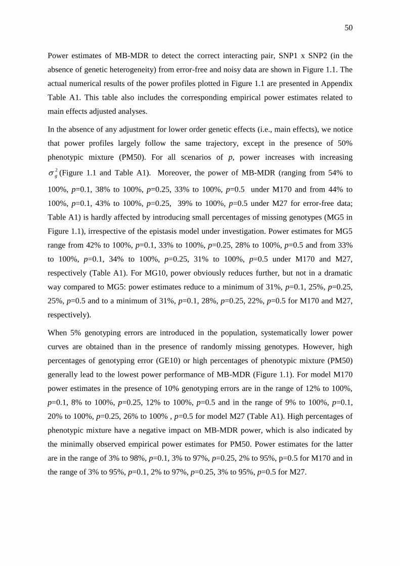
50

Power estimates of MB-MDR to detect the correct interacting pair, SNP1 x SNP2 (in the

absence of genetic heterogeneity) from error-free and noisy data are shown in Figure 1.1. The

actual numerical results of the power profiles plotted in Figure 1.1 are presented in Appendix

Table A1. This table also includes the corresponding empirical power estimates related to

main effects adjusted analyses.

In the absence of any adjustment for lower order genetic effects (i.e., main effects), we notice

that power profiles largely follow the same trajectory, except in the presence of 50%

phenotypic mixture (PM50). For all scenarios of p, power increases with increasing

2

g (Figure 1.1 and Table A1). Moreover, the power of MB-MDR (ranging from 54% to

100%, p=0.1, 38% to 100%, p=0.25, 33% to 100%, p=0.5 under M170 and from 44% to

100%, p=0.1, 43% to 100%, p=0.25, 39% to 100%, p=0.5 under M27 for error-free data;

Table A1) is hardly affected by introducing small percentages of missing genotypes (MG5 in

Figure 1.1), irrespective of the epistasis model under investigation. Power estimates for MG5

range from 42% to 100%, p=0.1, 33% to 100%, p=0.25, 28% to 100%, p=0.5 and from 33%

to 100%, p=0.1, 34% to 100%, p=0.25, 31% to 100%, p=0.5 under M170 and M27,

respectively (Table A1). For MG10, power obviously reduces further, but not in a dramatic

way compared to MG5: power estimates reduce to a minimum of 31%, p=0.1, 25%, p=0.25,

25%, p=0.5 and to a minimum of 31%, p=0.1, 28%, p=0.25, 22%, p=0.5 for M170 and M27,

respectively).

When 5% genotyping errors are introduced in the population, systematically lower power

curves are obtained than in the presence of randomly missing genotypes. However, high

percentages of genotyping error (GE10) or high percentages of phenotypic mixture (PM50)

generally lead to the lowest power performance of MB-MDR (Figure 1.1). For model M170

power estimates in the presence of 10% genotyping errors are in the range of 12% to 100%,

p=0.1, 8% to 100%, p=0.25, 12% to 100%, p=0.5 and in the range of 9% to 100%, p=0.1,

20% to 100%, p=0.25, 26% to 100% , p=0.5 for model M27 (Table A1). High percentages of

phenotypic mixture have a negative impact on MB-MDR power, which is also indicated by

the minimally observed empirical power estimates for PM50. Power estimates for the latter

are in the range of 3% to 98%, p=0.1, 3% to 97%, p=0.25, 2% to 95%, p=0.5 for M170 and in

the range of 3% to 95%, p=0.1, 2% to 97%, p=0.25, 3% to 95%, p=0.5 for M27.

51



induced simulation settings.

Legend Results are shown for MB-MDR analysis without main effects adjustment and

simulated scenarios other than GH.

52

Not surprisingly, there is a higher chance of identifying epistasis models for analyses without

main effects correction as compared to analyses that do account for lower-order effects. The

latter epistasis models usually involve other SNPs pairing with one of the functional SNPs

(results not shown) and should therefore be considered as false positives. Empirically

estimated false positive percentages, for a variety of scenarios, excluding GH settings, are

reported in Table A2 (―No Correction‖ versus ―Main Effects Correction‖ estimates). For

error-free data, and no adjustments for main effects, the false positive percentage of MB-

MDR of identifying a significant epistasis model not involving the actual functional pair of

SNPs ranges from 28% to 100%, p=0.1, 6% to 53%, p=0.25, 6% to 7%, p=0.5 for M170 and

from 15% to 99%, p=0.1, 26% to 100%, p=0.25, 38% to 100%, p=0.5 for M27. When main

effects are accounted for in error-free data, the false positive percentage ranges from 3% to

39%, p=0.1, 3% to 12%, p=0.25, 3% to 6%, p=0.5 under M170 and from 3% to 7%, p=0.1,

3% to 21%, p=0.25, 2% to 98%, p=0.5 under M27 (Table A2). In general, Table A2 shows

that irrespective of how the main effects adjustment is performed (using an additive or

codominant model) and irrespective of the type of noisiness introduced, false positive

percentages are typically lower than their ‖uncorrected‖ counterparts.

1.3.2 The impact of appropriately correcting an epistasis analysis for lower-order effects

Profiles for the empirical power estimates of MB-MDR to detect the correct two functional

loci from error-free data with (additive and codominant) main effects correction and without

main effects adjustment are plotted in Figure 1.2. Here, we observe that the power to identify

the correct causal pair is reduced when a main effects correction is performed, with the lowest

power levels obtained for codominant correction. The discrepancy between additive and

codominant main effects adjustment is particularly pronounced for M27 and p=0.5. For M170

and p=0.5, the nature of the lower-order effects adjustment has virtually no influence on

power. Power profiles for different sources of noise, according to main effects adjustment

method, are given in Figure A1-i (missing genotypes), Figure A1-ii (genotyping errors) and

Figure A1-iii (phenotypic mixture). The empirical power estimates used to generate Figures

A1 are also presented in Table A1. Here, drawing conclusions is more subtle, although

generally speaking, empirical power estimates are smaller with codominant correction as

opposed to additive correction.

53


correct interaction (SNP1 x SNP2) is significant at the 5% level, for error-free simulation

settings.

Legend No main effects adjustment (—), main effects adjustment via additive coding (…),

and codominant coding (---).

54

Numerical values on the effect of using different main effects adjustments on the false

positive percentage to identify incorrect two-locus models can be derived from Table A2. For

error-free data, the false positive percentages after additive main effects correction range from

5% to 39%, p=0.1, 5% to 12%, p=0.25, 3% to 6%, p=0.5 for M170 and from 4% to 7%,

p=0.1, 4% to 21%, p=0.25, 9% to 98%, p=0.5 for M27. Using codominant coding to adjust for

lower order effects, the false positive percentages range from 3% to 6%, p=0.1, 3% to 4%,

p=0.25 or p=0.5 for M170 and from 3% to 6%, p=0.1, 3% to 3%, p=0.25 and from 2% to 4%,

p=0.5 for M27. In fact, the practice of correcting an MB-MDR epistasis analysis using a

codominant main effects model has the tendency to be over-conservative (Table A2).

Genetic heterogeneity

So far, we have not yet discussed the performance of MB-MDR for quantitative traits in the

presence of genetic heterogeneity. Figure 1.3 shows empirical power curves to identify true

genetic interactions in the presence of GH in a variety of simulation settings. Results are

shown for MB-MDR analysis without main effects correction (Figure 1.3, row 1 for M170

and row 3 for M27) and with main effects correction (additive coding) adjustment (Figure 1.3,

row 2 for M170 and row 4 for M27). As in non-GH settings, power estimates are larger when

no correction for main effects is performed than when main effects are accounted for, with

generally the most severe power loss observed for codominant main effects correction.

However, when the contribution of main effects to the total genetic variance is ignored, false

positive percentages rise as well, ranging from 7% to 100% for M27 and from 4% to 97% for

M170. When we adjust for main effects (additive coding), power estimates to identify the first

pair (SNP1 x SNP2) drop to less than 50% for both M27 and M170, with the exception of

M170. For the latter, and a genetic variance of 0.1, MB-MDR power is estimated to be 95%

and 92% for p=0.25 and 0.5, respectively. Under a codominant correction, power estimates

drop to less than 7% for both models with the exception of p=0.25 or 0.5 and 2

g = 0.05 or

0.1. For the latter, power is estimated to be 15% and 26% for M170 and M27, respectively

when p=0.1 and 2

g =0.1. For M27, power=31%, p=0.25 and 2

g =0.1. For M170, p=0.25 or

0.5, power estimates are around 30% and 88% for 2

g =0.05 and 0.1, respectively. Detailed

information about empirical power estimates are given in Table A7.

55


correct interactions (SNP1 x SNP2) and/or (SNP3 x SNP4) are significant at the 5% level, in

the presence GH.

Legend First 2 rows: MB-MDR without and with main effects correction for model M170

respectively. Last 2 rows: MB-MDR without and with main effects correction for model M27

respectively. Main effects are corrected for via additive coding. Different definitions for

power are adopted: power to identify both interacting pairs SNP1 x SNP2 and SNP3 x SNP4

(cyan); power to identify SNP1 x SNP2 (black); power to identify SNP3 x SNP4 (magenta),

power to identify at least one of the interactive pairs (coral).

56

1.4 Discussion

Understanding the effects of genes on the development of complex diseases is a major aim of

genetic epidemiology. Several studies have indicated that MDR has good power to identify

gene-gene interactions in both simulated and real-life data [6]. Although MB-MDR has

profiled itself as a promising extension of MDR accommodating study designs that are more

complex than unrelated case-control settings [3, 9-11], a thorough investigation of its full

potential, under a variety of real-life distorting factors, such as missing genotypes, genotyping

errors, phenotypic mixtures and last but not least genetic heterogeneity, has never been carried

out in the context of quantitative traits.

This study has evaluated the power of MB-MDR for quantitative traits and unrelated

individuals, in identifying gene-gene interactions for two different epistasis models. Scenarios

with and without noisy data, as well as epistasis screening with and without lower-order

effects adjustments have been considered. Although our simulations only involved 10 SNPS,

conclusions about observed patterns largely remain the same when increasing the number of

genetic markers (e.g. empirical power results for non-GH settings without main effects

adjustment, Figure A2). Note that, an increasing number of SNPs will lead to an increasing

number of interacting pairs, resulting in an elevated multiple testing burden, and hence

resulting in reduced power.

A first important finding is that MB-MDR adequately deals with one of the most major

concerns in genetic association analysis studies (especially those targeting higher-order gene-

gene interactions), namely avoiding that the overall type I rate is out of control (Table 1.2).

The apparent slightly conservative results obtained when MB-MDR screening explicitly

accounts for lower-order main effects, are not surprising. Indeed, under the general null

hypothesis of no genetic association, adjusting for main effects involves over-fitting and

hence unnecessary over-correction. However, all the empirical estimates of the MB-MDR

type I error rate in Table 1.2 fall within the interval [0.025,0.075], satisfying Bradley‘s [12]

liberal criterion of robustness. This criterion requires that the type I error rates are controlled

for any level α of significance, if the empirical type I error rate ̂ is contained in the

interval 5.1ˆ5.0 . Note that we remark that, since MB-MDR assesses global

significance using resampling-based maxT adjusted p-values, the FWER will always be

weakly controlled at 5%, provided the assumptions of the Westfall and Young approach [13]

are attained.

57

A second important finding is that MB-MDR‘s power performance under different scenarios

can be largely explained by the quantification of the actual genetic variance 2

gen and by the

decomposition of the total genetic variance into contributions of main effects and epistasis,

and/or by the decomposition of main effects into additive and dominance variance. Empirical

decompositions based on classical variance components analysis of Sham [14], are reported in

Tables A3 for M170 and A4 for M27 in the absence of GH, and in Tables A5 in the presence

of GH. Each of these estimates is based on simulation setting‘s sample size (750 000

individuals). These results support our theoretically derived variance components, which are

summarized in Table A6.

In particular, the observed lowest power performances of non-GH settings for GE10 and

PM50 can be explained by the fact that over-representation of the minor allele as well as

introducing phenotypic mixture result in a loss of actual genetic variance (Table 1.1) and

therefore a loss of power. The theoretical results, indicating that a 50% reduction in total

genetic variability is established when 50% phenotypic mixture is introduced in error-free

data (Table 1.1) are supported by our empirical results (e.g., Tables A3 for M170 and A4 for

M27, comparing 2

gen with 2

g .

When 50% genetic heterogeneity is present, theory supports our empirical results in that the

total actual genetic variance due to the two causal pairs of markers is twice the total actual

genetic variance due to a single pair (Tables A5). Moreover, since we have introduced two

possible genetic routes for an individual to be genetically predisposed for the trait of interest

under GH (route 1 via SNP1 x SNP2 or route 2 via SNP3 x SNP4), the actual genetic variance

in the pooled data will be half the genetic variance in the error-free data (see also Tables A5-ii

for M170 and A5-iv for M27). The total genetic variance due to a single causal pair

approximates 42

g (Table A5-i and A5-iii), which is due to the fact that the 2 pairs have the

same minor allele frequencies. Therefore, the theoretical genetic variance is split between the

two pairs and thereafter between the 2 SNPs. MB-MDR was shown to be rather robust in the

presence of missing genotypes and genotyping error. Note that MB-MDR that MB-MDR

handles missing genotypes by using all available cases for the SNP pair under investigation.

Hence, no individuals with missing data are a priori removed from the analysis, except when

functional SNPs that are adjusted for in regression models have (partially) missing

information.

58

A third finding is that accounting for important lower-order genetic effects in epistasis

screening should be made standard. There is a debate about how to best model and test for

both main effects and interactions or for interactions only when epistasis is present [15].

Although a fully non-parametric screening approach (e.g., such as MDR) is beautiful in that it

does not require specifying particular genetic models, there is still a need to adjust for lower-

order genetic effects via a parametric paradigm when targeting significant gene-gene

interaction models. The Model-Based MDR (MB-MDR) offers a flexible framework to make

these adjustments. For MDR-like applications other than MB-MDR this is far from obvious.

For instance, MDR for binary traits, Ritchie et al. [6] does not accommodate taking corrective

measures for lower order effects. Although significant main effects can be filtered out prior to

an MDR screening, this happens at the cost of missing out on genuinely true interactions.

Furthermore, examining the decomposition of the total genetic variance has shed more light

on the scenarios in which an adjusted MB-MDR analysis is warranted. For instance, when the

minor allele frequency of the causal loci is 0.5, model M170 is a pure epistatic model (Table

A3: empirical estimates 22

genepi approximate 1). Hence in this scenario the effects of

correcting for main effects are taken to the extreme. Clearly, any correction for lower-order

effects would be an over-correction. On the other hand, since there is no true evidence for

main effects in this model, any adjustment for main effects will only remove a small portion

of the variability (Table A3: M170, p=0.5; empirical estimates of 22

genmain are close to

zero), resulting in false positives for the corrective analysis that are similar to those for the un-

corrective analysis (Table S2: M170, p=0.5; empirical estimates close to 5% also when not

adjusting for main effects). In effect, the contribution of main effects becomes increasingly

important with increasing p for M27 (≈32%, p=0.1, ≈61%, p=0.25 and ≈85%, p=0.5) and the

reverse holds for M170 (≈59%, p=0.1, ≈11%, p=0.25 and ≈0%, p=0.5) (Table A3, A4 and

Table A6).

For model M170 and GH scenarios involving p either 0.25 or 0.5 for the causal pairs, the

epistatic variance explains a relatively large proportion of the total genetic variance in the data

(22

genepi >87%; Table A5-ii), and correcting for main effects therefore has little effect on

power. In contrast, for Model M170 and p=0.1 for the causal pairs, main effects do make an

important contribution to the total genetic variance (22

genmain > 57%; Table A5-i and Table

A5-ii) compared to epistasis effects, which translates into a severe empirical power loss and

59

power is dramatically reduced when proper accountancy for lower order effects is being made

(Figure 1.3).

Summarizing, dealing with phenotypic mixtures and genetic heterogeneity will remain

challenging for epistasis screening methods, for some time to come. Our empirical results

suggest that more work is needed to better accommodate these particularities. Benefits may

be gained from identifying the trait-specific factors (genetic or non-genetic) that best

characterize mixed phenotypic populations. For genetic heterogeneity, the genes in which the

loci are present can be part of different etiological pathways leading to the same disease or be

part of the same pathway. According to Heidema et al. [16], irrespective of the biological

mechanism that gives rise to genetic heterogeneity, the association of the loci with the disease

will be reduced if the total sample is used for measuring the association, as was done in this

study. A method that is not robust in the presence of genetic heterogeneity will most likely

suffer from a decrease in power to detect genetic effects. As our main effects corrective

analyses have suggested, a way forward may be to use methods to identify the latent classes

and to adapt the epistasis screening accordingly.

Finally, any epistasis screening should properly account for lower-order effects in order to be

able to claim that an identified interaction involves a significant epistatic contribution to the

total genetic variance.

60

References

1. Ritchie MD, Hahn LW, Roodi N, B-ailey LR, Dupont WD, Parl FF, Moore JH:

Multifactor-dimensionality reduction reveals high-order interactions among

estrogen-metabolism genes in sporadic breast cancer. Am J Hum Genet 2001,

69:138-147.




80:1125-1137.




Individuals. PLoS One 2010, 5:e10304.

4. Broman K, Heath, SC: Managing and Manipulating Genetic Data, in Bioinformatics

for Geneticists: A Bioinformatics Primer for the Analysis of Genetic Data, Second

Edition (ed M. R. Barnes). John Wiley & Sons, Ltd, Chichester, UK; 2007.





6. Ritchie MD, Hahn LW, Moore JH: Power of multifactor dimensionality reduction

for detecting gene-gene interactions in the presence of genotyping error, missing

data, phenocopy, and genetic heterogeneity. Genet Epidemiol 2003, 24:150-157.

7. Akey JM, Zhang K, Xiong M, Doris P, Jin L: The effect that genotyping errors

have on the robustness of common linkage-disequilibrium measures. Am J Hum

Genet 2001, 68:1447-1456.

8. Evans DM, Marchini J, Morris AP, Cardon LR: Two-Stage Two-Locus Models in

Genome-Wide Association. PLoS Genet 2006, 2:e157.



data. Department of Systems Biology, UoV 2008a,



61



in Medicine 2008b, 27:6532-6546.

11. Mahachie John JM, Baurecht H, Rodriguez E, Naumann A, Wagenpfeil S, Klopp N,

Mempel M, Novak N, Bieber T, Wichmann HE, et al: Analysis of the high affinity

IgE receptor genes reveals epistatic effects of FCER1A variants on eczema risk.

Allergy 2010, 65:875-882.

12. Bradley JV: Robustness? British Journal of Mathematical and Statistical Psychology

1978, 31:144-152.




15. Verhoeven KJF, Casella G, McIntyre LM: Epistasis: Obstacle or Advantage for

Mapping Complex Traits? PLoS ONE 2010, 5:e12264.

16. Heidema AG, Boer J, Nagelkerke N, Mariman E, van der A D, Feskens E: The

challenge for genetic epidemiologists: how to analyze large numbers of SNPs in

relation to complex diseases. BMC Genetics 2006, 7:23.

Related publication

Jestinah M. Mahachie John, Tom Cattaert, François Van Lishout,

Elena S. Gusareva, Kristel Van Steen (2012) PLoS ONE 7(1): e29594. doi:10.1371/journal.pone.0029594

Chapter 2

Lower-order Effects Adjustment in Quantitative Traits Model-Based

Multifactor Dimensionality Reduction

63

Abstract

Identifying gene-gene interactions or gene-environment interactions in studies of human

complex diseases remains a big challenge in genetic epidemiology. An additional challenge,

often forgotten, is to account for important lower-order genetic effects during this process.

These may hamper the identification of genuine epistasis. If lower-order genetic effects

contribute to the genetic variance of a trait, identified statistical interactions may simply be

due to a signal boost of these effects. Via simulations, we assess the performance of different

corrective measures for lower-order genetic effects in Model-Based Multifactor

Dimensionality Reduction epistasis detection, using additive and codominant coding schemes.

Performance is evaluated in terms of power and family-wise error rate. Our simulations

indicate that empirical power estimates are reduced with correction of lower-order effects,

likewise family-wise error rates. Easy-to-use automatic SNP selection procedures, SNP

selection based on ―top‖ findings, or SNP selection based on p-value criterion for interesting

main effects result in reduced power but also almost zero false positive rates. Always

accounting for main effects in the SNP-SNP pair under investigation during Model-Based

Multifactor Dimensionality Reduction analysis adequately controls false positive epistasis

findings. This is particularly true when adopting a codominant corrective coding scheme. In

conclusion, automatic search procedures to identify lower-order effects to correct for during

epistasis screening should be avoided. The same is true for procedures that adjust for lower-

order effects prior to Model-Based Multifactor Dimensionality Reduction and involve using

residuals as the new trait. We advocate using ―on-the-fly‖ lower-order effects adjusting when

screening for SNP-SNP interactions using Model-Based Multifactor Dimensionality

Reduction analysis.

64

2.1 Introduction

Complex diseases commonly occur in a population and are a major source of discomfort,

disability and death worldwide. They are believed to arise from multiple predisposing factors,

both genetic and non-genetic, each factor potentially having a modifying effect on the other.

Detecting gene-gene interactions or epistasis in studies of human complex diseases is a big

challenge in genetic epidemiology. An additional challenge is to account for important lower-

order genetic effects in order to reduce false positive epistasis results.

To date, several strategies are available, within the context of genetic association studies that

specifically aim to identify and characterize gene-gene interactions. Among these strategies is

the Model-Based Multifactor Dimensionality Reduction (MB-MDR) which was first

introduced by Calle et al. [1]. The strategy of MB-MDR to tackle the dimensionality problem

in interaction detection involves reducing a potentially high dimensional problem to a one-

dimensional problem by pooling multi-locus genotypes into three groups based on association

testing or modeling (PART 1, Figure 1.4). It has been suggested that Model-Based

Multifactor Dimensionality Reduction is a useful method for identifying gene-gene

interactions in case-control or family-based design for both dichotomous and quantitative

traits [1-6]. Although a power study of MB-MDR detection with and without main effects

adjustment has been performed before by Cattaert et al. [3] and Mahachie et al. [6], these

studies only involved adjusting for the known functional SNPs contributing to an epistasis

effect. The preliminary results these studies gave rise to, emphasized the importance of lower-

order effects adjustment when searching for gene-gene interactions and warranted a more

detailed investigation, which is the topic of this chapter.

In this study, we perform a thorough simulation-based investigation of the power of

quantitative trait MB-MDR to identify gene-gene interactions, using different strategies to

adjust for lower-order genetic effects that may or not be part of the (functional) SNP-SNP

interaction under investigation. Performance criteria used are power and family-wise error

rate. We perform MB-MDR epistasis analyses first without any adjustment for main effects

and then with adjustments using several strategies. The proposed main effects corrections can

be grouped into two categories: 1) main effects screening followed by MB-MDR applied to

an adjusted trait and 2) main effect adjustment integrated in step 1 and step 2 of MB-MDR

(PART 1, Figure 1.4). These are depicted in Figure 2.1 and described in more detail in the

methods section.

65

Figure 2. 1 Different approaches to adjust for lower-order effects in MB-MDR epistasis

screening.

66


2.2.1 Strategies to adjust for lower-order genetic effects

Several methods exist to correct for lower-order effects in the context of quantitative MB-

MDR epistasis screening. An overview of the considered methods in this study is given in

Figure 2.1. A first strategy is to extensively look for potentially confounding main effects, to

transform the original trait to an adjusted trait accordingly, and to submit this newly defined

trait to MB-MDR for epistasis screening.

When correcting for main effects, a note about how to best code lower-order effects is

warranted. In a GWA study, SNPs are often coded in an additive way [7]. This coding works

well in practice, although power can be gained by acknowledging the true underlying genetic

models [8]. For instance, if the two homozygote genotypes at a locus exhibit the same risk,

different from the heterozygote risk (over-dominance), then the additive coding will have

reduced power irrespective of the sample size [9]. Alternatively, several coding schemes may

be investigated and a maximum statistic over screened main effects models may be selected

[10]. The differing unknown operating modes of inheritance throughout the genome make it

hard to flexibly and automatically acknowledge this complex inheritance spectrum.

Therefore, the route chosen in this paper, now in an epistasis context is to correct for main

effects by either assuming an additive or a codominant coding scheme, in scenarios that

involve different contributions of additive and dominance variance to main effects variance.

Although some of these scenarios may be better captured by non-additive and non-

codominant codings, the interest is in finding an all-purpose acceptable (in terms of power

and type I error) way to remove the main effects signals influencing epistasis signals.

Choosing between additive and codominant coding schemes implies choosing between the

least and most severe such removal of effects.

2.2.1.1 Main effects screening prior to MB-MDR

This screening procedure involves first adjusting for a chosen subset of main effects via

parametric (linear) regression models and then considering residuals from the fitted models as

a new trait for MB-MDR. For the adjustment methods involving significance assessments, we

remark that whenever none of the SNPs are significant, the original trait is submitted to MB-

MDR.

67

Single (univariate) regression-based searches

Important main effects can be identified via single-SNP regression models, as is done in a

classical GWA setting. Hence, SNPs that meet a stringent criterion (such as governed by a

Bonferroni criterion) will be labelled as ―important‖ and are therefore good candidates to

correct for in an epistasis screening. In this study, we prefer to take a less conservative route,

such as a selection based on step-down maxT adjusted p-values with 999 replicates (Figure

2.1; SRperm). However, targeting effects standing out in a GWA main effects screening while

maintaining overall type I error is quite different from targeting main effects to adjust for in

an epistasis screening. Therefore, we also consider selecting ―optimal‖ SNPs for main effects

correction in the quantitative MB-MDR screening on the basis of their significance without

correction for multiple testing (Figure 2.1; SR0.05) or on the basis of a ranking of the

corresponding raw p-values (Figure 2.1; SRtop5, SRtop10, SRtop15).

Multiple regression-based searches

Due to a large number of SNPs that are involved in a main effects genome-wide analysis,

multiple regression-based searches are often automated. One such automated approach uses

stepwise selection based on AIC (stepAIC in R package MASS, R 2.10.0). This procedure

iteratively adds and/or drops variables to seek the lowest AIC score. The final model

generates the list of main effects to correct for in the quantitative trait MB-MDR analysis

(Figure 2.1; MRAIC).

2.2.1.2 Main effects adjustment as an integral part of MB-MDR

In this scenario, main effects are adjusted for ―on-the-fly‖, i.e. SNPs are adjusted for during

the first 2 MB-MDR epistasis screening steps. Three types of adjustment are considered. A

first type is to always adjust for the SNPs in the pair under investigation (Figure 2.1; MB-

MDRadjust). Hence, the adjustment is done irrespective of whether a main effect is truly

present. A second type is to only adjust for SNPs that are identified by MB-MDR1D as

significant. Here, MB-MDR1D is run first and a list of genome-wide significant SNPs is

identified (based on step-down maxT with 999 permutation replicates). MB-MDR epistasis

screening is then performed while only adjusting for the identified SNPs for the pair under

investigation (Figure 2.1; MB-MDR1D). A third type is to only adjust for significant SNPs

obtained via single regression models and maxT significance assessment (Figure 2.1; MB-

68

MDRlist). Thus, for MB-MDR1D and MB-MDRlist, any of the following 3 situations can arise:

a) None of the 2 SNPs is significant and no correction is performed b) One of the 2 SNPs is

significant and this is adjusted for c) Both SNPS are significant and both SNPs are adjusted

for.

In order to account for potentially important SNPs as an integral part of MB-MDR, we remark

that the Student‘s t-test in MB-MDR steps 1-2 (PART 1, Figure 1.4) is replaced by the Wald

test for the interaction effect in a regression framework.


Simulated data as generated in Mahachie John et al. [6] are based on two epistasis models

for SNP1 and SNP2 that incorporate varying degrees of epistasis: Model M27 and Model

M170 of Evans et al. [11]. In order to increase the phenotypic mean, M27 requires an

individual to have at least one copy of the minor allele at both loci whereas M170 requires an

individual to be heterozygous at one locus and homozygous at the other. The phenotypic

means for the aforementioned epistasis models only take two values, µL (Low phenotypic

mean) and µH (High phenotypic mean). The total phenotypic variance2

tot , i.e. the sum of

genetic variance at both loci 22

12 main (the minor allele frequencies for the functional

SNPs are taken to be the same), epistasis variance2

epi , and environmental variance2

env , is

fixed at 1. SNP1 and SNP2 have minor allele frequency equal to p, with p one

of 0.5} 0.25, {0.1, . The minor allele frequencies of the other 98 markers are generated from a

random uniform distribution, U(0.05,0.5). MB-MDR screening is performed on 100 SNPs in

Hardy-Weinberg Equilibrium and linkage equilibrium. The total genetic variance 2

g is

varied as 0.1} 0.05, 0.03, 0.02, {0.01,2 g . The main effects variance 2

main consists of

additive variance 2

add and dominance variance 2

dom . As p increases, the contribution to the

total genetic variance of epistasis variance relative to main effects variance increases for

M170 and decreases for M27, and also the contributions of additive and dominance variance

to the total main effects variance change with p (Table 2.1).

69

Table 2. 1 Theoretically derived proportions of the genetic variance due to main effects

(additive and dominance) or epistasis.

Model p σ2main/ σ

2gen

σ2

add/ σ2main

σ2

dom/ σ2main

σ2

epi/ σ2

gen

0.1 0.319 0.947 0.053 0.681

M27 0.25 0.609 0.857 0.143 0.391

0.5 0.857 0.667 0.333 0.143

0.1 0.581 0.780 0.220 0.419

M170 0.25 0.118 0.400 0.600 0.882

0.5 0.000 0.947 0.053 1.000

For SNP3 and SNP4, main effects are imposed with associated variances 2

3 and 2

4 ,

selected from a uniform distribution U(0, 0.06) such that the total main effects variance of the

4 loci (SNP1, SNP2, SNP3, SNP4) is 2222 2 431main . The respective modes of

inheritance for SNP3 and SNP4 are additive and advantageous heterozygous. Note that SNP4

will therefore contribute to both the additive and dominance components of the main effects

variance. This scenario allows us to investigate the effect of global main effects correction

approaches for functional SNPs that are not part of a two-locus interaction.

In addition data are simulated under the null model for the functional pair (i.e. 02 g ) in two

ways, giving rise to two null hypotheses H01 and H02. H01: No genetic contribution apart from

SNP3 and SNP4 as main effects and H02: any genetic contribution from any of the SNPs

whatsoever.

In summary, a total of 36 simulation settings are considered. For each parameter setting, we

consider 500 simulation replicates, involving 2000 unrelated individuals.

70

2.3 Results

2.3.1 Familywise error rates and false positive rates

Table 2.2 shows results for settings simulated under the null hypotheses H01 and H02 of no

genetic associations with the trait, yet in the presence or absence of additional main effects

(SNP3 and SNP4).

We observe that MB-MDR type I error percentages are close to the nominal type I error rate

of 5%, when no correction for main effects is performed under settings where no additional

main effects act on the quantitative trait. Type I error rates are also kept under control when

correction for main effects is integrated in MB-MDR epistasis screening as well as prior to

MB-MDR for permutation based regression-based approach (MB-MDRadjust, MD-MDR1D,

MB-MDRlist and SRperm, respectively). In particular, additive correction under H02 and

codominant correction for both H01 and H02. When additional main effects are present in the

data, adjusting for their effects using additive correction give rise to inflated type I error rates

ranging from 55 to 74%. In contrast, when adopting a codominant correction, type I error is

under control for MRAIC, and single regression-based correction methods (except SRperm)

which are extremely conservative (Table 2.2: type I error rates are close to zero).

71

Table 2. 2 Type I error percentages for data generated under the null hypothesis of no genetic

association of the interacting pair.

Without correction and additional main effects

P present absent

0.1 0.982 0.046

0.25 No correction 0.984 0.050

0.5 0.982 0.050

With Correction and additional main effects

Way of

Correction Additive Codominant

present absent present absent

0.1 0.676 0.048 0.040 0.052

0.25 MB-MDRadjust 0.710 0.034 0.054 0.038

0.5 0.740 0.044 0.036 0.050

0.1 0.676 0.036 0.058 0.030

0.25 MB-MDR1D 0.722 0.040 0.042 0.036

0.5 0.746 0.040 0.038 0.030

0.1 0.682 0.038 0.056 0.030

0.25 MB-MDRlist 0.726 0.036 0.044 0.032

0.5 0.748 0.046 0.040 0.032

0.1 0.628 0.038 0.048 0.030

0.25 SRperm 0.660 0.036 0.058 0.030

0.5 0.678 0.046 0.044 0.032

0.1 0.576 0.014 0.006 0.010

0.25 SR0.05 0.604 0.006 0.012 0.000

0.5 0.636 0.022 0.008 0.008

0.1 0.552 0.008 0.000 0.002

0.25 MRAIC 0.578 0.004 0.002 0.000

0.5 0.616 0.012 0.000 0.006

0.1 0.582 0.014 0.008 0.008

0.25 SRtop5 0.616 0.002 0.020 0.000

0.5 0.638 0.026 0.010 0.010

0.1 0.560 0.012 0.000 0.008

0.25 SRtop10 0.592 0.006 0.004 0.000

0.5 0.626 0.022 0.006 0.006

0.1 0.556 0.010 0.000 0.006

0.25 SRtop15 0.588 0.006 0.002 0.000

0.5 0.618 0.016 0.004 0.006

Results are for scenarios: with and without additional main effects (SNP3 and SNP4) contributing to

the genetic variance. In bold are values within Bradley‘s liberal criterion of robustness.

72

False positive rate estimates generated by MB-MDR (i.e. referring to scenarios for which one

or more significantly interacting pairs other than the causal SNP pair (SNP1, SNP2)) using no

correction or an additive or codominant correction of main effects, are shown in Figure 2.2.

When no correction is performed, false positive rate estimates are around 100% under both

M170 and M27 genetic epistasis models. In general, for additive correction false positive rate

estimates range from 53 to 100% whereas for codominant correction, false positive rate

estimates are lower and range from 0 to 19%. In particular, false positive rates for MB-

MDRadjust (always adjusting for main effects SNPs) in a codominant way range from 4 to 7%,

rates that are within the interval (0.025, 0.075), satisfying Bradley‘s [12] liberal criterion of

robustness. This criterion requires that the type I error rates are controlled for any level α of

significance, if the empirical type I error rate ̂ is contained in the interval 5.1ˆ5.0 .

For MB-MDR1D and MB-MDRlist, false positive rates are not kept under control. The actual

numerical results of the false positive profiles plotted in Figure 2.2 are presented in the

Appendix Table A8 for M170 and Table A9 for M27.

73

Figure 2. 2 False positive percentages of MB-MDR based on additive (A) and co-dominant (B) correction.

Legend False positive percentage is defined as the proportion of simulation samples for which pairs other than the causal pair (SNP1, SNP2) are

significant

74

The main reason why we observe higher false positive rates under additive correction is due

to the fact that SNP4 contributes to both an additive and dominance component of the main

effects variance. Hence, there is also a higher chance of identifying ‗significant‘ interactions

for pairs involving SNP4. False positive rates are reduced when co-dominant correction is

performed. Table 2.3 shows observed false positive rates that involve pairing with SNP3

and/or SNP4 under additive and co-dominant correction. Only MB-MDRadjust (―on-the-fly‖

adjustment) results are shown. From Table 2.3, 2

g >0, we observe that under additive

codings, false positive rates range from 51 to 61% for interactions between SNP3 and SNP4.

However, for interactions with SNP3 (excluding SNP3, SNP4 interaction), false positive rates

range from 0 to 6%, except for Model 27, p=0.5 and 2

g of 0.05 and 0.1 where false positive

rates are 27 and 92%, respectively. As observed in Table 2.1, model M27, p=0.5 has the

highest relative contribution of dominance variance, hence, additive correction does not fully

account for SNP1 and SNP2.

75

Table 2. 3 False positive percentages of MB-MDRadjust involving SNP3 and/or SNP4.

False positive percentages shown are for identifying interaction between SNP3 and SNP4 and or

interactions between SNP3 or SNP4 and at least one other SNP for null data scenario under H01 and

for models M170 and M27.

Additive Codominant

p 2

g SNP3_

anyother

thanSNP4 SNP3_SNP4

SNP4_

anyother

thanSNP3

SNP3_

anyother

thanSNP4 SNP3_SNP4

SNP4_

anyother

thanSNP3

0.1

0.002 0.520 0.660 0.000 0.000 0.000

H01 0.25 0 0.000 0.556 0.688 0.000 0.000 0.000

0.5

0.002 0.608 0.722 0.004 0.000 0.002

0.01 0.002 0.584 0.704 0.004 0.000 0.000

0.02 0.008 0.582 0.724 0.002 0.000 0.000

0.1 0.03 0.000 0.572 0.690 0.000 0.000 0.000

0.05 0.008 0.534 0.676 0.002 0.000 0.000

0.1 0.072 0.540 0.752 0.000 0.000 0.000

0.01 0.002 0.598 0.714 0.000 0.000 0.004

0.02 0.000 0.558 0.712 0.002 0.000 0.002

M170 0.25 0.03 0.000 0.544 0.686 0.000 0.000 0.000

0.05 0.004 0.536 0.706 0.002 0.000 0.000

0.1 0.032 0.566 0.738 0.000 0.000 0.000

0.01 0.000 0.526 0.664 0.000 0.000 0.002

0.02 0.000 0.588 0.708 0.000 0.000 0.002

0.5 0.03 0.002 0.544 0.692 0.002 0.000 0.002

0.05 0.002 0.550 0.666 0.000 0.000 0.000

0.1 0.002 0.528 0.662 0.002 0.000 0.000

0.01 0.002 0.532 0.662 0.000 0.000 0.000

0.02 0.000 0.564 0.690 0.000 0.000 0.000

0.1 0.03 0.000 0.554 0.680 0.002 0.000 0.000

0.05 0.000 0.562 0.704 0.002 0.000 0.000

0.1 0.000 0.518 0.638 0.000 0.000 0.000

0.01 0.002 0.512 0.652 0.000 0.000 0.002

0.02 0.004 0.520 0.682 0.004 0.000 0.000

M27 0.25 0.03 0.000 0.562 0.700 0.002 0.000 0.000

0.05 0.000 0.546 0.700 0.000 0.000 0.002

0.1 0.042 0.564 0.734 0.002 0.000 0.000

0.01 0.000 0.546 0.672 0.000 0.000 0.002

0.02 0.020 0.508 0.684 0.000 0.000 0.000

0.5 0.03 0.060 0.518 0.706 0.000 0.000 0.002

0.05 0.272 0.536 0.806 0.000 0.000 0.000

0.1 0.912 0.590 0.974 0.000 0.000 0.000

76

2.3.2 Empirical power estimates

Power profiles of MB-MDR to detect the correct interacting pair (SNP1, SNP2) without and

with different ways of adjustment of main effects are shown in Figure 2.3. Empirical power

estimates are presented as Supplementary information (Table A8 for M170 and Table A9 for

M27). In this section, we focus on scenarios where there is some remarkable degree of main

effects contributing to the genetic variance (M170: p=0.1, M27: p=0.25 and 0.5). For a

detailed view on variance decomposition into main and epistatic effects, we refer to Sham

[13]. Under the aforementioned scenarios, the profile for no correction always has the highest

power.

Under M170, the empirical power estimates for this profile range from 33 to 100% for p=0.1.

Under M27, the power estimates range from 27 to 100% and from 15 to 100%, for p=0.25 and

0.5 respectively. Irrespective of whether main effects are corrected for using additive or

codominant coding, profiles for the considered multiple-regression, MRAIC and single

regression-based methods that do not involve multiple testing (SR0.05, SRtop5, SRtop10 and

SRtop15) tend to follow the same trajectory, giving rise to the lowest empirical power

estimates. With additive adjustments, empirical power estimates for these corrective ways

range from 0 to 100% for both models M27 and M170. With codominant adjustments, power

estimates range from 0 to 94% , for M170, p=0.1, from 0 to 100% and from 0 to 18%, for

model M27, p=0.25 and p=0.5 respectively. Estimates for MB-MDRadjust (corrective methods

that are integrated as part of MB-MDR) , range from 6 to 100% for M170, p=0.1, from 3 to

100% for M27 with p=0.25 and from 1 to 100% for M27 with p=0.5, when additive

corrections are performed. Under codominant corrections the estimates range from 4 to 100%

for M170 (p=0.1) and from 4 to 100% or from 0 to 68% for M27 (p=0.25 and p=0.5

respectively).

77

Figure 2. 3 Power to identify SNP1, SNP2, as significant for additive (A) and codominant (B) correction.

78

2.4 Discussion

The identification of genetic susceptibility loci for human complex diseases has been rather

successful due to the ability to combine different genome-wide association studies via meta-

analyses. In the quest for the missing heritability, genome-wide association interaction studies

have become increasingly popular and the field shows a boost in methodological

developments [14]. When lower-order effects are not appropriately accounted for in epistasis

screening, derived results may not be trustworthy and conclusions about genuine epistasis

may be ungrounded.

Indeed, the challenge is to find epistasis effects above and beyond singular marker

contributing effects, should there be any. In this work, we investigated the power of MB-

MDR for quantitative traits and unrelated individuals, while targeting gene–gene interactions

accounting for potential main effects.

As was already observed in Mahachie John et al. [6], MB-MDR adequately controls type I

rate at 5% when no association is present (null data). Under additive corrections, type I error

and false positive rates are high irrespective of the adjustment method considered but

controlled under codominant corrections. This is due to the existence of SNP4, which was

simulated with both additive and dominance effects (advantageous heterozygous). Hence,

additive adjustment does not fully remove the effect of SNP4. As shown before in Table 2.3,

the consequence is that a number of SNPs appear to be significantly interacting with SNP4.

Not surprisingly, this occurs more often under additive correction compared to codominant

correction. This is because when we correct for main effects using the codominant model, we

remove all the effect of SNP4, and hence false positive results are only by chance (5%

nominal error rate). When no main effects adjustment is implemented, MB-MDR gives even

higher false positive rate rates.

Lower power profiles under codominant corrections in Figure 2.3 are explained by the

different contributions of additive and dominance effects to the total main effects variance as

already shown in Table 2.1. When there is a remarkable contribution of dominance effect, as

mentioned before, additive coding does not fully remove main effect contribution of the

interacting SNPs. For instance, under M27, when the contribution of main effects is

maximum (p=0.5), almost 33% of the main effects variance is dominance, hence a huge

difference in the power profiles between additive and codominant codings.

79

Interestingly, easy-to-use automatic subset selection procedures (MRAIC) and single

regression-based identification of important main effects prior to MB-MDR screening result

in lower power and almost zero false positive rates. Often, a list of top SNPs is generated to

derive disease genetic risk scores. Some of these SNPs may reach user-defined significance,

some may even reach genome-wide significance and some may not be significant at all.

Hence, correcting for SNPs in such a list (e.g. top5, 10, 15) may remove more of the trait‘s

variability than is really necessary, especially when correction for multiple testing is not

performed. Note that we considered a minimum of 5 top findings since at least 4 SNPs were

allowed to contribute to the main effects variance.

In order to attain sufficient power, any main effects corrective method that leads to an over-

correction during epistasis screening should be avoided. All considered residual-based

approaches (MRAIC, SR0.05, SRperm, SRtop5, SRtop10, SRtop15) led to uncontrolled false positive

rates. This can be explained by either the way the residuals were obtained (inappropriate

main effects coding) or by the non-exhaustive list of markers considered in the residual

computation.

Only codominantly correcting for significant SNPs as integral part of MB-MDR screening

perform much better. However, the poor performance of MB-MDR1D and MB-MDRlist and

the excellent performance of MB-MDRadjust in terms of controlling false positive epistasis

rates support the intuition that it (only) matters to correct for those SNPs that are involved in

the SNP pair under investigation, when no other SNPs are expected to modify the effect of

that pair.

The aforementioned discussion clearly raises questions about how to best correct for lower-

order effects when higher-order (>2) interactions are targeted. In either case, to aid in

interpretation of results, it is always a good practice to assess the joint information of clusters

of SNPs that contribute to the trait variability [15].

Finally, we emphasize that most statistical epistasis detection methods can be decomposed

into a core component and a multiple testing correction component. Keeping the core

component, but using a more refined multiple testing correction can generally enhance its

performance. For instance, assumptions underlying the maxT procedure of Westfall and

Young [16] that is implemented in MB-MDR are likely to be violated for MB-MDR1D and

MB-MDRlist. Indeed, the null and the alternative hypotheses per pair of SNPs under

investigation are no longer the same for all interaction tests.

80

In conclusion, rather than adjusting for lower-order effects prior to MB-MDR and using

residuals as the new trait, or adjusting only for significant SNP(s), we advocate an ―on-the-

fly‖ main effects adjustment (MB-MDRadjust). This type of adjustment only removes potential

main effects contributions in the pair under investigation but keeps the null and alternative

hypotheses similar from one pair of SNPs to another. We have shown that the commonly used

additive coding in the ―on-the-fly‖ adjustment (MB-MDRadjust) is not sufficient and leads to

overly optimistic results and that codominant adjustments are to be preferred. This will

ensure an acceptable balance between type I error and power to identify the interactions.

Realistic settings often involve both additive and dominance genetic effects to the trait under

investigation. Equivalent to our codominant coding, a perhaps biologically more meaningful

coding involves introducing 2 variables X1 and X2 with values -1, 0, 1 and -1/2, 1/2, -1/2,

respectively, for homogenous wild type, heterozygote and homozygote mutant genotypes. In

such a coding scheme, both additive and dominant scales are represented. This 2-parameter

coding is statistically attractive since it is invariant to allele coding (i.e. whether coding

homogenous wild type as 1 or homozygote mutant genotypes as 1 for X1) [17]. The utility of

the aforementioned coding as a way to adjust for lower-order effects in MB-MDR higher-

order epistasis screening will be the subject of future research.

81

References



data. Department of Systems Biology, University of Vic, Spain website 2008a,




in Medicine 2008b, 27:6532-6546.








Allergy 2010, 65:875-882.




Genetics 2011, 75:78-89.




7. Gauderman WJ, Thomas DC, Murcray CE, Conti D, Li D, Lewinger JP: Efficient

Genome-Wide Association Testing of Gene-Environment Interaction in Case-

Parent Trios. American Journal of Epidemiology 2010, 172:116-122.

8. Slager SL, Schaid DJ: Case-Control Studies of Genetic Markers: Power and

Sample Size Approximations for Armitage’s Test for Trend. Human Heredity

2001, 52:149-153.

9. Balding DJ: A tutorial on statistical methods for population association studies.

Nat Rev Genet 2006, 7:781-791.

82

10. Hothorn LA, Hothorn T: Order-restricted Scores Test for the Evaluation of

Population-based Case–control Studies when the Genetic Model is Unknown.

Biometrical Journal 2009, 51:659-669.




1978, 31:144-152.



14. Van Steen K: Travelling the world of gene–gene interactions. Briefings in


15. Chanda P, Zhang A, Brazeau D, Sucheston L, Freudenheim JL, Ambrosone C,

Ramanathan M: Information-Theoretic Metrics for Visualizing Gene-

Environment Interactions. American journal of human genetics 2007, 81:939-963.


17. Ma S, Yang L, Romero R, Cui Y: Varying coefficient model for gene-environment

interaction: a non-linear look. Bioinformatics 2011.

Related publication

Jestinah M. Mahachie John, François Van Lishout,

Elena S. Gusareva, Kristel Van Steen (2012) Under Revision

Chapter 3

A Robustness Study of Parametric and Non-parametric Tests in Model-

Based Multifactor Dimensionality Reduction for Epistasis Detection

84

Abstract

Applying a statistical method implies identifying underlying (model) assumptions and

checking their validity in the particular context. One of these contexts is association modeling

for epistasis detection. Here, depending on the technique used, violation of model

assumptions may result in increased type I error, power loss, or biased parameter estimates.

Remedial measures for violated underlying conditions or assumptions include data

transformation or selecting a more relaxed modeling or testing strategy. Model-Based

Multifactor Dimensionality Reduction (MB-MDR) for epistasis detection relies on association

testing between a trait and a factor consisting of multilocus genotype information. For

quantitative traits, the framework is essentially ANalysis Of VAriance (ANOVA) that

decomposes the variability in the trait amongst the different factors. In this study, we assess

through simulations, the cumulative effect of deviations from normality and homoscedasticity

on the overall performance of quantitative Model-Based Multifactor Dimensionality

Reduction (MB-MDR) to detect 2-locus epistasis signals in the absence of main effects. Our

simulation study focuses on pure epistasis models with varying degrees of epistatic influence

on a quantitative trait. Conditional on a multilocus genotype, we consider quantitative trait

distributions that are normal, chi-square or Student‘s t with constant or non-constant

phenotypic variances. All data are analyzed with MB-MDR using the built-in Student‘s t-test

for association, as well as a novel MB-MDR implementation based on Welch‘s t-test. Traits

are either left untransformed or are transformed into new traits via logarithmic,

standardization or rank-based transformations, prior to MB-MDR modeling. The simulation

results show that MB-MDR controls type I error and false positive rates irrespective of the

association test considered. Empirically-based MB-MDR power estimates for MB-MDR with

Welch‘s t-tests are generally lower than those for MB-MDR with Student‘s t-tests. Trait

transformations involving ranks tend to lead to increased power compared to the other

considered data transformations. When performing MB-MDR screening for gene-gene

interactions with quantitative traits, we recommend to first rank-transform traits to normality

and then to apply MB-MDR modeling with Student‘s t-tests as internal tests for association.

85

3.1 Introduction

The search for epistasis or gene-gene interaction effects on traits of interest is marked by an

exponential growth. From an application point of view, these searches often focus on

candidate genes or pathways. The reasons for this are often logistic ones: First, genome-wide

screening for epistasis requires large sample sizes to ensure sufficient power detection, which

may only become available when having access to consortia data. Second, exhaustive

genome-wide epistasis screenings assumes the availability of sufficient computer power and

an adequate infrastructure to store and analyze the data, as well as to store and process the

analysis results. From a methodological point of view, searches for epistasis effects are

performed with the goal in mind to develop methods that can narrow the gap between

statistical and biological epistasis.

To date, several epistasis detection approaches exist, each addressing differential aspects of

the underlying theoretical epistasis model, and with different performances in terms of Type I

error control or power detection [1]. Although methods are often thoroughly compared to

competing methods in this sense, using a variety of simulation settings that are hoped to

reflect realistic mechanisms of disease-causing genetic variants, they usually do not involve

comprehensive statements neither about the underlying assumptions, nor about how violations

of these assumptions may affect the method‘s performance. Modeling or testing techniques

usually come with specific assumptions that need to be fulfilled in order to produce valid

analysis results. This also applies to methods to detect epistasis. Good standard practice in this

context would include 1) to investigate the underlying assumptions of the epistasis detection

or modeling technique, 2) to check whether these are valid, and 3) to take remedial measures

or to accommodate the effects of identified violations.

Model-Based Multifactor Dimensionality Reduction (MB-MDR) is an intrinsic non-

parametric method since no assumptions are made regarding genetic modes of inheritance [2].

The ‗modeling‘ part in MB-MDR arises from the need to embrace parametrics when adjusting

for lower-order (main) effects within a regression framework. The necessity of lower-order

effects corrections in quantitative MB-MDR analyses has been discussed elsewhere [3]. In

pure epistasis scenarios (i.e., no significant main effects), there is no need to adjust for main

effects and MB-MDR analysis essentially involves the consecutive application of one-way

Analysis of Variance (ANOVA) F-tests that compare (groups of) multi-locus genotype cells

with respect to the quantitative trait under study. Note that the result of a t-test is identical to

86

that of an ANOVA computed for two groups; the t-statistic is the square root of the F-statistic

used in ANOVA. Hence, in principle, the validity of MB-MDR epistasis results may depend

on whether or not ANOVA assumptions are met, which warrants further investigation. Many

authors have studied the effects of model violations in regression settings in general and have

suggested alternative strategies when violations cannot be remediated [4, 5].

Due to the aforementioned link between MB-MDR and ANOVA, we are particularly

interested in violations regarding the latter. The three main ANOVA assumptions are: 1) the

observations are independent, 2) the sample data have a normal distribution within factor

levels (e.g., multilocus genotype classes) and 3) the dependent variable‘s variances within

each factor level are homogeneous (homoscedasticity) [4]. Generally speaking, when either

the assumption of normality or homoscedasticity or both are violated, highly inflated type I

errors and false positives can arise, suggesting a non-robustness of parametric methods under

these scenarios [6]. It should be noted though that F- and t-tests are scarcely affected

by non-normality of population distributions (e.g, [7, 8]). Nevertheless, when the dependent

variable does not meet ANOVA‘s normality assumption, the non-parametric Kruskal-Wallis

or Mann-Whitney U test [9] is commonly taken to replace the ANOVA‘s F or a Student‘s t-

test. However, these non-parametric counterparts are not an immediate solution to the

problem of unequal variances (heteroscedasticity), as was shown before [10-12].

Alternatively, data transformations can be considered to induce normality. For instance,

Wolfe et al. [13] used the logarithmic transformation to transform a skewed distribution to a

distribution that is approximately normal. On the other hand, Jin et al. [14] highlighted that,

when the logarithmic transformation is used, it may over-compensate right-skewed data and

create left-skewed data, which can hardly be seen as an improvement. The Mann-Whitney U

test avoids making distributional assumptions other than requiring group distributions of

identical shape. For two-group comparisons, it is equivalent to an ordinary Student‘s t-test

performed on the ranks of the original outcome measurements and its p-values are

mathematically identical to Kruskal–Wallis one-way analysis of variance by ranks [15, 16].

The additional difficulties with data transformations prior to analysis (whether based on ranks

or not) are that a chosen transformation may not address all issues at once (this is: addressing

non-normality and unequal variances), and that several linear or non-linear data

transformations will have different implications on post-analysis interpretability. A road map

for the appropriate use of non-parametric and parametric two-group comparison tests when

group sizes are equal is given in Appendix Figure A3.

http://udel.edu/~mcdonald/statnormal.html

87

The event of unbalanced data (i.e., unequal sample sizes in group comparisons) affects the

choice for a particular test as well. Gibbons and Chakraborti [17] emphasized that for

unbalanced ANOVA designs, Mann–Whitney U tests are not a suitable replacement for

Student‘s t-tests when variances are unequal, irrespective of whether the assumption of

normality is satisfied or violated. When normality and homogeneity of variance are violated

together, Zimmerman and Zumbo [18] suggest that the Welch‘s t-test, alias the unequal

variance t-test, can effectively replace the Mann–Whitney U test when the data are first

transformed to ranks prior to testing. However, it has been reported in Danh [19] that the test

with Welch correction becomes too conservative when sample sizes are strongly unequal

compared to the Student‘s t-test. Instead, Szymczak [20] and Rupar [21] suggest focusing on

medians (e.g. Mood‘s Median test). However, Pett [22] has argued that medians tests are less

powerful than other non-parametric tests (e.g. Mann-Whitney and Kruskal-Wallis one-way

ANOVA by ranks) because these only use two possibilities for scores: scores either above or

below/equal to the median and the absolute value of the difference between the observed

scores and the median is not accounted for. Figure 3.1 summarizes the utility of some popular

parametric and non-parametric two-group comparison tests when group sizes are unequal

[23].

In the context of genetics, model violations and effects of imbalanced data have primarily

been discussed in the context of gene expression studies and t-test/ANOVA models (e.g., [20,

24, 25] . The topic is severely under-appreciated in the context of epistasis screening, as

indicated before. For the latter, violations may pertain to prioritization or pre-screening

algorithms, to the actual epistasis modeling and testing, as well as to the implemented

corrections for multiple testing. Also for MB-MDR it has never been investigated what the

cumulative effect is of violated association test assumptions, acknowledging that the presence

and extent of these violations may differ within and between several stages of the MB-MDR

analysis. However, concerns about distributional data assumptions for MB-MDR association

testing can easily be removed by adopting a non-parametric viewpoint based on ranks (Figure

3.1). In this study, we use simulations to assess the cumulative effect of deviations from

normality and homoscedasticity on the overall performance of quantitative Model-Based

Multifactor Dimensionality Reduction (MB-MDR) with variable association tests to detect 2-

locus epistasis signals. We investigate the utility of data transformations to maintain or to

increase MB-MDR‘s efficiency and to control false positive rates. Since important lower-

order genetic effects not adjusted for can also give rise to inflated type I errors or false

88

positive epistatic findings, as discussed in [2, 3], we restrict our attention to pure epistasis

two-locus models (i.e., no main effects).

Figure 3. 1 Group comparison test, maintaining adequate Type 1 error control, when group sizes

are unequal.

Legend When several tests are listed, they are listed from most (top) to least (bottom) powerful.

The tests in a square box and blue font should be avoided in MB-MDR due to reasons mentioned

next to them.

89


3.2.1 Analysis method: MB-MDR

Model-Based Multifactor Dimensionality Reduction (MB-MDR) is a data mining technique

that enables the fast identification of gene-gene interactions among 1000nds of SNPs, without

the need to make restrictive assumptions about the genetic modes of inheritance. The most

commonly used implementation of MB-MDR involves testing one multi-locus genotype cell

versus the remaining multi-locus cells (i.e. 1 cell versus 8 remaining cells, in case of 2 bi-

allelic loci). By construction, this procedure creates two (possibly highly) imbalanced genetic

groups that subsequently need to be compared in terms of mean or median trait differences.

To date, MB-MDR has used Student‘s t-test to make such group comparisons for quantitative

traits. This implementation is based on simulation studies that assumed traits to be normally

distributed with equal genotypic variances for each of the multi-locus genotype combinations

corresponding to a bi-allelic functional SNP pair [2, 3]. The MB-MDR outputted final test

statistics for epistasis evidence are presented as ANOVA F-statistics. Naturally, different

numbers of individuals contribute to specific multilocus genotype combinations. More

importantly, MB-MDR‘s internally performed group comparison tests involve possibly highly

unequal group sizes. Hence, parametric t-tests are always pooled variance t-tests. A novel

implementation allowing unequal group variances based on the Welch‘s t-test (WT) for two-

group comparisons is included in the MB-MDR software version 2.7.4.

All simulated data are analyzed with MB-MDR, with Student‘s t-test (ST) as well as the novel

Welch‘s t-test (WT) implementation to assess power and type I error. Prior to MB-MDR

submission, original traits are either left untransformed or transformed into new traits via

logarithm transformations (Log), standardization transformation (Stz) or via rank-based

transformations. The latter transformations involve the assignment of absolute ranks to all

available trait measurements in a serially increasing order (Rank), after which the ranks are

transformed to normality (Rtn). Data transformations are conducted in R.2.15.0 [26]. We are

currently working on a MB-MDR version that will optionally use a rank-transformation of

original trait values, allowing MB-MDR analyses with parametric t- or non-parametric Mann-

Whitney U- tests of association. Overall significance is assessed at 5% level of significance

after correction for multiple testing via the permutation-based step-down maxT multiple

testing correction of [27] (see also [28]). Permutations are based on 999 new data replicates.

90

Small group sizes in group comparisons are dealt with by requiring a minimum contribution

of 10 individuals to each group.


We simulate 18 two-locus settings of an epistasis model following Evans et al. [29], each

setting involving 1000 replicates and consisting of 500 unrelated individuals per replicate. In

particular, simulations are based on model M170 which requires an individual to be

heterozygous at one locus and homozygous at the other in order to have an increased

quantitative phenotype. Minor allele frequencies (MAFs) for the causal epistatic pair (SNP1

and SNP2) are prespecified at 50%, hereby a pure epistasis model (M170 becomes a pure

epistasis model when the MAFs of the two SNPs are set at 50%). An additional 98 SNPs are

generated with MAFs randomly sampled from a uniform distribution; U(0.05,0.5). We

assume all SNPs to be in Hardy-Weinberg Equilibrium and assume linkage equilibrium

between them. The proportion of phenotypic variation that is due to epistatic variation (2

g )

between individuals is varied as 0, 5 and 10%.

To assess the effect of violated normal trait distributions, we consider trait distributions that

are, apart from normal, also chi-squared or Student‘s t; the same distribution is assumed for

each of the 9 levels of the two-locus genotypes derived from SNP1 and SNP2 combined. To

investigate the MB-MDR cumulative effects of heteroscedasticity, we consider for every

aforementioned setting, constant and non-constant phenotypic variances according to the

following scenarios.

Scenario1: Normal distribution

We simulate 9 variances from U[1,10], one for every two-locus genotype combination

corresponding to SNP1 and SNP2. Homoscedasticity or constant variance is induced by

simulating traits with multi-locus specific variance equal to the average of the 9 genotypic

variances mentioned before.

Scenario 2: Chi-square distribution

Quantitative traits are generated from a central chi-square distribution with 2 degrees of

freedom (df), inducing a constant trait variance for every two-locus genotype combination. To

simulate settings with heteroscedasticity, non-central chi-square distributions are used, df

randomly selected from the uniform distribution U[2, 10]. The non-centrality parameter (ncp)

91

for every two-locus genotype combination is taken to be the difference between a preset

maximum (maxncp) of 10 and the genotype combination-specific df. This results in a

constant trait mean for all multi-locus genotypes (equal to maxncp) and phenotypic variances

(twice the df + 4 times the ncp) ranging from 20 to 36.

Scenario 3: t-distribution

We consider quantitative traits from a t-distribution with 3 degrees of freedom. Non-equal

phenotypic variances are introduced by generating data for the 9 multilocus genotype

combinations from the uniform distribution U[3, 10].

92

3.3 Results

3.3.1 Data related

Figure 3.2 shows density plots for the normal and chi-squared distributed original data (panel

A) and rank-transformed to normality traits (panel B) with equal and unequal variances. The 9

density groups refer to the 9 possible multi-locus genotypes the causal SNP pair and are based

on a single replicate, so as to keep the total sample size to 500 individuals. For each scenario,

the first generated dataset was used. Cell 0-0 on row 1 and column 1 (cell 2-2 on row 3 and

column 3) refers to homozygous most (least) frequent allele individuals. The contribution of

the epistatic variance to the trait variance is 10%. Other replicate data or assumptions about

epistatic evidence give rise to similar plots (not shown). Rank-transformation to normality

(Rtn) (cfr. panel B) effectively deals with multimodal data distributions (cfr. panel A). Testing

whether the multilocus genotype-specific traits can be assumed to come from a normal

population (Shapiro-Wilk‘s test) highlights a successful transformation from potentially non-

normal data (panel A) to approximate normal data (panel B).

For the same scenarios as before, yet using all SNP pairs, and the 999 permutations F-

statistics data, we create quantile-quantile plots (qq-plots) for a theoretical F distribution with

(g-1, n-g) degrees of freedom. Here, n=500 is the number of individuals in a dataset and g=2

is the number of groups (i.e. 1 cell versus 8 remaining cells). Note that since no missing data

were considered, all theoretical distributions for Student‘s t association tests within MB-

MDR, whatever SNP pair is considered, should be F(1,498). Whereas Figure 3.3 shows the

qq-plots for association tests (squared Student‘s t) comparing a single multi-locus genotype

(in particular, cell 0-0) with the 8 remaining ones, Figure 3.4 shows the qq-plots related to the

SNP pairs and their MB-MDR step 2 test statistics (i.e., the maximum of association tests

involving H-cells versus {L,O}-cells and one comparing the L-cells versus {H,O}-cells).

Comparison of Figure 3.3 with Figure 3.4 could suggest that deviations from a theoretical F-

distribution is not so much of a concern at MB-MDR‘s dimensionality reduction step (i.e.,

labeling of multilocus genotypes according to ―severity‖), but seems to be quite dramatic for

MB-MDR‘s step 2 two-locus test. This observation can be made, irrespective of whether traits

initially are normally or chi-squared distributed, and irrespective of whether the original traits

or rank-transforms to normality are considered.

93

Figure 3. 2 Density plots for original trait (panel A) and rank transformed traits (panel B) for

one simulated data replicate with epistatic variance, 10%.

Legend Numbers as they appear with color lines in the legend: 1=normal constant variance,

2=normal non-constant variance, 3=chi-square constant variance, 4=chi-square non-constant

variance. Wild-type individuals (homozygous for the major allele) are coded as 0, heterozygous

individuals as 1, and individuals homozygous for the minor allele as 2. Figures in brackets

represent sample sizes for the multi-locus genotype cells.

94

Figure 3. 3 Qq-plots of squared Student‘s t- test values for association between the multi-locus

genotype combination cell 0-0 versus the pooled remaining multi-locus genotypes, for normal

and chi-squared trait distributions or non-transformed and rank-transformed to normal data.

Legend Each time, one replicate with epistatic variance, 10% is considered and F-statistics are

pooled for all SNP pairs over the 999 permutations. A theoretical F-distribution according to

F(1,498) is taken as the reference.

95

Figure 3. 4 Qq-plots of MB-MDR step 2 test values (squared Student‘s t), for normal and chi-

squared trait distributions, and non-transformed or rank-transformed to normal data.

Legend For each setting, one replicate with genetic variance, 10% is considered and F-

statistics are pooled for all SNP pairs over the 999 permutations. A theoretical F-distribution

according to F (1,498) is taken as the reference.

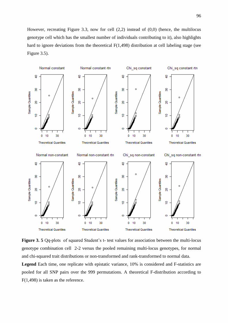
96

However, recreating Figure 3.3, now for cell (2,2) instead of (0,0) (hence, the multilocus

genotype cell which has the smallest number of individuals contributing to it), also highlights

hard to ignore deviations from the theoretical F(1,498) distribution at cell labeling stage (see

Figure 3.5).

Figure 3. 5 Qq-plots of squared Student‘s t- test values for association between the multi-locus

genotype combination cell 2-2 versus the pooled remaining multi-locus genotypes, for normal

and chi-squared trait distributions or non-transformed and rank-transformed to normal data.

Legend Each time, one replicate with epistatic variance, 10% is considered and F-statistics are

pooled for all SNP pairs over the 999 permutations. A theoretical F-distribution according to

F(1,498) is taken as the reference.

97

3.3.2 Familywise error rates and false positive rates

Table 3.1 and Table 3.2 report the familywise error rates (FWER) corresponding to the

simulation scenario 2

g =0 (no epistasis, no main effects) and false positive rates

corresponding to 2

g =0.05 and 0.1 (scenarios of epistasis in the absence of main effects). We

observe that, irrespective of the original trait distribution and whether or not a data

transformation preceded MB-MDR analysis, the estimated rates satisfy Bradley‘s [30] liberal

criterion of robustness for the significance level α=0.05 . This criterion requires that the error

rates are controlled for any level α of significance, if the empirical rate ̂ is contained in the

interval 5.1ˆ5.0 .

98

TRAIT STATUS Familywise error rate (Type I)

Distributions Variances ST WT Rank_ST Rank_WT Log_ST Log_WT Rtn_ST Rtn_WT

Normal Equal 0.040 0.053 0.049 0.049 0.044 0.051 0.050 0.058

Normal Unequal 0.058 0.066 0.044 0.051 0.064 0.056 0.053 0.058

Chi-square Equal 0.045 0.036 0.052 0.051 0.055 0.038 0.058 0.056

Chi-square Unequal 0.053 0.057 0.048 0.052 0.051 0.054 0.043 0.047

t-distribution Equal 0.048 0.053 0.050 0.059 0.049 0.056 0.052 0.057

t-distribution Unequal 0.057 0.044 0.042 0.051 0.053 0.048 0.045 0.039

ST-Student‘s t-test, WT-Welch‘s t-test, Rtn- Rank transformation to normal

Table 3. 1 Type I error rates for data generated under the null hypothesis of no genetic association.

TRAIT STATUS FALSE POSITIVES 2

g Distributions Variances ST WT Rank_ST Rank_WT Log_ST Log_WT Rtn_ST Rtn_WT

Normal Equal 0.040 0.047 0.053 0.048 0.051 0.047 0.050 0.051

Normal Unequal 0.051 0.060 0.044 0.061 0.052 0.065 0.048 0.068

Chi-square Equal 0.037 0.056 0.051 0.053 0.042 0.054 0.045 0.056

0.05 Chi-square Unequal 0.040 0.055 0.047 0.042 0.042 0.053 0.047 0.052



Normal Equal 0.040 0.067 0.058 0.058 0.053 0.061 0.054 0.063

Normal Unequal 0.050 0.065 0.044 0.058 0.048 0.063 0.045 0.057

Chi-square Equal 0.048 0.059 0.061 0.060 0.053 0.055 0.057 0.056




False positive percentage is defined as the proportion of simulation samples for which at least one pair other than the causal pair

(SNP1, SNP2) are significant.


Table 3. 2 False positive percentages of MB-MDR involving pairs other than the interacting pair (SNP1, SNP2).

99

3.3.3 Empirical power estimates

MB-MDR empirical power estimates for correctly identifying the causal epistatic SNP are

given in Table 3.3. For all scenarios higher MB-MDR power is achieved with increasing 2

g ,

i.e., with increasing proportion of epistatic variance to total trait variance. MB-MDR analysis

with Welch‘s t-test has generally lower power than MB-MDR with the Student‘s t-test. This

power loss is most severe for normal data. A (moderate) power gain is observed for settings

where traits are t-distributed, variance homogeneity is present, epistatic variance is 10% and

data are either left untransformed or are log-transformed prior to MB-MDR analysis.

Parametric Student‘s t-tests with the original trait measurements lead to reduced overall MB-

MDR power when trait distributions deviate from normality. For non-normally distributed

traits, there is a tendency for MB-MDR with Student‘s t applied to rank-transformed data to

outperform other MB-MDR analysis approaches (this is: association tests other than Student‘s

t and other types of transformation, or no transformation at all). A worthy competitor is MB-

MDR with Student‘s t after rank-transforming original traits to normality. The differences in

power performance between MB-MDR using untransformed traits or transformed traits are

the largest for rank-based transformations compared to logarithmic transformations. No

significant differences are observed between empirical power estimates derived from MB-

MDR analysis on untransformed traits compared to those analyses based on trait

standardization transformations (results not shown).

A graphical representation of the 1000 MB-MDR epistasis test results for the causal SNP pair

(p-values, multiple testing corrected, as outputted by the MB-MDR software), one for each

data set generated under a particular simulation setting (in particular, 2

g = 10%), is given in

Figure 3.6. Here, MB-MDR with Student‘s t is considered. Results are depicted for scenarios

where the original trait data are derived from a normal (symmetric) or from a chi-squared

(non-symmetric) distribution, and then subjected to different data transformation strategies.

The scatter plot matrices of Figure 3.6 suggest a tendency for smaller MB-MDR p-values to

be generated after rank-based data transformations compared to other type of transformations,

including the identity transformation (see for instance Panels A and B for normally distributed

traits). This tendency becomes more extreme for chi-square distributed traits with non-equal

variance (Panel D). Here, it becomes apparent that rank-transformation generally leads to

larger p-values as compared to rank-transformations to normality. For settings where traits are

chi-squared distributed and variance homogeneity is present, the scatter plots of Figure 3.6

100

(Panel C) are in agreement with the corresponding results in Table 3.3 (power estimates of

100% in the event of a non-identity transformation compared to 90% for MB-MDR applied to

untransformed traits). If there were no differences between the untransformed and

transformed trait results, we would expect all the points to lie along the diagonal.

101

TRAIT STATUS POWER 2

g Distributions Variances ST WT Rank_ST Rank_WT Log_ST Log_WT Rtn_ST Rtn_WT

Normal Equal 0.400 0.046 0.367 0.001 0.377 0.039 0.378 0.041

Normal Unequal 0.330 0.083 0.391 0.001 0.331 0.069 0.344 0.051

Chi-square Equal 0.221 0.000 0.953 0.130 0.929 0.466 0.978 0.802




Normal Equal 0.950 0.634 0.952 0.087 0.959 0.626 0.958 0.650

Normal Unequal 0.963 0.743 0.975 0.152 0.955 0.727 0.959 0.690

Chi-square Equal 0.897 0.126 1.000 0.922 1.000 1.000 1.000 1.000




Power is defined as the proportion of simulated samples of which the causal pair (SNP1, SNP2) is significant.


Table 3. 3 Power estimates of MB-MDR to detect the correct interacting pair (SNP1, SNP2).

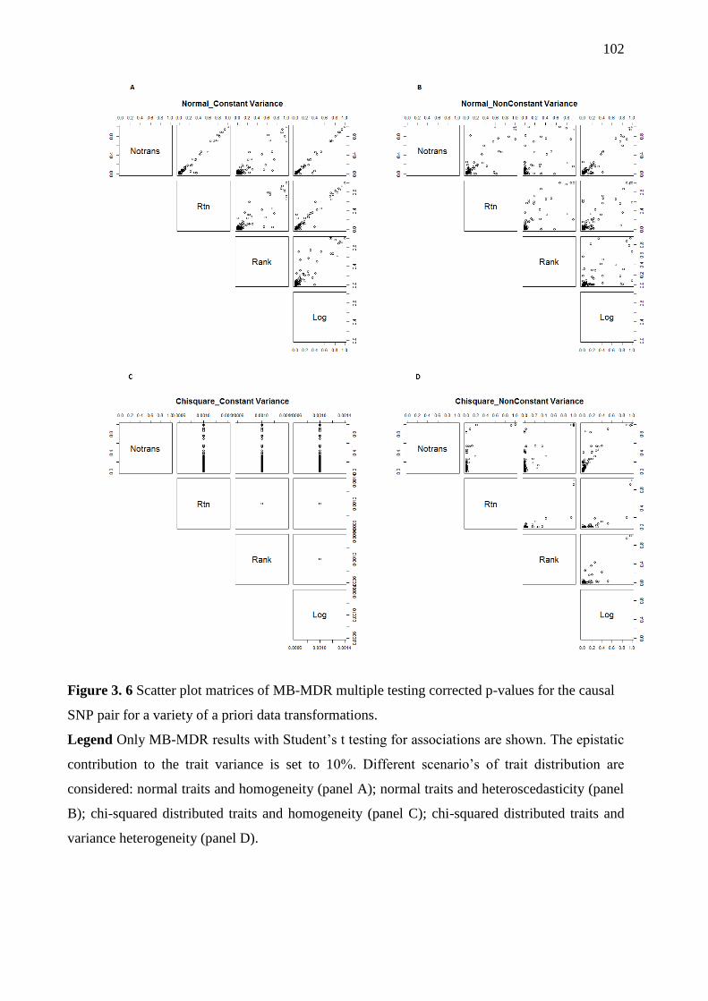
102

Figure 3. 6 Scatter plot matrices of MB-MDR multiple testing corrected p-values for the causal

SNP pair for a variety of a priori data transformations.

Legend Only MB-MDR results with Student‘s t testing for associations are shown. The epistatic

contribution to the trait variance is set to 10%. Different scenario‘s of trait distribution are

considered: normal traits and homogeneity (panel A); normal traits and heteroscedasticity (panel

B); chi-squared distributed traits and homogeneity (panel C); chi-squared distributed traits and

variance heterogeneity (panel D).

103

3.4 Discussion

Proposed data mining methods for epistasis detection are seldom thoroughly discussed in

terms of their underlying (model) assumptions and their effects on overall power or type I

error control. For instance, another well-known data dimensionality reduction method for

quantitative traits (generalized MDR - GMDR) [31] is based on score statistics to define

differential multilocus genotype groups related to the trait of interest. Although the GMDR

method is not necessarily likelihood-based (least-squares regression or other statistical

methods for non-normal continuous traits can be employed as well, in theory), continuous

phenotypes were only investigated in terms of a normal model, and the software

implementation for continuous traits relies on the classical linear regression paradigm to build

the score statistics. The authors did not explicitly investigate the power of their method when

non-normal continuous data are involved in the context of epistasis screening. Previously,

we commented on the advantages and disadvantages of GMDR-like methods compared to

MB-MDR (e.g., [28, 32]). Based on these comments, we here focused on MB-MDR while

investigating the effects of model-violations on the performance of 2-locus multifactor

dimensionality reduction methods for quantitative traits.

For every 2 loci (for 2 bi-allelic SNPs, there are theoretically 9 multilocus genotype

combinations), MB-MDR with association t-tests subsequently creates two groups, where one

group refers to one multilocus genotype and the other to the remaining multilocus genotype

combinations. Internally, 2-group comparison tests are performed so as to assign a ―label‖ to

each multilocus genotype. This procedure naturally creates highly imbalanced groups, with

potentially extreme cases of heteroscedasticity. Although Welch‘s test is designed to give a

valid t-test in the presence of different population variances, Welch‘s t-test combined with

MB-MDR shows no improved power over the Student‘s t-test for scenarios with unequal

variances, even for normally distributed traits (cfr Table 3.3). This can be explained by the

fact that the degrees of freedom for the Welch‘s test become smaller for strongly unequal

groups, resulting in a highly conservative test in the event of extreme unbalanced data (see

e.g., [33] and Figure 3.1). This motivates our choice to continue working with MB-MDR

analyses based on Student‘s t testing to identify groups of multilocus genotypes with

differential trait values, despite the underlying trait distribution.

It is well-know that parametric methods have improved statistical power over non-parametric

methods when all parametric model assumptions are valid [6, 34]. When an analysis of

104

residuals detects violations of assumptions of normality and heterogeneity of variance of

errors across groups for ANOVA, remedial measures that log-transform the dependent

variable and consideration of an ANOVA model assuming unequal variances, may work well.

However, in screening settings involving many factors at a time, it is usually impractical to

find a single transformation that is universally optimal for all factors. When study data do not

meet the distributional assumptions of parametric methods, even after transformation, or when

data involve non-interval scale measurements, a non-parametric context is more appropriate.

Such a context usually implies testing based on ranks or applying data rank transformations

prior to the application of a parametric test.

Strong power increases were observed when data were rank-transformed prior to MB-MDR

testing with Student‘s t association testing. This can be understood by noting that the ranks,

which are computed for the pooled set of all available quantitative trait measurements, in

general reduces the influence of skewness and deviations from normality in the population

distribution [35, 36]. The same is achieved by a percentile transformation (Rtn), which – at

the same time - preserves the relative magnitude of scores between groups as well as within

groups. Only for normally distributed data with equal variances, the ideal scenario for a t-test

on original traits, a small power loss is observed. Goh and Yap [36] also concluded that rank-

based transformation tends to improve power regardless of the distribution. In general, as with

traditional two group t-testing, deviations from normality seem to be more influential to the

power of an MB-MDR analysis with Student‘s t than deviations from homoscedasticity

(Table 3.3). This is also in line with the observation that power estimates generally become

more optimal for scenarios in which data are transformed to normality prior to MB-MDR

analysis compared to scenarios in which they are not. The identical results obtained for

untransformed traits and standardized traits (not shown) are not surprising as well.

Standardization involves linearly transforming original trait values using the overall trait

mean and overall standard deviation. Such a transformation does not affect the two-group t-

tests within MB-MDR.

Although data transformations are valuable tools, with several benefits, care has to be taken

when interpreting results based on transformed data. The inference of epistasis depends upon

the scale of measurement in a way that interaction effects can be reduced or eliminated by

non-linear monotonic transformations of a dependent variable [37], so also by some rank-

based transformations. However, for our simulation scenarios, we have not seen any evidence

of such a reduction in interaction signals when using rank-transformed data prior to MB-MDR

105

analysis (Tables 3.1-3.3, Rank). Application of any epistasis screening tool to real-life data

will face the challenge to match observed statistical significance with biological relevance [1].

Despite MB-MDR internal inflations (Figures 3.4 and 3.5), there is no evidence for a

cumulative or combined effect on MB-MDR‘s final results (Tables 3.1 and 3.2), irrespective

of the assumed model violation (in terms of deviations from normality or homoscedasticity).

This can be explained by the permutation-based step-down maxT approach, which is currently

adopted by MB-MDR to correct for multiple testing of SNP pairs.

In many of our practical applications, though we observed a tendency of increased numbers of

significant epistasis results with MB-MDR applied to quantitative traits, even after SNP

pruning (r2 below 75%) to avoid potential false positives (or redundant interactions) due to

highly correlated SNPs. No such observation was previously made for dichotomous traits. For

dichotomous traits, MB-MDR uses a score test, in particular, the Pearson's chi-squared test.

This test is known to be affected by unbalanced data, or sparse data, as is the case for rare

variants [38]. However, these data artifacts, which question the use of large sample

distributions for test statistics, are minimized by requiring a threshold sample size for a

multilocus genotype combination, irrespective of whether a dichotomous or quantitative trait

is used. Hence, an explanation for the apparent discrepancies between practical and theoretic

MB-MDR results may be found in the way the null distribution for multiple testing is derived.

It is often forgotten that also permutation-based multiple testing corrective procedures make

some assumptions. For instance, for the step-down maxT approach, currently the default

multiple testing strategy in MB-MDR, the Family-Wise Error Rate (FWER) is strongly

controlled provided the assumption of subset pivotality holds [27]. The subset pivotality

ensures that the distribution of any sub-vector of p-values does not depend on the truth or

falseness of the hypotheses not considered by this sub-vector [39].

Preliminary results on the effect of linkage disequilibrium on MB-MDR error control, as well

as on the effect of highly variable minor allele frequencies (and thus highly variable available

samples sizes for multilocus genotypes) show that subset pivotality is likely to be violated in

real-life settings, giving rise to inflated error rates in the presence of multiple epistasis signals

(work in progress). Note that the standard bootstrap method provides the asymptotically

correct null distribution for multiple testing and does not require the subset pivotality

condition given in Westfall and Young [27]. Resampling-based multiple testing with

asymptotic strong control of type I error as corrective method for multiple testing in MB-

MDR warrants further investigation.

106

Summarizing, we observed that non-normally distributed traits can affect the power of final

test statistics of MB-MDR with classical t-tests for association, and that this influence is

primarily driven by the sparser multilocus genotype combinations. Improved power can be

obtained by pre-analysis data transformation to normality. MB-MDR permutation-based

maxT correction for multiple testing keeps type I error and false positive rates under control,

since in all considered simulation scenarios‘, the assumption of the maxT permutation

strategy was plausible.

When performing MB-MDR screening for gene-gene interactions with quantitative traits, we

recommend to rank-transform traits to normality prior to MB-MDR analysis with Student‘s t

test as preferred association test.

107

References

1. Van Steen K: Travelling the world of gene-gene interactions. Briefings in








4. Kutner MH, Neter J, Nachtsheim CJ, Li W: Applied Linear Statistical Models: (mainly

chapter 18). McGraw-Hill College; 2004.

5. McDonald JH: Handbook of Biological Statistics. 2nd ed. edn: Sparky House

Publishing, Baltimore, Maryland.; 2009.

6. Freedman D: Statistical Models: Theory and Practice. Cambridge University Press;

2000.

7. Pearson ES: Note on tests for normality. Biometrika JSTOR 2332104 1931.

8. Bartlett MS: The effect of non-normality on the t distribution. Proc Camb Philos

Soc 1935:223-231.

9. Mann HB, Whitney DR: On a Test of Whether one of Two Random Variables is

Stochastically Larger than the Other. Annals of Mathematical Statistics 1947,

18:50-60.

10. Pratt J: Robustness of Some Procedures for the Two-Sample Location Problem.

Journal of the American Statistical Association 1964, 59:665-680

11. Keselman HJ, Rogan JC, Feir-Walsh BJ: An evaluation of some non-parametric

and parametric tests for location equality. British Journal of Mathematical and

Statistical Psychology 1977, 30:213-221.

12. Tomarken A, Serlin R: Comparison of ANOVA alternatives under variance

heterogeneity and specific noncentrality structures. Psychological Bulletin 1986,

99:90-99.

13. Wolfe R, Carlin JB: Sample-Size Calculation for a Log-Transformed Outcome

Measure. Controlled Clinical Trials 1999, 20:547-554.

14. Jin H, Zhao X: Transformation and Sample Size. Dalarna University,Department of

Economics and Society, PhD Thesis; 2009.

108

15. Conover W: Practical nonparametric statistics. Wiley; 1980.

16. Conover W, Iman R: Rank Transformations as a Bridge Between Parametric and

Nonparametric Statistics. The American Statistician 1981, 35:124-129

17. Gibbons J, Chakraborti S: Comparisons of the Mann-Whitney, Student's t and

alternative t tests for means of normal distributions. Journal of Experimental

Education 1991, 59:158-167.

18. Zimmerman D, Zumbo B: Rank Transformations and the Power of the Student

Test and Welch t' Test for Non-Normal Populations With Unequal Variances.

Canadian Journal of Experimental Psychology 1993, 47:523.

19. Danh V N: On estimating the proportion of true null hypotheses for false

discovery rate controlling procedures in exploratory DNA microarray studies.

Computational Statistics & Data Analysis 2004, 47:611-637.

20. Szymczak S IB-W, Ziegler A: Detecting SNP-expression associations: A

comparison of mutual information and median test with standard statistical

approaches. Statistics in Medicine 2009, 28:3581-3596.

21. Rupar K: Significance of Forecast Precision: The Importance of Ex-Ante

Expectations. Available at SSRN: http://ssrncom/abstract=1752217 or

http://dxdoiorg/102139/ssrn1752217 2011.

22. Pett M: Nonparametric Statistics for Health Care Research: Statistics for Small

Samples and Unusual Distributions. SAGE Publications; 1997.

23. Weber M, Sawilowsky S: Comparative Power Of The Independent t, Permutation

t, and WilcoxonTests. Journal of Modern Applied Statistical Methods 2009, 8:10-15.

24. Yang K, Li J, Gao H: The impact of sample imbalance on identifying differentially

expressed genes. BMC Bioinformatics 2006, 7:(Suppl 4):S8.

25. Jeanmougin M dRA, Marisa L, Paccard C, Nuel G, Guedj M Should We Abandon

the t-Test in the Analysis of Gene Expression Microarray Data: A Comparison of

Variance Modeling Strategies. PLoS ONE 2010, 5:e12336.

26. Development Core Team R: R. A language and environment for statistical

computing. R foundation for Statistical Computing. Retrieved from

http://www.R-project.org. Vienna, Austria 2012.




109


Individuals. PLoS ONE 2010, 5:e10304.




1978, 31:144-152.




80:1125-1137.




Genetics 2011, 75:78-89.

33. Sawilowsky SS: Fermat, Schubert, Einstein, and Behrens-Fisher: The Probable

Difference Between Two Means With Different Variances Journal of Modern

Applied Statistical Methods 2002, 1:461-472.

34. Howell DC: Statistical Methods for Psychology. Nelson Education; 2012.

35. Zimmerman DW, Zumbo BD: Can Percentiles Replace Raw Scores in the

Statistical Analysis of Test Data? Educational and Psychological Measurement

2005:616.

36. Goh L, Yap VB: Effects of normalization on quantitative traits in association test.

BMC Bioinformatics 2009, 10.

37. Mani R, St.Onge R, Hartman J, Giaever G, Roth F: Defining genetic interaction.

Proceedings of the National Academy of Sciences 2008, 105:3461-3466.

38. Mahachie John JM, Cattaert T, De Lobel L, Van Lishout F, Empain A, Van Steen K:

Comparison of genetic association strategies in the presence of rare alleles. BMC

Proc 2011, 5 Suppl 9:S32-S32.

39. Dudoit S, van der Laan MJ: Multiple Testing Procedures with Applications to

Genomics: Chapter 2. Springer; 2008.

PART 3

PRACTICAL APPLICATIONS

Related publication

J. M. Mahachie John*, H. Baurecht*, E. Rodrı´guez, A. Naumann, S. Wagenpfeil,

N. Klopp, M. Mempel, N. Novak, T. Bieber, H.E. Wichmann, J. Ring, T. Illig,

T. Cattaert, K. Van Steen, S. Weidinger (2010) *These authors contributed equally.

Allergy 65(7), 875-882. doi: 10.1111/j.1398-9995.2009.02297.x

Analysis 1

Analysis of the High Affinity IgE Receptor Genes Reveals Epistatic

Effects of FCER1A Variants on Eczema Risk

112

1.1 Aim of the Analysis

We investigated the association of 27 FCER1A, FCER1B (MS4A2), and FCER1G variants

with IgE in a large population-based cohort and tested for epistatic effects using the MB-

MDR method. In addition, we investigated a potential interaction between 10 FLG and

FCER1A variants in a large collection of eczema cases and population controls. We believe

that small-scaled genetic studies, based on candidate genes rather than genome-wide data, are

useful in methodological development: Due to the complexities of high-dimensional genomic

data analysis, both from the biology and statistics perspective, any statistical epistasis

detection method is believed to have little viability when not useful on a much smaller scale.

Thus, if a method does not work on small-scaled data it will certainly not work on large-scale

data sets.

1.2 Data description

KORA S4 is an epidemiological study group including 4261 unrelated German adult

individuals representative of the population within the age range of 25–74 years in the city

and region of Augsburg (Bavaria, Germany); probands were recruited from 1999 to 2001 [1].

In addition to demographic data, all subjects had to complete a standardized questionnaire that

included the basic allergy questions of the European Community Respiratory Health Survey

on respiratory health [2]. Total and specific IgE antibodies to aeroallergens (Sx1) were

measured using RAST FEIA CAP system (Pharmacia, Freiburg, Germany). Allergic

sensitization was defined as specific IgE levels ≥0.35KU/l (CAP class ≥1). DNA was

available for 4261 individuals (50.9% females), and all subsequent analyses were based on

this number. All German patients with eczema were unrelated and of white origin, with

eczema diagnosed on the basis of a skin examination by experienced dermatologists using the

UK diagnostic criteria [3]. The collection of 1018 individuals (59.5% females) was recruited

in the department of dermatology of the University hospitals of Bonn and Munich.

1.3 MB-MDR Results and Discussion

Results on total IgE indicated strong epistasis between the two FCER1A variants rs2251746

and rs16842010 (p-value <0.001). These variants were found to be weakly correlated (r2 =

0.003) and can thus be regarded as uncorrelated. Taking eczema as outcome, MB-MDR

indicated strong epistasis between FLG haploinsufficiency and several SNPs of the FCER1A

113

gene. Because of their known and confirmed remarkably strong effect on eczema risk, we

additionally performed the algorithm with adjustment for FLG effects to determine whether

these results were attributed to genuine epistasis. After this correction, the interaction between

FLG and FCER1A polymorphisms vanished, but we identified statistical epistasis between

the two FCER1A SNPs rs10489854 and rs2511211 (p-value =0.046). Concerning linkage

disequilibrium, the two variants of the FCER1A genes also showed a weak correlation (r2 =

0.01). With correction of main effects, no significant results were observed for variants of the

FCER1B and FCER1G and FLG genes. In addition, all investigated SNPs were in Hardy-

Weinberg Equilibrium. The significant interactions observed from the MB-MDR analysis

indicated that these outcome respective two SNPs jointly have a strong effect on total IgE and

on eczema.

Related publication

Jestinah M Mahachie John*, Tom Cattaert*, Lizzy De Lobel, François Van Lishout,

Alain Empain,Kristel Van Steen (2011) *These authors contributed equally.

BMC Proceedings, 5(Suppl 9):S32. doi:10.1186/1753-6561-5-S9-S32

Analysis 2

Comparison of Genetic Association Strategies in the Presence of Rare

Alleles

115


We explored the utility of several methods, both parametric and non-parametric, to test for or

model genetic associations using population-based and family-based data from Genetic

Analysis Workshop 17 (GAW17). Here, we focus on MB-MDR related analyses (MB-MDR-

population data and FAM-MDR-family data) incorporating the maxT and minP of Westfall

and Young [4] for multiple testing correction.


The data provided by GAW17 [5] included a subset of genes grouped according to pathways

that had sequence data available in the 1000 Genomes Project. Effect sizes for coding variants

within these genes were assigned using PolyPhen and SIFT predictions of the likelihood that

the variant would be deleterious. Two hundred replicates were generated. All simulated

singular SNP effects (C4S1861, C4S1873, C4S1874, C4S1877, C4S1878, C4S1879,

C4S1884, C4S1887, C4S1889, and C4S1890 in the KDR gene and C4S4935 in the VEGFC

gene) are assumed to be additive on the quantitative trait scale, such that each copy of the

minor allele increases or decreases the mean trait value by an equal amount. The sample size

for both population- and family-based data was 697 with family data comprising 8 families

with 202 founders and 3 offspring generations. The founders were randomly sampled from

the unrelated individuals‘ data set, and genotypes of offspring were sampled using Mendelian

inheritance.

Our analyses involved the quantitative trait Q1, which was simulated as a normally distributed

phenotype. Furthermore, we restricted attention to the available single-nucleotide

polymorphisms (SNPs) on chromosome 4 (944 SNPs). In total, 200 replicates were generated.


We observed that the MB-MDR approach for unrelated individuals had some power (0.14 for

max T and 0.34 for min P) to find C4S1878, the marker with the largest MAF (0.16), but also

elevated FWER estimates (0.13 and 0.50, respectively). On the other hand, the FAM-MDR

approach had not only some power (0.18 for max T and 0.17 for min P) to detect C4S4935

but also kept the FWER under control. The total contribution of markers in linkage

disequilibrium with functional markers (r2>0.9) was only 0.01 to FWER, hence this can be

ruled out as an explanation of the increased FWER. Lower MB-MDR power compared to our

116

MB-MDR analyses on simulation data with normal traits led us to postulate that the rarity of

certain marker alleles hampers the validity of model assumptions and distributional properties

of test statistics as well as assumptions underlying some commonly used measures to correct

for multiple testing or to control false-positive rates.

Related publication

Liesbet Henckaerts, Isabelle Cleynen, Marko Brinar, Jestinah Mahachie John,

Kristel Van Steen, Paul Rutgeerts, and Sèverine Vermeire (2011) Inflammatory Bowel Diseases, 17(6), 1392-1397. doi: 10.1002/ibd.21486

Analysis 3

Genetic Variation in the Autophagy Gene ULK1 and Risk of Crohn’s

Disease

118


We investigated polymorphisms in selected autophagy genes for their association with

susceptibility to Crohn‘s disease. Autophagy has been recently implicated in various human

pathological and physiological conditions including cancer, heart diseases, liver disease

Crohn‘s disease etc. The autophagy connection is presented in Figure 3.1.


In the framework of the IBD genetics study conducted at the IBD unit of the University

Hospital in Leuven, Belgium, we studied 1282 Crohn‘s disease (CD) patients of Western

European origin and a control group of 548 unrelated healthy volunteers without a family

history of IBD or other immune-related disorders. Diagnosis of IBD was based on accepted

clinical, endoscopic, radiologic, and histologic criteria [7, 8]. As an exploratory cohort, a total

of 70 haplotype tagging single nucleotide polymorphisms (tSNPs) in 12 genes were

genotyped in a cohort of 947 CD patients and 548 controls. A confirmatory cohort consisting

of 335 trios with father, mother, and a child affected with CD was also available. DNA was

extracted as described in Miller et al. [9]. Samples and data were stored in a coded and

anonymized database.


We found a novel association between one haplotype tagging SNP (rs12303764) in the ULK1

gene and CD. MB-MDR confirmed this association which also was found both in a single

SNP analysis and TDT in 335 parent–child CD trios. To further clarify the role of ULK1 in

CD, an in-depth investigation of the variation in the region and possible role for copy number

variation in this region should be evaluated. No significant epistasis results were observed.

119

Figure 3.1 The Autophagy Connection. Source: KLionsky , D J [10].

Related publication

Eveline Hoefkens, Jestinah Mahachie John, Kristel Van Steen, Kris Nys, Gert Van Assche,

Patrizia Agostinis, Paul Rutgeerts, Séverine Vermeire, and Isabelle Cleynen (2012) Under Review

Analysis 4

Crohn’s Disease Susceptibility Genes Involved in Microbial Sensing,

Autophagy and Endoplasmic reticulum (er) Stress and their Interaction

121


We investigated association between Chrohn‘s disease (CD) and 11 SNPs in the autophagy

genes ATG16L1, IRGM and MTMR3; the endoplasmic reticulum (ER) stress gene ORMDL3;

and the bacterial sensing gene NOD2 in a large Belgian CD cohort. In addition, we also

evaluated these SNPs in a large Belgian Ulcerative Colitis (UC) cohort, to determine whether

these variants were specific for CD or also important in UC.


The study population consisted of 3451 individuals in total: 1744 CD patients (42% males)

and 793 UC patients (55% males) from the IBD unit of the University Hospitals Leuven, and

a control group of 914 unrelated healthy controls (48% males). Both patients and controls

were of Caucasian origin. Diagnosis of CD or UC was based on accepted clinical, endoscopic,

radiologic and histological criteria [7]. Informed consent was obtained from all participants.

All DNA samples and data in this study were handled anonymously.


For CD, MB-MDR analysis showed a significant two-way interaction between ATG16L1 and

IRGM (p-value=0.001): rs2241880 (ATG16L1) – rs10065172 (IRGM). Both of these genes

belong to the autophagy pathway with a weak correlation between them, r² = 0.006. For UC,

no significant interactions were observed. Despite the known functional interaction between

pathways, we did not find gene-gene interactions between the three pathways of ER stress,

autophagy and microbial sensing. We did however found an interaction within the autophagy

pathway itself.

122

References

1. Holle R, Happich M, Lowel H, Wichmann HE: KORA - a research platform for

population based health research. Gesundheitswesen 2005, 67(Suppl. 1):S19-S25.

2. Burney PG, Luczynska C, Chinn S, Jarvis D: The European Community

Respiratory Health Survey. Eur Respir J 1994, 7:954-960.

3. Williams HC, Jburney PG, Hay RJ, Archer CB, Shipley MJ, Ahunter JJ, Bingham EA,

Finlay AY, Pembroke AC, Cgraham-Brown RA, et al: The U.K. Working Party's

Diagnostic Criteria for Atopic Dermatitis. British Journal of Dermatology 1994,

131:383-396.


5. http://www.gaworkshop.org/gaw17: 2010.



Proc 2011, 5 Suppl 9:S32-S32.

7. Podolsky DK: Inflammatory Bowel Disease. New England Journal of Medicine

2002, 347:1982-1984.

8. Lennard-Jones JE: Classification of inflammatory bowel disease. Scand J

Gastroenterol Suppl 1989, 170:2-6.

9. Miller SA, Dykes DD, Polesky HF: A simple salting out procedure for extracting

DNA from human nucleated cells. Nucleic Acids Research 1988, 16:1215.

10. Klionsky DJ: The autophagy connection. Dev Cell 2010, 19:11-12.

http://www.gaworkshop.org/gaw17:

PART 4

GENERAL DISCUSSION AND FUTURE PERSPECTIVES

124

Chapter 1: Discussion

1.1 General objective

The main objective of this thesis was to investigate the performance of Model-Based

Multifactor Dimensionality Reduction method for quantitative traits, under a variety of

settings and assumptions about the operation epistasis mechanisms.

1.2 General Discussion

Most common complex human diseases are caused by multiple genetic variants. Identifying

such genetic variants, as well as the potential modifying effect they have on each other has

been and still is a big challenge in genetic epidemiology. Indeed, although genome-wide

association (GWA) studies have highlighted many loci associated with common diseases

using (mostly) binary or quantitative traits, similar studies targeting gene–gene interactions

(epistasis), as in genome-wide association interaction (GWAI) studies have been less

successful. Yet, it is believed that epistatic interactions may play a significant role in

improving pathogenesis, prevention, diagnosis and treatment of complex human diseases, it

needs to be seen how important gene-gene interactions are as a potential source of the so-

called missing heritability [1]. The limited success of worldwide GWAI studies efforts as

compared to GWA studies efforts can be attributed to several factors. A major challenge in

analyzing epistasis in GWA studies is the enormous computational demands it involves while

analyzing billions of SNP combinations. Whereas many human GWA studies test on the order

of one million SNPs (only), considering all pairs of SNPs amounts to approximately 500

billion tests; the number of pairs of SNPs scales quadratically with the number of markers [2].

Due to the large number of interaction tests that need to be performed, in particular, when

using traditional statistical testing approaches, searching for epistatic effects poses both

computational and statistical challenges. Last but not least, there is a conceptual difficulty

related to the success of GWAI studies in that they aim to identify biological mechanisms via

mathematical/statistical models; models that may be too simplistic to capture the complexity

of the underlying phenomena and are often restricted by scales of measurements.

Having the aforementioned challenges in mind, several methods have been developed to

detect (causal) interacting genes. According to Onkamo and Toivonen [3], these methods can

be categorized into tree-based methods (e.g, random forests), pattern recognition methods

(e.g, support vector machines) or data reduction methods (e.g. model-based dimensionality

125

reduction). Driven by the popular case-control design, most of the developed methods are

restricted to dichotomous traits or at least require categorizing a given quantitative trait into

distinct phenotypic categories prior to application. Obviously, often the variability exhibited

by many traits fails to fit into distinct discrete phenotypic classes (discontinuous variability),

but instead forms a spectrum of phenotypes that blend imperceptively (continuous

variability), and this should be acknowledged [4].

We developed a data-mining method, Model-Based Multifactor Dimensionality Reduction

(MB-MDR) to detect epistatic interactions under different types of traits [5-7]. MB-MDR is a

data mining technique that enables the fast identification of gene-gene interactions among

1000nds of SNPs, without the need to make restrictive assumptions about the genetic modes

of inheritance. In this thesis, we zoomed in on curtailing the MB-MDR methodology to

quantitative traits and on finding the most optimal conditions and settings for quantitative trait

MB-MDR analysis via extensive simulation studies.

Most simulation studies in this thesis involve small data sets in terms of marker design (10 -

100 markers), though the quantitative MB-MDR method applies to GWA data as well.

However, given the fact the MB-MDR employs an exhaustive search strategy on the input

data, applying the method as such to genomewide SNP data might be infeasible, due to

limitations of the available IT environment that may not be able to handle the computational

and storage demands a GWAI study induces. To make the MB-MDR methodology less

dependent on the properties of the IT environment it operates in, we are developing a protocol

for optimal Genome-Wide Association Interaction (GWAI) analysis [8]. This minimal

protocol includes input/output data properties and pre-analysis data quality contol procedures

(involving Hardy-Weinberg Equilibrium test, marker call rates and marker frequencies)

related to GWA analysis in general and GWAI analysis in particular (missing data handling

and LD control). The protocol also gives recommendations with respect to integrating

available knowledge into the MB-MDR analysis by further reducing the interaction search

space, for instance via Biofilter [9].

Biofilter explicitly uses biological information about gene-gene relationships and gene-disease

relationships to construct multi-SNP models, hereby adopting a gene-centric approach. An

upgraded release of Biofilter is expected, and will allow using even a larger amount of

available biological and statistical knowledge on gene-gene interactions, for a priori data

filtering or a posteriori results interpreting.

126

It should be noted that pre-filtering can also be done based on statistical knowledge. For

instance, Hoh et al. [10] proposed a 2-stage approach in which SNPs that meet some

threshold in a test at the first stage are subsequently followed up for modeling interactions at

the second stage. Alternatively, Oh et al. [11] developed Gene-MDR. This analysis method is

also a 2-stage approach. The first stage, a within-gene analysis, summarises each gene‘s effect

from several SNPs within the same gene. The second stage, the between-gene analysis,

involves performing interaction analysis using summarized gene effects derived from stage 1.

Although pre-filtering or multi-stage analyses may come at the cost of losing potentially

interesting signals (for instance, failure to detect interactions involving markers without

significant marginal effects), in particular prefilitering may be highly beneficial in bridging

the gap between statistical and biological or genetical epistasis.

In traditional applications of MDR, model selection within a cross-validation framework is

used to select a single best model. This misses other important multilocus models that could

be biologically meaningful. Recently, Oki and Motsinger-Reif [12], developed a filter-based

approach, using MDR modeling to evaluate and rank (based on classification error) all

univariate effects and two-locus epistatic effects hereby prioritizing models for follow-up in

replication studies.

In this thesis, we focused on 2-order interactions for bi-allelic SNPs. The MB-MDR software

can handle multi-allelic genetic markers and is fairly easily extended to investigate higher-

order interactions (i.e. > 2-way interactions) [13]. However, it is questionable whether valid

biological interpretations can be given to higher order interactions (>2), when it is already so

difficult to do so for order 2. In addition, building sensible animal models to support the

statistical findings seems almost untangible. Yet, still emphasizing 2-way genetic interactions,

a beta-version of the MB-MDR software allows to tackle research questions such as ―How

does a fixed (non-) genetic factor (such as smoking or gender) modify the effect of gene-gene

interactions?‖ (see also [14] with smoking as a potential modifying explanatory variable), or

phrased differently ―Can we observe different gene-gene interaction patterns according to

different population subgroups?‖

We chose not to include multi-allelic markers in MB-MDR analyses, due to issues related to

―sparseness‖ and ―unavailable‖ multilocus genotypes. These issues require more detailed

investigations, as was indicated by our work on epistasis with rare variants. The latter clearly

showed that analyzing rare variants with current implementations of MB-MDR highly inflates

type I errors [14]. For bi-allelic SNPs, we controlled the sparseness effect on MB-MDR type

127

I errors by setting a lower bound on the number of individuals required for each multilocus

genotype (see Chapter 3 of PART 2). Additional measures are needed when multi-allelic

markers or rare variants are involved. In either case, as the aforementioned lower bound in the

context of bi-allelic SNPs increases, MB-MDR‘s type I errors decrease as well (results not

shown).

In general, in the case of missing genotypes, the implementation of MB-MDR uses available

data. However, MDR and MDR related extensions commonly require complete cases to run

the analysis. In order to have complete data, there are mainly two options to follow: 1) simply

removing individuals with missing genotypes or 2) imputing missing genotypes. The first

option is the least desirable option because it usually leads to invalid analyses when data are

not completely missing at random [15], besides throwing away possibly valuable (expensive)

information. The second option is to be preferred. The original MDR software adopted a

frequency-based imputation strategy to impute missing genotypes with the most common

genotype of the respective SNP. Thus, the imputation method is performed for one SNP at

the time, prior to MDR analysis. This may be a reasonable option when the extent of missing

genotypes is not dramatic, and when missingness occurs at random across cases and controls.

Recently, Namkung et al. [16] developed a procedure called ‗EM impute‘ which imputes

missing genotypes using the expectation-maximization (EM) algorithm within the MDR

process. Thus, unlike the frequency-based imputation, ‗EM impute‘ does not require a

separate step of imputation, but rather it imputes missing values within the MDR analysis.

‗EM impute‘ has been made available through the package imputeMDR of the R software

[17]. Actually, this R package also allows for two other ways of handling missing data: using

all available data for given number of SNPs under consideration, or treating missing

genotypes as another (usually fourth) genotype category.

The R software also offers a number of other imputation procedures through the R package

imputation [18]. These and other imputation software tools can obviously also be applied to

―complete‖ data prior to MB-MDR analysis. These tools were primarily developed in the

context of biostatistics or GWA studies. We specifically mention the BEAGLE software of

Browning and Browning [19], allowing to impute missing ungenotyped markers using a

reference panel. This panel may contain data for parent-offspring trios, parent-offspring pairs

or unrelated individuals. However, whereas GWA studies exploit LD between markers to find

the true causal variants, LD in GWAI studies may induce redundant [20, 21] interactions. (See

also following Section 2.2).

128

The practical application section presented in this thesis identified several significant genetic

interacation effects with quantitative MB-MDR that could be confirmed with other statistical

methodologies. The concern remains whether these findings can be translated into

biologically relevant mechanisms. In the general introduction of this thesis, we discussed the

difference between statistical epistasis and biological epistasis, and indicated that a

statistically significant interaction is not necessarily biologically significant. This leads into

the discussion about replicating epistastic findings. Should a finding be replicated in an

independent data set? Is that possible in the context of GWAI studies where large sample

sizes are needed and over 50 epistasis [22] models exist for two bi-allelic loci? Should

results be confirmed by animal models or human cell cultures? [23] When using the same

criteria as for GWA studies, replication in GWAI studies is likely to fail. In our opinion, not

being able to replicate epistasis findings in this sense is not the end of the story. As Greene at

al. [24] pointed out as well, failure to replicate may provide important clues about ‗some

hidden‘ genetic architecture, and it is should be our mission to unravel this architecture.

Chapter 2: Future Perspectives

2.1 Introduction

In this thesis, we presented epistasis screening results of MB-MDR on different scenarios. For

all simulated data, we assumed all SNPs to be in Hardy-Weinberg equilibrium and assumed

linkage equilibrium between them. In addition, analyses were performed on single traits

(univariate phenotypes). However, in reality, markers located on the same chromosome may

be in linkage disequilibrium, and when not properly accounted for may lead to spurious

results [25]. Moreover, genetic epidemiological studies typically contain data collected on

multiple traits that are jointly associated to genes and their interactions. Testing several traits

jointly may be more powerful than testing a single trait at a time [26]. Our ongoing and future

research activities aim at adjusting for linkage disequilibrium patterns and accommodating

multiple traits in MB-MDR epistasis screening. Thus, we intend to assess MB-MDR‘s

flexibility in handling data under linkage disequilibrium and/or data with multiple traits.

2.2 Linkage Disequilibrium

Modeling and detecting gene-gene interactions at multiple quantitative trait loci often assume

that the study population is in linkage equilibrium [27]. This assumption is often violated for

129

real-life GWAI study populations. Genetic association studies owe their success to the ability

to detect association signals via markers that are in high linkage disequilibrium (LD) with

disease predisposing loci. Indeed, an association between a genetic marker and a trait can be

direct (the allele under investigation directly influences the trait) or indirect (the allele is in

LD with the disease-predisposing mutation) [28]. The underlying assumption of genetic

association studies is that there are some disease causing loci in the genome, and that if the

SNPs under investigation and the disease-causing loci are in close proximity, the marker

alleles will be associated with the alleles at the disease-causing loci and can be used as proxy

to identify the true causal variant [29]. Motsinger et al. [30] showed that strong patterns of

LD increase the power of grammatical evolution neural networks (GENN) to detect genetic

associations: The higher the LD between the causal variants (involved in an interaction) and

their proxy‘s, the better the chance to find an epistatic association with the trait of interest. In

other words, whereas GWA studies exploit strong LD between a genetic marker and causative

variant, GWAI studies exploit relation between the causal pair and their proxys‘ [31].

Little is understood about how to best incorporate LD patterns between genetic markers or

genetic markers and true causal variants in epistasis studies, knowing that LD between two

genetic markers may induce a ‗redundant‘ epistatic effect of them on the trait under

investigation. According to Zhao et al. [32], LD-based measures can serve as useful statistics

to detect gene-gene interaction between two unlinked loci. These authors investigated the

effect of a variety of LD patterns on the power of an epistasis study, in the presence of gene-

gene interactions between two disease-susceptibility loci in Hardy-Weinberg equilibrium and

between two unlinked marker loci, each of which in LD with either of two interacting loci.

Grady et al. [33] investigated the effect of LD on MDR epistasis screening incoperating

varying amounts of LD and different positions of functional loci on a block(s) of LD.

In our future research, we aim at setting up simulations involving varying degrees of LD

between genetic markers and investigate the impact of LD within the context of MB-MDR

epistasis modeling. This study will enable us to validate the epistasis strategy when imputed

data are used, pruned back and then perfom analysis [34].

2.3 MB-MDR for Multivariate Traits

Many complex diseases such as asthma and Crohn‘s disease, consist of a large number of

highly related, rather than independent, clinical or molecular phenotypes.Identification of

genetic loci in complex traits has focused largely on one-dimensional genome scans to search

130

for associations between single markers and the phenotype, despite the fact that multiple trait

mapping has proven to be more powerful than single trait mapping in the regression

framework [35, 36]. A new technical challenge arises when identifying genetic variations

associated simultaneously with correlated traits.

A natural extension of Student‘s t testing (for 2-group comparisons) or ANOVA (for >2

comparisons) is testing based on Hotelling-Lawley‘s T2 (short: Hotelling‘s T

2). Therefore, we

developed a multivariate version of the MB-MDR strategy, replacing all univariate t2

association tests at steps 1 and 2 with their multivariate counterparts, and proposed a

discriminant function-based approach to differentiate between High and Low multilocus

genotype cells.

Multivariate MB-MDR can potentially be used to analyze categorical traits as well, by first

fitting a multinomial logistic regression model and second considering the multivariate

residuals as new traits for MB-MDR. In a pilot study, we applied our multivariate MB-MDR

1D to screen for main effects with a categorical outcome on wheezing, which was defined as a

categorical variable with 3 category levels. The data involved 1671 patients from the birth

cohort Prevalence and Incidence of Asthma and Mite Allergy (PIAMA) and 101 SNPs. In

practice, we fitted a multinomial logistic regression model adjusting for non-genetic

confounding factors and took residuals based on this model as the new traits for MB-MDR.

Goodness of fit for the residuals was performed via the score test of Goeman and Le Cessie

[37]. We then ranked the test results on all SNPs (highest rank translates to lowest p-value),

per analysis method. This led to a matrix of ranks with rows corresponding to ‗observations‘

(i.e., SNP pairs) and columns referring to ‗variables‘ (i.e., analysis methods). Next, we

performed a Principal Components Analysis (PCA) on the results matrix and visualized the

output via a biplot (surpressing the observations). The cosine of the angle between two

arrows approximates the correlation between the variables they represent. It can be seen from

Appendix Figure A4 that the results from a multivariate MB-MDR 1D and the standard

analysis method based on multinomial logistic regression (codominant coding) largely agree.

In our future research, we will thoroughly check the flexibility of MB-MDR for multivariate

traits to detect epistasis, by setting up simulations and evaluating power and type I error in the

same way we did for MB-MDR for univariate traits. One of the challenges is to incooperate

lower-order effects adjustments.

131

2.4 Molecular Reclassification of Cases

Most human diseases have a heterogeneous disorder with differences in severity, location or

behavior. The heterogeneity of the disease has important implications towards clinical

management, intensity of follow-up, therapy and mode of delivery [38]. For instance in

Crohn‘s disease (CD), patients with a more severe disease course might benefit from early

introduction of immunomodulators and/or biologicals, while patients with favorable disease

prognosis could be spared from intense treatment and possible side-effects [39]. We recently

showed in Cleynen et al. [39] that genetic variants enable the classification of CD patients in

distinct clusters (subgroups), which are different from clusters seen in healthy individuals. No

significant association between the genetic-based subgroups and a selection of clinical

phenotypes was found. Our results indicated that molecular markers show a promising role in

disease stratification and pathogenesis.

Some relevant questions in this context still remain: Do the genetically defined clusters in

[39] give clues to clinically meaningful subphenotypes of CD? Can we use these

subphenotypes as new traits or a multicategorical trait for epistasis screening? Do different

subphenotypes lead to or are dictated by different epistatic pattern?

In our future research, we aim to investigate whether interacting loci can contribute as well to

identifying sub-phenotypes.

2.5 Population Stratification

Genome-wide association studies have proven to be successful in identifying common SNPs

associated with complex and common traits [40, 41]. One of the common problems in

population-based GWA studies is population stratification. Several approaches have been

used to correct population stratification, including genomic control, structured association,

and principal components analysis [42, 43]. In GWA studies, population substructure can be

identified through a principal components analysis, which models ancestral genetic

differences between cases and controls and then corrects for this in the analysis [43]. If

population structure is not accounted for, it can lead to spurious associations GWA studies

and in this context several methods have been proposed to deal with this problem [44].

However, as much as population stratification has been investigated in GWA studies, very

few or none of the studies have given attention to population stratification in epistasis

screening. Spurious epistasis results may also occur in the presence of population

132

stratification. We performed a preliminary study in which we simulated data to assess the

effect of population stratification on epistasis screening using MB-MDR, hereby creating

three scenarios‘.

Scenario 1: We first generated null data (no population stratificiation, no main effects and no

epistasis), with a normally distributed trait. In particular, the data consisted of 100 replicates

with 1000 SNPs and 1000 individuals.

Scenario 2: Secondly, we simulated two heterogeneous populations using HAPSIMU, a

genetic platform for population based association studies of Zhang et al. [45]. The populations

consisted of the western European ancestry (CEPH) and Yoruba from Ibadan (YRI) of Africa.

Also these data had 100 replicated sets of 1000 SNPs (999 of which were null SNPs, 1 main

effect SNP) and 1000 individuals. In line with the recommendations given in PART 2,

Chapter 3, we rank-transformed to normal the traits under study (Rtn). In addition, we

derived residuals from a polygenic model for the Rtn traits (Polygenic_Rtn). The traits under

investigation (Rtn and Polygenic_Rtn) were additionally permuted in order to remove the

main effect and to create the 3rd

and last scenario.

Since none of the simulated data involved epistasis (SNP-SNP interaction), any MB-MDR

significant result should be labeled as ―false positive‖. MB-MDR results obtained from

exhaustive 2-locus epistasis screening showed that type I error was under control for

scenario‘s 1 and 3. Elevated false positive rates were observed for scenario 2 (see Figure A5

in Appendix).

Our next steps will include an in-depth investigation of the effects of population stratification

on epistasis screening, and an assessment of different strategies to correct for population

stratification in the framework of an MB-MDR analysis. Thus, we will use simulations

involving different population structures and will evaluate false positive rates.

2.6 Multiple Testing in MB-MDR Revisited

Clearly, due to the multi-stage nature of the MB-MDR methodology, step 2 MB-MDR test

statistics are not F-distributed (even for normal data, and constant variances – see Figure 3.4).

Hence, under all circumstances, marginal p-values (per two-locus test) need to be derived

from permutation based null distributions, after which a multiple testing correction can still

take place. There are several multiple testing procedures provided in the multtest package in

R [46].

133

In the methodological part of this thesis (Chapter 3), we observed that despite actual

deviations from the theoretical distribution of test statistics used in MB-MDR (e.g. Figures

3.3, 3.4 and 3.5), there was no evidence for a negative cumulative or combined effect on MB-

MDR‘s type I errors or false positive rates (Tables 3.1 and 3.2). This can be explained by the

fact that significance assessment in MB-MDR was done via the permutation-based step-down

maxT approach, which adjusts p-values to correct for large-scale multiple testing. It takes into

account the joint distribution of the epistasis test statistics and is less conservative than

Bonferroni [47], which is highly conservative in the presence of correlated tests (e.g., due to

the fact that they involve a common marker, or due to specific LD patterns between markers).

Note that our simulations assumed no LD between markers.

In real-life applications, we do not know a priori which nulls are true and which are false. In

addition, preliminary results on the effect of linkage disequilibrium on MB-MDR error

control, as well as on the effect of highly variable minor allele frequencies (and thus highly

variable available samples sizes for multilocus genotypes) show that subset pivotality is likely

to be violated in real-life settings, hampering strong control of FWER [47].

Our future steps will involve further investigation of resampling-based multiple testing

strategies in conjunction with MB-MDR.

2.7 Increased Efficiency in Lower-Order Effect Correction

In our methodological paper on ―Lower-order Effects Adjustment in Quantitative Traits

Model-Based Multifactor Dimensionality Reduction‖ [48], we concluded that always

correcting for lower-order effects during epistasis screening should be made standard. The

correction for lower-order effects is carried at both steps 1 and 2 of MB-MDR. Correction at

the two steps implies longer computation times, since what is done at step 1 in terms of

covariates adjustment is repeated at step 2. Computational intensity might seem not to be

much for 2-way interactions but increases dramatically for higher-order interactions.

In order to reduce the computational intensity, we assessed correction at step 2 only, using

same data with quantitative trait as used before (see PART 2, Chapter 2). The false positives

and power profiles under codominant correction are presented in Appendix Figures A6 and

A7. The profiles for this correction and the one on both steps are quite similar, with the new

implementation being approximately 2.5 times faster. This is a promising result. More work is

needed to investigate the pros and cons in full.

134

In our future research, we aim at rigorously comparing the two correction scenarios under a

variety of epistasis models, not only in terms of power performance and false positive

behavior, but also in terms of multilocus genotype cell labeling.

135

References

1. Gyenesei A, Moody J, Laiho A, Semple CAM, Haley CS, Wei W-H: BiForce

Toolbox: powerful high-throughput computational analysis of gene-gene

interactions in genome-wide association studies. Nucleic Acids Research 2012.

2. Kapur K, Schüpbach T, Xenarios I, Kutalik Zn, Bergmann S: Comparison of

Strategies to Detect Epistasis from eQTL Data. PLoS ONE 2011, 6:e28415.

3. Onkamo P, Toivonen H: A survey of data mining methods for linkage

disequilibrium mapping. Hum Genomics 2006, 2:336-340.

4. Linscott RJ, van Os J: Systematic Reviews of Categorical Versus Continuum

Models in Psychosis: Evidence for Discontinuous Subpopulations Underlying a

Psychometric Continuum. Implications for DSM-V, DSM-VI, and DSM-VII.

Annual Review of Clinical Psychology 2010, 6:391-419.








Allergy 2010, 65:875-882.




Genetics 2011, 75:78-89.


for GWAI Studies: Genome-wide epistasis screeing for Crohn's Disease. In;

Miami, United States of America. 2011

9. Bush WS, Dudek SM, Ritchie MD: Biofilter: a knowledge-integration system for

the multi-locus analysis of genome-wide association studies. Pac Symp Biocomput

2009:368-379.

10. Hoh J, Wille A, Zee R, Cheng S, Reynolds R, Lindpaintner K, Ott J: Selecting SNPs

in two-stage analysis of disease association data: a model-free approach. Annals of

Human Genetics 2000, 64:413-417.

136

11. Oh S, Lee J, Kwon M-S, Weir B, Ha K, Park K: A novel method to identify high

order gene-gene interactions in genome-wide association studies: Gene-based

MDR. BMC Bioinformatics 2012, 13:S5.

12. Oki N, Motsinger-Reif A: Multifactor dimensionality reduction as a filter based

approach for genome wide association studies. Frontiers in Genetics 2011, 2.







Proc 2011, 5 Suppl 9:S32-S32.

15. Little RJA, Rubin DB: Statistical Analysis with Missing Data Wiley, New York.;

1987.

16. Namkung J, Elston RC, Yang J-M, Park T: Identification of gene-gene interactions

in the presence of missing data using the multifactor dimensionality reduction

method. Genetic Epidemiology 2009, 33:646-656.

17. Namkung J, Hwang T, Kwon M, Yi S, Chung W: imputeMDR: The Multifactor

Dimensionality Reduction (MDR) Analysis for Imcomplete Data. 2011, R

package version 1.1.1.

18. Wong J: imputation: imputation. 2011, R package version 1.3.

19. Browning BL, Browning SR: A unified approach to genotype imputation and

haplotype phase inference for large data sets of trios and unrelated individuals.

Am J Hum Genet 2009, 84:210-223.

20. Moore JH: A global view of epistasis. Nature Genetics 2005, 37.

21. de Visser JAGM, Cooper TF, Elena SF: The causes of epistasis. Proceedings of the

Royal Society B: Biological Sciences 2011.



23. Moore JH, Williams SM: Epistasis and Its Implications for Personal Genetics. Am

J Hum Genet 2009, 85:309-320.

24. Greene CS, Penrod NM, Williams SM, Moore JH: Failure to Replicate a Genetic

Association May Provide Important Clues About Genetic Architecture. PLoS

ONE 2009, 4:e5639.

137

25. Balding DJ: Handbook of Statistical Genetics. John Wiley and Sons; 2007.

26. Shriner D: Moving toward System Genetics through Multiple Trait Analysis in

Genome-Wide Association Studies. Front Genet 2012.

27. Yang RC: Epistasis of Quantitative Trait Loci Under Different Gene Action

Models. Genetics 2004, 167:1493-1505.

28. Weinberger D, Harrison P: Schizophrenia. John Wiley and Sons (3rd edition); 2011.

29. Xu H, George V: A Monte Carlo test of linkage disequilibrium for single

nucleotide polymorphisms. BMC Research Notes 2011, 4.

30. Motsinger AA, Reif DM, Fanelli TJ, Davis AC, Ritchie MD: Linkage

Disequilibrium in Genetic Association Studies Improves the Performance of

Grammatical Evolution Neural Networks. Proc IEEE Symp Comput Intell

Bioinforma Comput Biol 2007:1-8.

31. Wei W, Hemani G, Hicks AA, Vitart V, Cabrera-Cardenas C, Navarro P, Huffman J,

Hayward C, Knott SA, Rudan I, et al: Characterisation of Genome-Wide

Association Epistasis Signals for Serum Uric Acid in Human Population Isolates.

PLoS ONE 2011, 6:e23836.

32. Zhao JY, Jin L, Xiong MM: Test for interaction between two unlinked loci. Am J

Hum Genet 2006, 79:831-845.

33. Grady BJ, Torstenson ES, Ritchie MD: The effects of linkage disequilibrium in

large scale SNP datasets for MDR. BioData Mining 2011, 4.


for GWAIS: Genome-Wide Epistasis Screening for Crohn's Disease. In Joint

statistical Meetings; Miami, Florida. 2011

35. Jiang C, Zeng ZB: Multiple trait analysis of genetic mapping for quantitative trait

loci. Genetics 1995, 140.

36. Zhang W, Zhu J, Schadt EE, Liu JS: A Bayesian Partition Method for Detecting

Pleiotropic and Epistatic eQTL Modules. PLoS Comput Biol 2010, 6:e1000642.

37. Goeman JJ, le Cessie S: A Goodness-of-Fit Test for Multinomial Logistic

Regression. Biometrics 2006, 62:980-985.

38. Vermeire S: Towards a Novel Molecular Classification of IBD. Dig Dis 2012,

30:425-427.

39. Cleynen I, Mahachie John JM, Henckaerts L, Van Moerkercke W, Rutgeerts P, Van

Steen K, Vermeire S: Molecular Reclassification of Crohn's Disease by Cluster

Analysis of Genetic Variants. PLoS ONE 2010, 5:e12952.

138

40. Baye TM, Martin LJ, Khurana GK: Application of genetic/genomic approaches to

allergic disorders. J Allergy Clin Immunol 2010, 126:425-436.

41. Morris AP, Zeggini E: An evaluation of statistical approaches to rare variant

analysis in genetic association studies. Genet Epidemiol 2010, 34:188-193.

42. Devlin B, Roeder K: Genomic control for association studies. Biometrics 1999,

55:997-1004.

43. Price AL, Patterson NJ, Plenge RM, Weinblatt ME, Shadick NA, Reich D: Principal

components analysis corrects for stratification in genome-wide association

studies. Nat Genet 2006, 38:904-909.

44. Janss L, de Los Campos G, Sheehan N, Sorensen DA: Inferences from Genomic

Models in Stratified Populations. Genetics 2012.

45. Zhang F, Liu J, Chen J, Deng H-W: HAPSIMU: a genetic simulation platform for

population-based association studies. 2008, 9:331.

46. Pollard KS, Gilbert HN, Ge Y, Taylor S, Dudoit S: multtest: Resampling-based

multiple hypothesis testing. R package version 2.12.0.





PART 5

CURRICULUM VITAE AND PUBLICATION LIST

140

Curriculum Vitae

On 02 April 1982, the nation of Zimbabwe was blessed with the birth of a baby girl whom the

parents named ―Jestinah Mutuku‖. Because of the father was filled with joy about this event,

he decided to add his own first name to the family name, Mahachie. In the end, the full names

of their lovely girl became ―Jestinah Mutuku Mahachie John‖. Jestinah went through her first

education in Zimbabwe and in August 2005, she received her Bachelor of Science Honors

degree in Statistics with a first class pass from the Department of Statistics, University of

Zimbabwe. From October 2005 to May 2006, Jestinah worked as a researcher at the Rural

Electrification Agency (REA). In June 2006, she left REA to become a research assistant at

the University of Zimbabwe, department of Human Resources Research Center (HRRC). In

the same month Jestinah received good news of her successful application to the Flemish

Interuniversity Council in Belgium to pursue a Master‘s degree. Hence, from July 2006 to

August 2006, Jestinah was already serving her notice period at HRRC. From September 2006

to September 2008, she was enrolled as an International student at the University of Hasselt

commonly known as ―Universiteit Hasselt‖, Belgium. She obtained 2 Master degrees in

subsequent years, Master in Applied Statistics with distinction (2007) and Master in

Biostatistics with satisfaction (2008). From July 2008 to July 2009, Jestinah worked as

biostatistician for the European Network of Excellence on Asthma and Allergy (GA²LEN)

affiliated with Ghent University, Belgium. At the same time, in October 2008, Jestinah was

already enrolled as a PhD student at the University of Liege, Belgium, of which this thesis is

the outcome. Jestinah is married to Genesis Chevure and the two have one handsome boy,

Takunda Chevure (born in Belgium on 2 September 2009).

141

List of Publications as first or contributing author

Impact Factor (IF) source: 2011 Journal Citation Report Science Edition (ISI Web of Knowledge)

Methodological papers

Jestinah M. Mahachie John,Tom Cattaert, François Van Lishout, Kristel Van Steen: Lower-

order Effects Adjustment in Quantitative Traits Model-Based Multifactor Dimensionality

Reduction (2012), PLoS ONE,7(1): e29594.doi: 10.1371/journal.pone.0029594: IF = 4.092

Jestinah M. Mahachie John, François Van Lishout, Kristel Van Steen: Model-Based

Multifactor Dimensionality Reduction to Detect Epistasis for Quantitative Traits in the

Presence of Error-free and Noisy data (2011), European Journal of Human Genetics, 19(6),

696-703. doi:10.1038/ejhg.2011.17: IF = 4.400

Jestinah M Mahachie John, Tom Cattaert, Lizzy De Lobel, François Van Lishout, Alain

Empain, Kristel Van Steen: Comparison of Genetic Association Strategies in the Presence

of Rare Alleles (2011), BMC Proceedings, 5(Suppl 9):S32. doi:10.1186/1753-6561-5-S9-

S32: no Impact Factor

Cattaert Tom, Calle Luz M, Dudek Scott T, Mahachie John Jestinah, Van Lishout François,

Urrea Victor, Ritchie Marylyn D: A detailed view on Model-Based Multifactor

Dimensionality Reduction for Detecting Gene-gene Interactions in Case-control Data in the

Absence and Presence of Noise (2011), Annals of Human Genetics, 75(1): 78–89. doi:

10.1111/j.1469-1809.2010.00604.x: IF = 2.565

Tom Cattaert, Vı´ctor Urrea, Adam C. Naj, Lizzy De Lobel, Vanessa De Wit, Mao Fu,

Jestinah M.Mahachie John, Haiqing Shen, M. Luz Calle, Marylyn D. Ritchie, Todd L.

Edwards, Kristel Van Steen: FAM-MDR_A Flexible Family-Based Multifactor

Dimensionality Reduction Technique to Detect Epistasis Using Related Individuals (2010),

PLoS ONE 5(4): e10304. doi:10.1371/journal.pone.0010304: IF = 4.092

Practical Papers

Inflammatory bowel disease related phenotypes

De Greef E, Hoffman I, D‘Haens G, Van Biervliet S, Smets F, Scaillon M, Dewit O, Peeters

H, Paquot I, Alliet P, Arts W, Hauser B, Vermeire S, Van Gossum A, Rahier JF, Etienne I,

Louis E, Coche JC, Mahachie John JM, Van Steen K and Veereman G for the IBD

working group of the Belgian Society of Pediatric Gastroenterology, Hepatology and

Nutrition (BeSPGHAN) and the Belgian IBD Research and Development Group (BIRD).

Safety and Cost of Infliximab for the Treatment of Belgian Pediatric Patients with Crohn‘s

Disease (2012). Acta Gastroenterologica Belgica - In Press: IF = 0.638

142

Liesbet Henckaerts, Isabelle Cleynen, Marko Brinar, Jestinah Mahachie John, Kristel Van

Steen, Paul Rutgeerts, Séverine Vermeire: Genetic Variation in the Autophagy Gene ULK1

and Risk for Crohn‘s Disease (2011), Inflammatory Bowel Diseases, 17(6), 1392-1397.

doi: 10.1002/ibd.21486: IF= 4.855

Matthias Jürgens, Jestinah M. Mahachie John, Isabelle Cleynen, Fabian Schnitzler, Herma

Fidde, Vera Ballet, Maja Noman, Ilse Hoffman, Gert Van Assche, Paul J. Rutgeerts, Kristel

Van Steen, Severine Vermeire: Clinical Usefulness of C-reactive Protein in the Long Term

Management of Crohn‘s Disease Patients Treated with Infliximab (2011), Clinical

gastroenterology and hepatology (CGH), 9(5) 421-427.e1: doi:10.1016/j.cgh.2011.02.008: IF

= 5.627

Isabelle Cleynen, Jestinah M. Mahachie John, Liesbet Henckaerts, Wouter Van

Moerkercke, Paul Rutgeerts, Kristel Van Steen, and Severine Vermeire: Molecular

Reclassification of Crohn‘s Disease by Cluster Analysis of Genetic Variants (2010), PLoS

One, 5(9): e12952. doi:10.1371/journal.pone.0012952: IF = 4.092

Asthma, Eczema and Cystic Fibrosis related phenotypes

Karin Lødrup Carlsen; Stephanie Roll; Kai-Håkon Carlsen; Petter Mowinckel; Alet Wijga;

Bert Brunekreef; Maties Torrent; Graham Roberts; Hasan Arshad; Inger Kull; Ursula Krämer;

Andrea von Berg; Esben Eller; Arne Høst; Claudia Kuehni; Ben Spycher; Jordi Sunyer; Chih-

Mei Chen; Andreas Reich; Anna Asarnoj; Carmen Puig; Olf Herbarth; Jestinah Mahachie

John; Kristel van Steen; Stefan N Willich; Hans Ulrich Wahn; Susanne Lau; Thomas Keil.

Pets in Infancy - Asthma or Allergy at School Age? Pooled Analysis of Individual Participant

Data from 11 European Birth Cohorts (2012), PLoS ONE, 7(8): e43214. doi:

10.1371/journal.pone.0043214: IF = 4.092

J. M. Mahachie John, H. Baurecht, E. Rodrı´guez, A. Naumann, S. Wagenpfeil, N. Klopp,

M. Mempel, N. Novak, T. Bieber, H.-E. Wichmann, J. Ring, T. Illig, T. Cattaert, K. Van

Steen, S. Weidinger: Analysis of the High Affinity IgE Receptor Genes Reveals Epistatic

Effects of FCER1A Variants on Eczema Risk (2010), Allergy 65(7), 875-882. doi:

10.1111/j.1398-9995.2009.02297.x: IF = 6.271

Haerynck F, Van Steen K, Cattaert T, Loeys B, Van Daele S, Schelstraete P, Claes K, Van

Thielen M, De Canck I, Mahachie John JM, De Baets F: Polymorphisms in the Lectin

Pathway Genes as a Possible Cause of early Chronic Pseudomonas Aeruginosa Colonization

in Cystic Fibrosis Patients (2012), Hum Immunol-In Press: 10.1016/j.humimm.2012.08.010:

IF= 2.837

Imaging related papers

Jan E. Vandevenne, Filip Vanhoenacker, Jestinah M. Mahachie John, Geert Gelin and Paul

M. Parizel: Fast MR Arthrography using VIBE Sequences to Evaluate the Rotator Cuff

(2009) , Skeletal Radiology, 38 (7), 669-674. doi: 10.1007/s00256-009-0677-y: IF = 1.541

143

Papers under revision, under review, submitted or currently under construction

François Van Lishout, Tom Cattaert, Jestinah M Mahachie John, Elena S Gusareva,

Victor Urrea, Isabelle Cleynen, Emilie Théâtre, Benoît Charloteaux, M. Luz Calle, Louis

Wehenkel and Kristel Van Steen. An Efficient Algorithm to Perform Multiple Testing in

Epistasis Screening- Under Revision

Jestinah M Mahachie John, Elena Gusareva, François Van Lishout, Kristel Van Steen. A

Robustness Study to Investigate the Performance of Parametric and Non-parametric tests

used in Model-Based Multifactor Dimensionality Reduction Epistasis Detection- Under

Revision

Isabelle Cleynen, Emilie Vazeille , Marta Artieda , Hein W Verspaget , Magdalena

Szczypiorska , Marie-Agnès Bringer , Peter L Lakatos , Frank Seibold , Kirstie Parnell ,

Rinse K Weersma , Jestinah M Mahachie John , Rebecca Morgan-Walsh , Dominiek

Staelens , Ingrid Arijs , Gert De Hertogh , Stefan Müller , Atilla Tordai , Daniel W Hommes

, Tariq Ahmad , Cisca Wijmenga , Sylvia L.F. Pender , Paul Rutgeerts , Kristel Van Steen ,

Daniel Lottaz , Séverine Vermeire , Arlette Darfeuille-Michaud. Genetic and Microbial

Factors Modulating the Ubiquitin Proteasome System in Inflammatory Bowel Disease-

Submitted

E.Hoefkens, J.M. Mahachie John, K.Van Steen, K.Nys, G.Van Assche, P.Agostinis,

P.Rutgeerts, S.Vermeire and I.Cleynen. Crohn‘s Disease Susceptibility Genes Involved in

Microbial Sensing, Autophagy and Endoplasmic Reticulum (er) Stress and their Interaction-

Submitted

Florian Beigel Julia Seiderer, Anni Steinborn, Fabian Schnitzler, Cornelia Tillack, Simone

Breiteneicher, Jestinah Mahachie John, Kristel Van Steen, Burkhard Göke, Stephan

Brand, Thomas Ochsenkühn. Increased Risk of Malignancies in IBD Patients Treated with

Thiopurines Compared to Anti-TNF-Antibody Treated Patients in a Large Single Center

Cohort- Submitted

E. De Greef, J. Mahachie John, I. Hoffman, F. Smets, S. Van Biervliet, M. Scaillon, B.

Hauser , I. Paquot , P. Alliet , W. Arts , O. Dewit, H. Peeters , F. Baert , G. D Haens, J.F.

Rahier, I. Etienne, O. Bauraind , A. Van Gossum, S. Vermeire , F. Fontaine, V. Muls, E.

Louis, F. Van De mierop , J.C. Coche, K. Van Steen, G. Veereman. Profile of Belgian

Pediatric Crohn‘s Disease (CD) Patients: Associations between Variables at Diagnosis-

Submitted

144

E. De Greef, B. Maus, I. Hoffman, F. Smets, S. Van Biervliet, M. Scaillon, B. Hauser , I.

Paquot , P. Alliet , W. Arts , O. Dewit, H. Peeters , F. Baert , G. D Haens, J.F. Rahier, I.

Etienne, O. Bauraind , A. Van Gossum, S. Vermeire , F. Fontaine, V. Muls, E. Louis, F. Van

De mierop , J.C. Coche, JM Mahachie John, K. Van Steen, G. Veereman. Diagnosing and

Treating Pediatric Crohn‘s Disease Patients: Is there a Difference between Adult and

Pediatric Gastroenterologist‘s Practices? Results of the Belcro Cohort- Under construction

Cleynen Isabelle, Vazeille Emilie, Artieda Marta, Szczypiorska Magdalena, Bringer Marie-

Agnès, Verspaget W. Hein, Lakatos L. Peter, Seibold Frank, Ahmad Tariq, Weersma K.

Rinse, Jestinah Mahachie John, Arijs Ingrid, Müller Stephan, Tordai Atilla, Hommes W.

Daniel, Parnell Kirstie, Wijmenga Ciska, Rutgeerts Paul, Lottaz Daniel, Van Steen Kristel,

Darfeuille-Michaud Arlette, and Vermeire Severine. Evidence for a Role of the Familial

Cylindromatosis Tumor Suppressor CYLD in Crohn‘s Disease: Results from a European

Consortium- Under construction

Gusareva ES, Mahachie John JM, Isaacs A, Van Steen K. Application of Mixed Polygenic

Model to Control for Cryptic/Genuine Relatedness and Population Stratification-Under

construction

APPENDIX: SUPPLEMENTARY MATERIAL

146

Table A1 Empirical power of MB-MDR to detect the correct two functional loci, excluding

scenarios of simulated genetic heterogeneity

Model 27 Model 170

No

Correction

Main Effects Correction No

Correction


p 2

g Noisiness Additive Codominant Additive Codominant

None 0.446 0.056 0.018 0.542 0.006 0.006

MG5 0.338 0.018 0.004 0.414 0.014 0.004

MG10 0.308 0.012 0.004 0.312 0.008 0.000

0.01 GE5 0.180 0.012 0.002 0.194 0.000 0.000

GE10 0.094 0.000 0.000 0.116 0.000 0.000

PM25 0.152 0.016 0.010 0.180 0.004 0.002

PM50 0.034 0.000 0.000 0.028 0.000 0.000

None 0.904 0.264 0.146 0.930 0.144 0.072

MG5 0.862 0.240 0.108 0.908 0.096 0.046

MG10 0.784 0.190 0.068 0.800 0.070 0.040

0.02 GE5 0.620 0.092 0.030 0.666 0.050 0.004

GE10 0.366 0.018 0.010 0.444 0.006 0.002

PM25 0.506 0.084 0.018 0.554 0.010 0.010

PM50 0.134 0.012 0.006 0.126 0.002 0.000

None 0.996 0.592 0.384 0.996 0.392 0.182

MG5 0.990 0.526 0.272 0.992 0.348 0.182

MG10 0.960 0.412 0.240 0.976 0.244 0.102

0.1 0.03 GE5 0.912 0.232 0.070 0.922 0.136 0.008

GE10 0.648 0.084 0.060 0.748 0.054 0.002

PM25 0.834 0.210 0.096 0.856 0.094 0.046

PM50 0.286 0.038 0.016 0.284 0.006 0.004

None 1.000 0.884 0.842 1.000 0.904 0.554

MG5 1.000 0.850 0.774 1.000 0.790 0.442

MG10 1.000 0.772 0.684 1.000 0.680 0.370

0.05 GE5 0.994 0.598 0.488 1.000 0.488 0.098

GE10 0.940 0.272 0.238 0.970 0.198 0.026

PM25 0.990 0.562 0.346 1.000 0.314 0.168

PM50 0.598 0.150 0.050 0.664 0.034 0.030

None 1.000 1.000 1.000 1.000 1.000 0.958

MG5 1.000 0.992 0.998 1.000 1.000 0.928

MG10 1.000 0.990 0.994 1.000 0.996 0.844

0.1 GE5 1.000 0.978 0.978 1.000 0.982 0.638

GE10 1.000 0.876 0.874 1.000 0.750 0.310

PM25 1.000 0.904 0.874 1.000 0.942 0.662

PM50 0.950 0.478 0.266 0.986 0.220 0.114

147

Table A1 Continued

Model 27 Model 170

No

Correction


Correction


p 2


None 0.424 0.038 0.024 0.376 0.300 0.180

MG5 0.340 0.042 0.030 0.332 0.266 0.154

MG10 0.284 0.018 0.010 0.248 0.184 0.082

0.01 GE5 0.298 0.012 0.010 0.232 0.184 0.084

GE10 0.198 0.018 0.006 0.084 0.070 0.032

PM25 0.146 0.010 0.000 0.144 0.112 0.048

PM50 0.024 0.002 0.000 0.026 0.014 0.006

None 0.912 0.178 0.138 0.908 0.864 0.710

MG5 0.836 0.150 0.108 0.846 0.780 0.616

MG10 0.780 0.130 0.104 0.766 0.714 0.532

0.02 GE5 0.840 0.136 0.088 0.674 0.626 0.440

GE10 0.696 0.078 0.050 0.428 0.342 0.210

PM25 0.480 0.046 0.040 0.440 0.384 0.250

PM50 0.116 0.012 0.006 0.110 0.080 0.040

None 0.998 0.500 0.444 0.992 0.990 0.952

MG5 0.984 0.426 0.356 0.992 0.984 0.936

MG10 0.970 0.306 0.252 0.972 0.960 0.856

0.25 0.03 GE5 0.980 0.310 0.242 0.922 0.886 0.752

GE10 0.930 0.212 0.130 0.728 0.668 0.484

PM25 0.796 0.122 0.096 0.788 0.722 0.546

PM50 0.224 0.016 0.006 0.234 0.182 0.090

None 1.000 0.878 0.838 1.000 1.000 1.000

MG5 1.000 0.822 0.784 1.000 1.000 1.000

MG10 1.000 0.740 0.678 1.000 1.000 0.998

0.05 GE5 1.000 0.730 0.630 0.998 1.000 0.994

GE10 1.000 0.546 0.384 0.978 0.964 0.906

PM25 0.992 0.434 0.362 0.990 0.978 0.934

PM50 0.580 0.078 0.054 0.588 0.528 0.328

None 1.000 1.000 1.000 1.000 1.000 1.000

MG5 1.000 1.000 1.000 1.000 1.000 1.000

MG10 1.000 0.996 0.996 1.000 1.000 1.000

0.1 GE5 1.000 1.000 0.992 1.000 1.000 1.000

GE10 1.000 0.986 0.982 1.000 1.000 1.000

PM25 1.000 0.960 0.932 1.000 1.000 1.000

PM50 0.970 0.342 0.288 0.970 0.954 0.878

148

Table A1 Continued

Model 27 Model 170

No

Correction


Correction


p 2


None 0.386 0.050 0.000 0.332 0.256 0.206

MG5 0.306 0.034 0.002 0.284 0.206 0.152

MG10 0.222 0.024 0.000 0.252 0.168 0.124

0.01 GE5 0.272 0.022 0.000 0.188 0.128 0.096

GE10 0.260 0.015 0.000 0.116 0.068 0.028

PM25 0.140 0.020 0.002 0.100 0.058 0.032

PM50 0.034 0.006 0.000 0.024 0.012 0.008

None 0.848 0.200 0.000 0.850 0.798 0.770

MG5 0.780 0.152 0.000 0.792 0.728 0.668

MG10 0.732 0.110 0.000 0.700 0.632 0.606

0.02 GE5 0.782 0.132 0.000 0.612 0.540 0.454

GE10 0.740 0.092 0.000 0.374 0.284 0.212

PM25 0.400 0.044 0.002 0.426 0.346 0.288

PM50 0.098 0.012 0.000 0.088 0.052 0.036

None 0.978 0.460 0.016 0.984 0.988 0.978

MG5 0.978 0.354 0.004 0.974 0.960 0.948

MG10 0.926 0.266 0.000 0.942 0.910 0.898

0.5 0.03 GE5 0.966 0.344 0.004 0.898 0.860 0.832

GE10 0.956 0.246 0.002 0.680 0.616 0.516

PM25 0.704 0.116 0.000 0.780 0.688 0.618

PM50 0.224 0.020 0.000 0.200 0.138 0.098

None 1.000 0.832 0.034 1.000 1.000 1.000

MG5 1.000 0.768 0.026 0.998 0.998 0.998

MG10 1.000 0.714 0.024 0.998 1.000 1.000

0.05 GE5 1.000 0.738 0.012 0.998 1.000 0.998

GE10 0.998 0.658 0.006 0.958 0.948 0.916

PM25 0.982 0.366 0.008 0.968 0.952 0.950

PM50 0.514 0.078 0.000 0.466 0.358 0.294

None 1.000 0.998 0.316 1.000 1.000 1.000

MG5 1.000 0.998 0.286 1.000 1.000 1.000

MG10 1.000 0.994 0.168 1.000 1.000 1.000

0.1 GE5 1.000 0.998 0.266 1.000 1.000 1.000

GE10 1.000 0.988 0.142 1.000 1.000 1.000

PM25 1.000 0.902 0.052 1.000 1.000 1.000

PM50 0.946 0.338 0.004 0.950 0.928 0.912

149

Table A2 False positive percentage of analyses with identified significant epistasis models

other than the correct two functional interacting loci, in the absence of GH.

Model 27 Model 170

No

Correction


Correction


p 2


None 0.148 0.038 0.034 0.278 0.062 0.056

MG5 0.124 0.046 0.044 0.216 0.046 0.040

MG10 0.126 0.050 0.044 0.200 0.034 0.032

0.01 GE5 0.114 0.046 0.044 0.146 0.046 0.044

GE10 0.102 0.048 0.038 0.154 0.058 0.048

PM25 0.082 0.050 0.054 0.142 0.038 0.040

PM50 0.064 0.046 0.046 0.086 0.044 0.038

None 0.282 0.048 0.044 0.556 0.054 0.032

MG5 0.290 0.048 0.038 0.534 0.034 0.020

MG10 0.242 0.040 0.030 0.470 0.054 0.040

0.02 GE5 0.224 0.034 0.038 0.374 0.050 0.034

GE10 0.182 0.038 0.032 0.286 0.028 0.030

PM25 0.156 0.042 0.038 0.286 0.044 0.044

PM50 0.084 0.044 0.034 0.120 0.052 0.046

None 0.534 0.042 0.032 0.792 0.092 0.052

MG5 0.436 0.026 0.024 0.766 0.038 0.024

MG10 0.432 0.046 0.042 0.742 0.088 0.066

0.1 0.03 GE5 0.338 0.058 0.050 0.608 0.052 0.036

GE10 0.232 0.034 0.030 0.436 0.042 0.032

PM25 0.240 0.042 0.034 0.434 0.054 0.038

PM50 0.122 0.044 0.044 0.182 0.050 0.042

None 0.754 0.036 0.034 0.986 0.160 0.038

MG5 0.750 0.022 0.018 0.988 0.100 0.030

MG10 0.694 0.048 0.034 0.970 0.096 0.038

0.05 GE5 0.682 0.054 0.056 0.920 0.062 0.032

GE10 0.514 0.034 0.022 0.754 0.076 0.062

PM25 0.480 0.050 0.040 0.776 0.080 0.038

PM50 0.184 0.048 0.038 0.288 0.060 0.042

None 0.990 0.072 0.056 1.000 0.394 0.050

MG5 0.988 0.050 0.030 1.000 0.340 0.030

MG10 0.970 0.066 0.048 1.000 0.302 0.042

0.1 GE5 0.944 0.068 0.050 1.000 0.172 0.044

GE10 0.884 0.050 0.036 0.996 0.078 0.030

PM25 0.822 0.050 0.036 0.992 0.158 0.038

PM50 0.404 0.034 0.036 0.690 0.060 0.036

Estimates exceeding 0.05 are highlighted in bold.

150

Table A2 Continued

Model 27 Model 170

No

Correction


Correction


p 2


None 0.260 0.044 0.034 0.060 0.050 0.026

MG5 0.212 0.044 0.036 0.074 0.056 0.048

MG10 0.218 0.060 0.048 0.076 0.070 0.048

0.01 GE5 0.250 0.060 0.052 0.088 0.066 0.060

GE10 0.210 0.032 0.026 0.052 0.038 0.042

PM25 0.158 0.042 0.044 0.060 0.046 0.038

PM50 0.082 0.048 0.048 0.072 0.044 0.038

None 0.556 0.048 0.032 0.108 0.048 0.034

MG5 0.522 0.050 0.038 0.092 0.058 0.042

MG10 0.534 0.050 0.036 0.092 0.058 0.044

0.02 GE5 0.518 0.066 0.046 0.094 0.052 0.040

GE10 0.452 0.066 0.056 0.080 0.044 0.032

PM25 0.268 0.056 0.040 0.076 0.052 0.040

PM50 0.128 0.040 0.030 0.054 0.048 0.032

None 0.850 0.064 0.028 0.122 0.056 0.034

MG5 0.786 0.054 0.028 0.134 0.056 0.042

MG10 0.728 0.052 0.040 0.110 0.054 0.044

0.25 0.03 GE5 0.738 0.072 0.036 0.106 0.048 0.030

GE10 0.694 0.050 0.026 0.120 0.056 0.030

PM25 0.492 0.018 0.018 0.074 0.038 0.028

PM50 0.198 0.058 0.042 0.064 0.040 0.032

None 0.992 0.098 0.034 0.242 0.082 0.044

MG5 0.976 0.078 0.032 0.208 0.062 0.028

MG10 0.964 0.078 0.038 0.190 0.064 0.034

0.05 GE5 0.984 0.076 0.024 0.206 0.070 0.034

GE10 0.934 0.066 0.020 0.176 0.056 0.038

PM25 0.786 0.054 0.026 0.132 0.058 0.034

PM50 0.354 0.062 0.046 0.086 0.046 0.040

None 1.000 0.212 0.028 0.528 0.120 0.032

MG5 1.000 0.196 0.040 0.502 0.110 0.032

MG10 1.000 0.178 0.036 0.462 0.078 0.022

0.1 GE5 1.000 0.216 0.040 0.412 0.112 0.036

GE10 0.998 0.154 0.040 0.358 0.088 0.040

PM25 0.992 0.108 0.044 0.286 0.090 0.032

PM50 0.748 0.052 0.028 0.122 0.058 0.042

151

Table A2 Continued

Model 27 Model 170

No

Correction


Correction


p 2


None 0.378 0.088 0.022 0.056 0.046 0.036

MG5 0.324 0.056 0.022 0.044 0.034 0.024

MG10 0.308 0.066 0.026 0.058 0.068 0.048

0.01 GE5 0.362 0.066 0.030 0.058 0.048 0.042

GE10 0.322 0.077 0.026 0.038 0.022 0.014

PM25 0.210 0.084 0.036 0.044 0.032 0.034

PM50 0.112 0.052 0.036 0.046 0.038 0.028

None 0.772 0.216 0.036 0.074 0.054 0.044

MG5 0.750 0.168 0.026 0.052 0.032 0.030

MG10 0.692 0.130 0.028 0.044 0.050 0.038

0.02 GE5 0.744 0.140 0.036 0.032 0.026 0.022

GE10 0.684 0.130 0.038 0.054 0.042 0.032

PM25 0.420 0.100 0.036 0.050 0.044 0.034

PM50 0.160 0.062 0.034 0.064 0.052 0.054

None 0.954 0.376 0.042 0.044 0.034 0.028

MG5 0.948 0.284 0.046 0.060 0.042 0.036

MG10 0.910 0.242 0.054 0.064 0.030 0.028

0.5 0.03 GE5 0.924 0.270 0.038 0.052 0.034 0.030

GE10 0.912 0.224 0.032 0.052 0.038 0.034

PM25 0.648 0.154 0.026 0.046 0.038 0.032

PM50 0.270 0.088 0.044 0.044 0.040 0.030

None 0.998 0.608 0.028 0.058 0.056 0.040

MG5 1.000 0.576 0.036 0.042 0.032 0.024

MG10 0.998 0.522 0.042 0.038 0.028 0.036

0.05 GE5 1.000 0.594 0.042 0.060 0.042 0.030

GE10 1.000 0.500 0.038 0.034 0.038 0.036

PM25 0.968 0.314 0.042 0.048 0.042 0.036

PM50 0.458 0.124 0.040 0.036 0.032 0.026

None 1.000 0.978 0.028 0.056 0.038 0.030

MG5 1.000 0.956 0.036 0.054 0.046 0.034

MG10 1.000 0.928 0.040 0.048 0.044 0.040

0.1 GE5 1.000 0.982 0.024 0.052 0.040 0.028

GE10 1.000 0.912 0.032 0.054 0.038 0.028

PM25 1.000 0.732 0.026 0.050 0.036 0.030

PM50 0.884 0.288 0.034 0.036 0.028 0.028

152

Table A3 Empirical variance decomposition for model M170, in the absence of GH.

p 2

g

Noisiness 2

add 22

mainadd 2

main 22

genmain 2

epi 22

genepi

2

gen

None 0.005 0.803 0.006 0.592 0.004 0.408 0.011

MG5 0.005 0.755 0.006 0.576 0.004 0.424 0.010

MG10 0.005 0.820 0.006 0.575 0.004 0.425 0.010

0.01 GE5 0.003 0.828 0.004 0.633 0.002 0.367 0.006

GE10 0.003 0.910 0.003 0.702 0.001 0.298 0.005

PM25 0.003 0.803 0.004 0.601 0.002 0.399 0.006

PM50 0.001 0.790 0.001 0.566 0.001 0.434 0.002

None 0.009 0.772 0.012 0.581 0.008 0.419 0.020

MG5 0.009 0.785 0.012 0.593 0.008 0.407 0.020

MG10 0.009 0.789 0.012 0.581 0.008 0.419 0.020

0.02 GE5 0.007 0.834 0.008 0.648 0.005 0.352 0.013

GE10 0.006 0.912 0.007 0.709 0.003 0.291 0.010

PM25 0.005 0.787 0.006 0.577 0.005 0.423 0.011

PM50 0.002 0.794 0.003 0.578 0.002 0.422 0.005

None 0.013 0.772 0.017 0.590 0.012 0.410 0.030

MG5 0.013 0.772 0.017 0.561 0.013 0.439 0.030

MG10 0.014 0.787 0.018 0.588 0.013 0.412 0.031

0.1 0.03 GE5 0.011 0.837 0.013 0.651 0.007 0.349 0.020

GE10 0.009 0.894 0.010 0.682 0.005 0.318 0.015

PM25 0.007 0.779 0.010 0.572 0.007 0.428 0.017

PM50 0.003 0.799 0.004 0.576 0.003 0.424 0.008

None 0.023 0.770 0.030 0.580 0.021 0.420 0.051

MG5 0.024 0.800 0.030 0.589 0.021 0.411 0.050

MG10 0.022 0.767 0.029 0.576 0.021 0.424 0.050

0.05 GE5 0.018 0.841 0.021 0.649 0.011 0.351 0.032

GE10 0.015 0.899 0.016 0.685 0.007 0.315 0.024

PM25 0.013 0.777 0.017 0.592 0.011 0.408 0.028

PM50 0.006 0.786 0.007 0.567 0.005 0.433 0.012

None 0.045 0.783 0.057 0.583 0.041 0.417 0.098

MG5 0.046 0.792 0.058 0.582 0.041 0.418 0.099

MG10 0.047 0.793 0.059 0.593 0.041 0.407 0.100

0.1 GE5 0.037 0.835 0.044 0.654 0.023 0.346 0.068

GE10 0.031 0.896 0.034 0.705 0.014 0.295 0.049

PM25 0.026 0.782 0.033 0.581 0.024 0.419 0.056

PM50 0.011 0.783 0.014 0.577 0.010 0.423 0.025

Whereas g2

represents the total genetic variance corresponding to error-free data, 2

gen now refers to

the empirical total genetic variance.

153

Table A3 Continued

p 2

g

Noisiness 2

add 22

mainadd 2

main 22

genmain 2

epi 22

genepi

2

gen

None 0.000 0.429 0.001 0.103 0.009 0.897 0.010

MG5 0.000 0.460 0.001 0.100 0.009 0.900 0.010

MG10 0.000 0.329 0.001 0.142 0.009 0.858 0.010

0.01 GE5 0.000 0.436 0.001 0.135 0.006 0.865 0.007

GE10 0.000 0.454 0.001 0.166 0.004 0.834 0.005

PM25 0.000 0.436 0.001 0.113 0.005 0.887 0.006

PM50 0.000 0.441 0.000 0.126 0.002 0.874 0.002

None 0.001 0.408 0.002 0.117 0.018 0.883 0.020

MG5 0.001 0.414 0.002 0.124 0.017 0.876 0.020

MG10 0.001 0.391 0.003 0.148 0.017 0.852 0.019

0.02 GE5 0.001 0.473 0.002 0.142 0.012 0.858 0.014

GE10 0.001 0.556 0.002 0.158 0.009 0.842 0.010

PM25 0.000 0.395 0.001 0.107 0.010 0.893 0.011

PM50 0.000 0.361 0.001 0.130 0.005 0.870 0.005

None 0.001 0.410 0.004 0.121 0.026 0.879 0.030

MG5 0.001 0.355 0.003 0.113 0.027 0.887 0.030

MG10 0.001 0.379 0.003 0.117 0.026 0.883 0.030

0.25 0.03 GE5 0.001 0.455 0.003 0.132 0.018 0.868 0.021

GE10 0.001 0.485 0.003 0.172 0.013 0.828 0.015

PM25 0.001 0.450 0.002 0.110 0.015 0.890 0.016

PM50 0.000 0.377 0.001 0.124 0.007 0.876 0.007

None 0.002 0.414 0.006 0.118 0.044 0.882 0.050

MG5 0.002 0.389 0.006 0.120 0.044 0.880 0.050

MG10 0.003 0.452 0.006 0.115 0.045 0.885 0.051

0.05 GE5 0.002 0.474 0.005 0.147 0.030 0.853 0.035

GE10 0.002 0.547 0.004 0.160 0.021 0.840 0.025

PM25 0.001 0.407 0.003 0.124 0.024 0.876 0.028

PM50 0.001 0.389 0.001 0.118 0.011 0.882 0.013

None 0.005 0.407 0.011 0.114 0.088 0.886 0.100

MG5 0.005 0.403 0.011 0.113 0.089 0.887 0.100

MG10 0.004 0.367 0.011 0.115 0.088 0.885 0.100

0.1 GE5 0.004 0.454 0.010 0.139 0.060 0.861 0.070

GE10 0.004 0.508 0.008 0.155 0.044 0.845 0.052

PM25 0.003 0.400 0.007 0.121 0.049 0.879 0.056

PM50 0.001 0.366 0.003 0.120 0.022 0.880 0.025

154

Table A3 Continued

p 2

g

Noisiness 2

add 22

mainadd 2

main 22

genmain 2

epi 22

genepi

2

gen

None 0.000 0.374 0.000 0.000 0.010 1.000 0.010

MG5 0.000 0.778 0.000 0.001 0.010 0.999 0.010

MG10 0.000 0.758 0.000 0.001 0.011 0.999 0.011

0.01 GE5 0.000 0.795 0.000 0.000 0.007 1.000 0.007

GE10 0.000 0.591 0.000 0.002 0.005 0.998 0.005

PM25 0.000 0.363 0.000 0.002 0.006 0.998 0.006

PM50 0.000 0.898 0.000 0.002 0.002 0.998 0.002

None 0.000 0.318 0.000 0.001 0.020 0.999 0.020

MG5 0.000 0.516 0.000 0.000 0.020 1.000 0.020

MG10 0.000 0.461 0.000 0.001 0.020 0.999 0.020

0.02 GE5 0.000 0.885 0.000 0.001 0.015 0.999 0.015

GE10 0.000 0.768 0.000 0.001 0.011 0.999 0.011

PM25 0.000 0.424 0.000 0.002 0.011 0.998 0.011

PM50 0.000 0.795 0.000 0.001 0.005 0.999 0.005

None 0.000 0.197 0.000 0.000 0.030 1.000 0.030

MG5 0.000 0.649 0.000 0.000 0.031 1.000 0.031

MG10 0.000 0.850 0.000 0.000 0.031 1.000 0.031

0.5 0.03 GE5 0.000 0.248 0.000 0.000 0.022 1.000 0.022

GE10 0.000 0.893 0.000 0.001 0.016 0.999 0.016

PM25 0.000 0.906 0.000 0.000 0.017 1.000 0.017

PM50 0.000 0.228 0.000 0.001 0.008 0.999 0.008

None 0.000 0.561 0.000 0.000 0.050 1.000 0.050

MG5 0.000 0.552 0.000 0.000 0.050 1.000 0.050

MG10 0.000 0.974 0.000 0.000 0.050 1.000 0.050

0.05 GE5 0.000 0.851 0.000 0.000 0.037 1.000 0.037

GE10 0.000 0.852 0.000 0.000 0.027 1.000 0.027

PM25 0.000 0.899 0.000 0.000 0.027 1.000 0.027

PM50 0.000 0.675 0.000 0.001 0.012 0.999 0.012

None 0.000 0.979 0.000 0.000 0.100 1.000 0.100

MG5 0.000 0.881 0.000 0.000 0.100 1.000 0.100

MG10 0.000 0.863 0.000 0.000 0.100 1.000 0.100

0.1 GE5 0.000 0.924 0.000 0.000 0.075 1.000 0.075

GE10 0.000 0.756 0.000 0.000 0.055 1.000 0.055

PM25 0.000 0.918 0.000 0.000 0.056 1.000 0.056

PM50 0.000 0.850 0.000 0.000 0.026 1.000 0.026

155

Table A4 Empirical variance decomposition for model M27, in the absence of GH.

p 2

g

Noisiness 2

add 22

mainadd 2

main 22

genmain 2

epi 22

genepi

2

gen

None 0.003 0.948 0.003 0.324 0.007 0.676 0.010

MG5 0.003 0.954 0.003 0.298 0.007 0.702 0.010

MG10 0.003 0.941 0.003 0.314 0.007 0.686 0.010

0.01 GE5 0.002 0.964 0.002 0.363 0.004 0.637 0.006

GE10 0.002 0.984 0.002 0.407 0.003 0.593 0.005

PM25 0.002 0.947 0.002 0.318 0.004 0.682 0.006

PM50 0.001 0.937 0.001 0.345 0.002 0.655 0.003

None 0.006 0.953 0.006 0.309 0.013 0.691 0.020

MG5 0.006 0.954 0.006 0.322 0.014 0.678 0.020

MG10 0.006 0.939 0.006 0.308 0.014 0.692 0.021

0.02 GE5 0.005 0.969 0.005 0.372 0.009 0.628 0.014

GE10 0.004 0.981 0.004 0.408 0.006 0.592 0.010

PM25 0.003 0.963 0.004 0.330 0.007 0.670 0.011

PM50 0.002 0.971 0.002 0.332 0.003 0.668 0.005

None 0.009 0.951 0.009 0.320 0.020 0.680 0.030

MG5 0.009 0.942 0.010 0.313 0.021 0.687 0.031

MG10 0.009 0.952 0.010 0.321 0.020 0.679 0.030

0.1 0.03 GE5 0.007 0.943 0.007 0.368 0.012 0.632 0.020

GE10 0.006 0.979 0.006 0.408 0.009 0.592 0.015

PM25 0.005 0.960 0.005 0.322 0.011 0.678 0.017

PM50 0.002 0.926 0.002 0.308 0.005 0.692 0.007

None 0.015 0.953 0.016 0.312 0.034 0.688 0.050

MG5 0.016 0.945 0.017 0.324 0.035 0.676 0.051

MG10 0.015 0.945 0.016 0.311 0.035 0.689 0.050

0.05 GE5 0.012 0.953 0.013 0.372 0.021 0.628 0.034

GE10 0.010 0.985 0.010 0.419 0.014 0.581 0.025

PM25 0.008 0.938 0.009 0.313 0.019 0.687 0.028

PM50 0.004 0.932 0.004 0.319 0.009 0.681 0.013

None 0.030 0.943 0.031 0.314 0.068 0.686 0.100

MG5 0.031 0.946 0.033 0.326 0.068 0.674 0.101

MG10 0.030 0.942 0.032 0.316 0.070 0.684 0.102

0.1 GE5 0.024 0.953 0.025 0.366 0.043 0.634 0.068

GE10 0.020 0.979 0.021 0.416 0.029 0.584 0.049

PM25 0.016 0.946 0.017 0.314 0.038 0.686 0.055

PM50 0.007 0.941 0.008 0.313 0.017 0.687 0.025

Whereas 2

g represents the total genetic variance corresponding to error-free data, 2

gen now refers to

the empirical total genetic variance.

156

Table A4 Continued

p 2

g

Noisiness 2

add 22

mainadd 2

main 22

genmain 2

epi 22

genepi

2

gen

None 0.005 0.856 0.006 0.605 0.004 0.395 0.010

MG5 0.005 0.855 0.006 0.630 0.004 0.370 0.010

MG10 0.005 0.845 0.006 0.624 0.004 0.376 0.010

0.01 GE5 0.005 0.865 0.006 0.649 0.003 0.351 0.009

GE10 0.004 0.900 0.005 0.667 0.002 0.333 0.007

PM25 0.003 0.867 0.004 0.623 0.002 0.377 0.006

PM50 0.001 0.861 0.001 0.571 0.001 0.429 0.003

None 0.010 0.865 0.012 0.617 0.008 0.383 0.020

MG5 0.011 0.869 0.012 0.625 0.007 0.375 0.020

MG10 0.010 0.851 0.012 0.613 0.007 0.387 0.019

0.02 GE5 0.010 0.856 0.011 0.637 0.006 0.363 0.018

GE10 0.009 0.892 0.010 0.658 0.005 0.342 0.015

PM25 0.006 0.859 0.007 0.624 0.004 0.376 0.011

PM50 0.003 0.871 0.003 0.628 0.002 0.372 0.005

None 0.016 0.852 0.019 0.609 0.012 0.391 0.031

MG5 0.016 0.864 0.019 0.610 0.012 0.390 0.030

MG10 0.015 0.861 0.018 0.606 0.012 0.394 0.030

0.25 0.03 GE5 0.014 0.870 0.017 0.642 0.009 0.358 0.026

GE10 0.013 0.885 0.015 0.652 0.008 0.348 0.022

PM25 0.009 0.864 0.010 0.610 0.007 0.390 0.017

PM50 0.004 0.853 0.005 0.623 0.003 0.377 0.007

None 0.026 0.855 0.031 0.609 0.020 0.391 0.050

MG5 0.026 0.855 0.030 0.605 0.020 0.395 0.050

MG10 0.026 0.851 0.030 0.611 0.019 0.389 0.050

0.05 GE5 0.024 0.864 0.028 0.641 0.015 0.359 0.043

GE10 0.022 0.873 0.025 0.666 0.012 0.334 0.037

PM25 0.015 0.864 0.017 0.605 0.011 0.395 0.028

PM50 0.007 0.856 0.008 0.618 0.005 0.382 0.012

None 0.052 0.861 0.060 0.609 0.039 0.391 0.099

MG5 0.053 0.862 0.062 0.609 0.040 0.391 0.102

MG10 0.052 0.853 0.061 0.611 0.039 0.389 0.100

0.1 GE5 0.046 0.855 0.054 0.632 0.031 0.368 0.085

GE10 0.044 0.885 0.049 0.656 0.026 0.344 0.075

PM25 0.029 0.856 0.033 0.599 0.022 0.401 0.056

PM50 0.013 0.858 0.016 0.612 0.010 0.388 0.025

157

Table A4 Continued

p 2

g

Noisiness 2

add 22

mainadd 2

main 22

genmain 2

epi 22

genepi

2

gen

None 0.006 0.667 0.009 0.844 0.002 0.156 0.010

MG5 0.006 0.698 0.009 0.845 0.002 0.155 0.010

MG10 0.006 0.662 0.009 0.854 0.001 0.146 0.010

0.01 GE5 0.005 0.693 0.008 0.874 0.001 0.126 0.009

GE10 0.005 0.705 0.008 0.875 0.001 0.125 0.009

PM25 0.003 0.653 0.005 0.851 0.001 0.149 0.006

PM50 0.001 0.708 0.002 0.857 0.000 0.143 0.002

None 0.012 0.675 0.017 0.852 0.003 0.148 0.020

MG5 0.011 0.655 0.017 0.863 0.003 0.137 0.020

MG10 0.011 0.660 0.017 0.846 0.003 0.154 0.020

0.02 GE5 0.011 0.697 0.016 0.859 0.003 0.141 0.018

GE10 0.010 0.702 0.015 0.877 0.002 0.123 0.017

PM25 0.006 0.667 0.010 0.850 0.002 0.150 0.011

PM50 0.003 0.677 0.004 0.859 0.001 0.141 0.005

None 0.017 0.664 0.026 0.855 0.004 0.145 0.030

MG5 0.017 0.680 0.026 0.865 0.004 0.135 0.030

MG10 0.017 0.679 0.025 0.856 0.004 0.144 0.030

0.5 0.03 GE5 0.016 0.683 0.024 0.870 0.004 0.130 0.027

GE10 0.016 0.717 0.022 0.870 0.003 0.130 0.026

PM25 0.009 0.661 0.014 0.864 0.002 0.136 0.016

PM50 0.004 0.646 0.007 0.866 0.001 0.134 0.008

None 0.028 0.669 0.042 0.854 0.007 0.146 0.049

MG5 0.029 0.669 0.043 0.858 0.007 0.142 0.050

MG10 0.028 0.659 0.042 0.851 0.007 0.149 0.050

0.05 GE5 0.027 0.669 0.040 0.871 0.006 0.129 0.046

GE10 0.026 0.693 0.038 0.876 0.005 0.124 0.043

PM25 0.016 0.678 0.024 0.858 0.004 0.142 0.028

PM50 0.007 0.659 0.011 0.856 0.002 0.144 0.013

None 0.058 0.672 0.086 0.862 0.014 0.138 0.100

MG5 0.057 0.669 0.085 0.855 0.014 0.145 0.099

MG10 0.057 0.667 0.085 0.856 0.014 0.144 0.100

0.1 GE5 0.055 0.682 0.080 0.864 0.013 0.136 0.093

GE10 0.052 0.701 0.074 0.875 0.011 0.125 0.085

PM25 0.032 0.663 0.049 0.861 0.008 0.139 0.056

PM50 0.014 0.665 0.021 0.855 0.004 0.145 0.025

158

Table A5-i Empirical variance decomposition of the total genetic variance due to

(SNP1,SNP2) in model M170, for several GH settings.

p1 p2 2

g 2

add 22

mainadd 2

main 2

,

2

pairgenmain 2

epi 2

,

2

pairgenepi

2

, pairgen

0.01 0.001 0.789 0.001 0.552 0.001 0.448 0.003

0.02 0.002 0.789 0.003 0.562 0.002 0.438 0.005

0.1 0.1 0.03 0.004 0.793 0.005 0.596 0.003 0.404 0.008

0.05 0.006 0.770 0.008 0.604 0.005 0.397 0.013

0.1 0.012 0.782 0.015 0.582 0.012 0.418 0.026

0.01 0.000 0.436 0.000 0.133 0.002 0.867 0.003

0.02 0.000 0.329 0.001 0.112 0.005 0.888 0.005

0.25 0.25 0.03 0.000 0.382 0.001 0.117 0.007 0.883 0.008

0.05 0.000 0.398 0.001 0.119 0.011 0.881 0.012

0.1 0.001 0.393 0.003 0.109 0.022 0.891 0.025

0.01 0.000 0.527 0.000 0.001 0.003 0.999 0.003

0.02 0.000 0.490 0.000 0.001 0.005 0.999 0.005

0.5 0.5 0.03 0.000 0.764 0.000 0.000 0.007 1.000 0.007

0.05 0.000 0.770 0.000 0.002 0.013 1.000 0.013

0.1 0.000 0.991 0.000 0.000 0.025 1.000 0.025

Whereas 2


, pairgen now refers

to the empirical total genetic variance due to a single interactive pair.

159

Table A5-ii Empirical variance decomposition of the total genetic variance due to

(SNP1,SNP2) and (SNP3,SNP4) in model M170, for several GH settings.

p1 p2 2

g 2

add 22

mainadd 2

main 2

2,

2

pairsgenmain 2

epi 2

2,

2

pairsgenepi

2

2, pairsgen

0.01 0.002 0.770 0.003 0.568 0.002 0.432 0.005

0.02 0.004 0.789 0.006 0.569 0.004 0.431 0.010

0.1 0.1 0.03 0.007 0.795 0.009 0.594 0.006 0.407 0.015

0.05 0.012 0.771 0.015 0.593 0.011 0.408 0.026

0.1 0.023 0.781 0.029 0.583 0.021 0.417 0.050

0.01 0.000 0.405 0.001 0.132 0.004 0.868 0.005

0.02 0.000 0.386 0.001 0.117 0.009 0.883 0.010

0.25 0.25 0.03 0.001 0.360 0.002 0.119 0.013 0.881 0.015

0.05 0.001 0.416 0.003 0.117 0.022 0.883 0.025

0.1 0.002 0.396 0.006 0.112 0.044 0.888 0.050

0.01 0.000 0.794 0.000 0.002 0.005 0.998 0.005

0.02 0.000 0.719 0.000 0.001 0.010 0.999 0.010

0.5 0.5 0.03 0.000 0.603 0.000 0.000 0.014 1.000 0.014

0.05 0.000 0.694 0.000 0.001 0.026 0.999 0.026

0.1 0.000 0.777 0.000 0.000 0.050 1.000 0.050

Whereas 2


2, pairsgen now

refers to the empirical total genetic variance due the two causal marker pairs.

160

Table A5-iii Empirical variance decomposition of the total genetic variance due to

(SNP1,SNP2) in model M27, for several GH settings.

p1 p2 2

g 2

add 22

mainadd 2

main 2

,

2

pairgenmain 2

epi 2

,

2

pairgenepi

2

, pairgen

0.01 0.001 0.956 0.001 0.320 0.002 0.680 0.003

0.02 0.001 0.947 0.002 0.287 0.004 0.713 0.005

0.1 0.1 0.03 0.002 0.934 0.002 0.293 0.006 0.707 0.008

0.05 0.004 0.955 0.004 0.338 0.008 0.662 0.013

0.1 0.008 0.940 0.008 0.324 0.017 0.676 0.025

0.01 0.001 0.853 0.002 0.557 0.001 0.443 0.003

0.02 0.003 0.859 0.003 0.607 0.002 0.393 0.005

0.25 0.25 0.03 0.004 0.856 0.005 0.615 0.003 0.386 0.007

0.05 0.006 0.857 0.007 0.605 0.005 0.395 0.012

0.1 0.013 0.845 0.016 0.604 0.010 0.396 0.026

0.01 0.001 0.669 0.002 0.849 0.000 0.151 0.003

0.02 0.003 0.671 0.004 0.868 0.001 0.132 0.005

0.5 0.5 0.03 0.004 0.645 0.007 0.869 0.001 0.131 0.008

0.05 0.007 0.662 0.011 0.863 0.002 0.137 0.013

0.1 0.014 0.667 0.021 0.855 0.004 0.145 0.025

Whereas 2


, pairgen now refers

to the empirical total genetic variance due to a single interactive pair.

161

Table A5-iv Empirical variance decomposition of the total genetic variance due to

(SNP1,SNP2) and (SNP3,SNP4) in model M27, for several GH settings.

p1 p2 2

g 2

add 22

mainadd 2

main 2

2,

2

pairsgenmain 2

epi 2

2,

2

pairsgenepi

2

2, pairsgen

0.01 0.002 0.953 0.002 0.314 0.004 0.686 0.005

0.02 0.003 0.953 0.003 0.307 0.007 0.693 0.010

0.1 0.1 0.03 0.004 0.939 0.005 0.307 0.011 0.693 0.015

0.05 0.008 0.948 0.008 0.322 0.017 0.678 0.025

0.1 0.015 0.935 0.016 0.323 0.034 0.677 0.050

0.01 0.003 0.868 0.003 0.603 0.002 0.398 0.005

0.02 0.005 0.861 0.006 0.625 0.004 0.375 0.010

0.25 0.25 0.03 0.008 0.856 0.009 0.609 0.006 0.391 0.015

0.05 0.013 0.858 0.015 0.610 0.010 0.391 0.025

0.1 0.026 0.847 0.031 0.607 0.020 0.393 0.050

0.01 0.003 0.675 0.004 0.851 0.001 0.149 0.005

0.02 0.006 0.666 0.008 0.845 0.002 0.155 0.010

0.5 0.5 0.03 0.009 0.656 0.013 0.867 0.002 0.133 0.015

0.05 0.014 0.659 0.022 0.858 0.004 0.142 0.025

0.1 0.028 0.665 0.042 0.852 0.007 0.149 0.050

Whereas 2


2, pairsgen now

refers to the empirical total genetic variance due the two causal marker pairs.

Table A6 Theoretically derived proportions of the genetic variance in error-prone or error-

free data due to main effects (additive and dominance) or epistasis.

22

genmain 22

genepi

Model p GE5 GE10 Other GE5 GE10 Other

0.1 0.373 0.420 0.319 0.627 0.580 0.681

M27 0.25 0.635 0.659 0.609 0.365 0.341 0.391

0.5 0.865 0.873 0.857 0.135 0.127 0.143

0.1 0.650 0.701 0.581 0.350 0.299 0.419

M170 0.25 0.139 0.161 0.118 0.861 0.839 0.882

0.5 0.000 0.000 0.000 1.000 1.000 1.000

22

mainadd

22

maindom

Model p GE5 GE10 Other GE5 GE10 Other

0.1 0.957 0.979 0.947 0.043 0.021 0.053

M27 0.25 0.865 0.884 0.857 0.135 0.116 0.143

0.5 0.680 0.698 0.667 0.320 0.302 0.333

0.1 0.837 0.898 0.780 0.163 0.102 0.220

M170 0.25 0.447 0.502 0.400 0.553 0.498 0.600

0.5 0.957 0.979 0.947 0.043 0.021 0.053

Results are presented for 5% and 10% GE scenarios. ―Other‖ scenarios refer to error-free settings,

MG5, MG10, PC25, PC50 and GH50.

162

Table A7 Power of MB-MDR to detect different power definitions from genetic

heterogeneity settings (Pair1=SNP1 x SNP2, Pair2=SNP3 x SNP4), and false positives, FP

(any pair that is not strictly a functional pair).

Model M27 Model M170

p1 p2 2

g Pair1 Pair2

Pair1

or

Pair2

Pair 1

and

Pair2

FP Pair1 Pair2

Pair1

or

Pair2

Pair1

and

Pair2

FP

0.01 0.014 0.022 0.036 0.000 0.074 0.018 0.022 0.040 0.000 0.110

0.02 0.102 0.144 0.234 0.012 0.130 0.138 0.108 0.224 0.022 0.172

0.1 0.1 0.03 0.296 0.306 0.508 0.094 0.212 0.294 0.298 0.512 0.080 0.380

0.05 0.650 0.572 0.852 0.370 0.336 0.690 0.688 0.906 0.472 0.688

0.1 0.936 0.958 0.994 0.900 0.742 0.976 0.980 1.000 0.956 0.968

0.01 0.020 0.016 0.036 0.000 0.116 0.016 0.020 0.036 0.000 0.072

0.02 0.100 0.094 0.186 0.008 0.200 0.096 0.078 0.168 0.006 0.076

0.25 0.25 0.03 0.226 0.266 0.442 0.050 0.368 0.224 0.196 0.378 0.042 0.066

0.05 0.564 0.596 0.830 0.330 0.628 0.510 0.546 0.792 0.264 0.112

0.1 0.980 0.964 1.000 0.944 0.962 0.960 0.972 1.000 0.932 0.202

0.01 0.020 0.044 0.064 0.000 0.148 0.016 0.022 0.038 0.000 0.052

0.02 0.070 0.072 0.134 0.008 0.278 0.074 0.072 0.138 0.008 0.062

0.5 0.5 0.03 0.206 0.174 0.332 0.048 0.520 0.162 0.172 0.306 0.028 0.054

0.05 0.490 0.488 0.750 0.228 0.810 0.494 0.430 0.710 0.214 0.036

0.1 0.938 0.958 0.996 0.900 1.000 0.954 0.918 1.000 0.872 0.080

0.01 0.002 0.002 0.004 0.000 0.024 0.002 0.000 0.002 0.000 0.030

0.02 0.006 0.006 0.012 0.000 0.036 0.002 0.002 0.004 0.000 0.038

0.1 0.1 0.03 0.040 0.024 0.064 0.000 0.036 0.002 0.012 0.014 0.000 0.036

0.05 0.096 0.106 0.192 0.010 0.014 0.030 0.034 0.062 0.002 0.060

0.1 0.476 0.482 0.718 0.240 0.058 0.280 0.286 0.494 0.072 0.128

0.01 0.000 0.000 0.000 0.000 0.030 0.012 0.006 0.018 0.000 0.042

0.02 0.008 0.004 0.012 0.000 0.028 0.078 0.040 0.116 0.002 0.048

0.25 0.25 0.03 0.012 0.016 0.028 0.000 0.044 0.152 0.168 0.284 0.036 0.036

0.05 0.056 0.066 0.118 0.004 0.042 0.438 0.496 0.740 0.194 0.028

0.1 0.348 0.346 0.586 0.108 0.074 0.954 0.962 0.998 0.918 0.056

0.01 0.000 0.004 0.004 0.000 0.054 0.006 0.006 0.012 0.000 0.030

0.02 0.008 0.008 0.016 0.000 0.064 0.044 0.038 0.076 0.006 0.042

0.5 0.5 0.03 0.016 0.014 0.030 0.000 0.118 0.108 0.112 0.204 0.016 0.036

0.05 0.066 0.048 0.110 0.004 0.180 0.430 0.336 0.606 0.160 0.026

0.1 0.312 0.356 0.572 0.096 0.500 0.920 0.898 0.994 0.824 0.054

0.01 0.000 0.000 0.000 0.000 0.016 0.000 0.000 0.000 0.000 0.024

0.02 0.000 0.004 0.004 0.000 0.036 0.002 0.000 0.002 0.000 0.026

0.1 0.1 0.03 0.016 0.008 0.024 0.000 0.024 0.004 0.008 0.012 0.000 0.032

0.05 0.036 0.042 0.078 0.000 0.010 0.024 0.030 0.054 0.000 0.028

0.1 0.260 0.264 0.454 0.070 0.028 0.154 0.162 0.294 0.022 0.028

0.01 0.000 0.000 0.000 0.000 0.014 0.000 0.000 0.000 0.000 0.034

0.02 0.006 0.006 0.012 0.000 0.018 0.036 0.030 0.066 0.000 0.038

0.25 0.25 0.03 0.008 0.012 0.020 0.000 0.030 0.072 0.070 0.136 0.006 0.022

0.05 0.044 0.032 0.072 0.004 0.026 0.296 0.316 0.540 0.072 0.018

0.1 0.310 0.280 0.514 0.076 0.028 0.874 0.854 0.976 0.752 0.014

0.01 0.000 0.000 0.000 0.000 0.024 0.002 0.006 0.008 0.000 0.022

0.02 0.000 0.000 0.000 0.000 0.018 0.024 0.016 0.038 0.002 0.028

0.5 0.5 0.03 0.000 0.000 0.000 0.000 0.014 0.078 0.064 0.132 0.010 0.032

0.05 0.002 0.000 0.002 0.000 0.018 0.324 0.296 0.526 0.094 0.014

0.1 0.010 0.014 0.024 0.000 0.018 0.894 0.876 0.992 0.778 0.038

Considered analyses methods are MB-MDR without main effects correction, with additive or

codominant lower order effects adjustment. False positive percentages higher than 0.05 are highlighted

in bold.

No

Mai

n E

ffec

ts C

orr

ecti

on

A

dd

itiv

e M

ain

Eff

ects

Co

rrec

tio

n

Co

do

min

ant

Mai

n E

ffec

ts

Co

rrec

tio

n

163

Table A8 MB-MDR power and false positives under the epistasis model M170

False positive percentage is defined as the proportion of simulation samples for which at least one pair

other than the causal pair (SNP1, SNP2) are significant. Power is defined as the proportion of

simulated samples of which the causal pair (SNP1, SNP2) is significant. Results are for correction of

main effects and for different ways of main effect correction. In bold are values within Bradley‘s

liberal criterion of robustness

Power False Positives

p 2

g No

Correction

Main Effects


No


MB-MDRadjust 0.064 0.036 0.726 0.074

MB-MDR1D 0.210 0.194 0.744 0.092

MB-MDRlist 0.226 0.208 0.752 0.084

0.01 0.326 SRperm 0.252 0.252 0.978 0.708 0.078

SR0.05 0.020 0.008 0.624 0.016

MRAIC 0.002 0.000 0.612 0.006

SRtop5 0.050 0.034 0.638 0.026

MB-MDRadjust 0.368 0.202 0.746 0.050

MB-MDR1D 0.642 0.534 0.748 0.052

MB-MDRlist 0.678 0.594 0.776 0.068

0.02 0.878 SRperm 0.582 0.496 0.982 0.728 0.128

SR0.05 0.060 0.014 0.640 0.012

MRAIC 0.024 0.004 0.620 0.004

SRtop5 0.122 0.050 0.638 0.022

MB-MDRadjust 0.794 0.540 0.708 0.060

MB-MDR1D 0.856 0.644 0.734 0.064

MB-MDRlist 0.874 0.696 0.766 0.060

0.1 0.03 0.996 SRperm 0.632 0.406 0.996 0.712 0.120

SR0.05 0.260 0.018 0.606 0.006

MRAIC 0.216 0.010 0.592 0.004

SRtop5 0.314 0.072 0.630 0.034

MB-MDRadjust 0.990 0.940 0.718 0.050

MB-MDR1D 0.992 0.922 0.724 0.034

MB-MDRlist 0.994 0.924 0.742 0.036

0.05 1.000 SRperm 0.874 0.290 1.000 0.686 0.058

SR0.05 0.840 0.176 0.618 0.006

MRAIC 0.842 0.166 0.582 0.002

SRtop5 0.842 0.190 0.630 0.014

MB-MDRadjust 1.000 1.000 0.854 0.054

MB-MDR1D 1.000 1.000 0.854 0.060

MB-MDRlist 1.000 1.000 0.852 0.050

0.1 1.000 SRperm 1.000 0.942 1.000 0.772 0.054

SR0.05 1.000 0.930 0.740 0.008

MRAIC 1.000 0.922 0.710 0.000

SRtop5 1.000 0.938 0.756 0.016

164

Table A8 Continued


p 2

g No

Correction

Main Effects


No


MB-MDRadjust 0.264 0.234 0.730 0.050

MB-MDR1D 0.234 0.232 0.740 0.064

MB-MDRlist 0.234 0.230 0.736 0.056

0.01 0.234 SRperm 0.262 0.280 0.988 0.680 0.058

SR0.05 0.228 0.214 0.638 0.018

MRAIC 0.208 0.126 0.614 0.002

SRtop5 0.234 0.226 0.648 0.020

MB-MDRadjust 0.872 0.862 0.724 0.040

MB-MDR1D 0.862 0.856 0.726 0.050

MB-MDRlist 0.862 0.860 0.730 0.048

0.02 0.864 SRperm 0.880 0.874 0.974 0.648 0.058

SR0.05 0.858 0.786 0.588 0.004

MRAIC 0.842 0.728 0.574 0.006

SRtop5 0.864 0.812 0.596 0.010

MB-MDRadjust 0.996 0.996 0.700 0.054

MB-MDR1D 0.996 0.996 0.700 0.050

MB-MDRlist 0.996 0.996 0.724 0.054

0.25 0.03 0.996 SRperm 0.996 0.994 0.982 0.662 0.070

SR0.05 0.994 0.982 0.590 0.006

MRAIC 0.986 0.964 0.572 0.000

SRtop5 0.990 0.988 0.602 0.012

MB-MDRadjust 1.000 1.000 0.728 0.040

MB-MDR1D 1.000 1.000 0.732 0.074

MB-MDRlist 1.000 1.000 0.746 0.082

0.05 1.000 SRperm 1.000 1.000 0.990 0.694 0.096

SR0.05 0.996 0.998 0.608 0.010

MRAIC 1.000 1.000 0.602 0.006

SRtop5 1.000 1.000 0.630 0.016

MB-MDRadjust 1.000 1.000 0.788 0.038

MB-MDR1D 1.000 1.000 0.806 0.082

MB-MDRlist 1.000 1.000 0.846 0.092

0.1 1.000 SRperm 1.000 1.000 0.992 0.820 0.132

SR0.05 1.000 1.000 0.668 0.006

MRAIC 1.000 1.000 0.630 0.004

SRtop5 1.000 1.000 0.688 0.016

165

Table A8 Continued


p 2

g No

Correction

Main Effects


No


MB-MDRadjust 0.312 0.436 0.686 0.044

MB-MDR1D 0.196 0.192 0.676 0.044

MB-MDRlist 0.194 0.192 0.692 0.040

0.01 0.196 SRperm 0.214 0.220 0.972 0.616 0.036

SR0.05 0.196 0.206 0.588 0.014

MRAIC 0.166 0.194 0.568 0.006

SRtop5 0.198 0.206 0.598 0.016

MB-MDRadjust 0.896 0.948 0.716 0.048

MB-MDR1D 0.804 0.802 0.728 0.062

MB-MDRlist 0.804 0.802 0.730 0.054

0.02 0.806 SRperm 0.830 0.840 0.984 0.676 0.044

SR0.05 0.826 0.818 0.616 0.004

MRAIC 0.804 0.794 0.604 0.000

SRtop5 0.828 0.826 0.626 0.006

MB-MDRadjust 0.998 1.000 0.716 0.054

MB-MDR1D 0.992 0.992 0.714 0.040

MB-MDRlist 0.992 0.992 0.710 0.036

0.5 0.03 0.992 SRperm 0.992 0.992 0.980 0.640 0.048

SR0.05 0.990 0.988 0.596 0.010

MRAIC 0.988 0.986 0.592 0.006

SRtop5 0.990 0.990 0.612 0.010

MB-MDRadjust 1.000 1.000 0.682 0.054

MB-MDR1D 1.000 1.000 0.684 0.030

MB-MDRlist 1.000 1.000 0.710 0.030

0.05 1.000 SRperm 1.000 1.000 0.984 0.640 0.026

SR0.05 0.998 0.998 0.584 0.004

MRAIC 1.000 1.000 0.572 0.000

SRtop5 1.000 1.000 0.586 0.010

MB-MDRadjust 1.000 1.000 0.686 0.040

MB-MDR1D 1.000 1.000 0.680 0.044

MB-MDRlist 1.000 1.000 0.684 0.044

0.1 1.000 SRperm 1.000 1.000 0.986 0.624 0.062

SR0.05 1.000 1.000 0.570 0.008

MRAIC 1.000 1.000 0.534 0.000

SRtop5 1.000 1.000 0.568 0.016

166

Table A9 MB-MDR power and false positives under the epistasis model M27


p 2

g No

Correction

Main Effects


No


MB-MDRadjust 0.088 0.140 0.672 0.032

MB-MDR1D 0.210 0.210 0.680 0.058

MB-MDRlist 0.212 0.216 0.700 0.050

0.01 0.242 SRperm 0.228 0.244 0.988 0.640 0.048

SR0.05 0.070 0.078 0.574 0.008

MRAIC 0.026 0.046 0.546 0.004

SRtop5 0.084 0.094 0.580 0.010

MB-MDRadjust 0.472 0.616 0.708 0.028

MB-MDR1D 0.774 0.778 0.728 0.062

MB-MDRlist 0.732 0.782 0.740 0.066

0.02 0.826 SRperm 0.680 0.754 0.98 0.676 0.086

SR0.05 0.236 0.274 0.618 0.018

MRAIC 0.110 0.096 0.592 0.002

SRtop5 0.344 0.414 0.620 0.030

MB-MDRadjust 0.834 0.926 0.706 0.070

MB-MDR1D 0.948 0.952 0.712 0.094

MB-MDRlist 0.936 0.952 0.718 0.094

0.1 0.03 0.968 SRperm 0.824 0.880 0.984 0.676 0.142

SR0.05 0.370 0.388 0.612 0.006

MRAIC 0.238 0.236 0.590 0.000

SRtop5 0.484 0.538 0.612 0.018

MB-MDRadjust 0.998 1.000 0.732 0.052

MB-MDR1D 0.994 0.994 0.766 0.120

MB-MDRlist 0.996 0.994 0.756 0.126

0.05 1.000 SRperm 0.876 0.916 0.998 0.698 0.156

SR0.05 0.636 0.702 0.600 0.012

MRAIC 0.572 0.638 0.598 0.002

SRtop5 0.692 0.766 0.644 0.026

MB-MDRadjust 1.000 1.000 0.672 0.066

MB-MDR1D 1.000 1.000 0.688 0.064

MB-MDRlist 1.000 1.000 0.700 0.062

0.1 1.000 SRperm 1.000 1.000 1.000 0.628 0.068

SR0.05 1.000 1.000 0.556 0.010

MRAIC 1.000 1.000 0.536 0.002

SRtop5 1.000 1.000 0.576 0.020

False positive percentage is defined as the proportion of simulation samples for which at least one pair

other than the causal pair (SNP1, SNP2) are significant. Power is defined as the proportion of simulated

samples of which the causal pair (SNP1, SNP2) is significant. Results are for correction of main effects

and for different ways of main effect correction. In bold are values within Bradley‘s liberal criterion of

robustness

167

Table A9 Continued


p 2

g No

Correction

Main Effects


No


MB-MDRadjust 0.032 0.042 0.662 0.048

MB-MDR1D 0.176 0.168 0.696 0.074

MB-MDRlist 0.152 0.170 0.700 0.062

0.01 0.266 SRperm 0.160 0.192 0.986 0.636 0.086

SR0.05 0.018 0.016 0.566 0.004

MRAIC 0.006 0.008 0.542 0.004

SRtop5 0.026 0.018 0.578 0.008

MB-MDRadjust 0.216 0.230 0.702 0.044

MB-MDR1D 0.588 0.558 0.722 0.096

MB-MDRlist 0.516 0.554 0.738 0.068

0.02 0.890 SRperm 0.440 0.410 0.998 0.666 0.106

SR0.05 0.106 0.094 0.582 0.010

MRAIC 0.094 0.096 0.570 0.010

SRtop5 0.124 0.104 0.602 0.016

MB-MDRadjust 0.514 0.538 0.734 0.032

MB-MDR1D 0.724 0.700 0.732 0.098

MB-MDRlist 0.698 0.676 0.756 0.064

0.25 0.03 0.996 SRperm 0.588 0.464 0.994 0.710 0.116

SR0.05 0.380 0.336 0.630 0.010

MRAIC 0.354 0.304 0.602 0.002

SRtop5 0.410 0.330 0.650 0.018

MB-MDRadjust 0.930 0.934 0.732 0.056

MB-MDR1D 0.938 0.926 0.734 0.064

MB-MDRlist 0.944 0.930 0.746 0.042

0.05 1.000 SRperm 0.862 0.838 1.000 0.668 0.052

SR0.05 0.840 0.822 0.608 0.004

MRAIC 0.836 0.796 0.596 0.000

SRtop5 0.854 0.834 0.628 0.022

MB-MDRadjust 1.000 1.000 0.826 0.062

MB-MDR1D 1.000 1.000 0.834 0.064

MB-MDRlist 1.000 1.000 0.836 0.046

0.1 1.000 SRperm 1.000 1.000 1.000 0.716 0.046

SR0.05 1.000 1.000 0.660 0.014

MRAIC 1.000 1.000 0.628 0.002

SRtop5 1.000 1.000 0.678 0.020

168

Table A9 Continued


p 2

g No

Correction

Main Effects


No


MB-MDRadjust 0.012 0 0.700 0.048

MB-MDR1D 0.084 0.068 0.714 0.100

MB-MDRlist 0.078 0.032 0.734 0.074

0.01 0.154 SRperm 0.074 0.04 0.980 0.682 0.080

SR0.05 0.006 0 0.582 0.006

MRAIC 0.004 0 0.570 0.006

SRtop5 0.006 0 0.610 0.016

MB-MDRadjust 0.120 0.006 0.736 0.050

MB-MDR1D 0.332 0.208 0.788 0.182

MB-MDRlist 0.312 0.062 0.994 0.790 0.086

0.02 0.712 SRperm 0.248 0.048 0.718 0.096

SR0.05 0.050 0 0.606 0.008

MRAIC 0.052 0 0.594 0.008

SRtop5 0.062 0 0.620 0.026

MB-MDRadjust 0.422 0.014 0.796 0.042

MB-MDR1D 0.556 0.17 0.844 0.144

MB-MDRlist 0.534 0.05 0.848 0.040

0.5 0.03 0.970 SRperm 0.386 0.008 1.000 0.786 0.058

SR0.05 0.262 0.002 0.676 0.010

MRAIC 0.266 0.002 0.658 0.008

SRtop5 0.278 0.002 0.688 0.016

MB-MDRadjust 0.858 0.134 0.898 0.042

MB-MDR1D 0.878 0.132 0.906 0.054

MB-MDRlist 0.878 0.112 0.918 0.032

0.05 1.000 SRperm 0.730 0 1.000 0.876 0.054

SR0.05 0.704 0.004 0.834 0.004

MRAIC 0.688 0.004 0.810 0.002

SRtop5 0.720 0.002 0.852 0.018

MB-MDRadjust 1.000 0.684 1.000 0.056

MB-MDR1D 1.000 0.646 1.000 0.056

MB-MDRlist 1.000 0.646 1.000 0.046

0.1 1.000 SRperm 1.000 0.186 1.000 0.998 0.050

SR0.05 1.000 0.172 0.998 0.008

MRAIC 1.000 0.146 0.998 0.002

SRtop5 1.000 0.178 0.998 0.032

169

Figure A1-i Empirical power estimates for MB-MDR as the percentage of analyses where the

correct interaction (SNP1 x SNP2) is significant at the 5% level, in the presence of 5% or

10% missing genotypes.

Legend no main effects adjustment (—), main effects adjustment via additive coding (…),

and co-dominant coding (---).

170

Figure A1-ii Empirical power estimates for MB-MDR as the percentage of analyses where

the correct interaction (SNP1 x SNP2) is significant at the 5% level, in the presence of 5% or

10% genotyping errors.

Legend no main effects adjustment (—), main effects adjustment via additive coding (…),and

co-dominant coding (---).

171

Figure A1-iii Empirical power estimates for MB-MDR as the percentage of analyses where

the correct interaction (SNP1 x SNP2) is significant at the 5% level, in the presence of 25% or

50% phenotypic mixture.

Legend no main effects adjustment (—), main effects adjustment via additive coding (…),

and co-dominant coding (---).

172

Figure A2 Empirical power estimates of MB-MDR as the percentage of analyses where the


induced simulation settings involving 250 SNPs.

Legend Results are shown for MB-MDR analysis without main effects adjustment and

simulated scenarios other than GH.

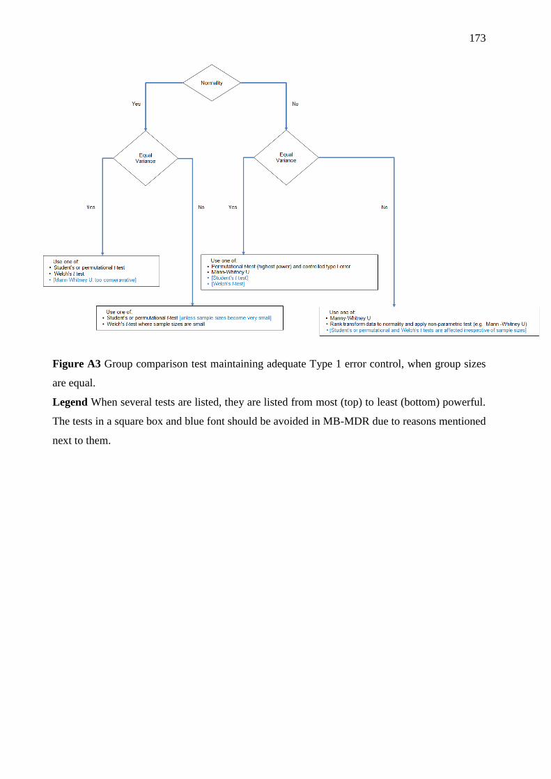
173

Figure A3 Group comparison test maintaining adequate Type 1 error control, when group sizes

are equal.

Legend When several tests are listed, they are listed from most (top) to least (bottom) powerful.

The tests in a square box and blue font should be avoided in MB-MDR due to reasons mentioned

next to them.

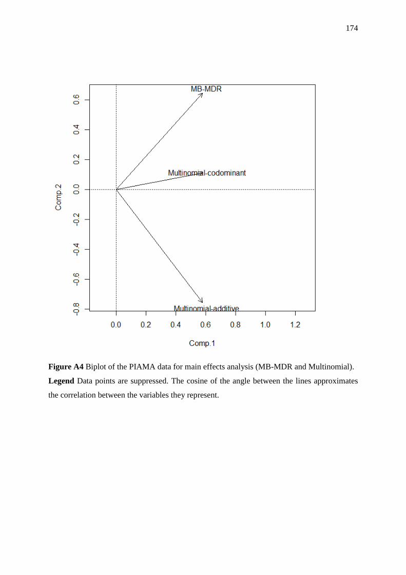
174

Figure A4 Biplot of the PIAMA data for main effects analysis (MB-MDR and Multinomial).

Legend Data points are suppressed. The cosine of the angle between the lines approximates

the correlation between the variables they represent.

175

Figure A5 MB-MDR 2-order epistasis screening results.

Legend Rtn– the quantitative trait normalized by rank transformation; Polygenic_Rtn – the

residuals derived from the polygenic model applied to the Rtn; ME adjust. – main effect

adjustment; FP- False positive rate is estimated as percentage of analyses with identified MB-

MDR significant results at alpha level 0.05.

176

Figure A6 False positive percentage of analyses with identified significant epistasis models

other than the correct two functional interacting loci (SNP1 x SNP2).

Legend Profiles are shown for codominant coding when no correction is performed,

correction performed at both MB-MDR steps and when correction is only perfomed at step2.

177

Figure A7 Empirical power estimates for MB-MDR as the percentage of analyses where the

correct interaction (SNP1 x SNP2) is significant at the 5% level.

Legend Profiles are shown for codominant coding when no correction is performed,

correction performed at both MB-MDR steps and when correction is only perfomed at step2.

Genomic Association Screening Methodology for High - ORBi

Documents

Transcript of Genomic Association Screening Methodology for High - ORBi