Influences of electric charges on an isolated drop - ORBi
176
Université de Liège Faculté des Sciences Département de Physique Influences of electric charges on an isolated drop Brandenbourger Martin Thèse présentée en vue de l’obtention du grade de Docteur en Sciences Physiques Année académique 2015-2016
-
Upload
khangminh22 -
Category
Documents
-
view
0 -
download
0
Transcript of Influences of electric charges on an isolated drop - ORBi

Université de LiègeFaculté des Sciences
Département de Physique
Influences of electric chargeson an isolated drop
Brandenbourger Martin
Thèse présentée en vue de l’obtentiondu grade de Docteur en Sciences
PhysiquesAnnée académique 2015-2016


Université de LiègeFaculté des Sciences
Département de physiqueGRASP
Thesis advisor: Dr. Stéphane Dorbolo
Université de LiègeFaculté des Sciences
Group for Research and Applications in Statistical PhysicsAllée du 6 août, 19 B-4000 Liège, Belgium
email: [email protected]
Cette Thèse a été réalisée dans le cadre d’une bourse de doctorat fournie par le Fondspour la formation à la Recherche dans l’Industrie et dans l’Agriculture (FRIA) financépar le Fonds de la Recherche Scientifique - FNRS (FRS - FNRS).
G R A S P
Thèse présentée en vue de l’obtention du gradede Docteur en Sciences Physiques
Annèe académique 2015-2016

Remerciements
En premier lieu, je tiens à remercier les professeurs Álvaro Marín, Antonin Eddi,Benoît Scheid, Hervé Caps et John Martin d’avoir accepté de faire partie de monJury de thèse. C’est une grande joie pour moi que chacun d’eux aient accepté deprendre le temps de juger mon travail.
En second lieu, j’aimerais remercier la personne qui m’a fait aimer la recherche,Stéphane Dorbolo. Stéphane, ton style unique et ton approche de la recherche m’onttoujours impressionnés. Cette façon de toujours trouver de nouveaux angles d’ap-proches et de monter de magnifiques projets a été très inspirante. Au-delà de cela,ton écoute et ton intarissable flot d’idées m’ont toujours motivés. Ta façon de toujoursapporter de la bonne humeur et surtout de la bonne entente au sein du laboratoiren’a pas de prix. Enfin, ta patiente et ta sincérité ont constitués le terreau fertile quim’amène aujourd’hui à présenter ce manuscrit. En somme, merci pour ton aide ettous ces chouettes moments partagés.
Bien entendu, cette thèse ne fut pas qu’un échange bilatéral, beaucoup d’autres in-tervenants ont contribué à la réalisation de ce travail. Cette thèse a été réalisée au seindu laboratoire GRASP. Je suis profondément convaincu que l’ambiance d’innovation,d’amitié et d’échange permanent ont énormément contribué à mon travail. En par-ticulier, j’aimerais tout d’abord remercier Laurent Maquet, Baptiste Darbois-Texier,Hervé Caps et Pierre-Brice Bintein.
Laurent, nos habitudes de vieux couple lors de nos sessions de mesures m’ontbeaucoup appris. C’est en faisant nos premiers pas d’expérimentateurs que nous noussommes rencontrés et c’est en vrais potes que l’on finit notre thèse à quelques moisd’intervalle. Qui aime bien châtie bien, je crois que ce dicton nous va incroyablementbien. Surtout ne change pas, sauf si ton médecin te le recommande.
Baptiste, tu es une personne incroyable, aussi bien dans le laboratoire qu’en dehors.Ta motivation et ton optimisme m’ont ouvert les yeux à de nombreuses reprises. Tesdeux ans passés au laboratoire ont sans aucun doute contribué à forger le chercheurque je suis aujourd’hui. Il va falloir trouver de nouvelles excuses pour encore travaillerensemble !
Hervé, tes compétences en matière de transfert de connaissance ont construit lephysicien que je suis. Evidemment, cette phrase doit être présente dans la majoritédes thèses du GRASP, mais ce qui est pour moi particulier, c’est que j’ai découvertl’université de Liège grâce à ta capacité à retirer une nappe d’une table sans fairebouger des assiettes. Grâce à toi, Science et Culture a donc été le catalyseur de mapassion pour la physique. Au-delà de ton instruction, je tiens à te remercier pour tousces bons moments passés ensemble, en particulier dans la région de Bordeaux !
ii
Pierre-Brice, le petit nouveau, je pense qu’on a beaucoup de point de ressem-blance. Je regrette terriblement de n’avoir pas eu plus de temps pour maniper avectoi. Occupe-toi bien de Stéphane après notre départ à Laurent et moi. Enfin, mercipour tes conseils avisés et pour avoir trouvé un titre à cette thèse.
Mes chers voisins de bureau, pour ne pas les citer Nicolas, Charles, Alexis etSofiene, nos petites discussions et les photos de Charles vont me manquer. Un mercitout particulier à Alexis pour ses relectures éclairées et éclairantes.
Je remercie également Geoffroy, Eric, Médéric et presque tous ceux cités plus hautpour les moments Pavé et Minus. Ces moments de pure détente ont aussi permis deforger un fort esprit d’équipe et de belles amitiés.
Dans le top des contributeurs de cette thèse, je me dois également de citer Médéric,Samuel, Jean-Claude, Florian et Chouaib. Les gars, vous avez des mains en or etdes compétences que je rêverais d’avoir. Ces deux dons ont permis de réaliser unebonne partie des montages présentés dans cette thèse et pour cela, je vous remercie.J’ajouterais une note toute particulière pour Médéric et Sam, avec qui j’ai passéde supers moments à l’ESTEC aux Pays-Bas. J’aurais voulu que ces moments sereproduisent plus souvent.
Bien entendu, le GRASP est constitué de beaucoup d’autres membres incroyables.Nicolas Vandewalle, Julien, Martial, Alexis Darras, François Ludwig, Maxime, Arianne,Boris, Florianne, Martin Poty, Galien et Sébastien, je vous remercie pour chacun deslongs ou brefs moments passés avec vous. En particulier, Nicolas, merci pour ton in-croyable soutien et Julien, merci pour tes incroyables blagues. De la même manière,je remercie Maryam, Florian Moreau, Felipe, Jérôme, Louis, Guillaume, Antonella etEline. Même si vos passages ont été trop brefs pour certains d’entre vous, j’ai vraimentapprécié chacune de vos personnalités.
I would like to extent a special thank to Tadd Truscott and his two PhD studentsZhao and Nathan. Tadd, thank for your stay in Belgium. I think I never learned somany things in such a small period of time. You are an amazing person, not only inresearch, but also in everyday life. I am really impressed by the way you are alwaysdriven by passion. Zhao, I love your efficiency and Nathan it was a real pleasure tohave you in the lab.
Durant ma première année de thèse, j’ai également eu l’occasion de passer troismois au laboratoire de la compagnie des interfaces, sous l’encadrement de DavidQuéré. David, merci de m’avoir ouvert la porte de ce laboratoire exceptionnel. Durantmon séjour, j’ai eu l’occasion de rencontrer des gens passionnants. Certains, sans que lehasard y soit pour quelque chose, ont déjà été cités plus haut. Ainsi, Eline, Philippe,Pierre-Brice, Baptiste, Dan, Guillaume, Timothée, Caroline et Adrien, merci pourtous ces chouettes moments partagés. Un remerciement spécial à Loïc, un Françaisde plus en Belgique !
Enfin, cette thèse a bénéficié de nombreuses aides gouvernementales et euro-péennes. J’aimerais remercier chacun des organismes qui ont contribué aux résultatsprésentés dans ce manuscrit. Je remercie tout d’abord le projet Micromast, financépar Belspo, ainsi que le FRIA, financé par le FNRS, pour m’avoir accordé le finance-ment de 4 ans d’études doctorales. Je remercie également L’ARD de l’Université deLiège, pour le financement de plusieurs voyages, ainsi que l’ESA pour le financement
iii
d’études en hyper et micro gravité.Je voudrais également profiter de cette section pour remercier toute ma famille :
Papa, maman, Alix, vous avez forgé l’homme qui je suis aujourd’hui et pour cela,merci. Parrain, merci pour nos longues conversations et ton insatiable intérêt à m’ou-vrir les yeux sur de nouvelles choses. Marraine, merci pour tout l’amour que tu m’asapporté. Chers Touristes, merci pour toutes nos aventures. Virginie, source intaris-sable de mes passions, c’est ton soutien inébranlable qui m’a conduit jusqu’ici. Mercipour ton amour, l’éternité n’est pas suffisante pour exprimer a quel point je t’aime.
Merci...
Liège, Septembre 2016Martin Brandenbourger


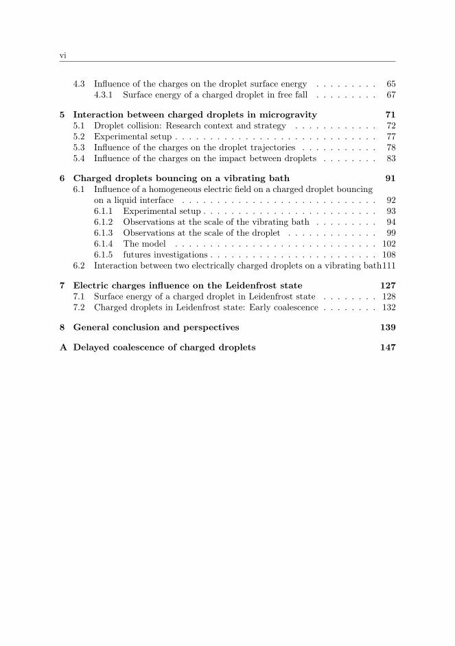
Table of Contents
Remerciements i
Publications vii
Résumé ix
English summary xi
1 Introduction 1
2 Research context 52.1 How does the droplet acquire an excess of charges? . . . . . . . . . . . 62.2 How does the charge affect the droplet? . . . . . . . . . . . . . . . . . 8
2.2.1 Influence of the charge on the droplet interface . . . . . . . . . 82.2.2 Charged droplets influenced by an external electric field . . . . 11
2.3 Take advantage of the charge in the droplet . . . . . . . . . . . . . . . 162.3.1 The electrospray . . . . . . . . . . . . . . . . . . . . . . . . . . 162.3.2 Use a charged droplet to manipulate liquid . . . . . . . . . . . 18
2.4 The need and the strategy . . . . . . . . . . . . . . . . . . . . . . . . . 19
3 Experimental details 233.1 Creating Charged droplets . . . . . . . . . . . . . . . . . . . . . . . . . 24
3.1.1 Charged droplet generators . . . . . . . . . . . . . . . . . . . . 263.1.2 Influence of the electric field on the droplet generation . . . . . 30
3.2 Measuring the charge of droplets . . . . . . . . . . . . . . . . . . . . . 333.3 Droplet storage methods . . . . . . . . . . . . . . . . . . . . . . . . . . 35
3.3.1 The microgravity . . . . . . . . . . . . . . . . . . . . . . . . . . 363.3.2 The vibrating bath . . . . . . . . . . . . . . . . . . . . . . . . . 403.3.3 The Leidenfrost effect . . . . . . . . . . . . . . . . . . . . . . . 43
4 Influence of the charge on the droplet 474.1 Influence of the liquid composition . . . . . . . . . . . . . . . . . . . . 484.2 Charge loss over time . . . . . . . . . . . . . . . . . . . . . . . . . . . 53
4.2.1 Charge loss of a bouncing droplet . . . . . . . . . . . . . . . . . 544.2.2 Model the charge loss of bouncing droplets . . . . . . . . . . . 554.2.3 Charge loss of droplets in microgravity and Leidenfrost state . 64
vi
4.3 Influence of the charges on the droplet surface energy . . . . . . . . . 654.3.1 Surface energy of a charged droplet in free fall . . . . . . . . . 67
5 Interaction between charged droplets in microgravity 715.1 Droplet collision: Research context and strategy . . . . . . . . . . . . 725.2 Experimental setup . . . . . . . . . . . . . . . . . . . . . . . . . . . . . 775.3 Influence of the charges on the droplet trajectories . . . . . . . . . . . 785.4 Influence of the charges on the impact between droplets . . . . . . . . 83
6 Charged droplets bouncing on a vibrating bath 916.1 Influence of a homogeneous electric field on a charged droplet bouncing
on a liquid interface . . . . . . . . . . . . . . . . . . . . . . . . . . . . 926.1.1 Experimental setup . . . . . . . . . . . . . . . . . . . . . . . . . 936.1.2 Observations at the scale of the vibrating bath . . . . . . . . . 946.1.3 Observations at the scale of the droplet . . . . . . . . . . . . . 996.1.4 The model . . . . . . . . . . . . . . . . . . . . . . . . . . . . . 1026.1.5 futures investigations . . . . . . . . . . . . . . . . . . . . . . . . 108
6.2 Interaction between two electrically charged droplets on a vibrating bath111
7 Electric charges influence on the Leidenfrost state 1277.1 Surface energy of a charged droplet in Leidenfrost state . . . . . . . . 1287.2 Charged droplets in Leidenfrost state: Early coalescence . . . . . . . . 132
8 General conclusion and perspectives 139
A Delayed coalescence of charged droplets 147
Publications
Parts of this manuscript have been published in peer reviewed revues, others aresubmitted. Those publications are listed below.
1. M. Brandenbourger, N. Vandewalle, and S. Dorbolo, Displacement of an elec-trically charged drop on a vibrating bath, PRL, 116, 044501 (2016).
2. M. Brandenbourger, H. Caps, J. Hardouin, Y. Vitry, and S. Dorbolo, Electricallycharged droplets in microgravity : Impact and Trajectories, Submitted to Icarus(2016).
3. L. Maquet, B. Darbois-Texier, A. Duchesne, M. Brandenbourger, B. Sobac, A.Rednikov, P. Colinet, and S. Dorbolo, Leidenfrost drops on a heated liquid pool,accepted in PRF (2016).
4. M. Brandenbourger, S. Dorbolo, Electrically charged droplet: case study of asimple generator, J. Can. Phys. 92, 1203 (2014).
Sometimes it is good to step back to better assess a situation. During my PhD the-sis, I had the opportunity to work on other projects. Projects that led to a publicationare listed below:
1. M. Brandenbourger, S. Dorbolo, and B. Darbois-Texier, Physics of a Toy Geyser,Submitted to PRF (2016).
2. L. Maquet, M. Brandenbourger, B. Sobac, A.-L. Biance, P. Colinet, S. Dorbolo,Leidenfrost drops : Effect of gravity, EPL 110, 24001 (2015).
3. S. Dorbolo, L. Maquet, M. Brandenbourger, F. Ludewig, G. Lumay, H. Caps,N. Vandewalle, S. Rondia, M. Melard, J. van Loon, A. Dowson, and S. Vincent-Bonnieu, Influence of the gravity on the discharge of a silo, Granular Matter.15, 263 (2013).
4. S. Dorbolo, M. Brandenbourger, F. Damanet, H. Dister, F. Ludewig, D. Ter-wagne, G. Lumay, and N. Vandewalle, Granular gas in a periodic lattice, Euro-pean Journal of Physics 32, 1465 (2011).


Résumé–Summary in French–
La célèbre expérience de Millikan, ainsi que l’étude des nuages d’orages, ont montréqu’un excès de charges électriques dans une goutte peut considérablement influencerson comportement. D’une part, l’excès de charges électriques influence les proprié-tés des gouttes, telles que sa fréquence d’oscillation ou sa pression interne. D’autrepart, les charges au sein de la goutte peuvent interagir avec des champs électriquesextérieurs. Dans cette thèse, on s’est intéressé à l’influence d’un excès de chargesélectriques sur une goutte millimétrique isolée électriquement.
Les précédentes recherches sur des gouttes chargées isolées ont souvent été can-tonnées à l’étude de gouttes micrométriques. Ceci s’explique par la difficulté d’isolerélectriquement cette goutte. Pour répondre à cette problématique, nous nous sommesintéressé à trois dispositifs permettant d’éviter la décharge d’une goutte : la microgra-vité, l’expérience du bain vibrant et l’effet Leidenfrost. A travers ces trois systèmes,nous avons étudié l’influence des charges électriques sur les propriétés physiques de lagoutte ainsi que sur son interaction avec les systèmes de stockages utilisés. En outre,nous nous sommes également intéressé à l’interaction d’une goutte chargée avec unchamp électrique extérieur. Ainsi, nous avons examiné l’interaction entre deux goutteschargées et l’interaction entre une goutte chargée et un champ électrique homogène.
L’ensemble de ces études nous a permis de mieux décrire le processus de migrationde charges au sein d’un liquide ainsi que le processus de perte de charges d’une goutte.En particulier, nous avons pu identifier et modéliser un nouveau mécanisme de pertesde charges se produisant en un temps caractéristique de plusieurs minutes. Nous avonségalement pu confirmer l’influence de la charge électrique sur l’énergie de surface d’unegoutte. Quant à l’utilisation de trois systèmes de stockages, nos études en microgra-vité nous ont permis de décrire l’influence de la répulsion ou de l’attraction électriquesur l’impact entre deux gouttes chargées. L’éventail de comportements observés a étécomparé au cas d’impacts entre deux gouttes neutres. Dans un autre registre, l’étuded’une goutte chargée se déplaçant à la surface d’un bain vibrant grâce à l’action d’unchamp électrique extérieur nous a permis d’en apprendre plus sur l’interaction entreune goutte et la surface d’un bain visqueux. Par exemple, nous avons observé unrégime “go-stop" dans lequel la goutte chargée se déplace durant son rebond et eststoppée durant son interaction avec le bain vibrant. Nous avons pu montrer qu’un telrégime apparait pour une goutte de volume important influencée par une force élec-trique faible. Dans cette configuration, la goutte se déplace avec une vitesse moyenneconstante, ce qui la rend facilement manipulable. En conséquence, cette étude a menée

x Résumé
au développement d’un prototype de microfludique permettant de contrôler le dépla-cement de gouttes en évitant toutes pollutions par contact. Dans cette optique, nousnous sommes également intéressé à l’interaction entre deux gouttes chargées stockéessur un bain vibrant. Cette étude a permis d’affiner notre compréhension de l’interac-tion entre deux gouttes chargées. Ainsi, nous avons pu montrer que deux gouttes demême charges se déplacent jusqu’à atteindre une distance d’équilibre. Cet équilibreest dû à la compensation de l’attraction capillaire par la répulsion électrique. Enfin,notre étude de gouttes chargées en Leidenfrost sur un bain liquide a démontré que laprésence de charges électriques produit une coalescence prématurée de la goutte avecle bain liquide. Plus généralement, nos mesures nous ont amené à mieux comprendrecomment la présence de charges électriques à la surface de deux interfaces liquidesséparées d’une fine couche de gaz tend à générer une forte attraction entre ces deuxinterfaces.
A la vue de nos résultats, nous pouvons conclure que la présence de charges au seinde gouttes millimétriques influence de façon visible leurs comportements intrinsèquesainsi que leurs interactions avec leur environnement. En outre, chacun des systèmesde stockages étudiés a apporté des réponses à différentes problématiques. L’étude enmicrogravité de l’impact entre deux gouttes chargées ébauche de nouvelles explica-tions quant au comportement des nuages d’orages. Les résultats accumulés quant àla manipulation de gouttes chargées sur bain vibrant ouvrent la voie à de nouveauxsystèmes microfluidiques. Enfin, l’analyse d’une goutte chargée en Leidenfrost décritun nouveau moyen d’étudier l’influence de charges électriques sur l’interaction entreinterfaces liquides.

English summary
Research such as the famous Millikan experiment or the studies concerning thun-derclouds have shown that droplets can be considerably influenced by an excess ofelectric charges. Indeed, an excess of charges can affect the intrinsic properties of adroplet, such as its natural oscillation frequency or its internal pressure. Moreover,the electric charges in excess in droplets can also interact with external electric fields.In this thesis, we investigated the influence of electric charges on millimetric dropletsthat are electrically isolated.
In literature, research on isolated charged droplets are mainly focused on dropletswith a micrometric size. The lack of studies concerning millimetric charged dropletsis explained by the difficulty storing them while avoiding charge leakage. In order toanswer to this issue, we examined three storage systems limiting the charge leakage:the microgravity, the vibrating bath method and the Leidenfrost effect. Throughthese systems, we studied the influence of electric charges on the droplet physicalproperties, but also the interaction between the charged droplet and its storage sys-tem. Furthermore, we investigated the interaction of charged droplets with externalelectric fields. More precisely, we studied the interaction between two electricallycharged droplets and the interaction between one charged droplet and an externalhomogeneous electric field.
A first set of experiments on electrically charged droplets allowed us modeling thecharge migration process in liquids and the charge leakage from a millimetric droplet.In particular, we identified and modeled a new mechanism of charges leakage occur-ring at a time scale of several minutes. Moreover, we confirmed the influence of theelectric charges on the droplet surface energy previously deduced from experimentson micrometric droplets. Concerning the three storage systems, the experiments per-formed in microgravity allowed us describing the influence of the electric interactionon the impact between two charged droplets. The diverse behaviors observed werecompared to the cases of impacts between two neutral drops. On a different note, thestudy of a charged droplet moving on the surface of a vibrating bath because of theinfluence of an external electric field gave new insights on the interaction between abouncing droplet and a viscous liquid bath. For example, we observed a “go-stop"motion during which the droplet horizontally moves when it bounces away and isstopped during its interaction with the liquid bath. We showed that this motion oc-curs when large droplets are influenced by a weak electric field. Droplets with thiskind of motion move with a constant average speed, which makes them easily manoeu-vrable. Therefore, the control of the droplet motion led to the development of a newmicrofluidic prototype. Via this new setup, basic microfluidic tasks can be performed
xii Summary
without polluting droplet via contacts with solids or liquids. With these results inmind, we also examined the interaction between two charged droplets bouncing onthe vibrating bath. This study brought new insights on the interaction between twocharged droplets. Indeed, we observed that two drops with the same charges tend toremain at an equilibrium distance. Our study showed that this equilibrium distanceis due to the compensation of the electric repulsion by capillary attraction at the sur-face of the vibrating bath. Finally, our study of charged droplet in Leidenfrost stateon a liquid bath led to a better understanding of the interaction between chargedliquid interfaces. Indeed, we showed that electric charges cause the early coalescenceof charged droplet because of an increase in the vapor layer drainage.
We conclude from our results that an excess of electric charges influences ostensiblythe intrinsic behavior of a droplet and its interaction with the environment. Further-more, each storage system studied brought answers to specific issues. The study ofthe impact between charged droplets in microgravity outlines new explanations onthe behavior of thunderclouds. The results accumulated on the micromanipulationof charged droplet bouncing on a vibrating bath opens the way to a new kind ofmicrofluidic system. Finally, the study on the charged Leidenfrost droplets describesnew ways to investigate the influence of electric charges on liquid interfaces.
1Introduction
This thesis aims at studying electrically charged drops (which will also be calledcharged droplets). The next Chapters are dedicated to the description of the obtainedresults and the validation of these results compared to the state of the art. But beforestudying in detail the behavior of electrically charged droplets, we have to define whatthey are.
Droplets, neutral or charged, can be simply described as being small volumes ofliquid (typically, few cubic millimeters). These small quantities of liquid are presenteverywhere on Earth and we encounter them every day of our lives. While wakingup, we feel few drops of sweat due to the heat of the night. Once out of bed, we feelagain droplets falling from the shower. It is now time to take the breakfast and whilepouring a glass of fresh orange juice, few droplets splash out of our glass. We wipethese droplets with paper towel and we go quickly to work. On our way, we complainabout the rain that announces a non-sunny day. The day has not yet begun, butdroplets have already been everywhere.
What do differentiate small quantities of liquids from large ones? At the scaleof a droplet, the surface forces become more effective than volume forces. Typically,the droplet surface tension overcomes the gravity force. Therefore, droplet does notanswer to the same laws as larger quantities of liquids. Volumes of liquids are generallyconsidered small when they have a characteristic length equal or smaller than thecapillary length lc =
√γ/ρg, where γ is the surface tension, ρ is the droplet density
and g is the acceleration of gravity. Water has a capillary length lc ≈ 3 mm. At thisscale, because the surface forces overcome the volume forces, the physics of liquidsvaries compared to observations made at the scale of a bowl or a pool filled with
2 Introduction
water. For example, liquids tend to reduce their surface rather than spread out. Asa consequence, droplets tend to take a spherical shape. The droplets studied duringthis thesis were composed of various liquids (essentially water and silicone oil), buthad a characteristic size l ≤ lc.
In our case, we study droplets that have an excess of positive or negative electriccharges. The interest in the study of charged drops is two fold.
1. The excess of electric charges in the droplet affects its fundamental behavior.Indeed, charges in excess in the droplets influences the droplet natural frequency,intern pressure,...
2. The excess of charges in droplets also means that the droplet reacts differentlyto external electric fields. The excess of electric charges may move in the dropletand affect its surface according to the applied electric field. In the same way,the droplet can be set in motion by the electric forces applied on the electriccharges.
Both aspects are studied throughout this manuscript. Because of the predomi-nance of its surface force, a droplet, charged or not, may take various shapes accord-ing to its environment. As shown in Fig. 1.1, droplets may spread on a solid surfaceaccording to its wettability. On the contrary, droplets take a lens shape at the surfaceof a fluid. Finally, a droplet can also be in contact only with gas. In such configura-tions, the droplet minimizes its volume because of the surface tension. Therefore, thedroplet takes a spherical shape. The three cited configurations are subject to differentresearch. For example, in the case neutral droplets in contact with a solid, researchinvestigated the angle of contact θ of the droplet as a function of the solid and liquidproperties. In the same way, in the case of charged droplets in contact with solids,studies investigated how the charge of the droplet varies this angle of contact θ. Thislast research topic is commonly named electrowetting.
In our case, we chose to stay away from these configurations and consider dropletsin contact only with gas. In particular, we studied droplets in contact with ambientair or in contact with their own vapor. In such configurations, there is no wetting. Thecharged droplet is only influenced by its surface tension, the air motion and eventuallyexternal forces. Moreover, given the low viscosity of air, the droplet deformation isnot damped by external interactions. Furthermore, gases are relatively good electricalinsulators. As a consequence, we can make the assumption that the droplet chargeloss is highly limited while the droplets are in contact only with gas. In other words,we can assume that the droplet is electrically isolated. Of course, this hypothesis hasto be checked throughout the thesis.
In short, our subject of research can be defined as the investigationof the behavior of a liquid droplet with an excess of electric charges, thedroplet being only in contact with ambient air. Naturally, electric charges are

Chapter 1 3
Non-conducting material
(e.g.. PVC)
Conducting material
(e.g. metal)Liquid
1 2 3
Figure 1.1: Examples of droplets in contact with a solid, with a liquid and with a gas.Note that the colors used on the schema define the color coding used for the entire of thismanuscript.
not observable by the naked eye. Therefore, it is not easy to differentiate a neutraldroplet from a charged droplet. Yet, charged droplets are present in Nature.
The Fig. 1.2 shows three natural spots where electrically charged droplets onlyin contact with ambiant air can be found. The thunderclouds are the most commonexample. Actually, thunderclouds can be defined as clusters of water droplets thatacquired an excess of electric charges. They are mostly recognized by their lightnings,occurring when the thundercloud discharge on the earth. Since Benjamin Franklin[1], numerous studies tried to describe the thunderclouds behavior. The state ofunderstanding is well summarized by Leblanc et al [2]. The difficulty resides in thefact that charged clouds are difficult to reproduce. Studies approached the problem bysimulating the process [3] or by direct measurements in thunderclouds [4]. Nowadays,thunderclouds are described as complex structures with different layers of electriccharges alternating in polarity [4]. Beyond the description of the interaction betweenseveral charged droplets, the interaction between two charged droplets is not fullyunderstood [5].
Clouds are not the only droplets concerned by electric charges. Naturally, rain-drops produced by a thundercloud are also charged [5, 6]. Charged droplets are alsoobservable in waterfalls [7] and in droplets at the surface of ocean [8, 9]. They cor-respond to sprays of small droplet visible on the Fig 1.2. The same questions as theones about thunderclouds arise when looking at these charged droplets.
Given their ability to influence the droplet properties and interact with electric

4 Introduction
Image Credit: Robert Arn
Image Credit: Derek Kind Image Credit: Laure Thibaut
Figure 1.2: Thunderclouds, waterfalls and droplets emitted from ocean are three examples ofthe natural presence of electrically charged droplets.
fields, charged droplets also play a role in industry. They are used in various domainssuch as agriculture research (pesticide spreading [10]), spectrometry (electrosprayionization technique [11]), satellite research (electric propulsion rocket engine [12]) ormicrofluidics [13]. These domains will be cited along the manuscript, but, as physicist,we primarily focus our attention on the droplet behavior itself and not their industrialapplications.
Now that the object “electrically charged droplet" has been defined, it remainsto describe in detail its behavior. In the next Chapter, we introduce the conceptof charges excess and the major discoveries made about charged droplets in contactonly with gas. Then, we highlight the remaining gray areas where understanding stillneeds to gain ground. Finally, we expose our strategy to take a part in this dialogue.

2Research context
Contents2.1 How does the droplet acquire an excess of charges? . . . 6
2.2 How does the charge affect the droplet? . . . . . . . . . . 8
2.2.1 Influence of the charge on the droplet interface . . . . . . 8
2.2.2 Charged droplets influenced by an external electric field . 11
2.3 Take advantage of the charge in the droplet . . . . . . . 16
2.3.1 The electrospray . . . . . . . . . . . . . . . . . . . . . . . 16
2.3.2 Use a charged droplet to manipulate liquid . . . . . . . . 18
2.4 The need and the strategy . . . . . . . . . . . . . . . . . . 19
In this Chapter, we summarize the state of knowledge on the behavior of elec-trically charged droplets. Firstly, we outline the different mechanisms describinghow droplets may acquire an excess of electric charges. Secondly, we explain resultsof studies investigating the influence of electric charges on the intrinsic behavior ofdroplets. Thirdly, we introduce different experiments that allowed understanding theinfluence of an external electric field on a charged droplet. Finally, we detail tworesearch domains that directly derive from the study of electrically charged droplets:the electrosprays and the digital microfluidics. Through all these research we identifyshadow zones that require further investigations. Once these lacks of understandingidentified, we construct the strategy of our research.
6 Research context
2.1 How does the droplet acquire an excess of charges?
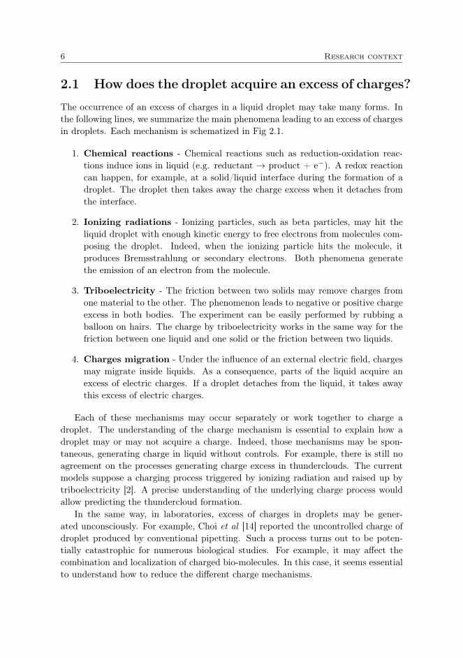
The occurrence of an excess of charges in a liquid droplet may take many forms. Inthe following lines, we summarize the main phenomena leading to an excess of chargesin droplets. Each mechanism is schematized in Fig 2.1.
1. Chemical reactions - Chemical reactions such as reduction-oxidation reac-tions induce ions in liquid (e.g. reductant → product + e−). A redox reactioncan happen, for example, at a solid/liquid interface during the formation of adroplet. The droplet then takes away the charge excess when it detaches fromthe interface.
2. Ionizing radiations - Ionizing particles, such as beta particles, may hit theliquid droplet with enough kinetic energy to free electrons from molecules com-posing the droplet. Indeed, when the ionizing particle hits the molecule, itproduces Bremsstrahlung or secondary electrons. Both phenomena generatethe emission of an electron from the molecule.
3. Triboelectricity - The friction between two solids may remove charges fromone material to the other. The phenomenon leads to negative or positive chargeexcess in both bodies. The experiment can be easily performed by rubbing aballoon on hairs. The charge by triboelectricity works in the same way for thefriction between one liquid and one solid or the friction between two liquids.
4. Charges migration - Under the influence of an external electric field, chargesmay migrate inside liquids. As a consequence, parts of the liquid acquire anexcess of electric charges. If a droplet detaches from the liquid, it takes awaythis excess of electric charges.
Each of these mechanisms may occur separately or work together to charge adroplet. The understanding of the charge mechanism is essential to explain how adroplet may or may not acquire a charge. Indeed, those mechanisms may be spon-taneous, generating charge in liquid without controls. For example, there is still noagreement on the processes generating charge excess in thunderclouds. The currentmodels suppose a charging process triggered by ionizing radiation and raised up bytriboelectricity [2]. A precise understanding of the underlying charge process wouldallow predicting the thundercloud formation.
In the same way, in laboratories, excess of charges in droplets may be gener-ated unconsciously. For example, Choi et al [14] reported the uncontrolled charge ofdroplet produced by conventional pipetting. Such a process turns out to be poten-tially catastrophic for numerous biological studies. For example, it may affect thecombination and localization of charged bio-molecules. In this case, it seems essentialto understand how to reduce the different charge mechanisms.
Chapter 2 7
+~E
++
++ +
--
-++
+- -
--
Charges migration
++ +-+
++-- --
+ ++ +--~vd
~vs
Charge by frictionCharge by redox reaction
+
e
Charge by ionizing radiation
+
M(s) ! M2+(aq) + 2e
Figure 2.1: Description of four different ways for a droplet to accumulate an excess ofcharges. The top left schema describes the droplet charge via redox reaction. The bottomleft schema describes the charge by ionizing radiation. The top right schema describes thetriboelectricity process. The bottom right schema describes the charge migration mechanism.Once the excess of charges is induced in the droplet, the droplet may detach from its sub-strate. When the droplet detaches from the substrate, a free electrically charged droplet hasbeen created.
8 Research context
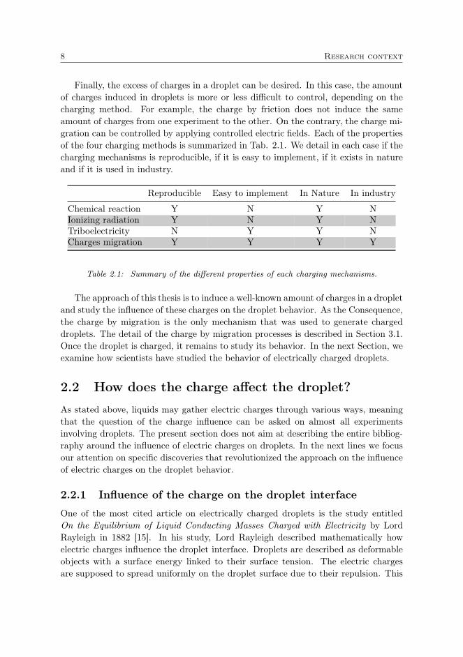
Finally, the excess of charges in a droplet can be desired. In this case, the amountof charges induced in droplets is more or less difficult to control, depending on thecharging method. For example, the charge by friction does not induce the sameamount of charges from one experiment to the other. On the contrary, the charge mi-gration can be controlled by applying controlled electric fields. Each of the propertiesof the four charging methods is summarized in Tab. 2.1. We detail in each case if thecharging mechanisms is reproducible, if it is easy to implement, if it exists in natureand if it is used in industry.
Reproducible Easy to implement In Nature In industry
Chemical reaction Y N Y NIonizing radiation Y N Y NTriboelectricity N Y Y NCharges migration Y Y Y Y
Table 2.1: Summary of the different properties of each charging mechanisms.
The approach of this thesis is to induce a well-known amount of charges in a dropletand study the influence of these charges on the droplet behavior. As the Consequence,the charge by migration is the only mechanism that was used to generate chargeddroplets. The detail of the charge by migration processes is described in Section 3.1.Once the droplet is charged, it remains to study its behavior. In the next Section, weexamine how scientists have studied the behavior of electrically charged droplets.
2.2 How does the charge affect the droplet?
As stated above, liquids may gather electric charges through various ways, meaningthat the question of the charge influence can be asked on almost all experimentsinvolving droplets. The present section does not aim at describing the entire bibliog-raphy around the influence of electric charges on droplets. In the next lines we focusour attention on specific discoveries that revolutionized the approach on the influenceof electric charges on the droplet behavior.
2.2.1 Influence of the charge on the droplet interface
One of the most cited article on electrically charged droplets is the study entitledOn the Equilibrium of Liquid Conducting Masses Charged with Electricity by LordRayleigh in 1882 [15]. In his study, Lord Rayleigh described mathematically howelectric charges influence the droplet interface. Droplets are described as deformableobjects with a surface energy linked to their surface tension. The electric chargesare supposed to spread uniformly on the droplet surface due to their repulsion. This

Chapter 2 9
basic model of a charged droplet is schematized in Fig. 2.2. In his study, LordRayleigh theoretically describes how a liquid with an excess of electric charges reactsto small perturbations. By comparing the electric potential to the cohesion energy ofthe system, he deduced the oscillation frequency for the normal modes of a sphericalmass of liquids:
f2 =l(l − 1)
4π2ρr3
(γ(l + 2)− q2
16π2ε0r3
)(2.1)
where f is the oscillation frequency of the spherical mass of liquid, l determines theoscillating mode of the liquid, ρ is the liquid density, r is the sphere radius, ε0 is thevacuum permittivity and q is the surface charge of the liquid. Typically, a dropletpossesses a charge between 1 pC and 100 pC. Note that from Eq. 2.1, the oscillationfrequency of a neutral droplet is expressed by f0 = l(l − 1)(l + 2)γ/4π2ρr3.
In the case of a neutral water droplet with r = 0.5 mm, ρ = 1000 kg/m3 andγ = 72 mN/m oscillating in its natural mode (l = 2), the droplet oscillates with afrequency f = 342 Hz. If the same droplet possess a charge q = 100 pC, the dropletnatural oscillation frequency corresponds to f = 306 Hz.
+
+++++++ + + ++ +
+++++ ++ + + + + + ++++++
++++++++
++
+++++++
+
Figure 2.2: Basic model of a charged droplet: A conductive and deformable charged sphere.Because of the charge repulsion, the charges in excess are spread homogeneously on the surfaceof the sphere.
From this study at small perturbations, Lord Rayleigh also deduced the limit ofstability for a charged liquid sphere. When the electric repulsion between chargesovercomes the cohesion energy of the liquid, it becomes unstable. If Eq. 2.1 can beexpressed in real numbers, the liquid sphere is stable. On the contrary, a frequencyexpressed by complex numbers corresponds to an unstable liquid sphere. As a conse-quence, the critical charge for the instability to occur can be directly deduced fromEq. 2.1:
qc =√
64π2r3γε0 (2.2)

10 Research context
The theoretical predictions of Lord Rayleigh were proven to be exceptionally ac-curate. The oscillation frequency has been successfully validated via experimentalsetups using pendant droplets [16] or levitating droplets [17] methods. In particular,Hill and Eaves [18] have successfully measured the frequency shift of a charged dropletfor several charges and oscillating modes thanks to diamagnetical levitation of a waterdroplet.
Of course, electric charges inside the droplet can also be influenced by an externalelectric field. As a consequence, the droplet oscillation frequency can be influencedby an external electric field. The oscillation frequency, theoretically deduced from thebalance of pressures applied on the droplet, was calculated by Brazier-Smith et al [16].The frequency shift was found to be in good agreement with their measurements.
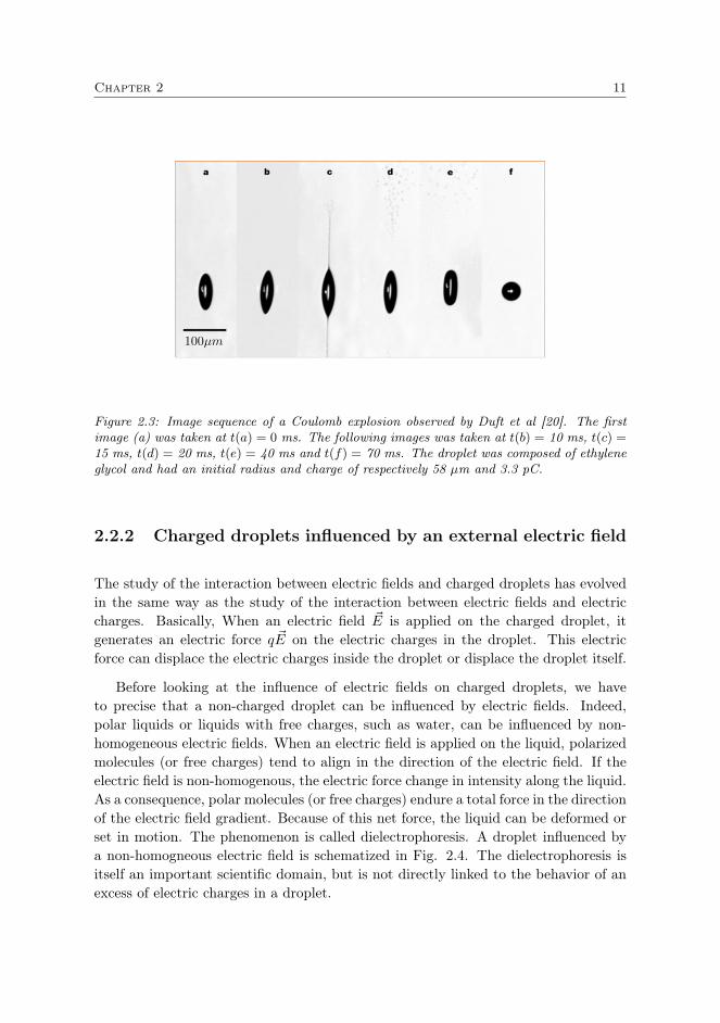
The stability limit predicted by Lord Rayleigh was also experimentally stud-ied. The charged droplet instability is now commonly named Coulomb instabilityor Coulomb explosion. Duft et al. [19, 20], have been able to precisely measure thelimit of the instability. For this purpose, they used an electrodynamic trap to levitatea charged ethylene glycol droplet. The electric field generated by the electrodynamictrap is adjusted in order to not affect the charged droplet oscillation. During thedroplet evaporation, the radius decreased until a critical size corresponding to thedroplet instability. They were able to observe microscopic images of the droplet de-formation resulting from this instability. The Fig. 2.3 shows the reproduction of theimage sequence obtained by Duft et al. [20]. The first image (a) was taken at t(a) = 0
ms. The following images was taken at t(b) = 10 ms, t(c) = 15 ms, t(d) = 20 ms,t(e) = 40 ms and t(f) = 70 ms. The droplet was composed of ethylene glycol andhad an initial radius and charge of respectively 58 µm and 3.3 pC. From image (a)to image (c), the droplet elongates until ejecting a fine jet of micro-droplets. Thesedroplets are highly charged. After the emission of the droplet jet, from image (d) toimage (f), the droplet stabilizes and goes back to a steady oscillation.
Since this major breakthrough, several studies have been focused on the descrip-tion of the dynamic of the Coulomb instability [21–24]. With Rayleigh work and thefollowing studies, the understanding of the charge influence on the interface betweengas and droplet is almost fully complete. However, as we will see in the Section 2.4,these studies do not answer to all the questions asked about the influence of chargeson droplets. Typically, the droplet can lose its charges via other mechanisms than theCoulomb explosion.
Finally, note that the surface energy of a charged droplet is the only intrinsic prop-erty that is significantly affected by the presence of electric charges. Other properties,such as the droplet density or the droplet viscosity only slightly vary with the dropletcharge.
Chapter 2 11
100µm
Figure 2.3: Image sequence of a Coulomb explosion observed by Duft et al [20]. The firstimage (a) was taken at t(a) = 0 ms. The following images was taken at t(b) = 10 ms, t(c) =15 ms, t(d) = 20 ms, t(e) = 40 ms and t(f) = 70 ms. The droplet was composed of ethyleneglycol and had an initial radius and charge of respectively 58 µm and 3.3 pC.
2.2.2 Charged droplets influenced by an external electric field
The study of the interaction between electric fields and charged droplets has evolvedin the same way as the study of the interaction between electric fields and electriccharges. Basically, When an electric field ~E is applied on the charged droplet, itgenerates an electric force q ~E on the electric charges in the droplet. This electricforce can displace the electric charges inside the droplet or displace the droplet itself.
Before looking at the influence of electric fields on charged droplets, we haveto precise that a non-charged droplet can be influenced by electric fields. Indeed,polar liquids or liquids with free charges, such as water, can be influenced by non-homogeneous electric fields. When an electric field is applied on the liquid, polarizedmolecules (or free charges) tend to align in the direction of the electric field. If theelectric field is non-homogenous, the electric force change in intensity along the liquid.As a consequence, polar molecules (or free charges) endure a total force in the directionof the electric field gradient. Because of this net force, the liquid can be deformed orset in motion. The phenomenon is called dielectrophoresis. A droplet influenced bya non-homogneous electric field is schematized in Fig. 2.4. The dielectrophoresis isitself an important scientific domain, but is not directly linked to the behavior of anexcess of electric charges in a droplet.

12 Research context
+++++++++++
----
+ +++
++-
-
-
~Fd
V
metallic piece liquid
-+-
+- Polarizable molecule
-
-
Figure 2.4: Schema of a droplet influenced by a dielectrophoretic force. Free charges inthe droplets (or polarized molecules) align with the electric field lines. Because of the non-homogeneity of the electric field, the electric force is more important on one side of thedroplet. As a consequence, the free charges and the polarized molecules endure a net force Fd
along the electric field. This net force can induce liquid deformation and liquid displacement.
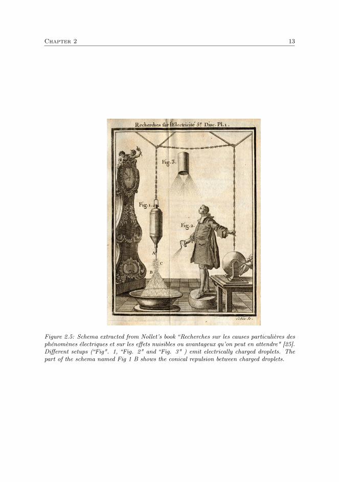
Charged droplet set in motion by an electric field
One of the first scientists to study the interaction between electric fields and chargeddroplets is Abbé Nollet [25]. Among numerous experiments concerning electricity, hestudied the water flow rates from an orifice with both charged and uncharged waterstreams. His description of the experiment is illustrated in Fig. 2.5. The differentsetups described as “Fig". 1, “Fig. 2" and “Fig. 3" corresponds to devices emittingdroplets. By charging the chain, Abbé Nollet was able the induce charge migrationin the ejected droplets. The experimental setup allowed him to demonstrate thatthe flow rate of charged droplets was more important than the flow rate of neutraldroplets. It is explained by the electric repulsion between the emitted droplets. Healso indicated that, for significant charges, droplets repels from each other in a conicalshape (see Fig. 2.5, “Fig 1 B"). This last observation is now a well known example ofthe interaction between electrically charged droplets. While charged droplets with thesame charge are emitted from the water stream, they endure both the gravity and theelectric repulsion between them. The two applied force explain the specific dropletmotion that lead to the conical shape of the droplet stream. Of course, the repulsionbetween charged droplets have been described in more details since the observationsof Abbé Nollet [26].
Abbé Nollet publications represent a first qualitative study of electrically charged
Chapter 2 13
Figure 2.5: Schema extracted from Nollet’s book “Recherches sur les causes particulières desphénomènes électriques et sur les effets nuisibles ou avantageux qu’on peut en attendre" [25].Different setups (“Fig". 1, “Fig. 2" and “Fig. 3" ) emit electrically charged droplets. Thepart of the schema named Fig 1 B shows the conical repulsion between charged droplets.

14 Research context
droplets. Later, with the evolution of the understanding on electric charges behav-ior, the charged droplets understanding has also evolved. In particular, the abilityto produce precise electric fields allowed studying in detail the interaction betweendroplets and electric fields. Currently, the simplest way to describe a charged dropletin an external electric field is to model the system by a point charge influenced by anelectric field. In this case, the electric force applied on the droplet is expressed by:
~Fel = q ~E (2.3)
where q is the total droplet charge and ~E the applied electric field. This model wasused in the famous Millikan experiment [27]. In his experiment, Millikan studiedthe motion of a charged droplet between two charged electrodes. The experimentis schematized in Fig. 2.6. The two charged electrodes were vertically aligned. Acharged droplet was produced and placed in between both electrodes. Once placedbetween both electrodes, the droplet endured the force due to its weight ~Fw, theelectric force due to the electric field produced by the electrodes ~Fel and the dragforce due to its motion ~Fd. By controlling the electric field, it was possible to controlthe direction and the speed of the droplet. Because of the drag force, the dropletacquired a constant speed after few seconds. This constant speed can be deduced bycalculating the equilibrium between the three forces. In doing so, we have:
vlim(E) = ±(
1
6πηr
)[4
3πr3g(ρh − ρa)− qE
](2.4)
where η is the air viscosity, r the radius of the droplet, g the acceleration of gravity, ρhthe droplet density and ρa the air density. The droplet can move upward or downward,which is expressed by the symbol ±. By measuring the droplet speed, Millikan wasable to deduce the droplet charge. By repeating the experiment on several dropletswith different charges, he deduced the value of the elementary charge (i.e. q=1.610−19 C).
Naturally, numerous experiments have been performed since the Millikan experi-ment [28,29]. In particular, studies have been focused on the influence of the dropletelectric charges on the surrounding electric field [28]. Indeed, the charged dropletproduces its own electric field, which can influence the overall electric field landscapeof the experiment. However, this phenomenon is a second order effect that can gen-erally be neglected. Experiments and simulations have also been developed to studyof the interaction between several charged droplets [3,30]. In this case, the motion ofone droplet in the electric field produced by one or many other charged droplets arestudied. Beyond these research, the precise motion of two charged droplets interactingwith each other still needs to be experimentally studied. Furthermore, the knowledgededuced from the Millikan experiment (i.e the droplet motion can be modeled as adroplet influenced by its weight, a simple electric force and the drag force) can beused in more complex systems where droplets endures other forces difficult to model.

Chapter 2 15
+V
~E~Fw + ~Fd
~Fel
Figure 2.6: The Millikan experiment. The displacement of a charged droplet is controlled byadjusting the external electric field. The electric field ~E can be oriented upward or downward.As a function of the applied electric force ~Fel, the droplet weight ~Fw and the drag force ~Fd,the droplet moves upward or downward.
Charged droplet deformed by an electric field
Beyond generating a displacement of the charged droplet, an external electric fieldcan also influence the droplet surface. Indeed, the electric charges on the dropletsurface endure an electric force due to their interaction with the electric field. Thepressure endured by the droplet can be expressed as:
P = Pin + Pel = γ
(1
R1+
1
R2
)− εrε0
2E2 (2.5)
where Pin is the droplet internal pressure without the influence of an external electricfield, Pel is the pressure endured by the droplet due to the electric field, R1 and R2 arethe droplet principal radii of curvature, E is the electric field on the droplet surfaceand εr is the droplet relative permittivity. Several studies have been focused on thedroplet deformation in an electric field [31,32]. In particular, studies investigated thedroplet deformation over time and the droplet instability that can result from thisdeformation. Indeed, when a charged droplet (or a charged liquid surface in general)is influenced by a significant electric field, it deforms in a conical shape named Taylorcone [33]. For an electric field significant enough, the charged surface is unstable andthe Taylor cone emits small droplets.
In this manuscript however, we limit our investigations to electric fields that doesnot deform droplet. The influence of an external electric field on the droplet shape is
16 Research context
described by the electric capillary number:
Ce =εrε0E
2r
γ(2.6)
The Eq. 2.6 is directly derived from Eq. 2.5. Our experiments studying the interactionbetween electric fields and charged droplets were limited to Ce ≈ 4 10−3. As aconsequence, the influence of the external electric field on the droplet shape wasconsidered negligible.
2.3 Take advantage of the charge in the droplet
The previous Section (see Section 2.2) exhibited the two major properties of dropletswith an excess of electric charges. (i) the charges influence the droplet properties (ii)the charges can be influenced by electric fields.
The progress in the charged droplet understanding allowed scientists developingnew setups that take advantage of the charged droplet properties. For example, thedroplet Coulomb explosion allowed developing sprays of very small droplets and theinteraction between charged droplet and electric field allowed controlling the dropletmotion. These new setups generated themselves new experimental configurations thatrequired new (or at least more detailed) explanations. In the next lines we examinethese new research topics, brought by the industry, which raised up new questions.
2.3.1 The electrospray
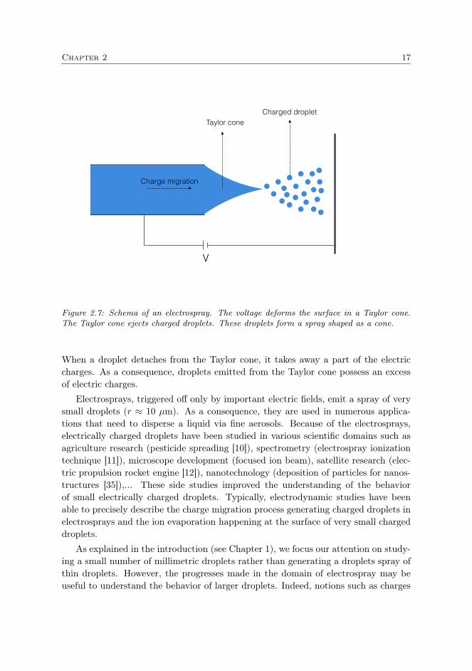
Electric fields and electrostatic interactions can be used to give information on morethan electrical phenomena. For example, spiderwebs take advantage of the chargeaccumulated on flying insects to increase their capture probabilities. Indeed, Ortega-Jimenez et al [34] have demonstrated that spiderwebs are attracted toward chargedinsect thanks to their electric conductivity.
In the same way, a significant part of the scientific research on charged droplets islinked to one of their applications: the electrosprays. The phenomenon is schematizedin Fig. 2.7. As explained in the previous Section (see Section 2.2), when a liquidsurface is subject to a significant electric field, the electric force applied on the surfacecan overcome forces due to surface tension. If the electric force is significant enough,the liquid surface deforms in a conical shape (i.e. a Taylor cone). When a certainelectric field threshold is reached, the Taylor cone emits a jet of small charged droplets.After their emission, the charged droplets quickly endure Coulomb explosions, whichproduce even smaller droplets. The whole charged jet is called an electrospray [11].
The droplet charge is due to the charge by migration process. When the electricfield is applied on the liquid, charges migrate toward the liquid interface. The electricforce applied on the charges at the interface explains the conical shape of the liquid.
Chapter 2 17
V
Taylor coneCharged droplet
Charge migration
Figure 2.7: Schema of an electrospray. The voltage deforms the surface in a Taylor cone.The Taylor cone ejects charged droplets. These droplets form a spray shaped as a cone.
When a droplet detaches from the Taylor cone, it takes away a part of the electriccharges. As a consequence, droplets emitted from the Taylor cone possess an excessof electric charges.
Electrosprays, triggered off only by important electric fields, emit a spray of verysmall droplets (r ≈ 10 µm). As a consequence, they are used in numerous applica-tions that need to disperse a liquid via fine aerosols. Because of the electrosprays,electrically charged droplets have been studied in various scientific domains such asagriculture research (pesticide spreading [10]), spectrometry (electrospray ionizationtechnique [11]), microscope development (focused ion beam), satellite research (elec-tric propulsion rocket engine [12]), nanotechnology (deposition of particles for nanos-tructures [35]),... These side studies improved the understanding of the behaviorof small electrically charged droplets. Typically, electrodynamic studies have beenable to precisely describe the charge migration process generating charged droplets inelectrosprays and the ion evaporation happening at the surface of very small chargeddroplets.
As explained in the introduction (see Chapter 1), we focus our attention on study-ing a small number of millimetric droplets rather than generating a droplets spray ofthin droplets. However, the progresses made in the domain of electrospray may beuseful to understand the behavior of larger droplets. Indeed, notions such as charges
18 Research context
migration or charges interaction with electric fields should not vary with the dropletsize. These progresses are discussed throughout this thesis according to their linkwith particular observations or theoretical developments.
2.3.2 Use a charged droplet to manipulate liquid
One of the last applications developed around electrically charged droplets concernsthe micromanipulation of droplets, i.e. doplet-based microfluidics. Generally, mi-crofluidics is associated with the use of closed micro-channels [36]. Studies used elec-trically charged droplets to control the droplet motion in channels networks [37, 38].However, closed micro-channels reduce the droplet motion to one dimension. As aconsequence, the droplet handling (i.e. the droplet generation, merging, mixing,..) islimited by the droplet flow in the micro-channel. Lately, research have been focusedon open microfluidics. Open microfluidics aims to transport and manipulate dropletsin two dimensions of space. The transport should be quick, without alteration of thedroplet content, and should allow one to perform operations including sorting, mixing,and analyzing the fluids. Open devices were demonstrated to be a more flexible wayto perform these different tasks, especially for micro-chemical analysis purposes [39].
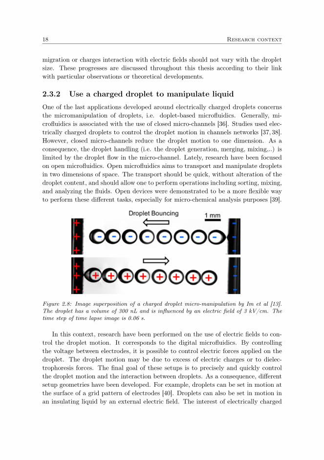
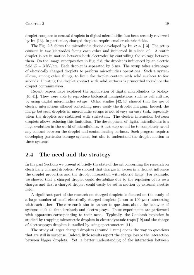
Figure 2.8: Image superposition of a charged droplet micro-manipulation by Im et al [13].The droplet has a volume of 300 nL and is influenced by an electric field of 3 kV/cm. Thetime step of time lapse image is 0.06 s.
In this context, research have been performed on the use of electric fields to con-trol the droplet motion. It corresponds to the digital microfluidics. By controllingthe voltage between electrodes, it is possible to control electric forces applied on thedroplet. The droplet motion may be due to excess of electric charges or to dielec-trophoresis forces. The final goal of these setups is to precisely and quickly controlthe droplet motion and the interaction between droplets. As a consequence, differentsetup geometries have been developed. For example, droplets can be set in motion atthe surface of a grid pattern of electrodes [40]. Droplets can also be set in motion inan insulating liquid by an external electric field. The interest of electrically charged
Chapter 2 19
droplet compare to neutral droplets in digital microfluidics has been recently reviewedby Im [13]. In particular, charged droplets require smaller electric fields.
The Fig. 2.8 shows the microfluidic device developed by Im et al [13]. The setupconsists in two electrodes facing each other and immersed in silicon oil. A waterdroplet is set in motion between both electrodes by controlling the voltage betweenthem. On the image superposition in Fig. 2.8, the droplet is influenced by an electricfield E = 3 kV/cm. Each droplet is separated by 6 ms. The setup takes advantageof electrically charged droplets to perform microfluidics operations. Such a systemallows, among other things, to limit the droplet contact with solid surfaces to fewseconds. Limiting the droplet contact with solid surfaces is primordial to reduce thedroplet contamination.
Recent papers have explored the application of digital microfluidics to biology[40, 41]. They were able to reproduce biological manipulations, such as cell culture,by using digital microfluidics setups. Other studies [42, 43] showed that the use ofelectric interactions allowed controlling more easily the droplet merging. Indeed, themerge between droplets in microfluidic setups is not always an easy task, especiallywhen the droplets are stabilized with surfactant. The electric interaction betweendroplets allows reducing this limitation. The development of digital microfluidics is ahuge evolution in the world of microfluidics. A last step would be to completely avoidany contact between the droplet and contaminating surfaces. Such progress requiresdeveloping particular storage systems, but also to understand the droplet motion inthese systems.
2.4 The need and the strategy
In the past Sections we presented briefly the state of the art concerning the research onelectrically charged droplets. We showed that charges in excess in a droplet influencethe droplet properties and the droplet interaction with electric fields. For example,we showed that a charged droplet could destabilize due to the repulsion of its owncharges and that a charged droplet could easily be set in motion by external electricfield.
A significant part of the research on charged droplets is focused on the study ofa large number of small electrically charged droplets (1 nm to 100 µm) interactingwith each other. These research aim to answer to questions about the behavior ofsystems such as thunderclouds and electrosprays. These experiments are performedwith apparatus corresponding to their need. Typically, the Coulomb explosion isstudied by trapping micrometric droplets in electrodynamic traps [19] and the chargeof electrosprays droplets is studied by using spectrometers [11].
The study of larger charged droplets (around 1 mm) opens the way to questionsthat are still in suspense. Indeed, little results report the charge loss or the interactionbetween bigger droplets. Yet, a better understanding of the interaction between

20 Research context
charged raindrops is needed. In the same way, the industry still needs to develop newways to manipulate such droplets. The study of millimetric charged droplets requiresa different approach. Indeed, setups such as electrodynamic traps may only store asmall volume of liquid. The droplet theoretical description is also different with, forexample, a smaller capillary pressure.
Currently, charged droplets with a size around lc = 3 mm have mainly been studiedin contact with solid surfaces. Domains such as electrowetting or digital microfluidicsreceived a lot of interest from industries and scientific research. The lack of studies onthe behavior of larger charged droplets without contact with liquid or solid surfacesis explained partially by the difficulty to store these charged droplets.
In this context, we propose to study the intrinsic behavior of millimetriccharged droplets as well as their interaction with electric fields. Thesestudies are performed by observing free falling droplets or by developingnew storage systems that avoid contact between the charged droplet andsolids or liquids.
These storage systems correspond to the microgravity, the vibrating bath exper-iment and the Leidenfrost effect. Throughout the manuscript, we describe thesedifferent environments and show that our approach gives new insights about electri-cally charged droplets. Furthermore, the interaction between charged droplets andnew storage systems give also new understandings on the storage systems themselves,just like the understanding of the Coulomb explosion gave explanations on the pro-duction of thin droplets by electrosprays. Beyond the Chapter 1 and 2, the resultsaccumulated throughout this thesis are described in the following Chapters:
• Chapter 3 - This chapter aims at describing the experimental setups that weredeveloped during this thesis. Throughout the Chapter, we detail the tools usedto induce an excess of charges in droplets, measure the droplet charge and storethe charged droplet without contact with fluids or solids.
• Chapter 4 - This chapter presents new progresses made on the understandingof the influence of the electric charge on the droplet. We describe how chargesmigrate in liquid as a function of the liquid composition and how it affects thedroplet charge. We also study the charge loss over time for millimetric droplets.Finally, we give new insights on the influence of the electric charge on the dropletsurface energy. In particular, we show that the droplet charge can be simplydeduced by looking at the droplet surface energy.
• Chapter 5 - This chapter is focused on the interaction between two chargeddroplets. The experiments were performed in microgravity in order to highlightthe electric interaction between droplets. During one experiment, two dropletswere sent toward each other. Experiments with or without impact betweendroplets were studied. In particular, we show how electric repulsion may avoid
Chapter 2 21
contact between moving droplets and how electric attraction may, on the con-trary, generate contact between charged droplets.
• Chapter 6 - This chapter is oriented toward the study of charged dropletsstored on a vibrating bath. We firstly study a charged droplet set in motionon the vibrating bath by an external electric field. Secondly, we study theinteraction between two charged droplets bouncing on the vibrating bath.
• Chapter 7 - This chapter presents new insights on the influence of electriccharges on the Leidenfrost state. We focus our attention on droplets storedin Leidenfrost state on a liquid pool. We first study how the electric chargeinfluences the shape of the liquid bath. Then, We study how electric chargesproduce early coalescence of the Leidenfrost droplet with the liquid bath.
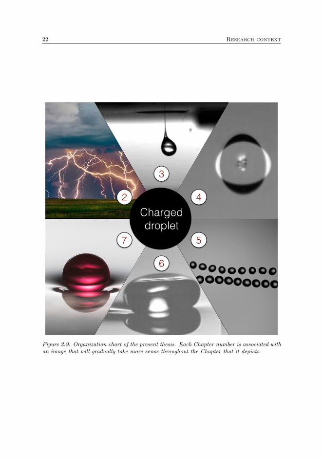
An organization chart of the Chapters 2, 3, 4, 5, 6 and 7, is shown in Fig.2.9. After the characterization of the research context (2), we are interested in theexperimental setups (3), the influence of the charge on the droplet (4), the chargeddroplets in microgravity (5), the charged droplets bouncing on a liquid bath (6)and the charged droplets in Leidenfrost state (7). Moreover, a small paragraph atthe end of each Section summarizes them. A line in the margin highlights thesesummaries. This paragraph possesses such a margin.
22 Research context
1 2 3
4 5 6
~E
1mm
2
5
3
3
6
7
Charged droplet
4
Figure 2.9: Organization chart of the present thesis. Each Chapter number is associated withan image that will gradually take more sense throughout the Chapter that it depicts.

3Experimental details
Contents3.1 Creating Charged droplets . . . . . . . . . . . . . . . . . . 24
3.1.1 Charged droplet generators . . . . . . . . . . . . . . . . . 26
3.1.2 Influence of the electric field on the droplet generation . . 30
3.2 Measuring the charge of droplets . . . . . . . . . . . . . . 33
3.3 Droplet storage methods . . . . . . . . . . . . . . . . . . . 35
3.3.1 The microgravity . . . . . . . . . . . . . . . . . . . . . . . 36
3.3.2 The vibrating bath . . . . . . . . . . . . . . . . . . . . . . 40
3.3.3 The Leidenfrost effect . . . . . . . . . . . . . . . . . . . . 43
In this Chapter, we describe the various tools that were developed throughout thisthesis to create and manage electrically charged droplets. In Section 3.1, we beginby describing the creating process of charged droplets. We show that the chargemigration process is a reliable way to charge droplets with a precisely known amountof charges. Then, we detail the ins and outs of the charged droplet generation. InSection 3.2, we explain how the droplet charge was measured. Finally, the Section3.3 is dedicated to the description of storage methods. Three setups are considered:the bouncing droplet, the microgravity and the Leidenfrost effect. Each of thesestorage systems limits the charge leakage from the droplet. Throughout the threeSections devoted to their description, we detail the advantages and disadvantages ofeach method.

24 Experimental details
3.1 Creating Charged droplets
As described in the introduction, there are four different methods to produce an excessof electric charges in droplets, namely via ionizing radiation, triboelectricity, chemicalreactions and charges migration. The charge by ionizing radiation and the charge byfriction are commonly used in Millikan famous experiment [27]. By charging a dropletand observing its motion in a homogeneous electric field, Millikan was able to measurethe charge quantification. However, both charging mechanisms are difficult to control.Indeed, there are no reliable laws that describe the amount of charges transferred toa droplet by friction. In the same manner, the electron loss induced by ionizingradiations requires to precisely control the kinetic energy of the ionizing particles andthe droplet exposure time. The charge by chemical reaction has also some drawbacks.Typically, the process requires the degradation of a chemical component, which limitsin time the droplet charge. On the contrary, the charge migration process generatesreliable and predictable charge excesses. Indeed, as its name indicates, electric chargesmigrate (thanks to the influence of an external electric field) into the droplet. Knowingthe electric field generating the charge migration, the amount of charges in excess inthe droplet can be deduced. In the next lines, we depict the experimental toolsnecessary to complete the charge migration mechanism and we describe the currentstate of understanding of such a process.
Basically, the charge migration, also named electrostatic induction, requires aliquid container (such as a needle), an electric field and a liquid containing free charges.The Fig. 3.1 shows the essential procedure of the experiment. A droplet hangs at theedge of the needle. Without any electric field, the droplet and the liquid containedin the needle are overall neutral. Once the system is immersed in an electric field,charges migrate from the liquid contained in the needle to the hanging droplet. As aconsequence, it induces an excess of charges in the droplet. At this point, when thedroplet detaches from the needle, it carries away an excess of electric charges.
Charged droplet generators using the charge migration process can have differentgeometries, according to their use. One of the first ways to generate charged dropletsvia charges migration is called the Kelvin drop generator (or Kelvin water dropper)[44]. This charged droplet generator corresponds to the simplest way to induce chargemigration in droplets. Indeed, it only consists in water falling in well connected cups.A schema of such a generator is shown in Fig. 3.2.
The setup is composed of two charged droplet generators and two droplet recep-tors interconnected. One charged droplet generator is composed of a droplet emitterand an electrode. When the electrode is charged, it generates an electric field near thedroplet emitter. This electric field induces charge migration in the droplet emitter.Once charged, the emitted droplets falls trough the electrode in the droplet receptor.The charge of the electrode is due to an avalanche process induced by the intercon-nection between both charged droplet generators and droplet receptors. On each side,

Chapter 3 25
~E
+
+
+ + ++
++
++
+
+
++
+
+
+
++
+
---
----
-- -
-+
- + -+
+-
+-
+
+
++
+
++
++
+
---
----
-- -
-
++
+
+
+
++
+
---
----
+
+
+ + ++
++
++
+
+
-- -
-
+++
1 2 3
Figure 3.1: Basic description of the charge migration process. The electric field generatescharges migration from the liquid container to the droplet. When the droplet detaches, ittakes away the excess of electric charges.
the droplet receptor is connected to the opposite electrode. Because of this intercon-nection, the electric charges accumulated in one droplet receptor induce an excess ofelectric charges in the opposed electrode. Therefore, the charged droplet generated bythe first generator induces charges migration in the second charged droplet generatorand vice versa. This avalanche process results in an important voltage between bothgenerators. Such a voltage can be put in evidence by inducing electric arcs betweenboth charged droplet generators. The drawback of the setup is that it is difficult tocontrol the charge of each electrode and, as a consequence, the charge induced in thedroplet. Nevertheless, the Kelvin drop generator is a beautiful experiment that eas-ily demonstrates the influence of the charge on the droplets. For example, we easilyobserve the electric repulsion between droplets when the experiment runs. This re-pulsion between droplets falling from the charged droplet emitter generates a conicalshape, exactly like the one observed by Abbé Nollet in his first experiments and theone observed on electrosprays.
Later, scientists developed systems for which the electric field applied on the hang-ing droplet was adjustable via a voltage generator. For example, Jones and Thong [45]have developed charged droplet generator composed of one needle and one plate. Avoltage between the needle and the plate allowed generating an electric field and, asa consequence, emitting charged droplets from the needle. Today, this geometry iscommonly used in electrospray devices [46]. More recently, new systems have beendeveloped to create charged droplets in microfluidic devices [37, 47, 48]. In the same

26 Experimental details
-
-
-
+
+
+
Positively charged conductor
Negatively charged conductor
PVC support
liquid
Spark gap
~E ~E
Charged droplet generator
Figure 3.2: Kelvin drop generator. The system is composed of two charged droplet generatorsinterconnected. The avalanche process allows generating high voltage between the electrodes.
way, the method remains the same but the geometry is adapted in order to respectthe requirements of small closed-channels generating the droplets.
3.1.1 Charged droplet generators
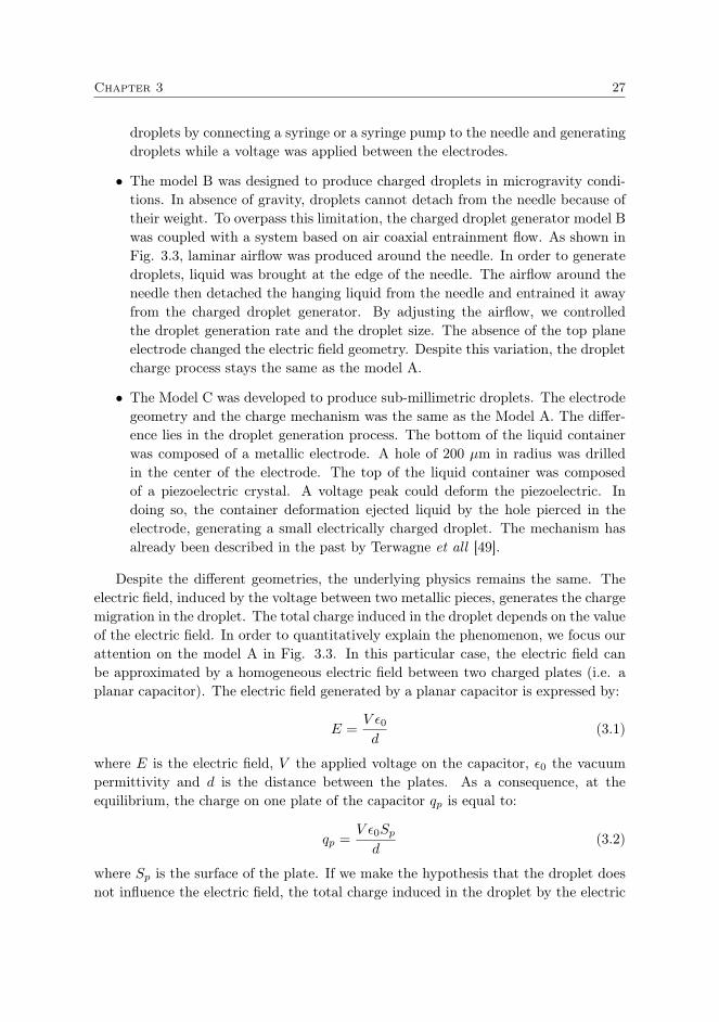
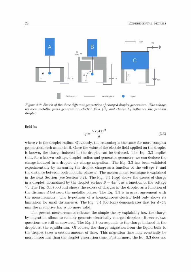
From the study of previous models, we developed our own generator geometries.The three geometries developed during the thesis are presented in Fig. 3.3. They arenamed model A, B and C in the rest of this thesis. In each case, the basic componentsof the charge migration process are present.
• The model A was designed to easily generate charged droplets with variousliquids (i.e. a large range of liquid surface tension, viscosity,...). We focusedits development on two specific aspects: (i) to be able to deal with low surfacetension fluids (ii) to be able to induce an electric field easy to model in order toquantify the charge migration process. In order to tackle these constraints, thecharged droplet generator was made of two metal disks, parallel and positionedalong a vertical axis. The top plate was pierced by a needle from which dropletswas formed. The bottom plate was drilled in its center to allow the dropletfalling away from the charged droplet generator. Both metallic plates were tiedtogether by an insulating plastic piece. The model A allowed to handily charge
Chapter 3 27
droplets by connecting a syringe or a syringe pump to the needle and generatingdroplets while a voltage was applied between the electrodes.
• The model B was designed to produce charged droplets in microgravity condi-tions. In absence of gravity, droplets cannot detach from the needle because oftheir weight. To overpass this limitation, the charged droplet generator model Bwas coupled with a system based on air coaxial entrainment flow. As shown inFig. 3.3, laminar airflow was produced around the needle. In order to generatedroplets, liquid was brought at the edge of the needle. The airflow around theneedle then detached the hanging liquid from the needle and entrained it awayfrom the charged droplet generator. By adjusting the airflow, we controlledthe droplet generation rate and the droplet size. The absence of the top planeelectrode changed the electric field geometry. Despite this variation, the dropletcharge process stays the same as the model A.
• The Model C was developed to produce sub-millimetric droplets. The electrodegeometry and the charge mechanism was the same as the Model A. The differ-ence lies in the droplet generation process. The bottom of the liquid containerwas composed of a metallic electrode. A hole of 200 µm in radius was drilledin the center of the electrode. The top of the liquid container was composedof a piezoelectric crystal. A voltage peak could deform the piezoelectric. Indoing so, the container deformation ejected liquid by the hole pierced in theelectrode, generating a small electrically charged droplet. The mechanism hasalready been described in the past by Terwagne et all [49].
Despite the different geometries, the underlying physics remains the same. Theelectric field, induced by the voltage between two metallic pieces, generates the chargemigration in the droplet. The total charge induced in the droplet depends on the valueof the electric field. In order to quantitatively explain the phenomenon, we focus ourattention on the model A in Fig. 3.3. In this particular case, the electric field canbe approximated by a homogeneous electric field between two charged plates (i.e. aplanar capacitor). The electric field generated by a planar capacitor is expressed by:
E =V ε0d
(3.1)
where E is the electric field, V the applied voltage on the capacitor, ε0 the vacuumpermittivity and d is the distance between the plates. As a consequence, at theequilibrium, the charge on one plate of the capacitor qp is equal to:
qp =V ε0Spd
(3.2)
where Sp is the surface of the plate. If we make the hypothesis that the droplet doesnot influence the electric field, the total charge induced in the droplet by the electric
28 Experimental details
PVC support metallic piece liquid
V V V2
~E ~E ~E
1 cm
A B
C
Air flow
V1
Figure 3.3: Sketch of the three different geometries of charged droplet generators. The voltagebetween metallic parts generate an electric field ( ~E) and charge by influence the pendantdroplet.
field is:
q =V ε04πr2
d(3.3)
where r is the droplet radius. Obviously, the reasoning is the same for more complexgeometries, such as model B. Once the value of the electric field applied on the dropletis known, the charge induced in the droplet can be deduced. The Eq. 3.3 impliesthat, for a known voltage, droplet radius and generator geometry, we can deduce thecharge induced in a droplet via charge migration. The Eq. 3.3 has been validatedexperimentally by measuring the droplet charge as a function of the voltage V andthe distance between both metallic plates d. The measurement technique is explainedin the next Section (see Section 3.2). The Fig. 3.4 (top) shows the excess of chargein a droplet, normalized by the droplet surface S = 4πr2, as a function of the voltageV . The Fig. 3.4 (bottom) shows the excess of charges in the droplet as a function ofthe distance d between the metallic plates. The Eq. 3.3 is in great agreement withthe measurements. The hypothesis of a homogeneous electric field only shows itslimitation for small distances d. The Fig. 3.4 (bottom) demonstrates that for d < 5
mm the predictive law is no more valid.The present measurements enhance the simple theory explaining how the charge
by migration allows to reliably generate electrically charged droplets. However, twoquestions are still unanswered. The Eq. 3.3 corresponds to the charge induced in thedroplet at the equilibrium. Of course, the charge migration from the liquid bulk tothe droplet takes a certain amount of time. This migration time may eventually bemore important than the droplet generation time. Furthermore, the Eq. 3.3 does not
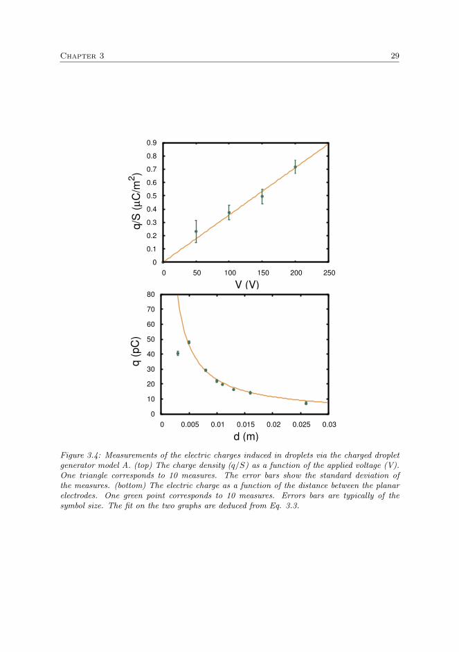
Chapter 3 29
0
0.1
0.2
0.3
0.4
0.5
0.6
0.7
0.8
0.9
0 50 100 150 200 250
q
/S (
µC
/m2)
V (V)
0
10
20
30
40
50
60
70
80
0 0.005 0.01 0.015 0.02 0.025 0.03
q
(p
C)
d (m)
Figure 3.4: Measurements of the electric charges induced in droplets via the charged dropletgenerator model A. (top) The charge density (q/S) as a function of the applied voltage (V).One triangle corresponds to 10 measures. The error bars show the standard deviation ofthe measures. (bottom) The electric charge as a function of the distance between the planarelectrodes. One green point corresponds to 10 measures. Errors bars are typically of thesymbol size. The fit on the two graphs are deduced from Eq. 3.3.
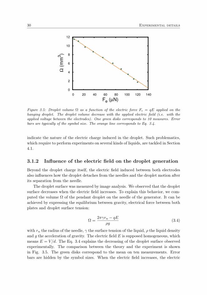
30 Experimental details
0
2
4
6
8
10
12
0 20 40 60 80 100 120 140
Ω (
mm
3)
Fe (µN)
Figure 3.5: Droplet volume Ω as a function of the electric force Fe = qE applied on thehanging droplet. The droplet volume decrease with the applied electric field (i.e. with theapplied voltage between the electrodes). One green disks corresponds to 10 measures. Errorbars are typically of the symbol size. The orange line corresponds to Eq. 3.4.
indicate the nature of the electric charge induced in the droplet. Such problematics,which require to perform experiments on several kinds of liquids, are tackled in Section4.1.
3.1.2 Influence of the electric field on the droplet generation
Beyond the droplet charge itself, the electric field induced between both electrodesalso influences how the droplet detaches from the needles and the droplet motion afterits separation from the needle.
The droplet surface was measured by image analysis. We observed that the dropletsurface decreases when the electric field increases. To explain this behavior, we com-puted the volume Ω of the pendant droplet on the needle of the generator. It can beachieved by expressing the equilibrium between gravity, electrical force between bothplates and droplet surface tension:
Ω =2πγrn − qE
ρg(3.4)
with rn the radius of the needle, γ the surface tension of the liquid, ρ the liquid densityand g the acceleration of gravity. The electric field E is supposed homogeneous, whichmeans E = V/d. The Eq. 3.4 explains the decreasing of the droplet surface observedexperimentally. The comparison between the theory and the experiment is shownin Fig. 3.5. The green disks correspond to the mean on ten measurements. Errorbars are hidden by the symbol sizes. When the electric field increases, the electric

Chapter 3 31
1 2
5 mm
Charged droplet
generator
Figure 3.6: The charged droplet generator ejects a viscous droplet. The voltage appliedbetween electrodes is V = 5000V. The liquid is composed of silicone oil 50 cSt. Because ofthe liquid high viscosity, the droplet separates from the liquid outside of the charged dropletgenerator, which limits the droplet charge.
force tends to pull the droplet away from the needle. As a consequence, the dropletvolume decreases with the applied electric force. The Eq. 3.4 is found to be in goodagreement with the observations.
It should be noted that the experiments performed during this thesis were alwayscarried out with liquids that are considered Newtonian liquids with a low viscosity(around 1 cSt). The charged droplet generator may be difficult to use with complexor viscous liquids. The present statement is illustrated in Fig. 3.6. The imagecorresponds the droplet generator model A working with a voltage V = 5000 V and aliquid composed of silicone oil 50 cSt. Because of the high viscosity of the silicone oil,the droplet drags away liquid when falling from the charged droplet generator. As aconsequence, the droplet is formed outside of the charged droplet generator, meaningthat the droplet does not charge as expected.
The electric field induced between both electrodes does not only influence thevolume of the charged droplet. It also influences its ejection speed. In order to measurethis influence, the droplet instantaneous speed u0 at 3 mm from the charged dropletgenerator was measured by high-speed imaging. The experiment is schematized inFig. 3.7. The measured droplet speed is shown in Fig. 3.8 as a function of the voltageV applied on the charged droplet generator multiplied by the charge q of the dropletand divided by the droplet radius. We deduce from the experiment that the dropletspeed increases with the voltage V and the charge q of the droplet.
When the charged droplet detaches from the generator, it still endures the electric
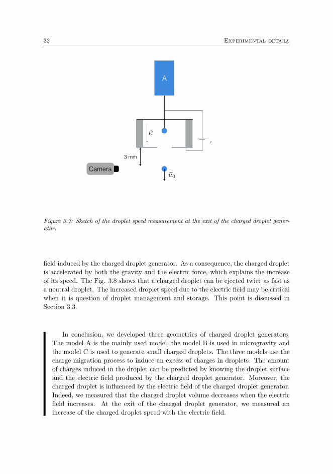
32 Experimental details
V
~E
A
Camera
3 mm
~u0
Figure 3.7: Sketch of the droplet speed measurement at the exit of the charged droplet gener-ator.
field induced by the charged droplet generator. As a consequence, the charged dropletis accelerated by both the gravity and the electric force, which explains the increaseof its speed. The Fig. 3.8 shows that a charged droplet can be ejected twice as fast asa neutral droplet. The increased droplet speed due to the electric field may be criticalwhen it is question of droplet management and storage. This point is discussed inSection 3.3.
In conclusion, we developed three geometries of charged droplet generators.The model A is the mainly used model, the model B is used in microgravity andthe model C is used to generate small charged droplets. The three models use thecharge migration process to induce an excess of charges in droplets. The amountof charges induced in the droplet can be predicted by knowing the droplet surfaceand the electric field produced by the charged droplet generator. Moreover, thecharged droplet is influenced by the electric field of the charged droplet generator.Indeed, we measured that the charged droplet volume decreases when the electricfield increases. At the exit of the charged droplet generator, we measured anincrease of the charged droplet speed with the electric field.

Chapter 3 33
0.35
0.4
0.45
0.5
0.55
0.6
0.65
0.7
0.75
0.8
0 500 1000 1500 2000 2500
u0
(m/s
)
qV/rd3 (CV/m3)
Figure 3.8: The speed, u0, as a function of qV/r3. The droplet speed increases with its chargeand with the voltage applied on the charged droplet generator. One green point correspondsto 10 measures. Errors bars are typically of the symbol size.
3.2 Measuring the charge of droplets
In the previous Section, we developed the theory necessary to understand the under-lying physics of the droplet charge by migration. We showed that by knowing theelectric field acting on the droplet and the droplet radius, it is possible to deduce thedroplet charge. However, the modeling of the electric field is not always necessary.Indeed, for a given setup configuration, the charge induced in the droplet is alwaysroughly the same. As a consequence, a calibration, via a charge measurement, isenough to know precisely the charge of the droplet. Therefore, the next step is todevelop a system able to measure the electric charge of a droplet.
Measurements of the charge induced in thousands of droplet conceived during thisthesis were performed by using a Faraday cup. This kind of device is commonly usedin ions beam experiments [50]. In practice, the Faraday cup gathers an ion beamand measures its charge over time. We developed a Faraday cup based on the sameprinciples but designed to measure the charge of mesoscopic objects, i.e. millimetriccharged droplets. A schema of the setup is presented in Fig. 3.9. Such a setupcan also be used to measure the charge of other mesoscopic objects such as granularmaterials [51].
The Faraday cup in Fig. 3.9 is composed of two concentric cups, which plays therole of electrodes. The sides of both cups, the electrodes, face each other and form acapacitor. The air between the electrodes plays the roles of insulator in the capacitor.The top of the cup was covered with an insulated cap to protect the device from
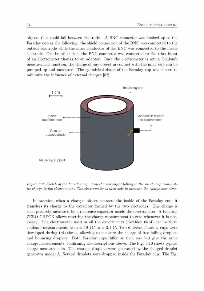
34 Experimental details
objects that could fall between electrodes. A BNC connector was hooked up to theFaraday cup as the following: the shield connection of the BNC was connected to theoutside electrode while the inner conductor of the BNC was connected to the insideelectrode. On the other side, the BNC connector was connected to the triax inputof an electrometer thanks to an adapter. Once the electrometer is set in Coulombmeasurement function, the charge of any object in contact with the inner cup can bepumped up and measured. The cylindrical shape of the Faraday cup was chosen tominimize the influence of external charges [52].
Connection toward the electrometer
Insulating cap
Insulating support
Outside cup/electrode
Inside cup/electrode
1 cm
Figure 3.9: Sketch of the Faraday cup. Any charged object falling in the inside cup transmitsits charge to the electrometer. The electrometer is then able to measure the charge over time.
In practice, when a charged object contacts the inside of the Faraday cup, ittransfers its charge to the capacitor formed by the two electrodes. The charge isthen precisely measured by a reference capacitor inside the electrometer. A functionZERO CHECK allows resetting the charge measurement to zero whenever it is nec-essary. The electrometer used in all the experiments (Keithley 6514) can performcoulomb measurements from ± 10 fC to ± 2.1 C. Two different Faraday cups weredeveloped during this thesis, allowing to measure the charge of free falling dropletsand bouncing droplets. Both Faraday cups differ by their size but give the samecharge measurements, confirming the descriptions above. The Fig. 3.10 shows typicalcharge measurements. The charged droplets were generated by the charged dropletgenerator model A. Several droplets were dropped inside the Faraday cup. The Fig.

Chapter 3 35
100
150
200
250
300
350
20 30 40 50 60 70
Q
(p
C)
t(s)
Figure 3.10: Typical measurement of droplet charges via the Faraday Cup. The charge of 6droplets was measured in 35 s. Half the points were plotted for the clarity of the graph.
3.10 shows the measurement on six of these charged droplets. During each contactbetween a charged droplet and the Faraday cup, we observe a leap in the charge mea-sured by the electrometer. The leap is the same for all the six charge measurements.This charge measurement confirms that the charged droplet generator induces thesame charge in each droplet generated.
Lastly, we have to mention the existence of a “dynamic" Faraday cup. Such aFaraday cup looks exactly the same as the “classic" Faraday cup except that itsbottom is hollowed (i.e. the electrodes are composed of two concentric cylindersinstead of cups). Instead of measuring the charge by transferring directly the chargefrom the droplet to the Faraday cup, the droplet falls trough the “dynamic" Faradaycup and induces charges to the electrodes. Such a model is less accurate than the“classic" Faraday cup but can be useful in certain experiments where the charge ofthe droplet have to be conserved over time. More information about this particularmethod can be found in [53] or [54].
In conclusion, the Faraday cup, similar to a cup-shaped capacitor, is found tobe a good way to measure precisely the charge of electrically charged droplets.
3.3 Droplet storage methods
As explained in the first description of the thesis (Section 2.4), we developed newtools that allow storing a droplet while limiting charge leakage. These new tools are
36 Experimental details
based on three well known phenomena: The microgravity, the bouncing droplet andthe Leidenfrost effect. The three storage methods are described in this Section. Theiradvantages and disadvantages are detailed.
3.3.1 The microgravity
The first idea that comes in mind when thinking about storing a charged droplet isto avoid the gravity. Indeed, without any attraction toward the Earth, the chargeddroplet should simply float in the air. Thanks to The European Space Agency, wehad the opportunity to achieve these conditions by means of parabolic flights.
An airplane, with good pilots, may perform parabola during a flight. While per-forming parabola, the airplane passengers endure various accelerations due to theplane motion. The airplane displacement during one parabola is schematized in Fig.3.11. The airplane altitude is plotted as a function of the time. At the beginning ofthe parabola, the airplane goes up with an acceleration of 0.8 g (g being the earthgravity). As a consequence, airplane passengers endure an acceleration equals to 1.8g. Near the top of the parabola, the airplane decelerates as precisely as possible toattain an acceleration of -1 g. After the top of the parabola, the pilot maintain thedeclaration of -1 g by stepping on the gas in order to compensate the air friction.During all the top part of the parabola, the airplane passengers are in microgravitycondition (i.e. at 0 g) in their frame of reference. Finally, the plane re-accelerates atthe end of the parabola to come back to its initial horizontal trajectory.
One parabola corresponds to 22 s of microgravity. The microgravity conditions areobtained with a precision of ± 0.05 g. During this period, a charged droplet can freelymove in the airplane. This last point is the best advantage of the microgravity. Indeed,no external forces are applied on the droplet, meaning that the droplet is free tointeract with its environnement. On the contrary, the storage via electrodynamic [19],diamagnetical [18] or acoustic [55] traps uses external forces to maintain the dropletin one specific position. In practice, we used the microgravity conditions to measurethe interaction between two charged droplets sent toward each other. The study isdescribed in details in Chap 5.
Naturally, the microgravity conditions imply specific adaptations. For example,the absence of gravity makes more difficult the droplet detachment from a needle. Asa consequence, during microgravity sessions, charged droplets were generated withthe charged droplet generator model B (see Fig. 3.3). A detailed schema of thecharged droplet generator is shown in Fig. 3.12. A cylindrical plastic piece (in grey)encircled a metallic needle. A metallic plate was fixed at the edge of the plastic piece.A hole pierced in the plastic piece allowed air to flow around the needle. Two supportscrews were screwed up in the plastic piece in order to maintain the metallic needlelocation. A voltage generator allowed controlling the voltage between the supportscrew (itself connected to the metallic needle) and the metallic plate. The chargeddroplet generator was coupled with an air pump. As shown in Fig. 3.12, laminar
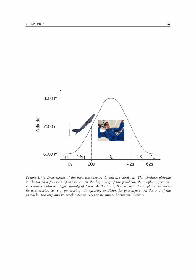
Chapter 3 37
6000 m
7500 m
8500 m
1g 1g1.8g 1.8g0g0s 20s 42s 62s
Altit
ude
Figure 3.11: Description of the airplane motion during the parabola. The airplane altitudeis plotted as a function of the time. At the beginning of the parabola, the airplane goes up,passengers endures a hyper gravity of 1.8 g. At the top of the parabola the airplane decreasesits acceleration to -1 g, generating microgravity condition for passengers. At the end of theparabola, the airplane re-accelerates to recover its initial horizontal motion.
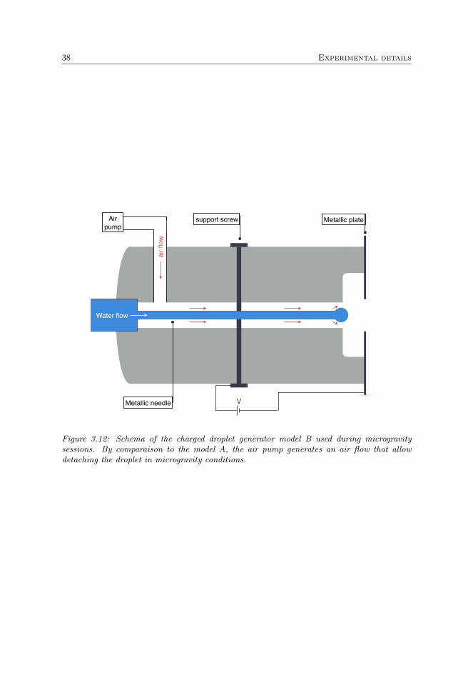
38 Experimental details
V
Water flow
air fl
ow
Metallic platesupport screw
Metallic needle
Airpump
Figure 3.12: Schema of the charged droplet generator model B used during microgravitysessions. By comparaison to the model A, the air pump generates an air flow that allowdetaching the droplet in microgravity conditions.
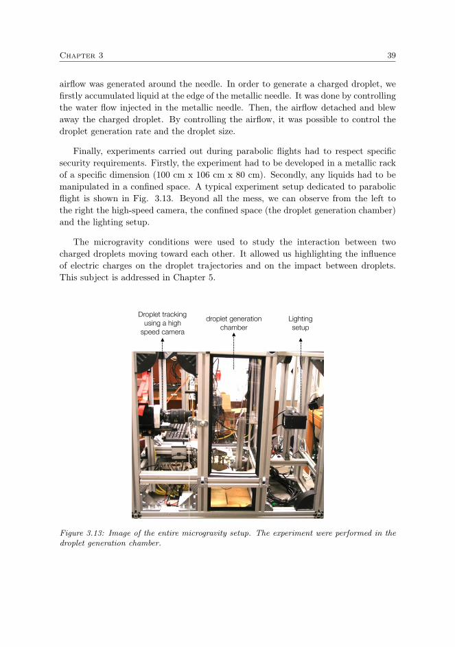
Chapter 3 39
airflow was generated around the needle. In order to generate a charged droplet, wefirstly accumulated liquid at the edge of the metallic needle. It was done by controllingthe water flow injected in the metallic needle. Then, the airflow detached and blewaway the charged droplet. By controlling the airflow, it was possible to control thedroplet generation rate and the droplet size.
Finally, experiments carried out during parabolic flights had to respect specificsecurity requirements. Firstly, the experiment had to be developed in a metallic rackof a specific dimension (100 cm x 106 cm x 80 cm). Secondly, any liquids had to bemanipulated in a confined space. A typical experiment setup dedicated to parabolicflight is shown in Fig. 3.13. Beyond all the mess, we can observe from the left tothe right the high-speed camera, the confined space (the droplet generation chamber)and the lighting setup.
The microgravity conditions were used to study the interaction between twocharged droplets moving toward each other. It allowed us highlighting the influenceof electric charges on the droplet trajectories and on the impact between droplets.This subject is addressed in Chapter 5.
droplet generation chamber
Droplet tracking using a high
speed camera
Lighting setup
Figure 3.13: Image of the entire microgravity setup. The experiment were performed in thedroplet generation chamber.

40 Experimental details
3.3.2 The vibrating bath
The microgravity session during one parabola is limited to 22 s. However, certainstudies require to observe the charged droplet behavior during longer times. Thevibrating bath answers to this requirement.
It is known since the work of Lord Rayleigh [56] that the collision between twodroplets may lead to a bounce. From this observation, other studies have been focusedon the delayed coalescence of a droplet falling on a liquid surface [57–59]. Theseobservations can be basically described by the following statement: when the fallingdroplet approaches the liquid surface, a thin air layer remains between both liquids. Ittakes a certain amount of time for the air between the droplet and the liquid surfaceto drain out. The drainage of the air layer is due to the pressure applied by thedroplet on the air trapped between the liquid interface and the droplet. During thetime needed for the air to drain out (generally about 1 s), the droplet stays on theliquid surface.
The delayed coalescence can be maintained by various methods. For example,generating a flow in the liquid bath can regenerate the air layer between the dropletand the liquid bath [59,60]. A second approach, developed by Couder et al [61] consistsin vibrating the liquid bath. Because of the bath oscillation, the droplet bounces onthe air layer between the droplet and the liquid bath. If the frequency and amplitudeof the oscillation are well chosen, the air layer between the bouncing droplet and theoscillating liquid may be regenerated at each bounce. The phenomenon is schematizedin Fig. 3.14 (top). An image of a silicone oil droplet (1 cSt) bouncing on a siliconeoil bath (1000 cSt) is shown in Fig. 3.14 (bottom).
The droplet bouncing on a liquid, seemingly simple, led to tremendous numbers ofresearch. Studies have been interested in the conditions for the bouncing to happen[62], but also to other phenomena that come out from this experiment. Indeed,according to the experiment configuration, the bouncing droplet can have differentbouncing modes [49] and can also propel itself [63, 64].
The bouncing droplet method is a good candidate for charged droplet storage.Indeed, it allows storing a droplet for a long time (several hours) while the dropletbeing only in contact with ambient air. The absence of contact with a conductoravoids the rapid charge leakage over time. Moreover, the setup answers to limitationsof other storage methods such as the use of diamagnetic or electrodynamic traps[18, 19], droplet storage in silicone oil pool [65] or acoustic traps [66, 67]. Indeed, thebouncing drop method allows keeping millimetric droplets on a relative horizontalplane. Charged droplet may be easily displaced on this horizontal plane and severaldroplets may be stored on the vibrating bath. The bouncing method also avoidsusing an external electric field that could influence the charges behavior. Moreover,the study may be performed in ambient air, allowing studying the droplet evaporation.
To perform our experiments, we used an electromagnetic shaker (model GW-V55or GW-V2). The bath was filed with high viscosity silicone oil (1000 cSt). The defor-
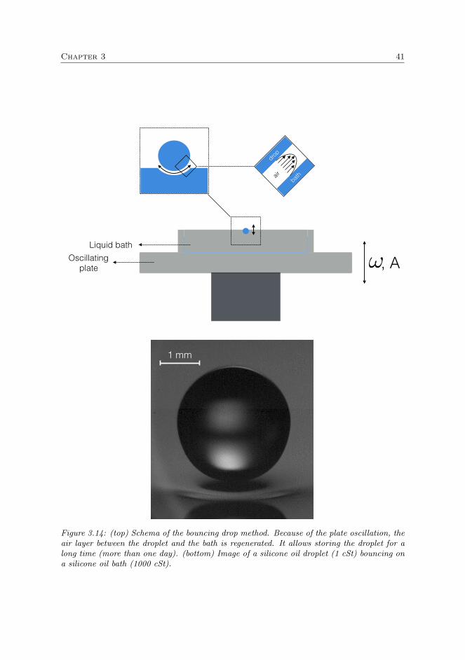
Chapter 3 41
Oscillating plate !
air
drop
bath
, ALiquid bath
1 mm
Figure 3.14: (top) Schema of the bouncing drop method. Because of the plate oscillation, theair layer between the droplet and the bath is regenerated. It allows storing the droplet for along time (more than one day). (bottom) Image of a silicone oil droplet (1 cSt) bouncing ona silicone oil bath (1000 cSt).
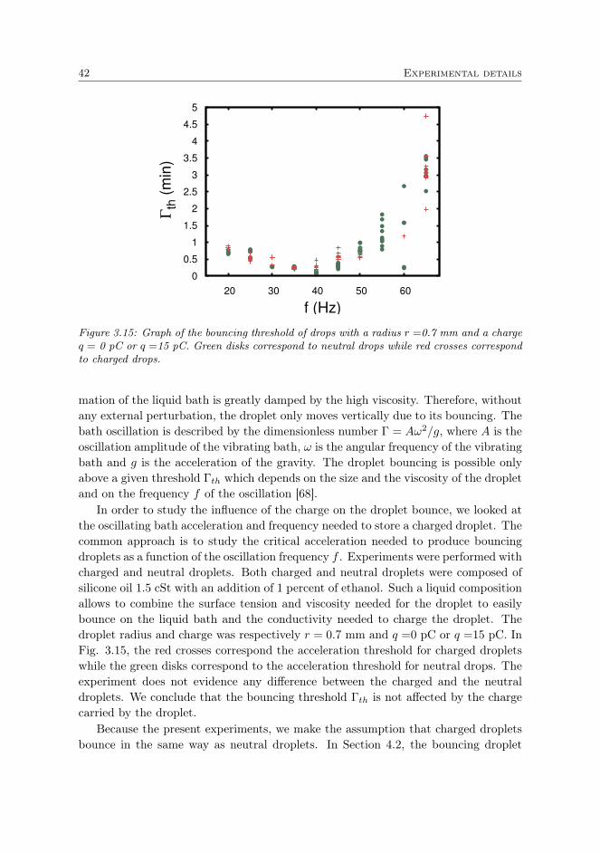
42 Experimental details
0
0.5
1
1.5
2
2.5
3
3.5
4
4.5
5
20 30 40 50 60
Γ
th (
min
)
f (Hz)
Figure 3.15: Graph of the bouncing threshold of drops with a radius r =0.7 mm and a chargeq = 0 pC or q =15 pC. Green disks correspond to neutral drops while red crosses correspondto charged drops.
mation of the liquid bath is greatly damped by the high viscosity. Therefore, withoutany external perturbation, the droplet only moves vertically due to its bouncing. Thebath oscillation is described by the dimensionless number Γ = Aω2/g, where A is theoscillation amplitude of the vibrating bath, ω is the angular frequency of the vibratingbath and g is the acceleration of the gravity. The droplet bouncing is possible onlyabove a given threshold Γth which depends on the size and the viscosity of the dropletand on the frequency f of the oscillation [68].
In order to study the influence of the charge on the droplet bounce, we looked atthe oscillating bath acceleration and frequency needed to store a charged droplet. Thecommon approach is to study the critical acceleration needed to produce bouncingdroplets as a function of the oscillation frequency f . Experiments were performed withcharged and neutral droplets. Both charged and neutral droplets were composed ofsilicone oil 1.5 cSt with an addition of 1 percent of ethanol. Such a liquid compositionallows to combine the surface tension and viscosity needed for the droplet to easilybounce on the liquid bath and the conductivity needed to charge the droplet. Thedroplet radius and charge was respectively r = 0.7 mm and q =0 pC or q =15 pC. InFig. 3.15, the red crosses correspond the acceleration threshold for charged dropletswhile the green disks correspond to the acceleration threshold for neutral drops. Theexperiment does not evidence any difference between the charged and the neutraldroplets. We conclude that the bouncing threshold Γth is not affected by the chargecarried by the droplet.
Because the present experiments, we make the assumption that charged dropletsbounce in the same way as neutral droplets. In Section 4.2, the bouncing droplet

Chapter 3 43
method is used to measure the droplet charge over time, while in Chapter 6 we studyboth the interaction between charged bouncing droplets and electric fields and theinteraction between two charged droplets on the vibrating bath.
3.3.3 The Leidenfrost effect
When a droplet is dropped on a surface hotter than the droplet boiling point, itproduces a vapor flux. If the vapor flux is important enough, an insulating vaporlayer is produced between the droplet and the heated surface. Droplets levitating ontheir own vapor are defined as being in Leidenfrost state. The phenomenon is namedaccording to one of the first scientists to discover the phenomenon [69].
The Leidenfrost effect is commonly studied with droplets levitating at the surfaceof a solid. Typically, a water droplet dropped on a surface heated to 250 C levitateson its own vapor [70–72]. The experiment is easily reproducible while cooking. Forexample, droplets moving quickly on the surface of a hot frying pan are in Leidenfroststate. However, we had difficulties to keep charges inside droplets in Leidenfrost stateabove a solid surface. It is explained by small contacts that can occur when thedroplet is dropped on the heated surface. The droplet contact does not influencethe Leidenfrost state itself. Indeed, liquid in contact with the solid interface quicklyevaporates, the majority of the droplet staying in Leidenfrost state. However, electriccharges have time to migrate from the liquid to the solid surface during these briefcontacts. In Section 4.1, we show that a contact of few milliseconds is sufficient forall the charges to migrate. As a consequence, the droplet is not able to keep itsexcess of charges while being in Leidenfrost state on a solid surface. Moreover, theelectric charges can affect the stability of the Leidenfrost droplet. The destabilizationof a charged droplet in Leidenfrost state at the surface of a solid has been studiedby Celestini et al [71]. They induced a voltage between a needle inserted in theLeidenfrost droplet and the solid substrate. They observed the decrease of the vaporlayer when increasing the voltage between the droplet and the liquid substrate. Forvoltages above 40 V, they observed a destabilization of the droplet leading to theannihilation of the Leidenfrost effect.
The Leidenfrost effect may also occur for droplets levitating above a liquid bath.In this case, the evaporation of the droplet or the evaporation of the liquid bathis important enough to maintain the air layer between the droplet and the liquidbath. Droplets levitating on the liquid bath vapor are defined as being in inverse-Leidenfrost state [73, 74]. On the contrary of the solid substrate, the liquid pooldoes not allow small contacts between the levitating droplet and the liquid surface.Indeed, one small contact would induce the coalescence between both liquids. As aconsequence, electrically charged droplets can be stored via this setup. In the past,inverse-Leidenfrost experiments were performed with water droplets at the surface ofliquid nitrogen [74]. However, the experimental setup associated with the experiment(thermostat limiting the nitrogen heating, droplet freezing,...) limits the usage of the

44 Experimental details
vapor
drop
pool
Droplet
Liquid pool
vapor
Figure 3.16: (top) Schema of a Leidenfrost droplet levitating on a liquid pool. The liquidpool is heated above the droplet boiling temperature. Because of the droplet evaporation, thevapor layer between the droplet and the bath is regenerated. (bottom) An ethanol drop withred dye levitates in the Leidenfrost state over a pool of silicone oil V20. The drop radius isR = 1.2 mm and the pool is at Tp = 80 C while the boiling point of ethanol is Tsat = 78 C.(Image credit: Florence Cavagnon).

Chapter 3 45
setup as a storage system.Recently, it has been shown that droplets can be set in Leidenfrost state at the
surface of heated silicone bath [75, 76]. During this thesis we used this particularexperimental setup to store electrically charged droplets. The Fig. 3.16 shows adroplet in Leidenfrost state at the surface of a heated silicone pool. In Fig. 3.16(top), we schematized the Leidenfrost droplet levitation. A thin vapor layer is presentbetween the droplet and the liquid pool. This vapor layer tends to drain out becauseof the droplet pressure. By evaporating, the droplet regenerates the vapor layer. InFig. 3.16 (bottom), the droplet was composed of ethanol while the liquid pool wascomposed of silicone oil 20 cSt. During the experiment, the liquid pool was heated atTp = 80 C (i.e. above the ethanol boiling temperature Tsat = 78 C). The setup waschosen for the experimental comfort. Indeed, the system is easy to set up and worksfor a large range of temperature (starting at the droplet boiling temperature, whichis exceptional for the Leidenfrost effect). Experiments were performed with two sortsof liquid: ethanol and HFE-7100. The thermal properties of both liquids make themideal for the study of the Leidenfrost effect.
The detail of the droplet in Leidenfrost state on a silicone bath is described in [76].The article is focused on the droplet evaporation rate and on both the shape of thedroplet and the deformation induced by the levitating drop on the liquid pool. Forthe purpose of the study of charged droplets, the Leidenfrost effect on a liquid bathpossess the following advantages compare: (i) the droplet is not deformed over time(ii) droplets with radii beyond the capillary length may be stored (iii) liquids withvarious chemical compositions may be stored. Naturally, the setup has also somedrawbacks: (i) The droplet freely moves on the liquid pool, which may complicateits imaging over time (ii) The Leidenfrost droplet does not have a spherical shape.Its shape depends on its own properties but also on the properties of the liquidpool. (iii) The quick evaporation of the droplet limits its study time. Beyond theadvantages and disadvantages of the storage method, the influence of electric chargeson the Leidenfrost state are interesting to study. Indeed, the Leidenfrost state on aliquid pool corresponds to two liquid surfaces separated by a thin vapor layer (witha thickness about 1 µm). At his scale, the electric interaction should be importantenough to influence the shape and the thickness of this vapor layer.
In this thesis we focus our attention on the influence of the electric charge on theLeidenfrost state. The Leidenfrost effect is studied in Chapter 7. We investigate howelectric charges influence the droplet shape and the droplet stability while stored ona heated liquid bath.
In conclusion, we used three storage methods to study electrically chargeddroplets. The microgravity conditions allow storing charged droplet without influ-encing their behavior. However, the experimental requirements and the durationof the storage limit the use of this method. The vibrating bath method allowsstoring charged droplets during several hours. The charged droplet is free to move

46 Experimental details
on the two dimensions of the liquid bath, but is deformed over time by its verticalbouncing. The Leidenfrost effect allows storing a charged droplet on its own vapor.We are interested in the influence of electric charges on the Leidenfrost dropletslevitating above a heated liquid pool.
4Influence of the charge on the droplet
Contents4.1 Influence of the liquid composition . . . . . . . . . . . . . 484.2 Charge loss over time . . . . . . . . . . . . . . . . . . . . . 53
4.2.1 Charge loss of a bouncing droplet . . . . . . . . . . . . . . 544.2.2 Model the charge loss of bouncing droplets . . . . . . . . 554.2.3 Charge loss of droplets in microgravity and Leidenfrost state 64
4.3 Influence of the charges on the droplet surface energy . 654.3.1 Surface energy of a charged droplet in free fall . . . . . . 67
In this Chapter, we focus our attention on the physical behavior of a chargeddroplet. The first questions arising from this subject concern the relationship betweenthe charge and the droplet. In other words, “how do the electric charges influence thedroplet?". But also, “how do the droplet properties influence the charge migration inthe droplet?". The Chapter 2 described previous research that attempted to answerto these questions. In this Chapter, we continue these investigations through differentexperiments.
The first Section (4.1) is dedicated to the influence of the liquid composition onthe charge migration in the droplet. In particular, we put in evidence the parametersgoverning the phenomenon (i.e. the liquid conductivity and relative permittivity).The Section 4.2 questions the charge loss of a droplet. By storing the droplet viathe vibrating bath method, we measure and model the droplet charge loss over time.Finally, the Section 4.3 is directed toward the study of the influence of the electriccharges on the droplet surface energy.
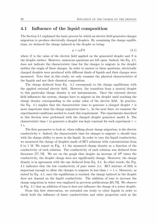
48 Influence of the charge on the droplet
4.1 Influence of the liquid composition
The Section 3.1 explained the basic process by which an electric field generates chargesmigration to produce electrically charged droplets. By examining the charge equilib-rium, we deduced the charge induced in the droplet as being:
q = ε0ES (4.1)
where E is the value of the electric field applied on the generated droplet and S isthe droplet surface. However, numerous questions are left open. Indeed, the Eq. 4.1,does not indicate the characteristic time for the charges to migrate in the dropletneither the origin of these charges. In order to answer to these questions, electricallycharged droplets were produced with different kinds of liquids and their charges weremeasured. Note that in this study, we only examine the physical characteristics ofthe liquids and not their chemical composition.
The charge deduced from Eq. 4.1 corresponds to the charge equilibrium withthe applied external electric field. However, the transition from a neutral dropletto this particular charge density is not instantaneous. Once the external electricfield influences the system, charges have to migrate in the droplet until reaching thecharge density corresponding to the scalar value of the electric field. In practice,the Eq. 4.1 implies that the characteristic time to generate a charged droplet τ ismore important than the charge migration time τc. In the next lines, we examine theexperimental conditions needed to reach this requirement. The experiments describedin this Section were performed with the charged droplet generator model A. Thecharacteristic time τ to generate a droplet was kept constant for each experiment τ =
1 s.The first parameter to look at, when talking about charge migration, is the electric
conductivity σ. Indeed, the characteristic time for charges to migrate τc should varywith the charge ability to move in the liquid. In order to vary the liquid conductivity,we measured the charge of droplets made of HCl solutions with concentrations from0 to 1 M. We report in Fig. 4.1 the measured charge density as a function of theconductivity of each solution. The conductivity of each solution was deduced fromliterature [77, 78]. We see on the graph that despite an increase of 106 times theconductivity, the droplet charge does not significantly change. Moreover, the chargedensity is in agreement with the one deduced from Eq. 3.1. In other words, the Fig.4.1 indicates that the low conductivity of pure water (i.e. HCl mixture of 0M) isimportant enough to allow the charges to migrate in less than τ = 1 s. Moreover, asstated by Eq. 4.1, once the equilibrium is reached, the charge induced in the dropletdoes not depend on the liquid conductivity. The addition of ions to increase thecharge migration in water was employed in previous publications [65,79]. We observein Fig. 4.1 that an addition of ions is does not influence the charge of a water droplet.
From this first observation, we extended our study to other liquids in order tocheck both the influence of lower conductivities and other properties such as the
Chapter 4 49
0.66
0.67
0.68
0.69
0.7
0.71
0.72
0.73
0.74
0.75
0.76
10-5
10-4
10-3
10-2
10-1
100
101
102
103
Q
/S (
µC
/m2)
σ (mS/cm)
Figure 4.1: Charge induced in HCl droplets with different molarities, normalized by thedroplet surface, as a function of the liquid conductivity. The highest conductivity correspondsto a droplet of HCL 1M. One red point corresponds to 10 measures. The error bars show thestandard deviation of the measures. Errors bars are typically of the symbol size.
surface tension or the relative permittivity of the liquid. In addition to the HClsolution, we generated electrically charged droplets composed of acetone, ethanol, n-octane, silicone oil and TritonX-100 solutions. The characteristics of all the liquidstested are shown in Tab. 4.1.
The Triton X-100 mixture corresponds to bidistilled water with an addition of1 CMC (critical micelle concentration, which correspond to 0.23 mM) of the non-ionic surfactant Triton X-100. This solution was used to check the influence of thesurface tension on the charge induced in the droplet. Acetone does not possess ions insolutions, it is then possible to check whether the charge in the droplet is due to ion(which compose the liquid) migration. Acetone and ethanol are also polar. On thecontrary, n-octane does not possess ions in solution and is apolar. Thus, it is possibleto inspect the influence of the molecule polarity. Finally, silicone oil at 1.5 cSt is aliquid with viscosity near water but with a smaller electrical conductivity than anyother liquids tested.
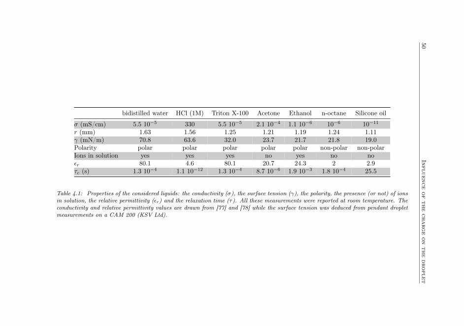
50In
fluen
ce
of
the
charg
eon
the
dro
plet
bidistilled water HCl (1M) Triton X-100 Acetone Ethanol n-octane Silicone oil
σ (mS/cm) 5.5 10−5 330 5.5 10−5 2.1 10−4 1.1 10−6 10−6 10−11
r (mm) 1.63 1.56 1.25 1.21 1.19 1.24 1.11γ (mN/m) 70.8 63.6 32.0 23.7 21.7 21.8 19.0Polarity polar polar polar polar polar non-polar non-polarIons in solution yes yes yes no yes no noεr 80.1 4.6 80.1 20.7 24.3 2 2.9τc (s) 1.3 10−4 1.1 10−12 1.3 10−4 8.7 10−6 1.9 10−3 1.8 10−4 25.5
Table 4.1: Properties of the considered liquids: the conductivity (σ), the surface tension (γ), the polarity, the presence (or not) of ionsin solution, the relative permittivity (εr) and the relaxation time (τ). All these measurements were reported at room temperature. Theconductivity and relative permittivity values are drawn from [77] and [78] while the surface tension was deduced from pendant dropletmeasurements on a CAM 200 (KSV Ltd).

Chapter 4 51
0
0.1
0.2
0.3
0.4
0.5
0.6
0.7
0.8
0.9
1
0 50 100 150 200 250
Q
/S (
µC
/m2)
V (V)
Figure 4.2: Charge induced in a droplet, normalized by the droplet surface, as a functionof the voltage applied on the charged droplet generator. Red triangles, purple pentagons,black squares, blue stars, green diamonds and yellow circles represent respectively measure-ments made on bidistilled water, Triton-x-100, acetone, ethanol, n-octane and silicon oil.Each point corresponds to 10 measures. The error bars show the standard deviation of themeasures. The red continuous line is a linear fit on these measurements.
The charge density induced in droplets composed of the various liquid tested isshown in Fig. 4.2 as a function of the voltage applied between the electrodes. In mostof the cases, no distinctions can be made between the charge induced in the differentliquids. The silicone oil is the only tested liquid that does not charge as well as theothers. Indeed, the silicone oil droplets do not charge significantly below 200V.
It seems that it is not surfactant, ions in solution or molecules polarity that causethe droplet to charge. No variation in the droplet charge density is observed foreach liquid tested except for the silicone oil, which possess a significantly low electricconductivity. In other words, the time to produce a charged droplet τ is smaller thanthe charge migration time τ only in the case of silicone oil.
In order to explain these observations, the link has to be made with another systeminvolving electrically charged droplets: electrosprays. As explained in Section 2.3, theliterature about electrosprays has grown tremendously in the past years, especiallybecause of the applications that derive from the phenomenon (mass spectrometry [80],colloid propulsion systems [12],...). In particular, scientists have used electrohydrody-namics to model the charges flow in electrosprays. A common model used to describethe droplet charge in electrosprays is the Hendricks model [12]. In their work, Pfeiferand Hendricks used simplified assumptions in order to model the charge migration ina low conductive liquid. In the next lines, we will see that this theoretical approachcan be applied to the charged droplet generator.

52 Influence of the charge on the droplet
When an imperfectly conducting liquid is subject to an external electric fieldE0, a residual electric field, assumed to be ε0E0/ε, is present within the liquid (ε0corresponds to the vacuum permittivity and ε = ε0εr corresponds to the liquid per-mittivity). Such an electric field induces a charge/ion migration through the liquidcontained in the needle, accumulating charges in the hanging droplet. The time evo-lution of the surface charge density of the droplet qσ(t) can be expressed as:
qσ(t) =
∫ t
0
σE(t′) dt′. (4.2)
If we suppose that there is no charge excess at t = 0 in the droplet (i.e. qσ(0) = 0),the electric field E(t′) can be expressed as:
E(t′) = (ε0E0/εr − qσ(t′)/ε) (4.3)
Indeed, at t = 0, there is no charge in the hanging droplet and the electric field insidethe droplet is ε0E0/ε. Then, charges migrate due to this electric field. Because ofthe charge migration, the electric field inside the liquid gradually decreases with thefactor qσ(t′)/ε. If the electric conductivity σ is assumed to be constant over time, wededuce from Eq. 4.2 and Eq. 4.3:
qσ(t) = ε0E0(1− exp(−σt/ε)) (4.4)
From Eq. 4.4, we can deduce a characteristic time under which charges haveenough time to migrate in the droplet:
τc = ε/σ (4.5)
If the time to generate droplets τ is larger than the migration time τc, the equilibriumcharge is reached and we have, as predicted by Eq. 4.1:
q(τ τc) = ε0E0S (4.6)
On the other side, if τ < τc, a lesser charge migrates in the droplet before its ejection.As a consequence, the droplet created by the charged droplet generator is less chargedthan expected. Such a reasoning explains the observation of a low charge induced inthe silicone oil droplet.
The Eq. 4.5 indicates that the time τc only depends on the electric conductivityσ and the liquid permittivity ε = ε0εr. As a consequence, only these two parametersshould influence the charge of the droplet. If we take a look back at Fig. 4.2, thetheory is endorsed by the experiments. The charge time τc has been calculated foreach liquid in Tab. 4.1. As expected, only the silicone oil as an ejection time τ smallerthan the charge migration time τc. Indeed, the small conductivity of the silicone oillead to a charge time τc of several seconds, which is larger than the droplet ejectiontime.

Chapter 4 53
One last question, which has not already been addressed, is the origin of thecharge carrier. Indeed, the description of the charge migration by Eq. 4.4 involvesthat the liquid contains charge carriers with a certain conductivity σ. In the case ofelectrolytes, which contains ions in solutions, the conductivity is defined by:
σ = n+q+µ+ + n−q−µ− (4.7)
where n+ and n− are the number of carriers, q+ and q− are the charge of the carriersand µ+ and µ− are the mobility of the carriers. However, the experimental resultsfrom Fig. 4.2 indicate that even non-electrolyte liquids can accumulate charges viacharges migration. The explanation that is commonly accepted nowadays [80] is thatfree charges are present in any liquids, electrolytes or not. The charge presence canbe explained by different factors. Firstly, the liquids used during experiments arenever perfectly pure. As a consequence, ions in solutions could be present in liquiddue to impurities. Secondly, electric charges may appear at the interface betweenthe liquid and the metallic needle due to redox reactions. Finally, charge exchangewith gas around the droplet may also occur. All these phenomena, even if they arelimited, can explain the presence of sufficient free charges to charge droplets. Indeed,a droplet created by the charged droplet generator possesses a typical charge of q =
100 pC. It means that 109 molecules with one extra electron or one electron deficithave to migrate in the droplet to charge it. By taking into account that there is 6.0221023 molecules in one mole, a very small amount of charged molecules are requiredto charge the droplet. As a consequence, the previous factors, even if limited, areadequate to explain the possibility of charge migration in any liquid.
The precise study of the ion composition of each liquid tested comes under thechemical study rather than the physical study. Previous publications, mainly in thedomain of electrosprays and mass spectrometry, have studied the origin of chargecarriers for numerous kinds of liquids and electrosprays configurations [11,81].
In conclusion, we studied in detail the influence of the liquid composition on thedroplet charge. We showed that the time for the charges to migrate in the dropletτc have to be smaller than the droplet generation time τ in order to charge a dropletto its maximum. We demonstrated that the charge migration time increases withthe conductivity and decreases with the liquid relative permittivity. Finally, weshowed that even non-electrolyte liquids could be charged by charge migration.
4.2 Charge loss over time
At this point, we understand how charges migrate in a droplet and what is the excessof charges induced in a droplet in any configuration whatsoever. However, nothing hasbeen said on the retention of this charge within the droplet. Once the charged droplet
54 Influence of the charge on the droplet
has been created, does the charges, after few seconds, escape from the droplet? Or onthe contrary, does the charges remain in the droplet until its complete evaporation?
Once again, the majority of the research answering these questions are focusedon electrospray droplets. In particular, the electrospray mass spectrometry requiresunderstanding how electric charges in electrospray droplets behave over time. As aconsequence, articles have been focused, with more and more precision, on the chargebehavior of micro droplets [11]. The absence of data on the charge loss of millimetricdroplets is explained by the lack of experimental setup allowing to store large dropletson a long period of time and measure their electric charge.
4.2.1 Charge loss of a bouncing droplet
Using the bouncing droplet method (see Section 3.3.2), a charged droplet can bestored over a very long period of time. In order to study the evolution of the dropletcharge for millimetric droplets, we developed a specific experiment that measures thecharge of droplets after their storage on a vibrating bath. The method is schematizedin Fig. 4.3. A bath was attached on the topside of a Faraday cup. The whole systemwas shacked by being attached on an oscillating plate. The oscillation of the plate wascontrolled via an electromagnetic shaker (GW-V55). Charged droplets were storedon the liquid bath. Their charge were measured by dropping them in the Faradaycup. The droplet charge over time was deduced by measuring the charge of dropletwith different storing times.
The liquid bath was composed of 1000 cSt silicone oil while the oscillation fre-quency was fixed at 40 Hz. Such a configuration maximizes the droplet stability onthe vibrating bath, as explained in Section. 3.3.2. Experiments were performed atthe room temperature (20-22 C) and with a relative humidity between 20 % and 30%. During each experiment, a charged droplet was dropped on the vibrating bath.After a certain amount of time, the charged droplet was pushed toward the edge ofthe vibrating bath. The droplet was move without contact by creating a meniscuson the bath thanks to a needle. Because of the meniscus, the droplet bounced on anon-horizontal surface, which generated a horizontal displacement. The phenomenonis showed in Fig. 4.4. At the edge of the vibrating bath, a spout allowed the droplet tofall into the Faraday cup. As the droplet moved trough the spout, the high viscosityoil allowed the droplet to bounce on the liquid until falling in the Faraday cup.
Measurements have been performed with droplets composed of soapy water andsilicone oil (1.5 cSt) mixed with 1 percent of ethanol. Both liquids have been chosenbecause of their bouncing stability on the vibrating bath. As stated by the Section4.1, silicone oil is supposed to be difficult to charge. However, the addition of 1percent of ethanol sufficiently increases the liquid conductivity to reduce the chargemigration time. For each droplet composition, the experiment was repeated withdifferent delays between the droplet creation and the droplet charge measurement.
The Fig. 4.5 presents the droplet charge over time. The green disks correspond
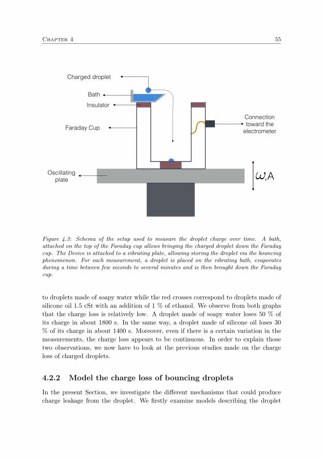
Chapter 4 55
Connection toward the
electrometerFaraday Cup
Bath
Charged droplet
Oscillating plate !
Insulator
,A
Figure 4.3: Schema of the setup used to measure the droplet charge over time. A bath,attached on the top of the Faraday cup allows bringing the charged droplet down the Faradaycup. The Device is attached to a vibrating plate, allowing storing the droplet via the bouncingphenomenon. For each measurement, a droplet is placed on the vibrating bath, evaporatesduring a time between few seconds to several minutes and is then brought down the Faradaycup.
to droplets made of soapy water while the red crosses correspond to droplets made ofsilicone oil 1.5 cSt with an addition of 1 % of ethanol. We observe from both graphsthat the charge loss is relatively low. A droplet made of soapy water loses 50 % ofits charge in about 1800 s. In the same way, a droplet made of silicone oil loses 30% of its charge in about 1400 s. Moreover, even if there is a certain variation in themeasurements, the charge loss appears to be continuous. In order to explain thosetwo observations, we now have to look at the previous studies made on the chargeloss of charged droplets.
4.2.2 Model the charge loss of bouncing droplets
In the present Section, we investigate the different mechanisms that could producecharge leakage from the droplet. We firstly examine models describing the droplet
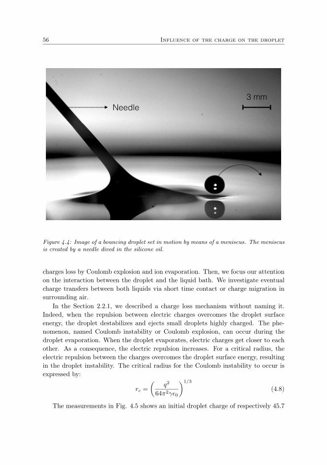
56 Influence of the charge on the droplet
Needle3 mm
Figure 4.4: Image of a bouncing droplet set in motion by means of a meniscus. The meniscusis created by a needle dived in the silicone oil.
charges loss by Coulomb explosion and ion evaporation. Then, we focus our attentionon the interaction between the droplet and the liquid bath. We investigate eventualcharge transfers between both liquids via short time contact or charge migration insurrounding air.
In the Section 2.2.1, we described a charge loss mechanism without naming it.Indeed, when the repulsion between electric charges overcomes the droplet surfaceenergy, the droplet destabilizes and ejects small droplets highly charged. The phe-nomenon, named Coulomb instability or Coulomb explosion, can occur during thedroplet evaporation. When the droplet evaporates, electric charges get closer to eachother. As a consequence, the electric repulsion increases. For a critical radius, theelectric repulsion between the charges overcomes the droplet surface energy, resultingin the droplet instability. The critical radius for the Coulomb instability to occur isexpressed by:
rc =
(q2
64π2γε0
)1/3
(4.8)
The measurements in Fig. 4.5 shows an initial droplet charge of respectively 45.7
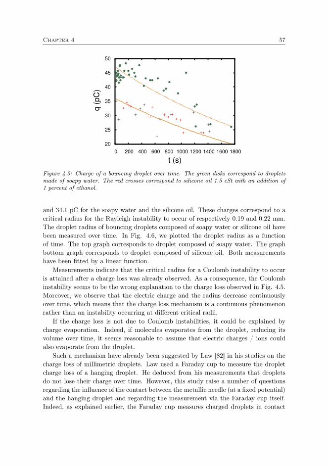
Chapter 4 57
20
25
30
35
40
45
50
0 200 400 600 800 1000 1200 1400 1600 1800
q
(p
C)
t (s)
Figure 4.5: Charge of a bouncing droplet over time. The green disks correspond to dropletsmade of soapy water. The red crosses correspond to silicone oil 1.5 cSt with an addition of1 percent of ethanol.
and 34.1 pC for the soapy water and the silicone oil. These charges correspond to acritical radius for the Rayleigh instability to occur of respectively 0.19 and 0.22 mm.The droplet radius of bouncing droplets composed of soapy water or silicone oil havebeen measured over time. In Fig. 4.6, we plotted the droplet radius as a functionof time. The top graph corresponds to droplet composed of soapy water. The graphbottom graph corresponds to droplet composed of silicone oil. Both measurementshave been fitted by a linear function.
Measurements indicate that the critical radius for a Coulomb instability to occuris attained after a charge loss was already observed. As a consequence, the Coulombinstability seems to be the wrong explanation to the charge loss observed in Fig. 4.5.Moreover, we observe that the electric charge and the radius decrease continuouslyover time, which means that the charge loss mechanism is a continuous phenomenonrather than an instability occurring at different critical radii.
If the charge loss is not due to Coulomb instabilities, it could be explained bycharge evaporation. Indeed, if molecules evaporates from the droplet, reducing itsvolume over time, it seems reasonable to assume that electric charges / ions couldalso evaporate from the droplet.
Such a mechanism have already been suggested by Law [82] in his studies on thecharge loss of millimetric droplets. Law used a Faraday cup to measure the dropletcharge loss of a hanging droplet. He deduced from his measurements that dropletsdo not lose their charge over time. However, this study raise a number of questionsregarding the influence of the contact between the metallic needle (at a fixed potential)and the hanging droplet and regarding the measurement via the Faraday cup itself.Indeed, as explained earlier, the Faraday cup measures charged droplets in contact

58 Influence of the charge on the droplet
0.4
0.5
0.6
0.7
0.8
0.9
1
1.1
0 100 200 300 400 500 600 700 800 900
r
(m
m)
t (s)
Figure 4.6: Radius of a bouncing droplet over time. The green disks correspond to dropletsmade of soapy water. The red crosses correspond to silicone oil 1.5 cSt with an addition of1 percent of ethanol.
but is also influenced by charges at distance. Thus, a variation in charge may beimpossible to measure via this method.
Despite the results of his experiments, Law cleverly described the charge evapora-tion process with few physical variables. He was able to link the charge evaporationrate to the molecule evaporation rate. The number of vapor molecules N leaving thecharged droplet can be expressed as :
dN
dt=NaM
dm
dt=NAρ4πr2
M
dr
dt(4.9)
where Na is the Avogadro number, M is the molar mass of the ion leaving the dropletand r is the droplet radius. The volume occupied by one molecule can be expressedas:
Vm =droplet volume
number of molecules in the droplet=
M
ρNA(4.10)
As a consequence, the number of molecules at the surface of the droplet can beexpressed as:
NS =droplet surface
area of one molecule=
4πr2
( MρNA
)2/3(4.11)
By multiplying Eq. 4.9 by the number of charges per molecules, q/Ns, we deduce:
q
Ns
dN
dt=
(NAρ
M
)1/3dr
dt=dq
dt(4.12)
The Eq. 4.12 allows to easily link the measurements of the radius and the charge

Chapter 4 59
variation over time:dq/dt
dr/dt=
(NAρ
M
)1/3
= α (4.13)
The comparison between the experiment and Eq. 4.13 is summarized in Tab. 4.2.We observe an important difference between Eq. 4.13 and the experiment for bothliquids tested. The Eq. 4.13 predicts a much faster charge evaporation than observed.
Silicone oil Soapy water
αexp 1.5 10−8 7.12 10−8αtheo 1.15 109 31.2 109
Table 4.2: Experimental and theoretical values of the parameter α deduced from Eq. 4.13.
The different between the experimental and the theoretical result could be ex-plained either by the absence of charges evaporation or by the limitation of the model.Since the model developed by Law, other models have been elaborated to describewith more precision the charge evaporation. These model are based on the chemicalbehavior of ions in excess in droplets produced from electropsrays. With this ap-proach, the charge evaporation corresponds to the displacement of an ion from theliquid droplet to the surrounding gas.
From this point of view, ions may leave the charged droplet if their free enthalpyof solvation becomes greater than zero. Iribarne and Thomson [83] showed that thecondition for the evaporation of ions can be expressed by:
∆G−G(E) > 0 (4.14)
where ∆G and G(E) are respectively the standard Gibbs free energy of solvation ofan ion and the energy reduction due to the charge interactions at the surface of thedroplets. If the process is supposed to be a first-order reaction, we can express theion evaporation over time with the following equation:
d lnN
dt= −(kT/h) exp (−(∆G−G(E))/kT ) (4.15)
where k is the Boltzmann constant, T is the absolute temperature and h is the Planckconstant. In other words, the charges/ions evaporation is modeled by the Arrheniusequation.
The Eq. 6.5 requires to know the standard Gibbs free energy of solvation of theevaporating ion, which is the main drawback of this approach. Indeed, as explainedin the Section 4.1, we do not know the exact nature of the charge induced in theelectrically charged droplet. As a consequence, it is impossible to know the standardGibbs free energy of solvation ∆G.
60 Influence of the charge on the droplet
However, studies summarized in Ref. [11] shows that the inequality expressed byEq. 4.14 is only reached for very small droplets. They showed that droplets shouldonly lose their charges via Coulomb explosion until reaching a small radius at whichcharge evaporation can occur. By calculating the free enthalpy of solvation of evapo-rating charged droplets, Hogan et al [84] have described the frontier between chargeloss via Coulomb explosion and charge evaporation. In their study, they examinedcharged droplets composed of 50 % of methanol and 50 % of water. The Fig. 4.7shows the study by Hogan et al [84] of the frontiers for the Rayleigh instability andthe ion evaporation. The droplet charge is plotted as a function of the droplet diam-eter. The continuous line corresponds to the Coulomb explosion frontier. The dottedline corresponds to the ion evaporation frontier. In practice, two scenarios, A or B,can occur.
The droplet with an amount of charges and a radius corresponding to the caseA firstly evaporates without any charge leakage. Then, the droplet reaches a criticalradius at which it endures a Coulomb explosion. The droplet instability results in animportant charge loss. After the Coulomb explosion, the droplet continues to evapo-rate. The droplet can eventually reach once again the limit of a Coulomb explosionand destabilize. This process repeats itself until reaching the charge evaporation limit.At this point, the droplet loses continuously its charge over time.
The second scenario possible corresponds to a droplet with an amount of chargesand a radius analogous to the case B. In this case, the droplet firstly evaporateswithout any charge leakage. Then, It directly reaches a critical radius at which itendures charge evaporation. We see in Fig. 4.7 that only droplet smaller than 40 nmmay loss their charge via charge evaporation.
As a consequence, even if we were not able to measure the free enthalpy of solvationof our charged droplets, we deduce from both the mismatch between experimentsand Eq. 4.13 (highlighted by Tab. 4.2), and the theory on electrospray droplets(highlighted by the Fig. 4.7) that charge evaporation should not occur in millimetriccharged droplets.
Another phenomenon to look at is the droplet interaction with the liquid bath.Indeed, as explained in the Section 3.3.2, droplets bounce on a thin air layer locatedbetween the liquid bath and the droplet. Such a small distance between the dropletand the liquid bath can eventually lead to charge loss over time. Ristenpart et al [65]have studied the interaction between charged droplets and liquid interfaces. Theyobserved that when the charged droplet approaches the liquid interface, the dropletslightly deforms and contacts the liquid interface during few milliseconds. Duringthe contact, the droplet exchanges charges with the liquid interface. Afterwards, thedroplet can coalesce or move away from the interface. They captured, with a high-speed camera, the deformation of the water droplet that leads to a contact with theliquid interface. They showed that, for thin deformations, droplets do not coalescewith the liquid interface but bounce on it. Such a mechanism may have appeared
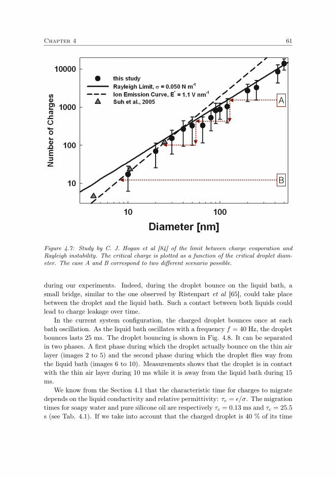
Chapter 4 61
A
B
Figure 4.7: Study by C. J. Hogan et al [84] of the limit between charge evaporation andRayleigh instability. The critical charge is plotted as a function of the critical droplet diam-eter. The case A and B correspond to two different scenario possible.
during our experiments. Indeed, during the droplet bounce on the liquid bath, asmall bridge, similar to the one observed by Ristenpart et al [65], could take placebetween the droplet and the liquid bath. Such a contact between both liquids couldlead to charge leakage over time.
In the current system configuration, the charged droplet bounces once at eachbath oscillation. As the liquid bath oscillates with a frequency f = 40 Hz, the dropletbounces lasts 25 ms. The droplet bouncing is shown in Fig. 4.8. It can be separatedin two phases. A first phase during which the droplet actually bounce on the thin airlayer (images 2 to 5) and the second phase during which the droplet flies way fromthe liquid bath (images 6 to 10). Measurements shows that the droplet is in contactwith the thin air layer during 10 ms while it is away from the liquid bath during 15ms.
We know from the Section 4.1 that the characteristic time for charges to migratedepends on the liquid conductivity and relative permittivity: τc = ε/σ. The migrationtimes for soapy water and pure silicone oil are respectively τc = 0.13 ms and τc = 25.5
s (see Tab. 4.1). If we take into account that the charged droplet is 40 % of its time

62 Influence of the charge on the droplet
1 2 3 4 5
6 7 8 9 10
1 mm
Figure 4.8: Image sequence of a charged droplet bouncing on a vibrating bath. Each image isseparated by 3.125 ms. The droplet can be considered near the liquid bath in 4 images overten.
in contact with the thin air layer, it means that it takes about 64 s for all the chargesto migrate from the silicone oil droplet to the liquid bath. The same reasoning canbe made with the soapy water. The water droplet should discharge in approximately0.325 ms.
As a consequence, the theory of the charge loss by thin contacts with the liquidbath is not in agreement with the observation. The charge migration time is too rapidto explain the observations.
However, contacts between the charged droplet and the liquid bath are not neces-sarily needed to produce charge loss. Charges may leave the droplet simply becauseof the proximity between the liquid bath and the charged droplet. Indeed, this prox-imity induces a non-negligible electric field between both interfaces. This electricfield may induce charge leakage. In order to describe the phenomenon, we decided tomodel the charged droplet and the liquid bath as a charged capacitor. The model isschematized in Fig. 4.9. In practice, the dielectric between the plates of a capacitorlets pass a small amount of leakage current, which leads to discharges over time. Asa consequence, a capacitor is modeled by a resistance and a capacitance in parallel.
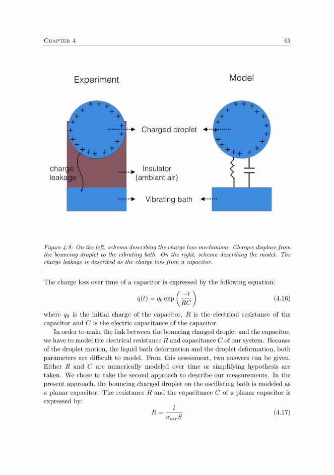
Chapter 4 63
++ + +++ ++
++++++ + +
+++
charge leakage
Insulator (ambiant air)
Charged droplet
Vibrating bath
Experiment Model
++ + +++ ++
++++++ + +
+++
Figure 4.9: On the left, schema describing the charge loss mechanism. Charges displace fromthe bouncing droplet to the vibrating bath. On the right, schema describing the model. Thecharge leakage is described as the charge loss from a capacitor.
The charge loss over time of a capacitor is expressed by the following equation:
q(t) = q0 exp
(−tRC
)(4.16)
where q0 is the initial charge of the capacitor, R is the electrical resistance of thecapacitor and C is the electric capacitance of the capacitor.
In order to make the link between the bouncing charged droplet and the capacitor,we have to model the electrical resistance R and capacitance C of our system. Becauseof the droplet motion, the liquid bath deformation and the droplet deformation, bothparameters are difficult to model. From this assessment, two answers can be given.Either R and C are numerically modeled over time or simplifying hypothesis aretaken. We chose to take the second approach to describe our measurements. In thepresent approach, the bouncing charged droplet on the oscillating bath is modeled asa planar capacitor. The resistance R and the capacitance C of a planar capacitor isexpressed by:
R =l
σairS(4.17)
64 Influence of the charge on the droplet
C =ε0S
l(4.18)
where l is the distance between the two plates of the capacitor, σair is the air con-ductivity and S is the surface of the plate capacitor. Such a description leads to thefollowing charge leakage from the bouncing droplet over time:
q(t) = q0 exp
(−σairtε0
)= q0 exp
(−tτc
)(4.19)
where τc = ε0/σair is the characteristic time of charge motion described in the Section4.1 (Eq. 6.5). Note that the case of charges leakage outside the droplet, τc is calculatedin the air and not in the liquid. We obtain τc ≈ 3000 s. The Eq. 4.19 has been plottedwithout any fitting parameters, for both the silicone oil and the soapy water, in Fig.4.5 (orange lines). We observe a good agreement between the measurements and Eq.4.19.
The Eq. 4.19 corresponds to the best model we found to describe the chargeleakage from the bouncing droplet. It correctly describes the charge leakage from thesoapy water and silicone oil droplets. The plan capacitor hypothesis allows avoidingmeasurements of the distance l between the droplet and the liquid bath as well as thesurface S of the droplet interacting with the liquid bath. The model indicates thatthe charge droplet tend to discharge over time because of its proximity with a solidor liquid interface.
4.2.3 Charge loss of droplets in microgravity and Leidenfroststate
The planar capacitor model shows that the charge leakage from droplets does notdepend on the distance between the droplet and the second interface. Naturally,this reasoning has to be used carefully, due to the significant assumption of a planarcapacitor geometry. For more complex geometries, the charge leakage may dependon the distance between the charged droplet and the second interface or even on thedroplet radius. In any case, our results show that the charge leakage due to thedroplet interaction with interfaces should be taken into account in any experiments.For example, droplet stored via electrodynamic or acoustics traps should also losetheir charges via this process. Of course, this charge leakage process is relatively slowand may be negligible in configurations where the droplet completely evaporates aftertwo or three minutes.
In our case, the model is in good agreement with the measurement on bouncingdroplets, but can also be used to describe other storage methods. The charge leakageof droplet stored in microgravity is difficult to describe. Indeed, the droplets are notnearby any interface, which makes the capacitor model difficult to apply. However,if we take into account the low charge migration time in the air (τc ≈ 3000 s) and

Chapter 4 65
the duration of one parabola (22 s), we can consider that a droplet keeps its chargeduring one experiment.
In the case of charged droplets stored via the Leidenfrost effect, the capacitormodel can be applied more easily. A droplet in Leidenfrost state levitates on a thinlayer of its own vapor. The capacitor model can be applied directly on the vaporlayer. Because the droplet levitates on its own vapor, the characteristic time τc hasto be calculated in the liquid vapor and not in dry air. Unfortunately, we do not haveaccess to the conductivity and relative permittivity of Ethanol and HFE-7100 vapor(the two liquids used to store charged droplets in Leidenfrost state). However, wecan suppose from data on water [85, 86] that the electric conductivity of the vaporphase only increase by a factor 10 or 100 compared to the electric conductivity of theair. At the same time, the permittivity increases with a factor 10. As a consequence,the characteristic time for the charges to migrate τc can decrease to a minimum of300 s. This characteristic time of charge leakage is important to take into accountin experiments involving Leidenfrost state. However, as we will see, experiments ondroplet in Leidenfrost state on liquid pool lasted about 30 s, which means that thecharge leakage had no influence on our measurements.
In conclusion, we measured the charge loss over time for millimetric chargeddroplets stored on a vibrating liquid bath. It takes about 1800 s for a soapy waterdroplet to lose half of its charge. The charge loss measured was not in agreementwith previous models such as the Coulomb explosion and the charge evaporation.A new model, inspired by the charge loss of a capacitor, quantitatively explainedthe observations. The application of the model on the two other storage systemsshowed that the droplet charge loss should not be taken into account given thetime scale involved in both systems.
4.3 Influence of the charges on the droplet surfaceenergy
As introduced in the Section 2.2.1, the excess of electric charges affects the intrinsicbehavior of the droplet. Lord Rayleigh showed that electric charges, by repellingeach other, influence the droplet surface energy. By looking at small perturbations onthe charged droplet, he expressed the influence of the energy decrease on the dropletnatural frequency. The charged droplet frequency is:
f2 =l(l − 1)(l + 2)
4π2ρr3
(γ − q2
16π2ε0r3(l + 2)
)(4.20)
where f is the oscillation frequency of the spherical mass of liquid, l determines theoscillating mode of the liquid, ρ is the liquid density, r is the droplet radius, q is thesurface charge of the droplet and ε0 is the vacuum permittivity. The droplet natural

66 Influence of the charge on the droplet
frequency corresponds to l =2. As a consequence, we have:
f2 =2
π2ρr3
(γ − q2
64π2ε0r3
)=
2
π2ρr3
(γ − q2σr
4ε0
)(4.21)
where qσ is the droplet surface charge density. The last term between brackets corre-sponds to the variation in the surface energy per surface unit due to electric charges.The initial surface energy by unit of surface corresponds to the droplet surface ten-sion, while the second term corresponds to the influence of the electric charge. Asexplained in the Section 2.2.1, the oscillation frequency of a charged droplet has beenverified experimentally several times [18]. It corresponds to one of the most famousexperiments demonstrating how electric charges affect the droplet behavior.
The influence of the electric charges on the droplet surface energy can also bededuced by looking at the pressure inside the charged droplet. The Laplace equationindicates the pressure inside a neutral droplet:
∆P =2γ
r(4.22)
If the droplet possesses an excess of electric charges, these charges in excess repeleach other. The pressure induced by electric charges at the surface of a conductingsphere corresponds to:
∆P = − q2σ2ε0
(4.23)
As a consequence, the total pressure inside a charged droplet is expressed by:
∆P =2γ
r− q2σ
2ε0(4.24)
The Eq. 4.21 and 4.24 show that the influence of electric charges in the dropletcan be seen as a variation in the surface energy by unit surface:
γ∗ = γ − q2σr
4ε0(4.25)
To summarize, the presence of electric charges in the droplet directly influencesits surface energy and, as a consequence, its internal pressure and its oscillation fre-quency. Note that the electric charge may also influence the evaporation of smalldroplets, as explained by Law [82]. Moreover, the Eq. 4.25 puts in evidence the threeinterconnected variables that govern the surface energy of a charged droplet (i.e thesurface tension γ, the charge q and the droplet radius r). In other words, once weknow these three parameters, we can deduce the charge influence on the droplet sur-face energy. Of course, the Eq. 4.25 can be turned around. For example, the knownvariables could be the surface energy by unit surface γ∗, the droplet radius r and thedroplet surface tension γ. Knowing these three parameters would allow to deduce thedroplet charge q.
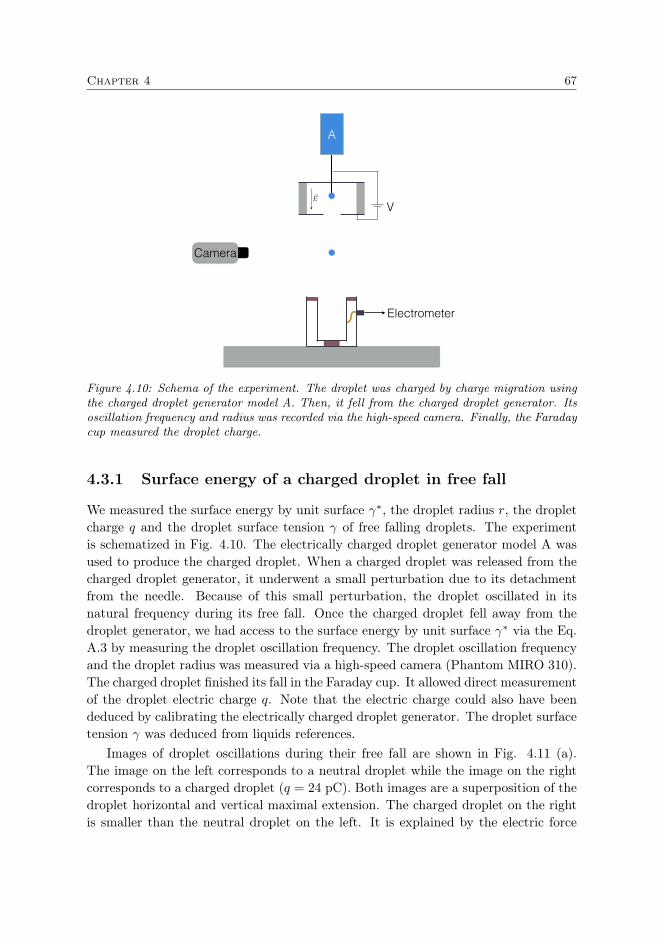
Chapter 4 67
~E
A
Camera
Electrometer
V
Figure 4.10: Schema of the experiment. The droplet was charged by charge migration usingthe charged droplet generator model A. Then, it fell from the charged droplet generator. Itsoscillation frequency and radius was recorded via the high-speed camera. Finally, the Faradaycup measured the droplet charge.
4.3.1 Surface energy of a charged droplet in free fall
We measured the surface energy by unit surface γ∗, the droplet radius r, the dropletcharge q and the droplet surface tension γ of free falling droplets. The experimentis schematized in Fig. 4.10. The electrically charged droplet generator model A wasused to produce the charged droplet. When a charged droplet was released from thecharged droplet generator, it underwent a small perturbation due to its detachmentfrom the needle. Because of this small perturbation, the droplet oscillated in itsnatural frequency during its free fall. Once the charged droplet fell away from thedroplet generator, we had access to the surface energy by unit surface γ∗ via the Eq.A.3 by measuring the droplet oscillation frequency. The droplet oscillation frequencyand the droplet radius was measured via a high-speed camera (Phantom MIRO 310).The charged droplet finished its fall in the Faraday cup. It allowed direct measurementof the droplet electric charge q. Note that the electric charge could also have beendeduced by calibrating the electrically charged droplet generator. The droplet surfacetension γ was deduced from liquids references.
Images of droplet oscillations during their free fall are shown in Fig. 4.11 (a).The image on the left corresponds to a neutral droplet while the image on the rightcorresponds to a charged droplet (q = 24 pC). Both images are a superposition of thedroplet horizontal and vertical maximal extension. The charged droplet on the rightis smaller than the neutral droplet on the left. It is explained by the electric force

68 Influence of the charge on the droplet
(a)
(b)
0.6
0.8
1
1.2
1.4
1.6
1.8
0 0.005 0.01 0.015 0.02 0.025 0.03 0.035 0.04
r
(mm
)
t (s)
Figure 4.11: (a) Images evidencing the droplet oscillations. Both images results from asubtraction of two snapshots, one on the maximum horizontal deformation (in black) andone on the maximum vertical deformation (in white). The first image, on the left, is thecase of a neutral droplet. The second image, on the right, is the case of a charged (24 pC)droplet. (b) Droplet vertical radius variation over time. Red crosses and green disks representmeasurements on a neutral droplet and a charged droplet (q = 24 pC) respectively. Half thepoints were plotted for the clarity of the graph.
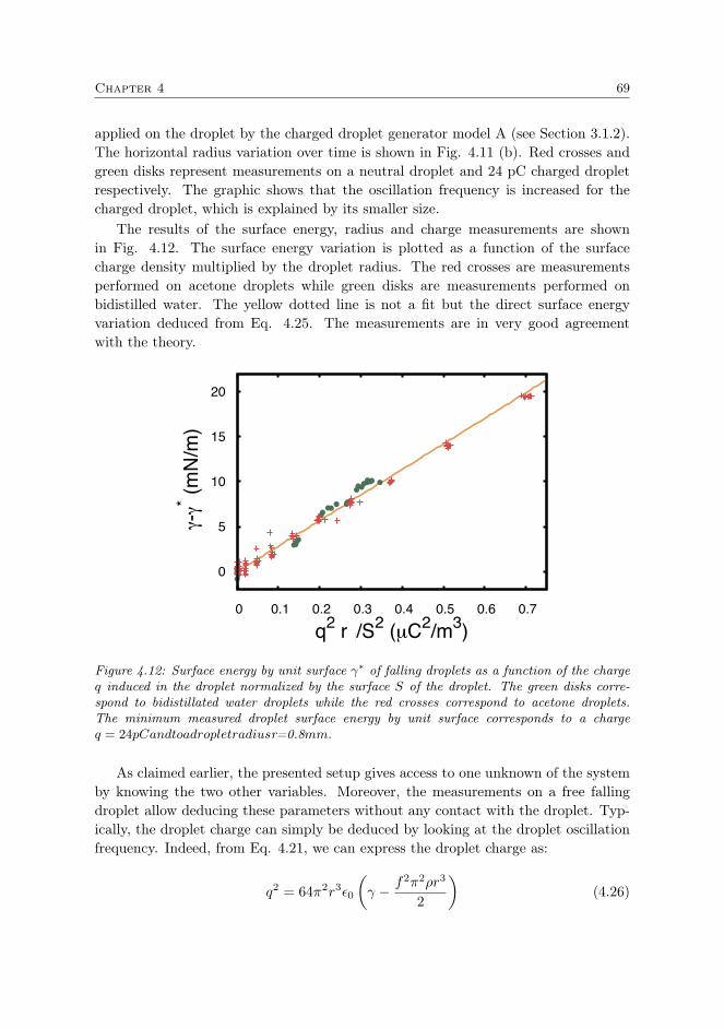
Chapter 4 69
applied on the droplet by the charged droplet generator model A (see Section 3.1.2).The horizontal radius variation over time is shown in Fig. 4.11 (b). Red crosses andgreen disks represent measurements on a neutral droplet and 24 pC charged dropletrespectively. The graphic shows that the oscillation frequency is increased for thecharged droplet, which is explained by its smaller size.
The results of the surface energy, radius and charge measurements are shownin Fig. 4.12. The surface energy variation is plotted as a function of the surfacecharge density multiplied by the droplet radius. The red crosses are measurementsperformed on acetone droplets while green disks are measurements performed onbidistilled water. The yellow dotted line is not a fit but the direct surface energyvariation deduced from Eq. 4.25. The measurements are in very good agreementwith the theory.
0
5
10
15
20
0 0.1 0.2 0.3 0.4 0.5 0.6 0.7
γ-
γ* (mN
/m)
q2 rd/S2 (µC2/m3)
Figure 4.12: Surface energy by unit surface γ∗ of falling droplets as a function of the chargeq induced in the droplet normalized by the surface S of the droplet. The green disks corre-spond to bidistillated water droplets while the red crosses correspond to acetone droplets.The minimum measured droplet surface energy by unit surface corresponds to a chargeq = 24pCandtoadropletradiusr=0.8mm.
As claimed earlier, the presented setup gives access to one unknown of the systemby knowing the two other variables. Moreover, the measurements on a free fallingdroplet allow deducing these parameters without any contact with the droplet. Typ-ically, the droplet charge can simply be deduced by looking at the droplet oscillationfrequency. Indeed, from Eq. 4.21, we can express the droplet charge as:
q2 = 64π2r3ε0
(γ − f2π2ρr3
2
)(4.26)
70 Influence of the charge on the droplet
By knowing the droplet oscillation frequency, surface tension and radius, thedroplet charge can be deduced. Contrary to the measurement performed via a Faradaycup, the charged droplet can still be used after this charge measurement. Further-more, the droplet charge can be measured over time while the droplet is stored insystems such as an oscillating liquid bath or in microgravity.
However, the deduction of the droplet charge by measuring the droplet oscillationfrequency requires knowing with precision the droplet surface tension, radius andoscillation frequency. In order to illustrate this limitation, we can take the exampleof an ethanol droplet with a charge q = 10 pC and a radius r = 1 mm. Thesecharacteristics lead to:
q2/64π2r3ε0 =
(γ − f2π2ρr3
2
)= 0.0018 N/m (4.27)
The Eq. 4.27 shows that the term in between brackets is about 1 mN/m. The surfacetension of ethanol corresponds to γ = 22 mN/m. As a consequence, each term inbetween parentheses should be known with high precision. Furthermore, the term inbetween parentheses depends on the frequency squared and the radius cubed, whichhighly increase the error propagation.
We can deduce from this example that small measurement errors on the dropletoscillation frequency, surface tension or radius can lead to a significant error on thedroplet charge. Moreover, this error decreases with the increase of the droplet charge.As a consequence, this method should be limited to high precision measurementsperformed on highly charged droplet. This reasoning explains why we chose to directlymeasure the droplet charge when we studied the droplet charge leakage over time inSection 4.2.
In conclusion, the electric charge affects the surface energy density of droplets.The influence of the electric charge can be observed by the variation in the dropletoscillation frequency or the droplet internal pressure. We measured the decreasein surface energy density for free falling droplets. Our measurements were inagreement with the theory. We deduced that the measurement of the surfaceenergy density could give information on the droplet charge.

5Interaction between charged droplets in
microgravity
Contents5.1 Droplet collision: Research context and strategy . . . . 725.2 Experimental setup . . . . . . . . . . . . . . . . . . . . . . 775.3 Influence of the charges on the droplet trajectories . . . 785.4 Influence of the charges on the impact between droplets 83
In this Chapter, we examine the behavior of charged droplets in microgravity. Asexplained in the Section devoted to the description of the microgravity storage method(see Section 3.3.1), the microgravity allows generating free floating charged droplets.We chose this experimental configuration to highlight the electric interaction betweentwo charged droplets.
The majority of the studies focused on the interaction between charged dropletshave been interested in thunderclouds or electrosprays. These systems correspondto several micro droplets interacting with each other. As explained in Section 2.4,this thesis aims to study millimetric droplets in order to bring new insights on thecharged droplet understanding. Through this process, we developed tools that allowgenerating charged droplets one by one. In this Chapter, we take advantage of thesetools to study the interaction between only two millimetric and charged droplets. Inparticular, we study the trajectory of two charged droplets sent towards each other.
Firstly, we introduce the past research performed on the interaction between

72 Interaction between charged droplets in microgravity
droplets and we describe our approach of the subject. Secondly, we describe in detailour experimental setup. Thirdly, we study the influence of the electric interaction onthe trajectories of both charged droplets. Finally, we examine experiments that leadto an impact between both charged droplets. From these experiments, we comparethe impact between charged droplets to the impact between neutral droplets.
5.1 Droplet collision: Research context and strategy
The physics of collisions between droplets has raised the interest of several scientistssince the early 1950s [87, 88]. In the particular case of water droplets, this interestcomes specifically from atmospheric research [89–91]. The main goal of these studieswas to understand how several collisions between droplets could affect their radiusdistributions. These experiments were focused on small droplets (i.e. r ≈ 150 µmto represent cloud droplets) and big drops (i.e. r ≈ 1 mm to represent raindrops).Over the years, various setups have been developed in order to accurately observe thedifferent panels of collision behaviors between droplets [92, 93]. Indeed, the result ofan impact between two or more droplets depends on their respective radius, speedand angle of impact. Recently, Gotaas et al [94], have developed a new setup able toprecisely study the boundary between each of the different sort of collisions.
The collision between two neutral droplets (a and b) of the same volume (i.e.the same radius, ra = rb = r) and the same composition is commonly described bya phase diagram comparing the collision parameter χ with the Weber number We.These parameters are respectively defined by:
χ =x
(ra + rb), (5.1)
We =ρv2relDm
γ, (5.2)
where x is the projected separation distance between the centers of the collidingdroplets normal to the relative velocity vector ~vrel (see Fig. 5.1), ra and rb are theradii of each droplet, ρ is the density of the droplet, Dm and γ are respectively thediameter and the surface tension of the droplets. In the case of neutral droplets, twodroplets sent toward each other move straight on until impacting. As a consequence,the direction of the relative speed vrel does not vary over time, which mean that thecollision parameter is also constant over time.
According to the parameters χ and We, the collision between neutral dropletsleads to different behaviors. The collision diagram, shown in Fig. 5.2 (top), pointsout each of these behaviors. If χ > 1, the droplets do not contact each other. Ifχ < 1, both droplets impact each other. Four different impacts can be observed: thebouncing between droplet, the coalescence, the stretching separation and the reflexiveseparation. The two first results are classics. The two last results are described by
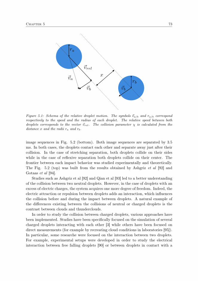
Chapter 5 73
~vrel
~va
~vb ~vb
ra
rb
x
Figure 5.1: Schema of the relative droplet motion. The symbols ~va/b and ra/b correspondrespectively to the speed and the radius of each droplet. The relative speed between bothdroplets corresponds to the vector ~vrel. The collision parameter χ is calculated from thedistance x and the radii ra and rb.
image sequences in Fig. 5.2 (bottom). Both image sequences are separated by 3.5ms. In both cases, the droplets contact each other and separate away just after theircollision. In the case of stretching separation, both droplets collide on their sideswhile in the case of reflexive separation both droplets collide on their center. Thefrontier between each impact behavior was studied experimentally and theoretically.The Fig. 5.2 (top) was built from the results obtained by Ashgriz et al [92] andGotaas et al [94].
Studies such as Ashgriz et al [92] and Qian et al [93] led to a better understandingof the collision between two neutral droplets. However, in the case of droplets with anexcess of electric charges, the system acquires one more degree of freedom. Indeed, theelectric attraction or repulsion between droplets adds an interaction, which influencesthe collision before and during the impact between droplets. A natural example ofthe differences existing between the collisions of neutral or charged droplets is thecontrast between clouds and thunderclouds.
In order to study the collision between charged droplets, various approaches havebeen implemented. Studies have been specifically focused on the simulation of severalcharged droplets interacting with each other [3] while others have been focused ondirect measurements (for example by recreating cloud conditions in laboratories [95]).In particular, some researche were focused on the interaction between two droplets.For example, experimental setups were developed in order to study the electricalinteraction between free falling droplets [90] or between droplets in contact with a
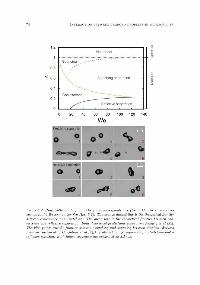
74 Interaction between charged droplets in microgravity
Coalescence
Bouncing
Stretching separation
Reflexive separation
No-impact
Sect
ion
4.3
Sect
ion
4.4
0
0.2
0.4
0.6
0.8
1
1.2
0 20 40 60 80 100 120 140
χ
We
1 2 3
4 5 6
1 2 3
4 5 6
Reflexive separation
Stretching separation 2 mm
2 mm
Figure 5.2: (top) Collision diagram. The y axis corresponds to χ (Eq. 5.1). The x axis corre-sponds to the Weber number We (Eq. 5.2). The orange dashed line is the theoretical frontierbetween coalescence and stretching. The green line is the theoretical frontier between coa-lescence and reflexive separation. Both theoretical predictions come from Ashgriz et al [92].The blue points are the frontier between stretching and bouncing between droplets (deducedfrom measurement of C. Gotaas et al [94]). (bottom) Image sequence of a stretching and areflexive collision. Both image sequences are separated by 3.5 ms.

Chapter 5 75
charging electrode [96,97]. These studies showed that the electric interaction betweentwo droplets could be modeled has the interaction between two charged spheres a andb. The electric force between two charged spheres is expressed by:
Fel = Fc + Fdip
=qaqb
4πε0d2+
1
4πε0q2arb
(1
d3− d
(d2 − r2b )2
)+
1
4πε0q22ra
(1
d3− d
(d2 − r2a)2
)+
1
4πε0qaqbrarb
(1
d4+
1
(d2 − r2a − r2b )2− 1
(d2 − r2a)2− 1
(d2 − r2b )2
) (5.3)
where Fc = qaqb4πε0d2
corresponds to the Coulomb interaction and Fdip correspondsto the dipolar forces. The charges qa and qb correspond respectively to the electriccharge of droplets a and b, d is the distance between the center of the droplets andε0 corresponds to the vacuum electrical permittivity. This electric force affects thedroplet trajectories before they impact each other. As a consequence, two neutraldroplets sent toward each other do not impact in the same way as two charged droplets.Even if the droplets initial trajectory is the same, the electric interaction affectsthe trajectory of a charged droplet while the neutral droplet remains on its initialtrajectory. The influence of this electric force on the droplet trajectories and impactsis the exact subject of our study.
Even if the electric interaction between two charged droplets is well known, themajority of the studies investigated the collision between neutral drops. To our knowl-edge, there is a lack of high speed imaging of the impact between electrically chargeddroplets. This lack of result is explained by the difficulty to highlight the influence ofthe electric interaction on the droplet trajectories. Indeed, a rapid calculation of theelectric force between two charged droplets shows that the electric force is 40 timessmaller than the droplet weight. As a consequence, two charged droplets sent towardeach other mainly endure the acceleration of gravity. They quickly acquire an impor-tant speed and the electric interaction becomes negligible compare to aerodynamicinteractions.
In order to surpass this limitation, we studied the collision between two chargeddroplets in microgravity. The microgravity was reached via parabolic flights, as ex-plained in Section 3.3.1. The use of microgravity conditions aims to minimize anyaerodynamic effect (e.g. a lift force due to air drive) and focus only on the elec-trostatic interaction between charged droplets. Indeed, the microgravity conditionsallow sending two droplets toward each other with a slow speed. In doing so, dropletskeep their slow speed throughout their motion and are not accelerated by gravity.
In the following Sections, we propose to compare collisions between charged dropletsto measurements and results deduced from the study of neutral droplets. In orderto maximize the influence of the electric charges, we focused our study on the inter-action between two electrically charged droplets with a radius r ∈ [0.41 − 0.97] mminteracting in microgravity conditions. The specific range of radius, which is higher
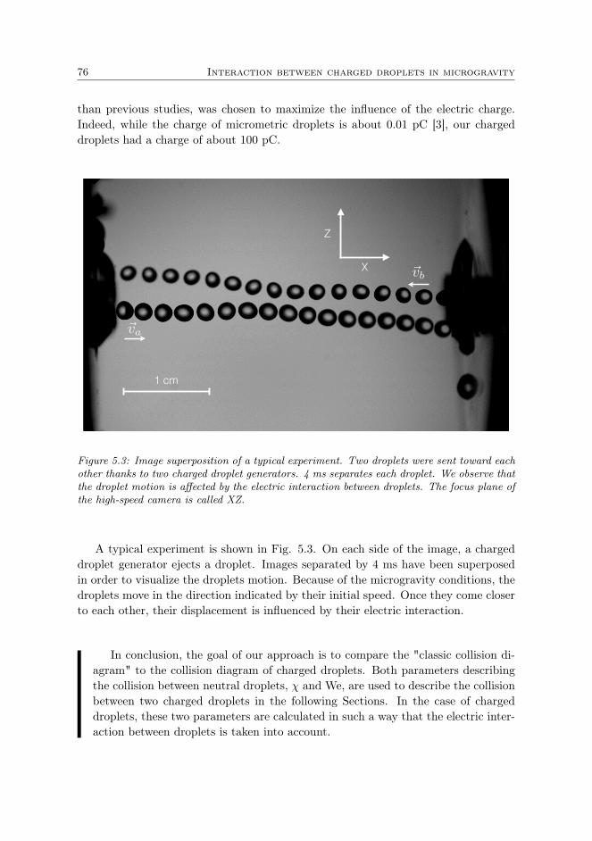
76 Interaction between charged droplets in microgravity
than previous studies, was chosen to maximize the influence of the electric charge.Indeed, while the charge of micrometric droplets is about 0.01 pC [3], our chargeddroplets had a charge of about 100 pC.
1 cm
Z
X
~va
~vb
Figure 5.3: Image superposition of a typical experiment. Two droplets were sent toward eachother thanks to two charged droplet generators. 4 ms separates each droplet. We observe thatthe droplet motion is affected by the electric interaction between droplets. The focus plane ofthe high-speed camera is called XZ.
A typical experiment is shown in Fig. 5.3. On each side of the image, a chargeddroplet generator ejects a droplet. Images separated by 4 ms have been superposedin order to visualize the droplets motion. Because of the microgravity conditions, thedroplets move in the direction indicated by their initial speed. Once they come closerto each other, their displacement is influenced by their electric interaction.
In conclusion, the goal of our approach is to compare the "classic collision di-agram" to the collision diagram of charged droplets. Both parameters describingthe collision between neutral droplets, χ and We, are used to describe the collisionbetween two charged droplets in the following Sections. In the case of chargeddroplets, these two parameters are calculated in such a way that the electric inter-action between droplets is taken into account.
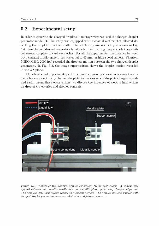
Chapter 5 77
5.2 Experimental setup
In order to generate the charged droplets in microgravity, we used the charged dropletgenerator model B. The setup was equipped with a coaxial airflow that allowed de-taching the droplet from the needle. The whole experimental setup is shown in Fig.5.4. Two charged droplet generators faced each other. During one parabola they emit-ted several droplets toward each other. For all the experiments, the distance betweenboth charged droplet generators was equal to 41 mm. A high-speed camera (PhantomMIRO M310, 2000 fps) recorded the droplets motion between the two charged dropletgenerators. In Fig. 5.3, the image superposition shows the droplet motion recordedin the XZ plane.
The whole set of experiments performed in microgravity allowed observing the col-lision between electrically charged droplets for various sets of droplets charges, speedsand radii. From these observations, we discuss the influence of electric interactionson droplet trajectories and droplet contacts.
Support screw
Metallic needle
Metallic plate
Air flowLiquid flow
Electric connexions
1 cm
Figure 5.4: Picture of two charged droplet generators facing each other. A voltage wasapplied between the metallic needle and the metallic plate, generating charges migration.The droplets were then ejected thanks to a coaxial airflow. The droplet motions between bothcharged droplet generators were recorded with a high-speed camera.
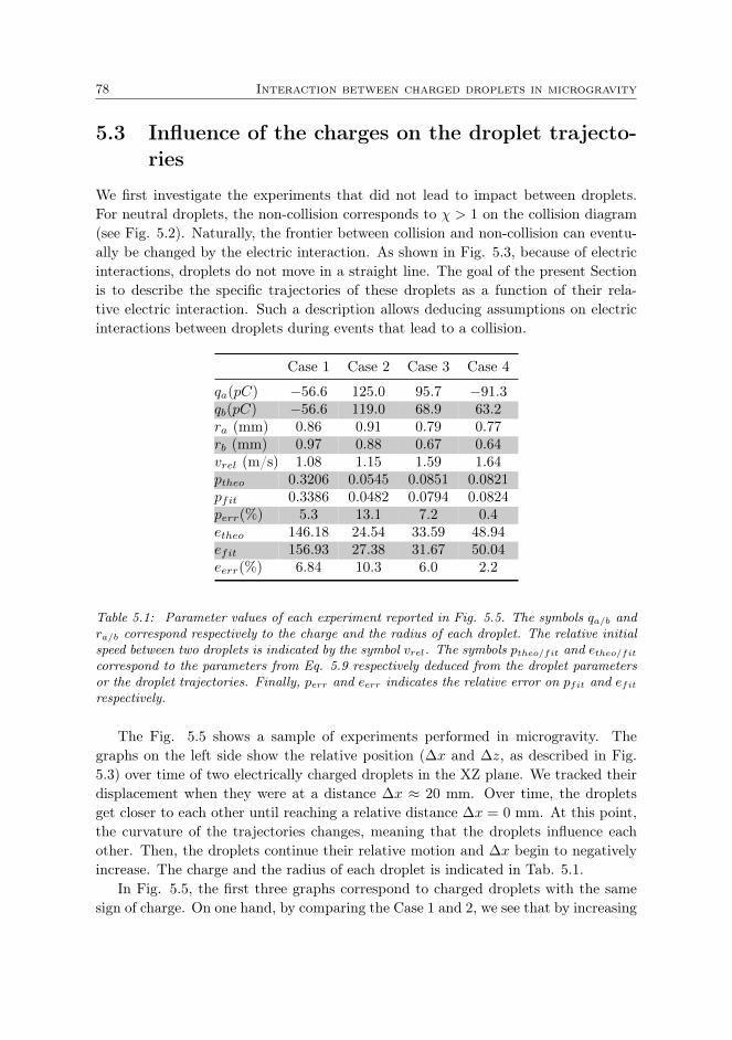
78 Interaction between charged droplets in microgravity
5.3 Influence of the charges on the droplet trajecto-ries
We first investigate the experiments that did not lead to impact between droplets.For neutral droplets, the non-collision corresponds to χ > 1 on the collision diagram(see Fig. 5.2). Naturally, the frontier between collision and non-collision can eventu-ally be changed by the electric interaction. As shown in Fig. 5.3, because of electricinteractions, droplets do not move in a straight line. The goal of the present Sectionis to describe the specific trajectories of these droplets as a function of their rela-tive electric interaction. Such a description allows deducing assumptions on electricinteractions between droplets during events that lead to a collision.
Case 1 Case 2 Case 3 Case 4
qa(pC) −56.6 125.0 95.7 −91.3qb(pC) −56.6 119.0 68.9 63.2ra (mm) 0.86 0.91 0.79 0.77rb (mm) 0.97 0.88 0.67 0.64vrel (m/s) 1.08 1.15 1.59 1.64ptheo 0.3206 0.0545 0.0851 0.0821pfit 0.3386 0.0482 0.0794 0.0824perr(%) 5.3 13.1 7.2 0.4etheo 146.18 24.54 33.59 48.94efit 156.93 27.38 31.67 50.04eerr(%) 6.84 10.3 6.0 2.2
Table 5.1: Parameter values of each experiment reported in Fig. 5.5. The symbols qa/b andra/b correspond respectively to the charge and the radius of each droplet. The relative initialspeed between two droplets is indicated by the symbol vrel. The symbols ptheo/fit and etheo/fitcorrespond to the parameters from Eq. 5.9 respectively deduced from the droplet parametersor the droplet trajectories. Finally, perr and eerr indicates the relative error on pfit and efitrespectively.
The Fig. 5.5 shows a sample of experiments performed in microgravity. Thegraphs on the left side show the relative position (∆x and ∆z, as described in Fig.5.3) over time of two electrically charged droplets in the XZ plane. We tracked theirdisplacement when they were at a distance ∆x ≈ 20 mm. Over time, the dropletsget closer to each other until reaching a relative distance ∆x = 0 mm. At this point,the curvature of the trajectories changes, meaning that the droplets influence eachother. Then, the droplets continue their relative motion and ∆x begin to negativelyincrease. The charge and the radius of each droplet is indicated in Tab. 5.1.
In Fig. 5.5, the first three graphs correspond to charged droplets with the samesign of charge. On one hand, by comparing the Case 1 and 2, we see that by increasing

Chapter 5 79
2.4 2.6 2.8
3 3.2 3.4 3.6 3.8
4 4.2 4.4
-20 -15 -10 -5 0 5 10 15 20 25
∆ z
(mm
)
∆ x (mm)
1.6 1.8
2 2.2 2.4 2.6 2.8
3 3.2 3.4 3.6 3.8
-25 -20 -15 -10 -5 0 5 10 15 20 25 30
∆ z
(mm
)
∆ x (mm)
1.4
1.6
1.8
2
2.2
2.4
2.6
2.8
3
-20 -15 -10 -5 0 5 10 15 20 25
∆ z
(mm
)
∆ x (mm)
-4
-3.5
-3
-2.5
-2
-1.5
-15 -10 -5 0 5 10 15
∆ z
(mm
)
∆ x (mm)
-10
-5
0
5
10
15
20
25
0 5 10 15 20 25 30
Fel
(µ
N)
Rrel
-3-2-1 0 1 2 3 4 5 6 7 8
0 5 10 15 20 25
Fel
(µ
N)
Rrel
-5
0
5
10
15
20
0 5 10 15 20
Fel
(µ
N)
Rrel
-8
-6
-4
-2
0
0 5 10 15 20 25 30
Fel
(µ
N)
Rrel
Case 1- -
Case 2+ +
Case 3+ +
Case 4+ +
Figure 5.5: The first three couples of graphs show experiments performed with droplets ofthe same sign of charge corresponding to cases 1,2 and 3 in Tab. 5.1. The last graph showsan experiment performed with droplets of opposite signs of charges corresponding to case 4in Tab. 5.1. The graphs on the left side exhibits the relative position ∆x and ∆z of twodroplets during their motion in the plane XZ. The orange lines correspond to fits of thetrajectory taking into account a Coulomb interaction between droplets. The graphs on theright side compare the value of the Coulomb force Fc (green disks), the dipole forces Fdip
(orange triangles) and the total electric force Fel (red crosses) as a function of the relativedistance Drel. Each force was calculated from Eq. 5.4.
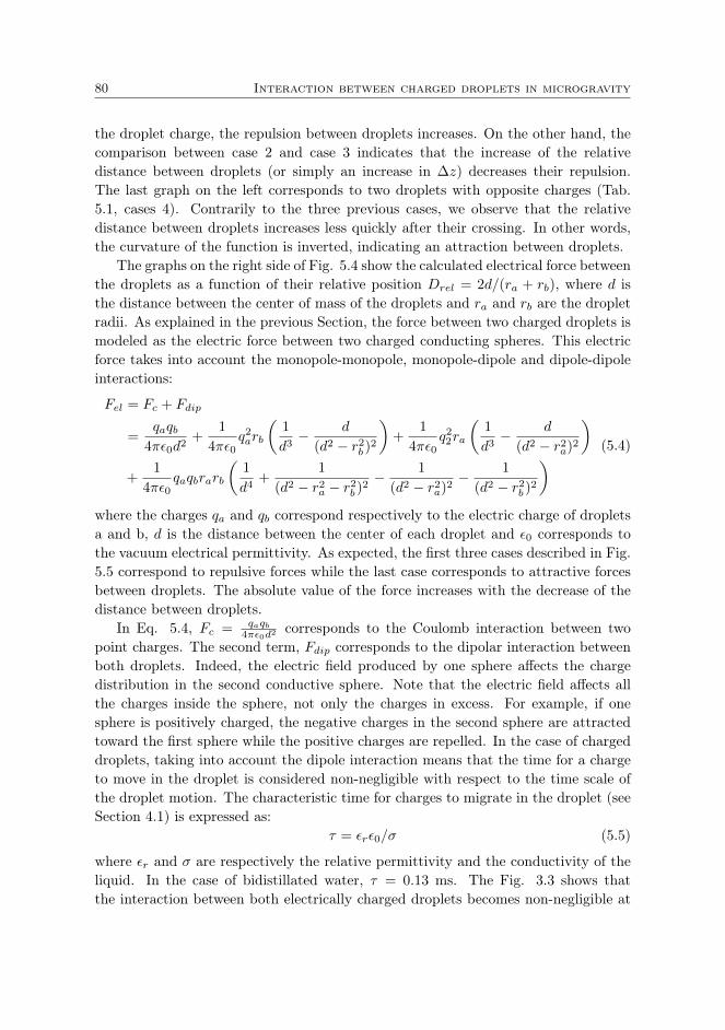
80 Interaction between charged droplets in microgravity
the droplet charge, the repulsion between droplets increases. On the other hand, thecomparison between case 2 and case 3 indicates that the increase of the relativedistance between droplets (or simply an increase in ∆z) decreases their repulsion.The last graph on the left corresponds to two droplets with opposite charges (Tab.5.1, cases 4). Contrarily to the three previous cases, we observe that the relativedistance between droplets increases less quickly after their crossing. In other words,the curvature of the function is inverted, indicating an attraction between droplets.
The graphs on the right side of Fig. 5.4 show the calculated electrical force betweenthe droplets as a function of their relative position Drel = 2d/(ra + rb), where d isthe distance between the center of mass of the droplets and ra and rb are the dropletradii. As explained in the previous Section, the force between two charged droplets ismodeled as the electric force between two charged conducting spheres. This electricforce takes into account the monopole-monopole, monopole-dipole and dipole-dipoleinteractions:
Fel = Fc + Fdip
=qaqb
4πε0d2+
1
4πε0q2arb
(1
d3− d
(d2 − r2b )2
)+
1
4πε0q22ra
(1
d3− d
(d2 − r2a)2
)+
1
4πε0qaqbrarb
(1
d4+
1
(d2 − r2a − r2b )2− 1
(d2 − r2a)2− 1
(d2 − r2b )2
) (5.4)
where the charges qa and qb correspond respectively to the electric charge of dropletsa and b, d is the distance between the center of each droplet and ε0 corresponds tothe vacuum electrical permittivity. As expected, the first three cases described in Fig.5.5 correspond to repulsive forces while the last case corresponds to attractive forcesbetween droplets. The absolute value of the force increases with the decrease of thedistance between droplets.
In Eq. 5.4, Fc = qaqb4πε0d2
corresponds to the Coulomb interaction between twopoint charges. The second term, Fdip corresponds to the dipolar interaction betweenboth droplets. Indeed, the electric field produced by one sphere affects the chargedistribution in the second conductive sphere. Note that the electric field affects allthe charges inside the sphere, not only the charges in excess. For example, if onesphere is positively charged, the negative charges in the second sphere are attractedtoward the first sphere while the positive charges are repelled. In the case of chargeddroplets, taking into account the dipole interaction means that the time for a chargeto move in the droplet is considered non-negligible with respect to the time scale ofthe droplet motion. The characteristic time for charges to migrate in the droplet (seeSection 4.1) is expressed as:
τ = εrε0/σ (5.5)
where εr and σ are respectively the relative permittivity and the conductivity of theliquid. In the case of bidistillated water, τ = 0.13 ms. The Fig. 3.3 shows thatthe interaction between both electrically charged droplets becomes non-negligible at

Chapter 5 81
a distance of approximately 3 mm (d < 3Drel). If we take a droplet speed of v = 1m/s (which is in agreement with Tab. 5.1), it takes 3 ms for a droplet to cross thisdistance. We deduce from this reasoning that the time scale of the charge displacementis negligible compared to the droplet motion time scale.
However, even if the charge migration generates dipole interactions, the Fig. 5.5(right) also shows that, in most of the cases, the dipolar component of the electricalforce is mainly negligible until a distance between droplets corresponding to approx-imately 3Drel. Indeed, the red crosses and the green disks are superposed duringthe majority of the experiments. As a consequence, the first step is to describe eachdroplet trajectory by only taking into account the Coulomb force (i.e. we supposethat Fel = Fc).
In order to model the trajectories of each droplet, we should solve the equation ofmotion:
ma/b
d2~sa/b
dt2= ~Fel (5.6)
where ma/b and ~sa/b are respectively the mass and the spatial position of the dropleta or b. However, given the complexity of the force ~Fel, the Eq. 5.6 has no analyticalsolutions. Hopefully, we showed that the electric force ~Fel can be, at the first order,described as a Coulomb force. By doing so, the droplet trajectory can be seen as atwo-body problem influenced by a Newtonian force:
~FN =k
d2~ud (5.7)
Where k is a constant (in our case k = qaqb/4πε0), d is the relative distance betweenthe droplets and ud is a unit vector. The classical way to resolve this two-body systemis to reduce the problem to a one-body system influenced by a central force:
µd2 ~d
dt2= ~FN (5.8)
The reduced mass is µ = m1m2
m1+m2and d is the relative distance between the droplets.
This classical problem has a solution in polar coordinates (d,θ). From Eq. 5.8 thedistance between the charged droplets as a function of θ is expressed as:
d(θ) =p
(∓)1 + e cos(θ − θ0)(5.9)
where p = (±)µC2
k and e = (±)( pd0 + 1). The sign (±) corresponds respectively todroplets with the same sign of charges and droplets with different signs of charges.The constant C = d2θ is derived from the angular momentum conservation and d0 isthe minimal distance between droplets. The angle θ0 depends on the initial conditions.
The trajectories in Fig. 5.5 have been fitted by Eq. 5.9. The results of the fitscorrespond to the orange lines in Fig. 5.5(left). A comparison between the fitting
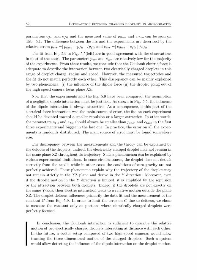
82 Interaction between charged droplets in microgravity
parameters pfit and efit and the measured value of ptheo and etheo can be seen onTab. 5.1. The difference between the fits and the experiments are described by therelative errors perr =| ptheo − pfit | /pfit and eerr =| etheo − efit | /efit.
The fit from Eq. 5.9 in Fig. 5.5(left) are in good agreement with the observationsin most of the cases. The parameters perr and eerr are relatively low for the majorityof the experiments. From these results, we conclude that the Coulomb electric force isadequate to describe the interaction between two electrically charged droplets in thisrange of droplet charge, radius and speed. However, the measured trajectories andthe fit do not match perfectly each other. This discrepancy can be mainly explainedby two phenomena: (i) the influence of the dipole force (ii) the droplet going out ofthe high speed camera focus plane XZ.
Now that the experiments and the Eq. 5.9 have been compared, the assumptionof a negligible dipole interaction must be justified. As shown in Fig. 5.5, the influenceof the dipole interaction is always attractive. As a consequence, if this part of theelectrical force interaction was the main source of error, the fits on each experimentshould be deviated toward a smaller repulsion or a larger attraction. In other words,the parameters pfit and efit should always be smaller than ptheo and etheo in the firstthree experiments and bigger in the last one. In practice, the error on all the exper-iments is randomly distributed. The main source of error must be found somewhereelse.
The discrepancy between the measurements and the theory can be explained bythe defocus of the droplets. Indeed, the electrically charged droplet may not remain inthe same plane XZ throughout its trajectory. Such a phenomenon can be explained byvarious experimental limitations. In some circumstances, the droplet does not detachcorrectly from the needle while in other cases the conditions of zero gravity are notperfectly achieved. These phenomena explain why the trajectory of the droplet maynot remain strictly in the XZ plane and derive in the Y direction. Moreover, evenif the droplet motion in the Y direction is limited, it is amplified by the repulsionor the attraction between both droplets. Indeed, if the droplets are not exactly onthe same Y-axis, their electric interaction leads to a relative motion outside the planeXZ. The droplet defocus influences primarily the data fit and the measurement of theconstant C from Eq. 5.9. In order to limit the error on C due to defocus, we choseto measure the constant only on portions where electrically charged droplets wereperfectly focused.
In conclusion, the Coulomb interaction is sufficient to describe the relativemotion of two electrically charged droplets interacting at distance with each other.In the future, a better setup composed of two high-speed cameras would allowtracking the three dimensional motion of the charged droplets. Such a systemwould allow detecting the influence of the dipole interaction on the droplet motion.
Chapter 5 83
5.4 Influence of the charges on the impact betweendroplets
If the electric interaction influences the droplet trajectories of two electrically chargeddroplets, one can understand that it also influences the impact between electricallycharged droplets. In this Section, we focus our attention on experiments where weobserved a contact between charged droplets. In the collision diagram between neutraldroplets, these experiments correspond to an impact parameter χ < 1. Naturally, thefrontier between impact and non-impact between charged droplets can eventuallyvary. In this Section, we compare the collision diagram for neutral droplets with thecollision diagram for charged droplets.
In the case of neutral drops, the respective motion of each droplet before theimpact is supposed to be straight. Indeed, neutral droplets do not interact at distancewith each other. As a consequence, the collision parameter χ = x/(ra + rb) is thesame whichever the distance d between the droplets. Experimentally, χ is generallycalculated when droplets are near each other, in order to minimize any measurementerrors. In the case of electrically charged droplets, the main goal is to highlightthe possible influence of the electric interaction. As a consequence, the collisionparameter is calculated at a particular distance at which the electric force is non-negligible. During the analysis of the impacts between two charged droplets, theelectrical force Fel (Eq. 5.4) was considered non-negligible when it corresponded to15 percent of its maximal value. The limit is chosen in order to minimize the erroron the measurements and maximize the influence of the electric force.
This modification in the calculation of the parameter χ implies that the collisiondiagram now takes into account the droplet trajectory just before the impact betweendroplets. In doing this, we highlight any influence of the electric charge just before theimpact or during the impact without changing the definition of χ for neutral droplets.
In the case of the parameter We, only a small adjustment on the droplet radiushas to be made. Because of the complexity to generate electrically charged dropletsin microgravity, the droplet radius may vary from 1 to 15 percent between bothinteracting droplets. As a consequence, the droplet diameter Dm, needed for thecalculation of the Weber number We, is defined as the mean diameter between bothdroplets (i.e. Dm = ra + rb).
In Fig. 5.6, the impacts between charged droplets observed in microgravity havebeen placed on the collision diagram. The parameters χ and We were calculatedas described in the preceding paragraph. In order to be consistent, the data in thediagram in Fig. 5.6 are given with an error bar corresponding to the variation inradii between both droplets. During our experiments, we observed collisions betweenelectrically charged droplets within a wide range of radii and charges (0.41 < r < 0.97
mm and 57 < |q| < 190 pC). According to the Weber number, we observed reflexivecollisions (red triangles), stretching separations (red circles) or no collisions at all
84 Interaction between charged droplets in microgravity
Coalescence
Bouncing
Stretching separation
Reflexive separation
No-impact
0
0.2
0.4
0.6
0.8
1
1.2
0 20 40 60 80 100 120 140
χ
We
Stretching separation different charge sign
Reflexive separation same charge sign
Stretching separation same charge sign
Non-collision
Figure 5.6: Collision diagram. The y axis corresponds to χ (Eq. 5.1). The x axis corre-sponds to the Weber number We (Eq. 5.2). The orange dashed line describes the theoreticalfrontier between coalescence and stretching. The green line describes the theoretical frontierbetween coalescence and reflexive separation. Both theoretical predictions come from Ashgrizet al [92]. The blue points describe the frontier between stretching and bouncing betweendroplets (deduced from measurement of Gotaas et al [94]). The red circles, triangles andcrosses describe the observed collisions. The red triangles correspond to reflexive separation.The red circles correspond to stretching collisions. The red cross corresponds to a non-collision Experiments performed with the same sign of charges are represented by an emptycircles/triangles while the collision between droplets with opposite charges are represented byfull circles/triangles. The red cross corresponds to an experiment performed with the samesign of charges. The error bars account for the small difference in radii between both collidingdroplets.

Chapter 5 85
(red crosses). Experiments performed with the same sign of charges are representedby empty circles/triangles while the collision between droplets with opposite sign ofcharges are represented by full circles/triangles. In order to compare the measure-ments performed on charged droplets to the collision between neutral droplets, wedrew in Fig. 5.6 the frontier between neutral collisions.
In the case of oppositely charged droplets, only stretching collisions were observed.The majority of these collisions is found in the expected zone of the neutral phasediagram. In other words, we observed mainly no differences between neutral dropletimpacts and charged droplet impacts. However, at high collision parameter χ, weobserved one reflexive collision in the classical bouncing region. Even if more obser-vations are needed to draw conclusions, it seems that the reflexive collision region isextended in the present case. The observation indicates that the bouncing betweentwo electrically charged droplets with opposite charges may be impossible.
In the same way, the majority of the experiments performed with colliding dropletsof the same sign of charge are well located in the neutral collision diagram. However,one specific observation, described as the red cross in Fig. 5.6, indicates once againthat the presence of electric charges has an effect on the boundary of the classicalcollision diagram. In this particular case, we observed repulsion between both chargeddroplets that is sufficient to avoid an impact between them. The present observationindicates that repulsion between droplets may be important enough to avoid thecollision between droplets in parts of the diagram where χ < 1.
In summary, we observed two specific experiments where the result of the impactwas different from the neutral predictions. Firstly, we observed a stretching separationin the classic bouncing zone. However, the absence of numerous measurements inthe present set of experiment does not allow developing a predictive theory on thewhole zone corresponding to bouncing between droplets. Indeed, the modeling of thebouncing between two colliding droplets is a difficult problem that was raised severaltimes. Such a phenomenon is linked to several parameters such as the ambient airpressure [93], the droplet surface tension or the droplet viscosity. The observationtends to show that the influence of the electric charge of both droplets can be addedto these other variables.
Secondly, we observed a non-collision between two charged droplets with the samesign of charge in the part of the diagram corresponding to χ < 1. In the next lines, wepropose a model to answer to this observation. In order to extrapolate the zone of thediagram where collisions may be avoided due to the electric repulsion, we investigatethe energy conservation in the reference frame corresponding to the center of mass ofboth droplets.
Thanks to the previous study of charged drop trajectories, we can take the follow-ing assumptions: (i) Droplets can be approximated to point charges (which implies aCoulomb repulsion and no droplet rotation); (ii) there is no dissipating force duringthe droplet motion. By comparing the energy of the system at an infinite distance
86 Interaction between charged droplets in microgravity
0
0.2
0.4
0.6
0.8
1
1.2
1.4
-1 -0.5 0 0.5 1
χ
Ve,min/Ek,∞
0
0.2
0.4
0.6
0.8
1
1.2
0 20 40 60 80 100 120 140
χ
We
B1
B2
Figure 5.7: (top) Collision parameter χ (Eq. 5.2) as a function of the ratio between the elec-tric energy and the kinetic energy. The red triangles represent interactions between dropletsthat lead to an impact. The green circles represent interactions between droplets that do notlead to an impact. The orange line corresponds to the limit of a non-impact between droplets(see Eq. 5.13) (bottom) Collision parameter χ as a function of the Weber number We. Theblack dash-dotted lines describe the frontier of an impossible collision in the case of dropletswith the same sign of charge. The curve named b1 corresponds to the configuration of theexperiment described by the red cross in Fig. 5.6. The curve named b2 corresponds to thesame experiments but with droplets two times more charged.

Chapter 5 87
between droplets to the system energy at the minimum distance between them, wehave:
µv2rel2
=k
d0+µC2
2d20(5.10)
The left hand side of the equation corresponds to the kinetic energy of the droplets,with vrel corresponding to the droplet relative speed when they are far from eachother. The electric energy is considered equal to zero at an infinite distance. On theright hand side of the equation, the first term corresponds to the electrostatic energyof the system. The distance d0 corresponds to the minimal distance between droplets.The second term corresponds to the rotational energy of the system. At the minimaldistance between droplets, the kinetic energy of the system equals to zero. Becauseof the angular momentum definition, we deduce:
C = χvrel(ra + rb) (5.11)
The Eq. 5.10 allows to express d0 as a function of χ. The limit of an impactcan be expressed as the point where the distance between the center of mass of thedroplet is smaller than the radius of both droplets:
d0 < (ra + rb) (5.12)
From Eq. 5.10 and 5.12, we then deduce the following limit for a possible impactbetween charged droplets:
χ <
√1− Ve,0
Ek,inf(5.13)
Where Ve,0 = k(ra+rb)
and Ek,inf =µv2rel
2 . By knowing Ve,0 and Ek,inf , we can deducethe range of χ for which it is impossible to observe any impact between droplets.
In a more general way, the Eq. 5.13 indicates that, for charged droplets, the limitof a possible collision is not anymore χ = 1. In the case of two droplets with oppositesign of charges, χ > 1 can lead to collision between droplets. On the other hand, inthe case of two droplets with the same sign of charge, collisions can be impossible forχ < 1.
In Fig. 5.7 (top), the theoretical limitation deduced from Eq. 5.13 is confirmedby experimental measurements. The droplet speeds vrel were calculated at the samedistance where the collision parameter χ were calculated. The green circles correspondto the observation of a non-contact between droplets while the red triangles correspondto the observation of a contact between droplets. The green circle on the orange line(i.e. at the edge between a contact and a non-contact between droplets) correspondsto the red cross presented in Fig. 5.6. The Fig. 5.7 (top) not only shows the validity ofEq. 5.13 but demonstrates also that the Weber number and the collision parameter arenot anymore sufficient to completely describe the collision between charged droplets.

88 Interaction between charged droplets in microgravity
Indeed, the measurements demonstrate that the electric repulsion/attraction beforethe impact have to be taken into account.
Now that a first theory is able to describe the behavior of the collision betweencharged droplets, the future aim is to confirm the diagram in Fig. 5.7 (top) withseveral measurements. Such a diagram helps to define the collision parameters χleading to an impact as a function of the range of energy Ve,0/Ek,inf . Indeed, asshown by the hatched lines in Fig. 5.7 (top), for a defined range of energy ratio,different χ are accessible. For example, we can study several collisions between twodroplets. These droplets can have the same charge and the same radii, but differentspeeds. The range of speed studied (e.g. 0 to 1 m/s) allow deducing the rangeof energy ratio Ve,0/Ek,inf accessible in Fig. 5.7 (top), and as a consequence, theparameter χ necessary to observe impacts.
If the set of droplets studied is composed of both positively and negatively chargeddroplets, the energy ratio Ve,0/Ek,inf can be negative, which means that both hatchedregions are accessible. We observe on Fig. 5.7 that for a given range of energy,impacts between oppositely charged droplets can occur on a larger range of collisionparameter χ. As a consequence, for a system where collision happens randomly, thereis a higher probability of collisions between droplets with different sign of charges.This observation implies that in the case of a system overall neutral composed ofoppositely charged droplets, the difference in collision probability leads to a fasterneutralization of the charged droplets due to collisions.
Thanks to this simplified theory, it is possible to predict if a collision is possibleor not. Unfortunately, the Fig. 5.7 (top) does not indicate the result of the collisionbetween the droplets (a coalescence, a stretching collision,...). However, for a fixeddroplet radius and charge, the non-impact boundary can be plotted as a function ofWe only. Indeed, the Weber number can be introduced in Eq. 5.13:
χ <
√1− kρ
Weµγ(5.14)
In the case of the experiment corresponding to the red cross in Fig. 5.6, the matchingfrontier has been plotted as a black dash-dotted line (b1) in Fig. 5.7 (bottom). Thecollisions above the black dash-dotted line are impossible due to charge repulsion. Onthe contrary, below the black dash-dotted line, the repulsion between droplets is noimportant enough to avoid collisions.
The frontier shows that, for particular droplet radius and charge, parts of theclassic collision diagram are not accessible. Indeed, the Fig. 5.7 (bottom) showsthat a part of the bouncing and the coalescence region is not accessible. Of course,in other configurations, with a more important droplet charge or a smaller radius,a more important part of the classical collision diagram may be inaccessible. Forexample, in the case of droplets with a charge two times more important, the secondfrontier (b2) shows that a larger part of the classic diagram is inaccessible.
Chapter 5 89
In conclusion, the present Chapter shows that electric charges influence di-rectly the droplets motion and the droplet collision. Throughout our experiments,we observed a soft influence of electric charges on the classic droplet motion andcollision. Indeed, we observed slight variation in the droplet trajectories due toelectric attraction or repulsion as well as slight variations in the classic collision di-agram. However, these small changes can result in significant changes of behavior.Typically, we showed that the electric interaction directly influences the collisionparameter between droplets and the collision results. Our approach gives a firstinsight on the influence of the electric charges on the classic droplet collision dia-gram. However, more experiments are needed to design the precise charged dropletcollision diagram. The natural next step would be to perform experiments with asetup comparable to the one developed by Gotaas et al [94] on earth. Such a set ofexperiments will need to be compared to experiments performed in microgravity. Ifthe aerodynamic forces are found to not affect the influence of the electric charges,the setup would allow to conclude on the collision between charged droplets.

6Charged droplets bouncing on a vibrating
bath
Contents6.1 Influence of a homogeneous electric field on a charged
droplet bouncing on a liquid interface . . . . . . . . . . . 926.1.1 Experimental setup . . . . . . . . . . . . . . . . . . . . . . 936.1.2 Observations at the scale of the vibrating bath . . . . . . 946.1.3 Observations at the scale of the droplet . . . . . . . . . . 996.1.4 The model . . . . . . . . . . . . . . . . . . . . . . . . . . 1026.1.5 futures investigations . . . . . . . . . . . . . . . . . . . . . 108
6.2 Interaction between two electrically charged dropletson a vibrating bath . . . . . . . . . . . . . . . . . . . . . . 111
The storage via vibrating bath has the great advantage of storing droplets fora long time (more than an hour) on the two dimensions of the oscillating liquidbath. The experimental setup leading to the bouncing of the droplet on the vibratingbath was described in Section 3.3.2. In the Section 4.2, we used the vibrating bathmethod to measure the droplet charges loss over time. However, we only tackled thecomplexity of the charged droplet bouncing on a vibrating bath. In particular, adroplet bouncing on a vibrating bath is kept at a relatively constant vertical position(except for the droplet bouncing), but can be displaced along the horizontal plane.Naturally, the droplet displacement on the vibrating bath is complex to describe.Indeed, the droplet, while bouncing, deforms the vibrating bath. In exchange, the
92 Charged droplets bouncing on a vibrating bath
deformed liquid bath influences the droplet bouncing.This relation between the liquid bath and the bouncing droplet can take several
shapes. For example, small droplets bouncing on low viscous vibrating bath can self-propel [64]. In our case, we focus our attention on millimetric droplets bouncing onhighly viscous liquid bath (1000 cSt). In this particular configuration, droplets donot displace on the surface of the liquid bath (at the exception of specific range offrequency that are not tackled in this Chapter [63]). Without external perturbations,the droplet indefinitely bounces at the same horizontal place.
This is where the excess of electric charge comes into play. Indeed, we showedin the Chapter describing the experimental setups (see Section 3.3.2) that electriccharges do not influence the way the droplet bounces on the vibrating bath. However,as shown during the study of droplets in microgravity (see Chapter 5), an electric fieldcan influence the motion of charged droplets. In this Chapter, we study how a chargeddroplet is set in motion via external electric fields. In the first Section (see Section 6.1)we investigate the basic case of a charged droplet sets in motion by a homogeneouselectric field. In the second Section (see Section 6.2), we study the case of two dropletsset in motion by their reciprocal electric interaction. Both Sections give new insightson droplets in motion on a high viscous vibrating bath.
6.1 Influence of a homogeneous electric field on acharged droplet bouncing on a liquid interface
When a high viscous liquid bath is oscillating, the droplet bounces on it verticallywhile keeping its horizontal position. However, an external horizontal force can beapplied on the droplet. If this horizontal force is important enough, the droplet moveson the surface of the liquid bath. For example, blowing air on the system inducesthe displacement of the droplet. In our case, we can take advantage of the excess ofcharges to move the droplet by applying an electric force via an external electric field.
The study of two charged droplets in microgravity (see Chapter 5) demonstratesthat the electric field generated by one electrically charged droplet can influence themotion of another charged droplet. For two charged droplets (q = 10 pC) separatedby 5 mm, we have typically E = 1
4πε0
qr2 =3.6 103 V/m. Such an electric field can be
easily overtaken by experimental setups. For example, two metallic plates separatedby 5 cm only need 180 V to produce the same electric field. Such an electric field,applied horizontally on the droplet should be sufficient to generate the horizontaldisplacement of the droplet on the vibrating bath.
In doing so, the droplet acquires a complex motion composed of its vertical bounc-ing and its horizontal displacement. The droplet interaction with the liquid bath asa function of the applied electric force determines the adopted motion. In the nextlines, we describe the experimental setup and model the observations obtained fromthe experiments.
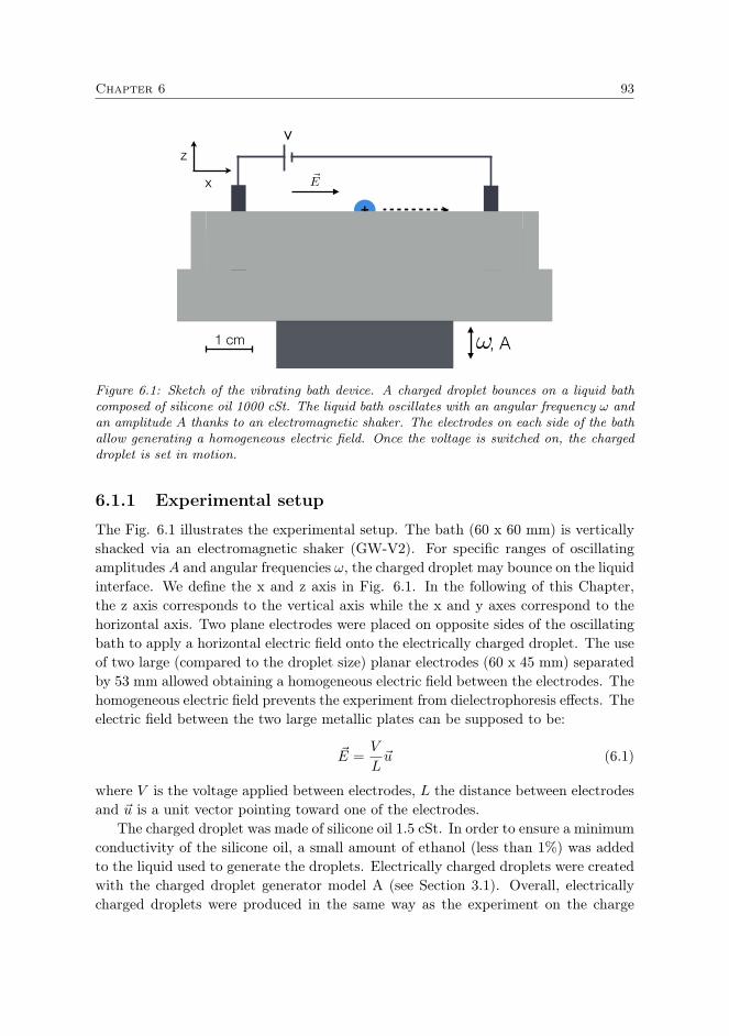
Chapter 6 93
+
x
zV
~E
!, A
-+
1 cm
Figure 6.1: Sketch of the vibrating bath device. A charged droplet bounces on a liquid bathcomposed of silicone oil 1000 cSt. The liquid bath oscillates with an angular frequency ω andan amplitude A thanks to an electromagnetic shaker. The electrodes on each side of the bathallow generating a homogeneous electric field. Once the voltage is switched on, the chargeddroplet is set in motion.
6.1.1 Experimental setup
The Fig. 6.1 illustrates the experimental setup. The bath (60 x 60 mm) is verticallyshacked via an electromagnetic shaker (GW-V2). For specific ranges of oscillatingamplitudes A and angular frequencies ω, the charged droplet may bounce on the liquidinterface. We define the x and z axis in Fig. 6.1. In the following of this Chapter,the z axis corresponds to the vertical axis while the x and y axes correspond to thehorizontal axis. Two plane electrodes were placed on opposite sides of the oscillatingbath to apply a horizontal electric field onto the electrically charged droplet. The useof two large (compared to the droplet size) planar electrodes (60 x 45 mm) separatedby 53 mm allowed obtaining a homogeneous electric field between the electrodes. Thehomogeneous electric field prevents the experiment from dielectrophoresis effects. Theelectric field between the two large metallic plates can be supposed to be:
~E =V
L~u (6.1)
where V is the voltage applied between electrodes, L the distance between electrodesand ~u is a unit vector pointing toward one of the electrodes.
The charged droplet was made of silicone oil 1.5 cSt. In order to ensure a minimumconductivity of the silicone oil, a small amount of ethanol (less than 1%) was addedto the liquid used to generate the droplets. Electrically charged droplets were createdwith the charged droplet generator model A (see Section 3.1). Overall, electricallycharged droplets were produced in the same way as the experiment on the charge
94 Charged droplets bouncing on a vibrating bath
leakage (see Section 4.2). The charged droplet generator was calibrated before eachexperiment by using a Faraday cup. The calibration consisted in measuring thedroplet radius and charge for the set of voltage used in each experiment. The typicalduration of an experiment was of the order of 1 min. As shown in the Section 4.2, thecharge loss during this duration is negligible. Throughout the experiments performedon the setup, the droplet radius r was tuned between 0.35 and 0.9 mm while themeasured charge carried by the droplet q was in the range between 11 and 20 pC.Experiments were also performed with negatively charged droplets and gave the sameresults as the one obtained for positively charged droplets.
The liquid bath was made of silicone oil with a kinematic viscosity of 1000 cSt.The high viscosity limits the liquid bath deformation. Typically, a droplet bouncingon the bath only slightly curves the liquid bath. The oscillation frequency of thevibrating bath was set at f = 40 Hz. As shown in Fig. 3.15 in Section 3.3.2, thisfrequency allows stabilizing the bouncing droplet on a large range of acceleration. Theoscillation amplitude of the vibrating bath was varied in order to study the influence ofthe bath oscillation on the droplet motion. The bath reduced acceleration Γ = Aω2/g
(A being the oscillation amplitude and ω being the angular frequency) was tunedbetween 0.5 and 1.75. The voltage V between electrodes was tuned between 1000 and10000 V.
A first camera allowed tracking the charged droplet from the top of the bath.The tracking was made at 25 fps. The top camera was equipped with a wide-anglelens, allowing capturing the droplet motion at the scale of the liquid bath. On theside of the liquid bath, we tracked the droplet motion with a high-speed camera(Phantom Miro M-310) at 2000 fps. The high-speed camera was equipped with azooming lens, allowing capturing the detail of the droplet motion. In the following,we firstly look at the observations obtained at the scale of the vibrating bath and thenfocus our attention on the droplet scale observations. The two different approaches(the macroscopic and the microscopic observations) allowed us to obtain a completeunderstanding of the system.
6.1.2 Observations at the scale of the vibrating bath
The Fig. 6.2 is the image superposition of the droplet motion took from the top ofthe vibrating bath. One second separates each droplet. The charged droplet is set inmotion from the left to the right thanks to the external electric field. On the rightside of the liquid bath, the droplet is kept away from the electrode because of theliquid meniscus.
The droplet moves along the x direction when a voltage is applied between bothelectrodes. The data in Fig. 6.3 (top) correspond to droplet trajectories taken fromexperiments for which the voltage was varied while the radius and the droplet chargewas kept constant (i.e. r = 0.8 mm and q = 15 ± 5 pC). The red crosses, greendisks and orange triangles correspond to applied voltages V of respectively 2000 V,
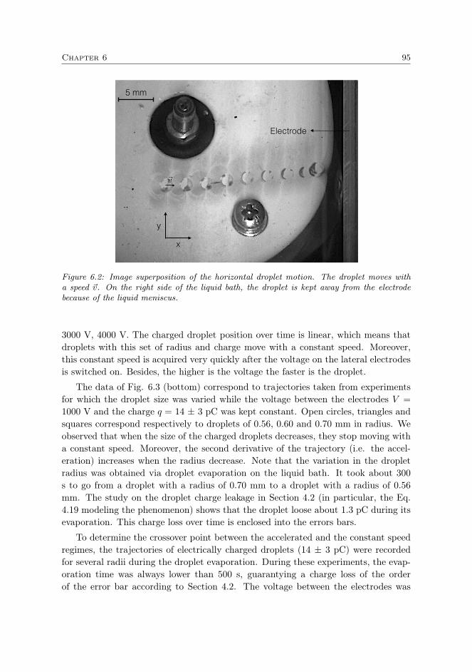
Chapter 6 95
Electrode
x
y
~v
5 mm
Figure 6.2: Image superposition of the horizontal droplet motion. The droplet moves witha speed ~v. On the right side of the liquid bath, the droplet is kept away from the electrodebecause of the liquid meniscus.
3000 V, 4000 V. The charged droplet position over time is linear, which means thatdroplets with this set of radius and charge move with a constant speed. Moreover,this constant speed is acquired very quickly after the voltage on the lateral electrodesis switched on. Besides, the higher is the voltage the faster is the droplet.
The data of Fig. 6.3 (bottom) correspond to trajectories taken from experimentsfor which the droplet size was varied while the voltage between the electrodes V =
1000 V and the charge q = 14 ± 3 pC was kept constant. Open circles, triangles andsquares correspond respectively to droplets of 0.56, 0.60 and 0.70 mm in radius. Weobserved that when the size of the charged droplets decreases, they stop moving witha constant speed. Moreover, the second derivative of the trajectory (i.e. the accel-eration) increases when the radius decrease. Note that the variation in the dropletradius was obtained via droplet evaporation on the liquid bath. It took about 300s to go from a droplet with a radius of 0.70 mm to a droplet with a radius of 0.56mm. The study on the droplet charge leakage in Section 4.2 (in particular, the Eq.4.19 modeling the phenomenon) shows that the droplet loose about 1.3 pC during itsevaporation. This charge loss over time is enclosed into the errors bars.
To determine the crossover point between the accelerated and the constant speedregimes, the trajectories of electrically charged droplets (14 ± 3 pC) were recordedfor several radii during the droplet evaporation. During these experiments, the evap-oration time was always lower than 500 s, guarantying a charge loss of the orderof the error bar according to Section 4.2. The voltage between the electrodes was
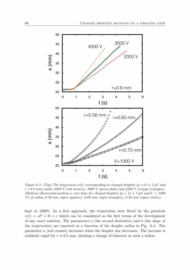
96 Charged droplets bouncing on a vibrating bath
20
25
30
35
40
45
50
0 1 2 3 4 5 6
x
(mm
)
t (s)
4000 V3000 V
2000 V
r=0.8 mm
20
25
30
35
40
45
50
0 1 2 3 4 5 6
x
(mm
)
t (s)
r=0.56 mm r=0.60 mm
r=0.70 mm
V=1000 V
Figure 6.3: (Top) The trajectories x(t) corresponding to charged droplets (q =15 ± 5 pC andr =0.8 mm) under 2000 V (red crosses), 3000 V (green disks) and 4000 V (orange triangles).(Bottom) Horizontal position x over time for charged droplets (q = 14 ± 3 pC and V = 1000V) of radius 0.70 mm (open squares), 0.60 mm (open triangles), 0.56 mm (open circles).
kept at 1000V. As a first approach, the trajectories were fitted by the parabolax(t) = at2 + bt + c which can be considered as the first terms of the developmentof any exact solution. The parameters a (the second derivative) and b (the slope ofthe trajectories) are reported as a function of the droplet radius in Fig. 6.4. Theparameter a (red crosses) increases when the droplet size decreases. The increase issuddenly rapid for r ≈ 0.5 mm, showing a change of behavior at such a radius.

Chapter 6 97
10-310-210-1100101102103104105
0.4 0.45 0.5 0.55 0.6 0.65 0.7 0.75 0.8 0.8510-4
10-3
10-2
10-1
100
101
102
a (m
m/s
2 )
b (m
m/s
)
r(mm)
Figure 6.4: Dependence of the fitting parameters a (red crosses) and b (green disks) fromthe fit x(t) = at2 + bt + c, as a function of the drop radius r. The orange curve is thedroplet average speed computed according to Eq. 6.4. The hatching describes the theoreticaldescription of the cross over between the two kinds of drop motion (i.e. when the accelerationis considered negligible or not, see Eq. 6.7). All the experiments were performed at V = 1000V with q = 14 ± 3 pC.
The observation of a movement with a constant speed may seem counter intuitive.Indeed, the charged droplet endures a constant horizontal force during its motion. Asa consequence, a constant acceleration is expected. However, the droplet also interactswith the liquid bath. This interaction between the droplet and the liquid bath is themajor unknown of the system. Indeed, macroscopic observations do not indicate howthe droplet deforms the vibrating bath neither how the bath deformation affects thedroplet bouncing. To better understand the droplet motion with a constant speed,we looked at the droplet speed as a function of the voltage applied on the electrodes(see Fig. 6.5 (top)). The dependence on the applied voltage for a large droplet wasdetermined by using a droplet of r =0.8 mm charged with q =11 ± 2 pC. The Fig. 6.5(top) shows that the droplet speed depends linearly on the voltage applied betweenelectrodes.
The droplet speed was measured as a function of the oscillation amplitude of theliquid bath A. The Fig. 6.5 (bottom) shows the droplet speed as a function of thereduced acceleration Γ = Aω2/g. The dependence on the reduced acceleration wasdetermined by using a droplet of r =0.8 mm charged with q = 20 ± 2 pC. We see inFig. 6.5 (bottom) that the droplet speed does not seem to vary with the bath reducedacceleration.
To summarize, small droplets are accelerated while larger droplets move with a

98 Charged droplets bouncing on a vibrating bath
0
0.5
1
1.5
2
2.5
3
3.5
4
4.5
0 2000 4000 6000 8000 10000
v
(mm
/s)
V (V)
0
1
2
3
4
5
6
7
8
0 0.5 1 1.5 2
v
(m/s
)
Γ Figure 6.5: (Top) Speed v of a charged droplet (q =11 ± 2 pC and r = 0.8 mm) as afunction of the voltage between both electrodes. The error bars are the standard deviation on10 experiments. The orange line is a fit based on Eq. 6.4. (Bottom) Speed v of a chargeddroplet (q = 20 ± 2 pC and r = 0.8 mm) as a function of the bath reduced acceleration Γ.The error bars are the standard deviation on 10 experiments.
constant speed. In the case of large droplets, the measurements performed at a timescale of few seconds do not present any transient regime between the droplet at restand the constant speed regime. As soon as the voltage is switched on, the dropletmoves with a constant speed. We deduce that the origin of the constant speed has tobe found on the time scale of one bounce.
Chapter 6 99
6.1.3 Observations at the scale of the droplet
We investigated the droplet motion at the scale of one bounce by placing a high-speed camera on the side of the oscillating bath. It allowed capturing the motion ofthe droplet in the XZ plane.
The details of a charged droplet (r = 0.9 mm and q = 19±5 pC) bounces isshown on the image sequence in Fig. 6.6 (top). Each image is spaced by 3.125ms. The voltage between both electrodes was V = 5000 V. The displacement ofthe center of mass of the charged droplet is shown in Fig. 6.6 (bottom). The zposition (vertical) and the x position (horizontal) are represented by red disks andgreen crosses respectively. Along the z axis, the drop bounces with a frequency of40 Hz, namely the same frequency as the oscillating bath. Between two cushionedimpacts with the bath, the droplet center of mass experiences successive parabolicflight in the z direction. The x(t) trajectory reveals a more complex structure thanthe macroscopic trajectory x(t) presented in Fig 6.3 (top). Indeed, the position overtime x(t) reveals that the droplet horizontal motion is the succession of the samepattern.
This periodic pattern is not observed for small droplets (r <0.5 mm) for whichthe trajectory is more complex. The Fig. 6.7 (top) shows an image sequence of asmall droplet in motion. Each image is spaced by 3.125 ms. We observe that thebath is less deformed by the impact of the small droplet. The voltage applied onthe droplet was V = 1000 V. The droplet had a radius r = 0.35 mm and a chargeq = 14 pC. The tracking of the droplet motion is plotted in Fig. 6.7 (bottom). Thez position (vertical) and the x position (horizontal) are represented by red disks andgreen crosses respectively. The droplet still has a periodic pattern in the verticaldirection. However, we do not observe any pattern in the horizontal direction. Theabsence of horizontal pattern between each bounce is put in evidence at the scale ofthe liquid bath in Fig. 6.8. The Fig. 6.8 is an image superposition of a small chargeddroplet (r =0.35 mm q = 14 ± 3 pC) set in motion by an external electric field V =
1000 V.In the case of the Fig. 6.6 (bottom), the horizontal motion of the bigger droplet
seems influenced by its interaction with the oscillating bath. Indeed, when the dropletvertical position is minimum, the droplet is slowed down (i.e. the slope of x(t) de-creases). A further look at the Fig. 6.6 (bottom) shows that the droplet interactionwith the liquid bath stops its horizontal motion. Indeed, a straight line can be drawnalong the green crosses. This straight line corresponds more or less to the diagonal ofthe graph. Such a line can only be drawn if the droplet endures a horizontal periodicmotion with a speed that is periodically reset to zero. The reset to zero of the droplethorizontal speed implies that the droplet moves with a constant average speed. Asa consequence, we observe a droplet motion with a constant speed at a macroscopicscale (i.e. a scale much larger than the bouncing droplet scale).
On the contrary, in Fig. 6.7 (bottom), the horizontal motion of smaller droplets is
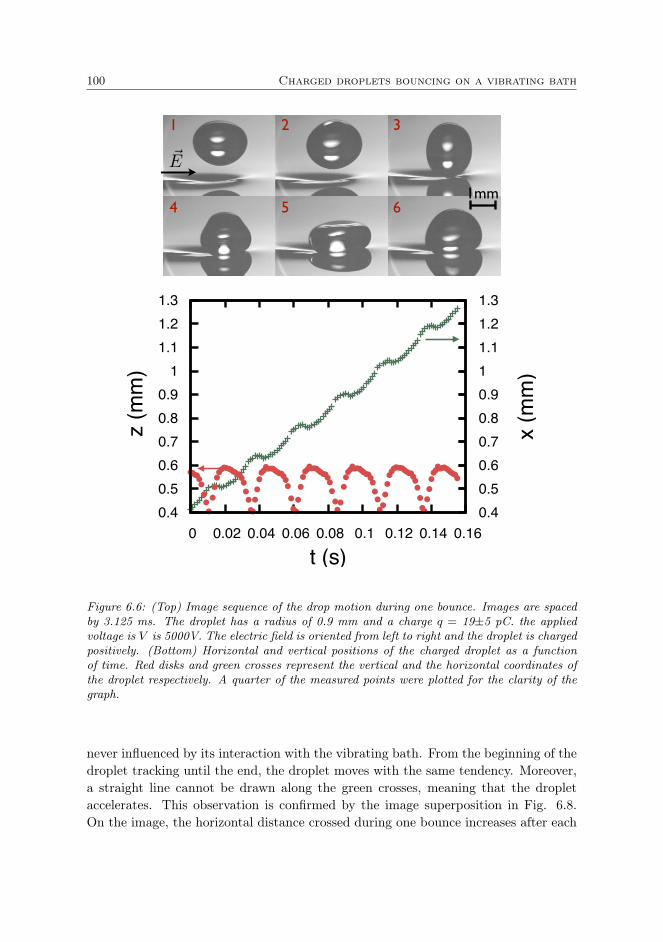
100 Charged droplets bouncing on a vibrating bath
1 2 3
4 5 6
~E
1mm
0.4 0.5 0.6 0.7 0.8 0.9
1 1.1 1.2 1.3
0 0.02 0.04 0.06 0.08 0.1 0.12 0.14 0.16 0.4 0.5 0.6 0.7 0.8 0.9 1 1.1 1.2 1.3
z (m
m)
x (m
m)
t (s)
Figure 6.6: (Top) Image sequence of the drop motion during one bounce. Images are spacedby 3.125 ms. The droplet has a radius of 0.9 mm and a charge q = 19±5 pC. the appliedvoltage is V is 5000V. The electric field is oriented from left to right and the droplet is chargedpositively. (Bottom) Horizontal and vertical positions of the charged droplet as a functionof time. Red disks and green crosses represent the vertical and the horizontal coordinates ofthe droplet respectively. A quarter of the measured points were plotted for the clarity of thegraph.
never influenced by its interaction with the vibrating bath. From the beginning of thedroplet tracking until the end, the droplet moves with the same tendency. Moreover,a straight line cannot be drawn along the green crosses, meaning that the dropletaccelerates. This observation is confirmed by the image superposition in Fig. 6.8.On the image, the horizontal distance crossed during one bounce increases after each
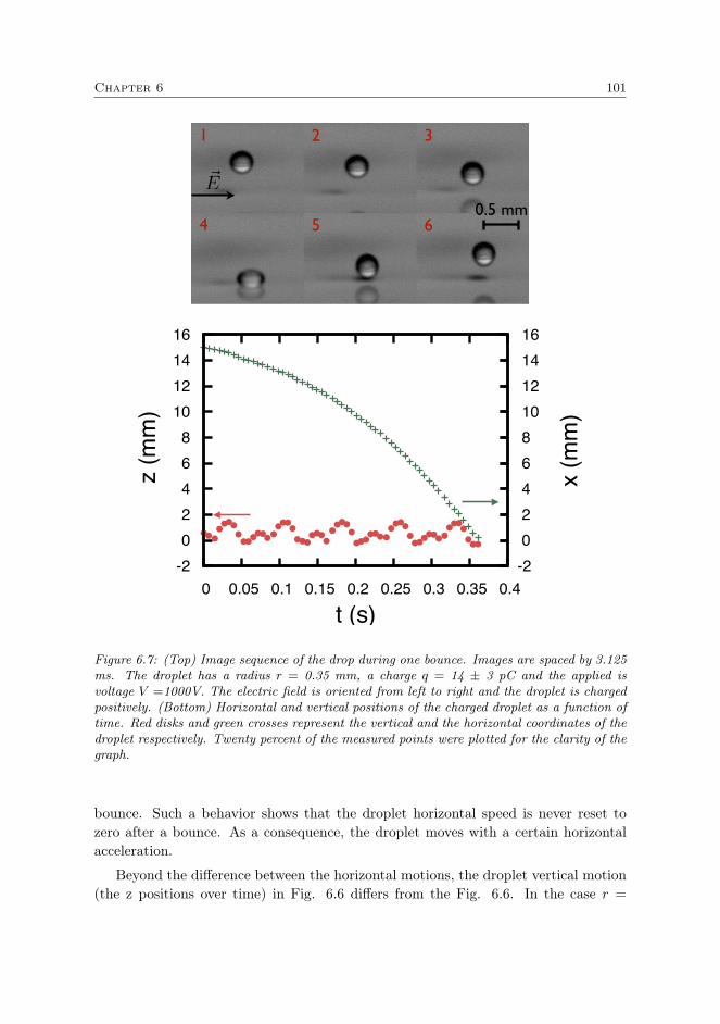
Chapter 6 101
~E
1 2 3
4 5 60.5 mm
-2 0 2 4 6 8
10 12 14 16
0 0.05 0.1 0.15 0.2 0.25 0.3 0.35 0.4-2 0 2 4 6 8 10 12 14 16
z (m
m)
x (m
m)
t (s)
Figure 6.7: (Top) Image sequence of the drop during one bounce. Images are spaced by 3.125ms. The droplet has a radius r = 0.35 mm, a charge q = 14 ± 3 pC and the applied isvoltage V =1000V. The electric field is oriented from left to right and the droplet is chargedpositively. (Bottom) Horizontal and vertical positions of the charged droplet as a function oftime. Red disks and green crosses represent the vertical and the horizontal coordinates of thedroplet respectively. Twenty percent of the measured points were plotted for the clarity of thegraph.
bounce. Such a behavior shows that the droplet horizontal speed is never reset tozero after a bounce. As a consequence, the droplet moves with a certain horizontalacceleration.
Beyond the difference between the horizontal motions, the droplet vertical motion(the z positions over time) in Fig. 6.6 differs from the Fig. 6.6. In the case r =
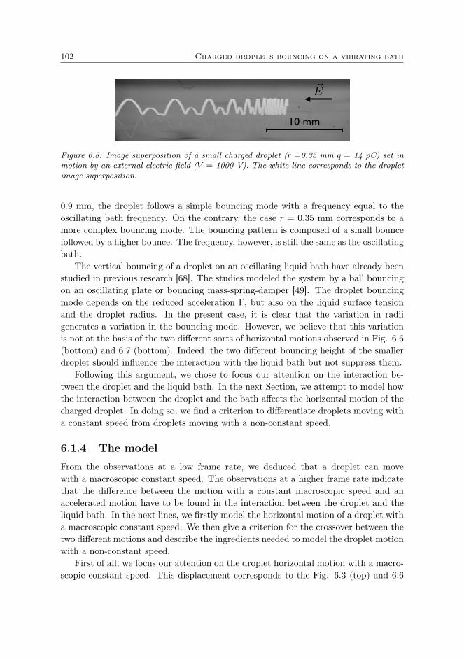
102 Charged droplets bouncing on a vibrating bath
10 mm
~E
Figure 6.8: Image superposition of a small charged droplet (r =0.35 mm q = 14 pC) set inmotion by an external electric field (V = 1000 V). The white line corresponds to the dropletimage superposition.
0.9 mm, the droplet follows a simple bouncing mode with a frequency equal to theoscillating bath frequency. On the contrary, the case r = 0.35 mm corresponds to amore complex bouncing mode. The bouncing pattern is composed of a small bouncefollowed by a higher bounce. The frequency, however, is still the same as the oscillatingbath.
The vertical bouncing of a droplet on an oscillating liquid bath have already beenstudied in previous research [68]. The studies modeled the system by a ball bouncingon an oscillating plate or bouncing mass-spring-damper [49]. The droplet bouncingmode depends on the reduced acceleration Γ, but also on the liquid surface tensionand the droplet radius. In the present case, it is clear that the variation in radiigenerates a variation in the bouncing mode. However, we believe that this variationis not at the basis of the two different sorts of horizontal motions observed in Fig. 6.6(bottom) and 6.7 (bottom). Indeed, the two different bouncing height of the smallerdroplet should influence the interaction with the liquid bath but not suppress them.
Following this argument, we chose to focus our attention on the interaction be-tween the droplet and the liquid bath. In the next Section, we attempt to model howthe interaction between the droplet and the bath affects the horizontal motion of thecharged droplet. In doing so, we find a criterion to differentiate droplets moving witha constant speed from droplets moving with a non-constant speed.
6.1.4 The model
From the observations at a low frame rate, we deduced that a droplet can movewith a macroscopic constant speed. The observations at a higher frame rate indicatethat the difference between the motion with a constant macroscopic speed and anaccelerated motion have to be found in the interaction between the droplet and theliquid bath. In the next lines, we firstly model the horizontal motion of a droplet witha macroscopic constant speed. We then give a criterion for the crossover between thetwo different motions and describe the ingredients needed to model the droplet motionwith a non-constant speed.
First of all, we focus our attention on the droplet horizontal motion with a macro-scopic constant speed. This displacement corresponds to the Fig. 6.3 (top) and 6.6
Chapter 6 103
(bottom). We deduced from our measurements that the macroscopic observation ofa constant speed corresponds to a periodic horizontal motion with a reset to a zerospeed at each period. The Fig. 6.9 shows the droplet horizontal position (x) as afunction of the time multiplied by the angular frequency of the vibrating bath (ωt).The graph is a zoom on two horizontal periodic motions of a charged droplet (r = 0.9
mm and 19±5 pC). For the clearness of the graph, the green crosses correspond tothe average horizontal position of the droplet calculated from ten bounces. The Fig.6.9 highlights the previous observation performed with the high-speed camera (seeFig. 6.6):
1. The droplet interacts with the bath (step I). During its interaction with theliquid bath, the droplet speed is quickly decreased to zero. The step I is locatedin the grey area of Fig. 6.9.
2. The droplet is in flight (step II). It is submitted to the electric force and there-fore, it is accelerated in the horizontal plane.
As a result of the step I and step II the droplet experiences a go-stop motion. InFig. 6.9, the times τb and τf corresponds respectively to the time during which thedroplet deforms the liquid bath and the time during which the droplet is away fromthe liquid bath (i.e. the charged droplet is “in flight"). The total time τ correspondsto the duration of one horizontal periodic motion. Because the droplet bounces withthe same frequency as the vibrating bath, we have τ = 1/f .
The characteristic times τb and τf can be estimated by looking at the bouncingmode of the charged droplet. As a first approximation, a bouncing droplet can bemodeled by a linear spring [98,99]. Thanks to this hypothesis, the interaction time τbduring the impact with the bath is constant and scales with the Rayleigh period [100]of vibration of a droplet, namely τb =
√3πm/8γd where m is the mass of the droplet
and γd the air-oil droplet surface tension. The deduced interaction time is τb ∼12ms. As observed previously, the droplet bounces with a frequency equal to the bathoscillation frequency, i.e 40 Hz. As a consequence, the flying time τf can be deducedfrom the equation τf = τ − τb.
During the interaction time, we observed that the droplet horizontal motion isvery quickly annihilated. In other words, the horizontal droplet speed is equal to zeroduring the contact time. As soon as the droplet takes off, the electric field exertsa force on the droplet due to the excess of charges carried by the droplet. In firstapproximation, the horizontal motion can be described by considering a point chargesubmitted to the electric force generated by the homogeneous electric field E = V/L.In this case, the point charge follows the simple law:
x(t) =act
2
2=qE
2mt2 =
3qV
8ρπr3Lt2 (6.2)
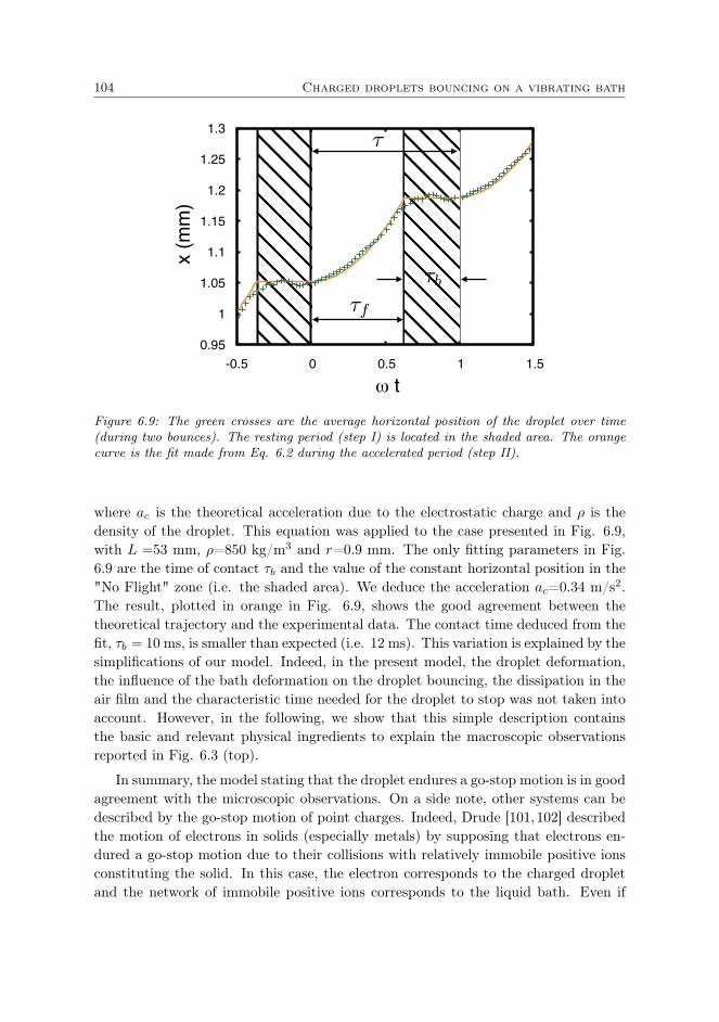
104 Charged droplets bouncing on a vibrating bath
0.95
1
1.05
1.1
1.15
1.2
1.25
1.3
-0.5 0 0.5 1 1.5
x (m
m)
ω t
f
b
Figure 6.9: The green crosses are the average horizontal position of the droplet over time(during two bounces). The resting period (step I) is located in the shaded area. The orangecurve is the fit made from Eq. 6.2 during the accelerated period (step II).
where ac is the theoretical acceleration due to the electrostatic charge and ρ is thedensity of the droplet. This equation was applied to the case presented in Fig. 6.9,with L =53 mm, ρ=850 kg/m3 and r=0.9 mm. The only fitting parameters in Fig.6.9 are the time of contact τb and the value of the constant horizontal position in the"No Flight" zone (i.e. the shaded area). We deduce the acceleration ac=0.34 m/s2.The result, plotted in orange in Fig. 6.9, shows the good agreement between thetheoretical trajectory and the experimental data. The contact time deduced from thefit, τb = 10 ms, is smaller than expected (i.e. 12 ms). This variation is explained by thesimplifications of our model. Indeed, in the present model, the droplet deformation,the influence of the bath deformation on the droplet bouncing, the dissipation in theair film and the characteristic time needed for the droplet to stop was not taken intoaccount. However, in the following, we show that this simple description containsthe basic and relevant physical ingredients to explain the macroscopic observationsreported in Fig. 6.3 (top).
In summary, the model stating that the droplet endures a go-stop motion is in goodagreement with the microscopic observations. On a side note, other systems can bedescribed by the go-stop motion of point charges. Indeed, Drude [101,102] describedthe motion of electrons in solids (especially metals) by supposing that electrons en-dured a go-stop motion due to their collisions with relatively immobile positive ionsconstituting the solid. In this case, the electron corresponds to the charged dropletand the network of immobile positive ions corresponds to the liquid bath. Even if
Chapter 6 105
the discovery of quantum mechanics showed that the Drude model is based on falsehypothesis, it provides a very good explanation of DC and AC conductivity in metals.
To confirm the validity of our approach, the model has to be confronted to themacroscopic behavior presented in Fig. 6.3 (bottom), 6.4 and 6.5. Because the dropspeed is reset to zero at each bounce, the memory of the previous jump is annihilated.This statement ensures that the horizontal motion is periodic and that the averagespeed is constant. This later is given by the sum of the distance covered during flighttime τf and during the interaction time τb divided by the period τ , namely:
〈v〉 =qV
2mL
τ2fτ
(6.3)
The flying time τf is deduced from the equation τf = τ − τb. As a consequence, theEq. 6.3 is written as:
〈v〉 =3qV
8πρr3L
(τ −
√π2ρr3/(2γd)
)2 1
τ(6.4)
The radius dependence can now be checked by comparing Eq. 6.4 and the averagespeed measurements in Fig. 6.4. The Eq. 6.4 was plotted in Fig. 6.4 by takingq = 14 pC, V = 1000 V, L = 53 mm, γd=0.017 N/m. The agreement between theexperimental data and the model is excellent.
The relation between the average speed 〈v〉 and the voltage V applied on theelectrodes is also captured by Eq. 6.4. Indeed, Eq. 6.4 predicts a linear dependenceof 〈v〉 with V , which is in agreement with the observations. The fit from Fig. 6.5(top) gives a slope of 0.36±0.02 µm/sV, which is in agreement, given the experimentalerror bars, with the slope computed from Eq. 6.4 (0.45±0.08 µm/sV).
Finally, we observed in Section 6.1.2 that the constant horizontal speed does notsignificantly vary with the reduced acceleration Γ. The physical parameter that wasvaried during the experiments was the oscillation amplitude. The bath oscillationfrequency was not varied. The non-dependence of the average speed with the oscilla-tion amplitude in Fig. 6.5 (bottom) is explained by the droplet bouncing mode. Thecharged droplet bounces with the same frequency as the bath oscillating frequency,independently of the bath oscillating amplitude. As a consequence, the total bounc-ing time τ does not vary with the bath oscillating amplitude. The flying time beingthe only parameter linked to the plate oscillation, it is clear that the average velocity(Eq. 6.4) should not depend on the bath oscillating amplitude. In other words, theEq. 6.4 also captures the horizontal speed non-dependence with the bath oscillatingamplitude.
A closer inspection of the Fig. 6.5 (bottom) shows, however, that the horizontaldroplet speed measured at Γ = 1.75 is lower than the other measurements. Thedisparity can be explained by a variation in the droplet bouncing mode. Indeed,for significant bath accelerations, the bouncing droplet can adopt different bouncing

106 Charged droplets bouncing on a vibrating bath
modes. Different bouncing modes can explain slight variations in the interaction timeτb and, by deduction, slight variations in the droplet horizontal speed.
As indicated by the variation of the second derivative a in Fig. 6.4, the approx-imation of a constant speed for the droplet is not valid for small droplets. In otherwords, small droplets are not stopped during their interaction with the bath. As aconsequence, a criterion on the droplet size has to be provided to set the domain ofvalidity of our model. When the droplet falls on the oil bath, the droplet slightlybends the liquid surface. The idea is to estimate the horizontal force (i.e. the electri-cal force in our case) necessary to extract the droplet out of this dimple. Indeed, ifthe electrostatic force exceeds the extraction force, the droplet is not stopped wheninteracting with the bath.
In order to describe the droplet-liquid bath interaction, we have to model the shapeadopted by the liquid bath. A basic model is to express the maximum depth of thebend in the liquid bath and suppose a linear growth toward the liquid surface. Themaximum depth of the deformation can be approximated by balancing the dropletkinetic energy and the energy necessary to deform the bath with a depth h:
2
3ρπr3v2i = γb2πrh (6.5)
where vi is the droplet speed just before interacting with the oil bath, γb the surfacetension of the oil bath and h is the depth of the deformation. The vertical speed vi isrelated to the flight time τf , i.e. vi = gτf/2 where τf = τ − τb. This equation leadsto a deformation of approximately 200 µm for a millimetric droplet. This order ofmagnitude is in agreement with the observation in Fig. 6.6 (top). In Fig 6.7 (top),we see that the bath deformation induced by the smaller bouncing droplet is far lesssignificant. The width of the bath deformation can be supposed as being equal to thedroplet radius r.
Let us consider that the droplet is on an incline plane when the droplet is at thebottom of the dimple. The problem is schematized in Fig. 6.10. The tangent of theslope tan(α) of the incline is given by the ratio h/R. The horizontal electric forceFe = qE is not able to extract the droplet when the projection along the paralleldirection of the incline of the electric force ~Fe,p is smaller than the projection of theweight of the droplet m~gp, namely:
qE cos(α) < mg sin(α) (6.6)
The inequality leads to the following criterion:
qE
hr2<
4
3πρg (6.7)
Equations (6.6) and (6.7) provide the conditions on r, E and q to observe aconstant speed motion of the droplet. In the present case, the radius r? below which
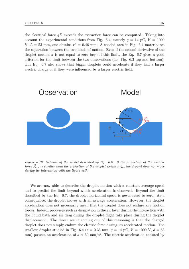
Chapter 6 107
the electrical force qE exceeds the extraction force can be computed. Taking intoaccount the experimental conditions from Fig. 6.4, namely q = 14 pC, V = 1000
V, L = 53 mm, one obtains r? = 0.46 mm. A shaded area in Fig. 6.4 materializesthe separation between the two kinds of motion. Even if the second derivative of thedroplet motion a is not equal to zero beyond this limit, the Eq. 6.7 gives a goodcriterion for the limit between the two observations (i.e. Fig. 6.3 top and bottom).The Eq. 6.7 also shows that bigger droplets could accelerate if they had a largerelectric charge or if they were influenced by a larger electric field.
Observation Model
~Fem~gp
m~gr
h ↵
~Fe,p
Figure 6.10: Schema of the model described by Eq. 6.6. If the projection of the electricforce ~Fe,p is smaller than the projection of the droplet weight m~gp, the droplet does not moveduring its interaction with the liquid bath.
We are now able to describe the droplet motion with a constant average speedand to predict the limit beyond which acceleration is observed. Beyond the limitdescribed by the Eq. 6.7, the droplet horizontal speed is never reset to zero. As aconsequence, the droplet moves with an average acceleration. However, the dropletacceleration does not necessarily mean that the droplet does not endure any frictionforces. Indeed, processes such as dissipation in the air layer during the interaction withthe liquid bath and air drag during the droplet flight take place during the dropletdisplacement. The direct result coming out of this reasoning is that the chargeddroplet does not simply endure the electric force during its accelerated motion. Thesmallest droplet studied in Fig. 6.4 (r = 0.35 mm, q = 14 pC, V = 1000 V, d = 53
mm) possess an acceleration of a ≈ 50 mm/s2. The electric acceleration endured by
108 Charged droplets bouncing on a vibrating bath
a point charge in the same electric field would be:
ae =3qE
ρ4πr3= 1.16 m/s2 (6.8)
As a consequence, the droplet interaction with the liquid bath still has to bemodeled to be able to fully describe the droplet motion. However, the establishmentof a model for the droplet motion faces two major problems. (i) The influence ofthe air layer on the droplet slow down is difficult to model. Indeed, there is noinformation on the dynamic thickness of the air layer. (ii) Experiments are moredifficult to perform because of the error on the acceleration measurements. Indeed, alarger liquid bath (L >53 mm) is needed in order to precisely measure an accelerationof the order of 100 mm/s2. This restriction comes with the difficulty to produce ahomogeneous electric field in a larger liquid bath.
6.1.5 futures investigations
In this Section, we take a brief look at further investigations that have been started.A first point concerns the use of a known charge and a known electric field to describean unknown interaction. In this particular case, the known droplet charge and electricfield allowed to describe the droplet motion. During the droplet motion, the mainunknown is the dynamic interaction between the droplet and the liquid bath. Such aninteraction could have been studied by moving the droplet via other applied forces. Forexample, it is possible to blow air on the droplet to generate the droplet displacement.However, the aerodynamic force is applied on the droplet surface and not on thedroplet bulk. Moreover, the aerodynamic force would be far more difficult to model.On the contrary, using a known electric force allows focusing the investigation onthe droplet interaction with the liquid bath. In the future, a complete model of thedynamic interaction between the droplet and the liquid bath could allow to deeplyunderstand the behavior of the air layer between the droplet and the liquid bath.
Beyond the fundamental understanding of the droplet/bath interaction, the sys-tem studied allows to remotely control the droplet motion on the two dimensions ofthe liquid bath. The droplet control can be put in evidence via a setup slightly differ-ent from the previous experiment. The image sequence in Fig. 6.11 presents the topview of the oscillating liquid bath. The bath is surrounded by four electrodes, mean-ing that an electric field can be applied on the droplet in both horizontal directions.Red lines indicate which electrode is switched on. Moreover, obstacles were placedin the liquid bath. They correspond to the white plastic pieces visible from the topview.
We were able to guide the electrically charged droplet around the obstacles bycontrolling the voltage V between electrodes. The Fig. 6.11 shows image sequence ofa charged droplet starting its motion on the bottom left of the liquid bath and endingits displacement on the top left of the liquid bath. The ability to precisely control

Chapter 6 109
1 2
3 4
+V +V
-V +V
1 cm
Figure 6.11: Top view of the 2D control of the charged droplet motion on the liquid bath. Redlines indicate which electrode is switched on. The positive or negative voltage is indicated bythe symbol ± V.
the charged droplet motion on the liquid bath could allow performing microfluidicmanipulations. As explained in the introduction (Section 2.3.2), the open microfluidicis booming. Open devices were demonstrated to be an interesting way to performthese different tasks especially for micro-chemical analysis purposes [39]. However,one of the remaining problems is the liquid alteration due to the contact with dirt onthe guiding surface. The bouncing droplet is a good answer to this kind of problem.Indeed, the bouncing droplet is only in contact with ambient air, which means thatdirt may only come from polluted surrounding air.
Moreover, the use of side electrodes in the previous experiments was due to theneed of a homogeneous electric field. However, such an electric field is not necessarilyneeded. As a consequence, submarine electrodes may be used to control the dropletmotion. Such a configuration is shown in Fig. 6.12. The submarine electrodes aredived in the liquid bath and connected to a voltage generator. An electric field canbe produced between them and generate droplet motion. Eventually, the final stepwould be to be able to tailor any electric potential landscape at the surface of thevibrating bath.

110 Charged droplets bouncing on a vibrating bath
The demonstration of the 2D electric control of the droplet motion on the os-cillating bath shows that it is possible to develop microfluidic system based on thistechnology. The study developed during this thesis showed that the system may beconfigured to move the droplet with a constant speed. Such a configuration allowsa precise manipulation of the electrically charged droplet. Of course, the technologystill needs to be developed before being able to perform specific lab-on-a-chip, or inthis case lab-on-a-bath, manipulations. We mainly need to study how to control theinteraction between two bouncing droplets.
A last restriction to the manipulation of droplets on a vibrating bath could be thenature of the droplet. Indeed, the stability of a droplet bouncing on a vibrating bathdepends on the liquid viscosity and surface tension. At this point, we can affirm thatliquids such as silicone oil and soapy water can be considered stable on the liquid bath.On the other side, other liquids such as ethanol and water can be considered usablebut with a lower stability. However, this limitation in the chemical composition of thedroplet could be overcome by encapsulating liquids in silicone oil droplets. Indeed,encapsulated liquids have been stored on vibrating bath with success [103].
Submarine electrodes
1 cm
Figure 6.12: Top view of the control of the charged droplet motion via submarine electrodes.Both electrodes are dived in the liquid bath and connected to a voltage generator. By control-ling the voltage between electrodes, an electric field can be applied on a bouncing droplet.
Finally, our discovery could play a key role in one of the most prolific studies onbouncing droplets: the walkers. Walkers are small droplets (r ≈ 0.5 mm) bouncingat half the forcing frequency on low viscous silicone oil (µ ≈ 20 cSt) near the Faradaythreshold of the oscillating liquid bath [64]. In this configuration, the droplet generateswaves when it bounces on the liquid bath. Furthermore, the bouncing droplet interacts
Chapter 6 111
with these waves. This interaction generates the self-propulsion of the droplet. Earlymeasurements have been made on charged walkers. The subject is tackled in thePerspectives (see Chapter 8).
In conclusion, we demonstrated that large droplets influenced by a weak electricforce move with a constant speed that is proportional to the charge and the voltage(see Eq. 6.3). The constant speed is due to the reset to zero of the droplet speedduring each oscillation. The droplet is accelerated in the air by the electricalforces and stopped during its interaction with the oscillating bath. Small dropletsinfluenced by a large electric force are not stopped during the contact period. Asa consequence, their horizontal motion is accelerated. A criterion was proposed toseparate both regimes (see Eq. 6.7). Moreover, first investigations showed that thedisplacement of a charged droplet on a vibrating bath could be useful for furtherdevelopments in microfluidics or in the study of walkers.
6.2 Interaction between two electrically charged dropletson a vibrating bath
In the Chapter focusing on droplets in microgravity (see Chapter 5), we studied theinteraction between two electrically charged droplets. Naturally, the interaction be-tween two charged droplets can also be studied via the vibrating bath setup. Thestudy is different from the experiment in microgravity because of the interaction be-tween the droplets and the vibrating bath. Moreover, in the last Section, we claimedthat the displacement generated by the electric field could be used for microfluidicsapplications. However, microfluidics rarely involves only one droplet. For example,the mixing between two small quantities of liquid requires two droplets. As a conse-quence, the interaction between two charged droplets bouncing on a vibrating bathshould be understood to perform these tasks. Questions about the influence of the at-traction or the repulsion between droplets on the droplet displacement or the dropletcoalescence need to be addressed.
The interaction between charged droplets is particularly decisive in the case oftwo droplets with the same sign of charges. Indeed, the repulsion between dropletscould prevent any contact between them. In the next lines, we focus our attention ontwo charged droplets with the same sign of charges interacting with each other whilebeing stored on a vibrating bath.
In order to store the droplet, we used a bath filed with silicone oil 1000 cSt. Thebath oscillated with a frequency f = 40 Hz and a reduced acceleration Γ = Aω2/g = 1.The charged droplets were created with the charged droplet generator model A. Thedroplets were composed of silicone oil 1.5 cSt with an addition of 1 % of ethanol. Weperformed experiments with three different droplet charges: neutral droplets (q=0),weakly charged droplets (q = 32 pC) and highly charged droplets (q = 44 pC).
112 Charged droplets bouncing on a vibrating bath
Cam
era
Oscillating plate , Af
+ +
Figure 6.13: Schema of the setup developed for the study of the interaction between twocharged droplets bouncing on a vibrating bath. Two droplets are released on the liquid bath.Their relative motion is then recorded over time by a camera located above the vibrating bath.
case 1 case 2 case 3
q (pC) 0 32 44r (mm) 1.0 0.8 0.8
Table 6.1: Charges and radii of the three configurations used to study the interaction betweencharged droplets bouncing on a vibrating bath.
As explained in the Section 3.1.2, the radius of charged droplets decreases with theelectric field applied by the charged droplet generator. The droplet charge and radiusof the three configurations are presented in Tab. 6.1. The experiment is schematizedin Fig.6.13. During one experiment, two droplets were dropped near each other onthe vibrating bath. A camera located at the top of the vibrating bath recorded thedroplets positions over time.
The motion over time for three typical experiments is reported in Fig. 6.14.The graphs show the x and y horizontal positions over time of both droplets on thevibrating bath. Both droplets were dropped on the vibrating bath at a time t0. Thefirst graph corresponds to neutral droplets (q = 0), the second graph correspondsto weakly charged droplets (q = 32 pC) and the third graph corresponds to highlycharged droplets (q = 44 pC). We observe in Fig. 6.14 that neutral droplets tend tomove closer to each other. In the case of charged droplets, the motion is more erratic.

Chapter 6 113
The erratic motion could be due to small external perturbations such as uncontrolledairflows. However, even if droplets seem to move erratically, they tend to stay at afixed distance from each other.
Beyond the horizontal motion of each droplet, we are interested in the motion ofone droplet compared to the other. In Fig. 6.15, we plotted the horizontal distancebetween droplets d over time. Each curve corresponds to one experiment. The firstgraph corresponds to neutral droplets (q=0), the second graph corresponds to weaklycharged droplets (q = 32 pC) and the third graph corresponds to highly chargeddroplets (q = 44 pC). As previously observed in Fig. 6.14, the graph displaying therelative distance between neutral droplets shows that droplets tend to move closerto each other over time. Moreover, the droplet displacement over time seems tobe suddenly accelerated around r ≈ 6 mm. The two following graphs show thatcharged droplets rapidly repel each other before remaining at an equilibrium distancede. Even if this equilibrium distance varies slightly over time, it fluctuates aroundthe same value over a very long period of time. The small variation in the relativedistance between droplets is the most likely due to the erratic motion of the droplets.By comparing the second and the third graph on the Fig 6.15, we observe that theequilibrium distance between droplets is slightly more important in the case of highlycharged droplets. The equilibrium distance de is respectively de ≈ 7 mm and de ≈ 9mm for the weakly and highly charged droplets.
In the following, we first examine the interaction between neutral droplets andthen study the interaction between charged droplets. Indeed, the attraction betweentwo neutral droplets observed in Fig. 6.14 and 6.15 should also exist for two chargeddroplets. As a consequence, charged droplets should repulse each other because oftheir charges and attract each other because of their bouncing. The attractive forcecan be isolated and measured by studying neutral droplets. Then, the attractive forcecan be compared to electric repulsion in the case of charged droplets.
The attractive force between two neutral droplets can be deduced by knowing thedroplet mass and calculating the second derivative of the relative distance d betweendroplets over time. The deduced attractive force is shown in Fig. 6.16. The force isplotted as a function of the relative distance between droplets d. We observe on thegraph that the attractive force increases when droplets move closer to each other untila critical distance. At a distance of approximately d =3.5 mm, the attractive forcedecreases with the distance decrease. For d < 3.2 mm, the force becomes repulsive.The maximum of the repulsive force, F = 40 nN, is located at d ≈ 2.5 mm, whichcorresponds approximately to two times the droplet radius. The maximum of theattractive force, F = 20 nN, is located at d = 3.5 mm.
The repulsive force between two neutral droplets close to each other can be ex-plained by direct interactions between droplets. Indeed, when droplets are close toeach other, we observe that droplets bounce on each other without coalescing. Thisis equivalent to the mechanism occurring for the droplet bouncing on the vibrating

114 Charged droplets bouncing on a vibrating bath
-28
-26
-24
-22
-20
-18
-16
18 20 22 24 26 28 30 32 34 36
y
(mm
)
x (mm)
-14
-12
-10
-8
-6
-4
-2
15 20 25 30 35 40
y
(mm
)
x (mm)
-27
-26
-25
-24
-23
-22
-21
-20
-19
16 18 20 22 24 26 28 30
y
(mm
)
x (mm)
= t0
= t0
= t0
Figure 6.14: Horizontal positions (x-y) over time for two droplets bouncing on the vibratingbath. The circles correspond to the time t0 at which both droplets were dropped on the bath.Each color corresponds to one droplet. The first graph corresponds to neutral droplets (case1), the second graph corresponds to weakly charged droplets (case 2) and the third graphcorresponds to highly charged droplets (case 3).

Chapter 6 115
0 2 4 6 8
10 12 14 16
0 200 400 600 800 1000
d
(mm
)
t (s)
0 2 4 6 8
10 12 14 16
0 200 400 600 800 1000 1200 1400
d
(mm
)
t (s)
0 5
10 15 20 25 30 35
0 200 400 600 800 1000 1200 1400
d
(mm
)
t (s)
Figure 6.15: Relative distance d between the two droplets bouncing on the vibrating bath overtime. The first graph corresponds to neutral droplets (case 1), the second graph correspondsto weakly charged droplets (case 2) and the third graph corresponds to highly charged droplets(case 3). Each color corresponds to one experiment. The black dashed lines correspond toguidelines of the equilibrium distance de.

116 Charged droplets bouncing on a vibrating bath
-20
-10
0
10
20
30
40
2 3 4 5 6 7 8
F
(nN
)
d (mm) Figure 6.16: Calculated force between two neutral droplets during their bouncing on thevibrating bath. The green disks correspond measurements from four different experiments.The force is deduced by taking the second derivative of the droplet relative displacement. Theorange dashed line corresponds to a guideline of the force between droplets.
bath. This bouncing between droplets corresponds to the repulsive force observed inFig. 6.16 between d = 2 mm and d = 3.2 mm. Both droplets being deformable, it isunderstandable that they bounce on each other at a distance larger than twice theirradius.
The attractive force between neutral droplets, observed for d > 3.2 mm, is moresurprising. Indeed, at this distance, droplets do not interact with each other by anyway. However, each droplet interacts with the vibrating bath. When the dropletbounces on the liquid bath composed of silicone oil 1000 cSt, the silicone oil is de-formed. This bath deformation is highlighted in Fig. 6.17 (top). We know fromNicolson [104] that two deformations at the surface of a liquid interact with eachother because of the liquid surface tension. The phenomenon is commonly calledCheerios effect and is schematized in Fig. 6.17 (bottom). A liquid interface alwaystends to reduce its surface. In order to do so, the two hollows generated by thebouncing droplets attract each other.
Naturally, the mechanism involved in this experiment is a bit more complex. In-deed, the droplet deforms the liquid bath during each bounce, which means that theattraction between both cavities evolves with the droplet motion itself. Furthermore,the droplet is not always interacting with the liquid bath, which means that the cap-illary attraction should not be applied permanently on the droplet. In order to modelthis behavior, we suppose that, at each bounce, the droplet resets the deformation ofthe liquid bath. In other words, when the droplet falls on the liquid bath, the liquid

Chapter 6 117
2 mm
~Fcap,1/2~Fcap,2/1
d
h
R
Figure 6.17: (top) Image of two neutral droplets bouncing near each other. In order tohighlight the bath deformation, the droplets bounced on an oscillating bath with a reducedacceleration Γ = 3.5. Both deformations in the liquid bath are attracted to each other dueto cheerios effect. (Bottom) Schema of two bath deformations attracted toward each other.The width and the depth of the deformation correspond respectively to R and h.

118 Charged droplets bouncing on a vibrating bath
-200
-150
-100
-50
0
50
100
3 4 5 6 7 8
F
(nN
)
d (mm) Figure 6.18: Recalculation of the attractive force between two droplets during their bouncingon the vibrating bath. The green disks correspond measurements from four different exper-iments. The attractive force is deduced by taking into account the time during which theattractive force is applied on the droplet. The maximum of the attractive force (F ≈ 100 nN)is observed at a distance d = 3.5 mm. The yellow curve corresponds to a fit by Eq. 6.9.
surface is deformed. Furthermore, during a time τb the bouncing droplet interactswith the liquid bath and both the droplet and the bath deformation endures the cap-illary force due to the Cheerios effect. Then, the droplet bounces away from the liquidbath and does not interact with the liquid bath during a time τf .
The direct consequence of this reasoning is that the attractive force observed inFig. 6.16 for d > 3.5 mm was underestimated. Therefore, it should be recalculated bytaking into account the correct time during which the force is applied on the droplet.Indeed, during the time of one bounce τ = τb + τf , the droplet is only subject tothe attractive force during a time τb. We showed in the previous Section (see Section6.1.4) that, for the present experimental conditions, τb = 10 ms and τf = 15 ms.Therefore, the droplet horizontally moves only during 40 % of one bounce. The newcalculation of the attractive force applied on the droplet is shown in Fig. 6.18. Themaximum of the attractive force (at a distance d = 3.5 mm) equals F ≈ 100 nN.This effective attractive force can be compared to capillary attraction between twodeformations in liquid surfaces. According to Kralchevsky et al [105], the capillaryattraction between two hollows of the same size can be expressed as:
Fcap =−2πγbQ
2
lcK1(
d
lc) (6.9)
where γb = 21 mN/m is the surface tension of the vibrating bath, Q is a geometric

Chapter 6 119
factor describing the hollow, lc =√γb/ρbg is the capillary length, ρb = 971 kg/m3
is the bath density, K1 is the modified Bessel function of the first order and d is thedistance between the center of both hollows. The geometric factor Q can be deducedby knowing the deformation depth h and width R of the hollow (see Fig. 6.17 (top)).
Q =h
K0(Rlc )(6.10)
Once the geometry of the hollow in the vibrating bath estimated, the capillary forcecan be deduced. In the previous section (see Section 6.1.4), we supposed that thewidth of the deformation was equal to the droplet radius R = r. Moreover, wecalculated the depth of the deformation by comparing the droplet kinetic energyand the liquid bath surface tension. We deduced that the bath deformation had adepth of approximately h = 200 µm. However, this deformation depth was possiblyoverestimated. Indeed, a smaller depth of h = 80 µm is in better agreement with thepresent observation. The capillary force calculated with h = 80 µm and R = r, isplotted as an orange line in Fig. 6.18. The Eq. 6.9 correctly reproduces the trend ofthe measurements in Fig. 6.18. Moreover, we observe in Fig. 6.18 that the attractiveforce rapidly increase around d ≈ 6 mm. It corresponds to the distance at whichdroplets move quickly to each other in Fig. 6.15.
Even if we were not able to measure the depth of the deformation h (see Fig.6.17), we can suppose that the correct depth is situated between h = 80 µm and h =
200 µm. Indeed, on one side, the comparison between the kinetic energy and the bathsurface tension did not take into account the droplet deformation, which led to anoverestimation of the depth h. On the other side, the bath deformation dynamicallyevolves with the droplet bouncing, which is not taken into account by the presentmodel. However, beyond the exact value of the hollow depth, the agreement betweenthe model and the measurements shows that the Cheerios effect correctly describesthe attraction between two neutral droplets bouncing on a liquid bath.
Once the attractive force between bouncing droplets described, we can add theelectric interaction between two charged droplets to our study of the phenomenon.As shown in Section 5.3 the electric force between two charged droplets is expressedby:
Fel = Fc + Fdip
=qaqb
4πε0d2+
1
4πε0q2arb
(1
d3− r
(d2 − r2b )2
)+
1
4πε0q2bra
(1
d3− d
(d2 − r2a)2
)+
1
4πε0qaqbrarb
(1
d4+
1
(d2 − r2a − r2b )2− 1
(d2 − r2a)2− 1
(d2 − r2b )2
)(6.11)
where Fc = qaqb4πε0d2
corresponds to the Coulomb interaction and Fdip corresponds tothe dipolar forces. The charges qa = qb = q and the radii ra = rb = r correspond

120 Charged droplets bouncing on a vibrating bath
-1000
-500
0
500
1000
1500
2000
2500
3 4 5 6 7 8
F
(nN
)
d (mm) Figure 6.19: Comparison between the total electric force Fel(red dotted line), the Coulombforce Fc (green line) and the force due to dipole interactions Fdip (orange dashed line). Theelectric forces are calculated from Eq. 6.11.
to the electric charge and radii of each droplet and ε0 corresponds to the vacuumelectrical permittivity.
In the following lines, we focus our attention on the case of droplets weakly charged(i.e. case 2, q = 32 pC). The scalar value of Fel (red dotted line), Fc (green line) andFdip (orange dotted line) for q = 32 pC are plotted in Fig. 6.19. We observe that,even for small distances between droplets d, the influence of the dipolar forces remainslow. However, the comparison between the capillary force in Fig. 6.18 and the electricforces in Fig. 6.19 indicates that the electric interaction is about ten times greaterthan the capillary attraction. As a consequence, we decided to take into account theentire electric force (see Eq. 6.11) in the following reasoning.
Even if the electric repulsion is more important than the capillary attraction, theyare not applied in the same way on the charged droplet. During our description ofthe motion of a neutral droplet, we showed that the droplet motion could be modeledby the following events:
1. The droplet interacts with the liquid bath and moves horizontally due to thecapillary attraction.
2. The droplet does not interact with the liquid bath and does not horizontallymove.
The motion of a charged droplet on the vibrating bath can be sliced in the same way:
Chapter 6 121
↵
~Fcap
~v0
~Fel
~g
x()
b
f
t = 0
t =
x()
~v0,x,2
d
Figure 6.20: Schema of both charged droplets bouncing on the vibrating bath over time.During the time τb the droplet interacts with the liquid bath and moves because of the capillaryattraction Fcap between both bath deformations. Then, the droplet bounces away from theliquid bath during a time τf . During this time, the droplets initial speed v0,x,2 tends to movecloser both droplets, the electric repulsion Fel draws them away. If x(τ) = 0, both dropletsdid not horizontally move during their bounce.

122 Charged droplets bouncing on a vibrating bath
1. The droplet interacts with the liquid bath and moves horizontally due to thecapillary attraction.
2. The droplet does not interact with the liquid bath and moves horizontally dueto the electric repulsion.
In the same way as the previous Section (see Section 6.1.4), we should be ableto explain macroscopic observations by modeling the microscopic displacement ofthe droplet (i.e. the droplet displacement during one bounce). In particular, theobserved equilibrium distance between droplets de should correspond to a horizontaldisplacement equals to zero during one bounce. In other words, if x describes thedroplet horizontal displacement and τ the time of one bounce, we should have:
x(τ) = 0 (6.12)
If we suppose that the droplet displacement during one bounce is very small com-pared to the distance between droplets, we can express the droplet motion as:
x(τ) = v0,x,1τb +Fcap2m
τ2b + v0,x,2τf +Fel2m
τ2f (6.13)
where m is the droplet mass, v0,x,1 is the droplet initial horizontal speed when thedroplet interacts with the liquid bath and v0,x,2 is the droplet initial horizontal speedwhen the droplet bounces away from the vibrating bath. The Eq. 6.13 corresponds tothe mathematical description of the two steps of the droplet horizontal motion. Thedisplacement of both charged droplets during one bounce is schematized in Fig. 6.20.
During the first step, the droplet interacts with the liquid bath. We showed inSection 6.1.4 that for Fel < 4
3πρghr2, the electric force is not important enough to
deform the vibrating bath. Thus, the droplet is subject to a go-stop motion duringits displacement. In the present configuration, this criterion is verified for dropletsseparated with a distance d ≈ 3 mm. Therefore, we can suppose that the droplethorizontal speed is reset to zero at the beginning of its interaction with the liquidbath. This reasoning leads to v0,x,1 = 0. As a consequence, when the charged dropletinteracts with the vibrating bath, it only endures the capillary attraction betweenboth bath deformations. If the droplet interacts with the vibrating bath during atime τb, we have: x(τb) =
Fcap
2m τ2b .After its interaction with the liquid bath, the droplet bounces away from the liquid
bath and does not interact with the liquid bath during a time τf . During this timethe droplet displacement is also governed by its initial speed and the forces appliedon the droplet. The only horizontal force applied on the droplet being the electricinteraction between both droplets, we have x(τf ) = v0,x,2τf + Fel
2m τ2f .
Combining both motions leads to a total displacement x(τ). If x(τ) = 0, thedroplet does not move during one bounce, which means that both droplets remain atan equilibrium distance. The key factor in the Eq. 6.13 is the droplet initial horizontal
Chapter 6 123
speed v0,x,2. This initial speed is composed of two terms, v0,x,2 = v0,x,2,a + v0,x,2,b.The first term v0,x,2,a corresponds to the horizontal speed acquired by the dropletduring its interaction with the liquid bath:
v0,x,2,a =Fcmτb (6.14)
The second term v0,x,2,b corresponds to the influence of the vibrating bath on thedroplet initial speed. Indeed, because the droplet is influenced by the electric force,it bounces on the side of the bath deformation. As a consequence, we can supposethat the droplet does not bounce on a horizontal plane, but on the slope of the bathdeformation. Therefore, the droplet bouncing generates an initial horizontal speed.While this term can be considered as negligible in other configurations such as the onein Section 6.1.4, the small forces involved in this study make this term non-negligible.The droplet initial speed when it leaves the vibrating bath can be calculated in thesame way as in the previous Section (see Section 6.1.4) and projected on the horizontalaxis by considering the slope of the bath deformation:
v0,x,2,b =−gτf
2sin(α) (6.15)
where gτf/2 is the initial speed of the droplet and α ≈ h/r is the average angle ofthe liquid bath deformation (see Fig. 6.20).
The distance crossed by the droplet during one bounce x(τ) is plotted as a functionof the distance between both droplets d in Fig. 6.21. The orange curve corresponds tothe weakly charged droplet (q = 32 pC). The positive value of x(τ) indicates that twodroplets close to each other tend to move away from each other. When the distancebetween droplets increases, the distance crossed by one droplet during one bouncedecreases. For d = 12 mm, the distance crossed by one droplet becomes negative.Such a behavior indicates that both droplets invert their motion and tend to movecloser to each other. As a consequence, the distance d = 12 mm can be considered asan equilibrium distance between droplets de. If droplets are artificially moved closerto each other, they tend to separate away. On the contrary, if both droplets aremoved away from this equilibrium distance, they tend to move closer to each other.In practice, we observed such an equilibrium distance at de ≈ 7 mm. We deducefrom the comparison between the model and the experiment that the model correctlypredicts the droplet behavior, even if it overestimates the equilibrium distance de.Note that the case of highly charged droplets (case 3, q = 44 pC) shows the sameoverestimation of the model compared to the experiment. Indeed, we observed anequilibrium distance de ≈ 9 mm, while the model predicts an equilibrium distancede = 17 mm.
Once the droplets reach an equilibrium distance de, they remain more or less atthe same equilibrium distance for several minutes. We showed in Section 4.2 that abouncing droplet slowly loses its charge over time. Therefore, the electric repulsion
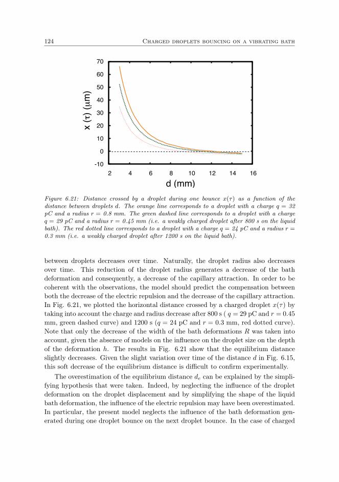
124 Charged droplets bouncing on a vibrating bath
-10
0
10
20
30
40
50
60
70
2 4 6 8 10 12 14 16
x
(τ) (µ
m)
d (mm) Figure 6.21: Distance crossed by a droplet during one bounce x(τ) as a function of thedistance between droplets d. The orange line corresponds to a droplet with a charge q = 32pC and a radius r = 0.8 mm. The green dashed line corresponds to a droplet with a chargeq = 29 pC and a radius r = 0.45 mm (i.e. a weakly charged droplet after 800 s on the liquidbath). The red dotted line corresponds to a droplet with a charge q = 24 pC and a radius r =0.3 mm (i.e. a weakly charged droplet after 1200 s on the liquid bath).
between droplets decreases over time. Naturally, the droplet radius also decreasesover time. This reduction of the droplet radius generates a decrease of the bathdeformation and consequently, a decrease of the capillary attraction. In order to becoherent with the observations, the model should predict the compensation betweenboth the decrease of the electric repulsion and the decrease of the capillary attraction.In Fig. 6.21, we plotted the horizontal distance crossed by a charged droplet x(τ) bytaking into account the charge and radius decrease after 800 s ( q = 29 pC and r = 0.45mm, green dashed curve) and 1200 s (q = 24 pC and r = 0.3 mm, red dotted curve).Note that only the decrease of the width of the bath deformations R was taken intoaccount, given the absence of models on the influence on the droplet size on the depthof the deformation h. The results in Fig. 6.21 show that the equilibrium distanceslightly decreases. Given the slight variation over time of the distance d in Fig. 6.15,this soft decrease of the equilibrium distance is difficult to confirm experimentally.
The overestimation of the equilibrium distance de can be explained by the simpli-fying hypothesis that were taken. Indeed, by neglecting the influence of the dropletdeformation on the droplet displacement and by simplifying the shape of the liquidbath deformation, the influence of the electric repulsion may have been overestimated.In particular, the present model neglects the influence of the bath deformation gen-erated during one droplet bounce on the next droplet bounce. In the case of charged
Chapter 6 125
droplets influenced by an external homogeneous electric field (see Section 6.1.4), thosehypothesis were justified by the importance of the forces involved. Indeed, the chargeddroplets were influenced by an external electric force Fel ≈ 10−5 N that generateda horizontal displacement during one bounce of x(τ) ≈ 0.02 mm. On the contrary,in the case of the interaction between two charged droplets, the applied forces anddistances crossed are several orders of magnitude smaller (see Fig. 6.18 and 6.19). Asa consequence, these simplifying hypothesis are less and less valid.
Given the number of hypothesis taken, this model should be treated cautiously. Inorder to confirm the present model, a precise description of the droplet motion duringone bounce is needed. This could be achieved by imaging the droplet motion via ahigh-speed camera, in the same way as the microscopic observations in Section 6.1.3.Moreover, a precise description of the bath deformation would allow understandingin a deeper way the influence of the droplet-bath interaction on the droplet motion.Methods aiming at the characterization of liquid surface [106] could be used to achievethis goal.
In conclusion, we studied the interaction between two droplets bouncing ona vibrating bath. In the case of neutral droplets, both droplets are attractedtoward each other. We deduced the attractive force between droplets from themeasurement of the droplets position over time. The force was successfully mod-eled by supposing that the liquid bath deformation generates capillary attractionbetween droplets. In the case of two positively charged droplets, we observed thatboth droplets separate away until remaining at an equilibrium distance de. Eventhough the capillary force was found to be several orders of magnitude smallerthan the electric repulsion, the model of the droplet motion during one bounceallowed explaining the presence of an equilibrium distance between droplets.


7Electric charges influence on the Leidenfrost
state
Contents7.1 Surface energy of a charged droplet in Leidenfrost state 128
7.2 Charged droplets in Leidenfrost state: Early coalescence 132
In this Chapter, we investigate the influence of electric charges on the Leidenfrosteffect. Previous studies examined the influence of electric interactions on Leidenfrostdrops levitating on heated solids [71]. We focus our attention on droplets in Leiden-frost state on a heated liquid pool. The experimental setup was described in Section3.3.3.
In Section 4.3, we showed that electric charges decrease the surface energy of adroplet. In the first Section of this Chapter (see Section 7.1), we examine the influenceof the surface energy decrease on the Leidenfrost droplet behavior. In particular, westudy the shape of the droplet and the shape of the liquid bath as a function of thecharge induced in the droplet.
In the second Section (see Section 7.2), we study the influence of electric chargeson the stability of a Leidenfrost droplet on a liquid pool. We show that Leidenfrostdroplets coalesce with the liquid pool at a given radius. Then, we attempt to modelthe critical radius leading to the extinction of the Leidenfrost effect as a function ofthe charge induced in the droplet.

128 Electric charges influence on the Leidenfrost state
7.1 Surface energy of a charged droplet in Leiden-frost state
As showed in Section 4.3, the surface energy γ∗ of a charged droplet can be expressedas:
γ∗ = γ − q2σr
4ε0(7.1)
where γ is the droplet surface tension, qσ is the droplet surface charge density, r isthe droplet radius and ε0 is the vacuum permittivity. In this Section, we show thatthis decrease in the surface energy influences the shape of a Leidenfrost droplet ona liquid pool and, as a consequence, the deformation induced by the droplet on theliquid pool.
12
1/10001/1001/10
γd/γp :
5011/1.95
ρp/ρd :
(a)
(b)
z
r
z
r
ρp/ρd = 1.20
γd/γp = 0.87
x
y
Figure 7.1: Study by Maquet et al [76] on the influence of the ratio of surface tensions γd/γpon Leidenfrost shapes. The droplet radius r = 3 and the density ration ρp/ρd = 1.2 are keptconstant.
The Leidenfrost effect on a heated liquid bath has been previously studied byMaquet et al [76]. Among other things, they demonstrated that the droplet shape,while levitating on the liquid bath, depends on the droplet radius and surface energy.In the same way, they showed that deformation of the liquid pool due to the levitatingdroplet also depends on the droplet surface tension. Their theoretical study is shownin Fig. 7.1. The droplet and liquid pool shape are plotted as a function of thenon-dimensional coordinates y and x. Both coordinates are non-dimensionalized bythe capillary length lc =
√γ/ρg. They showed that for different ratios between the
droplet surface tension γ and the liquid pool surface tension γp, the shape of the

Chapter 7 129
0.5 mm
Figure 7.2: Image of the liquid pool deformation induced by the charged droplet. The dropletcharge is q= 73 pC. The pool is at Tp = 100 C while the boiling point of ethanol is Tsat =78 C. The maximum deformation depth corresponds to approximately 0.25 mm.
droplet and the shape of the liquid pool varies. The droplet radius r = 3 and thedensity ratio ρp/ρd = 1.2 were kept constant. We see in Fig. 7.1 that an increase inthe surface tension ratio deepens the liquid pool deformation. On the opposite, thecase of a very small surface tension ratio is similar to the case of a Leidenfrost dropleton a solid surface.
In order to compare the theory to measurements, we looked at the shape of theliquid surface as a function of the droplet electric charge. A typical image of thepool deformation due to the levitating droplet is shown in Fig. 7.2. The image is aside view of the droplet took under the surface of the liquid pool. The symmetry ofthe image is explained by the reflection of the deformation on each side of the liquidsurface. Note that the influence of the charge on the droplet shape was not studied.This is explained by the difficulty to precisely measure the droplet shape while it islevitating on a liquid pool.
During the experiments we used a liquid bath composed of silicone oil 100 cStheated at Tp = 100 C and charged droplets composed of ethanol. The boiling pointof ethanol is Tsat = 78 C, which means that the droplet was in Leidenfrost statewhen levitating on the pool. The temperature of the liquid pool was tracked thanksto a thermocouple positioned at the surface of the liquid pool. The charged dropletgenerator model A was used to charge droplets. The experiment was carried outwith three different configurations: neutral droplets (q = 0 pC) and charged droplets(q =73.0 pC or q =110.7 pC). The shape of the liquid surface was obtained by usinga high-speed camera (Phantom MIRO 310). The use of a high-speed camera wasjustified by the need of capturing a focused image of droplets freely moving at thesurface of the heated liquid bath.
As explained in Section 3.1.2, the charged droplet generator influences the volumeof the generated droplet. As a consequence, the droplet radius decreases with the
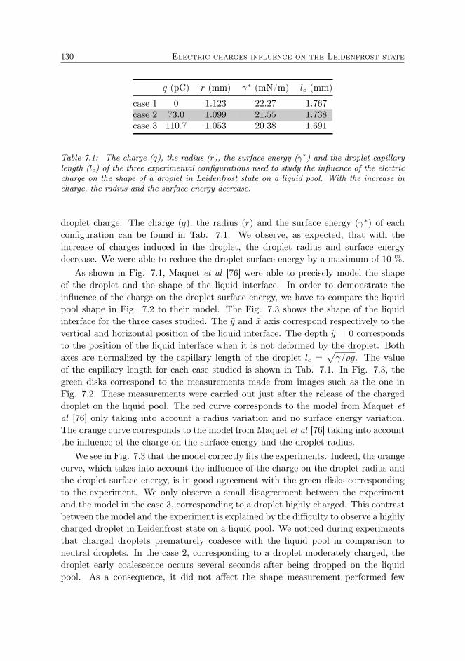
130 Electric charges influence on the Leidenfrost state
q (pC) r (mm) γ∗ (mN/m) lc (mm)
case 1 0 1.123 22.27 1.767case 2 73.0 1.099 21.55 1.738case 3 110.7 1.053 20.38 1.691
Table 7.1: The charge (q), the radius (r), the surface energy (γ∗) and the droplet capillarylength (lc) of the three experimental configurations used to study the influence of the electriccharge on the shape of a droplet in Leidenfrost state on a liquid pool. With the increase incharge, the radius and the surface energy decrease.
droplet charge. The charge (q), the radius (r) and the surface energy (γ∗) of eachconfiguration can be found in Tab. 7.1. We observe, as expected, that with theincrease of charges induced in the droplet, the droplet radius and surface energydecrease. We were able to reduce the droplet surface energy by a maximum of 10 %.
As shown in Fig. 7.1, Maquet et al [76] were able to precisely model the shapeof the droplet and the shape of the liquid interface. In order to demonstrate theinfluence of the charge on the droplet surface energy, we have to compare the liquidpool shape in Fig. 7.2 to their model. The Fig. 7.3 shows the shape of the liquidinterface for the three cases studied. The y and x axis correspond respectively to thevertical and horizontal position of the liquid interface. The depth y = 0 correspondsto the position of the liquid interface when it is not deformed by the droplet. Bothaxes are normalized by the capillary length of the droplet lc =
√γ/ρg. The value
of the capillary length for each case studied is shown in Tab. 7.1. In Fig. 7.3, thegreen disks correspond to the measurements made from images such as the one inFig. 7.2. These measurements were carried out just after the release of the chargeddroplet on the liquid pool. The red curve corresponds to the model from Maquet etal [76] only taking into account a radius variation and no surface energy variation.The orange curve corresponds to the model from Maquet et al [76] taking into accountthe influence of the charge on the surface energy and the droplet radius.
We see in Fig. 7.3 that the model correctly fits the experiments. Indeed, the orangecurve, which takes into account the influence of the charge on the droplet radius andthe droplet surface energy, is in good agreement with the green disks correspondingto the experiment. We only observe a small disagreement between the experimentand the model in the case 3, corresponding to a droplet highly charged. This contrastbetween the model and the experiment is explained by the difficulty to observe a highlycharged droplet in Leidenfrost state on a liquid pool. We noticed during experimentsthat charged droplets prematurely coalesce with the liquid pool in comparison toneutral droplets. In the case 2, corresponding to a droplet moderately charged, thedroplet early coalescence occurs several seconds after being dropped on the liquidpool. As a consequence, it did not affect the shape measurement performed few
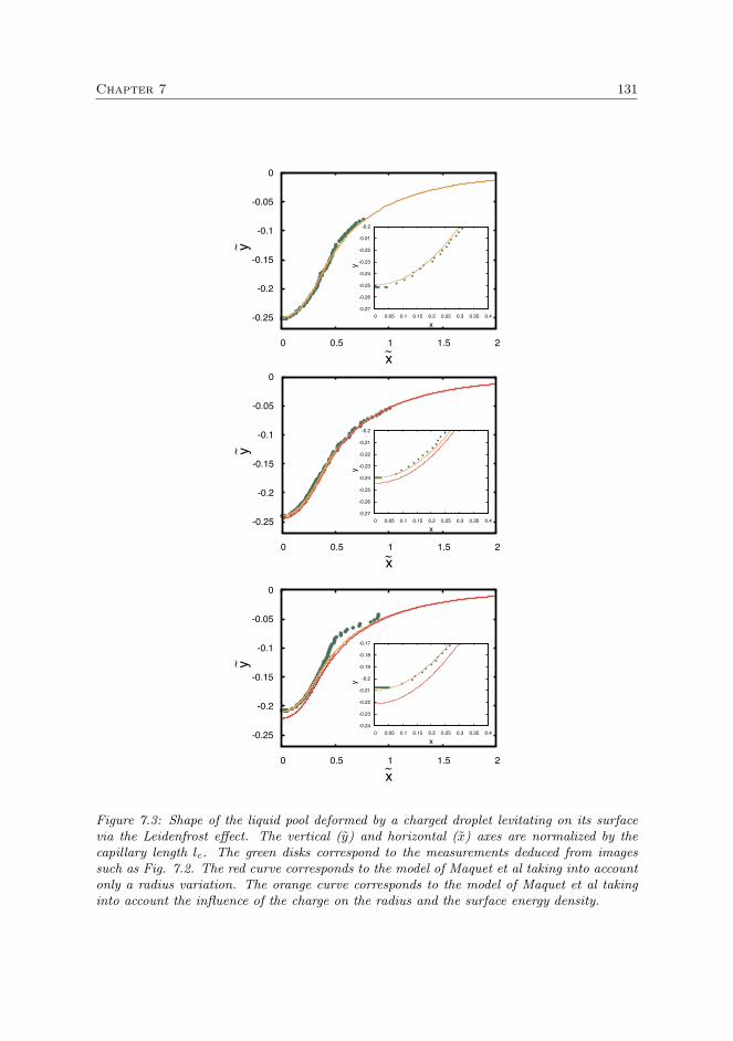
Chapter 7 131
-0.27
-0.26
-0.25
-0.24
-0.23
-0.22
-0.21
-0.2
0 0.05 0.1 0.15 0.2 0.25 0.3 0.35 0.4
y
x -0.25
-0.2
-0.15
-0.1
-0.05
0
0 0.5 1 1.5 2
y
x
-0.27
-0.26
-0.25
-0.24
-0.23
-0.22
-0.21
-0.2
0 0.05 0.1 0.15 0.2 0.25 0.3 0.35 0.4
y
x -0.25
-0.2
-0.15
-0.1
-0.05
0
0 0.5 1 1.5 2
y
x
-0.25
-0.2
-0.15
-0.1
-0.05
0
0 0.5 1 1.5 2
y
x
-0.24
-0.23
-0.22
-0.21
-0.2
-0.19
-0.18
-0.17
0 0.05 0.1 0.15 0.2 0.25 0.3 0.35 0.4
y
x
12
1/10001/1001/10
γd/γp :
5011/1.95
ρp/ρd :
(a)
(b)
z
r
z
r
ρp/ρd = 1.20
γd/γp = 0.87
1 21/1000
1/100
1/10
γd/γ
p:50 1 1/1.9
5
ρp/ρ
d:
(a)
(b)
z
r
z
r
ρp/ρ
d=
1.2
0
γd/γ
p=
0.8
7
12
1/10001/1001/10
γd/γp :
5011/1.95
ρp/ρd :
(a)
(b)
z
r
z
r
ρp/ρd = 1.20
γd/γp = 0.87
1 21/1000
1/100
1/10
γd/γ
p:50 1 1/1.9
5
ρp/ρ
d:
(a)
(b)
z
r
z
r
ρp/ρ
d=
1.2
0
γd/γ
p=
0.8
7
12
1/10001/1001/10
γd/γp :
5011/1.95
ρp/ρd :
(a)
(b)
z
r
z
r
ρp/ρd = 1.20
γd/γp = 0.87
1 21/1000
1/100
1/10
γd/γ
p:50 1 1/1.9
5
ρp/ρ
d:
(a)
(b)
z
r
z
r
ρp/ρ
d=
1.2
0
γd/γ
p=
0.8
7
Figure 7.3: Shape of the liquid pool deformed by a charged droplet levitating on its surfacevia the Leidenfrost effect. The vertical (y) and horizontal (x) axes are normalized by thecapillary length lc. The green disks correspond to the measurements deduced from imagessuch as Fig. 7.2. The red curve corresponds to the model of Maquet et al taking into accountonly a radius variation. The orange curve corresponds to the model of Maquet et al takinginto account the influence of the charge on the radius and the surface energy density.
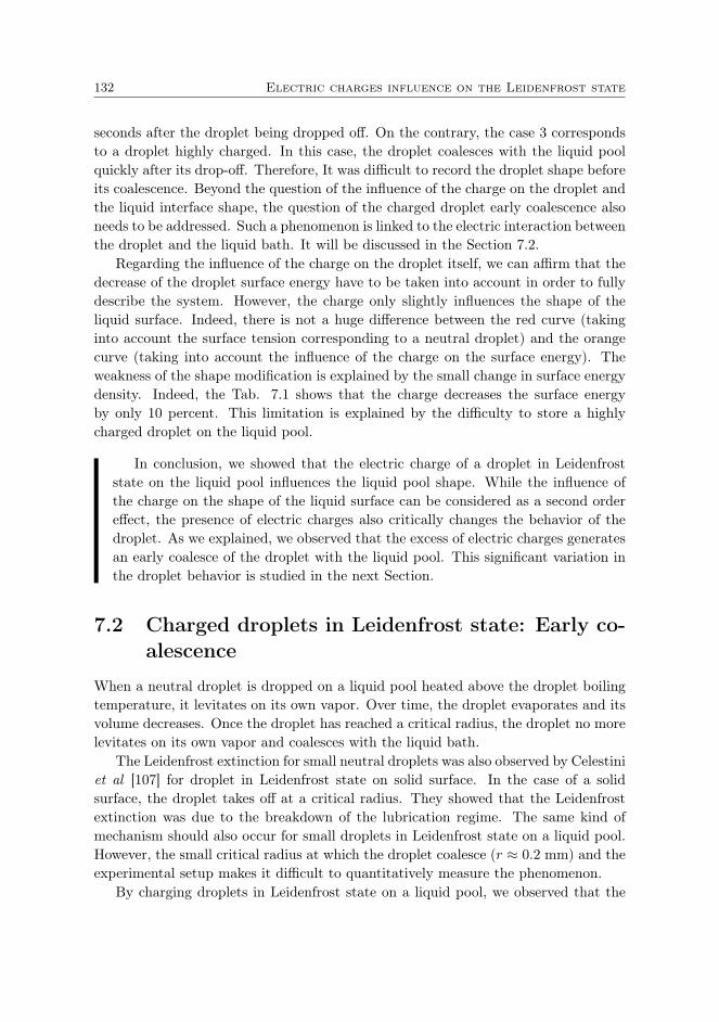
132 Electric charges influence on the Leidenfrost state
seconds after the droplet being dropped off. On the contrary, the case 3 correspondsto a droplet highly charged. In this case, the droplet coalesces with the liquid poolquickly after its drop-off. Therefore, It was difficult to record the droplet shape beforeits coalescence. Beyond the question of the influence of the charge on the droplet andthe liquid interface shape, the question of the charged droplet early coalescence alsoneeds to be addressed. Such a phenomenon is linked to the electric interaction betweenthe droplet and the liquid bath. It will be discussed in the Section 7.2.
Regarding the influence of the charge on the droplet itself, we can affirm that thedecrease of the droplet surface energy have to be taken into account in order to fullydescribe the system. However, the charge only slightly influences the shape of theliquid surface. Indeed, there is not a huge difference between the red curve (takinginto account the surface tension corresponding to a neutral droplet) and the orangecurve (taking into account the influence of the charge on the surface energy). Theweakness of the shape modification is explained by the small change in surface energydensity. Indeed, the Tab. 7.1 shows that the charge decreases the surface energyby only 10 percent. This limitation is explained by the difficulty to store a highlycharged droplet on the liquid pool.
In conclusion, we showed that the electric charge of a droplet in Leidenfroststate on the liquid pool influences the liquid pool shape. While the influence ofthe charge on the shape of the liquid surface can be considered as a second ordereffect, the presence of electric charges also critically changes the behavior of thedroplet. As we explained, we observed that the excess of electric charges generatesan early coalesce of the droplet with the liquid pool. This significant variation inthe droplet behavior is studied in the next Section.
7.2 Charged droplets in Leidenfrost state: Early co-alescence
When a neutral droplet is dropped on a liquid pool heated above the droplet boilingtemperature, it levitates on its own vapor. Over time, the droplet evaporates and itsvolume decreases. Once the droplet has reached a critical radius, the droplet no morelevitates on its own vapor and coalesces with the liquid bath.
The Leidenfrost extinction for small neutral droplets was also observed by Celestiniet al [107] for droplet in Leidenfrost state on solid surface. In the case of a solidsurface, the droplet takes off at a critical radius. They showed that the Leidenfrostextinction was due to the breakdown of the lubrication regime. The same kind ofmechanism should also occur for small droplets in Leidenfrost state on a liquid pool.However, the small critical radius at which the droplet coalesce (r ≈ 0.2 mm) and theexperimental setup makes it difficult to quantitatively measure the phenomenon.
By charging droplets in Leidenfrost state on a liquid pool, we observed that the
Chapter 7 133
critical radius rc at which the droplet coalesces with the liquid pool increases with theamount of charges induced in the droplet. In the next lines, we describe and attemptto model this observation. Our approach aims for two goals: (i) modeling the criticalradius as a function of the droplet charge rc(q) allows deducing precisely the criticalradius for a neutral droplet rc(q = 0). In other words, our approach allows studyingprecisely the underlying physics generating the Leidenfrost droplet extinction. (ii)Studying such a system give new insights on the influence of electric charges on thebehavior of thin layers.
The droplet coalescence with the liquid bath is shown on the image sequence inFig. 7.4. Images are separated by 3 ms. The charged droplet (q = 60 pC) composedof ethanol coalesces with the liquid bath at a critical radius rc = 9 mm. The liquidpool was composed of silicone oil 20 cSt and heated at a temperature Tp = 90 C.
1 2 3
4 5 6
3 mm
Figure 7.4: Image sequence of the coalescence of a charged droplet with the liquid pool. Theimages are separated by 3 ms. The droplet is composed of ethanol and has a charge of q =60 pC. The liquid pool is heated at 90 C.
In order to quantitatively describe the phenomenon, we studied the critical radiusrc at which the droplet coalesces with the liquid bath as a function of the charge in-duced in the droplet. Experiments were performed with droplets composed of ethanoland droplets composed of HFE. The ethanol and the HFE-7100 were chosen for theirability to easily levitate in Leidenfrost state and for their different properties. Indeed,the ethanol and the HFE-7100 possess quite different surface tensions, densities andthermal properties. Therefore, the influence of these parameters is highlighted. Con-trarily to the ethanol, the HFE-7100 is less commonly used. The diminutive HFEstands for Hydrofluoroether. It is a complex organic solvent commonly used as arefrigerant or heat-transfer fluid. The surface tension γ, density ρ and temperatureof boiling Tb are reported for both liquids in Tab. 7.2.
During the experiments, each charged droplet was generated by the charged droplet

134 Electric charges influence on the Leidenfrost state
γ (mN/m) ρ (kg/m3) Tb (C)
Ethanol 22.27 789 78HFE 13.6 1520 61
Table 7.2: Surface tension γ, density ρ and boiling temperature Tb of ethanol and HFE. TheHFE has a smaller surface tension than the ethanol, but a larger density.
generator model A. The droplet radius before its coalescence with the liquid bath wasmeasured thanks to a high-speed camera (Phantom Miro M-310). The initial dropletcharge was known by the calibration of the charged droplet generator via a Faradaycup. The liquid pool was composed of silicone oil 20 cSt. The temperature of theliquid pool was measured by using a thermocouple dived in the silicone oil and posi-tioned near the surface of the liquid pool. We performed three sets of experiments:(i) Ethanol droplets on a liquid pool at Tp = 90 C, (ii) Ethanol droplets on a liquidpool at Tp = 150 C and (iii) HFE droplets on a liquid pool at Tp = 100 C.
The result of the measurements is shown in Fig. 7.5. The graph shows the criticalradius rc at which a droplet coalesces with the liquid pool as a function of its initialcharge. The red crosses correspond to ethanol droplets in Leidenfrost state on a poolat a temperature Tp = 90 C. The orange triangles corresponds to ethanol droplets inLeidenfrost state on a pool at Tp = 150 C. The green disks corresponds to HFE-7100droplets in Leidenfrost state on a pool at Tp = 100 C. We observed that neutraldroplets coalesce with the liquid bath at a critical radius between 0.1 and 0.2 mm.Then, the critical radius of coalescence linearly increases with the charge induced inthe droplet. In the next lines, we attempt to model these observations.
In Fig. 7.4, the images were taken at the time when the droplet begins to coalescewith the liquid bath. The droplet destabilization begins at the bottom of the droplet.These images correspond to classic coalescence between a droplet and a liquid pool.From this observation, we conclude that the early coalescence of the charged dropletis due to the burst of the vapor layer between the droplet and the liquid pool. Twophenomena could explain the destabilization of the vapor layer, either the chargeddroplet destabilizes itself or the vapor layer becomes too thin to hold. These twoscenarios are examined in the next lines.
The first interpretation would correspond to a Coulomb explosion. As expressed inthe Section 2.2.1, the critical radius for a Coulomb explosion to occur, for a sphericaldroplet, corresponds to:
rc =
(q2
64π2γε0
)1/3
(7.2)
The equation indicates a non-linear dependence of the radius with the charge,which is in disagreement with the observations. However, a droplet in Leidenfroststate on the liquid bath is slightly flattened, which could affect Eq. 7.2. In order

Chapter 7 135
0
0.2
0.4
0.6
0.8
1
1.2
0 10 20 30 40 50 60 70 80
r
c (m
m)
Q (pC)
Figure 7.5: Critical radius at which a droplet coalesces with the liquid pool as a function ofthe droplet charge. The red crosses and orange triangles correspond to ethanol droplets on aliquid bath at a temperature of respectively Tp = 90 C and Tp = 150 C. The green diskscorrespond to HFE-7100 droplets on a liquid bath at temperature Tp = 100 C.
to force the linear dependence of the radius with the charge, we can perform a scaleanalysis of the system. If we suppose that the critical radius depends on the samevariables as expressed in Eq. 7.2, we have:
rc = ραgβεδ0γηq1 (7.3)
where α, β, δ and η are dimensionless numbers that need to be balanced in orderto respect the units of each parameter. By applying the well-known Buckingham π
theorem, we obtain:rc = (ρg)1/4ε
−1/20 γ−3/4q (7.4)
The Eq. 7.4 leads to a linear dependence between the charge and the radius. It alsoindicates that the critical radius decreases with the surface tension γ and increasewith the density ρ. However, it is not what is experimentally observed. Indeed, HFEhas a larger density and a smaller surface tension (see Tab. 7.2), which means thatthe slope of the HFE should be larger than the slope of the ethanol. In Fig. 7.5, theopposite is observed. As a consequence, the explanation of the early coalesce has tobe found somewhere else.
If the droplet does not destabilize, the disruption of the vapor layer between thedroplet and the liquid pool should be the reason why we observe the early coalescence.The vapor layer is schematized in Fig. 7.6. In the case of neutral droplet, the droplet
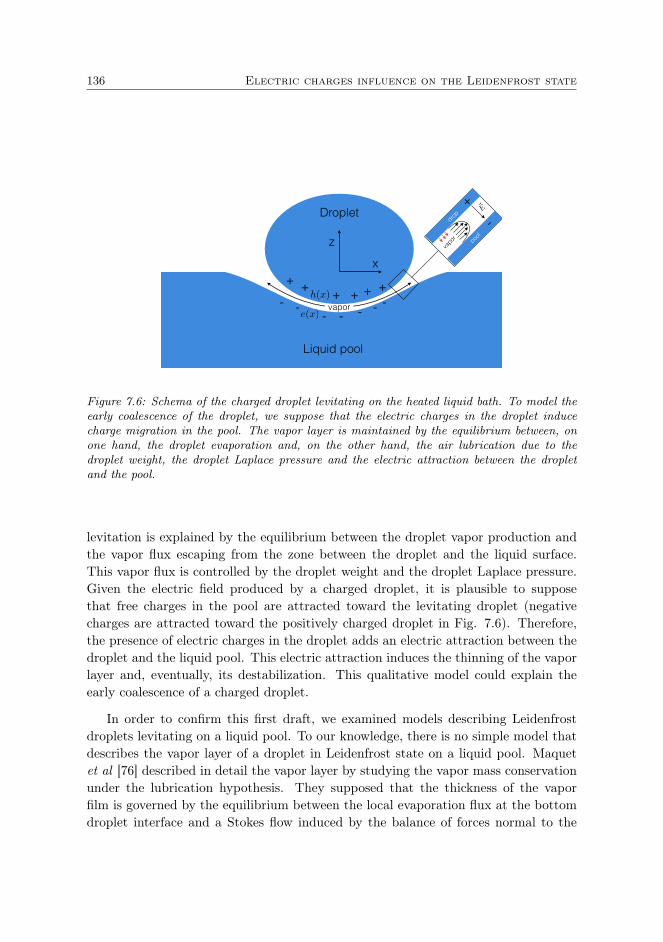
136 Electric charges influence on the Leidenfrost state
+ + + + + +- - - - - - -
vapor
drop
pool
Droplet
Liquid pool
vapor
+-
~E
z
x
h(x)
e(x)
Figure 7.6: Schema of the charged droplet levitating on the heated liquid bath. To model theearly coalescence of the droplet, we suppose that the electric charges in the droplet inducecharge migration in the pool. The vapor layer is maintained by the equilibrium between, onone hand, the droplet evaporation and, on the other hand, the air lubrication due to thedroplet weight, the droplet Laplace pressure and the electric attraction between the dropletand the pool.
levitation is explained by the equilibrium between the droplet vapor production andthe vapor flux escaping from the zone between the droplet and the liquid surface.This vapor flux is controlled by the droplet weight and the droplet Laplace pressure.Given the electric field produced by a charged droplet, it is plausible to supposethat free charges in the pool are attracted toward the levitating droplet (negativecharges are attracted toward the positively charged droplet in Fig. 7.6). Therefore,the presence of electric charges in the droplet adds an electric attraction between thedroplet and the liquid pool. This electric attraction induces the thinning of the vaporlayer and, eventually, its destabilization. This qualitative model could explain theearly coalescence of a charged droplet.
In order to confirm this first draft, we examined models describing Leidenfrostdroplets levitating on a liquid pool. To our knowledge, there is no simple model thatdescribes the vapor layer of a droplet in Leidenfrost state on a liquid pool. Maquetet al [76] described in detail the vapor layer by studying the vapor mass conservationunder the lubrication hypothesis. They supposed that the thickness of the vaporfilm is governed by the equilibrium between the local evaporation flux at the bottomdroplet interface and a Stokes flow induced by the balance of forces normal to the

Chapter 7 137
droplet surface. The equilibrium between both fluxes is expressed by:
~∇ · ~qv −Jρv
= 0 (7.5)
where ~qv is the volumetric vapor flux, J is the evaporation flux and ρv is the vapordensity. In the case of a neutral droplet, the excess of pressure in the air layer governsthe volumetric vapor flux. Namely, we have:
~qv = −~∇Pv12µv
(h− e)3 (7.6)
where µv is the vapor dynamic viscosity, Pv is the excess pressure in the air layer, h isthe vertical coordinate of the bottom of the droplet and e is the vertical coordinate ofthe liquid pool surface. Law [82] demonstrated that the charged droplet evaporationis influenced by its electric charges only for very small droplet radii (r < 0.1 µm). Asa consequence, the only parameters influenced by the electric charges are the dropletsurface tension and the balance of forces normal to the droplet surface. In order toresolve the Eq. 7.5, the first step is to take into account the adjusted droplet surfacetension. The second step is to add to the pressure of a neutral droplet the electricpressure applied by the droplet on the volumetric vapor flux. For a neutral droplet,the excess pressure is due to the droplet Laplace and hydrostatic pressures:
Pv = γκtop + ρg(ztop − h)− γκ (7.7)
where κ is the curvature of the droplet surface, κtop is the curvature at the top of thedrop, ztop corresponds to the vertical coordinate of the top of the droplet and h isthe vertical coordinate of the bottom of the droplet.
For a charged droplet, the electric attraction between the droplet and the liquidpool has to be taken into account. In a first approximation, we can suppose that theattraction between the droplet surface and the liquid pool surface corresponds to aplanar capacitor. In doing so, the excess of pressure due to electric attraction writes:
Pe =ε02
(qσε
)2(7.8)
where σ is the surface charge density and ε = εrε0 is the relative permittivity. Oncethe Stokes flow (Eq 7.6) is calculated with both pressure (Pv + Pe), we can deducethe profile of the thickness of the vapor layer.
Once the profile defined from Eq. 7.5, we can investigate the critical thickness ecas a function of the droplet radius and its charge. By computing the critical thicknessec for each set of critical radius rc and charge q measured, we could verify if thedroplet coalescence is due to the disruption of the air layer.

138 Electric charges influence on the Leidenfrost state
In conclusion, we have seen here that the charge may have critical effects onthe droplet behavior. In this case, the presence of electric charges induces an earlycoalescence of the droplet with the liquid pool. This early coalescence could beexplained by the electric attraction between the charged droplet and the liquidbath. A priori, this attraction generates a thinning of the vapor layer between thedroplet and the liquid pool. As a consequence, the droplet tends to coalesce withthe liquid bath at bigger volumes.

8General conclusion and perspectives
Conclusion
This thesis is a fundamental study of the influence of electric charges on millimetricisolated droplets. We investigated the intrinsic behavior of charged droplets as wellas their interaction with electric fields.
In Chapter 1, we defined our subject: electrically charged droplets with a milli-metric size. After this definition, we specified the environment in which this study isperformed: the charged droplet is in contact only with gas.
In Chapter 2, we introduced the previous research necessary to understand theins and outs of our study. We firstly described the different mechanisms generatingan excess of electric charges in a droplet. Then, we examined previous research thatstudied how the charge influences the behavior of the droplet. We summarized thepast discoveries made on the frequency shift, the Coulomb explosion and the motion ofa charged droplet in an electric field. In the last Section of this Chapter, we describedunresolved questions about charged droplets and explained the strategy adopted alongthis thesis. In particular, we showed that the lack of studies on millimetric dropletsis due to the difficult to store them while avoiding charge leakage. In response to thisissue, we chose to focus our attention on millimetric droplets in interaction with threedifferent storage systems: the microgravity, the vibrating bath and the Leidenfrosteffect.
In Chapter 3, we described the tools developed to study electrically chargeddroplets. We explained how the charge migration process can be easily used to in-duce a reproducible excess of charges inside droplets. A first model described how
140 General conclusion and perspectives
the amount of charges induced in the droplet could be predicted and quantified. Thedesign of three charged droplet generators was described according to their advan-tages and disadvantages. Once the charge mechanism described, we reported howthe droplet charge was measured. Given the reproducibility of the charged dropletgenerators, we simply had to calibrate them by the use of a Faraday cup. We thendescribed three storage methods that avoid the droplet contact with a solid or a fluid:the microgravity, the vibrating bath and the Leidenfrost effect. We firstly showedhow it is possible to generate microgravity conditions by the use of parabolic flights.Secondly, we explained how the delayed coalescence could be exploited to store adroplet on a vibrating liquid bath. Thirdly, we explained how the Leidenfrost effectallowed us storing droplet on their own vapor. We compared each storing systemsaccording to their own advantages. While the bouncing droplet is the more consistentstorage mode, it forces the droplet motion in the vertical direction. On the opposite,the microgravity is reduced in time but does not influence by any way the dropletdisplacement. Finally, the Leidenfrost effect allows studying the influence of electriccharges on two liquid surfaces near each other.
In the Chapter 4, we examined the influence of the electric charge on the dropletitself. We began by charging liquids with various chemical compositions. We showedthat the important variable to take into account is the time to generate the dropletcompared to the charge migration time. The charge migration time was found todepend on the liquid permittivity and conductivity. Once we understood how thecharges are induced in the droplet, it was essential to understand how the charge couldleave the droplet. We firstly summarized the previous models on charges leakage. Wethen brought for the first time measurements of the charge leakage from a millimetriccharged droplet. We demonstrated that the droplet charge leakage could be modeledby the charge leakage of a capacitor. In a third Section, we investigated the influenceof the charge on the surface energy density. From the well-known description by LordRayleigh of the charged droplet oscillation frequency, we studied the link between theelectric charge and the droplet surface energy.
In the Chapter 5, we were interested in the interaction between two electricallycharged droplets. We took advantage of the microgravity conditions to study theinteraction between two charged droplets launched one in front of the other. Theexperiments showed that the coulomb interaction is enough to describe the trajectoryof two charged droplets interacting with each other. During this set of experiments,impacts between droplets were also observed. We elaborated a sketch of the collisiondiagram between two charged droplets and compared it to the collision diagram oftwo neutral droplets. We concluded from this comparison that the droplet chargeaffects the possibility of a direct impact between droplets but also the nature of thedroplet impact.
In the Chapter 6, we studied the displacement of a charged droplet on a vibratingbath. In a first experiment, we studied the horizontal motion of droplets bouncing
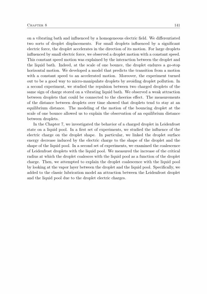
Chapter 8 141
on a vibrating bath and influenced by a homogeneous electric field. We differentiatedtwo sorts of droplet displacements. For small droplets influenced by a significantelectric force, the droplet accelerates in the direction of its motion. For large dropletsinfluenced by small electric force, we observed a droplet motion with a constant speed.This constant speed motion was explained by the interaction between the droplet andthe liquid bath. Indeed, at the scale of one bounce, the droplet endures a go-stophorizontal motion. We developed a model that predicts the transition from a motionwith a constant speed to an accelerated motion. Moreover, the experiment turnedout to be a good way to micro-manipulate droplets by avoiding droplet pollution. Ina second experiment, we studied the repulsion between two charged droplets of thesame sign of charge stored on a vibrating liquid bath. We observed a weak attractionbetween droplets that could be connected to the cheerios effect. The measurementsof the distance between droplets over time showed that droplets tend to stay at anequilibrium distance. The modeling of the motion of the bouncing droplet at thescale of one bounce allowed us to explain the observation of an equilibrium distancebetween droplets.
In the Chapter 7, we investigated the behavior of a charged droplet in Leidenfroststate on a liquid pool. In a first set of experiments, we studied the influence of theelectric charge on the droplet shape. In particular, we linked the droplet surfaceenergy decrease induced by the electric charge to the shape of the droplet and theshape of the liquid pool. In a second set of experiments, we examined the coalescenceof Leidenfrost droplets with the liquid pool. We measured the increase of the criticalradius at which the droplet coalesces with the liquid pool as a function of the dropletcharge. Then, we attempted to explain the droplet coalescence with the liquid poolby looking at the vapor layer between the droplet and the liquid pool. Specifically, weadded to the classic lubrication model an attraction between the Leidenfrost dropletand the liquid pool due to the droplet electric charges.
142 General conclusion and perspectives
Perspectives
Naturally research topics are never closed subjects. Every experiment and everymodel always need to be improved. Of course, some subjects appear to be moreimportant to study at specific times, depending on the general scientific interest oron the specific questions at which it could answer. In this Section, we indicate whatcould be studied in the extension of this thesis. This Section is addressed to anyonewho wish to bring new answers to the study of charged drops.
Adding data to the collision diagram of charged droplets
Going back to the Chapter 5, we believe that the study of the impact between dropletsneeds to be extended. Indeed, the experiment performed in microgravity gave newinsights on the influence of the charge on the collision between droplets. However,the microgravity sessions only allowed us exploring a part of the collision diagramcomprised between We = 25 and We = 60. We believe that the rest of the diagramneeds to be explored to deduce more general conclusions on the influence of theelectric charge on the impact between droplets. In particular, the part of the diagramlocated below We = 25 needs to be explored in detail. Indeed, our study of thecharged droplet trajectories demonstrated that the zone of low speed corresponds tothe part of the diagram where the electric charges have the most important influenceon the droplet motion. Moreover, the zone called bouncing zone, which correspondsto the bouncing between neutral droplets also needs to be studied in more details.One of our measurements showed that the bouncing between droplets is affected bytheir charges. Of course, one data is not enough to draw conclusion. However, givenprevious studies on the bouncing between droplets [65], this part of the diagram seemscritically influenced by the electric charges and, as a consequence, needs to be studiedin more details.
The part of the collision diagram that still needs to be explored has been high-lighted by the hatched area in Fig. 8.1. Futures experiments may be performedin two different ways. Given the difficulty to perform experiments in microgravityconfigurations, a first step is to develop the same experiment in a classic laboratory.Even if we believe that aerodynamic forces applied on free falling droplets affect theircollision, this phenomenon still has to be quantified. This second setup would allowexplaining how important is the microgravity to study the influence of the electriccharge on the droplet collision. Moreover, the laboratory being a more friendly envi-ronment, experiments could be performed with more precision and a more significantpart of the diagram could be explored. Secondly, the microgravity setup could stillbe improved. By controlling in a more precise way the ejection of charged droplets inmicrogravity, it would be easier to accumulate data on the collision diagram. In theend, those two ways to accumulate new data would allow comparing in a deeper wayour experiments to measurements made on thunderclouds.
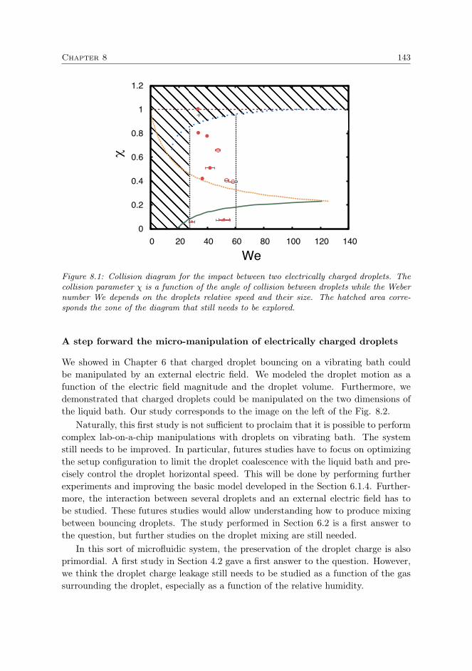
Chapter 8 143
0
0.2
0.4
0.6
0.8
1
1.2
0 20 40 60 80 100 120 140
χ
We Figure 8.1: Collision diagram for the impact between two electrically charged droplets. Thecollision parameter χ is a function of the angle of collision between droplets while the Webernumber We depends on the droplets relative speed and their size. The hatched area corre-sponds the zone of the diagram that still needs to be explored.
A step forward the micro-manipulation of electrically charged droplets
We showed in Chapter 6 that charged droplet bouncing on a vibrating bath couldbe manipulated by an external electric field. We modeled the droplet motion as afunction of the electric field magnitude and the droplet volume. Furthermore, wedemonstrated that charged droplets could be manipulated on the two dimensions ofthe liquid bath. Our study corresponds to the image on the left of the Fig. 8.2.
Naturally, this first study is not sufficient to proclaim that it is possible to performcomplex lab-on-a-chip manipulations with droplets on vibrating bath. The systemstill needs to be improved. In particular, futures studies have to focus on optimizingthe setup configuration to limit the droplet coalescence with the liquid bath and pre-cisely control the droplet horizontal speed. This will be done by performing furtherexperiments and improving the basic model developed in the Section 6.1.4. Further-more, the interaction between several droplets and an external electric field has tobe studied. These futures studies would allow understanding how to produce mixingbetween bouncing droplets. The study performed in Section 6.2 is a first answer tothe question, but further studies on the droplet mixing are still needed.
In this sort of microfluidic system, the preservation of the droplet charge is alsoprimordial. A first study in Section 4.2 gave a first answer to the question. However,we think the droplet charge leakage still needs to be studied as a function of the gassurrounding the droplet, especially as a function of the relative humidity.
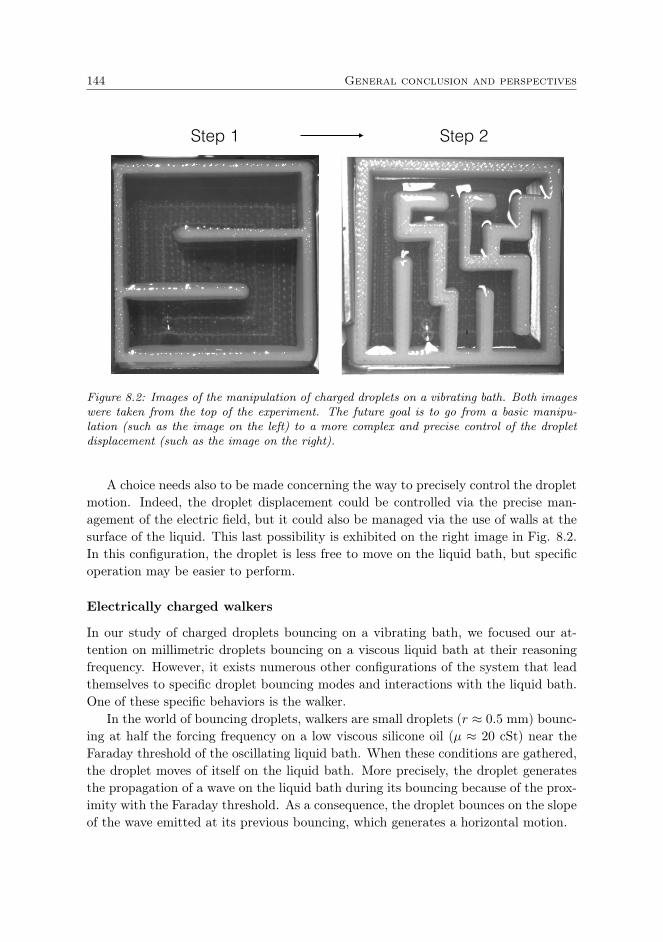
144 General conclusion and perspectives
Step 1 Step 2
Figure 8.2: Images of the manipulation of charged droplets on a vibrating bath. Both imageswere taken from the top of the experiment. The future goal is to go from a basic manipu-lation (such as the image on the left) to a more complex and precise control of the dropletdisplacement (such as the image on the right).
A choice needs also to be made concerning the way to precisely control the dropletmotion. Indeed, the droplet displacement could be controlled via the precise man-agement of the electric field, but it could also be managed via the use of walls at thesurface of the liquid. This last possibility is exhibited on the right image in Fig. 8.2.In this configuration, the droplet is less free to move on the liquid bath, but specificoperation may be easier to perform.
Electrically charged walkers
In our study of charged droplets bouncing on a vibrating bath, we focused our at-tention on millimetric droplets bouncing on a viscous liquid bath at their reasoningfrequency. However, it exists numerous other configurations of the system that leadthemselves to specific droplet bouncing modes and interactions with the liquid bath.One of these specific behaviors is the walker.
In the world of bouncing droplets, walkers are small droplets (r ≈ 0.5 mm) bounc-ing at half the forcing frequency on a low viscous silicone oil (µ ≈ 20 cSt) near theFaraday threshold of the oscillating liquid bath. When these conditions are gathered,the droplet moves of itself on the liquid bath. More precisely, the droplet generatesthe propagation of a wave on the liquid bath during its bouncing because of the prox-imity with the Faraday threshold. As a consequence, the droplet bounces on the slopeof the wave emitted at its previous bouncing, which generates a horizontal motion.

Chapter 8 145
This bouncing mode raised the interest of several research groups and led to severalpublications [61, 64]. One of the reasons of this enthusiasm is the parallel that canbe made between the walker (a particle moving on its own wave) and the quantumphysics. The addition of electric charges in walkers could provide new insights onthe experiment. The electric charge could, for example, allow to control the dropletmotion on its own wave in order to adjust the position of its bouncing on the wave.It could also be used as a tool to reproduce quantum experiments involving electricfields.
Naturally, the study of charged walkers requires developing specific tools to gen-erate them and control them. During this thesis, we already developed a chargeddroplet generator that can produce walkers. The charged walker generator was calledcharged droplet generator model C in the Section 3.1.1. This charged droplet gener-ator is a mixing between a neutral walker generator (described, for example, in [49])and a charged droplet generator. It emits small droplets thanks to a piezoelectriccrystal emitting droplets from a small hole in a metallic plate. A voltage between twometallic plates allows inducing charges in the ejected droplet. Such a charged dropletgenerator was found to create walkers properly. However, it still needs adjustmentsin order to eject droplets in an optimized way. Currently, the main limitation comesfrom the high speed of droplet ejection due to the electric force applied on the ejecteddroplet.
Note that the walkers have also been generated by a second method. By diving acharged metallic rod in the liquid oil and removing it quickly, we were able to generatewalkers with an excess of electric charges. This method still needs to be quantified.
Even if a walker and the setup involving its creation are simple to describe, itsexperimental management may be difficult to master. As a consequence, we justhad the occasion to perform preliminary experiments. We looked at the motion ofa charged walker in an external electric field. The difficulty of the experiment isto produce a homogeneous electric field (to avoid dielectrophoresis) on a large scale(to measure the accelerations/decelerations on several bounces). As a consequence,we only accumulated data on droplet motion in non-homogenous electric fields. Anexample of a typical experiment is shown in Fig. 8.3.
We examined the motion of a walker between two charged electrodes. An electricfield influenced the walker along its motion. The typical motion in the x and ydirections (indicated in Fig. 8.3) are shown in Fig. 8.4. At this time, no conclusionshave been drawn from these experiments, but we believe that the influence of theelectric field on the walker displacement could be deduced from these measurements.

146 General conclusion and perspectives
Guide channel
electrodex
y
Walker
Figure 8.3: Image of the study of the motion of a walker. The image was taken from thetop of the experiment. Two walls that pop out of the liquid bath guide the walker motion.The walker stored between the two walls is influenced by an electric field produced by twoelectrodes situated on each side of the liquid bath.
3
3.5
4
4.5
5
5.5
6
6.5
7
0 2 4 6 8 10 12
x (m
m)
t (s)
0
10
20
30
40
50
60
70
0 2 4 6 8 10 12
x (m
m)
t (s)
Figure 8.4: Displacement of a walker influenced by an external electric field over time. Thegraph on the left corresponds to its displacement along the direction x while the graph on theright corresponds to its displacement along the direction y.
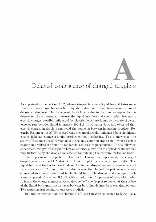
ADelayed coalescence of charged droplets
As explained in the Section 3.3.2, when a droplet falls on a liquid bath, it takes sometimes for the air layer between both liquids to drain out. The phenomenon is nameddelayed coalescence. The drainage of the air layer is due to the pressure applied by thedroplet on the air cornered between the liquid interface and the droplet. Generally,electric charges, possibly influenced by electric fields, are found to increase the coa-lescence rate between liquid interfaces [109–111]. In Chapter 5, we also observed thatelectric charges in droplets can avoid the bouncing between impacting droplets. Re-cently, Ristenpart et al [65] showed that a charged droplet influenced by a significantelectric field can contact a liquid interface without coalescing. To our knowledge, thestudy of Ristenpart et al corresponds to the only experimental setup in which electriccharges in droplets are found to reduce the coalescence phenomenon. In the followingexperiment, we give an insight on how an external electric force applied on the dropletmay further delay the droplet coalescence by reducing the pressure on the air layer.
The experiment is depicted in Fig. A.1. During one experiment, the chargeddroplet generator model A dropped off one droplet on a steady liquid bath. Theliquid bath and the bottom electrode of the charged droplet generator were separatedby a distance l =15 mm. The top electrode of the charged droplet generator wasconnected to an electrode dived in the liquid bath. The droplet and the liquid bathwere composed of silicone oil 5 cSt with an addition of 1 percent of ethanol in orderto insure the charge migration. Once dropped off, the droplet remained at the surfaceof the liquid bath until the air layer between both liquids interfaces was drained out.Two experimental configurations were studied.
In a first experiment, all the electrodes of the setup were connected to Earth. As a
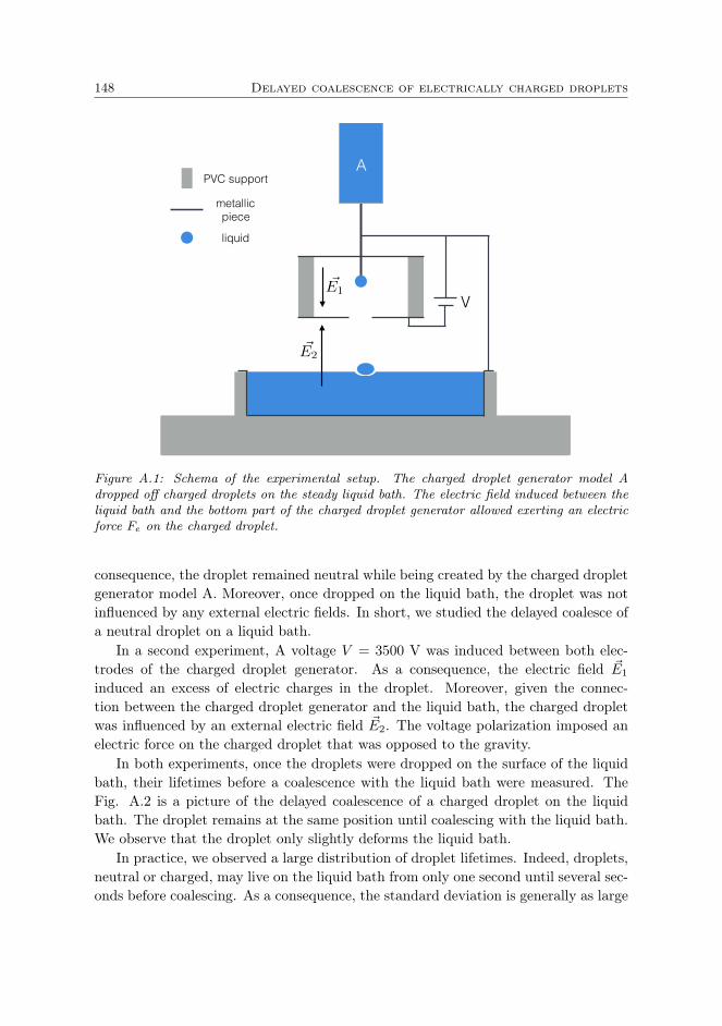
148 Delayed coalescence of electrically charged droplets
V
APVC support
metallic piece
liquid
~E1
~E2
Figure A.1: Schema of the experimental setup. The charged droplet generator model Adropped off charged droplets on the steady liquid bath. The electric field induced between theliquid bath and the bottom part of the charged droplet generator allowed exerting an electricforce Fe on the charged droplet.
consequence, the droplet remained neutral while being created by the charged dropletgenerator model A. Moreover, once dropped on the liquid bath, the droplet was notinfluenced by any external electric fields. In short, we studied the delayed coalesce ofa neutral droplet on a liquid bath.
In a second experiment, A voltage V = 3500 V was induced between both elec-trodes of the charged droplet generator. As a consequence, the electric field ~E1
induced an excess of electric charges in the droplet. Moreover, given the connec-tion between the charged droplet generator and the liquid bath, the charged dropletwas influenced by an external electric field ~E2. The voltage polarization imposed anelectric force on the charged droplet that was opposed to the gravity.
In both experiments, once the droplets were dropped on the surface of the liquidbath, their lifetimes before a coalescence with the liquid bath were measured. TheFig. A.2 is a picture of the delayed coalescence of a charged droplet on the liquidbath. The droplet remains at the same position until coalescing with the liquid bath.We observe that the droplet only slightly deforms the liquid bath.
In practice, we observed a large distribution of droplet lifetimes. Indeed, droplets,neutral or charged, may live on the liquid bath from only one second until several sec-onds before coalescing. As a consequence, the standard deviation is generally as large
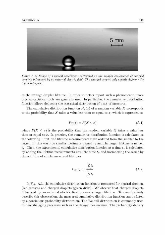
Appendix A 149
5 mm
Figure A.2: Image of a typical experiment performed on the delayed coalescence of chargeddroplets influenced by an external electric field. The charged droplet only slightly deforms theliquid interface.
as the average droplet lifetime. In order to better report such a phenomenon, moreprecise statistical tools are generally used. In particular, the cumulative distributionfunction allows deducing the statistical distribution of a set of measures.
The cumulative distribution function FX(x) of a random variable X correspondsto the probability that X takes a value less than or equal to x, which is expressed as:
FX(x) = P (X ≤ x) (A.1)
where P (X ≤ x) is the probability that the random variable X takes a value lessthan or equal to x. In practice, the cumulative distribution function is calculated asthe following. First, the lifetime measurements t are ordered from the smaller to thelarger. In this way, the smaller lifetime is named t1 and the larger lifetime is namedtf . Then, the experimental cumulative distribution function at a time tx is calculatedby adding the lifetime measurements until the time tx and normalizing the result bythe addition of all the measured lifetimes:
FX(tx) =
txΣi=1ti
tf
Σi=1ti
(A.2)
In Fig. A.3, the cumulative distribution function is presented for neutral droplets(red crosses) and charged droplets (green disks). We observe that charged dropletsinfluenced by an external electric field possess a larger lifetime. To quantitativelydescribe this observation, the measured cumulative distribution function can be fittedby a continuous probability distribution. The Weibull distribution is commonly usedto describe aging processes such as the delayed coalescence. The probability density

150 Delayed coalescence of electrically charged droplets
0 0.1 0.2 0.3 0.4 0.5 0.6 0.7 0.8 0.9
1
0 5 10 15 20 25 30
F
X(t)
t (s) Figure A.3: Cumulative distribution functions FX(t) of the droplet lifetime on the liquid bath.The lifetime increases for charged droplets influenced by an external electric field compare toneutral droplets non-influenced by external electric fields. Both measurement was fitted byEq. A.4.
function of a Weibull distribution is expressed by:
f(x;λ, k) =
kλ
(xλ
)k−1e−(x/λ)
k
x ≥ 0,
0 x < 0,(A.3)
where k > 0 is the shape parameter and λ > 0 is the scale parameter of the distri-bution. The cumulative distribution function of the Weibull function corresponds to:
F (x; k, λ) = 1− e−(x/λ)k
(A.4)
Such a distribution generally describes a time to failure. If k < 1, the failure ratedecreases over time. On the contrary, if k > 1 the failure rate increases with time.The particular case where k = 1 corresponds to a constant failure rate over time.In the case of droplet delayed coalescence, the failure rate is commonly supposed toincrease with time, leading to Weibull distributions with k > 1. The average failuretime of a Weibull distribution can be calculated via the following formula:
µ = λΓ(1 + 1/k). (A.5)
where Γ is the Gamma function Γ(t) =∫∞0xt−1e−x dx. In Fig. A.3, we fitted the
measurements with Eq. 4.16. In Tab. A.1, we reported the fitted variables k and λand the mean droplet lifetime µ calculated from the Weibull distribution. We observe

Appendix A 151
k λ µ
V = 0 V 1.15 0.72 0.67 sV = 3500 V 0.55 4.2 6.6 s
Table A.1: Fitting parameters and means of the Weibull distribution described by Eq. 4.16and A.5.
that the charged droplet influenced by an external electric field has an average lifetimeten times greater than the neutral droplet.
The average lifetime calculated from the Weibull distribution confirms the in-crease of the droplet lifetime for charged droplets influenced by an external electricfield. Such an experiment demonstrates that the external electric force applied on thedroplet can be used to reduce the drainage of an air layer between two liquid interfaces.Unfortunately, our conclusions cannot go further than this observation. Indeed, wewere not able to model the electric field ~E2 induced between the bottom electrode ofthe charged droplet generator and the liquid bath. Because of the hole in the bottomelectrode of the charged droplet generator and the influence of the top electrode, theelectric field ~E2 could not be reduced to a simple expression. As a consequence, theforce applied on the charged droplet has to be modeled by simulations.
Rather than quantitatively describe the observations, we can elaborate an explana-tion of the discrepancy between the behavior of a charged Leidenfrost droplet and thepresent experiment. Indeed, in the case of a charged droplet in Leidenfrost state ona liquid bath, we observed a decrease of the droplet lifetime with the droplet electriccharge (see Section 7.2). On the contrary, the present experiment shows an increaseof the lifetime in the case of charged droplets. Naturally, the difference between bothexperiments resides in the presence of an external electric field. Our reasoning isschematized in Fig. A.4. In the case of the Leidenfrost droplet, the electric chargesonly generate an additional pressure on the vapor layer between the droplet and theliquid bath. In the present experiment, the external electric field generates a volumet-ric force on the droplet that is opposed to the droplet weight. Moreover, the chargesinside the droplet migrate toward the top of the droplet because of the electric field.As a consequence, the droplet pressure on the air layer is reduced.

152 Delayed coalescence of electrically charged droplets
+ +
++ + +++
+
--
- - - --
~E+ +
+
+ +
++
+
-- -
-m~g + ~Fe,2
~Fe,1
m~g
1 2
Figure A.4: Schema of the difference between a charged Leidenfrost droplet (1) and thedelayed coalescence of a charged droplet influenced by a horizontal electric field (2). In thefirst case, the electric charges reduce the droplet lifetime. In the second case, the electriccharges increase the droplet lifetime.
References
[1] E. P. Krider, Benjamin Franklin and Lightning Rod, Phys Today, 59, 42 (2006).
[2] F. Leblanc, K.L. Aplin, Y. Yair, R.G. Harrison, J.P. Lebreton, and M. Blanc,Planetary Atmospheric Electricity, Space Sci. Rev. 137, 1 (2008).
[3] A. Khain, V. Arkhipov, and M. Pinsky, Rain Enhancement and Fog Eliminationby Seeding with Charged Droplets. Part I: Theory and Numerical Simulations,AMS 43, 1513 (2004).
[4] M. Stolzenburg, and T. C. Marshall, Charge Structure and Dynamics in Thun-derstorms, Space Sci Rev 137, 355 (2008).
[5] K. V. Bread, H. T. Ochs, and S. Liu, Collision between Small Precipitation Drops.Part III: Laboratory Measurements at Reduced Pressure, AMS 58, 13995 (2001).
[6] S. Chauzy, and S. Despiau, Rainfall Rate and Electric Charge and Charge ofRaindrops of Spring Showers, AMS 37, 1619 (1980).
[7] P. Lenard, Über der Electrizität der Wasserfälle, Ann. Phys. 46, 584 (1892).
[8] D. C. Blanchard, Electrically charged drops from bubbles in sea water and theirmeteorological significance, J. Meteor 15, 383 (1958).
[9] D. C. Blanchard, Flow of Electrical Current From World Ocean to Atmosphere,J. Geophys. Res. 90, 9147 (1985).
[10] S. E. Law, Agricultural electrostatic spray application: a review of significantresearch and development during the 20th century, J Electrostat 52, 25 (2001).
[11] P. Kebarle, and U. H. Verkerk, On the Mechanism of Electrospray IonizationMass Spectrometry (ESIMS), in Electrospray and MALDI Mass Spectrometry:Fundamentals, Instrumentation, Practicalities, and Biological Applications Sec-ond Edition (ed R. B. Cole), John Wiley Sons, Inc., Hoboken, NJ, USA. (2010).
[12] R. J. Pfeifer, and C. D. Hendricks, Parametric Studies of ElectrohydrodynamicSpraying, AIAA 66 (1967). Conference paper.
154 References
[13] D. J. Im, Next generation digital microfluidic technology: Electrophoresis ofcharged droplets, Korean J. Chem. Eng. 32, 1001 (2015).
[14] D. Choi, H. Lee, D. J. Im, I. S. Kang, G. Lim, D. S. Kim, and K. H. Kang,Spontaneous electrical charging of droplets by conventional pipetting, Sci. Rep. 3,2037 (2013).
[15] L. Rayleigh, On the Equilibrium of Liquid Conducting Masses Charged with Elec-tricity, Philos. Mag. 14, 184 (1882).
[16] P. R. Brazier-Smith, M. Brook, J. Latham, C. P. R. Saunders, and M. H. Smith,The Vibration of Electrified Water Drops, Proc. R. Soc. Lond. A 322, 523 (1971).
[17] C. P. R. Saunders, and B. S. Wonu, Vibrational frequencies of freely fallingchargedwater drops, J. Atmos. Sol.-Terr. Phys. 36, 707 (1974).
[18] R. J. A. Hill, and L. Eaves, Shape oscillations of an electrically charged diamag-netically levitated droplet, Appl. Phys. Lett. 100, 114106 (2012).
[19] D. Duft, H. Lebius, B. A. Huber, C. Guet, and T. Leisner, Shape Oscillationsand Stability of Charged Microdroplets, Phys. Rev. Lett. 89, 084503 (2002).
[20] D. Duft, T. Achtzehn, R. Muller, B. A. Huber, and T. Leisner, Coulomb fission- rayleigh jets from levitated microdroplets, Nature 421, 128 (2003).
[21] E. Giglio, B. Gervais, J. Rangama, B. Manil, B. A. Huber, D. Duft, R. Muller,T. Leisner, and C. Guet, Shape deformations of surface-charged microdroplets,Phys. Rev. E 77, 036319 (2008).
[22] T. Achtzehn, R. Muller, D. Duft, and T. Leisnera, The Coulomb instability ofcharged microdroplets: dynamics and scaling, Eur. Phys. J. D 34, 311 (2005).
[23] S. I. Betelu, M. A. Fontelos, U. Kindelán, and O. Vantzos, Singularities oncharged viscous droplets, Phys. Fluids 18, 051706 (2006).
[24] R. M. Thaokara, and S. D. Deshmukh, Rayleigh instability of charged drops andvesicles in the presence of counterions, Phys. Fluids 22, 034107 (2010).
[25] Abbé Nollet, Recherches sur les causes particulières des phénomènes électriqueset sur les effets nuisibles ou avantageux qu’on peut en attendre Paris (1752).
[26] M. Gamero-Castano, The structure of electrospray beams in vacuum, J. FluidMech. 604, 339 (2008).
[27] R. A. Millikan, On the elementary electrical charge and the avogadro constant,Phys. Rev. 2, 109 (1913).
References 155
[28] M. Jalaal, B. Khorshidi, and E. Esmaeilzadeh, An experimental study on themotion, deformation and electrical charging of water drops falling in oil in thepresence of high voltage D.C. electric field, Exp. Therm. Fluid Sci. 34, 1498(2010).
[29] D. J. Im, J. Noh, D. Moon, and I. S. Kang, Electrophoresis of a Charged Dropletin a Dielectric Liquid for Droplet Actuation, Anal. Chem. 83, 5168 (2011).
[30] M. Chiesa, J.A. Melheim, A. Pedersen, S. Ingebrigtsen, and G. Berg, Forcesacting on water droplets falling in oil under the influence of an electric field:numerical predictions versus experimental observations, Eur. J. Mech. B-Fluid24, 717 (2005).
[31] J. Eggers, Nonlinear dynamics and breakup of free-surface flows, Rev. Mod. Phys.69, 919 (1997).
[32] M. A. Fontelos, U. Kindelán, and O. Vantzos, Evolution of neutral and chargeddroplets in an electric field, Phys. Fluids 20, 092110 (2008).
[33] Sir G. Taylor, Disintegration of Water Droplets in an Electric Field, Proc. R.Soc. A 280, 383 (1964).
[34] V. M. Ortega-Jimenez, and R. Dudley, Spiderweb deformation induced by elec-trostatically charged insects, Sci. Rep. 3, 02108 (2013).
[35] Oleg.V. Salata, Tools of Nanotechnology: Electrospray, Curr. Nanosci. 1, 25(2005).
[36] A.B. Theberge, F Courtois, Y. Schaerli, M. Fischlechner, C. Abell, F. Hollfelder,and W.T.S. Huck, Microdroplets in Microfluidics: An Evolving Platform for Dis-coveries in Chemistry and Biology, Angew. Chem. Int. Ed. 49, 5846 (2010).
[37] H. Zhouab, and S. Yao, Electrostatic charging and control of droplets in microflu-idic devices, Lab Chip 13, 962 (2013).
[38] B. Ahn, K. Lee, R Panchapakesan, and K. W. Oh, On-demand electrostaticdroplet charging and sorting, Biomicrofluidics 5, 024113 (2011).
[39] ] M. Gunji, and M. Washizu, Self-propulsion of a water droplet in an electricfield, J. Phys. D 38, 2417 (2005).
[40] A. H.C. Ng, B. B. Li,M. D.Chamberlain, and A. R. Wheeler, Digital MicrofluidicCell Culture Biomedical Engineering 17 91 (2015).
[41] R. B. Fair, Digital microfluidics: is a true lab-on-a-chip possible?, MicrofluidNanofluidics 3, 245 (2007).

156 References
[42] D. R. Link, E. Grasland-Mongrain, A. Duri, F. Sarrazin, Z. Cheng, G. Cristo-bal, M. Marquez, and D. A. Weitz, Control of Droplets in MicrofluidicDevices,Angew. Chem. Int. Ed. 45, 2556 (2006).
[43] A. R. Thiam, N. Bremond, and J. Bibette, Breaking of an Emulsion under anac Electric Field, PRL 102, 188304 (2009).
[44] W. Thomson, On a self-acting apparatus for multiplying and maintaining electriccharges, with applications to the Voltaic Theory, Proc. R. Soc. Lond. 16, 67(1867).
[45] A. R. Jones, and K. C. Thong, The production of charged monodisperse fueldroplets by electrical dispersion, J. Phys. D: Appl. Phys. 4, 1159 (1971).
[46] D. B. Hibbert, Introduction to electrochemistry, MacMillan, Basingstoke, (1993).
[47] K. Choi, M. Im, J. Choi, and Y. Choi, Droplet transportation using a pre-chargingmethod for digital microfluidics, Microfluid Nanofluidics 12, 821 (2012).
[48] Á. G. Marín, W. van Hoeve, P. García-Sánchez, L. Shui, Y. Xie, M. A. Fontelos,J. C. T. Eijkel, A. van den Berg, and De. Lohse, The microfluidic Kelvin waterdropper, Lab Chip 13, 4503 (2013).
[49] D. Terwagne, F. Ludewig, N. Vandewalle, and S. Dorbolo, The role of the dropletdeformations in the bouncing droplet dynamics, Phys. Fluids 25, 122101 (2013).
[50] J. Hu, and J. L. Rovey, Faraday cup with nanosecond response and adjustableimpedance for fast electron beam characterization, Rev. Sci. Instrum. 82, 073504(2011).
[51] S. Matsusaka, H. Maruyama, T. Matsuyama, and M. Ghadiri, Triboelectric charg-ing of powders: A review, Chem. Eng. Sci. 65, 5781 (2010).
[52] Low Level Measurements Handbook - 7th Edition - Precision DC Current, Volt-age, and Resistance Measurements, Keithley, Tektronix.
[53] D. Kucerovsky, and Z. Kucerovsky, Analysis of the dynamic Faraday cup, J.Phys. D: Appl. Phys. 36, 2407 (2003).
[54] M. Brandenbourger, Gouttes chargées, Master thesis (2012).
[55] D. Foresti, M. Nabavi, and D. Poulikakos, On the acoustic levitation stabilitybehaviour of spherical and ellipsoidal particles, J. Fluid Mech. 709, 581 (2012).
[56] Lord Rayleigh, Investigations in Capillarity:—The size of drops.—The liberationof gas from supersaturated solutions.—Colliding jets.—The tension of contami-nated water-surfaces, Philos. Mag. 48, 321 (1899).
References 157
[57] G. P. Neitzel, and P. Dell’Aversana, Noncoalescence and nonwetting behavior ofliquids, Annu. Rev. Fluid Mech. 34, 267 (2002).
[58] Y. Amarouchene, G. Cristobal, and H. Kellay, Noncoalescing Drops, Phys. Rev.Lett. 87, 206104 (2001).
[59] K. R. Sreenivas, P. K. De, and J. H. Arakeri, Levitation of a drop over a filmflow, J. Fluid Mech. 380, 297 (1999).
[60] A. Duchesne, C. Savaro, L. Lebon, C. Pirat, and L. Limat, Multiple rotationsof a drop rolling inside a horizontal circular hydraulic jump, EPL 102, 64001(2013).
[61] Y. Couder, E. Fort, C.-H. Gautier, and A. Boudaoud, From Bouncing to Floating:Noncoalescence of Drops on a Fluid Bath, Phys. Rev. Lett. 94, 177801 (2005).
[62] T. Gilet, D. Terwagne, N. Vandewalle, and S. Dorbolo, Dynamics of a BouncingDroplet onto a Vertically Vibrated Interface, Phys. Rev. Lett. 100, 167802 (2008).
[63] S. Dorbolo, D. Terwagne, N. Vandewalle, and T. Gilet, Resonant and rollingdroplet, New J. Phys. 10, 113021 (2008).
[64] J. W. Bush, The new wave of pilot-wave theory, Phys. Today 68, 47 (2015).
[65] W. D. Ristenpart, J. C. Bird, A. Belmonte, F. Dollar, and H. A. Stone, Non-coalescence of oppositely charged drops, Nature 461, 377 (2009).
[66] R. T. Hilger, M. S. Westphall, and L. M. Smith, Controlling Charge on LevitatingDrops, Anal. Chem. 79, 6027 (2007).
[67] M. S. Westphall, K. Jorabchi, and L. M. Smith, Mass Spectrometry of Acousti-cally Levitated Droplets, Anal. Chem. 80, 5847 (2008).
[68] J. Molacek, and J. W. M. Bush, Drops bouncing on a vibrating bath, J. FluidMech. 727, 582 (2013).
[69] J. Leidenfrost, De aquae communis nonnullis qualitatibus tractatus Ovenius(1756).
[70] D. Quere, Leidenfrost Dynamics, Annu. Rev. Fluid Mech. 45, 197 (2013).
[71] F. Celestini, and G. Kirstetter, Effect of an electric field on a Leidenfrost droplet,Soft Matter 8, 5992 (2012).
[72] L. Maquet, M. Brandenbourger, B. Sobac , A. L. Biance, P. Colinet, and S.Dorbolo, Leidenfrost drops: Effect of gravity, EPL 110, 24001 (2015).

158 References
[73] R. S. Hall, S. J. Board, A. J. Clare, R. B. Duffey, T. S. Playle, and D. H. Poole,Inverse Leidenfrost Phenomenon, Nature 224, 266 (1969).
[74] M. Adda-Bedia, S. Kumar, F. Lechenault, S. Moulinet, M. Schillaci, and D. Vella,Inverse Leidenfrost Effect: Levitating Drops on Liquid Nitrogen, Langmuir 32,4179 (2016).
[75] M. Le Merrer, C. Clanet, D. Quéré, E. Raphaël, and F. Chevyd, Wave drag onfloating bodies, PNAS 108, 15064 (2011).
[76] L. Maquet, B. Darbois-Texier, A. Duchesne, M. Brandenbourger, B. Sobac, A.Rednikov, P. Colinet, and S. Dorbolo, Leidenfrost drops on a heated liquid pool,Accepted for publication in PRF (2016).
[77] P.N. Tshibangu, S. N. Ndwandwe, and E. Dixon Dikio, Density, Viscosityand Conductivity Study of 1-Butyl-3-Methylimidazolium Bromide, Int. J. Elec-trochem. Sci. 6, 2201 (2011).
[78] H. Moretto, M. Schulze, and G. Wagner, Ullmann’s encycplopedia of industrialchemistry Wiley, Weinheim (2012).
[79] M. I. Newton, D. L. Herbertson, S. J. Elliott, N. J. Shirtcliffe, and G. McHale,Electrowetting of liquid marbles, J. Phys. D: Appl. Phys. 40, 20 (2007).
[80] D. B. Hibbert, Introduction to electrochemistry MacMillan, Basingstoke (1993).
[81] J. F. Mora, G. J. Van Berkel, C. G. Enke, R. B. Cole, M. Martinez-Sanchez, andJ.B. Fenn, Electrochemical processes in electrospray ionization mass spectrometry,J. Mass Spectrom. 35, 939 (2000).
[82] S. E. Law, Charge and Mass Flux in the Radial Electric Field of an EvaporatingCharged Water Droplet: An Experimental Analysis, IEEE Trans. Ind. Appl. 25,1081 (1989).
[83] J. V. Iribarne, and B. A. Thomson, On the evaporation of small ions from chargeddroplets, J. Chem. Phys. 64, 2287 (1976).
[84] C. J. Hogan, P. Biswas, and D. Chen, Charged Droplet Dynamics in the Submi-crometer Size Range, J. Phys. Chem. B 113, 970 (2009).
[85] C. B. Moore, and B. Vonnegut, Measurements of the electrical conductivities ofair over hot water, J. Atmos. Sci. 45, 885 (1987).
[86] D. Retalis, A. Pitta, and P. Psallidas, The Conductivity of the Air and OtherElectrical Parameters in Relation to Meteorological Elements and Air Pollutionin Athens, Meteorol. Atmos. Phys. 46, 197 (1991).
References 159
[87] W. C. Swinbank, Collisions of Cloud droplets, Nature 159, 850 (1947).
[88] M. H. Davis, and J. D. Sartor, Theoretical Collision Efficiencies for Small CloudDroplets in Stokes Flow, Nature 215, 1371 (1967).
[89] F. Y. Testik, Outcome regimes of binary raindrop collisions, Atmos. Res. 94, 389(2009).
[90] K. V. Bread, H. T. Ochs, and S. Liu, Collision between Small Precipitation Drops.Part III: Laboratory Measurements at Reduced Pressure, AMS 58, 13995 (2001).
[91] C. N. Franklin, P. A. Vaillancourt, M. K. Yau, and P. Bartello, Collision Ratesof Cloud Droplets in Turbulent Flow, AMS 62, 2451 (2005).
[92] N. Ashgriz, and J. Y. Poo, Coalescence and separation in binary collisions ofliquid drops, J. Fluid Mech. 221, 183 (1990).
[93] J. Qian, and C. K. Law, Regimes of coalescence and separation in droplet colli-sion, J. Fluid Mech. 331, 59 (1997).
[94] C. Gotaas, P. Havelka, H. A. Jakobsen, and H. F. Svendsen, Evaluation of theimpact parameter in droplet-droplet collision experiments by the aliasing method,Phys. Fluids 19, 102105 (2007).
[95] K. V. Beard, R. I. Durkee, and H. T. Ochs, Coalescence Efficiency Measurementsfor Minimally Charged Cloud Drops, JAS 59, 233 (2002).
[96] J. C. Bird, W. D. Ristenpart, A. Belmonte, and H. A. Stone, Critical Anglefor Electrically Driven Coalescence of Two Conical Droplets, PRL 103, 164502(2009).
[97] J. Wang, B. Wang, and H. Qiu, Coalescence and Breakup of Oppositely ChargedDroplets, Sci. Rep. 4, 7123 (2014).
[98] K. Okumura, F. Chevy, D. Richard, D. Quéré, and C. Clanet, Water spring: Amodel for bouncing drops, Europhys. Lett. 62, 237 (2003).
[99] D. Terwagne, F. Ludewig, N. Vandewalle, and S. Dorbolo , The role of the dropletdeformations in the bouncing droplet dynamics, Phys. Fluids 25, 122101 (2013).
[100] Lord Rayleigh, On the Capillary Phenomena of Jets, Proc. R. Soc. London 29,71 (1879).
[101] P. Drude, Zur Elektronentheorie der metalle, Annalen der Physik. 306, 566(1900).
[102] P. Drude, Zur Elektronentheorie der Metalle; II. Teil. Galvanomagnetische undthermomagnetische Effecte, Annalen der Physik. 308, 369 (1900).
160 References
[103] D. Terwagne, N. Mack, S. Dorbolo, T. Gilet, J.-Y. Raty, and N. Vandewalle,The mayonnaise droplet, CHAOS 19, 041105 (2009).
[104] M.M. Nicolson, The interaction between floating particles, Proc. CambridgePhilos. Soc. 45, 288 (1949).
[105] P. A. Kralchevsky, and K. Nagayama, Capillary interactions between particlesbound to interfaces, liquid films and biomembranes, Adv. Colloid Interface Sci.85, 145 (2000).
[106] F. Moisy, M. Rabaud, and K. Salsac, A synthetic Schlieren method for themeasurement of the topography of a liquid interface, Exp Fluids 46, 1021 (2009).
[107] F. Celestini, T. Frisch, and Y. Pomeau, Take Off of Small Leidenfrost Droplets,PRL 109, 034501 (2012).
[108] T Umeki, M Ohata, H Nakanishi, and M Ichikawa, Dynamics of microdropletsover the surface of hot water, Sci. Rep. 5, 8046 (2015).
[109] J. C. Ahern, The Influence of Electric Charge and Electric Fields on the For-mation and Duration of Water Boules, PhD Thesis (2003).
[110] Lord Rayleigh, The influence of electricity on colliding water drops, Proc. R.Soc. Lond. 28, 405 (1879).
[111] R. S. Allan, and S. G. Mason, Effect on electric fields on coalescence in liq-uid+liquid systems, Trans. Faraday Soc. 57, 2027 (1961).