Search for the signatures of mass-exchange episodes ... - ORBi
152
-
Upload
khangminh22 -
Category
Documents
-
view
4 -
download
0
Transcript of Search for the signatures of mass-exchange episodes ... - ORBi

Search for the signatures of
mass-exchange episodes
in massive binaries
Françoise Raucq
Dissertation présentée en vue de l'obtention du grade de
Docteur en Sciences
Supervisor: Pr. Gregor Rauw
Co-supervisor: Dr. Laurent Mahy
Astrophysics, Geophysics and Oceanography DepartmentSpace sciences, Technologies and Astrophysics Research unit
University of Liège, Liège, Belgium
August 2017

Supervisors - Pr. Gregor RauwDr. Laurent Mahy
Jury - Pr. Marc-Antoine Dupret as PresidentPr. Gregor RauwDr. Laurent MahyDr. Ronny BlommeDr. Jean-Claude BouretDr. Éric GossetPr. Norbert Langer
Cover:The emission nebula NGC 6188 and the young stellar open cluster NGC6193, in the Ara OB1 associationCopyright to Ignacio Diaz Bobillo


Acknowledgments
Observing the sky is a passion of mine for as long as I can remember, and Ihave always dreamed, as a child, to become an astrophysicist. I would like tothank my supervisor, Pr. Gregor Rauw, for having given to me the opportunityto accomplish this dream through these four years of PhD thesis in the Grouped'AstroPhysique des Hautes Énergies. I also thank him for his help all overthese years, for his great support and his huge contribution to my papers andthis thesis manuscript. I thank my co-supervisor, Dr. Laurent Mahy, for hisavailability for my (numerous) questions and his precious help, in particularconcerning the CMFGEN code. I also thank Dr. Fabrice Martins and Dr. An-thony Hervé for their help in the very rst steps of my work with this verycomplex code. I am also grateful to Éric Gosset for his contribution to my workon the very unusual object LSS 3074.
I thank Pr. Marc-Antoine Dupret for accepting to be President of the Jury,and Pr. Gregor Rauw, Dr. Laurent Mahy, Dr. Ronny Blomme, Dr. Jean-ClaudeBouret, Dr. Éric Gosset and Pr. Norbert Langer for accepting to be membersof the jury.
Special thanks to my colleagues and friends Enmanuelle, for her friendshipand support all over our studies and as far as the other side of the world, andJudith and Clémentine, for the great moments spent around a well deservedcup of tea. I also thank my teammate in the GAPHE, Constantin, for beingavailable for any (sometimes stupid) question at any time over this thesis work.
Finally, I am very gratefull to my mother, Claudine, and father, Philippe,for being there at any time, for rising me up and helping me to become who Iam, and for encouraging me to follow my dreams, and even to plant the seedsof these dreams, through numerous nights observing the sky. Thank you also tomy brothers, Simon and Pierre-Yves, and sister, Zoé, for listening to my stories,even when they did not understand half of what I said.
And last but not least, I would like to express my deep gratitude and allmy love to my husband, Sylvain, who was there for me every single day, with agreat patience, particularly in the most dicult moments of the past years.
i


Abstract
Massive stars are known for their crucial role in our Universe, throughtheir extreme stellar parameters, leading to a strong impact on theirenvironment. However, there remain numbers of unanswered questionsconcerning the exact processes of their formation, their stability or theprocesses driving their strong stellar winds. In the context of this thesiswork, we adress one of the most interesting of their peculiarities: theirtendency to be part of binary of higher multiplicity systems. Whilst thismultiplicity does help to solve some open issues by allowing us to studysome of the fundamental properties of the stars, such as their minimummasses and radii as well as their stellar luminosities, it can also lead tointeractions between the components of a system, which aect the sub-sequent evolution of the stars and give rise to additional open questions onthe processes in place in such systems. Among the possible interactionstaking place within close binary systems is the possibility of a transfer ofmass and kinetic momentum through a Roche lobe overow. This processhas a huge impact on the subsequent evolution of both components andmany aspects of this phenomenon are not well understood yet.
The present work is devoted to the search for the signatures of suchpast mass-exchange episodes in a sample of four short-period massivemultiple systems: HD 149404, LSS 3074, HD 17505 and HD 206267. Wedetermined a new orbital solution for three of them. We then used phase-resolved spectroscopy to perform the spectral disentangling of the opticalspectra of the components. The spectral disentangling is a mathematicaltool which allows to separate the contributions of both components to theobserved spectra of a system. We then analysed the reconstructed spectrawith the CMFGEN atmosphere code to determine stellar parameters, suchas the eective temperatures and surface gravities, and to constrain thesurface chemical composition of each component.
The rst two parts of this dissertation are dedicated to the scienticbackground and the description of the numerical tools and methods usedin this work. The third part presents our studies of the selected massivesystems. We conrmed that the hypothesis of a past Roche lobe overow
v

vi
episode is most plausible to explain the observed properties of the com-ponents of HD 149404. Photometric data permitted us to conrm thatLSS 3074 is in an overcontact conguration, and a combined analysiswith spectroscopy showed that the system has lost a signicant fractionof its mass to its surroundings. We proposed several possible evolutionarypathways involving a Roche lobe overow process to explain the currentparameters of its components. We found no evidence of past mass-transferepisodes in the spectra of HD 17505 and showed that the current proper-ties of its components can be explained by single star evolutionary modelsincluding rotational mixing. We found clues of binary interactions in thespectra of HD 206267, but suggested that the system did not experiencea complete Roche lobe overow episode at this stage of its evolution.

Résumé
Les étoiles massives sont connues pour leur rôle fondamental dans l'Univers,au travers de leurs paramètres stellaires extrêmes, qui leur confèrent untrès grand impact sur leur environnement. Il reste toutefois de nombreusesquestions sans réponse quant aux processus exacts qui donnent lieu à leurformation, à leur stabilité ou encore aux processus liés à leurs vents stel-laires forts. Dans le cadre de ce travail de thèse de doctorat, nous nousintéressons en particulier à l'une de leurs spécicités : leur tendance àfaire partie de systèmes binaires ou de plus grande multiplicité. Si cettemultiplicité est très utile car elle permet d'étudier certaines propriétés fon-damentales des étoiles, telles que les masses minimales, les rayons et lesluminosités, elle peut aussi mener à des interactions entre les composantesd'un système, ce qui va aecter l'évolution ultérieure des étoiles et mener àdes interrogations supplémentaires sur les processus présents dans de telssystèmes. Parmi les interactions possibles dans les systèmes binaires mas-sifs à courte période, nous nous intéressons à la possibilité d'un transfertde matière et de moment cinétique au travers d'un dépassement de lobe deRoche. Ce processus a un impact très important sur l'évolution ultérieurede chacune des composantes et beaucoup d'aspects de ce phénomène nesont pas encore très bien compris à l'heure actuelle.
Le présent travail est basé sur la recherche de la signature spectraled'un tel épisode d'échange de matière dans un échantillon de quatre sys-tèmes multiples massifs à courte période : HD 149404, LSS 3074, HD17505 et HD 206267. Nous avons déterminé une nouvelle solution or-bitale pour trois de ces systèmes. Nous avons ensuite exploité des donnéesspectroscopiques dans le domaine visible et utilisé un outil mathématiqueconstruit pour séparer la contribution de chaque composante d'un systèmeaux spectres observés de celui-ci. Nous avons ensuite analysé les spectresainsi reconstruits au moyen du code de modélisation atmosphérique CM-FGEN, an de déterminer les paramètres stellaires de chacune des com-posantes, tels que les températures eectives et gravités de surface, ainsique la composition chimique de surface de ces étoiles.
Les deux premiers chapitres de cette dissertation sont dédiés à l'état de
vii

viii
l'art et à une description des outils et méthodes mathématiques que nousavons exploités au troisième chapitre de ce travail, qui décrit notre étudedes systèmes sélectionnés. Nous avons ainsi conrmé que l'hypothèse d'unépisode de dépassement de lobe de Roche antérieur aux observations estla plus plausible pour expliquer les propriétés observées des composantesde HD 149404. Dans le cas de LSS 3074, des données photométriquesnous ont permis de conrmer que ce système est dans une congur-ation dite d' over-contact, et une analyse combinée des données pho-tométriques et spectroscopiques a montré que le système a transféré unepartie signicative de sa masse au milieu environnant. Nous avons proposéplusieurs scénarios d'évolution incluant un processus de dépassement delobe de Roche pour expliquer les paramètres actuels de ses composantes.Nous n'avons en revanche trouvé aucune preuve d'épisode de transfert dematière antérieur dans les spectres de HD 17505 et nous avons montréque les propriétés observées de ses composantes peuvent être expliquéespar les modèles d'évolution d'étoiles isolées incluant un mélange rotation-nel. Finalement, nous avont trouvé des indices d'interaction binaires dansles spectres de HD 206267, mais avons suggéré que ce système n'a pasconnu de dépassement de lobe de Roche complet dans son état actueld'évolution.

Contents
Acknowledgments i
Abstract v
Résumé vii
Contents ix
1 Introduction 1
1.1 Structure and evolution of massive stars . . . . . . . . . . 21.2 Binary systems . . . . . . . . . . . . . . . . . . . . . . . . 6
1.2.1 Spectroscopic binaries . . . . . . . . . . . . . . . . 81.2.2 Eclipsing binaries . . . . . . . . . . . . . . . . . . . 9
1.3 Interactions in massive binary systems . . . . . . . . . . . 121.3.1 Wind-wind interactions . . . . . . . . . . . . . . . 121.3.2 Roche lobe overow mechanism . . . . . . . . . . . 141.3.3 Rotational mixing . . . . . . . . . . . . . . . . . . 181.3.4 Common-envelope evolution . . . . . . . . . . . . . 211.3.5 Binary products . . . . . . . . . . . . . . . . . . . 22
1.4 The present work . . . . . . . . . . . . . . . . . . . . . . . 26
2 Numerical tools and methods 27
2.1 Spectral disentangling . . . . . . . . . . . . . . . . . . . . 272.1.1 Method . . . . . . . . . . . . . . . . . . . . . . . . 272.1.2 Limitations . . . . . . . . . . . . . . . . . . . . . . 30
2.2 CMFGEN . . . . . . . . . . . . . . . . . . . . . . . . . . . 312.2.1 The code . . . . . . . . . . . . . . . . . . . . . . . 312.2.2 Main diagnostics for the modelling . . . . . . . . . 33
3 Studied systems 37
3.1 Our sample of targets . . . . . . . . . . . . . . . . . . . . 373.2 HD 149404 . . . . . . . . . . . . . . . . . . . . . . . . . . 40
ix

x CONTENTS
3.3 LSS 3074 . . . . . . . . . . . . . . . . . . . . . . . . . . . 553.3.1 Comparison with single-star evolutionary models . 783.3.2 SB1 orbital solution . . . . . . . . . . . . . . . . . 81
3.4 HD 17505 . . . . . . . . . . . . . . . . . . . . . . . . . . . 833.4.1 Introduction . . . . . . . . . . . . . . . . . . . . . 833.4.2 Observations and data reduction . . . . . . . . . . 843.4.3 New orbital solution . . . . . . . . . . . . . . . . . 853.4.4 Preparatory analysis . . . . . . . . . . . . . . . . . 89
3.4.4.1 Adjustment of the ternary spectra and spec-tral disentangling . . . . . . . . . . . . . 89
3.4.4.2 Spectral types . . . . . . . . . . . . . . . 923.4.4.3 Brightness ratio . . . . . . . . . . . . . . 94
3.4.5 Spectral analysis . . . . . . . . . . . . . . . . . . . 953.4.5.1 Rotational velocities and macroturbulence 953.4.5.2 Fit of the separated spectra with the CM-
FGEN code . . . . . . . . . . . . . . . . . 963.4.6 Discussion and conclusion . . . . . . . . . . . . . . 99
3.4.6.1 Evolutionary status . . . . . . . . . . . . 993.4.6.2 Summary and conclusion . . . . . . . . . 101
3.5 HD 206267 . . . . . . . . . . . . . . . . . . . . . . . . . . 1033.5.1 Introduction . . . . . . . . . . . . . . . . . . . . . 1033.5.2 Observations and data reduction . . . . . . . . . . 1033.5.3 New orbital solution . . . . . . . . . . . . . . . . . 1043.5.4 Preparatory analysis . . . . . . . . . . . . . . . . . 109
3.5.4.1 Adjustment of the ternary spectra and spec-tral disentangling . . . . . . . . . . . . . 109
3.5.4.2 Spectral types . . . . . . . . . . . . . . . 1113.5.4.3 Brightness ratio . . . . . . . . . . . . . . 113
3.5.5 Spectral analysis . . . . . . . . . . . . . . . . . . . 1143.5.5.1 Rotational velocities and macroturbulence 1143.5.5.2 Fit of the separated spectra with the CM-
FGEN code . . . . . . . . . . . . . . . . . 1153.5.6 Discussion and conclusion . . . . . . . . . . . . . . 119
3.5.6.1 Evolutionary status . . . . . . . . . . . . 1193.5.6.2 Summary and conclusion . . . . . . . . . 121
4 Conclusions 123
4.1 Our sample of binary systems . . . . . . . . . . . . . . . . 1234.1.1 HD 149404 . . . . . . . . . . . . . . . . . . . . . . 1234.1.2 LSS 3074 . . . . . . . . . . . . . . . . . . . . . . . 1244.1.3 HD 17505 . . . . . . . . . . . . . . . . . . . . . . . 1254.1.4 HD 206267 . . . . . . . . . . . . . . . . . . . . . . 125

CONTENTS xi
4.2 Future perspectives . . . . . . . . . . . . . . . . . . . . . . 126
Bibliography 129


Chapter 1
Introduction
Despite their rarity, massive stars (stars with masses ≥ 8− 10 M), andtheir evolved descendants the Wolf-Rayet (WR) stars, are a key ingredientin our Universe. Indeed, they display extreme parameters, among whichtheir high eective temperatures (Teff ≥ 20 000K) and high luminosit-ies (105-106 L). These two properties make them the main source ofUV and ionizing radiation of the Universe. Moreover, these propertiesalso result into huge radiation-driven stellar winds with large terminalvelocities (1000-3000 km s−1) and mass-loss rates (10−7-10−5 M yr−1).These winds have a huge inuence onto the environment of the stars, bycompressing the surrounding gas and thus triggering the formation of anew generation of stars. Moreover, massive stars have a relatively shortlifetime (a few million years), and they have another huge impact on theirsurroundings upon their death as supernovae. The mechanical powers ingalaxies due to supernova explosions and to the winds of O and WR starsare of comparable importance. Besides, both their strong winds and theirimpressive deaths play a key role in the chemical evolution of their hostgalaxies, through an enrichment of the interstellar medium (ISM) in heavyelements resulting from nucleosynthesis, mostly produced during the laststages of the evolution of the stars.
This thesis work is mainly concerned with another aspect of massivestars: their tendency to be part of binary systems. Recent studies havesuggested that most of the massive stars are part of binary or highermultiplicity systems (Sana et al. 2012). This multiplicity allows us to ob-servationally determine some fundamental parameters of the components,such as the stellar masses, radii and luminosities, but it can also lead tointeractions between these components, provided the orbital separation issmall. These interactions can highly complexify the subsequent evolutionof the stars, in a way that is not completely understood yet. We can
1

2 CHAPTER 1. INTRODUCTION
observe the results of the binary interactions in various features withinthe spectra of the stars (chemical abundances, rotational velocities, ...),which will serve as diagnostics of past or present interaction processes.
Despite considerable progress in our understanding of the physics ofmassive stars during the last decades, many questions still remain un-answered, both regarding their evolution and their fundamental proper-ties. The particular case of massive binaries is even more complicated, dueto the complexity of the interactions that the components will undergo.In-depth studies of these interactions are thus very important to improveour general understanding of massive stars and their evolution.
In this introductory chapter, we will give an overview of the life ofmassive stars and the dierent categories of binary systems we encounteredduring this thesis work. We will also introduce a few possible interactionswithin these systems. Finally, we specically introduce the present workon observational signatures of the particular case of mass-exchange epis-odes in a sample of massive binaries.
1.1 Structure and evolution of massive stars
It is nowadays admitted that low-mass star formation begins when denseparts of molecular clouds within the ISM collapse because of a suddengravitational instability. This instability can be either spontaneous, orinduced by external forces, such as a nearby supernova or the strongstellar winds of one or several massive stars.
However, although considerable theoretical progresses have been madeduring the last few years in our understanding of massive stars formation,this topic remains one of the nowadays most crucial astrophysical issues(Bonnell & Smith 2011, Bonnell et al. 2011). One of the main reasonsbehind these diculties to understand the earliest stages of their form-ation is that few massive stars have been seen forming, because of highdust extinction of their light during the earliest phases of their life, theshort duration of this evolutionary stage and the rarity of these objects.However, it is broadly admitted that massive stars form within a few 105
years.
In order to form massive stars, the initial giant molecular cloud musthave a H2 column density of 1023 to 1024 cm−2 (Zinnecker & Yorke 2007).When such a cloud collapses, it can either produce an OB cluster or anOB association of massive stars. A cluster is a dense population of starsgravitationally bound to each other (e.g. NGC 6231, see Sana et al. 2006).An association is a population of stars spread out over the extent of the

1.1. STRUCTURE AND EVOLUTION OF MASSIVE STARS 3
initial molecular cloud and not densely packed, with distances between thestars of several parsecs1 (e.g. Ara OB1 association, see Herbst & Havlen1977). Because of their short lifetime, massive stars are expected to beobserved at or near to their birth location, and most of them are indeedfound in young open clusters or OB associations. However, it is alsopossible to observe O stars outside these regions. Most of these outsidersare thought to be runaways, ejected from their birth cluster or associationbecause of close encounters and tidal interactions or after a supernova kickin a binary system. Only 4% of Population I O-type stars cannot be linkedto clusters and associations (de Wit et al. 2005), and may have formed inisolation. There is thus a small percentage of massive stars that may formisolated, but most of these objects are found relatively close to each other,which complicates the understanding of their formation process becauseof mutual interactions.
Protostars are gaseous objects in hydrostatic equilibrium, that increasetheir mass by accretion of neighboring gas. For low-mass stars, the ma-terial is accreted through a disk and the nal mass is reached when theaccretion stops. The protostars then continue their collapse and spenda long time in a contracting phase called the pre main-sequence phase.When the temperature in the core is suciently high, nuclear reactions setin, burning the hydrogen into helium in the core, and the outward pressureof the resulting radiation stops the collapse. The stars then enter theirmain-sequence phase, where they will spend the most signicant part oftheir life.
For high-mass stars, the H-burning in the core ignites before thesestars have reached their nal mass, and the accretion of material mustthen continue afterward. A problem arose in the past because the ob-served accretion rate for low-mass stars is too low to form stars of severaltens of M within a few 105 years, i.e. within less than a signicant frac-tion of the main-sequence lifetime of massive stars. However, Norberg& Maeder (2000) discuss the possible existence of higher accretion rates:higher temperature and density conditions and turbulence of the gas inmolecular clouds (Mckee & Tan 2003) that usually give birth to massivestars might result in much higher accretion rates than considered pre-viously. A second problem arose because a relatively massive protostarwould have a luminosity sucient to generate a radiation pressure highenough to decrease signicantly or even halt the accretion. Nevertheless,this barrier has been recently overcome by assuming an anisotropic radi-ation eld. According to these new models, most massive stars can formvia disk accretion because a massive accretion disk yields a strong aniso-
11 parsec = 3.08568025× 10¹³ km.

4 CHAPTER 1. INTRODUCTION
tropy in the radiation eld, releasing most of the radiation pressure in adirection perpendicular to the disk accretion ow (Kuiper et al. 2011 andreferences therein). Once a nearly Keplerian disk has formed around amassive protostar, further accretion is only possible if some angular mo-mentum is removed from the disk (through the formation of jets, outowsor disk winds) or eciently transported to the outer disk radii. Kuiper etal. (2011) have shown that self-gravitating instabilities are a major driverof angular momentum transport to the outer disk radii via the develop-ment of gravitational torques.
A second formation scenario was also proposed in dense stellar en-vironments, like the cores of clusters, where massive stars could formby coalescence of lower-mass protostars formed by the accretion scenario(Bonnell et al. 1998, Bonnell & Bate 2005). However, this scenario re-quires a relatively high stellar density and a relatively high number ofmerger events within a short time-scale. It can thus only occur in themost massive and densest clusters, thereby excluding it as the rst causeof the massive star formation.
It is thus nowadays admitted that the formation of massive stars ismost likely a scaled-up version of the formation of low-mass stars, with ahigher accretion rate (Zinnecker & Yorke 2007). This theoretical pictureis supported by a number of recent observations of circumstellar diskssurrounding high-mass protostars (see e.g. Chini et al. 2011, Chen et al.2013, Johnston et al. 2015).
For single stars up to solar masses, the combustion of H into He oc-curs via the proton-proton chain reaction (Bethe & Critcheld 1938). Onthe other hand, for heavier stars the CNO cycle dominates (Bethe 1939,Caughlan 1965; see Table 1.1). When the hydrogen is exhausted, thisnuclear reaction stops. If the star is less massive than 40 M, the corethen begins to contract, and the envelope expands. The star becomes ared giant, and starts burning H in a layer above the inert core of He. Ifthe star is more massive, it will enter a Luminous Blue Variable (LBV)phase after the main sequence. During this relatively short phase (∼ 104
years), the mass-loss rate of the star will be extremely high, of the order of10−3 M yr−1, and will mainly occur through short time-scale eruptionsrather than through steady winds (Langer 1999, van Marle et al. 2007).Moreover, if the star is more massive than 25 M, it will become a WRstar after its red giant or LBV phase (Conti 1976). These stars are highlyluminous and display very powerful winds (10−5-10−4 M yr−1). Thesewinds will progressively eject the outer H-rich layers of the stellar envel-ope, thereby revealing layers that are enriched with the products of formernucleosynthesis processes at the surface. The spectra of these stars dis-play broad emission lines: associated with ions of He and N during what

1.1. STRUCTURE AND EVOLUTION OF MASSIVE STARS 5
Table 1.1: The CNO cycle of hydrogen burning in massive stars. Theminimum temperature in the core needed for this cycle to dominate thenuclear processes is ∼ 2× 10⁷K.
12C + 1H → 13N + γ13N → 13C + e+ + ν
13C + 1H → 14N + γ14N + 1H → 15O + γ
15O → 15N + e+ + ν15N + 1H → 12C + 4He
and in 0.04% of the cases:15N + 1H → 16O + γ16O + 1H → 17F + γ
17F → 17O + e+ + ν17O + 1H → 14N + 4He
is called the WN sequence, and due to ions of He, C and O during theWC sequence. For single stars, the appearance and lifetime of these stagesdepend on the initial mass of the star, the mass-loss rate and its evolu-tion during the life of the star, the initial chemical composition and therotational velocity (Meynet et al. 2008).
When the temperature in the core reaches 108 K, new nuclear reactionsbegin, burning He into C. Once the He is consumed in the core, a He-burning layer above the inert C core will appear, until the temperature inthe core reaches ∼ 6× 10⁸ K and the C begins to burn into O. This stageis only possible for stars of initial masses higher than 9 M. Similar stageswill then follow for the combustion of O into Ne, Ne into Mg, Mg into Siand nally Si into Fe for temperatures in the core exceeding ∼ 3 × 10⁹
K and initial masses higher than 11 M. Each step is shorter than theprevious one, and the evolution thus accelerates progressively. At the endof their life, massive stars display an onion skin structure, with an inertiron core and successive shells of burning elements (see Fig. 1.1).
The inert Fe core continues to contract all over this stage, and itsdensity increases rapidly. When the core temperature reaches ∼ 5 × 10⁹
K, protons and energetic electrons will combine to form neutrons andneutrinos, which will lead to the creation of an extremely dense neutroncore. The layers of the stars, that will slowly continue to collapse, will thenbounce back on this stony heart and be ejected. The energy liberatedby these shocks reignites the nuclear fusion in the envelope.
The neutrinos, on the other hand, are trapped a few tens of a secondin the neutron core, then burst out and catch up with the shock wave,

6 CHAPTER 1. INTRODUCTION
Figure 1.1: The onion-skin structure of the core of a massive star at theend of its life (Credits: Pearson Education, Addison Wesley, 2004).
making the envelope explode in a supernova and expand into space. Thechemical elements beyond Fe are only produced during this supernova(SN) phase: Zn, Au, Pb,... The supernova explosions are categorizedaccording to the chemical composition of the exploding star: if there isstill some H in the envelope, it is called a type II SN, and if not it is atype Ib or Ic SN, for the explosion of WN and WC stars respectively, thathave already ejected their H layers through stellar winds. If the remainingcore has a mass between 1.4 and ∼ 2 − 3 M, it becomes what is calleda pulsar, i.e. a neutron star with a high rotational velocity and a strongmagnetic eld. If the mass of the core is higher, the collapse continuesand eventually forms a stellar-mass black hole.
1.2 Binary systems
A binary or multiple system is composed of two or several stars held to-gether by gravitation, orbiting their common centre of mass. Observationsof massive stars over the last decades have suggested that a large fractionof these objects are part of such systems (Sana et al. 2012 and referencestherein), and among them appear a large number of close binaries, oftenformed by two relatively similar components (i.e. displaying a mass-ratiosmaller than a factor of a few). Moreover, the observed fraction of mul-tiple systems could be biased because of the intrinsic diculties inherentto the observation of two relatively dierent components (displaying a

1.2. BINARY SYSTEMS 7
large mass-ratio or luminosity-ratio). However, this would imply that thebinary fraction is even higher than the one we actually observe. Still,the number of observed massive binaries displaying similar componentsremains signicant, which suggests that the formation of massive stars istightly related to the formation of massive multiple systems. All the sys-tems we studied in this thesis work are multiple systems: HD 149404 andLSS 3074 are binary systems, and HD 17505 and HD 206267 are thoughtto be at least triple systems.
There are three main theoretical scenarios discussed in the literatureto explain the formation process of multiple systems. The rst one isbased on the fragmentation process, which occurs when a molecular cloudoutside equilibrium breaks up in several parts. Under some conditions(Bonnell 2001), each part of the cloud can gravitationally collapse, givingbirth to several stars.
The second formation scenario is based on disk processes. When acloud contracts into a core of a protostar, it can generate an accretiondisk around this core. If this disk becomes gravitationally unstable, it canfragment, which in turn leads to the formation of one or more compan-ions for the main star (Adams et al. 1989, Bonnell & Bate 1994). Thesedierent protostars then continue to accrete matter from their parentalcloud. This formation process would lead to the formation of systemswith typical separation similar to the size of the disk, i.e. several tens ofAstronomical Units (AU2), and with companions displaying masses muchlower than the mass of the main star. This scenario is thus not sucient toexplain the formation of close binaries with components of similar masses.
The third category of formation process is the encounter and tidalcapture process. The protostars form as single stars and encounter tidalinteraction when they pass close to each other, leaving both objects grav-itationally bound (Bonnell et al. 1998). However, as in the case of thecoalescence scenario for single massive stars formation, this scenario re-quires a high stellar density and thus can only work in the densest clusters.
Binary systems are observed in various ways: some of them are de-tectable by eye or with the help of a telescope (the visual binaries), butmost of the binary or higher multiplicity systems are too far away fromEarth or have too small a separation to be angularly resolved, and wethus need alternative observational techniques to study them, dependingon the characteristics of a given system. Among these binary systems, wecan cite the spectroscopic and eclipsing binaries.
21 AU = 149 597 870 700 m.

8 CHAPTER 1. INTRODUCTION
1.2.1 Spectroscopic binaries
A spectroscopic binary is a binary system that displays periodic variationsof the wavelengths of its spectral lines. These variations come from therelative motion of the components in our line-of-sight: if the orbital planeis not perpendicular to the line-of-sight, both components will alternatelymove towards us or away from us during their orbital motion. Thesemotions induce a wavelength shift, related to the Doppler eect: thespectral lines of the approaching component appear blue-shifted, whilethe lines of the receding component are red-shifted. For a given line,the dierence between the observed wavelength (λ) and the wavelengthmeasured at rest in the laboratory (λ0) is directly related to the radialvelocity (V r, i.e. the velocity projected along the line-of-sight towards theobserver) of the observed star:
∆λλ0
= λ−λ0
λ0= Vr
c
where c is the speed of light. Hence measuring the wavelength as a func-tion of time allows us to determine the radial velocities.
We usually distinguish two main categories among the spectroscopicbinaries:
The SB1 systems, for which the spectrum of only one component isdirectly visible. The absence of a second component in the spectrummay have dierent causes. First, the second component may be astar too faint compared to the visible one. Second, the invisiblecomponent could be a compact object (white dwarf, neutron star orblack hole) that has no spectral features in the observed wavelengthdomain. Finally, the third possibility is that the observed objectis not a binary system and that the observed periodic variations ofthe radial velocity have another origin, such as pulsations in a singlestar.
The SB2 systems, for which we can measure the radial velocitycurves of both components of the binary system.
We can also add a third class of spectroscopic objects consisting of themultiple systems, composed of more than two stars gravitationally boundand orbiting around their common centre of mass. For some of thesesystems, companions of the central binary system may add their light tothe spectrum, thereby polluting the central binary spectrum and addingdiculties in the study of this central object, as we will see in Sect. 3.4and 3.5.

1.2. BINARY SYSTEMS 9
Measuring the Doppler shift of the lines within the spectrum of a SB1system as a function of its orbital phase gives the radial velocity curveof the brightest component (referred to as the primary). The analysis ofthis curve permits to determine the mass function of the system:
f(m) =m3
2 sin3 i(m1+m2)2 =
K31
2πGP (1− e2)3/2
where m1 and m2 are the masses of the primary and secondary com-ponents respectively, i is the orbital inclination of the system, K1 is theamplitude of the radial velocity curve of the primary, G is the gravita-tional constant (6.673× 10⁻¹¹m3kg−1s−2), P is the orbital period and eis the eccentricity of the orbit.
This function is the only available information on the masses in suchsystems, and is not sucient to determine the minimum masses (m1 sin3 iand m2 sin3 i) of each component.
On the other hand, for SB2 systems, the radial velocity curves of bothcomponents are available, making it possible to determine the mass ratioof the system q = m1
m2= K2
K1. Together with the mass function, this
ratio permits to determine the minimum masses of the components. Theshape of the radial velocity curve can also give us some information on theshape of the orbit. Indeed, if the orbit is circular, the curve will be a sinefunction. On the other hand, if we are dealing with an eccentric system,the curve will be distorted. It is thus particularly important to samplethe whole orbital cycle suciently well in order to determine accuratelythe physical parameters of the system.
In SB2 systems, the main unknown then remains the orbital inclinationi of the system. However, if this inclination is close enough to 90° or if thecomponents are suciently close to each other, the stars can eclipse eachother during the orbital cycle, temporarily decreasing the total observedbrightness. Such systems are called eclipsing binaries. The analysis ofthe light-curve of these systems provides useful information, such as themissing orbital inclination.
1.2.2 Eclipsing binaries
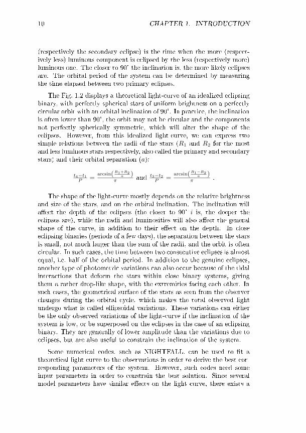
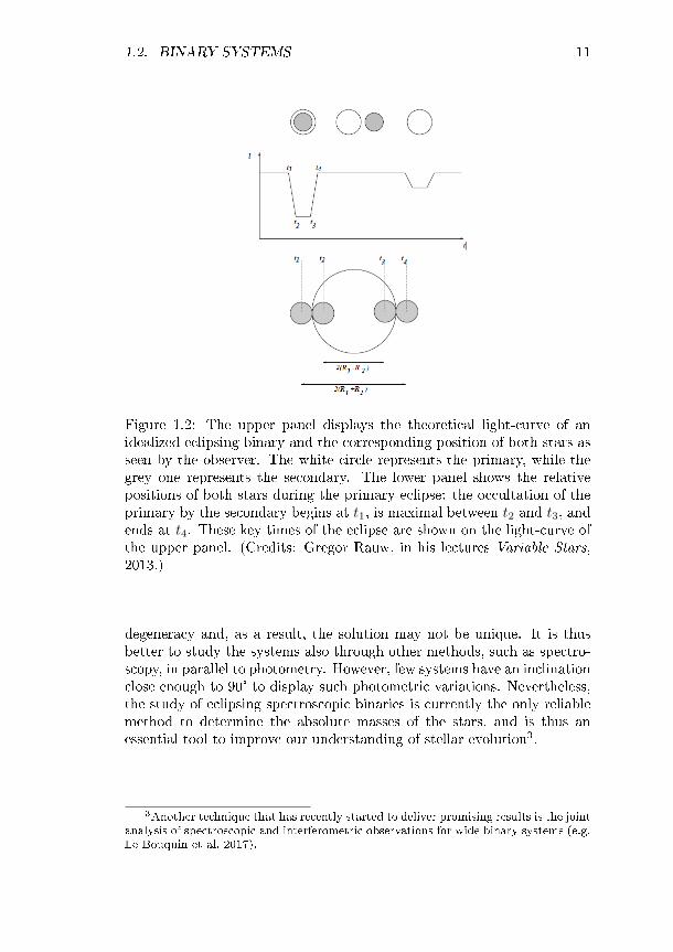
As mentioned in the previous section, the light-curves of eclipsing binar-ies display periodic decreases over the orbital cycle. These decreases arecaused by the passage of one component in front of the other, as seen fromthe observer's point of view. Therefore, the ux coming from the partlyhidden star is partly blocked, decreasing the total ux emitted by thesystem in our direction. The time of what is called the primary eclipse
10 CHAPTER 1. INTRODUCTION
(respectively the secondary eclipse) is the time when the more (respect-ively less) luminous component is eclipsed by the less (respectively more)luminous one. The closer to 90° the inclination is, the more likely eclipsesare. The orbital period of the system can be determined by measuringthe time elapsed between two primary eclipses.
The Fig. 1.2 displays a theoretical light-curve of an idealized eclipsingbinary, with perfectly spherical stars of uniform brightness on a perfectlycircular orbit with an orbital inclination of 90°. In practice, the inclinationis often lower than 90°, the orbit may not be circular and the componentsnot perfectly spherically symmetric, which will alter the shape of theeclipses. However, from this idealized light-curve, we can express twosimple relations between the radii of the stars (R1 and R2 for the mostand less luminous stars respectively, also called the primary and secondarystars) and their orbital separation (a):
t4−t1P =
arcsin(R1+R2a )
π and t3−t2P =
arcsin(R1−R2a )
π .
The shape of the light-curve mostly depends on the relative brightnessand size of the stars, and on the orbital inclination. The inclination willaect the depth of the eclipses (the closer to 90° i is, the deeper theeclipses are), while the radii and luminosities will also aect the generalshape of the curve, in addition to their eect on the depth. In closeeclipsing binaries (periods of a few days), the separation between the starsis small, not much larger than the sum of the radii, and the orbit is oftencircular. In such cases, the time between two consecutive eclipses is almostequal, i.e. half of the orbital period. In addition to the genuine eclipses,another type of photometric variations can also occur because of the tidalinteractions that deform the stars within close binary systems, givingthem a rather drop-like shape, with the extremities facing each other. Insuch cases, the geometrical surface of the stars as seen from the observerchanges during the orbital cycle, which makes the total observed lightundergo what is called ellipsoidal variations. These variations can eitherbe the only observed variations of the light-curve if the inclination of thesystem is low, or be superposed on the eclipses in the case of an eclipsingbinary. They are generally of lower amplitude than the variations due toeclipses, but are also useful to constrain the inclination of the system.
Some numerical codes, such as NIGHTFALL, can be used to t atheoretical light-curve to the observations in order to derive the best cor-responding parameters of the system. However, such codes need someinput parameters in order to constrain the best solution. Since severalmodel parameters have similar eects on the light curve, there exists a
1.2. BINARY SYSTEMS 11
Figure 1.2: The upper panel displays the theoretical light-curve of anidealized eclipsing binary and the corresponding position of both stars asseen by the observer. The white circle represents the primary, while thegrey one represents the secondary. The lower panel shows the relativepositions of both stars during the primary eclipse: the occultation of theprimary by the secondary begins at t1, is maximal between t2 and t3, andends at t4. These key times of the eclipse are shown on the light-curve ofthe upper panel. (Credits: Gregor Rauw, in his lectures Variable Stars,2013.)
degeneracy and, as a result, the solution may not be unique. It is thusbetter to study the systems also through other methods, such as spectro-scopy, in parallel to photometry. However, few systems have an inclinationclose enough to 90° to display such photometric variations. Nevertheless,the study of eclipsing spectroscopic binaries is currently the only reliablemethod to determine the absolute masses of the stars, and is thus anessential tool to improve our understanding of stellar evolution3.
3Another technique that has recently started to deliver promising results is the jointanalysis of spectroscopic and interferometric observations for wide binary systems (e.g.Le Bouquin et al. 2017).

12 CHAPTER 1. INTRODUCTION
1.3 Interactions in massive binary systems
In the previous section we introduced the main categories of binary sys-tems, how to observe them and how to interpret the variations we observein their spectra or light-curves. These variations are only due to our par-ticular observer status, and are not due to genuine interactions betweenthe components. However, Sana et al. (2012) showed that the majority ofmassive stars are part of close binaries and will eventually interact withtheir companion during stellar lifetimes, and one third of the systems willinteract while both stars are still on the main sequence. Such interactionsmay strongly inuence the subsequent evolution of the components in suchsystems. We will here introduce four types of interactions that are relev-ant in the context of this thesis work : the collision between the stellarwinds of both components, the Roche lobe overow (RLOF) mechanism,the inuence of binarity on the rotational mixing within the stellar atmo-spheres and the common-envelope evolution. We will also briey discussthe possible characteristics of post-interaction binary products.
1.3.1 Wind-wind interactions
When two massive stars are part of a binary system, their stellar windsinteract with each other, especially in close binaries. That is what iscalled colliding-wind binaries. This interaction can be either a collisionbetween the two stellar winds, or in some cases the collision between oneof the winds and the surface of the companion. Either ways, it breaks thespherical symmetry of the wind, and leaves some signatures throughoutthe electromagnetic spectrum of the system.
The wind interaction region is limited by two hydrodynamical shocks,each facing one of the components. If the winds have similar terminalvelocities and densities, the surface of contact discontinuity between theshocks is theoretically a plane midway between both stars (Fig. 1.3(a)). Ifthe winds are signicantly dierent, the momentum uxes will be dier-ent, and the contact discontinuity will no longer be a plane, but rather acurved surface with the concave side facing the star with the less energeticwind (Fig. 1.3(b)). The region between the shocks is called the wind in-teraction zone. The interaction of two stellar winds is however a complexhydrodynamical phenomenon, that can undergo large instabilities aect-ing the shape of the interaction zone (Stevens et al. 1992). Moreover, inthe specic case of close massive binaries, the Coriolis force due to theorbital motion of the stars also has a strong impact on the shape of theshocks and the interaction zone (e.g. Pittard & Parkin 2010).

1.3. INTERACTIONS IN MASSIVE BINARY SYSTEMS 13
Figure 1.3: The (a) panel displays a schematic diagram of colliding stellarwinds of identical strengths. The dashed line represents the contact dis-continuity, at equal distance from both stars. The solid lines represent thetwo hydrodynamical shocks (Stevens et al. 1992). The (b) panel displaysa hydrodynamic simulation of two stellar winds with dierent momentumuxes (Stevens et al. 1992). The primary star is located at the originof the axes, and the secondary star on the x-axis at x= 1. The dashedline is the surface of momentum balance (see Stevens et al. 1992 for moredetails) and the converging density contour lines in between the two windshocks indicate the contact discontinuity. (Credits: Stevens et al. 1992).
Since the strong winds of WR and O stars display supersonic velocit-ies (terminal velocities of 1000-3000 km s−1), the main signature of theshock-heated plasma in the collision zone between these winds is expec-ted to occur in the X-ray domain, with the associated emission displayingsignicant phase-locked variability, as a consequence of the changing windopacity along the line of sight towards the interaction zone, or as a resultof changing orbital separation in the case of eccentric binaries (Cazorla etal. 2014, see Rauw & Nazé 2016 for a review). However, we can see quitea few discrepancies with observations: some systems display either signi-cantly stronger or lower emission in the X-ray domain than expected bythe models, or lack the phase-locked variations in their emissions (see e.g.Rauw & Nazé 2016).
Other signatures of the interaction zone can also be observed in other
14 CHAPTER 1. INTRODUCTION
wavelength domains, such as phase-locked prole variations of some op-tical and UV lines of massive binaries, as we will see later in this work.For example, the Hα and He ii λ 4686 lines can display extra emission asa function of the orbital phase, as shown in Fig. 4 of Raucq et al. (2017),Sect. 3.3 of the present work. In some cases, the interaction zone can alsocreate features in the radio or infrared domains, but these specic casesgo beyond the eld of this thesis and will not be further discussed here.
1.3.2 Roche lobe overow mechanism
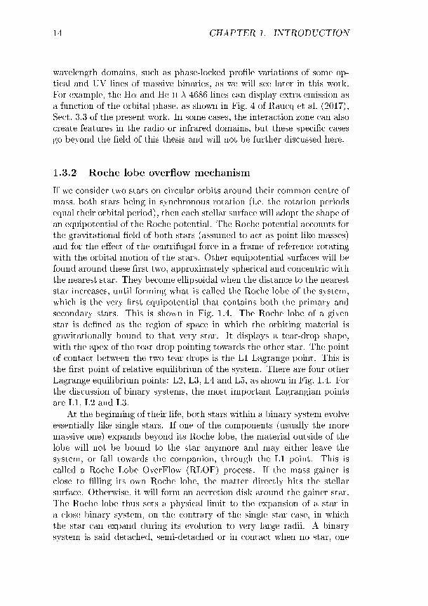
If we consider two stars on circular orbits around their common centre ofmass, both stars being in synchronous rotation (i.e. the rotation periodsequal their orbital period), then each stellar surface will adopt the shape ofan equipotential of the Roche potential. The Roche potential accounts forthe gravitational eld of both stars (assumed to act as point-like masses)and for the eect of the centrifugal force in a frame of reference rotatingwith the orbital motion of the stars. Other equipotential surfaces will befound around these rst two, approximately spherical and concentric withthe nearest star. They become ellipsoidal when the distance to the neareststar increases, until forming what is called the Roche lobe of the system,which is the very rst equipotential that contains both the primary andsecondary stars. This is shown in Fig. 1.4. The Roche lobe of a givenstar is dened as the region of space in which the orbiting material isgravitationally bound to that very star. It displays a tear-drop shape,with the apex of the tear-drop pointing towards the other star. The pointof contact between the two tear-drops is the L1 Lagrange point. This isthe rst point of relative equilibrium of the system. There are four otherLagrange equilibrium points: L2, L3, L4 and L5, as shown in Fig. 1.4. Forthe discussion of binary systems, the most important Lagrangian pointsare L1, L2 and L3.
At the beginning of their life, both stars within a binary system evolveessentially like single stars. If one of the components (usually the moremassive one) expands beyond its Roche lobe, the material outside of thelobe will not be bound to the star anymore and may either leave thesystem, or fall towards the companion, through the L1 point. This iscalled a Roche Lobe OverFlow (RLOF) process. If the mass gainer isclose to lling its own Roche lobe, the matter directly hits the stellarsurface. Otherwise, it will form an accretion disk around the gainer star.The Roche lobe thus sets a physical limit to the expansion of a star ina close binary system, on the contrary of the single star case, in whichthe star can expand during its evolution to very large radii. A binarysystem is said detached, semi-detached or in contact when no star, one
1.3. INTERACTIONS IN MASSIVE BINARY SYSTEMS 15
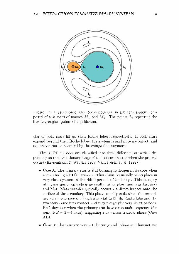
Figure 1.4: Illustration of the Roche potential in a binary system com-posed of two stars of masses M1 and M2. The points Li represent theve Lagrangian points of equilibrium.
star or both stars ll up their Roche lobes, respectively. If both starsexpand beyond their Roche lobes, the system is said in over-contact, andno matter can be accreted by the companion anymore.
The RLOF episodes are classied into three dierent categories, de-pending on the evolutionary stage of the concerned star when the processoccurs (Kippenhahn & Weigert 1967; Vanbeveren et al. 1998):
Case A: The primary star is still burning hydrogen in its core whenencountering a RLOF episode. This situation usually takes place invery close systems, with orbital periods of 2−4 days. This categoryof mass-transfer episode is generally rather slow, and may last sev-eral Myr. Mass transfer typically occurs via direct impact onto thesurface of the secondary. This phase usually ends when the second-ary star has accreted enough material to ll its Roche lobe and thetwo stars come into contact and may merge (for very short periods,P<2 days) or when the primary star leaves the main sequence (forperiods P ∼ 2−4 days), triggering a new mass transfer phase (CaseAB).
Case B: The primary is in a H burning shell phase and has not yet

16 CHAPTER 1. INTRODUCTION
begun to burn helium in its core. It occurs for periods ranging from4 days to 1000 days. Mass accretion in these systems occurs typic-ally via an accretion disk. The mass transfer rate is higher for widersystems, in which the donor is more evolved when the RLOF episodebegins (De Mink et al. 2013). On the other hand, these authors havealso shown that tighter systems evolve more conservatively, result-ing in more massive secondaries in comparison to wider systems.Surprisingly, in their simulations, the remaining main-sequence life-time of the secondary seems roughly independent of the amountof accreted mass or the orbital period, as a consequence of twocounteracting eects. Indeed, if higher stellar mass due to ecientaccretion implies shorter evolutionary timescales, i.e. a reductionof the remaining lifetime, the mass accretion also results in mixingof fresh hydrogen into the central regions, extending the remain-ing lifetime. Most systems with extreme mass ratios encounteringa case B RLOF episode are expected to enter a phase of commonenvelope evolution soon after the onset of mass transfer (see Sect.1.3.4). The tighter systems are expected to result in a merger, witha post-main-sequence star product, either a blue or red supergiant.In wider systems, the binding energy of the envelope of the primaryis smaller and the momentum and energy in the orbit are larger,and the envelope can be ejected.
Case C: When the orbital period is larger than 1000 days, the RLOFtakes place when the primary has exhausted the He in its core.When the primary star loses mass, we assume it reacts by expand-ing, resulting in very high mass transfer rates. As the Roche lobetypically shrinks, this leads to a common envelope phase (De Minket al. 2013).
Note that the period ranges quoted here are only rough indications anddepend on the mass of the donor star and on the metallicity of the system.For stars with initial masses larger than 40 M, the mass decrease ismainly due to the strong stellar wind during the LBV phase, reducingthe importance of the RLOF as a mass-losing process (Vanbeveren etal. 1998).
The mass transfer during a RLOF episode is far from being an an-ecdotic process: it has a huge role in the subsequent evolution of thecomponents. Indeed, it changes the relative masses, luminosities and ef-fective temperatures of both stars, thus changing their spectral types. Italso strongly aects the surface chemical abundances, since the primaryloses the H-rich layers of its atmosphere, revealing the deeper layers af-fected by the CNO cycle. The CNO abundances at the surface of the

1.3. INTERACTIONS IN MASSIVE BINARY SYSTEMS 17
primary star are thus enhanced (Vanbeveren 1982). Moreover, if thesecondary accretes during the RLOF episode, it may also receive CNOenhanced material from the primary, thus displaying slight overabund-ances in those elements at its surface (Vanbeveren & de Loore 1994). Itwill further receive angular momentum during the transfer, since the an-gular momentum of the whole system is conserved, which will speed-upits rotational velocity (Vanbeveren & de Loore 1994) and may induce en-hanced rotational mixing which will aect the subsequent evolution of thesecondary (see Sect. 1.3.3).
For massive binaries, the massive overcontact binary (MOB) evolu-tion has also been proposed by Marchant et al. (2016) to be an altern-ative formation channel of double compact objects (white dwarfs (WD),neutron stars (NS) and black holes (BH)) binary systems. This scenarioinvolves the chemically homogeneous evolution of rapidly rotating andvery massive stars in tidally locked binaries, i.e. very close binary sys-tems. Indeed, such very close and massive binaries are supposed to evolveinto contact, with both binary components lling and even overlling theirRoche lobes. The evolution during the over-contact phase diers from aclassical common-envelope phase (see Sect. 1.3.4) as co-rotation can, inprinciple, be maintained by the strong tidal forces as long as materialdoes not overow the L2 point. This means that a spiral-in due to viscousdrag can be avoided, resulting in a stable system evolving on a nucleartimescale. In this case, the stars remain fully mixed due to their tidallyinduced high spin.
Once both stars overow past the outer Lagrangian point, L2, Marchantet al. (2016) expect the system to merge rapidly, either due to mass lossfrom L2 carrying a high specic angular momentum or due to a spiral-indue to the loss of co-rotation. However, these authors nd that a largenumber of MOBs may swap mass several times but survive as a closebinary until the stars collapse. These MOB systems can thus lead to theformation of double black holes binaries that will eventually merge withina Hubble time. The gure 1.5 illustrates the binary stellar evolution of agiven system leading to the formation of such BH + BH binary.
The merger delay time, i.e. the time between the formation of the BH+ BH binary and the eventual merger, is a strong function of metallicity,where the merger delay times (at a given BH mass) are systematicallyshorter for lower metallicity. Moreover, if the black holes receive kicks atbirth, even higher-metallicity systems may merge very rapidly if the kickreduces the pericenter distance. One of the advantages of this scenario isthat it can lead to the formation of much more massive double BH binariescompared to other evolutionary pathways. Marchant et al. (2016) werealso able to reproduce observed local counterparts of various stages in the

18 CHAPTER 1. INTRODUCTION
Figure 1.5: Illustration of the binary stellar evolution of a given 70M +56M close binary system at a Z/50 metallicity (Marchant et al. 2016).The masses of the stars in solar masses are indicated with red numbers,and the orbital periods in days are given as black numbers. A phase ofcontact near the ZAMS causes mass exchange. Acronyms used in thegure. ZAMS: zero-age main sequence; TAMS: termination of hydrogenburning; He-star: helium star; SN: supernova; GRB: gamma-ray burst;BH: black hole. (Credits: Marchant et al. 2016).
MOB scenario, such as HD 5980, IC10 X-1 and NGC 300 X-1.
1.3.3 Rotational mixing
The rotation is thought to be a major factor in the evolution of massivestars, with huge consequences for their chemical compositions, ionizinguxes and nal fates (De Mink et al. 2009). Evolutionary models pre-dict that rotation has major eects on the core hydrogren-burning phase(Maeder & Meynet 2000; Heger & Langer 2000; Hirschi et al. 2004; Yoon

1.3. INTERACTIONS IN MASSIVE BINARY SYSTEMS 19
& Langer 2005; Brott et al. 2011b; Potter et al. 2012; Ekström et al.2012), and there is growing evidence that in a fraction of massive stars,the nal collapse and explosion is governed by rapid rotation, giving riseto hyper-energetic supernovae and long-duration gamma-ray bursts (Yoonet al. 2006; Woosley & Heger 2006; Georgy et al. 2009). Models of rotat-ing single stars can also successfully account for the surface enhancementsof N and He observed in massive main-sequence stars, but recent observa-tions have questioned the idea that rotational mixing is the main processresponsible for the surface enhancements, and other theories suggest thatstellar winds and binary interactions are probably at least partly respons-ible of such modications of the surface abundances (De Mink et al. 2009).
The origin of the distribution of initial stellar masses and initial stellarrotation rates are not yet fully understood (e.g. Krumholz 2011; Rosen etal. 2012). For example, it is a key issue whether stars inherit their rotationrates from their parental molecular clouds, since the specic angular mo-mentum of such clouds is several orders of magnitudes larger than whatcan be placed in a rotating star (e.g. Bodenheimer 1995). Several obser-vational studies suggest initial median stellar rotation rates for massivestars between 0.20× vcrit (Wol et al. 2006) and 0.40× vcrit (Huang et al.2010).
Either way, whatever the origin of their birth rotation rates is, severalprocesses may aect the rotation of massive stars during their life, causingdeviations from the initial values:
Modication of the stellar structure. During core hydrogen-burning,massive stars expand by about a factor of three. However, the cor-responding spin-down of the surface layers is prevented by analogouscontraction of the stellar core combined with an ecient transportof angular momentum from the core to the envelope (Ekström et al.2008; Brott et al. 2011a), and the rotational velocity at the equator,vrot, increases slightly over the main-sequence evolution of the star,until it reaches a value close to the Keplerian rotation rate. In theabsence of an ecient angular momentum loss mechanism, the starremains rotating close to this Keplerian limit, which drops as thestar evolves and expands. The change in radius of more massivestars during the main sequence is larger, resulting in a more sig-nicant drop in the Keplerian velocity. As a result, the Keplerianrotational velocity at the end of the main sequence is around 400km s−1 with only a weak dependence on the stellar mass. In themost luminous stars the eects of radiation pressure cannot be ig-nored and the Keplerian limit should be considered as an upper limitto the physical maximum.
20 CHAPTER 1. INTRODUCTION
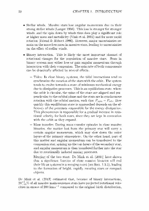
Stellar winds. Massive stars lose angular momentum due to theirstrong stellar winds (Langer 1998). This loss is stronger for strongerwinds, and the spin-down by winds thus does play a signicant roleat higher mass and metallicity (Vink et al. 2001) and for more rapidrotation (Friend & Abbott 1986). However, major uncertainties re-main on the mass-loss rates in massive stars, leading to uncertaintieson the eect of stellar winds.
Binary interaction. This is likely the most important channel ofrotational changes for the population of massive stars. Stars inbinary system may either lose or gain angular momentum throughinteraction with their companion. The spin rate of both componentscan be drastically aected by several eects.
Tides: In close binary systems, the tidal interactions tend tosynchronize the rotation of the stars with the orbit. The systemtends to evolve towards a state of minimum mechanical energydue to dissipative processes. This is an equilibrium state, wherethe orbit is circular, the spins of the stars are aligned and per-pendicular to the orbital plane and the stars are in synchronousrotation with the orbital motion, such that P spin = Porb. Howquickly this equilibrium state is approached depends on the ef-ciency of the processes responsible for the energy dissipation.This phenomenon is responsible for a gradual increase in rota-tional velocity for both stars, since they are kept in corotationwith the orbit as they expand.
Mass transfer: During mass transfer episodes in close massivebinaries, the matter lost from the primary star will carry acertain angular momentum, which may slow down the outerlayers of the primary atmosphere. On the other hand, part ofthis matter and angular momentum can be transferred to thecompanion star, spining up the top layers of the secondary star,and angular momentum is then transfered further into the stardue to rotationally induced mixing processes.
Merging of the two stars: De Mink et al. (2014) have shownthat a signicant fraction of close massive binaries will endtheir life as systems in a merging event (see Sect. 1.3.5), leadingto the formation of bright, rapidly rotating stars or compactobjects.
De Mink et al. (2013) estimated that, because of binary interactions,20+5−10% of all massive main-sequence stars have projected rotational velo-
cities in excess of 200 km s−1 compared to the original birth distribution,

1.3. INTERACTIONS IN MASSIVE BINARY SYSTEMS 21
the main uncertainties being the mass transfer eciency and the possibleeect of magnetic braking, which may also have a spin-down eect. Mostof the more rapid rotators, according to these authors, are products of aRLOF episode. A smaller number are merger products.
1.3.4 Common-envelope evolution
Common-envelope (CE) evolution is thought to play an important rolein the formation of numerous close binaries composed of two compactobjects. Indeed, as we have already discussed earlier, binary processes areneeded to explain some observed properties of some systems, such as thecurrent small orbital separation, often much smaller than the radii of theprogenitors, of some objects. In such cases, the CE evolution is a goodcandidate, since it is accompanied by a drag-force, arising from the motionof the in-spiralling object through the envelope of its companion star,which leads to the dissipation of some orbital angular momentum and thedeposition of orbital energy in the envelope. Hence, the global outcome ofa CE phase is a reduced binary separation and ejected envelope, unless thestars composing the system merge. The in-spiral of the companion starcan decrease the orbital separation by a factor of ∼100 or more (Kruckowet al. 2016).
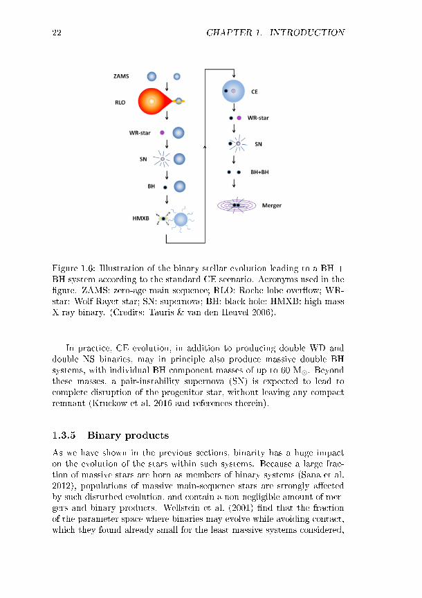
The main steps of CE evolution leading to a BH + BH system arepresented in Fig. 1.6.
There is observational evidence of such orbital shrinkage in a numberof known binary pulsars and WD pairs with an orbital period of a fewhours or even less. The central question in the CE theory is whether amassive binary will survive a CE evolution or result in an early mergerevent without ever forming a double compact system. For example, in thistheory, the systems always enter a CE phase after the high-mass X-raybinary (HMXB) stage, during which the secondary massive star becomesa red supergiant and captures its BH companion (Kruckow et al. 2016).Whether the donor star envelope is ejected successfully depends on thebinding energy of the envelope, the available energy resources to expel itand the ejection mechanism.
The possible ejection of the envelope thus depends on the mass andradius of the donor star. Envelope ejection is facilitated for giant starscompared to less evolved stars, and, as long as the in-spiralling BH mass ishigh enough, they probably succeed in ejecting the envelopes of their hoststars (Kruckow et al. 2016). However, if the in-spiralling object moves toofar inward, there is no possibility of ejecting the envelope, and the systemmerges.
22 CHAPTER 1. INTRODUCTION
Figure 1.6: Illustration of the binary stellar evolution leading to a BH +BH system according to the standard CE scenario. Acronyms used in thegure. ZAMS: zero-age main sequence; RLO: Roche lobe overow; WR-star: Wolf-Rayet star; SN: supernova; BH: black hole; HMXB: high-massX-ray binary. (Credits: Tauris & van den Heuvel 2006).
In practice, CE evolution, in addition to producing double WD anddouble NS binaries, may in principle also produce massive double BHsystems, with individual BH component masses of up to 60 M. Beyondthese masses, a pair-instability supernova (SN) is expected to lead tocomplete disruption of the progenitor star, without leaving any compactremnant (Kruckow et al. 2016 and references therein).
1.3.5 Binary products
As we have shown in the previous sections, binarity has a huge impacton the evolution of the stars within such systems. Because a large frac-tion of massive stars are born as members of binary systems (Sana et al.2012), populations of massive main-sequence stars are strongly aectedby such disturbed evolution, and contain a non-negligible amount of mer-gers and binary products. Wellstein et al. (2001) nd that the fractionof the parameter space where binaries may evolve while avoiding contact,which they found already small for the least massive systems considered,

1.3. INTERACTIONS IN MASSIVE BINARY SYSTEMS 23
becomes even smaller for larger initial primary masses. Assuming con-stant star formation, de Mink et al. (2014) nd that 8+9
−4% of a sample ofearly-type stars are the products of a merger resulting from a close binarysystem, and 30+10
−15% of massive main-sequence stars are the products ofbinary interactions.
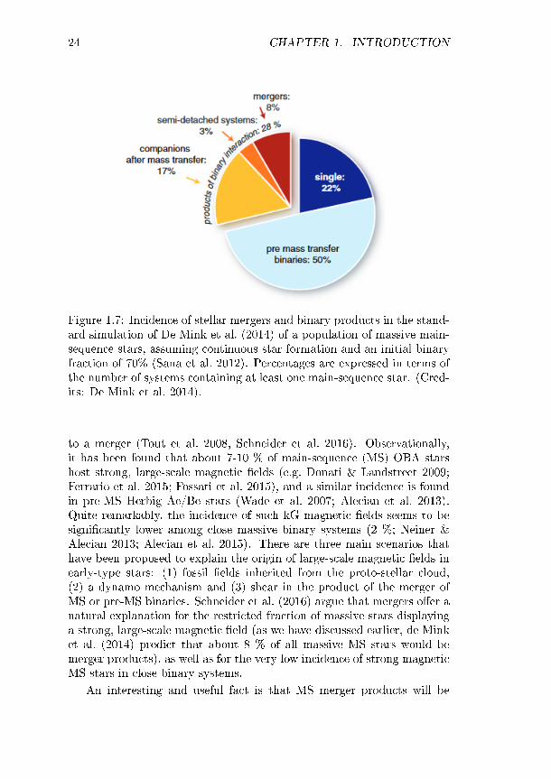
These authors started their simulations with 70% binaries and 30%single massive stars at birth. For the case of continuous star formation,their simulations end up to the results shown in Fig. 1.7. The contribu-tion of pre-interaction binaries in the current population goes down from70% to 50%, 22% of the stars are referred as single stars, and more thana quarter of the stars have been severely aected by interactions with acompanion. This group of post-interaction stars are composed of mer-gers (8%), semi-detached systems (i.e. systems currently undergoing masstransfer through RLOF; 3%) and stars that have previously gained massfrom a (former) companion (17%). The latter group is composed by sys-tems containing a main-sequence star accompanied by a helium star, aNS, a WD or a BH. Note that the low percentage of systems currentlyundergoing RLOF episodes is easily explainable by the short timescaleof such events, typically a few thermal timescales at most, compared tothe stellar lifetime. In their study of incidence, de Mink et al. (2014) didnot take into account post-interaction double compact systems. They con-clude that it is completely counter-productive to exclude detected binariesfrom a sample of early-type stars to reduce the contamination by binaryproducts on population statistics, since binary products are typically notdetected as such and will therefore represent a larger fraction of the samplethan genuine single stars.
In addition to such main-sequence binary products, we have also seenin Sect. 1.3.2 and Sect. 1.3.4 that massive binary systems may also evolveinto double compact systems, and particularly into BH + BH systems.What is important to note with such BH + BH systems is that, if theyare close enough, they may rapidly merge, leading to potential sourcesof gravitational waves. Kruckow et al. (2016) have shown that the CEformation channel in a low metallicity environment for binary systemswith initial masses of ∼ 50 M may lead to the production of relativelymassive systems like the progenitor of GW150914 and give birth to grav-itational waves. Moreover, these authors have shown that the CE form-ation channel could also explain the progenitor of GW151226 regardlessthe metallicity of its environment.
Another interesting consequence of binary evolution could be the gen-eration of a strong magnetic eld via a dynamo operating because of dif-ferential rotation and convection during CE evolution that (nearly) leads
24 CHAPTER 1. INTRODUCTION
Figure 1.7: Incidence of stellar mergers and binary products in the stand-ard simulation of De Mink et al. (2014) of a population of massive main-sequence stars, assuming continuous star formation and an initial binaryfraction of 70% (Sana et al. 2012). Percentages are expressed in terms ofthe number of systems containing at least one main-sequence star. (Cred-its: De Mink et al. 2014).
to a merger (Tout et al. 2008, Schneider et al. 2016). Observationally,it has been found that about 7-10 % of main-sequence (MS) OBA starshost strong, large-scale magnetic elds (e.g. Donati & Landstreet 2009;Ferrario et al. 2015; Fossati et al. 2015), and a similar incidence is foundin pre-MS Herbig Ae/Be stars (Wade et al. 2007; Alecian et al. 2013).Quite remarkably, the incidence of such kG magnetic elds seems to besignicantly lower among close massive binary systems (2 %; Neiner &Alecian 2013; Alecian et al. 2015). There are three main scenarios thathave been proposed to explain the origin of large-scale magnetic elds inearly-type stars: (1) fossil elds inherited from the proto-stellar cloud,(2) a dynamo mechanism and (3) shear in the product of the merger ofMS or pre-MS binaries. Schneider et al. (2016) argue that mergers oer anatural explanation for the restricted fraction of massive stars displayinga strong, large-scale magnetic eld (as we have discussed earlier, de Minket al. (2014) predict that about 8 % of all massive MS stars would bemerger products), as well as for the very low incidence of strong magneticMS stars in close binary systems.
An interesting and useful fact is that MS merger products will be

1.3. INTERACTIONS IN MASSIVE BINARY SYSTEMS 25
rejuvenated (Schneider et al. 2016 and references therein), i.e. they willappear younger than other stars formed at the same time such as othercluster members and companions in multiple systems. This rejuvenationis due to mixing of fresh fuel into the cores of merger products and shorterlifetimes associated with more massive stars, and is of the order of the realage of the merger, i.e. of the order of the nuclear timescale of the star.The rejuvenation is the stronger the more evolved the progenitors, thelower the masses of binaries and the larger the mass ratios. On the otherhand, merging pre-MS stars will not necessarily rejuvenate. They canlead to merger products that reach the ZAMS either earlier because ofthe decreased contraction timescale due to the increased mass, or laterbecause of the additional orbital energy that has to be radiated awaybefore the core heats up enough to start hydrogen burning. In any case,the delay is of the order of the thermal timescale and therefore practicallyundetectable.
As a conclusion, we can say that binary products are probably rathercommon in a massive star population, and not always easily distinguish-able from single stars. However, there are a number of hints that can helpto identify individual binary products, even if not all binary products areexpected to show all these characteristics and none of the characteristicsuniquely signies binary interaction.
Surface abundances anomalies may be found in binary products,indicating enhanced mixing, loss of the outer layers of the stellaratmosphere or accretion of enriched gas.
Peculiar rotation rates (see Sect. 1.3.3).
If binary interaction occured recently, there may be signs of sheddedmaterial in the circumstellar medium, either an ejection nebula or acircum-stellar disk. The typical lifetime of such a nebula is expectedto be ∼ 104 years (Langer 2012).
Several studies (e.g. Tout et al. 2008; Ferrario et al. 2009; Schneideret al. 2016) suggest that the merging of two stars may lead to thegeneration of a strong magnetic eld.
The supernova explosion of the primary may cause the system tobreak up, leading to the creation of runaway or walk-away sec-ondary stars.
Binary products are not expected to have a main-sequence compan-ion not showing any unusual properties.

26 CHAPTER 1. INTRODUCTION
If the former companion which has become a compact object is stillpresent, the system may show UV or X-ray excess when the compactobject accretes material from its companion.
Within their birth clusters, the binary products may be over-luminousand possibly appear younger than the age of the cluster.
1.4 The present work
In the previous sections, we have seen the importance of massive stars inthe Universe, and the huge inuence of the multiplicity on the evolutionof such stars. It is thus of the utmost importance to accurately constrainthe multiplicity and the fundamental parameters of individual componentsin order to better understand the evolution processes in a given binarysystem, and thus improve our understanding of these key ingredients ofthe Universe.
In this context, this thesis consists in the in-depth study of four mul-tiple systems, using high-quality observations. For each object, we haveused a disentangling procedure to separate the contributions of each com-ponent to the observed spectra of the system. In this way, we were ableto determine the individual parameters of each component as if the starswere single. We have then determined the spectral types of each com-ponent, and the brightness ratio of the system. This preparatory analysispermitted us to determine the rotational and macroturbulence velocities,and the fundamental properties of each star.
The two main numerical tools used in this study, the disentanglingprocedure and the CMFGEN model atmosphere code, are presented inthe next chapter.
The third chapter is then dedicated to the individual study of eachsystem: HD 149404, LSS 3074, HD 17505 and HD 206267.
Finally, in the last chapter, we recall the main results that we obtained,present the conclusions of this work, and propose some perspectives offuture work that could be done to complement this study and furtherimprove our knowledge and understanding of massive binary stars.

Chapter 2
Numerical tools and methods
2.1 Spectral disentangling
2.1.1 Method
As we have seen in the previous chapter, the study of individual compon-ents of a binary system is important to better understand the underlyingphysics of the system. In order to recover the separate contribution ofboth components to the observed binary spectrum, we applied a spectraldisentangling method. This way, we were able to study the fundamentalparameters of each star as if it were single.
For this purpose, we used our disentangling routine (Rauw 2007),which is based on the Iterative Doppler dierencing technique developedby González & Levato (2006). This method was previously used by, e.g.,Linder et al. (2008), and improved by Mahy et al. (2012) to introduce athird contribution in the spectra, either a third component of the systemor the ISM contribution.
The technique is based on an iterative process that allows to calcu-late both the spectra of the components and their radial velocities, in aspectroscopic binary system. The technique operates on the normalizedspectra of the binary system. It uses alternately the spectrum of onecomponent to calculate the spectrum of the other one. The spectra areexpressed in a logarithmic scale, i.e. as a function of x = ln λ instead ofλ. Since the radial velocities in normal binary systems are quite smallcompared to the speed of light, this permits to express the Doppler shiftin the following uniform way
27

28 CHAPTER 2. NUMERICAL TOOLS AND METHODS
lnλ = ln[λ0
(1 +
v
c
)]= lnλ0 + ln
(1 +
v
c
)' lnλ0 +
v
c
⇒ x ' x0 +v
c
For the typical values of radial velocities in binary systems, the Dopplereect hence results in a simple linear shift of the wavelength scale.
The rst step is to remove the interstellar contribution to the observedspectra, by setting the ux in the wavelength regions where they appearto unity, in order to keep only the contributions of the components of thesystem. The observed spectrum can thus be expressed as:
S(x) = A(x− vA(φ)
c
)+B
(x− vB(φ)
c
)with A(x) and B(x) the spectra of the primary and the secondary stars,respectively, in the heliocentric frame of reference, and vA(φ) and vB(φ)their respective radial velocities at the given orbital phase φ.
In order to recover the individual spectra of each component, we usean iterative process:
1. For each observation i, we subtract the current best estimate ofthe spectrum of component B, shifted by the radial velocities of thesecondary component at the corresponding phase, from the observedspectra.
2. The residual spectra are cross-correlated with a mask to obtain im-proved estimates of the radial velocities of the primary componentfor each observation. The residual spectra are then shifted into theprimary's frame of reference and combined into a weighted mean toyield our new best approximation of star A's spectrum.
3. We calculate the current best approximation of the spectrum of thesecondary, B, similarly to step 1, but reverting the roles of A and Bof step 1.
4. We rene the radial velocities of the secondary component, similarlyto step 2.

2.1. SPECTRAL DISENTANGLING 29
In order to begin this iterative process, a rst approximation of the radialvelocities is thus needed, then rened during the calculations. It is alsopossible to x the radial velocities to the values obtained from knownorbital solution of the system for the entire calculation. We chose thissolution for this thesis work, in order to avoid the appearance of problemsthat can arise in the RV determination (steps 2 and 4) when the lines ofboth components are not easily seen on the spectra. Another input neededto start this iterative process is a rst approximation of the spectrum ofone of the components. A at spectrum is usually used for the componentB as a starting point for the iterations. The spectrum A thus contains allspectral features of the observed spectra at the beginning of the process.
The nal spectra of the primary and secondary stars can thus be ex-pressed as follows:
A(x) = 1n
n∑i=1
[Si
(x+ vA(φi)
c
)−B
(x+ vA(φi)
c − vB(φi)c
)]and
B(x) = 1n
n∑i=1
[Si
(x+ vB(φi)
c
)−A
(x+ vB(φi)
c − vA(φi)c
)]where n is the number of observations and vA(φi) and vB(φi) are the radialvelocities of the primary and secondary stars, respectively, at phase φi.These expressions represent averages of the observed spectra from whichthe secondary (resp. the primary) spectrum shifted by the appropriatevelocity has been subtracted (González & Levato 2006). In each iteration,the residuals of the secondary lines still present in the A spectrum arereduced approximately by a factor 1/n. The convergence and the qualityof the reconstructed spectra of the primary and secondary componentsthus directly depend on the number of observed spectra. The quality ofthe input data has also a strong inuence on the quality of the outputspectra, especially for the weakest component, as we will further discussin Sect. 2.1.2 and Sect. 3.3.
A generalisation of this method has been performed by Mahy et al.(2012) in order to introduce a third component to the spectra, either athird stellar companion or the interstellar lines. The observed spectra canthus be expressed by
S(x) = A(x− vA(φ)
c
)+B
(x− vB(φ)
c
)+ C
(x− vC(φ)
c
).
This technique is similar to that for a binary system: the third com-ponent is rst approximated by a at spectrum, then we successively

30 CHAPTER 2. NUMERICAL TOOLS AND METHODS
calculate the mean spectra of two components, shifted by their respectiveradial velocities, and subtract them from the observed spectra in orderto compute the mean spectrum of the remaining component. At eachiteration, we create temporary residual spectra from the observed spectrafrom which the contributions of two components have been subtractedand we apply a cross-correlation technique on these templates to renethe determination of the radial velocities of the third object. For eachiteration, this process is applied to each component of the system.
At the end of the process, the mean spectra of each component can beexpressed by
A(x) = 1n
n∑i=1
[Si(x+
vA(φi)
c
)− B
(x+
vA(φi)
c − vB(φi)
c
)− C
(x+
vA(φi)
c − vC (φi)
c
)]
B(x) = 1n
n∑i=1
[Si(x+
vB(φi)
c
)− C
(x+
vB(φi)
c − vC (φi)
c
)− A
(x+
vB(φi)
c − vA(φi)
c
)]
and
C(x) = 1n
n∑i=1
[Si(x+
vC (φi)
c
)− A
(x+
vC (φi)
c − vA(φi)
c
)− B
(x+
vC (φi)
c − vB(φi)
c
)]
similarly to the case of a binary system.
2.1.2 Limitations
Unfortunately, as for any disentangling method, the technique that wedescribed in the previous section also has its limitations (González &Levato 2006).
First of all, the quality of the results strongly depends on the RV rangecovered by the observations. Moreover, the heavily blended spectra aremore dicult to disentangle than less blended ones. It is thus very im-portant to cover a signicant fraction of the orbital cycle observationally,especially around the quadrature phases, where the lines associated to thetwo components are least blended. This will cause us some problems inthe specic case of the triple systems studied in this thesis work, as wewill further develop in Sect. 3.4 and Sect. 3.5. And, as we have mentionedearlier, the convergence of the algorithm is also dependent on the numberof observations, that should thus be suciently high.
Secondly, small residual errors in the normalization of the input spec-tra can lead to oscillations of the continuum in the resulting separatedspectra on wavelength scales of several dozen Å.
Moreover, the dierent spatial frequencies in the spectra are not re-covered with the same precision: broad spectral features are not recovered

2.2. CMFGEN 31
as accurately as narrow ones. In practice, features wider than a few timesthe RV amplitude are barely recovered.
Concerning the calculation of the RVs, the most serious problem ariseswhen the amplitude of the RV curve is comparable to the width of thespectral lines in the observed spectra. In practice, good convergence ofRVs is obtained when the maximum RV dierence between the compon-ents is at least the same order as the FWHM of the spectral lines.
Finally, in the specic case of interacting-wind binaries, some emissionlines present in the observations may be partly due to the wind-windinteraction zone. This will make it dicult to recover properly the spectra,since the ux of the lines formed in the wind interaction zone will beerroneously assigned to the two components.
2.2 CMFGEN
2.2.1 The code
To constrain the fundamental parameters of the stars within the studiedsystems, we used the model atmosphere code CMFGEN (Hillier & Miller1998). This is a radiative transfer code designed to solve the radiativetransfer and statistical equilibrium equations in the co-moving frame inplane-parallel or spherical geometry for the cases of Wolf-Rayet and O-type stars, Luminous Blue Variables and supernovae. To facilitate theiterative simultaneous solution of these equations, a partial linearizationmethod is used.
The CMFGEN code produces non-LTE1 line-blanketed models thatinclude the eects of stellar winds. Indeed, these three characteristics areessential for the modelling of massive hot stars. First, on the contraryof cooler stars, the LTE approximation is not appropriate for early-typestars, since the radiation eld is suciently strong so that the radiativeprocesses dominate over the collisional processes. In addition, the strongstellar winds of O and WR stars induce a strongly extended and perman-ently expanding stellar atmosphere. For those stars, the radiative transferthus cannot be treated with the plane-parallel approximation: the spher-ical geometry of the atmospheres must be taken into account within theequations, together with the expanding motion. Finally, to determine re-liable stellar parameters, it is essential to include the eect of blanketingdue to the numerous overlapping lines of many chemical species, and par-ticularly the heavy elements. Indeed, this blanketing acts as a "screen"which blocks the radiation, back-scattering the photons towards the in-
1LTE = Local Thermodynamic Equilibrium.

32 CHAPTER 2. NUMERICAL TOOLS AND METHODS
ner part of the atmosphere, thus increasing the local temperature andthe degree of ionization of this region. This back-warming eect impliesthat for a given spectral classication the line-blanketed model requires alower eective temperature to reach the same ionization. In addition, thisscreen also has the eect of reducing the ionization in the outer layers ofthe stellar atmosphere.
However, the inclusion of line-blanketing in the models makes the num-ber of statistical equilibrium equations quite large. To reduce this number,and improve the accuracy of the models, Hillier & Miller (1998) introducedthe idea of super levels, rst proposed by Anderson (1989). In their ap-proach, the levels of similar excitation energies and properties are groupedtogether and treated as a unique level in the statistical equilibrium equa-tions. Within a given group, they assume identical departure coecients,and only the population of the super level needs to be explicitly solvedin order to fully specify the populations of the independent levels. Thisapproach allows a lot of exibility, since the number of super levels andtheir links to real atomic levels are easily modied, and it is thus easilypossible to test the accuracy associated with various super-level assign-ments. Moreover, it permits to recover exactly the LTE conditions in thedeeper layers.
The hydrodynamical structure (density, velocity) is given as an inputto the code, the velocity structure being constructed from a combina-tion of an inner structure and a β velocity law in the outer parts of theatmosphere. The radiative equilibrium is assumed in order to determ-ine the temperature structure from the equation of energy conservationthroughout the atmosphere. When the level populations have converged,the radiative force is calculated and a new approximation of the innerstructure is computed and connected to the same β velocity law. Theradiative eld and level populations are then re-computed until the fullconvergence of the model is achieved. We usually performed three of thesehydrodynamical iterations at the beginning of our modelling, resulting ina self-consistent hydrodynamical structure. The density structure is ob-tained from the mass conservation equation.
CMFGEN also needs numerous input data to compute a given model:
1. The stellar parameters: The eective temperature (Teff), surfacegravity (log g), the luminosity (L), the radius (R), the mass (M),and the chemical abundances. In our computations, we included thefollowing elements: H, He, C, N, O, Ne, Si, S, Ar, Ca, Fe, and Ni.
2. The wind parameters: The mass-loss rate (M), the terminal velocity(v∞), and the clumping factors (f1 and f2).

2.2. CMFGEN 33
3. Some "environment" parameters, such as the input velocity struc-ture, the extension of the atmosphere, the number of depth points,the chemical species and ionization stages, the levels/superlevels foreach element.
The emergent spectrum is then computed using the code CMF_FLUX(Busche & Hillier 2005), in which is included a depth-dependent micro-turbulent velocity, varying from 10-20 km s−1 in the deeper layers to 10%of the terminal velocity of a given model in the upper wind. This spectrumis convolved with the appropriate rotational and macroturbulent velocit-ies, and compared to the observations of a given star. This comparisonpermits to iteratively constrain the fundamental parameters of this star.
2.2.2 Main diagnostics for the modelling
In the present thesis work, we mainly analysed optical spectra of thestudied stars, and we will thus focus on optical diagnostics for the stellarparameters in the present section. However, it is important to note thatthere are also numerous diagnostic features in the UV and IR regions ofa spectrum. For a more complete review of the UV, optical and near-IRdiagnostics of massive stars, see Martins (2011).
For our study of O-type stars, we relied on the following indicators tot the observed spectra and constrain the fundamental stellar properties:
Rotational velocity: The v sin i were obtained by applying a Four-ier transform method (Simón-Díaz & Herrero 2007; Gray 2008) tothe proles of reference lines. The main lines we used are He i λλ4026, 4922, 5016, O iii λ 5592, and C iv λ 5812. We selected theselines because they are well isolated in the spectra and are thereforeexpected to be free of blends. Metallic lines, such as O iii λ 5592,should be used as main indicators. When available, the followinglines can also be used: C iv λ 5802 or He i λ 4713. The best estim-ate of the projected rotational velocity is obtained from the positionof the rst zero of the Fourier transform. The synthetic spectracomputed by CMFGEN are convolved by a rotational prole cor-responding to our value of v sin i. For the specic case of LSS 3074(see Sect. 3.3), the poor quality of the recovered spectra made itimpossible to use these reference lines, and we had to use less ideallines for the determination of the projected rotational velocities ofthe components: He i λ 4471, He ii λλ 4200, 4542, 6118 and N iii
λ 6075 lines for the primary star of the system, and He ii λ 5412 andSi iv λ 4089 lines for the secondary star.

34 CHAPTER 2. NUMERICAL TOOLS AND METHODS
Macroturbulent velocity: The macroturbulence is dened as a non-thermal motion in the stellar atmosphere for which the size of theturbulent cells is greater than the mean free-path of the photons.This turbulence has for main eect to add a broadening componentto the spectral lines. A rst approximation of this velocity can beobtained by using the auxiliary program MACTURB of the stellarspectral synthesis program SPECTRUM v2.76 developed by Gray(2010), which is based on the radial-tangential anisotropic macrotur-bulent broadening formulation of Gray (2008). The main diagnosticlines for the determination of the macroturbulence velocity are O iii
λ 5592 and He i λ 4713 but we can also use the wings of strongerlines, such as He i λλ 4026, 4471, 5016, and He ii λ 4542. Typicaluncertainties on these velocities are ∼10 km s−1.
Eective temperature: The eective temperature is usually con-strained by comparing the lines of ions of the same element butof dierent ionization states. The classical diagnostic is the ratiobetween the He i λ 4471 and He ii λ 4542 lines, but complement-ary lines of helium can also be used, such as He i λλ 4026, 4389,4713, 5876, and He ii λλ 4200 and 5412. The temperatures derivedwith CMFGEN from a comparison with optical spectra have typ-ical uncertainties of 500 to 2000 K, depending on the quality of theobservations and on the eective temperature itself.
Surface gravity: The log g is generally constrained from the widthsof the Balmer lines. However, Hα is usually not used for constrain-ing this parameter, since this particular line is highly inuenced bynumerous stellar wind parameters. Moreover, as we have seen inSect. 2.1.2, the wings of broad lines are not as accurately recoveredby the disentangling as narrower features. We have thus constrainedthe surface gravities, together with the stellar luminosities, by com-paring the spectroscopic mass ratio to the dynamical mass ratioobtained in the orbital solutions of our systems, as fully explainedin Raucq et al. (2016), Sect. 3.2 of the present work. The typicaluncertainties that we obtained on the log g are 0.15-0.20 dex.
Mass-loss rate: In the optical domain, the main diagnostic lines toconstrain the mass-loss rate are Hα and He ii λ 4686 (Puls et al.1996). The strengths of Hγ and Hδ can also be taken as secondaryindicators, and are less sensitive to other wind parameters. We thusmainly worked with the latter secondary diagnostics. However, theycan be aected by emission from the wind-wind collision zone inclose massive binaries, and in those cases the obtained value of themass-loss rate can only be considered as an upper limit.

2.2. CMFGEN 35
Terminal velocity: The terminal velocity v∞ is the velocity reachedby the stellar winds at a very large distance from the star. Themain diagnostics on this parameters are in the UV eld, making itsdetermination with optical spectra rather dicult. The only hintfor a rst approximation of this parameters in the optical eld isthrough the strength of the Hα line. For a given mass-loss rate, alarger terminal velocity will reduce the wind density and hence lowerthe emission in this line. However, since the Hα line is also stronglyaected by other wind parameters, and by possible emission in thewind-wind interaction zone in close massive binaries, the determinedv∞ is rather uncertain and can only be considered as a lower limit.
Clumping: Previous studies have shown that the winds of O starsare not homogeneous (see, e.g., Eversberg et al. 1998 for observa-tional evidence and Bouret et al. 2005 for hints from atmospheremodelling). The clumping formalism used in our CMFGEN modelsis
f(r) = f1 + (1=f1)e(=V (r)f2
)
with a clumping lling factor f1 , a clumping velocity factor f2 andV (r) the velocity of the wind. The clumping lling factor repres-ents the maximum clumping at the top of the atmosphere and theclumping velocity is a parameter indicating the position in the ve-locity eld where the wind starts to be signicantly clumped. Thefunction f (r) thus represents the volume lling factor of the windby the clumps, assuming an empty interclump medium. These twoclumping factors can be slightly adjusted through the strength andthe shape of Hα and Hβ lines.
Finally, once the fundamental properties of the stars have been estab-lished, we can investigate the CNO abundances within their atmosphere,through the strengths of associated lines. We ran several models changingonly these abundances, and then performed a χ2 analysis to determine theones giving the best t to selected lines, and the associated uncertainties.For each element, we normalized the χ2 function by its minimum χ²min.As a 1-σ uncertainty on the abundances, we then considered abundancesup to a normalized χ2 of 2.0, i.e. an approximation for 1 over χ²min,as suggested by Martins et al. (2015). We selected the diagnostic linesamong the following lists, depending on the quality of the spectra and onthe spectral type:

36 CHAPTER 2. NUMERICAL TOOLS AND METHODS
Carbon abundance: C iii λλ 4068-70, 4156, 4163, 4187 and 5826.One to ve lines were used, except in the specic case of LSS 3074,see Raucq al. (2017), in Sect. 3.3 of the present work.
Nitrogen abundance: N ii λλ 4004, 4379, and 5026, N iii λλ 4511,4515, 4518, 4525, 4530, and 4535. Four to seven lines were used.
Oxygen abundance: O iii λλ 5508 and 5592. The only system forwhich we did not use the two lines was the specic case of LSS 3074,see Raucq al. (2017), in Sect. 3.3 of the present work.
For cooler spectral types, Martins et al. (2015) propose numerous otherlines to complement the study of surface abundances.

Chapter 3
Studied systems
3.1 Our sample of targets
We can nd in the literature a signicant number of (post-)RLOF massivebinaries candidates. Indeed, previous studies have eciently shown theexistence of binary interactions in close massive binaries, such as Plas-kett's star (Linder et al. 2008). Nazé et al. (2017; and references therein)also listed a sample of 15 (post-)interacting massive binaries candidates,presented in Table 3.1.
In the context of this work, we have selected two systems showingstrong hints of binary interactions: HD 149404, that shows strongly vari-able emission lines suggesting the presence of colliding winds and displaysa secondary star presented in the literature as being enriched in nitrogen;and LSS 3074, that has a very short orbital period, a strong phase-lockedvariability of the emission lines, and for which previous studies reportedunusually low minimum masses, considering the supergiant spectral types,which suggests that the system experienced a mass loss at some point.Note that Nazé et al. (2017) did not nd any evidence of a magnetic eldin any of these two systems.
To complement our study, we selected two other short-period massivemultiple systems, HD 17505 and HD 206267, poorly studied in the literat-ure, and searched for similar hints of binary interactions in their spectra,that may suggest that they experienced RLOF episodes.
37

38 CHAPTER 3. STUDIED SYSTEMS
Table 3.1: List of (post-)RLOF candidates proposed by Nazé et al. (2017).
HD ID Other
name
Spectral
types
Porb (days) Hints of
interaction
References
HD1337 AOCas O9.7III+
O9.5V
3.5 SD; PA Stickland 1997;
Linder et al. 2008
HD25638 SZCam O9.5V-9IV+
B0-0.5V
2.7 PA Lorenz et al. 1998;
Harries et al.
1998 ; Tamajo
et al. 2012;
Gorda 2015,
and references
therein
HD35652 IUAur O9.5V+
B0.5IV-V
1.8 PA Harries et al.
1998; Özdemir
et al. 2003, and
references
therein
HD35921 LYAur O9III+
O9.5III
4.0 SD/OC; PA Li & Leung 1985;
Drechsel et al.
1989; Stickland
et al. 1994;Mayer
et al. 2013;
Zhao et al. 2014,
and references
therein
HD57060 29CMa O8.5I+
O9.7V
4.4 SD/OC; PA;
WW
Bagnuolo et al.
1994; Stickland
1997; Linder et
al. 2008;
Antokhina
et al. 2011
HD100213 TUMus O7.5V+
O9.5V
1.4 C; PA Linder et al. 2007;
Qian et al. 2007;
Penny et al. 2008,
and references
therein
The symbol SD stands for semi-detached conguration, while C and OCstand for contact and overcontact congurations. PA is used to point out thepresence of anomalies in the stellar properties (either masses, radii, temperat-ures, luminosities and surface gravities) compared to the evolutionary models forsingle stars, and AA stands for surface abundances anomalies in at least onestellar atmosphere. Finally, we use the symbol WW to highlight the presenceof a probable wind-wind collision zone in the systems.

3.1. OUR SAMPLE OF TARGETS 39
Table 3.1: List of (post-)RLOF candidates proposed by Nazé et al. (2017).(continued)
HD ID Other
name
Spectral
types
Porb (days) Hints of
interaction
References
HD106871 ABCru O8V+
B0.5
3.4 SD; PA; AA Lorenz et al. 1994
HD115071 O9.5V+
B0.2III
2.7 SD; PA Penny et al. 2002,
and references
therein
HD149404 O7.5If+
ON9.7I
9.8 WW; AA;
asynchronous
rotation
Rauw et al. 2001;
Thaller et al.
2001; Raucq et
al. 2016
HD152248 O7.5III(f)
+
O7III(f)
5.8 WW; C; PA Sana et al. 2001,
2004; Mayer et
al. 2008
HD190967 O9.5V+
B1I-II
6.5 SD; PA Harries et al.
1997;
Kumsiashvili
et al. 2005
HD209481 LZCep O9III+
ON9.7V
3.1 both stars
almost ll their
Roche lobes;
AA; PA; slight
asynchronicity
Harries et al.
1998; Mahy et
al. 2011;
Palate et
al. 2013
HD228854 V382Cyg O7.3V+
O7.7V
1.9 SD/OC; PA Harries et al. 1997;
Degirmenci
et al. 1999;
Mayer et al. 2002;
Qian et al. 2007;
Ya³arsoy &
Yakut 2013,
and references
therein
LSS 3074 O5.5If+
O6.5-7If
2.2 WW; low
minimum
masses
Niemela et al.
1992; Haefner et
al. 1994; Raucq
et al. 2017
XZCep O9.5V+
B1III
5.1 SD; PA Harries et al. 1997

40 CHAPTER 3. STUDIED SYSTEMS
3.2 HD 149404
HD 149404 is a detached, non eclipsing O-star binary situated in the AraOB1 association, at a distance of 1.3 ± 0.1 kpc (Herbst & Havlen 1977).Rauw et al. (2001) have revised the orbital solution of this system andfound an orbital period of 9.81 days and a circular orbit, with a probableinclination of 21°. This system displays two interesting hints of past orpresent binary interaction. Indeed, the spectrum of HD 149404 showsvariable He ii λ 4686 and Hα emission lines that are likely indicative ofa wind-wind interaction (Rauw et al. 2001, Thaller et al. 2001, Nazé etal. 2002). Moreover, the secondary component of HD 149404 is foundin the literature as being an ON star, suggesting a signicant nitrogenenrichment of its atmosphere. These properties, together with the shortorbital period of the system, make it a good candidate for our study ofpossible post-mass transfer objects.
Our investigation of HD 149404 is based on 17 échelle spectra previ-ously used by Rauw et al. (2001). Five of these spectra were collected inMay 1999 with the FEROS spectrograph mounted on the ESO 1.5m tele-scope, and the remaining twelve spectra were collected in February 2000with the Coralie spectrograph mounted on the 1.2m Euler Swiss telescopelocated at La Silla (Chile).
We applied the disentangling technique described in Sect. 2.1 on theseoptical spectra to separate the contribution of both primary and sec-ondary stars. The obtained reconstructed spectra then permitted us todetermine accurately the spectral types of the components, revealing asystem composed by an O7.5If primary and an ON9.7 secondary star.Since the disentangling method does not yield the brightness ratio of thecomponents, we determined it by comparing the equivalent widths of aset of diagnostic lines for both stars to the mean equivalent widths of thesame lines in synthetic spectra of stars of the same spectral type, andobtained a brightness ratio of l1/l2 = 0.70±0.12. We determined the pro-jected rotational velocities of the stars by means of a Fourier TransformMethod applied on selected isolated lines of the reconstructed spectra andobtained v sin i of 93±8 and 63±8 km s−1 for the primary and secondaryrespectively. The macroturbulence velocities were then estimated to be70 and 80 km s−1 respectively.
We then tted the individual reconstructed spectra with the CMFGENatmosphere code (see Sect. 2.2) to constrain the stellar parameters of eachstar. This way, we obtained that the primary has a T eff of 34 000 K anda log g of 3.55, and the secondary displays a T eff of 28 000 K and a log gof 3.05.
To complement our study in the optical domain and check whether

3.2. HD 149404 41
the CMFGEN models are also able to correctly reproduce the wind fea-tures, we investigated the UV eld with a sample of 25 short-wavelength,high-resolution (SWP) IUE spectra of HD 149404 from the IUE archives.These spectra were described by Stickland & Koch (1996). The parts ofthe UV spectra that feature strong and broad wind lines cannot be prop-erly recovered by the disentangling code (see Sect. 2.1.2). To circumventthis problem, we re-combined the synthetic CMFGEN UV spectra of theprimary and secondary taking into account the radial velocity shifts atthe time of the observations, for several orbital phases. We found goodagreement between the obtained synthetic binary spectra and the obser-vations.
This spectroscopic study of the binary system HD 149404 permittedus to highlight two hints of previous binary interaction. First, we con-rmed the strong overabundance in nitrogen in the secondary atmosphere([N/C]∼150 [N/C]), and a slight nitrogen overabundance in the primaryatmosphere ([N/C]∼5 [N/C]). Second, we inferred an asynchronous ro-tation of the two stars, the primary displaying a rotational period of3.77± 0.32 days and the secondary a period of 7.46± 0.95 days.
We conclude that the hypothesis of a past case A RLOF interactionin the system HD 149404 is the most plausible one to explain the currentchemical surface abundances and rotational asynchronicity of the com-ponents, despite the fact that some of the observed properties challengethe current case A binary evolutionary models.
The full analysis of the HD 149404 binary system is published in Raucqet al. (2016, see paper hereafter).

42 CHAPTER 3. STUDIED SYSTEMS

A&A 588, A10 (2016)DOI: 10.1051/0004-6361/201527543© ESO 2016
Astronomy&
Astrophysics
Observational signatures of past mass-exchange episodes
in massive binaries: The case of HD 149 404⋆,⋆⋆
F. Raucq1, G. Rauw1, E. Gosset1,⋆⋆⋆, Y. Nazé1,⋆⋆⋆⋆, L. Mahy1,†, A. Hervé2, and F. Martins3
1 Department of Astrophysics, Geophysics and Oceanography, Liège University, Quartier Agora, Allée du 6 Août 19c, Bat. B5c,4000 Liège, Belgiume-mail: [email protected]
2 Astronomical Institute of the Czech Academy of Sciences, Fricova 298, 251 65 Ondrejov, Czech Republic3 LUPM, Montpellier University 2, CNRS, place Eugène Bataillon, 34095 Montpellier, France
Received 12 October 2015 / Accepted 14 January 2016
ABSTRACT
Context. Mass and momentum exchanges in close massive binaries play an important role in their evolution, and produce severalobservational signatures such as asynchronous rotation and altered chemical compositions, that remain after the stars detach again.Aims. We investigated these effects for the detached massive O-star binary HD 149 404 (O7.5 If + ON9.7 I, P = 9.81 days), which isthought to have experienced a past episode of case A Roche-lobe overflow (RLOF).Methods. Using phase-resolved spectroscopy, we performed the disentangling of the optical spectra of the two stars. The reconstructedprimary and secondary spectra were then analysed with the CMFGEN model atmosphere code to determine stellar parameters, suchas the effective temperatures and surface gravities, and to constrain the chemical composition of the components. We complementedthe optical study with the study of IUE spectra, which we compare to the synthetic binary spectra. The properties of the stars werecompared to evolutionary models.Results. We confirmed a strong overabundance in nitrogen ([N/C] ∼ 150 [N/C]⊙) for the secondary and a slight nitrogen over-abundance ([N/C] ∼ 5 [N/C]⊙) for the primary star. Comparing the two stars, we found evidence for asynchronous rotation, with arotational period ratio of 0.50 ± 0.11.Conclusions. The hypothesis of a past case A RLOF interaction in HD 149 404 is most plausible to explain its chemical abundancesand rotational asynchronicity. Some of the observed properties, such as the abundance pattern, are clearly a challenge for current caseA binary evolution models, however.
Key words. stars: early-type – stars: fundamental parameters – binaries: spectroscopic – stars: individual: HD 149 404 – stars: massive
1. Introduction
As shown in recent studies (e.g. Sana et al. 2012), a large por-tion of massive stars belongs to binary or higher multiplicitysystems. Whilst this multiplicity permits observationally deter-mining the minimum masses of the stars through their orbitalmotion, it also leads to complications. For instance, the bina-rity of massive stars can result in interactions between their stel-lar winds that produce observational signatures throughout theelectromagnetic spectrum (e.g. Rauw 2013). Moreover, duringthe lifetime of a massive binary, the binarity influences the evo-lution of the stars in various ways (e.g. Langer 2012). Theseevolutionary effects range from tidally induced rotational mix-ing (e.g. de Mink et al. 2009) over exchange of matter and an-gular momentum through a Roche lobe overflow (RLOF) inter-action (e.g. Podsiadlowski et al. 1992; de Loore & Vanbeveren1994; Wellstein et al. 2001; Hurley et al. 2002) to the merg-ing of both stars (e.g. Podsiadlowski et al. 1992; Wellsteinet al. 2001). In RLOF interactions, three different situations are
⋆ Based on observations collected at the European SouthernObservatory (La Silla, Chile) and with the International UltravioletExplorer.⋆⋆ The reduced spectra are only available at the CDS via anonymousftp to cdsarc.u-strasbg.fr (130.79.128.5) or viahttp://cdsarc.u-strasbg.fr/viz-bin/qcat?J/A+A/588/A10⋆⋆⋆ Senior Research Associate F.R.S-FNRS.⋆⋆⋆⋆ Research Associate F.R.S-FNRS.
† Postdoctoral Researcher F.R.S-FNRS.
distinguished: case A, for which the RLOF episode occurs whenthe mass-donor is on the core-hydrogen burning main-sequence;case B, when the star is in the hydrogen-shell burning phase; andcase C, for which the star is in the helium-shell burning phase(Kippenhahn & Weigert 1967; Vanbeveren et al. 1998). Thesebinary interactions significantly affect the physical properties ofthe components and their subsequent evolution. Despite consid-erable progresses in theoretical models, there remain a numberof open questions such as the actual efficiency of accretion (e.g.Wellstein et al. 2001; de Mink et al. 2007; Dray & Tout 2007).To better understand this phenomenon, we need in-depth studiesof systems undergoing or having undergone mass exchange.
In this context, HD 149 404 is an interesting target. It is adetached, non-eclipsing O-star binary, member of the Ara OB1association, located at a distance of 1.3 ± 0.1 kpc (Herbst &Havlen 1977). The orbital parameters were revised by Rauwet al. (2001). These authors found an orbital period of 9.81 daysand a circular orbit. They also estimated an orbital inclinationof 21 by comparing “typical” masses of supergiants with sim-ilar spectral types to those of both components. The spectrumof HD 149404 displays variable emission lines (He λ 4686,Hα) that are likely indicative of a wind-wind interaction (Rauwet al. 2001; Thaller et al. 2001; Nazé et al. 2002). One of itscomponents was assigned an ON spectral type, which suggestsa significant nitrogen enrichment of its atmosphere.
In this study, we determine the fundamental parameters ofthe stars of this system through several analysis techniques.The data used in our study are presented in Sect. 2. In Sect. 3
Article published by EDP Sciences A10, page 1 of 11

A&A 588, A10 (2016)
we present the preparatory treatment of our data, which includeddisentangling the spectra of the binary system to reconstruct in-dividual spectra of the binary components, which are neededfor the subsequent spectral analysis. The spectral analyses weremade with the non-LTE model atmosphere code CMFGEN andare presented in Sect. 4. In Sect. 5 we discuss the evolutionarystate of HD 149 404 and compare it with similar systems.
2. Observational data
The optical spectra analysed here are the échelle spectra usedby Rauw et al. (2001) in their study of the orbital solution andwind interactions of HD 149 404. These data were collectedin May 1999 and February 2000 with the FEROS and Coraliespectrographs mounted on the ESO 1.5m telescope and 1.2mEuler Swiss telescope at La Silla, respectively. The FEROSand Coralie spectrographs have resolving powers of 48 000
and 50 000 and cover the wavelength ranges 3650–9200Åand 3875–6800Å, respectively. Further details on the instrumen-tation and the data reduction are given by Rauw et al. (2001).Because of some problems with the extraction of the FEROSdata of May 2000, the normalization of the latter was more un-certain, and we therefore excluded these data from the disen-tengling procedure, and thus from the further analysis.
To complement our optical data, we also retrieved 25 short-wavelength, high-resolution (SWP) IUE spectra of HD 149 404from the IUE archives. These spectra were previously describedby Stickland & Koch (1996).
Table 1 yields the journal of observations along with the or-bital phases computed according to the ephemerides of Rauwet al. (2001, their He λ 4471 orbital solution). The optical spec-tra provide a good sampling of the orbital cycle, which is impor-tant for the disentangling in Sect. 3.
3. Preparatory analysis
3.1. Spectral disentangling
The previous determination of the orbital solution of the systemperformed by Rauw et al. (2001) allowed us to recover the indi-vidual spectra of both components by separating the normalizedspectra of the binary system. For this purpose, we used our dis-entangling routine (Rauw 2007), which is based on the methodof González & Levato (2006) and was previously used by Linderet al. (2008) and improved by Mahy et al. (2012). The basicidea behind this technique is that the most natural way to handlespectra for radial velocity measurements is to express them as afunction of x = ln λ instead of as a function of λ. In this way, theDoppler shift for a line of rest wavelength λ0 can be expressed as
ln λ = ln[λ0
(1 +v
c
)]
= ln λ0 + ln(1 +v
c
)
≃ ln λ0 +v
c
⇒ x ≃ x0 +v
c·
Let A(x) and B(x) be the spectra of the primary and secondary inthe heliocentric frame of reference. In the absence of line profilevariability and eclipses, the spectrum observed at any phase φcan be written as
S (x) = A
(x − vA(φ)
c
)+ B
(x − vB(φ)
c
),
Table 1. Journal of the optical (top) and UV (bottom) spectra.
Optical spectroscopyHJD-2 450 000 Inst. φ
1299.796 FEROS 0.241300.788 FEROS 0.341301.792 FEROS 0.451302.783 FEROS 0.551304.792 FEROS 0.751578.866 Coralie 0.681579.879 Coralie 0.781580.872 Coralie 0.881581.864 Coralie 0.981582.869 Coralie 0.091583.877 Coralie 0.191584.857 Coralie 0.291585.845 Coralie 0.391586.870 Coralie 0.491587.861 Coralie 0.591588.886 Coralie 0.701590.886 Coralie 0.90
IUE SWP spectroscopyJD-2 440 000 φ JD-2 440 000 φ
3718.044 0.76 4450.176 0.353724.588 0.42 4460.090 0.363776.869 0.75 9564.333 0.423776.921 0.76 9565.329 0.523776.966 0.76 9817.595 0.233793.028 0.40 9818.630 0.333798.965 0.00 9840.402 0.553926.010 0.95 9910.425 0.684001.156 0.60 9911.396 0.784001.203 0.61 9912.400 0.884120.089 0.72 9913.396 0.994129.216 0.65 9915.391 0.194412.327 0.50
where vA(φ) and vB(φ) are the radial velocities of stars A and Bat orbital phase φ.
For a total of n observed spectra, the spectrum of the primarycan be computed as the average of the observed spectra fromwhich the secondary spectrum shifted by the appropriate radialvelocity (RV) has been subtracted (González & Levato 2006) :
A(x) =1n
n∑
i=1
[S i
(x +vA(φi)
c
)− B
(x − vB(φi)
c+vA(φi)
c
)]·
And similarly for the secondary:
B(x) =1n
n∑
i=1
[S i
(x +vB(φi)
c
)− A
(x − vA(φi)
c+vB(φi)
c
)].
Starting from an initial approximation for B(x) (a flat spectrum),vA(φi) and vB(φi), we then iteratively determined the primary andsecondary spectra and their radial velocities (see González &Levato 2006). For the separations we performed here, we fixedthe radial velocities of the binary components to those corre-sponding to the orbital solution of Rauw et al. (2001).
As for any disentangling method, this technique also has itslimitations (González & Levato 2006). A reasonable observa-tional sampling of the orbital cycle is needed because the qualityof the results depends on the radial velocity (RV) ranges cov-ered by these observations. Another important limitation is thatbroad spectral features are not recovered with the same accu-racy as narrow ones. This is the case for the wings of the Balmer
A10, page 2 of 11


A&A 588, A10 (2016)
Table 4. Stellar parameters of the primary and secondary stars as obtained with CMFGEN.
This study Rauw et al. (2001)Prim. Sec. Prim. Sec.
R (R⊙) 19.3 ± 2.2 25.9 ± 3.4 24.3 ± 0.7 28.1 ± 0.7M (M⊙) 50.5 ± 20.1 31.9 ± 9.5 54.8 ± 4.6 33.0 ± 2.8Teff (104 K) 3.40 ± 0.15 2.80 ± 0.15 3.51 ± 0.1 3.05 ± 0.04log ( L
L⊙ ) 5.63 ± 0.05 5.58 ± 0.04 5.90 ± 0.08 5.78 ± 0.08
log g (cgs) 3.55 ± 0.15 3.05 ± 0.15β 1.03 f 1.08 f
v∞ (km s−1) 2450 f 2450 f
M (M⊙ yr−1) 9.2 × 10⁻⁷ f 3.3 × 10⁻⁷ f
BC −3.17 −2.67Notes. The best-fit CMFGENmodel parameters are compared with the parameters obtained by Rauw et al. (2001) for an orbital inclination of 21.The effective temperatures from Rauw et al. (2001) were derived through the effective temperature calibration of Chlebowski & Garmany (1991)and permitted, along with the determined luminosities, inferring the stellar radii. The quoted errors correspond to 1σ uncertainties. The symbol( f ) in the table corresponds to values fixed from the literature (Howarth et al. 1997; Muijres et al. 2012). The bolometric corrections are taken fromLanz & Hubeny (2003), based on our best-fit Teff and log g.
Table 5. Chemical abundances of the components of HD 149 404.
Primary Secondary Sun
He/H 0.1 0.1 0.089
C/H 1.02+0.10−0.11 × 10⁻⁴ 1.89+0.47−0.47 × 10⁻⁵ 2.69 × 10⁻⁴
N/H 1.32+0.20−0.15 × 10⁻⁴ 7.15+2.5−1.8 × 10⁻⁴ 6.76 × 10⁻⁵
O/H 7.33+1.1−1.1 × 10⁻⁴ 7.85+1.8−1.1 × 10⁻⁵ 4.90 × 10⁻⁴
Notes. Abundances are given by number as obtained with CMFGEN.The solar abundances (Asplund et al. 2009) are quoted in the last col-umn. The 1σ uncertainty on the abundances was set to abundancescorresponding to a χ2 of 2.0. As only one line was considered for theC abundance of the secondary, the corresponding calculated uncertaintywas unrealistically low. A similar problem was encountered for theO abundance of the primary star, for which we only had two lines towork with and several absent lines over the spectrum, as specified inthe second paragraph of this section. To circumvent these problems, weset the uncertainties for these two abundances to values close to thosecalculated for the other two elements of the corresponding star.
We stress two interesting results from our spectral analysis.First of all, we confirm the large overabundance of N in the sec-ondary spectrum. Second, we infer an asynchronous rotation ofthe two stars. The radii determined with CMFGEN (Table 4),the mean projected rotational velocities (Table 1), and the in-clination estimate from Rauw et al. (2001) yield the rotationperiods of the primary and secondary stars: 3.77 ± 0.32 daysand 7.46±0.95 days, respectively, or a period ratio of 0.50±0.11.We note that within the uncertainties on the inclination, the sec-ondary rotational period is similar to the orbital period of thesystem (9.81 days).We return to these points in Sect. 5. Finally,we note that according to the radii determined here, none of thestars currently fills its Roche lobe. With the formula of Eggleton(1983), we estimate a Roche-lobe volume filling factor of 15%for the primary and 73% for the secondary.
As pointed out above, disentangling the IUE spectra ofHD 149404 was more problematic, especially for those parts ofthe UV spectra that feature strong and broad wind lines and/orare polluted by blends with numerous interstellar features. Theleft panel of Fig. 2 illustrates the comparison of the separatedspectra and the synthetic spectra obtained with CMFGEN overa wavelength range that is relatively free of interstellar lines andmainly hosts photospheric lines. The agreement is clearly quitereasonable.
To check whether our CMFGEN models are also able to cor-rectly reproduce the wind features, we re-combined the syntheticCMFGEN UV spectra of the primary and secondary takinginto account the radial velocity shifts at the time of the obser-vations. We did so for several orbital phases. The right panelof Fig. 2 illustrates the result for three selected IUE spectra(SWP03008, JD 2 443798.965, SWP02755, JD 2 443 776.869,and SWP54350, JD 2 449817.595), corresponding to conjunc-tion phase 0.00 and quadrature phases 0.75 and 0.25. The syn-thetic spectrum clearly agrees well with the observation, ex-cept for a few narrow absorptions that are due to the interstellarmedium, which are not taken into account in our model. This ad-ditionally supports our determination of the physical parametersof the system components. Moreover, the concordance betweenthe synthetic and observed UV spectra suggests that the P-Cygniprofiles form over parts of the stellar winds that are not signifi-cantly affected by the wind-wind interactions, the latter leadingto a loss of spherical symmetry of the line formation region.
The fluxed CMFGEN spectra also allow us to estimate thebrightness ratio (primary/secondary) in the UV. We find a valueof 0.912.
Furthermore, we found relatively little variability of theP-Cygni profiles over the orbital period. Both observations (lackof strong variability and little effect of wind interaction on theline morphology) are likely due to the low orbital inclination(i ∼ 21) of the system. This inclination implies that the ob-served spectrum arises mostly at high stellar latitudes, wherethe wind-wind interaction zone has less influence on the windstructure.
5. Discussion and conclusion
5.1. Evolutionary status
As we have shown in the previous section, the spectra of thecomponents of HD 149404 display the signatures of some
2 This result is at odds with the 0.7mag difference (i.e. pri-mary/secondary brightness ratio of 1.91) between the primary and sec-ondary UV fluxes inferred by Howarth et al. (1997). This situationmost likely stems from the differences in the spectral types adoptedby Howarth et al. (1997), who classified the system as O8.5 I + O7 III,whilst we have derived O7.5 If + ON9.7 I. This difference in spectraltypes directly affects the strength of the cross-correlation peaks of thespectra of the two components with the template spectrum of τ Sco(B0.2 IV) and thus the correction on the magnitude difference inferredby Howarth et al. (1997).
A10, page 6 of 11

F. Raucq et al.: Signatures of past mass exchange in HD 149 404
Phase 0.00
Phase 0.25 Phase 0.75
Fig. 2. Upper left panel: comparison between the separated IUE spectra (black) of the primary and secondary stars around the He λ 1640 line andthe corresponding synthetic spectra (red). The primary spectrum is shifted upwards by 0.5 for clarity. The other three panels display a comparisonbetween the SWP03008 (upper right), SWP54350 (lower left) and SWP02755 (lower right) IUE spectra taken at phases 0.0, 0.25 and 0.75 inblack and the synthetic binary spectra obtained through combination of CMFGEN primary and secondary spectra at given phases in red.
enrichment by the products of stellar nucleosynthesis processes.These properties indicate a previous mass-exchange episode.Figure 3 compares our inferred N/C and N/O ratios with the pre-dictions for the evolution of single massive stars (Ekström et al.2012) either without rotation (left panel) or with a rotational ve-locity of 0.4 × vcrit (right panel). This figure clearly shows thatfor the spectroscopic masses of the primary and secondary starsthese models cannot account for the observed CNO abundancepatterns. For instance, in the case of models without rotation(left-hand panel of Fig. 3), no chemical enrichment is expectedduring the main-sequence evolution for stars with mass <60 M⊙.Only for the M > 60 M⊙ model is the loss of material throughstellar wind sufficient to reveal the products of the CNO cy-cle at the surface before the end of the main-sequence evolu-tion. Adopting instead the rotating models (right-hand panel ofFig. 3), the enrichment of the secondary can only be explainedby single-star evolution if we assume at least a star with 60 M⊙,whilst the spectroscopic mass is about a factor two lower. Whenthe surface abundances of a single star of 60 M⊙ initial massreach the values observed for the secondary of HD 149404, thecurrent mass of the star is still about 50 M⊙, that is, it is muchhigher than the mass determined for the secondary star.
The observed CNO abundance pattern is qualitatively mucheasier to interpret if the present-day secondary star was formerly
the more massive component of the binary and transferred massand angular momentum to the present-day primary in an RLOFepisode. During this process, the outer envelope of the secondarywas removed, revealing layers of material that were previouslyinside the convective hydrogen-burning core (Vanbeveren 1982,2011).
We start by comparing our results with theoretical predic-tions from the literature. The expectation is that the more masshas been lost by the donor, the deeper the layers that are revealedat the surface and thus the higher the N/C ratio. The predictedCNO abundances for the mass loser after a case B mass-transferepisode are [N/C] = 100 [N/C]⊙ and [N/O] ≥ 5 [N/O]⊙(Vanbeveren 1982). This is indeed close to what we observe inour analysis. Moreover, the RLOF scenario is re-enforced bythe values of the primary star abundances. Classical radiativeequilibrium evolutionary models predict normal H and He abun-dances for the mass gainer of an RLOF episode, but an N abun-dance of two to three times solar (Vanbeveren& de Loore 1994),which agrees with our results.
There are some caveats here, however. First, the resultsof Vanbeveren (1982) apply to case B mass transfer, whereasHD 149404 is more likely to have undergone a case A mass ex-change (see below). Second, when the outer hydrogen-rich lay-ers are removed, an enrichment of the stellar surface of the mass
A10, page 7 of 11

A&A 588, A10 (2016)
Fig. 3. Comparison of the N/C and N/O ratios determined from our spectral analyses with predictions from single-star evolutionary models ofdifferent masses (Ekström et al. 2012). The primary and secondary stars are shown by the open and filled square symbols, respectively. The leftpanel illustrates the results for core hydrogen-burning phase tracks without stellar rotation, whilst the right panel corresponds to the same tracksfor stars rotating at 0.4 × vcrit.
donor in helium is expected. Our spectral modelling was madewith the He abundance set to solar, however, and there is no hintfor our models requiring a He enhancement in any of the stars.Although the predicted relative change of helium surface abun-dance is usually much smaller than for N, this result is nonethe-less surprising, especially in view of the large N overabundanceof the secondary star.
To illustrate the helium enrichment that might be expected,we consider once more the single-star evolutionary tracks withrotation of Ekström et al. (2012). In these models, a nitrogen sur-face abundance similar to the one observed for the secondary isalways accompanied by an increase of the surface helium abun-dance to values higher than y = 0.35 by mass. The fact that thespectrum of the secondary of HD 149404 can be fit with a solarhelium abundance (y = 0.1) suggests that the internal structureof the secondary before the onset of mass transfer must havebeen different from that expected from single-star evolutionarymodels. Moreover, the RLOF in HD 149404 must have cometo a (temporary) stop before the full hydrogen-rich envelope ofthe mass donor was removed. The latter conclusion is also sup-ported by our finding that both stars are currently well insidetheir Roche lobes.
Given the present-day spectroscopic masses, the secondarymust have lost at least 9.3 M⊙ assuming a fully conservativemass transfer. Conservative RLOF will increase the period of thebinary. If we assume a fully conservativemass transfer and applythe formula of Vanbeveren et al. (1998), we find that the orbitalperiod would have increased by 17% at most, the shortest pos-sible initial orbital period being 8.4 days for a mass exchangeof 9.3 M⊙. However, Petrovic et al. (2005) argued that in fastcase A RLOF, only about 15–20% of the mass shed by the massdonor is indeed accreted by its companion. If the mass-transferefficiency is that low, then the secondary must have lost a muchlarger amount of mass. Such a non-conservative mass transfercan result from the transfer of angular momentum. In fact, themass gainer can be spun up to critical rotation and will then re-pel additional mass (and angular momentum), leading to a non-conservative mass transfer (e.g. Langer et al. 2003; Vanbeveren2011; Langer 2012). In the previous section, we noted that the
components of the system are apparently not in synchronous ro-tation. This asynchronicity therefore also suggests the existenceof a past mass and angular momentum transfer episode, with aclear spin up of the primary star.
In Fig. 4 we present the positions of the primary and sec-ondary stars in the Hertzsprung-Russell diagram (HRD) (upperpanels) and in the logg–logTeff diagram (lower panels), alongwith the evolutionary tracks from Ekström et al. (2012) for thecore-hydrogen burning phase of single stars at solar metallic-ity, both for non-rotating (left panels) and rotating (right panels)stars. This figure again illustrates the failure of single-star evolu-tionary tracks to account for the properties of the components ofHD 149404. If we consider the models without rotational mix-ing, the position of the primary star in the HRD is relatively closeto the track corresponding to its present-day spectroscopic mass.However, the secondary appears too luminous for its present-daymass compared to these evolutionary tracks. If we compare thestars to the 40% critical rotation case, we find that the primary’sluminosity is below that expected for its present-day spectro-scopic mass. Moreover, the secondary lies outside the rangecovered by tracks in the core-hydrogen burning phase. If weconsider the non-rotating case, we see that in the log g–logTeffdiagram the primary star has a lower effective temperature and ahigher surface gravity than expected for a 50 M⊙ star, whilst thesecondary star displays parameters corresponding to stars twiceas massive as its present-day spectroscopic mass. For stars rotat-ing at 40% of their critical velocity, we find that both stars wouldhave initial masses of about 30 M⊙. The primary dynamicalmassis about a factor 2 higher, while for the secondary the agreementis good. Finally, in all cases (with and without rotation and forboth diagrams), the two components of HD 149 404 are not lo-cated on the same isochrone, although they would be expectedto have the same age3.
In a mass-transfer episode, the location of both stars in theHRD after the RLOF strongly depends on the details of theprocess. For instance, spinning-up the mass gainer can lead to
3 The age of the AraOB1 association of which HD 149 404 is a mem-ber was estimated in the literature as ∼3 Myr (Wolk et al. 2008).
A10, page 8 of 11

F. Raucq et al.: Signatures of past mass exchange in HD 149 404
Fig. 4. Position of the primary (open square) and secondary (filled square) stars in the Hertzsprung-Russell diagram (upper panels) and the log g–log Teff diagram (lower panels) along with evolutionary tracks for single massive stars at solar metallicity during the core-hydrogen burning phase(Ekström et al. 2012). In the left panels, the evolutionary tracks correspond to non-rotating stars, whilst the right panels yield the results for starsrotating at 0.4 × vcrit. The dotted red lines correspond to isochrones of 3.2 and 6.3million years for the left panels and of 4.0 and 8.0million yearsfor the right panels.
almost complete mixing of the latter. In this situation, modelspredict that He would be enhanced in the atmosphere of the massgainer and that the latter would become bluer and overluminousfor its mass (Vanbeveren & de Loore 1994). If there is no strongspin-up and the accretion occurs rather slowly and is accompa-nied by a fast diffusion process, then the location of the gainerin the HRD should be very close to that of a normal star of thesame mass and chemical composition (Vanbeveren et al. 1998).The star is rejuvenated, however: it lies on an isochrone that cor-responds to a younger age than its actual age. The location of theprimary in the HRD suggests that in the present case the secondscenario is likely to apply with a very moderate rejuvenation, ifany, of the primary. This conclusion is supported by the lack of
a strong He enrichment, but it is at odds with the highly non-synchronous rotation of the primary reported above.
5.2. Comparison with other post-RLOF systems
In this section, we briefly compare the properties of HD 149 404with those of two other O-type binaries, Plaskett’s Star andLZCephei, which are probably in a post-case A RLOF evolu-tionary stage and have been analysed in a way similar to thepresent work (Linder et al. 2008; Mahy et al. 2011).
Plaskett’s Star (HD 47 129) is an O8 III/I + O7.5 III binarywith an orbital period of 14.4 days, slightly longer than that ofHD 149404, and a mass ratio near unity. Two observational
A10, page 9 of 11

A&A 588, A10 (2016)
facts suggest that the initially more massive primary has under-gone a case A RLOF episode in the past (Linder et al. 2008).First, the projected rotational velocity of the secondary star isremarkably high (mean value of 272.5 ± 35.0 km s−1) comparedto that of the primary (mean value of 65.7 ± 6.3 km s−1). Thisstrongly asynchronous rotation likely stems from a spin-up ofthe secondary star through a recent transfer of angular momen-tum from the primary star. Second, the primary star displaysnitrogen overabundance (N/N⊙ = 16.6 ± 5.0) and carbon de-pletion (C/C⊙ = 0.2 ± 0.1), as is typical of an advanced evo-lutionary stage, whilst no such nitrogen enrichment is seen inthe secondary spectrum4. Given the present-day configurationof HD 47 129, it seems that the transfer of angular momentumand the resulting spin-up of the mass gainer (the secondary inthis case) might have prevented accretion of a larger portion ofthe primary’s mass.
LZCephei (HD 209481) is an O9 III + ON9.7V binary witha short orbital period of 3.07 days (Kameswara Rao 1972) anda mass ratio (primary/secondary) of 2.53 (Mahy et al. 2011).Both components of LZCep almost fill their Roche lobe (Mahyet al. 2011; Palate et al. 2013). Mahy et al. (2011) found thatthe secondary displays a strong nitrogen enrichment (18 timessolar), carbon and oxygen depletion (0.1 times solar), and ahigh helium content (4 times solar), suggesting a very advancedstate of evolution. On the other hand, the primary displays onlyslightly altered surface abundances consistent with single-starevolution. This suggests that the mass transfer was strongly non-conservative. Mahy et al. (2011) noted a slight asynchronicity ofthe rotation periods of the order of 10–20%, but concluded thatthe system is probably on the verge of achieving synchroniza-tion. Comparison with single-star evolutionary tracks indicates asimilar age discrepancy as we have found here for HD 149404.The evolutionary masses (25.3+6.2−4.0 and 18.0+2.4−2.5 M⊙, for the pri-mary and secondary respectively) are significantly higher thantheir dynamical masses (16.9±1.0 and 6.7±1.0 M⊙ respectively,Mahy et al. 2011; Palate et al. 2013).
Although our sample is currently too limited to draw firmconclusions, the above comparison reveals several interesting re-sults that are worth studying in more detail with a larger sample.First, we note that in all three systems, the components appeareither over- or under-luminous when compared with single-starevolutionary tracks corresponding to their present-day masses.During its initial phases, case A mass transfer occurs on a ther-mal timescale leading to a very rapid mass exchange. However,the mass transfer subsequently slows down and occurs on a nu-clear timescale instead. By the time the mass transfer ends, bothstars would therefore be expected to be in thermal equilibriumagain. Since all three systems under consideration are in a de-tached configuration, the stars should thus have settled onto theirnew post-RLOF evolutionary tracks. The discrepancy betweenthe observed luminosities and those predicted by the single-starevolutionary tracks most likely stems from several effects, suchas observational uncertainties, altered chemical compositions(and hence opacities of the stellar material), and a rotational ve-locity history that differs from that assumed in the single-starmodels.
Our comparison shows that the degree of asynchronicity inthe three post-RLOF systems increases with orbital period (from
4 The apparent N underabundance of the secondary inferred by Linderet al. (2008) could be an artefact that is due to the relatively shallownitrogen lines of the secondary being washed out by its fast rotation andthe difficulties of properly normalizing echelle spectra with such broadand shallow features (see also Fig. 1 of Palate & Rauw 2014).
LZCep, over HD 149404 to HD 47 129). This is most proba-bly due to the higher efficiency of the tidal forcing in shorterperiod systems, or it might be seen as evidence that momen-tum transfer has played a larger role in those systems that havea wider present-day orbital separation. This is expected sincebinary evolution models predict spin-up to be less efficient incloser systems because in such systems the accretion stream di-rectly affects the mass gainer without forming an accretion disk(e.g. Langer 2012). The questions of synchronization and circu-larization in close binary systems with early-type stars, featuringradiative envelopes and convective cores, have been addressedby Zahn (1975) and Tassoul (1987). Zahn (1975) considered ra-diative damping of the dynamical tide in the outer layers of thestellar envelopes as the main mechanism for synchronization.The corresponding synchronization timescales strongly dependupon the tidal torque constant E2 , which varies by several or-ders of magnitude during the main-sequence lifetime of the star(Zahn 1977). Siess et al. (2013) provided a parametrization ofthis parameter as a function of stellar mass and relative ageof the star. Assuming that their formalism holds for the masses ofthe stars considered here and adopting an age of half the main-sequence age of the stars, we estimated the values of E2. Wethen evaluated the synchronization times following Eq. (4.28) ofZahn (1975) by means of moments of inertia tabulated by Claret& Giménez (1992). The results are 5.6× 10⁵ and 1.4× 10⁴ yearsfor the primary and secondary stars of HD 149404, respec-tively, 4.4 × 10⁶ and 27.6 × 10⁶ years for the primary and sec-ondary of Plaskett’s star, and 2.8 × 10⁴ and 2.5 × 10⁴ years forthe primary and secondary components of LZ Cephei. Tassoul(1987), on the other hand, proposed that the most effectivemechanism for synchronization is provided by large-scale hy-drodynamic motions in the interiors of the tidally distortedbinary components. The resulting timescales are considerablyshorter than those estimated following the formalism of Zahn(1975). We estimate synchronization timescales of 2.1 × 10⁴
and 3.2×10³ years for HD 149 404, 7.2×10⁴ and 2.0×10⁵ yearsfor Plaskett’s star, and 1.6 × 10³ and 6 × 10² years for LZ Cep.Regardless of which of the two formalisms is most appropriateto describe the evolution of rotation in the systems consideredhere, we find that, except perhaps for Plaskett’s Star, which hasa longer synchronization timescale, the RLOF phase probablymust have ended less than a few 104 years ago.
Another puzzling result is the fact that the post-RLOF mass-ratio deviates most from unity for the shortest period system(LZCep). Therefore, in this system, the RLOF must have beencomparatively more efficient than in the longer period systems.As discussed above, the mass transfer in LZCep was most likelyhighly non-conservative. If the material lost by the system doesnot carry away angular momentum in addition to the intrinsicorbital angular momentum, such a non-conservative mass lossleads to a widening of the orbital separation a given by
a
a= − M
M,
where M < 0 is the mass-loss rate (Singh & Chaubey 1986; Tout& Hall 1991). Assuming a fully non-conservativemass loss, thiswould imply that the initial orbital period of LZCep must havebeen shorter than 1.5 days. The duration of the RLOF episodedepends on the evolution of the Roche-lobe filling factor of themass donor. The evolution of the size of the Roche lobe is setby the relative importance of the orbit expansion and the shrink-ing of the relative size of the mass donor’s Roche lobe. In ad-dition, the evolution of the radius of the mass donor needs tobe accounted for (see Tout & Hall 1991). Since massive stars
A10, page 10 of 11

F. Raucq et al.: Signatures of past mass exchange in HD 149 404
with radiative envelopes contract considerably on a dynamicaltimescale (Tout & Hall 1991) and in view of the current mass-ratio of LZCep (Mahy et al. 2011), it seems unlikely that a non-conservative RLOF could be the explanation for a more efficientmass loss. Alternatively, if the material lost by the system car-ried off additional angular momentum, then the result could be ashrinking of the orbit. In active, low-mass stars, such a situationcould arise if the material lost by the donor corotates with thelatter under the effect of a magnetic field out to a wide distance(Tout & Hall 1991). However, strong magnetic fields are fairlyrare among single massive stars (∼7%), and their incidence ap-pears even lower among massive binaries (Neiner et al. 2015).Hence, this scenario also appears very unlikely in the case ofLZCep.
Clearly, the above trends call for confirmation by studyinga larger sample of post-case A RLOF massive binary systems.We are currently undertaking such studies, and the results willbe presented in forthcoming publications.
5.3. Summary and conclusion
We analysed the fundamental properties of the binary sys-tem HD 149 404 by means of spectral disentangling and theCMFGEN atmosphere code. Our investigation of this object rep-resents a significant improvement over previous studies becausewe have obtained the individual spectra of each component. Thisled to the determination of a number of stellar parameters thatwere used to constrain the evolutionary status of the system.
We established the existence of a large overabundance in Nand a C and O depletion in the secondary star and also founda slight N enhancement in the primary’s spectrum. We showedthat these surface abundances cannot be explained by single-starevolutionary models. Furthermore, we inferred an asynchronousrotation of the two stars of the system. These two results indi-cate a previous mass and angular momentum-exchange phasethrough a Roche-lobe overflow episode. Given the present statusof HD 149404 as an O+O binary, this mass transfer probablywas a case A RLOF. However, dedicated theoretical studies areneeded to understand the details of the evolution of this system.
Acknowledgements. The Liège team acknowledges support from the Fondsde Recherche Scientifique (FRS/FNRS) including especially an FRS/FNRSResearch Project (T.0100.15), as well as through an ARC grant for ConcertedResearch Actions financed by the French Community of Belgium (Wallonia-Brussels Federation), and an XMM PRODEX contract (Belspo). Anthony Hervéis supported by grant 14-02385S from GA CR.
References
Asplund, M., Grevesse, N., Sauval, A. J., & Scott, P. 2009, ARA&A, 47, 481Chlebowski, T., & Garmany, C. D. 1991, ApJ, 368, 241Claret, A., & Giménez, A. 1992, A&AS, 96, 255Conti, P. S. 1973, ApJ, 179, 161Conti, P. S. 1974, ApJ, 187, 539Conti, P. S., & Alschuler, W. R. 1971, ApJ, 170, 325Conti, P. S., & Frost, S. A. 1977, ApJ, 212, 728
de Loore, C., & Vanbeveren, D. 1994, A&A, 292, 463de Mink, S. E., Pols, O. R., & Hilditch, R. W. 2007, A&A, 467, 1181de Mink, S. E., Cantiello, M., Langer, N., et al. 2009, A&A, 497, 243Dray, L. M., & Tout, C. A. 2007, MNRAS, 376, 61Eggleton, P. P. 1983, ApJ, 268, 368Ekström, S., Georgy, C., Eggenberger, P., et al. 2012, A&A, 537, A146González, J. F., & Levato, H. 2006, A&A, 448, 283Gray, D. F. 2008, The Observation and Analysis of Stellar Photospheres, 3rd edn.
(Cambridge University Press)Gray, R. O. 2010, http://www.appstate.edu/~grayro/spectrum/spectrum276/node38.html
Herbst, W., & Havlen, R. J. 1977, A&AS, 30, 279Hillier, D. J., & Miller, D. L. 1998, ApJ, 496, 407Howarth, I. D., Siebert, K. W., Hussain, G. A. J., & Prinja, R. K. 1997, MNRAS,
284, 265Hurley, J. R., Tout, C. A., & Pols, O. R. 2002, MNRAS, 329, 897Kameswara Rao, N. 1972, PASP, 84, 563Kippenhahn, R., & Weigert, A. 1967, Z. Astrophys., 66, 58Lanz, T., & Hubeny, I. 2003, ApJS, 146, 417Langer, N. 2012, ARA&A, 50, 107Langer, N., Wellstein, S., & Petrovic, J. 2003, Proc. IAU Symp., 212, 275Linder, N., Rauw, G., Martins, F., et al. 2008, A&A, 489, 713Mahy, L., Martins, F., Machado, C., et al. 2011, A&A, 533, A9Mahy, L., Gosset, E., Sana, H., et al. 2012, A&A, 540, A97Martins, F. 2011, Bull. Soc. Roy. Sci. Liège, 80, 29Martins, F., & Hillier, D. J. 2012, A&A, 545, A95Martins, F., & Plez, B. 2006, A&A, 457, 637Martins, F., Schaerer, D., & Hillier, D. J. 2005, A&A, 436, 1049Martins, F., Hervé, A., Bouret, J.-C., et al. 2015, A&A, 575, A34Muijres, L. E., Vink, J. S., de Koter, A., Müller, P. E., & Langer, N. 2012, A&A,
537, A37Nazé, Y., Carrier, F., & Rauw, G. 2002, in Interacting Winds from Massive Stars,
eds. A. F. J. Moffat, & N. St-Louis, ASP Conf. Proc., 260, 457Neiner, C., Mathis, S., Alecian, E., et al. 2015, in Proc. IAU, 305, 61Palate, M., & Rauw, G. 2014, A&A, 572, A16Palate, M., Rauw, G., & Mahy, L. 2013, Central European Astrophysical
Bulletin, 37, 311Petrovic, J., Langer, N., & van der Hucht, K. A. 2005, A&A, 435, 1013Podsiadlowski, P., Joss, P. C., & Hsu, J. J. L. 1992, ApJ, 391, 246Rauw, G. 2007, DSc Thesis, University of Liège, BelgiumRauw, G. 2013, in Setting a New Standard in the Analysis of Binary Stars, eds.
K. Pavlovski, A. Tkachenko, & G. Torres, EAS Pub. Ser., 64, 59Rauw, G., Nazé, Y., Carrier, F., et al. 2001, A&A, 368, 212Reed, B. C. 2003, AJ, 125, 2531Sana, H., de Mink, S. E., de Koter, A., et al. 2012, Science, 337, 444Siess, L., Izzard, R. G., Davis, P. J., & Deschamps, R. 2013, A&A, 550, A100Simón-Díaz, S., & Herrero, A. 2007, A&A, 468, 1063Simón-Díaz, S., & Herrero, A. 2014, A&A, 562, A135Singh, M., & Chaubey, U. S. 1986, Ap&SS, 124, 389Stickland, D. J., & Koch, R. H. 1996, The Observatory, 116, 145Tassoul, J.-L. 1987, ApJ, 322, 856Thaller, M. L., Gies, D. R., Fullerton, A. W., Kaper, L., & Wiemker, R. 2001,
ApJ, 554, 1070Tout, C. A., & Hall, D. S. 1991, MNRAS, 253, 9Vanbeveren, D. 1982, A&A, 105, 260Vanbeveren, D. 2011, Bull. Soc. Roy. Sci. Liège, 80, 530Vanbeveren, D., & de Loore, C. 1994, A&A, 290, 129Vanbeveren, D., de Loore, C., Van Rensbergen, W. 1998, A&ARv, 9, 63van der Hucht, K. A. 1996, in Wolf-Rayet stars in the framework of stellar
evolution, Liège Int. Astrophys. Colloq., 33, eds. J.-M. Vreux, A. Detal, D.Fraipont-Caro, E. Gosset, & G. Rauw, 1
Wellstein, S., Langer, N., & Braun, H. 2001, A&A, 369, 939Wolk, S. J., Comerón, F., & Bourke, T. 2008, Handbook of Star Forming
Regions, Vol. II: The Southern Sky, ASP Monograph Publications, Vol. 5.ed. Bo Reipurth, 388
Zahn, J.-P. 1975, A&A, 41, 329Zahn, J.-P. 1977, A&A, 57, 383
A10, page 11 of 11

54 CHAPTER 3. STUDIED SYSTEMS

3.3. LSS 3074 55
3.3 LSS 3074
LSS 3074 is a short-period O-star binary system, with an orbital period of2.185 days, located behind the Coalsack region. We selected this systemfor our study due to this very short period, which makes it a good can-didate for a past RLOF episode. Besides, the primary star of LSS 3074is listed in the literature as being one of the few known O4f stars. Theseobjects are rare since they are thought to represent a short-lived trans-ition phase in the evolution of massive O-type stars before they becomeWolf-Rayet stars. Obtaining a good orbital and photometric solution ofthis system and determining the fundamental properties of its compon-ents oer therefore a precious opportunity to better understand these raretransition objects. Moreover, previous studies of LSS 3074 have providedsurprisingly low minimum masses for such early-type objects (8 and 9 M,Morrell & Niemela 1990, Niemela et al. 1992).
Our analysis of LSS 3074 is based on three EMMI spectra takenin March 2002 at the 3.5m New Technology Telescope (NTT) at theEuropean Southern Observatory (La Silla ESO), three Fiber-fed ExtendedRange Optical Spectrograph (FEROS) échelle spectra collected in April2002 with the ESO 1.52m telescope at La Silla and nine FEROS échellespectra taken in May 2003 and May 2004 with the 2.2m ESO/MPE tele-scope at La Silla. The system was also observed in photometry with theYale 1m telescope at the Cerro Tololo Interamerican Observatory betweenMarch and May 2001, using the Johnson system B, V, R, and I lters.Finally, XMM-Newton (Jansen et al. 2001) observed LSS 3074 twice. Therst observation, taken in August 2001, is centered on the system itself,and the second observation, taken in January 2003, is centered on the lowmass X-ray binary XB 1323-619, located at 6.9 arcmin from LSS 3074.The corresponding X-ray images of the eld are shown in Fig. 3.1.
Based on a number of well deblended lines in the optical spectra ofLSS 3074, we computed an orbital solution of the system, assuming acircular orbit. We determined the orbital period by combining a Fourieranalysis of the radial velocity curves and the photometric time series,and we obtained Porb = 2.1852 ± 0.0006 days. Our orbital solution alsoleads to low minimum masses (m sin3 i = 8.0± 0.5 and 9.3± 0.7 M forthe primary and secondary respectively), similar to those determined byNiemela et al. (1992).
This orbital solution then permitted us to recover the individual spec-tra of both components, using the disentangling method presented in Sect.2.1. We then determined the spectral types of O5.5 If for the primary andof O6.5-7 If for the secondary from the reconstructed individual spectra.By comparing the equivalent widths of a number of spectral lines in the
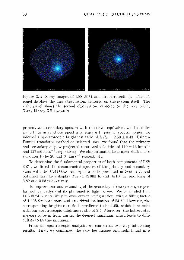
56 CHAPTER 3. STUDIED SYSTEMS
Figure 3.1: X-ray images of LSS 3074 and its surroundings. The leftpanel displays the rst observation, centered on the system itself. Theright panel shows the second observation, centered on the very brightX-ray binary XB 1323-619.
primary and secondary spectra with the mean equivalent widths of thesame lines in synthetic spectra of stars with similar spectral types, weinferred a spectroscopic brightness ratio of l1/l2 = 2.50 ± 0.43. Using aFourier transform method on selected lines, we found that the primaryand secondary display projected rotational velocities of 110 ± 13 km s−1
and 127±6 km s−1 respectively. We also estimated their macroturbulencevelocities to be 20 and 50 km s−1 respectively.
To determine the fundamental properties of both components of LSS3074, we tted the reconstructed spectra of the primary and secondarystars with the CMFGEN atmosphere code presented in Sect. 2.2, andobtained that they display T eff of 39 900 K and 34 100 K, and log g of3.82 and 3.83 respectively.
To improve our understanding of the geometry of the system, we per-formed an analysis of its photometric light curves. We concluded thatLSS 3074 is very likely in overcontact conguration, with a lling factorof 1.008 for both stars and an orbital inclination of 54.5°. However, thecorresponding brightness ratio is predicted to be 1.09, which is at oddswith our spectroscopic brightness ratio of 2.5. Moreover, the hottest starappears to be in front during the deepest minimum, which leads to di-culties to t this minimum.
From the spectroscopic analysis, we can stress two very interestingresults. First, we conrmed the very low masses and radii found in a

3.3. LSS 3074 57
previous study by Morrell & Niemela (1990), which is unusual for starswith such spectral types. Second, we found a strong overabundance in Nand a strong depletion in C and O in both primary and secondary stars.In addition, the primary star also displays a strong He enrichment in itsatmosphere. We proposed several evolutionary pathways through a RLOFprocess to explain both the low masses and the chemical abundances ofboth components of LSS 3074. Moreover, we conrmed that the systemis apparently in an overcontact conguration and has lost a signicantfraction of its mass to its surroundings. We suggested that some of thediscrepancies between the spectroscopic and photometric properties of thesystem may come from a strong radiation pressure of the primary.
The complete analysis of the LSS 3074 binary system is published inRaucq et al. (2017, see paper hereafter).

58 CHAPTER 3. STUDIED SYSTEMS
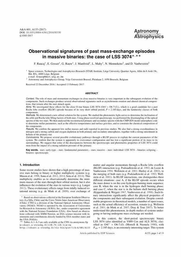
A&A 601, A133 (2017)DOI: 10.1051/0004-6361/201630330c© ESO 2017
Astronomy&Astrophysics
Observational signatures of past mass-exchange episodesin massive binaries: the case of LSS 3074⋆,⋆⋆
F. Raucq1, E. Gosset1, G. Rauw1, J. Manfroid1, L. Mahy1, N. Mennekens2, and D. Vanbeveren2
1 Space sciences, Technologies and Astrophysics Research (STAR) Institute, Liège University, Quartier Agora, Allée du 6 Août 19c,Bât. B5c, 4000 Liège, Belgiume-mail: [email protected]
2 Astronomy and Astrophysics Group, Vrije Universiteit Brussel, Pleinlaan 2, 1050 Brussels, Belgium
Received 22 December 2016 / Accepted 13 February 2017
ABSTRACT
Context. The role of mass and momentum exchanges in close massive binaries is very important in the subsequent evolution of thecomponents. Such exchanges produce several observational signatures such as asynchronous rotation and altered chemical composi-tions, that remain after the stars detach again.Aims. We investigated these effects for the close O-star binary LSS 3074 (O4 f + O6-7:(f):), which is a good candidate for a pastRoche lobe overflow (RLOF) episode because of its very short orbital period, P = 2.185 days, and the luminosity classes of bothcomponents.Methods. We determined a new orbital solution for the system. We studied the photometric light curves to determine the inclination ofthe orbit and Roche lobe filling factors of both stars. Using phase-resolved spectroscopy, we performed the disentangling of the opticalspectra of the two stars. We then analysed the reconstructed primary and secondary spectra with the CMFGEN model atmosphere codeto determine stellar parameters, such as the effective temperatures and surface gravities, and to constrain the chemical composition ofthe components.Results. We confirm the apparent low stellar masses and radii reported in previous studies. We also find a strong overabundance innitrogen and a strong carbon and oxygen depletion in both primary and secondary atmospheres, together with a strong enrichment inhelium of the primary star.Conclusions. We propose several possible evolutionary pathways through a RLOF process to explain the current parameters of thesystem. We confirm that the system is apparently in overcontact configuration and has lost a significant portion of its mass to itssurroundings. We suggest that some of the discrepancies between the spectroscopic and photometric properties of LSS 3074 couldstem from the impact of a strong radiation pressure of the primary.
Key words. stars: early-type – stars: fundamental parameters – stars: massive – stars: individual: LSS 3074 – binaries: eclipsing –binaries: spectroscopic
1. Introduction
Some recent studies have shown that a high percentage of mas-sive stars belong to binary or higher multiplicity systems (e.g.Mason et al. 1998; Sana et al. 2012, 2014; Sota et al. 2014). Thismultiplicity enables us to observationally determine the mini-mum masses of the stars through their orbital motion, but it alsoinfluences the evolution of the stars in various ways (e.g. Langer2012). These evolutionary effects range from tidally induced ro-tational mixing (e.g. de Mink et al. 2009), over exchange of
⋆ Based on observations collected at the European Southern Observa-tory (La Silla, Chile) and the Cerro Tololo Inter-American Observatory(Chile). CTIO is a division of the National Optical Astronomy Obser-vatory (NOAO). NOAO is operated by the Association of Universitiesfor Research in Astronomy (AURA), Inc., under cooperative agreementwith the National Science Foundation (USA). Also based on observa-tions collected with XMM-Newton, an ESA science mission with in-struments and contributions directly funded by ESA member states andthe USA (NASA).⋆⋆ Tables A.1–A.3 are only available at the CDS via anonymous ftpto cdsarc.u-strasbg.fr (130.79.128.5) or viahttp://cdsarc.u-strasbg.fr/viz-bin/qcat?J/A+A/601/A133
matter and angular momentum through a Roche lobe overflow(RLOF) interaction (e.g. Podsiadlowski et al. 1992; de Loore &Vanbeveren 1994; Wellstein et al. 2001; Hurley et al. 2002), tothe merging of both stars (e.g. Podsiadlowski et al. 1992; Well-stein et al. 2001). In RLOF interactions, one distinguishes threedifferent situations: case A, if the RLOF episode occurs whenthe mass donor is on the core hydrogen-burning main sequence;case B, when the star is in the hydrogen shell burning phase;and case C, when the star is in the helium shell burning phase(Kippenhahn & Weigert 1967, Vanbeveren et al. 1998). Such bi-nary interactions significantly affect the physical properties ofthe components and their subsequent evolution. Despite consid-erable progresses in theoretical models, a number of open issues,such as the actual efficiency of accretion, remain (e.g. Wellsteinet al. 2001; de Mink et al. 2007; Dray & Tout 2007). To betterunderstand this phenomenon, in-depth studies of systems under-going or having undergone mass exchange are needed.
In this context, the short-period spectroscopic binaryLSS 3074 (also identified as V889 Cen and ALS 3074), clas-sified as O4f+ + O6-7:(f): (Morrell & Niemela 1990), withPorb = 2.185 days, is an extremely interesting target. This system
Article published by EDP Sciences A133, page 1 of 19

A&A 601, A133 (2017)
is located behind the Coalsack region. The distance of this re-gion was evaluated as 188 ± 4 pc (Seidensticker 1989; andSeidensticker & Schmidt-Kaler 1989). LSS 3074 harbours oneof the very few known O4f stars. These objects are rare sincethey probably represent a short-lived transition phase in the evo-lution of massive O-type stars before they become Wolf-Rayetstars. In addition, the very short orbital period of this systemmakes it a good candidate for a past RLOF episode. Obtaining agood orbital and photometric solution for this system and deter-mining the fundamental properties of its components are there-fore of the utmost importance to better understand these transi-tion objects.
A first preliminary orbital solution of LSS 3074 was pre-sented by Morrell & Niemela (1990). The low m sin3i valuesinferred from this orbital solution (8 and 9 M⊙) are rather sur-prising for such early-type objects. Niemela et al. (1992) pro-vided an improved orbital solution and they discussed the phase-locked polarization variability of this system. Fitting a model tothese variations, they inferred an inclination of i = 75, yield-ing very low absolute masses of 10–11 M⊙ and 11–12 M⊙ forthe O4f+ and the O6-7 component, respectively. Niemela et al.cautioned however that tidal deformations could introduce addi-tional polarization, biasing the inclination towards 90. Opticallight variations of LSS 3074 were first reported by Haefner et al.(1994), although these authors did not achieve a phase coverageof the light curve allowing them to clearly distinguish ellipsoidalvariations from photometric eclipses. Haefner et al. suggestedan inclination of 50–55, yielding again rather low masses of17–21 M⊙ for both components.
In the present study, we discuss our determination of theorbital solution of this system and of the fundamental parame-ters of its components through several analysis techniques. Somevery preliminary results were given in Gosset et al. (2005). Thedata used in our study are discussed in Sect. 2. In Sect. 3 andSect. 4, we present the optical spectrum of LSS 3074 and our de-termination of its orbital solution. In Sect. 5, we perform a lineprofile variability study of several important lines of the opti-cal spectrum of LSS 3074. In Sect. 6, we present the prepara-tory treatment of our data, including the disentangling of theobserved spectra to reconstruct individual spectra of the binarycomponents needed for the subsequent spectral analysis, and inSect. 7, we analyse the light curve. The spectral analyses, car-ried out with the non-LTE model atmosphere code CMFGEN,are presented in Sect. 8. In Sect. 9, we conclude by a discussionconcerning the evolutionary status of LSS 3074.
2. Observations and data reduction
2.1. Spectroscopy
Optical spectra of LSS 3074 were gathered with different instru-ments during several observing runs between 2002 and 2004 (seeTable 1).
Three spectra were obtained with the EMMI instrument onthe New Technology Telescope (NTT) at the European SouthernObservatory (ESO) at La Silla during a three-day observing runin March 2002. The EMMI instrument was used in the échellemode with grating #9 and grism #3, providing a resolving powerof 7700. The data were reduced using the ECHELLE context ofMIDAS, and 16 usable spectral orders, covering the wavelengthdomain from 4040 to 7000 Å, were extracted and normalizedindividually.
Twelve échelle spectra of LSS 3074 were taken withthe Fiber-fed Extended Range Optical Spectrograph (FEROS;Kaufer et al. 1999). In April 2002, the spectrograph was attachedto the ESO 1.52 m telescope at La Silla, while in May 2003 andMay 2004, it was used at the 2.2 m ESO/MPE telescope at LaSilla. The exposure times were 40–75 min. The detector was anEEV CCD with 2048× 4096 pixels of 15 µm×15 µm. We usedan improved version of the FEROS context within the MIDASpackage provided by ESO to reduce the data (Sana et al. 2006a).
2.2. Photometry
During March-April-May 2001, LSS 3074 was observed inphotometry with the Yale 1 m telescope at the Cerro TololoInteramerican Observatory. The telescope was operated in ser-vice mode (project A01A0098, PI E. Gosset) by the YALO con-sortium. The telescope was equipped with the imaging cameraANDICAM.
Beyond some shortening due to bad weather conditions, therun was initially split into two periods: from HJD 2 451 992(2001-03-24) to HJD 2 452 003 (2001-04-04) and fromHJD 2 452 023 (2001-04-24) to HJD 2 452 037 (2001-05-08). Itwas designed to optimize the Fourier spectral window for perioddetermination with the least observing effort, while reaching afrequency resolution corresponding to a total duration of about50 days without being hampered by the aliasing due to the cen-tral gap. In order to reduce the effect of the one-day aliasing inthe photometric data, we tried to observe the star three times pernight roughly at 3 h before meridian, at meridian and at 3 h afterit.
The ANDICAM camera was equipped with a Loral CCD of2048 by 2048 15 µm pixels. The projection of a pixel on the skycorresponds to 0.30′′ allowing a convenient sampling. The wholefield was thus covering a 10′ by 10′ square on the sky. The CCDwas read out with two amplifiers. At the time of the observationsit was characterized by a 11 e−/pixel readout noise; the gain wasset to 3.6 e− per ADU. Half of the CCD presented a variablenoise pattern but the amplitude was sufficiently small not to be aconcern. Moreover, LSS 3074 was systematically centred on thebest half of the CCD.
The various measurements were performed using theJohnson system B, V , R, and I filters. Each measurement con-sisted of exposures of 2× 10 s in B, 2× 3 s in V , 1× 1 s inR, and 2× 1 s in I. For each night, a minimum of five domeflat fields in each filter and of 20 bias frames were acquired.A few Stetson standard fields (PG0918, PG1047, PG1323,PG1633, and SA107) were observed on three good nights(May 4, 5, and 8) to calibrate the above-mentioned photomet-ric observations.
We reduced the raw data in the standard way (bias subtrac-tion, division by a combined flat field, etc.) independently forthe two halves of the CCD. The list of objects were built and therelevant instrumental magnitudes were extracted via DAOPHOT(Stetson 1987) under IRAF with both an aperture integration ap-proach and a psf-fitting technique. A consistent natural systemwas established using a multi-night, multi-star, and multi-filtermethod as described in Manfroid (1993; see also Manfroid et al.2001). A set of constant stars was iteratively constructed to per-form precise relative photometry. The differential data were cal-culated with an aperture radius of 1.5′′. A least-square fit of thestandard star data allowed us to obtain absolute zero points andcolour transformation coefficients using the large aperture (3.3′′)
A133, page 2 of 19

F. Raucq et al.: Signatures of past mass exchange in LSS 3074
Table 1. Journal of the spectroscopic observations of LSS 3074.
HJD-2 450 000 Instrument Exp. time φ RV1 RV2 RV1,corr RV2,corr
(min.) (km s−1) (km s−1) (km s−1) (km s−1)2353.719 EMMI 60 0.48 –68.9 –70.32354.691 EMMI 60 0.93 –183.6 72.4 –184.2 78.62355.720 EMMI 60 0.40 108.3 –160.7: 101.2 –154.4:2381.596 FEROS 60 0.24 165.8 –203.6 161.9 –197.42382.597 FEROS 60 0.70 –246.7: 170.8: –251.8: 159.1:2383.598 FEROS 60 0.15 127.9: –178.9: 123.2: –172.6:2783.576 FEROS 60 0.19 169.9: –192.9 165.2: –196.72784.620 FEROS 60 0.67 –255.6: 177.8: –256.1: 173.8:3130.613 FEROS 60 0.01 –51.3 –51.83131.594 FEROS 75 0.46 –31.8 –29.13132.576 FEROS 75 0.90 –198.0 77.3: –203.1 69.1:3133.629 FEROS 40 0.39 81.5 –156.3 76.9 –161.33133.660 FEROS 40 0.40 68.5 –151.3: 63.8 –156.3:3134.578 FEROS 40 0.82 –266.7 154.7 –267.0 151.33134.608 FEROS 40 0.83 –257.8 162.8 –258.3 160.8
Notes. The phases (φ) are computed according to the ephemerides listed in Table 5. The radial velocities are presented in Sect. 4. The typicaluncertainties on the RVs are 10−15 km s−1. The colons indicate uncertainties larger than 20 km s−1.
data. The derived colour transformation equations were
(B − V)std = 0.0236 (±0.0255) (1)+0.9991 (±0.0323) (B − V)ctio
(V − R)std = 0.1016 (±0.0153) (2)+0.7804 (±0.0316) (V − R)ctio
(V − I)std = 0.0404 (±0.0237) (3)+0.9396 (±0.0249) (V − I)ctio
Vstd = −0.0145 (±0.0181)−0.0219 (±0.0229) (B − V)ctio + Vctio. (4)
The internal precision of the data corresponds to σ= 0.007,0.010, 0.013, and 0.013 mag for the B, V , R, and I filters respec-tively, whereas the accuracy of the absolute magnitudes turnedout to be σ= 0.02 mag. The measurements for LSS 3074 areavailable at the CDS in Table A.1. During the iterative removingof the variable stars, two stars were rejected early in the processand turned out to be significantly variable, i.e. HD 116827 andLSS 3072. They are further discussed in Appendix A and the cor-responding measurements are available at the CDS in Tables A.2and A.3.
2.3. XMM-Newton observations
XMM-Newton (Jansen et al. 2001) observed LSS 3074 twice.The first observation (ObsID 0109100201), taken in Au-gust 2001, was centred on LSS 3074 itself. The three EPIC(Strüder et al. 2001; Turner et al. 2001) cameras were operatedin full-frame mode and the medium filter was used to discardoptical and UV light. The corresponding X-ray image of thefield can be found in Gosset et al. (2005). A second observa-tion (ObsID 0036140201), centred on the low-mass X-ray binaryXB 1323-619, was taken in January 2003. This time, the EPIC-pn camera and the central chip of the EPIC-MOS1 were operatedin timing mode, whilst the EPIC-MOS2 was used in full-framemode. All EPIC cameras were used in combination with the thinfilter. The detectors used in timing mode do not provide data
Table 2. Journal of X-ray observations of LSS 3074.
Rev. Instrument Duration JD (start) JD (end)(ks) –2 450 000 –2 450 000
0309 MOS1 & pn 9.9 & 6.0 2138.830 2138.9450575 MOS1 & MOS2 50.5 & 50.8 2668.865 2669.452
concerning LSS 3074. But since the star is located relatively faroff axis in the second observation, it fell on one of the periph-eral CCD chips of both MOS detectors. The raw data were pro-cessed with SAS v15.0.0 using calibration files available in June2016 and following the recommendations of the XMM-Newtonteam1. We notably filtered the data to keep only best-quality data(pattern of 0–12 for EPIC-MOS and 0–4 for EPIC-pn data).Whilst the background level was high during the first observa-tion, no genuine background flares due to soft protons affectedeither of the two observations. In the first observation, LSS 3074falls very close to the out-of-time events of the very bright X-raybinary in the MOS2 data, thus rendering these specific data dif-ficult to use.
We extracted the EPIC spectra of LSS 3074 via the task es-pecget. For the source regions, we used a circular region withradius 30′′, centred on the Simbad coordinates of the binary.The background was evaluated over an annulus with inner andouter radii of 30 and 45′′, respectively. Specific ARF and RMFresponse files were computed to calibrate the flux and energyaxes. The EPIC spectra were grouped with the SAS commandspecgroup to obtain an oversampling factor of five and to ensurethat a minimum signal-to-noise ratio of 3 (i.e. a minimum of10 counts) was reached in each spectral bin of the background-corrected spectra.
The EPIC spectrum of LSS 3074 peaks between 1.0and 2.0 keV. It contains very few photons at energies be-low 1.0 keV (mainly as a result of the heavy absorption)and displays very weak emission at energies above 2 keV.
1 http://xmm.esac.esa.int/sas/current/documentation/threads/
A133, page 3 of 19

A&A 601, A133 (2017)
Table 3. X-ray spectral fits of LSS 3074.
Rev. log Nwind kT Norm χ2ν fX f un
X(cm−2) (keV) (cm−5) (10−14 erg cm−2 s−1)
0309 21.83+.25−.48 0.99+.65
−.33 (1.26+1.06−0.57) 10−4 1.55(7) 3.6 8.7
0575 22.07+.18−.16 0.47+.17
−.18 (4.72+24.08−2.54 ) 10−4 1.55(14) 2.6 8.3
comb. 22.00+.15−.16 0.57+.21
−.14 (2.61+2.38−1.03) 10−4 1.64(24) 2.9 8.6
Notes. The normalization of the apec models is given as 10−14∫
ne nH dVd2 where d is the distance of the source (in cm), ne and nH are the electron and
hydrogen densities of the source (in cm−3). The error bars indicate 1σ uncertainties.
The fits of the X-ray spectra were performed with xspec(Arnaud 1996) version 12.9.0i. To evaluate the neutral hydro-gen column density due to the interstellar medium (ISM), weadopt B − V = 1.44. Accounting for the intrinsic (B − V)0quoted by Martins & Plez (2006) and using the conversion be-tween colour excess and neutral hydrogen column density ofBohlin et al. (1978), we estimate NH = 0.99 × 1022 cm−2. TheX-ray absorption by the ISM was modelled using the Tübingen-Boulder model (Wilms et al. 2000). X-ray spectra from massivestars can be further absorbed by the material of the ionized stel-lar wind. To model such an absorption, we imported the stel-lar wind absorption model of Nazé et al. (2004) into xspec asa multiplicative tabular model (hereafter labelled as wind). Tothe first approximation, the emission from massive stars can berepresented by models of collisionally ionized equilibrium op-tically thin thermal plasmas. In our fits, we used apec models(Smith & Brickhouse 2001) computed with ATOMBD v2.0.2 asprovided within xspec. The plasma abundances were taken tobe solar (Asplund et al. 2009). Given the rather low quality ofthe spectra, reasonable fits were obtained for models of the kindtbabs×wind×apec. The results are listed in Table 3. Whilst thebest-fit parameters of the two observations differ, these differ-ences could be due to the ambiguity between a soft, highly ab-sorbed plasma and a harder, less absorbed plasma. We have thusalso performed a fit of the combined datasets. The results areagain quoted in Table 3.
We find that the X-ray flux corrected for the ISM absorp-tion is close to 8.6× 10⁻¹⁴ erg cm−2 s−1. If we consider the B andV magnitudes of LSS 3074 along with the bolometric correc-tions from Martins & Plez (2006), we obtain log LX/Lbol ≃ −7.3which, given the uncertainties on both the X-ray and bolometricfluxes, is entirely compatible with the canonical value observedfor most O-type stars (Sana et al. 2006b; Nazé 2009, and refer-ences therein).
3. Optical spectrum of LSS 3074
The spectrum of LSS 3074 is illustrated in Fig. 1. The stel-lar spectrum displays many absorption lines of H i, He i, He ii,N iii, N iv, and Nv. The most prominent emission lines are He iiλ 4686, N iii λλ 4634-41, Hα, and He i λ 5876. Weaker emissionlines of Si iv λλ 4089, 4116, 6668, and N iv λλ 4058, 6212-20as well as P-Cygni emission components in He ii λ 5412 andHβ lines are also seen. In addition to some interstellar absorp-tion lines (Na i, CH, CH+), there are also numerous (and ratherstrong) diffuse interstellar bands (DIBs; see Herbig 1995). Thestrength of these features is an indication of the heavy interstellarabsorption towards LSS 3074.
Table 4. Adopted wavelengths of the lines used to measure the RVs ofLSS 3074.
Spectrum Wavelength (Å)H i 4340.47He i 4471.48He ii 4541.59He ii 5411.52He i 5875.62He ii 6406.44He i 7065.24
Spectrum Wavelength (Å)N iv 4057.80Nv 4603.83Nv 4619.90N iii 4634.16N iii 4640.64
Notes. These effective wavelengths are taken from Underhill (1995).The top part displays the lines we used for the determination of the or-bital solution of the system. The bottom part shows the main N emissionand absorption lines.
The presence of Nv λλ 4604 and 4620 may indicate thatone of the components of LSS 3074 is rather hot (O3-O4,Walborn 2001, Walborn et al. 2002). The radial velocities ofthe N iii λλ 4634, 4641, and N iv λ 4058 emission lines and theN v absorption lines are shown in Fig. 3 below and analysed inSect. 6.2.
Several emission lines in the spectrum of the system displaystrong line profile variations. The most prominent modulationsare seen in the He ii λ 4686, He i λ 5876, and Hα lines (see Fig. 4)and they are presented in Sect. 5.
4. Orbital solution
Since LSS 3074 is a rather faint and heavily reddened object,the accuracy of any radial velocity (RV) determination is mainlylimited by the S/N ratio of the data. Therefore, we have concen-trated our efforts on the strongest absorption lines that are essen-tially free from blends with other features. In this way, we havemeasured the RVs of Hγ, He i λλ 4471, 5876, and 7065 and He iiλλ 4542, 5412, and 6406 in the spectra. We adopted the effectivewavelengths of Underhill (1995), as listed in Table 4.
For each observation, the RVs of the primary and secondarycomponents were computed as the mean of the corresponding
A133, page 4 of 19
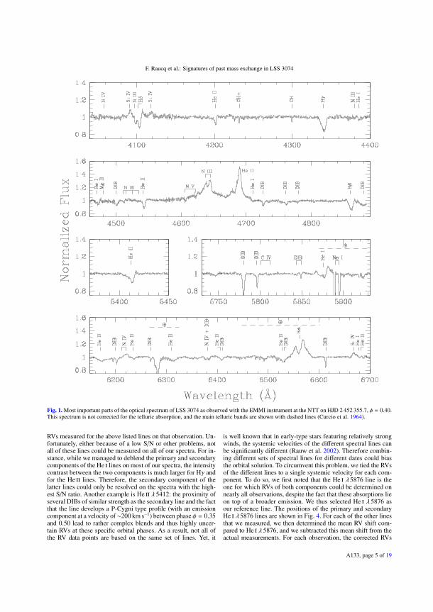
F. Raucq et al.: Signatures of past mass exchange in LSS 3074
Fig. 1. Most important parts of the optical spectrum of LSS 3074 as observed with the EMMI instrument at the NTT on HJD 2 452 355.7, φ = 0.40.This spectrum is not corrected for the telluric absorption, and the main telluric bands are shown with dashed lines (Curcio et al. 1964).
RVs measured for the above listed lines on that observation. Un-fortunately, either because of a low S/N or other problems, notall of these lines could be measured on all of our spectra. For in-stance, while we managed to deblend the primary and secondarycomponents of the He i lines on most of our spectra, the intensitycontrast between the two components is much larger for Hγ andfor the He ii lines. Therefore, the secondary component of thelatter lines could only be resolved on the spectra with the high-est S/N ratio. Another example is He ii λ 5412: the proximity ofseveral DIBs of similar strength as the secondary line and the factthat the line develops a P-Cygni type profile (with an emissioncomponent at a velocity of ∼200 km s−1) between phase φ = 0.35and 0.50 lead to rather complex blends and thus highly uncer-tain RVs at these specific orbital phases. As a result, not all ofthe RV data points are based on the same set of lines. Yet, it
is well known that in early-type stars featuring relatively strongwinds, the systemic velocities of the different spectral lines canbe significantly different (Rauw et al. 2002). Therefore combin-ing different sets of spectral lines for different dates could biasthe orbital solution. To circumvent this problem, we tied the RVsof the different lines to a single systemic velocity for each com-ponent. To do so, we first noted that the He i λ 5876 line is theone for which RVs of both components could be determined onnearly all observations, despite the fact that these absorptions lieon top of a broader emission. We thus selected He i λ 5876 asour reference line. The positions of the primary and secondaryHe i λ 5876 lines are shown in Fig. 4. For each of the other linesthat we measured, we then determined the mean RV shift com-pared to He i λ 5876, and we subtracted this mean shift from theactual measurements. For each observation, the corrected RVs
A133, page 5 of 19

A&A 601, A133 (2017)
were then averaged, resulting in a homogeneous set of values,expressed in the rest frame of the He i λ 5876 line.
These resulting RVs are listed in Table 1. For most datapoints, the uncertainties on these RVs are about 10–15 km s−1.In some cases however (indicated by the colons in Table 1), theuncertainties are larger than 20 km s−1 and can reach ∼40 km s−1
in one case (HJD 2 452 382.597). To adopt the same notations asprevious investigators, we refer to the brightest and hottest com-ponent of LSS 3074 as the primary, though its present-day massappears to be lower than that of its companion (see below).
Owing to the severe aliasing problem, it is extremely diffi-cult to obtain an independent determination of the orbital periodof LSS 3074 from our set of RV measurements only. A Fourieranalysis of the RV1 and RV2 data yields the highest peaks aroundν = 0.46020 d−1 (Porb = 2.1730 days) and ν = 0.45762 d−1
(Porb = 2.1852 days). However, we caution that there are manymore aliases that could hide the actual orbital period. It is worthpointing out that the second peak yields almost exactly the sameperiod as found by Niemela et al. (1992). We performed thesame Fourier analysis for each of the four bandpasses of thephotometric data, B, V , R, and I, and obtained a highest peakat ν = 0.9158 d−1, which corresponds to an orbital frequency ofν = 0.9158/2 = 0.4579 d−1, corresponding to Porb = 2.184 days.While the periodogram of the photometric time series allows usto unambiguously identify the correct alias, the natural width ofits peaks is much larger than in the case of our spectroscopictime series. In fact, folding the RVs into the photometric periodyields an unacceptably large scatter. Therefore, combining theresults from periodograms of the photometric and spectroscopictime series, we find that the most likely period of LSS 3074 is2.1852± 0.0006 days, with the error bars given as 1σ deviation.
Also, the T 0 obtained with the photometric curves isHJD 2 452 000.9568, which corresponds to a phase shift of∼0.05 with the T 0 obtained with the RV data. If we lock theRV data to this T 0, we obtain a period of 2.1849 days. Consid-ering that this result is well within the error bars of our previouscalculations, we can admit the phase alignment of the RV andphotometric data.
As a consistency check, we also combined our measurementsin the V band with those taken by Haefner et al. (1994) and ob-tained a highest peak of the periodogram at ν = 0.9153 d−1,which corresponds to an orbital frequency of ν = 0.9153/2 =0.45765 d−1, corresponding to Porb = 2.1851 days. This resulttends to confirm the quality of our determination of the orbitalperiod of the system.
Adopting an orbital period of 2.1852 days, we computedan orbital solution assuming a circular orbit. The RVs wereweighted according to their estimated uncertainties. The resultis shown in Fig. 2 and the corresponding orbital elements areprovided in Table 5.
The RV amplitudes of our solution are in reasonable agree-ment with values from the literature (K1 = 222 and K2 =218 km s−1; Niemela et al. 1992). Consequently our orbital so-lution also leads to low minimum masses, similar to those ofNiemela et al. (m sin3 i = 9.5 and 10 M⊙ for the O4f primaryand the secondary, respectively). The apparent systemic veloc-ity of the primary is significantly more negative than that of thesecondary. This most likely indicates that the absorption lines ofthe primary are not entirely formed in the static photosphere, butarise at least partly from an expanding stellar wind.
Figure 3 shows the RVs of the nitrogen emission and absorp-tion lines in the spectrum of LSS 3074. The adopted effectivewavelengths of the studied lines are listed in Table 4. All the linesseem to move with the primary, but the scatter of the velocities
Table 5. Orbital solution computed from our RV data of LSS 3074 as-suming a circular orbit and an orbital period of 2.1852 days.
Primary SecondaryT 0 (HJD - 2 450 000) 2000.851 ± 0.008γ (km s−1) –66.0 ± 5.0 –21.7 ± 4.7K (km s−1) 228.5 ± 7.1 196.0 ± 6.1a sin i (R⊙) 9.9 ± 0.3 8.5 ± 0.3q = m1/m2 0.86 ± 0.04m sin3i (M⊙) 8.0 ± 0.5 9.3 ± 0.7RRL/(a1 + a2) 0.37 ± 0.01 0.39 ± 0.01RRL sin i (R⊙) 6.7 ± 0.2 7.2 ± 0.2σfit 3.11
Notes. T 0 refers to the time of conjunction with the primary being infront. γ, K and a sin i denote respectively the apparent systemic veloc-ity, the semi-amplitude of the radial velocity curve and the projectedseparation between the centre of the star and the centre of mass of thebinary system. RRL stands for the radius of a sphere with a volume equalto that of the Roche lobe computed according to the formula of Eggleton(1983). All error bars indicate 1σ uncertainties.
Fig. 2. Radial velocities of the components of LSS 3074 assuming aperiod of 2.1852 days. The RVs of the primary and secondary stars areshown with filled and empty circles, respectively. The solid and dashedlines indicate the orbital solution from Table 5.
of the various lines is rather large, especially at phases betweenthe 0.25 quadrature and 0.5 conjunction. During this phase inter-val, the N iii emission lines yield systematically larger velocitiesthan the Nv absorption.
5. Line profile variability
The most prominent emission lines in the optical spectrum ofLSS 3074 show strong profile variations (see Fig. 4). For in-stance, the He ii λ 4686 line evolves from a broad and skewedemission (around φ = 0.0) into a double-peaked feature withrather narrow individual peaks and the strongest peak closelyfollowing the orbital motion of the primary (at phases near 0.5).
On the other hand, the Hα emission features a double-peakedprofile on most of our spectra and the profiles observed aroundthe two conjunctions are very similar. At phases near quadrature,the peaks are broader and less clear cut. Apart from the movingabsorption lines, the He i λ 5876 profile has a morphology rela-tively similar to that of the Hα line.
A133, page 6 of 19

F. Raucq et al.: Signatures of past mass exchange in LSS 3074
Fig. 3. Radial velocities of the N iii and N iv emission lines and the Nvabsorptions in the spectrum of LSS 3074. The meaning of the varioussymbols is given in the upper left corner. The solid line yields the orbitalsolution of the primary from Table 5.
We measured the equivalent widths (EWs) of the Hα line be-tween 6513 and 6604 Å. We find that EW = 4.09 ± 0.60 Å. Al-though the dispersion around the mean is quite large, no obviousphase-locked behaviour is apparent. In particular, we do not seeany variations attributable to the modulation of the continuum.
These complex line morphologies make it impossible to as-sign a single RV to the He ii λ 4686 and Hα emission lines, andsuggest that these lines do not arise in the atmosphere of oneof the two stars, but stem from an extended emission region. Tofurther quantify this situation, we used the method of Dopplertomography to map the emitting regions of the He ii λ 4686and Hα lines in velocity space. Our method is based on theFourier-filtered back projection technique (Horne 1991; Rauwet al. 2002; Mahy 2011). The radial velocity of any gas flow thatis stationary in the rotating frame of reference of the binary canbe expressed as
v(φ) = vx cos (2 π φ) − vy sin (2 π φ) + vz (5)
where φ stands for the orbital phase with φ = 0.0, correspondingto the primary star being in front. The (vx, vy, vz) are the veloc-ity coordinates of the gas flow. The x and y axes are located inthe orbital plane. The x-axis runs from the primary to the sec-ondary, whilst the positive y-axis points in the direction of theorbital motion of the secondary. The vz component represents theapparent systemic velocity of the line under consideration. TheDoppler map consists of a projection of relation given by (5) onthe (vx, vy) plane. For a given value of vz, each pixel in a Dopplermap, specified by its velocity coordinates, is therefore associatedwith a particular form of Eq. (5). All our spectra listed in Table 1were given equal weights. The Doppler maps, computed adopt-ing vz = −44 km s−1, are shown in Fig. 5. They reveal extendedline formation regions in velocity space with different morpholo-gies for the two lines. The He ii λ 4686 line features an emissionlobe on the negative vx side and mostly with negative vy. Thisemission seems thus mostly associated with the primary star. TheHα Doppler map displays two lobes, extending on both sides ofthe Roche lobes in velocity space, with the strongest one closelymatching the emission lobe of the Doppler map of He ii λ 4686.
A full interpretation of these Doppler maps in terms of wind-wind interactions is beyond the scope of the present paper. How-ever, it is interesting to compare our Doppler maps with those
of Algol-type systems where a cool star fills up its Roche lobeand transfers matter to a hotter companion (Richards et al. 2014).Our maps are clearly different from those presented by Richardset al. (2014). The structures seen in Fig. 5 neither resemble thoseproduced by gas streams that directly impact the mass gainernor do they feature the ring-like structure, centred on the massgainer, that appears for systems with Keplerian accretion disks.These results therefore do not support the presence of an accre-tion disk or an accretion stream in LSS 3074.
6. Preparatory analysis
6.1. Spectral disentangling
The determination of the orbital solution allowed us to recoverthe individual spectra of both components through the disentan-gling of the normalized spectra of the binary system. For thispurpose, we used our disentangling routine (Rauw 2007) basedon the method of González & Levato (2006), previously usedby Linder et al. (2008) and improved by Mahy et al. (2012).In this procedure, the mean spectra of each binary componentare reconstructed in an iterative way by shifting the observeddata into the frame of reference of one star and subtracting thebest approximation of the spectrum of the other star shifted to itsobserved radial velocity. In the disentangling carried out in thiswork, we fixed the RVs of the binary components to those cor-responding to the orbital solution of Sect. 4. For a more detaileddescription of the method, see Raucq et al. (2016).
As for any disentangling method, this technique also has itslimitations (González & Levato 2006). An important limitationfor our study is that broad spectral features are not recoveredwith the same accuracy as narrow ones. Indeed, features that arewider than a few times the RV amplitude are barely properlyrecovered. This is the case of the wings of the Balmer lines, forexample. Moreover small residual errors in the normalization ofthe input spectra can lead to oscillations of the continuum in theresulting disentangled spectra on wavelength scales of severaldozen Å, and a reasonable observational sampling of the orbitalcycle is needed because the quality of the results depends onthe radial velocity ranges covered by the observations. Finally,spectral disentangling works on continuum-normalized spectraand does not yield the brightness ratio of the stars, which mustbe determined by other techniques (see below).
In the particular case of LSS 3074, we also encounteredproblems due to the large brightness ratio of the system. Indeed,as shown in Sect. 6.3, the primary star appears much brighterthan the secondary star, meaning that the latter is faint in theobserved spectra, which induces difficulties in the disentanglingprocedure, a lower S/N ratio, and thus larger uncertainties on theresulting secondary spectrum.
6.2. Spectral types
We then determined the spectral types of the stars through themeasurement of the equivalent width ratio of some spectral linesof the reconstructed individual line spectra of the primary andsecondary components. We used the He i λ 4471 and He ii λ 4542lines, on the one hand, and Si iv λ 4089 and He i λ 4143 lines,on the other hand, and applied the Conti quantitative classifi-cation criteria for O-type stars (Conti & Alschuler 1971; Conti& Frost 1977; see also van der Hucht 1996) for both spectraltypes and luminosity classes. In this way, we obtain O5.5 I andO6.5-7 I classifications for the primary and secondary, respec-tively. The strong He ii λ 4686 and N iii λλ 4634-41 emission
A133, page 7 of 19
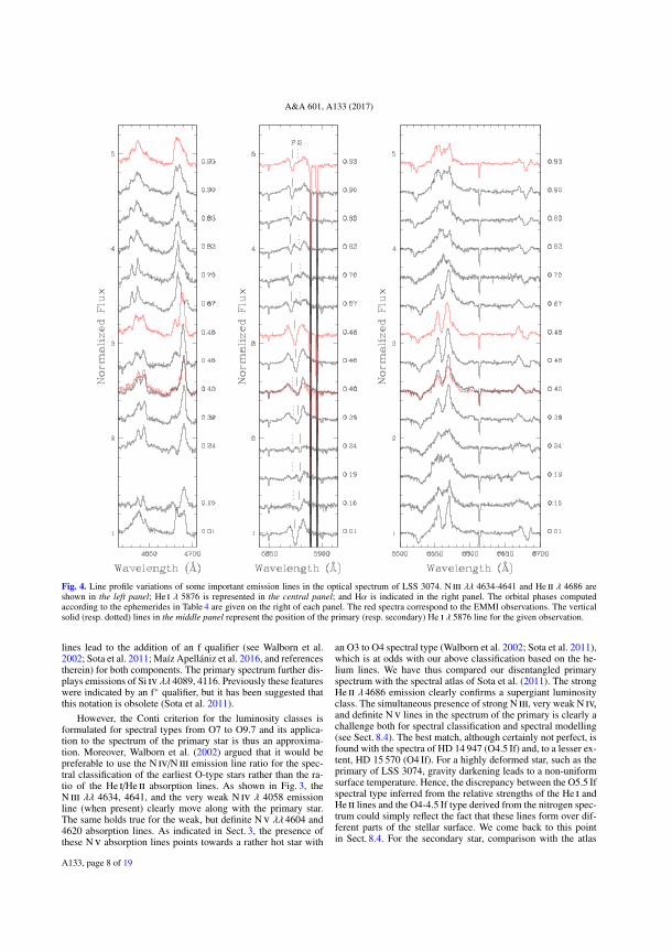
A&A 601, A133 (2017)
Fig. 4. Line profile variations of some important emission lines in the optical spectrum of LSS 3074. N iii λλ 4634-4641 and He ii λ 4686 areshown in the left panel; He i λ 5876 is represented in the central panel; and Hα is indicated in the right panel. The orbital phases computedaccording to the ephemerides in Table 4 are given on the right of each panel. The red spectra correspond to the EMMI observations. The verticalsolid (resp. dotted) lines in the middle panel represent the position of the primary (resp. secondary) He i λ 5876 line for the given observation.
lines lead to the addition of an f qualifier (see Walborn et al.2002; Sota et al. 2011; Maíz Apellániz et al. 2016, and referencestherein) for both components. The primary spectrum further dis-plays emissions of Si iv λλ 4089, 4116. Previously these featureswere indicated by an f+ qualifier, but it has been suggested thatthis notation is obsolete (Sota et al. 2011).
However, the Conti criterion for the luminosity classes isformulated for spectral types from O7 to O9.7 and its applica-tion to the spectrum of the primary star is thus an approxima-tion. Moreover, Walborn et al. (2002) argued that it would bepreferable to use the N iv/N iii emission line ratio for the spec-tral classification of the earliest O-type stars rather than the ra-tio of the He i/He ii absorption lines. As shown in Fig. 3, theN iii λλ 4634, 4641, and the very weak N iv λ 4058 emissionline (when present) clearly move along with the primary star.The same holds true for the weak, but definite Nv λλ 4604 and4620 absorption lines. As indicated in Sect. 3, the presence ofthese Nv absorption lines points towards a rather hot star with
an O3 to O4 spectral type (Walborn et al. 2002; Sota et al. 2011),which is at odds with our above classification based on the he-lium lines. We have thus compared our disentangled primaryspectrum with the spectral atlas of Sota et al. (2011). The strongHe ii λ 4686 emission clearly confirms a supergiant luminosityclass. The simultaneous presence of strong N iii, very weak N iv,and definite Nv lines in the spectrum of the primary is clearly achallenge both for spectral classification and spectral modelling(see Sect. 8.4). The best match, although certainly not perfect, isfound with the spectra of HD 14 947 (O4.5 If) and, to a lesser ex-tent, HD 15 570 (O4 If). For a highly deformed star, such as theprimary of LSS 3074, gravity darkening leads to a non-uniformsurface temperature. Hence, the discrepancy between the O5.5 Ifspectral type inferred from the relative strengths of the He i andHe ii lines and the O4-4.5 If type derived from the nitrogen spec-trum could simply reflect the fact that these lines form over dif-ferent parts of the stellar surface. We come back to this pointin Sect. 8.4. For the secondary star, comparison with the atlas
A133, page 8 of 19

F. Raucq et al.: Signatures of past mass exchange in LSS 3074
−800 −600 −400 −200 0 200 400 600 800Vx (km s−1 )
−800
−600
−400
−200
0
200
400
600
800
V y (k
m s−1
)
Doppler Map
−0.12
0.00
0.12
0.24
0.36
0.48
0.60
0.72
0.84
0.96
−800 −600 −400 −200 0 200 400 600 800Vx (km s−1 )
−800
−600
−400
−200
0
200
400
600
800
V y (k
m s−1
)
Doppler Map
0.000
0.104
0.208
0.312
0.416
0.520
0.624
0.728
0.832
0.936
Fig. 5. Doppler maps of the He ii λ 4686 (left) and Hα (right) emission lines in the spectrum of LSS 3074. The crosses correspond to the radialvelocity amplitudes of the centre of mass of the primary (negative vy) and secondary (positive vy), whereas the dashed lines indicate the Rochelobe in velocity space for a mass ratio m1/m2 = 0.86. The colour scale indicates the level of the line emissivity relative to its maximum value.
of Sota el al. (2011) yields a spectral classification O6.5-7 If, inagreement with the results from the relative strengths of the he-lium lines.
Finally, since our classification is based on the disentangledspectra, it is less sensitive to a possible phase dependence of theline strengths and should thus be more robust than a classifica-tion based only on spectra collected near quadrature phases.
6.3. Brightness ratio
The spectral disentangling yields the strength of the lines in theprimary and secondary stars relative to the combined continuum.But as we mentioned earlier, it does not allow us to establish therelative strengths of the continua. We therefore needed to firstestablish the brightness ratio of the stars to further analyse thereconstructed spectra.
To estimate the optical brightness ratio of the componentsof LSS 3074, we measured the equivalent widths, referring tothe combined continuum of the two stars, of a number of spec-tral lines on the reconstructed primary and secondary spectra.The results are listed in Table 6 along with the mean equiva-lent widths of the same lines in synthetic spectra of stars of thesame spectral type, computed with the non-LTE model atmo-sphere code CMFGEN (Hillier & Miller 1998), which we de-scribe in Sect. 8.2. For comparison, we also list the mean equiva-lent widths of the same lines in spectra of stars of similar spectraltype as measured by Conti (1973, 1974) and Conti & Alschuler(1971).
The brightness ratio of the two stars can then be evaluatedfrom
l1l2
=
(EW1
EW2
)
obs
(EWO7
EWO5.5
)
mean·
By combining our measurements with those from synthetic spec-tra, we derive an optical brightness ratio of 2.50 ± 0.43. As aconsistency check, we can also determine the brightness ratiothrough a comparison with the measurements made by Conti,and we obtain 2.61 ± 0.41.
The disentangled continuum normalized primary and sec-ondary optical spectra are shown in Fig. 8.
7. Light curve
To improve our understanding of the system LSS 3074, and inparticular its geometry, we performed an analysis of the photo-metric light curves by modelling the system using the eclipsingbinary star simulator NIGHTFALL2, developed by Wichmann,Kuster and Risse. We worked in an iterative way. First of all,we fixed the mass ratio and orbital period to the values obtainedfrom the orbital solution (see Table 5) and the effective tempera-tures to typical values for stars of similar spectral types (Martinset al. 2005). This permitted us to obtain a first estimation of thephotometric solution and of the stellar radii and masses. Basedon these approximated parameters, together with the effectivetemperatures, we calculated the associated surface gravities andstellar luminosities. This first approximation of the stellar fun-damental parameters was then used as starting point input inour study of the atmosphere modelling procedure (see Sects. 8.2and 8.3). This procedure then permitted us to accurately deter-mine the effective temperatures of the stars, giving us a new inputfor the light curve study with NIGHTFALL.
Inspection of the light curve reveals a lack of a plateau be-tween the minima, indicating important contributions of ellip-soidal variations to the photometric variability. Actually, theshape of the light curve suggests that almost the entire photo-metric variations could stem from such ellipsoidal variations,thereby implying that at least one of the stars must fill or over-flow its Roche lobe.
The only evidence for the existence of genuine eclipsescomes from the fact that the secondary minimum seems about0.02 mag deeper than the primary minimum. The primary min-imum corresponds to the occultation of the primary star by thesecondary. What is surprising here is that the deeper minimumactually corresponds to the spectroscopically hotter star being infront. Given the level of dispersion in the light curve, it is quitepossible that the small difference in depth of the minima is notsignificant and could arise, for example, from intrinsic variationsof the stars. An alternative explanation for this situation couldbe an atmospheric eclipse produced by the wind of the primary
2 For more details, see the NIGHTFALL user manual by Wichmann(1998) available at the URL: http://www.hs.uni-hamburg.de/DE/Ins/Per/Wichmann/Nightfall.html
A133, page 9 of 19

A&A 601, A133 (2017)
Table 6. Brightness ratio determination from the dilution of prominent lines.
Line Equivalent width (Å) l1/l2Observations Synthetic spectra Conti (1973, 1974)
Primary Secondary O5.5 O7 O5.5 O7He i λ 4026 0.42 0.19 0.51 0.69 0.46 0.61 3.00He ii λ 4200 0.41 0.17 0.53 0.45 0.58 0.59 2.00Hγ 0.90 0.34 1.56 1.75 1.85 2.22 3.00He i λ 4471 0.25 0.26 0.29 0.61 0.29 0.59 2.08He ii λ 4542 0.56 0.19 0.62 0.53 0.75 0.67 2.43
Notes. The measured EWs are compared with values for the same lines in synthetic spectra of the same spectral type and in the compilation ofmeasurements from the literature. The last column yields the brightness ratio for each line considered, using the synthetic spectra EWs.
star. Antokhina et al. (2013) studied the impact of free electronscattering in the wind of one star on the light curves of closeeclipsing binaries. For a contact binary made of otherwise equalstars, these authors show that the presence of a stellar wind withM = 10−5 M⊙ yr−1 around one component deepens the eclipsecorresponding to the star with the wind passing in front of itscompanion by about 0.08 mag. At the same time, the depth ofthe other eclipse is slightly reduced. In the case of LSS 3074,the fact that most emission lines closely follow the motion ofthe primary star suggests that this star has the strongest wind,thus lending support to this explanation. However, as pointed outby Antokhina et al. (2013), a quantitative assessment of the im-pact on the light curve requires some independent determinationof the wind parameters (mass-loss rate, asymptotic velocity andexponent of velocity law). In our case, this is difficult to achieve(see Sect. 8). This is because of the lack of UV spectroscopyand the complexity of the line emission regions. Indeed, as re-vealed by our tomographic analysis, at least parts of the Hα andHe ii λ 4686 emissions arise from an interaction zone and theselines hence do not necessarily reflect the genuine properties ofthe winds. Yet, our best-fit model atmosphere parameters (seethe forthcoming Table 10) yield upper limits on the wind densitythat could be consistent with the observed difference in eclipsedepth. However, these best-fit parameters also suggest that bothbinary components lose material at a similar rate. Hence, onewould expect both eclipses to be affected by stellar wind absorp-tion. We thus conclude that a better knowledge of the wind pa-rameters of LSS 3074 is required before we can attempt a modelof the light curve accounting for the effects of the stellar winds.Whatever the origin of the slight difference in depth of the min-ima, we need to keep in mind that this situation affects the qualityof the fits of the light curve.
To explain the shape of the secondary minimum by the soleeffect of ellipsoidal variations, we at least need to assume thateither both components of the binary system fill up (contact-contact) or even overflow their Roche lobes (overcontact), or thatone of the components must be much smaller and much fainterthan the other star that fills up its Roche lobe. In the former case,one expects both stars to be of very comparable size and, giventheir effective temperatures, also of rather comparable bright-ness. To explain the depth of almost 0.2 mag by the sole effect ofellipsoidal variations is actually not possible here without requir-ing the presence of true eclipses. In this context, the necessity toinvoke a contact-contact or an overcontact configuration remainsvalid, along with the conclusion that sizes and brightness of bothstars should be comparable.
This is precisely the outcome of our fits with the NIGHT-FALL code. The best-fit quality (χ2
ν = 4.4) is achieved for
Table 7. Photometric solution for LSS3074.
Parameters Primary Secondaryi () 54.5 ± 1.0
q = m1/m2 0.86 (fixed)Filling factora 1.008 ± 0.010 1.008 ± 0.010
Teff (K) 39 900 (fixed) 34 100 (fixed)m (M⊙) 14.8 ± 1.1 17.2 ± 1.4
Rpole (R⊙) 7.8 8.4χ2 1820.7
Nd.o.f. 415
Notes. Nd.o.f. is the number of degrees of freedom. (a) The filling factorof a given binary component is defined here as the fraction of its polarradius over the polar radius of its Roche lobe.
overcontact configurations with a filling factor of 1.008 (i ≃54.5), where the corresponding V-band brightness ratio is pre-dicted to be 1.09. The corresponding photometric solution is pre-sented in Table 7 and the associated plot is shown in Fig. 6. Yet,our spectroscopic analysis suggests an optical brightness ratio(primary/secondary) near 2.50. This situation is thus clearly atodds with explaining the photometric light curve via a doublecontact or overcontact configuration. To achieve a brightness ra-tio of 2.50±0.43, the ratio between the mean radii of the primaryand secondary stars would have to be 1.15±0.10. This translatesinto a ratio of the filling factors of 1.23 ± 0.11, which is onlypossible for detached or semi-detached configurations. As couldbe expected, the fact that the hotter star is in front during thedeepest minimum leads to difficulties to fit this minimum.
Since the eclipses are only partial, one way to solve this is-sue would be to postulate the existence of a dark spot on theside of the secondary star facing the primary. Such a spot wouldthen lead to a deeper minimum when the primary star is in front.From a purely numerical point of view this would improve the fitquality significantly with χ2
ν now approaching 2.9. In addition, itwould certainly help to bring the spectroscopic and photomet-ric brightness ratios into better agreement. Yet, aside from thedifficulty of explaining the physical origin of such a spot, thereis another issue that concerns the fact that the spot size and itsdim factor (i.e. the reduction in local temperature) are not fullyindependent and we lack any objective constraints on these pa-rameters. Test calculations have shown that for some situations,the best-fit model would actually correspond to a spot that coversmore than 75% of the surface of the secondary, which is clearlynot physical.
As an alternative to the overcontact configuration, one mightconsider a scenario where the primary star overflows its Roche
A133, page 10 of 19

F. Raucq et al.: Signatures of past mass exchange in LSS 3074
-0.2 0 0.2 0.4 0.6
12.9
12.8
12.7
11.7
11.6
11.5
11
10.9
10.8
-0.2 0 0.2 0.4 0.6
10.2
10.1
10
9.9
Fig. 6. Photometry of LSS 3074. The observational data are presentedas black dots, and the solid black line corresponds to the best-fit theo-retical light curve fit with NIGHTFALL with the parameters presentedin Table 7. The zero phase corresponds to the secondary eclipse, whenthe primary is occulting the secondary.
lobe and transfers matter to a geometrically thick accretion diskaround the more massive secondary star. This kind of scenariohas been proposed to explain the light curves of β Lyrae (Wilson1974), RY Sct (Antokhina & Kumsiashvili 1999), and V455 Cyg(Djuraševic et al. 2012), among others. On the positive side ofsuch a scenario, it might help reconcile the photometric andspectroscopic brightness ratios. On the negative side, we havethe lack of a clear signature of an accretion disk in the Dopplermaps of the Hα line and the fact that LSS 3074 is a very com-pact system, leaving very little room for the formation of a disk,unless the secondary star is very small. To test this scenario, weused the disk option in the NIGHTFALL code. In addition tothe effective temperatures that we fixed at the values obtainedfrom our model atmosphere fits (see Sect. 8.3), we set the Rochelobe filling factor of the primary star to unity and that of thesecondary star to 0.75. This choice results in a brightness ratiothat is consistent with our spectroscopic value. We tested variousoptions for the disk available in the NIGHTFALL code (simpledisk with uniform temperature, isothermal disk and reprocessingdisk), which correspond to different prescriptions of the varia-tions of the disk height and temperature with radius. Since thedisk in our models resembles more an annulus than a genuinedisk, these three options actually yield nearly identical results.These models fail to reproduce the width of the secondary mini-mum. This failure increases the χ2 of the fits. Still, we managedto find fits with χ2
ν ∼ 4.6, but this was only possible for a disktemperature exceeding the temperatures of both stars, which ismost probably not physical3. Better quality fits can be obtainedif the Roche lobe filling factor of the secondary is allowed todrop below 0.75: we obtained χ2
ν = 3.9 for a secondary fillingfactor of 0.47 (which would correspond to a secondary radius of
3 Raising the disk temperature allows the model to better reproducethe depth of the primary minimum, hence partially compensating forthe increase of χ2 due to the poor fit of the secondary minimum.
Table 8. Fit of the light curves of LSS 3074 by a sine function.
FilterB V R I
P = 1.0926 da(P) 0.0901 0.0910 0.0964 0.0980σa 0.0022 0.0022 0.0039 0.0027χ2ν 5.96 2.92 2.65 2.66σfit 0.0171 0.0171 0.0212 0.0212
P = 2.1852 da1(P) 0.0118 0.0125 0.0107 0.0125σa1 0.0020 0.0020 0.0038 0.0020
a2(P/2) 0.0896 0.0905 0.0958 0.0905σa2 0.0019 0.0019 0.0037 0.0019χ2ν 4.60 2.20 2.38 1.30σfit 0.0150 0.0148 0.0200 0.0148
N 120 122 58 118σ 0.007 0.010 0.013 0.013
Notes. P is the adopted period, ai the semi-amplitudes, σai the 1σ er-ror on semi-amplitude, χ2
ν the minimum reduced χ2, σfit the rms of theresiduals, N the number of points and σ the expected error.
only 3.9 R⊙) and a disk temperature of 51 300 K. Both parame-ters (secondary radius and disk temperature) are most probablynot physical. We thus conclude that a disk model cannot solvethe issues raised above any better than the pure Roche potentialmodel.
From a purely phenomenological point of view, we can ex-pand the light curve into a sum of sine functions. We tried aperiod of 2.1852/2= 1.0926 days and a mere sine and a periodof 2.1852 days and the fundamental sine plus its harmonic. Theresults are given in Table 8. The photometric observations ex-hibit a variation with a semi-amplitude of 0.09 mag in all filters.The semi-amplitude associated with the modulation on the or-bital period is 0.01 mag reflecting the above-mentioned differ-ence between the depths of the two minima. The correspondingχ2ν are lower than for any other fit we tried but still not satisfac-
tory. Including a larger number of harmonics in our expansiondoes not improve the situation. However, in terms of standardbinary models, this fit is unphysical since a modulation with asemi-amplitude as large as 0.09 mag cannot be explained by el-lipsoidal variations for such models. The fit of the B light curvecorresponds to a larger χ2
ν; the corresponding χ2ν would be simi-
lar to those found for the data from the other filters provided thatthe photometric errors used to normalize the χ2
ν were 0.010 maginstead of 0.007 mag.
The χ2ν of Table 8 are too large and this anomaly could have
several origins. One possibility is that the above-mentioned pho-tometric errors deduced from the comparison stars might not ap-ply to the case of LSS 3074. This could be due to an unfortu-nate location on the CCDs or for example to strange behaviourdue to peculiar stellar colours. This interpretation is however notvery likely. Alternatively, the fitted mathematical model mightnot be correct. Since any periodic function can be expanded intoa Fourier series and we found that our sine fits do not requireadditional terms, the additional, non-periodic component of themodel behaves similarly to an observational noise although itmust have a different origin. A possible explanation could bean intrinsic variability of the star at high frequencies since nolow-frequency variations were previously detected beyond theorbital one. Of course, this additional component has an upperlimit. Since the sine fits are our best models, we can consider
A133, page 11 of 19
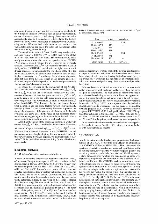
A&A 601, A133 (2017)
estimating this upper limit from the corresponding residuals. Inthe V filter for instance, we would need an additional variabilitycompared to the expected σ = 0.010 mag photometric error thatquadratically adds to it to reach σfit = 0.0148 mag for the twoperiods fit or σfit = 0.0171 mag for the single period fit. Consid-ering that the difference in depth between the two minima is notwell established, we can adopt the latter and the relevant valuewould thus be σfit = 0.0171 mag.
The transition from σ = 0.010 to 0.0171 mag translates intoa change from σ = 0.009 to σcorr = 0.0185 mag for the globalfit of the data from all four filters. The substitution by thesenewly estimated errors alleviates the rejection of the NIGHT-FALL model, since it reduces the χ2. However, this is purelyartificial. In addition, the χν2 of 4.4 could still be due to a lack ofability of the NIGHTFALL model to fit the light curve, even ifit were noiseless. However, under the hypothesis of the fit of theNIGHTFALL model, the errors on the parameters must be mod-ified to remain coherent. Even though this additional dispersiondoes not stem from the same origin as the genuine photomet-ric errors, impact of this dispersion on the derived parameters issimilar to that of photometric errors.
To obtain the 1σ error on the parameters of the NIGHT-FALL models, we have to consider the dispersion at χ2
min +∆χ21σ
where ∆χ21σ = 2.3 for the 1σ confidence interval of the simul-
taneous adjustment of two free parameters (i and f illp = f illsas is the case when we fit the light curve assuming an overcon-tact configuration with NIGHTFALL). From the values of the χ2
of our best-fit NIGHTFALL model, the 1σ error bars on the or-bital inclination and the filling factors would be unrealisticallysmall (e.g. about 0.1 for the error on i). However, as pointed outabove, the dispersion of the photometric data about the best-fitsynthetic light curve exceeds the value of our estimated photo-metric errors, suggesting that there could be an intrinsic photo-metric variability in addition to the orbital modulation.
Admitting the impact of the additional dispersion, we have tocorrect the ∆χ2
1σ = 2.3 to take this effect into account. Therefore,
we have to adopt a corrected ∆χ21σ,corr = ∆χ
21σ ×
(σcorr
σ
)2= 8.9.
We have then estimated the errors on the NIGHTFALL modelparameters by accordingly adopting this new corrected value. Inthis way, rounding the values uppards, we estimate errors of 1.0and of 0.01 for the inclination and the filling factors of both stars,respectively.
8. Spectral analysis
8.1. Rotational velocities and macroturbulence
In order to determine the projected rotational velocities (v sin i)of the stars of the system, we applied a Fourier transform method(Simón-Díaz & Herrero 2007; Gray 2008). For the primary star,we used the profiles of the He i λ 4471, He ii λλ 4200, 4542,6118, and N iii λ 6075 lines of the reconstructed spectrum. Weselected these lines as they are rather well isolated in the spectraand should thus be free of blends. Unfortunately, we could notuse the same lines for the secondary star because they are partic-ularly deformed. Indeed, the red wing of these lines is steeperthan the blue wing. We then used the He ii λ 5412 and Si ivλ 4089 lines to determine the projected rotational velocity of thesecondary star. The results are presented in Table 9. The meanv sin i of the primary star is (110 ± 13) km s−1, while that of thesecondary is (127 ± 6) km s−1. Owing to the small number oflines usable to study the rotation of the secondary star, we couldnot use a classical standard deviation method to determine the
Table 9. Projected rotational velocities (v sin i expressed in km s−1) ofthe components of LSS 3074.
Line Primary SecondarySi iv λ 4089 – 126He ii λ 4200 115 –He i λ 4471 97 –
He ii λ 4542 119 –He ii λ 5412 – 128N iii λ 6075 92 –He ii λ 6118 125 –Mean value 110 ± 13 127 ± 6
associated error bars. We thus studied the Fourier transforms fora sample of rotational velocities to estimate these errors. Fromthese values of v sin i and considering the inclination of the sys-tem from Sect. 7, we found that the stars are in synchronous ro-tation with a rotational period very close to the orbital period ofthe system.
Macroturbulence is defined as a non-thermal motion in thestellar atmosphere with turbulent cells larger than the meanfree-path of the photons. The main effect of macroturbulence isan additional broadening of the spectral lines. An approxima-tion of the macroturbulence velocities was obtained by apply-ing the radial-tangential anisotropic macroturbulent broadeningformulation of Gray (2008) on the spectra, after the inclusionof rotational velocity broadening. For this purpose, we used theauxiliary program MACTURB of the stellar spectral synthesisprogram SPECTRUM v2.76 developed by Gray (2010). We ap-plied this technique to the lines He i λλ 4026, 4471, and 5016,and He ii λ 4542 and obtained macroturbulence velocities of 20and 50 km s−1, for the primary and secondary stars, respectively.
Both rotational and macroturbulence velocities were appliedon the synthetic spectra (see Sect. 8.2) before comparing the lat-ter with the disentangled spectra.
8.2. CMFGEN code
In order to determine the fundamental properties of both com-ponents of LSS 3074, we used the non-LTE model atmospherecode CMFGEN (Hillier & Miller 1998). This code solves theequations of radiative transfer and statistical equilibrium in theco-moving frame, is designed to work for both plane-parallel andspherical geometries, and can be used to model Wolf-Rayet stars,O stars, luminous blue variables and supernovae. A super-levelapproach is adopted for the resolution of the equations of sta-tistical equilibrium. The CMFGEN code also further accountsfor line blanketing and its impact on the energy distribution. Thehydrodynamical structure of the stellar atmosphere is directlyspecified as an input to the code, and a β law is used to describethe velocity law within the stellar winds. We included the fol-lowing chemical elements and their ions in our calculations: H,He, C, N, O, Ne, Mg, Al, Si, S, Ca, Fe, and Ni. The solution ofthe equations of statistical equilibrium is used to compute a newphotospheric structure, which is then connected to the same βwind velocity law. The radiative transfer equations were solvedbased on the structure of the atmosphere with a microturbulentvelocity varying linearly with wind velocity from 20 km s−1 inthe photosphere to 0.1× v∞ at the outer boundary, and generatedsynthetic spectra were compared to the reconstructed spectra ofthe primary and secondary stars.
A133, page 12 of 19

F. Raucq et al.: Signatures of past mass exchange in LSS 3074
As a first approximation, the mass-loss rates and β param-eters were taken from Muijres et al. (2012) for the spectraltypes of both stars, whilst the wind terminal velocity was as-sumed equal to the mean value for stars of the same spectraltype (Prinja et al. 1990). We then estimated the surface gravi-ties, stellar masses, radii, and luminosities from our study of thephotometric curves. The relevant parameters were then adjustedvia an iterative process, as each adjustment of a given param-eter leads to some modifications in the value of other parame-ters. This process and the results we obtained are presented inSects. 8.3 and 8.4, respectively. As explained in Sect. 6, this iter-ative process was then coupled with a second iterative process,through the study of the photometric light curve.
8.3. Method
The first step is to adjust the effective temperature in the modelsof the stars. To do so, we adjusted the relative strengths of theHe i λ 4471 and He ii λ 4542 lines (Martins 2011). Final valuesare 39 900 and 34 100 K for the primary and secondary stars, re-spectively. Once the effective temperatures were determined, weused them, together with the stellar radii obtained in our studyof the photometric curves, to constrain the luminosities of thestars. We therefore obtained luminosities of 1.38 × 10⁵ L⊙ and8.49 × 104 L⊙ for the primary and secondary stars.
Subsequently, the binarity of the studied system causes someproblems. Indeed, the next step is to adjust the surface gravitiesin the models, but as we mentioned in Sect. 6.1, the wings of theBalmer lines are too broad to be properly recovered by the spec-tral disentangling. To circumvent this problem, we recombinedthe models of the primary and secondary star spectra for severalphases and compared the resulting binary spectra directly to theobservations. This permitted us to better adjust the gravities, butwith larger uncertainties than in the case of a single star.
A second problem arises with the adjustment of the wind pa-rameters. Indeed, the He ii λ 4686 and Balmer lines may be pol-luted by some emission from the wind-wind interaction zone.Therefore, the uncertainties on the terminal velocity, the β of thevelocity law, the clumping factor, the clumping velocity factor,and the mass-loss rate are quite high. Indeed, considering thepossible existence of such additional emission polluting thesediagnostic lines, the adjustment of the models onto the recon-structed spectra may lead to an underestimate of the terminal ve-locity, and an overestimate of the β of the velocity law, clumpingfactor, clumping velocity factor, and mass-loss rate. Therefore,the obtained values can only be considered as lower and upperlimits of the real properties of the stellar winds. However, westill adjusted them as well as possible: we obtained for the pri-mary and secondary stars values of 2615 and 3055 km s−1 forv∞, 1.30 and 1.40 for β and 3.00× 10⁻⁶ and 3.51× 10⁻⁶ M⊙ yr−1
for the mass-loss rate, based on the strength of Hα, the width ofthe He ii λ 4686 and Hα lines, and both the strengths of Hγ andHδ, respectively. The clumping formalism used in the CMFGENmodel is
f (r) = f1 + (1 − f1)e(− V(r)
f2
)
with a clumping filling factor f1 of 0.7, a clumping velocity fac-tor f2 of 200 kms−1 and V(r) the velocity of the wind for bothprimary and secondary stars, and we adjusted these two clump-ing factors through the strength and shape of Hα and Hβ lines.
Finally, once the fundamental properties of the stars had beenestablished or fixed, we investigated the CNO abundances withintheir atmosphere through the strengths of associated lines. At
that point, we encountered several problems. Indeed, there is novisible O line in both primary and secondary spectra, and theonly present C lines are the C iv λλ 5801 and 5812 lines, whichcannot be considered in the determination of the surface C abun-dance since they can exhibit complex profiles influenced by var-ious phenomena among which is continuum fluorescence (Conti1974; Bouret et al. 2012). We thus were only able to determineupper limits for C and O abundances. We used the N iii λ 4379and N iii λλ 4511-15-18-24-30-35 lines to adjust the N abun-dance for the primary star. The same lines were used for thesecondary star except for the N iii λ 4530 and N iii λ 4535 lines.These N abundance diagnostic lines are taken from Martins et al.(2015) study of a sample of 74 objects comprising all luminosityclasses and spectral types from O4 to O9.7. We selected, fromtheir study, all the suggested lines that were significantly seenin our observations. We performed a normalized χ2 analysis todetermine the best fit to these lines (Martins et al. 2015). The nor-malization consists in dividing the χ2 by its value at minimum,χ2
min. As a 1σ uncertainty on the abundances, we then consid-ered abundances up to a χ2 of 2.0, i.e. an approximation for 1over χ2
min, as suggested by Martins et al. (2015).
8.4. Results
Figure 8 shows the best fit of the optical spectra of the primaryand secondary stars obtained with CMFGEN, and we present inTable 10 the associated stellar parameters.
Figure 8 reveals that we encountered a lot of difficulty ad-justing the spectra of the components of LSS 3074. First of all,it clearly shows that the noise is strongly enhanced in the re-constructed secondary spectrum, because of the high brightnessratio of the system. This peculiarity makes the adjustment of thesecondary spectrum even more difficult. Second, if we can seethat the He lines are generally well reproduced for both stars,some of these lines in the observed spectra, especially for thesecondary star, feature some emission in their wings that is notreproduced by the models. We can also see that the Balmer andHe ii λ 4686 lines are not perfectly well recovered, probably ow-ing to the complexity of the winds and the presence of a wind-wind interaction zone, as discussed in Sect. 8.3.
Concerning the N lines, most N iii features are reasonablywell reproduced by the models, but a few lines of other nitro-gen ions are not, especially in the primary spectrum. Indeed,the model predicts a rather strong N iv λ 4058 emission, whilethe observations clearly show that this is not the case. Anotherremarkable issue is the presence in the observed primary spec-tra of the Nv λλ 4604, 4620 lines, which are not predicted bythe model. These Nv lines are seen in the spectra of the earli-est O supergiants (starting from O4 If Walborn et al. 2002; Sotaet al. 2011) and, in some cases, in the spectra of early O main-sequence stars (e.g. Mahy et al. 2012), and could suggest thatour value of the primary effective temperature (39 900 K) is toolow. To test this hypothesis, we computed a set of CMFGENmodels with temperatures ranging from 38 000 to 44 000 K. Asone can see in Fig. 7, a temperature of about 44 000 K wouldbe needed to reproduce the strength of the Nv lines. However,in this case, the model predicts N iii emissions that are muchweaker than observed as well as a huge N iv line that is clearlynot observed. To reproduce the strength of the observed N iiiand N iv lines, a lower temperature of 38 000 K seems more in-dicative. But this lower temperature is clearly not sufficient toproduce the Nv lines. The temperature that we determined inour CMFGEN fits is the temperature that properly reproduces
A133, page 13 of 19
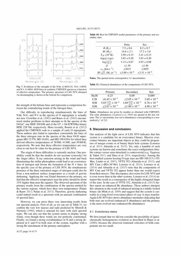
A&A 601, A133 (2017)
Prim.
38kK
40kK
42kK
44kK
Fig. 7. Evolution of the strength of the N iii λλ 4634-41, N iv λ 4058,and Nv λλ 4604, 4620 lines in synthetic CMFGEN spectra as a functionof effective temperature. The primary spectrum of LSS 3074 obtainedvia disentangling is shown at the bottom for comparison.
the strength of the helium lines and represents a compromise be-tween the contradicting trends of the nitrogen lines.
Our difficulty in reproducing simultaneously the lines ofN iii, N iv, and Nv in the spectra of O supergiants is actuallynot new. Crowther et al. (2002) and Rauw et al. (2002) encoun-tered similar problems in their attempts to fit the spectra of theO4 Iaf+ star HDE 269 698 and of the O7 + O4 If/WN8ha binaryHDE 228 766, respectively. More recently, Bouret et al. (2012)applied the CMFGEN code to a sample of early O supergiants.These authors also failed to reproduce consistently the lines ofthe three nitrogen ions in the spectra of the three O4 If super-giants HD 15 570, HD 16 691, and HD 190 429A for which theyderived effective temperatures of 38 000, 41 000, and 39 000 K,respectively. We note that these effective temperatures are veryclose to our best-fit value for the primary of LSS 3074.
The origin of these difficulties is currently unclear. One pos-sibility could be that the models do not account (correctly) forthe Auger effect. X-ray emission arising in the wind and backilluminating the stellar photosphere could lead to an overioniza-tion of nitrogen and favour the formation of the N v lines. Inthe specific case of the primary of LSS 3074, the simultaneouspresence of the three ionization stages of nitrogen could also befrom a non-uniform surface temperature as a result of gravitydarkening. Applying the von Zeipel theorem to the primary, wefind that the effective temperature near the poles should be about15% higher than near the equator. The observed spectrum of theprimary results from the combination of the spectra emitted bythe various regions, which have their own temperatures (Palate& Rauw 2012; Palate et al. 2013). Therefore, gravity darkeningcould indeed result in a spectrum with an unusual combinationof spectral lines.
However, we can stress three very interesting results fromour spectral analysis. First of all, as we can see in Table 10, weconfirm the very low masses and radii predicted by Morrell &Niemela (1990), which is unusual for stars with such spectraltypes. We can also see that the system seems to display strongwinds, even though these winds are not perfectly constrained.Finally, we found a strong overabundance in N and a strong de-pletion in C and O in both stars of the system, together with astrong He enrichment of the primary atmosphere.
Table 10. Best-fit CMFGEN model parameters of the primary and sec-ondary stars.
Prim. Sec.R (R⊙) 7.5 ± 0.6 8.2 ± 0.7M (M⊙) 14.6 ± 2.1 17.2 ± 3.0
Teff (104 K) 3.99 ± 0.15 3.41 ± 0.15log(g) (cgs) 3.82 ± 0.20 3.83 ± 0.20
log(
LL⊙
)5.14 ± 0.07 4.93 ± 0.08
β ≤1.30 ≤1.40v∞ (km s−1) ≥2615 ≥3055
M/√
f1 (M⊙ yr−1) ≤3.00 × 10⁻⁶ ≤3.51 × 10⁻⁶
Notes. The quoted errors correspond to 1σ uncertainties.
Table 11. Chemical abundances of the components of LSS 3074.
Primary Secondary SunHe/H 0.25 0.09 0.089C/H ≤6.45 × 10⁻⁵ ≤2.05 × 10⁻⁵ 2.69 × 10⁻⁴
N/H 5.65+4.07−3.02 × 10⁻⁴ 3.69+0.83
−0.91 × 10⁻⁴ 6.76 × 10⁻⁵
O/H ≤2.67 × 10⁻⁵ ≤1.00 × 10⁻⁵ 4.90 × 10⁻⁴
Notes. Abundances are given by number as obtained with CMFGEN.The solar abundances (Asplund et al. 2009) are quoted in the last col-umn. The 1σ uncertainty was set to abundances corresponding to a nor-malized χ2 of 2.0.
9. Discussion and conclusions
Our analysis of the light curve of LSS 3074 indicates that thissystem is a candidate for an overcontact binary. Massive over-contact binaries are important objects as they could be progeni-tors of merger events or of binary black hole systems (Lorenzoet al. 2014; Almeida et al. 2015). Yet, only a handful of suchsystems are known and sometimes the exact configuration (dou-ble contact versus semi-detached) is controversial (e.g. Yasarsoy& Yakut 2013; and Zhao et al. 2014, respectively). Among thebest-studied systems hosting O-type stars are HD 100 213 (=TUMus, Linder et al. 2007), VFTS 352 (Almeida et al. 2015), andMY Cam (=BD+56864, Lorenzo et al. 2014). Lorenzo et al.(2014) and Almeida et al. (2015) note that the components ofMY Cam and VFTS 352 appear hotter than one would expectfrom their masses. This discrepancy also exists for LSS 3074 andis even worse than in the other systems. Lorenzo et al. (2014) in-terpret this result as a consequence of the highly elongated shapeof the stars. In the case of VFTS 352, Almeida et al. (2015) fur-ther report an enhanced He abundance. These authors interpretthis situation as the result of enhanced mixing in a tidally lockedbinary (de Mink et al. 2009) and suggest that the system is cur-rently in a long-lived overcontact phase of case A mass transfer.Again LSS 3074 also shows abundance anomalies indicating thatboth stars are evolved (enhanced N abundance) and the primaryis the more evolved star (enhanced He abundance).
9.1. Evolutionary status
We first remark that we did not consider the possibility of quasi-chemically homogeneous evolution as described in Heger et al.(2000), because the observed rotational velocities of both com-ponents are too small.
A133, page 14 of 19

F. Raucq et al.: Signatures of past mass exchange in LSS 3074
Fig. 8. Part of the normalized separated spectra of the primary (top, shifted upwards by 0.5 continuum units in the first three panels, and by 1.0continuum units for the last panel) and secondary stars (bottom), along with the best-fit CMFGEN model spectra (red).
The altered CNO abundances in the atmosphere of the pri-mary, the luminosity of primary, and the increased helium abun-dance are strong arguments that the star is in the slow phaseof case B RLOF. If the star were post-RLOF, accounting forthe present mass, its luminosity would have to be log ( L
L) = 5.5
rather than the observed 5.14 (e.g. Vanbeveren et al. 1998, for-mula 5.4). Moreover, the observed CNO abundances of the sec-ondary seem to indicate that at least some mass lost by the pri-mary was accreted by the secondary. The normal (solar) heliumabundance, on the other hand, lead us to conclude that not allthe helium enhanced layers lost by the primary were accretedby the secondary. Accounting for these facts a theoretical studycan be undertaken to attempt to identify its possible progeni-tors. For this purpose, the Brussels binary population synthesiscode is used. This code uses as input thousands of detailed evo-lutionary calculations performed with the Brussels binary evo-lution code. Both codes are described in detail in De Donder &Vanbeveren (2004). However, the theoretical treatment of binaryevolution is still subject to a number of uncertainties, which aretypically implemented by means of parameters. For the presentdiscussion, two uncertain aspects of binary mass transfer, char-acterized in population synthesis by two parameters, are of in-terest. The first is the fraction of the mass lost by the donorstar that is actually accreted by the gainer star. This fractionnecessarily lies between zero (i.e. totally non-conservative masstransfer) and one (i.e. totally conservative mass transfer), and is
characterized in population synthesis by the parameter βRLOF4
(hence 0 ≤ βRLOF ≤ 1). If βRLOF < 1, and thus mass is lost fromthe system, a second critical assumption concerns how much an-gular momentum is taken along from the system by this lostmass. This is determined by a parameter η (for a formal defini-tion, see De Donder & Vanbeveren 2004). For the present discus-sion, it suffices to know that the larger η, the more angular mo-mentum is removed from the binary by a given amount of massloss. A common assumption made in many population synthesisstudies is that the mass lost takes along only the specific orbitalangular momentum of the gainer star (and thus leaves this starin a spherically symmetric way). This results in a low angularmomentum loss, characterized by a low value of η ∼ 0.05. Analternative assumption is that mass is lost through the second La-grangian point and forms a circumbinary ring, taking along someof the orbital angular momentum of this ring. This entails a muchlarger angular momentum loss, and has been shown to result inη = 2.3. Various other, less common assumptions are also pos-sible (e.g. gainer orbital plus spin angular momentum and spe-cific binary angular momentum), which all result in intermediatecases and can be approximated by taking η = 1. The purpose ofthis paragraph is to investigate, for various combinations of the
4 The usual designation for this parameter is β, but we used the βRLOFdesignation to avoid any confusion with the β of the velocity law in thestellar winds.
A133, page 15 of 19

A&A 601, A133 (2017)
Table 12. Initial masses and orbital period, leading to a 14.8+17.2 M⊙,2.2 d post-RLOF binary for different combinations of βRLOF and η.
βRLOF = 1 βRLOF = 0.5 βRLOF = 0.1η = 2.3 no solution 34+7.9 M⊙, 560 d 34+15 M⊙, 1000 dη = 1 no solution 34+7.9 M⊙, 90 d 34+15 M⊙, 80 dη ∼ 0.05 no solution 34+7.9 M⊙, 5.3 d 34+15 M⊙, 1.4 d
parameters βRLOF and η, whether they can indeed result in theformation of a binary in the slow phase of case B RLOF with thephysical parameters (masses and orbital period) of LSS3074, andif so, originating from which initial conditions. All calculationsare performed for solar-like metallicity.
Table 12 shows the initial masses and orbital period, depend-ing on the assumed values of βRLOF and η, which produce a14.8+17.2 M⊙ binary in the slow phase of case B RLOF andwith an orbital period of 2.2 days.
Our simulations reveal that the primary progenitor was a starwith initial mass 30–35 M⊙. We find no physically realistic so-lution if the RLOF is treated conservatively. If it is assumed thatβRLOF = 0.5, we have to start with an initial 34+7.9 M⊙ binary.It is however doubtful that a binary with such an extreme initialmass ratio would avoid merging. Our best guess is then a modelwith βRLOF < 0.5, such as the βRLOF = 0.1 model of Table 12.If the matter that leaves the binary takes with it the specific an-gular momentum of the gainer (η = 0.05), the initial period ofthe binary had to be very small (of the order of 1 or 2 days) andthis means that the progenitor binary first went through a case ARLOF phase followed by case B. Interestingly, our simulationsshow that the slow case B RLOF will stop after some 10 000 yr.The primary star then will be a 11–12 M⊙ WR star, i.e. the binarywill be very similar to the WR binary CQ Cep.
9.2. Summary and conclusions
From what we have seen above, LSS 3074 is clearly a very pecu-liar binary system that challenges our current methods of binaryspectral analysis. In this paper, we have tried to get a deeperunderstanding of this system, but we encountered a number ofproblems that prevent us from establishing a fully consistent ex-planation of all the properties of the system. Here we discussthese problems and try to highlight some avenues for possiblesolutions.
The properties of the components of LSS 3074 that we deter-mined from our spectral and photometric analysis do not concurwith those of genuine early O-type supergiants as determined,for instance, by Bouret et al. (2012). Indeed, these latter authorsused the CMFGEN code to analyse UV and optical spectra oftypical early and mid-O supergiants. They found that O4-4.5supergiants have radii between 18.5 and 21.6 R⊙, log g in therange 3.51 to 3.66 and log L/L⊙ between 5.83 and 5.96. For O6-7.5 supergiants, Bouret et al. (2012) determined radii between20.5 and 21.3 R⊙, log g between 3.41 and 3.54, and log L/L⊙in the range 5.68 to 5.80. The components of LSS 3074 havesignificantly smaller radii, which are actually even smaller thanthe typical radii of early-O main-sequence stars. Stars as bigas the supergiants analysed by Bouret et al. (2012) would notfit into such a short-period binary system as LSS 3074, evenconsidering, as we have here, the possibility of an overcontactconfiguration. The luminosities of the components of LSS 3074are also far from those determined by Bouret et al. (2012), andare again lower than those of main-sequence stars of the samespectral type. As for the log g of the stars in LSS 3074, theirvalues are higher than those of genuine supergiants, indicating a
more compact stellar atmosphere than for supergiants. The val-ues we found are intermediate between those of giants and main-sequence stars. Last but not least, the masses of the components(14.6 and 17.2 M⊙ for the primary and secondary, respectively)are considerably lower than the spectroscopic or evolutionarymasses of genuine O supergiants, which are around 50 M⊙ forearly-O supergiants and around 40 M⊙ for mid-O supergiants(Bouret et al. 2012). In fact, the masses that we determined aremore compatible with those of O9-B0 main-sequence stars.
Yet, despite these very discrepant stellar properties, the spec-trum of the primary star of LSS 3074 is very similar to the spec-trum of HD 16 691 (O4 If) analysed by Bouret et al. (2012), in-cluding the presence of Nv λλ 4605-4620 in absorption and theweakness of N iv λ 4058. This situation suggests that the spec-tra of the LSS 3074 could be biased in some way. Our spectralanalysis relies on the individual spectra reconstructed via spec-tral disentangling. Such a reconstructed spectrum is a brightness-weighted mean over the various parts of the stellar surface thatcan be observed given the inclination of the system. Owing to theeffect of gravity darkening, the temperature at the surface of a ro-tating star is not uniform: the polar regions that have the highervalue of log g are hotter than the equatorial regions where log gis lower. Things are even more complicated in a close binary sys-tem, where the local acceleration of gravity is determined by thegradient of the Roche potential ∇Ω (e.g. Palate & Rauw 2012;Palate et al. 2013). To evaluate whether or not this situation leadsto a surface gravity that comes close to that of a supergiant, wecomputed |∇Ω| over the surface of the primary star, adopting aRoche lobe filling factor of 1.008. We then compared this valueto the acceleration of gravity one would have for a single star ofsame mass and radius. Except for a small region near the bridgeof material that connects both stars, |∇Ω| is typically between 3and 9 times larger than the g value for a single star. Therefore,the Roche potential should lead to an increase of log g comparedto its value if binarity is neglected. Hence, this situation can-not explain the discrepancy between the stellar properties andthe observed spectrum. A possible way out could be the effectof the radiation pressure on the potential. Howarth (1997) hasshown that radiation pressure leads to a scaling of the potentialand a reduction of the local gravity by a factor 1 − Γ, where Γ isa measure of the relative importance of radiation pressure overgravity. The primary star of LSS 3074 could have lost a sub-stantial fraction of its initial mass to the surroundings and, as aresult, appears now as a very hot object, significantly hotter thanexpected from its mass. This assumption is strengthened by theHe and CNO primary surface abundances, as shown in Sect. 9.1.Given the high temperature of the components of LSS 3074, theresulting strong radiation pressure appears then to be the bestcandidate to explain why the stars display unusual spectra.
Another odd feature of LSS 3074 is the discrepancy betweenthe brightness ratios inferred from spectroscopy and photometry.The spectroscopic brightness ratio mainly stems from the weak-ness of the secondary spectral lines. One possibility could bethat these lines are filled in by emission either from the primarystar or from circumstellar material. Some evidence for circum-stellar emission can be seen in the He i λ 5876 and He ii λ 5412lines of the recontructed spectra, which are flanked by emissionwings in the case of the secondary. Yet, it seems unclear whetherthis effect applies to all spectral lines and would be sufficient toexplain the discrepancy between photometry and spectroscopy.
The fact that the light curve of LSS 3074 is actually betterfitted by a simple sine function than by the NIGHTFALL modelsuggests that the components of the binary system might actuallybe more elongated than expected from the Roche potential. The
A133, page 16 of 19

F. Raucq et al.: Signatures of past mass exchange in LSS 3074
inclusion of radiation pressure in the calculation of the surfaceshape can actually lead to systems that are detached whilst theywould be in a contact configuration based only on the Roche po-tential (Drechsel et al. 1995; Palate et al. 2013). Radiation pres-sure also changes the ellipticity of the stars, making them appearless elongated for a given value of the polar radius (e.g. Fig. 3Palate et al. 2013), although a further increase in the polar radiuscould lead to a higher ellipticity whilst preserving a detachedconfiguration (Drechsel et al. 1995). Whilst a detailed modellingof the light curve of LSS 3074, including the effect of radiationpressure, is beyond the scope of the present study, we note thatthe temperature distribution at the surface of the stars will alsobe altered and this could possibly help explain the observed lightcurve. A detached configuration resulting from the effect of radi-ation pressure could in principle also help bring the photometricand spectroscopic brightness ratios into better agreement.
Acknowledgements. The Liège team acknowledges support from the Fonds dela Recherche Scientifique (F.R.S/FNRS) including especially an F.R.S/FNRSResearch Project (T.0100.15), as well as through an ARC grant for ConcertedResearch Actions financed by the French Community of Belgium (Wallonia-Brussels Federation), and an XMM PRODEX contract (Belspo). We are particu-larly grateful to Reinhold Haefner for having made his IBVS data available andto Ella Antokhina and Igor Antokhin for discussions on the photometric solution.EG is greatly indebted to Stephanie Wachter and Suzanne Tourtelotte for havingspared no pains in facilitating the interaction with the YALO archives. We aregrateful to I. Stevens, H. Sana, Y. Nazé, J.-M. Vreux, and M. da Silva Pires fortaking some of the spectroscopic data or for discussions on earlier versions ofthis work. We thank John Hillier for making his code available.
References
Almeida, L. A., Sana, H., de Mink, S. E., et al. 2015, ApJ, 812, 102Antokhina, E. A., & Kumsiashvili, M. I. 1999, Astron. Lett., 25, 662Antokhina, E. A., Antokhin, I. I., & Cherepashchuk, A. M. 2013, Astron.
Astrophys. Trans., 28, 3Arnaud, K. A. 1996, in Astronomical Data Analysis Software and Systems V,
eds. G. Jacoby, & J. Barnes, ASP Conf. Ser., 101, 17Asplund, M., Grevesse, N., Sauval, A. J., & Scott, P. 2009, ARA&A, 47, 481Bohlin, R. C., Savage, B. D., & Drake, J. F. 1978, ApJ, 224, 132Bouret, J.-C., Hillier, D. J., Lanz, T., & Fullerton, A. W. 2012, A&A, 544, A67Conti, P. S. 1973, ApJ, 179, 161Conti, P. S. 1974, ApJ, 187, 539Conti, P. S., & Alschuler, W. R. 1971, ApJ, 170, 325Conti, P. S., & Frost, S. A. 1977, ApJ, 212, 728Crowther, P. A., Hillier, D. J., Evans, C. J., et al. 2002, ApJ, 579, 774Curcio, J. A., Drummeter, L. F., & Knestrick, G. L. 1964, Appl. Opt., 3, 1401De Donder, E., & Vanbeveren, D. 2004, New Astron. Rev., 48, 861de Loore, C., & Vanbeveren, D. 1994, A&A, 292, 463de Mink, S. E., Pols, O. R., & Hilditch, R. W. 2007, A&A, 467, 1181de Mink, S. E., Cantiello, M., Langer, N., et al. 2009, A&A, 497, 243Djuraševic, G., Vince, I., Antokhin, I. I., et al. 2012, MNRAS, 420, 3081Dray, L. M., & Tout, C. A. 2007, MNRAS, 376, 61Drechsel, H., Haas, S., Lorenz, R., & Gayler, S. 1995, A&A, 294, 723Eggleton, P. P. 1983, ApJ, 268, 368González, J. F., & Levato, H. 2006, A&A, 448, 283Gosset, E., Royer, P., Rauw, G., Manfroid, J., & Vreux, J.-M. 2001, MNRAS,
327, 435Gosset, E., Rauw, G., Manfroid, J., et al. 2005, Proceedings of Massive Stars and
High-Energy Emission in OB Associations, a workshop of the JENAM 2005,Distant Worlds, held in Liège (Belgium), July 4–7, eds. G. Rauw, Y. Nazé, R.Blomme, & E. Gosset, 77
Gray, D. F. 2008, The Observation and Analysis of Stellar Photospheres, 3rd edn.(Cambridge University Press)
Gray, R. O. 2010, http://www.appstate.edu/~grayro/spectrum/spectrum276/node38.html
Haefner, R., Simon, K. P., & Fiedler, A. 1994, IBVS, 3969, 1Heger, A., Langer, N., & Woosley, S. E. 2000, ApJ, 528, 368Herbig, G. 1995, ARA&A, 33, 19Hillier, D. J., & Miller, D. L. 1998, ApJ, 496, 407Horne, K. 1991, in Fundamental Properties of Cataclysmic Variable Stars: 12th
North American Workshop on Cataclysmic Variables and Low Mass X-rayBinaries, ed. A. W. Shafter (SDSU Press), 23
Houk, N., & Cowley, A. P. 1975, in University of Michigan Catalogue of two-dimensional spectral types for the HD stars, Vol. I. Declinations –90 to –53
Howarth, I. D. 1997, The Observatory, 117 335Hurley, J. R., Tout, C. A., & Pols, O. R. 2002, MNRAS, 329, 897Jansen, F., Lumb, D., Altieri, B., et al. 2001, A&A, 365, L1Kaufer, A., Stahl, O., Tubbesing, S., et al. 1999, The Messenger, 95, 8Kippenhahn, R., & Weigert, A. 1967, Z. Astrophys., 65, 251Langer, N. 2012, ARA&A, 50, 107Linder, N., Rauw, G., Sana, H., De Becker, M., & Gosset, E. 2007, A&A, 474,
193Linder, N., Rauw, G., Martins, F., Sana, H., De Becker, M., & Gosset, E. 2008,
A&A, 489, 713Lorenzo, J., Negueruela, I., Val Baker, A. K. F., et al. 2014, A&A, 572,
A110MacConnell, D. J. 1981, A&AS, 44, 387Mahy, L. 2011, Ph.D. Thesis, University of Liège, BelgiumMahy, L., Gosset, E., Sana, H., et al. 2012, A&A, 540, A97Maíz Apellániz, J., Sota, A., Arias, J. I., et al. 2016, ApJS, 224, 4Manfroid, J. 1993, A&A, 271, 714Manfroid, J., Royer, P., Rauw, G., & Gosset, E. 2001, in Astronomical Data
Analysis Software and Systems X, eds. F. Harnden, F. Primini, & H. Payne,ASP Conf. Ser., 238, 373
Martins, F. 2011, Bull. Soc. Roy. Sci. Liège, 80, 29Martins, F., & Plez, B. 2006, A&A, 457, 637Martins, F., Schaerer, D., & Hillier, D. J. 2005, A&A, 436, 1049Martins, F., Hervé, A., Bouret, J.-C., et al. 2015, A&A, 575, A34Mason, B. D., Gies, D. R., Hartkopf, W. I., et al. 1998, AJ, 115, 821Morrell, N. I., & Niemela, V. S. 1990, in Properties of hot luminous stars, ASP
Conf. Ser., 7, 57Muijres, L. E., Vink, J. S., de Koter, A., Müller, P. E., & Langer, N. 2012, A&A,
537, A37Nazé, Y. 2009, A&A, 506, 1055Nazé, Y., Rauw, G., Vreux, J.-M., & De Becker, M. 2004, A&A, 417, 667Niemela, V. S., Cerruti, M. A., Morrell, N. I., & Luna, H. G. 1992, in
Evolutionary Processes in Interacting Binary Stars (Dordrecht Kluwer: Acad.Publ.), 505
Palate, M., & Rauw, G. 2012, A&A, 537, A119Palate, M., Rauw, G., Koenigsberger, G., & Moreno, E. 2013, A&A, 552,
A39Pigulski, A., & Pojmanski, G. 2008, A&A, 477, 917Podsiadlowski, P., Joss, P. C., & Hsu, J. J. L. 1992, ApJ, 391, 246Prinja, R. K., Barlow, M. J., & Howarth, I. D. 1990, ApJ, 361, 607Raucq, F., Rauw, G., Gosset, E., et al. 2016, A&A, 588, A10Rauw, G. 2007, DSc Thesis, University of Liège, BelgiumRauw, G., Crowther, P. A., Eenens, P. R. J., Manfroid, J., & Vreux, J.-M. 2002,
A&A, 392, 563Reed, B. C. 2003, AJ, 125, 2531Richards, M. T., Cocking, A. S., Fisher, J. G., & Conover, M. J. 2014, ApJ, 795,
160Sana, H., Gosset, E., & Rauw, G. 2006a, MNRAS, 371, 67Sana, H., Rauw, G., Nazé, Y., Gosset, E., & Vreux, J.-M. 2006b, MNRAS, 372,
661Sana, H., de Mink, S. E., de Koter, A., et al. 2012, Science, 337, 444Sana, H., Le Bouquin, J.-B., Lacour, S., et al. 2014, ApJS, 215, 15Seidensticker, K. J. 1989, A&AS, 79, 61Seidensticker, K. J., & Schmidt-Kaler, Th. 1989, A&A, 225, 192Simón-Díaz, S., & Herrero, A. 2007, A&A, 468, 1063Smith, R. K., Brickhouse, N. S., Liedahl, D. A., & Raymond, J. C. 2001, ApJ,
556, L91Sota, A., Maíz Apellániz, J., Walborn, N. R., et al. 2011, ApJS, 193, 24Sota, A., Maíz Apellániz, J., Morrell, N. I., et al. 2014, ApJS, 211, 10Stetson, P. B. 1987, PASP, 99, 191Strüder, L., Briel, U., Dennerl, K., et al. 2001, A&A, 365, L18Turner, M. J. L., Abbey, A., Arnaud, M., et al. 2001, A&A 365, L27Underhill, A. B. 1995, ApJS, 100, 433Vanbeveren, D., de Loore, C., Van Rensbergen, W. 1998, A&ARv, 9, 63van der Hucht, K. A. 1996, in Wolf-Rayet stars in the framework of stellar evo-
lution, Liège International Astrophysical Colloquium, 33, eds. J.-M. Vreux,A. Detal, D. Fraipont-Caro, E. Gosset, & G. Rauw, 1
Walborn, N. R. 2001, in Eta Carinae and Other Mysterious Stars: The hiddenopportunities of emission spectroscopy, eds. T. R. Gull, S. Johannson, & K.Davidson, ASP Conf. Ser., 242, 217
Walborn, N. R., Howarth, I. D., Lennon, D. J., et al. 2002, AJ, 123, 2754Wellstein, S., Langer, N., & Braun, H. 2001, A&A, 369, 939Wilms, J., Allen, A., & McCray, R. 2000, ApJ, 542, 914Wilson, R. E. 1974, ApJ, 189, 319Yasarsoy, B., & Yakut, K. 2013, AJ, 145, 9Zhao, E., Qian, S., Li, L., et al. 2014, New Astron., 26, 112
A133, page 17 of 19

A&A 601, A133 (2017)
Appendix A
During the above-mentioned iterative process to derive theequivalent of global differential magnitudes (see Sect. 2.2), afew stars were rejected owing to suspected variability. Two starsturned out to be significantly variable: they are analysed herebelow.
A.1 HD 116827 ≡ CPD -613706
HD 116827 is known to have Hα in emission and is thusclassified as a Be star (MacConnell 1981). The Hβ line alsopresents a weak emission within the absorption profile; thespectral type is B2Ve-B5Ve as derived by Houk & Cowley(1975). Pigulski & Pojmanski (2008) observed it in photometryas part of the ASAS-3 endeavour and reported the presenceof two pulsation modes with periods 0.22429 d and 0.45217 d;they concluded to a β Cep nature for this object. We confirmthe variable nature of this star and the magnitudes measuredin the framework of the present work are given in Table A.2,available at the CDS. These magnitudes have been analysedusing the same multi-frequency Fourier methods as referred toin the main text. For each filter, we decomposed the light curveinto deterministic processes considering up to three frequenciesand an additional white-noise process. The dominant frequencypeaks are ν = 2.312, 4.455, 3.349 d−1 for the B bandpass (semi-amplitudes 0.013, 0.012, and 0.012, respectively), ν = 1.210,2.213, and 4.458 d−1 for the V bandpass (semi-amplitudes0.012, 0.011, and 0.010, respectively), ν = 4.761, 2.236, and1.235 d−1 for the R bandpass (semi-amplitudes 0.012, 0.011,and 0.010, respectively), and, finally, ν = 1.288, 2.287, and4.492 d−1 for the I bandpass (semi-amplitudes 0.020, 0.019,and 0.018, respectively). Considering that the one-day aliasingremains strong in the sample, we conclude that the dominantfrequencies for the different bandpasses could in some casesshare the same single origin. No frequency other than thedominant frequencies seems to present some ubiquity amongthe various filters, indicating that we are nearing the noiselevel. We removed the mean magnitude from each dataset andmerged the four light curves aiming at decreasing the noise.The corresponding Fourier (semi-amplitude) periodogram isgiven in Fig. A.1. Four main frequency peaks can be spotted
0 1 2 3 4 5
0
0.005
0.01
0.015
Fig. A.1. Fourier (semi-amplitude) periodogram for HD 116827.
at ν = 2.286 d−1 (semi-amplitude 0.013), ν = 1.286 d−1 (semi-amplitude 0.011), ν = 3.319 d−1 (semi-amplitude 0.011), andν = 4.355 d−1 (semi-amplitude 0.010). The one-day alias makesno doubt and we should be careful while making such a list. Wealso analysed the global data with the multi-frequency methodintroduced by Gosset et al. (2001). Two independent frequen-cies were found to be ν = 2.286 d−1 (semi-amplitude 0.014) andν = 4.493 d−1 (semi-amplitude 0.014), but no other significantfrequency can be spotted. The two derived independent frequen-cies are strongly reminiscent of those reported on the basis of theASAS-3 photometry (ν = 4.459 d−1 and ν = 2.212 d−1), particu-larly taking into account the 0.03 d−1 aliasing.
A.2 LSS3072 ≡ CPD -613692
This object appears in the catalogue of OB stars of Reed (2003)and is classified as O9. The magnitudes measured in the frame-work of the present work are given in Table A.3, available at theCDS. It is clearly variable and the light curve is plotted againsttime in Fig. A.2. A search for periods results in the detection ofthe possible frequency ν = 0.1092 d−1 (P = 9.16 d) for each ofthe four bandpasses and for the combined data (semi-amplitude0.023 mag in B, 0.023 in V , 0.024 in R and 0.023 in I). Twobumps are clearly present in Fig. A.2. A few discrepant datapoints are present at HJD 2 451 999.71 and at HJD 2 452 027.54.The deletion of these data points does not change the result of theperiod search. However, it is worth noticing that they are sepa-rated by some three entire cycles and could thus be related tothe possible main period. We have no particular reason to rejectthese possible outliers.
A133, page 18 of 19

F. Raucq et al.: Signatures of past mass exchange in LSS 3074
1990 1995 2000 2005 20107.8
7.9
8
8.1
8.2I
Hel. Julian Date (2450000+)
1990 1995 2000 2005 20108.6
8.7
8.8
8.9
9R
1990 1995 2000 2005 20109.4
9.5
9.6
9.7
9.8V
1990 1995 2000 2005 201010.8
10.9
11
11.1
11.2B
2020 2025 2030 2035 20407.8
7.9
8
8.1
8.2I
Hel. Julian Date (2450000+)
2020 2025 2030 2035 20408.6
8.7
8.8
8.9
9R
2020 2025 2030 2035 20409.4
9.5
9.6
9.7
9.8V
2020 2025 2030 2035 204010.8
10.9
11
11.1
11.2B
Fig. A.2. Light curve of LSS 3072.
A133, page 19 of 19

78 CHAPTER 3. STUDIED SYSTEMS
3.3.1 Comparison with single-star evolutionary models
As we have shown in Raucq et al. (2017), the spectra of both componentsof LSS 3074 display the signature of some abundance modications inCNO. In Fig. 3.2, we compare our inferred N/O and N/C ratios withthe predictions from the Geneva evolution models of single massive starsof dierent masses (Ekström et al. 2012), either without rotation (leftpanel) or with a rotational velocity of 0.4 × vcrit (right panel). Since wewere only able to obtain upper limits for the C and O abundances in ouranalysis (see Raucq et al. 2017, Sect. 8.3), the obtained N/C and N/Oratios can only be considered as lower limits of the real abundances inthe stellar atmospheres of the components of LSS 3074. The lower errorbars for these limits are determined from the lower error bars of the Nabundances (see Raucq et al. 2017, Table 11).
The gure clearly shows that, considering the spectroscopic masses of14.6 and 17.2 M obtained in our analysis for the primary and second-ary stars respectively, these models cannot account for the observed CNOabundance patterns. Indeed, if we compare our results to the modelswithout any rotation (left panel of Fig. 3.2), there is no chemical enrich-ment expected over the duration of the main-sequence evolutionary phasefor stars with masses < 60 M. Surface chemical abundances in CNO onlybegin to change for models of stars with masses > 60 M, when the loss ofmaterial through the stellar wind is sucient to reveal the products of theCNO cycle at the surface before the end of the main-sequence evolution.
On the other hand, if we consider the models including an initial ro-tational velocity of 0.4× vcrit (Fig. 3.2, right panel), the CNO abundancepatterns of both primary and secondary atmospheres may only be ex-plained by single star evolution if we consider stars with initial masses of60 M. Following these models, the surface abundances of a single starof 60 M initial mass reach the values observed for the primary and sec-ondary stars with a current mass of about 45 M, while the spectroscopicmasses of both stars are 14.6 and 17.2 M respectively1.
Figure 3.3 represents the positions of the primary (empty square) andsecondary stars (lled squares) in the Hertzsprung-Russel diagram (HRD;upper panels) and in the log g-log Teff diagram (lower panels), along withthe evolutionary tracks from Ekström et al. (2012) for the core hydrogenburning phase of single stars at solar metallicity, both for non-rotating(left panels) and rotating stars (right panels). This gure illustrates once
1In the specic case of LSS 3074, the spectroscopic masses of the primary andsecondary stars (14.6 and 17.2 M, respectively) obtained with the CMFGEN codeare almost identical to the dynamical masses obtained from the photometric solution(14.8 and 17.2 M, respectively).
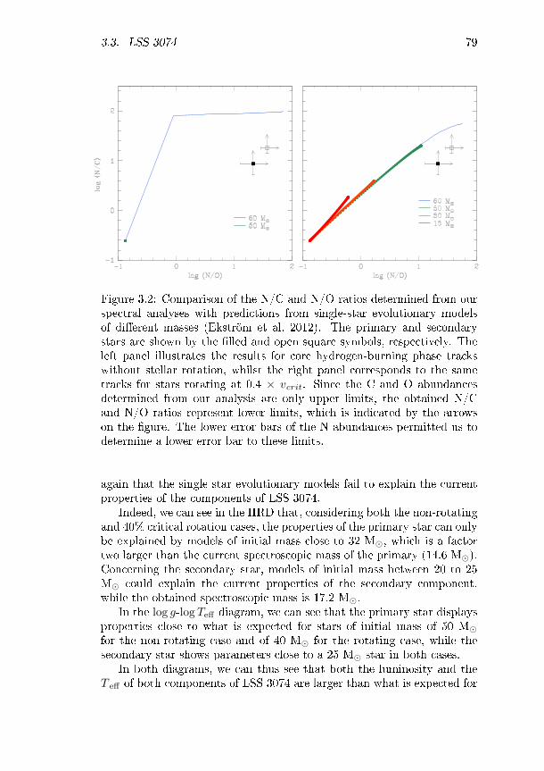
3.3. LSS 3074 79
Figure 3.2: Comparison of the N/C and N/O ratios determined from ourspectral analyses with predictions from single-star evolutionary modelsof dierent masses (Ekström et al. 2012). The primary and secondarystars are shown by the lled and open square symbols, respectively. Theleft panel illustrates the results for core hydrogen-burning phase trackswithout stellar rotation, whilst the right panel corresponds to the sametracks for stars rotating at 0.4 × vcrit. Since the C and O abundancesdetermined from our analysis are only upper limits, the obtained N/Cand N/O ratios represent lower limits, which is indicated by the arrowson the gure. The lower error bars of the N abundances permitted us todetermine a lower error bar to these limits.
again that the single star evolutionary models fail to explain the currentproperties of the components of LSS 3074.
Indeed, we can see in the HRD that, considering both the non-rotatingand 40% critical rotation cases, the properties of the primary star can onlybe explained by models of initial mass close to 32 M, which is a factortwo larger than the current spectroscopic mass of the primary (14.6 M).Concerning the secondary star, models of initial mass between 20 to 25M could explain the current properties of the secondary component,while the obtained spectroscopic mass is 17.2 M.
In the log g-log Teff diagram, we can see that the primary star displaysproperties close to what is expected for stars of initial mass of 50 Mfor the non-rotating case and of 40 M for the rotating case, while thesecondary star shows parameters close to a 25 M star in both cases.
In both diagrams, we can thus see that both the luminosity and theT eff of both components of LSS 3074 are larger than what is expected for
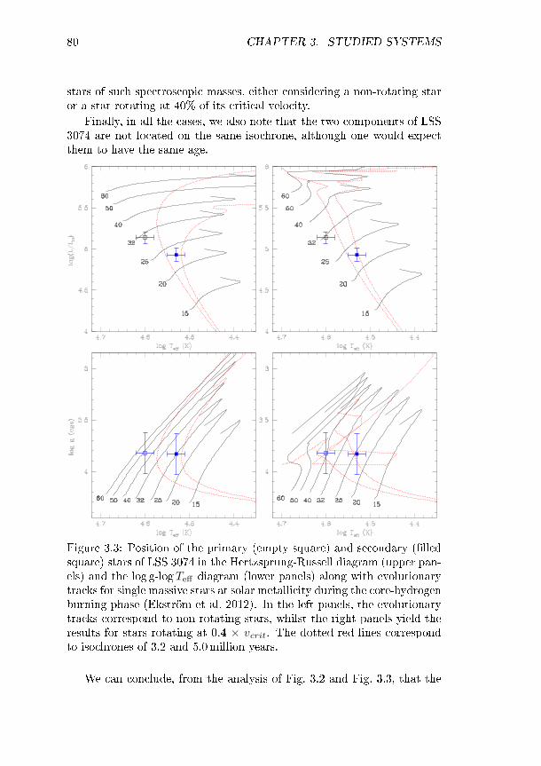
80 CHAPTER 3. STUDIED SYSTEMS
stars of such spectroscopic masses, either considering a non-rotating staror a star rotating at 40% of its critical velocity.
Finally, in all the cases, we also note that the two components of LSS3074 are not located on the same isochrone, although one would expectthem to have the same age.
Figure 3.3: Position of the primary (empty square) and secondary (lledsquare) stars of LSS 3074 in the Hertzsprung-Russell diagram (upper pan-els) and the log g-logTeff diagram (lower panels) along with evolutionarytracks for single massive stars at solar metallicity during the core-hydrogenburning phase (Ekström et al. 2012). In the left panels, the evolutionarytracks correspond to non-rotating stars, whilst the right panels yield theresults for stars rotating at 0.4 × vcrit. The dotted red lines correspondto isochrones of 3.2 and 5.0million years.
We can conclude, from the analysis of Fig. 3.2 and Fig. 3.3, that the

3.3. LSS 3074 81
system LSS 3074 has been, and may still be, signicantly aected bybinary interaction, and that both stars have probably lost a signicantamount of matter.
3.3.2 SB1 orbital solution
We presented in Raucq et al. (2017) the orbital solution of LSS 3074 (seeSect. 4 of the paper, presented here-before). We also showed that the RVsof the N emission and absorption lines in the spectrum of LSS 3074 seemto move along with the primary, with a rather large scatter of velocitiesof the various RVs, especially at phases between 0.25 quadrature and 0.5conjunction (see Fig. 3 of Raucq et al. 2017).
To complement our study of the behaviour of these nitrogen lines,we performed four SB1 orbital solutions based on the N iii λλ 4634 and4641 emission lines, N iii λ 4379 absorption line, N iv λ 4058 line andN v λλ 4604 and 4620 lines respectively. A comparison between theseSB1 solutions and the SB2 orbital solution of the system is presented inTable 3.2, and the corresponding RV curves are shown in Fig. 3.4. Theorange stars and purple squares represent the measured values of the RVsof N iv λ 4058 and N iii λ 4379 lines, respectively, and the orange andpurple curves show the corresponding SB1 orbital solutions. The redcurve represents the SB1 orbital solution obtained with the RVs of theN iii λλ 4634 (lled triangles) and 4641 (open triangles) lines, and theblue curve displays the SB1 orbital solution based on the RVs of the Nv
λλ 4604 (lled circles) and 4620 (open circles) lines. The black dashedcurve shows the primary curve of the SB2 orbital solution presented inRaucq et al. (2017). To perform these orbital solutions, we used theLiège Orbital Solution Package (LOSP) program (Sana et al. 2009, andreferences therein), and we weighted the RVs according to their estimateduncertainties.
This study of the nitrogen lines conrmed that most of these linesseem to be produced by the primary star. We can see here that thecurves corresponding to all of the N lines are in phase with the generalprimary SB2 curve, considering that they display the same T 0, within theerror bars. This indicates that they are indeed produced by the primarystar. Moreover, the curves corresponding to the N iii absorption lines andthe N iv and Nv lines have the same amplitude than the general primarySB2 curve, which suggests that they are produced in the same zone of theprimary atmosphere than the other absorption lines that we consideredfor the general orbital solution (see Raucq et al. 2017, Sect. 4). On theother hand, the larger amplitude of the velocity curve associated to theN iii emission lines suggests that these lines are mainly produced overparts of the primary's atmosphere opposite to the secondary star.
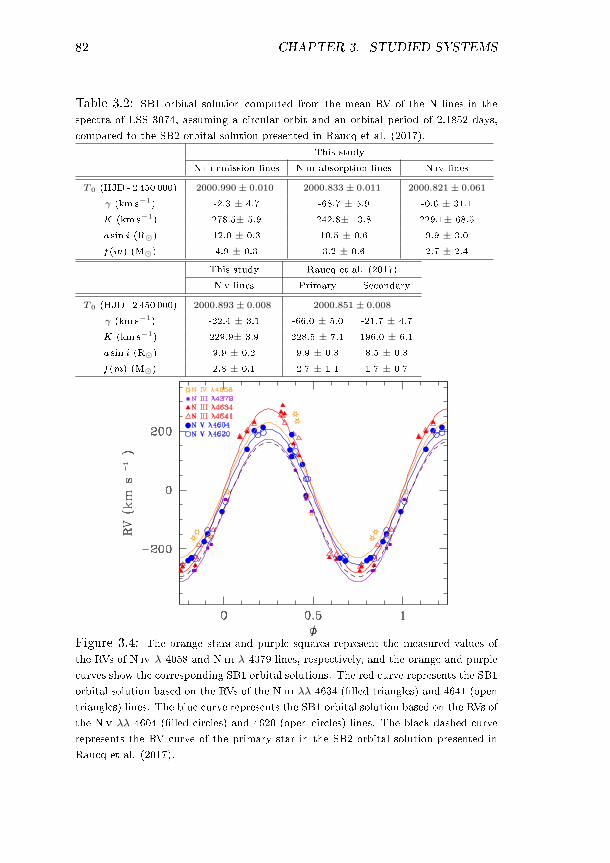
82 CHAPTER 3. STUDIED SYSTEMS
Table 3.2: SB1 orbital solution computed from the mean RV of the N lines in the
spectra of LSS 3074, assuming a circular orbit and an orbital period of 2.1852 days,
compared to the SB2 orbital solution presented in Raucq et al. (2017).
This study
N iii emission lines N iii absorption lines N iv lines
T 0 (HJD - 2 450 000) 2000.990± 0.010 2000.833± 0.011 2000.821± 0.061
γ (km s−1) -2.3 ± 4.7 -68.7 ± 5.9 -0.6 ± 31.1
K (km s−1) 278.5± 5.9 242.8± 13.8 229.1± 68.5
a sin i (R) 12.0 ± 0.3 10.5 ± 0.6 9.9 ± 3.0
f (m) (M) 4.9 ± 0.3 3.2 ± 0.6 2.7 ± 2.4
This study Raucq et al. (2017)
N v lines Primary Secondary
T 0 (HJD - 2 450 000) 2000.893± 0.008 2000.851± 0.008
γ (km s−1) -22.4 ± 3.1 -66.0 ± 5.0 -21.7 ± 4.7
K (km s−1) 229.9± 3.9 228.5 ± 7.1 196.0 ± 6.1
a sin i (R) 9.9 ± 0.2 9.9 ± 0.3 8.5 ± 0.3
f (m) (M) 2.8 ± 0.1 2.7 ± 1.1 1.7 ± 0.7
Figure 3.4: The orange stars and purple squares represent the measured values of
the RVs of N iv λ 4058 and N iii λ 4379 lines, respectively, and the orange and purple
curves show the corresponding SB1 orbital solutions. The red curve represents the SB1
orbital solution based on the RVs of the N iii λλ 4634 (lled triangles) and 4641 (open
triangles) lines. The blue curve represents the SB1 orbital solution based on the RVs of
the N v λλ 4604 (lled circles) and 4620 (open circles) lines. The black dashed curve
represents the RV curve of the primary star in the SB2 orbital solution presented in
Raucq et al. (2017).
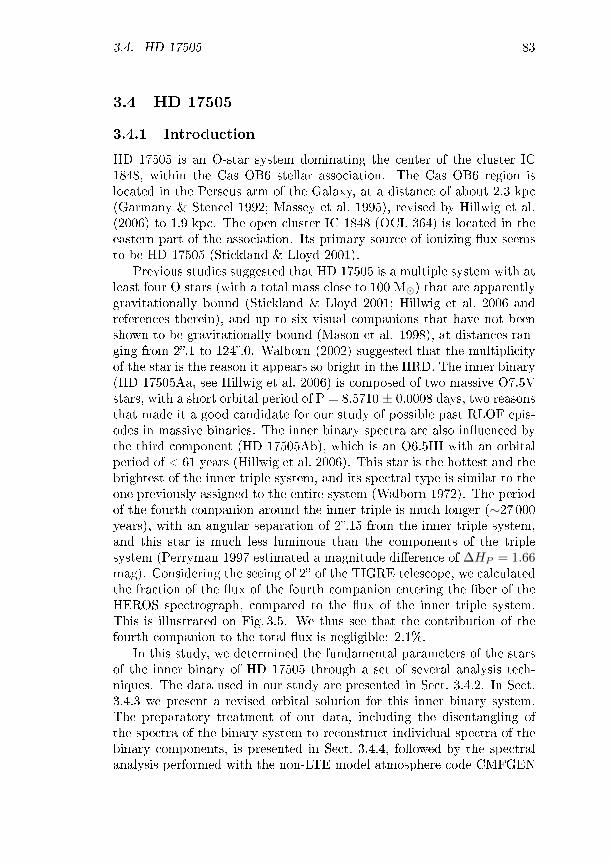
3.4. HD 17505 83
3.4 HD 17505
3.4.1 Introduction
HD 17505 is an O-star system dominating the center of the cluster IC1848, within the Cas OB6 stellar association. The Cas OB6 region islocated in the Perseus arm of the Galaxy, at a distance of about 2.3 kpc(Garmany & Stencel 1992; Massey et al. 1995), revised by Hillwig et al.(2006) to 1.9 kpc. The open cluster IC 1848 (OCL 364) is located in theeastern part of the association. Its primary source of ionizing ux seemsto be HD 17505 (Stickland & Lloyd 2001).
Previous studies suggested that HD 17505 is a multiple system with atleast four O stars (with a total mass close to 100 M) that are apparentlygravitationally bound (Stickland & Lloyd 2001; Hillwig et al. 2006 andreferences therein), and up to six visual companions that have not beenshown to be gravitationally bound (Mason et al. 1998), at distances ran-ging from 2.1 to 124.0. Walborn (2002) suggested that the multiplicityof the star is the reason it appears so bright in the HRD. The inner binary(HD 17505Aa, see Hillwig et al. 2006) is composed of two massive O7.5Vstars, with a short orbital period of P = 8.5710 ± 0.0008 days, two reasonsthat made it a good candidate for our study of possible past RLOF epis-odes in massive binaries. The inner binary spectra are also inuenced bythe third component (HD 17505Ab), which is an O6.5III with an orbitalperiod of < 61 years (Hillwig et al. 2006). This star is the hottest and thebrightest of the inner triple system, and its spectral type is similar to theone previously assigned to the entire system (Walborn 1972). The periodof the fourth companion around the inner triple is much longer (∼27 000years), with an angular separation of 2.15 from the inner triple system,and this star is much less luminous than the components of the triplesystem (Perryman 1997 estimated a magnitude dierence of ∆HP = 1.66mag). Considering the seeing of 2 of the TIGRE telescope, we calculatedthe fraction of the ux of the fourth companion entering the ber of theHEROS spectrograph, compared to the ux of the inner triple system.This is illustrated on Fig. 3.5. We thus see that the contribution of thefourth companion to the total ux is negligible: 2.1%.
In this study, we determined the fundamental parameters of the starsof the inner binary of HD 17505 through a set of several analysis tech-niques. The data used in our study are presented in Sect. 3.4.2. In Sect.3.4.3 we present a revised orbital solution for this inner binary system.The preparatory treatment of our data, including the disentangling ofthe spectra of the binary system to reconstruct individual spectra of thebinary components, is presented in Sect. 3.4.4, followed by the spectralanalysis performed with the non-LTE model atmosphere code CMFGEN

84 CHAPTER 3. STUDIED SYSTEMS
Figure 3.5: Fraction of ux of the fourth component entering the bercompared to the ux of the inner triple system of HD 17505.
in Sect. 3.4.5. Finally, we discuss the results of our study of HD 17505 inSect. 3.4.6.
3.4.2 Observations and data reduction
Fifteen high-resolution optical spectra of HD 17505 were obtained withthe HEROS spectrograph, mounted on the 1.2 m TIGRE telescope atLa Luz Observatory (Mexico; Schmitt et al. 2014), between the 26th ofAugust 2014 and the 25th of October 2014. The HEROS spectrographcovers two spectral domains, ranging from 3500 to 5600 Å (the blue chan-nel) and from 5800 to 8800 Å (red channel), with a resolution of ∼20 000.The spectra were automatically reduced with an Interactive Data Lan-guage (IDL) pipeline based on the reduction package REDUCE writtenby Piskunov & Valenti (2002; see Schmitt et al. 2014).
We also collected one reduced spectrum from the ELODIE archive anda set of six medium-resolution reduced spectra from the FIES archive.The ELODIE échelle spectrograph was mounted on the 1.93 m telescopeat the Observatoire de Haute Provence (OHP, France) from 1993 to 2006,and covered the spectral range from 3850 to 6800 Å with a resolutionof∼42 000. The FIES échelle spectrograph is mounted on the 2.5 m NordicOptical Telescope (NOT) located at the Observatorio del Roque de losMuchachos (La Palma, Spain). It covers the spectral range from 3700 to7300 Å with a resolution of ∼46 000 in medium-resolution mode.
The journal of the observations is presented in Table 3.3.

3.4. HD 17505 85
Table 3.3: Journal of the spectra of HD 17505.
HJD Instrument Exp. time φ RV1 RV2 RV3
-2 450 000 (min) (km s−1)
3327.473 ELODIE 60 0.75 -191.0 114,3 -31.35447.762 FIES 15 0.19 115,5 -193,3 -31.75577.414 FIES 13.7 0.32 90,8 -163,3 -1.15:5812.692 FIES 11.8 0.78 -208,3 113.0 -13.6:5814.677 FIES 9.2 0.01 -28,1 -28,1 -13.6:5816.755 FIES 8.3 0.25 106,3 -200,4 -13.6:6285.436 FIES 15 0.95 -128,1 43,0 9.1:6895.965 HEROS 60 0.20 126,2 -160,5 -37.66897.853 HEROS 60 0.42 36,3: -88,5: -37.66907.940 HEROS 60 0.60 -36,1 -4,1: -37.66910.888 HEROS 40 0.94 -136,1 80,5 -37.66911.915 HEROS 60 0.06 -38,2 -38,2 -37.66918.869 HEROS 60 0.88 -168,5 126,3 -37.66925.891 HEROS 60 0.69 -127,1: 94,7 -37.66939.829 HEROS 60 0.32 139,1 -152,3 -37.66941.814 HEROS 60 0.55 -28,2 -28,2 -37.66943.801 HEROS 60 0.79 -171,4 136,1 -37.66945.770 HEROS 60 0.01 -26,4 -26,4 -37.66947.861 HEROS 60 0.26 144,8 -166,1 -37.66949.855 HEROS 20 0.49 -21,8 -21,8 -37.66953.787 HEROS 20 0.95 -126,8 85,6 -37.66955.785 HEROS 60 0.18 128,8 -142,9 -37.6
The phases (φ) are computed according to the ephemerides listed in Table 3.4.The radial velocities are presented in Sect. 3.4.3. The typical uncertainties onthe RVs are 5 − 15 km s−1. The colons indicate uncertainties larger than 20km s−1. For the third component, we calculated the mean value of the RVs overeach run of observations, given its large orbital period (< 61 years) around theinner binary system.
3.4.3 New orbital solution
From our set of observations, we determined a revised orbital solution ofthe inner binary system of HD 17505. To do so, we have concentratedour eorts on the strongest absorption lines that are essentially free fromblends with other features. In this way, we have measured the RVs ofthe Hγ, He i λλ 4026, 4471, 5876, and 7065 and He ii λλ 4542, and 5412

86 CHAPTER 3. STUDIED SYSTEMS
lines by a multi-Gaussian t in the observed spectra. We adopted theeective wavelengths of Underhill (1995). For each observation, the RVsof the primary and secondary stars were determined as the mean of thecorresponding RVs measured for each of the above-listed lines in that givenobservation.
These resulting RVs are listed in Table 3.3. For most data points, theuncertainties on these RVs are about 5-15 km s−1. In some cases however(indicated by the colons in Table 3.3), the uncertainties are larger than 20km s−1. We adopted the same notations as Hillwig et al. (2006) to referto the primary and secondary stars. We note that both stars seem to havethe same spectral types, thereby leading to some diculties to distinguishthe two stars.
We then performed a Fourier analysis of the RV1 and RV2 data, thatyielded a highest peak around ν = 0.1167 d−1, i.e. Porb = 8.5690 days,which is very close to the orbital period determined in the previous studyof Hillwig et al. (2006; Porb = 8.5710±0.0008 days). For completeness, wealso performed the same Fourier analysis with our RVs combined to thosemeasured by Hillwig et al. (2006) and obtained a highest peak around ν =0.1167 d−1 as well, suggesting that our period determination is consistentwith their work.
Adopting an orbital period of 8.5690 days, we thus computed an orbitalsolution with the LOSP code (Sana et al. 2009, and references therein)assuming an eccentric orbit, since the previous orbital solution of Hillwiget al. (2006) indicated an eccentricity of 0.095 ± 0.011. The RVs wereweighted according to their estimated uncertainties. The result is shown inFig. 3.6 (upper panel) and the corresponding orbital elements are providedin Table 3.4. We also computed an orbital solution based on both ourmeasured RVs with those measured by Hillwig et al. (2006). The resultis shown in Fig. 3.6 (lower panel) and the corresponding orbital elementsare also given in Table 3.4.
The RV amplitudes of both our single and combined solutions are lowerthan values from previous works (K1 = 166.5 and K2 = 170.8 km s−1,Hillwig et al. 2006), and our determined eccentricities are slightly higherthan the one they found: 0.128 and 0.118 vs 0.095. The minimum massesthat we determined are also signicantly lower than what Hillwig et al.found: 11.7 and 12.5 M for the primary and secondary stars respectivelyin our solution based on our measurements, 14.6 and 14.8 M for theprimary and secondary stars respectively in our combined solution, and17.1 and 16.6 M in Hillwig et al. 2006). These signicant dierences inthe minimum masses come from the dierences in RV amplitude in thedierent orbital solutions.

3.4. HD 17505 87
Table 3.4: Orbital solution of the inner binary computed from our RVdata of HD 17505, assuming an eccentric orbit and a period of 8.5690 days,compared to the orbital solution proposed by Hillwig et al. (2006) and anorbital solution obtained by combining our RVs with those measured bythese authors.
This study Combined solutionPrimary Secondary Primary Secondary
T 0 (HJD - 2 450 000) 3329.656 ± 0.313 3328.910 ± 0.173e 0.128± 0.037 0.118± 0.018γ (km s−1) -27.8 ± 4.7 -27.6 ± 4.5 -27.7 ± 2.3 -25.9 ± 2.3K (km s−1) 156.7 ± 6.3 146.7 ± 5.9 162.8 ± 3.2 160.8 ± 3.1a sin i (R) 26.3 ± 1.0 24.6 ± 1.0 27.4 ± 0.5 27.0 ± 0.5q = m1/m2 0.94 ± 0.05 0.99 ± 0.02ω (°) 257.4 ± 14.0 271.5 ± 7.5m sin3i (M) 11.7 ± 1.2 12.5 ± 1.3 14.6 ± 0.7 14.8 ± 0.8RRL/(a1 + a2) 0.37 ± 0.01 0.38 ± 0.01 0.38 ± 0.01 0.38 ± 0.01RRL sin i 19.0 ± 0.6 19.6 ± 0.6 20.6 ± 0.3 20.7 ± 0.3σfit 3.18 1.86
Hillwig et al. (2006)Primary Secondary
T 0 (HJD - 2 450 000) 1862.696 ± 0.016e 0.095± 0.011γ (km s−1) -25.8 ± 1.8 -26.3 ± 1.2K (km s−1) 166.5 ± 1.8 170.8 ± 1.8a sin i (R) 56.8 ± 0.4q = m1/m2 1.03 ± 0.02ω (°) 252 ± 6m sin3i (M) 17.1 ± 0.6 16.6 ± 0.6
T 0 refers to the time of conjunction with the primary being in front. γ, K anda sini denote respectively the apparent systemic velocity, the semi-amplitude ofthe radial velocity curve and the projected separation between the centre of thestar and the centre of mass of the binary system. RRL stands for the radius ofa sphere with a volume equal to that of the Roche lobe computed according tothe formula of Eggleton (1983). All error bars indicate 1σ uncertainties.

88 CHAPTER 3. STUDIED SYSTEMS
Figure 3.6: Radial velocities of the components of the inner binary of HD17505, assuming a period of 8.5690 days. The upper panel shows the RVscorresponding to the measurements taken for this study, while the lowerpanel displays the solution obtained by combining our measurements withthose taken by Hillwig et al. (2006). The RVs of the primary and secondarystars are shown with the lled and empty circles, respectively. The solidand dashed lines indicate the orbital solutions from Table 3.4.

3.4. HD 17505 89
3.4.4 Preparatory analysis
3.4.4.1 Adjustment of the ternary spectra and spectral
disentangling
Once the orbital solution of the inner binary had been determined, thenatural step to follow would have been to disentangle the spectra of thethree components of the central object of HD 17505, the triple systemHD 17505A, considering a non-moving tertiary object, which is a rathergood approximation since the orbital period of the third star around theinner binary is very large (< 61 years) compared to the time span ofthe observations. However, when we applied our disentangling routineadapted to triple systems (see the end of Sect. 2.1.1), we observed theappearance of artefacts in the resulting reconstructed primary, secondaryand tertiary spectra. Indeed, as we can see on Fig. 3.7, the wings ofbroad features in the resulting tertiary spectrum appear in emission, witha general prole very similar to a mirrored prole of the wings of thecorresponding lines in the primary and secondary spectra.
Figure 3.7: Parts of the reconstructed spectra of the primary (middle),secondary (top, shifted upwards by 0.2 continuum units) and tertiary (bot-tom, shifted downwards by 0.2 continuum units) stars after an attemptof spectral disentangling of the triple system.
The appearance of such artefacts may be due to the method used inthe disentangling code itself. Indeed, this method is based on the Dopplershift of the lines associated to the dierent components of a system due totheir motion along their orbit. In this particular triple system, it causessome problems because the lines of the third object are located betweenthe lines of the other two stars at every observed phase. This peculiarity,combined with the RV amplitudes of the primary and secondary stars

90 CHAPTER 3. STUDIED SYSTEMS
and the broadening of the respective lines of the three objects due torotational velocities and macroturbulence, implies that the wings of thelines of the tertiary star are always partially blended with the neighbouringwings of the corresponding lines of the primary and secondary stars. Thedisentangling code thus encounters problems to interpret the behaviourof these wings, and produces artefacts during its calculation.
To circumvent this problem, we used the same method as for the IUEspectra of HD 149404, in Sect. 4.4 of Raucq et al. (2016). We recombinedsynthetic spectra of each component of HD 17505A, shifted by the appro-priate RVs for every observations, and compared the obtained syntheticternary spectrum to the observations of the system.
To constrain the fundamental physical parameters of each componentof the inner triple system of HD 17505, we used the non-LTE model at-mosphere code CMFGEN, described in Sect. 2.2. A β law was used todescribe the velocity law in the stellar winds, and a super-level approachwas adopted for the resolution of the equations of statistical equilibrium.The following chemical elements and their ions were included in the cal-culations: H, He, C, N, O, Ne, Mg, Al, Si, S, Ca, Fe, and Ni. A newphotospheric structure was computed from the solution of the equationsof statistical equilibrium, and was then connected to the same β windvelocity law. We assumed a microturbulent velocity in the atmospherevarying linearly with wind velocity from 10 km s−1 in the photosphere to0.1 × v∞ at the outer boundary. The generated synthetic spectra werethen recombined and compared to the spectra of the triple system to con-strain iteratively the fundamental properties of the three stars, with thefollowing method.
As a starting point, we assumed that these fundamental propertieswere close to typical values of stars of the same spectral type. We thustook the surface gravities, stellar masses, radii, luminosities and eectivetemperatures from Martins et al. (2005), the mass-loss rates and β of thevelocity law from Muijres et al. (2012) and the terminal velocities fromPrinja et al. (1990).
In order to have a rst approximation of the rotational velocities, weused a multi-Gaussian tting technique within MIDAS on the lines He iλλ 4471 and 4922, O iii λ 5592 and C iii λ 5812 for the most deblendedobserved spectra, and we applied a Fourier transform method (Simón-Díaz& Herrero 2007, Gray 2008) to the best tting Gaussians. We estimatedthe macroturbulence velocities with the auxiliary program MACTURB ofthe stellar spectral synthesis program SPECTRUM v2.76 developed byGray (2010), applying this technique to the wings of He i λ 4026, 4471,4713 and 5016, and He ii λ 4542 for several phases.
We estimated the respective contribution of the three components to

3.4. HD 17505 91
the spectra of the triple system through the following formula on selectedlines:
lili+lj+lk
= li
lj(lilj
+1+lklj
)with
lilj
=(EWi
EWj
)obs
(EWSTj
EWSTi
)mean
where i, j and k are representing either the primary, secondary or tertiarystars, depending on the contribution we were calculating. The EW i rep-resent the equivalent widths of the studied lines of star i referring to thecombined continuum of the three stars and EWSTi the same measure-ment in the synthetic spectrum of a typical star of the same spectral typeas star i, computed with CMFGEN. We considered the spectral typespreviously determined by Hillwig et al. (2006; O7.5V((f)) + O7.5V((f))+ O6.5III((f))). This way, we obtained that the primary, secondary andtertiary contributions to the total ux are 29%, 34% and 37%, respect-ively, which is close to what Hillwig et al. (2006) found in their study ofHD 17505 (30%, 30% and 40%, respectively).
We then constrained the physical properties of each star by an iterativeprocess, because each adjustment of a given parameter leads to somemodications in the value of others, and each modication in the spectrumof one of the three stars may require some modications in the spectrumof one of the other two. For each star, the following process is used toadjust the t of the spectra.
The rst step is to adjust the eective temperature in the models.This parameter is mainly determined through the relative strengths ofHe i λ 4471 and He ii λ 4542 lines (Martins 2011).
Then comes a rst approximation of the surface gravities through thewidth of the Balmer lines, which were approximatively reconstructed witha multi-Gaussian t on a number of observations at dierent phases.
Subsequently, the multiplicity of the object may cause some problems.Indeed, the next step is to adjust the wind parameters, but the He ii λ 4686and the Balmer lines may be polluted by some emission from a wind-windinteraction zone within the inner binary of HD 17505. Therefore, con-sidering the possible existence of such additional emission polluting thediagnostic lines, the adjustment of the models onto the observed spectramay lead to an underestimate of the terminal velocities, and an overes-timate of the β of the velocity law, the clumping factors, the clumpingvelocity factors, and the mass-loss rates of the primary and secondarystars. The values obtained with such a t should thus only be considered

92 CHAPTER 3. STUDIED SYSTEMS
as lower and upper limits of the real properties of the corresponding stel-lar winds. However, we nevertheless adjusted them as well as possible.The spectrum of the third component, however, should not be aected bysuch pollution, since it is too distant from the inner binary to induce suchwind-wind interactions. The diagnostic lines of the terminal velocities, βand the mass-loss rates are the strength of Hα, the width of He ii λ 4686and Hα, and the strengths of Hγ and Hδ, respectively, while the clumpinglling factors and the clumping velocity factors are based on the shape ofthe Hα and Hβ lines.
Once the fundamental stellar parameters were established, we invest-igated the CNO abundances through the strengths of associated lines. Weperformed a normalized χ2 analysis to determine the best t to selectedlines, as done by Martins et al. (2015; see also Raucq et al. 2016; 2017)and explained in Sect. 2.2.2. We used the C iiiλλ 4068-70, 4156, 4163,and 4187; N ii λ 4379, and N iii λλ 4511, 4515, and 4525; and O iii λλ5508 and 5592 lines to adjust the C, N and O abundances, respectively,for both stars.
In Fig. 3.8 we show parts of the observed spectra at dierent phaseswith the corresponding recombined synthetic spectra of the triple system.
Once we obtained a good t of the triple system for all the observa-tions, we substracted the synthetic tertiary spectrum from each observa-tion, to recover the spectra of the inner binary. After removal of the thirdobject, we then treated the spectra with the disentangling code, in thesame way as for the other binary systems, HD 149404 (see Sect. 3.1 ofRaucq et al. 2016) and LSS 3074 (see Sect. 6.1 of Raucq et al. 2017).
3.4.4.2 Spectral types
Once we obtained the individual reconstructed spectra of the primaryand secondary components of HD 17505, we determined their respectivespectral types. To do so, we applied Conti's quantitative classicationcriterion for O-type stars (Conti & Alschuler 1971, Conti & Frost 1977,see also van der Hucht 1996) for the spectral types, based on the equivalentwidth ratio of the spectral lines He i λ 4471 and He ii λ 4542. This way, weobtained that both primary and secondary stars are O7 stars. However,it was not possible to use Conti's criterion for the luminosity classes,based on the equivalent width ratio of the spectral lines Si iv λ 4088 andHe i λ 4143, since the latter line is very weak or even non existent in thereconstructed spectra. We thus used the Walborn criterion (Walborn &Fitzpatrick 1990 and references therein) to determine that both stars areV stars, since they display a strong He ii λ 4686 absorption. In addition tothe strong absorption of He ii λ 4686, the spectra of both stars also display

3.4. HD 17505 93
4470
0.8
1
1.2
1.4
1.6
1.8
4540 5590
Figure 3.8: He i λ 4471 (left panel), He ii λ 4542 (middle panel) and O iii
λ 5592 lines (right panel) of the recombined synthetic spectrum (red) ofthe triple system HD 17505 for dierent observations (black). The phasesof the dierent observations, according to the ephemerides of Table 3.4,are presented at the left side of the gure.
N iii λλ 4634-40-42 emission, leading to the addition of a ((f)) qualier totheir spectral types. We thus found that both primary and secondarystars are O7V((f)) stars. Our classication being based on the separatedspectra, it is less sensitive to a possible phase-dependence of some specicspectral features, and should thus be more robust than a classicationbased only on spectra taken near quadrature phases. But we can notethan we nd an excellent agreement with the spectral types proposed by

94 CHAPTER 3. STUDIED SYSTEMS
Hillwig et al. (2006, O7.5V((f)) + O7.5V((f))), which they determinedvia tomographic reconstruction of the individual spectra.
3.4.4.3 Brightness ratio
Whilst the spectral disentangling yields the strength of the lines in bothprimary and secondary spectra compared to the combined continuum,it does not permit to establish the relative strengths of the individualcontinua. To further analyse the reconstructed spectra, we therefore needto establish the brightness ratio of the stars in an independant way.
To determine the brightness ratio of the primary and secondary com-ponents of HD 17505, we used a similar technique as done in Sect. 3.4.4.1to estimate the contribution of the three components of the triple systemto the observations. Here, instead of measuring the equivalent widths ona multi-Gaussian t, we measured the equivalent widths of a number ofselected spectral lines on the separated spectra of the primary and sec-ondary stars, but referring to the combined continuum of the two stars.
The results are listed in Table 3.5. From these equivalent widths, thebrightness ratio of two stars can be calculated from
l1l2
=(EW1
EW2
)obs
(EWST2
EWST1
)mean
with the same conventions as in the previous section. In the particularcase of HD 17505, since the spectral types of the primary and secondarystars are identical, the second term of the equation is equal to 1, and thebrightness ratio of the two stars can be simply evaluated as the ratio oftheir respective equivalent widths, averaged over the selected lines.
This way, we derived a primary over secondary brightness ratio of0.88 ± 0.09. This value is very close to what we inferred from our pre-liminary study of the contributions of the dierent components to theobserved spectra of the triple system, based on the multi-Gaussian t, i.e.l1/l2 = 29/34 = 0.85, and is slightly lower than the brightness ratio of1.00 proposed by Hillwig et al. (2006).
Høg et al. (2000) give a mean V magnitude of 7.356±0.010 and B−Vcolor of 0.308±0.019 for the inner triple system, HD 17505A. The intrinsic(B − V )0 of O7 stars being -0.27 (Martins & Plez 2006), we determined anextinction AV of 1.792± 0.059, assuming RV = 3.1. Assuming the ∼ 1.9kpc distance (Hillwig et al. 2006), we inferred an absolute magnitudeMV = −5.830 ± 0.059 for the system. With the previously determinedbrightness ratio, we then calculated individual absolute magnitudes ofMPV = −5.005± 0.079 and MS
V = −5.145± 0.079.The reconstructed normalized primary and secondary optical spectra
are shown and discussed in Sect. 3.4.5.2.
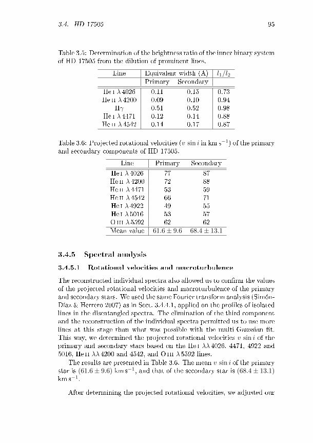
3.4. HD 17505 95
Table 3.5: Determination of the brightness ratio of the inner binary systemof HD 17505 from the dilution of prominent lines.
Line Equivalent width (Å) l1/l2Primary Secondary
He i λ 4026 0.11 0.15 0.73He ii λ 4200 0.09 0.10 0.94
Hγ 0.51 0.52 0.98He i λ 4471 0.12 0.14 0.88He ii λ 4542 0.14 0.17 0.87
Table 3.6: Projected rotational velocities (v sin i in km s−1) of the primaryand secondary components of HD 17505.
Line Primary SecondaryHe i λ 4026 77 87He ii λ 4200 72 88He ii λ 4471 53 59He ii λ 4542 66 71He i λ 4922 49 55He i λ 5016 53 57O iii λ 5592 62 62Mean value 61.6± 9.6 68.4± 13.1
3.4.5 Spectral analysis
3.4.5.1 Rotational velocities and macroturbulence
The reconstructed individual spectra also allowed us to conrm the valuesof the projected rotational velocities and macroturbulence of the primaryand secondary stars. We used the same Fourier transform analysis (Simón-Díaz & Herrero 2007) as in Sect. 3.4.4.1, applied on the proles of isolatedlines in the disentangled spectra. The elimination of the third componentand the reconstruction of the individual spectra permitted us to use morelines at this stage than what was possible with the multi-Gaussian t.This way, we determined the projected rotational velocities v sin i of theprimary and secondary stars based on the He i λλ 4026, 4471, 4922 and5016, He ii λλ 4200 and 4542, and O iii λ 5592 lines.
The results are presented in Table 3.6. The mean v sin i of the primarystar is (61.6± 9.6) km s−1, and that of the secondary star is (68.4± 13.1)km s−1.
After determining the projected rotational velocities, we adjusted our

96 CHAPTER 3. STUDIED SYSTEMS
determination of the macroturbulence velocities for the primary and sec-ondary stars. To do so, we used the auxiliary program MACTURB de-veloped by Gray (2010), based on the radial-tangential anisotropic mac-roturbulent broadening formulation of Gray (2008), on the lines He iλλ 4026, 4471, 4713 and 5016, and He ii λ 4542 in the individual spectra,after including the rotational velocity broadening. This way, we obtainedmacroturbulence velocities of 60 and 65 km s−1 for the primary and sec-ondary stars respectively.
Both rotational and macroturbulence broadening eects were appliedon the synthetic spectra before comparing the latter with the individualreconstructed spectra of the primary and secondary stars of HD 17505.
3.4.5.2 Fit of the separated spectra with the CMFGEN code
Once we obtained the separated spectra of the primary and secondarystars of HD 17505, their brightness ratio, rotational velocities and mac-roturbulence velocities, we then improved our determination of the fun-damental properties of both stars with the CMFGEN code. We followedthe same procedure as exposed in Sect. 3.4.4.1 to constrain the dierentstellar parameters.
However, as explained in Sect. 2.1.2, the Balmer lines are too broad tobe well recovered by the disentangling process, and their wings are thusnot perfectly reliable to adjust the surface gravities. We thus used aniterative process to contrain the luminosities together with these gravit-ies. From the rst estimate of log g given by the t of the triple system,performed in Sect. 3.4.4.1, and our determination of the eective temper-atures, we inferred the bolometric corrections (Lanz & Hubeny 2003), thenthe individual bolometric luminosities, using the absolute V magnitudesof the components derived in Sect. 3.4.4.3. These bolometric luminositiesand the eective temperatures then permitted us to compute the ratio ofthe stellar radii RP
RS. Together with the assumed surface gravities, this
ratio yielded the spectroscopic mass ratio MP
MS, which we compared to the
dynamical mass ratio inferred from the orbital solution (Sect. 3.4.3). Thedierence between these mass ratios then permitted us to produce a newestimate of the surface gravities. This iterative process was repeated untilthe spectroscopic and dynamical mass ratios agreed with each other, andthe CMFGEN synthetic spectra produced for the new surface gravitiesmatched the observations as well as possible.
Figure 3.9 shows the best t of the optical spectra of the primary andsecondary stars of HD 17505 obtained with CMFGEN, and Table 3.7 liststhe corresponding stellar parameters. Table 3.8 compares the chemicalabundances of these best-t models with the solar abundances taken from

3.4. HD 17505 97
Asplund et al. (2009).
Figure 3.9: Part of the normalized disentangled spectra of the primary(top, shifted by 0.5 continuum units) and secondary (bottom) stars of HD17505, along with the best-t CMFGEN model spectra (red).
Figure 3.9 shows that the Balmer, He, C and N lines are very wellreproduced by the models for both stars. The case of oxygen raises morequestions. Indeed, while the O iii λλ 5508 and 5592 lines are well adjusted,several other O iii lines (e.g. Oiii λλ 4448, 4454, and 4458 lines) are present

98 CHAPTER 3. STUDIED SYSTEMS
Table 3.7: Best-t CMFGEN model parameters of the primary and sec-ondary stars of HD 17505.
Prim. Sec.R (R) 13.4± 1.0 13.6± 1.0M (M) 22.7± 8.6 24.2± 9.0Teff (104 K) 3.70± 0.15 3.67± 0.15log ( L
L) 5.26± 0.03 5.31± 0.03
log g (cgs) 3.80± 0.15 3.73± 0.15β ≤ 1.07 ≤ 1.07
v∞ (km s−1) ≥ 2200 ≥ 2200
M/√f1 (M yr−1) ≤ 2.30× 10⁻⁷ ≤ 3.70× 10⁻⁷
f1 ≤ 0.1 ≤ 0.2f2 (km s−1) ≤ 250 ≤ 180
BC −3.40 −3.38f1 and f2 represent the clumping lling factor and the clumping velocityfactor, presented in Sect. 2.2.2. The quoted errors correspond to 1σ un-certainties. The bolometric corrections are taken from Lanz & Hubeny(2003), based on our best-t Teff and log g.
Table 3.8: Chemical surface abundances of the primary and secondarystars of HD 17505.
Primary Secondary SunHe/H 0.1 0.1 0.089C/H 1.91+0.37
−0.40 × 10⁻⁴ 1.97+0.39−0.42 × 10⁻⁴ 2.69× 10⁻⁴
N/H 1.37+0.25−0.21 × 10⁻⁴ 9.70+1.1
−0.84 × 10⁻⁵ 6.76× 10⁻⁵
O/H 3.87+1.2−0.92 × 10⁻⁴ 4.73+2.2
−1.5 × 10⁻⁴ 4.90× 10⁻⁴
Abundances are given by number as obtained with CMFGEN. The solarabundances (Asplund et al. 2009) are quoted in the last column. The 1σuncertainty on the abundances was set to abundances corresponding to anormalized χ2 of 2.0 (see Sect. 2.2.2 of this work, Sect. 4.3 of Raucq etal. 2016 and Sect. 8.3 of Raucq et al. 2017; see also Martins et al. 2015).The values of the He abundances have been xed in the models.
in the synthetic CMFGEN spectra of both stars, but are not visible in theseparated spectra, nor in the observed spectra of the system before thedisentangling procedure. We encountered similar problems with the samelines in the case of HD 149404 (see Raucq et al. 2016).
We can stress here three important results. First of all, by couplingthe stellar masses obtained with CMFGEN (Table 3.7) with the minimummasses obtained with the orbital solution (Table 3.4), we obtain an inclin-

3.4. HD 17505 99
ation of the system i ∼ 53.3°. With this inclination, we can see from ourdetermination of the stellar radii with CMFGEN compared to the radiiof the Roche lobes obtained in the orbital solution (Table 3.4) that bothstars are well into their Roche lobes: they display a Roche lobe llingfactor of 0.57 ± 0.08 and 0.56 ± 0.08, respectively. Second, we note thatthere is a slight enhancement of the N abundance, coupled with an evenslighter C and O depletion at the surface of both stars. However, thesemodications of the surface abundances are low enough to be explainedby rotational mixing in the star (see Sect. 3.4.6.1), with no need to includemass-exchange episode in the history of the system. The third result is alsopointing in the same direction. Indeed, from the inclination determinedearlier, we can derive the absolute rotational velocities and we obtain 76.8and 85.3 km s−1 for the primary and secondary stars respectively. Finally,by combining these rotational velocities with the stellar radii determinedwith CMFGEN (Table 3.7), we nd that the primary and secondary starsof HD 17505 are in perfectly synchronous rotation: PP = 8.83, PS = 8.07and P orb = 8.569 days. Moreover, if we calculate the critical velocities
of the stars, vcrit =(
2GM3RP
)1/2
, based on our results from the CMFGENt, we nd that the current rotational velocities of the primary and sec-ondary stars correspond to 0.16× vcrit and 0.18× vcrit respectively, whichcorrespond to the median value of birth rotational velocities for stars ofsimilar masses, according to the study of Wol et al. (2006). This suggeststhat there has not been any kinetic momentum exchange between the twocomponents in the past history of the inner binary system. These threeresults suggest that this system has not yet experienced a RLOF episodeduring its evolution. We will come back to these results in Sect. 3.4.6.1.
3.4.6 Discussion and conclusion
3.4.6.1 Evolutionary status
As we have shown in the previous section, the spectra of the primaryand secondary components of HD 17505 display the signatures of a slightmodication of the CNO surface abundances. Figure 3.10 compares ourinferred N/C and N/O ratios with the predictions for the evolution ofsingle massive stars (Ekström et al. 2012). The left panel shows the caseof non-rotating stars, whilst the right panel shows the case of stars rotat-ing at 0.4× vcrit. This gure shows that the current surface abundancesof both stars are dicult to explain in the non-rotating case: the onlypossibility for the secondary would be an initial mass of 60M, while itsspectroscopic mass is a factor 2.4 lower, and none of the theoretical pre-dictions can explain the surface abundances of the primary star. However,

100 CHAPTER 3. STUDIED SYSTEMS
Figure 3.10: Comparison of the N/C and N/O ratios obtained from ourspectral analysis with predictions from single star evolutionary models ofdierent masses (Ekström et al. 2012). The lled (resp. empty) squaresdisplay the characteristics of the primary (resp. secondary) star. Theleft panel illustrates the results for core hydrogen burning phase trackswithout stellar rotation, and the right panel corresponds to the sametracks for stars with a rotation of 0.4× vcrit.
both primary and secondary abundances can be explained by the rotatingmodels, with single stars of initial masses close to 25-30M, which is closeto the masses we inferred from our spectroscopic analysis for both stars(Table 3.7).
In Figure 3.11 we present the positions of the primary and secondarystars in the Hertzsprung-Russell diagram (HRD; upper panels) and in thelog g-log Teff diagram (lower panels), with the evolutionary tracks fromEkström et al. (2012) for the core-hydrogen burning phase of single stars atsolar metallicity. Once again, the left panels display the non-rotating starscase and the right panels show the tracks for stars rotating at 0.4× vcrit.
If we consider the case without any rotational mixing, we can see thatthe positions of the primary and secondary stars in the HRD are relativelyclose to the tracks corresponding to stars with an initial mass of 30M,which is close to their current spectroscopic masses of 24-25M, and maybe located on a common isochrone between 3.2 and 4.0million years. Inthe log g-log Teff diagram, however, while they are located again on thesame isochrone at 3.2 million years, they are closer to the 40M evolu-tionary track, which is signicantly higher than their observed masses.

3.4. HD 17505 101
Considering now the case of stars rotating at 40% of their criticalvelocity, we see that both stars would have initial masses of 30-32M,which is again close to their spectroscopic masses, and they would bothbe ∼4.0million years old.
Both our results in Sect. 3.4.5.2 and the Figures 3.10 and 3.11 showthat both primary and secondary stars current properties can be explainedby single star evolutionary models with a rotational velocity of 0.4 ×vcrit, which suggests that the inner binary system of HD 17505 did notexperience strong binary interactions at this stage of its life.
3.4.6.2 Summary and conclusion
We have studied the fundamental properties of the inner binary systemof HD 17505 by means of several techniques. To do so, our rst step wasto t the inner triple system with a combination of synthetic CMFGENspectra of the three components shifted by their associated RVs for eachobservation, in order to substract the third component from the observedspectra and recover the spectra of the inner binary. We then used ourdisentangling code to recover the individual spectra of the primary andsecondary stars. From these reconstructed spectra, we determined accur-ately a number of stellar parameters, partly with the CMFGEN modelatmosphere code, and used them to constrain the evolutionary status ofthe system.
We established the existence of a slight overabundance in N and slightC and O depletions in both primary and secondary spectra and we foundno evidence of asynchronous rotation between the primary and secondarystars. We showed that these properties can be explained by single starevolutionary models of initial mass of 30-32M, with a rotational velocityof 40% of their critical velocity. We thus concluded that this system hasnot experienced binary interactions at this stage of its evolution.

102 CHAPTER 3. STUDIED SYSTEMS
Figure 3.11: The upper panels show the positions of the primary(empty square) and secondary (lled square) stars of HD 17505 in theHertzsprung-Russell diagram, while the lower panels show their positionsin the log g-logTeff diagram, along with evolutionary tracks for singlemassive stars at solar metallicity during the core-hydrogen burning phase(Ekström et al. 2012). In the left panels, the evolutionary tracks cor-respond to non-rotating stars, whilst the right panels yield the results forstars rotating at 0.4 × vcrit. The dotted red lines correspond to isochronesof 3.2 and 4.0million years for the left panels and of 4.0 and 5.0millionyears for the right panels.

3.5. HD 206267 103
3.5 HD 206267
3.5.1 Introduction
HD 206267 is a multiple system dominating the young open cluster Trumpler37 and the H ii region IC 1396, embeded in the Cep OB2 association. Thissystem was rst studied by Plaskett in 1923, and directly presented prob-lems for the observers, since its spectrum displays rather diuse lines,some of them being double and showing variable strength and prole.Stickland (1995) suspected the system to be triple, with a third constant-velocity component, and presented a new orbital solution of the innerbinary based on high-resolution, short-wavelength (SWP) IUE spectra.He found a short orbital period of 3.71 days for the inner binary system.In addition to the short period, the massive character of both primaryand secondary stars (O6.5 V + O9.5 V) determined by Burkholder etal. in 1997 makes this system a good candidate for our search of pastmass-exchange episodes in massive binaries.
In this study, we constrained the fundamental parameters of the starsof the inner binary of HD 206267 with a set of several techniques of ana-lysis. We present the data used in our study in Sect. 3.5.2 and our revisedorbital solution of the inner system in Sect. 3.5.3. The preparatory ana-lysis of our data, including the reconstruction of the individual spectra ofthe primary and secondary components with our spectral disentanglingcode, are presented in Sect. 3.5.4 and the spectral analysis performedwith the non-LTE atmosphere code CMFGEN in Sect. 3.5.5. Finally, wediscuss the results of our study of HD 206267 in Sect. 3.5.6.
3.5.2 Observations and data reduction
For our study of HD 206267, we collected twenty-two high-resolutionoptical spectra with the HEROS spectrograph, mounted on the 1.2 mTIGRE telescope at La Luz Observatory (Mexico; Schmitt et al. 2014).The spectra were collected during two observing runs: the rst half betweenthe 26th of August 2014 and 27th of October 2014, and the second halfbetween the 2nd of August 2015 and the 28th of October 2015. TheHEROS spectrograph covers two spectral domains: from 3500 to 5600 Å(the blue chanel) and from 5800 to 8800 Å (red channel), with a resolutionof ∼ 20 000. The spectra were automatically reduced with an InteractiveData Language (IDL) pipeline based on the reduction package REDUCEwritten by Piskunov & Valenti (2002).
We also retrieved a series of reduced spectra from dierent archives.One spectrum from the ELODIE archives, taken in September 1997, onespectrum from the ESPaDOnS archives, taken in August 2011, and nine
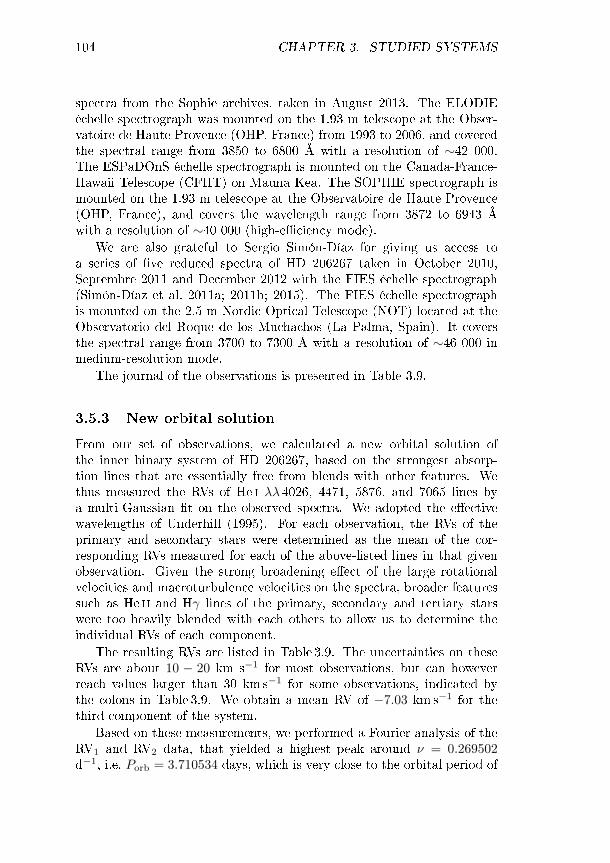
104 CHAPTER 3. STUDIED SYSTEMS
spectra from the Sophie archives, taken in August 2013. The ELODIEéchelle spectrograph was mounted on the 1.93 m telescope at the Obser-vatoire de Haute Provence (OHP, France) from 1993 to 2006, and coveredthe spectral range from 3850 to 6800 Å with a resolution of ∼42 000.The ESPaDOnS échelle spectrograph is mounted on the Canada-France-Hawaii Telescope (CFHT) on Mauna Kea. The SOPHIE spectrograph ismounted on the 1.93 m telescope at the Observatoire de Haute Provence(OHP, France), and covers the wavelength range from 3872 to 6943 Åwith a resolution of ∼40 000 (high-eciency mode).
We are also grateful to Sergio Simón-Díaz for giving us access toa series of ve reduced spectra of HD 206267 taken in October 2010,Septembre 2011 and December 2012 with the FIES échelle spectrograph(Simón-Díaz et al. 2011a; 2011b; 2015). The FIES échelle spectrographis mounted on the 2.5 m Nordic Optical Telescope (NOT) located at theObservatorio del Roque de los Muchachos (La Palma, Spain). It coversthe spectral range from 3700 to 7300 Å with a resolution of ∼46 000 inmedium-resolution mode.
The journal of the observations is presented in Table 3.9.
3.5.3 New orbital solution
From our set of observations, we calculated a new orbital solution ofthe inner binary system of HD 206267, based on the strongest absorp-tion lines that are essentially free from blends with other features. Wethus measured the RVs of He i λλ 4026, 4471, 5876, and 7065 lines bya multi-Gaussian t on the observed spectra. We adopted the eectivewavelengths of Underhill (1995). For each observation, the RVs of theprimary and secondary stars were determined as the mean of the cor-responding RVs measured for each of the above-listed lines in that givenobservation. Given the strong broadening eect of the large rotationalvelocities and macroturbulence velocities on the spectra, broader featuressuch as He ii and Hγ lines of the primary, secondary and tertiary starswere too heavily blended with each others to allow us to determine theindividual RVs of each component.
The resulting RVs are listed in Table 3.9. The uncertainties on theseRVs are about 10 − 20 km s−1 for most observations, but can howeverreach values larger than 30 km s−1 for some observations, indicated bythe colons in Table 3.9. We obtain a mean RV of −7.03 km s−1 for thethird component of the system.
Based on these measurements, we performed a Fourier analysis of theRV1 and RV2 data, that yielded a highest peak around ν = 0.269502d−1, i.e. Porb = 3.710534 days, which is very close to the orbital period of

3.5. HD 206267 105
Table 3.9: Journal of the spectra of HD 206267.
HJD-2 450 000 Instrument Exp. time φ RV1 RV2
(min) (km s−1) (km s−1)0710.4441 ELODIE 22.3 0.42 -166.64: 279.785494.3031 FIES 3.3 0.95 163.71 -298.865729.1077 ESPaDOnS 7.5 0.24 -144.38 95.925812.5828 FIES 2.1 0.74 107.95 -113.76:5816.4969 FIES 2.1 0.80 116.34: -141.13:5817.5170 FIES 2.6 0.07 70.20: -233.196285.3231 FIES 3.4 0.17 -7.10 -7.106527.4539 SOPHIE 5 0.44 -160.71 294.966527.5577 SOPHIE 5 0.47 -160.47 291.806528.4396 SOPHIE 5 0.71 -13.17 -13.176528.5550 SOPHIE 5 0.74 -13.17 -13.176529.4943 SOPHIE 5 0.99 180.19 -301.366530.3561 SOPHIE 5 0.22 -137.16 80.186530.5523 SOPHIE 5 0.28 -149.83 164.456531.4081 SOPHIE 5 0.51 -170.80 251.796531.5479 SOPHIE 5 0.54 -140.55 221.306895.7500 HEROS 30 0.72 -4.52 -4.526897.7738 HEROS 30 0.26 -133.61 128.006907.7219 HEROS 30 0.95 123.25: -312.95:6909.7156 HEROS 30 0.48 -147.36 291.916911.7011 HEROS 30 0.02 149.51 -279.746920.6768 HEROS 30 0.44 -162.35 276.12:6926.6468 HEROS 30 0.05 159.82 -252.976939.6036 HEROS 30 0.54 -145.36 223.146941.6020 HEROS 30 0.08 167.72 -227.506944.6560 HEROS 30 0.90 160.05 -278.836957.5806 HEROS 30 0.38 -146.99 273.99:7236.7624 HEROS 15 0.64 -142.53 164.157236.7729 HEROS 15 0.64 -117.50 165.157238.7444 HEROS 30 0.17 -3.96 -3.967264.8159 HEROS 30 0.20 -3.96 -3.967271.7659 HEROS 30 0.08 161.57 -229.727286.6714 HEROS 30 0.09 162.89 -180.757288.6617 HEROS 30 0.63 -145.56 131.03:7290.7237 HEROS 30 0.19 -3.96 -3.967292.6865 HEROS 30 0.72 -92.04: 158.667308.6686 HEROS 30 0.02 170.45 -278.457323.5769 HEROS 30 0.04 178.21 -257.39
The phases (φ) are computed according to the ephemerides of the combinedorbital solution listed in Table 3.10. The radial velocities are presented inSect. 3.5.3. The typical uncertainties on the RVs are 10 − 20 km s−1. Thecolons indicate uncertainties larger than 30 km s−1. The mean value of the RVsof the third component is −7.03 km s−1.
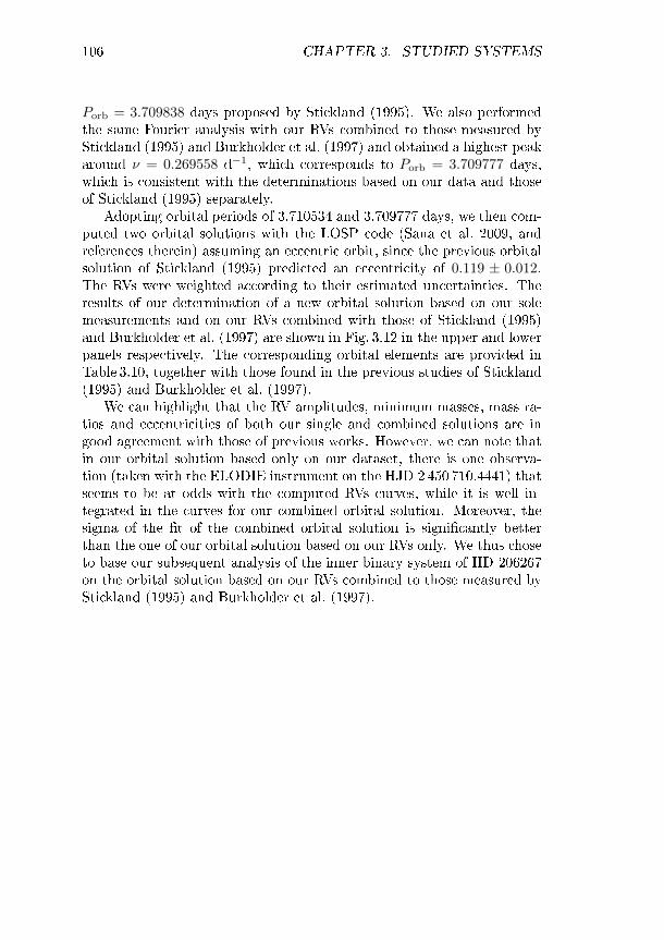
106 CHAPTER 3. STUDIED SYSTEMS
Porb = 3.709838 days proposed by Stickland (1995). We also performedthe same Fourier analysis with our RVs combined to those measured byStickland (1995) and Burkholder et al. (1997) and obtained a highest peakaround ν = 0.269558 d−1, which corresponds to Porb = 3.709777 days,which is consistent with the determinations based on our data and thoseof Stickland (1995) separately.
Adopting orbital periods of 3.710534 and 3.709777 days, we then com-puted two orbital solutions with the LOSP code (Sana et al. 2009, andreferences therein) assuming an eccentric orbit, since the previous orbitalsolution of Stickland (1995) predicted an eccentricity of 0.119 ± 0.012.The RVs were weighted according to their estimated uncertainties. Theresults of our determination of a new orbital solution based on our solemeasurements and on our RVs combined with those of Stickland (1995)and Burkholder et al. (1997) are shown in Fig. 3.12 in the upper and lowerpanels respectively. The corresponding orbital elements are provided inTable 3.10, together with those found in the previous studies of Stickland(1995) and Burkholder et al. (1997).
We can highlight that the RV amplitudes, minimum masses, mass ra-tios and eccentricities of both our single and combined solutions are ingood agreement with those of previous works. However, we can note thatin our orbital solution based only on our dataset, there is one observa-tion (taken with the ELODIE instrument on the HJD 2 450 710.4441) thatseems to be at odds with the computed RVs curves, while it is well in-tegrated in the curves for our combined orbital solution. Moreover, thesigma of the t of the combined orbital solution is signicantly betterthan the one of our orbital solution based on our RVs only. We thus choseto base our subsequent analysis of the inner binary system of HD 206267on the orbital solution based on our RVs combined to those measured byStickland (1995) and Burkholder et al. (1997).

3.5. HD 206267 107
Table 3.10: Orbital solution of the inner binary computed from our RVdata of HD 206267, assuming an eccentric orbit and a period of 3.710534days, compared to the orbital solutions proposed by Stickland (1995) andBurkholder et al. (1997), and a solution obtained by combining our RVswith those measured by these authors.
This study Combined solutionPrimary Secondary Primary Secondary
Porb (days) 3.710534 3.709777T 0 (HJD - 2 450 000) 5494.385 ± 0.128 5494.503 ± 0.069e 0.1303 ± 0.0231 0.1306 ± 0.0149γ (km s−1) -19.4 ± 5.0 9.9 ± 6.3 -14.9 ± 3.1 0.1 ± 4.0K (km s−1) 184.0 ± 6.2 275.4 ± 9.2 186.1 ± 3.6 295.5 ± 5.7a sin i (R) 13.4 ± 0.4 20.0 ± 0.7 13.5 ± 0.3 21.5 ± 0.4q = m1/m2 1.50 ± 0.07 1.59 ± 0.04ω (°) 31.2 ± 12.7 21.3 ± 6.9m sin3i (M) 21.8 ± 1.8 14.5 ± 1.1 25.7 ± 1.2 16.2 ± 0.7RRL/(a1 + a2) 0.41 ± 0.01 0.34 ± 0.01 0.42 ± 0.01 0.34 ± 0.01RRL sin i 13.8 ± 0.4 11.6 ± 0.3 14.7 ± 0.2 11.9 ± 0.2σfit 6.08 2.28
Stickland (1995) Burkholder et al. (1997)Primary Secondary Primary Secondary
Porb (days) 3.709838 ± 0.000010 3.709838 ± 0.000010 (f)T 0 (HJD - 2 440 000) 9239.720 ± 0.067 9239.720 ± 0.067 (f)e 0.119 ± 0.012 0.119 ± 0.012 (f)γ (km s−1) -24.8 ± 1.4 -10.7 ± 9.4 -6.8 ± 8.3K (km s−1) 161.1 ± 2.5 288.0 ± 11.5 187.5 ± 5.7 307.6 ± 3.8a sin i (R) 11.7 ± 0.18 13.6 ± 0.4 22.4 ± 0.3q = m1/m2 1.79 1.64ω (°) 13.1 ± 6.7 13.1 ± 6.7 (f)m sin3i (M) 22.1 ± 2.5 12.3 ± 0.8 28.4 ± 1.5 17.3 ± 1.5
γ, K and a sini denote respectively the apparent systemic velocity, the semi-amplitude of the radial velocity curve and the projected separation between thecentre of the star and the centre of mass of the binary system. RRL stands forthe radius of a sphere with a volume equal to that of the Roche lobe computedaccording to the formula of Eggleton (1983). All error bars indicate 1σ uncer-tainties. The (f) symbol in the orbital solution derived by Burkholder et al.(1997) correspond to values xed by these authors to the previous determinationof Stickland (1995).
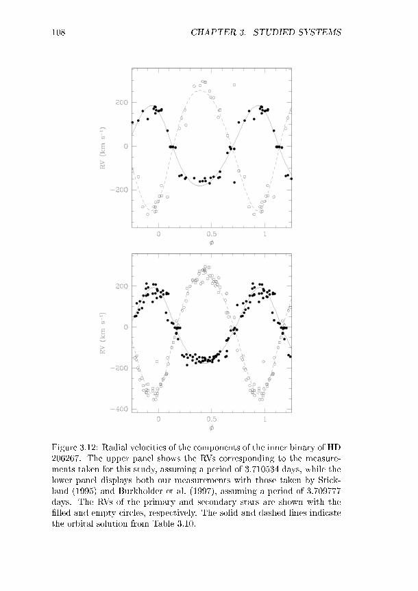
108 CHAPTER 3. STUDIED SYSTEMS
Figure 3.12: Radial velocities of the components of the inner binary of HD206267. The upper panel shows the RVs corresponding to the measure-ments taken for this study, assuming a period of 3.710534 days, while thelower panel displays both our measurements with those taken by Stick-land (1995) and Burkholder et al. (1997), assuming a period of 3.709777days. The RVs of the primary and secondary stars are shown with thelled and empty circles, respectively. The solid and dashed lines indicatethe orbital solution from Table 3.10.

3.5. HD 206267 109
3.5.4 Preparatory analysis
3.5.4.1 Adjustment of the ternary spectra and spectral
disentangling
After the determination of the orbital solution, we usually perform thespectral disentangling of the observed spectra (see Sect. 2.1) to recover theindividual contributions of the three components of HD 206267. However,as we have seen in Sect. 3.4.4.1, there may be great complications inour disentangling techniques when we apply them to spectra of a triplesystem with the third almost non-moving component (over the range ofour set of observations) whose lines are always partly blended with thelines of the other two components, leading to the apperance of artefactsin the separated spectra (see Fig. 3.7). This is also the case for HD206267, with, in addition, rather high projected rotational velocities andmacroturbulence velocities (see Sect. 3.5.5.1). We thus applied the samemethod as we have done for HD 17505, recombining synthetic spectra ofall three components, shifted by the corresponding RVs, and comparingthe obtained ternary spectra directly to the observations.
We then constrained the fundamental properties of each componentwith the non-LTE model atmosphere code CMFGEN (Sect. 2.2), with aβ law to describe the velocity law in the stellar winds, and a super-levelapproach for the resolution of the equations of statistical equilibrium.The following chemical elements and their ions were included in the cal-culations: H, He, C, N, O, Ne, Mg, Al, Si, S, Ca, Fe, and Ni. A newphotospheric structure was computed from the solution of the equationsof statistical equilibrium, and then connected to the same β wind velocitylaw. We assumed a microturbulent velocity in the atmosphere varying lin-early with velocity from 10 km s−1 in the photosphere to 0.1× v∞ at theouter boundary. The generated synthetic spectra of the three componentswere then shifted by their associated RVs, recombined and compared tothe observed spectra of HD 206267. We then constrained iteratively thephysical properties of each one of the three stars, as we have done in Sect.3.4.4.1 for HD 17505:
Starting point from the literature (Martins et al. 2005; Muijres et al.2012; Prinja et al. 1990), assuming that the fundamental propertiesof each star were close to typical values of stars of the same spectraltypes;
First approximation of the rotational velocities from a multi-Gaussiantting technique within MIDAS on the lines He i λλ 4026 and 4471,
110 CHAPTER 3. STUDIED SYSTEMS
and O iii λ 5592 for the most deblended spectra and a Fourier trans-form method (Simón-Díaz & Herrero 2007, Gray 2008) to the ob-tained Gaussians;
Estimation of the macroturbulence velocities with the auxiliary pro-gram MACTURB of the stellar spectral synthesis program SPEC-TRUM v2.76 developed by Gray (2010), applying this technique tothe wings of He i λ 4026, 4471, 4713 and 5016, and He ii λ 4542 forseveral phases;
Estimation of the respective contribution of the three componentsto the spectra of the triple system through the following formula onselected lines:
lili+lj+lk
= li
lj(lilj
+1+lklj
)
with
lilj
=(EWi
EWj
)obs
(EWSTj
EWSTi
)mean
where i, j and k are representing either the primary, secondary ortertiary stars, depending on the contribution we were calculating.The EW i represent the equivalent widths of the studied lines of thei star referring to the combined continuum of the three stars andEWSTi indicates the same measurement in a synthetic spectrum ofa typical star of the same spectral type as the i star, computed withCMFGEN. We considered the spectral types previously determinedby Burkholder et al. (1997; O 6.5V((f))+O9.5:V) for the innerbinary system, and the one determined by Harvin et al. (2003; O 8V)for the third component. This way, we obtained that the primary,secondary and tertiary contributions to the total ux are 60%, 15%and 25%, respectively.
First determination of the eective temperature in the models, throughthe relative strengths of He i λ 4471 and He ii λ 4542 lines (Martins2011);
First approximation of the surface gravities through the width ofthe Balmer lines, which were approximatively reconstructed with amulti-Gaussian t on a number of observations at dierent phases;

3.5. HD 206267 111
Estimation of the terminal velocities, the β of the velocity law, andthe mass-loss rates, through the strength of Hα, the width of He iiλ 4686 and Hα, and the strengths of Hγ and Hδ, respectively, and es-timation of the clumping factors, and the clumping velocity factors,based on the shape of Hα and Hβ lines. Note that these estimatesof the terminal velocities of the primary and secondary stars canonly be considered as lower limits, while the estimates of the otherwind parameters of the same stars can only be considered as upperlimits. This is due to the possible existence of a wind-wind inter-action zone, which may lead to an excess emission in the Balmerlines, and thus to an underestimate of the terminal velocities, andan overestimate of the β of the velocity law, the clumping factors,the clumping velocity factors, and the mass-loss rates of the primaryand secondary stars. The third object should be free from such apollution, since it is too distant from the inner binary to induce suchwind-wind interactions;
Adjustment of the CNO abundances through the strengths of asso-ciated lines, with a normalized χ2 analysis to determine the best tto selected lines, as done by Martins et al. (2015; see also Raucqet al. 2016; 2017) and explained in Sect. 2.2.2. We used the C iii
λλ 4068-70; N ii λ 4379, N iii λλ 4511, 4515, and 4525; O iii λλ 5508and 5592 lines to adjust the C, N and O abundances, respectively, forthe primary star, and the C iii λλ 4163 and 4187 and N iii λλ 4530and 4535 lines in addition to the previous lines for the secondarystar.
In Fig. 3.13 we show parts of the observed spectra at dierent phases withthe corresponding recombined synthetic spectra of the triple system.
Once we obtained a good t of the triple system for all of the obser-vations, we substracted the synthetic tertiary spectrum from each obser-vation, to recover the spectra of the inner binary system. We were thenable to treat the obtained binary spectra with the disentangling code, aswe did for the other binary systems, HD 149404 (see Sect. 3.1 of Raucqet al. 2016) and LSS 3074 (see Sect. 6.1 of Raucq et al. 2017).
3.5.4.2 Spectral types
Based on the reconstructed individual primary and secondary spectra, wethen determined the respective spectral types of the components of theinner binary of HD 206267. To do so, we applied Conti's quantitativeclassication criterion for O-type stars (Conti & Alschuler 1971, Conti &Frost 1977, see also van der Hucht 1996) for the spectral types, based

112 CHAPTER 3. STUDIED SYSTEMS
4470
0.8
1
1.2
1.4
1.6
1.8
4540 4550 5590 5600
Figure 3.13: He i λ 4471 (left panel), He ii λ 4542 (middle panel) and O iii
λ 5592 lines (right panel) of the recombined synthetic spectrum (red) ofthe triple system HD 206267 for dierent observations (black). The phasesof the dierent observations, according to the ephemerides of Table 3.10,are presented on the left side of the gure.
on the equivalent width ratio of the spectral lines He i λ 4471 and He iiλ 4542, and found that the primary is an O5.5 star and the secondary anO9.5 star. We then used Conti's quantitative criterion for the luminosityclasses, based on the equivalent width ratio of the spectral lines Si ivλ 4088 and He i λ 4143, and obtained that the secondary is a V star.However, since this criterion is designed for stars from O7 to O9.5, wecould not use it to determine the luminosity class of the primary star.

3.5. HD 206267 113
We thus used the Walborn criterion (Walborn & Fitzpatrick 1990 andreferences therein) to determine that the primary is a V star, since itsspectrum displays a strong He ii λ 4686 absorption. In addition to thestrong absorption of He ii λ 4686, the spectrum of the primary star alsodisplays N iii λλ 4634-40-42 emission, leading to the addition of a ((f))qualier to its spectral types. We thus found that the primary is anO5.5V((f)) star and the secondary an O9.5V star. We can see that ourdetermination of the spectral type of the secondary is exactly the same asdetermined by Burkholder et al. (1997), but we obtain a slightly earlierspectral type for the primary component: O5.5 vs. O6.5 in the studyof these authors. Since our spectral classication of the primary andsecondary stars of HD 206267 is based on the reconstructed spectra afterremoval of the polluting third component, it should be less sensitive to apossible phase-dependence of some specic spectral features, and shouldthus be more robust than a classication based only on spectra of the triplesystem taken near the quadrature phases of the inner binary system.
3.5.4.3 Brightness ratio
As we have seen in Sect. 2.1, the spectral disentangling yields the strengthof the lines in both primary and secondary spectra compared to the com-bined continuum, but it does not permit to establish the relative strengthsof the individual continua. We therefore need to establish the brightnessratio of the stars in an independant way in order to further analyse thereconstructed spectra of the primary and secondary components of HD206267.
To do so, we used a similar technique as done in Sect. 3.5.4.1 withmulti-Gaussian ts of selected lines to estimate the contribution of thethree components of the triple system to the observations. Here, we dir-ectly measured the equivalent widths of a number of selected spectral lineson the separated spectra of the primary and secondary stars, but referringto the combined continuum of the two stars, and calculated the brightnessratio of the two stars with the following formula:
l1l2
=(EW1
EW2
)obs
(EWST2
EWST1
)mean
with the same conventions as in the previous section. The results of ourmeasurements are listed in Table 3.11.
This way, we derived a mean primary over secondary brightness ratioof 4.75±1.79. This value is coherent, within the error bars, with what weinferred from our preliminary study of the contributions of the dierent

114 CHAPTER 3. STUDIED SYSTEMS
Table 3.11: Determination of the brightness ratio of the inner binarysystem of HD 206267 from the dilution of prominent lines.
Line Equivalent Width (Å) l1/l2
Observations Synthetic spectraPrimary Secondary O5.5 O9.5
He i λ 4026 0.27 0.09 0.74 1.02 4.22He ii λ 4200 0.32 0.02 0.76 0.16 4.18Hγ 1.27 0.19 2.11 2.52 8.16He i λ 4471 0.18 0.11 0.41 1.04 4.29He ii λ 4542 0.48 0.02 0.92 0.13 2.87
components to the observed spectra of the triple system, based on themulti-Gaussian t, i.e. l1/l2 = 60/15 = 4.00.
The mean V magnitude of the system is found in the VizieR OnlineData Catalog (2002) as being 5.738 ± 0.033, and the (B − V ) color is0.210± 0.010. The intrinsic (B − V )0 of O5.5V stars is -0.28 and that ofO9.5V stars -0.26, with a mean value of -0.27 for the system (Martins &Plez 2006). We determined an extinction AV of 1.457 ± 0.031, assumingRV = 3.1. Assuming a distance modulus of 9.9 ± 0.5 (Burkholder etal. 1997), we inferred an absolute magnitude MV = −5.619 ± 0.502 forthe system. With the previously determined brightness ratio, we thencalculated individual absolute magnitudes of MP
V = −5.412 ± 0.605 andMSV = −3.720± 0.605.The reconstructed normalized primary and secondary optical spectra
are shown and discussed in Sect. 3.5.5.2.
3.5.5 Spectral analysis
3.5.5.1 Rotational velocities and macroturbulence
The reconstructed individual spectra of the primary and secondary starsof HD 206267 also permitted us to rene the values of the projectedrotational velocities and macroturbulence of both stars. We used thesame Fourier transform analysis (Simón-Díaz & Herrero 2007) as in Sect.3.4.4.1, applied on the proles of isolated lines in the disentangled spec-tra. The elimination of the third component and the reconstruction of theindividual spectra permitted us to use more lines at this stage than whatwas possible with the multi-Gaussian t. We determined the projectedrotational velocities v sin i of the primary star based on the He i λλ 4026,4471, 4922 and 5016, He ii λλ 4200 and 4542, and O iii λ 5592 lines, and

3.5. HD 206267 115
Table 3.12: Projected rotational velocities (v sin i in km s−1) of theprimary and secondary components of HD 206267.
Line Primary SecondaryHe i λ 4026 170 104He ii λ 4200 133 110He ii λ 4471 175 96He ii λ 4542 125 113He i λ 4922 166 99He i λ 5016 195 96O iii λ 5592 171 -Mean value 162.1± 22.8 103.0± 6.6
that of the secondary star based on the same lines except the O iii λ 5592line.
The results are presented in Table 3.12. The mean v sin i of theprimary star is (162.1± 22.8) km s−1, and that of the secondary star is(103.0± 6.6) km s−1.
Once we have determined the mean projected rotational velocities,we adjusted our determination of the macroturbulence velocities of bothprimary and secondary stars, with the auxiliary program MACTURB de-veloped by Gray (2010), based on the radial-tangential anisotropic mac-roturbulent broadening formulation of Gray (2008). We worked on thelines He i λλ 4026, 4471, 4713 and 5016, and He ii λ 4542 in the indi-vidual spectra, after including the rotational velocity broadening, and weobtained macroturbulence velocities of 80 and 120 km s−1 for the primaryand secondary stars respectively.
Both rotational and macroturbulence broadening eects were appliedon the synthetic spectra before comparing the latter with the individualreconstructed spectra of the primary and secondary stars of HD 206267.
3.5.5.2 Fit of the separated spectra with the CMFGEN code
Once we obtained the reconstructed spectra of the primary and second-ary stars of HD 206267, and determined their brightness ratio, rotationalvelocities and macroturbulence velocities, we improved our determinationof the fundamental parameters of both stars with the CMFGEN code. Wefollowed the same procedure as in Sect. 3.5.4.1 to constrain the dierentstellar properties.
As mentionned in Sect. 2.1.2, however, the Balmer lines are too broadto be perfectly recovered by the disentangling procedure, and their wings

116 CHAPTER 3. STUDIED SYSTEMS
may thus not be entirely reliable to adjust de surface gravities. To circum-vent this problem, we used the following iterative process to constrain thesurface gravities together with the stellar luminosities. Based on our rstestimate of the log g with the t of the triple system (see Sect. 3.5.4.1)and our determination of the eective temperatures of the stars, we in-ferred the associated bolometric corrections (Lanz & Hubeny 2003) andthe individual bolometric luminosities, using the absolute V magnitudesof the components derived in Sect. 3.5.4.3. From these bolometric lumin-osities and the eective temperatures, we computed the ratio of the stellarradii RPRS , which, together with the assumed surface gravities, yielded thespectroscopic mass ratio MP
MS. By comparing this spectroscopic mass ratio
with the dynamical one inferred from the orbital solution we obtained anew estimate of the surface gravities. We repeated this iterative processuntil the spectroscopic and dynamical mass ratios agreed with each other,and the CMFGEN synthetic spectra produced for the new surface gravit-ies of both stars matched the reconstructed individual spectra as well aspossible.
Figure 3.14 displays the best t of the optical spectra of the primaryand secondary stars of HD 206267 obtained with CMFGEN. The cor-responding stellar parameters are listed in Table 3.13, and Table 3.14compares the chemical abundances of these best-t models with the solarabundances taken from Asplund et al. (2009).
Table 3.13: Best-t CMFGEN model parameters of the primary and sec-ondary stars of HD 206267.
Prim. Sec.R (R) 11.2± 1.8 5.8± 1.0M (M) 27.7± 12.3 17.6± 5.9Teff (104 K) 4.10± 0.15 3.55± 0.15log ( L
L) 5.54± 0.12 4.70± 0.12
log g (cgs) 3.75± 0.15 4.14± 0.15β ≤ 0.85 ≤ 0.50
v∞ (km s−1) ≥ 2300 ≥ 3500
M/√f1 (M yr−1) ≤ 8.98× 10⁻⁸ ≤ 9.16× 10⁻⁷
f1 ≤ 0.2 ≤ 0.3f2 (km s−1) ≤ 100 ≤ 300
BC −3.68 −3.28f1 and f2 represent the clumping lling factor and the clumping velocityfactor, presented in Sect. 2.2.2. The quoted errors correspond to 1σ un-certainties. The bolometric corrections are taken from Lanz & Hubeny(2003), based on our best-t Teff and log g.

3.5. HD 206267 117
Figure 3.14: Part of the normalized disentangled spectra of the primary(top, shifted by 0.5 continuum units) and secondary (bottom) stars of HD206267, along with the best-t CMFGEN model spectra (red).
Figure 3.14 shows that the Balmer, He, C, N and O lines are wellreproduced by the models for both stars.
By coupling the stellar masses obtained with CMFGEN (Table 3.13)with the minimum masses obtained with the combined orbital solution(Table 3.10), we then obtained an inclination of the system i ∼ 76.7°. Thisinclination then permitted us, together with the stellar radii determined
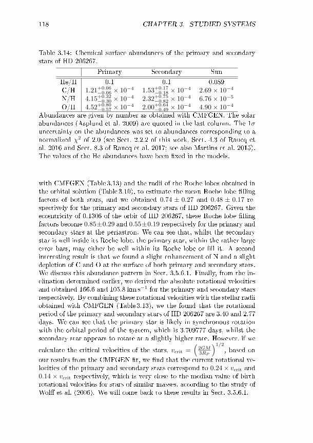
118 CHAPTER 3. STUDIED SYSTEMS
Table 3.14: Chemical surface abundances of the primary and secondarystars of HD 206267.
Primary Secondary SunHe/H 0.1 0.1 0.089C/H 1.21+0.06
−0.06 × 10⁻⁴ 1.53+0.17−0.18 × 10⁻⁴ 2.69× 10⁻⁴
N/H 4.15+0.32−0.30 × 10⁻⁴ 2.32+0.75
−0.82 × 10⁻⁴ 6.76× 10⁻⁵
O/H 4.52+0.80−0.57 × 10⁻⁴ 2.00+0.64
−0.49 × 10⁻⁴ 4.90× 10⁻⁴
Abundances are given by number as obtained with CMFGEN. The solarabundances (Asplund et al. 2009) are quoted in the last column. The 1σuncertainty on the abundances was set to abundances corresponding to anormalized χ2 of 2.0 (see Sect. 2.2.2 of this work, Sect. 4.3 of Raucq etal. 2016 and Sect. 8.3 of Raucq et al. 2017; see also Martins et al. 2015).The values of the He abundances have been xed in the models.
with CMFGEN (Table 3.13) and the radii of the Roche lobes obtained inthe orbital solution (Table 3.10), to estimate the mean Roche lobe llingfactors of both stars, and we obtained 0.74 ± 0.27 and 0.48 ± 0.17 re-spectively for the primary and secondary stars of HD 206267. Given theeccentricity of 0.1306 of the orbit of HD 206267, these Roche lobe llingfactors become 0.85±0.29 and 0.55±0.19 respectively for the primary andsecondary stars at the periastron. We can see that, whilst the secondarystar is well inside its Roche lobe, the primary star, within the rather largeerror bars, may either be well within its Roche lobe or ll it. A secondinteresting result is that we found a slight enhancement of N and a slightdepletion of C and O at the surface of both primary and secondary stars.We discuss this abundance pattern in Sect. 3.5.6.1. Finally, from the in-clination determined earlier, we derived the absolute rotational velocitiesand obtained 166.6 and 105.8 km s−1 for the primary and secondary starsrespectively. By combining these rotational velocities with the stellar radiiobtained with CMFGEN (Table 3.13), we the found that the rotationalperiod of the primary and secondary stars of HD 206267 are 3.40 and 2.77days. We can see that the primary star is likely in synchronous rotationwith the orbital period of the system, which is 3.709777 days, whilst thesecondary star appears to rotate at a slightly higher rate. However, if we
calculate the critical velocities of the stars, vcrit =(
2GM3RP
)1/2
, based onour results from the CMFGEN t, we nd that the current rotational ve-locities of the primary and secondary stars correspond to 0.24× vcrit and0.14 × vcrit respectively, which is very close to the median value of birthrotational velocities for stars of similar masses, according to the study ofWol et al. (2006). We will come back to these results in Sect. 3.5.6.1.

3.5. HD 206267 119
3.5.6 Discussion and conclusion
3.5.6.1 Evolutionary status
We have shown in the previous section that the spectra of the primaryand secondary components of HD 206267 show the signatures of a slightmodication of the CNO surface abundances. In Fig. 3.15, we compareour inferred N/C and N/O ratios with the predictions from the Genevaevolutionary models of single massive stars (Ekström et al. 2012). Inthe left panel, we show the case of non-rotating stars, whilst the rightpanel shows the case of stars rotating at 0.4× vcrit. We can note on thisgure that the observed abundances of both stars are dicult to explainin the non-rotating case, but are close to what is predicted by singlestar evolutionary models for stars of initial masses close to 20-25 and30 M, for the primary and secondary stars respectively, which is closeto the masses we inferred from our spectroscopic analysis of the system(Table 3.13).
Figure 3.15: Comparison of the N/C and N/O ratios obtained from ourspectral analysis with predictions from single star evolutionary models ofdierent masses (Ekström et al. 2012). The lled (resp. empty) squaresdisplay the characteristics of the primary (resp. secondary) star. Theleft panel illustrates the results for core hydrogen burning phase trackswithout stellar rotation, and the right panel corresponds to the sametracks for stars with a rotation of 0.4× vcrit.
In Figure 3.16, we show the positions of the primary and secondarystars in the Hertzsprung-Russell diagram (HRD; upper panels) and in the

120 CHAPTER 3. STUDIED SYSTEMS
log g-log Teff diagram (lower panels), with the evolutionary tracks fromEkström et al. (2012) for the core-hydrogen burning phase of single starsat solar metallicity. The left panels display the non-rotating stars caseand the right panels show the tracks for stars rotating at 0.4× vcrit.
If we consider the case without any rotational mixing, we see that theposition of the secondary star in the HRD and in the log g-log Teff diagramis close to the tracks corresponding to stars with initial masses of 20M,which is close to its current spectroscopic mass of 17.6 M. However, theposition of the primary star in the HRD suggests an initial mass closeto 40M, and its position in the log g-log Teff diagram is in favour of aninitial mass of 60M, while its spectroscopic mass is a factor two to threetimes smaller. Moreover, both stars do not seem to be located on thesame isochrone in either of the diagrams.
Considering the case of single stars rotating at 0.4×vcrit, we see in thegure that both stars may be located on the 3.2million years isochroneand that the postion of the secondary star is once again close to the 20-25 tracks in both HRD and log g-log Teff diagram. However, the positionof the primary star in both diagrams suggests an initial mass of 40M,which is a factor two larger than the observed mass.
Considering the slightly higher rotation rate of the secondary star ofHD 206267 found in Sect. 3.5.5.2 and our analysis of Figure 3.16, thesystem may have encountered some kind of binary interactions during itsevolution and its current status is thus hardly explainable by single starevolutionary models. However, the abundance patterns can be explainedby these single star models, which suggests that the system probablydid not go through a full RLOF process, which should have aected thesurface abundances of the donor star in a much stronger way (see thecases of HD 149404 and LSS 3074) and should also have led to orbitalcircularization, which is currently not the case. One way to explain thecurrent status of HD 206267 would be an intermittent RLOF processaround periastron, where case A mass transfer occurs temporarily, andis then interrupted until the next periastron passage. At this stage, westress however that our spectra of the system do not reveal any obvioussignature of such an interaction, such Hα emission, that would appear atphases near periastron. Therefore, if such intermittent RLOF has takenplace, it should have ceased now.
One possible reason for such an interruption could be the dynamicalinuence of the third component in a hierarchical triple system. Indeed,the presence of a third component in the system can produce the ap-pearance of Lidov-Kozai cycles, for example (Toonen et al. 2016, andreferences therein). In such cases, angular momentum exchange betweenthe inner and outer orbits can occur, due to a mutual torque between
3.5. HD 206267 121
these orbits. Since the orbital energy, and therefore the semi-major axes,are conserved, the orbital eccentricity of the inner binary system and themutual inclination between the two orbits can vary periodically. ThisLidov-Kozai mechanism could therefore lead to a periodic modulation ofthe binary interaction at periastron passage. Given the angular separa-tion of 0.1 arcsec at an assumed distance of 950 pc, we nd a separationof at least 95 AU between the inner binary system and the third compon-ent. The orbital period of the third component would thus be at least 115years. Since the timescale of the Lidov-Kozai cycle scales with the squareof the ratio between the outer and inner orbital periods (Toonen et al.2016), we estimate a minimum timescale of the order 1.3 Myr. Althoughthis timescale is quite long, it might be suciently short to modulate aslow episodic (i.e. occurring only around periastron) case-A mass transfer.HD206267 appears thus as an interesting candidate of such triple-systemevolution.
In future studies, it would be highly interesting to collect photometricdata of this system. Indeed, with a period of 3.7 days and an estim-ated inclination of 77°, it appears likely that the system displays at leastellipsoidal variations that might help to further constrain its parameters.
3.5.6.2 Summary and conclusion
We have studied the fundamental properties of the inner binary system ofHD 206267. The rst step has been to t the triple system spectra witha combination of synthetic CMFGEN spectra of the three componentsshifted by their associated RVs for each observation, then to substractthe third component from the observed spectra and recover the spectraof the inner binary. We then used our disentangling code to recover theindividual spectra of the primary and secondary stars. Once we obtainedthese reconstructed spectra, we determined the fundamental propertiesof the primary and secondary components with the CMFGEN code andused them to constrain the evolutionary status of the system.
We established the existence of a slight overabundance in N and slightC and O depletions in both primary and secondary atmospheres, thatmay be explained by single star evolutionary models. We found that theprimary star is in synchronous rotation with the orbital period, but thesecondary star displays a slightly higher rotation rate. We also foundthat the single star evolutionary models cannot explain the position ofthe primary star in the HRD and log g-log Teff diagram. We concludedthat the system may have experienced binary interactions in the past, butmay not have experienced a complete RLOF episode at this stage of itsevolution.

122 CHAPTER 3. STUDIED SYSTEMS
Figure 3.16: The upper panels show the positions of the primary(empty square) and secondary (lled square) stars of HD 206267 in theHertzsprung-Russell diagram, while the lower panels show their positionsin the log g-logTeff diagram, along with evolutionary tracks for singlemassive stars at solar metallicity during the core-hydrogen burning phase(Ekström et al. 2012). In the left panels, the evolutionary tracks cor-respond to non-rotating stars, whilst the right panels yield the results forstars rotating at 0.4 × vcrit. The dotted red lines correspond to isochronesof 3.2 and 4.0million years.
Chapter 4
Conclusions
4.1 Our sample of binary systems
In this thesis, we have studied the fundamental properties of four short-period massive binary systems, in order to conrm or to search for thepresence of clues of past-RLOF episodes in their previous evolution. Wehave mainly worked on high quality optical spectra of the systems, andalso investigated a sample of IUE spectra for the rst system, HD 149404.For the second system, LSS 3074, we also investigated photometric data.For LSS 3074, HD 17505 and HD 206267, we determined new orbitalsolutions for the systems. We have used a disentangling procedure toseparate the contributions of each component to the observed spectraof the systems, to be able to investigate independently the fundamentalproperties of these components as if they were single stars. This way, wehave investigated the spectral types of each star and the brightness ratiofor each binary system. We then used the non-LTE model atmospherecode CMFGEN to study the fundamental properties of each star. For eachsystem, we discussed the evolutionary status of the components comparedto single star evolutionary models. The results concerning HD 149404 andLSS 3074 are presented in Raucq et al. (2016) and Raucq et al. (2017),respectively. A summary of our main results for each object is presentedhere below.
4.1.1 HD 149404
This system is a detached, non-eclipsing O7.5I(f) + ON9.7I system, witha circular orbit and an orbital period of 9.81 days. We worked on veFEROS spectra, 12 Coralie spectra and 25 IUE spectra.
We have quantied the strong overbundance in nitrogen in the sec-
123

124 CHAPTER 4. CONCLUSIONS
ondary atmosphere, together with a C and O depletion. We also founda slight N overabundance in the primary atmosphere. These abundancepatterns cannot be explained by single star evolutionary models, but areclose to what can be found in the literature for post-case B RLOF sys-tems: [N/C] = 100 [N/C] and [N/O] ≥ 5 [N/O] (Vanbeveren 1982) forthe donor star, and [N/C] ∼ 2 − 3 [N/C] for the gainer star (Vanbev-eren & de Loore 1994). However, there are still some caveats since, givenits present status as an O+O binary, HD 149 404 is more likely to haveundergone a case A RLOF episode. A second important result is that wefound evidence for asynchronous rotation, with a rotational period ratioof 0.5± 0.11. We have also shown that, given their spectroscopic masses,single star evolutionary models cannot account for the fundamental prop-erties of both components of the system. Moreover, in our analysis, thetwo components of HD 149404 were not located on the same isochrone inthe Hertzsprung-Russel and log g-log Teff diagrams, although they wouldbe expected to have the same age.
The hypothesis of past RLOF interaction in this system, with a massand kinetic momentum transfer from the current secondary to the currentprimary star, is most plausible to explain its chemical abundances androtational asynchronicity, and the impossibility to explain the currentfundamental properties of both components with single star evolutionarymodels.
4.1.2 LSS 3074
LSS 3074 is a circular short-period O5.5If + O6.5-7If binary system, withan orbital period of 2.1852 days. We studied three EMMI spectra andtwelve FEROS spectra. We also worked on photometric data taken withthe Yale 1m telescope at the CTIO.
From these photometric lightcurves, we found that the system is inan overcontact conguration, with a lling factor of 1.008 for both starsand an orbital inclination of 54.5°. Based on our spectroscopic analysis,we conrmed the very low masses and radii found in previous studies,which is unusual for stars with such spectral types. In addition, we founda strong overabundance in N and a strong depletion in C and O in bothprimary and secondary stars, and a strong He enrichment in the primaryatmosphere. We have shown that these abundance patterns cannot beexplained by single star evolutionary models, neither can be the funda-mental properties of both components. Moreover, we found an apparentage discrepancy between the primary and secondary stars of LSS 3074.
However, there are still some caveats in the analysis of the lightcurves,since the hottest star appears to be in front during the deepest minimum

4.1. OUR SAMPLE OF BINARY SYSTEMS 125
and there is a discrepancy between the spectroscopic and the photometricbrightness ratios. We suggested that some of the discrepancies betweenthe spectroscopic and photometric properties of the system may comefrom a strong radiation pressure of the primary.
We proposed several evolutionary pathways through a RLOF processto explain both the low masses and the chemical abundances of both com-ponents of LSS 3074, and concluded that the system has been, and maystill be, signicantly aected by binary interaction, and that both starshave probably lost a signicant fraction of their mass to the surroundings.
4.1.3 HD 17505
HD 17505 is a multiple system composed of at least seven visual com-panions, with an O-star central triple system, composed of an eccentricO7V((f)) + O7V((f)) inner binary system, with an orbital period of 8.5690days, and a more distant O6.5III star (Porb < 61 years). We studied asample of fteen HEROS spectra, one ELODIE spectrum and six FIESspectra. We modelled the spectra of the triple system for all of the obser-vations and substracted the synthetic spectrum of the third componentfrom each observation to recover the spectra of the inner binary and studyindependently the primary and secondary components through our disen-tangling procedure.
We established the existence of a slight N overabundance and a slightC and O depletion in both stars, and showed that these properties andthe fundamental properties of both stars can be explained by single starevolutionary models with the inclusion of rotational velocity.
We thus suggested that the inner binary system of HD 17505 has notexperienced binary interactions at this stage of its evolution.
4.1.4 HD 206267
HD 206267 is a triple system composed of an eccentric O5.5V((f)) +O9.5V inner binary system, with an orbital period of 3.709777 days, anda more distant, third O component with a constant velocity. We stud-ied a sample of twenty-two HEROS spectra, one ELODIE spectrum, oneESPaDOnS spectrum, nine SOPHIE spectra and ve FIES spectra. Werecombined synthetic spectra of the three components to model all theobserved spectra of the triple system and substracted the synthetic spec-trum of the third component from each observation to recover the spectraof the inner binary system. We then used our disentangling procedure toreconstruct the primary and secondary spectra and to study the funda-mental properties of these two stars independently.

126 CHAPTER 4. CONCLUSIONS
We established the existence of a slight overabundance in N and aslight depletion in C and O in both primary and secondary atmospheres,and showed that some of the properties of both stars cannot be explainedby single star evolutionary models.
We suggested that the system did not experienced a complete RLOFepisode at this stage of its evolution, but could have undergone an episodeof intermittent mass-transfer around its periastron.
4.2 Future perspectives
From an observational point of view, this thesis work was based on alarge number of high-quality data. It allowed us to better understandthe interaction phenomena taking place in the considered systems, suchas the RLOF process, and to get insight into their evolutionary status.However, the studied systems were very complex, and there are still somecaveats in our analysis:
In the case of LSS 3074, we have found discrepancies between thespectroscopic and photometric studies, that may need additionaldata to understand their possible origins. Very high S/N spectrawould be needed to better resolve the rather faint secondary star.An additional study dedicated to the detailed modelling of the light-curve of LSS 3074, including the eect of radiation pressure, wouldalso shed some light on the observed discrepancies. Such studiesmay also bring some explanation to the simultaneous presence ofN iii, N iv and Nv lines in the primary spectra.
The cases of the triple systems HD 17505 and HD 206267 have alsohighlighted the limitations of our disentangling procedure. An inter-esting perpective of future work would be to improve our procedureto avoid the appearance of artefacts in the reconstructed spectra ofthe third component of a triple system, which would permit us tostudy more deeply this third component along with the primary andsecondary stars of a triple system.
From a theoretical point of view, we have seen, throughout this study, thatsome of the selected objects display strong hints of binary interactions,and that their fundamental properties cannot be explained by single starevolutionary models, and the predictions for binary evolutionary mod-els are often lacking or do not apply to the specic cases of post-RLOFO-type binaries. Indeed, we have seen for the case of HD 149404, forexample, that the determined chemical abundances correspond to a post-case B RLOF system while the current spectral types of both components

4.2. FUTURE PERSPECTIVES 127
would suggest that they would have gone through a case A RLOF episode.We have also shown that, whilst the abundance pattern of the compon-ents of HD 206267 can be explained by single star evolutionary models,we found some discrepancies between some of the fundamental propertiesof the components of this system and the predictions from the models.This system has an eccentric orbit and binary interaction might just bestarting and be limited to a short phase interval around pariastron pas-sage. For such systems, a dedicated theoretical study would be needed tounderstand the details of their evolution. It is also of the outmost import-ance to continue such studies of massive close binary systems to searchfor similar systems and enlarge our sample. This way, we may be able toimprove the constraints on binary evolutionary models, and improve ourunderstanding of the interaction processes taking place in massive closebinaries in general.

Bibliography
Adams, F. C., Ruden, S. P., & Shu, F. H. 1989, ApJ, 347, 959
Alecian, E., Neiner, C., Wade, G. A., et al. 2015, in IAU Symposium,Vol. 307, New Windows on Massive Stars, ed. G. Meynet, C. Georgy,J. Groh, & P. Stee, 330335
Alecian, E., Wade, G. A., Catala, C., et al. 2013, MNRAS, 429, 1001
Anderson, L. S. 1989, ApJ, 339, 558
Antokhina, E. A., Srinivasa Rao, M., & Parthasarathy, M. 2011, NewAstronomy, 16, 177
Asplund, M., Grevesse, N., Sauval, A. J., & Scott, P. 2009, ARA&A, 47,481
Bagnuolo, Jr., W. G., Gies, D. R., Hahula, M. E., Wiemker, R., & Wiggs,M. S. 1994, ApJ, 423, 446
Bethe, H. A. 1939, Phys. Rev., 55, 434
Bethe, H. A., & Critcheld, C. L. 1938, Phys. Rev., 54, 248
Bodenheimer, P. 1995, ARA&A, 33, 199
Bonnell, I. A. 2001, in IAU Symposium, Vol. 200, The Formation of BinaryStars, ed. H. Zinnecker & R. Mathieu, 23
Bonnell, I. A., Bate, M. R., & Zinnecker, H. 1998, MNRAS, 298, 93
Bonnell, I. A., Smith, R. J., Clark, P. C., & Bate, M. R. 2011, MNRAS,410, 2339
Bonnell, I. A., & Bate, M. R. 1994, MNRAS, 271, 999
Bonnell, I. A., & Bate, M. R. 2005, MNRAS, 362, 915
129

130 BIBLIOGRAPHY
Bonnell, I. A., & Smith, R. J. 2011, in IAU Symposium, Vol. 270, Com-putational Star Formation, ed. J. Alves, B. G. Elmegreen, J. M. Girart,& V. Trimble, 5764
Bouret, J.-C., Lanz, T., & Hillier, D. J. 2005, A&A, 438, 301
Brott, I., de Mink, S. E., Cantiello, M., et al. 2011a, A&A
Brott, I., Evans, C. J., Hunter, I., et al. 2011b, A&A
Burkholder, V., Massey, P., & Morrell, N. 1997, ApJ, 490, 328
Busche, J. R., & Hillier, D. J. 2005, AJ, 129, 454
Caughlan, G. R. 1965, ApJ, 141, 688
Cazorla, C., Nazé, Y., & Rauw, G. 2014, A&A, 561, A92
Chen, Z., Nürnberger, D. E. A., Chini, R., et al. 2013, A&A, 557, A51
Chini, R., Homeister, V. H., & Nürnberger, D. 2011, Bulletin de laSociete Royale des Sciences de Liege, 80, 217
Conti, P. S. 1976, Memoires of the Société Royale des Sciences de Liège,9, 193
Conti, P. S., & Alschuler, W. R. 1971, ApJ, 170, 325
Conti, P. S., & Frost, S. A. 1977, ApJ, 212, 728
de Mink, S. E., Cantiello, M., Langer, N., et al. 2009, A&A, 497, 243
de Mink, S. E., Langer, N., Izzard, R. G., Sana, H., & de Koter, A. 2013,ApJ, 764, 166
de Mink, S. E., Sana, H., Langer, N., Izzard, R. G., & Schneider, F. R. N.2014, ApJ, 782, 7
de Wit, W. J., Testi, L., Palla, F., & Zinnecker, H. 2005, A&A, 437, 247
Degirmenci, Ö. L., Sezer, C., Demircan, O., et al. 1999, A&AS, 134, 327
Donati, J.-F., & Landstreet, J. D. 2009, ARA&A, 47, 333
Drechsel, H., Lorenz, R., & Mayer, P. 1989, A&A, 221, 49
Ducati, J. R. 2002, VizieR Online Data Catalog, 2237
Eggleton, P. P. 1983, ApJ, 268, 368

BIBLIOGRAPHY 131
Ekström, S., Georgy, C., Eggenberger, P., et al. 2012, A&A, 537, A146
Ekström, S., Meynet, G., Maeder, A., & Barblan, F. 2008, A&A, 478, 467
Eversberg, T., Lépine, S., & Moat, A. F. J. 1998, ApJ, 494, 799
Ferrario, L., Melatos, A., & Zrake, J. 2015, SSRv, 191, 77
Ferrario, L., Pringle, J. E., Tout, C. A., & Wickramasinghe, D. T. 2009,MNRAS, 400, L71
Fossati, L., Castro, N., Schöller, M., et al. 2015, A&A, 582, A45
Friend, D. B., & Abbott, D. C. 1986, ApJ, 311, 701
Garmany, C. D., & Stencel, R. E. 1992, A&AS, 94, 211
Georgy, C., Meynet, G., Walder, R., Folini, D., & Maeder, A. 2009, A&A,502, 611
González, J. F., & Levato, H. 2006, A&A, 448, 283
Gorda, S. Y. 2015, Astronomy Letters, 41, 276
Gray, D. F. 2008, The Observation and Analysis of Stellar Photospheres
Gray, R. O. 2010, MACTURB, http://www.appstate.edu/ grayro/spectrum/spectrum276/node38.html
Haefner, R., Simon, K. P., & Fiedler, A. 1994, Information Bulletin onVariable Stars, 3969
Harries, T. J., Hilditch, R. W., & Hill, G. 1997, MNRAS, 285, 277
Harries, T. J., Hilditch, R. W., & Hill, G. 1998, MNRAS, 295, 386
Harvin, J. A., Gies, D. R., & Penny, L. R. 2003, in Bulletin of theAmerican Astronomical Society, Vol. 35, American Astronomical So-ciety Meeting Abstracts, 1223
Heger, A., & Langer, N. 2000, ApJ, 544, 1016
Herbst, W., & Havlen, R. J. 1977, A&AS, 30, 279
Hillier, D. J., & Miller, D. L. 1998, ApJ, 496, 407
Hillwig, T. C., Gies, D. R., Bagnuolo, Jr., W. G., et al. 2006, ApJ, 639,1069
Hirschi, R., Meynet, G., & Maeder, A. 2004, A&A, 425, 649

132 BIBLIOGRAPHY
Høg, E., Fabricius, C., Makarov, V. V., et al. 2000, A&A, 355, L27
Huang, W., Gies, D. R., & McSwain, M. V. 2010, ApJ, 722, 605
Jansen, F., Lumb, D., Altieri, B., et al. 2001, A&A, 365, L1
Johnston, K. G., Robitaille, T. P., Beuther, H., et al. 2015, ApJ, 813, L19
Kippenhahn, R., & Weigert, A. 1967, Z. Astrophys., 65, 251
Kruckow, M. U., Tauris, T. M., Langer, N., et al. 2016, A&A, 596, A58
Krumholz, M. R. 2011, ApJ, 743, 110
Kuiper, R., Klahr, H., Beuther, H., & Henning, T. 2011, ApJ, 732, 20
Kumsiashvili, M. I., Kochiashvili, N. T., & Djurasevi, G. 2005, Astro-physics, 48, 44
Langer, N. 1998, A&A, 329, 551
Langer, N. 1999, in Lecture Notes in Physics, Berlin Springer Verlag,Vol. 523, IAU Colloq. 169: Variable and Non-spherical Stellar Windsin Luminous Hot Stars, ed. B. Wolf, O. Stahl, & A. W. Fullerton, 359
Langer, N. 2012, ARA&A, 50, 107
Lanz, T., & Hubeny, I. 2003, ApJS, 146, 417
Le Bouquin, J.-B., Sana, H., Gosset, E., et al. 2017, A&A, 601, A34
Li, Y.-F., & Leung, K.-C. 1985, ApJ, 298, 345
Linder, N., Rauw, G., Martins, F., et al. 2008, A&A, 489, 713
Linder, N., Rauw, G., Sana, H., De Becker, M., & Gosset, E. 2007, A&A,474, 193
Lorenz, R., Mayer, P., & Drechsel, H. 1994, A&A, 291
Lorenz, R., Mayer, P., & Drechsel, H. 1998, A&A, 332, 909
Maeder, A., & Meynet, G. 2000, ARA&A, 38, 143
Mahy, L., Gosset, E., Sana, H., et al. 2012, A&A, 540, A97
Mahy, L., Martins, F., Machado, C., Donati, J.-F., & Bouret, J.-C. 2011,A&A, 533, A9

BIBLIOGRAPHY 133
Marchant, P., Langer, N., Podsiadlowski, P., Tauris, T. M., & Moriya,T. J. 2016, A&A, 588, A50
Martins, F. 2011, Bulletin de la Societe Royale des Sciences de Liege, 80,29
Martins, F., Hervé, A., Bouret, J.-C., et al. 2015, A&A, 575, A34
Martins, F., Schaerer, D., & Hillier, D. J. 2005, A&A, 436, 1049
Martins, F., & Plez, B. 2006, A&A, 457, 637
Mason, B. D., Gies, D. R., Hartkopf, W. I., et al. 1998, AJ, 115, 821
Massey, P., Johnson, K. E., & Degioia-Eastwood, K. 1995, ApJ, 454, 151
Mayer, P., Drechsel, H., Harmanec, P., Yang, S., & lechta, M. 2013,A&A, 559, A22
Mayer, P., Harmanec, P., Nesslinger, S., et al. 2008, A&A, 481, 183
Mayer, P., Lorenz, R., & Drechsel, H. 2002, A&A, 388, 268
McKee, C. F., & Tan, J. C. 2003, ApJ, 585, 850
Meynet, G., Ekström, S., Georgy, C., Maeder, A., & Hirschi, R. 2008,in IAU Symposium, Vol. 252, The Art of Modeling Stars in the 21stCentury, ed. L. Deng & K. L. Chan, 317327
Morrell, N. I., & Niemela, V. S. 1990, in Astronomical Society of thePacic Conference Series, Vol. 7, Properties of Hot Luminous Stars, ed.C. D. Garmany, 5759
Muijres, L. E., Vink, J. S., de Koter, A., Müller, P. E., & Langer, N. 2012,A&A, 537, A37
Nazé, Y., Carrier, F., & Rauw, G. 2002, in Astronomical Society of thePacic Conference Series, Vol. 260, Interacting Winds from MassiveStars, ed. A. F. J. Moat & N. St-Louis, 457
Nazé, Y., Neiner, C., Grunhut, J., et al. 2017, MNRAS, 467, 501
Neiner, C., & Alecian, E. 2013, in EAS Publications Series, Vol. 64, EASPublications Series, ed. K. Pavlovski, A. Tkachenko, & G. Torres, 7579
Niemela, V. S., Cerruti, M. A., Morrell, N. I., & Luna, H. G. 1992, inIAU Symposium, Vol. 151, Evolutionary Processes in Interacting BinaryStars, ed. Y. Kondo, R. Sistero, & R. S. Polidan, 505

134 BIBLIOGRAPHY
Norberg, P., & Maeder, A. 2000, A&A, 359, 1025
Özdemir, S., Mayer, P., Drechsel, H., Demircan, O., & Ak, H. 2003, A&A,403, 675
Palate, M., Rauw, G., & Mahy, L. 2013, Central European AstrophysicalBulletin, 37, 311
Penny, L. R., Gies, D. R., Wise, J. H., Stickland, D. J., & Lloyd, C. 2002,ApJ, 575, 1050
Penny, L. R., Ouzts, C., & Gies, D. R. 2008, ApJ, 681, 554
Piskunov, N. E., & Valenti, J. A. 2002, A&A, 385, 1095
Pittard, J. M., & Parkin, E. R. 2010, MNRAS, 403, 1657
Plaskett, J. 1923, Publications of the Dominion Astrophysical Observat-ory Victoria, 2, 269
Potter, A. T., Tout, C. A., & Eldridge, J. J. 2012, MNRAS, 419, 748
Prinja, R. K., Barlow, M. J., & Howarth, I. D. 1990, ApJ, 361, 607
Puls, J., Kudritzki, R.-P., Herrero, A., et al. 1996, A&A, 305, 171
Qian, S.-B., Yuan, J.-Z., Liu, L., et al. 2007, MNRAS, 380, 1599
Raucq, F., Gosset, E., Rauw, G., et al. 2017, A&A, 601, A133
Raucq, F., Rauw, G., Gosset, E., et al. 2016, A&A, 588, A10
Rauw, G. 2007, DSc Thesis, University of Liège
Rauw, G., Nazé, Y., Carrier, F., et al. 2001, A&A, 368, 212
Rauw, G., & Nazé, Y. 2016, AdSpR, 58, 761
Rosen, A. L., Krumholz, M. R., & Ramirez-Ruiz, E. 2012, ApJ, 748, 97
Sana, H., de Mink, S. E., de Koter, A., et al. 2012, Science, 337, 444
Sana, H., Gosset, E., & Evans, C. J. 2009, MNRAS, 400, 1479
Sana, H., Rauw, G., & Gosset, E. 2001, A&A, 370, 121
Sana, H., Rauw, G., Nazé, Y., Gosset, E., & Vreux, J.-M. 2006, MNRAS,372, 661
BIBLIOGRAPHY 135
Sana, H., Stevens, I. R., Gosset, E., Rauw, G., & Vreux, J.-M. 2004,MNRAS, 350, 809
Schmitt, J. H. M. M., Schröder, K.-P., Rauw, G., et al. 2014, Astronomis-che Nachrichten, 335, 787
Schneider, F. R. N., Podsiadlowski, P., Langer, N., Castro, N., & Fossati,L. 2016, MNRAS, 457, 2355
Simón-Díaz, S., Castro, N., Garcia, M., Herrero, A., & Markova, N. 2011a,Bulletin de la Societe Royale des Sciences de Liege
Simón-Díaz, S., Garcia, M., Herrero, A., Maíz Apellániz, J., & Neguer-uela, I. 2011b, in Stellar Clusters Associations: A RIA Workshop onGaia
Simón-Díaz, S. & Herrero, A. 2007, A&A, 468, 1063
Simón-Díaz, S., Negueruela, I., Maíz Apellániz, J., et al. 2015, in High-lights of Spanish Astrophysics VIII, ed. A. J. Cenarro, F. Figueras,C. Hernández-Monteagudo, J. Trujillo Bueno, & L. Valdivielso, 576581
Stevens, I. R., Blondin, J. M., & Pollock, A. M. T. 1992, ApJ, 386, 265
Stickland, D. J. 1995, The Observatory, 115, 180
Stickland, D. J. 1997, The Observatory, 117, 37
Stickland, D. J., Koch, R. H., Pachoulakis, I., & Pfeier, R. J. 1994, TheObservatory, 114, 107
Stickland, D. J., & Koch, R. H. 1996, The Observatory, 116, 145
Stickland, D. J., & Lloyd, C. 2001, The Observatory, 121, 1
Tamajo, E., Munari, U., Siviero, A., Tomasella, L., & Dallaporta, S. 2012,A&A, 539, A139
Tauris, T. M., & van den Heuvel, E. P. J. 2006, Formation and evolutionof compact stellar X-ray sources, ed. W. H. G. Lewin & M. van derKlis, 623665
Thaller, M. L., Gies, D. R., Fullerton, A. W., Kaper, L., & Wiemker, R.2001, ApJ, 554, 1070
Toonen, S., Hamers, A., & Portegies Zwart, S. 2016, Computational As-trophysics and Cosmology, 3, 6
136 BIBLIOGRAPHY
Tout, C. A., Wickramasinghe, D. T., Liebert, J., Ferrario, L., & Pringle,J. E. 2008, MNRAS, 387, 897
Underhill, A. B. 1995, ApJS, 100, 433
van der Hucht, K. A. 1996, in Liege International Astrophysical Colloquia,Vol. 33, Liege International Astrophysical Colloquia, ed. J. M. Vreux,A. Detal, D. Fraipont-Caro, E. Gosset, & G. Rauw, 1
van Marle, A. J., Langer, N., & García-Segura, G. 2007, A&A, 469, 941
Vanbeveren, D. 1982, A&A, 105, 260
Vanbeveren, D., De Loore, C., & Van Rensbergen, W. 1998, A&ARv, 9,63
Vanbeveren, D., & De Loore, C. 1994, A&A, 290, 129
Vink, J. S., de Koter, A., & Lamers, H. J. G. L. M. 2001, A&A, 369, 574
Wade, G. A., Bagnulo, S., Drouin, D., Landstreet, J. D., & Monin, D.2007, MNRAS, 376, 1145
Walborn, N. R. 1972, AJ, 77, 312
Walborn, N. R. 2002, AJ, 124, 507
Walborn, N. R., & Fitzpatrick, E. L. 1990, PASP, 102, 379
Wellstein, S., Langer, N., & Braun, H. 2001, A&A, 369, 939
Wol, S. C., Strom, S. E., Dror, D., Lanz, L., & Venn, K. 2006, AJ, 132,749
Woosley, S. E., & Heger, A. 2006, ApJ, 637, 914
Ya³arsoy, B., & Yakut, K. 2013, AJ, 145, 9
Yoon, S.-C., Langer, N., & Norman, C. 2006, A&A, 460, 199
Yoon, S.-C., & Langer, N. 2005, A&A, 443, 643
Zhao, E., Qian, S., Li, L., et al. 2014, New Astronomy, 26, 112
Zinnecker, H., & Yorke, H. W. 2007, ARA&A, 45, 481