Forthcoming in the Journal of Mental Health Policy and Economics

Estimating Determinants of Multiple Treatment Episodes for Substance Abusers

Allen C. Goodman*

Janet R. Hankin**

David E. Kalist***

Yingwei Peng****

Stephen J. Spurr*

September 2001

Number of Words: 6,541

Short Title: Multiple Treatment Episodes

* Department of Economics, Wayne State University, Detroit MI 48202 USA

** Department of Sociology, Wayne State University, Detroit, MI 48202 USA

*** Department of Economics, Oakland University, Rochester MI 48309 USA

**** Department of Mathematics and Statistics, Memorial University of Newfoundland, St. John’sNewfoundland A1C 5S7 Canada

Sources of Funding: The research is partially supported by Grant DA10828 from the NationalInstitute on Drug Abuse (NIDA), and from a grant from the Blue Cross Blue Shield Foundation.The data analyzed were purchased from MEDSTAT Systems, Inc under NIDA grant DA08711.

Acknowledgments: We thank Thomas McLellan for his advice and technical expertise. Thefindings are ours and do not represent NIDA, the Blue Cross Blue Shield Foundation, or WayneState University.

Corresponding Author: Allen C. Goodman, Department of Economics, Wayne State University,2145 FAB, 656 W. Kirby, Detroit, MI 48202 USA; e-mail: allen.goodman@wayne.edu;Phone: 313-577-3235; FAX: 313-577-0149.

1

Estimating Determinants of Multiple Treatment Episodes for Substance Abusers

Abstract

Background: Health services researchers have increasingly used hazard functions to examine

illness or treatment episode lengths and related treatment utilization and treatment costs. There has

been little systematic hazard analysis, however, of mental health/substance abuse (MH/SA)

treatment episodes.

Aims of the Study: This article uses proportional hazard functions to characterize multiple treat-

ment episodes for a sample of insured clients with at least one alcohol or drug treatment diagnosis

over a three-year period. It addresses the lengths and timing of treatment episodes, and the relation-

ships of episode lengths to the types and locations of earlier episodes. It also identifies a problem

that occurs when a portion of the sample observations is “possibly censored.” Failure to account for

sample censoring will generate biased hazard function estimates, but treating all potentially

censored observations as censored will overcompensate for the censoring bias.

Methods: Using insurance claims data, the analysis defines health care treatment episodes as all

events that follow the initial event irrespective of diagnosis, so long as the events are not separated

by more than 30 days. The distribution of observations ranges from 1 day to 3 years, and

individuals have up to 10 episodes. Due to the data collection process, observations may be right

censored if the episode is either ongoing at the time that data collection starts, or when the data

collection effort ends. The Andersen-Gill (AG) and Wei-Lin-Weissfeld (WLW) estimation

methods are used to address relationships among individuals’ multiple episodes. These methods are

then augmented by a probit censoring model that estimates censoring probability and adjusts

estimated behavioral coefficients and medians accordingly.

2

Results: Five sets of variables explain episode duration: (1) individual; (2) insurance; (3) employer;

(4) binary, indicating episode diagnosis, location, and sequence; and (5) linkage, relating current

diagnoses to previous diagnoses in a sequence. Sociodemographic variables such as age or gender

have impacts at both the individual and at the firm level. Coinsurance rates and deductibles also

have impacts at the individual and the firm levels. Binary variables indicate that surgical/outpatient

episodes were the shortest, and psychiatric/outpatient episodes were the longest. Linkage variables

reveal significant impacts of prior alcoholism, drug, and psychiatric episodes on the lengths of

subsequent episodes.

Discussion: Health care treatment episodes are linked to each other both by diagnosis and by

treatment location. Both the AG and the WLW models have merit for treating multiple episodes.

The AG model permits more flexibility in estimating hazards, and allows researchers to model

impacts of prior diagnoses on future episodes. The WLW model provides a convenient way to

examine impacts of sociodemographic variables across episodes. It also provides efficient pooled

estimates of coefficients and their standard errors.

Limitations: The insurance claims data set covers 1989 through 1991, predating current managed

care plans. It cannot identify untreated substance abusers, nor can it identify those with out-of-plan

use. It provides treatment information only if services are covered by the insurance plan and are

defined with a substance abuse diagnosis code. Like medical records, insurance claims will not

specify substance abuse treatment received within the context of other health care (and thus

identified by a non-substance abuse diagnosis code) or community services

Implications for Policy and Research: This article characterizes multiple health treatment

episodes for a sample of insured clients with at least one alcohol or drug treatment diagnosis within

a three-year period. We identify both individual and employer effects on episode length. We find

3

that episode lengths vary by the diagnosis type, and that the lengths (and by inference cost and

utilization) may depend on the treatments that occurred in previous episodes. We also recognize

that health care or illness episodes may be ongoing at times of health care events prior to the ends of

data collection periods, leading to uncertain episode lengths. Corresponding estimates of costs or

utilization are also uncertain. We provide a method that adjusts the episode lengths according to the

probability of censoring.

1. Introduction

Health services researchers have increasingly used hazard functions to examine illness or

treatment episode lengths, and related treatment utilization and treatment costs. This article

addresses the lengths and timing of multiple episodes within a three-year observation window. It

also addresses the relationships of individual episodes’ lengths to the types and locations of previous

episodes and it considers a class of problems in which a portion of the sample observations is

“possibly censored.” Although failure to account for sample censoring will generate biased

estimates in hazard function analysis, treating all potentially censored observations as censored will

overcompensate for the censoring bias.

We apply the analysis to the lengths of health care treatment episodes. We show how

various classes of individual, employer, diagnosis and sequence characteristics affect episode

length. We then use resampling techniques to provide unbiased estimates for medians. When

applied to a health insurance claims database, the estimator provides larger medians than those

calculated with no censoring adjustments, but smaller than those that assume that all potentially

censored observations are, in fact, censored.

2. Methods

2.1 Treatment Episodes

Episode definition and analysis have provided an intuitive yet elusive framework for anal-

yzing health services utilization and costs. For many conditions, costs and utilization begin when

episodes begin, and end when the episodes end, irrespective of the calendar. It is important to un-

derstand episode lengths and patterns in order to determine personnel and facility needs and health

care costs, and to assure health care quality. Screening procedures or health care treatments that can

prevent or shorten episodes may have substantive impacts on health care use and health care costs.

Unfortunately, episode definition may be quite arbitrary and difficult to implement. An

2

illness episode may begin some time before treatment is sought, and end some time after treatment

is finished. Treatment episodes may span numerous treatment locations (providers’ offices, clinics,

and/or hospitals), leading to problems in tracing the subjects and in collecting the data. Definitions

of either illness or treatment episodes are often quite arbitrary because different studies may define

episodes by treatment locations (inpatient or outpatient), mental health/substance abuse (MH/SA) or

non-MH/SA diagnoses, or arbitrary time separations, typically 30 or 60 days.

Our analysis focuses on treatment rather than illness episodes. The distinction is important

because illness episodes, especially for chronic illnesses with vague symptoms and imprecise

beginning dates, may be difficult to define in terms of start, duration, and conclusion. Treatment

episodes, in contrast, can be defined with specific beginning and ending treatment events.

Measuring episode length is of more than academic significance, because it can improve

cost estimates for substance abuse treatment. Frank and McGuire characterize the MH/SA

treatment cost estimates as among the “most variable” components of the entire 1993-94 debate

initiated by the proposed Health Security Act.1 Mechanic, Schlesinger and McAlpine implicitly

frame the issue of episodes in the context of managed care, noting that those with drug or alcohol

consumption may struggle over an extended period, often requiring a series of different forms of

treatment or continuing aftercare and supportive services.2

There are three major issues in constructing and analyzing health treatment episodes:

(1) which services to include; (2) whether episodes should be limited to single diagnoses or include

multiple diagnoses; and, (3) when one episode ends and another begins. There is a lack of

consensus regarding treatment norms concerning which services to include. Some studies refer

only to episodes of inpatient care, but this approach fails to recognize the importance of outpatient

visits before and after the hospitalization.3-5 We choose a more inclusive method that uses both

3

inpatient and outpatient events to define a treatment episode.6

The second issue is whether an episode should be defined with only one diagnosis or a set of

related diagnoses. Solon (1967) suggests that it may be important whether conditions are medically

managed separately or with a coordinated plan. A series of RAND studies refer to a “medical

problem” as the basis for grouping episode expenses.7-12 Thus services found to be related to the

same problem are grouped into one episode.

The time interval between the end of one episode and the beginning of another is a third

issue, requiring a definition of the episode’s beginning and end. Typically, with claims data or

medical records, the treatment episode begins with a condition’s first diagnosis and ends when the

condition is no longer being treated. It is possible to define an episode’s start as the most recent

patient/provider encounter prior to the diagnosis of a specific condition. An alternative is to define

the episode’s beginning as the point at which a treatment protocol is initiated.13 The episode’s end

may also reflect exhaustion of insurance benefits.

The interval between episodes depends on the medical condition being considered and is

often determined by clinical consensus. Moscovice uses physician estimates to determine the ex-

pected time frame for several acute conditions.14 The episode begins with the first medical event

within the time frame and ends with the last. If a second event occurs, the reason for the visit is used

to determine if the treatment represents a new episode or part of the last one. Cave refers to a

“reasonable” time to consider follow-up visits as part of the same episode.15 For example, a gap of

20 days between treatment events for the same diagnosis may represent a single treatment episode,

while a gap of 35 days between two events may signal the beginning of a new treatment episode.

Chronic conditions such as psychiatric and substance abuse problems present additional

problems in distinguishing one episode from the next. Typically, arbitrary intervals during which

4

there was no treatment are used to separate episodes of care. Kessler et al. use 8 weeks between

psychiatric treatments to define different episodes, but this definition has not been rigorously

analyzed in other settings.16 Intervals of 8 weeks, 2 months, or 60 days have commonly delineated

different episodes in both psychiatric and other types of health care literature.6, 17–19 Berndt, Busch,

and Frank also use an 8-week period without treatment to define new episodes, but note that

alternative definitions such as 6 or 12 week intervals leave the results “essentially unaffected.”20

We define episodes based on a 30-day break point, suggested by technical consultant

Thomas McLellan. We include all events that follow an episode’s initiation irrespective of

diagnosis, so long as they are not separated by more than 30 days. Several major agencies use the

proportion of people discharged from a treatment setting (particularly inpatient) and readmitted

within 30 days as a key clinical “performance indicator”. Most of these agencies also wish to see

patients transfered from more intensive care (inpatient, intensive outpatient) to less intensive care

settings (outpatient), again within 30 days of discharge. These include the National Committee on

Quality Assurance (NCQA), American Managed Behavioral Health Association (AMBHA), and

Substance Abuse and Mental Health Services Administration (SAMHSA).

This cut-off reflects the premise that maintaining people in treatment for long time periods

by “transitioning” them through a “continuum of care” (hospital, residential, intensive

outpatient/halfway house, outpatient) leads to the best outcomes. Thus the patient’s receiving

repeated treatments at intervals within 30 days indicates that the episode is not yet completed.

2.2 Defining Episodes with Hazard Functions

We begin our analyses of episode lengths by assuming that episodes are seen in their

entirety (i.e. there is no censoring). Suppose that a researcher has collected data on subjects who

may have had a treatment for a specific illness. The goal is to characterize the length T of the

5

treatment episode. The cumulative distribution of T is:

∫ == t

0 dssftF )()( Prob (T ≤ t), (1)

where s represents the episode length, and f(s) is a probability density function (PDF). The survival

function S (t) is the probability that an episode will still be in progress at length t.:

S (t) = 1 - F (t) = Prob (T > t), (2)

To address a particular episode length, and the probability that it will end in the next interval ∆ t,

define hazard rate )(/)()( tStft =λ as the instantaneous rate of episode termination for an episode

still in progress at length t.

Both the hazard function and the survival function from equation (2) provide important

episode-related information. The hazard function indicates whether it is more or less likely that

episodes will end as duration increases. An increasing hazard (more likely to end) thus means a

shorter episode, and a decreasing hazard means a longer one.

The survival function provides statistical insight into the definition of episode length. Recall

that function S (t) varies between 1 (the shortest episode) and 0 (the longest episode). The median

occurs at S (t) = 0.5 since half of the observations are longer and half are shorter. We calculate the

median episode length by solving for t such that S (t) = 0.5.

2.3 Appropriate Specifications for Multiple Episode Hazard Function Models

The 153,000 episodes in this sample are grouped among the individuals and hence not

independent. As a result, standard errors calculated by conventional regression packages are likely

to be underestimated, with t-statistics and significance levels overstated. Allison21 and Kelly and

Lim22 present good discussions and descriptions of analytical methods of grouping observations.

The general models begin with Cox’s proportional hazards model:23

βλ iXettH )()( 0= (3)

where λ0 is an unspecified hazard. Andersen and Gill (AG) assume that the risk of an event for a

6

given subject is unaffected by any earlier events that have occurred to the same subject, unless

terms that capture such dependence are included explicitly in the model as covariates.24 In contrast,

Wei, Lin, and Weissfeld (WLW) allow for dependence among multiple event times, providing

efficient pooled estimates of the coefficients and their standard errors.25 Whereas the AG model

assumes constant impacts, unless explicitly modeled, the WLW model allows the parameters for an

individual’s episode 1 to differ from the parameters for episode 2 and so on, with a common effect

(and variance) calculated among all of the individual’s episodes.

In our application, the observations range from 1 day to 3 years. Episode lengths may be

right censored if episodes are either ongoing at the time that data collection starts, or when the data

collection effort ends. Failure to account for right censoring will lead to a downward- biased

estimate of episode lengths, since we know that episodes are at least as long as those observed.

The discussion above assumes that the researcher knows whether or not a response is

censored. We argue that treatment episodes exemplify a class of responses with probabilistic

censoring. An episode may begin two weeks before the end of the data collection period. Because

all treatment within 30 days of the episode initiation is considered as part of the episode, it is

possible, although not certain, that the episode is censored. Assuming that there is no censoring

leads to well-known downward biases. However, assuming that all of the potentially censored

episodes are censored almost certainly biases estimates of episode lengths upward.

This uncertainty is not unique to MH/SA treatment. In the biometrics literature Hougaard26

notes that menopause is defined as the time of the last menstrual bleeding but that it is not possible

to say whether an occurrence of bleeding at Time A is the last until a whole lifespan has passed.

Operationally, observers wait for one year before determining that menopause occurred at Time A,

but Hougaard notes that if a woman dies after a half year without bleeding “it is forever unknown

7

whether she should count as having obtained menopause.” Alternatively the estimated age at which

menopause occurs is uncertain. Hougaard does not suggest how to address this uncertainty.

Dropping all potentially censored observations could lead to three serious problems:

1. Loss of information – Omitting observations sacrifices information. Of the 153,115 episodes,

14,924 or (9.75%) are potentially censored. With longer separations (eight weeks or 60 days

rather than 30 days), or shorter data windows (one or two years rather than three years), the

information loss would be even more severe.

2. Selection bias – Omitting observations may result in selection bias by differentially deleting

patients with coverage limitations. Also, specific diagnoses (often MH/SA-related) may be

selectively deleted, again due to insurance limitations.

3. Characterizing the distribution – For treatment episodes, the potential censoring occurs at the

beginning or at the end of a calendar year. Because health insurance may limit utilization levels

or expenditures by calendar year, utilization and/or costs may be concentrated at the beginning

(pent-up demand from the previous year) or at the end (exhausting the year’s benefits) of a year.

Systematically omitting such episodes will bias estimates of episode length, utilization, and

costs downward. This may lead to serious financial consequences for providers and insurers.

After describing the database, we present an estimator to address probable censoring issues, and

allowing us to use all of the data.

2.4 Data

The study population was selected from a large health insurance claims database of 36 self-

insured employers, for all treatment events starting January 1, 1989, and ending December 31, 1991.

We included claims of all beneficiaries less than 65 years of age (to avoid Medicare overlap) who

incurred at least one drug abuse or alcoholism treatment event in the 3-year period. For tractability

8

we limited the database to those subjects with between one and ten episodes in the three-year

period. (Data cells became too small for reliable estimation when more than 10 episodes were used.)

This provided 153,115 episodes over 33,998 subjects.

Episodes were classified by their initiating events. Drug abuse episodes were defined by

principal International Classification of Disease (ICD-9) diagnoses of 292 (drug psychoses), 304

(drug dependence), or 305.1-305.9 (drug abuse). Alcoholism episodes used diagnoses of 303

(alcohol dependence), 305.0 (alcohol abuse), or 291 (alcohol psychoses). Psychiatric episodes

(ICD-9 codes 290, 293-299, 300-302, and 306-319) were similarly identified. The remaining

episodes were defined through ICD-9 diagnoses as surgical or as “medical.” Obstetric-

gynecological treatment for women was excluded to facilitate gender comparisons.

Treatment events are classified as either inpatient or outpatient events. Inpatient events

consist of all services provided between and including the first and last dates of admissions

involving at least an overnight stay. All other services constitute outpatient events. Thus five

exclusive diagnostic treatment episode categories (alcoholism, drug, psychiatric, surgical, and

medical) are defined at the inpatient and the outpatient levels, for a total of 10 categories.

(Table 1 – Fractions of Episode by Sequence)

Table 1 summarizes episode types for each patient by diagnosis and by sequence number

(the patient’s 1st through 10th episode). Slightly over 14.3% of all episodes (summing the ALC

column) are initiated by an alcoholism diagnosis. About 7.8% are initiated by a drug abuse treat-

ment diagnosis, and almost 11.4% are initiated by a psychiatric diagnosis. Approximately 22.2%

(row 1) are initial episodes, and over 78.2% of all episodes are accounted for by the first five

episodes per subject. In total there are 138,305 outpatient episodes, and 14,810 inpatient episodes.

Goodman, Hankin, Kalist, and Sloan find that characterizing episodes by the initiating event

is a valid process, particularly for episodes initiated by inpatient care.27 For inpatient episodes,

9

upwards of 90% of the utilization and costs occur in the same category as the initiating event.

Outpatient events are somewhat more heterogeneous, but in episodes initiated by outpatient drug

abuse treatment, for example, over 85% of the costs occur in MH/SA categories.

(Table 2 – One-Day v. Multi-day Episodes)

Table 2 shows the large percentage of one-day episodes. From the second line, 41.6% of the

episodes are one-day episodes (a one-day treatment event followed by 31 or more days without

treatment). Separate tabulations indicate that only 452 of the 63,761 one-day episodes (0.7%) are

inpatient episodes. This means that the remaining 63,309 one-day episodes account for 45.8% of

the 138,305 outpatient episodes, a highly skewed distribution whose median is substantially smaller

than the mean of 31.55 days. The outpatient mean of 31.55 days and the inpatient mean of 38.61

days differ by only a week, but the outpatient median is far smaller. One would expect this finding

because most outpatient care is for acute illnesses.

Men are slightly more likely to have one-day episodes and older subjects are slightly more

likely to have multi-day episodes. Insurance deductibles are higher for patients with multi-day

episodes (longer episodes mean higher deductibles to be paid), and the copayment rate for multi-day

episodes is slightly higher (8.91%, compared to 8.41% for single-day episodes).

Database strengths include size, completeness relative to other databases, and accuracy.

With the low prevalence of substance abuse treatment, and the stigma of reporting it, population

surveys most often provide very small data cells. Clinic-based substance abuse treatment data

provide important information on treatment and outcomes at the clinic, but often no information on

non-clinic treatment. (Non-clinic treatment includes non-substance abuse treatment, as well as

therapy through Alcoholics or Narcotics Anonymous, groups that do not consider themselves to

provide medical treatment.) In contrast, we use a large and varied database that examines a host of

MH/SA treatments as well as all of the covered treatment for other conditions.

10

As for weaknesses, the data set cannot identify untreated substance abusers, nor can it

identify those with out-of-plan use. It provides treatment information only if services are covered

by the insurance plan and are defined with a substance abuse diagnosis code. Like medical records,

insurance claims will not specify substance abuse treatment received within the context of other

health care (and thus identified by a non-substance abuse diagnosis code) or community services.

2.5 Specifying Models and Interpreting Coefficients

In analyzing episode durations we will compare the AG and the WLW hazard models. We

propose the following AG model:

∑∑ ∑∑∑∑ ∑∑=

=

=

=

++++=i k

uv

kv

v

ku

uuvikmikm

mj ggg

nnnjjikm zLfyxlogT

1 1

ραηδβ . (4)

Tikm refers to the duration of the ith episode in the sequence, with diagnosis k, at treatment location m.

Variables xj refer to individual level variables including subject’s age, gender, and employment

status. Variables yn refer to individual insurance variables, coinsurance and deductible levels. With

perfect information and with no variation among employees in the firm, these would be the

definitive measures for the individual.

Variables fg characterize the employer where the subject either works or has coverage as the

dependent of a worker. One might use employer-specific binary variables to measure differences

among employers, but such variables only indicate that different employers are different. Instead

we characterize employers with employer-specific year-specific (ESYS) measures (based on our

population of subjects with either an alcoholism or a drug treatment) such as mean age, mean

employment status, or mean percentage male, since employer health care benefits packages may

reflect the types of workers that are covered.

We also calculate ESYS mean coinsurance rates and deductibles because employers may

offer more than one insurance product, with different copayment rates and different deductibles.

11

The mean may again proxy for employer-specific insurance experience. A second interpretation

involves possible errors either in employer policy administration or in data quality. Investigator

experience with insurance claims has shown that reported claims may differ from the stated policy.

Sometimes these are coding errors; sometimes policies are simply administered differently for

different people. In either case the employer mean may be a better variable than the individual

measure. Using both individual and employer measures controls for either possibility.

We explicitly model the episode diagnosis, location, and sequence number with Likm, and zuv

relate the initiating diagnosis of the current episode to the diagnosis of the previous episode. For

example, suppose that the patient’s current episode is the third episode in the treatment window,

that it is initiated by outpatient psychiatric care, and that it follows the second episode, which was

initiated by outpatient alcoholism care. Here, variable Likm is EPS_3PO with a value of 1,

indicating that the current episode is the third (3) episode in the sequence and is a psychiatric (P)

outpatient (O) episode. Variable zuv is PSY_P_ALC (“PSYch episode where the Previous episode

was an ALCoholism episode”) has a value of 1, indicating that the episode preceding the current

(psychiatric) episode was an alcoholism episode.

(Table 3 –Linkages for Second Through Tenth Episodes)

Table 3a describes the episode linkages, with the 25 cells summing to the 77.8% of the

episodes subsequent to Episode 1 (i.e. the 2nd through 10th episodes). For example 3.46% of all

episodes were initiated by alcoholism treatment, immediately preceded by a previous alcoholism

treatment episode. Not surprisingly, the largest linkage (0.3276) is for medical treatment, where the

immediately preceding treatment was also medical treatment.

Table 3b converts Table 3a into column fractions summing to 1. For example, 36.1% of the

alcoholism treatment episodes were immediately preceded by episodes initiated by alcoholism

treatment. Almost 28% of the drug episodes were immediately preceded by drug episodes, and

12

nearly 49% of the psychiatric episodes were immediately preceded by psychiatric episodes.

In contrast to the AG model, the WLW model estimates separate relationships for each of

episodes 1 through 10:

∑∑∑

∑∑∑

++=

++=

nnn

ggg

jjjkm

nnn

ggg

jjjkm

yfxlogT

yfxlogT

,10,01,10,10

1111

...............

δηβ

δηβ

(5)

As with equation (4), Tikm refers to the duration of the ith episode in the sequence, with diagnosis k,

at treatment location m. Explanatory variables xj refer to the subject’s age, gender, and employment

status, yn to individual insurance variables, and fg to the employer. WLW explicitly estimates

separate effects for each episode (1 through 10), and provides tests for equality across episodes.

However, unlike AG, the WLW formulation does not permit linkage among episodes.

2.6 Probable Censoring

Because our database ends December 31, 1991, episodes with events occurring after

December 1, 1991 may have right censored lengths since an unobserved event may occur after the

close of the data collection window, but less than 30 days after the initial event. Similarly, because

the database begins on January 1, 1989, any treatment episode length starting between January 1

and January 31, 1989 is also potentially right censored (although the starting dates are potentially

left censored), because the 30-day treatment window may have begun before January 1.

The right censoring is subject to a probability distribution rather than a certainty. Suppose

Person 1 had a single event on December 2, 1991 and Person 2 had a single event on December 20,

1991. E1 is a censored episode only if Person 1 had treatment on January 1, 1992; if he or she had

treatment on that date, and there was no further treatment for the next 30 days, then E1 lasts 30 days.

If there was no treatment on January 1, 1992 (even if there was subsequent later treatment), then E1

was an uncensored episode with a length of 1 day.

13

E2’s censoring probability is potentially larger than E1 since any treatment for Person 2

occurring up to January 19, 1992 would be considered part of episode E2. Eleven days have passed

(between December 20 and December 31) without an event but it is still possible that an event

(which we cannot observe) could occur in the next 20 days. A similar argument with similar logic

applies to treatments beginning in the first 30 days of the data window.

Censoring variable c is customarily observed with values of 0 (for right censored obser-

vations) or 1 (for uncensored observations). Because we view the censoring variable as a random

variable for the possibly censored observations, we cannot estimate either the AG or the WLW

models with existing procedures in SAS or in other statistical packages. As a result, new compu-

tational methods and estimators are required to handle c and to estimate the model parameters.

Our estimator for median episode length uses comparable episode information to estimate

censoring probabilities. Consider, for example, the set of possibly censored episodes that included

December 1991. The data available indicate the starting date, the episode length at the last event,

and the episode type and location. One may use episodes that included December 1989 (and

December 1990) to estimate the probability that an episode with a December event will actually

extend into the following month. If 1989, for example, were in fact the last year of the database,

then December 1989 episodes extending into 1990 would be censored. A probit model is used

predict censoring for 1989 and 1990, and its results then applied to December data for 1991.

Goodman et al. discuss alternative estimators in detail.28

Our database contains two relevant types of December 1989 and 1990 episodes.

1. Type O (ongoing) episodes started before December 1 and were ongoing the date of the last

observed event (after December 1), thus possibly censored. We know the episode length on that

date. Censoring probabilities for episodes extending into December 1991 that started prior to

14

December 1, 1991, will be predicted by probit regressions for 1989 and 1990 Type O episodes.

Pr (cens) = θ0 + θ1 * Ep. Length (as of 12/1) +

θ2 * Ep. Location (inpatient or outpatient) + θ31

k ktype

k

Treatment=

∑ . (6a)

2. Type A (after) episodes started after December 1. Since this starting date was within 30 days of

the probable censoring date, these episodes were possibly censored. As with the Type O

episodes, we know how long these episodes lasted, but we do not know the sequencing of the

events. Censoring probabilities for December 1991 episodes that started after December 1,

1991 will be predicted by probit regressions for 1989 and 1990 Type A episodes.

Pr (cens) = γ0 + γ1 * Start date +

γ2 * Ep. Location (inpatient or outpatient) + ∑=

k

typekkTreatment

13γ . (6b)

The alternative estimator for episodes starting within the first 30 days of the data window (January

1 through January 30, 1989) is analogous. We use January 1990 and January 1991 episodes to

generate censoring probabilities for January 1989.

Equations (6a) and (6b) assign each potentially censored observation a probabilistic value

(either 0 or 1) for the censoring indicator c. The relevant censoring adjustment is made if 0 is

assigned, and the hazard function is estimated conditional on the draw. Over a repeated set of

drawings, individual observations will approach their asymptotic probability of being censored. We

will adjust the median episode lengths based on these probabilities.

3. Results

This section presents estimation results. Table 4 examines the hazard function estimates

using the AG specification and Table 5 the WLW specification. The two specifications are then

compared. Table 6 shows the probit censoring adjustments. Subsequent analyses and accompany-

ing figures address the estimates of episode lengths after adjusting for probable censoring.

15

3.1 AG Estimators

Table 4 presents the AG analysis. The five sets of variables grouped together are:

(1) individual; (2) insurance; (3) employer-specific year-specific (ESYS); (4) binary, relating to

episode type and sequence; and (5) linkage.

(Table 4 –Proportional Hazard Function Using the AG specification)

For the same employer, men’s episodes had an 11.6% (or e0.1102) higher hazard than

women’s episodes, meaning they were likely to be shorter. The negative hazard for age suggests

slightly longer episodes for older subjects. Active workers (those currently employed) had slightly

longer episodes (negative hazard), as did primary beneficiaries (measured by PT_SELF). The later

the episode started (EPS_STR0), the shorter it was likely to be.

It is instructive to examine the individual and the employer variables jointly. As noted

above, for the same employer, men’s episodes had an 11.6% higher hazard than women’s episodes.

At the employer level, the higher the percentage men (MALE_AVG), the shorter still the episode.

Comparing an employer for which 60% of those covered were male with one with 50% coverage,

the hazard was 1.26% (that is, e(0.6 – 0.5) x 0.1264) higher. Although hourly and non-hourly individual

workers’ episodes were not significantly different at the individual level, subjects with employers

having higher proportions of covered hourly workers (HRLY_AVG) had significantly shorter

episodes.

Insurance variables also demonstrated both individual and employer effects. Holding em-

ployer constant, subjects with higher deductibles had longer episodes, but individual coinsurance

rates were insignificant. However subjects working at employers with higher deductibles had

shorter episodes. One obtains the joint impact by adding the deductible coefficients for EPS_DCT

and DCT_AV = -0.0043 + 0.0049 = 0.00053. A 100 dollar deductible increase for all individuals at

a given employer was related to a 5.4% increase in the hazard (and a decrease in episode length).

16

The individual coinsurance rate was not statistically significant, but the employer coinsur-

ance rate was. The joint impact of EPS_CPR and CPR_AV = -0.0036 - 0.2337 = -0.2373,

suggesting that an increase in the coinsurance rate from 0.05 to 0.10 decreased the hazard by

approximately 1.2% (the product of 0.05 and coefficient -0.2373).

The binary episode type and sequence descriptors provide useful insights into the sequential

nature of the episodes. We characterize the first 5 episodes by both inpatient/outpatient status and

by diagnosis type. A comparison of the binary terms indicates the impact of the specific diagnosis/

location pair on the hazard. For Episode 1, episodes initiated by surgical/outpatient care have the

largest coefficient (-1.1248), indicating the shortest duration; episodes initiated by psychiatric/

outpatient care have the smallest Episode 1 coefficient (-1.9120), indicating a significantly lower

hazard, and hence longer duration, suggesting a sequence of events.

The linkage variables add depth to the analyses. Consider an alcoholism treatment episode

immediately preceded by another alcoholism episode (ALC_P_ALC). The coefficient of 0.2366

implies a greater hazard than if this alcoholism episode had been immediately preceded by a medi-

cal episode (ALC_P_MED) with a coefficient of -0.0085. In contrast, consider a drug treatment

episode preceded by another drug episode. Variable DRG_P_DRG (coefficient of 0.0760) shows

that a repeat drug episode is likely to be longer (lower hazard) than a repeat alcoholism episode

(ALC_P_ALC coefficient of 0.2366). A general perusal of these linkages indicates that following

either a drug or an alcoholism event implied a slightly higher hazard (increased probability of

ending and hence shorter episode) than the omitted category (following surgery).

3.2 WLW Estimators

We estimate 10 hazard functions with the WLW method – one for each episode in the

sequence. The common hazard, a weighted average of the episode-specific hazards, can be com-

17

pared to the AG hazards in order of magnitude, and significance. One can also test (using F-tests)

whether the covariates have constant impacts across the sequence. Men, for example, have higher

hazards than women for all episodes, but significantly higher for earlier ones than for later ones.

(Table 5 –Proportional Hazard Function Using the WLW specification)

For some variables, impacts differ both quantitatively and qualitatively depending on where

in the sequence they occur. Episode starting date EPS_STR0 is a prime example. For early episodes

later starting dates imply higher hazards (shorter episodes); for later episodes (Episodes 5 through

10), later starting dates imply lower hazards (longer episodes). The common effect is positive

(because there are greater numbers of Episodes 1 through 3 than Episodes 5 through 10 contributing

to the weighted common effect), but the event-specific coefficients are significantly different.

The coefficients for alcoholism, drug, and psychiatric hazards are all significantly negative,

indicating smaller hazards (longer episodes) than the omitted surgery category. Looking at Table 5,

the alcoholism treatment coefficient is lowest (-0.3440) in Episode 1, indicating the longest episode,

and highest in Episode 10 (-0.0338). The weighted mean of -0.2756 differs significantly from 0; the

F-test rejects coefficient equality over the 10 episodes. The drug and psychiatric treatment

coefficients have similar patterns, weighted means, and F-statistics.

3.3 Comparing AG and WLW Estimators

There is no direct way to compare the AG and the WLW methods, but we propose to

examine the differences by calculating the hazards of specific sequences of events. Figure 1

investigates a stylized set of events in which drug episodes (1, 3, 5, 7, and 9) alternate with alco-

holism episodes (2, 4, 6, 8, and 10). The WLW relative hazards are read directly from the episode-

specific estimates in Table 5. Assuming that 10% of the episodes are inpatient and 90% are out-

patient; the hazards vary from -0.38 (Episode 1) to –0.07 (Episode 10). The AG relative hazards,

using the type and sequence variables and the linkage variables (and assuming the same proportions

18

inpatient and outpatient) show considerably more variation, from -1.45 (Episode 1) to +0.19

(Episode 10). Figure 2 considers a stylized set of 10 consecutive drug episodes. Once again, there

is considerably more variation in the hazards with the AG estimator that with the WLW estimator.

(Figures 1 and 2 – Comparative Hazards by Episode Number for AG and WLW Estimators)

What accounts for the difference? The WLW model computes the episode-specific hazards

(and hence the survival rates) directly. It also estimates the coefficients and the within-subject cor-

relation more directly than does the AG method. However, the AG method allows the researcher to

link characteristics of preceding and succeeding episodes explicitly, an option that is not available

with WLW. Also, even with a fast personal computer with substantial storage (27 gB) and memory

(384 mB), some variables had to be omitted from the WLW analysis. The model presented has 190

coefficients (19 variables over 10 events). Efforts to add further coefficients were not successful.

3.4 Probit Censoring Adjustments

Table 6 displays the probit censoring adjustments discussed in Section 2.6. All were esti-

mated with two years of data. For ongoing December 1 episodes (Table 6.a) estimated with 1989

and 1990 data, the positive coefficient on EPS_LENGTH (0.0027) indicates that episodes of greater

length on December 1 are more likely to extend past December 31. This implies censoring when

the probit equation is applied to possibly censored 1991 observations. Inpatient episodes, with a

coefficient on EPS_LOC of -0.2661, are less likely to imply censoring. ALC, DRUG, PSYCH, or

MED are all more likely to imply censoring than the omitted surgery category.

For the Type A – December adjustment (Table 6.b), again estimated for 1989 and 1990, the

coefficient of 0.0303 for episode starting date (START) implies that the later in December the

episode starts, the more likely that it will extend past December 31. Inpatient episodes are more

likely to imply censoring. Again, ALC, DRUG, PSYCH, or MED are more likely imply censoring

than the omitted surgery category.

19

(Table 6 – Probit Censoring Adjustments)

The January adjustments estimated for 1990 and 1991, to be applied to episodes starting in

January 1989, are qualitatively similar. The Type O – January adjustment implies that the longer

the current episode lasts after January 31, the more likely that it will have started before January 1,

implying censoring. The Type A – January adjustment, with a negative start date coefficient,

indicates that the later in January the episode started, the less likely that it will have started before

January 1. Note that the coefficients of the start dates for both Type A adjustments are similar in

absolute impacts (0.0303 for December; -0.0320 for January). This implies that the closer the start

date to the last (for December) or first (for January) day of the window, the more likely it will either

extend past December 31, or start before January 1. When applied to the possibly censored

episodes, this increased likelihood implies more probable censoring.

3.5 Survival Functions and Median Episode Lengths

Thus far we have estimated the covariates of episode length, but we have not addressed the

estimated median length. Failure to adjust for potential censoring implies that episode length,

utilization, and costs are as measured; however if episode censoring occurs, this must imply in-

creased utilization (which lengthens the episode) and increased costs. Assuming that any poten-

tially censored episode is in fact censored, almost certainly overadjusts for the potential censoring.

This section presents WLW survival functions for the cases of: (1) no censoring NC; (2)

probable censoring PC; and (3) all censoring AC. While AC estimates will be higher than the NC

estimates (with the PC estimates in between) the magnitudes of the differences, and their

distributions over the different episodes (1st through 10th) in the sequence, are not apparent. Since

the WLW estimator provides separate estimators for each of the 10 episodes in the sequence, it is

the easier of the two methods to use for estimating the medians.

Figure 3 demonstrates the substantial differences. The median episode length for the

20

Episode 1 is longer than for all other episodes with the NC median length slightly over 12 days.

Assuming that all potentially censored episodes are censored provides an AC median length of

almost 24 days. The PC estimator gives a median of slightly more than 15 days, indicating that the

AC method overadjusts for probable censoring by 9 days.

(Figure 3 – Differences in Medians – All-censored, probably censored, and uncensored)

There is less variation among the three estimators for Episodes 2 through 5. Because these

episodes must occur after the first 30 days, they are less likely to be censored. For Episode 4, the

AC, PC, and NC estimated medians of 7.7, 7.2, and 7.0 (respectively) vary by less than one day.

Moving toward Episode 10 (the end of the three-year window), the censoring probabilities increase,

and so do the differences among the AC (14.5 days), PC (8.5 days), and NC (7.6 days) estimators.

Figure 3 demonstrates several key points. Different episodes in the sequence have different

median lengths. Second, censoring adjustments are necessary; otherwise episode length estimates

are biased downward. Third, assuming that all potentially censored episodes are censored,

overestimates the median length, and by inference utilization and cost. Adjusting for probable

censoring tempers these upward-biased adjustments.

4. Discussion and Conclusions

This article characterizes multiple health treatment episodes for a sample of 33,998 insured

clients with at least one alcohol or drug treatment diagnosis between January 1, 1989 and December

31, 1991, using proportional hazard models. We address (1) determinants of episode length,

(2) methods for examining individuals’ multiple episodes, and (3) the impacts of probable censoring

on estimated lengths.

• Determinants of episode length. We identify both individual and employer effects on episode

length. We find that episodes vary in length by coinsurance rate, insurance deductible,

diagnosis type, and treatment location (inpatient or outpatient). Further, we show that episode

21

lengths may depend on the treatments that occurred in previous episodes.

• Multiple episodes. Multiple episodes require special statistical methods because the individual

observations are not independent. Both the AG and the WLW models have merit. The AG

model appears to permit more flexibility in estimating hazards, and allows researchers to model

impacts of prior diagnoses on future episodes. The WLW model provides a convenient way to

examine impacts of sociodemographic variables across episodes. It also provides efficient

pooled estimates of coefficients and their standard errors.

• Probable censoring. Probable censoring arises because the very nature of health care treatment

episodes allows for some time to elapse between observed events. If the observation window

closes before the appropriate period of time lapses, the duration may be censored. Just as

ignoring the censoring problem results in estimated lengths (implying treatment utilization and

costs) that are too low, assuming that all of the potentially censored observations are censored,

leads to lengths that are too high. We provide a method that adjusts the medians appropriately

according to the probability of censoring.

The methods developed here are important in analyzing MH/SA treatment episodes, and can

be applied to a wide range of health services research in which censoring is probabilistic rather than

certain. Unless the last observed treatment event corresponds to the last day of the data collection

period, it is uncertain whether episodes are truly censored and whether estimates of costs or

utilization are accurate. We propose a method that addresses these censoring issues and we provide

an estimator that is easy for analysts and practitioners to use.

22

References

1. Frank R, McGuire T. Estimating costs of mental health and substance abuse coverage. Health

Affair 1995; 14: 102-115.

2. Mechanic D, Schlesinger M, McAlpine DD. Management of mental health and substance abuse

services: State of the art and early results. Milbank Q 1995; 73: 19-55.

3. Greene, SB, Gunselman DL. The conversion of claims files to an episode data base: A tool for

management and research. Inquiry – J Health Care 1984; 21: 189-94.

4. Levy ST, Ninan PT (Eds). Schizophrenia: Treatment of Acute Psychotic Episodes. Washington:

American Psychiatric Press, 1989.

5. Buczko W. Inpatient transfer episodes among aged Medicare beneficiaries. Health Care Financ

Rev 1993; 15: 71-87.

6. Haas-Wilson D, Cheadle A, Scheffler R. Demand for mental health services: An episode of

treatment approach. Southern Econ J 1989; 56: 219-32.

7. Solon JA, Feeney JJ, Jones SH, et al. Delineating episodes of medical care. Am J Public Health

1967; 57: 401-408.

8. Ball JK, Roskamp J. General methods for diagnosis- and service-specific analyses. Med Care

1986; 24: S7-S17.

9. Keeler EB, Rolph JE. The demand for episodes of treatment in the Health Insurance Experiment.

J Health Econ 1988; 7: 337-367.

10. Keeler EB, Manning WG Jr., Wells KB. The demand for episodes of mental health services. J

Health Econ 1988; 7: 369-392.

11. Newhouse JP and the Insurance Experiment Group. Free for All: Lessons from the Rand Health

Insurance Experiment. Cambridge, MA: Harvard University Press, 1993.

23

12. Wells, KB, Keeler E, Manning W G Jr. Patterns of outpatient mental health care over time:

Some implications for estimates of demand and for benefit design. Health Serv Res 1990

24: 773-790.

13. Hornbrook MC, Hurtado AV, Johnson RE. Health care episodes: Definition, measurement, and

use. Med Care Rev 1985; 42: 163-218.

14. Moscovice I. A method for analyzing resource use in ambulatory care settings. Med Care 1977;

15: 1024-1044.

15. Cave DG. Profiling physician practice patterns using diagnostic episode clusters. Med Care

1995; 33: 463-486.

16. Kessler LG, Steinwachs DM, Hankin JR. Episodes of psychiatric utilization. Med Care 1980;

18: 1219-1227.

17. Reynolds, CF, Frank E, Perel JM, et al.. Treatment of consecutive episodes of major depression

in the elderly. Am J Psychiatry 1994; 151: 1740-3.

18. Branch, LG, Goldberg HB, Cheh VA, Williams J. Medicare home health: A description of total

episodes of care. Health Care Financ Rev 1993; 14: 59-74.

19. Holmes, AM, Deb P. Provider choice and use of mental health care: Implications for gatekeeper

models. Health Serv Res 1998; 13: 1263-1284.

20. Berndt ER, Busch SH, Frank RG. Price indexes for acute phase treatment of depression,

National Bureau of Economic Research, Working Paper 6799, November 1998.

21. Allison, PD. Survival Analysis Using the SAS System: A Practical Guide. Cary NC: SAS

Institute Inc., 1995.

22. Kelly PJ, Lim L L-Y. Survival analysis for recurrent event data: An Application to Childhood

Infectious Diseases. Stat Med 2000; 19: 13-33.

24

23. Cox, DR. Regression models and life tables. J Roy Stat Soc 1972; B34: 187-220.

24. Andersen PK, Gill RD. Cox’s regression model for counting processes: A large sample study.

Ann Stat 1982; 10: 1100-1120.

25. Wei LJ, Lin DY, Weissfeld L. Regression analysis of multivariate incomplete failure time data

by modeling marginal distributions. J Am Stat Assoc 1989; 84: 1065-1073.

26. Hougaard P. Fundamentals of survival data. Biometrics 1999; 55: 13-22.

27. Goodman AC, Hankin JR, Kalist DE, Sloan JJ. Episode profiles for substance abusers: What do

episodes look like? Wayne State University, November 2000.

28. Goodman, AC, Hankin JR, Kalist DE, Peng Y, Spurr SJ. Estimating episode lengths when some

observations are probably censored. Wayne State University, July 2001.

25

Variable Definitions

Tables 1-5

PT_MALE – 1 if patient is male; 0 otherwisePT_AGE – patient age in yearsPT_HRLY – 1 if the patient is an hourly employee; 0 otherwisePT_ACTVE – 1 if the patient is currently employed; 0 otherwisePT_SELF – 1 if the patient is the primary beneficiary; 0 otherwiseEPS_LOC – 1 if inpatient; 0 otherwiseEPS_STR0 – starting date of episode (January 1, 1989 =1; December 31, 1991 = 1065)EPS_CPR – episode coinsurance rate (0 = no out-of-pocket; 1 = full)EPS_DCT – episode deductible in dollarsMALE_AVG – employer (year-specific) mean of covered employees who are maleAGE_AVG – employer (year-specific) mean age of covered employeesHRLY_AVG – employer (year-specific) mean of hourly employeesACTV_AVG – employer (year-specific) mean of currently employed subjectsSELF_AVG – employer (year-specific) mean of employees who are primary beneficiariesCPR_AVG – employer (year-specific) mean of coinsurance rateDCT_AVG – employer(year-specific) mean deductible paymentALC – 1 if initiating event was alcoholism treatment; 0 otherwiseDRUG – 1 if initiating event was drug treatment; 0 otherwisePSYCH – if initiating event was psychiatric treatment; 0 otherwiseMED – 1 if initiating event was medical treatment; 0 otherwiseALC – 1 if initiating event was alcoholism treatment; 0 otherwiseTYP_AVG – employer (year-specific) mean of inpatient v. outpatient episodeEPS_ikm – 1 if episode is of sequence i, diagnosis k, at location m; 0 otherwise i = 1,10; k = ALC, DRG, PSYCH, MED, SURG; m = inpatient, outpatientu_P_v – 1 if episode is of type u, and previous episode was of type v; 0 otherwise u, v = ALC, DRG, PSYCH, MED, SURG

Table 6

START – episode start date (January 1 = 1; December 31 = 365)EPS_LENGTH – length of Type O episode in days on December 1 (January 31)EPS_LOC – 1 if inpatient; 0 otherwiseALC – 1 if initiating event was alcoholism treatment; 0 otherwiseDRUG – 1 if initiating event was drug treatment; 0 otherwisePSYCH – if initiating event was psychiatric treatment; 0 otherwiseMED – 1 if initiating event was medical treatment; 0 otherwise

26

Table 1 – Fractions of Episode by Sequence Number

FractionRow Cumulative

Total ALC DRG PSYCH MED SURG Sum Row Sum

Episode in Sequence

1 (first) 33998 0.0472 0.0282 0.0190 0.1100 0.0176 0.22202 (second) 28459 0.0305 0.0163 0.0196 0.1025 0.0170 0.1859 0.4079

3 23449 0.0211 0.0111 0.0175 0.0895 0.0139 0.1531 0.56114 18904 0.0150 0.0076 0.0146 0.0755 0.0108 0.1235 0.68455 14898 0.0107 0.0052 0.0121 0.0605 0.0088 0.0973 0.78186 11515 0.0073 0.0035 0.0099 0.0477 0.0069 0.0752 0.85707 8632 0.0049 0.0023 0.0080 0.0362 0.0049 0.0564 0.91348 6230 0.0033 0.0017 0.0060 0.0260 0.0037 0.0407 0.95419 4256 0.0021 0.0011 0.0043 0.0177 0.0026 0.0278 0.9819

10 2774 0.0011 0.0006 0.0029 0.0117 0.0018 0.0181 1.0000

Column Sum 153115 0.1432 0.0776 0.1139 0.5774 0.0880

27

Table 2 – One-Day v. Multi-day Episodes – Variable Means

Total 1-Day Multi-day

Number 153115 63761 89354

Fraction 1.0000 0.4164 0.5836Duration 32.5116 1.0000 54.9975

PT_MALE 0.6828 0.6885 0.6787PT_AGE 36.7794 36.2680 37.1444PT_HRLY 0.5403 0.5373 0.5424PT_ACTVE 0.8541 0.8547 0.8537PT_SELF 0.5886 0.5716 0.6008EPS_STR0 505.5964 530.2268 488.0207EPS_DCT 36.8618 18.1130 50.2405EPS_CPR 0.0870 0.0841 0.0891

28

Table 3 –Linkages for Second Through Tenth Episodes

a. Fractions Linked by Diagnoses

Current Episode

ALC DRUG PSYCH MED SURG

Previous Episode

ALC 0.0346 0.0025 0.0067 0.0430 0.0079DRUG 0.0024 0.0137 0.0046 0.0258 0.0041PSYCH 0.0063 0.0041 0.0463 0.0310 0.0042MED 0.0449 0.0252 0.0330 0.3276 0.0394SURG 0.0078 0.0038 0.0042 0.0398 0.0149

b. Column Fractions

Current Episode

ALC DRUG PSYCH MED SURG

Previous Episode

ALC 0.3607 0.0516 0.0710 0.0921 0.1118DRUG 0.0250 0.2776 0.0487 0.0553 0.0576PSYCH 0.0654 0.0822 0.4881 0.0664 0.0591MED 0.4673 0.5110 0.3474 0.7010 0.5598SURG 0.0816 0.0775 0.0447 0.0852 0.2117

Sum 1.0000 1.0000 1.0000 1.0000 1.0000

Table 4 – Multiple Episode Durations – AG Estimator

Variable Coefficient Std. error t-statIndividual

PT_MALE 0.1102 0.0064 17.15PT_AGE -0.0028 0.0002 -11.50PT_HRLY -0.0003 0.0071 -0.04PT_ACTVE -0.0262 0.0091 -2.87PT_SELF -0.0637 0.0067 -9.51EPS_STR0 0.0006 0.0000 48.80

Insurance

EPS_DCT -0.0043 0.0000 -97.13EPS_CPR -0.0036 0.0295 -0.12

Employer

MALE_AVG 0.1264 0.0809 1.56AGE_AVG -0.0010 0.0013 -0.79HRLY_AVG 0.1615 0.0148 10.93ACTV_AVG -0.1302 0.0207 -6.28SELF_AVG -0.4878 0.0473 -10.31DCT_AVG 0.0049 0.0002 25.65CPR_AVG -0.2337 0.0820 -2.85

Type and Sequence

EPS_1AI -1.3651 0.0322 -42.41EPS_1AO -1.4057 0.0313 -44.97EPS_1DI -1.3864 0.0352 -39.42EPS_1DO -1.4611 0.0354 -41.27EPS_1MI -1.2254 0.0679 -18.05EPS_1MO -1.2215 0.0278 -43.91EPS_1PI -1.5723 0.0589 -26.71EPS_1PO -1.9120 0.0373 -51.21EPS_1SI -1.4812 0.0992 -14.93EPS_1SO -1.1248 0.0347 -32.38EPS_2AI -1.0210 0.0423 -24.14EPS_2AO -0.7891 0.0387 -20.40EPS_2DI -0.9961 0.0527 -18.90EPS_2DO -0.6985 0.0497 -14.07EPS_2MI -0.5738 0.0706 -8.13EPS_2MO -0.3936 0.0252 -15.62EPS_2PI -1.1198 0.0666 -16.82EPS_2PO -0.8689 0.0397 -21.89EPS_2SI -0.6467 0.0988 -6.55EPS_2SO -0.2541 0.0362 -7.03EPS_3AI -0.9062 0.0479 -18.94EPS_3AO -0.6882 0.0401 -17.16EPS_3DI -0.8615 0.0618 -13.95

1

EPS_3DO -0.5541 0.0517 -10.72EPS_3MI -0.3828 0.0811 -4.72EPS_3MO -0.1937 0.0249 -7.79EPS_3PI -1.0001 0.0724 -13.81EPS_3PO -0.6970 0.0400 -17.42EPS_3SI -0.4668 0.1104 -4.23EPS_3SO -0.0656 0.0371 -1.77EPS_4AI -0.8251 0.0532 -15.50EPS_4AO -0.5871 0.0424 -13.84EPS_4DI -0.7282 0.0703 -10.36EPS_4DO -0.4621 0.0562 -8.22EPS_4MI -0.4374 0.0898 -4.87EPS_4MO -0.0767 0.0249 -3.08EPS_4PI -0.9230 0.0868 -10.63EPS_4PO -0.5756 0.0408 -14.12EPS_4SI -0.3045 0.1181 -2.58EPS_4SO 0.0527 0.0389 1.35EPS_5AI -0.7604 0.0621 -12.26EPS_5AO -0.4989 0.0451 -11.07EPS_5DI -0.6461 0.0801 -8.07EPS_5DO -0.3824 0.0608 -6.29EPS_5MI -0.2008 0.1121 -1.79EPS_5MO 0.0006 0.0251 0.02EPS_5PI -0.7105 0.0991 -7.17EPS_5PO -0.4200 0.0421 -9.97EPS_5SI -0.6835 0.1536 -4.45EPS_5SO 0.0768 0.0408 1.88EPS_6A -0.5639 0.0461 -12.23EPS_6D -0.4386 0.0622 -7.05EPS_6P -0.3529 0.0435 -8.12EPS_6S 0.0581 0.0427 1.36EPS_6M -0.0104 0.0256 -0.40EPS_7A -0.5003 0.0508 -9.84EPS_7D -0.4009 0.0697 -5.75EPS_7P -0.3268 0.0452 -7.23EPS_7S 0.0943 0.0471 2.00EPS_7M 0.0532 0.0265 2.01EPS_8A -0.4311 0.0588 -7.34EPS_8D -0.2757 0.0773 -3.57EPS_8P -0.3238 0.0490 -6.60EPS_8S 0.1764 0.0527 3.35EPS_8M 0.0798 0.0280 2.85EPS_9A -0.3542 0.0695 -5.09EPS_9D -0.2244 0.0955 -2.35EPS_9P -0.2351 0.0541 -4.35EPS_9S 0.1932 0.0618 3.13EPS_9M 0.1284 0.0306 4.20

2

Linkage

ALC_P_ALC 0.2366 0.0312 7.58ALC_P_DRG 0.1959 0.0605 3.24ALC_P_PSY 0.1261 0.0434 2.91ALC_P_MED -0.0085 0.0300 -0.28DRG_P_ALC 0.1681 0.0645 2.61DRG_P_DRG 0.0760 0.0446 1.70DRG_P_PSY -0.0032 0.0565 -0.06DRG_P_MED 0.0062 0.0415 0.15PSY_P_ALC 0.1149 0.0456 2.52PSY_P_DRG 0.0774 0.0506 1.53PSY_P_PSY 0.1479 0.0342 4.32PSY_P_MED -0.0785 0.0353 -2.23MED_P_ALC 0.2804 0.0180 15.57MED_P_DRG 0.3173 0.0207 15.32MED_P_PSY -0.0253 0.0197 -1.28MED_P_MED 0.0217 0.0135 1.61SRG_P_ALC 0.1654 0.0365 4.54SRG_P_DRG 0.1320 0.0462 2.86SRG_P_PSY -0.0892 0.0458 -1.95SRG_P_MED -0.0984 0.0245 -4.01

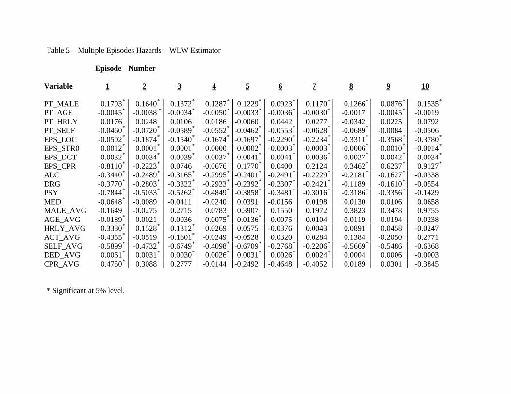
Table 5 – Multiple Episodes Hazards – WLW Estimator

Episode Number Variable 1 2 3 4 5 6 7 8 9 10

PT_MALE 0.1793* 0.1640* 0.1372* 0.1287* 0.1229* 0.0923* 0.1170* 0.1266* 0.0876* 0.1535*

PT_AGE -0.0045* -0.0038 * -0.0034* -0.0050* -0.0033* -0.0036* -0.0030* -0.0017 -0.0045* -0.0019

PT_HRLY 0.0176 0.0248 0.0106 0.0186 -0.0060 0.0442 0.0277 -0.0342 0.0225 0.0792

PT_SELF -0.0460* -0.0720* -0.0589* -0.0552* -0.0462* -0.0553* -0.0628* -0.0689* -0.0084 -0.0506

EPS_LOC -0.0502* -0.1874* -0.1540* -0.1674* -0.1697* -0.2290* -0.2234* -0.3311* -0.3568* -0.3780*

EPS_STR0 0.0012* 0.0001* 0.0001* 0.0000 -0.0002* -0.0003* -0.0003* -0.0006* -0.0010* -0.0014*

EPS_DCT -0.0032* -0.0034* -0.0039* -0.0037* -0.0041* -0.0041* -0.0036* -0.0027* -0.0042* -0.0034*

EPS_CPR -0.8110* -0.2223* 0.0746 -0.0676 0.1770* 0.0400 0.2124 0.3462* 0.6237* 0.9127*

ALC -0.3440* -0.2489* -0.3165* -0.2995* -0.2401* -0.2491* -0.2229* -0.2181* -0.1627* -0.0338

DRG -0.3770* -0.2803* -0.3322* -0.2923* -0.2392* -0.2307* -0.2421* -0.1189 -0.1610* -0.0554

PSY -0.7844* -0.5033* -0.5262* -0.4849* -0.3858* -0.3481* -0.3016* -0.3186* -0.3356* -0.1429

MED -0.0648* -0.0089 -0.0411 -0.0240 0.0391 -0.0156 0.0198 0.0130 0.0106 0.0658

MALE_AVG -0.1649 -0.0275 0.2715 0.0783 0.3907 0.1550 0.1972 0.3823 0.3478 0.9755AGE_AVG -0.0189* 0.0021 0.0036 0.0075* 0.0136* 0.0075 0.0104 0.0119 0.0194 0.0238HRLY_AVG 0.3380* 0.1528* 0.1312* 0.0269 0.0575 -0.0376 0.0043 0.0891 0.0458 -0.0247ACT_AVG -0.4355* -0.0519 -0.1601* -0.0249 -0.0528 0.0320 0.0284 0.1384 -0.2050 0.2771SELF_AVG -0.5899* -0.4732* -0.6749* -0.4098* -0.6709* -0.2768* -0.2206* -0.5669* -0.5486 -0.6368DED_AVG 0.0061* 0.0031* 0.0030* 0.0026* 0.0031* 0.0026* 0.0024* 0.0004 0.0006 -0.0003CPR_AVG 0.4750* 0.3088 0.2777 -0.0144 -0.2492 -0.4648 -0.4052 0.0189 0.0301 -0.3845

* Significant at 5% level.

1

Table 5 (cont.)Common Standard Equal Joint

Variable Coefficient error t-stat Coeffs? Effect?

PT_MALE 0.140400 0.0074 19.030 No YesPT_AGE -0.003700 0.0003 -14.110 Yes YesPT_HRLY 0.017200 0.0078 2.210 Yes NoPT_SELF -0.056500 0.0077 -7.320 Yes YesEPS_LOC -0.151800 0.0086 -17.670 No YesEPS_STR0 0.000200 0.0000 19.380 No YesEPS_DCT -0.003600 0.0001 -63.840 No YesEPS_CPR -0.115900 0.0303 -3.820 No YesALC -0.275600 0.0116 -23.800 No YesDRG -0.290400 0.0134 -21.620 No YesPSY -0.483400 0.0124 -39.070 No YesMED -0.015500 0.0096 -1.620 Yes NoMALE_AVG 0.084900 0.0891 0.950 Yes NoAGE_AVG 0.001100 0.0014 0.790 Yes YesHRLY_AVG 0.110400 0.0161 6.860 No YesACT_AVG -0.125400 0.0189 -6.630 No YesSELF_AVG -0.526000 0.0534 -9.850 Yes YesDED_AVG 0.003400 0.0002 16.130 No YesCPR_AVG 0.150000 0.0910 1.650 Yes No

Table 6 – Probit Estimate of Censoring Probabilities

a. Ongoing Episodes – Type O

Type O – December Type O – January

Variable Coefficient Std. Error Coefficient Std. Error

INTERCEPT -0.2771 0.0508* -0.2561 0.0520*EPS_LENGTH 0.0027 0.0001* 0.0028 0.0001*EPS_LOC -0.2661 0.0474* -0.0424 0.0456ALC 0.2698 0.0615* -0.1302 0.0609*DRUG 0.2401 0.0710* -0.1708 0.0686*PSYCH 0.3852 0.0594* -0.0040 0.0585MED 0.1417 0.0535* 0.0078 0.0544

b. Episodes Starting after December 1 or Before January 31 – Type A

Type A – December Type A – January

Variable Coefficient Std. Error Coefficient Std. Error

INTERCEPT -10.9882 0.6391* 0.0263 0.0553START 0.0303 0.0018* -0.0320 0.0016*EPS_LOC 0.5532 0.0617* 0.7002 0.0560*ALC 0.4457 0.0667* 0.1676 0.0630*DRUG 0.4893 0.0777* 0.0993 0.0713PSYCH 0.5564 0.0674* 0.1706 0.0638*MED 0.0316 0.0533 -0.0151 0.0530

* indicates 5% significance

1

Impacts on Hazards - Drug-Alc Sequence

-1.6000

-1.4000

-1.2000

-1.0000

-0.8000

-0.6000

-0.4000

-0.2000

0.0000

0.2000

0.4000

D1 A2 D3 A4 D5 A6 D7 A8 D9 A10

Episode Number

Impa

ct AGWLW

Figure 1 – Hazards of Drug – Alcoholism Sequence

2

Impacts on Hazards - Drug Sequence

-1.6000

-1.4000

-1.2000

-1.0000

-0.8000

-0.6000

-0.4000

-0.2000

0.0000

0.2000

D1 D2 D3 D4 D5 D6 D7 D8 D9 D10

Episode Number

Impa

ct AG

WLW

Figure 2 – Hazards of Drug Sequence

3

Median Episode Length

0.00

5.00

10.00

15.00

20.00

25.00

1 2 3 4 5 6 7 8 9 10

Episode Number

Epi

sode

Len

gth

(in

days

)

AC

PC

NC

Figure 3 – Differences in Medians – All-censored, probably censored, and uncensored

ii.iv.