Micro-economic models for analysing policy changes in Dutch ...
162
Micro-economic models for analysing policy changes in Dutch arable farming Alfons Oude Lansink
-
Upload
khangminh22 -
Category
Documents
-
view
1 -
download
0
Transcript of Micro-economic models for analysing policy changes in Dutch ...
Micro-economic models
for analysing policy changes
in Dutch arable farming
Alfons Oude Lansink

Hingen
Wanneer paneldata beschikbaar zijn, bieden Maximum Entropy schattingsme-
thoden de mogelijkheid om preciezere voorspellingen te doen over de effecten
van beleidsveranderingen dan Fixed-Effect schattingsmethoden (Golan, A., G.
Judge and D. Miller (1996). Maximum Entropy Econometrics : Robust Estima-
tion with Limited Data, Chichester)
Het begrip zuinigheid behoeft opwaardering in het kader van de noodzaak om
zuinig om te gaan met uitputbare hulpbronnen.
Wetenschappers moeten zich er bij uitstek van bewust zijn dat op 'human
capital' moet worden afgeschreven.
Studies die beogen technische efficiency verschillen tussen bedrijven te meten,
meten vaker het effect van het weglaten van inputs die belangrijk zijn in het
productieproces dan echte technische efficiency verschillen.
Het gebruik van een Fixed Effects schattingsmethode resulteert in kleinere
prijselasticiteiten dan schattingsmethoden die zowel van variatie tussen groepen
als variatie binnen groepen gebruikmaken, (dit proefschrift)
In economisch mindere tijden prefereren Nederlandse akkerbouwers afschrijven
boven actief desinvesteren als middel om de hoeveelheid machines te optima
liseren (dit proefschrift).

Het omvangrijke systeem van fiscale aftrekposten ondermijnt in sterke mate de
progressiviteit van het Nederlandse belastingstelsel.
Trouwen danwel samenwonen verhoogt de transactiekosten van het beëindigen
van een relatie en vergroot zodoende de stabiliteit ervan (Dixit, A. and R.
Pindyck (1994). Investment under uncertainty, New Jersey).
De "warme deken" van de kleine dorpsgemeenschap kan zowel comfortabel als
verstikkend zijn.

Micro-economic models
for analysing policy changes
in Dutch arable farming
Alfons Oude Lansink
0000 0872 3955
Promotor : dr.ir. A J . Oskam Hoogleraar in de Algemene Agrarische Economie en Landbouwpolitiek
Co-promotor : dr. G J . Thijssen Universitair Hoofddocent bij de vakgroep Algemene Agrarische Economie

Alfons Oude Lansink
o ~> - \ \ o ft 0
Micro-economic models
for analysing policy changes
in Dutch arable farming
Proefschrift ter verkrijging van de graad van doctor
op gezag van de rector magnificus van de Landbouwuniversiteit Wageningen,
dr. C M . Karssen, in het openbaar te verdedigen op vrijdag 14 februari 1997
des namiddags te vier uur in de Aula.

ISBN : 90-5485-648-3
BIBLIOTHEEK LANDBOUWUNTVERSITHT
WAGSNÏNGBN

Preface
The thesis that lies in front of you is the product of four years of research that I performed
as a PhD. student (A.I.O.) at the department of Agricultural Economics and Policy of
Wageningen Agricultural University. I started the work back in September, 1992 after I
graduated as a master student in Agricultural Economics, at the same university. Part of the
research was also performed at the department of Agricultural Economics and Rural Sociology
of the Pennsylvania State University, where I spent four months in the summer of 1995.
Several chapters of the thesis have been written together with other researchers and/or have
been published in journals and series. Chapter 2 was written together with Geert Thijssen and
was published as Oude Lansink and Thijssen (1994), whereas Chapter 3 was published as
Oude Lansink (1995). Chapters 4 and 5 have been written together with Jack Peerlings and
were published as Oude Lansink and Peerlings (1996) and Oude Lansink and Peerlings (1997).
Chapter 7, finally is co-authored with Spiro Stefanou from Pennsylvania State University.
I am very much indebted to my supervisors Arie Oskam and Geert Thijssen, for their
valuable comments on earlier drafts and for allowing me freedom in selecting research topics
and methods. They have also been very helpful to me in developing a critical attitude and
learning professional skills.
I also wish to thank the colleagues from the department of agricultural Economics and
Policy and all who visited the department, for creating a pleasant and professional environ
ment. Especially I want to mention Wilbert Houweling for his technical assistance, Alison
Burrell for her valuable comments on all chapters of the thesis and Jack Peerlings and Spiro
Stefanou, with whom I have collaborated intensively during the research of this thesis and
whom I owe insights and motivation through numerous discussions. I am also grateful to all
fellows of the Network for Quantitative Economics, who provided courses, that increased my
understanding and theoretical knowledge of economics.
Special thanks also go the Agricultural Economics Research Institute (LEI-DLO) in the
Hague for its willingness to provide the data that have been used intensively in this thesis.
And last but not least, I want to thank Ingeborg for her dedicated support throughout the
years that I worked on my thesis and, when necessary, for being very helpful in diverting my
thoughts away from economics.
Wageningen, August 1996

Table of Contents
1 Introduction 1
1.1 Background and Scope 1
1.2 Outline of the thesis 3
1.3 Data 7
2 Testing among Functional Forms : An Extension of the Generalised Box-Cox
Formulation 10
2.1 Introduction 10
2.2 Three Functional Forms as Special Cases of the linear Box-Cox 12
2.3 Testing Against Generalised Box-Cox 16
2.4 Data and Estimation 21
2.5 Results 23
2.5.1 DLR test 23
2.5.2 Regularity Conditions and other Criteria 24
2.6 Discussion and Conclusions 28
3 Effects of input quotas in Dutch arable farming 29
3.1 Introduction 29
3.2 Theoretical model 30
3.3 Empirical Model 35
3.4 Data and estimation 38
3.5 Estimation results 39
3.6 Effects of four policy options 43
3.6 Discussion and Conclusions 45

4 Modelling the new EU cereals and oilseeds regime in the Netherlands 47
4.1 Introduction 47
4.2 Theoretical Model 48
4.3 Data 51
4.4 Empirical Model 52
4.4.1 Before the 1992 CAP reform 52
4.4.2 After the 1992 CAP reform 54
4.5 Model simulations 56
4.5.1 Policy simulations 56
4.5.2 Results 57
4.6 Discussion and conclusions 60
5 Effects of N-surplus Taxes : Combining Technical and Historical Information 61
5.1 Introduction 61
5.2 Including the externality in the theoretical model 63
5.3 Empirical model 65
5.4 Model simulations 70
5.4.1 Policy simulations 70
5.4.2 Results 72
5.5 Discussion and conclusions 75
6 Area allocation under price uncertainty : a dual approach 76
6.1 Introduction 76
6.2 Theoretical model 78
6.3 Empirical model 80
6.4 Risk attitude 82
6.5 Data and Estimation 83
6.6 Results 86
6.7 Discussion and conclusions 91

7 Asymmetric Adjustment of Dynamic Factors at the Firm Level 92
7.1 Introduction 92
7.2 The Standard Dual Model 94
7.3 The Threshold Model 96
7.4 Empirical Model 98
7.5 Data 104
7.6 Results 106
7.7 Simulations 110
7.8 Discussion and Conclusions 112
8 Concluding comments and future research 114
8.1 Introduction 114
8.2 Concluding Comments 114
8.3 Future Research 119
References 121
Appendix 130
Samenvatting (Summary in Dutch) 146
Publications 150
Curriculum 151
Chapter 1
l
Introduction
1.1 Background and scope
Environmental and agricultural policy measures are sources of an increasing number
of restrictions on agricultural production. Examples of environmental policy that will
influence Dutch arable farming are the long-term crop protection plan (LCPP) and
mineral policy. The LCPP aims among other things to lower the average 1984-'88 level
of pesticide use. The arable sector uses about two thirds of all pesticides used in the
Netherlands. Targeted reductions for this sector are 39% in 1995 and 60% in 2000 (MJP-
G, 1991 : 101). Mineral policy aims at reducing the flow of phosphates and nitrogen to
the environment. Policy with respect to the arable sector will probably take the form of a
mandatory registration of mineral flows on the farm. The surplus that is calculated using
this information will serve as a tax base (Tweede Kamer, 1995). Future environmental
policy with respect to the arable farming sector may also involve variables as CO,
emission, water use and nature/landscape production, but this thesis will not deal with
these issues.
Other policy changes that affect arable farming stem from the Common Agricultural
Policy (CAP). In 1992, the EU reduced price support for cereals and abolished the
deficiency payments for oilseeds and protein crops. To compensate farmers for their
income loss, subsidies per hectare were introduced. However, farmers growing more than
92 tonnes of cereals equivalents have to set aside a predetermined share of their area of
cereals, oilseeds and protein crops (LNV, 1992). Also, as a result of the CAP-reform,
prices of cereals will be less stable than before.
The (proposed) policy changes often have detailed implications at the farm level and
require therefore explicit modelling in order to determine their effects on economic (e.g.
income, input and output levels) and environmental variables (e.g. mineral surplus).

2
Because no system of first order conditions has to be solved to derive input demand and/or output supply equations (Shumway, 1995).
Farms in the Dutch arable sector are mainly small scale farms operated by the
farmer and his family. This implies that arable farmers are price takers in the markets of
inputs and outputs and that neoclassical production theory and especially its dual form
(e.g. profit function) is a convenient framework for describing economic behaviour of
arable farmers. Advantages of the dual form over the primal form include conceptual and
computational convenience and simplicity and the possibility of using a broader range of
functional forms1 (Shumway, 1995).
Developments in the literature on applied duality theory can be characterised along
three broad lines :
Application of static duality theory : Following Lau and Yotopoulos (1972) many
authors (e.g. Binswanger 1974; Sidhu and Baanante, 1981; Shumway, 1983;
Weaver, 1983; Wall and Fisher, 1986) have applied duality theory to agricultural
economic issues (see also Shumway, 1995).
Application of dynamic duality theory : Theoretical contributions of McLaren and
Cooper (1980) and Epstein (1981) were soon followed by applications to agriculture
(e.g. Taylor and Monson, 1985; Vasavada and Chambers, 1986; Howard and
Shumway, 1988).
Duality under uncertainty : Several authors have now established duality results in
the static framework under price uncertainty Coyle, 1992; Saha and Just, 1996;
Paris, 1989) and output uncertainty (Chavas and Pope, 1994; Pope and Just, 1996;
Coyle, 1995). Duality under price uncertainty in a dynamic framework has recently
been addressed by Arnade and Coyle (1995).
The application of static duality theory under price certainty is well developed in
the literature, so the first purpose of this thesis is to determine the effects of the
aforementioned policy changes using static dual micro economic models. The contribution
of this thesis is that it explicitly incorporates the technical details of the policy changes. A
further contribution lies in the use of farm level data. Previous authors have used farm

3
It is important to note that many applied studies use aggregate data (e.g. sector level), although the theory that is used, holds at the level of the individual firm. Testing micro economic theory while using aggregate data is not necessarily valid, since there is no reason to assume a priori that the theory holds for an aggregate of firms, even if it holds for each firm separately (Shumway, 1995).
level data for estimation and testing2 (Elhorst, 1991; Thijssen, 1992a) and provided
model results for an 'average' farm. This thesis extends their analyses by using farm level
data for simulating policy changes and calculating the effects for different classes of farms
and the sector.
Applications of duality under uncertainty in both the static and dynamic framework
are still very scarce in the literature, so the second purpose of the thesis is to make a
contribution in this area by providing an application of static duality theory under price
uncertainty.
Applications of dynamic duality theory have frequently used aggregate data. The
use of farm level data brings about additional problems related to the occurrence of zero
investments in fixed factors. Therefore, the third purpose of this thesis is to develop a
methodology for modelling individual farmers' investment behaviour in a dynamic dual
framework.
This thesis starts however with a more general chapter that contributes to the
literature by developing a general framework for testing functional specifications of the
profit function. The purpose of this chapter is to provide a rigorous criterion for selecting
functional forms in the remaining chapters of the thesis.
1.2 Outline of the thesis
In this section, a short discussion of the background and main contents of chapters
2-7 is provided.
The performance of flexible functional forms : Testing against the Box-Cox The specification of the functional form for the profit function can be viewed as a
random model specification, i.e. it is an approximation to the 'true' function. The
literature on functional form selection however frequently relies on ad hoc criteria such as

4
theoretical consistency, domain of applicability, flexibility, computational ease, plausibil
ity of the estimated elasticities and others (Lau, 1986; Baffes and Vasavada, 1989).
Chapter 2 presents a unifying approach to allowing the data reveal the specification
by employing the Generalised Box-Cox framework and using Double Length artificial
Regression. Three different linear functional form specifications of the profit function
(Normalised Quadratic, Symmetric Normalised Quadratic and Generalised Leontief) are
tested on the data set that is used for the analyses in the following chapters. An extended
version of the Generalised Box-Cox is developed which includes these three specifications
as nested hypotheses. A Lagrange Multiplier test that avoids estimation is used to test
(subsets of) functional forms against (simplifications of) the linear GBC. Functional forms
are also evaluated in terms of regularity conditions, parameter significance and
reasonability of elasticities. The Normalised Quadratic outperforms the other forms on
most criteria and is used in most chapters in the thesis.
Effects of input quotas in Dutch arable farming Taxes, subsidies and quantitative restrictions are among the most commonly
used instruments in environmental policy (Baumol and Oates, 1988). When introducing
combined tax/quota policies, one should take into account that price elasticities are
affected by the introduction of the quota (Guyomard and Mahe, 1993). In particular, the
own price elasticities are smaller in absolute terms, when an input or output is restricted :
the Le Chatelier-Samuelson effect.
Chapter 3 considers the effects for an average arable farm of a hypothetical
introduction of a pesticides quota. The methodology that is used in this chapter is already
known from consumption theory, but has recently been extended to production theory
(Fulginiti and Perrin (1993), Guyomard and Mahe (1993) and Squires (1993)). In
particular, attention is paid to the effects on price elasticities, elasticities of intensity and
shadow prices of fixed inputs and the restricted quantity of pesticides after the quota
introduction. Furthermore, the possibilities of the methodology are demonstrated by
calculating the effects on netput quantities and income of a combination of input quotas
and taxes.
5
Modelling EU cereals and oilseeds regime in the Netherlands Following the new regime for cereals and oilseeds in the EU, area and set-aside
premiums are coupled to the area of cereals, oilseeds and pulses. The quantity of land set
aside depends on the farmer's area of these crops. In previous research either one or both
of these aspects have not been accounted for. Guyomard et al. (1993) analysed the new
CO regime assuming that area premiums are either fully coupled or fully decoupled from
price levels. Moreover, set-aside decisions were exogenous in their model. Jensen and
Lind (1993) accounted for the fact that area and set-aside premiums are decoupled from
price support, but they did not allow set-aside decisions to be endogenous in their model.
The contribution of Chapter 4 to the existing literature analysing the new CO regime is
that both these aspects are accounted for. This is possible because the effects are
examined at the level of the individual farm. The decision to participate in the set-aside
programme is endogenous in our model and depends among other things on prices of
inputs and outputs and the level of the area and set-aside premiums. Regional aspects of
the new regulation are also taken into account as are environmental effects concerning the
use of pesticides and N-fertiliser.
The reactions of arable farms in the Netherlands are examined using a simulation
model consisting of equations that are estimated using panel data for Dutch arable farms.
The results of the estimation are used in a simulation model that calculates the short-term
effects of the new CO regime for the farms that are in the panel. Simulation results are
aggregated for different classes of farms and for the sector as a whole.
Effects of N-surplus taxes : Combining technical and historical information Future policies on minerals will probably oblige all farms to keep a mineral account
for flows of nitrogen and phosphates from manure as well as artificial fertiliser (Tweede
Kamer, 1995). In this way detailed information on uptake of minerals by crop products
and supply of minerals through artificial fertiliser and manure will be available. The
difference between supply and uptake, minus a threshold level for acceptable mineral
losses per hectare, constitutes mineral surpluses per farm which will be taxed.
In Chapter 5 the effects of a tax on Nitrogen surplus are determined. To this end, a
general methodology is developed that allows technical information on the production of
6
an externality to be included in a dual profit function to yield insight into the effects of a
tax on the externality. This methodology is used to extend the model that was developed
in the previous chapter with nitrogen surplus equations. The model that is thus obtained is
capable of determining the effects of agricultural policy measures and mineral policy
measures simultaneously.
Area allocation under price uncertainty : A dual approach Although empirical evidence has shown that income uncertainty is an important
determinant in area allocation (Freund, 1958; Collender and Zilberman, 1985; Babcock et
al.,1987; Chavas and Holt, 1990), so far a dual framework has not been developed for
simultaneous area allocation and production/input decisions under income risk. Advan
tages of the dual versus the primal framework have been discussed extensively in the
literature (Pope, 1982; Shumway, 1995). They include computational convenience,
simplicity, estimation efficiency and the possibility to use a broader range of functional
forms.
Chapter 6 uses a Mean-Standard deviation utility function to build a dual model that
simultaneously determines area allocation and production/input decisions under price
uncertainty. The specification of the Mean-Standard deviation utility function is sufficient
ly flexible to characterise various risk configurations. Moreover, regularity conditions of
the underlying indirect utility function (symmetry, convexity) and the producers risk
preferences are tested.
Asymmetric adjustment of dynamic factors at the firm level While in the short term, some inputs or outputs may be assumed fixed, in the long
term this assumption does not hold. A dynamic specification of a profit function enables
modelling decisions on quasi-fixed inputs explicitly.
In the standard approach to modelling quasi-fixed factor demand, zero investments
are optimal if the shadow value of the quasi-fixed factor is zero. The observation from
firm level data where investments are frequendy zero questions the consistency of the
standard approach to modelling firm level decision making. A theoretical problem thus
arising is that the first order condition for optimization of the value function, which is
implicit in the dual approach, is not necessarily satisfied. An econometric problem arising

7
3 In chapters 2 and 3, the data set covered the period 1970-1988. Data over the period 1989-1992 were not available at the time these chapters were written.
in both the primal and dual approach is that the data are censored in the presence of zero
investments. This implies that the standard assumption of independent and identically
distributed errors no longer applies and results in biased estimates, if not corrected.
Chapter 7 addresses these shortcomings of past approaches through the specification
and estimation of a threshold model to characterise investment demand. The threshold
model maintains investments are zero if the shadow value of capital is between a lower
and an upper threshold. This model is estimated in two stages. The first stage determines
the decision whether to invest, disinvest or do nothing. This information is used to correct
the error terms in the second stage which comprises the estimation of a system of output
supply and variable and quasi-fixed factor demand equations. Since the value function
does not necessarily exist for zero investments, only the observations for which invest
ments are non-zero are used in the second stage.
1.3 Data
The models in this thesis are estimated on data on specialised arable farms,
covering the period 1970-19923. These data were obtained from a stratified sample of
Dutch farms which kept accounts on behalf of the LEI-DLO farm accounting system.
Specialised arable farms are defined as farms with more than 80% of output coming from
marketable crops. Farms stay in the panel for only five to six years, so the panel is
incomplete.
The models include outputs, variable inputs and quasi-fixed inputs. Outputs
primarily comprise sugar beet, ware potatoes, seed potatoes and starch potatoes, winter-
wheat, barley, oats, oilseeds, and animal output. Variable inputs are mainly pesticides,
fertilisers, services, non-nitrogenous fertiliser, seed and planting materials, purchased feed
input, energy.
Quasi-fixed inputs are land, labour and capital. Land is measured in hectares.
Labour is measured in quality-corrected man years, and includes family as well as hired
labour. Hired labour accounts for a small portion (17%) of total labour at the farm level
8
4 Input and output categories are not the same in all models of this thesis. A more detailed description of the data can be found in chapters 2-7.
and is included as a fixed input since labour contracts cannot easily be terminated. Capital
includes capital invested in machinery and livestock, and is measured at constant 1980
prices. Capital invested in buildings was not included since it proved impossible to obtain
a reliable value of buildings for all farms in the sample (Elhorst, 1990: p.84).
Table 1 gives an overview of the mean and standard deviation of variables that are
included in the empirical models4. Quantities of outputs, variable inputs, land and capital
increased in the period 1970-1992 whereas labour remained almost constant. A more
general description of characteristics of Dutch arable farming and developments in farm
structure etc in the past two decades can be found in LEI-DLO (1995a).
In the empirical models of chapters 2-7, variable inputs and outputs are aggregated
to categories of implicit input and output quantity indices. Implicit quantity indices are
obtained as the ratio of value to price index. Prices of individual components of aggre
gates are obtained from LEI-DLO, whereas prices of input and output aggregates are
defined as Tornqvist price indices and are well documented in e.g. Higgins (1986) and
Thijssen (1992a). The implication of using Tornqvist price indices is that the underlying
aggregator function is translog (Diewert, 1976). Price indexes vary over the years but not
over the farms, implying that differences in the composition of a netput or quality
differences are reflected in the quantity (Cox and Wohlgenant, 1986; Thijssen, 1992a).
Output prices are not known at the time decisions are made on planting and the use
of variable inputs, so expected rather than actual prices have to be used. Expected output
prices were constructed, assuming that price expectations are formed according to an
autoregressive (AR) proces. The implication of using expected rather than actual prices is
that expected profit is assumed to be maximised instead of actual profit. Expected profit
is defined as expected revenue (expected prices times quantities of outputs) minus the total
value of the variable inputs actually used.

9
Table 1 : Mean values of variables for arable farms in the period 1970-1992 (standard deviations in parentheses).
year output8 variable inputs8 land" labour1 capital"
1970 173.0 89.2 40.0 19.7 136.7 (96.6) (1.5) (4.3) (10.1) (87.0)
1971 213.3 93.2 42.5 18.6 146.1 (146.3) (63.0) (30.6) (10.6) (94.2)
1972 184.9 87.4 42.4 16.8 147.6 (111.8) (51.4) (26.1) (7.5) (92.9)
1973 200.8 91.7 45.2 17.1 162.8 (115.1) (54.9) (26.0) (8.1) (94.3)
1974 200.4 91.2 44.7 16.7 165.7 (119.9) (54.2) (27.7) (8.1) (103.1)
1975 199.7 91.3 47.1 17.3 186.3 (120.6) (53.3) (32.0) (8.7) (118.8)
1976 220.9 100.0 47.5 17.3 196.0 (148.7) (60.6) (32.3) (9.4) (128.8)
1977 274.3 114.7 47.5 17.2 215.0 (217.5) (73.7) (31.9) (9.3) (145.5)
1978 276.3 114.1 49.6 17.6 244.9 (186.2) (72.3) (34.9) (9.3) (165.3)
1979 281.2 114.4 50.9 17.4 262.1 (193.7) (77.6) (35.9) (9.2) (176.9)
1980 272.3 112.0 52.0 16.9 275.4 (181.3) (72.1) (39.1) (9.3) (178.4)
1981 273.9 111.2 52.4 17.0 286.8 (188.4) (87.6) (39.3) (9.5) (186.7)
1982 325.7 112.3 53.3 16.1 284.3 (207.6) (70.5) (39.3) (8.3) (177.6)
1983 263.1 117.3 53.2 16.5 293.1 (166.2) (74.7) (39.2) (8.1) (181.6)
1984 367.4 134.0 55.9 17.1 317.8 (248.3) (81.0) (37.5) (9.2) (193.1)
1985 376.2 136.3 57.3 17.3 329.7 (260.9) (80.6) (37.3) (9.5) (211.3)
1986 415.8 139.5 59.3 17.1 333.3 (294.8) (92.5) (44.0) (9.8) (227.5)
1987 408.0 135.6 59.3 16.6 333.4 (293.0) (84.0) (40.4) (8.6) (232.5)
1988 386.5 129.4 59.4 16.3 338.4 (269.3) (80.2) (40.1) (8.3) (236.9)
1989 408.7 135.1 61.3 16.6 339.1 (259.4) (82.2) (40.7) (8.6) (246.3)
1990 444.6 139.6 61.7 16.7 341.9 (290.4) (84.9) (40.3) (8.6) (242.6)
1991 438.6 139.1 60.7 16.4 344.8 (290.5) (83.1) (39.0) (8.3) (235.7)
1992 589.4 131.9 63.1 16.8 359.7 (430.3) (76.4) (37.9) (8.3) (236.0)
a) 1000 guilders of 1980 b) hectares c) man years x 10

Chapter 2
10
Testing among Functional Forms :
An Extension of the Generalised Box-Cox Formulation
Summary
This chapter uses the Generalised Box-Cox framework and Double Length artificial
Regression to test whether different specifications of the profit function are able to mimic
the technology underlying panel data of Dutch arable farms for the period 1970-1988. To
this end, a linear GBC is developed that includes the Generalised Leontief, Normalised
Quadratic and Symmetric Normalised Quadratic as special cases. A Lagrange multiplier
test that avoids estimation of the linear GBC is used to test (subsets of) functional forms
against (simplifications of) the linear GBC. Functional form results are also evaluated in
terms of regularity conditions, parameter significance and reasonability of elasticities.
On this data set, the NQ outperforms the other forms on most criteria.
2.1 Introduction
The behavioural and technological characterisation of decision making has
important implications for policy analysis. The question is how to let the data reveal such
characterisations without imposing the limiting restrictions of functional specification and
the estimation procedures to develop point estimates. Empirical work (e.g. Baffes and
Vasavada, 1989) has demonstrated that parameter estimates and elasticities are sensitive to
the functional form chosen. Hence the functional specification of a profit or cost function
can be viewed as a random model specification; i.e. is profit adequately represented by a
Normalised Quadratic, Generalised Leontief specification or something else?.
The Cobb-Douglas and the CES function were very popular before duality theory

11
became widely employed. These forms are simple, their parameters are easy to interpret
in economic terms, and they are usually not rejected by empirical evidence. However,
they impose constraints on production relationships. Since the early 1970s a number of
flexible functional forms (FFFs) has been introduced, the most commonly used being the
Translog introduced by Christensen, Jorgenson and Lau (1973), the Generalised Leontief
(GL) introduced by Diewert (1971), and the Normalised Quadratic (NQ) introduced by
Lau (1978). In 1987 Diewert and Wales introduced the Symmetric Generalised
MacFadden, which was extended by Kohli (1993) to the Symmetric Normalised Quadratic
(SNQ).
Selecting functional forms has been one way the choice of the functional form has
been addressed in the literature. This literature frequently relies on ad hoc selection
criteria such as theoretical consistency, domain of applicability, flexibility, computational
ease, factual conformity, satisfying curvature restrictions, plausibility of the estimated
elasticities and others (Lau, 1986; Baffes and Vasavada, 1989). Baffes and Vasavada,
(1989) could not select a functional form, because different functional forms yielded
inconsistent results for the same data set.
Few researchers have tried to test whether a particular functional form
outperforms all others. One approach uses Monte Carlo experiments to generate data
from a known technology and examines the ability of the various forms to track this
technology (e.g. Guilkey et al. 1983). Since the data generating process is known, this
approach is appropriate if interest is centred on the general performance of a functional
form; conclusions drawn from it do not necessarily carry over to other data sets. Yet
another approach uses real data and estimates the Generalised Box-Cox (GBC), which is
considered to be the 'true' function underlying the unknown data generating process. The
GBC includes a variety of functional forms as nested hypotheses and parametric tests are
carried out to test these against the GBC (Applebaum, 1979; Chalfant, 1984).
Unfortunately the Box-Cox function has the disadvantage of rendering the model highly
nonlinear in parameters and only few researchers have succeeded in actually estimating
the Box-Cox.
This chapter presents an approach to allowing the data to reveal the character of
technology by employing the Generalised Box-Cox framework and using double length
artificial regressions (DLR) to employ a rigorous criteria towards identifying an
12
appropriate specification of the profit function. The Box Cox model is extended to allow
for the NQ and SNQ as special cases. The advantage of DLR is that it avoids
cumbersome estimation of the Box-Cox in order to test nested forms against it (Davidson
and MacKinnon (1984, 1993)). This chapter shows that DLR is also useful in testing
against simplifications of the GBC, which are created by imposing restrictions on the
GBC's transformation parameters. In this respect a test for linear homogeneity of the
functions is developed. The model is estimated using panel data of Dutch arable farms
over the period 1970-1988. The availability of panel data was explicitly taken into
account in the sense that farm-specific effects are added to the equations.
This study focuses on the performance of the class of linear functional forms,
thereby excluding the Translog. Although the Translog imposes fewer restrictions a priori
on the technology than linear functional forms do (Lopez, 1985), it has some serious
drawbacks that restrict its applicability. First, the log transformation of profit restricts the
domain of applicability to positive profits. Negative profits may frequently occur when
using a profit function that includes one or more restricted outputs (see Moschini, 1988;
Helming et al., 1993). Second, the Translog is not capable of dealing with zero profit
shares of inputs or outputs that may occur when using panel data. Third, the Translog
does not allow for imposing curvature conditions globally, without destroying its
flexibility (Diewert and Wales, 1987). The characteristic of testing and/or imposing
curvature conditions globally is desirable when estimation results are used for e.g. policy
simulations. Fourth, in dynamic models or models including risk behaviour the Translog
form is not very useful because it results in functions that are difficult or impossible to
estimate (Coyle, 1992).
The remainder of this chapter is organised as follows. In Section 2.2, the linear
Box-Cox model is developed and the three linear functional forms distinguished are
derived. An explanation of the DLR approach and a description of the steps involved are
given in Section 2.3. The data and the estimation method are described in Section 2.4 and
the empirical results are presented in Section 2.5. In addition to the tests performed with
DLR against the Box-Cox, the functional forms are evaluated in terms of conditions
following from duality theory, parameter significance and reasonability of the elasticities.
This chapter concludes with comments on this research.

13
Previous studies (e.g. Applebaum (1979), Berndt and Khaled (1979) and Shumway
(1989)) have shown that the family of quadratic forms and the Generalised Leontief can
be obtained as special or limiting cases of the Generalised Box-Cox (GBC). To date, the
Normalised Quadratic and the Symmetric Normalised Quadratic have not been accounted
for explicitly in the framework of the GBC. To be able to incorporate them, there must
be a more general representation of the GBC, which we propose to call the linear
Generalised Box-Cox :
x(r) = u a(.v,.(X,r) + \ ( £ V / ' T £ «,v,.(X,r) v /X , r ) - ^ £ j S / r / X )
«•»1 Z 4-1 M M j-1 (2.1) 3 3 3 3 3
+ ^ ( E W " r £ £ CJ<*>+ E E ^ V A - T )
where
7r(T) = ir /v 3
r ( 2 - 2 )
V , . ( X , T ) = ( V , . / V 3 J X for i=l,2 ( 2 - 3 )
V 3 ( X , T ) = ( 1 - T ) ( ( V 3 / V 3 ' ) X ' - r) (2-4>
and
C;(X)=c" ( 2 - 5 )
represent a simplified Box-Cox transformation (Box and Cox, 1964) of respectively profit
(IT), netput prices (v) and fixed inputs (c)1. The Box-Cox transformation used in this
chapter is simplified because, unlike previous studies (Applebaum, 1979; Berndt and
Profit is defined as revenue minus variable costs; in this study three nerputs and three fixed inputs are distinguished, but any other number of netputs and fixed inputs could have been chosen.
2.2 Three Functional Forms as Special Cases of the linear Box-Cox

14
Table 2.1 : Functional forms nested in the linear Generalised Box-Cox
X T Implied functional form
0.5 1 Generalised Leontief
1 1 Normalised Quadratic
1 0 Symmetric Normalised Quadratic
In this study, the G, are the average share of netput i in total cost plus revenue. They can be interpreted as fixed weights for the price index £ 9 , V j (Kohli, 1993).
Khaled, 1979), log-linear forms (e.g. Translog) are not included in this study.
The r and X parameters are the parameters which are used to obtain the three
functional forms, whereas u, a, 0, and y are the parameters of the profit function. The 0{
parameters are non-negative constants used in the SNQ, which may be selected by the
researcher2; all other parameters can be estimated. In our GBC specification, we largely
followed the notation used by other authors, as far as X is concerned. However, we
included the parameter T to allow linear homogeneity to be imposed either through
normalisation by v 3 in case of the NQ and GL or by the term E J U M m c a s e °f the SNQ.
It can be seen that the term EjU^v, appears in the nested forms when T is zero; at the same
time, all BjCj terms drop out when the Box-Cox transformation is written out. These are
necessary conditions for the SNQ in order to satisfy linear homogeneity in prices. The
quadratic expression of T is required before that of BjCj, because otherwise the jSj
parameters, which are not estimated in the SNQ model will be necessary to construct the
DLR (section 2.3). The numeraire price v3 is operational when r is one, whereas the
terms (1-T) and - T in the Box-Cox transformation of v3 ensure that all terms V 3 ( X , T )
disappear at the same time. As a result, the coefficients related to v3 are not necessary to
construct the DLR of the GL and NQ (see section 2.3).
Before discussing the three functional forms that we analyse in greater detail, we
will introduce some notation that will be useful in the rest of this chapter : v*=\-J\3
T and
x*=x/v/. The three functional forms can be obtained as limiting or special cases of the
GBC by varying the parameters X and r (see Table 2.1).

The GL is given by
15
* * = « + £ «,.(v/f 5
+ £ ^ ° - 5
+ £ £ « , ( v , . * v / ) - + £ £ / J , ( c , . c / 5 - £ £ 7 , ( V ^ ) ° -(-1 ;=1 /=1 y=l M J-l i=l >1 ( 2 . 6 )
where all prices and profit are normalised by the price of other variable inputs in order to
impose linear homogeneity in prices. Imposing symmetry requires « ¡ ¡ = 0 ^ and 8^=6^ for
all i and j . These symmetry restrictions apply to all functional forms distinguished.
The NQ takes the form :
v / + £ ^ l £ £ * , v > / + ^ £ £ t e + E E v < * < y ( 2 . 7 )
1=1 ;= i * ;=i > i ^ i=i y=i ;=i j= i
whereas the SNQ is derived as :
3 3 3 3 3 3 3 3 3
™ £ «<V i ( £ W £ £ < W + 1 ( £ ekvj£ £ /3,c ;c.+ £ £ 7 , v 6 . ( 2 - 8 ) i=l * 4=1 i=l > 1 ^ 4=1 1=1 y=l i=l > 1
For the SNQ function u should be equal to zero because the linear homogeneity
restriction allows no constant term in this function. In order to identify all parameters,
additional restrictions have to be imposed on the SNQ:
3
where y is an arbitrary point or observation. In this study y; equals the sample mean.
It is important to note that the linear GBC is not linear homogeneous in prices and
that linear homogeneity is imposed in the functional forms that are distinguished.
Therefore, the test of the NQ, SNQ and GL against the linear GBC is not only a test of
the specific transformation that is applied but also a test of linear homogeneity in prices.
16
Apart from testing against the linear GBC, it is also possible to simplify the linear
Generalised Box-Cox, by imposing restrictions on the parameters of the linear GBC a
priori. The restriction that we analyse is linear homogeneity of the GL, NQ and SNQ by
testing on T while maintaining X=0.5 and X=l, respectively.
2.3 Testing Against Generalised Box-Cox
Assuming that the linear GBC is the true model, we want to test whether one of the FFFs
in the previous section is an acceptable simplification. The simplest way would be to
estimate the linear Box-Cox and perform parametric tests on the three nested models. The
linear generalised Box-Cox model, equation (2.1), is highly non-linear in parameters and
is therefore difficult to estimate. Therefore if the only objective is to test the adequacy of
simplifications of the Generalised Box-Cox, it is better to avoid such estimation (Davidson
and MacKinnon, 1985). A possible solution would be to perform a grid search over
values of the linear Box-Cox parameters (X and T) and estimate the parameters a, ¡3, and
7 conditional on the Box-Cox parameters. Another approach is to rescale the dependent
variable. However, neither of these methods generates valid estimates of the covariance
matrix of the parameters (Davidson and MacKinnon, 1993; 486-488).
Another strategy would be to calculate the values of the log-likelihood functions
for various values of the linear Box-Cox parameters and to use an LR test to select among
them. One disadvantage of this approach is that more than one model may turn out to be
plausible. A second disadvantage is that the approach cannot tell us anything about the
validity of the preferred model. The model might even be rejected if we actually tested it
against the linear Box-Cox model (Davidson and MacKinnon, 1993; 489-492).
Several tests have been developed in the literature for the special case of testing
the linear against the log-linear model. Godfrey et al. (1988) give an overview and
provide some Monte Carlo evidence on the finite sample behaviour of several tests. The
test based on Double Length artificial Regression (DLR - see Davidson and MacKinnon,
1984) is generally the most powerful one when the disturbances are normally distributed.
Consequenüy, this test proves to be sensitive to failures of the normality assumption.
To understand the test based on DLR, let us develop the likelihood function of

17
equation (2.1). We add an additive disturbance term to this equation to take account of
measurement errors in the dependent variable, optimisation errors and effects of a large
number of omitted variables. The disturbance terms are assumed to be normally
distributed with mean zero and variances a2. We rewrite equation (2.1) by subtracting the
regressors from the regressand and dividing the resulting term on the left-hand side by a.
The resulting equation can be written as
m„ (y„, co) = e„ 1. .N (2.9)
where each m n is a function of observation n which depends on the dependent variable yn,
the exogenous variables, vector of parameters w; en has a standard normal distribution;
and N is the number of observations. The parameter ca contains a, j3, y, X, r and a. The
density of e n is equal to:
fi(e„) 1 exp ( - % en
2) (2.10)
In order to construct the likelihood function, we need the density of yn rather than the
density of en. The density of yn is given by:
f2(y„) = ft K(y n ,co)) 3y„
1 2 exp ( - V2 m n (y n,w))
(2.11)
3mn(y t t,co)
3y»
The contribution of the n* observation to the log-likelihood function l(y,a>) is the
logarithm of (2.11)
K ( y ^ ) = " 1 / 2 l n (2T) - V2m n
2(y n ,û)) + k n (y n ,u) (2.12)
where: k n (yn,«j) = In 9 m n ( y n . M )
ay„

18
g(y,co) = ( -M ' (y ,« ) K'(y,co) My,03) (2.13)
where: (yn,co) s da.
K„, s 3 CO;
and m(y,co) is an N vector with typical element mn(y,co) and i denotes an N vector each
element of which is 1.
Using this result we can construct the DLR, developed by Davidson and
MacKinnon (1984). Artificial regressions are simply linear regressions that are used as
calculating devices. The regressand and the regressors are constructed in such a way that
when the artificial regression is run, certain of the numbers printed by the regression
program are quantities which we want to compute. The DLR looks as follows:
m(y,co) -M(y.u) b + residuals (2.14)
i K(y,co)
This artificial regression has 2N artificial observations. The regressand is mn(y,co) for
observation n and unity for observation n+N, and the regressors corresponding to b are
-Mn(y,co) for observation n and K„(y,co) for observation n+N, where M n and Kn denote,
respectively, the n m rows of M and K. We need a double-length regression because each
observation makes two contributions to the log-likelihood function: a sum-of-squares term
-Vi m2 and a term kn. The DLR can be estimated by OLS when an estimate for co is
available. If the artificial regression is evaluated at unrestricted ML estimates co, the
estimates of b are equal to:
b = -M'(y,w)K'(y,d>)) -M(y,co) K(y,«)
( -M'(y,«)K'(y,&)) m(y,co)
t (2.15)
Since all the observations are independent, the log-likelihood function itself is merely the
sum of the contributions ln(yn,w). The gradient of l(y,<a) is

19
The last product in this term is equal to the gradient of the log-likelihood function l(y,co)
evaluated at 6 and is therefore equal to zero. Therefore, the estimates of b are zero.
Another possibility is to evaluate the DLR at restricted estimates of w. As shown in
Section 2.2, the functional forms are restrictions of the Box-Cox model. When a
functional form is appropriate, the resulting estimates of b should also be close to zero.
Davidson and MacKinnon (1984) show that an F-test is valid for testing the hypothesis
that the coefficient on the regressors related to X and T are zero.
To make this result operational we derive the formulas of the variables in the DLR
based on equation (2.1) (multiplied by a). The first N elements of the regressand follow
directly from equation (2.9). The regressors that correspond to u are
where the upper and lower quantities inside the tall brackets denote, respectively the n*
and (n + N)"1 elements of the regressor. The regressors that correspond to a{ are
The regressors corresponding to a», ft, ftj and are similar. The element of - M(y,co)
that corresponds to X is:
1 (2.16) 0
v, ( X , T ) (2.17) 0
2 3 3 3
£ [in V (v,* ) x] a , + ( £ £ <V/X,r) + E YjtfX)
3 3 3
+ ( l~r ) [ lnv 3 > 3 ^] « 3 + ( £ V,r'E « 3 / > ( ^ ) - E V > ( X ) (2.18)
The element of K(y,co) that corresponds to X is zero.

20
The regressor that corresponds to r is:
l n v 3 ( 7 r ( T ) ) - \ £ ( l n v 3 ( v 1 ( \ , T ) ) i=l
( (v 3 *) x -T + (l-T)(\lnv 3(v 3*) x + l))
k=l j=l j=l
« 3
+ ( E W E VjCX.r) + £ -y3jCj(X,r) k=l j=l
3 3
z k=l k»l
(2.19)
i - l H
(E W1EE W W 1 + 2r£/3.c j(X)
-oinv,
3
I k=l
The regressor that corresponds to a is:
m n ( 7 r n ( 8 , e , T ) , c < j ) la
-1 (2.20)
Using these results the regressors of the DLR for specific values of X and T can be
calculated. (These calculations are available from the authors upon request.)
To summarise, the steps to be undertaken when using the test based on the DLR are:
i) Estimate the functional form using maximum likelihood. OLS gives the same
estimates for a, @ and y, only the estimate of a should be corrected.
ii) Construct the DLR using equations (2.9), (2.16)-(2.20).
iii) Check the correctness of the constructed DLR by running the DLR without the
21
2.4 Data and Estimation
The data used cover the period 1970-1988 and were provided by the Agricultural
Economic Research Institute (LEI). Data on specialised arable farms (farms with more
than 80% of total output consisting of marketable crops) were selected from a stratified
sample of Dutch farms which kept accounts of their farming for the LEI book keeping
system. The data set used for estimation includes 3249 observations on 733 different
farms (see Appendix I, table 1.1 for a description of data and variability).
One output and two3 variable input categories (pesticides and other inputs) are
distinguished. Other inputs consists of services, fertilisers, seed and planting materials,
purchased feed input, energy and other variable inputs. Fixed inputs are land, labour and
capital. Land is measured in ares. Labour is measured in quality-corrected man-years, and
includes family as well as hired labour. Capital includes capital invested in machinery and
livestock and is measured at constant 1980 prices. Capital invested in buildings was not
included, since it proved impossible to obtain a reliable value of buildings for all farms in
the sample.
The profit function was also estimated using three categories of variable inputs : pesticides, nitrogenous fertiliser and other variable inputs. The results were not very different from those of this specification.
regressor corresponding to the parameters X and T. This regression should have no
explanatory power if everything has been constructed correctly.
iv) Estimate the DLR using OLS.
v) Use the F-test to test the hypothesis that the coefficients on the regressor related to
X and T are zero. If this hypothesis is not rejected the functional form is not
rejected against the linear Box-Cox model and is therefore an acceptable
simplification of that model.
Below, the DLR is also used for the tests described in Section 2.2, whenever
simplifications of the linear Box-Cox model are involved. These tests are straightforward
simplifications of the DLR test described in this section.

22
Tomqvist price indexes were calculated for the two composite netput categories
(output and other input). Price indexes vary over the years but not over the farms,
implying that differences in the composition of a netput or quality differences are
reflected in the quantity (Cox and Wohlgenant 1986). Implicit quantity indexes were
obtained as the ratio of value to the price index.
The prices of arable products are not known at the time decisions are made on
planting and the use of variable inputs, so expected rather than realised output prices have
to be used (Higgins 1986). Expected output prices were constructed by applying an AR(1)
fdter. About 50% of the crops grown in the Netherlands are under a market regulation
and prices of these crops are stable over the years. Therefore, the assumption that
expected prices are generated by an AR(1) process is not simplistic. Expected profit was
defined as expected revenue (expected prices times quantity of output) minus total value
of the actual use of variable inputs.
A time trend and corresponding cross-products were added to equation (2.1) in
order to allow for technological change. The regressors in the DLR that correspond to
these terms look similar to equation (2.17).
The availability of panel data was expliciuy. taken into account in the steps to be
undertaken for the DLR. We take as a constant plus error term in the linear GBC
u h t = u + r/h + e h t h = 1....H, t = l....T h (2.21)
where r]h is the specific effect (fixed or random) of farm h representing the effect of those
variables peculiar to the h f t individual in more or less the same fashion over time. Th is
the number of years of records on farm h. Total number of observations is N. In Section
2.3 we introduced e h t as a normally distributed variable with mean zero and variances o2.
The mean of uh, is assumed to be equal to u. For the SNQ function u should be equal to
zero, this will be tested in the following section.
The steps to be undertaken for the DLR are adjusted:
i) In equations (2.6)-(2.8) a farm specific effect is introduced. We use the fixed
effects transformation to estimate these equations. The random effects estimator is
generally more efficient but makes the unrealistic assumption that the individual
23
effects and the regressors are independent.
ii) Equation (2.16) for farm h of the DLR looks similar, but the upper quantity inside
the bracket denote the hf observation. For every farm we get a dummy variable,
which is equal to one for observations on this farm and zero elsewhere.
iii) and iv) Estimate the DLR by OLS after transforming the data. The transformation ma
trix consists of the usual fixed effects transformation matrix in the top left corner.
The lower right corner is the identity matrix, the other elements are zero. So, the
fixed effects transformation is only applied to the (1..N) observations; the
remaining (N+1..2N) observations are transformed by the identity matrix. This
transformation matrix is symmetric and idempotent. Therefore, the proof that this
transformation is valid is similar to the proof given by Hsiao (1986: 31-32) for the
fixed effects transformation,
v) Use F and t tests and correct for the decrease in degrees of freedom due to the
fixed effect estimation.
We developed the DLR for one equation. To increase the efficiency of parameter
estimates we estimate the profit functions along with the netput equations (given in
Appendix VII) for the calculation of price elasticities and elasticities of intensity.
The Iterative SUR estimation technique is applied here because the disturbance
terms may be correlated across equations and because of the cross-equation parameter
restrictions. In all cases we dropped the equation of other input in order to ensure non-
singularity. The results of the NQ, SNQ and GL are not invariant with respect to the
equation deleted. Error terms like equation (2.21) are also integrated into these systems.
Thijssen (1992) shows that the common fixed effects transformation can also be applied to
an incomplete panel, using a SUR estimation method.
2.5 Results
2.5.1 DLR Test
In order to use the DLR approach we performed steps i-v as described in Sections 2.3

24
Table 2.2: Results of the DLR : F and t-values of nested hypotheses.
Test
GL NQ SNQ
Linear GBC 37.43 5.00 9.54
Linear Homogeneity 2.05 0.58* 4.28
not significant at the 5 % level
2.5.2 Regularity Conditions and other Criteria
In addition to testing the three functional forms against the linear GBC, they are also
evaluated in terms of regularity conditions, parameter significance, and elasticities of
and 2.4. For every functional form, the explanatory power of the DLR was checked in a
separate regression without the terms corresponding to X and r. In these regressions, all
the estimates of the parameters were very small and t values were zero, and therefore the
condition in step iii was satisfied. The parameter restrictions of the SNQ (see section 2.2)
were also imposed at this stage and at the following stage, since they follow immediately
from (2.17). The F values of step v are given in the first row of Table 2.2.
The test against the generalised linear Box-Cox model reveals that all functional
forms are rejected at the critical 5% level, since all F values are larger than F2,5635,6=o.as
(=3.00). The F value for the NQ is however close to the critical 1% level (of 4.61). As
pointed out in Section 2.2, these test results imply that the transformation applied
(through X and T) and linear homogeneity are simultaneously rejected, i.e. it does not
necessarily imply that the specific transformation through X is rejected. Linear
homogeneity, conditional on the transformation (see Section 2.2), is tested by a t test on
the parameter of the regressor corresponding to T in the DLR (equation 2.19). The test of
linear homogeneity of the GL, NQ and SNQ points out that linear homogeneity is rejected
(at 5%) for the GL and SNQ, but not for the NQ.

25
Table 2.3 : Evaluation of regularity conditions and parameter significance.
FFF
percent of violations
convexity in monotonicity2 increasing in fixed
prices' inputs^
percent of
parameters
significant at 5 %
GL
NQ
SNQ
43.39
0
0
0.61
0.12
0.15
4.86
0.09
62.01
62.96
59.25
57.14
1) Convexity was checked by the determinantal test of the hessian. The GL was checked at each
observation since their hessians are not constant.
2) Monotonicity and increasing in fixed inputs were rejected if this condition failed to hold for at least one
netput or fixed input. The percentage of violations would have been lower if calculated as percentage of
total number of netputs or fixed inputs.
prices and intensity. The regularity conditions of the profit function are convexity in
prices, monotonicity (increasing in output prices, decreasing in input prices) and
increasing in fixed inputs. Table 2.3 shows that the GL violates convexity in prices for
approximately half the number of observations; convexity is not violated for the NQ and
SNQ at any observation. Monotonicity in prices is slightly violated for all functional
forms. In previous empirical studies, the condition of convexity in prices was often
violated, so our results are not unusual. The monotonicity condition has also rarely been
violated in previous empirical work. For an overview and interesting discussion on
evaluation of regularity conditions, see Fox and Kivanda (1994) and the related
comments.
The SNQ performs very poorly in terms of the condition that the function is
increasing in fixed inputs. Given that its performance in the other tests in this table,
including the percentage of significant parameters, is good, this is surprising.

26
Table 2.4 : Price elasticities at the sample mean (estimated standard deviation in
parentheses).
price of
output pesti other input
cides
output GL 0.02 (0.03) -0.01 (0.00) -0.04 (0.03)
NQ 0.05 (0.02) -0.00 (0.00) -0.05 (0.02)
SNQ 0.10 (0.03) -0.01 (0.00) -0.11 (0.03)
pesticides GL 0.07 (0.03) -0.46 (0.09) 0.40 (0.10)
NQ 0.06 (0.03) -0.24 (0.08) 0.18 (0.09) SNQ -0.09 (0.03) -0.55 (0.11) 0.64 (0.12)
other input GL 0.06 (0.08) 0.09 (0.02) -0.15 (0.09)
NQ 0.06 (0.08) 0.04 (0.02) -0.20 (0.08)
SNQ 0.33 (0.09) 0.14 (0.03) -0.47 (0.09)
Table 2.4 shows the price elasticities (see Appendix I, table 1.2 for their
expressions) that were calculated from the estimated parameters at the sample mean. The
price effects are small in general, especially those that relate to the output. This reflects
the crop rotation restrictions in Dutch arable farming, and also the restricted availability
In section 2.4 we have demonstrated that the SNQ is only linearly homogeneous in
prices when the error component u is zero. This error component can be determined by
calculating the mean of all composite error terms from the profit function. The value of u
from the ITSUR estimation was found to be -26770, with a t value of 0.37. From this we
infer that u is not significantly different from zero (at 5 %) and linear homogeneity of the
SNQ is not violated by using a fixed effects model.

27
Table 2.5: Elasticities of intensity at the sample mean (estimated standard deviation in
parentheses).
amount of
land labour capital trend
output GL 0.43 (0.02) 0.33 (0.02) 0.14 (0.01) 0.02 (0.07)
NQ 0.50 (0.02) 0.38 (0.02) 0.22 (0.02) 0.03 (0.00)
SNQ 0.83 (0.03) 0.26 (0.03) 0.11 (0.02) 0.03 (0.00)
pesti GL 0.94 (0.06) 0.15 (0.04) 0.14 (0.03) 0.05 (0.03)
cides NQ 0.80 (0.05) 0.14 (0.03) 0.13 (0.02) 0.05 (0.00)
SNQ 0.01 (0.06) 0.08 (0.04) -0.05 (0.03) 0.03 (0.08)
other GL 0.53 (0.14) -0.04 (0.10) 0.07 (0.07) -0.04 (0.07)
input NQ 0.69 (0.08) 0.15 (0.05) 0.25 (0.04) -0.00 (0.00)
SNQ 0.70 (0.15) 0.59 (0.12) 0.41 (0.09) 0.01 (0.02)
of land. Pesticides are found to be gross substitutes with respect to other input. Most
price elasticities correspond well, although some large differences are found between the
SNQ and NQ for pesticides with respect to its own price and the price of other input; the
same holds for the own price elasticity of other input.
The elasticities of intensity (see Appendix I, table 1.2 for their expression) are
presented in Table 2.5. The SNQ reveals that capital is a substitute for pesticides and the
GL reveals that labour is a substitute for other input. In addition, all other relations
between fixed inputs and variable inputs are characterised by complementarity. Large
differences are mainly found between the SNQ and GL for output with respect to land
and for other input with respect to labour and capital.
28
2.6 Discussion and conclusions
This chapter uses the Generalised Box-Cox framework and Double Length
artificial Regression to test whether different linear specifications of the profit function
are able to mimic the technology underlying panel data of Dutch arable farms for the
period 1970-1988. Functional form results are also evaluated in terms of regularity
conditions, parameter significance and reasonability of elasticities.
The NQ and SNQ were included explicitly in the linear GBC and a test based on
DLR was used in order to avoid cumbersome estimation of the linear GBC. The test
based on DLR rejected all functional forms against the linear GBC, the F values of the
NQ were much lower, however. The proposed test on linear homogeneity comes out in
favour of the NQ.
The NQ also outperforms all other forms on the regularity conditions that were
examined. The GL violates convexity in prices for approximately half the number of
observations, whereas the SNQ is often non-increasing in fixed inputs. Also, the price
elasticity estimates of the FFFs were in accordance with neo-classical theory. However,
large differences between price elasticities within the class of linear FFFs are found
between the NQ and SNQ. This reflects a serious shortcoming of the NQ, namely that
estimation results are not invariant with respect to the choice of the numeraire.
Testing the three functional forms against the linear GBC using DLR allows the
data to tell what functional form is preferred and avoids estimating the linear GBC.
Moreover useful simplifications can easily be made within the linear GBC and tested
using DLR.

29
Summary
The effects of a hypothetical introduction of a quota on pesticides are analysed
using a short-term profit function which is derived from duality theory. A normalised
quadratic function is estimated using panel data from Dutch arable farms over the period
1970-1988.
Price elasticities and elasticities of intensity are calculated before and after the
introduction of the quota. The effects on price elasticities are small in general. Fixed
inputs show an increasing or decreasing complementarity depending upon the previous
relation between the variable and former variable input (pesticides).
The shadow price of pesticides will rise by about 85% above the previous market
price due to a 10% cut in the pesticide quota. Shadow prices affixed inputs decrease
after the hypothetical introduction due to complementarity with pesticides.
3.1 Introduction
Environmental measures and agricultural policy are sources of an increasing
number of restrictions on agricultural production. A case of present interest in Dutch
agriculture is the Long-term Crop Protection Plan (LCPP) which aims among other things
to lower the average 1984-1988 level of pesticide use. About two third of those pesticides
are used in arable farming. Targeted reductions for this sector - measured in terms of
active ingredient - are 39% in 1995 and 60% by 2000 (MJP-G, 1991 : 101). Besides this,
the government aims at reducing the flow of nitrates and phosphates to the environment.
These plans can be translated into various measures. Taxes, subsidies and quanti
tative restrictions are among the most commonly used instruments (Baumol and Oates,
1988). When introducing combined tax/quota policies, one should take into account that
price elasticities are affected by the introduction of the quota (Guyomard and Mahe
Chapter 3
Effects of input quotas in Dutch arable farming

30
7r(v) = max{v.q; (q)eT; v > 0 } i
(3.1)
(1993) and Fulginiti and Perrin (1993)). The same holds for shadow prices of a priori
fixed inputs and elasticities of intensity.
Helming et al. (1993) evaluated these effects in the case of milk quota by using
data before and after the introduction of quotas. Fulginiti and Perrin (1993) and
Guyomard and Mahe (1993), however, showed that the parameters of a restricted profit
function (after a quota) can be determined with those of an unrestricted (before quota)
one, when only the latter are known and vice versa. This study applies the latter
methodology to micro data in order to determine the effects of a hypothetical introduction
of a pesticides quota on price elasticities, elasticities of intensity and shadow prices of
fixed inputs and pesticides. Furthermore the methodology will be illustrated through
simulations with four different policy options.
The structure of this chapter is as follows. The theoretical and empirical models
are discussed in section 3.2 and 3.3, respectively. Section 3.4 describes the estimation
procedure and the data used for this research, while the estimation results and the analysis
for the pesticides quota are presented in section 3.5. The application with four policy
options are discussed in section 3.6 and the chapter concludes with comments on this
research.
3.2 Theoretical model
Neoclassical production theory forms the framework for our analysis of the effects
of quantitative restrictions and taxes on detrimental inputs. The theory is more widely
discussed in Chambers (1988) and will only briefly be surveyed here. This section will
concentrate on the theory underlying the determination of restricted price elasticities and
shadow prices after a hypothetical introduction of a quota from the parameters of an
unconstrained profit function.
' To begin, it is assumed that all inputs and outputs, or more compactly "netputs",
are freely disposable (variable). Profit maximisation conditional on a convex production
possibility set or technology T can be denoted as :

31
where q is a vector of netput quantities (negative for inputs, positive for outputs) and v a
vector of netput prices. The profit function x is assumed to be non-negative, non-
decreasing in output prices, non-increasing in input prices, convex and linearly
homogeneous in prices, continuous and twice differentiable.
Applying Hotelling's lemma to (3.1) yields the optimal level of netputs as a function of v:
where x v is the vector of first derivatives of x with respect to v.
Next the netput vector q is partitioned into vectors qj and c&, where q! is, as
before, a vector of freely disposable netputs, but where Oj is now a vector of fixed
netputs (or equivalently, netputs which are under a quota). Vj and v2 are the
corresponding price vectors. Furthermore, G represents the general restricted profit
function (McFadden, 1978 : 66) which incorporates the fixed quantity :
G has the same properties as x except that it is not necessarily non-negative and besides
that, it is decreasing in quantities of fixed netputs. Note that G includes the more familiar
cost (revenue) functions as special cases, that is when qi is a vector of input (output)
quantities and a vector of output (input) quantities. Applying Hotelling's Lemma to
(3.3) yields optimal levels of q 1 ( now as a function of Vj and q :
where G v l denotes the first derivative of G with respect to v^ An intuitive explanation of
q2 is that of a vector of netputs, which are fixed in the short term, but variable in the long
term. In that case x can be regarded as a long-term profit function, which can also be
seen by expressing (3.1) as :
x v = q(v) (3.2)
G{vvq2) = max {vvqx; (qvq2)e T; v, > 0} (3.3)
G v , = ? l ( V l . ? 2 ) (3.4)
x(v) = max {v2.q2 + Givvq2y, (q,,q2)eT; vvv2>0} (3.5)
(3.5) implies profit maximisation over the remaining vector q given that q : is at the
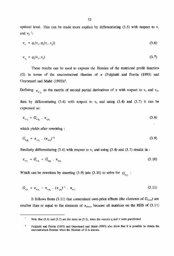
32
* V = ? i ( v i ^ 2 ( v i . v 2 ) ) (3.6)
\ = 4 2 ( V 1 ' V
2 ) ( 3 - 7 )
These results can be used to express the Hessian of the restricted profit function
(G) in terms of the unconstrained Hessian of ir (Fulginiti and Perrin (1993) and
Guyomard and Mah6 (1993))2.
Defining 1 r v v as the matrix of second partial derivatives of ir with respect to Vj and v2,
then by differentiating (3.6) with respect to v2 and using (3.4) and (3.7) it can be
expressed as:
which yields after rewriting :
Gvq = *VV . (TTvvyl (3.9)
"tfl v\vz V2V2
Similarly differentiating (3.6) with respect to v t and using (3.4) and (3.7) results in :
ir = G + G .it (3.10) Which can be rewritten by inserting (3.9) into (3.10) to solve for G '•
G = ir - I T . (TT Y1 . ir (3.11) v,v, v,v, v,Vj v v , v / " v 2 v , v '
It follows from (3.11) that constrained own-price effects (the elements of G v l v l) are
smaller than or equal to the elements of 7 r v l v l , because all matrices on the RHS of (3.11)
Note that (3.6) and (3.7) are the same as (3.2), since the vectors q and v were partitioned
Fulginiti and Perrin (1993) and Guyomard and Mahe (1993) also show that it is possible to obtain the unconstrained Hessian when the Hessian of G is known.
optimal level. This can be made more explicit by differentiating (3.5) with respect to v t
and v2

33
3 Positive semi-definiteness of the Hessian follows from convexity of the profit function in prices.
are positive semi-definite3. This result is more commonly known as the Le Chatelier-
Samuelson effect (Chambers, 1988 : 134). For the off-diagonal elements of G v l v l , it has
been shown that restricting one netput (in which case T T v 2 v 2 is lxl) will increase
substitutability and reduce complementarity ( Guyomard and Mahe, 1993). The second
term on the RHS of (3.11) is also referred to as the indirect effect, whereas the term on
the LHS of (3.11) is usually called the direct effect (Moschini, 1988).
The quantity of a fixed netput in the vector q has a value for the producer, that is
called the shadow price. The vector of shadow prices of the fixed netputs is determined as
minus the first derivative of G with respect to qj :
vs = ~G„ (3.12)
Essentially, the shadow price equals marginal cost in the case of outputs, and marginal
revenue product in the case of inputs; Furthermore, the shadow price is equal to the
market price when the netput is freely disposable and the producer is maximising profit.
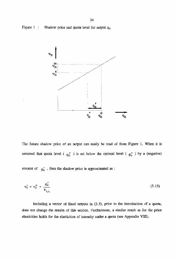
Figure 1 gives a graphical representation of the effects of an introduction of a quota on
the shadow price of a formerly freely disposable input. It follows that the shadow price
(v2i
s) depends upon the severeness of the restriction and the slope of the marginal revenue
product curve (which equals l / 7 r v 2 i v 2 i under the assumption of a linear marginal revenue
product curve). A relaxation of the constraint lowers the shadow price of an input. The
shadow price of an input will be at least as high as its market price v 2 i
m whenever the
quota is binding.
34
r
0 ^21
The future shadow price of an netput can easily be read of from Figure 1. When it is
assumed that quota level ( ^ * ) is set below the optimal level ( q£ ) by a (negative)
amount of ^ , then the shadow price is approximated as :
vi = v5 + (3.13)
Including a vector of fixed netputs in (3.5), prior to the introduction of a quota,
does not change the results of this section. Furthermore, a similar result as for the price
elasticities holds for the elasticities of intensity under a quota (see Appendix VUI).
Figure 1 : Shadow price and quota level for netput

3.3 Empirical model
35
The preceding section presented a method for obtaining price elasticities in a
situation where one or more netputs is restricted from those under unconstrained profit
maximisation. This section will translate this theoretical model into an estimable form. In
order to calculate the effect of a combined pesticide quota and N-fertiliser tax, the price
elasticities which hold under a quota on pesticides are needed.
The Normalised Quadratic is the functional form that is used in this chapter, because it
overall came out more favourable than the other functional forms that were tested in
Chapter 2. Other reasons for choosing the Normalised Quadratic are its simplicity and the
fact that it has a hessian of constants implying that convexity in prices can be tested
globally. The Normalised Quadratic takes the form :
3 3 1 3 3
T = « o + E a ; vi+ £ + Tf+
w»w+öEEa«v/v/ /=i y = i i = i y=i
+ EEte + ^ v 2 + £ £ w + (3-14) 3 3 3 3 E v; E <w + Er* + E w
i=i M y=i y = i
where ir is normalised variable profit4, v, are normalised netput prices, with i = l
(output), 2 (pesticides) and 3 (nitrogenous fertiliser). Furthermore, z{ are fixed inputs with
i= l , (land), 2 (labour) and 3 (capital). Finally, technological change is represented by a
time trend (t), and w represents a weather index. Symmetry is imposed by requiring
a — t t j i and 6 ij=BJi, for all i and j .
The output supply and input demand equations are obtained by differentiating
(3.14) with respect to the vector of normalised prices :
All prices and profit have been normalised by the price of other variable inputs. This ensures linear homogeneity in prices.
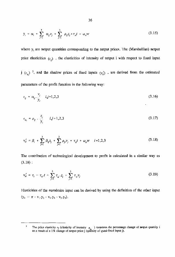
36
3 3
yt = a i + £ + E p i j z j + 7 v f + <v (3-15)
where y, are netput quantities corresponding to the netput prices. The (Marshallian) netput
price elasticities ( e p , the elasticities of intensity of netput i with respect to fixed input
j (ek) s, and the shadow prices of fixed inputs ( V J ) , are derived from the estimated
parameters of the profit function in the following way:
e.. = ar
V-i iV=l,2,3 (3.16) y i
• P9 • Zj- ij = 1,2,3 (3-17)
< = 0/ + E + E Pjivj + V - û>„w /=1,2,3 (3-18)
The contribution of technological development to profit is calculated in a similar way as
(3.18) :
3 3 va
s = T, + T r r + £ V z , + £ (3-19)
Elasticities of the numéraire input can be derived by using the definition of the other input
(y4 = ic - Vt .y! - v 2.y 2 - v3.y3).
The price elasticity ev (elasticity of intensity e . ) measures the percentage change of netput quantity i as a result of a 1 % change of netput price j (quantity of quasi-fixed input j).

37
M ^ f = i ; = i z ;=i i=i (3.20)
Next the pesticide quota is introduced and it is assumed that producers are faced
with a 10% cut in pesticides use at the onset of the quota regime. The effects on the price
elasticities and elasticities of intensi'ies will then be twofold. The first effect will be the
change in the parameters of the profit function (see section 3.2), whereas the second
effect comes from the change in the quantities of netputs due to the quota reduction. New
netput quantities (y*) are calculated with the elasticity of intensity of the remaining
netputs with respect to the quantity of pesticides (e. ) , using (3.9) :
Netput prices and fixed inputs are assumed not to change, since prices are exogenous and
because this model is only capable of determining short-term effects, respectively.
^2 , K «22 ' y I
¿ = 1,3 (3.21)
The pesticide (netput 2) restricted netput price elasticities (e£) and elasticities of
intensity ( /) are calculated in the following way :
a.2) . -L ¿ = 1,3 7 = 1,3 yt
(3.22)
¿ = 1,3 7 = 1,2,3 (3.23)
Finally the shadow price of pesticides after the 10% cut is
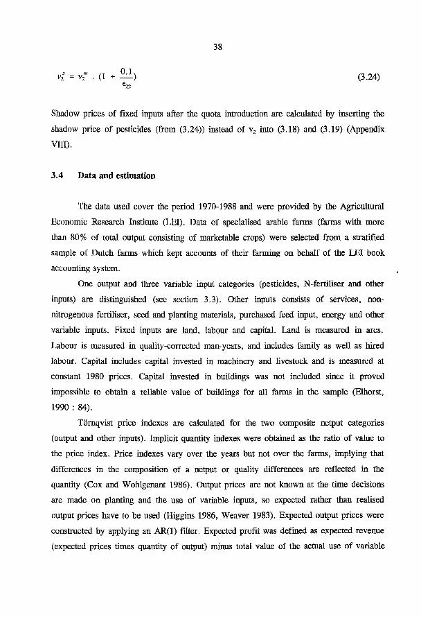
38
vï = v? . (1 + H ) (3.24) Ê22
Shadow prices of fixed inputs after the quota introduction are calculated by inserting the
shadow price of pesticides (from (3.24)) instead of v2 into (3.18) and (3.19) (Appendix
Vffl).
3.4 Data and estimation
The data used cover the period 1970-1988 and were provided by the Agricultural
Economic Research Institute (LEI). Data of specialised arable farms (farms with more
than 80% of total output consisting of marketable crops) were selected from a stratified
sample of Dutch farms which kept accounts of their farming on behalf of the LEI book
accounting system.
One output and three variable input categories (pesticides, N-fertiliser and other
inputs) are distinguished (see section 3.3). Other inputs consists of services, non-
nitrogenous fertiliser, seed and planting materials, purchased feed input, energy and other
variable inputs. Fixed inputs are land, labour and capital. Land is measured in ares.
Labour is measured in quality-corrected man-years, and includes family as well as hired
labour. Capital includes capital invested in machinery and livestock and is measured at
constant 1980 prices. Capital invested in buildings was not included since it proved
impossible to obtain a reliable value of buildings for all farms in the sample (Elhorst,
1990 : 84).
Törnqvist price indexes are calculated for the two composite netput categories
(output and other inputs). Implicit quantity indexes were obtained as the ratio of value to
the price index. Price indexes vary over the years but not over the farms, implying that
differences in the composition of a netput or quality differences are reflected in the
quantity (Cox and Wohlgenant 1986). Output prices are not known at the time decisions
are made on planting and the use of variable inputs, so expected rather than realised
output prices have to be used (Higgins 1986, Weaver 1983). Expected output prices were
constructed by applying an AR(1) filter. Expected profit was defined as expected revenue
(expected prices times quantity of output) minus total value of the actual use of variable

39
inputs. The weather index used is a weighted index of marketable crops and was calcula
ted as the annual deviation of actual from systematic yield, such that 'average' weather
yields a unit weather index (Oskam, 1991).
The profit functions are estimated along with the netput equations6 in order to
increase efficiency. Disturbance terms are added to these to take account of
misspecification, measurement errors in dependent variables and optimisation errors.
Because the disturbance terms may be correlated across equations, ITSUR is an
appropriate estimation technique. This estimator converges to the Maximum Likelihood
estimator and iterates the covariance matrix until it stabilises (Magnus, 1978). Every farm
is assumed to have a different intercept reflecting differences in farm characteristics. This
assumption is explicitly accounted for by estimating a fixed effects model, that can also
be applied to an incomplete panel (Thijssen, 1992).
3.5 Estimation results
The parameter estimates and (corrected for fixed effects) standard errors can be
found in Appendix U (Table U.2). 53% of all parameters are significant at the 5% critical
level. Convexity in prices was checked by the eigenvalue test (Lau, 1978 : 447) and was
not violated7. This implies that the Normalised Quadratic will be convex over the whole
range of observations, since it has a Hessian of constants.
The price elasticities that were obtained from the parameter estimates and the
values of the dependent variables at the sample mean (see Appendix n , table DLl), are
presented in Table 3.1. The price elasticities that relate to the output are generally small.
The own-price elasticity of pesticides of -0.12 is smaller than an earlier finding on
aggregate data of the LEI book accounting system of -0.21 (Oskam et al. 1992 : 69). The
own-price elasticity of N-fertiliser of -0.43 is often found in this range in the literature
(see Burrell 1989). Pesticides and N-fertiliser are found to be gross complements,
whereas pesticides and N-fertiliser are gross substitutes with respect to other inputs.
6 One equation has to be deleted in order to insure non-singularity of the covariance matrix.
1 A sufficient condition for quasi-convexity of an men matrix is that the number of nonnegative eigenvalues be greater than or equal to (n-l)x(n-l) (Lau, 1978 :417)

40
Table 3.1 : Price elasticities and elasticities of intensity before the hypothetical
pesticide quota introduction (estimated standard error in parentheses)
price elasticities elasticities of intensity
Output Pesti N-fer Other Land Labour Capital Trend
cides tiliser inputs
Output 0.08 -0.00 -0.00 -0.08 0.53 0.28 0.14 0.02
(0.02) (0.00) (0.00) (0.02) (0.02) (0.02) (0.02) (0.00)
Pesticides 0.08 -0.12 -0.02 0.06 0.78 0.08 0.14 0.05
(0.03) (0.08) (0.05) (0.08) (0.05) (0.03) (0.02) (0.00)
N-fertiliser 0.09 -0.05 -0.43 0.39 0.85 0.03 0.08 0.01
(0.06) (0.14) (0.16) (0.21) (0.09) (0.06) (0.05) (0.01)
Other inputs 0.27 0.02 0.03 -0.32 0.66 0.17 0.25 -0.01
(0.08) (0.02) (0.02) (0.08) (0.10) (0.07) (0.05) (0.01)
The elasticities of intensity indicate complementarity between all variable inputs
and fixed inputs. Output supply and input demand are most heavily affected by variations
in land. The elasticities of intensity that relate to the output can be considered as
production elasticities given that variable inputs can be adapted freely to the optimal level
at the same time. Technological development encourages the use of pesticides and N-
fertiliser, but reduces the use of other inputs. Most elasticities are found to be significant
at the critical 5 % level.
The restricted price elasticities and elasticities of intensity after the hypothetical
introduction, and 10% reduction, of the pesticide quota are presented in Table 3.2.
At first sight, most price elasticities have not been affected at all. Moreover, some effects
of the pesticide quota on the price elasticities do not seem to conform to the theoretical
results in Section 3.3. For example, the own price elasticity of N-fertiliser has increased,
whereas a decrease was expected according to the Le Chatelier-Samuelson effect. This is
because netput quantities have changed after the introduction of the pesticide quota. The
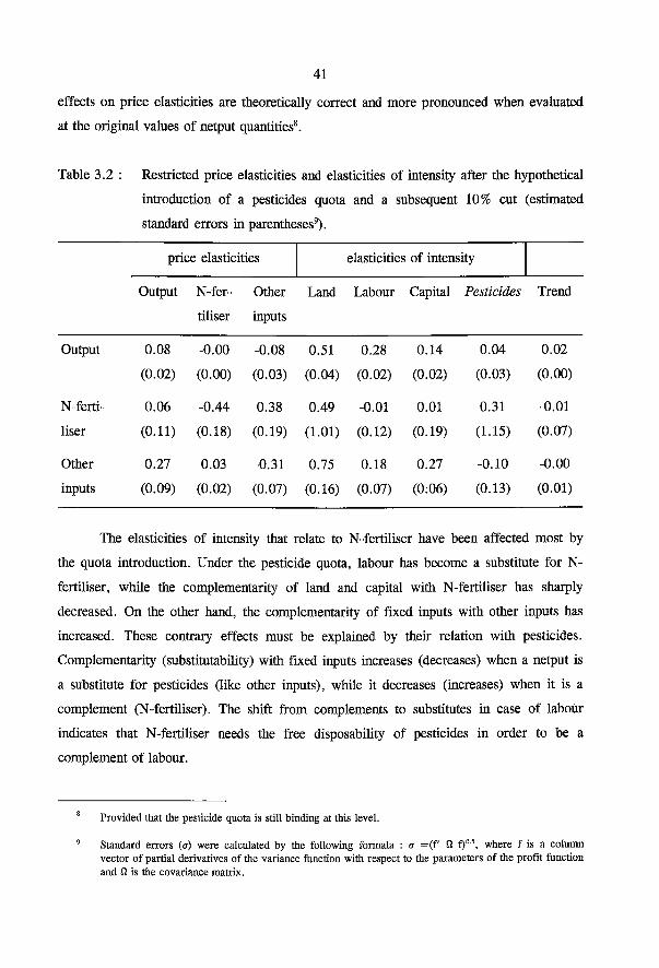
41
Table 3.2 : Restricted price elasticities and elasticities of intensity after the hypothetical
introduction of a pesticides quota and a subsequent 10% cut (estimated
standard errors in parentheses9).
price elasticities elasticities of intensity
Output N-fer Other Land Labour Capital Pesticides Trend
tiliser inputs
Output 0.08 -0.00 -0.08 0.51 0.28 0.14 0.04 0.02
(0.02) (0.00) (0.03) (0.04) (0.02) (0.02) (0.03) (0.00)
N-ferti 0.06 -0.44 0.38 0.49 -0.01 0.01 0.31 -0.01
liser (0.11) (0.18) (0.19) (1.01) (0.12) (0.19) (1.15) (0.07)
Other 0.27 0.03 -0.31 0.75 0.18 0.27 -0.10 -0.00
inputs (0.09) (0.02) (0.07) (0.16) (0.07) (0:06) (0.13) (0.01)
The elasticities of intensity that relate to N-fertiliser have been affected most by
the quota introduction. Under the pesticide quota, labour has become a substitute for N-
fertiliser, while the complementarity of land and capital with N-fertiliser has sharply
decreased. On the other hand, the complementarity of fixed inputs with other inputs has
increased. These contrary effects must be explained by their relation with pesticides.
Complementarity (substitutability) with fixed inputs increases (decreases) when a netput is
a substitute for pesticides (like other inputs), while it decreases (increases) when it is a
complement (N-fertiliser). The shift from complements to substitutes in case of labour
indicates that N-fertiliser needs the free disposability of pesticides in order to be a
complement of labour.
Provided that the pesticide quota is still binding at this level.
Standard errors (a) were calculated by the following formala : a =(f' O f) 0- 5, where f is a column vector of partial derivatives of the variance function with respect to the parameters of the profit function and O is the covariance matrix.
effects on price elasticities are theoretically correct and more pronounced when evaluated
at the original values of netput quantities8.
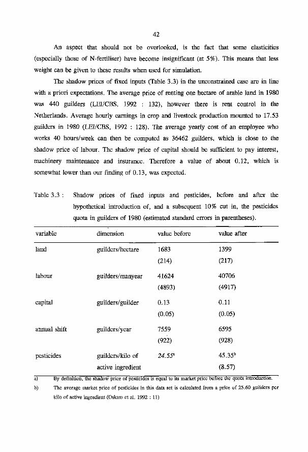
42
Table 3.3 : Shadow prices of fixed inputs and pesticides, before and after the
hypothetical introduction of, and a subsequent 10% cut in, the pesticides
quota in guilders of 1980 (estimated standard errors in parentheses).
variable dimension value before value after
land guilders/hectare 1683 1399
(214) (217)
labour guilders/manyear 41624 40706
(4893) (4917)
capital guilders/guilder 0.13 0.11
(0.05) (0.05)
annual shift guilders/year 7559 6595
(922) (928)
pesticides guilders/kilo of 24.55" 45.35"
active ingredient (8.57)
a) By definition, the shadow price of pesticides is equal to its market price before the quota introduction.
b) The average market price of pesticides in this data set is calculated from a price of 25.60 guilders per
kilo of active ingredient (Oskam et al. 1992 : 11)
An aspect that should not be overlooked, is the fact that some elasticities
(especially those of N-fertiliser) have become insignificant (at 5%). This means that less
weight can be given to these results when used for simulation.
The shadow prices of fixed inputs (Table 3.3) in the unconstrained case are in line
with a priori expectations. The average price of renting one hectare of arable land in 1980
was 440 guilders (LEI/CBS, 1992 : 132), however there is rent control in the
Netherlands. Average hourly earnings in crop and livestock production mounted to 17.53
guilders in 1980 (LEI/CBS, 1992 : 128). The average yearly cost of an employee who
works 40 hours/week can then be computed as 36462 guilders, which is close to the
shadow price of labour. The shadow price of capital should be sufficient to pay interest,
machinery maintenance and insurance. Therefore a value of about 0.12, which is
somewhat lower than our finding of 0.13, was expected.

43
The shadow price of pesticides rises to almost 85% above the pre-quota market
price when the pesticide quota is cut by 10 percent. This means that, on average, farmers
are willing to pay approximately 85% of the market price for the opportunity to use an
additional unit of pesticides, at this quota level. This also means that a 85% ad valorem
tax on pesticides would result into the same (10%) reduction of pesticides use. Of all
fixed inputs, land faces the sharpest relative decrease in the shadow price following a
10% cut in the pesticide quota. This is not very surprising given the high (in absolute
terms) value of p2j (since the change in the shadow price of fixed input j is calculated as
p 2 j times the change in the shadow price of pesticides). It can be seen that
complementarity with pesticides leads to a decrease in the shadow price of the fixed
inputs. If one fixed input had been a substitute for pesticides, then the opposite would
have occurred for that input.
3.6 Effects of four policy options
This section will use the model and methodology, presented in the preceding
sections (and Appendix VTA) to determine the effects of four different policy options on
netput quantities and income. A preference for a specific option is subject to several
criteria. The first is the exact aim of the environmental policy; are pesticides and N-
fertiliser considered to be equally harmful and what are the environmental effects of other
inputs? Other criteria may be the weight of income effects and the question whether
environmental policy can be an instrument for output control. The following policy
options are investigated :
1) Pesticide quota (-10%)
2) Pesticide quota / N-fertiliser tax (-10% / 10%)
3) N-fertiliser quota (-10%)
4) N-fertiliser quota / pesticide tax (-10% / 10%)
The effects of these options are reported in Table 3.4. The pesticide quota
contributes to the reduction of N-fertiliser in the absence of fertiliser reducing policy.
Moreover, a 10% tax on N-fertiliser can achieve an additional 5% reduction of N-

44
fertiliser use with relatively small effects on output and income. A perceived reduction of
N-fertiliser use can be obtained with an N-fertiliser quota, with small effects on income
and other netputs. An additional pesticides tax has small effects on netput quantities but
reduces income by 1%. These two options are therefore not very suitable for
environmental policy that aims to reduce pesticides to a greater extent than N-fertiliser.
Their income effects are however smaller than those of the first two options.
A few remarks about the relevance of these results for policy makers are in order
here. First, no account was taken of the effects of technological developments on the use
of pesticides and N-fertiliser. Recent experience has shown that it can play a major role
in reducing the use of nitrogen and pesticides. Second, it is not clear what should be
considered as the reference level for input reduction. In this study, the sample mean was
taken. Third, the approach that was followed in this study does not make a distinction
between different types of farms; it gives the results for an average farm. Obviously,
farms that use pesticides and N-fertiliser more intensively will be more severely hit by the
environmental measures that were analysed in this study. Fourth, it was assumed in this
study that pesticides and N-fertiliser are homogeneous products. In particular, for
pesticides however, environmental policy is more directed towards specific applications
and types of pesticides rather than the whole group. Finally, results would have been of
greater interest if outputs had been disaggregated. The mutual effects of EC and
environmental policy on output supply and input use could be included in that case.
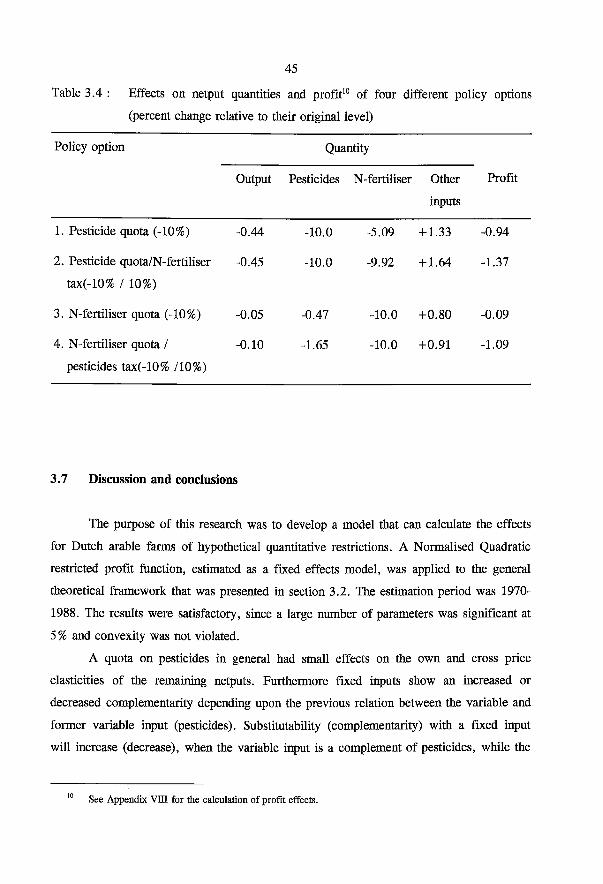
45
Policy option Quantity
Output Pesticides N-fertiliser Other
inputs
Profit
1. Pesticide quota (-10%) -0.44 -10.0 -5.09 + 1.33 -0.94
2. Pesticide quota/N-fertiliser -0.45 -10.0 -9.92 + 1.64 -1.37 tax(-10% / 10%)
3. N-fertiliser quota (-10%) -0.05 -0.47 -10.0 +0.80 -0.09
4. N-fertiliser quota / -0.10 -1.65 -10.0 +0.91 -1.09
pesticides tax(-10% /10%)
3.7 Discussion and conclusions
The purpose of this research was to develop a model that can calculate the effects
for Dutch arable farms of hypothetical quantitative restrictions. A Normalised Quadratic
restricted profit function, estimated as a fixed effects model, was applied to the general
theoretical framework that was presented in section 3.2. The estimation period was 1970-
1988. The results were satisfactory, since a large number of parameters was significant at
5 % and convexity was not violated.
A quota on pesticides in general had small effects on the own and cross price
elasticities of the remaining nerputs. Furthermore fixed inputs show an increased or
decreased complementarity depending upon the previous relation between the variable and
former variable input (pesticides). Substitutability (complementarity) with a fixed input
will increase (decrease), when the variable input is a complement of pesticides, while the
See Appendix VIII for the calculation of profit effects.
Table 3.4 : Effects on netput quantities and profit10 of four different policy options
(percent change relative to then original level)
46
reverse will occur when it is a substitute for pesticides. More specifically labour switched
from complements into substitutes for N-fertiliser when a pesticides quota was introduced.
Shadow prices are calculated for fixed inputs and pesticides before and after the
introduction of the pesticide quota. The shadow price of pesticides rises by about 85%
above the previous market price due to a 10% cut in the pesticide quota. Shadow prices
of fixed inputs decrease after the introduction due to complementarity with pesticides.
The policy options that were discussed have very different effects on netput
quantities and profit. A 10% reduction in the use of pesticides can be achieved by a tax
that raises the price of pesticides to the level of the shadow price (at a tax rate of 85%) or
by introducing a quota that is subsequently cut by 10 percent. Such a quota, combined
with an N-fertiliser tax can also achieve a substantial reduction in the use of N-fertiliser.
Profit decreases by approximately 1% as a result of these measures. An N-fertiliser quota
combined with a 10% pesticides tax has smaller effects on other netputs and profit and
will be a suitable instrument for reducing the level of N-fertiliser only.
The methodology used can give some interesting insights into the short-term
effects of a hypothetical introduction of input constraints. The producer was therefore
assumed to be in an equilibrium given the availability of fixed inputs. In the long term
however the assumption of short-term fixity is not very likely to hold and a dynamic
approach is needed.

Chapter 4
47
Modell ing the new E U cereals and oilseeds regime
in the Netherlands
Summary
This chapter examines the regional, farm-specific and sectoral effects of the new CAP regime for cereals and oilseeds (CO) with a simulation model of Dutch arable
farming. The model is estimated with panel data on Dutch arable farms over the period 1970-1992. Simulation results are aggregated for different farm classes and for the whole sector.
Simulation of the new CO regime shows a reduction in the output of CO crops and other outputs by respectively 8.9% and 0.4%. Production ofrootcrops increases by 0.4%. Pesticide and N-fertiliser use fall by respectively 2.8% and 6.7% and profit by 2%. Most large farms react to the new CO regime by reducing the area of CO crops and participating in the set-aside arrangements. In aggregate, 2% of total arable area is set aside. However, the results differ strongly between groups of farms.
4.1 Introduction
In 1992, the European Union reduced the price support for cereals and abolished the deficiency payments for oilseeds. To compensate farmers for their income loss, subsidies per hectare were introduced. In the Netherlands the rate of the subsidy differs between low and high productivity regions. Farms growing more than 12.9 hectares of cereals and oilseeds (in the high productivity region) or 18.2 hectares (in the low productivity region) have two choices. First, they can accept the set-aside obligation1, in which case they receive the area subsidy for their total planted area of cereals and oilseeds (CO crops) and set-aside premium for their set-aside land. Second, they can avoid the set-aside obligation by applying for area subsidies for 12.9 or 18.2 hectares according to then region. The 12.9 and 18.2 hectares are equivalent to 92 tonnes of cereals for the average farm in each region (see LNV, 1992).
In 1992 the set-aside obligation was 15%, it changed to 12% in 1995, and for the season 1995/1996 it will be 10%. We used 12% in the calculations.
48
Following the new CO regime, area and set-aside premiums are coupled to the area of cereals, oilseeds and pulses. The quantity of land set aside depends on the farmer's area of these crops. In previous research either one or both of these aspects have not been accounted for. Guyomard et al. (1993) analysed the new CO regime assuming that area premiums are either fully coupled or fully decoupled from price levels. Moreover, set-aside decisions were exogenous in then model. Jensen and Lind (1993) accounted for the fact that area and set-aside premiums are decoupled from price support, but they did not allow set-aside decisions to be endogenous in their model. The contribution of this chapter to the existing literature analysing the new CO regime is that both these aspects are accounted for. This is possible because the effects are examined at the level of the individual farm. The decision to participate in the set-aside programme is endogenous in our model and depends among other things on prices of inputs and outputs and the level of the area and set-aside premiums. Regional aspects of the new regulation are also taken into account as are environmental effects concerning the use of pesticides and N-fertiliser.
The reactions of arable farms in the Netherlands are examined using a simulation model consisting of equations that are estimated using panel data for Dutch arable farms. In the model there are three outputs: CO crops, rootcrops and other outputs; three variable inputs: pesticides, N-fertiliser and other inputs; two fixed inputs: labour and capital; and land. Although total land and land used for rootcrops are fixed, land can shift between CO crops and other outputs. All farms are allowed to have a different technology through farm-specific and regional parameters. Furthermore it is assumed that a change in one output price affects the production of the other two outputs only through adjustments in the allocation of fixed inputs over outputs, i.e. the technology is non-joint in variable inputs. The results of the estimation are used in a simulation model that calculates the short-term effects of the new CO regime for the farms that are in the panel. Simulation results are aggregated for different classes of farms and for the sector as a whole.
In this chapter, the theoretical model is elaborated in section 4.2 and the data are discussed in section 4.3. The empirical model is presented in section 4.4, while section 4.5 offers a discussion of the simulations and simulation results. The chapter concludes with some comments.
4.2 Theoretical model
The theoretical model that serves as a base for the empirical model in section 4.4 starts with a profit function that is non-joint in variable inputs (Chambers and Just, 1989) from which a coherent set of output supply equations and input and area demand equations can
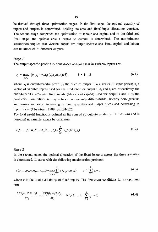
49
be derived through three optimisation stages. In the first stage, the optimal quantity of inputs and outputs is determined, holding the area and fixed input allocations constant. The second stage comprises the optimisation of labour and capital and in the third and final stage, the optimal area allocated to outputs is determined. The non-jointness assumption implies that variable inputs are output-specific and land, capital and labour can be allocated to different outputs.
Stage 1
The output-specific profit functions under non-jointness in variable inputs are:
IT,. = max {p..yrw.xl;(yi,xi,ai,z)eT} i = 1,..,3 (4.1)
where IT-, is output-specific profit; p-t the price of output i; w a vector of input prices; xt a vector of variable inputs used for the production of output i, a-t and Z\ are respectively the output-specific area and fixed inputs (labour and capital) used for output i and T is the production possibilities set. IT-, is twice continuously differentiable, linearly homogeneous and convex in prices, increasing in fixed quantities and output prices and decreasing in input prices (Chambers, 1988: pp. 124-126). The total profit function is defined as the sum of all output-specific profit functions and is non-joint in variable inputs by definition.
3
ir(pv..,p3,w,a1,..a3,zi,..,z3)=Y, -(P.-.w.a Zj) ( 4 - 2 )
Stage 2 In the second stage, the optimal allocation of the fixed inputs z across the three activities is determined. It starts with the following maximisation problem:
3 3
•K(pl,..,pvw,av..,a3,z)=maxY/Tri(pi,w,ai,z) s.t. £ z , = z ( 4 - 3 ) Z,.Z,,Z, (=1 (=1
where z is the total availability of fixed inputs. The first-order conditions for an optimum are:
d-KSpvw,avzx) = dirj^w^zp v ^ s { £ = z ( 4 4 )
9Zj 3Zj ;=1

50
a i = a-^Px,P2,Pi^AAvz) (4.8)
and imply that the shadow prices of the fixed inputs are equalised across the three activities (outputs). This optimisation yields the optimal allocation of the fixed inputs, z„ as a function of all input and output prices, the output-specific areas and total availability of z.
zl"Zl(pv..,pvw,av..,a3,z) i = 1,..,3 (4.5)
Inserting (4.5) into (4.2) yields the expression on the LHS of (4.3). At this stage, land allocated to the three outputs is still assumed to be fixed.
Stage 3
At the third stage, land is allocated to the outputs. At the level of the individual farm, the area of rootcrops is always at a technologically-constrained maximum, because these crops give much higher gross margins per hectare than other crops do. Shadow prices of areas of rootcrops will therefore also be higher than those of the other outputs and CO crops. However, in general area can shift easily between other outputs and CO crops. The optimisation over land will therefore be somewhat different compared to the optimisation over fixed inputs, since land adjustments can only be made between CO crops and other outputs. The total area used for CO crops and other outputs, and the area of rootcrops, are held fixed in the short term. This third stage of the optimisation has the following form:
2
ir(pv..,p3,w,a,a3,z) = max Tr(pvp2,p3,w,ava2,a3,z) s.t. Y^ara ^4'6^
where a is the total land used for the CO crops and other outputs. The first-order condition for this optimisation problem is similar to (4.4).
dir(pvp2,p3,w,ava2,a3,z) = d-K2(pvp2,p3,w,avavavz) 2
= ( 4 y )
da, da2 t f ''
and means that shadow prices of the area used for other outputs and CO crops are equalised. From this optimisation the demand function for the area of CO crops can be derived as:

51
The input demand and output supply functions can be derived by differentiating the profit function (4.6) with respect to input and output prices respectively (Hotelling's Lemma).
4.3 Data
Data on specialised arable farms2, covering the period 1970-1992, were obtained from a stratified sample of Dutch farms which kept accounts on behalf of the LEI-DLO farm accounting system3. Farms stay in the panel for only five to six years, so the panel is incomplete. The data set used for estimation contained 5260 observations on 1047 farms.
Three outputs (CO crops, rootcrops and other outputs) and three variable inputs (pesticides, N-fertiliser and other inputs) are distinguished. CO crops consist of winter-wheat, barley, oats and oilseeds. The cereals included account for approximately 85% of the total area of cereals on the farms in the sample. Rootcrops include sugar beet, ware potatoes, seed potatoes and starch potatoes. Other outputs are combined in an aggregate index covering all other marketable crops not accounted for in the previous category, and animal output. Other inputs consist of services, non-nitrogenous fertiliser, seed and planting materials, purchased feed input, energy and other variable inputs.
Fixed inputs are rootcrop-specific area, the total area of CO crops and other outputs, labour and capital. Areas are measured in hectares allocated to each output. Labour is measured in quality-corrected man years, and includes family as well as hired labour. Capital includes capital invested in machinery and livestock, and is measured at constant 1980 prices. Capital invested in buildings was not included since it proved impossible to obtain a reliable value of buildings for all farms in the sample (Elhorst, 1990: p.84).
Tornqvist price indexes were calculated for the three outputs and other inputs (prices were obtained from the LEI-DLO, CBS). The price indexes vary over the years but not over the farms, implying that differences in the composition of a netput or quality differences are reflected in the quantity (Cox and Wohlgenant, 1986). Implicit quantity indexes were obtained as the ratio of value to the price index.
Output prices are not known at the time decisions are made on planting and the use of variable inputs, so expected rather than actual prices have to be used. Expected output prices were constructed by applying an AR(1) filter to the price of CO crops and other outputs and an AR(2) filter to the price of rootcrops. The implication of using expected
Farms with more than 80% of output coming from marketable crops.
3 A complete description of the sample can be found in LEI-DLO, 1992.

52
4.4 Empirical model
4.4.1 Before the 1992 CAP reform
The Normalised Quadratic is the functional form adopted in this study, because overall it came out more favourable on the data set that is used in this study than other linear flexible functional forms. Furthermore, it is empirically simple and has a Hessian of constants allowing convexity in prices to be checked and/or imposed globally. The Normalised Quadratic profit function (see (4.6)), with prices and profit normalised by the price of the other inputs is expressed as:
* = «o +E«,-v,. +i:fe. +lEi:a,v,.v y . +iEEto +EEw (4-9> ¡=1 i=l ^ i=l y=l ^ (=1 ;=1 1=1 j-l
where Vi is a vector of normalised netput prices with i= l (CO crops), 2 (other outputs), 3 (rootcrops), 4 (pesticides) and 5 (N-fertiliser). Furthermore, Z\ are areas, fixed inputs, and other variables with i= l (area CO crops), 2 (area other outputs), 3 (area rootcrops), 4 (labour), 5 (capital), 6 (time trend) and 7 (regional dummy). Symmetry is imposed by requiring that a g =aj, and for all i and j . The netput (positive for outputs, negative for inputs) equations are derived by differentiating (4.9) with respect to the normalised price of netputs (Hotelling's Lemma):
r ^ E v ^ E p ^ «=i,-.,5 (4.io) 7=1 J"l
The equation for the numeraire netput can be derived by using the definition of normalised profit: it = vvqx + v2.q2 + v3.cj3 + v4.q4 + vs.qs + q6.
*.-°b-E te-±EE + i E E t o ( 4 , 1 1 )
j-i ¿1-1 /=i z i = i ;=i
From the optimisation across areas in section 4.2 it follows that shadow prices of the areas of CO crops (zi) and other outputs (z2) are equalised, holding the total area of these
rather than actual prices is that expected profit is assumed to be maximised instead of actual profit. Expected profit was defined as expected revenue (expected prices times quantities of outputs) minus the total value of the variable inputs actually used.
Other variables that were included in the empirical model are a time trend, and a regional dummy that accounts for the two production regions (=1 for the high productivity region, 0 for the low productivity region).

53
two crops (a) fixed. This results in one independent area demand equation, which has the following form for CO crops (see (4.8)) before the implementation of the new CO regime:
z 1
1 (0u+t322-2(3n) •
The (total) profit function is estimated together with the netput and the area demand equations in order to increase efficiency. Since the area of CO crops correlates with the error term, an instrumental variable estimator should be applied. Endogenous variables are 7r, qn Zi and all cross products of z, with v¡ (j = l,..,5) and z s(i=1,..,7)4. Instruments are all exogenous variables (v¡ (j = l,..,5) and z¡ (i=3,..,7)), quadratic and cubic terms of exogenous variables and a weather index (see Oskam, 1991). Error terms may be correlated across equations so non-linear 3SLS is an appropriate technique (Judge, et al., 1988: 655). Convexity in prices was imposed by the Wiley, Schmidt and Bramble (1973) technique (see e.g. Dupont, 1991, for an application of this technique).
Every farm is assumed to have different intercepts in the profit function, netput equations and area demand equation reflecting differences in farm characteristics5. This assumption is explicitly accounted for by a fixed effects model, the necessary transformation6 can also be applied to an incomplete panel like our data set (Thijssen, 1992). The parameter estimates7 and standard errors8 of the estimated system of equations ((4.9)-(4.10) and (4.12)) can be obtained from the authors. More than 71% of the parameters are significant at the critical 5% level. Another indication of the performance of the model is given by the deviation of calculated (Appendix III : III. 1) from actual (Appendix HI : Table m .2) values of endogenous variables in 1992. Output quantities are in general
- / 3 I + O J 2 2 - 0 1 2 ) a + £ ( 0 2 j
>3
(4.12)
4 Zi + z2 = a is imposed during estimation, so z, also appears in variables corresponding to B2, B2 j and p, 2.
5 Because the netput equations are the first-order derivatives of the profit function with respect to the netput prices, the farm-specific effects should appear as slope coefficients in the profit function. Following Thijssen (1992) we have not done this, thus creating an inconsistency. Including these additional terms would make the system of profit, netput and area demand equations impossible to estimate because of matrix inversion problems.
6 The fixed effects for all equations can be determined in a second stage estimation (Judge, et al., 1988, p.468).
7 Parameters a¡¡ are non-linear combinations of parameters actually estimated (see Dupont, 1991)
8 All standard errors have been corrected for degrees of freedom, which is not accounted for during estimation. Standard errors of the parameters or¡j have been calculated according to Rao (1973)
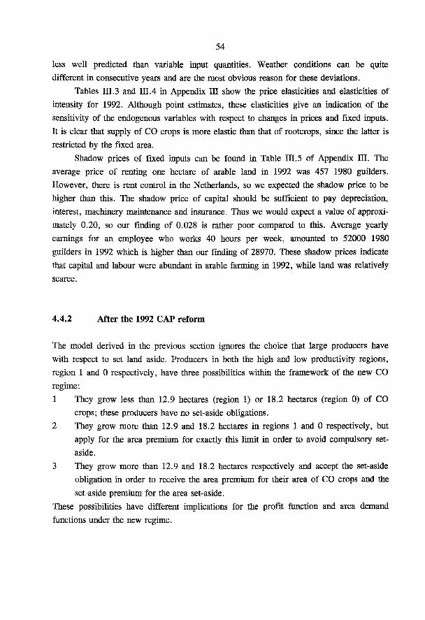
54
less well predicted than variable input quantities. Weather conditions can be quite different in consecutive years and are the most obvious reason for these deviations.
Tables III.3 and HJ.4 in Appendix HI show the price elasticities and elasticities of intensity for 1992. Although point estimates, these elasticities give an indication of the sensitivity of the endogenous variables with respect to changes in prices and fixed inputs. It is clear that supply of CO crops is more elastic than that of rootcrops, since the latter is restricted by the fixed area.
Shadow prices of fixed inputs can be found in Table ni .5 of Appendix in . The average price of renting one hectare of arable land in 1992 was 457 1980 guilders. However, there is rent control in the Netherlands, so we expected the shadow price to be higher than this. The shadow price of capital should be sufficient to pay depreciation, interest, machinery maintenance and insurance. Thus we would expect a value of approximately 0.20, so our finding of 0.028 is rather poor compared to this. Average yearly earnings for an employee who works 40 hours per week, amounted to 52000 1980 guilders in 1992 which is higher than our finding of 28970. These shadow prices indicate that capital and labour were abundant in arable farming in 1992, while land was relatively scarce.
4.4.2 After the 1992 CAP reform
The model derived in the previous section ignores the choice that large producers have with respect to set land aside. Producers in both the high and low productivity regions, region 1 and 0 respectively, have three possibilities within the framework of the new CO regime: 1 They grow less than 12.9 hectares (region 1) or 18.2 hectares (region 0) of CO
crops; these producers have no set-aside obligations. 2 They grow more than 12.9 and 18.2 hectares in regions 1 and 0 respectively, but
apply for the area premium for exactly this limit in order to avoid compulsory set-aside.
3 They grow more than 12.9 and 18.2 hectares respectively and accept the set-aside obligation in order to receive the area premium for then area of CO crops and the set-aside premium for the area set-aside.
These possibilities have different implications for the profit function and area demand functions under the new regime.

5 5
Situation 2 Large producers receive the area premium for the maximum number of hectares of CO crops that carries no set-aside obligation (12.9 or 18.2 hectares). The profit function for this category now includes an additional term 12.9H or 18.2/7. The area demand function however remains as in (4.12), because no area premium is received for marginal increases in the area of CO crops.
Situation 3 Large producers have to set 12% of the area of CO crops aside. The profit function for these producers becomes more complex. There is a set-aside premium and an area premium (S and H), so the term (0.88H+0.12S).Zi will appear in their profit function. However, these producers have to set 12% of the area of CO crops fo) aside in order to obtain the area premium, so all terms z t in (4.9) must be multiplied by 0.88. For example the terms ByZiZj become O ^ B ^ Z i for j = l and 0.88 B ^ Z j for j=2..7. The area demand function then becomes:
( 0 . 8 8 ^ n + ^ - 1 . 7 6 ^ 1 2 )
7
02-0.880, +(/?22~O.88012)a + E (/%-°-88|8iPz/ > 3 (4.14)
^(p ; 2 -0.88p, 7 )v,-0.88^-0.12S
When using the model for simulation, the profit and area demand for CO crops are calculated in all three situations. It is then assumed that the producer chooses the option with the highest profit.
Situation 1 For small producers in both regions, the profit function (4.9) must now include the term H.Zu where H is the premium per hectare and Z\ the area of CO crops. The area demand function then becomes:
7 5
ß2-ßx + (ß22-ßl2)a + £ ( / V 0 i , V £ (Pa-PuX-H ( 4 - 1 3 )
> 3 1=1
4.5 Model simulations
56
In this section the model simulations together with the simulation results are discussed. The results are aggregated for 12 different farm classes.
4.5.1 Policy simulations
The model that is presented in the previous sections is used to calculate the effects of the new CO regime. The price reduction for CO crops, normalised by the price of the numéraire input, was taken as 34%9. The area premium is 866 guilders and 616 guilders per hectare of CO crops in regions 1 and 0 respectively. The area premiums are weighted averages of the actual 1996 area premiums for grains and oilseeds using the share of oilseeds in total production of grains and oilseeds in 1988 and 1991 (2.7%). The set-aside premium is 1075 guilders and 765 guilders per hectare of CO crops in regions 1 and 0 respectively. The area and set-aside premiums are also deflated by the price of the numéraire input. This simulation is the base simulation.
Three other simulations were performed to test the sensitivity of the base simulation with respect to policy parameters: (1) abolition of the set-aside obligation and premiums (area premiums unchanged), (2) a 25% reduction in area premiums (set-aside premiums unchanged) and (3) a price reduction for CO crops that leaves total profit unchanged (area and set-aside premiums unchanged).
These measures are simulated for every farm in the sample in 1992. Because of the large number of farms in the sample used for simulation (232) and in order to simplify the interpretation of the model outcomes, results were aggregated for different classes of farms and sector as a whole using the number of farms in the sector that each farm in the sample represents as weights. The classification of farms in table 4.1 is based on the fact that farms in region 1 have no set-aside obligations if they grow less than 12.9 hectares of CO crops; in region 0 this is 18.2 hectares. Whereas the size of the farm, measured as the area of CO crops, indicates the absolute importance of CO crops for a farm, the intensity of the farm, measured as the share of rootcrops in the crop rotation, indicates the relative importance of CO crops. The share of 50% is close to the average share of rootcrops for the farms in the sample (49%). Farms were classified using the calculated values for the area of CO crops and the actual share of rootcrops in 1992. The policy simulations cause farms to shift from one class to another because the area of CO crops can vary.
9 This is the decrease in the intervention price for soft wheat in 1996 compared to 1992 corrected for the numeraire price in 1992.

5 7
Table 4.1. Arable farm classification (1 to 12) and the number of farms in each class (in parentheses).
Intensity / Area of CO crops £ 12.9 ha 12.9-18.2 ha a 18.2 ha
Region 0 flow productivity)
< 50% ha potatoes and sugar beet 1 (569) 2(58) 3 (49)
50% ha potatoes and sugar beet 4 (1334) 5 (59) 6(111)
Region 1 (high productivity)
< 50% ha potatoes and sugar beet 7 (1793) 8 (1123) 9 (1390)
a: 50% ha potatoes and sugar beet 10 (1529) 11 (318) 12 (266)
4.5.2 Results
The results of the base simulation are presented in table 4.2. All farm classes reduce then output and area of CO crops; this holds in particular for small producers in the low productivity region (farm classes 1 and 4). The reduction of the output and area of CO crops leads to sometimes substantial changes in the production of other outputs. A reduction of other outputs and CO crops is found for large farms (farm classes 3, 8, 9, 11 and 12) that participate in the set-aside arrangements. The production of other outputs increases on those farms that increase the area of other outputs; it decreases on farms that participate in the set-aside, and therefore, decrease the area of other outputs. The highest percentages of land set-aside are found for large extensive farms in both regions (farm classes 3 and 9).
A profit reduction is found for all farms. This implies that the compensatory payments are too low to compensate farmers for their loss in profit due to the lower price for CO crops. Furthermore farms that participate in the set-aside arrangements (especially in the high productivity region) are faced with a larger reduction in profit than other farms. These farms are relatively more dependent upon CO crops. For the sector as a whole, profit decreases by 2%.

5 8
Table 4.2. Effects' of the new CO regime : The base simulation (upper part) and the base simulation without set-aside (lower part).
netput quantities miscellaneous
farm CO crops other rootcrops pesticides N-fertiliser other Area CO Area of other % of total area profit3
class outputs inputs crops2 outputs set-aside
Base simulation 1 -55.99 0.96 0.09 -4.49 -9.72 1.88 -57.07 9.05 0.00 -0.37 2 -12.19 6.71 0.10 -5.38 -7.09 -10.61 -11.53 18.61 0.00 -3.06 3 -10.76 -5.07 1.30 -4.60 -9.46 -4.73 -9.98 -4.50 4.79 -3.05 4 -44.06 3.63 0.05 -2.67 -5.80 -1.76 -41.06 14.16 0.00 -0.55 5 -14.22 10.67 0.04 -2.43 -3.34 -4.21 -10.35 38.11 0.00 -0.70 6 -12.14 1.61 0.26 -1.60 -3.15 -3.74 -9.70 7.51 1.02 -0.96 7 -6.01 0.74 -0.19 -2.86 -6.66 2.34 -6.40 4.38 0.00 -2.04 8 -6.87 -1.51 0.67 -3.57 -7.27 2.03 -7.67 -0.69 2.66 -2.87 9 -6.10 -5.36 1.45 -3.42 -6.99 1.92 -7.39 -9.47 5.21 4 .05 10 -8.06 0.81 -0.09 -1.96 -7.23 1.87 -8.38 5.59 0.00 -0.77 11 -6.01 -2.24 0.37 -1.89 -5.22 0.27 -7.03 -5.12 2.70 -1.65 12 -6.90 -4.45 0.60 -2.18 -6.37 1.43 -8.53 -9.88 3.95 -2.53 sector -8.91 -0.44 0.39 -2.83 -6.65 0.81 -9.97 2.08 2.06 -1.99 Base simulation without set-aside4
3 -4.67 2.55 0.03 -2.05 -3.55 -7.67 -4.07 8.00 0 -1.59 6 -10.26 4.55 0.03 -1.34 -2.46 -3.44 -8.03 11.89 0 -0.99 8 -3.35 0.82 -0.16 -2.32 -4.17 1.65 -3.41 3.30 0 -2.95 9 -1.56 0.64 -0.10 -1.33 -2.19 0.17 -1.65 2.98 0 -3.16 11 -2.95 0.77 -0.07 -1.19 -2.84 0.84 -3.11 6.42 0 -1.91 12 -1.72 0.73 -0.05 -0.87 -2.09 0.16 -1.87 5.25 0 -2.00 sector -5.89 1.18 -0.07 -2.10 -4.48 0.39 -6.26 6.20 0 -1.75 T: percentage changes in quantities of netputs, area of CO crops and other outputs, land set-aside and profit compared to the calculated 1992 level 2: Excluding area set-aside 3: Normalised value of all netputs10 4: Results for other farm classes remain unchanged
'This calculated profit differs in general from profit calculated with the profit function (4.9), because every netput equation has a fixed effect that does not appear in the profit function.

59
The new measures result in a 2.8% overall reduction in pesticide use. This reduction is highest for farms that substantially reduce the area of CO crops and/or participate in the set-aside arrangement. This is because CO crops use pesticides more intensively than other outputs. CO crops also use N-fertiliser more intensively than other outputs. Therefore, due to the reduction of the area of CO crops and the lower price of CO crops, a reduction in N-fertiliser use is found for all farm types.
A measure of the dynamics of the sector as a result of the new CO regime can be found in the change of the number of farms per class. Farms cannot move from one region to an other, or change the intensity of the farm, since the total area and the area of rootcrops are fixed, but they can adjust their area of CO crops. Simulations show that if farms move to another farm class this is in general because the CO area decreases (farms move from farm class 2 to 1, from 6 to 5, from 8 to 7, from 11 to 10 and from 12 to 11). Table III. 6 shows that most large farms, in the new situation, participate in the set-aside arrangements.
The effects of the abolition of the set-aside arrangements, a 25% reduction of the area premiums and a price reduction leaving profit unchanged are given in Tables 4.2 and HI.7. Here the results are summarised. Abolishing the set-aside arrangement has little effect relative to the base simulation. Not surprisingly, at the sector level the reduction in CO output is smaller (-5.9%), and the decrease in profit is smaller (-1.8%). The reduction in pesticide use is now 2.1%, so participation in the set-aside arrangements for large farmers accounts for an additional 0.7% reduction in pesticide use. Changes in model results compared to the base simulation at the sector level are caused by farms that participated in the set-aside arrangements in the base simulation.
A 25% reduction of the area premiums, leaving the set-aside arrangements intact, makes CO crops unattractive: production and area decrease by 14.6% and 16.5% respectively (see table ffl.7). The production of other outputs increases by 1.2% and that of rootcrops by 0.5%. Profit falls by 3.2%. The area set-aside (1.9%) is slightly smaller than in the base simulation (2.1%) because growing CO crops has become less attractive. Pesticide and N-fertiliser use fall by 3.7% and 8.5% respectively.
A 24% price reduction for CO crops, together with the area and set-aside premiums of the base simulation, would give a zero overall profit change (see table III.7). In this case production of CO crops falls less (-0.7%) and more land is set aside (2.3%). The production and area of other outputs fall by 2.7% and 7.8% respectively, and the decreases in pesticide and N-fertiliser use are smaller (1.3% and 3.2% respectively).
The results of all three simulations show large difference between groups of farms.

60
4.6 Discussion and conclusions
At the sector level, simulations of the new CO regime show a reduction of the output of CO crops and other outputs of 8.9% and 0.4%, respectively, and an increase in rootcrop output of 0.4%. Pesticide and N-fertiliser use decrease by 2.8% and 6.7%, respectively. Profit falls by 2%. Further, it is shown that large farms react to the new measures by reducing the area of CO crops and opting for set-aside. Data on participation in the set-aside for 1993 (LEI-DLO, 1995) indicate that 2.1% of the land in arable farming was set-aside, which is close to our findings (although the set-aside percentage was 15 in 1993). Moreover, preliminary data (LEI-DLO/CBS, 1994) show that it is large extensive farms in both regions that set land aside.
From table 4.2 and m.7 it can be seen that area premiums are not fully decoupled from price levels because the quantities of all netputs change due to a change of the area premiums. Moreover, it can be seen that the new CO regime contributes to a reduction of N-fertiliser and pesticides use.
When interpreting the results, it is important to be aware of the following points. First, during estimation and simulation, the occurrence of corner solutions, i.e. zero observations for outputs and areas, was not taken into account. This implies that the calculated values of these variables could be negative. For example, the calculated area of both CO crops and other outputs in 1992 was negative in 6 instances. Second, in the model all prices, technological change, the area of rootcrops and the total area of CO crops and other outputs are exogenous, which is an unrealistic assumption in the long run. Third, the model does not take into account that farms are allowed to manage the set-aside land so as to improve future soil fertility or to grow agro-industrial crops. The latter use of set-aside land is however not very important in the Netherlands (LEI-DLO/CBS, 1995). Fourth, the price reduction for CO crops that we used in the simulations is rather uncertain. The European Union has reduced the intervention price, but the market price will also depend on market conditions. Moreover, as a result of the regime switch, the price of CO crops will be less stable than before, in which case the reaction of risk-averse producers will be different from that of risk-neutral producers.
In conclusion, the model provides predictions of the regional, farm-specific and sectoral effects of the new CO regime. The model can easily determine the simultaneous effects of different policy changes (e.g. abolishing set-aside obligations and reducing area premiums).
61
Chapter 5
Effects of N-surplus Taxes :
Combining Technical and Historical Information
Summary
Technical information on the production of an externality can be included in a dual profit function to yield insight into the effects of a tax on the externality. The methodology is applied to a tax on Nitrogen-surplus in the context of future mineral policies for Dutch arable farms. In future policy, N-surplus will probably be calculated using an accounting relationship that relates inputs and outputs to N-surplus.
The simulation model used to determine the effects of the tax on N-surplus is based on equations that have been estimated with panel data.
A 0.27 guilder tax per kg N-surplus with a threshold of acceptable N-losses of 75 kg/ha and a 18% levy on N-fertiliser were found to give the same reduction of N-surplus as a 1 guilder tax on N-surplus with a 125 kg/ha threshold. The N-surplus taxes induce producers with a high N-surplus to lower the N-surplus more than producers with a small N-surplus and should therefore be preferred from an environmental perspective.
Keywords : N-surplus, panel data, simulation model
5.1 Introduction
Optimal environmental policy requires taxing an externality rather than the inputs or outputs generating the externality (Baumol and Oates, 1988: 46). Ideally, in order to analyse the effects of a tax on the externality, using econometric models, one should have historical information on prices and quantities of netputs together with levies on, and the quantity of, the externality. Usually, however, this information is not available at the time of the introduction of the policy.
The lack of independent information in the data set on the quantity of the externality produced as prices vary necessitates calculating its value from actual use of inputs and/or production of outputs. In previous research, the quantity of the externality that is thus obtained was included as a fixed netput when estimating the profit function, so as to infer information on its marginal value product (e.g. Fontein et al., 1994). This approach

62
is, however, not satisfactory for a number of reasons. First, fixed other inputs strongly correlated with the externality have to be excluded during estimation in order to avoid multicollinearity. Doing so, however, obscures the true underlying production relationships and biases the estimated marginal value product of the externality. Second, if an externality is closely related with a short-term variable netput, then including the externality in the profit function as a fixed netput in the profit function is theoretically inconsistent, because this suggests that the quantity of the externality is invariable in the short term.
This chapter shows that including the level of the externality, either as an observed or an imputed value in the profit function to be estimated can be avoided. Inference regarding the effects of a tax on an externality can be obtained by simulation, using a dual profit function representing producers' decisions prior to the introduction of the tax, into which a production function for the externality is introduced.
The methodology is illustrated in the context of a policy to tax the nitrogen surplus generated by arable farms in the Netherlands. Nitrogen surplus is used as a proxy for pollution, and the formula for calculating the N-surplus plays the role of the "production function" for the externality. Current policy on minerals for the arable sector involves a limit on the use per hectare of phosphates of animal origin. Future policies on minerals will probably oblige all farms to keep a mineral account for flows of nitrogen and phosphates from manure as well as artificial fertiliser (Tweede Kamer, 1995 and 1996). In this way detailed information on the uptake of minerals by crop products and the supply of minerals through artificial fertiliser and manure will be available. The difference between supply and uptake, minus a threshold level for acceptable mineral losses per hectare, constitutes mineral surpluses per farm that will be taxed. This chapter examines the effects of this policy, applied to nitrogen surpluses1,2, for arable farms. The effects will be compared with a tax on N-fertiliser.
The reactions of arable farms in the Netherlands are examined using an extended version of the simulation model of Dutch arable farming that was developed in Chapter 4.
1 This policy is planned to be applied to intensive livestock farms in 1998. Extensive livestock, horticultural and arable farms are provisionally exempted.
2 We omitted nitrogen from manure during estimation and simulation, although the use of animal manure increased importantly during the eighties. However, arable farmers apply manure mainly as a means of increasing the organic matter content of the soil (Baltussen et al., 1992: 52). The application of manure in the fall causes the effectiveness of N from manure to be low. Moreover, there is evidence that farmers do not take the supply of N into account when choosing levels of N from N-fertiliser (Baltussen et al., 1992: 52). Therefore we believe that excluding animal manure during estimation does not bias the coefficients related to the price of N-fertiliser. The effect of excluding the use of animal manure from the simulations is small since the scenarios that are under review in this paper are so comtraining, that they do not allow for applying any animal manure at all (LEI-DLO, 1995).

63
5.2 Including the externality in the theoretical model
This section assumes that knowledge about the production function of an externality is available and shows how this knowledge can be included in the theoretical model of Chapter 4 to yield information about the effect of a levy on an externality.
The basic theoretical model of Chapter 4 is given by :
2
ir(p,w,a,avz) = max -w{p,-w,avavavz) s.t.'Y^a.=a ( 5-l)
where IT is profit, defined as p.q - w.x; p a vector of output prices; w a vector of input prices; x and z are vectors of variable and fixed inputs respectively, q a vector of outputs and ax is the output-specific area, with i = l (CO crops), 2 (other outputs) and 3 (root-crops). 7r is assumed to be twice continuously differentiable, linearly homogeneous and convex in prices, increasing in fixed quantities and output prices and decreasing in input prices (Chambers, 1988: 124-126). The maximisation problem (5.1) implies that areas can shift between CO crops and other outputs.
In order to include the information on the production function of the externality, the vector x of variable input quantities in maximisation problem (5.1) is partitioned into two subsets of inputs xx and x2 with corresponding prices wx and w2. The externality is produced with a known production function F(.) by subset x2 only. This production function is given by :
q0 = F(x2) (5.2)
where q0 is the quantity of the externality. The properties of F(.) are discussed below.
Maximisation problem (5.1) is rewritten as
The simulation model calculates the short-term effects of the nitrogen policies for the farms in the panel. Simulation results are aggregated for different classes of farms and for the sector as a whole.
In this chapter, the theoretical model is elaborated in section 5.2 and the empirical model is presented in section 5.3. Section 5.4 offers a discussion of the simulations and simulation results and the chapter concludes with comments.

64
Tr(p,wvw2,a,avz) = max{ •x-(p,wl,w2,a1,a2,a3,z)} s.t.^a.^a (5.3)
where
ir(p,wvw2,ava2,avz) = max{G(p,w1,x2,ava2,avz) - w2- x2 \ (q,xvx2,ava2,avz) e7} (5.4) x2
T is the technology set containing all feasible input-output combinations and G(.) is a restricted profit function, defined as p.q - w,.x,. The parameters from G(.) can be derived from those of ir(.) and vice versa by using standard methods (Fulginiti and Perrin, 1993; Guyomard and Mahe, 1993) (see also Appendix IX). If firms pay a tax p 0 for producing the externality, the profit maximisation problem (5.4) becomes:
n(p,p0,w1,w2,flj,fl2,a3,z) = max{G(.) - w ^ - / ^ ( x , ) | (q,qa^2,ax,a2,ayz) G T} (5.5)
and has first order condition:
3G(.) 9F(x2) -^-^-^-^r^ (5-6)
The second order condition for profit maximisation requires that the matrix :
d2GQ _ ( 5 . 7 )
dx2dx2
0 dx2dx2
is negative semi-definite. Note that the second order condition for profit maximisation in (5.4) requires
d2G(-) dx2dx2
to be negative semi-definite. Therefore, a sufficient but not necessary condition for (5.7) to be negative semi-definite is that
dx2dx2

65
is positive semi-definite, i.e. Ffx^ is convex in x2. Convexity of FfxJ in x 2 implies that the production function of the externality exhibits a non-decreasing marginal product with respect to input levels. As Helfand and House (1995) note, this is a characteristic that is typically exhibited by pollution functions.
Equation (5.6) states that, due to the tax on the externality, the value of the marginal product of x 2 (dGf.j/dx^) increases3 by p0.dF(X2)/dx2. Therefore the optimal quantity after the tax fe") is lower than the optimal quantity before the tax: x2. Solving the first order condition (5.6) yields the demand function for x2* after the policy has been implemented:
x2* = x2 (p,p0,wvw2,ava2,avz) (5-8)
The supply equation for the externality can be obtained by inserting (5.8) into (5.2), whereas the netput equations can be derived by applying Hotelling's Lemma to G(.) and subsequently inserting (5.8). The CO crops area demand equation is obtained by performing an optimisation across a, and a2 (see also chapter 4 : section 4.2) :
dW(p,pQ,wvw2,avavavz) = m*(p,PyWvw2,avavayz) s t a + a = a (5.9) da, da2
1 2
where rf(p,j?0,w1)w2)ûi,a2,a3,z) = p.q~wl-x,~w2-x2* ~p0• q0
5.3 Empirical model
In this section, the empirical model of Chapter 4 is extended with an accounting relationship for N-surplus that is used by the government as a base for taxing Dutch arable farms. It should be noted that N-surplus is determined using an accounting relationship rather then a 'true' production function. This is because an accounting
5 The marginal product increases since, according to first order condition (6), the vector dG{.)/dx2 - pndF(x2)/dx2
has to equal w 2 . Since w 2 does not change and because p0dF/3x2 is non-negative, the elements of the vector of marginal value products (3G/3x2) have to increase. A larger marginal value product corresponds with lower optimal quantities in x 2 under the tax policy.

66
4 Data on net uptake by crop are available at the level of individual crops that the aggregate outputs are composed of (Janssens and Groenwold, 1993 : 64). Net uptakes given by y,,y2 and y% are farm specific, since the composition of outputs differs by farm.
relationship as a base for taxing farmers will be used in the policy on minerals for the intensive livestock sector, and therefore, probably will be used in future policy for the arable sector. The government could also decide to use very detailed agronomic information on the relationship between farming practice and N-surplus, but such a policy would be more costly and perhaps also impossible to monitor. This is because the 'true' N-surplus depends on variables as yield per hectare, weather, soil type, etcetera.
In order to determine the effects of a tax on N-surplus, the post-CAP reform equations have to be adjusted as described in section 5.2. First, the equation for the N-surplus on farm h is specified, followed by the equations for netputs and the area of CO crops. These equations are given for situations 1-3 that apply for all arable farms after the 1992 CAP reform (see Chapter 4 : section 4.4.2), to begin with situation 1.
The specification of the N-surplus function assumes that under the tax policy farmers are obliged to keep accounts of N flows on the farm. Information that is available through the accounts includes uptake by crops and purchases of N-fertiliser. Total N-surplus at the farm level (q0h) is calculated using an accounting relationship :
%k = s m ~ D m + E m ~ T m ( 5 - 1 0 )
where (SNh) is Nitrogen supplied by N-fertiliser, Dm is uptake by crop products, 7iNh is exogenous deposition (mainly through ammonia) and Tm is a threshold level for acceptable N losses. Nitrogen supplied by N-fertiliser (S^) is calculated by transforming the implicit quantity of N-fertiliser (which is in 1980 guilders) to kg N, using the average normalised price per kg N in 1992: p N . Algebraically:
S m = ~y&„ (5-n)
where ys=l/(pK). Net uptake (uptake by crop products minus supply through seeds and planting materials)4
of N by output is calculated using yield and soil type independent norms per crop and per farm (Janssens and Groenwold, 1993). This simplification will probably be used in the policy with regard to the arable sector because it is already used for the intensive livestock sector.
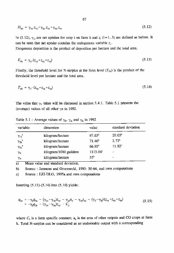
67
(5.12)
In (5.12), yitl are net uptakes for crop i on farm h and Z\ (i = 1..3) are defined as before. It can be seen that net uptake contains the endogenous variable zx. Exogenous deposition is the product of deposition per hectare and the total area.
Em = yE-(Zik+Z2k+ZiH) ( 5 - 1 3 )
Finally, the threshold level for N-surplus at the farm level (rNh) is the product of the threshold level per hectare and the total area.
Tm = 7 r - ( W Z 3 / , ) ( 5 - 1 4 )
The value that y T takes will be discussed in section 5.4.1. Table 5.1 presents the (average) values of all other 7 s in 1992.
Table 5.1 : : Average values of Y s , y i h and y E in 1992
variable dimension value standard deviation
kilogram/hectare 97.63" 20 .03"
72ha kilogram/hectare 71.46" 2.73"
73ha kilogram/hectare 66.95" 11.82"
7s kilogram/1000 guilders 1113.04 C -
7 E kilogram/hectare 53" -
a) Mean value and standard deviation. b) Source : Janssens and Groenwold, 1993: 30-64, and own computations c) Source : LEI-DLO, 1995a and own computations
Inserting (5.11)-(5.14) into (5.10) yields:
Qm = - t & " ( Y I A - 7 H ) Z U " " T t o f c * " ^ T ~ y ^ W ^ ( 5 . 1 5 ) = ~yfi$h ~ ( 7 U _ 7 2 A ) Z 1 A _
where Ch is a farm specific constant; ah is the area of other outputs and CO crops at farm h. Total N-surplus can be considered as an undesirable output with a corresponding

68
(negative) price representing the tax that is imposed on surplus. It can be seen that the N-surplus function is linear in inputs. If the government used a 'true' production relationship that was strictly convex instead of linear in polluting inputs, then farmers with a high production intensity would be more heavily taxed than in the case of a linear relationship. This is because farmers with a high production intensity use polluting inputs (e.g. N-fertiliser) more intensively than farmer with a low production intensity. Notice that linearity of the accounting relationship implies that d2q0hldqlh is zero, i.e. the second order condition for profit maximisation of (5.5) is fulfilled. After specifying the N-surplus function, the area demand and netput equations are derived using the methodology that was elaborated in section 5.2. Defining v0 as the normalised levy on N-surplus, the netput equation is :
5 7
the equation for the numéraire netput is:
7 ^ 5 5 1 1
^^E^v^EEw,-+ EE^y-E ^ « ^ 0 - ^ 5 5 ^
z (=1 j-i M j-1 1-1 z
(5.17)
and the area demand equation is :
z, = O3 n + 0 2 2 -2/3 1 2 ) > 3
+ E 0 > a - P « ) v i + ( T s ( P 5 2 - P 5 1 ) + ( T a " T i » ) ) v o ~ H
(5.18)
For large farms that do not participate in the set-aside (situation 2 in 4.4.2), the netput equations and the equation for the numeraire input are the same as those for small farms ((5.16)-(5.17)). The area demand equation becomes :
1 (0 n + / 3 2 2 -2 i 8 1 2 ) J*
+E W - P a X + ( T > 5 2 -PJI ) + ( 7 2 A -Y i* ) )v 0
(5.19)

69
<7o7 = -7s?s* ~ ( ° - 8 8 7 i A - 7 2 A ~ 0 . 1 2 7 r ) z 1 A - ^ ^ H Z y , " ^ - ^ / , ) - 7 2 A-7 3 / ,Z3 / , (5 .20) = -7A* - ( 0 . 8 8 7 u - 7 M - 0 . 1 2 7 r ) z u - Ck
The netput equations are:
? r = « i + E^v . + 0 .88p , 7 Z l ^p , Z . + 7 s a, ,v 0 M. . . .5 ( 5 - 2 1 ) ;=1 ;=2
The equation for the numerahe netput is:
<76 = a 0 + 0 .88 / J l Z l + £ ^ " i l E W + io.88Xz. 2 + 0 .885: /3 l M . +
j-i z i = i > i z ;'=2 (5.22) 1 1
i=2 ;'=2 i = l *
And finally, the area demand equation is:
z, = - j82-0.880, + (022-O.880,2)a + £ 08^-0.88/3^ • /=3 (5.23) (O.8820„+022-1.76/3 I2)
+ E(p o -0 . 88p„ )v l +(7 s (p S 2 -0 . 88p s l )+ (0 .127 r +72 . - 0 . 887 u ) )v 0 -0 . 88 f f -0 .125
The N-surplus for farms that participate in the set-aside (situation 3 in 4.4.2) has to be corrected for the fact that the area set-aside (12% of the total area of CO crops) does not contribute to removal of N by crop products.

5.4 Model simulations
70
In this section the model simulations together with the simulation results are discussed. The results are aggregated for 4 different farm classes.
5.4.1 Policy simulations
The model presented in the previous sections is used to calculate the effects of a tax on N-surplus. All effects are compared to a base simulation that represents the new EU regime for cereals and oilseeds in 1993. In this base simulation, the prices of all netputs except for the price of CO crops are assumed to remain at their 1992 level. The price reduction for CO crops, normalised by the price of the numéraire input, is taken as 22 %5. The area premium is 494 guilders and 352 guilders per hectare of CO crops in regions 1 and 0 respectively. The area premiums are weighted averages of the actual 1993 area premiums for grains and oilseeds using the share of oilseeds in total production of grains and oilseeds in 1988 and 1991 (2.7%). The set-aside premium is 849 guilders and 604 guilders per hectare of CO crops in regions 1 and 0 respectively. The area and set-aside premiums are also deflated by the price of the numéraire input. The calculated values in the base simulation can be found in Appendix IV (Table IV. 1).
After constructing this base simulation, three different policy simulations are performed. In the First simulation, farms pay a 1 guilder per kg N tax on the calculated N-surplus with a prespecified threshold level of 125 kilograms N per hectare (as suggested by the LEI-DLO, 1995b). In the second simulation, farms pay a tax on the calculated N-surplus with a prespecified threshold level of 75 kilograms N per hectare. The third simulation involves a tax on N-fertiliser. The taxes in the second and third simulations are such that the total reduction of N-surplus per hectare at the sector level is equal to that in the first simulation.
Figure 1 shows the decision sequence that is used in order to calculate the effects of a tax on N-surplus (first and second simulation). In stage I, farms that have an N-surplus after the base simulation (SP > 0) are separated from farms that do not have an N-surplus (SP<0). The end solution is obtained at this stage for farms that do not have an N-surplus. Farms that have an N-surplus are confronted in stage II with the tax on N-surplus. The end solution is obtained here for farms that still have an N-surplus under the tax regime. Farms that have no N-surplus after the introduction of the tax (SP<0) have a
This is the decrease in the intervention price for soft wheat in 1993 compared to 1992 corrected for the numeraire price in 1992.

71
figure 1 : simulation steps
base simulation
shadow tax
III SP = 0
comer solution for the N-surplus, these farms will optimise profit at SP=0. This is imposed in the simulation model by calculating a farm-specific shadow tax (stage III) that yields SP=0. The shadow tax is used to calculate the quantities of netputs and the area of CO crops; the actual tax that farms pay is zero.
The simulations are performed for every farm in the sample in 1992. Because of the large number of farms in the sample used for simulation6 (232) and in order to simplify the interpretation of the model outcomes, results were aggregated for different classes of farms and for the sector as a whole using the number of farms in the sector that
The model was estimated over the period 1970-1992 using data on 1047 farms. However, the panel is unbalanced, because farms stay in the panel for 5-6 years. Therefore only 232 farms were in the panel in 1992 and these farms were used for simulations. These farms represent the arable farming sector in the Netherlands in 1992.

72
each farm in the sample represents as weights. The classification of farms in table 5.2 is based on the region and the size of the N-surplus after the base simulation. The threshold level that is used is 125 kg per hectare. Farms were classified using the calculated values for the N-surplus after the 1992 CAP reform. The policy simulations cause farms to shift from one class to another because the N-surplus can vary.
Table 5.2. Arable farm classification (1 to 4) and the number of farms in each class in
5.4.2 Results
The results of the simulations can be found in Table 5.3. Farms in classes 1 and 2 have an N-surplus that is smaller than 125 kg per hectare in the base simulation. Thus, there are no changes for these farms under the first scenario, whereas farms in classes 3 and 4 reduce their output and area of CO crops, since N-losses are larger for CO crops than for other outputs. Part of the decrease in the N-surplus comes from a lower intensity of production of both CO crops and other outputs, since the decrease (increase) in the area of CO crops (other outputs) is smaller (larger) than the decrease (increase) in the output of CO crops (other outputs).
The lower intensity of production is also apparent from the substantial reduction of N-fertiliser use on both farms. The N-surplus decreases by 40 and 28 kg/hectare in region 0 and 1 respectively. The regional difference in the reduction of N-surplus is explained by the fact that farms in region 0 use N-fertiliser more intensively than farms in region 1. The effects on other variables are small, but the policy is very successful in bringing the N-surplus at the farm level below the threshold level of 125 kg/hectare : 87% of farms in class 3 and 74% of the farms in class 4 have decreased the surplus to or below 125 kg/hectare. The government might also decide to introduce a prohibitive levy on N-surplus, i.e. a levy that induces all arable farmers to reduce the N-losses below the 125 kg/hectare threshold level. This model calculates that a levy of 4.1 guilders per kg N-surplus is sufficient for that.
The levy on N-surplus with a threshold of 75 kg that brings about the same change of N-surplus at the sector level as a levy of one guilder/kg with a threshold of 125 kg is calculated as 0.27 guilder/kg. All farms react to this levy by reducing the area CO crops
the raised sample (in parentheses).
Surplus low productivity region N-surplus <S 125 kg/ha 1 (1276) N-surplus > 125 kg/ha 3 (904)
high productivity region 2 (5303) 4 (1116)

73
and decreasing the intensity of production of CO crops and other outputs. Also in this simulation, the effects are larger for farms in region 0 than for farms in region 1. The reduction of the N-surplus is much larger for farms that have an N-surplus that exceeds 125 kg per hectare in the base simulation (farms in classes 3 and 4). At the sector level, the effects of the one guilder levy on N-surplus with a 125 kg threshold are almost the same as the effects of this simulation. In this simulation, 12% of the farms that initially had an N-surplus larger than 75 kg per hectare in region 0 and 41% of the farms in region 1 have decreased the N-surplus to or below the level of 75 kg per hectare. Given the size of the levy, it may be expected that a one guilder levy with a 75 kg threshold will have more substantial effects. This can also be seen in Table 5.3 where the profit reduction at sector level is found to be 1.05%. This implies that farmers are on average 1165 guilders worse off if the government decides to impose a levy of 1 guilder with a threshold of 75 kg/hectare instead of the 0.27 guilder/kg levy with the same threshold.
An ad valorem levy on N-fertiliser of 18.73% was calculated to give the same reduction of the N-surplus as the one guilder levy on N-surplus with a 125 kg per hectare threshold. Table 5.3 shows that the proportionate reduction of the N-surplus is now almost equal for all farms, implying that farms that initially have a large N-surplus do not reduce the surplus more than farms that initially have a small N-surplus. This is also shown by the fact that 15% of the farms in class 3 and 17% of the farms in class 4 have reduced the N-surplus to or below the level of 125 kg/hectare. Moreover, the reduction in profit is larger (approximately 350 guilders) than the profit reduction in the N-surplus simulations. This shows that this policy is not preferable either from an environmental or an efficiency point of view. It should be mentioned however that the profit reduction in the N-surplus simulations was underestimated since the costs of keeping accounts of N-flows have not been allowed for. For farmers, no such costs are involved in the case of an N-fertiliser levy. The 18.73% levy on N-fertiliser corresponds to a 0.17 guilder/kg tax on actual N-fertiliser use. By contrast, the 1 guilder/kg and 0.27 guilder/kg levy on N-surplus correspond to a 111% and 30% levy on the price of N per kg N-surplus, respectively.
Policy makers may also be interested in the effects of agricultural policy measures on N-surplus. One such a policy measure is abolishing the set-aside arrangements for large farmers under the new regime for cereals and oilseeds in the EU. Appendix IV (Table IV.2) show that abolishing the set-aside arrangements increases the N-surplus at the sector level by more than 2 kg/hectare. However, the increase for intensive farms in region 1 is almost 5 kg/hectare.
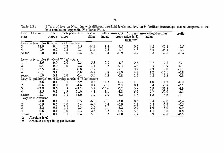
74
Table 5.3 : Effects of levy on N-surplus with different threshold levels and levy on N-fertiliser (percentage change compared to the
farm CO crops other root- pesticides N-fer other Area CO Area set- Area other N-surplus2 profit class outputs crops tiliser inputs crops aside in % outputs
profit
total area1
Levy on N-surplus threshold 125 kg/hectare 3 -14.0 0.4 0.2 1.5 -14.2 1.4 -9.5 0.2 4.2 -40.1 -1.5 4 -1.9 0.2 0.2 1.3 -11.6 2.2 -1.7 4.8 3.6 -28.1 -1.3 sector -1.0 0.1 0.0 0.4 -5.0 0.4 -0.9 2.2 0.8 -7.8 -0.4
Levy on N-surplus threshold 75 kg/hectare 1 -3.6 0.0 0.0 0.3 -5.8 0.1 -2.7 0.3 0.7 -7.4 -0.1 2 -0.4 0.0 0.0 0.2 -3.1 0.2 -0.3 2.3 0.3 -3.9 -0.1 3 -7.5 0.2 0.1 0.8 -7.7 0.1 -5.1 0.2 2.3 -19.0 -1.1 4 -1.1 0.1 0.1 0.8 -6.7 0.8 -1.0 4.8 2.2 -16.1 -0.8 sector -1.0 0.1 0.0 0.4 -5.0 0.3 -0.8 2.2 0.8 -7.8 -0.3 Levy (1 guilder/kg) on N-Surplus threshold 75 kg/hectare 1 -5.6 0.1 0.1 -8.9 0.3 -4.2 0.3 1.0 1.0 -11.3 -0.2 2 -0.6 0.0 0.0 -4.6 0.4 -0.5 2.3 0.4 0.4 -5.8 -0.1 3 -22.9 0.6 0.4 -23.3 3.2 -15.6 0.2 6.9 6.9 -57.8 -4.3 4 -3.5 0.3 0.3 -21.0 4.8 -3.1 4.8 6.7 6.7 -50.9 -3.3 sector -2.3 0.1 0.1 -12.0 1.2 -2.0 2.2 1.8 1.8 -18.6 -1.1 Levy on N-fertiliser 1 -4.0 0.1 0.1 0.3 -6.3 -0.1 -3.0 0.3 0.8 -8.0 -0.4 2 -0.9 0.1 0.0 0.4 -6.4 0.4 -0.9 2.3 0.8 -7.9 -0.5 3 -3.2 0.1 0.1 0.3 -3.2 -0.1 -2.2 0.2 1.0 -8.0 -0.9 4 -0.6 0.1 0.0 0.3 -2.8 0.2 -0.5 4.8 1.1 -6.8 -0.8 sector -1.1 0.1 0.1 0.4 -5.0 0.3 -1.0 2.2 0.9 -7.8 -0.5 1: Absolute level 2: Absolute change in kg per hectare
75
Following the introduction of the Long-term Crop Protection Plan (LCPP) in 1991, pesticides use is an other environmental variable that is currently of interest to policy makers (MJP-G, 1991: 101). The simulations performed indicate that pesticides use increases as a result of the policies that aim at reducing N-surplus. The effect on pesticides use should also be taken into account when assessing the environmental gains of different policies.
5.5 Discussion and conclusions
This chapter shows how technical information on the production of an externality can be included in a dual profit function to yield insight in the effects of a tax on the externality. The methodology is applied to a tax on N-surplus which probably will be proposed as a part of future mineral policies for Dutch arable farms. A 0.27 guilder tax per kg N-surplus with a threshold of 75 kg/hectare and a 18% levy on N-fertiliser were found to result in the same reduction of the N-surplus as a 1 guilder tax on N-surplus with a 125 kg/hectare threshold. The N-surplus taxes, however, induce intensive producers to decrease the N-surplus more than extensive producers and should therefore be preferred from an environmental perspective. The N-surplus tax also leads to a lower profit reduction. However, monitoring costs were not taken into account and policy makers should decide whether the costs of monitoring the N-surplus policy outweigh the environmental gains of the N-surplus tax. Of course, it remains true that taxing N-surplus, calculated by the N-surplus formula, is not the same as taxing the pollution
•generated by the "true" production function for the externality, as specified in our theoretical model.
A number of caveats regarding this model have been mentioned before in Chapter 4. A further problem arising in the simulations reported in this chapter is that there was no information on supply of N through animal manure, which was small but not totally absent in the estimation period. Moreover, only one element of the mineral surplus policies (N-surplus) was dealt with in this chapter. Policy makers are more interested in the effects on arable farming of the entire package of the mineral policies, i.e. the effects of taxes on phosphate and nitrogen surplus.
The contribution of this chapter is to provide a general framework for calculating the effects of a tax on an externality. Although the application to N-surplus policy assumes a linear relationship between inputs and a single externality, the methodology presented allows for multiple externalities and more complex production functions for externalities. The approach pursued in this chapter also enables a comparison of (combinations of) different policies on economic and environmental outcomes.

76
Summary
This chapter uses a Mean-Standard deviation utility function to build a dual model
that simultaneously determines area allocation and production/input levels under output
price uncertainty. The specification of the Mean-Standard deviation utility function is
sufficiently flexible to characterise various risk configurations. Regularity conditions of the
indirect utility function (symmetry, convexity) and the producers risk preferences are
tested. The framework is applied to a rotating sample of Dutch arable farms.
Dutch arable farmers are found to exhibit the risk configuration Increasing Absolute
Risk Aversion and Constant Relative Risk Aversion. All other risk configurations are
rejected. A bootstrap resampling method is used to determine the mean and standard
deviation of price elasticities and to test the conditions of regularity. Both symmetry and
convexity are rejected. Price elasticities show the usefulness of determining both the area
allocation and production/input decisions.
6.1 Introduction
Many authors have focused on the problem of area allocation in agriculture. Early
literature on area allocation typically assumes that area allocation and the choice of levels
of crop specific input and output levels (intensity) are two separate decisions. In later
developments, these decisions have been incorporated in one consistent dual framework
assuming risk neutrality (Chambers and Just, 1989; Oude Lansink and Peerlings, 1996;
Guyomard et al., 1996; Jensen and Lind, 1993). Although empirical evidence has shown
that income uncertainty is an important determinant in area allocation (Freund, 1958;
Collender and Zilberman, 1985; Babcock et al.,1987; Chavas and Holt, 1990), so far a
dual framework has not been developed for simultaneous decisions on area allocation and
intensity levels under income risk. Advantages of the dual versus the primal framework
have been discussed extensively in the literature (Pope, 1982; Shumway, 1995) and
Chapter 6
Area allocation under price uncertainty : a dual approach

77
include among others computational convenience, simplicity, estimation efficiency and the
possibility to use a broader range of functional forms.
In the literature, uncertainty is included either directly through the specification of
an Expected Utility or Mean-Variance function (Collender and Zilberman, 1985; Babcock
et al.,1987), or indirectly through the incorporation of wealth variables (Chavas and Holt,
1990). A general weakness of existing approaches (with the exception of Sana et al.
(1994) and Saha (1996a)) is that they do not allow the producer to reveal different
configurations of (relative and absolute) risk aversion.
This chapter addresses both shortcomings of past approaches through the specifica
tion of a Mean-Standard deviation (M-S) utility function that builds on earlier work from
Saha (1996a). The M-S utility function is sufficiently flexible to characterise all configur
ations of risk aversion that are commonly used in the literature. Furthermore, the model
simultaneously determines multiple input demand, multiple output supply and the optimal
area allocation across crops. A further contribution of this chapter is that it provides a
framework for testing the producers' risk attitude as well as conditions of regularity of the
indirect utility function underlying the M-S utility function.
Although both yield and price uncertainty are important in arable farming, this
chapter focuses on price uncertainty and assumes that farmers face no yield uncertainty.
The reason for this is the renewed interest in the effects of price uncertainty following the
1992 CAP reform in EU countries. In case of cereals, fluctuations of world market prices
have a greater impact on EU producer prices after the substantial lowering of the
intervention price since 1992.
The next section elaborates upon the M-S utility approach, followed by the
presentation of the empirical model. A discussion of alternative risk considerations
implied by parametric restrictions of the empirical model is the focus of section 6.4. The
chapter ends with an application to a rotating sample of specialised Dutch arable farms
and concluding comments.
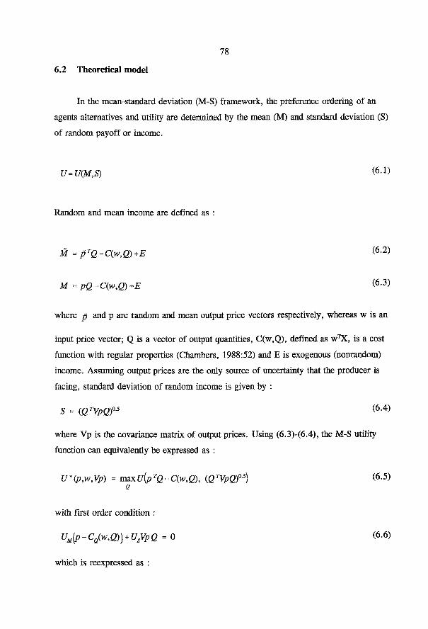
6.2 Theoretical model
78
In the mean-standard deviation (M-S) framework, the preference ordering of an
agents alternatives and utility are determined by the mean (M) and standard deviation (S)
of random payoff or income.
Random and mean income are defined as :
M = pTQ-C(w,Q)+E (-6-2"
M = pQ-C(w,Q)+E (6J)
where p and p are random and mean output price vectors respectively, whereas w is an
input price vector; Q is a vector of output quantities, C(w,Q), defined as w ^ , is a cost
function with regular properties (Chambers, 1988:52) and E is exogenous (nonrandom)
income. Assuming output prices are the only source of uncertainty that the producer is
facing, standard deviation of random income is given by :
where Vp is the covariance matrix of output prices. Using (6.3)-(6.4), the M-S utility
function can equivalently be expressed as :
U=U(M,S) (6.1)
S = (QTVpQf (6.4)
U'(p,w,Vp) = maxU{pTQ~C(w,Q), (QTVpQfs) (6.5) e
with first order condition :
UM(p-CQ(w,Q)) + UsVpQ = 0 (6.6)
which is reexpressed as :

79
p-CJw,Q) U.
irVpQ (6.7)
U * (p,w, Vp) is an indirect utility function as opposed to U(M,S) which is the
direct utility function. The familiar "price is marginal cost" condition is obtained if either
U s is zero or if price variance is zero (i.e. Vp is a null matrix). -US/UM is a measure
reflecting the producers' risk attitude and is the central focus of section 6.4. As under
risk neutrality or price certainty, first order condition (6.7) characterises output supply,
i.e. by solving for Q to yield Q* as a function of w and moments of p :
2 * = Q*(P,W,VP) (6-8>
Furthermore, by using the envelope theorem and first order condition (6.7) it can
be shown that input demand equations can be obtained by differentiating either u * (p,w,Vp)
or C(W,Q) with respect to input prices w.
X(p,w,Vp) = -?E^^ = W™^l = X(w,Q*) (6-9> dw dw
Curvature properties for the indirect Utility function have been derived by Saha
(1996b) and Saha and Just (1996). Define the matrix H as:
H = Yr - YMY' (6-10>
where Y is (Q,-X), r is (p,w) (i.e. Y and r are vectors of netput quantities and netput
prices) and Y r and Y M are the first derivatives of Y to r and M respectively; H has
dimension (n x n) where n is the number of inputs and outputs. In Saha (1996b) and Saha
and Just (1996) it is shown that matrix H is positive semi-definite and symmetric. A
procedure for testing these curvature properties is discussed in section 6.6.
80
i) Specify a utility function over the mean and standard deviation of random income.
ii) Specify a cost function.
iii) Solve first order conditions for utility maximisation for Q.
iv) Determine input demand equations by differentiating the cost function with respect
to w.
The next section will take these steps subsequently.
6.3 Empirical model
Following Saha (1996a) the M-S utility function is specified as :
U(M,S) = Mi - Se (6-n>
As shown in section 6.4 this specification allows for a fully flexible characterisation of
producers risk attitudes. This section continues with the specification of a short term cost
function. The Normalised Quadratic is used here because, overall it came out more
favourable on this data set than other functional forms in chapter 2. An other reason for
choosing the Normalised Quadratic is its computational ease. Normalised costs1 are :
All input prices and costs are normalised by the price of other inputs.
Summarising, in order to obtain a system of input demand and output supply
equations under price uncertainty, the following steps have to be taken :
81
c = a 0 + E ^ + Efe + E X A
+ i E E w + | E E t o +
^ M M z w M (6.12) ôE V* + E E w + E E w + E E w
2 7
where Vj are normalised input prices with i = l (pesticides) and 2 (N-fertiliser). qj are
quantities of outputs with i= l (Cereals and Oilseeds (CO crops)), 2 (other outputs) and 3
(rootcrops), Z\ are areas, fixed inputs and other variables with i = l (area CO crops), 2
(area other output), 3 (area of rootcrops), 4 (labour), 5 (capital), 6 (time trend) and 7
(regional dummy =1 for high productivity region). Symmetry in input prices and fixed
quantities is imposed by requiring o ^ a * and 8^=8^ and \ = \ .
The first order condition for utility maximisation, is derived as2 :
yM 7-1 H j-i M
es6 E W = 0 j = l,..,3 (6.13)
and is rewritten to yield the i=l , . ,3 output supply equations :
3 3 7 3 y M T - 1 P r \ ~ E VrEVy-E^y - es"-1 E m
\uyM^+dSe-lVpa
(6.14
The input equations are derived by differentiating (6.12) with respect to the normalised price of inputs (Shephard's Lemma):
2 7 3 x r a i + E t t s V E ¥ i + E V i i = 1 - 2 ( 6 - 1 5 )
1-1 1-1 M
The equation for the numeraire input can be derived by using the definition of normalised
costs : C = Vi .Xj + v2.x2 + x3.
2 p is now the normalised mean output price.
82
* 3 = « o + £ te -E X A - i E E TO + 1 E E te
^ w M -¿¡=1 > i (6.16) i=l 3 3
i E E V # + E E w Z M ;=i ¡=1 > i
Finally, CO crops area demand equation is derived by maximising U(M,S) with respect to
zx and under the restriction z ; + z2 = a, where a is the total area of CO crops and
other outputs. The assumption that underlies this optimisation is that the area of CO crops
and other outputs are employed optimally, whereas the area of rootcrops remains fixed in
the short term (see Chapter 4 for more details). The first order condition of this
optimisation implies that marginal utilities of z, and Zj are equalised (compare Chambers
and Just, 1989). Using first order condition (6.7), however this reduces to the condition :
dC(W,Q,z) a c ( w , e , z ) s t ( 6 1 7 )
dzx dz2
which can be solved for z, to yield the optimal area allocation to CO crops :
z - 1 x
032 -0,) + 03 2 2 -0 2 1)a +E 0Y v-7v>v, +E «v-fVv-È G^-Mvte, > i H j'-i
(6.18)
6.4 Risk attitude
Using the utility function that has been specified in the previous section, the
producers risk attitude -US/UM is given by :
A(M,S) = -^1=IM1^S6-1 (6-19)

83
3 4
Farms with more than 80% of output coming from marketable crops.
A complete description of the sample can be found in LEI-DLO (1992).
Following Sana (1996a), it can be shown that this specification of the utility function is
sufficiently flexible to characterise various combinations of relative and absolute risk
aversion.
1) Assuming that U M > 0 V M, risk aversion, risk neutrality and risk affinity corre
spond to 6 > 0, = 0 and < 0 respectively.
2) AM < 0 (=0, >0) represents decreasing (constant, increasing) absolute risk
aversion. This translates in the parameter restriction -y > 1 (= 1, < 1).
3) At(tM,tS) < 0 (= 0, > 0) Vt>0 represents decreasing, constant and increasing
relative risk aversion. This holds for y>9, y=6 and y<6 respectively.
Table 6.1 presents an overview of different risk configurations and corresponding
parameter restrictions.
A few comments on the specification of the utility function in (6.11) are in order.
The specification implies that risk preferences solely depend on parameter values such
that risk preferences can be tested globally. While this characteristic may be desirable if
the focus is on testing risk preferences, at the same time it conceals differences in risk
preferences between farmers caused by e.g. farmer specific preferences and farm specific
endowments of fixed inputs or exogenous income. Estimating the parameters of the utility
function for different groups of farmers is a way to capture this.
6.5 Data and Estimation
Data
Data on specialised arable farms3, covering the period 1974-1992, were obtained
from a stratified sample of Dutch farms which kept accounts on behalf of the LEI-DLO
farm accounting system*. Farms stay in the panel for only five to six years, so the panel
is incomplete. The data set used for estimation contained 3571 observations on 784 farms.
84
Three outputs (CO crops, rootcrops and other outputs) and three variable inputs
(pesticides, N-fertiliser and other inputs) are distinguished. CO crops consist of winter-
wheat, barley, oats and oilseeds. The cereals included account for approximately 85% of
the total area of cereals on the farms in the sample. Rootcrops include sugar beet, ware
potatoes, seed potatoes and starch potatoes. Other outputs are combined in an aggregate
index covering all other marketable crops not accounted for in the previous category, and
animal output. Other inputs consist of services, non-nitrogenous fertiliser, seed and
planting materials, purchased feed input, energy and other variable inputs.
Fixed inputs are the rootcrop specific area, the total area of CO crops and other
outputs, labour and capital. The areas are measured in hectares allocated to every output.
Labour is measured in quality-corrected man years, and includes family as well as hired
labour. Capital includes capital invested in machinery and livestock and is measured at
constant 1980 prices.
Exogenous income (E) is defined as income from social security payments and non-
farm assets and is also deflated by the price of other inputs.
Regional differences, e.g in soil quality, are accounted for by including a dummy
variable (=1 for the high productivity region, 0 for the low productivity region).
Tornqvist price indexes were calculated for the three outputs and the other input.
The price indexes vary over the years but not over the farms, implying that differences in
the composition of a netput or quality differences are reflected in the quantity (Cox and
Wohlgenant, 1986). Implicit quantity indexes were obtained as the ratio of value to the
price index.
Output prices are not known at the time decisions are made on planting and the use
of variable inputs, so expected rather than realised prices have to be used. Expected
output prices were constructed by applying an AR(1) filter to CO crops and other outputs
and an AR(2) filter to rootcrops. All prices are deflated by the price of other inputs.
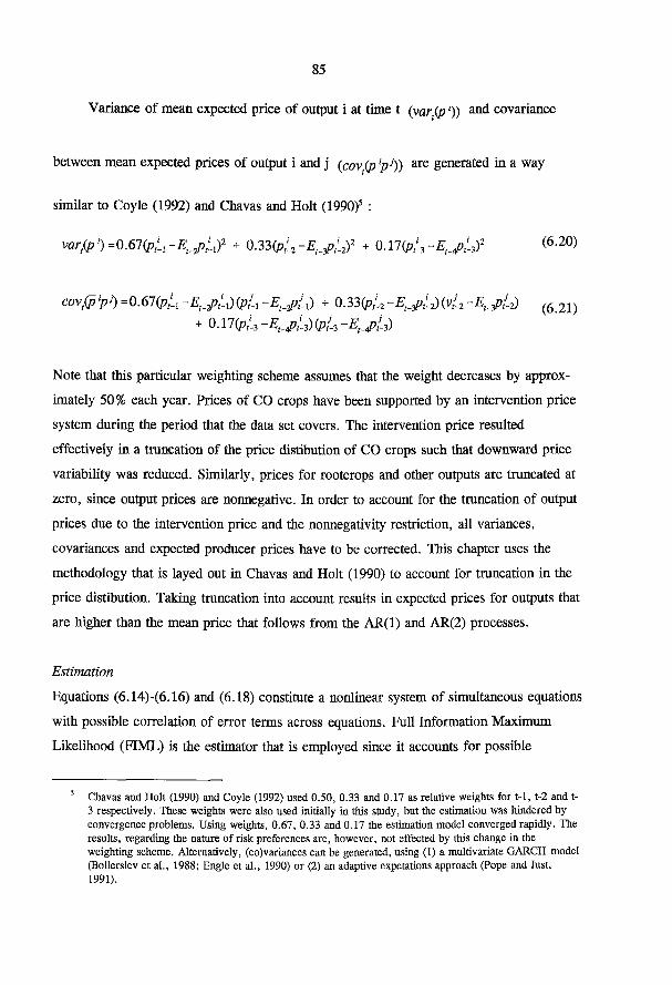
85
Variance of mean expected price of output i at time t (vart(p')) a n c * covariance
between mean expected prices of output i and j (covfp p1)) generated in a way
similar to Coyle (1992) and Chavas and Holt (1990)5 :
var,(p<) =0.67^,-E^Uf + 0.33(p(i2 -Et^Uf + 0. YHpU-E^Uf (6-20>
covfr'pl) =0.67(p(i,-E,_j>U)(pL -E^JJU) + 0.33(p/;2-Et U)(yU ~ET_J)U) (6 21)
+ 0.\HpU ~Et_j>U) <pU -Et^U)
Note that this particular weighting scheme assumes that the weight decreases by approx
imately 50% each year. Prices of CO crops have been supported by an intervention price
system during the period that the data set covers. The intervention price resulted
effectively in a truncation of the price distibution of CO crops such that downward price
variability was reduced. Similarly, prices for rootcrops and other outputs are truncated at
zero, since output prices are nonnegative. In order to account for the truncation of output
prices due to the intervention price and the nonnegativity restriction, all variances,
covariances and expected producer prices have to be corrected. This chapter uses the
methodology that is layed out in Chavas and Holt (1990) to account for truncation in the
price distibution. Taking truncation into account results in expected prices for outputs that
are higher than the mean price that follows from the AR(1) and AR(2) processes.
Estimation
Equations (6.14)-(6.16) and (6.18) constitute a nonlinear system of simultaneous equations
with possible correlation of error terms across equations. Full Information Maximum
Likelihood (FIML) is the estimator that is employed since it accounts for possible
5 Chavas and Holt (1990) and Coyle (1992) used 0.50, 0.33 and 0.17 as relative weights for t-1, t-2 and t-3 respectively. These weights were also used initially in this study, but the estimation was hindered by convergence problems. Using weights, 0.67, 0.33 and 0.17 the estimation model converged rapidly. The results, regarding the nature of risk preferences are, however, not effected by this change in the weighting scheme. Alternatively, (co)variances can be generated, using (1) a multivariate GARCH model (Bollerslev et al., 1988; Engle et al., 1990) or (2) an adaptive expetations approach (Pope and Just. 1991).

86
The availability of panel data usually leads to a panel data estimation method (fixed or random effects) as a natural choice. The characteristic of a panel data estimation method is that it weighs the cross section and time-series variation differently compared to non-panel data estimation methods (Greene, 1993 : 472-473). Estimation of a fixed or random effects model with a large number of farms is however only feasible by making the implausible assumption that fixed or random effects only appear in the input demand equations (see also Chapter 4).
simultaneity bias as well as possible cross equation correlation of error terms. Endoge
nous variables in the estimation model are qj (i = l,..,3), X; (i=l,2), z t , M and S. The
estimator that is applied attaches an equal weight to cross section and time series variation
of the data6.
6.6 Results
The results of the estimation of the system of output supply, input demand and area
allocation equation can be found in the Appendix V (Table V.2). Approximately 80% of
the parameters is found to be significant from zero at the critical 5% level. Interestingly,
also the parameters that relate to the utility function, y and 6, are found to be very
significant (at 5%). An easy test for risk neutrality is provided by testing HQ:9=0 against
the alternative R^.d^O. Table V.2 shows that this hypothesis is firmly rejected at the
critical 5% level.
Using the estimates of this model, alternative risk configurations as described in
section 6.4 are tested. Table 6.1 shows that all hypotheses, except for the CARA/CRRA
hypothesis involve two simultaneous inequality restrictions, or a combination of an
equality and inequality restriction. The Bonferroni t-statistics can be used to test for the
significance of the individual parameter restrictions, given that EL, involves multiple
restrictions (Morey, 1986; Miller, 1966). If the overall level of significance of the test is
0.05, having two inequality restrictions (or one equality restriction and one inequality
restriction), implies that the Bonferroni t-statistics for the individual t-ratios are given by
the Student t-distribution at the critical 0.025 level (0.05/2). The critical regions for
parameter restrictions I and II are given in the final column of Table 6.1.
t-values for parameter restriction I and U are -139.80 and 0.01 respectively.
Therefore, all risk configurations are rejected at the critical 5 % level except for the

87
DARA/DRRA 7 > 1 y-t ? > 0 [ 1 . 9 6 , 0 0 > < 1 . 9 6 , o o >
DARA/CRRA 7 > 1 y-t ?=0 [ 1 . 9 6 , 0 0 > < - o o , - 2 . 2 4 ] [2.24,oo >
DARA/TRRA 7 > 1 y-t ? < 0 [1.96,oo > < - o o , - 1 . 9 6 ]
CARA/DRRA 7 = 1 y-i > 0 < - o o , - 2 . 2 4 ] [2.24,oo > < 1.96,oo >
CARA/CRRA 7 = 1 y-6 = 0 < - o o , - 2 . 2 4 ] [ 2 . 2 4 , o o > < - o o , - 2 . 2 4 ] [ 2 . 2 4 , o o >
CARA/IRRA 7 = 1 y-i < 0 < - o o , - 2 . 2 4 ] [2.24,oo > < - o o , -1.96]
IARA/DRRA 7 < 1 y-t ? > 0 < - o o , - 1 . 9 6 ] [1.96,oo >
IARA/CRRA 7 < 1 y-t ?=0 < - o o ,-1.96] < - o o , - 2 . 2 4 ] [2.24,oo >
IARA/IRRA T \ rmn—/l irr
7 < 1 V 1 TA1
y-t ? < 0 < - o o ,-1.96] < -oo,-1 .96]
a) DARA, CAKA and 1AKA represent Decreasing, Constant and Increasing Absolute Risk Aversion;
DRRA, CRRA, IRRA represent Decreasing, Constant and Increasing Relative Risk Aversion.
functional forms used in the literature to test for the structure of risk preferences,
preclude the presence of IARA a priori. An explanation for the fact that Dutch arable
farmers exhibit IARA may be that small size farms are relatively more dependent for
their income on risky crops as potatoes (in rootcrops) than large size farms.
configuration Increasing Absolute Risk Aversion/Constant Relative Risk Aversion. The
implication of IARA is that high income Dutch arable farmers are more risk averse than
low income arable farmers. Accordingly it may be expected that the cropping pattern of
high income arable farmers involves less risky crops than the cropping pattern of low
income arable farmers. Although Decreasing Absolute Risk Aversion is often considered
as a stylised fact, evidence for Increasing Absolute Risk Aversion has been found before
in the literature (Wolf and Pohlman, 1983). It should also be noted that many of the
Table 6.1 : Tests of alternative risk configurations8
Hypothesis Parameter Critical regions
restrictions
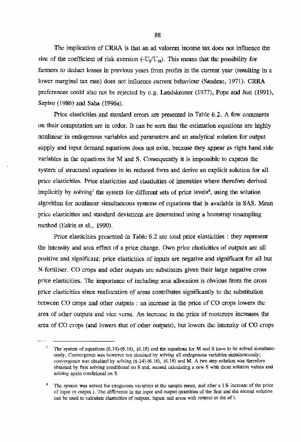
88
7 The system of equations (6.14)-(6.16), (6.18) and the equations for M and S have to be solved simultaneously. Convergence was however not obtained by solving all endogenous variables simultaneously; convergence was obtained by solving (6.14)-(6.16), (6.18) and M. A two step solution was therefore obtained by first solving conditional on S and, second calculating a new S with these solution values and solving again conditional on S.
8 The system was solved for exogenous variables at the sample mean, and after a 1% increase of the price of input or output i. The difference in the input and output quantities of the first and the second solution can be used to calculate elasticities of outputs, inputs and areas with respect to the of i.
The implication of CRRA is that an ad valorem income tax does not influence the
size of the coefficient of risk aversion ( - I V U M ) . This means that the possibility for
farmers to deduct losses in previous years from profits in the current year (resulting in a
lower marginal tax rate) does not influence current behaviour (Sandmo, 1971). CRRA
preferences could also not be rejected by e.g. Landskroner (1977), Pope and Just (1991),
Szpiro (1986) and Saha (1996a).
Price elasticities and standard errors are presented in Table 6.2. A few comments
on their computation are in order. It can be seen that the estimation equations are highly
nonlinear in endogenous variables and parameters and an analytical solution for output
supply and input demand equations does not exist, because they appear as right hand side
variables in the equations for M and S. Consequently it is impossible to express the
system of structural equations in its reduced form and derive an explicit solution for all
price elasticities. Price elasticities and elasticities of intensities where therefore derived
implicitly by solving7 the system for different sets of price levels8, using the solution
algorithm for nonlinear simultaneous systems of equations that is available in SAS. Mean
price elasticities and standard deviations are determined using a bootstrap resampling
method (Eakin et al., 1990).
Price elasticities presented in Table 6.2 are total price elasticities : they represent
the intensity and area effect of a price change. Own price elasticities of outputs are all
positive and significant; price elasticities of inputs are negative and significant for all but
N-fertiliser. CO crops and other outputs are substitutes given their large negative cross
price elasticities. The importance of including area allocation is obvious from the cross
price elasticities since reallocation of areas contributes significantly to the substitution
between CO crops and other outputs : an increase in the price of CO crops lowers the
area of other outputs and vice versa. An increase in the price of rootcrops increases the
area of CO crops (and lowers that of other outputs), but lowers the intensity of CO crops

89
parentheses).
CO Other Root- Pestici N-fer Other Ex. crops outputs crops des tiliser inputs income
CO crops 2.90* (0.08)
-1.95* (0.05)
0.11 (0.01)
-0.30* (0.05)
-0.09* (0.03)
-0.67* (0.08)
0.03* (0.00)
Other outputs -1.73* (0.05)
3.72* (0.10)
-0.30 (0.01)
-0.10* (0.02)
0.03 (0.01)
-1.58' (0.05)
-0.05* (0.00)
Rootcrops -0.31' (0.01)
-0.29 (0.01)
0.52* (0.02)
0.07* (0.00)
0.06* (0.00)
0.02* (0.02)
-0.09* (0.00)
Pesticides 0.50' (0.12)
0.34* (0.04)
0.08* (0.01)
-0.60* (0.13)
-0.07 (0.05)
-0.23 (0.15)
-0.03* (0.00)
N-fertiliser 0.59* (0.16)
0.02 (0.06)
-0.16* (0.01)
-0.27* (0.14)
-0.08 (0.15)
-0.12 (0.23)
0.03* (0.00)
Other inputs 0.18* (0.04)
1.05* (0.03)
0.10* (0.02)
-0.02 (0.04)
0.02 (0.02)
-1 .2 / (0.07)
-0.05* (0.00)
CO crops area 1.69* (0.06)
-2.14* (0.05)
0.14* (0.01)
-0.17 (0.10)
-0.43* (0.06)
0.88* (0.11)
0.03* (0.00)
Other outputs area -2.11* (0.08)
2.67* (0.07)
-0.17* (0.01)
0.21 (0.12)
0.54* (0.07)
-1.10* (0.14)
-0.04* (0.00)
Significant at 5 %
Since convexity and symmetry conditions do not directly translate into parameter
restrictions, using the M-S model that is developed in this chapter, an alternative
(and of other outputs) through a reallocation of fixed, but allocatable resources, labour
and capital. The positive (negative) area allocation effect of CO crops (other outputs)
dominates (strengthens) the negative reallocation effect of labour and capital. The positive
effect of rootcrops price on the area of CO crops is a result of the fact that rootcrops
production needs a sufficiently large area of cereals.
All variable inputs are complements (with the exception of a small and
nonsignificant substitution relation between other inputs and N-fertiliser). The negative
impacts of pesticides and N-fertiliser on CO crops area indicate that CO crops are
relatively more dependent on these inputs than other outputs are. An increase in
exogenous income has an overall negative impact on intensity and favors the area of (less
risky) CO crops to the detriment of the area of other outputs.
Table 6.2 : Total price elasticities at the sample mean (Estimated standard deviations in

90
Table 6.3 : Estimated Choleski values and t-statistics.
Parameter Estimate t-statistic
D„ 140.16 1150.29
D 2 2 174.31 633.76
D 3 3 86.95 184.16
D 4 4 5.95 101.37
D55 0.33 1.19
D« -28.49 -8.83
Testing for symmetry and curvature conditions under risk, is an area that has
remained largely unresolved in the literature. Coyle (1992) has tested for symmetry in a
approach is necessary. The approach adopted in this chapter employs a bootstrap resampl
ing method (Eakin et al., 1990) to generate 1000 observations of the matrix H in (6.10).
Next OLS is used to estimate the mean and standard deviation of individual components
and perform tests on symmetry and convexity.
The test on symmetry involves 15 parameter restrictions on the individual compo
nents of H. These restrictions can be usefully tested using an F-test. The statistic that is
found for H0: H^IL , v i j is 96696.60 which is larger than F i 50 0 5 =1.67, so H 0 is
firmly rejected at the critical 5% level. The test on convexity of H in prices uses the fact
that almost every symmetric positive definite matrix can be represented as a nonlinear
factorisation LDL' where L is a unit lower triangular matrix and D is a diagonal matrix
whose elements are the (nonnegative) Choleski values. Testing for convexity however
requires that symmetry is imposed. The Choleski values of H are reported in Table 6.3.
One Choleski values is negative. The significance of this violation can be tested, using the
Bonferroni t-statistics. If the overall level of significance of the test is 0.05 then, having
six simultaneous inequality restrictions implies that the one tailed critical value of the test
is 0.05/6 = 0.0083. The null hypothesis EC0: D„S:0, i = l,..,6, against the alternative H, :
Dj^O for at least one i is rejected if at least one t-value is smaller than -2.39. It can be
seen in Table 6.3 that negative Choleski value is significant at the 5% level. Therefore
the null hypothesis that the matrix H is positive semidefinite is rejected.

91
restrictive linear mean-variance model and rejected it statistically. A recent survey of the
relatively rich literature of empirical applications of duality theory under risk neutrality by
Shumway (1995), shows that also here, curvature conditions and especially symmetry, are
often rejected. In conclusion, the failure of the model that was presented in this chapter,
to satisfy conditions of regularity is not exceptional.
6.7 Discussion and conclusions
This chapter has presented a dual model that simultaneously determines area
allocation and intensity levels under price uncertainty. The Mean-Standard deviation
utility function that underlies the producers decisions is sufficiently flexible to characterise
various risk configurations. The framework is applied to a rotating sample of Dutch
arable farms.
Dutch arable farmers are found to exhibit the risk configuration Increasing Absolute
Risk Aversion and Constant Relative Risk Aversion. All other risk configurations are
rejected. A bootstrap resampling method is used to determine the mean and standard
deviation of price elasticities and to test the conditions of regularity. Both symmetry and
convexity are rejected. Price elasticities show the usefulness of determining the area
allocation and intensity levels simultaneously.
Although the framework of the model that is developed in this chapter is dual, since
technology can be recovered from the parameters of the cost function, the model partially
loses advantages of dual forms as computational ease and simplicity by including the first
order conditions for utility maximisation. Estimation efficiency and the possibility to use a
broader range of functional forms are, however maintained.
A natural extension of the M-S model in this chapter is the incorporation of output
uncertainty. The specification of cost functions under output uncertainty has been
addressed by Chavas and Pope (1994) and an empirical implementation can be found in
Pope and Just (1996). Qualitative properties of the firms optimal choices under price and
production risk have been explored by Saha (1995) and Coyle (1996).
92
Summary
This chapter provides a framework for consistent estimation of a dynamic dual
model of investment for the case where data reveal zero and non-zero investments. The
threshold model that is developed maintains that investments are zero if the shadow value
of machinery is between a lower and an upper threshold. Separate equations are
estimated for the investment and the disinvestment regime. A significant difference
between the parameters of the investment and disinvestment equations is found; the test
for differences in individual parameters indicates a significant difference for two of the
twelve parameters. Short and long term price elasticities conditional on the regime that
applies are derived. The adjustment rates for machinery reveal adjustment terms of 7-8
years for disinvestments and 14 years for investments.
7.1 Introduction
Most theoretical and empirical research on dynamic adjustment models focus on the
modelling of the adjustment costs and their implications for investment and expansion
strategies.1 Despite the differences in the methodologies (e.g., dynamic primal versus
dynamic dual, static versus nonstatic price expectations) the analytical framework
Eisner and Strotz (1963), Lucas (1967), Gould (1968), Treadway (1969, 1970, 1971), Rothschild (1971), Mortensen (1973), McLaren and Cooper (1980), Epstein (1981) and Caputo (1990) develop a consistent theoretical background for the adjustment cost model. Recent empirical models focus on testing for the presence of adjustment costs and evaluating the impact of the adjustment behavior on production decision making [e.g., Pindyck and Rothemberg (1983), Epstein and Denny (1983), Vasavada and Chambers (1986), Shapiro (1987), Howard and Shumway (1988)]. More recent work generalizes production structure and growth measures to the dynamic case [e.g., Luh and Stefanou (1991, 1993), Fernandez et al (1992), Stefanou et al (1992), Fousekis and Stefanou (1996)].
Chapter 7
Asymmetric Adjustment of Dynamic Factors at the F i r m Level

93
2 In the classical business cycle theories, the accelerator principles are often used as the single most important cause of the cyclical fluctuations. Kalecki (1935) initiated using stock-adjustment investment functions to feature the cycles. Kaldor (1940), Hicks (1950) and Goodwin (1951) interject the nonlinearity notion into the investment function to both explain the cycles and trace out the time path of an actual cycle which is asymmetrical. Another nonlinear approach developed by Smithies (1957) uses the ratchet treatment to incorporate the asymmetry in generating both the cyclical and secular aspects of the GNP movements.
maintains an intertemporal profit maximising (or cost minimising) assumption under
which a linear accelerator adjustment mechanism is commonly maintained for the
determination of dynamic factor demand functions.
Previous studies of the firm facing adjustment costs are constrained by the assump
tion of symmetric adjustment responses; i.e., the same degree of sluggishness exists in the
quasi-fixed factor adjustment process for expansions and contractions. Conceivably, it is
often easier to scale back one's operations during hard times than it is to expand during
prosperous times to a scale of operation that is out the manager's experience. The notion
of asymmetric adjustment has been emphasised by Goodwin (1951) in his work on
nonlinear accelerator principle as the factor in explaining the persistence of business
cycles.2 More recently Neftci (1984), Hamilton (1989), Madan and Prucha (1989), Pfann
and Palm (1993) and Pfann (1996) observe business cycles fluctuating along long-run
secular trends using economic time series models incorporating discrete regime changes.
In the standard approach to modelling quasi-fixed factor demand, zero investments
are optimal if the shadow value of the quasi-fixed factor is zero. Observations from firm
level data where zero investment are observed questions the consistency of the standard
approach to modelling firm level decision making. A theoretical problem arising is that
the first order condition for optimisation of the value functions implicit in the dual
approach is not necessarily satisfied. Data are censored in the presence of zero invest
ments leading to econometric problems for both the primal and dual approach. This
implies the standard assumption of independent and identically distributed errors no
longer applies resulting in biased estimates if not corrected.
The modelling of asymmetry, nonlinearity and zero gross investment are combined
by applying a regime shifting method to formulate a generalised dynamic adjustment cost
model. The generalisation endogenises capital accumulation and provides a natural linkage
between firm size and exogenous economic variables (e.g., netput price changes, govern
ment policies). In this sense, structural change is inherent in the evolution described by

94
Whereas a solution is tractable for a standard quadratic adjustment cost function, the problem becomes highly complex for more flexible specifications of adjustment costs, e.g. interactions between investments and the capital stock or third order effects (Pindyck and Rotemberg, 1993; Shapiro, 1986).
this optimisation process. The asymmetric model nests symmetric adjustment rates and
presents the opportunity to test statistically for the superiority of specifying asymmetric
adjustment rates.
This chapter addresses the shortcomings of past approaches through the specifica
tion and estimation of a threshold model to characterise investment demand. The dual
framework is employed which does not require a closed form solution for the Euler
equation to derive factor demand equations.3 The threshold model maintains investments
are zero if the shadow value of capital is between a lower and an upper threshold. This
model is estimated in two stages. The first stage determines the decision whether to
invest, disinvest or do nothing. This information is used to correct the error terms in the
second stage which comprises the estimation of a system of output supply and variable
and quasi-fixed factor demand equations. Since the value function does not necessarily
exist for zero investments, only the observations for which investments are non-zero are
used in the second stage.
The next section elaborates upon the standard dual approach and illustrates how the
maintained assumptions of the adjustment cost function allow for zero investments as
optimal under restrictive conditions. This is followed by the presentation of a threshold
model explaining the occurrence of zero investments along with discussion of the
empirical model, econometric specification and estimation considerations. An application
to a rotating sample of specialised Dutch cash crop farms is the focus of the application
followed by concluding comments.
7,2 The Standard Dual Model
The standard dual model and the underlying adjustment cost function provide a reference
point for the development of the threshold model. The standard dual model starts with the
maximisation of the discounted flow of profit for the firm producing multiple outputs
using variable and multiple quasi-fixed factors taking the form
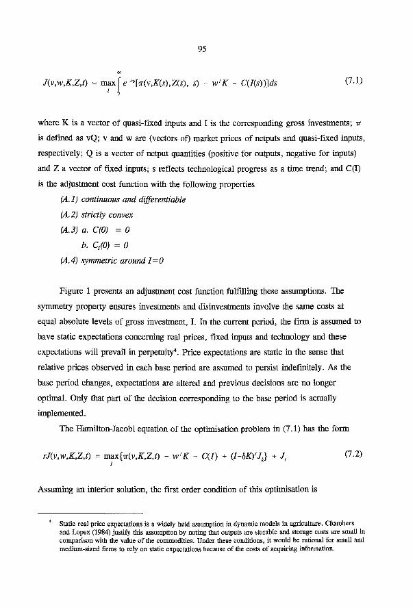
95
J(v,w,K,Z,f) = max[e-rs[ir(v,K(s),Z(s), s) - w'K - C(I(s))]ds C 7 - 1 ) ' \
where K is a vector of quasi-fixed inputs and I is the corresponding gross investments; ir is defined as vQ; v and w are (vectors of) market prices of netputs and quasi-fixed inputs,
respectively; Q is a vector of netput quantities (positive for outputs, negative for inputs)
and Z a vector of fixed inputs; s reflects technological progress as a time trend; and C(I)
is the adjustment cost function with the following properties
(A. 1) continuous and differentiable
(A. 2) strictly convex
(A. 3) a. C(0) = 0
b. C;(0) = 0
(A.4) symmetric around 1=0
Figure 1 presents an adjustment cost function fulfilling these assumptions. The
symmetry property ensures investments and disinvestments involve the same costs at
equal absolute levels of gross investment, I. In the current period, the firm is assumed to
have static expectations concerning real prices, fixed inputs and technology and these
expectations will prevail in perpetuity4. Price expectations are static in the sense that
relative prices observed in each base period are assumed to persist ^definitely. As the
base period changes, expectations are altered and previous decisions are no longer
optimal. Only that part of the decision corresponding to the base period is actually
implemented.
The Hamilton-Jacobi equation of the optimisation problem in (7.1) has the form
rJ(y,w,K,Z,t) = rmx{ir(v,K,Z,t) - w'K - C(I) + (I-6K)'Jk} + J, (7-2)
Assuming an interior solution, the first order condition of this optimisation is
4 Static real price expectations is a widely held assumption in dynamic models in agriculture. Chambers and Lopez (1984) justify this assumption by noting that outputs are storable and storage costs are small in comparison with the value of the commodities. Under these conditions, it would be rational for small and medium-sized firms to rely on static expectations because of the costs of acquiring information.

96
C, = (7.3)
implying the shadow price of capital equals the marginal adjustment cost. Netput equa
tions are derived by differentiating the optimised Hamiltonian-Jacobi equation in (7.2)
with respect to v and applying the envelope theorem to yield
Investment demand equations can be derived similarly by differentiating the optimal
value function with respect to quasi-fixed factor prices and applying the envelope theorem
leading to
The properties of the value function, J, depend crucially on the characteristics of
the underlying adjustment cost function (A.l) - (A.4).
7.3 The Threshold Model
The standard dual model suggests zero investments only occur if the shadow value of
capital equals zero. However, this is not consistent with the observation from firm level
data where zero investments occur frequently.
Hsu and Chang (1990) show that a discontinuity of the adjustment cost function at
1=0 is sufficient for asset fixity to occur. The occurrence of a discontinuity arises when
buyers are not able to evaluate the quality of the factor/product properly (Dixit and
Pindyck, 1994). The quality for used machinery on the market is below the average
quality of machinery in the sector since sellers are reluctant to sell an item with an above
average quality. This significantly lowers the price for used machinery. Hence, a lower
price can be seen as an adjustment cost. A discontinuity may also arise as a result of
government regulation (Dixit and Pindyck, 1994). A firm may have to repay an invest
ment subsidy if it decides to sell the asset within the limits set by the subsidy program.
Properties (A.l) and (A.3b) no longer hold if a discontinuity in the adjustment cost
function occurs.
2 = rJv - JJL - J, tv (7.4)
K = J£ (rJw + K-JJ (7.5)

Figure 1: Standard adjustment
cost function
97
Figure 2 Threshold model with
fixed adjustment costs
In a more general framework than Hsu and Chang (1990), Abel and Eberly (1994)
indicate that fixed adjustment costs may also give rise to the occurrence of zero invest
ments thereby relaxing (A. 3a). Figure 2 illustrates an adjustment cost function no longer
satisfying properties A.l and A.3. The optimality condition is Jk=C,. With a discontinuity
occurring at 1=0, C,(0) does not necessarily exist and investments are zero for the range
of shadow values described by
limC/7) > 0
limCf(7) < 0
Equation (7.6) depicts the lower and upper limit values of C,(0) while bearing in
mind the first order conditions in (7.3) makes it clear why zero investments are likely to
occur when the adjustment cost function has the form as in figure 2. With the symmetry
condition relaxed in the adjustment cost function, the investment regime differs from the
disinvestment regime. Following Abel and Eberly (1994) this adjustment cost function
results in the following decision rule for the optimal investment regime
K < 0 if Jk<q, K = K = 0 if q^Jk^q2 V-7
K>0 if Jk>q2

98
The previous literature on dynamic investment demands has employed the Normalised
Quadratic specification for the optimal value function (Vasavada and Chambers, 1986;
Stefanou et al., 1992). This functional form has the advantage of empirical simplicity at
the cost of using an arbitrary numeraire input or output in order to impose linear homo
geneity in prices. As a result, estimation results are not invariant with respect to the
choice of the numeraire (Mahmud et al, 1987). The Normalised Quadratic is more
troublesome in the context of this chapter since the specification of external adjustment
costs precludes the derivation of the equation of the numeraire input. The Symmetric
Normalised Quadratic (Kohli, 1993; Diewert and Wales, 1987) has the advantage of
avoiding the derivation of the numeraire input and estimation results are invariant with
respect to choice of the numeraire (see also Chapter 2). The value function takes the
following form
J(v,w,z,K,t) = ( û j O , ) V
+ -(0'v)-1 ( v w ) A C V
+ -(0'v)-1 ( v w ) w 2 C B w
D G H z 0 P R z
G' EL K + ( v w ) K + ( v w ) S M
H' V F t t
(7.8)
where 0 represents a vector of average shares of netputs in total costs plus revenues. In
order to identify all parameters, additional restrictions have to be imposed :
where q, and o& are threshold levels for the shadow price of capital. Investments are
negative if the shadow value of capital is smaller than q, and investments are positive for
all shadow values larger than q .
7.4 Empirical Model

99
£ V i = 0 J = l,..,5
£ c , v ( = o y = i , 2
where v . is an arbitrary point or observation (in this chapter it is the sample mean).
Using (7.5), the demand equation for investments can be derived as
k=(m+M)K+rM(a2 + (fiv)-1(Bw + Cv)+Sz + Ut) - Mil (7-9)
implying a multivariate linear accelerator mechanism
K" = (ru + M)(K - K') ( 7 - 1 0 )
where K* is the optimal stock of K,
K" = rAT(a2 + (ev)-1(Bw + CV)+& + Ur)-iV17 ( 7 - n )
and N is -[ra +M]~lM • The shadow value of capital is5
Jk = a4 + (d'v)(G'z +E'K+L'f) +M'vw+P'v (7-12)
Assume the case of two quasi-fixed factors, K, and K2, where asymmetric adjust
ment is possible for K2. Using the demand equation for investment, ^ , and the shadow
value of K2, these equations are compactly expressed as
K 2 = J 2 X (7.13)
where X is (v, w, z, K, t). The netput equation is
Note that qi and qj in the Abel and Eberly model include the price of capital.
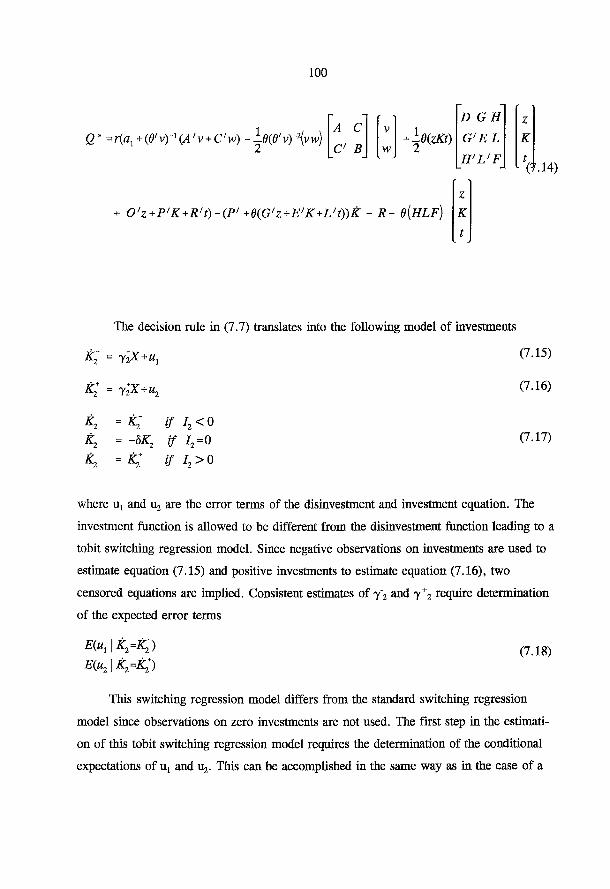
100
g" =r(aj +(d'vy1(A'v + C/w) --8(e'vy2{vw) A C V
C> B w
+ 0>z+P'K+R't)~(P' +B(G'z+E'K+L't))K - R- 6{HLF)
D G H z G'EL K
H'L'F t 1 (4 • 14)
The decision rule in (7.7) translates into the following model of investments
k* = y;x+u2 (7-16)
K\ = K~2 if i2<o K\ = if / 2 = 0
K\ = if Z2 > 0
(7.17)
where u t and u2 are the error terms of the disinvestment and investment equation. The
investment function is allowed to be different from the disinvestment function leading to a
tobit switching regression model. Since negative observations on investments are used to
estimate equation (7.15) and positive investments to estimate equation (7.16), two
censored equations are implied. Consistent estimates of y2 and y+
2 require determination
of the expected error terms
E(ux I k^ki)
E(u21 i ^ ^ * ) (7.18)
This switching regression model differs from the standard switching regression
model since observations on zero investments are not used. The first step in the estimati
on of this tobit switching regression model requires the determination of the conditional
expectations of U; and This can be accomplished in the same way as in the case of a

101
standard switching regression model except there are two limits, 0" and 0 + , instead of
one. Defining a dummy variable A
A=0 ifl2<0 A = l ifl2=0 (7.19) A=2 ifl2>0
and expressing (7.15)-(7.17) as the two limits in the tobit switching regression model6
=y2~X+u1 if u<qx-$X K° = -bK\ if qr0X<u<q2-0X (7-20) K^=y2X+u2 if u>q2~0X
The decision about the investment regime is now determined by an ordered probit model.
Assume u u u 2, and u have a trivariate normal distribution and let o",u and a 2 u denote the
covariances of u and u,, u2, respectively. The conditional expectations of % and u, are
derived from the estimates of the ordered probit model
£(8^<)=-ff"H!- a& (7-21)
E(u2 [ = = a2uW2 (7-22) l-$(c-j8X)
where, c/>(-)and $(-)are the probability density and the cumulative density functions,
respectively, of the normal distribution. Note that becomes a part of BX during
estimation and that the parameter c equals c^-q^ Substituting W i ; i = 1, 2, in (7.15) and
(7.16) yields the K2 demand equations
K2^y'2X-auW1+el ( 7 2 3 )
K2^y*2X+a2uW2 + e2
Through cross parameter restrictions, the parameter M 2 2 appears in BX as well as 7X. Theoretically, the parameter M 2 2 in BX should be different for the investment and disinvestment regime. The assumption that M 2 2 is the same in both regimes in the first stage estimation of the switching regression model is not unusual (Maddala, 1983).
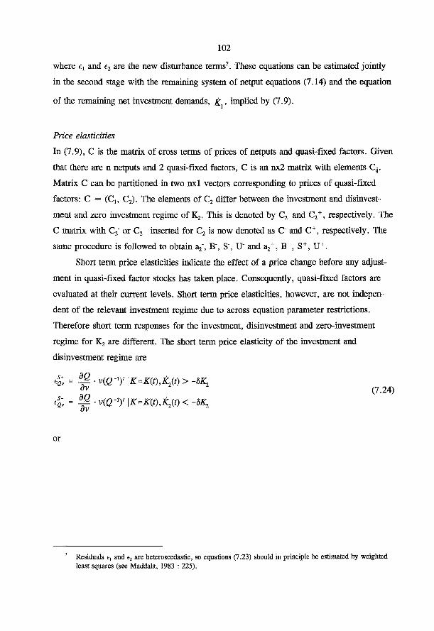
102
where and e2 are the new disturbance terms7. These equations can be estimated jointly
in the second stage with the remaining system of netput equations (7.14) and the equation
Price elasticities
In (7.9), C is the matrix of cross terms of prices of netputs and quasi-fixed factors. Given
that there are n netputs and 2 quasi-fixed factors, C is an nx2 matrix with elements Q j .
Matrix C can be partitioned in two nxl vectors corresponding to prices of quasi-fixed
factors: C = (Cu C2). The elements of C2 differ between the investment and disinvest
ment and zero investment regime of K2. This is denoted by C2" and C 2
+ , respectively. The
C matrix with C 2 " or C 2
+ inserted for C 2 is now denoted as C" and C + , respectively. The
same procedure is followed to obtain a^, B", S", U" and a 2
+ , B + , S + , U + .
Short term price elasticities indicate the effect of a price change before any adjust
ment in quasi-fixed factor stocks has taken place. Consequently, quasi-fixed factors are
evaluated at their current levels. Short term price elasticities, however, are not indepen
dent of the relevant investment regime due to across equation parameter restrictions.
Therefore short term responses for the investment, disinvestment and zero-investment
regime for K2 are different. The short term price elasticity of the investment and
disinvestment regime are
of the remaining net investment demands, % , implied by (7.9).
v(Q-y\K=K(t),K2(t)>-dK2
v{Q-1)'' \K=K(J),K2(t)< -dK^ (7.24)
or
7 Residuals e, and e2 are heteroscedastic, so equations (7.23) should in principle be estimated by weighted least squares (see Maddala, 1983 : 225).

103
eQv~ «v) (B'vf
A1 _(A/v + C-'w)a/
(9'v) (0'v)2 id1 -ee'(e'vy2(vw)
A C* V
C*'B* w
A C V
C'B~ w
•r-v(Q-1)'
(7.25)
where Q 1 ' is the vector with the i f t element, the inverse of If investments in K2 are
zero, the optimal value function may not exist for all values of exogenous parameters and
a price elasticity cannot be calculated. However, the expected investment in K2 can be
determined using the parameters of the investment and disinvestment regime and can be
regarded as a proxy for the short term response for the zero investment regime. The
specification of price elasticities under the zero investment regime must allow for
K*(t) = k~(f) = ~S.fir.jto be imposed in the netput equations corresponding to the
disinvestment and investment regime. The expectation is constructed as a weighted mean
of the conditional price elasticities of the investment and disinvestment regime
^ • v(Q-y \K=K(t),K2(t) = -!>K2 (7.26)
where p^t) < -bKJt) | K2(t) * -<5ig and p^t) > -6^ (0 | K2(t) * are computed
using the estimates of the ordered probit model.
In the long run, quasi-fixed factor stocks can adjust to optimal levels. The adjust
ment for a quasi-fixed factor depends on the regime that applies since a given price
change may imply an investment, a disinvestment or no investment at all. Therefore, a
first step in determining long term price elasticities is to determine the relevant regime
using the results of the ordered probit model. The relevant equation for investments in K2
is used to determine the long term effects of price changes. For the investment and
disinvestment regimes these can be determined by using

104
4 = { 4 + <WVvl K=K", k2(t)<-8K2(t)}
4v = {4v + V ^ - v l K=K*\ k2(t)>-8K2\
Using (7.14) the long term price elasticities are
£J2V = eQv + r P + e(G'E'L')
L* S* P + 6(G'E'L')
z K •rN~ c-
t -
(0'v)
z K •rN* C*
t (6>v)
t (6>v)
(B-w + C-v)e, (9'vy2
(d'vy
(7.27)
(7.28)
(7.29)
(7.30)
The long term price elasticities for the zero investment regime are determined in a way
similar to their short term counterparts
dv dK dv
PiK, <-&K7\t2* -8KJ • 4 ; , M + K*i > SK, | K2 * -8KJ •
(7.31)
7.5 Data
Data on specialised cash crop farms covering the period 1971-1992 are obtained from a stratified sample of Dutch farms keeping accounts on behalf of the LEI-DLO farm accounting system. Farms deriving more than 80 percent of their output from marketable crops are the focus of this application. These farms remain in the panel for only five to six years. The data set used for estimation of the ordered probit model contains 4040 observations. Investments in machinery are negative for 95 observations (2.4 percent), zero for 1189 observations (29.4 percent) and positive in 2756 cases (68.2 percent). Only non-zero observations (2851) on investments in machinery are used for the second stage
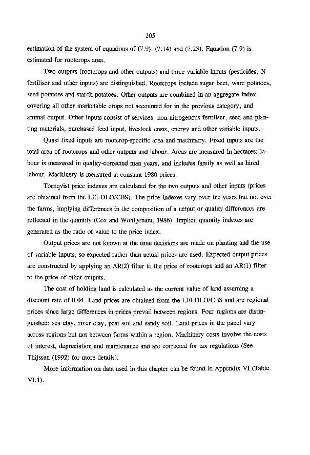
105
estimation of the system of equations of (7.9), (7.14) and (7.23). Equation (7.9) is
estimated for rootcrops area.
Two outputs (rootcrops and other outputs) and three variable inputs (pesticides, N-
fertiliser and other inputs) are distinguished. Rootcrops include sugar beet, ware potatoes,
seed potatoes and starch potatoes. Other outputs are combined in an aggregate index
covering all other marketable crops not accounted for in the previous category, and
animal output. Other inputs consist of services, non-nitrogenous fertiliser, seed and plan
ting materials, purchased feed input, livestock costs, energy and other variable inputs.
Quasi fixed inputs are rootcrop-specific area and machinery. Fixed inputs are the
total area of rootcrops and other outputs and labour. Areas are measured in hectares; la
bour is measured in quality-corrected man years, and includes family as well as hired
labour. Machinery is measured at constant 1980 prices.
Tornqvist price indexes are calculated for the two outputs and other inputs (prices
are obtained from the LEI-DLO/CBS). The price indexes vary over the years but not over
the farms, implying differences in the composition of a netput or quality differences are
reflected in the quantity (Cox and Wohlgenant, 1986). Implicit quantity indexes are
generated as the ratio of value to the price index.
Output prices are not known at the time decisions are made on planting and the use
of variable inputs, so expected rather than actual prices are used. Expected output prices
are constructed by applying an AR(2) filter to the price of rootcrops and an AR(1) filter
to the price of other outputs.
The cost of holding land is calculated as the current value of land assuming a
discount rate of 0.04. Land prices are obtained from the LEI-DLO/CBS and are regional
prices since large differences in prices prevail between regions. Four regions are distin
guished: sea clay, river clay, peat soil and sandy soil. Land prices in the panel vary
across regions but not between farms within a region. Machinery costs involve the costs
of interest, depreciation and maintenance and are corrected for tax regulations (See
Thijssen (1992) for more details).
More information on data used in this chapter can be found in Appendix VI (Table
VI.l).

7.6 Results
106
The threshold model is estimated in two stages. In the first stage, the ordered probit
model is estimated (equation (7.12)). Parameter results (see Appendix VI : Table VI.2)
are used to calculate the expected error terms (7.18) which are included in the equations
for investment and disinvestment in machinery. These equations are estimated in the
second stage together with the netput equations and the demand equation for the area of
rootcrops using Seemingly Unrelated Regressions. The SUR estimator applied takes into
account that the equations in the system have unequal numbers of observations (Judge et
al., 1988 P: 463-465). This model contains 92 parameters, including 2 parameters related
to the expected error terms in (7.18). The estimated model generates 49 percent of the
parameters estimated significant (see Appendix VI : Table VI.3) at the critical 5 percent
level. A x2 test is used to test the hypothesis that no parameter differences exist for the
investment and disinvestment regime of machinery (y~2 = y+%)- The null hypothesis of no
parameter differences is firmly rejected (x2i2..o5 < 121.16). Table 7.1 presents results of
tests on differences between the investment and disinvestment regime for individual pairs
of parameters. The critical X2I,.<K is 3.84 and it is found that the null hypothesis of no
parameter difference between the investment and disinvestment regime is not rejected for
the adjustment parameter of machinery (M^) and the parameter relating machinery invest
ments to the quantity of labour (S^).
Table 7.1: Tests of hypotheses for parameter symmetry
Null Hypothesis Test statistic Null Hypothesis Test statistic
a 3 2 + = a 3 2 0.86 C4 2
+ = c 4 2 0.00 + = B21" 1.42 M 2 1
+ = M2f 2.28 -*22+ = ~*22 0.00 M 2 2
+ = M22" 8.88
c + — c -^12 M2
0.57 S 2 1
+ = S 2 1 1.99 C2 2
+ = C22 0.00 S22+ = S22 7.98
Q 2 +
= C32 0.00 u 2
+ = u2- 0.00

107
Table 7.2 : Short term price elasticities.
root- other pestici N-fertili other in land machi
crops outputs des ser puts nery
rootcrops 0.041 0.008 0.014 0.003 -0.038 0.035 -0.063
other outputs 0.012 -0.070 -0.018 -0.033 -0.017 0.030 0.095
pesticides -0.121 0.091 -0.360 0.149 0.138 -0.008 0.112
N-fertiliser -0.068 0.519 0.451 -0.086 -0.418 -0.029 -0.369
other inputs -0.072 0.091 0.049 -0.030 -0.121 0.075 0.007
In order to calculate long term price elasticities, the relevant investment regime for
machinery must be determined. Using average values of the data used in this chapter the
following probabilities are found: 0.02 for I 2 < 0, 0.27 for I2 =0 and 0.71 for I 2 > 0.
Therefore, the predicted regime is the (positive) investment regime and the parameters
used for calculating the long term price elasticity in (7.28) are a +
3 2 , B +
2 1 , etc. The own
price elasticity of other outputs still has the wrong sign (although the size is not large in
absolute terms). Other own price elasticities, including those of the quasi-fixed factors
have the expected sign. Other outputs and rootcrops are long term complements. This
indicates that rootcrops cannot be grown in the long term without a sufficiently large area
of other outputs in the crop rotation. Typically, other outputs are necessary to decrease
the pressure of soil diseases in narrow crop rotations with rootcrops. Another way
farmers maintain a large area of rootcrops is to use high levels of nematicides. This is
reflected by the result that pesticides and rootcrops area are complements.
Machinery is a long term substitute for pesticides and a long term complement for
N-fertiliser and other inputs. Farmers need machinery for applying fertiliser and pesti
cides indicating a complementary relation. In the case of pesticides, farmers also have the
Short term price elasticities are calculated using (7.25) and are presented in Table
7.2. The own short term price elasticity of other outputs is negative but the size is small
and is not inconsistent with the adjustment cost theory (Mortensen, 1973; Caputo 1990).
N-fertiliser and other inputs are substitutes for pesticides and the other variable input is a
complement for N-fertiliser.

108
Table 7.3 : Long term price elasticities
root- other pesti N-fertili other land machi
crops outputs cides ser inputs nery
rootcrops 0.037 -0.002 0.015 0.001 -0.027 0.036 -0.060
other outputs 0.043 -0.089 -0.013 -0.039 -0.019 0.038 0.080
pesticides -0.142 0.104 -0.363 0.153 0.140 -0.014 0.123
N-fertiliser -0.093 0.543 0.446 -0.080 -0.423 -0.037 -0.358
other inputs -0.097 0.112 0.045 -0.024 -0.123 0.068 0.019
area rootcrops -0.337 -0.134 -0.014 -0.002 0.306 -0.011 0.189
machinery 0.781 -0.838 0.165 -0.211 0.227 0.279 -0.365
Tables 7. 4 and l.i i indicate h ind is a complement for all short and long term
variable inputs where labour is a complement for all inputs except for N-fertiliser.
Technological progress, as represented by a time trend, has been more beneficial to root-
crops than to other outputs and has also encouraged the use of pesticides more than the
uses of N-fertiliser and other inputs. Technological progress in the area of rootcrops and
the volume of machinery is very small.
option to substitute pesticides for machinery for purposes of mechanical weeding. The
results in Table 7.3 suggest the substitution of pesticides for machinery dominates the
complementarity effect of applying chemicals and machinery. The complementary relation
between the area of rootcrops and N-fertiliser indicates that rootcrops use N-fertiliser
more intensively than other outputs.
An increase in the price of rootcrops leads to a small decrease in the area of root-
crops indicating rootcrops area is an inferior input in the production of rootcrops. This
may be explained by the fact that the production of rootcrops is relatively more labour
demanding than the production of other outputs (PAGV, 1993).

109
land labour trend
rootcrops 0.471 0.694 0.042
other outputs 0.837 0.282 0.020
pesticides 0.935 0.228 0.035
N-fertiliser 1.255 -0.353 0.022
other inputs 0.548 0.466 0.009
Table 7.5: Long term elasticities of intensity and trends
land labour trend
rootcrops 0.503 0.702 0.040
other outputs 0.823 0.292 0.018
pesticides 0.943 0.224 0.036
N-fertiliser 1.249 -0.369 0.023
other inputs 0.550 0.455 0.010
area rootcrops 0.960 0.243 -0.007
machinery 0.398 0.765 -0.008
Table 7.6 presents adjustment rates of rootcrops area and machinery for two cases.
The first and second columns are generated from the estimates of the threshold model
which was estimated on 2851 non-zero observations. The third column presents adjust
ment rates generated from estimates of the standard (symmetric) adjustment cost model
estimated on all 4040 observations. In both the threshold model and the standard adjust
ment model, the adjustment rate of rootcrops area is small, indicating a 12 and 14 year
term of adjustment respectively. Both models also indicate the adjustment of rootcrops
area is independent from the adjustment of machinery. Comparison of the adjustment
rates of the expanding and contracting regime suggests that machinery adjusts slower in
the investment regime (14 years) than in the disinvestment regime (7-8 years). This
supports the hypothesis that it is easier for a producer to scale back the operation during
hard times than it is to expand during prosperous times. A higher adjustment rate for
capital during phases of contractions is also found by Pfann (1996) for the Dutch and
Table 7.4: Short term elasticities of intensity and trends

110
Table 7.6 : Adjustment rates (t-values in parentheses).
Threshold model Standard adjustment cost model
expanding contracting
m n -0.08 (-16.36) -0.08 (-16.36) -0.07 (-19.67)
m 1 2 -0.001 (-1.20) -0.001 (-1.20) 0.00 (0.05)
m 2 1 0.27 (4.83) 0.01 (0.09) 0.16 (5.20)
% -0.07 (-13.64) -0.13 (-8.12) -0.07 (-20.31)
The adjustment rate of rootcrops area cannot be compared directly with other
models since other studies have not estimated the adjustment rate of the area under a
particular crop. The adjustment rate for capital on the other hand has been estimated in
many previous studies. Using panel data on Dutch dairy farms Thijssen (1994) finds an
adjustment rate for capital of approximately -0.26. Adjustment rates for capital on
aggregate data range from -0.15 for the U.S. production agriculture (Luh and Stefanou,
1991) to -0.55 in the Southeastern U.S. production agriculture (Taylor and Monson,
1985). The adjustment rate for machinery estimated in this chapter is small in compari
son.
7.7 Simulations
The model developed in the previous sections is used to determine the impacts of
asymmetric responses in investments in machinery under three different price scenarios.
The first is the baseline simulation holding all prices at their 1992 levels. This represents
U.K. manufacturing sector. Another finding from Table 7.6 is that machinery does not
adjust independently from rootcrops area in the expanding regime while it adjusts
independently in the contracting regime. Interestingly, the adjustment rates are effected
negligibly by estimating the dual model assuming a standard adjustment cost function.

I l l
the scenario when 1992 prices persist throughout the simulation period. The second
simulation is a low profit scenario involving a scheme where all output prices are lowered
and all input prices are increased by 10 percent each year. The third simulation is a high
profit price scenario involving an increase of all output prices and a decrease of all input
prices by 10 percent each year.
The simulations are projected over a 5 year period (1992-1997) for all cash crop
farms in the sample in 1992 and are presented in Table 7.7. Results of the simulations are
aggregated to the sector level using the number of farms in the sector that each farm in
the sample represents as weights.
The stock of machinery under the disinvestment and investment regime are calcu
lated using the equations in (7.23). The machinery stock under the zero investment
regime in year t equals the machinery stock in year t-1 less depreciation fixed at 10
percent. The expected machinery stock is calculated from the stocks and probabilities of
each regime. Investment in machinery in year t is conditioned on the expected machinery
stock in year t. The machinery stock in the initial year, 1992, is the same in all simula
tions.
In the base simulation, the probability of each regime remains fairly constant over
time. In the low profit simulation, the probabilities of the disinvestment and zero invest
ment regime increase. Farms must decrease the size of the farm operation, but lower the
capital stock more by letting assets depreciate than by actively disinvesting. In the high
profit simulation there are virtually no more firms disinvesting whereas the probability of
zero investment has deceased by 62 percent. The expected machinery stock increases by
more than 15 percent indicating that farms increase the size of the farm operation in this
simulation. However, the increase in the farm size is hampered by inactivity, also under
very favourable price conditions.
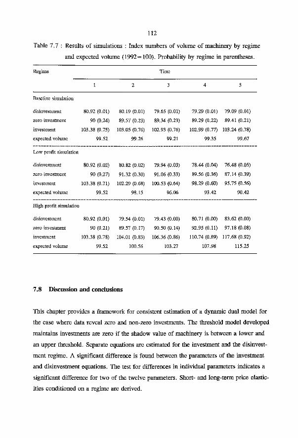
112
Regime Time
1 2 3 4 5
Baseline simulation
disinvestment 80.92 (0.01) 80.19 (0.01) 79.65 (0.01) 79.29 (0.01) 79.09 (0.01)
zero investment 90 (0.24) 89.57 (0.23) 89.34 (0.23) 89.29 (0.22) 89.41 (0.21)
investment 103.38 (0.75) 103.05 (0.76) 102.93 (0.76) 102.99 (0.77) 103.24 (0.78)
expected volume 99.52 99.26 99.21 99.35 99.67
Low profit simulation
disinvestment 80.92 (0.02) 80.82 (0.02) 79.94 (0.03) 78.44 (0.04) 76.48 (0.05)
zero investment 90 (0.27) 91.32 (0.30) 91.06 (0.33) 89.56 (0.36) 87.14 (0.39)
investment 103.38 (0.71) 102.29 (0.68) 100.53 (0.64) 98.29 (0.60) 95.75 (0.56)
expected volume 99.52 98.15 96.06 93.42 90.42
High profit simulation
disinvestment 80.92 (0.01) 79.54 (0.01) 79.43 (0.00) 80.71 (0.00) 83.62 (0.00)
zero investment 90 (0.21) 89.57 (0.17) 90.50 (0.14) 92.95 (0.11) 97.18 (0.08)
investment 103.38 (0.78) 104.01 (0.83) 106.36 (0.86) 110.74 (0.89) 117.68 (0.92)
expected volume 99.52 100.56 103.27 107.98 115.25
7 .8 Discussion and conclusions
This chapter provides a framework for consistent estimation of a dynamic dual model for
the case where data reveal zero and non-zero investments. The threshold model developed
maintains investments are zero if the shadow value of machinery is between a lower and
an upper threshold. Separate equations are estimated for the investment and the disinvest
ment regime. A significant difference is found between the parameters of the investment
and disinvestment equations. The test for differences in individual parameters indicates a
significant difference for two of the twelve parameters. Short- and long-term price elastic
ities conditioned on a regime are derived.
Table 7.7 : Results of simulations : Index numbers of volume of machinery by regime
and expected volume (1992=100). Probability by regime in parentheses.
113
The adjustment rates for machinery reveal adjustment terms of 7-8 years for
disinvestments and 14 years for investments. The difference in the adjustment parameters
implies it is easier for the producer to scale back rather than to expand the size of the
operation. The own adjustment rate for machinery that is found, assuming a standard
adjustment cost function, is equal to the adjustment rate of the investment regime.
However, a standard adjustment cost function conceals differential behavior since the
threshold model allows farmers to exhibit different adjustment rates for different regimes.
The simulations performed with the threshold model have demonstrated farmers'
differential reactions to price changes. Under unfavourable price conditions, active
disinvestment is less attractive as a means of contracting than passive disinvestment
through depreciation.
Results in this chapter show that a significant difference exists between the contract
ing and expanding regime for investments in machinery. Hence they question for machin
ery the validity the assumptions in the standard adjustment cost model that ensure
symmetric adjustment. In future research, asymmetric adjustment may also be tested for
other quasi-fixed factors.

114
8.2 Concluding Comments
Functional forms
Chapter 2 shows that different functional forms give different results (e.g. price
elasticities) on the data set that was used in this thesis. This is the central motivation for
paying explicit attention to the choice of functional forms. The main criteria for selecting
among functional forms in Chapter 2 is the performance on a test against a linear
Generalised Box-Cox that includes three flexible linear functional forms as nested
hypotheses. All functional forms were rejected against the linear Generalised Box-Cox.
However, the performance of the Normalised Quadratic was less unfavourable on this test
than that of the other functional forms, and it also performed better on criteria as
regularity conditions and parameter significance.
Chapter 8
Concluding comments and future research
8.1 Introduction
This thesis has presented several applications of micro economic theory on panel
data of Dutch arable farms. Models that were presented in chapters 3-5 were used for
analysing policy changes. The focus in chapters 2 and 6-7 was on the methodology of
testing among functional forms, modelling simultaneous production/input and area
allocation decisions under price uncertainty and modelling investment behaviour on firm
level data, respectively. Conclusions were given at the end of the corresponding chapters.
This chapter provides a general discussion of model assumptions and results and gives
prospects for future research.

115
Note that convexity in prices was imposed during estimation in the model of chapters 4-5.
Although the results of the tests in Chapter 2 were important for motivating the
choice of the Normalised Quadratic in chapters 3-6, other criteria also played a role
there. Its computational ease and simplicity was an important criteria in chapters 3-6 and
the possibility to check and/or impose curvature conditions globally played a role in
chapters 3-5. The Normalised Quadratic was conceptually infeasible in chapter 7, since
the equation of the numeraire input could not be derived in the framework that was
adopted here. The Symmetric Normalised Quadratic that was used instead, avoids the
need to derive the equation of the numeraire netput, although it should be noted that the
Generalised Leontief has the same feature (see Howard and Shumway, 1988). However,
the Symmetric Normalised Quadratic was not used before in a dynamic model and
employing this functional form provides a new element in the literature.
It is important to note that the tests of different functional forms in chapter 2 were
performed within a static framework, assuming price certainty (or risk neutrality) and
using a specific separability structure with one output and two variable inputs. These
conditions are similar to those in Chapter 3, but more different from those in Chapters 4-
7. Therefore, the weight that can be attached to the test results in Chapter 2 for selecting
functional forms is larger in Chapter 3 than in the remaining chapters.
Separability
Researchers are often faced with the need to aggregate inputs and outputs in
composite indexes of inputs and outputs. One reason is that regularity conditions often fail
to hold when distinguishing a large number of inputs and outputs; convexity in prices also
failed to hold in this thesis for all models that distinguish multiple inputs and outputs
(Chapters 4-7)'. An other reason for aggregating inputs and output to broad composite
indexes applies when farm level data are used. That is, the occurrence of observations
reporting zero levels of inputs and outputs may be substantial when maintaining a very
low level of aggregation. A sufficient condition for aggregating inputs and outputs in
composite input and output categories is weak separability.

116
Criteria that were used for aggregating inputs and outputs in this thesis are (1) the
technical constraints of arable production and (2) the aim of the model i.e. analysing
policy changes. Technical constraints played a role in defining potatoes and sugar beet in
one index (rootcrops), since both crops are faced with production constraints caused by
quotas (sugar beets) and/or crop rotation diseases. The aim of using the model for policy
analysis was important in distinguishing CO crops, pesticides and N-fertiliser in chapters
3-5.
The sufficient condition of weak separability was not tested empirically in either of
the chapters of thesis, because a test on weak separability does not exist (except for a
more restrictive test on homothetic separability (see Pope and Hallam, 1988)).
Price elasticities
Several estimates of price elasticities have been presented in Chapters 2-7. Table
8.1 gives an overview of model structure, estimators applied and estimates of own price
elasticities of outputs and variable inputs.
Own price elasticities become larger (in absolute terms) if more inputs become
variable, which is the Le Chatelier-Samuelson effect (Chambers, 1988 : 275). This can be
seen by comparing own price elasticities in Chapters 2-3, with those in Chapters 4-5. In
Chapters 4-5 there is one additional variable input (CO crops area) and own price
elasticities are all larger (in absolute terms) than the models based on the same functional
form in Chapters 2-3.
Own price elasticities also increase if an estimator is applied that uses both cross
sectional and time series variation of the data (like in Chapters 6 and 7). The fixed effects
estimator that is used in chapters 2-5 excludes the impact of farm-specific variables (e.g.
soil quality) on the size of farmers' responses (since it uses only time-series or "within
groups" variation) and is therefore likely to generate smaller (in absolute terms) own
price elasticities.

117
Chap- Model3 #Out- #Var. Own output Own input Estimatorb Func. page ter puts inputs price elastici- price elastici- formc
ties ties
2 S-T/C 1 3' 0.05 -0.20 - -0.24 FE/TTSUR NQ 26 2 S-T/C 1 3' 0.10 -0.47 - -0.55 FE/ITSUR SNQ 26 2 S-T/C 1 3' 0.02 -0.15 - -0.46 FE/ITSUR GL 26 3 S-T/C 1 3' 0.08 -0.12 - -0.43 FE/ITSUR NQ 40
4/5 S-T/C 3 d 4 8 0 .14- 0.90 -0.25 - -0.48 FE/3SLS NQ 135
6 S-T/U 3" 4 8 0 .52 - 3.72 -0.08 - -1.27 FIML NQ 89 7 L-T/C T 5 h -0.09 - 0.04 -0.08 - -0.36 SUR SNQ 108
a) S-T = Short-Term, L-T = Long Term, C = price certainty, U = price uncertainty b) FE = Fixed effect estimator, ITSUR = Iterative Seemingly Unrelated Regression, 3SLS = Three Stage
Least Squares, FIML = Full Information Maximum Likelihood. c) NQ = Normalised Quadratic, SNQ = Symmetric Normalised Quadratic, GL = Generalised Leontief. d) Cereals/Oilseeds, Rootcrops and Other Outputs e) Rootcrops and Other Outputs f) Pesticides, N-fertiliser and Other variable Inputs g) Pesticides, N-fertiliser, Other variable Inputs and CO crops area h) Pesticides, N-fertiliser, Other variable Inputs, Rootcrops crops area and Machinery
Incorporating policy measures in micro economic models
A general characteristic of Chapters 3-5 is that policy measures were explicitly
incorporated in micro economic models that were estimated on data from a period where
the policy measure was not yet implemented. These chapters therefore combine historical
information on the production technology with policy parameters that are known at the
time of the introduction (area premium, target reduction levels of detrimental inputs,
accounting relationships for mineral surpluses etc.), to yield information on the effects of
policy measures or combinations of policy measures.
Heterogenous reactions
The availability of panel data for this thesis allowed for an examination of the
effects of policy changes or changes in exogenous variables at the level of the individual
farm. Within the sector reactions of farms or groups of farms may be quite different.
Table 8.1 : Model stracture, estimators applied and estimates of price elasticities in
Chapters 2-7.

118
This thesis has examined two different causes for the occurrence of heterogeneous
reactions within the sector.
The first cause for heterogenous reaction within the sector is dealt with in chapters
4-5. Policy changes that were modelled there require a farm-specific approach, since the
way the measures work out at the farm level is conditional on variables that are endoge
nous to the farmer (e.g. area of CO crops and N-surplus). As a result of this, it may be
expected that reactions of different farms on policy changes are quite different. To
account for this, the effects of the policy changes are determined for individual farms.
For presentation purposes, results are aggregated for different farm classes and for the
sector. To a certain extent, differences in reactions that are found between farms in
Chapters 4-5, are also caused by differences in technology through farm-specific and
regional dummies.
An other cause for heterogenous reactions, that is dealt with in Chapter 7, are
asymmetric adjustment costs for machinery. Chapter 7 shows that, by allowing for
asymmetric adjustment costs, farms can either invest, disinvest or remain inactive.
Farmers can also exhibit differential behaviour for investments and disinvestments.
Price uncertainty
The effects of price uncertainty on Dutch arable farmers' behaviour were investi
gated in Chapter 6. Dutch arable farmers are found to exhibit the risk configuration
Increasing Absolute Risk Aversion/Constant Relative Risk Aversion. The evidence for
risk aversion that is found in Chapter 6 has implications for the results that are found in
Chapters 4-5, since the model that is used in these chapters assumes that farmers are risk
neutral and/or do not face price uncertainty. The increase in variability of cereals prices
after the 1992 CAP reform conceivably leads to an increase in price uncertainty and
implies that risk averse farmers will make a trade off between risky income from cereals
and oilseeds production and certain income from area and set aside premiums. Since risk
averse farmers attach a higher value to save income than to risky income, under increased
price uncertainty, they have a larger area of CO crops with a lower intensity of produc-
119
8.3 Future Research
This thesis has dealt with a selection of research questions that relate to arable
farming. Chapter 1 mentions a few issues that are not covered by this thesis, and that are
still open for future research : the use of natural resources (e.g. water use, genetic
variability), nature/landscape production and C0 2 emission. The effect of a reduction of
pesticides use on yield variability and soil fertility is an other issue that is relevant
regarding the policy measures that are proposed for arable farming. Although the problem
of the mineral surplus is not irrelevant to arable farming, it is certainly more urgent in
other sectors, especially in dairy farming and intensive livestock farming. The methodol
ogy for analysing the effects of mineral surplus policy, that is proposed in chapter 5 can
also be applied to these sectors, although more variables (number of animals, manure
production and application) are needed there.
tion and are more likely to participate in the set-aside arrangement than risk neutral farmers.
Short versus Long term effects
Effects of policy measures that are presented in chapters 3-5 are short term effects,
i.e. they are conditional on quantities of fixed inputs and the state of the technology. Of
course it is conceivable that the policy measures affect quantities of fixed input and the
producers' technology in the long term. Chapter 7 shows that the volume of machinery
and the area of rootcrops are responsive to changes in exogenous variables. Theoretically
therefore, the long term effects of the policy changes in Chapters 3-5 are larger than the
effects that are reported. A further increase of the effects will occur if adjustments in the
volumes of land and labour, technological change and entry/exit behaviour are accounted
for.
120
Future research should also aim at making achievements in explaining investments
in quasi-fixed inputs that are closely related to entry-exit decisions. Land and labour are
examples of such variables in arable farming. Neoclassical theory assumes that firms are
maximising the discounted value of future profits and assumes that adjustment costs cause
sluggishness of investments. Pindyck and Dixit (1994) however show that uncertainty
over future profits also plays an important role in entry-exit/investment decisions. Long
term decisions may however also be affected by other objectives of the firm such as
savings and excellent technical results, or by household characteristics such as the
availability of a successor and age/education of the farmer.
An area that can also be explored is the effect of an increase in price variability on
producers behaviour and the role that hedging can play in reducing price risk. Given the
role for pesticides in reducing output risk and the fact that policy is aiming at reducing
pesticides use, the simultaneous effects of output and price risk are a very relevant and
interesting area for future research.
Similarly, the frequently perceived role for new technologies in solving environ
mental problems requires a modification for modelling technological change. The models
that were developed in this thesis have assumed that technological change follows a time
trend. However, when the use of detrimental inputs become subject to binding con
straints, technological change will be biased towards relieving their severeness, i.e.
technological change becomes endogenous.
Finally, future research may involve the use of relatively new methods, such as
nonparametric or semi-parametric estimation techniques (Hardle, 1989) in combination
with panel data estimation methods (Horowitz and Markatou, 1996). Error-correction
methods for panel data (Breitung, 1994; Lindquist, 1994) are an alternative way of
analysing long term relationships. A new and promising area is the estimation of farm-
specific profit functions using maximum Entropy-based methods (Golan et al., 1996;
Paris and Howitt, 1996).

121
References
Abel, A.B. and J.C. Eberly (1995). A unified model of investment under uncertainty. American Economic Review, 84; 1369-1384.
Agricultural Economics Research Institute and Netherlands Central Bureau of Statistics (LEI-DLO/CBS, various years) Landbouwcijfers The Hague.
Agricultural Economics Research Institute (LEI-DLO, 1992). Het LEI-boekhoudnet van A tot Z, The Hague.
Agricultural Economics Research Institute (LEI-DLO, 1995a) Akkerbouw 1975-1995, Periodieke rapportage 5-93, The Hague.
Agricultural Economics Research Institute (LEI-DLO, 1995b). Verkenning van sociaal-economische gevolgen van diverse rekenvarianten voor fosfaat en stikstofverliesnor-men. Rapport van de werkgroep Sociaal-economische gevolgen van P- en N-verliesnormen.
Applebaum, E. (1979). On the choice of functional forms. International Economic Review, 20; 449-458.
Arnade, C. and B.T. Coyle (1995). Dynamic Duality with Risk Aversion and Price Uncertainty : A Linear Mean-Variance Aproach. U.S.D.A. and University of Manitoba, working paper.
Babcock, B.A., J.A. Chalfant, and R.N. Collender (1987). Simultaneous input demands and land allocation in agricultural production under uncertainty. Western Journal of Agricultural Economics, 12; 207-215.
Baffes, J., U. Vasavada (1989). On the choice of functional forms in agricultural production analysis. Applied Economics, 21; 1053-1061.
Baltussen, W.H.M., R. Hoste, C.H.G. Daatselaar en S.R.M. Janssens (1992). Verschillen in mineralenoverschotten tussen bedrijven in de melkveehouderij en de akkerbouw.Agricultural Economics Research Institute, Onderzoekverslag 101.
Baumol, W.J., W.E. Oates (1988). The theory of environmental policy. Cambridge, Cambridge University Press.
Berndt, E.R., M.S. Khaled (1979). Parametric productivity measurement and choice among flexible functional forms. Journal of Political Economy, 87; 1220-1245.
Binswanger, H.P. (1974). A cost function approach to the measurement of elasticities of factor demand and elasticities of substitution. American Journal of Agricultural Economics, 56; 377-386.
Bollerslev, T., R.F. Engle and J.M. Wooldridge (1988). A Capital Asset Pricing Model with Time-varying Covariances. Journal of Political Economy, 96; 116-131.

Box, G.E.P., D.R. Cox (1964). An analysis of transformations. Journal of the Royal Statistical Society, Series B, 26; 211-43.
Breitung, J. (1994). Testing for unit roots in panel data using a GMM approach. Humboldt University of Berling, draft working paper.
Burrell, A. (1989). The demand for fertiliser in the United Kingdom. Journal of Agricultural Economics, 40; 1-20.
Caputo, M. (1990). Comparative dynamics via envelope methods in variational calculus. Review of Economic Studies, 57; 689-697.
Chalfant, J.A. (1984). Comparison of alternative functional forms with application to agricultural input data. American Journal of Agricultural Economics, 66; 216-220.
Chambers, R.G. and R.E. Lopez (1984). A general, dynamic supply response model. Northeastern Journal of Agricultural and Resource Economics, 12; 142-154.
Chambers, R.G. (1988). Applied production analysis : a dual approach. Cambridge
University press, Cambridge. Chambers, R.G., R. Just (1989). Estimating multioutput technologies, American Journal
of Agricultural Economics, 71; 981-995. Chavas. J.P. and R.D. Pope (1994). Cost Functions under Production Uncertainty.
American Journal of Agricultural Economics, 76; 196-204. Chavas, J.P. and M.T. Holt (1990). Acreage decisions under risk: the case of corn and
soybeans. American Journal of Agricultural Economics, 72; 529-538. Chiang, A.C. (1984). Fundamental methods of mathematical economics. Singapore,
MacGraw-Hill. Christensen, L.R., D.W. Jorgenson, L.J. Lau (1973). Transcendental Logarithmic
Production Frontiers. Review of Economics and Statistics, 55; 28-45. Collender, R.N., and D. Zilberman (1985). An alternative approach to decisions under
uncertainty using the empirical moment-generating function. American Journal of Agricultural Economics, 67; 779-786.
Coyle, B.T. (1992). Risk aversion and price risk in duality models of production: A linear mean variance approach. American Journal of Agricultural Economics, 74; 849-859.
Coyle, B.T. (1995). Risk Aversion and Yield Uncertainty in duality models of Production : A Mean-Variance Approach. University of Manitoba, working paper.
Cox, T.L., M.K. Wohlgenant (1986). Prices and quality effects in cross-sectional demand analysis. American Journal of Agricultural Economics, 68; 908-919.
Davidson, R. and J.G. MacKinnon (1984). Model specification tests based on artificial regressions. International Economic Review, 25, 482-502.
123
Davidson, R. and J.G. MacKinnon (1985). Testing linear and loglinear regressions against Box-Cox alternatives. Canadian Journal of Economics, 18; 499-517.
Davidson, R. and J.G. MacKinnon (1993). Estimation and inference in econometrics. Oxford University Press.
Diewert, W.E. (1971). An application of the Shephard duality theorem, a generalised Leontief production function. Journal of Political Economy, 79; 481-507.
Diewert, W.W. (1976). Exact and superlative index numbers. Journal of Econometrics, 4; 115-145.
Diewert, W.E., T.J. Wales (1987). Flexible functional forms and global curvature conditions. Econometrica, 55; 43-68.
Diewert, W.E., T.J. Wales (1988). A Normalised quadratic semiflexible functional form. Journal of Econometrics, 37; 327-342.
Dixit, A.K. and R.S. Pindyck. Investmem Under Uncertainty. Princeton University Press, Princeton, 1994.
Dupont, D.P. (1991). Testing for input substitution in a regulated fishery. American Journal of Agricultural Economics, 73; 155-164.
Eakin, B.K., D.P. McMillen, M.J. Buono (1990). Constructing confidence intervals using the bootstrap: An application to a multi-product cost function. Review of Economics and Statistics, 72; 339-344.
Eisner, R. and R.H. Strotz (1963). Determinants of Business Investment. Research Study Two in Impacts of Monetary Policy, New York: Prentice-Hall Inc.
Elhorst, J.P. (1990). De inkomensvorming en de inkomensverdeling in de Nederlandse landbouw verklaard vanuit de huishoudproduktietheorie. Agricultural Economics Research Institute, Onderzoeksverslag 72, the Hague.
Engle, R.F., V.K. Ng and M. Rothschild (1990). Asset Pricing with a Factor-Arch Covariance Structure : Empirical Estimates for Treasury Bills. Journal of Econometrics, 45; 213-237.
Epstein, L.G. (1981). Duality Theory and Functional Forms for Dynamic Factor Demands. Review of Economic Studies, 48; 81-95.
Epstein, L.G. and M.G.S. Denny (1983). The Multivariate Flexible Accelerator: Its Empirical Restrictions and an Application to U.S. Manufacturing. Econometrica, 51; 647-674.
Fernandez-Cornejo, J., CM. Gempesaw n , J.G. Elterich, and S.E. Stefanou (1992). Dynamic Measures of Scope and Scale Economies: An Application to German Agriculture. American Journal of Agricultural Economics, 74; 329-342.

Fontein, P.F., G.J. Tbijssen, J.R. Magnus, J. Dijk (1994). On levies to reduce the Nitrogen surplus : The case of Dutch pig farms. Environmental and Resource Economics 4, pp. 455-478.
Fousekis, P. and S.E. Stefanou (1996). Capacity Utilization Under Dynamic Profit Maximization. Empirical Economics, formcoming.
Fox, G. and L. Kivanda (1994). Popper of production? Canadian Journal of Agricultural Economics, 42; 1-13.
Freund, R.J. (1958). Introduction of risk into programming model. Econometrica, 14; 253-263.
Fulginiti, L. and R. Perrin (1993). : The theory and measurement of producer response under quotas. The Review of Economics and Statistics, 75; 97-106.
Godfrey, L.G., M. McAleer, C.R. McKenzie (1988). Variable addition and Lagrange Multiplier tests for linear and logarithmic regression models. Review of Economics and Statistics, 70; 492-503.
Golan, A., G. Judge and D. Miller (1996). Maximum Entropy Econometrics John Wiley and Sons, New York.
Goodwin, R.M. (1951). The nonlinear accelerator and the persistence of business cycles. Econometrica, 19; 1-17.
Gould, J.P. (1968). Adjustment Costs in the Theory of Investment of the Firm. Review of Economic Studies, 35; 47-55.
Greene, W.H. (1993). Econometric Analysis. Second Edition. Prentice Hall, Englewood Cliffs.
Guilkey, D.K., C.A.K. Lovell, R.C. Sickles. (1983). A comparison of the performance of three flexible functional forms. International Economic Review, 24; 591-616.
Guyomard, H., L.P. Mahe (1993). Producer behaviour under strict rationing. Economic Development Center, University of Minnesota, Bulletin Number 93-2.
Guyomard, H., C. Le Model, U. Vasavada (1993). Applying duality theory in agricultural production economics as a basis of policy decision making. Paper presented at the international workshop Rennes, July 1993.
Guyomard, H., C. Le Model, Y. Surry (1993). The CAP reform and the grain sector a disaggregated and issue specific analysis. In Brito Soares, F., F. Gomez da Silva, J. Mendes Espada. EC agricultural policy by the end of the century. Wissenschaftsverlag Vauk Kiel, 1993.
Guyomard, H., M. Baudry and A. Carpentier (1996). Estimating crop supply response in the presence of farm programmes : An application to the Common Agricultural Policy. European Review of Agricultural Economics, 23 (forthcoming).

125
Hamilton, J.D. (1989). A new approach to the economic analysis of nonstationary time series and the business cycle. Econometrica, 50; 1029-1054.
Hardle, W. (1989). Applied nonparametric regression. Econometric Society Monographs, Cambridge University Press, Cambridge.
Helfand, G.E., B.W. House (1995). Regulating nonpoint source pollution under heterogeneous conditions. American Journal of Agricultural Economics, 77; 1024-1032.
Helming J., A. Oskam, G. Thijssen (1993). A micro-economic analysis of dairy farming in the Netherlands. European Review of Agricultural Economics, 20; 343-363.
Hicks, J.R. (1950). A Contribution to the Theory of the Trade Cycle.Oxford: Clarendon Press.
Higgins, J. (1986). Input demand and output supply on Irish farms - A micro economic approach. European Review of Agricultural Economics, 13; 477-493.
Horowitz, J.L. and M. Markatou (1996). Semiparametric estimation of regression models for panel data. Review of Economics and Statistics, 63; 145-168.
Howard, W.H. And C.R. Shumway (1988).Dynamic adjustment in the U.S. dairy industry. American Journal of Agricultural Economics, 70; 837-847.
Hsiao, C. (1986). Analysis of panel data. Cambridge, Cambridge University Press. Hsu, S. and C. Chang (1990). An adjustment cost rationalization of asset fixity theory.
American Journal of Agricultural Economics, 72; 299-308. Jensen, J.D. and K.M. Lind (1993). Price and compensation effects on Danish crop
production and land use. Volume D: Aspects of the Common Agricultural Policy VTIth EAAE Congress Stresa Italy.
Judge, G., R. Carter Hill, W. Griffiths, L. Liitkepohl and T. Lee (1988). Introduction to the theory and practice of econometrics. Wiley, New York.
Kaldor, N. (1940). A Model of the Trade Cycle. Economic Journal, 50; 78-92. Kalecki, M. (1935). A Macro-dynamic Theory of Business Cycle. Econometrica, 3; 327-
344. Kohli, U. (1993). A Symmetric Normalised Quadratic GNP function and the U.S.
demand for imports and supply of exports. International Economic Review, 34; 243-255.
Landskroner, Y. (1977). Nonmarketable Assets and the Determinants of the Market Price of Risk. Review of Economic Studies, 59; 482-514.
Lau, L.J., and P. A. Yotopoulos (1972). Profit, supply and factor demand functions. American Journal of Agricultural Economics, 54; 11-18.
Lau, L.J. (1978). Applications of profit functions. In : M. Fuss and D. McFadden (eds.) Production Economics : A dual approach to theory and applications. Amsterdam, North-Holland.

126
Lau, L.J. (1986). Functional forms in econometric model building. In: Z. Griliches and M. Intriligator (eds.)Handbook of Econometrics, Volume 3, North Holland, Amsterdam.
Lindquist, K.G. (1994). The existence of factor substitution in the primary aluminium industry : A multivariate error-correction approach using Norwegian panel data. Statistics Norway, draft working paper.
Lopez, R.E. (1985). Structural implications of a class of flexible functional forms for profit functions. International Economic Review, 26; 593-601.
Lopez, R.E. (1986). Supply response and investment in the Canadian food processing industry. American Journal of Agricultural Economics, 68; 40-48.
Lucas, R.E.(1967). Adjustment Costs and the Theory of Supply. Journal of Political Economics, 75; 321-334.
Luh, Y. and S.E. Stefanou (1991). Productivity growth in U.S. agriculture under dynamic adjustment. American Journal of Agricultural Economics, 73; 1116-1125.
Luh, Y. and S.E. Stefanou (1993). Learning-By-Doing and the Sources of Productivity Growth : A Dynamic Model with Application to U.S. Agriculture. Journal of Productivity Analysis, 4; 353-370.
Madan, D.B. and I.R. Prucha (1989). A note on the estimation of nonsymmetric dynamic factor demand models. Journal of Econometrics, 42; 275-283.
Maddala, G.S. (1983) Limited Dependent and Qualitative Variables in Econometrics. Cambridge University Press.
Magnus, J.R. (1978). : Maximum Likelihood estimation of the GLS model with unknown parameters in the disturbance covariance matrix. Journal of Econometrics, 7; 281-312.
Mahmud, S. F., A.L. Robb and W.M. Scarth (1987) On estimating dynamic factor demands. Journal of Applied Econometrics, 2; 69-75.
McFadden, D. (1978). Cost, revenue and profit functions, in: Fuss, M. and D. McFadden (eds.), Production economics : A dual approach to theory and applications. Amsterdam, North-Holland, p. 3-109.
McLaren, K. R. and R. Cooper (1980). Intertemporal Duality: Application to the Theory of the Firm. Econometrica, 48; 1755-1762.
Miller, R.G. (1966). Simultaneous Statistical Inference, (New York : McGraw Hill) Ministerie van Landbouw, Natuurbeheer en Visserij (MJP-G, 1991). Meerjarenplan
Gewasbescherming; Regeringsbeslissing. Tweede Kamer, vergaderjaar 1990-1991, 21677, nr. 3-4. Den Haag, Staatsuitgeverij.
Ministerie van Landbouw Natuurbeheer en Visserij (LNV, 1992). Beschikking steunverlening producenten akkerbouwgewassen, The Hague.
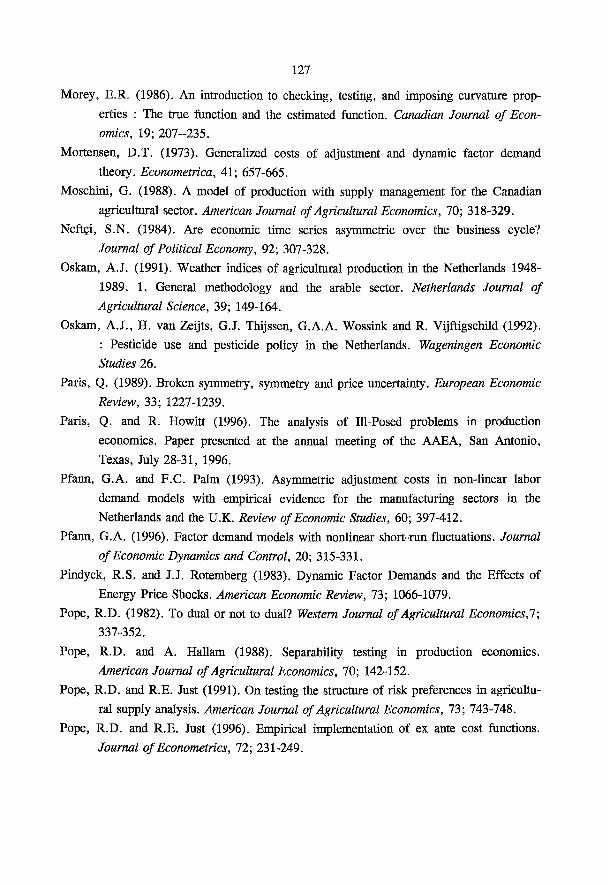
Morey, E.R. (1986). An introduction to checking, testing, and imposing curvature properties : The true function and the estimated function. Canadian Journal of Economics, 19; 207-235.
Mortensen, D.T. (1973). Generalized costs of adjustment and dynamic factor demand theory. Econometrica, 41; 657-665.
Moschini, G. (1988). A model of production with supply management for the Canadian agricultural sector. American Journal of Agricultural Economics, 70; 318-329.
Neftci, S.N. (1984). Are economic time series asymmetric over the business cycle? Journal of Political Economy, 92; 307-328.
Oskam, A.J. (1991). Weather indices of agricultural production in the Netherlands 1948-1989. 1. General methodology and the arable sector. Netherlands Journal of Agricultural Science, 39; 149-164.
Oskam, A.J., H. van Zeijts, G.J. Thijssen, G.A.A. Wossink and R. Vijftigschild (1992). : Pesticide use and pesticide policy in the Netherlands. Wageningen Economic Studies 26.
Paris, Q. (1989). Broken symmetry, symmetry and price uncertainty. European Economic Review, 33; 1227-1239.
Paris, Q. and R. Howitt (1996). The analysis of Ill-Posed problems in production economics. Paper presented at the annual meeting of the AAEA, San Antonio, Texas, July 28-31, 1996.
Pfann, G.A. and F.C. Palm (1993). Asymmetric adjustment costs in non-linear labor demand models with empirical evidence for the manufacturing sectors in the Netherlands and the U.K. Review of Economic Studies, 60; 397-412.
Pfann, G.A. (1996). Factor demand models with nonlinear short-run fluctuations. Journal of Economic Dynamics and Control, 20; 315-331.
Pindyck, R.S. and J.J. Rotemberg (1983). Dynamic Factor Demands and the Effects of Energy Price Shocks. American Economic Review, 73; 1066-1079.
Pope, R.D. (1982). To dual or not to dual? Western Journal of Agricultural Economics,!; 337-352.
Pope, R.D. and A. Hallam (1988). Separability testing in production economics. American Journal of Agricultural Economics, 70; 142-152.
Pope, R.D. and R.E. Just (1991). On testing the structure of risk preferences in agricultural supply analysis. American Journal of Agricultural Economics, 73; 743-748.
Pope, R.D. and R.E. Just (1996). Empirical implementation of ex ante cost functions. Journal of Econometrics, 72; 231-249.

Proefstation voor de Akkerbouw en Groenteteelt in de Vollegrond (PAGV, 1993). Kwantitatieve informatie voor de akkerbouw en groenteteelt in de vollegrond. Bedrijfssynthese 1993-1994, Publication number 69, Lelystad.
Rao, C. (1973). Linear statistical inference and its applications. Wiley, New York. Rothschild, M. (1971). On the Cost of Adjustment. Quarterly Journal of Economics, 75;
605-622. Saha, A., C.R. Shumway and H. Talpaz (1994). Joint estimation of risk preference
structure and technology using expo-power utility. American Journal of Agricultural Economics, 76; 173-184.
Saha, A. (1996a). Risk preference estimation in the nonlinear mean standard deviation approach. Draft working paper.
Saha, A. (1996b). A firm's choices under price risk : Duality results in the nonlinear mean-standard deviation framework.
Saha, A. and R.E. Just (1996). Duality under Uncertainty. Texas A&M University working paper.
Sandmo, A. (1971). On the Theory of the Competitive Firm Under Price Uncertainty. American Economic Review, 61; 65-73.
Shapiro, M. (1986). The dynamic demand for capital and labor. Quarterly Journal of Economics, 90; 513-542.
Shumway, C.R. (1983). Supply, demand and technology in a multiproduct industry: Texas field crops. American Journal of Agricultural Economics, 65; 748-760.
Shumway, C.R. (1989). Testing structure and behavior with first- and second-order Taylor series expansions. Canadian Journal of Agricultural Economics, 37; 95-109.
Shumway, C.R. (1995). Recent Duality Contributions in Production Economics. Journal of Agricultural and Resource Economics, 20; 178-194.
Sidhu, S.S. and C.A. Baanante (1981). Estimating Farm-level Input Demand and Wheat Supply in the Indian Punjab Using a Translog Profit Function. American Journal of Agricultural Economics, 63; 237-246.
Smithies, A. (1957). Economic Fluctuations and Growth. Econometrica, 25; 1-52. Stefanou, S.E., J. Fernandez-Cornejo, CM. Gempesaw and J.G. Elterich (1992).
Dynamic structure of production under a quota : The case of milk production in the Federal Republic of Germany. European Review of Agricultural Economics, 19; 283-299.
Szpiro, G.G. (1986). Measuring risk aversion : An alternative approach. Review of Economics and Statistics, 68; 156-159

129
Taylor, T.G. and M.J. Monson (1985). Dynamic factor demands for aggregate Southeastern United States agriculture. Southern Journal of Agricultural Economics, 17; 1-9.
Thijssen, G. (1992a). Micro-Economic Models of Dutch Dairy Farms. Wageningen Economic Studies 25.
Thijssen, G. (1992b). A comparison of production technology using primal and dual approaches : The case of Dutch dairy farms. European Review of Agricultural Economics, 19; 51-67.
Thijssen, G. (1994). Supply response and dynamic factor demand of Dutch dairy farms. European Review of Agricultural Economics, 21; 241-258.
Treadway, A.B. (1969). On Rational Entrepreneurial Behavior and the Demand for Investment. Review of Economic Studies, 36; 227-239.
Treadway, A.B. (1970). Adjustment Costs and Variable Inputs in the Theory of the Competitive Firm. Journal of Economic Theory, 2; 329-347.
Treadway, A.B. (1971). The Rational Multivariate Flexible Accelerator. Econometrica, 39; 845-855.
Tweede Kamer (1995). Notitie mest en ammoniak beleid. Vergaderjaar 1995-1996. 24445 nr. 1.
Tweede Kamer (1996). Wijziging van de Meststoffenwet. Vergaderjaar 1995-1996. 24782 nr. 2.
Vasavada, U. and R.G. Chambers (1986). Investment in U.S. Agriculture. American Journal of Agricultural Economics, 68; 950-960.
Wall, C.A. & Fisher, B.S. (1987). Modelling a multiple output production system: Supply response in the Australian sheep industry. Research report no.ll , Department of Agricultural Economics, University of Sydney, Sydney.
Wansbeek, T. and A. Kapteyn (1989). Estimation of the error components model with incomplete panels. Journal of Econometrics, 41; 341-361.
Weaver, R.D. (1983). Multiple input, multiple output production choices and technology in the U.S. wheat region. American Journal of Agricultural Economics 65; 45-56.
Wiley, D.E., W.H. Schmidt and W.J. Bramble (1973). Studies of a class of covariance structures. Journal of the American Statistical Association, 68; 317-323.
Wolf, C. and L. Pohlman (1983). The revovery of risk preferences from actual choices. Econometrica, 51; 843-850

130
Table 1.1 : Mean and standard deviation of variables in Chapter 2.
Variable Dimension/base year Symbol period : 1970-88 observations : 3249 number of farms : 733
mean standard deviation
Price indexes Output base year 1980 0.94 0.20 Pesticides base year 1980 v2
1.00 0.16 Other inputs base year 1980 0.93 0.22
Quantities Output prices of 1980 q. 299648 219578 Pesticides prices of 1980 -19822 16428 Other inputs prices of 1980 <h -96283 61588
land ares Ci 5289 3686 labour many ears * 10 C2 17.18 8.99 capital inventory value of machinery C3 138214 99999
and livestock (1980 prices)
technology trend (1970=1) c 4 10.90 4.81
Appendix I : Tables used in Chapter 2.

131
Table 1 . 2 : Derivation of price elasticities and elasticities of intensity from the parameters of the profit function
FFFAe eii eij %
GL 0 . 5 a . ( v , . * ) ° - 5 + a , .
3 „0-5 A _^ j-i (v, )0-5
( v / ) ° T„(4)054
NQ a . . . .
4=1 4=1 T) This is the expression for the price elasticity at the sample mean. The expression at other points
involves additional terms. £ = price elasticity netput i with respect to price j . 6. = elasticity of intensity of netput i with respect to fixed input j
ICj

132
Price indexes Output base year 1980 Vi 1.06 0.26 Pesticides base year 1980 v2
1.11 0.16 N-fertilizer base year 1980 v3
0.96 0.10
Quantities Output prices of 1980 qi 299504 220279 Pesticides prices of 1980 qa -19802 16413 N-fertilizer prices of 1980 qs -8090 7687 other inputs prices of 1980 q. -88158 557300
land ares Cl 5284 3682 labour manyears * 10 17.15 8.99 capital inventory value of machinery c 3 138031 99962
and livestock (prices of 1980)
other technology trend (1970=1) t 11.91 4.80 weather average weather =1 w 1.00 0.06
Appendix II : Tables used in Chapter 3.
Table II. 1 : Mean and standard deviation of variables used in Chapter 3.
Variable Dimension/base year Symbol period : 1970-'88 observations : 3258 number of farms : 733
mean standard deviation

133
Table JJ.2 : Results of e s t i m a t i o n
p a r a m e t e r e s t i m a t e s t a n d a r d e r r o r
p a r a m e t e r e s t i m a t e S t a n d a r d
e r r o r
«i -328874.14 20609.01 0 .30 0.03 a2 -4475.91 14679.78 P21 -2 .94 0.18 a3 1662.59 16304.74 P22 -95.02 36.25
ßi -23.87 5.64 P23 -0 .02 3E-3 ß 2
7300.49 2057.29 P31 -1 .29 0 .14 ß 3
0.20 0.19 P 3 2 -15.29 29 .60
Tt 4662.13 1890.69 J°33 -5E-3 3E-3
C d w -1742611.08 461972.59 T v l 7324.55 608 .14 « 1 1 23093.12 6808.41 T v 2
-996.65 69.77 « 1 2 -1389.45 539.66 7"v3 -84.92 56 .88 « 1 3 -702.46 447.08 " v i 252743.73 18360.47
«22 2105.39 1471.98 W v 2 6651.38 1602.97
« 2 3 416.31 993.78 <av3 50.22 1328.41 « 3 3 3620.95 1372.39 Tzl 0.27 0.15
ß l l 13E-5 2E-4 ra -62.28 49 .07
ßl2 10E-3 0.08 Ta -3E-3 5E-3
ß« 7E-6 7E-6 w z i 7.86 4.81
ß 2 2 42.55 30.25 -7233.71 1931.00 ß 2 3 -7E-3 2E-3 a)¿j -0.31 0 .17
ß 3 3 5E-7 3E-7 Tu -306.31 13.25
Pu 30.49 1.21 Www 1842471.01 47052.89 Pu 4872 .02 342.05

134
Appendix HI : Tables used in Chapter 4.
netput quantities1 fixed inputs profit1
farm CO crops other root- pesti N-fer- other Area CO - Area other Area root- Labour3 Capital1
class outputs crops cides tiliser inputs crops2 outputs2 crops2
1 10.43 295.96 121.32 -15.18 -4.75 -80.12 2.83 17.83 10.85 21.10 231.43 185.92 2 47.90 42.47 113.16 -12.66 -6.51 -36.01 13.99 8.67 17.36 12.27 134.40 118.12 3 125.20 111.67 401.70 -33.22 -13.00 -91.86 39.60 20.17 41.71 23.38 500.45 525.69 4 13.26 78.54 239.17 -25.50 -7.96 -66.55 3.93 11.39 32.44 14.22 235.52 143.81 5 41.09 26.69 303.15 -28.01 -13.81 -80.10 15.59 4.24 44.24 14.72 244.94 183.73 6 56.93 62.63 412.71 -50.95 -18.71 -88.31 20.09 13.57 57.70 17.30 429.12 267.56 7 32.94 100.31 132.72 -14.64 -4.09 -52.49 7.94 11.39 11.69 11.78 192.31 90.94 8 59.08 90.93 160.53 -18.06 -6.54 -57.83 14.90 15.41 16.74 13.09 280.13 98.53 9 126.62 116.90 263.75 -31.36 -12.45 -81.50 30.83 17.05 26.89 16.26 413.16 222.99 10 24.57 91.65 271.92 -21.33 -3.77 -71.70 6.06 9.08 22.05 14.31 279.89 166.34 11 67.21 97.31 361.84 -35.07 -9.58 -104.59 16.35 7.92 33.30 15.57 329.15 195.12 12 114.83 102.07 543.81 -47.91 -13.01 -122.87 27.15 9.69 46.07 24.84 635.15 346.85 sector 50.26 108.41 225.41 -23.14 -7.15 -70.17 12.59 12.72 22.70 14.83 287.88 158.80 T) 1980 guilders x 10* 2) hectares 3) manyears x 10
Table HJ..1 Average calculated values of variables in 1992.

135
Table JU.2 Actual values of endogenous variables in 19921. farm CO - other root- pesti- N-fer o'her Area CO Area profit class crops outputs crops cides tiliser !nputs crops other
outputs 1 8.97 356.54 117.19 -13.37 -3.93 -83.43 2.85 17.81 215.68 2 40.33 46.04 136.11 -11.23 -5.44 -38.73 11.18 11.48 105.67 3 124.84 114.56 518.73 -37.90 -18.05 -109.18 40.68 19.09 391.42 4 8.05 85.91 288.38 -24.03 -6.43 -70.55 2.62 12.67 180.14 5 36.91 23.52 357.23 -38.97 -11.69 -89.10 15.51 4.31 194.54 6 50.46 78.76 518.63 -50.71 -14.61 -95.66 16.76 16.90 322.49 7 29.46 114.79 140.82 -14.24 -3.71 -58.05 6.99 12.57 123.13 8 57.40 97.11 174.45 -17.14 -5.68 -61.01 14.21 16.10 149.33 9 128.61 125.94 291.43 -30.69 -10.49 -87.40 29.28 18.61 260.46 10 20.28 98.94 293.50 -20.94 -2.87 -73.89 5.25 9.89 202.49 11 66.75 115.29 416.04 -33.25 -9.05 -100.55 15.65 8.62 293.94 12 118.88 140.78 584.38 -47.23 -10.15 -141.95 25.29 11.55 416.95 sector 47.91 122.24 250.41 -22.34 -6.03 -74.59 11.57 13.75 197.70 1) See Table HI. 1 for dimensions
Table HI.3 Price elasticities in 1992 (weighted average). CO crops other outputs rootcrops pesticides N-fertiliser other
inputs CO crops 0.90 -0.44 -0.07 -0.12 -0.06 -0.21 other outputs -0.22 0.14 -0.07 0.01 0.00 0.14 rootcrops -0.01 -0.03 0.24 0.00 0.03 -0.23 pesticides 0.17 -0.03 0.00 -0.48 0.02 0.32 N-fertiliser 0.38 -0.06 -0.09 0.09 -0.25 -0.07 other inputs -0.24 0.03 0.51 0.14 0.01 -0.45 area CO crops 1.01 -0.51 -0.11 -0.11 -0.05 -0.23 area other outputs -1.03 0.51 0.11 0.11 0.05 0.25
Table III.4 Elasticities of intensity in 1992 (weighted average). area CO crops and area rootcrops
other outputs Labour Capital
CO crops 0.62 0.36 0.01 -0.23 other outputs 0.45 -0.24 0.21 0.40 rootcrops -0.12 0.66 0.14 0.12 pesticides 0.17 0.45 0.08 0.27 N-fertiliser 0.50 0.62 -0.07 -0.06 other inputs -0.04 0.28 -0.07 0.59 area CO crops 0.78 0.39 0.04 -0.33 area other outputs 1.22 -0.38 -0.04 0.33
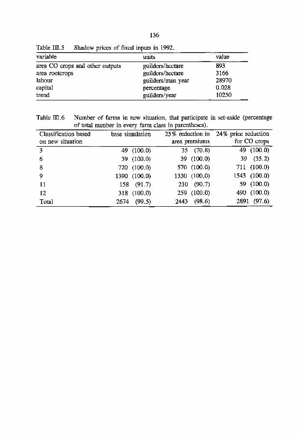
136
variable units value area CO crops and other outputs guilders/hectare 893 area rootcrops guilders/hectare 3166 labour guilders/man year 28970 capital percentage 0.028 trend guilders/year 10250
Table HI.6 Number of farms in new situation, that participate in set-aside (percentage of total number in every farm class in parentheses).
Classification based base simulation 25% reduction in 24% price reduction on new situation area premiums for CO crops 3 49 (100.0) 35 (70.8) 49 (100.0) 6 39 (100.0) 39 (100.0) 39 (35.2) 8 720 (100.0) 570 (100.0) 711 (100.0) 9 1390 (100.0) 1330 (100.0) 1543 (100.0) 11 158 (91.7) 210 (90.7) 59 (100.0) 12 318 (100.0) 259 (100.0) 490 (100.0) Total 2674 (99.5) 2443 (98.6) 2891 (97.6)
Table JH.5 Shadow prices of fixed inputs in 1992.

137
Table UI.7 Effects' of the new CO regime with a 25% reduction in area premiums (upper part) and with a 24% price reduction for CO crops (lower part). netput quantities miscellaneous
farm CO crops other outputs rootcrops pesticides N-fertiliser other Area Area of other % of profit class inputs CO
crops2
outputs total area set-aside
The new CO regime with a 25 % reduction in area premiums 1 -78.80 1.40 0.28 -5.56 -12.16 -2.43 -81.16 12.86 0.00 -0.43 2 -17.16 9.76 0.30 -6.67 -8.87 -14.54 -16.39 26.46 0.00 -4.32 3 -9.76 1.14 0.61 -3.76 -7.16 -15.58 -8.85 7.75 1.91 -3.57 4 -62.00 5.28 0.14 -3.31 -7.26 -2.20 -58.39 20.14 0.00 -0.72 5 -20.00 15.53 0.11 -3.01 -4.18 -5.73 -14.72 54.18 0.00 -1.62 6 -16.18 3.74 0.30 -1.91 -3.74 ^1.94 -12.98 12.57 0.99 -1.78 7 -16.14 2.56 0.05 -4.41 -10.64 7.46 -18.42 12.60 0.00 -3.36 8 -11.20 1.16 0.60 -4.38 -8.69 5.53 -12.50 6.56 1.81 -5.30 9 -8.49 -3.69 1.51 -4.05 -8.10 2.68 -10.19 -3.72 5.05 -6.24 10 -21.64 2.80 0.02 -3.03 -11.55 5.91 -24.13 16.11 0.00 -1.29 11 -9.82 -0.58 0.42 -2.38 -6.45 1.81 -11.50 5.15 2.56 -2.97 12 -9.50 -2.42 0.62 -2.58 -7.39 2.00 -11.65 0.64 3.74 -3.74 sector -14.63 1.24 0.47 -3.65 -8.50 2.75 -16.49 9.29 1.86 -3.16
The new CO regime with a 24% price reduction for CO crops 1 -12.95 0.17 -0.15 -1.93 -4.01 -0.54 -12.22 1.94 0.00 -0.13 2 -2.82 1.18 -0.16 -2.31 -2.93 -2.58 -2.47 3.98 0.00 -0.59 3 -7.48 -7.35 1.27 -3.55 -7.62 0.86 -7.08 -10.98 4.95 -1.63 4 -10.19 0.64 -0.08 -1.15 -2.39 -0.54 -8.79 3.03 0.00 -0.10 5 -3.29 1.87 -0.06 -1.05 -1.38 -1.04 -2.22 8.16 0.00 0.64 6 -6.66 -1.18 0.23 -1.03 -2.08 -2.01 -5.35 0.66 1.08 0.32 7 7.20 -1.79 -0.33 -0.32 -0.41 -3.97 9.02 -7.04 0.33 0.39 8 -1.74 -3.72 0.67 -2.03 -4.44 -1.15 -2.01 -7.29 3.03 0.91 9 -2.87 -7.54 1.40 -2.30 -5.07 1.22 -3.66 -17.14 5.42 -0.48 10 9.94 -1.90 -0.18 -0.18 -0.28 -3.13 12.17 -8.85 0.18 0.22 11 -1.69 -4.07 0.36 -1.11 -3.29 -1.23 -2.07 -16.75 2.89 0.54 12 -3.01 -7.47 0.60 -1.41 4.48 0.86 -3.91 -25.75 4.29 -0.46 sector -0.72 -2.65 -0.31 -1.29 -3.22 -1.27 -0.77 -7.77 2.26 0.00 Ti Percentage changes in quantities of netputs, area of CO crops and other outputs, land set-aside and profit compared to the calculated 1992 level 2: Excluding area set-aside

138
Appendix IV Tables used in Chapter 5.
Table IV. 1 Average values of endogenous variables by farm in base simulation.
farm CO crops' other root- pesticides' N-fer- other Area CO - Area set- Area other N-surplus profit1
class outputs' crops' tiliser1 inputs' crops2 aside in % outputs2 threshold 125 total area kg/ha
1 12.96 163.96 225.69 -23.37 -5.39 -5.29 -76.35 3.96 0.32 15.80 53.55 188.48 2 50.08 95.47 227.73 -21.28 -10.59 -71.23 12.11 2.30 13.11 50.87 141.57 3 16.07 93.77 210.90 -23.66 -11.87 -60.87 5.36 0.16 12.19 170.59 141.53 4 84.41 115.89 234.38 -26.78 -6.72 -71.77 20.04 4.84 10.35 161.53 195.41 sector 45.45 108.11 226.52 -22.56 -70.97 11.22 2.17 13.05 80.04 155.51
1) 1980 guilders x 10* 2) hectares
Table IV.2 : Results of simulation : no set-aside / no levy farm CO crops other rootcrops pesticides N-fer-tiliser other inputs Area CO - Area set-aside Area other N-surplus profit class outputs crops in % total outputs threshold 125
area' kg/ha2
1 1.8 0.2 -0.1 0.1 0.4 0.2 1.8 0 0.5 0.3 Û.1 2 4.2 1.8 -0.5 1.0 3.6 -0.5 5.3 0 3.4 2.5 0.3 3 0.7 0.2 -0.0 0.1 0.1 0.0 0.6 0 0.4 0.2 0.0 4 5.5 3.8 -1.2 1.8 3.7 -0.6 7.0 0 12.0 4.6 1.1 sector 4.3 1.5 -0.5 0.9 2.7 -0.3 5.3 0 3.5 2.2 0.4 1: Absolute level 2: Absolute change per hectare
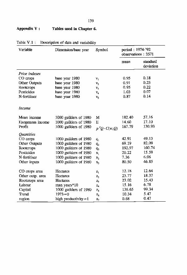
Appendix V : Tables used in Chapter 6.
Table V.l : Description of data and variability
Variable Dimension/base year Symbol period : 1974-'92 observations : 3571
mean standard deviation
Price indexes CO crops base year 1980 Vi 0.95 0.18 Other Outputs base year 1980 v2
0.91 0.25 Rootcrops base year 1980 v3
0.95 0.22 Pesticides base year 1980 v4
1.03 0.07 N-fertiliser base year 1980 v5
0.87 0.14
Income
Mean income 1000 guilders of 1980 M 182.40 57.16 Exogenous income 1000 guilders of 1980 E 14.60 17.10 Profit 1000 guilders of 1980 pTQ-C(w,Q) 167.79 130.93
Quantities CO crops 1000 guilders of 1980 q i 42.91 49.13 Other Outputs 1000 guilders of 1980 qz 69.19 82.09 Rootcrops 1000 guilders of 1980 q s 192.97 160.74 Pesticides 1000 guilders of 1980 20.22 15.59 N-fertiliser 1000 guilders of 1980 7.36 6.06 Other inputs 1000 guilders of 1980 80.50 46.85
CO crops area Hectares - 1 12.18 12.64 Other outp. area Hectares 23.77 18.37 Rootcrops area Hectares z3
23.02 15.43 Labour man years*10 - 4 15.16 6.78 Capital 1000 guilders of 1980 ~5 136.65 99.34 Trend 1973=0 - 6 10.34 5.47 region high productivity=1 ~7 0.68 0.47

140
Table V.2 : Parameter estimates and t-values.
parameter value t-value parameter value t-value
«0 33.861 5.15 X22 0.002 44.66 «1 15.184 3.85 X23 -0.000 -8.56 C Ü 15.494 3.07 X33 0.001 56.91 ß l -0.990 -2.49 7 1 1 -0.447 -1.91 (32 -2.913 -10.34 712 -0.024 -0.14 (33 0.174 1.02 713 0.493 20.09 (34 -3.152 -8.06 7 1 4 -0.251 -3.20 (35 -0.329 -10.40 715 -0.003 -0.39 (36 -2.935 -5.33 7 I 6 -0.144 -2.62 ß l -16.689 -4.85 717 -0.080 -0.18 XI 1.123 14.65 7 2 1 -1.002 -5.29 X2 1.296 27.87 7 2 2 0.939 6.81 X3 0.490 41.97 7 2 3 0.211 8.59 a l l -9.806 -4.14 7 2 4 0.277 4.19 a l 2 -3.648 -1.51 7 2 5 0.041 5.90 «22 -11.907 -3.17 T 2 6 -0.054 -0.71 (311 -0.040 -4.87 T 2 7 -3.362 -7.02 (312 0.142 31.48 5)11 0.205 4.15 (313 -0.014 -4.84 1112 0.062 1.93 314 0.048 7.96 JJ13 0.029 16.65 (315 0.009 21.44 i)21 0.228 6.00 (316 0.075 7.59 »/22 -0.151 -5.80 017 -0.116 -1.14 7,23 -0.019 -9.18 ß22 -0.008 3.95 f i l l -0.008 -4.01 023 0.002 1.03 1x12 -0.040 -33.4 324 -0.016 -4.02 ftl3 0.006 8.71 325 0.002 7.35 /xl4 -0.014 -11.03 326 0.074 11.82 1x15 -0.002 -22.21 327 0.062 0.78 1x16 -0.044 -22.28 333 0.007 2.93 fil8 -0.026 -1.49 334 0.004 0.70 ¿¿21 -0.030 -37.17 335 0.0004 0.93 ti22 -0.002 -8.91 336 0.015 1.85 ¿«23 0.006 32.11 337 0.802 8.13 1x24 -0.007 -20.41 344 0.021 1.36 ix25 -0.001 -19.61 345 0.006 5.58 1x26 -0.036 -35.82 346 0.060 3.76 1x28 0.075 11.20 347 0.670 3.48 Ii31 -0.001 -3.54 355 0.000 0.17 1x32 -0.00 -0.55 356 0.007 5.79 1x33 -0.003 -33.61 357 0.001 0.06 1x34 -0.001 -4.51 366 0.052 1.21 1x35 -0.000 -25.41 367 1.544 7.05 ¿¿36 -0.012 -24.94 M l 0.007 13.66 1x38 -0.120 -30.14 M2 0.006 32.94 y 0.116 17.15 M3 0.000 3.11 e 0.117 15.72

Appendix VI : Tables used in Chapter 7.
Table VI. 1 : Description of data and variability
Variable Dimension/base year Symbol period : 1971-'92 observations : 4040
mean standard deviation
Price indexes Rootcrops base year 1980 Vi 0.97 0.61 Other outputs base year 1980 0.97 0.68 Pesticides base year 1980 v3
1.07 1.27 N-fertilizer base year 1980 V 4 0.91 0.16
Land 1000 guilders Wi 1.29 0.47 Machinery - w2 0.15 0.02
Quantities Rootcrops 1000 guilders of 1980 Q i 188.85 151.12 Other Outputs 1000 guilders of 1980 Qa 108.96 94.61 Pesticides 1000 guilders of 1980 Q3
-19.56 15.24 N-fertilizer 1000 guilders of 1980 Q 4 -7.48 6.11 Other inputs 1000 guilders of 1980 Q5
-82.14 45.78
Rootcrops area Hectares K, 23.04 15.04 Machinery 1000 guilders of 1980 K2 135.39 96.27 Total land Hectares Zl 47.34 26.57 Labor man years*10 22 15.62 6.73
Trend 1970=0 t 11.75 5.86
Table VL2 : Estimates of ordered probit model.
parameter value t-value parameter value t-value
Pl2 0.248 1.47 E 1 2 0.006 3.59 I?22 0.371 1.13 E22 0.001 2.81 P32 0.238 0.31 G 21 -0.008 -7.01 P42 0.242 0.61 G22 -0.018 -4.01 P52 -1.405 -2.03 L2 0.021 0.77 M"'21 -0.179 -2.54 Cl 2.210 3.89
3.763 1.21 <h 1.568 35.09

142
Table VI.3 : Estimates of system of netput and dynamic factor demand equations. parameter value t-value parameter value t-value »n 2525.910 5.71 L, -0.013 -0.24 a ,2 222.976 0.60 U -0.053 -5.48 a'u -5775.800 -0.93 M„ -0.123 -16.36 «13 -92.460 -1.12 M u -0.001 -1.20 a l 4 -155.460 •4.05 M +
2 1 0.2678 4.83 »13 -516.780 -1.01 M+22 -0.105 -13.64 a 2i 70.937 0.79 0.013 0.09 a n 2115.480 1.29 -0.174 -8.12 A„ 80.389 0.37 o„ 52.454 17.32 A,2
153.671 0.90 260.688 20.72 A a 34.229 1.27 0 2 , 53.641 25.51 A„ 46.273 2.66 O22 87.871 10.11
-8.034 -0.03 03, -8.364 -24.31 -46.752 -0.75 0 3 2 -0.451 -0.31
A2 4 -80.912 -2.25 0 « 4.511 -30.92 171.186 2.54 0 « 6.895 11.42 -83.050 -2.26 O w
-18.646 -13.86 A44 22.658 0.56 o M
-32.666 -5.66 B„ 0.208 0.01 P.. 6.081 10.50 By 477.870 -1.91 P,2
-0.042 -0.40 B 22 5551.270 0.98 P2, -3.253 -8.07 B-,2
247.318 0.58 P22 0.394 5.33 B"22 2936.850 0.37 P„ -0.355 -5.48 c,, 104.238 1.67 P32 0.035 2.91 c2, 50.589 0.90 P4, -0.044 -1.56 c„ -0.493 -0.04 P« 0.028 5.46 c4, 3.211 0.52 P31
-1.128 4.52 c*,2 -1945.68 -3.00 P H
0.250 5.49 C 22 1954.420 2.64 R, 188.285 10.89 C%2 -373.730 -1.33 R, 44.496 2.98 C 42 499.449 2.68 R3 -21.763 -7.13 C 12 -1214.850 -1.34 R4 -5.653 -3.37
1589.090 1.76 R, -32.644 -2.98 ^32 -381.200 -1.18 s„ -7.738 -9.97
488.758 2.37 -6.756 -2.47 D„ -0.128 -2.01 sy -6.999 -0.80
0.246 1.04 S 22 -94.569 4.05 D22 -3.373 -2.63 S" 21 17.423 1.22 E„ 0.0002 0.01 45.815 1.04 E„ -0.003 -1.06 u, 3.314 0.99
0.001 1.55 U*2 12.866 0.35 F 8.858 3.59 U'2
33.707 0.80 G„ -0.003 -0.17 0"2u 23.495 2.17 G„ 0.001 0.49 °t. 12.960 0.85 G2, 0.013 0.26 Hi 1.234 4.64 G^ -0.015 -1.67 H2
6.343 6.45

143
Appendix VII : Netput equations of the Generalised Leontief, Quadratic and Symmetric Normalised Quadratic
Generalised Leontief 2 0.5 3 3 3 0.5
a i . VJ T " ^ a 0.5 „0.5 0
cj
V,- >1.<V/ V,- M >1 y-1 V,-
Normalised Quadratic 2 3
?/ = «/ + E a#v; + E 7iicj
Symmetric Normalised Quadratic

144
Appendix VDI : Elasticities of intensity, shadow prices of fixed inputs and profit after a quota.
Elasticities of intensity after a quota
Profit maximisation under the restriction of a vector of fixed inputs can be depicted analogous to (2.5) as :
T(v pv 2,z)=max{v 2- q2 + G(v1,q2,z);(q1,q2,z)eT;v1,v2>0} (VHJ.l)
Differentiating with respect to Vj and v 2 results into the netput equations : \ = ? , ( v 1 , f c ( v „ v 2 , z ) , z ) (vm .2) \ = <7 2 ( v i^ 2 ,z)
The same procedure as in section 3.2 can now be followed to obtain the elasticities of intensity, after the introduction of a quota on a former freely disposable netput, from the unconstrained profit function : G = 7 T - 7 T • ( ? T r 1 • 7 T (Vffl.4)
Shadow prices of fixed inputs and profit after a quota
When netput is constrained at level q/, constrained profit (if) is given by :
if(vvv2,q2\z) = G (vvq2\z) + v 2 - q2'
whereas unconstrained profit at level q/ is :
r(vvv2\z) = G (vvq2\z) + v2
s- q2' Constrained profit (if) and unconstrained profit (IT) are equal at shadow price v2
s for the constrained netput that yields q/ as the solution in the unconstrained profit function :
^(vvv2\q2* ,z) = ir(vvv2
s,z) Using (Vin.5)-(VJJI.7), the following relation between if and IT is obtained :
if(vvv2,q2' ,z) = ir(vvvlz) +(v2 -v2
s) • q2* W - 8 )
Differentiating (VTTI.8) with respect to z yields :
Since the expression between brackets is zero, it follows that the shadow price of fixed inputs after the introduction of the quota can be calculated by inserting the shadow price of the newly constrained netput into the unconstrained profit function (TT) (Fulginiti and Perrin (1993)). The effect on profit is calculated by determining the value of IT before and if after the introduction of the quota.

145
Appendix IX : Derivation of netput equations under the N-surplus tax
This Appendix shows how the parameters of G(.) in equation (5.4) in Chapter 5 can be obtained from parameter estimates of ir(.). The results given here are derived from Fulginiti and Perrin (1993) and applied to the situation here, where one input, the quantity of N-fertiliser (qs), is restricted. The pollution function also contains the area of CO crops, but this area is optimised in a latter stage. Fulginiti and Perrin (1993) derive the following relations between parameters of IT and G(.):
G, ""v.v.Ov.v)"1
(IX. 1)
v,v, vvt V.VA v . v / v.v, G = 7 T - T r ( î r ) _ 1 7 r
where e.g. G q 5 q 5 and 7 r v 5 v 5 are the second derivative of G(.) to q5 and IT to v5. Netput equations under a restriction on qs are :
Qi = «," a., a, '55 « 5 5 M
First order condition (5.6) is written as :
Vy + E y'=i
avPq Zj + — ft
« 5 5
(IX.2)
« 5 5 « 5 5 j^l ( * 5 5 ; = 1 « 5 5 ^55 y = l «55
and can be solved for qs as
ax .3 )
5 7
45* = «5
+ E»5y V y + E Vy + ^ t t 5 5 V 0 > i y-i
Inserting this in (IX.2) yields netput i equation under the N-surplus tax policy :
(IX.4)
a, + E ^ y (IX.5)
Samenvatting
146
Vanuit het Gemeenschappelijk landbouwbeleid en het milieubeleid krijgt de
landbouw in toenemende mate te maken met restricties die aan haar worden opgelegd.
Voorbeelden van milieubeleid die de Nederlandse akkerbouw zullen beïnvloeden zijn het
Meerjaren Plan Gewasbescherming en het mineralen beleid. Een doelstelling van het
MJP-G is o.a. het reduceren van het gebruik van pesticiden met 39% in 1995 en 60% in
2000. Het mineralen beleid beoogt een reductie van de vervuiling van het grond- en
oppervlaktewater door fosfaten en nitraten.
Het gemeenschappelijk landbouwbeleid (GLB) van de EU vormt een andere bron
van restricties die aan de akkerbouw in Nederland worden opgelegd. De hervorming die
in 1992 plaatsvond houdt in dat prijsondersteuning voor granen drastisch werd verlaagd
en dat deficiency payments voor oliezaden werden afgeschaft. Ter compensatie van de
ontstane inkomensdaling ontvangen producenten van deze gewassen nu subsidies per
hectare. Grote producenten die in aanmerking willen komen voor de hectare subsidies,
moeten echter een (tot nog toe per jaar verschillend) percentage van hun areaal met deze
gewassen braakleggen. Als gevolg van de hervorming van het GLB zullen de prijzen van
met name granen ook meer fluctueren dan het geval was onder het oude regime.
Het bepalen van de effecten van deze beleidsmaatregelen vereist dat de technische
details van de maatregelen expliciet worden gemodelleerd. Uitgangspunt bij het bouwen
van de modellen in dit proefschrift is de Neoklassieke produktietheorie gebruikt en in het
bijzonder de duale benadering daarvan. Bedrijven in de Nederlandse akkerbouw zijn
overwegend kleinschalige familiebedrijven, zodat er wordt voldaan aan de voorwaarde die
de produktietheorie stelt, namelijk dat producenten prijsnemers zijn in de markten van
inputs en outputs.
Zowel de theorie als de toepassing van de statisch (korte termijn) duale modellen
is reeds sterk ontwikkeld in de literatuur. Daarom is de eerste doelstelling van dit
proefschrift om de korte termijn effecten van de hiervoor besproken beleidsveranderingen
te bepalen. De toepassing van de dualiteitstheorie onder prijsonzekerheid verkeert nog in
het beginstadium van ontwikkeling. Daarom is een tweede doelstelling van dit proefschrift
om een bijdrage aan de literatuur te leveren in de vorm van duaal model onder
prijsonzekerheid. Investeringsbeslissingen kunnen worden gemodelleerd met behulp van
147
de dynamische dualiteitstheorie. Toepassingen van de dynamische dualiteitstheorie hebben
veelal gebruik gemaakt van geaggregeerde data. Gebruik van panel data levert echter een
groot aantal methodologische problemen op. Een derde doelstelling is dan ook om een
methode te ontwikkelen om investeringsbeslissingen te modelleren op bedrijfsniveau, met
gebmikmaking de dynamische dualiteitstheorie.
Het proefschrift begint echter met een meer algemeen hoofdstuk, waarin
verschillende flexibele functionele benaderingen van de winstfunctie worden getest op de
dataset van Nederlandse akkerbouwbedrijven die wordt gebruikt voor de te ontwikkelen
micro-economische modellen. Getest worden de Genormaliseerde Kwadratische, de
Symmetrisch Genormaliseerde Kwadratische, en de Gegeneraliseerde Leontief. Om de
verschillende functies tegen elkaar te kunnen testen wordt een Gegeneraliseerde Box-Cox
functie ontwikkeld die al deze ftmctievormen omvat als parameter restricties. Een
Lagrange Multiplier test, gebaseerd op "Doublé Length artificial Regression", kan deze
parameterrestricties testen zonder dat de Gegeneraliseerde Box-Cox ook daadwerkelijk te
schatten. De ftmctievormen worden ook vergeleken op criteria als het voldoen aan
regulariteitscondities en de mate waarin parameters significant zijn. Resultaten tonen aan
dat de Genormaliseerde Kwadratische functie in zijn geheel genomen beter voldoet dan de
overige functievormen.
Een stelsel van heffingen en input restricties is een optie voor de Nederlandse
overheid om de doelstellingen van milieubeleid te halen. Wanneer echter een input die
voorheen vrij beschikbaar (en dus variabel) was voor producenten, onder een
quotumrestrictie komt, heeft dit gevolgen voor de prijselasticiteiten van de overige inputs
en outputs. De overheid moet hiermee rekening houden, wanneer zij tegelijkertijd een
heffing/subsidie op een andere input of output legt. In hoofdstuk 3 wordt gekeken naar de
effecten van een quotering voor pesticiden op prijselasticiteiten, elasticiteiten van
intensiteit en schaduwprijzen van vaste inputs. Het effect van de pesticidenquotering op
prijselasticiteiten is klein, en het effect op de elasticiteit van intensiteit is afhankelijk van
de relatie die pesticiden voorheen had met de variabele inputs (complementen of
substituten). Schaduwprijzen van vaste inputs dalen als gevolg van de quotering aangezien
pesticiden een complementaire relatie hebben met alle vaste inputs.
De korte termijn effecten van de hervorming van het GLB in 1992 voor de

148
Nederlandse akkerbouw worden bepaald in hoofdstuk 4. Ten behoeve hiervan, wordt een
simulatiemodel ontwikkeld dat bestaat uit vraag- en aanbod vergelijkingen van inputs en
outputs die zijn geschat op paneldata van Nederlandse akkerbouw bedrijven. Elk bedrijf in
de steekproef heeft een bedrijfsspecifieke technologie door middel van bedrijfsspecifieke
(fixed effects) en regionale dummies. De resultaten van de simulaties worden
geaggregeerd voor verschillende groepen van bedrijven, en voor de sector als geheel,
door het aantal bedrijven in de sector dat elk bedrijf in de steekproef vertegenwoordigt te
gebruiken als gewicht. De simulaties tonen aan dat de productie van granen en oliezaden
met bijna 9% afneemt in 1996, terwijl de hoeveelheden van de overige outputs nauwelijks
verandert. Het nieuwe regime heeft ook een extensivering tot gevolg. De simulaties laten
verder zien, dat de meeste grote bedrijven reageren op de beleidsverandering door deel te
nemen aan de braakleggingsregeling. Het met het model gevonden percentage van het
totale akkerbouwareaal dat wordt braakgelegd komt dicht in de buurt van het werkelijke
percentage in 1993.
Het in hoofdstuk 4 ontwikkelde model wordt in hoofdstuk 5 uitgebreid met een
module waarin het gebruik van inputs en de samenstelling van het bouwplan worden
gerelateerd aan het N-overschot. Het N-overschot wordt op soortgelijke wijze bepaald in
de mineralen boekhouding voor akkerbouwbedrijven, die als onderdeel van het
mineralenbeleid wordt voorgesteld. In hoofdstuk 5 wordt een methode ontwikkeld
waarmee dit soort technische informatie kan worden opgenomen in een econometrisch
gebaseerd simulatiemodel, zodat het effect kan worden bepaald van verschillende
beleidsmaatregelen. In het hoofdstuk worden de effecten bepaald van een heffing op N-
overschot bij verschillende drempels van acceptabele verliezen en van een heffing op
kunstmest. Ook wordt gekeken naar de effecten van een verandering van het huidige GLB
op het N-overschot. Een heffing van 27 cent per kilo N-overschot bij een drempel van 75
kilo/hectare en een 18% heffing op kunstmest hebben de zelfde vermindering van het N-
overschot op sector niveau tot gevolg als een heffing van 1 gulden per kilo N-overschot
bij een drempel van 125 kilo per hectare. De N-overschot heffingen geven echter een
grotere impuls tot vermindering aan bedrijven met een groot overschot, en hebben op
sector niveau een lagere winstdaling tot gevolg dan de heffing op kunstmest.
In hoofdstuk 6 wordt gebruik gemaakt van een "Mean-Standard deviation"
nutsfunctie om licht te werpen op het effect van prijsonzekerheid op het gedrag van
149
Nederlandse akkerbouwers. In het bijzonder wordt getoond hoe de simultane areaal
allocatie en input/output beslissingen in een duaal model kunnen worden opgenomen. De
specificatie van de nutsfunctie die wordt gebruikt is flexibel genoeg om alle mogelijke
risico configuraties van producenten te kunnen testen. Verder wordt een methode
besproken om regulariteitscondities van de onderliggende indirecte nutsfunctie te testen.
Uit de resultaten van de testen blijkt voor Nederlandse akkerbouwers de risico
configuratie "Toenemend Absoluut Risico Avers/Constant Relatief Risico Avers" niet
wordt verworpen. Regulariteits condities van de onderliggende nutsfunctie worden
verworpen.
In hoofdstuk 7 wordt een methode ontwikkeld waarmee de dynamische
dualiteitstheorie kan worden gebruikt om investeringsbeslissingen te modelleren op
paneldata. Het ontwikkelde "Threshold model" houdt in dat investeringen nul zijn indien
de schaduwprijs van het investeringsgoed zich tussen een beneden - en boven drempel
bevindt. Investeringen zijn daarentegen positief (negatief) indien de schaduwprijs van het
investeringsgoed hoger (lager) is dan de boven (beneden) drempel. Afzonderlijke
vergelijkingen worden geschat voor negatieve en positieve investeringen. De parameters
uit beide vergelijkingen zijn significant verschillend van elkaar. Aanpassmgstermijnen
voor machines voor negatieve investeringen zijn 7-8 jaren voor desinvesteringen en 14
jaren voor investeringen. Ook worden voorwaardelijke (afhankelijk van
investeringsregime) korte en lange termijn prijselasticiteiten en elasticiteiten van intensiteit
bepaald.
In Hoofdstuk 8 tenslotte, worden een aantal veronderstellingen besproken die in
het proefschrift zijn gemaakt en worden resultaten uit verschillende hoofdstukken aan
elkaar gerelateerd. Tevens worden enige aanbevelingen gedaan voor toekomstig
onderzoek.

150
Publications
Boots, M., A. Oude Lansink and J. Peerlings (1997). Transaction costs and distortions in Dutch Milk quota trade. European Review of Agricultural Economics (forthcoming).
Oude Lansink, A.G.J.M. (1994). Effects of input quotas in Dutch arable farming. Tijdschrift voor Sociaal-wetenschappelijk onderzoek in de Landbouw, 9; 197-217.
Oude Lansink, A.G.J.M., and G. Thijssen (1994). The choice of the functional form. Wageningen Economie Papers 5, 1994.
Oude Lansink, A.G.J.M., and A.J. Oskam (1995). Landshare analysis of EU erop production. Tijdschrift voor Sociaal-wetenschappelijk onderzoek in de Landbouw 10; 174-190.
Oude Lansink, A.G.J.M., and J.H.M Peerlings (1995). Farm-specific impacts of quantitative restriction on N-fertiliser use in Dutch arable farming. Tijdschrift voor Sociaal-wetenschappelijk onderzoek in de Landbouw, 11; 40-60.
Oude Lansink, A.G.J.M., and J.H.M. Peerlings (1995). Farm-specific impacts of. Paper presented at the workshop on pesticides, Wageningen, August, 24-27, 1995.
Oude Lansink, A.G.J.M., and J.H.M. Peerlings (1996). Modelling the new EU cereals and oilseeds regime in the Netherlands. European Review of Agricultural Economics, 23; 161-178.
Oude Lansink, A.G.J.M., and S.E. Stefanou (1996). Asymmetric adjustment of dynamic factors at the firm level. Paper presented at the VJJI EAAE meeting, 3-7 September 1996, Edinburgh.
Oude Lansink, A., and G. Thijssen (1996). Testing among functional forms : An extension of the Box-Cox formulation. Paper presented at the AAEA meeting, 3-7 July 28-31, 1996, San Antonio.
Oude Lansink, A., and J. Peerlings (1997). Effects of N-surplus taxes : Combining Technical and Historical information. European Review of Agricultural Economics (forthcoming)

Curriculum
151
Alfons Oude Lansink werd geboren op 22 augustus 1967 te Fleringen (Overijssel). Van 1979 tot 1985 doorliep hij het Voorbereidend Wetenschappelijk Onderwijs (V.W.O.) op het Twents Carmellyceum in Oldenzaal. Vervolgens studeerde hij van 1985 tot 1987 Nederlandse Landbouw aan de H.A.S in Deventer; deze opleiding werd echter halverwege beëindigd. Na eerst de rnilitaire dienst te hebben vervuld begon hij in 1989 aan de studie Agrarische Economie waarbinnen hij in 1992 in de richtingen Agrarische Economie, Landbouwpolitiek en Agrarische Geschiedenis afstudeerde. Aansluitend is hij, eerst als Assistent in Opleiding (A.I.O.) en vanaf september 1996 als Post-Doctoraal onderzoeker, verbonden geweest aan de vakgroep Algemene Agrarische Economie van de Landbouwuniversiteit Wageningen.