Competition-dutch-coffee-market (2)

Research Memorandum

No 141

Competition on the Dutch coffee market

L. Bettendorf (CPB) andF. Verboven (UFSIA and Tilburg University)

Central Planning Bureau, The Hague, June 1998

Central Planning BureauVan Stolkweg 14P.O. Box 805102508 GM The Hague, The Netherlands

Telephone +31 70 33 83 380Telefax +31 70 33 83 350

ISBN 90 5635 112 50

The responsibility for the contents of this Research Memorandum remains withthe author(s)

CONTENTS Page

1. Introduction 3

2. The Model 6

3. Data sources and data handling 11

4. Results 12 4.1 Experiment 1 12 4.2 Experiment 2 14 4.3 Experiment 3 16

5. Understanding the evolution of the Dutch coffee industry 18

6. Concluding remarks 22

References 23

Abstract 25

3

1. Introduction

World coffee bean prices have shown large fluctuations during the past years. Consumerprices for roasted coffee, in contrast, have varied considerably less. Figure 1 illustratesthe relationship between coffee bean and consumer prices in the Netherlands. Beanprices dropped at the end of 1992, but consumer prices did hardly respond. When beanprices more than doubled in the middle of 1994 (due to a frost in Brazil), consumerprices increased by only 50 percent. Dutch industry observers have offered twoalternative explanations for the observed weak relationship between coffee bean andconsumer prices (N.R.C., 29 March 1997). First, coffee beans constitute only a part ofthe production costs for roasted coffee. Labor costs and packaging costs are otherpotentially important determinants. Second, coffee roasters may feel constrained to raisetheir prices by too much due to negative demand responses by consumers. If this is thecase, firms may absorb bean price increases by reducing their markups.

This paper seeks to carefully evaluate both the cost and the markup explanations for theobserved relationship between coffee bean and final consumer prices. For that purpose,we estimate a structural model of coffee supply and demand, following recent advancesin the growing field of the ‘New Empirical Industrial Organization’ (Bresnahan, 1989).The theoretical framework reveals that the cost explanation may be relevant to the extentthat labor and packaging influence the marginal cost of producing coffee. The markupexplanation may be relevant to the extent that firms recognize their oligopolisticinterdependence and behave closer to the cartel rather than the competitive outcome.The structural parameter estimates enables us to assess the relative importance of bothexplanations. In addition, they allow us to simulate the model and ask how prices wouldhave evolved under alternative assumptions on firm behavior, such as full cartel,Cournot duopoly or perfect competition.

A third explanation that is often used to explain the weak relationship between bean andconsumer prices (or, more generally, input and output prices) goes as follows. Coffeeroasters insure themselves against the price volatility of their main input by making longterm future contracts. If a coffee roaster has a contract that guarantees the sale of coffeebeans in six months at a price per kg of 3 guilders, an unexpected jump in the spot priceto 6 guilders does not affect its costs, so that there is no need to increase consumerprices. The problem with this argument is that it fails to distinguish between accountingcosts and economic (or opportunity) costs. Even if the futures contract enables the firmto purchase a certain amount at a cost of 3 guilders per kg, its opportunity cost is stillthe spot price of 6 guilders, since that is the price at which it would be able to resell itsbeans if it decided to do so. A main advantage of the ‘New Empirical Industrial

4

1 The application of competition policy in the agro-food sector is discussed in OECD(1996b).

60

80

100

120

140

160

180

200

220

Jan 1992 Jul 1992 Jan 1993 Jul 1993 Jan 1994 Jul 1994 Jan 1995 Jul 1995 Jan 1996 Jul 1996

world price consumer price

Organization’ approach is precisely that it does not rely upon accounting data tomeasure cost, but instead indirectly infers marginal costs from firm behavior, seeBresnahan (1989). Figure 1 Evolution of coffee price index (1990=100)

Within our structural framework the strong volatility in bean prices, mainly caused byexogenous weather conditions such as a late frost or enduring drought, provides a uniquenatural experiment to analyze the coffee roasters’ oligopolistic behavior. An analysis ofthis behavior is relevant because of the widespread suspicion that market power issignificant in the food-processing industries. Sutton (1991, Table 4.3) provides ampleevidence that a small number of firms dominates many food-stuff markets. Furthermore,OECD (1996a) reports that the agri-food sector, after the labor market, is the secondmost exempted or favorable treated area under competition laws.1 According to thisstudy (p. 23) ‘the limited coverage of competition laws in agriculture may depend lesson judgments about ‘appropriate’ economic considerations of natural monopoly andeconomies of scale and more on protectionist, political, cultural or national securityconsiderations’. It argues in favor of enhancing competition in the production and saleof agricultural goods.

5

2 A similar approach is followed by Bhuyan and Lopez (1997) to estimate oligopoly power in forty U.S. foodand tobacco industries. They found significant market power for the roasted coffee sector.

3 Karp and Perloff (1996) consider a dynamic model of the coffee market. Their focus is on export markets,whereas we consider a domestic market.

Despite the attention paid by policy makers, structural empirical applications on thepresence of market power in the food-processing industries remain relatively scarce, seefor example Lopez (1984) on the Canadian aggregate food sector, Buschena and Perloff(1991) on the coconut oil export market, and Genesove and Mullin (1995) on the U.S.sugar industry at the beginning of this century. Roberts (1984) considered the U.S.coffee industry and found quite competitive behavior2. Our approach differs quitesignificantly from Roberts’. First, we do not make use of accounting data to obtain adirect estimate of marginal costs, see Bresnahan (1989) for potential problems with suchdata. Instead, we indirectly infer marginal costs from the evolution of input prices,making use of a priori knowledge of the coffee roasting production process to restrictand interpret the parameters to be estimated. Furthermore, we fully integrate the demandside into our structural model, and carefully investigate the robustness of our resultswith respect to the choice of functional form. Our approach is made feasible by the largefluctuations of coffee bean prices.

Feuerstein (1996) considered the German coffee market. She estimates the long-runrelationship between bean prices and consumer prices in a dynamic error correctionmodel. Her approach, however, is not structural and does not allow to understand theprecise economic determinants of the relationship between both price series.Explanations of her empirical findings need to be found outside of her econometricframework.3

Our study makes use of publicly available data. The Dutch coffee market ischaracterized by one dominating firm, Douwe Egberts. This firm roughly accounts forbetween 60% and 70% of total sales. Many small firms compete in the remainingsegment. Imports are relatively small, though increasing.

The outline of the paper is as follows. Section 2 presents the econometric model basedon our prior knowledge of the coffee sector. The following section discusses the dataand the estimation procedure. Section 4 covers the empirical results. A final section usesour estimates to explain the evolution of consumer prices and simulate the model underalternative behavioral assumptions.

6

4 According to marketing studies, up to 25 percent of prepared coffee now ends in the kitchen sink (Trends,27 February 1997).

(1)

�-� �

0 0

(2)

2. The Model

The model consists of a demand and a supply side. Consumer demand for coffee isperfectly competitive and is represented by an aggregate demand function that ishomogeneous of degree zero in prices and income:

where Qt represents total coffee demand in period t, pt is the consumer price of coffee,pt

s is the price of a potential substitute tea, pt0 is the price of other goods, and yt is

income. An increase in the coffee price may reduce demand for several reasons. First,consumers may drink less and switch to substitutes. Second, they may use a lowerdosage of coffee. Finally, consumers may become more careful and prevent spilling.4

Notice that equation (1) ignores possible dynamic aspects of coffee demand, arisingfrom habit formation. We did experiment with a more general, dynamic demandspecification, based on Becker and Murphy’s (1988) rational addiction model, asimplemented on the U.S. coffee market by Olekalns and Bardsley (1996). Our empiricalresults generated imprecise parameter estimates, from which it was not possible to drawreliable inferences on habit formation and long term price elasticities. This follows fromthe fact that our data set covers a relatively short time period (5 years), with a strongmulticollinearity between the lagged and leaded variables in the dynamic specification.A longer time period is required to study the dynamic implications of habit formation.

Coffee supply is determined by the condition that perceived marginal revenue equal themarginal cost of production. Following the New Empirical Industrial Organization(Bresnahan, 1989), this condition can be written in aggregate form in the followingflexible way:

7

5 Various alternative interpretations for � have been given in the literature, such as the ‘conjectural variation’(the expected reaction of rival firms to output changes), or the weight firms put on other firms profits. Theseinterpretations have game-theoretic problems, so we prefer not to use these interpretations.

�- �

�

J(2)’

where mct denotes marginal cost in period t. The left hand side is the firms’ perceivedmarginal revenue and is now explained intuitively. The parameter - reflects factors thatdrive a wedge between the consumer price, pt, and the wholesale price of coffee,pt/(1+-), e.g.due to value added taxes. The parameter � captures the degree ofoligopolistic interdependence in the industry. If � equals zero, perceived marginalrevenue is equal to the (wholesale) market price, and coffee supply is perfectlycompetitive. If � equals 1, perceived marginal revenue is equal to the marginal revenueof a monopolist, so that the coffee industry effectively behaves as a cartel. In betweenthese two extremes are various models of oligopolistic interdependence, such as thewell-known Cournot model. When an estimate of � between zero and one is found, itis useful to stick to one clear interpretation of �. In the discussion of the parameterestimates below, we follow the interpretation of 1/� as the ‘Cournot-equivalent numberof firms’. This is the number of firms that is consistent with the data if one believes thatthe industry behaves according to the symmetric Cournot oligopoly model.5 Forexample, an estimate of � of 0.25 implies that the industry behaves as if there are fouridentical Cournot-competing firms in the industry. It is important to emphasize that theparameter � summarizes aggregate conduct in our framework. The degree of anti-competitive behavior by individual firms may deviate from this.

Our main research question is in understanding the relationship between coffee bean andconsumer prices. This does not imply, however, that we should focus exclusively onestimating the supply equation (2). As can be seen from slightly rearranging (2), theconsumer price for coffee depends on both marginal costs and the price elasticity ofdemand, Jt = -(0Q/0pt)(pt/Qt):

Bean prices influence consumer prices both directly through their impact on marginalcost, and indirectly through their impact on the price elasticity of demand. Given ourresearch question, it is therefore necessary to specify functional forms for both marginalcost and demand in the coffee market.

8

�-

�-

�

J(2)"

� � �

�

�(3)

Before we turn to this specification, it is useful to introduce the Lerner-index, L. Thisindex measures market power, and is defined as the percentage markup of price overmarginal cost. It can be easily computed from (2):

According to the Lerner index, market power is strong if there is strong oligopolisticinterdependence or if consumers feature inelastic demand.

Demand

Specify the following functional form for demand equation (1):

The intercept �0t contains a constant, linear terms for the price of tea and income, andthree quarterly season effects. The parameter � performs a Box-Cox transformation onthe coffee price variable, and is a convenient way to flexibly model the shape of thedemand curve. If � is equal to 1, demand is linear; if � is less than 1, demand is convex;and if � is greater than 1, demand is concave. Below we present estimates of the demandequation under three scenarios for the price variable: logarithmic (�=0), linear (�=1) andquadratic (�=2). The data did not show sufficient variability to estimate � precisely, soone should essentially view (3) as a convenient way to present the three demandspecifications.

Marginal costs

The theory of cost minimization implies that marginal costs are homogeneous of degree1 in input prices. In addition to this restriction, we use knowledge of the coffee roastingproduction process to impose two further restrictions on the cost function. As discussed

9

6 We limit ourselves to a discussion of ‘regular’ coffee. The production process of instant coffee, whichdiffers in the required capital investments, can be safely ignored since it has a relatively small consumptionshare of 12 percent, as reported in VNKT (1997).7 However, the constant returns to scale hypothesis was rejected for the U.S. coffee sector by Bhuyan andLopez (1997).8 We decided not to introduce a factor demand equation for coffee beans, although our data allow for this.The main reason is that short-run factor demand follows a complicated process due to speculative inventorybehaviour.

� � � � �(4)

�- � � � � �

�

�

�

(5)

for example in Sutton (1991), the production process is quite simple.6 It involvesroasting and grinding the coffee beans into the final coffee substance, which is thenpackaged for consumer use. Coffee beans, packaging and labor are essentially used infixed proportions. Furthermore, economies of scale in production are extremely limited,making average variable and marginal cost independent of output.7 These facts yield thefollowing fixed proportions, constant returns to scale specification for marginal cost:

where wtb is the price of coffee beans, wt

l is the wage rate and wt0 is the price of other

inputs (mainly packaging). The coefficient �1 can be interpreted as the transformationrate of beans into roasted coffee. According to experts, e.g. the International CoffeeOrganization, the production of one kg of roasted coffee requires 1.19 kg of beans.About 20 percent of the raw coffee beans consists of water and evaporates during theroasting process. This number is roughly confirmed by our data: during our completesample period, the total input demand for coffee beans (in kg) was 1.2 times the totaloutput of roasted coffee (in kg).8

It is now straightforward to complete the specification of the supply side (2). Computingthe demand derivatives from (3) and substituting marginal cost given by (4), rewrite thesupply equation after some rearrangements as:

10

where � is specified as 0, 1 or 2, in the logarithmic, linear and quadratic demandspecifications, respectively. We add error terms to equations (3) and (5), and estimatethe system simultaneously using the generalized method of moments (Hansen, 1982).This is a consistent and asymptotically efficient estimator. It takes into account theendogenity of price and quantity, using the exogenous demand and cost shifters asinstruments. Furthermore, it incorporates possible correlation between the error termsin both equations. Finally, it computes standards errors that are heteroskedasticity-consistent and robust to autocorrelation.

11

9 VNKT (1997, Table 7) reports that the share of arabica’s and robusta’s in total imports of green coffee was70% and 30% in 1996, respectively.

3. Data sources and data handling

The analysis is performed on the aggregated Dutch market with publicly availablemonthly data over the years 1992-1996. Production is measured as the sum of quantitiessold by domestic producers on the domestic and foreign markets (source: ‘Commissievoor Koffie en Thee’). Data on imports and exports of roasted coffee are taken from theCentral Bureau for Statistics (CBS, ‘Maandstatistiek van de Buitenlandse Handel’).Since figures on stock changes are missing, coffee consumption Qt is approximated asproduction minus net exports of roasted coffee. On average, 19% of consumption isimported. Series on consumer prices are reported in CBS, ‘Bijvoegsel van deMaandstatistiek van de Prijzen’. The same source reports total consumer expenditures,our measure for income.

Taxes, represented by -, were constant at 6 percent during our sample period. The priceof beans, wt

b, is computed as the ratio of the value to the volume of imported greencoffee, as published in CBS, ‘Maandstatistiek van de Buitenlandse Handel’. By takingthis measure for the bean price, an automatic correction is involved for the possiblychanging mix between the variants arabica and robusta9. Similarly, exchange ratemovements are automatically taken into account. Figure 1 (presented in theintroduction) plots the coffee bean and consumer price series. Wages, wt

l, arerepresented by the collectively negotiated wage for the food sector (source: ‘StatistischBulletin’ CBS). Data for prices of other variable inputs, wt

0, mainly packaging, are notpublicly available for the coffee industry. To resolve this issue, we conduct threealternative ‘experiments’. In our first experiment, we assume that other input pricesevolve according to the general price index; in our second experiment, we impose afurther restriction on the share of bean costs in average variable costs, based on industrywisdom; in our final experiment, we take a different perspective and assume that otherinput prices evolve according to the coffee bean price index.

12

10 For the U.S. Roberts (1984) reported a price elasticity of 0.25 whereas Pagoulatos et al. (1986) estimateda value of 0.11. However, Bhuyan and Lopez (1997) estimated an elasticity of 0.53. The estimate forGermany in Feuerstein (1996) equals 0.18.

4. Results

Before we present and discuss the empirical results of the full supply and demandmodel, it is useful to start with a brief discussion of the demand side separately. Allspecifications (logarithmic, linear and quadratic) yield positive, but insignificantestimates for the tea price and income variable, so we drop them in our full model. Thecoffee price coefficient is significantly negative. The implied price elasticity of demandroughly takes the same mean value of about 0.2 (in absolute terms) in all specifications,and is consistent with estimates for the U.S. and Germany.10 We can draw a firstinference about industry conduct from this robust result. Since marginal costs cannot benegative, supply equation (2)’ implies that the conduct parameter � cannot exceed theprice elasticity Jt, i.e. ��Jt. With our estimated elasticity, this means that � cannotexceed 0.2 so that cartel behavior can be rejected. This finding is just a restatement ofthe intuition that a monopolist (or cartel) operates at the elastic part of its demandfunction. More precisely, we may expect that the industry behaves as if there are at leastfive Cournot-competing firms.

We now turn to the results from the full model. Recall that we present results for threealternative demand specifications: logarithmic (�=0), linear (�=1) and quadratic (�=2).The data did not show sufficient variability to estimate � precisely: a point estimate ofaround -3.2 was obtained, with a large standard deviation of 16.8.

4.1 Experiment 1

In the first experiment, we assume that the other input prices, wt0, evolve proportionally

to the general price index, i.e. wt0=7 pt

0, where 7 is the factor of proportionality. Withthis assumption, the first term in equation (5) effectively becomes a constant, i.e.�0

*=7�0. The insignificant parameter estimates (for tea price, income and wages) areexcluded in our regressions.

The estimates of the demand coefficients are similar to the single equation estimatesdiscussed above. The �2, �3 and �4-coefficients reflect seasonal effects. Coffee demandis lowest in the first quarter and highest in the final quarter of a year. The marginal costsper kilo attributable to inputs other than beans, �0

*, vary between 4.5 and 5 real 1990

13

guilders in all three specifications. Interestingly, the transformation rate of beans intoroasted coffee varies between 1.4 and 1.8. This is of a same order of magnitude, thoughsomewhat larger than the rate of 1.19 implied by the production process of roastingcoffee. One explanation for this result is that there is not just a physical loss (of water)in the coffee production process, but also a percentage monetary loss on the value ofoutput, as reflected by the parameter - in equation (5). Taxes are one source of monetaryloss, and have already been taken into account using the observed tax rate of 6 percent.In addition, distribution and transportation costs may account for a systematic monetaryloss, at least to the extent that manufacturers need to pay for these services as apercentage on the value of output. At present, we have no prior knowledge on themagnitude of these percentage monetary losses. Assuming that the physical rate oftransformation equals 1.19, our results imply percentage monetary losses on the valueof output of around 18%, 41% and 47%, in the three respective specifications.

Table 1 Empirical results of experiment 1

Logarithmic demand Linear demand Quadratic demand

coefficient stand. error coefficient stand. error coefficient stand.error

�0 1.012 0.123 0.788 0.047 0.716 0.027

�1 6 0.143 0.046 6 0.109 0.031 6 0.819 0.209

�2 0.032 0.016 0.032 0.017 0.031 0.017

�3 0.039 0.019 0.038 0.019 0.035 0.019

�4 0.094 0.020 0.099 0.020 0.101 0.020

�0* 5.147 0.571 4.400 1.382 4.560 2.244

�1 1.408 0.151 1.676 0.055 1.810 0.179

� 0.033 0.022 0.028 0.025 0.016 0.026

J 0.209 0.067 0.211 0.061 0.233 0.060

L-index 0.156 0.087 0.134 0.112 0.070 0.110

Notes: GMM estimates with standard errors that are heteroskedasticity-consistent and robust toautocorrelation. The price coefficient is multiplied by 10 in the linear specification, and by 1000 in thequadratic specification. The price elasticity of demand and the Lerner index (computed by (2)’’) are evaluatedat sample mean values. The standard error of the estimated Lerner index is computed using the delta-method.

14

Finally, the conduct parameter � is estimated rather small in all specifications. In allspecifications, the hypothesis of monopoly (�=1) is rejected at a 5 percent significancelevel; the same is true for Cournot duopoly (�=0.5) and for any Cournot-equivalentnumber of firms less than twelve (�>.083). The hypothesis of perfect competition cannotbe rejected (�=0), but neither can the hypothesis of oligopolistic interdependence witha Cournot-equivalent number of 15 or more firms (�<.068). Despite the relatively smallestimates of �, the Lerner index of market power is relatively high, though impreciselyestimated. This is of course due to the low estimate for the price elasticity of demand,as can be seen from (2)’.

4.2 Experiment 2

In the previous experiment the part of costs attributable to inputs other than beans (theconstant) is estimated between 4.5 and 5 guilders per kilo, with a quite high standarderror in the linear and quadratic specifications. With a bean price of about 3 guildersduring the first (relatively stable) years of the studied period, beans have a cost share ofabout 55%, 52% and 54% in the logarithmic, linear and quadratic specifications,respectively. Although of a reasonable order of magnitude, we find these point estimatesrather low. A rough rule of thumb in the industry states that -- on average -- about 60%of total costs consists of bean costs (Financieel Dagblad, 3 May 1997). Given theimportance of fixed costs (e.g. advertising, as emphasized by Sutton, 1991), the shareof beans in the variable and marginal costs may even be higher, say 70%. We thereforenow conduct a second experiment. Assuming that bean costs have on average been afraction 7 of unit costs, one can easily check that the constant may be pinned at�0

*=�1(1/7-1)(wab/pa

0), where the subscript a denotes the average of a variableover the studied period. We estimate the three specifications with this restriction,setting 7 equal to 60% or 70%. The results are presented in Table 2.

The t-statistics on the first row test whether the 60 % and 70 % restrictions arerejected by the data, conditional on the maintained demand specification. Moreformally, based on the parameter estimates of Experiment 1, they test thehypothesis that the constant �0

* equals �1(1/7-1)(wab/pa

0) where 7 is 60% or 70%. Thet-statistics reveal that the restricted model cannot be rejected by the data in the linearand quadratic specification, both when the 60% and when the 70% rule are applied. Thisis intuitive given the relatively high standard errors of the constant in the unrestrictedmodel of experiment 1. In these two specifications, we may therefore interpret oursecond experiment as a way to incorporate our prior information to increase theprecision of our estimates. In the logarithmic specification, in contrast, both the 60% and

15

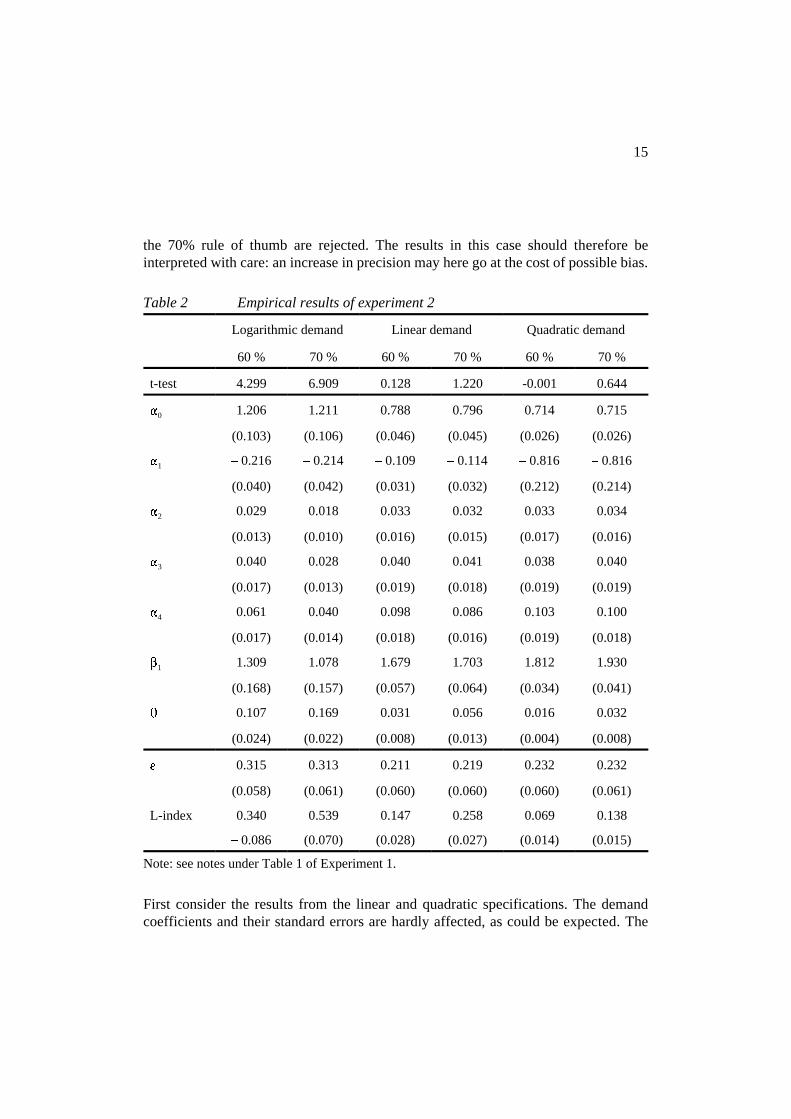
the 70% rule of thumb are rejected. The results in this case should therefore beinterpreted with care: an increase in precision may here go at the cost of possible bias.



60 % 70 % 60 % 70 % 60 % 70 %

t-test 4.299 6.909 0.128 1.220 -0.001 0.644

�0 1.206 1.211 0.788 0.796 0.714 0.715

(0.103) (0.106) (0.046) (0.045) (0.026) (0.026)

�1 6 0.216 6 0.214 6 0.109 6 0.114 6 0.816 6 0.816

(0.040) (0.042) (0.031) (0.032) (0.212) (0.214)

�2 0.029 0.018 0.033 0.032 0.033 0.034

(0.013) (0.010) (0.016) (0.015) (0.017) (0.016)

�3 0.040 0.028 0.040 0.041 0.038 0.040

(0.017) (0.013) (0.019) (0.018) (0.019) (0.019)

�4 0.061 0.040 0.098 0.086 0.103 0.100

(0.017) (0.014) (0.018) (0.016) (0.019) (0.018)

�1 1.309 1.078 1.679 1.703 1.812 1.930

(0.168) (0.157) (0.057) (0.064) (0.034) (0.041)

� 0.107 0.169 0.031 0.056 0.016 0.032

(0.024) (0.022) (0.008) (0.013) (0.004) (0.008)

J 0.315 0.313 0.211 0.219 0.232 0.232

(0.058) (0.061) (0.060) (0.060) (0.060) (0.061)

L-index 0.340 0.539 0.147 0.258 0.069 0.138

6 0.086 (0.070) (0.028) (0.027) (0.014) (0.015)

Note: see notes under Table 1 of Experiment 1.

First consider the results from the linear and quadratic specifications. The demandcoefficients and their standard errors are hardly affected, as could be expected. The

16

major change occurs at the supply side: the standard errors drop quite dramatically incomparison with the results in Table 1. We can therefore become more confident in ourresults on cost and conduct, which were still presented very cautiously in theunrestricted first experiment. Since our estimate of �1 remains quite high compared tothe value of 1.2 for the physical rate of transformation of beans into roasted coffee, itis likely that there are indeed also systematic monetary losses involved in the long chainfrom production to final consumption. The point estimates of the conduct parameterincrease, especially under the 70% rule. Due to the substantially increased precision ofour estimates (at no cost of bias), we now reject the hypothesis of perfectly competitivebehavior in favor of oligopolistic interdependence. The industry roughly behaves as ifthere were a Cournot-equivalent number of firms between 25 and 30. Finally, the Lernerindex which summarizes market power is estimated much more precisely. Under the 70% rule it becomes quite high. The outcomes are between the U.S. estimates of 6%,obtained by Roberts (1984), and 51% by Bhuyan and Lopez (1997).

Next consider the logarithmic specification, in which the 60 % and 70 % restrictionswere not supported by the data. More care in the interpretation should be taken here,since some of the parameters may now be biased. One example of this may be theestimate of the price elasticity (evaluated at the sample mean), which becomes muchlarger than in the other specifications. The estimate of the conduct parameter is alsomuch larger, consistent with a Cournot equivalent number of firms of 10 (60 % case)and 6 (70 % case). The overall effect of the increased elasticity and increased conductparameter on the estimated Lerner-index is positive: it reaches values of .34 and .54.

4.3 Experiment 3

Experiment 1 and 2 have been based on the assumption that other factor prices moveaccording to the general price index. In our final experiment, we take a quite differentdirection and arbitrarily assume that other factor prices evolve according to bean prices.This is equivalent to assuming that coffee beans have a constant share of marginal costs,i.e. �1wt

b=7mct, at every period t. The specification for marginal costs then becomesmct=�1wt

b/7, where 7 is set to 60%. Note that in this specification the constant term ofexperiment 1 effectively drops, so that we can apply a standard nested hypothesis test(as in experiment 2) to examine the plausibility of our third experiment. The results arepresented in Table 3. The t-statistics (based on Table 1 estimates) reveal that for allspecifications the restriction implied by Experiment 3 is rejected.

17



coefficient stand.error



t-test 9.010 3.183 2.032

�0 1.152 0.114 0.805 0.044 0.717 0.025

�1 6 0.189 0.045 6 0.117 0.031 6 0.805 0.212

�2 0.010 0.006 0.027 0.012 0.033 0.014

�3 0.016 0.008 0.039 0.015 0.042 0.018

�4 0.025 0.009 0.065 0.013 0.088 0.016

�1 0.453 0.089 1.067 0.047 1.318 0.037

� 0.215 0.040 0.103 0.024 0.065 0.016

J 0.275 0.065 0.226 0.060 0.229 0.060

L-index 0.782 0.047 0.458 0.023 0.284 0.015

Note: see notes under Table 1 of Experiment 1.

Given the high t-statistics, extreme caution should be taken in interpreting the - possiblybiased - parameter estimates in this experiment. We note here that the bean pricecoefficient is significantly below the physical rate of transformation, a result that isdifficult to interpret economically. We also observe that the precision of the supplyparameters is not improved relative to the unrestricted model of Experiment 1. We leavean interpretation of the other parameter estimates to the reader.

18

11 An analytic solution to (3) and (5) is easily obtained for the linear and quadratic demand specification; forthe logarithmic specification, the solution was obtained numerically.

5. Understanding the evolution of the Dutch coffee industry

We now use our estimates to more closely analyze the evolution of the Dutch coffeeindustry during our sample period, 1992-1996. Based on our parameter estimates, wefirst simulate our two equation model (3)-(5) and compute the endogenous price andquantity variables under alternative behavioral scenarios: perfect competition (�=0),duopoly (�=0.5) and monopoly (�=1).11 Next, we explain the evolution of actual prices,and compare this with the evolution of prices under alternative modes of conduct. Wefocus on the changes that occurred during 1994, the year of the drastic bean priceincreases due to the frost in Brazil.

We base our analysis on the results of experiment 2 (60 % case), our preferred model.As discussed above, experiment 2 imposed the restriction based on our prior informationthat bean costs on average made up about 60 % of marginal costs. This restriction wasnot rejected by the data in the second and the third specification.

Consider first the prices evaluated at the sample mean. If the industry would be able toenforce a cartel (monopoly) instead of the current situation, prices would more thandouble (+120 %) in the quadratic specification, more than triple (+230 %) in the linearspecification, and increase to almost 10 times the current value in the logarithmicspecification. In contrast to our econometric estimates, the simulation results are quitesensitive to the demand specification that has been used. This is quite intuitive: themonopoly prices are an out of sample prediction and depend crucially on the specifiedcurvature of the demand function, which could not be estimated precisely. Naturally,monopoly prices are predicted to be the largest in the convex demand specification. Amore precise idea on the monopoly prices may be obtained if the curvature of thedemand function can be estimated more precisely. Whatever the specification, thesimulations show that prices would increase substantially if the monopoly outcomecould be enforced. Even a duopoly would charge much higher prices than is presentlythe case. These findings should be kept in mind if concentration in the coffee sectorwould grow in the future and move the equilibrium closer to the monopoly outcome.

19

Table 4 Evolution of the Dutch coffee industry under alternative behavioralassumptions, 1992-1996

mean standarddeviation

minimum maximum change from1:1994 to1:1995

logarithmic demand specification (convex)

elasticity 0.319 0.035 0.254 0.418 + 0.040

Lerner-index 0.340 0.037 0.257 0.422 6 0.047

marginal cost 8.25 1.53 6.29 11.61 + 4.23

actual price 13.19 2.09 11.02 17.71 + 5.08

duopoly price 56.17 5.18 47.31 67.15 + 6.20

monopoly price 121.90 11.86 103.83 140.59 + 3.88

linear demand specification

elasticity 0.215 0.048 0.154 0.337 + 0.108

Lerner-index 0.151 0.030 0.092 0.201 6 0.073

marginal cost 10.58 1.96 8.05 14.88 + 5.42

actual price 13.19 2.09 11.02 17.71 + 5.08

duopoly price 32.26 1.77 29.52 36.74 + 3.61

monopoly price 43.11 1.97 40.08 47.72 + 2.71

quadratic demand specification (concave)

elasticity 0.244 0.097 0.139 0.462 + 0.253

Lerner-index 0.075 0.026 0.035 0.116 6 0.064

marginal cost 11.42 2.11 8.69 16.07 + 5.85

actual price 13.19 2.09 11.02 17.71 + 5.08

duopoly price 24.38 1.18 22.68 27.38 + 2.97

monopoly price 29.97 1.06 27.36 31.68 + 2.30

bean price 3.78 1.17 2.28 6.35 + 3.23

Note: The results are based on the estimates of Table 2 (60 % case). Model simulations on equation (3) and (5) forperfect competition (�=0), duopoly (�=0.5) and monopoly (�=1). Marginal cost and prices are expressed in real terms.

20

12 For the linear and the quadratic specification, this is directly clear from our reported t-statistics in Table2 which do not reject a share of other inputs of 40 %. For the logarithmic specification, a share of 40 % isrejected, because shares of even larger than 40 % are in fact favoured by the data.

�

�

�

J �

�J

J

(6)

�

�

�

�

Next, consider the evolution of actual and simulated prices during our studied period.Consider in particular the changes that took place during 1994, in response to theupward jump of bean prices by 3.23 guilders, or 104%. Consumer prices increased byonly 45%. To interpret this, consider equation (2)’, from which it can be derived thatconsumer prices changes (in percentage terms) can be decomposed in marginal costchanges and changes in the price elasticity of demand:

The percentage increase in marginal cost in (6) can in turn be written as the weightedsum of percentage increase in bean prices and other factor prices:

where the weight stb is the share of bean costs in marginal costs.

The jump of the bean prices by 3.23 guilders, or 104%, is directly expressed in anincrease in marginal costs by a larger absolute amount, between 4.23 and 5.85 guildersin Table 4. The percentage increase in marginal costs, however, is smaller, e.g. only57% in the linear demand case. This is due to the relatively large share of costs otherthan bean costs, which did not follow the same evolution as the bean prices. A share ofat least 40 % (on average) could not be rejected by the data.12 Therefore, the costargument hypothesized in the introduction, accounts for at least part of the explanationfor the weak relationship between bean and consumer prices.

A second dampening effect on consumer prices may stem from markup absorption. Howimportant was this during the 1994 shock? As can be read from the second term inequation (6), markup absorption takes place provided that (1) there is oligopolisticinterdependence (�>0), and (2) the price elasticity of demand increases with consumerprices. Table 4 shows that the price elasticity indeed increased during the 1994 bean

21

13 Our results on markup absorption partly follow from the demand specification (3), which implies (for ourthree specifications) that the price elasticity of demand is increasing in price (in absolute value). We did notconsider a constant elasticity specification, implying constant percentage markups, since in this case theconduct parameter � is not identified (Bresnahan, 1982). A specification with decreasing (in absolute value)price elasticity of demand is unconventional and economically unappealing. If we had imposed such aspecification, then the reverse of markup absorption would have occurred (if �>0). In any event, ourconclusion that marginal costs rather than markups explain the weak relationship between coffee bean andconsumer prices would remain unaltered.

14 Note that the mentioned markup change (-8%) and marginal cost change (+57%) do not exactly add upto the consumer price increase of 45%. This is because the changes are large, so that an interaction termcannot be neglected.

15 The only exception to this statement is the move towards duopoly in the logarithmic specification. In thiscase prices would have increased by more than was actually the case in absolute terms (though prices wouldagain have increased by less in percentage terms).

price shock, especially in the linear and quadratic specifications (increases by about 50%and 100%, respectively). This led to a reduction in the markups, e.g. by -8% in the lineardemand case. This is not much, due to the fact that the conduct parameter �, thoughsignificant, was estimated to be relatively small13. In sum, we find that the 1994 increasein consumer prices by 45%, compared to an increase in the bean prices by 104%, canbe explained partly by markup absorption (-8% under linear demand), but for the mostsignificant part by the modest increase in marginal cost (only 57% under linear demand)because of the relatively large share of other costs than bean costs14 .

We finally ask how prices in 1994 would have responded if behavior had been differentfrom what we actually observed. We consider both duopoly (�=0.5) and monopoly(�=1). In this case, markups would be much larger as shown by the mean predictedprices discussed above. Equilibrium price elasticities of demand (not shown) would nowbe well above unity. As the last column of Table 4 indicates, both the absolute andpercentage price increases of coffee would be even less than what was actuallyobserved.15 This follows of course from the fact that under duopoly and monopolymarkup absorption becomes quantitatively more important.

22

6. Concluding remarks

This paper has analyzed the observed weak relationship between coffee bean andconsumer prices in the Netherlands. Using a structural model of oligopolisticinteraction, it is shown that the relatively large share of costs other than bean costs isresponsible for a substantial part of the observed weak relationship. The remaining partfollows from markup absorption, but is less important since oligopolisticinterdependence is relatively competitive. Simulations of the model show that consumerprices would have been much higher and fluctuated even less in response to bean pricefluctuations if the industry had behaved according to a Cournot duopoly or a cartel.

We employed publicly available data on the Dutch coffee market. The strong volatilityof bean prices has provided a natural experiment to analyze firm behavior. Given themoderate data requirements, we hope that our analysis will stimulate further researchto investigate firm behavior and market power in other sectors of the economy.

At the same time, there is room for a more in-depth analysis of firm behavior in thecoffee industry, provided that additional data can be obtained. With firm-level data, itbecomes possible to analyze firm-specific oligopoly behavior. The present analysisreveals interdependent, though rather competitive conduct at the aggregate level, but itis possible that one of the firms possesses strong individual market power. Furthermore,more detailed data would allow to consider interesting dynamic aspects in the industry.For example, inventory costs, adjustment costs or consumer loyalty may to some extentinfluence the relationship between bean prices and consumer prices.

23

References

Becker, G.S. and K.M. Murphy (1988), A theory of rational addiction, Journal ofPolitical Economy 96, 675-700.

Bhuyan, S. and R.A. Lopez (1997), Oligopoly power in the food and tobacco industries,American Journal of Agricultural Economics 79, 1035-1043.

Bresnahan, T.F. (1982), The oligopoly solution concept is identified, Economics Letters10,87-92.

Bresnahan, T.F. (1989), Empirical studies of industries with market power, in R.Schmalensee and R.D. Willig (ed.), Handbook of Industrial Organization, North-Holland.

Buschena, D. and J. Perloff (1991), The creation of Dominant Firm Market Power inthe Coconut Oil Export Market, American Journal of Agricultural Economics 73,1000-1008.

Feuerstein, S. (1996), Do Coffee Roasters Benefit from High Prices of Green Coffee?,Tinbergen Institute Working Paper, TI 96-133/4.

Genesove, D. and W.P. Mullin (1995), Validating the conjectural variation method: thesugar industry 1890-1914, NBER Working Paper 5314, Cambridge MA.

Hansen, L.P. (1982), Large sample properties of Generalized Method of Momentsestimation, Econometrica 50, 1029-54.

Karp, L.S. and J.M. Perloff (1996), Dynamic models of oligopoly in rice and coffeeexport markets, in D. Martimort (ed.), Agricultural markets: mechanisms, failures andregulations, North-Holland, 171-204.

Lopez, R.E. (1984), Measuring oligopoly power and production responses of theCanadian food processing industry, Journal of Agricultural Economics 35, 219-30

OECD (1996a), Antitrust and market access; the scope and coverage of competitionlaws and implications for trade, Paris.

24

OECD (1996b), Competition policy and the agro-food sector, Internet version, Paris.

Olekalns, N. and P. Bardsley (1996), Rational addiction to coffee: an analysis of coffeeconsumption, Journal of Political Economy 104, 1100-1104.

Pagoulatos, E. and R. Sorensen (1986), What determines the elasticity of industrydemand, International Journal of Industrial Organization 4, 237-50.

Roberts, M.J. (1984), Testing oligopolistic behavior, International Journal of IndustrialOrganization 2, 367-83.

Sutton, J. (1991), Sunk costs and market structure, MIT Press, Cambridge.

Vereniging van Nederlandse Koffiebranders en Theepakkers (Association of Dutchcoffee and tea producers) (1997), Jaarverslag 1996, Amsterdam.

25

16 We thank R. Alessie, J. Boone, M. Canoy, H. Degrijse, R. van Assouw and H. Vandenbussche for helpfulcomments. We are grateful to R. Rosenbrand (CPB) and P. van der Salm (Commissie voor Koffie en Thee)for data collection. Corresponding author: L. Bettendorf, CPB, P.O. Box 80510, 2508 GM Den Haag, TheNetherlands, email: [email protected].

Abstract16

World coffee bean prices have shown large fluctuations during the past years, whereasconsumer prices for roasted coffee have varied considerably less. This paper seeks toexplain the weak relationship between coffee bean and consumer prices. We adopt andestimate an aggregate model of oligopolistic interaction. It is shown that the relativelylarge share of costs other than bean costs accounts for the most important part of theweak relationship between bean and consumer prices. The remaining part follows frommarkup absorption, but is less important since oligopolistic interdependence is relativelycompetitive. The estimates are used to simulate the model under alternative behavioralassumptions: duopoly and monopoly. The computations show that consumer priceswould have been much higher and would have fluctuated even less (due to greatermarkup absorption) under these alternative regimes.

Keywords: coffee market, oligopoly power

Competition-dutch-coffee-market (2)

Documents

Transcript of Competition-dutch-coffee-market (2)