Methods for Haplotype Anaysis

Shehnaz K. Hussainskhussain@ucla.edu

Epidemiology 244

Outline

Definitions (review)Background: Why are haplotypesimportant in genetic association studies?How are haplotypes inferred?How are haplotypes analyzed?

Traditional methodsHaplotypes vs. diplotypesHaplotype reduction methods

? T ? G ? A

? T ? G ? A

A T G G A A

T T C G T A

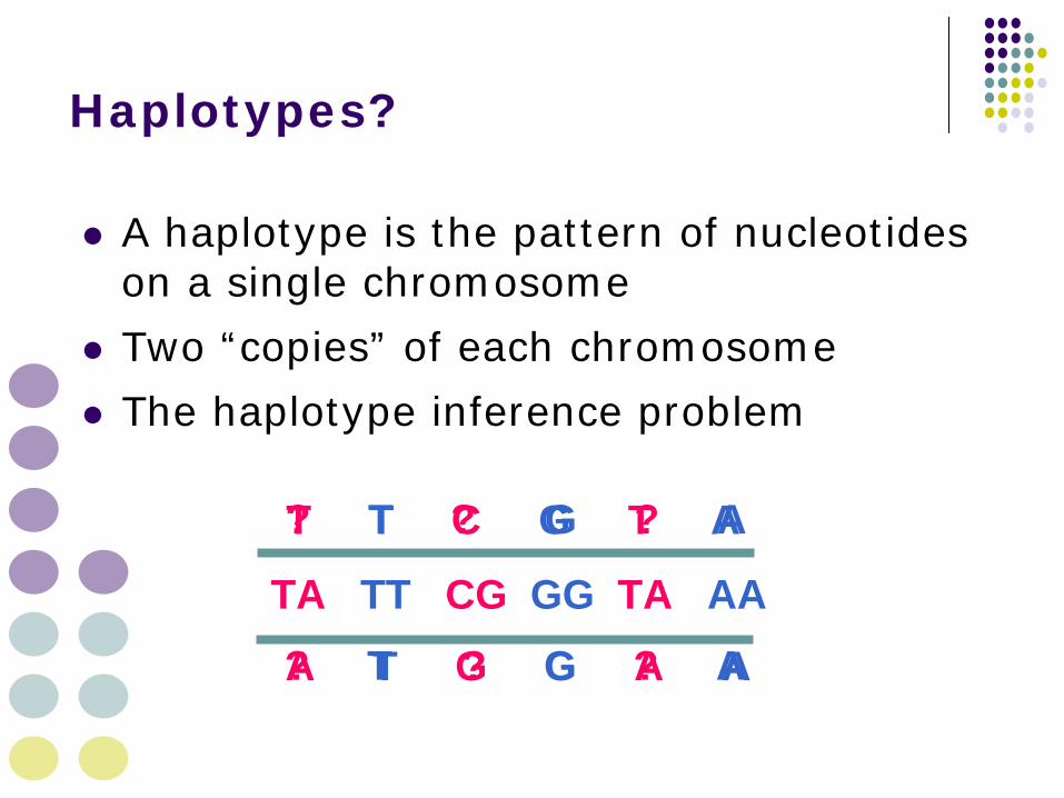
Haplotypes?

A haplotype is the pattern of nucleotides on a single chromosome

Two “copies” of each chromosome

The haplotype inference problem

TA TT CG GG TA AA

T T C G T A

A T G G A A

Diplotypes?

A pair of haplotypes is called a diplotype

Diplotypes are to haplotypes, what genotypes are to allele

Linkage Disequilibrium (LD)?

LD describes the association between alleles on the same haplotype

Two popular LD statistics: D´ , r2

Example: 2 SNPs, 4 possible haplotypes

A B

A B Unequal allele frequency, allelic association is as strong as possible

3 haplotypes observed

No detected recombination between SNP

D´ = 1

r2 < 1

Complete LD

Perfect LDA B Equal allele frequency,

allelic association is as strong as possible

2 haplotypes observed

No detected recombination between SNP

D´ = 1

r2 = 1

Background

Why do we care about haplotypes?

Known SNPs do not capture all patterns of variation in the human genomeBasing haplotypes on known SNPs will increase the diversity of observable patterns of variation

L. Kruglyak and D. Nickerson, Nat Genet 27:234-236 2001

minimal allelefrequency

expected SNPs(millions)

expected SNPfrequency (bp)

expected % indatabase

1% 11.0 290 11-1210% 5.3 600 18-2030% 2.0 1570 23-2740% 0.97 3280 24-28

Why do we care about haplotypes? (2)

Help us identify associations with the causal variant if the causal variant is rare and on one of our observed haplotypes

Used to address higher order associations (G X G effects)

Statistical Inference of Haplotypes

When is phase ambiguous?

Haplotypes can be reconstructed with 100% accuracy if no more than 1 SNP is heterozygous

Otherwise, phase is ambiguous and there will be uncertainty

Genotype AA Aa aa

BB AB AB AB aB aB aB

Bb AB Ab AB ab or Ab aB aB ab

bb Ab Ab Ab ab ab ab

Algorithms for Haplotype Inference

Bayesian methodse.g. PHASE (Stevens, 2002), HAPLOTYPER (Niu, 2002)

Likelihood-based methodExpectation-Maximization algorithm: e.g. SNPHAP (Clayton, 2001), Haploview(Barret, 2005)

Haplotype Analysis

There are MANY approaches: programs in SAS GENETICS, Stata, R

Zhao et al. (2000) Hum HeredEHPLUS/GENECOUNTING, global+haplotype specific tests

Zaykin et al. (2002) Hum HeredHTR, Haplotype trend regression

Schaid et al. (2002), Lake et al. (2003), Burkett et al. (2004) Hum Hered

haplo.score, haplo.stats and hapassoc, generalised linear model (GLM) framework

Zhao et al. (2003) Am J Hum GenetHplus, generalised estimation equations (GEE) framework

Epstein & Satten (2003) Am J Hum GenetCHAPLIN, logistic regression

Tzeng et al. (2006) Am J Hum GenetR program, GLM with haplotype clustering

PHASE (Stevens, 2002)

Haplotype reconstruction, and recombination rate estimation from population data

Can get global p-value for binary outcome

Linux and Windows

fastPHASEHandles larger data-sets (e.g., hundreds of thousands of markers in thousands of individuals)

Haplotype estimates are slightly less accurate

PHASE input data format10974P 495 993 2038 2340SSSS

230100G T C C T G C C

230171G G C T T G C C

230472T T C C T T C C

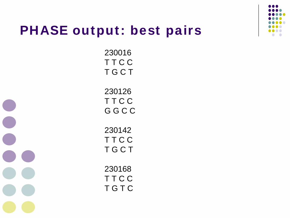
PHASE output: best pairs

230016T T C C T G C T

230126T T C C G G C C

230142T T C C T G C T

230168T T C C T G T C

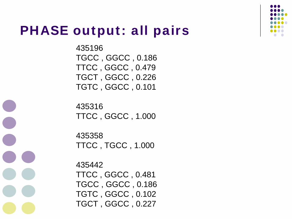
435196TGCC , GGCC , 0.186TTCC , GGCC , 0.479TGCT , GGCC , 0.226TGTC , GGCC , 0.101

435316TTCC , GGCC , 1.000

435358TTCC , TGCC , 1.000

435442TTCC , GGCC , 0.481TGCC , GGCC , 0.186TGTC , GGCC , 0.102TGCT , GGCC , 0.227

PHASE output: all pairs

Regression analysis accounting for Phase uncertainty

xi: logistic cursmoke i.il2_hap [pw=prob], cluster(studyid)

IFNG tagSNPs & cigarette smoking interaction in cervical cancer risk

IFNG tagSNP/genotype N

Current Smoker

(%)

Interaction odds ratio (95% CI)

Unrestricted model

Recessive model

rs2069705 TT 139 35 1.001.00

TC 126 44 1.4 (0.9-2.3)CC 43 23 0.6 (0.3-1.2) 0.5 (0.2-1.0)

rs2069707 CC 277 36 1.00--CG 31 42 1.3 (0.6-2.7)

rs2430561 AA 89 36 1.001.00

TA 150 41 1.2 (0.7-2.1)TT 69 30 0.8 (0.4-1.5) 0.7 (0.4-1.2)

rs2069727 AA 89 36 1.001.00AG 147 40 1.2 (0.7-2.1)

GG 69 30 0.8 (0.4-1.5) 0.7 (0.4-1.2)

IFNG diplotypes & cigarette smoking interaction in cervical cancer risk

Haplotype 1 Haplotype 2

Diplotype Frequencies

Interaction odds ratio (95% CI)

Non/Former smoking

cases (N=194)

Current smoking

cases (N=114)

T-C-T-G C-C-A-A 0.25 0.32 reference

T-C-T-G T-C-T-G 0.25 0.18 0.6 (0.3-1.1)

C-C-A-A C-C-A-A 0.17 0.09 0.4 (0.2-0.9)

T-C-A-A T-C-T-G 0.12 0.15 0.9 (0.4-2.0)

T-C-A-A C-C-A-A 0.09 0.11 1.0 (0.4-2.3)

T-C-T-G T-G-A-A 0.07 0.05 0.6 (0.2-1.6)

T-C-A-A T-C-A-A 0.02 0.03 1.3 (0.3-7.0)

T-G-A-A C-C-A-A 0.02 0.03 1.8 (0.4-8.4)

T-C-A-A T-G-A-A 0.01 0.02 2.6 (0.2-30.5)

PHASE output: recombination

495 993 2038 2340

0.0017338 2.96705 0.114492 0.41096 0.0017338 1.29485 0.452523 0.371537 0.00088415 0.521105 0.883367 1.45202 0.00520925 0.947913 0.213301 1.55976 0.00745335 0.222116 0.257865 1.27791 0.00141796 0.0262087 2.3126 1.84699 0.00142289 0.0846501 0.724828 0.038566 0.00341374 0.0846501 0.724828 0.038566 0.00190891 0.706078 0.731375 0.0137336 0.00861576 0.706078 0.731375 0.0137336 0.00415992 0.706078 0.731375 0.0137336 0.00274154 0.350819 0.611303 0.201631 0.00952453 0.412365 0.318064 0.20452

Recombination hotspot in SELP

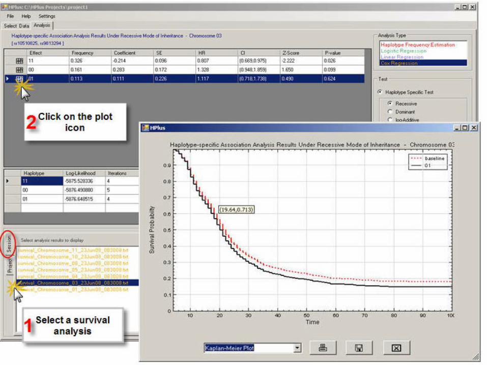
HPlus (Li and Zhao, 2003)

Haplotype reconstruction and association testingBinary outcome, continuous outcome, survivalCovariates and gene-environment interactions Outputs risk estimates and 95% CIWindows

Pitfalls of traditional haplotype analysis methods

Multiple testing (false positives increase)For 4 SNPs in a gene, there are 24 =16 possible hapltoypes; for 10 SNPs there are 1024

Rare haplotypes (false negatives increase)Common SNPs can still lead to rare haplotypes, and your study may not be adequately powered for that

Solution: combine haplotypes…

But how?

Rapidly evolving methods

Cladistic and Phyogenetic analyses (Durrant, 2004; Tamura, 2007)

Clustering (Liu, 2001; Yu, 2004;Morris, 2005; Waldron, 2006)

Coalescent methods (Zollner and Pritchard, 2005)

Haplotype sharing (McPeek and Strahs, 1999; Beckman,2005)

Variable-sized sliding window(Li, 2007)

Sequential haplotype scan (Yu & Schaid, 2007)

MEGA, version 3.1

Infers ancestral relationships between statistically inferred haplotypes

Inferences are based on the number of nucleotide differences between haplotypesfrom the root

Branch lengths are proportional to these differences

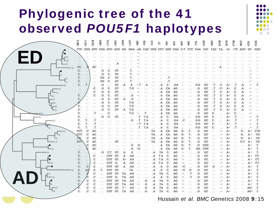
Phylogenic tree of the 41 observed POU5F1 haplotypes

Hussain et al. BMC Genetics 2008 9:15

AD

ED

Sequential haplotype scan

When evaluating the significance of a SNP, neighboring SNPs are added in a sequential manner

SNPs are kept if their contribution to the haplotype association with disease is warranted conditional on current SNPs in the haplotype

The conditional test is a Mantel-Hansel, which is computationally easy

Example: CD83 gene & cervical cancer risk

There are 16 SNPs, generally in low LD

SNP Allele (major/minor)

Freq. minor allele

rs12205252 A/G 0.21 rs6929821 A/G 0.26 rs3799925 C/G 0.45 rs3799924 A/G 0.19 rs4715877 G/A 0.29 rs853358 T/A 0.21 rs7743206 G/A 0.15 rs9296925 G/A 0.49 rs853360 G/A 0.27 rs3734665 A/G 0.19 rs10949227 A/G 0.36 rs9370729 A/G 0.40 rs17354216 A/G 0.05 rs853366 C/G 0.20 rs750749 A/G 0.20 rs853369 G/C 0.40

Sequential scan results for CD83

seq-loc-1 1seq-loc-2 2seq-loc-3 3 4seq-loc-4 4seq-loc-5 5seq-loc-6 6seq-loc-7 7 8 9seq-loc-8 8 9seq-loc-9 9seq-loc-10 10 11 9 seq-loc-11 11seq-loc-12 12 11seq-loc-13 13 seq-loc-14 14 13 seq-loc-15 15

(removed one SNP in high LD with one left in)

SNPs in haplotype§ Haplotype* Haplotype frequency‡

Freq. among controls‡

Freq. among cases‡ OR (95% CI)‡

rs3799925, rs3799924 (chi-square, 2-df: P=0.10) CA 0.56 0.55 0.57 1.00 (ref.) GG 0.18 0.20 0.15 0.71 (0.50-1.02) GA 0.26 0.25 0.28 1.11 (0.82-1.51) rs7743206, rs9296925, rs853360 (chi-square, 3-df: P=0.01) GGG 0.36 0.34 0.40 1.00 (ref.) GAA 0.25 0.27 0.19 0.55 (0.38-0.79) AGG 0.16 0.16 0.16 0.83 (0.56-1.21) GAG 0.23 0.22 0.25 0.93 (0.66-1.32) rs9296925, rs853360 (chi-square, 2-df: P<0.01) GG 0.52 0.50 0.57 1.00 (ref.) AA 0.25 0.27 0.19 0.59 (0.42-0.83) AG 0.23 0.22 0.25 0.98 (0.71-1.36) rs853360, rs3734665, rs10949227 (chi-square, 4-df: P=0.01) GAG 0.31 0.29 0.35 1.00 (ref.) AAA 0.20 0.22 0.15 0.49 (0.32-0.76) GAA 0.27 0.27 0.25 0.74 (0.52-1.06) GGA 0.15 0.14 0.18 0.97 (0.63-1.50) rs10949227, rs9370729 (chi-square, 3-df: P=0.14) AG 0.41 0.42 0.39 1.00 (ref.) AA 0.23 0.24 0.20 0.93 (0.66-1.30) GA 0.35 0.33 0.40 1.32 (0.97-1.78) rs17354216, rs750749 (chi-square, 2-df: P=0.02) AA 0.75 0.73 0.80 1.00 (ref.) AG 0.20 0.21 0.18 0.75 (0.53-1.05) GA 0.05 0.05 0.02 0.40 (0.19-0.88)