STATISTICAL METHODS For - Manonmaniam Sundaranar ...
183
MANONMANIAM SUNDARANAR UNIVERSITY DIRECTORATE OF DISTANCE & CONTINUING EDUCATION TIRUNELVELI 627012, TAMIL NADU Post Graduate Diploma in Statistical Methods and Applications DKSM1 - STATISTICAL METHODS (From the academic year 2016-17) Most Student friendly University - Strive to Study and Learn to Excel For more information visit: http://www.msuniv.ac.in
-
Upload
khangminh22 -
Category
Documents
-
view
1 -
download
0
Transcript of STATISTICAL METHODS For - Manonmaniam Sundaranar ...
MANONMANIAM SUNDARANAR UNIVERSITY
DIRECTORATE OF DISTANCE & CONTINUING EDUCATION
TIRUNELVELI 627012, TAMIL NADU
Post Graduate Diploma in Statistical Methods and Applications
DKSM1 - STATISTICAL METHODS (From the academic year 2016-17)
Most Student friendly University - Strive to Study and Learn to Excel
For more information visit: http://www.msuniv.ac.in
Manonmaniam Sundaranar University, Directorate of Distance & Continuing Education, Tirunelveli. 1
P.G. DIPLOMA IN STATISTICAL METHODS AND APPLICATIONS
DKSM1 : STATISTICAL METHODS
SYLLABUS
Unit - I
Origin, scope, limitations and misuses of Statistics – Collection - Classification-
Tabulation of data. Frequency Distribution – Nominal, ordinal, Interval and ratio.
Diagrammatic presentation of data – graphic representation: line diagram, frequency polygon,
frequency curve, histogram and Ogive curves.
Unit - II
Measures of central tendency - mean, median, mode, geometric mean and harmonic
mean. Partition values: Quartiles, Deciles and Percentiles. Measures of Dispersion: Mean
deviation, Quartile deviation and Standard deviation – Coefficient of variation. Measures of
Skewness - Pearson’s and Bowley’s Coefficients of skewness, Coefficient of Skewness –
co-efficient of Kurtosis.
Unit - III
Linear correlation - scatter diagram, Pearson’s coefficient of correlation, computation
of co-efficient of correlation from a bivariate frequency distribution, Rank correlation,
Coefficient of concurrent deviation - Regression equations – fitting of regression equations -
properties of regression coefficients.
Unit - IV
Partial and multiple correlation co-efficients – multiple linear regression model and
fitting – simple problems without derivation.
Unit - V
Sampling - Census and Sample survey - Sampling and non sampling errors - Simple
random sampling - Sampling from finite populations with and without replacements.
Stratified sampling, systematic sampling and cluster sampling.
BOOKS FOR STUDY:
1. Anderson, T.W. and Sclove, S.L. (1978) Introduction to Statistical Analysis of Data,
Houghton Mifflin, Boston.
2. Bhat, B.R., Srivenkataramna, T. and Madhava Rao, K.S. (1996) statistics A Beginner’s
Text, Vol. I, New Age International, New Delhi.
3. Croxton, F.E. and Cowden, D.J. (1969) Applied General Statistics, Prentice Hall,
New Delhi.
4. Goon, A.M., M.K. Gupta and B. Das Gupta (2002) Fundamentals of Statistics- Vol. I.
World Press Ltd, Kolkata.
5. Spiegel, M.R. and Stephens, L. (2010) Statistics, Schaum’s Outline Series, Mc Graw Hill,
New York.
Manonmaniam Sundaranar University, Directorate of Distance & Continuing Education, Tirunelveli. 2
CONTENTS
No. Title Page No.
1.1
1.2
1.3
1.4
1.5
1.6
1.7
1.8
1.9
1.10
Unit – I
Introduction
Origin
Functions of statistics
Scope of statistics
Limitations and Misuses of Statistics
Collection of data
Classification
Tabulation
Frequency Distributions
Diagrammatic and graphical representation
Questions
5
8
10
12
15
17
24
28
30
37
48
2.1
2.2
2.3
Unit – II
Measures of Central Tendency
Mean
Median
Mode
Geometric mean
Harmonic mean
Partition values
Quartiles
Deciles
Percentiles
Measures of Dispersion
Range
Mean deviation
Quartile deviation
Standard deviation
Coefficient of variation
48
50
55
64
72
73
76
76
81
83
86
87
89
97
102
107

Manonmaniam Sundaranar University, Directorate of Distance & Continuing Education, Tirunelveli. 3
2.4 Measures of skewness
Pearson‟s and Bowley‟s Coefficients of skewness,
Coefficient of skewness
Kurtosis (or) Co-efficient of Kurtosis
Questions
110
111
119
119
121
3.1
3.2
3.3
3.4
3.5
3.6
3.7
3.8
3.9
Unit - III
Linear correlation
Scatter diagram
Pearson‟s coefficient of correlation
Computation of co-efficient of correlation from a
bivariate frequency distribution
Rank correlation
Coefficient of concurrent deviation
Regression equations
Fitting of regression equations
Regression Coefficients and properties of regression
coefficients
Questions
127
129
135
140
143
147
149
153
153
159
4.1
4.2
4.3
Unit - IV
Partial and Multiple correlation coefficients
Multiple linear regression model and fitting
Simple problems without deviation
Questions
163
166
167
179
Manonmaniam Sundaranar University, Directorate of Distance & Continuing Education, Tirunelveli. 4
5.1
5.2
5.3
Unit - V
Sampling-Census and sample survey
Sampling and non sampling errors
Methods of Selection of Samples
Simple random sampling
Sampling from finite populations with and without
replacements.
Stratified sampling
Systematic sampling
Cluster sampling.
Questions
180
185
187
200
Manonmaniam Sundaranar University, Directorate of Distance & Continuing Education, Tirunelveli. 5
UNIT – I
1.1 INTRODUCTION
Statistics has been defined differently by different statisticians from
time to time. These definitions emphasize precisely the meaning, scope and
limitations of the subject. The reasons for such a variety definitions may be
stated as follows:
The field of utility of statistics has been increasing steadily.
The word statistics has been used to give different meaning in
singular (the science of statistical methods) and plural (numerical set of
data) sense.
Definitions:
Webster:
“Statistics are the classified facts representing the conditions of the
people in a State... specially those facts which can be stated in number
or in tables of numbers or in any tabular or classified arrangement”.
A.L. Bowley:
i. The science of counting
ii. The science of averages
iii. The science of measurements of social phenomena, regarded as a
whole in all its manifestations.
iv. A subject not confined to any one science.
Yule and Kendall:
“By Statistics we mean quantitative data affected to a marked extent
by multiplicity if causes”

Manonmaniam Sundaranar University, Directorate of Distance & Continuing Education, Tirunelveli. 6
A.M. Tuttle:
“Statistics are measurements, enumerations or estimates of natural
phenomenon, usually systematically arranged, analysed and
presented as to exhibit important inter-relationships among them”.
Prof. Horace Secrist:
“Statistics may be defined as the aggregate of facts affected to a
marked extent by multiplicity of causes, numerically expressed,
enumerated of estimated according to a reasonable standared of
accuracy, collected in a systematic manner, for a predetermined
purpose and placed in relation to each other”.
Croxton and Cowden:
Statistics may be defined as the science of collection, presentation
analysis and interpretation of numerical data from the logical
analysis. It is clear that the definition of statistics by Croxton and
Cowden is the most scientific and realistic one. According to this
definition there are four stages:
Collection of Data:
It is the first step and this is the foundation upon which the entire
data set. Careful planning is essential before collecting the data. There are
different methods of collection of data such as census, sampling, primary,
secondary, etc., and the investigator should make use of correct method.
Presentation of data:
The mass data collected should be presented in a suitable, concise
form for further analysis. The collected data may be presented in the form of
tabular or diagrammatic or graphic form.
Manonmaniam Sundaranar University, Directorate of Distance & Continuing Education, Tirunelveli. 7
Analysis of data:
The data presented should be carefully analysed for making inference
from the presented data such as measures of central tendencies, dispersion,
correlation, regression etc.,
Interpretation of data:
The final step is drawing conclusion from the data collected. A valid
conclusion must be drawn on the basis of analysis. A high degree of skill
and experience is necessary for the interpretation.
Every day, we come across the different types of quantitative
information in newspapers, magazines, over radio and television. For
example, we may hear or read that population of India had increased at the
rate of 2.5% per year (per annum) during the period 1981-1991, number of
admission in National Open School had gone up by say 20% during 1996-97
as compared to 1995-96 etc. We would like to know that what these figures
mean. These quantitative information or expression called statistical data or
statistics.
Statistics is concerned with scientific methods for collecting,
organising, summarising, presenting and analysing data as well as deriving
valid conclusions and making reasonable decisions on the basis of this
analysis. Statistics is concerned with the systematic collection of numerical
data and its interpretation. The word „statistic‟ is used to refer to
1. Numerical facts, such as the number of people living in particular area.
2. The study of ways of collecting, analysing and interpreting the facts.
1.2 ORIGIN
The science of statistics developed gradually and its field of
application widened day by day. The subject of Statistics, as it seems, is not
a new discipline but it is as old as the human society itself. It origin can be
Manonmaniam Sundaranar University, Directorate of Distance & Continuing Education, Tirunelveli. 8
traced to the old days when it was regarded as the „Science of State-craft‟
and was the by-product of the administrative activity if the State. The word
„Statistics‟ seems to have been derived from the latin word „status‟ or the
Italian word „statista‟ or the German word „statistik each of which means a
„political state‟.
In ancient times, the government used to collect the information
regarding the population and „property or wealth‟ of the country-the former
enabling the government to have an idea of the man-power of the country,
and the latter providing it a basis for introducing new taxes and levies.
In India, an efficient system of collecting official and administrative
statistics existed even more than 2,000 years ago, in particular, during the
reign of Chandra Gupta Maurya (324-300 B.C). From Kautilya‟s
Arthshastra it is known that even before 300 B.C. a very good system of
collecting „Vital Statistics‟ and registration of births and deaths was in
vogue. During Akbar‟s reign (1556-1605 A. D.), Raja, Todarmal, the then
land and revenue minister, maintained good records of land and agricultural
statistics.
In Alina-e-Akbari written by Abul Fazl (in 1596-97), one of the nine
gems of Akbar, we find detailed accounts of the administrative and
statistical surveys conducted during Akbar‟s reign. In Germany, the
systematic collection of official statistics originated towards the end of the
18th century when, in order to have an idea of the relative strength of
different German States, information regarding population and output-
industrial and agricultural was collected.
In England, statistics were the outcome of Napoleonic wars. The wars
necessitated the systematic collection of numerical data to enable the
government to assess the revenues and expenditure with greater precision
and then to levy new taxes in order to meet the cost of war. Seventeenth
century saw the origin of the „Vital Statistics‟. Captain John grant of
London (1960-1674), known as the „father‟ of Vital Statistics, was the first
man to study the statistics of births and deaths.

Manonmaniam Sundaranar University, Directorate of Distance & Continuing Education, Tirunelveli. 9
The theoretical development of the so-called, modern statistics came
during the mid-seventeenth century with the introduction of ‘Theory of
Probability’ and „Theory of Games and Chance’. The chief contributors being
mathematicians and gamblers of France, Germany and England. Statistics
is an old science, originated during the time of Mahabharat. For the last few
countries, it has remained a part of mathematicians like Pascal (1623-1662),
James Bernouli (1654-1705), De Moivre (1667-1754), Laplace (1749-1827),
gauss (1777-1855), lagrange, Bayes, Markoff, Euler etc. These
mathematicians were mainly interested in the development of the theory of
probability as applied to the theory of games and other chance phenomena.
Till the early nineteenth century, statistics was mainly concerned population
and area of land under cultivation, etc., of a state or kingdom.
A Ronald. A. Fisher (1890-1962) who applied statistics to a variety of
diversified fields such as genetics, biometry, psychology and education,
agriculture, etc and which is rightly termed as the Father of Statistics. His
contributors to the subject of Statistics are described in the following words:
‘R.A. Fisher is the real giant in the development of the theory of
Statistics’
The varied and outstanding contributions of R.A. fisher put the
subject of Statistics on a very firm footing and earned for it the status of
fully fledged science.
Indian statisticians have also made notable contributions to the
development of Statistics in various diversified fields. The valuable
contributions of P.C. Mahalanobis and P.V. Sukhatme (Sample Surveys);
R.C. Bose, Panse, J.N. Srivatsva (Design of experiments in Agriculture); S.N.
Roy (Multivariate Analysis); C.R. Rao (Statistical Inference); Parthasarathy
(Theory of Probability), to mention only a few, have earned for India a high
position in the world map of Statistics.

Manonmaniam Sundaranar University, Directorate of Distance & Continuing Education, Tirunelveli. 10
1.3 FUNCTIONS OF STATISTICS
Statistics is viewed not as a more device for collecting numerical data
but as a means of developing sound techniques for their handling and
analysis and drawing valid inferences from them.
We know discuss briefly the functions of statistics. Let us consider the
following important functions.
It simplifies facts in a definite Form:
Any conclusions stated numerically are definite and hence more
convincing than conclusions stated qualitatively. Statistics presents facts in
a precise and definite form and thus helps for a proper comprehension of
what is stated.
Condensation:
The generally speaking by the word „to condense‟, we mean to reduce
or to lessen. Condensation is mainly applied at embracing the
understanding of a huge mass of data by providing only few observations. If
in a particular class in Chennai School, only marks in an examination are
given, no purpose will be served. Instead if we are given the average mark in
that particular examination, definitely it serves the better purpose. Similarly
the range of marks is also another measure of the data. Thus, Statistical
measures help to reduce the complexity of the data and consequently to
understand any huge mass of data.
It facilitates Comparison:
The various statistical methods facilitate comparison and enable
useful conclusions to be drawn. The classification and tabulation are the
two methods that are used to condense the data. They help us to compare
data collected from different sources. Grand totals, measures of central
tendency measures of dispersion, graphs and diagrams, coefficient of
correlation etc provide ample scope for comparison. If we have one group of
data, we can compare within itself. If the rice production (in Tonnes) in
Manonmaniam Sundaranar University, Directorate of Distance & Continuing Education, Tirunelveli. 11
Tanjore district is known, then we can compare one region with another
region within the district. Or if the rice production (in Tonnes) of two
different districts within Tamilnadu is known, then also a comparative study
can be made. As statistics is an aggregate of facts and figures, comparison is
always possible and in fact comparison helps us to understand the data in a
better way.
It helps in the formation of policies:
Scientific analysis of statistical data constitutes the starting point in
all policy making. Decisions relating to import and export of various
commodities, production of particular products etc., are all based on
statistics.
It helps in Forecasting:
Plans and policies of organizations are invariably formulated well in
advance of the time of their implementation. The word forecasting, mean to
predict or to estimate beforehand. Given the data of the last fifteen years
connected to rainfall of a particular district in Tamilnadu, it is possible to
predict or forecast the rainfall for the near future. In business also
forecasting plays a dominant role in connection with production, sales,
profits etc. Analysis of time series and regression analysis plays an
important role in forecasting.
Estimation:
One of the main objectives of statistics is drawn inference about a
population from the analysis for the sample drawn from that population.
The four major branches of statistical inference are
Estimation theory
Tests of Hypothesis
Non Parametric tests
Sequential analysis
In estimation theory, we estimate the unknown value of the population
parameter based on the sample observations.
Manonmaniam Sundaranar University, Directorate of Distance & Continuing Education, Tirunelveli. 12
1.4 SCOPE OF STATISTICS
There are many scopes of statistics. Statistics is not a mere device for
collecting numerical data, but as a means of developing sound techniques
for their handling, analysing and drawing valid inferences from them.
Statistics is applied in every sphere of human activity – social as well as
physical – like Biology, Commerce, Education, Planning, Business
Management, Information Technology, etc. It is almost impossible to find a
single department of human activity where statistics cannot be applied. We
now discuss briefly the applications of statistics in other disciplines.
Statistics and Industry:
Statistics is widely used in many industries. In industries, control
charts are widely used to maintain a certain quality level. In production
engineering, to find whether the product is conforming to specifications or
not, statistical tools, namely inspection plans, control charts, etc., are of
extreme importance. In inspection plans we have to resort to some kind of
sampling – a very important aspect of Statistics.
Statistics and Commerce:
Statistics are lifeblood of successful commerce. Any businessman
cannot afford to either by under stocking or having overstock of his goods.
In the beginning he estimates the demand for his goods and then takes
steps to adjust with his output or purchases. Thus statistics is
indispensable in business and commerce. As so many multinational
companies have invaded into our Indian economy, the size and volume of
business is increasing. On one side the stiff competition is increasing
whereas on the other side the tastes are changing and new fashions are
emerging. In this connection, market survey plays an important role to
exhibit the present conditions and to forecast the likely changes in future.
Statistics and Agriculture:
Analysis of variance (ANOVA) is one of the statistical tools developed
by Professor R.A. Fisher, plays a prominent role in agriculture experiments.

Manonmaniam Sundaranar University, Directorate of Distance & Continuing Education, Tirunelveli. 13
In tests of significance based on small samples, it can be shown that
statistics is adequate to test the significant difference between two sample
means. In analysis of variance, we are concerned with the testing of equality
of several population means.
For an example, five fertilizers are applied to five plots each of wheat
and the yield of wheat on each of the plots are given. In such a situation, we
are interested in finding out whether the effect of these fertilisers on the
yield is significantly different or not. In other words, whether the samples
are drawn from the same normal population or not. The answer to this
problem is provided by the technique of ANOVA and it is used to test the
homogeneity of several population means.
Statistics and Economics:
Statistics data and techniques of statistical analysis have proved
immensely useful in solving a variety of economic problems.
Statistical methods are useful in measuring numerical changes in
complex groups and interpreting collective phenomenon. Nowadays the uses
of statistics are abundantly made in any economic study. Both in economic
theory and practice, statistical methods play an important role.
Alfred Marshall said, “Statistics are the straw only which I like every
other economists have to make the bricks”. It may also be noted that
statistical data and techniques of statistical tools are immensely useful in
solving many economic problems such as wages, prices, production,
distribution of income and wealth and so on. Statistical tools like Index
numbers, time series Analysis, Estimation theory, Testing Statistical
Hypothesis are extensively used in economics.
Statistics and Education:
Statistics is widely used in education. Research has become a
common feature in all branches of activities. Statistics is necessary for the
Manonmaniam Sundaranar University, Directorate of Distance & Continuing Education, Tirunelveli. 14
formulation of policies to start new course, consideration of facilities
available for new courses etc. There are many people engaged in research
work to test the past knowledge and evolve new knowledge. These are
possible only through statistics.
Statistics and Planning:
Statistics is indispensable in planning. In the modern world, which
can be termed as the “world of planning”, almost all the organisations in the
government are seeking the help of planning for efficient working, for the
formulation of policy decisions and execution of the same. In order to
achieve the above goals, the statistical data relating to production,
consumption, demand, supply, prices, investments, income expenditure etc
and various advanced statistical techniques for processing, analysing and
interpreting such complex data are of importance. In India statistics play an
important role in planning, commissioning both at the central and state
government levels.
Statistics and Medicine:
Statistical tools are widely used in Medical sciences. In order to test
the efficiency of a new drug or medicine, t-test is used to compare the
efficiency of two drugs or two medicines; t-test for the two samples is used.
More and more applications of statistics are at present used in clinical
investigation.
1.5 LIMITATIONS AND MISUSES OF STATISTICS
Although statistics is indispensable to almost all sciences: social,
physical and natural and very widely used in most of spheres of human
activity. It suffers from the following limitations. Statistics with all its wide
application in every sphere of human activity has its own limitations. Some
of them are given below.

Manonmaniam Sundaranar University, Directorate of Distance & Continuing Education, Tirunelveli. 15
Statistics deals only with aggregate of facts and not with individuals:
Statistics does not give any specific importance to the individual
items; in fact it deals with an aggregate of objects. Individual items, when
they are taken individually do not constitute any statistical data and do not
serve any purpose for any statistical enquiry.
Statistics does not study of qualitative phenomenon:
Since statistics is basically a science and deals with a set of numerical
data, it is applicable to the study of only these subjects of enquiry, which
can be expressed in terms of quantitative measurements. As a matter of
fact, qualitative phenomenon like honesty, poverty, beauty, intelligence etc,
cannot be expressed numerically and any statistical analysis cannot be
directly applied on these qualitative phenomenons. Nevertheless, statistical
techniques may be applied indirectly by first reducing the qualitative
expressions to accurate quantitative terms. For example, the intelligence of
a group of students can be studied on the basis of their marks in a
particular examination.
Statistics laws are tone only on an average:
It is well known that mathematical and physical sciences are exact.
But statistical laws are not exact and statistical laws are only
approximations. Statistical conclusions are not universally true. They are
true only on an average.
Statistics table may be misused:
Statistics must be used only by experts; otherwise, statistical methods
are the most dangerous tools on the hands of the inexpert. The use of
statistical tools by the inexperienced and untraced persons might lead to
wrong conclusions. Statistics can be easily misused by quoting wrong
figures of data.
Manonmaniam Sundaranar University, Directorate of Distance & Continuing Education, Tirunelveli. 16
Statistics is only, one of the methods of studying a problem:
Statistical method do not provide complete solution of the problems
because problems are to be studied taking the background of the countries
culture, philosophy or religion into consideration. Thus the statistical study
should be supplemented by other evidences.
Statistics is only inappropriate information:
Unskilled, idle and inexperienced person often collect data. As a
result, erroneous, puzzling and partial information is collected. As a result,
very often improper decision is taken.
Statistics is purposive Misuses:
The most total limitation of statistics is that its purposive misuse. Very
often erroneous information may be collected. But sometimes some
institutions use statistics for self interest and puzzling other organizations.
1.6 COLLECTION OF DATA
Everybody collects, interprets and uses information, much of it in
numerical or statistical forms in day-to-day life. It is a common practice that
people receive large quantities of information everyday through
conversations, televisions, computers, the radios, newspapers, posters,
notices and instructions. It is just because there is so much information
available that people need to be able to absorb, select and reject it. In
everyday life, in business and industry, certain statistical information is
necessary and it is independent to know where to find it how to collect it. As
consequences, everybody has to compare prices and quality before making
any decision about what goods to buy. As employees of any firm, people
want to compare their salaries and working conditions, promotion
opportunities and so on. In time the firms on their part want to control costs
and expand their profits.
One of the main functions of statistics is to provide information which
will help on making decisions. Statistics provides the type of information by
Manonmaniam Sundaranar University, Directorate of Distance & Continuing Education, Tirunelveli. 17
providing a description of the present, a profile of the past and an estimate
of the future. The following are some of the objectives of collecting statistical
information.
To consider the status involved in carrying out a survey.
To analyse the process involved in observation and interpreting.
To describe the methods of collecting primary statistical information.
To define and describe sampling.
To analyse the basis of sampling.
To describe a variety of sampling methods.
Statistical investigation is a comprehensive and requires systematic
collection of data about some group of people or objects, describing and
organizing the data, analyzing the data with the help of different statistical
method, summarizing the analysis and using these results for making
judgements, decisions and predictions. The validity and accuracy of final
judgement is most crucial and depends heavily on how well the data was
collected in the first place. The quality of data will greatly affect the
conditions and hence at most importance must be given to this process and
every possible precaution should be taken to ensure accuracy while
collecting the data.
Nature of data:
It may be noted that different types of data can be collected for
different purposes. The data can be collected in connection with time or
geographical location or in connection with time and location. The following
are the three types of data:
Time series data.
Spatial data.
Spacio-temporal data.
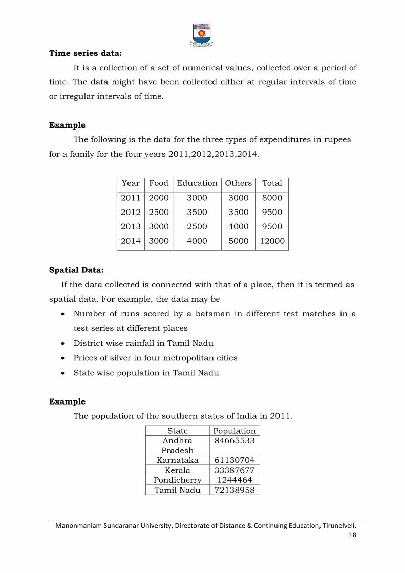
Manonmaniam Sundaranar University, Directorate of Distance & Continuing Education, Tirunelveli. 18
Time series data:
It is a collection of a set of numerical values, collected over a period of
time. The data might have been collected either at regular intervals of time
or irregular intervals of time.
Example
The following is the data for the three types of expenditures in rupees
for a family for the four years 2011,2012,2013,2014.
Year Food Education Others Total
2011
2012
2013
2014
2000
2500
3000
3000
3000
3500
2500
4000
3000
3500
4000
5000
8000
9500
9500
12000
Spatial Data:
If the data collected is connected with that of a place, then it is termed as
spatial data. For example, the data may be
Number of runs scored by a batsman in different test matches in a
test series at different places
District wise rainfall in Tamil Nadu
Prices of silver in four metropolitan cities
State wise population in Tamil Nadu
Example
The population of the southern states of India in 2011.
State Population
Andhra
Pradesh
84665533
Karnataka 61130704
Kerala 33387677
Pondicherry 1244464
Tamil Nadu 72138958
Manonmaniam Sundaranar University, Directorate of Distance & Continuing Education, Tirunelveli. 19
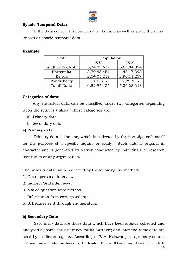
Spacio Temporal Data:
If the data collected is connected to the time as well as place then it is
known as spacio temporal data.
Example
State Population
1981 1991
Andhra Pradesh 5,34,03,619 6,63,04,854
Karnataka 3,70,43,451 4,48,17,398
Kerala 2,54,03,217 2,90,11,237
Pondicherry 6,04,136 7,89,416
Tamil Nadu 4,82,97,456 5,56,38,318
Categories of data:
Any statistical data can be classified under two categories depending
upon the sources utilized. These categories are,
a) Primary data
b) Secondary data
a) Primary data
Primary data is the one, which is collected by the investigator himself
for the purpose of a specific inquiry or study. Such data is original in
character and is generated by survey conducted by individuals or research
institution or any organisation.
The primary data can be collected by the following five methods.
1. Direct personal interviews.
2. Indirect Oral interviews.
3. Mailed questionnaire method.
4. Information from correspondents.
5. Schedules sent through enumerators.
b) Secondary Data
Secondary data are those data which have been already collected and
analysed by some earlier agency for its own use; and later the same data are
used by a different agency. According to W.A. Neiswanger, a primary source

Manonmaniam Sundaranar University, Directorate of Distance & Continuing Education, Tirunelveli. 20
is a publication in which the data are published by the same authority
which gathered and analysed them. A secondary source is a publication,
reporting the data which have been gathered by other authorities and for
which others are responsible‟.
Sources of Secondary data
In most of the studies the investigator finds it impracticable to collect
first-hand information on all related issues and as such he makes use of the
data collected by others. There is a vast amount of published information
from which statistical studies may be made and fresh statistics are
constantly in a state of production. The sources of secondary data can
broadly be classified under two heads:
a) Published sources
b) Unpublished sources
a) Published Sources:
Generally, published sources are international, national, govt., semi-
Govt, private corporate bodies, trade associations, expert committee and
commission reports and research reports. They collect the statistical data in
different fields like national income, population, prices, employment, wages,
export, import etc. These reports are published on regular basis i.e.,
annually, quarterly, monthly, fortnightly, weekly, daily and so on. These
published sources of the secondary data are given below:
i) Govt. Publications
The Central Statistical Organization (CSO) and various state govt. collect
compile and publish data on regular basis. Some of the important such
publications are:
Indian Trade Journals
Reports on Currency and Finance
Indian Customs and Central Excise Tariff
Statistical Abstract of India
Reserve Bank of India Bulletin

Manonmaniam Sundaranar University, Directorate of Distance & Continuing Education, Tirunelveli. 21
Labour Gazette
Agricultural Statistics of India
Bulletin of Agricultural Prices
Indian Foreign Statistics
Economic Survey and so on.
ii) International Bodies
All foreign Governments and international agencies publish regular
reports of international significance. These reports are regularly published
by the agencies like;
United Nations Organization
World Health Organization
International Labour Organization
Food and Agriculture Organization
International Bank for Reconstruction and Development
World Meteorological Organization.
iii) Semi Govt. Publications
Semi govt, organizations municipalities, District Boards and others
also publish reports in respect of birth, death and education, sanitation and
many other related fields.
iv) Reports of Committee and Commissions
Central Govt, or State Govt, sometimes appoints committees and
commissions on matters of great importance. Reports of such committees
are of great significance as they provide invaluable data. These reports are
like, Shah Commission Report, Sarkaria Commission Report and Finance
Commission Reports etc.
v) Private Publications
Some commercial and research institutes publish reports regularly.
They are like Institutes of Economic Growth, Stock Exchanges, National

Manonmaniam Sundaranar University, Directorate of Distance & Continuing Education, Tirunelveli. 22
Council of Education Research and Training (NCERT), National Council of
Applied Economic Research (NCAER) etc.
vi) Newspapers and Magazines
Various newspapers as well as magazines also do collect data in
respect of many social and economic aspects. Some of them are as:
Economic Times
Financial Express
Hindustan Times
Indian Express
Business Standard
Economic and Political Weekly
Main-stream
Kurukshetra
Yojna etc.
vii) Research Scholars:
Individual research scholars collect data to complete their research
work which further is published with their research papers.
b) Unpublished Source
There are certain records maintained properly by the govt, agencies,
private offices and firms. These data are not published.
Limitations of Secondary Data
One should not use the secondary data without care and precautions. As
such, secondary data suffers from pitfalls and limitations as stated below:
No proper procedure is adopted to collect the data.
Sometimes, secondary data is influenced by the prejudice of the
investigator.
Secondary data sometimes lacks standard of accuracy.
Secondary data may not cover the full period of investigation.
Manonmaniam Sundaranar University, Directorate of Distance & Continuing Education, Tirunelveli. 23
1.7 CLASSIFICATION
Classification defined as: “the process of arranging things in groups or
classes according to their resemblances and affinities and gives expression
to the unity of attributes that may subsist amongst a diversity of
individuals”.
The Collected data, also known as raw data or ungrouped data are
always in an un organised form and need to be organised and presented in
meaningful and readily comprehensible form in order to facilitate further
statistical analysis. It is, therefore, essential for an investigator to condense
a mass of data into more and more comprehensible and assailable form. The
process of grouping into different classes or sub classes according to some
characteristics is known as classification, tabulation is concerned with the
systematic arrangement and presentation of classified data. Thus
classification is the first step in tabulation. For Example, letters in the post
office are classified according to their destinations viz., New Delhi, Mumbai,
Bangalore, Chennai etc.,
Objects of Classification:
The following are main objectives of classifying the data:
It eliminates unnecessary details.
It facilitates comparison and highlights the significant aspect of data.
It enables one to get a mental picture of the information and helps in
drawing inferences.
It helps in the statistical treatment of the information collected.
Types of classification:
Statistical data are classified in respect of their characteristics. Broadly
there are four basic types of classification namely
Qualitative classification
Manonmaniam Sundaranar University, Directorate of Distance & Continuing Education, Tirunelveli. 24
Quantitative classification
Chronological classification
Geographical classification
Qualitative classification
Qualitative classification is done according to attributes or non-
measurable characteristics; like social status, sex, nationality, occupation,
etc.
For example, the population of the whole country can be classified
into four categories as married, unmarried, widowed and divorced.
When only one attribute, e.g., sex, is used for classification, it is called
simple classification.
When more than one attributes, e.g., deafness, sex and religion, are
used for classification, it is called manifold classification.
Quantitative classification
If the data are classified on the basis of phenomenon which is capable
of quantitative measurements like age, height, weight, prices, production,
income expenditure, sales, profits, etc., it s itemed as quantitative variable.
For example the daily incomes of different retail shops in a town may
be classified as under.
Daily earnings in rupees of 100 retail shop in a town
Daily earnings No. of retail shops
Upto 100 9
101 - 200 25
201 - 300 33
301 - 400 28
401 - 500 2
Above 500 8

Manonmaniam Sundaranar University, Directorate of Distance & Continuing Education, Tirunelveli. 25
In the above classification, the daily earnings of the shops are termed
as variable and the number of shops in each class or group as the
frequency. This classification is called grouped frequency distribution.
Hence this classification is often called „classification by variables‟.
Variable:
A variable in statistics means any measurable characteristic or
quantity which can assume a range of numerical values within certain
limits, e.g., income, height, age, weight, wage, price, etc. A variable can be
classified as either a) Discrete, b) Continuous.
a) Discrete variable
A variable which can take up only exact values and not any fractional
values, is called a „discrete‟ variable. Number of workmen in a factory,
members of a family, students in a class, number of births in a certain year,
number of telephone calls in a month, etc., are examples of discrete-
variable.
b) Continuous variable
A variable which can take up any numerical value
(integral/fractional) within a certain range is called a „continuous‟ variable.
Height, weight, rainfall, time, temperature, etc., are examples of continuous
variables. Age of students in a school is a continuous variable as it can be
measured to the nearest fraction of time, i.e., years, months, days, etc.
Chronological classification
When the data are classified on the basis of time then it is known as
chronological classification. Such series are also known as time series
because one of the variables in them is time. If the population of India
during the last eight censuses is classified it will result in a time series or
chronological classification.
Manonmaniam Sundaranar University, Directorate of Distance & Continuing Education, Tirunelveli. 26
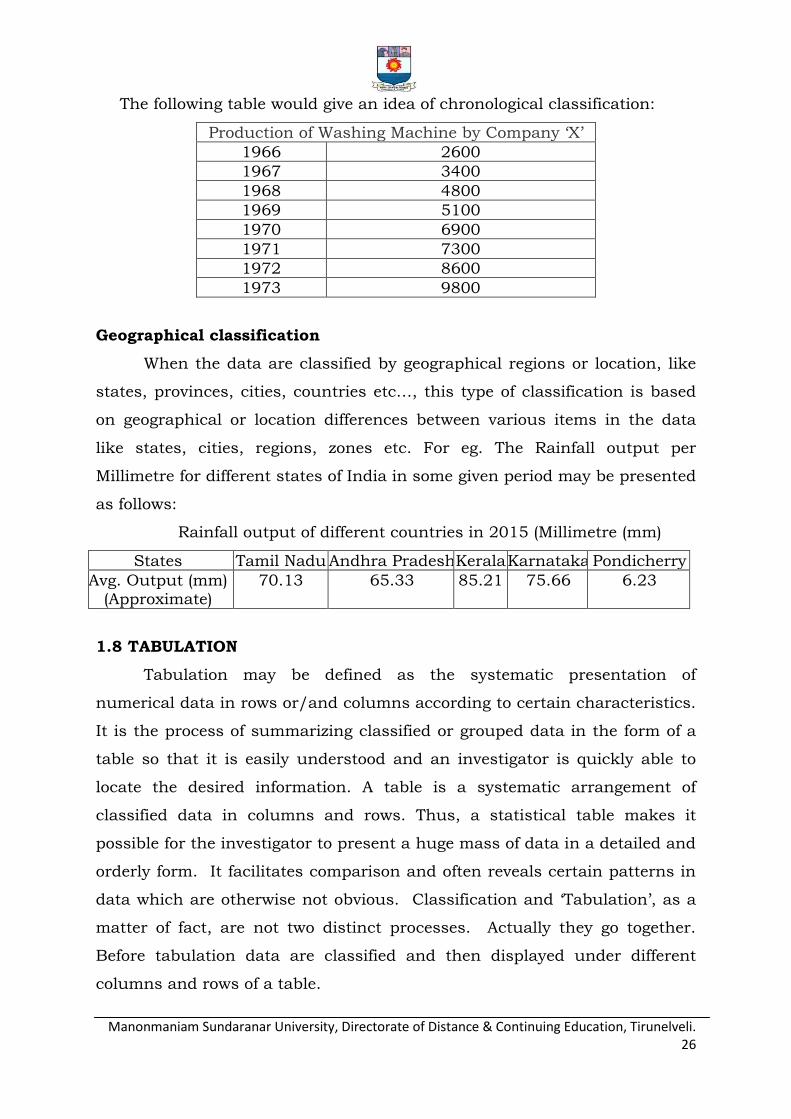
The following table would give an idea of chronological classification:
Production of Washing Machine by Company „X‟
1966 2600
1967 3400
1968 4800
1969 5100
1970 6900
1971 7300
1972 8600
1973 9800
Geographical classification
When the data are classified by geographical regions or location, like
states, provinces, cities, countries etc…, this type of classification is based
on geographical or location differences between various items in the data
like states, cities, regions, zones etc. For eg. The Rainfall output per
Millimetre for different states of India in some given period may be presented
as follows:
Rainfall output of different countries in 2015 (Millimetre (mm)
States Tamil Nadu Andhra Pradesh Kerala Karnataka Pondicherry
Avg. Output (mm) (Approximate)
70.13 65.33 85.21 75.66 6.23
1.8 TABULATION
Tabulation may be defined as the systematic presentation of
numerical data in rows or/and columns according to certain characteristics.
It is the process of summarizing classified or grouped data in the form of a
table so that it is easily understood and an investigator is quickly able to
locate the desired information. A table is a systematic arrangement of
classified data in columns and rows. Thus, a statistical table makes it
possible for the investigator to present a huge mass of data in a detailed and
orderly form. It facilitates comparison and often reveals certain patterns in
data which are otherwise not obvious. Classification and „Tabulation‟, as a
matter of fact, are not two distinct processes. Actually they go together.
Before tabulation data are classified and then displayed under different
columns and rows of a table.
Manonmaniam Sundaranar University, Directorate of Distance & Continuing Education, Tirunelveli. 27
Objectives of Tabulation:
The main objectives of tabulation are following
To carry out investigation;
To do comparison;
To locate omissions and errors in the data;
To use space economically;
To study the trend;
To simplify data;
To use it as future reference.
Advantages of Tabulation:
The advantages of Tabulation are following
It simplifies complex data and the data presented are easily
understood.
It facilitates comparison of related facts.
It facilitates computation of various statistical measures like averages,
dispersion, correlation etc.
It presents facts in minimum possible space and unnecessary
repetitions and explanations are avoided. Moreover, the needed
information can be easily located.
Tabulated data are good for references and they make it easier to
present the information in the form of graphs and diagrams.
Table:
The making of a compact table itself an art. This should contain all
the information needed within the smallest possible space. What the
purpose of tabulation is and how the tabulated information is to be used are
the main points to be kept in mind while preparing for a statistical table. An
ideal table should consist of the following main parts are: (i)Table number;
(ii) Title of the table; (iii) Captions or column headings; (iv) Stubs or row
designation; (v) Body of the table; (vi) Footnotes; and (vii) Sources of data.
Manonmaniam Sundaranar University, Directorate of Distance & Continuing Education, Tirunelveli. 28
Types of Tables:
The tables can be classified according to their purpose, stage of
enquiry, nature of data or number of characteristics used. On the basis of
the number of characteristics, tables classified as follows: (i) Simple or one-
way table; (ii) Two way table; and (iii) Manifold table.
A good statistical table is not merely a careless grouping of columns
and rows but should be such that it summarizes the total information in an
easily accessible form in minimum possible space. Thus while preparing a
table, one must have a clear idea of the information to be presented, the
facts to be compared and he points to be stressed.
1.9 FREQUENCY DISTRIBUTION:
A frequency distribution is an arrangement where a number of
observations with similar or closely related values are put in separate
groups, each group being n order of magnitudes in the arrangement based
on magnitudes. It is a series when a number of observations with similar or
closely related values are put in separate bunches or groups, each group
being in order of magnitude in a series. It is simply a table in which the data
are grouped into classes and the numbers of cases which fall in each class
are recorded. It shows the frequency of occurrence of different values of a
single Phenomenon.
The frequency distribution is constructed for three main reasons are: (i)
To facilitate the analysis of data.
(ii) To estimate frequencies of the unknown population distribution
from the distribution of sample data.
(iii) To facilitate the computation of various statistical measures.
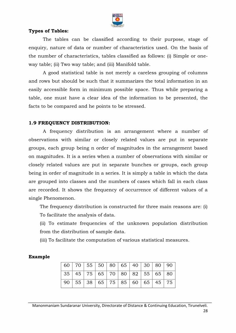
Example
60 70 55 50 80 65 40 30 80 90
35 45 75 65 70 80 82 55 65 80
90 55 38 65 75 85 60 65 45 75

Manonmaniam Sundaranar University, Directorate of Distance & Continuing Education, Tirunelveli. 29
The above figures are nothing but raw or ungrouped data and they are
recorded as they occur without any pre consideration. This representation
of data does not furnish any useful information and is rather confusing to
mind. A better way to express the figures in an ascending or descending
order of magnitude and is commonly known as array. But this does not
reduce the bulk of the data. The above data when formed into an array is in
the following form:
30 35 38 40 45 45 50 55 55 55
60 60 65 65 65 65 65 65 70 70
75 75 75 80 80 80 80 85 90 90
The array helps us to see at once the maximum and minimum values.
It also gives a rough idea of the distribution of the items over the range.
When we have a large number of items, the formation of an array is very
difficult, tedious and cumbersome. The Condensation should be directed for
better understanding and may be done in two ways, depending on the
nature of the data.
Discrete frequency distribution
Discrete frequency distribution shows the number of times each value
and not to a range of values, of the variable occurs in the data set. Discrete
frequency distribution is called ungrouped frequency distribution. In this
form of distribution, the frequency refers to discrete value. Here the data are
presented in a way that exact measurement of units is clearly indicated.
There are definite differences between the variables of different groups of
items. Each class is distinct and separate from the other class. Non-
continuity from one class to another class exists. Data as such facts like,
the number of rooms in a house, the number of companies registered in a
country, the number of children in a family, etc.
Example
In a survey of 40 families in a village, the number of children per family was
recorded and the following data obtained.
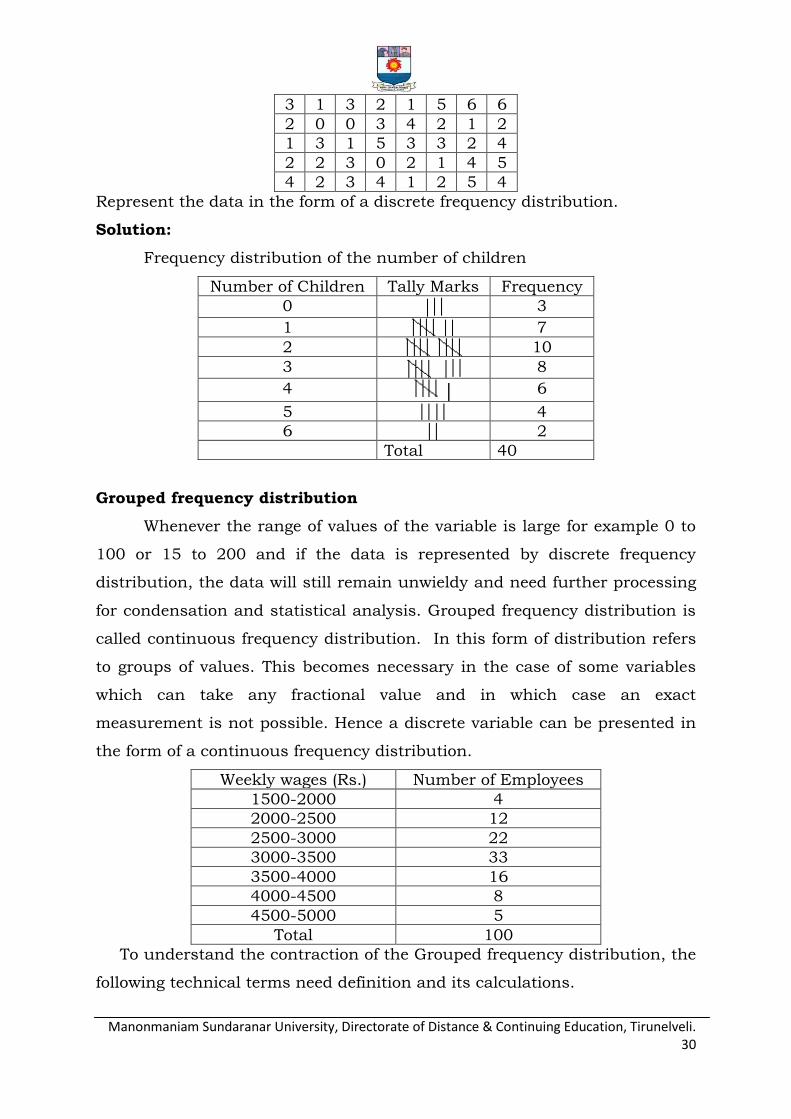
Manonmaniam Sundaranar University, Directorate of Distance & Continuing Education, Tirunelveli. 30
3 1 3 2 1 5 6 6
2 0 0 3 4 2 1 2
1 3 1 5 3 3 2 4
2 2 3 0 2 1 4 5
4 2 3 4 1 2 5 4
Represent the data in the form of a discrete frequency distribution.
Solution:
Frequency distribution of the number of children
Number of Children Tally Marks Frequency
0 3
1 7
2 10
3 8
4 │ 6
5 4
6 2
Total 40
Grouped frequency distribution
Whenever the range of values of the variable is large for example 0 to
100 or 15 to 200 and if the data is represented by discrete frequency
distribution, the data will still remain unwieldy and need further processing
for condensation and statistical analysis. Grouped frequency distribution is
called continuous frequency distribution. In this form of distribution refers
to groups of values. This becomes necessary in the case of some variables
which can take any fractional value and in which case an exact
measurement is not possible. Hence a discrete variable can be presented in
the form of a continuous frequency distribution.
Weekly wages (Rs.) Number of Employees
1500-2000 4
2000-2500 12
2500-3000 22
3000-3500 33
3500-4000 16
4000-4500 8
4500-5000 5
Total 100
To understand the contraction of the Grouped frequency distribution, the
following technical terms need definition and its calculations.

Manonmaniam Sundaranar University, Directorate of Distance & Continuing Education, Tirunelveli. 31
Class interval
The various groups into which the values of the variable are
classified are known as class intervals or simply classes. For
example, the symbol 25-35 represents a group or class which
includes all the values from 25 to 35.
Class limits
The two values (maximum and minimum) specifying the
class intervals are called the class limits. The lowest value is
called the lower limit and the height value the upper limit of
the class.
Length or width of the class is defined as the difference
between the upper and the lower limits of the class.
That is Class mark or Midpoint of a class = (Lower
Limit+Upper Limit)/2
Example
Consider a class denoted as 25 – 50
The class 25-50 includes all the values in between 25 to 50
The lower limit of the class is 25 and the upper limit 50
The length of the class is given by:
Length = Upper limit – Lower limit = 50 – 25 = 25.
The class mark or mid value of the class is given by
Mid value = (Lower Limit + Upper Limit) / 2
= (25 + 50) / 2 = 37.5
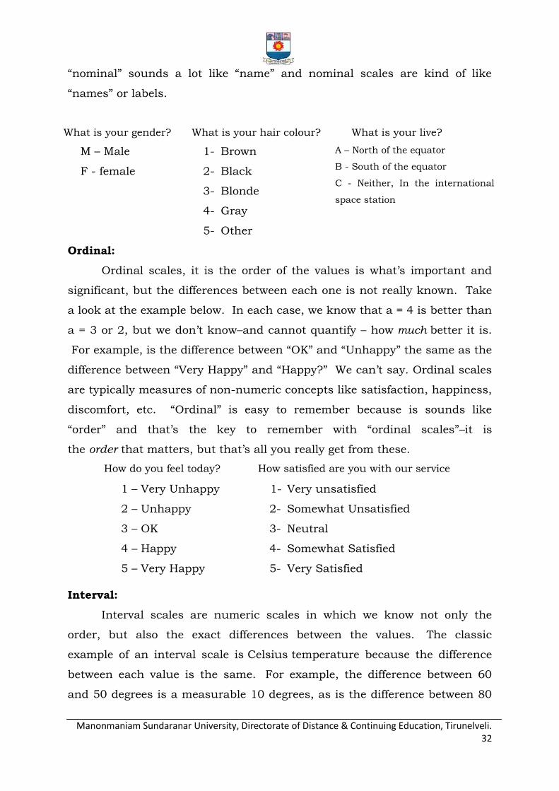
Nominal:
Let‟s start with the easiest one to understand. Nominal scales are
used for labelling variables, without any quantitative value. “Nominal” scales
could simply be called “labels.” Here are some examples, below. Notice that
all of these scales are mutually exclusive (no overlap) and none of them has
any numerical significance. A good way to remember all of this is that
Manonmaniam Sundaranar University, Directorate of Distance & Continuing Education, Tirunelveli. 32
“nominal” sounds a lot like “name” and nominal scales are kind of like
“names” or labels.
What is your gender? What is your hair colour? What is your live?
M – Male
F - female
1- Brown
2- Black
3- Blonde
4- Gray
5- Other
A – North of the equator
B - South of the equator
C - Neither, In the international
space station
Ordinal:
Ordinal scales, it is the order of the values is what‟s important and
significant, but the differences between each one is not really known. Take
a look at the example below. In each case, we know that a = 4 is better than
a = 3 or 2, but we don‟t know–and cannot quantify – how much better it is.
For example, is the difference between “OK” and “Unhappy” the same as the
difference between “Very Happy” and “Happy?” We can‟t say. Ordinal scales
are typically measures of non-numeric concepts like satisfaction, happiness,
discomfort, etc. “Ordinal” is easy to remember because is sounds like
“order” and that‟s the key to remember with “ordinal scales”–it is
the order that matters, but that‟s all you really get from these.
How do you feel today? How satisfied are you with our service
1 – Very Unhappy
2 – Unhappy
3 – OK
4 – Happy
5 – Very Happy
1- Very unsatisfied
2- Somewhat Unsatisfied
3- Neutral
4- Somewhat Satisfied
5- Very Satisfied
Interval:
Interval scales are numeric scales in which we know not only the
order, but also the exact differences between the values. The classic
example of an interval scale is Celsius temperature because the difference
between each value is the same. For example, the difference between 60
and 50 degrees is a measurable 10 degrees, as is the difference between 80

Manonmaniam Sundaranar University, Directorate of Distance & Continuing Education, Tirunelveli. 33
and 70 degrees. Time is another good example of an interval scale in which
the increments are known, consistent, and measurable. Interval scales are
nice because the realm of statistical analysis on these data sets opens up.
For example, central tendency can be measured by mode, median, or
mean; standard deviation can also be calculated. Like the others, you can
remember the key points of an “interval scale” pretty easily. “Interval” itself
means “space in between,” which is the important thing to remember–
interval scales not only tell us about order, but also about the value between
each item. Here‟s the problem with interval scales: they don‟t have a “true
zero.” For example, there is no such thing as “no temperature.” Without a
true zero, it is impossible to compute ratios. With interval data, we can add
and subtract, but cannot multiply or divide. Confused? Ok, consider this:
10 degrees + 10 degrees = 20 degrees. No problem there. 20 degrees is not
twice as hot as 10 degrees, however, because there is no such thing as “no
temperature” when it comes to the Celsius scale. I hope that makes sense.
Bottom line, interval scales are great, but we cannot calculate ratios, which
brings us to our last measurement scale…
Ratio:
Ratio scales are the ultimate nirvana when it comes to measurement
scales because they tell us about the order, they tell us the exact value
between units, and they also have an absolute zero–which allows for a wide
range of both descriptive and inferential statistics to be applied. At the risk
of repeating myself, everything above about interval data applies to ratio
scales + ratio scales have a clear definition of zero. Good examples of ratio
variables include height and weight. Ratio scales provide a wealth of
Manonmaniam Sundaranar University, Directorate of Distance & Continuing Education, Tirunelveli. 34
possibilities when it comes to statistical analysis. These variables can be
meaningfully added, subtracted, multiplied, divided (ratios). Central
tendency can be measured by mode, median, or mean; measures of
dispersion, such as standard deviation and coefficient of variation can also
be calculated from ratio scales.
This Device Provides Two Examples of Ratio Scales (height and weight)
1.10 DIAGRAMMATIC AND GRAPHICAL REPRESENTATION
One of the most convincing and appealing ways in which statistical
results may be presented is through diagrams and graphs. Representation
of statistical data by means of pictures, graphs and geometrical figures is
called diagrammatic and graphical representations. The difference between
the two is that in the case of diagrammatic representation the quantities are
represented by diagrams and pictures and in case of graphical
representation they are represented by points which are plotted on a graph
paper.
Diagrammatic Representation:
Diagrammatic representation is used when the data relating to
different times and places are given and they are independent of one
another. One of the most convincing and appealing ways in which statistical
results may be presented is through diagrams and graphs. Just one diagram
is enough to represent a given data more effectively than thousand words.
Moreover even a layman who has nothing to do with numbers can also
understands diagrams. Evidence of this can be found in newspapers,
magazines, journals, advertisement, etc. An attempt is made in this chapter
Manonmaniam Sundaranar University, Directorate of Distance & Continuing Education, Tirunelveli. 35
to illustrate some of the major types of diagrams and graphs frequently used
in presenting statistical data. Diagram is a visual form for presentation of
statistical data, highlighting their basic facts and relationship. If we draw
diagrams on the basis of the data collected they will easily be understood
and appreciated by all. It is readily intelligible and save a considerable
amount of time and energy.
Significance of Diagrams and Graphs:
Diagrams and graphs are extremely useful because of the following
reasons.
They are attractive and impressive.
They make data simple and intelligible.
They make comparison possible
They save time and labour.
They have universal utility.
They give more information.
They have a great memorizing effect.
General rules for constructing diagrams:
The construction of diagrams is an art, which can be acquired through
practice. However, observance of some general guidelines can help in
making them more attractive and effective. The diagrammatic presentation
of statistical facts will be advantageous provided the following rules are
observed in drawing diagrams.
A diagram should be neatly drawn and attractive.
The measurements of geometrical figures used in diagram should be
accurate and proportional.
The size of the diagrams should match the size of the paper.
Every diagram must have a suitable but short heading.
The scale should be mentioned in the diagram.
Diagrams should be neatly as well as accurately drawn with the help
of drawing instruments.
Manonmaniam Sundaranar University, Directorate of Distance & Continuing Education, Tirunelveli. 36
Index must be given for identification so that the reader can easily
make out the meaning of the diagram.
Footnote must be given at the bottom of the diagram.
Economy in cost and energy should be exercised in drawing diagram.
Types of diagrams:
In practice, a very large variety of diagrams are in use and new ones are
constantly being added. For the sake of convenience and simplicity, they
may be divided under the following heads:
One-dimensional diagrams
Two-dimensional diagrams
Three-dimensional diagrams
Pictograms and Cartograms
One-dimensional diagrams
In such diagrams, only one-dimensional measurement, i.e height is
used and the width is not considered. These diagrams are in the form of bar
or line charts and can be classified as
Line Diagram
Simple Diagram
Multiple Bar Diagram
Sub-divided Bar Diagram
Percentage Bar Diagram
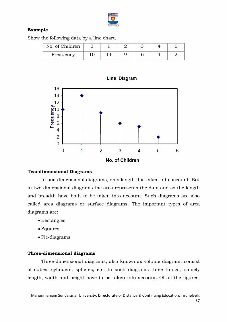
Line Diagram:
Line diagram is used in case where there are many items to be shown and
there is not much of difference in their values. Such diagram is prepared by
drawing a vertical line for each item according to the scale. The distance
between lines is kept uniform. Line diagram makes comparison easy, but it
is less attractive.
Manonmaniam Sundaranar University, Directorate of Distance & Continuing Education, Tirunelveli. 37
Example
Show the following data by a line chart.
No. of Children 0 1 2 3 4 5
Frequency 10 14 9 6 4 2
Two-dimensional Diagrams
In one-dimensional diagrams, only length 9 is taken into account. But
in two-dimensional diagrams the area represents the data and so the length
and breadth have both to be taken into account. Such diagrams are also
called area diagrams or surface diagrams. The important types of area
diagrams are:
Rectangles
Squares
Pie-diagrams
Three-dimensional diagrams
Three-dimensional diagrams, also known as volume diagram, consist
of cubes, cylinders, spheres, etc. In such diagrams three things, namely
length, width and height have to be taken into account. Of all the figures,
Manonmaniam Sundaranar University, Directorate of Distance & Continuing Education, Tirunelveli. 38
making of cubes is easy. Side of a cube is drawn in proportion to the cube
root of the magnitude of data.
Pictograms and Cartograms
Pictograms are not abstract presentation such as lines or bars but
really depict the kind of data we are dealing with. Pictures are attractive and
easy to comprehend and as such this method is particularly useful in
presenting statistics to the layman. When Pictograms are used, data are
represented through a pictorial symbol that is carefully selected.
Cartograms or statistical maps are used to give quantitative information as a
geographical basis. They are used to represent spatial distributions. The
quantities on the map can be shown in many ways such as through shades
or colours or dots or placing pictogram in each geographical unit.
GRAPHICAL REPRESENTATION:
The graphical representation is used when we have to represent the
data of a frequency distribution and a time series. A graph represents
mathematical relationship between the two variables whereas a diagram
does not. A graph is a visual form of presentation of statistical data. A
graph is more attractive than a table of figure. Even a common man can
understand the message of data from the graph. Comparisons can be made
between two or more phenomena very easily with the help of a graph.
Finally graphs are more obvious, precise and accurate than diagrams and
are quite helpful to the statistician for the study of slopes, rates of changes
and estimation, whenever possible. However here we shall discuss only
some important types of graphs which are more popular and they are
Histogram
Frequency Polygon
Frequency Curve
Ogive
Lorenz Curve

Manonmaniam Sundaranar University, Directorate of Distance & Continuing Education, Tirunelveli. 39
Histogram
A histogram consists of bars or rectangles which are erected over the
class intervals, without giving gaps between bars and such that the areas of
the bars are proportional to the frequencies of the class intervals. It is a bar
chart or graph showing the frequency of occurrence of each value of the
variable being analysed. In histogram, data are plotted as a series of
rectangles. Class intervals are shown on the „X-axis‟ and the frequencies on
the „Y-axis‟. The height of each rectangle represents the frequency of the
class interval. Each rectangle is formed with the other so as to give a
continuous picture. Such a graph is also called staircase or block diagram.
However, we cannot construct a histogram for distribution with open-end
classes. It is also quite misleading if the distribution has unequal intervals
and suitable adjustments in frequencies are not made.
Example
Draw a histogram for the following data.
Daily wages Number of Workers
0-50 50-100
100-150 150-200 200-250
250-300
8 16
27 19 10
6
Manonmaniam Sundaranar University, Directorate of Distance & Continuing Education, Tirunelveli. 40
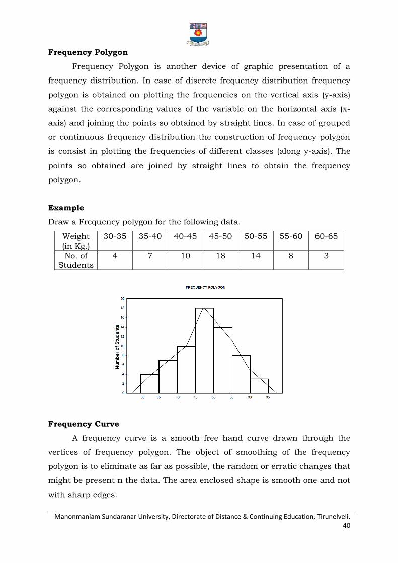
Frequency Polygon
Frequency Polygon is another device of graphic presentation of a
frequency distribution. In case of discrete frequency distribution frequency
polygon is obtained on plotting the frequencies on the vertical axis (y-axis)
against the corresponding values of the variable on the horizontal axis (x-
axis) and joining the points so obtained by straight lines. In case of grouped
or continuous frequency distribution the construction of frequency polygon
is consist in plotting the frequencies of different classes (along y-axis). The
points so obtained are joined by straight lines to obtain the frequency
polygon.
Example
Draw a Frequency polygon for the following data.
Weight
(in Kg.)
30-35 35-40 40-45 45-50 50-55 55-60 60-65
No. of Students
4 7 10 18 14 8 3
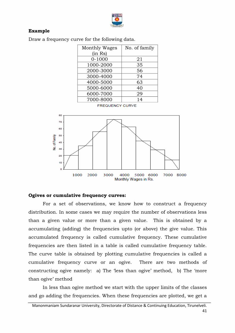
Frequency Curve
A frequency curve is a smooth free hand curve drawn through the
vertices of frequency polygon. The object of smoothing of the frequency
polygon is to eliminate as far as possible, the random or erratic changes that
might be present n the data. The area enclosed shape is smooth one and not
with sharp edges.
Manonmaniam Sundaranar University, Directorate of Distance & Continuing Education, Tirunelveli. 41
Example
Draw a frequency curve for the following data.
Monthly Wages
(in Rs)
No. of family
0-1000 21
1000-2000 35
2000-3000 56
3000-4000 74
4000-5000 63
5000-6000 40
6000-7000 29
7000-8000 14
Ogives or cumulative frequency curves:
For a set of observations, we know how to construct a frequency
distribution. In some cases we may require the number of observations less
than a given value or more than a given value. This is obtained by a
accumulating (adding) the frequencies upto (or above) the give value. This
accumulated frequency is called cumulative frequency. These cumulative
frequencies are then listed in a table is called cumulative frequency table.
The curve table is obtained by plotting cumulative frequencies is called a
cumulative frequency curve or an ogive. There are two methods of
constructing ogive namely: a) The „less than ogive‟ method, b) The „more
than ogive‟ method
In less than ogive method we start with the upper limits of the classes
and go adding the frequencies. When these frequencies are plotted, we get a
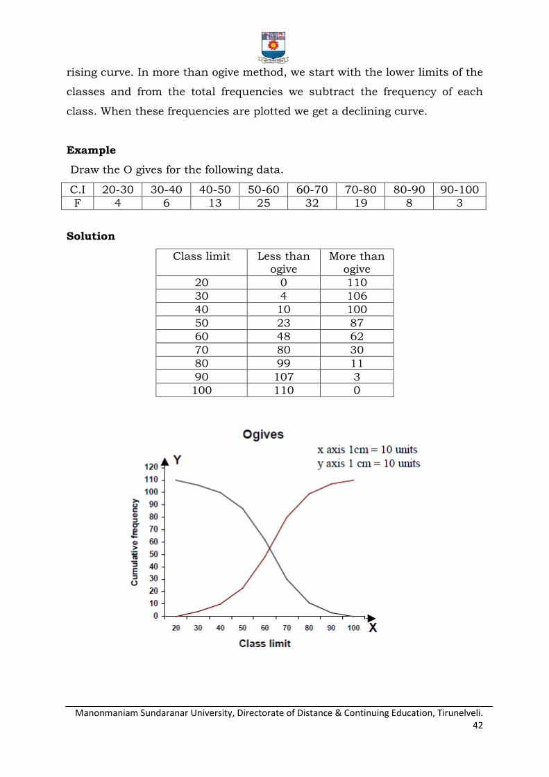
Manonmaniam Sundaranar University, Directorate of Distance & Continuing Education, Tirunelveli. 42
rising curve. In more than ogive method, we start with the lower limits of the
classes and from the total frequencies we subtract the frequency of each
class. When these frequencies are plotted we get a declining curve.
Example
Draw the O gives for the following data.
C.I 20-30 30-40 40-50 50-60 60-70 70-80 80-90 90-100
F 4 6 13 25 32 19 8 3
Solution
Class limit Less than ogive
More than ogive
20 0 110
30 4 106
40 10 100
50 23 87
60 48 62
70 80 30
80 99 11
90 107 3
100 110 0
Manonmaniam Sundaranar University, Directorate of Distance & Continuing Education, Tirunelveli. 43
QUESTIONS
1. Explain the origin of statistics.
2. Write the meaning and definitions of statistics.
3. Write the definitions of statistics as given by Croxton and Crowden?
Explain the four stages in statistics.
4. Explain the categories of data.
5. Explain the classification and objects of classification.
6. Describe the advantages of tabulation.
7. Explain the process of preparing a table
8. Explain the scales of measurement?
9. Write the general rules of constructing diagrams.
10. Explain the functions of statistics.
11. Describe the scope of statistics.
12. What are the limitations of statistics?
13. Explain the collection of data.
14. Explain the classification and Tabulation.
15. Describe the frequency distribution.
16. Write the types of diagrams and graphs

Manonmaniam Sundaranar University, Directorate of Distance & Continuing Education, Tirunelveli. 44
UNIT – II
2.1 MEASURES OF CENTRAL TENDENCY
The collected data such are not suitable to draw conclusions about
the mass from which it has been taken. Some inferences about the
population can be drawn from the frequency distribution of the observed
values. This process of condensation of data reduces the bulk of data and
the frequency distribution is categorised by certain constraints known as
parameters.
R. A. Fisher has rightly said, “The inherent inability of the human
mind to grasp entirely a large body of numerical data compels us to seek
relatively few constants that will adequately describe the data.”
It is not possible to grasp any idea about the characteristic when we
look at all the observations. So it is better to get one number for one group.
That number must be a good representative one for all the observations to
give a clear picture of that characteristic. Such representative number can
be a central value for all these observations. This central value is called a
measure of central tendency or an average or a measure of locations. There
are five averages. Among them mean, median and mode are called simple
averages and the other two averages geometric mean and harmonic mean
are called special averages.
The meaning of average is nicely given in the following definitions. “A
measure of central tendency is a typical value around which other figures
congregate.” “An average stands for the whole group of which it forms a part
yet represents the whole.” “One of the most widely used set of summary
figures is known as measures of location.” There are three popular
measures of central tendency namely,
Mean
Median
Mode
Manonmaniam Sundaranar University, Directorate of Distance & Continuing Education, Tirunelveli. 45
Each of these will be discussed in detail here. Besides these, some
other measures of location are also dealt with, such as quartiles, deciles and
percentiles
Characteristics for a good or Measures of Central tendency:
There are various measures of central tendency. The difficulty lies in
choosing the measure as no hard and fast rules have been made to select
any one. A measure of central tendency is good or satisfactory if it possesses
the following characteristics,
It should be based on all the observations.
It should not be affected by the extreme values.
It should be close to the maximum number of observed values as
possible.
It should be based on all items in the data.
It is definition shall be in the form of a mathematical formula
It should be defined rigidly which means that it should have a definite
value. The experimenter or investigator should have no discretion.
It should not be subjected to complicated and tedious calculations.
It should be capable of further algebraic treatment.
It should be stable with regard to sampling.
MEAN
Mean of a variable is defined as the sum of the observed values of
asset divided but the number of observations in the set is called a mean or
an averaged. If the variable x assumes n values then the
mean, , is given by
Manonmaniam Sundaranar University, Directorate of Distance & Continuing Education, Tirunelveli. 46
This formula is for the ungrouped or raw data.
Under this method an assumed or an arbitrary average (indicated by
A) is used as the basis of calculation of deviations from individual values.
The formula is
A = the assumed mean or any value in x.
d = the deviation of each value from the assumed mean
Example
The heights of five runners are 160 cm, 137 cm, 149 cm, 153 cm and
161 cm respectively. Find the mean height per runner.
Mean height = Sum of the heights of the runners/number of runners
= (160 + 137 + 149 + 153 + 161)/5 cm
= 760/5 cm
= 152 cm.
Hence, the mean height is 152 cm.
Example
A Student‟s marks in 5 subjects are 15, 25, 35, 45, 55, 65. Find his
average mark.

Manonmaniam Sundaranar University, Directorate of Distance & Continuing Education, Tirunelveli. 47
Solution:
X d = x-A
15 25
35 45 55
65
-30 -20
-10 0 10
20
Total -30
A = 45
= 45 + (-5)
= 40
Grouped Data:
The mean for grouped data is obtained from the following formula:
Where x = the mid-point of individual class
f = the frequency of individual class
N = some of the frequencies of total frequencies
Another method:
Where
A = any value in x, N = Total frequency, C= width of the class interval
Example
Calculate the arithmetic mean, given the following Income of No.of
persons.
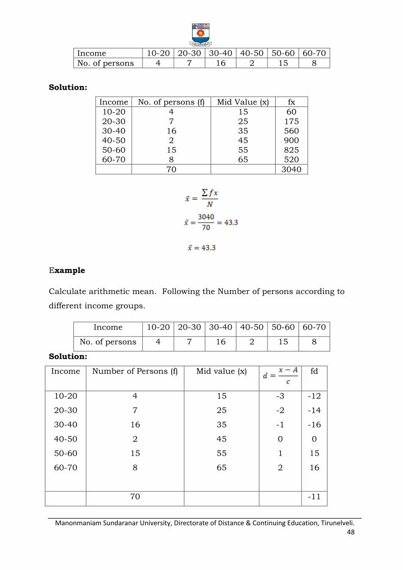
Manonmaniam Sundaranar University, Directorate of Distance & Continuing Education, Tirunelveli. 48
Income 10-20 20-30 30-40 40-50 50-60 60-70
No. of persons 4 7 16 2 15 8
Solution:
Income No. of persons (f) Mid Value (x) fx
10-20
20-30 30-40 40-50
50-60 60-70
4
7 16 2
15 8
15
25 35 45
55 65
60
175 560 900
825 520
70 3040
Example
Calculate arithmetic mean. Following the Number of persons according to
different income groups.
Income 10-20 20-30 30-40 40-50 50-60 60-70
No. of persons 4 7 16 2 15 8
Solution:
Income Number of Persons (f) Mid value (x)
fd
10-20
20-30
30-40
40-50
50-60
60-70
4
7
16
2
15
8
15
25
35
45
55
65
-3
-2
-1
0
1
2
-12
-14
-16
0
15
16
70 -11

Manonmaniam Sundaranar University, Directorate of Distance & Continuing Education, Tirunelveli. 49
A = 45, C.I = 10
Mean
= 45 – 1.57
Mean = 43.43
Merits and demerits of Arithmetic mean:
Merits
1. It is rigidly defined.
2. It is easily to understood and easily to calculated
3. It is every item is taken calculated.
4. It can further be subjected to algebraic treatment unlike other measures
i.e. mode and median.
5. If the number of items is sufficiently large, it is more accurate and more
reliable.
6. It is a calculated value and is not based on its position in the series.
7. It is possible to calculate even if some of the details of the data are
lacking.
8. It provides a good basis for comparison.
Demerits
1. It cannot be obtained by inspection nor located through a frequency
graph.
2. It cannot be in the study of qualitative phenomena not capable of
numerical measurement i.e. Intelligence, beauty, honesty etc.,
3. It can ignore any single item only at the risk of losing its accuracy.
4. It is affected very much by extreme values.
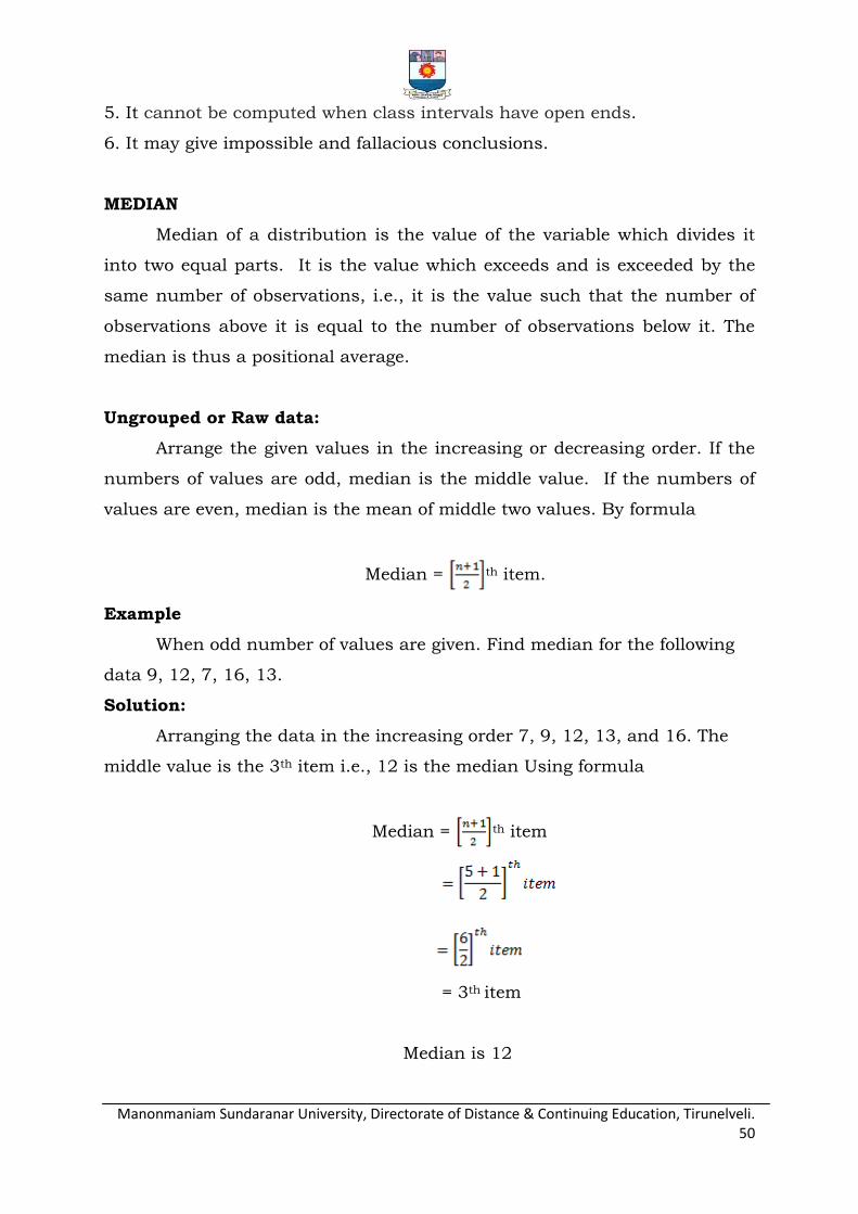
Manonmaniam Sundaranar University, Directorate of Distance & Continuing Education, Tirunelveli. 50
5. It cannot be computed when class intervals have open ends.
6. It may give impossible and fallacious conclusions.
MEDIAN
Median of a distribution is the value of the variable which divides it
into two equal parts. It is the value which exceeds and is exceeded by the
same number of observations, i.e., it is the value such that the number of
observations above it is equal to the number of observations below it. The
median is thus a positional average.
Ungrouped or Raw data:
Arrange the given values in the increasing or decreasing order. If the
numbers of values are odd, median is the middle value. If the numbers of
values are even, median is the mean of middle two values. By formula
Median = th item.
Example
When odd number of values are given. Find median for the following
data 9, 12, 7, 16, 13.
Solution:
Arranging the data in the increasing order 7, 9, 12, 13, and 16. The
middle value is the 3th item i.e., 12 is the median Using formula
Median = th item
= 3th item
Median is 12
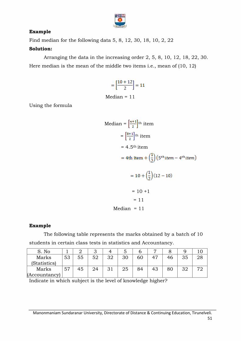
Manonmaniam Sundaranar University, Directorate of Distance & Continuing Education, Tirunelveli. 51
Example
Find median for the following data 5, 8, 12, 30, 18, 10, 2, 22
Solution:
Arranging the data in the increasing order 2, 5, 8, 10, 12, 18, 22, 30.
Here median is the mean of the middle two items i.e., mean of (10, 12)
Median = 11
Using the formula
Median = th item
= th item
= 4.5th item
= 10 +1
= 11
Median = 11
Example
The following table represents the marks obtained by a batch of 10
students in certain class tests in statistics and Accountancy.
S. No 1 2 3 4 5 6 7 8 9 10
Marks (Statistics)
53 55 52 32 30 60 47 46 35 28
Marks (Accountancy)
57 45 24 31 25 84 43 80 32 72
Indicate in which subject is the level of knowledge higher?
Manonmaniam Sundaranar University, Directorate of Distance & Continuing Education, Tirunelveli. 52
Solution:
For such question, median is the most suitable measure of central
tendency. The mark in the two subjects are first arranged in increasing
order as follows:
S. No 1 2 3 4 5 6 7 8 9 10
Marks (Statistics)
53 55 52 32 30 60 47 46 35 28
Marks (Accountancy)
57 45 24 31 25 84 43 80 32 72
Median = th item = th item
= 5.5th item
=
Median (Statistics) = = 46.5
Median (Accountancy) = = 44
Grouped Data:
In a grouped distribution, values are associated with frequencies.
Grouping can be in the form of a discrete frequency distribution or a
continuous frequency distribution. Whatever may be the type of
distribution, cumulative frequencies have to be calculated to know
the total number of items.
Cumulative frequency:
Cumulative frequency of each class is the sum of the frequency of the
class and the frequencies of the pervious classes, i.e., adding the frequencies
successively, so that the last cumulative frequency gives the total number of
items.
Discrete Series:
Step1: Find cumulative frequencies.
Step 2: Find
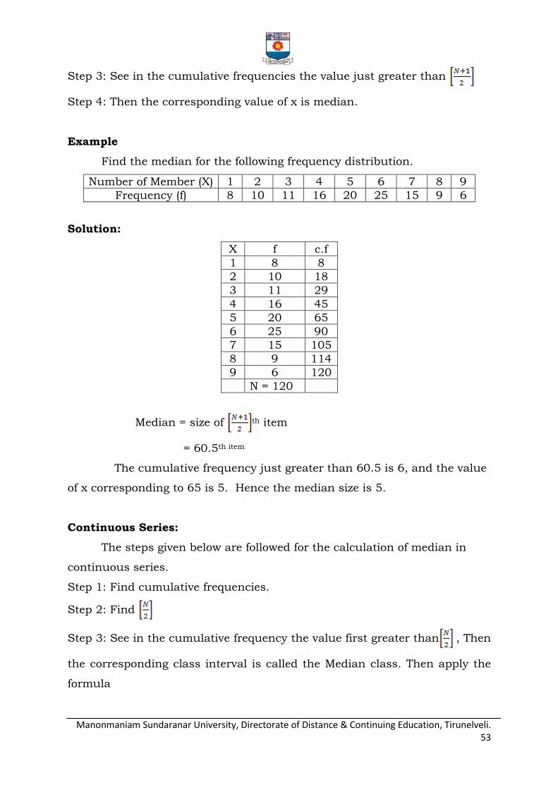
Manonmaniam Sundaranar University, Directorate of Distance & Continuing Education, Tirunelveli. 53
Step 3: See in the cumulative frequencies the value just greater than
Step 4: Then the corresponding value of x is median.
Example
Find the median for the following frequency distribution.
Number of Member (X) 1 2 3 4 5 6 7 8 9
Frequency (f) 8 10 11 16 20 25 15 9 6
Solution:
X f c.f
1 8 8
2 10 18
3 11 29
4 16 45
5 20 65
6 25 90
7 15 105
8 9 114
9 6 120
N = 120
Median = size of th item
= 60.5th item
The cumulative frequency just greater than 60.5 is 6, and the value
of x corresponding to 65 is 5. Hence the median size is 5.
Continuous Series:
The steps given below are followed for the calculation of median in
continuous series.
Step 1: Find cumulative frequencies.
Step 2: Find
Step 3: See in the cumulative frequency the value first greater than , Then
the corresponding class interval is called the Median class. Then apply the
formula
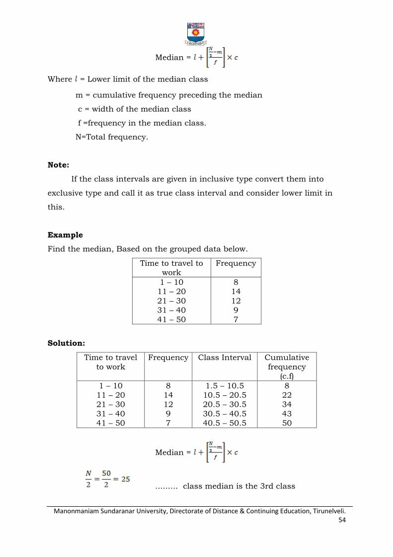
Manonmaniam Sundaranar University, Directorate of Distance & Continuing Education, Tirunelveli. 54
Median =
Where = Lower limit of the median class
m = cumulative frequency preceding the median
c = width of the median class
f =frequency in the median class.
N=Total frequency.
Note:
If the class intervals are given in inclusive type convert them into
exclusive type and call it as true class interval and consider lower limit in
this.
Example
Find the median, Based on the grouped data below.
Time to travel to work
Frequency
1 – 10 11 – 20
21 – 30 31 – 40
41 – 50
8 14
12 9
7
Solution:
Time to travel
to work
Frequency Class Interval Cumulative
frequency (c.f)
1 – 10 11 – 20 21 – 30
31 – 40 41 – 50
8 14 12
9 7
1.5 – 10.5 10.5 – 20.5 20.5 – 30.5
30.5 – 40.5 40.5 – 50.5
8 22 34
43 50
Median =
......... class median is the 3rd class
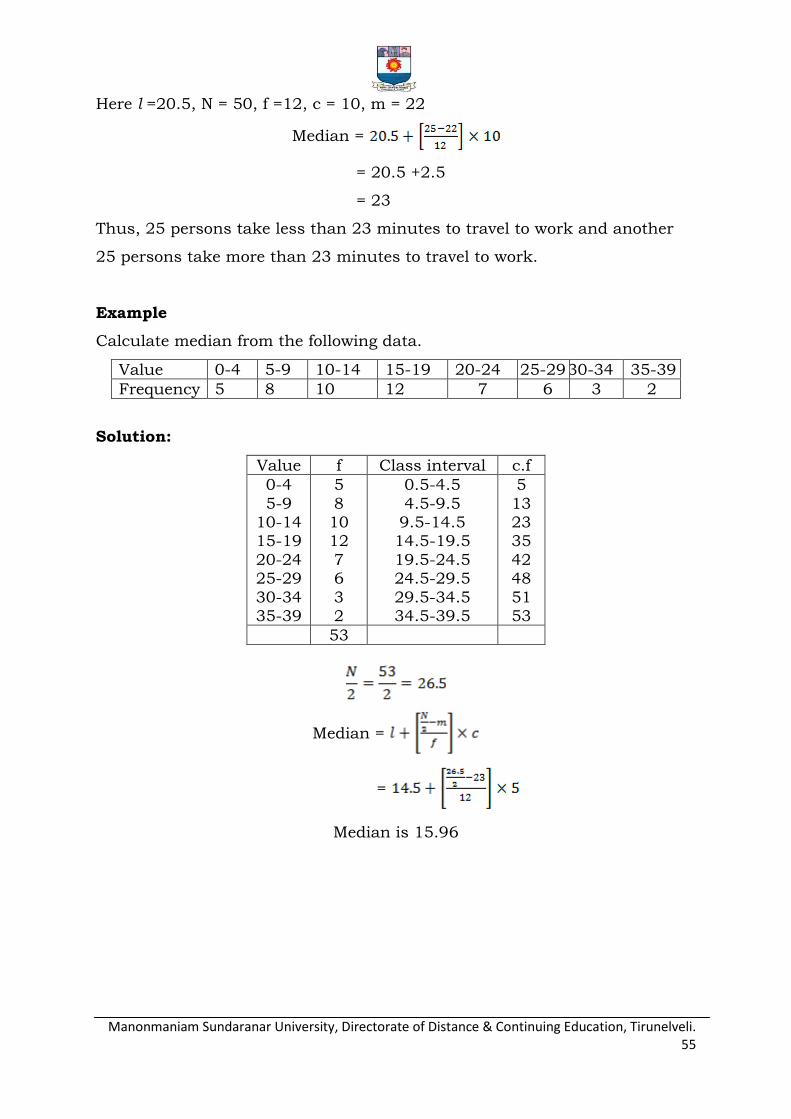
Manonmaniam Sundaranar University, Directorate of Distance & Continuing Education, Tirunelveli. 55
Here l =20.5, N = 50, f =12, c = 10, m = 22
Median =
= 20.5 +2.5
= 23
Thus, 25 persons take less than 23 minutes to travel to work and another
25 persons take more than 23 minutes to travel to work.
Example
Calculate median from the following data.
Value 0-4 5-9 10-14 15-19 20-24 25-29 30-34 35-39
Frequency 5 8 10 12 7 6 3 2
Solution:
Value f Class interval c.f
0-4
5-9 10-14 15-19
20-24 25-29
30-34 35-39
5
8 10 12
7 6
3 2
0.5-4.5
4.5-9.5 9.5-14.5 14.5-19.5
19.5-24.5 24.5-29.5
29.5-34.5 34.5-39.5
5
13 23 35
42 48
51 53
53
Median =
=
Median is 15.96
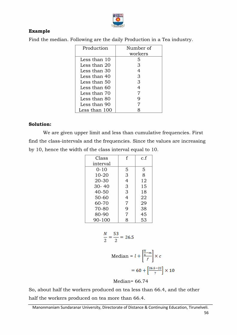
Manonmaniam Sundaranar University, Directorate of Distance & Continuing Education, Tirunelveli. 56
Example
Find the median. Following are the daily Production in a Tea industry.
Production Number of
workers
Less than 10
Less than 20 Less than 30 Less than 40
Less than 50 Less than 60
Less than 70 Less than 80 Less than 90
Less than 100
5
3 4 3
3 4
7 9 7
8
Solution:
We are given upper limit and less than cumulative frequencies. First
find the class-intervals and the frequencies. Since the values are increasing
by 10, hence the width of the class interval equal to 10.
Class interval
f c.f
0-10 10-20 20-30
30- 40 40-50
50-60 60-70 70-80
80-90 90-100
5 3 4
3 3
4 7 9
7 8
5 8 12
15 18
22 29 38
45 53
Median =
Median= 66.74
So, about half the workers produced on tea less than 66.4, and the other
half the workers produced on tea more than 66.4.
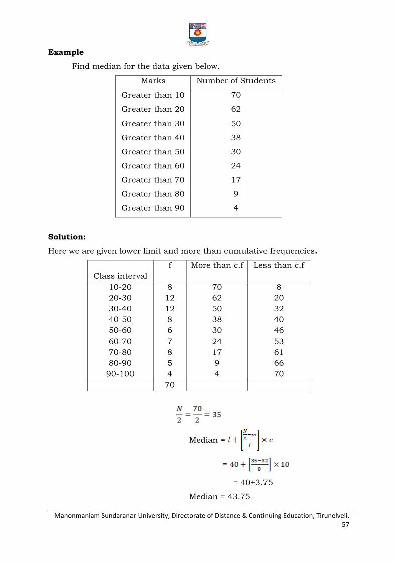
Manonmaniam Sundaranar University, Directorate of Distance & Continuing Education, Tirunelveli. 57
Example
Find median for the data given below.
Marks Number of Students
Greater than 10
Greater than 20
Greater than 30
Greater than 40
Greater than 50
Greater than 60
Greater than 70
Greater than 80
Greater than 90
70
62
50
38
30
24
17
9
4
Solution:
Here we are given lower limit and more than cumulative frequencies.
Class interval
f More than c.f Less than c.f
10-20
20-30
30-40
40-50
50-60
60-70
70-80
80-90
90-100
8
12
12
8
6
7
8
5
4
70
62
50
38
30
24
17
9
4
8
20
32
40
46
53
61
66
70
70
Median =
=
= 40+3.75
Median = 43.75
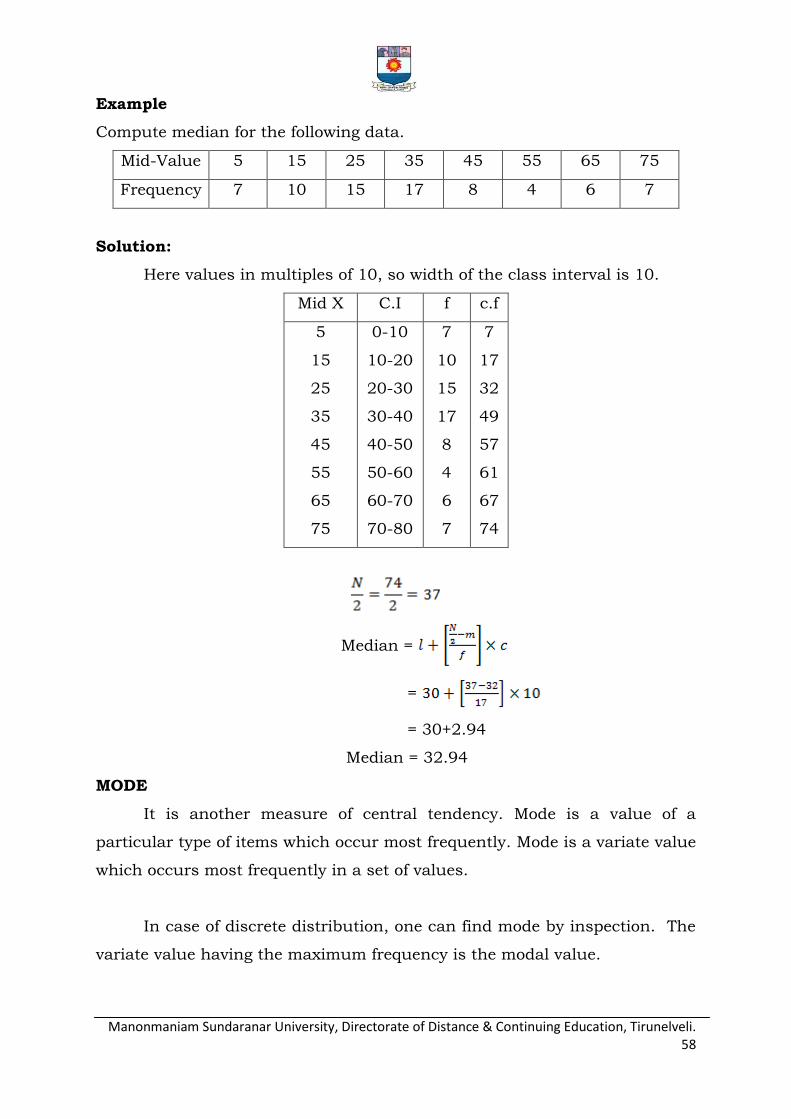
Manonmaniam Sundaranar University, Directorate of Distance & Continuing Education, Tirunelveli. 58
Example
Compute median for the following data.
Mid-Value 5 15 25 35 45 55 65 75
Frequency 7 10 15 17 8 4 6 7
Solution:
Here values in multiples of 10, so width of the class interval is 10.
Mid X C.I f c.f
5
15
25
35
45
55
65
75
0-10
10-20
20-30
30-40
40-50
50-60
60-70
70-80
7
10
15
17
8
4
6
7
7
17
32
49
57
61
67
74
Median =
=
= 30+2.94
Median = 32.94
MODE
It is another measure of central tendency. Mode is a value of a
particular type of items which occur most frequently. Mode is a variate value
which occurs most frequently in a set of values.
In case of discrete distribution, one can find mode by inspection. The
variate value having the maximum frequency is the modal value.

Manonmaniam Sundaranar University, Directorate of Distance & Continuing Education, Tirunelveli. 59
Ungrouped or Raw Data:
For ungrouped data or a series of individual observations, mode is
often found by mere inspection.
Example
Find the mode for the following ungrouped data.6, 5, 5, 7, 4, 8 3, 4, 4
Answer: Mode is 4
In Some cases the mode may be absent while in some cases there may
be more than one mode.
Example
Find the mode of the following observations. 4, 6, 8, 6, 7, 8, 8. In the given
data, the observation 8 occurs maximum number of times (3) Mode is 8
Example
Find the mode of the following observations. 2, 4, 6, 8, 10, 12.
Answer: no mode
Grouped data:
For Discrete distribution, see the highest frequency and corresponding
value of X is mode.
Continuous distribution:
See the highest frequency then the corresponding value of class
interval is called the modal class. Then apply the formula.
Mode =
l = Lower limit of the model class
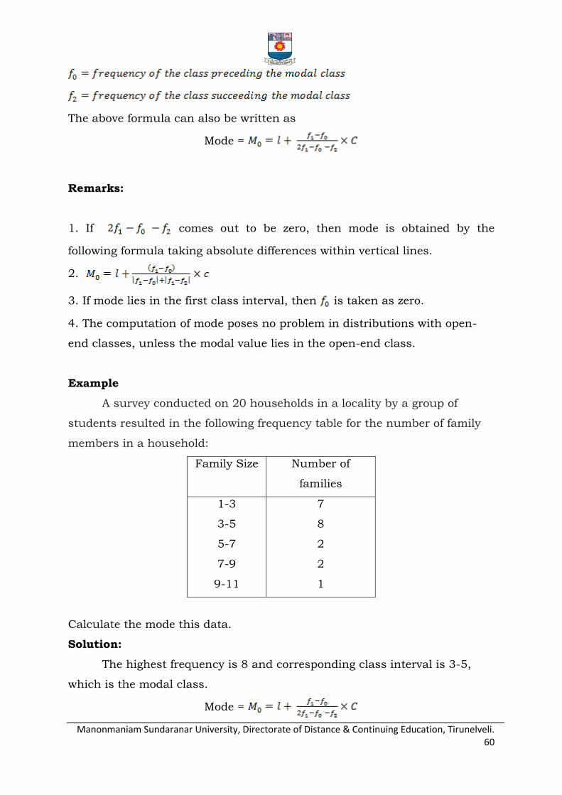
Manonmaniam Sundaranar University, Directorate of Distance & Continuing Education, Tirunelveli. 60
The above formula can also be written as
Mode =
Remarks:
1. If comes out to be zero, then mode is obtained by the
following formula taking absolute differences within vertical lines.
2.
3. If mode lies in the first class interval, then is taken as zero.
4. The computation of mode poses no problem in distributions with open-
end classes, unless the modal value lies in the open-end class.
Example
A survey conducted on 20 households in a locality by a group of
students resulted in the following frequency table for the number of family
members in a household:
Family Size Number of
families
1-3
3-5
5-7
7-9
9-11
7
8
2
2
1
Calculate the mode this data.
Solution:
The highest frequency is 8 and corresponding class interval is 3-5,
which is the modal class.
Mode =
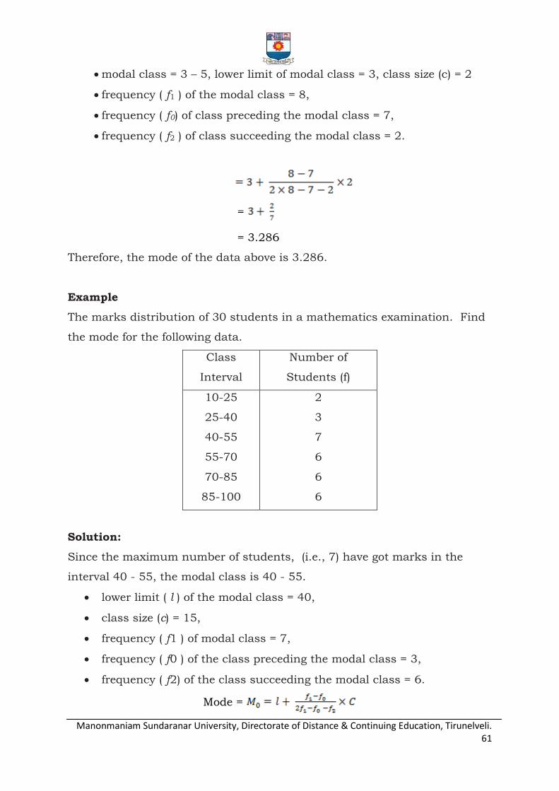
Manonmaniam Sundaranar University, Directorate of Distance & Continuing Education, Tirunelveli. 61
modal class = 3 – 5, lower limit of modal class = 3, class size (c) = 2
frequency ( f1 ) of the modal class = 8,
frequency ( f0) of class preceding the modal class = 7,
frequency ( f2 ) of class succeeding the modal class = 2.
=
= 3.286
Therefore, the mode of the data above is 3.286.
Example
The marks distribution of 30 students in a mathematics examination. Find
the mode for the following data.
Class
Interval
Number of
Students (f)
10-25
25-40
40-55
55-70
70-85
85-100
2
3
7
6
6
6
Solution:
Since the maximum number of students, (i.e., 7) have got marks in the
interval 40 - 55, the modal class is 40 - 55.
lower limit ( l ) of the modal class = 40,
class size (c) = 15,
frequency ( f1 ) of modal class = 7,
frequency ( f0 ) of the class preceding the modal class = 3,
frequency ( f2) of the class succeeding the modal class = 6.
Mode =

Manonmaniam Sundaranar University, Directorate of Distance & Continuing Education, Tirunelveli. 62
The mode marks is 52.
Definition of Mode:
In a grouped frequency distribution, it is not possible to determine the
mode by looking at the frequencies. Here, we can only locate a class with the
maximum frequency, called the modal class.
Determination of Modal class:
For a frequency distribution modal class corresponds to the maximum
frequency. But in any one (or more) of the following cases
If the maximum frequency is repeated
If the maximum frequency occurs in the beginning or at the end of the
distribution
If there are irregularities in the distribution, the modal class is
determined by the method of grouping.
Steps for Calculation:
We prepare a grouping table with 6 columns
In column I, we write down the given frequencies.
Column II is obtained by combining the frequencies two by two.
Leave the 1st frequency and combine the remaining frequencies two
by two and write in column III
Column IV is obtained by combining the frequencies three by three.
Leave the 1st frequency and combine the remaining frequencies three
by three and write in column V
Leave the 1st and 2nd frequencies and combine the remaining
frequencies three by three and write in column VI.
Mark the highest frequency in each column. Then form an analysis
table to find the modal class. After finding the modal class use the formula
to calculate the modal value.
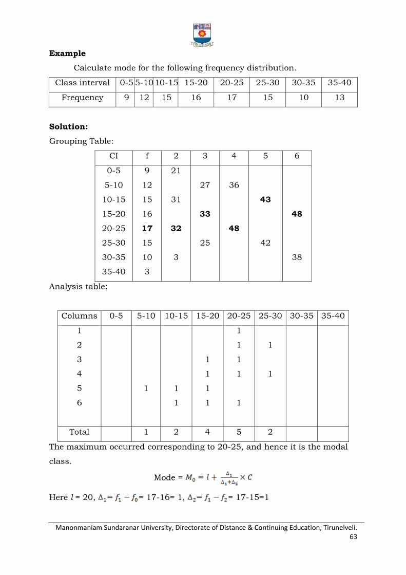
Manonmaniam Sundaranar University, Directorate of Distance & Continuing Education, Tirunelveli. 63
Example
Calculate mode for the following frequency distribution.
Class interval 0-5 5-10 10-15 15-20 20-25 25-30 30-35 35-40
Frequency 9 12 15 16 17 15 10 13
Solution:
Grouping Table:
CI f 2 3 4 5 6
0-5
5-10
10-15
15-20
20-25
25-30
30-35
35-40
9
12
15
16
17
15
10
3
21
31
32
3
27
33
25
36
48
43
42
48
38
Analysis table:
Columns 0-5 5-10 10-15 15-20 20-25 25-30 30-35 35-40
1
2
3
4
5
6
1
1
1
1
1
1
1
1
1
1
1
1
1
1
Total 1 2 4 5 2
The maximum occurred corresponding to 20-25, and hence it is the modal
class.
Mode =
Here l = 20, = 17-16= 1, = 17-15=1
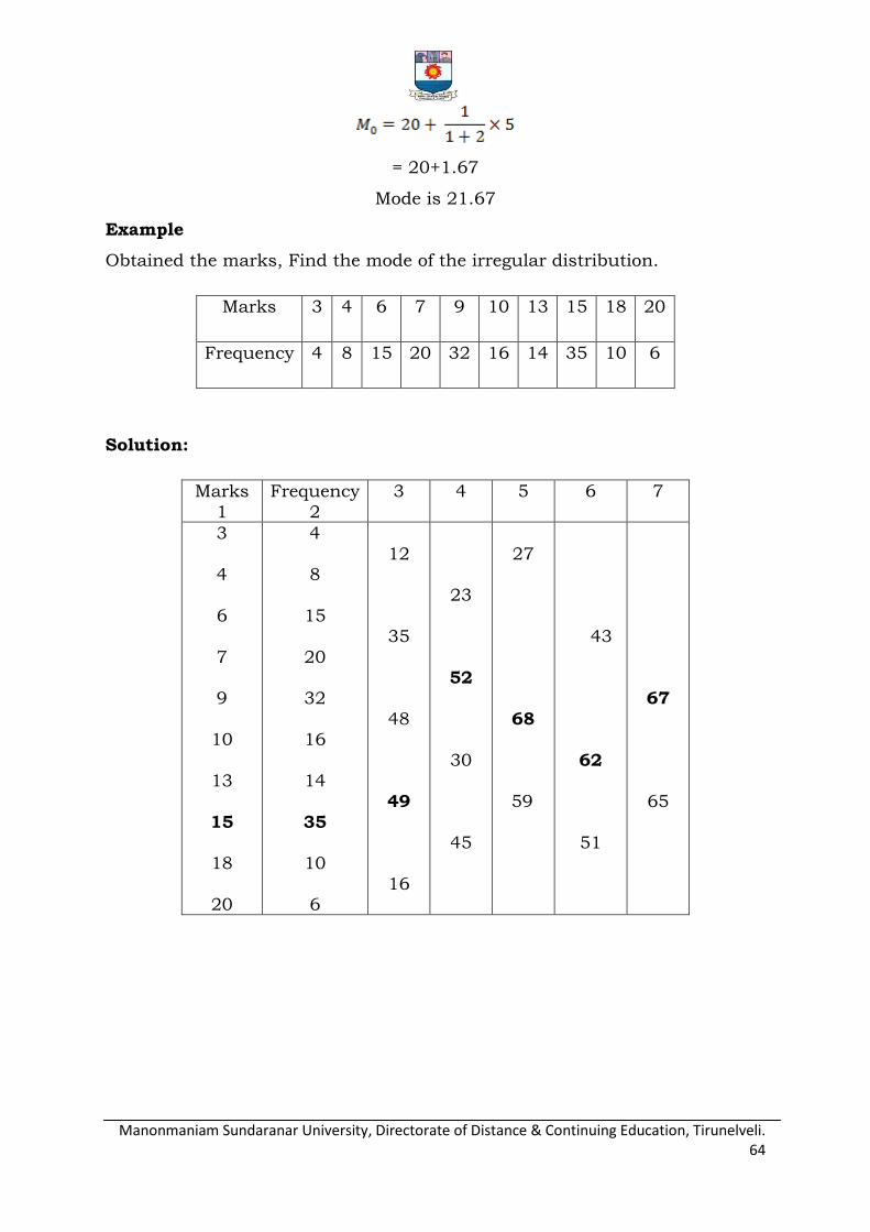
Manonmaniam Sundaranar University, Directorate of Distance & Continuing Education, Tirunelveli. 64
= 20+1.67
Mode is 21.67
Example
Obtained the marks, Find the mode of the irregular distribution.
Marks 3 4 6 7 9 10 13 15 18 20
Frequency 4 8 15 20 32 16 14 35 10 6
Solution:
Marks
1
Frequency
2
3 4 5 6 7
3
4
6
7 9
10
13
15
18
20
4
8
15
20
32
16
14
35
10
6
12
35
48
49
16
23
52
30
45
27
68
59
43
62
51
67
65
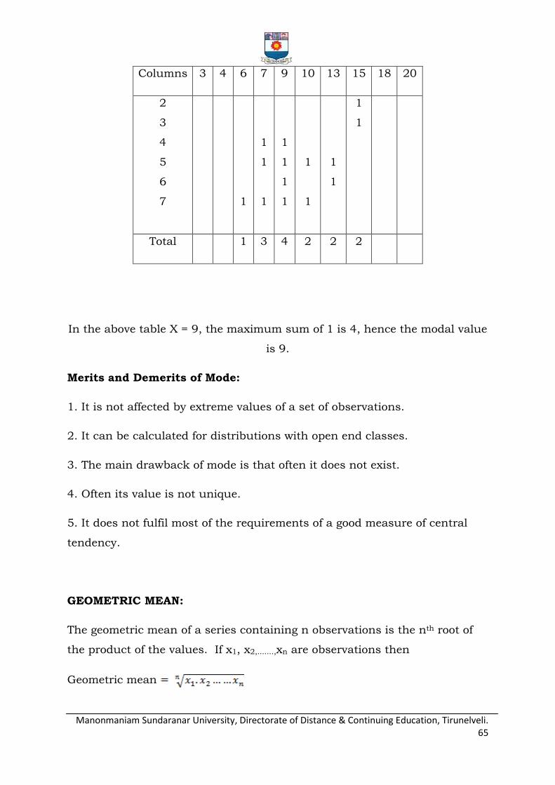
Manonmaniam Sundaranar University, Directorate of Distance & Continuing Education, Tirunelveli. 65
Columns 3 4 6 7 9 10 13 15 18 20
2
3
4
5
6
7
1
1
1
1
1
1
1
1
1
1
1
1
1
1
Total 1 3 4 2 2 2
In the above table X = 9, the maximum sum of 1 is 4, hence the modal value
is 9.
Merits and Demerits of Mode:
1. It is not affected by extreme values of a set of observations.
2. It can be calculated for distributions with open end classes.
3. The main drawback of mode is that often it does not exist.
4. Often its value is not unique.
5. It does not fulfil most of the requirements of a good measure of central
tendency.
GEOMETRIC MEAN:
The geometric mean of a series containing n observations is the nth root of
the product of the values. If x1, x2,.......,xn are observations then
Geometric mean
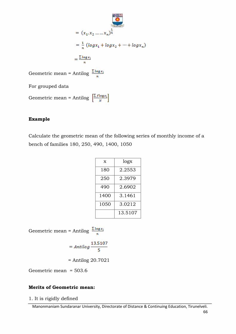
Manonmaniam Sundaranar University, Directorate of Distance & Continuing Education, Tirunelveli. 66
Geometric mean = Antilog
For grouped data
Geometric mean = Antilog
Example
Calculate the geometric mean of the following series of monthly income of a
bench of families 180, 250, 490, 1400, 1050
x logx
180 2.2553
250 2.3979
490 2.6902
1400 3.1461
1050 3.0212
13.5107
Geometric mean = Antilog
= Antilog 20.7021
Geometric mean = 503.6
Merits of Geometric mean:
1. It is rigidly defined
Manonmaniam Sundaranar University, Directorate of Distance & Continuing Education, Tirunelveli. 67
2. It is based on all items
3. It is very suitable for averaging ratios, rates and percentages
4. It is capable of further mathematical treatment.
5. Unlike AM, it is not affected much by the presence of extreme values.
Demerits of Geometric mean:
1. It cannot be used when the values are negative or if any of the
observations is zero
2. It is difficult to calculate particularly when the items are very large or
when there is a frequency distribution.
3. It brings out the property of the ratio of the change and not the absolute
difference of change as the case in arithmetic mean.
4. The GM may not be the actual value of the series.
HARMONIC MEAN
Harmonic mean of a set of observations is defined as the reciprocal of the
arithmetic average of the reciprocal of the given values. If x1, x2,.......,xn are n
observations then
Harmonic Mean =
For a frequency distribution
Harmonic mean =
Example
From the given data calculate Harmonic mean 5, 10, 17, 24, 30.

Manonmaniam Sundaranar University, Directorate of Distance & Continuing Education, Tirunelveli. 68
Solution:
x
5 0.2000
10 0.1000
17 0.0588
24 0.0417
30 0.0333
0.4338
Harmonic Mean =
=
Harmonic mean = 11.526
Example
The marks secured by some students of a class are given below. Calculate
the harmonic mean.
x 20 21 22 23 24 25
f 4 2 7 1 3 1
Solution:
Marks x
No of students f
20 21
22 23
24 25
4 2
7 1
3 1
0.0500 0.0476
0.0454 0.0435
0.0417 0.0400
0.2000 0.0952
0.3178 0.435
0.1251 0.0400 0.8216
18

Manonmaniam Sundaranar University, Directorate of Distance & Continuing Education, Tirunelveli. 69
Harmonic mean =
Harmonic mean = 21.91
Merits of Harmonic mean:
1. It is rigidly defined.
2. It is defined on all observations.
3. It is amenable to further algebraic treatment.
4. It is the most suitable average when it is desired to give greater weight to
smaller observations and less weight to the larger ones.
Demerits of Harmonic mean:
1. It is not easily understood.
2. It is difficult to compute.
3. It is only a summary figure and may not be the actual item in the series
4. It gives greater importance to small items and is therefore, useful only
when small items have to be given greater weightage.
2.2 PARTITION VALUES
When data is arranged in ascending order, it can be divided into
various parts by different values such as quartiles, deciles and percentiles.
These values are collectively called quantiles and are the extension of
median formula which divides data into two equal parts. Since the basic
purpose of these partition values is to divide data into different parts
therefore a relationship exists between them.
QUARTILES
The quartiles are the three values that dived the ordered data set in
four, perceptually equal, parts. There are three quartiles, usually
represented by Q1, Q2, and Q3. The first quartile, Q1, has the lowest value
Manonmaniam Sundaranar University, Directorate of Distance & Continuing Education, Tirunelveli. 70
that is greater than a one fourth of the data; that is, the variable‟s value that
is greater than 25% of the observations and is smaller than the 75% of the
observations.
The second quartile, Q2, (that coincides, it is identical or similar to the
median, Q2 = M d), is the lowest value that is greater than half of the data,
that is 50% of the observations have a greater value than the median and
50% have a lower value.
The third quartile, Q3, has the lowest value that is greater than three
fourths of the data, that is, the value of the variable that has a value greater
75% of the observations and of a lower value than 25% of the observations.
Raw or ungrouped data:
First arrange the given data in the increasing order and use the
formula for Q1 and Q3 then quartile deviation, Q.D is given by
Where th item and th item
Example
Compute quartiles for the data given below 25, 18, 30, 8, 15, 5, 10, 35, 40,
and 45.
Solution:
Now arranging the ascending order 5, 8, 10, 15, 18, 25, 30, 35, 40, 45
th item
= th item
= (2.75)th item
= 2nd item + (3rd item – 2nd item)
= 8 + (10 – 8)
Manonmaniam Sundaranar University, Directorate of Distance & Continuing Education, Tirunelveli. 71
= 8 +
= 8 + 1.5
Q1 = 9.5
th item
= 3× (2.75)th item
= (8.25)th item
= 8th item + (9th item – 8th item)
= 35 +
= 35+1.25
Q3 = 36.25
Discrete Series:
Step1: Find cumulative frequencies.
Step 2: Find
Step 3: See in the cumulative frequencies, the value just greater than ,
and then the corresponding value of x is Q1
Step 4: Find 3
Step 5: See in the cumulative frequencies, the value just greater than 3 ,
then the corresponding value of x is Q3.
Example
Compute quartiles for the data given bellow.
53 74 82 42 39 20 81 68 58 28
67 54 93 70 30 55 36 37 29 61
Solution:
Q1 = th item = = = 5.25th item
Manonmaniam Sundaranar University, Directorate of Distance & Continuing Education, Tirunelveli. 72
The value of 5th item is 36 and that of the 6th item is 37. Thus the first
quartile is a value 0.25th of the way between 36 and 37, which are 36.25.
Therefore, = 36.25. Similarly,
Q3 = 3 th item = = = 15.75th item
The value of the 15th item is 68 and that of the 16th item is 70. Thus
the third quartile is a value 0.75th of the way between 68 and 70. As the
difference between 68 and 70 is 2, so the third quartile will be 68 + 2(0.75) =
69.5. Therefore, = 69.5.
Continuous series:
Step1: Find cumulative frequencies
Step 2: Find
Step3: See in the cumulative frequencies, the value just greater than ,
and then the corresponding class interval is called first quartile class.
Step 4: Find 3 see in the cumulative frequencies the value just greater
than 3 then the corresponding class interval is called 3rd quartile class.
Then apply the respective formulae.
Where l1 = lower limit of the first quartile class
f1 = frequency of the first quartile class
c1 = width of the first quartile class
m1 = c.f. preceding the first quartile class

Manonmaniam Sundaranar University, Directorate of Distance & Continuing Education, Tirunelveli. 73
l3 = 1ower limit of the 3rd quartile class
f3 = frequency of the 3rd quartile class
c3 = width of the 3rd quartile class
m3 = c.f. preceding the 3rd quartile class
Example
The following series relates to the Monthly per capita expenditure classes.
Find the quartiles.
Monthly per capita expenditure classes (Rs.) Number of families
140-150
150-160 160-170
170-180 180-190 190-200
200-210 210-220 220-230
230-240 240-250
17
29 42
72 84 107
49 34 31
16 12
Solution:
Monthly per capita expenditure classes (Rs.)
Number of families Cumulative frequency
140-150 150-160
160-170 170-180
180-190 190-200 200-210
210-220 220-230 230-240
240-250
17 29
42 72
84 107 49
34 31 16
12
17 46
88 160
244 351 400
434 465 481
493
....................... = 369.75

Manonmaniam Sundaranar University, Directorate of Distance & Continuing Education, Tirunelveli. 74
= 170+4.90 = 174.90
= = 200+3.83 = 203.83
DECILES
The procedure for locating the ith decile class is to calculate iN/10 and
search that minimum cumulative frequency in which this value is
contained. The class corresponding to this cumulative frequency is ith decile
class. The unique value of ith decile can be calculated by the formula.
Deciles for Raw data or ungrouped data:
Example
Compute D5 for the data given below 5, 24, 36, 12, 20, 8.
Solution:
Arranging the given values in the increasing order 5, 8, 12, 20, 24, 36
th observation
th observation
th observation
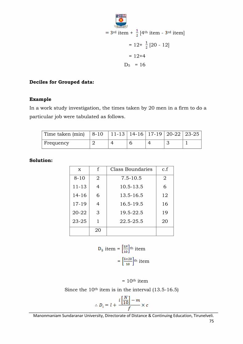
Manonmaniam Sundaranar University, Directorate of Distance & Continuing Education, Tirunelveli. 75
rd item + [4th item - rd item]
= 12+ [20 - 12]
= 12+4
D5 = 16
Deciles for Grouped data:
Example
In a work study investigation, the times taken by 20 men in a firm to do a
particular job were tabulated as follows.
Time taken (min) 8-10 11-13 14-16 17-19 20-22 23-25
Frequency 2 4 6 4 3 1
Solution:
x f Class Boundaries c.f
8-10
11-13
14-16
17-19
20-22
23-25
2
4
6
4
3
1
7.5-10.5
10.5-13.5
13.5-16.5
16.5-19.5
19.5-22.5
22.5-25.5
2
6
12
16
19
20
20
item = th item
= th item
= 10th item
Since the 10th item is in the interval (13.5-16.5)

Manonmaniam Sundaranar University, Directorate of Distance & Continuing Education, Tirunelveli. 76
= 13.5 + 2
= 15.5
item = th item
= th item
= 4th item
Since the 10th item is in the interval (10.5 – 13.5)
c
= 10.5 -1
= 9.5
PERCENTILES
To locate ith percentile class, calculate iN/100 (i = 1, 2, ....., 99) and
that minimum cumulative frequency which contains this value. The class
corresponding to this minimum cumulative frequency is the percentile class.
Unique value of ith percentile can be calculated by the formula,
Relationship:
P25 = Q1; P50 = D5 = Q2 = Median and P75 = Q3
Percentile for Raw Data or Ungrouped Data:
Example
Calculate P15 for the data given below: 5, 24, 36, 12, 20, 8

Manonmaniam Sundaranar University, Directorate of Distance & Continuing Education, Tirunelveli. 77
Solution:
Arranging the given values in the increasing order. 5, 8, 12, 20, 24, 36
th item
th item
= (1.05)th item
= 1st item +0.05(2nd item – 1st item)
= 5+0.05(8-5)
= 5+0.15
= 5.15
Percentile for grouped data:
Example
Find P25, P50 for the following frequency distribution.
Class Interval
f
85.5-90.5 90.5-95.5
95.5-100.5 100.5-105.5 105.5-110.5
110.5-115.5
6 4
10 6 3
1
Solution:
Class
Interval
f C.f
85.5-90.5
90.5-95.5
95.5-100.5
100.5-105.5
105.5-110.5
110.5-115.5
6
4
10
6
3
1
6
10
20
26
29
30
30

Manonmaniam Sundaranar University, Directorate of Distance & Continuing Education, Tirunelveli. 78
= 7.5
so, P25 group is 90.5–95.5 containing the 7.5th observation
=
= 92.375
= 15
so, P50 group is 95.5–100.5 containing the 15th observation
=
= 98
2.3 MEASURES OF DISPERSION
The measure of central tendency serves to locate the centre of the
distribution, but they do not reveal how the items are spread out on either
side of the centre. This characteristic of a frequency distribution is
commonly referred to as dispersion. In a series all the items are not equal.
There is difference or variation among the values. The degree of variation is
evaluated by various measures of dispersion. Small dispersion indicates
high uniformity of the items, while large dispersion indicates less uniformity.
Characteristics of a good measure of dispersion:
An ideal measure of dispersion is expected to possess the following
properties
1. It should be rigidly defined
2. It should be based on all the items.
3. It should not be unduly affected by extreme items.
Manonmaniam Sundaranar University, Directorate of Distance & Continuing Education, Tirunelveli. 79
4. It should lend itself for algebraic manipulation.
5. It should be simple to understand and easy to calculate.
Absolute and Relative Measures:
There are two kinds of measures of dispersion, namely
Absolute measure of dispersion
Relative measure of dispersion
Absolute measure of dispersion indicates the amount of variation in a
set of values in terms of units of observations. For example, when rainfalls
on different days are available in mm, any absolute measure of dispersion
gives the variation in rainfall in mm. On the other hand relative measures of
dispersion are free from the units of measurements of the observations.
They are pure numbers. They are used to compare the variation in two or
more sets, which are having different units of measurements of
observations. The various absolute and relative measures of dispersion are
listed below.
Absolute measure Relative measure
1. Range 1.Co-efficient of Range
2. Quartile deviation 2.Co-efficient of Quartile deviation
3. Mean deviation 3. Co-efficient of Mean deviation
4. Standard deviation 4.Co-efficient of variation
RANGE
The range is difference between two extreme observations of the
distribution. If L and S are the greatest and smallest observations
respectively in a distribution, then its range is given by
Range = L – S.
Where L = Largest value.
S = Smallest value.

Manonmaniam Sundaranar University, Directorate of Distance & Continuing Education, Tirunelveli. 80
In individual observations and discrete series, L and S are easily identified.
In continuous series, the following two methods are followed.
Method 1:
L = Upper boundary of the highest class
S = Lower boundary of the lowest class.
Method 2
L = Mid value of the highest class.
S = Mid value of the lowest class.
Co-efficient of Range:
Co-efficient of Range =
Example
Find the value of range and its co-efficient range for the following data.
89, 73, 84, 91, 87, 77, 94.
Solution:
73, 77, 84, 87, 89, 91, 94.
L=94, S = 73.
Range = L – S = 94 - 73
Range= 21
Co-efficient of Range =
=
=
Co- efficient of range = 0.125
Example
Calculate range and its co efficient from the following distribution.

Manonmaniam Sundaranar University, Directorate of Distance & Continuing Education, Tirunelveli. 81
Size 10-15 15-20 20-25 25-30 30-35
Number 2 8 10 14 8
Solution:
L = Upper boundary of the highest class = 35
S = Lower boundary of the lowest class = 10
Range = L-S = 35-10
Range = 15
Co-efficient of range = =
Co-efficient of range = 0.555
Merits and Demerits of Range:
Merits
1. It is simple to understand.
2. It is easy to calculate.
3. In certain types of problems like quality control, weather forecasts, share
price analysis, range is most widely used.
Demerits
1. It is very much affected by the extreme items.
2. It is based on only two extreme observations.
3. It cannot be calculated from open-end class intervals.
4. It is not suitable for mathematical treatment.
5. It is a very rarely used measure.
MEAN DEVIATION
The measures of dispersion discussed so far are not satisfactory in the
sense that they lack most of the requirements of a good measure. Mean
deviation is a better measure than range and Quartile deviation.
Definition:
Mean deviation is the arithmetic mean of the deviations of a series
computed from any measure of central tendency; i.e., the mean, median or
Manonmaniam Sundaranar University, Directorate of Distance & Continuing Education, Tirunelveli. 82
mode, all the deviations are taken as positive i.e., signs are ignored.
According to Clark and Schekade, “Average deviation is the average amount
scatter of the items in a distribution from either the mean or the median,
ignoring the signs of the deviations”. We usually compute mean deviation
about any one of the three averages mean, median or mode. Sometimes
mode may be ill defined and as such mean deviation is computed from mean
and median. Median is preferred as a choice between mean and median. But
in general practice and due to wide applications of mean, the mean
deviation is generally computed from mean. M.D can be used to denote
mean deviation.
Coefficient of mean deviation:
Mean deviation calculated by any measure of central tendency is an
absolute measure. For the purpose of comparing variation among different
series, a relative mean deviation is
required. The relative mean deviation is obtained by dividing the mean
deviation by the average used for calculating mean deviation.
Coefficient of mean deviation =
If the result is desired in percentage, the coefficient of mean
Deviation =
Example
Calculate Mean deviation from mean and median for the following data, also
calculate coefficients of Mean Deviation. 111.5, 111.2, 102.3, 112.4, 108.8,
125.3, 116.5, 132.7
Solution
Arrange the data in ascending order 102.3, 104.6, 108.8, 111.2,
111.5, 112.4, 116.5, 125.3, 132.7
Mean =
Mean =
Median = Value of
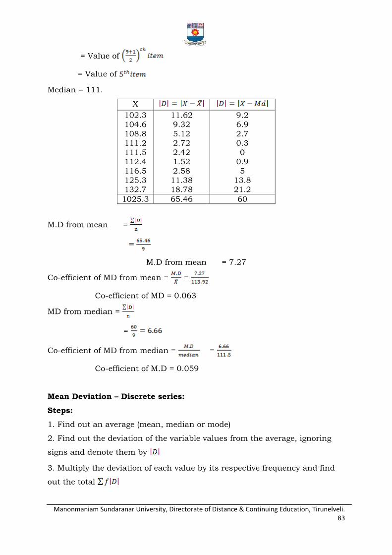
Manonmaniam Sundaranar University, Directorate of Distance & Continuing Education, Tirunelveli. 83
= Value of
= Value of
Median = 111.
X 102.3
104.6 108.8
111.2 111.5 112.4
116.5 125.3 132.7
11.62
9.32 5.12
2.72 2.42 1.52
2.58 11.38 18.78
9.2
6.9 2.7
0.3 0
0.9
5 13.8 21.2
1025.3 65.46 60
M.D from mean =
M.D from mean = 7.27
Co-efficient of MD from mean = =
Co-efficient of MD = 0.063
MD from median =
=
Co-efficient of MD from median = =
Co-efficient of M.D = 0.059
Mean Deviation – Discrete series:
Steps:
1. Find out an average (mean, median or mode)
2. Find out the deviation of the variable values from the average, ignoring
signs and denote them by
3. Multiply the deviation of each value by its respective frequency and find
out the total

Manonmaniam Sundaranar University, Directorate of Distance & Continuing Education, Tirunelveli. 84
4. Divide by the total frequencies N Symbolically, MD from median =
Example
Compute Mean deviation from mean and median from the following data:
Height
(in cm)
158 159 160 161 162 163 164 165 166
No. of
persons
15 20 32 35 33 22 20 10 8
Also compute coefficient of mean deviation.
Solution:
Height
X
No. of persons D=x-A
A=162
fd
158
159
160
161
162
163
164
165
166
15
20
32
35
33
22
20
10
8
-4
-3
-2
-1
0
1
2
3
4
-60
-60
-64
-35
0
22
40
30
32
3.51
2.51
1.51
0.51
0.49
1.49
2.49
3.49
4.49
52.65
50.20
48.32
17.85
16.17
32.78
49.80
34.90
35.92
195 -95 338.59
= 162 – 0.49
= 161.51
MD from median =
=
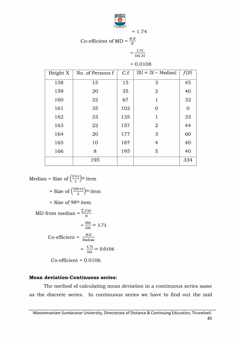
Manonmaniam Sundaranar University, Directorate of Distance & Continuing Education, Tirunelveli. 85
= 1.74
Co-efficient of MD =
=
= 0.0108
Height X No. of Persons f C.f
158
159
160
161
162
163
164
165
166
15
20
32
35
33
22
20
10
8
15
35
67
102
135
157
177
187
195
3
2
1
0
1
2
3
4
5
45
40
32
0
33
44
60
40
40
195 334
Median = Size of th item
= Size of th item
= Size of th item
MD from median =
=
Co-efficient =
=
Co-efficient = 0.0106
Mean deviation-Continuous series:
The method of calculating mean deviation in a continuous series same
as the discrete series. In continuous series we have to find out the mid
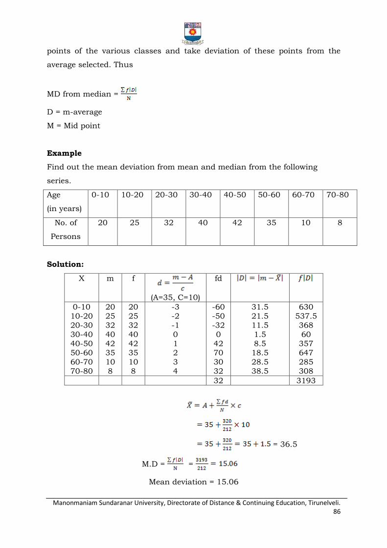
Manonmaniam Sundaranar University, Directorate of Distance & Continuing Education, Tirunelveli. 86
points of the various classes and take deviation of these points from the
average selected. Thus
MD from median =
D = m-average
M = Mid point
Example
Find out the mean deviation from mean and median from the following
series.
Age
(in years)
0-10 10-20 20-30 30-40 40-50 50-60 60-70 70-80
No. of
Persons
20 25 32 40 42 35 10 8
Solution:
X m f
(A=35, C=10)
fd
0-10 10-20 20-30
30-40 40-50 50-60
60-70 70-80
20 25 32
40 42 35
10 8
20 25 32
40 42 35
10 8
-3 -2 -1
0 1 2
3 4
-60 -50 -32
0 42 70
30 32
31.5 21.5 11.5
1.5 8.5 18.5
28.5 38.5
630 537.5 368
60 357 647
285 308
32 3193
= 36.5
M.D = =
Mean deviation = 15.06

Manonmaniam Sundaranar University, Directorate of Distance & Continuing Education, Tirunelveli. 87
Calculation of median and M.D from median
X m f
0-10
10-20
20-30
30-40
40-50
50-60
60-70
70-80
20
25
32
40
42
35
10
8
20
25
32
40
42
35
10
8
20
45
77
117
159
194
204
212
32.25
22.25
12.25
2.25
7.75
17.75
27.75
37.75
645
556.25
392
90
325.50
621.25
277.50
302
Total 3209.50
l = 30, m = 77, f = 40, c = 10
Median =
=
=
=
= 37.25
M.D =
=
= 15.14
Coefficient of M.D =
= = 0.41
Co efficient mean deviation = 0.41
Manonmaniam Sundaranar University, Directorate of Distance & Continuing Education, Tirunelveli. 88
Merits and Demerits of Mean Deviation:
Merits
1. It is simple to understand and easy to compute.
2. It is based on all the observations of series.
3. It is not very much affected by the fluctuations of sampling.
4. It is less affected by the extreme items.
5. It is flexible, because it can be calculated from any average.
6. It facilitates comparison between different items of a series.
7. It has practical usefulness in the field of business and commerce.
Demerits
1. It is not a very accurate measure of dispersion.
2. It is not suitable for further mathematical calculation.
3. It is rarely used. It is not as popular as standard deviation.
4. Algebraic positive and negative signs are ignored.
5. It is not suitable for sociological study.
QUARTILE DEVIATION (Q.D):
Co–efficient of quartile deviation is an absolute quantity and is useful
to compare the variability among the middle 50% observations. The
quartiles are the values which divide the whole distribution into four equal
parts.
Definition:
The interquartile range, half of the difference between the first and
third quartiles interquartile range that is Quartile deviation. Hence, it is
called Semi Inter Quartile Range.
In Symbols, Q.D = . Among the quartiles Q1, Q2 and Q3, the
range Q3 - Q1 is called inter quartile range and , Semi inter quartile
range.

Manonmaniam Sundaranar University, Directorate of Distance & Continuing Education, Tirunelveli. 89
Co-efficient of Quartile Deviation:
Co-efficient of Q.D =
Example
The wheat production (in Kg) of 20 acres is given as: 1120, 1240,
1320, 1040, 1080, 1200, 1440, 1360, 1680, 1730, 1785, 1342, 1960, 1880,
1755, 1720, 1600, 1470, 1750, and 1885. Find the quartile deviation and
coefficient of quartile deviation.
Solution:
Arranging the observations in ascending order
1040, 1080, 1120, 1200, 1240, 1320, 1342, 1360, 1440, 1470, 1600, 1680,
1720, 1730, 1750, 1755, 1785, 1880, 1885, 1960.
is
=
= 5.25th value
= 5th value + 0.25 (6th value – 5th value)
= 1240+0.25(1320-1240)
= 1240+20
is
= =
= 15th value + 0.75 (6th value – 5th value)
= 1750 + 0.75 (1755 – 1750)
= 1753.75.

Manonmaniam Sundaranar University, Directorate of Distance & Continuing Education, Tirunelveli. 90
Quartile deviation =
=
=
Quartile deviation = 246.875
Co-efficient of Quartile deviation =
=
Co-efficient of Quartile deviation = 0.164
Example
Calculate the quartile deviation and coefficient of quartile deviation from the
data given below
Maximum Weight
(Short tonnes)
Number of
Packets
9.25-9.75 2
9.75-10.25 5
10.25-10.75 12
10.75-11.25 17
11.25-11.75 14
11.75-12.25 6
12.25-12.75 3
12.75-13.25 1
Solution:
Maximum Weight (Short tonnes)
Number of Packets
C.f
9.25-9.75 2 2
9.75-10.25 5 7
10.25-10.75 12 19
10.75-11.25 17 36
11.25-11.75 14 50
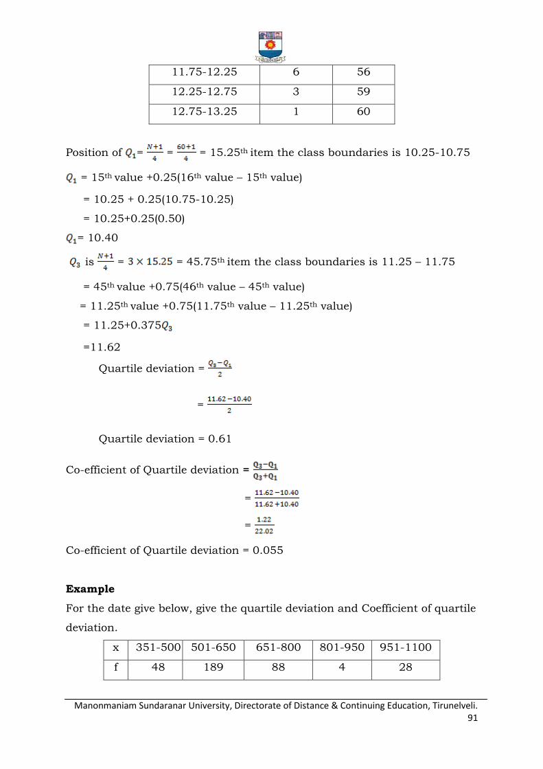
Manonmaniam Sundaranar University, Directorate of Distance & Continuing Education, Tirunelveli. 91
11.75-12.25 6 56
12.25-12.75 3 59
12.75-13.25 1 60
Position of = = = 15.25th item the class boundaries is 10.25-10.75
= 15th value +0.25(16th value – 15th value)
= 10.25 + 0.25(10.75-10.25)
= 10.25+0.25(0.50)
= 10.40
is = = 45.75th item the class boundaries is 11.25 – 11.75
= 45th value +0.75(46th value – 45th value)
= 11.25th value +0.75(11.75th value – 11.25th value)
= 11.25+0.375
=11.62
Quartile deviation =
=
Quartile deviation = 0.61
Co-efficient of Quartile deviation =
=
=
Co-efficient of Quartile deviation = 0.055
Example
For the date give below, give the quartile deviation and Coefficient of quartile
deviation.
x 351-500 501-650 651-800 801-950 951-1100
f 48 189 88 4 28
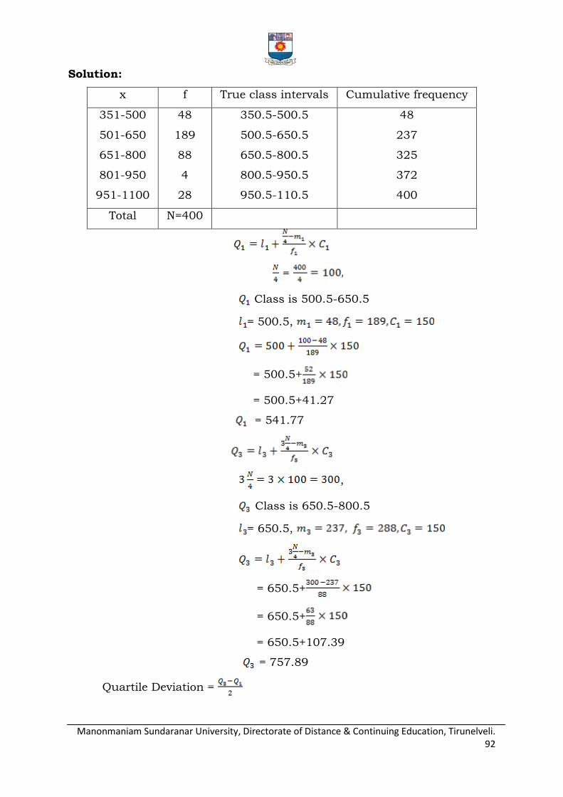
Manonmaniam Sundaranar University, Directorate of Distance & Continuing Education, Tirunelveli. 92
Solution:
x f True class intervals Cumulative frequency
351-500
501-650
651-800
801-950
951-1100
48
189
88
4
28
350.5-500.5
500.5-650.5
650.5-800.5
800.5-950.5
950.5-110.5
48
237
325
372
400
Total N=400
=
Class is 500.5-650.5
= 500.5,
= 500.5+
= 500.5+41.27
= 541.77
,
Class is 650.5-800.5
= 650.5,
= 650.5+
= 650.5+
= 650.5+107.39
= 757.89
Quartile Deviation =
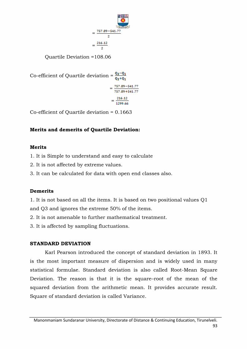
Manonmaniam Sundaranar University, Directorate of Distance & Continuing Education, Tirunelveli. 93
=
=
Quartile Deviation =108.06
Co-efficient of Quartile deviation =
=
=
Co-efficient of Quartile deviation = 0.1663
Merits and demerits of Quartile Deviation:
Merits
1. It is Simple to understand and easy to calculate
2. It is not affected by extreme values.
3. It can be calculated for data with open end classes also.
Demerits
1. It is not based on all the items. It is based on two positional values Q1
and Q3 and ignores the extreme 50% of the items.
2. It is not amenable to further mathematical treatment.
3. It is affected by sampling fluctuations.
STANDARD DEVIATION
Karl Pearson introduced the concept of standard deviation in 1893. It
is the most important measure of dispersion and is widely used in many
statistical formulae. Standard deviation is also called Root-Mean Square
Deviation. The reason is that it is the square–root of the mean of the
squared deviation from the arithmetic mean. It provides accurate result.
Square of standard deviation is called Variance.
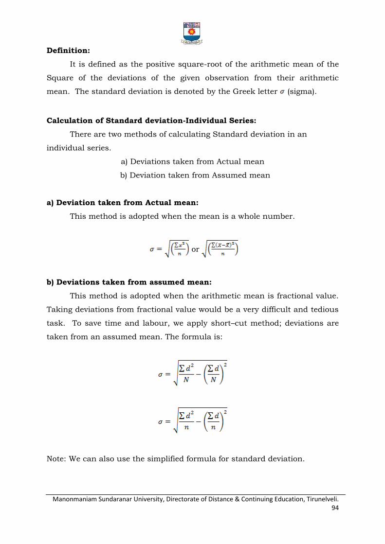
Manonmaniam Sundaranar University, Directorate of Distance & Continuing Education, Tirunelveli. 94
Definition:
It is defined as the positive square-root of the arithmetic mean of the
Square of the deviations of the given observation from their arithmetic
mean. The standard deviation is denoted by the Greek letter (sigma).
Calculation of Standard deviation-Individual Series:
There are two methods of calculating Standard deviation in an
individual series.
a) Deviations taken from Actual mean
b) Deviation taken from Assumed mean
a) Deviation taken from Actual mean:
This method is adopted when the mean is a whole number.
or
b) Deviations taken from assumed mean:
This method is adopted when the arithmetic mean is fractional value.
Taking deviations from fractional value would be a very difficult and tedious
task. To save time and labour, we apply short–cut method; deviations are
taken from an assumed mean. The formula is:
Note: We can also use the simplified formula for standard deviation.

Manonmaniam Sundaranar University, Directorate of Distance & Continuing Education, Tirunelveli. 95
For the frequency distribution
Example
Calculate the standard deviation from the following data 6, 2, 3, 1.
Solution:
Find the square of the distance from each data point to the mean.
x
6
2
3
1
3
-1
0
2
9
1
0
4
12 14
Standard deviation = 1.87
Example
Calculate the standard deviation, for the following data.
Student 1 2 3 4 5 6
Marks 2 4 6 8 10 12
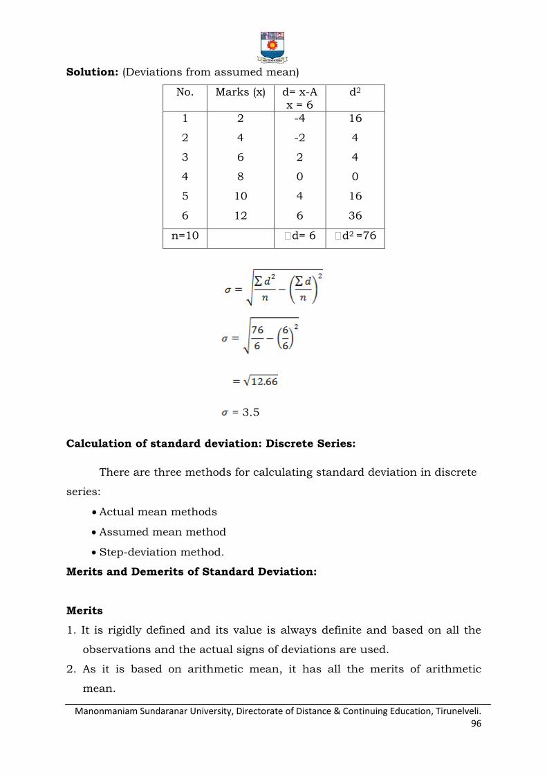
Manonmaniam Sundaranar University, Directorate of Distance & Continuing Education, Tirunelveli. 96
Solution: (Deviations from assumed mean)
No. Marks (x) d= x-A
x = 6
d2
1
2
3
4
5
6
2
4
6
8
10
12
-4
-2
2
0
4
6
16
4
4
0
16
36
n=10 d= 6 d2 =76
= 3.5
Calculation of standard deviation: Discrete Series:
There are three methods for calculating standard deviation in discrete
series:
Actual mean methods
Assumed mean method
Step-deviation method.
Merits and Demerits of Standard Deviation:
Merits
1. It is rigidly defined and its value is always definite and based on all the
observations and the actual signs of deviations are used.
2. As it is based on arithmetic mean, it has all the merits of arithmetic
mean.

Manonmaniam Sundaranar University, Directorate of Distance & Continuing Education, Tirunelveli. 97
3. It is the most important and widely used measure of dispersion.
4. It is capable of further algebraic treatment as it has a lot of algebraic
properties.
5. It is less affected by the fluctuations of sampling and hence stable.
6. It is the basis for measuring the coefficient of correlation and sampling.
7. It can be calculated through a good number of methods yielding the same
results.
8. It has a good number of algebraic properties for which it is possible to
determine the number of many connected factors like combined standard
deviation of two or more series.
Demerits
1. It is not easy to understand and it is difficult to calculate.
2. It gives more weight to extreme values because the values are squared up.
3. As it is an absolute measure of variability, it cannot be used for the
purpose of comparison.
4. It cannot be used for comparing the dispersion of two or more series given
in different units.
COEFFICIENT OF VARIATION
All the measures of dispersion discussed so far have units. If two
series differ in their units of measurement, their variability cannot be
compared by any measure given so far. Also, the size of measure of
dispersion depends upon the size of values. Hence in situations where
either the two series have different units of measurements, or their means
differ sufficiently in size, the coefficient of variation should be used as a
measure of dispersion and also takes into account size of the means of the
two series. It is the best measure to compare the variability of two series or
sets of observations. A series with less coefficient of variation is considered
more consistent.
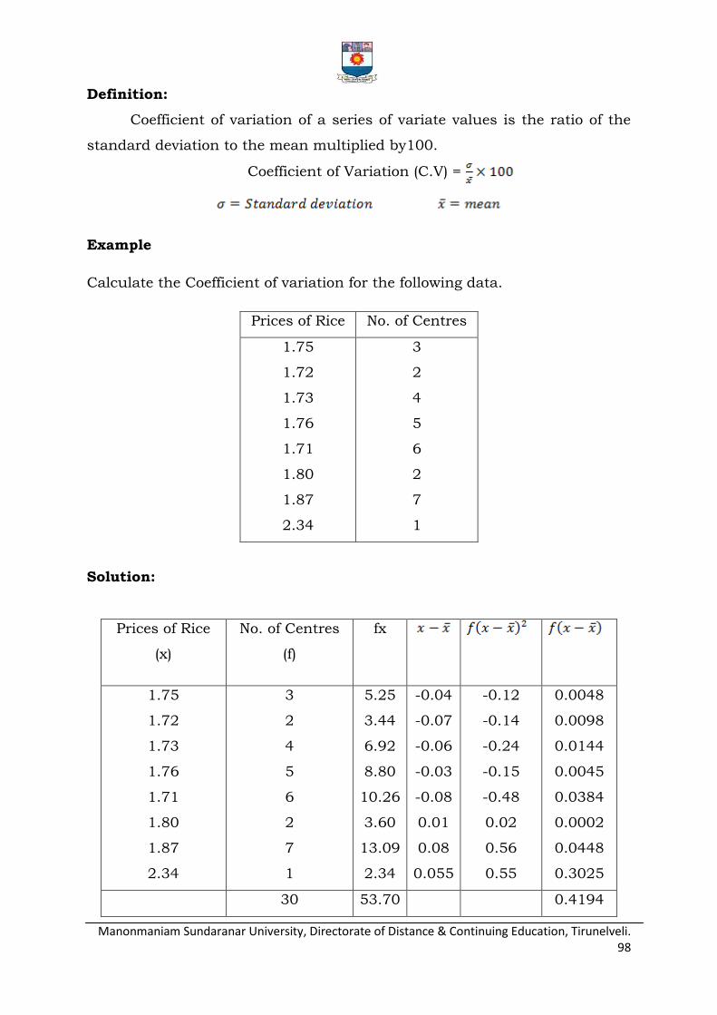
Manonmaniam Sundaranar University, Directorate of Distance & Continuing Education, Tirunelveli. 98
Definition:
Coefficient of variation of a series of variate values is the ratio of the
standard deviation to the mean multiplied by100.
Coefficient of Variation (C.V) =
Example
Calculate the Coefficient of variation for the following data.
Prices of Rice No. of Centres
1.75
1.72
1.73
1.76
1.71
1.80
1.87
2.34
3
2
4
5
6
2
7
1
Solution:
Prices of Rice
(x)
No. of Centres
(f)
fx
1.75
1.72
1.73
1.76
1.71
1.80
1.87
2.34
3
2
4
5
6
2
7
1
5.25
3.44
6.92
8.80
10.26
3.60
13.09
2.34
-0.04
-0.07
-0.06
-0.03
-0.08
0.01
0.08
0.055
-0.12
-0.14
-0.24
-0.15
-0.48
0.02
0.56
0.55
0.0048
0.0098
0.0144
0.0045
0.0384
0.0002
0.0448
0.3025
30 53.70 0.4194
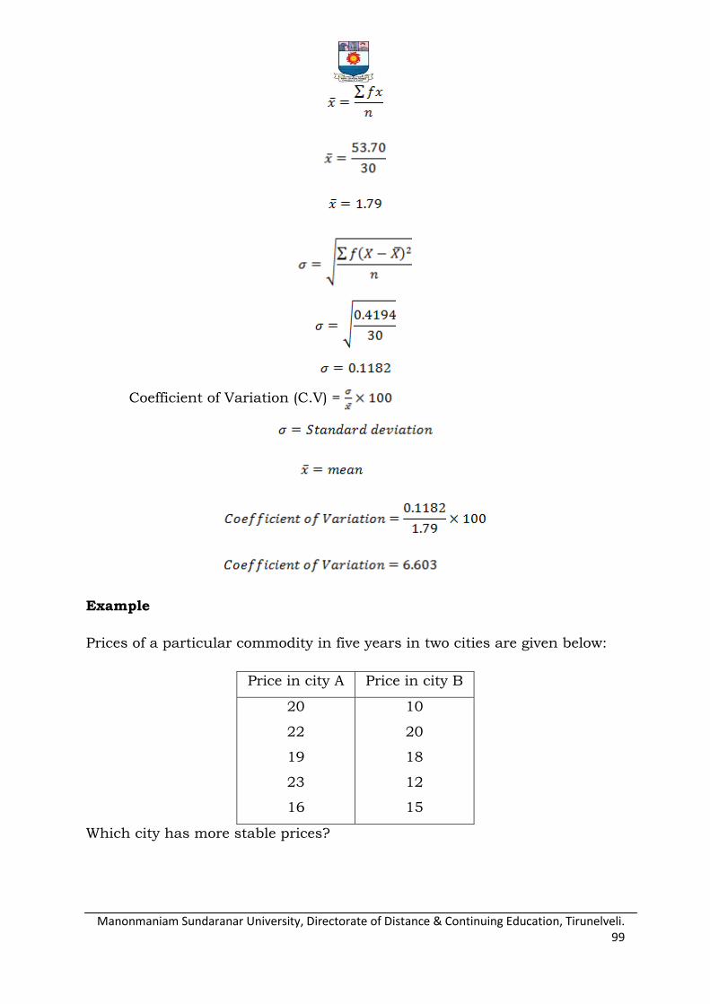
Manonmaniam Sundaranar University, Directorate of Distance & Continuing Education, Tirunelveli. 99
Coefficient of Variation (C.V) =
Example
Prices of a particular commodity in five years in two cities are given below:
Price in city A Price in city B
20
22
19
23
16
10
20
18
12
15
Which city has more stable prices?

Manonmaniam Sundaranar University, Directorate of Distance & Continuing Education, Tirunelveli. 100
Solution:
Actual mean method:
City A City B
Prices (X)
Deviations from =20
dX
dX2 Prices (Y)
Deviations from =20
dY
dY2
20 22
19 23 16
0 2
-1 3 -4
0 4
1 9 16
10 20
18 12 15
-5 5
3 -3 0
25 25
9 9 0
100 0 30 75 0 68
City A:
= 2.45
C.V(X) =
=
= 12.25 %
City B:
= 3.69
C.V(X) =
=
= 24.6 %
City A had more stable prices than City B, because the coefficient of
variation is less in City A.

Manonmaniam Sundaranar University, Directorate of Distance & Continuing Education, Tirunelveli. 101
2.4MEASURES OF SKEWNESS
The important measures of skewness consisting of absolute and
relative measures. The relative measure is called the coefficient of skewness.
The signs of the skewness indicate whether the distribution is positively
skewed or negatively.
Karl – Pearson‟s coefficient of skewness.
Bowley‟s coefficient of skewness.
Measure of skewness based on moments.
PEARSON’S AND BOWLEY’S COEFFICIENT OF SKEWNESS
Karl – Pearson’s Coefficient of skewness:
According to Karl – Pearson, the absolute measure of skewness =
mean – mode. This measure is not suitable for making valid comparison of
the skewness in two or more distributions because the unit of measurement
may be different in different series. To avoid this difficulty use relative
measure of skewness called Karl – Pearson‟s coefficient of skewness given
by:
Karl – Pearson‟s Coefficient Skewness =
In case of mode is ill – defined, the coefficient can be determined by the
formula:
Coefficient of skewness =
Example
Find the coefficient of skewness from the data given below.
Size 30 40 50 60 70 80 90 100
Frequency 7 10 14 35 102 136 43 8
Solution:
A = 10, C = 10
x frequency (f)
fdx fd2x
30 40
50
7 10
14
4 -3
-2
-28 -30
-28
112 90
56

Manonmaniam Sundaranar University, Directorate of Distance & Continuing Education, Tirunelveli. 102
60
70 80 90
100
35
102 136 43
8
-1
0 1 2
3
-35
0 136 86
24
35
0 136 172
72
335 125 673
Maximum frequency is 136 hence the value of mode is 80
Karl Pearson coefficient Skewness =
=
Karl Pearson coefficient Skewness = 0.487
Example
Calculate the Karl Pearson‟s coefficient of skewness for the following data.
Variable 0-5 5-10 10-15 15-20 20-25 25-30 30-5 35-40
No. of Workers 2 5 7 13 21 16 8 3

Manonmaniam Sundaranar University, Directorate of Distance & Continuing Education, Tirunelveli. 103
Solution:
Karl Pearson coefficient Skewness =
A = 175, C = 5
x f Mid x dx fdx fd2x
0-5
5-10
10-15
15-20
20-25
25-30
30-35
35-40
2
5
7
13
21
16
8
3
2.5
7.5
12.5
17.5
22.5
27.5
32.5
37.5
-3
-2
-1
0
1
2
3
4
-6
-10
-7
0
21
32
24
12
18
20
7
0
21
64
72
48
75 66 250
Mode =
=
Mode = 23.07
Mean = 21.9
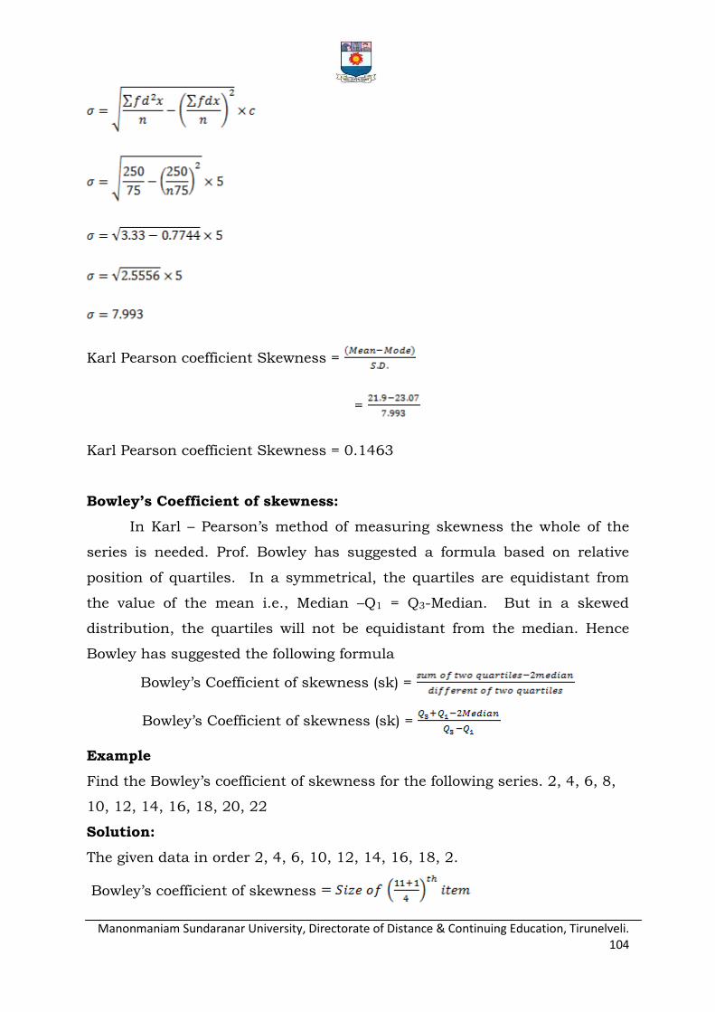
Manonmaniam Sundaranar University, Directorate of Distance & Continuing Education, Tirunelveli. 104
Karl Pearson coefficient Skewness =
=
Karl Pearson coefficient Skewness = 0.1463
Bowley’s Coefficient of skewness:
In Karl – Pearson‟s method of measuring skewness the whole of the
series is needed. Prof. Bowley has suggested a formula based on relative
position of quartiles. In a symmetrical, the quartiles are equidistant from
the value of the mean i.e., Median –Q1 = Q3-Median. But in a skewed
distribution, the quartiles will not be equidistant from the median. Hence
Bowley has suggested the following formula
Bowley‟s Coefficient of skewness (sk) =
Bowley‟s Coefficient of skewness (sk) =
Example
Find the Bowley‟s coefficient of skewness for the following series. 2, 4, 6, 8,
10, 12, 14, 16, 18, 20, 22
Solution:
The given data in order 2, 4, 6, 10, 12, 14, 16, 18, 2.
Bowley‟s coefficient of skewness
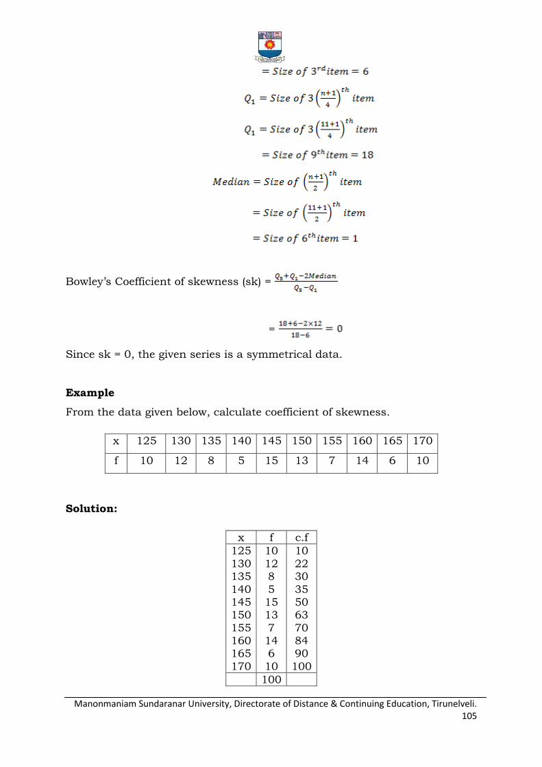
Manonmaniam Sundaranar University, Directorate of Distance & Continuing Education, Tirunelveli. 105
Bowley‟s Coefficient of skewness (sk) =
=
Since sk = 0, the given series is a symmetrical data.
Example
From the data given below, calculate coefficient of skewness.
x 125 130 135 140 145 150 155 160 165 170
f 10 12 8 5 15 13 7 14 6 10
Solution:
x f c.f
125
130 135
140 145 150
155 160 165
170
10
12 8
5 15 13
7 14 6
10
10
22 30
35 50 63
70 84 90
100
100
Manonmaniam Sundaranar University, Directorate of Distance & Continuing Education, Tirunelveli. 106
Median = 150
Bowley‟s Coefficient of skewness (sk) =
=
Bowley‟s Coefficient of skewness = 0.2
Example
Calculate the value of the Bowley‟s coefficient of skewness from the following
series.
Wages (in Rs)
10-20 20-30 30-40 40-50 50-60 60-70 70-80
No. of persons
1 3 11 21 43 32 9
Solution:
Wages (Rs) f C.f
10-20
20-30 30-40 40-50
1
3 11 21
1
4 15 36
Manonmaniam Sundaranar University, Directorate of Distance & Continuing Education, Tirunelveli. 107
50-60
60-70 70-80
43
32 9
79
111 120
N=120
Class = 40-50
= 40+7.14
= 47.14
Class = 50-60
= 55.58
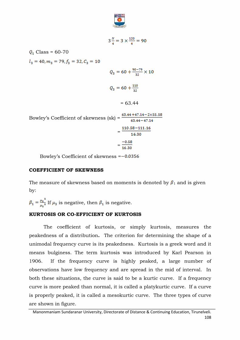
Manonmaniam Sundaranar University, Directorate of Distance & Continuing Education, Tirunelveli. 108
Class = 60-70
= 63.44
Bowley‟s Coefficient of skewness (sk) =
=
=
Bowley‟s Coefficient of skewness =
COEFFICIENT OF SKEWNESS
The measure of skewness based on moments is denoted by 1 and is given
by:
If is negative, then is negative.
KURTOSIS OR CO-EFFICIENT OF KURTOSIS
The coefficient of kurtosis, or simply kurtosis, measures the
peakedness of a distribution. The criterion for determining the shape of a
unimodal frequency curve is its peakedness. Kurtosis is a greek word and it
means bulginess. The term kurtosis was introduced by Karl Pearson in
1906. If the frequency curve is highly peaked, a large number of
observations have low frequency and are spread in the mid of interval. In
both these situations, the curve is said to be a kurtic curve. If a frequency
curve is more peaked than normal, it is called a platykurtic curve. If a curve
is properly peaked, it is called a mesokurtic curve. The three types of curve
are shown in figure.
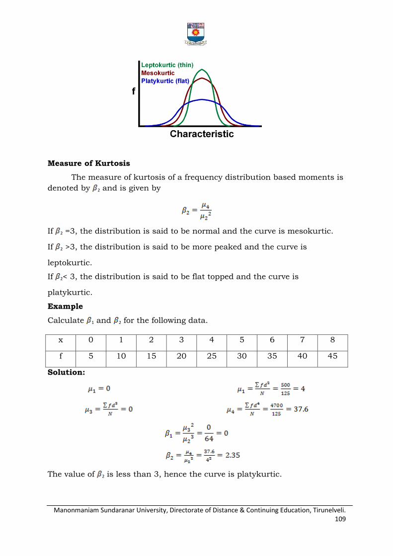
Manonmaniam Sundaranar University, Directorate of Distance & Continuing Education, Tirunelveli. 109
Measure of Kurtosis
The measure of kurtosis of a frequency distribution based moments is
denoted by 2 and is given by
If 2 =3, the distribution is said to be normal and the curve is mesokurtic.
If 2 >3, the distribution is said to be more peaked and the curve is
leptokurtic.
If 2< 3, the distribution is said to be flat topped and the curve is
platykurtic.
Example
Calculate 1 and 2 for the following data.
x 0 1 2 3 4 5 6 7 8
f 5 10 15 20 25 30 35 40 45
Solution:
The value of 2 is less than 3, hence the curve is platykurtic.

Manonmaniam Sundaranar University, Directorate of Distance & Continuing Education, Tirunelveli. 110
Example
The first four central moments of a distribution are 0, 2.5, 0.7, 18.75,
Examine the Kurtosis of the distribution.
Hence the curve is mesokurtic curve
QUESTIONS
1. What are the desirable characteristics of a good measurable central tendency?
2. Define Mean (or) Arithmetic mean.
3. Find the mean 6, 8, 11, 5, 2, 9, 7, and 8.
4. A student‟s marks in 5 subjects are 75, 68, 80, 92, and 56. Find his
average mark.
5. Calculate the mean for the following data.
X 5 8 12 15 20 24
F 3 4 6 5 3 2
6. Given the following frequency distribution. Calculate the arithmetic mean.
Marks 64 63 62 61 60 59
No. of
Students
8 18 12 9 7 6
7. Calculate the Arithmetic mean.
Income 0-10 10-20 20-30 30-40 40-50 50-60 60-70
No. of
persons
6 8 10 12 7 4 3
8. Give the merits and demerits of Arithmetic mean.
9. Define Median.
10. Determine median following data?
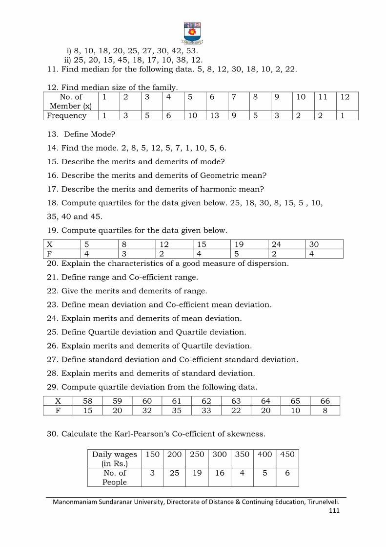
Manonmaniam Sundaranar University, Directorate of Distance & Continuing Education, Tirunelveli. 111
i) 8, 10, 18, 20, 25, 27, 30, 42, 53. ii) 25, 20, 15, 45, 18, 17, 10, 38, 12.
11. Find median for the following data. 5, 8, 12, 30, 18, 10, 2, 22.
12. Find median size of the family.
No. of Member (x)
1 2 3 4 5 6 7 8 9 10 11 12
Frequency 1 3 5 6 10 13 9 5 3 2 2 1
13. Define Mode?
14. Find the mode. 2, 8, 5, 12, 5, 7, 1, 10, 5, 6.
15. Describe the merits and demerits of mode?
16. Describe the merits and demerits of Geometric mean?
17. Describe the merits and demerits of harmonic mean?
18. Compute quartiles for the data given below. 25, 18, 30, 8, 15, 5 , 10,
35, 40 and 45.
19. Compute quartiles for the data given below.
X 5 8 12 15 19 24 30
F 4 3 2 4 5 2 4
20. Explain the characteristics of a good measure of dispersion.
21. Define range and Co-efficient range.
22. Give the merits and demerits of range.
23. Define mean deviation and Co-efficient mean deviation.
24. Explain merits and demerits of mean deviation.
25. Define Quartile deviation and Quartile deviation.
26. Explain merits and demerits of Quartile deviation.
27. Define standard deviation and Co-efficient standard deviation.
28. Explain merits and demerits of standard deviation.
29. Compute quartile deviation from the following data.
X 58 59 60 61 62 63 64 65 66
F 15 20 32 35 33 22 20 10 8
30. Calculate the Karl-Pearson‟s Co-efficient of skewness.
Daily wages
(in Rs.)
150 200 250 300 350 400 450
No. of
People
3 25 19 16 4 5 6
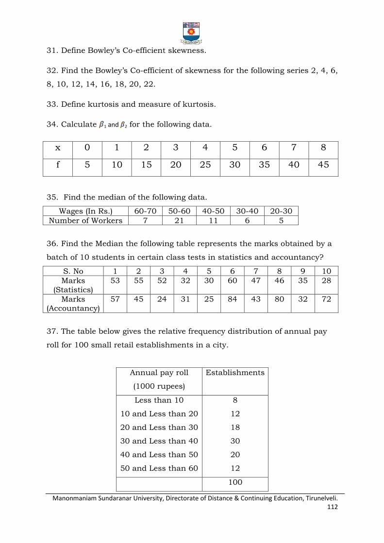
Manonmaniam Sundaranar University, Directorate of Distance & Continuing Education, Tirunelveli. 112
31. Define Bowley‟s Co-efficient skewness.
32. Find the Bowley‟s Co-efficient of skewness for the following series 2, 4, 6,
8, 10, 12, 14, 16, 18, 20, 22.
33. Define kurtosis and measure of kurtosis.
34. Calculate 1 and 2 for the following data.
x 0 1 2 3 4 5 6 7 8
f 5 10 15 20 25 30 35 40 45
35. Find the median of the following data.
Wages (In Rs.) 60-70 50-60 40-50 30-40 20-30
Number of Workers 7 21 11 6 5
36. Find the Median the following table represents the marks obtained by a
batch of 10 students in certain class tests in statistics and accountancy?
S. No 1 2 3 4 5 6 7 8 9 10
Marks
(Statistics)
53 55 52 32 30 60 47 46 35 28
Marks
(Accountancy)
57 45 24 31 25 84 43 80 32 72
37. The table below gives the relative frequency distribution of annual pay
roll for 100 small retail establishments in a city.
Annual pay roll
(1000 rupees)
Establishments
Less than 10
10 and Less than 20
20 and Less than 30
30 and Less than 40
40 and Less than 50
50 and Less than 60
8
12
18
30
20
12
100

Manonmaniam Sundaranar University, Directorate of Distance & Continuing Education, Tirunelveli. 113
Calculate Median pay.
38. Calculate the median from the data given below.
Wages
(in Rs.)
Above
30
Above
40
Above
50
Above
60
Above
70
Above
80
Above
90
No. of
Workers
520 470 399 210 105 45 7
39. Calculate median from the following data
Value 0-4 5-9 10-
14
15-
19
20-
24
25-
29
30-
34
35-
39
Frequency 5 8 10 12 7 6 3 2
40. Find median for the data given below.
Marks Number of
Students
Greater than 10
Greater than 20
Greater than 30
Greater than 40
Greater than 50
Greater than 60
Greater than 70
Greater than 80
Greater than 90
70
62
50
38
30
24
17
9
4
41. Find the mode for the following data.
Class
Interval
0-5 5-10 10-15 15-20 20-25 25-30 30-35 35-40
Frequency 9 12 15 16 17 15 10 13
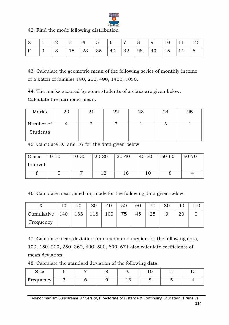
Manonmaniam Sundaranar University, Directorate of Distance & Continuing Education, Tirunelveli. 114
42. Find the mode following distribution
X 1 2 3 4 5 6 7 8 9 10 11 12
F 3 8 15 23 35 40 32 28 40 45 14 6
43. Calculate the geometric mean of the following series of monthly income
of a batch of families 180, 250, 490, 1400, 1050.
44. The marks secured by some students of a class are given below.
Calculate the harmonic mean.
Marks 20 21 22 23 24 25
Number of
Students
4 2 7 1 3 1
45. Calculate D3 and D7 for the data given below
Class
Interval
0-10 10-20 20-30 30-40 40-50 50-60 60-70
f 5 7 12 16 10 8 4
46. Calculate mean, median, mode for the following data given below.
X 10 20 30 40 50 60 70 80 90 100
Cumulative
Frequency
140 133 118 100 75 45 25 9 20 0
47. Calculate mean deviation from mean and median for the following data,
100, 150, 200, 250, 360, 490, 500, 600, 671 also calculate coefficients of
mean deviation.
48. Calculate the standard deviation of the following data.
Size 6 7 8 9 10 11 12
Frequency 3 6 9 13 8 5 4
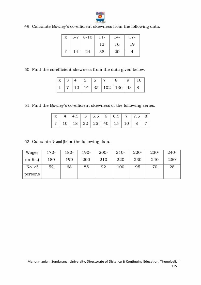
Manonmaniam Sundaranar University, Directorate of Distance & Continuing Education, Tirunelveli. 115
49. Calculate Bowley‟s co-efficient skewness from the following data.
x 5-7 8-10 11-
13
14-
16
17-
19
f 14 24 38 20 4
50. Find the co-efficient skewness from the data given below.
x 3 4 5 6 7 8 9 10
f 7 10 14 35 102 136 43 8
51. Find the Bowley‟s co-efficient skewness of the following series.
x 4 4.5 5 5.5 6 6.5 7 7.5 8
f 10 18 22 25 40 15 10 8 7
52. Calculate 1 and 2 for the following data.
Wages
(in Rs.)
170-
180
180-
190
190-
200
200-
210
210-
220
220-
230
230-
240
240-
250
No. of
persons
52 68 85 92 100 95 70 28
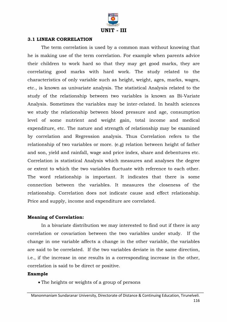
Manonmaniam Sundaranar University, Directorate of Distance & Continuing Education, Tirunelveli. 116
UNIT - III
3.1 LINEAR CORRELATION
The term correlation is used by a common man without knowing that
he is making use of the term correlation. For example when parents advice
their children to work hard so that they may get good marks, they are
correlating good marks with hard work. The study related to the
characteristics of only variable such as height, weight, ages, marks, wages,
etc., is known as univariate analysis. The statistical Analysis related to the
study of the relationship between two variables is known as Bi-Variate
Analysis. Sometimes the variables may be inter-related. In health sciences
we study the relationship between blood pressure and age, consumption
level of some nutrient and weight gain, total income and medical
expenditure, etc. The nature and strength of relationship may be examined
by correlation and Regression analysis. Thus Correlation refers to the
relationship of two variables or more. (e.g) relation between height of father
and son, yield and rainfall, wage and price index, share and debentures etc.
Correlation is statistical Analysis which measures and analyses the degree
or extent to which the two variables fluctuate with reference to each other.
The word relationship is important. It indicates that there is some
connection between the variables. It measures the closeness of the
relationship. Correlation does not indicate cause and effect relationship.
Price and supply, income and expenditure are correlated.
Meaning of Correlation:
In a bivariate distribution we may interested to find out if there is any
correlation or covariation between the two variables under study. If the
change in one variable affects a change in the other variable, the variables
are said to be correlated. If the two variables deviate in the same direction,
i.e., if the increase in one results in a corresponding increase in the other,
correlation is said to be direct or positive.
Example
The heights or weights of a group of persons

Manonmaniam Sundaranar University, Directorate of Distance & Continuing Education, Tirunelveli. 117
The income and expenditure is positive and correlation between
Price and demand of a commodity
The volume and pressure of a perfect gas; is negative
Correlation is said to be perfect if the deviation one variable is followed by a
corresponding and proportional deviation in the other.
Definitions:
Ya-Kun-Chou:
Correlation Analysis attempts to determine the degree of relationship
between variables.
A.M. Tuttle:
Correlation is an analysis of the covariation between two or more
variables. Correlation expresses the inter-dependence of two sets of
variables upon each other. One variable may be called as (subject)
independent and the other relative variable (dependent). Relative
variable is measured in terms of subject.
Uses of correlation:
1. It is used in physical and social sciences.
2. It is useful for economists to study the relationship between variables like
price, quantity.
4. Businessmen estimates costs, sales, price etc. using correlation.
4. It is helpful in measuring the degree of relationship between the variables
like income and expenditure, price and supply, supply and demand etc.
5. Sampling error can be calculated.
6. It is the basis for the concept of regression.
3.2 SCATTER DIAGRAM
Scatter diagram pertaining independent variables, it is easily verifiable
that if any line is drawn through the plotted points, not more than two
points will be lying on the line most of the other points will be at a
considerable distance from this line. Scatter diagram that the two variables

Manonmaniam Sundaranar University, Directorate of Distance & Continuing Education, Tirunelveli. 118
are linearly related, the problem arises on deciding which of the many
possible lines the best fitted line is. The lease square method is the most
widely accepted method of fitting a straight line and is discussed here
adequately.
Use of Scatter Diagram:
When you have paired numerical data
When trying to identify potential root causes of problems.
After brain storming causes and effects using a bishbone diagram, to
determine objectively whether a particular cause and effect are related.
When determining whether two effects that appear to be related both
occur with the same cause
It is the simplest method of studying the relationship between two
variables diagrammatically. One variable is represented along the horizontal
axis and the second variable along the vertical axis. For each pair of
observations of two variables, we put a dot in the plane. There are as many
dots in the plane as the number of paired observations of two variables. The
direction of dots shows the scatter or concentration of various points. This
will show the type of correlation.
Perfect positive perfect Negative
Correlation Correlation
Y r = +1 Y (r = -1)
O X axis O X axis
1. If all the plotted dots lie on a straight line falling from upper left hand
corner to lower right hand corner, there is a perfect negative
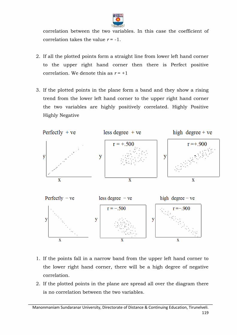
Manonmaniam Sundaranar University, Directorate of Distance & Continuing Education, Tirunelveli. 119
correlation between the two variables. In this case the coefficient of
correlation takes the value r = -1.
2. If all the plotted points form a straight line from lower left hand corner
to the upper right hand corner then there is Perfect positive
correlation. We denote this as r = +1
3. If the plotted points in the plane form a band and they show a rising
trend from the lower left hand corner to the upper right hand corner
the two variables are highly positively correlated. Highly Positive
Highly Negative
1. If the points fall in a narrow band from the upper left hand corner to
the lower right hand corner, there will be a high degree of negative
correlation.
2. If the plotted points in the plane are spread all over the diagram there
is no correlation between the two variables.

Manonmaniam Sundaranar University, Directorate of Distance & Continuing Education, Tirunelveli. 120
Merits:
1. It is a simplest and attractive method of finding the nature of correlation
between the two variables.
2. It is a non-mathematical method of studying correlation. It is easy to
understand.
3. It is not affected by extreme items.
4. It is the first step in finding out the relation between the two variables.
5. We can have a rough idea at a glance whether it is a positive correlation
or negative correlation.
Demerits:
By this method we cannot get the exact degree or correlation between the
two variables.
Types of Correlation:
Correlation is classified into various types. The most important ones are
Positive and negative.
Linear and non-linear.
Partial and total.
Simple and Multiple.
Positive and Negative Correlation
It depends upon the direction of change of the variables. If the two
variables tend to move together in the same direction (i. e) an increase in the
value of one variable is accompanied by an increase in the value of the
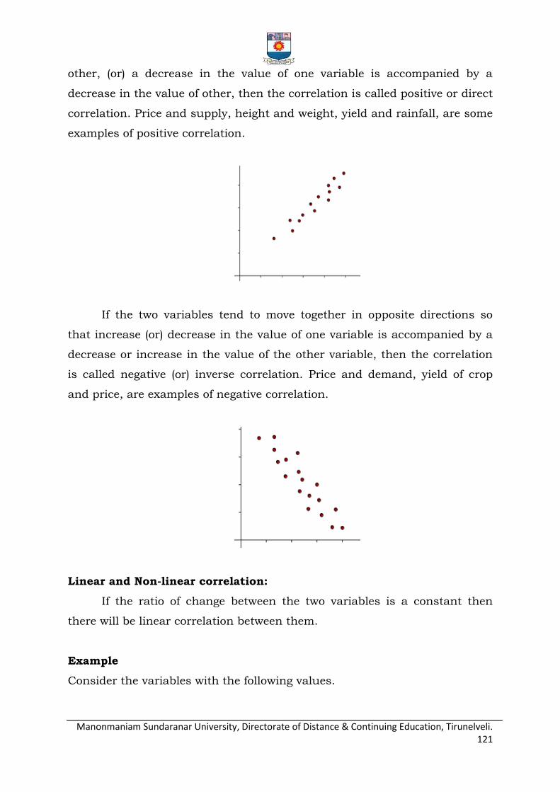
Manonmaniam Sundaranar University, Directorate of Distance & Continuing Education, Tirunelveli. 121
other, (or) a decrease in the value of one variable is accompanied by a
decrease in the value of other, then the correlation is called positive or direct
correlation. Price and supply, height and weight, yield and rainfall, are some
examples of positive correlation.
If the two variables tend to move together in opposite directions so
that increase (or) decrease in the value of one variable is accompanied by a
decrease or increase in the value of the other variable, then the correlation
is called negative (or) inverse correlation. Price and demand, yield of crop
and price, are examples of negative correlation.
Linear and Non-linear correlation:
If the ratio of change between the two variables is a constant then
there will be linear correlation between them.
Example
Consider the variables with the following values.
Manonmaniam Sundaranar University, Directorate of Distance & Continuing Education, Tirunelveli. 122
X 10 20 30 40 50
Y 20 40 60 80 100
Here the ratio of change between the two variables is the same. If we
plot these points on a graph we get a straight line.
If the amount of change in one variable does not bear a constant ratio
of the amount of change in the other. Then the relation is called Curve-
linear (or) non-linear correlation. The graph will be a curve.
Example
Consider the variables with the following values
X 10 20 30 40 50
Y 10 30 70 90 120
Here there is a non linear relationship between the variables. The ratio
between them is not fixed for all points. Also if we plot them on the graph,
the points will not be in a straight line. It will be a curve.
Simple and Multiple correlation:
When we study only two variables, the relationship is simple
correlation. For example, quantity of money and price level, demand and
price. But in a multiple correlation we study more than two variables
simultaneously. The relationship of price, demand and supply of a
commodity are an example for multiple correlations.
Partial and total correlation:
The study of two variables excluding some other variable is called
Partial correlation. While mathematically controlling the influence of a third
variable by holding is constant.

Manonmaniam Sundaranar University, Directorate of Distance & Continuing Education, Tirunelveli. 123
Example
We study price and demand eliminating supply side. Relationship
between one dependent and one independent variable. This is called Total
Correlation.
Coefficient of simple determination: r2yx1 (or) r2yx2 (or) r2x1x2
Computation of correlation
When there exists some relationship between two variables, we have
to measure the degree of relationship. This measure is called the measure of
correlation (or) correlation coefficient and it is denoted by „r‟.
Co-variation:
Covariance and correlation are both describe the degree of similarity
between two random variables. Suppose that X and Y are real-valued
random variables for the experiment with means E(X), E(Y) and
variances Var(X), Var(Y), respectively. The co-variation between the
variables x and y is defined as
n
yyxxYXCov
))((),(
Where yx, are respectively means of x and y and „n‟ is the number of pairs of
observations.
3.3 KARL PEARSON’S COEFFICIENT OF CORRELATION
Karl Pearson‟s a British Biometrician (1867 – 1936), degree of linear
relationship between the two variables. It is most widely used method in
practice and it is known as Pearson‟s coefficient of correlation. It is denoted
by „r‟.
Correlation coefficient between two random variables X and Y usually
denoted by r(X, Y) or simply is a numerical measure of linear
relationship between them and is defined as.

Manonmaniam Sundaranar University, Directorate of Distance & Continuing Education, Tirunelveli. 124
2 2
( , ), .
.
, ,.
x y
x y
x y
Cov x yr where are S D of x and y respectively
xyr
n
XYr X x x Y y y
X Y
When the deviations are taken from the actual mean we can apply any
one of these methods. Simple formula is the third one. The third formula is
easy to calculate, and it is not necessary to calculate the standard
deviations of x and y series.
Steps:
1. Find the mean of the two series x and y.
2. Take deviations of the two series from x and y. X = x - x, Y = y - y
3. Square the deviations and get the total, of the respective squares of
deviations of x and y and denote by ∑ X2, ∑ Y2 respectively.
4. Multiply the deviations of x and y and get the total and Divide by n. This
is covariance.
5. Substitute the values in the formula.
2 2
( ) ( ) /cov( , )
. ( ) ( )x y
x x y y nx yr
x x y y
n n
The above formula is simplified as follows
2 2, ,
.
XYr X x x Y y y
X Y
Example
Find Karl Pearson‟s coefficient of correlation from the following data between
height of father (x) and son (y).
x 64 65 66 67 68 69 70
y 66 67 65 68 70 68 72

Manonmaniam Sundaranar University, Directorate of Distance & Continuing Education, Tirunelveli. 125
Solution:
x y X = X-x
x = 67
X2 Y = Y-y
y = 68
Y2 XY
64
65
66
67
68
69
70
66
67
65
68
70
68
72
-3
-2
-1
0
1
2
3
9
4
1
0
1
4
9
-2
-1
-3
0
2
0
4
4
1
9
0
4
0
16
6
2
3
0
2
0
12
469 476 0 28 0 34 25
2 2
469 47667; 68
7 7
25 25 250.81
30.8528 34 952.
x y
XYr
X Y
r = 0.91
Example:
Calculate coefficient of correlation from the following data.
x 1 2 3 4 5 6 7 8 9
y 9 8 10 12 11 13 14 16 15
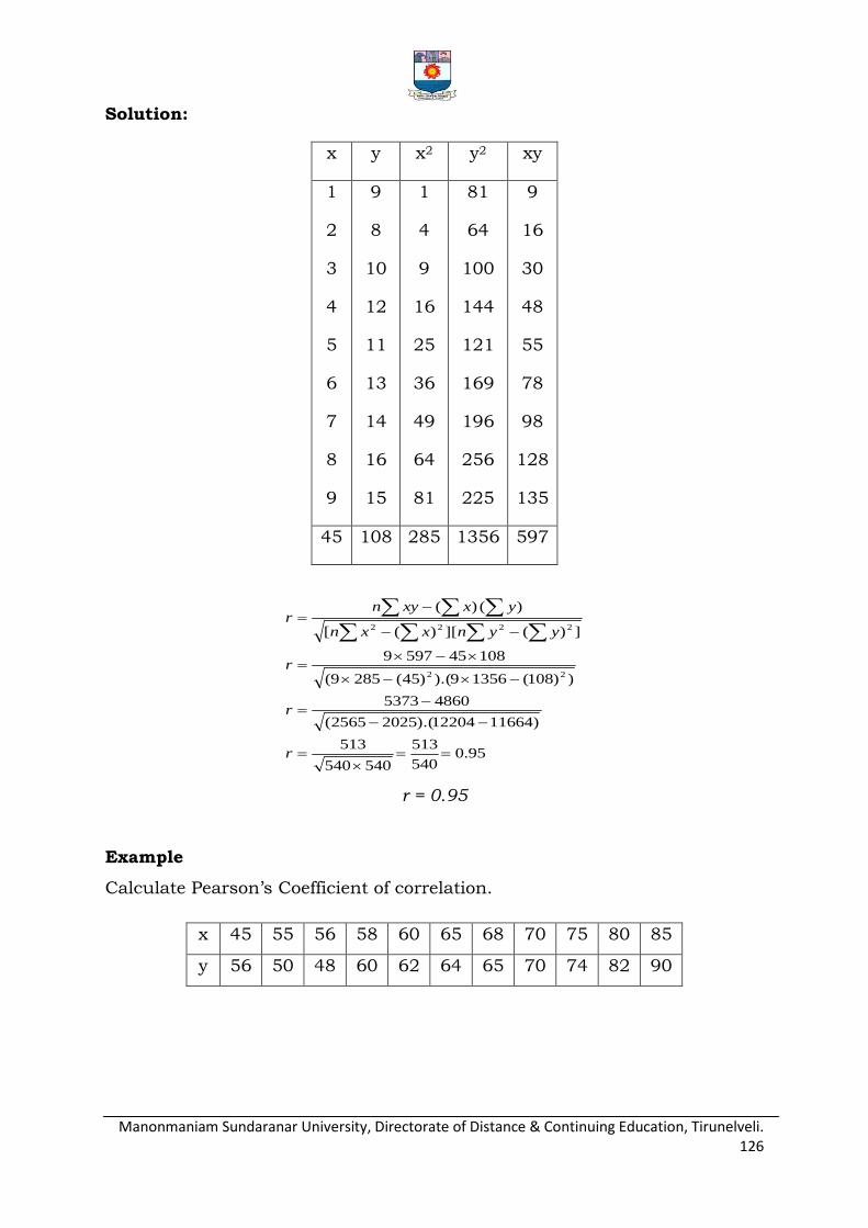
Manonmaniam Sundaranar University, Directorate of Distance & Continuing Education, Tirunelveli. 126
Solution:
x y x2 y2 xy
1
2
3
4
5
6
7
8
9
9
8
10
12
11
13
14
16
15
1
4
9
16
25
36
49
64
81
81
64
100
144
121
169
196
256
225
9
16
30
48
55
78
98
128
135
45 108 285 1356 597
95.0540
513
540540
513
)1166412204).(20252565(
48605373
))108(13569).()45(2859(
108455979
])([])([
)()(
22
2222
r
r
r
yynxxn
yxxynr
r = 0.95
Example
Calculate Pearson‟s Coefficient of correlation.
x 45 55 56 58 60 65 68 70 75 80 85
y 56 50 48 60 62 64 65 70 74 82 90
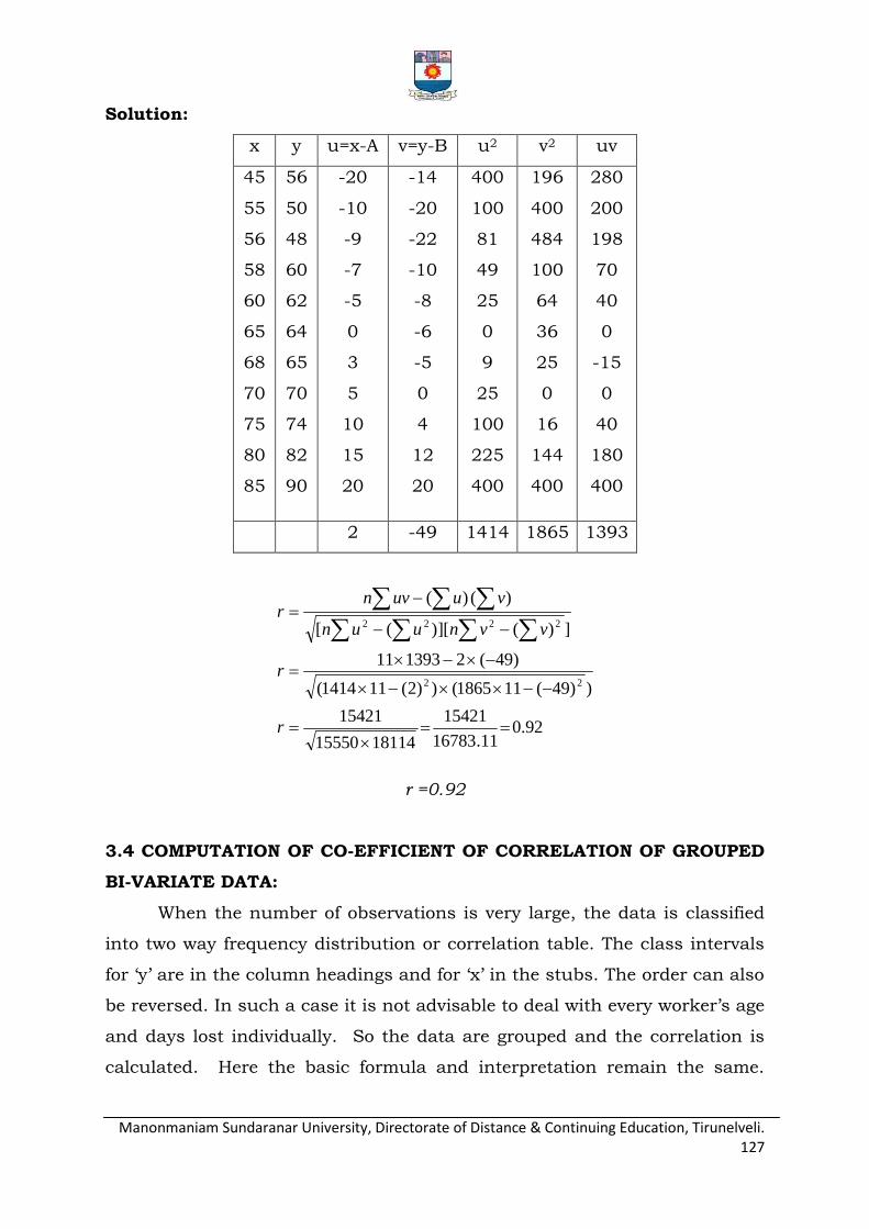
Manonmaniam Sundaranar University, Directorate of Distance & Continuing Education, Tirunelveli. 127
Solution:
x y u=x-A v=y-B u2 v2 uv
45
55
56
58
60
65
68
70
75
80
85
56
50
48
60
62
64
65
70
74
82
90
-20
-10
-9
-7
-5
0
3
5
10
15
20
-14
-20
-22
-10
-8
-6
-5
0
4
12
20
400
100
81
49
25
0
9
25
100
225
400
196
400
484
100
64
36
25
0
16
144
400
280
200
198
70
40
0
-15
0
40
180
400
2 -49 1414 1865 1393
92.011.16783
15421
1811415550
15421
))49(111865())2(111414(
)49(2139311
])([)]([
)()(
22
2222
r
r
vvnuun
vuuvnr
r =0.92
3.4 COMPUTATION OF CO-EFFICIENT OF CORRELATION OF GROUPED
BI-VARIATE DATA:
When the number of observations is very large, the data is classified
into two way frequency distribution or correlation table. The class intervals
for „y‟ are in the column headings and for „x‟ in the stubs. The order can also
be reversed. In such a case it is not advisable to deal with every worker‟s age
and days lost individually. So the data are grouped and the correlation is
calculated. Here the basic formula and interpretation remain the same.
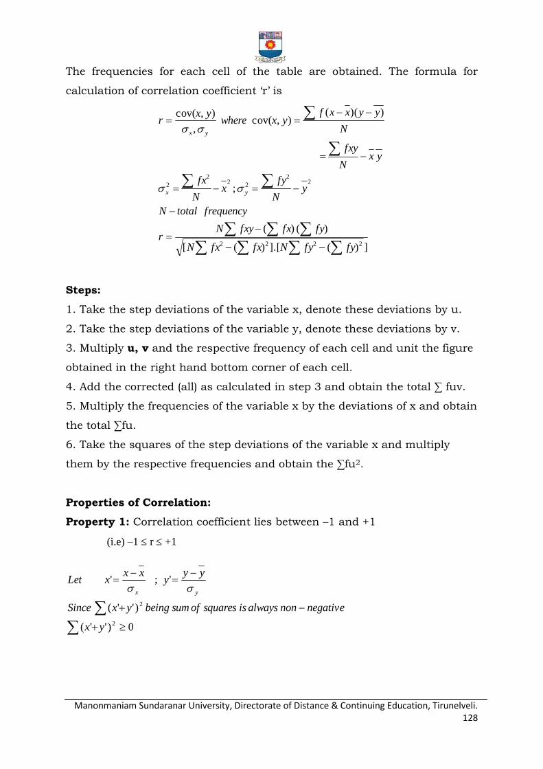
Manonmaniam Sundaranar University, Directorate of Distance & Continuing Education, Tirunelveli. 128
The frequencies for each cell of the table are obtained. The formula for
calculation of correlation coefficient „r‟ is
])(].[)([
)()(
;
))((),cov(
,
),cov(
2222
22
22
2
2
fyfyNfxfxN
fyfxfxyNr
frequencytotalN
yN
fyx
N
fx
yxN
fxy
N
yyxxfyxwhere
yxr
yx
yx
Steps:
1. Take the step deviations of the variable x, denote these deviations by u.
2. Take the step deviations of the variable y, denote these deviations by v.
3. Multiply u, v and the respective frequency of each cell and unit the figure
obtained in the right hand bottom corner of each cell.
4. Add the corrected (all) as calculated in step 3 and obtain the total ∑ fuv.
5. Multiply the frequencies of the variable x by the deviations of x and obtain
the total ∑fu.
6. Take the squares of the step deviations of the variable x and multiply
them by the respective frequencies and obtain the ∑fu2.
Properties of Correlation:
Property 1: Correlation coefficient lies between –1 and +1
(i.e) –1 r +1
0)''(
)''(
';'
2
2
yx
negativenonalwaysissquaresofsumbeingyxSince
yyy
xxxLet
yx
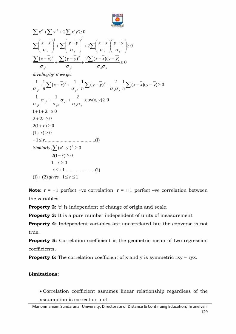
Manonmaniam Sundaranar University, Directorate of Distance & Continuing Education, Tirunelveli. 129
11)2()1(
)2.....(....................1
01
0)1(2
0)''(,
)1..(........................................1
0)1(
0)1(2
022
0211
0),cov(.211
0))((12
)(1
.1
)(1
.1
''
0))((2)()(
02
0''2''
2
22
22
22
22
2
2
2
2
22
22
rgives
r
r
r
yxSimilarly
r
r
r
r
r
yx
yyxxn
yyn
xxn
getwenbydividing
yyxxyyxx
yyxxyyxx
yxyx
yxx
x
x
x
yxyx
yxyx
yxyx
Note: r = +1 perfect +ve correlation. r = 1 perfect –ve correlation between
the variables.
Property 2: „r‟ is independent of change of origin and scale.
Property 3: It is a pure number independent of units of measurement.
Property 4: Independent variables are uncorrelated but the converse is not
true.
Property 5: Correlation coefficient is the geometric mean of two regression
coefficients.
Property 6: The correlation coefficient of x and y is symmetric rxy = ryx.
Limitations:
Correlation coefficient assumes linear relationship regardless of the
assumption is correct or not.
Manonmaniam Sundaranar University, Directorate of Distance & Continuing Education, Tirunelveli. 130
Extreme items of variables are being unduly operated on correlation
coefficient.
Existence of correlation does not necessarily indicate cause effect
relation.
Interpretation:
The following rules helps in interpreting the value of „r‟.
When r = 1, there is perfect +ve relationship between the variables.
When r = -1, there is perfect –ve relationship between the variables.
When r = 0, there is no relationship between the variables.
If the correlation is +1 or –1, it signifies that there is a high degree of
correlation, (+ve or –ve) between the two variables. If r is near to zero
(i.e.) 0.1,-0.1, (or) 0.2 there is less correlation.
3.5 RANK CORRELATION
It is not always possible to take measurements on units or objects.
Many characters are expressed in comparative terms such as beauty,
smartness, temperament, honesty, colour, beauty, intelligence, character,
morality etc. In such case the units are ranked pertaining to that particular
character instead of taking measurements on them. Sometimes, the units
are also ranked according to their quantitative measure. In these types of
studies, two situations arise.
The same set of units is ranked according to two characters.
Two judges give ranks to the same set of units independently.
This method is based on ranks. The individuals in the group can be
arranged in order and there on, obtaining for each individual a number
showing his/her rank in the group. This method was developed by the
psychologist; Charles Edward Spearman in 1906 developed a formula for

Manonmaniam Sundaranar University, Directorate of Distance & Continuing Education, Tirunelveli. 131
correlation coefficient, which is known as Rank correlation or Spearman‟s
correlation. It is defined as
nn
Dr
3
261
r = rank correlation coefficient.
The formula is
nn
mmmmD
r
3
332 ...)(12
1)(
12
16
1
Where „m‟ is the number of items. The value of „r‟ also lies between
-1 and +1.
Example
In a marketing survey the price of tea and coffee in a town based on
quality was found as shown below. Could you find any relation between and
tea and coffee price?
Price of Tea 88 90 95 70 60 75 50
Price of Coffee 120 134 150 115 110 140 100
Solution:
Price of Tea Rank Price of Coffee Rank D D2
88 90
95 70
60 75 50
3 2
1 5
6 4 7
120 134
150 115
110 140 100
4 3
1 5
6 2 7
1 1
0 0
0 2 0
1 1
0 0
0 4 0
50 7 100 7 0 0
8929.0
1071.01336
361
77
661
61
33
2
nn
Dr
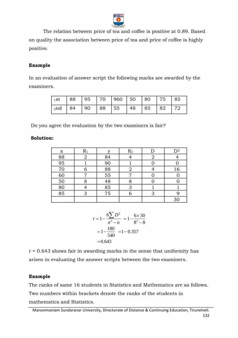
Manonmaniam Sundaranar University, Directorate of Distance & Continuing Education, Tirunelveli. 132
The relation between price of tea and coffee is positive at 0.89. Based
on quality the association between price of tea and price of coffee is highly
positive.
Example
In an evaluation of answer script the following marks are awarded by the
examiners.
1st 88 95 70 960 50 80 75 85
2nd 84 90 88 55 48 85 82 72
Do you agree the evaluation by the two examiners is fair?
Solution:
x R1 y R2 D D2
88 2 84 4 2 4
95 1 90 1 0 0
70 6 88 2 4 16
60 7 55 7 0 0
50 8 48 8 0 0
80 4 85 3 1 1
85 3 75 6 3 9
30
643.0
357.01540
1801
88
3061
61
33
2
nn
Dr
r = 0.643 shows fair in awarding marks in the sense that uniformity has
arisen in evaluating the answer scripts between the two examiners.
Example
The ranks of same 16 students in Statistics and Mathematics are as follows.
Two numbers within brackets denote the ranks of the students in
mathematics and Statistics.
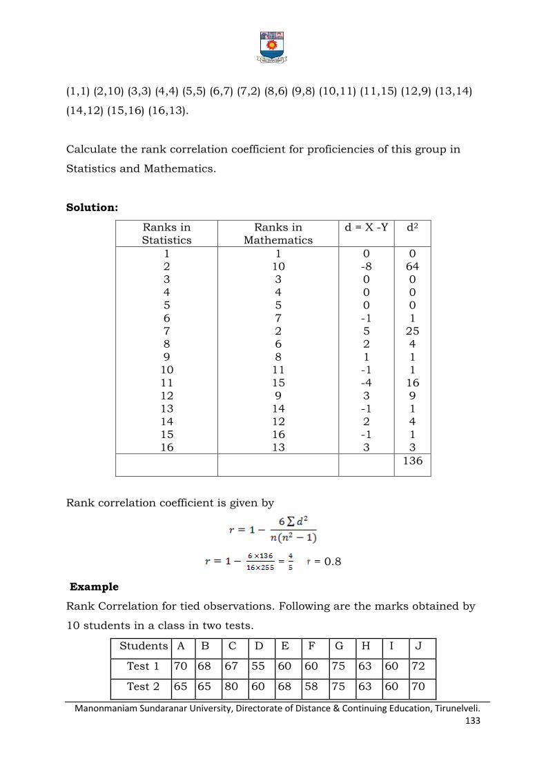
Manonmaniam Sundaranar University, Directorate of Distance & Continuing Education, Tirunelveli. 133
(1,1) (2,10) (3,3) (4,4) (5,5) (6,7) (7,2) (8,6) (9,8) (10,11) (11,15) (12,9) (13,14)
(14,12) (15,16) (16,13).
Calculate the rank correlation coefficient for proficiencies of this group in
Statistics and Mathematics.
Solution:
Ranks in Statistics
Ranks in Mathematics
d = X -Y d2
1 2 3
4 5
6 7 8
9 10
11 12 13
14 15 16
1 10 3
4 5
7 2 6
8 11
15 9 14
12 16 13
0 -8 0
0 0
-1 5 2
1 -1
-4 3 -1
2 -1 3
0 64 0
0 0
1 25 4
1 1
16 9 1
4 1 3
136
Rank correlation coefficient is given by
= = 0.8
Example
Rank Correlation for tied observations. Following are the marks obtained by
10 students in a class in two tests.
Students A B C D E F G H I J
Test 1 70 68 67 55 60 60 75 63 60 72
Test 2 65 65 80 60 68 58 75 63 60 70
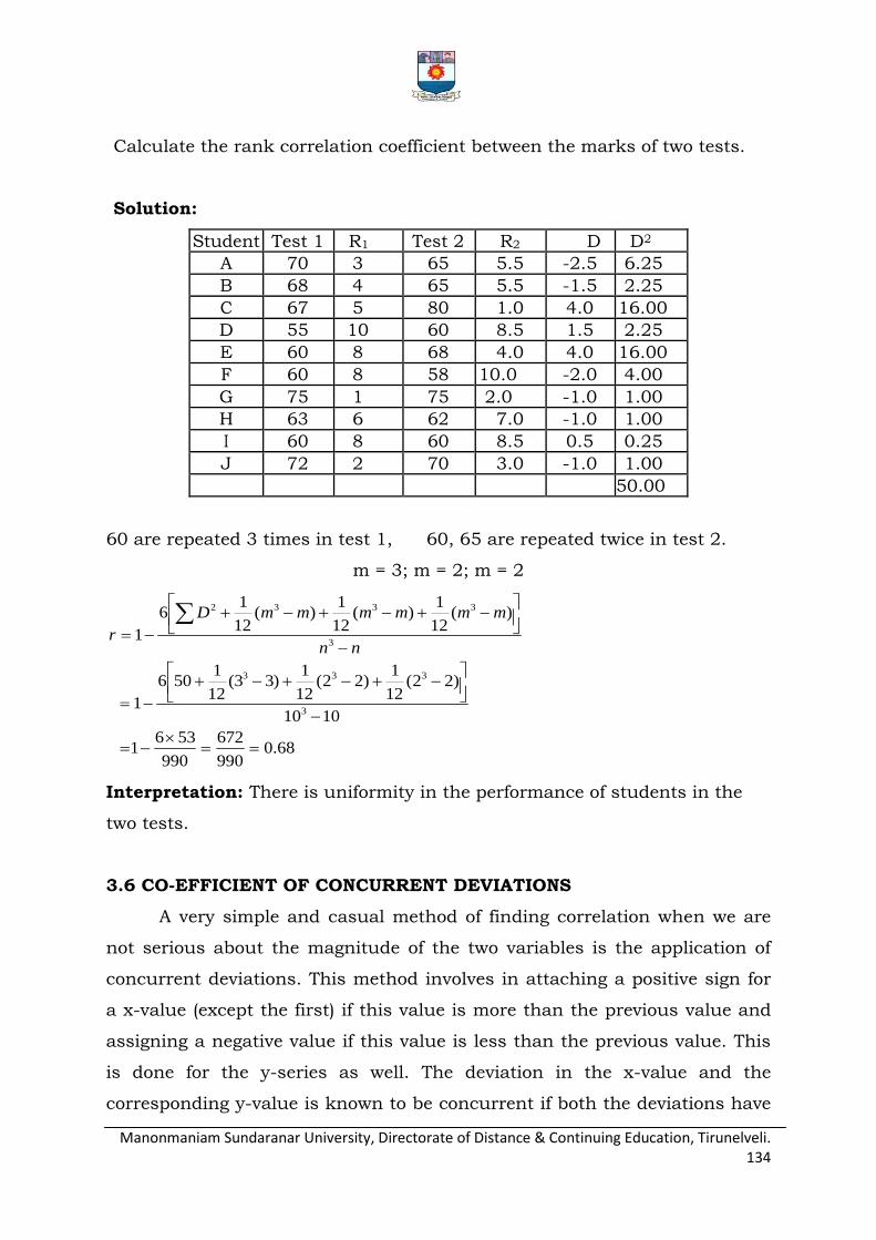
Manonmaniam Sundaranar University, Directorate of Distance & Continuing Education, Tirunelveli. 134
Calculate the rank correlation coefficient between the marks of two tests.
Solution:
Student Test 1 R1 Test 2 R2 D D2
A 70 3 65 5.5 -2.5 6.25
B 68 4 65 5.5 -1.5 2.25
C 67 5 80 1.0 4.0 16.00
D 55 10 60 8.5 1.5 2.25
E 60 8 68 4.0 4.0 16.00
F 60 8 58 10.0 -2.0 4.00
G 75 1 75 2.0 -1.0 1.00
H 63 6 62 7.0 -1.0 1.00
I 60 8 60 8.5 0.5 0.25
J 72 2 70 3.0 -1.0 1.00
50.00
60 are repeated 3 times in test 1, 60, 65 are repeated twice in test 2.
m = 3; m = 2; m = 2
68.0990
672
990
5361
1010
)22(12
1)22(
12
1)33(
12
1506
1
)(12
1)(
12
1)(
12
16
1
3
333
3
3332
nn
mmmmmmD
r
Interpretation: There is uniformity in the performance of students in the
two tests.
3.6 CO-EFFICIENT OF CONCURRENT DEVIATIONS
A very simple and casual method of finding correlation when we are
not serious about the magnitude of the two variables is the application of
concurrent deviations. This method involves in attaching a positive sign for
a x-value (except the first) if this value is more than the previous value and
assigning a negative value if this value is less than the previous value. This
is done for the y-series as well. The deviation in the x-value and the
corresponding y-value is known to be concurrent if both the deviations have
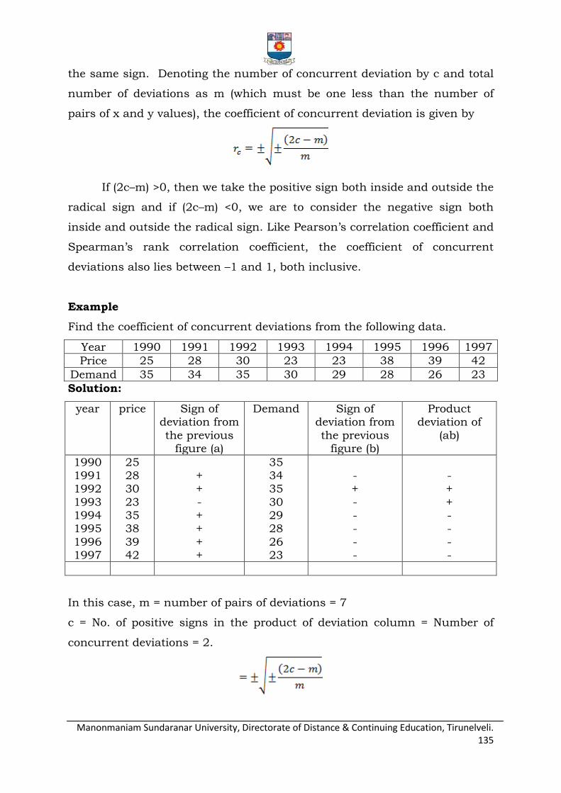
Manonmaniam Sundaranar University, Directorate of Distance & Continuing Education, Tirunelveli. 135
the same sign. Denoting the number of concurrent deviation by c and total
number of deviations as m (which must be one less than the number of
pairs of x and y values), the coefficient of concurrent deviation is given by
If (2c–m) >0, then we take the positive sign both inside and outside the
radical sign and if (2c–m) <0, we are to consider the negative sign both
inside and outside the radical sign. Like Pearson‟s correlation coefficient and
Spearman‟s rank correlation coefficient, the coefficient of concurrent
deviations also lies between –1 and 1, both inclusive.
Example
Find the coefficient of concurrent deviations from the following data.
Year 1990 1991 1992 1993 1994 1995 1996 1997
Price 25 28 30 23 23 38 39 42
Demand 35 34 35 30 29 28 26 23
Solution:
year price Sign of deviation from
the previous figure (a)
Demand Sign of deviation from
the previous figure (b)
Product deviation of
(ab)
1990 1991 1992
1993 1994 1995
1996 1997
25 28 30
23 35 38
39 42
+ +
- + +
+ +
35 34 35
30 29 28
26 23
- +
- - -
- -
- +
+ - -
- -
In this case, m = number of pairs of deviations = 7
c = No. of positive signs in the product of deviation column = Number of
concurrent deviations = 2.
Manonmaniam Sundaranar University, Directorate of Distance & Continuing Education, Tirunelveli. 136
Thus there is a negative correlation between price and demand.
3.7 REGRESSION EQUATION
If two variables have linear relationship then as the independent
variable (X) changes, the dependent variable (Y) also changes. If the
different values of X and Y are plotted, then the two straight lines of best fit
can be made to pass through the plotted points. These two lines are known
as regression lines. Again, these regression lines are based on two equations
known as regression equations. These equations show best estimate of one
variable for the known value of the other. The equations are linear. Linear
regression equation of Y on X is also known as the mathematical model for
linear regression equation, the main difference between the Cartesian
equation of a line is that a regression line is a probabilistic model which
enables to develop procedures for making inferences about the parameters a
and b of the model. In this model, the expected value of Y is a linear
function of X, but for fixed X, the variable Y differs from its expected value
by a random amount.
Y = a + bX ……. (1)
And X on Y is
X = a + bY……. (2)
a, b are constants.
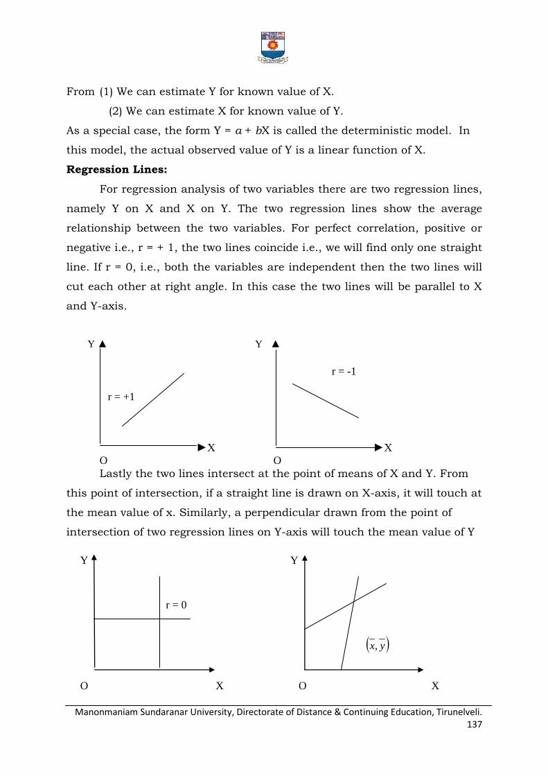
Manonmaniam Sundaranar University, Directorate of Distance & Continuing Education, Tirunelveli. 137
From (1) We can estimate Y for known value of X.
(2) We can estimate X for known value of Y.
As a special case, the form Y = a + bX is called the deterministic model. In
this model, the actual observed value of Y is a linear function of X.
Regression Lines:
For regression analysis of two variables there are two regression lines,
namely Y on X and X on Y. The two regression lines show the average
relationship between the two variables. For perfect correlation, positive or
negative i.e., r = + 1, the two lines coincide i.e., we will find only one straight
line. If r = 0, i.e., both the variables are independent then the two lines will
cut each other at right angle. In this case the two lines will be parallel to X
and Y-axis.
Y ▲ Y ▲
r = -1
r = +1
►X ►X
O O
Lastly the two lines intersect at the point of means of X and Y. From
this point of intersection, if a straight line is drawn on X-axis, it will touch at
the mean value of x. Similarly, a perpendicular drawn from the point of
intersection of two regression lines on Y-axis will touch the mean value of Y
Y Y
r = 0
yx,
O X O X
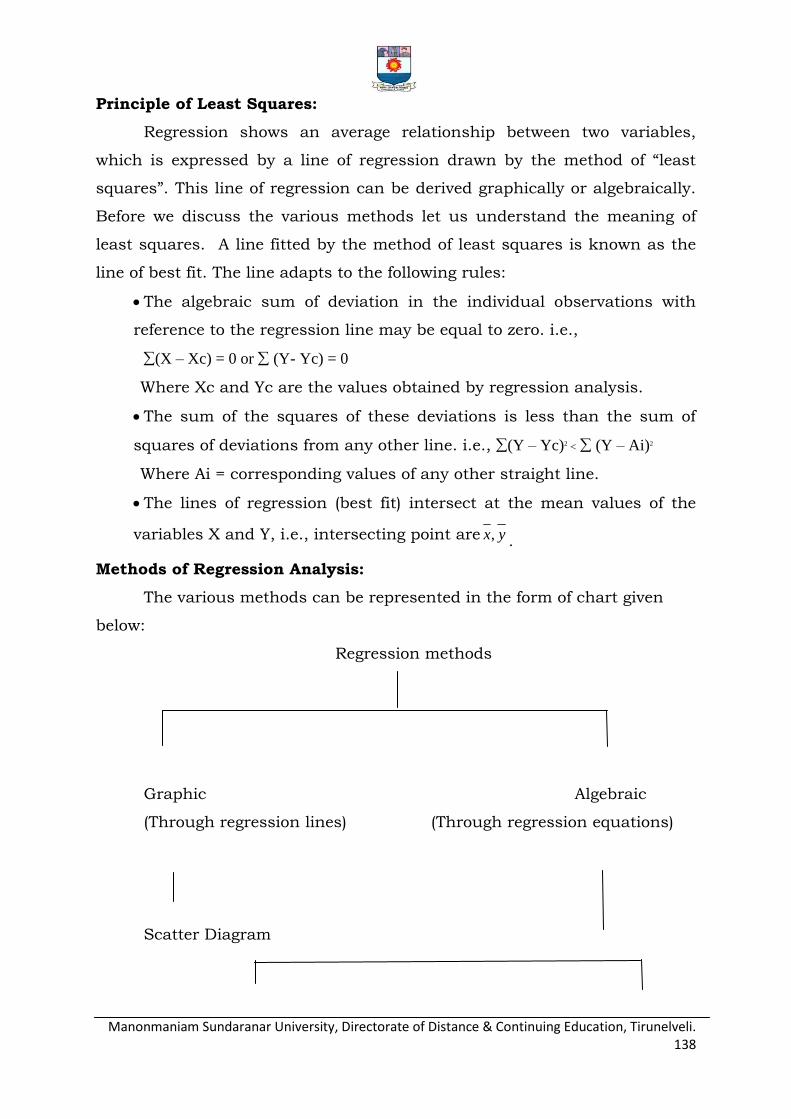
Manonmaniam Sundaranar University, Directorate of Distance & Continuing Education, Tirunelveli. 138
Principle of Least Squares:
Regression shows an average relationship between two variables,
which is expressed by a line of regression drawn by the method of “least
squares”. This line of regression can be derived graphically or algebraically.
Before we discuss the various methods let us understand the meaning of
least squares. A line fitted by the method of least squares is known as the
line of best fit. The line adapts to the following rules:
The algebraic sum of deviation in the individual observations with
reference to the regression line may be equal to zero. i.e.,
(X – Xc) = 0 or (Y- Yc) = 0
Where Xc and Yc are the values obtained by regression analysis.
The sum of the squares of these deviations is less than the sum of
squares of deviations from any other line. i.e., (Y – Yc)2 < (Y – Ai)2
Where Ai = corresponding values of any other straight line.
The lines of regression (best fit) intersect at the mean values of the
variables X and Y, i.e., intersecting point are yx, .
Methods of Regression Analysis:
The various methods can be represented in the form of chart given
below:
Regression methods
Graphic Algebraic
(Through regression lines) (Through regression equations)
Scatter Diagram
Manonmaniam Sundaranar University, Directorate of Distance & Continuing Education, Tirunelveli. 139
Regression Equations Regression
Equations
(Through normal equations) (Through regression coefficient)
Graphic Method:
Scatter Diagram
Under this method the points are plotted on a graph paper
representing various parts of values of the concerned variables. These points
give a picture of a scatter diagram with several points spread over. A
regression line may be drawn in between these points either by free hand or
by a scale rule in such a way that the squares of the vertical or the
horizontal distances (as the case may be) between the points and the line of
regression so drawn is the least. In other words, it should be drawn
faithfully as the line of best fit leaving equal number of points on both sides
in such a manner that the sum of the squares of the distances is the best.
3.8 FITTING OF REGRESSION EQUATION
The two regression equations for X on Y; X = a + bY
And for Y on X; Y = a + bX
Where X, Y are variables, and a,b are constants whose values are to be
determined
For the equation, X = a + bY
The normal equations are
X = na + b Y and
XY = aY + bY2
For the equation, Y= a + bX, the normal equations are
Y = na + bX and
XY = aX + bX2
From these normal equations the values of a and b can be determined.
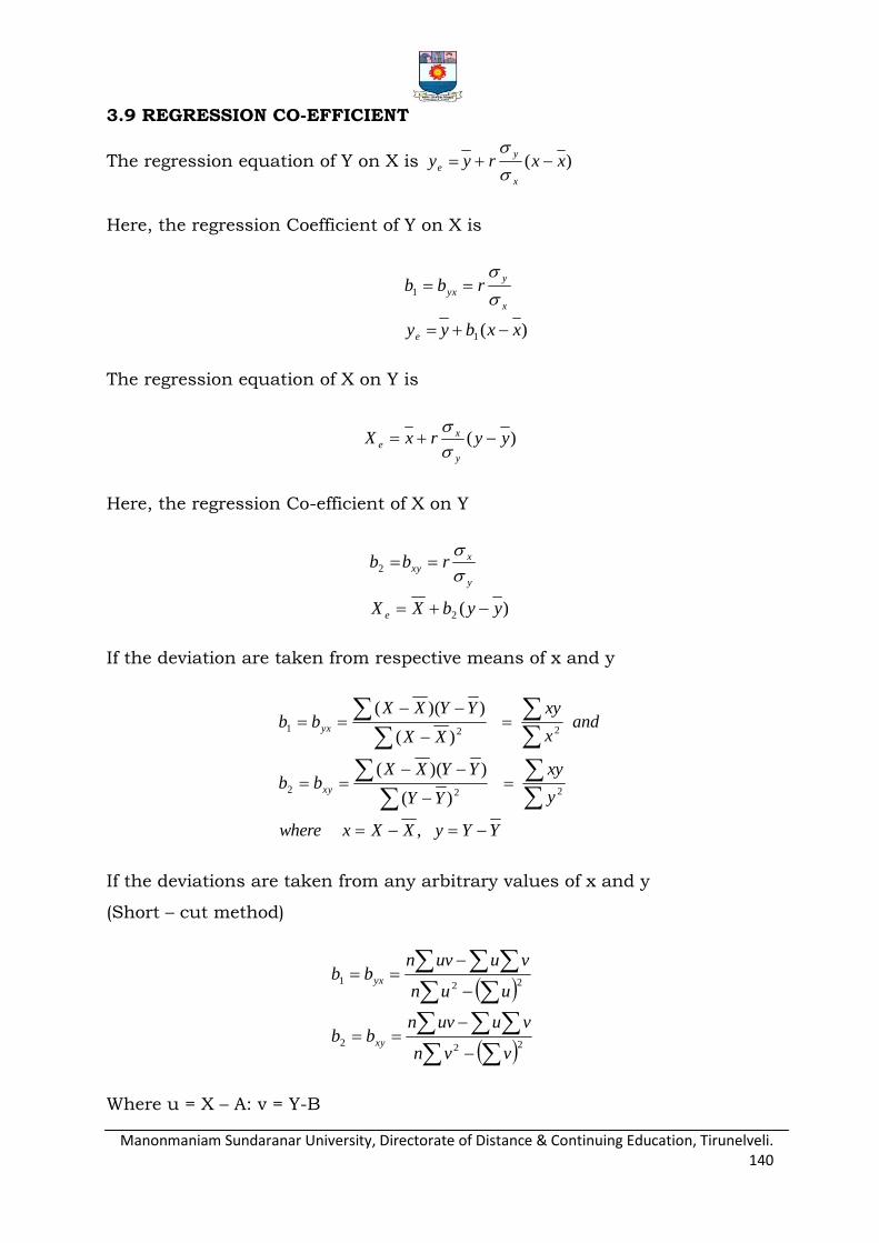
Manonmaniam Sundaranar University, Directorate of Distance & Continuing Education, Tirunelveli. 140
3.9 REGRESSION CO-EFFICIENT
The regression equation of Y on X is )( xxryyx
y
e
Here, the regression Coefficient of Y on X is
)(1
1
xxbyy
rbb
e
x
y
yx
The regression equation of X on Y is
)( yyrxXy
xe
Here, the regression Co-efficient of X on Y
)(2
2
yybXX
rbb
e
y
xxy
If the deviation are taken from respective means of x and y
YYyXXxwhere
y
xy
YY
YYXXbb
andx
xy
XX
YYXXbb
xy
yx
,
)(
))((
)(
))((
222
221
If the deviations are taken from any arbitrary values of x and y
(Short – cut method)
222
221
vvn
vuuvnbb
uun
vuuvnbb
xy
yx
Where u = X – A: v = Y-B
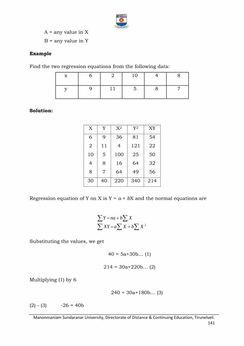
Manonmaniam Sundaranar University, Directorate of Distance & Continuing Education, Tirunelveli. 141
A = any value in X
B = any value in Y
Example
Find the two regression equations from the following data:
x 6 2 10 4 8
y 9 11 5 8 7
Solution:
X Y X2 Y2 XY
6
2
10
4
8
9
11
5
8
7
36
4
100
16
64
81
121
25
64
49
54
22
50
32
56
30 40 220 340 214
Regression equation of Y on X is Y = a + bX and the normal equations are
2XbXaXY
XbnaY
Substituting the values, we get
40 = 5a+30b… (1)
214 = 30a+220b… (2)
Multiplying (1) by 6
240 = 30a+180b… (3)
(2) - (3) -26 = 40b
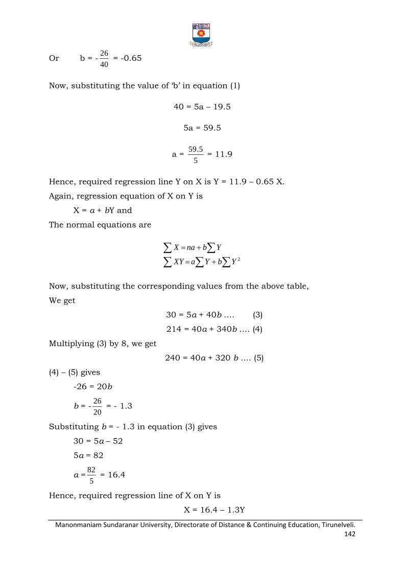
Manonmaniam Sundaranar University, Directorate of Distance & Continuing Education, Tirunelveli. 142
Or b = -40
26 = -0.65
Now, substituting the value of „b‟ in equation (1)
40 = 5a – 19.5
5a = 59.5
a = 5
5.59 = 11.9
Hence, required regression line Y on X is Y = 11.9 – 0.65 X.
Again, regression equation of X on Y is
X = a + bY and
The normal equations are
2YbYaXY
YbnaX
Now, substituting the corresponding values from the above table,
We get
30 = 5a + 40b …. (3)
214 = 40a + 340b …. (4)
Multiplying (3) by 8, we get
240 = 40a + 320 b …. (5)
(4) – (5) gives
-26 = 20b
b = -20
26 = - 1.3
Substituting b = - 1.3 in equation (3) gives
30 = 5a – 52
5a = 82
a =5
82 = 16.4
Hence, required regression line of X on Y is
X = 16.4 – 1.3Y

Manonmaniam Sundaranar University, Directorate of Distance & Continuing Education, Tirunelveli. 143
Properties of Regression Co-efficients:
Both regression coefficients must have the same sign, ie either it will
be positive or negative.
The correlation coefficient is the geometric mean of two regression
coefficients.
Correlation coefficient is the geometric mean of the regression
coefficients ie, 21bbr
.
The value of the coefficient of correlation cannot exceed unity i.e.
1. Therefore, if one of the regression coefficients is greater than unity,
the other must be less than unity.
The correlation coefficient will have the same sign as that of the
regression coefficients.
If one regression coefficient is greater than unity, then other
regression coefficient must be less than unity.
The sign of both the regression coefficients will be same, i.e. they
will be either positive or negative. Thus, it is not possible that one
regression coefficient is negative while the other is positive.
Regression coefficients are independent of origin but not of scale.
The coefficient of correlation will have the same sign as that of the
regression coefficients, such as if the regression coefficients have a
positive sign, then “r” will be positive and vice-versa.
Arithmetic mean of b1 and b2 is equal to or greater than the
coefficient of correlation. Symbolically rbb
2
21
If r=0, the variables are uncorrelated, the lines of regression become
perpendicular to each other.
The regression coefficients are independent of the change of origin,
but not of the scale. By origin, we mean that there will be no effect on
the regression coefficients if any constant is subtracted from the value
of X and Y. By scale, we mean that if the value of X and Y is either

Manonmaniam Sundaranar University, Directorate of Distance & Continuing Education, Tirunelveli. 144
multiplied or divided by some constant, then the regression coefficients
will also change.
If r= ±1, the two lines of regression either coincide or parallel to each
other
Angle between the two regression lines is
21
211
1tan
mm
mm
Where m1 and, m2 are the slopes of the regression lines X on Y and Y
on X respectively.
The angle between the regression lines indicates the degree of
dependence between the variables.
QUESTIONS
1. What is the correlation? Distinguish between positive and negative
correlation.
2. Define Karl Pearson‟s coefficient of correlation. Interpret r, when r = 1, -1
and 0.
3. Distinguish between linear and non-linear correlation.
4. Mention important properties of correlation coefficient.
5. What is Rank correlation? What are its merits and demerits?
6. Cov (x, y) = 18.6; Var(x) = 20.2; Var(y) = 23.7. Find „r‟.
7. Rank correlation coefficient r = 0.8.ΣD2 = 33. Find „n‟.
8. Calculate the coefficient of correlation between X and y for the following
x 1 3 4 5 7 8 10
y 2 6 8 10 14 16 20
9. Find the correlation coefficient between the marks obtained by ten
students in economics and statistics.
Marks in
(Maths)
70 68 67 55 60 60 75 63 60 72
Marks in
(Statistics)
65 65 80 60 68 58 75 62 60 70
10. Two judges gave the following ranks to eight competitors in a beauty
contest. Examine the relationship between their judgements.

Manonmaniam Sundaranar University, Directorate of Distance & Continuing Education, Tirunelveli. 145
Judge
A
4 5 1 2 3 6 7 8
Judge
B
8 6 2 3 1 4 5 7
11. From the following data, calculate the coefficient of rank correlation.
x 36 56 20 65 42 33 44 50 15 60
y 50 35 70 25 58 75 60 45 80 38
12. Calculate spearman‟s coefficient of Rank correlation for the following
data.
x 53 98 95 81 75 71 59 55
y 47 25 32 37 30 40 39 45
13. Obtain the rank correlation coefficient for the following data.
X 68 64 75 50 64 80 75 40 55 64
Y 62 58 68 45 81 60 68 48 50 70
14. What is a scatter diagram? How is it useful in the study of Correlation?
15. Explain different types of correlation with examples.
16. Distinguish between Karl Pearson‟s coefficient of correlation and
Spearman‟s correlation coefficient.
17. Compute the coefficient of correlation of the following score of A and B.
A 5 10 5 11 12 4 3 2 7 1
B 1 6 2 8 5 1 4 6 5 2
18. Calculate coefficient of Correlation between price and supply. Interpret
the value of correlation coefficient.
Price 8 10 15 17 20 22 24 25
Supply 25 30 32 35 37 40 42 45

Manonmaniam Sundaranar University, Directorate of Distance & Continuing Education, Tirunelveli. 146
19. Find out Karl Pearson‟s coefficient of correlation in the following series
relating to prices and supply of a commodity.
Price
(Rs.)
11 12 13 14 15 16 17 18 19 20
Supply
(Rs.)
30 29 29 25 24 24 24 21 18 15
20. Compute the coefficient of correlation from the following data.
Age of
workers
40 34 22 28 36 32 24 46 26 30
Days
absent
2.5 3 5 4 2.5 3 4.5 2.5 4 3.5
21. Calculate Karl Pearson‟s coefficient of correlation, for the following data.
Class Interval
0 1 2 3 4 5 6 7 8 Total
20-29 2 1 2 2 - 1 - 1 1 10
30-39 - 2 - 1 - 2 - 1 2 8
40-49 - 2 - 2 - - 1 -1 1 6
50-59 1 - 2 - - - - 1 - 4
60-69 - - - - - 1 - 1 - 2
22. Find the coefficient of correlation between the ages of 100 mothers and
daughters
Age of daughters in years (Y)
Age of mothers in
years (X)
5-10 10-15 15-20 20-25 25-30 Total
15-25 6 3 - - - 9
25-35 3 16 10 - - 29
35-45 - 10 15 7 - 32
45-55 - - 7 10 4 21
55-65 - - - 4 5 9
Total 9 29 32 21 9 100
23. The following table gives class frequency distribution of 45 clerks in a
business office according to age and pay. Find correlation between age and
pay if any.
Manonmaniam Sundaranar University, Directorate of Distance & Continuing Education, Tirunelveli. 147
Pay
Age 60-70 70-80 80-90 90-100 100-110 Total
20-30 4 3 1 - - 8
30-40 2 5 2 1 - 10
40-50 1 2 3 2 1 9
50-60 - 1 3 5 2 11
60-70 - - 1 1 5 7
Total 7 11 10 9 8 45
24. Find the correlation coefficient between two subjects marks scored by 60
candidates.
Marks in Statistics
Marks in economics
5-15 15-25
25-35
35-45 Total
0-10 1 1 - - 2
10-20 3 6 5 1 15
20-30 1 8 9 2 20
30-40 - 3 9 3 15
40-50 - - 4 4 8
Total 5 18 27 10 60
25. The following table gives the no. of students having different heights and
weights. Do you find any relation between height and weight?
Weight in Kg
Height in
cms
50-
60
60-
65
6570 70-
75
75-
80
Total
150-155 1 3 5 7 2 18
155-160 2 4 10 7 4 27
160-165 1 5 12 10 7 35
165-70 - 3 8 6 3 20
Total 4 15 37 28 16 100
26. Apply spearman‟s Rank difference method and calculate coefficient of
correlation between x and y from the data given below.
x 22 28 31 23 29 31 27 22 31 18
y 18 25 25 37 31 35 31 29 18 20

Manonmaniam Sundaranar University, Directorate of Distance & Continuing Education, Tirunelveli. 148
27. Find the rank correlation coefficients.
Marks
in Test
I
70 68 67 55 60 60 75 63 60 72
Marks
in Test
II
65 65 80 60 68 58 75 62 60 70
28. Calculate spearman‟s Rank correlation coefficient for the following table
of marks of students in two subjects.
First subject 80 64 54 49 48 35 32 29 20 18 15 10
Second
Subject
36 38 39 41 27 43 45 52 51 42 40 52
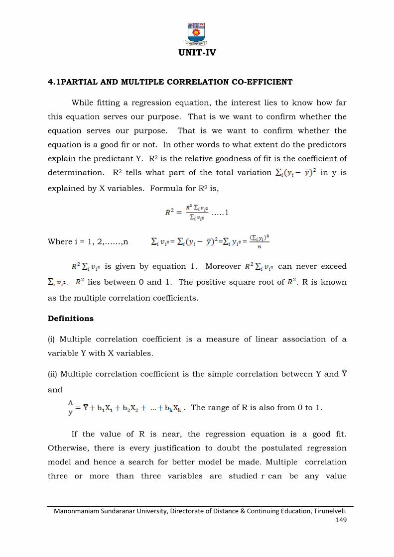
Manonmaniam Sundaranar University, Directorate of Distance & Continuing Education, Tirunelveli. 149
UNIT-IV
4.1PARTIAL AND MULTIPLE CORRELATION CO-EFFICIENT
While fitting a regression equation, the interest lies to know how far
this equation serves our purpose. That is we want to confirm whether the
equation serves our purpose. That is we want to confirm whether the
equation is a good fir or not. In other words to what extent do the predictors
explain the predictant Y. R2 is the relative goodness of fit is the coefficient of
determination. R2 tells what part of the total variation in y is
explained by X variables. Formula for R2 is,
.....1
Where i = 1, 2,……,n = = =
is given by equation 1. Moreover can never exceed
. lies between 0 and 1. The positive square root of . R is known
as the multiple correlation coefficients.
Definitions
(i) Multiple correlation coefficient is a measure of linear association of a
variable Y with X variables.
(ii) Multiple correlation coefficient is the simple correlation between Y and
and
. The range of R is also from 0 to 1.
If the value of R is near, the regression equation is a good fit.
Otherwise, there is every justification to doubt the postulated regression
model and hence a search for better model be made. Multiple correlation
three or more than three variables are studied r can be any value
Manonmaniam Sundaranar University, Directorate of Distance & Continuing Education, Tirunelveli. 150
from 0 to +1. Where the closer r is to one, the stronger the linear
association
If r equals zero , then there is no linear association between the
dependent variable and the independent variables.
R =
= correlation coefficient between y &
= correlation coefficient between y &
= correlation coefficient between &
Regression:
After knowing the relationship between two variables we may be
interested in estimating (predicting) the value of one variable given the value
of another. The variable predicted on the basis of other variables is called
the “dependent” or the „explained‟ variable and the other the
„independent‟ or the „predicting‟ variable. The prediction is based on average
relationship derived statistically by regression analysis. The equation, linear
or otherwise, is called the regression equation or the explaining equation.
For example, if we know that advertising and sales are correlated we may
find out expected amount of sales for a given advertising expenditure or the
required amount of expenditure for attaining a given amount of sales. The
relationship between two variables can be considered between, say, rainfall
and agricultural production, price of an input and the overall cost of
product, consumer expenditure and disposable income. Thus, regression
analysis reveals average relationship between two variables and this makes
possible estimation or prediction.
The term “regression” literally means “stepping back towards the
average”. It was first used by British biometrician Sir Francis Galton
1822 – 1911, in connection with the inheritance of stature. In regression
analysis there are two types of variable. The variable whose value is
Manonmaniam Sundaranar University, Directorate of Distance & Continuing Education, Tirunelveli. 151
influenced or is to be predicted is called dependent variable and the variable
which influences the values or is used for prediction is called independent
variable. In regression analysis independent variable is also known as
regressor of predictor or explanatory variable while the dependent variable is
also known as regressed or explained variable.
Definition:
Regression analysis is a mathematical measure of the average
relationship between two or more variables in terms of the original
units of the data
Types of Regression
The regression analysis can be classified into
Simple and Multiple
Linear and Non –Linear
Simple and Multiple:
In case of simple relationship only two variables are considered, for
example, the influence of advertising expenditure on sales turnover. In the
case of multiple relationships, more than two variables are involved. On this
while one variable is a dependent variable the remaining variables are
independent ones. For example, the turnover (y) may depend on advertising
expenditure (x) and the income of the people (z). Then the functional
relationship can be expressed as y = f (x, z).
Linear and Non-linear:
The linear relationships are based on straight-line trend, the equation
of which has no-power higher than one. But, remember a linear relationship
can be both simple and multiple. Normally a linear relationship is taken into
account because besides its simplicity, it has a better predictive value; a
linear trend can be easily projected into the future. In the case of non-linear
Manonmaniam Sundaranar University, Directorate of Distance & Continuing Education, Tirunelveli. 152
relationship curved trend lines are derived. The equations of these are
parabolic.
4.2 MULTIPLE LINEAR REGRESSION MODEL
Multiple linear regressions the most common form linear regression
analysis. As a predictive analysis, the multiple linear regressions used to
explain the relationship between on continuous dependent variable from two
or more independent variables. The independent variables can be
continuous or categorical. Suppose that the yield in pounds of conversion
in a chemical process depends on temperature and the catalyst
concentration. A regression model that involves more than on regressor
variable is called a multiple regression model. A multiple regression model
that might describe relationship is
Where y denotes the yield denotes the temperature denotes the
chemical concentration. This is multiple linear regression model with two
regressor variables. Multiple linear regression models or often used as
empirical models or approximating functions. That is true functional
relationship between y and , ……, is unknown, but over certain ranges
of the regressor variables the linear regression model is an adequate
approximation to the true unknown function.
Uses of Regression Analysis:
1. Regression analysis helps in establishing a functional relationship
between two or more variables.
2. Since most of the problems of economic analysis are based on cause and
effect relationships, the regression analysis is a highly valuable tool in
economic and business research.
3. Regression analysis predicts the values of dependent variables from the
values of independent variables.
4. We can calculate coefficient of correlation (r) and coefficient of
determination (r2) with the help of regression coefficients.

Manonmaniam Sundaranar University, Directorate of Distance & Continuing Education, Tirunelveli. 153
5. In statistical analysis of demand curves, supply curves, production
function, cost function, consumption function etc., regression analysis is
widely used.
4.3 SIMPLE PROBLEMS
Example
If two regression coefficients are b1=5
4 and b2 =
20
9 .What would be the
value of r?
Solution:
The correlation coefficient, 21bbr
6.010
6
100
36
20
9
5
4
Example
Given b1=5
3
8
152 band , Find r.
Solution:
21bbr
06.18
9
5
3
8
15
r = 1.06
It is not possible since r, cannot be greater than one. So the given values are
wrong
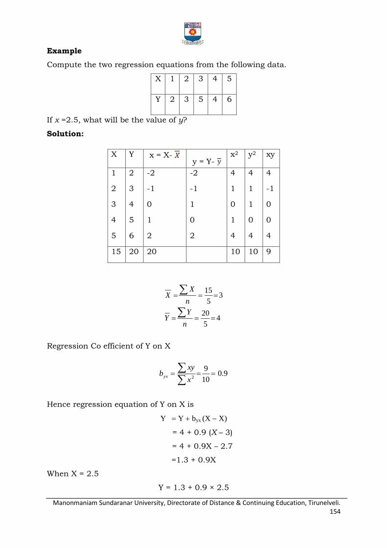
Manonmaniam Sundaranar University, Directorate of Distance & Continuing Education, Tirunelveli. 154
Example
Compute the two regression equations from the following data.
X 1 2 3 4 5
Y 2 3 5 4 6
If x =2.5, what will be the value of y?
Solution:
X Y x = X- y = Y-
x2 y2 xy
1
2
3
4
5
2
3
4
5
6
-2
-1
0
1
2
-2
-1
1
0
2
4
1
0
1
4
4
1
1
0
4
4
-1
0
0
4
15 20 20 10 10 9
45
20
35
15
n
YY
n
XX
Regression Co efficient of Y on X
9.010
92
x
xybyx
Hence regression equation of Y on X is
Y Y byx (X X)
= 4 + 0.9 (X – 3)
= 4 + 0.9X – 2.7
=1.3 + 0.9X
When X = 2.5
Y = 1.3 + 0.9 × 2.5

Manonmaniam Sundaranar University, Directorate of Distance & Continuing Education, Tirunelveli. 155
= 3.55
Regression co efficient of X on Y
9.010
92
x
xybyx
So, regression equation of X on Y is
X X bxy(Y Y)
= 3 + 0.9 (Y – 4)
= 3 + 0.9Y – 3.6
= 0.9Y - 0.6
Short-cut method
Example
Obtain the equations of the two lines of regression for the data given below:
x 45 42 44 43 41 45 43 40
y 40 38 36 35 38 39 37 41
Solution:
x y u = X-A u2 v = Y-B v2 uv
46
42
44
43
41
45
43
40
40
38
36
35
38
39
37
41
3
-1
1
0
-2
2
0
-3
9
1
1
0
4
4
0
9
2
0
-2
-3
0
1
-1
3
4
0
4
9
0
1
1
9
6
0
-2
0
0
2
0
-9
0 28 0 28 -3
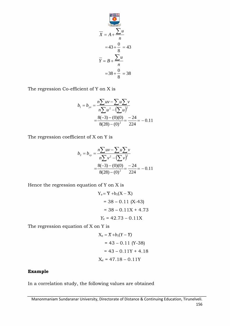
Manonmaniam Sundaranar University, Directorate of Distance & Continuing Education, Tirunelveli. 156
388
038
438
043
n
uBY
n
uAX
The regression Co-efficient of Y on X is
11.0224
24
)0()28(8
)0)(0()3(82
221
uun
vuuvnbb yx
The regression coefficient of X on Y is
11.0224
24
)0()28(8
)0)(0()3(82
222
vvn
vuuvnbb xy
Hence the regression equation of Y on X is
Ye ͞Y b1(X ͞X)
= 38 – 0.11 (X-43)
= 38 – 0.11X + 4.73
Ye = 42.73 – 0.11X
The regression equation of X on Y is
Xe ͞X b1(Y ͞Y)
= 43 – 0.11 (Y-38)
= 43 – 0.11Y + 4.18
Xe = 47.18 – 0.11Y
Example
In a correlation study, the following values are obtained
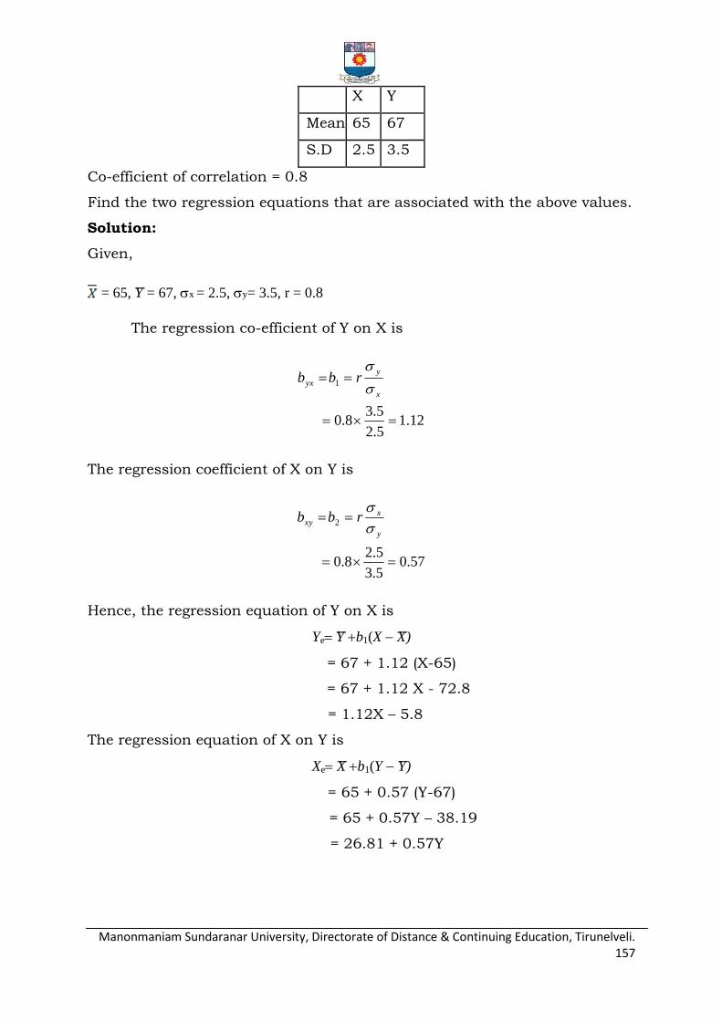
Manonmaniam Sundaranar University, Directorate of Distance & Continuing Education, Tirunelveli. 157
X Y
Mean 65 67
S.D 2.5 3.5
Co-efficient of correlation = 0.8
Find the two regression equations that are associated with the above values.
Solution:
Given,
= 65, ͞Y = 67, x = 2.5, y= 3.5, r = 0.8
The regression co-efficient of Y on X is
12.15.2
5.38.0
1
x
y
yx rbb
The regression coefficient of X on Y is
57.05.3
5.28.0
2
y
xxy rbb
Hence, the regression equation of Y on X is
Ye͞Y b1(X ͞X)
= 67 + 1.12 (X-65)
= 67 + 1.12 X - 72.8
= 1.12X – 5.8
The regression equation of X on Y is
Xe ͞X b1(Y ͞Y)
= 65 + 0.57 (Y-67)
= 65 + 0.57Y – 38.19
= 26.81 + 0.57Y
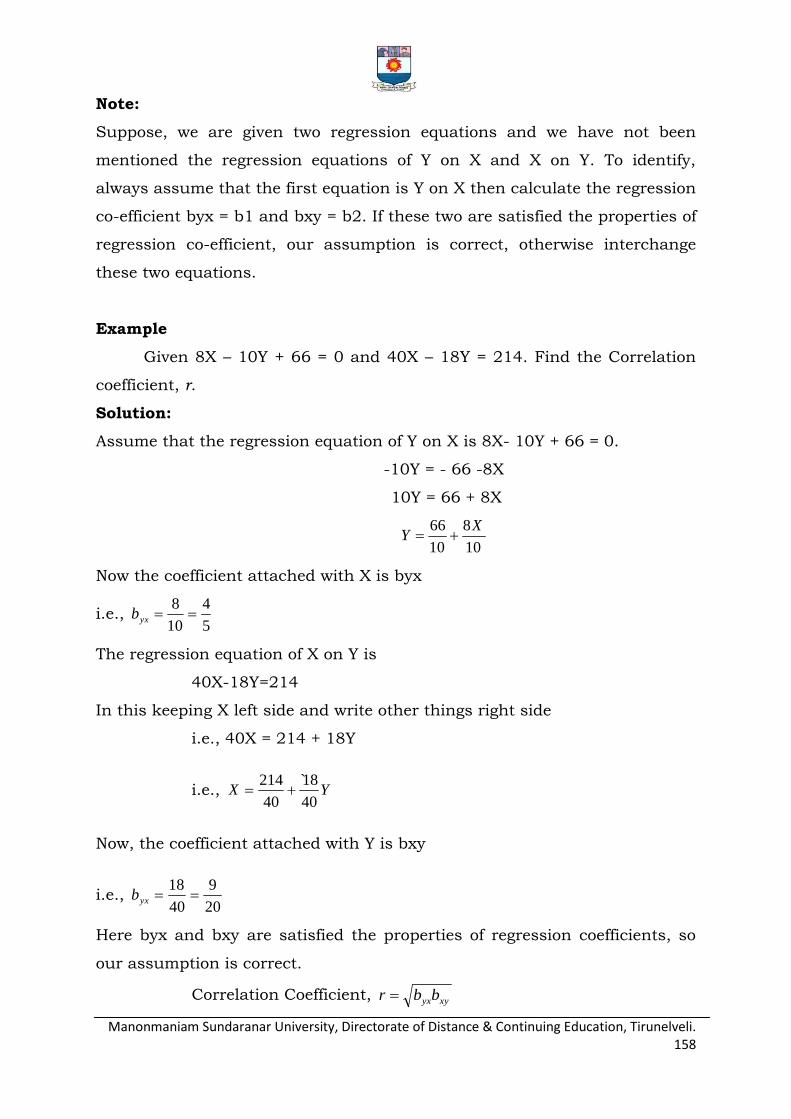
Manonmaniam Sundaranar University, Directorate of Distance & Continuing Education, Tirunelveli. 158
Note:
Suppose, we are given two regression equations and we have not been
mentioned the regression equations of Y on X and X on Y. To identify,
always assume that the first equation is Y on X then calculate the regression
co-efficient byx = b1 and bxy = b2. If these two are satisfied the properties of
regression co-efficient, our assumption is correct, otherwise interchange
these two equations.
Example
Given 8X – 10Y + 66 = 0 and 40X – 18Y = 214. Find the Correlation
coefficient, r.
Solution:
Assume that the regression equation of Y on X is 8X- 10Y + 66 = 0.
-10Y = - 66 -8X
10Y = 66 + 8X
10
8
10
66 XY
Now the coefficient attached with X is byx
i.e., 5
4
10
8yxb
The regression equation of X on Y is
40X-18Y=214
In this keeping X left side and write other things right side
i.e., 40X = 214 + 18Y
i.e., YX40
18`
40
214
Now, the coefficient attached with Y is bxy
i.e., 20
9
40
18yxb
Here byx and bxy are satisfied the properties of regression coefficients, so
our assumption is correct.
Correlation Coefficient, xyyxbbr
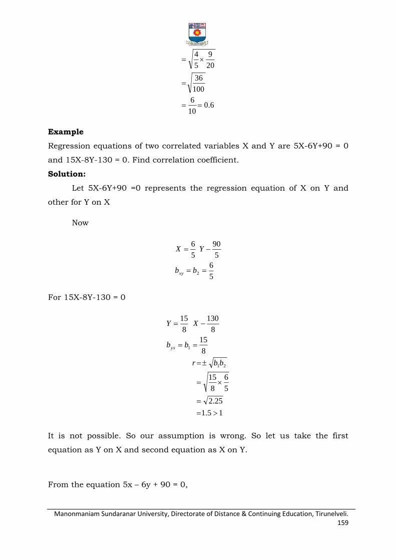
Manonmaniam Sundaranar University, Directorate of Distance & Continuing Education, Tirunelveli. 159
6.010
6
100
36
20
9
5
4
Example
Regression equations of two correlated variables X and Y are 5X-6Y+90 = 0
and 15X-8Y-130 = 0. Find correlation coefficient.
Solution:
Let 5X-6Y+90 =0 represents the regression equation of X on Y and
other for Y on X
Now
5
6
5
90
5
6
2
bb
YX
xy
For 15X-8Y-130 = 0
15.1
25.2
5
6
8
15
8
15
8
130
8
15
21
1
bbr
bb
XY
yx
It is not possible. So our assumption is wrong. So let us take the first
equation as Y on X and second equation as X on Y.
From the equation 5x – 6y + 90 = 0,
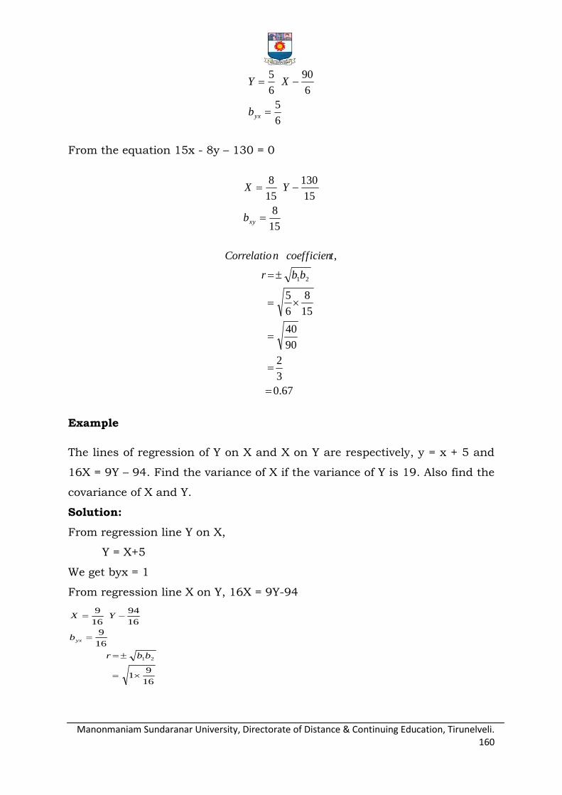
Manonmaniam Sundaranar University, Directorate of Distance & Continuing Education, Tirunelveli. 160
6
5
6
90
6
5
yxb
XY
From the equation 15x - 8y – 130 = 0
15
8
15
130
15
8
xyb
YX
67.0
3
2
90
40
15
8
6
5
,
21
bbr
tcoefficiennCorrelatio
Example
The lines of regression of Y on X and X on Y are respectively, y = x + 5 and
16X = 9Y – 94. Find the variance of X if the variance of Y is 19. Also find the
covariance of X and Y.
Solution:
From regression line Y on X,
Y = X+5
We get byx = 1
From regression line X on Y, 16X = 9Y-94
16
91
16
9
16
94
16
9
21
bbr
b
YX
yx
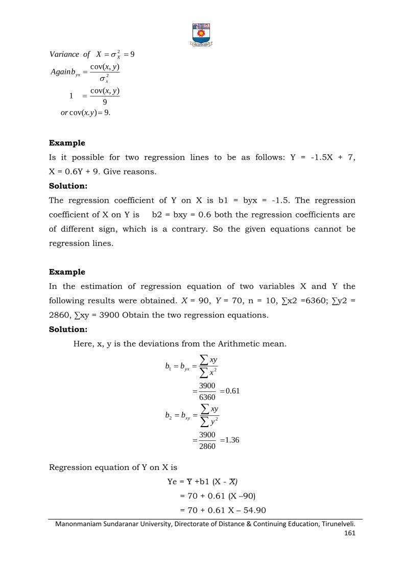
Manonmaniam Sundaranar University, Directorate of Distance & Continuing Education, Tirunelveli. 161
.9).cov(
9
),cov(1
),cov(
9
2
2
yxor
yx
yxbAgain
XofVariance
x
yx
X
Example
Is it possible for two regression lines to be as follows: Y = -1.5X + 7,
X = 0.6Y + 9. Give reasons.
Solution:
The regression coefficient of Y on X is b1 = byx = -1.5. The regression
coefficient of X on Y is b2 = bxy = 0.6 both the regression coefficients are
of different sign, which is a contrary. So the given equations cannot be
regression lines.
Example
In the estimation of regression equation of two variables X and Y the
following results were obtained. X = 90, Y = 70, n = 10, ∑x2 =6360; ∑y2 =
2860, ∑xy = 3900 Obtain the two regression equations.
Solution:
Here, x, y is the deviations from the Arithmetic mean.
36.12860
3900
61.06360
3900
22
21
y
xybb
x
xybb
xy
yx
Regression equation of Y on X is
Ye = ͞Y +b1 (X - ͞X)
= 70 + 0.61 (X –90)
= 70 + 0.61 X – 54.90
Manonmaniam Sundaranar University, Directorate of Distance & Continuing Education, Tirunelveli. 162
Ye = 15.1 + 0.61X
Xe = ͞X +b1 (Y - ͞Y )
= 90 + 1.36 (Y –70)
= 90 + 1.36 Y – 95.2
Xe = 1.36Y – 5.2
QUESTIONS
1. Explain the different Types of Regression,
2. Describe the partial and multiple correlation coefficient.
3. Explain the Multiple Linear Regression Model.
4. From the following data, find the regression equation
5. Find the regression equation. Given b1=5
3
8
152 band .
6. What is coefficient of determination?
7. What do you understand by regression model?
8. What are the uses of regression analysis?
9. Calculate the two regression equations from the following data.
x 1 2 3 4 5
y 2 3 5 4 6
If x = 2.5, what will be the value of y?
10. Following the data pertaining to the production(x) and export(y) rice in
lakh tonnes in India from 1991 to 1992.
x 37.4 31.1 38.7 39.5 47.9 42.6 48.4 64.6 58.4 38.6 51.4 84.0
y 3.90 1.33 1.10 4.39 9.41 9.67 3.41 2.51 8.62 9.90 6.64 6.50
Find the regression of Y on X.
Manonmaniam Sundaranar University, Directorate of Distance & Continuing Education, Tirunelveli. 163
11. In a correlation studies, the following values are obtained:
X Y
Mean 12 15
S.D 2 3
r = 0.5, Find the two regression equations.
12. Given X=90, Y=70, bxy = 1.36, byx = 0.61
(i) The most probable values of X, when Y = 50,
(ii) The coefficient of correlation between X and Y.
13. Regression equations of two correlated variables X and Y are 5X-6Y+90 =
0 and 15X-8Y-130 = 0. Find correlation coefficient.
14. From the two regression equations, find the value of r, and
4Y = 9X+15 and 25X = 6Y + 7
15. Given the following equation 8X – 10Y + 66 = 0 and 40X – 18Y = 214.
Find the Correlation coefficient and r.
Manonmaniam Sundaranar University, Directorate of Distance & Continuing Education, Tirunelveli. 164
UNIT-V
5.1 SAMPLING – CENSUS AND SAMPLE SURVEY
Sampling is very often used in our daily life. In a statistical
investigation the interest usually lies in the assessment of the general
magnitude and the study of variation with respect to one or more
characteristics relating to individuals belonging to a group. For example,
while purchasing food grains from a shop we usually examine a handful
from the bag to assess the quality of the commodity. A doctor examines a
few drops of blood as sample and draws conclusion about the blood
constitution of the whole body. Thus most of our investigations are based on
samples. In this chapter, let us see the importance of sampling and the
various methods of sample selections from the population. If the population
is infinite, complete enumeration is not possible. Also if the units are
destroyed in the course of inspection. But even if the population is finite or
the inspection is not destructive.
Population:
In a statistical enquiry, all the items, which fall within the purview of
enquiry, are known as Population or Universe. In other words, the
population is a complete set of all possible observations of the type which is
to be investigated. Total numbers of students studying in a school or college,
total number of books in a library, total number of houses in a village or
town are some examples of population. Sometimes it is possible and
practical to examine every person or item in the population we wish to
describe. We call this a complete enumeration or census. We use sampling
when it is not possible to measure every item in the population. Statisticians
use the word population to refer not only to people but to all items that have
been chosen for study.
Finite population and infinite population
A population is said to be finite if it consists of finite number of units.
Numbers of workers in a factory, production of articles in a particular day
Manonmaniam Sundaranar University, Directorate of Distance & Continuing Education, Tirunelveli. 165
for a company are examples of finite population. The total number of units
in a population is called population size. A population is said to be infinite if
it has infinite number of units. For example the number of stars in the sky,
the number of people seeing the television programmers etc. Information on
population can be collected in two ways.
Census method
Sample method
Census Method:
The census method is every element of the population is included in
the investigation. Census method refers to the complete enumeration of a
universe. For example, if we study the average annual income of the
families of a particular village or area, and if there are 1000 families in that
area, we must study the income of all 1000 families. In this method no
family is left out, as each family is a unit.
Population census of India
The population census of our country is taken at 10 yearly intervals.
The latest census was taken in 2011. The first census was taken in
1871 – 72.
Merits and limitations of Census method:
Merits
1. The data are collected from each and every item of the population
2. The results are more accurate and reliable, because every item of the
universe is required.
3. Intensive study is possible.
4. The data collected may be used for various surveys, analyses etc.
Limitations
1. It requires a large number of enumerators and it is a costly method
2. It requires more money, labor, time energy etc.
3. It is not possible in some circumstances where the universe is infinite.
Manonmaniam Sundaranar University, Directorate of Distance & Continuing Education, Tirunelveli. 166
Demerits of Census method
1. This method is inconvenient because it take much time
2. This method is possible only in few cases of data collection
3. This method is possible only in limited universe
4. It is much time and labour consuming.
5. It requires a lot of people to involve in data collection.
6. Data collected through this method would have more statistical errors.
Sampling:
The theory of sampling has been developed recently but this is not
new. In our everyday life we have been using sampling theory as we have
discussed in introduction. In all those cases we believe that the samples give
a correct idea about the population. Most of our decisions are based on the
examination of a few items that is sample studies. In the sampling
techniques, we inspect or study only a selected representative and finite sub
set of the population.
Example
The housewife usually tastes a spoonful of the cooked products for the
proper quantity of salt or sugar. The consumer ascertains the quality of rice
by testing few grains in hand and so on.
Merits:
1. It is economical than census methods interms of time, money and
manpower.
2. Since time and money are saved, we can employ trained persons or
experts, hence the error may be minimized
3. We can check result of census method with the help of sampling
techniques.
Demerits:
1. If the sampling process is not properly planned.
2. The sampling technique give in accurate and misleading results.
Manonmaniam Sundaranar University, Directorate of Distance & Continuing Education, Tirunelveli. 167
3. The conclusion drawn by unskilled person unreliable.
4. Sometimes the sample size is too large and the technique used is also
highly complicated.
Sample:
A finite size of statistical individuals in a population is called a sample
and the number of individuals in a sample is called the sample size.
Sampling unit:
The constituents of a population which are individuals to be sampled
from the population and cannot be further subdivided for the purpose of the
sampling at a time are called sampling units.
Sampling frame:
For adopting any sampling procedure it is essential to have a list
identifying each sampling unit by a number. Such a list or map is called
sampling frame. A list of voters, a list of house holders, a list of villages in a
district, a list of farmers etc. are a few examples of sampling frame.
Reasons for selecting a sample:
Sampling is inevitable in the following situations:
1. Complete enumerations are practically impossible when the population is
infinite.
2. When the results are required in a short time.
3. When the area of survey is wide.
4. When resources for survey are limited particularly in respect of money
and trained persons.
5. When the item or unit is destroyed under investigation.
Parameters and statistics:
We can describe samples and populations by using measures such as
the mean, median, mode and standard deviation. When these terms
describe the characteristics of a population, they are called parameters.
Manonmaniam Sundaranar University, Directorate of Distance & Continuing Education, Tirunelveli. 168
When they describe the characteristics of a sample, they are called
statistics. A parameter is a characteristic of a population and a statistic is a
characteristic of a sample. Since samples are subsets of population
statistics provide estimates of the parameters. That is, when the parameters
are unknown, they are estimated from the values of the statistics. In
general, we use Greek or capital letters for population parameters and lower
case Roman letters to denote sample statistics.
Principles of Sampling
Samples have to provide good estimates. The following principle tell us
that the sample methods provide such good estimates
Principle of statistical regularity:
A moderately large number of units chosen at random from a large
group are almost sure on the average to possess the characteristics of the
large group.
Principle of Inertia of large numbers:
Other things being equal, as the sample size increases, the results
tend to be more accurate and reliable.
Principle of Validity:
This states that the sampling methods provide valid estimates about
the population units (parameters).
Principle of Optimization:
This principle takes into account the desirability of obtaining a
sampling design which gives optimum results. This minimizes the risk or
loss of the sampling design.
The foremost purpose of sampling is to gather maximum information
about the population under consideration at minimum cost, time and
human power. This is best achieved when the sample contains all the
properties of the population.
Manonmaniam Sundaranar University, Directorate of Distance & Continuing Education, Tirunelveli. 169
5.2 SAMPLING ERRORS AND NON-SAMPLING ERRORS
The two types of errors in a sample survey are sampling errors and
non - sampling errors.
Sampling errors:
Although a sample is a part of population, it cannot be expected
generally to supply full information about population. So there may be in
most cases difference between statistics and parameters. The discrepancy
between a parameter and its estimate due to sampling process is known as
sampling error.
Non-sampling errors:
In all surveys some errors may occur during collection of actual
information. These errors are called Non-sampling errors.
Advantages and Limitation of Sampling:
There are many advantages of sampling methods over census method.
They are as follows:
1. Sampling saves time and labor.
2. It results in reduction of cost in terms of money and man-hour.
3. Sampling ends up with greater accuracy of results.
4. It has greater scope.
5. It has greater adaptability.
Limitations:
1. Sampling is to be done by qualified and experienced persons. Otherwise,
the information will be unbelievable.
2. Sample method may give the extreme values sometimes instead of the
mixed values.
3. There is the possibility of sampling errors. Census survey is free from
sampling error.
Manonmaniam Sundaranar University, Directorate of Distance & Continuing Education, Tirunelveli. 170
Types of Sampling
The technique of selecting a sample is of fundamental importance in
sampling theory and it depends upon the nature of investigation. The
sampling procedures which are commonly used may be classified as
Probability sampling.
Non-probability sampling.
Mixed sampling.
Probability sampling (Random sampling):
A probability sample is one where the selection of units from the
population is made according to known probabilities. A method of sampling
that enables the researcher to specify for each case in the population the
probability of its inclusion in the sample. (e.g.) Simple random sample,
probability proportional to sample size etc.
Non-Probability sampling:
It is the one where discretion is used to select „representative‟ units
from the population (or) to infer that a sample is „representative‟ of the
population. This method is called judgment or purposive sampling. This
method is mainly used for opinion surveys; a common type of judgment
sample used in surveys is quota sample. This method is not used in general
because of prejudice and bias of the enumerator. However if the enumerator
is experienced and expert, this method may yield valuable results. For
example, in the market research survey of the performance of their new car,
the sample was all new car purchasers.
Mixed Sampling
Here samples are selected partly according to some probability and
partly according to a fixed sampling rule; they are termed as mixed samples
and the technique of selecting such samples is known as mixed sampling.
Manonmaniam Sundaranar University, Directorate of Distance & Continuing Education, Tirunelveli. 171
5.3 METHODS OF SELECTION OF SAMPLES
Here we shall consider the following three methods:
Simple random sampling.
Stratified random sampling.
Systematic random sampling.
SIMPLE RANDOM SAMPLING:
A simple random sample from finite population is a sample selected
such that each possible sample combination has equal probability of being
chosen. It is also called unrestricted random sampling. The simple random
sample is the underlying model for probability sampling, although
researchers don't actually use it much. Simple random samples are
incorporated into and provide the foundation for more advanced probability
sampling designs. A sample designed in such a way as to ensure that:
Every member of the population has an equal chance of being chosen.
Every combination of „N‟ members has an equal chance of being
chosen.
SIMPLE RANDOM SAMPLING WITHOUT REPLACEMENT: (SRSWOR)
In this method the population elements can enter the sample only
once, the method of sampling in which every Kth member (K is a ratio
obtained by dividing the population size by the desired sample size) in the
total population is chosen for inclusion in the sample after the first member
of the sample is selected at random from among the first K members of the
population. Systematic random samples give results very similar to those of
simple random samples.
SIMPLE RANDOM SAMPLING WITH REPLACEMENT: (SRSWR)
In this method the population units may enter the sample more than
once. Simple random sampling may be with or without replacement.
A method of sampling obtained by:
Manonmaniam Sundaranar University, Directorate of Distance & Continuing Education, Tirunelveli. 172
Dividing the population into subgroups based on one or more
variables central to our analysis,.
Drawing a simple random sample from each of the subgroups.
Procedure of selection of a random sample:
The procedure of selection of a random sample follows the following steps
1. Identify the N units in the population with the numbers 1 to N.
2. Choose any random number arbitrarily in the random number table and
start reading numbers.
3. Choose the sampling unit whose serial number corresponds to the
random number drawn from the table of random numbers.
4. In case of SRSWR, all the random numbers are accepted ever if repeated
more than once. In case of SRSWOR, if any random number is repeated,
then it is ignored and more numbers are drawn.
Such process can be implemented through programming and using
the discrete uniform distribution. Any number between 1 and N can be
generated from this distribution and corresponding unit can be selected into
the sample by associating an index with each sampling unit. Many
statistical software‟s like R, SAS, and etc. have inbuilt functions for drawing
a sample using SRSWOR or SRSWR.
Methods of selection of a simple random sampling
The following are some methods of selection of a simple random
sampling.
Lottery Method:
This is the most popular and simplest method. In this method all the
items of the population are numbered on separate slips of paper of same
Manonmaniam Sundaranar University, Directorate of Distance & Continuing Education, Tirunelveli. 173
size, shape and colour. They are folded and mixed up in a container. The
required numbers of slips are selected at random for the desire sample size.
For example, if we want to select 5 students, out of 50 students, then we
must write their names or their roll numbers of all the 50 students on slips
and mix them. Then we make a random selection of 5 students. This method
is mostly used in lottery draws. If the universe is infinite this method is
inapplicable.
Table of Random numbers:
As the lottery method cannot be used, when the population is infinite,
the alternative method is that of using the table of random numbers. There
are several standard tables of random numbers.
Tippet‟s table.
Fisher and Yates‟ table.
Kendall and Smith‟s table are the three tables among them.
A random number table is so constructed that all digits 0 to 9 appear
independent of each other with equal frequency. If we have to select a
sample from population of size N= 100, then the numbers can be combined
three by three to give the numbers from 001 to 100.
Procedure to select a sample using random number table:
Units of the population from which a sample is required are assigned
with equal number of digits. When the size of the population is less than
thousand, three digit number 000, 001, 002… 999 are assigned. We may
start at any place and may go on in any direction such as column wise or
row- wise in a random number table. But consecutive numbers are to be
used. On the basis of the size of the population and the random number
table available with us, we proceed according to our convenience. If any
random number is greater than the population size N, then N can be
subtracted from the random number drawn. This can be repeatedly until the
number is less than N or equal to N.
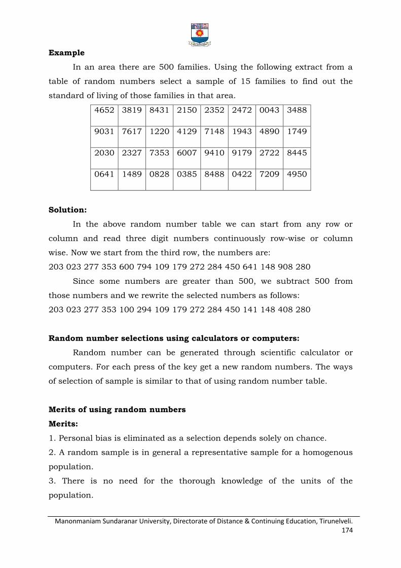
Manonmaniam Sundaranar University, Directorate of Distance & Continuing Education, Tirunelveli. 174
Example
In an area there are 500 families. Using the following extract from a
table of random numbers select a sample of 15 families to find out the
standard of living of those families in that area.
4652 3819 8431 2150 2352 2472 0043 3488
9031 7617 1220 4129 7148 1943 4890 1749
2030 2327 7353 6007 9410 9179 2722 8445
0641 1489 0828 0385 8488 0422 7209 4950
Solution:
In the above random number table we can start from any row or
column and read three digit numbers continuously row-wise or column
wise. Now we start from the third row, the numbers are:
203 023 277 353 600 794 109 179 272 284 450 641 148 908 280
Since some numbers are greater than 500, we subtract 500 from
those numbers and we rewrite the selected numbers as follows:
203 023 277 353 100 294 109 179 272 284 450 141 148 408 280
Random number selections using calculators or computers:
Random number can be generated through scientific calculator or
computers. For each press of the key get a new random numbers. The ways
of selection of sample is similar to that of using random number table.
Merits of using random numbers
Merits:
1. Personal bias is eliminated as a selection depends solely on chance.
2. A random sample is in general a representative sample for a homogenous
population.
3. There is no need for the thorough knowledge of the units of the
population.
Manonmaniam Sundaranar University, Directorate of Distance & Continuing Education, Tirunelveli. 175
4. The accuracy of a sample can be tested by examining another sample
from the same universe
when the universe is unknown.
5. This method is also used in other methods of sampling.
Limitations:
1. Preparing lots or using random number tables is tedious when the
population is large.
2. When there is large difference between the units of population, the simple
random sampling
may not be are preventative sample.
3. The size of the sample required under this method is more than that
required by stratified random sampling.
4. It is generally seen that the units of a simple random sample lie apart
geographically. The cost and time of collection of data are more.
STRATIFIED RANDOM SAMPLING:
Of all the methods of sampling the procedure commonly used in
surveys is stratified sampling. This technique is mainly used to reduce the
population heterogeneity and to increase the efficiency of the estimates.
Stratified random sampling is a technique which attempts to restrict the
possible samples to those which are ``less extreme'' by ensuring that all
parts of the population are represented in the sample in order to increase
the efficiency. Stratification means division into groups. In this method the
population is divided into a number of subgroups or strata. The strata
should be so formed that each stratum is homogeneous as far as possible.
Then from each stratum a simple random sample may be selected and these
are combined together to form the required sample from the population.
Useful when the population is heterogeneous and it is possible to establish
strata which are reasonably homogeneous within each one
Types of Stratified Random Sampling
There are two types of stratified sampling. They are
Manonmaniam Sundaranar University, Directorate of Distance & Continuing Education, Tirunelveli. 176
Proportional
Non-proportional.
In the proportional sampling equal and proportionate representation
is given to subgroups or strata. If the number of items is large, the sample
will have a higher size and vice versa. The population size is denoted by N
and the sample size is denoted by „n‟ the sample size is allocated to each
stratum in such a way that the sample fractions is a constant for each
stratum. That is given by n/N = c. So in this method each stratum is
represented according to its size. In non-proportionate sample, equal
representation is given to all the sub-strata regardless of their existence in
the population.
Proportional:
The sample size of each stratum in this technique is proportionate to
the population size of the stratum when viewed against the entire
population. This means that the each stratum has the same sampling
fraction.
Non-proportional:
The only difference between proportionate and disproportionate
stratified random sampling is their sampling fractions. With
disproportionate sampling, the different strata have different sampling
fractions.
Example
A sample of 50 students is to be drawn from a population consisting of 500
students belonging to two institutions A and B. The number of students in
the institution A is 200 and the institution B is 300. How will you draw the
sample using proportional allocation?
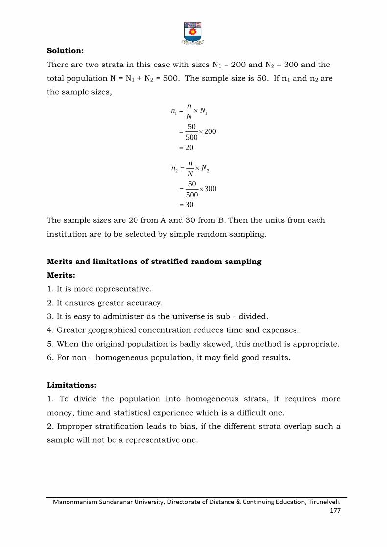
Manonmaniam Sundaranar University, Directorate of Distance & Continuing Education, Tirunelveli. 177
Solution:
There are two strata in this case with sizes N1 = 200 and N2 = 300 and the
total population N = N1 + N2 = 500. The sample size is 50. If n1 and n2 are
the sample sizes,
20
200500
50
11
NN
nn
30
300500
50
22
NN
nn
The sample sizes are 20 from A and 30 from B. Then the units from each
institution are to be selected by simple random sampling.
Merits and limitations of stratified random sampling
Merits:
1. It is more representative.
2. It ensures greater accuracy.
3. It is easy to administer as the universe is sub - divided.
4. Greater geographical concentration reduces time and expenses.
5. When the original population is badly skewed, this method is appropriate.
6. For non – homogeneous population, it may field good results.
Limitations:
1. To divide the population into homogeneous strata, it requires more
money, time and statistical experience which is a difficult one.
2. Improper stratification leads to bias, if the different strata overlap such a
sample will not be a representative one.
Manonmaniam Sundaranar University, Directorate of Distance & Continuing Education, Tirunelveli. 178
SYSTEMATIC SAMPLING
This method is widely employed because of its ease and convenience.
selecting sample units at random can introduce logistical challenges that
preclude collecting data efficiently. If the chance of introducing a bias is low
or if ideal dispersion of sample units in the population is a higher priority
that a strictly random sample, then it might be appropriate to choose
samples non‐randomly. Like simple random sampling, systematic sampling
is a type of probability sampling where each element in the population has a
known and equal probability of being selected. The probabilistic framework
is maintained through selection of one or more random starting points. A
frequently used method of sampling when a complete list of the population
is available is systematic sampling. It is also called Quasi-random
sampling.
Selection procedure:
The whole sample selection is based on just a random start. The first
unit is selected with the help of random numbers and the rest get selected
automatically according to some pre designed pattern is known as
systematic sampling. With systematic random sampling every Kth element
in the frame is selected for the sample, with the starting point among the
first K elements determined at random. For example, if we want to select a
sample of 50 students from 500 students under this method Kth item is
picked up from the sampling frame and K is called the sampling interval.
10
500
50
size Population
size Sample
n
N=K interval, Sampling
K = 10 is the sampling interval. Systematic sample consists in selecting a
random number say i K and every Kth unit subsequently. Suppose the
random number „i‟ is 5, then we select
5, 15, 25, 35, 45… The random number „i‟ is called random start. The
technique will generate K systematic samples with equal probability.
Manonmaniam Sundaranar University, Directorate of Distance & Continuing Education, Tirunelveli. 179
Merits and Limitations of Systematic Sampling
Merits:
1. This method is simple and convenient.
2. Time and work is reduced much.
3. If proper care is taken result will be accurate.
4. It can be used in infinite population.
Limitations:
1. Systematic sampling may not represent the whole population.
2. There is a chance of personal bias of the investigators.
3. Choose a starting point at random
4. Select samples at uniform intervals there after
5. Systematic sampling is preferably used when the information is to be
collected from trees in a forest, house in blocks, entries in a register
which are in a serial order etc.
CLUSTER SAMPLING
It is one of the basic assumptions in any sampling procedure that the
population can be divided into a finite number of distinct and identifiable
units, called sampling units. The smallest units into which the population
can be divided are called elements of the population. The groups of such
elements are called clusters.
In many practical situations and many types of populations, a list of
elements is not available and so the use of an element as a sampling unit is
not feasible. The method of cluster sampling or area sampling can be used
in such situations.
A cluster sample is a probability sample in which each sampling unit
is a collection or a group of elements.
This general method is known as multistage sampling, although it is
also sometimes loosely described as cluster sampling.
As only a sample of clusters are sampled, the ones selected need to
represent the ones unselected; this is best done when the clusters are
Manonmaniam Sundaranar University, Directorate of Distance & Continuing Education, Tirunelveli. 180
as internally heterogeneous in the survey variables as possible in
cluster sampling.
Divide the whole population into clusters according to some well
defined rule.
Treat the clusters as sampling units.
Choose a sample of clusters according to some procedure.
Carry out a complete enumeration of the selected clusters, i.e., collect
information on all the sampling units available in selected clusters.
The cluster sampling in two types
One stage cluster sampling.
Two stage cluster sampling.
Conditions under which the cluster sampling is used:
Cluster sampling is preferred when
1. No reliable listing of elements is available and it is expensive to prepare it.
2. Even if the list of elements is available, the location or identification of the
units may be difficult.
3. A necessary condition for the validity of this procedure is that every unit
of the population under study must correspond to one and only one unit of
the cluster so that the total number of sampling units in the frame may
cover all the units of the population under study without any omission or
duplication. When this condition is not satisfied, bias is introduced.
Advantages:
1. Generating sampling frame for clusters is economical, and sampling
frame is often readily available at cluster level.
2. Most economical form of sampling.
3. Larger sample for a similar fixed cost.
4. Less time for listing and implementation
5. Also suitable for survey of institutions.

Manonmaniam Sundaranar University, Directorate of Distance & Continuing Education, Tirunelveli. 181
Disadvantages:
1. May not reflect the diversity of the community.
2. Other elements in the same cluster may share similar characteristics.
3. Provides less information per observation than an SRS of the same size.4.
Standard errors of the estimates are high, compared to other sampling
designs with same sample size.
QUESTIONS
1. Define a Population. Explain the finite and infinite population with
examples.
2. Write short notes on following terms.
Sample
Sample Size
Census
Sampling unit
Sampling frame
3. Describe the difference between census and sampling.
4. Explain the census method?
5. Define sampling with examples?
6. What were the reasons for selecting sample?
7. Explain the principles of sampling
8. Explain the sampling errors and non sampling errors.
9. Write down the Advantages and Limitations of sampling.
10. What are the merits and limitations of simple random sampling?
11. Explain the Merits and limitations of random numbers.
12. Explain the procedure of selection of a random sample.
13. Explain the different types of Stratified Random sampling.
14. What are the conditions to use the cluster sampling?
15. Explain the different types of sampling.
16. Explain the Method of selection of samples.
17. Explain the different methods of selection of a simple random sampling.
18. Explain the Stratified random sampling with example? And merits,
limitations.
Manonmaniam Sundaranar University, Directorate of Distance & Continuing Education, Tirunelveli. 182
19. Discuss the systematic sampling with selection procedure of systematic
sampling?
20. Write the briefly explain of cluster sampling.
BOOKS FOR STUDY:
1. Anderson, T.W. and Sclove, S.L. (1978) Introduction to Statistical
Analysis of data, Houghton Mifflin, Boston.
2. Bhat, B.R., Srivenkataramna, T. and Madhava Rao, K.S. (1996) Statistics
a Beginner‟s Text, Vol. I, New Age International, New Delhi.
3. Croxton, F.E. and Cowden, D.J. (1969) Applied General Statistics,
Prentice Hall, New Delhi.
4. Goon, A.M., M.K. Gupta and B. Das Gupta (2002) Fundamentals of
Statistics- Vol. I., World Press Ltd, Kolkata.
5. Spiegel, M.R. and Stephens, L. (2010) Statistics, Schaum‟s Outline Series,
Mc Graw Hill, New York.
Course Material Prepared by
Dr. P. ARUMUGAM
Associate Professor, Department of Statistics
Manonmaniam Sundaranar University, Tirunelveli - 627 012.