Staying out of Sight? Concentrated Policing and Local Political Action
Upload
khangminh22Category
view
0download
0
MEMBRANE DISTILLATION
OF CONCENTRATED BRINES
Lynette Mariah
BSc(Hons), (Natal)
Submitted in fulfillment of the academic
requirements for the degree of
Doctor of Philosophy
in the
School of Chemical Engineering
University of KwaZulu-Natal, Durban
March 2006

The fear of the LORD is the beginning of knowledge: but fools despise wisdom and instruction.
Proverbs 1:7
To my Father
PREFACE
vi
I, Lynette Mariah, declare that unless indicated, this thesis is my own work and that it has not
been submitted, in whole or in part, for a degree at another University or Institution.
………………………
Lynette Mariah
March 2006

ACKNOWLEDGEMENTS
iii
To God Almighty, the Lord Jesus Christ, without whom nothing is possible. For being my rock
and my fortress and granting me the fortitude to live each day.
To my parents, for my very existence, and nurturing me in an upright way, giving me the
opportunities to reach for my goals even though it meant painful sacrifices at times. Ma,
hopefully now your nights will be a bit more restful.
To my siblings, my brother for being my brains and my sister my mouth so that I always had
someone to count on no matter what the situation. My nephew Keenan – your presence in my
life has alleviated more than one stressful and somber moments.
To Antonio, my soulmate, “Tra sparare o sparire, scelgo ancora di sperare, finché ho te da
respirare” (C. Baglioni).
Grazie per tutti i sacrifici che hai sofferto per la nostra favola.
I would like to express my thanks and utmost gratification to my supervisor and co-supervisors:
Prof. Chris Buckley, for being more than just an instructor and curator but granting me grand
opportunities which have aided my development into the individual that I’ve become.
Prof. Deogratius Jaganyi whose benevolence to co-supervise me has highly facilitated the
progression of my studies. Your hospitality and unhesitating advice is most graciously
appreciated.
Mr. Chris Brouckaert for helping me out when things got tough!
I wish to express my thanks to the following people and organizations:
The members of Staff at the School of Chemistry at Pietermaritzburg for laying the foundations
of this work. The thermodynamics research unit at the Howard College campus, for their
assistance during the experimentation that was performed in these labs.

ACKNOWLEDGEMENTS
iv
To Prof. Drioli, for granting me the opportunity to work at his laboratories and the continuous
assistance and collaboration during this work. To Efrem, for guiding me during the initial
stages of an unbeknown area of work and, not to mention, an unknown habitat! To my Italian
friends, Fausta, Silvia, Anna, Luca, Jurian (Olandese) and others, for making my stay in a
foreign country much more easier and lots of fun at times.
“È sempre doloroso separarsi dalle persone che si conoscono da poco. Si può sopportare
l'assenza di vecchi amici con animo sereno. Ma perfino una momentanea separazione da
qualcuno a cui si è appena stati presentati risulta quasi insopportabile” Oscar Wilde
My friends, Gaish, Jess, Uresh, Jaz, Judith, Vish and others for keeping the laughter strong.
Venashree and Keshika, for enabling more than one lonely and sad moments of being far from
home, pass with much more ease, Desigan for watching my back as long as I needed and all
others who have assisted me through the years in more than one way. Thanks.
Finally, these studies would have not been possible without the financial support of Sasol, the
National Research Foundation (NRF) and The Technology and Human Resources for Industry
Programme (THRIP).

ABSTRACT
v
Salinity is one of the most critical environmental problems for water scarce countries,
deteriorating water quality and threatening economic and social consequences. This research
encompasses the investigation of a system to appropriately manage concentrated aqueous
brines. Membrane distillation and crystallisation is a useful adjunct to seawater and other
desalination processes in order to further process the resulting brine streams. This technique
becomes particularly valuable when treating solutions of extremely high concentration which
other processes such as reverse osmosis are incapable of handling. The process uses low grade
heat (which is often present in excess in many industries) and operates at about atmospheric
pressure. This work demonstrates how membrane distillation and crystallisation was used to
obtain pure crystalline products and water from solutions of sodium chloride and magnesium
sulphate of concentrations near to saturation (exceeding 5 m).
A problem that is faced during membrane distillation is that of a rapid decline in distillate flux
once crystal disengagement begins, after which the flux diminishes to zero. In order to gain a
better understanding of the process, a new approach to the modelling of the membrane
distillation process enables the prediction of driving force for the process by estimating the
vapour pressure from chemical speciation calculations. The measurement of the vapour
pressure is not readily achieved during the course of the experiment itself. The calculations
were verified by performing experimental vapour pressure measurements in a dynamic vapour
liquid equilibrium still.
The modelling of vapour pressures and hence driving force enabled it to be compared with the
distillate flux. The thermodynamics of high ionic strength solutions were used to arrive at this
correlation. This comparison revealed a marked similarity between driving force and distillate
flux implying that reduction in the driving force is one of the mechanisms which causes the
distillate flux to fall zero, along with membrane fouling and crystallisation on the membrane.
Further simulations were performed which illustrates how membrane distillation could be used
to recover solid products from a mixed solution of salts whilst maintaining a positive driving
force at extremely high solute concentrations thus reducing both the cost and environmental
impacts of brine disposal while being an energy conserving process. It was found that in order
for reverse osmosis to operate at these concentrations, pressures exceeding 45 MPa have to be
applied in order to overcome the osmotic pressure barrier.

CONTENTS
vii
Figures xii
Tables xvii
Nomenclature xx
Abbreviations xxv
1 INTRODUCTION
1.1 The Industrial Water Scenario 1-1
1.1.1 The Ash Water System 1-3
1.1.2 The Mine Water System 1-4
1.2 The Salination Scenario 1-5
1.3 Green Chemistry and Sustainable Development 1-7
1.4 Industrial Approach to Salinity 1-9
1.4.1 Desalination Technologies 1-10
1.4.2 Brine Handling Options 1-11
1.5 Project Objectives 1-13
1.5.1 Proposed Membrane Technique 1-14
1.5.2 Specific Aims 1-14
1.6 Thesis Outline 1-16
1.7 Chapter References 1-17
2 LITERATURE REVIEW
2.1 Salinity 2-1
2.1.1 Brine Chemistry 2-1

CONTENTS
viii
2.1.1.1 Fractional Crystallisation 2-2
2.1.1.2 Equilibrium Crystallisation 2-5
2.1.2 Uses of Salts 2-5
2.1.2.1 Industrial Uses 2-5
2.1.2.2 Water Softening 2-6
2.1.2.3 Human and Animal Nutrition 2-6
2.1.2.4 Highway de-icing and anti-icing for safety and mobility 2-6
2.1.2.5 Food Industry 2-7
2.1.2.6 Uses of Epsom Salt 2-7
(Magnesium sulphate heptahydrate, MgSO4.7H2O)
2.2 Desalination 2-8
2.2.1 Thermal Desalination Processes 2-8
2.2.1.1 Multi-stage Flash Distillation 2-8
2.2.1.2 Multi-effect Distillation 2-10
2.2.1.3 Vapour Compression Distillation 2-11
2.2.1.4 Assessment of the Suitability of Distillation Technologies 2-12
for Desalination
2.2.2 Membrane Desalination Processes 2-14
2.2.2.1 Electrodialysis and Electrodialysis Reversal 2-14
2.2.2.2 Reverse Osmosis and Nanofiltration 2-15
2.2.2.2 (a) Membrane Configurations for RO and NF 2-17
2.2.2.2 (b) Applications of RO and NF 2-19
2.2.2.2 (c) RO versus Thermal Processes 2-20
2.2.3 Problems in the Desalination of Concentrated Salt Solutions 2-20
2.3 Membrane Distillation-Crystallisation 2-22
2.3.1 Process Description 2-23
2.3.1.1 Membrane Configurations 2-24

CONTENTS
ix
2.3.1.2 Transport Across the Membrane 2-25
2.3.1.2 (a) Mass Transfer 2-26
2.3.1.2 (b) Heat Transfer 2-30
2.3.2 Process Parameters 2-32
2.3.3 Membrane Modules and Design 2-33
2.3.4 Advantages of Membrane Distillation 2-34
2.3.5 Applications of Membrane Distillation 2-35
2.3.6 Potential Problems of Membrane Distillation 2-36
2.3.6.1 Temperature and Concentration Polarisation 2-36
2.3.6.2 Flux Decay 2-38
2.3.7 Membrane Crystallisers 2-40
2.4 Integrated Desalination and Separation Technologies 2-42
2.4.1 Pre-treatment with Pressure Driven Membrane Operations 2-42
2.4.2 Integrated MF/UF-NF-RO-MCr/MD System 2-44
2.5 Chapter References 2-47
3 MDC OF CONCENTRATED BRINES
3.1 Experimental 3-1
3.2 Results and Discussion 3-3
3.2.1 Single Electrolyte System 3-3
3.2.1.1 Crystallisation of Epsomite 3-4
3.2.2 Mixed electrolyte System 3-10
3.2.2.1 Crystallisation of Sodium Chloride 3-11
3.3 Conclusions 3-16
3.4 Chapter References 3-17

CONTENTS
x
4 HIGH IONIC STRENGTH ELECTROLYTE MODELLING
4.1 Thermodynamics of High Ionic Strength Solutions 4-1
4.2 Geochemical Equilibrium Modelling 4-8
4.2.1 PHRQPITZ 4-9
4.2.1.1 Precautions and Limitations of PHRQPITZ 4-10
4.2.1.2 How to Solve a Problem with PHRQPITZ 4-12
4.3 Chapter References 4-14
5 VAPOUR PRESSURE MODELLING AND EXPERIMENTS
5.1 Determination of Vapour Pressures 5-1
5.1.1 PHRQPITZ Modelling 5-2
5.1.2 Vapour-liquid Equilibrium Measurements 5-5
5.1.2.1 The Vapour-liquid Equilibrium Still 5-6
5.1.2.2 Experimental 5-8
5.2 Results and Discussion 5-9
5.2.1 Vapour Pressure Measurements using the VLE still 5-10
5.2.1.1 Verification of VLE Method 5-10
5.2.1.2 Measurements of Vapour Pressures of the Mixed Salts 5-15
Solutions using VLE
5.2.2 Comparison Between Modelled and Experimental Vapour Pressures 5-17
5.2.3 Evaluation of Driving Force using PHRQPITZ 5-18
5.3 Prediction of High Water Recoveries 5-24
5.4 Conclusions 5-25
5.5 Chapter References 5-25

CONTENTS
xi
6 CONCLUSIONS
6.1 Concluding Remarks 6-1
6.2 Recommendations for Future Work 6-3
APPENDICES
A MODELLING
A.1 Obtaining PHRQPITZ A-1
A.2 Creating an Input file in PITZINPT A-1
A.3 Example of PHRQPITZ Input File A-13
A.4 Evaporation Modelling in PHRQPITZ A-16
B DATA
B.1 Membrane Distillation Data B-1
B.1.1 Crystal Size Distribution B-4
B.2 Vapour Pressures Obtained using PHRQPITZ B-6
B.3 VLE Experiments B-7
B.3.1 Suitability of VLE to Measure Vapour Pressures of Inorganic Salts B-7
B.3.2 Experimental Vapour Pressures of Salts Mixes B-13
B.4 Comparison Between Measured and Modelled Vapour Pressures B-14
B.5 Appendix References B-15
C PAPERS
Paper 1 C-2
Paper 2 C-11
Paper 3 C-21
Paper 4 C-33

FIGURES
xii
1.1 Schematic diagram of the Sasol Secunda complex water distribution 1-2
systems
1.2 Average daily figures of water and salt flows within the SSF complex 1-6
2.1 Possible pathways for the model evaporation of natural waters 2-3
2.2 Schematic of multi-stage flash distillation process 2-9
2.3 Schematic of multi-effect distillation process 2-11
2.4 Schematic of mechanical vapour compression distillation system 2-12
2.5 Principle of operation of electrodialysis 2-14
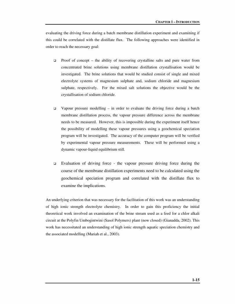
2.6 (I) Simplified RO/NF plant setup. A: feed tank, B: pressure pump, 2-16
C: feed stream, D: membrane module, E: retentate stream, F: permeate
Stream. (II) Schematic showing mechanism of separation with associated
plot of water flow (Jw) as a function of applied pressure (∆P)
2.7 Spiral-wound membrane module commonly used during NF and RO 2-17
2.8 Schematic representation of the air gap MD process showing the flow of 2-23
vapour and temperature profile across the membrane
2.9 Types of membrane configurations. (a) direct contact membrane 2-24
distillation, (b) air gap membrane distillation, (c) sweeping gas
membrane distillation, (d) vacuum membrane distillation
2.10 Mass transfer resistances in MD 2-26

FIGURES
xiii
2.11 Cells for MD membrane module: (a) direct contact or sweeping gas cell, 2-33
(b) air gap cell
2.12 Schematic of a membrane crystallizer unit 2-41
2.13 An integrated MF-NF-RO system for seawater desalination 2-44
2.14 Proposed ideal integrated membrane systems for seawater desalination 2-45
3.1 Experimental setup for membrane distillation-crystallisation of 3-2
concentrated salts
3.2 Epsomite crystals obtained from the MDC of a single salt 3-5
solution of initial concentration 375 g/ℓ, first sampled approximately
17 h from the start of the MD process. Concentration of magnesium
sulphate and precipitation was 1.34 kg/ℓ. The average crystal size
per sample is indicated. The indicated times refer to the sampling times
after the first visual appearance of crystals.
3.3 Crystal size distribution for the crystallisation of a concentrated solution of 3-6
Magnesium sulphate of 375 g/ℓ using MDC. The indicated times refer to the
experimental sampling times after the first visual appearance of crystals.
3.4 Average length of crystals in sample at time of sampling from the start of 3-7
Crystallisation, to determine the crystal growth rate
3.5 Transmembrane flux and electrolyte concentration during MDC of 3-8
Magnesium sulphate of initial concentration 375 g/ℓ
3.6 Trend of transmembrane flux and concentration of magnesium sulphate 3-9
during the first half of the MDC of a concentrated solution of magnesium
sulphate of 625 g/ℓ
3.7 Sodium chloride crystals obtained from a mixed salt system of varying 3-11
ratios of sodium chloride and magnesium sulphate as indicated (25X)

FIGURES
xiv
3.8 Evolution of crystal size distribution for the crystallisation of sodium 3-12
chloride with increasing amounts of magnesium sulphate in solution
3.9 Trend of transmembrane flux and concentration of salts during the 3-13
course of the MDC of the 1:1 mix
3.10 Temperature profile for the 1:1 mix during the MD process 3-14
3.11 Trend of transmembrane flux and concentration of salts during the 3-15
course of the MDC of the 1:2 mix
3.12 Trend of transmembrane flux and concentration of salts during the 3-16
course of the MDC of the 1:3 mix
4.1 Sequence of solving a problem in PHRQPITZ 4-13
5.1 Vapour pressure curve for the 1:1 mix predicted through PHRQPITZ 5-4
modelling; pure water vapour pressure curve shown for comparison
5.2 Vapour pressure curves for the 1:2 and 1:3 mixes predicted through PHRQPITZ 5-5
modelling; pure water vapour pressure curve shown for comparison
5.3 Schematic diagram of the vapour-liquid equilibrium still 5-7
5.4 Block diagram of VLE system 5-8
5.5 Vapour pressure curves together with the fitted Antoine curves for 5-10
solutions of sodium chloride in varying concentrations
5.6 Vapour pressure locus curve for sodium chloride solution 5-11
5.7 Antoine fit to the data of Lui and Lindsay for each concentration of 5-12
sodium chloride at the corresponding temperature

FIGURES
xv
5.8 Comparison between literature (Lui and Lindsay,1972 ) and measured vapour 5-13
pressures for each concentration of sodium chloride solution
5.9 Comparison between literature (Sparrow, 2003) and measured vapour 5-15
pressures for each concentration of sodium chloride solution
5.10 Experimental vapour pressure curve obtained from VLE measurements 5-16
for the 1:1 mix together with the fitted Antoine curve
5.11 Experimental vapour pressure curve obtained from VLE measurements 5-16
for the 1:2 mix together with the fitted Antoine curve
5.12 Experimental vapour pressure curve obtained from VLE measurements 5-17
for the 1:3 mix together with the fitted Antoine curve
5.13 Comparison between modelled and measured vapour pressures for each 5-18
of the salt mixes
5.14 Vapour pressures of respective streams in membrane distillation of a 5-19
1:1 mix, emphasising the significant change in activities of the pure water
retentate streams at outlet and inlet of the membrane module. The curves labelled
“pure retentate (hot water)” are calculated for pure water at the same temperatures
as the brine at that point in the run
5.15 Vapour pressures of respective streams in membrane distillation of a 5-20
1:2 mix
5.16 Variation of transmembrane flux and the log mean driving force as a 5-21
function of time for the 1:1 mix, indicating that the flux decline is due to
a decline in driving force as seen from the similarity in these trends
5.17 Variation of transmembrane flux and the log mean driving force as a 5-22
function of time for the 1:2 mix indicating the similarity in these trends

FIGURES
xvi
5.18 Transmembrane flux as a function of log mean driving force during 5-23
the distillation of the 1:1 and 1:2 magnesium sulphate and sodium
chloride solutions. The graph displays a non-zero intercept
5.19 Evolution of flux with the saturation index of epsomite and sodium 5-25
chloride for the 1:1 mix obtained from modelling using PHRQPITZ
B.1 Standard plots of Lui and Lindsays concentrations at varying temperatures B-12
used to extrapolate our concentrations

TABLES
xvii
1.1 Summary of the various brine handling technologies at Sasol 1-12
5.1 Example of a section of an output file from PHRQPITZ 5-3
A.1 Elements in the PHRQPITZ database A-6
A.2 Minerals in the PHRQPITZ database A-10
A.3 Input file for PITZINPT A-13
A.4 Output file from PHRQPITZ A-14
A.5 Output from PHRQPITZ for the evaporation of a solution of NaCl and MgSO4 A-16
until the halite phase boundary is reached
B.1 MD of a 375 g/ℓ magnesium sulphate solution (initial solution volume = 3 ℓ) B-1
B.2 MD of a 625 g/ℓ magnesium sulphate solution (initial solution volume = 2 ℓ) B-2
B.3 Data from the MD of a 1:1 salt mix B-2
B.4 Data from the MD of a 1:2 salt mix B-3
B.5 Data from the MD of a 1:3 salt mix B-3
B.6a CSD for sample 1 for the MD of a 375 g/ℓ magnesium sulphate solution B-4
B.6b CSD for sample 2 for the MD of a 375 g/ℓ magnesium sulphate solution B-4
B.6c CSD for sample 3 for the MD of a 375 g/ℓ magnesium sulphate solution B-5

TABLES
xviii
B.6d CSD for sample 4 for the MD of a 375 g/ℓ magnesium sulphate solution B-5
B.7 Vapour pressures of various streams during MD of 1:1 mix together B-6
with calculated log mean vapour pressure
B.8 Vapour pressures of various streams during MD of 1:2 mix together B-7
with calculated log mean vapour pressure
B.9 Non-linear regression for fitting Antoine’s constants to experimental B-8
VLE data for 20 g/ℓ NaCl solution
B.10 Non-linear regression for fitting Antoine’s constants to experimental B-8
VLE data for 200 g/ℓ NaCl solution
B.11 Non-linear regression for fitting Antoine’s constants to experimental B-9
VLE data for 280 g/ℓ NaCl solution
B.12 Calculation of vapour pressures from Sparrows (2003) equations B-9
for comparison to experimental VLE data for 20 g/ℓ NaCl solution
B.13 Calculation of vapour pressures from Sparrows (2003) equations for B-10
comparison to experimental VLE data for 200 g/ℓ NaCl solution
B.14 Calculation of vapour pressures from Sparrows (2003) equations for B-10
comparison to experimental VLE data for 280 g/ℓ NaCl solution
B.15 Non-linear regression for fitting Antoine’s constants to literature data B-11
for 20 g/ℓ NaCl solution
B.16 Non-linear regression for fitting Antoine’s constants to literature data B-11
for 200 g/ℓ NaCl solution
B.17 Non-linear regression for fitting Antoine’s constants to literature data B-11
for 280 g/ℓ NaCl solution

TABLES
xix
B.18 Extrapolated literature values for vapour pressures of NaCl solutions B-12
B.19 Non-linear regression for fitting Antoine’s constants to experimental B-13
VLE data for 1:1 mix
B.20 Non-linear regression for fitting Antoine’s constants to experimental B-13
VLE data for 1:2 mix
B.21 Non-linear regression for fitting Antoine’s constants to experimental B-14
VLE data for 1:3 mix
B.22 Measured and modelled vapour pressures to test accuracy of modelling B-14
for 1:1 mix
B.23 Measured and modelled vapour pressures to test accuracy of modelling B-15
for 1:2 mix
B.24 Measured and modelled vapour pressures to test accuracy of modelling B-15
for 1:3 mix

ABBREVIATIONS
xxv
General Abbreviations
AGMD Air Gap Membrane Distillation
CAPS Compact Accelerated Precipitation Softening
CPC Concentration Polarisation Coefficient
CSD Crystal Size Distribution
CV Coefficient of Variation
DCMD Direct Contact Membrane Distillation
DGM Dusty Gas Model
ED Electrodialysis
EDR Electrodialysis Reversal
GFW gram formula weight
IAP ion activity product
MC Membrane Contactor
MCr Membrane Crystalliser
MD Membrane Distillation
MDC Membrane Distillation Concentration
MED Multi-Effect Distillation
MF Microfiltration
MOD Membrane Osmotic Distillation
MSF Multi-Stage Flash (distillation)
NF Nanofiltration
OD Osmotic Distillation
OPPT Office of Pollution Prevention and Toxics
PE Polyethylene
PP Polypropylene
PTFE Polytetrafluoroethylene
PVC Polyvinyl Chloride
PVDF Polyvinylidene Fluoride
RO Reverse Osmosis
SGL Stripped Gas Liquor
SGMD Sweeping Gas Membrane Distillation

ABBREVIATIONS
xxvi
SHMP Sodium Hexametaphosphate
SI Saturation Index
SPARRO Slurry Precipitation and Recycle Reverse Osmosis
SRO Seeded Reverse Osmosis
SSF Sasol Synthetic Fuels
SWRO Spiral Wound Reverse Osmosis
TDS Total Dissolved Solids
TPC Temperature Polarisation Coefficient
TRO Tubular Reverse Osmosis
UF Ultrafiltration
UNEP United Nations Environment Programme
USGS United States Geological Survey
VCD Vapour Compression Distillation
VLE Vapour liquid equilibrium
VMD Vacuum Membrane Distillation
List of Minerals
Anhydrite CaSO4
Calcite CaCO3
Epsom Salt MgSO4.7H2O (Magnesium sulphate heptahydrate)
Gypsum (CaSO4.2H2O)
Halite NaCl
Mirabilite (Na2SO4.10H2O)
Magnesium sulphate MgSO4
Sodium chloride NaCl
Sepiolite [MgSi3O6(OH)2]

NOMENCLATURE
xx
Symbols
a solvent activity
b universal empirical parameter
Aγ Debye-Hückel parameter for activity coefficient
Aφ Debye-Hückel parameter for osmotic coefficient
B geometric factor determined by pore structure (in Equation 2.27)
Bs solute permeability coefficient
Bij(I) second virial coefficients
BMX functions of ionic strength
c molar concentration of ions
C membrane mass transfer coefficient
Cijk(I) third virial coefficients respectively
CMX single electrolyte third virial coefficients
CV Coefficient of variation
dw density
D diffusion coefficient
Dw dielectric constant of water
F cumulative crystal size distribution
f(I) Debye-Hückel type term in Equation 4.9
Gex excess free energy
H effective heat transfer coefficient
∆Hvap molar heat of vaporisation

NOMENCLATURE
xxi
I ionic strength of the solution
J mass flux
km thermal conductivity of porous membrane
Kp equilibrium constant for the pth phase
Ksp solubility product
ℓ parameter which expresses the distance at which the electrostatic energy for
singly charged ions in the dielectric just equals thermal energy (Equation 4.6b)
m molality
M molecular weight
nw mass of water
N0 Avagadro’s number
p solute permeability
P water vapour pressure
∇pi gradient in partial pressure
∇P gradient in the total pressure
∆Plm logarithmic mean vapour pressure
∆Pappl applied pressure
Pnet net pressure
Q heat flux
r pore radius
rmax largest pore radius
R universal gas constant
Rrej rejection coefficient
T temperature
Yln mole fraction of air
x mole fraction

NOMENCLATURE
xxii
X salt mass fraction of a solution
z charge on an ion
Subscripts
a anion
avg average
c cation
b bulk
C conductive heat
D molecular diffusion model
f feed
h heat
K Knudsen diffusion model
L latent heat
m membrane surface
P Poiseuille flow model
p permeate
s solute
Th threshold
w water
x mole fraction of dissolved species
MX mixed electrolyte
DH Debye Hückel

NOMENCLATURE
xxiii
Superscripts
D diffusive flux
f feed
p permeate
V viscous flux
Greek Symbols
α activity
χ pore tortuosity
δ membrane thickness
ε membrane porosity
Φij mixed electrolyte coefficient
γ concentration polarisation coefficient
γL liquid surface tension
γ± mean activity coefficient
η gas viscosity
λ thermal or heat conductivity
λij(I) second virial coefficient (Equation 4.9)
µ fluid viscosity
µijk third virial coefficient (Equation 4.9)
π osmotic pressure
θ liquid-solid contact angle

NOMENCLATURE
xxiv
θij single parameter for each pair of anions or cations (Equation 4.13)
σr reflection coefficient
σ function in Equation 4.5b
τ temperature polarisation coefficient
ψijk mixed electrolyte coefficient
ν number of ions
φ osmotic coefficient

Chapter 1
INTRODUCTION
1-1
This research encompasses the investigation of a system to appropriately manage
concentrated aqueous brines. In this thesis, the main process being investigated is
the membrane distillation of concentrated brine solutions for the recovery of
crystalline products from brine effluents. This chapter provides a background to
this work. Section 1.1 serves as an overview of the water situation in South
Africa. The utilisation and distribution of water within the Sasol industrial
complex is specifically discussed. Section 1.2 addresses the issue of salinity in
South Africa as a whole, and in industry in particular. Section 1.3 introduces the
concepts of green chemistry and sustainable development and discusses their
indispensability in any research or thought process in general. Section 1.4
summarises the various approaches that industry have adopted and those still
under consideration in order to address the issue of salinity and brine disposal.
Section 1.5 lays down the hypotheses and project objectives, and briefly describes
the technique of membrane distillation that would be used to reach these
objectives. Also described in Section 1.5 is the series of methods that would be
followed to achieve the overall goal. This chapter concludes with the outline of
this thesis in Section 1.6.
1.1 THE INDUSTRIAL WATER SCENARIO
Water is the backbone of the country’s economy. The demand for pure water is on the rise
within the social and economic sectors, whilst the availability of pure water is on the downward
trend. South Africa experiences an average rainfall of 500 mm per year and, together with other
natural resources such as rivers and lakes, is still inadequate to meet these demands
(FAO, 2005). Industry poses as one of the chief consumers of large volumes of water together
with the generation of vast quantities of wastewater (Mann and Liu, 1999). Industrial water
traverses various operational arrays within the industrial domain.
The Sasol group of companies encompasses a diverse field of manufacturing and marketing
operations within the sphere of fuels and chemicals. Sasol is world leading in the conversion of

CHAPTER 1 – INTRODUCTION
1-2
low-grade coal to fuels, chemicals and gas and in so doing is South Africa’s single largest
industrial investor directly contributing about R 40 billion (ca 4 %) to South Africa’s annual
gross domestic product during the year (SASOL, 2005). The unique Fischer-Tropsch
technology is the heart of this process. The initial stage in this process, known as gasification,
requires coal to be reacted under pressure and high temperature and, following exposure to
steam and oxygen, is converted into crude synthesis feed. As such, Sasol utilises large volumes
of fresh water for the various operations which includes steam generation, process cooling and
generation of electricity. The Sasol operations in South Africa alone consume water in excess
of 300 Mℓ/d (Ginster and Jeevaratnam, 2003). Figure 1.1 is a schematic representation of
Sasol’s incoming water supplies and how these various water sources are distributed within the
plant.
UTILITY WATER SYSTEM PROCESS WATER SYSTEM
Figure 1.1: Schematic diagram of the Sasol Secunda complex water distribution systems
(Phillips and du Toit, 2002)
Flocculation
Raw water from Vaal River
Utility cooling water system
Boiler feed water preparation
� Hot lime softening � Dolomite filtration
EDR/spiral wound reverse
osmosis
Boiler plant
Tubular reverse osmosis
Wet ash handling
Spiral wound reverse osmosis
Salty water evaporators
Heat exchanger
backflushing
Oil separation
Utility washing water
Process cooling water system
Water recovery � Activated
sludge � Buffer
dams
Evaporation ponds
Mine water Storm water & oily sewers
Stripped gas liquor & Fischer
Tropsch acid water
To evaporator crystalliser
Permeate
Blowdown
Blowdown
Regen effluents
Concentrate
Distillate Concentrate
Permeate
Concentrated waste from evaporators
Blowdown
to ash
Concentrate
Oily
water

CHAPTER 1 – INTRODUCTION
1-3
Three main organic effluent streams arise from Sasol’s operations:
(i) Stripped Gas Liquor (SGL) is the largest effluent stream. SGL emanates from the
condensate of gasification which has undergone separation processes such as gravity
separation, liquid-liquid extraction and steam stripping in order to retrieve
by-products.
(ii) Oily sewer water, resulting from plant drainage from the operations, gives rise to the
second largest effluent stream.
(iii) Fischer-Tropsch acid water forms the third largest of these effluent streams. Residual
water emanating from the Fischer-Tropsch reaction is rich in organic compounds.
These compounds are recovered by distillation, concomitantly yielding a distillate
stream rich in organic acid (C1 to C6). This stream is known as the Fischer-Tropsch
acid water.
Appropriate treatment of these organic effluent streams renders possible the recycling of these
effluents as process cooling water. The majority of the blowdown from the process cooling
water system is sent to the wet ash handling system and the remainder is recycled to the water
recovery plant. The reason for the large flow of blowdown to the ash system initially arose
from low rates of evaporation from the evaporation ponds. In order to overcome this hurdle, all
initial downstream unit processes at the water recovery plant, such as clarification, filtration and
ion exchange, were eliminated which facilitated a reduction in saline effluents. However, to
compensate for the reduced quality of make-up to the process cooling water system, the cycles
of concentration in the cooling system were reduced with the net effect of doubling the
blowdown to the ash system.
1.1.1 The Ash Water System
Ash is a residue of coal combustion. Sasol produces large quantities of utility boiler ash
comprising a mixture of fly ash and bottom ash. Sasol adopts a wet ash handling system. In
this system the ash is conveyed to the ash heaps as a slurry. The excess water is recovered and
stored in a series of dams prior to re-use. To overcome the positive water balances in the wet
ash water system (due to the increased load from the process cooling water system), a combined
reverse osmosis (RO) plant comprising of a primary tubular reverse osmosis (TRO) unit and a
secondary spiral wound reverse osmosis (SWRO) unit has been installed to treat clear ash
effluent (Figure 1.1). Regeneration effluents from the boiler feed water preparation plant is sent

CHAPTER 1 – INTRODUCTION
1-4
to the ash handling system. Permeate from the SWRO unit is recycled as boiler feed water.
The chemistry of the ash water (TRO brine) is similar to that of mine water, with sulphate and
sodium forming the major components. Some iron, potassium, manganese, copper and silica
are also present in small amounts. Most of the ash produced in South Africa is disposed on
landfills. However, the rapidly increasing size of the ash systems is becoming a mounting threat
to industries.
1.1.2 The Mine Water System
South Africa holds fifth position on a global basis as a coal producing country (Azzie, 2001).
Moreover, Sasol alone operates one of the world’s largest underground coal mining complexes.
Coal mining requires large volumes of water for operations including, amongst others, drilling,
dust suppression, environmental cooling and hydropower generation. The remains of these
activities tend to increase the contamination of mine water which collects in the underground
mining complex. The characteristic mine water can be typified as acidic, saline and containing
high metal concentrations. A system was installed to purify this water for re-use as boiler feed
water. It consisted of an electrodialysis reversal (EDR) plant followed by a SWRO plant
(Figure 1.1). A major portion of the chemistry of the EDR and mine water constitutes sulphate,
sodium, calcium, chloride and magnesium, in order. A small fraction of potassium and silicate
are also present giving rise to a total dissolved solids (TDS) content of 20 g/ℓ and 5 g/ℓ for EDR
and mine water, respectively. Depending on the particular treatment technology that the mine
water undergoes, the correspondent waste residue stream may be in the following forms (Du
Plessis, 2005):
� Neutralization sludges with a typical composition of metal hydroxides, carbonates and
gypsum.
� Sulphur sludges from biological treatment processes.
� Softening sludges with a high calcium carbonate content.
� Brines with variable concentrations of various salts dependent on the chemical profile
of the mine water feed.
Despite the recovery and re-use of the mine water, another problem which will be aggravated
over the years is that of seepage of surface and underground water into the mined-out areas. A
proposal for the treatment of this water to produce water which could substitute or complement

CHAPTER 1 – INTRODUCTION
1-5
the raw water stream is being analysed, however the capital and operating costs of this process
may make the system uneconomic.
A generic water balance, developed by Pulles et al. (2001) for the South African coal mining
industries, explicitly describes the industry-wide patterns of water sources, water utilisation and
water disposal around coal mines. This water balance enables industries or other role players to
set benchmarks that can be used to evaluate the water management performance of individual
mines. With the accumulation of mine water being on the increase, it seems improbable that the
solution to the problem lies simply in the treatment of this water. An alternative and possibly
innovative strategy needs to be devised before this challenge can be overcome.
1.2 THE SALINATION SCENARIO
Salinity is the general term associated with the build-up of salts in soil or water. Saline water,
in particular, refers to water containing dissolved solids which are in excess of the limits of
potable water (U.S. Bureau of Reclamation and Sandia National Laboratories, 2003). Salinity
has become one of South Africa’s most critical challenges, threatening economic and social
consequences. Saline waters have two major origins - natural and anthropogenic (DWAF,
2005). The salination of river water is a natural, inevitable cause borne by the geology of the
land. Man-made causes are manifold. The large volumes of aqueous waste that are discharged
by industries represents one of the sources of salts. However, a greater predicament is that of
diffuse pollution as it impacts over a much larger area on the water resource. This scattered
form of pollution has its origins from, amongst others, poor or deficient administration of urban
settlements, land pollution from waste deposits and accumulation of the remains of mining
activities.
The Sasol operations alone contribute two of the major sources of saline aqueous effluents, i.e.
internal to the water circuits and ash systems or external on the mining operations. Figure 1.2 is
an illustration of the distribution of water and salt within the Sasol Synthetic Fuels (SSF)
complex together with an indication of the quantity of these streams that pass through the plant
on a daily basis.

CHAPTER 1 – INTRODUCTION
1-6
Department of water 245.3 37 Effluent evaporation 98 Process salts 110.3 Blowdown to river 31 Rain water 50 In process 78.1 Mine water 12.2 73 Raw water evaporation 2.6 Evaporation from dams 17.7 Irrigation 1.7 Solar ponds 75
To Ash 129.8
To river 13.8
TOTAL 307.5 Mℓ/d 220.3 t/d 220.3 t/d 307.5 Mℓ/d
Figure 1.2: Average daily figures of water and salt flows within the SSF complex
(SASOL, 2004)
The internal salt generation arises from water treatment processes such as desalination for water
recovery, ion exchange regeneration for water softening to produce boiler feed water and
cooling systems which produce blow down. Furthermore, when ash comes into contact with
water a saline alkaline leachate is formed.
With the increase in the demand of fresh water in South Africa, particularly within the industrial
sector, and with salination reducing the availability of pure water, an urgent need arises for the
clean-up or prevention of saline effluents. Numerous measures against salination are being
implemented both in industry and on the urban frontier. These include reducing salts in the
water supply and during domestic and industrial use, proper management of water resources
(release of part of the water resource to sea), suitable irrigation systems and practices, soil
conditioning and desalination of water and wastewater (Juanicó, 2005). However, if one would
consider treatment of the source of the problem in the first instance, this would ultimately
prevent build-up and a dilemma at the end-of-pipe stage.
SALT IN (t/d)
SSF FACTORIES
WATER
OUT (Mℓ/d)
SA
LT
O
UT
(t/
d)
Accumulate in systems
WATER IN (Mℓ/d)

CHAPTER 1 – INTRODUCTION
1-7
1.3 GREEN CHEMISTRY AND SUSTAINABLE DEVELOPMENT
The United States Pollution Prevention Act of 1990 prompted the U.S. Environmental
Protection Agency to take action and develop preventative approaches against pollution
(Nameroff et al., 2004). The Office of Pollution Prevention and Toxics (OPPT) was founded
and focuses on being able to improve existing infrastructure and to prevent the recurrence of
previous shortcomings in new developments (Hjeresen et al., 2000). It was the U.S.
Environmental Protection Agency who first introduced the concept of Green Chemistry and
defined it as the utilization of a set of principles that reduces or eliminates the use or generation
of hazardous substances in the design, manufacture and application of chemical products
(EHSC, 2002). Globalisation of the concept of green chemistry has expanded this definition
and it now covers a wider range of issues than those reflected in the original statement. The
green chemistry programme has impinged on many areas of society and developed various
collaborations with academia, industry and other governmental agencies such that green
chemistry is now being envisaged as a way to think rather than just a new branch of science.
Over the years it has been realised that through the implementation of various sub-disciplines of
chemistry and molecular sciences, there is a rising positive reception that this flourishing area of
chemistry is needed in the design and attainment of sustainable development.
In 1987, the United Nation’s Brundtland Commission defined sustainable development as
meeting the needs of the present without compromising the ability of future generations to meet
their own needs (United Nation’s General Assembly, 1987). This definition is very broad and
could have many different interpretations. As such, there have been many debates over the
definition of sustainability. Since the Brundtland Report, sustainability has been given
numerous definitions as (i) maintaining intergenerational well-being, (ii) maintaining the
subsistence of the humankind, (iii) satisfying the productivity of economic systems,
(iv) maintaining biodiversity, and (v) maintaining evolutionary prospective (Tisdell, 1991).
However, despite these various ways of defining sustainability this is a concept that is vague by
nature. The concept of sustainability may assist in decision making for the establishment or
progression toward a sustainable business, enterprise or society; however the ambivalent
character of the concept, i.e. trying to sustain something that exists in a milieu of perpetual
change, is both theoretically and functionally challenging. But if one considers that life itself
revolves around change, it is not surprising then, that sustainability is a principle of life about
both sustaining a particular resilient state and adjusting to changing internal conditions (Köhn et

CHAPTER 1 – INTRODUCTION
1-8
al., 2000). Over the years sustainable development has become an accepted aim of the world.
This paradigm may also be explained by the perception, from the late 1960s, that the world is
facing a meta crisis, including crises of development, environment and security (Kirkby et al.,
1995).
With Green Chemistry and Chemical Engineering, one works toward sustainable development
by inventing, designing and implementing chemical products that fulfil the following ideologies
of overcoming the environmental pollution hurdle (Anastas and Warner, 1998; Frederick, 2005
and ACS, 1987):
� Preventative approach – seizing the problem at the roots thus preventing aggravation
with time and adversity at maturity.
� Atom economy – making maximum use of starting materials to yield the final product.
� Minimisation of the use of hazardous products – a synthetic route should be planned
so as to prevent the use and generation of harmful or toxic reagents and products or, if
certain auxiliaries are indispensable, the minimum quantities should be used.
� Design of safer chemicals and chemistry – chemical products should be designed with
reduced toxicity and potential for chemical accidents, while still maintaining efficacy
in functionality.
� Energy conservation and waste minimisation – energy and use of non-renewal
resources should be reduced as much as possible during the manufacture and use
phases of a product.
� Less hazardous solvents and auxiliaries – selecting the most appropriate solvents with
minimum toxicity.
� Design of appropriate starting materials and products – a raw material or feedstock
should carry renewable end properties while products should be biodegradable.
� Reduction in derivatives – use of protection / deprotection groups and blocking groups
during chemical syntheses should be minimal or avoided if possible as such steps
generate additional waste.
� Efficient use of catalysts – selective catalysts should be preferred wherever possible.
� Real-time analysis for pollution prevention – development of analytical methods to
allow for real-time in-process monitoring and control prior to hazardous material
formation.

CHAPTER 1 – INTRODUCTION
1-9
If the above mentioned principles are adhered to, particularly by industry, it is proposed that
within two decades the following should be possible (Sanghi, 2000):
� Complete eradication of emissions from polymer manufacturing and processing.
� Substitution of all environmentally hazardous solvents and acid-based catalysts with
solids or more eco-friendly alternatives.
� Waste reduction between 30 and 40 %.
� More than 50 % reduction in the amount of plastics in landfills.
Recently, a strategy for implementing the relationships between industry and academia has been
proposed. This philosophy known as the triple bottom line predicts that an enterprise or
business association would be economically sustainable if the objectives of environmental
protection, societal benefit, and market advantage are all satisfied (Tundo et al., 2000). This
three fold philosophy is a strong hypothesis for evaluating the success of industry or
environmental technologies.
Industry would be a good starting point for the promotion and implementation of green
chemistry thus providing the pathway for others to follow to a cleaner and greener country.
Recent advancements to Sasol’s industrial chemical plant have proved to be making valuable
progress in this direction. A project involving the utilisation of natural gas, brought in from
Mozambique, as a substitute to their large coal requirements as a source of energy, lead to
significant reductions in this industries overall environmental emissions. The use of natural gas
has decreased Sasol’s coal requirements by a factor of 60 to 70 % and was said to yield
significant environmental benefits (BCSD, 2003).
Any technical solution to the problem of salinity needs to be assessed by applying the principles
of green chemistry and sustainable development.
1.4 INDUSTRIAL APPROACH TO SALINITY
Desalination technologies have been recognised as the primary method of generating surplus
water supplies and is so rapidly developing that the efficiency of desalination technologies
evolves at a rate of approximately four percent per year (U.S. Bureau of Reclamation and
Sandia National Laboratories, 2003). It is therefore this approach of desalination that industries

CHAPTER 1 – INTRODUCTION
1-10
have adopted in order to produce freshwater from saline effluents for re-use or recycling and
forms an attractive approach, especially if the particular industry is situated within water scarce
catchments. Section 1.4.1 lists some of the desalination technologies that are currently in use.
However, it must be realised that every desalination and water purification technology generates
two process streams – a water product stream and a brine or concentrate stream. The latter
contains species that did not pass through the membrane during desalination using membrane
technologies or of the backwash from low pressure processing. These waste streams contain
high concentration of salts and other contaminants. Disposal of these streams is currently
posing a major problem to industries. Some approaches that have been considered by industries
for brine handling and disposal is discussed in Section 1.4.2.
1.4.1 Desalination Technologies
Recent years have seen significant progress in the improvement of desalination technologies in
industry and mining and a number of new desalination plans are currently being devised. Listed
below are some of the technologies that are used for the desalination and purification of saline
water.
� Membrane technologies – makes use of semi-permeable or selective membranes in
order to remove contaminants during the desalination or purification of water.
Examples include microfiltration, ultrafiltration, nanofiltration, reverse osmosis and
electrodialysis (these are discussed in detail in Chapter 2).
� Thermal technologies – requires energy (heating or cooling) for selective retention of
contaminants with the production of pure water.
� Reuse / Recycling technologies – modified membrane or alternate technologies which
are appropriately adjusted to accommodate for increased contaminant loads due to
their end applications (valuable or saleable products).
The basis of all desalination technologies is conversion of part of the inlet feedwater flow into
fresh water. This inevitably results in a stream of water which is relatively concentrated in
dissolved salts. This concentrated stream is a major obstacle which creates uncertainty and
hinders the implementation of desalination technologies, as the management and containment of
these inorganic waste products (sludges and brines) pose a serious problem.

CHAPTER 1 – INTRODUCTION
1-11
1.4.2 Brine handling options
In the past most of the waste streams arising from the various mining and manufacturing
activities were discharged to surface waters or the ocean. However, more rigid current and
future environmental regulations will make these disposal routes less feasible, therefore other
disposal options need to be sought. It seems that technologies that are available for managing
these waste products are either prohibitively uneconomic (exceeding the cost of water treatment
or desalination) or unsatisfactory because of long term liabilities and associated risks they pose
to water resources (Du Plessis, 2005).
Andrews and Witts (1993) have discussed some options concerning the handling of RO
concentrates and, more recently, Du Plessis (2005) has suggested future trends in brine disposal.
Apart from surface water discharge, they have described the following as typical means of
concentrate disposal:
� Spray irrigation / land application.
� Deep well injection in appropriate geological environments.
� Waste water treatment facilities which are capable of accommodating concentrate
loads without disturbing its own treatment operations.
� Thermal evaporation and solar evaporation ponds.
� Drain fields and boreholes where discharge is to the surficial aquifers.
� Disposal in old underground mine workings, similar to existing backfill operations.
� Solidification and deposit in underground vaults.
However, the extent of use of these methods is subject to the composition or, in some instances,
quality of the concentrate, government regulations, economic implications and site-specific
factors.
Table 1.1 lists an evaluation of some brine disposal options considered by industry, together
with the advantages and disadvantages associated with these technologies.

CHAPTER 1 – INTRODUCTION
1-12
Table 1.1: Summary of the various brine handling technologies at Sasol (Ginster et al., 2003)
Name Description Advantages Disadvantages
Brine to Brick In this process an ash
cement brick which is
more economical is
made from brine.
• A stronger brick as
opposed to bricks
manufactured using
tap water.
• Performance over
prolonged periods is
unknown and
requires further
investigation.
Evaporator / crystalliser Further concentration
of brine coming from
EDR membrane
desalination.
• Tried and tested.
• A dry product is
produced which is
preferred for land
disposal.
• The crystallised
salts do not carry
high saleable value.
• Added cost for salt
disposal.
• Little or no further
brine handling
options.
Waste backfilling Co-disposal of brine
with ash backfills into
mine workings.
• The formation of
acid rock drainage
is suppressed and
less water can seep
into the mine.
• Mine-life can be
prolonged.
• This concept has
been well-applied
internationally;
however, local
implementation is
limited.
• Pumping and flow
rates are limited.
• Requires
cementitous agent to
bind the salt.
Salt splitting Uses bi-polar
membranes to split
salts of sodium
sulphate to sodium
hydroxide and
sulphuric acid.
• Generation of
reagents that can be
re-used within
process streams.
• Bi-polar membranes
are intolerant to
certain impurities
such as iron and
silica present in
brine effluents.
Solar ponds Modification of
existing salt storage
ponds.
• Widely used.
• Operationally
economic.
• Contamination to
groundwater.
• Temporary solution.
Considering the two major sources of saline aqueous effluents within the Sasol complex
discussed in Section 1.2, the internal salt generation needs to be addressed through a range of

CHAPTER 1 – INTRODUCTION
1-13
interventions including waste minimisation, process optimisation and water pinch but ultimately
concentrated brine streams will be produced. Considering the mining operations there are three
ways to respond to salinity:
i) A preventative approach – by changing land use practices responsible for the
aggravation of the problem and to prevent further damage.
ii) Management and containment – by schemes such as salt interception to control the
groundwater movement through the subsurface or by lowering the water tables.
iii) Considering the salts as a sustainable resource for the next two thousand years –
instead of viewing salinity as a problem, it could be viewed as an opportunity to obtain
value while simultaneously improving the situation.
Much work has been performed on being able to solve this salinity crisis. However, bearing in
mind the concept of sustainable development, the third tactic to this problem of salinity forms
an attractive approach. We can view these saline waters as an environmental problem or we can
turn this environmental problem into an economic resource by viewing these saline waters as a
sustainable resource of salts (Mariah et al., 2004). Several of the waste streams contain
potentially recoverable and saleable products. Sustainable salt sinks can be achieved by
considering the formation of valuable salts when designing a saline water circuit and the
composition of the streams that enter the circuit. The separation and concentration processes
need to be combined to produce high value products.
1.5 PROJECT OBJECTIVES
Based on the premise that inorganic concentrates can be separated into high purity chemicals
and reusable water, this research addresses the need for industries such as Sasol to ensure an
adequate supply of water of sufficient quality while at the same time being able to manage the
inorganic brines arising from its manufacturing and mining activities. The chlor alkali salt
preparation circuit is an example of a process that requires a pure sodium chloride feed for a
subsequent synthesis step (electrolysis) (Gianadda, 2002). Suitably purified and concentrated
brine streams could substitute for the imported raw salt which is used as the feed chemical. A
technique is therefore required in order to separate and recover these concentrates with the
concomitant release of pure water. Section 1.5.1 discusses a membrane technique which is
proposed. Section 1.5.2 describes the approach that was followed during this study.

CHAPTER 1 – INTRODUCTION
1-14
1.5.1 Proposed Membrane Technique
Many techniques have been investigated for the desalination of water and separation of salts.
The most commonly used is that of RO although other techniques such as thermal desalination
and evaporation have been investigated (Kurbiel et al., 1995). The main shortcoming of RO is
the need for excessively high pressures at high solute concentrations, as is the case of high
saline industrial water such as ash and mine water (Mariah et al., 2006a). This elevated pressure
is required in order to overcome the osmotic pressure barrier in concentrate processing. In
processes such as thermal evaporation, for example, high temperatures are required in order to
achieve evaporation and salt recovery. A need therefore seems to arise for a process which
would achieve the recovery of crystalline products and pure water and is capable of operating at
high solute concentrations while still maintaining engineering feasibility of simple operating
conditions.
Membrane distillation (and crystallization) is a technique which potentially leads to an almost
complete water recovery and the elimination of the brine disposal problem. Chemical
manufacturing complexes frequently have an excess of low-grade heat. This energy can be used
to create a temperature gradient across a hydrophobic microporous membrane. The resulting
vapour pressure difference produces a flux of water vapour through the membrane thus aqueous
brine solutions can be concentrated and crystallised. This process does not have the limitations
of processes such as RO and thermal evaporation as this process can operate at high solute
concentrations, at low concentration gradients, moderate temperatures and atmospheric pressure
(Mariah et al., 2006b). Recent innovative designing of integrated membrane processes have led
to process intensification and reduction in pre-treatment costs (Drioli et al., 2002). Integration
of various single membrane units might assist in overcoming the shortfalls otherwise
experienced if these units operate independently, i.e. many specialised separations as opposed to
one big concentration step.
1.5.2 Specific Aims
This thesis is concerned with the technique of membrane distillation for the separation and
recovery of salts from concentrated brine effluents. A study into the process of membrane
distillation, paying attention to the driving force for the separation process, is examined. This
work addresses the problem faced by membrane scientists of the decreasing flux trend by
CHAPTER 1 – INTRODUCTION
1-15
evaluating the driving force during a batch membrane distillation experiment and examining if
this could be correlated with the distillate flux. The following approaches were identified in
order to reach the necessary goal:
� Proof of concept – the ability of recovering crystalline salts and pure water from
concentrated brine solutions using membrane distillation crystallisation would be
investigated. The brine solutions that would be studied consist of single and mixed
electrolyte systems of magnesium sulphate and, sodium chloride and magnesium
sulphate, respectively. For the mixed salt solutions the objective would be the
crystallisation of sodium chloride.
� Vapour pressure modelling – in order to evaluate the driving force during a batch
membrane distillation process, the vapour pressure difference across the membrane
needs to be measured. However, this is impossible during the experiment itself hence
the possibility of modelling these vapour pressures using a geochemical speciation
program will be investigated. The accuracy of the computer program will be verified
by experimental vapour pressure measurements. These will be performed using a
dynamic vapour-liquid equilibrium still.
� Evaluation of driving force - the vapour pressure driving force during the
course of the membrane distillation experiments need to be calculated using the
geochemical speciation program and correlated with the distillate flux to
examine the implications.
An underlying criterion that was necessary for the facilitation of this work was an understanding
of high ionic strength electrolyte chemistry. In order to gain this proficiency the initial
theoretical work involved an examination of the brine stream used as a feed for a chlor alkali
circuit at the Polyfin Umbogintwini (Sasol Polymers) plant (now closed) (Gianadda, 2002). This
work has necessitated an understanding of high ionic strength aquatic speciation chemistry and
the associated modelling (Mariah et al., 2003).

CHAPTER 1 – INTRODUCTION
1-16
1.6 THESIS OUTLINE
Chapter 1 provides an introduction to the research work presented in this thesis. The scope of
this work is outlined together with the project objectives and the series of methods that would
be followed in order to achieve these aims.
Chapter 2 summarises the relevant literature and outlines the important concepts necessary for
the development of this work. The review begins with a description of the chemistry of natural
waters followed by a discussion of the various techniques of desalination leading to the
technique of membrane distillation crystallisation that will be used in this work. The
advantages and disadvantages of these methods are specifically discussed.
Chapter 3 presents the results of the membrane distillation of single salt solutions of
magnesium sulphate and that of mixed salt systems of sodium chloride and magnesium sulphate
in varying mass ratios, chosen in order to crystallise sodium chloride. Details of the
experimental procedure are provided together with a discussion of the implication of the results.
Chapter 4 provides a background of the chemistry of high ionic strength solutions and the
various models available for the determination of the thermodynamic properties of these
solutions. The use of chemical speciation models for the determination of these properties is
discussed focussing on the particular model used during this work.
Chapter 5 forms the core results and discussion of this work. This Chapter begins by providing
the results obtained from speciation modelling procedures used to determine the vapour
pressures of the salt solutions. This is then followed by experimental verification of the
computed results. The experimental technique used to obtain the vapour pressures of the salt
solutions is described together with the outcome. This research is then drawn together by a
correlation of the results obtained from the individual procedures and a discussion thereof.
Chapter 6 brings this work to a close by concluding all major findings and suggesting
possibilities for future advancements.

CHAPTER 1 – INTRODUCTION
1-17
1.7 CHAPTER REFERENCES
ACS (AMERICAN CHEMICAL SOCIETY, 1987). Cleaning our environment – A chemical
perspective. In: A report by the committee on environmental improvement. 2nd edition.
Washington, D. C. ISBN 80084758.
ANASTAS PT and WARNER JC (1998). Green Chemistry, Theory and practice, Oxford
University Press, New York. ISBN: 0-19-850234-8.
ANDREWS LS AND WITTS GM (1993) An overview of RO concentrate disposal methods. In
Reverse Osmosis: Membrane Technology, Water Chemistry, and Industrial Applications,
AMJAD Z, ed., Van Nostrand Reinhold, New York. ISBN: 0-442-23964-5. 379-388.
AZZIE BA and FEY MV (2001) A classification of mine water, reflecting both quality and
geochemistry. In Cidu, R. (ed) 10th International Symposium on Water-Rock
Interaction (WRI 10), Villasimius, Italy, Proceedings Volume 1: 1177-1180.
BCSD (BUSINESS COUNCIL FOR SUSTAINABLE DEVELOPMENT): SOUTH AFRICA
(2003) Sustainable development update.
DRIOLI E, CRISUOLI A and CURCIO E (2002) Integrated membrane operations for seawater
desalination. Desalination 147 77-81.
DWAF (2005) Water Quality Management in South Africa. Department of Water Affairs and
Forestry, South Africa. Accessed on 12 September 2005 at URL http://www-
dwaf.pwv.gov.za/Dir_WQM/wqm.htm.
DU PLESSIS M (2005) Draft Terms of Reference for a Solicited WRC Project. Key Strategic
Area: Water use and waste management. Proceedings of the Workshop to Develop the
Terms of Reference for an Investigation of Innovative Approaches to Brine Handling (that
will significantly reduce the potential impacts of brines on the water environment).
Rietfontein, Pretoria, South Africa, May 19, 2005.
EHSC Note (2002) Green chemistry. Environment, Health and Safety Committee, RSC. 1-4.

CHAPTER 1 – INTRODUCTION
1-18
FAO (2005) Aquastat: South Africa. Food and Agricultural Organisation of the United Nations.
Accessed on 2nd September 2005 at URL http://www.fao.org/ag/agl/aglw/ aquastat/water_res
/south_africa/index.stm.
FREDERICK J (2005) Green Chemistry and Chemical Engineering. Accessed on
7 September 2005 at URL http://greenchemistry.jimfred.info.
GIANADDA P (2002) The development and application of combined water and materials
pinch analysis to a chlor-alkali plant. PhD thesis. Pollution Research Group, University of
Natal, South Africa.
GINSTER M, COERTZEN M, ENSLIN W and HUGO DJ (2003). Preliminary review on
alternative brine handling options. Water and Environmental Research – Sasol Technology
R&D.
GINSTER M and JEEVARATNAM EG (2003). Chemical analysis of sasol brine streams.
Water and Environmental Research – Sasol Technology R&D.
HJERESEN DL, SCHUTT DL and JANET MB (2000) Green chemistry and education. J Chem
Ed 77 (12) 1543-1547.
JUANICÓ – Environmental Consultants Ltd. International consulting firm on high-tech low-
cost low-energy solutions for warm climates. Salination. Accessed on 14 September 2005 at
URL http://www.juanico.co.il/Main%20frame%20-%20English/Issues/Salination.htm.
KIRKBY J, O’KEEFE P and TIMBERLAKE L (1995). The earthscan reader in sustainable
development. Earthscan Publications Ltd., London. ISBN: 1-85383-216-2.
KÖHN J, GOWDY J, HINTERBERGER F and VAN DER STRAATEN J (2000).
Sustainability in action: sectoral and regional case studies in Advances in Ecological
Economics. Edward Elgar, UK. ISBN: 1-84064-067-7.

CHAPTER 1 – INTRODUCTION
1-19
KURBIEL J, BALCERZAK W, RYBICKI MS and ŚWIST K (1995). Selection of the best
desalination technology for highly saline drainage water from coal mines in southern
Poland. Desalination 106 415-418.
LAWSON KW and LLOYD DR (1997). Membrane Distillation: Review. J Membr Sci 124
1-25.
MANN JG and LIU YA (1999) Industrial water reuse and wastewater minimization. McGraw-
Hill, New York. ISBN: 0-07-134855-7.
MARIAH L, JEAN R, BUCKLEY CA and JAGANYI D (2003) Chemical Speciation
Modelling of an Industrial Hydroponics system using a Geochemical Equilibrium
Speciation Model. South African Chemical Institute, KwaZulu-Natal Research
Colloquim, University of KwaZulu-Natal, Pietermaritzburg, South Africa.
MARIAH L, BUCKLEY CA, JAGANYI D, DRIOLI E and CURCIO E (2004), The
Development of Sustainable Salt Sinks – Evaluation of an Integrated Membrane
System for the Recovery and Purification of Magnesium Sulphate and Sodium
Chloride from Brine Streams, The 37th National Convention of the South African
Chemical Institute, CSIR International Convention Centre, Pretoria, South Africa,
July 4-9.
MARIAH L, BUCKLEY CA, BROUCKAERT CJ, JAGANYI D, CURCIO E and
DRIOLIE (2006a). Membrane Distillation for the Recovery of Crystalline Products from
Concentrated Brines. WISA Biennial Conference, Durban, South Africa, May 21-25.
MARIAH L, BUCKLEY CA, BROUCKAERT CJ, CURCIO E, DRIOLI E,
JAGANYI D, and RAMJUGERNATH D (2006b) Membrane distillation of
concentrated brines – role of water activities in the evaluation of driving force.
J Membr Sci. 280 (1-2) 937-947.
NAMEROFF TJ, GARANT RJ and ALBERT MB (2004). Adoption of green chemistry: an
analysis based on US patents. Research Policy 33 959-974.

CHAPTER 1 – INTRODUCTION
1-20
PHILLIPS TD and du TOIT FJ (2002). Water reuse and re-cycling at Sasol. Proceedings of the
3rd International Conference and Exhibition on Integrated Environmental Management in
Southern Africa (CEMSA 2002), Johannesburg, South Africa.
PULLES W, BOER RH and NEL S (2001). A generic water balance for the South African coal
mining industry. Report to the Water Research Commission on the Project A generic water
balance for the South African coal mining industry. WRC Report No. 801/1/01. ISBN: 1-
86545-777-X.
SANGHI R (2000) Better living through sustainable green chemistry. Current Science 79 (12)
1662-1665.
SASOL (2004) Ash water system: Technical evaluation on salts. Data Sheet.
SASOL (2005) Annual Report 2004. Accessed on 2nd September 2005 at URL
http://sasol.quickreport.co.za/sasol_ar_2004/.
TISDELL CA (1991). Economics of environmental conservation In: Economics for
environmental and ecological management. Elsevier, Amsterdam. ISBN 0-444-89075-0.
TUNDO P, ANASTAS P, BLACK D, BREEN J, COLLINS T, MEMOLI S, MIYAMOTO J,
POLYAKOFF M and TUMAS W (2000) Synthetic pathways and processes in green
chemistry. Introduction overview. Pure Appl Chem 72 (7) 1207-1228.
UNITED NATIONS GENERAL ASSEMBLY (1987) Report of the World Commission of
Environment and Development (1987) Our Common Future (became commonly known as
the Brundlandt Report).Official Records of the general Assembly, 42nd Session, Supplement
No. 25, (A/42/25). Pg. 24.
U.S. BUREAU OF RECLAMATION and SANDIA NATIONAL LABORATORIES (2003)
Desalination and water purification technology roadmap – A Report of the Executive
Committee. Bureau of Reclamation, Denver Federal Center, Water Treatment Engineering &
Research Group, Denver, USA.

Chapter 2
LITERATURE REVIEW
2-1
Salinity is a broad concept and the chemistry of saline waters is complicated.
Section 2.1 introduces the concept of salinity; it is followed by a description of the
chemistry of brine. A significant amount of research has been performed concerning
the desalination of these waters to produce, amongst other components, pure water.
Desalination processes and their principle of separation are described in Section 2.2.
The operation and evaluation of these membrane processes are described within this
Section. As membrane distillation is the subject of this thesis it is described in detail in
Section 2.3. Section 2.4 concludes this chapter by demonstrating how these various
desalination and separation operations can be brought together to form integrated
membrane systems ultimately leading to process intensification.
2.1 SALINITY
The term salinity encompasses a description of a range of waters of differing total dissolved
solids (TDS) content. These include fresh water, brackish water, saline water and brine. The
TDS content governing the distinction between these terms is < 1 g/ℓ, 1 to 20 g/ℓ, 20 to 50 g/ℓ
and > 50 g/ℓ, respectively (Smith, 2000). As described in Section 1.2, industrial mine water has
a TDS content of more than 20 g/ℓ. These waters are therefore considered saline or brine. The
chemistry of brine is complicated and is described in Section 2.1.1. However, if this saline
water can be desalinated to produce pure salts, Section 2.1.2 describes how the value of these
salts could be exploited.
2.1.1 Brine Chemistry
Brine is a form of water which is significantly more saline than seawater. The chemistry of a
brine is determined from the chemistry of the inflow waters (Eugster, 1980). Section 1.2
outlined the major industrial sources of brine. Natural brines consists of six primary ions, Na+,
Mg2+, Ca2+, Cl-, SO42- and HCO3
-, although the major contributor to the TDS of mine water is
SO42- resulting from bacterial and chemical oxidation of pyrites (Juby et al., 1996). The

CHAPTER 2 – LITERATURE REVIEW
2-2
abundance, diversity and interaction of these ions in solution are complicated and are
determined by chemical speciation of the sample. In evaporation ponds, saline waters are
concentrated until minerals become saturated. If the saturation index (SI) of a particular mineral
is reached, i.e. SI = 0, the mineral will precipitate out of solution and certain elements are
removed from the brine while the remaining elements become residually enriched. According
to Eugster and Jones (1979) this evaporation and crystallisation process causes all inflow waters
of varying chemical composition to tend towards a similar end product. This type of
crystallisation is known as fractional crystallisation and implies that the crystallised minerals
have no further interaction with the brine (Harvie and Weare, 1980). Equilibrium
crystallisation, on the other hand, differs in that the precipitating minerals continue to react with
the brine while maintaining equilibrium with the brine. These types of mineral crystallisation
are described in more detail in Section 2.1.1.1 and Section 2.1.1.2.
2.1.1.1 Fractional Crystallisation
The Hardie-Eugster model (Figure 2.1) describes how brines evolve through the chemistry of
the waters. Mineral precipitation gives rise to chemical divides – junctions where the
composition of the brine can change course and follow a new path. Based on the general
principle: whenever a binary salt is precipitated during evaporation, and the effective ratio of
the two ions in the salt is different from the ratio of the concentrations of these ions in solution,
further evaporation will result in an increase in the concentration of the ion present in greater
relative concentration in solution and a decrease in the concentration of the ion present in
lower relative concentration, a series of pathways can be followed (Drever, 1997).
Calcite (CaCO3) is typically the first mineral to precipitate and therefore demarks the first
chemical divide. The initial pathway is then governed by the ratio of bicarbonate to alkali-earth
metals, i.e. whether the calcium concentration (TCa
m 22 + ) is greater or less than the carbonate
alkalinity (TCOTHCO
mm 2
332 −− + ), where T signifies total analytical concentration. In a water
where solutes are completely obtained from atmospheric CO2 and dissolution of calcite, the
charge balance equation is:
−−−++ ++=+OHCOHCOHCa
mmmmm 233
2 22 [2.1]
If +Hm and −OH
m are ignored then:

CHAPTER 2 – LITERATURE REVIEW
2-3
−−+ += 233
2 22COHCOCa
mmm [2.2]
This case defines the balance point of the chemical divide (Drever, 1997). Evaporation of these
waters will result in the precipitation of calcite, without the accumulation of Ca2+ relative to
alkalinity or vice versa. If the conditions of Equation 2.2 are not fulfilled this will result in
either the build up of Ca2+ or alkalinity following which, one of a series of five pathways may
be followed.
Figure 2.1: Possible pathways for the model evaporation of natural waters (adapted from
Drever, 1997 after Hardie and Eugster, 1970)
The pathways are described below (Eugster and Jones, 1979 and Drever, 1997):
� Pathway I: HCO3 >> Ca. A low Ca concentration restricts the amount of calcite that
can precipitate. During evaporation essentially all the calcium will be removed from
solution and the solution will consequently tend toward an alkaline carbonate brine.
This ion deficiency results in a brine that is rich in Na-Mg-CO3-SO4-Cl. Following this
pathway the next mineral to precipitate and cause a chemical divide is sepiolite
(MgSi3O6(OH)2). This chemical divide involves three species – Mg2+, HCO3- and
H4SiO4. The determinant is whether the Mg concentration is greater or less than the
Na, Ca, Mg, HCO3, SO4, Cl
Na, Ca, Mg, SO4, Cl
Na, Ca, Mg, Cl
Na, Mg, CO3, SO4, Cl
Na, Mg, SO4, Cl
Calcite (CaCO3) precipitates
+< 2Ca2malkalinity +> 2Ca2malkalinity
II I
+>− 2Cam24SOm −>+ 24SOm2Cam
V VI IV III
+> 2M2mg
alkalinity +< 2M2m
galkalinity
Gypsum (CaSO4.2H2O) precipitates
Na, Mg, SO4, Cl Na, CO3, SO4, Cl
Sepeolite [MgSi3O6(OH)2] precipitates

CHAPTER 2 – LITERATURE REVIEW
2-4
carbonate alkalinity after calcite precipitation. Depending on this criterion either
pathway III or IV will be followed.
� Pathway II: HCO3 << Ca. This case is the converse of pathway I. The surplus calcium
allows for the formation of gypsum (CaSO4.2H2O) and the eventual precipitation of this
mineral results in a chemical divide. The solution then tends towards a neutral sulphate
or chloride path consisting of Na-Ca-Mg-SO4-Cl. Depending on the calcium
concentration after calcite precipitation either pathway V or VI can be followed.
� Pathway III: HCO3 >> Mg. If the magnesium concentration, after calcite precipitation,
is less than the alkalinity, either gypsum or mirabilite (Na2SO4.10H2O) can precipitate
and the resulting water will become an alkali carbonate brine consisting of Na-CO3-
SO4-Cl.
� Pathway IV: HCO3 << Mg. If the magnesium concentration, after calcite precipitation,
is greater than the alkalinity, the solution will tend toward a carbonate-free sulphate or
chloride brine, Na-Mg-SO4-Cl.
� Pathway V: SO4 << Ca. If the calcium concentration, after calcite precipitation, is
greater than the sulphate concentration the resulting brine will have chlorides of Na-Ca-
Mg as the major solutes.
� Pathway VI: SO4 >> Ca. If the calcium concentration, after calcite precipitates is less
than the sulphate concentration, the resulting brine will be in the form of Na-Mg-SO4-
Cl.
In summary, the Hardie–Eugster model demonstrates that the composition of the brine could be
determined by the composition of the water source from where the brines were derived and
should contain relatively few ions as the major species. However, criticism has arisen as to the
simplicity of the Hardie–Eugster model and since then more sophisticated models have been
developed (Al-Droubi et al., 1980, Drever, 1997 and Harvie et al., 1984).

CHAPTER 2 – LITERATURE REVIEW
2-5
2.1.1.2 Equilibrium Crystallisation
In this situation both the mineral sequence and quantities of precipitation differ from that of
fractional crystallisation. This process can occur, for example, when fresh water flows into a
pond with existing water. A process known as back-reaction occurs when the new brine begins
to equilibrate with the old brine or its precipitates. An example is anhydrite (CaSO4) and
gypsum back-reacting with the brine to form glauberite (CaSO4.Na2SO4) and polyhalite
(2CaSO4.MgSO4.K2SO4.2H2O). The remaining brine composition is changed and new minerals
are formed which are often compound salts (Smith, 2000).
The chemistry of brine is complex and suitable chemical speciation methods need to be carried
out before the chemical composition of a particular brine can be fully understood. Furthermore,
chemical speciation requires the thorough knowledge of thermodynamic properties such as
activity coefficients – the modelling of which is rather complex.
2.1.2 Uses of Salts
Salt is one of the basic raw materials of all modern industries. The total salt produced in the
world in 2002 was 225 million tons, the majority being produced in the United States of
America (Salt Institute, 2005). South Africa does not form part of the top ten salt producing
countries but contributes a significant proportion to the overall production. Listed in
Sections 2.1.2.1 to 2.1.2.6 are just some of the uses of salt.
2.1.2.1 Industrial Uses
One of the most important uses of salt (NaCl) is as a feedstock to the chlor-alkali industry, used
for the manufacture of chlorine and caustic soda and many other industrial and inorganic
chemicals, and allied products. Chlorine is an effective disinfectant and bleach. Downstream,
vinyl chloride and polyvinyl chloride (PVC) and their derivatives are produced from chlorine.
Caustic soda is used in pulp processing, and to make cellulose chemicals and their derivatives.
Sodium chlorite is used in the textile industry. Other chemicals manufactured from salt are
metallic sodium and sodium chlorate. Salt is used directly by many industries such as in textile
dyeing and in industrial uses like curing animal hides whether done commercially or
domestically (Salt Institute, 2005). A variety of materials, each of which is used in the

CHAPTER 2 – LITERATURE REVIEW
2-6
production of many products, are produced by different treatments, or processing of rock salt or
salt brine. Some of these include sodium carbonate and sulphate, used in the manufacture of
glass, pulp and paper; sodium nitrate, a component of fertilizers and explosives; liquid sodium,
used as a coolant or heat exchanger; metallic sodium, used in making brass or bronze and
hydrochloric acid, used in making synthetic rubber, amongst other uses. Salt is also
significantly useful in the manufacture of soap and glycerine. Fats and oils are saponified using
caustic soda while the soap is salted out from solution using a strong brine (Hugo, 1974).
Saturated brine is used during the drilling of oil wells to preserve the core intact.
2.1.2.2 Water softening
The hardness of water is defined as the concentration of ions in the water that will react with a
sodium soap to precipitate an insoluble residue (Drever, 1997). Hard water containing
excessive magnesium and calcium has become an increasing problem in many parts of the
world. Zeolites used for water softening are hydrated aluminosilicates with exchangeable Na or
K ions (Grillot, 1956). Therefore, when hard water is passed through a tank containing zeolites,
the Ca and Mg are retained by the zeolite in exchange for Na and K. After numerous exchange
processes, such that the original sodium zeolite becomes almost completely converted into a Ca
and Mg zeolite, the original zeolite may be restored by passing an excess of NaCl through the
bed.
2.1.2.3 Human and animal nutrition
Salt is an essential and one of the most demanding components of a human being. Apart from
being essential to the nutritional and physiological processes of the body, salt also forms an
important flavouring substance in food. Animals have a more well-defined appetite for sodium
chloride than any other compound in nature, except water (Salt Institute, 2005). In addition to
the basic nutritional requirements in animals, salt functions as a carrier of trace minerals such as
iron, copper, zinc, manganese, cobalt, iodine and selenium.
2.1.2.4 Highway de-icing and anti-icing for safety and mobility
When salt is applied to ice and snow it creates a brine that has a lower freezing temperature than
the surrounding ice or snow. The use of salt for snow and ice controls was first introduced in
the 1930s (Salt Institute, 2005). In the late sixties it increased in popularity facilitating easy

CHAPTER 2 – LITERATURE REVIEW
2-7
mobility without danger during the winter seasons. Its availability, low-cost, harmless and
easily manageable properties makes salt ideal for this purpose.
2.1.2.5 Food Industry
Salt is extensively used in the food industry as an antiseptic and a preservative. It is added to a
variety of food products to control the microbial populations therein (Hugo, 1974). Recently,
the simultaneous brine thawing / salting operations has been proposed for the processing of
frozen meat products which are salted after thawing (Barat et al., 2005). Particularly, Barat and
co-workers (2005) showed that the post-salting period is shortened when using the brine
salting / thawing method as compared to the tradition pile-salting method, during the production
of Spanish cured ham. Salt is also used in aquaculture for example, by fish farmers to keep
their product healthy. During the canning of vegetables, salts are added to hot blanching water
to add tenderness to peas, beans, cucumbers, etc. (Hugo, 1974).
2.1.2.6 Uses of Epsom salt (magnesium sulphate heptahydrate, MgSO4.7H2O)
Epsomite, MgSO4.7H2O, is a widely used fertilizer and has other important applications in the
medical field such as the administration during cardiac arrest, hypokalaemia, eclampsia and
severe asthma. General uses are listed below (Mani Agro Chem, 2005):
� Micro nutrient in agriculture.
� Raw material in soaps and detergents.
� Laxative in medicine.
� Refreshing additive in bath water.
� Raw material in the manufacture of other magnesium compounds.
� Feed supplement in the manufacture of poultry and cattle feed.
� Coagulant in the manufacture of plastics.
The use of these various salts such as sodium chloride, epsomite, caustic soda, etc. in the
numerous fields discussed, makes it an indispensable part of many technological processes. The
spent solution containing salt, together with several organic matter such as protein or
polysaccharides are produced during these processes. Biological methods are traditionally used
for wastewater treatment however more stringent government regulations have further lowered
the limit of effluent discharge (Gryta et al., 2001). As a result these methods are becoming less

CHAPTER 2 – LITERATURE REVIEW
2-8
popular as they are unable to meet these new restrictions. However, the demand for freshwater
and the increasing value of salts requires processes to be able to desalinate brines with the
concomitant production of fresh water and high value chemicals.
2.2 DESALINATION
Desalination can be defined as any process that removes salts from water (Krishna, 2004). This
process is used commercially around the world to produce fresh water for many communities
and industrial sectors. Desalination processes are divided into (i) thermal methods, in which
water is heated to its boiling point to produce water vapour, and (ii) membrane processes, which
make use of a relatively permeable membrane for the transport of either water or salt to induce
two zones of differing concentrations to produce fresh water (Winter et al., 2001). Descriptions
of these desalination processes are given in Sections 2.2.1 and 2.2.2 that follow. Section 2.2.3
outlines some of the drawbacks of these desalination processes.
2.2.1 Thermal Desalination Processes
The main thermal method employed for desalination is distillation, where saline water is
progressively heated in subsequent vessels at lower pressures and then condensed to produce
fresh water. The various distillation processes that are used to produce fresh water are multi-
stage flash distillation (MSF), multi-effect distillation (MED) and vapour compression
distillation (VCD). In all of these processes conservation of thermal energy is a fundamental
objective, therefore distillation involves the production of vapour using low temperatures by
reducing the vapour pressure inside the unit thus reducing the boiling point temperature
requirement. It therefore appears that the major requirement for these distillation processes is
providing the heat for vaporisation to the feedwater.
2.2.1.1 Multi-stage Flash Distillation
MSF is the most widely used desalination method forming 70 % of the total world installation
desalination plants (Ismail, 1998). Figure 2.2 provides a schematic representation of the MSF
plant setup. In this process saline water is heated in flash chambers to very high temperatures
and then passed through vessels of reducing pressure to induce maximum vapour production
(Winter, 2001).

CHAPTER 2 – LITERATURE REVIEW
2-9
Figure 2.2: Schematic of multi-stage flash distillation process (adapted from Darwish and El-
Dessouky, 1995)
The vapour pressure in each stage is carefully controlled so that the brine enters each stage at
the precise temperature and pressure (each lower than the previous) to ensure instantaneous
violent boiling / evaporation (UNEP, 1997). The water vapour is condensed to produce fresh
water which is collected at each stage and passed on from stage to stage in conjunction with the
brine. The product water is also flash boiled at each stage so that it can be cooled. The surplus
heat that is subsequently generated is then recycled and used for preheating the feedwater. The
exhausted brine is partially re-circulated to gain a higher water recovery, and partially rejected
to the sea in order to maintain a proper brine density in the system (Van der Bruggen, 2003).
The main advantage of MSF distillation is the ease and reliability of the process. Further
advantages are listed below (Van der Bruggen and Vandecasteele, 2002):
Brine Heater
Condensate
Heating steam
Heat input section
Heat recovery section Heat rejection section
Sea water
Fresh water
Feed
Rejected brine
1 2 3 n-1 n
Steam
Water
Recirculated brine
Rejected cooling water

CHAPTER 2 – LITERATURE REVIEW
2-10
� There is little or no contact between the heat exchanging surfaces and the brine which
avoids problems of corrosion and erosion therefore minimising the likelihood of
reduced heat transfer by scaling.
� The precipitation of inorganics within the chambers is a possibility but the occurrence
of such may be reduced by applying acid or antiscalants.
� The growth of bacteria may be suppressed by the addition of biocides. Due to the
concept of operation of MSF these biocides will not be present in the final product
water.
� MSF is insensitive to the initial feed concentration and the presence of suspended
particles.
� The product water has a TDS content of less that 50 mg/ℓ which is within the potable
water limits of less that 1 000 mg/ℓ (Drever, 1997).
The most important disadvantage of MSF is the low performance ratio which is limited at about
1 ℓ related to a maximum top brine temperature of approximately 110 oC (Van der Bruggen,
2003). Consequently, MSF requires a much higher energy consumption making the process less
economic. However, much work is still being carried out with regards to the energy
consumption during MSF distillation, and in other studies, modifications to the design of the
plants for improved performance with reduced cost factors are being undertaken (Cardona et al.,
2003, Farwati, 1997 and Garciá-Rodríguez and Gómez-Camacho, 1999).
2.2.1.2 Multi-effect Distillation
This technique represents one of the oldest techniques of desalination (Al-Shammiri and Safar,
1999). Figure 2.3 provides a schematic representation of a MED setup. The principle of
operation of this process is similar to that of MSF only with a lower temperature requirement.
As the name suggests, in MED steam is condensed in multiple-effect units on one side of a tube
wall while saline water is evaporated on the other side (Krishna, 2004). The steam produced in
this way is used for a subsequent step or effect which operates at a slightly lower temperature
and pressure as with MSF. The heat produced during the condensation of the steam is used as
the energy for the evaporation process. The saline water is introduced to the tubes in the form
of a thin film. This ensures rapid heat transfer rates and hence evaporation. The process
efficiency is proportional to the number of effects that the brine passes through. A typical range
is between 8 and 16 effects for MED (Van der Bruggen, 2003).

CHAPTER 2 – LITERATURE REVIEW
2-11
Figure 2.3: Schematic of multi-effect distillation process (Van der Bruggen and Vandecasteele,
2002)
MED however, unlike MSF, is more susceptible to corrosion effects due to direct contact
between the brine and heat exchange surfaces. Scaling of heat exchangers by oversaturated
compounds such as calcium sulphate is more likely to occur in MED. Although MED has been
in the market longer than MSF, it has not been as extensively utilised as a primary method of
desalination compared to MSF. However, recent developments in MED is threatening technical
and economic performances of MSF (Engelien and Skogestad, 2005 and Kumar and Tiwari,
1999).
2.2.1.3 Vapour Compression Distillation
This process is a variation of MED and is normally run in combination with MED, but also
operates independently. The difference with VCD is that the heat for evaporating the water
comes from the compression of vapour as opposed to condensation of the vapour like in MED
and MSF. The subsequent latent heat of the vapour released during the compression is reused in
the evaporation process (Figure 2.4).
Condenser back to boiler
Seawater
Steam
1st evaporator
steam 95 oC
2nd
evaporator 90
oC
3rd
evaporator 85
oC
4th evaporator
80 oC
Cooling water
Brine
Fresh water
condenser

CHAPTER 2 – LITERATURE REVIEW
2-12
Figure 2.4: Schematic of mechanical vapour compression
distillation system (Darwish and El-Dessouky, 1995)
Water vapour is drawn from the evaporation chamber by a compressor and, apart from the first
stage, is condensed on the outside of tubes in the same chamber as shown in Figure 2.4 (Howe,
1956).
Due to its complex nature, the independent application of VCD is limited to small-scale plants
although combination with MED may result in improved process control (Krishna, 2004).
2.2.1.4 Assessment of the Suitability of Distillation Technologies for Desalination
The technical factors affecting the choice of thermal desalination processes can be summarised
as follows (Darwish and El-Dessouky, 1995):
� VCD appears to be a better choice of thermal desalination when desalters are directly
operated by conventional or waste-heat boilers.
� MED is superior to MSF in terms of thermodynamics and heat transfer efficiency.
Steam
Compressed Vapour
Power
Mechanical Compressor
Feed
Preheater Distillate Sea water Rejected brine
Preheater
Water
Falling Film Evaporator

CHAPTER 2 – LITERATURE REVIEW
2-13
� MED can operate at low top brine temperatures to reduce scale formation. However, it
is impractical to run MSF at similar temperatures, as a result MSF is more susceptible
to scaling and corrosion of the chambers.
� For the same energy consumption VCD uses much smaller heat transfer surfaces than
either MSF and MED.
Some of the major advantages and disadvantages of desalination using distillation methods are
listed below.
Advantages (UNEP, 1997):
� In comparison to other desalination technologies, distillation was found to have lower
operating and maintenance costs associated with the process.
� Usually distillation does not require pre-treatment of the feedwater such as the addition
of chemicals or water softening agents.
� Low temperature distillation plants are energy-efficient and economic.
� Due to automation of the distillation plants only a few number of personnel are required
for operation and control.
� The impact on the environment by distillation processes is not so harsh, provided that
brine disposal is accounted for in the design.
� The technology produces fresh water of high quality with TDS content within the limits
of potable water consumption.
� Distillation can be integrated with other processes, for example, coupling of heat energy
from an electric power generation plant.
Disadvantages (UNEP, 1997):
� Large distillation plants may not be as economic in terms of energy efficiency.
� The cost factor for running distillation processes, particularly MSF, is very high.
� The design and operation of the distillation process requires significant technical
knowledge and aptitude.
� In some instances, the technology may require the use of acids which require
precautionary handling and utilisation.

CHAPTER 2 – LITERATURE REVIEW
2-14
With the development of newer and improved desalination technologies the use of distillation
methods for desalination is becoming less popular and is limited to use in countries where cheap
energy is available or in resort hotels and high-value-added industries.
2.2.2 Membrane Desalination Processes
Until recently, membrane technologies for desalination were subdivided into two main
categories, electrodialysis /electrodialysis reversal (ED/EDR) and reverse osmosis (RO)
(nanofiltration (NF) is also included in this category). These are described in the
Sections 2.2.2.1 and 2.2.2.2.
2.2.2.1 Electrodialysis and Electrodialysis Reversal
ED was first introduced commercially in the 1960s primarily for the desalination of saline,
brackish water. In this process, an electric potential is applied across a membrane causing salts
to move through the membrane leaving pure water behind. The principle of operation of the
process is depicted in Figure 2.5.
Figure 2.5: Principle of operation of electrodialysis (Mulder, 1996)
cathode anode
Cation-exchange membrane
Anion-exchange membrane
Feed solution
Diluate
Concentrate

CHAPTER 2 – LITERATURE REVIEW
2-15
The process consists of cation- and anion-exchange membranes alternatively placed between a
cathode and an anode. The principle of separation is basic. When a saline solution is fed into
the system and a current is applied, the positively charged sodium ions (from NaCl) migrate to
the cathode and the negative chloride ions migrate to the anode. These ions are unable to
permeate the similarly charged membrane and thus a build up of ionic concentration occurs in
alternating compartments and a decrease in ionic concentration in the other compartments. As a
result, concentrated and dilute solutions are created in the spaces between the membranes.
The production of potable water is one of the most important applications of electrodialysis.
One other important application of electrodialysis is the contrary, i.e. the production of salt. In
this case the concentrate is the product stream whereas, during the production of potable water,
the diluate stream is the product stream (Mulder, 1996). Other applications include the
treatment of industrial effluents where ions have to be removed from process streams such as
demineralisation of whey, the production of boiler feedwater, the deacidification of fruit juices
and the separation of amino acids from each other (Bhattacharyya and Williams, 1992).
2.2.2.2 Reverse Osmosis and Nanofiltration
RO and NF are pressure driven membrane separation processes. As such the production of
water is achieved by applying a pressure as the driving force to transport pure water through a
semi-permeable membrane. This results in a product water stream and a concentrated brine
stream. Both processes have the same basic operational principles (Mulder, 1996).
Furthermore, they are both used for desalination of water, NF having a more open structure
membrane network, is specific for the retention of multivalent ions such as Ca2+ and CO23-,
therefore suitable only for brackish water desalination whilst RO is particular for the retention
of Na+ and Cl- and can therefore treat both brackish and seawater. Slight differences arise with
regard to the selectivity of the membrane and energy consumption. Whilst RO achieves a finer
filtration process it lacks the economic energy reduction of NF (Al-Shammiri and Al-Dawas,
1997).
RO, as the name suggests, is based on the principle of osmosis, only in that an applied pressure
provides transport in the reverse direction. Figure 2.6 (I) is an illustration of a RO (or NF) plant
that may be used for desalination.
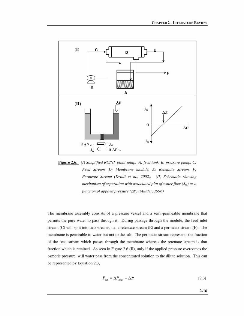
CHAPTER 2 – LITERATURE REVIEW
2-16
(I)
(II)
Figure 2.6: (I) Simplified RO/NF plant setup. A: feed tank, B: pressure pump, C:
Feed Stream, D: Membrane module, E: Retentate Stream, F:
Permeate Stream (Drioli et al., 2002). (II) Schematic showing
mechanism of separation with associated plot of water flow (JW) as a
function of applied pressure (∆P) (Mulder, 1996)
The membrane assembly consists of a pressure vessel and a semi-permeable membrane that
permits the pure water to pass through it. During passage through the module, the feed inlet
stream (C) will split into two streams, i.e. a retentate stream (E) and a permeate stream (F). The
membrane is permeable to water but not to the salt. The permeate stream represents the fraction
of the feed stream which passes through the membrane whereas the retentate stream is that
fraction which is retained. As seen in Figure 2.6 (II), only if the applied pressure overcomes the
osmotic pressure, will water pass from the concentrated solution to the dilute solution. This can
be represented by Equation 2.3,
π∆−∆= applnet PP [2.3]
A
B
C D
E
F
∆P
∆π
0
JW
JW
if ∆P >
π
∆∆∆∆P
if ∆P <
π
JW
JW

CHAPTER 2 – LITERATURE REVIEW
2-17
where the applied pressure (Pappl) is necessary to overcome the osmotic pressure (π) and the
remaining pressure forms the net pressure (Pnet) which drives the water through the membrane
(Hassan et al., 1998). Until this constraint is overcome the water will flow in the opposite
direction. As more and more water passes through the membrane, the retentate stream becomes
increasingly concentrated. In NF and RO the applied pressure ranges from 1.5 to 2.5 MPa for
brackish water desalination and for seawater desalination using RO, pressures between 4 and
8 MPa are applied (Mulder, 1996).
2.2.2.2 (a) Membrane Configurations for RO and NF
Membranes for RO and NF are available in several different configurations, viz. tubular,
hollow-fibre, plate-and-frame, and spiral-wound. The versatility of an individual membrane
design depends on the particular application and is affected by factors such as viscosity,
concentration of suspended solids, particle size, and temperature. Furthermore, the
configuration and material composition of the membrane used is of environmental significance
as it represents an important factor in the selection of the method for pre-treatment and chemical
conditioning of the feedwater (Morton et al., 1996). The spiral-wound membrane module
(Figure 2.7) is one of the more common modules used for NF or RO.
Figure 2.7: Spiral-wound membrane module commonly used during NF and RO
(adapted from Mulder, 1996)
permeate
permeate
permeate
membrane
retentate retentate
permeate
feed feed
Central permeate pipe
Module housing
Membrane feed spacer
Porous permeate spacer

CHAPTER 2 – LITERATURE REVIEW
2-18
A spiral-wound module constitutes several pairs or envelopes of flat sheet membranes wrapped
around a central permeate collection tube. The membrane envelopes constitute two flat sheets
of membrane with an external active surface, separated by a thin support mesh and glued
together along three sides (Rautenbach and Albrecht, 1981).
The open end of the envelope is glued to a perforated collection tube. The pressurised
feedwater follows a spiral path along the membrane envelope, and desalinated water is collected
in the central tube. The direction of the feed flow is axial to the cylindrical module, parallel
along the central pipe, whereas the permeate flows radially toward the central pipe.
The spiral wound membrane configuration offers several attractive advantages for industrial
users. These include higher membrane area per unit volume, which allows greater flows, and
also spacers between membranes, which promote turbulent flow, an important feature that
reduces fouling and extends membrane life (Bhattacharyya and Williams, 1992).
The selectivity of a membrane for a given solute is expressed by the retention coefficient or the
rejection coefficient, R. The Spiegler-Kedem equation for the rejection is represented in
Equation 2.4 (Spiegler and Kedem, 1966):
( )
−−
−−=
p
JR
wr
r
r
rejσ
σ
σ
exp1
11 [2.4]
The solute rejection, Rrej, is given as a function of the water flux, Jw, and the solute permeability,
p. The reflection coefficient, σr, of the membrane towards a particular solute, accounts for the
fact that in reality the membrane may not be entirely non-permeable to solute and there may be
some passage of low molecular weight solutes through the membrane.
Considering that w
s
pJ
Jc = where cp is the solute concentration in the permeate, and the solute
flux sss cBJ ∆= ,where Bs is the solute permeability coefficient and pfs ccc −=∆ , where cf is
the solute concentration in the feed, Equation 2.4 can then be simplified to Equation 2.5.

CHAPTER 2 – LITERATURE REVIEW
2-19
f
p
f
pf
rejc
c
c
ccR −=
−= 1 [2.5]
Equation 2.4 shows that as rejection increases the water flux also increases until the limiting
value σr (at infinitely high water fluxes) is reached. At this limit, the diffusive flux of the solute
transport is negligible, leaving the reflection coefficient σr, as a function of the convective
transport of the solute alone. A reflection coefficient of 100 % indicates that solute transport
through convection is absent, as is the case of RO membranes as these membranes have a
denser structure with no pores thereby preventing the convective transport of solutes. However,
solute transport may take place by solution-diffusion yielding a reflection coefficient less than
100 %. In the case of NF membranes, the pores on the membranes allow for the passage of
small solute molecules yielding a reflection coefficient less than 100 %.
2.2.2.2 (b) Applications of RO and NF
NF and RO have gained popularity mainly due to their application in desalination of waters with
a TDS content in the range of brackish and seawater. These processes are also used when low
molecular weight solvents have to be separated from solutions. Some examples of these solutes
are inorganic salts or small organic molecules such as glucose and sucrose. Furthermore, NF
has a high retention for micropollutants or microsolutes such as herbicides, insecticides and
pesticides and for other low molecular weight components such as dyes and sugars and is
therefore used in the production of potable water from polluted low TDS surface water. NF is
also used in water softening, fractionation and demineralisation of effluents and concentration
of organic dyes (Garcia-Aleman and Dickson, 2004). It was also found that NF membranes are
able to keep their retention selectivity for ions in electrolyte solutions up to concentrations of
200 g/ℓ (Karelin et al., 1996). This feature enables NF membranes to be used for the separation
of multicomponent solutions into binary ones, from which the corresponding salts can be
recovered by vaporization.
Apart from the desalination of seawater that governs the applicability of RO, this process is also
useful in the electronic industry during the production of ultrapure water, in the food industry
for the concentration of fruit juice and milk, for the recovering and recycling of valuable
products in waste streams from various industries and in the pharmaceutical industry for the
clarification and concentration of fermentation broth. RO can be extensively used in the

CHAPTER 2 – LITERATURE REVIEW
2-20
treatment of industrial effluents such as electroplating process effluents, power station effluents,
pulp and paper bleach effluents and mine drainage (Buckley et al., 1993)
2.2.2.2 (c) RO versus Thermal Processes
The 1970s saw the rapid growth and utilisation of thermal desalination, particularly MSF, as the
primary desalination process. Following this era, the introduction and advancement of RO as a
method of desalination has grown and mostly overcome MSF as the primary desalination
technique. RO has almost succeeded thermal desalination processes for the following reasons
(Brandt et al., 1993):
� It requires only half the amount of energy as opposed to the energy demand of thermal
plants (Espino et al., 2003).
� Ambient temperatures are sufficient and no phase changes are needed for the operations
of RO.
� The RO plant is designed using non-corrosive polymeric materials rather than metallic
materials, as is the case in thermal operations.
� The RO plant requires a smaller area capacity for installation as opposed to thermal
plants.
� Transport and installation of RO plants are more facilitated as the entire plant is built in
modular components.
� RO can be easily started up and shut down.
� The operation of RO requires minimal technical skills due to its simplicity.
Overall the choice of RO or thermal processes for desalination depends on economic factors and
aptness of the surrounding environment to accommodate the technology.
2.2.3 Problems in the Desalination of Concentrated Salt Solutions
One of the major drawbacks for the use of RO for desalination is the susceptibility of the
membrane to scaling, particularly pronounced during the desalination of waters with high TDS
content such as seawater. In general, scaling refers to the formation of mineral deposits
precipitating from the feed stream on to the surface of the membrane (Van Paassen et al., 1998).
The main constituents of scale are the alkaline soft salts CaCO3 and Mg(OH)2 and the non-
alkaline hard salt CaSO4 and its derivatives, although BaSO4, SrSO4, CaF2 and SiO2 can also

CHAPTER 2 – LITERATURE REVIEW
2-21
result in membrane scaling (Van de Lisdonk et al., 2000). The formation of non-alkaline hard
salts is pronounced at high temperatures as their solubility is inversely related to the
temperature. During the production of fresh water by RO, the concentration of dissolved salts
increases in the retentate stream inevitably leading to deposition of precipitates on the
membrane surface. This scaling phenomenon hinders the maximal operation of the RO unit by
half of its full potential (Ohya et al., 2001). Four methods of overcoming this hurdle of
membrane scaling are currently in place (Al-Shammiri and Al-Dawas, 1997). The first method
is used when the major scale component is calcium carbonate. In this case acid is added for the
partial consumption of bicarbonate in the feed for the conversion to carbon dioxide. The second
method involves the use of antiscalants such as sodium hexametaphosphate (SHMP). These
antiscalants function as inhibitors against the formation and growth of scale-forming
components. The third approach is to run RO at lower recovery levels thus remaining under the
saturation levels of scaling salts. The final method employs a water softening approach in
which lime or soda ash is added to precipitate the carbonates as CaCO3. A novel approach to
this problem was described by Juby et al. (1996) for the desalination of calcium sulphate scaling
mine water. The membrane desalination technology which is termed SPARRO (slurry
precipitation and recycle reverse osmosis) incorporates seeded reverse osmosis (SRO)
technology which is based on incorporating a slurry of seed crystals into the feed water to
conventional tubular reverse osmosis (O’Neail et al., 1981). During the concentrate processing
to produce desalinated water, as the concentration of ions such as Ca2+ increases in solution, the
seed serves as a growth medium for these ions. Due to preferential growth on the seed, this
prevents the precipitation and build-up of scale on the membrane surface itself. Seeded
crystallisation may be carried out in one of two forms: (i) seeds of the same material as the
crystallising salt can be incorporated in the slurry which leads to the spontaneous growth of the
seeds or (ii) seeds of a foreign (heterogeneous) material may be incorporated in the slurry. In the
latter case nucleation is still required for crystallisation but the energy barrier for the
heterogeneous seeded nucleation is lower that that of the homogenous nucleation resulting in
the former occurring at a much lower saturation level (Sluys et al., 1996). The SPARRO
process addressed and overcame, to some extent, the shortcomings of other seeded systems
concerning energy consumption and recirculation rates, however, this process failed with
regards to stability of membrane performance particularly concerning the salt rejection and
membrane flux values, which indicated overall membrane fouling and shortened membrane life.
This is due to the high concentration of salts or certain ions within the water at which point this
process failed.

CHAPTER 2 – LITERATURE REVIEW
2-22
Another problem during the desalination of waters containing high concentrations of strong
electrolytes is that of impurities, macroparticles and macroorganisms, which may lead to
membrane fouling. In order to prevent fouling of the RO membrane surface, pre-treatment of
the source water must be performed. Large, suspended solids present in the water must first be
removed and the water appropriately pre-treated to prevent precipitation of salt or microbial
growth on the membrane. Furthermore, apart from high degree of hardness of the water, a high
turbidity in the feed lowers the plant performance.
Waters that contain a high TDS content pose a significant economic problem during
desalination as considerable amount of pressure is required to overcome the osmotic pressure
barrier (Mariah et al., 2006a). This can be explained by considering Equation 2.3 again. The
higher the TDS content of the water, the higher the ionic molar concentration resulting in
increasing feed osmotic pressure. From Equation 2.3 this consequence implies that a higher
applied pressure is required to overcome this osmotic pressure barrier in order to gain a net
pressure to transport the water through the membrane. As a result considerable pressure is
required during RO concentrate processing and, together with membrane scaling, is the major
drawbacks of RO.
2.3 MEMBRANE DISTILLATION-CRYSTALLISATION
Membrane distillation (MD) may be considered as a combination of both of the main categories
of desalination processes described in Section 2.2, i.e. MD is a thermally driven membrane
desalination / separation process (Mariah et al., 2006b). After a few subtle prefaces to MD in
the 1960s under U.S. patents, MD was finally introduced commercially on a small scale in the
1980s (Lawson and Lloyd, 1997). As the name implies, the process combines both the use of
membranes and distillation which occurs across the membrane. In the process, saline water is
heated to enhance vapour production, and this vapour is exposed to a membrane that can pass
vapour but not water. After the vapour passes through the membrane, it is condensed on a
cooler surface to produce pure water. In the liquid form, the pure water cannot pass back
through the membrane, so it is trapped and collected at the output of the plant. The main
advantages of MD lie in its simplicity and the need for only small temperature differentials to
operate. One important advantage of MD, which differentiates it from other membrane
processes such as RO for example, is the independence of the quality of the permeate from the
quality of the feed solution; MD can handle highly concentrated feed solutions without a

CHAPTER 2 – LITERATURE REVIEW
2-23
significant decay in membrane activity. RO, however, is strongly affected by the osmotic
pressure if the feed solution is very concentrated resulting in higher applied pressure
requirements furthermore, increasing the susceptibility of the membrane to fouling.
Sections 2.3.1 to 2.3.7 serve to expand the concept of MD describing how a separation is
achieved, membrane properties, factors affecting MD and applications of this process.
2.3.1 Process Description
During thermally driven membrane processes, the membrane separates two phases held at
different temperatures. Typically this will result in heat flow from the high-temperature side to
the low-temperature side (Figure 2.8). Fourier’s law governs the heat flux (Jh) according to the
thermal or heat conductivity (λ). Fourier’s law therefore describes the heat flux through the
membrane as:
dx
dTJ h λ−= [2.6]
Figure 2.8: Schematic representation of the air gap MD process showing
the flow of vapour and temperature profile across the
membrane (Fane et al., 1987, Kimura and Nakao, 1987 and
Kurokawa et al., 1990)
0=x
Warm feed side
Membrane
l=x
Cooled surface
Vapour flow
Gap Tb
f
Tmp
Tbp
Permeate
Tm
Pmf
Pmp
Pm
cbf
cmf
Cooling water side
Tmf

CHAPTER 2 – LITERATURE REVIEW
2-24
Figure 2.8 is a schematic representation of the transport of vapour molecules across the
membrane. This concept is expanded in Section 2.3.1.2. During MD a microporous
hydrophobic membrane separates a warm aqueous solution from a cold solution. If the liquids
do not wet the membrane, then pure water vapour is transported from the warm side to the cold
side. This process has been described as a sequence of events: (i) the formation of a vapour gap
at the warm solution-membrane interface (ii) transport of the vapour phase through the
microporous system and (iii) condensation at the cold membrane-solution interface (Drioli and
Wu, 1985). The hydrophobicity of the membrane prevents the aqueous solution from entering
the pores thus creating a vapour-liquid interface at each of the pore entrances. The driving force
for the separation process is therefore the vapour pressure difference arising from the
temperature difference across the membrane. The distance between the membrane and the
cooling surface is referred to as the diffusion gap and its composition varies according to the
membrane configuration that is chosen.
2.3.1.1 Membrane configurations
There are numerous types of methods that can be used to maintain the vapour pressure
difference across the membrane to produce an overall solvent flux. MD can be configured as
direct contact membrane distillation (DCMD), air-gap membrane distillation (AGMD), vacuum
membrane distillation (VMD) and sweeping gas membrane distillation (SGMD). Figure 2.9
provides a schematic illustration of these methods.
(a) (b) (c) (d)
Figure 2.9: Types of membrane configurations. (a) direct contact membrane distillation, (b)
air gap membrane distillation, (c) sweeping gas membrane distillation,
(d) vacuum membrane distillation (adapted from Lawson and Lloyd, 1997)
Air Gap
Co
ld S
urf
ace
Sweep Gas
Va
cuu
m
Aq Soln
Aq Soln
Aq Soln
Aq Soln
Aq Soln
Membrane

CHAPTER 2 – LITERATURE REVIEW
2-25
In the DCMD configuration, two solutions are held at different temperatures in direct contact
with the membrane surfaces, while vapour is trapped within the membrane pores. The permeate
side contains a cooler solution in direct contact with the membrane. The membrane serves to
establish a vapour-liquid interface through which solvent molecules from the warm solution
side evaporate, diffuse through the membrane and condense on the cooler side. DCMD is the
most frequently applied membrane configuration during MD processes and is most useful for
desalination and concentrating aqueous solutions where water is the major permeate component.
This method is also most attractive as it requires the least equipment and is easy to operate
(Calabro et al., 1991, Fujii et al., 1992, Laganà et al., 2000, Schofield et al., 1990 and Zolotarev
et al., 1994).
In AGMD a condensing surface is separated from the membrane by an additional air gap; in
VMD a vapour phase is stripped away from the liquid through the membrane and the
condensation, if necessary, takes place in a separate vessel and in SGMD a stripping gas is used
as a carrier instead of a vacuum (Gostoli and Sarti, 1989). In DCMD and AGMD a diffusive
flux of volatile components takes place at the vapour-liquid interface. In VMD the downstream
pressure (on the permeate side) is lowered below the equilibrium vapour pressure so that the
mass transfer is ruled by the convective transport mechanism (Bandini et al., 1992). The
driving force for the process is therefore linked to both the partial pressure gradient and the
thermal gradient across the membrane (Cabassud and Wirth, 2002). SGMD and VMD are more
suited to applications such as removing volatile organic components such as the removal of
ethanol from fermentation broths or when dissolved gases need to be removed from solution
(Basini et al., 1987, Cabassud and Wirth, 2003, Saavedra et al., 1992 and Sarti et al., 1993).
AGMD covers a much wider spectrum of applications, being useful in almost any type of
application (Banat and Simandl, 1993 and Kimura and Nakao, 1987). In particular, the AGMD
configuration is very suitable for the desalination of geothermal resources, and the energy
demand for pumping is lower (El Amali et al., 2004).
2.3.1.2 Transport across the Membrane
The theory of heat and mass transport has been used to establish a MD theory that is widely
used for the description of the MD process. This theory is a combination of heat and mass
transfer coefficient functions through both the membrane and the liquid surfaces contacting the
membrane on either side. The development of this theory is explained in Sections 2.3.1.2
CHAPTER 2 – LITERATURE REVIEW
2-26
(a) and 2.3.1.2 (b). Most of the derivations are based on the description of the process as
depicted in Figure 2.8.
2.3.1.2 (a) Mass Transfer
Literature provides two models for the description of mass transfer, or the vapour flux across a
DCMD membrane. These are the Dusty Gas Model (DGM) and a model proposed by Schofield
et al. (1987), albeit, the latter being a combination of different models based on the DGM
(Lawson and Lloyd, 1997). Both models are based on the kinetic theory of gas transport to
describe the vapour flux through the membrane pores. The choice of an appropriate model
depends on the properties of the vapour and the membrane, i.e. the mean free path and mean
free pore size (Phattaranawik et al., 2003). Vapour transported through the membrane pores are
subjected to two types of molecular resistance: (i) by air trapped in the pores of the membrane
and (ii) by the physical structure of the pore (Cath et al., 2004). Figure 2.10 illustrates these
mass transfer resistances in MD.
Figure 2.10: Mass transfer resistances in MD (Lawson and Lloyd, 1997)
Surface
Knudsen Molecular
Viscous
1/hf 1/hp

CHAPTER 2 – LITERATURE REVIEW
2-27
Resistance to mass transfer within the membrane stems from the transfer of momentum to the
membrane (viscous or momentum transfer resistance), or Knudsen resistance resulting from the
collisions of a diffusing molecule with other molecules (Lawson and Lloyd, 1997). The model
proposed by Schofield et al. (1987), to account for the resistances imposed by the membrane
structure, assumed that in the transition region between the Knudsen and viscous flows, the
permeability of the membrane can be considered as a linear combination of the Knudsen and
viscous permeabilities, being described by the Knudsen diffusion and the Poiseuille flow
models, respectively. The latter dominates when the membrane pore size is larger than the
mean free path of vapour molecules, but as this is not the case in MD, both models were
considered (Schofield et al., 1987). The mass flux from the Knudsen diffusion model is
expressed according to Equation 2.7.
( )p
m
f
mK PPRT
MrJ −
=
2
1
064.1χδ
ε [2.7]
where r is the pore radius, ε the membrane porosity, χ the pore tortuosity, δ the membrane
thickness, M the water molecular weight, R the gas constant, T the temperature and Pfm and Pp
m
the vapour pressures at the membrane surface of the feed and permeate, respectively. However,
Pfm and P
pm are also dependent on the temperature at the membrane surface of the feed and
permeate, respectively; hence the flux dependence on temperature is not simply T-1/2.
The mass flux from the Poiseuille flow model is expressed as,
( )p
m
f
m
m
P PPRT
MPrJ −
=
2
12
125.0ηχδ
ε [2.8]
where Pm is the water vapour pressure in the membrane and η is the gas viscosity.
To account for the resistance imposed by the air trapped in the membrane pores, the molecular
diffusion model was described (Equation 2.9),
( )p
m
f
mD PPRT
MD
YJ −=
χδ
ε
ln
1 [2.9]

CHAPTER 2 – LITERATURE REVIEW
2-28
where Yln is the mole fraction of air and D the diffusion coefficient.
A common trend is displayed by these three models and as such the linear relationship
according to Equation 2.10 can be approximated,
mPCJ ∆= [2.10]
making C a membrane mass transfer coefficient for the system and ∆P the vapour pressure
difference across the membrane. C is temperature dependent and dependent on membrane pore
geometry or the mole fraction of air within the pores, the discriminating factor being whether
convective or diffusive transport is dominant, respectively. Many authors refer to this model, or
modifications thereof, when describing vapour flux across the membrane. Furthermore, as the
vapour pressure within the membrane is not directly measurable, some authors have found it
more convenient to express Equation 2.10 in terms of temperature (Hsu et al., 2002 and
Schofield et al., 1987),
( )p
m
f
m
T
TTdT
dPCJ
m
−
= [2.11]
where (Tfm-T
pm) is the temperature gradient across the membrane. When Tf
m-Tp
m < 15oC (dilute
solutions), then (dP/dT) can be approximately evaluated using the Clausius-Clapeyron equation,
2m
vap
RT
MHP
dT
dP ∆= [2.12]
where ∆Hvap is the molar heat of vaporisation and P can be evaluated from the Antoine
equation,
1
11ln
CT
BAP
++= [2.13]
where P is the pressure in Pascal, T is the temperature in Kelvin and A1, B1 and C1 are constants
which are substance dependent. Furthermore, it has been shown by Sarti et al. (1985) that
Equation 2.11 must be modified before its application to more concentrated solutions, in order
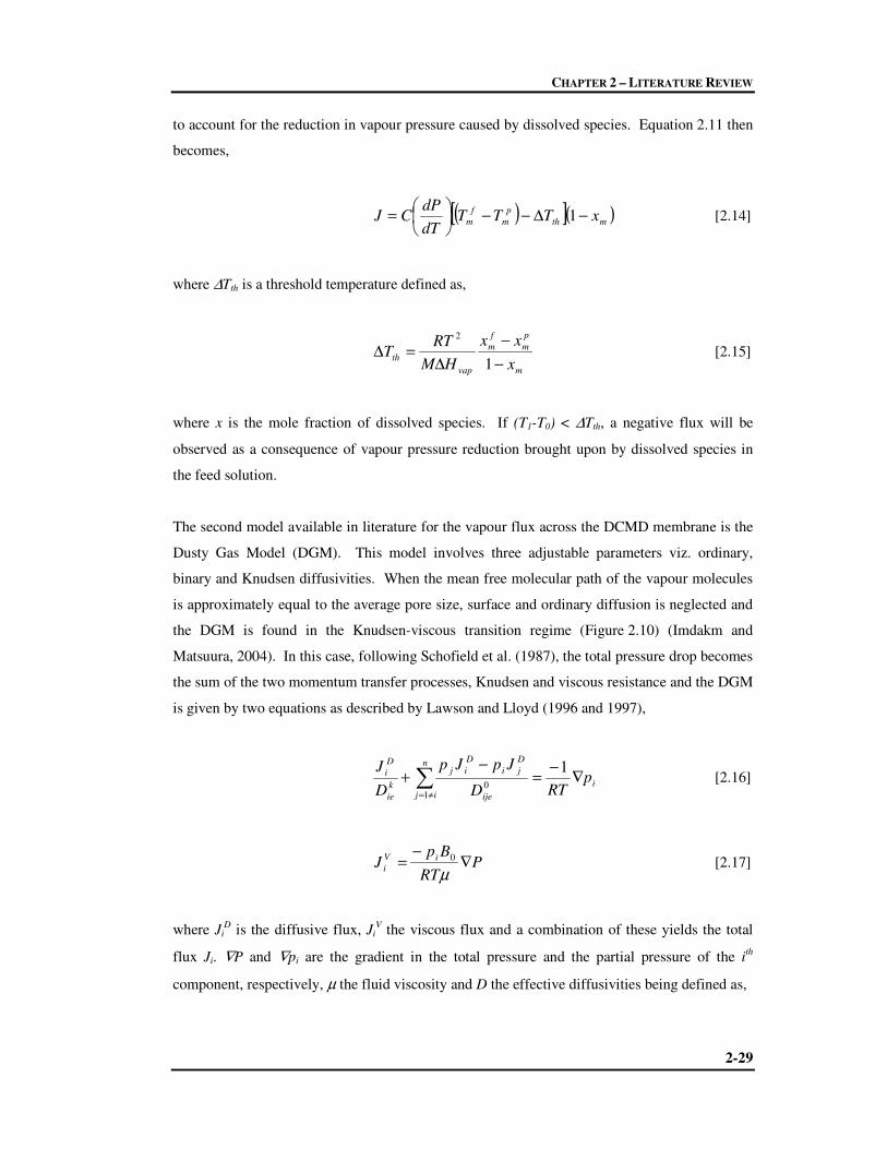
CHAPTER 2 – LITERATURE REVIEW
2-29
to account for the reduction in vapour pressure caused by dissolved species. Equation 2.11 then
becomes,
( )[ ]( )mth
p
m
f
m xTTTdT
dPCJ −∆−−
= 1 [2.14]
where ∆Tth is a threshold temperature defined as,
m
p
m
f
m
vap
thx
xx
HM
RTT
−
−
∆=∆
1
2
[2.15]
where x is the mole fraction of dissolved species. If (T1-T0) < ∆Tth, a negative flux will be
observed as a consequence of vapour pressure reduction brought upon by dissolved species in
the feed solution.
The second model available in literature for the vapour flux across the DCMD membrane is the
Dusty Gas Model (DGM). This model involves three adjustable parameters viz. ordinary,
binary and Knudsen diffusivities. When the mean free molecular path of the vapour molecules
is approximately equal to the average pore size, surface and ordinary diffusion is neglected and
the DGM is found in the Knudsen-viscous transition regime (Figure 2.10) (Imdakm and
Matsuura, 2004). In this case, following Schofield et al. (1987), the total pressure drop becomes
the sum of the two momentum transfer processes, Knudsen and viscous resistance and the DGM
is given by two equations as described by Lawson and Lloyd (1996 and 1997),
∑≠=
∇−
=−
+n
ij
i
ije
D
ji
D
ij
k
ie
D
i pRTD
JpJp
D
J
10
1 [2.16]
PRT
BpJ iV
i ∇−
=µ
0 [2.17]
where JiD is the diffusive flux, Ji
V the viscous flux and a combination of these yields the total
flux Ji. ∇P and ∇pi are the gradient in the total pressure and the partial pressure of the ith
component, respectively, µ the fluid viscosity and D the effective diffusivities being defined as,

CHAPTER 2 – LITERATURE REVIEW
2-30
2
1
010 8
and
==
i
k
ieijijeM
RTKDPDKD
π [2.18]
where Dij is the ordinary diffusion coefficient and Mi is the molecular weight of the ith
component and the term 2
1
8
iM
RT
πis the mean molecular speed. K0, K1 and B0 are constants
depending on the membrane geometry and molecular interactions with the membrane.
Evaluation of these parameters have been performed by various authors (Guijt et al., 2000,
Lawson and Lloyd, 1996). A combination of the above equations can be re-written to yield a
general expression for the DGM (Imdakm and Matsuura, 2004 and Drioli et al., 2004),
∇+∇
−= P
pBp
M
RTK
RTJ
avgi
i
i
avg
avg
iµπ
,0
2
1
0
81 [2.19]
Following the work of Schofield et al. (1987) and Lawson and Lloyd (1997) many theories have
been developed, some of which are simply modifications of the above (Banat and Simandl,
1993, Ding et al., 2002, Fane et al., 1987, Kurokawa et al., 1990, and Martínez and Florido-
Díaz, 2001(a)) or entirely new models on their own (Agashichev and Sivakov, 1993, Bouguecha
et al., 2002 and Imdakm and Matsuura, 2004). For example, Burgoyne and Vahdati (1999) used
these theories to develop a model to predict permeate fluxes produced at specific operating
conditions. Gryta and Tomaszewska (1998) arrived at a heat transfer model with the
assumption that the flow of vapour was non-isenthalpic and the temperature distribution was
non-linear. These are related to the theories that were developed by Gaeta et al. (1992) for the
non-isothermal transport of matter in porous membranes. They then used the temperature at the
membrane boundary on the permeate side as the thermodynamic reference temperature in the
derivation of their model.
2.3.1.2 (b) Heat Transfer
Simultaneous to mass transport, heat transport occurs across the membrane. This heat transfer
occurs by two mechanisms, viz. the latent heat associated with the vapour which directly serves
the evaporation process and the heat conducted across the membrane and boundaries of the
system (Martínez-Díez et al., 1999). The latter is considered as heat loss as it is no longer

CHAPTER 2 – LITERATURE REVIEW
2-31
available for use in evaporation. These two forms of heat transfer are described in
Equations 2.20 to 2.22.
For dilute solutions the latent heat flux is:
vapL HJQ ∆= [2.20]
From Equation 2.11, Equation 2.20 becomes,
( ) vap
p
m
f
m
T
L HTTdT
dPCQ
m
∆−
= [2.21]
And the conductive heat flux is,
( )p
m
f
m
m
C TTk
Q −
=
δ [2.22]
where km is the thermal conductivity of the porous membrane.
The total flux is then given by Equation 2.23,
( )
( )
m
p
m
f
m
m
vap
p
m
f
m
m
vap
T
CL
THQ
TTk
HJ
TTk
HdT
dPC
QQQ
m
∆=
−+∆=
−
+∆
=
+=
simplyor
δ
δ
[2.23]
where H is the effective heat transfer coefficient. This series of equations is a demonstration of
how mass transfer gives rise to heat transfer during the MD process. Much work has been
undertaken to explain the flow of heat across the membrane, most of which recognise that heat

CHAPTER 2 – LITERATURE REVIEW
2-32
transfer and mass transfer are related, the latter giving rise to the former (Bandini et al., 1991,
Phataaranawik et al., 2003 and Phataaranawik and Jiraratananon, 2001).
In this work, the average spatial values of inlet parameters will be considered and the local
variations (axial and radial) of concentrations, temperatures, flows and partial pressures will not
be considered. To describe the variation between inlet and outlet parameters a logarithmic
average between the high temperature and low temperature sides of the module will be
calculated. The logarithmic mean is considered as the most appropriate average driving force in
a counter-current mass or heat transfer device.
2.3.2 Process Parameters
Probably the main criterion of this process is that the membrane must not be wetted by the
liquid, in other words, the pores of the membrane must only be filled with vapour. Once the
liquid wets the membrane, the membrane’s pores become immediately filled with the liquid as a
result of capillary action. One of the criteria for the prevention of wetting is a low affinity
between the liquid and the polymeric material of the membrane. This low affinity was found to
occur at contact angles greater than 90o (Peña et al., 1993). The relationship between a
membrane’s largest allowable pore size and operating conditions is given by Equation 2.24, also
known as the Laplace (Cantor) equation.
max
L
entryinterfacevapourliquid
r
B
PPPP
θγ cos2−=
∆<∆=−
[2.24]
Where γL is the liquid surface tension, θ is the liquid-solid contact angle, rmax is the largest pore
radius, and B is a geometric factor determined by pore structure. It is therefore evident that the
wettability of the membrane depends on all three of these factors. If θ > 90o then cosθ < 0 and
∆P > 0, and the Laplace equation demonstrates that only if a threshold pressure is applied will
the liquid penetrate the membrane. Therefore, from Equation 2.24 it can be deduced that in
order to avoid wettability of the membrane, the maximum pore size must be small (0.1 to
0.5 µm), the surface tension of the liquid high and the surface energy of the membrane material
low (Banat and Simandl, 1993). Membranes fabricated from hydrophobic microporous material
such as polypropylene (PP), polytetrafluoroethylene (PTFE), polyethylene (PE) and
polyvinylidene fluoride (PVDF) meet these requirements (Wu et al., 1992). The value of
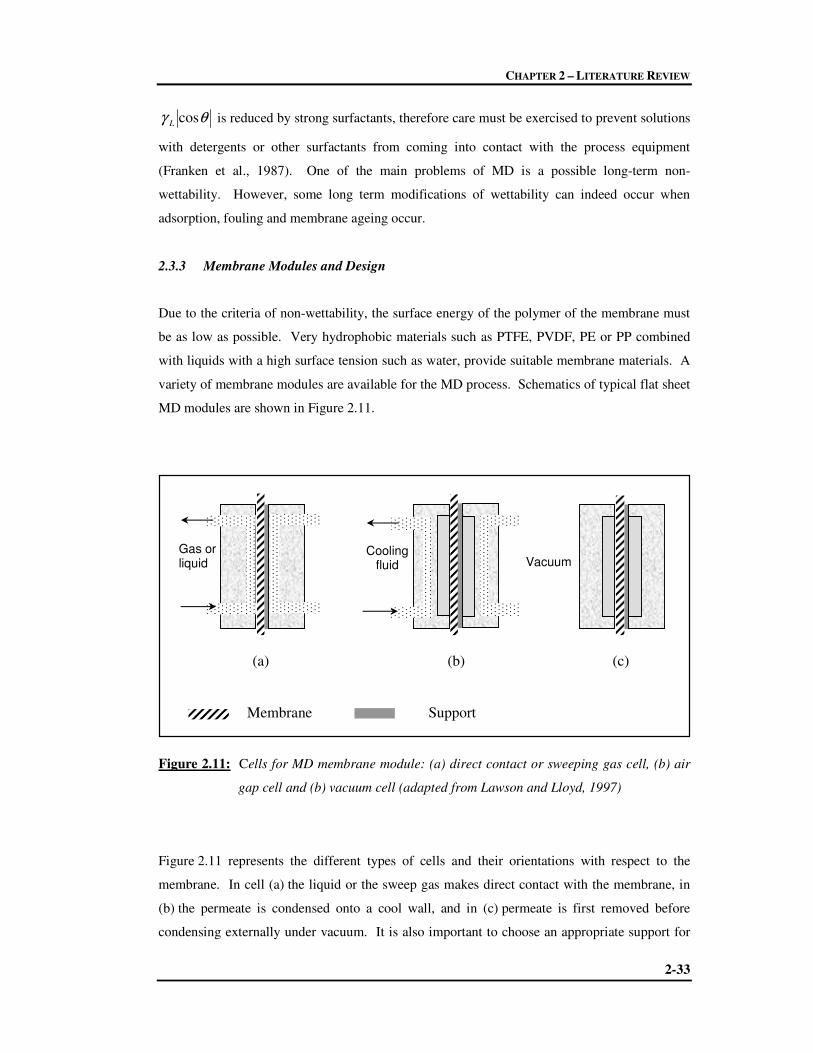
CHAPTER 2 – LITERATURE REVIEW
2-33
θγ cosL is reduced by strong surfactants, therefore care must be exercised to prevent solutions
with detergents or other surfactants from coming into contact with the process equipment
(Franken et al., 1987). One of the main problems of MD is a possible long-term non-
wettability. However, some long term modifications of wettability can indeed occur when
adsorption, fouling and membrane ageing occur.
2.3.3 Membrane Modules and Design
Due to the criteria of non-wettability, the surface energy of the polymer of the membrane must
be as low as possible. Very hydrophobic materials such as PTFE, PVDF, PE or PP combined
with liquids with a high surface tension such as water, provide suitable membrane materials. A
variety of membrane modules are available for the MD process. Schematics of typical flat sheet
MD modules are shown in Figure 2.11.
(a) (b) (c)
Membrane Support
Figure 2.11: Cells for MD membrane module: (a) direct contact or sweeping gas cell, (b) air
gap cell and (b) vacuum cell (adapted from Lawson and Lloyd, 1997)
Figure 2.11 represents the different types of cells and their orientations with respect to the
membrane. In cell (a) the liquid or the sweep gas makes direct contact with the membrane, in
(b) the permeate is condensed onto a cool wall, and in (c) permeate is first removed before
condensing externally under vacuum. It is also important to choose an appropriate support for
Gas or liquid
Cooling fluid Vacuum

CHAPTER 2 – LITERATURE REVIEW
2-34
the membrane, one that does not significantly affect the heat and mass transfer resistance, but
must be strong enough to prevent deflection or rupture of the membrane.
Characteristics of a well-designed membrane module are one that provides optimum heat and
mass transfer between the bulk solution and the solution-membrane interface. Numerous work
in this field has demonstrated that DCMD is probably the most simple, economical and efficient
configuration to achieve the vapour-liquid equilibria necessary for the operation of the MD
process (El Amali et al., 2004, Fane et al., 1987 and Sarti et al., 1985).
2.3.4 Advantages of Membrane Distillation
The main advantages of MD over conventional membrane and distillation processes can be
summarised as follows:
Membrane distillation,
� Can be performed at lower operating pressure and lower temperatures than the boiling
point of the feed solutions (Andersson et al., 1985, Khayet et al., 2003 and Sarti et al.,
1985) and a relatively low temperature difference between the two liquids in contact
with the membrane surface gives relatively high fluxes.
� Requires lower vapour space as the vapour-liquid interface is developed by a
hydrophobic membrane in MD as opposed to conventional distillation which relies on
high vapour velocities to establish a vapour-liquid interface (Jonsson et al., 1985). As
such they are very compact and very little equipment space is required. Furthermore,
the possibility to overcome corrosion problems by using plastic equipment exists (Banat
and Simandl, 1993).
� Is not limited by high osmotic pressure and fouling as the membrane works at
atmospheric pressure and is not directly involved in the separation process but acts
merely as a support. As such there is reduced chemical interaction between the
membrane and process solution (Hsu et al., 2002). Furthermore, due to this
characteristic membranes can be fabricated from a variety of chemically resistant
polymers (Gekas and Hallstrom, 1987).

CHAPTER 2 – LITERATURE REVIEW
2-35
� Displays selectivity higher than any other membrane process (Alklaibi and Lior, 2004).
MD therefore allows very high separation factors for ions, macromolecules, colloids,
cells and other non-volatile solutes in comparison to UF, NF and RO processes
(Martínez-Díez and Florida- Díez, 2001(b) and Lawson and Lloyd, 1997).
� Has low sensitivity to feedwater concentrations and has potential applications for
concentrating aqueous solutions or producing high-purity water even at very high
feedwater concentrations (Alklaibi and Lior, 2004, Kubota et al., 1998, Mariah et al.,
2005(a) and (b), Tomaszewska, 1993, and Wu et al., 1991).
� Does not require elevated temperatures therefore the heat can be supplied by solar
collectors or other forms of heat such as low-grade waste heat from factories or
geothermal energy (Hogan et al., 1991 and Walton et al., 2004).
MD is one of the membrane processes in which the membrane is not directly involved in the
separation. The membrane acts only as a support for a vapour-liquid interface and does not
contribute to the separation mechanism. Selectivity is determined by the vapour-liquid
equilibrium involved. Hence, the component with the highest partial pressure will show the
highest permeation rate. For this reason, the separation of NaCl from salted solutions is
achieved in very high purity with MD. This is because in water-NaCl mixtures, only water has
a vapour pressure (the vapour pressure of NaCl can be neglected), which implies that only water
can permeate through the membrane, hence achieving very high selectivities.
2.3.5 Applications of Membrane Distillation
One of the most important applications of MD is in the production of pure water. Studies have
shown that a high quality permeate can be obtained during MD. This feature of MD makes this
process invaluable in the desalination of seawater, in industry for boiler feedwater and in the
semiconductor industry (Mulder, 1996). Other area in which MD is used to treat waste water is
in the textile industry (Calabro et al., 1991 and Wu et al., 1991). In the case of a solution
containing non-volatile components, e.g. NaCl, only water vapour flows through the membrane,
therefore, the retention degree of solutes in MD is close to 100 % (Gryta et al., 2001). This
allows the concentration of solutions up to solute saturation (Mariah et al., 2006b). The
concentrating process of MD may be exploited in the food industry for the concentration of fruit

CHAPTER 2 – LITERATURE REVIEW
2-36
juices and milk (Calabro et al., 1994, Kimura and Nakao, 1987 and Laganà et al., 2000).
Gostoli and Sarti (1989) and later Sarti et al. (1993) have found VCMD to be very useful for the
separation of alcohol-water mixtures such as the extraction of organic components, ethanol and
methylterbutyl from aqueous streams. Similarly, Bernado et al. (2003) investigated the
potentiality of membrane technologies, including MD, for the substitution of some typical
technologies during a traditional ethylene process. Criscuoli et al. (2002) evaluated MD for the
treatment of uraemia by employing this process for the purification of human plasma
ultrafiltrate and the re-circulation of the purified water to the patients. The feasibility of
breaking down azeotropic mixtures by the removal of water has been explored by Udriot et al.
(1994). Gryta et al. (2001) used MD for the treatment of NaCl solutions subsequent to use in
the food industry. The concept was to produce pure water together with a concentrate
containing substances present in the initial solution which could be separated by crystallisation
thus facilitating their disposal and potential recycling of the water produced. Based on a similar
concept, Tomaszewska (1993) used MD for the concentration of the sulphuric acid solution
obtained after the removal of apatite phosphogypsum. This residue contains lanthane
compounds which may be recovered by crystallisation after successive concentration steps with
MD.
2.3.6 Potential Problems of Membrane Distillation
MD has significant advantages over other processes as described in Section 2.3.4. However,
some factors that significantly affect the performance of MD do exist. These include
concentration phenomena and flux decay, the former leading to the latter. These constraints are
discussed in Sections 2.3.6.1 and 2.3.6.2.
2.3.6.1 Temperature and Concentration Polarisation
Due to the presence of boundary layers at both sides of the membrane, the transmembrane
temperature difference, ∆Tm, is lower than the bulk temperature difference, ∆Tb. This
phenomenon is called temperature polarisation and the useful energy for mass transfer of
vapours to the total energy input to the process then becomes known as the temperature
polarisation coefficient (TPC),τ, (Cath et al., 2004). The value of the TPC is given as the ratio
of the temperature difference between the evaporation and condensation surfaces, and the bulk
of the feed and permeate (Smolders and Franken, 1989).

CHAPTER 2 – LITERATURE REVIEW
2-37
p
b
f
b
p
m
f
m
TT
TT
−
−=τ [2.25]
From Figure 2.8 it is obvious that the differences between Tbf and Tm
f and between Tm
p and Tbp
will increase as the mass flux increases (i.e. with increasing evaporation rates) and as such the
membrane boundary on the feed side has the highest salt concentration (Hsu et al., 2002). This
further gives rise to concentration polarisation and the concentration polarisation coefficient
(CPC),γ, is defined (Equation 2.26) to measure the increase of solute concentration on the
membrane surface with respect to that in the bulk (Martínez, 2004).
f
b
f
b
f
m
c
cc −=γ [2.26]
Tmf, Tm
p and cmf cannot be measured directly, but many models have been proposed for their
approximation (Gostoli and Sarti, 1989, Gryta and Tomaszewska, 1998 and Martínez, 2004).
These polarisation phenomena restricts the permeate flux as an increase in the latter tends to
induce more severe polarisation (Hsu et al., 2002). Fane et al. (1987) used the model developed
by Schofield et al. (1987) of mass and heat transfer to deduce the source of potential
inefficiencies due to these transport processes. Three main causes were highlighted: (i) air
present in the membrane pores which restricts vapour flow, (ii) heat loss through conduction
and (iii) temperature polarisation which results in loss of driving force. Two of these
inefficiencies, (i) and (ii) were found to decrease significantly through deaeration which
increases the permeate flux seven-fold, however, the consequence of such was a drastic increase
in temperature polarisation (Schofield et al., 1990). Schofield et al (1990) found that in order to
overcome this, very high film heat transfer coefficients had to be used. Much work has been
performed by MD researchers in order to bring the TPC as close to unity as possible. It was
found that the dominating factor determining the temperature polarisation coefficient is the
thickness of the heat conduction boundary layers on either side of the membrane (Dittscher and
Woermann, 1994). The main concept behind the reduction of the TPC was around the
improvement of module design and / or operation, such as, using higher flow rates to achieve
better mixing and the use of channel spacers to induce turbulent flow (Lawson and Lloyd, 1996,
Martínez-Díez and Vázquez-González, 1998 and Ortiz De Zárate et al., 1990 and 1993). More
recently, Laganà et al. (2000) found that temperature polarisation is more important than
concentration polarisation, during their experiments on the concentration of apple juice. Flux
rates were found to be dependent on the TPC and the effect of the CPC was negligible.

CHAPTER 2 – LITERATURE REVIEW
2-38
Chernyshov et al. (2003) developed a model that was capable of predicting supersaturation
fields of sparingly soluble salts such as BaSO4. Their model calculations demonstrated that if
the solubility of the salt is an inverse function of temperature, then maximum supersaturation
can occur in the bulk of the flow rather than at the membrane surface thus reducing
concentration polarisation. Kurokawa et al. (1990) studied the effect of concentration
polarisation by using concentrated solutions of LiBr and H2SO4. They found that by using
concentrated solutions as the feed, this drastically effected the permeate flux due to polarisation
phenomena. Accounting for concentration polarisation together with heat and mass transfer,
they were able to accurately estimate these permeate fluxes.
2.3.6.2 Flux decay
Although the concentration of the solvent has only a slight effect on the flux the phenomenon of
flux decay has still been observed by the majority of MD researchers. The exact explanation as
to the cause of this decline is not well understood as very few researchers have performed long
term experiments in order to quantify and characterise this phenomenon. Drioli and Wu (1985)
are some of the researchers who performed long-term experiments on MD. They observed a
decrease in permeate flowrate after the first four days of the experiment, after which the
permeate flow rate reached steady-state. They found that transmembrane fluxes increased at
constant ∆T with a decrease in the solute concentration of the warm solution and increased with
increasing temperature, when the concentration of the warm solution was kept constant. Similar
conclusions were also arrived at by other researchers (Li et al., 2003). The work of Drioli and
Wu (1985) was expanded by Drioli et al. (1987) when studying the MD of solutions of glucose
and NaCl (of maximum feed concentration of 0.5 M). Apart from the above mentioned
conclusions, they attributed the flux decline at higher concentration to the increase in solution
viscosity, being related to transport phenomena occurring at the membrane-solution interface.
This flux decline is therefore expected to increase at higher solute concentrations. Long-term
MD experiments were performed by Banat and Simandl (1994) who found that the flux
increased during an initial two day period. However, during the course of this period, the flux
was only steady during short time intervals (3 h) but could be considered unsteady over the
average length of time. After this initial increase period, there was a decline in flux for about
seven days before reaching steady state.
Many hypotheses have been proposed for the explanation of this flux decay. Kubota et al.
(1988), found that the permeate flux not only depends on the operating temperature and

CHAPTER 2 – LITERATURE REVIEW
2-39
temperature difference across the membrane, but that the flow rate of the brine and cooling
water also play an important role. Franken et al. (1987) explained this phenomenon in terms of
membrane wetting. Their theory was that with time during MD, an increasing number of pores
became wetted, which result in a back flow of permeate to the feed. They justified their theory
experimentally by changing the hydrostatic pressure of the permeate and observed an inverse
relationship between the permeate pressure and flux. However, this theory does not hold for the
case in which the hydrostatic pressure of the feed is higher than that of the permeate and the
pore wetting leads to enhanced flux, but a deterioration in quality. Apart from membrane
wetting, another cause of flux decline is membrane fouling. However, this phenomenon is not as
pronounced in MD as is in RO or ultrafiltration (UF), for example, due to MD membranes
having larger pore sizes therefore being less susceptible to clogging (Alklaibi and Lior, 2004).
Despite this advantage, fouling of the membrane in MD still occurs. There are several factors
which lead to membrane fouling and subsequently, pore clogging which include, biological
fouling through bacterial growth on the membrane surface, scale build-up due to high solute
concentrations and the entrapment of particulate or colloid species at the membrane-liquid
interface (Lawson and Lloyd, 1997). Gryta et al. (2001) also observed a rapid decline in the
flux due to fouling caused by the deposition of organic matter on the membrane surface. Hsu et
al. (2002) studied the effect of the type of feed on permeate flux, product water quality and
membrane fouling. They found the build-up of scale on the membrane can be suppressed by
reducing the degree of polarisation if NaCl solution is used as the feed fluid. However, this is
not effective when seawater is the feed. Martínez-Díez and Florido-Díaz (2001) studied the
effect of recirculation rate, mean temperature and salt concentration on water fluxes. They
found that water flux: (i) increases as the mean temperature in the membrane system increases,
(ii) increases with the recirculation rate and (iii) decreases, almost linearly, with the salt
concentration of the feed solution. Cath et al. (2004) found that by applying a slightly negative
pressure to the permeate stream, reduced temperature polarisation and permeability obstructions
in the DCMD salt solutions could be achieved. They showed that fluxes are almost doubled by
running the DCMD at reduced pressure as compared to fluxes in the DCMD mode alone. A
recent work performed by Tun et al. (2005) looked at the MD of concentrated solutions of
sodium chloride and sodium sulphate. They found that a steep decline in the flux occurred
beyond the supersaturation point. They attributed this to the growth of crystal deposition on the
membrane and loss of membrane permeability.
During these investigations the main drawback was the inability to evaluate the flux and driving
force during the distillation operation. This was due to the fact that the vapour pressures cannot

CHAPTER 2 – LITERATURE REVIEW
2-40
be directly measured during the MD process and, as a result, can only be evaluated by a series
of equations derived from the theoretical models described. The direct estimation of the vapour
pressure driving force would be an advantage in estimating membrane performance and flux
decline.
2.3.7 Membrane Crystallisers
The high value commercial exploitation of inorganic salts requires that crystalline products have
the correct quality and structural properties. Crystallisation from solution is a widely used
technique to produce large quantities of pure solid product, usually in a single processing step.
However, some crystallisation techniques may require large energy inputs and process
requirements in order to obtain a good quality product. For example, to produce vacuum
evaporated salt with high purity from a natural feedstock, a relatively high volume of mother
liquor needs to be purged. These purge streams not only result in a loss of salt but also pose
large environmental problems (Samhaber et al., 2001). Recent advances in MD have led to the
extension of this process to the crystallisation stage. Membrane crystallisation (MCr) was
introduced by Curcio et al. (2001) who undertook investigations to produce high quality crystals
from solutions. The advantages of this technique become evident when compared to
conventional crystallisation techniques such as the circulating-magma crystalliser. In the latter
case solvent evaporation and solute crystallisation occur in the same place. This results in
temperature gradients between the surface and the bulk of the body often compromising the
suspension uniformity of the crystalline products (Curcio et al., 2001). In MCr however, these
two phenomena occur in separate reactors – the solvent evaporation occurs within the MD
module whereas the crystallisation takes place in a separate crystalliser. Furthermore,
membrane crystallisers functioning under forced solution flow conditions are characterised by
an axial flux, in laminar regime of the crystallising solution through the membrane fibres
(Curcio et al., 2005). This apparently induces a well-organised orientation of the particles thus
resulting in crystals with improved quality and size distribution which is important when
crystals need to undergo further treatment or reactions (Curcio et al., 2005).
In the MCr unit (Figure 2.12) the warm brine (retentate) flows counter current to the cold
distillate (pure water). The two streams are separated by a microporous hydrophobic membrane
in the form of capillary tubes. Continual removal of water from the retentate increases the
concentration in the mother liquor. Nucleation and crystal growth is initialised in the
crystalliser. The crystallisation process must be controlled in order avoid crystal deposition on

CHAPTER 2 – LITERATURE REVIEW
2-41
the membrane thus blocking the membrane pores. Therefore, a suitable heating system must
exist which would ensure that the solution flowing through the membrane is always at an
appropriately high temperature in order to maintain under saturation conditions, while the
crystallisation tank should be at a temperature that would favour crystal formation.
Figure 2.12: Schematic of a membrane crystalliser unit (Curcio et al., 2001)
A significant feature of membrane crystallisers is that the membrane does not merely serve as a
support for the vapour-liquid interface, but it also induces heterogeneous nucleation due to the
low supersaturation ratios (Curcio et al., 2005). The crystals obtained show improved quality
and size distribution which is important for the quality of the final product and in turn
influences the performance of downstream processes, crystals separation from mother liquor,
drying and storage (Drioli et al., 2004).
Recently, Curcio et al. (2003) used this technique in the field of protein science for the
crystallisation of lysozyme from supersaturated solutions. Another recent study performed by
Drioli et al. (2004) used the membrane crystalliser to obtain epsomite (MgSO4.7H2O) and
sodium chloride as solid products from NF retentate streams. The kinetics of crystallisation for
sodium chloride were studied in this and an earlier investigation by Curcio et al., 2001.
Preliminary data concerning the growth rate and morphological quality of magnesium sulphate
crystals has been evaluated for low ionic strength solutions (Drioli et al., 2004).
Feed inlet
Heate
r
Cooler
Pure water
Product discharge
Distillate line
Rete
nta
te lin
e
MD module
Circulation pump
Circulation pump

CHAPTER 2 – LITERATURE REVIEW
2-42
2.4 INTEGRATED DESALINATION AND SEPARATION TECHNOLOGIES
In order to address some of the shortcomings of membrane processes such as RO, UF and NF,
integrated membrane operations have gained much popularity within recent years. Integrated
operations involve the combination of various membrane processes to achieve process
intensification – a concept with a strategic approach towards major improvements in processing,
reduction in equipment size / production-capacity ratio, reduced energy consumption, waste
production, raw and hazardous materials utilisation, and recycling waste materials, resulting in
more economic and sustainable technologies (Stankiewicz and Moulijn, 2002). Furthermore,
the unified effect of the integration of various single membrane units might assist in overcoming
the shortfalls otherwise experienced if these units operate independently. Various pre-treatment
stages have been studied in order to treat the feedwater, prior to exposure to the RO membrane,
in order to remove hardness, turbidity and microorganisms which ultimately lead to higher
water recovery levels coupled with a reduction in energy consumption. Section 2.4.1 describes
some of the more common pre-treatment operations such as NF, UF and microfiltration (MF)
integrated with further water recovery processes such as RO, and Section 2.4.2 describes how
MD and MCr can be incorporated into integrated membrane systems.
2.4.1 Pre-treatment with Pressure Driven Membrane Operations
One method of reducing fouling phenomena and prolonging the lifetime of RO membranes is
by using pressure driven membrane processes, such as MF and UF for pre-treatment. The
principle of separation in these techniques is based on a sieving mechanism using microporous
hydrophobic membranes. The pore size for MF and UF membranes range between 10 and
0.05 µm and 0.05 µm to 1 nm, respectively (Mulder, 1996). This therefore makes these
processes suitable for the retention of suspensions and emulsions or macromolecules and
colloids, depending on their respective size range. Research has shown that when MF or UF is
used as a pre-treatment to RO a 39 % reduction in operating and maintenance costs of water
treatment for potable water production is achieved together with a reduction in RO capital costs
(Drioli et al., 2002). In another study performed by Cassano et al. (2003) UF was placed ahead
of RO followed by osmotic distillation (OD) in order to clarify and concentrate citrus and carrot
juices. UF functioned to clarify the raw juice while RO acted on the UF permeate by pre-
concentrating it before entering the OD stage for the final concentration. The advantages of
concentrating fruit juices using membrane technology as opposed to conventional thermal

CHAPTER 2 – LITERATURE REVIEW
2-43
concentration are that the juices retain their colour and a large part of their aroma which is
otherwise lost in conventional processes. Hsu et al. (2002) studied the effect of product water
quality and permeate flux using different feed solutions. They found that in the case were the
raw water was pre-treated by MF, the permeate flux increased by about 25 %. It is now a
common practice to use MF and UF as pre-treatment to RO and has become the industry
standard for the treatment of municipal wastewater in indirect potable reuse projects including
aquifer recharge, industrial uses and irrigation (Durham et al., 2001 and Schaefer, 2001).
Another pretreatment option considered by Kedem and Zalmon (1997) includes the use of
compact accelerated precipitation softening (CAPS) as a pre-treatment for membrane
desalination. This process achieves the rapid precipitation of calcium carbonate by cake
filtration through a fast equilibration. This pretreatment step reduces potential scaling effects
thereby increasing the recovery ratio in membrane desalination. Pretreatment by CAPS also
acts as an effective filtration step reducing the turbidity and the silt density index consequently
reducing the potential for membrane fouling. In another study performed by Turek (2002), an
integrated membrane system which couples ED-MSF-crystallisation stages has been described
for the simultaneous production of desalinated water and valuable products.
Together with MF and UF, the removal and recovery of scale components from seawater by NF
ahead of RO units is increasing in reliability. Based on this premise, investigations on NF
membranes are underway, as pretreatment systems in order to remove hardness, to reduce TDS
and decrease turbidity thus achieving recovery factors near to 70 % coupled to a reduction of
energy consumption by about 25-30 % (Drioli, 2002). Hassan et al. (1998) have investigated
the first NF-RO, NF-MSF and NF-ROreject-MSF fully integrated systems for seawater
desalination. They reported that when NF is placed ahead of RO, the NF unit reduced turbidity
and microorganisms, removed hardness ions of Ca2+, Mg2+, SO42-, HCO3
- and total hardness by
89.6 %, 94 %, 97.8 %, 76.6 % and 93.3 %, respectively. Furthermore, the system also effected
a reduction of monovalent ions of Cl-, Na+, K+ and an overall TDS reduction of 57.7 %. This
led to the added benefit of being able to run a MSF plant at top brine temperatures of 120 oC
without the risk of added antiscalant or acid formation. This integrated system also fulfilled
many of the principles of green chemistry including lower thermal load with reduced chemical
consumption thereby making the process less hazardous to the environment. An earlier study
performed by Turek and Gonet (1996) demonstrated how pre-treatment of coal-mine brines by
NF decreases the concentration of divalent ions in the permeate with almost no changes in the

CHAPTER 2 – LITERATURE REVIEW
2-44
NaCl concentration. This pre-treatment then facilitated subsequent concentration in evaporation
processes such as MSF, using lower energy, as there was no risk of gypsum crystallisation.
From their work on energetic and exergetic analyses of an integrated system, Criscuoli and
Drioli (1999) showed that by operating a RO unit without NF pre-treatment, the quality and
quantity of freshwater produced is reduced and the energy consumption remains high.
Figure 2.13 represents an integrated system of MF-NF-RO proposed by Drioli et al. (2002) for
the desalination of seawater.
Water recovery from the individual pressure-driven membrane units, MF, NF and RO was
found to be 94.7 %, 75.3 % and 50.5 % respectively through this integrated system (Drioli et al.,
2002).
Figure 2.13: An integrated MF-NF-RO system for seawater desalination (adapted from Curcio
et al., 2005 and Drioli et al., 1999)
2.4.2 Integrated MF/UF-NF-RO-MCr/MD System
Following the integration of the membrane units represented in Figure 2.13, Drioli et al. (1999)
extended this system to incorporate a MD unit to process the RO brine and proposed an ideal
high-recovery process for the desalination of seawater (Figure 2.14). The integrated system
proposed a pre-treatment stage which included MF/UF-NF-MC and a processing stage
consisting of RO-MD. The pre-treatment stage included a gas-liquid membrane contactor unit
(MC). This MC operation serves to reduce the amount of dissolved gases such as CO2 and O2
blowdown
MF RO NF 1 2
3
4 5
6
7 8
9
10
Feed NF permeate
RO brine
MF permeate
Fresh water

CHAPTER 2 – LITERATURE REVIEW
2-45
that are present in the feed solution, if deemed necessary. The MC operation is simply a
distillation across a microporous hydrophobic membrane. These membranes serve as an
interface for the mass transfer between phases of the adsorption stage. An energetic and
exergetic analysis of this integrated membrane system indicated that the recovery factor of the
MD unit was 77 % and the RO unit alone yielded a recovery factor of 40 %. However, by
coupling these two membrane units the global recovery factor was a high of 87.6 % (Criscuoli
and Drioli, 1999).
Figure 2.14: Proposed ideal integrated membrane system for seawater desalination (Drioli
et al, 1999)
Later, Drioli et al. (2004) exploited this CO2 removal by MC for the reactive transfer into
sodium hydroxide solutions for the production of NaHCO3 / Na2CO3 salts. These carbonate
solutions were necessary for the precipitation of Ca2+ ions as carbonates. The aim was to lower
the Ca2+ ion content in solution as this led to the formation of CaSO4 which is one of the major
scale-forming components. Furthermore Drioli et al. (2004) aimed at the crystallisation of
MgSO4.7H2O (epsomite), as one of the salts, from solution and the formation of the soluble
CaSO4 ion pair hindered the formation and precipitation of epsomite by harbouring SO42- ions.
Further conclusions were drawn from the exergetic and energetic analysis by Criscuoli and
Drioli (1999) on the systems similar to the ones described above. From their analyses it was
MF/UF NF MC RO
MD blowdown
Feed
Gas stream
Fresh water
RO brine
MD brine
Fresh water
Feed

CHAPTER 2 – LITERATURE REVIEW
2-46
found that by placing NF ahead of RO the osmotic pressure of the feed solution is lowered and
hence a lower applied pressure is required to move water through the membrane. The added
electrical energy that is required to run NF as a pre-treatment to RO can be offset by using the
NF concentrate to pre-pressurise the feedwater thus reducing the RO electrical energy
requirements. For the coupling of RO with MD a higher thermal demand arises due to the MD
process. However, when these two units are further coupled with NF it was found that this
energy demand is lowered. In summary, the NF-RO-MD integrated system operates at the
highest performance level, and is particularly appropriate if excess low-grade thermal energy is
available.
Other integrated MD operations proposed by Wang et al. (2001) consisted of the integration of
MD and OD to form the overall process which they termed membrane osmotic distillation
(MOD). Furthermore, their experimental system involved the circulation of brine in the cold
side of the MD. They found that with the integration of these systems, and with brine circulated
on the cold side, the water flux increased through the membrane due to a decrease in the water
vapour pressure in the brine side. Furthermore, the integrated MOD process resulted in higher
heat efficiencies.
Following the proposal of the ideal integrated system of Figure 2.14, a further investigation by
Drioli et al. (2002) incorporated a membrane crystalliser to form the NF-RO-MCr integrated
system. The membrane crystalliser achieves the complete recovery of desalted water and solid
salts. Feeding the MD unit with RO retentate allows the production of sodium chloride crystals.
Although this system represents a higher thermal energy requirement, it does, however,
eliminate the environmental problems related to brine disposal and if there is excess low-grade
thermal energy available within the plant, it could be used making the overall energy
requirement then comparable to an NF-RO coupled system (Drioli et al., 2002).
Van der Bruggen et al. (2004), proposed an integrated membrane system which leads to process
intensification in the textile finishing industry. This system consisted of MF as a pre-treatment
to used finishing baths, followed by a dual NF unit. Furthermore, the concentrate stream from
the first NF unit is fed to a MD unit, making advantageous use of the high temperature for
further concentration, and the concentrate from the second NF unit is fed to a membrane
crystalliser for salt recovery and reuse for new finishing baths. Although their concept needs
experimental verification they nonetheless proposed an overall waste minimisation and
reduction in energy and water losses thus fulfilling the concept of process intensification.

CHAPTER 2 – LITERATURE REVIEW
2-47
Curcio et al. (2005) extended the work of Drioli et al. (2004) by performing an energetic,
exergetic and cost analysis on the systems MF-NF-RO and NF-MC-RO-MCr. In one instance,
the NF retentate from the integrated system represented in Figure 2.14 was mixed with Na2CO3,
produced from the reactive adsorption of CO2 via MC, for the removal of Ca2+ ions as CaCO3,
before entering the MCr unit. In the second instance the RO brine was subjected to CaCO3
precipitation before reaching the crystalliser. In the former case a global recovery factor of
water of up to 58.6 % was achieved and in the latter case a 70.1 % global water recovery was
achieved. Although the membrane crystalliser requires additional energy for its operation, in
addition to drinking water this system allows for the recovery of solid salts of NaCl and
MgSO4.7H2O. Proceeds arising from the sale of these salts could counterbalance the high unit
cost of water production. A further advantage of completing this integrated system with a
crystalliser stage is that both the cost and environmental impacts of brine disposal operations are
considerably reduced thus favouring the concepts of green chemistry and moving towards
sustainable industrial growth.
2.5 CHAPTER REFERENCES
AGASHICHEV SP and SIVAKOV AV (1993) Modeling and calculation of temperature-
concentration polarisation in the membrane distillation process (MD). Desalination 93 245-
258.
AL-DROUBI A, FRITZ B, GAC J-Y and TARDY Y (1980) Generalised residual alkalinity
concept; application to prediction of natural waters by evaporation. Am J Sci 280 560-572.
ALKLAIBI AM and LIOR N (2004) Membrane-distillation desalination: status and potential.
Desalination 171 111-131.
AL-SHAMMIRI M and AL-DAWAS M (1997) Maximum recovery from seawater reverse
osmosis plants in Kuwait. Desalination 110 37-48.
AL-SHAMMIRI M and SAFAR M (1999) Multi-effect distillation plants: state of the art.
Desalination 126 45-59.

CHAPTER 2 – LITERATURE REVIEW
2-48
ANDERSSON SI, KJELLANDER N and RODESJO B (1985) Design and field tests of a new
membrane distillation desalination process. Desalination 56 345-354.
BANAT FA and SIMANDL J (1993) Theoretical and experimental study in membrane
distillation. Desalination 95 39-52.
BANDINI S, GOSTOLI C and SARTI GC (1991) Role of heat and mass transfer in membrane
distillation process. Desalination 184 91-106.
BANDINI S, GOSTOLI C and SARTI GC (1992) Separation efficiency in vacuum membrane
distillation. J Membr Sci 73 217-229.
BARAT JM, GRAU R, IBÁÑEZ JB and FITO P (2005) Post-salting studies in Spanish cured
ham manufacturing. Time reduction using brine thawing-salting. Meat Science 69 201-208.
BASINI L, ANGELO GD, GOBBI M, SARTI GC and GOSTOLI C (1987) A desalination
process through seeping gas membrane distillation Desalination 64 245-257.
BHATTACHARYYA D and WILLIAMS ME (1992) Chapter 21. Reverse Osmosis.
Introduction and Definitions. In Membrane Handbook, WINSTON HO WS and
SIRKAR KK, Van Nostrand Reinhold, pg. 265.
BERNARDO P, CRISCUOLI A, CLARIZIA G, BARBIERI G, DRIOLI E, FLERES G and
PICCIOTTI M (2003) Applications of membrane unit operations in ethylene process. Clean
Technologies and Environmental Policy, Springer-Verlag, DOI 10.1007/s10098-003-0225-8.
BOUGUECHA S, CHOUIKH R and DHAHBI M (2002) Numerical study of the coupled heat
and mass transfer in membrane distillation. Desalination 152 245-252.
BRANDT DC, LEITNER GF and LEITNER WE (1993) Reverse osmosis membranes: State of
the art. In Reverse Osmosis: Membrane Technology, Water Chemistry, and Industrial
Applications, AMJAD Z, ed., Van Nostrand Reinhold, New York, ISBN: 0-442-23964-5,
pg. 1.

CHAPTER 2 – LITERATURE REVIEW
2-49
BURGOYNE A and VAHDATI MM (1999) Permeate flux modelling of membrane distillation.
Filtration and Separation 49-53.
BUCKLEY CA, BROUCKAERT CJ and KERR CA (1993) RO application in brackish water
desalination and in the treatment of industrial effluents. In Reverse Osmosis: Membrane
Technology, Water Chemistry, and Industrial Applications, AMJAD Z, ed., Van Nostrand
Reinhold, New York. ISBN: 0-442-23964-5. pg. 275.
CABASSUD C and WIRTH D (2002) Water desalination using membrane distillation:
comparison between inside/out and outside/in permaeation Desalination 147 139-145.
CABASSUD C and WIRTH D (2003) Membrane distillation for water desalination: how to
chose an appropriate membrane? Desalination 157 307-314.
CALABRO V, DRIOLI E and MATERA F (1991) Membrane distillation in the textile
wastewater treatment. Desalination 83 209-224.
CALABRO V, JIAO BL and DRIOLI E (1994) Theoretical and experimental study on
membrane distillation in the concentration of fruit juice. Ind Eng Chem Res 33 1803-1808.
CARDONA E, CULOTTA S and PIACENTINO A (2003) Energy saving with MSF-RO series
desalination plants. Desalination, 153 167-171
CASSANO A, DRIOLI E, GALAVERNA G, MARCHELLI R, DI SILVESTRO G and
CAGNASSO P (2003) Clarification and concentration of citrus and carrot juices by
integrated membrane processes. Journal of Food Engineering 57 153-163.
CATH TY, ADAMS VD and CHILDRESS AE (2004) Experimental study of desalination using
direct contact membrane distillation: a new approach to flux enhancement. J Membr Sci 228
5-16.
CHERNYSHOV MN, MEINDERSMA GW and de HAAN AB (2003) Modelling temperature
and salt concentration distribution in membrane distillation feed channel. Desalination 157
315-324.

CHAPTER 2 – LITERATURE REVIEW
2-50
CRISCUOLI A and DRIOLI E (1999) Energetic and exergetic analysis of an integrated
membrane desalination system. Desalination 124 243-249.
CRISCUOLI A, DRIOLI E, CAPUANO A, MEMOLI B and ANDREUCCI VE (2002) Human
plasma ultrafiltrate purification by membrane distillation: process optimization and
evaluation of its possible application on-line. Desalination 147 147-148.
CURCIO E, CRISCUOLI A and DRIOLI E (2001) Membrane crystallizers. Ind Eng Chem Res
40 2679-2684.
CURCIO E, DI PROFIO G and DRIOLI E (2003) A new membrane-based crystallization
technique: tests on lysozyme. J Crystal Growth 247 166-176.
CURCIO E, DI PROFIO G, MARIAH L and DRIOLI E (2005) A fully integrated membrane
operation for sea water and brackish water desalination. Proceedings of the World
Conference for Chemical Engineers, Glascow, 2005.
DARWISH MA and EL-DESSOUKY H (1995) The heat recovery thermal vapour-compression
desalting system: A comparison with other thermal desalination processes. Applied Thermal
Engineering 16 (6) 523-537.
DING Z, MA R and FANE AG (2002) A new model for mass transfer in direct contact
membrane distillation. Desalination 151 217-227.
DITTSCHER U and WOERMANN D (1994) Temperature polarization in membrane
distillation of water using a porous hydrophobic membrane. Ber Bunsenges Phys Chem
98(8) 1056-1061.
DREVER, JI (1997). The Geochemistry of Natural Waters: Surface and Groundwater
Environments 3rd edition. Prentice-Hall, New Jersey. ISBN: 0-13-272790-0.
DRIOLI E, CRISCUOLI A and CURCIO E (2002) Integrated membrane operations for
seawater desalination. Desalination 147 77-81.

CHAPTER 2 – LITERATURE REVIEW
2-51
DRIOLI E, CURCIO E, CRISCUOLI A and DI PROFIO G (2004) Integrated system for
recovery of CaCO3, NaCl and MgSO4.7H2O from nanofiltration retentate. J Membr Sci 239
27-38.
DRIOLI E, LAGANÁ F, CRISCUOLI A and BARBIERI G (1999) Integrated membrane
operations in desalination processes. Desalination 122 141-145.
DRIOLI E and WU Y (1985) Membrane distillation: an experimental study. Desalination 53
339-346.
DRIOLI E, WU Y and CALABRO V (1987) Membrane distillation in the treatment of aqueous
solutions. J Membr Sci 33 277-284.
DURHAM B, BOURBIGOT MM and PANKRATZ T (2001) Membranes as pre-treatment to
desalination in wastewater reuse: operating experience in the municipal and industrial
sectors. Desalination 138 83-90.
EL AMALI A, BOUGUECHA S and MAALEJ M (2004) Experimental study of air gap and
direct contact membrane distillation configurations: application to geothermal and seawater
desalination. Desalination 168 357.
ENGELIEN HK and SKOGESTAD S (2005) Multi-effect distillation applied to an industrial
case study. Chemical Engineering and Processing 44(8) 819-826.
ESPINO T, PEÑATE B, PIERNAVIEJA G, HEROLD D and NESKAKIS A (2003) Optimised
desalination of seawater by a PV powered reverse osmosis plant for a decentralised coastal
water supply. Desalination 156 349-350.
EUGSTER H.P (1980) Geochemistry of evaporitic lacustrine deposits. Ann Rev Earth Planet
Sci 8 35-63.
EUGSTER HP and JONES BF (1979) Behaviour of major solutes during closed-basin brine
evolution. American Journal of Science 279 609-631.

CHAPTER 2 – LITERATURE REVIEW
2-52
FANE AG, SCHOFIELD RW and FELL CJD (1987) The efficient use of energy in membrane
distillation. Desalination 64 234-243.
FARWATI MA (1997) Theoretical study of a multi-stage flash distillation using solar energy.
Desalination 22 1-5.
FRANKEN ACM, NOLTEN JAM, MULDER MHV, BARGEMAN D and SMOLDERS CA
(1987) Wetting criteria for the applicability of membrane distillation. J Membr Sci 33 315-
328.
FUJII Y, KIGOSHI S, IWATANI H and AOYAMA M (1992) Selectivity and characteristics of
direct contact membrane distillation type experiment. I. Permeability and selectivity through
fried hydrophobic fine porous membranes. J Membr Sci 72 53-72.
GAETA FS, ASCOLESE E, BENCIVENGA U, ORTIZ de ZÁRATE, PAGLIUCA N, PERNA
G, ROSSI S and MITA DG (1992) Theories and experiments on nonisothermal matter
transport in porous membranes. J Phys Chem 96 6342-6354.
GARCIA-ALEMAN J and DICKSON JM (2004) Mathematical modelling of nanofiltration
membranes with mixed electrolyte solutions. J Membr Sci 235 1-13.
GARCIÁ-RODRÍGUEZ L and GÓMEZ-CAMACHO C (1999) Conditions for economical
benefits of the use of solar energy in multi-stage flash distillation. Desalination 125 133-138.
GEKAS V and HALLISTROM B (1987) Mass transfer in the membrane concentration
polarization layer under turbulent cross flow. I. Critical literature review and adaptation of
existing Sherwood correlations to membrane operations. J Membr Sci 30 153-170.
GOSTOLI C and SARTI GC (1989) Separation of liquid mixtures by membrane distillation. J
Membr Sci 41 211-224.
GRILLOT G (1956) The biological and agricultural problems presented by plants tolerant of
saline or brackish water and the employment of such water for irrigation. In Utilization of
saline water, Reviews of research, 2nd edition, UNESCO, France, 9.

CHAPTER 2 – LITERATURE REVIEW
2-53
GRYTA M and TOMASZEWSKA M (1998) Heat transport in the membrane distillation
process. J Membr Sci 144 211-222.
GRYTA M, TOMASZEWSKA M, GRZECHULSKA J and MORAWSKI AW (2001) Short
Communication. Membrane distillation of NaCl solution containing natural organic matter.
J Membr Sci 181 179-187.
GUIJT CM, RÁCZ IG, REITH T and de HAAN AB (2000) Determination of membrane
properties for use in the modeling of a membrane distillation module. Proceedings of the
Conference on Membranes in Drinking and Industrial Water Production, Volume 2,
Desalination Publications L’Aquila, Italy 511-517 ISBN 0-86689-060-2.
HARDIE LA and EUGSTER HP (1970) The evolution of closed-basin brines. Mineralogical
Soc Am Spec Publ 3 273-290.
HARVIE CE and WEARE JH (1980) The prediction of mineral solubilities in natural waters:
the Na-K-Mg-Ca-Cl-SO4-H2O system from zero to high concentration at 25oC. Geochimica
et Cosmochimica Acta 44 981-997.
HARVIE, C.E., MØLLER, N. and WEARE, J.H. (1984). The prediction of mineral solubilities
in natural waters: The Na-K-Mg-Ca-H-Cl-SO4-OH-HCO3-CO3-CO2-H2O system to high
ionic strengths at 25°C. Geochimica et Cosmochimica Acta 48 723-751.
HASSAN AM, AL-SOFI AK, AL-AMOUDI AS, JAMALUDDIN ATM, FAROOQUE AM,
ROWAILI A, DALVI AGI, KITHER NM, MUSTAFA GM and AL-TISAN IAR (1998) A
new approach to membrane and thermal seawater desalination processes using
nanofiltration membranes (Part 1). Desalination 118 35-51.
HOGAN PA, SUDJITO, FANE AG and MORRISON GL (1991) Desalination by solar heated
membrane distillation. Desalination 81 81-90.
HOWE DE (1956) Utilisation of seawater. In Utilization of saline water, Reviews of research,
2nd edition, UNESCO, France, 73.

CHAPTER 2 – LITERATURE REVIEW
2-54
HSU ST, CHENG KT and CHIOU JS (2002) Seawater desalination by direct contact
membrane distillation. Desalination. 143 279-287.
HUGO PJ (1974) Salt in the Republic of South Africa. Department of mines Geological Survey,
Memoir 65, The Government Printer, Pretoria.
IMDAKM AO and MATSUURA T (2004) A Monte Carlo simulation model for membrane
distillation processes: direct contact (MD). J Membr Sci 237 51-59.
ISMAIL A (1998) Control of multi-stage flash desalination plants: A survey. Desalination 116
145-156.
JONSSON AS, WIMMERSTEDT R and HARRYSON AC (1985) Membrane distillation – a
theoretical study of evaporation through microporous membranes. Desalination 56 237-249.
JUBY GJG, SCHUTTE CF and VAN LEEUWEN J (1996) Desalination of calcium sulphate
scaling mine water: Design and operation of the SPARRO process. Water SA 22 (2) 161-
171.
KARELIN FN, ASKERNIYA AA, GRIL ML and PARILOVA OF (1996) Salt concentration
and recovery from aqueous solutions using pressure-driven membrane processes.
Desalination 104 69-74.
KEDEM O and ZALMON G (1997) Compact accelerated precipitation softening (CAPS) as a
pre-treatment for membrane desalination 1. Softening by NaOH. Desalination 113 65-71.
KHAYET M, GODINO MP and MENGUAL JI (2003) Theoretical and experimental studies on
desalination using the sweeping gas membrane distillation method. Desalination 157 297-
305.
KIMURA S and NAKAO S-I (1987) Transport phenomena in membrane distillation. J Membr
Sci 33 285-298.

CHAPTER 2 – LITERATURE REVIEW
2-55
KRISHNA HJ (2004) Introduction to desalination technologies. TWDB Volume 2: Technical
papers, case studies and desalination technology resources. Accessed on 05 September 2005
at URL http://www.twdb.state.tx.us/Desalination/The%20Future%20of%20 Desalination
%20in%20Texas%20-%20Volume%202/documents/C1.pdf#search='vapor% 20
compression%20distillation %20for%20desalination'.
KUBOTA A, OHTA K, HAYANO I, HIRAI M, KIKUCHI K and MURAYAMA Y (1988)
Experiments on seawater desalination by membrane distillation. Desalination 69 19-26.
KUMAR S and TIWARI GN (1999) Optimization of design parameters for multi-effect active
distillation systems using the Runge-Kutta method. Desalination 121 87-96.
KUROKAWA H, EBARA K, KURODA O and TAKAHASHI S (1990) Vapor permeate
characteristics of membrane distillation. Sep Sci & Technol 25(13-15) 1349-1359.
LAGANÁ F, BARBIERI G and DRIOLI E (2000) Direct contact membrane distillation:
modeling and concentration experiments. J Membr Sci 166 1-11.
LAWSON KW and LLOYD DR (1996) Membrane distillation. II. Direct contact MD. J Membr
Sci 120 123-133.
LAWSON KW and LLOYD DR (1997) Review. Membrane distillation. J Membr Sci 124 1-25.
LI J-M, XU Z-K, LIU Z-M, YUAN W-F, XIANG H, WANG S-Y and XU Y-Y (2003)
Microporous polypropylene and polyethylene hollow fiber membranes. Part 3. Experimental
studies on membrane distillation for desalination. Desalination 155 153-156.
MANI AGRO CHEM (2005). Magnesium sulphate heptahydrate (MgSO4.7H2O). Accessed on
02 November 2005 at URL http://www.indiamart.com/maniagrochem/#magnesium-
sulphate-hepta-hydrate.
MARIAH L, BUCKLEY CA, BROUCKAERT CJ, JAGANYI D, CURCIO E and DRIOLI E
(2006a) Membrane distillation for the recovery of crystalline products from concentrated
brines. WISA Biennial Conference, Durban, South Africa, 21-25 May.

CHAPTER 2 – LITERATURE REVIEW
2-56
MARIAH L, BUCKLEY CA, BROUCKAERT CJ, CURCIO E, DRIOLI E, JAGANYI D, and
RAMJUGERNATH D (2006b) Membrane distillation of concentrated brines – role of water
activities in the evaluation of driving force. J Membr Sci. 280 (1-2) 937-947.
MARIAH L, BUCKLEY CA, JAGANYI D, DRIOLI E and CURCIO E (2005a), The
Development of Sustainable Salt Sinks – Evaluation of an Integrated Membrane System for
the Recovery and Purification of Magnesium Sulphate and Sodium Chloride from Brine
Streams, 6th WISA MTD Workshop, Membrane Technical Division (MTD). Eastern Cape,
14-15 March.
MARIAH L, BUCKLEY CA, BROUCKAERT CJ, RAMJUGERNATH D, JAGANYI D,
CURCIO E and DRIOLI E (2005b), The role of water activities in membrane distillation of
concentrated brines for recovery of crystalline products from brine effluents. IWA-WISA,
Sandton Convention Centre, Johannesburg, South Africa, 9-12 August.
MARTÍNEZ L (2004) Comparison of membrane distillation performance using different feeds.
Desalination 168 359-365.
MARTÍNEZ L and FLORIDO-DÍAZ FJ (2001a) Theoretical and experimental studies on
desalination using membrane distillation. Desalination 139 373-379.
MARTÍNEZ-DÍEZ L and FLORIDO-DÍAZ FJ (2001b) Desalination of brines by membrane
distillation. Desalination 137 267-273.
MARTÍNEZ-DÍEZ L, FLORIDO-DÍAZ FJ and VÁZQUEZ-GONZÁLEZ MI (1999) Study of
evaporation efficiency in membrane distillation. Desalination 126 193-198.
MARTÍNEZ-DÍEZ L and VÁZQUEZ-GONZÁLEZ MI (1998) Study of membrane distillation
using channel spacers J Membr Sci 144 45-56.
MORTON AJ, CALLISTER IK and WADE NM (1996) Environmental impacts of seawater
distillation and reverse osmosis processes. Desalination 108 1-10.
MULDER M (1996) Basic principles of membrane technology. Kluwer Academic Press, The
Netherlands. ISBN: 0-7923-4248-8.

CHAPTER 2 – LITERATURE REVIEW
2-57
OHYA H, SUZUKI T and NAKAO S (2001) Integrated system for complete usage of
components in seawater. A proposal of inorganic chemical combinat on seawater.
Desalination 134 29-36.
ORTIZ DE ZÁRATE, GARCÍA-LÓPEZ and MENGUAL JI (1990) Temperature polarization
in non-isothermal mass transport through membranes. J Chem Soc Faraday Trans 86(16)
2891-2896.
ORTIZ DE ZÁRATE JM, VELAZQUEZ A, PENA L and MEGUAL JI (1993) Influence of
temperature polarization on separation by membrane distillation. Sep Sci & Technol 28(7)
1421-1436.
O’NEAIL TM, KIRCHNER OE and DAY WJ (1981) Achieving high recovery from brackish
water with seeded reverse osmosis systems. Proceedings of the 42nd Annu Meeting, Int Water
Conf, Pittsburgh, Pennsylvania, October.
PEÑA L, ORTIZ DE ZARATE JM and MENGUAL JI (1993) Steady states in membrane
distillation: Influence of membrane wetting. J Chem Soc Faraday Trans 89(24) 4333-4338.
PHATTARANAWIK J and JIRARATANANON R (2001) Rapid Communication. Direct
contact membrane distillation: effect of mass transfer on heat transfer. J Membr Sci 188
137-143.
PHATTARANAWIK J, JIRARATANANON R and FANE AG (2003) Heat transport and
membrane distillation coefficients in direct contact membrane distillation. J Membr Sci 212
177-193.
RAUTENBACH R and ALBRECHT R (1981) Membrane processes. John Wiley & Sons,
Switzerland. ISBN 0-471-91110-0.
SAAVEDRA A, BANDINI S and SARTI GC (1992) Separation of v. o. c. from aqueous
streams through vacuum membrane distillation, Proc. Of the Euromembrane Conf., Paris,
France,119-204.

CHAPTER 2 – LITERATURE REVIEW
2-58
SALT INSTITUTE (2005) What is salt used for? Accessed on 4 October 2005 at URL
http://www.saltinstitute.org/30.html.
SAMHABER WM, KRENN K and SCHWAIGER H (2001) Field test results of nanofiltration
for separating almost saturated brine solutions of the vacuum salt production. ECCE,
Nürnberg 26.
SARTI GC, GOSTOLI C and BANDINI S (1993) Extraction of organic components from
aqueous streams by vacuum membrane distillation. J Membr Sci 80 21-33.
SARTI GC, GOSTOLI C and MATULLI S (1985) Low energy cost desalination processes
using hydrophobic membranes. Desalination 56 277-286.
SCHAEFER J (2001) Reliable water supply by reusing wastewater after membrane treatment.
Desalination 138 91.
SCHOFIELD RW, FANE AG and FELL CJD (1987) Heat and mass transfer in membrane
distillation. J Membr Sci 33 299-313.
SCHOFIELD RW, FANE AG and FELL CJD (1990) Gas and vapour transport through
microporous membranes. II. Membrane Distillation. J Membr Sci 53 173-185.
SLUYS JTM, VERDOES D and HANEMAAIJER JH (1996) Water treatment in a Membrane-
Assisted Crystallizer (MAC). Desalination 104 135-139.
SMITH M (2000) A geochemical investigation of the Darling and Ysterfontein saline pans,
Western Cape, South Africa. MSc Thesis. University of Cape Town, South Africa.
SMOLDERS K and FRANKEN ACM (1989) Terminology for membrane distillation.
Desalination 72 249-262.
SPIEGLER KS and KEDEM O (1966) Thermodynamics of hyperfiltration, criteria for efficient
membranes Desalination 1 311-326.

CHAPTER 2 – LITERATURE REVIEW
2-59
STANKIEWICZ A and MOULIJN JA (2002) Process intensification. Ind Eng Chem Res 41 (8)
1920.
TOMASZEWSKA M (1993) Concentration of the extraction fluid from sulfuric acid treatment
of phosphogypsum by membrane distillation. J Membr Sci 78 277-282.
TUN CM, FANE AG, MATHEICKAL JT and SHEIKHOLESLAMI R (2005) Membrane
distillation crystallization of concentrated salts – flux and crystal formation. J Membr Sci
257 144-155.
TUREK M (2002) Dual-purpose desalination-salt production electrodialysis. Desalination 153
377-381.
TUREK M and GONET M (1996) Nanofiltration in the utilization of coal-mine brines.
Desalination 108 171-177.
UDRIOT H, ARAQUE A and von STOCKAR U (1994) Azeotropic mixtures may be broken by
membrane distillation. The Chemical Engineering Journal 54 87-93.
UNEP (1997) Source book of alternative technologies for freshwater augmentation in Latin
America and the Caribbean. International Environmental Technology Centre, United
Nations Environmental Programme. Accessed on 05 September 2005 at URL
http://www.oas.org/osde/publications/Unit/oea59e/begin.htm#Contents.
VAN DER BRUGGEN B (2003) Desalination by distillation and by reverse osmosis – trends
towards the future. Membrane Technology Feature 6-9.
VAN DER BRUGGEN B, CURCIO E and DRIOLI E (2004) Process intensification in the
textile industry: the role of membrane technology. Journal of Environmental Management 73
267-274.
VAN DER BRUGGEN B and VANDECASTEELE C (2002) Distillation vs. membrane
filtration: overview of process evolutions in seawater desalination. Desalination 143 207-
218.

CHAPTER 2 – LITERATURE REVIEW
2-60
VAN DE LISDONK CAC, VAN PAASSEN JAM and SCHIPPERS JC (2000) Monitoring
scaling in naofiltration and reverse osmosis membrane systems. Desalination 132 101-108.
VAN PAASSEN JAM, KRUITHOF JC, BAKKER SM and KEGEL FS (1998) Integrated
multi-objective membrane systems for surface water treatment: pre-treatment of
nanofiltration by riverbank filtration and conventional groundwater treatment. Desalination
118 239-248.
WALTON J, LU H, TURNER C, SOLIS S and HEIN H (2004) Solar and waste heat
desalination by membrane distillation. Desalination and Water Purification Research and
Development Program Report No. 81. Agreement No. 98-FC-81-0048. U.S. Department of
Interior, Bureau of Reclamation, Denver Federal Center, USA.
WANG Z, ZHENG F and WANG S (2001) Experimental study of membrane
distillation with brine circulated in the cold side. J Membr Sci 183 171-179.
WINTER T, PANNELL DJ and McCANN L (2001) The economics of desalination and
its potential application in Australia. SEA News Issue No. 9. Sustainability and
Economics in Agriculture (SEA) GRDC Project UWA251.
WU Y, KONG Y, LIN X, LUI W and XU J (1992) Surface-modified hydrophilic
membranes in membrane distillation. J Membr Sci 72 189-196.
WU Y, KONG Y, LIU J, ZHANG J and XU J (1991) An experimental study on
membrane distillation – crystallization for treating waste water in Turine production.
Desalination 80 235-242.
ZOLOTAREV PP, UGROZOV VV, VOLKINA IB and NIKULIN VN (1994)
Treatment of waste water for removing heavy metals by membrane distillation. J.
Membr. Sci. 37 77-82.

Chapter 3
MDC OF CONCENTRATED BRINES
3-1
Having studied the various desalination processes and their advantages and
disadvantages, it appears that membrane distillation forms a very attractive
approach to the production of pure water and recovery of crystalline products,
from concentrated salt solutions. This chapter therefore forms the first in the
series of methods outlined in Section 1.4 for providing a proof of the concept of
membrane distillation crystallisation for the recovery of solid products from
concentrated salt solutions. The experimental equipment design and operational
characteristics are described in Section 3.1. Section 3.2 provides and discusses the
results for two series of experiments that were identified, i.e. single electrolyte and
mixed electrolyte systems. The important findings from this experimental work
are then summarised in Section 3.3.
3.1 EXPERIMENTAL
The experimental plant design that was used during these series of membrane distillation and
crystallisation (MDC) experiments is shown in Figure 3.1. The MD equipment was operated in
a batch concentration mode where the recirculating permeate stream, consisting of deionized
water, and the retentate stream flowed countercurrent through the membrane module. The
membrane module, MD 020CP-2N, supplied by Microdyn, contained 40 hydrophobic
polypropylene capillary fibres of 0.1 m2
total interfacial area and 45 cm in length. The nominal
pore size of the polypropylene membranes was 0.2 µm and the internal and shell diameters of
the fibres were 1.8 mm and 21 mm, respectively. The thickness of the membrane was 120 µm
with a packing density of 70 %.
During the process the solution in the retentate line was heated. A vapour-liquid interface was
established at the membrane surface and water vapour molecules from the retentate stream
diffuse across the membrane and condenses in the permeate stream.

CHAPTER 3 – MDC OF CONCENTRATED BRINES
3-2
The performance of the membrane was evaluated by calculating the water flux or permeation
rate (Equation 3.1).
(h) interval time)(m areaunit
(g) extracted water of mass Flux
2×
= [3.1]
Figure 3.1: Experimental setup for membrane distillation crystallisation of concentrated salts
Continual removal of pure water from the retentate leads to the concentration of the remaining
solution resulting in a mother liquor in which nucleation and crystal growth is initialised.
Crystallisation occurs in a separate vessel from which a centrifugal pump (Caster Pump mono-
phase 0.25 CV, 2780 rpm) circulates the mother liquor through the membrane module. Both
the feed and crystallisation tanks were plastic containers of approximately 3 ℓ in volume. The
temperature was measured at module inlet and outlet for both the retentate and permeate lines as
shown in Figure 3.1 and the precision was estimated to be ±0.1 °C. The pipes that were used to
circulate the solution were plastic pipes of approximately 20 mm in diameter. The flowrate was
Heate
r
Cooler Permeate line
Rete
nta
te lin
e
MD module
Circulation pump
Circula
tion
pum
p
Feed solution/ crystallization tank
tank
Pure water tank
Balance
Crystal formation
T
T
T T

CHAPTER 3 – MDC OF CONCENTRATED BRINES
3-3
of the order of 100 ℓ/h. Samples were routinely withdrawn from the crystallisation tank and
visually examined and photographed using a video-camera, (Axiovert 25), equipped with
optical head 25 X, to determine the crystal size distribution. Nucleation rate has been evaluated
by microscopic visualization, i.e. monitoring the evolution in time of the crystal size
distribution.
3.2 RESULTS AND DISCUSSION
For the series of MDC experiments, two types of systems were investigated. Although some
work has been done concerning the MDC of magnesium sulphate for the recovery of crystalline
product (Drioli et al., 2004), solutions of high concentration (close to saturation) have not been
performed. Therefore, the first part of this work investigated the MDC of concentrated
solutions of magnesium sulphate for the crystallisation of epsomite. This was then followed by
the MDC of concentrated solutions of a mixture of sodium chloride and magnesium sulphate, in
varying ratios, aimed at the crystallisation of sodium chloride.
3.2.1 Single Electrolyte System
For this purpose, concentrated solutions of magnesium sulphate of 375 g/ℓ (1.93 m) and 625 g/ℓ
(3.98 m) were prepared by dissolving the appropriate amount of solid magnesium sulphate
heptahydrate (MgSO4.7H2O) in demineralised water. The solution was fed into the membrane
distillation equipment which operated in the manner described in Section 3.1. The temperature
was set to an approximate value for the feed solution and the solution gradually heated before
starting the MDC process. Once the appropriate temperature was reached the permeate cooler,
circulating pumps and weighing balance were switched on. However, the temperature did
fluctuate during the initial stages of the process as the temperature difference across the
membrane was established. The average temperatures at module inlet on retentate and distillate
sides were 29.8 ± 1.6 ºC and 17.6 ± 4.4 ºC, respectively. (the effect of temperature polarisation,
cf. Section 2.3.6.1, was beyond the scope of this work, but could be a useful parameter to
evaluate). The water flux was evaluated by measuring the amount of water extracted at time
intervals during the course of the experiment according to Equation 3.1. The permeate
conductivity was measured at random time intervals to ensure that there was no salt passing
through the membrane, thus implying membrane wetting. The approximate Reynolds number

CHAPTER 3 – MDC OF CONCENTRATED BRINES
3-4
on the tube and shell sides were 448 and 2389, respectively, corresponding to calm and regular
laminar flow.
3.2.1.1 Crystallisation of Epsomite
For the solution containing 375 g/ℓ of epsomite, the first visual appearance of crystals
was observed after approximately 15 h of operation of the distillation plant. The
crystals were sampled and immediately photographed (Figure 3.2) and it was seen that
the salt crystallised in the typical orthorhombic geometry characteristic of epsomite
crystals, at a concentration of 1.34 kg/ℓ. Figure 3.2 represents the crystal samples that
were withdrawn at the indicated times after the first appearance of crystals together with
the average length of the crystals in each sample. The crystal size distribution (CSD) was
determined by evaluating the coefficient of variation, CV, for each crystal sample withdrawn.
This parameter, which governs the shape of CSD, is defined in Equation 3.2.
1002 %50
%20%80 ×−
=F
FFCV [3.2]
where F is the cumulative crystal size distribution. Analysis of the experimental cumulative
size distribution functions enabled CV values to be calculated and was found to be in the range
of 10 – 30 %.

CHAPTER 3 – MDC OF CONCENTRATED BRINES
3-5
0 h 119 µm 0.5 h 162 µm
1.9 h 189 µm 4.4 h 300 µm
Figure 3.2: Epsomite crystals obtained from the MDC of a single salt solution of initial
concentration 375 g/ℓ, first sampled approximately 17 h from the start of the MD
process. Concentration of magnesium sulphate at precipitation was 1.34 kg/ℓ.
The average crystal size per sample is indicated. The indicated times refer to the
sampling times after the first visual appearance of crystals
The CSD for the crystallisation of epsomite (Figure 3.3) shows that the initial peak of the CSD
progressively migrates towards increasing crystal size due to the crystal growth process. The
indicated times (t) refer to the time intervals at which the crystals were sampled after the first
visual appearance of crystals.

CHAPTER 3 – MDC OF CONCENTRATED BRINES
3-6
0
10
20
30
0 200 400 600
Crystal length (µµµµm)
Siz
e d
istr
ibu
tio
n (
%)
t = 0 mint = 32 mint = 82 mint = 150 min
Figure 3.3: Crystal size distribution for the crystallisation of a concentrated solution of
magnesium sulphate of 375 g/ℓ using MDC. The indicated times refer to the
experimental sampling times after the first visual appearance of crystals.
From a plot of the average crystal length per sample against the sampling time, the crystal
growth rate can be determined from the linear regression (Figure 3.4). A crystal growth rate of
38.8 µmh-1
≡1.08×10⁻⁸
ms-1
was found for the crystallisation of epsomite. Furthermore,
Figure 3.4 also indicates that the initial crystallisation occurred more than 3 h before the first
crystals were detected. Al-Jibbouri et al. (2002) reported a growth rate of 2.82×10⁻⁷ ms-1 for the
crystallisation of epsomite at 24 oC at a supersaturation of 0.64 g epsomite/100g H2O.
Ramalingom et al. (2003) showed that epsomite, in the presence of urea, crystallised at a rate of
1.85×10⁻⁸ ms-1 through seeded crystallisation. Drioli et al. (2004) reported a growth rate of
5×10⁻⁷ ms-1 of epsomite at 25 oC from a solution containing a mixture of salts representing that
of seawater.

CHAPTER 3 – MDC OF CONCENTRATED BRINES
3-7
y = 38.818x + 126.36
R2 = 0.978
0
100
200
300
-4 -2 0 2 4
Sampling time (h)
Mea
n c
rys
tal
len
gth
(µµ µµ
m)
Figure 3.4: Average length of crystals in sample at time of sampling from the start of
crystallisation, to determine the crystal growth rate
Apart from the highly concentrated solutions used in this work, the techniques and experimental
conditions under which the mentioned crystallisations were performed differ from those used in
this work. Therefore, the diminished growth rate observed in this work could be attributed to
the fact that kinetics of crystallisation as well as crystal morphology is strongly related to the
different components present in the crystallising solution, degree of supersaturation,
temperature and hydrodynamic conditions. However, it is difficult to draw any meaningful
conclusions from the comparison between the crystallisation rate observed in this study and
those from the literature, because of the different composition of the solutions. For example,
Al-Jibbouri et al. (2002) showed that the presence of NaCl in the crystallising solution tends to
increase the growth rate of epsomite which explains the increased growth rate observed by
Drioli et al. (2004) for the crystallisation of epsomite from a solution in which NaCl was present
in an appreciable amount, as opposed to that observed in this experiment where epsomite
existed alone in solution.
The flux for the distillation was evaluated and plotted as a function of elapsed time during the
MD process (Figure 3.5). However, the flux trend could not be adequately evaluated as seen by
the gap in the graph from 2 to 12 h of the MD process. The reason for this was that the

CHAPTER 3 – MDC OF CONCENTRATED BRINES
3-8
distillation was performed overnight, hence only a few data points were recorded during the first
stages of the distillation and the majority of the data points were recorded during the final
stages, just before and during the crystallisation.
0
300
600
900
0 300 600 900 1200
Time (min)
Flu
x(g
h-1
m-2
)
0
10
20
30
Co
nce
ntr
ati
on
(m)
Figure 3.5: Transmembrane flux and electrolyte concentration during MDC of
magnesium sulphate of initial concentration 375 g/ℓ
Nevertheless, the overall decrease in transmembrane flux with a concomitant rise in the
electrolyte concentration until supersaturation and crystallisation is evident. The continual
concentration of the solution through the extraction of water resulted in a decrease in the
solution activity coefficient and hence a decrease in the vapour pressure of the solution. As a
result the transmembrane flux, which is governed by the vapour pressure difference across the
membrane, decreased during the process. This effect is more severe when one deals with
solutions of high concentration (Sarti et al., 1985).
A second set of experiments was performed on a solution of epsomite of initial concentration of
625 g/ℓ. The operating conditions of the equipment were not changed. For this distillation
process the transmembrane flux was evaluated, paying particular attention to the first portion of
the experiment in order to fill the gap in Figure 3.5 and improve the understanding of the
behaviour of the transmembrane flux before the onset of supersaturation and crystallisation.

CHAPTER 3 – MDC OF CONCENTRATED BRINES
3-9
The corresponding trend in transmembrane flux and electrolyte concentration with time is
featured in Figure 3.6.
0
200
400
600
0 100 200 300 400 500
Time (min)
Flu
x(g
h-1
m-2
)
0
2
4
6
8
10
Co
ncen
trati
on
(m)
Figure 3.6: Trend of transmembrane flux and concentration of magnesium sulphate
during the first half of the MDC of a concentrated solution of magnesium
sulphate of 625 g/ℓ
The experiments were performed in a closed (non-continuous) membrane system evolving with
time. At the beginning of the experimental run depicted in Figure 3.6 (and Figure 3.5), the brine
heater, the permeate cooler and the circulating pumps for both streams were switched on. There
was an initial rise in flux as the temperature difference across the membrane was established.
Thereafter the flux declined as the brine concentration increased. Thus the initial rise in the flux
that is observed in Figures 3.5 and 3.6 (and Figures 3.9, 3.11 and 3.12 below) is due to the
stabilisation of concentration and temperature profiles as well as fluid dynamic conditions
inside the membrane module. In Figure 3.6 from an initial value of approximately 600 gh-1m-2,
the water flux progressively decreased in accordance with the increase of solution concentration
and the consequent decrease of the solution activity coefficient. After the solution had been
concentrated to supersaturation, i.e. once a metastable phase had been formed, the global
reduction in transmembrane flux was evaluated at approximately 52 %. Furthermore, the
salinity increase displays a linear increase at a rate of 39.1 g/ℓ/h. As exhibited by Figure 3.6,

CHAPTER 3 – MDC OF CONCENTRATED BRINES
3-10
after this metastable stage and crystal disengagement, the transmembrane flux decreases rapidly
reaching a zero value as observed in Figure 3.5. In general, it is typical that when a
crystallisation run is carried out in a batch concentration mode i.e. the retentate line is not
continuously replenished with fresh feed solution, the flux will decrease with time (once the
system has stabilised) as the solution becomes more concentrated (Crisuoli and Drioli, 1999 and
Drioli et al., 2004). This has been variously attributed to the growth of crystals on the
membrane thus blocking the membrane pores (Tun et al., 2005) and to the reduction of the
vapour pressure gradient due to the increase of the concentration of salts in the solution (Drioli
et al., 2004). Knowledge of the vapour pressures of the salt solutions, and hence the driving
force during the distillation process, will highly facilitate a deeper and more rigorous
understanding of the latter postulation. Furthermore, some crystal deposition was seen to form
within the pipes (and suspected to form on the membrane surface as well) after crystal
disengagement began as the crystals were re-circulated to the membrane module. This is
thought to be an added factor to flux decline as established by Tun et al. (2005).
3.2.2 Mixed Electrolyte System
During the series of mixed electrolyte system experiments, solutions of magnesium sulphate and
sodium chloride were prepared and subject to MDC, which aimed at the crystallisation of only
sodium chloride. Aqueous solutions of analytical grade magnesium sulphate heptahydrate
(MgSO4.7H2O) and sodium chloride were prepared in mass ratios of 1:1, 1:2 and 1:3,
respectively, with initial concentrations of 225 g/ℓ of MgSO4 and NaCl for the 1:1 mix (i.e. 1.16
and 4.89 m, respectively); 138 g/ℓ and 275 g/ℓ of MgSO4 and NaCl (i.e. 0.686 and 5.78 m),
respectively, for the 1:2 mix; and 93 g/ℓ and 280 g/ℓ of MgSO4 and NaCl (i.e. 0.451 and
5.72 m), respectively for the 1:3 mix. These were fed into the distillation plant, the conditions
of which, and characteristics of the membrane module, being the same as that described in
Section 3.1. The average temperatures at module inlet on retentate and distillate sides for the
1:1 mix was 32.6 ± 1.7 ºC and 16.0 ± 0.5 ºC, respectively; for the 1:2 mix 32.6 ± 1.2 ºC and
16.8 ± 0.4 ºC, respectively; and for the 1:3 mix 33.6 ± 2.6 ºC and 14.8 ± 0.5 ºC, respectively.
The average temperatures at module outlet on retentate and distillate sides for the 1:1 mix was
29.3 ± 1.4 ºC and 16.9 ± 0.7 ºC, respectively; for the 1:2 mix 30.5 ± 1.0 ºC and 17.4 ± 0.7 ºC,
respectively; and for the 1:3 mix 27.6 ± 1.0 ºC and 16.1 ± 0.6 ºC, respectively. The water flux
was evaluated and samples were routinely withdrawn from the crystallisation tank and visually
examined and photographed.

CHAPTER 3 – MDC OF CONCENTRATED BRINES
3-11
3.2.2.1 Crystallisation of Sodium Chloride
For the 1:1, 1:2 and 1:3 mixes, the first visual appearance of crystals was observed after
approximately 8, 13 and 17 h of operation of the membrane distillation equipment, respectively.
The crystals were sampled and photographed as shown in Figure 3.7. Although, the general
trend in the crystal geometry seems to follow the characteristic cubic geometry typically
displayed by sodium chloride crystals, there does, however, in some instances seem to appear a
distortion of the crystal geometry exemplified by an elongation of the crystal shape.
1:1 mix 1:2 mix
1:3 mix
Figure 3.7: Sodium chloride crystals obtained from a mixed salt system of varying ratios of
sodium chloride and magnesium sulphate as indicated (25 X)

CHAPTER 3 – MDC OF CONCENTRATED BRINES
3-12
It was noted that this effect is more intense for the 1:2 mix whereas the 1:3 mix shows less
distortion of crystal geometry. The 1:1 mix, however, lies in the middle of these two extremes
as can be seen from the crystal size distribution of samples taken approximately 1 h from the
start of crystallisation of each of the mixes (Figure 3.8).
0
5
10
15
20
25
0 10 20 30 40 50
Crystal length (µµµµm)
Siz
e d
istr
ibu
tio
n (
%)
137.5g/L
93.3g/L
280g/L
Figure 3.8: Evolution of crystal size distribution for the crystallisation of sodium chloride
with increasing amounts of magnesium sulphate in solution.
Again, as described in Section 3.2.1.1, this change in morphology of the crystal structure is
attributed to the fact that crystal kinetics and morphology is strongly affected by other
components present in the crystallising solution (Al-Jibbouri and Ulrich, 2001 and 2002). The
authors studied the effect of MgCl2 on the crystallisation kinetics of sodium chloride in a
fluidised bed crystalliser. They found that the solubility of NaCl is reduced with increasing
amount of MgCl2 in the solution. Furthermore, the growth rate of the NaCl crystals is also
inhibited; being more pronounced at high MgCl2 concentrations. This offers a plausible
explanation of the increase in times of solution supersaturation and onset of crystallisation of
NaCl as the concentration of magnesium sulphate in the solution is increased, i.e. as we move
from the 1:1 mix to the 1:3 mix the time of the first visual appearance of crystals is lengthened.
The authors did not specify the effect of impurities on the morphology of the NaCl crystals.
However, it is known that significant changes in ionic strength could effect the growth of the

CHAPTER 3 – MDC OF CONCENTRATED BRINES
3-13
crystal and its morphology (Davey and Garside, 2000). Furthermore, this change in crystal
shape could merely be just a change in external shape but not necessarily a change in the crystal
lattice, i.e. the crystal still displays cubic geometry with the same space group. This can only be
verified by performing a crystal structure analysis of each of the crystals either by Xray
crystallography or powder diffraction to examine the crystal lattice and point group of these
different crystal shapes.
The fluxes for each of the runs were evaluated and are shown, together with the concentration of
the salts, in molality units, for the three mixes in Figures 3.9, 3.11 and 3.12. The overall trend
of an initial rise in the flux, followed by gradual decline, is generally observed in Figures 3.9,
3.11 and 3.12.
0
100
200
300
0 100 200 300 400 500
Time (min)
Flu
x(g
h-1
m-2
)
0
2
4
6
8
Co
nc
en
trati
on
(m)
[NaCl]
MgSO4
Figure 3.9: Trend of transmembrane flux and concentration of salts during the course of
the MDC of the 1:1 mix
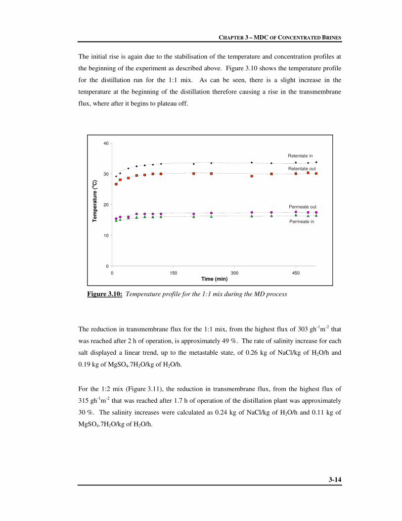
CHAPTER 3 – MDC OF CONCENTRATED BRINES
3-14
The initial rise is again due to the stabilisation of the temperature and concentration profiles at
the beginning of the experiment as described above. Figure 3.10 shows the temperature profile
for the distillation run for the 1:1 mix. As can be seen, there is a slight increase in the
temperature at the beginning of the distillation therefore causing a rise in the transmembrane
flux, where after it begins to plateau off.
0
10
20
30
40
0 150 300 450
Time (min)
Te
mp
era
ture
(oC
)
Retentate in
Retentate out
Permeate in
Permeate out
Figure 3.10: Temperature profile for the 1:1 mix during the MD process
The reduction in transmembrane flux for the 1:1 mix, from the highest flux of 303 gh-1m-2 that
was reached after 2 h of operation, is approximately 49 %. The rate of salinity increase for each
salt displayed a linear trend, up to the metastable state, of 0.26 kg of NaCl/kg of H2O/h and
0.19 kg of MgSO4.7H2O/kg of H2O/h.
For the 1:2 mix (Figure 3.11), the reduction in transmembrane flux, from the highest flux of
315 gh-1m-2 that was reached after 1.7 h of operation of the distillation plant was approximately
30 %. The salinity increases were calculated as 0.24 kg of NaCl/kg of H2O/h and 0.11 kg of
MgSO4.7H2O/kg of H2O/h.

CHAPTER 3 – MDC OF CONCENTRATED BRINES
3-15
0
100
200
300
0 100 200 300 400
Time (min)
Flu
x(g
h-1
m-2
)
0
2
4
6
8
Co
ncen
trati
on
(m)
[NaCl]
[MgSO ]4
Figure 3.11: Trend of transmembrane flux and concentration of salts during the course
of the MDC of the 1:2 mix
The transmembrane flux for the 1:3 mix (Figure 3.12) was reduced by 60 % from its highest
value of 278 gh-1
m-2
that was reached after 3 h of operation of the distillation plant. The salinity
increases were of the order 0.12 kg of NaCl/kg of H2O/h and 0.04 kg of MgSO4.7H2O/kg of
H2O/h.

CHAPTER 3 – MDC OF CONCENTRATED BRINES
3-16
0
100
200
300
0 100 200 300Time(min)
Flu
x(g
h-1
m-2
)
0
2
4
6
Co
nc
en
tra
tio
n(m
)
[MgSO ]4
[NaCl]
Figure 3.12: Trend of transmembrane flux and concentration of salts during the course
of the MDC of the 1:3 mix
The characteristic trend of decreasing transmembrane flux will be investigated by examining the
vapour pressure driving force for the MD process to see if these two relationships could be
correlated. This is discussed in Chapter 5 of this thesis.
3.3 CONCLUSIONS
The MDC technique has proved successful for the recovery of solid products from concentrated
salt solutions. Due to the characteristics described in Chapter 2, this process overcomes many
shortcomings of conventional purification and crystallisation processes. A maximum
temperature of only 33 oC on the retentate line and a minimum of approximately 17 oC on the
distillate line was necessary to afford a significant vapour pressure difference and hence driving
force for the separation. Furthermore, pure water was produced with the recovery of crystalline
product without the need for additional applied pressure or elevated temperature gradients.
However, one of the main shortcomings of this process as seen above, is the rapid decline in
flux that is observed after the metastable phase, when crystallisation occurs. This flux decline
prevents the concentration process from proceeding after the initial crystallisation has
commenced. The flux could be more accurately evaluated if knowledge of the vapour pressures

CHAPTER 3 – MDC OF CONCENTRATED BRINES
3-17
of the solutions was possible. This would enable the assessment of the process on the basis of
the driving force and improve the predictability of the separation. Therefore it becomes crucial
to be able to evaluate the vapour pressures of the solutions. However, this determination cannot
be performed during the experiment itself. Furthermore, the chemistry of strong electrolytes is
complicated and the evaluation of the activity coefficient of these systems leads one to
encountering a series of complex thermodynamic models.
3.4 CHAPTER REFERENCES
AL-JIBBOURI S and ULRICH J (2001) The influence of impurities on crystallisation kinetics
of sodium chloride. Cryst Res Technol 234 (12) 1365-1375.
AL-JIBBOURI S and ULRICH J (2002) The growth and dissolution of sodium chloride in a
fluidized bed crystallizer. J Cryst Growth 234 237-246.
AL-JIBBOURI S, STREGE C and ULRICH J (2002) Crystallization kinetics of epsomite
influenced by pH-value and impurities. J Cryst Growth 236 400-406.
CRISCUOLI A and DRIOLI E (1999) Energetic and exergetic analysis of an integrated
membrane desalination system. Desalination 124 243-249.
DAVEY RJ and GARSIDE J (2000) From molecules to crystallisers. Oxford University Press
Inc., New York. ISBN: 0 19 850489 6.
DRIOLI E, CURCIO E, CRISCUOLI A and DI PROFIO G (2004) Integrated system for
recovery of CaCO3, NaCl and MgSO4.7H2O from nanofiltration retentate. J Membr Sci 239
27-38.
RAMALINGOM S, PODDER J, NARAYANA S and BOCELLI G (2003) Habit modification
of epsomite in the presence of urea. J Cryst Growth 247 523-530.
SARTI GC, GOSTOLI C and MATULLI S (1985) Low energy cost desalination processes
using hydrophobic membranes. Desalination 56 277-286.

CHAPTER 3 – MDC OF CONCENTRATED BRINES
3-18
TUN CM, FANE AG, MATHIECKAL JT and SHEIKHOLESLAMI R (2005) Membrane
distillation crystallization of concentrated salts – flux and crystal formation. J Membr Sci
257 144-147.

Chapter 4
HIGH IONIC STRENGTH ELECTROLYTE
MODELLING
4-1
Knowledge of the thermodynamic properties, such as activity and osmotic
coefficients, of the components in a system is essential in any chemically related
field. This chapter therefore provides an overview of the methods that are
available for the modelling of electrolytes systems, particularly focussing on high
ionic strength electrolyte systems. In Section 4.1 the theoretical equations
concerning the calculation of osmotic and activity coefficients of high ionic
strength solutions are described together with an evaluation of the shortcomings
of certain models and suitability of others for modelling these systems. The Pitzer
approach appears to be the most suitable for modelling of high ionic strength
electrolyte systems. Section 4.2 describes the geochemical equilibrium computer
model known as PHRQPITZ which uses the Pitzer virial coefficient approach for
calculation of activity coefficients in brines and other related systems. The
features and ability of this program for modelling high ionic strength systems are
described.
4.1 THERMODYNAMICS OF HIGH IONIC STRENGTH SOLUTIONS
In subjects such as sea water desalination, solution crystallisation, extractive distillation,
geothermal energy recovery, chemical oceanography, pulp and paper chemistry and prediction
of vapour-liquid equilibrium data in systems containing salts, knowledge on the solubility of the
electrolytes is essential (Anderko et al., 2002, Das, 2003 and Hu and Guo, 1999). In order to
ascertain these solubility predictions, thorough knowledge of the principle thermodynamic
properties, such as the chemical speciation and osmotic and activity coefficients, is mandatory.
Failure to do so could lead to large errors when predicting the solubility in aqueous
multicomponent ionic solutions of high ionic strength, irrespective if only a few chemical
species are present in the solution. For this purpose, there is a growing interest in the
determination of activity coefficients and solubility data of electrolytes in solutions.

CHAPTER 4 – HIGH IONIC STRENGTH ELECTROLYTE MODELLING
4-2
There have been extensive experimental and theoretical investigations into the thermodynamic
properties of aqueous electrolytes. Literature provides various models for the determination of
these thermodynamic properties (Anderko et al., 2002, Bromley, 1973, Davies, 1938,
Guggenheim and Turgeon, 1954, Hu and Guo, 1999, Meissner et al., 1972, Meissner and Kusik,
1972, Meissner and Tester, 1972, Pitzer, 1973 and Wang et al., 2002 and 2004). Most of these
models are based on work performed by Debye and Hückel (1923) on the thermodynamic
properties of electrolyte solutions. The formulae derived by Debye and Hückel were based on
the model of rigid ions, all of which were assumed to have equal diameters. The Debye-Hückel
Limiting Law calculates the mean activity coefficient, γ±, according to Equation 4.1,
IBzz I||log10 −+± −=γ [4.1]
where, BI is a quantity that depends on properties such as molar absorptivity and temperature, z
is the charge on the ion and I is the ionic strength of the solution and is described according to
Equation 4.2,
∑=i
ii zcI2
2
1 [4.2]
where ci is the molar concentration of the ions of type i (Laidler and Meiser, 1999). The
limiting law depends only on the valences of the ions, the temperature and dielectric constant of
the solvent. However, in concentrated solutions the sizes of the ions and their effects on the
dielectric constants must be taken into accounted (Scatchard, 1936). If the theory is modified to
account for the space occupied by the ions by assuming that the ions are restricted to a distance
a between them, then Equation 4.1 is modified to Equation 4.3,
IaB
IBzz
I
I
'101
||log
+−= −+
±γ [4.3]
where BI’ is the new constant. Furthermore one needs to take into account the orientation of
solvent molecules by the ionic atmosphere (Equation 4.4),
ICIaB
IBzzI
I
I ++
−= −+± '10
1
||log γ [4.4]

CHAPTER 4 – HIGH IONIC STRENGTH ELECTROLYTE MODELLING
4-3
where CI is a constant and the term CII, known as the salting-out term, which dominates at high
ionic strengths thus accounting for the lowered solubility of salts under these concentrations
(Laidler and Meiser, 1999). Equation 4.4 is known as the extended Debye-Hückel formula. The
application of the extended Debye-Hückel equation to binary systems (e.g. NaCl in H2O) has
been well studied by Robinson (1965). They found reasonable agreement to ionic strengths of
up to 1 m. However, the use of this model for more complex systems of higher ionic strength
has been found to be inadequate (Harvie and Weare, 1980). For this reason numerous attempts
were made in order to establish equations to fit the high ionic strength behaviour of brines. One
of the most primitive attempts for mixed electrolyte systems was the Brönsted-Guggenheim
specific interaction model. This approach, proposed by Guggenheim (1935) based on
Brönsted’s (1922) principle of specific interaction, appears to be theoretically and
experimentally consistent, and is an extension of the Debye-Hückel limiting law for mixed
electrolytes by using a second virial expansion of the activity coefficient. In the Brönsted-
Guggenheim model the second virial coefficient was included to account for the short range
forces that are experienced by pairs of ions of opposite charge as well as the solvent structure
(Harvie and Weare, 1980). The general form for the activity coefficient, γMX, and the osmotic
coefficient, φ, for a mixed electrolyte is shown in Equations 4.5.
∑ ∑+
++
+
+
−=a c
cXc
XM
XMaa
XM
MXM
MX mm
I
IzzAβ
νν
νβ
νν
νγ
γ 22
1
||ln
2
1
2
3
[4.5a]
∑∑∑ ∑ +
−
+=−
−
c a
caac
c a
ac mmIIAmm βσφ φ2
1
2
31
21 [4.5b]
where νM and νX are the numbers of ions in the formula, m is the conventional molality and the
sums cover all cations c and all anions a. The function σ(x) and the Debye-Hückel parameters
Aγ and Aφ,, have the form shown in Equations 4.6.
( )( )
( )
+−
+−+
= x
xx
xx 1ln2
1
11
33
σ [4.6a]

CHAPTER 4 – HIGH IONIC STRENGTH ELECTROLYTE MODELLING
4-4
φγ
φ
π
A
kTD
el
ldN
A
w
w
3A
where
1000
2
3
1
2
2
32
1
0
=
=
=
[4.6b]
Aγ and Aφ are the Debye-Hückel coefficients for the activity and osmotic functions, respectively,
N0 Avagadro’s number and dw and Dw are the density and dielectric constant of water at 25 °C,
respectively. ℓ is a parameter which expresses the distance at which the electrostatic energy for
singly charged ions in the dielectric just equals thermal energy (Pitzer, 1973). The parameters β
are constants at a given temperature.
For single 1-1 electrolytes, Equations 4.5 takes the form of Equations 4.7 below.
m
m
mAMXβγ
γ2
1
ln2
1
2
1
+
+
−= [4.7a]
mmmA MXβσφ φ +
−=− 2
1
2
1
1 [4.7b]
Guggenheim and Turgeon (1954) demonstrated that Equations 4.7 were in good agreement with
experiment data up to concentrations of 0.1 m for 1-1 electrolytes in water at 0 °C and room
temperature. However, above these concentrations considerable discrepancies occur. For
mixed electrolyte systems, the work of Whitfield (1973 and 1974) confirmed that this theory is
accurate for concentrations up to 4 m. However, for concentrations above 4 m Scatchard
(1968), Scatchard et al. (1970) and Pitzer (1973) demonstrated that third or higher order virial
coefficients must be included to account for the short range potential between like-charged ions
and solvent structure which become important at significantly high concentrations. Mayer
(1950) suggested that the virial expansion will result in Equation 4.4 taking the form of,
( ) ( )∑ ∑ +++=j jk
kjijkjijDHi mmICmIB ...lnln γγ [4.8]

CHAPTER 4 – HIGH IONIC STRENGTH ELECTROLYTE MODELLING
4-5
where Bij(I) and Cijk(I) are the second and third virial coefficients respectively, and lnγDH is the
Debye-Hückel coefficient from Equation 4.4. Harvie and Weare (1980) demonstrated that
second and third virial coefficients are essential to predict mineral solubilities and
thermodynamically stable paragenesis. For this reason the Pitzer equation seems to be the most
appropriate choice to model high ionic strength electrolyte systems.
The Pitzer approach begins with a virial expansion of the excess free energy and takes the form
of Equation 4.6. This approach is used because, in order to predict mineral solubilities
knowledge of the osmotic and activity coefficients is required. However, these quantities are
not independent and must be consistent with the laws of thermodynamics (Harvie and Weare,
1980). The excess free energy, Gex, is the difference in the actual free energy and the free
energy of an ideal solution of the same composition.
( ) ( )
++= ∑ ∑∑∑∑
i i j k
kjiijkji
j
ijw
ex mmmmmIIfnRT
Gµλ [4.9]
where nw is the mass of water, mi and mj the molality of species i and j, respectively, f(I) is the
Debye-Hückel type term and λij(I) and µijk are the second and third virial coefficients
respectively. λij(I) represents short-range interaction in the presence of the solvent between
solute particles i and j. This second virial coefficient parameter, for ions, depends on ionic
strength, the type of solute species i and j, and the temperature and pressure. For neutral species
however, there is no composition dependence (Pitzer, 1991). The third virial coefficient
parameter µijk, in principle should be ionic strength dependent, but there is no experimental
verification for this observation (Pitzer, 1991). The derivative of Equation 4.9, with respect to
the number of moles of each component, results in expressions for the osmotic and activity
coefficients. Since the functionality λij(I) cannot be determined experimentally, but sums and
differences of λ’s are measurable, Equation 4.9 is re-written in terms of the sums and
differences of the measurable quantities λ’s and µ’s. Therefore in the Pitzer ion interaction
model the fundamental equations for the osmotic coefficient, φ and activity coefficients, γΜ and
γX, for cations and anions respectively, in a mixed electrolyte system, are given in
Equations 4.10 (Harvie and Weare, 1980, Pitzer, 1973, Pitzer, 1991 and Plummer et al., 1988).
The equations considered below are for those in mixtures of strong electrolytes, as is the case of
this work.

CHAPTER 4 – HIGH IONIC STRENGTH ELECTROLYTE MODELLING
4-6
( )
( )
+Φ
+
+Φ
++++
−
=−
∑ ∑ ∑
∑ ∑ ∑
∑∑
∑<
<
' '''
' '''
21
23
1
21
aac
caacaaaa
cca
accacccc
c a
cacaac
i
i
mmm
mmm
ZCBmmbI
IA
m
ψ
ψφ
φ
φ
φφ
[4.10a]
( )
∑∑
∑ ∑ ∑ ∑∑ ++
+Φ+++=
<
c a
caacM
a caa Maaaa
a
McaaMccMaMaaMM
Cmmz
mmmmZCBmFz
||
22ln' ''
2 ψψγ
[4.10b]
( )
∑∑
∑ ∑ ∑ ∑∑ ++
+Φ+++=
<
c a
caacX
c acc Xcccc
c
XaccXaacXcXcXX
Cmmz
mmmmZCBmFz
||
22ln' ''
2 ψψγ
[4.10c]
where mc is the molality of cation c with charge zc. The subscripts M, c and c’ refer to cations
and X, a and a’ anions. The summation index c refers to the sum over all cations and the double
summation index c<c’ the sum over all distinguishable pairs of dissimilar cations; similarly, for
the anions. The other quantities have the form as shown in Equations 4.11 to 4.13.
The quantity F includes the Debye-Hückel terms amongst others as shown by Equation 4.11a.
( )
∑∑ ∑ ∑ ∑ ∑< <Φ+Φ+
+
++
+−=
c acc aa aaaacccccaac mmmmBmm
IbbIb
IAF
' '
'''
'''
'
1ln2
1
φ
[4.11a]
and Aφ has been defined in Equation 4.6b. Aφ is 0.392 for water and b is a universal empirical
parameter assigned to be 1.2 at 25 °C.

CHAPTER 4 – HIGH IONIC STRENGTH ELECTROLYTE MODELLING
4-7
The coefficients BMX are functions of ionic strength and are defined as,
( )( ) IIgB
IgB
eB
MXMX
MXMXMX
I
MXMXMX
/')1('
)1()0(
)1()0(
αβ
αββ
ββ αφ
=
+=
+= −
[4.11b]
where g and g’ are,
( )[ ]
2
2
2
2
1112
)('
112)(
x
exx
xg
x
exxg
x
x
++−−
=
+−=
−
−
[4.11c]
and Ix α= .
The remaining terms in Equations 4.10 contain either single electrolyte third virial coefficients,
CMX, or mixed electrolyte coefficients, Φij and ψijk. The latter two terms account for interactions
of like sign. Z is a concentration dependence function.
|| ii
i
zmZ ∑= [4.12]
The parameters Φij and ψijk are determined from aqueous mixtures of two salts. Φij accounts for
like-charge interactions, cation-cation and anion-anion, while ψijk accounts for interactions of
the form cation-cation-anion and anion-anion-cation. Values of Φij are given in Equation 4.13.
( ) ( )
( )
( )I
I
III
ij
E
ij
ij
E
ijij
ij
E
ij
E
ijij
''
'
θ
θθ
θθθφ
=Φ
+=Φ
++=Φ
[4.13]
θij is a single parameter for each pair of anions or cations and the terms Eθij(I) and Eθ’ij(I)
account for electrostatic unsymmetric mixing effects of cation-cation and anion-anion pairs.

CHAPTER 4 – HIGH IONIC STRENGTH ELECTROLYTE MODELLING
4-8
The main characteristics of models of Pitzer and similar ion interaction models, take into
account interactions between pairs of ions of like sign and also triplets of ions. This
consideration enables calculations to be performed for multicomponent solutions at high
concentrations (Pitzer, 1991). Pitzer’s model has gained much popularity since the 1990s
especially within the geochemical field. Perhaps the most extensive geochemical application of
the Pitzer model is for the studies of mineral solubilities in brines (Pitzer, 1986). These are
widespread and include the calculation of gypsum and halite solubility, study of evaporate
sequences, alkaline earth sulphate solubilities in deep brines, scale mineral formation in oilfield
brines and equilibria in acid mine drainage waters (Fürst and Renon, 1982 and Pitzer, 1991).
The model has also been extended to include neutral species and incorporated into geochemical
computer models such as PHRQPITZ (Plummer et al., 1988).
4.2 GEOCHEMICAL EQUILIBRIUM MODELLING
The origin and evolution of natural systems has been described by numerous geochemical
models based on thermodynamics from as early as 1912 after Van’t Hoff’s first interpretation to
clarify field observations (Harvie and Weare, 1980 and Harvie et al., 1984). Reviews of
Nordstrom et al. (1979), Kerrisk (1981) and Bethke (1996) exemplifies the extent of work that
has been performed on thermodynamic equilibrium modelling of natural saline brines. A
number of mathematical models encompassing years of research is now available for the
modelling of geochemical systems. These include programs such as PHREEQE, PHREEQC,
MINTEQA2 and WATEQ, amongst others. For the representation of the behaviour of mixed
electrolyte systems up to high concentrations, a specific model based on virial expansion with
ionic strength dependent virial coefficients is required (Harvie et al., 1984). For this reason the
models mentioned above are inappropriate as the activity coefficient calculations are mainly
based on equations such as the Debye-Hückel and Davies equations. As such these models are
limited to calculations in systems of low ionic strength. For systems of high ionic strength the
Pitzer virial coefficient approach for calculating osmotic and activity coefficients therefore
seems to fit the above requirements aptly.

CHAPTER 4 – HIGH IONIC STRENGTH ELECTROLYTE MODELLING
4-9
4.2.1 PHRQPITZ
The computer program, PHRQPITZ, is able to perform geochemical calculations in brines and
other electrolyte systems to high concentrations (Plummer et al., 1988). This is possible as the
main code of this program uses the Pitzer virial coefficient approach for activity coefficient
corrections according to the works of Harvie (1980) and Harvie et al. (1984) for the prediction
of mineral solubilities in natural waters for the Na-K-Mg-Ca-H-Cl-SO4-OH-HCO3-CO3-CO2-
H2O system to high ionic strengths. PHRQPITZ is an adaptation of the original program called
PHREEQE in that the aqueous model of the latter has been replaced with the Pitzer virial
coefficient approach, in order to extend the modelling capability range in terms of ionic strength
(Parkhurst, 1995). This approach is described mainly in the equations presented in Section 4.1.
The activity of water, aH2O, is computed from the osmotic coefficient, φ, given in
Equation 4.10a, according to Equation 4.14.
50837.55ln
2
∑−= i
i
OH
m
a
φ
[4.14]
where mi is the molality of the ith ion in solution and there are 55.0837 moles of water per
kilogram of water.
The main input parameters into the program include the total analytical content of the system as
well as information such as pH and temperature. However, the number and type of input
parameters that the program would require varies according to the reaction being modelled
(Appendix A gives a detailed description of the input and output files from PHRQPITZ). Some
of the main reaction modelling potentials of PHRQPITZ includes (Plummer et al., 1988):
� Aqueous speciation and mineral-saturation index.
� Mineral solubility.
� Mixing or titrations of aqueous solutions.
� Irreversible reactions and mineral-water mass transfer.
� Reaction path.
The general types of reactions that can be simulated in PHRQPITZ are as follows:

CHAPTER 4 – HIGH IONIC STRENGTH ELECTROLYTE MODELLING
4-10
� Mixing of two solutions.
� Titrating one solution with a second solution.
� Adding or subtracting a net stoichiometric reaction (changing total concentrations of
elements in proportion to a given stoichiometry).
� Adding a net stoichiometric reaction until the phase boundary of a specified mineral is
reached.
� Equilibrating with mineral phases. Any condition which can be written in the form
( ) ( )∑=i
iipp acK loglog , [4.15]
where ai is the activity of the ith aqueous species, cp,i is the stoichiometric coefficient of
the ith aqueous species in the p
th phase, and Kp is the equilibrium constant for the pth
phase, is considered a mineral phase.
� Changing temperature.
The output of the calculations performed with PHRQPITZ includes the osmotic coefficient,
water activity, mineral saturation indices, mean-activity coefficients, total-activity coefficients,
and scale-dependent values of pH, individual ion activities and individual ion activity
coefficients.
4.2.1.1 Precautions and Limitations of PHRQPITZ
Although the program can be applied to a wide range of hydrogeochemical environments, there
does exist some limitations to the use of this program for modelling. Of the precautions and
limitations described by Parkhurst (1995) and Plummer et al. (1988) a few of the more possibly
applicable ones to the modelling performed in this work are described below:
� The temperature range for the equilibria in the PHRQPITZ database is variable and is
from 0 to 60 °C, if ∆Ηr is known. However, the values in the database for the NaCl
system are valid to a temperature of approximately 350 °C, and those for the carbonate
system are consistent to approximately 100 °C. The precaution in terms of temperature
limitations is provided, as the solubility of the minerals in the PHRQPITZ database is
not precisely known and could lead to large errors if calculations are made outside these

CHAPTER 4 – HIGH IONIC STRENGTH ELECTROLYTE MODELLING
4-11
temperature ranges for these solids. Furthermore, PHRQPITZ provides a (nonfatal)
warning when the temperature is outside the interval 0 to 55 °C.
� PHRQPITZ is based on the Na-K-Mg-Ca-H-Cl-SO4-OH-HCO3-CO3-CO2-H2O system
of Harvie et al. (1984). The mineral database is therefore limited to these mineral
precipitates. Other minerals such as Fe2+, Mn2+, Sr2+, Ba2+, Li+ and Br- have been
manually included, however, this extension to the database has not been validated.
� As the individual ion activities and activity coefficients are not independently
measurable quantities, Equations 4.10b and 4.10c are only valid when individual ion
activity coefficients are combined to define properties of neutral combinations of ions,
e.g. in the calculation of mean activity coefficients, saturation indices and solubility. As
such, the individual ion activities and activity coefficients are only meaningful on a
relative scale. Therefore, the individual values of these parameters would depend on
the choice of scale convention. PHRQPITZ provides a choice of two scale conventions,
viz. no scaling which results in Equations 4.10b and 4.10c being used to calculate the
individual ion activity coefficients, or scaling using the MacInnes convention. In the
latter case the activity coefficient of Cl is defined to be equivalent to the mean activity
coefficient of KCl in a KCl solution of equal ionic strength, i.e. KClMacCl ±≡ γγ )( . A
problem may arise when the measured pH is introduced in geochemical calculations
and may lead to erroneous calculations of mean activities and saturation indices. This is
because the measured pH is unlikely to be on the same activity coefficient scale as the
aqueous model as the buffers used to define pH are conventional (Plummer et al.,
1988). Furthermore, it has been observed that even if the measured pH is on the same
scale as the aqueous model, uncertainties in the calibration of pH in brines, like those
due to liquid-junction potentials, will introduce inconsistencies in activity coefficient
computations (Bates, 1973 and Wescott 1978). Therefore, when using measured pH
values of brines, it is important to recognise the magnitude of error that can accompany
the evaluation of mean activity and saturation indices due to the differences in the scale
of activity coefficients. This problem of pH is particularly important when performing
calculations in carbonate systems of high ionic strength brines.

CHAPTER 4 – HIGH IONIC STRENGTH ELECTROLYTE MODELLING
4-12
4.2.1.2 How to Solve a Problem with PHRQPITZ
Like in any analyses, one is initially faced with a problem relating to real world situations
(Figure 4.1). The first step therefore, is the conversion of a real problem into chemical terms.
Ideal components necessary to formulate the problem must be considered together with possible
separations (if necessary). Once the problem has been formulated, it then needs to be input into
the computer program.
There are certain limitations considering the use of a program for modeling and these must be
considered before commencing with the problem solution. Restrictions such as the available
species in the thermodynamic database and ionic strength limitations must be taken into
account. The application of a geochemical equilibrium model to an environmental problem
involves four basic steps (Allison et al., 1991 and Wadley and Buckley, 1997):
i) Formulate one or more precise and relevant chemical questions that can be answered
if one knows the equilibrium composition of the system. The formulation of the
chemical questions must respect the inherent limitations in the site-specific data such
as incomplete sampling or incomplete chemical analyses of samples.
ii) Pose the chemical questions to the model in terms of those symbols and formats
appropriate to the computer program and from which the program may interpret a
mathematical problem.
iii) Cause the program, i.e. the geochemical equilibrium model, to solve the mathematical
problem.
iv) Interpret the output from the model in terms of the original environmental problem.
PHRQPITZ is designed to carry out a series of simulations in a single computer run. Each
simulation consists of two separate problems – processing of an initial solution and / or
modelling of a reaction (Plummer et al., 1988). The first step is almost always the most
difficult – the ability to do this well improves with each application of the program. The input
file for the program is PITZINPT and is designed to perform step (ii) by asking questions about
the chemical system to be modelled and building the appropriate input file from the answers
(this is described in detail in Appendix A). Step (iii), the actual execution of the calculations is
automatic once initiated. In some instances computational problems may occur during
execution which would require the user to modify the input file accordingly.

CHAPTER 4 – HIGH IONIC STRENGTH ELECTROLYTE MODELLING
4-13
Figure 4.1: Sequence of solving a problem in PHRQPITZ (adaptation of Allison et al., 1991
and Wadley and Buckley, 1997)
Analytical Information
Add other components
Define problem to be modelled
Choose components, ideal reactants,
separations, etc.
Exclude kinetically unfavourable
reactions
Add or modify thermodynamic
data
Add or modify empirical constants
Input information into model
Determine interactions between
components
Obtain formation constants
Adjust constants for temperature/concen-
tration
Calculate speciation/reaction &
create output file
Interpret model in terms of original
problem
Validate by comparing with
experiments
translate
“Chemistry”
problem
RE
VIS
E M
OD
EL
NO
PITZINPT
PHRQPITZ
“Real world”
problem
Use model for next problem
Are results acceptable?
YES

CHAPTER 4 – HIGH IONIC STRENGTH ELECTROLYTE MODELLING
4-14
Step (iv) is executed by the user by examining the PHRQPITZ output file and relating the
results to the initial problem. This is then followed by validation of the results. This can only
be performed physically by the necessary experiments and comparison with the appropriate
literature.
4.3 CHAPTER REFERENCES
ALLISON JD, BROWN DS and NOVO-GRADAC KJ (1991) MINTEQA2/PRODEFA2, A
geochemical assessment model for environmental systems: Version 3.0 User’s Manual,
EPA/600/3-91/021, Environmental Research Laboratory, Office of Research and
Development, US Environmental Protection Agency, Athens, Georgia.
ANDERKO A, WANG P and RAFAL M (2002) Electrolyte solutions: from thermodynamic
and transport property models to the simulation of industrial processes. Fluid Phase
Equilibria 194-197 123-142.
BATES RG (1973) Determination of pH, Theory and Practice, 2nd edition, John Wiley and
Sons, New York. ISBN: 0-471-05647-2.
BETHKE CM (1996) Geochemical Reaction Modeling: Concepts and applications, Oxford
University Press, New York. ISBN: 0 19 509475 1.
BROMLEY LA (1973) Thermodynamic properties of strong electrolytes in aqueous solutions.
AIChE Journal 19(2) 313-320.
BRÖNSTED JN (1922) Studies on solubility. IV. The principle of the specific interaction of
ions. J Am Chem Soc 44(5) 877-898.
DAS B (2003) Pitzer ion interaction parameters of single aqueous electrolytes at 25oC. J Soln
Chem 33(1) 33-45.
DAVIES CW (1938) The extent of dissociation of salts in water. Part VIII. An equation for the
mean ionic activity coefficient of an electrolyte in water, and a revision of the dissociation
constants of some sulphates. J Chem Soc 2093-2098.

CHAPTER 4 – HIGH IONIC STRENGTH ELECTROLYTE MODELLING
4-15
DEBYE and HÜCKEL (1923) Zur theorie der electrolyte. Phys Z 24 185-208.
FÜRST W and RENON H (1982) Effect of the various parameters in the application of Pitzer’s
model to solid-liquid equilibrium. Preliminary study for strong 1-1 electrolytes. Ind Eng
Chem Process Des Develop 21 396-400.
GUGGENHEIM EA (1935) The specific thermodynamic properties of aqueous solutions of
strong electrolytes. Philos Mag 19 588-643.
GUGGENHEIM EA and TURGEON JC (1954) Specific interaction of ions. Trans Faraday Soc
51 747-761.
HARVIE CE, MØLLER N and WEARE JH (1984) The prediction of mineral solubilities in
natural waters: The Na-K-Mg-Ca-H-Cl-SO4-OH-HCO3-CO3-CO2-H2O system to high ionic
strengths at 25 °C. Geochimica et Cosmochimica Acta 48 723-751.
HARVIE CE and WEARE JH (1980) The prediction of mineral solubilities in natural waters:
the Na-K-Mg-Ca-Cl-SO4-H2O system from zero to high concentration at 25 °C. Geochimica
et Cosmochimica Acta 44 981-997.
HU Y-F and GUO T-M (1999) Thermodynamics of electrolytes in aqueous systems containing
both ionic and non-ionic solutes. Application of the Pitzer-Simonson-Clegg equations to
activity coefficients and solubilities of 1:1 electrolytes in four electrolyte-non-electrolyte-
H2O ternary systems at 298.15 K. Phys Chem Chem Phys 1 3303-3308.
KERRISK JF (1981) Chemical equilibrium calculations for aqueous geothermal brines. Los
Alamos Sci Lab Report LA-8851-MS., Los Alamos, N.M. 87545.
LAIDLER KJ and MEISER JH (1999) Physical Chemistry, 3rd edition, Houghton Mifflin
Company, New York. ISBN 0-395-91848-0.
MAYER JE (1950) The theory of ionic solutions. J Chem Phys 18 1426-1436.
MEISSNER HP and KUSIK CL (1972) Activity coefficients of strong electrolytes in
multicomponent aqueous solutions. AIChE Journal 18(2) 294-298.

CHAPTER 4 – HIGH IONIC STRENGTH ELECTROLYTE MODELLING
4-16
MEISSNER HP, KUSIK CL and TESTER JW (1972) Activity coefficients of strong electrolytes
in aqueous solution-effect of temperature. AIChE Journal 18(3) 661-662.
MEISSNER HP and TESTER JW (1972) Activity coefficients of strong electrolytes in aqueous
solutions. Ind Eng Chem Process Des Develop 11(1) 128-133.
NORDSTROM PK, PLUMMER LN, WIGLEY TM, WOLERY TJ, BALL JW, JENNE EA,
BASSET RL, CRERAR DA, FLORENCE TM, FRITZ B, HOFFMAN M,
HOLDREN GR.Jr., LAFON GM, MATTIGOD SV, McDUFF RE, MOREL F, REDDY
MM, SPOSITO G and THRAILKILL J (1979) A comparison of computerized chemical
models for equilibrium calculation in aqueous systems. ACS Symposium Series No. 93, 857-
892.
PARKHURST DL (1995) User’s guide to PHREEQC – A computer program for speciation,
reaction-path, advective-transport and inverse geochemical calculations, US Geological
Survey, Water-Resources Investigations Report 95-4227, Lakewood, Colorado.
PITZER KS (1973) Thermodynamics of electrolytes I: Theoretical basis and general equations.
J Phys Chem 77 268-277.
PITZER KS (1986) Theoretical considerations of solubility with emphasis on mixed aqueous
electrolytes. Pure Appl Chem 58 1599 1612.
PITZER KS (1991) Chapter 3. Theory: Ion Interaction Approach. In Activity coefficients in
electrolyte solutions, PYTKOWICZ RM, ed., Boca Raton Fla: CRC , London. ISBN:
0-8493-5411-0, 77.
PLUMMER LN, PARKHURST DL, FLEMING GW and DUNKLE SA (1988) A computer
program incorporating Pitzer’s equations for calculation of geochemical reactions in brines,
US Geological Survey, Water-Resources Investigations Report 88-4153, Reston, Virginia.
ROBINSON RA and SROKES RH (1965) Electrolyte Solutions, Butterworths, London.
SCATCHARD G (1936) Concentrated solutions of strong electrolytes. Chem Rev 19 309 -327.

CHAPTER 4 – HIGH IONIC STRENGTH ELECTROLYTE MODELLING
4-17
SCATCHARD G (1968) The excess free energy and related properties of solutions containing
electrolytes. J Am Chem Soc 90 3124-3127.
SCATCHARD G, RUSH RM and JOHNSON JS (1970) Osmotic and activity coefficients for
binary mixtures of sodium chloride, sodium sulphate, magnesium sulphate and magnesium
chloride in water at 25 °C. III: Treatment with the ions as components. J Phys Chem 74
3786-3796.
WADLEY S and BUCKLEY CA (1997) Chemical speciation self-study work manual, WRC
Project No. K8/208, Pollution Research Group, Department of Chemical Engineering,
Durban, South Africa.
WANG P, ANDERKO A and YOUNG RD (2002) A speciation-based model for mixed-solvent
electrolyte systems. Fluid Phase Equilibria 203 141-176.
WANG P, SPRINGER RD, ANDERKO A and YOUNG RD (2004) Modeling phase equilibria
and speciation in mixed-solvent electrolyte systems. Fluid Phase Equilibria 222-223 11-17.
WESCOTT CC (1978) pH measurements, Academic Press, New York. ISBN: 0-12-745150-1
WHITFIELD M (1973) A chemical model for the major electrolyte components of seawater
based on Brönsted-Guggenheim hypothesis. Mar Chem 1 251-266.
WHITFIELD M (1974) An improved specific interaction model for seawater at 25 °C and
1 atmosphere total pressure. Mar Chem 3 197-213.

Chapter 5
VAPOUR PRESSURE MODELLING AND
EXPERIMENTS
5-1
This Chapter forms the second and final approaches in the series of methods
described in Chapter 1, i.e. the determination of vapour pressures and evaluation
of driving force. The decline in transmembrane flux experienced during the MD
experiments described in Chapter 3 is addressed by evaluating the vapour
pressures of the solution and hence driving force of the MD process which will
indicate the nature of the flux decline. Section 5.1.1 illustrates the use of the
computer program PHRQPITZ to model vapour pressures. The suitability of the
program to accurately model vapour pressures was validated by vapour-liquid
equilibrium experiments performed using the dynamic vapour-liquid equilibrium
still which is described in Section 5.1.2. The results obtained are described in
Section 5.2 - the results of the VLE experiments are discussed in Section 5.2.1
while the comparison between the experimental data and those modelled are
shown in Section 5.2.2. PHRQPITZ was then used to model the vapour pressures
of the solutions throughout the MD process which led to the evaluation of the
driving force. Section 5.2.3 compares and discusses the trend displayed between
the flux and driving force. Section 5.3 demonstrates the potential of PHRQPITZ
to predict and thus possibly enable finer control of the MD process. This chapter
ends with a summary in Section 5.4.
5.1 DETERMINATION OF VAPOUR PRESSURES
The initial purpose of this stage of the research stems from the work that was performed with
MD as described in Chapter 3. The problem of the decline in transmembrane flux that was
observed during the batch MD of concentrated salt solutions is an inhibiting factor to the
prolonged functioning of the process. Our aim is to establish why the flux declines, in
accordance with the process description. The only way in which this transmembrane flux could
be evaluated is by measuring the actual driving force for the process, i.e. the vapour pressures of
the solutions which give rise to the driving force for the flux and transport. Since this cannot be

CHAPTER 5 – VAPOUR PRESSURE MODELLING AND EXPERIMENTS
5-2
performed during the experiment itself, one needs a means of evaluating the vapour pressures.
Being able to computationally model the performance of the system outside to the process itself
is an excellent and valuable means of predicting the outcome of the process. The computer
program PHRQPITZ described in Chapter 4 seems to contain the necessary modelling
capabilities for the purposes of this work. Therefore, this program was used in order to
determine the vapour pressures of the solutions that were subject to MD and the results are
described in Section 5.1.1. Before this program could be used further to evaluate the flux
decline during MD, its suitability and accuracy for modelling vapour pressures was validated by
experimental vapour-liquid equilibrium measurements, described in Section 5.1.2.
5.1.1 PHRQPITZ modelling
The program PHRQPITZ is designed to execute a series of simulations in a single computer run
by solving two separate problems: (i) processing of an initial solution/s and (or) (ii) modelling
of a reaction (Plummer, 1988). There are a variety of reactions that can be modelled but in each
type of reaction the initial solutions must be specified. The total concentrations of species as
well as information such as pH and temperature are input into a specific solution which is
assigned a unique number. Any further reactions or mineral equilibria are then performed on
this solution. The output of the calculations performed with PHRQPITZ includes the osmotic
coefficient, water activity, mineral saturation indices, mean-activity coefficients, total-activity
coefficients, and scale-dependent values of pH, individual ion activities and individual ion
activity coefficients. For the purposes of this work, the activity of water was the crucial output
required from PHRQPITZ which was then used to obtain the solution vapour pressures directly
(Equation 5.1), of the three mixes of salt solutions over a range of temperatures. The effective
vapour pressure of a solution (Psoln) is defined as the product of the vapour pressure of pure
water (PH2O) at the same temperature as the solution and the activity of water (αH2O) in the
solution.
OHOHsoln PP22
α= [5.1]
An example of a section of a typical output file, containing the necessary information required
for the purposes of this work, is shown in Table 5.1 with the key information highlighted. The
initial information that was fed to the program was the concentration of the solutions, as shown
under “TOTAL MOLALITIES OF ELEMENTS” and the temperature of the solution. The aim was to

CHAPTER 5 – VAPOUR PRESSURE MODELLING AND EXPERIMENTS
5-3
obtain the activity of water of this solution from which the corresponding vapour pressure was
calculated. Further details of the modelling procedure are explained in Appendix A.
Table 5.1: Example of a section of an output file from PHRQPITZ
MD process for retentate temperatures
0000020000 0 0 0.00000
SOLUTION 1
time=0
4 0 0 7.00 4.00 27.3 1.00
5 1.163D+00 16 1.163D+00 6 4.895D+00 14 4.895D+00
1SOLUTION NUMBER 1
TOTAL MOLALITIES OF ELEMENTS
----- ---------- -- --------
ELEMENT MOLALITY LOG MOLALITY
MG 1.163000D+00 0.0656
NA 4.895000D+00 0.6898
CL 4.895000D+00 0.6898
S 1.163000D+00 0.0656
----DESCRIPTION OF SOLUTION----
PH = 7.0000
ACTIVITY H2O = 0.7391
OSMOTIC COEFFICIENT = 1.3853
IONIC STRENGTH = 9.5469
TEMPERATURE = 27.3000
PRESSURE = 1.0000 ATM
DENSITY OF H2O = 0.9964 G/CC
ELECTRICAL BALANCE = -7.0283D-05
TOTAL ALKALINITY = 7.0567D-05
ITERATIONS = 1
-----------------------
DISTRIBUTION OF SPECIES
-----------------------
UNSCALED UNSCALED
I SPECIES Z MOLALITY LOG MOLAL ACTIVITY LOG ACT GAMMA LOGGAM
1 H+ 1.0 3.005E-08 -7.522 1.000E-07 -7.000 3.327E+00 0.522
3 H2O 0.0 7.391E-01 -0.131 7.391E-01 -0.131 1.000E+00 0.000
5 MG+2 2.0 1.163E+00 0.066 1.179E+00 0.072 1.014E+00 0.006
6 NA+ 1.0 4.895E+00 0.690 3.882E+00 0.589 7.930E-01 -0.101
14 CL- -1.0 4.895E+00 0.690 8.073E+00 0.907 1.649E+00 0.217
16 SO4-2 -2.0 1.163E+00 0.066 2.982E-02 -1.526 2.564E-02 -1.591
31 OH- -1.0 2.526E-07 -6.598 8.822E-08 -7.054 3.493E-01 -0.457
40 HSO4- -1.0 2.539E-07 -6.595 3.029E-07 -6.519 1.193E+00 0.077
85 MGOH+ 1.0 7.031E-05 -4.153 1.651E-05 -4.782 2.348E-01 -0.629
Initially PHRQPITZ was used to gain the activity of water for mixtures of the compositions of
the salt mixes that were used during MD, i.e. 1:1 mix (225 g/ℓ NaCl and MgSO4, i.e. 4.89 and

CHAPTER 5 – VAPOUR PRESSURE MODELLING AND EXPERIMENTS
5-4
1.16 m, respectively), 1:2 mix (275 g/ℓ NaCl and 137.5 g/ℓ MgSO4, i.e. 5.78 and 0.686 m,
respectively) and 1:3 mix (280 g/ℓ NaCl and 93.3 g/ℓ MgSO4, i.e. 5.72 and 0.451 m,
respectively) as described in Section 3.2.2, with arbitrarily chosen temperatures ranging from
303 to 373 K in order to test the applicability of PHRQPITZ to model vapour pressures.
Figures 5.1 and 5.2 show the vapour pressure curves that were obtained for each of the salt
mixes together with that of pure water for comparison.
0
30
60
90
290 310 330 350 370
Temperature (K)
Vap
ou
r p
ress
ure
(kP
a)
1:1 mix
Water
Figure 5.1: Vapour pressure curve for the 1:1 mix predicted through PHRQPITZ
modelling; pure water vapour pressure curve shown for comparison.
The vapour pressure of pure water is higher than that of the hot brine (1:1 mix) at a particular
temperature. It is this difference in vapour pressure that drives the separation during the MD
process as described in Section 2.3.1. The same is true for the other salt concentrations shown
in Figure 5.2 below.

CHAPTER 5 – VAPOUR PRESSURE MODELLING AND EXPERIMENTS
5-5
0
20
40
60
80
100
290 310 330 350 370 390
Temperature (K)
Va
po
ur
pre
ss
ure
(k
Pa
)
1:2 mix
Water
0
20
40
60
80
100
290 310 330 350 370 390
Temperature (K)
Va
po
ur
pre
ss
ure
(k
Pa
)
1:3 mix
Water
Figure 5.2: Vapour pressure curves for the 1:2 and 1:3 mixes predicted through
PHRQPITZ modelling; pure water vapour pressure curve shown for
comparison.
Before proceeding with any further calculations concerning the actual MD process and the
actual temperature and concentration changes occurring during the process, as described in
Section 4.2.1.2, the next stage, in any modelling procedure, is the validation of the vapour
pressure predictions. This can be performed by physically conducting the necessary
experiments or by comparison with the literature.
5.1.2 Vapour-liquid equilibrium measurements
Apart from the purposes of our measurements, which are to obtain the vapour pressure of
inorganic salt solutions, vapour-liquid equilibrium (VLE) data are required in the design of
chemical processes as well as mass transfer equipment such as distillation and absorption
columns (Şeker and Somer, 1993). However, the acquisition of VLE data is not a
straightforward task. Accurate theoretical determination of VLE data is often less feasible due
to the uncertainties in the properties of liquid mixtures. These include parameters such as
fugacity and activity coefficients that cannot merely be estimated by simple theoretical
approaches as they are dependent on the chemical structure and compositions of the compounds.
Furthermore, the majority of theoretical approaches are based on dilute solutions which are not
always appropriate in real situations such as concentration and precipitation. Therefore,
experimental methods for the measurement of VLE data in non-ideal solutions become
mandatory. Various methods exist for the direct measurement of VLE data.

CHAPTER 5 – VAPOUR PRESSURE MODELLING AND EXPERIMENTS
5-6
They are grouped according to the following (Şeker and Somer, 1993):
� Distillation methods.
� Circulation method – mechanical circulation of vapour.
� Static method.
� Dew and bubble point method.
Each of these methods has their characteristic operational parameters and advantages and
disadvantages associated with them (Raal and Mühlbauer, 1998). In the present work the
apparatus known as the vapour-liquid equilibrium still was used to measure the vapour
pressures of solutions of mixtures of inorganic salts, sodium chloride and magnesium sulphate,
as a function of temperature.
5.1.2.1 The vapour-liquid equilibrium still
The particular VLE still developed by Raal and Mühlbauer (1998) has two essential parts:
(i) vaporiser and (ii) equilibrium chamber (Figure 5.3). The binary liquid mixture is placed in
the boiling chamber where it is vaporized by an electrical heating coil within the chamber and a
further external heater which permits rapid boiling of the mixture. The mixture in the boiling
chamber is stirred which ensures that the returning equilibrium mixture is thoroughly mixed
with the original mixture before further evaporation – this prevents flashing. The vapour-liquid
mixture is then forced up the Cottrell tube into the equilibrium chamber. The mixture then
flows downwards through the packing which consists of stainless steel wire mesh cylinders of
3 mm dimension. Close contact between the liquid and vapour in this packed section allows
rapid attainment of equilibrium (Joseph et al., 2001). The temperature in the chamber is
recorded by the thermometer (Pt-100) which extends well inside the equilibrium chamber. The
resulting equilibrium mixture leaves the chamber through the drain holes perforated at the
bottom of the chamber. The released equilibrium liquid then flows down over the stainless steel
mixing spiral before a portion of the liquid is caught in the liquid trap for sampling, whilst the
remainder is returned to the boiling chamber.

CHAPTER 5 – VAPOUR PRESSURE MODELLING AND EXPERIMENTS
5-7
Figure 5.3: Schematic diagram of the vapour-liquid equilibrium still
(Joseph et al., 2001).
The discharged vapour, on the other hand, flows upward forming a thermal lagging around the
equilibrium chamber and, together with the vacuum jacket that insulates the upper portion of the
still, provides an adiabatic environment for the operation of the equilibrium chamber. The
vapour then flows through the condenser where it is cooled and condensed into the condensate
receiver where it can be sampled before returning to the boiling chamber. The condensate
receiver is equipped with a magnetic stirrer which prevents the possibility of temperature and
concentration gradients which enables sample concentrations to be reproduced accurately.
SS wire mesh packing
Drain holes
Pt-100 bulb Vacuum jacket
Magnetic stirrer
SS mixing spiral
Insulated Cottrell tube
Vacuum jacket
Internal heater
Capillary
Drain valve
Condenser attached here
Liquid and vapour sampling points

CHAPTER 5 – VAPOUR PRESSURE MODELLING AND EXPERIMENTS
5-8
The VLE still is incorporated in an environment where the temperature and pressure is
monitored and controlled. A block diagram of the VLE measurement system is shown in
Figure 5.4.
Figure 5.4: Block diagram of VLE system (Joseph et al., 2001)
The central component of the system consists of the VLE still whilst secondary components
which enable pressure and temperature to be controlled consist of a 6.5 digit multimeter, a
Sensotec Super TJ pressure transducer, two solenoid valves, a vacuum pump, differential
mercury manometer, two ballasts flasks and a computer. The multimeter functioned to record
the temperature of the Pt-100 temperature sensor; the pressure transducer serving the purpose of
monitoring the pressure. The two solenoid valves together with the computer are used in a
method based on pulse-width modulation which controls the temperature within a range of 0.01
to 0.05 K, depending on the composition of the mixture (Joseph et al., 2001).
5.1.2.2 Experimental
The VLE still was used to measure the vapour pressure of the solutions of sodium chloride and
magnesium sulphate of a similar range in compositions to those used in the MD experiments.
VLE Still
Mercury Manometer
Multimeter
Pressure Transducer
Ballast Flask
Ballast Flask
Vacuum Pump
Atmospheric Valve
Vacuum Valve

CHAPTER 5 – VAPOUR PRESSURE MODELLING AND EXPERIMENTS
5-9
The still was initially calibrated in order to determine the correction factors that needed to be
applied to the temperature and pressure that were recorded by the computer. The calibrations
led to the corrections taking the form of Equations 5.2 and 5.3 for temperature and pressure,
respectively.
61.2595881.2 )()( −=° ohmC RT [5.2]
3267.09945.0)( −= dispkPa PP [5.3]
Where Rohm is the resistance in ohms measured by the multimeter and Pdisp is the pressure
displayed by the computer.
The composition and concentration of the mixed electrolyte solutions are the same as those
described in Section 3.2.2 of this thesis. However, before these measurements took place, the
performance and suitability of the still to measure vapour pressures of inorganic salt solutions
were tested by performing measurements on solutions of known concentrations of sodium
chloride and comparing the experimental results to those reported in literature. For this purpose
concentrated solutions of analytical grade sodium chloride were prepared in concentrations of
20 g/ℓ, 200 g/ℓ and 280 g/ℓ and the vapour pressure of these solutions were measured as a
function of temperature between 298 and 373 K. The temperature and pressure in the still were
computer controlled and the accuracies were estimated to be ±0.02 K and ±0.03 kPa,
respectively. The desired temperature was set and once vapour-liquid equilibrium was
established, the corresponding pressure was recorded.
5.2 RESULTS AND DISCUSSION
Section 5.2.1 provides the results that were obtained from the VLE experiments on pure and
mixed salt solutions, the former being performed to test the applicability of the VLE still for
measuring the vapour pressures of inorganic salts, by comparison to literature. The vapour
pressures measured for the solutions of mixed salts at different temperatures were then
compared to those modelled using PHRQPITZ. This comparison is illustrated in Section 5.2.2.
Section 5.2.3 then shows how PHRQPITZ was used to measure the vapour pressure of the
solution throughout the MD process and, when compared to the transmembrane flux,
demonstrates the importance of taking into account the activities of water when calculating the
driving force for the MD process.

CHAPTER 5 – VAPOUR PRESSURE MODELLING AND EXPERIMENTS
5-10
5.2.1 Vapour pressure measurements using the VLE still
Section 5.2.1.1 describes the results that were obtained from the measurements of pure
solutions of sodium chloride that were used as a verification of the VLE method. The results
were compared to two literature sources. Once the suitability of the method was verified,
measurements concerning the mixed salt solutions were undertaken. These results are described
in Section 5.2.1.2.
5.2.1.1 Verification of VLE method
Figure 5.5 represents the vapour pressure curves that were obtained for each sodium chloride
solution followed by the vapour pressure locus curve in Figure 5.6. The Antoine equation
(Equation 2.13) was fitted to the experimental vapour pressure data by using a regression
procedure to determine the parameters. The constants A, B and C in the Antoine equation that
were obtained from the regression procedure are given in Appendix B.
0
20
40
60
80
100
290 310 330 350 370
Temperature (K)
Va
po
ur
Pre
ss
ure
(kP
a)
20 g/l
200 g/l
280 g/l
Figure 5.5: Vapour pressure curves together with the fitted Antoine curves for solutions
of sodium chloride in varying concentrations

CHAPTER 5 – VAPOUR PRESSURE MODELLING AND EXPERIMENTS
5-11
290
310
330
350
370
390
300 320 340 360 380
Temperature of Water (K)
Tem
pe
ratu
re o
f B
rin
e (
K)
20 g/l200 g/l280 g/l
5kPa
10kPa
70kPa60kPa
50kPa
40kPa
30kPa
20kPa
15kPa
100kPa90kPa
80kPa
Figure 5.6: Vapour pressure locus curve for sodium chloride solutions
The experimental vapour pressure data were compared to two literature sources. Liu and
Lindsay (1972) performed vapour pressure lowering experiments on concentrated solutions of
sodium chloride (from 4 m to saturation) and at temperatures from 348 K to 573 K. The vapour
pressure measurements performed in this work on the concentrated sodium chloride solutions
were performed at temperatures from 298 K to 373 K. As no literature data were found
containing measurements which fall within these precise concentrations and temperature ranges,
graphs of vapour pressures against concentration at each of the temperature ranges studied by
Lui and Lindsay were plotted (Appendix B) from which the vapour pressures at the
concentrations used in this work were extrapolated and plotted against the temperatures studied
by Lui and Lindsay. The Antoine equation was then fitted to these points and then extrapolated
to the temperatures studied in this work. The plots of Antoine’s regressions to Lui and
Lindsay’s data are shown in Figure 5.7.

CHAPTER 5 – VAPOUR PRESSURE MODELLING AND EXPERIMENTS
5-12
0
200
400
600
800
1000
340 370 400 430 460
Temperature (K)
Pre
ss
ure
(kP
a)
20 g/l
200 g/l
280 g/l
Figure 5.7: Antoine fit to the data of Lui and Lindsay (1972) for each concentration of
sodium chloride at the corresponding temperature
The sum of the square of the residuals for the fit of the Antoine regression to the experimental
data of Lui and Lindsay were 6.202 × 10⁻⁴, 6.787 × 10⁻⁴ and 6.249 × 10⁻⁴ kPa2 for the 20, 200
and 280 g/ℓ sodium chloride solutions, respectively. A comparison between the experimental
data obtained from the VLE measurements performed in this work and that of Lui and Lindsay
for each concentration studied is shown in Figure 5.8.

CHAPTER 5 – VAPOUR PRESSURE MODELLING AND EXPERIMENTS
5-13
0
20
40
60
80
100
0 20 40 60 80 100
Experimental (kPa)
Lit
era
ture
(kP
a)
20 g/l
200 g/l
280 g/l
Figure 5.8: Comparison between literature (Lui and Lindsay, 1972) and measured
vapour pressures for each concentration of sodium chloride solution
The relative error between the VLE experimental data and those extrapolated from literature,
range between -0.030 to -0.19 for the 20 g/ℓ solution, -0.057 to -0.19 for the 200 g/ℓ solution
and -0.065 to -0.18 for the 280 g/ℓ solution. Considering the accumulated error that would have
occurred during the extrapolation procedures, it can be concluded that there is good agreement
between the experimental and literature data.
The empirical equations presented by Sparrow (2003) for thermodynamic properties of aqueous
NaCl were used as a second comparison with the data obtained from these VLE experiments.
The empirical equations of Sparrow are functions of temperature and concentration and are
useful for estimating the solubility, density, vapour pressure, specific enthalpy and entropy of
aqueous sodium chloride for temperatures from 273 to 573 K, and concentrations extending to
saturation (Sparrow, 2003). The equation derived by Sparrow for the evaluation of vapour
pressures is shown in Equation 5.4 with the explanations following.
432ETDTCTBTAPVAP ++++= [5.4]

CHAPTER 5 – VAPOUR PRESSURE MODELLING AND EXPERIMENTS
5-14
when KTK 15.42315.273 ≤≤
( ) 3432 10.82.2736.31945.0569.09083.0 −+−+−= XXXXA
( ) 3432 10.091.2676.01668.00582.00669.0 −−+−+−= XXXXB
( ) 6432 10.7.11562.52482.6143.5541.7 −+−+−= XXXXC
( ) 6432 10.986.18024.01313.00649.00922.0 −−+−+−= XXXXD
( ) 9432 10.61.14964.61448.0753.0237.1 −+−+−= XXXXE
where X is the salt mass fraction of a solution and is related to the molality of the salt according
to Equation 5.5.
( )NaCl
NaCl
mM
mMX
+=
1000 [5.5]
The comparison between the experimental vapour pressure measurements and those calculated
from the empirical equations of Sparrow are shown in Figure 5.9.

CHAPTER 5 – VAPOUR PRESSURE MODELLING AND EXPERIMENTS
5-15
0
20
40
60
80
100
0 20 40 60 80 100
Experimental (kPa)
Lit
era
ture
(k
Pa
)
20 g/l
200 g/l
280 g/l
Figure 5.9: Comparison between literature (Sparrow, 2003) and measured vapour
pressures for each concentration of sodium chloride solution
The relative error between the VLE experimental data and those calculated from the empirical
equations of Sparrow range between -0.021 to -0.11 for the 20 g/ℓ solution, 0.0030 to -0.11 for
the 200 g/ℓ solution and -0.035 to -0.10 for the 280 g/ℓ solution. There is therefore good
agreement between the measured vapour pressures and those calculated from literature.
From the above work, the agreement between literature and the measured vapour pressures for
each of the sodium chloride solutions was substantial to acknowledge VLE as a suitably
accurate apparatus for obtaining the vapour pressures of inorganic salt solutions. This apparatus
was then used to measure the vapour pressures of the solutions of the mixed salts.
5.2.1.2 Measurement of vapour pressures of the mixed salt solutions using VLE
The temperatures and concentrations that were used during the modelling using PHRQPITZ
were adhered to for comparison. The vapour pressure curves that were obtained for these salt
mixes are shown in Figures 5.10 to 5.12 together with the Antoine fit to the experimental data.
The regression constants for the Antoine fit are featured in Appendix B.

CHAPTER 5 – VAPOUR PRESSURE MODELLING AND EXPERIMENTS
5-16
0
20
40
60
80
270 290 310 330 350 370
Temperature (K)
Pre
ssu
re (
kP
a)
Figure 5.10: Experimental vapour pressure curve obtained from VLE measurements for
the 1:1 mix together with the fitted Antoine curve
0
20
40
60
80
270 290 310 330 350 370
Temperature (K)
Pre
ss
ure
(k
Pa
)
Figure 5.11: Experimental vapour pressure curve obtained from VLE measurements for
the 1:2 mix together with the fitted Antoine curve

CHAPTER 5 – VAPOUR PRESSURE MODELLING AND EXPERIMENTS
5-17
0
20
40
60
80
270 290 310 330 350 370
Temperature (K)
Pre
ssu
re (
kP
a)
Figure 5.12: Experimental vapour pressure curve obtained from VLE measurements for
the 1:3 mix together with the fitted Antoine curve
5.2.2 Comparison between modelled and experimental vapour pressures
Having successfully measured experimentally the vapour pressures of the salt solutions, these
data were compared to the modelled data in order to ascertain whether the modelling procedure
is accurate. The comparison between the experimental VLE data and that modelled using
PHRQPITZ is shown in Figure 5.13 for each of the salt mixes.

CHAPTER 5 – VAPOUR PRESSURE MODELLING AND EXPERIMENTS
5-18
0
20
40
60
80
0 20 40 60 80
Measured (kPa)
Mo
delled
(kP
a)
1:1 mix
1:2 mix
1:3 mix
Figure 5.13: Comparison between modelled and measured vapour pressures for each of
the salt mixes
The relative errors between the vapour pressures modelled and those obtained experimentally
range between -0.0014 to 0.096 for the 1:1 mix, -0.019 to -0.058 for the 1:2 mix and -0.014 to -
0.033 for the 1:3 mix. There is therefore excellent agreement between the modelled data and
those obtained experimentally through VLE measurements. The larger deviations are those at
higher vapour pressures. This is due to the limitation of the input data to PHRQPITZ, with
regards to the uncertainty in PHRQPITZ calculations above 60°C (cf. Section 4.2.1.1). This
uncertainty, however, does not affect the outcome of the results in this study as the maximum
retentate temperature did not exceed 33 °C and it is seldom that MD, in general, would operate
at temperatures above 60 °C. It therefore appears that the vapour pressures of concentrated
mixed salt solutions of sodium chloride and magnesium sulphate can be sufficiently accurately
modelled using PHRQPITZ.
5.2.3 Evaluation of driving force using PHRQPITZ
Knowing the temperature and concentration of the inlet and outlet retentate and distillate
streams during the course of a batch concentration run, the vapour pressures of these streams
were calculated at each time interval (water recovery level) during the MD process.

CHAPTER 5 – VAPOUR PRESSURE MODELLING AND EXPERIMENTS
5-19
Figures 5.14 and 5.15 show the variation of the vapour pressures of each of the streams as
indicated in the legend for the 1:1 and 1:2 mixes1. The pure retentate stream refers to the pure
hot water that enters the module, i.e. the activity of water at the temperature of the brine at
module inlet and outlet. The retentate stream on the other hand, refers to the activity of the
brine according to its temperature when entering and leaving the module. The permeate streams
refer to the cooling pure water streams at module inlet and outlet.
0
2
4
6
0 100 200 300 400 500
Time (min)
Va
po
ur
pre
ssu
re(k
Pa
)
Pure retentate (hot water) in
Pure retentate (hot water) out
Retentate (brine) out
Retentate (brine) in
Permeate out
Permeate in
Figure 5.14: Vapour pressures of respective streams in membrane distillation of a
1:1 mix, emphasising the significant change in activities of the pure water
retentate streams at outlet and inlet of the membrane module. The curves
labelled "pure retentate (hot water)" are calculated for pure water at the
same temperatures as the brine at that point in the run.
1The vapour pressures for each stream for the 1:3 mix could not be completely evaluated as data were unavailable
for the temperatures at the module outlet for the retentate and distillate streams due to some experimental
difficulty. The calculations therefore performed for the evaluation of flux and driving force included the 1:1 and
1:2 mixes only.

CHAPTER 5 – VAPOUR PRESSURE MODELLING AND EXPERIMENTS
5-20
0
2
4
6
0 100 200 300
Time (min)
Va
po
ur
pre
ss
ure
(kP
a)
Pure retentate (hot water) in
Pure retentate (hot water) out
Retentate (brine) in
Retentate (brine) out
Permeate out
Permeate in
Figure 5.15: Vapour pressures of respective streams in membrane distillation of a
1:2 mix
The most salient feature of these plots is the significant difference in vapour pressures over time
between the pure retentate streams at module inlet and outlet contrasted to the negligible
difference between the pure water vapour pressures for the distillate at the module inlet and
outlet (the gradual increase at the beginning of the distillation process up to approximately
100 mins, is again due the instability in temperature during the start of the process,
cf. Section 3.2.1.1). It then follows that when determining the driving force for the process it
becomes mandatory to take into account these changes in water activities of the pure rentetate
streams. For this reason the logarithmic mean vapour pressure (∆Plm) differences between the
high temperature and low temperature sides of the module were calculated when evaluating the
driving force for the process (Equation 5.6).
( ) ( )
( )( )in distillate -out Retentate
out distillate -in Retentateln
in distillate -out Retentateout distillate -in Retentate − [5.6]

CHAPTER 5 – VAPOUR PRESSURE MODELLING AND EXPERIMENTS
5-21
The logarithmic mean is generally considered as the most appropriate average driving force in a
counter-current mass or heat transfer device. The log mean vapour pressure difference is
plotted together with the transmembrane flux time relationships in Figures 5.16 and 5.17 for the
1:1 and 1:2 mixes, respectively.
0
100
200
300
0 100 200 300 400 500
0
0.4
0.8
1.2
1.6
Time (min)
Flu
x (
gh
m)
-1-2
∆P
lm
Figure 5.16: Variation of transmembrane flux and the log mean vapour pressure driving
force as a function of time for the 1:1 mix, indicating that the flux decline is
due to a decline in driving force as seen from the similarity in these trends

CHAPTER 5 – VAPOUR PRESSURE MODELLING AND EXPERIMENTS
5-22
0
100
200
300
0 100 200 300 400
0
0.4
0.8
1.2
1.6
Time (min)
Flu
x (
gh
m)
-1-2
∆P
lm
Figure 5.17: Variation of transmembrane flux and the log mean driving force as a
function of time for the 1:2 mix indicating the similarity in these trends
Figures 5.16 and 5.17 reveal a marked similarity between the transmembrane flux and driving
force for the process. The flux and driving force show a constant rise after which it slightly
plateaus before rapidly declining. As previously described, the initial rise in flux is due to the
stabilisation of concentration and temperature profiles as well as fluid dynamic conditions
inside the membrane module. However, Figure 5.17 also demonstrates that a simultaneous rise
in the driving force occurs during this period hence the relationship between flux and driving
force also holds during this phase. As the initial solute content of the 1:2 mix (275 g/ℓ NaCl
and 138 g/ℓ MgSO4) is lower than that of the 1:1 mix (225 g/ℓ NaCl and 225 g/ℓ MgSO4), the
flux decline is less profound for the former as opposed to the latter as can be seen from their
corresponding plots (Figures 5.16 and 5.17). From the relationships above, it can be deduced
that one of the reasons for the decline in the transmembrane flux is due to a decline or loss of
driving force for the process. This has been revealed by accounting for the activity of water at
module inlet and outlet which seems to play an important role, particularly concerning
concentrated salt solutions.
In Figure 5.18 the data are re-plotted to show the relationship between flux and vapour pressure
driving force.

CHAPTER 5 – VAPOUR PRESSURE MODELLING AND EXPERIMENTS
5-23
0
100
200
300
0 0.4 0.8 1.2
1:1 mix
1:2 mix
∆Plm
Flu
x (
gh
m)
-1- 2
Figure 5.18: Transmembrane flux as a function of log mean driving force during the
distillation of 1:1 and 1:2 magnesium sulphate and sodium chloride
solutions. The graph displays a non-zero intercept
The initial steep rising parts of the curves in Figures 5.16 and 5.17 have been excluded in the
construction of Figure 5.18 as it is believed that, because the temperatures were changing too
rapidly to record an accurate measurement of the corresponding fluxes, this resulted in a lag in
the measurement of flux relative to the measurement of temperature. A notable feature of the
plot in Figure 5.18 is the non-zero intercept where the flux is zero, although the apparent vapour
pressure driving force is positive. This can be explained as an interaction between the
transmembrane concentration and temperature differences, conductive heat transfer and
temperature polarization (Mariah et al., 2006a). In the case where the pure water and brine
streams are at the same temperature, the brine vapour pressure is depressed by the salt
concentration, causing a reverse flux of water across the membrane - i.e. from the pure water
side to the brine side. As the brine temperature is raised, its vapour pressure is raised,
counteracting the concentration effect. At the point where the temperature effect balances the
concentration effect exactly, the flux is zero, which is the intercept point on the graph. Because
there is no mass flux at this point, there is no concentration polarisation; however the
temperature difference across the membrane causes a conductive heat flux across the

CHAPTER 5 – VAPOUR PRESSURE MODELLING AND EXPERIMENTS
5-24
membrane, so there is temperature polarisation. This means that the difference between the
bulk temperatures of the brine and water streams is greater than the difference between the
temperatures at the membrane surfaces. Hence the apparent vapour pressure driving force,
calculated from the bulk stream temperatures, is greater than the true driving force based on the
membrane surface temperatures. This effect is usually negligible for dilute solutions, but has
been observed in concentrated solutions by other investigators (Walton et al., 2004).
5.3 PREDICTION OF HIGH WATER RECOVERIES
Having obtained a way to accurately estimate the vapour pressures, it becomes possible to
predict the course of a batch MD by accounting for the continual concentration of salts in the
solution, which subsequently decreases the vapour pressure and hence the driving force. In
Figure 5.19 the starting solution is that of the 1:1 mix with a brine temperature of 55 °C and a
pure water temperature of 20 °C. The solution is modelled so as to calculate the saturation
index (SI) of the salts at each water recovery level according to the experimental findings. Once
crystallisation of sodium chloride begins, i.e. SINaCl = 0, the system is modelled so as to keep the
SI of sodium chloride at 0 (by continual removal of the crystals) while the concentration of
magnesium sulphate increases. The saturation index (SI) of a salt is defined as the logarithm of
the ratio of the ion activity product (IAP) and the solubility product (Ksp), Equation 5.7.
TK
IAPSI
sp
log= [5.7]
If the crystals are continually removed from the re-circulating solution, Figure 5.19 illustrates
how the initial rapid decline in driving force is changed to a subtle decline once crystal
disengagement begins at a concentration factor of approximately 1.2. Previously, when the
crystals were not removed from the re-circulating solution, part of the crystals was re-circulated
back to the membrane module causing the flux to rapidly fall to zero once crystallisation began
and bringing the process to a halt. Figure 5.19 shows that the continuous removal of the
crystallised salt enables the process to proceed for an extended period of time.

CHAPTER 5 – VAPOUR PRESSURE MODELLING AND EXPERIMENTS
5-25
0
40
80
120
160
1 1.5 2 2.5 3 3.5 4
Concentration factor
-2
0
2
4
6
8
10
Driving force (kPa)
Solid NaCl recovered (g/l)
SI NaCl
SI MgSO4
Figure 5.19: Evolution of flux with the saturation index of epsomite and sodium chloride
for the 1:1 mix obtained from modelling using PHRQPITZ
It can be seen that MD can concentrate the solution up to the point of sodium chloride
crystallisation and beyond with approximately 150 g/L of pure crystalline sodium chloride
being recovered and a 74 % water recovery being achieved before epsomite would start to
precipitate, while still maintaining an existent vapour pressure driving force. It was calculated
that in order for RO to produce a positive driving force at these concentrations, a minimum
pressure of approximately 44 MPa has to be applied before the osmotic pressure barrier is
overcome, to obtain a resultant driving force (Mariah et al., 2006b).
5.4 CONCLUSIONS
The investigations performed in this Chapter have revealed one of the mechanisms of the flux
decline that occurs during the MD of concentrated salt solutions described in Chapter 3 - the
key aspect being the difference in the water activities at module inlet and outlet which must be
accounted for when evaluating the driving force for the process. The complexity of performing
thermodynamic calculations such as activity and vapour pressure evaluations on solutions of
strong electrolytes is alleviated by the use of a speciation program incorporating the algorithm

CHAPTER 5 – VAPOUR PRESSURE MODELLING AND EXPERIMENTS
5-26
for these calculations within the program code. This program therefore provides a means of
calculating the fundamental solution parameters for the MD process, i.e. the vapour pressure,
which otherwise cannot be performed during the process itself. PHRQPITZ can model and
predict changes in the MD process.
5.5 CHAPTER REFERENCES
JOSEPH MA, RAAL JD and RAMJUGERNATH D (2001) Phase equilibrium properties of
binary systems with diacetyl from a computer controlled vapour-liquid equilibrium still.
Fluid Phase Equilibria 182 157-176.
LIU C and LINDSAY WT (1972) Thermodynamics of sodium chloride solutions at high
temperatures. J Soln Chem 1 45-69.
MARIAH L, BUCKLEY CA, BROUCKAERT CJ, CURCIO E, DRIOLI E, JAGANYI D, and
RAMJUGERNATH D (2006a) Membrane distillation of concentrated brines – role of water
activities in the evaluation of driving force. J Membr Sci. 280 (1-2) 937-947.
MARIAH L, BUCKLEY CA, BROUCKAERT CJ, JAGANYI D, CURCIO E and DRIOLI E
(2006b) Membrane distillation for the recovery of crystalline products from concentrated
brines. WISA Biennial Conference, Durban, South Africa, 21-25 May.
PLUMMER LN, PARKHURST DL, FLEMING GW and DUNKLE SA (1988) A computer
program incorporating Pitzer’s equations for calculation of geochemical reactions in brines,
US Geological Survey, Water-Resources Investigations Report 88-4153, Reston, Virginia.
RAAL JD and MÜHLBAUER AL (1998) Phase equilibria: measurement and computation.
Taylor and Francis, Washington DC. ISBN: 1-560-32550-X.
ŞEKER E and SOMER TG (1993) Vapour-liquid equilibrium still – a new design. Meas Sci
Technol 4 776-779.
SPARROW BS (2003) Empirical equations for the thermodynamic properties of aqueous
sodium chloride. Desalination 159 161-170.

CHAPTER 5 – VAPOUR PRESSURE MODELLING AND EXPERIMENTS
5-27
WALTON J, LU H, TURNER C, SOLIS S and HEIN H (2004) Solar and waste heat
desalination by membrane distillation. Desalination and Water Purification Research and
Development Program Report No. 81. Agreement No. 98-FC-81-0048. U.S. Department of
Interior, Bureau of Reclamation, Denver Federal Center, USA.

Chapter 6
CONCLUSIONS
6-1
6.1 CONCLUDING REMARKS
The investigations performed in this work dealt with the batch membrane distillation of
concentrated mixed brines for the recovery of crystalline products. The main focus of this study
was to evaluate the driving force during the experiments in order to determine whether this
correlated with the declining flux that is experienced during a batch membrane distillation
experiment. Furthermore, as the measurement of vapour pressures during the membrane
distillation experiment is not a readily accomplishable task, a method to evaluate vapour
pressures and hence driving forces during MD would be invaluable to the membrane researcher.
In terms of the original objectives of this study described in Chapter 1, the following
conclusions can be drawn:
� The membrane distillation of concentrated solutions of single and mixed salts is
possible. MD was capable of producing water and solid crystalline products
from high ionic strength (exceeding 5 m) solutions and at average feed and
distillate temperatures of 33 °C and 17 °C, respectively and at atmospheric
pressure. At these high ionic strengths the osmostic pressure would be
approximately 44 MPa and hence a minimum applied pressure of this order and
over would be required to obtain a resultant flux during reverse osmosis
processes (Mariah et al., 2006).
� Using a geochemical speciation program specific for modelling high ionic
strength electrolyte solutions, the vapour pressures of the concentrated salt
solutions subject to MD can be suitably accurately modelled. The current
database for this computer program is limited to a temperature range of
0 to 60 ºC which is sufficient for our system, and MD in general, as seldom an
operating temperature of 40 ºC is exceeded.

CHAPTER 6 – CONCLUSIONS
6-2
� The trend of driving force is similar to the distillate flux during a typical batch
MD experiment. We can therefore conclude that one of the reasons for the MD
flux decline is due to the decline in the vapour pressure driving force.
Furthermore, it has been found that for concentrated solutions the activities of
water at outlet and inlet of the membrane module must be accounted for when
attempting to evaluate the driving force for the process. The magnitude of the
ionic strength of the solutions also plays an important role when correlating the
distillate flux with the driving force in that the graph of the latter displays a non-
zero intercept due to the effects of simultaneous heat and mass transfer. This
causes the temperatures and vapour pressures at the membrane surface to be
different from those in the bulk thus giving rise to temperature polarisation.
Because of the conductive heat transfer through the membrane, this discrepancy
occurs even when there is no flux of vapour through the membrane, which
accounts for the non-zero intercept. This effect is usually negligible for dilute
solutions, but for concentrated solutions is more pronounced.
The ability to model vapour pressures and hence driving forces during a MD experiment enables
predictions of changes during the MD process and of water and salt recoveries. Preliminary
modelling have revealed that, if the crystallising salt is continuously removed from the
recirculating solution, the driving force for the process can be extend up to very high water and
salt recoveries. Furthermore, these recoveries can be performed by retentate and distillate
temperatures of 55 and 20°C, respectively and, as is the case in many industries, an excess of
low-grade thermal energy could be used for this energy requirement thus making MD a more
economic process as opposed to processes such as RO which would require exceptionally high
applied pressures in order to overcome the osmotic pressure barriers when concentrating
solutions with the same magnitude of ionic strength. Therefore MD fulfils the major concepts
of green chemistry by not making use of hazardous starting materials or reagents, being an
energy conserving process and furthermore, the crystalliser stage enables the recovery of
crystalline products as such both the cost and environmental impacts of brine disposal can be
considerably reduced (as valuable end products could be made from these purified salts or used
as a substitute for raw material process streams) thus moving towards sustainable industrial
growth.

CHAPTER 6 – CONCLUSIONS
6-3
6.2 RECOMMENDATIONS FOR FUTURE WORK
An evaluation of the kinetics of crystallisation of the salts is necessary to complete the
understanding of the process. These need to be well understood as the process must avoid
crystallisation in the membrane module (which is another proposed mechanism of flux decline,
Tun et al., 2005) while producing a high quality final product which influences the performance
of downstream processes (solid-liquid separation steps, drying and storage).
6.3 CHAPTER REFERENCES
MARIAH L, BUCKLEY CA, BROUCKAERT CJ, JAGANYI D, CURCIO E and DRIOLI E
(2006) Membrane distillation for the recovery of crystalline products from brines, WISA
Biennial Conference, Durban, South Africa, 21-25 May 2006.
TUN CM, FANE AG, MATHEICKAL JT and SHEIKHOLESLAMI R (2005) Membrane
distillation crystallization of concentrated salts – flux and crystal formation. J Membr Sci
257 144-155.
Appendix A
MODELLING
A-1
This Appendix provides a summary of the PHRQPITZ computer programming
procedures. Obtaining the program is described, followed by a description of
options that are available for modelling in the PHRQPITZ database and choice of
appropriate options according to the desired output. Examples of input and
output files are provided together with an explanation of the important results and
how PHRQPITZ could be used for solving specific geochemical-related problems.
A.1 OBTAINING PHRQPITZ
PHRQPITZ can be downloaded from the USGS website at the following URLs:
http://wwwbrr.cr.usgs.gov/projects/GWC_coupled/phrqpitz/
http://wwwbrr.cr.usgs.gov/projects/GWC_coupled/phreeqc/index.html1
Part of the PHRQPITZ software is an application called PITZINP.exe which allows easy
creation of input files for PHRQPITZ. The following sections serve as an explanation of the
various options available for modelling using PHRQPITZ.
A.2 CREATING AN INPUT FILE IN PITZINPT
The PITZINPT file can be run from Windows Explorer. The program offers a number of
options for data input. It is best to read through the following questions first and decide which
options are appropriate before running the program, as there is no way to undo and the program
has to be rerun from the beginning if one makes a mistake. Italics indicate text shown by the
program.
1 The PHRQPITZ program itself has become obsolete during the time of writing this thesis as the original PHREEQC
program has been modified to include the Pitzer activity coefficient model in the pitzer.dat database, eliminating
the need for a separate program. New users are directed to PHREEQC version 2.12.
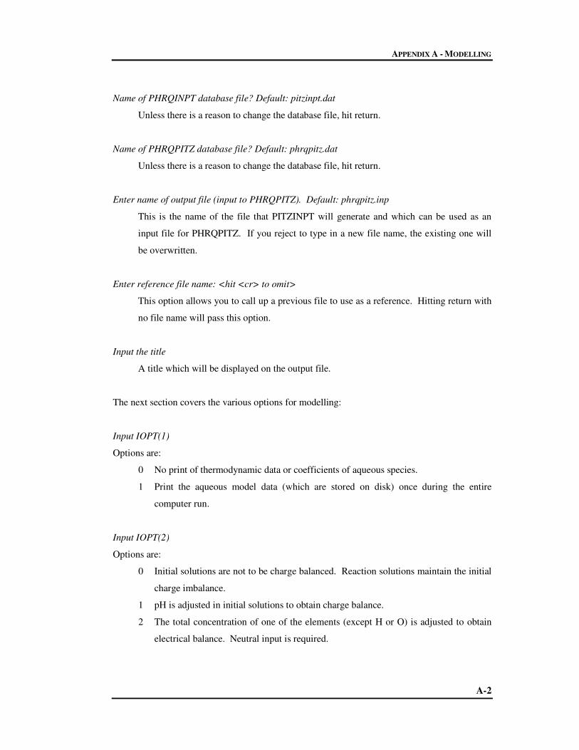
APPENDIX A - MODELLING
A-2
Name of PHRQINPT database file? Default: pitzinpt.dat
Unless there is a reason to change the database file, hit return.
Name of PHRQPITZ database file? Default: phrqpitz.dat
Unless there is a reason to change the database file, hit return.
Enter name of output file (input to PHRQPITZ). Default: phrqpitz.inp
This is the name of the file that PITZINPT will generate and which can be used as an
input file for PHRQPITZ. If you reject to type in a new file name, the existing one will
be overwritten.
Enter reference file name: <hit <cr> to omit>
This option allows you to call up a previous file to use as a reference. Hitting return with
no file name will pass this option.
Input the title
A title which will be displayed on the output file.
The next section covers the various options for modelling:
Input IOPT(1)
Options are:
0 No print of thermodynamic data or coefficients of aqueous species.
1 Print the aqueous model data (which are stored on disk) once during the entire
computer run.
Input IOPT(2)
Options are:
0 Initial solutions are not to be charge balanced. Reaction solutions maintain the initial
charge imbalance.
1 pH is adjusted in initial solutions to obtain charge balance.
2 The total concentration of one of the elements (except H or O) is adjusted to obtain
electrical balance. Neutral input is required.

APPENDIX A - MODELLING
A-3
Input IOPT(3)
Options are:
0 No reactions modelled. Only the initial solutions are solved.
1 Solution 1 is mixed (a hypothetical constant volume process) with solution 2 in
specified reaction steps. Steps input and a value for nsteps are required. Minerals
input may be included.
2 Solution 1 is titrated with solution 2 in specific reaction steps. Steps input, a value
for nsteps and a value for V0 are required. Minerals input may be included.
3 A stoichiometric reaction is added in specified reaction steps. Reaction input, Steps
input, a value for nsteps and a value for ncomps are required. Minerals input may be
included.
4 A net stoichiometric reaction is added in nsteps equal increments. Reaction input,
Steps input, a value for nsteps and a value for ncomps are required. Minerals input
may be included. Only one value for the total reaction is read in Steps.
5 Solution 1 is equilibrated with mineral phases only. No other reaction is performed.
Minerals input is required.
6 A reaction is added to solution 1 until equilibrium is attained with the first phase in
mineral input (equilibrium with other minerals is maintained throughout the reaction).
Reaction input, a value for ncomps, and Minerals input are required. No Steps input
is required. Note: there should be a common element in the reaction and the first
phase in Minerals input.
Input IOPT(4)
Options are:
0 The temperature of the reaction solution is: (a): the same as the initial solution if
adding a reaction, or (b): calculated linearly from the end members if mixing or
titrating. No Temp input is required.
1 The temperature is constant during the reaction steps and differs from that of the
initial solution(s). One value is read in Temp input.
2 The temperature is varied from T(0) to T(F) in nsteps equal increments, during the
reaction steps.
3 The temperature of each reaction step is specified in Temp input, in order. Nsteps
values are needed.

APPENDIX A - MODELLING
A-4
IOPT(5)
This option is automatically set and does not appear but its explanation is as below.
0 The pe of the initial solution (defined to be 4.0 if PITZINPT is used to construct input
sets) is held constant during all the reaction steps for the simulation. Redox reactions
are currently not considered.
IOPT(6)
This option is also automatic.
2 Activity coefficients are calculated according to the Pitzer model. No other options
are available.
Input IOPT(7)
Options are:
0 Do not save the aqueous phase composition at the end of a reaction for additional
simulations.
1 Save the final reaction solution in solution number 1.
2 Save the final reaction solution in solution number 2.
Input IOPT(8)
Options are:
0 The debugging print routine is not called.
1 A long printout is output at each iteration in each problem. This print is to be used
only if there are convergence problems with the program (see subroutine Pbug).
Input IOPT(9)
Options are:
0 No printout of each array inverted.
1 A long printout occurs of the entire array to be inverted at each iteration. This print is
to be used only if there are convergence problems (see subroutine SLNQ).
Input IOPT(10)
Options are:
0 No convention for activity coefficient is used.
1 MacInnes convention is used.

APPENDIX A - MODELLING
A-5
Input nsteps
Number of steps. A value is required if IOPT(3) = 1, 2, 3 or 4 or if IOPT(4) = 2 or 3.
Input V0
Initial volume of solution 1 when modelling a titration. This unit of V0 must be the same
as that of nstep (see Steps input) if IOPT(3) = 2. Otherwise V0 is not required.
Input ncomps
The number of constituents in a net stoichiometric reaction. A constituent may be any
element with an index number between 4 and 30 inclusive. No aqueous species with
index numbers >30 may be included as reaction constituents except H2 and O2. Any
constituent with index number greater than 30 is assumed to be either H2 or O2 and has
the effect of raising or lowering the redox state of the solution depending on the assigned
valence (thmean). A value for ncomps is required if IOPT(3) = 3, 4 or 6.
Keyword data blocks
There are 11 keywords which can be used to design the modelling input. These are described
below.
ELEMENTS
Defines a name and index of all elements in the aqueous model database.
Input tname
Alphanumeric name of element. Type LIST to bring up a list of the elements currently in
the database (Table A.1).
Input NELT
Index number assigned to element. Number must be between 4 and 30 inclusive.
Input TGFW
GFW of species used to report analytical data. If solution data is to include alkalinity,
TGFW for element C must be the equivalent weight of the reported alkalinity species.

APPENDIX A - MODELLING
A-6
Table A.1: Elements in the PHRQPITZ database
Elements Index
number
Gram
formula
weight
(GFW)
Input formula
corresponding
to GFW
Master
species OPV
***** 1 0 ***** ***** +0.00
***** 2 0 ***** ***** +0.00
***** 3 18.0152 ***** ***** +0.00
Ca 4 40.0800 Ca2+ Ca2+ +0.00
Mg 5 24.3050 Mg2+
Mg2+
+0.00
Na 6 22.9898 Na+
Na+
+0.00
K 7 39.0983 K+ K+ +0.00
Fe 8 55.8470 Fe2+ Fe2+ +2.00
Mn 9 54.9380 Mn2+
Mn2+
+2.00
Ba 11 137.330 Ba2+ Ba2+ +0.00
Sr 12 87.6200 Sr2+ Sr2+ +0.00
Cl 14 35.4530 Cl-
Cl-
+0.00
C 15 44.0098 CO2 CO32- +4.00
S 16 96.0600 SO42- SO4
2- +6.00
B 18 10.8100 B B(OH)3 +0.00
Li 21 6.9410 Li+ Li+ +0.00
Br 22 79.9040 Br- Br- +0.00
SPECIES
Defines names, index numbers and composition of all aqueous species in the aqueous model
data base.
Input I
Index number assigned to aqueous species. Numbers 4 through 30 are reserved for
master species. 250 is the maximum index number for an aqueous species.
Input SNAME
Alphanumeric species name
Input NSP
Total number of master species in the association reaction that forms this species. Do not
count the species itself unless the species is a master species.
Input KFLAG
Options are:

APPENDIX A - MODELLING
A-7
0 Van’t Hoff expression is used to calculate temperature dependence of the association
constant for this species.
1 An analytical expression is used to calculate temperature dependence of the
association constant.
Input GFLAG
Options are:
0 The extended Debye-Hückel or Davis expression (according to IOPT(6)) is used to
calculate the activity coefficient for this species.
1 The Wateq-Debye-Hückel expression is used to calculate the activity coefficient for
this species (regardless of the value of IOPT(6)).
Input ZSP
Charge on this aqueous species.
Input DHA
The extended Debye-Hückel A-0 term.
Input ALKSP
The alkalinity assigned to this aqueous species.
Input LKTOSP
Log K at 25°C where log K = A1 + A2(T) + A3/T + (A4 * log(T)) + A5/T2
Input DHSP
Standard enthalpy of association reaction at 25°C (H(R), in kcal/mol).
SOLUTION
Used to define starting solution.
Input solution number
A number, either 1 or 2, indicating the solution number of the following data.
Input solution heading
Title or comments about the solution.

APPENDIX A - MODELLING
A-8
Input NTOTS
The number of total concentrations to be read from card input, for example, if the
starting solution is MgCl2-NaHCO3 solution, NTOTS = 4 (for Mg, Cl, Na and C).
Input IALK
Flag which indicates whether total C or total alkalinity is to be input.
0 indicates total concentration of C (not alkalinity) is input in the units specified by
IUNITS.
N 4<N<30 where N is the index number for the element C (in PHRQPITZ.DATA, N =
15), indicates total alkalinity is being entered. Elements input may be required. The
units of alkalinity are specified by IUNITS and if IUNITS > 0, the GFW of the
element C is critically important. The GFW in the case of alkalinity must be the
gram equivalent weight (g/equivalent) of the chemical species in which alkalinity is
being reported. The following is a list of species commonly used for reporting
alkalinity and their corresponding equivalent weight:
CaCO3 = 50.0446 g/eq
HCO3- = 61.0171 g/eq
CO32-
= 30.0046 g/eq
In PHRQPITZ.DATA, 44.010 is the GFW of C which is suitable for entering C as
total CO2. This GFW must be changed via Elements input if alkalinity is to be
entered as mg/l or ppm (IUNITS = 2 or 3). If IUNITS = 0, alkalinity must be input as
eq/kg H2O and in this case the GFW need not be changed since no conversion is
necessary.
Input IUNITS
Flag describing units of input concentrations. The program makes all of its calculations
in terms of molality and any other allowed concentration units (mmol/ℓ, mg/ℓ, ppm or
mmol/kg) must be converted to molality before calculation may begin. To make the
conversions it is necessary to know the GFW in g/mole of the chemical formula in which
elemental analyses are reported. The GFW is an input parameter under Elements input
and must be in agreement with the analytical units for each solution dataset. (If the units
are molality, no conversion is necessary and the GFW’s are not used). Note: All elements
must have the same units. It is not possible to enter mg/l of one element and molality of
another.

APPENDIX A - MODELLING
A-9
0 concentration of elements entered as molality of each element, or for alkalinity,
equivalents/kg H2O.
1 concentration of elements entered as mmol/ℓ of each element, or for alkalinity meq/ℓ.
2 concentration of elements entered as mg/ℓ of the species which has a GFW given in
Elements input (Elements input may be required).
3 concentration of elements entered as ppm of the species which has a GFW given in
Elements input (Elements input may be required).
4 concentration of elements entered as mmol/kg solution.
Input pH
The pH of the solution (estimate if IOPT(2) = 1)
Input PE (automatic)
Automatically set at 4.0 as PHRQPITZ does not currently treat redox reactions.
Input Temp
Temperature of solution in °C.
Input LT(NTOTS)
LT = index number of element N
Input DTOT(NTOTS)
Total concentration of the element in molality, mmols/kg, mg/ℓ or ppm according to
Iunits.
MINERALS
Defines phases which will be maintained at equilibrium with each of the reaction solutions.
Pre-constructed mineral data are available. Do you wish to have any of them? (see Table A.2).

APPENDIX A - MODELLING
A-10
Table A.2: Minerals in the PHRQPITZ database
1. Anhydrite 2. Aragonite 3. Arcanite 4. Bischofite 5. Bloedite
6. Brucite 7. Burkeite 8. Calcite 9. Carnallite 10. Dolomite
11. Epsomite 12. Gaylussite 13. Glaserite 14. Glauberite 15. Gypsum
16. Halite 17.Hexahydrite 18. Kainite 19. Kalcinite 20. Kieserite
21. Labile S 22. Leonhardite 23. Leonite 24. Magnesite 25. Mirabilite
26. Misenite 27. Nahcolite 28. Natron 29. Nesquehonite 30. PCO2
31. Pentahydrite 32. Pirssonite 33. Polyhalite 34. Portlandite 35. Schoenite
36. Sylvite 37. Syngenite 38. Trona 39. Borax 40. B-Acid, S
41. KB5O84W 42. K2B4O74W 43. NABO24W 44. NAB5O85W 45. Teepleite
More minerals to be typed in from the terminal?
Input MNAME
Alphanumeric name of mineral
Input NMINO
Number of different species in the mineral dissociation reaction (including H+, e-, and
H2O). NMINO must be ≤ 10.
Input LKTOM
Log of the equilibrium constant at 25°C for reaction
Input DHMIN
Delta Hro (Kcal/mol) for the Van’t Hoff expression
Input MFLAG
0 The Van’t Hoff expression is used to calculate the temperature dependence of the
equilibrium constant.
1 The analytical expression is used to calculate the temperature dependence of the
equilibrium constant.

APPENDIX A - MODELLING
A-11
Input SIMIN
Saturation index (log IAP/Ksp) desired in the final solution. SIMIN = 0.0 would result in
equilibrium with the mineral while 1.0 would produce a solution 10 times supersaturated
(SI = 1.0). This variable is useful in specifying the partial pressure of a gas. The Henry’s
Law constant for the gas would be entered using the Van’t Hoff (LKTOM) or analytical
expression (AMIN) and the log of the partial pressure would be entered for SIMIN.
Input LMIN(NMINO)
Index number of species (not necessarily master species) in the dissociation reaction for
this mineral.
Input CMIN(NMINO)
Stoichiometric coefficient of species in dissociation reaction.
LOOKMIN
Provides information on the saturation state of aqueous phases with respect to desired minerals.
Minerals in this block of input do not affect calculations of initial solution or any of the reaction
solutions. Never mandatory.
Do you want to delete all old minerals?
Input variables as for Minerals keyword block.
TEMP
Varies temperature during reaction steps. It is not required when IOPT(4) = 0.
Input XTEMP(NSTEP)
Temperature in degrees C.
STEPS
Defines steps of reaction process. Not required when IOPT(3) = 0, 5 or 6.
Input XSTEP(NSTEP)
The value of XSTEP will vary depending on IOPT(3).
1 The fraction of solution 1 to be mixed with solution 2

APPENDIX A - MODELLING
A-12
2 Volume of solution 2 to be titrated into solution 1. Units must be the same as V0
3 The moles of reaction to be added to solution 1.
4 Total number of moles of reaction to be added in NSTEPS steps. NSTEPS reaction
solutions will be calculated. The ith solution will have I XSTEP/NSTEPS moles of
reaction added to solution 1.
REACTION
Describes the stoichiometry and valence of elements to be added as reaction.
Input LREAC(1)
Index number of element for the reaction. LREAC must be between 4 and 30 inclusive.
If LREAC>30 the program considers this constituent to be H2 or O2 and only uses CREAC
and THMEAN to change the oxidation state of the reaction solution.
Input CREAC(1)
Stoichiometric coefficient of element in reaction.
NEUTRAL
Thus input defines elements to be used to adjust the initial solutions to electrical neutrality (i.e.
IOPT(2) =2).
Input LPOS
Index number of an element with a cation master species.
Input LNEG
Index number of an element with an anion master species.
SUMS
Sums the molalities of aqueous species which are then printed in the output of reaction. These
sums do not affect the calculations in any way and are never mandatory.
Do you want to delete all old sums?

APPENDIX A - MODELLING
A-13
Input SUNAME
Alphanumeric name to be printed to identify reaction.
Input NSUM
The number of index numbers to be read (<50)
Input LSUM(NSUM)
Index numbers of species in sum.
END
Terminates input operations for a single simulation. Any computer run has at least one end line.
More simulations?
If yes…
Do you wish to define the previous output as your new reference?
Enter reference file name? Etc, etc…..
A.3 EXAMPLE OF PHRQPITZ INPUT FILE
Table A.3 shows a typical input file for a basic speciation of a solution of magnesium sulphate
and sodium chloride. Below is an explanation of each line.
Table A.3: Input file for PITZINPT
MD process for retentate temperatures
0000020000 0 0 0.0
SOLUTION 1
time=0
4 0 0 7. 4.0 29.2 1.0
5 1.164 16 1.164 6 4.926 14 4.926
END
Where: Line(1): Title
Line(2): Iopt(1); Iopt(2); Iopt(3); Iopt(4), Iopt(5), Iopt(6), Iopt(7), Iopt(8),
Iopt(9), Iopt(10), Nsteps; Ncomps V.O.
Line(3): Keyword “Solution” plus solution number
Line(4): Solution heading
Line(5): Ntots; Ialk; Iunits; pH; pe; Temp; Solution number

APPENDIX A - MODELLING
A-14
Line(6): Concentration input in format: Index number of element (from
Table A1); Total concentration of element in units according to Iunits
Table A.4 lists the corresponding output file associated with this run followed by an
explanation.
Table A.4: Output file from PHRQPITZ
DATA READ FROM DISK
ELEMENTS
SPECIES
LOOK MIN
MEAN GAM
1MD process for retentate temperatures
0000020000 0 0 0.00000
SOLUTION 1
time=0
4 0 0 7.00 4.00 29.2 1.00
5 1.164D+00 16 1.164D+00 6 4.926D+00 14 4.926D+00
1SOLUTION NUMBER 1
time=0
TOTAL MOLALITIES OF ELEMENTS
----- ---------- -- --------
ELEMENT MOLALITY LOG MOLALITY
MG 1.164000D+00 0.0660
NA 4.926000D+00 0.6925
CL 4.926000D+00 0.6925
S 1.164000D+00 0.0660
----DESCRIPTION OF SOLUTION----
PH = 7.0000
ACTIVITY H2O = 0.7379
OSMOTIC COEFFICIENT = 1.3853
IONIC STRENGTH = 9.5819
TEMPERATURE = 29.2000
PRESSURE = 1.0000 ATM
DENSITY OF H2O = 0.9959 G/CC
ELECTRICAL BALANCE = -8.2610D-05
TOTAL ALKALINITY = 8.2911D-05
ITERATIONS = 1
-----------------------
DISTRIBUTION OF SPECIES
-----------------------
UNSCALED UNSCALED
I SPECIES Z MOLALITY LOG MOLAL ACTIVITY LOG ACT GAMMA LOG GAM
1 H+ 1.0 3.000E-08 -7.523 1.000E-07 -7.000 3.334E+00 0.523
3 H2O 0.0 7.379E-01 -0.132 7.379E-01 -0.132 1.000E+00 0.000
5 MG+2 2.0 1.164E+00 0.066 1.164E+00 0.066 1.000E+00 0.000
6 NA+ 1.0 4.926E+00 0.692 3.934E+00 0.595 7.985E-01 -0.098
14 CL- -1.0 4.926E+00 0.692 8.118E+00 0.909 1.648E+00 0.217
16 SO4-2 -2.0 1.164E+00 0.066 2.985E-02 -1.525 2.565E-02 -1.591

APPENDIX A - MODELLING
A-15
31 OH- -1.0 2.926E-07 -6.534 1.014E-07 -6.994 3.464E-01 -0.460
40 HSO4- -1.0 2.707E-07 -6.568 3.199E-07 -6.495 1.182E+00 0.072
85 MGOH+ 1.0 8.262E-05 -4.083 1.914E-05 -4.718 2.317E-01 -0.635
UNSCALED UNSCALED
SPECIES TOTAL MOL ACTIVITY TOTAL GAMMA
H+ 3.0069D-07 1.0000D-07 3.3257D-01
MG+2 1.1640D+00 1.1641D+00 1.0001D+00
NA+ 4.9260D+00 3.9336D+00 7.9855D-01
CL- 4.9260D+00 8.1182D+00 1.6480D+00
SO4-2 1.1640D+00 2.9851D-02 2.5645D-02
OH- 8.2911D-05 1.0136D-07 1.2225D-03
---- MEAN ACTIVITY COEFFICIENT ----
FORMULA MEAN GAMMA
MGCL2 1.3953D+00
MGSO4 1.6015D-01
MG(OH)2 1.1434D-02
NACL 1.1472D+00
NA2SO4 2.5383D-01
NAOH 3.1245D-02
HCL 7.4032D-01
H2SO4 1.4155D-01
---- LOOK MIN IAP ----
PHASE LOG IAP LOG KT LOG IAP/KT
BISCHOFI 1.0929 4.4421 -3.3493
BLOEDITE -2.3225 -2.3470 0.0245
BRUCITE -13.9223 -10.8753 -3.0469
EPSOMITE -2.3831 -1.8309 -0.5523
HALITE 1.5043 1.5759 -0.0717
HEXAHYDR -2.2511 -1.5850 -0.6662
KIESERIT -1.5911 -0.1230 -1.4681
LEONHARD -1.9871 -0.8870 -1.1001
MIRABIL -1.6556 -1.0286 -0.6270
PENTAHYD -2.1191 -1.2850 -0.8341
The first four keywords that appear, ELEMENTS, SPECIES, LOOK MIN and MEAN GAM
were printed as appropriate data from the PHRQPITZ.DATA were read. The computed output
begins with a print of the total molalities of all elements in Solution 1 followed by a description
of the solution and distribution of species. Computed variables under the heading “Description
of Solution” include the activity of water, osmotic coefficient, ionic strength, pressure (in
atmosphere) together with the vapour pressure line of pure water (if the temperature is greater
than 100 °C), the density of pure water at the given temperature and pressure, the electrical
imbalance (in equivalents per kilogram H2O), and the total concentration of inorganic carbon
(moles per kg H2O). The “Distribution of species” lists the molality, activity, and activity

APPENDIX A - MODELLING
A-16
coefficient (and log values) of all aqueous species in the PHRQPITZ.DATA file for which an
input concentration was given. This output is followed by tables of total molalities, activities,
activity coefficients, mean activity coefficients and saturation indices. The saturation indices
are given under the heading LOOK MIN IAP as log(IAP/KT).
A.4 EVAPORATION MODELLING IN PHRQPITZ
PHRQPITZ can be used to determine the amount of water that needs to be extracted from a
given starting solution in order to reach a stipulated mineral phase boundary (in this example the
mineral phase is halite). For our series of experiments it is useful to know at what stage or
exactly how much of water needs to be removed (by MD) before the crystallisation will begin.
In PHRQPITZ evaporation of the solution is achieved by setting IOPT(3) = 6, i.e. specifying
that a reaction will be added until the first mineral of MINERALS input is just saturated, and
defining the reaction under REACTION input as water (LREAC(1) = 3 and CREAC (1) = 1.0).
PHRQPITZ identifies this combination of input as the special case of evaporation (or dilution, if
the starting solution is oversaturated with the first mineral of MINERALS input) and additional
output is provided as seen in Table A.5 for the evaporation of a solution of magnesium sulphate
and sodium chloride until the halite phase boundary is reached.
Table A.5: Output from PHRQPITZ for the evaporation of a solution of NaCl and MgSO4 until
the halite phase boundary is reached
DATA READ FROM DISK
ELEMENTS
SPECIES
LOOK MIN
MEAN GAM
1evaporation with halite saturation of 1:1 mix, 225g/l
0060020000 0 1 0.00000
SOLUTION 1
MgSO4:NaCl, 1:1
4 0 0 7.00 4.00 33.0 1.00
5 1.869D+00 16 1.869D+00 6 3.850D+00 14 3.850D+00
MINERALS
HALITE 2 0.00 1.6 0.00 1 0.000
6 1.00 14 1.00
-7.1346E+02 -1.2012E-01 3.7302E+04 2.6246E+02 -2.1069E+06
0 0.00 0.00 0.00 0 0.000
REACTION
3 1.000 0.000
1SOLUTION NUMBER 1
MgSO4:NaCl, 1:1

APPENDIX A - MODELLING
A-17
TOTAL MOLALITIES OF ELEMENTS
----- ---------- -- --------
ELEMENT MOLALITY LOG MOLALITY
MG 1.869000D+00 0.2716
NA 3.850000D+00 0.5855
CL 3.850000D+00 0.5855
S 1.869000D+00 0.2716
----DESCRIPTION OF SOLUTION----
PH = 7.0000
ACTIVITY H2O = 0.7488
OSMOTIC COEFFICIENT = 1.4037
IONIC STRENGTH = 11.3258
TEMPERATURE = 33.0000
PRESSURE = 1.0000 ATM
DENSITY OF H2O = 0.9947 G/CC
ELECTRICAL BALANCE = -1.1625D-04
TOTAL ALKALINITY = 1.1668D-04
ITERATIONS = 1
-----------------------
DISTRIBUTION OF SPECIES
-----------------------
UNSCALED UNSCALED
I SPECIES Z MOLALITY LOG MOLAL ACTIVITY LOG ACT GAMMA LOG GAM
1 H+ 1.0 3.839E-08 -7.416 1.000E-07 -7.000 2.605E+00 0.416
3 H2O 0.0 7.488E-01 -0.126 7.488E-01 -0.126 1.000E+00 0.000
5 MG+2 2.0 1.869E+00 0.272 1.021E+00 0.009 5.463E-01 -0.263
6 NA+ 1.0 3.850E+00 0.585 2.635E+00 0.421 6.845E-01 -0.165
14 CL- -1.0 3.850E+00 0.585 8.217E+00 0.915 2.134E+00 0.329
16 SO4-2 -2.0 1.869E+00 0.272 5.995E-02 -1.222 3.208E-02 -1.494
31 OH- -1.0 4.973E-07 -6.303 1.355E-07 -6.868 2.725E-01 -0.565
40 HSO4- -1.0 3.935E-07 -6.405 7.155E-07 -6.145 1.818E+00 0.260
85 MGOH+ 1.0 1.162E-04 -3.935 2.343E-05 -4.630 2.017E-01 -0.695
UNSCALED UNSCALED
SPECIES TOTAL MOL ACTIVITY TOTAL GAMMA
H+ 4.3189D-07 1.0000D-07 2.3154D-01
MG+2 1.8690D+00 1.0210D+00 5.4629D-01
NA+ 3.8500D+00 2.6354D+00 6.8451D-01
CL- 3.8500D+00 8.2172D+00 2.1343D+00
SO4-2 1.8690D+00 5.9951D-02 3.2076D-02
OH- 1.1668D-04 1.3552D-07 1.1614D-03
---- MEAN ACTIVITY COEFFICIENT ----
FORMULA MEAN GAMMA
MGCL2 1.3551D+00
MGSO4 1.3237D-01
MG(OH)2 9.0325D-03
NACL 1.2087D+00
NA2SO4 2.4678D-01
NAOH 2.8196D-02
HCL 7.0299D-01
H2SO4 1.1981D-01

APPENDIX A - MODELLING
A-18
---- LOOK MIN IAP ----
PHASE LOG IAP LOG KT LOG IAP/KT
BISCHOFI 1.0848 4.4307 -3.3460
BLOEDITE -2.0962 -2.3470 0.2508
BRUCITE -13.7270 -10.8677 -2.8593
EPSOMITE -2.0925 -1.7868 -0.3057
HALITE 1.3356 1.5803 -0.2448
HEXAHYDR -1.9669 -1.5396 -0.4273
KIESERIT -1.3388 -0.1230 -1.2158
LEONHARD -1.7157 -0.8870 -0.8287
MIRABIL -1.6367 -0.8721 -0.7646
PENTAHYD -1.8413 -1.2850 -0.5563
1STEP NUMBER 1
0--------------
TOTAL MOLALITIES OF ELEMENTS
----- ---------- -- --------
ELEMENT MOLALITY LOG MOLALITY
MG 1.869000D+00 0.2716
NA 3.850000D+00 0.5855
CL 3.850000D+00 0.5855
S 1.869000D+00 0.2716
----PHASE BOUNDARIES----
MASS PRECIPITATED/DISSOLVED FROM INITIAL KILOGRAM WATER
PHASE DELTA PHASE* LOG IAP LOG KT LOG IAP/KT
HALITE 0.000000D+00 1.5803 1.5803 0.0000
+ **
* NEGATIVE DELTA PHASE INDICATES PRECIPITATION
AND POSITIVE DELTA PHASE INDICATES DISSOLUTION.
** 1.138248D+00 IS THE EVAPORATION FACTOR NECESSARY TO REACH THE
HALITE PHASE BOUNDARY.
MOLES OF ELEMENTS REMAINING AFTER REACTION
----- -- -------- --------- ----- --------
ELEMENT MOLES LOG MOLES
MG 1.869000D+00 0.2716
NA 3.850000D+00 0.5855
CL 3.850000D+00 0.5855
S 1.869000D+00 0.2716
8.785435D-01 KILOGRAMS OF WATER REMAINING

APPENDIX A - MODELLING
A-19
---- LOOK MIN IAP ----
PHASE LOG IAP LOG KT LOG IAP/KT
BISCHOFI 1.4534 4.4307 -2.9773
BLOEDITE -1.6348 -2.3470 0.7122
BRUCITE -14.0297 -10.8677 -3.1620
EPSOMITE -1.9815 -1.7868 -0.1946
HALITE 1.5803 1.5803 0.0000
HEXAHYDR -1.8262 -1.5396 -0.2866
KIESERIT -1.0501 -0.1230 -0.9271
LEONHARD -1.5158 -0.8870 -0.6288
MIRABIL -1.6712 -0.8721 -0.7991
PENTAHYD -1.6710 -1.2850 -0.3860
TOTAL MOLALITIES OF ELEMENTS
----- ---------- -- --------
ELEMENT MOLALITY LOG MOLALITY
MG 2.127385D+00 0.3278
NA 4.382253D+00 0.6417
CL 4.382253D+00 0.6417
S 2.127385D+00 0.3278
----DESCRIPTION OF SOLUTION----
PH = 6.7613
ACTIVITY H2O = 0.6995
OSMOTIC COEFFICIENT = 1.5238
IONIC STRENGTH = 12.8916
TEMPERATURE = 33.0000
PRESSURE = 1.0000 ATM
DENSITY OF H2O = 0.9947 G/CC
ELECTRICAL BALANCE = -1.1625D-04
TOTAL ALKALINITY = 1.1700D-04
ITERATIONS = 5
-----------------------
DISTRIBUTION OF SPECIES
-----------------------
UNSCALED UNSCALED
I SPECIES Z MOLALITY LOG MOLAL ACTIVITY LOG ACT GAMMA LOG GAM
1 H+ 1.0 4.671E-08 -7.331 1.733E-07 -6.761 3.709E+00 0.569
3 H2O 0.0 6.995E-01 -0.155 6.995E-01 -0.155 1.000E+00 0.000
5 MG+2 2.0 2.127E+00 0.328 1.750E+00 0.243 8.226E-01 -0.085
6 NA+ 1.0 4.382E+00 0.642 3.232E+00 0.509 7.375E-01 -0.132
14 CL- -1.0 4.382E+00 0.642 1.177E+01 1.071 2.686E+00 0.429
16 SO4-2 -2.0 2.127E+00 0.328 7.279E-02 -1.138 3.422E-02 -1.466
31 OH- -1.0 2.738E-07 -6.563 7.306E-08 -7.136 2.669E-01 -0.574
40 HSO4- -1.0 7.057E-07 -6.151 1.505E-06 -5.822 2.133E+00 0.329
85 MGOH+ 1.0 1.167E-04 -3.933 2.165E-05 -4.665 1.854E-01 -0.732

APPENDIX A - MODELLING
A-20
UNSCALED UNSCALED
SPECIES TOTAL MOL ACTIVITY TOTAL GAMMA
H+ 7.5242D-07 1.7327D-07 2.3029D-01
MG+2 2.1274D+00 1.7498D+00 8.2253D-01
NA+ 4.3823D+00 3.2319D+00 7.3750D-01
CL- 4.3823D+00 1.1772D+01 2.6864D+00
SO4-2 2.1274D+00 7.2793D-02 3.4217D-02
OH- 1.1700D-04 7.3056D-08 6.2441D-04
---- MEAN ACTIVITY COEFFICIENT ----
FORMULA MEAN GAMMA
MGCL2 1.8106D+00
MGSO4 1.6776D-01
MG(OH)2 6.8449D-03
NACL 1.4076D+00
NA2SO4 2.6501D-01
NAOH 2.1459D-02
HCL 7.8655D-01
H2SO4 1.2197D-01
The first paragraph in the initial section of the output (which actually is a portion of the input
file) is the same as described above. The difference occurs in the second paragraph as a
MINERALS input has been included. These lines described the characteristics of the mineral
that has been defined. A REACTION has also been specified as described above and this is
shown in the last few lines of the first section of the output file. PHRQPITZ performs the usual
calculations on the initial solution and is described in the output under the various headings as
before. However, in this case, the saturation step with halite appears under the heading “step
number 1”. After the print of mass transfer under the heading “phase boundaries”, PHRQPITZ
prints the evaporation factor necessary to reach saturation with the first mineral in the
MINERALS input (halite). In this case the evaporation factor is 1.138 which means that the
concentration of an inert component in the initial solution would increase by a factor of 1.138
upon evaporation to the phase boundary. PHRQPITZ also furnishes the output with the total
moles of elements remaining with regards to the initial solution defined in solution 1 together
with the amount of water remaining. The output is completed with a full description of the
resulting solution.

Appendix B
DATA
B-1
This appendix provides the raw data that were used to process the results featured
in Chapter 3 and Chapter 5 of this thesis. The data recorded during the MD of the
salt mixes are presented first followed by that of the experiments performed using
the VLE still. The method of linear regression using Antoine’s equation to fit the
experimental vapour pressure data is shown, together with the comparisons
between literature and measured vapour pressures. Data used during the
evaluation of the flux and driving force are also listed.
B.1 MEMBRANE DISTILLATION DATA
Table B.1 to B.5 provide the data that were collected during the membrane distillation of the
individual and mixed salt solutions.
Table B.1: MD of a 375 g/ℓ magnesium sulphate solution (initial solution volume = 3 ℓ)
Time
(h)
H2O
removed (g)
Ret. in temp.
(°°°°C)
Dist. in
temp. (°°°°C)
Flux
(g/hm2)
[MgSO4]
(g/ℓ)
0.15 18.9 28.8 8.9 630.0 377.4
0.85 151.4 28.8 14.1 946.4 395.0
1.58 289.6 31.9 17.4 942.3 415.1
12.77 1900.2 30.3 20.6 720.1 1022.9
13.45 1992.7 31.2 20.5 676.8 1116.9
13.80 2027.6 31.1 20.3 498.6 1156.9
15.08 2163.2 30.0 20.0 259.6 1344.4
15.50 2181.9 30.0 19.8 224.4 1375.1
15.85 2202.6 30.2 19.7 166.7 1410.8
15.97 2206.3 30.1 19.7 158.6 1417.4
18.60 2194.0 17.6 13.0 56.1 1395.8
19.83 2196.8 17.9 11.2 11.4 1400.7
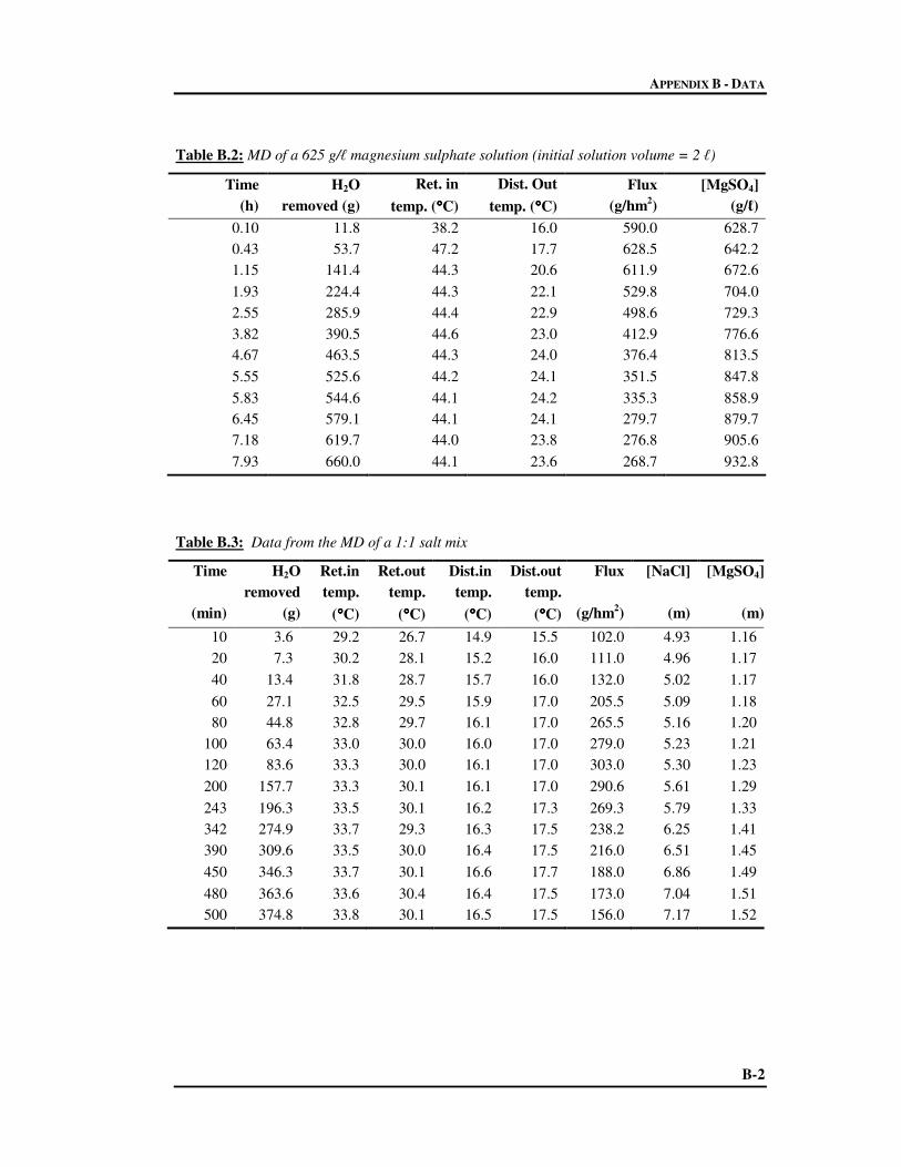
APPENDIX B - DATA
B-2
Table B.2: MD of a 625 g/ℓ magnesium sulphate solution (initial solution volume = 2 ℓ)
Time
(h)
H2O
removed (g)
Ret. in
temp. (°°°°C)
Dist. Out
temp. (°°°°C)
Flux
(g/hm2)
[MgSO4]
(g/ℓ)
0.10 11.8 38.2 16.0 590.0 628.7
0.43 53.7 47.2 17.7 628.5 642.2
1.15 141.4 44.3 20.6 611.9 672.6
1.93 224.4 44.3 22.1 529.8 704.0
2.55 285.9 44.4 22.9 498.6 729.3
3.82 390.5 44.6 23.0 412.9 776.6
4.67 463.5 44.3 24.0 376.4 813.5
5.55 525.6 44.2 24.1 351.5 847.8
5.83 544.6 44.1 24.2 335.3 858.9
6.45 579.1 44.1 24.1 279.7 879.7
7.18 619.7 44.0 23.8 276.8 905.6
7.93 660.0 44.1 23.6 268.7 932.8
Table B.3: Data from the MD of a 1:1 salt mix
Time
(min)
H2O
removed
(g)
Ret.in
temp.
(°°°°C)
Ret.out
temp.
(°°°°C)
Dist.in
temp.
(°°°°C)
Dist.out
temp.
(°°°°C)
Flux
(g/hm2)
[NaCl]
(m)
[MgSO4]
(m)
10 3.6 29.2 26.7 14.9 15.5 102.0 4.93 1.16
20 7.3 30.2 28.1 15.2 16.0 111.0 4.96 1.17
40 13.4 31.8 28.7 15.7 16.0 132.0 5.02 1.17
60 27.1 32.5 29.5 15.9 17.0 205.5 5.09 1.18
80 44.8 32.8 29.7 16.1 17.0 265.5 5.16 1.20
100 63.4 33.0 30.0 16.0 17.0 279.0 5.23 1.21
120 83.6 33.3 30.0 16.1 17.0 303.0 5.30 1.23
200 157.7 33.3 30.1 16.1 17.0 290.6 5.61 1.29
243 196.3 33.5 30.1 16.2 17.3 269.3 5.79 1.33
342 274.9 33.7 29.3 16.3 17.5 238.2 6.25 1.41
390 309.6 33.5 30.0 16.4 17.5 216.0 6.51 1.45
450 346.3 33.7 30.1 16.6 17.7 188.0 6.86 1.49
480 363.6 33.6 30.4 16.4 17.5 173.0 7.04 1.51
500 374.8 33.8 30.1 16.5 17.5 156.0 7.17 1.52

APPENDIX B - DATA
B-3
Table B.4: Data from the MD of a 1:2 salt mix
Time
(min)
H2O
removed
(g)
Ret.in
temp.
(°°°°C)
Ret.out
temp.
(°°°°C)
Dist.in
temp.
(°°°°C)
Dist.out
temp.
(°°°°C)
Flux
(g/hm2)
[NaCl]
(m)
[MgSO4]
(m)
10 5.0 30.3 28.4 16.0 16.5 105.0 5.80 0.64
20 12.7 30.8 29.1 16.2 16.5 231.0 5.83 0.64
30 21.9 31.5 29.6 16.3 16.5 276.0 5.86 0.65
40 31.5 31.8 30.0 16.5 17.0 288.0 5.89 0.65
70 59.5 32.5 30.4 16.6 17.0 303.0 6.00 0.66
100 89.3 33.0 30.9 16.9 17.5 315.0 6.12 0.68
110 99.4 33.1 30.8 17.0 17.5 303.0 6.16 0.68
120 109.3 33.2 31.0 17.1 17.5 297.0 6.20 0.68
180 167.8 33.4 31.3 17.2 17.9 279.5 6.44 0.71
240 224.1 33.6 31.3 17.4 18.0 272.3 6.70 0.74
270 250.0 33.5 31.4 17.2 18.0 259.0 6.83 0.75
300 276.0 33.7 31.4 17.5 18.5 260.0 6.96 0.77
330 300.7 33.5 31.2 17.2 18.0 247.0 7.09 0.78
421 369.2 33.4 31.0 17.1 18.0 221.8 7.48 0.83
Table B.5: Data from the MD of a 1:3 salt mix
Time
(h)
H2O
removed
(g)
Ret. in
temp.
(°°°°C)
Dist. in
temp.
(°°°°C)
Flux
(g/hm2)
[NaCl]
(m)
[MgSO4]
(m)
10 11.8 28.7 13.7 138.00 5.742 0.450
20 18.1 30.6 13.9 189.00 5.758 0.451
50 31.1 31.0 14.2 207.00 5.780 0.453
60 38.4 32.7 14.6 219.00 5.826 0.456
72 48.1 32.7 14.7 242.50 5.852 0.458
180 113.1 33.2 14.9 278.18 5.887 0.461
210 130.6 34.9 15.3 175.00 6.132 0.480
245 147.2 35.3 15.4 142.29 6.201 0.485
283 161.1 36.2 15.4 109.74 6.269 0.491
311 171.4 37.7 15.2 110.36 6.326 0.495

APPENDIX B - DATA
B-4
B.1.1 Crystal Size Distribution
The data sets that were used in order to obtain the CSD for the MD and crystallisation of a
375 g/ℓ magnesium sulphate solution are listed in Tables B6a to B6d. This data was used
according to Equation 3.2 and the general approach of characterisation of size distribution, in
order to obtain the overall CSD as shown in Figure 3.3.
Table B.6a: CSD for sample 1 for the MD of a 375 g/ℓ magnesium sulphate solution
Length (cm) Range N (cm) % distribution
0 0.1-0.4 0 0
5.5 0.4-0.7 7 6.73
8.5 0.7-1.0 26 25.00
11.5 1.0-1.3 32 30.77
14.5 1.3-1.6 28 26.92
17.5 1.6-1.9 6 5.77
20.5 1.9-2.2 5 4.81
SUM 104
MEDIAN 11.9
Table B.6b: CSD for sample 2 for the MD of a 375 g/ℓ magnesium sulphate solution
Length (cm) Range N (cm) % distribution
0 0.4-0.7 0 0
8.5 0.7-1.0 30 9.04
11.5 1.0-1.3 71 21.39
14.5 1.3-1.6 90 27.11
17.5 1.6-1.9 56 16.87
20.5 1.9-2.2 36 10.84
23.5 2.2-2.5 23 6.93
26.5 2.5-2.8 15 4.52
29.5 2.8-3.1 6 1.81
32.5 3.1-3.4 5 1.51
SUM 332
MEDIAN 16.2

APPENDIX B - DATA
B-5
Table B.6c: CSD for sample 3 for the MD of a 375 g/ℓ magnesium sulphate solution
Length (cm) Range N (cm) % distribution
0 0.4-0.7 0 0
8.5 0.7-1.0 5 2.14
11.5 1.0-1.3 41 17.52
14.5 1.3-1.6 63 30.00
17.5 1.6-1.9 37 15.81
20.5 1.9-2.2 25 10.68
23.5 2.2-2.5 26 11.11
26.5 2.5-2.8 11 4.70
29.5 2.8-3.1 11 4.70
32.5 3.1-3.4 8 3.42
35.5 3.4-3.7 5 2.14
38.5 3.7-4.0 2 0.85
SUM 234
MEDIAN 19.0
Table B.6d: CSD for sample 4 for the MD of a 375 g/ℓ magnesium sulphate solution
Length (cm) Range N (cm) % distribution
0 0.4-0.7 0 0
8.5 0.7-1.0 6 2.58
11.5 1.0-1.3 15 6.44
14.5 1.3-1.6 31 13.30
17.5 1.6-1.9 21 27.00
20.5 1.9-2.2 23 14.87
23.5 2.2-2.5 24 12.30
26.5 2.5-2.8 24 10.30
29.5 2.8-3.1 27 11.59
32.5 3.1-3.4 17 7.30
35.5 3.4-3.7 17 7.30
38.5 3.7-4.0 7 3.00
41.5 4.0-4.3 6 2.58
44.5 4.3-4.6 5 2.15
47.5 4.6-4.9 4 1.72
50.5 4.9-5.2 3 1.29
53.5 5.2-5.5 3 1.29
SUM 233
MEDIAN 30.0

APPENDIX B - DATA
B-6
B.2 VAPOUR PRESSURES OBTAINED USING PHRQPITZ
The modelling of vapour pressures performed using the PHRQPITZ computer program for each
of the streams during the MD of the 1:1 and 1:2 salt mixes are listed in Table B.7 and 8. The
log mean vapour pressures (∆Plm), calculated from the difference between the inlet and outlet
retentate and distillate streams, are also shown.
Table B.7: Vapour pressures of various streams during MD of 1:1 mix together with calculated
log mean vapour pressure
Ret. in
(kPa)
Ret.
out
(kPa)
Pure
Ret. in
(kPa)
Pure
Ret.
out
(kPa)
Dist. In
(kPa)
Dist.
Out
(kPa)
∆∆∆∆P1
(kPa)
∆∆∆∆P2
(kPa)
∆∆∆∆Plm
(-)
2.99 2.59 4.06 3.51 1.70 1.76 1.23 0.89 1.05
3.16 2.80 4.30 3.81 1.73 1.82 1.34 1.07 1.20
3.45 2.88 4.71 3.94 1.78 1.82 1.63 1.10 1.35
3.57 3.01 4.90 4.13 1.81 1.94 1.63 1.20 1.40
3.61 3.02 4.98 4.17 1.83 1.94 1.67 1.19 1.42
3.63 3.05 5.04 4.25 1.82 1.94 1.69 1.23 1.45
3.66 3.03 5.12 4.25 1.83 1.94 1.72 1.20 1.45
3.55 2.96 5.12 4.27 1.83 1.94 1.62 1.13 1.36
3.53 2.90 5.18 4.27 1.84 1.98 1.55 1.06 1.29
3.41 2.64 5.24 4.08 1.84 2.00 1.41 0.80 1.08
3.28 2.68 5.18 4.25 1.87 2.00 1.28 0.82 1.03
3.21 2.60 5.24 4.27 1.89 2.03 1.18 0.71 0.93
3.13 2.60 5.21 4.35 1.87 2.00 1.13 0.73 0.92
3.12 2.52 5.27 4.27 1.88 2.00 1.12 0.64 0.86

APPENDIX B - DATA
B-7
Table B.8: Vapour pressures of various streams during MD of 1:2 mix together with calculated
log mean vapour pressure
Ret. in
(kPa)
Ret.
out
(kPa)
Pure
Ret. in
(kPa)
Pure
Ret.
out
(kPa)
Dist. In
(kPa)
Dist.
Out
(kPa)
∆∆∆∆P1
(kPa)
∆∆∆∆P2
(kPa)
∆∆∆∆Plm
(-)
3.15 2.82 4.32 3.87 1.82 1.88 1.27 1.00 1.13
3.23 3.12 4.45 4.30 1.88 1.94 1.29 1.24 1.27
3.35 3.13 4.63 4.32 1.89 1.94 1.42 1.24 1.33
3.40 3.14 4.71 4.35 1.89 1.94 1.47 1.25 1.36
3.51 3.23 4.90 4.47 1.93 2.00 1.51 1.31 1.41
3.57 3.26 5.04 4.55 1.94 2.01 1.56 1.32 1.44
3.58 3.24 5.06 4.57 1.96 2.05 1.53 1.28 1.40
3.59 3.22 5.09 4.55 1.96 2.07 1.53 1.25 1.39
3.56 3.20 5.15 4.60 1.96 2.07 1.50 1.23 1.36
3.52 3.10 5.21 4.55 1.96 2.07 1.46 1.14 1.29
3.46 3.05 5.18 4.52 1.95 2.07 1.40 1.10 1.24
3.46 3.04 5.24 4.55 1.95 2.07 1.39 1.08 1.23
3.38 3.00 5.18 4.55 1.96 2.07 1.32 1.03 1.17
3.24 2.91 5.15 4.50 1.95 2.07 1.17 0.96 1.07
B.3 VLE EXPERIMENTS
The experimental VLE data are listed below. The non-linear regressions for fitting Antoine’s
constants to the experimental data are also shown. Section B3.1 lists the results obtained for the
pure sodium chloride solutions that were investigated as a test of the suitability of the VLE still
to measure vapour pressures of inorganic salts. This is confirmed by a comparison of the
experimental vapour pressures to those obtained from literature. Section B.3.2 then lists the
vapour pressures that were measured for each of the salt mixes.
B.3.1 Suitability of VLE to measure vapour pressures of inorganic salts
Table B.9 to B.11 lists the measured vapour pressures for three sodium chloride solutions that
were studied together with the Antoine’s regression that was used to fit the experimental points.

APPENDIX B - DATA
B-8
Table B.9: Non-linear regression for fitting Antoine’s constants to experimental VLE data for
20 g/ℓ NaCl solution
A
18.6
B
5139
C
-6.00
∑∑∑∑ ri2
7.13×10⁻³
Temp. (K) Pexpt (kPa) Pcalc (kPa) lnPexpt lnPcalc r
298 2.64 2.72 0.970 1.00 8.69×10⁻⁴
303 3.77 3.65 1.33 1.30 1.03×10⁻³
313 6.75 6.41 1.91 1.86 2.70×10⁻³
323 10.7 10.9 2.37 2.39 1.82×10⁻⁴
333 17.9 17.8 2.89 2.88 2.41×10⁻⁵
343 28.6 28.4 3.36 3.34 6.12×10⁻⁵
353 44.3 44.1 3.79 3.79 2.01×10⁻⁵
363 66.6 66.7 4.20 4.20 3.32×10⁻⁶
373 96.0 98.8 4.56 4.59 8.25×10⁻⁴
Table B.10: Non-linear regression for fitting Antoine’s constants to experimental VLE data for
200 g/ℓ NaCl solution
A
18.0
B
4958
C
-7.21
∑∑∑∑ ri2
3.91×10⁻³
Temp. (K) Pexpt (kPa) Pcalc (kPa) lnPexpt lnPcalc r
298 2.637 2.520 0.970 0.924 2.06×10⁻³
303 3.400 3.361 1.224 1.212 1.36×10⁻⁴
313 5.750 5.811 1.749 1.760 1.11×10⁻⁴
323 9.648 9.705 2.267 2.273 3.41×10⁻⁵
333 15.645 15.706 2.750 2.754 1.53×10⁻⁵
343 24.745 24.701 3.209 3.207 3.13×10⁻⁶
353 37.932 37.843 3.636 3.633 5.47×10⁻⁶
363 56.817 56.604 4.040 4.036 1.41×10⁻⁵
373 81.968 82.824 4.406 4.417 1.08×10⁻⁴
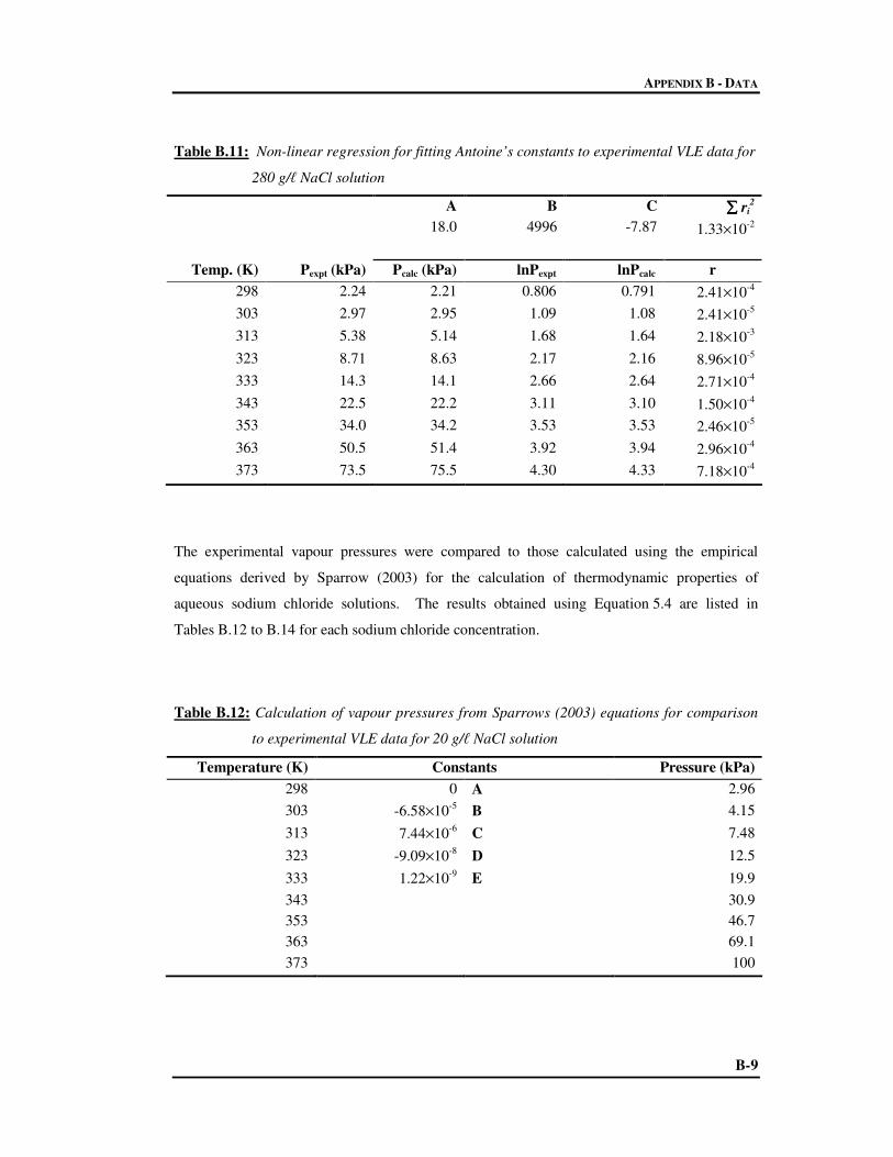
APPENDIX B - DATA
B-9
Table B.11: Non-linear regression for fitting Antoine’s constants to experimental VLE data for
280 g/ℓ NaCl solution
A
18.0
B
4996
C
-7.87
∑∑∑∑ ri2
1.33×10⁻²
Temp. (K) Pexpt (kPa) Pcalc (kPa) lnPexpt lnPcalc r
298 2.24 2.21 0.806 0.791 2.41×10⁻⁴
303 2.97 2.95 1.09 1.08 2.41×10⁻⁵
313 5.38 5.14 1.68 1.64 2.18×10⁻³
323 8.71 8.63 2.17 2.16 8.96×10⁻⁵
333 14.3 14.1 2.66 2.64 2.71×10⁻⁴
343 22.5 22.2 3.11 3.10 1.50×10⁻⁴
353 34.0 34.2 3.53 3.53 2.46×10⁻⁵
363 50.5 51.4 3.92 3.94 2.96×10⁻⁴
373 73.5 75.5 4.30 4.33 7.18×10⁻⁴
The experimental vapour pressures were compared to those calculated using the empirical
equations derived by Sparrow (2003) for the calculation of thermodynamic properties of
aqueous sodium chloride solutions. The results obtained using Equation 5.4 are listed in
Tables B.12 to B.14 for each sodium chloride concentration.
Table B.12: Calculation of vapour pressures from Sparrows (2003) equations for comparison
to experimental VLE data for 20 g/ℓ NaCl solution
Temperature (K) Constants Pressure (kPa)
298 0 A 2.96
303 -6.58×10⁻⁵ B 4.15
313 7.44×10⁻⁶
C 7.48
323 -9.09×10⁻⁸
D 12.5
333 1.22×10⁻⁹ E 19.9
343 30.9
353 46.7
363 69.1
373 100

APPENDIX B - DATA
B-10
Table B.13: Calculation of vapour pressures from Sparrows (2003) equations for comparison
to experimental VLE data for 200 g/ℓ NaCl solution
Temperature (K) Constants Pressure (kPa)
298 7.93×10⁻⁴ A 2.59
303 -6.01×10⁻⁵
B 3.65
313 6.64×10⁻⁶
C 6.58
323 -8.22×10⁻⁸
D 11.0
333 1.08×10⁻⁹ E 17.6
343 27.2
353 41.2
363 60.9
373 88.1
Table B.14: Calculation of vapour pressures from Sparrows (2003) equations for comparison
to experimental VLE data for 280 g/ℓ NaCl solution
Temperature (K) Constants Pressure (kPa)
298 7.41 ×10⁻⁴
A 2.35
303 -6.01×10⁻⁵
B 3.31
313 6.34×10⁻⁶
C 5.98
323 -7.97×10⁻⁸ D 9.97
333 1.02×10⁻⁹ E 15.9
343 24.7
353 37.3
363 55.3
373 80.1
The second set of comparisons of was to the data of Lui and Lindsay (1972). However, their
data had first to be extrapolated to the appropriate concentrations and temperatures of our
experiments. These were performed by calculating Antoine’s constants for their data and
extrapolating for the values used in this work. The data are listed in Tables B.15 to B.17.

APPENDIX B - DATA
B-11
Table B.15: Non-linear regression for fitting Antoine’s constants to literature data for 20 g/ℓ
NaCl solution (Lui and Lindsay, 1972)
A
17.8
B
4999
C
5.50
∑∑∑∑ ri2
6.20×10⁻⁴
Temp. (K) Pexpt (kPa) Pcalc (kPa) lnPexpt lnPcalc r
348 39.2 39.69 3.67 3.68 1.48×10⁻⁴
373 101.8 100.9 4.62 4.62 7.79×10⁻⁵
398 231.6 228.7 5.45 5.43 1.62×10⁻⁴
423 473.2 470.9 6.16 6.16 2.47×10⁻⁵
448 882.7 895.5 6.78 6.80 2.07×10⁻⁴
Table B.16: Non-linear regression for fitting Antoine’s constants to literature data for 200 g/ℓ
NaCl solution (Lui and Lindsay, 1972)
A
17.7
B
4996
C
3.50
∑∑∑∑ ri2
6.79×10⁻⁴
Temp. (K) Pexpt (kPa) Pcalc (kPa) lnPexpt lnPcalc r
348 33.3 33.7 3.51 3.52 1.75×10⁻⁴
373 87.6 86.6 4.47 4.46 1.09×10⁻⁴
398 200.5 197.8 5.30 5.29 1.75×10⁻⁴
423 411.6 410.0 6.02 6.02 1.49×10⁻⁵
448 772.8 783.9 6.65 6.67 2.05×10⁻⁴
Table B.17: Non-linear regression for fitting Antoine’s constants to literature data for 280 g/ℓ
NaCl solution (Lui and Lindsay, 1972)
A
17.7
B
4996
C
2.55
∑∑∑∑ ri2
6.25×10⁻⁴
Temp. (K) Pexpt (kPa) Pcalc (kPa) lnPexpt lnPcalc r
348 30.5 30.9 3.42 3.43 1.61×10⁻⁴
373 80.5 79.7 4.39 4.38 9.74×10⁻⁵
398 185.1 182.7 5.22 5.21 1.69×10⁻⁴
423 381.2 379.9 5.94 5.94 1.17×10⁻⁵
448 718.5 728.4 6.58 6.59 1.86×10⁻⁴

APPENDIX B - DATA
B-12
Figure B.1 shows the plots of vapour pressure against concentration for each of the temperatures
studied by Lui and Lindsay from which our conditions were extrapolated using Antoines
constants. The data are showed in Table B.18.
y = -32.68x + 894.03
R2 = 0.9996
y = -18.339x + 479.67
R2 = 0.9998
y = -9.2745x + 234.86
R2 = 0.9995
y = -4.2672x + 103.38
R2 = 0.9999y = -1.6947x + 39.59
R2 = 0.99810
100
200
300
400
500
600
700
800
3 3.5 4 4.5 5 5.5 6 6.5 7 7.5 8
Concentration (m)
Pre
ssu
re (
kP
a)
175 C
75 C
100 C
125 C
150 C
Figure B.1: Standard plots of Lui and Lindsays concentrations at varying
temperatures used to extrapolate our concentrations
Table B.18: Extrapolated literature values for vapour pressures of NaCl solutions
NaCl concentration (g/ℓ)
Temperature (K) 20 200 280
298 3.87 3.20 2.89
303 5.05 4.20 3.79
313 8.40 7.02 6.36
323 13.5 11.4 10.3
333 21.2 18.0 16.3
343 32.4 27.5 25.1
353 48.3 41.2 37.7
363 70.6 60.3 55.4
373 100.9 86.6 79.7

APPENDIX B - DATA
B-13
B.3.2 Experimental vapour pressures of salt mixes
Tables B.19 to B.21 lists the vapour pressures that were measured for each of the salt mixes
using the VLE still.
Table B.19: Non-linear regression for fitting Antoine’s constants to experimental VLE data for
1:1 mix
A
16.1
B
3987
C
-34.5
∑∑∑∑ ri2
7.97×10⁻²
Temp. (K) Pexpt (kPa) Pcalc (kPa) lnPexpt lnPcalc r
298 2.94 2.55 1.19 0.936 6.36×10⁻²
303 3.17 3.38 1.26 1.22 1.72×10⁻³
313 5.06 5.75 1.69 1.75 3.55×10⁻³
323 8.65 9.44 2.20 2.25 2.01×10⁻³
333 14.2 15.0 2.68 2.71 8.74×10⁻⁴
343 22.1 23.1 3.12 3.14 6.29×10⁻⁴
353 34.0 34.7 3.54 3.55 2.90×10⁻⁵
363 51.0 50.7 3.94 3.93 2.90×10⁻⁴
373 73.5 72.6 4.31 4.29 4.80×10⁻⁴
Table B.20: Non-linear regression for fitting Antoine’s constants to experimental VLE data for
1:2 mix
A
16.0
B
4002
C
-34.3
∑∑∑∑ ri2
7.06×10⁻²
Temp. (K) Pexpt (kPa) Pcalc (kPa) lnPexpt lnPcalc r
298 2.90 2.34 1.06 0.851 4.51×10⁻²
303 3.01 3.11 1.10 1.13 1.07×10⁻³
313 4.73 5.30 1.55 1.67 1.30×10⁻²
323 8.19 8.70 2.10 2.16 3.76×10⁻³
333 13.1 13.8 2.58 2.63 2.61×10⁻³
343 21.3 21.4 3.06 3.06 1.66×10⁻⁵
353 32.9 32.1 3.50 3.47 6.57×10⁻⁴
363 47.4 47.0 3.86 3.85 9.18×10⁻⁵
373 69.3 67.3 4.24 4.21 8.92×10⁻⁴

APPENDIX B - DATA
B-14
Table B.21: Non-linear regression for fitting Antoine’s constants to experimental VLE data for
1:3 mix
A
16.0
B
3987
C
-34.3
∑∑∑∑ ri2
5.41×10⁻²
Temp. (K) Pexpt (kPa) Pcalc (kPa) lnPexpt lnPcalc r
298 2.91 2.43 1.07 0.888 3.18×10⁻²
303 3.00 3.22 1.10 1.17 5.24×10⁻³
313 5.02 5.48 1.61 1.70 7.56×10⁻³
323 8.48 8.99 2.14 2.20 3.48×10⁻³
333 13.7 14.3 2.62 2.66 1.73×10⁻³
343 21.9 22.0 3.09 3.09 1.12×10⁻⁵
353 33.5 32.9 3.51 3.50 3.32×10⁻⁴
363 49.5 48.2 3.90 3.88 7.63×10⁻⁴
373 71.8 69.0 4.27 4.23 1.66×10⁻³
B.4 COMPARISON BETWEEN MEASURED AND MODELLED VAPOUR
PRESSURES
Tables B.22 to B.24 list the experimental and modelled vapour pressures obtained from VLE
experiments and PHRQPITZ modelling, respectively, for each of the salt mixes.
Table B.22: Measured and modelled vapour pressures to test accuracy of modelling for 1:1 mix
Temperature
(K)
Expt. Psoln
(kPa)
Expt.
ααααΗ2ΟΗ2ΟΗ2ΟΗ2Ο
Modelled
Psoln (kPa)
Modelled
ααααH2O
Pmeasured/Pmodelled
303 3.17 0.811 2.90 0.740 1.096
313 5.06 0.739 5.09 0.743 0.994
323 8.65 0.750 8.61 0.747 1.01
333 14.2 0.756 14.1 0.751 1.01
343 22.1 0.750 22.2 0.755 0.994
353 34.0 0.755 34.1 0.759 0.995
363 51.0 0.762 51.1 0.763 0.999
373 73.5 0.756 74.6 0.768 0.984

APPENDIX B - DATA
B-15
Table B.23: Measured and modelled vapour pressures to test accuracy of modelling for 1:2 mix
Temperature
(K)
Expt. Psoln
(kPa)
Expt.
ααααΗ2ΟΗ2ΟΗ2ΟΗ2Ο
Modelled
Psoln (kPa)
Modelled
ααααH2O
Pmeasured/Pmodelled
303 3.00 0.768 2.85 0.729 1.05
313 4.73 0.690 5.01 0.732 0.942
323 8.19 0.710 8.47 0.735 0.966
333 13.2 0.702 13.8 0.738 0.951
343 21.3 0.722 21.8 0.742 0.974
353 32.9 0.731 33.5 0.746 0.981
363 47.4 0.709 50.2 0.750 0.945
373 69.3 0.713 73.3 0.754 0.946
Table B.24: Measured and modelled vapour pressures to test accuracy of modelling for
1:3 mix
Temperature
(K)
Expt. Psoln
(kPa)
Expt.
ααααΗ2ΟΗ2ΟΗ2ΟΗ2Ο
Modelled
Psoln (kPa)
Modelled
ααααH2O Pmeasured/Pmodelled
303 2.99 0.765 2.91 0.745 1.03
313 5.02 0.733 5.12 0.747 0.982
323 8.47 0.735 8.63 0.749 0.982
333 13.7 0.731 14.1 0.751 0.973
343 21.9 0.744 22.2 0.754 0.986
353 33.6 0.746 34.1 0.757 0.985
363 49.5 0.740 50.9 0.760 0.974
373 71.8 0.738 74.2 0.764 0.967
B.5 APPENDIX REFERENCES
LIU C and LINDSAY WT (1972) Thermodynamics of sodium chloride solutions at high
temperatures. J Soln Chem 1 45-69.
SPARROW BS (2003) Empirical equations for the thermodynamic properties of aqueous
sodium chloride. Desalination 159 161-170.

Appendix C
PAPERS
C-1
This Appendix is comprised of four papers:
(i) Mariah L, Buckley CA, Brouckaert CJ, Ramjugernath D, Jaganyi D, Curcio E and
Drioli E, The role of water activities in the membrane distillation of concentrated brines
for the recovery of crystalline products from brine effluents, IWA/WISA Conference:
Management of Residues Emanating from Water and Wastewater Treatment, Sandton
Conference Centre, Johannesburg, South Africa, 9-12 August 2005.
(ii) Curcio E, Di Profio G, Mariah L and Drioli E, A fully integrated membrane operation
for sea water and brackish water desalination. Proceedings of the World Conference
for Chemical Engineers, Glascow, 2005.
(iii) Mariah L, Buckley CA, Brouckaert CJ, Curcio E, Drioli E, Jaganyi D and
Ramjugernath D (2006) Membrane distillation of concentrated brines – role of water
activities in the evaluation of driving force. J Membr Sci. 280 (1-2) 937-947.
(iv) Mariah L, Buckley CA, Brouckaert CJ, Jaganyi D, Curcio E and Drioli E, Membrane
distillation for the recovery of crystalline products from concentrated brines. WISA
Biennial Conference, Durban, South Africa, 21-25 May 2006.


The role of water activities in membrane distillation of
concentrated brines for recovery of crystalline products from
brine effluents
L. Mariah*, C. A. Buckley*, C. J. Brouckaert*, D. Ramjugernath*, D. Jaganyi**, E. Curcio***
and E. Drioli***
* School of Chemical Engineering, University of KwaZulu-Natal, Durban, 4041, South Africa.
(E-mail: [email protected]; [email protected]; [email protected], [email protected] ) ** School of Chemistry, Private Bag X01, University of KwaZulu-Natal, Scottsville, 3209, South Africa
(E-mail: [email protected]) *** Institute on Membrane Technology (ITM-CNR), Via P. Bucci 17/C, c/o University of Calabria, 87030,
Rende (CS), Italy
(E-mail: [email protected]; [email protected])
Abstract Membrane distillation for the desalination of sea water and purification of other effluent streams
has been explored to quite an extent over the last years. Many theories have been postulated to
account for the decline in flux that is experienced during a batch membrane distillation run, the
majority of which are with respect to low concentration solutions. This paper demonstrates the
importance of taking into account the activities of water during the membrane distillation of
concentrated solutions of mixed electrolytes, which, in the case of dilute solutions, are often
neglected. The geochemical equilibrium speciation program, PHRQPITZ, provides a means of
accurately modeling these activities. The suitability of the program for this application was
verified by experiments performed with the aid of a dynamic vapour liquid equilibrium (VLE)
still. This accountability of water activities showed how the trend of decreasing flux fitted with
that of the driving force for the distillation process. These effects are particularly important in the
membrane distillation of concentrated brines for the recovery of crystalline products from brine
effluents.
Keywords
Brines, membrane distillation/crystallization, desalination, activities, vapour pressure
INTRODUCTION Salinity is one of South Africa’s most critical environmental problems, threatening economic and
social consequences. Industries such as Sasol and Eskom currently have reverse osmosis (RO)
plants producing waste brine, but brine disposal is a problem. If there is no intervention, the
completed mining operations will produce saline aqueous effluents for hundreds of years.
Exploiting the fact that inorganic concentrates can be separated into high value chemicals and
reusable water, membrane distillation (and crystallization) is a technique which potentially leads to
a 100 % water recovery and the elimination of the brine disposal problem. This is achieved by the
production of pure water by concentrating aqueous solutions through the existence of a vapour
pressure difference induced by a transmembrane temperature gradient resulting in highly
concentrated mother liquors in which nucleation and crystal growth occurs (Lawson and
Lloyd, 1997; Curcio et al, 2001). This process does not have the limitations of processes such as
reverse osmosis and thermal evaporation as this process can operate at higher concentrations, at low
concentration gradients, moderate temperatures and atmospheric pressure. Despite the fact that
much work has been performed in the field of membrane distillation over the last years, this work
still suffers from inadequate or speculative accounting for the subsequent decrease in
transmembrane flux observed during a typical membrane distillation run. Some authors (Franken et
al, 1987; Calabro et al, 1994; Hsu et al, 2002; Tzahi et al, 2004) have attributed the decrease to
membrane wettability or membrane fouling. These accounts, however, dealt with solutions of low
concentrations, or at least not up to concentrations at saturation levels. When considering such
solutions, it becomes necessary to take into account the activities of water on either side of the
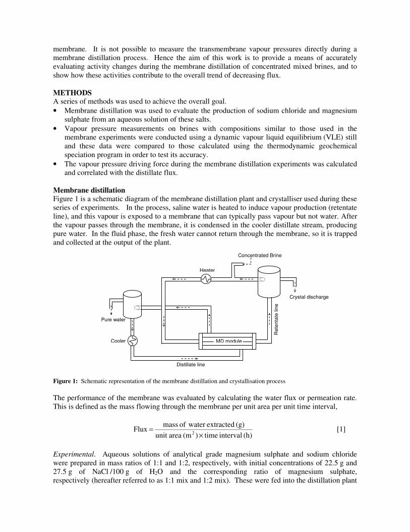
membrane. It is not possible to measure the transmembrane vapour pressures directly during a
membrane distillation process. Hence the aim of this work is to provide a means of accurately
evaluating activity changes during the membrane distillation of concentrated mixed brines, and to
show how these activities contribute to the overall trend of decreasing flux.
METHODS A series of methods was used to achieve the overall goal.
• Membrane distillation was used to evaluate the production of sodium chloride and magnesium
sulphate from an aqueous solution of these salts.
• Vapour pressure measurements on brines with compositions similar to those used in the
membrane experiments were conducted using a dynamic vapour liquid equilibrium (VLE) still
and these data were compared to those calculated using the thermodynamic geochemical
speciation program in order to test its accuracy.
• The vapour pressure driving force during the membrane distillation experiments was calculated
and correlated with the distillate flux.
Membrane distillation
Figure 1 is a schematic diagram of the membrane distillation plant and crystalliser used during these
series of experiments. In the process, saline water is heated to induce vapour production (retentate
line), and this vapour is exposed to a membrane that can typically pass vapour but not water. After
the vapour passes through the membrane, it is condensed in the cooler distillate stream, producing
pure water. In the fluid phase, the fresh water cannot return through the membrane, so it is trapped
and collected at the output of the plant.
Figure 1: Schematic representation of the membrane distillation and crystallisation process
The performance of the membrane was evaluated by calculating the water flux or permeation rate.
This is defined as the mass flowing through the membrane per unit area per unit time interval,
(h) interval time)(m areaunit
(g) extracted water of mass Flux
2 ×= [1]
Experimental. Aqueous solutions of analytical grade magnesium sulphate and sodium chloride
were prepared in mass ratios of 1:1 and 1:2, respectively, with initial concentrations of 22.5 g and
27.5 g of NaCl /100 g of H2O and the corresponding ratio of magnesium sulphate,
respectively (hereafter referred to as 1:1 mix and 1:2 mix). These were fed into the distillation plant
Concentrated Brine
Heater
Cooler
Pure water
Crystal discharge
Distillate line
Rete
nta
te lin
e
MD module
which was operated in a batch concentration mode where the recirculating permeate stream,
consisting of deionized water, and the retentate stream flowed countercurrent through the
membrane module. The membrane module, MD020CP-2N, supplied by Microdyn, contains 40
hydrophobic polypropylene hollow fibres of 0.1 m2
total interfacial area. The nominal pore size of
the polypropylene membranes was 0.2 µm and the external diameter was 1.8 mm. The
crystallisation vessel operated at 25 ºC and atmospheric pressure. The average temperatures at
module inlet on retentate and distillate sides were 33 ± 2 ºC and 17 ± 1 ºC, respectively. The water
flux was evaluated by measuring the amount of water extracted at time intervals during the course
of the experiment.
Vapour liquid equilibrium still The vapour liquid equilibrium (VLE) still developed by Raal and Mühlbauer (1998) was used to
measure the vapour pressures as a function of the temperature of aqueous solutions of pure sodium
chloride and solutions of mixtures of sodium chloride and magnesium sulphate corresponding to the
range of compositions of those used during the distillation process. The design and operation of the
still is described by Joseph et al (2001). The vapour pressures are related to temperature by the
Antoine equation.
CT
BAP
+−=ln [2]
where P is the pressure in pascal, T is the temperature in Kelvin and A, B and C are constants
which vary from substance to substance. The Antoine equation was used in a regression procedure
to determine parameters to fit the experimental vapour pressure data.
Experimental. The preparation of the solutions followed the same procedure as that used for
membrane distillation. Varying concentrations of aqueous solutions of pure sodium chloride were
prepared in order to gain data for comparison with literature to substantiate the progression of
investigations into our systems. The temperature and pressure in the still were computer controlled.
The desired temperature was set and once vapour-liquid equilibrium was established, the
corresponding pressure was recorded.
Geochemical equilibrium speciation program, PHRQPITZ PHRQPITZ is a computer program which enables geochemical calculations in brines and other
electrolyte solutions at high concentrations by making use of the Pitzer-virial coefficient approach
for activity coefficient corrections (Plummer et al, 1988). In addition to being able to calculate the
activity coefficients for the above solutions with temperature, the program is also able to model
mineral solubility thus predicting the evaporation factor needed in order to reach supersaturation
and crystallisation. For the purposes of this paper, this program was used to test its applicability for
modeling vapour pressures by comparison to the data obtained from the VLE experiments. The
effective vapour pressure of a solution is the product of the vapour pressure of pure water at the
same temperature as the solution and the activity of water in the solution.
There does, however, exist some limitations concerning the use of this code for modeling purposes.
One which applies to our system is that the temperature range for equilibria in the PHRQPITZ
database is variable and is within the range 0 to 60 °C but the sodium chloride system is valid up to
approximately 350 °C.

RESULTS AND DISCUSSION
Membrane Distillation The performance of the membrane distillation was evaluated by examining the water flux trend as
illustrated in Figure 2. This trend represents that of a solution containing equal amounts of each salt
per 100 g H2O (1:1 mix).
0
50
100
150
200
250
300
350
0 50 100 150 200 250 300 350 400 450 500
Time(min)
Flu
x(g
.h-1
.m-2
)
0
0.5
1
1.5
2
2.5
3
3.5
4
4.5
5
Co
nc
en
tra
tio
n (
M)
flux
[NaCl]
[MgSO4]
Figure 2: Trends of the water transmembrane flux and the concentration of magnesium sulphate and sodium chloride
with time for a solution containing equal masses of each salt per 100 gram of water
Typically, if a crystallisation run is carried out in a batch concentration mode i.e. the retentate line is
not continuously replenished with fresh feed solution, the flux will decrease with time as the
solution becomes more concentrated. A similar trend was obtained for the 1:2 MgSO4:NaCl
solution.
Vapour-liquid equilibrium still In order to test the performance of the still the vapour pressure of aqueous solutions of pure sodium
chloride was measured as a function of temperature and was found to be in good agreement with
those of previous authors (Lui and Lindsay, 1971; Sparrow, 2003). The vapour pressures obtained
for the subsequent mixes of salt solutions, in addition to that of pure water are shown in Figure 3. It
can be clearly seen that the difference in vapour pressure between the hot (brine) and
cold (pure water) sides drives the separation process.
0
20
40
60
80
100
120
0 20 40 60 80 100
Temperature (oC)
Pre
ssu
re (
kP
a)
1:2
1:1
water
Figure 3: Vapour pressures of salt mixes containing magnesium sulphate and sodium chloride 1:1 solution, 1:2 solution
and pure water

PHRQPITZ PHRQPITZ was used to obtain the activity coefficients, hence the vapour pressures, of the two
mixes of salt solutions at the range of temperatures used during the VLE experiments. Figure 4
shows the comparison of the vapour pressure trend obtained from both methods and Figure 5
compares the activities calculated in both cases. The slight deviation of the experimental results
from those of PHRQPITZ at increasing temperatures in Figure 5 is attributed to the uncertainty in
PHRQPITZ calculations above 60 ºC. This uncertainty, however, does not effect the outcome of
the results in this study as the membrane distillation plant operates at an average retentate
temperature of 33 ºC. It therefore appears that the vapour pressure can be sufficiently accurately
modeled using PHRQPITZ for the analysis of the experimental membrane distillation results.
0
10
20
30
40
50
60
70
80
20 30 40 50 60 70 80 90 100 110
Temperature (oC)
Pre
ss
ure
(k
Pa
)
PHRQPITZ
VLE experiments
Figure 4: Vapour pressures obtained for 1:1 salt mix from PHRQPITZ calculations and VLE experiments.
0
0.1
0.2
0.3
0.4
0.5
0.6
0.7
0.8
0.9
1
20 30 40 50 60 70 80 90 100 110
Temperature(oC)
Ac
itiv
ity
of
H2O
PHRQPITZ 1:1 mix
VLE expts. 1:1 mix
PHRQPITZ 1:2 mix
VLE expt. 1:2 mix
Figure 5: Comparison of activities calculated from PHRQPITZ and VLE experiments for each of the salt mixes
This then led to a further investigation into the decline of flux experienced during the membrane
distillation run. The speciation program was used to calculate the activities from the temperature of
the retentate and distillate streams and concentration of the solutions at time intervals during the
separation process. Appropriate treatment of these data yielded the driving force at these time
intervals. Figure 6 shows the variation of the vapour pressures of each of the streams as indicated
in the legend. It emphasises the significant change in activities between the inlet and outlet
retentate and permeate streams and the negligible change in the pure water vapour pressure between
the inlet and outlet streams.

0.000
1.000
2.000
3.000
4.000
5.000
6.000
0 50 100 150 200 250 300 350 400 450 500
Time (min)
Pre
ssu
re (
kP
a)
Retentate inRetentate outPermeate inPermeate outPure retentate inPure retentate out
Figure 6: Vapour pressures of respective streams in membrane distillation of a 1:1 mix
The driving force, expressed as the log mean vapour pressures differences (∆Plm), where calculated
and plotted on the same graph as the transmembrane flux time relationship. Figure 7 demonstrates
the similarity in trend between the driving force and transmembrane flux for the distillation of the
1:1 mix revealed by accounting for the change in water activities at either ends of the membrane.
0.000
0.200
0.400
0.600
0.800
1.000
1.200
1.400
1.600
1.800
0 50 100 150 200 250 300 350 400 450 500
Time(min)
Pre
ssu
re (
kP
a)
0
50
100
150
200
250
300
350
Flu
x (
g.h
-1.m
-2)
dP lm
flux
Figure 7: Variation of transmembrane flux with the driving force as a function of time for the 1:1 mix
In Figure 8 the data are replotted to show the relationship between flux and vapour pressure driving
force. A notable feature of this plot is the non-zero intercept, which can be explained in terms of
the simultaneous heat and mass transfer through the membrane, which causes the temperatures and
vapour pressures at the membrane surfaces to be different from those in the bulk liquid. Because of
the conductive heat transfer through the membrane, this discrepancy occurs even when there is no
flux of vapour through the membrane, which accounts for the observed non-zero intercept. This
effect is usually negligible for dilute solutions, but has been observed elsewhere for concentrated
solutions (Walton et al, 2004).

0
50
100
150
200
250
300
350
0.00 0.20 0.40 0.60 0.80 1.00 1.20 1.40 1.60 1.80
∆Plm (kPa)
Flu
x (
g.h
-1.m
-2)
1:1 mix
1:2 mix
Figure 8: Transmembrane flux as a function of driving force during the distillation of 1:1 and 1:2 magnesium sulphate
and sodium chloride solutions
Conclusions The water activities during the membrane distillation of concentrated solutions of varying ratios of
magnesium sulfate and sodium chloride were sufficiently accurately modeled using a computer
program specific for geochemical calculations in concentrated brines. This program is limited to
calculations within a temperature range of 0 to 60 ºC which is inconsequential to our system, and
membrane distillation in general, being an energy economic separation process which, within the
norm, seldom exceeds an operating temperature of 40 ºC. The resulting vapour pressure driving
force showed notable similarity with the flux trend thus rationalizing the behaviour of the latter
during the membrane distillation process.
An evaluation of the kinetics of crystallisation of the salts is necessary to complete the
understanding of the process. These need to be well understood as the process must avoid
crystallisation in the membrane module while producing a high quality final product which
influences the performance of downstream processes (separation of crystals from mother liquor,
drying, storage etc.)
Acknowledgements
The financial support of Sasol (Pty) Ltd., the National Research Foundation (NRF) and the
Technology and Human Resources for Industry Programme (THRIP) which made the investigations
possible is gratefully acknowledged. The assistance of the thermodynamics group at the University
of KwaZulu-Natal, Durban, particularly that of Scott Clifford and Prathieka Naidoo, is highly
appreciated.
References Calabro V., Jiao B. L. and Drioli E. (1994) Theoretical and experimental study on membrane
distillation in the concentration of orange juice. Ind. Eng. Chem. Res., 33, 1803-1808.
Curcio E., Criscuoli A. and Drioli E. (2001). Membrane Crystallizers. Ind. Eng. Chem. Res., 40,
2679-2684.
Franken A. C. M., Nolten J. A. M., Mulder, M. H. V., Bargeman D. and Smolders C. A. (1987)
Wetting criteria for the applicability of membrane distillation. J. Membr. Sci., 33, 315-328.
Hsu S. T., Cheng K. T. and Chiou J. S. (2002) Seawater desalination by direct contact membrane
distillation. Desalination, 143, 279-287.
Joseph M. A., Raal J. D. and Ramjugernath D. (2001) Phase equilibrium properties of binary
systems with diacetyl from a computer controlled vapour-liquid equilbrium still. Fluid Phase
Equilibria, 182, 157-176.
Lawson K. W. and Lloyd D. R. (1997). Membrane Distillation: review. J. Membr. Sci., 124, 1-25.
Liu C. and Lindsay W. T. (1971) Thermodynamics of sodium chloride solutions at high
temperatures. Journal of Solution Chemistry, 1(1), 1972.
Plummer L. N., Parkhurst D. L., Fleming G. W. and Dunkle S. A. (1988) A computer program
incorporating Pitzer’s equations for calculation of geochemical reactions in brines. U.S.
Geological Survey Water-Resources Investigations, Report 88-4153, U. S. Department of the
Interior, Reston, Virginia, USA.
Raal J. D. and Mühlbauer A. L. (1998) Phase Equilibria: measurement and computation, Bristol,
PA.
Sparrow B. S. (2003) Empirical equations for the thermodynamic properties of aqueous sodium
chloride. Desalination, 159, 161-170.
Tzahi Y. C., Adams V. D. and Childress A. E. (2004) Experimental study of desalination using
direct contact membrane distillation: a new approach to flux enhancement. J. Membr. Sci., 228, 5-
16.
Walton J., Lu H., Turner C., Solis S. and Hein H. (2004) Solar and waste heat desalination by
membrane desalination. Desalination and water purification research and development program
report (DWPR) no. 81, Bureau of Reclamation, Denver Federal Center, USA.


A Fully Integrated Membrane Operation for Sea Water and Brackish Water Desalination
Efrem Curcio1,2, Gianluca Di Profio1, Lynette Mariah3, Enrico Drioli1,2
1 University of Calabria, Department of Chemical Engineering an Materials, Rende, Italy 2 Institute on Membrane Technology, ITM-CNR, c/o University of Calabria, Italy
Tel: +39.0984.492039 Fax: +39.0984.402103 Email: [email protected] Pollution Research Group, Department of Chemical Engineering, University of Kwa-Zulu Natal, Durban,
South Africa Abstract Water scarcity already represents the major problem in many countries. Considerable progresses have been reached by introducing pressure driven membrane operations as alternative to thermal desalination systems. Today, a large part of new desalination plants are almost completely based on Reverse Osmosis, eventually integrated with Microfiltration and Nanofiltration for pre-treatment. The introduction of these technologies has already evidenced interesting cost reduction and operational flexibility. However, membrane desalination technology still requires further improvements in the direction of: higher water recovery factors, further cost reduction, implementation of innovative strategies for brine disposal, improved process flexibility with respect to feed water composition, better quality of produced water for different potential end-users (ultrapure water, drinking water, agricultural and industrial water). In order to achieve these goals, the strategy of Process Intensification - that represent, today, one of the most realistic answer to a sustainable industrial growth – should be extended to the industrial segment of desalination. In this respect, fully integrated membrane operations seem to offer, in principle, interesting perspectives. In this work, authors present the energetic and exergetic analysis of an integrated membrane desalination system and discuss some appropriate parameters for improving the performance of the desalination plant in the logic of process intensification. A preliminary cost analysis based on different combinations of the membrane units, including the possibility to produce crystals from brines, is also provided. Keywords: Integrated membrane systems; process intensification; desalination Introduction Water shortage is now becoming acute in many countries so challenging governments to find solutions to the conflict over available water resources and rapid population increasing. In many arid zones, coastal or inland, desalination of sea or brackish water is the only solution to supply of fresh water. Due to the strategic nature of the product, several countries have drastically expanded the investments on desalination technologies. At the beginning of this millennium, the world production capacity was above 106 m3/d and the number of operating units was more than 12,500. Desalination plants are today present in more than 120 countries and the current production capacity is almost twice what it was a decade ago [Drioli, E. and Romano, M., 2001]. Mediterranean countries, including Spain, Malta and Cyprus, as well as Israel, have reverted from traditional MSF to the RO method during the past two decades. Despite the great success of membrane systems in water treatment, some critical problems still remain open: improve the water quality, enhance the recovery factors in high-pressure membrane systems, reduce the global costs, minimize the brine disposal impact. In this work, authors aim to demonstrate that integrated membrane operations might be a solution for improving desalination and water treatment systems in the logic of Process Intensification (PI). Process Intensification represents today one of the most promising strategy believed to bring drastic improvements in manufacturing and processing, substantially decreasing equipment-size/production-capacity ratio, reducing raw materials, saving energy input, replacing
1

and reducing hazardous, recycling waste materials [Stankiewicz, A. and Moulijn, J.A., 2002]. In this contest, membrane science and technology is expected to give a substantial contribution to satisfy the PI goal and to develop sustainable pathways, thus providing reliable options for both industrial growth and environmental protection. Membrane operations, with their intrinsic characteristics of efficiency and operational simplicity, high selectivity and permeability for the transport of specific components, compatibility between different membrane operations in integrated systems, low energetic requirements, good stability under operative conditions, environment-compatibility, easy control and scale-up, and large flexibility, can offer an interesting answer for the rationalisation of the chemical production. At present, the possibility to redesign important industrial production cycles by combining various membrane operations available in the separation and conversion units, so realizing highly integrated membrane processes, is an attractive opportunity because of the synergic effects that can be reached. It is today well accepted that costs related to conventional pre-treatments can be minimized using pressure driven processes such as Microfiltration (MF), Ultrafiltration (UF) and Nanofiltration (NF). MF is a low energy-consuming technique extensively used to remove suspended solids and to lower COD/BOD and Silt Density Index (SDI) to values below 5. UF retains suspended solids, bacteria, macromolecules and colloids; although operating at higher pressure than MF, UF remains competitive against conventional pre-treatment. The use of NF leads to significant improvement in the reliability of Reverse Osmosis (RO): turbidity, microorganisms and hardness are strongly reduced, as well as the most part of multivalent ions; monovalent species are also retained by 10-50% depending on the membrane properties. As consequence, the osmotic pressure of the RO feed stream is decreased, thus allowing the unit to operate at high recovery factors without scaling problems. Alternative designs and engineering approaches need to be developed not only to drive down the cost of water and to ensure the quality of water supply. Cost effective and environmentally sensitive concentrate management is today recognized as a significant hurdle to extensive implementation of desalination technologies. At present, a large part of desalination facilities discharge their concentrate waste stream back to surface waters or oceans. This disposal methods represents currently the least expensive option for both small systems and for larger systems located near coastal regions. However, the promulgation of more and more stringent environmental protection regulations will reduce progressively this opportunity. Recently, the R&D activity about concentrate disposal subject has been considered in the U.S. Roadmap on Desalination & Water Purification Technology [U.S. Bureau of Reclamation, 2003] as a research area of strategic importance, and alternative design pathways for brine concentration is encouraged as viable opportunity to obtain value from saline waste streams, with consequent benefits in terms of overall costs reduction. In this respect, authors of the present paper consider an innovative Membrane Crystallization device [Curcio, E. et al., 2001] as additional option for integrated membrane desalination systems able to recover dissolved salts present in seawater (NaCl, MgSO4·7H2O), and to increase the yield of desalted water. Membrane Crystallization (a schematic representation is reported in figure 1) has been recently proposed as one of the most interesting and promising extension of the MD concept: solutions, concentrated above their saturation limit, achieve a metastable state (supersaturation) in which crystals nucleate and grow. The driving force of the process, the vapour pressure gradient between both sides of the membrane, can be activated by a temperature or concentration gradients. Membrane Crystallizers, when working under forced solution flow regime, are characterized by an axial flux, in laminar regime, of the crystallizing solution through the membrane fibres. This is expected to promote a well ordered organization of the molecules, finally resulting in the formation of crystals with better structural properties. One of the main features of the MCr systems is that the membrane does not act simply as support for the solvent evaporation, but it also induces
2

heterogeneous nucleation starting at low supersaturation ratios, depending on the surface characteristics of the membrane.
water inlet
water outlet
HEATEXCHANGER
MEMBRANEMODULE
steam inlet
steam outlet
CIRCULATIONPUMP
feed inlet
productdischarge
CRYSTALLIZERBODY
NaCl
a bMgSO4·7H2O
Figure 1- a) Scheme of a Membrane Crystallizer; b) crystalline products of interest. Energy and exergy analysis for quantifying the energetic requirements of the various membrane systems and their efficiency – evaluated in terms of entropic losses – is carried out. The feasibility of different integrated flow sheets are discussed in terms of energy demand, productivity and quality of fresh water, brine disposal reduction and cost analysis.
Energy and exergy analysis Three different flow sheets have been analysed; starting form the case study (FS1) that concerns the combination MF/NF/RO (figure 2), additional schemes include a Membrane Crystallization unit working: i) downstream the NF retentate (FS2, figure 3); ii) downstream the RO retentate (FS3, figure 4). In all cases, the same feed water flowrate (1000 kg/h) and composition (table 1) is considered.
Flowrate: 1050 m3/hCl-:19,345 ppmNa+:10,752 ppmSO4
2-: 2,701 ppmMg2+: 1,295 ppmCa2+: 0.416 ppmHCO3
-: 0.145 ppm
MF NF RO
Flowrate: 750 m3/hCl-:16,830 ppmNa+:8,378 ppmSO4
2-: 0,270 ppmMg2+: 0,142 ppmCa2+: 0.048 ppmHCO3
-: 0.055 ppm
Flowrate: 378 m3/hCl-:0,177 ppmNa+:0,091 ppmSO4
2-: 0,0010 ppmMg2+: 0,0006 ppmCa2+: 0.0001 ppmHCO3
-: 0.008 ppm
Flowrate: 372 m3/hCl-:33,800 ppmNa+:16,840 ppmSO4
2-: 0,544 ppmMg2+: 0,287 ppmCa2+: 0.0973 ppmHCO3
-: 0.110 ppm
1 2
3
4 5
6
8 9 12
10
retentate
7 11
Figure 2- Flow sheet 1 (FS1): an integrated MF/NF/RO system.
3

MCrysNa2CO3
NaClMgSO4 7H2O
1'
2' 2"
7
fromNF
RETENTATE
fromRO
PERMEATE12
3'
FRESH WATER
4'
CaCO3
Figure 3- Flow sheet 2 (FS2):the additional Membrane Crystallizer working downstream NF retentate completes FS1.
MCrysNa2CO3
NaCl
1'
2' 2"
11
fromRO
RETENTATE
fromRO
PERMEATE12
3'
FRESH WATER
4'
CaCO3
Figure 4 - Flow sheet3 (FS3):the additional Membrane Crystallizer working downstream RO retentate completes FS1.
Ion Concentration (ppm) Cl- 19,345 Na+ 10,752 SO4
2- 2,701 Mg2+ 1,295 Ca2+ 0,416 HCO3
- 0,145 Table 1 – Feed water composition
4

Water recovery factors of the different pressure-driven membrane units are: 94.7% for Microfiltration, 75.3% for Nanofiltration, [Drioli, E. et al., 2004] and 50.5% for Reverse Osmosis (Nanofiltration reduces the scaling potential due to bivalent ions Ca2+ and Mg2+ and allows to operate RO at higher recovery factor). For what concerns the performance of a Membrane Crystallizer, the possibility to reduce up to 95% Ca2+ ions by reactive unseeded precipitation of calcium carbonates, to crystallize 78% of dissolved sodium chloride, and to produce 8.4 kg MgSO4·7H2O per cubic meter of NF retentate was experimentally verified in a previous work [Drioli, E. et al., 2004]. The fresh water coming out from RO is used as cold water stream in the Membrane Crystallizer. The basic equations for energy and exergy analysis are below described [Criscuoli, A. et al., 1999]. Exergy (Ex), defined as the maximum useful work that a system can do when it passes from an actual state to the reference state where it is in equilibrium with the surroundings, is calculated as sum of three contributions:
cPT ExExExEx ++= (1) • Temperature exergy term (1.a) • Pressure exergy term (1.b)
) ( )(
• Concentration exergy term ( )10 ln xRTNGEx sc −= (1.c)
[ ]00 shT −( )[ ]ρ/0PPP −
0 sThGEx −−=GEx =
where G is the mass flowrate, s the specific entropy, h the specific entalpy, P the pressure, T the temperature, (subscript 0 indicates the reference status), ρ the density, R the gas constant, x1 the molar fraction of the solvent, and Ns is:
( ) MWcN is //1000 ρΣ−= (1.d) ([{ iiiss MWcNNx )]}ρβ //1 Σ+= (1.e)
In equations (1.d-e), ci concentration of i-th component, β is the number of particles formed by dissociation of i-th component in solution, MW the molecular weight. The exergy balance is expressed as:
ExWWTR uus ∆−−= '0 (2)
where RsT0 is the entropy production, ∆Ex is the exergy variation between inlet and outlet streams, Wu is the electrical exergy supplied to the cycle, W’u is the thermal exergy supplied to the cycle, calculated assuming that saturated vapour loses its latent heat transferring exergy to the fluid to be heated:
( ) ([ cvcvvu ssThhGW −−−= 0' )] (2.1)
Gv is the steam mass flow rate; subscripts v and c refer to vapour and condensed steam, respectively. Primary energy (PE), defined as the energy supplied by fuel combustion to produce energy, is evaluated as:
8.0⋅= vGPE (3) Mass flowrate, total concentration of ionic species, pressure and temperature and exergy terms of each stream in FS1-3 are reported in tables 2-4.
Stream 1 2 3 4 5 6 7 8 9 10 11 12G (kg/h)
P (MPa)T (K)
c (g/l)
Exc (kJ/h)ExP (kJ/h)ExT (kJ/h)
34.654
1,050,000
0.1
293
2,808,300
0
0
1,050,000
34.654
0.2
293
2,808,300
105,000
0
34.654
55,000
0.1
293
148,800
0
0
995,000
34.654
0.1
293
2,659,500
0
0
995,000
34.654
1.1
293
2,659,500
995,000
0
61.852
245,000
1.0
293
1,113,400
2,213,000
0
61.852
245,000
0.1
293
1,113,400
0
0
25.733
750,000
0.1
293
1,541,300
0
0
25.733
750,000
6.9
293
1,541,300
5,097,000
0
51.679
372000
6.8
293
372,000 378,000
1,520,500
2,476,000
0
0.1
51.679
293
1,520,500
18,600
0
0.270
0.1
293
8,280
0
0 Table 2 – Stream properties in FS1.
5

Stream 1' 2' 2" 3' 4'G (kg/h)
P (MPa)T (K)
c (g/l)
Exc (kJ/h)ExP (kJ/h)ExT (kJ/h)
-
894
0.1
293
-
-
-
244,100
62.270
0.1
293
1,138,000
0
0
62.270
244,100
0.1
323
1,138,000
1,432,000
0
233,300
0
0.1
313
0
638,000
0
10,800
-
0.1
293
-
0
0 Table 3 – Stream properties in FS2.
Stream 1' 2' 2" 3' 4'G (kg/h)
P (MPa)T (K)
c (g/l)
Exc (kJ/h)ExP (kJ/h)ExT (kJ/h)
-
85.4
0.1
293
-
-
-
371,900
51..705
0.1
293
1,521,000
0
0
51.705
371,900
0.1
323
1,521,000
2,170,000
0
359,400
0
0.1
313
0
963,000
0
12,500
-
0.1
293
-
0
0 Table 4 – Stream properties in FS3. Tables 5-7 report the results of the analysis for the three different flow sheets in terms of product characteristics, energy and exergy. .
Brine flow rateBrine concentration
Fresh flow rate
WuWu'RsT0
Electrical energy
672 m3/h53.986 g/l378 m3/h
6,523,600 kJ/h0 kJ/h
1,812 kWh
Fresh flow rate concentration 0.270 g/l
PEGv
0 Mcal/h0 kg/h
6,522,300 kJ/h
Brine flow rateBrine concentration
Fresh flow rate
WuWu'RsT0
Electrical energy
426 m3/h49.457 g/l624 m3/h
6,524,000 kJ/h7,129,000 kJ/h
1,812 kWh
Fresh flow rate concentration 0.166 g/l
PEGv
10,750 Mcal/h13,400 kg/h
14,764,000 kJ/h
Table 5 – Product characteristics and thermodynamic characteristics of FS1.
Table 6 – Product characteristics and thermodynamic characteristics of FS2.
Brine flow rateBrine concentration
Fresh flow rate
WuWu'RsT0
Electrical energy
312 m3/h56.827 g/l738 m3/h
6,524,000 kJ/h10,803,000 kJ/h
1,812 kWh
Fresh flow rate concentration 0.138 g/l
PEGv
16,300 Mcal/h20,350 kg/h
18,864,000 kJ/h
Table 7 – Product characteristics and
thermodynamic characteristics of FS3.
6

The opportunity to improve the water recovery factor by using Membrane Crystallization is evident in both FS2 and FS3. In the latter case, fresh water flowrate increases by 95%,whereas brine flowrate decreases by 53% with respect to data from FS1. Globally, the recovery factors are of 36%, 59% and 71% in FS1, FS2 and FS3, respectively. A progressive enhancement of the fresh water quality, evaluated in terms of amount of dissolved salts, is also observed when analysing FS2 and FS3. In addition to drinking water, FS2 offers the possibility to recover from NF retentate 8.7 tons NaCl/h and 2.1 tons MgSO4·7H2O/h in crystalline form. Before the crystallization stage, a reactive precipitation is needed in order to eliminate calcium ions and related scaling problems due to gypsum precipitation. Because of bivalent ions are retained by NF, a Membrane Crystallizer working on RO retentate (FS3) is able to produce only NaCl crystals in larger quantity (12.5 tons/h). From an energetic point of view, the integrated system related to FS1 is the most convenient: only electrical energy is requested to drive the medium- and higher- pressure pumps (1,812 kWh). The exergetic efficiency is also interesting and the entropic losses are moderate. With respect to conventional RO desalination plants, NF units allows to pre-pressurize the feed to RO train, leading to a reduction of the electrical power requested to drive the RO pumps. NF offers further benefits in terms of reduction of membrane fouling and, consequently, of related maintenance and replacement costs. The integration of Membrane Crystallization in FS2 and FS3 introduces a thermally energy requirement which increases the globally energy demand; as from tables 6 and 7, additional 10,750 Mcal/h and 16,300 Mcal/h are needed for heating the NF retentate and RO retentate streams, respectively, up to 323K (inlet temperature to Membrane Crystallization modules). Entropic losses are also increased. Although the estimation of energy saving is an important parameter, it could not be the determining factor in the selection of the more appropriate flow sheet. Plant economics and productivity, drinking water quality and disposal are additional key issues to be taken into account. Cost analysis Capital and operating costs for seawater and brackish water desalting tend to be high for small-capacity plants and to decrease for plant capacities above 3 MGD. Principal components to direct costs are represented by membranes ($90/m2 for Microfiltration membranes, also suitable for application in Membrane Crystallization, $30/m2 for Nanofiltration and Reverse Osmosis membranes) and equipments (high-pressure pumps, tubes, controllers, heat exchangers etc.). Additional costs must be included for chemicals, brine disposal, steam and electric power, labor and membrane replacement. Cost analysis has been carried out using the following financial factors [Ettouney, H.M. et al., 2002; Peters, M.S. et al., 2002]: • interest rate: 5%; • plant life: 30 yr; • amortization factor: 0.0651 yr-1 ; • plant availability: 0.9; • electric cost: 0.09 $/KWh; • heating steam cost: 0.0032 $/lb; • specific chemicals cost: 0.025 $/m3; • specific cost of operative labor: 0.05 $/m3 ; • specific cost of brine disposal: 0.0015 $/m3 ; The obtained results are summarised in tables 8-10.
7

Direct Capital Cost
Plant CapacityElectric Power Consumption
Fixed ChargesSteam
Electric PowerChemicals
Brine Disposal CostLabor
Membrane ReplacementTotal Annual Cost
Unit Cost Water ProductionBasis
$ 2,594,0009.080 m3/d
4.79 kWh/m3
$ 100,900 /yr-
$ 1,290,000 /yr$ 74,600 /yr$ 7,930 /yr
$ 149,000 /yr$ 188,300 /yr
$ 1,810,730 /yr
$ 0.61 /m3
Direct Capital CostPlant Capacity
Electric Power ConsumptionFixed Charges
SteamElectric Power
ChemicalsBrine Disposal Cost
LaborMembrane Replacement
Total Annual CostUnit Cost Water Production
Basis
$ 5,898,00014.800 m3/d2.94 kWh/m3
$ 108,000 /yr$ 738,400 /yr
$ 1,286,000 /yr$ 655,600 /yr$ 5,030 /yr
$ 243,000 /yr$ 827,700 /yr
$ 3,863,730 /yr
$ 0.80 /m3
Table 8 – Cost analysis of FS1. Table 9 – Cost analysis of FS2. Direct Capital Cost
Plant CapacityElectric Power Consumption
Fixed ChargesSteam
Electric PowerChemicals
Brine Disposal CostLabor
Membrane ReplacementTotal Annual Cost
Unit Cost Water ProductionBasis
$ 7,563,00017.700 m3/d2.46 kWh/m3
$ 110,000 /yr$ 1,119,000 /yr$ 1,286,000 /yr$ 196,400 /yr$ 3,500 /yr
$ 291,000 /yr$ 1,154,000 /yr$ 4,159,900 /yr
$ 0.72 /m3
Table 10 – Cost analysis of FS3. Conclusions Three different flow sheets have been analysed for desalination purpose. In FS1, pre-treatment by MF and NF allows to increase the recovery factor of the RO stage up to 50.5%; the global recovery of fresh water is 36% with a unit cost water production of $ 0.61/m3. FS2 and FS3 require higher energy consumption due to the additional thermal demand; however, the increased overall performance makes them an attractive alternative with respect to conventional desalination schemes. The introduction of a Membrane Crystallization unit downstream the NF retentate (FS2) enhances the global water recovery factor of water up to 58.6%, although the unit cost increases up to $0.80/m3 as consequence of additional expenses for membrane replacement, chemicals and steam. However, this gap can be potentially offset by 8.4 M$/yr resulting form the production of 8.7 tons NaCl/h (0.044$/kg) and 2.1 tons Epsomite/h (0.33$/kg). In FS3, the membrane crystallizer works on RO retentate: the global water recovery factor of water increases up to 70.1%, and both cost and environmental impact of brine disposal operations are drastically reduced. Once more, the additional production of 12,5 tons NaCl/h might counterbalance the higher unit cost of water production (4.3 M$/yr, $0.72/m3).
8

Bibliography Criscuoli, A., Drioli, E., 1999.Energetic and exergetic analysis of an integrated membrane desalination system. Desalination (125) 243
Curcio, E., Criscuoli, A., Drioli, E., 2001. Membrane Crystallizers. Ind. Eng. Chem. Res. (40) 2679
Drioli, E., Curcio, E., Criscuoli, A., Di Profio, G., 2004. Integrated system for recovery of CaCO3, NaCl and MgSO4·7H2O from nanofiltration retentate. Journal of Membrane Science (239) 27
Drioli, E., Romano, M., 2001. Progress and new perspectives on integrated membrane operations for sustainable industrial growth. Ind. Eng. Chem. Res. (40) 1277
Ettouney, H. M., El-Dessouky, H. T., Faibish, R. S., Gowin, P. J. 2002. Evaluating the Economics of Desalination. CEP Magazine (December) 32
Peters, M.S., Timmerhaus, K. D., West, R. E. Plant Design and Economics for Chemical Engineers, Mc Graw Hill, 2002
Stankiewicz, A., Moulijn, J.A., 2002. Process Intensification. Ind. Eng. Chem Res. 41(8) 1920
U.S. Bureau of Reclamation, Sandia National Laboratories. 2003. Desalination and Water Purification Technology Roadmap- A Report of the Executive Committee
9


MEMBRANE DISTILLATION FOR THE RECOVERY OF CRYSTALLINE PRODUCTS FROM CONCENTRATED BRINES
L. Mariah1, CA Buckley1, CJ Brouckaert1, D Jaganyi2, E Curcio3,4 and
E Drioli3,4
1Pollution Research Group, University of KwaZulu-Natal, Durban, South Africa
E-Mail: [email protected], Tel: +27 31 260-3131, Fax: +27 31 260-3241 2School of Chemistry, University of KwaZulu-Natal, Pietermaritzburg
3Institute on Membrane Technology (ITM-CNR), Via P. Bucci 17/C, c/o University of Calabria, 87030, Rende (CS), Italy.
4Department of Chemical Engineering and Materials, University of Calabria, via P. Bucci 45/A, 87030, Rende (CS), Italy
Membrane distillation and crystallisation (MDC) is a useful adjunct to seawater and other desalination processes in order to further process the resulting brine streams. MDC becomes particularly valuable when treating solutions of extremely high concentration which other processes such as reverse osmosis are incapable of handling. The process uses low grade heat and operates at about atmospheric pressure. This work demonstrates how membrane distillation and crystallisation is used to obtain pure crystalline products and pure water from solutions of sodium chloride and magnesium sulphate of concentrations near to saturation. Furthermore, a new approach to the modelling of the MDC process has been achieved which enables the prediction of driving force for the process by estimating the vapour pressure from chemical speciation calculations.. These modelling procedures are used to illustrate the gradual decline in the driving force during the membrane distillation process of solutions containing high concentrations of salt in contrast to the drastic decline in driving force in reverse osmosis. Further simulations are performed which illustrate how membrane distillation could be used to recover solid products from a mixed solution of salts whilst maintaining a driving force at extremely high solute concentrations. 1. BACKGROUND Salinity is one of South Africa’s most critical environmental problems, threatening economic and social consequences. Industries such as Sasol and Eskom currently have reverse osmosis (RO) plants producing waste brine, but brine disposal is a problem. If there is no intervention, the completed mining operations will continue to produce saline aqueous effluents for hundreds of years after mine closure. In the past most of the waste streams arising from the various mining and manufacturing activities were discharged to surface waters or the ocean. However, more rigid current and future environmental regulations will make these disposal routes less feasible therefore other disposal options need to be sought. It seems that technologies that are available for managing these waste products are either prohibitively uneconomic (exceeding the cost of water treatment or desalination) or unsatisfactory because of long term liabilities and associated risks they pose to water resources. Evaporation ponds appear to be one of the widely used means of disposal. However, low rates of evaporation due to highly concentrated waste streams or insufficient

driving force for evaporation, especially in areas where the humidity is relatively high, has resulted in a build-up in the inventory of these facilities. Much work has been performed on being able to solve this salinity crisis. However, bearing in mind the concept of sustainable development, we can deem these saline waters an environmental problem or we can turn this environmental problem into an economic resource by viewing these saline waters as a sustainable resource of salts. Several of the waste streams contain potentially recoverable and saleable products. Some of these include calcium carbonate, magnesium sulphate and calcium sulphate. Sustainable salt sinks can be achieved by considering the formation of valuable salts when designing a saline water circuit and the composition of the streams that enter the circuit. The separation and concentration processes need to be combined to produce high-value products. The chlor-alkali salt preparation circuit is an example of a process that requires a pure sodium chloride feed for a subsequent synthesis step (electrolysis) (1). Suitably purified and concentrated brine streams could substitute for the imported raw salt which is used as the feed chemical. A technique is therefore required in order to separate and recover these concentrates with the concomitant release of pure water. Many techniques have been investigated for the desalination of water and separation of salts. The most commonly used is that of reverse osmosis although other techniques such as thermal desalination and evaporation have been investigated (2). The main shortcoming of reverse osmosis is the high osmotic pressure of the feed stream at high solute concentrations. In reverse osmosis an excess pressure is required to overcome the solution osmotic pressure in order to concentrate the feed. In processes such as thermal evaporation, for example, elevated temperatures are required in order to achieve evaporation and salt recovery. Large heat transfer areas are required and scaling of the heat transfer surfaces reduces the efficiency of the process. There is a need for a process which would achieve the recovery of crystalline products and pure water and is capable of operating at high solute concentrations.. Exploiting the fact that inorganic concentrates can be separated into high value chemicals and reusable water, membrane distillation and crystallization (MDC) is a technique which potentially leads to a 100 % water recovery and the elimination of the brine disposal problem (3). This is achieved by the production of pure water by concentrating aqueous solutions through a vapour pressure difference induced by a transmembrane temperature gradient resulting in highly concentrated mother liquors in which nucleation and crystal growth occurs in a controlled fashion. This process does not have the limitations of reverse osmosis as this process can operate at higher concentrations, at low concentration gradients and atmospheric pressure. The advantage over distillation is that the mass transfer and heat transfer surfaces are combined, they consist of polymer fibres which have a higher packing density and lower cost that conventional corrosion resistant heat transfer surfaces. This paper therefore proposes the technique of membrane distillation crystallisation (MDC) for the recovery of crystalline products from brine concentrates and the production of pure water. The benefits of MDC as opposed to other membrane processes such as RO are discussed. Furthermore, a step is taken which is new to the MDC process is that of being able to computational model the process in terms of the evaluation of driving force and to examine some of the constraints of the latter. 2. MEMBRANE DISTILLATION As the name implies, the process combines both the use of distillation and membranes. In the process, saline water is heated to increase the vapour of water, and this vapour is exposed to

a hydrophobic polymeric membrane that can pass water vapour but not water. After the vapour passes through the membrane, it is condensed on a cooler surface (or in a cold water stream) to produce fresh water. In the liquid form, the fresh water cannot pass back through the membrane, so it is trapped and collected at the output of the plant. The main advantages of membrane distillation lie in its simplicity and the need for only small temperature differentials. One important advantage of membrane distillation in contrast to reverse osmosis, is because of the independence of the quality of the permeate from the feed solution concentrations, membrane distillation can handle highly concentrated feed solutions without a reduction in membrane selectivity. Reverse osmosis, however, is strongly affected by the osmotic pressure if the feed solution is highly concentrated resulting in higher applied pressure demands furthermore, increasing the susceptibility of the membrane to fouling. Recent innovative designing of integrated membrane systems (IMS) have lead to process intensification and reduction in pre-treatment costs (4). Integration of various single membrane units might assist in overcoming the shortfalls otherwise experienced if these units operate independently, i.e. many specialised separations as opposed to one big concentration step. Figure 1 shows an integrated system proposed by Drioli et al. (5). This system consisted of a pre-treatment stage which included MF/UF-NF-MC and a processing stage consisting of RO-MD. The pre-treatment stage included a gas-liquid membrane contactor unit (MC). This MC operation serves to reduce the amount of dissolved gases such as CO2 and O2 that is present in the feed solution, if deemed necessary. An energetic and exergetic analysis of this IMS indicated that the recovery factor of the MD unit was 77 % and the RO unit alone yielded a recovery factor of 40 %. However, by coupling these two membrane units the global recovery factor was a high of 87.6 % (6).
MF/UF NF MC RO
MD blowdown
Feed
Gas stream
Fresh water
RO brine
MD brine
Fresh water
Feed
Figure 1: Proposed ideal integrated membrane system for seawater desalination (5)
Furthermore, from their analyses it was found that by placing NF ahead of RO the osmotic pressure of the feed solution is lowered and hence a lower applied pressure is required to move water through the membrane. The added electrical energy that is required to operate the NF as a pre-treatment to RO can be offset by using the NF concentrate to pre-pressurise the feed water thus reducing the RO electrical energy requirements. For the coupling of RO with MD a higher thermal demand arises because of MD. However, when these two units are further coupled with NF it was found that this energy demand is lowered. If excess thermal energy is already present in the plant (as is the case in most industries such as Sasol where

there is an excess of low-grade thermal energy), then the surplus energy required by this system can be offset. Following the proposal of the ideal integrated system of Figure 1, later work performed by Drioli et al (4) incorporated a membrane crystalliser to form the NF-RO-MCr integrated system. The membrane crystalliser achieves the complete recovery of desalted water and solid salts. Feeding the MD unit with RO retentate represents the brine as the concentrated mother liquor which promotes nucleation and crystal growth. Curcio et al. (7) performed an energetic, exergetic and cost analysis on the systems MF-NF-RO and NF-MC-RO-MCr. In one instance, the NF retentate from the integrated system represented in Figure 1 was mixed with Na2CO3, produced from the reactive adsorption of CO2 via MC, for the removal of Ca2+ ions as CaCO3, before entering the MCr unit. In the second instance the RO retentate was subjected to CaCO3 precipitation before reaching the crystalliser. In the former case a global recovery factor of water of up to 58.6 % is achieved and in the latter case a 70.1 % global water recovery is achieved. Although the membrane crystalliser system represents a higher thermal energy requirement, it does, however, considerably reduce both the cost and environmental impacts of brine disposal operations thus favouring the concepts of green chemistry and moving towards sustainable industrial growth and, as already stated, if there is excess thermal energy already available within the plant, it could be used to supplement this added energy demand of the MCr unit making the overall energy requirement then comparable to an NF-RO coupled system (4). The main advantages of MD over conventional membrane and distillation processes can be summarised as follows: Membrane distillation,
� Can be performed at lower operating pressure and lower temperatures than the boiling point of the feed solutions (8-10) and a relatively low temperature difference between the two liquids in contact with the membrane surface gives relatively high fluxes.
� Requires lower vapour space as the vapour-liquid interface is developed by a hydrophobic membrane in membrane distillation as opposed to conventional distillation which relies on high vapour velocities to establish a vapour-liquid interface (11). As such they are very compact and very little equipment space is required. Furthermore, the possibility to overcome corrosion problems by using plastic equipment exists (12).
� Is unlimited by high osmotic pressure and fouling as the membrane works at atmospheric pressure and is not directly involved in the separation process but acts merely as a support. As such there is reduced chemical interaction between the membrane and process solution (13). Furthermore, due to this characteristic membranes can be fabricated from a variety of chemically resistant polymers (14).
� Displays selectivity higher than any other membrane process (15). MD therefore allows very high separation factors for ions, macromolecules, colloids, cells and other non-volatile solutes in comparison to UF, NF and RO processes (16,17)
� Has low sensitivity to feedwater concentrations and has potential applications for concentrating aqueous solutions or producing high-purity water even at very high feedwater concentrations (15, 18, 19)
� Does not require elevated temperatures therefore the heat can be supplied by solar collectors or other forms of heat such as low-grade waste heat from factories or geothermal energy (20).

Membrane distillation is one of the membrane processes in which the membrane is not directly involved in the separation. The membrane acts only as a support for a vapour-liquid interface and does not contribute to the separation mechanism. Selectivity is determined by the vapour-liquid equilibrium involved. One of the most important applications of MD is in the production of pure water. Studies have shown that a high quality permeate can be obtained during MD. This feature of MD makes this process invaluable in the desalination of seawater, in industry for boiler feedwater and in the semiconductor industry (21). Other areas in which MD is used to treat waste water is in the textile industry (22-23). In the case of a solution containing non-volatile components, e.g. NaCl, only water vapour flows through the membrane. Therefore, the retention degree of solutes in MD is close to 100 % (24). This allows the concentration of solutions up to solute saturation. The concentrating process of MD may be exploited in the food industry for the concentration of fruit juices and milk (25-27). Gostoli and Sarti (28) and later Sarti et al. (29) have found vacuum membrane distillation to be very useful for the separation of alcohol-water mixtures such as the extraction of organic components, ethanol and methylterbutyl from aqueous streams. Criscuoli et al. (30) evaluated MD for the treatment of uraemia by employing this process for the purification of human plasma ultrafiltrate and the re-circulation of the purified water to the patients. The feasibility of breaking down azeotropic mixtures by the removal of water using MD has been explored by Udriot et al. (31). Gryta et al. (24) used MDC for the treatment of NaCl solutions subsequent to use in the food industry. The concept was to produce pure water together with a concentrate containing substances present in the initial solution which could be separated by crystallisation thus facilitating their disposal and potential recycling of the water produced. 3. EXPERIMENTAL The experimental plant design that was used during these series of MDC experiments is depicted in Figure 2. The distillation plant was operated in a batch concentration mode where the recirculating permeate stream, consisting of deionised water, and the retentate stream flowed counter current through the membrane module. The membrane module, MD020CP 2N, supplied by Microdyn, contained 40 hydrophobic polypropylene hollow fibres of 0.1 m2 total interfacial area. The nominal pore size of the polypropylene membranes was
0.2 µm and the external diameter was 1.8 mm. During the process the solution in the retentate line is heated and flows toward the membrane and converges in a counter current manner with the cold permeate stream. A vapour-liquid interface is established at the membrane surface and water vapour molecules from the retentate stream diffuse across the membrane and condenses in the cold permeate. Continual removal of water in the retentate line leads to the concentration of the remaining solution resulting in a mother liquor in which nucleation and crystal growth is initialised. Crystallisation occurs in a vessel in which a centrifugal pump receives and returns the mother liquor to the membrane module on the retentate line. The crystallisation vessel operated at room temperature and atmospheric pressure. Samples were routinely withdrawn from the crystallisation tank and visually examined and photographed using a video-camera model, Axiovert 25, equipped with optical head 25 X, to determine the crystal size distribution.

Figure 2: Experimental setup for membrane distillation-crystallisation of concentrated salts
For the series of MDC experiments, two types of systems were investigated. Although some work has been done concerning the MDC of epsomite for the recovery of crystalline product (32), solutions of high concentration (close to saturation) have not been performed. Therefore, the first part of this work investigates the MDC of concentrated solutions of epsomite of concentrations 375 g/ℓ and 625 g/ℓ. This is then followed by the MDC of concentrated solutions of a mixture of sodium chloride and epsomite, in varying ratios, aimed at the crystallisation of sodium chloride. For this purpose aqueous solutions of analytical grade epsomite and sodium chloride were prepared in mass ratios of 1:1, 1:2 and 1:3, respectively, with initial concentrations of 225 g/ℓ of epsomite and NaCl for the 1:1 mix; 137.5 g/ℓ and 275 g/ℓ of epsomite and NaCl, respectively, for the 1:2 mix; and 93.3 g/ℓ and 280 g/ℓ of epsomite and NaCl, respectively for the 1:3 mix. The average temperatures at
module inlet on retentate and distillate sides were 29.8 ± 1.6 ºC and 17.6 ± 4.4 ºC, respectively, for the MD of the pure magnesium sulphate solutions. The average
temperatures at module inlet on retentate and distillate sides for the 1:1 mix was 32.6 ± 1.7 ºC
and 16.0 ± 0.5 ºC, respectively; for the 1:2 mix 32.6 ± 1.2 ºC and 16.8 ± 0.4 ºC, respectively;
and for the 1:3 mix 33.6 ± 2.6 ºC and 14.8 ± 0.5 ºC, respectively. The average temperatures
at module outlet on retentate and distillate sides for the 1:1 mix was 29.3 ± 1.4 ºC and
16.9 ± 0.7 ºC, respectively; for the 1:2 mix 30.5 ± 1.0 ºC and 17.4 ± 0.7 ºC, respectively; and
for the 1:3 mix 27.6 ± 1.0 ºC and 16.1 ± 0.6 ºC, respectively. The water flux was evaluated by measuring the amount of water extracted at time intervals during the course of the experiment. The flux of pure water through the membrane is more fully described in (33) but
ranged from 0.1 to 0.3 L/m2h for temperatures of 55 and 20 °C.
Heate
r
Cooler Permeate line
Rete
nta
te lin
e
MD module
Circulation pump
Circula
tion
pum
p
Feed solution/crystallisation tank
Pure water tank
Balance
Crystal formation

4. RESULTS The detailed results of the MD experiments have been described in a previous work by the authors (33). Therefore only a brief discussion of the results will be considered here. Figure 3 shows the photographs of the crystals that were taken during the crystallisation of magnesium sulphate from a pure solution of this salt and the crystallisation of sodium chloride from a mixture of sodium chloride and magnesium sulphate in equal mass ratios. The crystals display the characteristic geometries associated with their crystal forms, i.e. orthorhombic magnesium sulphate and cubic sodium chloride crystals.
Figure 3: Magnesium sulphate and sodium chloride crystals obtained from MDC
For the crystallisation of magnesium sulphate the evolution of the particle size distribution shows that the initial peak progressively migrates towards increasing crystal size due to the crystal growth process. The shape of the particle size distribution is governed by a coefficient of variation, CV, which is defined according to Equation 1,
1002
%50
%20%80 ×−
=F
FFCV [1]
where F is the cumulative particle size distribution. Analysis of the experimental cumulative size distribution functions enabled CV values to be calculated and was found to be in the range of 10 – 30 %. 5. MODELLING A computer program, PHRQPITZ, is able to perform geochemical calculations in brines and other electrolyte systems to high concentrations (34). This is possible as the main code of this program uses the Pitzer virial coefficient approach for activity coefficient corrections according to the works of Harvie (35) and Harvie et al. (36) for the prediction of mineral solubilities in natural waters for the Na-K-Mg-Ca-H-Cl-SO4-OH-HCO3-CO3-CO2-H2O system to high ionic strengths. The water activity values can be used to calculate water vapour pressures and osmotic pressures. The computer program PHRQPITZ was tested for its suitability of modelling vapour pressures. The details of the program and modelling and measurement procedures of vapour pressures have been described in a previous work by the
0.1 mm 0.1 mm

authors (37). The suitability of the program for modeling vapour pressures was verified by experiments performed with the aid of a dynamic vapour liquid equilibrium (VLE) still. A fit of the modelled vapour pressures to those measured experimentally is shown in Figure 4.
0
10
20
30
40
50
60
70
80
0 10 20 30 40 50 60 70 80
Measured (kPa)
Mo
de
lle
d (
kP
a)
1:1 mix
1:2 mix
1:3 mix
Figure 4: Comparison between modeled and measured vapour pressures
The relative errors between the vapour pressures modelled and those obtained experimentally range between -0.0014 to 0.0956 for the 1:1 mix, -0.0191 to -0.0576 for the 1:2 mix and -0.0136 to -0.0333 for the 1:3 mix. There therefore appears to be excellent agreement between the modelled and measured vapour pressures. The larger deviations are those at higher temperatures. This is due to the limitation of the input data to PHRQPITZ,
with regards to the uncertainty in PHRQPITZ calculations above 60°C. Hence, the program PHRQPITZ was deemed suitably accurate for modelling vapour pressures. Having a program capable of modelling the vapour pressures and osmotic pressures and hence driving force during MD (and RO) is a powerful tool which enables the prediction of the MD process. Figure 5 represents the vapour pressure driving force that was modelled for a solution containing approximately 100 g/ℓ of sodium chloride. This is compared to a driving force that would be obtained using RO on the same solution. The net driving force in RO is calculated as the difference in the applied pressure and that of the osmotic pressure of the solution calculated from the water activity according to Equation 2 (38, 39).
w
wV
RTαπ ln−= [2]
where π is the osmotic pressure in kPa, αw the activity of water, R the universal gas constant (= 8.314 ℓ.kPa.mol-1K-1), T is the absolute temperature in Kelvin and Vw is the molar volume of water in ℓ.mol-1.

The vapour pressure of the initial solution was 14.75 kPa and the osmotic pressure was 9.86 MPa. Thus a minimum applied pressure of approximately 10MPa is required in order to exceed the osmotic pressure. In Figure 5 an initial pressure of 10.5 MPa was applied. This applied pressure however, becomes insufficient at a concentration factor of less than 1.13 %
whereas MD (with a brine temperature of 55 °C and a pure water temperature of 20 °C) maintains a vapour pressure driving force of approximately 12.3 kPa which extends to very high concentration factors with only a gradual decline. It has been calculated that in order for RO to maintain a positive driving force at higher concentration factors, pressures of up to12 MPa and over would have to be applied.
0.0
0.5
1.0
1.5
2.0
2.5
3.0
1 1.02 1.04 1.06 1.08 1.1 1.12 1.14
Concentration factor
log
dri
vin
g f
orc
e
RO net pressure driving force
MD vapour pressure driving force
Figure 5: Comparison of RO and MD driving force for a 100 g/ℓ sodium chloride solution In order to further illustrate the capability of MD to concentrate a solution up to saturation and crystal formation is shown in Figure 6. This plot represents a MD concentration of a mixture of sodium chloride and magnesium sulphate each at a concentration of 225 g/ℓ (1:1 mix described above). The initial vapour pressure of this solution is 11.8 kPa and the osmotic
pressure is 43MPa. With a brine temperature of 55 °C and a pure water temperature of
20 °C, it can be seen that MD can concentrate the solution up to the point of sodium chloride crystallisation and beyond with approximately 150 g/L of pure crystalline sodium chloride being recovered and a 74 % water recovery being achieved before magnesium sulphate would start to precipitate, while still maintaining an existent vapour pressure driving force. It was calculated that in order for reverse osmosis to perform at these levels of concentration, an enormously elevated applied pressure of approximately 50 MPa is required in order to obtain a positive driving force. Furthermore, this applied pressure would become insufficient at an extremely low water recovery factor.

0
40
80
120
160
1 1.5 2 2.5 3 3.5 4
Concentration factor
-2
0
2
4
6
8
10
Driving force (kPa)
Solid NaCl recovered (g/l)
SI NaCl
SI MgSO4
Figure 6: MD process showing evolution of driving force and solid NaCl recovery with water recovery
6. CONCLUSION The computer program PHRQPITZ has facilitated the modelling of driving forces in MD and RO processes thereby illustrating the incapacity of the latter to operate at extremely high solute concentrations without the application of excessively high pressures. Furthermore, the vapour pressure driving force during MD allows a solution to be concentrated up to saturation and beyond thus facilitating the recovery of crystalline products. MD is a relatively new technique and its applications are imminent. 7. ACKNOWLEDGEMENTS The financial support of Sasol (Pty) Ltd., the National Research Foundation (NRF) and the Technology and Human Resources for Industry Programme (THRIP) which made the investigations possible is gratefully acknowledged. 8. REFERENCES 1. P Giannadda, The development and application of combined water and materials pinch
analysis to a chlor-alkali plant PhD thesis, Pollution Research Group, University of Natal, South Africa (2002).
2. J Kurbiel, W Balcerzak, MS Rybicki and K Swist, Desalination, 106 p.415 (1996). 3. E Curcio, A Criscuoli and E Drioli, Ind. Eng. Chem. Res., 40, p.2679 (2001). 4. E Drioli, A Criscuoli and E Curcio, Desalination, 147, p.77 (2002). 5. E Drioli, F Lagana, A Criscuoli and G Barbieri, Desalination, 122, p.141 (1999). 6. A Criscuoli and E Drioli, Desalination, 124, p.243 (1999).

7. E Curcio, G Di Profio, L Mariah and E Drioli, Proc. 7th World Conference for Chemical Engineers, Glascow, 2005.
8. SI Andersson, N Kjellander and B Rodesjo, Desalination, 56, p.345 (1985). 9. M Khayet, MP Godino, and JI Mengual, Desalination, 157, p.297 (2003). 10. GC Sarti, C Gostoli and S Matulli, Desalination, 56, p.277 (1985). 11. AS Jonsson, R Wimmerstedt and AC Harryson, Desalination, 56, p.237 (1985). 12. FA Banat and J Simandl, Desalination, 95, p.39 (1993). 13. ST Hsu, KT Cheng and JS Chiou, Desalination, 143, p.279 (2002). 14. V Gekas and B Hallstrom, J. Membr. Sci., 30, p.153 (1987). 15. AM Alklaibi and N Lior, Desalination, 171, p.111 (2004). 16. L Martinez-Diez and FJ Florida-Diaz, Desalination, 137, p.267 (2001). 17. KW Lawson and DR Lloyd, J. Membr. Sci., 124, p.1 (1997). 18. Y Wu, Y Kong, J Liu, J Zhang and J Xu, J. Membr. Sci., 69, p.72 (1992). 19. A Kubota, K Ohta, I Hayana, M Hirai, K Kikuchi and Y Murayama, Desalination, 69, p.19
(1988). 20. PA Hogan, Sudjito, AG Fane and GL Morrison, Desalination, 81, p.81 (1991). 21. M Mulder, Basic principles of membrane technology, Kluwer Academic Press, p. 48
(1996). 22. V Calabro, E Drioli and F Matera, Desalination, 83, p.209 (1991). 23. Y Wu, Y Kong, J Liu, J Zhang and J Xu, Desalination, 80, p.235 (1991). 24. M Gryta, M Tomaszewska, J Grzechulska and AW Morawski, J. Mebr. Sci., 181, p.179
(2001). 25. S Kimura and S-I Nakao, J. Membr. Sci., 33, p.285 (1987). 26. F Lagana, G Barbieri and E Drioli, J. Membr. Sci., 166, p.1 (2000). 27. V Calabro, BL Jiao and E Drioli, Ind. Eng. Chem. Res., 33, p.1803 (1994). 28. C Gostoli and GC Sarti, J. Membr. Sci., 41, p.211 (1989). 29. GC Sarti, C Gostoli and S Bandini, J. Membr. Sci., 80, p.21 (1993) 30. A Criscuoli, E Drioli, A Capuano, B Memoli and VE Andreucci, Desalination, 147, p.147
(2002). 31. H Udriot, A Araque and U Von Stockar, The Chemical Engineering Journal, 54, p.87
(1994). 32. E Drioli, E Curcio, A Criscuoli and G Di Profio, J. Membr. Sci., 239, p.27 (2004). 33. L Mariah, CA Buckley, CJ Brouckaert, E Curcio, E Drioli, D Jaganyi and D
Ramjugernath, submitted J. Membr. Sci (2005) 34. LN Plummer, DL Parkhurst, GW Fleming and SA Dunkle, US Geological Survey, Water-
Resources Investigations Report 88-4153, Reston, Virginia (1988). 35. CE Harvie and JH Weare, Geochimica et Cosmochimica Acta, 44, p.981 (1980). 36. CS Harvie, N Møller and JH Weare, Geochimica et Cosmochimica Acta, 48, p.723
(1984). 37. L Mariah, CA Buckley, CJ Brouckaert, E Curcio, E Drioli, D Jaganyi and D
Ramjugernath, Proc. IWA/WISA Conference: Management of Residues Emanating from Water and Wastewater Treatment, Johannesburg, South Africa (2005).
38. RA Robinson and RH Stokes, Electrolytes Solutions, 2nd Edition, Butterworths Scientific Publications, London (1959).
39. CJ Brouckaert, S Wadley and QE Hurt, Research on the Modelling of Tubular Reverse Osmosis, WRC Report No 325/1/95 (1995).
Copyright © 2022 FDOKUMEN