Thermal Energy Storage by PCM-air Heat Exchangers: Temperature Maintenance in a Room
Upload
khangminh22Category
view
0download
0
Medium Temperature Thermal Energy Storagefor High Efficiency Solar Cooling Applications
A thesis submitted in fulfillment of the requirements for the degree of
Doctor of Philosophy
Sergio PintaldiBEng Mech - Polytechnic of Turin, ItalyMEng Mech - University of Trieste, Italy
Supervisors:Prof G. Rosengarten (RMIT), Dr S. White (CSIRO)
Co-supervisor:Dr S. Sethuvenkatraman (CSIRO)
School of EngineeringCollege of Science, Engineering and Health
RMIT University
August 2017

Declaration
I certify that except where due acknowledgement has been made, the work is that ofthe author alone; the work has not been submitted previously, in whole or in part, toqualify for any other academic award; the content of the thesis is the result of workwhich has been carried out since the official commencement date of the approvedresearch program; any editorial work, paid or unpaid, carried out by a third party isacknowledged; and, ethics procedures and guidelines have been followed.
Sergio Pintaldi30th August, 2017

Abstract
This thesis analyses thermal energy storage options for medium-temperaturehigh-efficiency solar cooling systems with absorption chillers, by exploring new ther-mal storage technologies and advanced control strategies. Considerable effort wasspent on building modelling and experimental tools required to systematically eval-uate the control strategy and storage material impact in a solar cooling plant. Theyare:
a) A detailed system level dynamical model of a solar air conditioning system hasbeen developed in the software TRNSYS as a part of this study. The systemlevel model integrates both sensible and latent heat storage models. In orderto accurately simulate the phase change heat transfer, a detailed numericalmodel for a latent heat TES was developed and validated with experimentaldata from a test rig built as a part of the thesis work.
b) In a typical solar air conditioning system, the controller functions to managethe plant response according to load demand without any information on theexpected availability of energy sources or load. A Model Predictive Controller(MPC) with knowledge of solar and load forecast information can improve theperformance of these systems. A Genetic algorithm (GA) based predictivecontroller was built and integrated with a simplified solar cooling numericalmodel.
c) As part of the project were the design, the installation and the commissioningof a test rig at the CSIRO Energy Centre in Newcastle, Australia for evalu-ating high efficiency solar air conditioning operation. The test rig consistedof 28 m2 single axis tracking Fresnel concentrating collectors, 1500 L thermalstorage system, 20 kW backup heater and a 10 kWc double stage absorptionchiller. Instrumentation and controllers were installed as part of the test rigto evaluate various operational strategies for improving the operation of a so-lar air conditioning plant. System level models were calibrated and improvedthrough measured data from the test rig and used for further investigation ofcontrol strategies. A fan heat rejection system was used during the tests tomimic the chiller heat load.
iii

iv
d) In order to verify the benefits of MPC in an operating system with TES, adeveloped control framework was integrated with the test rig data loggingand controls software (LabVIEW ). Successful MPC implementation requiredseamless integration and feeding of test rig data to the MPC model, consid-eration of component response times (e.g heater), limitations such as pumpminimum and maximum flow rates. The MPC controller of the test rig wasimplemented in Python.
The work reported in this thesis has improved our understanding and has devel-oped suggestions and methods for optimal operation of solar air conditioning plantswith thermal storage systems. Main learnings and outputs can be summarised asbelow:
• This thesis provides a generalised methodology for evaluating the suitabilityof sensible and latent heat materials as thermal storage media for solar airconditioning applications. Solar cooling system annual simulations have beencarried out under different scenarios to estimate the energy saving benefit oftwo sensible (water and thermal oil), two phase change (solar salt, Aluminiumtin alloy) storage media. Comparison of the results showed that despite latentheat storage exhibiting higher storage performance, the performance of thecomplete solar cooling system is lower than plants with sensible heat storagedue to higher temperature operation of the collector and the indirect heattransfer related losses. High thermal conductivity phase change material didnot perform better than sensible storage materials. Proper alignment of phasechange temperature and storage temperature could help in improve the per-formance of latent heat storage plants.
• Component level tests showed the collector operating with 32 % efficiencyand with intermittent tracking related problems. Storage tank showed typicalstratification and heat loss coefficient of 4.9 W/K, as per design specifications.Test results showed non optimal operation of chiller. The latter delivered anintermittent cooling power of 6 kW, whilst absorbing 10 kW of heat, resultingin a Coefficient of Performance (COP) < 1. Therefore complete solar planttests were carry out with a fan heat rejection system. During the test period,the solar collector produced 22.6 kWh of heat, and 10 kWh of heat was rejectedthrough the fan heat exchanger. As a result, more than 50 % of heat was lostdue to thermal losses in the system. These results stress the importance ofrunning preliminary test on single component performance, and using conser-vative performance data in the design phase. Nevertheless the test rig can usesome simple control strategies and can be used for MPC evaluation.
• Numerical simulations of GA-based MPC of a solar cooling plant model showed

v
the ability of the MPC to take advantage of the heat stored in the tank, andsuccessfully reduce backup heater usage. Ten day simulations using typicalweather data have been carried out to compare conventional or Rule-BasedControl (RBC) and MPC. Auxiliary heat reduction with respect RBC is upto 15 %. Detailed analysis of the MPC performance showed that benefit ismaximum over period of low solar availability.
• The objective of MPC implementation in the test rig is to gather first handoperational experience in a real world scenario, as the performance of thecontroller is strongly dependent on the real plant operation including the dy-namics of the components. A subsystem of the test rig was utilised to evaluatea RBC versus a MPC strategy. The objective of the controller was to maintainthe thermal store at a set point temperature throughout the day with minimalelectricity cost incurred for heating. A time of use electricity tariff structurewas used with peak rates after 0200 pm.
• Comparison of RBC and MPC controller responses showed the MPC tends toutilise part load settings of the heater and the pump rather than the ON – OFFused in RBC. However, limitations due to pump operating range and heatersettings made the control signal implemented in the real plant different fromthe MPC model control output. It is possible to overcome these limitationsby incorporating the response behaviour of the pump and the heater in theMPC model.
• Before implementing the MPC in real operating plant, a numerical modelof the real plant was utilised to evaluate the benefits of MPC. Rather thanoperating the pump and the heater in ON – OFF mode, the MPC controlleroperated the system at part load conditions and achieved a 14 % reduction inthe cost function.
• Tests have been carried out to evaluate the potential of MPC in reducingbackup energy cost with a-priori knowledge of solar radiation availability. Thescope of the control logic was to charge the storage system to a set-point tem-perature at the end of the day with a time varying electricity cost. The resultsshowed the ability of MPC to use forecast information related to radiation andelectricity cost.

Acknowledgments
Firstly I would like to thank all my family: my father, my mother and mybrother for the constant support and love over this adventure, thought we are apartin different continents. Another special thank go to my extended family – mygrandmother, uncle, auntie and cousins – for supporting me all my life. Family isthe most important thing, and without it I would not be here.
A special thank, for their support and mentoring, to Prof Rosengarten (RMIT)and Dr White (CSIRO), who helped me as supervisors during this journey. Otherspecial thanks to Dr Sethuvenkatraman (CSIRO) for the constant supervision andcollaboration, and to all the CSIRO solar cooling technical team, who is the verybest (Mark P, Roger and Stuart). I want to thank Mark G for his modelling tips, andNariman for helping me with my optimisation problems. I acknowledge the followingCSIRO (ex)staff: Cristian P for introducing me to the amazing world of Python andfor his debugging tips, Zhou for his kindness, tips and culinary experiences, Josh Wfor being supportive and friendly, Julio for being available when in need, Sam W forhis precious tips and nerdy conversations, Tim J and Kenrick for helping in dealingwith chemicals, Ben for sharing his Python scripts, Thomas and Scott for their verypeculiar and interesting conversations, Tim M for his support and banter, Saad fororganising volleyball, Dan L for being funny and supportive, all the (ex)students(Clothilde, Lyle, Walied, Karsten, Olmo, Magda, Larissa, etc.) for their incrediblepersonality, Adrian for sharing his book, Russel for his banter, all the people of theprocess bay and all the rest of the people of the CSIRO Energy Centre in Newcastle,who obviously I forgot to mention.
I would like to thank Thermax Limited for providing the data of the tripleeffect absorption chiller, the Australian Renewable Energy Agency (ARENA) forproviding the funds to carry out this research work as a part of Micro Urban SolarIntegrated Concentrators (grant No. “1-USO MUSIC”) project, the developers ofPython packages Pandas and Matplotlib for make their tools freely available withfull documentation and Prof R Wang, the director of the Thermal Energy & Nano-materials Lab of Arizona State University (Phoenix, Arizona), to let me carry outDSC measurements in his lab.
vi

vii
Finally I thank all my close friends – especially Annette – and the people that Imeet during this experience as they enriched myself with their personality, cultureand background.

Contents
Abstract iii
List of Figures xii
List of Tables xvi
Nomenclature xvii
1 Introduction 1
1.1 Rationale . . . . . . . . . . . . . . . . . . . . . . . . . . . . . . . . . 1
1.2 Research Questions and Scope . . . . . . . . . . . . . . . . . . . . . . 5
1.2.1 Research Questions . . . . . . . . . . . . . . . . . . . . . . . . 5
1.2.2 Approach . . . . . . . . . . . . . . . . . . . . . . . . . . . . . 6
1.3 Thesis Structure . . . . . . . . . . . . . . . . . . . . . . . . . . . . . 7
1.4 Publications . . . . . . . . . . . . . . . . . . . . . . . . . . . . . . . . 8
2 Literature Review 10
2.1 Storage Materials and Devices . . . . . . . . . . . . . . . . . . . . . . 10
2.1.1 Storage Materials . . . . . . . . . . . . . . . . . . . . . . . . . 11
2.1.2 Heat Transfer Methods . . . . . . . . . . . . . . . . . . . . . . 17
2.2 Solar Cooling Systems . . . . . . . . . . . . . . . . . . . . . . . . . . 21
2.2.1 Solar Cooling Systems with Absorption Chiller . . . . . . . . 21
2.2.2 Examples of SC Installations with Thermal Storage . . . . . . 22
2.3 Control Strategies of SC systems . . . . . . . . . . . . . . . . . . . . 24
2.3.1 Conventional Control . . . . . . . . . . . . . . . . . . . . . . . 25
viii

CONTENTS ix
2.3.2 Advanced Control Approaches . . . . . . . . . . . . . . . . . . 27
2.4 Storage Design & System Integration . . . . . . . . . . . . . . . . . . 31
2.5 Literature Summary . . . . . . . . . . . . . . . . . . . . . . . . . . . 33
3 Latent Heat Storage Model Development and Calibration 36
3.1 Introduction . . . . . . . . . . . . . . . . . . . . . . . . . . . . . . . . 36
3.2 Model Development and Implementation . . . . . . . . . . . . . . . . 39
3.3 Experiments and Model Validation . . . . . . . . . . . . . . . . . . . 42
3.3.1 Literature Validation . . . . . . . . . . . . . . . . . . . . . . . 42
3.3.2 Experimental Validation . . . . . . . . . . . . . . . . . . . . . 43
3.4 Chapter Summary . . . . . . . . . . . . . . . . . . . . . . . . . . . . 46
4 Thermal Storage Media Evaluation for a Solar Cooling System 47
4.1 Background . . . . . . . . . . . . . . . . . . . . . . . . . . . . . . . . 47
4.2 Solar Cooling Dynamic Model . . . . . . . . . . . . . . . . . . . . . . 49
4.2.1 System Model and Configurations . . . . . . . . . . . . . . . . 49
4.2.2 Component Models . . . . . . . . . . . . . . . . . . . . . . . . 51
4.2.3 SC system overall controls strategy . . . . . . . . . . . . . . . 58
4.3 Preliminary Simulation Results . . . . . . . . . . . . . . . . . . . . . 59
4.4 Thermal Storage Material Selection and System Design . . . . . . . . 63
4.4.1 Storage Design Methodology . . . . . . . . . . . . . . . . . . 63
4.4.2 SC system design for storage material comparison . . . . . . . 67
4.5 Comparison of Sensible and Latent Thermal Storage Materials . . . . 69
4.5.1 Constant Cooling Load System Performance . . . . . . . . . . 70
4.5.2 Variable Cooling Load System Performance . . . . . . . . . . 77
4.6 Chapter Summary . . . . . . . . . . . . . . . . . . . . . . . . . . . . 80
5 Real Operation of a Solar Cooling System 82
5.1 Facility Overview and Details . . . . . . . . . . . . . . . . . . . . . . 83
5.1.1 System Schematics . . . . . . . . . . . . . . . . . . . . . . . . 83
5.1.2 Main Component Details . . . . . . . . . . . . . . . . . . . . 85
5.1.3 Instrumentation and Control Details . . . . . . . . . . . . . . 88
CONTENTS x
5.2 Test Rig Operation . . . . . . . . . . . . . . . . . . . . . . . . . . . . 90
5.2.1 Storage-only Operational Mode . . . . . . . . . . . . . . . . . 91
5.2.2 Full-system Operational Mode . . . . . . . . . . . . . . . . . . 91
5.3 Experimental Activity . . . . . . . . . . . . . . . . . . . . . . . . . . 92
5.3.1 Preliminary Tests . . . . . . . . . . . . . . . . . . . . . . . . . 92
5.3.2 Solar Cooling System Tests . . . . . . . . . . . . . . . . . . . 100
5.3.3 Control Test Implementation . . . . . . . . . . . . . . . . . . 103
5.4 Chapter Summary . . . . . . . . . . . . . . . . . . . . . . . . . . . . 104
6 Model Predictive Control of a Solar Cooling System 106
6.1 Solar Cooling System and Controls . . . . . . . . . . . . . . . . . . . 107
6.1.1 Solar Cooling System and Conventional Control . . . . . . . . 107
6.1.2 MPC Model Formulation . . . . . . . . . . . . . . . . . . . . 110
6.2 Result Analysis of SC MPC Simulations . . . . . . . . . . . . . . . . 114
6.2.1 Constant Load System Performance . . . . . . . . . . . . . . 114
6.2.2 Variable Load System Performance . . . . . . . . . . . . . . . 117
6.3 MPC Implementation in a Test Rig . . . . . . . . . . . . . . . . . . . 121
6.3.1 Solar Cooling Subsystem and RBC . . . . . . . . . . . . . . . 121
6.3.2 MPC Development and Implementation for a SC Subsystem . 122
6.4 Experimental and Numerical Results . . . . . . . . . . . . . . . . . . 128
6.5 MPC with Solar and Backup Heating Sources . . . . . . . . . . . . . 133
6.5.1 MPC formulation . . . . . . . . . . . . . . . . . . . . . . . . . 133
6.5.2 Results of the Experiments . . . . . . . . . . . . . . . . . . . 135
6.6 Chapter Summary . . . . . . . . . . . . . . . . . . . . . . . . . . . . 138
7 Conclusions 139
7.1 Outputs and Findings . . . . . . . . . . . . . . . . . . . . . . . . . . 139
7.2 Recommendations and Future Work . . . . . . . . . . . . . . . . . . 142
Bibliography 144
A Appendix One 161

CONTENTS xi
A.1 Uncertainty Propagation Analysis . . . . . . . . . . . . . . . . . . . . 161
A.1.1 Collector Power . . . . . . . . . . . . . . . . . . . . . . . . . . 161
A.1.2 Collector Efficiency . . . . . . . . . . . . . . . . . . . . . . . . 162
A.1.3 TRNSYS Outlet Temperature . . . . . . . . . . . . . . . . . . 162
A.2 Tables for Literature Review . . . . . . . . . . . . . . . . . . . . . . . 163
A.3 Additional Schematics . . . . . . . . . . . . . . . . . . . . . . . . . . 166

List of Figures
1.1 Alignment of solar irradiance with cooling demand . . . . . . . . . . 2
1.2 Typical SC system with absorption chiller . . . . . . . . . . . . . . . 3
1.3 Storage size variation . . . . . . . . . . . . . . . . . . . . . . . . . . . 4
2.1 Storage volume for different storage materials . . . . . . . . . . . . . 11
2.2 Storage configurations to achieve stratification . . . . . . . . . . . . . 18
2.3 Water storage heat exchanger designs . . . . . . . . . . . . . . . . . . 19
2.4 Example of PCM storage configurations . . . . . . . . . . . . . . . . 20
2.5 Generic solar cooling system . . . . . . . . . . . . . . . . . . . . . . . 22
2.6 A LHTES installation . . . . . . . . . . . . . . . . . . . . . . . . . . 24
2.7 MPC generic framework . . . . . . . . . . . . . . . . . . . . . . . . . 29
2.8 Storage backup configurations . . . . . . . . . . . . . . . . . . . . . . 32
3.1 Latent Storage model with PCM . . . . . . . . . . . . . . . . . . . . 39
3.2 PCM model validation with literature data . . . . . . . . . . . . . . . 43
3.3 PCM model validation test rig . . . . . . . . . . . . . . . . . . . . . . 44
3.4 Salt DSC measurements . . . . . . . . . . . . . . . . . . . . . . . . . 45
3.5 PCM model validation plot . . . . . . . . . . . . . . . . . . . . . . . 46
4.1 Generic SC system with controls . . . . . . . . . . . . . . . . . . . . 50
4.2 Absorption chiller model calibration . . . . . . . . . . . . . . . . . . . 53
4.3 Building load for Sydney . . . . . . . . . . . . . . . . . . . . . . . . . 55
4.4 Temperature and Hysteresis Controllers . . . . . . . . . . . . . . . . 58
4.5 Chiller and building typical daily temperatures . . . . . . . . . . . . 60
4.6 Solar fraction for hysteresis and temperature controller . . . . . . . . 61
xii

LIST OF FIGURES xiii
4.7 Storage thermal losses and collector yield . . . . . . . . . . . . . . . . 62
4.8 Storage volume for storage comparison . . . . . . . . . . . . . . . . . 65
4.9 Storage temperature sensors . . . . . . . . . . . . . . . . . . . . . . . 68
4.10 SC system with LHTES temperature states . . . . . . . . . . . . . . 70
4.11 Storage thermal losses for two insulation values . . . . . . . . . . . . 72
4.12 Average annual LHTES discharging effectiveness . . . . . . . . . . . . 73
4.13 Storage efficiency for constant cooling load . . . . . . . . . . . . . . . 73
4.14 Solar fraction for constant cooling load . . . . . . . . . . . . . . . . . 74
4.15 Collected energy and storage losses for constant load . . . . . . . . . 75
4.16 Collector efficiency for constant cooling load . . . . . . . . . . . . . . 75
4.17 Storage top, bottom, and top-to-bottom temperature difference forconstant cooling load . . . . . . . . . . . . . . . . . . . . . . . . . . . 76
4.18 Chiller part load duration and requested temperatures . . . . . . . . 77
4.19 Storage efficiency for variable cooling load . . . . . . . . . . . . . . . 78
4.20 Solar fraction for variable cooling load . . . . . . . . . . . . . . . . . 78
4.21 Collected energy and storage losses for variable load . . . . . . . . . . 79
5.1 Test rig picture . . . . . . . . . . . . . . . . . . . . . . . . . . . . . . 83
5.2 SC test rig schematic . . . . . . . . . . . . . . . . . . . . . . . . . . . 84
5.3 Chromasun Micro-Concentrator collectors . . . . . . . . . . . . . . . 85
5.4 Collector test rig configuration . . . . . . . . . . . . . . . . . . . . . . 86
5.5 TES prototype . . . . . . . . . . . . . . . . . . . . . . . . . . . . . . 87
5.6 Calibration equipment for temperature sensors . . . . . . . . . . . . . 88
5.7 SC test rig data acquisition and control . . . . . . . . . . . . . . . . . 89
5.8 LabVIEW TM interface . . . . . . . . . . . . . . . . . . . . . . . . . . 90
5.9 Storage charging rig operation . . . . . . . . . . . . . . . . . . . . . . 91
5.10 Issues with collector RTD signals above 150 ◦C . . . . . . . . . . . . 93
5.11 Collector performance test with constant flow . . . . . . . . . . . . . 94
5.12 Collector performance test with variable flow . . . . . . . . . . . . . . 96
5.13 Storage charging test . . . . . . . . . . . . . . . . . . . . . . . . . . . 96
5.14 Storage thermal stratification . . . . . . . . . . . . . . . . . . . . . . 97

LIST OF FIGURES xiv
5.15 Heater section and pipe test . . . . . . . . . . . . . . . . . . . . . . . 98
5.16 Chiller operation at 170 ◦C . . . . . . . . . . . . . . . . . . . . . . . 99
5.17 SC plant operation test . . . . . . . . . . . . . . . . . . . . . . . . . . 100
5.18 SC plant operation storage detail . . . . . . . . . . . . . . . . . . . . 102
5.19 SC plant operation thermal losses . . . . . . . . . . . . . . . . . . . . 102
5.20 Control test schematic and strategy . . . . . . . . . . . . . . . . . . . 103
5.21 Preliminary standard control test . . . . . . . . . . . . . . . . . . . . 104
6.1 SC plant model for MPC simulations . . . . . . . . . . . . . . . . . . 108
6.2 Irradiance and cooling load for MPC . . . . . . . . . . . . . . . . . . 108
6.3 RBC for a solar cooling plant with fixed load . . . . . . . . . . . . . 115
6.4 MPC for a solar cooling plant with fixed load . . . . . . . . . . . . . 116
6.5 RBC and MPC cost function comparison for fixed load . . . . . . . . 118
6.6 RBC for a solar cooling plant with variable load . . . . . . . . . . . . 118
6.7 MPC for a solar cooling plant with variable load . . . . . . . . . . . . 119
6.8 RBC and MPC cost function comparison for variable load . . . . . . 121
6.9 RBC control test of SC subsystem . . . . . . . . . . . . . . . . . . . 122
6.10 Pipe model calibration . . . . . . . . . . . . . . . . . . . . . . . . . . 123
6.11 Heater pipe model calibration . . . . . . . . . . . . . . . . . . . . . . 124
6.12 Storage model calibration . . . . . . . . . . . . . . . . . . . . . . . . 124
6.13 Model states vs test data for a RBC test . . . . . . . . . . . . . . . . 125
6.14 Specific electricity cost profile . . . . . . . . . . . . . . . . . . . . . . 127
6.15 MPC LabVIEW control framework . . . . . . . . . . . . . . . . . . . 127
6.16 Preliminary MPC test results . . . . . . . . . . . . . . . . . . . . . . 129
6.17 Comparison of MPC vs RBC test results . . . . . . . . . . . . . . . . 130
6.18 Comparison of MPC vs RBC test cost functions . . . . . . . . . . . . 131
6.19 Comparison of MPC vs RBC simulation results . . . . . . . . . . . . 132
6.20 Scheme of the MPC controlled system with solar and backup . . . . . 134
6.21 Solar irradiance scenarios for MPC with solar . . . . . . . . . . . . . 135
6.22 MPC with simulated solar source for a sunny day . . . . . . . . . . . 136
6.23 MPC with simulated solar source for a cloudy day . . . . . . . . . . . 136

LIST OF FIGURES xv
6.24 MPC with simulated solar source for a cloudy afternoon day . . . . . 137
A.1 Detailed schematic of the SC test rig . . . . . . . . . . . . . . . . . . 166

List of Tables
2.1 Sensible heat materials for solar cooling applications . . . . . . . . . 12
2.2 Latent heat materials for double effect chiller systems . . . . . . . . . 14
2.3 Latent heat materials for triple effect chiller systems pt1 . . . . . . . 15
2.4 Latent heat materials for triple effect chiller systems pt2 . . . . . . . 16
3.1 PCM thermo-physical properties of CaCl2 · 6H2O . . . . . . . . . . . 43
3.2 PCM thermo-physical properties of KNO3/NaNO3 . . . . . . . . . . 45
4.1 Absorption chiller model parameters . . . . . . . . . . . . . . . . . . 54
4.2 TES materials for comparison analysis . . . . . . . . . . . . . . . . . 64
5.1 Chromasun equation parameters . . . . . . . . . . . . . . . . . . . . . 95
6.1 Daily Performance RBC fixed load scenario . . . . . . . . . . . . . . 116
6.2 Daily Performance MPC fixed load scenario . . . . . . . . . . . . . . 116
6.3 Daily Performance RBC variable load scenario . . . . . . . . . . . . . 120
6.4 Daily Performance MPC variable load scenario . . . . . . . . . . . . . 120
A.1 Literature examples of PCM storage designs . . . . . . . . . . . . . . 163
A.2 Literature examples of SC studies pt1 . . . . . . . . . . . . . . . . . . 164
A.3 Literature examples of SC studies pt2 . . . . . . . . . . . . . . . . . . 165
xvi

Nomenclature
Abbreviations
ABCB Australian Building Code Board
AHU Air Handling Unit
BCA Building Code of Australia
BV Ball Valve
CFD Computational Fluid Dynamics
CHTES Thermo-Chemical Energy Storage
COP Coefficient of Performance
CPC Compound Parabolic Collector
CSP Concentrated Solar Power
CTF Conduction Transfer Function
DER-CAM Distributed Resources Customer Adoption Model
DSC Differential Scanning Calorimetry
ETC Evacuated Tube Collector
EU European Union
FHU Fluid Handling Unit
FPC Flat Plate Collector
FR Flow Rate
FVM Finite Volume Method
GA Genetic Algorithm
xvii

NOMENCLATURE xviii
GHG Green House Gas
HTF Heat Transfer Fluid
HVAC Heating Ventilation and Air-Conditioning
IEA International Energy Agency
LBNL Lawrence Berkeley National Laboratory, Berkeley, California, USA
LHTES Latent Thermal Energy Storage
LHTESS(s) Latent Thermal Energy Storage System(s)
LMTD Log Mean Temperature Difference
MCT Micro-Concentrator
MINLP Mixed-Integer Non-Linear Programming
MIP Mixed-Integer Problem
MPC Model Predictive Control
MSDS Material Safety Data Sheet
NHPTF National HVAC Performance Test Facility
NP Non deterministic Polynomial time
NREL National Renewable Energy Laboratory, Golden, Colorado, USA
NTU Number of Heat Transfer Units
PCM(s) Phase Change Material(s)
PDE Partial Differential Equation
PI Proportional Integral
PID Proportional Integral Derivative
PnV Pneumatic Valve
PRV Pressure Relief Valve
PV Photovoltaic
PVT Photovoltaic Thermal

NOMENCLATURE xix
PWM Pulse-Width Modulation
RBC Rule-Based Control
RTD Resistance Temperature Detector
SAC Solar Air-Conditioning
SC Solar Cooling
SDHW Solar Domestic Hot Water
SHC Solar Heating and Cooling
SSM State Space Model
SSR Solid State Relay
STES Sensible Thermal Energy Storage
STESS(s) Sensible Thermal Energy Storage System(s)
TES Thermal Energy Storage
TESS(s) Thermal Energy Storage System(s)
TMY Typical meteorological Year
VSD Variable Speed Drive
Mathematical Symbols
βi Individual of a GA Population −
χi Randomly Generated Individual of a GA Population −
∆∆t Characteristic Temperature Function K
∆T Temperature Difference K
∆t Time Step s
m Mass Flow Rate kg/s
Q Power W
η Efficiency −
λt Encoded Storage-to-Chiller Flow Rate as part of an Individual −

NOMENCLATURE xx
ωi GA Population of i-th Iteration −
ϕt Encoded Burner Flow Rate as part of an Individual −
ψt Encoded Collector Flow Rate as part of an Individual −
ρ Density kg/m3
ε Effectiveness −
A Area m2
c, n NTU model coefficients −
C Cost of Electricity $
c1 Collector First Order Heat Loss Coefficient W/(m2K)
c2 Collector Second Order Heat Loss Coefficient W/(m2K2)
c5 Collector Effective Thermal Capacity per Unit of Area J/(m2K)
cp Specific Heat Capacity at constant pressure J/(kgK)
Cap Heat Capacity J/K
COP Coefficient of Performance −
costel Specific Cost of Electricity $/kWh
D Diameter m
dh Hydraulic Diameter m
e Enthalpy J/kg
Est Energy Stored J
Ev Volumetric Energy Density J/m3
F ′(τα)en Collector Efficiency Factor or Zero-Loss Efficiency −
H Height (between two storage nodes) m
h Convective Heat Transfer Coefficient W/(m2K)
I Solar Irradiance W/m2
J Cost Function −

NOMENCLATURE xxi
k Thermal Conductivity W/(mK)
KΘ Incidence Angle Modifier −
L Tube Length m
LH Latent Heat J/kg
m Mass kg
N Number of Tubes or Number of Time Steps −
NTU Number of Transfer Units −
Nu Nusselt Number −
Pr Prandtl Number −
Q Energy J
r radial coordinate m
R2 Coefficient of Determination −
rhtr Heater Power Ratio −
Rth Thermal Insulance m2K/W
Re Reynolds Number −
s, r, a, e Chiller Model Coefficients −
SF Solar Fraction −
T Temperature K
t Time s
Uloss, U Heat Loss Coefficient W/(m2K)
V Volume m3
w Weight in Cost Function −
y y coordinate m
Subscripts
AC absorber condenser

NOMENCLATURE xxii
air air
airn air-node
aux auxiliary
b beam
bot bottom section/node
burn burner
by bypass
charg charging
chil chiller
coll collector
d diffuse
disch discharging
dump dumped
E evaporator
el electricity
env environmental
eq equivalent
G generator
htf heat transfer fluid
htr heater
i inlet or inside
inf infiltration
ini initial
int, g internal gain
lam laminar

NOMENCLATURE xxiii
lb lower bound
liq liquid
load load/storage, usually store-to-chiller
los loss
m mean (usually between inlet and outlet)
max maximum
nom nominal
o outlet or outside
pc phase change
pcm phase change material
sat saturated
sec section
sol, g solar gain
sol solid
sp set-point
src source
st stored
sto storage
surf surface
temp temperature
top top section/node
tube tube
turb turbulent
ub upper bound
vent ventilation
wat water
wav waving

Chapter 1
Introduction
1.1 Rationale
Currently the energy market is dominated by the transition to renewable en-ergy. One of the most important driving factors for this transition is the abilityto isolate energy production from usage. This ability can be achieved by adoptingenergy storage solutions. Particularly, Thermal Energy Storage (TES) will play animportant role for the future energy sector as the demand of thermal energy – heat– still remains the main energy need, accounting for 52 % of global energy con-sumption [1]. Given the peculiar intermittent characteristic of the solar radiation,TES is essential in every solar thermal system in order to smoothen the solar poweroscillations and makes continuous heat available to the load.
Among solar thermal technologies, Solar Cooling (SC) or Solar Air-Conditioning(SAC) is particularly attractive due to its ability of make use of thermally acti-vated cooling processes, and therefore reducing electricity peak demand for coolingpurposes. Historically cooling demand has been fulfilled by conventional vapour-compression chillers which are driven by electrical energy. In regions of the worldwhere solar heat is quite abundant, and the cooling demand is the predominant en-ergy need in the building sector (e.g. Australia), high level of solar energy generallymatches with correspondent high cooling loads as illustrated in figure 1.1. Thereforesolar cooling could bring substantial economical and environmental benefits, suchas lowering the impact on the electricity network, and contributing to the reductionof green house gas (GHG) emissions.
Production of cooling using solar energy can be achieved in two ways: (i) systemsthat convert incident solar radiation into heat and use this heat to generate cooling.Heat is generated through thermal collectors. Cooling is generated when this heatis used in sorption cycles (absorption, adsorption), desiccant systems and ejector
1

CHAPTER 1. INTRODUCTION 2
Figure 1.1: Matching of high solar irradiance with need of cooling energy for atypical summer day.
refrigeration systems. (ii) Systems powered by photovoltaic panels (PV) that drivevapour-compression chillers. The most efficient SC systems are medium temperatureabsorption chiller driven ones [2]. In fact their system overall efficiency is higher thanother configurations, PV included: a double effect system have a system efficiencyof 55 %, compared to 50 % of PV with vapour-compression chiller. In Europe, themost prevalent installations concern solar thermal powered cycles, the majority ofwhich are absorption solar cooling technology [3].
A typical solar cooling system with an absorption chiller is represented in fig-ure 1.2. This system consists of thermal collectors to generate heat from incidentradiation and an absorption chiller to generate cooling using heat as energy input:the machine absorbs heat at high and low temperature (hot and cold sides) and re-jects heat at medium temperature. Hence a cooling tower is an integral SC systempart and performs the function of heat rejection to atmosphere. A thermal storagesystem with a backup heat source is integrated between the collector and chiller tocope with solar radiation intermittency and run the chiller during periods of nonsolar availability.
Thermal Energy Storage Systems (TESS) are relevant in solar cooling systems,where thermally activated chillers need the heat source to be available for continuousoperation. The importance of such systems relies in the possibility to run the SCsystem with higher solar usage, by storing solar heat in the TESS, thus reducingthe need of conventional backup resource (e.g. gas burner) to produce the heatingpower.
In the previous literature the role of thermal storage in SC, in term of systembenefits, integration and control has been partially investigated. Most of the pub-lished studies on TES regards the application of storage in solar power plants [5]

CHAPTER 1. INTRODUCTION 3
Figure 1.2: Generic layout of a solar cooling system with absorption chiller [4].
(temperature range above 300 ◦C) or low temperature (below 100 ◦C) solar heatingand cooling applications [6]. In the latter, improving the storage stratification hasbeen proven to yield higher storage energy efficiency and system benefits. Mediumtemperature application of TESS (temperature range of 150 ◦C to 250 ◦C) for so-lar cooling systems is very scarce. Some examples can be found for double effectabsorption systems (temperature range of 140 ◦C to 190 ◦C), e.g. [7].
The application of new thermal storage technologies, such Latent TESS (LHT-ESS) is relatively recent. Such type of TES is based on storing heat in the latentform across a phase change process in the storage media. The materials used inLHTESS – Phase Change Materials (PCMs) – have been well known, however theirapplication as storage media is quite new. The literature reports on studies withPCM storage configurations, that analyse mostly the heat rate while storing heatacross a phase change process and the way to improve it. For example Agyenim & al[8] studied a LHTESS with Erythritol, to be used to deliver heat at nearly constanttemperature to a LiBr/H2O absorption chiller. The investigation involved testingof four configurations with different heat transfer enhancements such as fins andmulti-tubes. Few examples are available of complete testing of storage unit, mostlyon low temperature applications, e.g. solar domestic hot water (SDHW) tanks [9].There are also examples on modelling LHTESS for both low and high tempera-ture applications, e.g. in concentrated solar power (CSP) [10]. Most of the studieshowever regard the storage unit itself, without considering its integration in therespective system. Further, little literature can be found for medium temperaturestorage (temperature range from 150 to 250 ◦C) with PCM for SC applications.
The role of the control strategy, in terms of system benefits, has not been ex-tensively investigated, although its importance has already been highlighted [11].

CHAPTER 1. INTRODUCTION 4
Though the literature reports on studies with both standard – or rule based control(RBC) – and advanced controllers in SC systems with storage, no comparison amongthem is outlined. For example Menchinelli & Bemporad [12] described an “HybridModel Predictive Control” for a solar air-conditioning plant: the authors report thedescription of the model and successful implementation in a real plant. A standardcontrol approach for a medium temperature solar thermal system for an industrialapplication is described in [13]: the system is governed by a set of “if-then” con-trol relationships. It is not clear what is the benefit that advanced controllers haveover more conventional controls, and eventually how performance benefits can beachieved. In other terms, what are the point of leverage for the advanced controlsin order to yield substantial advantages. Further, the role of thermal storage withinthe control framework is not fully explained in the literature. For example, someauthors suggest that predictive controllers can take advantage of storage particu-larly in periods with scarce solar availability (cloud coverage) [14]. On the otherside, no clear strategy for using storage with standard control can be found in theliterature, and its role seems to be only as a buffer to smooth oscillation in the solarheat source.
Lastly no information on storage design guidelines/criteria (e.g. storage volumedesign “Rule of the Thumb”) can be found in the literature. For example figure1.3 shows the storage volume per unit of collector area for various installations: noclear relationship can be deducted from the scatter of data, as a reflection of thevariability of the applications and locations of the installation. Moreover, on the
Figure 1.3: Variability of the storage size vs collector area ratio for differenttypes of collectors (FPC, ETC, CPC) of 46 solar cooling installations, from [15].
LHTESS design, the procedures for system sizing and comparison with conventionalsensible TES are not well explained in the literature.
In this context the project aims to investigate medium temperature solar cool-ing TESS technology, with particular focus on non-conventional storage materi-als/methods and heat storing and releasing management (control strategy), in or-

CHAPTER 1. INTRODUCTION 5
der to analyse and assess the thermal performance, collect data and provide newknowledge on such systems. Anticipated benefits of the research range from theproduction of new literature (conference and journal papers) to data collection andstorage control scheme prototypes, as well as providing storage design guidelines.Environmental impacts such as GHG emissions reduction and more efficient energyusage are some of the indirect benefits derived from the deployment of the thesisoutcomes.
1.2 Research Questions and Scope
The thesis aims to investigate, develop and analyse thermal energy storage sys-tems (TESSs) for medium-temperature (150 to 250 ◦C) high-efficiency solar coolingapplications along with the associated system control strategies. Particular focus ofthe investigation is on latent heat storage and advanced controllers, namely modelpredictive control (MPC) approaches for high efficiency SC systems.
A detailed literature review of thermal storage media and system design optionssuitable for solar cooling applications was carried out during the first year of thethesis. The review covered solar cooling applications with heat input in the range of60 to 250 ◦C. Special attention was focused on medium temperature (> 100 ◦C) highefficiency cooling applications that have been largely ignored. The review includedsolar thermal air-conditioning system designs from material level as well as plantlevel considerations. This included evaluating various control aspects that aid inoptimal functioning of a solar air conditioning plant. Details of the literature revieware provided in chapter 2. Drawing inputs from literature review, the followingresearch gaps have been identified and the research questions for the thesis has beenformulated.
1.2.1 Research Questions
The thesis project aims to answer to the following research questions, whichregard three aspects of TES applied to SC systems. The main topics, which are thenovelty of the thesis are: LHTESS benefits and control strategies. The last one,which is a minor part of the main questions or derived from previous literature is:TES stratification.Thus the main research questions are:
RQ1. LHTESS benefits: the application of latent TES within solar cooling sys-tems is quite novel and their performance are not fully understood. What are

CHAPTER 1. INTRODUCTION 6
the energy benefits of latent heat storage systems in comparison to sensiblethermal storage systems?
RQ2. Control strategies: the role of the control strategy in storing and releas-ing heat has not been articulated well in the literature, although it has beenpointed out that it is integral to the system efficiency. How does the con-trol strategy influence the energetic performance of medium temperature-highefficiency SC systems? What is the role of thermal storage in the controlframework? Would advanced control logic (e.g. predictive controllers) bringany advantages (e.g. energy savings) respect to conventional ones, and whatwould be their capabilities?
Secondary research question:
RQ3. TES stratification: currently the available commercial systems – SDHWstorage – are designed to take advantage of thermal stratification effects insidethe storage tank, due to their high temperature distribution (∼ 40 ◦C) alongthe storage vertical axis. What is the average temperature difference top-to-bottom inside the tank, in the case of medium temperature solar coolingsystems? Should the storage design aim at promoting thermal stratification?
1.2.2 Approach
The thesis aims to answer the research questions, formulated above, with thefollowing steps:
• Analyse the state of the art of thermal storage system with particular focus onmedium temperature solar cooling applications, and point out the gap, whichneed to be filled for the uptake of next generation TESSs.
• Develop an accurate latent heat TES model for the analysis of the performanceof latent heat storage with different PCMs, within a solar cooling system.Build a test rig to validate the model.
• Develop a solar cooling simulation model to assess the performance of differentTES systems and control strategies.
• Compare various storage materials and types for a medium temperature SCapplication.
• Design and built a test facility to capture experimentally the dynamics of amedium temperature solar cooling system with thermal energy storage.
• Use the experimental data to calibrate model parameters.• Develop an advanced control framework for TES integrated in medium tem-
perature SC systems.

CHAPTER 1. INTRODUCTION 7
• Investigate the role of the control strategy – conventional and advanced con-trollers – and its influence on the system performances.
• Integrate advanced controllers in the solar cooling model.• Use the test rig to run experiments and analyse experimentally the perfor-
mance of a TES with advanced control strategies.• Compare the performance of conventional and advanced control for a medium
temperature SC system with TES.
The thesis project has been carried out at CSIRO Energy Centre in Newcastle, Aus-tralia. As part of the project collaboration between RMIT University and CSIROEnergy, some of the research have been developed by the CSIRO staff. The PhDstudent task was to develop the foundations of the research and conduct the ex-periments. In the thesis the contribution of CSIRO staff is acknowledged whererelevant.
1.3 Thesis Structure
The thesis is structured in seven chapters. This chapter 1 introduced the topicof the thesis, the background and the motivation, as well as the thesis scope andobjectives.
Chapter 2 presents a review of thermal energy storage related technologies withfocus on solar cooling applications. The review outlines the information on thermalstorage materials, heat transfer methods, design criteria and controls. The relevantinformation for this thesis are summarised at the end of the chapter.
Chapter 3 gives the theoretical mathematical background for the developedlatent heat TES with PCM. The chapter illustrates then the model validation againstliterature and experimental data. The description of a simple test rig to gather thevalidation data is reported.
Chapter 4 defines a numerical model of a SC plant with thermal storage forsimulating the effect of different storage materials and standard controls on thesystem performance. The section describes a methodology for designing and com-paring different storage materials. It addresses fully the main research questionRQ1., partially the main research question RQ2., and the secondary question RQ3..
The description of a real solar cooling plant operation with thermal storage isthe topic of chapter 5. The latter summarises the experiments, the plant limitationsand flaws. The section addresses partially the secondary research question RQ3..
Chapter 6 focuses on the developed advanced control strategies. It presents the

CHAPTER 1. INTRODUCTION 8
details of the developed predictive controllers as well as the comparison betweenconventional and advanced control frameworks. Such comparison has been carriedout numerically for a complete SC system with TES, and experimentally with a smallthermal system with storage. The section addresses mainly the research questionRQ2..
Chapter 7 outlines the conclusion of the thesis, the level of fulfilment of theresearch questions and the recommendations for future work.
1.4 Publications
As part of the research, the following publications have been produced. Theauthor is the main contributor of all the listed publications, a part from the lasttwo. Chapter 2, 3, 4, 6 are based on the respective journal publications:
• S. Pintaldi, C. Perfumo, S. Sethuvenkatraman, et al., “A review of thermalenergy storage technologies and control approaches for solar cooling,” Renew-able and Sustainable Energy Reviews, vol. 41, no. 1, pp. 975–995, 2015. doi:10.1016/j.rser.2014.08.062
• S. Pintaldi, S. Sethuvenkatraman, S. White, et al., “Energetic evaluation ofthermal energy storage options for high efficiency solar cooling systems,” Ap-plied Energy, vol. 188, pp. 160–177, 2017. doi: 10.1016/j.apenergy.2016.11.123
• S. Pintaldi, J. Li, C. Perfumo, et al., “Model predictive control of high effi-ciency solar thermal cooling systems with thermal storage (under review),”Applied Energy, vol. XX, no. XX, p. XX, 2017
Chapter 3, 4, 6 are based on the respective conference publications:
• S. Pintaldi, A. Shirazi, S. Sethuvenkatraman, et al., “Simulation results ofa high-temperature solar-cooling system with different control strategies,” inAsia-Pacific Solar Research Conference, Sydney, Australia: APVI, 2014
• S. Pintaldi, S. Sethuvenkatraman, S. White, et al., “Evaluation of a eutecticsalt mixture as a thermal energy storage material for high temperature solarcooling,” in 6th International Conference on Solar Air-Conditioning, Rome,Italy: OTTI, 2015
• S. Pintaldi, N. Mahdavi, S. Sethuvenkatraman, et al., “A comparison of amodel predictive control approach and standard control for a medium tem-perature solar thermal system (under review),” in ISES Solar World Congress2017, vol. XX, 2017, p. XX

CHAPTER 1. INTRODUCTION 9
Chapter 4, 5 are based on the following publications, in which the author partiallycontributed:
• A. Shirazi, S. Pintaldi, S. D. White, et al., “Solar-assisted absorption air-conditioning systems in buildings: Control strategies and operational modes,”Applied Thermal Engineering, vol. 92, pp. 246–260, 2016. doi: 10.1016/j.applthermaleng.2015.09.081
• S. White, S. Sethuvenkatraman, M. Peristy, et al., “Multi-effect absorptionchiller with concentrating solar collectors,” in The Solar Cooling Design Guide:Case Studies of Successful Solar Air Conditioning Design, D. Mugnier, D.Neyer, and S. White, Eds., Wiley, 2017, ch. 4, p. 132

Chapter 2
Literature Review
A detailed literature review of: i) thermal energy storage media, ii) solar coolingsystem configurations, iii) control systems have been carried out. Thermal storagerelevant materials and heat transfer methods are presented as a literature surveyin the first part, identifying the suitable technologies for medium temperature solarcooling applications. The second part reports a brief introduction on solar coolingsystems with main focus on medium temperature absorption chiller based technol-ogy, which are the system analysed in the thesis. The last part reviews standardand advanced control practices with application on solar cooling systems. Finally, abrief summary is outlined in order to gather the relevant information for developingthe thesis.
2.1 Storage Materials and Devices
Thermal energy can be stored in the form of sensible, latent and thermo-chemicalheat. Depending on which form the heat is stored, thermal energy storage materialsare divided in the three categories:
i. Sensible heat materialsii. Latent heat materialsiii. Thermo-chemical materials
Figure 2.1 summarises the difference among the types of storage materials: thermo-chemical materials required the lowest volume to store the same amount of energy(10MJ). The classification for the heat transfer methods or devices in TES forsolar cooling is the same for solar domestic hot water systems (SDHW): they can bedivided into (i) active and (ii) passive, depending on the way the heat is suppliedto or withdrawn from the store [16]. In active systems, heat is delivered to the
10

CHAPTER 2. LITERATURE REVIEW 11
Figure 2.1: Comparison of storage volumes for different storage materials tostore 10MJ of thermal energy.
storage device by means of a circulation pump, while in passive systems heat istransferred via natural convection. Passive thermal energy storage devices are notdiscussed further in this thesis due to their limited applicability in solar coolinginstallations. The following subsections discuss in details the materials and the heattransfer methods for TES in SC applications.
2.1.1 Storage Materials
Sensible Heat Materials
Thermal energy is stored in a sensible heat materials via increasing the temper-ature of the material, as a results the amount of heat stored is proportional to thedifference between the storage material final and initial temperatures, the mass ofthe storage medium and its heat capacity [17]. Before entering in the details of thespecific materials for sensible heat storage systems, it is necessary to introduce someperformance parameters in order to allow further evaluation.
The relevant parameters for selection and comparison of sensible heat storagematerials are [5]:
• Specific heat capacity (kJ/kgK): the material ability to store thermal energyfor a given mass.
• Volumetric heat capacity (kJ/m3K): the material ability to store thermalenergy for a given volume.
• Thermal conductivity (W/mK): the material ability to rapidly transfer heatby conduction. This is important in indirect heat transfer-based thermal stor-age systems, as discussed in section 2.1.2.

CHAPTER 2. LITERATURE REVIEW 12
• Cost per unit of energy ($/kWh or $/kJ): the cost of the material for storingone unit of heat energy in a given thermal store.
Sensible heat materials can be grouped according their physical state of matter,into: a) solids, b) liquids and c) gases. The latter is not further discussed due to itslow volumetric heat capacity and scarce application as SC TES. Among the liquidmaterials, water is the predominant material for storing thermal energy as sensibleheat. Its high heat capacity, wide availability, chemical stability and low cost arethe factors that make it a good storage media, especially in low temperature solarthermal storage applications [6]. In higher temperature solar cooling applications(for details see section 2.2) the use of water in the storage system requires pressuri-sation: as example, in the case of triple-effect absorption chiller based systems, withoperational temperatures higher than 200 ◦C, the storage vessel and piping systemneed to be designed for a nominal pressure of 35 bar to handle water in the liquidstate. Another liquid storage medium that have been applied in storage systems forsolar cooling is thermal oil [5].
Table 2.1: Sensible heat materials for solar cooling applications.
Physicalproperties
Synthe-tic Oil
Water@20◦C
ReinforcedConcrete
Sand-rock-mineral oil
NaClSolid
Castiron
Silica fi-re bricks
Magnesiafire bricks
Graphite@200◦C
Specific heatcapacity(kJ/(kgK))
2.3 4.18 0.85 1.30 0.85 0.56 1.00 1.15 1.2
Density(kg/m3) 900 1000 2200 1700 2160 7200 1820 3000 1600
Thermalconductivi-ty (W/mK)
0.11 0.58 1.5 1 7 37 1.5 1 80
Volumetricheat capacity(kJ/(m3K))
2070 4182 1870 2210 1836 4032 1820 3450 1920
Cost ratio 1 3261 1 54 163 163 1087 1087 2174 2750Cost(USD/kWh)2 117.4 0.02 5.3 10.4 15.9 160.7 90.0 156.5 189.8
Energy den-sity ratio 0.49 1.00 0.45 0.53 0.44 0.96 0.43 0.82 0.46
Reference [5] [18], [19] [5], [20] [5], [20] [5], [20] [5], [20] [5], [20] [5], [20] [21], [22]
Thermal oil is a type of synthetic oil which properties have been tuned to makeit suitable as a heat transfer fluid and storage media (e.g. chemical stability inthe nominal temperature range). Example of commercial products are Therminol®
[23] and DowthermTM [24]. In high temperature solar thermal applications, i.e.concentrated solar power plants (CSP), other liquid sensible heat materials havebeen investigated. Examples of such materials are liquid sodium and molten salts[25]. The latter are a potential candidate for solar cooling systems, as their cost
1The cost assumed for water is 0.92× 10⁻³USD/kg [19]2The energy density has been evaluated considering a temperature difference of 40 ◦C of an
ideal thermal process relative to water

CHAPTER 2. LITERATURE REVIEW 13
is low. The literature reports only on molten salt for CSP application where theoperating temperature range is considerably higher than solar cooling applications.
Among the solid storage media for sensible heat storage, Laing et al [26] studiedthe performance of concrete and castable ceramics as heat storage media for solarpower plants. Concrete resulted to be more attractive for lower cost, higher strengthand simplicity in handling. No literature on solid storage materials for solar coolingcould be founded.
A report, provided by NREL [27], described in details various materials forthermal storage application with both sensible and latent heat materials. Basedon the previous literature, the sensible heat materials selected from literature aresummarised in table 2.1. Additional sensible heat materials with potential as storagemedia due to energy density close to water are asphalt sheets and steel slabs [28].
Latent Heat Materials
The heat storage process in these materials is characterised by a phase transitionof the material. Latent heat materials store an amount of heat proportional to thematerial mass, the fraction of material that undergoes the phase change, and thematerial heat of fusion. The materials used in latent heat storage are also known asphase change materials (PCMs). The phase change can take place in various ways:solid-solid, solid-liquid, solid-gas and liquid-gas. The first case is related to storingheat by transition between different kinds of crystallisation forms. It is characterisedby a relative low latent heat and small volume changes compared to the others [29].The solid-gas and liquid-gas transitions are associated with a big change in volume,leading to system complexity and containment problems, hence they are not suitablein TES applications. Although the solid-liquid phase change has relatively lowerlatent heat compared to the liquid-gas ones, their change in volume is smaller. Forthat reason, they have been widely studied in past years [27], [30], [31]. Phasechange materials used in latent heat thermal energy storage can be divided intothree categories [29]: organic, inorganic and eutectic. In practical applications, themost widespread materials are paraffins (organics), hydrated salts (inorganics) andfatty acids (inorganics) [29]. Recently the use of metal alloys as PCM for thermalstorage have been investigated [32], as they could provide a solution to the lowthermal conductivity of solid organics and salts. Mechanisms for enhancing thethermal performance of common PCM organic salts are reported by Fernandes etal [20]. The analysis identified the metal foam technique as the most promisingand suitable approach to enhance the thermal conductivity of a PCM from a cost,handling and availability point of view.
CHAPTER 2. LITERATURE REVIEW 14
The ideal characteristics of PCMs suitable in thermal storage applications are[29]:
1. suitable phase change temperature2. good thermal conductivity3. small volume change during the phase change process4. chemical stability5. safety6. cost effectiveness
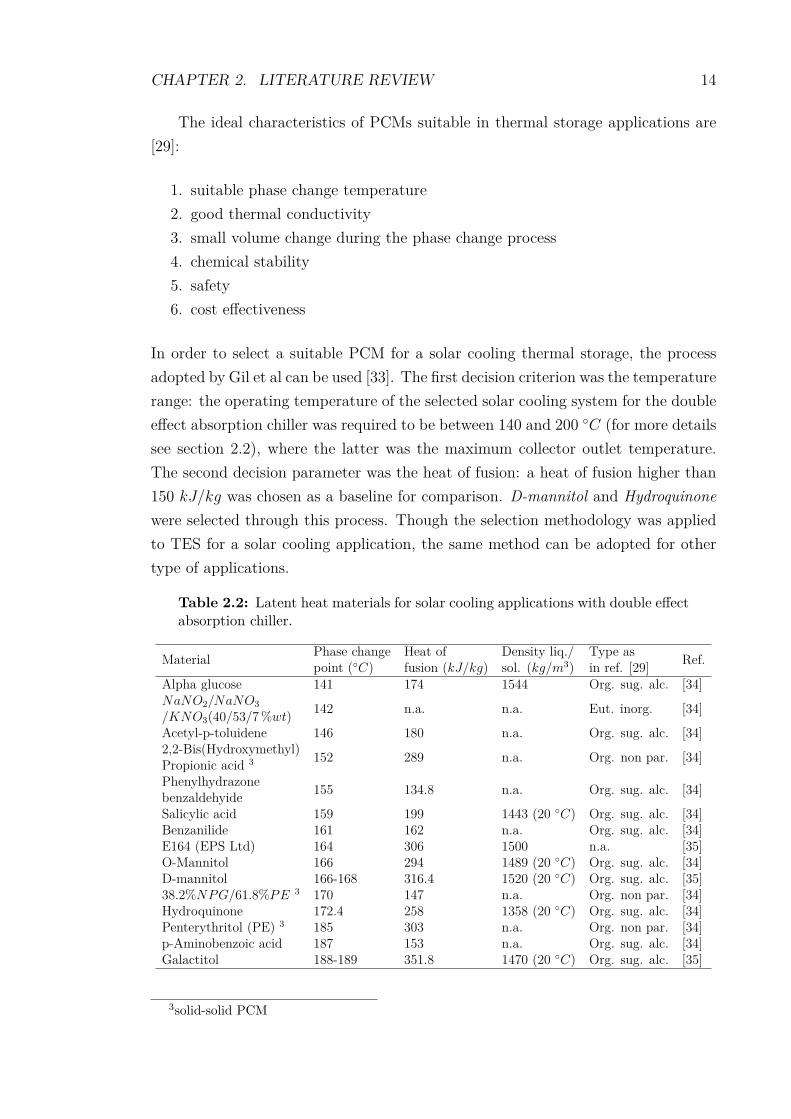
In order to select a suitable PCM for a solar cooling thermal storage, the processadopted by Gil et al can be used [33]. The first decision criterion was the temperaturerange: the operating temperature of the selected solar cooling system for the doubleeffect absorption chiller was required to be between 140 and 200 ◦C (for more detailssee section 2.2), where the latter was the maximum collector outlet temperature.The second decision parameter was the heat of fusion: a heat of fusion higher than150 kJ/kg was chosen as a baseline for comparison. D-mannitol and Hydroquinonewere selected through this process. Though the selection methodology was appliedto TES for a solar cooling application, the same method can be adopted for othertype of applications.
Table 2.2: Latent heat materials for solar cooling applications with double effectabsorption chiller.
Material Phase changepoint (◦C)
Heat offusion (kJ/kg)
Density liq./sol. (kg/m3)
Type asin ref. [29] Ref.
Alpha glucose 141 174 1544 Org. sug. alc. [34]NaNO2/NaNO3
/KNO3(40/53/7%wt)142 n.a. n.a. Eut. inorg. [34]
Acetyl-p-toluidene 146 180 n.a. Org. sug. alc. [34]2,2-Bis(Hydroxymethyl)Propionic acid 3 152 289 n.a. Org. non par. [34]
Phenylhydrazonebenzaldehyide 155 134.8 n.a. Org. sug. alc. [34]
Salicylic acid 159 199 1443 (20 ◦C) Org. sug. alc. [34]Benzanilide 161 162 n.a. Org. sug. alc. [34]E164 (EPS Ltd) 164 306 1500 n.a. [35]O-Mannitol 166 294 1489 (20 ◦C) Org. sug. alc. [34]D-mannitol 166-168 316.4 1520 (20 ◦C) Org. sug. alc. [35]38.2%NPG/61.8%PE 3 170 147 n.a. Org. non par. [34]Hydroquinone 172.4 258 1358 (20 ◦C) Org. sug. alc. [34]Penterythritol (PE) 3 185 303 n.a. Org. non par. [34]p-Aminobenzoic acid 187 153 n.a. Org. sug. alc. [34]Galactitol 188-189 351.8 1470 (20 ◦C) Org. sug. alc. [35]
3solid-solid PCM

CHAPTER 2. LITERATURE REVIEW 15
The literature on phase change materials is quite wide and cover applicationswith different operational temperature ranges. It is worth summarise latent heatmaterials for medium temperature solar cooling systems (see section 2.2.1 for moredetails) with double and triple effect chillers in table 2.2 and 2.3.
Literature on PCMs suitable for triple effect chiller based systems does notexist, a part for some metal alloys and organic salts. Therefore, potential PCMcandidates have been identified from databases such as CRC handbook [36]. Thesematerials were chosen to have melting point between 200 and 240 ◦C, relativelyhigh heat of fusion and safety requirements (according to MSDS [37]) suitable fora rooftop application (e.g. high flashing point). The available information lackson details like cost and some physical properties. Table 2.3 summarises the resultof the identification process. Additional materials for solar cooling systems with
Table 2.3: Latent heat materials identified as suitable for solar cooling applica-tions with triple effect absorption chiller, part 1.
Material Meltingpoint (◦C)
Energy den-sity (kWh/m3)
Specific energy(kWh/kg)
Latent heat offusion (kJ/kg)
Thermal conduc-tivity (W/mK)
Mass density(kg/m3) Ref.
68.1%KCl/31.9%ZnCl2
235 136.4 0.055 198 0.8 2480 [38]
Solar saltKNO3/NaNO3
220 53.7 0.028 100.7 0.56 1920 [39]
Sn 232 119.8 0.016 59 66.8 7365/6990(25/232◦C) [36], [40]
Al-Sn 232 119.4 n.a. 59 237 n.a. [32]Inv Struct Al-Sn 232 41.9 n.a. n.a. n.a. n.a. [32]4-Hydroxybenzoic acid 213 90.9 0.062 223.7 n.a. 1463 [36]
Propazine 217 58.8 0.051 182.3 n.a. 1162 [36]N,N’-Diphe-nylurea 236 56.1 0.045 163 n.a. 1239 [36]
Caffeine 236.1 38.8 0.031 113.3 n.a. 1232 [36]Indium(I)chloride 225 71.2 0.017 61.2 n.a. 4190 [36]
Metaboric acid(γ form) 236 225.4 0.091 326.3 n.a. 2487 [36]
Potassium hydr-ogen fluoride 238.8 55.8 0.024 84.8 n.a. 2370 [36]
Myo-inositol 224 126.4 0.072 260 n.a. 1750 [36]
thermal storage above 200 ◦C are some ionic salts described in [39]. Information onphase change transition temperature and latent heat of fusion are the only availableinformation for those materials. In conclusion, the shortage on property information(thermo-physical, cost data as noted in the tables) and performance testing resultsdoes not allow the designer to confidently down-select suitable materials. From oneside, metals look attractive due to their high energy density and the good thermalproperties. However their cost is considerably higher than salt [40]. On the otherhand, organic salt (e.g. solar salt) have thermal conductivity issues that can beaddressed by thermal properties enhancing techniques as mentioned above. Theabove novel materials need a detailed economic analysis and long term performancetests before they can be treated as potential candidates along with water for mediumtemperature applications.

CHAPTER 2. LITERATURE REVIEW 16
Thermo-chemical Materials
Heat in Thermo-CHemical Thermal Energy Storage (CHTES) materials is ab-sorbed and released in breaking and reforming molecular bonds in a completelyreversible chemical reaction. Among the three categories of TES materials, theyhave the highest energy density [41]. Another big advantage of CHTES is verysmall thermal losses because energy is stored as reactants at ambient temperature.Instead, physical thermal storage (sensible and latent) materials have thermal lossesthrough heat conduction, convection and radiation. The general characteristics ofthese materials are [42]: i) temperature range of 20 to 2500 ◦C; ii) higher storagedensity compared to sensible and latent heat materials; iii) lifetime depends on re-actant degradation; iv) advantages include high storage density, low heat losses,suitability for long storage period (seasonal storage), possibility of long distancetransport, highly compact energy storage system; v) high capital costs and techni-cally complexity are some disadvantages. CHTES materials are predominantly inresearch and development phase. Literature of CHTES for solar cooling applicationis limited on one sorption system by Climatewell®, a Swedish solar cooling systemsupplier [43], which has demonstrated a Lithium Chloride (LiCl) salt based thermalstorage system. Generally in CHTES, heat is stored through a chemical reactionby combining reactants or splitting the product in reactants. Instead in sorptionsystems, which are also normally considered as thermo-chemical storage, heat isneeded to overcome the bonding between working fluid molecules and the sorptionmaterial molecules. As a result, the sorption material is dried. When the workingfluid molecule is adsorbed on the sorption material, heat is released. Sorption ma-terials are normally investigated for their refrigeration applications. A summary ofpossible chemical reactions suitable for solar cooling applications with absorptionchiller (see section 2.2.1 for suitable temperature ranges) are listed in table 2.4.
Table 2.4: Latent heat materials identified as suitable for solar cooling applica-tions with triple effect absorption chiller, part 2.
Thermo-chemical material Charging tem-perature (◦C) Reaction Energy dens-
ity (kWh/m3) Ref.
Strontium bromide exahydrate 70-80 SrBr2 · 6H2O ↔ SrBr2 ·H2O + 5H2O 60 [28]Sodium sulphide pentahydrate 83 Na2S · 5H2O ↔ Na2S · 2H2O + 3H2O 510-780 [28]Magnesium Sulphate heptahydrate 122-150 MgSO4 · 7H2O ↔MgSO4 + 7H2O 420 [28]Magnesium Chloride exahydrate 150 MgCl2 · 6H2O ↔MgCl2 · 2H2O + 4H2O 589 [44]Magnesium Sulphate heptahydrate 150 MgSO4 · 7H2O ↔MgSO4 ·H2O + 6H2O 686 [44]Calcium Chloride dihydrate 150 CaCl2 · 2H2O ↔ CaCl2 + 2H2O 400 [44]Aluminium Sulphate octadechydrate 150 Al2(SO4)3 · 18H2O ↔ Al2(SO4)3 · 5H2O + 13H2O 600 [44]Iron Carbonate 180 FeCO3 ↔ FeO + CO2 722 [5]Copper sulphate pentahydrate 200 CuSO4 · 5H2O ↔ CuSO4 ·H2O + 4H2O 574 [28], [45]Metal hydrides 200-300 metalxH2 ↔ metalyH2 + (metalx −metaly)H2 1111 [5]Methanol 200-250 CH3OH ↔ CO + 2H2 n.a. [5]Magnesium Oxide 250-400 Mg(OH)2 ↔MgO +H2O 917 [5]

CHAPTER 2. LITERATURE REVIEW 17
2.1.2 Heat Transfer Methods
The Thermal Energy Storage System (TESS) has the role of containing thestorage media, and providing a means to transfer heat to and from the media, eitherthrough heat transfer equipment or directly. An ideal storage system will segregateheat such that the heat transfer fluid is directed to the thermally driven coolingdevice at the highest possible temperature, while maximising energy stored at theuseful temperature. For a practical TESS design, the details of the storage material(as discussed in section 2.1.1) and the operational constraints of other componentsof the plant (e.g. solar collector, chiller) are required.
Active thermal storage systems are divided into (a) direct and (b) indirect sys-tems. In direct systems, a single heat transfer fluid is used for i) transferring heatfrom the solar collector to the thermal store, ii) transferring heat from the thermalstore to the thermal cooling device and iii) storing the heat as the heat storagemedium. This type of systems are predominately with sensible heat materials (i.e.water). Alternatively, in indirect systems, solar heat from the collectors is trans-ferred into a different medium, via a heat exchanger. Direct storage systems have themain advantage of reducing the storage cost, since they do not require any additionalheat exchangers. The latter in fact would yield in a degradation of temperature fromthe solar source to the thermal cooling device and require additional pumped flowcircuits with associated parasitic power consumption. Avoiding the temperaturedegradation is important for maintaining cooling capacity in the thermal coolingdevice during periods of reduced solar radiation (cooling capacity modulation isachieved by temperature regulation as described in section 2.2.1). The literatureavailable on active thermal storage systems is presented as (a) direct/indirect sys-tems based on sensible storage media (mainly water) and (b) indirect systems withphase change storage media. Although being a possible valid option, storage sys-tems used in solar power generation are not reported as they are not been appliedto solar cooling applications. More details about CSP storage systems can be foundin [5], [10], [27], [46]–[48].
Active Direct/Indirect Thermal Storage with Water
In sensible heat thermal energy storage systems (STESS), water can be pumpeddirectly into the thermal store from the solar collectors, when frost protection mech-anisms are not needed. Solar heated hot water enters the top of the storage tankand cooler water is pumped from the bottom to the solar collectors. A sufficienttemperature rise in the collector or low storage supplied heat rate can cause ther-mal stratification in the store. That’s being characterised by a distinct temperature
CHAPTER 2. LITERATURE REVIEW 18
separation between hot water at the top and cooler water at the bottom of thetank. Vice versa, if the temperature rise over the solar collectors is low, or if themixing effect of water flowing into and out of the tank is high, then the water inthe tank may rise and fall as a single block of well mixed fluid. Stratification hasbeen demonstrated to yield storage thermodynamic benefits (increase in exergy andthermal performance) [49], [50]. Hence the design of hot water storage tank requirescareful consideration of stratification effects, flow management and other overall so-lar cooling system design considerations. Operation at elevated temperatures maydictate the use of a heat exchanger between the collectors and the storage tank, dueto the cost of a pressurised systems. Indirect heat exchanger arrangements are alsorequired for freezing protection [51].
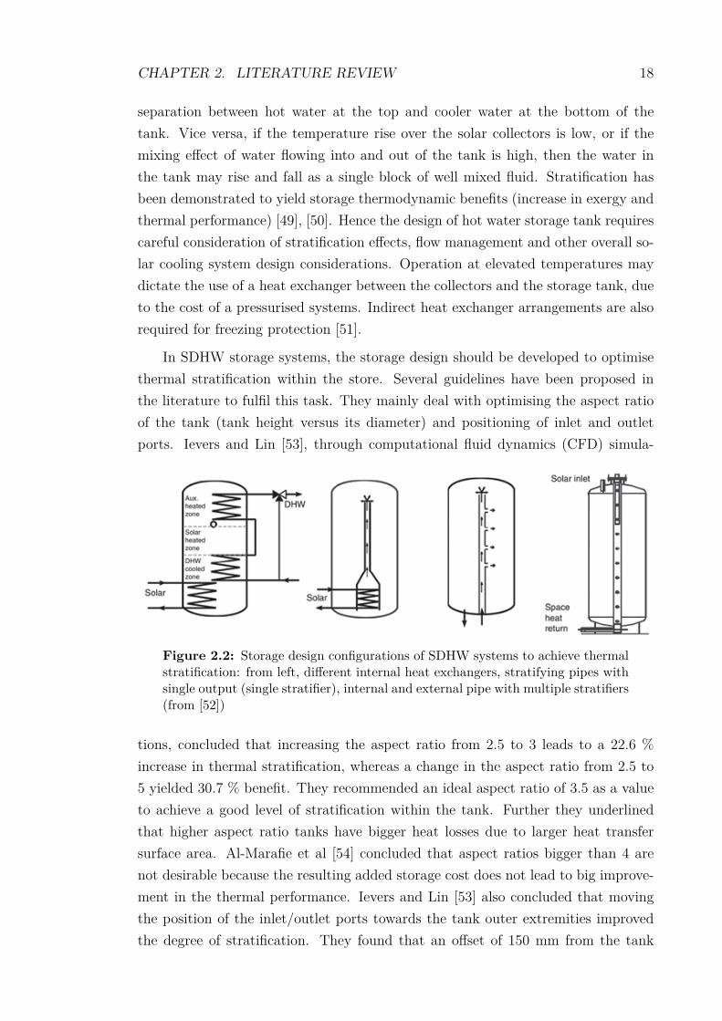
In SDHW storage systems, the storage design should be developed to optimisethermal stratification within the store. Several guidelines have been proposed inthe literature to fulfil this task. They mainly deal with optimising the aspect ratioof the tank (tank height versus its diameter) and positioning of inlet and outletports. Ievers and Lin [53], through computational fluid dynamics (CFD) simula-
Figure 2.2: Storage design configurations of SDHW systems to achieve thermalstratification: from left, different internal heat exchangers, stratifying pipes withsingle output (single stratifier), internal and external pipe with multiple stratifiers(from [52])
tions, concluded that increasing the aspect ratio from 2.5 to 3 leads to a 22.6 %increase in thermal stratification, whereas a change in the aspect ratio from 2.5 to5 yielded 30.7 % benefit. They recommended an ideal aspect ratio of 3.5 as a valueto achieve a good level of stratification within the tank. Further they underlinedthat higher aspect ratio tanks have bigger heat losses due to larger heat transfersurface area. Al-Marafie et al [54] concluded that aspect ratios bigger than 4 arenot desirable because the resulting added storage cost does not lead to big improve-ment in the thermal performance. Ievers and Lin [53] also concluded that movingthe position of the inlet/outlet ports towards the tank outer extremities improvedthe degree of stratification. They found that an offset of 150 mm from the tank

CHAPTER 2. LITERATURE REVIEW 19
top/bottom reduced thermal stratification by 28 % and an offset of 300 mm yielded72 % reduction in thermal stratification. Rosen et al [50] proposed a “good design”in terms of port location: inlet/outlet at the top/bottom tank. Streicher and Bales[52] investigated four different configurations, with direct and indirect heat transfersystems, to achieve stratification through tank design as shown in figure 2.2. Hanet al [51] analyzed the ways to inhibit turbulence that results in mixing of hot andcold water in the store. As a result of their work, measures such as adding a baffleplate at tank inlet, adding a porous mesh to slow down water flow and adding adiffuser at the inlet would maintain thermal stratification. In the case of indirect
Figure 2.3: Design concepts for indirect heat exchanger solar hot water systems[55].
storage systems (systems with a heat exchanger), beside the configurations reportedin figure 2.2, Spur et al [55] compared three new designs, as illustrated in figure 2.3.The design configuration with bottom and top coil was found to have the best ther-mal stratification performance for a given realistic daily domestic hot water draw-offprofile.
Active Indirect Thermal Storage with PCM
Latent heat based active Thermal Energy Storage Systems (LHTESS) heattransfer methods are divided into three groups: 1) exchanging heat at the outersurface of the thermal store, 2) exchanging heat on large surfaces within the ther-mal store, 3) and exchanging heat by exchanging the storage medium itself (mainlyPCM slurries) [56]. The first two methods are purely indirect, instead the last one istechnically a direct heat transfer system but not many application are found in theliterature. Storage systems embedded in the fabric of an air-conditioned buildingand other house elements belong to the first heat transfer method. The heat trans-fer process in the latter is mainly dominated by the heat transfer coefficient (i.e.natural convection on the surface). The second group have predominant heat trans-fer through the large storage internal surface. Among the them, two heat transferdesign concepts for LHTESS are widely found in the literature:

CHAPTER 2. LITERATURE REVIEW 20
a) Packed bed storageb) Shell and tube heat exchanger storage
The packed bed storage system consists of a storage tank filled with solid capsules orsolid material. The heat transfer fluid passes through this bed. The solid materialsfill the storage container as shown in figure 2.4a. An example of such configurationare cold storage with ice spherical capsules, which is well known in the literature[57]. The shell and tube LHTES with PCM was heavily investigated from the late
Figure 2.4: Two LHTESS concepts: packed bed (a) and shell-and-tube (b) heatstorage designs (from [16], [58])
1970’s until the 1990’s [59]–[62]. According to Longeon et al. [63] the shell and tubeis the most promising technology with LHTES since it lowers the system cost. Theconcept consists of a series of tubes grouped in a bundle and embedded in a mantleor shell, as shown in figure 2.4b. Some researchers investigated the configurationwith the PCM filling the annular space between the outer tube surface and the shell,others the encapsulation of the PCM within the pipe. Jegadheeswaran and Pohekar[64] have summarised studies on finned tubes in LHTES with PCM.
Table A.1 summarises the literature on packed bed and shell-and-tube heatstorage systems. More information about packed bed latent heat thermal energystorage with PCMs capsules can be found in the review by Regin et al. [65]. Morerecently, Oró et al. [66] have focused on the development of a LHTES based on ashell and tube design for solar cooling applications involving double effect chillers(see section 2.2.1). The experiments with Hydroquinone as storage media wereperformed for two different designs: finned and un-finned shell-and-tube TES [67].The aim of the work was to experimentally test and compare the average effectivenessof the two TES systems.

CHAPTER 2. LITERATURE REVIEW 21
2.2 Solar Cooling Systems
Solar cooling (SC) or solar air-conditioning (SAC) systems are a technologythat convert solar power into cooling power for building air-conditioning purposes.They are divided into two main category: electricity driven and thermally drivensystems. The first ones use photovoltaic (PV) panels to convert incident sunlight intoelectricity to power a conventional electric chiller (vapour compression chiller). Thesecond category of solar cooling technologies makes use of a thermal activated cycleto produce the cooling effect. The latter can be divided in open-loop and closed-loop systems. The first one involves devices that apply a set of thermodynamictransformations directly on the supply air to the building. The dominant technologyin this sub-group is the desiccant wheel system. The closed-loop thermally drivenSAC systems are characterised by thermal transformations on a working fluid, whichafter being cooled in the cycle, is used in a heat exchanger (i.e. cooling coils) forcooling the supply air in inlet to the building. The systems based on absorptionand adsorption chillers are part of closed-loop cycle SC technologies. Since thescope of the thesis is to discuss application of TES technologies related to mediumtemperature SAC systems, which are plants based on absorption chillers, adsorptionchiller systems are not further discussed. Details on such solar cooling systems canbe found in [68]–[70].
2.2.1 Solar Cooling Systems with Absorption Chiller
An absorption chiller based SAC system consists of a solar collector, whichabsorb the solar radiation and heat up a working fluid; a thermal storage device,in which thermal energy is stored for later usage; a cooling device, the absorptionchiller; and a heat rejection system, the cooling tower. Literature on absorptionchiller based SC systems reports many system configurations [71]. Given that thefocus of the thesis is the thermal storage integration in the system, the adoptedsystem configuration is pertinent to a generic solar cooling system with absorptionchiller. Such system with thermal energy storage is shown in figure 2.5. This genericsolar thermal cooling system consists of two flow loops separated by the hot thermalstorage component. The solar heating flow loop conveys heat from solar thermalcollectors to the thermal store. The chiller flow loop conveys heat from the thermalstore to the thermal cooling device. When the heat arriving from the collectorsexceeds the heat being consumed by the thermal cooling device, then the thermalstore is charged. Conversely, when the demand for heat to the thermal cooling deviceexceeds the supplied solar heat, the thermal store is discharged to match demand.
The cooling effect is produced by the absorption chiller, through a thermally

CHAPTER 2. LITERATURE REVIEW 22
Figure 2.5: Generic solar cooling system with absorption chiller and thermalenergy storage
driven chemical absorption process, in which heat is absorbed at high and low tem-peratures in the generator and evaporator (G and E of figure 2.5), on the hot andchilled sides respectively, and rejected at medium temperature, in the absorber-condenser (A-C) in the cooling side. The machine is widely available in the marketand has a coefficient of performance (COP) that can vary from approximately 0.7 to1.8 depending on the generator stages. Thus the absorption chillers can be groupedin:
1. Single effect: hot inlet temperature range of 70-90 ◦C, and COP ∼ 0.72. Double effect: hot inlet temperature range of 150-180 ◦C, and COP ∼ 1.43. Triple effect: hot inlet temperature of 210-230 ◦C, and COP ∼ 1.8
The outlet chilled temperature ranges from 15 to 7 ◦C, while the nominal inletcooling temperature can vary between 30 to 35 ◦C. Medium temperature highefficiency solar cooling systems uses triple effect absorption chiller that requiresheat at the temperature range of 200-240 ◦C.
2.2.2 Examples of SC Installations with Thermal Storage
According to published information, the number of operational solar heatingand cooling commercial systems in the EU region is estimated to be around 100[72], [73]. Most of these systems, according to Preisler [3] are with single stageabsorption chillers and water as the working fluid. Following, the section reviewspublished information on practical solar cooling installations, categorised into sys-tems with Sensible heat based Thermal Energy Storage (STES) and Latent Heatbased Thermal Energy Storage (LHTES) systems, which are the predominant in-stallations.

CHAPTER 2. LITERATURE REVIEW 23
Systems based on STES
Table A.2, in the appendix, provides a summary of the SC installations withsensible heat storage media, and examples of various solar collector applications inlast 10 years. The main points that arise from the table are:
• Single effect absorption chillers have used non concentrating solar heat collec-tion methods (e.g. evacuated tubes)
• Double effect chiller based systems have used concentrating heat collectionmethods (e.g. parabolic trough)
• Some of the cases have no storage included in the solar cooling plant
Installations of solar thermal heat sources to drive a triple effect chiller is veryscarce. Recently researchers from Kawasaki® published a paper on the benefits of asteam driven triple effect absorption chiller operated with solar heat [74]. In India,at the solar energy centre in Gurgaon, Thermax® [75] have installed a triple effectabsorption chiller powered by parabolic trough collectors. The literature does notreport on storage aspects of these triple effect absorption chiller installations.
In the IEA Solar Heating and Cooling (SHC) program “Solar Air-conditioningand Refrigeration” Task 38, Sparber et al [15] reviewed the volume of storage in-stalled in a sample of actual SHC installations. They found that there was noconsistent trend in the storage volume design, employed in the plants. This prob-ably reflects i) the diversity of applications of SC systems (e.g. along or not withSDHW sub-system) and ii) the relative sizing of collector area and chiller capacity.A large collector area with small chiller is likely to have spare solar heat availableto be stored, whereas an undersized collector field (relative to the chiller) will useup all the available solar heat, leaving nothing to be stored. In any case, a minimalamount of thermal energy storage will be required to ensure stable operation of thechiller and prevents rapid start-up/ shut-down events (chiller on-off cycling). Thisis particularly important with absorption chillers which have slow start up times(from 30 minutes to hours depending on the size) due to high thermal mass, andreaction kinetics of the machine chemical cycle.
Systems based on LHTES
There are only a small number of latent heat storage examples applied to solarair-conditioning applications that are reported by the literature. Laboratory proto-types for LHTES for SHC systems have been investigated as a part of IEA SHC taskforce (Task 32) [76]. At the University of Lleida, in Spain, a pilot plant has been

CHAPTER 2. LITERATURE REVIEW 24
built in order to test different TESSs and materials [58], [67], [77] within the temper-ature range suitable for medium temperature SAC applications with double effectabsorption chillers. This facility was used to compare the performance of Hydro-quinone and D-mannitol as latent heat storage materials with phase change around170 ◦C. In contrast to Hydroquinone, tests showed that undesirable sub-cooling (be-low the material freezing temperature) occurred for D-mannitol during the storagedischarge cycle. Tests also explored the impact of two different thermal store heatexchanger designs based on finned and un-finned shell-and-tube configuration [67].Based on these laboratory results, a 300 kWh PCM storage tank was designed andbuilt to work in a real solar cooling plant in Seville, Spain [77]. It was installedas part of the HVAC installation on the roof of the Engineering School building atUniversity of Seville, Spain (see figure 2.6). Its main function is to provide heatto the solar cooling system during periods of radiation unavailability. The designconsists of a cylindrical vessel with a tube bundle inside (shell and tube design).The heat transfer fluid is circulated inside the tubes, organised in a triangular pitch,while the PCM is located in the outer tube part, the storage housing.
Figure 2.6: A LHTES system with Hydroquinone as PCM and capacity of 300kWh at the University of Seville, Spain, from [77].
2.3 Control Strategies of SC systems
In the previous chapters the literature review focused mainly on the solar coolingsystem configuration, storage materials and thermal storage equipment involved inthe design of a solar air-conditioning plant, but with limited focus on its continuousoperation. Clearly a practical operating system needs a set of control strategies/rulesto manage charging and discharging of the thermal store, and operation of the otherdevices in a manner that is robust and efficient under all scenarios. From a control

CHAPTER 2. LITERATURE REVIEW 25
perspective, this is not straightforward because the thermal energy store is highlyintegrated with other parts of the system such as the solar loop, the absorptionchiller loop and any backup heat source. Importantly system efficiency is highlyinfluenced by the set of controls implemented in the system [68]. The control of a SCplant involves management of both continuous states (e.g. temperatures, speeds ofvariable-speed pumps, position of three-way mixing valves) and discrete states (e.g.open-closed valves, on-off state of backup boilers, on-off state of pumps) subjectto variations in cooling demand and solar irradiation, the main source of energy.The latter cannot be manipulated and its intermittent nature is well established.Further, time delays are present due to fluid transportation, thermal inertia andprocess dynamics. Some author claims that the solar and storage loops of a solarsystem are the most challenging to control because they are highly affected by thetransient nature of solar irradiation [78]. The main objective of the controller is tocompensate for the intermittent solar radiation by implementing a robust controlstrategy that guarantees the load requirements and maximises heat usage from thesolar source.
2.3.1 Conventional Control
Conventional control or rule based control (RBC) or “Model-free” control of aSC system reported in figure 2.5 consists mainly in the control settings of the solarloop and chiller loop. This part of the system in fact has the role of collecting thesolar heat, storing it and deliver it at the required conditions to the chiller. Thecontrol of the cooling and chilled loop are not treated in this thesis. It is assumed atemperature control in the cooling loop based on a PI-type controller to maintain aconstant inlet chiller temperature and a on-off control in the chilled loop, based onthe cooling demand. More details on such control strategies can be found in [78],[79]. The controlled variable is the solar circuit mass flow rate and the collectoroutlet temperature is the measured variable.
The heat source control strategies for charging the thermal store via the solarcollector are described by Kohlenbach [78]:
1. Differential on-off: A constant flow pump is switched on or off based on thetemperature difference between the fluid in the collector and the thermal store.In order to avoid control instabilities, a hysteresis dynamic is adopted by usingthe tank bottom and top temperatures. This approach is simple and commonbut presents large fluctuations in collector outlet temperature and can resultin higher collector thermal losses and lower solar gains.
2. Temperature difference based: A proportional (P) controller is used to drive

CHAPTER 2. LITERATURE REVIEW 26
a variable-speed pump based on the temperature difference between the solarcollector and the thermal store. The results of the control strategy are smallertemperature oscillations, reduced thermal losses due to less collector standbytime.
3. Radiation based: Again a proportional controller is used to drive the pumpspeed, but based on measurement of relative changes in solar radiation (e.g.with a PV cell). For each SAC system, a different empirical correlation be-tween radiation and pump speed is necessary. This controller can achievealmost constant values in collector outlet temperatures.
Small domestic systems usually adopt the first two control schemes, while theradiation-based strategy is predominately used for large systems, where very sta-ble output temperatures are worth the extra hardware cost of the more complexcontroller. The second controller should be applied in the case of a LHTESS tomatch the collector outlet temperature with the phase change temperature. In thisway the storage media can undergo the phase change process and stores thermalenergy as latent heat.
The three control frameworks were compared with a set of simulations. A 6 %higher collector yield factor was obtained by the third control strategy respect to thefirst and second ones (which had similar performance). However similar performanceacross all three techniques was observed in a real system. Hence the conclusion wasthat the simplest control technique (differential on-off) was as valid as the others interms of yield factor for that particular plant [78]. Bujedo et al [79] have studiedthree control strategies applied to a real SAC plant operating over three years, withboth hot and cold storage:
• Strategy 1 (business as usual): The mass flow of hot water going into thechiller is fixed and the load control is done by cycling the chiller on and off.The pumps in the solar collector switch on anytime the radiation exceeds athreshold (300 W/m2). Solar-heated water is delivered to the chiller (i.e. thebackup boiler is turned off) any time the temperature of the highest part ofthe tank is higher than that of the generator outlet of the chiller.
• Strategy 2: consists of varying the temperature of the condenser inlet (A-C inthe cooling circuit of figure 2.5) to the chiller as a function of the generatortemperature to maintain maximum COP. Variable-speed pumps in the solarcollector are triggered by the critical solar radiation value, which is the mini-mum radiation necessary to overcame the thermal losses in the collector [80].This strategy optimises the use of available radiation and uses less electricityby running collector pumps in variable speed mode. The chiller is still cycled.

CHAPTER 2. LITERATURE REVIEW 27
• Strategy 3: the goal is to maintain the temperature at the bottom of the coldstorage at a constant 10 ◦C. Similar to strategy 2, the temperature of thecondenser is varied but also the generator mass flow is adjusted as a functionof the system load. Thus, the chiller works without interruptions, resulting inhigher COP because there is no cycling.
The experimental results showed that strategy 3 outperformed both strategies 1and 2 by achieving, for example, 12.61 % more solar field efficiency and almosttripled the solar fraction of strategy 1. Most of the control literature on SC plants,excluding the previous example, involves different hardware designs that require newcontrollers. Therefore, rather than improving the operation of an existing system,these approaches focus on how to obtain maximum benefit from new equipment.For example, Rosiek & Batlles [81] aimed to reduce the energy consumption of asolar-assisted air conditioning system for a research centre by applying chilled waterstorage and occupancy sensors. Their main control variables were whether or noteach of the 16 fan-coil units was operating (based on the occupancy sensors) andwhere the chilled water comes from (cold storage or absorption chiller, and in thecase of the latter, whether or not it is necessary to switch on the backup heater).The modified system used 42 % less energy than the original configuration. Thework by Li & Sumathy [82] is another example of a modified system, where the hotstorage tank is divided in two partitions. The upper one is a quarter of the tankvolume. The controller decides whether to operate the system using the whole tankor just the upper partition. The decision is made depending on the temperature ofthe stored hot water, and whether or not the useful solar energy gain is larger thanthe cooling load. By using the partition early in the day and switching to full tankas enough solar energy becomes available later, the authors report a 2 hours earliersystem starting time and a system COP increase of 15 %.
2.3.2 Advanced Control Approaches
So far none of the control approaches takes into account future (look-ahead)events (disturbances from a control perspective) such as weather and building oc-cupation predictions or cooling load. The advantage and thus attractiveness ofadvanced controllers is that they can plan for the future by considering alterna-tive strategies (trajectories) beyond the scope of the above “model-free” controllers(RBC controllers). In fact the look-ahead controllers optimise the values of interest(e.g., temperature in air conditioned spaces and energy cost) using a model of thesystem and several forecasts (weather, occupancy, electricity price) and yield theoptimal control trajectory. For example, based on the weather and building occupa-

CHAPTER 2. LITERATURE REVIEW 28
tion forecast for the following day, a look-ahead controller might decide to dischargethe thermal store only partially the day before. The use of such predictive controlscould provide additional potential for better exploitation of the solar heat sourcewith the consequences of reduced backup energy consumption.
The development of mathematical models is fundamental for the implementa-tion process of a look-ahead controller. In fact the model allows to simulate thesystem response under the input conditions and enables planning of the best controltrajectory for these conditions. For example, Pasamontes et al. [83] identified amodel for a solar hot water system using fist-principle equations and used artificialintelligence methods to identify the best values for unknown system parameters.Models like these can be used to develop look-ahead controllers. Mammoli et al[84] optimised the operation of a solar-assisted HVAC system with both hot andcold thermal storage, based on temperature and solar irradiance forecasts. In theircontrol strategy, the hot store is charged using solar collectors and used to run anabsorption chiller, whereas the cold store is charged (normally overnight) using anelectric chiller. The optimisation objective, the minimum energy costs, was achievedby selecting a) the time to run the absorption chiller and b) how much cold storageis needed for the following day. The temperature and irradiance forecasts were usedto estimate the available cooling power from the absorption chiller, thus updatingthe information on how much the cold store needs to be charged (control signalb). They demonstrated that the absorption chiller scheduling using the forecasts,yielded 29 % more annual energy savings in comparison to the regular scheduling,in which the cold storage if fully charged every night and the absorption chiller runswhenever there is sufficient energy in the hot store. The system was modelled andoptimised using the Lawrence Berkeley National Laboratory (LBNL)’s DistributedResources Customer Adoption Model (DER-CAM).
A promising technique for look-ahead controllers is the well-known control struc-ture called model predictive control (MPC) [85]. In MPC, a model of the systemis used to simulate the effect of different possible control sequences and an opti-misation problem is solved, given a certain time horizon to seek the best controltrajectory for a given set of objectives. MPC takes into account the fact that nei-ther models nor forecasts are perfect by only implementing on the plant the veryfirst control of the obtained sequence. Iteratively, when feedback information aboutthe actual state of the system arrives, the optimisation problem is solved again, andthe control signal corresponding to a new time step is implemented. A schematic ofthe MPC framework with all its features is showed in figure 2.7.
Application of MPC to hybrid systems, such as a SC plant, consists in an optimi-sation problem with both real and integer decision variables and a set of constraints.
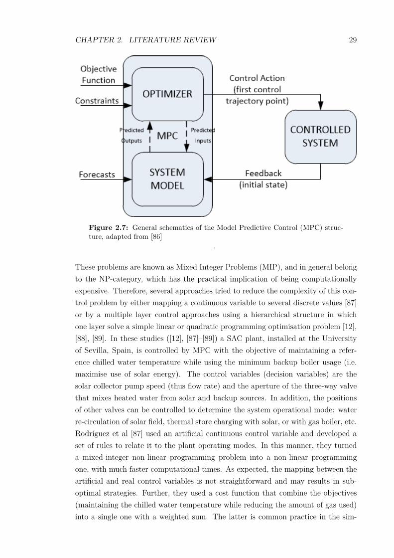
CHAPTER 2. LITERATURE REVIEW 29
Figure 2.7: General schematics of the Model Predictive Control (MPC) struc-ture, adapted from [86]
.
These problems are known as Mixed Integer Problems (MIP), and in general belongto the NP-category, which has the practical implication of being computationallyexpensive. Therefore, several approaches tried to reduce the complexity of this con-trol problem by either mapping a continuous variable to several discrete values [87]or by a multiple layer control approaches using a hierarchical structure in whichone layer solve a simple linear or quadratic programming optimisation problem [12],[88], [89]. In these studies ([12], [87]–[89]) a SAC plant, installed at the Universityof Sevilla, Spain, is controlled by MPC with the objective of maintaining a refer-ence chilled water temperature while using the minimum backup boiler usage (i.e.maximise use of solar energy). The control variables (decision variables) are thesolar collector pump speed (thus flow rate) and the aperture of the three-way valvethat mixes heated water from solar and backup sources. In addition, the positionsof other valves can be controlled to determine the system operational mode: waterre-circulation of solar field, thermal store charging with solar, or with gas boiler, etc.Rodríguez et al [87] used an artificial continuous control variable and developed aset of rules to relate it to the plant operating modes. In this manner, they turneda mixed-integer non-linear programming problem into a non-linear programmingone, with much faster computational times. As expected, the mapping between theartificial and real control variables is not straightforward and may results in sub-optimal strategies. Further, they used a cost function that combine the objectives(maintaining the chilled water temperature while reducing the amount of gas used)into a single one with a weighted sum. The latter is common practice in the sim-

CHAPTER 2. LITERATURE REVIEW 30
plification of the optimisation formulation, but poses the hard question of choosingthe right weight values. Usually the weight attribution process is a trial-and-errorprocedure. Lastly, the MPC used a 15 minutes prediction horizon so, even thoughtheir approach is look-ahead, it involves a short horizon and thus they need no fore-casts. The same plant has been controlled in [89] using a hierarchical controller: thecontrol layer are a configuration level and a regulatory level. The configuration levelselects the system operating mode by solving a linear function with variable weights,which depend on the state of the plant and weather conditions. Once the operatingmode is selected, the regulatory level adjusts the process variables for the currentoperational mode. Although the authors did not report any comparison with RBC,they claimed the benefit of maintaining the temperature level despite the adverseweather conditions. A similar hierarchical approach is presented by Menchinelli& Bemporad [12]: the supervisory level decides the operating modes by solving alinear problem, while the low-level controller ensures robust tracking of the modeset-points. The approached adopted by Sonntag et al [88] to control the Spanishplant is a supervisory control scheme. They used insight from experiments as wellas results from a simplified model to design a set of rules that define the operationmode and the values of the continuous variables that minimise energy consumption.The benefits of this control scheme are not quantified beyond reporting that thecontroller is able to maintain the chilled water temperature at the desired level.
Besides examples of MPC controlled SC systems, the literature reports otherexamples of MPC application on solar thermal systems with storage [14], [90]–[94].Pichler et al [90] described a hybrid model predictive approach for the auxiliaryheating control of a “Combistorage” system. The storage device is modelled asstate-space model (SSM), the controlled variable is the tank top temperature andthe backup heater power is the control input. In comparison with the base case,the developed MPC showed reduction of auxiliary energy demand up to 40 %, withincrease in monthly solar fraction of 4-5 %. Powell et al [14] dynamically optimiseda thermal energy storage over 24 hr periods for the optimal heat supply of a so-lar thermal power plant. The MPC formulation included temperatures and storagevolumes as the system states, while the separate circuit flow rates as the control vari-ables. The advanced controller operated the plant with lower set-points allowing forpart-load operation of the storage. Additionally, the predictive controller was ableto fully exploit new system operational features (e.g. storage bypass). The authorsobserved benefits particularly during periods with cloud coverage. Halvgaard et al[91] implemented an economic model predictive control to a solar tank in order tobalance heat production from solar collectors and demand in a residential house.In order to supply heat during low solar irradiance intervals, heating elements wereswitched on-off inside the store. The results of yearly simulations showed electricity

CHAPTER 2. LITERATURE REVIEW 31
cost savings up to 30 %. Berkenkamp and Gwerder [13] described a generalisedMPC applied to a stratified thermal storage device, independently from knowledgeof the detailed heat source and sink sub-systems. The authors used short term loadand source forecast data for the optimal management of the store. They solved thecontrol non-linearities in the tank model by using a bi-linear model of the stratifiedtank. Although no comparison with Rule Based Control (RBC) was reported, theyconcluded the approach is suitable for implementation in real plants with manyheat sources and sinks. Li et al [93] reported a benefit of about 35 % reduction inelectrical consumption for a photovoltaic-thermal system coupled with storage byimplementing the optimal storage trajectory found by the MPC controller. Morerecently, Fiorentini et al [94] developed and applied a two-layer hierarchical hybridMPC (HHMPC) to the HVAC system of a Solar Decathlon house. The controlledsystem consisted in air-based photovoltaic thermal (PVT) collectors, a PCM storageintegrated in the air handling unit (AHU) and a ducted reverse-cycle heat pump.The experimental results showed the ability of the advanced controller to maintainthe building comfort requirements while operating the system at higher coefficientof performance (COP).
2.4 Storage Design & System Integration
Integration of storage in a SC system consists of choosing the layout configu-ration for charging and discharging heat to and from the store. In the literature,many configuration are reported. In the case of solar domestic hot water systems,stores with four ports are used, as showed in figure 2.2, which allow for chargingwhile discharging. Some SC systems adopted the same configuration as the logi-cal integration with SDHW systems [95]. Other layouts adopted a two ports tank,with alternating charging/discharging phases [96]. Further, the use of hot and coldstorage devices has added complexity in the SC system layout [97]. In this thesis,for sake of simplicity, the adopted configuration is the conventional four ports withsimultaneous charging-discharging, as depicted in figure 2.5. Another aspects in theconfiguration of a thermal store is the backup heat source integration. It can beeither i) integrated into the storage tank via a heat exchanger or ii) located exter-nally to the storage tank in the chiller loop (see figure 2.5 for loop details) [98], [99].Those configurations are illustrated in figure 2.8.
The storage design process, besides the selection of the storage material, heattransfer methods, control strategy and system integration, more importantly consistsin the selection of the storage capacity. As a first instance, the storage size can bechosen by using the general energy storage equation, assuming a value for each of

CHAPTER 2. LITERATURE REVIEW 32
Figure 2.8: Configurations of the backup heater system: (a) integrated in thetank via a heat exchanger, (b) in parallel or (c) in series with the store
its parameters. In the case of sensible heat materials, the design equation is:
Q = mcp ∆T (2.1)
For example, the energy Q stored in 40 kg of mass m of water (specific heat capacitycp = 4.186 kJ/(kgK)) for a temperature difference ∆T of 30 ◦C is 5 MJ . In thecase of latent heat materials, as most of the energy is stored in the latent heat, thedesign equation is:
Q = mLH (2.2)
Where m is the mass of the storage media in kg and LH is the latent heat of thephase change in kJ/kg.
The impact of storage design and integration in the system has been analysedmore in details by means of dynamical system simulations. Those simulations werecarried out in a solar energy modelling package such TRNSYS or INSEL. The typicalperformance evaluation figures of merit in order to optimise the system and thestore include i) annual primary energy savings, ii) primary energy ratio, iii) solarfraction and iv) cost of primary energy [100]. Some results of such dynamical studiesare that storage volume has limited impact on overall system performance whencollector area is small relative to chiller size and oppositely with higher collector area,increased storage volume led to higher solar fraction [101]. Henning [102] found thatvarying the thermal storage size and the chiller size yielded significant variations inthe cost of primary energy. Other more advanced optimisation methodologies (e.g.Artificial Neural Networks) have been employed to optimise the storage design [103].Regarding latent heat storage type, dynamical system simulations in TRNSYS arereported in the literature as an adopted tool in the design process [104]. While theabove simulation studies assume a sensible or a latent storage system, Noro et al[105] used TRNSYS to compare the benefits of a solar cooling system with sensibleand/or latent TESS alternatives, and with different quantities of storage capacity.In conclusion as evident from figure 1.3, dynamical simulation and other designprocesses do not appear to yield in any consistent “Rule-of-thumb” sizing principles.The latter is the result of the variety of applications and the variety of optimisation

CHAPTER 2. LITERATURE REVIEW 33
objectives.
2.5 Literature Summary
In this section a literature summary is reported with the intent of selecting theimportant information that will be used in the next chapters of the thesis. Thischapter presented an overview of thermal storage materials, storage systems andcontrol approaches relevant for SC applications (for different set of temperatureranges). A summary of main outcomes from this literature survey are listed below:
• Several examples of operating/demonstration units of single stage absorptionchiller based solar cooling systems have been reported in literature. Most ofthese systems use water as storage media. Few installations of double effectabsorption chillers also use water as the storage media. Use of steam andthermal oil as storage media for double effect chiller systems, have also beenreported by the literature. Few potential phase change materials have beeninvestigated for double effect solar cooling systems apart from Hydroquinoneand D-mannitol which have been tested in a pilot plant in terms of heatstorage performance. The lack of literature on triple effect devices avoids anyfurther analysis on the storage materials. Other than water and synthetic oil,materials such as concrete and asphalt are seen as potential sensible storagematerials.
• Many potential latent heat storage materials have been listed. They have beenclassified according to their suitability for double and triple effect chillers. Itis seen that information on cost are mostly not available due to the novelty ofthe materials and salts have low thermal conductivity values. Phase changebased storage materials have not been investigated for triple effect chiller basedsystems. Hence available database of chemicals and examples from previousliterature have been used to identify potential candidate materials. Metals(e.g. Sn) and metal alloys (e.g. AlSn) show high potential due to theirmelting point, thermal conductivity and energy density. However, their costindices are likely to be orders of magnitude higher than salts.
• Thermo-chemical reactions with high storage energy density suitable for solarcooling system temperature ranges have been listed. It is seen that devel-opment of these materials are still in the research and development phaseprecluding them from further evaluation, though they have extremely highenergy densities.

CHAPTER 2. LITERATURE REVIEW 34
• Hot water storage tank based storage system designs have been reviewed.Some of these designs permit the use of heat transfer fluid directly in the tankwhereas some other designs have a heat exchanger between the solar collectorand the tank, or between the store and the heat sink. Methods to enhanceand retain stratification in these tanks have been summarised. It is seen thataspect ratio, location of inlet and outlet pipes and mass flow rate are theeffective parameters while designing stratification based storage tanks.
• Latent heat based indirect storage systems use either packed bed storage orshell and tube heat exchangers while charging and discharging the storagemedia. It is also noted that majority of literature in latent heat system designspertain to low temperature heat storage (< 50 ◦C).
• Controlling the operation of a solar air conditioning plant is challenging dueto the complexity of the system and the fluctuating nature of the main en-ergy source. Although the control problem has traditionally been dealt withusing rule-based, model-free algorithms, more model-based strategies appearin literature. These strategies are amenable to modern control theory toolsand facilitate look-ahead approaches that incorporate predictions, making itpossible to realise more efficient operational schedules during long periods oftime such as an entire day.
• Currently there are no design approaches or standards on solar cooling systemdesign including thermal storage. A review of the design process approachesin optimising TESS for solar AC systems have been presented. Dynamicalsimulation tools (e.g. TRNSYS) in conjunction with optimisation algorithms(e.g. GA) can be valid instruments in the selection process of a solar coolingTES.
Based on this literature review, key gaps in the solar air-conditioning thermal storageresearch topic to-date (topics for further investigation) include:
▷ New PCM (at ∼ 180 to 250 ◦C) for reducing the size of thermal storage inmedium-temperature high-efficiency solar cooling applications. Comparedwith more conventional low temperature single stage chiller systems, the ex-tra cost (compared to water) of phase change materials would be justified bythe potential reduction in pressure vessel costs, code compliance and thermallosses.
▷ A systematic analysis of benefits of sensible and latent heat TES systems,both at component and system level. Given that LHTES have lower heat

CHAPTER 2. LITERATURE REVIEW 35
losses compared to STES due to their compact size, such advantage is notclear on a system level.
▷ New advanced look-ahead controls which have the ability to manage the charg-ing and discharging of the thermal store based on forecast demand from thebuilding and forecast availability of the solar resource. These control strate-gies could be used to increase solar fraction, or potentially enable greatercertainty of comfort outcomes in autonomous solar thermal air-conditioningapplications.
▷ Role of thermal energy storage in the predictive control decision strategy: theprevious literature on solar thermal systems have shown that storage plays animportant function by shifting heat supply. Detailed analysis of how thermalstorage can help in improving the predictive controllers benefit has not beencarried out.

Chapter 3
Latent Heat Storage ModelDevelopment and Calibration
This chapter describes the development of the model for a latent heat thermalstorage with phase change materials. In order to analyse LHTES storage in a SCsystem, and compare them with the respective STES based system, we need anaccurate model of TES with PCM. Such model should reflect the type of heatexchanger and capture adequately the phase change process. Hence a model wasdeveloped and validated with experimental data. The first part of this chapterreviews the models reported in the literature. Then the mathematical description ofthe model is outlined. The third part reports on the experimental apparatus usedto validate the model, and the model validation with experimental and literaturedata.
3.1 Introduction
In the literature several studies report the description of mathematical modelsof storage with PCMs. Castell and Solé [106] reviewed the model methodologiesfor liquid-solid latent storage devices for design purposes. The design methods wereclassified in six categories: 1) empirical correlations, 2) dimensional analysis andcorrelations, 3) effectiveness-NTU, 4) Log Mean Temperature Difference (LMTD),5) Conduction Transfer Functions (CTF), 6) numerical models. The first group ofmethodologies is based on experimental or numerical observation, from which sim-ple equations are derived for a particular system, PCM and operational condition.Since they are limited to a specific design condition, they usually fail as a gener-alised method. However, the output can be of great use for the design process. Thesecond category of models are based on the well known dimensional analysis. The
36

LHTES MODEL DEVELOPMENT AND CALIBRATION 37
main advantage of this group is the reduction of the total number of variables thatdominate the physical process (in this case the charging or discharging or thermalenergy). They normally yield generalised correlation that are geometry and materialspecific. The effectiveness-NTU design methodology is based on the heat exchangertheory, and can be useful in the storage analysis particularly for steady-state-likeprocesses (e.g. slow dynamics due to limited global heat transfer coefficient). Mostof the models assumed a constant or average number of Heat Transfer Units (NTU),which in practise does not describe the heat transfer process during the phase changeprocess, due to movement of the melting front. Some authors proposed the introduc-tion of a variable, the phase change fraction, to cope with the variability of the NTU,and thus effectiveness, with time. The Log Mean Temperature Difference (LMTD)methodology is a classical methodology in the heat exchanger theory, based on aconstant global heat transfer coefficient (U-value) and the average temperature dif-ference between the hot and cold flows. Its application to PCM modelling is notappropriate as it assumes constant thermo-physical properties, relies on temperatureand does not take into account the enthalpy of the phase change process, and thevariability of the U-value in the thermal energy storage process. The second lastcategory, the Conduction Transfer Functions (CTF) methodology, allows to predictthe transient heat conduction process. It is based on constant physical properties,hence it is not appropriate to model phase change phenomena.
Numerical models are a very powerful methodology to describe the storage ofheat across the phase change. Their main advantages compared to the rest of modelsare:
1. Variability of thermo-physical properties.2. Transient dynamics.3. Inclusion of non-linearities.4. Inclusion of the details of the thermal storage geometry.5. Can capture the physics of the problem.
Although more accurate than other methods, numerical models require a more com-plex implementation, are usually difficult to generalise and they need developmentfor each application or system. They are mostly based on sets of differential equa-tions that describe the energy balance of the system, with conservation of mass andspecies. In most of the cases, to simplify the model, only the energy balance equa-tion is used (the temperature equation) and the phase change process is modelledusing three different approaches [107]:
a) enthalpy method,b) equivalent heat capacity method,

LHTES MODEL DEVELOPMENT AND CALIBRATION 38
c) temperature-transforming model.
The first two approaches are the most adopted in the literature and are basedon a non-linear relationship between temperature and enthalpy or heat capacity.In order to solve the energy balance equation across the whole storage volume,the differential equations need to be discretized using a well-known method (e.g.Finite Volume Method, FVM). As a consequence of the multiple numerical modelimplementation techniques and the variability of PCM applications, there is anabundance of studies in the literature [61], [108], [109]. Some relevant examples ofPCM numerical models applied to solar heat storage are reported below as the basefor the developed numerical model in this thesis. They are both for shell-and-tubeand packed bed configurations - see section 2.1.2.
In a report of the IEA SHC task, Streicher [110] summarised numerical modelsthat simulate a water tank with inclusion of PCM capsules of different shapes orPCM slurry. The enthalpy approach was used, and PCM sub-cooling and hysteresisare considered with different enthalpy vs temperature functions for heating andcooling processes. Bony and Citherlet [111] developed a latent heat storage modelwith PCM, and incorporated in TRNSYS, a well known software to simulate solarsystems, as type 860. It predicted the thermal performance of a water storage tankwith different PCM modules. The enthalpy approach is used to simulate the phasechange process. Sub-cooling, hysteresis, conduction and convection effects in thePCM are taken into account. Convection in the liquid phase is accounted withan effective thermal conductivity. More recently Gallego et al [112] developed amodel, used in hierarchical control strategies, of a storage system with PCM fora SC plant with a double-effect absorption chiller. The model is a shell and tubedesign, with PCM encapsulated in the shell and the HTF flowing inside the tubes.The model considered the storage divided in two sections: the outer region, andthe inner one. The model set of differential equations are solved for the two regionand the parameters are fitted using a non-linear optimisation process. The mainassumption of such model is that heat is stored mainly in the latent form, hence themodel treats the storage material as a semi-infinite medium with initial conditionsas the phase change temperature.
In this thesis a detailed latent heat storage model with PCM has been developedand validated against literature and experimental data. The storage system waschosen to be a shell-and-tube configuration with pipes as the encapsulation system,and HTF flowing on the outside. Such storage configuration was chosen based onthe following advantages and practical prototype design considerations:
1. Possibility of retrofit of existing systems, by including the capsules in the

LHTES MODEL DEVELOPMENT AND CALIBRATION 39
existing storage housing.2. Design simplicity as the integration with existing system would be straight
forward, due to same number of port for charging and discharging. Suchdesign allows for simultaneous charging and discharging.
3. Simple control strategy, e.g. similar to SDHW storage systems.4. Simple integration in the solar cooling system layout adopted in this thesis
(figure 2.5).5. Simple encapsulation design for medium temperature operational range (i.e.
PCM can be poured in a stainless steel tube and sealed with Swagelok® caps).
The details of the model are described in the next section.
3.2 Model Development and Implementation
The schematic of the developed latent heat thermal storage model is shownin figure 3.1. It consists of a shell-and-tube design with PCM contained insidevertically mounted tubes, and HTF flowing externally, in the annular space. Thestorage configuration has four ports located at the top and bottom sections, similarto hot water storage systems.
Figure 3.1: Schematics of the latent heat storage model with PCM. Left: Lateralview. Centre: Sectional view of lumped model element. Right: Axial view oflumped model element with grid details.
The thermal model is based on the following assumptions:
• The HTF flow direction is axial, heat losses from the HTF occurs only at thetank boundaries.
• Convection from HTF to the tube wall is estimated using correlations basedon the case of flow in annular concentric ducts as described in the VDI HeatAtlas [113].

LHTES MODEL DEVELOPMENT AND CALIBRATION 40
• Heat transfer in the PCM is considered conduction dominated along the ra-dial and axial direction. Parry et al. [114] have concluded that the naturalconvection effects, in the liquid phase, can be neglected while modelling heatexchanger geometries with a high number of tubes. Thus, natural convectionis neglected in the liquid phase of the PCM.
• The thermo-physical properties of HTF and tube material are assumed to beconstant, while the PCM properties vary depending on the phase.
• The phase change is modelled using the enthalpy approach as described byprevious researchers (e.g. [115]).
• The store is modelled as a number of equivalent single tube-in-tube configura-tion elements with the representative element being discretized into differentcontrol volumes along the axial and radial direction, see figure 3.1. The HTFand Tube elements have been discretized with a single node in the radial di-rection.
Following the above assumptions, the coupled energy equations for the HTF,tube and PCM domains are (with reference to figure 3.1):∫
V
ρcp∂Thtf∂t
dV +
∫V
uρcp∂Thtf∂y
dV =∫Ay
k∂Thtf∂y
dA+
∫ADo
h(Thtf − Ttube)dA+
∫ADshell
Uloss(Thtf − Tenv)dA (3.1)
∫V
ρcp∂Ttube∂t
dV =
∫Ay
k∂Ttube∂y
dA+
∫Ar
k∂Ttube∂r
dA (3.2)
∫V
ρ∂e(T )
∂tdV =
∫Ay
k∂Tpcm∂y
dA+
∫Ar
k∂Tpcm∂r
dA (3.3)
The equations are subject to the following boundary conditions:
−k∂Ttube∂r
∣∣∣∣r=RDo
= h(Thtf − Ttube)
∣∣∣∣r=RDo
(3.4)
−k∂Ttube∂r
∣∣∣∣r=RDi
= −k∂Tpcm∂r
∣∣∣∣r=RDi
(3.5)
−k∂Ttube∂y
∣∣∣∣y=0
= −k∂Ttube∂y
∣∣∣∣y=L
= 0 (3.6)

LHTES MODEL DEVELOPMENT AND CALIBRATION 41
−k∂Tpcm∂r
∣∣∣∣r=0
= −k∂Tpcm∂y
∣∣∣∣y=0
= −k∂Tpcm∂y
∣∣∣∣y=L
= 0 (3.7)
The initial conditions are:
Thtf |t=0 = Tini,htf Ttube|t=0 = Tini,tube Tpcm|t=0 = Tini,pcm (3.8)
The phase change is modelled using the enthalpy approach, according the followingequation:
e(T ) =
ρsolcp,sol(T − Tpc,sol) T ≤ Tpc,solρsol+ρliq
2LH
T−Tpc,sol
Tpc,liq−Tpc,solTpc,sol < T < Tpc,liq
ρliqcp,liq(T − Tpc,liq) +ρsol+ρliq
2LH T ≥ Tpc,liq
(3.9)
The convective heat transfer coefficient of equations 3.1-3.4 has been calculatedaccording the correlations for flow in annular concentric ducts [113]:
Nu(Re) =hdhk
(3.10)
Where:
Nu(Re) =
Nulam Re < 2300
(1− γ)Nulam,Re=2300 + γNuturb,Re=104 2300 ≤ Re ≤ 104
Nuturb Re > 104
(3.11)
γ =Re− 2300
104 − 23000 ≤ γ ≤ 1 (3.12)
Nulam = 3
√Nu31 +Nu32 +Nu33 (3.13)
Nu1 = 3.66 + 1.2a0.5 (3.14)
Nu2 = fg3√RePr dh/L (3.15)
Nu3 =( 2
1 + 22Pr
)1/6
(RePr dh/L)1/2 (3.16)

LHTES MODEL DEVELOPMENT AND CALIBRATION 42
Nuturb =(εann/8)RePr
k1 + 12.7√εann/8(Pr2/3 − 1)
[1 +
dhL
2/3]Fann (3.17)
The detailed calculation of the correlation coefficients fg, εann, k1, Fann, annular ratioa, and hydraulic diameter dh are reported in the VDI Heat Atlas [113].
The Partial Differential Equations (PDE) 3.1-3.3 have been discretized accordingto the Finite Volume Method (FVM) [116], integrated in the relative control volumeand linked together using the boundary conditions. The adopted discretizationscheme is an explicit difference scheme in time and central discretization schemein space. For the computation of the equivalent thermal conductivity across twocontrol volumes, the harmonic mean given by (Voller & Swaminathan [117]):
keq =2 kleft krightkleft + kright
(3.18)
has been used, where left and right are a pair of control volumes. In first place, theequations that form the numerical model have been developed in the programminglanguage Python [118]. In order to avoid numerical instability, and comply withthe Von Neumann stability condition [116], the model adopts an “internal” time-step for the time integration process: the model external inputs (e.g. flow rate) areconsidered constant during the internal time-step calculations. The internal time-step can be estimated using the Courant number. Subsequently, the model has beenre-coded in C++, using an external linear algebra library [119], and linked into thesoftware TRNSYS, for usage in the solar cooling system simulation. Validation ofthe developed numerical model against literature and experimental data is presentedin the next section.
3.3 Experiments and Model Validation
In this section the validation of the model against literature and experimentaldata is described. In order to experimentally validate the model, a simple test righas been built: description of the experimental process is reported below.
3.3.1 Literature Validation
The latent heat storage model was validated with the published data of Zivkovicet al [109]. The authors reported an experiment where a block of PCM – CaCl2 ·6H2O was charged up to a temperature of 60 ◦C, using an air bath kept at constanttemperature. After the PCM was submerged in the air bath, its temperature, mea-

LHTES MODEL DEVELOPMENT AND CALIBRATION 43
sured at the centre of the block, started to rise untill phase change is reached. Atthis stage the measured temperature was almost constant. Once the phase changehas finished the temperature started to increased again, as the PCM was completelymelted. The developed numerical model has been validated against the results ob-tained from both experiment and model data published by the authors. The prop-erties of the PCM are summarised in table 3.1. A time-step of 5 s, a node spacing of2 mm and a convective coefficient of 16 W/m2K for the boundary conditions wereused as input in the model validation process, according to the literature data. The
Table 3.1: Thermo-physical properties of CaCl2 · 6H2O from [109]
MeltingPoint (◦C)
Latent Heat(kJ/kg)
Density(kg/m3)
Specific Heat(kJ/kgK)
Thermal condu-ctivity (W/mK)
29.9 187 Solid 1710Liquid 1530
Solid 1.4Liquid 2.2
Solid 1.09Liquid 0.53
result of the literature validation process are shown in figure 3.2. The model showsgenerally good agreement with the published data. It diverges from the Zivkovicmodel in the liquid phase after the termination of the phase change process.
Figure 3.2: Validation of the developed numerical latent heat storage modelagainst literature data from [109].
3.3.2 Experimental Validation
Most of the data available in the literature for validation are space averagedvalues, providing only single temperature data for the entire PCM volume. Forthis reason an experimental test rig was built to obtain spatial and temporal vari-ation in the phase change temperature data. The rig consisted of a single tube-in-

LHTES MODEL DEVELOPMENT AND CALIBRATION 44
tube configuration where a stainless steel tube was filled with a eutectic mixture ofKNO3/NaNO3 (54/46%wt). The storage media tube capsule was then incorpo-
Figure 3.3: Left: picture of the test rig built for validate the LHTES model.Right: schematic of the same test rig with details of flow, location of sensors andPCM encapsulation.
rated into a bigger tube in which the HTF – air – flows. The temperature of thePCM was measured at three heights (top, middle and bottom) in the tube capsulesystem using Type K thermocouples accurate to ±5K. The tube was well insulatedwith two layers of rock-wool, to limit thermal losses towards the environment. Fivetemperature sensors were also located on the air side (at the inlet and outlet of thetube, and in the annular space at axial locations corresponding to positioning of thePCM temperature sensors) as shown in figure 3.3. The three temperature sensor lo-cations along the axial direction, in the PCM, enabled the capture of the progressivemelting front. The supplied hot air through a blower, was heated by a temperaturecontrolled heater, and flowed around the annular gap, heating the PCM tube cap-sule. The PCM material KNO3/NaNO3 has been provided as a custom chemicalmixture, with uncertain thermal properties. Hence the thermo-physical propertiesof enthalpy and temperatures of crystallisation were measured using the DifferentialScanning Calorimetry (DSC) technique. A typical DSC measure is shown in figure3.4: a sample of the salt is heated from 160 to 260 ◦C, then cooled to 160 ◦C tocapture the phase change process of melting and solidification. The salt thermo-physical properties, derived from both experimental measurements and literaturedata (thermal conductivity and density were assumed from [120], [121]), and usedin the model validation process are reported in table 3.2.

LHTES MODEL DEVELOPMENT AND CALIBRATION 45
Figure 3.4: Result of DSC measurement of a sample of KNO3/NaNO3
(54/46%wt).
Table 3.2: Thermo-physical properties of a custom mixture ofKNO3/NaNO3 (54/46%wt)
Crystallisationtemperatures (◦C)
Enthalpy of cristal-lisation (kJ/kg) Density (kg/m3) Specific heat (J/kgK) Thermal conduc-
tivity (W/mK)Initial 217.62Final 207.86 90 2000 Solid 2050
Liquid 1500 0.5
For a typical validation test, the PCM was heated using annular air flow until thesystem reached steady state conditions at 250 ◦C. The heater was then switched offand a reduced flow of ambient temperature air was used to cool the salt down. Theresulting plot of the experimentally measured radial centre-point PCM temperaturesat the bottom and middle of the tube, as the salt cools down with time, is shown infigure 3.5. The temperature data relative to the top PCM temperature sensor arenot reported as no phase change process was observed: the sensor was located justbelow the PCM surface, hence it might have logged data of air temperature, dueto thermal expansion/contraction phenomena. The figure also shows the equivalenttemperatures predicted by the model. The quality of the experimental results wasassessed by computing the energy balance. The experimental convective heat trans-fer coefficient between air and the stainless steel tube (22.8 W/m2K) was comparedwith the one derived from the correlation equations 3.11-3.17 (23.08 W/m2K), tofurther confirm the validity of the experimental data. The model is able to capturethe relevant features of the cooling process. A comparison of the model results withthe experimental data suggests that the model is capable of predicting the phasechange energy transfer within 3 % accuracy: the coefficient of determination R2 for

LHTES MODEL DEVELOPMENT AND CALIBRATION 46
Figure 3.5: Validation of the latent heat thermal storage model against a set ofexperimental data (uncertainty on temperature ±5K).
middle and bottom temperature fit are 0.977 and 0.988.
3.4 Chapter Summary
A detailed numerical model of PCM based storage system has been developedand linked in the main solar cooling simulation environment. The storage configu-ration of the model is a shell-and-tube heat exchanger with PCM encapsulated inthe tube and HTF flowing in the outer shell. This model allows for simultaneouscharging and discharging of the latent heat storage system. Such modes would bedictated by system requirements (e.g. abundant solar heat triggers the chargingmode). Lastly the model has been verified with experimental data, and the resultsconfirmed its ability to predict the physics of the phenomena with high accuracy.This model will be used in the following chapter to simulate LHTES in a whole solarcooling system.

Chapter 4
Thermal Storage MediaEvaluation for a Solar CoolingSystem
The chapter describes the developed solar cooling system model and the adoptedmethodology, in order to evaluate medium-temperature solar thermal storage op-tions for high-efficiency solar cooling applications. The first part sets the backgroundfor the discussion. The second part details the mathematical model adopted and theimplementation in TRNSYS software. A preliminary investigation on the perfor-mance of standard control strategies and backup configuration designs is reported,to determine the final system layout for the storage comparison analysis. The fourthsection presents the adopted methodology to design and compared storage materi-als integrated in the SC system. The last part discusses the results of the thermalstorage material simulations.
4.1 Background
Double-effect (heat inlet in the range of 160 ◦C to 180 ◦C) and triple-effect(heat inlet temperature of 200 ◦C to 230 ◦C) absorption chiller based solar coolingsystem design requires careful consideration of storage medium choice, driven by thefollowing factors:
• Simple and cost effective system design:Hot water storage for high temperature applications requires use of pressurevessels and the additional costs of handling of high pressure in the piping. Forexample, a triple effect chiller operating with 200 ◦C heat input might need
47

THERMAL STORAGE MEDIA ANALYSIS FOR A SC SYSTEM 48
the storage vessel and the piping to be designed for 25 bar. An alternativeheat transfer fluid and thermal storage media is thermal oil. Thermal oil hasbeen commonly used as a heat transfer fluid in parabolic trough power plants[122]. Thermal oil can be used at atmospheric pressure for double and tripleeffect chiller applications. Unfortunately, the cost of thermal oil is significantlyhigher than that of water. Solid storage media such as reinforced concrete isalso a potential candidate due to its low cost and high strength. Concrete hasbeen evaluated as a potential storage material up to 400 ◦C [26]. However,use of solid storage media will require additional heat exchangers to transferthe heat from the collector loop to the storage material and from the storagematerial to the chiller.
• Minimise heat losses and match the storage to given application:Due to heat storage at high temperatures, thermal losses from the storagetank can be significant. As a result, a compact thermal store that uses a highvolumetric energy density storage material, can provide considerable energysaving benefits. Phase Change Materials (PCM) with high latent energy stor-age density and phase change temperature matching the solar cooling heatrequirement could be suitable for high temperature solar cooling applications.Gil et al [33], [58] evaluated the suitability of latent heat storage with PCMwith heat inlet temperature of 150 ◦C to 200 ◦C. Fan et al [123] and Gil et al[77] have assessed Hydroquinone as suitable phase change material for doubleeffect chiller applications.
Studies of latent storage materials specifically intended for triple effect chillers (200◦C to 230 ◦C) do not exist. Tamme et al [124], Bayón et al [125] have evalu-ated KNO3/NaNO3 eutectic mixtures as phase change storage materials for directsteam generation in solar thermal plants and for industrial heat applications. Thesesalts have phase change temperatures of around 220 ◦C and have been tested in aprototype heat exchanger with steam as the heat transfer fluid.
There are very limited studies focused on the usefulness of a PCM based storagesystem and comparing its benefit against a sensible heat storage system. Studiescarried out for a Domestic Hot Water (DHW) application [126]–[128] have shownthat there is negligible energy saving benefit in using a PCM storage material relativeto a sensible storage material. Annual simulations carried out by Talmatsky andKribus [126] have shown that use of PCM in the storage tank does not yield anysignificant energy benefit to the end user due to increased heat losses over the nighttime due to reheating of the water by the PCM. Kousksou et al [127] confirmedthese findings independently, establishing that there was no energy saving benefitof using a PCM for DHW applications. These researchers stressed the importance
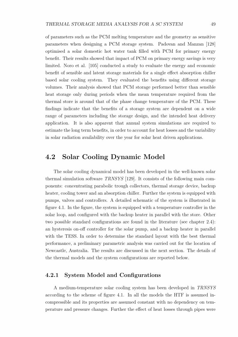
THERMAL STORAGE MEDIA ANALYSIS FOR A SC SYSTEM 49
of parameters such as the PCM melting temperature and the geometry as sensitiveparameters when designing a PCM storage system. Padovan and Manzan [128]optimised a solar domestic hot water tank filled with PCM for primary energybenefit. Their results showed that impact of PCM on primary energy savings is verylimited. Noro et al. [105] conducted a study to evaluate the energy and economicbenefit of sensible and latent storage materials for a single effect absorption chillerbased solar cooling system. They evaluated the benefits using different storagevolumes. Their analysis showed that PCM storage performed better than sensibleheat storage only during periods when the mean temperature required from thethermal store is around that of the phase change temperature of the PCM. Thesefindings indicate that the benefits of a storage system are dependent on a widerange of parameters including the storage design, and the intended heat deliveryapplication. It is also apparent that annual system simulations are required toestimate the long term benefits, in order to account for heat losses and the variabilityin solar radiation availability over the year for solar heat driven applications.
4.2 Solar Cooling Dynamic Model
The solar cooling dynamical model has been developed in the well-known solarthermal simulation software TRNSYS [129]. It consists of the following main com-ponents: concentrating parabolic trough collectors, thermal storage device, backupheater, cooling tower and an absorption chiller. Further the system is equipped withpumps, valves and controllers. A detailed schematic of the system is illustrated infigure 4.1. In the figure, the system is equipped with a temperature controller in thesolar loop, and configured with the backup heater in parallel with the store. Othertwo possible standard configurations are found in the literature (see chapter 2.4):an hysteresis on-off controller for the solar pump, and a backup heater in parallelwith the TESS. In order to determine the standard layout with the best thermalperformance, a preliminary parametric analysis was carried out for the location ofNewcastle, Australia. The results are discussed in the next section. The details ofthe thermal models and the system configurations are reported below.
4.2.1 System Model and Configurations
A medium-temperature solar cooling system has been developed in TRNSYSaccording to the scheme of figure 4.1. In all the models the HTF is assumed in-compressible and its properties are assumed constant with no dependency on tem-perature and pressure changes. Further the effect of heat losses through pipes were

THERMAL STORAGE MEDIA ANALYSIS FOR A SC SYSTEM 50
not considered as those are pertinent to a specific system and not to a generic sys-tem adopted in this thesis. Heat losses are considered in the storage and collectormodels. Besides the LHTESS, the absorption chiller, the heater, and some mix-ing/diverting valves, all the other component models – referenced as Type – werefrom the software library. The LHTESS, the high efficiency absorption chiller and
Figure 4.1: Generic solar cooling system layout with controls: temperaturecontroller for solar pump and backup heater in parallel with thermal store
a SC subsystem –heater and mixing/diverting valves– were developed in C++ andlinked into the software as an external library. The subsystem is represented bythe auxiliary heater, the mixer and diverter valves and their controller. The lattersubsystem was implemented as a single Type, in order to speed up the simulationsand reduce the complexity of the simulated system. The thermal models of the SCplant devices are described in the next sub-section.
The general system dynamics of the SC plant of figure 4.1 can be summarisedin three points:
• the solar loop collects heat at high temperature (> 150 ◦C) and stores it inthe TESS
• when the building requires cooling, the chiller is switched on and heat is sup-plied to the machine via the store and/or the backup heater
• the system can regulate the chiller hot inlet temperature for capacity control,via the re-circulation or bypass pipe
The building thermal load was applied to the SC system simulation deck as anexternal data file, with matching weather file. Hence the system, according to theenergy management and control scheme, provides the energy necessary to match thecooling load in the data file.

THERMAL STORAGE MEDIA ANALYSIS FOR A SC SYSTEM 51
4.2.2 Component Models
This sub-section documents the thermal models of the devices that forms theabove generic SC plant.
Solar Collector Model
The solar collector thermal model is based on the theoretical collector efficiencyequation [80]:
ηcoll =Qcoll
Acoll I= F ′(τα)en − c1
Tm − TenvI
− c2(Tm − Tenv)
2
I(4.1)
where:
Qcoll = mcoll cp(To − Ti) Tm =Ti + To
2(4.2)
The model is implemented by the TRNSYS Type 536, and includes details likeIncidence Angle Modifiers (IAM), concentration ratio, corrective coefficients for nonrated flow conditions and collectors in series. The collector efficiency parametersadopted in this model, for a NEP small parabolic trough, are F ′(τα)en = 0.689,c1 = 0.36W/(m2K), c2 = 0.0011W/(m2K2) [130].
Sensible Heat Storage Model
The sensible heat storage model is Type 534. The tank is modelled as a stratifiedstore with nine sections with equal volume. The source-sink inlet-outlet ports arelocated at the top and bottom sections. Thermal losses through the storage surfaceand the environment are taken into account with a global heat transfer coefficient.The thermal model is derived from the energy balance equation at each section ornode of the store. For the top section, the final equation of the model is:
ρ cp VsecdTtopdt
= msrc cp Tsrc − mload cp Ttop +k Asec
H(Ttop+1 − Ttop)+
UAlos,top(Tenv − Ttop)−
cp(msrc − mload)Ttop msrc > mload
cp(msrc − mload)Ttop+1 msrc ≤ mload
(4.3)

THERMAL STORAGE MEDIA ANALYSIS FOR A SC SYSTEM 52
Where Ttop+1 is the section below the top one (the section numbering is ascendingfrom top to bottom). For the bottom section, the thermal model is:
ρ cp VsecdTbotdt
= mload cp Tload − msrc cp Tbot +k Asec
H(Tbot−1 − Tbot)+
UAlos,bot(Tenv − Tbot)−
cp(msrc − mload)Tbot−1 msrc > mload
cp(msrc − mload)Tbot msrc ≤ mload
(4.4)
A i-th section in the middle is modelled as follow:
ρ cp VsecdTidt
=k Asec
H(Ti+1 − 2Ti + Ti−1) + UAlos,i(Tenv − Ti)−cp(msrc − mload)(Ti−1 − Ti) msrc > mload
cp(mload − msrc)(Ti+1 − Ti) msrc ≤ mload
(4.5)
The model, to account for temperature changes due to density gradients, assumes aninstantaneous and adiabatic mixing between two sections with inverted temperatures(e.g. a section with higher temperature than the above one) at the end of eachsimulation time-step.
Absorption Chiller Model
An absorption chiller consists of four essential parts: the generator, the evap-orator, the absorber and the condenser. The refrigerant is successively evaporatedin the generator, condensed in the condenser at higher pressure, then evaporated atlow pressure and finally absorbed by a chemical solution.
A detailed thermodynamic model for absorption chillers is quite complex toimplement and computationally expensive to be adopted in long term system energyperformance simulations. Hence a simplified model, based on the characteristictemperature function ∆∆t [131], has been selected. The model energy balanceequations are:
QAC = QE + QG + Qaux (4.6)
COP =QE
QG + Qaux
(4.7)
Q = m cp(To − Ti) (4.8)

THERMAL STORAGE MEDIA ANALYSIS FOR A SC SYSTEM 53
Where QAC,E,G,aux is the thermal power of the absorber-condenser, the evaporator,the generator and the auxiliary power. The formula of the evaporator and generatorpower is:
QE,G = sE,G ∆∆t+ rE,G (4.9)
Where the characteristic temperature function is:
∆∆t = tG + a tAC + e tE (4.10)
The model coefficients s, r, a, e are defined in table 4.1. The model parameters havebeen tuned to simulate the performance of a triple-effect hot water fired absorptionchiller. The calibration process is a multi-variable linear regression on the coolingcapacity, as suggested in [132], from data provided by Thermax® [75]. The Python
Figure 4.2: Parameter fitting of the triple-effect absorption chiller model
package Scikit-learn [133] was used for the parameter fitting. The obtained modelparameters are summarised in table 4.1, while the statistical regression on the man-ufacturer data is depicted in figure 4.2. The linear regression shows an agreementwith the chiller data with coefficients of determination R2 of 0.98 and 0.95 for evap-orator and generator capacities. Finally, the model has been developed in C++ andlinked to TRNSYS as a Type for system simulations.

THERMAL STORAGE MEDIA ANALYSIS FOR A SC SYSTEM 54
Table 4.1: Absorption chiller model and rated parameters
Model Parameters Value Flow Rates Value Rated Parameters Valuea -2.63 Hot water 5.3 m3/h capacity 103.4 kWe 3.95 Cooling water 32.8 m3/h COP 1.81sE 1.19 Chilled water 20.2 m3/h Hot Inlet 210 ◦CrE -76.91 Cool Inlet 32 ◦CsG 0.54 Chilled Outlet 7 ◦CrG -25.96
Backup Heater Model
The backup heater is modelled as an ideal heater with infinite capacity and nothermal losses. Its expression is:
Thtr,o =
{Thtr,i Qhtr = 0 Thtr,i > Thtr,sp
Thtr,sp Qhtr = m cp(Thtr,sp − Thtr,i) Thtr,i ≤ Thtr,sp(4.11)
Where Thtr is the heater inlet or outlet temperature, Thtr,sp is the heater temperatureset-point and Qhtr is the heater thermal power.
Cooling Tower Model
A wet cooling tower in a counter flow arrangement is adopted. The coolingtower model is Type 51. It is based on an ε-NTU approach, where the user specifiesthe manufacturer mass transfer constant and exponent (c and n of equation 4.14).Such parameters have been obtained from [134]. The size of the cooling tower waschosen from the manufacturer catalogue based on the cool water design inlet andoutlet temperatures, the maximum air wet bulb temperature (from the weather dataof the simulations) and the chiller cooling rated flow rate. The main equations ofthe model are reported below.
Q = ε ma(esat,wat,i − eair,i) (4.12)
where esat,wat,i is the enthalpy of the saturated air at the water inlet temperature,and eair,i the enthalpy of the air at the environment temperature. The expressionof effectiveness is:
ε =1− e−NTU(1−m∗)
1−m∗e−NTU(1−m∗)(4.13)

THERMAL STORAGE MEDIA ANALYSIS FOR A SC SYSTEM 55
where:
NTU = c(mwat,i
mair
)n
m∗ =mairCapsat
mwat,iCapp,wat
(4.14)
The model has the feature to set a variable air flow rate in order to modulate thecooling capacity of the device. More details of the model can be found in the softwaredocumentation [129].
Building Model
The cooling load is represented by a typical office building located in Australia.It belongs to the category of “type A”, according to the Australian Building CodeBoard (ABCB) [135]. It is a single storey, of a multiple storey building and it hasa fully enclosed square footprint area of approximately 1000 m2. The dimensions ofeach of the sides is 31.6 m, and the height (floor to ceiling) is 2.7 m. The walls andfabric are designed to meet minimum requirements (e.g. global wall heat transfercoefficient ≤ 0.4W/(m2K)) provided by the Building Code of Australia (BCA). Theinternal loads are based on 100 people occupancy and a low infiltration rate (0.25 airchanges per hour). Loads associated with lighting and equipment are also includedin the model. An indoor temperature of 26 ◦C has been used as the set point forcooling mode operation. The air conditioning operating time for meeting comfortrequirements is set between 7 am to 6 pm, during working days of the week. Overthe weekend, no cooling load is specified. The building thermal model has been
Figure 4.3: Left: a typical summer daily cooling load for Sydney, Australia.Right: the respective monthly cooling load
developed in TRNBuild. It is based on the thermal energy balance on an air-node,which is the control volume with uniform temperature. In this thesis, for the sakeof simplicity, the building level is assumed as a single thermal zone. The energybalance equation for an air-node includes the convective gains from internal sources

THERMAL STORAGE MEDIA ANALYSIS FOR A SC SYSTEM 56
(e.g. people, Qint,g), walls (Qsurf ), ventilation (Qvent), infiltration (Qinf ) and solarthrough its windows (Qsol,g). The air-node thermal gain (Qairn) expression is:
Qairn = Qsurf + Qinf + Qint,g + Qvent + Qsol,g (4.15)
The thermal requirements of the zone have been calculated assuming an ideal HVACsystem with infinite capacity. The building has predominately cooling needs, hencethe heating load was neglected. In the simulations the weather data of Sydney andNewcastle, Australia, have been chosen, depending on the scenarios. As an example,figure 4.3 shows a typical summer daily load and monthly cooling requirements forthe location of Sydney, Australia.
Other System Models
The SC system includes pumps, valves and controllers. Since the scope of thethesis is the evaluation of the thermal performance of the SC system, the pumps aremodelled as an ideal components with no electrical consumption. Hence their roleis to impose a predetermined flow rate in the relative loop.
The valves installed in a typical plant are usually (i) a pressure relief valve,(ii) three way valves (mixers and diverters), (iii) other valves (e.g. non returnvalve). For simplicity only the first two valves were included in the system model,as essential for the SC system control. The pressure relief valve (PRV), located atthe collector outlet, acts as a safety measure by releasing to the environment thermalenergy when the temperature and/or pressure exceed its set point. This is a safetyrequirement to avoid system overheating when the maximum collector pump flowrate is achieved but is still unable to drop the temperature to the control set point.In this model, the pressure effects are not taken into account, hence the PRV istemperature activated. It is modelled as:
To =
{Ti Qdump = 0 Ti ≤ Tmax
Tmax Qdump = m cp(Ti − Tmax) Ti > Tmax
(4.16)
The mixers and diverters models assumes adiabatic mixing and no thermal losses.For a diverter with one inlet and two outlets, the model is:
mi = m1,o + m2,o Ti = T1,o = T2,o (4.17)
For a mixer with two inlets and one outlet, the model is:
mo = m1,i + m2,i To =m1,iT1,i + m2,iT2,i
mo
(4.18)

THERMAL STORAGE MEDIA ANALYSIS FOR A SC SYSTEM 57
The amount of bypass flow is controlled to keep a set-point temperature at the mixeroutlet.
The controllers installed in the generic solar cooling system of figure 4.1 are:
1. Solar loop pump controller: the controller activates the solar collector pumpand charges the tank irrespective of the load requirement. The signal thattriggers the pump depends on the controller type. Two standard controllers,as shown in figure 4.4 are used:
i) Temperature controller: it is usually a proportional-integrative (PI) con-troller, that drives a variable speed (VSD) pump. The controlled variableis the collector outlet temperature. The controller varies the flow in orderto maintain a set-point temperature.
ii) Hysteresis ON-OFF controller: it is a simple ON-OFF controller thatdrives a fixed speed pump. Hence the flow rate provided by such controlstrategy is fixed. Two temperature bands are used to prevent cyclingand instabilities of the controller. The controlled variable is usually thebottom temperature of the store: the thermal store is being charged ifits temperature is lower than the collector outlet temperature, otherwisethe solar pump is switched off, if it is not.
2. Cooling controller: it is the master controller that activates the absorptionchiller and its pumps, as well as the heat delivering controller. It switchesthose device on when the building requires cooling.
3. Cooling tower controller: a PI controller, that drives the VSD fan of thecooling tower, is adopted. The controlled variable is the chiller inlet coolingtemperature. The controller varies the air flow in the cooling tower in orderto maintain a set-point temperature of the cooling water.
4. Chiller heat delivering controller: it controls the heat delivered to the chillervia the tank and/or the heater (depending on the heater position) as well asthe ratio of flow in the bypass pipe for chiller hot inlet temperature regulation.The bypass is controlled to maintain a set-point temperature to regulate thecapacity of the chiller. This temperature is provided by the chiller model,given the known inlet cooling temperature and the chilled water outlet set-point of 7 ◦C. The configurations of the backup heater (case b and c of figure2.8) are:
i. In series with the tank: the tank is always discharged when the buildingrequired cooling. If the tank outlet temperature is lower than the heaterset-point temperature, the heater is switched on, heating up the HTF tothe heater set-point temperature.

THERMAL STORAGE MEDIA ANALYSIS FOR A SC SYSTEM 58
ii. In parallel with the tank: the controller activates or not heat deliveringfrom the store depending on its temperature. When the store is not used,the controller activates it when the temperature at 25 % from the tankbottom is higher than the set-point requested by the chiller (e.g. 210 ◦C),otherwise the auxiliary heater is used. If the tank was previously beingused, the controller will keep withdrawing heat until the temperature 25% from the top falls below the chiller required hot temperature. In thisway the tank is allowed to charge to a level suitable to deliver heat tothe chiller at the required temperature. The heights of the sensors thattrigger the charging/discharging status are chosen to avoid the mixingregions at the top and bottom sections of the store.
Figure 4.4: Left: Temperature controller for constant collector outlet tem-perature. Right: Hysteresis controller triggered by temperature sensors at thecollector outlet and store bottom.
4.2.3 SC system overall controls strategy
This sub-section is given a summary of the overall control strategy of the SCplant of figure 4.1. The solar loop works according to the following logic:
• The collector controller controls the flow rate via a VSD pump to maintain aconstant collector outlet temperature (temperature controller) or via a fixedspeed pump (hysteresis controller) to charge the storage system. The controlaction is applied when the solar radiation is higher than 150W/m2 (critical ra-diation value). The controller temperature set-point is 210 ◦C for the temper-ature controller, while the dead bands for the hysteresis controller are 15 and5 K (pump on when Tcoll,o−Ttank,bot > 15 K, off when Tcoll,o−Ttank,bot < 5 K).
• A PRV limits the maximum temperature of the system, discharging energy tothe environment if the collector outlet temperature is higher than the systemmaximum operating temperature – set to 220 ◦C.
The process fluid/chiller circuit loop works as follows:

THERMAL STORAGE MEDIA ANALYSIS FOR A SC SYSTEM 59
• Cooling is required Monday to Friday, between 7 am to 6 pm, as advised bythe BCA. Hence the chiller and its pumps are switch on during those times.
• The cooling tower, when the chiller operates, is controlled by a PI controllerthat regulates the fan speed, hence the cooling capacity, to keep the chillercooling inlet temperature to the set-point of 32 ◦C.
• The cooling load is met by regulating the chiller hot inlet temperature. Thechiller model calculates the requested temperature, which is delivered by mix-ing some portion of the cooled HTF exiting the chiller with hot HTF sourcedfrom the tank and/or the backup heater. The details of storage and/or backupheat delivering are illustrated in subsection 4.2.2 above.
In order to confirm the validity of the simulations, sanity checks on overall mass andenergy balances were implemented.
4.3 Preliminary Simulation Results
In this section the results of the preliminary simulations with the two collectorcontrols and two backup configurations are presented. The scope is to identify thefinal system layout that have the best thermal performance over a year, which will beadopted in the storage materials analysis. In the analysis, the storage dimensionsare expressed with the residence time in hr, derived assuming a fixed dischargepower. Before presenting the results, a summary of the system design and systemkey performance indicators, that were used in the analysis, is given below.
The system design is as follows:
• The chiller size was chose to be 10 kW .• The building location is Newcastle, Australia. Temperature set-points of 26
and 20 ◦C for the cooling and heating were used. The maximum cooling loadover an hour is 111 kW , while the annual cooling and heating demands are15 MWh and 0.3 MWh. Hence the heating load was neglected. The coolingload as well as the chiller model parameters were scaled to match the chillersize.
• Four values of the specific collector area (m2/kWchiller) were used in the para-metric analysis: 0.615, 1.23, 1.85 and 2.46 m2/kWchiller.
• Five values of the storage size were used in the parametric analysis: 0.167,0.5, 1, 3 and 5 hr (0.09, 0.26, 0.51, 1.54 and 2.57 m3).
• The global heat loss coefficient was set to 0.83 W/m2K (Rock-wool with k =
0.045W/(mK) at 150 ◦C and thickness of 5 cm).

THERMAL STORAGE MEDIA ANALYSIS FOR A SC SYSTEM 60
• The HTF and storage media is pressurised water with properties: cp = 4.49
kJ/kgK, ρ = 853 kg/m3 (@200 ◦C and 20 bar).
In this set of simulations three thermal parameters were used to compare the per-formance of the SC plant:
• Solar fraction (SF): the ratio between the solar collected heat to the totalheat used by the system over the simulation time. It states the percentageof building demand that is satisfied by the solar energy, compared with theamount satisfied by the backup energy. Its expression is:
SF =
∑Qsolar∑
Qsolar +∑Qbackup
(4.19)
• The collector yield: the amount of heat collected over the simulation time perunit of collector area kWh/m2.
• The storage thermal losses over the simulation time MWh.
In the simulations, a typical daily profile for the chiller and building tempera-tures is shown in figure 4.5. As mentioned before, cooling is required from 7 am to
Figure 4.5: Typical chiller and building temperature profiles for a summer dayin Newcastle, Australia (temperature profiles outside load requirements are notphysical as the chiller model is steady state).
6 pm, hence during this time the system keeps the building at the set-point temper-ature of 26 ◦C. The chiller is working at part load between 30 to 100 % capacity inorder to satisfied the cooling requirements. Since the chiller inlet cooling tempera-ture is kept close to 32 ◦C by the cooling tower PI controller, the chiller inlet hot

THERMAL STORAGE MEDIA ANALYSIS FOR A SC SYSTEM 61
temperature is controlled and varied during the day, to regulate the cooling capac-ity. At beginning of the day, a low amount of cooling is necessary, hence the chillerhot inlet temperature is about 150 ◦C. In the afternoon, when more cooling poweris needed, the chiller hot inlet temperature raises to 190 ◦C. This temperature isdelivered by the heating source of the system, either from solar or backup heater.
The results of the parametric analysis with five storage sizes, four collectorareas, two solar pump controllers and two backup configurations are explained below.Figure 4.6 on the left shows the annual SF for various storage and collector sizes,for a system with hysteresis controller. As expected, the solar fraction rises as thecollector area increases. For a given specific collector area (m2/kWchiller), SF fallsas storage volume increases. This is attributed to greater heat losses from largerstorage tanks: tank losses increase about eight times due to a thirty times increase instorage time (see figure 4.7). The effect of backup burner positioning in the overall
Figure 4.6: Variability of the solar fraction with storage and collector sizes, forbackup in series and parallel with the store, while using an hysteresis controller(left), and a temperature controller (right) for the collector pump.
system layout can also be seen in figure 4.6. The parallel position of the backupheat source resulted in higher solar fraction, which is evident for large storage tankvolumes and low collector areas. The analysis of component-level heat contributionshowed the solar collector provided nearly similar heat to the system for series andparallel burner positioning. However, tank heat losses from a parallel positionedconfiguration were less, due to decoupling of the tank from the backup heat source.For example, in the operating case with 0.615 m2/kWchiller specific collector areaand 5 hr storage residence time, the tank heat loss for a series configuration wasnearly twice that of a parallel backup configuration (as shown in figure 4.7). Themean tank temperature was also nearly 20 ◦C higher for a series backup heatingconfiguration.

THERMAL STORAGE MEDIA ANALYSIS FOR A SC SYSTEM 62
Figure 4.7: Comparison of collector yield (annual averages of daily values) andstorage thermal losses (annual values) for systems equipped with hysteresis solarpump controller. Top: influence of specific collector areas and storage sizes onthe collector yield, for series and parallel backup configurations. Bottom: thermallosses from store to environment for different storage sizes and specific collectorareas, for series and parallel backup configurations.
Figure 4.7 shows the effect of collector area and storage tank volume on thecollector yield. Collector yield falls as collector area increases for all storage tankvolumes. The reduction in yield is more pronounced for smaller storage sizes than forlarger ones. In fact, larger stores have lower collector inlet temperatures, resultingin lower collector thermal losses. The position of the backup has minimal influenceon the annual collector yield.
Figure 4.6 on the right shows the effect of the backup heater configuration,storage and collector sizes on SF while using a temperature controller for the collectorpump. During operation of this control, a variable speed pump alters the flowrate through the collector to maintain a fixed set point temperature at collectoroutlet. Comparison of this control strategy with hysteresis control strategy showshigher solar fraction obtained by this controller for higher specific collector areavalues. This controller is able to generate SF higher than 0.9. The collector outlettemperature set-point values closer to chiller requirements resulted in higher tankoutlet temperatures for the temperature controller driven system. As a result, thebackup burner was utilised less to meet the cooling load, resulting then in highersolar fractions. SF difference between the two backup configurations are small dueto the effect of the temperature controller: it allows for a more efficient collectoroperation by lowering its average temperature, hence smoothing the negative impact

THERMAL STORAGE MEDIA ANALYSIS FOR A SC SYSTEM 63
of the backup configuration seen in the previous scenario. Similarly to the hysteresiscontroller performance analysis, the effect of increased storage size is to reduce SFat low specific collector area (the tank is too big, resulting in high thermal losses).On the other side, at high specific collector area, increasing the storage dimension,increases SF till the optimal value around 3 hr of storage time.
In conclusion, these results indicate that the temperature controller with VSDcollector pump with parallel backup configuration, provides higher solar fractions.Hence such configuration will be used in the storage material comparison analysis.
4.4 Thermal Storage Material Selection and Sys-tem Design
In this section a methodology for design, comparison and analysis of storagematerials for SC systems is presented. Though the methodology was developed forSC systems, the method is valid for generic thermal systems with thermal storagedevices. Details of the SC system design are also given in the last sub-section. Thenext section will present and discuss the results of the simulations with the storagesystems designed in this section.
4.4.1 Storage Design Methodology
Two sensible and two latent heat storage materials have been chosen for thestudies. Water and thermal oil have been chosen as the sensible heat storage media.The nominal operating temperature of the triple effect chiller is 210 ◦C. Hencephase change materials with phase change temperature range of 220 ◦C to 230 ◦C
have been chosen for the studies. KNO3/NaNO3 eutectic salt (known as solar salt)has a phase change temperature of around 220 ◦C [124]. Moreover, these salts arecommercially available. However, these salts have poor thermal conductivity thatcan limit the charging and discharging effectiveness of the storage system. Hence ahigh conductivity metal phase change material with phase change temperature of230 ◦C [32] has been chosen as the second phase change material for evaluation.Table 4.2 summarises the materials properties as well as the HTF used in each ofthe systems.
Generic approaches for comparing sensible and latent heat storage systems havenot been clearly established. This issue is compounded by the wide variety of ap-proaches used for designing a PCM based storage system. Castell and Solé [67]have summarised design methodologies used in liquid - solid phase change storage

THERMAL STORAGE MEDIA ANALYSIS FOR A SC SYSTEM 64
systems. Amin et al. [136] have suggested that both volume of PCM in the storagesystem, and energy storage effectiveness are parameters to consider when designinga PCM based storage system.
Table 4.2: Properties of the storage materials adopted in the storage comparisonanalysis.
Storage material HTF usedMassDensity(kg/m3)
SpecificHeatCapacity(kJ/(kgK))
Thermalconduc-tivity(W/(mK))
Phase ChangeTemperature(◦C)
LatentHeat(kJ/kg)
EnergyDensity1
(kWh/m3)
SpecificEnergy1(kWh/kg)
Cost(USD/kWh)
Water @20bar,200◦C
Water 853 4.49 0.664 - - 21.3 2.5e−2 0.02
Therminol 55@204◦C
Therminol 737 2.56 0.107 - - 10.5 1.4e−2 117.4
Solar salt(KNO3/NaNO3)
Therminol 2000 1.5 0.5 221 100.7 55.9 2.8e−2 n.a.
Aluminium-TinAlloy (AlSn)2 Therminol 6823(s)
6500(l)0.237(s)0.263(l)
75(s)42(l) 231/232 50 92.5 1.4e−2 n.a.
Hence, hereby a methodology is described in order to carry out a systematicanalysis. Similarly to the work of Noro et al [105], the developed approach consistsof comparing the thermal performance of the storage device by including it in acomplete SC system simulation platform. Hence its performance is evaluated ona system level rather than a component level, by using system key performanceparameters (e.g. solar fraction), and system simulation over a long period (generallya year). The difference of the developed methodology is established by the storagedesign process: while Noro et al assumed equal storage volume for different storagemedia, the developed method assumed equal total nominal stored energy across thestorage systems. In this way, the amount of thermal energy that can be stored inthe media is constant. Noro et al instead assumed constant storage volume, hencePCMs with higher volumetric energy density would have stored more thermal energythan the sensible heat materials. Besides the storage design process, the comparisonfollows the dynamical annual system simulation approach described by [105].
This storage design methodology that enables direct comparison of differentstorage materials, have the following constraints:
(a) Constant nominal total stored energy.Nominal total energy stored in the storage materials is made constant for allthe scenarios. STESSs directly store heat in a fluid by increasing its tempera-ture. In order to compute the energy density, a temperature difference of 20 Kis chosen for sensible heat storage materials. For LHTESSs, a shell and tubedesign with PCM in-tube configuration has been chosen (see chapter 3). As aresult, this system also stores energy in the tubes and in the HTF. The storedlatent energy in the PCM was chosen to be 80 % of the total energy stored.
1calculated using a temperature difference of 20 K for sensible heat materials2Ref. [32], [137], [138]

THERMAL STORAGE MEDIA ANALYSIS FOR A SC SYSTEM 65
The rest of the stored energy is equally distributed between the tube materialand the HTF. Increase in storage time is then achieved by either adding moretubes or by increasing the tube length.
(b) Constant heat transfer area.In the design of LHTES, the heat transfer area of the heat exchanger hasbeen kept constant so that a given PCM-based storage system does not per-form better due to superior heat transfer design. In the shell-and-tube heatexchanger design parameters identification process, it has been ensured thatthe design value for the storage system heat transfer effectiveness is above0.8. This effectiveness has been estimated a priori using nominal dischargingcondition (storage fully charged at maximum temperature).
(c) Minimum heat loss area on the shell side.For the sake of limiting the search space of the design configurations, the areaof heat losses has been constrained by using a shell diameter-to-height ratioof 1.
Energy storage values have been chosen such that the storage system can provide0.5 to 5 hr of storage, to allow heat supply in cases that range from cloud coveragethrough overcast afternoon. The storage volume of the chosen materials for variousstorage times is shown in figure 4.8. As expected, latent heat storage materialsprovides more compact stores, due to their high volumetric energy density.
Figure 4.8: Total volume of storage for different storage materials and storagetimes, adopted in the storage comparison analysis.
The sensible heat storage design process is quite straight forward: from storagetime, storage energy and material energy density values, the storage size can be

THERMAL STORAGE MEDIA ANALYSIS FOR A SC SYSTEM 66
derived (first two steps of below method). The design of latent heat storage systemsinstead involves more steps, as per following:
1. Estimation of total energy stored by the storage system from design require-ments (nominal chiller capacity, COP):
Est =Qnom,chiller
COP× storage time (4.20)
2. Obtain the total volume of the system and the volume of HTF, PCM andthe tube from the volumetric energy storage density data and application ofconstraint (a). This results in:
Vshell = VHTF + Vtube + VPCM (4.21)
Vshell =0.1Est
Ev,HTF
+0.8Est
Ev,PCM
+0.1Est
Ev,tube
(4.22)
3. The design of the shell and tube heat exchanger requires additional dimen-sional details of tubes (outer and inner diameter and length), shell size andthe number of tubes. From constraint (c), the diameter of the shell is equalto its height. Thus one obtains the diameter and height of the shell as:
Dshell = Hshell =3
√4Vshellπ
(4.23)
Considering the tube length (L) is equal to shell height, length of the tubescan be estimated.
4. From design constraint (a), we obtain:
VPCM
Vtube=
NπD2iL/4
Nπ(D2o −D2
i )L/4=
D2i
D2o −D2
i
(4.24)
The tube dimensions can then be chosen from commercially available sizes(DN 15-20-25-32-40-50) to fit equation 4.24.
5. Finally the number of tubes can be obtained from the total volume of thestorage material once the tube inner diameter and the length are known.
Design steps 1-5 were followed in the LHTES design process with the second latentheat storage material. Two levels of sanity checks were carried out to ensure thedesign meets the requirements. The first one is the constraints fulfilment, establishedby the equations below:

THERMAL STORAGE MEDIA ANALYSIS FOR A SC SYSTEM 67
i. Conditions set by constraint (b) results in:
Do,salt
Do,AlSn
=NAlSn
Nsalt
LAlSn
Lsalt
(4.25)
ii. Conditions set by constraint (a) results in:
Ev,salt
Ev,AlSn
=D2
i,AlSn
D2i,salt
(4.26)
As a second sanity check, the shell diameter was always compared with the minimumdiameter required for arranging the chosen tubes inside the shell diameter, calculatedfrom the “circles in circle” optimisation problem [139] to check if the design isrealistic. For example, in the case of salt with 0.5 hr of storage, the estimatedshell diameter is 1.02 m and the total number of tube chosen is 302. The minimumphysical diameter for best packing of 302 tubes with a tube outer diameter of 48.3mm is 0.913 m. Since the design process requires approximations (e.g. rounding offthe tube length to nearest integer and the choosing a combination of inner and outertube diameters to the nearest available commercial sizes), the chosen configurationsmatched the total energy stored and heat transfer area design constraints within 3% relative error.
4.4.2 SC system design for storage material comparison
The solar cooling plant has been design to meet the cooling load requirementsof a commercial building in Sydney, Australia. The chosen building, which is thesame of section 4.2.2, required 109 MWh of cooling and 4 MWh of heating undersuch weather conditions (see figure 4.3 for daily and monthly loads). The heatingload was not considered in the simulations, as the building predominately requiredcooling. The maximum cooling demand over an hour is 85 kW. Hence, the load hasbeen scaled to match the triple-effect chiller parameters of table 4.1. The design ofthe SC plant (e.g. cooling tower size) has been scaled as well to match the chillersize of 103 kW .
The SC system is configured with a temperature controller and backup heaterin parallel with the store (figure 4.1): such configuration yielded the highest thermalperformance, as reported in section 4.3. Therefore the overall control strategy is thesame as described in section 4.2.3. There are few difference mainly regarding theoperating temperature set-points:
• In sensible heat cases, the solar pump controller temperature set-point is 210◦C as per nominal chiller requirement. Instead, for latent heat cases, a set-

THERMAL STORAGE MEDIA ANALYSIS FOR A SC SYSTEM 68
point temperature 10 ◦C higher than phase change temperature was adopted,to account for heat exchanger specification. As a consequence of that, thelimit on the maximum temperature of the PRV was increased in the case ofsystem with LHTES (e.g. if collector set point temperature is 220 ◦C, thePRV is set to operate at 230 ◦C).
• Chiller heat delivered from the tank is only allowed when the tank is sufficientlycharged. Such conditions is established depending on the type of storagesystem:
– For sensible heat storage, the tank controller operates the storage tankaccording a hysteresis cycle, as explained above in section 4.2.2. Thelocation of the temperature sensors for discharging is depicted in figure4.9.
– In the case of latent heat storage, the tank controller operates the tankaccording the following cycle: if the tank was previously not discharged,the controller let the thermal store to be charged until the temperature atthe tube bottom is higher than the phase change final temperature, thenthe thermal store is discharged and delivers heat to the chiller. On theother hand, if the tank was previously being used, the thermal store keepsdelivering heat until the temperature at the tube top is lower than thephase change temperature, and then switches off the heat delivering fromthe thermal store. As a result, this control allows the PCM to operate inthe phase change region, storing the energy as latent heat. The locationof the temperature sensor of this controller is shown in figure 4.9.
Figure 4.9: Location of the temperature sensors in the TES for activation ofheat delivering to the chiller. Left: sensible heat store (sensors located at thevery top and bottom zones). Right: latent heat storage system (sensors locatedat the very top and bottom sections of the tubes).

THERMAL STORAGE MEDIA ANALYSIS FOR A SC SYSTEM 69
4.5 Comparison of Sensible and Latent ThermalStorage Materials
In this section the results of the simulations that compare different storagematerials are illustrated and discussed. First, the key performance indicators needto be introduced for the subsequent discussion. The overall thermal performanceof the system is evaluated based on the solar fraction. This parameter is definedby equation 4.19. A SF close to 1 indicates that the cooling demand is totallysatisfied by solar energy. Besides the SF, a range of other indicators provide usefulinformation on the performance of the components and can be used to explain themechanisms responsible for high or low solar fraction. These additional indicatorsinclude:
• Solar collector yield (defined in section 4.3).• Heat losses from the surface of the thermal storage tank.• The effectiveness of the latent heat storage tank heat exchanger in discharge
mode. This is estimated using an average annual calculated value from in-stantaneous temperature data. It quantifies the performance of the heat ex-changer, during the heat transfer process between the HTF and the PCM. Theeffectiveness is defined as the ratio of the actual heat transfer rate versus themaximum possible rate [140]. As the heat capacity of the HTF is lower thanthe PCM one, its expression is:
εdisch =1
time
∑ THTF,top − THTF,bot
TPCM,top − THTF,bot
∆t (4.27)
• Storage efficiency, defined as the ratio of energy delivered to the chiller fromthe tank to the energy supplied by collector field to storage system, over thechiller operating time. It is an indirect measure of the storage thermal lossesand expresses the capacity of storing useful energy that will be discharged tothe heat sink. The first term is computed as the sum of negative changes instorage internal energy and the second term, the denominator, is computed asthe sum of the positive changes in internal energy [17].
ηsto =
∑Edisch∑Echarg
=
∑|∆enthalpy−|∑∆enthalpy+
(4.28)
The simulations were carried out over a year time-frame with 5 min time-step,and a parametric analysis of the collector and storage designs was implemented toanalyse the variability of the performance and individuate an optimal design. Fourlevels of collector area (1 to 4 m2/kWchiller) and storage duration (30 min, 1, 3

THERMAL STORAGE MEDIA ANALYSIS FOR A SC SYSTEM 70
and 5 hr) have been used to evaluate the effect of component sizing on the systembenefits. In the next sub-sections, two cooling scenarios have been evaluated, namelythe system operating with a constant cooling load and a variable cooling load. Inthe first, the chiller is working at constant nominal operational conditions in orderto simulate the system with base load operation, while in the second scenario thechiller is allowed to operate in part load, with a capacity modulation between 40 %to 120 % of the nominal.
4.5.1 Constant Cooling Load System Performance
Before discussing the annual performance of the system, the performance ofthe system main components (collector, store and chiller) are reported in figure4.10 for typical working days (Monday to Friday). For sake of clarity, the chillertemperature profiles are set to zero when the device is not in operation. The figureshows the temperature states of the storage system both HTF and PCM (solar saltin this case) sides, top, middle and bottom locations. As evident from the figure,the temperature distribution in the store is not uniform due to system dynamics.Hence the PCM might undergoes phase change only in one location.
Figure 4.10: A weekly working days system performance of collector, store andchiller for constant cooling load and latent storage with salt.

THERMAL STORAGE MEDIA ANALYSIS FOR A SC SYSTEM 71
On the first day, heat from the thermal store is delivered to the chiller while thecollector simultaneously supplies heat to the store: the store is in charging-while-discharging condition. A unique feature of the shell and tube design for latent heatstorage is simultaneous heat collection and delivery in the storage system during op-erational periods. During the charge phase, the heat is delivered from the collectorsto the PCM storage tank and the mass flow rate (FR) from the collector exceedsthat going to the chiller such that HTF flows from the top to the bottom of thestore. In the discharge phase, the HTF flows from the bottom to the top gainingheat from the thermal store. In this configuration the storage state of charging ordischarging is subject to system controller dynamics. For example if the collectorcontroller sets the collector flow rate at 14000 kg/hr and the chiller controller – dueto temperature requirement of the chiller – sets the process flow rate to 3000 kg/hr,the thermal store is charging due to the resulting net flow from top to bottom. Thepresence of the HTF in the shell side ensures there is a mixing region at the topand bottom of the tank that allows simultaneous heat collection and delivery, eventhough the tubes, filled with PCM, are either charging or discharging.
At the end of the first day, when the solar collector stops, the PCM dischargesheat to the chiller and its temperature falls below the phase change temperature(221 ◦C). Although the amount of solar radiation is scarce on the second day, thecollector charges the storage in two stages. At the end of the second stage the PCMis charged again. The third day is characterised by high level of solar radiation, thusthe storage system is fully charged at the maximum temperature. The fourth day,due to low solar radiation, the PCM is fully discharged. At the end of the day, theradiation increases and the collector starts charging the store. Between the fourthand fifth day, storage temperature drop due to losses is limited by the latent heat ofthe phase change. During the fifth day, the storage charging is completed and then,due to load requirements, heat is withdrawn from PCM, resulting in discharging.Over the weekend, the chiller is not in operation and the storage system is fullycharged, if solar irradiance is available.
The influence of storage insulation on the annual performance of the storewas evaluated by comparing two insulation values: Rth = 3m2K/W and Rth =
6m2K/W . The annual storage losses as a percentage of the total heat collectedfrom solar are depicted in figure 4.11. A parametric analysis of the thermal losses isshown in the figure, to analyse the influence of the design parameters (collector areaand storage dimension). In all cases the material with the highest energy densityand lowest storage time (AlSn) has the lowest heat losses, and vice versa, the ma-terial with the lowest energy density and highest storage time (thermal oil) has thehighest heat losses. Longer storage duration significantly increases the heat losses

THERMAL STORAGE MEDIA ANALYSIS FOR A SC SYSTEM 72
Figure 4.11: Parametric analysis of storage thermal losses for collector andstorage dimension and two insulation values, in the constant cooling load scenario.
due to increase in storage dimensions. The benefit of LHTES material is particularlyevident in figure 4.11. Sensible heat materials due to their larger storage volumerequirement, lose over 20 % of collected energy if careful selection of insulation ma-terial is not carried out. Rth = 6m2K/W insulation results in tank losses that areless than 20 % of solar heat gain. Commercially available insulation materials canprovide such thermal insulance with a thickness of 150 mm. Thus, all subsequentanalysis in this study has been carried out using Rth = 6m2K/W as the thermalinsulance of the storage insulation material. The thermal losses for this system arelarge due to heat only being required five days per week.
The annual average storage heat exchanger effectiveness (equation 4.27) duringdischarge, for each of the two latent heat storage materials, is shown in figure 4.12. Itcan be seen that both salt and AlSn materials have high effectiveness values duringall the scenarios. The effectiveness is relatively independent of specific collector areabut increases with increase in storage time, due to the increase in heat transfer area.AlSn has the highest effectiveness due to its very good heat transfer properties. Theheat exchanger effectiveness, for the salt PCM with low storage duration, drops offsignificantly due to the reduced heat transfer area in the small tank and the largertubes with lower thermal conductivity. The heat transfer area is not designed toabsorb all the heat made available from the collectors. In contrast, at high storagetimes, the salt PCM heat exchanger effectiveness is almost constant, even with thehigher specific collector area. This is due to the high heat transfer area in the storagetank.
Figure 4.13 shows the storage efficiency for various materials while providing

THERMAL STORAGE MEDIA ANALYSIS FOR A SC SYSTEM 73
Figure 4.12: LHTES average annual effectiveness for solar salt and AlSn alloy,for different collector and storage sizes and constant cooling load.
Figure 4.13: Annual TES efficiency variability with system design for variousstorage materials and constant cooling load.
heat to a SC system with constant cooling load. Storage efficiency is the highestfor lowest storage times: at low storage time the heat losses are the lowest due toreduced storage dimension. An increase in specific collector area has no effect instorage efficiency at low storage times. At high storage sizes, an increase in thecollector field results in increase in storage efficiency. Overall latent heat materialshave the highest storage efficiency due to their compact storage dimensions comparedto sensible heat materials. Though differences in storage efficiency between differentmaterials, all the values are above 94 %, showing good storage performance.
Figure 4.14 shows the variation of solar fraction with storage time and collectorarea for different storage materials and constant cooling load. As expected, solarfraction increases with increasing collector area for all the storage materials cases:collected heat from solar is higher at high areas. For a given collector area, the solar

THERMAL STORAGE MEDIA ANALYSIS FOR A SC SYSTEM 74
fraction increases with increasing storage volume: more solar heat is stored in thetank and thus made available to the chiller. Sensible and latent storage materials
Figure 4.14: Annual solar fraction for sensible and latent heat energy storagesystems with constant cooling load.
have similar solar fraction values at low collector areas whereas for higher collectorarea values, the sensible materials have a higher solar fraction than the latent heatmaterials. The sensible thermal storage materials have high solar fraction despitehaving higher tank losses due to their larger size (figure 4.15).
The lower solar yield for latent heat storage scenarios is attributed to the highercollector set point temperature required to achieve the phase change of these mate-rials. Solar salt has a phase change temperature of 221 ◦C, AlSn alloy has a phasechange temperature of 230 ◦C. As a result, the collector outlet temperature setpoints are 20 ◦C or 30 ◦C higher than the set points used by sensible heat materials(210 ◦C). Additionally, for sensible heat storage materials, the HTF is also thestorage media whereas latent heat materials require an additional heat exchangerresulting in higher HTF fluid temperature requirements. To verify the effect ofphase change temperature on the collector heat gain, AlSn phase change temper-ature was artificially set to 215 ◦C and the collector outlet temperature set to 220◦C, and annual simulations were carried out for the case with solar collector areaof 3 m2/kWc. This improved the collector heat gain and the solar fraction by 2to 3 % for various storage sizes. The latter is the confirmation of the impact ofhigher collector temperatures required by latent heat storage materials, respect tothat required for sensible materials.

THERMAL STORAGE MEDIA ANALYSIS FOR A SC SYSTEM 75
Figure 4.15: Left: annual solar heat collected. Right: annual tank losses forconstant cooling load scenario.
Figure 4.16: Average annual collector efficiency for various combination of stor-age sizes and collector areas for constant cooling load scenario.

THERMAL STORAGE MEDIA ANALYSIS FOR A SC SYSTEM 76
Annual average solar collector efficiency is depicted in figure 4.16. Generally,collector efficiency increases with storage time as bigger stores have higher heatlosses, so the collector return temperature decreases. Efficiency is lowest at highestspecific collector size due to higher amount of heat available to be stored in the tank,resulting in the collector running at hotter temperatures.
Water and oil have similar collector efficiency over the whole range of designcases. Solar salt and AlSn alloy cases have comparable collector efficiency onlyat lower storage dimensions. Solar salt configurations, due to lower phase changetemperature requirements – thus lower collector operational set-point temperature– have higher collector efficiency than AlSn design cases. As a result of lowertemperature collected heat and higher storage losses in sensible liquid storage media,the bottom of the tank is always colder than the top. For a latent heat storage tank,losses are reduced by the higher storage compactness but heat collection happens athigher temperatures due to phase change requirements. Thus the collector return(storage bottom temperature) is always warmer compared to sensible heat materialcases (see figure 4.17). Higher thermal conductivity and phase change temperature
Figure 4.17: Storage annual average top and bottom temperatures, and top-to-bottom temperature difference during system operation for various storagematerials and constant cooling load.
of the AlSn seems to be contributing to higher tank bottom temperatures than thesolar salt resulting in higher collector heat losses.
Analysis of the results for constant cooling load scenario have shown that SCsystem performance are mainly driven by collected energy. Latent heat materialsyielded lower collector field performance due to high operational temperature re-quirements and lower heat losses. Latent storage systems with PCM may performbetter in cases where insulation is poorer, as figure 4.11 shows higher heat loss
THERMAL STORAGE MEDIA ANALYSIS FOR A SC SYSTEM 77
differences between sensible and latent materials.
4.5.2 Variable Cooling Load System Performance
The absorption chiller is allowed to operate in part load between 40 and 120% of its nominal capacity. The temperature requirements and operational durationfor part load operation of the chiller are reported in figure 4.18. It is evident thatfor this building and climate condition, the chiller works most of the time at theminimum of 40 % of its nominal capacity, hence the corresponding requested heatis supplied at lower temperatures for much of the year.
Figure 4.18: Chiller percentages of operation at different part load ratios andcorresponding operational temperatures.
The influence of storage material, storage duration and collector size on thestorage efficiency for variable cooling load scenario is depicted in figure 4.19. Sim-ilar to constant load case, the storage efficiency is the highest for the lowest tankstorage time and it is almost constant as specific collector size varies. In contrastwith constant cooling load cases, it can be noticed that difference in storage effi-ciency between sensible and latent heat materials is less noticeable. This is becausethe sensible heat materials have the capacity to make heat available at lower tem-peratures commensurate with the chiller part load temperature requirement, thusallowing higher discharge energy and lower heat losses toward the environment. Incontrast, the supply temperature produced by LHTESS is set by the high phasechange temperature.
Figure 4.20 shows the influence of storage material, storage duration and col-lector size on the solar fraction for the variable cooling load case. SF is generallygreater for the variable cooling load case compared with the constant load case. Thisis because of the lower chiller temperature requirement at part load, as reported in

THERMAL STORAGE MEDIA ANALYSIS FOR A SC SYSTEM 78
Figure 4.19: Annual TES efficiency variability with system design for variousstorage materials and variable cooling load.
Figure 4.20: Annual solar fraction for sensible and latent heat energy storagesystems with variable cooling load.

THERMAL STORAGE MEDIA ANALYSIS FOR A SC SYSTEM 79
figure 4.18. As before, higher specific collector area and thermal storage volumesincrease solar fraction. However, the difference between sensible and latent heat ma-terials performance is more accentuated due to the high phase change temperatureof the PCMs.
Collected energy and tank losses for various collector-to-storage configurationsand variable cooling load scenario are shown in figure 4.21. It is evident that thermal
Figure 4.21: Left: annual solar heat collected. Right: annual tank losses forvariable cooling load scenario.
storage losses are similar to constant load case, while collected energy has decreaseddue to lower load temperature requirements and reduced heat demand for coolingpurposes. Also in this case as the storage size increases, storage losses and collectedenergy increase due to higher loss area and higher storage volume available to storecollected heat.
A comparison of solar fraction benefits for constant and variable cooling loads(figures 4.14 and 4.20) shows that latent heat materials perform poorly compared tosensible heat storage materials when delivering heat to a variable cooling load. Thisis attributed to the capability of sensible heat materials to deliver heat at lowertemperatures, while latent heat materials are less flexible due to the fixed phasechange temperature. This suggests that it may be appropriate to choose a phasechange material with a temperature that is better aligned with load weighted meanoperating temperature of the chiller (figure 4.18). Storage average top-to-bottomtemperature difference during chiller operation is lower than 20 ◦C, as shown infigure 4.17, for constant cooling load scenario. In the case of variable cooling load,such temperature difference is just above 20 ◦C, on average. Only the case of lowestspecific collector area have higher values, as collected heat is lower and the solar

THERMAL STORAGE MEDIA ANALYSIS FOR A SC SYSTEM 80
pump temperature controller dictates a low flow rate to charge the store at the setpoint temperature. AlSn alloy has top-to-bottom storage temperature differencearound 10 ◦C due to its high heat transfer properties.
4.6 Chapter Summary
In this chapter a generalized methodology for comparing sensible and latentstorage materials has been presented and applied to medium temperature high ef-ficiency solar cooling systems. The process involves the selection of a generic solarcooling plant layout. Hence preliminary simulations have been carried out to inves-tigate the best performing configuration in term of solar collector pump controller(hysteresis on-off vs temperature controller) and backup heat source location (inseries or parallel respect to storage system). After the identification of the plantlayout, a material selection process identified four storage materials – two latentand two sensible heat materials. Thus a step-by-step design process has been de-scribed for the selection of dimensions of a shell and tube heat exchanger. Finallyannual solar air-conditioning system simulations have been carried out to study theeffect of parameters such as the tank heat losses, collector area, and storage timeon the key performance indicators. Energy performance of the system has beenevaluated under a constant and variable cooling load scenarios.
Latent heat storage materials, due to their high energy storage density, showedhigher storage efficiency compared to the sensible storage options. Results illustratethat improper insulation choices can result in tank heat losses of over 20 % ofcollected energy when using thermal oil as the storage medium. The AlSn alloystore, due to its high thermal conductivity, had an annual heat transfer effectivenessof over 95 % for the chosen storage time options.
For the chosen location (Sydney, Australia), solar fraction for both sensible andlatent heat materials increased with increasing collector area and storage time. Re-sults show that a specific collector area of at least 2 m2/kWc is required to achievesolar fractions over 0.5 while the system operates with constant cooling load. Sen-sible heat materials provided higher solar fraction benefits for the constant coolingload scenario despite having higher tank losses. It is seen that bottom of the tank forsensible storage cases is cooler than the latent heat storage cases resulting in highercollector yield for sensible storage systems. Among the latent heat storage options,solar salt based systems performed marginally better at higher storage volumes thanAlSn alloy.
In the case of variable load, heat supply temperature requirements are lower

THERMAL STORAGE MEDIA ANALYSIS FOR A SC SYSTEM 81
than constant cooling load, allowing the system to achieve higher solar fractionrelative to a constant cooling load system. Sensible and latent heat storage materialsperformed with solar fractions over 0.5 for the chosen combination of collector areaand storage sizes. Sensible materials, due to their heat discharge capability at lowertemperatures provided higher solar fraction than latent heat storage cases.

Chapter 5
Real Operation of a Solar CoolingSystem
Data on medium-temperature high-efficiency solar cooling systems are veryscarce as discussed in chapter 2. Though component level published data are avail-able (storage, chiller and collector), detailed system level performance and standardor advanced control strategy experimental activities are limited.
In order to compare the results from numerical simulations, it is essential tocharacterise a real solar cooling plant. The experiments, in fact, not only couldimprove the model predictions, by calibration of its parameters, but also bring upnew aspects, that are not clearly described in the model (e.g. control strategy issues,thermal losses). Therefore the objectives of this chapter are: a) ensure correctoperation of the test rig by identifying and resolving operational issues, b) detailedunderstanding of rig operation, c) generate data and use them for calibration of thenumerical models, d) use the test rig for further control strategy evaluation tests.
The first part of the chapter focuses on the description of the SC test rig, bothcomponent and system levels. Operational modes of single components and plant arethe topic of the second part. The third part describes the experiments, compatiblewith the operational modes, that were carried out to analyse the thermal dynamicsof the overall system and components, and to calibrate the thermal models. Thelast part provides a summary of the key-results of the chapter and introduces to thenext one.
82

CHAPTER 5. REAL OPERATION OF A SOLAR COOLING SYSTEM 83
5.1 Facility Overview and Details
The solar cooling system rig is located at the CSIRO Energy Centre in New-castle, Australia. It consists of the following components: eight Micro-Concentrator(MCTs) solar collectors, a thermal energy storage system, an electric heater, a fluidhandling unit (FHU) with cooling tower and a double-effect absorption chiller. Fig-ure 5.1 shows a picture of the experimental rig with details of main components.Other components are the valves, the data acquisition system, the control system,
Figure 5.1: Picture of the complete SC test rig with store, collectors, chiller andFHU.
the pumps and other heat transfer devices (e.g. heat exchanger). Two heat transferfluids were adopted in the system: Therminol® and water. In order to avoid extracost of a pressurised system, the thermal oil was adopted in the fluid circuit thatincludes collectors and storage system. Heat is transferred to the second HTF – wa-ter, which is the working fluid of the chiller, via a coil heat exchanger located insidethe tank. The rig design guidelines and a detailed description of its components arereported below along with the limits of the experimental apparatus.
5.1.1 System Schematics
The complete solar cooling test rig schematic is illustrated in figure 5.2. Thefigure shows the system includes valves, expansion tanks, and pumps. Two HTFcircuits are presents: the oil loop (from collectors to store) and the water loop (fromstorage heat exchanger to chiller). In the design phase, solar collectors and storage

CHAPTER 5. REAL OPERATION OF A SOLAR COOLING SYSTEM 84
Figure 5.2: Detailed solar cooling test rig schematic: the black lines representthe thermal oil loop, and the red lines the water loop.
system were integrated with a previous installation, which includes a thermal chillerand a fluid handling unit. The double effect absorption chiller uses pressurisedhot water at 16 bar as the working fluid, like most of the commercially availablechillers. Pressurising water implies extra costs of a high pressure system (e.g. annualinspection). Therefore the choice of using a non pressurised fluid in the solar loop.
In the oil loop an expansion tank has been installed to cope with the thermalexpansion of the oil due to temperature changes. The vessel is open to the atmo-sphere, hence the oil loop is at the environment pressure. This circuit also includesa fan heat exchanger to perform storage discharging tests and as a safety device tocool down the system in case of emergency.
Heat is transferred from the oil loop to the water loop via a coil heat exchangerlocated inside the store, in the upper section. The heat exchanger was positionedinside the storage unit to avoid an external heat exchanger, which would add highercost to the facility (more insulated pipes and another pump) and would be anothersource of heat loss.
The water loop is pressurised to 16 bar, as per chiller specifications at thenominal temperature of 180 ◦C. The circuit is equipped with a 5 kW electric heaterto heat up the water when solar heat is not available, in the control strategy tests.The heater, the ball valves to disconnect storage heat supply and the water expansiontank are placed in the fluid handling unit. In the FHU is also a water-to-air fanheat exchanger, installed afterwards due to chiller faulty operation, to simulate heatextraction from the hot fluid by the chiller. In summary, the FHU allows to performtests with simulated chiller operation and control strategy tests (e.g. running chillerwith solar and/or auxiliary heat source).

CHAPTER 5. REAL OPERATION OF A SOLAR COOLING SYSTEM 85
The solar and chiller pumps, and the chiller loop fan heat exchanger are run byvariable speed drive (VSD) electric motors, controlled by inverters. More details arereported in the section 5.1.3.
The components are interconnected via pipes, that have been insulated with a125 mm thick layer of rockwool (R = 1.7m2K/W ). For the water pipe section,the insulation thickness is between 63 to 100 mm. Finally the system has beensupplied with temperature, flow and pressure sensors, which are described below,while control and system operation are reported in the next section.
5.1.2 Main Component Details
In this sub-section a detailed description of single components of the system isreported.
Solar Collectors
Figure 5.3: Left: Cross-sectional view of the Chromasun MCTs with sun lighttracking 1. Right: MCT set up on the CSIRO NHPTF roof.
Solar heat is captured through the use of eight concentrating collectors or Micro-Concentrator (MCTs) manufactured by Chromasun. These collectors are single axistracking linear Fresnel concentrators, for higher temperature heat collection. Thereflectors and receivers are encapsulated in a glass housing to reduce the convectiveheat losses [141].
The tracking system works with eight RTD temperature sensors installed onright and left edges of the absorbers at the front and back locations of the MCT. Thetracking system controls the mirror rotation angle by minimising the temperaturedifference across the left and right pairs of temperature sensors while maximising theabsolute temperature measured by the sensors, in order to keep the solar radiationfocused on the receiver.
The left side of figure 5.3 shows a cross-section of the collector with tracking ofthe sun light: the two sections reflect the solar radiation onto two receiver tubes,

CHAPTER 5. REAL OPERATION OF A SOLAR COOLING SYSTEM 86
located at the edges of the collector top cover. According to the manufacturer,
Figure 5.4: Schematics of collector configuration on the CSIRO NHPTF roof,with details of temperature sensors.
this collector is able to achieve a thermal efficiency of nearly 50 % for operatingtemperatures of 180 ◦C, hence the units should deliver 10 kW of heat at thattemperature. Figure 5.3 also shows on the right the installation of the eight MCTunits on the roof of the CSIRO National HVAC Performance Test Facility (NHPTF).The collectors were set up with a tilt angle of 30◦ facing north (surface azimuth angleof 180◦ from south). Such slope is optimal for maximum solar gain for the locationof Newcastle. At the time of installation, the collector manufacturing company wasin liquidation and no customer assistance was provided. The four collectors wereconnected in series to to form a bank. The two collector banks were then connectedin parallel as shown in figure 5.4. Temperature sensors were fitted on the two banksto monitor and log the performance.
Thermal Energy Storage System
An image of a longitudinal section of the storage unit is shown in figure 5.5.The store consists of a shell closed by two big flanges at the extremities. It hasa double coil heat exchanger positioned in the upper part of the unit, to transferheat from thermal oil to water. The heat exchanger was designed to take advantageof the stratification and to allow inclusion of PCM capsule in the bottom part forLHTES tests. The internal diameter of the unit is 0.91 m with and height of 2.3m. Such height to diameter ratio was chosen to promote thermal stratificationinside the store. The storage volume is approximately 1500 l, which correspondapproximately to 1.5 hr of storage with Therminol®55, for a design storage top-to-

CHAPTER 5. REAL OPERATION OF A SOLAR COOLING SYSTEM 87
Figure 5.5: Left: longitudinal section of the TES model. Right: picture of theTES system, installed in the experimental rig.
bottom temperature difference of 20 K. The storage insulation material is rockwool(R = 1.7m2K/W ), with a thickness of 125 mm, and Aluminum cladding. Asillustrated in figure 5.5, the store is equipped with four ports, for charging anddischarging, two port (inlet, outlet) of the heat exchanger at the top, three groundsupports, internal support plates for PCM module positioning and a drain pipe atthe storage bottom flange. In order to monitor and log the temperature state of thestore, nine temperature sensors were positioned inside the store at different heights(10, 50, 80, 110, 140, 170, 200, 220 and 226 cm from the top of the store). Suchheights were constrained by the sensor lengths available in the market. The locationof the storage system can be depicted in the simplified fluid schematic of figure 5.2,for a detail schematic figure A.1 in the appendix.
Heater
The heater is electric with a nominal power of 20 kW . It is located in serieswith collectors. Such configuration allows to charge the store from both collectorand heater. Two temperature sensors at the inlet and outlet locations were installedto monitor and log the temperature of HTF across the heater section. Details ofschematic of such locations are reported in figure A.1 in the appendix, or alterna-tively in the simplified schematics of figure 5.2.

CHAPTER 5. REAL OPERATION OF A SOLAR COOLING SYSTEM 88
Fluid Handling Unit and Chiller
The fluid handling unit is part of a previous installation and includes a series ofdevices: a cooling tower, valves, pressure and temperature sensors, a 5 kW electricheater and other components that were not used in the experimental activity. Detailsof the complete FHU schematics are illustrated in figure A.1 in the appendix, whilethe simplified schematics of figure 5.2 shows the FHU devices that were used in theexperiments: the 5 kW electric heater, the valves and an expansion vessel.
A 10 kW cooling capacity Lithium-Bromide/Water (LiBr/H2O) double-effectabsorption chiller has been custom made for research and development purposesby Thermax®. The machine was recommissioned with the support of Thermax®
technicians, but after preliminary tests the chiller yielded inconsistent performance,and was prone to crystallisation in various part of the device. The cause appearedto be corrosion of internal parts of the machine. Therefore a fan heat exchanger wasinstalled at the hot side of the chiller to simulate absorption of heat from chiller.Thus, a model, described in section 4.2.2, and calibrated on Broad data, simulatesthe produced virtual cooling for testing purposes.
5.1.3 Instrumentation and Control Details
The SC test rig in figure 5.2 has been equipped with a series of sensors to mea-sure temperature and flow in different part of the system. The temperature sensorsare type Type K thermocouples with uncalibrated accuracy of ±5K. The sensorswere calibrated against a reference thermometer to temperature up to 250 ◦C us-ing a heater, an insulated aluminum block (which holds the sensors) and a heatercontroller, to change the calibration temperature point (see figure 5.6). All the
Figure 5.6: Left: reference thermometer and aluminum block heater controller.Middle: plate heater with aluminum block, that hold thermocouples. Right: lowtemperature bath calibrator.
temperature sensors were calibrated over six points spread across 0 to 300 ◦C tem-

CHAPTER 5. REAL OPERATION OF A SOLAR COOLING SYSTEM 89
perature range. A bath calibrator was used for calibration up to 125 ◦C. Afterthe calibration the error bands were inserted in the data acquisition system (Lab-VIEW TM in this case) for computing the calibration curve. The calibration processincreased the accuracy of the temperature measurement up to ±0.5K.
The flow in the collector and tank circuit (oil circuit: see scheme in figure 5.2)was monitored via a Coriolis-type KROHNE flow meter with accuracy of ±0.1%
of the actual measurement. Such flow meter allows to measure temperature as wellas mass density. The flow in the water circuit is measured via a mass flow meterinstalled inside the chiller. The latter is a Vortex-type Proline Prowirl flow meterwith accuracy of ±1%.
The data acquisition and control system is illustrated in figure 5.7. The system
Figure 5.7: Scheme of the data acquisition and control system of the test rig.
performs operation of reading electrical signals and converting them into a read-able output (e.g. temperature) for monitoring purposes, and writing signals forcontrolling purposes. A LabVIEW TM program developed as an interface with therig (see figure 5.8) and running on a desktop PC is the supervisor controller. Itis connected to a NI Compact DAQ digital converter and digital I/O card and aUSB-to-MODBUS converter (RS232 to RS485 converter).
The NI Compact DAQ digital converter and digital I/O card acquires the analogsignals of the temperature and pressure sensors, as well as the digital signals of thepneumatic valves, the chiller flow meter and the solar loop fan heat exchanger.Hence the user can change the three-way valve positions or turn on-off the fan heatexchanger via the NI Compact DAQ.
The USB-to-MODBUS converter communicates with the inverters, that control

CHAPTER 5. REAL OPERATION OF A SOLAR COOLING SYSTEM 90
Figure 5.8: LabVIEW TM program for data acquisition and control of the testrig.
the solar loop and chiller loop pumps, and the fan of the chiller loop heat exchanger.It also communicate with the solar loop KROHNE flow meter and the Eurothermcontroller, that control the solar loop electric heater. The user can control the heaterby specifying the heater maximum power and heater outlet temperature set-point inthe Eurotherm controller. The latter thus apply the user settings via Pulse-WidthModulation (PWM) and a Solid State Relay (SSR). The temperature settings haspriority on the power setting: the controller applies the power setting to the heater,when the heater outlet temperature is getting closer to the temperature set-point, thecontroller starts modulating the power independently from the user power setting.However if the power control input resulting from the temperature set-point controlaction is higher than the user power setting, the latter is applied. In order to avoidhigh temperatures on the heater elements and potential ignition of the thermal oilvapor (the thermal oil flash point is 177 ◦C), caused by low flow conditions and highpower settings, limits on the heater settings were applied by a software routine.
5.2 Test Rig Operation
The SC cooling test rig can be operated in two modes:
1. “Storage-only” operational mode.2. “Full-system” operational mode.
Details of each of the operational modes are reported in the following sub-sections.

CHAPTER 5. REAL OPERATION OF A SOLAR COOLING SYSTEM 91
5.2.1 Storage-only Operational Mode
In the first operational mode, or “storage-only”, the system can perform exper-iments that test the operation of the storage system, without involving the waterloop sub-system. Essentially this operation mode regards the charging or discharg-ing of the store. It can be run in manual or automatic control depending on theuser needs. In manual control, the user can change the control settings (e.g. valveposition) manually on the LabVIEW TM program. In automatic control, when a set-point temperature is achieved in the store, the heater is switched off as well as thepump. The automatic control operation also allows testing of a complete automaticcontrol logic, like in a realistic plant.
In the case of storage charging, the system can supply heat to the store via thecollector field or the heater as shown in figure 5.9. With the collector charging, the
Figure 5.9: Storage charging procedures. Left: with collector field and electricheater. Right: with heater only.
pump is usually set in variable flow mode to keep a temperature set-point at thecollector outlet. This operation is realised using a PI control routine in LabVIEW TM.When heat is supplied by the electric heater, the flow is usually set to a constantvalue and the temperature is controlled by the Eurotherm controller.
Testing storage discharge is carried out by switching the valve PnV2 to directthe flow from the pump to the fan heat exchanger. During the discharging tests,oil can be withdrawn from the bottom or top section of the store by changing theposition of the valve PnV3.
5.2.2 Full-system Operational Mode
The “full-system”, or second operational mode, consists of the whole solar cool-ing system of figure 5.2. The oil circuit can be operated according the modes de-scribed in the previous section (figure 5.9). Heat can be supplied to the chiller via

CHAPTER 5. REAL OPERATION OF A SOLAR COOLING SYSTEM 92
the storage system and/or the chiller electric heater. Usually the water circuit elec-tric heater supplies heat while the store is charging: the ball valves BV3 and BV4are closed, and BV5 is open. When the tank temperature is high enough for heatdelivery (dictated by load requirements), the valves BV3 and BV4 are manuallyopened and BV5 closed, and the water loop heater is switched off.
In order to simulate heat absorption in the hot side of the chiller, the fan ofthe water-air heat rejection system is controlled to yield a temperature drop ofapproximately 12 ◦C, between the chiller inlet and outlet temperature sensors.
5.3 Experimental Activity
In this section, the test results of the SC system are reported. Preliminary testhave been carried out to characterise the thermal performance of the system and tocalibrate some of the thermal models. Specifically to:
• Test the collectors,• Test storage charging and discharging,• Determine piping thermal losses,• Test heater performance, and• Test the effect of an absorption chiller.
After the preliminary tests, experiments on a part and on the whole solar coolingsystem were carried on. Control strategy tests were carried on using the oil flowcircuit only as it can be automatically controlled. Instead, experiments with thewhole solar cooling system were carried out to observe the performance on a systemlevel and to compare with previous numerical simulations.
From a system operation and control strategy perspective, the system ran asplanned. However, initial commissioning and fault finding took significant time,mainly due to lack of support from the solar collector manufacturer and the customdesign nature of double effect absorption chiller. Details of the issues are reportedin the next paragraphs.
5.3.1 Preliminary Tests
The preliminary tests involved the assessment of the thermal performance ofthe collector field, the storage system and the chiller, as well as the analysis of thethermal losses in the piping.

CHAPTER 5. REAL OPERATION OF A SOLAR COOLING SYSTEM 93
Collector Field Tests
The Chromasun Micro-Concentrator collector operation was problematic due tothe fact that the company was in liquidation at the time of rig commissioning.Further the MCTs were shipped with no control system, and when the controlhardware was received from a project partner, it did not contain instructions. Giventhese premises, the issues with the collector field were of two types:
i) Hardware related issues.ii) Tracking control system related issues.
Intermittent sensor errors started appearing during collector operation beyond 150◦C. Figure 5.10 shows the erroneous RTD readings that resulted in the collectornot tracking the sun and the controller freezing. Further investigations revealedpotential sensor cable issues with the collector. Hence these cables were replacedbefore subsequent testing, and connections re-welded in the collector control boards.
Figure 5.10: Screen-shot of collector control interface with errors in the RTDsignals.
The tracking control systems was found not reliable as the angular positions ofthe mirrors did not always match. All these issues led to drop in thermal output ofthe Chromasun collectors.

CHAPTER 5. REAL OPERATION OF A SOLAR COOLING SYSTEM 94
Although issues in the control system, successful tests were carried on to char-acterise the thermal performance of the collectors and the SC system (see nextsection for the latter). Figure 5.11 depicts the power output and temperatures ofthe collector field, during a test with constant flow. Before starting the tests, the oil
Figure 5.11: Performance test of collector field with constant flow and respec-tive performance from TRNSYS model (uncertainty on temperature ±0.5K, onradiation ±5%, on flow ±0.1%, see section A.1 for error propagation).
circuit was taken to the steady state temperature of approximately 170 ◦C. Thenthe collector mirrors were set to “test on sun” from the control interface. The mirrortook approximately 6 min to start tracking the sun, and a tangible temperature riseacross the collector was observed. The figure also reports the performance of theTRNSYS model Type 1288, with parameters taken from SRCC certification (Ameri-can SRCC Standard 600 “Test Methods and Minimum Standards for ConcentratingCollectors”) [142], and equal inputs (inlet temperature, flow rate and solar irra-diance) of the test. The certification reports the following collector performanceequation, which is implemented in the Type 1288 (see table 5.1 for parameters):
Qcoll
A= F ′(τα)en(KΘbIb +KΘdId)− c1(Tm − Tenv)− c2(Tm − Tenv)
2 − c5dTmdt
(5.1)
Figure 5.11 also shows the instantaneous collector efficiency defined as the net

CHAPTER 5. REAL OPERATION OF A SOLAR COOLING SYSTEM 95
Table 5.1: Parameters of the Chromasun collector performance equation accord-ing the SRCC certification [142].
Symbol Description Value UnitQcoll collector thermal power - WA collector aperture area 3.39 (1 unit) m2
F ′(τα)en collector efficiency factor 0.565 -
KΘbIAM for solar beam radiation, function of solartransversal and longitudinal incidence angles KΘb(Θt,Θl) -
KΘd IAM for the solar diffuse radiation 0.12 -Ib beam solar irradiance on the collector surface - W/m2
Id diffuse solar irradiance on the collector surface - W/m2
c1 first order heat loss coefficient 0.54 W/(m2K)
Tmaverage temperature between the collector inletand outlet - K
Tenv environment temperature - Kc2 second order heat loss coefficient 0.0032 W/(m2K2)c5 effective thermal capacity 7800 J/m2Kt time - s
output power versus the beam irradiance on the collector surface:
ηcoll =Qcoll
AIb(5.2)
The average measured collector efficiency was about 32 % while the TRNSYS modelyielded an average efficiency of 38 %. It can be noticed the experimental efficiencydrops at the end of the test, when the solar incidence angle is higher. The measuredefficiency was lower than expected from the manufacturers data, which under idealconditions should have been 50 % for a collector mean temperature of 180 ◦C. Thisdifference is most probably due to the errors in the tracking system and to the effectof the solar incidence angle.
Another test was carried out with variable flow to analyse the collector perfor-mance with constant outlet temperature. The results are shown in figure 5.12. Thetemperature controller was set up to achieve a collector outlet temperature of 200◦C. In this test the outlet measured and predicted temperatures differs consider-ably, hence the difference in power output is even bigger. The experimental averagecollector efficiency (defined as per equation 5.2) was about 30 %, while the TRNSYSmodel had an average efficiency of 35 %. In the test, the collector controller failedtwice due to error in the temperature measurements, hence the two negative dropsin power, outlet temperature and flow.

CHAPTER 5. REAL OPERATION OF A SOLAR COOLING SYSTEM 96
Figure 5.12: Performance test of collector field with variable flow and respec-tive performance from TRNSYS model (uncertainty on temperature ±0.5K, onradiation ±5%, on flow ±0.1%, see section A.1 for error propagation).
Storage Tests
Testing with the storage system was carried out to characterise the thermal per-formance of the storage (e.g. heat loss coefficient), and hence calibrate the numericalmodels for control strategies research (calibration process is reported in section 6).In order to calibrate the model, a storage charging test was carried out (figure 5.13).The temperature range of the test is between 150 and 180 ◦C, which is the required
Figure 5.13: Experimental test of the 1500 l store charging.
range for chiller operation. In order to start the test, the system was heated tothe steady state temperature of 150 ◦C. Hence the storage system was charged

CHAPTER 5. REAL OPERATION OF A SOLAR COOLING SYSTEM 97
via the temperature controlled heater, till its temperature reached 180 ◦C. Thenafter steady state condition at 180 ◦C, the solar pump and heater were switched off.In this experiment, the thermocline layer induced from stratification effects can beseen: the 20 kW electric heater was able to raise the HTF temperature from 150 toapproximately 168 ◦C, at the test flow condition. When the bottom section reachedapproximately 168 ◦C, the temperature could increase further.
Figure 5.13 shows that some sections had higher temperatures than their abovesections (e.g. temperature at height 226 cm is slightly higher than the immediateabove temperature – height 220 cm). The latter is due to changes in location of thetemperature sensors – e.g. thermal stress could caused the sensor to bend. For suchreason, and for the sake of simplify the storage model, the tank temperatures wereinterpolated based on the height to yield three virtual temperatures, representingthe average temperatures of top, middle and bottom sections, as shown in the figure.
The storage thermal stratification during the charging test of figure 5.13 wasanalysed by plotting the temperature data on the x axis and the respective heightson the y axis, for different instants of the process. The results are shown in figure5.14. The heights corresponding to the storage bottom section are in the bottom
Figure 5.14: Storage thermal stratification evolution during a charging test (aheight of 0 cm corresponds to the storage bottom section, while 220 cm to thestorage top section).
part of the picture, vice versa the top part of the figure refers to the storage topsection. At the beginning of the test (1213 hr), the storage is approximately at thetemperature of 150 ◦C. Hence the storage charging process starts as explained aboveand a thermocline layer appears in the figure. The thermocline is a zone of the storethat divides the hot fluid from the cold one. Once the charging process starts thethermocline layer moves from the top section to the bottom one. A “perfect” strat-ified storage have the thermocline layer as thin as possible and “perfect” separationbetween the hot and cold fluid parts of the store can be observed [50] (in practicea horizontal line should develop in the heights vs temperature plot, that gradually

CHAPTER 5. REAL OPERATION OF A SOLAR COOLING SYSTEM 98
moves from the top to the bottom section). In this case instead, the storage ismoderately stratified (according to [143]) as there is no exact separation betweenthe hot and cold fluid zones, while at the same time the storage has a temperaturegradient between the top and bottom sections and is not fully mixed.
Lastly from the analysis of the test results, the storage heat loss coefficient wasderived by calibrating the storage model with the experimental data. It was foundlower than than the design value: 4.9 W/K compared to the design value of 5.6W/K.
Although storage discharging test were performed, the data were not requiredas a heat sink was not included in the MPC control experiments. Hence the dataare not reported.
Piping and Heater Tests
The heater pipe section (length 6.2 m) and the store to heater pipe (length5.4 m) were analysed in details for calibration of the models, that are part of theMPC controller, and to obtain information about thermal losses coefficients. Fig-ure 5.15 shows the temperature of these two sections during the storage chargingtest, reported above. Temperature of inlet, outlet sections and average section tem-
Figure 5.15: Heater and store-to-heater section temperatures during a storagecharging test.
peratures are reported. From the model calibration process (see chapter 6), thecalculated global thermal losses coefficient is 12.2 W/K for a pipe length of 6.22 m,while the design value is 7.9 W/K for a length of 10 m.

CHAPTER 5. REAL OPERATION OF A SOLAR COOLING SYSTEM 99
Chiller Tests
The double effect chiller is a custom designed 10 kWc system supplied by Ther-max. During the recommissioning tests, the chiller was not producing any cooling.Initial investigations concluded crystallised solution blocked the machine pipes. Asthe chiller a custom unit with small capacity, valves and pipes are much smallerthan typical vapour absorption machines, and more prone to blockages caused byLithium Bromide crystallisation. Further, the service valves were not installed in anumber of locations within the circuit, making it difficult to pinpoint the blockagelocations. After time-consuming tests to fully recrystallise the unit, replacement ofan internal flow regulation valve, and removal of some portion of the refrigerant –water, the machine produced some cooling effect and the re-commissioning activ-ities were completed. Subsequent operation of the chiller identified another issue,whereby the unit would routinely trip out on a low refrigerant level fault, and ceasecooling for several minutes. Addition of the refrigerant was performed to maximiseperformance.
Figure 5.16 shows results from a typical test during March 2016 to characterisethe performance of the chiller under various inlet temperature conditions. The water
Figure 5.16: Typical operational performance of the double-effect absorptionchiller with hot inlet temperature of 170 ◦C.
loop electric heater was used to maintain hot inlet temperature set points (170 ◦C
in this case) during the tests. The chiller operated with 10 ◦C temperature dropon the heat input side. The figure also shows the temperature of cooling waterand chilled water in the chiller. The chilled water system was connected to a fancoil unit installed in the laboratory area. This data shows two operational issueswith the chiller: a) the chilled water temperature at evaporator inlet was 16 ◦C

CHAPTER 5. REAL OPERATION OF A SOLAR COOLING SYSTEM 100
instead of a set point of 7 ◦C; b) the unit delivered about 7 kWc of cooling duringthis period while utilising 10 kW of heat resulting in a COP of less than 1. Thischiller is rated to operate with COP values of 1.3 at rated conditions (180 ◦C heatinlet temperature). Operational issues with the chiller such as the dilution of therefrigerant charge and impurities in the refrigerant mixture are attributed to thereported poor performance.
After addition of more refrigerant, in another test, the chiller was able to achievethe minimum chilled water temperature of 10 ◦C. During the operation, 10 kW ofheat was absorbed by the machine, but the cooling delivered was intermittent andstill far below the rated cooling capacity. It was decided to abandon tests with thefaulty chiller. Consequently the installed water-to-air fan heat exchanger was usedto mimic chiller heat absorption during operation in the test loop and to conductrepeatable cooling load tests. A calibrated model then would estimate the amountof cooling produced.
5.3.2 Solar Cooling System Tests
Tests with a complete SC system were successfully carried out using the aircooled heat rejection system as the simulated chiller delivering a constant coolingload. Typical test data during a sunny day in November 2016 is shown figure 5.17,for a test scenario requiring constant chiller cooling capacity. The tank was heated
Figure 5.17: Typical operational performance of the SC plant with fan heatrejection system during a manual control test.
in the morning until the bottom reached 180 ◦C. The heat from the tank (solar heat)

CHAPTER 5. REAL OPERATION OF A SOLAR COOLING SYSTEM 101
was then used to drive the chiller. The tests were run such that the substitute chiller–fan heat exchanger– was delivering a fixed cooling load (4.6 kW ) irrespective of theheat source. The collector loop was controlled such that it maintained a fixed outlettemperature of 190 ◦C during the tests. The collector pump control functionedto vary the collector loop flow rate to maintain the outlet temperature. Due toheat losses in the collector return loop and mixing inside the tank, the tank toptemperature however was only 186 ◦C. This heat was transferred to the chillerthrough the water circulating in the helical coil heat exchanger installed inside thetank. Piping losses resulted in heat inlet temperature to the chiller at 178 ◦C. Thewater flow rate in the chiller loop was chosen such that the temperature drop acrossthe heat exchanger was similar to hot side temperature drop in typical double effectchillers (∼ 12 ◦C). The cooling delivered by the chiller (marked by a * in figure5.17) was estimated using the characteristic chiller equations (see section 4.2.2) fordouble effect chillers based on the temperature drop in the air cooled heat exchanger(i.e. the chiller hot water inlet and outlet conditions).
During the test period, the total cooling delivered was 19.9 kWh and the backupheat usage consumed 2.8 kWh, resulting in a solar fraction of 0.89. As seen in thefigure, the solar heat was capable of maintaining the chiller load for three hours.During the test period, the collector delivered 22.6 kWh of heat. The collector loopstopped delivering heat to the tank at around 1545 hr as the collectors were notcapable of meeting the temperature set point. However, until 1605 hr, heat wasdrawn from the tank to operate the chiller. Due to the heat draw from the tankwithout any heat addition, the temperature at the top of the tank dropped. When itreached 175 ◦C, the system operation shifted to backup mode (valve BV5 opened),and the tank loop was decoupled from the chiller loop (valves BV3 and BV4 closed)to avoid to heat the store with the backup heater. During the rest of the day, thebackup heater delivered heat to sustain the chiller performance. When the heatdelivery from collectors to tank stopped, the tank continued to incur heat losses tothe ambient: the top and bottom sections were losing heat faster than other sectionsdue to higher heat transfer area – lateral and edges areas.
Figure 5.18 depicts in details the temperature of the store at the nine locations ofthe sensors (position relative to storage top lid), during the plant test. The temper-atures from top to middle sections (from top to 110 cm), were higher than the rest,which had similar values. This is the effect of the storage internal heat exchangerlocated between the top and the middle sections: heat is withdraw from those sec-tions, and as a result the temperature decrease. Hence the fan heat exchanger is notable to take full advantage of the total storage capacity of approximately 1.5 hr. Infact when heat delivery from collector stopped, the storage was only able to supply

CHAPTER 5. REAL OPERATION OF A SOLAR COOLING SYSTEM 102
Figure 5.18: Storage and collector temperatures during a typical solar coolingplant test.
heat to the load for about 20 min as seen in figure 5.17.
The chiller hot water loop (manufactured overseas) was manufactured to a poorstandard, particularly with regard to insulation. An infrared camera was used toidentify the sources of excessive heat leakage. Significant heat loss resulted fromuninsulated valves in the pipework. Hence new insulation was installed in a numberof areas. Nevertheless the system thermal losses results quite high as shown in figure5.19. Although the solar collectors produced a thermal output of ∼ 9.5 kW , at the
Figure 5.19: Thermal losses during a typical SC plant test.
beginning of the test, the heat supplied to the storage system was only 7 kW . Afurther 4 kW of heat was lost between the storage heat exchanger and chiller/fanheat exchanger. Heat losses are still quite significant, indicating that further work isrequired to identify and rectify the causes of heat loss from the system. It should benoted, however, that heat losses would be easier to control in larger (intended) scalesystems. In the narrow temperature range of operation of the absorption chiller,there is only limited dependence on hot water supply temperature. This reflects thefact that the control strategy requires the thermal storage tank temperature to benear that of the absorption chiller’s design operating temperature.

CHAPTER 5. REAL OPERATION OF A SOLAR COOLING SYSTEM 103
5.3.3 Control Test Implementation
Due to operational constraints of the solar cooling plant imposed by collectorcontrol, higher thermal losses in the loop, and not full automation of control system(e.g. manual operation of valves), automated control strategy evaluation tests werecarried out using the heater and store sub system (see figure 5.20). In this test
Figure 5.20: Left: control strategy evaluation test rig schematic. Right: con-ventional or Rule Based Control (RBC) logic.
the storage is charged via the 20 kW electric heater (figure 5.20) to a set-pointtemperature, then it is kept at that temperature. The control inputs are the flowrate and the heater power ratio (0-100 %), while the controlled variable is the storagebottom temperature. The heat sink is represented by the system thermal losses.Figure 5.20 on the right illustrates the detailed control framework of the Rule BasedControl (RBC): every control time step – 10 min – the master controller switcheson or off the heater and pump depending on the storage bottom temperature beinghigher than set point temperature of 170 ◦C. Figure 5.21 shows one of the initialtests. The control framework switches on the pump and the heater at the beginningof the test: the flow is set to 1500 kg/hr and the heater setting is 100 % and175 ◦C for the heater outlet temperature. The Eurotherm controller applies thissetting to the heater and starts reducing the heater power when the storage bottomtemperature gets close to 175 ◦C. When the storage bottom temperature risesabove the set point temperature of 170 ◦C, the system switches off the pump andthe heater: the store cools down due to thermal losses to the environment. Inthe initial charging phase, the dip in heater ratio was due to the control program inLabVIEW causing the heater controller to reset its power set-point to zero for safetyreasons. Besides the initial charging, the store needs small steps of control actions

CHAPTER 5. REAL OPERATION OF A SOLAR COOLING SYSTEM 104
Figure 5.21: Results of a preliminary standard control test in which the storeis charged from 150 to 170 ◦C, then its temperature is kept at 170 ◦C.
to keep its temperature set-point. When the storage bottom section temperaturedrops below 170 ◦C, the system turns the heater back on and the pump, with theequal settings, mentioned above. In this case the heater is constantly working atpart load (∼ 50%).
The RBC strategy is effective in keeping the storage temperature close to thechosen set point temperature, hence more tests were carried out to confirm theresults and to compare the data with the advanced control tests, as described inchapter 6.
5.4 Chapter Summary
In this chapter the description of the experimental rig was reported. Preliminarytests of single components highlighted poor performance of some of them. To over-came the poor performance of the absorption chiller and simulate heat absorption,a new heat rejection system was installed – a water-to-air fan heat exchanger. Thecollector tracking malfunction was solved by re-wiring collector temperature sensorsto tracking controller. That allowed to carry out tests and measure the collector ef-ficiency. The latter was found to be 32 %, while TRNSYS model yielded a collectorefficiency of 38 % at 180 ◦C. In spite of that, the collector still showed intermittenttracking-related problems, and consequently its operation was not reliable.
Control strategy evaluation tests showed effective implementation of a control

CHAPTER 5. REAL OPERATION OF A SOLAR COOLING SYSTEM 105
strategy. A test of complete solar cooling plant revealed that the system is ableto deliver solar heat to the chiller, in order to keep a constant inlet temperatureat the chiller hot inlet location. Backup heat was activated when solar heat wasnot enough to maintain the operational set point temperature. Plant operation wascharacterised in general by high thermal losses in the piping system, much higherthan designed ones (e.g. pipe heat loss coefficient is 12 W/K, while the designvalue is 7.9 W/K). The heat loss from collector to chiller was 50 % of the collectedheat, hence that needs to be improved. Also location of the storage internal heatexchanger allowed partial discharge of the solar stored heat for load requirements.
Test data were acquired to calibrate numerical models for control test evaluation.Automated control strategy evaluation tests were achieved by using thermal oil asthe heat transfer fluid, a separate heater and store sub system. A simple standardcontrol framework to charge the storage to a set point temperature was developedand tested successfully. This part of the rig can be used for MPC implementationand evaluation tests.

Chapter 6
Model Predictive Control of aSolar Cooling System
Review of literature on MPC, discussed in section 2.3.2, showed that applicationof MPC on both solar thermal and solar air-conditioning systems yields superiorperformances with respect to their conventional control strategies. However theprevious studies on SC applications focused mainly on the implementation aspectsof advanced control systems. Information on the following aspects has been widelyignored:
• Detailed understanding of performance provided by the controller so that theend user can implement MPC fully aware of its benefits and limitations.
• Comparison of system performance between conventional and predictive con-trol: it is essential to establish a comparison of energy saving benefits of thetwo control approaches in order to justify its industry implementation.
• Advanced control of high efficiency systems: such SC systems operate at highertemperatures (150 to 250 ◦C). At that temperature range the effect of thermallosses has higher impact on the thermal performance, hence predictive controlcan help to reduce such negative influences.
The chapter describes the formulation of a MPC control strategy for a medium-temperature high-efficiency SC system, and analyses the results from both numericalsimulations and experiments. The first two sections explain the development of aMPC control strategy for a complete SC system, and evaluates its performance ina standard control scenario, by means of numerical simulations. The second twosections refer to an application of MPC to a SC subsystem: a MPC formulation ispresented and numerical and experimental results are analysed and compared. Asubsystem was necessarily chosen for the analysis as it wasn’t possible to run theexperiments on a complete SC system. The fifth section describes the formulation
106

MPC OF A SC SYSTEM 107
of MPC framework for a system with both solar and auxiliary heating sources. Italso includes discussion on the experimental results of such control in three solarscenarios. Finally, the last section summarises the outcomes of the chapter.
6.1 Solar Cooling System and Controls
This section illustrates a simplified model for a solar cooling system along withits conventional control strategy. The main objective, by controlling a solar air-conditioning system, is to minimise auxiliary energy used in the system over thecontrol horizon. This optimisation function is expressed as:
min J(x, u) =N−1∑k=0
Qaux,k (6.1)
The variable x is the system state – in this case the system temperature – and u
is the control input – the system flow rates. The generic control step is k and thecontrol horizon is N steps. Qaux is the auxiliary energy, also referred to as “backupheater energy”. Its mathematical expression, with reference to figure 6.1, is:
Qaux,k = mburn,k cp (Tburn,SP − Tchill out,k) (6.2)
Where mburn,k is the burner flow rate at the k − th step, cp is the fluid specificheat, Tburn,SP is the heater outlet set-point temperature and Tchill out,k is the chilleroutlet temperature at the k − th step. The optimisation problem is non-linear asthe relationship between control actions, system states and optimisation objectivefunction is interdependent. To solve non-linear MPC problems, a number of optimi-sation methods have been reported in the literature [144]–[146]. Genetic Algorithms(GA) for optimisation are appealing due to their ability to find global optima andefficiently reduce the search space [147]. Hence a GA-based MPC formulation hasbeen adopted for the control of a complete SC system (see section 6.1.2 below).
6.1.1 Solar Cooling System and Conventional Control
A medium-temperature SC plant is depicted in figure 4.1. For the sake ofsimplicity and to reduce the computational times, a simplified model is adopted(figure 6.1).
The system is configured in a similar manner to that described in section 4.2.1,hence the plant consists of a solar field with concentrated collectors, a triple effectabsorption chiller, a backup heater in parallel with the store, a bypass pipe and the

MPC OF A SC SYSTEM 108
Figure 6.1: Simplified SC plant model adopted in the MPC numerical simula-tions.
load. The following features and assumptions were adopted in the model:
• Collector: parabolic trough. Model details are described in section 4.2.2. Thecollector area has been set to 12 m2 (chosen from figure 4.6 to achieve annualSF of roughly 0.6).
• Chiller: triple-effect absorption type with nominal COP of 1.82. Details arereported in section 4.2.2. The model coefficients have been scaled to match achiller cooling capacity of 10 kW .
• The building load, described in section 4.2.2, has been scaled to match thecooling capacity of the chiller. It is located in Newcastle, Australia. A typicalload profile, during sunny and overcast days, adopted in the simulations isshown in figure 6.2.
Figure 6.2: Typical solar irradiance and cooling load profiles adopted in controlsimulations.
• The storage system is designed to have a height to diameter ratio of 2.5, topromote stratification [51] and a volume of 1 m3 – approximately 3 hr ofstorage (chosen from figure 4.6 to achieve annual SF of roughly 0.6).

MPC OF A SC SYSTEM 109
• The HTF is pressurised hot water with constant properties for the temperaturerange of 150 to 220 ◦C and 25 bar of pressure.
• The effect of the heat losses through pipes were not considered as those arepertinent to a specific system and not to the generic system adopted in thisstudy.
• The pumps, heater and valves were considered as ideal components, i.e. thereis no heat dissipation and flow mixing is considered adiabatic.
• The cooling system has been designed to provide the maximum cooling re-quired (as averaged over an hour) by the building, to maintain a set-pointtemperature of 26 ◦C.
• No pressure relief valve: all the collected solar heat is delivered and stored inthe thermal storage vessel.
• The load has been modelled separately and is applied to the solar cooling sys-tem as an external data file with matching weather file. The system, accordingto the energy management and control scheme, provides the energy necessaryto match the cooling load in the data file.
• The collector area and tank size have been designed to achieve daily burnerusage over the considered simulation period, to allow performance comparisonbetween standard and advanced controllers.
• In order to simplify the control model, the cooling tower loop was not modelled.The simulations assume a constant cooling water chiller inlet temperature of32 ◦C. In practice, a constant temperature can be easily achieved using a PIcontroller on the fan speed of the cooling tower.
The controlled system behaviour with conventional control (i.e. controllingbased solely on knowledge of current conditions) is referred as Rule-Based Control(RBC) scenario. Control of the above mentioned solar cooling system is dividedinto control of both the solar loop and the chiller loop, as described below:
• Solar loop control: the solar loop consists of collectors, solar collector pumpand a storage tank. The controller runs the collector loop pump at constantspeed based on temperature signals at the collector outlet and temperatures atthe top and bottom of the storage tank, like the hysteresis controller describedin section 4. In this control strategy the storage tank is charged when itsinternal bottom temperature is lower than the collector outlet temperature –the temperature band used is 10 ◦C.
• Chiller loop control: the chiller loop consists of the storage system, backupheater and bypass. The capacity regulation of the chiller for load matchingpurposes is operated by the chiller hot inlet temperature variation. A fraction

MPC OF A SC SYSTEM 110
of the returning cooled hot water flow is recirculated through to regulate thechiller hot inlet temperature. The controller, based on the tank temperatureand load requirements, (de)activates the tank (solar heat) or the auxiliaryheater (backup heat) – if the stored water is hot enough then the tank isactive, otherwise the backup heater is active (as per description in section 4).
6.1.2 MPC Model Formulation
The standard framework of a Model Predictive Controller is described in section2.3.2. In this MPC formulation, for each time steps, an optimisation algorithmuses the physics-based model of the solar cooling system combined with forecastinformation to find an optimal set of control inputs for future time steps over aspecified time horizon. These control inputs are communicated to the solar coolingplant to change its behaviour, in anticipation of changing conditions that will beexperienced in the future. In order to evaluate the potential benefits of MPC in asolar cooling system, the controlled system is chosen to be identical to the systemmodel.
The simplified physics-based model represented in figure 6.1 was programmedin Python [118]. It consists of the following models: solar collectors, storage tank,backup heater, mixing and diverting valves and triple-effect absorption chiller. Thesolar collectors were modelled with equations 4.1-4.2. Equations 4.3-4.5 describe thestorage system, divided, from top to bottom, into five section. The chiller model isdescribed by equations 4.6-4.10. The mixing valves are located on the load side offigure 6.1, at the intersection between the return pipe from tank and backup andthen at the bypass. The corresponding diverting valves are located on the returnpipe from chiller to tank. The valves are considered adiabatic, thus the model ofthe mixing valve is:
mchil Tchil,in =mburn Tburn,SP + mload Ttank,top
mburn + mload
+ mby Tchil,out (6.3)
Where mchil is the chiller flow rate, Tchil,in the chiller hot side inlet temperature andthe bypass flow rate. The model for the diverting valve is based on the mass balanceof the three flow:
mchil = mburn + mload + mby (6.4)
At any instance during the RBC simulation the system is in solar mode (mburn = 0)or in backup heating mode (mload = 0).
In this MPC framework (figure 2.7) the optimiser is chosen to be a Genetic

MPC OF A SC SYSTEM 111
Algorithm. The forecast information on future weather and load (known a priori)are an input of the GA. Based on such forecast information, the GA solves theoptimal control problem by finding a set of control inputs that minimise a costfunction, defined later in the section. Two simulated load scenarios have been used:a variable load as illustrated in figure 6.2 and a constant load of 10 kW during 700to 1800 hr. The GA starts by generating an initial population (typically random-generated) of solutions for the problem to be solved. The solutions are encoded asstrings of symbols from an alphabet. The cardinality varies from two – indicatingboolean values – to infinity – indicating a continuum of real values. Once theinitial population is generated, the algorithm enters a loop that mimics the iterativeprocess of natural selection. This loop stops when a criterion is satisfied – commonstop criteria for GA include a minimum solution quality threshold, or a maximumnumber of generations. For each generation (iteration), the quality of every solutionin the population is assessed. Then, an intermediate population of individuals isselected to be “genetically crossed” with others to generate new solutions. Thehigher the quality of the individual, the higher the probability of selection. Thegenetic characteristics of the individuals in the selected sub-population are combinedusing a mechanism known as crossover, which creates new individuals. To broadenthe gene pool and thus explore new regions of the search space, a mutation operatoris applied, usually with low probability, to randomly modify parts of the strings thatencode the solutions. Then, a new population replaces the current generation. Thenew generation is selected from both parents and offspring, increasing the probabilitythat individuals with high fitness will be selected. Finally, when the stop criterionis satisfied, the best individual in the current population is returned as the solutionto the optimisation problem. The algorithm was implemented in Python, using theDEAP package [148].
The MPC objective is to maintain the chiller load demand in the building whileminimising backup energy consumption. In designing the genetic algorithm we needto determine the individual (parameter set); the metric for evaluating the qualityof an individual; and, how to genetically cross individuals to produce the nextgeneration. Two of the challenges include individual definition and fitness functiondesign.
The first phase in GA is defining the individuals of a population, i.e. to finda set of parameter values that can maximise or minimise a fitness function – costfunction, i.e. maximise the solar heat usage while meeting the chiller load demand.Chiller load demand of building is maintained through manipulating a set of con-trol signals, which include flow rate through the collectors, burner and tank. Thesecontrol signals for future time are defined as individuals in our algorithm. By ma-

MPC OF A SC SYSTEM 112
nipulating these control signals the variables, such as chiller inlet temperature, willbe controlled. Suppose an i− th individual is represented as βi:
βi = [ψt, λt, ϕt] (6.5)
With time t = t0 +∆t, t0 + 2∆t, . . . , t0 +N ∆t. N is the GA optimisation windowsize or horizon: in this analysis a horizon of 18 hr has been chosen. Where ψt is flowrate through collectors (mcoll); λt is flow rate through tank (mload); ϕt is flow ratethrough burner (mburn). The population is composed of L individuals from RBCsolution and M individuals randomly generated. Thus the population at initialgeneration (ω0) is represented as:
ω0 =
β0...
βL−1
χ0
...χM−1
(6.6)
Where β0 = βi = βL−1 = [ψt, λt, ϕt] with i = 0, . . . , L are the RBC solutionsand χ0,...,M−1 are the randomly generated individuals. The transformation to andfrom individuals (coding and encoding) has been done using the normalised controlvalues.
After every population is generated, every individual of the population mustbe evaluated to find the “best” individuals, in relation to their fitness value. Thisis done by mapping the objective or cost function to a “fitness function”, whichis a non-negative well-behaved measure of relative fitness. Lower fitness valuessignify resource actions that can achieve better system performance. Our objective isidentify control actions that minimise system energy consumption whilst satisfyingtemperature requirements of the cooling system. So the fitness function includestwo parts. One is total auxiliary energy used for the solar cooling system, the otherpart is a penalty for some bad system behaviour, such as temperature exceedingrequired temperature boundaries, or temperature changes not being smooth, etc. Itis represented as:
minu0,...,uN−1
J(x, u) =N−1∑k=0
(Qaux,k(xk, uk) + Pk(xk, uk)
), (6.7)
Where xk is the generic k-th system temperature state, uk is the generic k-th systemcontrol input –flow rate– and Qaux,k is the backup energy defined as per equation

MPC OF A SC SYSTEM 113
6.2. Pk is the penalty function for chiller hot inlet temperature exceeding coolingload required hot inlet temperature (a tolerance of ±5K is applied) and excessivetemperature difference between consecutive time steps. The penalty function will:
• Penalise heat input to the chiller above or below a set-point.• Penalise large difference in optimised chiller hot inlet temperature between
subsequent time steps.
The penalty function is in the form of
Pk = wub
(xk(uk)− xub,k
)2+ wlb
(xk(uk)− xlb,k
)2+ wwav
(xk(uk)− xk−1(uk−1)
)2,
(6.8)
where the weight relative to upper bound is wub, xub,k the upper bound at the k− thstep, wlb is the weight relative to lower bound, xlb,k is the lower bound at the k− th
step, and wwav the weight relative to excessive state waving.
In order to speed up GA optimisation process, three strategies are implemented:
a. Local optimal solutions:A conventional MPC algorithm seeks the exact global solution of non-linearprogramming, which requires the global solution to be implemented on-line atevery sampling time. Unfortunately, finding the global solution of non-linearprogramming problems is infeasible, given the real time constraints, not tomention that, in general, are computationally impossible. The author decidedto find a local optimal control sequence which satisfies the constraints of thecooling system, and has relatively less computational demands than globaloptima.
b. RBC solutions as seeds to start the optimisation:For conventional GA, initial populations for control signals are randomly gen-erated. The search space for these control signals is huge and relationshipamong them is an unknown function. To make these populations convergeneeds a lot of generations, which is computationally expensive and time con-suming. To overcome these problems, for each time step, the control settingsgenerated by RBC model are used as seeds for part of initial populations ofGA. Since RBC control inputs are the base-line solutions of the control prob-lem, the values are included in the population to guarantee that they areevaluated as part of the optimisation process. It makes the search speed ofGA much faster.
c. Using optimised values in previous time step as initial individuals of currenttime step:

MPC OF A SC SYSTEM 114
Each time step, only the first values of the optimal control trajectory are sentas control inputs to the system, the rest will be used as the initial values forthe individuals of the next iteration. That technique proved to speed up thecalculations.
The last part of an optimisation formulation problem is constraints handling. Theconstraints have been incorporated partially in the coding-encoding transformation(i.e. mass balance of load side) and partly in the penalty function (temperaturelimit).
6.2 Result Analysis of SC MPC Simulations
Results from the simulation study carried out over a ten day period for constantand variable cooling load scenarios are presented in this section. The time windowhas been chosen such that it contains a combination of sunny and overcast daysfor the chosen location: the first day is characterised by high irradiance valuesfollowed by five days of low irradiance and four of medium level of solar radiationintensity (figure 6.2). TMY data for Newcastle, Australia were used as the solarresource. The initial temperature of the system is set to 100 ◦C. A simulationwith variable cooling load takes approximately six days on a single node with 48logical cores of a high performance computing server with Intel® Xeon architecture.Results from a standard controller (RBC) and advanced controller (MPC) havebeen provided to illustrate the benefits. The figures present both system states(temperatures) and control inputs (flow rates) to show the dynamics of the systems.Then, tables with data on energetic performance are reported in order to assessthe overall system operation. Ultimately the cost function evolution over time iscalculated and compared among the two control strategies.
6.2.1 Constant Load System Performance
Figure 6.3 shows the system states (temperatures) and control inputs (flow rates)for the RBC scenario with fixed load. For the sake of clarity only the collector out-let temperature (Tcoll), tank top and bottom temperatures (Ttank,top, Ttank,bot) andchiller inlet temperature (Tchil,in) have been displayed. The collector pump operatesat rated speed to charge the tank during the first day due to high availability of solarradiation, as seen in figure 6.2. While the tank is being charged, the system suppliesheat to the thermal chiller through the backup heater. Over the night, storage ther-mal losses are observed. The storage temperatures at the top and bottom sections

MPC OF A SC SYSTEM 115
Figure 6.3: RBC system states (temperature of collector Tcoll, storage top andbottom Ttank,top,bot, and inlet to chiller Tchil,in) and control inputs (flow rate ofcollector mcoll, tank to chiller mload, burner mburn, bypass pipe mby, and chillermchil) for fixed load scenario.
reach a value suitable for delivering solar heat to the chiller during the afternoonof the second day. When the tank is charged, the controller starts supplying heatto the load from the storage device. During the third to sixth days, the tank tem-peratures are closer to the chiller inlet temperature: the low solar irradiance doesnot allow the store to be charged, thus the system delivers heat to the chiller frombackup and tank alternatively. On the seventh day, due to high solar irradiance,the tank temperatures rise above the chiller inlet temperature: the system is mostlysupplying solar heat to the chiller. A similar behaviour is observed during the lastdays of the 10 day period.
The solar cooling system, while operating with MPC (figure 6.4) behaves differ-ently to a RBC control. The first observation is about the solar loop control: thepredictive controller runs the collector pump in variable flow mode. As a result, thecollector outlet temperature oscillates significantly. Thus the tank temperaturesshow a higher temperature shift between top and bottom sections. The secondobservation is about the control of tank discharge and burner. While the RBCcontroller delivers heat from the tank and burner alternatively, the MPC controllerdelivers heat to the load from both tank and backup simultaneously. Thus the heatstored in the tank is well exploited, reducing the burner heat requirement to meetthe load (see energy data in table 6.2). The temperature at the storage top section(Ttank,top) is maintained close to the chiller inlet temperature (Tchil,in). It can be no-ticed that in the case of the MPC, the controller is able to maintain the cooling load(by maintaining the chiller inlet temperature close to the set-point temperature)

MPC OF A SC SYSTEM 116
Figure 6.4: MPC system states (temperature of collector Tcoll, storage top andbottom Ttank,top,bot, and inlet to chiller Tchil,in) and control inputs (flow rate ofcollector mcoll, tank to chiller mload, burner mburn, bypass pipe mby, and chillermchil) for fixed load scenario.
for the whole simulation time as evident from the heat delivered to the chiller dataprovided in table 6.2. This table also shows the thermal losses in the storage devicefor RBC and MPC operated scenarios are similar, despite the top and bottom tanktemperatures being quite different in the two control scenarios. It is seen that thethermal losses are mainly influenced by average tank temperature which is similarfor both the scenarios. Table 6.1 and table 6.2 show daily and cumulative energy
Table 6.1: Daily energy usage statistics for RBC fixed load scenario.
Day 1 2 3 4 5 6 Total6 days 7 8 9 10 Total
10 daysHeat collected (MJ) 120.9 47.7 15.2 21.7 15.4 23.0 243.8 74.2 63.5 76.3 12.8 470.6Burner usage (MJ) 75.6 57.8 64.5 60.1 69.0 60.1 387.1 6.7 20.0 8.9 66.7 489.5Heat delivered (MJ) 75.6 75.6 75.6 75.6 75.6 75.6 453.9 75.6 75.6 75.6 75.6 756.5Tank losses (MJ) -4.5 -6.8 -7.0 -7.0 -7.0 -7.1 -39.5 -7.1 -7.2 -7.1 -7.1 -68.0Tank energy stored (MJ) 116.4 23.1 -2.9 -0.9 1.6 0.3 137.6 -1.9 0.7 2.5 -3.2 135.7
Table 6.2: Daily energy usage statistics for MPC fixed load scenario.
Day 1 2 3 4 5 6 Total6 days 7 8 9 10 Total
10 daysHeat collected (MJ) 109.6 47.9 16.9 23.2 18.4 23.5 239.5 66.6 60.2 68.6 14.8 449.7Burner usage (MJ) 86.9 40.3 58.9 48.6 53.8 71.4 360.0 20.1 19.2 12.4 47.2 458.8Heat delivered (MJ) 73.7 73.7 73.7 73.7 73.7 73.7 441.9 73.7 73.7 73.7 73.7 736.6Tank losses (MJ) -4.8 -6.6 -6.6 -6.4 -6.2 -6.3 -37.0 -6.7 -6.9 -6.8 -6.5 -63.8Tank energy stored (MJ) 118.1 8.0 -4.4 -8.3 -7.7 14.9 120.6 6.3 -1.1 0.5 -18.1 108.2
performance data of a solar cooling system operating with RBC and MPC controlwhile delivering heat to a fixed cooling load. Data on heat collected by solar field,heat generated by backup heater, heat supplied to load, tank thermal losses and
MPC OF A SC SYSTEM 117
stored thermal energy are reported. Thermal losses are negative as the system islosing heat to the environment, while positive stored energy indicates the tank isbeing charged. Daily energy balance is met by the system as the heat input (sum ofsolar heat collected and burner heat) matches with the heat delivery to the chillerplus thermal losses and stored energy in the system. As mentioned above heat sup-plied by the RBC and the MPC is similar, with an overall difference at the endof six day period being ∼ 4MJ . Thermal losses in storage system are comparableamong the two control strategies. A penalty function (equation 6.8) is used in theMPC to maintain the chiller hot inlet temperature close to the set point, within atolerance limit. Thus heat supplied to the chiller by the predictive controller is notsame as the RBC. It is seen that at the end of the six day period, reduction in burnerusage for MPC controller is considerable. Even after accounting for the reduction inheat delivered to the chiller, MPC operation provides ∼ 15MJ reduction in burnerenergy usage. This is due to better storage heat utilisation by the MPC controller.Based on a priori knowledge of heat utilisation and weather forecast, the predictivecontroller decided to discharge more heat from tank during the third to fifth days(when solar irradiance is scarce), as shown by the data. Instead conventional controldecided to charge the store during the first day and mostly discharge it in the sec-ond day. The reduction in burner usage occurs during cloudy days as shown in thetable. From the seventh day, the MPC benefit decreases, since the heat collectionreduction drastically increases from ∼ 4MJ to ∼ 21MJ (as shown in figure 6.5).Nevertheless at the end of the simulation, the MPC still provides benefits by reduc-ing the auxiliary heater usage by ∼ 11MJ , given that the reduction of deliveredheat between the two scenarios is ∼ 20MJ .
As discussed before, objective of a MPC is to minimise the cost function (equa-tion 6.7). A comparison of cost function for RBC and MPC demonstrates effec-tiveness of MPC. Figure 6.5 shows the evolution of the burner usage term of thecost function for RBC and MPC for fixed load scenario. It can be seen that overallburner usage cost function is lower for MPC driven system with maximum benefitobtained during cloudy days. In fact at the end of the overcast period (sixth day),the cost difference between RBC and MPC is the highest, as displayed in the lowergraph of figure 6.5. Cost function benefit change for every day shows that the benefitof MPC driven system is dependent on solar radiation for a given configuration.
6.2.2 Variable Load System Performance
In variable load scenario, chiller load varies throughout the day to keep thebuilding indoor temperature at the set point. Load control of the chiller is achieved

MPC OF A SC SYSTEM 118
Figure 6.5: Comparison of cost function and cost function difference betweenRBC and MPC for fixed load scenario.
by varying the hot side inlet temperature as per manufacturer data. RBC systemtemperature states and flow rates are illustrated in figure 6.6. At the beginning of
Figure 6.6: RBC system states (temperature of collector Tcoll, storage top andbottom Ttank,top,bot, and inlet to chiller Tchil,in) and control inputs (flow rate ofcollector mcoll, tank to chiller mload, burner mburn, bypass pipe mby, and chillermchil) for variable load scenario.
the simulation, the storage system is fully discharged and the RBC control suppliesheat by means of the backup heater, while the collector field, operated in fixed flow,charges the tank until it reaches 160 ◦C at the end of the first day. At the beginningof the second day, heat from tank is available to be delivered to the load. When thetank temperature drops below the required level, the controller activates the heater.When the store is charged again, solar heat is supplied in the afternoon. This ismore evident in the flow rates graph below: the burner flow is positive during thecentral hours of the day. A similar behaviour is observed for third to sixth days:

MPC OF A SC SYSTEM 119
solar stored heat is used during the morning and afternoon, while the backup heateris active during the central part of the day. Heat usage from the heater is due tothe poor solar radiation level – little solar energy was made available to the system.From day seven, due to medium solar availability, the system is able to supply heatfrom solar source all the times. In this period the temperatures in the tank rise wellabove the chiller supplied temperature (Tchil,in).
Figure 6.7 depicts the system states and control inputs of MPC with variableload scenario. The predictive controller is able to maintain the chiller inlet temper-
Figure 6.7: MPC system states (temperature of collector Tcoll, storage top andbottom Ttank,top,bot, and inlet to chiller Tchil,in) and control inputs (flow rate ofcollector mcoll, tank to chiller mload, burner mburn, bypass pipe mby, and chillermchil) for variable load scenario.
ature around the set-point – chiller inlet temperature (Tchil,in) of the RBC scenario.On the first day, standard control uses the backup heater to deliver heat to theload. However, in the MPC controlled system, the temperature at the top of thetank reaches load requirements, so the system is able to utilise heat from solar. Thiscan be achieved by running the collector loop in variable flow mode as shown inthe lower part of figure 6.7. MPC controller keeps the storage system temperaturesat a lower level than RBC, thus potentially reducing thermal losses and minimisingheater utilisation. Same considerations of fixed load section apply to this case: MPCcontroller forces collector to operate at various flow rates, rather than fixed flow (i.e.max flow or no flow) mode. This results in collector delivering heat to the tank ata suitable temperature for chiller operation. As a consequence, since the first day,solar heat is drawn from tank with burner functioning in part load mode to makeup for any thermal storage deficit in chiller heat requirement. Continuous drawingof heat from the tank ensures that burner never operates at 100 % load.

MPC OF A SC SYSTEM 120
Variable load scenario performance data for RBC and MPC are shown in table6.3 and table 6.4 respectively. MPC provides 23MJ burner energy usage reduction
Table 6.3: Daily energy usage statistics for RBC variable load scenario.
Day 1 2 3 4 5 6 Total6 days 7 8 9 10 Total
10 daysHeat collected (MJ) 82.4 36.3 13.7 18.9 14.5 18.2 183.9 53.8 45.5 52.2 9.8 345.2Burner usage (MJ) 40.5 23.2 28.8 21.5 17.9 19.4 151.2 0.0 0.0 0.0 0.0 151.2Heat delivered (MJ) 41.4 36.7 40.4 35.7 30.6 32.6 217.6 35.4 24.9 27.1 25.6 330.5Tank losses (MJ) -4.0 -5.5 -5.7 -5.6 -5.6 -5.5 -31.9 -5.8 -6.3 -6.7 -6.7 -57.3Tank energy stored (MJ) 77.5 17.2 -3.6 -1.0 -3.9 -0.5 85.7 12.6 14.4 18.3 -22.4 108.6
Table 6.4: Daily energy usage statistics for MPC variable load scenario.
Day 1 2 3 4 5 6 Total6 days 7 8 9 10 Total
10 daysHeat collected (MJ) 79.6 34.7 14.5 19.4 15.2 18.1 181.5 52.6 34.5 35.3 11.3 315.3Burner usage (MJ) 29.7 7.5 37.5 12.1 28.5 13.0 128.3 4.5 2.7 5.3 1.5 142.4Heat delivered (MJ) 41.0 36.2 39.9 35.3 30.2 32.2 214.9 34.9 24.5 26.7 25.1 326.1Tank losses (MJ) -4.0 -5.0 -5.0 -5.0 -5.0 -5.1 -29.1 -5.3 -5.7 -5.9 -5.7 -51.7Tank energy stored (MJ) 64.3 1.0 7.1 -8.8 8.4 -6.1 65.8 17.0 7.1 8.0 -18.0 79.8
compared to RBC at the end of the six day period, which is more than twice the oneover ten days (∼ 9MJ). The reduction in delivered heat between RBC and MPCcases is ∼ 3MJ . Similar to the constant load scenario, this benefit is attributedto efficient utilisation of stored heat from the tank, and simultaneous heat deliveryfrom the tank and the backup. It can be noticed that in standard control, the burneris required only in the first six days, from the seventh day the system is able to meetload heat requirements with solar. The reduction in burner usage is then lower atthe end of the ten days. However MPC controller reduces the auxiliary heat usageby ∼ 5MJ , given that delivered heat is ∼ 4MJ less than RBC case. Reductionin delivered heat in both six and ten days period is minimal as shown by the data,despite MPC heat collection is lower.
Comparison of the burner term of the cost function for RBC and MPC withvariable load scenario is depicted in figure 6.8. As expected, overall cost functionis lower for MPC driven system. Comparison of figure 6.5 and figure 6.8 shows thecost function benefit provided by the MPC with variable load scenario is higherthan the constant load scenario. In fact, the controller is able to use the heat in thestorage tank to meet the load requirements before utilising the backup, due to lowertemperature demand. In this scenario as well, figure 6.8 lower graph shows that costdifference between RBC and MPC is the highest during the overcast period.

MPC OF A SC SYSTEM 121
Figure 6.8: Comparison of cost function and cost function difference betweenRBC and MPC for variable load scenario.
6.3 MPC Implementation in a Test Rig
Fully automated control of the experimental test rig, described in details insection 5, was not possible due to manual control of some of its component (e.g. ballvalves) and issues with some devices (e.g. solar collectors). As a result, automaticcontrol experimental activity with a subsystem was carried out.
This section describes a MPC model adopted in the control tests of the electricheater/storage tank subsystem. Firstly the solar thermal subsystem is describedin details, and its conventional control strategy or Rule-Based Control (RBC) isintroduced. Hence the chapter details the development and implementation of anMPC strategy.
6.3.1 Solar Cooling Subsystem and RBC
The system used for control experiments consists of a thermal storage system,an electrical heater and the connecting pipes, as shown in figure 5.20 on the left.The objective of the control strategy is simple: charging the store and keeping it ata set-point temperature by counteracting storage heat losses with the addiction ofheat from the heater. In detail, the store is charged when its bottom temperaturereaches 170 ◦C. The storage was not discharged, so no load was used in theseexperiments.
The RBC steps to achieve such objective are as follow:
1. The pump is switched on when the storage bottom temperature is below theset-point temperature of 170 ◦C. The flow rate is fixed at 1500 kg/hr.
2. The heater is switched on and its temperature controller (Eurotherm) regulatesits power to keep the heater outlet set-point temperature of 175 ◦C.

MPC OF A SC SYSTEM 122
3. The heater and pump are turned off when the storage bottom section achievesthe temperature set-point of 170 ◦C.
4. The control actions are applied every 10 min to avoid on-off cycling of theheater and pump.
Figure 6.9: Results of a RBC test for the solar cooling subsystem on the left offigure 5.20.
An experimental test of such control framework was carried out to observe theperformance of the strategy, during a whole day of operation. Figure 6.9 reports theRBC control test. The bottom reference temperature is chosen to be the averagetemperature of one third of the storage volume, located at the bottom (calculatedby height-based interpolation of the nine temperature measurements). After theinitial heating period, where the heater is at 100 % power, the heater controllerstarts to decrease the heater power because the outlet temperature is over the set-point. When the temperature of bottom section of the store rises over 170 ◦C, theheater and pump are switched off. They are turn back on when the bottom storagetemperature falls below the set-point. Those control steps are repeated till the endof the experiment. The storage bottom temperature is kept at values close to theset-point temperature of 170 ◦C.
6.3.2 MPC Development and Implementation for a SC Sub-system
The first step in the development of a MPC control framework for the systemdepicted on the left of figure 5.20, is the development and calibration of a system

MPC OF A SC SYSTEM 123
model. In this case a physical model was adopted.
The solar cooling subsystem was divided in three model parts: (i) the pipe fromstore bottom to heater inlet position; (ii) the pipe from heater inlet to storage inletat the top section; (iii) the storage system. In the case of pipe from store to heater,the physical model is
CappipedTm,pipe
dt= m cp(Tin,pipe − Tout,pipe) + UApipe(Tenv − Tm,pipe), (6.9)
where
Cappipe = ρ Vpipe cp Tm,pipe =Tin,pipe + Tout,pipe
2(6.10)
The parameters of the model –Cappipe and UApipe– were calibrated with a typicalstorage charging test, reported in figure 5.13. The results of the calibration pro-cess are illustrated in figure 6.10. The model is able to predict the measured data
Figure 6.10: Comparison of output from pipe calibrated model and measureddata (error on temperature ±0.5K).
with reasonable accuracy: the coefficient of determination R2 for the pipe meantemperature and outlet pipe temperature are 0.96 and 0.97.
The equation that models the pipe section from heater inlet to storage top inletis
CaphtrdTm,htr
dt= m cp(Tin,htr − Tout,htr) + UAhtr(Tenv − Tm,htr) + rhtrQmax, (6.11)
where
Caphtr = ρ Vhtr cp Tm,htr =Tin,htr + Tout,htr
2rhtr ∈ [0, 1] (6.12)

MPC OF A SC SYSTEM 124
Similarly to the pipe section, the parameters of the heater pipe model –Caphtr andUAhtr– were calibrated on a typical storage charging test, reported in figure 5.13.The results of the calibration process are illustrated in figure 6.11. The model
Figure 6.11: Comparison of output from heater pipe calibrated model andmeasured data (error on temperature ±0.5K).
is able to predict the measured data with excellent accuracy: the coefficient ofdetermination R2 for the heater pipe mean temperature and outlet temperature are0.999 and 0.998.
The storage is modelled as three sections named “Top”, “Mid” and “Bot”, de-scribed by equations 4.3-4.5. In this case the calibration process output is shownin figure 6.12. After the calibration, the model is able to predict the measured
Figure 6.12: Comparison of output from calibrated storage model and measureddata (error on temperature ±0.5K).
data with reasonable accuracy, given the thermocline is represented by only threetemperatures: the coefficients of determination R2 for the top, middle and bottomtemperatures are 0.988, 0.987 and 0.980.

MPC OF A SC SYSTEM 125
Though the single model parts were calibrated, and hence they predict the re-spective system behaviour, it is essential in the MPC development process to checkthe ability of the system model –the three coupled equations– to accurately predictthe storage temperatures. Therefore another standard control test was carried outand the control input test data – heater power ratio and flow rate – were used in thesystem model to compare the outputs with the experimental data. A comparisonof the whole model outputs and measured data during a standard control test isshown in figure 6.13. Though there were issues with the control interface and loss
Figure 6.13: Comparison between model and test data with equal control inputsfor a RBC test.
of connection between the desktop PC and the rig (see negative peaks in heaterpower and flow rate measurements), the test ran successfully. The figure shows theexperimental measured temperature states and the predicted temperatures statesby the physical model. The model is able to predict the measured data with a rea-sonable accuracy, in fact the coefficient of determination R2 for the storage bottomtemperatures is 0.89. Nevertheless, at the end of the test, there is a temperaturedifference of ∼ 5 ◦C between the measured data and the model output, at the stor-age bottom section. During non flow conditions, it appears evident that the modeldoes not predict the data for the heater and pipe sections. The latter is due to thefact that calibration was done with flow conditions, because that was the behaviourthat the model needs to capture for reasonable prediction of the storage tempera-

MPC OF A SC SYSTEM 126
tures. Under no flow, the heat loss coefficient of the equation 6.9 is lower than withflow, as the internal convective heat transfer coefficient is lower. To capture thesystem behaviour without flow, the pipe and heater models need to have the heatloss coefficient expressed as a function of the flow (e.g. function of the Reynoldsnumber).
The model accuracy can be verified even further by developing a simulatedcontrol strategy model to simulate the controller physical behaviour. Obviously thisstep is quite simple but the results given from the simulated control strategy andthe actual tests data will differ quite significantly, given the control of a system isa dynamical process and every small error in the prediction magnifies the differencebetween model and test outputs. In conclusion this is not a necessary step in themodel development as the model accuracy has already been proven by figure 6.13.
After the calibration of the model, the next step in the development of a MPCframework is the formulation of the optimal control problem. The scope of thecontrol is to keep the storage bottom temperature at the set-point with minimalcost of electricity. Therefore, the predictive data on electricity cost variations canhelp the optimisation process, by taking advantage of periods of low electricity price.In mathematical terms, the objective is expressed as follows
minu0,...,uN−1
J =N−1∑k=0
[wtemp(Tbot − TSP )
2 + welC2el
], (6.13)
where
ui =
[rhtr
m
]Cel = costelQhtr Qhtr = rhtrQmax (6.14)
And k is the generic i-th control time step. The optimal control problem is subjectto the following constraints:
0 ≤ m ≤ 1600 kg/hr 0 ≤ rhtr ≤ 1 (6.15)
For the specific cost of electricity costel the daily profile in figure 6.14 was assumed.The weights –wtemp, wel– were chosen such that the two terms of the cost functionare of the same order of magnitude. The control horizon was chosen to be 5 hr,with a control time step of 10 min. The above MPC framework was programmedin Python using the package Pyomo [150]. Given that flow and temperature areinterdependent, the optimal control problem is non-linear. Hence a non-linear solveris adopted: the open source interior point Ipopt [151]. With regards forecast data(e.g. environment temperature), a commercial data subscription from Solargis [152]
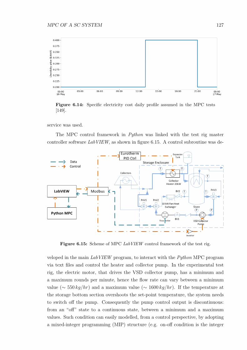
MPC OF A SC SYSTEM 127
Figure 6.14: Specific electricity cost daily profile assumed in the MPC tests[149].
service was used.
The MPC control framework in Python was linked with the test rig mastercontroller software LabVIEW, as shown in figure 6.15. A control subroutine was de-
Figure 6.15: Scheme of MPC LabVIEW control framework of the test rig.
veloped in the main LabVIEW program, to interact with the Python MPC programvia text files and control the heater and collector pump. In the experimental testrig, the electric motor, that drives the VSD collector pump, has a minimum anda maximum rounds per minute, hence the flow rate can vary between a minimumvalue (∼ 550 kg/hr) and a maximum value (∼ 1600 kg/hr). If the temperature atthe storage bottom section overshoots the set-point temperature, the system needsto switch off the pump. Consequently the pump control output is discontinuous:from an “off” state to a continuous state, between a minimum and a maximumvalues. Such condition can easily modelled, from a control perspective, by adoptinga mixed-integer programming (MIP) structure (e.g. on-off condition is the integer

MPC OF A SC SYSTEM 128
state and the values between a minimum and a maximum are the continuous states).In addition, the non-linearity of the optimal control problem yields a MINLP op-timisation problem. Such type of optimisation problems is quite computationallyexpensive, and appropriate solver are needed. For this reason the control problemwas simplified and solved as follows:
1. The decision to turn on or off the pump and the heater was implemented in aLabVIEW subroutine, based on the temperature signal at the storage bottomsection – if the storage bottom temperature overshoots the set point, then thepump and heater are switched off, otherwise are switched on.
2. During the heater and pump operation, LabVIEW interacts with the PythonMPC program to control the flow and heater power. For the sake of reducingthe control variables, the heater temperature control set-point was set to avery high value, hence only the heater power ratio was controlled.
The above MPC framework was then tested in the experimental rig. The resultsare reported and analysed in the next section. The solution of the optimal controlproblem in Python for an horizon took approximately 2 s on a common desktop PC,hence the developed MPC framework was easily integrated as a controller of thedynamics of the test rig.
6.4 Experimental and Numerical Results
This section describes, analyses and compares the experimental results of testsusing MPC with those using RBC. Firstly a preliminary test was carried out andanalysed to check the proper operation of the predictive control structure. Figure6.16 shows a preliminary test carried out in May 2017. The top chart in the figureshows the temperatures at the top, middle and bottom sections of the store andthe predicted temperatures – during the first time step of every optimal controltrajectory – for the bottom section. The second chart, from the figure top, depictsthe control inputs data as well as the control signals from the MPC framework (e.g.“flow ctrl mpc”). The bottom chart shows the test environment temperature andthe one provided by the forecast data.
At the beginning of the test the MPC control strategy provides control inputs(dotted points in the middle plot) to heat up the store. When the storage bottomtemperature set point was achieved, the control structure switches the pump andheater off. Thus the MPC program is not called and does not perform its internaloptimisation calculation. The control strategy calls the MPC routine again when

MPC OF A SC SYSTEM 129
Figure 6.16: Results of a preliminary MPC test with the heater and store rig.Ttop,mind,bot is the top, middle and bottom storage temperature; Tbot,predicted is thepredicted temperature by the MPC routine; flow is the measured experimentalflow rate; htr ratio is the measured experimental heater power ratio; flow ctrl mpcand htr ctrl mpc are the control inputs given by the MPC routine to the rig forflow rate and heater power ratio; Tenv is the measured experimental environmentaltemperature while Tenv,forecast is the environmental temperature supplied by theforecast.
the storage temperature drops below the set point due to thermal losses to theenvironment.
The first observation from figure 6.16 is about the mismatch between controlinputs from MPC framework and measured controls. In the case of the flow rate,the mismatch is mainly due to the fact that in the MPC structure the flow isconstrained between 0 and 1600 kg/hr, whilst the pump can deliver a flow ratebetween 550 and 1600 kg/hr, as mentioned above. For this reason, when a flowrate control input below is the minimum flow, LabVIEW sets the pump at theminimum flow. Other than that difference, the flow control inputs and measureddata match. The only other mismatch in flow values is just before noon, where anissue in the communication between LabVIEW and Python most likely occurred.The heater power ratio negative peaks between 1100 and 1200 hr are an evidence ofsuch communications problems. On the other hand, the mismatch between heaterpower ratio control inputs and measured data is far more evident. This is due tothe fact that the heater power settings in the rig are limited by the flow for safetyreasons (as mentioned in section 5.1.3). In practice the heater ratio can assume the

MPC OF A SC SYSTEM 130
following values, depending on the flow:
rhtr =
≤ 0.85 m ≥ 1500 kg/hr
≤ 1 1000 ≤ m < 1500 kg/hr
≤ 0.18 m < 1000 kg/hr
(6.16)
Inclusion of such limitations in the MPC formulation is quite complex, hence werenot modelled.
Although the discrepancy between MPC control inputs and measured controlvalues, the controller is able to predict, in the short term, the storage bottom sec-tion temperature with good accuracy: the coefficient of determination between thepredicted values and the corresponded measured values is 0.987.
After the preliminary MPC tests, a series of tests were carried on to comparethe performance of MPC and RBC frameworks. The tests were run in consecutivedays with similar weather conditions. The results of one of these tests are illustratedin figure 6.17. In the RBC test, negative peaks, caused by communication problems
Figure 6.17: Comparison of system states and control inputs for a MPC andRBC tests, during two consecutive days with similar weather conditions.
between LabVIEW and rig instrumentation, appear in the first hour. In the MPCdata, at the beginning of the test the flow is set to the minimum, but no heater

MPC OF A SC SYSTEM 131
power is applied. Such behaviour is due to incorrect exchange of control inputsbetween Python MPC program and the LabVIEW program or LabVIEW failure inapplication of the control settings received from Python MPC program. Despitesuch issues, both control tests were successful and the results can be compared forperformance analysis.
The first difference between MPC and RBC tests is in the control input sequence:MPC strategy has variable flow inputs. In the MPC test, the pump and heaterare activated more often than during RBC ones. The RBC strategy achieves thebottom set point temperature of 170 ◦C earlier than MPC one. For this reason thecost function is higher for MPC test (see figure 6.18).
Figure 6.18 shows the evolution of the cost function, electricity price and tem-perature cost terms for the MPC and RBC controlled system tests. As mentioned
Figure 6.18: Comparison of cost function, electricity price cost and temperaturecost for a MPC and RBC tests, during two consecutive days with similar weatherconditions.
earlier in the section, the cost function is the true figure that can compare the per-formance of the two strategies. In term of the overall cost function the RBC strategyperforms better than MPC one. This result derived from the temperature cost termof the cost function as seen in the bottom chart of the figure. In fact, MPC strategyis successful in reducing the electricity cost term (middle plot of the figure) butpenalises the temperature cost term. Such outcome is the consequence of the modellimitation: the power setting limitations due to flow conditions are not included inthe MPC model. Hence the system cannot run the heater at 100 % power settingin the first charging phase of the test. Therefore for every instant that the systemdoes not match the set point temperature the cost function increases further and
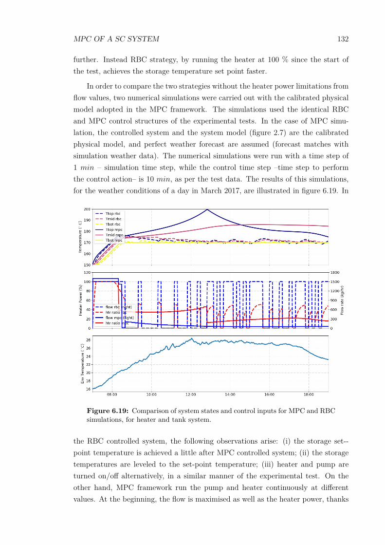
MPC OF A SC SYSTEM 132
further. Instead RBC strategy, by running the heater at 100 % since the start ofthe test, achieves the storage temperature set point faster.
In order to compare the two strategies without the heater power limitations fromflow values, two numerical simulations were carried out with the calibrated physicalmodel adopted in the MPC framework. The simulations used the identical RBCand MPC control structures of the experimental tests. In the case of MPC simu-lation, the controlled system and the system model (figure 2.7) are the calibratedphysical model, and perfect weather forecast are assumed (forecast matches withsimulation weather data). The numerical simulations were run with a time step of1 min – simulation time step, while the control time step –time step to performthe control action– is 10 min, as per the test data. The results of this simulations,for the weather conditions of a day in March 2017, are illustrated in figure 6.19. In
Figure 6.19: Comparison of system states and control inputs for MPC and RBCsimulations, for heater and tank system.
the RBC controlled system, the following observations arise: (i) the storage set--point temperature is achieved a little after MPC controlled system; (ii) the storagetemperatures are leveled to the set-point temperature; (iii) heater and pump areturned on/off alternatively, in a similar manner of the experimental test. On theother hand, MPC framework run the pump and heater continuously at differentvalues. At the beginning, the flow is maximised as well as the heater power, thanks

MPC OF A SC SYSTEM 133
to no limit in heater settings for flow conditions. When the storage bottom tem-perature achieves the set-point, the heater power ratio and flow are reduced. Thetemperature of the storage top section is increased till approximately 1300 hr, whenthe cost of electricity increases (figure 6.14). Hence the heater settings are droppedbelow 20 %, and the storage top temperature decreases, due to thermal losses to theenvironment and to the other sections.
A comparison of the cost function for both strategies reveals that MPC frame-work performs better than RBC one. The superior performance of the MPC frame-work is because the controller is able to maximise heater power at the beginning ofthe simulation, to achieve the bottom set-point temperature faster than RBC sys-tem. In fact in the numerical simulations the heater power setting is not limited byflow condition, like in the test rig. This result stresses the importance of accuracyin implementation of all the control limitations and details.
The next section investigates the MPC control framework with solar heatingsource as an extra degree of freedom for the system.
6.5 MPC with Solar and Backup Heating Sources
In this section the formulation and the results of an experimental MPC frame-work for a system with both solar and backup heating sources are reported. Bothauxiliary and solar sources were simulated based on three different weather scenar-ios: a sunny day, a day with an overcast afternoon and cloudy day. In order to testsuch system, some specific constraints were adopted as illustrated below.
6.5.1 MPC formulation
The developed MPC framework is designed for the system depicted in figure6.20. In such configuration the electric heater and solar sources are arranged inseries. From the practical point of view both the heating sources were simulated bythe 20 kW electrical heater.
The formulation of the MPC framework is similar to the one described in section6.3.2. The differences are as follows:
• The flow rate is fixed to 1500 kg/hr. Hence the only control input is the heaterpower ratio.
• The objective of the control strategy is to achieve the set-point temperature of175 ◦C at the storage bottom section at the end of the test, while minimising

MPC OF A SC SYSTEM 134
Figure 6.20: Scheme of the MPC controlled rig for simulation tests of solar andbackup heating sources.
the cost of electricity. In mathematical language, the cost function is expressedas follows:
minu0,...,uN−1
J =[wtemp(Tbot,N−1 − TSP )
2 +N−1∑k=0
welC2el,k
](6.17)
• The following constraints for simulated heater and solar sources are includedin the optimal control formulation:
Qhtr + Qsolar ≤ Qmax Qmax = 20000W (6.18)
• The solar contribution is calculated from an ideal collector field with constantefficiency (not depending on the collector temperature). The collector size waschosen such that during the sunny period the system run predominately onsolar and with a power output not higher than 10 kW .
• The heater section model was modified to fit the solar contribution in theenergy balance equation:
CaphtrdTm,htr
dt= m cp(Tin,htr − Tout,htr) + UAhtr(Tenv − Tm,htr) + Qhtr + Qsolar
(6.19)
where the heater ratio control input to be applied in the test rig is calculated

MPC OF A SC SYSTEM 135
as follows:
rhtr =Qhtr + Qsolar
Qmax
(6.20)
The weather scenarios of the tests are illustrated in figure 6.21.
Figure 6.21: Solar radiation profile for three different scenarios: sunny day,overcast afternoon and low irradiance day.
6.5.2 Results of the Experiments
The first test results are for a sunny day scenario, as showed in figure 6.22. Thesystem is continuously controlled by the MPC Python program till the temperatureat the storage bottom section reaches the set-point. Hence the master control inLabVIEW turns the heater and pump off (condition of zero flow and power in thefigure). When the store cools down due to thermal losses to the environment, thecontroller calls the MPC routine again and switches the heater and pump back on.Despite initial issues and communication drops (e.g. negative drops in measuredheater power), the test was successful and the system achieved the objective storageset-point temperature: the bottom chart shows the system is heated up mainlyby the simulated solar source. Further, as shown in the bottom plot, the heatercontribution is mainly given in the first half of the test (∼ 0.5 kW ). Instead whenelectricity prices increase in the second half, the controller does not run the backupheater.
MPC controller ability in achieving the objectives – i) temperature set point inthe storage bottom section, ii) use solar to supply heat to the store, iii) reduce thebackup heater electricity cost – is more evident in the second test, which was carriedon during a overcast day. The results are depicted in figure 6.23. Although the storeis charged predominately by the backup heater, with minimal contribution of solar,the predictive control minimises the cost of electricity by reducing heater usage in

MPC OF A SC SYSTEM 136
Figure 6.22: Experimental test results of MPC control with simulated solar andbackup heating sources for a sunny day scenario.
Figure 6.23: Experimental test results of MPC control with simulated solar andbackup heating sources for a overcast day scenario.

MPC OF A SC SYSTEM 137
the second half of the test. In the morning the backup heater power is around 10 kWuntill 1400 hr, when it dropped to minimum values due to higher electricity costs.The MPC controller in fact takes full advantage of the predicted cost of electricity,by applying a higher heater power setting in the morning to achieve the temperatureset point and a lower power in the afternoon, to keep the storage temperature atthe set point. Hence the cost to achieve the set storage temperature is minimised.
In a similar manner, in the last test – overcast afternoon scenario – MPC achievesthe objectives of minimising the cost of electricity while achieving the storage tem-perature set point. In this case, the predictive controller makes the most out of solarheat, given its knowledge of future low solar irradiance. These results are showed infigure 6.24. The controller utilises solar and backup heat in the morning to increase
Figure 6.24: Experimental test results of MPC control with simulated solar andbackup heating sources for an overcast afternoon scenario.
the temperature of the store, as shown in the bottom part of the figure. In theafternoon the electricity price is higher, hence the backup heater power is reduced.
It is pretty clear that a priori knowledge of solar irradiance allows the MPCframework to maximise the solar collection over the day and achieve the storagetemperature set point while minimising the daily cost of electricity.

MPC OF A SC SYSTEM 138
6.6 Chapter Summary
This chapter presented applications of MPC on:
1. A solar cooling system, by means of numerical simulations.2. Experimental test rig with an electrical heater and a storage unit, as well as
numerical model with equal system.3. Experimental test rig with simulated solar and backup heating sources.
Numerical simulations of MPC applied to a medium-temperature high-efficiencysolar cooling system showed better performance respect to RBC controlled system,by delivering heat to the load via store and backup heater simultaneously and byexploiting stored heat across days with low solar irradiance.
Experimental tests with heater and store subsystem showed how complex isthe implementation of a predictive control strategy in a real system, where controlinputs are highly constrained. In fact RBC outperformed MPC controlled systemdue to a modelling limitation. Further numerical simulations of such system withno limitation in control details demonstrated superior performance of the MPCstrategy.
Lastly MPC tests with solar contribution under three different scenario, estab-lished the ability of the predictive control logic to profit from forecast data on solarirradiance and electricity price, by maximising solar usage while achieving storagetemperature set point, and ,at the same time, minimising cost of electricity fromthe backup heater.
In conclusion despite the complexity of implementation, the results showed MPCcontroller is able to provide system performance benefit by taking advantage of theforecast data. Nevertheless careful consideration should be given to MPC modelcontrol details in order to yield superior performance respect to RBC framework.

Chapter 7
Conclusions
7.1 Outputs and Findings
This thesis illustrates application of thermal energy storage to medium-temperaturehigh-efficiency solar cooling systems with double and triple effect absorption chillers.Particular focus was given to novel thermal energy storage devices based on latentheat materials (PCM) and an advanced control strategy, namely Model PredictiveControl.
Water was found as the most used storage media in low temperature systemwith single effect absorption chillers. There are only a few examples of plants withdouble effect absorption chillers employing water and thermal oil as storage material.Besides water and thermal oil, other sensible heat materials, such concrete andasphalt were identified as potential low cost thermal storage media.
Latent heat materials were reported based on temperature requirements fordouble and triple effect absorption chiller based systems. Other than phase changetemperature, heat transfer properties such as thermal conductivity, and volumetricenergy density were identified as parameters for selection of an appropriate latentheat material. Though cost is among the selection criteria, comprehensive mate-rial information are not available in the literature. Among latent heat materials,Hydroquinone and D-mannitol, due to their high energy density, were investigatedand tested as potential phase change materials for delivering heat to double effectchiller systems. Currently no application of PCM to triple effect chiller systems havebeen reported. Therefore potential candidates for such systems were selected fromavailable chemical databases and journal articles. Metals and metal alloys (e.g. Al-Sn) show high potential thanks to their high heat transfer properties (e.g. thermalconductivity). On the other hand, salts (e.g. solar salt) have higher energy densityand likely have cost values of lower order of magnitude.
139

CHAPTER 7. CONCLUSIONS 140
Different designs for hot water storage tanks with and without heat exchangerare used in the literature. Methods to achieve and retain thermal stratificationwithin the storage device are illustrated. Among those, diameter-to-height ratio,location of inlet and outlet pipes and mass flow rate are important parameters whendesigning stratification based storage tanks. The design of latent heat thermalstorage systems use a packed bed or shell-and-tube configuration. However there isonly limited design experience for latent heat stores in solar cooling applications,with the majority of literature in latent heat system designs pertaining to coldstorage at low temperature.
Thermo-chemical energy storage materials and systems have the highest volu-metric energy density, hence the potential to reduce storage cost. Nevertheless theyare predominately in the research and development phase. Literature examples ofsuch thermal energy storage technology are very limited for solar air conditioningplants.
Review of conventional control strategy and operation of solar cooling plantreveals that simple on-off control with temperature dead band are the most commoncontroller. More complex closed loop controllers with feedback (e.g. PID controller)are used in the collector loop to achieve a constant outlet temperature in the solarfield. Besides conventional controls, advanced “look-ahead” controllers are reportedas a promising technique in controlling solar cooling systems. Among those, ModelPredictive Control has been studied in low temperature solar thermal systems (e.g.SDHW) and concentrated solar power plants. Due to its knowledge of solar and loadforecast, MPC can yield substantial benefits respect to classical control approaches.While some examples of different implementations of MPC strategies are reported,no detailed comparison of performance respect to classic controls is found. Further,the role of thermal storage and details of motivation behind the predictive controltrajectories are not fully explained in the literature examples.
Dynamical simulations tools (e.g. TRNSYS) have been widely adopted in theliterature to optimise the design of the thermal energy storage in solar cooling sys-tems, based on specific information of plant and meteorological data. The widerange of applications and differences in optimisation objectives, did not result in aconsistent sizing “Rule of Thumb”. Moreover, detailed comparison methodologieswhile analysing sensible and latent heat storage system for solar air-conditioningplants are not reported in the reviewed literature.
Based on the literature review a methodology to analyse and compare the ther-mal performance of sensible and latent thermal energy storage systems was devel-oped and presented. Firstly a detailed model to predict and capture the physicalbehaviour of a latent storage system with phase change materials was developed

CHAPTER 7. CONCLUSIONS 141
and validated against experimental data. Such model reflects a shell-and-tube de-sign with PCM encapsulated inside the tubes, while the heat transfer fluid flowsin the shell. This configuration can easily integrated in existing systems due toits four ports that allow simultaneous charging and discharging. The thermal per-formance of the storage device is evaluated by integrating it into a complete solarcooling plant and simulating the plant response over a year. Hence a set of relevantstorage and plant figures of merit were used to evaluate the thermal performance.The analysis was carried on for two load scenarios and four storage materials – twosensible and two latent heat materials. Such methodology can be applied to othersolar thermal system with thermal energy storage. The results show that, althoughlatent heat storage have the highest storage efficiency due to limited thermal losses,the respective plant performance are lower than sensible heat based system. Themain reason behind such outcome is the poorer collector thermal performance in thecase of latent heat based systems. In fact, due to the phase change requirements,the collector field operates at higher temperature than conventional storage mate-rial systems. Also the bottom of the tank for sensible storage cases is cooler thanthe latent heat storage cases resulting in higher collector yield for sensible storagesystems. Among the latent heat storage options, solar salt based systems performedmarginally better at higher storage volumes than Al-Sn alloy. The latter due to itshigh heat transfer properties, and higher phase change temperature keeps the storeat higher temperature. Therefore the collector field operates at high temperaturewith poor thermal efficiency. Sensible materials, due to their heat discharge capa-bility at lower temperatures provided even higher solar fraction than latent heatstorage cases, under the variable load scenario.
An experimental test rig facility has been build, consisting of east-west trackingmicro-concentrator collectors, 1500 L storage system with internal coil oil-to-waterheat exchanger, auxiliary electric heaters, double effect absorption chiller, pipes,valves and pumps. The solar cooling test rig is meant for model calibration andcontrol strategy experiments. Thermal characterisation of plant components re-vealed non optimal collector thermal performance, high heat losses in the pipingsystem and fluid handling unit, as well as issues in operation of the double effectabsorption chiller. In order to simulate the heat absorption from the hot side of thechiller, a water-to-air fan heat exchanger was installed.
A complete solar cooling test with constant load and simulated cooling wascarried out, proving the rig is able to operate in a real-like scenario. In spite of that,the control system of the plant is partially manual and complete fully automaticcontrol experiments are not possible at the present stage. In order to carry outcontrol strategy experimental activity, a subsystem, composed by the collector side

CHAPTER 7. CONCLUSIONS 142
electric heater and the store, was used. Rule based control strategy tests weresuccessfully carried on by charging the tank to a set-point temperature and maintainit.
A numerical physics based model was developed to carry out numerical sim-ulations with Rule Based Control and Model Predictive Control strategies. Theresults show how the predictive controller is able to achieve lower backup heaterusage by unlocking new system capabilities (e.g. chiller heat delivering with bothstorage and heater systems), and by smart dispatch of the thermal energy stored inthe tank. The benefits were observed particularly in days with low solar coverage.Despite minimising the backup heater usage, the MPC control trajectory resultedis non maximum heat collection. The latter is due to optimal control and objectivefunction formulations. Such result shows the complexity in implementing effectiveMPC control strategies and stresses the importance of properly tuned the objectivesof the optimal control problem.
In order to calibrate the MPC system model, extensive characterisation of thethermal storage system, pipes and heater was carried out. Testing of the developedMPC strategy revealed issues in interfacing the programmed controller with theexisting test rig data acquisition and control system. Nevertheless successful testswere carried out and the results show how the predictive controller is able to achievea storage set-point temperature and maintaining it by running the pump at differentflow rates and the electrical heater in partial power settings.
Comparison of experiments with RBC and MPC strategies shows that con-ventional controller outperforms the predictive controller. The advanced controlstrategy does not include heater power limitations with flow conditions. There-fore a numerical simulation with perfect forecast was carried out to analyse MPCcontrolled system performance without modelling limitations. As expected the nu-merical results showed that MPC framework outperformed RBC controlled system.Lastly MPC controlled system experiments with simulation of both solar and electricheat sources were carried out for three weather profiles. The results demonstratethe ability of the predictive controller to reduce the cost of electricity by takingmaximum advantage of solar availability and period of low electricity cost.
7.2 Recommendations and Future Work
Literature, examples and methodology for thermal storage application to medium-temperature high-efficiency solar cooling systems are quite scarce. There is a gap inphase change materials for application within the temperature range of 200 to 300

CHAPTER 7. CONCLUSIONS 143
◦C. Research and development of latent heat materials with good thermal and heattransfer characteristics need to be carried on.
Though a detailed methodology for comparing sensible and latent heat stor-age systems was developed, some of the assumptions required simplification (e.g.calculation of storage energy for latent system assumed only latent heat, while inreality due to load requirements the sensible heat may not be negligible). Besidesthe methodology to compare the thermal performance, a detailed methodology forcomparing economic figures of merit of such storage application need to be devel-oped. Some of the issues of such analysis might be estimation of some costs (e.g.cost of a pressurised piping system).
Numerical simulations that compared latent and sensible heat material applica-tion on a solar cooling plant showed poorer performance of phase change materialsfor their higher temperature requirements. Perhaps a latent heat materials withphase change temperature aligned with mean operating temperature requirementsrather than the peak operating temperature requirements of the chiller could improvethe performance of the latent heat based storage system. With regard developmentand implementation of predictive control strategies, the work revealed the complex-ity of the look ahead controllers. Such complexities are related to the formulationand solution of the optimal control problem, and the practical implementation. Forexample, more work need to be done on reducing the computational time of thesolution of the optimal control problem. This can be achieved by changing theformulation of the optimal control problem, or by adopting a different solver (i.e.non-linear interior point solver).
The chosen MPC formulation revealed poorer experimental performance respectto conventional controls. A different formulation and inclusion of rig control con-straints might help in improving the outcome of the predictive controller.

Bibliography
[1] IEA, World Energy Outlook 2016, ser. World Energy Outlook. IEA, 2016.doi: 10.1787/weo-2016-en.
[2] R. M. Lazzarin, “Solar cooling: PV or thermal? A thermodynamic and eco-nomical analysis,” International Journal of Refrigeration, vol. 39, pp. 38–47,2014. doi: 10.1016/j.ijrefrig.2013.05.012.
[3] A. Preisler, “Appendix 1 to IEA SHC Task 38 report D-A5: ”List of existingsmall scale solar heating and cooling plants”,” IEA SHC, Tech. Rep., 2009.
[4] B. M. Becker, M. Helm, and C. Schweigler, “Collection of selected systemsschemes “ Generic Systems ”, IEA SHC Task 38 Report A2,” IEA SHC, Tech.Rep., 2009.
[5] L. F. Cabeza, C. Sole, A. Castell, E. Oró, and A. Gil, “Review of SolarThermal Storage Techniques and Associated Heat Transfer Technologies,”Proceedings of the IEEE, vol. 100, no. 2, pp. 525–538, 2012. doi: 10.1109/JPROC.2011.2157883.
[6] V. Basecq, G. Michaux, C. Inard, and P. Blondeau, “Short-term storagesystems of thermal energy for buildings: a review,” Advances in BuildingEnergy Research, vol. 7, no. 1, pp. 66–119, 2013. doi: 10.1080/17512549.2013.809271.
[7] M. Balghouthi, M. Chahbani, and A. Guizani, “Investigation of a solar cool-ing installation in Tunisia,” Applied Energy, vol. 98, pp. 138–148, 2012. doi:10.1016/j.apenergy.2012.03.017.
[8] F. Agyenim, P. Eames, and M. Smyth, “A comparison of heat transfer en-hancement in a medium temperature thermal energy storage heat exchangerusing fins,” Solar Energy, vol. 83, no. 9, ISES 2007, Ed., pp. 1509–1520, 2009.doi: 10.1016/j.solener.2009.04.007.
[9] L. F. Cabeza, M. Ibáñez, C. Solé, J. Roca, and M. Nogués, “Experimentationwith a water tank including a PCM module,” Solar Energy Materials and
144

BIBLIOGRAPHY 145
Solar Cells, vol. 90, no. 9, pp. 1273–1282, 2006. doi: 10.1016/j.solmat.2005.08.002.
[10] A. Gil, M. Medrano, I. Martorell, A. Lázaro, P. Dolado, B. Zalba, and L. F.Cabeza, “State of the art on high temperature thermal energy storage forpower generation. Part 1—Concepts, materials and modellization,” Renew-able and Sustainable Energy Reviews, vol. 14, no. 1, pp. 31–55, 2010. doi:10.1016/j.rser.2009.07.035.
[11] S. Furbo, E. Andersen, J. Fan, Z. Chen, and B. Perers, “Thermal performanceof marketed SDHW systems under laboratory conditions,” in Eurosun 2012,Croatia, 2012.
[12] P. Menchinelli and A. Bemporad, “Hybrid Model Predictive Control of aSolar Air Conditioning Plant,” European Journal of Control, vol. 14, no. 6,pp. 501–515, 2008. doi: 10.3166/ejc.14.501-515.
[13] M. Bunea, C. Hildbrand, A. Duret, S. Eicher, L. Péclat, and S. Citherlet,“Analysis of a Medium Temperature Solar Thermal Installation with HeatStorage for Industrial Applications,” Energy Procedia, vol. 91, pp. 601–610,2016. doi: 10.1016/j.egypro.2016.06.211.
[14] K. M. Powell, J. D. Hedengren, and T. F. Edgar, “Dynamic optimization ofa solar thermal energy storage system over a 24 hour period using weatherforecasts,” in 2013 American Control Conference, IEEE, 2013, pp. 2946–2951.doi: 10.1109/ACC.2013.6580282.
[15] B. W. Sparber, A. Napolitano, G. Eckert, and A. Preisler, “State of the arton existing solar heating and cooling systems, IEA SHC Task 38 Subtask Breport B1,” IEA SHC Task 38, Tech. Rep., 2009.
[16] P. Pinel, C. a. Cruickshank, I. Beausoleil-Morrison, and A. Wills, “A review ofavailable methods for seasonal storage of solar thermal energy in residentialapplications,” Renewable and Sustainable Energy Reviews, vol. 15, no. 7,pp. 3341–3359, 2011. doi: 10.1016/j.rser.2011.04.013.
[17] I. Dincer and M. Rosen, Thermal Energy Storage: Systems and Applications,2nd Edition. Wiley, 2011.
[18] Berndt Wischnewski, Water/Steam Properties, 2013.
[19] Http://everylittledrop.com.au, The Cost of Water, 2014.
[20] D. Fernandes, F. Pitié, G. Cáceres, and J. Baeyens, “Thermal energy stor-age: “How previous findings determine current research priorities”,” Energy,vol. 39, no. 1, pp. 246–257, 2012. doi: 10.1016/j.energy.2012.01.024.
[21] Graphite (C) - Classifications, Properties and Applications of Graphite.

BIBLIOGRAPHY 146
[22] Polycrystalline Graphite - Thermal Conductivity - NETZSCH Analyzing &Testing.
[23] Solutia Inc., Therminol 55, 2013.
[24] D. C. Corporation, Dowtherm - Synthetic Organic Fluids, 2017.
[25] Y. Tian and C. Zhao, “A review of solar collectors and thermal energy storagein solar thermal applications,” Applied Energy, vol. 104, pp. 538–553, 2013.doi: 10.1016/j.apenergy.2012.11.051.
[26] D. Laing, W.-D. Steinmann, R. Tamme, and C. Richter, “Solid media thermalstorage for parabolic trough power plants,” Solar Energy, vol. 80, no. 10,pp. 1283–1289, 2006. doi: 10.1016/j.solener.2006.06.003.
[27] P. S. I. Gmbh, “Survey of Thermal Storage for Parabolic Trough PowerPlants, NREL/SR-550-27925,” NREL, Tech. Rep. September, 2000, p. 61.
[28] P. Tatsidjodoung, N. Le Pierrès, and L. Luo, “A review of potential materialsfor thermal energy storage in building applications,” Renewable and Sustain-able Energy Reviews, vol. 18, pp. 327–349, 2013. doi: 10.1016/j.rser.2012.10.025.
[29] A. Sharma, V. Tyagi, C. Chen, and D. Buddhi, “Review on thermal energystorage with phase change materials and applications,” Renewable and Sus-tainable Energy Reviews, vol. 13, no. 2, pp. 318–345, 2009. doi: 10.1016/j.rser.2007.10.005.
[30] F. Graeter and J. Rheinländer, “Thermische Energiespeicherung mit Phasen-wechsel im Bereich von 150 bis 400 °C,” in Proc. ForschungsVerbund Sonnenen-ergie Workshop Wärmespeicherung, Cologne, Germany, 2001.
[31] W. Streicher, L. F. Cabeza, and A. Heinz, “Inventory of Phase Change Ma-terials ( PCM ) Report C2 of Subtask C,” IEA SHC Task 32, Tech. Rep.February, 2005, p. 33.
[32] H. Sugo, E. Kisi, and D. Cuskelly, “Miscibility gap alloys with inverse mi-crostructures and high thermal conductivity for high energy density ther-mal storage applications,” Applied Thermal Engineering, vol. 51, no. 1-2,pp. 1345–1350, 2013. doi: 10.1016/j.applthermaleng.2012.11.029.
[33] A. Gil, E. Oró, G. Peiró, S. Álvarez, and L. F. Cabeza, “Material selectionand testing for thermal energy storage in solar cooling,” Renewable Energy,vol. 57, pp. 366–371, 2013. doi: 10.1016/j.renene.2013.02.008.
[34] S. D. Sharma and K. Sagara, “Latent Heat Storage Materials and Systems: AReview,” International Journal of Green Energy, vol. 2, no. September 2013,pp. 1–56, 2005. doi: 10.1081/GE-200051299.
BIBLIOGRAPHY 147
[35] M. Kenisarin and K. Mahkamov, “Solar energy storage using phase changematerials,” Renewable and Sustainable Energy Reviews, vol. 11, no. 9, pp. 1913–1965, 2007. doi: 10.1016/j.rser.2006.05.005.
[36] CRC, Handbook of Chemistry & Physics Online.
[37] Sigma-Aldrich.
[38] S. Pincemin, R. Olives, X. Py, and M. Christ, “Highly conductive compositesmade of phase change materials and graphite for thermal storage,” SolarEnergy Materials and Solar Cells, vol. 92, no. 6, pp. 603–613, 2008. doi:10.1016/j.solmat.2007.11.010.
[39] M. M. Kenisarin, “High-temperature phase change materials for thermal en-ergy storage,” Renewable and Sustainable Energy Reviews, vol. 14, no. 3,pp. 955–970, 2010. doi: 10.1016/j.rser.2009.11.011.
[40] Http://www.infomine.com, Tin prices, 2014.
[41] Y. Kato, “Chemical energy conversion technologies for efficient energy use,”in In: Paksoy HO (ed.) NATO Sciences Series, II. Mathematics, Physics andChemistry, Vol. 234 : Thermal Energy Storage for Sustainable Energy Con-sumption: Fundamentals, Case Studies and Design, pp. 377–391. Dordrecht:Springer. 2007.
[42] A. H. Abedin, “A Critical Review of Thermochemical Energy Storage Sys-tems,” The Open Renewable Energy Journal, vol. 4, no. 1, pp. 42–46, 2011.doi: 10.2174/1876387101004010042.
[43] C. Bales, P. Gantenbein, D. Jaenig, H. Kerskes, K. Summer, M. Van Es-sen, and R. Weber, “Laboratory Tests of Chemical Reactions and PrototypeSorption Storage Units, IEA SHC Task 32 Subtask B report B4,” IEA SHC,Tech. Rep., 2008, 55p.
[44] V. van Essen, L. Bleijendaal, B. Kikkert, H. Zondag, M. Bakker, and P. Bach,“Development of a compact heat storage system based on salt hydrates,” inPresented at the International Conference on Solar Heating, Cooling andBuildings 28 September – 1 October 2010, Graz, Austria, 2010.
[45] F. Bertsch, B. Mette, S. Asenbeck, H. Kerskes, and H. Müller-Steinhagen,“Low temperature chemical heat storage – an investigation of hydration re-actions,” in In proceeding of: Effstock 2009, 2009.
[46] S. Kuravi, J. Trahan, D. Y. Goswami, M. M. Rahman, and E. K. Stefanakos,“Thermal energy storage technologies and systems for concentrating solarpower plants,” Progress in Energy and Combustion Science, vol. 39, no. 4,pp. 285–319, 2013. doi: 10.1016/j.pecs.2013.02.001.

BIBLIOGRAPHY 148
[47] M. Medrano, A. Gil, I. Martorell, X. Potau, and L. F. Cabeza, “State of theart on high-temperature thermal energy storage for power generation. Part2—Case studies,” Renewable and Sustainable Energy Reviews, vol. 14, no. 1,pp. 56–72, 2010. doi: 10.1016/j.rser.2009.07.036.
[48] S. M. Flueckiger, Z. Yang, and S. V. Garimella, “Review of Molten-Salt Ther-mocline Tank Modeling for Solar Thermal Energy Storage,” Heat TransferEngineering, vol. 34, no. 10, pp. 787–800, 2013. doi: 10.1080/01457632.2012.746152.
[49] G. Rosengarten, G. Morrison, and M. Behnia, “A Second Law Approach toCharacterising Thermally Stratified Hot Water Storage With Application toSolar Water Heaters,” Journal of Solar Energy Engineering, vol. 121, no. 4,p. 194, 1999. doi: 10.1115/1.2888166.
[50] M. A. Rosen, R. Tang, and I. Dincer, “Effect of stratification on energyand exergy capacities in thermal storage systems,” International Journal ofEnergy Research, vol. 28, no. 2, pp. 177–193, 2004. doi: 10.1002/er.960.
[51] Y. Han, R. Wang, and Y. Dai, “Thermal stratification within the water tank,”Renewable and Sustainable Energy Reviews, vol. 13, no. 5, pp. 1014–1026,2009. doi: 10.1016/j.rser.2008.03.001.
[52] W. Streicher and C. Bales, “Combistores,” in Thermal Energy Storage forSolar and Low Energy Buildings, J.-c. Hadorn, Ed., Spain: Universitat deLleida, 2005, ch. 5, pp. 29–40.
[53] S. Ievers and W. Lin, “Numerical simulation of three-dimensional flow dy-namics in a hot water storage tank,” Applied Energy, vol. 86, no. 12, pp. 2604–2614, 2009. doi: 10.1016/j.apenergy.2009.04.010.
[54] A. Al-Marafie, S. M. Moustafa, and A. Al-Kandarie, “Factors Affecting StaticStratification of Thermal Water Storage,” Energy Sources, vol. 11, no. 3,pp. 183–199, 1989. doi: 10.1080/00908318908908953.
[55] R. Spur, D. Fiala, D. Nevrala, and D. Probert, “Performances of moderndomestic hot-water stores,” Applied Energy, vol. 83, no. 8, pp. 893–910, 2006.doi: 10.1016/j.apenergy.2005.10.001.
[56] Z. Youssef, A. Delahaye, L. Huang, F. Trinquet, L. Fournaison, C. Pollerberg,and C. Doetsch, “State of the art on phase change material slurries,” EnergyConversion and Management, vol. 65, pp. 120–132, 2013. doi: 10.1016/j.enconman.2012.07.004.
[57] H. Mehling and L. F. Cabeza, Heat and cold storage with PCM, D. Mewes andF. Mayinger, Eds., ser. Heat and Mass Transfer. Berlin, Heidelberg: SpringerBerlin Heidelberg, 2008. doi: 10.1007/978-3-540-68557-9.
BIBLIOGRAPHY 149
[58] A. Gil, C. Barreneche, P. Moreno, C. Solé, A. Inés Fernández, and L. F.Cabeza, “Thermal behaviour of d-mannitol when used as PCM: Comparisonof results obtained by DSC and in a thermal energy storage unit at pilotplant scale,” Applied Energy, vol. 111, pp. 1107–1113, 2013. doi: 10.1016/j.apenergy.2013.04.081.
[59] N. Shamsundar and R. Srinivasan, “Analysis of energy storage by phasechange with an array of cylindrical tubes,” In: Thermal storage and heattransfer in solar energy systems; Proceedings of the Winter Annual Meeting,San Francisco, Calif., December 10-15, 1978. (A79-26201 09-44) New York,American Society of Mechanical Engineers, 1978, p. 35-40, pp. 35–40, 1978.
[60] S. Saxena, “A preliminary model for phase change thermal energy storage ina shell and tube heat exchanger,” Solar energy, vol. 29, no. 3, pp. 257–263,1982.
[61] M. Lacroix, “Numerical simulation of a shell-and-tube latent heat thermalenergy storage unit,” Solar energy, vol. 50, no. 4, pp. 357–367, 1993.
[62] Z.-X. Gong, “Finite-element analysis of cyclic heat transfer in a shell-and-tube latent heat energy storage exchanger,” Applied thermal engineering,vol. 17, no. 6, pp. 583–591, 1997.
[63] M. Longeon, A. Soupart, J.-F. Fourmigué, A. Bruch, and P. Marty, “Ex-perimental and numerical study of annular PCM storage in the presenceof natural convection,” Applied Energy, vol. 112, pp. 175–184, 2013. doi:10.1016/j.apenergy.2013.06.007.
[64] S. Jegadheeswaran and S. D. Pohekar, “Performance enhancement in latentheat thermal storage system: A review,” Renewable and Sustainable EnergyReviews, vol. 13, no. 9, pp. 2225–2244, 2009. doi: 10.1016/j.rser.2009.06.024.
[65] a. F. Regin, S. Solanki, and J. Saini, “Heat transfer characteristics of ther-mal energy storage system using PCM capsules: A review,” Renewable andSustainable Energy Reviews, vol. 12, no. 9, pp. 2438–2458, 2008. doi: 10.1016/j.rser.2007.06.009.
[66] E. Oró, A. Gil, L. Miró, G. Peiró, S. Álvarez, and L. F. Cabeza, “Ther-mal Energy Storage Implementation Using Phase Change Materials for SolarCooling and Refrigeration Applications,” Energy Procedia, vol. 30, pp. 947–956, 2012. doi: 10.1016/j.egypro.2012.11.107.

BIBLIOGRAPHY 150
[67] A. Gil, E. Oró, A. Castell, and L. F. Cabeza, “Experimental analysis ofthe effectiveness of a high temperature thermal storage tank for solar coolingapplications,” Applied Thermal Engineering, vol. 54, no. 2, pp. 521–527, 2013.doi: 10.1016/j.applthermaleng.2013.02.016.
[68] H.-M. Henning, “Solar assisted air conditioning of buildings – an overview,”Applied Thermal Engineering, vol. 27, no. 10, pp. 1734–1749, 2007. doi: 10.1016/j.applthermaleng.2006.07.021.
[69] A. Allouhi, T. Kousksou, A. Jamil, P. Bruel, Y. Mourad, and Y. Zeraouli,“Solar driven cooling systems: An updated review,” Renewable and Sustain-able Energy Reviews, vol. 44, pp. 159–181, 2015. doi: 10.1016/j.rser.2014.12.014.
[70] R. Wang and T. Ge, Advances in solar heating and cooling.
[71] E. F. Camacho, M. Berenguel, F. R. Rubio, and D. Martínez, Control ofSolar Energy Systems, ser. Advances in Industrial Control. London: SpringerLondon, 2012, pp. 1–416. doi: 10.1007/978-0-85729-916-1.
[72] SOLAIR, Solair consortium, Increasing the market implementation of solarair conditioning systems for small and medium applications in residential andcommercial buildings, 2014.
[73] F. Calise, “High temperature solar heating and cooling systems for differ-ent Mediterranean climates: Dynamic simulation and economic assessment,”Applied Thermal Engineering, vol. 32, pp. 108–124, 2012. doi: 10.1016/j.applthermaleng.2011.08.037.
[74] H. Yabase and K. Makita, “Steam Driven Triple Effect Absorption SolarCooling System,” in International Refrigeration and Air Conditioning Con-ference, 2012.
[75] Thermax, ”Thermax Unveils a Unique Solar Cooling System”, 2014.
[76] W. Streicher, “Laboratory Prototypes of PCM Storage Units, IEA SHC Task32 Report C4,” IEA SHC task 32, Tech. Rep., 2007.
[77] A. Gil, E. Oró, L. Miró, G. Peiró, Á. Ruiz, J. M. Salmerón, and L. F.Cabeza, “Experimental analysis of hydroquinone used as phase change mate-rial (PCM) to be applied in solar cooling refrigeration,” International Journalof Refrigeration, vol. 39, pp. 95–103, 2014. doi: 10.1016/j.ijrefrig.2013.05.013.
[78] P. Kohlenbach, “Solar Cooling with Absorption Chillers: Control Strate-gies and Transient Chiller Perfomance,” PhD thesis, Technical Universityof Berlin, 2006. doi: 10.14279/depositonce-1364.

BIBLIOGRAPHY 151
[79] L. a. Bujedo, J. Rodríguez, and P. J. Martínez, “Experimental results ofdifferent control strategies in a solar air-conditioning system at part load,”Solar Energy, vol. 85, no. 7, pp. 1302–1315, 2011. doi: 10.1016/j.solener.2011.03.009.
[80] J. A. Duffie and W. A. Beckman, Solar Engineering of Thermal Processes,4th Editio. Wiley, 2013.
[81] S. Rosiek and F. Batlles, “Reducing a solar-assisted air-conditioning system’senergy consumption by applying real-time occupancy sensors and chilled wa-ter storage tanks throughout the summer: A case study,” Energy Conversionand Management, vol. 76, pp. 1029–1042, 2013. doi: 10.1016/j.enconman.2013.08.060.
[82] Z. Li and K. Sumathy, “Experimental studies on a solar powered air con-ditioning system with partitioned hot water storage tank,” Solar Energy,vol. 71, no. 5, pp. 285–297, 2001. doi: 10.1016/S0038-092X(01)00064-0.
[83] M. Pasamontes, J. Álvarez, J. Guzmán, M. Berenguel, and E. Camacho,“Hybrid modeling of a solar-thermal heating facility,” Solar Energy, vol. 97,pp. 577–590, 2013. doi: 10.1016/j.solener.2013.09.024.
[84] A. Mammoli, M. Stadler, N. Deforest, H. Barsun, R. Burnett, C. Marnay,E. Energy, and T. Division, “Software-as-a-Service Optimised Scheduling ofa Solar-Assisted HVAC System with Thermal Storage,” in 3rd InternationalConference on Microgeneration and Related Technologies, vol. 11231, Naples:Ernest Orlando Lawrence Berkeley National Laboratory, 2013.
[85] C. E. García, D. M. Prett, and M. Morari, “Model predictive control: Theoryand practice—A survey,” Automatica, vol. 25, no. 3, pp. 335–348, 1989. doi:10.1016/0005-1098(89)90002-2.
[86] E. F. Camacho and C. Bordons, Model Predictive control, ser. AdvancedTextbooks in Control and Signal Processing. London: Springer London, 2007.doi: 10.1007/978-0-85729-398-5.
[87] M. Rodríguez, C. De Prada, F. Capraro, and S. Cristea, “Logic EmbeddedNMPC of a Solar Air Conditioning Plant,” European Journal of Control,vol. 14, no. 6, pp. 484–500, 2008. doi: 10.3166/ejc.14.484-500.
[88] C. Sonntag, H. Ding, and S. Engell, “Supervisory Control of a Solar AirConditioning Plant with Hybrid Dynamics,” European Journal of Control,vol. 14, no. 6, pp. 451–463, 2008. doi: 10.3166/ejc.14.451-463.
[89] D. Zambrano and W. Garcia-Gabin, “Hierarchical Control of a Hybrid SolarAir Conditioning Plant,” European Journal of Control, vol. 14, no. 6, pp. 464–483, 2008. doi: 10.3166/ejc.14.464-483.

BIBLIOGRAPHY 152
[90] M. F. Pichler, W. Lerch, A. Heinz, G. Goertler, H. Schranzhofer, and R.Rieberer, “A novel linear predictive control approach for auxiliary energysupply to a solar thermal combistorage,” Solar Energy, vol. 101, pp. 203–219, 2014. doi: 10.1016/j.solener.2013.12.015.
[91] R. Halvgaard, P. Bacher, B. Perers, E. Andersen, S. Furbo, J. B. Jørgensen,N. K. Poulsen, and H. Madsen, “Model Predictive Control for a Smart So-lar Tank Based on Weather and Consumption Forecasts,” Energy Procedia,vol. 30, pp. 270–278, 2012. doi: 10.1016/j.egypro.2012.11.032.
[92] F. Berkenkamp and M. Gwerder, “Hybrid model predictive control of strat-ified thermal storages in buildings,” Energy and Buildings, vol. 84, pp. 233–240, 2014. doi: 10.1016/j.enbuild.2014.07.052.
[93] S. Li, J. Joe, J. Hu, and P. Karava, “System identification and model-predictive control of office buildings with integrated photovoltaic-thermalcollectors, radiant floor heating and active thermal storage,” Solar Energy,vol. 113, pp. 139–157, 2015. doi: 10.1016/j.solener.2014.11.024.
[94] M. Fiorentini, J. Wall, Z. Ma, J. H. Braslavsky, and P. Cooper, “Hybridmodel predictive control of a residential HVAC system with on-site thermalenergy generation and storage,” Applied Energy, vol. 187, pp. 465–479, 2017.doi: 10.1016/j.apenergy.2016.11.041.
[95] R. Fedrizzi, G. Franchini, D. Mugnier, P. N. Melograno, M. Theofilidi, A.Thuer, B. Nienborg, L. Koch, R. Fernandez, A. Troi, W. Sparber, and B. W.Sparber, “Assessment of Standard Small-Scale Solar Cooling Configurationswithin the SolarCombi+ Project,” in 3rd International Conference Solar Air-Conditioning – Palermo 2009, OTTI Renewable Energies, 2009.
[96] M. Helm, C. Keil, S. Hiebler, H. Mehling, and C. Schweigler, “Solar heatingand cooling system with absorption chiller and low temperature latent heatstorage: Energetic performance and operational experience,” InternationalJournal of Refrigeration, vol. 32, no. 4, pp. 596–606, 2009. doi: 10.1016/j.ijrefrig.2009.02.010.
[97] A. H. H. Ali, P. Noeres, and C. Pollerberg, “Performance assessment of anintegrated free cooling and solar powered single-effect lithium bromide-waterabsorption chiller,” Solar Energy, vol. 82, no. 11, pp. 1021–1030, 2008. doi:10.1016/j.solener.2008.04.011.
[98] a. Pongtornkulpanich, S. Thepa, M. Amornkitbamrung, and C. Butcher, “Ex-perience with fully operational solar-driven 10-ton LiBr/H2O single-effectabsorption cooling system in Thailand,” Renewable Energy, vol. 33, no. 5,pp. 943–949, 2008. doi: 10.1016/j.renene.2007.09.022.

BIBLIOGRAPHY 153
[99] L. Cabeza, “Thermal Energy Storage,” in Comprehensive Renewable Energy,vol. 3, Elsevier, 2012, ch. 3.07, pp. 211–253. doi: 10.1016/B978- 0- 08-087872-0.00307-3.
[100] IEA SHC Task 38 ”Solar Air-Conditioning and Refrigeration” Subtask A:Pre-engineered Systems for Residential and Small Commercial Applications,2011.
[101] U. Eicker and D. Pietruschka, “Design and performance of solar poweredabsorption cooling systems in office buildings,” Energy and Buildings, vol. 41,no. 1, pp. 81–91, 2009. doi: 10.1016/j.enbuild.2008.07.015.
[102] H.-M. Henning, “Comparison of solar thermal versus PV in buildings – an ex-ample,” IEA SHC Task 38 “Solar Air-Conditioning and Refrigeration” – 9thexpert meeting, IEA SHC Task 38 – 9th expert meeting, Graz - AUSTRIA,Tech. Rep., 2010.
[103] S. A. Kalogirou, “Optimization of solar systems using artificial neural-networksand genetic algorithms,” Applied Energy, vol. 77, no. 4, pp. 383–405, 2004.doi: 10.1016/S0306-2619(03)00153-3.
[104] C. Arkar, B. Vidrih, and S. Medved, “Efficiency of free cooling using latentheat storage integrated into the ventilation system of a low energy building,”International Journal of Refrigeration, vol. 30, no. 1, pp. 134–143, 2007. doi:10.1016/j.ijrefrig.2006.03.009.
[105] M. Noro, R. Lazzarin, and F. Busato, “Solar cooling and heating plants:An energy and economic analysis of liquid sensible vs phase change material(PCM) heat storage,” International Journal of Refrigeration, vol. 39, no. 0,pp. 104–116, 2014. doi: 10.1016/j.ijrefrig.2013.07.022.
[106] A. Castell and C. Solé, “An overview on design methodologies for liquid–solidPCM storage systems,” Renewable and Sustainable Energy Reviews, vol. 52,pp. 289–307, 2015. doi: 10.1016/j.rser.2015.07.119.
[107] A. Faghri and Y. Zhang, “Melting and Solidification,” in Transport Phe-nomena in Multiphase Systems, A. F. Zhang, Ed., Boston: Elsevier, 2006,pp. 421–530. doi: 10.1016/B978-0-12-370610-2.50011-8.
[108] M. Esen and T. Ayhan, “Development of a model compatible with solar as-sisted cylindrical energy storage tank and variation of stored energy with timefor different phase change materials,” Energy Conversion and Management,vol. 37, no. 12, pp. 1775–1785, 1996. doi: 10.1016/0196-8904(96)00035-0.
[109] B. Zivkovic and I. Fujii, “An analysis of isothermal phase change of phasechange material within rectangular and cylindrical containers,” Solar Energy,vol. 70, no. 1, pp. 51–61, 2001. doi: 10.1016/S0038-092X(00)00112-2.

BIBLIOGRAPHY 154
[110] W. Streicher, “Simulation Models of PCM Storage Units, IEA SHC Task32 Report C5,” A Report of IEA Solar Heating and Cooling …, no. March,Report C5, 2007.
[111] J. Bony and S. Citherlet, “Numerical model and experimental validation ofheat storage with phase change materials,” Energy and Buildings, vol. 39,no. 10, pp. 1065–1072, 2007. doi: 10.1016/j.enbuild.2006.10.017.
[112] A. Gallego, A. Ruız-Pardo, A. Cerezuela-Parish, J. Sánchez, C. Martın-Macareno,L. Cabeza, E. Camacho, and E. Oró, “Mathematical modeling of a PCM stor-age tank in a solar cooling plant,” Solar Energy, vol. 93, pp. 1–10, 2013. doi:10.1016/j.solener.2013.03.026.
[113] V. Gnielinski, “G2 Heat Transfer in Concentric Annular and Parallel PlateDucts,” in VDI Heat Atlas, Berlin, Heidelberg: Springer Berlin Heidelberg,2010, pp. 701–708. doi: 10.1007/978-3-540-77877-6_35.
[114] A. J. Parry, P. C. Eames, and F. B. Agyenim, “Modeling of Thermal EnergyStorage Shell-and-Tube Heat Exchanger,” Heat Transfer Engineering, vol. 35,no. 1, pp. 1–14, 2014. doi: 10.1080/01457632.2013.810057.
[115] V. R. Voller, “An Overview of Numerical Methods for Solving Phase ChangeProblems,” in Advances in Numerical Heat Transfer, W. J. Minkowycz andE. M. Sparrow, Eds., Volume 1, Taylor & Francis, 1996, ch. 9, p. 341.
[116] C. Hirsch, Numerical computation of internal and external flows : funda-mentals of computational fluid dynamics. Elsevier/Butterworth-Heinemann,2007, p. 656.
[117] V. R. Voller and C. R. Swaminathan, “TREATMENT OF DISCONTINU-OUS THERMAL CONDUCTIVITY IN CONTROL-VOLUME SOLUTIONSOF PHASE-CHANGE PROBLEMS,” Numerical Heat Transfer, Part B:Fundamentals, vol. 24, no. 2, pp. 161–180, 1993. doi: 10.1080/10407799308955887.
[118] T. E. Oliphant, “Python for Scientific Computing,” Computing in Science &Engineering, vol. 9, no. 3, pp. 10–20, 2007. doi: 10.1109/MCSE.2007.58.
[119] G. Guennebaud and B. Jacob, Eigen v3, 2010.
[120] X. Zhang, J. Tian, K. Xu, and Y. Gao, “Thermodynamic evaluation of phaseequilibria in NaNO3-KNO3 system,” Journal of Phase Equilibria, vol. 24,no. 5, pp. 441–446, 2003. doi: 10.1361/105497103770330091.
[121] T. Bauer, D. Laing, and R. Tamme, “Overview of PCMs for ConcentratedSolar Power in the Temperature Range 200 to 350°C,” Advances in Scienceand Technology, vol. 74, pp. 272–277, 2010. doi: 10.4028/www.scientific.net/AST.74.272.

BIBLIOGRAPHY 155
[122] U. Herrmann and D. W. Kearney, “Survey of Thermal Energy Storage forParabolic Trough Power Plants,” Journal of Solar Energy Engineering, vol. 124,no. 2, p. 145, 2002. doi: 10.1115/1.1467601.
[123] Z. Fan, C. Infante Ferreira, and A. Mosaffa, “Numerical modelling of hightemperature latent heat thermal storage for solar application combining withdouble-effect H2O/LiBr absorption refrigeration system,” Solar Energy, vol. 110,pp. 398–409, 2014. doi: 10.1016/j.solener.2014.09.036.
[124] R. Tamme, T. Bauer, J. Buschle, D. Laing, H. M?ller-Steinhagen, and W.-D.Steinmann, “Latent heat storage above 120?C for applications in the indus-trial process heat sector and solar power generation,” International Journalof Energy Research, vol. 32, no. 3, pp. 264–271, 2008. doi: 10.1002/er.1346.
[125] R. Bayón, E. Rojas, L. Valenzuela, E. Zarza, and J. León, “Analysis ofthe experimental behaviour of a 100 kWth latent heat storage system fordirect steam generation in solar thermal power plants,” Applied ThermalEngineering, vol. 30, no. 17-18, pp. 2643–2651, 2010. doi: 10 . 1016 / j .applthermaleng.2010.07.011.
[126] E. Talmatsky and A. Kribus, “PCM storage for solar DHW: An unfulfilledpromise?” Solar Energy, vol. 82, no. 10, pp. 861–869, 2008. doi: 10.1016/j.solener.2008.04.003.
[127] T. Kousksou, P. Bruel, G. Cherreau, V. Leoussoff, and T. El Rhafiki, “PCMstorage for solar DHW: From an unfulfilled promise to a real benefit,” SolarEnergy, vol. 85, no. 9, pp. 2033–2040, 2011. doi: 10.1016/j.solener.2011.05.012.
[128] R. Padovan and M. Manzan, “Genetic optimization of a PCM enhancedstorage tank for Solar Domestic Hot Water Systems,” Solar Energy, vol. 103,pp. 563–573, 2014. doi: 10.1016/j.solener.2013.12.034.
[129] M. Solar Energy Laboratory, University of Wisconsin, TRNSYS 17, A Tran-sient Simulation Program, 2011.
[130] NEP Solar.
[131] A. Kühn and F. Ziegler, “Operational results of a 10 kW absorption chillerand adaptation of the characteristic equation,” in Proceedings of the 1st In-ternational Conference Solar Air Conditioning, Bad-Staffelstein, 2005, pp. 5–9.

BIBLIOGRAPHY 156
[132] M. Puig-Arnavat, J. López-Villada, J. C. Bruno, and A. Coronas, “Analy-sis and parameter identification for characteristic equations of single- anddouble-effect absorption chillers by means of multivariable regression,” In-ternational Journal of Refrigeration, vol. 33, no. 1, pp. 70–78, 2010. doi:10.1016/j.ijrefrig.2009.08.005.
[133] F. Pedregosa, G. Varoquaux, A. Gramfort, V. Michel, B. Thirion, O. Grisel,M. Blondel, P. Prettenhofer, R. Weiss, V. Dubourg, J. Vanderplas, A. Passos,D. Cournapeau, M. Brucher, M. Perrot, and É. Duchesnay, “Scikit-learn:Machine Learning in Python,” J. Mach. Learn. Res., vol. 12, pp. 2825–2830,2011.
[134] EVAPCO Australia Pty Ltd, Evapco Colling Towers, 2014.
[135] ACADS-BSG PtyLtd and Elms Consulting Engineers, “ABCB Energy Mod-elling of Office Buildings For Climate Zoning (Class 5 Climate Zoning Con-sultancy) Stages 4 & 5,” Australian Building Codes Board, Tech. Rep., 2002.
[136] N. Amin, M. Belusko, F. Bruno, and M. Liu, “Optimising PCM thermalstorage systems for maximum energy storage effectiveness,” Solar Energy,vol. 86, no. 9, pp. 2263–2272, 2012. doi: 10.1016/j.solener.2012.04.020.
[137] A. Rawson, E. Kisi, H. Sugo, and T. Fiedler, “Effective conductivity of Cu?Feand Sn?Al miscibility gap alloys,” International Journal of Heat and MassTransfer, vol. 77, pp. 395–405, 2014. doi: 10.1016/j.ijheatmasstransfer.2014.05.024.
[138] T. Fiedler, A. J. Rawson, H. Sugo, and E. Kisi, “Thermal capacitors madefrom Miscibility Gap Alloys (MGAs),” in WIT Transactions on Ecology andthe Environment, vol. 186, 2014, pp. 479–486. doi: 10.2495/ESUS140411.
[139] E. Specht and Otto von Guericke University Magdeburg Germany, The bestknown packings of equal circles in a circle, 2015.
[140] F. P. Incropera, D. P. DeWitt, T. L. Bergman, and A. S. Lavine, Funda-mentals of Heat and Mass Transfer, Sixth Edit. John Wiley and Sons, 2006,p. 1024.
[141] T. Sultana, G. L. Morrison, and G. Rosengarten, “Thermal performance ofa novel rooftop solar micro-concentrating collector,” Solar Energy, vol. 86,no. 7, pp. 1992–2000, 2012. doi: 10.1016/j.solener.2012.04.002.
[142] Chromasun.
[143] a. Arteconi, N. Hewitt, and F. Polonara, “State of the art of thermal storagefor demand-side management,” Applied Energy, vol. 93, pp. 371–389, 2012.doi: 10.1016/j.apenergy.2011.12.045.

BIBLIOGRAPHY 157
[144] J. Sousa, R. Babuška, and H. Verbruggen, “Fuzzy predictive control appliedto an air-conditioning system,” Control Engineering Practice, vol. 5, no. 10,pp. 1395–1406, 1997. doi: 10.1016/S0967-0661(97)00136-6.
[145] P. D. Vuković, “One-step ahead predictive fuzzy controller,” Fuzzy Sets andSystems, vol. 122, no. 1, pp. 107–115, 2001. doi: 10.1016/S0165-0114(00)00048-8.
[146] D. Ernst, M. Glavic, F. Capitanescu, and L. Wehenkel, “Reinforcement Learn-ing Versus Model Predictive Control: A Comparison on a Power SystemProblem,” IEEE Transactions on Systems, Man, and Cybernetics, Part B(Cybernetics), vol. 39, no. 2, pp. 517–529, 2009. doi: 10.1109/TSMCB.2008.2007630.
[147] S. Wang and Z. Ma, “Supervisory and Optimal Control of Building HVACSystems: A Review,” HVAC&R Research, vol. 14, no. 1, pp. 3–32, 2008. doi:10.1080/10789669.2008.10390991.
[148] F.-A. Fortin, F.-M. De Rainville, M.-A. Gardner, M. Parizeau, and C. Gagné,“DEAP: Evolutionary Algorithms Made Easy,” Journal of Machine LearningResearch, vol. 13, pp. 2171–2175, 2012.
[149] OriginEnergy, NSW RESIDENTIAL Energy Price Fact Sheet - Origin Sup-ply, 2016.
[150] W. Hart, J. Watson, and D. Woodruff, “Pyomo: modeling and solving math-ematical programs in Python,” Mathematical Programming, vol. 3, no. 3,pp. 219–260, 2011.
[151] A. Wöchter and L. T. Biegler, “On the implementation of an interior-point fil-ter line-search algorithm for large-scale nonlinear programming,” Mathemat-ical Programming, vol. 106, no. 1, pp. 25–57, 2006. doi: 10.1007/s10107-004-0559-y.
[152] T. Cebecauer and M. Suri, “Site-adaptation of satellite-based DNI and GHItime series: Overview and SolarGIS approach,” 2016, p. 150 002. doi: 10.1063/1.4949234.
[153] J.-M. Buchlin, “Experimental and Numerical Modeling of Solar Energy Stor-age in Rockbeds and Encapsulated Phase Change Material Packings,” in En-ergy Storage Systems, B. Kilkis and S. Kakac, Eds., NATO ASI S, Dordrecht:Springer Netherlands, 1989, pp. 249–301. doi: 10.1007/978-94-009-2350-8_11.

BIBLIOGRAPHY 158
[154] J. Bédécarrats, F. Strub, B. Falcon, and J. Dumas, “Phase-change thermalenergy storage using spherical capsules: performance of a test plant,” In-ternational Journal of Refrigeration, vol. 19, no. 3, pp. 187–196, 1996. doi:10.1016/0140-7007(95)00080-1.
[155] N. Nallusamy, S. Sampath, and R. Velraj, “Experimental investigation ona combined sensible and latent heat storage system integrated with con-stant/varying (solar) heat sources,” Renewable Energy, vol. 32, no. 7, pp. 1206–1227, 2007. doi: 10.1016/j.renene.2006.04.015.
[156] S. Wu and G. Fang, “Dynamic performances of solar heat storage systemwith packed bed using myristic acid as phase change material,” Energy andBuildings, vol. 43, no. 5, pp. 1091–1096, 2011. doi: 10.1016/j.enbuild.2010.08.029.
[157] R. I. ElGhnam, R. a. Abdelaziz, M. H. Sakr, and H. E. Abdelrhman, “Anexperimental study of freezing and melting of water inside spherical capsulesused in thermal energy storage systems,” Ain Shams Engineering Journal,vol. 3, no. 1, pp. 33–48, 2012. doi: 10.1016/j.asej.2011.10.004.
[158] T. Aldoss, “Latent Solar Thermal Storage Systems: Packed Beds With Spher-ical Phase Change Capsules of Different Physiochemical Properties,” in ASME2013 7th International Conference on Energy Sustainability, Minneapolis,Minnesota, USA: ASME, 2013, V001T09A003. doi: 10.1115/ES2013-18142.
[159] A. Erek, Z. ?lken, and M. A. Acar, “Experimental and numerical investiga-tion of thermal energy storage with a finned tube,” International Journal ofEnergy Research, vol. 29, no. 4, pp. 283–301, 2005. doi: 10.1002/er.1057.
[160] M. Akgün, O. Aydın, and K. Kaygusuz, “Thermal energy storage performanceof paraffin in a novel tube-in-shell system,” Applied Thermal Engineering,vol. 28, no. 5-6, pp. 405–413, 2008. doi: 10.1016/j.applthermaleng.2007.05.013.
[161] G. Chaxiu, D. Hexin, and W. Xinli, “Performance Enhancement of a PCMCold Storage under Condition of Heat Flux,” in 2010 International Confer-ence on Challenges in Environmental Science and Computer Engineering,IEEE, 2010, pp. 499–502. doi: 10.1109/CESCE.2010.37.
[162] K. Nithyanandam and R. Pitchumani, “Analysis and optimization of a latentthermal energy storage system with embedded heat pipes,” InternationalJournal of Heat and Mass Transfer, vol. 54, no. 21-22, pp. 4596–4610, 2011.doi: 10.1016/j.ijheatmasstransfer.2011.06.018.
BIBLIOGRAPHY 159
[163] M. A. Ezan, M. Ozdogan, and A. Erek, “Experimental study on chargingand discharging periods of water in a latent heat storage unit,” InternationalJournal of Thermal Sciences, vol. 50, no. 11, pp. 2205–2219, 2011. doi: 10.1016/j.ijthermalsci.2011.06.010.
[164] S. Jegadheeswaran, S. D. Pohekar, and T. Kousksou, “Preface,” Energy Pro-cedia, vol. 14, p. 1, 2012. doi: 10.1016/j.egypro.2011.12.887.
[165] K. Nithyanandam and R. Pitchumani, “Computational studies on a latentthermal energy storage system with integral heat pipes for concentratingsolar power,” Applied Energy, vol. 103, pp. 400–415, 2013. doi: 10.1016/j.apenergy.2012.09.056.
[166] N. Tay, F. Bruno, and M. Belusko, “Experimental investigation of dynamicmelting in a tube-in-tank PCM system,” Applied Energy, vol. 104, pp. 137–148, 2013. doi: 10.1016/j.apenergy.2012.11.035.
[167] M. Avci and M. Y. Yazici, “Experimental study of thermal energy storagecharacteristics of a paraffin in a horizontal tube-in-shell storage unit,” EnergyConversion and Management, vol. 73, pp. 271–277, 2013. doi: 10.1016/j.enconman.2013.04.030.
[168] a. Syed, M. Izquierdo, P. Rodríguez, G. Maidment, J. Missenden, A. Lecuona,and R. Tozer, “A novel experimental investigation of a solar cooling system inMadrid,” International Journal of Refrigeration, vol. 28, no. 6, pp. 859–871,2005. doi: 10.1016/j.ijrefrig.2005.01.007.
[169] D. Zambrano, C. Bordons, W. Garcia-Gabin, and E. F. Camacho, “Modeldevelopment and validation of a solar cooling plant,” International Journal ofRefrigeration, vol. 31, no. 2, pp. 315–327, 2008. doi: 10.1016/j.ijrefrig.2007.05.007.
[170] C. Monné, S. Alonso, F. Palacín, and L. Serra, “Monitoring and simulationof an existing solar powered absorption cooling system in Zaragoza (Spain),”Applied Thermal Engineering, vol. 31, no. 1, pp. 28–35, 2011. doi: 10.1016/j.applthermaleng.2010.08.002.
[171] S. Rosiek and F. Batlles, “Integration of the solar thermal energy in theconstruction: Analysis of the solar-assisted air-conditioning system installedin CIESOL building,” Renewable Energy, vol. 34, no. 6, pp. 1423–1431, 2009.doi: 10.1016/j.renene.2008.11.021.
[172] M. Ortiz, H. Barsun, H. He, P. Vorobieff, and A. Mammoli, “Modeling ofa solar-assisted HVAC system with thermal storage,” Energy and Buildings,vol. 42, no. 4, pp. 500–509, 2010. doi: 10.1016/j.enbuild.2009.10.019.

BIBLIOGRAPHY 160
[173] Z. Lu, R. Wang, Z. Xia, X. Lu, C. Yang, Y. Ma, and G. Ma, “Study of anovel solar adsorption cooling system and a solar absorption cooling systemwith new CPC collectors,” Renewable Energy, vol. 50, pp. 299–306, 2013.doi: 10.1016/j.renene.2012.07.001.
[174] W. S. Duff, R. Winston, J. J. O’Gallagher, J. Bergquam, and T. Henkel,“Performance of the Sacramento demonstration ICPC collector and doubleeffect chiller,” Solar Energy, vol. 76, no. 1-3, pp. 175–180, 2004. doi: 10.1016/j.solener.2003.08.022.
[175] A. Lokurlu, F. Richarts, and D. Kruger, “High efficient utilisation of solarenergy with newly developed parabolic trough collectors (SOLITEM PTC)for chilling and steam production in a hotel at the Mediterranean coastof Turkey,” International Journal of Energy Technology and Policy, vol. 3,no. 1/2, p. 137, 2005. doi: 10.1504/IJETP.2005.006745.
[176] M. Qu, H. Yin, and D. H. Archer, “A solar thermal cooling and heatingsystem for a building: Experimental and model based performance analysisand design,” Solar Energy, vol. 84, no. 2, pp. 166–182, 2010. doi: 10.1016/j.solener.2009.10.010.
[177] C. Weber, M. Berger, F. Mehling, A. Heinrich, and T. Núñez, “Solar coolingwith water–ammonia absorption chillers and concentrating solar collector– Operational experience,” International Journal of Refrigeration, vol. 39,pp. 57–76, 2014. doi: 10.1016/j.ijrefrig.2013.08.022.
[178] Y. Hu, L. Schaefer, and V. Hartkopf, “Energy and Exergy Analysis of Inte-grating compound parabolic collectors (CPC) with Lithium Bromide (Li-Br)Absorption Chiller for Building Heating and Cooling to Achieve Net ZeroBuildings.pdf,” ASHRAE Transactions, vol. 117, pp. 174–182, 2011.
[179] P. Bermejo, F. J. Pino, and F. Rosa, “Solar absorption cooling plant inSeville,” Solar Energy, vol. 84, no. 8, pp. 1503–1512, 2010. doi: 10.1016/j.solener.2010.05.012.

Appendix A
Appendix One
A.1 Uncertainty Propagation Analysis
Given the function f = f(x, y), the generic equation to calculate the propagationof the uncertainty is the following:
δf =
√(∂f∂x
)2
δx2 +(∂f∂y
)2
δy2 + 2∂f
∂x
∂f
∂yρxy δx δy (A.1)
where δx, δy are the uncertainties on the measured variables, and ρxy is the cor-relation coefficient between the two measured variables. In the calculation below,the correlation coefficient is assumes to be zero (uncorrelated variables) since themeasurements are taken from different sensors and are assumed independent fromeach other.
A.1.1 Collector Power
The collector power is derived from the measurements of inlet and outlet tem-peratures of the HTF and the mass flow rate. Its equation is:
Qcoll = m∆e = m(eo − ei) (A.2)
where the enthalpy of the fluid in inlet and outlet is obtained from:
e(T ) = aT 2 + bT + c (A.3)
161

APPENDIX A. APPENDIX ONE 162
Therefore the uncertainty on the enthalpy results:
δe =
√(2aT + b)2δT 2 (A.4)
The uncertainty on the enthalpy difference is then:
δ∆e =√δe2o + δe2i (A.5)
Finally the uncertainty on the collector output thermal power is:
δQ =√m2δ∆e2 +∆e2δm2 (A.6)
A.1.2 Collector Efficiency
The collector efficiency can be derived using the following equation:
η =Q
A I(A.7)
Where A is the collector area, and I is the solar irradiance. Therefore its uncertaintyis:
δη =
√( δQA I
)2
+(− Q δI
A I2
)2
(A.8)
A.1.3 TRNSYS Outlet Temperature
The outlet temperature can be derived from the expression of the thermal powerof a fluid stream. Its equation is then:
To = Ti +Q
m cp(A.9)
Using the general formula, the resultant uncertainty is:
δTo =
√δT 2 +
( δQ
m cp
)2
+(− Q δm
m2 cp
)2
(A.10)

APPENDIX A. APPENDIX ONE 163
A.2 Tables for Literature Review
Table A.1: Summary on the studies on packed bed (PB) and shell-and-tube(S&T) heat storage systems with PCM
Type Study PCM HTF Activity/Conclusions/Results Ref.
PBTest of three configu-rations of storageunits with PCMs
Various AirPB performed better than the LHTESunits with horizontal or vertical encapsulated PCMcylinders in terms of heat transfer rate
[153]
PBTesting thermal energystorage for air conditioning/refrigeration
n.a.Antifreezesolution
Simulation of the (dis)charging process taking intoconsideration the heat transfer within the PCM packingsystem and with the surrounding heat transfer fluid
[154]
PBExperimental investigationon combined sensible andlatent PB
Paraffin(Tm 60°C)
WaterResults showed that combined unit gavebetter performance if there was direct mixingof HTF with tank hot water
[155]
PBInvestigation on the dynamicperformance of solar heatstorage system using packed bed
Myristicacid Water
Influences of HTF inlet temperature and flow rate,initial temperatures of HTF and PCM on the latentefficiency and heat release rate were analysed
[156]
PBStudy on the effect of different capsule sizesand materials as well as the effect of varyingthe HTF flow rate and inlet temperature
Water/Ice Water+35wt%Ethylene glycol
EER (defined as the ratio of the average energy regainedrate to the average energy stored rate under the sameoperational conditions) is better with metallic capsules
[157]
PB New PB concept design n.a. n.a.Application of spherical capsules of different sizesin order to best match the required temperatureprofile (stratification) along the storage tank
[158]
S&T Experimental and numerical investigationof finned S&T HEX Water/Ice Ethyl-alcohol
Numerical simulations to investigate the effect of fin andflow parameters on energy storage and amount ofsolidification. Comparison with experimental results.
[159]
S&T Novel shell-in-tube TES: shell inclinedin order to assist with natural convection Paraffin Water Three types of paraffin tested. The configuration was
found to be very useful since the heat transfer improved [160]
S&T Study of performance of cold storage dur-ing the solidification process (discharge)
UnknownPCMTm 8◦C
n.a. The foils were found to be an efficient way for enhancingthe heat transfer because foil has high heat conductivity [161]
S&T Optimisation of a LHTES with embeddedheat-pipes KNO3 Therminol
Development of a thermal resistance network model ofa shell-and-tube tank with embedded heat pipes.The study serves as guideline for design a LHTES.
[162]
S&T Experiments on charging and dischargingperiods on LHTES Water/Ice n.a.
The experimental data indicated that after short heatconduction dominated period, the heat transfer was mainlydriven by natural convection. For charging, the tubethermal conductivity, HTF inlet temperature and shelldiameter had a strong influence on the storage heatcapacity; for discharge, the most important parameterwas the HTF inlet temperature
[163]
S&TInvestigation of the performanceenhancement of a S&T with dispersionof high conductivity nano-particles
Paraffinwax andhydratedsalt
Water
Comparison of two enhanced PCMs (org. and inorg.) basedon charging/discharging modes, exergy stored/recoveredand exergy efficiency. The hydrated salt (inorg.) compositesshowed better exergy efficiency than paraffin wax (org.) dueto their higher thermal conductivity, althoughthe former stored/recovered less exergy than the other.
[164]
S&T Study on integral heat pipes forconcentrating solar power (CSP) KNO3 Therminol
An approach to reduce the thermal resistance of PCM hasbeen investigated: immersion of the heat pipes intothe PCM matrix in different configurations. Highereffectiveness was obtained with the four tubes configurationfor both the modules.
[165]
S&T Experimental investigation of the dynamicmelting in a LHTES
Water andhydratedsalt
non-combustible,aqueous basedfluid with dissol-ved ionic solids
The approach to enhance the heat transfer involved recirc-ulation of the melted PCM. The technique had higher effecti-veness and shorter melting times, further the effective PCMthermal conductivity doubled without a reduction in thecompactness factor
[166]
S&T Experiments on horizontal S&T LHTES Paraffin Distilledwater
The melting behaviour dramaticallychanged between the bottom andtop part of the storage unit.
[167]
S&T Modelling of a S&T LHTES Erythritol Dow Corning550 oil
Simulations of different pipes configurations. The simplified3D approach predicted heat transfer rates to within8.5% compared to the 2D detailed model.
[114]

APPEN
DIX
A.
APPEN
DIX
ON
E164
Table A.2: Summary of literature on solar cooling systems with sensible thermal storage (SE for single-effect, DE for double effectabsorption chillers, FPC for flat-plate, ETC for evacuated tube, PTC for parabolic trough, CPC for compound parabolic concentrator andLFC for Linear Fresnel Concentrating collectors) part 1.
Chillerdetails
Hear colle-ction system
Solar col-lector HTF
ChillerHTF
TESmedia TES system/method
Chiller hotside temprange (◦C)
Conclusions/Findings/Features/Type of study Ref.
35 kWc
SE50m2
FPCWater(+Pro-pylene Glycol) Water Water 2m3 stratified hot wat-
er storage/indirect 65-90The use of a storage buffer (i) extended the daily cooling period,(ii) gave higher system efficiency and (iii) prevented cyclingof the absorption chiller due to variations of the solar radiation
[168]
35 kWc
SE151 m2
FPC Water Water Water 2500l two tanks work-ing in parallel/direct 75-100
Development of a dynamic model for a demonstration solar coolingplant. The model resulted validated with a 3% tolerance on the en-ergy balance. The model allowed checking the correct operation ofthe systems. The simulations indicated that the better system per-formance is obtained when the chiller generator power is more stable.
[169]
35.2 kWc
SE72 m2
ETC Water Water Water400l hot water tank+200l cold waterstorage/direct
70-95
LPG fired heating unit in parallel with the storage tank. The instal-lation demonstrated the potential of solar cooling, compared to con-ventional chillers, in providing environmentally friendlyair-conditioning.
[98]
35 kWc
SE108 m2
ETCWater+anti-freeze Water Water
6.8m3 hot water tank+1.5m3 cold watertank/indirect
50-90 In the cold tank, the cold can be either provided by the chillerevaporator or by free cooling, obtained from the cooling tower [97]
4.5 kWc
SE37.5 m2
FPC n.a. Water Water 700l stratifiedtank/indirect n.a.
Storage does not operate in the normal system operation: thedynamic simulations evaluated new control strategies to operatethe storage
[170]
70 kWc
SE162 m2
FPC Water Water Water Two stratified 5000lstorage tanks/direct 70-95
The authors emphasised the role of the storage in providing heatnot only in radiation unavailability period but also in thestart-up moments in the morning.
[171]
70 kWc
SE108 m2
ETC
Water+35%wtpropyleneGlycol
Water Water 8x51.5m3 Concretetanks/indirect 70-95
The stratification is achieved using linear diffusers for both hotwater inlet and cold water outlet: water mixing is avoided due tolow flow velocity and uniform temperature flow in andout of the tank
[172]
10 kWc
SE105 m2
CPC-ET Water Water Water Hot water tank/n.a. n.a.The study focused on the comparison of two systems: adsorptionand absorption coupled with CPC collectors. No detailedinformation on the TES system has been found.
[173]

APPEN
DIX
A.
APPEN
DIX
ON
E165
Table A.3: Summary of literature on solar cooling systems with sensible thermal storage (SE for single-effect, DE for double effectabsorption chillers, FPC for flat-plate, ETC for evacuated tube, PTC for parabolic trough, CPC for compound parabolic concentrator andLFC for Linear Fresnel Concentrating collectors) part 2.
Chillerdetails
Hear colle-ction system
Solar col-lector HTF
ChillerHTF
TESmedia
TES system/method
Chiller hotside temprange (◦C)
Conclusions/Findings/Features/Type of study Ref.
70 kWc
DE
106.5 m2
IntegratedCPC-ET
Pressurisedwater
Pressurisedwater
Pressurisedwater
Insulated 3900lhorizontal steeltank/direct
150 The work does not report further information on the TES, sinceit is focused on the collector and chiller performance [174]
DE 360 m2
PTCPressurisedwater
Pressurisedwater
Pressurisedwater
6m3 hot watertank+Chilledwater tank/direct
155-180 Demonstration of the advantages of steam fired DE absorptionchillers coupled with PTC. [175]
16 kWc
DE52 m2
PTC
Pressurisedsolution ofwater+50%wtpropyleneGlycol
n.a. None None 140-160
Smallest high temperature solar cooling system in the world atthat stage. Simulation included a storage in order to investigateits benefits. The storage tank did not improve the systemperformance of solar cooling. The study provided guidelinesfor future designs.
[176]
16 kWc
DE40 m2
PTCThermaloil
Thermaloil
Thermaloil
400l drainbacktank+ 200lBuffer/direct
150-160
The storage tank did not improve the system performance of solarcooling. The installation of the new 400l drainback tank to avoidstart-up delays of chiller due to radiant heat losses of the HTF inthe night, lead to increasing the solar fraction of the systemfrom 0.54 to 0.77
[7]
25 kWc
DE LFC Pressurisedwater/steam
Pressurisedwater
Pressurisedwater/steam
Steam Drum + Feedwater tank; 1200lice storage/(in)direct
140-200 Different control strategies and chiller operationmodes investigated. [177]
16 kWc
2xDE
30 m2
ExternalCPC-ET
Pressurisedwater
Steam orwater/natural gas
None None n.a.
The solar heating and cooling plant is located at Carnegie MellonUniversity. Two absorption chillers are installed: steam fired and hotwater/natural gas fired. The study regards the exergy analysis of thesystem with the hot water fired machine.No storage is mentioned.
[178]
174 kWc
DE352 m2
LFCPressurisedwater
Pressurisedwater None None n.a.
The article focused on the operational behaviour of the coolingplant installed at University of Seville. No storage is installed;the heat demand is balanced by mean of a direct-firednatural gas burner.
[179]

APPENDIX A. APPENDIX ONE 166
A.3 Additional Schematics
Figure A.1: Detailed schematics of the solar cooling test rig, installed at theCSIRO Energy Centre in Newcastle, Australia.
Copyright © 2022 FDOKUMEN