MECHANICAL CHARACTERIZATION OF CERVICAL TISSUE

MECHANICAL CHARACTERIZATION OF

CERVICAL TISSUE

by

Laura María Peralta Pereira

A thesis submitted to the Department of Structural Mechanics and

Hydraulic Engineering,

in partial fulfillment of the requirements for the degree of

MASTER OF STRUCTURAL ENGINEERING

Supervisor: Dr. Guillermo Rus Carlborg

Department of Structural Mechanics

University of Granada, E.T.S.I.C.C.P.,

18071 Granada, Spain

December 2011

Abstract

A multi-scale constitutive model for the nonpregnant cervical tissue is presented. The mechan-

ical response of the cervix is described by a model which takes into account material properties

at different structural hierarchies of tissue through a multi-scale coupling scheme. The model

introduces the deformation mechanisms of collagen fibrils at the microscale into a macroscopic

continuum description of the mechanical behavior of tissue. The mechanical behavior of the

cervix is governed by the directional structures in the collagen fiber architecture. The prefer-

entially aligned fibers are responsible for the typical anisotropic behavior to the material and

the solid matrix (ground substance) originates its incompressible response. The model assumes

uncoupled contributions of the matrix and collagen fibers. The matrix is modeled as a simple

isotropic material. On the other hand, results from a constitutive model of randomly crimped

collagen fibers are used to modeled the fibrous part, and a parameter to quantify the stochas-

tic dispersion of the collagen orientation is introduced. The collective mechanical behavior of

collagen fibers is presented in terms of an explicit expression for the strain-energy function

(SEF). And at the macro-scale, the constitutive response of the cervical tissue is formulated by

homogenizing a fiber-reinforced material.

Non-destructive evaluation using ultrasonic signals is a well-established method to obtain

physically relevant mechanical parameters. This work aims to understand the ultrasonic trans-

mission through soft tissues, in order to develop a useful tool to quantify mechanical parameters,

ii

which may be applied as a future diagnosis method. To this end, experimental ultrasound mea-

surements were carried out in soft tissue samples, as well as simulations by finite difference

time-domain method. Finally, a comparative study between experimental and simulated signals

is presented.

Results show the ability to describe the mechanical behavior of the cervical tissue like a

fiber reinforced material, and that the ultrasonic wave propagation phenomena can be exploited

to reconstruct the mechanical properties of soft tissues, and thus to diagnose pathologies that

manifest by tissue consistency changes.

Resumen

Se presenta un modelo constitutivo multi-escala para el tejido cervical de mujeres no em-

barazadas. La respuesta mecánica del cuello del útero se describe por un modelo que tiene en

cuenta las propiedades del material en las diferentes jerarquías estructurales del tejido a través

de un esquema de acoplamiento multi-escala. El comportamiento macromecánico del tejido

introduce los mecanismos de deformación de la fibras de colágeno que ocurren en la escala

microscópica. Las direcciones preferentes de las fibras de colágeno rigen el comportamiento

mecánico del cervix, creando el comportamiento anisotrópico típico del tejido, siendo la matriz

(sustancia fundamental) la responsable de su respuesta incompresible. El modelo supone con-

tribuciones desacoplados para la matriz y las fibras de colágeno. La matriz se modela como un

material isotrópico sencillo. Por otro lado, se utiliza un modelo constitutivo de fibras onduladas

de colágeno para la parte fibrosa, donde se introduce un parámetro para cuantificar la disper-

sión estocástica en la orientación de las fibras. El comportamiento colectivo de las fibras de

colágeno se presenta en términos de potencial de energía de deformación (SEF). La respuesta

constitutiva del tejido cervical en la macro escala se formula para la homogeneización de un

material reforzado con fibras.

La evaluación no destructiva utilizando señales ultrasónicas es un método reconocido para

obtener parámetros mecánicos físicamente pertinentes. Este trabajo tiene tiene como objetivo

comprender la transmisión de ultrasonidos a través de los tejidos blandos, para conseguir una

iv

herramienta útil para cuantificar los parámetros mecánicos y convertirse en la base de un futuro

método de diagnóstico. Se han realizado medidas experimentales con ultrasonidos y una sim-

ulación por el método de las diferencias finitas en muestras de tejido blando. Finalmente, se

presenta un estudio comparativo entre las señales experimentales y simuladas.

Los resultados muestran la capacidad de describir el comportamiento mecánico del tejido

del cuello uterino como un material reforzado con fibras, y que los fenómenos de propagación

de ondas ultrasónicas pueden ser explotados para reconstruir las propiedades mecánicas de los

tejidos blandos por los que viajan, y por lo tanto, como herramienta para el diagnóstico de

patologías que se manifiestan por cambios en la consistencia de los tejidos.

Acknowledgments

First of all, I would like to thank my supervisor, Dr. Guillermo Rus Carlborg of the department

of Structural Mechanics, to whom I owe gratitude for giving me the opportunity to work in such

a challenging research field. He has played an imperative role in the success of this project, and

I am indebted to him for his many advices and his boundless enthusiasm.

Also I would like to express my gratitude to the members of the departments of Histology

and Gynecology, University of Granada, who have received me into their laboratory for teaching

and instructing. They helped me to understand the complex structure of soft tissues.

I do not forget my colleague and friend Nicolas Bochud, who gave me a hand whenever I

needed it. Thanks are due to all of my colleagues of the Non Destructive Evaluation Laboratory,

we have had a lot of enjoyable experiences and memories that made this work easier.

Finally, I am most grateful to all members of my family, for their constant support, patience

and encouragement, especially to my brother Antonio, who animated me to start my research

career.

This work has been supported by the Ministry of Science and Innovation of Spain through

FPI grant BES-2011-044970 within Proyect number DPI2010-17065 (MICINN).

vi

Contents

Abstract ii

Acknowledgments vi

Contents viii

List of Figures xi

List of Tables xii

1 Introduction 1

1.1 The uterine cervix . . . . . . . . . . . . . . . . . . . . . . . . . . . . . . . . . 3

1.1.1 Cervical morphology . . . . . . . . . . . . . . . . . . . . . . . . . . . 3

1.1.2 Cervical histology . . . . . . . . . . . . . . . . . . . . . . . . . . . . 5

1.1.2.1 The extracellular matrix (ECM) . . . . . . . . . . . . . . . . 5

1.1.2.2 Collagen . . . . . . . . . . . . . . . . . . . . . . . . . . . . 6

1.1.2.3 Collagen synthesis and assembly . . . . . . . . . . . . . . . 6

1.1.2.4 Collagen orientation in the cervical tissue . . . . . . . . . . . 7

1.1.2.5 Elastin . . . . . . . . . . . . . . . . . . . . . . . . . . . . . 10

1.1.2.6 Proteoglycans and glycosaminoglycans . . . . . . . . . . . . 11

vii

1.1.3 Cervix during pregnancy . . . . . . . . . . . . . . . . . . . . . . . . . 11

1.1.4 Mechanical behavior . . . . . . . . . . . . . . . . . . . . . . . . . . . 13

1.1.4.1 Hierarchical structure of collagen composite tissues . . . . . 14

1.1.4.2 Fibrilar deformation mechanics . . . . . . . . . . . . . . . . 18

1.1.4.3 Overview of the mechanical properties of the cervix . . . . . 21

1.2 Continuum-Mechanical framework . . . . . . . . . . . . . . . . . . . . . . . . 23

1.2.1 Kinematics . . . . . . . . . . . . . . . . . . . . . . . . . . . . . . . . 23

1.2.2 Hyperelastic stress response . . . . . . . . . . . . . . . . . . . . . . . 27

1.2.3 Elasticity tensors . . . . . . . . . . . . . . . . . . . . . . . . . . . . . 30

2 Constitutive model of the cervix 33

2.1 Micromechanics of collagen fibers . . . . . . . . . . . . . . . . . . . . . . . . 34

2.1.1 Random crimp of a single fiber . . . . . . . . . . . . . . . . . . . . . . 34

2.1.2 Constitutive model of a single fiber . . . . . . . . . . . . . . . . . . . 37

2.2 Collagen fibre orientations . . . . . . . . . . . . . . . . . . . . . . . . . . . . 38

2.3 Model for the fibers . . . . . . . . . . . . . . . . . . . . . . . . . . . . . . . . 45

2.3.1 Fibers behavior during monotonic loading . . . . . . . . . . . . . . . . 45

2.3.2 Fibers behavior during unloading/reloading . . . . . . . . . . . . . . . 48

2.4 Model for the matrix . . . . . . . . . . . . . . . . . . . . . . . . . . . . . . . 49

2.5 General mechanical behavior . . . . . . . . . . . . . . . . . . . . . . . . . . . 50

2.5.1 Multiplicative decomposition of the constitutive formulation . . . . . . 52

3 Methodology 56

3.1 Ultrasound to quantify tissue mechanics . . . . . . . . . . . . . . . . . . . . . 56

3.1.1 Experimental work description . . . . . . . . . . . . . . . . . . . . . . 57

3.1.1.1 Samples preparation . . . . . . . . . . . . . . . . . . . . . . 57

3.1.1.2 Experimental setup . . . . . . . . . . . . . . . . . . . . . . 59

3.2 The finite differences method . . . . . . . . . . . . . . . . . . . . . . . . . . . 62

3.2.1 Equations for the finite diferences code . . . . . . . . . . . . . . . . . 62

3.2.2 Discretization and derivative . . . . . . . . . . . . . . . . . . . . . . . 63

3.2.3 Boundary condition . . . . . . . . . . . . . . . . . . . . . . . . . . . . 66

4 Results and discussion 67

4.1 Experimental results . . . . . . . . . . . . . . . . . . . . . . . . . . . . . . . 67

4.1.1 Hypothesis . . . . . . . . . . . . . . . . . . . . . . . . . . . . . . . . 67

4.1.2 Calibration . . . . . . . . . . . . . . . . . . . . . . . . . . . . . . . . 70

4.1.3 Mechanical test . . . . . . . . . . . . . . . . . . . . . . . . . . . . . . 73

4.2 Numerical results . . . . . . . . . . . . . . . . . . . . . . . . . . . . . . . . . 77

4.2.1 Simplified matricial model . . . . . . . . . . . . . . . . . . . . . . . . 77

4.2.2 Constitutive model: A numerical example . . . . . . . . . . . . . . . . 78

4.2.3 FDTD computational implementation . . . . . . . . . . . . . . . . . . 82

5 Conclusions and outlook 94

Appendices 97

A Getting geometric parameters from micrographs 98

Bibliography 102

List of Figures

1.1 The location of the cervix in the non-pregnant state. (Modified from www.cervix.cz) . 3

1.2 Schematic view of hierarchical characteristics of collagen, ranging from the amino acid

sequence level at nanoscale up to the scale of collagen fibrils at microscale (Modified

from www.http://chemistry.gravitywaves.com). . . . . . . . . . . . . . . . . . . . 7

1.3 Schematic diagram showing the preferred orientation of collagen fibrils in a human

cervix as observed from X-ray diffraction. (Modified from literature [3]). . . . . . . . 8

1.4 Fractional anisotropy index-weighted-coded diffusion vector maps of a transverse sec-

tion of the non-pregnant cervix. Color code for the main diffusion vector: red: left-right

direction; green: top-down direction; blue: through-plane direction. OCL = outer cir-

cular layer. (Modified from literature [44]). . . . . . . . . . . . . . . . . . . . . . 9

1.5 Fibril assembly and hierarchical structure of bundle of fibers. . . . . . . . . . . . . . 15

1.6 Crimped aspect of fibers observed in micrograph from the cervical tissue. . . . . . . . 17

1.7 Different scales levels of collagenous tissues. (Modified from literature [15]). . . . . . 18

1.8 Schematic diagram of a typical stress-strain curve for collagenous tissues. (Modified

from literature [15]). . . . . . . . . . . . . . . . . . . . . . . . . . . . . . . . . 19

1.9 Mechanical cervical stroma responses under different test configurations. (Modified

from literature [31]) . . . . . . . . . . . . . . . . . . . . . . . . . . . . . . . . . 22

1.10 Description of the deformation. (Modified from literature [20]). . . . . . . . . . . . 24

x

2.1 Schematic representation of a single fiber. (Modified from literature [10]). . . . . . . 35

2.2 P versus ` for different values of σ2. . . . . . . . . . . . . . . . . . . . . . . . . 36

2.3 Stress-stretch behavior of a single fiber. (Modified from literature [10]). . . . . . . . . 38

2.4 Relation between the dispersion parameter κ and the concentration parameter b of the

(transversely isotropic) von Mises distribution. (Modified from literature [17]). . . . . 42

2.5 Three-dimensional graphical representation of the orientation density of the collagen

fibres based on the transversely isotropic density function (2.20) for a representative set

of values of the dispersion parameter κ . (Modified from literature [17]). . . . . . . . 43

2.6 Two-dimensional graphical representation of the (transversely isotropic) von Mises dis-

tribution of the collagen fibres. (Modified from literature [17]). . . . . . . . . . . . . 44

3.1 Range of variations of bulk versus shear moduli in different tissues. . . . . . . . . . . 57

3.2 Ligament samples to test. . . . . . . . . . . . . . . . . . . . . . . . . . . . . . . 58

3.3 Experimental setup. . . . . . . . . . . . . . . . . . . . . . . . . . . . . . . . . . 59

3.4 Schematic view of the test. . . . . . . . . . . . . . . . . . . . . . . . . . . . . . 61

3.5 Finite Differences code scheme: Upper left figure represents the discretization scheme

for the space-time relation, whereas upper right figure represents the space discretiza-

tion scheme. Lower figure represents the compatibility differentiation scheme, and its

behavior at the space limits. . . . . . . . . . . . . . . . . . . . . . . . . . . . . . 64

4.1 Reproducibility of measurements. . . . . . . . . . . . . . . . . . . . . . . . . . . 68

4.2 Path of waves generated by boundary effects. . . . . . . . . . . . . . . . . . . . . 69

4.3 Measured realized in water. . . . . . . . . . . . . . . . . . . . . . . . . . . . . . 71

4.4 Cross-correlation of signals measured in water, to determine the time-of-flight of the

different wave components. . . . . . . . . . . . . . . . . . . . . . . . . . . . . . 71

4.5 Measured realized in rubber material. . . . . . . . . . . . . . . . . . . . . . . . . 72

4.6 Measured realized in rubber material. . . . . . . . . . . . . . . . . . . . . . . . . 73

4.7 Cross-correlating of signal measured in rubber. . . . . . . . . . . . . . . . . . . . . 73

4.8 Signals obtained with P-waves transducers. . . . . . . . . . . . . . . . . . . . . . 74

4.9 Cross-correlating signals obtained with P-waves transducers. . . . . . . . . . . . . . 74

4.10 Signals obtained with the traction test. . . . . . . . . . . . . . . . . . . . . . . . . 75

4.11 Resulting signals of convoluting the time-domain with a Hamming window of echoes

length. . . . . . . . . . . . . . . . . . . . . . . . . . . . . . . . . . . . . . . . 75

4.12 Cross-correlation between windowed and excitation signals. . . . . . . . . . . . . . 76

4.13 Quantification of amplitude reduction. . . . . . . . . . . . . . . . . . . . . . . . . 76

4.14 Evolution of wave velocities and amplitude ratio for increasing traction load. . . . . . 77

4.15 Evolution of fiber deformation for increasing traction load. . . . . . . . . . . . . . . 78

4.16 Matricial model. . . . . . . . . . . . . . . . . . . . . . . . . . . . . . . . . . . 79

4.17 Stress component σyy (in Y-direction) versus stretch λ applied in the Y-direction. . . . 80

4.18 Stiffness in shear waves direction propagation. . . . . . . . . . . . . . . . . . . . . 81

4.19 Micrographic image used in simulations. . . . . . . . . . . . . . . . . . . . . . . . 82

4.20 Effects of model size (spatial window). . . . . . . . . . . . . . . . . . . . . . . . 84

4.21 Spatial discretizations with different element sizes. . . . . . . . . . . . . . . . . . . 85

4.22 Response signals for different element size. . . . . . . . . . . . . . . . . . . . . . 86

4.23 Different values of thresholds. . . . . . . . . . . . . . . . . . . . . . . . . . . . . 86

4.24 FFDT Results for S-waves excitation in a cervical tissue, with fiber orientation 0o, for

different thresholds of segmentation. . . . . . . . . . . . . . . . . . . . . . . . . . 87

4.25 FFDT Results for P-waves excitation in a cervical tissue for different thresholds of

segmentation. In the first one, the fibers are parallel to the excitation, and in the second

one fibers are orientated 45o. . . . . . . . . . . . . . . . . . . . . . . . . . . . . 87

4.26 Simulated P-waves for different values of Young Modulus: E1 = 3 GPa, E2 = 4 GPa,

E3 = 5 GPa, E4 = 6 GPa. . . . . . . . . . . . . . . . . . . . . . . . . . . . . . . 88

4.27 Simulated P-waves for different values of fiber orientation: 0, 20, 45 and 90. . . . . . 88

4.28 Simulated P-waves for different values of fibers stretch: 100, 120, 140 and 160 %. . . 89

4.29 Simulated S-waves for different values of Young Modulus: E1 = 3 GPa, E2 = 4 GPa,

E3 = 5 GPa, E4 = 6 GPa. . . . . . . . . . . . . . . . . . . . . . . . . . . . . . . 89

4.30 Simulated S-waves for different values of fibers density, expressed by the following

threshold values: 40, 60, 80 and 100. . . . . . . . . . . . . . . . . . . . . . . . . 90

4.31 FDTD simulated dependency of P-wave Velocity and Damping ratio on Young modulus

of collagen fibers. . . . . . . . . . . . . . . . . . . . . . . . . . . . . . . . . . . 90

4.32 FDTD simulated dependency of P-wave Velocity and Damping ratio on the relative

orientation between fibers and incoming ultrasonic wave. . . . . . . . . . . . . . . . 92

4.33 FDTD simulated dependency of P-wave Velocity and Damping ratio on tissue elongation. 92

4.34 FDTD simulated dependency of S-wave Velocity and Damping ratio on Young modulus

of collagen fibers. . . . . . . . . . . . . . . . . . . . . . . . . . . . . . . . . . . 93

4.35 FDTD simulated dependency of S-wave Velocity and Damping ratio on the density of

collagen fibers. . . . . . . . . . . . . . . . . . . . . . . . . . . . . . . . . . . . 93

A.1 Micrographs of a human cervix longitudinal and cross sections. . . . . . . . . . . . . 100

A.2 Crimped collagen fibers in different zones of the cervical tissue. . . . . . . . . . . . 101

List of Tables

1.1 Main constituents of cervical tissue in non-pregnant women [13]. . . . . . . . . . . . 5

3.1 Dimensions of sample tissues. . . . . . . . . . . . . . . . . . . . . . . . . . . . . 59

4.1 Parameter values used for the numerical example. . . . . . . . . . . . . . . . . . . 80

4.2 Mechanical parameter values used for the simulations of the waves propagation. . . . 83

4.3 Results of the parametric study. . . . . . . . . . . . . . . . . . . . . . . . . . . 91

A.1 Geometric parameters of cervical tissue. . . . . . . . . . . . . . . . . . . . . . . . 99

xiv

Chapter 1Introduction

The cervix is a biochemically active tissue that changes its biomechanical properties in a re-

modeling process during pregnancy to be prepared for parturition. The process of cervical

softening involves catabolic processes leading to degradation of collagen. The change in the

GAG and collagen concentrations as well as altered balance of the GAG distribution during

the maturation process are associated with changes of the mechanical properties of the stroma.

Preterm delivery is associated with undesired cervical changes bound to cervical ripening. Con-

trol of cervical ripening is hence considered one of the most pressing problems in obstetrics.

Although the causes of spontaneous preterm birth are heterogeneous, in some patients, unde-

sired cervical changes appear to be caused by impaired mechanical properties of the cervical

tissue. Hence, early detection of early maduration of cervix is one of the keys to prevent preterm

birth. Pregnancy and delivery have a profound effect on the cervix, so it is necessary to begin

understanding the mechanical behavior in non-gestational state.

The composition of soft tissues like cervical tissue, consists of a distribution of cells embed-

ded in an extracellular matrix. The microstructure of cervical extracellular matrix is composed

of dense, hydrated and highly cross-linked collagen network embedded in a viscous proteo-

glycan ground substance. The mechanical behavior of cervix can be largely due to different

constituents of its extracellular matrix, which functions as a fiber-reinforced composite, and

1

2

the collagen fibers are the major responsible for its mechanical strength. The macroscopic me-

chanical properties of cervical stroma arise from its complex hierarchical structure, i.e. the

way in which the organization of collagen molecules (nanometer scale) influences properties

of collagen fibrils (micrometer scale), which determines macroscopic mechanical properties

(centimeter scale) [15]. Directional structures in the collagen fiber architecture govern the me-

chanical behavior and give the typical anisotropic behavior to the material, and the solid matrix

(ground substance) is responsible for its incompressible response.

In the last few years there has been a significant growth in interest in the mechanical prop-

erties of biological soft tissue treated from the continuum mechanical perspective. Based on

Spencer’s [43] continuum mechanics theory for fiber-reinforced composites, we first develop

a nonlinear anisotropic constitutive model for the non-pregnant cervical tissue with crimped

fibers embedded in an incompressible matrix.

Non-destructive evaluation (NDE) enables to characterize advanced biomaterials in medi-

cal science. Quantitative non-destructive evaluation (QNDE) techniques are based on the use

of theoretical models of wave propagation to extract additional information from experimen-

tal measurements. We propose to get mechanical properties from the measured distortion of a

transmitted ultrasonic wave due to the propagation through the tissue. For the interpretation of

these experiments as well as for the design of future experiments, a simulation tool should be de-

veloped and evaluated. A big part of this study consists in the finite differences method (FDTD)

developed in MATLAB, based on the wave propagation phenomenon in fiber-reinforced mate-

rials.

This work is structured as follows: Chapter 1 outlines the main histological and mechanical

aspects of soft tissues, focusing on the cervical tissue. A second part of this chapter, pro-

vides an overview of the kinematical background relevant to the development of constitutive

laws for fibre-reinforced materials, while Chapter 2 describes in detail the constitutive model

proposed for the cervical tissue. In Chapter 3, experimental and numerical methodology is pre-

sented, where we describe the experimental tests performed and the proposed numerical method

1.1. The uterine cervix 3

for simulations (the finite differences method). Chapter 4 discuss the results obtained from

methodology,doing comparisons between numerical and experimental measurements. And fi-

nally, Chapter 5 presents a summary of the outcomes of the work conducted in this study,

followed by some suggestions for future work.

1.1 The uterine cervix

1.1.1 Cervical morphology

The uterine cervix is a dense fibrous organ that is situated at the end of the female uterus. It

is divided from the uterus by a fibromuscular junction, the internal OS separating this fibrous

cervix from the muscular corpus. The cervix has a cylindrical shape, but conical and barrel-

shaped are acceptable terms too. In the nulliparas the cervix is cylindrical, amounting to some

2.5 to 3.0 cm in length, and only slightly less in diameter, about 2.0-2.5 cm, and is noted

to increase in size as a result of parity or infection [39]. It decreases in size following the

menopause. It is noteworthy that these dimensions these dimensions depend on age, number of

previous births and the menstrual cycle of woman [8]. Figure 1.1 illustrates the localization of

the cervix in the female pelvic region.

Figure 1.1: The location of the cervix in the non-pregnant state. (Modified from www.cervix.cz)


The passage between the uterus and the vagina is the endocervical canal, which is continu-

ous with the endometrial cavity above at the level of the internal os and with the vagina below

at the external os. The canal of the cervix is fusiform in shape, flattened from front to back, and

broader at the middle third than at cither extremity. The widest diameter is usually 6 to 8 mil-

limeters, but multiparity, previous surgical procedures, or infection may result in alterations of

the shape [24]. It should not be forgotten that the endocervical canal is a dynamic structure with

the diameter of the external os being influenced by cyclical changes, with alterations resulting

in the dimensions of the canal itself, in tissue vascularity and in the quantity and biophysical

characteristics of the mucus secreted from the endocervix [23].

The cervix is a backstop against infection in non-pregnant women, and during pregnancy it

holds the fetus inside the uterus. At time of delivery the cervical tissue must soften to dilate.

This process of cervical softening is referred to as cervical maturation and is a prerequisite for

vaginal delivery. It begins with a biochemical events triggered by hormonal change [35]. The

cervix is a biochemically active tissue that changes its biomechanical properties in a remodeling

process during pregnancy to be prepared for parturition.

The cervix is held in position by its ligaments, namely the uterosacral and lateral ligaments.

It is thought to hold the cervix in its normal position helps to maintain the uterus in its anteverted

position. The lateral ligaments, which are also known as the transverse cervical ligaments

provide the principal means of support to the cervix.

Three different tissue layers comprise the cervix. The core is a dense connective tissue

region called the stroma. The stroma is the maximum responsible for the mechanical strength

of the cervix. Surrounding the stroma are the fascia and the mucosa. The fascia surrounds the

outside of the cervix, while the mucosa lines the inner canal.

The covering cervical epithelium has an underlying stroma that is composed predominantly

of elastic tissue with a small amount of smooth muscle. The elastic tissue is composed of

collagen and elastin. In the next sections, the ultrastructure of stroma cervical is describing in

detail.


1.1.2 Cervical histology

The biochemical characteristics and the microstructure of the cervix determine its mechanical

behavior.

The stroma is responsible for the mechanical strength and integrity of the cervix. The mi-

crostructure of the cervical stroma is composed of dense, hydrated and highly cross-linked

collagen network embedded in a viscous proteoglycan ground substance. These biochemical

components exist on varying length scales from the nanometer to the millimeter and act to-

gether in a cooperative nature to give the cervix its tensile and compressive strength.

1.1.2.1 The extracellular matrix (ECM)

The extracellular matrix (ECM) supports cervical cells, mainly fibroblasts and smooth mus-

cle cells. The cellular content of the stroma is typically around 5-10% per weight [12].The

constituents of cervical extracellular matrix include a three dimensional collagen network em-

bedded in a highly viscous proteoglycan ground substance which is interlaced with the pro-

tein elastin. The collagen network contains highly cross-linked type I and III fibrils, and

the ground substance is composed of intersticial fluid, proteoglycans (PGs) and glycosamin-

oclycans (GAGs). Collagen accounts for 70 % of dry tissue weight, while the GAGs and the

PGs represent between 0.2 % and 1.5 % of the dry weight of the tissue. Table 1.1 shows the

percentage of each constituent.

Water 80 %

Dry tissue 20 %

Collagen GAGs Elastin Smooth muscle cells

70 % 0.2 % 0.9 - 2.4 % 5-8 %

Type I Type III Dermatan sulfate Heparan sulfate Hyaluronic acid

70 % 30 % 76 % 13 % 11 %

Table 1.1: Main constituents of cervical tissue in non-pregnant women [13].

Because of their negative fixed charge density, the glycosaminoglycans attract free positive


ions from the interstitial fluid to create charge disbalance. As a result, a high osmotic pressure

is created in the tissue, which governs fluid flow and swells the cervical stroma.

1.1.2.2 Collagen

The tensile strength and firmness of the cervix is derived from the collagen that is the predomi-

nant protein of the extracellular matrix of the cervix. Consequently, it will be described in more

details in the next sections.

1.1.2.3 Collagen synthesis and assembly

Collagen is the most abundant fibrous proteins and fulfills a variety of mechanical functions,

particularly in mammals. There exist more than 25 different collagen types [15]. The extra-

cellular matrix of soft tissues contains a high percentage of fibril collagen with strong tensile

strength. Type I and III collagens are the main components in the ECM of the human cervical

stroma. In the cervix, type I collagen accounts for about 70% of the collagen composition and

type III accounts for the remaining 30 % of collagen [12]. Type I and III collagen belong to

fibrillar collagen subfamily. Classical collagen fibrils are characterized by a repeating banding

pattern with a so-called D periodicity of 67 nm. Within the fibril, collagen molecules (tropocol-

lagen) of length 300 nm and width 1.5 nm are staggered with respect to their neighbors by

multiples of D [15].

Each tropocollagen molecule consists of a spatial arrangement of three polypeptides, two

α1 and one α2 chains. The peptide chains have a repeating triplet amino acid sequence of

Gly-X-Y. The three peptide chains form a right handed helix with three amino acids per turn.

The tropocollagen self assembles laterally to form the collagen fibril.

The fibril assembly is stabilized by covalent cross-links between adjacent tropocollagen

molecules. The cross-links are particulary important for fibrillar collagens as they increase the

tensile strength of the fibers and promotes tissue integrity [9]. Fibrils can aggregate into larger

beam of fibrils, known as collagen fibers.[34]. This aggregation of fibrils is tissue and function


Figure 1.2: Schematic view of hierarchical characteristics of collagen, ranging from the amino

acid sequence level at nanoscale up to the scale of collagen fibrils at microscale (Modified from

www.http://chemistry.gravitywaves.com).

specific. A scheme of the main hierarchical features of collagen is shown in Figure 1.2.

1.1.2.4 Collagen orientation in the cervical tissue

Aspden [3] investigated the collagen organization in the cervix and its relation to mechanical

function using a X-ray diffraction technique. The study demonstrated that non-pregnant human

cervix contained three zones of organized collagen with gradual transition between them. The

innermost and outermost zones of stroma contain collagen fibrils preferentially aligned in the

longitudinal direction, whereas the middle zone contains collagen fibers preferentially aligned

in the circumferential direction. Figure 1.3 shows an scheme of the different zones of aligned

collagen in the cervical stroma. In the central part of the cervix the three layers are well defined

with thickness of 3-5 mm in the outermost and the innermost layers, and 5-12 mm thickness in


the middle zone.

Figure 1.3: Schematic diagram showing the preferred orientation of collagen fibrils in a human cervix

as observed from X-ray diffraction. (Modified from literature [3]).

Fibrils are most effective when they are oriented along the directions in which tensile strains

are developed. Cervical stroma has three preferred orientated collagen zones that will provide

strength both along and around the tissue. Longitudinal fibers will provide resistance to the

cervix being torn off the uterus, while circumferential fibers will provide resistance against

dilatation of the organ. According to this study, collagen concentration and fibrils orientation

define the direction in which the cervix can most effectively withstand distention, as long as the

cervix is considered as a fiber reinforced material. Aspden displays that the collagen orientation

and concentration controls the mechanical behavior of the cervical tissue [2].

A subsequent study by Weiss et al [44] investigated ex vivo measurements on five speci-

mens from nonpregnant patients using three-dimensional magnetic resonance (MIR) diffusion

tensor imaging (DTI). Magnetic resonance (MR) diffusion tensor imaging (DTI) is a noninva-

sive method to determine the amount of anisotropic diffusion of water molecules in objects. It

is based on the assumption that water diffuses inside and along directed structures rather than

perpendicular to them. The study identifies the main orientation of the muscle and collagen


fibers in the human uterus and cervix.

The results confirmed the existence of directional structures in the fiber architecture of the

human cervix. Collagen fibers preferentially aligned in the circumferential direction were ob-

served in the outer part, as well as mostly longitudinal fibers in the inner part of the cervix.

Figure 1.4 shows the different zones. Green and red main diffusion vectors are predominant in

the outer circular layer (OCL), whereas the inner components are rather longitudinal (bluish).

The results of Weiss were not totally consistent with the findings of Aspden, only the circular

fiber system and part of the longitudinal fibers were found. In that sense, the diffusion vectors

and the reconstructed fibers of the cervix can only be understood as globally average properties.

Figure 1.4: Fractional anisotropy index-weighted-coded diffusion vector maps of a transverse section

of the non-pregnant cervix. Color code for the main diffusion vector: red: left-right direction; green:

top-down direction; blue: through-plane direction. OCL = outer circular layer. (Modified from literature

[44]).

According to the results obtained in both papers, the methodology describes hereafter as-

sumes that the mechanical behavior of the cervix is governed by the directional structures in the

collagen fiber architecture.


1.1.2.5 Elastin

Elastin, like collagen, is a protein which is one of the mayor constituent of the extracellular ma-

trix of soft tissue and it present as thin strands. Elastin fibers have the features of elastic recoil,

characterized by sustaining large deformation under small loads and a high degree of reversible

extensibility [7]. The long flexible elastin molecules build up a three-dimensional (rubber-like)

network, which may be stretched to about 2.5 % of the initial length of the unloaded configura-

tion.

The cervical stroma has a small composition of mature and cross-linked elastin ranging

between 0.9% and 2.4% of dry tissue weight (see Table 1.1). In contrast to the stiff collagen

fibrils of the cervix, the elastic fibers in the uterus are soft and extensible [7].

The thin elastic fibers in the non-pregnant cervix form a loose network structure composed

of membranes and fibrils interconnected to give a fishnet-like appearance, which runs parallel to

and between the layers of the collagen fibers. Orientation of the elastic fibres within the cervix

has been described in detail by [27], who showed that elastic fibers are noted to be sparsely

distributed in the cervical stroma. They are orientated from the external os to the periphery and

from there in a band upwards towards the internal os, where they become sparse in that area of

the cervix that contains the greatest amount of smooth muscle, just below the internal os.

It is believed that elastin has rubber-like characteristics and its mechanical behavior may be

explained within the concept of entropic elasticity. As a rubber, the random molecular confor-

mations, and hence the entropy, change with deformation. According to the rubber theory, such

a network is in a state of maximum disorder or entropy, and extension of the material aligns the

elastic fibers in the direction of the applied deformations, thus reducing the number of possible

configurations for the fibers and decreasing the entropy of the system. Elastin is essentially a

linearly elastic material and upon release, the elastic fibers spontaneously return to their initial

random configurations in order to restore the original entropy level [32]. Because of their me-

chanical behavior it is believed that the elastic fibers play a major role after parturition, when

by means of elastic recoil they facilitate the recovery of the distended organ of the uterus [12].


Rotten et al. [38] assessed the evolution of the elastic fibre network in the cervix during and

after pregnancy. They showed a decline in the cervical elastin content as pregnancy progressed,

with a constant decline, dissociation and disorganization of these fibres becoming more clearly

evident as gestation progressed. In the postpartum period (5-7 weeks), the elastic fibre net-

work has become completely restructured, and these findings supported a role for elastin in the

process of cervical maturation and reconstruction during pregnancy and after delivery.

1.1.2.6 Proteoglycans and glycosaminoglycans

Another constituent abundant in the extracellular matrix of connective tissues are the proteo-

glycans and the glycosaminoglycans. They consisting of a core protein to which at least one

glycosaminoglycan chain is covalently attached. The simplest GAG structure is hyaluronic acid

which consists of alternating polymers of the monosaccharides N-Acetylgalactosamine and glu-

curonic acid.

The main proteoglycan in cervical tissue is decorin, a dermatan sulfate proteoglycan. It

belongs to a family of PGs called Small Leucine Proteoglycans (SLRPs). The common feature

of this family is their three domain structures. The SLRP family is involved with regulating cell

proliferation, differentiation, adhesion and migration [19].

Proteoglycans and structural glycosaminoglycans are embebed within the collagen network

of the extracellular matrix. Collagen fibrils interact to maintain a balance of internal forces in

the tissue and to regulate the mechanical function of the extracellular matrix [6]. Their main

function is to generate high osmotic pressure, maintaining tissue hydration and allowing the

tissue to sustain compressive forces, and to regulate collagen fibril formation and spacing.

1.1.3 Cervix during pregnancy

Pregnancy and delivery have a profound effect on the cervix. During normal pregnancy the

cervix has several demanding functions. It serves as a barrier that separates the vaginal bac-

terial flora from the uterine cavity and moreover it provides mechanical resistance to ensure a


normal development of the fetus. As pregnancy advances, collagen bundles, smooth muscle and

fibroblasts come into alignment, presumably to increase the resistance of the tissue in response

to the increasing load of the fetus. The competent cervix is firm and its canal is closed.

The changes occurring during pregnancy prepare the cervix for the enormous physiological

task that it must perform during labour when its diameter alone increases 10-fold [23]. At

delivery time, the cervical tissue dramatically softens and dilates to allow the baby passage.

The process of cervical softening is called maturation, and it begins with a biochemical cascade

of events triggered by hormonal change and involves catabolic processes leading to degradation

of collagen. The factors that regulate the remodeling of the tissue in pregnancy have not yet

been well understand. With the onset of pregnancy, the water content increases and the total

collagen content is decreasing whereas the collagen solubility is increasing. The total amount

of glycosaminoglycans increases too. The change in the GAG and collagen concentrations as

well as altered balance of the GAG distribution during the maturation process are associated

with changes of the mechanical properties of the stroma. The changes occurring in the cervix

over the gestation encompass the transformation of the collagen network from alignable fibrous

matrix to an amorphous, hydrated matrix capable of undergoing large distention [38].

Many mechanical and biochemical changes take place during the gestation. Rechberger et

al.[36] studied a cervical biopsy specimen of postpartum and nonpregnant women. Comparing

both specimens, they found that postpartum cervical tissue presented a more reduced mechani-

cal strength than nonpregnant cervical tissue, that is, a 50 % reduction in the concentrations of

collagen and sulfated glycosaminoglycans, a 35 % reduction in hyaluronic acid, an increase in

collagen extractability, and a fivefold increase in collagenolytic activity.

The process of dilatation is assisted by the viscoelastic behavior of the cervix and occurs

passively when the presenting part of the fetus is pushed against it during the contractions.

Immediately after birth the collagen fibers are diminished and separated into their fibrils and

the cervix is extremely soft. Within one month the cervix returns to its nonpregnant shape, i.e.

the stroma comes back to a dense and tightly packed collagen network [32].


1.1.4 Mechanical behavior

Cervical tissue is a type of soft tissue. Soft tissues have some typical mechanica behavior

which can be described by nonlinearity, inelasticity, heterogeneity and anisotropy. Depending

on how the fibers, cells and ground substance are organized into the structure, the mechanical

properties of the tissue vary. Soft connective tissues are complex fiber-reinforced composite

structures. Their mechanical behavior is strongly influenced by the concentration and structural

arrangement of constituents such as collagen and elastin, the hydrated matrix of proteoglycans,

and the topographical site and respective function in the organism.

Soft tissues behave anisotropically because of their fibers which tend to have preferred direc-

tions. In a microscopic sense they are non-homogeneous materials because of their composition.

The tensile response of connective tissue is nonlinear stiffening and tensile strength depends on

the strain rate. In contrast to hard tissues, soft tissues may undergo large deformations. Some

soft tissues show viscoelastic behavior, which has been associated with the shear interaction of

collagen with the matrix of proteoglycans (the matrix provides a viscous lubrication between

collagen fibrils) [15].

The macroscopic mechanical properties of cervical stroma arise from its complex hierar-

chical structure. Structural hierarchy refers to the way in which the organization of collagen

molecules (nanometer scale) influences properties of collagen fibrils (micrometer scale), which

determines macroscopic mechanical properties (centimeter scale). So, next sections describe

the behavior of collagenous fibers and its hierarchical structure.

In the human cervix the fiber orientation is organized into three distinct zones that blend

smoothly into each other on passing radially outward from the canal. Adjacent to the canal and

in the outermost zone the fibrils are oriented predominantly longitudinally, that is, parallel to the

canal. In the middle zone the fibers have a preferred orientation in a circumferential direction

[3, 44]. The orientation of the collagen fibrils determines the directions in which the tissue can

best withstand tensile stress.The change in collagen concentration and organization in the cervix

is mainly responsible for the change in its mechanical properties observed during pregnancy.


Each constitutive framework and its associated set of material parameters requires detailed

studies of the particular material of interest. Its reliability is strongly related to the quality and

completeness of available experimental data, which may come from appropriate in vivo tests

or from in vitro tests that mimic real loading conditions in a physiological environment. In the

case of cervix, studies of the mechanical properties are relatively scarce and moreover, samples

of human cervix of sufficient size to allow mechanical characterization are difficult to obtain.

Finally, investigators have noted marked mechanical heterogeneity, even among samples from

the same patient [21].

1.1.4.1 Hierarchical structure of collagen composite tissues

Understanding the hierarchical structure of biological materials is a key to the understanding of

their mechanical properties. Hierarchical structure in collagenous connective tissue have many

scales or levels, highly specific interactions between these levels, and have the architecture to

accommodate a complex spectrum of property requirements.

All soft connective tissues have remarkably similar chemistry at the macromolecular and

fibrillar levels of structure. This similitude extends through the collagen fibril which is the

basic building block of all soft connective tissues. These basic building blocks are combined,

oriented, and laid up to form higher ordered structures with a particular morphology to suit

the requirements of a tissue [4]. The hierarchical structure of a tissue reflects and depends

upon the different stress states in which the tissue is required to function. The overwhelming

consideration in the arrangement of collagen fibrils to form connective tissues is its function in

the body.

For most biological materials the internal architecture determines the mechanical behavior

more than the chemical composition does. So, to understand the mechanical properties of more

complex collagen-based materials such as cervical stroma, it is critical to begin with a thorough

understanding of the behavior of the smallest levels.

The unique hierarchical structure of fibrillar collagen is considered to be crucial in deter-


Figure 1.5: Fibril assembly and hierarchical structure of bundle of fibers.

mining the mechanical properties. A collection of tropocollagen molecules forms a collagen

fibril. Collagen fibrils have a thickness in the range from 50 to a few hundred nanometers and

assembles in a complex hierarchical structure into macroscopic structures. Their length and di-

ameter tend to vary depending on anatomical location. In an electron microscope, the collagen

fibrils appear to be cross-striated, where the periodic length of the striation D, is 64 nm in native

fibrils and 68 nm in moistened fibrils. The length of each molecule is 4.4 times that of the period

of the striation D. Hence each molecule consists of five segments, four of them have a length

D, whereas the fifth is shorter, of length 0.4D. In a parallel arrangement of these molecules, a

gap of 0.6D is left between the ends of successive molecules. The gap appears as the lighter

part of the striation. The typical hierarchical structure of bundle fibers and the alignment of the

molecules are depicted in Figure 1.5.


At the lowest level, there are the collagen molecules, which are triple helical protein chains

with a length of 300 nm and a diameter of 1.5 nm. Five of these molecules are aligned lon-

gitudinally with an overlap of approximately one-quarter of the molecular length, to form a

microfibril of approximately 4 nm diameter. This so-called quarter stagger combined with the

gap between successive macromolecules is responsible for the characteristic 64 nm banding

pattern observed in the electron microscope and by x-ray diffraction. The microfibrils are then

assembled into collagen fibrils, that have variables diameters from 35 nm to 500 nm, depending

on the tissue. Finally, these basic building blocks are combined, oriented, and laid up to form

higher ordered structures, fibers and bundles of fibers, with a particular morphology to suit the

requirements of a tissue. They may vary in thickness from 0.2 to 12 µm, depending on the

tissue.

The collagen fibrils are surrounded by an extracellular matrix that maintains the integrity and

architecture of the collagen. The primary component of this matrix is high molecular weight

hyaluronic acid with a highly branched aggregate of proteoglycans. This is the ability of the

proteoglycans to imbibe water which swells the matrix and supports the collagen fibrils. The

mechanical properties of the matrix are regulated by its water content which, in turn, affects the

properties of the composite tissue as a whole.

When the fibers are observed in between crossed polarizers in the optical microscope, they

have an undulating appearance. This typical waveform is usually a planar zig-zag or crimp

rather than an helix. The waviness observed in collagen fibers is found in many connective tis-

sue types, such as tendon, ligament, cervix, cornea and intestine. This generality across species

and tissue lines indicates the ubiquitousness of this crimp morphology and its importance in

determining the mechanical response of all soft connective tissues. Figure 1.6 highlights the

waviness of collagen fibers observed in a micrograph from the cervical tissue. As the upper

levels of structural architecture are varied to meet the mechanical and other environmental re-

quirements of a particular tissue, so are the parameters of the crimp waveform altered to adjust

the mechanical response of that tissue. This is the wavy conformation of the fibrils at the mi-


Figure 1.6: Crimped aspect of fibers observed in micrograph from the cervical tissue.

croscopic level of the structure that imparts a high degree of elasticity to soft tissues, enabling

them to be stretched repeatedly longitudinally (for example, tendons) without damaging the

underlying structure at the nano and molecular levels.

Figure 1.7 shows the different scales, from nano to macro, of collagenous tissues. The

macroscopic mechanical tissue behavior is controlled by the interplay of properties throughout

various scales. Due to the multi-scale hierarchical structure, different deformation mechanisms

may occur at each scale.

The behavior of a simple macromolecular network found in a connective tissue depends

principally on collagen fiber orientation. The mechanical behavior of soft tissues may be subdi-

vided on the basis of the directional alignment of their component collagen fibers with respect

to the loading axis in tension, as well as to the content and arrangement of extracellular matrix

constituents other than collagen [15].

Even if considering the collagen orientation as the principal characteristic responsible for the

mechanical behavior of soft tissues is a oversimplification, this hypothesis can be used to model


Figure 1.7: Different scales levels of collagenous tissues. (Modified from literature [15]).

the behavior of aligned collagen networks. There exist many mechanical models of aligned

collagen networks, such as tendon, skin, cartilage or vessels [30], [40], [41]. In the main,

the physical structure and its relation to the mechanical properties of connective tissues are

important to understand since otherwise an analysis of the viscoelastic behavior of the tissues

becomes a curve-fitting process without any biomechanical frame of reference.

1.1.4.2 Fibrilar deformation mechanics

The mechanical properties of collagen tissues are crucially dependent on the hierarchical archi-

tecture at the nanometer and micrometer length scale.

Soft tissues can, be damaged and broken by overload, but they also susceptible to the pro-

longed application of a lesser load. The majority of studies are related to bone and tendon.

Therefore, this section focuses on collagenous tissues in general.


The mechanical behavior of many soft connective tissues is explained by the J-shaped (ten-

sile) stress-strain curve. Figure 1.8 shows how the collagen fibers straighten with increasing

stress. The typical J-shaped of stress-strain curve of collagen fibrils embedded in a soft tissue

can be traced back to miscellaneous phenomena occurring at different levels of the hierarchical

structure of collagen. Without loss of generality, the tensile stress-strain behavior is explained

here for tendons, which are representative of the mechanical behavior of many soft tissues.

Figure 1.8: Schematic diagram of a typical stress-strain curve for collagenous tissues. (Modified from

literature [15]).

Fratzl et al.[14] studied the deformation at the fibrillar level in tendon collagen. They con-

sidered that the stress-strain curve is separated into several regions or phases of deformation

considering the changes in fibrillar structure at each stage [14]: macroscopic crimp (toe re-

gion), the heel region with concave upward curvature, elastic (linear) regime and late linear

regime just prior to fiber failure. To show the predominant mechanisms involved at each stage

in the different scales, X-ray diffraction and scattering techniques (by varying the sample to de-

tector distance, short sample to detector distance or WAXD and long sample to detector distance

or SAXS) were used.


The region of small strains (the toe region) corresponds to the removal of the macroscopic

crimp at the fibrillar level. At larger strains (the heel region) the nonlinear material response

may correspond to straightening of molecular kinks within the gap regions of microfibrils. If

collagen fibrils are stretched beyond the heel region, the elastic response is assumed to result

from stretching of the collagen triplehelices and from gliding of neighboring molecules. This

last region of the material response of collagen fibrils, linear region, is characterized by a linear

relation between stretch and stress.

Toe region: In the absence of load the collagen fibers are in relaxed conditions and appear

wavy and crimped. Initially low stress is required to achieve large deformations of the individual

collagen fibers without requiring stretch of the fibers. In this region the stress-strain relation is

approximately linear.

Heel region: At strains approximately beyond 3%, the stiffness increases considerably with

the extension. The collagen fibers tend to line up with the load direction and bear loads.

By X-ray scattering experiment, it was observed as a reduction of the disorder in the lat-

eral molecular packing within fibrils, resulting from the straightening of kinks in the colla-

gen molecules[14].The crimped collagen fibers gradually elongate and they interact with the

hydrated matrix. The length of this region is variable, and depends to a large degree on the

specific experimental protocol used to clamp the samples.

Linear region: When collagen is stretched beyond the heel region of the stress-strain curve,

the crimp patterns disappear and the collagen fibers become straighter. They are primarily

aligned to one another in the direction in which the load is applied. The straightened collagen

fibers resist to the load strongly and the tissue becomes stiff at higher stresses.

Beyond the third region the ultimate tensile strength is reached and fibers begin to break.

It may be concluded that the nonlinear elastic response (toe and heel region) of soft tissues

is mainly caused by straightening of crimps or kinks of the collagen fibril structure, first at the

fibrillar level than at the molecular level.


1.1.4.3 Overview of the mechanical properties of the cervix

The stress-strain behavior of cervical stroma is nonlinear both in tension and compression, with

a stiffer response and reduced extensibility in tension, and a more compliant response in com-

pression [31, 33]. It is not surprising that cervical tissue displays nonlinear behavior, given that

the collagen fibril is known to display a nonlinear stress response with differences in tension and

compression. Collagen fibrils display ”rope-like“ mechanical behavior. When pulled along the

axis of its triple helix, the fibril is remarkably stiff. However, when compressed, the fibril buck-

les under small load. Extrapolating from mechanics of fibrils to 3D tissue behavior is complex.

However, it can be inferred that the mechanical response of cervical tissue is controlled by the

complex interplay between the tensile response of the collagen network and the compressive

response of the hydrated GAGs.

Some studies have shown that cervical tissue features change with obstetric history, bio-

chemical content, anatomical localization and direction of loading [31]. Petersen et al. [33],

made an mechanical study of cervical samples from non-pregnant women, and showed that

the mechanical properties of cervical tissue were dependent on the direction of loading. They

found that tissue cut in the longitudinal direction had a higher creep rate that tissue cut in the

circumferential direction.

Other studies found that non-pregnant cervix were significantly stiffer than pregnant cervix,

and there was a progressive increase in cervical distensibility during pregnancy, with a decrease

in distensibility postpartum [31, 11]. Also, in the cervix the non-linear stiffening behavior

observed in the non-pregnant cervix dissapeared in the pregnant cervix, which continued to

elongate under constant load. These studies too showed that mechanical strength varies longi-

tudinally and radially.

Mazza et al. [29] carried out an in-vivo study of the mechanical properties of the human

cervix. Eight experiments were made in-vivo, and four samples were tested ex-vivo. The results

showed that the ex-vivo mechanical response of the cervical tissue did not differ considerably

from that observed in-vivo, and the differences might be masked by the variability of the mea-


(a) Cervical stroma response to uniaxial com-

pression.

(b) Cervical stroma response in tension.

(c) Cervical stroma response to ramp-

relaxation in confined compression.

(d) Cervical stroma response to ramp-

relaxation in unconfined compression.

Figure 1.9: Mechanical cervical stroma responses under different test configurations. (Modified from

literature [31])

sured data.

Recently, Myers et al. [31] investigated investigated mechanical and biochemical properties

of cervical samples from different human hysterectomy specimens: nonpregnant patients with

previous vaginal deliveries; nonpregnant patients with no previous vaginal deliveries; and preg-

nant patients at time of cesarean section. The samples were tested in confined compression,

unconfined compression and tension. Results indicated that cervical stroma had a nonlinear,

1.2. Continuum-Mechanical framework 23

time-dependent stress response with varying degrees of conditioning and hysteresis depending

on its obstetric background. Figure 1.9 shows the averaged stress responses of the tissue to

the tension cycles, the load-unload compression cycles, and the ramp-relaxation tests in un-

confined and confined compression. It was found that women with previous vaginal deliveries

had a more compliant stroma when compared to women who had never had a vaginal delivery,

and the nonpregnant tissue was significantly stiffer than the pregnant tissue in both tension and

compression.

In conclusion, the cervical tissue is characterized by a anisotropic behavior, with a non-

linear and time-dependent stress response and for large strains, the response in tension is stiffer

than in compression. The mechanical properties are dependent not only on direction of loading,

but also depend on anatomical location and biochemical content. These mechanical properties

are practically the same to in-vivo and in-vitro measurements.

1.2 Continuum-Mechanical framework

Continuum mechanics is commonly use for modeling soft tissues, so that the identification of an

appropriate strain energy function (SEF) from which stress-strain relations and local elasticity

tensors can be derived. The degree of structure present in a SEF will depend on the level of

detail used for its definition. The large variability in structure and composition exhibited by

biological soft tissue may be included this information in the definition of the SEF.

In this section, the basic continuum mechanical framework is introduced in order to establish

the notation used over the course of this study. Here we summarize the finite deformation

kinematics and the equations of hyperelasticity following the work by Holfapfel et al. [20].

1.2.1 Kinematics

Let Ω0 be a continuum body defined as a set of points in a certain assumed (fixed) reference

configuration. Furthermore, we assume that there is a one-to-one mapping χ : Ω0→R3 con-


tinuously differentiable (as well as its inverse χ−1) which puts into correspondence Ω0 with

some region Ω, the deformed configuration, in the Euclidean space. This one-to-one mapping

χ transforms a typical material point X ∈ Ω0 to a position x = χ(X) ∈ Ω in the deformed

configuration, denoted Ω (with material and spatial coordinates X1,X2,X3 and x1,x2,x3). (See

Figure 1.10). The deformation gradient tensor F is defined by F = Grad x, and by conven-

tion, its cartesian components are taken to be given in the form Fiα = ∂xi/∂Xα , where Grad

is the gradient operator in Ω0 and xi and Xα are the components of x and X, respectively, for

i,α ∈ 1,2,3. We require F to be non-singular, and we use the standard notation and convention

J(X) = det(F)> 0, which is the local volume ratio. Note that when there is no deformation Ω

coincides with Ω0, we have x = X and F = I the identity tensor.

Figure 1.10: Description of the deformation. (Modified from literature [20]).


It is sometimes useful to consider the multiplicative decomposition of F [20]

F = J1/3IF (1.1)

into volume-changing (spherical or dilatational) and volume-preserving (unimodular or distor-

tional) parts, where I is the second-order identity tensor. Note that det(F) = 1. From this, it

is now possible to define the right and left Cauchy-Green deformation tensors, C and B, re-

spectively, and their corresponding modified counterparts, denoted C and B, associated with F.

From Equation (1.1) then we have

C = FT F = J2/3C, C = FT F, (1.2)

B = FFT = J2/3B, B = FFT,

where we have defined the modified deformation gradient and the right and left Cauchy-Green

tensor with the conditions det (F) = (det C)1/2 = 1. The terms J1/3I, J2/3I are associated with

volume-changing, and F,C with volume-preserving deformations of the material. Note that

J = 1 is the condition for an isochoric motion.

In addition, it is introduced the Green-Lagrange strain tensor E, and through Equation (1.1),

its associated modified strain measure E. Thus,

E =12(C− I) = J2/3E+

12(J2/3−1)I, E =

12(C− I) (1.3)

For a hyperelastic material, the stress at a point x = χ(X) is only a function of the defor-

mation gradient F at that point. A change in stress obeys only to a change in configuration. In

addition, for isothermal and reversible processes, there exists a scalar function, a SEF Ψ, from

which the hyperelastic constitutive equations at each point X can be derived, i.e., a so-called

hyperelastic material postulates the existence of a Helmholtz free-energy function Ψ, which is

defined per unit reference volume rather than per unit mass.

The function Ψ must obey the Principle of Material Frame Indifference which states that

constitutive equations must be invariant under changes of the reference frame

Ψ(X,C) = Ψ(X,QCQT ) ∀(Q,C) ∈Q+×S+ (1.4)


where

S+ = C ∈L (R3,R3) : C = CT , C positive definite

Q+ = Q ∈L (R3,R3) : QT Q = 1 (1.5)

and L (R3,R3) denotes the vector space of linear transformations in R3.

Associated with both b and C are their principal invariants, which are defined by

I1 = tr(C) (1.6)

I2 =12[I2

1 − tr(C2)] (1.7)

I3 = (detF)2 (1.8)

Numerous materials like soft tissues are composed of a matrix material (ground substance)

and one or more family of fibers. These type of materials, which they are called composite

materials or fiber-reinforced composites, have strong directional properties and their mechanical

responses are regarded as anisotropic. We suppose that the only anisotropic property of the solid

comes from the presence of the fibers. For a material which is reinforced by only one family

of fibers, the stress at a material point depends not only on the deformation gradient F but also

on that single preferred direction, which we call the fiber direction. The direction of a fiber at

point X ∈ Ω0 is defined by a unit vector field n0(X), |n0| = 1. The fiber under a deformation

moves with the material points of the continuum body and arrives at the deformed configuration

Ω. Hence, the new fiber direction at the associated point x ∈Ω is defined by a unit vector field

n(x, t)|n|= 1.

Allowing length changes of the fibers, we must determine the stretch λ of the fiber along

its direction n0. It is defined as the ratio between the length of a fiber element in the deformed

and deformed reference configuration. We find λn(x, t) = F(X, t)n0(X), which relates the fiber

directions in the reference and the deformed configurations. Consequently, since |n| = 1, we

find the square of stretch λ following the symmetry λ 2 = n0 ·FT Fn0 = n0 ·Cn0. This means,

that the fiber stretch depends on the fiber direction of the undeformed configuration, i.e. the unit

vector field n0, and the strain measure, i.e. the right Cauchy-Green tensor C.


For fiber reinforced materials, the function SEF Ψ depends on both the right Cauchy-Green

tensor, C, and the fiber directions. In the case of a single family of aligned fibres the mate-

rial response is then transversely isotropic. This is reflected in the form of Ψ, which we now

write as Ψ(C,n0). Moreover, if the material properties are independent of the sense of n0 then

Ψ(C,n0) = Ψ(C,−n0) and then Ψ depends on n0 only through the tensor product n0⊗n0. A

transversely isotropic strain energy function Ψ(C,n0⊗n0) can then be regarded as an isotropic

function of C and n0⊗n0. With these two tensors are associated two additional independent

invariants, which typically ara taken to be

I4 = n0 · (Cn0) (1.9)

I5 = n0 · (C2n0) (1.10)

Note that invariants I1 and I2 are directly related to the deformation of the matrix, while I4

is the square of the stretch in the direction of n0, so that it represents a direct stretch measure

of the family of fibers and therefore has a clear physical interpretation. The invariant I5 also

is associated with anisotropy generated by the family of fibers and is related to fiber shear

deformation. And for a incompressible material, the invariant I3 = 1.

Finally, for a transversely isotropic material the free energy can be written in terms of the

five independent scalar invariants

Ψ = Ψ[I1(C), I2(C), I3(C), I4(C,n0), I5(C,n0)] (1.11)

1.2.2 Hyperelastic stress response

For isothermal and reversible processes, there exists a SEF, Ψ, from which the hyperelastic

constitutive equations are

P =∂Ψ(F)

∂F(1.12)

σ = J−1PFT = J−1 ∂Ψ(F)∂F

FT = J−1F(

∂Ψ(F)∂F

)T

= σT (1.13)


where σ is the symmetric Cauchy stress tensor and the derivative of the function Ψ with

respect to the tensor variable F determines the gradient of Ψ. It is a second-order tensor which

we know as the first Piola-Kirchhoff stress tensor P.

We introduce further the second Piola-Kirchhoff stress tensor S which does not admit a

physical interpretation in terms of surface tractions. The contravariant material tensor field is

symmetric and parameterized by material coordinates. Therefore, it often represents a very use-

ful stress measure in computational mechanics and in the formulation of constitutive equations.

S = F−1P = JF−1σF−T (1.14)

The reduced forms of constitutive equations for hyperelastic materials at finite strains are

P = 2F∂Ψ(C)

∂C(1.15)

S = 2∂Ψ(C)

∂C=

∂Ψ(E)∂E

(1.16)

σ = J−1F(

∂Ψ(F)∂F

)T

= 2J−1F∂Ψ(C)

∂CFT (1.17)

For an anisotropic material with one or more family of fibers, we know that the function Ψ

depends on both the right Cauchy-Green tensor, C, and the fiber directions n0i in the reference

configuration. The SEF is usually written in the decoupled form

Ψ(C,n0i) =U(J)+Ψ(C,n0i) (1.18)

where U and Ψ are purely volumetric and isochoric contributions to the material response re-

spectively, and n0i, i = 1, . . . ,n are unit vectors along preferred directions of the material. Fur-

ther, the isochoric component Ψ is additively split into a part Ψiso associated with isotropic

deformations and a part Ψaniso associated with anisotropic deformations [20]. The isotropic

part is related to the mechanical response of the matrix and the anisotropic part by the fibers.

Hence, the strain energy potential Ψ is written as

Ψ(C,n0i) =U(J)+Ψiso(C)+Ψaniso(C,n0i⊗n0i) (1.19)


Then, the second Piola-Kirchhoff stress tensor S can be written in the decoupled form

S = Svol +S (1.20)

with Svol = 2∂U(J)∂C and S = 2∂Ψ(C,n0i)

∂C .

We shall also require the standard results

∂J∂C

=12

JC−1,∂C∂C

= J−2/3(I− 1

3C⊗C−1

), (1.21)

where I = (I⊗I+ I⊗I)/2 is the fourth-order identity tensor, which in index notation has the

form (I)IJKL = (δIKδJL + δILδJK)/2, and ⊗ and ⊗ are nonstandard dyadic product operators

defined by

⊗=

R3×3×R3×3→R3×3×3×3,

AiIgi⊗gI,B j

Jg j⊗gJ 7→ AiIB

jJgi⊗g j⊗gI⊗gJ,

(1.22)

⊗=

R3×3×R3×3→R3×3×3×3,

AiIgi⊗gI,B j

Jg j⊗gJ 7→ AiIB

jJgi⊗gJ⊗gI⊗g j,

(1.23)

We found the decoupled form of stresses

S =−JpC−1 +Smatrix +S f ibers (1.24)

where J = (det C)1/2 denotes the volume ratio, with J = 1 for the incompressible limit, and p

is the hydrostatic pressure (p = dU(J)dJ ). The tensor S is the second Piola-Kirchhoff stress tensor,

and Smatrix and S f ibers are the contributions to it from the matrix and fibers, respectively.

It may be useful to express the constitutive equations in terms of invariants. By use of the

chain rule, the second Piola-Kirchhoff stress tensor S and the the Cauchy stress tensor σ are

given as a function of the scalar invariants. For the particular case of a single family of fibers

there are five scalar invariants. Then, the constitutive equations are

S = 2[(

∂Ψ

∂ I1+ I1

∂Ψ

∂ I2

)I− ∂Ψ

∂ I2C+ I3

∂Ψ

∂ I3C−1

+∂Ψ

∂ I4n0⊗n0 +

∂Ψ

∂ I5(n0⊗Cn0 +n0C⊗n0)

] (1.25)


σ = 2J−1[

I3∂Ψ

∂ I3I+(

∂Ψ

∂ I1+ I1

∂Ψ

∂ I2

)B− ∂Ψ

∂ I2B2

+I4∂Ψ

∂ I4n⊗n+ I4

∂Ψ

∂ I5(n⊗Bn+nB⊗n)

] (1.26)

where n(x, t) denotes de fiber direction in the deformed configuration and C and B are the right

and left Cauchy-Green deformation tensors respectively. And the derivatives of the invariants

with respect to C have the form

∂ I1

∂C=

∂ trC∂C

=∂ (I : C)

∂C= I (1.27)

∂ I2

∂C=

12

(2trC I− ∂ tr(C2)

∂C

)= I1I−C (1.28)

∂ I3

∂C= I3C−1 (1.29)

∂ I4

∂C= n0⊗n0 (1.30)

∂ I5

∂C= n0⊗Cn0 +n0C⊗n0 (1.31)

1.2.3 Elasticity tensors

An efficient application of a (nonlinear) hyperelastic constitutive model within the finite element

method requires the derivation of its elasticity tensor, i.e. the consistent linearization of the

underlying stress response. The material elasticity tensor C is defined through

dS = C :12

dC (1.32)

with

C= 2∂S(C)

∂C(1.33)

which, by means of the chain rule, reads, in terms of the Green-Lagrange strain tensor

E = (C− I)/2,

C=∂S(E)

∂E(1.34)

the quantity C characterizes the gradient of function S and relates the work conjugate pairs of

stress and strain tensors. It measures the change in stress which results from a change in strain


and is referred to as the elasticity tensor in the material description or the referential tensor of

elasticities.

Based on the decoupled structure of the strain-energy function we derive the associated

elasticity tensor.

C= Cvol +Ciso (1.35)

which represents the completion of the additive split of the stress response. And the volumetric

and isochoric contribution, Cvol,Ciso, are defined as

Cvol = 2∂Svol

∂C= pC−1⊗C−1−2JpC−1C−1 (1.36)

Ciso = 2∂S∂C

= P : C : PT+

23

J−2/3Tr[S]P− 23(C−1⊗ S+ S⊗C−1) (1.37)

where the scalar function

p = Jp+ JdpdJ

,

the Lagrangian (fictitious) elasticity tensor

C := 4J−4/3 ∂ 2Ψ(C)

∂ C∂ C,

and the fourth-order tensor

−(C−1C−1)IJKL =−12(C−1

IK C−1JL +C−1

IL C−1JK ) =

∂C−1IJ

∂CKL,

are introduced. Moreover, the referential trace operator Tr[•] := [•] : C and the referential

fourth-order projection tensor P := C−1C−1− 13C−1⊗C−1 are utilized. A standard push-

forward of equations (1.36) and (1.37) defines the spatial elasticity tensor, i.e.

cvol = pI⊗ I−2JpI (1.38)

Jciso = p : c : p+23

tr[τ]p− 23(I⊗ τ + τ⊗ I) (1.39)

where c denotes de Eulerian (fictitious) elasticity tensor and the spatial trace operator

tr[•] := [•] : I is utilized. The Eulerian (fictitious) elasticity tensor can be interpreted as the

push-forward of C via the unimodular deformation, i.e. [c]i jkl = FiIFjJFkKFlL[C]IJKL.


They are compact notations for the material elasticity tensor, but an efficient finite element

implementation requires these expressions to be elaborated for a particular constitutive model.

Chapter 2Constitutive model of the cervix

To describe the constitutive behavior of the material, a strain energy density function (SEF) is

applied. A number of structural SEFs have been developed for a variety of soft tissues such as,

cartilage, skin, lung, ligaments or arteries. The huge variability in structure and composition

shown by soft tissue makes it necessary to include, to some extent, this information in the

definition of the SEF.

The constitutive response of the cervical tissue is formulated by homogenizing a fiber re-

inforced material and based on the micromechanical of fibers. The cervix is modeled as a

cylindrical tube consisting of three layers with different preferred alinement of the collagen

fibers. Each layer is treated as a fiber-reinforced material with a single family of fibers corre-

sponding with the collagenous component of the cervical stroma. The fibers are aligned in the

circumferential direction in the middle layer, and in the inner and outer layers the fibers are

aligned in longitudinal direction. The choice of fiber orientations is based on the studies [3, 44].

The model assumes uncoupled contributions for the matrix and collagen fibers. Each layer is

composed of a non-collagenous matrix (ground substance), which is treated as an isotropic ma-

terial, and a single family of fibers with different orientation in each layer. These fibers induce

the anisotropy in the mechanical response. To represent the dispersion of the collagen fibre

orientation, the model incorporates an scalar structure parameter proposed by [17].

33

2.1. Micromechanics of collagen fibers 34

The behavior of the matrix in which the fibers are embedded is considered isotropic, and

it is modeled by a neo-Hookean material, whose properties are described in terms of a single

material constant.

To model the collagenous fibers, we consider the randomly crimped morphology of indi-

vidual collagen fibers. Following [10], we propose a statistical and constitutive description of a

single collagen fiber, where the probability density function and the mean length depend only

on the variance, which can be obtained from the fiber morphology. The collective mechanical

behavior of collagen fibers is presented in terms of an explicit expression for the strain-energy

function.

In the next sections the proposed model is developed in details, from a single fiber up to a

continuum tissue.

2.1 Micromechanics of collagen fibers

2.1.1 Random crimp of a single fiber

In this work, it is applied the model proposed by Cacho et al. [10], which incorporates the

random crimp of collagen fibers.

Let be a set of randomly generated data in an interval of length L0 +w on the X-axis such

that at any point x within that interval the associated coordinates y and z are independent and

normally distributed random variables with zero mean. Under this condition the data generated

can be regarded as white Gaussian noise, and characterized by the variance σ2. For simplify, it

is assumed that the fiber undulates with equal characteristics in all directions orthogonal to the

X-axis (the variances in the Y- and Z-directions are equal).

A filter h is applied, which averages the coordinates of the points in a neighborhood

[−w/2,w/2] of each point, a derived set of data in the interval [0,L0] is obtained. The resulting

data are also random and normally distributed with zero mean since the filtering operation does

not affect the Gaussian nature of the distribution. As a consequence, the variance of the new


Figure 2.1: Schematic representation of a single fiber. (Modified from literature [10]).

random variable is unequivocally related to that of the white Gaussian noise through the filter.

The infinitesimal arc-length of the fiber dl is (see figure 2.1):

dl = (dx2 +dy2 +dz2)1/2 (2.1)

where dy and dz are related to dx through the derivative of the filter. Thus, it is possible to

write d = dy/dx = dz/dx, where d is a zero mean, normally distributed random variable whose

variance σ2d can be directly related to σ2. Therefore, it follows that

dl =√

2d2 +1dx = `dx (2.2)

where ` is a random variable, which is neither zero mean nor normally distributed. It is possible

to derived the probability density function of the variable `. Define now r = 2d2, which is a

random variable whose distribution is χ2 with σd , and thus

P (r) =1

2σ2d

exp(− r

2σ2d

), r ∈ [0,∞) (2.3)

From the definitions of ` and r it follows that r = `2− 1. Now for ` ≥ 1 we may derive the

probability density function, and from (2.3) we find that

P(`) = P[r(`)]∣∣∣∣∂ r(`)

∂`

∣∣∣∣= 12σ2

dexp(−`2−1

2σ2d

)|2`| (2.4)


Therefore, ` is always a positive variable, its probability function is

P =`

σ2d

exp(−`2−1

2σ2d

), `≥ 1 (2.5)

1 1.5 2 2.5 3 3.5 40

1

2

3

4

P

σ2

d = 0.5

σ2d = 1.0

σ2d = 1.5

Figure 2.2: P versus ` for different values of σ2.

Relation (2.1) describes the arc-length at infinitesimal scale within a single fiber. It is nec-

essary to establish (2.5) at the fiber level, i.e.

l =∫ L0

x=0` dx≈ `L0 (2.6)

where ` is a fiber-specific quantity that denotes the mean or expected value of `.

`=∫

∞

`=1``

σ2d

exp(−`2−1

2σ2d

)d` (2.7)

Using the variable change t = `2/(2σ2d ), and applying the incomplete Gamma function (Γ(α,x)=∫

∞

x tα−1e−tdt), the mean value is obtained.

` =∫

∞

`=1

`2

σ2d

exp(−`2−1

2σ2d

)d`

= σd

√2exp(1/σ2

d )∫

∞

t=1/(2σ2d )

t1/2 exp(−t)dt

=√

2σ2d exp(1/σ2

d )Γ

(32,

12σ2

d

)(2.8)


As L0 increases with respect to the fiber wavelength, approximation (2.6) improves so that

we can assume that the linear relationship l = `L0 holds for (very) long fibers like those in

fibrous tissues.

At this point it is important to note that the probability density function P and the mean `

depend only on the variance σ2d , which is a (measurable) quantity that can be obtained from the

fiber morphology typically seen in micrographs. This quantity is determined by the frequency

content of the fiber. The question therefore arises as to what the range of σ2d should be since it is

clear that the higher its value the more is the waviness. Cacho et al. [10] propose a restriction of

the values of σ2d to the interval [0,2.25], to be account some images taken through a microscope.

2.1.2 Constitutive model of a single fiber

The wavy appearance of collagen fibers in the reference configuration motivates the assumption

that they are unable to sustain compressive loads. So for the modeling of the tensile behavior

developed by Cacho [10], considers that a given fiber carries load only after unfolding, assuming

that the force necessary to perform this is negligible. Once the fiber starts to bear load, it is

assumed that it follows Hooke´s law until rupture. The parameter `, thus, enters the constitutive

model as the stretch at which the fiber becomes mechanically active, and, subsequently, it will

be called (zero force) “stretchability”. In terms of the engineering stress Pf in a single collagen

fiber, the constitutive model may be written piece-wise as

Pf =

0, λ ≤ `

k(λ − `), ` < λ ≤ `+ εmax

0, λ > `+ εmax

(2.9)

where the subindex f emphasizes the fact that this relationship applies to a single fiber, k denotes

the elastic modulus of the fiber, λ is the fiber stretch, and εmax is the maximum stretch the fiber

can undergo after unfolding (before failure), as we can see in figure 2.3. Note that, while `

is a fiber-specific (geometric) quantity, εmax and k may be considered as material constants

2.2. Collagen fibre orientations 38

with physical meaning. The symbol ε is used here to denote finite (unidimensional) stretch.

Z-directions are equal).

Figure 2.3: Stress-stretch behavior of a single fiber. (Modified from literature [10]).

As Pf and λ are work conjugates, the associated elastic strain energy ψ f stored in a single

fiber with stretch λ is

ψ f (λ , `) =k2(λ − `)2, ` < λ ≤ `+ εmax (2.10)

Hence, the energy needed to rupture a fiber equals the elastic energy stored at maximum stretch,

i.e.

ψmax =k2

ε2max (2.11)

which is independent of the fiber-specific (geometric) morphology.

2.2 Collagen fibre orientations

The higher-order structure of fibrous tissues is formed by fiber bundles, which are groups of

fibers that share a common (mean) orientation, subsequently called fiber families. In the cervix,

the orientation of collagen fibres is dispersed, as shown [44], so the model incorporates an scales

structure parameter that characterizes the dispersed collagen orientation proposed by [17]. We


consider a statistical distribution of fiber orientation, i.e. within a fiber family the fibers have a

dispersed orientation around a preferred direction. Gasser et al. [17] represent the distributed

fibres in a continuum sense and this concept is based on the definition of a generalized structure

tensor.

We assume the existence of a orientation density function ρ(M) which characterizes the

distribution of fibres in the reference configuration Ω0 with respect to the referential orientation

M. The vector M is an arbitrary unit vector located in three dimensional Eulerian space. Thus,

|M| = 1. By characterizing M in terms of two Eulerian angles Θ ∈ [0,π] and Φ ∈ [0,2π] we

obtain

M(Θ,Φ) = sinΘcosΦe1 + sinΘsinΦe2 + cosΘe3 (2.12)

where e1,e2,e3 denote the axes of a rectangular Cartesian coordinate system. Note that each

fibre is double counted by the above ranges of values of the Euler angles, i.e. for each M,-M is

also included.

The density function ρ(M) is defined such that ρ(M(Θ,Φ))sinΘdΘdΦ represents the (nor-

malized) number of fibres with orientations in the range [(Θ,Θ+dΘ),(Φ,Φ+dΦ)], and it has

to obey the symmetry requirement ρ(M) ≡ ρ(−M). In addition, it is assumed that ρ(M) is

normalized, such that1

4π

∫ω

ρ(M(Θ,Φ))dω (2.13)

holds, where ω is the unit sphere and dω = sinΘdΘdΦ.

Subsequently, ρ(M) is limited to general orthotropic distributions, where, without loss of

generality, the preferred directions of the distribution are assumed to coincide with the axes

e1,e2,e3 of the underlying cartesian coordinate system.

We introduce a (symmetric) generalized structure tensor of second order, defined by

H =1

4π

∫ω

ρ(M(Θ,Φ))M(Θ,Φ)⊗M(Θ,Φ)dω (2.14)

which represents the fibre distribution. On use of Equation (2.12) the generalized structure


tensor (2.14) can be written in the compact form

H = αi jei⊗ e j (2.15)

where there is summation over i and j from 1 to 3 and the coefficients αi j = α ji are defined by

α11 =1

4π

∫ω

ρ(M)sin3Θcos2

ΦdΘdΦ

α22 =1

4π

∫ω

ρ(M)sin3Θsin2

ΦdΘdΦ

α33 =1

4π

∫ω

ρ(M)cos2ΘsinΘdΘdΦ

α12 =1

4π

∫ω

ρ(M)sin3ΘsinΦcosΦdΘdΦ (2.16)

α23 =1

4π

∫ω

ρ(M)sin2ΘcosΘsinΦdΘdΦ

α13 =1

4π

∫ω

ρ(M)sin2ΘcosΘcosΦdΘdΦ

Consequently, once the density distribution function is given, Equations (2.15) and (2.16) allow

the computation of the generalized structure tensor H, which is an alternative measure of the

fibre distribution.

Now, we particularize the continuum representation of distributes collagen fibres, assuming

that in each layer a single family of fibers is embedded and the orientations of the collagen fibres

within each family are dispersed. For a given family the fibres are distributed with rotational

symmetry about a mean referential (preferred) direction, say n0 (a unit vector), so that the family

contributes a transversely isotropic character to the overall response of the material. Without

loss of generality, we take the preferred direction n0 to coincide with the Cartesian basis vector

e3. The density function is then independent of Φ, i.e. ρ(M(Θ,Φ))→ ρ(Θ). The normalization

condition (2.13) then reduces to∫

π

0 ρ(Θ)sinΘdΘ= 2, the off-diagonal coefficients α12 =α23 =

α13 of H defined in Equation (2.16) vanish, and the diagonal terms remaining are, on use of the

normalization condition, given by

α11 = α22 = κ, α33 = 1−2κ (2.17)


where we have introduced the notation

κ =14

∫π

0ρ(Θ)sin3

ΘdΘ (2.18)

Consequently, the generalized structure tensor H may be given in the compact form

H = κI+(1−3κ)n0⊗n0 (2.19)

where I denotes the identity tensor. Hence, H depends on a single dispersion (structure) param-

eter κ , which represents the fibre distribution in an integral sense and describes its “degree of

anisotropy”. A remarkable result from the above derivation is that every transversely isotropic

fibre distribution is represented by a “linear mixture” of I and n0⊗n0 according to Equation

(2.19). In general, we can regard κ as a structure parameter that can be obtained from exper-

imental data, but it is nevertheless instructive to examine the character of the density function

ρ(Θ) for a specific distribution of fibre orientations.

In order to discuss the dispersion parameter κ we assume that the embedded collagen fi-

bres are distributed according to a transversely isotropic and π-periodic von Mises distribution.

Therefore, the standard π-periodic von Mises distribution is modified in order to satisfy the

normalization condition (2.13). The resulting density function ρ(Θ) becomes

ρ(Θ) = 4

√b

2π

exp[b(cos(2Θ)+1)]erf i(√

2b)(2.20)

where b > 0 is the concentration parameter associated with the von Mises distribution, and

erf i(x) = −i erf(x) denotes the imaginary error function, the error function itself being given

by

erf(x) =2√π

∫ x

0exp(−t2)dt (2.21)

Since the von Mises distribution is the projection of the normal distribution into the unit circle,

the density function (2.20) can be interpreted similarly as a projection of the normal distribution

onto the unit sphere.


It may be interesting to discuss the derivation of (2.20) from the standard π-periodic von

Mises distribution. We start with a density function for the standard π-periodic von Mises

distribution, centered at Θ = 0, i.e.

ρ(Θ) =exp(bcos(2Θ))

2πI0(b)(2.22)

where I0(x) denotes the modified Bessel function of the first kind of order zero.

I0(b) =1π

∫π

0exp(bcosΘ)dΘ (2.23)

Integration of (2.23) according to the normalization condition (2.13) gives, for b> 0, the relation

I ≡∫

π

0ρ(Θ)sinΘdΘ≡ exp(−b)

2√

2πberf i(√

2b)I0(b)

(2.24)

Finally, Equation (2.20) is obtained by the normalization of ρ with I, i.e. ρ(Θ) = ρ(Θ)/I.

Figure 2.4: Relation between the dispersion parameter κ and the concentration parameter b of the

(transversely isotropic) von Mises distribution. (Modified from literature [17]).

The relation between the dispersion parameter κ and the concentration parameter b is illus-

trated in figure 2.4, where κ is plotted against b, κ being computed by numerical integration of

(2.18) using (2.20). As can be seen from figure 2.4, there is a one-to-one relation between κ


and b for b > 0. Note that while the von Mises distribution is defined for b > 0, ρ(Θ)→ 1 as

b→ 0, so that κ = 1/3 for b = 0 and κ ∈ [0,1/3].

The lower limit of the dispersion parameter, i.e. κ = 0, describes the ideal alignment of

collagen fibres, which is represented by b→ ∞ in Equation (2.20). In this case, the Dirac delta

function characterizes the density function, and the generalized structure tensor (2.19) reduces

to n0⊗n0. The upper limit of the dispersion parameter, i.e. κ = 1/3, describes the isotropic

distribution of the collagen fibres, which is represented by b→ 0 in Equation (2.20). In this case

the density function is constant, i.e. ρ ≡ 1, and the generalized structure tensor (2.19) reduces

to I.

Figure 2.5: Three-dimensional graphical representation of the orientation density of the collagen fi-

bres based on the transversely isotropic density function (2.20) for a representative set of values of the

dispersion parameter κ . (Modified from literature [17]).

A graphical representation of the density function (2.20) is provided in Figure 2.5, in which

the surface defined by the apex of the vector ρ(M)M is plotted with respect to the Eulerian

angles Θ and ΦF. Six different distributions are shown, corresponding to κ = 0,1/15,2/15,1/5,

4/15,1/3. In this representation, the isotropic distribution (κ = 1/3) gives a sphere, while the


ideal aligned fibres (κ = 0) are characterized by an infinitely long line in the direction of n0.

The transversely isotropic distributions between these limits are characterized by “bone-like”

surfaces, where n0 defines their longitudinal axes. Note that for representative purposes the

objects shown in figure 2.5 are scaled differently.

Figure 2.6: Two-dimensional graphical representation of the (transversely isotropic) von Mises distri-

bution of the collagen fibres. (Modified from literature [17]).

Due to the symmetry about n0 the density function (2.20) can also be represented by means

of a two-dimensional plot. Figure 2.6 shows this representation with respect to the Eulerian

angle Θ. Therein, the isotropic distribution of the collagen fibres (κ = 1/3) is represented by

the horizontal line at ρ = 1, while their perfect alignment (κ = 0) is characterized by the Dirac

delta function. In between these limits the density function is typically “bell-shaped”. Note that

this type of representation is frequently used in the literature to present histological data, such

as experimentally determined collagen distributions for planar collagenous tissues.

2.3. Model for the fibers 45

2.3 Model for the fibers

The morphology of fibers is independent of the orientation. However, that each fiber can have a

different waviness due to the intrinsic randomness of the fiber assembly process. This leads to

the realization that the stretchability ` is a statistically distributed variable in the tissue (across

the fibers), with distribution P(`).

In the subsequent development, without loss of generality, we consider a fibrous tissue with

only one family of collagen fibers (N = 1). At a given stretch λ some fibers in the tissue may

still be slack, if ` is greater than the stretch λ . Therefore, only those fibers that have been

already unfolded can contribute to Ψ f ibers according to

Ψ f ibers =∫

λ

`=1Ψ f (λ , `)P(`)d` (2.25)

Remembering the expected value of `

`=√

2σ2d exp(1/σ2

d )Γ

(32,

12σ2

d

)(2.26)

it easy to see that ` depends non-linearly on σ2d , which has a limited range. Numerical tests

suggest that P(`) can be approximated satisfactorily by the Beta function, which has lower

and upper limits and can represent symmetric and non-symmetric datasets. In what follows, the

lower limit is denoted by a, i.e. the value of ` when σ2d takes on its smallest value, while the

upper limit is denoted by a+m, i.e. the value of ` at which σ2d is a maximum. Hence, m is the

range of ` describing the fiber morphology across the tissue. The (symmetric) Beta function is

β (η ,γ) =Γ(η)Γ(γ)

Γ(η + γ)(2.27)

where η and γ are called shape parameters, and Γ(•) denotes the Gamma function with argu-

ment •.

2.3.1 Fibers behavior during monotonic loading

For subsequent developments it is convenient to introduce the modified parameters λ = λ − a

and ˜ = `− a, where ˜ is then within the range [0, m]. With these variable changes and the


introduction of a as the lower limit, Equation (2.25) can be rewritten as

Ψ =∫

λ

˜=0Ψ f (λ , ˜)β m

0 (η ,γ; ˜)d ˜ (2.28)

where

βm0 (η ,γ; ˜) =

1m

1β (η ,γ)

( ˜

m

)γ−1(1−

˜

m

)η−1

(2.29)

represents the two-parameter Beta distribution of ˜∈ [0,m]. Consequently, by introducing the

hypergeometric function 2F1, the integral in (2.28) can be written as

Ψ = 2B

(λ

m

)γ+2

2F1

(1−η ,γ,γ +3,

λ

m

)(2.30)

B =k2

1β (η ,γ)

m2

γ(γ +1)(γ +2)

with 0 6 λ 6 min(m,εmax), and β given by (2.27). Note that, although the behavior of a single

fiber is considered to be linear, the tissue as a whole behaves non-linearly, as described in

Equation (2.30).

When a fibrous tissue is subject to tensile loading in the direction of the fiber orientation,

we then distinguish between two cases for the proposed model:

(i) m 6 εmax: in this case the fibers are gradually recruited, as the tissue is stretched. At a

certain point, all fibers are then unfolded and the stiffness due to the fibers is constant.

Hence, a fully recruited elastic phase is reached before tissue failure.

(ii) m > εmax: in this case the fibers start to fail when the maximum stretch εmax is reached,

while other fibers are still slack. This is a phase we call "mixed recruitment/failure".

For case (i), Equation (2.28) can be simplified to

Ψ =k2

[λ

2− 2mγλ

η + γ+

γ(γ +1)m2

(η + γ)(η + γ +1)

](2.31)

m < λ 6 εmax


while, for case (ii), integration of (2.28) gives the strain energy

Ψ = 2B

(λ

m

)γ+2

2F1

(1−η ,γ,γ +3,

λ

m

)+ Ψ (2.32)

εmax < λ 6 m

where the notations

Ψ = − B

(λ

m

)γ+1λ + εmax

m(γ +1)(γ +2)2F1 (2.33)

×(

1−η ,γ,γ +1,λ

m

)

+ 2B

(λ

m

)γ+1λ

mγ(γ +2)2F1

(1−η ,γ +1,γ +2,

λ

m

)

− B

(λ

m

)γ+2

γ(γ +1)2F1

(1−η ,γ +2,γ +3,

λ

m

)

and λ = λ − εmax have been used.

If λ increases beyond max(m,εmax) (beyond either full recruitment or mixed recruitment/failure)

the strain energy required to stretch the tissue until complete failure (i.e. at λ = m+ εmax) is

Ψ =k2

[λ

2− 2mγλ

η + γ+

γ(γ +1)m2

(η + γ)(η + γ +1)

]+ Ψ (2.34)

max(m,εmax)< λ 6 m+ εmax

Equations (2.30) to (2.34) define the various energies required to stretch the (fibrous part of

the) tissue monotonically along the fiber orientation. For m 6 εmax we then have

Ψ =

Eq.(2.30), 0 6 λ 6 m

Eq.(2.31), m 6 λ 6 εmax

Eq.(2.34), εmax < λ 6 m+ εmax

(2.35)


while the equations summarize for m > εmax according to

Ψ =

Eq.(2.30), 0 6 λ 6 εmax

Eq.(2.32), εmax 6 λ 6 m

Eq.(2.34), m < λ 6 m+ εmax

(2.36)

Note that the first and third rows in (2.35) and (2.36)) involve the same equations, however, the

range of λ is different; depending on the relative values of m and εmax.

2.3.2 Fibers behavior during unloading/reloading

We assume that reloading follows the last unloading path, and neglect viscous effects. Similar

to behavior during loading, for the unloading/ reloading process we may also distinguish two

cases:

(i) elastic unloading/reloading, where the fibers are unfolded (gradually recruited) as before.

(ii) tissue damage occurs due to individual fiber failure upon further stretching (mixed re-

cruitment/failure phase).

The energy required for elastic unloading/reloading is

Ψ = 2B

(λ

m

)γ+2

2F1

(1−η ,γ,γ +3,

λ

m

)+Ψb (2.37)

b 6 λ 6 min(m,εmax)

where it is used the notation

Ψb = − Bλ

2

m2

(bm

)γ

(γ +1)(γ +2)2F1

(1−η ,γ,γ +1,

bm

)(2.38)

+ 2Bλ

m

(bm

)γ+1

γ(γ +2)2F1

(1−η ,γ +1,γ +2,

bm

)− B

(bm

)γ+2

γ(γ +1)2F1

(1−η ,γ +2,γ +3,

bm

)

2.4. Model for the matrix 49

and b = λmax− a− εmax have been used, where εmax denotes the maximum stretch reached

during the loading history.

For m 6 εmax all non-failed fibers can be stretched in the unloading/reloading path, and the

above expression turns into

Ψ =k2

[λ

2− 2mγλ

η + γ+

γ(γ +1)m2

(η + γ)(η + γ +1)

]+Ψb (2.39)

m < λ 6 b+ εmax

Expressions (2.35) to (2.39) can now be reconciled, and written for general loading condi-

tions as

Ψ =

if λ = λ max and ∂λ > 0, Eq.(2.35) for m 6 εmax

Eq.(2.36) for m > εmax

else if b 6 λ 6 min(m,εmax), Eq.(2.37)

else if m < λ 6 b+ εmax, Eq.(2.39)

else if b < λ , 0

(2.40)

where ∂λ represents an admissible variation of λ .

2.4 Model for the matrix

The fibrous tissue is assumed to be (nearly) incompressible. The behavior of the matrix in

which the fibers are embedded is considered isotropic. In this work, it is used the classical

neo-Hookean model to determine the isotropic response in the matrix.

Ψmatrix =c2(I1−3) (2.41)

where c > 0 is a stress-like parameter, which for the neo-Hookean material in isolation may be

identified as the shear modulus of the material in the reference configuration.

2.5. General mechanical behavior 50

2.5 General mechanical behavior

As it is shown in previos sections, the mechanical behavior of the cervical tissue can be de-

scribed by the decoupled strain energy function

Ψtissue = Ψmatrix(C)+N

∑i=1

Ψ f ibers(C,Hi) (2.42)

where it is considered N distinct fiber families with specific orientations, each of which is

described by means of a unit vector ni0 in the reference configuration. In Equation (2.42),

Ψmatrix(C) and Ψ f ibers(C,Hi) represent the behavior of the matrix and the family of fibers i,

respectively. Both functions were described in previous sections. The quantity Hi is the struc-

ture tensor associated with the family of fibers i, that incorporates a scalar structure parameter,

0 6 κ 6 1/3, that characterizes the level of dispersion of the collagen orientations (see Equa-

tion (2.19)). When κ = 0, the fibers are perfectly aligned (no dispersion), and when κ = 1/3,

the fibers are randomly distributed and the material becomes isotropic. A value of κ = 0,20 is

used in the numerical simulation, although for comparison, numerical tests are also carried out

assuming ideal alignment of the collagen fibers (κ = 0).

We model the cervical tissue as a three layers cylindrical tube, where each layer is charac-

terized by a single family of preferred aligned fibers. The tensors Hi characterize the structure

of the layer, and are given by

H = κiI+(1−3κi)n0i⊗n0i, i = I,M,O (2.43)

where the subindex I, M, O correspond to inner, middle and outer layer respectively, as it is

illustrated in figure 1.3. In a cylindrical polar coordinate system, the components of the direction

vectors n0i have, in matrix notation, the form

n0I =

0

0

1

, n0M =

0

1

0

, n0O =

0

0

1

(2.44)


and the scalar structure parameter κ , that characterize the level of dispersion of the collagen

orientation, can to be different for each layer.

Therefore, the corresponding stretch λi of the family of fibers i is

λi = (C : Hi)1/2, i = I,M,O (2.45)

For the concrete case of a single families of fibers, there exist one direction n0, and its associated

structure tensor (H = κiI+(1−3κi)n0⊗n0). Then, the SEF is

Ψtissue = Ψmatrix(C)+Ψ f ibers(C,Hi) (2.46)

The stresses are derived from the strain-energy function according to continuum theory [20].

Stissue = 2∂Ψtissue

∂C= Smatrix +S f ibers

Remembering the model proposed to the matrix and fibers and applying the chain rule, we find

the expressions

Smatrix = 2∂Ψmatrix(C)

∂C= cI (2.47)

S f ibers = 2∂Ψ f ibers(C,Hi)

∂C=

1λi

∂Ψ f ibers(λi)

∂λiHi (2.48)

The derivative Ψλi =∂Ψ f ibers

∂λimay be obtained explicitly by applying the following property of

the hypergeometric function 2F1 [1]:

∂ 2F1(a,b,c,z)∂ z

=abc 2F1(a+1,b+1,c+1,z) (2.49)

The material elasticity tensor Ctissue associated with Stissue is

Ctissue = 2∂Stissue

∂C= Cmatrix +C f ibers (2.50)

Cmatrix is reduced to the fourth-order zero tensor for the neo-Hookean model. And for the

fibrous part, the elasticity tensor is

C f ibers = 2∂S f ibers

∂C=

(1

λ 2i

∂ 2Ψ f ibers(λi)

∂λ 2i

− 1λ 3

i

∂Ψ f ibers(λi)

∂λi

)Hi⊗Hi (2.51)


As we can see in chapter 1, an efficient finite element implementation requires the material

and spatial representations of the elasticity tensor. These fourth-order tensors are crucial within

the concept of linearization in the finite elements method. Cervical tissue, like soft tissues,

is a quasi-incompresible material (ν ' 0.5). Incompresible materials present inconveniences

of volumetric locking. Volumetric locking causes numerical instabilities in the finite element

implementation, so a mathematical treatment is required for preventing the volumetric locking

during simulation. For overcoming the problem, the constitutive formulations for the cervical

tissue described in this work are reformulated by considering a multiplicative decomposition

of the deformation into purely isochoric and purely volumetric contributions. Then, in a future

finite element simulation, the decoupled formulation should be implemented.

2.5.1 Multiplicative decomposition of the constitutive formulation

The volumetric locking is caused by the fact that there are too many incompressibility con-

straints imposed on a discretized solution relative to the number of degrees of freedom. Volu-

metric locking in fluid and solid mechanics is an undesirable consequence of a given numerical

technique which produces erroneous numerical solutions.

In order to prevent volumetric locking, the incompressibility constraint of a material is re-

leased by treating the material as nearly incompressible. For a nearly incompressible material,

the constitutive relations are decoupled into isochoric and volumetric parts.

The free energy function for the nearly incompressible material is decoupled into

Ψ =U(J)+Ψiso(C)+Ψaniso(C,n0⊗n0) (2.52)

where U and Ψ are purely volumetric and isochoric contributions to the material response re-

spectively. Further, the isochoric component Ψ is additively split into a isotropic part that is

related to the mechanical response of the matrix, and an anisotropic part that is associated with

the fibers.


For the volumetric part we choose a function as

U(J) =D1

2(J−1)2 (2.53)

Then, it is possible to get the decoupled total Cauchy Stress

σ =1J

FSFT =2J

F(

∂Ψ

∂C+

∂U(J)∂C

)FT =

1J

F(Siso +SV)FT = σiso +σV (2.54)

where S = Siso +SV is the second Piola-Kirchhoff tensor.

For the volumetric part, SV and σV are

SV = JpC−1 (2.55)

σV = pI (2.56)

where we have used the derivatives and definitions presented in Chapter 1.

We have chosen a Neo-Hookean model to represent the matrix contribution

(Ψmatrix = c2(I1 − 3)). So, their second Piola-Kirchhoff tensor and the stress tensor can be

written as

Smatrix = cIJ−2/3P (2.57)

σmatrix = J−1c(B− 13

I1I) (2.58)

Finally, for the fibers (model described previosly), we have

S f ibers = J−2/3 1

λ

∂Ψ

∂λ

(Hi−

13

λ2C−1

)(2.59)

σ f ibers =1J

1

λ

∂Ψ

∂λ

(BHi−

13

λ2I)

(2.60)

where p = dU(J)/dJ is the hydrostatic pressure, Hi = κiI+ (1− 3κi)n01⊗ n01 is structural

tensor of i-family of fibers, and P= I− 13C−1⊗C is a fourth-order tensor.

In conclusion, the total Cauchy stress can be expressed in the decoupled form

σ = σV +σmatrix +σ f ibers (2.61)


The tangent modulus can be obtained by using Equations (2.56), (2.58) and (2.60).

C= CV +Cmatrix +C f ibers (2.62)

with

CV = J pC−1⊗C−1−2JpC−1C−1 (2.63)

Cmatrix =

[23

(J−2/3cI

): C]P− 2

3(C−1⊗Smatrix +Smatrix⊗C−1) (2.64)

C f ibers = P : C : PT +23

Tr(

J−2/3S f ibers

)P− 2

3(C−1⊗S f ibers +S f ibers⊗C−1) (2.65)

where we have used the the following definitions and notation

C= 2J−4/3 ∂S f

∂C= 4J−4/3 ∂ 2Ψ f (C)

∂C∂C(2.66)

Tr(•) = (•) : C (2.67)

P= I− 13

C−1⊗C (2.68)

P= C−1C−1− 13

C−1⊗C−1 (2.69)

S = 2∂Ψ(C)

∂C(2.70)

By using the push-forward operator, we have the elasticity tensor in the spatial description

c=1J

FFCFT FT (2.71)

and moreover it can be written in the decoupled form:

c= cvol +cmatrix +c f ibers (2.72)

with the purely volumetric, matrix and fiber contributions

cvol = pI⊗ I−2pI (2.73)

cmatrix =23J

Tr(τ)p− 23J

(I⊗ τiso + τiso⊗ I) (2.74)

c f ibers = J−1p : c : p+23J

Tr(τ)p− 23J

(I⊗ τiso + τiso⊗ I) (2.75)


where we have used the notation

p = p+ JdpdJ

(2.76)

p= I− 13

I⊗ I (2.77)

τ = Jσ (2.78)

τiso = Jσiso (2.79)

σiso = p : σ (2.80)

σ = 2J−1 ∂Ψ(C)

∂CC (2.81)

In addition, we introduced the definitions of the fourth-order fictitious elasticity tensor c in the

spatial description and the trace tr(•) according to

c= 4C∂ 2Ψ(C)

∂C∂CC (2.82)

tr(•) = (•) : I (2.83)

Simplifying, the full expression for the tangent modulus is,

cvol = pI⊗ I−2pI (2.84)

cmatrix =23J

cI(I− 13

I⊗ I)− 43J

cB⊗ I (2.85)

c f ibers =1J

(1

λ2

∂ 2Ψ

∂λ2 −

1

λ3

∂Ψ

∂λ

)(CHi⊗HiC

)+ (2.86)

+13J

(1

λ

∂Ψ

∂λ− ∂ 2Ψ

∂λ2

)(CHi⊗ I

)−

− 13J

(1

λ

∂Ψ

∂λ+

∂ 2Ψ

∂λ2

)(I⊗HiC)+

+19J

λ

(λ

∂ 2Ψ

∂λ2 +

∂Ψ

∂λ

)I⊗ I−

− 2

3Jλ

∂Ψ

∂λ(HiC⊗ I)+

23J

λ∂Ψ

∂λI

The decoupled constitutive formulations in Equations (2.61) and (2.71) should be imple-

mented in a future finite element simulation.

Chapter 3Methodology

3.1 Ultrasound to quantify tissue mechanics

Ultrasound is chosen as the physical magnitude for several reasons. First, it is a mechanical

wave, controlled by and therefore most sensitive to the mechanical parameters than any other

indirect measurement. Second, the wave is generated at a low strain regime, which has been

observed to be more sensitive to variations due to pathology than high strain ([28]). In the same

manner that shear waves have recently been believed far more sensitive to tissue classification

than standard compressional waves (used by echography), but are troublesome to quantify, some

experimental observation may tangentially suggest that hysteretic and/or nonlinear mechanical

properties may be a key signature to quantify and classify the cervical behavior, even better

than just bulk or shear moduli (see module ranges in Figure 3.1). We therefore hypothesize

in this work that the viscous, dispersive and classical and hysteretic nonlinearity properties

of tissue are strongly sensitive to tissue changes and easily unveil deeper dimensions of its

micro and macrostructure. Ultrasonics are high frequency mechanical waves, and are therefore

suited for sensing mechanical properties. Parameters such as Rayleigh damping, density and

elastic modulus, have all been demonstrated feasible to inspect the conditions of a material or a

structure. Instead of the echogenic principle that is the base for most of the current techniques, a

56

3.1. Ultrasound to quantify tissue mechanics 57

Figure 3.1: Range of variations of bulk versus shear moduli in different tissues.

transmission setup is proposed where the complete waveform is recorded in order to find out the

linear-elastic constants. For best measuring the velocity and attenuation, a transmission setup

with a low frequency ultrasonic pulse containing a wide range of frequencies and a high power

of penetration is adopted.

The physical principle to mechanically characterize the tissue is the following. A physical

magnitude is propagated along the medium to be analyzed, which distorts the wave until it is

measured at an accessible surface.

3.1.1 Experimental work description

3.1.1.1 Samples preparation

Due to the several difficulties of dealing with human cervical tissue, and since the collagen

network is the principal responsible for the mechanical strength and integrity of the cervix, an

alternative collagenous tissue was tested. Some samples were extracted from bovine ligaments.

It is known that ligaments are soft tissues formed by fibrillar collagen, that is, the same type

that constitutes the cervical stroma. Furthermore, its collagen network is characterized by fibers

aligned in a preferred direction. In the case of the cervical tissue, as mentioned in previous sec-

tions, we can find three different zones of aligned collagen in a preferred direction (longitudinal

and circumferential directions).


Figure 3.2: Ligament samples to test.

Three samples were obtained from the bovine ligament, cut along the fiber direction. Each

extracted sample has a rectangular shape, as depicted in Figure 3.2.Their approximated dimen-

sions are highlighted in Table 3.1.


Specimen length (mm) width (mm) thickness (mm)

1 180 11 2

2 175 10 2.1

3 253 17 4.6

Table 3.1: Dimensions of sample tissues.

3.1.1.2 Experimental setup

The setup of the experimental framework used to register the ultrasonic signals is composed of

six main units (see Figure 3.3), an electric pulse generator, two transducers, coupling medium

gel, an amplifier and pre-amplifier, and a personal computer. The specifications, capabilities

and other properties of these six units of the testing system are presented hereafter.

Figure 3.3: Experimental setup.

• The electric pulse generator. Generally, low frequency signals are preferred for composite


materials to reduce the noise and to improve the signals capabilities to represent the inves-

tigated properties of the material. Agilent Model 33220A, arbitrary waveform generator,

with a maximum bandwidth range of 1 kHz-20 MHz was used in this research.

• The ultrasonic transducers and the type of waves being used for testing directly affects

the results. Longitudinal and shear waves are widely used in ultrasonic testing. For

longitudinal waves, the propagation and the particle motion directions are the same while

they are perpendicular to each other for shear waves. In this study, a pair of 100 kHz

panametrics transducers (V1548, Videoscan) and another pair of 1 MHz, were used for

S-wave and P-waves tests, respectively.

• Coupling gel. Used due to the high impedance of the interface air/solid, in order to favor

the transmission of the ultrasonic waves.

• An Amplifier, used for amplifying the signal produced from the electric pulse generator.

Amplifier Research Model 150A100B, of 150 Watt and range of frecquency 10 kHz-100

MHz.

• A personal computer is the final unit of the testing system. The acquired signals are stored

in the computer and signal processing methods are applied using MATLAB software.

So the cycle of communication will start from the electric pulse generator generates the

signal which is fed to the amplifier. After amplification by the amplifier the resulting high

voltage electric pulse is fed to the transducer which is acting as the transmitter. At the receiving

end of specimen another transducer is placed which is connected to the computer to observe the

output signal.

The specimen was excited by a low-frequency ultrasonic burst of a sine, consisting of a

shear-wave at a central frequency of 250 KHz, a duration of one cycle and an amplitude that

amounts to 100 mVpp. Due to the high impedance of the interface air/solid, the transducers

were adhered to the specimen with a coupling gel, in order to favor the transmission of the


ultrasonic waves. The signal response was measured in the center of the specimen. Two dif-

ferent kinds of measurement were done for each specimen. A first measurements in an initially

unloaded configuration, and a second group of measurements, where the specimen was incre-

mentally loaded in the fiber direction, as depicted in Figure 3.4.

Figure 3.4: Schematic view of the test.

Measurement procedure was repeated five times and registered during 50 µs, in order to

ensure the repeatability of the measurements procedure. Each measurement corresponds to the

resulting average of 200 captures of the signal, providing an effective reduction of the noise of

the detected response signal, according to the signal-to-noise relation defined as,

10 · log10(200)≈ 23dB (3.1)

3.2. The finite differences method 62

3.2 The finite differences method

In this method, the fundamental wave equations are discretised directly in their differential

notation. Therefore, the spatially and temporally partial derivatives are replaced by central,

finite differential quotients. This leads to an explicit linear system of equations.

3.2.1 Equations for the finite diferences code

The formulation of the dynamic equilibrium equations is obtained by applying the linear mo-

mentum theorem for each direction of the dimensional orthonormal basis. This equilibrium

formulation is given in index notation as,

ρ ui + γρ ui = bi +σi j, j (3.2)

where ui is the displacement vectorial field, vi = ui =duidt the speed, ui =

d2uidt2 the acceleration, x

is the space field, σ i j the stress tensorial field, γ = η

ρis the damping scalar field to viscosity η ,

and ρ denotes the density of the medium in which the waves are propagating.

The kinematic relations establish a relation between the displacement field and the strain

tensor as,

εi j =12(ui, j +u j,i) (3.3)

Finally, the relations between the stress and the strain tensor are established by the constitutive

equation as,

σi j = σi j(εkl) (3.4)

σi j = ci jklεkl (3.5)

σi j = λδi jεkk +2µεi j (3.6)

where εi j, with i, j = x,y,z are the cartesian components of the strain tensor, δi j is the Kronecker

symbol, ci jkl is the stiffness coefficient tensor,and λ and µ are the Lamé constants. Note that,


Equation (3.4) describes the general case, whereas Equation (3.5) and (3.6) describe the linear

and isotropic case. The relations between the Lamé constants and the engineering moduli are,

λ =Eν

(1+ν)(1−2ν), µ =

E2(1+ν)

(3.7)

where E and ν denote the Young modulus and the Poisson ratio, respectively, which describe

the behavior of linear elastic, isotropic materials.

Applying some transformation to remove one time derivative, the elasticity equations can

be rewritten as,

ρ vi + γρvi = bi +σi j, j (3.8)

εi j =12(vi, j + v j,i) (3.9)

σi j + γσi j = ci jkl εkl (3.10)

σi j + γσi j = λδi jεkk +2µεi j (3.11)

where Equations (3.8)-(3.11) are the equilibrium, compatibility and constitutive equations for

the linear and isotropic cases, respectively.

3.2.2 Discretization and derivative

Time is discretized into t = tn, and space into x = xa. The uniform discretization spacing are de-

noted by ∆t and ∆x, respectively. Functions of space and time are discretized as f (x, t) = f n[a]

by

f n[a] = f (x = xa, t = tn). The derivatives are replaced by a difference quotient of the values of

the independent variables at the discrete grid points of the domain. The numerical approxima-

tion of the first time derivative is given as follows,

f∣∣xa,tn =

d fdt

∣∣∣∣xa,tn

=f n+1/2[a]− f n−1/2[a]

∆t+O(∆t2) (3.12)

Space derivative numerical approximation is,

f ,a|xa,tn =d fdxa

∣∣∣∣xa,tn

=f n[a+1/2]− f n[a−1/2]

∆x+O(∆x2) (3.13)


The consequence of the centered derivative is that velocity and strain/stress variables are defined

at alternating positions and times shifted by a half-step in space and time (see Figure 3.5). This

is called Staggered Grid Stencil discretization. Possible reasons for numerical errors are the

Figure 3.5: Finite Differences code scheme: Upper left figure represents the discretization scheme for

the space-time relation, whereas upper right figure represents the space discretization scheme. Lower

figure represents the compatibility differentiation scheme, and its behavior at the space limits.

phase and the amplitude errors. The first group of errors is called numerical dispersion and is

related to the spatial discretisation. The numerical dispersion cannot be eliminated but reduced

to an acceptable level by decreasing the lateral step sizes. And the second group of errors


are the amplitude errors. If the time step ∆t is too large compared to the element size ∆x, the

calculated amplitude increases exponentially, and the code becomes unstable. Here, the stability

is achieved by the following criteria on the step size,

∆x <min(c)

20max f(3.14)

∆t <∆x√

Dimmax(c)(3.15)

where Dim = 2D, two dimensions in this particular case. Therefore, the discrete differential

equations are: Equilibrium equations,

vn+11[a,b] = e−γ∆tvn

1[a,b]+∆t

ρ∆xb1[a,b] f

n+1/2

+ e−γ∆t2

∆tρ∆x

[σ

n+1/211[a+1/2,b]−σ

n+1/211[a−1/2,b]

+ σn+1/212[a,b+1/2]−σ

n+1/212[a,b−1/2]

] (3.16)

vn+12[a+1,b+1/2] = e−γ∆tvn

2[a+1,b+1/2]+∆t

ρ∆xb2[a+1,b+1/2]

+ e−γ∆t2

∆tρ∆x

[σ

n+1/212[a+1,b+1/2]−σ

n+1/212[a+1,b+1/2]

+ σn+1/222[a+1/2,b+1]−σ

n+1/222[a+1/2,b]

] (3.17)

Compatibility equations,

εn+111[a+1/2,b] =

1∆x

[vn+1

1[a+1/2,b]− v1[a,b]n+1

](3.18)

εn+112[a+1,b+1/2] =

12∆x

[vn+1

1[a+1,b+1]− vn+11[a+1,b] (3.19)

+ vn+12[a+3/2,b+1/2]− vn+1

2[a+1/2,b+1/2]

](3.20)

εn+122[a+1/2,b+1] =

1∆x

[vn+1

2[a+1/2,b+3/2]− vn+12[a+1/2,b+1/2]

](3.21)

Constitutive linear isotropic equations,

σn+3/2i j[x,y] = e−γ[x,y]∆t

σn+1/2i j[x,y]

+ e−γ[x,y]∆t

2∆t

ρ[x,y]∆x

[λ [x,y]δi jε

n+1kk[x,y]+2µ[x,y]εn+1

i j[x,y]

] (3.22)


3.2.3 Boundary condition

The boundary conditions are modeled as absorbing boundaries, which are made of a N-elements

size boundary around the field of interest. An optimal trade-off between almost total energy

absorption of the absorbing layer and problem size is found for absorbing layer thickness

ab = 30.

Chapter 4Results and discussion

In this chapter, results from the proposed methodology are presented. A first part shows the

analysis of experimental measurements. Withotu loss of generality, only results from one of the

tested specimen are presented, since the other tests lead to similar results. In a second part, the

numerical results obtained with the different proposed methods are analyzed, and contrasted

against the experiments. We provide a representative numerical example that demonstrates the

applicability of the proposed constitutive model and a FDTD simulations of the wave propaga-

tion in a constitutive tissue are analyzed.

4.1 Experimental results

4.1.1 Hypothesis

In order to ensure the reproducibility of the measurement procedure, the measurements were

repeated five times on each specimen and location of interest, as depicted in Figure 4.1.

The obtained signals consist of a P-wave of low amplitude (at approximately 3 µs), followed

by a serie of wave. It is worth to note that those waves are not waves that travel several times

between the transducers/specimen interface, but some internal resonances within the transducer

itself (at around 140 kHz), which act as excitation too. For sake of simplicity, the analysis of

67

4.1. Experimental results 68

0 50 100 150−1

−0.5

0

0.5

1

Time, t (μs)

Nor

mal

ized

sign

al,s

(V)

s1s2s3s4s5

Figure 4.1: Reproducibility of measurements.

the measurements takes only into account the P-wave and the first wave generated by these

resonances (at approximately 12 mus). The interpretation of the nature of the former wave

requires a careful study of the transducer functioning.

After in-depth study of several materials, a hypothesis to explain the function of the trans-

ducer is proposed. Figure 4.2 shows a schematic view of phenomena that occur during the wave

generation and transmission. Due to boundary effects of the piezoelectric and the casing, a P-

wave is generated at the transducer circumference. This is the first wave that can be appreciated

in measurements. For several reasons, the latter is the first received wave: (1) this is the first

wave generated by the transducer; (2) it propagates perpendicular to the specimen thickness,

that is, the shortest possible path. A careful inspection of the transducer reveals a second P-

wave, which is as well due to boundary effects of the piezoelectric ceramic, the matching layer

and the casing. This wave is generated with an incident angle (α)at the transducer boundary,

and then propagates diagonally across the specimen. When this second P-wave reaches the

receiver, it is converted into a surface wave, which propagates over the surface of the receiver

matching layer (ceramic material), up to its recording at the receiver boundary. The velocity of

this second P-wave depends upon incidence angle, α , and the velocity of Rayleigh waves (cR).

It is noteworthy that this second wave reaches the receiver later than the first one, because it was

emitted later, not because it propagates slower.


Figure 4.2: Path of waves generated by boundary effects.

According to Figure 4.2, te following nomenclature are used: red line is called P1-wave,

blue line is called P2-wave, and the green one corresponds to the Rayleigh-wave. Velocity of

P1-wave is calculated as,

cp1 =δ

∆t(4.1)

where the specimen thickness increment δ = d2−d1, and the wave traveling time ∆t = t1,2−t1,1

(see figures below). For the P2-wave, the time-delays for two specimens of different thicknesses

can be obtained as,

t2,1 =L

cp2+

lcR

=d1

cp2 · sin(α)+

(D− d1

tan(α)

)1cR

(4.2)

=DcR

+d1

[1

cp2 · sin(α)− 1

cR · tan(α)

]t2,2 =

DcR

+d2

[1

cp2 · sin(α)− 1

cR · tan(α)

](4.3)


∆t ′ = t2,2− t1,2 = δ

[1

cp2 · sin(α)− 1

cR · tan(α)

](4.4)

=δ

cp2

[1

sin(α)− r

tan(α)

]where r = cp2/cR is the ratio between the P2-wave and the Rayleigh wave velocities, respec-

tively. From Equation (4.1.1), δ = cp1 ·∆t. Moreover, for isotropic materials such as water and

rubber, cp1/cp2 = 1. Therefore, a relation between α and r can be obtained from Equation (4.5)

as,∆t ′

∆t=

1sin(α)

− rtan(α)

(4.5)

While, for anisotropic material, the ratio of velocities is,

cp2 =1[

∆t ′cp1 ∆t +

1cR tan(α)

]sin(α)

cp1 (4.6)

4.1.2 Calibration

To validate the aforementioned hypothesis, and characterize the two received waves, measure-

ments were first done on classical material, such as water and rubber. Water has been chosen to

ensure that the observed waves are longitudinal waves, whereas the second material has been

chosen for its hyperelastic properties. In water, four measurements were made for different

separations between transducers, as depicted in Figure 4.3. The control signal shows that there

is a critical transducers separation (larger than the transducer diameter), for which the second

P-wave disappears. The latter observation supports the statement that the second wave may

propagate with an incident angle α , and that this angle may be larger than 45 degrees.

The time-delays are obtained for both P-waves, by cross-correlating the signals obtained for

specimens thickness d1 and d2, with respect to the reference signal (d0) (see Figure 4.4),

t1,1 = 4.58µs, t1,2 = 6.33µs (4.7)

t2,1 = 2.20µs, t2,2 = 3.15µs (4.8)

where first subscripts refers to the different tests, and second subscripts corresponds to the first

and second received waves, respectively.


0 10 20 30 40

−1

−0.5

0

0.5

1

Time, t (μs)

Sig

nal

,s

(V)

d0 [mm]d1 [mm]d2 [mm]Control

Figure 4.3: Measured realized in water.

0 10 20 30 40−0.5

0

0.5

Time, t (μs)

Sig

nal

,s

(V)

t0,1 [μs]t1,1 [μs]t2,1 [μs]

0 10 20 30 40

−1

−0.5

0

0.5

1

Time, t (μs)

Sig

nal

,s

(V)

t0,2 [μs]t1,2 [μs]t2,2 [μs]

Figure 4.4: Cross-correlation of signals measured in water, to determine the time-of-flight of the differ-

ent wave components.

Inserting Equation (4.8) into Equation (4.1.1) yields a value for the wave velocity that

amounts to approximately 1500 m/s. As expected, the former corresponds to the well-known

value for longitudinal wave velocity in water. Furthermore, inserting Equation (4.8) into Equa-

tion (4.5) and considering that cR = 2500 (from literature), leads to an incident angle that

amounts to 70 degrees. To validate these results, a further test is applied to rubber. Let us

first measure the wave velocity of three samples of rubber with a transducer that generates

a longitudinal plane wave. The samples consist of three different thickness: d0 = 0.7 mm,


d1 = 3.4 mm, and d2 = 9.8 mm, as depicted in Figure 4.5 (left subfigure). The time-delays are

obtained by cross-correlating both larger specimens with respect to the thin specimen, leading

to t1 = 2.18µs and t2 = 6.45µs. Thus, the P-wave velocity of rubber is easily obtained as,

cpr = (d2−d1)/(t2− t1) = 1500m/s (4.9)

and corresponds to literature values, which range between 1000-2000 m/s. A second mea-

0 10 20 30 40

−0.5

0

0.5

1

Time, t (μs)

Sig

nal

,s

(V)

d0 [mm]d1 [mm]d2 [mm]

0 10 20 30 40

−0.5

0

0.5

1

Time, t (μs)

Sig

nal

,s

(V)

t0 [μs]t1 [μs]t2 [μs]

Figure 4.5: Measured realized in rubber material.

surement was done, according to the experiment performed in water. The measured signals are

shown in Figure 4.6. The time-delays are obtained for both waves, leading to,

t1,1 = 4.15µs, t1,2 = 5.94µs (4.10)

t2,1 = 2.29µs, t2,2 = 3.40µs (4.11)

Thus, in this case, the P-wave velocity of rubber is obtained for first wave as,

c1pr= (d2−d1)/(t2− t1)' 1500m/s (4.12)

which corresponds, as expected, to the wave velocity of P-wave obtained with the longitudinal

plane wave transducer. For the second received wave, we obtain as well an incidence angle that

amounts to approximately 70 degree.


Therefore, the hypothesis has been validated for two classical materials, and the analysis

can now be applied to a more complex structure.

0 10 20 30 40 50−1

−0.5

0

0.5

1

Time, t (μs)

Sig

nal

,s

(V)

d0 [mm]d1 [mm]d2 [mm]

Figure 4.6: Measured realized in rubber material.

0 10 20 30 40

−0.05

0

0.05

Time, t (μs)

Sig

nal

,s

(V)

t0,1 [μs]t1,1 [μs]t2,1 [μs]

0 10 20 30 40

−0.5

0

0.5

1

Time, t (μs)

Sig

nal

,s

(V)

t0,2 [μs]t1,2 [μs]t2,2 [μs]

Figure 4.7: Cross-correlating of signal measured in rubber.

4.1.3 Mechanical test

This section shows the measurements where the specimen was incrementally loaded in the fiber

direction (see Figure 3.4). Firstly, a transducer that generates a longitudinal plane wave (P-

waves) was used. Measurements are depicted in Figure 4.8. Time-delays were calculated by


cross-correlation technique (according to previous section), and the obtained signals are shown

in Figure (4.9). P-waves velocities throw the tissue (P1-wave and P2-wave) were calculated.

0 10 20 30 40

−0.2

−0.1

0

0.1

0.2

0.3

0.4

Time, t (μs)

Sig

nal,

s(V

)

Excitationd = 2 [mm]

0 10 20 30 40

−0.2

−0.1

0

0.1

0.2

0.3

0.4

Time, t (μs)

Sig

nal,

s(V

)

Excitationd = 2 [mm]

Figure 4.8: Signals obtained with P-waves transducers.

0 10 20 30 40

−0.2

−0.1

0

0.1

0.2

0.3

0.4

Time, t (μs)

Sig

nal

,s

(V)

t0 [μs]t1 [μs]

0 10 20 30 40

−0.2

−0.1

0

0.1

0.2

0.3

0.4

Time, t (μs)

Sig

nal

,s

(V)

t0 [μs]t1 [μs]

Figure 4.9: Cross-correlating signals obtained with P-waves transducers.

the velocity depends upon the fiber orientation, and thus we can obtain the velocity of waves

propagating diagonally from Equation (4.5).

cp2 =1[

∆t ′cp1∆t +

1cR sin(α)

] (4.13)


0 10 20 30 40

−1

−0.5

0

0.5

1

Time, t (μs)

Sig

nal

,s

(V)

Excitation0 MPa1.5 MPa3 MPa4.6 MPa6.1 MPa7.6 MPa9.2 MPa10.7 MPa

Figure 4.10: Signals obtained with the traction test.

Figure 4.10 shows some samples of the signals obtained with the traction test, as well as the

excitation signal. The applied loads yield two main effects on the waveforms: time-delay and

amplitude reduction.

0 10 20 30 40

−1

−0.5

0

0.5

Time, t (μs)

Sig

nal

,s

(V)


0 10 20 30 40

−1

−0.5

0

0.5

1

Time, t (μs)

Sig

nal

,s

(V)


Figure 4.11: Resulting signals of convoluting the time-domain with a Hamming window of echoes

length.

The time-delays are directly related to the time-of-flight (TOF) of the waves propagating

through the ligaments. To extract properly the TOF evolution of each wave component at the

different stage of the traction test, fundamental signal-processing techniques are applied. First,

the wave components are isolated by convoluting the time-domain signals with a Hamming


0 10 20 30 40

−1

−0.5

0

0.5

Time, t (μs)

Sig

nal,

s(V

)


0 10 20 30 40

−1

−0.5

0

0.5

1

Time, t (μs)

Sig

nal,

s(V

)


Figure 4.12: Cross-correlation between windowed and excitation signals.

window of echoes length, as depicted in Figure 4.11. Secondly, the time-delays are obtained by

cross-correlating the windowed signals with the excitation signals, as depicted in Figure 4.12.

0 0.5 1 1.5 2−40

−30

−20

−10

0

10

20

30

Frequency, f (MHz)

Mag

nitude

spec

trum

,|S

(ω)|

(dB

)

0 MPa1.5 MPa3 MPa4.6 MPa6.1 MPa7.6 MPa9.2 MPa10.7 MPa

0 0.5 1 1.5 2−40

−20

0

20

40

Frequency, f (MHz)

Mag

nitude

spec

trum

,|S

(ω)|

(dB

)

0 MPa1.5 MPa3 MPa4.6 MPa6.1 MPa7.6 MPa9.2 MPa10.7 MPa

Figure 4.13: Quantification of amplitude reduction.

On the other hand, the amplitude reduction can be quantified by determining the amplitude

ratio of the magnitude spectra of the obtained wave components, as illustrated in Figure 4.13.

Figure 4.14 represents the evolution of the wave velocities and amplitude ratio for increasing

traction load.

As can be observed, both characteristics of the applied linear acoustic technique deliver

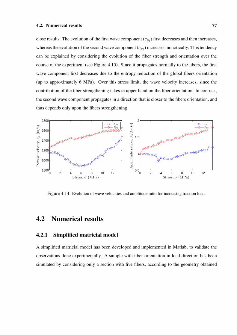
4.2. Numerical results 77

close results. The evolution of the first wave component (cp1) first decreases and then increases,

whereas the evolution of the second wave component (cp2) increases monotically. This tendency

can be explained by considering the evolution of the fiber strength and orientation over the

course of the experiment (see Figure 4.15). Since it propagates normally to the fibers, the first

wave component first decreases due to the entropy reduction of the global fibers orientation

(up to approximately 6 MPa). Over this stress limit, the wave velocity increases, since the

contribution of the fiber strengthening takes te upper hand on the fiber orientation. In contrast,

the second wave component propagates in a direction that is closer to the fibers orientation, and

thus depends only upon the fibers strengthening.

0 2 4 6 8 10 121800

2000

2200

2400

2600

2800

Stress, σ (MPa)

P-w

ave

velo

city

,c p

(m/s

)

cp1

cp2

0 2 4 6 8 10 120.5

1

1.5

2

Stress, σ (MPa)

Am

plitu

de

ration

,A

/A0

(-)

cp1

cp2

Figure 4.14: Evolution of wave velocities and amplitude ratio for increasing traction load.

4.2 Numerical results

4.2.1 Simplified matricial model

A simplified matricial model has been developed and implemented in Matlab, to validate the

observations done experimentally. A sample with fiber orientation in load-direction has been

simulated by considering only a section with five fibers, according to the geometry obtained


Figure 4.15: Evolution of fiber deformation for increasing traction load.

from micrographs. A separation between fibers of 1 µm was supposed. An articulated beam

structure was solved, where each beam represents a single fiber with a circular cross section

(0.5 µm diameter). Mechanical properties of collagen were taken from literature [45] (E = 3

GPa, G = 1GPa). Figure 4.16 shows a schematic view of the model. A equivalent mechanical

parameters for a continuum tissue were obtained. We found approximate values of Young

modulus of the order 165.17 MPa. This result does not contradict the data reported in literature,

where it is possible to find values close to this result for the cervical tissue [36]. Although, this

results leads to a velocity of S-wave slightly slow, compared with the others values obtained in

this work. It would be due to the simplicity of the model. Also, it must to be account that only

a reduced fiber density was considered. On the other hand, stretch of fibers plays a hard role in

mechanical behavior, so that a larger stretching fiber could lead to more consistent results.

4.2.2 Constitutive model: A numerical example

A numerical example was implementes in Matlab. The parameters used for the constitutive

model are chosen based on micrographs and previous studies ([44], [3], [45], [10]), and are

summarized in Table 4.1.

We consider only a layer of tissue, i.e., a collagenous tissue with a single collagen fiber

family subject to stretch-controlled uniaxial extension along the fiber direction. The fibers are


2 4 6 8 10 12

x 10−5

0

1

2

3

x 10−4

x (m)

y (

m)

1

2

3

4

5

6

7

8

9

10

11

1213

14

15

16

17

18

19

20

21

22

23

24

25

26

27

28

29

30

31

32

33

34

35

Figure 4.16: Matricial model.

located in the X-Y plane. We reproduced a simplified essay made by experimental measure-

ments (see Figure 3.4). The tissue is stretched in the Y-direction. For that kinematics the matrix

representation of the right Cauchy-Green tensor C for a incompressible tissue, has the form,

C =

1

λ 2 0 0

0 λ 2 0

0 0 1

(4.14)

where λ denotes the stretch in the Y-direction. In Figure 4.17 the Cauchy stress component

σyy in the Y direction is plotted versus the stretch λ for a longitudinal fiber orientation, and for

monotonic loading up to λ = 0.5. This behavior is close to the typical J-shaped of stress-strain

curve for collagenous tissues [14].

Let us consider, that fibers are mechanically active to calculated the stiffness. From equa-


Parameter Symbol Value Dimension

Elastic modulus of the fiber k 3000 MPa

Maximum fiber stretch εmax 0.2 -

Shape parameters η 4.0 -

γ 2.5 -

Range of ` m 0.15, 0.25 -

Range of damaged fibers b 0.05 -

Dispersion parameter κ 0.1 -

Young modulus Matrix E 90 MPa

Poisson’s ratio matrix ν 0.5 -

Table 4.1: Parameter values used for the numerical example.

0 0.1 0.2 0.3 0.4 0.50

50

100

150

stretch(λ)

σf 22

[MPa]

Figure 4.17: Stress component σyy (in Y-direction) versus stretch λ applied in the Y-direction.

tions obtained in Chapter 2, we can easily calculate the stiffness tensor, ci jkl , which is the linear


transformation that takes the strain tensor to the stress tensor,

ci jkl =

c1111 c1122 c1133 c1112 c1113 c1123

c2211 c2222 c2233 c2212 c2213 c2223

c3311 c3322 c3333 c3312 c3313 c3323

c1211 c1222 c1233 c1212 c1213 c1223

c1311 c1322 c1333 c1312 c1313 c1323

c2311 c2322 c2333 c2312 c2313 c2323

=

c11 c12 c13 c14 c15 c16

c21 c22 c23 c24 c25 c26

c31 c32 c33 c34 c35 c36

c41 c42 c43 c44 c45 c46

c51 c52 c53 c54 c55 c56

c61 c62 c63 c64 c65 c66

0 0.2 0.4 0.6 0.8 10

50

100

150

200

250

300

εyy

c 21

=c 2

3[M

Pa]

Figure 4.18: Stiffness in shear waves direction propagation.

The velocity of a shear waves, is controlled by modulus of rigidity. Then, for the proposed

orthotropic tissue, the speed of S-wave is calculated as,

cs =

√c21

ρor cs =

√c23

ρ(4.15)

since both stiffness components have the same value. Assuming ρ = 1000 kg/m3 for soft tissue,

the value of velocity of S-waves obtained is cs ' 550 m/s.


4.2.3 FDTD computational implementation

A finite difference time-domain code was implemented in Matlab, which simulates the two-

dimensional linear-elastic wave propagation through cervical tissue. A segmentation of micro-

graphs from the cervical tissue was used to modeled and discretized the spatial medium. As a

result, the Von Misses stress field is obtained.

Figure 4.19: Micrographic image used in simulations.

We performed simulations of the wave propagation in a cervical tissue of dimensions 4×3.2

mm, which correspond to the specimen thickness and length respectively. The original image

used for simulating the propagation was taken by electronic microscope, as shown in Figure

4.19. The tissue is considered as a fiber-reinforced material. The image was segmented by

defining a segmentation threshold, normalized into RGB interval and converted into a binary

image, where fiber density is monotonically related to the segmentation threshold. Mechanical

parameters used for the simulations are given in Table 4.2.

The dimensions of image were chosen after several simulations, where different values of

spatial windowing have been applied (see Figure 4.20).

P-waves and S-waves Simulations were made. The temporal shape of the excitation is one


Parameter Symbol Value Dimension

Lamé’s first parameter matrix λ 2.2 ·109 Pa

Lamé’s second parameter matrix µ 30 ·103 Pa

Density matrix ρ 1000 kg/m3

Damping γ 5 ·104 s−1

Young modulus collagen E 3 GPa

Density collagen ρ 1200 kg/m3

Poisson’ratio collagen ν 0.35 -

Table 4.2: Mechanical parameter values used for the simulations of the waves propagation.

sinusoidal oscillation at 250 kHz, with 1 mVpp amplitude.

To evaluate the mesh convergency, numerically calculated simulations with values of ele-

ment size 5, 10, 20 y 40 µm, were performed. The spatial discretization used in each sample

and the correspond simulations are shown in Figures 4.21 and 4.22.

The spatial discretization was done with a step size of 20 µ and 10 µ in the two cartesian

directions, for P-waves and S-waves simulations, respectively.

In a collagenous tissue, the velocities of plane waves vary depending on their propagation

directions, the stretch and preferred direction of fibers. In order to validate the FDTD code,

some different cases are simulated numerically. To quantify how the fibers density affects the

mechanical behavior of tissue, simulations were made for different segmentation thresholds.

Figure 4.23 shows images with different values of threshold. Results are plotted in Figures 4.24

and (4.25).

Speed and amplitude of waves is shown to increase with the density of fibers, due to the

increase of the material stiffness.

A parametric study was made, for different values of fiber Young modulus (E f ), thresh-

old, wave type (P-waves and S-waves), the fiber orientation, and stretch of fibers. Results are


0 5 10 15 20 25 30 35 40 45 50−1.5

−1

−0.5

0

0.5

1

1.5x 10

−9

Time t, [μs]

TransmissionReceptionIndividual

(a) length = 10 mm

0 5 10 15 20 25 30 35 40 45 50−1.5

−1

−0.5

0

0.5

1

1.5

2x 10

−9

Time t, [μs]


(b) length = 15 mm

0 5 10 15 20 25 30 35 40 45 50−2

−1.5

−1

−0.5

0

0.5

1

1.5

2

2.5x 10

−9

Time t, [μs]


(c) length = 20 mm

0 5 10 15 20 25 30 35 40 45 50−1.5

−1

−0.5

0

0.5

1

1.5

2

2.5x 10

−9

Time t, [μs]


(d) length = 25 mm

Figure 4.20: Effects of model size (spatial window).

shown in Figures 4.26-4.30. This numerical simulation shows the relation between velocity and

attenuation of waves, for increasing values of velocity we get decreasing attenuations.

Results obtained by FDTD simulations are summarized in Table 4.3 and in figures 4.31 to

4.35.

As a first conclusion, the positive dependency of speed of both P and S waves on the Young

modulus of collagen is correctly predicted by FDTD and qualitatively corresponds to experi-


x, [μm]

y, [

μm]

μ, [Pa]

500 1000 1500 2000 2500 3000 3500 4000

500

1000

1500

2000

2500

30001

2

3

4

5

6

7

8

9

10

11

x 108

(a) ∆x = 5µm

x, [μm]

y, [

μm]

μ, [Pa]

500 1000 1500 2000 2500 3000 3500 4000

500

1000

1500

2000

2500

3000 1

2

3

4

5

6

7

8

9

10

11

x 108

(b) ∆x = 10µm

x, [μm]

y, [

μm]

μ, [Pa]

500 1000 1500 2000 2500 3000 3500 4000

500

1000

1500

2000

2500

3000 1

2

3

4

5

6

7

8

9

10

11

x 108

(c) ∆x = 20µm

x, [μm]

y, [

μm]

μ, [Pa]

500 1000 1500 2000 2500 3000 3500 4000

500

1000

1500

2000

2500

3000 1

2

3

4

5

6

7

8

9

10

11

x 108

(d) ∆x = 40µm

Figure 4.21: Spatial discretizations with different element sizes.

mental observations. The dependency of the attenuation is also predicted.

Second, the relative orientation between fibers and incoming ultrasonic wave is predicted to

affect the speed of P-waves and attenuation in agreement with experimental observations. The

speed is lower at 0 and 90 degrees, whereas it increases at intermediate angles. Furthermore,

the attenuation is stronger at intermediate angles, which can be explained by the increased

scattering when the wave travels along misoriented interfaces.

Third, the effect of tissue stretch on speed and attenuation is computed and compared to the

experiment in the load test. Whereas the speed is observed to increase with stretch, possibly


0 10 20 30 40 50−1

−0.8

−0.6

−0.4

−0.2

0

0.2

0.4

0.6

0.8

1x 10

−9

Time, t (μs)

Δx = 5μmΔx = 10μmΔx = 20μmΔx = 40μm

Figure 4.22: Response signals for different element size.

x, [μm]

y, [

μm]

μ, [Pa]

500 1000 1500 2000 2500 3000 3500 4000

500

1000

1500

2000

2500

30001

2

3

4

5

6

7

8

9

10

11x 10

8

(a) threshold = 25%

x, [μm]

y, [

μm]

μ, [Pa]

500 1000 1500 2000 2500 3000 3500 4000

500

1000

1500

2000

2500

30001

2

3

4

5

6

7

8

9

10

11x 10

8

(b) threshold = 50%

Figure 4.23: Different values of thresholds.

due to alignment of fibers, the attenuation increases.

Finally, the density of fibers is correctly modeled to positively affect the speed by modifying

the segmentation threshold.


0 10 20 30 40 50−1.5

−1

−0.5

0

0.5

1

1.5x 10

−9

Time, t (μs)

thres. = 25%thres. = 50%thres. = 75%thres. = 100%

Figure 4.24: FFDT Results for S-waves excitation in a cervical tissue, with fiber orientation 0o, for

different thresholds of segmentation.

0 10 20 30 40 50−3

−2

−1

0

1

2

3x 10

−10

Time, t (μs)


(a) α = 0o

0 10 20 30 40 50−2.5

−2

−1.5

−1

−0.5

0

0.5

1

1.5

2x 10

−10

Time, t (μs)


(b) α = 45o

Figure 4.25: FFDT Results for P-waves excitation in a cervical tissue for different thresholds of seg-

mentation. In the first one, the fibers are parallel to the excitation, and in the second one fibers are

orientated 45o.


0 10 20 30 40

−5

0

5

10x 10

−9

Time, t (μs)

Sig

nal,

s(V

)

ExcitationE1E2E3E4

0 10 20 30 40

−5

0

5

10x 10

−9

Time, t (μs)

Sig

nal,

s(V

)

ExcitationE1E2E3E4

Figure 4.26: Simulated P-waves for different values of Young Modulus: E1 = 3 GPa, E2 = 4 GPa,

E3 = 5 GPa, E4 = 6 GPa.

0 10 20 30 40

−5

0

5

10x 10

−9

Time, t (μs)

Sig

nal

,s

(V)

Excitation0204590

0 10 20 30 40

−5

0

5

10x 10

−9

Time, t (μs)

Sig

nal

,s

(V)

Excitation0204590

Figure 4.27: Simulated P-waves for different values of fiber orientation: 0, 20, 45 and 90.


0 10 20 30 40

−5

0

5

10x 10

−9

Time, t (μs)

Sig

nal,

s(V

)

Excitation100120140160

0 10 20 30 40

−5

0

5

10x 10

−9

Time, t (μs)

Sig

nal,

s(V

)

Excitation100120140160

Figure 4.28: Simulated P-waves for different values of fibers stretch: 100, 120, 140 and 160 %.

0 10 20 30 40 50−1

−0.5

0

0.5

1x 10

−8

Time, t (μs)

Sig

nal,

s(V

)

ExcitationE1E2E3E4

0 10 20 30 40

−5

0

5

10x 10

−9

Time, t (μs)

Sig

nal,

s(V

)

ExcitationE1E2E3E4

Figure 4.29: Simulated S-waves for different values of Young Modulus: E1 = 3 GPa, E2 = 4 GPa,

E3 = 5 GPa, E4 = 6 GPa.


0 10 20 30 40 50−1

−0.5

0

0.5

1x 10

−9

Time, t (μs)

Sig

nal,

s(V

)

Excitation406080100

0 10 20 30 40 50−1

−0.5

0

0.5

1x 10

−9

Time, t (μs)

Sig

nal,

s(V

)

Excitation406080100

Figure 4.30: Simulated S-waves for different values of fibers density, expressed by the following thresh-

old values: 40, 60, 80 and 100.

3 3.5 4 4.5 5 5.5 6520

540

560

580

600

620

Young Modulus, E [GPa]

Vel

oci

ty,c s

[m/s

]

3 3.5 4 4.5 5 5.5 60.7

0.75

0.8

0.85

0.9

0.95

1


Dam

pin

gra

tio,

[-]

Figure 4.31: FDTD simulated dependency of P-wave Velocity and Damping ratio on Young modulus

of collagen fibers.


Table 4.3: Results of the parametric study.

Wave-types Characteristics Cases Velocity [m/s] Damping ratio [-]

P−wave

Modulus E [GPa]

3 1882 1.00

4 2038 0.90

5 2162 0.84

6 2266 0.79

Orientation α []

0 1849 1.00

20 1858 0.93

45 1873 0.90

90 1855 1.41

Tissue elongation ε [%]

0 1849 1.00

20 1849 0.99

40 1846 0.98

60 1843 1.02

S−wave

Modulus E [GPa]

3 529 1.00

4 553 0.93

5 589 0.79

6 614 0.74

Segmentation threshold [%]

40 532 1.00

60 637 1.20

80 721 0.87

100 788 0.33


40 50 60 70 80 90 100500

550

600

650

700

750

800

Threshold, T [−]

Vel

oci

ty,c s

[m/s

]

40 50 60 70 80 90 1000.2

0.4

0.6

0.8

1

1.2

Threshold, T [−]

Dam

pin

gra

tio,

[-]

Figure 4.32: FDTD simulated dependency of P-wave Velocity and Damping ratio on the relative orien-

tation between fibers and incoming ultrasonic wave.

3 3.5 4 4.5 5 5.5 61800

1900

2000

2100

2200

2300


Vel

oci

ty,c p

[m/s

]

3 3.5 4 4.5 5 5.5 60.75

0.8

0.85

0.9

0.95

1


Dam

pin

gra

tio,

[-]

Figure 4.33: FDTD simulated dependency of P-wave Velocity and Damping ratio on tissue elongation.


0 20 40 60 801845

1850

1855

1860

1865

1870

1875

Orientation, α []

Vel

oci

ty,c p

[m/s]

0 20 40 60 800.9

1

1.1

1.2

1.3

1.4

1.5

Orientation, α []

Dam

pin

gra

tio,

[-]

Figure 4.34: FDTD simulated dependency of S-wave Velocity and Damping ratio on Young modulus

of collagen fibers.

0 10 20 30 40 50 601840

1842

1844

1846

1848

1850

Tissue elongation, ε [%]

Vel

oci

ty,c p

[m/s

]

0 10 20 30 40 50 600.98

0.99

1

1.01

1.02

1.03

1.04

Tissue elongation, ε [%]

Dam

pin

gra

tio,

[-]

Figure 4.35: FDTD simulated dependency of S-wave Velocity and Damping ratio on the density of

collagen fibers.

Chapter 5Conclusions and outlook

The distribution of fibrils as fibers or fibril bundles occurs as a common motif in many tissues,

with the fiber direction being aligned to provide the bespoke mechanical characteristics of the

tissue. The response of the tissue to the applied stress strongly depends upon the strain rate,

where high strain rates cause elongation of the collagen molecules and initiate shearing effects

within fibrils. While at small strains there is a straightening of kinks in the collagen structure

(first at the fibrillar and then at the molecular level). Waviness of fiber is responsible, in part, the

mechanical behavior and creep of tissue. In the cervical micrographs analyzed, the middle zone

of the cervix, where fibers are aligned in the circumferential direction, presents lower waviness

than zones with longitudinal fibers. This is hypothesized to be due to the fact that the higher

values of waviness that tissue cut in the longitudinal direction has a higher creep rate that tissue

cut in the circumferential direction.

The results show the ability to describe mechanical behavior of the cervical tissue like as

a fiber reinforced material. This work shows that the ultrasonic wave propagation phenomena

can be exploited to reconstruct the mechanical properties of the soft tissues they travel through,

in particular the cervical tissue.

This technique was tested experimentally on a consistent basis. Results show how ultra-

sound waves interact with collagen fibers (micro-scale), which determines macroscopic proper-

94

95

ties (centimeter scale) and are responsible for the mechanical behavior of connective tissue.

Achieved results, as well as weaknesses found in the methodology and possible future works

are set out below:

• Statement of contributions:

– Constitutive model considering crimped fibers and dispersed collagen orientation

for soft tissues.

– Analysis of transmitted ultrasonic wave through the tissue, and its interactions with

micro-scale (collagen fibers).

– Numerical simulation of ultrasound waves through a soft tissue, employing S-wave

transducers.

• Limitations and capabilities of the technique:

– Attenuation of S waves, due to design of transducers.

– Model lacks fiber-matrix interaction.

• Applications:

– Determination of mechanical properties of soft tissues.

– Design a optimal ultrasound sensor for soft tissues

• Prospects for improvement:

– Incorporate more features in the model and improve understanding of the interaction

between mechanical, biological and chemical responses.

– Finite element programming implementating constitutive model as UMAT subrou-

tine in Abaqus.

– Process a wider range of micrographs to characterize geometric parameters of cer-

vical tissue.

96

– Test using P-waves with different incidence angles.

– Test various combinations of soft tissues, including cervical tissue from biopsy.

• Future applications:

– Diagnostic tool for obstetrics.

– Monitorization of stiffness variations in soft tissues.

Appendices

97

Appendix AGetting geometric parameters from

micrographs

The geometric parameters used in different models were obtained from some micrographs of

human cervical tissue samples. Two samples were analyzed: a longitudinal and a cross section.

A general view of sections is shown in Figure A.1. Parameters were measured from several

locations of the samples. In each analyzed image, the average value of the geometric parameters

has been calculated, and then used in the proposed models.

Due to the impossibility of extracting samples from healthy cervical tissue, specimens were

obtained from women with any cervical pathology. Those pathologies can be perfectly iden-

tified in the micrographs. Thus, the parameters of interest were measured only in the regions

without pathologies.

We characterized three different zones that may correspond to the inner, middle and outer

areas, that should contain collagen fibers preferentially aligned in the longitudinal, circumfer-

ential and longitudinal directions, respectively (see Figure 1.3). Table A.1 shows the average

geometric parameters calculated in each zone. Where ` is the stretch at which the fiber be-

comes mechanically active, σ2 is the variance of its distribution, α indicates the angle of fiber

orientation makes with the horizontal in degree, and κ is the scalar structure parameter that

98

99

Zonestretch fibers active variance fiber orientation dispersion of orientations

` σ2 α(o) κ

outer 1.3017 0.07 78.25 0.10

middle 1.044 0.16 5.47 0.17

inner 1.0373 0.08 69.24 0.08

Table A.1: Geometric parameters of cervical tissue.

characterizes the level of dispersion of the collagen orientations.

As depicted in Table A.1, we obtained orientations approximately in parallel and perpendic-

ular to the cervical canal. The main difference appears in the waviness of fibers, i.e., the outer

zone presents more crimped fibers than the other zones. Figure A.2 highlights collagen fibers in

the inner, middle and outer zones, respectively. It would be related with, in part, the dependence

on direction of the mechanical behavior of cervix, it is known that tissue cut in the longitudinal

direction has a higher creep rate that tissue cut in the circumferential direction [33].

100

(a) Longitudinal section.

(b) Cross section.

Figure A.1: Micrographs of a human cervix longitudinal and cross sections.

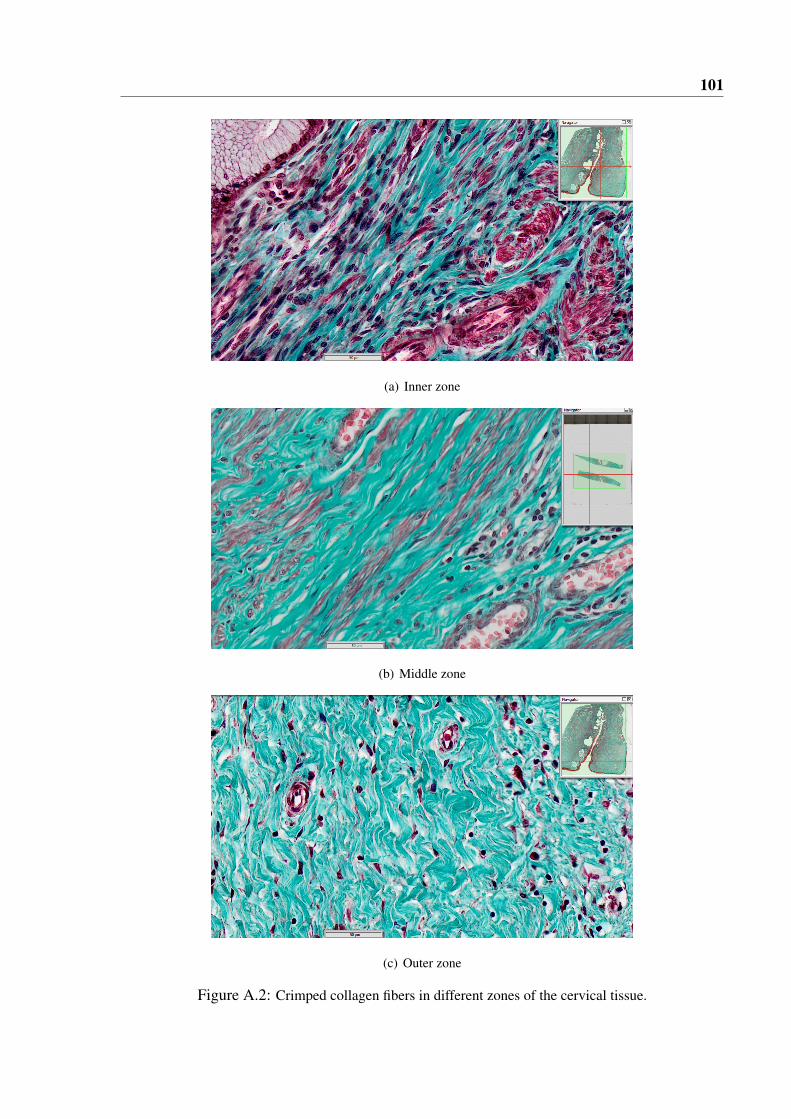
101

(a) Inner zone

(b) Middle zone

(c) Outer zone

Figure A.2: Crimped collagen fibers in different zones of the cervical tissue.

Bibliography

[1] M. Abramowitz, I.A. Stegun. Handbook of mathematical functions with formulas, graphs,

and mathematical tables. National Bureau of Standards, Applied Mathematics Series, vol.

55, New York, 1972.

[2] R.M. Aspden. The theory of fibre-reinforced composite materials applied to changes in

the mechanical properties of the cervix during pregnancy. Journal of Theoretical Biology,

130, 213-221, 1988.

[3] R.M. Aspden. Collagen organisation in the cervix and its relation to mechanical function.

Collagen and related research, 8:103-112, 1988.

[4] E. Baer, J.J. Cassidy, and Anne Hiltner. In viscoelasticity of biomaterials. ACS Sympo-

sium Series. American Chemical Society. Washington, D.C., 1992.

[5] J.M. Ball. Convexity conditions and existence theorems in nonlinear elasticity. Archive for

Rational Mechanics and Analysis, 337-403, 1977.

[6] P.J. Basser, R. Schneiderman, R.A. Bank, E. Wachtel, and A. Maroudas. Mechanical prop-

erties of the collagen network in human articular cartilage as measured by osmotic stress

technique. Archieves of Biochemiestry and Biophysics, 351(2):207-219, March 1998.

102

Bibliography 103

[7] J.F. Bateman, S.R. Lamande, and J.A.M. Ramshaw. Extracellular matrix: molecular com-

ponentes and interactions, chapter 3: The elastic fiber. Overseas Publishers Association,

1996.

[8] M. Bauer, E. Mazza, A. Nava, W. Zeck, M. Bajka, F. Cacho, Uwe Lang, and GA

Holzapfel. In vivo characterization of the mechanics of human uterine cervices. Annals

of the New York Academy of Sciences, 1101(1):186, 2007.

[9] M.J. Buehler. Nanomechanics of collagen fibrils under varying cross-link densities: Atom-

istic and continuum studies. Journal of the Mechanical Behavior of Biomedical Materials

I, 59-67, 2008.

[10] F. Cacho, P.J. Elbischger, J.F. Rodríguez, M. Doblaré, G.A. Holzapfel. A constitutive

model for fibrous tissues considering collagen fiber crimp. International Journal of Non-

Linear Mechanics, 42:391-402, 2007.

[11] J.T. Conrad, R.D. Tokarz, J.F. Williford. Dilatation of the uterine cervix: connective tissue

biology and clinical management. New York: Raven Press, 1980.

[12] G. Ekman, H. Almstrom, L. Granstrom, A. Malmstrom, M. Norman and J.F. Woessner Jr.

The extracellular matrix of the uterus, cervix and fetal membranes: synthesis, degradation

and hormonal regulation. Perinatology Press, 1991.

[13] S. Febvay, S. Socrate and M.D. House. Biomechanical modeling of cervical tissue. A quan-

titative investigation of cervical funneling. Proceedings of the ASME 2003 International

Mechanical Engineering Congress and Exposition, Washington, D.C., November 2003.

[14] P. Fratzl, K. Misof, I. Zizak, G. Rapp, H. Amenitsch and S. Bernstorff. Fibrillar structure

and mechanical properties of collagen. Journal of Structural Biology, 122:119-122, 1998.

[15] P. Fratzl. Collagen: structure and mechanics. Springer Science-Business Media, LLC,

2008.

Bibliography 104

[16] S. Doll, K. Schweizerhof. On the development of volumetric strain energy functions.

Transactions of the ASME. Journal of Applied Mechanics, 17-21, 2000.

[17] T.C. Gasser, R.W. Ogden, G.A. Holzapfel. Hyperelastic modelling of arterial layers with

distributed collagen fibre orientations. Journal of the Royal Society Interface, 3:15-35,

2006.

[18] R. Hill. On uniqueness and stability in the theory of finite elastic strain. Journal of the

Mechanics and Physics of Solids, 229-241, 1957.

[19] A.M. Hocking, T. Shinomura, and D. McQuillan. Leucine-rich glycoproteins of the extra-

cellular matrix. Matrix Biology, 17:1-19,1998.

[20] G.A. Holzapfel. Nonlinear solid mechanics: A continuum approach for engineering.

Chichester : Wiley, 2000.

[21] M. House, M.L. Kaplan, S. Socrate. Relationships between mechanical properties and

extracellular matrix. Seminars in Perinatology, 33:300-307, 2009.

[22] D.W.L. Hukins and R.M. Aspden. Composition and properties of connective tissues.

Trends in Biochemical Science 10:260-264, 1985.

[23] J.A. Jordan and A. Singer. The functional anatomy of the cervix, the cervical epithelium

and the stroma, in the cervix, Second Edition (eds J. A. Jordan and A. Singer), Blackwell

Publishing Ltd., Oxford, UK., 2009.

[24] K.E. Krantz and W. Patton Phillips. Anatomy of the human uterine cervix, gross and mi-

croscopic. Annals of the New York Academy os Sciences, vol. 97, 551-563, september

1962.

[25] O. Kratky, G. Porod. Rötgenuntersushung gelöster fagenmoleküle. Recueil des Travaux

Chimiques des Pays-Bas, vol. 68, 1106-1123, 1949.

Bibliography 105

[26] Y. Lanir. Constitutive equations for fibrous connective tissues. Journal of Biomechanics.

16:1-12, 1983.

[27] P.C. Leppert, J.M. Cerreta, I. Mandl. Orientation of elastic fibers in the human cervix.

American Journal of Obstetrics and Gynecology, 155(1), 219-224, 1986.

[28] T. Matsumura, T. Umemoto, Y. Fujihara, E. Ueno, T. Shiina, and T. Mitake. Measurement

of elastic property of breast tissue for elasticity imaging. IEEE International Ultrasonics

Symposium (IUS), Roma, Italy, 2009.

[29] E. Mazza, A. Nava, M. Bauer, R. Winter, M. Bajka, G.A. Holzapfel. Mechanical proper-

ties of the human uterine cervix: An in vivo study. Medical Image Analysis 10:125-136,

2006.

[30] E. Mosler, W. Folkhard, E. Knorzer, H. Nemetschek-Gansler, T.H. Nemetschek, M.H.

Koch. Stress-induced molecular arrangement in tendon collagen. Journal of Molecular

Biology 182(4), 589-596, 1985.

[31] K.M. Myers, A.P. Paskaleva, M. House, S. Socrate. Mechanical and biochemical proper-

ties of human cervical tissue. Acta Biomaterialia 104-116, 2008.

[32] A. Paskaleva. Biomechanics of cervical function in pregnancy - Case of cervical insuffi-

ciency. PhD thesis, Massachusetts Institute of Technology, Dept. of Mechanical Engineer-

ing, 2007.

[33] L.K. Petersen, H. Oxlund, N. Uldbjerg, A. Forman. In vitro analysis of muscular contrac-

tile ability and passive biomechanical properties of uterine cervical samples from non-

pregnant women. Obstetrics and Gynecology 77:772-776, 1991.

[34] G.N. Ramachandran, G. Kartha. Structure of collagen. Nature 176:593-595, 1955.

Bibliography 106

[35] C.P. Read, R.A. Word, M.A. Ruscheinsky, B.C. Timmons, and M.S. Mahendroo. Cervical

remodeling during pregnancy and parturition: molecular characterization of the softening

phase in mice. Reproduction, 134(2):327-340, 2007.

[36] T. Rechberger, N. Uldbjerg, H. Oxlund. Connetive tissue changes in the cervix during

normal pregnancy and pregnancy complicated by cervical incompetence. Obstetrics and

Gynecology, vol. 71, 4:563-567, 1988.

[37] J.F. Rodriguez, F. Cacho, J.A. Bea, M. Doblare. A stochastic-structurally based three

dimensional finite strain damage model for fibrous soft tissue. Journal of the Mechanics

and Physics of Solids, 54(4):864-886, 2006.

[38] Rotten D, Gavignet C, Colin MC et al. Evolution of the elastic fibre network of the human

uterine cervix before, during and after pregnancy. A quantitative evolution by automated

image analysis. Clinics in Physiology and Biochemistry 6(5): 285-292, 1988.

[39] M.D. Seymour Zemlyn. The length of the uterine cervix and its significance. Journal of

Clinical Ultrasound, vol. 9, issue 6, 267-269, 1981.

[40] F.H. Silver, D.L. Christiansen, P. Snowhill, Y. Chen. Role of storage on changes in the

mechanical properties of tendon and self-assembled collagen fibers. Connective Tissue

Research, 41, 155-164, 2000.

[41] F.H. Silver, J. Freeman, D. DeVore. Viscoelastic properties of human skin and processed

dermis. Skin Research and Technololy, 7, 18-23, 2001.

[42] J.C. Simo. On a fully three-dimensional finite-strain viscoelastic damage model: formula-

tion and computational aspects. Computer Methods in Applied Mechanics and Engineer-

ing, 60, 153-173, 1987.

[43] A.J.M. Spencer. Continuum Mechanics. Longman Scientific & Technical, Essex, 1980.

Bibliography 107

[44] S. Weiss, T. Jaermann, P. Schmid, P. Staempfli, P. Boesiger, P. Niederer, R. Caduff, and M.

Bajka. Three-dimensional fiber arqchitecture of the nonpregnant human uterus determined

ex vivo using magnetic resonance diffusion tensor imaging. The Anatomical record Part

A, 288A:84-90, 2006.

[45] M.P.E. Wenger, L. Bozec, M.A. Horton, and P. Mesquida. Mechanical properties of col-

lagen fibrils. Biophysical Journal, vol. 93, 1255-1263, 2007.

MECHANICAL CHARACTERIZATION OF CERVICAL TISSUE

Documents

Transcript of MECHANICAL CHARACTERIZATION OF CERVICAL TISSUE