MPRAMunich Personal RePEc Archive

Measuring the recreational use value ofmigratory shorebirds on the DelawareBay

Kelley H. Myers and George R. Parsons and Peter E.T.

Edwards

University of Delaware, National Oceanic and AtmosphericAdministration

2010

Online at http://mpra.ub.uni-muenchen.de/26126/MPRA Paper No. 26126, posted 10. January 2012 04:33 UTC

247

Marine Resource Economics, Volume 25, pp. 247–264 0738-1360/00 $3.00 + .00Printed in the U.S.A. All rights reserved. Copyright © 2010 MRE Foundation, Inc.

Kelley H. Myers is a PhD candidate and George R. Parsons is a professor, College of Earth, Ocean, and Environment, University of Delaware, Newark, DE 19716 USA (email: kelleyhmyers@gmail.com; gpar-sons@UDel.edu). Peter E.T. Edwards is a natural resource economist, National Oceanic and Atmospheric Administration, 1315 East West Highway, SSMC3 Rm. 14709, Silver Spring, MD 20910 USA (email: Peter.Edwards@noaa.gov). We thank Kevin Kalasz, state wildlife biologist with the Department of Natural Resources and Environ-mental Control (DNREC), for his contribution to our research. We also thank Dawn Webb of DNREC for providing us with a base location during our onsite surveying and Sally O’Byrne and Derek Stoner of the Delmarva Ornithological Society for introducing us to bird watching and assisting us with the development of our survey mechanism. Finally, we thank several graduate students in the Marine Policy program at the University of Delaware who assisted us during the onsite survey: Meredith Blades Lilley, John Lilley, Andy Krueger, and Kate Semmens.

Measuring the Recreational Use Value of Migratory Shorebirds on the Delaware Bay

KELLEy H. MyERSGEORGE R. PARSONSUniversity of DelawarePETER E.T. EDWARDSNational Oceanic and Atmospheric Administration

Abstract In this article we estimate the recreational use value of household trips to view shorebirds during the annual horseshoe crab/shorebird migra-tion on the Delaware Bay. We use contingent valuation to estimate the value of day and overnight trips separately and use a discrete choice question fol-lowed by a payment-card question to generate our valuation data. Our best estimates for the value of a day trip are about $66–$90/household and for an overnight trip about $200–$425/household (2008$). Our data are from the 2008 season, and our average household size is 1.66. For some context, esti-mates from four other studies report values that vary from $63/trip/person to $442/trip/person. These studies vary in method and specific birding popula-tions studied and mix day and overnight trips.

Key words Contingent valuation, discrete choice, bird watching, use value.

JEL Classification Codes Q5.

Introduction

According to the U.S. Fish and Wildlife Service, nearly 23 million residents aged 16 years or older traveled a mile or more from their home to observe or photograph wildlife in 2006 (Aiken 2009). The growth of wildlife-based recreation in the USA and the mount-ing concern over the preservation of our natural resources has increased the demand for information on the costs and benefits of activities related to wildlife. Individuals who engage in wildlife watching have measurable welfare resulting from their experience, and government action can play an active role in affecting this experience. To put recreation experiences in monetary terms, non-market valuation techniques, like the travel cost or contingent valuation methods, are used to estimate the value of wildlife watching to an individual or household.

Myers, Parsons, and Edwards248

In this article, we extend the non-consumptive wildlife valuation literature using a contingent valuation study of recreational bird watching on the Delaware Bay. Each spring, the Delaware Bay is considered the largest staging area for migratory shorebirds in eastern North America. The visiting shorebirds time their arrival with the spawning season of adult horseshoe crabs in early May. The birds stay for two to three weeks eating horse-shoe crab eggs for up to 14 hours a day before flying north. This combination of migratory shorebirds and spawning horseshoe crabs is unseen elsewhere in the world, making the Delaware Bay a popular destination for wildlife enthusiasts and recreational birders. Four species of migratory birds draw the most attention during the horseshoe crab/shorebird occurrence—red knot, ruddy turnstones, sanderlings, and semipalmated sand-pipers. Over the last decade, scientists have documented a decline in both the horseshoe crab and shorebird populations. This may be attributed, in part, to the increased commer-cial harvest of the horseshoe crab in the mid 1990s. The red knot, in particular, has drawn attention because some scientists believe it is on a path to extinction. Some say it could be lost within 5 to10 years (NJDEP 2007). In our application, we focus on recreational use values and use survey data from 370 recreational birders to estimate the willingness to pay (WTP) for a household trip during the 2008 annual shorebird migration. We intercepted birders onsite and used a mail-back paper survey. We used a referendum-style discrete choice question followed by a payment card to generate our preference data. In the following section, we briefly discuss some other applications of contingent valuation to bird watching. Then we present our study design, model, and results.

Values for Bird Watching Trips from other Contingent Valuation Studies

There are a number of contingent valuation studies of bird watching and general wildlife viewing trips in the literature. A sampling is shown in table 1—four birdwatching stud-ies and three wildlife viewing studies. There are also several travel cost studies of bird watching (e.g., Gürlük and Rehber 2007) and stated preference studies of the total value of protecting bird and other wildlife populations (Richardson and Loomis 2008; Loomis and White 1996). None of these are included in the table. For the purpose of this article, we will briefly review the studies that use contingent valuation to estimate the use value of bird watching trips. These applications are closest to ours. Hvenegaard, Butler, and Krystofiak (1989) estimated the value of bird watching in Point Pelee National Park in Canada during the spring migration in 1987. They conducted random onsite personal interviews of over 600 birders during the peak spring birding season. Using an open-ended response format, respondents were asked to consider the highest increase in trip cost they would be willing to pay before canceling their most recent trip to Point Pelee. The average WTP, which mixed day and overnight trips, was $442/trip/person. Cooper and Loomis (1991) estimated the value of a bird watching trip with data from a mail survey of 3,000 randomly selected California households in 1987. The authors used a dichotomous choice referendum format that asked respondents to consider a hypothetical increase in the cost of their most recent trip. Bid values ranged from $2 to $200 and WTP was estimated under three different conditions: current, 50% increase in birds viewed, and 100% increase in birds viewed. The mean WTP for a trip, which again included day and overnight trips, under current conditions in California was about $63/trip/household. Eubanks, Ditton, and Stoll (1998) and Eubanks and Stoll (2000) estimated the con-sumer surplus of a bird watching trip during two annual migration events: the sandhill crane in Nebraska and shorebirds in New Jersey. Both studies used an open-ended ques-tion format and asked respondents to state the maximum they would be willing to pay before canceling their most recent trip. The sandhill crane study was a combination of

Shorebird Valuation 249

onsite intercepts and a mail-based survey of randomly selected bird watchers from seven Nebraska Wildlife organizations. The estimated values were $77/trip/person. The New Jersey study used a data set that combined intercepted birders with a mail survey of members of the Cape May Bird Observatory and the New Jersey Audubon Society. The estimated values were $324/trip/person. Again, day and overnight trips were mixed in both analyses. The WTP estimates from these four studies then vary from $63 to $442/trip. All of the studies mix day and overnight trips in their analysis. Interestingly, all of the studies except Cooper and Loomis (1991) estimate the value of a bird watching trip during a mi-gration event. The Eubanks and Stoll study is particularly interesting because it is applied to the same horseshoe crab/migratory shorebird resource we study, except that it is on the New Jersey side of the Bay.

Table 1Contingent Valuation Studies of the Non-Consumptive Use Value of Wildlife

CVM Survey Mean WTP Per Reference Resource Method Respondents Trip or Per Day (2008$)

Hvenegaard, Butler, Bird watching OE Visitors to Point $442/trip/person& Krystofiak 1989 Pelee National Park, Canada Cooper & Loomis 1991 Bird watching DC Mail survey of CA $63/trip/household residents

Eubanks, Ditton, & Stoll Bird watching OE Visitors to Platte River $77/trip/person 1998 and mail survey of NE birding associations

Boyle, Roach, & Wildlife watching DC U.S. households $28/day/personWaddington 1998

Clayton & Mendelsohn Wildlife watching OE, Visitors to McNeil $366–$420/trip/ 1993 DC River person

Eubanks & Stoll Bird watching OE Visitors to DE Bay $324/trip/person2000 in NJ and mail survey of NJ birding associations Aiken 2009 Wildlife watching OE U.S. households $61/day/person

OE = open ended; DC = dichotomous choice.

Study Design

Study Site and Sampling

There are approximately 20 different locations along the coast of the Delaware Bay on the Delaware side that are suitable for viewing shorebirds during the migration. During a field trip in 2007 and based on conversations with state wildlife biologists and major bird-ing organizations in the area, we identified two major sites that most, if not all, birders

Myers, Parsons, and Edwards250

visit on a trip to the Delaware Bay: Port Mahon and Mispillion Harbor.1 For this reason, we confined our sampling in 2008 to these sites.2 This saved time, increased our sample and, in our judgment, introduced little bias. The sites are shown in figure 1. Port Mahon is about 26 miles north of Mispillion Harbor. There are no public facilities, nature centers, or trails to speak of at Port Mahon. Visitors view birds from their car (or just outside their car) along a mile-long stretch of road that runs parallel to the shore. At Mispillion Harbor, on the other hand, there is a new Nature Center, parking area, mounted scopes for view-ing birds, and facilities. It is an ideal location for viewing the migration. The spring shorebird migration takes place during the month of May and into early June. In order to capture visiting birders, we defined our sampling timeframe from May 1 to June 15, 2008. Our goal was to distribute a total of 600 surveys onsite. Respondents were asked to complete one survey per household at the end of the day and mail it back in the postage-paid return envelope. Sampling took place over the course of 11 days (4 of which were weekend days). Due to the low visitation rates per hour and the number of surveyors onsite, we were able to approach and distribute surveys to virtually all bird watchers during sampling.3

Figure 1. Delaware Bay Birding Sites

1 We took up residence on the Bay in 2007 for seven days and visited each of the 20 proposed sites. We interviewed and gathered preliminary trip data on approximately 75 birders on this field trip. We also interviewed approximate-ly 12 members of the Delmarva Ornithological Society—one of the largest bird watching clubs in Delaware.2 Initially, we did a small amount of sampling at the Prime Hook National Wildlife Refuge. We spent a short amount of time there in 2007 and believed that it might serve as a third major site. In 2008, we quickly learned that most of the visitors to Prime Hook were not in the area to view the horseshoe crab/shorebird migration. We also discovered that visitors to Prime Hook who were in the area to view the migration eventually made their way to Mispillion Harbor, so we stopped sampling Prime Hook. 3 People returning the survey were eligible to participate in a drawing for a wood carving of a red knot, one the four species targeted by almost every birder making a trip to the Bay during this migration. We included a sepa-rate postcard for respondents to return with their address. About half of the sample chose to participate.

Shorebird Valuation 251

Questionnaire

We designed our survey to obtain information about household trips on the day the respondent received the survey. The questions were organized in five main parts: i) in-troductory questions pertaining to where the trip began and ended, group size and type, and number of household members on the trip; ii) specific questions about the birding trip, such as total hours spent birding, what sites were visited, and other general activi-ties; iii) detailed questions about the trip type (day or overnight), trip expenditures, and the economic valuation question; iv) follow-up questions about past and future trips to the Delaware Bay during the defined season; and v) birding intensity, experience, and demo-graphic questions. In part 3 of the survey, we asked respondents to classify their trip as either a day or overnight trip to view shorebirds on the day they were intercepted. Using a discrete choice question, we then asked if they would have made the trip on the day they were in-tercepted if trip cost had been higher by some hypothetical amount. Our response format allowed people to reply definitely yes, probably yes, probably no, or definitely no. Imme-diately after the discrete choice question, we asked respondents to specify their maximum WTP using a question in a payment card format. The choice questions are shown in fig-ures 2 and 3. The bid amount, or cost for the discrete choice question, varied across 12 different versions of the survey. For day trip respondents, the bid amounts ranged from $10 to $300. For overnight respondents, it ranged from $20 to $2,000. In the payment card follow-up question, we asked respondents to consider the largest cost increase they would tolerate before they would no longer make the trip. They were asked to circle 1 of 15 different amounts from less than $5 to greater than $400 if on a day trip, and from less than $10 to greater than $2,000 if on an overnight trip. We used the initial discrete choice question, in part, as a set up for the payment card question. The less precise and easier-to-answer discrete choice question was intended to get people thinking about the trip cost and what they might tolerate. Including definitely and probably responses made this question easier to answer than a simple yes-no dichoto-mous choice. The commitment is lower. The second, more precise and more difficult to answer payment card question then asked respondents to hone in on a specific amount.

Figure 2. Example of Discrete Choice Day Trip Question

Myers, Parsons, and Edwards252

Response Rate and Data

Of the 581 distributed surveys, 376 were returned by mid-August (2008) for a response rate of 65%. Of the 376 returned surveys, 6 were discarded due to incomplete informa-tion, respondent error, or the respondent being outside of the sample frame (e.g., person under the age of 18, volunteers of Delaware Shorebird Project, group leader of an edu-cational trip). As mentioned earlier, we asked respondents to tell us whether or not they were on a day or overnight trip to the area. If a respondent did not indicate the type of trip, we used the information about their starting and ending location on the day of the intercept to make our decision. Using this information, we segmented the sample by day and overnight trips. We have 223 day trips and 147 overnight trips in our sample. Table 2 shows the sample characteristics by trip type.4 The characteristics do not vary significant-ly by trip type with the exception of group size, which is twice as large for households on an overnight trip. The average household size is slightly below two, and the average age is in the late 50s. It is an educated population and the income is more than twice the me-dian household income in the USA (U.S. Census Bureau 2008). Average expenditures per trip were about $50/household for day trips and about $400/household for overnight trips. Table 3 shows the distribution of responses by offer price to the discrete choice question, and table 4 shows the distribution for payment card responses. The lower sample sizes shown in the tables are due to item non-response on the choice questions. For the purpose of this study, a household was birding if they were viewing shore-birds for at least a half hour on the day of the intercept. For the entire sample, the average number of days spent birding in the past 12 months was 49.4. We also find that almost 70% of the sample keeps at least a modestly detailed lifetime list of all the birds they observe. The average market value for all birding related gear and equipment is $3,652/household. We also find that 55% of the sampled population belongs to either a local or national birding society. These findings suggest that our sample population is both an ac-tive and avid population of recreational bird watchers. In addition to birding intensity, we ask about the respondent’s activities on the day of the intercept. Almost 80% of the sample population indicated that they were in the area primarily to observe the horseshoe crab/shorebird occurrence. The same fraction of the population also indicated that they observed the red knot on the day of their trip.

Figure 3. Example of Payment Card Day Trip Question

4 Since these are onsite data, households taking more trips have a higher probability of being sampled. Since our interest is in estimating mean per-trip values over all trips taken, the onsite correction often done with travel cost models is inappropriate. If we were interested in mean per-trip values over respondents (and not trips), then the correction would be needed.

Shorebird Valuation 253

Table 2Mean Sample Characteristics by Trip Type

Day Trip (n=223) Overnight Trip (n=147)Category Mean Std. Dev. Mean Std. Dev.

Household size 1.66 0.78 1.86 0.96Group size 1.93 3.59 3.81 6.14Hours birding on Delaware Bay 5.11 2.98 5.54 3.13during the tripDays birding in past 12 months 52.25 37.27 47.59 37.70Market value of birding equipment $3,662 6,135 $3,622 6,599Age (years) 57.31 12.51 58.44 10.26Education (years) 16.53 2.68 17.31 3.09Household income (2008$) $106,132 67,244 $122,591 74,779Average trip expenditures (2008$) $52.46 44.82 $401.58 331.72

Table 3Distribution of Responses to the Discrete Choice Question

Day TripsBid Amount ($) Def_yES Prob_yES Prob_NO Def_NO Total

10 11 3 1 0 1520 8 5 1 0 1425 10 2 3 0 1530 8 4 2 0 1440 7 8 4 0 1950 4 12 4 0 2060 3 8 5 1 1775 1 6 7 2 16100 3 7 6 1 17150 4 4 5 7 20200 2 6 8 2 18300 1 1 7 6 15Total 62 66 53 19 200

Overnight TripsBid Amount ($) Def_yES Prob_yES Prob_NO Def_NO Total

20 4 0 0 0 430 6 7 0 0 1340 3 2 0 0 550 8 4 0 0 1275 2 5 0 0 7100 5 6 1 0 12250 3 3 2 1 9500 1 2 3 3 9750 0 3 5 3 111,000 0 0 4 0 41,500 0 0 4 8 122,000 1 0 4 7 12Total 33 32 23 22 110

Myers, Parsons, and Edwards254

Models

We estimate two models using the discrete choice data. In both cases we use a standard dichotomous choice random utility maximization (RUM) model. Model 1 treats the defi-nitely yes and probably yes responses as yes responses. Model 2 treats only the definitely yes responses as yes. Assuming some of the probably yes responses are indeed yes and some are not, this approach should give us reasonable bounds on the actual value. For day trips, 31% of the respondents answered definitely yes, and 33% answered probably yes. In the overnight trip data, 30% answered definitely yes, and 29% answered probably yes. In both models the definitely and probably no responses are treated as no responses. Our modeling approach follows a standard dichotomous choice analysis. The method is shown in Haab and McConnell (2002, pp. 24–36). The basic binary logistic model(s) where a yes response is a success and a no response is a failure has the form:

Pr(yesj) = [1 +exp(–(αzj – βtj))]–1, (1)

where α and β are normalized parameters to be estimated, zj is a vector of individual char-acteristics believed to influence choice, and tj is the offer amount the respondent has on his or her survey. Haab and McConnell show that the expected WTP from this model has the form:

E(WTPj) = αzj/β. (2)

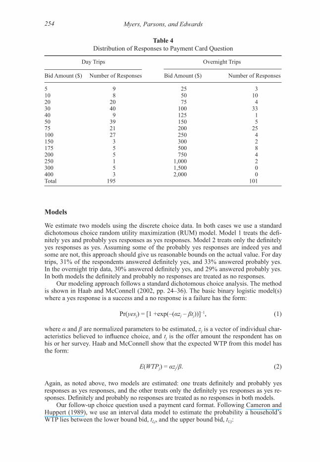
Again, as noted above, two models are estimated: one treats definitely and probably yes responses as yes responses, and the other treats only the definitely yes responses as yes re-sponses. Definitely and probably no responses are treated as no responses in both models. Our follow-up choice question used a payment card format. Following Cameron and Huppert (1989), we use an interval data model to estimate the probability a household’s WTP lies between the lower bound bid, tLj, and the upper bound bid, tUj:

Table 4Distribution of Responses to Payment Card Question

Day Trips Overnight Trips

Bid Amount ($) Number of Responses Bid Amount ($) Number of Responses

5 9 25 310 8 50 1020 20 75 430 40 100 3340 9 125 150 39 150 575 21 200 25100 27 250 4150 3 300 2175 5 500 8200 5 750 4250 1 1,000 2300 5 1,500 0400 3 2,000 0Total 195 101

Shorebird Valuation 255

Pr(WTPj ⊆ (tLj, tUj)) = Pr((tLj – αzj) < nj < (tUj + αzj)), (3)

where nj is a standard normal variable, and α is a vector of normalized parameters to be estimated. The probability in equation (3) can be rewritten as the difference between two cumulative standard normal distribution functions and the parameters estimated using standard interval data regression. Mean WTP in the grouped data model has the form:

E(WTPj) = αzj. (4)

Our results for all models are presented in the following section.

Results

Discrete Choice Models

Table 5 presents results for the two discrete choice models. Model 1 treats the definitely yes and probably yes response as yes, and Model 2 treats only the definitely yes respons-es as yes. Definitely no and probably no responses are treated as no in both models. The recoding of the discrete choice responses in Model 2 was designed to address the issue of hypothetical bias. In Blumenschein et al. (1998) for example, the contingent valuation responses were recoded in a similar fashion and provided results that mirrored an actual payment treatment. The day and overnight models are shown in table 5. In both models we introduce covariates that we believed would have an effect on WTP. The variables WS, EQUIP, and CLUB are measures of birding intensity. WS is a dummy variable that indicates the respondent made a trip to Delaware to view a rare siting of a wood sand-piper, EQUIP is the current market value of household birding equipment, and CLUB is a dummy variable that indicates whether or not the respondent belongs to a local birding society.5 PM is a dummy variable for surveys handed out at Port Mahon to test for sensi-tivity to sampling site, NIGHTS is the number of nights a person spent in the area while on an overnight birding trip, and INCOME is household income. Table 6 provides defini-tions and descriptive statistics for all of these variables. The coefficient on BID is negative and significant in all models. As expected, the size of the constant term in Model 2 is lower than in Model 1 due to fewer responses coded as yes. The coefficients on CLUB, EQUIP, and INCOME show some statistical significance across the models, but not in all cases. There appears to be no difference in WTP between those sampled at Port Mahon versus Mispillion Harbor, since the coefficient on PM shows no statistical significance. And finally, the number of NIGHTS a person spends on a trip shows no significance in either overnight trip model. The mean welfare estimates for each specification are shown at the bottom of table 5. The mean values for Model 1 are $134/trip/household for day trips and $563/trip/house-hold for overnight trips. The values are considerably lower in Model 2 at $24 and $70. This is not surprising given that about 30% of the sample reported probably yes to the discrete choice question in both the day and overnight trip data. The probably yes responses may be due to a number of factors—uncertainty, ambiva-lence, or perhaps an unwillingness to commit (Ready, Whitehead, and Bloomquist 1995). In any case, we take the estimates from these two models as bounds over the actual val-

5 Prior to (but not during) the 2008 horseshoe crab/shorebird season there was a sighting of a rare bird species in the area—a wood sandpiper. Many bird watchers made trips specifically to see the wood sandpiper. We decided to include a variable WS (WS = 1 if you had viewed the sandpiper) as a measure of a person’s birding intensity. It had no significance in any of the day trip models, and no one in the overnight model had viewed the bird.

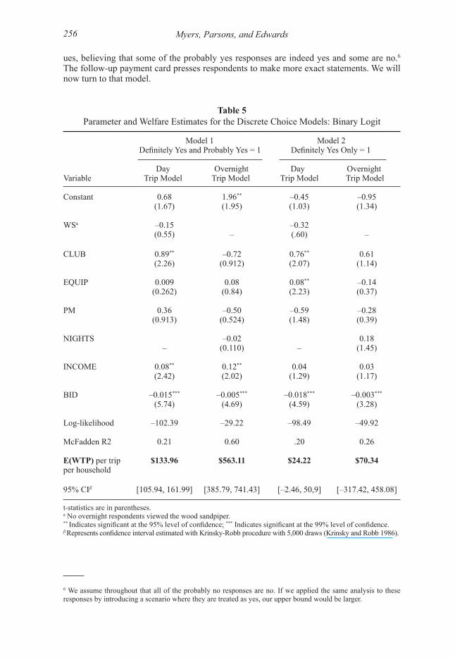
Myers, Parsons, and Edwards256

ues, believing that some of the probably yes responses are indeed yes and some are no.6 The follow-up payment card presses respondents to make more exact statements. We will now turn to that model.

6 We assume throughout that all of the probably no responses are no. If we applied the same analysis to these responses by introducing a scenario where they are treated as yes, our upper bound would be larger.

Table 5 Parameter and Welfare Estimates for the Discrete Choice Models: Binary Logit

Model 1 Model 2 Definitely Yes and Probably Yes = 1 Definitely Yes Only = 1

Day Overnight Day Overnight Variable Trip Model Trip Model Trip Model Trip Model

Constant 0.68 1.96** –0.45 –0.95 (1.67) (1.95) (1.03) (1.34)

WSa –0.15 –0.32 (0.55) – (.60) –

CLUB 0.89** –0.72 0.76** 0.61 (2.26) (0.912) (2.07) (1.14)

EQUIP 0.009 0.08 0.08** –0.14 (0.262) (0.84) (2.23) (0.37)

PM 0.36 –0.50 –0.59 –0.28 (0.913) (0.524) (1.48) (0.39)

NIGHTS –0.02 0.18 – (0.110) – (1.45)

INCOME 0.08** 0.12** 0.04 0.03 (2.42) (2.02) (1.29) (1.17)

BID –0.015*** –0.005*** –0.018*** –0.003***

(5.74) (4.69) (4.59) (3.28)

Log-likelihood –102.39 –29.22 –98.49 –49.92

McFadden R2 0.21 0.60 .20 0.26

E(WTP) per trip $133.96 $563.11 $24.22 $70.34per household

95% CIβ [105.94, 161.99] [385.79, 741.43] [–2.46, 50,9] [–317.42, 458.08]

t-statistics are in parentheses.a No overnight respondents viewed the wood sandpiper.** Indicates significant at the 95% level of confidence; *** Indicates significant at the 99% level of confidence.β Represents confidence interval estimated with Krinsky-Robb procedure with 5,000 draws (Krinsky and Robb 1986).

Shorebird Valuation 257

Payment Card Models

Table 7 presents the results from the interval data model using the payment card data. NIGHTS and INCOME show some statistical significance across the models. We also investigated whether or not anchoring might play a role in the payment card responses by using BID as an explanatory variable. A positive and significant coefficient suggests that there indeed is some evidence of anchoring in the day trip model—the higher the offer amount in the discrete choice question, the higher the circled payment card amount. The WTP estimates are shown at the bottom of table 7. The first row does not correct for an-choring, but the second does by setting DC_BID = 0 in the simulation across the sample. This correction gives the lowest possible anchor and thus a lower bound estimate. The values are $78.71 per trip per household for day trips and $228.04 for overnight trips without the correction. With the correction, the values drop to $66.01 and $201.54. Table 8 shows the consistency between our discrete choice and payment card re-sponses. The third column shows the percent of respondents, by type of discrete choice response, that had inconsistent payment card responses or, put differently, reversed their discrete choice response in their payment card response. One would expect these percent-ages to be low for the definitely yes and definitely no groups, and they are. They are also low for the probably no responses, but the probably yes group shows a large reversal. As we said at the outset, we expected that some of these probably yes responses would indeed be true yes responses and some would be true no responses. If you believe the payment card data, it appears as though 25% of the probably yes responses are no in the day trip data and 23% are no in overnight model. Table 9 presents a dichotomous choice model, where the probably yes responses to the discrete choice question are recoded to be consistent with the payment card response. The WTP values are $96/trip/household for day trips and $429/trip/household for overnight trips (2008$). Again, these fall be-tween the results for Models 1 and 2 in previous section. The adjusted day trip value is

Table 6Descriptive Statistics by Trip Type

Mean Standard Deviation

Variable Definition Day Overnight Day Overnight

WS 1 if the respondent viewed 0.125 – 0.331 – the wood sandpiper; 0 otherwise

CLUB 1 if the respondent belongs to 0.535 0.627 0.500 0.485 a birding club/society; 0 otherwise

EQUIP Current market value of birding 3.809 4.382 6.326 7.173 equipment (divided by $1,000)

PM 1 if the respondent received the 0.310 0.200 0.464 0.402 survey at Port Mahon; 0 otherwise

NIGHTS Number of nights spent in the – 2.56 – 1.993 area (overnight model only)

INCOME Mid-point of income range 10.52 12.34 6.76 7.99 (divided by $10,000)

BID Offered amount from survey 90.02 581.22 81.74 683.03

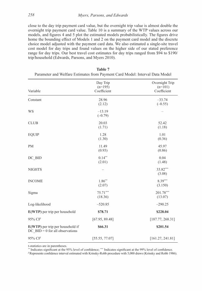
Myers, Parsons, and Edwards258

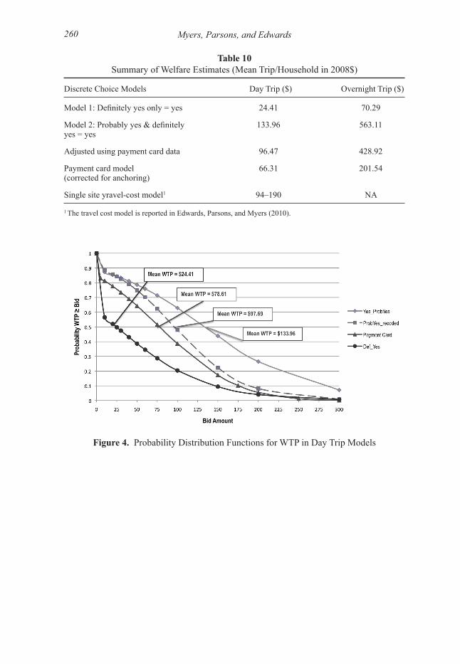
close to the day trip payment card value, but the overnight trip value is almost double the overnight trip payment card value. Table 10 is a summary of the WTP values across our models, and figures 4 and 5 plot the estimated models probabilistically. The figures drive home the bounding effect of Models 1 and 2 on the payment card model and the discrete choice model adjusted with the payment card data. We also estimated a single-site travel cost model for day trips and found values on the higher side of our stated preference range for day trips. Our best travel cost estimates for day trips ranged from $94 to $190/trip/household (Edwards, Parsons, and Myers 2010).

Table 7Parameter and Welfare Estimates from Payment Card Model: Interval Data Model

Day Trip Overnight Trip (n=195) (n=101)Variable Coefficient Coefficient

Constant 28.96 –33.74 (2.12) (–0.55)

WS –13.19 – (–0.79) CLUB 20.03 52.42 (1.71) (1.18)

EQUIP 1.28 1.01 (1.30) (0.36)

PM 11.49 45.97 (0.93) (0.86)

DC_BID 0.14** 0.04 (2.01) (1.48)

NIGHTS – 33.82***

(3.08)

INCOME 1.86** 8.39***

(2.07) (3.150)

Sigma 75.71*** 201.78***

(18.36) (13.07)

Log-likelihood –520.85 –290.25

E(WTP) per trip per household $78.71 $228.04

95% CIβ [67.95, 89.48] [187.77, 268.31]

E(WTP) per trip per household if $66.31 $201.54DC_BID = 0 for all observations

95% CIβ [55.55, 77.07] [161.27, 241.81]

t-statistics are in parentheses.** Indicates significant at the 95% level of confidence; *** Indicates significant at the 99% level of confidence.β Represents confidence interval estimated with Krinsky-Robb procedure with 5,000 draws (Krinsky and Robb 1986).

Shorebird Valuation 259

Table 8Consistency of Payment Card and Discrete Choice Responses

Response to Total Number Number of Reversals onDiscrete Choice of Responses Payment Card Response1 Percent of Total

Day Trip ModelDefinitely Yes 61 3 5Probably yes 63 16 25Probably No 52 1 2Definitely No 19 0 0Total 195 20 10

Overnight Trip ModelDefinitely Yes 27 2 7Probably yes 31 7 23Probably No 22 0 0Definitely No 21 0 0Total 101 9 91 A reversal occurs when a payment card response is inconsistent with a discrete choice response. For example, if a person replies ‘probably yes’ to making a trip at a $50 increase in trip cost on the discrete choice question, and then circles $25 in the payment card question as the maximum amount she would pay and still make the trip, there is an inconsistency or reversal of responses.

Table 9Parameter and Welfare Estimates from Adjusted Probably Yes Models: Binary Logit

Day Trip (n=195) Overnight Trip (n=101)Variable Coefficient Coefficient

Constant 0.44 0.98 (1.04) (1.19)WS –0.85 – (–1.55) CLUB 1.30*** 0.58 (3.15) (0.92)EQUIP 0.02 0.02 (0.68) (0.44)PM 0.19 –0.51 (0.46) (–0.68)NIGHTS – 0.003 (0.02)INCOME 0.10*** 0.05 (2.89) (1.28)BID –0.02*** –0.004***

(–6.07) (–4.29)Log-likelihood –92.11 –37.03McFadden R2 0.31 0.47E(WTP) per trip per household $96.47 $428.9395% CIβ [79.36,113.58] [267.67, 590.19]

t-statistics are in parentheses. *** Indicates significant at the 99% level of confidence.β Represents confidence interval estimated with Krinsky-Robb procedure with 5,000 draws (Krinsky and Robb 1986).

Myers, Parsons, and Edwards260

Table 10 Summary of Welfare Estimates (Mean Trip/Household in 2008$)

Discrete Choice Models Day Trip ($) Overnight Trip ($) Model 1: Definitely yes only = yes 24.41 70.29

Model 2: Probably yes & definitely 133.96 563.11yes = yes

Adjusted using payment card data 96.47 428.92

Payment card model 66.31 201.54(corrected for anchoring)

Single site yravel-cost model1 94–190 NA

1 The travel cost model is reported in Edwards, Parsons, and Myers (2010).

Figure 4. Probability Distribution Functions for WTP in Day Trip Models

Shorebird Valuation 261

Figure 5. Probability Distribution Functions for WTP in Overnight Trip Model

Aggregate Welfare Estimate

To compute aggregate welfare estimates, we used information obtained onsite (number of surveys distributed, repeats, refusals, and hours sampled) during the sampling days to predict the total number of household visitation days over the season. We used two differ-ent approaches that produce similar results. The first assumes a constant hourly visitation rate equal to the average visitation rates we observed while sampling. We separate the rates by weekday and weekend and by the two primary sites. The weekday rates for Port Mahon and Mispillion Harbor are 1.6 and 1.9 households per hour. The weekend rates are 3.8 and 4.9. These rates are adjusted to account for people visiting both sites. Assuming 14 hours of daylight each day, 28 weekdays, and 7 weekend days at each site over the season, we estimate 3,092 household birding days to view the horseshoe crab/shorebird occurrence. This includes a day on site during a day trip or an overnight trip. Weather conditions were variable across the season, but different conditions were represented in our sample means. In our second approach we used data gathered by the staff at the DuPont Nature Cen-ter at Mispillion Harbor. The DuPont staff keeps a daily log of the number of visitors to the center (bird watchers, family trips, stop-ins, etc.). If bird watchers are a constant share of the full visitation rate, we should be able to use the correlation between our count of visit days and their visitation rates to predict visit days to view birds on the days we did not sample. We use a simple linear regression of our household visit days (HHDaysi) re-gressed on the Nature Center count data (xi) over the 11 days we sampled:

HHDaysi = α + βxi + εj, (5)

where i denotes one of our 11 sample days. The estimates are shown in table 11 for both sites. The Mispillion Harbor regression gives a sharper estimate than the Port Mahon regression. This is no surprise, since the DuPont Nature Center, where the visitation data are gathered, is located at Mispillion Harbor. For each day we did not sample, we used equation (5) to predict the number of household days at Mispillion Harbor and Port Mahon using the visit count reported by the Center for that day. Using this approach we

Myers, Parsons, and Edwards262

estimate that there were 3,363 household days to view the shorebird migration in 2008, slightly higher than our first approach that uses simple average rates. Using the household per day trip WTP estimate from the payment card model ($78) and assuming 3,363 household days (near the mean of the two approaches we used), we calculated the aggregate seasonal value of birding during the annual spring migration near $263 thousand (2008$). This assumes a day on site is valued the same if it is on a day or overnight trip. Assuming the estimated benefits accrue indefinitely over time with no growth or decline in visitation and using a discount rate of 3%, the estimated asset value of the sites for bird watching during the six weeks of the horseshoe crab/shorebird occur-rence is approximately $8.8 million (2008$). This ignores any use value for households that visit other sites without visiting Port Mahon or Mispillion Harbor. We may overstate the value to some extent by using a somewhat longer average season (six weeks) than may actually be observed each year. We performed a sensitivity analysis over the discount rate (1, 3, 4, and 5%) and visitation growth rate (0, 4.5, and 6%) to generate a range of plausible asset values. The ranges of growth rates are based on findings in Leeworthy et al. (2005). The asset value ranges from as low as $5 million to near $95 million depend-ing on the visitation growth rate and discount rate used. All of these values ignore nonuse and other uses of the resource areas.

Table 11Prediction Equation for Days on Site by Site of Intercept

Coefficients Mispillion Harbor Port Mahon

α 19.28 27.77 (2.34) (2.59)

β 0.36 0.22 (4.92) (1.59)

N = days on site 11 11

t-statistics in parentheses.

Conclusion

Using an onsite intercept survey of 370 recreational birders who visited the Delaware Bay during the 2008 horseshoe crab/shorebird migration, we collected stated preference data and estimate household WTP for bird watching trips. Our best estimates are $66–$96/trip/household for a day trip and $201–$428/trip/household for an overnight trip. Using an average household size of 1.66 in our sample, our values per person are about $40–$60 for day trips and $120–$250 for overnight trips. For some context, estimates from four other studies report values that vary from $63 to $442/trip/person. These studies vary in method and specific birding populations studied and mix day and overnight trips. All values are in 2008$. We also calculated the aggregate seasonal value of birding during the annual spring migration at near $263 thousand (2008$). Using different discount rates and growth rates for number of trips, the asset values varied from a low estimate of $5 million to a high estimate of $95 million. These ignore nonuse values and other values associated with using the resource area. We used two valuation questions in our analysis—discrete choice followed by a pay-ment card. The easier, less precise discrete choice question was used, in part, as a set up

Shorebird Valuation 263

for the more difficult, but more precise, payment card. The discrete choice response al-lowed people to respond definitely or probably yes and definitely or probably no. When we treated probably yes responses as certain yes responses in a dichotomous choice mod-el, the results gave estimates greater than the payment card values. When we treated the probably yes responses as certain no responses, the results were lower than the payment card values. Assuming some of the probably yes responses were indeed yes and some no, this is the outcome one would expect. Finally, when we recoded the probably yes responses as a certain yes or certain no to be consistent with the payment card responses, the discrete choice logit models gave values close to the payment card results.

References

Aiken, R. 2009. Net Economic Values of Wildlife-Associate Recreation: Addendum to the 2006 National Survey of Fishing, Hunting and Wildlife-Associate Recreation. U.S. Fish and Wildlife Service Report 2006–5. Washington, D.C.

Blumenschein, K., G.C. Bloomquist, M. Johannassen, N. Horn, and P. Freeman. 1998. Experimental Results on Expressed Certainty and Hypothetical Bias in Contingent Valuation. Southern Economic Journal 118(1):114–37.

Boyle, K.J., B. Roach, and D.B. Waddington. 1998. 1996 Net Economic Values for Bass, Trout and Walleye Fishing, Deer, Elk, and Moose Hunting and Wildlife Watching: Addendum to the 1996 National Survey of Fishing, Hunting and Wildlife-Associated Recreation. U.S. Fish and Wildlife Service Report 96–2. Washington, D.C.

Cameron, T.A., and D.D. Huppert. 1989. OLS versus ML Estimation of Nonmarket Resource Values with Payment Card Interval Data. Journal of Environmental Eco-nomics and Management 17:230–46.

Clayton, C., and R. Mendelsohn. 1993. The Value of Watchable Wildlife: A Case Study of McNeil River. Journal of Environmental Management 39:101–06.

Cooper, J., and J. Loomis. 1991. Economic Value of Wildlife Resources in the San Joaquin Valley: Hunting and Viewing Values. The Economics and Management of Water and Drainage in Agriculture, A. Dinar and D. Zilberman, eds., pp. 447–62. Boston, MA: Kluwer Academic Publishers.

Edwards, P., G. Parsons, and K. Myers. Under Review. The Economic Value of Migra-tory Shorebirds on the Delaware Bay: An Application of the Single Site Travel Cost Model Using Onsite Data. Human Dimensions of Wildlife.

Eubanks, T., R.B. Ditton, and J. Stoll. 1998. The Economic Impact of Wildlife Watching on the Platte River in Nebraska. Report prepared by Fermata, Inc., Houston, TX.

Eubanks, T., and J. Stoll. 2000. Wildlife-Associated Recreation on the New Jersey Dela-ware Bayshore. Report prepared by Fermata, Inc., Houston, TX.

Gürlük, S., and E. Rehber. 2007. A Travel Cost Study to Estimate Recreational Value for a Bird Refuge at Lake Manyas, Turkey. Journal of Environmental Management 88:1350–60.

Haab, T., and K. McConnell. 2002. Valuing Environmental and Natural Resources: Econometrics of Non-Market Valuation. Cheltenham, UK: Edward Elgar.

Hvengaard, G.T., J.R. Butler, and D.K. Krystofiak. 1989. Economic Values of Bird Watching at Point Pelee National Park, Canada. Wildlife Society Bulletin 17:526–31.

Krinsky, I., and A. Robb. 1986. On Approximating the Statistical Properties of Elastici-ties. The Review of Economics and Statistics 86:715–19.

Leeworthy, R., J. Bowker, J. Hospital, and E. Stone. 2005. Projected Participation in Ma-rine Recreation: 2005 & 2010 National Survey on Recreation and the Environment 2000. US Department of Commerce. National Oceanic and Atmospheric Administra-tion, National Ocean Service. Special Projects. Silver Spring, MD.

Loomis, J.B., and D.S. White. 1996. Economic Benefits of Rare and Endangered Species: Summary and Meta-analysis. Ecological Economics 18:197–206.

Myers, Parsons, and Edwards264

New Jersey Department of Environmental Protection (NJDEP). 2007. Status of the Red Knot in the Western Hemisphere. Report prepared for U.S. Fish and Wildlife Service, Pleasantville, NJ.

Ready, R., J. Whitehead, and G. Bloomquist. 1995. Contingent Valuation when Re-spondents are Ambivalent. Journal of Environmental Economics and Management 29:181–96.

Richardson, L., and J.B. Loomis. 2008. The Total Economic Value of Threatened, En-dangered and Rare Species: An Updated Meta-analysis. Ecological Economics 68:1535–48.

U.S. Census Bureau, News Room: Press Releases (n.d.). 2008. Retrieved Feb-ruary 9 from <http://www.census.gov/PressRelease/www/releases/archives/income_wealth/012528.html>.