Opleiding Natuur- en Sterrenkunde

Measurements on electrical properties ofwater while acoustically levitated

Bachelor Thesis

Allard Kors Veenstra

Supervisors:

Dr. S. FaezDebye Institute

B. Yeroshenko MScDebye Institute

January 16, 2019

Abstract

With the use of an acoustic levitator, I remotely measured the capacitance of water,with the idea of obtaining the dielectric constant. A water droplet was trapped insidethe central node of the acoustic field and its capacitance measured, the field was thenturned on and off to allow the measurement of the electrodes without the water andto calculate the difference. The capacitance was measured with the help of a self buildLC-circuit that relies on the resonance between a capacitor and inductor. To verifymeasurements a Fluke PM6306 RCL-meter was used with the same measurement rou-tine. Resistance was also measured using the same RCL-meter at different frequenciesand salt concentrations to see the effect on the resistivity. The droplet was placed atthe same node and two small electrodes were brought into the droplet on either side.

i

CONTENTS ii

Contents

1 Introduction 1

2 Theory 22.1 Complex way of writing impedance . . . . . . . . . . . . . . . . . . . . . . . 22.2 Ways of measuring capacitance . . . . . . . . . . . . . . . . . . . . . . . . . 32.3 Parasitic capacitance . . . . . . . . . . . . . . . . . . . . . . . . . . . . . . . 5

3 Experiment 63.1 Acoustic trap . . . . . . . . . . . . . . . . . . . . . . . . . . . . . . . . . . . 63.2 Electrodes . . . . . . . . . . . . . . . . . . . . . . . . . . . . . . . . . . . . . 63.3 Apparatus . . . . . . . . . . . . . . . . . . . . . . . . . . . . . . . . . . . . . 73.4 Measuring capacitance . . . . . . . . . . . . . . . . . . . . . . . . . . . . . . 8

3.4.1 Capacitance with distance . . . . . . . . . . . . . . . . . . . . . . . . 103.4.2 Capacitance of a water droplet . . . . . . . . . . . . . . . . . . . . . 11

3.5 Measuring resistance . . . . . . . . . . . . . . . . . . . . . . . . . . . . . . . 11

4 Results and discussion 124.1 Capacitance . . . . . . . . . . . . . . . . . . . . . . . . . . . . . . . . . . . . 12

4.1.1 Distance dependence . . . . . . . . . . . . . . . . . . . . . . . . . . . 124.1.2 Measurements with water . . . . . . . . . . . . . . . . . . . . . . . . 13

4.2 Resistance . . . . . . . . . . . . . . . . . . . . . . . . . . . . . . . . . . . . . 174.3 Schering bridge . . . . . . . . . . . . . . . . . . . . . . . . . . . . . . . . . . 18

5 Conclusion 20

6 References 21

A Appendix 22

1 INTRODUCTION 1

1 Introduction

The use of an acoustic levitator allows us to measure properties of materials without touchingthem. This technique has gotten a big boost with the advent of 3D-printers, allowing peopleto more easily and cheaply build them [1]. Because liquids take the shape of the containerthey are in, measurements on a liquid without deforming the surface are hard to do. Alevitated droplet will take the shape of a sphere or oblate spheroid since this is the shapewith the lowest surface area to volume ratio. In liquids there is a disconnection betweenbulk and surface charge, changing one of them alters the electrical properties of the liquid.Because when a drop is levitated it hardly has any outside interference. Thus the electricaleffects can be studied without having to account for discrepancies at a boundary of anothermaterial. Things to measure are the complex impedance which can lead us to expressionsfor the carrier density, charge mobility, Debye length or dielectric constant. Two types ofmeasurements are done, one measurement of the capacitance to obtain the dielectric constantand another to measure the resistance and obtain conductivity.

Measuring the capacitance is done by floating a droplet in the acoustic levitator. Firstmeasuring the capacitance with a droplet between two electrodes and later measuring thecapacitance with out the liquid in between. Subtracting the two values will give us thecapacitance of the droplet. Consequently measuring the capacitance allows for a measurementof the dielectric constant of that liquid. Two ways of measuring the capacitance are exploredin this thesis, using a Schering bridge or with a LC-circuit, the self-build devices are alsochecked with a more conventional RCL-meter. The Schering bridge works on the principleof balancing two arms of a parallel circuit and the LC-circuit on the resonance frequencythat exists when a capacitor and inductor are in the same circuit. I measured the resistanceby placing two small electrode points on either side of the droplet while it is levitated. Theresistance is measured at different frequencies and salt concentrations to see the effect ofthese changes. Especially changing the salt concentration is interesting since this changesthe bulk properties of the liquid. The resistance is measured with the RCL-meter.

Following are, first a section of theory on how capacitance can be measured, then a sectionabout the instruments and set-up that was used. Finally the results will be packed in withthe discussion.

2 THEORY 2

2 Theory

Unless referenced otherwise all information in the theory section comes from the book: Theart of electronics by Paul Horowitz and Winfield Hill[2]

2.1 Complex way of writing impedance

A capacitor(C) consists of two conductors closely separated by an insulator. Putting a voltageacross the two conductors charges the capacitor with a charge Q on one side and -Q on theother. This leads to the familiar equation: Q = CV with C a constant that depends onthe shape of the capacitor and the dielectric constant of the material in between. There isa simple equation for the capacity of two parallel plates of surface area A with distance dbetween them,

C =εA

d. (1)

With ε the absolute permittivity which can be written as, ε = ε0εr with ε0 the permittivityof a vacuum ( 8.85× 10−12Fm−1[3] ) and εr the relative permittivity.

Because current is a change of charge over time, if we take the derivative of Q = CV weget: I(t) = C dV

dt. If the current were to be oscillating as I(t) = I0 sin (ωt), then by equating

these two we get: dVdt

= I0 sin (ωt)C

. Integrating this gives us equation 2 which can be used tofind something that resembles a resistance in equation 3, this is called the reactance. Whatcan also be seen from the equation for voltage and current is that the current is 90 aheadof the voltage. A similar relation holds true for an inductor only with voltage ahead of thecurrent and a different reactance.

V (t) = −I0 cos (ωt)

Cω(2)

Xc =|V ||I|

=I0ωC

I0=

1

ωC(3)

As can be seen from the above formulations we have to solve differential equations toexplain the behaviour of capacitors. The same holds for inductors, thus circuits with these el-ements in them have increasingly harder differential equations to solve. To combat this prob-lem it is easier to write them in a complex form and use something called the Impedance(Z),this is the generalized resistance. Because capacitors and inductors have a 90 phase shiftbetween voltage and current they are reactive and have a reactance(X). Resistors have volt-age and current in phase and are resistive, they have a resistance(R). The impedance is:impedance = resistance + reactance or Z = R + jX, with j the imaginary number.

The voltage and current can also be written as complex numbers, V (t) = V0 cos (ωt+ φ) =V0<(ej(ωt+φ)). This, combined with the impedance allows us to use a more general formof Ohm’s law on every circuit containing linear components like resistors, capacitors and

2 THEORY 3

inductors. The impedance for the various components are,

ZR = R (4)

ZL = jωL (5)

ZC =1

jωC. (6)

Knowing this we can more easily get the equations that describe the circuits that wereused.

2.2 Ways of measuring capacitance

Two ways of measuring capacitance were tested in the experiments: a resonant frequency-and a bridge balancing-circuit. The resonance frequency circuit works on the principle thatwhen a inductor and capacitor are in parallel there is a frequency were the impedance goesto infinity.

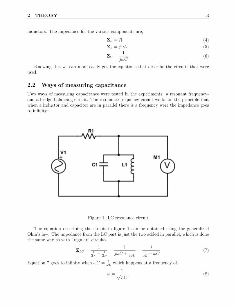
Figure 1: LC resonance circuit

The equation describing the circuit in figure 1 can be obtained using the generalizedOhm’s law. The impedance from the LC part is just the two added in parallel, which is donethe same way as with ”regular” circuits.

ZLC =1

1ZL

+ 1ZC

=1

jωC + 1jωL

=j

1ωL− ωC

(7)

Equation 7 goes to infinity when ωC = 1ωL

which happens at a frequency of,

ω =1√LC

. (8)

2 THEORY 4

At this frequency the measured voltage will spike and using a known inductor the capacitancecan be calculated from the obtained frequency.

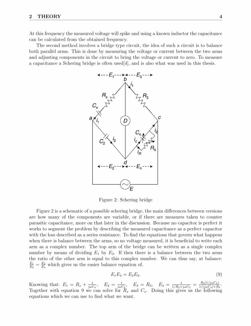
The second method involves a bridge type circuit, the idea of such a circuit is to balanceboth parallel arms. This is done by measuring the voltage or current between the two armsand adjusting components in the circuit to bring the voltage or current to zero. To measurea capacitance a Schering bridge is often used[4], and is also what was used in this thesis.

Figure 2: Schering bridge

Figure 2 is a schematic of a possible schering bridge, the main differences between versionsare how many of the components are variable, or if there are measures taken to counterparasitic capacitance, more on that later in the discussion. Because no capacitor is perfect itworks to segment the problem by describing the measured capacitance as a perfect capacitorwith the loss described as a series resistance. To find the equations that govern what happenswhen there is balance between the arms, so no voltage measured, it is beneficial to write eacharm as a complex number. The top arm of the bridge can be written as a single complexnumber by means of dividing E1 by E3. If then there is a balance between the two armsthe ratio of the other arm is equal to this complex number. We can thus say, at balance:E1

E3= E2

E4which gives us the easier balance equation of,

E1E4 = E2E3. (9)

Knowing that: E1 = Rx + 1jωCx

, E2 = 1jωC2

, E3 = R3, E4 = 11/R4+jωC4

= R4(1/jωC4)1/(jωC4)+R4

.Together with equation 9 we can solve for Rx and Cx. Doing this gives us the followingequations which we can use to find what we want.

2 THEORY 5

Rx = C4R3

C2

, Cx = R4C2

R3

(10)

2.3 Parasitic capacitance

As mentioned above, when dealing with circuits no component is perfect and each has alwaysa certain loss or side-effect associated with them. One of these side-effects is parasitic capac-itance, prevalent when there are two wires or other conducting material close to each otherwith alternating current flowing through them. Parasitic capacitance is proportional to thefrequency of the power source, just as with normal capacitance. The higher the frequencythe lower the impedance of such a capacitor which can lead to unwanted losses. The distancebetween the wires is very important as well, since this determines the constant C.

3 EXPERIMENT 6

3 Experiment

3.1 Acoustic trap

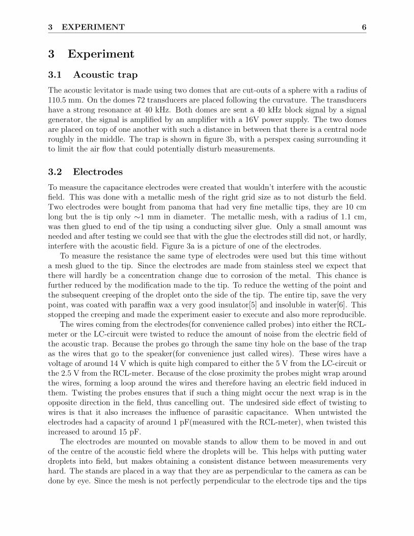
The acoustic levitator is made using two domes that are cut-outs of a sphere with a radius of110.5 mm. On the domes 72 transducers are placed following the curvature. The transducershave a strong resonance at 40 kHz. Both domes are sent a 40 kHz block signal by a signalgenerator, the signal is amplified by an amplifier with a 16V power supply. The two domesare placed on top of one another with such a distance in between that there is a central noderoughly in the middle. The trap is shown in figure 3b, with a perspex casing surrounding itto limit the air flow that could potentially disturb measurements.

3.2 Electrodes

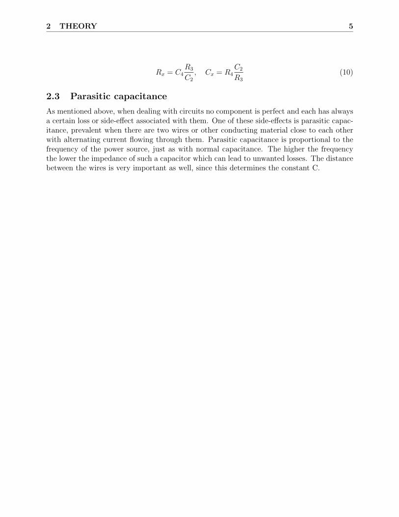
To measure the capacitance electrodes were created that wouldn’t interfere with the acousticfield. This was done with a metallic mesh of the right grid size as to not disturb the field.Two electrodes were bought from panoma that had very fine metallic tips, they are 10 cmlong but the is tip only ∼1 mm in diameter. The metallic mesh, with a radius of 1.1 cm,was then glued to end of the tip using a conducting silver glue. Only a small amount wasneeded and after testing we could see that with the glue the electrodes still did not, or hardly,interfere with the acoustic field. Figure 3a is a picture of one of the electrodes.

To measure the resistance the same type of electrodes were used but this time withouta mesh glued to the tip. Since the electrodes are made from stainless steel we expect thatthere will hardly be a concentration change due to corrosion of the metal. This chance isfurther reduced by the modification made to the tip. To reduce the wetting of the point andthe subsequent creeping of the droplet onto the side of the tip. The entire tip, save the verypoint, was coated with paraffin wax a very good insulator[5] and insoluble in water[6]. Thisstopped the creeping and made the experiment easier to execute and also more reproducible.

The wires coming from the electrodes(for convenience called probes) into either the RCL-meter or the LC-circuit were twisted to reduce the amount of noise from the electric field ofthe acoustic trap. Because the probes go through the same tiny hole on the base of the trapas the wires that go to the speaker(for convenience just called wires). These wires have avoltage of around 14 V which is quite high compared to either the 5 V from the LC-circuit orthe 2.5 V from the RCL-meter. Because of the close proximity the probes might wrap aroundthe wires, forming a loop around the wires and therefore having an electric field induced inthem. Twisting the probes ensures that if such a thing might occur the next wrap is in theopposite direction in the field, thus cancelling out. The undesired side effect of twisting towires is that it also increases the influence of parasitic capacitance. When untwisted theelectrodes had a capacity of around 1 pF(measured with the RCL-meter), when twisted thisincreased to around 15 pF.

The electrodes are mounted on movable stands to allow them to be moved in and outof the centre of the acoustic field where the droplets will be. This helps with putting waterdroplets into field, but makes obtaining a consistent distance between measurements veryhard. The stands are placed in a way that they are as perpendicular to the camera as can bedone by eye. Since the mesh is not perfectly perpendicular to the electrode tips and the tips

3 EXPERIMENT 7

(a)

One of the electrodes used to measure thecapacitance. The ones used to measure theresistance are the same model but with a

sharp point at the end.

(b)

The set-up with the acoustic trap, behind itis a heater mat not relevant for ourexperiment, the stands on which the

electrodes are attached are also visible thesilver coloured knobs allow the top part to

move. The electrodes are positioned in a waythat the led and the camera are on one line in

between the electrodes.

Figure 3

of the other kind of electrode are very thin it was assumed that a perfect 90 angle wasn’tnecessary. The 90 angle would be important because it allows the camera to determine thedistance between the electrodes more accurately. The distance between the electrodes wasmeasured by first calibrating a picture of a ruler and then converting the distance in pixelsinto meters. The ImageJ program was used for this task, using the plot profile function toget an accurate distance between marks on the ruler.

3.3 Apparatus

For the measurement of the capacitance a self-made device was used, a professional devicewas used to verify measurements and be able to get more accurate results. Two circuitswere made, a Schering bridge and a resonant LC-circuit, how these work is explained in the

3 EXPERIMENT 8

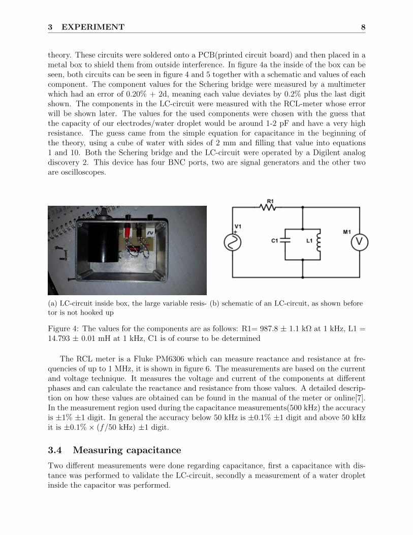
theory. These circuits were soldered onto a PCB(printed circuit board) and then placed in ametal box to shield them from outside interference. In figure 4a the inside of the box can beseen, both circuits can be seen in figure 4 and 5 together with a schematic and values of eachcomponent. The component values for the Schering bridge were measured by a multimeterwhich had an error of 0.20% + 2d, meaning each value deviates by 0.2% plus the last digitshown. The components in the LC-circuit were measured with the RCL-meter whose errorwill be shown later. The values for the used components were chosen with the guess thatthe capacity of our electrodes/water droplet would be around 1-2 pF and have a very highresistance. The guess came from the simple equation for capacitance in the beginning ofthe theory, using a cube of water with sides of 2 mm and filling that value into equations1 and 10. Both the Schering bridge and the LC-circuit were operated by a Digilent analogdiscovery 2. This device has four BNC ports, two are signal generators and the other twoare oscilloscopes.

(a) LC-circuit inside box, the large variable resis-tor is not hooked up

(b) schematic of an LC-circuit, as shown before

Figure 4: The values for the components are as follows: R1= 987.8 ± 1.1 kΩ at 1 kHz, L1 =14.793 ± 0.01 mH at 1 kHz, C1 is of course to be determined

The RCL meter is a Fluke PM6306 which can measure reactance and resistance at fre-quencies of up to 1 MHz, it is shown in figure 6. The measurements are based on the currentand voltage technique. It measures the voltage and current of the components at differentphases and can calculate the reactance and resistance from those values. A detailed descrip-tion on how these values are obtained can be found in the manual of the meter or online[7].In the measurement region used during the capacitance measurements(500 kHz) the accuracyis ±1% ±1 digit. In general the accuracy below 50 kHz is ±0.1% ±1 digit and above 50 kHzit is ±0.1%× (f/50 kHz) ±1 digit.

3.4 Measuring capacitance

Two different measurements were done regarding capacitance, first a capacitance with dis-tance was performed to validate the LC-circuit, secondly a measurement of a water dropletinside the capacitor was performed.

3 EXPERIMENT 9

(a) The Schering bridge, the large variable resistorshown in figure 4a is connected to this circuit viathe two wires coming out of it

(b) schematic of an Schering bridge, as shown be-fore

Figure 5: The values for the components are as follows: R3 = 295.2 ± 0.8 kΩ, C2 = 15 pF(could not be measured with multimeter), C4 = 68 pF (””), R4 is variable up to 300 kΩ

Figure 6: The RCL-meter with the electrodes hooked up, the twist in the wires is visible ontop of the device.

3 EXPERIMENT 10

3.4.1 Capacitance with distance

Because the distance between the two electrodes can be altered with a turning knob this wasused as a frame of reference to move the two plates together at a roughly consistent pace.Since this measurements is just to validate the LC-circuit and see if our mesh works as a platethe acoustic field was turned off. The electric signals to the speakers would just interferewith the measurements. Now a description of how a measurement is done, the initial part isshared among both the LC-circuit measurements and those with the RCL-meter.

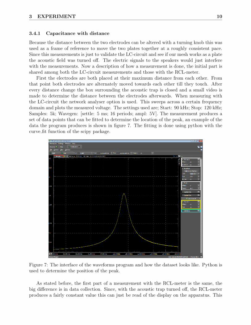
First the electrodes are both placed at their maximum distance from each other. Fromthat point both electrodes are alternately moved towards each other till they touch. Afterevery distance change the box surrounding the acoustic trap is closed and a small video ismade to determine the distance between the electrodes afterwards. When measuring withthe LC-circuit the network analyser option is used. This sweeps across a certain frequencydomain and plots the measured voltage. The settings used are; Start: 90 kHz; Stop: 120 kHz;Samples: 5k; Wavegen: [settle: 5 ms; 16 periods; ampl: 5V]. The measurement produces aset of data points that can be fitted to determine the location of the peak, an example of thedata the program produces is shown in figure 7. The fitting is done using python with thecurve fit function of the scipy package.

Figure 7: The interface of the waveforms program and how the dataset looks like. Python isused to determine the position of the peak.

As stated before, the first part of a measurement with the RCL-meter is the same, thebig difference is in data collection. Since, with the acoustic trap turned off, the RCL-meterproduces a fairly constant value this can just be read of the display on the apparatus. This

3 EXPERIMENT 11

greatly reduces measurement time. Since the RCL-meter can measure at different frequenciesa certain frequency has to be chosen to measure at. Some considerations have to be takeninto account when choosing such a frequency. Too low and the output might be too low to bereliably detected, since a capacitor can act like a high-pass filter. Using a high frequency willalso mitigate any potential interference with the 40 kHz signal from the speakers. For thosereasons 500 kHz was selected as the measuring frequency of choice. Because the uncertaintyof the device is known, data processing is straight forward.

Even though the Schering bridge was build it proved insufficient in measuring any data.A brief rundown of why the Schering bridge did not work can be found in the results anddiscussion section.

3.4.2 Capacitance of a water droplet

To measure the capacitance of a water droplet first a droplet is placed inside the acoustictrap, the electrodes are then brought into close proximity. After the doors are closed and apicture has been taken a measurement is done with either the LC-circuit or the RCL-meter.Because moving the wires from the electrodes slightly alters the measured capacitance it isbest to leave them be till after the complete measurement. Once the measurement is donethe acoustic field is turned off and the droplet will drop down. Put the field back on todo a second measurement, this time without the water droplet. Since no other things weretouched the only variable that has changed is whether there is a water droplet between thecapacitor plates. The measurements are then processed in a similar way as described above.

3.5 Measuring resistance

Measuring resistance is done with the electrodes without a plate glued to the end. Thismeasurement is done with the RCL-meter, this time using different frequencies to get thefrequency response of a water droplet. The measurement is repeated with different NaClconcentrations in demi water to also get the salinity dependence. The frequencies and saltconcentrations at which were measured are shown in table 1.

f (Hz) 50 100 200 400 800 1.2k 2.4k 5k 10k 25k 50k 70k 310k 570k 970kc(g/L) 200 50 20 10 1 0.1

Table 1: The different frequencies(f) and concentrations(c) measured at

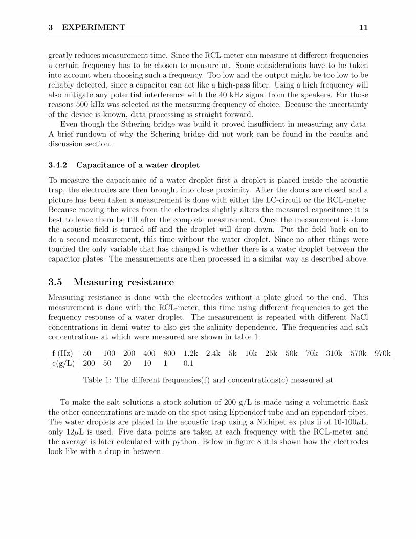
To make the salt solutions a stock solution of 200 g/L is made using a volumetric flaskthe other concentrations are made on the spot using Eppendorf tube and an eppendorf pipet.The water droplets are placed in the acoustic trap using a Nichipet ex plus ii of 10-100µL,only 12µL is used. Five data points are taken at each frequency with the RCL-meter andthe average is later calculated with python. Below in figure 8 it is shown how the electrodeslook like with a drop in between.

4 RESULTS AND DISCUSSION 12

Figure 8: Pictures taken during the measurement of 200 g/L.

4 Results and discussion

Due to errors made during the building of devices and being unsuccessful in measuring whatwas initially the plan the results and discussion will be written in tandem. The initial questionwas to measure the impedance and relate this to the surface and bulk charges but due to timeconcerns only test measurements were possible. Because the measurements of the resistancecame after the measurements of capacitance these are less accounted for. This is noticeablein both the method of measuring and what was measured, picking the data points more oninterest than relevance. These can be seen as test measurements.

The section about the Schering bridge is there because a lot of time was put into makingit, yet it did not work due to errors made in planning.

4.1 Capacitance

4.1.1 Distance dependence

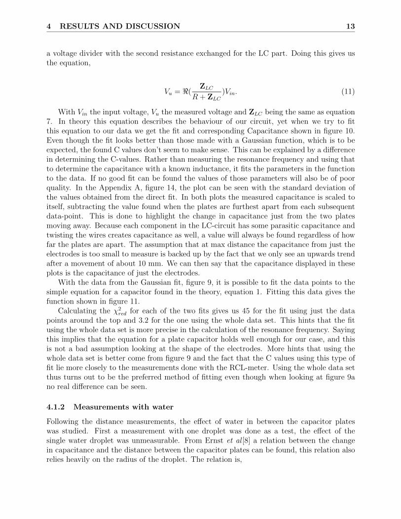
To validate the electrodes and the build LC-circuit the change in capacitance with distancewas measured. This was done in a procedure as stated in the experiment section. With theLC-circuit 27 measurements were taken, with the RCL-meter 21. During the measurementswith the RCL-meter an error was made while turning the knobs, this caused the measureddistances to be different with the LC-circuit. A plot of the data can be found in figure 9a,shown in the left picture is a fit made using a Gaussian function to find the position ofthe peak. Since all we need to measure is the x-position of the peak, it is possible to onlytake a data sample around the top. Both the method of taking all the data and only fromaround the top are tried. To find which one is better the data will later be fit to the functionfor a plate capacitor, equation 1. Another way of fitting would be to fit the data to thefunction that describes the circuit. This can be easily found since the LC-circuit is basically

4 RESULTS AND DISCUSSION 13

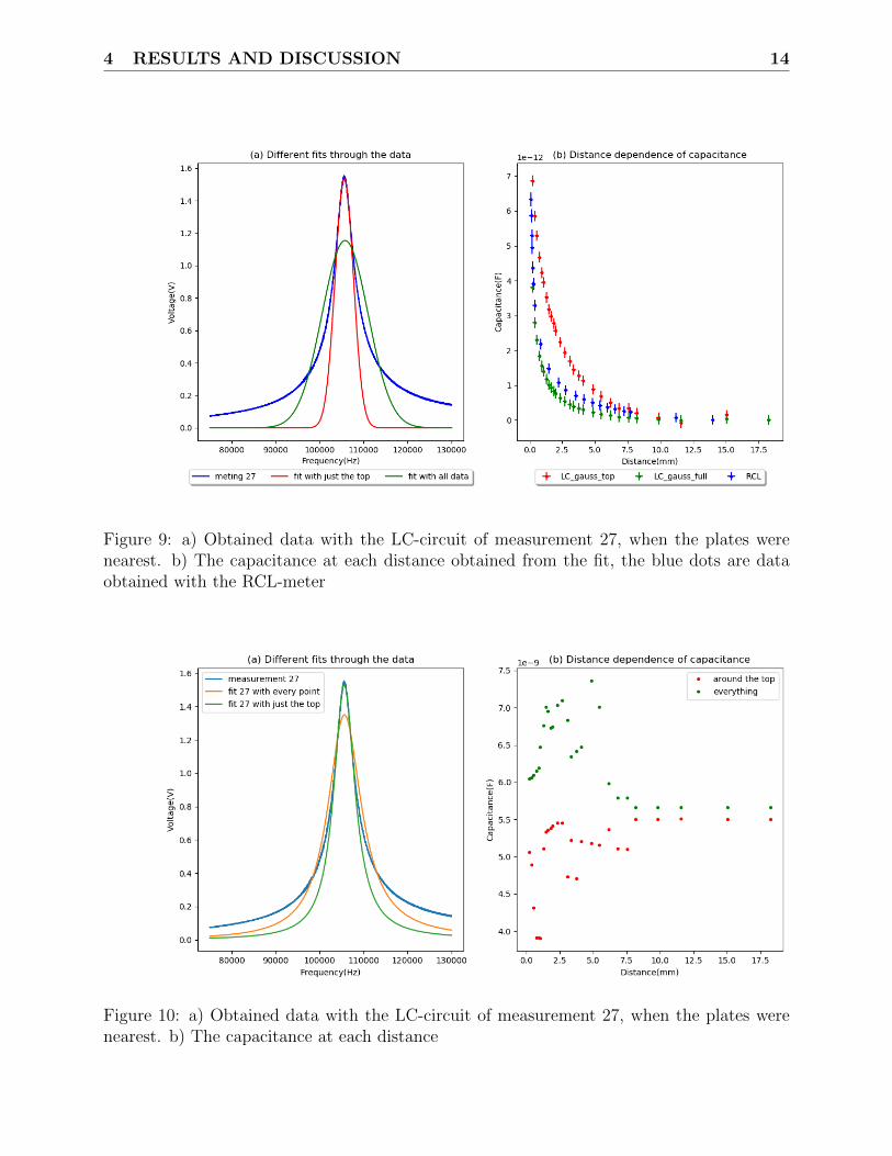
a voltage divider with the second resistance exchanged for the LC part. Doing this gives usthe equation,

Vu = <(ZLC

R + ZLC)Vin. (11)

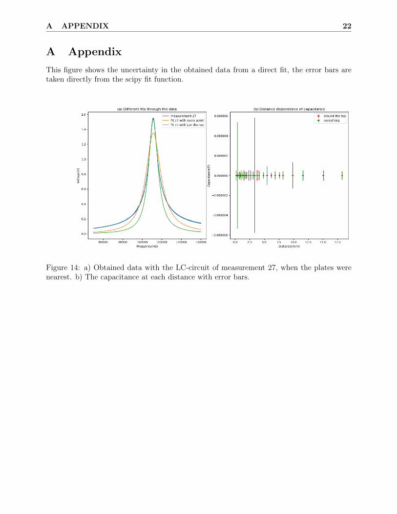
With Vin the input voltage, Vu the measured voltage and ZLC being the same as equation7. In theory this equation describes the behaviour of our circuit, yet when we try to fitthis equation to our data we get the fit and corresponding Capacitance shown in figure 10.Even though the fit looks better than those made with a Gaussian function, which is to beexpected, the found C values don’t seem to make sense. This can be explained by a differencein determining the C-values. Rather than measuring the resonance frequency and using thatto determine the capacitance with a known inductance, it fits the parameters in the functionto the data. If no good fit can be found the values of those parameters will also be of poorquality. In the Appendix A, figure 14, the plot can be seen with the standard deviation ofthe values obtained from the direct fit. In both plots the measured capacitance is scaled toitself, subtracting the value found when the plates are furthest apart from each subsequentdata-point. This is done to highlight the change in capacitance just from the two platesmoving away. Because each component in the LC-circuit has some parasitic capacitance andtwisting the wires creates capacitance as well, a value will always be found regardless of howfar the plates are apart. The assumption that at max distance the capacitance from just theelectrodes is too small to measure is backed up by the fact that we only see an upwards trendafter a movement of about 10 mm. We can then say that the capacitance displayed in theseplots is the capacitance of just the electrodes.

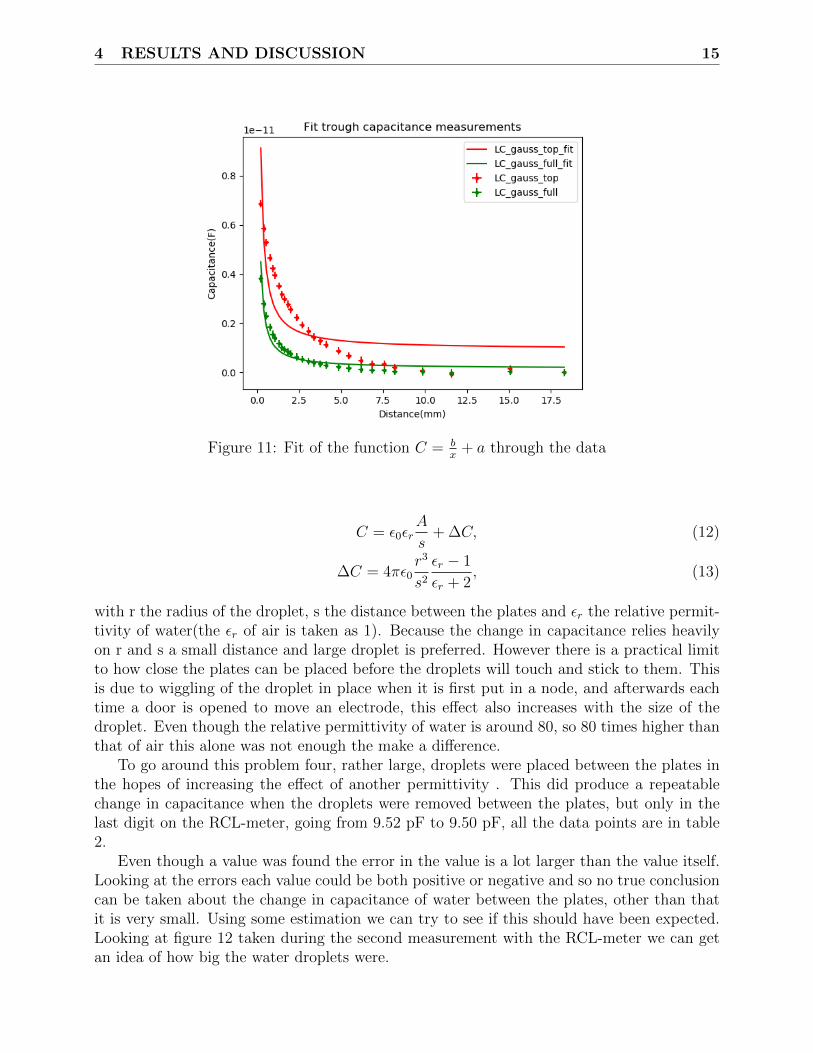
With the data from the Gaussian fit, figure 9, it is possible to fit the data points to thesimple equation for a capacitor found in the theory, equation 1. Fitting this data gives thefunction shown in figure 11.

Calculating the χ2red for each of the two fits gives us 45 for the fit using just the data

points around the top and 3.2 for the one using the whole data set. This hints that the fitusing the whole data set is more precise in the calculation of the resonance frequency. Sayingthis implies that the equation for a plate capacitor holds well enough for our case, and thisis not a bad assumption looking at the shape of the electrodes. More hints that using thewhole data set is better come from figure 9 and the fact that the C values using this type offit lie more closely to the measurements done with the RCL-meter. Using the whole data setthus turns out to be the preferred method of fitting even though when looking at figure 9ano real difference can be seen.

4.1.2 Measurements with water

Following the distance measurements, the effect of water in between the capacitor plateswas studied. First a measurement with one droplet was done as a test, the effect of thesingle water droplet was unmeasurable. From Ernst et al [8] a relation between the changein capacitance and the distance between the capacitor plates can be found, this relation alsorelies heavily on the radius of the droplet. The relation is,

4 RESULTS AND DISCUSSION 14

Figure 9: a) Obtained data with the LC-circuit of measurement 27, when the plates werenearest. b) The capacitance at each distance obtained from the fit, the blue dots are dataobtained with the RCL-meter

Figure 10: a) Obtained data with the LC-circuit of measurement 27, when the plates werenearest. b) The capacitance at each distance

4 RESULTS AND DISCUSSION 15

Figure 11: Fit of the function C = bx

+ a through the data

C = ε0εrA

s+ ∆C, (12)

∆C = 4πε0r3

s2εr − 1

εr + 2, (13)

with r the radius of the droplet, s the distance between the plates and εr the relative permit-tivity of water(the εr of air is taken as 1). Because the change in capacitance relies heavilyon r and s a small distance and large droplet is preferred. However there is a practical limitto how close the plates can be placed before the droplets will touch and stick to them. Thisis due to wiggling of the droplet in place when it is first put in a node, and afterwards eachtime a door is opened to move an electrode, this effect also increases with the size of thedroplet. Even though the relative permittivity of water is around 80, so 80 times higher thanthat of air this alone was not enough the make a difference.

To go around this problem four, rather large, droplets were placed between the plates inthe hopes of increasing the effect of another permittivity . This did produce a repeatablechange in capacitance when the droplets were removed between the plates, but only in thelast digit on the RCL-meter, going from 9.52 pF to 9.50 pF, all the data points are in table2.

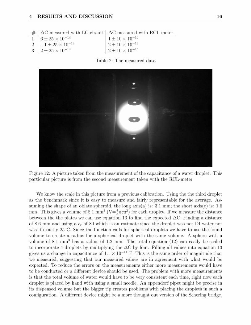
Even though a value was found the error in the value is a lot larger than the value itself.Looking at the errors each value could be both positive or negative and so no true conclusioncan be taken about the change in capacitance of water between the plates, other than thatit is very small. Using some estimation we can try to see if this should have been expected.Looking at figure 12 taken during the second measurement with the RCL-meter we can getan idea of how big the water droplets were.

4 RESULTS AND DISCUSSION 16

# ∆C measured with LC-circuit ∆C measured with RCL-meter1 6± 25× 10−14 1± 10× 10−14

2 −1± 25× 10−14 2± 10× 10−14

3 2± 25× 10−14 2± 10× 10−14

Table 2: The measured data

Figure 12: A picture taken from the measurement of the capacitance of a water droplet. Thisparticular picture is from the second measurement taken with the RCL-meter

We know the scale in this picture from a previous calibration. Using the the third dropletas the benchmark since it is easy to measure and fairly representable for the average. As-suming the shape of an oblate spheroid, the long axis(a) is: 3.1 mm; the short axis(c) is: 1.6mm. This gives a volume of 8.1 mm3 (V=4

3πca2) for each droplet. If we measure the distance

between the the plates we can use equation 13 to find the expected ∆C. Finding a distanceof 8.6 mm and using a εr of 80 which is an estimate since the droplet was not DI water norwas it exactly 25C. Since the function calls for spherical droplets we have to use the foundvolume to create a radius for a spherical droplet with the same volume. A sphere with avolume of 8.1 mm3 has a radius of 1.2 mm. The total equation (12) can easily be scaledto incorporate 4 droplets by multiplying the ∆C by four. Filling all values into equation 13gives us a change in capacitance of 1.1× 10−14 F. This is the same order of magnitude thatwe measured, suggesting that our measured values are in agreement with what would beexpected. To reduce the errors on the measurements either more measurements would haveto be conducted or a different device should be used. The problem with more measurementsis that the total volume of water would have to be very consistent each time, right now eachdroplet is placed by hand with using a small needle. An eppendorf pipet might be precise inits dispensed volume but the bigger tip creates problems with placing the droplets in such aconfiguration. A different device might be a more thought out version of the Schering bridge,

4 RESULTS AND DISCUSSION 17

or another device build for measuring very small capacitance.

4.2 Resistance

Before the measurements could begin a salt solution had to be created, this was done asdescribed above. Weighing 10 grams of NaCl using a Mettler P1210N and dissolving thisin an erlenmeyer with 40 mL of demi water. After dissolving, the solution was transferredto a 50 mL volumetric flask were it was brought op to 50 mL. During/after homogenizationsome solution was lost due to a bad cork, following this experiment we assume that theconcentration was not affected. If it was affected this would only be a systematic error inevery following solution and not a problem for a difference in concentration. The solutionof 200 g/L was made on the 13th of December and placed in a plastic container sealed withlaboratory wax. The actual measurements were done on the seventh of January, again theassumption is made that this does not alter the concentration in any significant way. Theconcentration should be high enough that any solvating gasses do not introduce a significantchange.

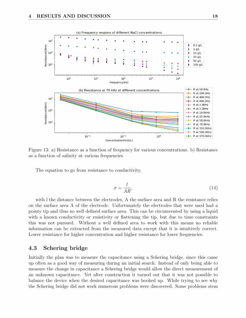
The other concentrations were made as described in the experiment section, using anichipet ex ii to make the other solutions. Since the range is between 10 and 100 µL to makethe 1 and 0.1 g/L one respectively two extra steps were needed. Going first to 10 g/L andfrom there to 1 g/L doing either an experiment with 1 g/L or continuing further down to0.1 g/L. The voltage of the acoustic trap was at 12 V and a volume of 12 µL was used foreach droplet. The distance between the tip of the electrodes is approximately 1.6 mm. Withthese parameters the data presented in figure 13 could be collected.

For the plot of resistance as a function of salinity the measurement at 100 Hz is omittedbecause one of the data points is made at 120 Hz. The fact that when resistance is plottedagainst the frequency there is asymptotic behaviour at low frequencies, not clearly visible onthis figure, can be attributed to the reactance. The two electrodes act like a capacitor andthe reactance behaves as in equation 3.

There are some general remarks to be made about the way the measurement was per-formed. Because the RCL-meter could not be hooked to a computer every data point had tobe written down on paper from the small display on the device. If the measured value wasconstant with time this would not have been a big issue, merely a nuisance. But because CO2

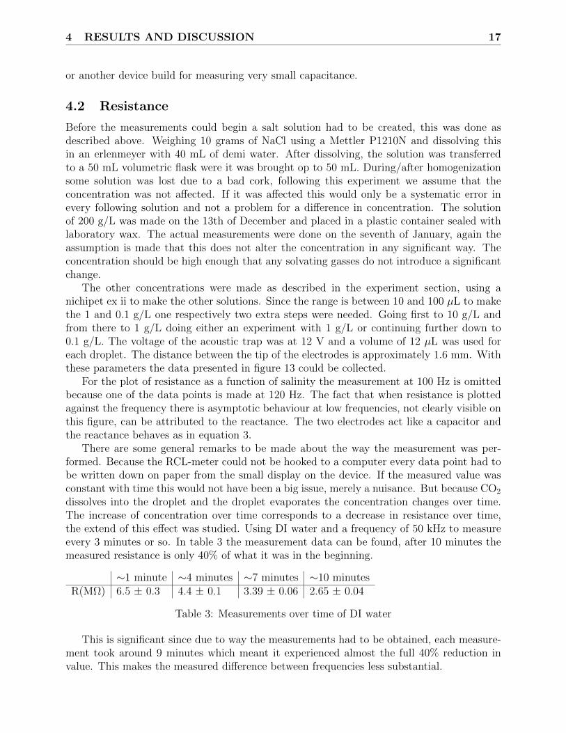
dissolves into the droplet and the droplet evaporates the concentration changes over time.The increase of concentration over time corresponds to a decrease in resistance over time,the extend of this effect was studied. Using DI water and a frequency of 50 kHz to measureevery 3 minutes or so. In table 3 the measurement data can be found, after 10 minutes themeasured resistance is only 40% of what it was in the beginning.

∼1 minute ∼4 minutes ∼7 minutes ∼10 minutesR(MΩ) 6.5 ± 0.3 4.4 ± 0.1 3.39 ± 0.06 2.65 ± 0.04

Table 3: Measurements over time of DI water

This is significant since due to way the measurements had to be obtained, each measure-ment took around 9 minutes which meant it experienced almost the full 40% reduction invalue. This makes the measured difference between frequencies less substantial.

4 RESULTS AND DISCUSSION 18

Figure 13: a) Resistance as a function of frequency for various concentrations. b) Resistanceas a function of salinity at various frequencies

The equation to go from resistance to conductivity,

σ =l

AR, (14)

with l the distance between the electrodes, A the surface area and R the resistance relieson the surface area A of the electrode. Unfortunately the electrodes that were used had apointy tip and thus no well defined surface area. This can be circumvented by using a liquidwith a known conductivity or resistivity or flattening the tip, but due to time constraintsthis was not pursued. Without a well defined area to work with this means no reliableinformation can be extracted from the measured data except that it is intuitively correct.Lower resistance for higher concentration and higher resistance for lower frequencies.

4.3 Schering bridge

Initially the plan was to measure the capacitance using a Schering bridge, since this cameup often as a good way of measuring during an initial search. Instead of only being able tomeasure the change in capacitance a Schering bridge would allow the direct measurement ofan unknown capacitance. Yet after construction it turned out that it was not possible tobalance the device when the desired capacitance was hooked up. While trying to see whythe Schering bridge did not work numerous problems were discovered. Some problems stem

4 RESULTS AND DISCUSSION 19

from bad design and planning of the circuit while others are more profound and require amore substantial change.

A problem that was immediately noticeable was the fact that due to the low value capac-itors used in the circuit the circuit would act like a highpass-filter. Having a too low voltageoutput at lower frequency to be easily measured. This limited the range of frequencies thatcould be used to higher frequencies only. Because parasitic capacitance is larger at higherfrequencies the use of lower frequencies is preferred. Another problem was the wrong use ofa BNC/coax connection, the measurement between the two arms was with a connection toa single coax cable. Thus connecting one of the arms to the ground of the oscilloscope. Thisin of itself rendered the device unusable since it would be impossible to know if the armswould be balanced. And finally a design flaw was made in the use of components, using onlyone variable component. This makes it almost impossible, unless the unknown componenthas just the right value, to balance the two arms. In the equations 10 we can see this, ifan equation has no variable component this equation can not be balanced. And without abalance no measurement can be done.

The more substantial problem is the parasitic capacitance. Not putting enough variablecomponents in the circuit or connecting the ground in the circuit are problems that caneasily be fixed, but a different solution is needed for the parasitic capacitance. For a Scheringbridge to work the value of each component must be known to measure the unknown value, ifthese differ due to parasitic capacitance it is not possible to reliably determine the unknowncomponent. There are ways around this problem, like a Wagner earth, with this addition tothe circuit one can first balance the circuit without the unknown component and compensatefor the parasitic capacitance. After introducing the unknown component another balancegives the value of the desired component. To explain this circuit in more detail is beyond thescope of this thesis, but for further research or experiments a Schering bridge with a Wagnerearth is worth considering.[4]

5 CONCLUSION 20

5 Conclusion

The complex impedance and following that the permittivity of water was investigated usingan acoustic levitator. Two possible ways of measuring were build, the Schering bridge andthe LC resonance circuit, a third pre-build device was also used, a Fluke PM6306 RCL-meter.After testing the Schering bridge proved insufficient in measuring the capacitance and wasthus dropped, the failure was mainly due to poor build design. For measuring capacitancethe LC circuit proved adequate in measuring the distance variations of a plate capacitor,being able to measure differences in the order of 0.5 pF. Even though the prediction of thecapacitance of a water droplet was guessed at 1 pF the LC circuit and the pre-build RCL-meter proved unable to reliably measure the capacitance of water droplets placed betweenthe plates. A measurement of the relation between resistance, frequency and salinity wasalso done. Due to a badly defined surface area of the electrodes no further information couldbe extracted from the measurement, a flatter electrode tip or the use of a calibration solutioncould make this measurement work better.

REFERENCES 21

6 References

References

[1] Asier Marzo, Adrian Barnes, and Bruce W. Drinkwater. Tinylev: A multi-emitter single-axis acoustic levitator. Review of Scientific Instruments 88, July 2017.

[2] Paul Horowitz and Winfield Hill. The art of electronics. Cambridge University Press,2016.

[3] Peter J. Mohr, Barry N. Taylor, and David B. Newell. Codata recommended values ofthe fundamental physical constants: 2006. Reviews of Modern Physics, 2008.

[4] HTS rens en rens. meetinstrumenten en metingen. les 22. old booklet from the HTS rensen rens(1960), pagina 59 tot 68.

[5] Kaye and Laby. Electrical insulating materials. National Physical Laboratory, 2017.http://www.kayelaby.npl.co.uk/general_physics/2_6/2_6_3.html.

[6] Spencer L. Seager and Michael Slabaugh. Alkane reactions. Chemistry for Today: Gen-eral, Organic, and Biochemistry. Charles Hartford Developmental, 2008.

[7] Fluke. Programmable automatic RCL meter. http://www.jicheng.net.cn/products/

downloadfile/Fluke_PM6306_umeng0200.pdf.

[8] A.Ernst, W. Streule, N. Schmitt, R.Zengerle, and P.Koltay. A capacitive sensor for non-contact nanoliter droplet detection. Sensors and Actuators A: Physical, 2009.

A APPENDIX 22

A Appendix

This figure shows the uncertainty in the obtained data from a direct fit, the error bars aretaken directly from the scipy fit function.

Figure 14: a) Obtained data with the LC-circuit of measurement 27, when the plates werenearest. b) The capacitance at each distance with error bars.