Measurements of hydroxyl radical reactivity and formaldehyde ...
270
Measurements of hydroxyl radical reactivity and formaldehyde in the atmosphere Danny Russell Cryer Submitted in accordance with the requirements for the degree of Doctor of Philosophy The University of Leeds School of Chemistry September, 2016
-
Upload
khangminh22 -
Category
Documents
-
view
1 -
download
0
Transcript of Measurements of hydroxyl radical reactivity and formaldehyde ...

Measurements of hydroxyl radical reactivity and formaldehyde in
the atmosphere
Danny Russell Cryer
Submitted in accordance with the requirements for the degree of
Doctor of Philosophy
The University of Leeds
School of Chemistry
September, 2016


The candidate confirms that the work submitted is his own, except where work
which has formed part of jointly-authored publications has been included. The
contribution of the candidate and the other authors to this work has been explicitly
indicated below. The candidate confirms that appropriate credit has been given
within the thesis where reference has been made to the work of others.
The observations of OH reactivity presented in Chapter 5 of the thesis have
appeared in publication as follows:
Stone, D., Whalley, L. K., Ingham, T., Edwards, P. M., Cryer, D. R., Brumby, C. A.,
Seakins, P. W. and Heard, D. E.: Measurement of OH reactivity by laser flash
photolysis coupled with laser-induced fluorescence spectroscopy, Atmospheric
Measurement Techniques, 9, 2827-2844, 2016.
I was responsible for the ambient measurements of OH reactivity that were made
during the York 2014 ‘missing’ OH reactivity campaign, along with L. K. Whalley
and D. E. Heard, and for the processing and analysis of the observational data.
This copy has been supplied on the understanding that it is copyright material and
that no quotation from the thesis may be published without proper
acknowledgement.
© 2016 The University of Leeds and Danny Russell Cryer


i
Acknowledgements
So the time has finally come to write the acknowledgements after finishing the rest
of this book. I have to say it felt like this day would never come! There are a number
of people I need to thank who have helped me in a manner of ways through the
course of my PhD, without help from these people this work would not have been
possible.
Firstly I would like to thank my supervisors Dwayne and Lisa for their support and
guidance over the past four years. I would also like to thank them for providing me
with the opportunity to do this PhD in the first place. I also need to thank past and
present members of the Heard group who I have worked alongside. I would like to
thank Trev in particular for all the help and advice he has given me both in the lab
and in the field. Due to the collaborative nature of the fieldwork I have been
involved in there are many people from other institutions who are due
acknowledgement and thanks. However, there are far too many for them to
individually name them all here so I would like to thank everybody who I have
worked with in the field.
During my four years in Leeds I’ve met many people both inside and outside of the
department. In particular I would like to thank Charlotte for her unwavering support
and confidence in me. I’m sure I would have lost considerably more hair writing this
thesis without her! Thanks are also due to Anna for her friendship and the often late
night tea/coffee breaks that I’m sure stopped both of us losing the plot! Furthermore
I would also like to thank my friends Graham, Adam, Laura and many others (there
are too many to name) for providing me with a social life.
No acknowledgements would be complete without mentioning my family. I would
like to thank my parents for supporting me not only through my PhD, but through
life in general. The time and effort they invested in my education through my school
years made this PhD possible.


ii
Abstract
Results from the laboratory characterisation of a new design of hydroxyl radical
(OH) flow reactor are presented. Further to this details of its coupling with a gas
chromatograph time of flight mass spectrometer (GC-TOF-MS) system, to form a
new instrument for the identification of ‘missing’ OH reactivity is discussed.
Preliminary measurements in ambient air demonstrated the potential value of this
system which could be used to chemically identify ‘missing’ OH sinks in various
environments, and also to determine bimolecular rate coefficients for their reaction
with OH. Observations of OH reactivity and formaldehyde (HCHO) are presented
from an urban background site in York in the summer of 2014. OH reactivity was
measured using laser flash photolysis coupled with laser induced fluorescence
spectroscopy (LFP-LIF). The average ‘missing’ OH reactivity was ~27 % when
measurements were compared with values predicted by a calculation that utilised
measured concentrations of a very detailed suite of volatile organic compounds
(VOCs). It is concluded that a combination of unidentified VOCs and products of
VOC photo-oxidation account for this discrepancy. HCHO was measured using a
new fast response (1 s time resolution) laser induced fluorescence (LIF)
spectroscopy instrument and some evidence of daytime diurnal behaviour suggested
that the dominant HCHO source was photo-chemical (~1.3 ppb diurnal peak).
Observations of OH reactivity and HCHO are also presented from a coastal site in
Weybourne, Norfolk, using the same instrumentation during the summer of 2015.
The average ‘missing’ OH reactivity was ~44 %. It is concluded that much of the
‘missing’ reactivity was likely due to unmeasured VOCs and their photo-oxidation
products. Strong diurnal behaviour of HCHO was observed and is consistent with an
atmosphere where the dominant source is photo-chemical (~1.1 ppb diurnal peak).
Unusual behaviour was observed for HCHO during a thunderstorm where sharp
fluctuations in concentration were observed. It has so far not been possible to
conclude the exact cause of this, however, it is suggested that the source was marine.
Finally, preliminary results from three experiments of an intercomparison of OH
reactivity instrumentation are presented. The results demonstrate the reliability of
the Leeds LFP-LIF instrument for the measurement of ambient OH reactivity.


iii
Table of Contents
LIST OF ABBREVIATIONS……………………………………………………….I
LIST OF FIGURES……………………………………………………………….IV
LIST OF TABLES………………………………………………………………VIII
CHAPTER 1. INTRODUCTION…………………………………………………..1
1.1 Atmospheric chemistry………………………………………………...1
1.2 ROx in the Troposphere………………………………………………. 2
1.2.1 Overview of chemistry……………………………………….2
1.2.2 ROx formation……………………………………………….. 3
1.2.3 ROx termination……………………………………………... 5
1.3 Tropospheric ozone production………………………………………..6
1.4 FAGE detection of OH……………………………………………….. 8
1.5 Measurement of OH reactivity………………………………………...9
1.5.1 Definition and motivation for measurement………………….9
1.5.2 Total OH loss rate method (TOHLM)……..………………...12
1.5.3 Laser flash photolysis coupled with laser induced
fluorescence spectroscopy (LFP-LIF)……………………….13
1.5.4 Comparative reactivity method (CRM)…...…………………15
1.5.5 Instrumentation in the literature……………………………..16
1.5.6 Comparison of techniques…………………………………...17
1.6 Review of ground based OH reactivity measurements………………. 18
1.6.1 Forest atmospheres with low anthropogenic
Influence……………………………………………………..18
1.6.2 Urban atmospheres…………………………………………..24
1.6.3 Rural and other atmospheres………………………………...30
1.7 Limitations of OH reactivity measurements…………………………..33
1.8 Formaldehyde in the Troposphere…………………………………… 33
1.9 Measurement of formaldehyde………………………………………..35
1.9.1 Direct spectroscopic measurement…………………………..35
1.9.2 Indirect spectroscopic measurement…………………………38
1.9.3 Other methods and intercomparisons………………………..39
1.10 Review of ground based formaldehyde measurements……………….43
1.11 Project aims……………………………………………………………43

iv
1.12 References……………………………………………………………. 44
CHAPTER 2. EXPERIMENTAL METHODS……………………………………55
2.1 Overview……………………………………………………………... 55
2.2 Measurement of OH reactivity………………………………………..55
2.2.1 Instrument overview and principle of operation……………. 55
2.2.2 The Leeds FAGE container………………………………….59
2.2.3 The 266 nm photolysis laser………………………………....60
2.2.4 The flow tube and FAGE cell………………………………..61
2.2.5 The 308 nm detection laser…………………………………..64
2.2.6 Data acquisition……………………………………………...65
2.2.7 Instrument configurations……………………………………67
2.2.8 Determination of k’OH(raw)……………………………………69
2.2.9 Measurement validation with standard gases………………..72
2.2.10 Determination of physical loss rate of OH…………………..75
2.2.11 Effect of NO recycling………………………………………80
2.3 Measurement of formaldehyde………………………………………..80
2.3.1 Instrument overview and principle of operation…................. 80
2.3.2 The 353 nm detection laser…………………………………..82
2.3.3 The detection cell…………………………………………… 83
2.3.4 The reference cell……………………………………………85
2.3.5 Data acquisition……………………………………………...86
2.3.6 Instrument configurations……………………………………89
2.3.7 Calibration methods………………………………………….92
2.4 Summary………………………………………………………………99
2.5 References…………………………………………………………… 100
CHAPTER 3. OH REACTIVITY INTERCOMPARISON………………………101
3.1 Overview of intercomparison………………………………………...101
3.1.1 Aim of comparison………………………………………….101
3.1.2 The SAPHIR chamber………………………………………102
3.1.3 Participating instrumentation………………………………..104
3.2 Sampling method……………………………………………………..105
3.3 Results………………………………………………………………...108
3.3.1 Addition of CO……………………………………………...108
3.3.2 Oxidation of monoterpenes and real biogenic emissions…...110
3.3.3 Correlations…………………………………………………114
3.4 Summary and conclusions……………………………………………116
v
3.5 References…………………………………………………………… 118
CHAPTER 4. DEVELOPMENT OF AN OH FLOW REACTOR………….……120
4.1 Motivation for the development of an OH flow reactor……………...120
4.2 Design process………………………………………………………. 123
4.3 Characterisation………………………………………………………131
4.3.1 Methodology………………………………………………...131
4.3.2 Optimisation of injector position……………………………132
4.3.3 Quantification of OH present at mixing point……................134
4.3.4 Measurement of OH loss rate……………………………….137
4.4 Simulated removal of VOCs………………………………………… 140
4.5 Coupling with GC-TOF-MS………………………………………….145
4.6 Observations in ambient air…………………………………………..148
4.7 Summary and conclusions……...…………………………………….151
4.8 References…………………………………………………………… 152
CHAPTER 5. YORK 2014 ‘MISSING’ OH REACTIVITY CAMPAIGN……... 153
5.1 Background to the York 2014 project……………………………….. 153
5.2 Aims…………………………………………………………………. 153
5.3 Site description, measurement suite and conditions………………….154
5.4 OH reactivity………………………………………………………… 158
5.4.1 OH reactivity observations………………………………….158
5.4.2 Interpretation of OH reactivity observations………………..161
5.4.2.1 Diurnal behaviour………………………………….161
5.4.2.2 Correlations with other measurements…………….163
5.4.2.3 Calculation of OH reactivity………………………166
5.4.2.4 Measured and calculated OH reactivity…………...168
5.4.2.5 Accounting for ‘missing’ OH reactivity…………...176
5.5 Formaldehyde………………………………………………………...181
5.5.1 Formaldehyde observations…………………………………181
5.5.2 Interpretation of formaldehyde observations………………..185
5.5.2.1 Diurnal behaviour………………………………….185
5.5.2.2 Correlation with other measurements…………….. 187
5.6 Summary and conclusions……………………………………………188
5.7 References…………………………………………………………… 190
CHAPTER 6. INTEGRATED CHEMISTRY OF OZONE IN THEATMOSPHERE CAMPAIGN…………………………………….195
6.1 Background to the ICOZA project…………………………………... 195

vi
6.2 Aims ………………………………………………………………….195
6.3 Site description, measurement suite and conditions………………….196
6.4 OH reactivity………………………………………………………… 202
6.4.1 OH reactivity observations………………………………….202
6.4.2 Interpretation of OH reactivity observations………………..205
6.4.2.1 Diurnal behaviour………………………………….205
6.4.2.2 Correlation with other measurements……………...206
6.4.2.3 Relationship with wind direction and origin of
air mass…………………………………………….209
6.4.2.4 Calculation of OH reactivity………………………216
6.4.2.5 Measured and calculated OH reactivity…………...218
6.5 Formaldehyde………………………………………………………...227
6.5.1 Formaldehyde observations…………………………………227
6.5.2 Interpretation of formaldehyde observations………………..230
6.5.2.1 Diurnal behaviour………………………………….230
6.5.2.2 Correlation with other species measured…………. 232
6.5.2.3 Relationship with wind direction and origin of
air mass…………………………………………….234
6.6 Summary and conclusions……………………………………………238
6.7 References…………………………………………………………… 240
CHAPTER 7. SUMMARY AND FUTURE WORK…………………………..... 244
7.1 Summary…………………………………………………………….. 244
7.2 Future work………………………………………………………….. 246

I
List of Abbreviations
BEARPEX Biosphere effects on aerosols and photochemistry experiment
BNC Berkeley Nuceleonics Corporation
BST British summer time
BVOC Biogenic volatile organic compound
CABINEX Community atmosphere-biosphere interactions experiment
CalNex California Nexus
CIMS Chemical ionisation mass spectrometer
ClearFlo Clean air for London
CPM Channeltron photomultiplier
CRM Comparative reactivity method
CWT Concentration weighted trajectory
DOAS Differential optical absorption spectroscopy
DOMINO Diel oxidant mechanisms in relation to nitrogen oxides
FAGE Fluorescence assay by gas expansion
FMI Finnish meteorological institute
GABRIEL Guyanas atmosphere biosphere exchange and radicals
intensive experiment with the Learjet
GC Gas chromatograph
GC-FID Gas chromatograph coupled with flame ionisation detector
GC-PID Gas chromatograph coupled with photoionisation detector
GC-TOF-MS Gas chromatograph coupled with time of flight mass
spectrometer
GCxGC-FID Comprehensive gas chromatograph coupled with flame
ionisation detector
GCxGC-TOF-MS Comprehensive gas chromatograph coupled with time of flight
mass spectrometer
HPLC High performance liquid chromatography
HUMPPA-COPEC Hyytiälä united measurement of photochemistry and particles
– comprehensive organic particle and environmental chemistry
HYSPLIT Hybrid single particle lagrangian integrated trajectory model
IC Ion chromatography

II
ICOZA Integrated chemistry of ozone in the atmosphere
ID Inner diameter
IR Infra-red
IUPAC International union of pure and applied chemistry
LFP-LIF Laser flash photolysis coupled with laser induced fluorescence
spectroscopy
LIF Laser induced fluorescence
LOPAP Long path absorption photometry
LP-DOAX Long path differential optical absorption spectrometery
LSCE Laboratory of the sciences of climate and the environment
MAX-DOAS Multiaxis differential optical absorption spectrometry
MCM Master chemical mechanism
MCMA Mexico City metropolitan area
MEGAPOLI Megacities: emissions, urban, regional and global atmospheric
pollution and climate effects, and integrated tools for
assessment and mitigation
MPIC Max Planck Institute for Chemistry
NOAA National Oceanic and Atmospheric Administration
NPL National Physical Laboratories
NPT National pipe thread
OASIS Ocean-atmosphere-sea ice-snowpack
OD Outer diameter
OP3 Oxidant and particle photochemical processes
ORSUM OH reactivity specialists uniting meeting
PMT Photomultiplier tube
PMTACS-NY PM2.5 technology assessment and characteristics study – New
York
PMTACS-NY-WFM PM2.5 technology assessment and characteristics study – New
York – Whiteface Mountain
POPR Perturbed ozone production rate
PRD Pearl river delta
PRF Pulse repetition frequency
PRIDE-PRD Program of regional integrated experiments on air quality over
the pearl river delta

III
PROPHET Program for research on oxidants: photochemistry, emissions
and transport
PT Pressure transducer
PTR-MS Proton transfer mass spectrometer
QCLS Quantum cascade laser spectrometer
RACM Regional atmospheric chemistry model
SAPHIR Simulation of atmospheric photochemistry in a large reaction
chamber
SAPHIR-PLUS SAPHIR plant chamber unit for simulation
SCAPE Schenandoah cloud and photochemistry experiment
SHG Second harmonic generator
SLM Standard litres per minute
SOS Southern oxidants study
SRS Stanford research systems
TDLAS Tuneable diode laser absorption spectroscopy
TexAQS Texas air quality study
THG Third harmonic generator
TOF-MS Time of flight mass spectrometer
TOHLM Total OH loss rate method
TORCH Tropospheric organic chemistry experiment
TRAMP TexAQS radical measurements project
TTL Transistor transistor logic pulse
UEA University of East Anglia
UPS Uninteruptable power supply
UTC Coordinated universal time
UV Ultra-violet
VOC Volatile organic compound
WACL Wolfson Atmospheric Chemistry Laboratories
WAO Weybourne Atmospheric Observatory

IV
List of Figures
1.1 Simplified ROx reaction cycle………………………………………...3
1.2 Relationship between O3 production, NOx and VOCs………………..7
1.3 TOHLM instrument diagram………………………………………...13
1.4 LFP-LIF instrument diagram………………………………………...14
1.5 CRM OH reactor diagram………………………………………...… 16
1.6 ‘Missing’ OH reactivity versus temperature during PROPHET…….19
1.7 Measured and calculated reactivity for PMTACS-NY WFM……….20
1.8 Measured and calculated reactivity for PMTACS-NY 2001……….. 26
1.9 Measured and calculated reactivity for TRAMP 2006………………27
1.10 Schematic diagram to illustrate HCHO LIF excitation……………...36
1.11 Liquid phase Hantzsch cyclisation reaction………………………… 38
2.1 The LFP-LIF OH reactivity instrument……………………………...57
2.2 Photograph of LFP-LIF OH reactivity instrument…………………..58
2.3 Diagram of the FAGE container……………………………………..59
2.4 Photolysis laser system of the LFP-LIF instrument………………… 60
2.5 Photograph of the FAGE cell of the LFP-LIF instrument…………...62
2.6 Detection laser system of the LFP-LIF instrument…………………. 64
2.7 Reference cell for tuning detection laser wavelength………………..65
2.8 Timings for detection of OH in LFP-LIF instrument FAGE cell……66
2.9 Timings for recording an OH decay with LFP-LIF instrument…….. 67
2.10 Scale diagram of new LFP-LIF instrument FAGE cell inlet………...68
2.11 Timing of LFP-LIF instrument photon counting bins……………….70
2.12 Example LFP-LIF instrument bi-exponential decays………………..71
2.13 Example LFP-LIF instrument single-exponential decays…………...72
2.14 Experimental set-up used to measure rate coefficients……………... 73
2.15 Bimolecular plot for kOH+CO………………..………………………...74
2.16 Bimolecular plot for kOH+CH4………………………………………... 75
2.17 Experimental set-up used to measure k’OH(zero)………………………76
2.18 Measurements of k’OH(zero) made in York……………………………77
2.19 Example of a k’OH(physical) decay signal measured at SAPHIR……….79
2.20 Photograph of the HCHO LIF instrument…………………………...81
2.21 Detection laser system for HCHO LIF instrument…………………..82
2.22 Scale diagram of the HCHO LIF instrument detection cell………… 84

V
2.23 Scale diagram of the HCHO LIF instrument reference cell…………85
2.24 Timings for detection of HCHO with HCHO LIF instrument……… 87
2.25 Example of a reference cell signal of the HCHO LIF instrument…...88
2.26 HCHO LIF instrument configuration 1.……………………………..90
2.27 HCHO LIF instrument configurations 2 and 3……….……………...91
2.28 HCHO LIF instrument configuration 1 calibration.…………………93
2.29 HCHO LIF instrument configuration 2 calibration.…………………94
2.30 HCHO LIF instrument configuration 3 calibration…….……………96
2.31 HCHO LIF instrument configuration 3 calibration….………………97
2.32 Example HCHO LIF signals………………………………………... 98
3.1 Photograph of the SAPHIR chamber……………………………….103
3.2 Photograph of SAPHIR chamber inlet port………………………...103
3.3 Positioning of shipping containers at SAPHIR……………………. 105
3.4 Photograph showing the FAGE container beneath SAPHIR……… 106
3.5 Photograph showing the LFP-LIF instrument……………………...107
3.6 Results from CO addition to SAPHIR……………………………...109
3.7 Results from monoterpenes addition to SAPHIR ………………….111
3.8 Results from addition plant chamber emissions to SAPHIR……….113
3.9 Summary of experiments with ‘simple’ species …….......................115
3.10 Summary of experiments with biogenic species…………………... 116
4.1 Experimental set-up used by Kato et al (2011)……………………..120
4.2 Relative rate plot reported by Kato et al (2011)…………………….122
4.3 OH flow reactor prototype design………………………………….124
4.4 Results from reactor prototype test with 30 VOC mix….………….126
4.5 Relative rate plot from reactor prototype test with 30 VOC mix…..127
4.6 Results from reactor prototype photolysis test with 30 VOC mix… 128
4.7 Redesigned OH flow reactor………………………………………. 130
4.8 Experimental set-up used for optimising reactor injector position... 133
4.9 Example HCHO signal from injector optimisation experiment……134
4.10 Experimental set-up used for quantifying OH in the reactor…….... 135
4.11 Example HCHO signal from OH quantification experiment……… 136
4.12 HCHO signal recorded during measurement of kloss……………….138
4.13 Results from measurement of kloss………………………………….139
4.14 Reactor performance simulation results at 4.05 SLM total flow…...142
4.15 Reactor performance simulation results at 3.05 SLM total flow…...143
4.16 New instrument for identification of k’OH(missing)……………..……. 145

VI
4.17 Photograph of new instrument for identification of k’OH(missing)…… 147
4.18 Reactor versus non-Reactor relative response plots………...……...149
4.19 Relative rate plot from ambient measurements in York……………150
5.1 Location of the measurement site in York………………………… 155
5.2 Photograph of the FAGE container in York………………………..156
5.3 Photograph of the LFP-LIF instrument in York……………………158
5.4 Measurements of OH reactivity in York…………………………... 160
5.5 Diurnal profile of OH reactivity in York………………………….. 161
5.6 NOx observations from York……………………………………….163
5.7 Correlations of OH reactivity and NOx in York……………………164
5.8 Correlations of OH reactivity with four VOCs in York……………165
5.9 Measured and calculated OH reactivity in York……………….......169
5.10 Measured versus calculated OH reactivity in York……………….. 170
5.11 Daily plots of measured and calculated OH reactivity in York…….171
5.12 Daily plots of measured and calculated OH reactivity in York…….172
5.13 Measured and calculated OH reactivity (GC-FID VOCs)………….174
5.14 Measured and calculated OH reactivity (all identified VOCs)…......175
5.15 Measured and calculated OH reactivity (with grouped VOCs)…….177
5.16 Measured and calculated OH reactivity (three scenarios)………….179
5.17 Measured and modelled OH reactivity (three scenarios)…………...180
5.18 Photograph of the HCHO LIF instrument in York…………………182
5.19 Measurements of HCHO in York…………………………………..183
5.20 HCHO observations from 04/06/14 in York………………………..185
5.21 Diurnal profile of HCHO in York…………………………………. 186
5.22 Correlations of HCHO with NOx in York………………………….187
5.23 Correlations of HCHO with temperature and J(O1D) in York……..188
6.1 Location of the Weybourne Atmospheric Observatory…………….197
6.2 Photograph of the Weybourne Atmospheric Observatory………….198
6.3 Photograph of the sampling tower………………………………….200
6.4 Meteorological parameters recorded in Weybourne………………. 201
6.5 Photograph of the LFP-LIF instrument in Weybourne……………. 202
6.6 Measurements of OH reactivity in Weybourne…………………….204
6.7 Diurnal profile of OH reactivity in Weybourne…………………… 205
6.8 Correlations of OH reactivity and NOx……………….…………… 207
6.9 Correlations of OH reactivity and VOCs……………….…………. 208
6.10 Correlations of OH reactivity with isoprene and temperature……...209

VII
6.11 OH reactivity wind rose for ICOZA………………………………..210
6.12 OH reactivity and back trajectories during ICOZA heatwave…...... 212
6.13 Clustered four day back trajectories for ICOZA…………………...213
6.14 Daily average OH reactivities identified by air mass type…………214
6.15 CWT mean contribution to OH reactivity for ICOZA……………..215
6.16 Measured versus calculated OH reactivity for ICOZA…………….219
6.17 Measured and calculated OH reactivity for ICOZA………………..220
6.18 Daily plots of measured and calculated OH reactivity for ICOZA...221
6.19 Daily plots of measured and calculated OH reactivity for ICOZA...222
6.20 Daily plots of measured and calculated OH reactivity for ICOZA...223
6.21 Photograph of the HCHO LIF instrument in Weybourne…………. 228
6.22 Measurements of HCHO in Weybourne…………………………... 229
6.23 Measurements of HCHO during a thunder storm in Weybourne…..230
6.24 Diurnal profile of HCHO in Weybourne…………………………...231
6.25 Correlation of HCHO and NOx......................................................... 232
6.26 Correlations of HCHO with temperature and J(O1D)……………...233
6.27 HCHO wind rose for ICOZA………………………………………235
6.28 HCHO and back trajectories during ICOZA thunder storm…..........236

VIII
List of Tables
1.1 OH reactivity instrumentation described in the literature……………17
1.2 Measurements of OH reactivity in forest atmospheres………………22
1.3 Measurements of OH reactivity in urban atmospheres………………29
1.4 Measurements of OH reactivity in rural and other atmospheres…….32
1.5 Example forest HCHO observations………………………………...40
1.6 Example urban HCHO observations………………………………...41
1.7 Example rural and coastal HCHO observations……………………..42
3.1 Participating OH reactivity instrumentation at SAPHIR…………...104
4.1 VOCs used in OH reactor performance simulation……….………..141
4.2 Predicted changes in VOC levels in OH reactor…………………....144
5.1 Instrumentation used for measurements in York…………………...157
5.2 Species measured in York used to calculate OH reactivity………...167
5.3 Classes of unidentifiable VOCs detected in York………………….177
6.1 Instrumentation used for measurements in Weybourne……………199
6.2 Species measured in Weybourne used to calculate OH reactivity… 217


1
Chapter 1 - Introduction
1.1 Atmospheric chemistry
The field of atmospheric chemistry is composed largely of three interdependent
disciplines; these are field measurements, laboratory measurements and computer
modelling. Observations from field measurements are used to investigate
atmospheric processes and composition. They can be used to build and test the
quality of global climate and air quality models by comparison with their
predictions. Model simulations contain the current state of our knowledge of the
atmosphere and can also be used to predict future change. Laboratory measurements
are used to determine physical constants such as rate coefficients for use in
computer models, and to complement analysis of data recorded in the field. They
can also be used to investigate complicated chemical and physical processes which
occur in the atmosphere, ranging from single reaction kinetic studies to complex
multiple reaction studies in atmospheric simulation chambers. Further to this,
laboratory measurements are often used as a means to test and characterise
instrumentation prior to field deployment.
Managing air quality and climate change are two of the biggest environmental
challenges we face as a society. Poor air quality resulting from pollution contributes
to over two million premature deaths worldwide each year (World Health
Organisation, 2005). Over the previous few decades there has been an international
effort to reduce the level of pollutants emitted into the atmosphere. However,
decreasing emissions do not scale linearly with the level of pollutants that are
detected in the air, and pollutants can also travel long distances and adversely affect
air quality across boarders and continents (European Environment Agency, 2008,
Maas and Greenfelt, 2016). The work presented in this thesis is particularly relevant
to the production of Tropospheric ozone. It is a major pollutant and greenhouse gas
which is formed through the removal of volatile organic compounds (VOCs), in the

Chapter 1 2 Introduction
presence of nitrogen oxides (NOx), from the atmosphere by reaction with the
hydroxyl radical, (OH) (Sillman, 1999). It can also be formed during long range
transport of air masses from the pollutant emission sources. In order to accurately
predict changes in Tropospheric O3 and plan effective mitigation strategies, it is
crucial that we have a clear understanding of the range of VOCs that are removed
from the atmosphere by OH. The measurement of OH reactivity (the pseudo first
order rate coefficient for OH loss) provides a valuable tool to test our understanding
of this. Additionally, measurement of gas phase formaldehyde is a useful
investigative tool as it acts as an overall tracer of VOC removal by OH. The ability
of a computer model simulation to accurately predict formaldehyde levels as
measured in the field has the potential to highlight uncertainties in our understanding
of VOC + OH chemistry. This thesis investigates the completeness of our
knowledge of the VOCs that are removed from the atmosphere by OH, in two
contrasting chemical environments. Chapter 2 describes the methodologies and
experimental techniques used to measure OH reactivity and formaldehyde for this
work. Chapters 5 and 6 present field observations of OH reactivity and
formaldehyde that were made at an urban background site in York and a coastal site
in Norfolk, respectively. Further to this Chapter 4 details the laboratory
characterisation of a new field instrument that can be used to investigate the
chemical identity of currently unidentified VOCs which react with OH, and also
measure rate coefficients for their reaction with OH. In Chapter 3 results from an
intercomparison study are presented where 9 instruments for the measurement of
OH reactivity simultaneously sampled gas from an atmospheric simulation chamber.
1.2 ROx in the troposphere
1.2.1 Overview of chemistry
The troposphere occupies the first ~15 km of the atmosphere and the lowest ~1 km
is known as the boundary layer (Holloway and Wayne, 2010). Approximately 90%
of atmospheric mass resides in the troposphere (Wayne, 2000). ROx, the collective
term for hydroxyl radicals (OH), hydroperoxyl radicals (HO2) and alkoxy radicals
(RO2), plays a central role in controlling tropospheric pollutant and greenhouse gas
levels. Therefore complete and detailed knowledge of ROx chemistry is crucial when
assessing the impact of ever changing emissions on air quality, climate and health. A

Chapter 1 3 Introduction
significant portion of this work is focussed on the chemistry of OH in the
troposphere, and its removal via reaction with volatile organic compounds (VOCs).
1.2.2 ROx formation
R 1.1 and R 1.2 show the photolysis of ozone and subsequent reaction of the product
O(1D) with water vapour, this is the main pathway for the formation of tropospheric
OH.
Oଷ + hν(ழଷସ୬୫ ) → Oଶ + O( ଵܦ ) R 1.1
O൫ ଵܦ ൯+ HଶO → 2OH R 1.2
However, O(1D) can also undergo collisional quenching with a bath gas M (most
commonly O2 or N2) to form O(3P) which can react with O2 in the presence of M to
reform ozone, R 1.3 and R 1.4. Only a small fraction (< 3 %) of O(1D) formed
through photolysis of O3 leads to the production of OH, with the rest reacting back
again to O3 (ESPERE, 2017).
O൫ ଵܦ ൯+ M → O൫ ଷ ൯+ M R 1.3
O൫ ଷ ൯+ Oଶ + M → Oଷ + M R 1.4
The processes shown in R 1.1, R 1.2, R 1.3 and R 1.4 are displayed in Figure 1.1 in
addition to other atmospherically relevant processes involving ROx.
Figure 1.1: Schematic to show a simplified ROx reaction cycle, halogen atoms arerepresented by X and alkyl groups are represented by R. Taken from Smith (2007).
Chapter 1 4 Introduction
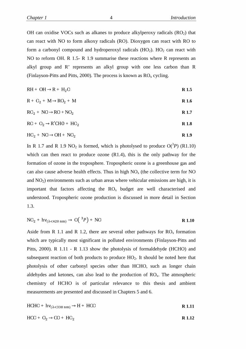
OH can oxidise VOCs such as alkanes to produce alkylperoxy radicals (RO2) that
can react with NO to form alkoxy radicals (RO). Dioxygen can react with RO to
form a carbonyl compound and hydroperoxyl radicals (HO2). HO2 can react with
NO to reform OH. R 1.5- R 1.9 summarise these reactions where R represents an
alkyl group and R’ represents an alkyl group with one less carbon than R
(Finlayson-Pitts and Pitts, 2000). The process is known as ROx cycling.
RH + OH → R + HଶO R 1.5
R + Oଶ + M→ ROଶ + M R 1.6
ROଶ + NO→RO +NOଶ R 1.7
RO + Oଶ→ R′CHO + HOଶ R 1.8
HOଶ + NO→ OH + NOଶ R 1.9
In R 1.7 and R 1.9 NO2 is formed, which is photolysed to produce O(3P) (R1.10)
which can then react to produce ozone (R1.4), this is the only pathway for the
formation of ozone in the troposphere. Tropospheric ozone is a greenhouse gas and
can also cause adverse health effects. Thus in high NOx (the collective term for NO
and NO2) environments such as urban areas where vehicular emissions are high, it is
important that factors affecting the ROx budget are well characterised and
understood. Tropospheric ozone production is discussed in more detail in Section
1.3.
NOଶ + hν(ழସଶ୬୫ ) → O൫ ଷ ൯+ NO R 1.10
Aside from R 1.1 and R 1.2, there are several other pathways for ROx formation
which are typically most significant in polluted environments (Finlayson-Pitts and
Pitts, 2000). R 1.11 - R 1.13 show the photolysis of formaldehyde (HCHO) and
subsequent reaction of both products to produce HO2. It should be noted here that
photolysis of other carbonyl species other than HCHO, such as longer chain
aldehydes and ketones, can also lead to the production of ROx. The atmospheric
chemistry of HCHO is of particular relevance to this thesis and ambient
measurements are presented and discussed in Chapters 5 and 6.
HCHO + hν(ழଷଷ୬୫ ) → H + HCO R 1.11
HCO + Oଶ→ CO + HOଶ R 1.12

Chapter 1 5 Introduction
H + Oଶ + M→HOଶ + M R 1.13
The photolysis of nitrous acid (HONO) also produces OH (R 1.14) (Johnston and
Graham, 1974), as does the photolysis of hydrogen peroxide (H2O2) and alkyl
peroxide (ROOH) (R 1.15 and R 1.16) (Jacob, 1999). Halogen oxoacids (HOX,
where X commonly represents Cl, Br or I) can also be photolysed to produce OH
(R 1.17).
HONO + hν(ழସ୬୫ ) → OH + NO R 1.14
HଶOଶ + hν(ழଷସ୬୫ ) → 2OH R 1.15
ROOH + hν(ழଷ୬୫ ) → OH + RO R 1.16
HOX + hν(ழସ୬୫ ) → OH + X R 1.17
Another route for the production of OH is the reaction between ozone and alkenes.
Ozone can add to the double bond of an alkene to form a carbonyl compound and
energy rich intermediate (Atkinson, 2007, Atkinson and Carter, 1984). This is
known as a Criegee intermediate and can either be quenched by collisions with M,
or it can decompose in a variety of ways and sometimes form OH (Heard et al.,
2004). R 1.18 and R 1.19 demonstrate this type of OH formation by example of
ethene reacting with ozone.
CHଶ = CHଶ + Oଷ→HଶCO +[HଶCOO]∗ R 1.18
[HଶCOO]∗→OH + HCO R 1.19
The OH yield from this type of reaction has been shown to be dependent on several
factors. For the reaction of ozone with ethene the OH yield has been reported as ~16
%, whereas for more substituted alkenes, and those with different isomeric
properties, higher yields (e.g. 90 % for 2,3-dimethyl-2-butene) have been reported.
OH yields have also been found to vary as a function of pressure. A recent review of
Crigee intermediates formed during tropospheric ozonolysis can be found in Taatjes
et al. (2014).
1.2.3 ROx termination
Pathways for ROx termination are different in high and low NOx environments. In
high NOx environments ROx propagation by R 1.7 and R 1.9 is rapid resulting in the
partitioning of ROx being skewed towards OH. Nitric acid (HNO3) formation from

Chapter 1 6 Introduction
the reaction between OH and NO2 is a dominant ROx termination mechanism in
these environments, R 1.20 (Finlayson-Pitts and Pitts, 2000). In low NOx
environments there is less ROx propagation due to a lack of NO, in this case radical-
radical reactions present the main termination mechanism, most commonly R 1.21
and R 1.22. The products of R 1.20, R 1.21 and R 1.22 can all lead to permanent
radical loss through dry or wet deposition on surfaces or particles (Wayne, 2000).
OH + NOଶ + M → HNOଷ + M R 1.20
HOଶ + HOଶ→ HଶOଶ R 1.21
HOଶ + ROଶ→ ROOH R 1.22
1.3 Tropospheric ozone production
The atmospheric chemistry of ozone in the troposphere plays a key role in numerous
processes relating to air quality and climate change as it is both a pollutant and a
greenhouse gas. O3 is a major constituent of photochemical smog and is a known
respiratory irritant, exposure to excessive levels has been shown to be linked with
increased mortality rates in a number of European cities; daily deaths have been
shown to increase by 0.3 % per every ~5 ppb increase in O3 exposure (World Health
Organisation, 2005). In addition to this, tropospheric O3 is damaging to crops; it can
harm yields and reduce quality (Krupa et al., 1998). Tropospheric O3 is often
produced as a product from the photo-oxidative processing of VOCs in the presence
of NOx through the reaction of O(3P) with O2, where O(3P) was formed from the
photolysis of NO2 that resulted from the reaction between NO and RO2, or HO2.
Environments are often characterised as NOx or VOC limited when considering O3
production. When the loading of NOx in the atmosphere is low, catalytic ROx
cycling (as described in Section 1.2) is slow, meaning that there is a high frequency
of radical termination reactions and net O3 destruction. As the level of NOx
increases, there is a linear increase in O3 production until a threshold (known as the
O3 compensation point) is reached. At this point there is a change from net O3
destruction, to net O3 production. At NOx levels beyond this point the linear increase
in O3 production continues. However, there comes a point where the termination
reaction of OH with NO2 (R1.20) begins to slow down the cycling of ROx (because
OH is lost) and subsequently the rate of O3 production reaches a maximum. As NOx
increases beyond this maximum, the rate of O3 production begins to decrease. The
Chapter 1 7 Introduction
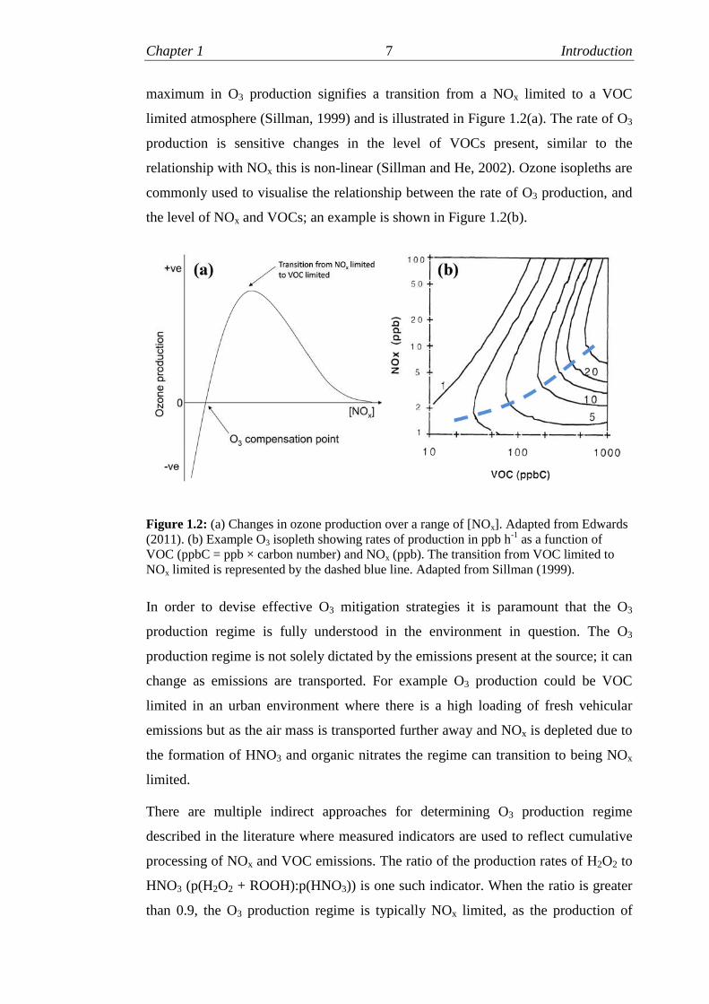
maximum in O3 production signifies a transition from a NOx limited to a VOC
limited atmosphere (Sillman, 1999) and is illustrated in Figure 1.2(a). The rate of O3
production is sensitive changes in the level of VOCs present, similar to the
relationship with NOx this is non-linear (Sillman and He, 2002). Ozone isopleths are
commonly used to visualise the relationship between the rate of O3 production, and
the level of NOx and VOCs; an example is shown in Figure 1.2(b).
Figure 1.2: (a) Changes in ozone production over a range of [NOx]. Adapted from Edwards(2011). (b) Example O3 isopleth showing rates of production in ppb h-1 as a function ofVOC (ppbC = ppb × carbon number) and NOx (ppb). The transition from VOC limited toNOx limited is represented by the dashed blue line. Adapted from Sillman (1999).
In order to devise effective O3 mitigation strategies it is paramount that the O3
production regime is fully understood in the environment in question. The O3
production regime is not solely dictated by the emissions present at the source; it can
change as emissions are transported. For example O3 production could be VOC
limited in an urban environment where there is a high loading of fresh vehicular
emissions but as the air mass is transported further away and NOx is depleted due to
the formation of HNO3 and organic nitrates the regime can transition to being NOx
limited.
There are multiple indirect approaches for determining O3 production regime
described in the literature where measured indicators are used to reflect cumulative
processing of NOx and VOC emissions. The ratio of the production rates of H2O2 to
HNO3 (p(H2O2 + ROOH):p(HNO3)) is one such indicator. When the ratio is greater
than 0.9, the O3 production regime is typically NOx limited, as the production of

Chapter 1 8 Introduction
peroxides constitute major radical loss. When the ratio is less than 0.1 the O3
production regime is typically VOC limited, as the loss of radicals through
formation of peroxides is insignificant and NO2 is a dominant sink of OH (Sillman,
1999). Another indicator reported is the total concentration of reactive nitrogen
(NOy), a modelling study reported by Milford et al. (1994) showed that when NOy is
below a threshold in the range 10 – 25 ppb the O3 production regime is predicted to
be NOx limited, whereas when NOy is above a threshold in the range 20 – 30 ppb the
O3 production regime is predicted to be VOC limited. Tropospheric ozone and the
concept of NOx and VOC limiting environments bear particular importance to
Chapter 6 of this thesis where measurements are presented from a campaign at a UK
coastal site, a major aim of which was to measure the rate of O3 production directly.
1.4 FAGE detection of OH
A large portion of the work presented in this thesis is focussed on the measurement
of OH reactivity (defined in Section 1.5.1) using the laser flash photolysis coupled
with laser induced fluorescence spectroscopy technique (LFP-LIF, described in
Section 1.5.1). A key requirement of this technique is the sensitive and selective
detection of OH using the fluorescence assay by gas expansion (FAGE) technique,
the principles of which are described in this section.
Hard et al. (1979) pioneered the FAGE technique for the detection of OH; through
the course of development several modifications have been necessary to overcome
various chemical and spectral interferences (Heard and Pilling, 2003). In the FAGE
technique, air is sampled through a pinhole into a low pressure (~2 Torr) cell where
it expands and OH is detected by laser induced fluorescence (LIF) spectroscopy.
The use of low pressure minimises interference from photolysis of ozone and
consequent formation of OH (R 1.1 and R 1.2) through a reduction in the number
density of H2O vapour; interference from Rayleigh and Mie scattering is also
reduced.
In early FAGE instruments 282 nm laser light was used for OH excitation, the
wavelength of the induced fluorescence was longer than the scattered laser light
meaning it could be easily discriminated. Smith and Crosley (1990), however,
reported results from a modeling study which revealed the presence of a significant
ozone interference with this excitation regime with the use of high energy low pulse
repetition frequency (PRF) lasers. Following this the FAGE community adapted to

Chapter 1 9 Introduction
excite using 308 nm low energy high PRF lasers. The absorption cross section of
ozone at 308 nm is ~9.8 × 10⁻¹⁹ cm2 compared with ~2.8 × 10⁻¹⁸ cm2 at 282 nm
(Sander et al., 2003), thus after the change in excitation regime the ozone
interference was no longer significant. An added benefit to the 308 nm excitation
regime was an increase in sensitivity due to the absorption cross section of OH being
~6 times higher than at 282 nm (Heard and Pilling, 2003).
The gating of the fluorescence detector and function of the vacuum pump systems
are crucial when exciting OH at 308 nm with a low energy higher PRF laser in
FAGE. When OH is excited at 308 nm the resulting laser induced fluorescence is
also at ~308 nm, a process known as on-resonance fluorescence. In such a system it
is vital that the gating of the fluorescence detector is timed carefully in order to
discriminate fluorescence against laser scatter. The efficiency of the pump system
becomes very important with the use of high PRF lasers. It needs to remove air fast
enough so that the excitation region within the FAGE cell is completely cleared
between laser pulses in order to avoid cumulative ozone interference. For example if
the laser PRF is 5 kHz the pump system should have the capability to clear the
excitation region within 200 µs.
1.5 Measurement of OH reactivity
1.5.1 Definition and motivation for measurement
It is important that computer model simulations accurately predict OH levels
because OH is the primary tropospheric oxidising agent. It is responsible for the
removal of many trace species including greenhouse gases and compounds that pose
health hazards such as CO and benzene (Heard and Pilling, 2003). Concentrations of
ambient OH measured in the field are frequently compared with concentrations
outputted from zero-dimensional box models that do not take transport of the air
mass into account. This is a very good way to test our understanding of the
atmospheric chemistry of OH at the time and place of field measurement. The zero-
dimensional box model - measurement comparison approach is acceptable for OH as
it is a very short lived intermediate, meaning that its concentration is exclusively
determined by chemistry, not transport. In the recent review by Stone et al. (2012)
there is extensive discussion of OH and HO2 field measurement and model
comparisons.

Chapter 1 10 Introduction
Direct measurement of OH reactivity can help us as an investigative tool in the
search for the source of discrepancies between model simulations and measured OH
levels. The measurement of OH reactivity is central to this thesis and observations
from field measurements are presented in Chapters 5 and 6. Some results from an
intercomparison study where different techniques were used to measure OH
reactivity are also presented in Chapter 3. The present and following five sections
detail the motivation, theory behind, methods used, and the instruments reported in
the literature for total OH reactivity measurements.
As the lifetime of OH is very short, ranging from approximately 1s in the cleanest to
approximately 1 ms in polluted environments (O'Brien and Hard, 1993), its
concentration in ambient air can be assumed to be in the steady state (Ren et al.,
2008). When in the steady state, it can be assumed that the sum of the rates of
production, and the sum of the rates of loss of OH are equal, E 1.8. [ܪ] is the
steady state concentration of OH, ∑ ைு
is the total OH production rate and
∑ ைுܮ
[ܪ] is the total OH loss rate.
[ܪ]
ݐ= ைு
− ைுܮ
[ܪ]
= 0E 1.1
When OH is reacting under pseudo – first order conditions (concentrations of sinks
higher than OH concentration to the extent that they can be assumed constant), total
OH reactivity can be defined as the pseudo – first order rate coefficient for OH loss
( ′ைு ). By inspection of E 1.1, ′ைு is equal to ∑ ைுܮ
, which (if all chemical OH
removal processes are assumed to be bimolecular) is equal to ∑ ைுା
[ ], E 1.8.
ைுା
is the bimolecular rate coefficient for the reaction of OH and a compound
responsible for its removal from the atmosphere (an OH sink). [ ] is the
concentration of such a sink.
′ைு = ைுܮ
= ைுା
[ ]E 1.2
As discussed above it is important that the OH concentration is accurately predicted
by models. If model OH predictions are greater than field measurement values, it is
likely that there are compounds removing OH from the atmosphere that are not used
to constrain model simulations. These are commonly known as ‘missing’ sinks
which are not routinely measured during field campaigns. It is also worth noting,

Chapter 1 11 Introduction
however, that the OH concentration could be under predicted by a model simulation
when there are still ‘missing’ sinks. This is often the case when there are ‘missing’
OH sources that outweigh the ‘missing’ sinks.
Approximately 104 - 105 organic species in the atmosphere have been identified,
however the real number present could be much greater (Goldstein and Galbally,
2007). Lewis et al. (2000) reported the identification of over 500 organic species and
suggested that many studies prior to theirs may have underestimated VOC levels,
this highlights the difficulty in measuring a complete suite of VOCs. Clearly the
measurement of every atmospheric species that could react with OH is not possible
(Wood and Cohen, 2006). Direct measurement of ܪ′ allows assessment of the
extent to which ‘missing’ sinks are removing OH from the atmosphere.
Field measurements of total OH reactivity can be compared with calculated
estimates ( ′ைு()). These estimates are calculated as the sum of the product of
co-located concentration measurements of known OH sinks ,([ܣ]) and their
respective bimolecular rate coefficients for reaction with OH ( ܣ+ܪ
), E 1.8.
′ைு() = ைுା
[ܣ]E 1.3
Zero-dimensional chemical box models can also be used to estimate total OH
reactivity ( )ܪ′ )). These estimates are typically larger than those calculated with
E 1.8 because they take unmeasured OH reactive products of photo-oxidation into
account.
The difference between ܪ′ and the reactivity calculated or modeled using co-
located VOC concentration measurements is termed the ‘missing’ reactivity. Direct
measurement of total OH reactivity allows us to test the hypothesis that unmeasured
sinks are reacting with OH and are also the cause of model over prediction (Kovacs
et al., 2003). Chapter 4 of this thesis details the development of new instrumentation
to detect and identify species that contribute to ‘missing’ OH reactivity. In Chapters
5 and 6 field measurements of OH reactivity are presented and in Chapter 3 results
from an inter-comparison of OH reactivity instrumentation are presented. There are
three techniques with which it is possible to measure OH reactivity, these are
described in the following five sections. A review of OH reactivity measurements in
Chapter 1 12 Introduction
the literature is presented in Section 1.5, the reader is also referred to a recent review
by Yang et al. (2016) for details of published field measurements.
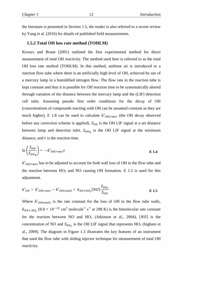
1.5.2 Total OH loss rate method (TOHLM)
Kovacs and Brune (2001) outlined the first experimental method for direct
measurement of total OH reactivity. The method used here is referred to as the total
OH loss rate method (TOHLM). In this method, ambient air is introduced to a
reaction flow tube where there is an artificially high level of OH, achieved by use of
a mercury lamp in a humidified nitrogen flow. The flow rate in the reaction tube is
kept constant and thus it is possible for OH reaction time to be systematically altered
through variation of the distance between the mercury lamp and the (LIF) detection
cell inlet. Assuming pseudo first order conditions for the decay of OH
(concentrations of compounds reacting with OH can be assumed constant as they are
much higher), E 1.8 can be used to calculate ′ைு(௪ ) (the OH decay observed
before any correction scheme is applied). ைு is the OH LIF signal at a set distance
between lamp and detection inlet, ைு is the OH LIF signal at the minimum
distance, and isݐ the reaction time.
lnቆைு
ைு
ቇ= − ′ைு(௪ ݐ( E 1.4
′ைு(௪ ) has to be adjusted to account for both wall loss of OH in the flow tube and
the reaction between HO2 and NO causing OH formation. E 1.5 is used for this
adjustment.
′ைு = ′ைு(௪ ) − ′ைு(௪) + ேைାுைమ[]
ுைమ
ைுE 1.5
Where ′ைு(௪) is the rate constant for the loss of OH to the flow tube walls,
ேைା�ுைమ (8.8 × 10ଵଶ cm3 molecule-1 s-1 at 298 K) is the bimolecular rate constant
for the reaction between NO and HO2 (Atkinson et al., 2004), [] is the
concentration of NO and ுைమ is the OH LIF signal that represents HO2 (Ingham et
al., 2009). The diagram in Figure 1.3 illustrates the key features of an instrument
that used the flow tube with sliding injector technique for measurement of total OH
reactivity.

Chapter 1 13 Introduction
Figure 1.3: Diagram of the Total OH Loss Measurement (TOHLM) instrument used for themeasurements of total OH reactivity. Taken from Kovacs and Brune (2001).
A flow tube with sliding injector technique but with a different detector also exists
and was first reported by (McGrath, 2010); the method of detection used is chemical
ionisation mass spectrometry (CIMS). This instrument was deployed during the
OASIS campaign in Alaska to record the first total OH reactivity measurements in
an arctic environment (McGrath et al., 2009), it was also deployed during the NIFTy
campaign at a forested site (McGrath, 2010). A similar instrument is also reported to
have been constructed by the German Weather Service (Heard, 2012). Full details of
measurements using the flow tube with sliding injector - CIMS technique are not
currently present in the literature.
1.5.3 Laser flash photolysis coupled with laser induced fluorescencespectroscopy (LFP-LIF)
The feasibility of a second laser induced fluorescence method for the measurement
of total OH reactivity was demonstrated by Calpini et al. (1999) and Jeanneret et al.
(2001). This method is termed as the laser flash photolysis coupled with laser
induced fluorescence spectroscopy (LFP-LIF) technique and was first successfully
implemented by Sadanaga et al. (2004b) for field measurements in urban Tokyo. A
schematic of the instrument used is shown in Figure 1.4.

Chapter 1 14 Introduction
Figure 1.4: Schematic of the Tokyo Metropolitan University laser induced fluorescencepump and probe instrument. Taken from Sadanaga et al. (2004b).
OH is produced in a reaction flow tube by photolysis of O3 using a 266 nm pump
laser and subsequent reaction of O(1D) with water vapour present in ambient air
(R 1.1 and R 1.2). The OH decay is then recorded in real time by FAGE (described
in Section 1.4). Similar to the flow tube with sliding injector technique, this method
relies on the assumption that the decay of OH is occurring under pseudo first order
conditions. E 1.6 (essentially E 1.4 rearranged) can be used to represent the pseudo
first order OH decay.
ைு = ைு exp(− ′ைு(௪ (ݐ( E 1.6
When a single exponential curve is fitted to the observed OH decay signal, the
expression of the fitted curve can be used to obtain a value for Ԣைுሺ௪ሻ. Similar to
the flow tube with sliding injector technique, corrections have to be made to account
for physical processes that affect the OH decay signal, such as escape of OH from
the detection zone in the flow tube by diffusion and turbulence (Sadanaga et al.,
2004b). To achieve this, the decay of OH in zero air ( Ԣைுሺ௭ሻ) has to be recorded,
E 1.8 is then used to calculate Ԣைு .

Chapter 1 15 Introduction
′ைு = ′ைு(௪ ) − ′ைு(௭) E 1.7
Interference is also possible from the HO2 + NO reaction at high NO (but only
above ~20 ppbv); this scales with NO concentration and is much smaller than in the
flow tube with sliding injector technique (where corrections need to be made above
~5 ppbv). Often in the literature ambient air samples have either been diluted prior
to analysis to avoid this interference, or when NO was very high measurements have
been omitted from further analysis due to the large uncertainty incurred (Yoshino et
al., 2012). Lou et al. (2010) have reported that ′ைு can be estimated using a bi-
exponential fit (to account for radical recycling) to within less than 10 % error at NO
levels of up to 30 ppbv.
The LFP-LIF method was used for the measurements of OH reactivity presented in
this work (Chapters 3, 5 and 6). Specific details of the instrument used can be found
in Chapter 2 and also in a recent publication by Stone et al. (2016).
1.5.4 Comparative reactivity method (CRM)
Sinha et al. (2008) first reported the comparative reactivity method (CRM) for the
measurement of total OH reactivity. Pyrrole (a compound that is not commonly
found in ambient air) competes with trace species in ambient air to react with OH.
E 1.8 is used to calculate ′ைு(௪ ) where ଵܥ is the concentration of pyrrole detected
when no OH is generated, ଶܥ is the concentration of pyrrole detected when OH is
generated in the absence of ambient air, ଷܥ is the concentration of pyrrole detected
when OH is generated in the presence of ambient air and ௬ାைு is the rate constant
for the reaction between pyrrole and OH (1.03 × 10ଵ cm3 molecule-1 s-1), which is
widely reported in literature (Wallington, 1986).
′ைு(௪ ) =−ଷܥ ଶܥ−ଵܥ ଷܥ
௬ାைுܥଵ E 1.8
Figure 1.5 shows a diagram of the glass reactor used in the majority of CRM studies
of total OH reactivity. Pyrrole and ambient or zero air are introduced through arm A.
Humidified Nitrogen is flowed through arm B where UV radiation from a Hg pen-
ray lamp is used to produce OH. The exhaust is pumped out of arm C and arm D is
used to transfer the analyte to the Proton Transfer Mass Spectrometer (PTR-MS) for
the detection of pyrrole.

Chapter 1 16 Introduction
Figure 1.5: Schematic diagram of the glass reactor used in a comparative reactivity method(CRM) instrument for measurement of total OH reactivity. Taken from Sinha et al. (2008).
Total OH reactivity measurements made using the CRM also have to be adjusted to
account for HO2 + NO recycling. The adjustment is made by systematic addition of
NO to the reactor and analysis of the absolute changes in OH reactivity. These
changes are then plotted against NO concentration, and linear functions from linear
best fits are used to correct Ԣைுሺ௪ሻ values to Ԣைு values. In contrast to the flow
tube with sliding injector and laser flash photolysis methods, all CRM measurements
are corrected, even at very low NO concentrations.
Nölscher et al. (2012a) have recently reported that a CRM instrument with a Gas
Chromatograph - Photoionisation Detector (GC - PID) in place of a PTR-MS has
potential as an economical instrument for total OH reactivity measurements.
However, an instrument of this type has not yet been extensively used for field
measurements.
1.5.5 Instrumentation in the literature
Flow tube with sliding injector, laser flash photolysis and comparative reactivity
method instruments have all been used extensively for the measurement of total OH
reactivity by various research groups worldwide. Table 1.1 provides a summary of
the instruments currently in the literature that have been used for the measurement
of total OH reactivity.

Chapter 1 17 Introduction
Technique Group k’OH(physical) (s-1) Uncertainty (1σ) Reference
TOHLM (LIF)* Pennsylvania StateUniversity, USA
5.1 ± 0.6 ± 14 % Kovacs et al. (2003)
TOHLM (LIF) ‡ University of Leeds, UK 1.6 ± 0.4 ± 10 % Ingham et al. (2009)
TOHLM (LIF) † Pennsylvania StateUniversity, USA
Not available Not available Mao et al. (2010)
TOHLM (LIF) Indiana University, USA 3.6 ± 0.2 ± (1.2 s-1 + 4 %) Hansen et al. (2014)
TOHLM (CIMS)** University of Colarado,USA
Not available Not available McGrath (2010)
TOHLM (CIMS)** German WeatherService, Germany
Not available Not available Heard (2012)
LFP-LIF Tokyo MetropolitanUniversity, Japan
3.0 ± 0.15 ± 10 % Sadanaga et al.(2004b)
LFP-LIF JülichForschungszentrum,Germany
1.4 ± 0.3 ± 10 % Lou et al. (2010)
LFP-LIF** University of Lille,France
Not available Not available Amedro et al. (2012)
LFP-LIF University of Leeds,UK 1.1± 1.0 s-1 ± 6 % Stone et al. (2016)
CRM (PTRMS) Max Planck Institute forChemistry, Mainz,Germany
Not applicable 25 % Sinha et al. (2008)
CRM (PTRMS) University of Colarado,USA
Not applicable 30 % Kim et al. (2011)
CRM (GC-PID) Max Planck Institute forChemistry, Mainz,Germany
Not applicable 25 % Nölscher et al.(2012a)
CRM (PTRMS) Mines Douai NationalGraduate School ofEngineering, France
Not applicable 17-25% Michoud et al. (2015)
CRM (PTRMS) Laboratory of theSciences of Climate andthe Environment(LSCE), France
Not applicable 35 % Zannoni et al. (2016)
Table 1.1: Instruments for the direct measurement of total OH reactivity that have beenreported in the literature. * Total OH Loss rate Method (TOHLM) instrument, no longer inoperation. ‡ Instrument no longer in operation. † A new TOHLM instrument was built atPennsylvania State University. ** No published data available from field measurements.Values were correct at the time of publication. k’OH(physical) can be considered as theinstrument artefact and is not applicable to CRM type instruments.
In addition to the instruments listed in Table 1.1, a new instrument for the
measurement of total OH reactivity has been developed at the University of Leeds as
a replacement for the old flow tube with sliding injector instrument described by
Ingham et al. (2009). Full details of this new instrument are presented in this work.
1.5.6 Comparison of techniques
Laser flash photolysis pump and probe instruments present the only method for
recording total OH reactivity in real time, thus they are ideally suited for
measurements in places where trace species composition is highly variable, e.g.
urban environments. This is due to their averaging times being considerably shorter

Chapter 1 18 Introduction
than for the TOHLM or CRM technique. They also produce zero HO2 initially,
whereas the flow tube with sliding injector and comparative reactivity method
instruments do produce HO2 initially, due to the use of an Hg(Ar) penray lamp (Lou
et al., 2010) at 185 nm to photolyse water vapour to give OH and H. A result of this
is that correction for interference from HO2 + NO is only necessary at high NO
(above approximately 20 ppbv). This is another reason why pump and probe
instruments are suited to urban environments. In contrast, flow tube with sliding
injector measurements require correction when NO is above approximately ~1 ppbv
(Shirley et al., 2006) and comparative reactivity method measurements require
corrections to be made when any NO is detected (Michoud et al., 2015). A
disadvantage to the laser flash photolysis pump and probe technique is that the
instrument requires two lasers which incurs additional cost and can be technically
more demanding. As discussed in Section 1.4.4 a new comparative reactivity
method instrument with a GC-PID detector is reported to have potential as a
relatively low cost instrument for total OH reactivity measurement. Photolysis of
pyrrole and VOCs within the OH reactors of comparative reactivity method
instruments has also been reported to affect measurements of ′ைு , full details of the
significance of this effect have recently been reported by Michoud et al. (2015).
1.6 Review of ground-based OH reactivity measurements
1.6.1 Forest atmospheres with low anthropogenic influence
Di Carlo et al. (2004) reported the first total OH reactivity measurements from a
forested site at Great Lakes, MI, USA during the the program for research on
oxidants: photochemistry, emissions and transport (PROPHET) campaign. Missing
OH reactivity was observed to be exponentially dependant on temperature above
284 K, below 284 K the missing OH reactivity was less than 0.5 s-1. It was found to
be as high as ~4 s-1 at around 297 K. The authors concluded that this missing
reactivity could have been caused by emissions of biogenic volatile organic
compounds (BVOCs) such as terpenes which also display a temperature dependant
emission. Figure 1.6 demonstrates the exponential dependence of missing reactivity
on temperature.

Chapter 1 19 Introduction
Figure 1.6: Missing OH reactivity observed by Di Carlo et al. (2004) at a forested site inGreat Lakes, MI, USA. The solid line has been fitted to the data points shown; the dashedline is a derived temperature dependence of terpene emissions. Taken from Di Carlo et al.(2004).
Measurements of total OH reactivity have been reported from a forested site at
Whiteface Mountain, NY, USA during the PMTACS-NY Whiteface Mountain
campaign (Ren et al., 2006b). The measured and calculated reactivities were in good
agreement and no relationship was found between the magnitude of the missing
reactivity and temperature, in contrast to the temperature dependent missing
reactivity reported from PROPHET. Figure 1.7 shows the campaign average
relationship between Ԣைு and Ԣைுሺሻ.

Chapter 1 20 Introduction
Figure 1.7: Plot showing all k’OH values measured campaign (small dots) and the campaignaverage k’OH (calc) (large circles connected with a line) during the PMTACS-NY WFMcampaign. Taken from Ren et al. (2006b).
Sinha et al. (2008) reported total OH reactivity measurements from a tropical
rainforest site, however only 2 hours of data were obtained. The measurements were
taken at the Brownsberg national park in Suriname and the average reactivity was
approximately 53 s-1. Ԣைுሺሻwas determined using concentrations of OH reactive
species that were measured prior to the two hours of reactivity measurements, the
average missing reactivity was ~65 %.
Whalley et al. (2011) and Edwards et al. (2013) reported high total OH reactivity
measurements from a rainforest during the OP3-I campaign in the Sabah Region of
Malaysian Borneo. Diurnal behaviour was observed in the form of a peak around
midday. The entire campaign diurnal average Ԣைு was ~29 s-1. Edwards et al.
(2013) reported missing reactivity determined by comparison with a chemical box
model, of approximately 53 %. When this box model was forced to include a greater
contribution from photo-oxidation products by constraint to observed OH levels
(which were also underestimated by the model by approximately 70 %), the missing
reactivity decreased to ~38 %. This indicated that missing sources of OH as well as
sinks contributed to the discrepancy of measured k’OH and k’OH (calc).
Sinha et al. (2010) reported total OH reactivity measurements taken in 2008 from
within the canopy of a Finnish boreal forest. The averaged OH reactivity observed

Chapter 1 21 Introduction
during the campaign was ~9 s-1. Diurnal behaviour was not observed and the lowest
reactivities were below the limit of detection (3.5 s-1) whereas the largest were
typically around 20 s-1. Except during one episode of high pollution where values of
up to 60 s-1 were reported, the authors concluded that this was due to biogenic
emissions from a local saw mill, which had previously been reported as a strong
source of VOCs (particularly monoterpenes) at the site (Eerdekens et al., 2009). On
average, approximately 50% missing reactivity was observed during this campaign
and it was concluded that its cause was many unmeasured primary BVOCs at low
levels, not products of photo-oxidation. This is because the measurements were
taken from within the canopy so it is unlikely that there were high concentrations of
unmeasured oxidation products. Also contributions to calculated OH reactivity from
measured primary emissions were higher than their measured oxidation products.
Hansen et al. (2013) reported total OH reactivity measurements from the community
atmosphere-biosphere interaction experiment (CABINEX) campaign that took place
during the summer at the same site in Great Lakes MI, USA as the PROPHET 2000
campaign (Di Carlo et al., 2004). The flow tube with sliding injector technique was
used to take measurements at 21 m and 31 m above, and 6 m below the deciduous
forest canopy. The missing reactivities were found to be ~42 % and ~43 % above
the canopy (21 m and 31 m, respectively). Measurements of total OH reactivity
within the canopy were found to be in good agreement with the calculated
reactivities. Missing reactivity above the canopy was observed to have a similar
exponential dependence on temperature to that observed by (Di Carlo et al., 2004).
However, the authors concluded that during CABINEX 2009 missing reactivity was
most likely due to unmeasured BVOC oxidation products, rather than BVOCs.
The comparative reactivity method was used by Nölscher et al. (2012b) to measure
both in canopy and above canopy total OH reactivities from a boreal forest site in
Finland during the HUMPPA-COPEC 2010 campaign. Values varied throughout the
course of the campaign and reactivity was typically higher inside the canopy for the
majority. However, reactivity was found to be higher above the canopy when
plumes from Russian wildfires were transported to the site. Missing reactivity was
only assessed for above canopy measurements and was found to be ~68 % on
average for the whole campaign. Table 1.2 provides a summary of all total OH
reactivity field measurements at forested sites with low anthropogenic influence in
the literature.

Chapter 1 22 Introduction
Campaign Dates Technique Location Average k’OH(missing) (s-1) Reference
PROPHET Jul – Aug,2000
TOHLM (LIF) Great Lakes,MI, USA
~50 % * (~10 m abovecanopy)
Di Carlo et al. (2004)
PMTACS-NY-WFM
Jul – Aug,2002
TOHLM (LIF) WhitefaceMountain, NY,USA
Small *† (withincanopy, on ground)
Ren et al. (2006b)
GABRIEL Oct, 2005 CRM(PTRMS)
Brownsberg,Brokopondo,Suriname
~65 % *(within canopy,~35 m above ground)
Sinha et al. (2008)
OP3-I Apr – May,2008
TOHLM (LIF) Sabah, Borneo,Malaysia
~53 % ** (withincanopy, ~5m aboveground)
Edwards et al. (2013)
BFORM Aug, 2008 CRM(PTRMS)
Hytiӓlӓ, Juupajoki,Finland
~50 % * (within canopy,~12 m above ground)
Sinha et al. (2010)
CABINEX Jul – Aug2009
TOHLM (LIF) Great Lakes,MI, USA
~42 %* (~21 m abovecanopy)
~43 %* (~31 m abovecanopy)
Small*† (~6 m belowcanopy)
Hansen et al. (2014)
HUMPPA-COPEC
Jul – Aug2010
CRM(PTRMS)
Hytiӓlӓ, Juupajoki,Finland
~68 % * (~24 m abovecanopy)
Nölscher et al. (2012b)
Table 1.2: Summary of total OH reactivity field measurements taken at forested sites withlow anthropogenic influence. *Average missing reactivity determined by comparisonwith′� ,() determined using just measured sinks. **Average missing reactivity
determined by comparison with′� ) ( determined considering model generated
intermediates. †Average missing reactivity could not be determined due to a lack ofnumerical values in the literature.
A total of seven field measurements of total OH reactivity have been reported for
forested sites. In the majority of which, significant levels of missing reactivity have
been observed. Four measurements have been made using the flow tube with sliding
injector technique and another three with the comparative reactivity method.
Perhaps one of the most striking studies is that of Di Carlo et al. (2004), where the
missing reactivity in a mixed transition forest site during the PROPHET 2000
campaign was found to be exponentially dependent upon temperature when
measured using the flow tube with sliding injector technique. Missing reactivity
ranged from 0.5-3.7 s-1 as temperature increased from 284 K to 299 K and was
concluded to be due to unmeasured BVOC emissions which were also expected to
be temperature dependent. Most recently (Hansen et al., 2013) have reported total
OH reactivity measurements from the same site using the same method and
observed a similar temperature dependence during the CABINEX 2009 campaign.
However, in this case it was found to be inconsistent with predictions for the

Chapter 1 23 Introduction
temperature dependence of BVOC emissions; this led to the conclusion that
unmeasured photo oxidation products contributed the most to missing reactivity.
No such temperature dependency has been described at sites other than the one used
for PROPHET 2000 and CABINEX 2009, however during HUMPPA-COPEC 2010
the greatest missing reactivity was recorded after a period of elevated temperature.
Also in other campaigns such as OP3-I in Borneo the temperature did not fluctuate
significantly throughout the course of measurement meaning that any temperature
dependency could not have been properly assessed (Edwards et al., 2013).
In contrast to OH reactivities reported from other forested sites, no significant
missing reactivity was observed during the PMTACS-NY-WFM campaign in 2002
(Ren et al., 2006b). The small amount of missing reactivity reported was not found
to be temperature dependant, the daytime campaign average temperature was 291 K
(a temperature at which significant missing reactivity would not have been observed
at the PROPHET 2000 site). This and the observation that isoprene only accounted
for small portion of calculated OH reactivity (as opposed to PROPHET 2000 where
it accounted for a much larger portion), led to the conclusion that the small and high
missing reactivities at Whiteface Mountain and the PROPHET site, respectively
were due to differences in BVOC emissions.
Two measurements of total OH reactivity have been reported for tropical rainforests.
Sinha et al. (2008) reported measurements from project GABRIEL (2005). Only a
small quantity (~2 hours) of data were collected due to a lack of availability of the
PTR-MS instrument that was also being used for hydrocarbon measurements.
However, the average missing reactivity that could be determined was ~65 %
(Edwards, 2011). A much more extensive survey of OH reactivity in a tropical
rainforest has since been reported by Whalley et al. (2011) and (Edwards et al.,
2013) for the OP3-I campaign in Malaysian Borneo. The average missing reactivity
for the entire campaign was also high and box modeling indicated that missing OH
sources influenced the discrepancy between measured k’OH and k’OH(calc).
Two sets of measurements (both from summer) have been reported from the same
site in a boreal forest (Hyytiӓlӓ, Juupajoki, Finland). Sinha et al. (2010) found there
to be approximately 50 % average missing reactivity from in-canopy measurements.
More recently a much more extensive set of total OH reactivity measurements
(above-canopy and in-canopy) have been reported by Nölscher et al. (2012b).

Chapter 1 24 Introduction
Missing reactivity was only assessed for above-canopy measurements due to
availability of hydrocarbon data and averaged ~68 % for the entire campaign.
Similar to PROPHET 2000, HUMPPA-COPEC 2010 and CABINEX 2009, large
missing reactivity was associated with high temperatures; missing reactivity was
~89 % during a hot period at the start of the campaign. This led to the conclusion
that unmeasured BVOCs significantly contributed to missing reactivity as Yassaa et
al. (2012) reported that high temperatures were accompanied by BVOC emission
diversification at this site.
In summary, there are large gaps in our knowledge of the OH chemistry in forested
environments where total OH reactivity has been directly measured. Further field
measurements from a variety of forest biomes in conjunction with leaf enclosure
studies are required to assess the global misunderstanding.
1.6.2 Urban atmospheres
The first field measurement of total OH reactivity was at an urban site and was
reported in 2001, a full analysis of the results was published in 2003 (Kovacs and
Brune, 2001, Kovacs et al., 2003). The measurements were taken at an urban
background site in Nashville, TN, USA during the summer of 1999. The measured
reactivity was considerably larger than that initially calculated from co-located VOC
concentration measurements (~30 %). The authors concluded that the cause for this
missing reactivity was VOCs that were either not included in the suite of ambient
concentration measurements, or that some of the OH reactive compounds present
were below the limit of detection. Anthropogenic VOC emissions from a nearby
tunnel were scaled down proportionally using the CO concentration. The scaled
down concentrations of species that were below the limit of detection at the
measurement site were then included in the calculation of total OH reactivity. This
led to a reduction in the average missing reactivity so that it was ~10 %.
Di Carlo et al. (2004) have reported total OH reactivity measurements from an urban
background site at LaPorte, TX, USA. The measurements were taken at an airport
where the air mass was influenced by anthropogenic emissions from Houston,
petrochemical plants and a nearby shipping canal. The magnitude of the average
missing reactivity was small (~4 %) and no temperature dependence was observed.
Summer measurements from an urban background site in New York City, NY, USA
have also been reported (Ren et al., 2003b, Ren et al., 2003c). The total OH

Chapter 1 25 Introduction
reactivity was about twice that observed in Nashville and the ‘missing’ OH
reactivity was ~10 %.
OH reactivity measurements were taken in 2003 at a site located in the Mexico City
Metropolitan Area (MCMA) (Shirley et al., 2006). Strong diurnal behaviour was
observed, reactivity was found to be extremely high (approximately 120 s-1) during
the morning rush hour, about five times higher than the peak observed in PMTACS-
NY 2001. 72 % of the measured OH reactivity was attributable to VOCs and the
diurnal profile of NOx was similar to that for OH reactivity, and suggests that
vehicular emissions were a driver in the daily changes observed in OH reactivity.
The average missing reactivity for the whole campaign was approximately 30 %.
Sadanaga et al. (2004b) reported the first field measurements of total OH reactivity
using the laser induced fluorescence pump and probe technique from a site in urban
Tokyo during the summer. Following this a more in detailed report of these
measurements has been given by Sadanaga et al. (2005). Yoshino et al. (2006) have
since reported winter, spring and autumn measurements from the same site.
Measured OH reactivity ranged from 10 to 100 s-1during observations for all four
seasons. During summer measurements OH reactivity was found to correlate well
with NOx levels. During winter, spring and autumn NOx was generally high and OH
reactivity was found to correlate well with NO levels. Significant missing reactivity
(~30%) between calculated values and observed values was observed in summer,
spring and autumn. On the other hand the missing reactivity was much lower (~5%)
in winter, indicating that missing OH sinks in urban Tokyo are related to
photochemical activities.
In 2004, OH reactivity measurements were taken during winter at the same site as
PMTACS-NY 2001 (a summer campaign) (Ren et al., 2006a). Diurnal behaviour
was present in the form of two peaks in reactivity. These peaks were seen in the
morning and afternoon and were likely due to increased vehicular emissions at these
times. There was overall good agreement between calculated and measured
reactivities, however there was clearly ‘missing’ OH reactivity during the rush hour
as demonstrated by the plots in Figure 1.8.

Chapter 1 26 Introduction
Figure 1.8: (a) Plot showing the relationship between measured (circles) and calculated(grey dots) total OH reactivities from a field campaign during the winter in New York City,2004. (b) Plot showing the campaign average diurnal profiles of measured (circles) andcalculated (squares) total OH reactivities. Taken from Ren et al. (2006a).
Sinha et al. (2008) reported total OH reactivity measurements from an urban site in
Mainz, Germany during the summer, the average value was ~10.4 s-1. A diurnal
peak in reactivity was also observed during the afternoon. Missing reactivity could
not be assessed as no co-located VOC concentration measurements were taken so no
comparison between calculated and observed reactivity could be made.
Mao et al. (2010) reported total OH reactivity measurements from an urban
background site near Houston, TX, USA during the TRAMP 2006 campaign. A
diurnal peak was observed due to the morning rush hour and on average the
agreement between measured and calculated reactivities was very good, as
demonstrated by Figure 1.9.

Chapter 1 27 Introduction
Figure 1.9: Plot showing the relationship between the diurnal average measured (redcircles) and calculated (black squares) observed during the TRAMP 2006 campaign. Takenfrom Mao et al. (2010).
Chatani et al. (2009) first reported total OH reactivities from the centre of the
metropolitan area of Tokyo in the summer of 2007. More recently Yoshino et al.
(2012) have reported measurements from the same site for the winter of 2007 and
the autumn of 2009. The missing reactivity observed in all three data sets was
similar to that reported from Hachioji (Sadanaga et al., 2004a, Sadanaga et al., 2005,
Yoshino et al., 2006). The total OH reactivity in the summer 2007 measurements
ranged from 15 to 70 s-1. Model predictions reported by Chatani et al. (2009)
indicated that products of photo-oxidation and primary species were responsible for
missing reactivity (~26.5% average). The total OH reactivity in the winter 2007
measurements ranged from 10 to 80 s-1. The winter 2007 data were excluded from
missing reactivity analysis due to high morning rush NO levels (no diurnal average
for morning rush available, however average daytime NO was 37.4 ppbv) causing
OH recycling (from HO2 + NO) and consequently large uncertainties. Total OH
reactivity in the autumn 2009 measurements also ranged from 10 to 80 s-1 and
significant missing reactivity was observed (~34.7% on average).
The first total OH reactivity measurements for a European megacity were taken in
Paris during the 2010 MEGAPOLI campaign reported by Dolgorouky et al. (2012).
Reactivity had a strong dependence on the origin of the air mass present. When

Chapter 1 28 Introduction
polluted continental air masses were present at the site, average measured
reactivities were approximately 120-130 s-1 and the missing reactivity was the
highest ever registered in an urban area (approximately 74 %). However, when
cleaner marine influenced air masses reached the site the OH reactivity was
approximately 20 s-1 and the average missing reactivity was low (approximately 12
%). The authors concluded that oxidised compounds from photo chemically
processed anthropogenic emissions were the cause of such high missing reactivity.
A recent study by Brune et al. (2016) presented observations of OH reactivity that
were made during the California Nexus (CalNex) campaign at an urban background
site south of Bakersfield , CA, US. The measurements were made in a car park in
close proximity (<1 km) to a major road and a few hundred metres from agricultural
land. A diurnal trend in OH reactivity (ranging from ~10 – 25 s-1) was observed that
showed evidence of influence from morning rush hour traffic emissions. The
‘missing’ OH reactivity determined through comparison of the measurements with
model predictions was ~41 % on average. The site used for OH reactivity
measurements during CalNex shared similarities with the site used for OH reactivity
measurements in York that are presented in Chapter 5 of this thesis. Both were on
the edge of a large city, near agricultural land and main roads.
One of the studies most relevant to the work presented in this thesis is that reported
by Whalley et al. (2016) where measurements of OH reactivity made in urban
London are presented from the clean air for London (ClearFlo) campaign. The
measurements were made using the same LFP-LIF instrument that is described in
Chapter 2 of this thesis and was used to make the measurements of OH reactivity
that are presented in Chapters 5 and 6. The results showed a strong diurnal peak
(~27 s-1) in the mornings due to rush hour traffic emissions. When concentrations of
all of the measured OH sinks were used in a model simulation, the predicted OH
reactivity was typically ~15 % lower than the measured OH reactivity. Further
discussion of the observations from ClearFlo are discussed in the context of the
results from this work in Chapters 5 and 6. A summary of OH reactivity
measurements in the literature is presented in Table 1.3.

Chapter 1 29 Introduction
Campaign Dates Technique Location Average k’OH(missing) (s-1) Reference
SOS Jun – Jul,1999
TOHLM (LIF) Nashville, TN,USA
~10 % * Kovacs et al. (2003)
TexAQS Aug – Sep,2000
TOHLM (LIF) La Porte, TX,USA
~4 % * Di Carlo et al. (2004)
PMTACS-NY Jun – Aug,2001
TOHLM (LIF) New YorkCity, NY,USA
~10 % * Ren et al. (2003b)
MCMA Apr, 2003 TOHLM (LIF) Iztapalapa,Mexico City,Mexico
~30 % * Shirley et al. (2006)
- Jul and Aug,2003
Jan, Feb ,Mayand Nov, 2004
LFP-LIF Hachioji,Tokyo, Japan
~30 %
(summer, spring andautumn)
~5 %
(winter)
Yoshino et al. (2006)
- Jan – Feb,2004
TOHLM (LIF) New YorkCity, NY,USA
Small * † Ren et al. (2006a)
- Aug, 2005 CRM(PTRMS)
Mainz,Rhineland-Palatinate,Germany
*** Sinha et al. (2008)
TRAMP Aug – Sep,2006
TOHLM (LIF) Houston, TX,USA
Small * Mao et al. (2010)
- Aug and Dec,2007
Oct, 2009
LFP-LIF Koto-Ku,Tokyo, Japan
~27 %
(summer)
~35%
(autumn)
Yoshino et al. (2012)
MEGAPOLI Jan – Feb2010
CRM(PTRMS)
13th District,Paris, France
~54 % * Dolgorouky et al.(2012)
CalNex May-Jun 2010 TOHLM (LIF) Bakersfield,CA, US
~41 %** Brune et al. (2016)
ClearFlo Jul- Aug 2012 LFP-LIF NorthKensington,London, UK
~15 %** (Whalley et al., 2016)
Table 1.3: Summary of total OH reactivity field measurements taken at urban sites with lowanthropogenic influence. Data from field measurements at Hachioji are also available inother publications (Sadanaga et al., 2005, Sadanaga et al., 2004b, Sadanaga et al., 2004a).Data from field measurements at Koto-Ku are also available in Chatani et al. (2009).*Average missing reactivity determined by comparison with′� .() **Average missing
reactivity determined by comparison with′� ) .( ***Missing reactivity was not
assessed due to there being no co-located VOC concentration measurements. †Averagemissing reactivity could not be determined due to a lack of numerical values in theliterature.
OH reactivity measurements from urban and urban background sites are more
widely reported in literature than measurements for forested environments.
Measurements taken using all three techniques have been reported and in general
missing reactivity is lower than it is at forested sites.

Chapter 1 30 Introduction
Measurements from New York and Tokyo urban background sites, and a central
Tokyo site have been reported for both summer and winter (Ren et al., 2003b,
Yoshino et al., 2006, Yoshino et al., 2012). At the background sites the average
missing reactivity was found to be lower in winter than summer (~30 % compared
with ~5 % for the Tokyo background site); thus indicating that photo-oxidation
products of primary emissions account for a large portion of missing urban
reactivity. This is because concentrations of primary emissions are typically higher
in winter than summer due to lower actinic flux and a compressed boundary layer.
The missing reactivity at the central Tokyo site in winter could not be fully assessed;
this was due to very high NOx (NO: 37.4 ppbv, NO2: 35.8 ppbv) levels leading to
large experimental uncertainty from HO2 + NO recycling.
Missing urban reactivity is often lower when large portions of ′ைு() or
′ைு( ௗ) are accounted for by known OH reactive pollutants such as NOx and CO.
The missing reactivities reported from PMTACS-NY-2001 and MCMA (~10 % and
~30 %, respectively) demonstrate this. On average in PMTACS-NY-2001 NOx and
CO accounted for 42 % and 12 % of the campaign average ′ைு(), respectively,
whereas in MCMA NOx and CO accounted for 12 % and 7 % of the campaign
average ′ைு(), respectively.
In summary, the percentage of ‘missing’ OH reactivity at urban background and
central urban sites is typically smaller than for forested sites, however there are still
gaps in our knowledge. Where missing reactivity has been observed, a common
conclusion is that it was a result of unmeasured concentrations of primary emissions
and their photo-oxidation products not being included in the calculation of ′ைு()
or ′ைு( ௗ). Measurements of OH reactivity from an urban background site in
York are presented in Chapter 5 of this thesis.
1.6.3 Rural and other atmospheres
In 2005 OH reactivity measurements from a rural site in an Appalachian valley in
Rock Springs, PA, USA were reported (Ren et al., 2005). The site was surrounded
by agricultural fields, near to a road and close enough to some large cities to be
influenced by anthropogenic emissions (Ren et al., 2003a). No co-located VOC
concentration data were available so missing reactivity could not be assessed. When

Chapter 1 31 Introduction
a computer model was constrained using measured total OH reactivity, OH and HO2
mixing ratio predictions were in good agreement with field measurements.
Total OH reactivity measurements from 2004 at a coastal site in Weybourne,
Norfolk, UK were reported by Lee et al. (2009). The average measured OH
reactivity was ~4.9 s-1 with minimum and maximum values of ~1.3 and ~9.7 s-1,
respectively. No diurnal behaviour was observed owing to the variety of air masses
that reached the site; UK/South Westerly Air and Northerly Air. These acted upon
the site at irregular intervals and OH reactivity was found to be variable during
episodes of UK/South Westerly air but less so with Northerly air. Also, it was
typically higher during episodes of UK/South Westerly air than Northerly air.
Missing reactivity was first calculated using co-located VOC concentration
measurements and was found on average to be 1.9 s-1 (~40%). Secondly, the Master
Chemical Mechanism (MCM) (Jenkin et al., 1997, Saunders et al., 2003) was used
to model missing reactivity and on average this was found to be 1.4 s-1 (~30%).
Whilst there was better agreement between measured and modeled reactivity,
missing reactivity is still significant, even in episodes of clean air. The authors
concluded that the missing reactivity was likely to be due to many high molecular
mass VOCs at low concentrations which were not included in the suite of VOC
measurements. In Chapter 6 of this thesis measurements of OH reactivity from the
same site in Weybourne are presented and comparisons are made with the OH
reactivity calculated using the concentrations of measured OH sinks.
In 2006 total OH reactivity measurements were reported from a regional background
site in the Pearl River Delta (PRD), China (Lou et al., 2010). The measured total OH
reactivities ranged from 10 to 120 s-1. Diurnal behaviour was observed and
correlated well with anthropogenic pollutant levels such as CO, NO2 and propene.
Total OH reactivity was calculated from co-located VOC concentration
measurements and on average missing reactivity was ~50 %. In an attempt to
account for some of the missing reactivity, the Regional Atmospheric Chemistry
Model (RACM) was used to predict total OH reactivity by taking into account the
reactions with OH of photo-oxidation products of the measured VOCs. Three
models were used to predict OH reactivity. The first and most basic model used only
data from the co-located VOC measurements and rate constants. The second took
into account additional recycling of OH. The third was constrained using OH
concentrations measured during the field campaign. Similar to the calculated OH

Chapter 1 32 Introduction
reactivities, the correlation between model prediction and observed OH reactivity
was good. Missing reactivity was reduced to approximately 10 % using the basic
RACM model predictions for daytime measurements, however it was still found to
be significant (approximately 30 %) for night time measurements.
Sinha et al. (2012) reported winter total OH reactivity measurements taken in 2008
from southern Spain at a site near the Atlantic Ocean, the campaign average
reactivity was 18 s-1. Total OH reactivity was found to be very dependent on the
origin of the air mass present. Assessment of the missing reactivity at this site was
not possible due to an absence of certain key VOC measurements. Table 1.4
provides a summary of all total OH reactivity field measurements that have been
taken at sites, that are not forested or urban, but do have significant anthropogenic
influence.
Campaign Dates Technique Location Average k’OH(missing) (s-1) Reference
- May – Jun,2002
TOHLM (LIF) Rock Springs,PA,USA
*** Ren et al. (2005)
TORCH-2 May, 2004 TOHLM (LIF) Weybourne,Norfolk, UK
~40 % *
~30 % **
Lee et al. (2009)
PRIDE-PRD Jul, 2006 LFP-LIF Guangzhou,Guandong,China
~50 % *
Small **†
Lou et al. (2010)
DOMINO Nov – Dec,2008
CRM(PTRMS)
El Arenosillo,Magazón,Spain
*** Sinha et al. (2012)
Table 1.4: Summary of total OH reactivity field measurements taken at rural or urban sites.*Average missing reactivity determined by comparison with′� .() **Average missing
reactivity determined by comparison with′� ) .( ***Missing reactivity was not
assessed due to there being no co-located VOC concentration measurements. †Averagemissing reactivity could not be determined due to a lack of raw data in the literature.
Total OH reactivity measurements have also been reported from several rural and
coastal sites where the air mass is periodically influenced by anthropogenic
emissions. Only for two of these campaigns could the missing reactivity be assessed.
Missing reactivities were reported from comparisons with calculated and modeled
reactivities, for both campaigns the missing reactivity was smaller when modeled
values were used.
Missing reactivity was assessed during both the TORCH-2 campaign and the
PRIDE-PRD campaign. When determined by comparison of measured reactivities
with those calculated from co-located VOC concentration measurements the average
missing reactivities for TORCH-2 and PRIDE-PRD were approximately 40 % and

Chapter 1 33 Introduction
50 % respectively. When the MCM model was used to predict OH reactivity at the
TORCH-2 site the missing reactivity was reduced to approximately 30 % indicating
that unmeasured VOCs contributed significantly to OH reactivity as well as
unmeasured photo oxidation products. When the RACM model was used to predict
OH reactivity at the PRIDE-PRD site, the predicted reactivity was reduced so that it
was in good agreement with measured values, thus indicating that photo-oxidation
products of primary emissions were significant contributors to OH reactivity.
1.7 Limitations of OH reactivity measurements
In the majority of OH reactivity field measurements that have been made in a range
of atmospheres, ‘missing’ OH reactivity has been reported. A common conclusion is
that this is due to species reacting with OH that were not measured by co-located
OH sink concentration measurements, and so were not considered when making a
prediction of OH reactivity using a calculation or computer model. The origin and
identity of these compounds is open to speculation and no rigorous method for their
quantification and identification is described in the literature. Kato et al. (2011)
reported a method to estimate the contribution from detectable, however
unidentifiable, VOCs to ‘missing’ OH reactivity. A relative rate analysis of gas
chromatograph flame ionisation detector (GC-FID) peaks was used to determine
biomolecular rate coefficients for the reactions between such species and OH. This
study is described in detail in Chapter 4 of this thesis where the development of new
instrumentation for the identification of species contributing to ‘missing’ OH
reactivity is also described.
1.8 Formaldehyde in the troposphere
Section 1.2 details the chemistry of the photo-oxidation of VOCs in the troposphere,
via the HOx cycle, which is driven through a catalytic conversion between OH and
HO2, and NO and NO2. Whilst HCHO plays a key role in the HOx cycle as a
photolytic source of HO2 (R 1.11), it is also a dominant byproduct of VOC photo-
oxidation (Lee et al., 1998). Consequently HCHO is often viewed as a trace species
for overall VOC oxidation (DiGangi et al., 2011). It can be measured from space
using satellites, and observations provide a proxy for mapping emissions of VOCs
that would be more challenging to measure themselves (Palmer et al., 2001, Chance

Chapter 1 34 Introduction
et al., 2000). For example Isoprene emissions can be mapped in this way (Palmer et
al., 2003).
HCHO is a useful target species in atmospheric modelling studies to assess the
accuracy of oxidation schemes. Whalley et al. (2016) reported better accuracy of
HCHO predictions by a zero-dimensional chemical box model to be concurrent with
better agreement between measured and modelled OH reactivity in the urban
atmosphere of London. In addition to production from photo-oxidation of VOCs,
HCHO is also a primary pollutant emitted directly from a number of sources such as
incomplete combustion of fossil fuels and has also been shown to be a direct
biogenic and soil emission (Anderson et al., 1996, Kaiser et al., 2015).
Whilst the importance of HCHO as a trace species in the atmosphere, and the
usefulness of its measurement is highlighted above, the chemistry of HCHO in
indoor atmospheres is also important. HCHO is the most common and best known
indoor pollutant (Salthammer et al., 2010). There are a number of direct indoor
HCHO sources ranging from combustion of tobacco, to emissions from building
materials or consumer products (IARC, 2006, Kelly et al., 1999). There are also a
complex range of secondary indoor HCHO sources such as the ozonolysis of
terpenes (Nazaroff and Weschler, 2004, Uhde and Salthammer, 2007). However, the
contribution from secondary HCHO to indoor atmospheres is not fully understood
and is an active field of research.
Understanding the outdoor and indoor atmospheric chemistry of HCHO is crucial in
managing air quality as high levels are known to cause adverse health effects in
humans, HCHO is a known carcinogen and respiratory irritant (Kaden et al., 2010).
The iterative process of measuring HCHO in an atmosphere and comparing the
observations to predictions from computer models serves as a strong investigative
tool to improve our understanding. To maximise the potential for such study and
provide adequate scope to fully investigate HCHO sources, it is desirable to be able
to measure rapid changes in HCHO in ambient air. A new LIF instrument for this is
described in Chapter 2 which is capable of making HCHO measurements every
second. Laboratory measurements made with this instrument are presented in
Chapter 4 where HCHO was observed in experiments conducted to characterise new
instrumentation for the identification ‘missing’ OH reactivity. Measurements of
HCHO in ambient air are presented in Chapters 5 and 6. Many methods for the

Chapter 1 35 Introduction
measurements of HCHO in the atmosphere are reported in the literature. Those used
most frequently in the field of atmospheric chemistry are described in Section 1.8
and a review of a selection of ambient measurements reported in the literature is
presented in Section 1.9.
1.9 Measurement of formaldehyde
1.9.1 Direct spectroscopic measurement
Many measurements of HCHO as a trace species in the atmosphere are made using
spectroscopic techniques where HCHO is detected directly in ambient air, there is
no derivitisation prior to detection. Möhlmann (1985) reported the first direct
spectroscopic measurement of gas phase HCHO, where detection was achieved
using LIF and ~10 ppb of gas phase HCHO could be determined in 100s. More
recently measurements of HCHO using LIF have been reported where significantly
lower levels can be detected. Hottle et al. (2008) reported that measurements as low
as ~0.051 ppb could be made in 1s using LIF where HCHO was excited in the
50,5←51,4 rotational transition of the 4 A1A2←X1A1 vibronic band at 353.370 nm. A
new instrument for the measurement of HCHO using this technique is described in
this work and full experimental details are presented in Chapter 2, the key features
of the technique are summarised here.
For the measurement of HCHO by LIF ambient air is sampled into a low pressure
cell (130 Torr) where it is irradiated with pulsed UV radiation at 353.370 nm from a
laser light source. Molecules of HCHO in the gas sampled become electronically
excited into a higher vibrational energy level. From here they undergo collisional
quenching with other molecules present in the gas to a lower vibrational energy
level of the electronically excited state, where relaxation back to the ground
electronic state occurs resulting in broadband (laser induced) fluorescence at 390 –
550 nm. Figure 1.10 summarises this process.

Chapter 1 36 Introduction
Figure 1.10: Schematic energy level diagram to illustrate the key processes occurringduring LIF measurement of gas phase HCHO.
Photons resulting from LIF are detected using a PMT and photon counter. A
background signal, recorded at an ‘offline’ wavelength where photons from HCHO
LIF are not observed, is subtracted. The background subtracted HCHO LIF signal
determined is proportional to the level of HCHO present in the gas sampled. It is
used in conjunction with a calibration factor, determined through the addition of
known quantities of HCHO to the instrument, to determine the level of HCHO that
was present.
Another direct spectroscopic method for the measurement of HCHO in ambient air
is differential optical absorption spectroscopy (DOAS). Unlike HCHO LIF this
method is absolute and no calibration of the instrumentation is required. There are
two variations of DOAS that are often used for the measurement of HCHO as a trace
species in ambient air long path (LP) and multi axis (MAX) DOAS. An in depth
discussion of the LP-DOAS and MAX-DOAS techniques is beyond the scope of this
work, however, the key features of each technique are summarised here.
In LP-DOAS there are two key pieces of instrumentation; a light source and a
spectrometer which are arranged such that light can be sent and received through the
atmosphere studied. A continuous light source is typically used for this and a range
of wavelengths (dependant on the species of study) is scanned using the
spectrometer. Spectra recorded during the LP-DOAS measurement of HCHO are
typically for near-UV radiation. Interferences arise from the presence of species
other than those targeted, which are known to absorb (e.g. NO2 and O3) in the same
wavelength region. Contributions for these are subtracted using appropriate
reference spectra which are measured at regular intervals during the course of
Laser excitation
LIF
Collisional quenching
Excited state
Ground state

Chapter 1 37 Introduction
operation of the instrument. A reference spectrum for the target species is then fitted
to the resulting spectra and a concentration is determined using the Beer-Lambert
law.
When measurements are made by MAX-DOAS scattered sunlight is used as the
light source instead of, for example, a lamp which could be used in LP-DOAS. An
advantage to the MAX-DOAS technique is that spectra can be recorded at discreet
viewing angles, meaning that vertical concentration gradients of target species can
be measured. A telescope is often used to achieve variation of the viewing angle and
focusses light into an optical fibre so that it can be transmitted to a spectrometer.
The spectra are typically recorded for mid-UV radiation and are processed in a
similar manner to the description above for LP-DOAS to account for other species
known to absorb in the studied region. The concentrations are determined using the
Beer-Lambert law.
The limits of detection for a measurement of HCHO by LP-DOAS or MAX-DOAS
are typically significantly higher than measurements made by LIF. MacDonald et al.
(2012) reported that measurements made using LP-DOAS at a rainforest in
Malaysian Borneo were subject to a limit of detection of 300-400 ppt for a
measurement made over 60 minutes. A further disadvantage to the DOAS
techniques is that meteorological factors such as cloud and fog can result in
measurements that are subject to greater uncertainty. Cloud cover can be particularly
obstructive for MAX-DOAS measurements as it results in a decrease in the intensity
of natural sunlight that is used to record spectra.
A third direct spectroscopic technique that is used for the measurement of
atmospheric HCHO is tuneable diode laser absorption spectrometry (TDLAS) (Fried
et al., 1997). In this technique ambient air is drawn into a multipass absorption cell,
where IR radiation from a diode laser is used to scan a HCHO absorption feature at
2831.6417 cm-1 (Fried and Richter, 2006). A reference spectrum for HCHO is then
subtracted from the resulting absorption spectrum to determine a concentration of
HCHO. Fried et al. (2003) reported a 2σ limit of detection in the range 50-80 ppt for
measurements made over one minute using this technique. In addition to tunable
diode lasers, similar systems that utilise quantum cascade lasers have also been
reported e.g. Choi et al. (2010).

Chapter 1 38 Introduction
1.9.2 Indirect spectroscopic measurement
In addition to the direct spectroscopic methods for HCHO measurement described in
Section 1.8.1 it is possible to measure HCHO indirectly using spectroscopic
methods. The most common such method reported in the literature is Hantzsch
Fluorimetry and was first reported by Kelly and Fortune (1994). The majority of
measurements reported in the literature that were obtained using this technique were
made using a commercial instrument (AL4001 or similar, Aerolaser GmbH,
Germany) The basis of the measurement of HCHO using this technique relies upon
a liquid phase reaction of HCHO to produce a product which can be detected by
fluorescence. For this to be possible gas phase HCHO must first be transferred to the
liquid phase. Ambient air is flowed into a stripping coil which also receives a flow
of an aqueous solution of sulphuric acid, within this coil gas phase HCHO enters the
liquid phase with an efficiency of 98 % (Kaiser et al., 2014). The solution is isolated
from the gas phase and passed into a liquid flow reactor so that the HCHO can
undergo reaction in order to be detected. Within the reactor the solution is mixed
with 2,4-pentadione and ammonia to produce 3,5-diacetly-1,4-dihydrolutidine
(DDL) in a Hantzsch cyclization reaction, Figure 1.11. The DDL produced absorbs
light at 410 nm and fluoresces strongly at ~510 nm.
Figure 1.11: Liquid phase Hantzsch cyclization reaction utilised in the HantzschFluorimetry method for the measurement of HCHO.
Upon exit from the liquid flow reactor the solution is irradiated with 410 nm
radiation typically from a phosphor coated mercury lamp. The intensity of the
resulting fluorescence is recorded using a detector such as a PMT and is
proportional to the level of HCHO that existed in the gas that was sampled by the
instrument. It is necessary to calibrate systems that use the Hantzsch Fluorimetery

Chapter 1 39 Introduction
method to measure HCHO. Calibrations are performed by using liquid standards
containing a known quantity of HCHO in place of aqueous sulphuric acid in the
stripping coil and monitoring the instrument response.
1.9.3 Other methods and intercomparisons
There are many non-spectroscopic methods that have been reported in the literature
for the measurement of gas phase HCHO and an in depth discussion of all is beyond
the scope of this work. A comprehensive review of techniques for detecting gas
phase HCHO can be found in Chung et al. (2013). Non-spectroscopic measurements
of HCHO reported include those by gas chromatography (GC), high performance
liquid chromatography (HPLC) and ion chromatography (IC) (Dumas, 1982, Mann
and Grayeski, 1987, Lorrain et al., 1981, Hunter et al., 1998). Measurements have
also been reported using a polarographic technique (Septon and Ku, 1982).
There are numerous intercomparisons of instrumentation, and methods used for the
measurement of HCHO in the atmosphere. One of the most thorough of such is that
reported by Hak et al. (2005) where four methods were compared in urban air at a
site in Milan, Italy. The techniques used were LP-DOAS (1 instrument), Hantzsch
Fluorimetry (5 instruments), HPLC (1 instrument) and IR absorption (1 instrument).
During the comparison period up to 13 ppb of HCHO were observed and the
measurements made using the DOAS, Hantzsch Fluorimetry and IR absorption
instruments were all in agreement to within ±11 %. Measurements made using the
HPLC instrument were up to 25 % lower. More recently an intercomparison study
was reported by Kaiser et al. (2014) for measurements made using a LIF type
instrument (similar to that described in Chapter 2 of this thesis) and a Hantzsch
Fluorimetry type instrument. During this study gas from an atmospheric simulation
chamber was simultaneously analysed by both instruments under a range of
conditions. The measurements were shown to correlate well (R2 > 0.997) and agree
to within the uncertainties that were associated with each technique.
1.10 Review of ground-based formaldehyde measurements
Measurements of gas phase HCHO have been reported in the literature from a wide
variety of atmospheres ranging from those heavily influenced by biogenic emissions
to those heavily influenced by anthropogenic emissions, and those influenced by a

Chapter 1 40 Introduction
mixture of emissions. In this section a selection of measurements in different
atmospheres of gas phase HCHO from the literature are discussed.
A typical example of a biogenically influenced atmosphere, within which HCHO
measurements have been reported in the literature, is that of a forest. A variety of
levels of HCHO have been observed in forested atmospheres, example observations
from two such studies are summarised in Table 1.5.
Campaign Dates Technique Location Maximum[HCHO]
Reference
OP3 April/May 2008
June/July 2008
LP-DOAS
MAX-DOAS
Sabah, Borneo,Malaysia
4.5 ppb MacDonald et al.(2012)
BEARPEX September/October2007
QCLS Sierra Nevada,California, US
20 ppb Choi et al.(2010)
Table 1.5: HCHO observations from two field campaigns in forest atmospheres reported inthe literature.
Choi et al. (2010) reported measurements from the Biosphere Effects on Aerosols
and Photochemistry Experiment (BEARPEX) at an elevated site on the western
slope of the Sierra Nevada Mountains in California. The measurements were made
using a quantum cascade laser spectrometer (QCLS). The level of HCHO was found
to increase sharply at sunrise and peak around midday on hotter days and decrease
through the afternoon hours into the evening. The cause of this was concluded to be
a combination of high photochemical activity and emission of biogenic VOCs which
could be photo-chemically processed to HCHO. The maximum level of HCHO
detected was 20 ppb.
MacDonald et al. (2012) reported measurements made using both LP-DOAS and
MAX-DOAS from a rainforest in the Sabah region of Malaysian Borneo during the
OP3 campaign in 2008. Measurements were made for two intensive periods during
this campaign; the first was in April and May and the second in June and July. The
LP-DOAS and MAX-DOAS measurements were typically in good agreement and
for both sets of measurements the level of HCHO was seen to peak at around
midday, which was likely attributable to increased photo-oxidation of biogenic
VOCs such as isoprene. The maximum level of HCHO observed was 4.5 ppb.
HCHO has been extensively studied in atmospheres influenced by anthropogenic
emissions, such as those in urban locations. There are many urban measurements of
HCHO reported in the literature so a selection of examples are reviewed here. Most
measurements reported for urban atmospheres were conducted using an HPLC

Chapter 1 41 Introduction
technique where HCHO in ambient air was derivatised in a sampling cartridge
which was then analysed at a later date. There are also a number of examples of
measurements which have been made using the Hantzsh Fluorimetry technique.
Most observations are typically in the range 1-10 ppb, Table 1.6 summarises the
results from eleven studies.
Dates Technique Location Average [HCHO] Reference
October 1986
June/July 1988
July 1988
HPLC Sao Paulo, Brazil 9.4 ppb Grosjean et al. (1990)
Septermber 1987 HPLC Rio de Janeiro,Brazil
4.2 ppb Grosjean et al. (1990)
September 1988 HPLC Salvador, Brazsil 10.4 ppb Grosjean et al. (1990)
September 1993 HPLC Los Angeles,
California, US
5.3 ppb Grosjean et al. (1996)
October 1984 HPLC Los Angeles,California, US
0.8 ppb Kawamura et al. (2000)
July-August 1998
November-February 1999
HPLC Las Vegas,Nevada, US
0.26 ppb (summer)
0.79 ppb (winter)
Jing et al. (2001)
1999-2001 HPLC Elizabeth, NewJersey, US
5.3 ppb (spring)
3.9 ppb (summer)
4.7 ppb (autumn)
5.7 ppb (winter)
Liu et al. (2006)
June/July 1999 Hantzsch Nashville,Tennessee, US
4.1 Dasgupta et al. (2005)
August 1999 Hantzsch Atlanta, Georgia,US
8.0 Dasgupta et al. (2005)
August/September 2001 Hantzsch Houston, Texas,US
4.5 Dasgupta et al. (2005)
June/July 2002 Hantzsch Philadelphia,Pennsylvania, US
3.1 Dasgupta et al. (2005)
Table 1.6: Summary of HCHO observations from eleven field campaigns in urbanatmospheres reported in the literature.
Grosjean et al. (1990) reported measurements from three urban locations in
Brazilian cities; Sao Paulo, Rio de Janeiro and Salvador. The average levels
measured were 9.4, 4.2 and 10.4 ppb, respectively. Additionally there have been
many studies of ambient HCHO in large US cities. Grosjean et al. (1996) and
Kawamura et al. (2000) reported an average level of 5.3 and 0.8 ppb, respectively, in
Los Angeles. Jing et al. (2001) reported summer and winter measurements from a
site in Las Vegas, 0.26 and 0.79 ppb on average, respectively. An extensive set of
measurements spanning over two complete years was reported by Liu et al. (2006)
from residential areas in Elizabeth, New Jersey, US. The seasonal average values
ranged from 3.9 ppb in summer to 5.7 ppb in winter. Dasgupta et al. (2005) reported

Chapter 1 42 Introduction
measurements made using Hantzsch Fluorimetry from a further four US cities.
Average values measured in Nashville, Atlanta, Houston and Philadelphia were 4.1,
8, 4.5 and 3.1 ppb, respectively. Measurements of HCHO at an urban background
site in York are presented in Chapter 5 of this thesis.
Further to studies of forested and urban atmospheres, there are numerous examples
of HCHO measurements reported in the literature that do not fit either category.
Such as those made a rural locations where there is a mixture of anthropogenic and
biogenic influence, and also coastal locations where clean marine air could be
influenced by anthropogenic and biogenic emissions. Table 1.7 summarises results
from studies of HCHO in ambient air in seven such atmospheres.
Campaign Dates Technique Location Average[HCHO]
Reference
SOS July/Augst 1991
June 1992
HPLC George SmithState Park,Geogia, US
3.6 ppb (1991)
3.1 ppb (1992)
Lee et al. (1995)
SCAPE September 1990 HPLC ShenandoahNational Park,Virginia, US
1.0 ppb Munger et al.(1995)
- January/February1980
HPLC Juelich, NorthRhine-Westphalia,Germany
0.3 ppb Lowe andSchmidt (1983)
PRIDE-PRD July 2006 MAX-DOAS Guangzhou,Guandong, China
7 ppb Li et al. (2013)
- November/December2003
HPLC Cape Grim,Australia
~0.4 ppb Ayers et al.(1997)
TORCH-2 May 2004 HantzschFluorimetry
Weybourne,Norfolk, UK
~0.8 ppb Lee et al. (2009)
- November-June 2006 LP-DOAS Sao Vicente,Cape Verde
~0.5 ppb Mahajan et al.(2011)
Table 1.7: Summary of HCHO observations from four field campaigns in rural atmospheresand three field campaigns in coastal marine atmospheres.
Similar to urban environments a number of measurements have been made using the
HPLC technique. Lee et al. (1995) reported average measured HCHO levels of 6.6
ppb in 1991 and 3.1 ppb in 1992 that were made as part of the Southern Oxidants
Study (SOS) at a rural site in the George Smith State Park in Georgia, US. At
another US rural site Munger et al. (1995) reported a 1 ppb average level of HCHO
at the Shenandoah National Park, Virginia during the Shenandoah Cloud and
Photochemistry Experiment (SCAPE). During the PRIDE-PRD campaign
measurements were made at a rural location in the pearl river delta in China using
the MAX-DOAS technique, the average level of HCHO detected was 7 ppb.

Chapter 1 43 Introduction
In addition to measurements made in rural atmospheres that are summarised in
Table 1.7, results from three studies in coastal marine atmospheres are also
summarised. The average levels of HCHO measured during these studies are lower
than many of those quoted above in this section for other atmospheres, likely a result
of marine air typically having a comparatively low loading of biogenic and
anthropogenic emissions that can be photo chemically processed to produce HCHO.
Ayers et al. (1997) reported an average level of HCHO measured using an HPLC
technique of 0.4 ppb in a clean marine atmosphere at Cape Grim, Australia and
Mahajan et al. (2011) reported an average level of HCHO measured by LP-DOAS of
0.5 ppb in clean marine air at site in Cape Verde. Observations from the TORCH-2
campaign reported by Lee et al. (2009) gave an average level of HCHO measured
using Hantzsch Fluorimetry at a coastal site in Weybourne, Norfolk, UK of ~0.8
ppb. It is likely that this is higher than what has been reported at other coastal sites
as the waters local to the site in Weybourne contain many busy shipping lanes.
Measurements of HCHO from the same site in Weybourne are presented in Chapter
6 of this work.
1.11 Project aims
The direct measurement of OH reactivity provides a valuable tool for assessing the
state of our knowledge of OH sinks that are present in ambient air. OH reactivity is
routinely estimated through calculation, and computer model simulation, where the
resulting values are compared with those measured. It is often the case that
measured OH reactivity exceeds the estimated OH reactivity, and the difference is
commonly referred to as the ‘missing’ OH reactivity. Where there is significant
‘missing’ OH reactivity in a given air mass, it can be concluded that OH reactive
species are present which have not been identified. This means for the air mass in
question our knowledge of OH chemistry is incomplete and likely merits further
study. In order to accurately quantify ‘missing’ OH reactivity, we have to first have
confidence in our ability to measure OH reactivity. Three techniques for the
measurement of OH reactivity are reported in the literature and each have various
advantages and disadvantages, as described in Section 1.5. A major aim of this work
was to assess the performance of the Leeds LFP-LIF instrument for the
measurement of OH reactivity through participation in a series of inter-comparison
experiments. Chapter 3 details results from these experiments where nine

Chapter 1 44 Introduction
instruments simultaneously measured the OH reactivity of a variety gases from a
large atmospheric simulation chamber.
Another aim of this work was to develop a new instrument for the chemical
identification of species that contribute to ‘missing’ OH reactivity. Chapter 4 details
the design and characterisation of an OH flow reactor as a component of this new
instrumentation. This instrumentation was utilised for the analysis of ambient air
during a measurement campaign at an urban background site in York, UK. Aside
from the development of the OH flow reactor, a major aim of this work was to
measure OH reactivity using the Leeds LFP-LIF instrument during the same
campaign, and compare observations with predicted values calculated using
concentrations of co-measured sinks. The purpose of this was to conduct a detailed
analysis of factors that drove changes observed in OH reactivity, and to quantify any
‘missing’ OH reactivity, thus giving potential for any observations made using the
newly developed instrument to be analysed in context. A significant portion of this
thesis is focussed on the measurement of HCHO. Another objective of the
measurement campaign in York was to make the first ambient measurements of
HCHO using a newly developed LIF instrument. The measurements of OH
reactivity and HCHO from York are presented and discussed in Chapter 5.
Tropospheric ozone as a pollutant was discussed in Section 1.3 and is a topic central
to the work presented in Chapter 6 of this thesis. Here results are presented from a
measurement campaign at a site on the North Norfolk Coast, UK. The main
objective of which, was to field test an instrument that has been recently developed
by researchers at the University of Birmingham, for the direct measurement of the
rate of ozone production in ambient air. The specific aims of this thesis in relation to
this campaign were to co-measure OH reactivity and HCHO, and to interpret the
resulting observations in the context of ozone production and complement the
analysis of any direct measurements of ozone production rate.
1.12 References
AMEDRO, D., MIYAZAKI, K., PARKER, A., SCHOEMAECKER, C. &FITTSCHEN, C. 2012. Atmospheric and kinetic studies of OH and HO2 bythe FAGE technique. Journal of Environmental Sciences, 24, 78-86.
ANDERSON, L. G., LANNING, J. A., BARRELL, R., MIYAGISHIMA, J.,JONES, R. H. & WOLFE, P. 1996. Sources and sinks of formaldehyde andacetaldehyde: An analysis of Denver's ambient concentration data.Atmospheric Environment, 30, 2113-2123.

Chapter 1 45 Introduction
ATKINSON, R. 2007. Gas-phase tropospheric chemistry of organic compounds: areview. Atmospheric Environment, 41, Supplement, 200-240.
ATKINSON, R., BAULCH, D. L., COX, R. A., CROWLEY, J. N., HAMPSON, R.F., HYNES, R. G., JENKIN, M. E., ROSSI, M. J. & TROE, J. 2004.Evaluated kinetic and photochemical data for atmospheric chemistry:Volume I - gas phase reactions of Ox, HOx, NOx and SOx species. Atmos.Chem. Phys., 4, 1461-1738.
ATKINSON, R. & CARTER, W. P. L. 1984. Kinetics and mechanisms of the gas-phase reactions of ozone with organic compounds under atmosphericconditions. Chemical Reviews, 84, 437-470.
AYERS, G. P., GILLETT, R. W., GRANEK, H., DE SERVES, C. & COX, R. A.1997. Formaldehyde production in clean marine air. Geophysical ResearchLetters, 24, 401-404.
BRUNE, W. H., BAIER, B. C., THOMAS, J., REN, X., COHEN, R. C., PUSEDE,S. E., BROWNE, E. C., GOLDSTEIN, A. H., GENTNER, D. R.,KEUTSCH, F. N., THORNTON, J. A., HARROLD, S., LOPEZ-HILFIKER,F. D. & WENNBERG, P. O. 2016. Ozone production chemistry in thepresence of urban plumes. Faraday Discussions, 189, 169-189.
CALPINI, B., JEANNERET, F., BOURQUI, M., CLAPPIER, A., VAJTAI, R. &VAN DEN BERGH, H. 1999. Direct measurement of the total reaction rateof OH in the atmosphere. Analusis, 27, 328-336.
CHANCE, K., PALMER, P. I., SPURR, R. J. D., MARTIN, R. V., KUROSU, T. P.& JACOB, D. J. 2000. Satellite observations of formaldehyde over NorthAmerica from GOME. Geophysical Research Letters, 27, 3461-3464.
CHATANI, S., SHIMO, N., MATSUNAGA, S., KAJII, Y., KATO, S.,NAKASHIMA, Y., MIYAZAKI, K., ISHII, K. & UENO, H. 2009.Sensitivity analyses of OH missing sinks over Tokyo metropolitan area inthe summer of 2007. Atmos. Chem. Phys., 9, 8975-8986.
CHOI, W., FALOONA, I. C., BOUVIER-BROWN, N. C., MCKAY, M.,GOLDSTEIN, A. H., MAO, J., BRUNE, W. H., LAFRANCHI, B. W.,COHEN, R. C., WOLFE, G. M., THORNTON, J. A., SONNENFROH, D.M. & MILLET, D. B. 2010. Observations of elevated formaldehyde over aforest canopy suggest missing sources from rapid oxidation of arborealhydrocarbons. Atmos. Chem. Phys., 10, 8761-8781.
CHUNG, P.-R., TZENG, C.-T., KE, M.-T. & LEE, C.-Y. 2013. Formaldehyde GasSensors: A Review. Sensors (Basel, Switzerland), 13, 4468-4484.
DASGUPTA, P. K., LI, J., ZHANG, G., LUKE, W. T., MCCLENNY, W. A.,STUTZ, J. & FRIED, A. 2005. Summertime Ambient Formaldehyde in FiveU.S. Metropolitan Areas: Nashville, Atlanta, Houston, Philadelphia, and Tampa. Environmental Science & Technology, 39, 4767-4783.
DI CARLO, P., BRUNE, W. H., MARTINEZ, M., HARDER, H., LESHER, R.,REN, X., THORNBERRY, T., CARROLL, M. A., YOUNG, V., SHEPSON,P. B., RIEMER, D., APEL, E. & CAMPBELL, C. 2004. Missing OHReactivity in a Forest: Evidence for Unknown Reactive Biogenic VOCs.Science, 304, 722-725.
DIGANGI, J. P., BOYLE, E. S., KARL, T., HARLEY, P., TURNIPSEED, A., KIM,S., CANTRELL, C., MAUDLIN III, R. L., ZHENG, W., FLOCKE, F.,HALL, S. R., ULLMANN, K., NAKASHIMA, Y., PAUL, J. B., WOLFE,G. M., DESAI, A. R., KAJII, Y., GUENTHER, A. & KEUTSCH, F. N.2011. First direct measurements of formaldehyde flux via eddy covariance:

Chapter 1 46 Introduction
implications for missing in-canopy formaldehyde sources. Atmos. Chem.Phys., 11, 10565-10578.
DOLGOROUKY, C., GROS, V., SARDA-ESTEVE, R., SINHA, V., WILLIAMS,J., MARCHAND, N., SAUVAGE, S., POULAIN, L., SCIARE, J. &BONSANG, B. 2012. Total OH reactivity measurements in Paris during the2010 MEGAPOLI winter campaign. Atmos. Chem. Phys., 12, 9593-9612.
DUMAS, T. 1982. Determination of formaldehyde in air by gas chromatography.Journal of Chromatography A, 247, 289-295.
EDWARDS, P. M. 2011. Tropospheric oxidation from the tropics to the poles. PhD,University of Leeds.
EDWARDS, P. M., EVANS, M. J., FURNEAUX, K. L., HOPKINS, J., INGHAM,T., JONES, C., LEE, J. D., LEWIS, A. C., MOLLER, S. J., STONE, D.,WHALLEY, L. K. & HEARD, D. E. 2013. OH reactivity in a South EastAsian tropical rainforest during the Oxidant and Particle PhotochemicalProcesses (OP3) project. Atmos. Chem. Phys., 13, 9497-9514.
EERDEKENS, G., YASSAA, N., SINHA, V., AALTO, P. P., AUFMHOFF, H.,ARNOLD, F., FIEDLER, V., KULMALA, M. & WILLIAMS, J. 2009. VOCmeasurements within a boreal forest during spring 2005: on the occurrenceof elevated monoterpene concentrations during night time intense particleconcentration events. Atmos. Chem. Phys., 9, 8331-8350.
ESPERE. 2017. ESPERE Climate Encyclopaedia [Online]. 2017].EUROPEAN ENVIRONMENT AGENCY, E. 2008. Air pollution harms human
health and the environment. In: AGENCY, E. E. (ed.) Air pollution.Copenhagen: European Environment Agency.
FINLAYSON-PITTS, B. J. & PITTS, J. N. 2000. Chemistry of the upper and loweratmosphere, California, Academic Press.
FRIED, A., CRAWFORD, J., OLSON, J., WALEGA, J., POTTER, W., WERT, B.,JORDAN, C., ANDERSON, B., SHETTER, R., LEFER, B., BLAKE, D.,BLAKE, N., MEINARDI, S., HEIKES, B., O'SULLIVAN, D., SNOW, J.,FUELBERG, H., KILEY, C. M., SANDHOLM, S., TAN, D., SACHSE, G.,SINGH, H., FALOONA, I., HARWARD, C. N. & CARMICHAEL, G. R.2003. Airborne tunable diode laser measurements of formaldehyde duringTRACE-P: Distributions and box model comparisons. Journal ofGeophysical Research: Atmospheres, 108, n/a-n/a.
FRIED, A. & RICHTER, D. 2006. Infrared Absorption Spectroscopy. In: HEARD,D. E. (ed.) Analytical techniques for atmopspheric measurement. Oxford:Blackwell.
FRIED, A., SEWELL, S., HENRY, B., WERT, B. P., GILPIN, T. &DRUMMOND, J. R. 1997. Tunable diode laser absorption spectrometer forground-based measurements of formaldehyde. Journal of GeophysicalResearch: Atmospheres, 102, 6253-6266.
GOLDSTEIN, A. H. & GALBALLY, I. E. 2007. Known and Unexplored OrganicConstituents in the Earth's Atmosphere. Environmental Science &Technology, 41, 1514-1521.
GROSJEAN, D., MIGUEL, A. H. & TAVARES, T. M. 1990. Urban air pollution inBrazil: Acetaldehyde and other carbonyls. Atmospheric Environment. Part B.Urban Atmosphere, 24, 101-106.
GROSJEAN, E., GROSJEAN, D., FRASER, M. P. & CASS, G. R. 1996. AirQuality Model Evaluation Data for Organics. 2. C1−C14 Carbonyls in Los Angeles Air. Environmental Science & Technology, 30, 2687-2703.

Chapter 1 47 Introduction
HAK, C., PUNDT, I., TRICK, S., KERN, C., PLATT, U., DOMMEN, J.,ORDÓÑEZ, C., PRÉVÔT, A. S. H., JUNKERMANN, W., ASTORGA-LLORÉNS, C., LARSEN, B. R., MELLQVIST, J., STRANDBERG, A.,YU, Y., GALLE, B., KLEFFMANN, J., LÖRZER, J. C., BRAATHEN, G.O. & VOLKAMER, R. 2005. Intercomparison of four different in-situtechniques for ambient formaldehyde measurements in urban air. Atmos.Chem. Phys., 5, 2881-2900.
HANSEN, R. F., GRIFFITH, S. M., DUSANTER, S., RICKLY, P. S., STEVENS,P. S., BERTMAN, S. B., CARROLL, M. A., ERICKSON, M. H., FLYNN,J. H., GROSSBERG, N., JOBSON, B. T., LEFER, B. L. & WALLACE, H.W. 2013. Measurements of total hydroxyl radical reactivity duringCABINEX 2009; Part 1: Field measurements. Atmos. Chem. Phys. Discuss.,13, 17159-17195.
HANSEN, R. F., GRIFFITH, S. M., DUSANTER, S., RICKLY, P. S., STEVENS,P. S., BERTMAN, S. B., CARROLL, M. A., ERICKSON, M. H., FLYNN,J. H., GROSSBERG, N., JOBSON, B. T., LEFER, B. L. & WALLACE, H.W. 2014. Measurements of total hydroxyl radical reactivity duringCABINEX 2009; Part 1: field measurements. Atmos. Chem. Phys., 14, 2923-2937.
HARD, T. M., O'BRIEN, R. J., COOK, T. B. & TSONGAS, G. A. 1979.Interference suppression in HO fluorescence detection. Appl. Opt., 18, 3216-3217.
HEARD, D. E. Field measurements of tropospheric OH and HO2 radicals:Comparisons with model calculations, novel chemical mechanisms, andtechnique development. International Global Atmospheric Chemistry 2012,2012 Beijing.
HEARD, D. E., CARPENTER, L. J., CREASEY, D. J., HOPKINS, J. R., LEE, J.D., LEWIS, A. C., PILLING, M. J., SEAKINS, P. W., CARSLAW, N. &EMMERSON, K. M. 2004. High levels of the hydroxyl radical in the winterurban troposphere. Geophysical Research Letters, 31.
HEARD, D. E. & PILLING, M. J. 2003. Measurement of OH and HO2 in theTroposphere. Chemical Reviews, 103, 5163-5198.
HOLLOWAY, A. M. & WAYNE, R. P. 2010. Atmospheric Chemistry, Cambridge,RSC Publishing.
HOTTLE, J. R., HUISMAN, A. J., DIGANGI, J. P., KAMMRATH, A.,GALLOWAY, M. M., COENS, K. L. & KEUTSCH, F. N. 2008. A LaserInduced Fluorescence-Based Instrument for In-Situ Measurements ofAtmospheric Formaldehyde. Environmental Science & Technology, 43, 790-795.
HUNTER, M. C., BARTLE, K. D., LEWIS, A. C., MCQUAID, J. B., MYERS, P.,SEAKINS, P. W. & VAN TILBURG, C. 1998. The Use of the HeliumIonization Detector for Gas Chromatographic Monitoring of TraceAtmospheric Components. Journal of High Resolution Chromatography, 21,75-80.
IARC 2006. IARC Working Group on the Evaluation of Carcinogenic Risk toHumans. Formaldehyde, 2-Butoxyethanol and 1-tert-Butoxypropan-2-ol,Lyon, IARC.
INGHAM, T., GODDARD, A., WHALLEY, L. K., FURNEAUX, K. L.,EDWARDS, P. M., SEAL, C. P., SELF, D. E., JOHNSON, G. P., READ, K.A., LEE, J. D. & HEARD, D. E. 2009. A flow-tube based laser-induced

Chapter 1 48 Introduction
fluorescence instrument to measure OH reactivity in the troposphere. Atmos.Meas. Tech. Discuss., 2, 621-657.
JACOB, D. J. 1999. Introduction to atmospheric chemistry, New Jersey, PrincetonUniversity Press.
JEANNERET, F., KIRCHNER, F., CLAPPIER, A., VAN DEN BERGH, H. &CALPINI, B. 2001. Total VOC reactivity in the planetary boundary layer 1.Estimation by a pump and probe OH experiment. J. Geophys. Res., 106,3083-3093.
JENKIN, M. E., SAUNDERS, S. M. & PILLING, M. J. 1997. The troposphericdegradation of volatile organic compounds: a protocol for mechanismdevelopment. Atmospheric Environment, 31, 81-104.
JING, L., STEINBERG, S. M. & JOHNSON, B. J. 2001. Aldehyde and monocyclicaromatic hydrocarbon mixing ratios at an urban site in Las Vegas, Nevada. JAir Waste Manag Assoc, 51, 1359-66.
JOHNSTON, H. S. & GRAHAM, R. 1974. Photochemistry of NOx and HNOxCompounds. Canadian Journal of Chemistry, 52, 1415-1423.
KADEN, D. A., MANDIN, C., G.D, N. & WOLKOFF, P. 2010. Formaldehyde.WHO Guidelines for Indoor Air Quality: Selected Pollutants. Geneva: WorldHealth Organisation.
KAISER, J., LI, X., TILLMANN, R., ACIR, I., HOLLAND, F., ROHRER, F.,WEGENER, R. & KEUTSCH, F. N. 2014. Intercomparison of Hantzsch andfiber-laser-induced-fluorescence formaldehyde measurements. Atmos. Meas.Tech., 7, 1571-1580.
KAISER, J., WOLFE, G. M., BOHN, B., BROCH, S., FUCHS, H., GANZEVELD,L. N., GOMM, S., HÄSELER, R., HOFZUMAHAUS, A., HOLLAND, F.,JÄGER, J., LI, X., LOHSE, I., LU, K., PRÉVÔT, A. S. H., ROHRER, F.,WEGENER, R., WOLF, R., MENTEL, T. F., KIENDLER-SCHARR, A.,WAHNER, A. & KEUTSCH, F. N. 2015. Evidence for an unidentified non-photochemical ground-level source of formaldehyde in the Po Valley withpotential implications for ozone production. Atmos. Chem. Phys., 15, 1289-1298.
KATO, S., SATO, T. & KAJII, Y. 2011. A method to estimate the contribution ofunidentified VOCs to OH reactivity. Atmospheric Environment, 45, 5531-5539.
KAWAMURA, K., STEINBERG, S. & KAPLAN, I. R. 2000. Homologous seriesof C1–C10 monocarboxylic acids and C1–C6 carbonyls in Los Angeles airand motor vehicle exhausts. Atmospheric Environment, 34, 4175-4191.
KELLY, T. J. & FORTUNE, C. R. 1994. Continuous Monitoring of GaseousFormaldehyde Using an Improved Fluorescence Approach. InternationalJournal of Environmental Analytical Chemistry, 54, 249-263.
KELLY, T. J., SMITH, D. L. & SATOLA, J. 1999. Emission Rates ofFormaldehyde from Materials and Consumer Products Found in CaliforniaHomes. Environmental Science & Technology, 33, 81-88.
KIM, S., GUENTHER, A., KARL, T. & GREENBERG, J. 2011. Contributions ofprimary and secondary biogenic VOC to total OH reactivity during theCABINEX (Community Atmosphere-Biosphere INteractions Experiments)-09 field campaign. Atmos. Chem. Phys, 11, 8613-8623.
KOVACS, T. A. & BRUNE, W. H. 2001. Total OH Loss Rate Measurement.Journal of Atmospheric Chemistry, 39, 105-122.
KOVACS, T. A., BRUNE, W. H., HARDER, H., MARTINEZ, M., SIMPAS, J. B.,FROST, G. J., WILLIAMS, E., JOBSON, T., STROUD, C., YOUNG, V.,

Chapter 1 49 Introduction
FRIED, A. & WERT, B. 2003. Direct measurements of urban OH reactivityduring Nashville SOS in summer 1999. J. Environ. Monit., 5, 68-74.
KRUPA, S. V., NOSAL, M. & LEGGE, A. H. 1998. A numerical analysis of thecombined open-top chamber data from the USA and Europe on ambientozone and negative crop responses. Environmental Pollution, 101, 157-160.
LEE, J. D., YOUNG, J. C., READ, K. A., HAMILTON, J. F., HOPKINS, J. R.,LEWIS, A. C., BANDY, B. J., DAVEY, J., EDWARDS, P., INGHAM, T.,SELF, D. E., SMITH, S. C., PILLING, M. J. & HEARD, D. E. 2009.Measurement and calculation of OH reactivity at a United Kingdom coastalsite. Journal of atmospheric chemistry, 64, 53-76.
LEE, Y.-N., ZHOU, X. & HALLOCK, K. 1995. Atmospheric carbonyl compoundsat a rural southeastern United States site. Journal of Geophysical Research:Atmospheres, 100, 25933-25944.
LEE, Y. N., ZHOU, X., KLEINMAN, L. I., NUNNERMACKER, L. J.,SPRINGSTON, S. R., DAUM, P. H., NEWMAN, L., KEIGLEY, W. G.,HOLDREN, M. W., SPICER, C. W., YOUNG, V., FU, B., PARRISH, D.D., HOLLOWAY, J., WILLIAMS, J., ROBERTS, J. M., RYERSON, T. B.& FEHSENFELD, F. C. 1998. Atmospheric chemistry and distribution offormaldehyde and several multioxygenated carbonyl compounds during the1995 Nashville/Middle Tennessee Ozone Study. Journal of GeophysicalResearch: Atmospheres, 103, 22449-22462.
LEWIS, A. C., CARSLAW, N., MARRIOTT, P. J., KINGHORN, R. M.,MORRISON, P., LEE, A. L., BARTLE, K. D. & PILLING, M. J. 2000. Alarger pool of ozone-forming carbon compounds in urban atmospheres.Nature, 405, 778-781.
LI, X., BRAUERS, T., HOFZUMAHAUS, A., LU, K., LI, Y. P., SHAO, M.,WAGNER, T. & WAHNER, A. 2013. MAX-DOAS measurements of NO2,HCHO and CHOCHO at a rural site in Southern China. Atmos. Chem. Phys.,13, 2133-2151.
LIU, W., ZHANG, J., KWON, J., WEISEL, C., TURPIN, B., ZHANG, L., KORN,L., MORANDI, M., STOCK, T. & COLOME, S. 2006. Concentrations andsource characteristics of airborne carbonyl compounds measured outsideurban residences. J Air Waste Manag Assoc, 56, 1196-204.
LORRAIN, J. M., FORTUNE, C. R. & DELLINGER, B. 1981. Sampling and ionchromatographic determination of formaldehyde and acetaldehyde.Analytical Chemistry, 53, 1302-1305.
LOU, S., HOLLAND, F., ROHRER, F., LU, K., BOHN, B., BRAUERS, T.,CHANG, C. C., FUCHS, H., HÄSELER, R. & KITA, K. 2010. AtmosphericOH reactivities in the Pearl River Delta - China in summer 2006:measurement and model results. Atmos. Chem. Phys, 10, 11243-11260.
LOWE, D. C. & SCHMIDT, U. 1983. Formaldehyde (HCHO) measurements in thenonurban atmosphere. Journal of Geophysical Research: Oceans, 88, 10844-10858.
MAAS, R. & GREENFELT, P. E. 2016. Towards Cleaner Air. ScientificAssessment Report, Oslo, United Nations Economic Commission for Europe.
MACDONALD, S. M., OETJEN, H., MAHAJAN, A. S., WHALLEY, L. K.,EDWARDS, P. M., HEARD, D. E., JONES, C. E. & PLANE, J. M. C. 2012.DOAS measurements of formaldehyde and glyoxal above a south-east Asiantropical rainforest. Atmos. Chem. Phys., 12, 5949-5962.
MAHAJAN, A. S., WHALLEY, L. K., KOZLOVA, E., OETJEN, H., MENDEZ,L., FURNEAUX, K. L., GODDARD, A., HEARD, D. E., PLANE, J. M. C.

Chapter 1 50 Introduction
& SAIZ-LOPEZ, A. 2011. DOAS observations of formaldehyde and itsimpact on the HOx balance in the tropical Atlantic marine boundary layer.Journal of Atmospheric Chemistry, 66, 167-178.
MANN, B. & GRAYESKI, M. L. 1987. New chemiluminescent derivatizing agentfor the analysis of aldehydes and ketones by high-performance liquidchromatography with peroxyoxalate chemiluminescence. Journal ofChromatography A, 386, 149-158.
MAO, J. Q., REN, X. R., CHEN, S. A., BRUNE, W. H., CHEN, Z., MARTINEZ,M., HARDER, H., LEFER, B., RAPPENGLUCK, B., FLYNN, J. &LEUCHNER, M. 2010. Atmospheric oxidation capacity in the summer ofHouston 2006: Comparison with summer measurements in othermetropolitan studies. Atmospheric Environment, 44, 4107-4115.
MCGRATH, J., MAULDIN, L. & KOSCIUCH, E. OH and OH ReactivityMeasurements during the OASIS Campaign at Barrow, Alaska. AmericalGeophysical Union, Fall Meeting 2009, 2009 San Francisco.
MCGRATH, J. A. 2010. Measurements of hydroxyl radical reactivity using achemical ionization mass spectrometry technique. PhD, University ofColarado at Boulder.
MICHOUD, V., HANSEN, R. F., LOCOGE, N., STEVENS, P. S. & DUSANTER,S. 2015. Detailed characterizations of the new Mines Douai comparativereactivity method instrument via laboratory experiments and modeling.Atmos. Meas. Tech., 8, 3537-3553.
MILFORD, J. B., GAO, D., SILLMAN, S., BLOSSEY, P. & RUSSELL, A. G.1994. Total reactive nitrogen (NO y ) as an indicator of the sensitivity ofozone to reductions in hydrocarbon and NO x emissions. Journal ofGeophysical Research: Atmospheres, 99, 3533-3542.
MÖHLMANN, G. R. 1985. Formaldehyde Detection in Air by Laser-InducedFluorescence. Applied Spectroscopy, 39, 98-101.
MUNGER, J. W., JACOB, D. J., DAUBE, B. C., HOROWITZ, L. W., KEENE, W.C. & HEIKES, B. G. 1995. Formaldehyde, glyoxal, and methylglyoxal in airand cloudwater at a rural mountain site in central Virginia. Journal ofGeophysical Research: Atmospheres, 100, 9325-9333.
NAZAROFF, W. W. & WESCHLER, C. J. 2004. Cleaning products and airfresheners: exposure to primary and secondary air pollutants. AtmosphericEnvironment, 38, 2841-2865.
NÖLSCHER, A. C., SINHA, V., BOCKISCH, S., KLÜPFEL, T. & WILLIAMS, J.2012a. A new method for total OH reactivity measurements using a fast GasChromatographic Photo-Ionization Detector (GC-PID). Atmos. Meas. Tech.Discuss., 5, 3575-3609.
NÖLSCHER, A. C., WILLIAMS, J., SINHA, V., CUSTER, T., SONG, W.,JOHNSON, A. M., AXINTE, R., BOZEM, H., FISCHER, H., POUVESLE,N., PHILLIPS, G., CROWLEY, J. N., RANTALA, P., RINNE, J.,KULMALA, M., GONZALES, D., VALVERDE-CANOSSA, J., VOGEL,A., HOFFMANN, T., OUWERSLOOT, H. G., VILÃ -GUERAU DEARELLANO, J. & LELIEVELD, J. 2012b. Summertime total OH reactivitymeasurements from boreal forest during HUMPPA-COPEC 2010. Atmos.Chem. Phys., 12, 8257-8270.
O'BRIEN, R. J. & HARD, T. M. 1993. Tropospheric hydroxyl radical. In:NEWMAN, L. (ed.) Measurement challenges in atmospheric chemistry. 1ed. Washington: American Chemical Society.

Chapter 1 51 Introduction
PALMER, P. I., JACOB, D. J., CHANCE, K., MARTIN, R. V., SPURR, R. J. D.,KUROSU, T. P., BEY, I., YANTOSCA, R., FIORE, A. & LI, Q. 2001. Airmass factor formulation for spectroscopic measurements from satellites:Application to formaldehyde retrievals from the Global Ozone MonitoringExperiment. Journal of Geophysical Research: Atmospheres, 106, 14539-14550.
PALMER, P. I., JACOB, D. J., FIORE, A. M., MARTIN, R. V., CHANCE, K. &KUROSU, T. P. 2003. Mapping isoprene emissions over North Americausing formaldehyde column observations from space. Journal ofGeophysical Research: Atmospheres, 108, n/a-n/a.
REN, X., BRUNE, W. H., MAO, J., MITCHELL, M. J., LESHER, R. L., SIMPAS,J. B., METCALF, A. R., SCHWAB, J. J., CAI, C., LI, Y., DEMERJIAN, K.L., FELTON, H. D., BOYNTON, G., ADAMS, A., PERRY, J., HE, Y.,ZHOU, X. & HOU, J. 2006a. Behavior of OH and HO2 in the winteratmosphere in New York City. Atmospheric Environment, 40, Supplement 2,252-263.
REN, X., BRUNE, W. H., OLIGER, A., METCALF, A. R., SIMPAS, J. B.,SHIRLEY, T., SCHWAB, J. J., BAI, C., ROYCHOWDHURY, U., LI, Y.,CAI, C., DEMERJIAN, K. L., HE, Y., ZHOU, X., GAO, H. & HOU, J.2006b. OH, HO2, and OH reactivity during the PMTACS-NY WhitefaceMountain 2002 campaign: Observations and model comparison. J. Geophys.Res, 111, D10S03.
REN, X., EDWARDS, G. D., CANTRELL, C. A., LESHER, R. L., METCALF, A.R., SHIRLEY, T. & BRUNE, W. H. 2003a. Intercomparison of peroxyradical measurements at a rural site using laser-induced fluorescence andPeroxy Radical Chemical Ionization Mass Spectrometer (PerCIMS)techniques. J. Geophys. Res., 108, 4605.
REN, X., HARDER, H., MARTINEZ, M., LESHER, R. L., OLIGER, A.,SHIRLEY, T., ADAMS, J., SIMPAS, J. B. & BRUNE, W. H. 2003b. HOx
concentrations and OH reactivity observations in New York City duringPMTACS-NY2001. Atmospheric Environment, 37, 3627-3637.
REN, X., HARDER, H., MARTINEZ, M., LESHER, R. L., OLIGER, A., SIMPAS,J. B., BRUNE, W. H., SCHWAB, J. J., DEMERJIAN, K. L., HE, Y.,ZHOU, X. & GAO, H. 2003c. OH and HO2 Chemistry in the urbanatmosphere of New York City. Atmospheric Environment, 37, 3639-3651.
REN, X., OLSON, J. R., CRAWFORD, J. H., BRUNE, W. H., MAO, J., LONG, R.B., CHEN, Z., CHEN, G., AVERY, M. A., SACHSE, G. W., BARRICK, J.D., DISKIN, G. S., HUEY, L. G., FRIED, A., COHEN, R. C., HEIKES, B.,WENNBERG, P. O., SINGH, H. B., BLAKE, D. R. & SHETTER, R. E.2008. HOx chemistry during INTEX-A 2004: Observation, modelcalculation, and comparison with previous studies. Journal of GeophysicalResearch: Atmospheres, 113, n/a-n/a.
REN, X. R., BRUNE, W. H., CANTRELL, C. A., EDWARDS, G. D., SHIRLEY,T., METCALF, A. R. & LESHER, R. L. 2005. Hydroxyl and peroxy radicalchemistry in a rural area of Central Pennsylvania: Observations and modelcomparisons. Journal of atmospheric chemistry, 52, 231-257.
SADANAGA, Y., YOSHINO, A., KATO, S. & KAJII, Y. 2005. Measurements ofOH Reactivity and Photochemical Ozone Production in the UrbanAtmosphere. Environmental Science & Technology, 39, 8847-8852.
SADANAGA, Y., YOSHINO, A., KATO, S., YOSHIOKA, A., WATANABE, K.,MIYAKAWA, Y., HAYASHI, I., ICHIKAWA, M., MATSUMOTO, J.,

Chapter 1 52 Introduction
NISHIYAMA, A., AKIYAMA, N., KANAYA, Y. & KAJII, Y. 2004a. Theimportance of NO2 and volatile organic compounds in the urban air from theviewpoint of the OH reactivity. Geophys. Res. Lett., 31, L08102.
SADANAGA, Y., YOSHINO, A., WATANABE, K., YOSHIOKA, A.,WAKAZONO, Y., KANAYA, Y. & KAJII, Y. 2004b. Development of ameasurement system of OH reactivity in the atmosphere by using a laser-induced pump and probe technique. Review of Scientific Instruments, 75,2648-2655.
SALTHAMMER, T., MENTESE, S. & MARUTZKY, R. 2010. Formaldehyde inthe Indoor Environment. Chemical Reviews, 110, 2536-2572.
SANDER, S. P., FRIEDL, R. R., GOLDEN, D. M., KURYLO, M. J., HUIE, R. E.,ORKIN, V. L., MOORTGAT, G. K., RAVISHANKARA, A. R., KOLB, C.E., MOLINA, M. J. & FINLAYSON-PITTS, B. J. 2003. Chemical kineticsand photochemical data for use in atmospheric studies. JPL Publication, 02-25.
SAUNDERS, S. M., JENKIN, M. E., DERWENT, R. G. & PILLING, M. J. 2003.Protocol for the development of the Master Chemical Mechanism, MCM v3(Part A): tropospheric degradation of non-aromatic volatile organiccompounds. Atmospheric Chemistry and Physics, 3, 161-180.
SEPTON, J. C. & KU, J. C. 1982. Workplace air sampling and polarographicdetermination of formaldehyde. Am Ind Hyg Assoc J, 43, 845-52.
SHIRLEY, T. R., BRUNE, W. H., REN, X., MAO, J., LESHER, R., CARDENAS,B., VOLKAMER, R., MOLINA, L. T., MOLINA, M. J., LAMB, B.,VELASCO, E., JOBSON, T. & ALEXANDER, M. 2006. Atmosphericoxidation in the Mexico City metropolitan area (MCMA) during April 2003.Atmospheric Chemistry and Physics, 6, 2753-2765.
SILLMAN, S. 1999. The relation between ozone, NOx and hydrocarbons in urbanand polluted rural environments. Atmospheric Environment, 33, 1821-1845.
SILLMAN, S. & HE, D. 2002. Some theoretical results concerning O3-NOx-VOCchemistry and NOx-VOC indicators. Journal of Geophysical Research:Atmospheres, 107, ACH 26-1-ACH 26-15.
SINHA, V., WILLIAMS, J., CROWLEY, J. N. & LELIEVELD, J. 2008. TheComparative Reactivity Method – a new tool to measure total OHReactivity in ambient air. Atmos. Chem. Phys., 8, 2213-2227.
SINHA, V., WILLIAMS, J., DIESCH, J. M., DREWNICK, F., MARTINEZ, M.,HARDER, H., REGELIN, E., KUBISTIN, D., BOZEM, H., HOSAYNALI-BEYGI, Z., FISCHER, H., ANDRéS-HERNáNDEZ, M. D., KARTAL,D., ADAME, J. A. & LELIEVELD, J. 2012. Constraints on instantaneousozone production rates and regimes during DOMINO derived using in-situOH reactivity measurements. Atmos. Chem. Phys., 12, 7269-7283.
SINHA, V., WILLIAMS, J., LELIEVELD, J., RUUSKANEN, T. M., KAJOS, M.K., PATOKOSKI, J., HELLEN, H., HAKOLA, H., MOGENSEN, D. &BOY, M. 2010. OH reactivity measurements within a boreal forest: evidencefor unknown reactive emissions. Environmental science & technology, 44,6614-6620.
SMITH, G. P. & CROSLEY, D. R. 1990. A photochemical model of ozoneinterference effects in laser detection of tropospheric OH. Journal ofGeophysical Research: Atmospheres, 95, 16427-16442.
SMITH, S. C. 2007. Atmospheric measurements of OH and HO2 using the FAGEtechnique: Instrument development and data analysis. PhD, University ofLeeds.

Chapter 1 53 Introduction
STONE, D., WHALLEY, L. K. & HEARD, D. E. 2012. Tropospheric OH and HO2radicals: field measurements and model comparisons. Chemical SocietyReviews, 41, 6348-6404.
STONE, D., WHALLEY, L. K., INGHAM, T., EDWARDS, P. M., CRYER, D. R.,BRUMBY, C. A., SEAKINS, P. W. & HEARD, D. E. 2016. Measurementof OH reactivity by laser flash photolysis coupled with laser-inducedfluorescence spectroscopy. Atmos. Meas. Tech., 9, 2827-2844.
TAATJES, C. A., SHALLCROSS, D. E. & PERCIVAL, C. J. 2014. Researchfrontiers in the chemistry of Criegee intermediates and troposphericozonolysis. Physical Chemistry Chemical Physics, 16, 1704-1718.
UHDE, E. & SALTHAMMER, T. 2007. Impact of reaction products from buildingmaterials and furnishings on indoor air quality—A review of recent advancesin indoor chemistry. Atmospheric Environment, 41, 3111-3128.
WALLINGTON, T. J. 1986. Kinetics of the gas phase reaction of OH radicals withpyrrole and thiophene. International Journal of Chemical Kinetics, 18, 487-496.
WAYNE, R. P. 2000. Chemistry of Atmospheres, New York, Oxford UniversityPress.
WHALLEY, L. K., EDWARDS, P. M., FURNEAUX, K. L., GODDARD, A.,INGHAM, T., EVANS, M. J., STONE, D., HOPKINS, J. R., JONES, C. E.,KARUNAHARAN, A., LEE, J. D., LEWIS, A. C., MONKS, P. S.,MOLLER, S. J. & HEARD, D. E. 2011. Quantifying the magnitude of amissing hydroxyl radical source in a tropical rainforest. Atmos. Chem. Phys.,11, 7223-7233.
WHALLEY, L. K., STONE, D., BANDY, B., DUNMORE, R., HAMILTON, J. F.,HOPKINS, J., LEE, J. D., LEWIS, A. C. & HEARD, D. E. 2016.Atmospheric OH reactivity in central London: observations, modelpredictions and estimates of in situ ozone production. Atmos. Chem. Phys.,16, 2109-2122.
WOOD, E. C. & COHEN, R. C. 2006. Fluorescence Methods. In: HEARD, D. E.(ed.) Analytical techniques for atmospheric measurement. Oxford:Blackwell.
WORLD HEALTH ORGANISATION, W. 2005. Air Quality Guidelines GlobalUpdate 2005.
YANG, Y., SHAO, M., WANG, X., NÖLSCHER, A. C., KESSEL, S.,GUENTHER, A. & WILLIAMS, J. 2016. Towards a quantitativeunderstanding of total OH reactivity: A review. Atmospheric Environment,134, 147-161.
YASSAA, N., SONG, W., LELIEVELD, J., VANHATALO, A., BÄCK, J. &WILLIAMS, J. 2012. Diel cycles of isoprenoids in the emissions of Norwayspruce, four Scots pine chemotypes, and in Boreal forest ambient air duringHUMPPA-COPEC-2010. Atmos. Chem. Phys., 12, 7215-7229.
YOSHINO, A., NAKASHIMA, Y., MIYAZAKI, K., KATO, S., SUTHAWAREE,J., SHIMO, N., MATSUNAGA, S., CHATANI, S., APEL, E.,GREENBERG, J., GUENTHER, A., UENO, H., SASAKI, H., HOSHI, J.-Y., YOKOTA, H., ISHII, K. & KAJII, Y. 2012. Air quality diagnosis fromcomprehensive observations of total OH reactivity and reactive trace speciesin urban central Tokyo. Atmospheric Environment, 49, 51-59.
YOSHINO, A., SADANAGA, Y., WATANABE, K., KATO, S., MIYAKAWA, Y.,MATSUMOTO, J. & KAJII, Y. 2006. Measurement of total OH reactivity

Chapter 1 54 Introduction
by laser-induced pump and probe technique - comprehensive observations inthe urban atmosphere of Tokyo. Atmospheric Environment, 40, 7869-7881.
ZANNONI, N., GROS, V., LANZA, M., SARDA, R., BONSANG, B.,KALOGRIDIS, C., PREUNKERT, S., LEGRAND, M., JAMBERT, C.,BOISSARD, C. & LATHIERE, J. 2016. OH reactivity and concentrations ofbiogenic volatile organic compounds in a Mediterranean forest of downy oaktrees. Atmos. Chem. Phys., 16, 1619-1636.

55
Chapter 2 - Experimental Methods
2.1 Overview
The first part of this chapter (Section 2.2) describes a LFP-LIF instrument used for
the measurement of OH reactivity in the atmosphere. The exploitation of this
instrument during two field campaigns is described in Chapters 5 and 6 and
observations are also presented. In Chapter 3 measurements are presented from an
inter-comparison study where multiple instruments utilising a range of techniques
were used to measure OH reactivity. The second part of this chapter (Section 2.3)
describes a new LIF instrument for the measurement of HCHO, this instrument was
first used in the laboratory in experiments to characterise an OH flow reactor as part
of a new instrument for the identification of ‘missing’ OH reactivity (Chapter 4).
The first deployments of the HCHO LIF instrument to the field are detailed in
Chapters 5 and 6 where observations are also presented.
2.2 Measurement of OH reactivity
2.2.1 Instrument overview and principle of operation
The measurements of OH reactivity presented in this work were all made using the
Leeds laser flash photolysis coupled with laser induced fluorescence (LFP-LIF)
instrument. Light from a 266 nm laser is pulsed through a flow tube to photolyse
ozone and produce O(1D) and O2(1Δg) (Matsumi and Kawasaki, 2003), R 2.1. The
O(1D) produced subsequently reacts with water vapour to produce two molecules of
OH, R 2.2.
Oଷ + hν(ଶ୬୫ ) → O൫ ଵܦ ൯+ Oଶ൫ ∆ଵ ൯ R 2.1
O൫ ଵܦ ൯+ HଶO→ + 2OH R 2.2
Following its production, in addition to physical losses, the OH is lost to reaction
with any sinks that are present in the air that was sampled. This loss is observed in

Chapter 2 56 Experimental
real-time as a LIF signal from a FAGE cell for OH detection. The decay signal
recorded is used to determine the OH reactivity of the sample through analysis of the
exponent of the best fitting exponential decay function to the signal. Specific details
regarding the determination of a raw OH loss rate (k’OH(raw)) from a decay signal are
presented in Section 2.1.7. To determine k’OH from k’OH(raw) it is necessary to
subtract a loss rate of OH due to physical processes occurring within the flow tube
of the instrument, mainly diffusion of OH out of the photolysed volume sampled and
wall loss. Specific details regarding the determination of k’OH(physical) are presented in
Section 2.1.10.
When the LFP-LIF instrument was used to measure OH reactivity in the field for
this work, levels of ambient ozone and water vapour were always sufficient to
generate sufficient OH, via R2.1 and R2.2 for the instrument to operate. However, it
is necessary to introduce ozone and water vapour in laboratory experiments, as these
are not present in zero air or VOC standards, by irradiating some synthetic air with
UV light and also passing some air through a water bubbler, to entrain water vapour.
Irradiation of the air with UV light results in the production of ozone through
photolysis of dioxygen, and subsequent reaction of oxygen atoms formed with
dioxygen, R 2.3 and R 2.4.
Oଶ + hν → O൫ ଷ ൯+ O൫ ଷ ൯ R 2.3
O൫ ଷ ൯+ Oଶ + M → Oଷ + M R 2.4
Figure 2.1 shows a schematic diagram of the Leeds laser flash photolysis instrument.
The key features of the current configuration are labelled, however, it should be
noted that the instrument was continually developed through the course of this work.
Where measurements are described in later chapters a specific instrument
configuration is referred to. Details of each configuration are provided in Section
2.2.8. In all configurations of the instrument ambient air is drawn through a stainless
steel flow tube at ~0.14 m s-1 using a scroll pump, and the pressure inside flow tube
is monitored using a pressure transducer (MKS 120AD). The 266 nm light is
provided at a pulse repetition frequency of 1 Hz at 80 mJ, specific details of the laser
used for this are provided in Section 2.1.3. The 266 nm light enters the flow tube via
a fused silica window to produce a column of OH that is assumed to be radially
uniform in concentration and generated through R 2.1 and R 2.2 as described above.

Chapter 2 57 Experimental
Fig
ure
2.1
:S
chem
atic
dia
gram
of
the
Lee
ds
lase
rfl
ash
ph
oto
lysi
sin
stru
men
t(n
otto
scal
e).
PT
1st
and
sfo
rp
ress
ure
tran
sdu
cer
1(M
KS
120
AD
).P
T2
stan
dsfo
rpr
essu
retr
ansd
uce
r2
(SE
NS
OT
EC
27
80
6-0
17
A).
26
6n
mp
ho
toly
sis
lase
r
Gal
ilean
bea
mex
pan
de
r
UV
turn
ing
mir
rors
PT2
PD
PT1
MFM
Sam
ple
ente
rsfl
ow
tub
eth
rou
ghP
FAtu
bin
g
Sam
plin
gp
inh
ole
Bu
tter
fly
valv
eu
sed
toth
rott
lesc
roll
pu
mp
Exce
ssfl
ow
exit
sto
scro
llp
um
p
Flo
wfr
om
FAG
Ece
lle
xits
toro
ots
bac
ked
rota
ryp
um
pin
FAG
Eco
nta
ine
r
Pu
lse
d3
08
nm
rad
iati
on
fro
mTi
:Sap
ph
ire
lase
rin
FAG
Eco
nta
ine
rd
eliv
ered
tod
ete
ctio
nce
llvi
ao
pti
calf
ibre
FAG
Ece
ll
Stai
nle
ssst
eelr
eact
ion
flo
wtu
be,
85
cmle
ngt
h,5
0m
min
tern
ald
iam
ete
r

Chapter 2 58 Experimental
The flow tube, FAGE cell and 266 nm laser head of the LFP-LIF instrument were
securely fixed to an aluminium table top for all measurements of OH reactivity
reported in this work, which was either kept on the roof of the FAGE container,
inside the FAGE container or inside the laboratory. Figure 2.2 illustrates how the
266 nm laser, the flow tube, and the optics used to deliver 266 nm light into it were
arranged on the table top.
Figure 2.2: Photograph showing the 266 nm laser, and the optics used to deliver 266 nmlight into the flow tube (also shown) of the LFP-LIF OH reactivity instrument. Thecomponents are shown fixed to an aluminium table top which can either be kept on the roofof the FAGE container for field measurements, or inside for laboratory measurements.

Chapter 2 59 Experimental
2.2.2 The Leeds FAGE container
The ground based FAGE instrument is housed within a shipping container that has
been converted into a mobile laboratory, thus enabling easy transportation for in situ
ROx concentration and total OH reactivity measurements in a range of environments
worldwide. The layout of the container, and the instrumentation used for the
quantification of OH and HO2 are summarised in Figure 2.3.
Figure 2.3: Diagram illustrating the key features of the Leeds FAGE shipping container, notto scale. Taken from Whalley et al. (2010).
Within the container electrical power is supplied to all apparatus, except for the
vacuum system, via several uninterruptable power supplies (UPS). The vacuum
system (roots backed by rotary pumps) is used to provide low pressure (~2 Torr
each) to the two fluorescence cells shown on the roof, the reference cell and the cell
of the laser flash photolysis OH lifetime instrument for measuring total OH
reactivity (not shown here). The laser produces low energy high PRF UV light at
308 nm for OH detection by FAGE (the system is described in detail in section
2.2.2.). Optical fibre launchers (Elliot Gold) are used in conjunction with partially
reflecting UV mirrors (beam splitters) to distribute 308 nm radiation from the optical
bench to the various detection cells and the reference cell. The remaining laser
power exiting the reference cell is monitored by a photodiode (New focus 2032) and

Chapter 2 60 Experimental
used in the normalisation of OH signals. Details of the laser wavelength drift
correction system, detection and data acquisition systems, and the calibration system
are all given in later sections.
2.2.3 The 266 nm photolysis laser
A Quantel USA CFR 200 lamp pumped solid state laser is used to produce 266 nm
radiation for OH production (through R2.1 and R2.2) in the LFP-LIF instrument.
The schematic diagram in Figure 2.4 summarises the key optical components of this
laser and the delivery of 266 nm light to the flow tube of the instrument.
Figure 2.4: Schematic of the Quantel USA CFR 200 lamp pumped solid state laser used inthe University of Leeds flash photolysis instrument for OH lifetime. The path of the beamwithin the laser head is for illustrative purposes only. Detail of the flow tube is shown inFigure 2.1.
In order to generate the 266 nm light, pulsed infra-red (1064 nm) radiation is
produced using an optical cavity which houses a flash lamp, Nd:YAG rod and Q-
switch containing a LiNbO3 crystal. The flash lamp is used to pump the Nd:YAG
rod with broadband IR radiation, causing excitation of Neodymium ions and
consequently allowing the creation of a population inversion. As relaxation occurs
from the excited state, photons are emitted from the Nd:YAG rod into the cavity
where they are attenuated by the Q-switch. When the population inversion becomes
Flow tube
Nd:YAG cavityoptics
1064 nm 532 nm 266 nm
Doubling crystal(second harmonic
generator)
Doubling crystal(fourth harmonic
generator)
Nd:YAGrod
Q switchFlash lamp
Galilean beam expanding telescope

Chapter 2 61 Experimental
sufficient, the Q-switch is turned on and radiation within the cavity is no longer
attenuated; it becomes available to stimulate the Nd:YAG rod and cause mass
release of photons through relaxation of the Neodymium ion population inversion.
The result is a large pulse of laser radiation at 1064 nm. Subsequently this pulse is
passed through two doubling crystals to generate fourth harmonic ultra violet
radiation at 266 nm which is outputted by the laser head. This light is delivered to
the flow tube of the instrument via a Galilean beam expanding telescope which
expands the beam diameter to ~10 mm. The beam expander consisted of a fused
silica plano concanve lens (F = -30 mm, D = 25.4 mm, LC4252, ThorLabs) and a
fused silica plano convex lens (F = 50 mm, D = 25.4 mm, LA4148, ThorLabs)
which were housed in a lens tube (SM1M20, ThorLabs) and separated by 20 mm.
The laser head is powered and controlled by an Integrated Cooler and Electronics
unit (ICE450) and is securely attached to the instrument bench top by three metal
supports.
2.2.4 The flow tube and FAGE cell
The flow tube has been designed so that when the instrument is in operation it
contains a laminar flow profile within, which is essential as the diameter of the flash
photolysis laser pulse (~10 mm) is much less than the diameter of the flow tube (~50
mm). If the flow profile was non-laminar, the rates of OH diffusion in and out of the
column of generated OH would be higher due to turbulence, and consequently also
the value of ′ைு(௭). In a laminar flow regime there is a velocity gradient acting
radially across the flow tube meaning that molecules further away from the centre
move slower meaning that diffusion of OH out of the photolysed volume is slower.
The distribution of flow velocities across the flow velocities is currently
uncharacterised and should be studied in future characterisation experiments.
However, the Reynolds number (Re) for flow within the tube is ~450, corresponding
to laminar flow, Re is calculated using E 2.4.
=ܦݒߩ
ߤ E 2.1
ߩ� is the density of gas flowing through the tube, ݒ is the mean velocity of the gas
(~0.14 m s-1), D is the diameter of the flow tube and ߤ is the dynamic viscosity of
the gas. E 2.4 shows that Re is independent of length of the flow tube.

Chapter 2 62 Experimental
The cell of the LFP-LIF OH reactivity instrument, shown in Figure 2.5 detects OH
using the FAGE technique, as described in Section 1.3. It is constructed from a 15
cm cube of black anodised aluminium. Holes have been machined through each face
to produce a cavity inside and to allow the fitting of the sampling inlet,
photomultiplier tube, side arms, reflector and connection to the vacuum pump. The
inlet shown here was used in configuration 1 of the LFP-LIF OH reactivity
instrument.
Figure 2.5: Labelled photograph of the FAGE fluorescence cell of the LFP-LIF OHreactivity instrument.
In all instrument configurations a collimator (Oz Optics, HPUCO-23A-308-M-
25PQ) is used to deliver the 308 nm beam from the optical fibre to the baffled side
entrance arm. The baffles within the side arms and the black anodised coating are
used to reduce scatter of the 308 nm beam, thus minimising the background signal
observed by the detector.
Fluorescence photons are detected perpendicular to the axis of the laser using a
gated channeltron photomultiplier (CPM, Perkin Elmer C934P). A description of the
method used for gating the CPM and recording a LIF signal is presented in Section
2.2.6. Fluorescence photons are focussed onto the photocathode of the CPM by a
series of optics. First in the series was a biconvex collimating lens (Melles-Griot,
focal length = 50 mm at λ = 546.1, diameter = 50 mm) which was followed by a
narrow band UV interference filter (Barr Associates Inc, 308 nm). Finally the
fluorescence was delivered to the CPM by two plano-convex focusing lenses (UGQ
Optics Ltd, focal length = 75 mm at λ = 250 nm, diameter = 50 mm). To boost the
Chapter 2 63 Experimental
fluorescence signal a retro-reflector (CVI Optics fused silica plano concave
spherical mirror, high UV reflectance coating) is used to maximise the photons that
are focussed onto the CPM photocathode.
It is not essential to know the sensitivity of this detection cell when measuring total
OH reactivity, but with better sensitivity, the signal to noise ratio for the decay
measured after each photolysis pulse will be improved. When the signal to noise
ratio is maximised OH decay signals can be integrated over a shorter period of time,
improving the time resolution for measurements of total OH reactivity. For example,
in urban atmospheres, the loading of VOCs, and consequently the OH reactivity, can
change rapidly. For example in London spikes in OH reactivity of up to ~ 60 s-1
have been observed over the course of a ~5 minutes (Whalley et al., 2016).
Therefore it is important that changes in OH reactivity are observable on the shortest
timescale possible in order to fully investigate any potential sources.
2.2.5 The 308 nm detection laser
A solid state Nd:YAG pumped Ti:Sapphire laser is used to produce 308 nm UV
light for the detection of OH in the FAGE cell of the LFP-LIF OH reactivity
instrument. A Photonics Industries DS-532-18 Nd:YAG laser was used to pump the
Ti:Sapphire cavity for this. Inside the laser head broadband near IR laser radiation at
>30 W from diodes is used to pump a Q-switched Nd:YAG rod cavity with an intra-
cavity doubling crystal. Green light at 532 nm (~10 W) with a PRF of 5 kHz exits
this cavity and subsequently the Nd:YAG laser head. The green light is focussed and
guided to a cavity containing a Ti:Sapphire crystal that is pumped to produce near
IR radiation in the range 690 – 1000 nm. A series of prisms is then used to expand
the beam onto a rotatable diffraction grating, the angle of which is used to tune the
wavelength of the near IR beam to 924 nm which exits the Ti:Sapphire cavity with a
power of ~1.6 W. Following this the beam is refocused and a portion is frequency
doubled by a second harmonic generator (SHG) crystal to produce 462 nm radiation;
this is then sum frequency mixed in a third harmonic generator (THG) crystal with
residual 924 nm radiation to produce 308 nm radiation at ~80 mW. The schematic in
Figure 2.6 illustrates the key optical components of the 308 nm laser used for OH
detection in the FAGE cell of the LFP-LIF OH reactivity instrument.

Chapter 2 64 Experimental
Figure 2.6: Schematic of the Nd:YAG (DS-532-18) pumped Ti:Sapphire detection laser ofthe Leeds ground based FAGE instrument. M1 and M2 are 532 nm turning mirrors; M3 andM4 are input couplers (high transmittance at 532 nm and high reflectance and 924 nm; M5is an output coupler; M6 and M7 are 924 nm turning mirrors; M8 and M9 are 308 nmturning mirrors; L1 and L2 are focussing lenses; WP is a half waveplate at 532 nm; DWP isa half / full waveplate at 462 / 924 nm; SHG and THG are second and third harmonicgenerators (both Cesium Lithium Borate crystals).
The wavelength of the 308 nm laser described above is grating tuned to ensure that
the LIF response from OH is maximised; this is achieved through the use of a
reference cell (kept at ~2 Torr). A small flow of ambient air is pumped through a
water bubbler to this reference cell where there is a hot wire filament supplied with
5 V at a current of 5 A. Thermolysis of water vapour results in OH production at
levels several orders of magnitude higher than what is often present in ambient air.
The reference cell is fitted with a CPM and gating (Section 2.2.6) is not required as
the OH signal is large compared to the scattered light signal. Diffraction tuning of
the 308 nm laser wavelength is achieved by rotating the diffraction grating within
the Ti:Sapphire cavity using a computer controlled stepper motor. This enables a
range of wavelengths in the 308 nm region to be systematically swept. The FAGE
data collection software monitors the reference cell OH signal detected by the CPM
during this process. The wavelength of blue light exiting the Ti:Sapphire laser is
monitored using a Coherent Wavemaster 33-2650, with 1 pm accuracy. After the
range of wavelengths has been swept, the position of the diffraction grating is
readjusted automatically so that the OH signal detected in the reference cell is again
at its maximum (within 95 %). When the diffraction grating resides in this position
the wavelength of the 308 nm laser is considered to be ‘online’. The wavelength is
fixed online for a pre-set period of time during which it is possible to record OH
decay signals. The process of sweeping the wavelength and recording OH signal is
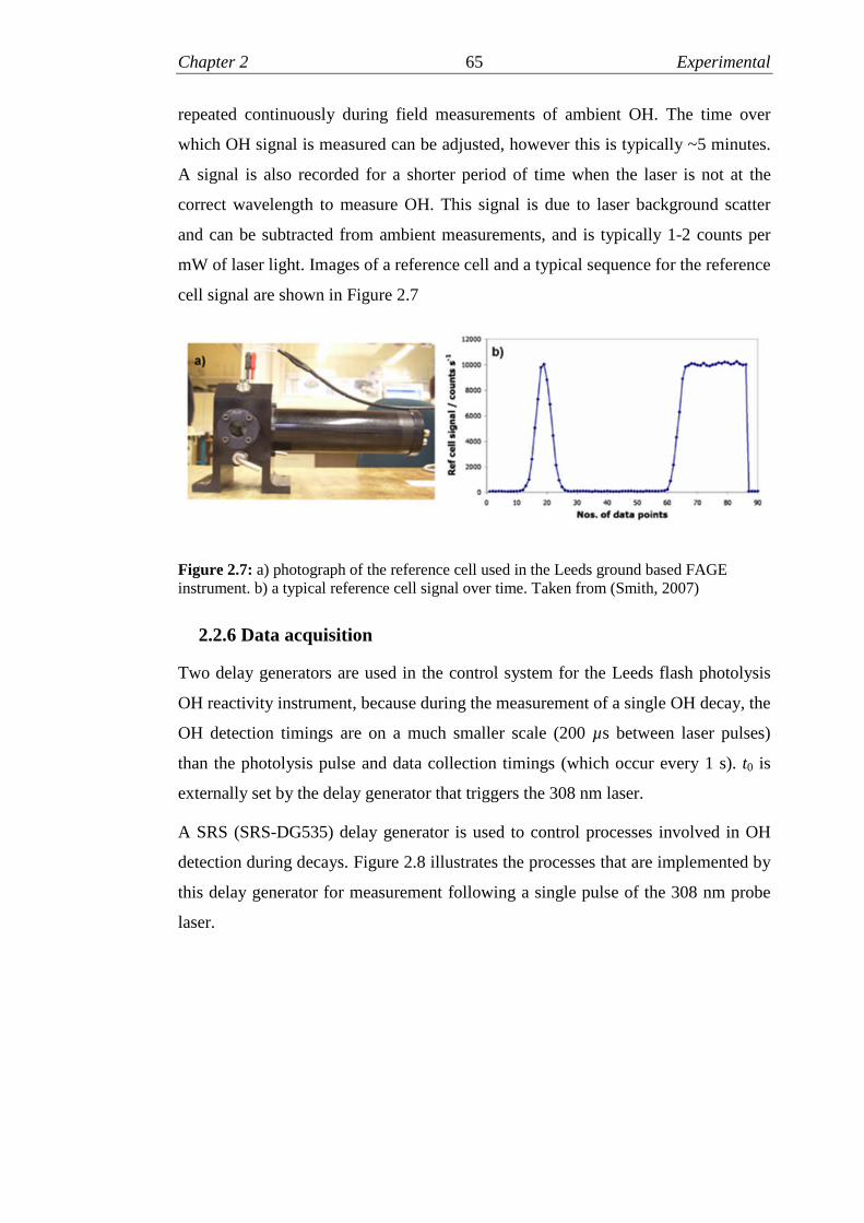
Chapter 2 65 Experimental
repeated continuously during field measurements of ambient OH. The time over
which OH signal is measured can be adjusted, however this is typically ~5 minutes.
A signal is also recorded for a shorter period of time when the laser is not at the
correct wavelength to measure OH. This signal is due to laser background scatter
and can be subtracted from ambient measurements, and is typically 1-2 counts per
mW of laser light. Images of a reference cell and a typical sequence for the reference
cell signal are shown in Figure 2.7
Figure 2.7: a) photograph of the reference cell used in the Leeds ground based FAGEinstrument. b) a typical reference cell signal over time. Taken from (Smith, 2007)
2.2.6 Data acquisition
Two delay generators are used in the control system for the Leeds flash photolysis
OH reactivity instrument, because during the measurement of a single OH decay, the
OH detection timings are on a much smaller scale (200 µs between laser pulses)
than the photolysis pulse and data collection timings (which occur every 1 s). t0 is
externally set by the delay generator that triggers the 308 nm laser.
A SRS (SRS-DG535) delay generator is used to control processes involved in OH
detection during decays. Figure 2.8 illustrates the processes that are implemented by
this delay generator for measurement following a single pulse of the 308 nm probe
laser.

Chapter 2 66 Experimental
Figure 2.8: Schematic diagram to show timings controlled by the SRS delay generator forchannel photomultiplier (CPM) and PMS card gating in the detection of the OH laserinduced fluorescence. The fluorescence detected is indicated by the blue hatched region.Taken from Edwards (2011).
The CPM detector is held in a low gain state until after a pulse from the Ti:Sapphire
laser (described in Section 2.2.5) and any associated scatter has decayed. The CPM
is then switched to a high gain state by a gating box to record the LIF signal from
the photolytically generated OH radicals. The processes depicted in Figure 2.8 are
repeated every 200 µs (for each probe pulse) and these individual measurements of
OH LIF signal can be used to construct an OH chemical decay following each
photolysis laser pulse. One decay is recorded for each pulse of 266 nm light and the
individual decay signals are summed over a set period of time before being written
into memory on the instrument computer.
A Berkeley Nucleonics Corporation (BNC-555) delay generator is used to control
the frequency of photolysis laser pulses and also the data collection cycles for each
OH decay measured. Figure 2.9 illustrates the processes that are controlled by this
delay generator.

Chapter 2 67 Experimental
Figure 2.9: Schematic diagram to show timings of the photolysis laser and PMS cardtriggers controlled by the BNC delay generator. Adapted from Edwards (2011).
At the beginning of each decay measurement a photon counter card (Becker and
Hickl, PMS200A) in the computer of the LFP-LIF instrument is triggered to start
collecting data. The photolysis laser is delayed for 0.1s after this to allow for
measurement of the background signal detected by the cell. The PMS card continues
to record data for 0.3 s after this. The processes depicted in Figure 2.9 are repeated
for each measurement of OH decay signals. The residence time of the gas within the
flow tube is ~4 seconds meaning that during operation of the LFP-LIF instrument
that same sample of gas is irradiated with 266 nm light multiple times. Tests where
the repetition rate of the 266 nm laser was varied have shown that measurements are
not impacted by the number of times the gas sample has been irradiated (Stone et al.,
2016).
2.2.7 Instrument configurations
As a result of continual development of the LFP-LIF OH reactivity instrument
through the course of this work, it is necessary here to describe two different
configurations in which it was operated. configuration 1 was used for the
measurements presented in Chapter 5 from the York 2014 ‘missing’ OH reactivity
campaign. configuration 2 was used for the measurements presented in Chapter 6

Chapter 2 68 Experimental
from the integrated chemistry of ozone in the atmosphere (ICOZA) campaign, and
also for measurements presented in Chapter 3 from comparison experiments at the
SAPHIR chamber.
The biggest difference between configurations 1 and 2 was the FAGE cell inlet and
method for pumping excess gas from the flow tube. In configuration 1 the inlet used
was shown already in Figure 2.5. The inlet was lined with a nylon insert to reduce
wall loss of OH prior to detection. A stainless steel circular disk (0.5mm thick) was
positioned at the end of the inlet and held in place by evacuating the cell with a seal
made by a rubber O-ring, this contained the sampling pinhole (0.8 mm diameter).
The excess gas was removed by the scroll pump via a tube of the same dimensions
as the flow tube however 50 cm in length. In configuration 2 a new inlet for the
FAGE cell was fitted and the method for pumping out excess gas from the flow tube
was changed as shown in Figure 2.10. In configuration 2 the gas exits radially
compared to configuration 1 where it turned a corner (as shown in Figure 2.1). The
pinhole (0.8 mm diameter) of the inlet was attached to a new flange which was fixed
directly to the body of the FAGE cell. A short tube protruded from the FAGE cell
and terminated in a KF50 flange which was connected to the end of the flow tube.
The flange fixed to the FAGE cell had eight equally spaced holes perpendicular to
the axis of the sampling pinhole to pump out excess gas from the flow tube. From
these eight holes ~30 cm long ¼” internal diameter Teflon tubes were connected to a
small metal chamber which connected to the scroll pump in order to pull gas through
the flow tube.
Figure 2.10: Cutaway scale diagram of the redesigned inlet attached to the FAGE cell ofthe LFP-LIF OH reactivity instrument. Provided by Dr. Trevor Ingham.
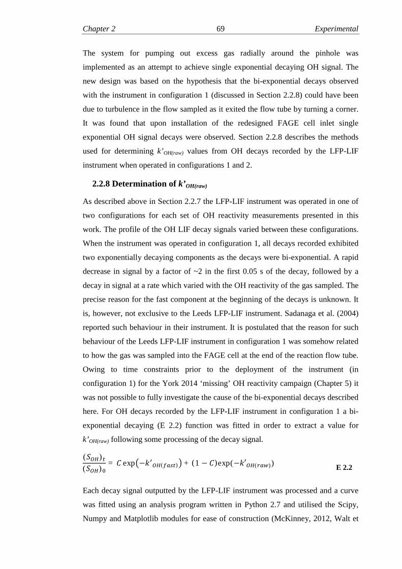
Chapter 2 69 Experimental
The system for pumping out excess gas radially around the pinhole was
implemented as an attempt to achieve single exponential decaying OH signal. The
new design was based on the hypothesis that the bi-exponential decays observed
with the instrument in configuration 1 (discussed in Section 2.2.8) could have been
due to turbulence in the flow sampled as it exited the flow tube by turning a corner.
It was found that upon installation of the redesigned FAGE cell inlet single
exponential OH signal decays were observed. Section 2.2.8 describes the methods
used for determining k’OH(raw) values from OH decays recorded by the LFP-LIF
instrument when operated in configurations 1 and 2.
2.2.8 Determination of k’OH(raw)
As described above in Section 2.2.7 the LFP-LIF instrument was operated in one of
two configurations for each set of OH reactivity measurements presented in this
work. The profile of the OH LIF decay signals varied between these configurations.
When the instrument was operated in configuration 1, all decays recorded exhibited
two exponentially decaying components as the decays were bi-exponential. A rapid
decrease in signal by a factor of ~2 in the first 0.05 s of the decay, followed by a
decay in signal at a rate which varied with the OH reactivity of the gas sampled. The
precise reason for the fast component at the beginning of the decays is unknown. It
is, however, not exclusive to the Leeds LFP-LIF instrument. Sadanaga et al. (2004)
reported such behaviour in their instrument. It is postulated that the reason for such
behaviour of the Leeds LFP-LIF instrument in configuration 1 was somehow related
to how the gas was sampled into the FAGE cell at the end of the reaction flow tube.
Owing to time constraints prior to the deployment of the instrument (in
configuration 1) for the York 2014 ‘missing’ OH reactivity campaign (Chapter 5) it
was not possible to fully investigate the cause of the bi-exponential decays described
here. For OH decays recorded by the LFP-LIF instrument in configuration 1 a bi-
exponential decaying (E 2.2) function was fitted in order to extract a value for
k’OH(raw) following some processing of the decay signal.
( ைு)௧( ைு)
= +exp൫−ᇱைு(௦௧)൯ܥ (1 − −)exp(ܥ ′ைு(௪ ))E 2.2
Each decay signal outputted by the LFP-LIF instrument was processed and a curve
was fitted using an analysis program written in Python 2.7 and utilised the Scipy,
Numpy and Matplotlib modules for ease of construction (McKinney, 2012, Walt et

Chapter 2 70 Experimental
al., 2011, Hunter, 2007). As 308 nm light for the detection of OH had a PRF of 5
kHz the time between pulses was 200 µs, photons were counted in 50 µs bins.
Considering that the fluorescence lifetime of OH in a FAGE cell is on the order of a
few 100 ns it is the case that between each photon counting bin where OH
fluorescence signal is detected, there are three photon counting bins where no OH
fluorescence signal is detected. Figure 2.11 summarises the timing of the OH
fluorescence and non-fluorescence photon counting bins as they are recorded in the
signal array that is outputted by the LFP-LIF instrument. Three bins containing no
fluorescence signal are shown for every bin containing fluorescence signal.
Figure 2.11: Schematic to represent the timing of the array of photon counting bins used torecord OH decays in the LFP-LIF OH reactivity instrument. Blue blocks represent binswhere photons from OH fluorescence are recorded (fluorescence bins) and clear blocksrepresent bins where OH fluorescence is not recorded (non-fluorescence bins). The OH LIFsignal is seen to decay with time. Taken from Edwards et al (2011).
The analysis program removed the non-fluorescence photon counting bins from the
data to obtain a signal containing only that of OH fluorescence. Every five elements
in this array was then summed and assigned the time of the first element included in
the sum in order to reduce noise in the signal. The resulting signal was averaged
between 0.00005 and 0.09905 s to obtain a value for the background signal which
was subsequently subtracted from each value. The function given in E 2.2 was fitted
to the resulting background subtracted decay using a Levenberg-Marquardt
algorithm between the time corresponding to the highest signal and the end of the
decay. The analysis program outputs an image of the plotted background subtracted
signal and the function fitted to the data to allow visual inspection of the quality of
the fitted function. An example of such an image is shown in Figure 2.12.

Chapter 2 71 Experimental
Figure 2.12: Examples of bi-exponential decays recorded by the LFP-LIF OH reactivityinstrument whilst operated in configuration 1. The red lines are representative of the bestfitted bi-exponential decay function (E 2.2) to the data. (a) k’OH(raw) = 6.8 (± 0.1) s-1 (b)k’OH(raw) = 11.7 (± 0.6) s-1.
The parameters from the fitted function (E 2.2)were also outputted by the analysis
program in addition to their 1 σ statistical uncertainties. The value of k’OH(raw) could
then be used to determine k’OH through the subtraction of k’OH(physical) as described in
Section 2.1.10.
Upon return of the LFP-LIF instrument from the York 2014 ‘missing’ OH reactivity
campaign the inlet of the FAGE cell was redesigned in an attempt to eliminate the
presence of k’OH(fast) in the OH decay signals and improve the sensitivity for OH
detection. The redesigned inlet is described in Section 2.2.7 and was used in
configurations 2 of the instrument. The signals recorded by the LFP-LIF instrument
in configuration 2 consisted of only one exponentially decaying component.
Therefore, it was possible to determine a k’OH(raw) value from these decays using a
single exponential decay function, E 2.3.
( ைு)௧( ைு)
= exp(− ′ைு(௪ (ݐ( E 2.3
An analysis program written in python very similar to that described above was used
to determine k’OH(raw) values from the OH decays signal recorded by the LFP-LIF
instrument in configuration 2. The process for fitting the function was identical
except that in this case the portion of the decay signal that was fitted to could be
adjusted. The start time for the fitting was chosen so that it was at the beginning of
the decay signal and the end time was chosen so that data close to the background
level did not influence the fit. Figure 2.13 shows two examples of a single-
exponential decay recorded by the instrument and a fitted single exponential-decay

Chapter 2 72 Experimental
function. The k’OH(raw) values determined through fitting the single exponential
functions to signals recorded by the LFP-LIF instrument in configuration 2 are used
to determine k’OH through subtraction of k’OH(physical) as described in Section 2.1.10.
Figure 2.13: Examples of single exponential decays recorded by the LFP-LIF OH reactivityinstrument whilst operated in configuration 2 or 3. The red lines are representative of thebest fitted single exponential decay function (E 2.3) to the data. (a) k’OH(raw) = 14.2 (± 0.3) s-1
(b) k’OH(raw) = 31.2 (± 0.9) s-1.
2.2.9 Measurement validation with standard gases
In order to validate the OH loss rates measured configuration 1, kOH+CO was
measured by the addition of known quantities of CO to the flow entering the
instrument in a laboratory experiment. Synthetic air (BTCA) from a cylinder was
flowed into the instrument in place of ambient air. A Hg(Ar) pen ray lamp (Lot-
Oriel, LSP035) and water bubbler were used to add ozone and water vapour to the
flow entering the instrument. A CO cylinder and additional mass flow controller
were used to vary the mixing ratio of CO entering the flow tube, a schematic
diagram of the experimental set-up is shown in Figure 2.14.

Chapter 2 73 Experimental
Figure 2.14: Schematic diagram to summarise the experimental set-up used for themeasurement of kOH+CO with the laser flash photolysis total OH reactivity instrument.
17.00 SLM of zero air were flowed through a water bubbler and mixed with 1.00
SLM of zero air that had been irradiated with a Hg(Ar) pen ray lamp (operated at ~8
mA) for ozone production (by R 2.3 and R 2.4); the resulting flow contained ozone
at ~30 ppb. A flow from the CO cylinder (ranging between 0 and 20 sccm) was
mixed into the bulk flow so that the mixing ratio of CO in the flow to the reactivity
instrument could be varied between 0 and ~6200 ppb. This flow correlated to a
range of [CO] within the flow tube of 0 to ~ 1.5 x 10¹⁴ molecule cm-3 when the
measured pressure in the flow tube (~730 Torr) and assumed temperature (298 K)
are taken into account. As [CO] within the flow tube was increased, it could be seen
by inspection of the OH decay profiles, that the loss rate of OH increased. The
Python analysis program described in Section 2.1.7 was used to extract a value of
k’OH(raw) from each OH decay recorded as [CO] was varied in the flow tube. The
values obtained were plotted against [CO] to produce a bimolecular plot which is
shown in Figure 2.15, the gradient of which is equal to the measured bimolecular
rate coefficient for the reaction of OH + CO.
Air
MF
C2
MF
C1
Pen ray lamppower supply
2.00 SLM or more vented
16.00 SLM sampled intoflow tube of OH reactivityinstrument via flow meter
Hg(Ar) pen ray lampheld in metal block
UV light enters glass cell via fusedsilica window for ozone production
Water bubbler
CO
MFC3
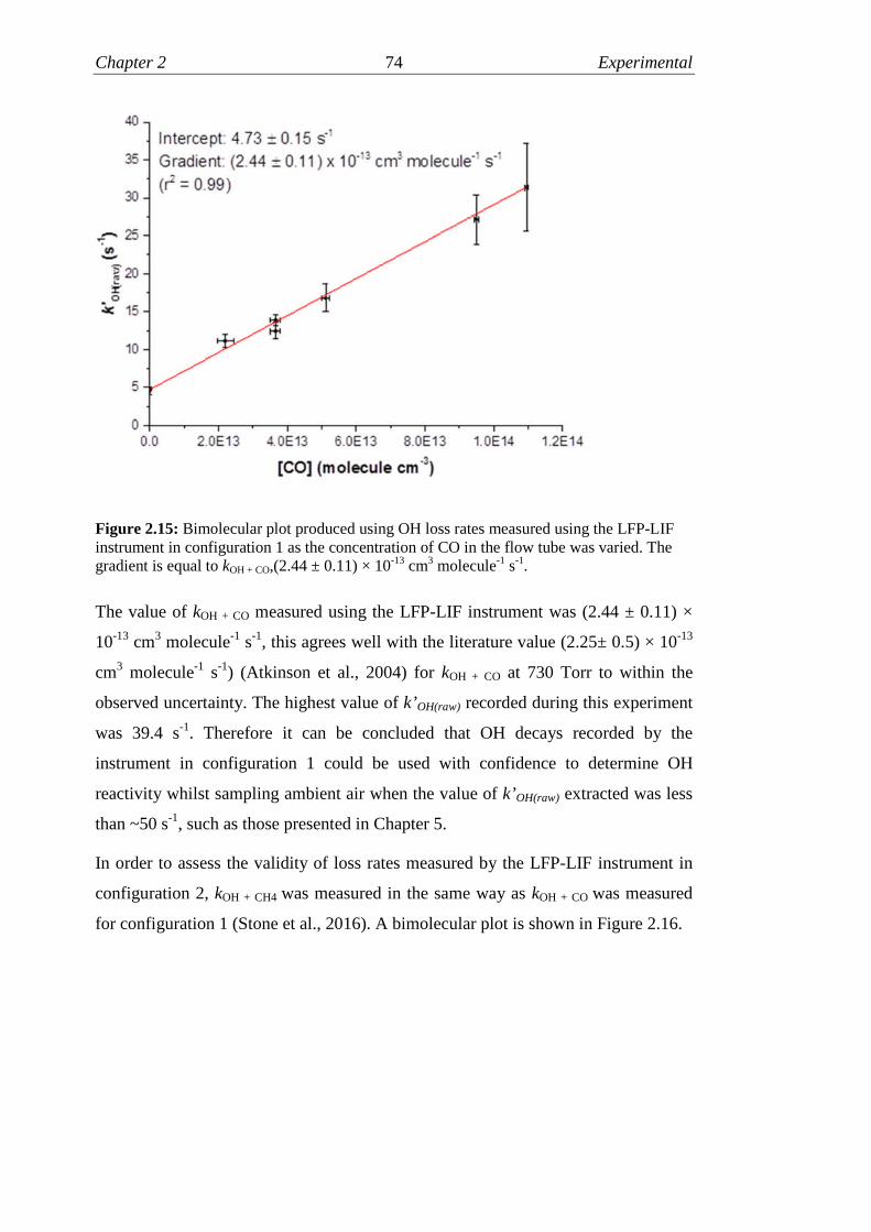
Chapter 2 74 Experimental
Figure 2.15: Bimolecular plot produced using OH loss rates measured using the LFP-LIFinstrument in configuration 1 as the concentration of CO in the flow tube was varied. Thegradient is equal to kOH + CO,(2.44 ± 0.11) × 10-13 cm3 molecule-1 s-1.
The value of kOH + CO measured using the LFP-LIF instrument was (2.44 ± 0.11) ×
10-13 cm3 molecule-1 s-1, this agrees well with the literature value (2.25± 0.5) × 10-13
cm3 molecule-1 s-1) (Atkinson et al., 2004) for kOH + CO at 730 Torr to within the
observed uncertainty. The highest value of k’OH(raw) recorded during this experiment
was 39.4 s-1. Therefore it can be concluded that OH decays recorded by the
instrument in configuration 1 could be used with confidence to determine OH
reactivity whilst sampling ambient air when the value of k’OH(raw) extracted was less
than ~50 s-1, such as those presented in Chapter 5.
In order to assess the validity of loss rates measured by the LFP-LIF instrument in
configuration 2, kOH + CH4 was measured in the same way as kOH + CO was measured
for configuration 1 (Stone et al., 2016). A bimolecular plot is shown in Figure 2.16.

Chapter 2 75 Experimental
Figure 2.16: Bimolecular plot produced using OH loss rates measured using the LFP-LIFinstrument in configuration 2 as the concentration of CH4 in the flow tube was varied. Thegradient is equal to kOH + CH4, (6.4 ± 0.6) × 10-15 cm3 molecule-1 s-1. The blue line representsthe line of best fit (least squares) to the measured loss rates and the red line represents theliterature value: (6.4± 1.2) × 10-15 cm3 molecule-1 s-1 (Atkinson et al., 2004) . Adapted fromStone et al. (2016).
The value of kOH + CH4 measured using the LFP-LIF instrument was (6.4 ± 0.6) × 10-
15 cm3 molecule-1 s-1, this agrees well with the literature value (6.4± 1.2) × 10-15 cm3
molecule-1 s-1 (Atkinson et al., 2004). These results confirm that OH decays
recorded by the instrument in configuration 2, such as those presented in Chapters 3
and 6, can be used with confidence to determine OH reactivity whilst sampling
ambient air when the value of k’OH(raw) extracted was as high as ~120 s-1.
2.2.10 Determination of physical loss rate of OH
To obtain a measurement of k’OH from k’OH(raw), determined through fitting an
exponentially decaying function (E2.2 or E2.3, Section 2.1.7) to an OH signal
recorded by the LFP-LIF instrument, it is necessary to subtract a value for
k’OH(physical). This section provides details on how k’OH(physical) was determined for
each configuration of the instrument.
In principle, if moist synthetic air (free from OH reactive impurities) contained
sufficient water vapour and ozone to generate sufficient OH to observe an OH

Chapter 2 76 Experimental
decay, and was supplied to the instrument, the k’OH(raw) value (minus a very small
(<0.01 s-1) contribution from the reaction between OH and O3) determined would
equal k’OH(physical). When a supply of synthetic air containing OH reactive impurities
is used in the measurement of k’OH(physical), the value determined would be artificially
high. If such a value was subtracted from k’OH(raw) the value determined in ambient
air k’OH would be artificially low, and consequently any ‘missing’ OH reactivity
would be underestimated. To successfully determine k’OH(physical) for each
configuration it was necessary to have access to very high purity synthetic air so that
any chemical contribution to the loss rates observed is minimal. It is also imperative
that the water in the bubbler used to humidify the flow to the instrument is as pure as
possible.
At the beginning and end of the deployment of the LFP-LIF instrument for the York
2014 ‘missing’ OH reactivity campaign (where the instrument was operated in
configuration 1), BTCA synthetic air was used in an attempt to determine
k’OH(physical). Values of k’OH(raw) determined from OH decays in synthetic BTCA air
from a cylinder are referred to as k’OH(zero) in this work. The schematic diagram in
Figure 2.17 summarises the experimental set-up that was used for this.
Figure 2.17: Diagram to summarise the experimental set-up used for the measurement ofk’OH(zero) whilst the LFP-LIF OH reactivity instrument was operated in configuration 1
1 SLM of zero air was passed through a glass cell and irradiated via a fused silica
window with UV radiation from a Hg(Ar) pen ray lamp (Lot-Oriel, LSP035)

Chapter 2 77 Experimental
operated at 8.2 mA for the production of ozone. It was mixed with 17 SLM from the
same cylinder that had passed through a water bubbler so that 18 SLM in total were
available to the instrument. An ozone analyser (Thermo Electron Corporation 49C)
was used to measure that the flow contained ~30 ppb of ozone. The scroll pump
used to draw gas through the flow tube of the instrument was throttled using a
butterfly valve until the flow meter indicated that 16 SLM were entering the
instrument. k’OH(zero) values were determined through fitting a bi-exponentially
decaying function as described in Section 2.1.7, all of these values are plotted in
Figure 2.18.
Figure 2.18: Measurements of the loss rate of OH in synthetic air (k’OH(zero)) measuredduring the York 2014 ‘missing’ OH reactivity campaign where the LFP-LIF instrument wasoperated in configuration 1. The y error bars represent the 1σ standard deviation in the value of k’OH(zero) as determined from the covariance matrix associated with the bi-exponentialdecay function fitted to the decay data, outputted by the scipy optimize function.
The average k’OH(zero) recorded was 4.22 ± 0.29 s-1 (1σ standard deviation). It is
known that there are impurities (CO, NOx and unspecified VOCs) present in BTCA
synthetic air cylinders and only upper limits regarding these are available from the
manufacturer (BOC, 2016). It is also possible that there could be OH reactive
impurities present in the water used to humidify the flow to the instrument.
Therefore, it was not possible to say with certainty what portion of the average zero
loss rate in the BTCA synthetic air could be attributed to chemical impurities.
Measurements of k’OH(zero) were made before and after the ICOZA campaign for
which the LFP-LIF instrument was deployed in configuration 2. The method used
was very similar to that described above. However, in this case 1 SLM of synthetic
air was irradiated with the pen ray lamp and mixed with 15 SLM that was
humidified with the water bubbler. There was no vent in the system prior to the gas

Chapter 2 78 Experimental
entering the instrument as for configuration 1 of the instrument. In this case all 16
SLM entered the instrument and the pressure of the flow tube was monitored whilst
the butterfly valve that throttled the scroll pump was adjusted until a stable pressure
of ~760 Torr was achieved. The average (from six measurements prior to
deployment and two post deployment) k’OH(zero) value determined for ICOZA was
5.22 ± 0.21 s-1 (1σ standard deviation).
Access to a very clean synthetic air supply at the SAPHIR chamber, during an OH
reactivity comparison campaign (Chapter 3), provided a valuable opportunity to
investigate the magnitude of any contribution from impurities in synthetic air to the
k’OH(zero) values determined for configurations 1 and 2 of the LFP-LIF instrument.
The synthetic air supply at SAPHIR was generated through the boil off of liquid
nitrogen and oxygen (80% and 20%, respectively). It is assumed that this air was the
purest that had ever been available for use in experiments to determine the true value
of k’OH(physical), equal to the k’OH(raw) determined from an OH decay recorded in this
zero air. The instrument was operated in configuration 2 when these measurements
were made and the method for measurement was identical to that used for
measurements of k’OH(zero) before and after the ICOZA campaign, except in this case
the SAPHIR synthetic air supply was used in place of a cylinder. The OH signal was
found to decay significantly slower in this case than in the pre and post-ICOZA
measurements, visual inspection of the signal revealed that the signal decay was so
slow that there was still evidence of a decay in the period during which the
background signal is recorded prior to the triggering of the 266 nm photolysis pulse.
A result of this was that it was not possible to use the method for extracting a
k’OH(raw) as described in Section 2.1.7, as subtracting a background from the decays
that included a contribution from OH LIF is not appropriate. Instead the back ground
signal was determined separately through operation of the instrument, in the absence
of 266 nm light, for one measurement cycle of an OH decay. This was subtracted
from the OH decays recorded in the SAPHIR synthetic air to obtain a background
subtracted signal, the natural logarithm of which was taken and a straight line was
fitted so that a loss rate could be extracted. An example of such a signal used to
determine k’OH(physical) is shown in Figure 2.19.

Chapter 2 79 Experimental
Figure 2.19: Example OH decay signal recorded in very clean synthetic air (produced byboil-off of liquid nitrogen and oxygen) at the SAPHIR chamber. k’OH(physical) = 2.18 s-1.
The value of k’OH(physical) for the LFP-LIF instrument when operated in configuration
2 was determined as the average of five individual k’OH(physical) measurements. This
was 2.25 ± 0.21 s-1 (1σ standard deviation) and is the value which was subtracted
from the ambient measurements made during ICOZA (Chapter 6).
The value for k’OH(physical) that was subtracted from the measurements made during
ICOZA was not appropriate for subtraction from the measurements made during the
York 2014 ‘missing’ OH reactivity campaign. The reason for this is that during
ICOZA the instrument was operated in the same configuration as it was during the
experiments with the SAPHIR synthetic air supply. During the ambient
measurements in York the instrument was operated in configuration 1 where the
inlet of the FAGE cell and method of removing excess gas from the flow tube were
very different and would very likely have had an impact on the loss rate of OH due
to physical processes occurring within the flow tube. For the purpose of determining
k’OH(physical) for the instrument in configuration 1, it was assumed that the level of OH
reactive impurities that were present in the flow to the instrument during the
measurement of k’OH(zero) for the instrument in both configurations were the same. It
is very likely that this was the case as laboratory measurements have shown there to
be little variation in the value of k’OH(zero) measured with different cylinders of
BTCA synthetic air and water (always from the same sources) used in the bubbler.
The difference between k’OH(zero) for configuration 2 (5.22 ± 0.21 s-1, average of
measurements pre and post-ICOZA deployment) and k’OH(physical) measured with the
0
1
2
3
4
5
6
0 0.05 0.1 0.15 0.2 0.25 0.3 0.35 0.4
ln((
S OH) t
)
t (s)

Chapter 2 80 Experimental
SAPHIR synthetic air supply was assumed to be equivalent to the contribution from
OH reactive impurities to k’OH(zero) that was measured at the beginning and end of
the measurements in York. This difference was subtracted from k’OH(zero) for
configuration 1 (4.22 ± 0.28 s-1, average of measurements at the beginning and end
of measurements in York) to determine k’OH(physical) for configuration 1. The value
determined was 1.25 ± 0.42 s-1 and this was subtracted from all of the ambient
measurements from the York 2014 ‘missing’ OH reactivity campaign presented in
Chapter 5.
2.2.11 Effect of NO recycling
Stone et al. (2016) reported a modelling study on the potential interferences from
OH recycling, at elevated NO levels, on measurements of k’OH. OH decays in the
LFP-LIF instrument were simulated under a range of conditions. Whilst it is an
advantage of the LFP-LIF technique that the method used for the generation of OH
does not also generate HO2 (as in the TOHLM technique), it is possible for HO2 to
be generated within the instrument from the reaction of OH and CO. It is also
possible for RO2 radicals to be generated from the reactions between OH and VOCs.
Any HO2 or RO2 generated within the instrument has the potential produce recycled
OH when NO is present in the gas sampled (as described in Section 1.2.1). If the
rate of recycled OH production was very high it is possible that OH signals recorded
by the LFP-LIF instrument could be artificially raised at longer decay times. It was
concluded by Stone et al. (2016) that the LFP-LIF instrument does not suffer from
any significant interference resulting from production of HO2 and RO2 within the
instrument.
2.3 Measurement of formaldehyde
2.3.1 Instrument overview and principle of operation
The methodology for the detection of HCHO with the Leeds LIF instrument is based
on that outlined by Hottle et al. (2008). Gas is sampled into a low pressure
aluminium cell (Section 2.2.3) and UV radiation from a fibre laser (Section 2.2.2) is
used to excite HCHO in the 50,5 ← 51,4 rotational transition of the 4 A1A2 ←X1A1
vibronic band at 353.370 nm. Resulting photons from broadband fluorescence of
HCHO are detected orthogonal to the path of the laser beam, the count rate of which
(Section 2.2.5) is proportional to concentration of HCHO in the gas sampled. A

Chapter 2 81 Experimental
calibration factor determined experimentally (Section 2.2.7) is used to determine the
concentration of HCHO in the gas sampled.
The HCHO LIF instrument is relatively compact and the majority of components are
contained within one shock insulated 19” rack housed within a plastic gasket sealed
case with removable side panels for easy transportation. Figure 2.20 shows the
arrangement of the key components within the case.
Figure 2.20: Photograph showing the arrangement of key componenets (labelled) of theHCHO LIF instrument within the 19” rack.
The case is shown with both side panels removed, however, when fitted, a computer
fan was situated in the bottom of back panel to draw air into the case which exited
through a hole in the top of the front panel; this was to prevent overheating of the

Chapter 2 82 Experimental
laser, computer and other components. A hole (50 mm diameter) was in the centre of
the back panel to allow gas lines and cables to enter whilst the case is sealed. A 19”
rack enclosure at the bottom of the rack contained a computer and other data
acquisition hardware, and above this was the control unit of the fibre laser which
was also housed within a 19” rack enclosure. Fixed as a shelf in the top of the rack
was an optical breadboard, to which the fibre laser head was fixed in addition to all
other optical components and the detection cell and a reference cell. The HCHO LIF
instrument was developed through the course of this work and consequently it is
necessary that each configuration used to obtain measurements presented in this
work is described. Details of three configurations are provided in Section 2.3.6
which differed only with regards to the layout and contents of the optical
breadboard.
2.3.2 The 353 nm detection laser
UV radiation from a pulsed (300 kHz) tuneable fibre laser (TFL3000, Novawave)
was then used to excite HCHO in the LIF instrument described here. The majority of
the optical components of this laser are built into the control unit which is housed
inside a 19” rack enclosure, this is connected to the laser head via an optical fibre.
Figure 2.21 summarises the key optical components housed within the laser control
unit and laser head.
Figure 2.21: Schematic diagram to illustrate the key processes occurring within thetuneable fibre laser used to excite HCHO. SHG: second harmonic generating crystal, THG:third harmonic generating crystal.
The operating principle of the fibre laser for the generation of UV light differs
considerably from that of a Ti:Sapphire laser (Section 2.2.5). In the fibre laser, a Yb-
doped glass fibre laser is used as a cavity and main oscillator where laser excitation
IR pumpdiodes
Seed laserYb-glass fibrering oscillator
Laser head
1059 nm transmittedthrough optical fibre
SHGTHG353 nm
Laser control unit

Chapter 2 83 Experimental
can occur. The Yb-doped glass fibre cavity is bonded directly to an optical fibre
which transmits radiation from broadband IR pump diodes. A second optical fibre
bonded to the main oscillator is used to transmit radiation from an IR (1059 nm)
seed laser diode, The specific wavelength outputted is controlled through adjustment
of the current supplied to the seed diode and is controlled through the application of
an analogue voltage to the laser control unit. The radiation from the seed diode is
amplified by the main oscillator to output ~1W of 1059 nm radiation which is
delivered to the laser head via an optical fibre. Inside the laser head this is tripled by
sum frequency mixing using a second harmonic generating crystal and a third
harmonic generating crystal. Following this 353 nm UV light exits the laser head, in
addition to some excess green light (second harmonic).
2.3.3 The detection cell
The main body of the detection cell of the HCHO LIF instrument was very similar
in design to that of the LFP-LIF instrument (described in Section 2.1.3). There were,
however, differences regarding the method for achieving low pressure in the cell and
also for sampling air into it. The pressure inside the cell of the HCHO LIF
instrument does not have to be as low as inside a FAGE cell for OH measurement,
owing to the fluorescence lifetime being significantly longer for HCHO, and also
that there is no need for gating of the detector as an off-resonant spectroscopic
feature is used. Measurements of HCHO are typically made at cell pressures in the
range 110 - 120 Torr. It is possible to achieve such a cell pressure using a scroll
pump (Agilent Technologies, IDP3), as opposed to a roots backed rotary pump and
pinhole that would be required for a FAGE cell. The diagram in Figure 2.22
illustrates the design of the HCHO detection cell.

Chapter 2 84 Experimental
Figure 2.22: Cutaway scale diagram of the detection cell of the HCHO LIF instrument.Provided by Dr. Trevor Ingham.
The unit orthogonal to the baffled arms for the entry and exit of laser light housed
the photo multiplier tube (PMT, Sens-Tech P25PC photodetector module), and also
a set of optics to image photons from HCHO florescence onto the photocathode of
this detector. Two plano-convex lenses (diameter = 50 mm, focal length = 52 mm)
were used to collimate the fluorescence through an interference filter (Barr
Associates, 390 – 550 nm) which was used to discriminate HCHO fluorescence
photons from scatter at 353 nm. Following this a further two plano-convex lenses
(diameter = 50 mm, focal length = 52 mm) were used to focus the filtered
fluorescence signal onto the PMT photocathode. An uncoated circular Suprasil
window between two o-rings was used to form an airtight seal between the unit
housing the PMT and the LIF cell. A retro-reflector (CVI Optics fused silica plano-
concave spherical mirror) was mounted directly opposite the PMT to deflect photons
from HCHO fluorescence, which were emitted in the direction opposite to the
detector, towards the detector to maximise sensitivity. The two cell faces orthogonal

Chapter 2 85 Experimental
to both the detection and laser axis were used for pumping out and sampling air into
the cell, only one such face is visible in Figure 2.22.
2.3.4 The reference cell
A reference cell was developed to enable the automation of tuning the wavelength of
the fibre laser to optimise the HCHO signal. The reference cell, as shown in
Figure 2.23 was constructed from a block of 75 x 75 x 75 mm aluminium, into the
centre of one face of which a hole, 30 mm in diameter, and 70 mm deep, was
machined to form the inner walls. Two short cylindrical aluminium arms (30 mm
maximum length, 15 mm OD) fitted with fused silica Brewster windows were used
to allow laser light to enter and exit the cell. Three ¼” Swagelok fittings were
attached to the top of the cell to allow gas flow in and out, and to enable a pressure
sensor (26PCDFA1G, Honeywell) to be fitted. The diagram in Figure 2.23 illustrates
the design of the reference cell of the HCHO LIF instrument.
Figure 2.23: Cutaway scale diagram of the reference cell of the HCHO LIF instrument.Provided by Dr. Trevor Ingham.
The PMT housed in the detection arm of the reference cell was identical to that used
in the main cell, the timings for measurement of the HCHO signal (Section 2.3.5)
were also the same. However, no interference filter or focussing optics were used in
the reference cell as achieving good sensitivity is not important. After exiting the
main detection cell the laser light was directed by two UV turning mirrors into the
reference cell. A high background signal (200,000 -300,000 count s-1) was not
positioned on the HCHO transition, as a result of laser scatter from the inner walls of
the cell which did not have a black-anodised coating.

Chapter 2 86 Experimental
In order to scan the wavelength of the tuneable fibre laser and observe a resulting
change in the reference cell signal representative of the rotational spectroscopic
structure of HCHO, it was necessary to elevate the level of HCHO inside the
reference cell to levels significantly higher than in ambient air. Depolymerisation of
paraformaldehyde (SIGMA-ALDRICH, P6148, reagent grade, crystalline) using
heat was chosen as a method to achieve this.
The two remaining ¼” Swagelok fittings of the reference cell were each connected
to quarter-turn valves and both were set to their closed position. The line to the
scroll pump, that was routinely used to evacuate the main detection cell, was
connected to one of these valves. The remaining valve was connected to ~1 m length
of ¼” internal diameter Teflon tubing, the other end of which was connected to a
short piece of capped ¼” stainless steel tubing which contained a few granules of the
crystalline paraformaldehyde (the HCHO reservoir). The valve to the scroll pump
was partially opened and closed when the pressure within the reference cell was
reduced to ~100 Torr. The HCHO reservoir was then heated with a heat gun for ~5 s
whilst the valve connecting it to the reference cell was opened. This enabled gas
phase HCHO formed by depolymerisation of paraformaldehyde to enter the
reference cell; a pressure increase of ~50 Torr was observed. Following this the
valve to the HCHO reservoir was closed and the valve to the scroll pump was
partially opened until the pressure was again ~100 Torr. The resulting system was
completely sealed and the level of HCHO in the gas phase was sufficient for the
peak of the spectral line at 353.370 nm to be observed at ~400,000 count s-1 above
the background. The signal from the new reference cell was used to automate the
process of tuning the wavelength of the fibre laser on to the spectroscopic line at
353.370 nm so that HCHO could be measured in ambient air with the main detection
cell. Further details of this process are provided in Section 2.3.5
2.3.5 Data acquisition
The master clock of the fibre laser was used to control timing for photon counting in
the HCHO detector. For every pulse from the fibre laser a transistor-transistor logic
(TTL) pulse was used to trigger a delay generator card in the computer. Upon
receiving this trigger, the delay generator card waited 400 ns before providing a TTL
pulse (1000 ns duration) to trigger a photon counting card that was operated in the
‘multiscaler’ mode (PMS400A, Becker and Hickl). After a further 200 ns elapsed

Chapter 2 87 Experimental
following the triggering of the photon counting card, another TTL pulse (200 ns
duration) from the delay generator card was used to un-gate a channel on the photon
counting card. Photons from laser induced fluorescence of HCHO were collected
within these 200 ns. The fluorescence lifetime of HCHO is approximately 200 ns at
~120 Torr so this collection window should provide ample time for detection (Hottle
et al., 2008). The schematic diagram in Figure 2.24 summarises the sequence of
events that occurred during the measurement of the HCHO LIF signal that followed
one pulse from the fibre laser.
Figure 2.24: Schematic diagram to summarise the timings of the sequence of events for themeasurement of the HCHO LIF signal following one pulse from the fibre laser. Diagram notto scale
It was necessary to trigger the photon counting card well in advance of the LIF
signal as the PMS400A card has a ‘dead time’ of 50 ns between bins; i.e. if the card
was triggered and un-gated simultaneously a maximum of 50 ns worth of LIF signal
could be lost. Operating the photon counting card in multiscaler mode meant that the
photons counted were logged as a function of time; the LIF signal recorded was
outputted in count s-1, where all of the photons that were detected in the 200 ns
detection window (within 1 s) were summed. In order to determine the level of
HCHO present in ambient air it is necessary to subtract a background signal from
the signals described above. The background subtracted signal is equivalent to a

Chapter 2 88 Experimental
concentration of HCHO as governed by a calibration factor, details regarding the
calibration of the HCHO LIF instrument are provided in Section 2.3.7.
The signal from the reference cell (described in Section 2.3.4) was used to automate
the tuning of the wavelength of the fibre laser between that of the spectroscopic line
of HCHO at 353.370 nm and a lower wavelength (353.360 nm) before the feature,
referred to here as the ‘offline’ wavelength. There were four defined stages to this
measurement cycle.
In the first stage a voltage was applied to the ‘seed’ laser diode of the tuneable fibre
laser in order to increase its temperature by a small amount, which in turn resulted in
an increase in wavelength from its starting (‘offline’) position. The wavelength of
the fibre laser was increased by ~10 pm so that a peak corresponding to the HCHO
rotational transition at 353.370 nm was observed in the reference cell signal.
Following this the wavelength was decreased during the second stage until the
reference cell signal was within 95 % of the maximum value observed during the
first stage. This defined the start of the third stage where the wavelength was fixed
for ten minutes whilst the ‘online’ HCHO signal from the main detection cell was
recorded (1 s data). On completion of the third stage the wavelength was returned to
its starting value and the ‘offline’ HCHO signal from the main detection cell was
recorded for one minute. The plot in Figure 2.25 shows a typical reference cell
signal that was observed during one measurement cycle.
Figure 2.25: A typical reference cell signal observed during one complete measurementcycle of the LIF HCHO instrument. Time resolution between adjacent points is 1s.

Chapter 2 89 Experimental
For every measurement cycle each point in the ‘online’ and ‘offline’ signals from
the main detection are normalised for laser power using a photodiode. The ‘offline’
normalised is averaged and subtracted from every online point to yield a signal that
could be used in combination with a calibration factor to determine the
concentration of gas phase HCHO in the gas sampled.
2.3.6 Instrument configurations
Due to continual development of the HCHO LIF instrument through the course of
this work, it is necessary here to describe three different configurations in which it
was operated. configuration 1 was used for the measurements presented in Chapter 4
where the instrument was used in experiments to characterise a newly developed OH
flow reactor. configuration 2 was used for the ambient measurements presented in
Chapter 5 from the York 2014 ‘missing’ OH reactivity campaign. configuration 3
was used for the ambient measurements presented in Chapter 6 from the ICOZA
campaign. The main difference between the configuration 1, and configurations 2
and 3 was the layout of the optical breadboard and the maximum laser power that
was available for use. The only difference between configurations 2 and 3 was the
amount of laser power that was available for use.
In configuration 1 there was no reference cell in operation to automate the
measurement process. In the OH reactor characterisation experiments described in
Chapter 4, the wavelength of the fibre laser was tuned between the online and
offline position manually. The signal from the main cell was monitored whilst
laboratory air was sampled and the wavelength was increased by ~10 pm (through
increasing the temperature of the seed diode) from the starting value. Due to there
being ~20 mW of UV laser power available and the relatively high level of HCHO
in the laboratory air sampled (5 ppb) it was possible to see the main spectroscopic
feature at 353.370 nm clearly peaking at ~1000 count s-1 above the background
(~150 count s-1). As the level of HCHO in the laboratory air was fairly constant, it
was possible to stop and restart the wavelength scan so that it could be stopped again
when the signal had returned to its maximum value. The instrument was considered
‘online’ for measurements when in this state. Figure 2.26 summarises the set-up of
the optical components of the HCHO LIF instrument when operated in configuration
1.

Chapter 2 90 Experimental
Figure 2.26: Schematic diagram to summarise the key features of the optical set-up and thedetection cell used in configuration 1of the LIF HCHO detector. Diagram not to scale.
UV radiation exited the fibre laser head and was directed into the entry arm of the
detection cell by two UV turning mirrors. Upon exiting the detection cell a third UV
turning mirror was used to direct the laser beam onto a power meter probe so that
the power could be tuned and monitored without disruption of the measurement of
HCHO. Excess green light from the fibre laser head was directed into a wave meter
probe so that the wavelength could be monitored as a proxy for the wavelength of
the UV light.
Following the completion of the OH reactor characterisation experiments described
in Chapter 4, problems were encountered with the fibre laser of the HCHO LIF
instrument. On return to the manufacturers it was determined that the optical fibre
used to deliver IR radiation to the laser head had become burned. This was repaired,
however, to prevent reoccurrence of this problem it was advised that the laser
outputted a maximum of 10 mW UV light. When the laser was re-integrated into the
rack of the HCHO LIF instrument a reference cell was also installed to enable the

Chapter 2 91 Experimental
automation of tuning the wavelength and data acquisition. Figure 2.27 summarises
the set-up of the optical components of the HCHO LIF instrument when operated in
configuration 2.
Figure 2.27: Schematic diagram to summarise the key features of the optical set-up and thedetection cell used in configuration 2 (and also configuration 3, see below) of the LIFHCHO detector. Diagram not to scale.
The optical set-up of configuration 2 was the same as it was in configuration 1 prior
to where the UV light exited the main detection cell. Upon exit from the main
detection cell the UV light was redirected by two turning mirrors through the
reference cell, upon exit from which it was terminated onto the active-area of a fast
photodiode. The signal from the photodiode was used to record laser power so that
the LIF signals recorded from the main detection cell could be normalised for laser
power in mW.
configuration 3 of the HCHO LIF instrument was exactly the same as configuration
2 with regards to the optical components. However, the maximum UV laser power
available in this configuration was ~6 mW following a second repair by the
manufacturer which was necessary due to a burned crystal in the laser head. The

Chapter 2 92 Experimental
reduced laser power made it very difficult to calibrate the photodiode which
previously measured laser power for normalising the LIF signal. Consequently,
signals recorded by the HCHO LIF instrument in configuration 3 were normalised
for laser power in V (the raw signal from the photodiode) rather than mW.
2.3.7 Calibration methods
As LIF is not an absolute method of measurement it is necessary to calibrate the
HCHO LIF instrument so the LIF signals could be converted to concentrations using
a calibration factor (CHCHO). Two calibration methods were used in this work. In
configurations 1 and 2 the instrument was calibrated using a method analogous to
that used for calibrating a FAGE cell for OH detection, as described by Commane et
al. (2010). However, in this case MeOH vapour was photolysed at 184.9 nm in a
turbulent flow tube (termed the ‘wand’) for HCHO production rather than photolysis
of H2O vapour for OH production.
The aircraft FAGE instrument calibration ‘wand’ was used to calibrate the detection
cell of the LIF HCHO instrument in configurations 1 and 2. 38 SLM of synthetic
(BOC, BTCA) air were mixed with another 4 SLM that had passed through a
MeOH bubbler. The mixture was flowed into the wand so that a known
concentration of HCHO could be produced through MeOH photolysis by UV light
from a Hg(Ar) pen ray lamp (Lot-Oriel, LSP035) at 184.9 nm in the presence of O2,
R 2.5.
MeOH + hνమሱሮ HCHO + HOଶ R 2.5
The level of HCHO produced was varied through adjustment of the current supplied
to the Hg(Ar) pen ray lamp within the ‘wand’ in order to vary the flux of photons
that irradiated the flow containing the MeOH vapour (F). This is determined as a
function of lamp current separately in an experiment where NO is used as a
chemical actinometer. The method for determining F as a function of lamp current is
described in Commane et al. (2010) and the values used for the calibration of the
HCHO LIF instrument in configuration 1 were provided by Dr. Trevor Ingham. The
concentration of HCHO exiting the ‘wand’ was calculated using E 2.4.
[ܪܥܪ] = ܯ] ଵସ.ଽ)ߪ[ܪ )ெ ைு∅ுுைݐܨ E 2.4
[MeOH] is the concentration of methanol in the flow to the ‘wand’ (~3 x 10¹⁷
molecule cm-3) calculated using the vapour pressure at the measured bubbler

Chapter 2 93 Experimental
temperature (~5 ºC), σ(184.9 nm)MeOH is the absorption cross section of MeOH at 184.9
nm (6.65 x 10⁻¹⁹ cm2 molecule-1), Ø is the quantum yield of HCHO (assumed to be
equal to 1 in air) and t is the irradiation time (0.008 s) that was calculated using the
‘wand’ dimensions and 42 SLM total flow rate.
The wavelength of the fibre laser was tuned to its ‘online’ value and the current
supplied to the pen ray lamp in the ‘wand’ was varied between ~1.5 and 6.5 mA.
HCHO LIF signals were recorded at five lamp currents, each for ~2 minutes. The
averaged signals recorded for each lamp current were plotted against the
corresponding lamp currents to produce a calibration plot as shown in Figure 2.28.
The value for CHCHO ((9.25 ± 13.1) × 10-9 count s-1 molecule-1 cm3) determined was
used for the conversion of HCHO LIF signals to concentrations for the
measurements presented in Chapter 4. This corresponds to a detection limit of ~54
ppt in 1 s for a signal to noise ratio of 1.
Figure 2.28: Results from the calibration of the LIF HCHO in configuration 1. The gradientof the line of best fit is equal to the sensitivity (CHCHO) which is 9.25 x 10⁻⁹ count s-1
molecule-1 cm3. y-error bars represent ± 1σ standard deviation in the LIF signals recorded. It was not possible to determine x-error bars due to a number of parameters, such as flowrates, not being logged.
The instrument was calibrated using the same method when in configuration 2
during its deployment for the York 2014 ‘missing’ OH reactivity campaign. The
1 2 3 40
100
200
300
400
500
600
700
LIF
sig
na
l(co
un
ts
-1)
[HCHO] (1010 molecule cm-3)
Intercept: 255.5 13.1 count s-1
Gradient: (9.25 13.1) x 10-9 count s-1 molecule-1 cm3
(r2 = 0.989)

Chapter 2 94 Experimental
ground based FAGE calibration wand was used for this and the experimental
conditions were very similar to what is described above, however there were two
differences. Firstly for the calibration in configuration 2 a total flow of 30 SLM of
synthetic air was supplied to the ‘wand’ and all of this passed through the MeOH
bubbler. The value of t used in the calculation of [HCHO] was also different (t =
0.012 s) as the dimensions of the ground based FAGE ‘wand’ were slightly different
to the aircraft ‘FAGE’ wand and the total flow rate through the wand was different.
The relationship between F and lamp current used for this ‘wand’ was supplied by
Dr. Lisa Whalley. The LIF signals were also normalised for laser power in mW for
calibrations in configuration 2 as this included a calibrated photodiode. The
calibration plot for the HCHO LIF instrument in configuration 2 is shown in
Figure 2.29. The value for CHCHO ((1.46 ± 0.034) × 10-9 count s-1 mW-1 molecule-1
cm3) determined was used for the conversion of HCHO LIF signals to
concentrations for the ambient measurements from York presented in Chapter 5.
This corresponds to a limit of detection of ~81 ppt in 1 s for a signal to noise ratio of
1.
Figure 2.29: Results from the calibration of the LIF HCHO instrument during the York2014 ‘missing’ OH reactivity field campaign. The gradient of the line of best fit is equal tothe sensitivity (CHCHO) which is 1.46 × 10⁻⁹ count s-1 mW-1 molecule-1 cm3. y-error barsrepresent ± 1σ standard deviation in the LIF signals recorded. x-error bars represent the uncertainty in the calculated [HCHO] supplied to the instrument, as determined throughpropagation of the uncertainties in each parameter used to calculated [HCHO] using E 2.4.
0 2 4 6 8 10
0
20
40
60
80
100
120
140
160
180
LIF
sig
na
l(cou
nts
-1m
W-1)
[HCHO] (1010 molecule cm-3)
Intercept: 19.9 1.3 count s-1 mW -1
Gradient: (1.46 0.034) x 10-9 count s-1 mW -1 molecule-1 cm3
(r2 = 0.998)

Chapter 2 95 Experimental
It can be seen that the lines of best fit to the data in Figure 2.28 and Figure 2.29 both
have positive y-intercepts. The reason for this is due to a constant background level
of HCHO contaminant present in the flow from the MeOH bubbler in both case.
Tests for both configurations of the instrument have shown that no LIF signal was
observable above the background when neat synthetic air was sampled by the
detection cell.
A permeation source of gas phase HCHO was used to calibrate the HCHO LIF
instrument when operated in configuration 3. The main reason for this was that
using the ‘wand’ calibration method described above can be challenging and time
consuming in the field. The performance of pen ray lamps can also deteriorate
rapidly, and if the value for F used is incorrect due to this, it may not be possible to
rationalise any discrepancies between calibrations. For example, if the relationship
between F and lamp current was determined at the beginning and end of a field
campaign (it would not be practical to measure this regularly during the campaign),
any differences might be difficult to reconcile. In this case it would be unknown if a
change in CHCHO was due to deterioration of the pen ray lamp or if it was a genuine
change in sensitivity.
A commercial permeation tube source containing paraformaldehyde (Kintek
Analytical) was used to provide gas phase HCHO at a known emission rate of 10 ng
min-1 at 60 ˚C. The emission rate of the permeation tube source is checked
gravimetrically periodically. During the calibration of the instrument in
configuration 3 the permeation tube was contained in a stabilised oven (Kintek
Analytical, temperature variation <±0.1 ˚C) at 60 ˚C. A constant flow of 75 SCCM
of synthetic air (BOC, BTCA) was passed through the volume containing the
permeation tube and this resulted in a known gas phase concentration of 2.67 ×10¹²
molecule cm-3 of HCHO (calculated using 10 ng min-1 emission rate) on exit. This
flow was mixed with a larger flow from the same cylinder to dilute the HCHO
before it was passed to the HCHO LIF instrument. The dilution flow was adjusted to
change the level of HCHO in the flow to the instrument and was adjusted between 2
and 15 SLM to give a range in [HCHO] between ~1-9 × 10¹⁰ molecule cm-3. Points
for zero HCHO were measured using a neat flow of synthetic air. As discussed in
Section 2.3.6 it was not possible to normalise the LIF signals recorded for laser
power measured in mW owing to it being difficult to accurately measure the reduced
power of the UV laser light following a repair. For the calibration of the instrument

Chapter 2 96 Experimental
in configuration 3, which was used for the ICOZA deployment (Chapter 6), signals
are plotted in count s-1 V-1. However, the laser power was very stable during ICOZA
and it is estimated that the ‘online’ UV laser power was typically ~4 mW.
Figure 2.30 shows the calibration plot that was determined for configuration 3 of the
HCHO LIF instrument during its deployment for the ICOZA campaign.
Figure 2.30: Results from the calibration of the LIF HCHO instrument during the ICOZAcampaign. The gradient of the line of best fit is equal to the sensitivity (CHCHO) which is 1.06× 10⁻⁸ count s-1 V-1 molecule-1 cm3. y-error bars represent ± 1σ standard deviation in the LIF signals recorded. x-error bars represent the uncertainty in the calculated [HCHO] supplied tothe instrument, as determined through propagation of the uncertainties in the flow of gasover the permeation source, and the dilution flow.
The HCHO LIF instrument was recalibrated at the end of the ICOZA campaign
using the same method to check the stability of its sensitivity over time. This also
provided a good opportunity to test for any dependency of the sensitivity of the
instrument on cell pressure. During normal operation of the instrument the pressure
of the main detection cell was ~115 Torr. However, this has been observed to drift
by a few Torr over time. Each point in the calibration at the end of ICOZA was
repeated three times, each at a different cell pressure (110, 115 and 120 Torr).
Figure 2.31 shows the calibration plot that was determined for configuration 3 of the
0 2 4 6 8 10
0
200
400
600
800
1000
Intercept: -50.8 3.1 count s-1
V-1
Gradient: (1.06 0.015) x 10-8
count s-1
V-1
molecule-1
cm3
(r2
= 0.995)
LIF
sig
na
l(cou
nts
-1V
-1)
[HCHO] (1010
molecule cm-3)

Chapter 2 97 Experimental
HCHO LIF instrument at the end of the ICOZA campaign. The signals recorded for
each concentration of HCHO did not vary significantly as the pressure of the
detection cell was adjusted, indicating no quantifiable pressure dependency of
CHCHO in the range 110-120 Torr.
Figure 2.31: Results from the calibration of the LIF HCHO instrument at the end of theICOZA campaign. The gradient of the line of best fit is equal to the sensitivity (CHCHO)which is 1.16 × 10⁻⁸ count s-1 V-1 molecule-1 cm3. Three points at each level of HCHO wererecorded each at different cell pressures (110, 115 and 120 Torr). y-error bars represent ± 1σ standard deviation in the LIF signals recorded. x-error bars represent the uncertainty in thecalculated [HCHO] supplied to the instrument, as determined through propagation of theuncertainties in the flow of gas over the permeation source, and the dilution flow.
It can be seen from Figure 2.30 and Figure 2.31 that both calibration plots show a
small negative intercept, indicating that there was a negative signal differential when
neat synthetic air was supplied to the instrument. This was not expected as in
configurations 1 and 2 of the instrument this behaviour was not observed. It is likely
that the cause of this was due to non-linearity between the response of the
photodiode used to normalise the LIF signals and laser power.
Given the persistent presence of the negative intercept in the calibration plots it was
used in the conversion of HCHO LIF signals to concentrations. This intercept and
the CHCHO values determined from both calibrations were very similar with only
0 2 4 6 8 10
0
200
400
600
800
1000
LIF
sig
na
l(c
ou
nts
-1V
-1)
[HCHO] (1010
molecule cm-3)
Intercept: -76.4 3.1 count s-1
V-1
Gradient: (1.16 0.016) x 10-8 count s-1 V-1 molecule-1 cm3
(r2 = 0.996)
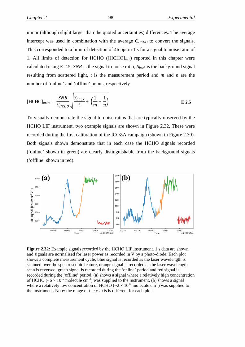
Chapter 2 98 Experimental
minor (although slight larger than the quoted uncertainties) differences. The average
intercept was used in combination with the average CHCHO to convert the signals.
This corresponded to a limit of detection of 46 ppt in 1 s for a signal to noise ratio of
1. All limits of detection for HCHO ([HCHO]min) reported in this chapter were
calculated using E 2.5. SNR is the signal to noise ratio, Sback is the background signal
resulting from scattered light, t is the measurement period and m and n are the
number of ‘online’ and ‘offline’ points, respectively.
[HCHO] =
ுுைܥඨ
ݐ+ ൬
1
+
1
൰ E 2.5
To visually demonstrate the signal to noise ratios that are typically observed by the
HCHO LIF instrument, two example signals are shown in Figure 2.32. These were
recorded during the first calibration of the ICOZA campaign (shown in Figure 2.30).
Both signals shown demonstrate that in each case the HCHO signals recorded
(‘online’ shown in green) are clearly distinguishable from the background signals
(‘offline’ shown in red).
Figure 2.32: Example signals recorded by the HCHO LIF instrument. 1 s data are shownand signals are normalised for laser power as recorded in V by a photo-diode. Each plotshows a complete measurement cycle; blue signal is recorded as the laser wavelength isscanned over the spectroscopic feature, orange signal is recorded as the laser wavelengthscan is reversed, green signal is recorded during the ‘online’ period and red signal isrecorded during the ‘offline’ period. (a) shows a signal where a relatively high concentrationof HCHO (~6 × 10¹⁰ molecule cm-3) was supplied to the instrument. (b) shows a signalwhere a relatively low concentration of HCHO (~2 × 10¹⁰ molecule cm-3) was supplied tothe instrument. Note: the range of the y-axis is different for each plot.

Chapter 2 99 Experimental
2.4 Summary
In this chapter two field instruments have been described, details regarding their
principle of operation, data acquisition method, and component parts are presented.
A LFP-LIF instrument for the measurement of OH reactivity is described in Section
2.2. Observations of OH reactivity made using this instrument, in ambient air at an
urban background site in York, UK and a coastal site in Norfolk, UK are presented
in Chapters 5 and 6 of this thesis, respectively. Observations of OH reactivity made
using this instrument, during an inter-comparison study at the SAPHIR chamber are
presented in Chapter 3. The LFP-LIF instrument has been continually developed
through the course of this work and as a result its configuration has changed
between the studies described in Chapters 3, 5 and 6. Two configurations of the
LFP-LIF instrument are described in Section 2.2.7, configuration 1 was used for
measurements in York and configuration 2 was used for measurements in Norfolk
and at the SAPHIR chamber. Section 2.2.9 details the determination of the loss rate
of OH due to physical process within the flow tube for each configuration of the
LFP-LIF instrument, this was 1.25 ± 0.42 s-1 for configuration 1 and 2.25 ± 0.21 s-1
for configuration 2.
In Section 2.3 of this chapter details of an LIF instrument for the detection of gas
phase HCHO are presented. The instrument was used in laboratory measurements of
HCHO that are presented in Chapter 4, it was used to make measurements of HCHO
in ambient air in York and Norfolk, simultaneous to the deployment of the LFP-LIF
instrument. Similar to the LFP-LIF instrument the HCHO LIF instrument was
continually developed through the course of this work. Three configurations are
described in Section 2.3.6. configuration 1 was used for the laboratory experiments
in Chapter 4 and configurations 2 and 3 were used for the York and Norfolk
deployments, respectively. Section 2.3.7 details two methods for the calibration of
the instrument; one where a known quantity of HCHO is produced through
photolysis of MeOH for addition to the instrument, and one where a known quantity
of OH is added to the instrument using a commercial permeation source. The first
method was used to calibrate the instrument for the laboratory measurements
presented in Chapter 4, and the measurements from York presented in Chapter 5.
The second method was used to calibrate the instrument for the measurements from
Norfolk presented in Chapter 6.

Chapter 2 100 Experimental
2.5 References
ATKINSON, R., BAULCH, D. L., COX, R. A., CROWLEY, J. N., HAMPSON, R.F., HYNES, R. G., JENKIN, M. E., ROSSI, M. J. & TROE, J. 2004.Evaluated kinetic and photochemical data for atmospheric chemistry:Volume I - gas phase reactions of Ox, HOx, NOx and SOx species. Atmos.Chem. Phys., 4, 1461-1738.
BOC. 2016. Automotive Speciality Gases [Online]. BOC. Available:http://www.boconline.co.uk/en/industries/manufacturing/automotive/automotive-speciality-gases/automotive-speciality-gases.html 2016].
COMMANE, R., FLOQUET, C. F. A., INGHAM, T., STONE, D., EVANS, M. J. &HEARD, D. E. 2010. Observations of OH and HO2 radicals over WestAfrica. Atmos. Chem. Phys., 10, 8783-8801.
EDWARDS, P. M. 2011. Tropospheric oxidation from the tropics to the poles. PhD,University of Leeds.
HOTTLE, J. R., HUISMAN, A. J., DIGANGI, J. P., KAMMRATH, A.,GALLOWAY, M. M., COENS, K. L. & KEUTSCH, F. N. 2008. A LaserInduced Fluorescence-Based Instrument for In-Situ Measurements ofAtmospheric Formaldehyde. Environmental Science & Technology, 43, 790-795.
HUNTER, J. D. 2007. Matplotlib: A 2D Graphics Environment. Computing inScience & Engineering, 9, 90-95.
MATSUMI, Y. & KAWASAKI, M. 2003. Photolysis of Atmospheric Ozone in theUltraviolet Region. Chemical Reviews, 103, 4767-4782.
MCKINNEY, W. 2012. Python for data analysis, CA, O'Reilly Media Inc.SMITH, S. C. 2007. Atmospheric measurements of OH and HO2 using the FAGE
technique: Instrument development and data analysis. PhD, University ofLeeds.
STONE, D., WHALLEY, L. K., INGHAM, T., EDWARDS, P. M., CRYER, D. R.,BRUMBY, C. A., SEAKINS, P. W. & HEARD, D. E. 2016. Measurementof OH reactivity by laser flash photolysis coupled with laser-inducedfluorescence spectroscopy. Atmos. Meas. Tech., 9, 2827-2844.
WALT, S. V. D., COLBERT, S. C. & VAROQUAUX, G. 2011. The NumPy Array:A Structure for Efficient Numerical Computation. Computing in Science& Engineering, 13, 22-30.
WHALLEY, L. K., STONE, D., BANDY, B., DUNMORE, R., HAMILTON, J. F.,HOPKINS, J., LEE, J. D., LEWIS, A. C. & HEARD, D. E. 2016.Atmospheric OH reactivity in central London: observations, modelpredictions and estimates of in situ ozone production. Atmos. Chem. Phys.,16, 2109-2122.

101
Chapter 3 - OH reactivity intercomparison
3.1 Overview of intercomparison
3.1.1 Aim of intercomparison
The field of OH reactivity measurements in the atmosphere has grown rapidly
through the course of the last decade with several techniques to achieve such
measurements reported. A detailed review of OH reactivity measurements in the
literature is provided in Chapter 1. There are three techniques reported for the
measurement of OH reactivity and these are the TOHLM (Kovacs and Brune, 2001),
LFP-LIF (Sadanaga et al., 2004) and CRM (Sinha et al., 2008) methods. To date
there is only one comparison of techniques for OH reactivity measurement reported
in the literature. Hansen et al. (2015) reported a comparison of ambient
measurements from a NOx rich site situated on the campus of the University of Lille
in Villeneuve d’Ascq, France for two weeks in October 2012. Measurements were
made with a LFP-LIF instrument operated by researchers of the University of Lille
and a CRM instrument operated by researchers of the Mines Douai National
Graduate School of Engineering. The comparison showed that the CRM
measurements under predicted OH reactivity by ~20 % as a result of direct
photolysis of OH reactive species in the glass OH reactor of the instrument.
Adjustment of the configuration of the OH reactor on completion of the ambient
measurements was found to reduce this affect to a negligible level, highlighting the
value of conducting comparative studies of OH reactivity instrumentation. The
comparison also highlighted the importance of accurately determining k’OH(physical)
for LFP-LIF instruments, as it was concluded that impurities in the zero air used to
measure this likely inflicted a negative bias of ~2 s-1 on the measurements.
It was proposed at the first OH Reactivity Specialists Uniting Meeting (ORSUM) in
October 2014 at the Max Planck Institute for Chemistry in Mainz, Germany, that a
formal intercomparison of all techniques for the measurement of OH reactivity

Chapter 3 102 OH reactivity comparison
would be beneficial to the community, where as many instruments as reasonably
possible were deployed. It was decided at the ORSUM meeting that this study would
take place at the Simulation of Atmospheric Photochemistry in a Large Reaction
(SAPHIR) chamber at the Jülich Forschungszentrum. The study took place in
October 2015 and included participation from 8 research groups operating a total of
9 instruments (1 TOHLM, 4 LFP-LIF and 4 CRM). The aim was to compare the
performance of all instruments in a variety of simulated atmospheric compositions.
This chapter summarises the study and presents some results from experiments
where the chamber contained ‘simple’ OH reactive species (CO) and more complex
OH reactive species; monoterpenes and real biogenic emissions from a plant
chamber, SAPHIR-PLUS (Plant Chamber under SAPHIR). The author was
responsible for measurements of OH reactivity made using the Leeds LFP-LIF
instrument (described in Section 2.2) in these experiments. These measurements are
identified as ‘LIF-4’ through the chapter. Measurements of OH reactivity reported
by other participating institutions during these experiments are anonymised.
However, the instruments used to make these measurements will be revealed in a
future publication.
3.1.2 The SAPHIR chamber
The SAPHIR chamber is located at the Jülich Forschungszentrum, Germany, and is
operated by researchers of the Institute of Chemistry and Dynamics of the
Geosphere – Troposphere. The chamber is cylindrical in shape and the walls consist
of double walled Teflon foil through which UV radiation from the sun is
transmissible, allowing the sun to serve as a natural light source for the study of
photo chemically initiated reactions. It is operated at 50 Pa above ambient pressure
and a large louvre roof system allows the chamber to be blocked from sunlight to
allow reactions to be studied in the dark. The total volume of the chamber is ~270
m3 and more detailed descriptions can be found in Bohn et al. (2005), Rohrer et al.
(2005) and Wegener et al. (2007). Figure 3.1 shows a photograph of the SAPHIR
chamber exposed to sunlight with the louvre roof open.
SAPHIR is designed so that there is room for multiple shipping containers housing
instrumentation to be positioned underneath. The advantage of this is that relatively
short sampling lines can be used as they can pass through the floor of the chamber
and be routed to instrumentation through the roof of a shipping container. There are

Chapter 3 103 OH reactivity comparison
five inlet port panels in the floor of the chamber to allow for this, one of such is
shown in Figure 3.2.
Figure 3.1: The SAPHIR chamber pictured with the louvre roof open to allow exposure tosunlight. Taken from (EUROCHAMP, 2016).
Figure 3.2: One of five inlet port panels in the floor of the SAPHIR chamber to allow gassamples to be transferred to instrumentation in shipping containers below. Taken from(EUROCHAMP, 2016).

Chapter 3 104 OH reactivity comparison
3.1.3 Participating instrumentation
A total of 9 instruments were used for the measurement of OH reactivity during the
comparison study at the SAPHIR chamber. The institutions which deployed these
instruments are listed in Table 3.1 in addition to the measurement techniques used
and appropriate references.
Institution Technique Reference
Penn State University(USA)
TOHLM Kovacs and Brune (2001)
University of Leeds(UK)
LFP-LIF Stone et al. (2016)
Jülich Forschungszentrum (FZJ)(Germany)
LFP-LIF Lou et al. (2010)
Jülich Forschungszentrum (FZJ)(Germany)
LFP-LIF Fuchs et al. (2016)
University of Lille(France)
LFP-LIF Amedro et al. (2012)
Max Planck Institute for Chemistry(MPIC) (Germany)
CRM Sinha et al. (2008)
Mines Douai National Graduate Schoolof Engineering (France)
CRM Michoud et al. (2015)
Laboratory of the Sciences of Climateand the Environment (LSCE) (France)
CRM Zannoni et al. (2016)
Finnish Meteorological Institute (FMI)(Finland)
CRM Not available
Table 3.1: Instruments for the measurement of OH reactivity used in the intercomparisonstudy at the SAPHIR chamber in October 2015.
Each of the 9 instruments listed were housed in shipping containers below the
chamber during the comparison study. The positioning of these containers is
summarised by the diagram in Figure 3.3. Areas displayed in red are where
containers were placed specifically for the OH reactivity comparison study
described here, all other spaces shown were occupied by containers that were a
permanent fixture at SAPHIR. The space labelled Leeds was occupied by the Leeds
FAGE container and housed the Leeds LFP-LIF instrument which was operated in
configuration 2 (described in Chapter 2) and shared an inlet port panel with the
University of Lille LFP-LIF instrument. The method for sampling from SAPHIR
with the Leeds LFP-LIF instrument is described in Section 3.2. In one of the
containers adjacent to the Leeds FAGE container three CRM instruments were
housed and all sampled from the same inlet port panel. To the other side of the
Leeds FAGE container was a container which housed the Penn State TOHLM
instrument which shared an inlet port panel with two Jülich Forschungszentrum
LFP-LIF instruments which were operated from a container opposite. The LSCE

Chapter 3 105 OH reactivity comparison
CRM instrument was operated from another container along with some
instrumentation for ancillary measurements. These shared an inlet port panel with
some GC instrumentation that were used to measure VOCs.
Figure 3.3: Diagram to show the placement of instrumentation within shipping containersbelow the SAPHIR chamber during the OH reactivity intercomparison study in October2015. Areas shown in red were occupied by containers that were placed underneath thechamber for the purpose of the comparison. Areas shown in blue were occupied bycontainers that were a permanent fixture at SAPHIR. Provided by Dr. Hendrik Fuchs, JülichForschungszentrum.
3.2 Sampling method
The Leeds LFP-LIF instrument was operated in configuration 2 (as described in
Section 2.2.7) from inside the Leeds FAGE container (described in Section 2.2.2).
The container was positioned at SAPHIR such that ~1/3 of its roof area was covered
and the main door was facing away from the chamber. The image shown in
Figure 3.4 shows the position of the FAGE container at SAPHIR whilst
measurements were made during the OH reactivity intercomparison.

Chapter 3 106 OH reactivity comparison
Figure 3.4: Image showing the Leeds FAGE container at the SAPHIR chamber during theOH reactivity comparison in October 2015.
Owing to it being necessary to position the FAGE container beneath SAPHIR to
minimise the length of the sampling line, it was not possible to position the
instrument on the roof of the container as is usually the case for ambient
measurements in the field. The components which would usually be fixed to a table
top, were removed and fixed to a new aluminium panel in the same way as they had
been fixed to the table top. This panel fitted to the top of the rack inside the FAGE
container above the 308 nm detection laser as shown in Figure 3.5.

Chapter 3 107 OH reactivity comparison
Figure 3.5: Photograph of the LFP-LIF instrument above the racking inside the FAGEcontainer. Visible key features are labelled.
A PFA sampling line ~5 m in length (½” OD) connected the instrument to the inlet
port panel (example shown in Figure 3.2) through which it protruded ~30 cm into
the chamber. It was connected to the flow tube of the instrument via a ½” Swagelok
t-piece where one of the connectors was reduced to ¼” Teflon tubing which in turn
was connected to a ¼” valve. This valve was fitted to a glass cell where a flow of
synthetic air could be irradiated with a Hg(Ar) pen ray lamp to generate ozone to be
photolysed by 266 nm laser radiation in the flow tube of the instrument. In all
experiments conducted during the comparison the chamber was humidified to a
sufficient level for OH decays to be observed by all LFP-LIF instruments and in
most experiments ozone was also added to the chamber for this. However, in some
experiments such as those where monoterpenes and biogenic emissions were
oxidised through ozonolysis, it was not possible for ozone to be in the chamber prior
to the initiation of ozonolysis (through addition of ozone). During these experiments
ozone was added to the gas sample prior to entrance to the flow tube using the
system described above so that OH decays were observable. For this 1 SLM of
synthetic air supplied locally at SAPHIR through the boil off of liquid nitrogen and
Chapter 3 108 OH reactivity comparison
oxygen was irradiated in the glass cell and mixed with 15 SLM of gas sampled from
the chamber. Measurements using an ozone analyser (Thermo Scientific) showed
that this would result in ~60 ppb of ozone within the flow tube of the instrument,
when the pen ray lamp was operated at 21 mA (max output). These conditions were
the same for every experiment where the addition of ozone was necessary.
It was not practically feasible to routinely check the flow rate of the gas sample into
the LFP-LIF instrument through periodically fitting the flow meter (MKS 179A, 0-
20 SLM) to the sampling line, as is usually the case during ambient measurements.
The sampling line had to remain connected to the chamber at all times. To enable
constant monitoring of the flow of gas sampled it was necessary to first determine
the flow rate into the FAGE cell. Experiments were conducted where the flow meter
was fitted to the end of the ~5 m sampling line and the gas lines that are usually used
for pumping excess gas out of the flow tube were capped. A flow rate of 3.6 SLM
was measured and found to be stable over a range of FAGE cell pressures (1.1 – 4.8
Torr) whilst the flow tube pressure was stable at ~760 Torr. Upon connecting the
sampling line to SAPHIR, the flow meter was fitted to the tubing to the scroll pump
so that the flow rate of excess gas leaving the instrument could be monitored.
During the intercomparison experiments the reading from the flow meter was
continually monitored and the butterfly valve that was used to throttle the scroll
pump was adjusted to maintain a flow of 12.4 SLM (16 SLM in total entering the
flow tube).
During experiments where no ozone was added to the instrument (e.g. that described
in Section 3.3.1), k’OH(physical) for the instrument in configuration 2 was subtracted
directly from k’OH(raw) that was determined from the decay signals to obtain k’OH.
However, during experiments where it was necessary for ozone to be added (e.g.
those described in Section 3.3.2) to the instrument, the k’OH(raw) determined from the
decay signals were first adjusted according to the dilution by the ozone containing
flow.
3.3 Results
3.3.1 Addition of CO
Several experiments were conducted during the OH reactivity intercomparison
where known quantities of OH reactive species were added to SAPHIR to test and

Chapter 3 109 OH reactivity comparison
compare the response of each instrument. The results from such an experiment with
CO are presented here. Humidified synthetic air and ozone ~40 ppb were supplied to
the chamber at the beginning of the experiment and ~ 1 hour elapsed before the first
addition of ~2 ppb of CO was made. No further additions were made for ~1.5 hours
to allow ample time for CRM instruments to obtain 3 or more measurements, as the
time resolution for CRM instruments is significantly longer than for LIF type
instruments. Following this, similar additions of CO were made to SAPHIR in the
same way until a maximum level of ~35 ppm was reached. Figure 3.6 shows
measurements of k’OH that were reported for this experiment from each participating
instrument. Measurements labelled as ‘LIF-4’ were made using the Leeds LFP-LIF
instrument.
Figure 3.6: Time series of k’OH measured in SAPHIR by nine instruments where knownquantities of CO were supplied to the chamber in stepwise additions. Results areanonymised with techniques separated into two categories LIF and CRM where LFP-LIFand TOHLM measurements are both classified as LIF instruments. The shaded area isrepresentative of the OH reactivity calculated to be attributable to the CO added. ‘LIF-4’measurements were made using the Leeds LFP-LIF instrument. Provided by Dr. HendrikFuchs, Jülich Forschungszentrum.
The results show that the measurements made using the Leeds LFP-LIF (‘LIF-4’)
instrument were in agreement with those made by other instruments in this

Chapter 3 110 OH reactivity comparison
experiment, particularly the other LIF type instruments. Observations reported from
all instruments followed the profile of the OH reactivity calculated to be attributable
to the CO that was added to the chamber (shaded in pink). The agreement is shown
to be particularly close when k’OH is below ~100 s-1. However, above this there is
considerably more scatter between points for all instruments, indicating that
measurements made by participating instruments may become less reliable above
this threshold. This is true for the Leeds LFP-LIF measurements which show
significantly more scatter following the final two additions of CO than for the rest of
the experiment. However, the OH reactivity calculated using the CO concentration
here is greater than 100 s-1. This is far beyond (35 ppm) what is typically observed
in ambient air for any environment, the scatter observed during this experiment
should not significantly affect the precision of field measurements made using the
Leeds LFP-LIF instrument.
The points representing measurements by the CRM instruments show more variation
than the LIF measurements when k’OH is below ~50 s-1. The cause of this is likely
that changes in pyrrole concentration which need to be quantified to determine k’OH
in CRM type instruments (described in Section 1.5.4), are subject to greater
uncertainty at lower reactivities, owing to the changes in pyrrole concentration being
closer to the limit of detection of the instrumentation used for detection.
3.3.2 Oxidation of monoterpenes and real biogenic emissions
To test the performance of the participating instruments with more complex gas
mixtures some experiments were conducted with known quantities of monoterpenes,
characteristic of biogenically influenced atmospheres, and also real biogenic
emissions from plants. It was important to compare the performance of the
instrumentation under such conditions as ‘missing’ OH reactivity is often postulated
to be the result of undetected biogenic emissions, such as monoterpenes. Di Carlo et
al. (2004) and Edwards et al. (2013) reported ‘missing’ reactivities as high as ~50 %
from forest atmospheres where k’OH was measured using the TOHLM technique.
High ‘missing’ OH reactivity has also been reported from forest atmospheres using
the CRM technique, for example Sinha et al. (2008) reported 65 % ‘missing’
reactivity and Nölscher et al. (2012) reported 68 % ‘missing’ reactivity. There are no
observations of OH reactivity for a biogenically dominated environment reported in
the literature from a LFP-LIF instrument at present. Although measurements in

Chapter 3 111 OH reactivity comparison
forested environments reported in the literature for different techniques are from
various locations, simultaneous measurements of OH reactivity have not been made
in such an environment using more than one technique.
The first of these experiments described here involved stepwise addition of a
mixture of monoterpenes (containing equal quantities of α-pinene, limonene and
myrcene) to SAPHIR to cover a range of OH reactivities up to ~20 s-1. Following
this ozone was added to the chamber to initiate an ozonolysis reaction. Figure 3.7
shows measurements of k’OH that were reported for this experiment from each
participating instrument. Measurements labelled as ‘LIF-4’ were made using the
Leeds LFP-LIF instrument.
Figure 3.7: Time series of k’OH measured in SAPHIR by nine instruments where knownquantities of monoterpenes were supplied to the chamber in stepwise addition followed bythe addition of ozone for the initiation of ozonolysis. Results are anonymised withtechniques separated into two categories, LIF and CRM, where LFP-LIF and TOHLMmeasurements are classified as LIF instruments. The shaded area is representative of the OHreactivity calculated to be attributable to the monoterpenes added. ‘LIF-4’ measurementswere made using the Leeds LFP-LIF instrument. Provided by Dr. Hendrik Fuchs, JülichForschungszentrum.
The results show that the measurements made using the Leeds LFP-LIF (‘LIF-4’)
instrument tracked the profile of the measurements made with the other instruments

Chapter 3 112 OH reactivity comparison
well, particularly the other LIF type instruments. However, they are typically offset
by ~3-5 s-1 through the course of this experiment. It can be seen that in the ‘zero’
period (before the addition of any monoterpenes to SAPHIR) that there was some
variability in the Leeds LFP-LIF measurements. The most probable explanation for
this is that some OH reactive contaminants contributed to the OH reactivity that was
measured. This experiment was the first of the intercomparison where it was
necessary to add O3 to the flow tube of the instrument, owing to it being absent from
the chamber. It is possible that contaminants originated in the system used to supply
O3 to the instrument.
With the exception of the Leeds LFP-LIF instrument, which had a positive bias
likely due to contaminants as discussed above, the LIF type instruments were in
good agreement through the course of this experiment and tracked the profile of the
calculated OH reactivity attributable to the monoterpenes well (shaded in blue).
Measurements from the CRM instruments in this experiment are shown to be
considerably more scattered than the LIF measurements and are typically lower. It is
possible that these measurements could have underestimated k’OH as a result of
direct photolysis of VOCs within the glass OH reactors of these instruments.
The ozonolysis reaction was initiated at ~1330 and from this time the values of OH
reactivity measured are shown to decrease gradually, as was the calculated OH
reactivity attributable to the monoterpenes. However, the measurements decreased at
a slower rate which would be expected in this scenario, when it is considered that
OH reactive ozonolysis products that are OH reactive would have formed and these
are not included in the calculated reactivity.
In the second experiment described here a plant chamber (SAPHIR PLUS) was used
to supply real biogenic emissions to SAPHIR (Hohaus et al., 2016). Upon
completion of humidification of SAPHIR at the beginning of the experiment at
~0800 a gas line was opened to allow the transfer of biogenic emissions from plants
held within SAPHIR PLUS to SAPHIR. The transfer line was kept open until a
maximum of ~6 ppb of emissions had been transferred. Following this, ozone was
added to initiate ozonolysis of these emissions at ~1500. Figure 3.8 shows
measurements of k’OH that were reported for this experiment from each participating
instrument. Measurements labelled as ‘LIF-4’ were made using the Leeds LFP-LIF
instrument.

Chapter 3 113 OH reactivity comparison
Figure 3.8: Time series of k’OH measured in SAPHIR by nine instruments where realbiogenic emissions were to the chamber from a plant chamber (SAPHIR PLUS). Results areanonymised with techniques separated into two categories, LIF and CRM, where LFP-LIFand TOHLM measurements are classified as LIF instruments. ‘LIF-4’ measurements weremade using the Leeds LFP-LIF instrument. Provided by Dr. Hendrik Fuchs, JülichForschungszentrum.
It is shown again that the profile of the observations from most of the LIF type
instruments are very similar (including those made using the Leeds LFP-LIF (‘LIF-
4’) instrument) and that the most scatter is shown in the observations from CRM
instruments. Many observations from CRM instruments are also lower than those
from LIF type instruments and the OH reactivity calculated from monoterpene
concentrations quantified by a proton transfer mass spectrometer (PTR-MS) and
GC-FID. It is possible that these measurements were artificially low due to direct
photolysis of OH reactive species within the glass reactors of the CRM instruments.
Both the measurements and the calculated reactivity decrease upon addition of
ozone to SAPHIR indicating that biogenic emissions from SAPHIR PLUS were
removed through ozonolysis reactions. Following the addition of ozone there is also
a significant discrepancy between the measured and calculated OH reactivities.

Chapter 3 114 OH reactivity comparison
Similar to the previous experiment this is likely due to the formation of OH reactive
ozonolysis products that were not measured.
3.3.3 Correlations
In total during the OH reactivity comparison at SAPHIR 10 experiments were
conducted, anonymised results from three of these are presented and discussed
above. The measurements made using the Leeds LFP-LIF instrument are identified
as ‘LIF-4’. Results from all experiments undertaken, and a thorough comparison of
the measurements from each instrument will form the basis of a future publication.
Each experiment conducted fitted into one of two categories. In some experiments
known quantities of relatively ‘simple’ (e.g. CO and CH4) OH reactive species were
added to SAPHIR and no reaction was initiated. In contrast, in other experiments
more complex mixtures of OH reactive species were added and ozonolysis reactions
were initiated through the addition of ozone, or the chamber contents was
photochemically processed through exposure to sunlight.
In experiments where the concentrations of ‘simple’ OH reactive species added to
SAPHIR were known, it was possible to examine the relative relationships between
the response of each participating instrument and the calculated k’OH. Whilst full
results for only one such experiment are presented above (Figure 3.6), the
relationship between measured and calculated OH reactivity for all of these
experiments combined is summarised by Figure 3.9. A graph is shown for measured
OH reactivity from each instrument that participated versus calculated OH
reactivity.
The results show that there was strong correlation between the measurements of OH
reactivity that were made using the Leeds LFP-LIF instrument and the OH reactivity
calculated from measured OH sinks (R2 = 0.97). The correlation between measured
and calculated reactivity was typically stronger for LIF type instruments than the
CRM instruments (0.97 vs 0.59 average R2). It is also shown that the majority of
instruments slightly over predicted the calculated OH reactivity, this is possibly
because only OH reactive species that were intentionally added to the chamber were
included in the calculation of k’OH. It is likely that there were OH reactive impurities
present in the chamber that contributed to the measured values.

Chapter 3 115 OH reactivity comparison
Figure 3.9: Graphs which summarise the relationship between measured and calculatedk’OH from all experiments conducted during the OH reactivity comparison at SAPHIRwhere ‘simple’ OH reactive species were added to the chamber and no reaction wasinitiated. Each colour used for the points plotted represent data from a different experiment.‘LIF-4’ is identified as the Leeds LFP-LIF instrument. Provided by Dr. Hendrik Fuchs,Jülich Forschungszentrum.
In experiments such as those described in Section 3.3.2 where more ‘complex’ OH
reactive monoterpenes were added to SAPHIR, the overall response of each
instrument was compared. It was not possible for the complete inventory of
emissions from SAPHIR PLUS to be characterised in one of the experiments to
enable reliable calculation of OH reactivity. Therefore, it was decided that the
response of each instrument would be compared to a reference instrument. LIF-1
was chosen as this made observations of k’OH that were the least scattered. Figure
3.10 shows data from the two experiments described in Section 3.3.2 for the other
instruments plotted against those from LIF-1.

Chapter 3 116 OH reactivity comparison
Figure 3.10: A summary of the relationship between measured k’OH from each participatinginstrument and a reference instrument (LIF-1) for both experiments described in Section3.3.2 where biogenic emissions were added to SAPHIR and an ozonolysis reaction wasinitiated. Green points represent data recorded prior to the addition of ozone. Blue pointsrepresent data after the addition of ozone. ‘LIF-4’ is identified as the Leeds LFP-LIFinstrument. Provided by Dr. Hendrik Fuchs, Jülich Forschungszentrum.
Again it is shown that the measurements obtained using the LIF type instruments are
considerably less scattered than those obtained using the CRM instruments. It can be
seen that for most instruments the relationship (slope and scatter) demonstrates no
difference in the presence and absence of ozone. However, there appears to be a
distinct difference between data recorded by LIF-3. The reason for this is currently
unclear and future analysis of these data will be presented in a future publication
based on the results from the intercomparison.
3.4 Summary and conclusions
The Leeds LFP-LIF instrument for the measurement of OH reactivity was
successfully deployed to the SAPHIR chamber at the Jülich Forschungszentrum,

Chapter 3 117 OH reactivity comparison
Germany to take part in an intercomparison campaign. A total of nine instruments
from eight different institutions were used for measurements (1 TOHLM, 4 LFP-LIF
and 4 CRM). Ten experiments were conducted in total and results from three of
these are presented in this chapter. In the first of these, known quantities of CO were
added stepwise to SAPHIR whilst the response of each instrument was monitored. It
was found that the measurements from all instruments tracked the calculated OH
reactivity attributable to CO well. Significantly more scatter was observed for the
CRM measurements during this experiment, particularly at lower k’OH. It is likely
this was due to corresponding smaller changes in pyrrole concentrations that needed
to be observed, in order to successfully determine k’OH, being closer to the limits of
detection of instrumentation used for the measurement of pyrrole.
In the second two experiments described in this chapter mixtures of more complex
OH reactive species were added to the chamber to simulate a biogenically
influenced atmosphere. In the first of these a 1:1:1 mixture of α-pinene, limonene
and myrcene was added to the chamber in stepwise additions until the OH reactivity
reached ~20 s-1. Following this an ozonolysis reaction was initiated and the
measurements were all shown to decrease. It was shown in this experiment that
observations from most instruments tracked the changes in calculated reactivity well
and that again more scattered observations were reported from the CRM
instruments. In the third experiment described in this chapter real biogenic emissions
from a plant chamber (SAPHIR PLUS) were flowed into SAPHIR. The process took
place over several hours until ~6 ppb total monoterpenes had been added, and the
ozonolysis reaction was then initiated. For both experiments described where a
biogenically influenced atmosphere was simulated it was found that CRM
measurements had a tendency to be lower than the LIF type measurements. A
possible explanation for this is that the more complex OH reactive species present
were photolysed in the OH reactors of the CRM instruments leading to artificially
low measurements, as was reported by Hansen et al. (2015).
It should be noted that the observations and comparisons presented in this chapter
are preliminary and only the measurements from one of the LIF type instruments
(LIF-4) is directly attributable to the author. A more in-depth analysis of all of the
data will be conducted by researchers at Jülich Forschungszentrum in order to
comprehensively examine the performance of each instrument, in the context of
each experiment.

Chapter 3 118 OH reactivity comparison
3.5 References
AMEDRO, D., MIYAZAKI, K., PARKER, A., SCHOEMAECKER, C. &FITTSCHEN, C. 2012. Atmospheric and kinetic studies of OH and HO2 bythe FAGE technique. Journal of Environmental Sciences, 24, 78-86.
BOHN, B., ROHRER, F., BRAUERS, T. & WAHNER, A. 2005. Actinometricmeasurements of NO<sub>2</sub> photolysis frequencies in the atmospheresimulation chamber SAPHIR. Atmos. Chem. Phys., 5, 493-503.
DI CARLO, P., BRUNE, W. H., MARTINEZ, M., HARDER, H., LESHER, R.,REN, X., THORNBERRY, T., CARROLL, M. A., YOUNG, V., SHEPSON,P. B., RIEMER, D., APEL, E. & CAMPBELL, C. 2004. Missing OHReactivity in a Forest: Evidence for Unknown Reactive Biogenic VOCs.Science, 304, 722-725.
EDWARDS, P. M., EVANS, M. J., FURNEAUX, K. L., HOPKINS, J., INGHAM,T., JONES, C., LEE, J. D., LEWIS, A. C., MOLLER, S. J., STONE, D.,WHALLEY, L. K. & HEARD, D. E. 2013. OH reactivity in a South EastAsian Tropical rainforest during the Oxidant and Particle PhotochemicalProcesses (OP3) project. Atmos. Chem. Phys. Discuss., 13, 5233-5278.
EUROCHAMP. 2016. EUROCHAMP [Online]. Available: www.eurochamp.com[Accessed].
FUCHS, H., TAN, Z., LU, K., BOHN, B., BROCH, S., BROWN, S. S., DONG, H.,GOMM, S., HÄSELER, R., HE, L., HOFZUMAHAUS, A., HOLLAND, F.,LI, X., LIU, Y., LU, S., MIN, K. E., ROHRER, F., SHAO, M., WANG, B.,WANG, M., WU, Y., ZENG, L., ZHANG, Y., WAHNER, A. & ZHANG,Y. 2016. OH reactivity at a rural site (Wangdu) in the North China Plain:Contributions from OH reactants and experimental OH budget. Atmos.Chem. Phys. Discuss., 2016, 1-30.
HANSEN, R. F., BLOCQUET, M., SCHOEMAECKER, C., LÉONARDIS, T.,LOCOGE, N., FITTSCHEN, C., HANOUNE, B., STEVENS, P. S., SINHA,V. & DUSANTER, S. 2015. Intercomparison of the comparative reactivitymethod (CRM) and pump–probe technique for measuring total OH reactivityin an urban environment. Atmos. Meas. Tech., 8, 4243-4264.
HOHAUS, T., KUHN, U., ANDRES, S., KAMINSKI, M., ROHRER, F.,TILLMANN, R., WAHNER, A., WEGENER, R., YU, Z. & KIENDLER-SCHARR, A. 2016. A new plant chamber facility, PLUS, coupled to theatmosphere simulation chamber SAPHIR. Atmos. Meas. Tech., 9, 1247-1259.
KOVACS, T. A. & BRUNE, W. H. 2001. Total OH Loss Rate Measurement.Journal of Atmospheric Chemistry, 39, 105-122.
LOU, S., HOLLAND, F., ROHRER, F., LU, K., BOHN, B., BRAUERS, T.,CHANG, C. C., FUCHS, H., HÄSELER, R. & KITA, K. 2010. AtmosphericOH reactivities in the Pearl River Delta - China in summer 2006:measurement and model results. Atmos. Chem. Phys, 10, 11243-11260.
MICHOUD, V., HANSEN, R. F., LOCOGE, N., STEVENS, P. S. & DUSANTER,S. 2015. Detailed characterizations of the new Mines Douai comparativereactivity method instrument via laboratory experiments and modeling.Atmos. Meas. Tech., 8, 3537-3553.
NÖLSCHER, A. C., WILLIAMS, J., SINHA, V., CUSTER, T., SONG, W.,JOHNSON, A. M., AXINTE, R., BOZEM, H., FISCHER, H., POUVESLE,N., PHILLIPS, G., CROWLEY, J. N., RANTALA, P., RINNE, J.,KULMALA, M., GONZALES, D., VALVERDE-CANOSSA, J., VOGEL,

Chapter 3 119 OH reactivity comparison
A., HOFFMANN, T., OUWERSLOOT, H. G., VILÃ -GUERAU DEARELLANO, J. & LELIEVELD, J. 2012. Summertime total OH reactivitymeasurements from boreal forest during HUMPPA-COPEC 2010. Atmos.Chem. Phys., 12, 8257-8270.
ROHRER, F., BOHN, B., BRAUERS, T., BRÜNING, D., JOHNEN, F. J.,WAHNER, A. & KLEFFMANN, J. 2005. Characterisation of the photolyticHONO-source in the atmosphere simulation chamber SAPHIR. Atmos.Chem. Phys., 5, 2189-2201.
SADANAGA, Y., YOSHINO, A., WATANABE, K., YOSHIOKA, A.,WAKAZONO, Y., KANAYA, Y. & KAJII, Y. 2004. Development of ameasurement system of OH reactivity in the atmosphere by using a laser-induced pump and probe technique. Review of Scientific Instruments, 75,2648-2655.
SINHA, V., WILLIAMS, J., CROWLEY, J. N. & LELIEVELD, J. 2008. TheComparative Reactivity Method – a new tool to measure total OHReactivity in ambient air. Atmos. Chem. Phys., 8, 2213-2227.
STONE, D., WHALLEY, L. K., INGHAM, T., EDWARDS, P. M., CRYER, D. R.,BRUMBY, C. A., SEAKINS, P. W. & HEARD, D. E. 2016. Measurementof OH reactivity by laser flash photolysis coupled with laser-inducedfluorescence spectroscopy. Atmos. Meas. Tech., 9, 2827-2844.
WEGENER, R., BRAUERS, T., KOPPMANN, R., RODRÍGUEZ BARES, S.,ROHRER, F., TILLMANN, R., WAHNER, A., HANSEL, A. &WISTHALER, A. 2007. Simulation chamber investigation of the reactions ofozone with short-chained alkenes. Journal of Geophysical Research:Atmospheres, 112, n/a-n/a.
ZANNONI, N., GROS, V., LANZA, M., SARDA, R., BONSANG, B.,KALOGRIDIS, C., PREUNKERT, S., LEGRAND, M., JAMBERT, C.,BOISSARD, C. & LATHIERE, J. 2016. OH reactivity and concentrations ofbiogenic volatile organic compounds in a Mediterranean forest of downy oaktrees. Atmos. Chem. Phys., 16, 1619-1636.

120
Chapter 4 - Development of an OH flow
reactor
4.1 Motivation for the development of an OH flow reactor
A discussion of the concept of ‘missing’ OH reactivity is presented in Chapter 1, in
addition to details of measurements reported in the literature where significant
‘missing’ OH reactivity has been observed. There is currently no method presented
in the literature for the identification of species that contribute to ‘missing’ OH
reactivity. However, Kato et al. (2011) reported a method to estimate the
contribution from OH reactive species that were detectable, but not identifiable, to
‘missing’ OH reactivity. The study took the form of a relative rate experiment
utilising gas chromatograph – flame ionisation detector (GC-FID) peaks. An OH
flow reactor was coupled to a GC-FID instrument and ambient air was analysed
where it had, and had not been, exposed to OH in a flow reactor. Figure 4.1 shows
the schematic diagram in of the instrumental set-up used by Kato et al. (2011) in this
study.
Figure 4.1: Schematic of the experimental set-up used by Kato et al. (2011) to estimate thecontribution from unidentified VOCs to OH reactivity. (a) ambient air exposed to OH, (b)ambient air not exposed to OH. Taken from Kato et al. (2011).
The gas to be analysed (1 SLM, either from a standard gas mixture or ambient air)
was mixed with nitrogen (1 SLM) which had been humidified using a water bubbler.
This either had (OH formation) or had not (no OH formation) been exposed to UV

Chapter 4 121 OH flow reactor
radiation from a UV lamp. When the humidified nitrogen flow was irradiated, OH
was generated through photolysis of water vapour using the 184.9 nm spectral line
from the UV lamp, R 4.1.
HଶO + ℎʋ(~ଵସ.ଽ ) → OH + H R 4.1
Rate equations for the reaction of OH with identified (Ai) and unidentified (Xi)
species can be expressed as shown in E 4.1 and E 4.2, respectively. kAi and kXi are
bimolecular rate coefficients for the reaction of OH with Ai and Xi, respectively.
[ܣ]
ݐ= −
[ܣ][ܪ] E 4.1
[]
ݐ= −
[][ܪ] E 4.2
Both of these rate equations can be rearranged and integrated to obtain E 4.3 and E
4.4 below. [Ai]0 and [Xi]0 are the concentrations of the identified and unidentified
species, respectively, which were determined from integration of peaks in the
chromatogram of the sample which was not exposed to OH. [Ai]∞ and [Xi]∞ are the
concentrations of the identified and the unidentified species, respectively, which
again were determined from the chromatogram of the sample which was exposed to
OH in the flow reactor.
lnቆ[ܣ]ஶ[ܣ]
ቇ= න [ܪ] dݐ E 4.3
lnቆ[][]ஶ
ቇ= න [ܪ] dݐ E 4.4
In E 4.3 and E 4.4 the integral of [OH] with respect to time is a common factor, thus
it was possible to use the relationship between ln([Ai]0/[Ai]∞) and kAi,to determine
∫[OH]dt, and subsequently calculate bimolecular rate coefficients for the reaction
between the unidentified species and OH. Assuming that VOCs present in the
ambient air or standard gas flowed into the reactor were removed exclusively
through their reaction with OH, relative rate theory dictates that the relationship
should be linear. The relationship should also be unique to the composition of
ambient air or standard gas sampled. Figure 4.2 shows the relationship between
ln([Ai]0/[Ai]∞) and kAi resulting from the analysis of a standard mixture containing 60
VOCs that was reported by Kato et al. (2011).

Chapter 4 122 OH flow reactor
Figure 4.2: The natural logarithm of the ratio of the concentrations of known species (Ai)that have and have not been exposed to OH, respectively vs their literature rate coefficientsfor reaction with OH. The gradient is equal to the integral of [OH] with respect to time andis ~2×10⁹ molecule cm-3 s. Taken from Kato et al. (2011).
The data exhibit a linear trend as is expected to be the case when E4.3 is considered.
Owing to the linearity associated with the GC-FID technique, between the
concentrations of species analysed, and their observed peak areas in the
chromatograms, the argument of the logarithm in E 4.4 is equal to the ratio of peak
areas for Xi. If the standard mixture contained unidentified OH reactive species, kXi
values could have been determined using E4.4 and ∫[OH]dt that was determined
from the relationship between ln([Ai]0/[Ai]∞) and kAi. Using this same method but
with ambient air in place of the standard mix, Kato et al. (2011) reported that the
relationship between ln([Ai]0/[Ai]∞) and kAi could be used to determine ∫[OH]dt over
time in the field. This subsequently could be used in conjunction with E4.4 to
determine kXi values for OH reactive species that were detectable but not identifiable
in the field.

Chapter 4 123 OH flow reactor
The retention times for the unidentified species in the chromatograms could be used
to estimate their carbon number and subsequently response factors which were used
to calculate estimated values for [Xi]0. These could then be multiplied by
corresponding kXi values (determined using the method outlined above), to obtain an
estimate for the contribution from Xi to ‘missing’ OH reactivity in s-1.
Kato et al. (2011) deployed the instrumentation described above for ambient
measurements in urban Tokyo. A total of 28 unidentified species were found to
contribute to ‘missing’ OH reactivity, they accounted on average for ~6 % of the
total OH reactivity that was measured using a laser flash photolysis pump and probe
instrument. However, the average ‘missing’ OH reactivity was ~20 % for the
measurement period meaning that ~14 % of the total OH reactivity was still not
accounted for by the identified and unidentified VOCs detected, or other routinely
measured OH sinks (e.g. NOx and CO). Whilst the study by Kato et al. (2011) broke
new ground in the investigation of the source of ‘missing’ OH reactivity, no
discoveries were reported relating to the chemical identities of Xi that were detected.
The work detailed in this chapter aimed to address this through the development of a
new instrument for the chemical identification of ‘missing’ OH reactivity.
The first sections details the design, characterisation, and predicted performance of
the new OH flow reactor for use in a system similar to that reported by Kato et al.
(2011), but with the capability to identify species that contributed to ‘missing’ OH
reactivity. A gas chromatograph time of flight mass spectrometer (GC-TOF-MS)
was used for this in the final version of the experimental set up to enable such
identification. The final sections provide details of the resulting new instrument for
the identification of species contributing to ‘missing’ OH reactivity and some
preliminary observations from the analysis of ambient air during the York 2014
‘missing’ OH reactivity campaign.
4.2 Design process
The first prototype of the OH flow reactor consisted of a glass (borosilicate)
flowtube (1 inch OD) within which a Hg(Ar) pen ray lamp was positioned. N2,
humidified using a water bubbler, was flowed through the tube over the lamp to
produce OH through R3.1. Downstream from the lamp, ~5 cm, a flow of standard
gas containing VOCs was introduced through a ¼ inch arm for the laboratory tests.
If this design of OH reactor was deployed for ambient measurements, ambient air

Chapter 4 124 OH flow reactor
would have been introduced here. Just after the point of this addition there was a
~45˚ bend in the flow tube, the purpose of this was to try to minimise exposure of
UV light from the pen ray lamp to VOCs in the standard gas introduced to prevent
their loss due to direct photolysis. For the system to be successful in a relative rate
study VOCs must be lost exclusively to their reaction with OH and not photolysis.
After passing through another ~20 cm of flow tube, where OH + VOC reactions
could occur, the gas would be sampled for analysis. There was also a vent at the end
of the system to allow excess gas to exit the system. This prototype design of the
OH reactor was transported to the University of York where it was coupled with a
GCxGC-TOF-MS instrument so that characterisation experiments could be
conducted. Figure 4.3 summarises the key features of the glass OH flow reactor
prototype.
Figure 4.3: Schematic diagram showing the key features of a prototype glass (borosilicate)OH flow reactor that was interfaced with a GCxGC-TOF-MS instrument at the Universityof York for testing. Diagram not to scale.
Some characterisation experiments for the prototype glass OH flow reactor
described above were conducted in which a national physical laboratories (NPL)
mixture of 30 VOCs was flowed into the OH flow reactor in place of ambient air.
The standard was flowed into the reaction flow tube and tests were first conducted to
assess the efficiency of VOC removal. The outflow from the reactor was analysed
by the GCxGC-TOF-MS instrument three times with the lamp on, and three times
with the lamp off. Average peak areas for 19 VOCs that could be clearly resolved

Chapter 4 125 OH flow reactor
for quantification are shown in Figure 4.4. All of the VOCs for which data were
available were found to decrease when the pen ray lamp was switched on (OH
generated), indicating that VOCs were being removed through their reaction with
OH. Isoprene (kOH+isoprene = 1 × 10⁻¹⁰ cm3 molecule-1 s-1 at 298 K) (Atkinson et al.,
2006) was removed to the greatest extent (~99 %) whereas benzene (kOH+benzene = 1.2
× 10-12 cm3 molecule-1 s-1 at 298 K) (Atkinson et al., 2006) was removed to the least
extent (~28 %).
The decreases in the levels of the VOCs in the standard mixture that were observed
upon exposure to OH were used to construct a plot of ln([Ai]0/[Ai]∞) vs kAi, as shown
Figure 4.5. A linear trend was found to exist, therefore indicating that the
chromatographic peaks representing compounds for which data are plotted,
decreased by quantities that scaled with their bimolecular rate coefficients for
removal by OH (the basis of the relative rate method). If the only VOC removal
process occurring within the reaction flow tube (when the pen ray lamp was
switched on) by reaction with OH, the y intercept of the line best fit shown on
Figure 4.5 would be expected to be zero. However, it is shown that there is an
intercept (0.84); this indicates that there was another pathway for the loss of VOCs
in the OH flow reactor other than removal by reaction with OH. It was concluded
that the most likely reason for this was that a portion of the VOCs were removed
through direct photolysis by stray UV light from the pen ray lamp that was used to
generate OH.

Chapter 4 126 OH flow reactor
Figure 4.4: Chart to show differences in the concentrations of 18 VOCs with the Hg pen raylamp off and on, (of the NPL 30 standard) detected in the outflow of the glass OH reactorprototype with the water bubbler present. The data shown are averaged values for threeanalyses. Error bars are the 1σ standard deviation of the peak areas determined from each analysis that were used to calculate the average values. Data supplied by Dr. NoeliaRamirez, University of York.
If the system consisting of the prototype glass OH flow reactor coupled to the
GCxGC-TOF-MS instrument was deployed to the field for ambient measurements,
it would have been necessary to construct a plot similar to that shown in Figure 4.5
for each sample of ambient air that was studied. Decreases observed in peaks for
identifiable species would have been used to calculate ln([Ai]0/[Ai]∞) and these
would have been plotted against kAi values from the literature. ∫[OH]dt would have
been determined as the gradient the line of best fit to the points plotted and this
would have been used to determine kXi values, and subsequently contributions to OH
reactivity. The gradient of the line best fit shown on Figure 4.5 is not representative
of ∫[OH]dt if it is the case that VOCs were also lost via direct photolysis.
ln([Ai]0/[Ai]∞) values for each point plotted would have varied by different amounts
depending on the absorption cross sections of the compound in question (over the
spectral range of the pen ray lamp). For example, isoprene is known to absorb light
at 184.9 nm, σ = 1.3×10⁻¹⁷ cm2 molecule-1 (Martins et al., 2009). If some of the
0 20 40 60 80
2-methylpropane
2-methylbutane
pent-1-ene
pentane
trans-pent-2-ene
isoprene
2-methylpentane
hexane
benzene
2,2,4-trimethylpentane
heptane
toluene
octane
ethylbenzene
m / P - xylene
o- xylene
1,3,5 - trimethylbenzene
1,2,4 - trimethylbenzene
1,2,3 - trimethylbenzene
Peak area (105) / arbitrary units
Hg lamp off
Hg lamp on

Chapter 4 127 OH flow reactor
isoprene were removed by direct photolysis, the data point representing isoprene
would have influenced the value of ∫[OH]dt determined and consequently the kXi
values calculated. Points representing other VOCs would also influence ∫[OH]dt in a
similar way but to varying extents depending upon their absorption cross sections
over the spectral range of the pen ray lamp. It was therefore necessary to study the
extent to which VOCs were removed in the system by direct photolysis.
Figure 4.5: The natural logarithm of the ratio of concentrations of compounds within theNPL 30 standard VOC mix with the pen ray lamp of the prototype glass OH flow reactorswitched off and on versus the bimolecular rate coefficient for the reactions of these specieswith OH. Y-error bars represent the uncertainty calculated through propagation of the 1 σ standard deviation of peak areas observed between analyses. Linear least squares gradient:3.54 × 10¹⁰ molecule cm-3 s, intercept: 0.84, R2: 0.85. Rate coefficients used are the same asthose used by Kato et al. (2011). Raw data used to assemble plot supplied by Dr. NoeliaRamirez, University of York.
In order to assess whether or not VOCs were removed through direct photolyis in
the prototype glass OH flow reactor, tests were conducted where the water bubbler
was removed from the system (no OH generated). GCxGC-TOF-MS analyses were
conducted with the pen ray lamp switched on, and switched off (three times each).

Chapter 4 128 OH flow reactor
Figure 4.6 summarises the average peak areas for 18 of the 30 compounds in the
NPL 30 standard, with and without the pen ray lamp switched on.
Figure 4.6: Chart to show differences in the concentrations of 18 VOCs with the Hg pen raylamp off and on, (of the NPL 30 standard) detected in the outflow of the glass OH reactorprototype with no water bubbler present. The data shown are averaged values for threeanalyses. Error bars are the 1σ standard deviation of the peak areas determined from each analysis that were used to calculate the average values. Raw data supplied by Dr. NoeliaRamirez, University of York.
Peak areas were found to decrease for a significant portion of the VOCs for which
data are shown when the pen ray lamp was switched on, supporting the hypothesis
that direct photolysis was responsible for some of the decreases observed when OH
was present. The photolysis testing also showed that peak areas increased for a small
number of compounds, e.g. benzene and toluene. A cause for this could have been
accumulation of these compounds on surfaces within the system over time on the
glass walls, followed by subsequent desorption due to a heating effect (~3 ºC
increase) from the lamp when switched on.
The OH flow reactor was redesigned to address the problem of direct photolysis of
VOC’s, and also to prevent heating of the system upon switching the lamp on which
was shown to also influence changes in the levels of some species studied. The flow
tube of the new OH flow reactor was constructed from aluminium box tubing and
0 20 40 60 80
2-methylpropane
2-methylbutane
pent-1-ene
pentane
trans-pent-2-ene
isoprene
2-methylpentane
hexane
benzene
2,2,4-trimethylpentane
heptane
toluene
octane
ethylbenzene
m / P - xylene
o- xylene
1,3,5 - trimethylbenzene
1,2,4 - trimethylbenzene
Peak area (105) / arbitrary units
Hg lamp off
Hg lamp on

Chapter 4 129 OH flow reactor
contained a movable injector for the addition of ambient air (or standard gas) to a
flow of nitrogen containing generated OH. This made it possible to adjust the
distance between the flow mixing point and that of OH generation so that it could be
optimised to prevent direct photolysis of VOC’s, and also maximise their exposure
to OH. Figure 4.7 summarises the key features of the redesigned OH flow reactor.
The end of the flow tube closest to the lamp was capped with a square piece of
aluminium connected to a bored through Swagelok tee-piece via an NPT fitting to
form a leak tight seal. The ¼” connector perpendicular to the flow tube was used to
introduce humidified nitrogen for OH generation. The moveable injector entered the
flow tube through the remaining fitting parallel to the flow tube and a Cajon type
fitting formed a temporary leak tight seal. This enabled the position of the injector,
and subsequently the mixing point of ambient air and the flow containing OH, to be
adjusted. The moveable injector was constructed from ~30 cm of 1/8” (OD)
stainless steel tubing (which is opaque to the UV light), the end of which was
capped to allow ambient air to exit through four radial holes, all in the same plane
and equally spaced, ~5 mm from the injector tip.
The Hg(Ar) pen ray lamp was housed within a block of aluminium independent to
the flow tube where it was flushed with a small flow of nitrogen. This was done in
order to minimise the heating effect induced by switching the lamp on that was
shown to influence changes in the levels of some species in the previous design. A
tightly packed block of ~40 small stainless steel tubes (1/8” OD, 0.15 mm wall
thickness, 8 mm long) were used to collimate the UV light from the lamp before
entry to the flow tube through a Suprasil window. The purpose of this was to reduce
the divergence of light within the flow tube to ensure that the boundaries of the
photolysis region for OH generation were well defined, in a similar way to the
‘wand’ HOx calibration source. The redesigned OH flow reactor was characterised
by experiments conducted using the fast response LIF HCHO detector described in
Chapter 2. These experiments are described in addition to discussion of the results in
Section 4.3.

Chapter 4 130 OH flow reactor
Fig
ure
4.7
:S
chem
atic
dia
gram
toil
lust
rate
the
key
feat
ure
sof
the
red
esig
ned
OH
flo
wre
acto
r.K
eyfe
atu
res
are
lab
elle
d.
Tw
op
osit
ions
for
the
inje
ctor
tip
are
mar
ked
;O
refe
rsto
the
op
tim
ump
osit
ion
,an
dP
refe
rsto
an
on
op
tim
alp
osi
tio
nw
her
eth
efl
ow
fro
mth
ein
ject
or
isir
radi
ated
mea
nin
gsp
ecie
sp
rese
nt
cou
ldb
edi
rect
lyp
hoto
lyse
d.

Chapter 4 131 OH flow reactor
4.3 Characterisation
4.3.1 Methodology
Each GCxGC-TOF-MS analysis for the characterisation experiments described in
Section 4.2 took ~90 minutes to complete, this made it very time consuming to
assess the performance of the reactor and make an adjustment if necessary. It was
decided that the redesigned OH flow reactor described at the end of Section 4.2
would be characterised in Leeds prior to interfacing with any instrumentation in
York.
The OH flow reactor was characterised in Leeds using a fast response laser induced
fluorescence (LIF) formaldehyde detector (described in Chapter 2, operated in
configuration 1). HCHO production within the OH flow reactor was well suited for
study in these characterisation experiments where methanol (MeOH) was flowed
through the movable injector in place of ambient air (or standard VOC mixture).
HCHO is useful to monitor as it is a product of both the direct photolysis of MeOH
(σ184.9 nm(MeOH) = (6.65 ± 0.33) x 10-19 cm2 molecule-1), and the reaction of MeOH
with OH (kMeOH + OH = 9.10 × 10⁻¹³ cm3 molecule-1 s-1 at 298 K and 101 kPa) (R 4.2
and R 4.3) (Dillon et al., 2005, Picquet et al., 1998). Monitoring HCHO made it
possible to assess whether or not species present in ambient air would be photolysed
directly within the reaction flow tube, and also to investigate the extent to which
they would be removed through reaction with OH.
MeOH + OHమሱሮ HCHO + HOଶ R 4.2
MeOH୦, మሱ⎯⎯ሮ HCHO + HOଶ R 4.3
It was expected that the performance of the reactor would differ depending on the
flow rates of gases used. The [OH] available for reaction would be likely dependent
upon the flow rate of humidified nitrogen, at lower flow rates more OH would be
lost to the walls of the flow tube and impurities before mixing, at higher flow rates
the residence time in the photolysis region may not be long enough for sufficient OH
generation. Additionally, the optimum position of the movable injector would be
dependent upon the flow rates as these would have played a role in governing the
rate of diffusion of the flow from the injector tip into the photolysis region where
OH is generated. The OH flow reactor was characterised under two sets of flow
conditions. These were termed the 4.05 and 3.05 SLM conditions and are described

Chapter 4 132 OH flow reactor
in detail in Section 4.3.2. In each case 1.05 SLM of synthetic air containing MeOH
vapour was flowed through the moveable injector and mixed with either 2.00 or 3.00
SLM of nitrogen. The nitrogen was either humidified or, not humidified depending
on the aim of the characterisation experiment.
HCHO was detected as a product of MeOH photolysis during experiments to
optimise the position of the moveable injector to prevent direct photolysis of VOCs.
All experiments for the optimisation of the injector position were conducted in the
absence of OH (nitrogen not humidified). The experimental method is outlined in
detail in Section 4.3.2 in addition to discussion of the results.
HCHO was detected as a product of the reaction between MeOH and OH. It was
necessary to generate OH in these experiments (nitrogen humidified) so that the
amount available for reaction at the flow mixing point (i.e. the injector tip) could be
quantified. The experimental method is outlined in Section 4.3.3 in addition to
discussion of the results. Characterisation experiments were also conducted where
OH was generated in the reactor to determine its loss rate (to both the walls of the
reactor and impurities in the gases used). The experimental method for this is
outlined in Section 4.3.4 in addition to discussion of the results.
4.3.2 Optimisation of injector position
The results from the characterisation experiments of the prototype glass OH reactor
described in Section 4.2 showed evidence for direct photolysis of VOC’s within the
flow tube. A moveable injector was incorporated into the redesigned OH flow
reactor so that the distance between the introduction point for ambient air (or
standard VOC mixture), and the irradiation zone for OH generation could be varied.
The position of the injector in the redesigned OH flow reactor was optimised for
both the 4.05 and 3.05 SLM total flow conditions. In both cases 50 sccm of nitrogen
was flowed through a MeOH bubbler (submersed in an ice bath to lower the MeOH
vapour pressure), mixed with 1.00 SLM of synthetic air and introduced to the
reactor via the moveable injector. This was mixed with either 3.00 or 2.00 SLM (for
the 4.05 or 3.05 SLM conditions, respectively) of nitrogen in the flow tube
containing generated OH; in all experiments the concentration of MeOH was in the
order of 1016 molecule cm-3 (calculated using the MeOH vapour pressure at 0 °C).
Figure 4.8 summarises the experimental set up that was used in experiments to
optimise the position of the moveable injector.

Chapter 4 133 OH flow reactor
Figure 4.8: Schematic diagram to summarise the experimental set up used for optimisingthe position of the moveable injector within the OH flow reactor. The flow of nitrogenirradiated by the pen ray lamp was diverted around the water bubbler in this case to preventthe formation of OH.
In all OH reactor characterisation experiments it was not possible to eliminate a
background HCHO signal within the system of ~1000 count s-1 (that was not formed
from MeOH oxidation or photolysis). This was thought to be mainly due to HCHO
present as an impurity in the MeOH bubbler and HCHO formed as a product from
photolysis of impurities present in the N2 cylinder following irradiation by the pen
ray lamp. The direct contribution from the nitrogen and air cylinders was thought to
be negligible as when gas from each was sampled by the HCHO detector no HCHO
LIF signal was observable above the noise.
The injector was fully inserted into the reactor so that the distance between the flow
mixing point and the edge of the Suprasil window (as shown in Figure 4.7) was ~6
cm. Following this the injector was withdrawn slowly and the HCHO signal was
monitored; this remained constant until a rise was observed due to HCHO
production from photolysis of MeOH (R 3.3). This position is labelled as ‘P’ in
Figure 4.7. Following this the injector was pushed back the other way until the
formaldehyde signal returned to its previous constant value. The resulting position
was considered to be the optimum, as indicated by the ‘O’ label in Figure 4.7. Under
the 4.05 and 3.05 SLM total flow regimes the optimum distances between the edge

Chapter 4 134 OH flow reactor
of the Suprasil window and injector tip were ~1 and 2 cm, respectively. Thus
suggesting that diffusion of the MeOH flow back into the photolysis region was
enhanced as the total flow decreased, this observation also highlights the necessity
of optimising the injector each time the flow conditions within the reactor are
changed. It confirms that the optimum position of the injector is unique to the flow
conditions. Figure 4.9 illustrates a typical profile for the formaldehyde signal
observed during an injector optimisation experiment, the signals recorded at the ‘O’
and ‘P’ positions are indicated.
Figure 4.9: Example of an HCHO LIF signal resulting from MeOH photolysis, observedduring an experiment to optimise the position of the movable injector within the redesignedOH flow reactor operated under the 4.05 SLM flow conditions.
4.3.3 Quantification of OH present at mixing point
Once the position of the moveable injector was optimised for a particular flow
regime (so that it was sufficiently far away from the photolysis region as to avoid
MeOH photolysis), the nitrogen flow was redirected through the water bubbler to
enable OH production within the reactor. This made it possible to quantify the [OH]
available for reaction with species present in the flow exiting the injector tip. This
was achieved through the detection of HCHO formed from the reaction between
0 100 200
1000
1200
1400
1600
HC
HO
Sig
na
l(c
ou
nts
-1)
Measurement point
Injector tipmoved closerto the lamp
Injector tipmoved awayfrom the lamp
O
P

Chapter 4 135 OH flow reactor
MeOH and OH (R 4.2). Figure 4.10 summarises the experimental set up that was
used in these experiments that were conducted under both the 4.05 and 3.05 SLM
flow conditions.
Figure 4.10: Schematic diagram to summarise the experimental set up used for quantifying[OH] present at the flow mixing point within the OH reactor. The flow of nitrogen irradiatedby the pen ray lamp was passed through the water bubbler in this case to enable OHformation.
Upon passing the nitrogen flow through the water bubbler a significant increase in
HCHO LIF signal was observed which then decreased over a period of a few
minutes to reach a constant level. This was likely due to HCHO that had
accumulated in the headspace of the water bubbler being flushed out. Once the
signal stabilised, the injector was modulated between its optimum (where maximum
OH oxidation took place without direct photolysis) and fully inserted position (all
OH lost to walls of flow tube before mixing); a reproducible step change in the
HCHO signal was observed. Figure 4.11 shows a typical HCHO signal that was
observed during an experiment to quantify [OH] available for reaction.

Chapter 4 136 OH flow reactor
Figure 4.11: HCHO signal observed during an experiment to quantify [OH] available forreaction within the OH flow reactor under the 4.05 SLM total flow conditions. See text fordetails of changes in signal observed.
The sharp rise in HCHO signal following the redirection of the nitrogen flow
through the water bubbler is shown just after measurement point 600 (each point is 1
second averaging). Following this the signal decreased to reach a near constant level
at around measurement point 850. The signal at the constant level reached was in
part due to HCHO production from the reaction of MeOH with OH. There was also
a contribution from HCHO produced as an end product from the oxidation and
photolysis of impurities present in the flow of humidified nitrogen used for OH
generation. The step changes in signal as a result of modulation of the injector
position can be seen from around measurement point 900 onwards. The sharp spike
at around measurement point 950 was due to the injector being pulled back past the
optimum position, thus resulting in high HCHO production from direct photolysis of
MeOH, and also from increased exposure to OH due to there being less time for loss
to walls and other impurities before mixing.
As MeOH was higher in concentration (in the order of 1016 molecule cm-3) than the
expected [OH] present at the mixing point (in the order of 1010 molecule cm-3), it
was assumed that each molecule of OH available for reaction produced one
600 800 1000 1200 1400 1600 1800 2000
0
2000
4000
6000
8000
10000
12000
14000
16000
18000
HC
HO
Sig
na
l(cou
nts
-1)
Measurement point

Chapter 4 137 OH flow reactor
molecule of HCHO. The change in [HCHO] represented by the step change in signal
was calculated using a calibration determined for the HCHO detector. As MeOH
was in such great excess (kOH+MeOH[MeOH] >> kloss), the [HCHO] change was
assumed to be equal to the [OH] available for reaction with species in ambient air
exiting the tip of the movable injector under the same flow conditions. Under the
4.05 and 3.05 SLM total flow conditions this was found to be 7.6 (± 4.0) x 1010 and
2.6 (± 1.5) x 1010 molecule cm-3, respectively. The shorter residence time of the flow
containing OH for the 4.05 SLM total flow conditions, likely contributed to the
value measured being higher as there is less time for wall loss to occur in this case.
The shorter distance between the injector tip and irradiated volume within the flow
tube would have also had a similar effect on the residence time and wall loss.
4.3.4 Measurement of OH loss rate
By detecting HCHO in the outflow from the reactor at a range of sliding injector
positions (between the optimum and fully inserted), it was possible to quantify the
loss rate of OH in the reaction flow tube, kloss (to both the walls and OH reactive
impurities present) before mixing with the MeOH flow from the movable injector.
The OH loss rate in the reaction flow tube was measured under the 4.05 SLM total
flow conditions described in Section 4.3.2 using the experimental set up shown in
Figure 4.10. The injector was moved to its optimum position using the method
outlined in Section 4.3.2 and HCHO was detected in the outflow from the reactor.
The injector was then pushed inwards in 10 mm increments so that the distance
between the flow mixing point and the photolysis region increased. Figure 4.12
shows the HCHO LIF signal that was recorded during the measurement of OH loss
rate in the reaction flow tube.
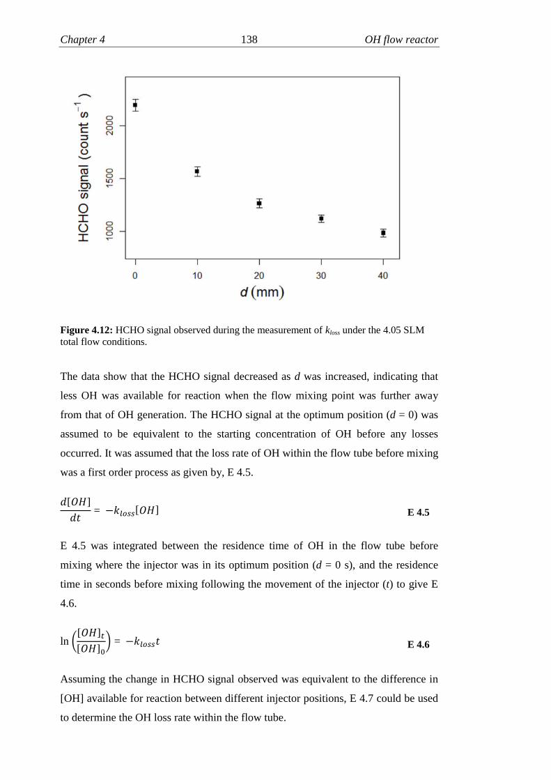
Chapter 4 138 OH flow reactor
Figure 4.12: HCHO signal observed during the measurement of kloss under the 4.05 SLMtotal flow conditions.
The data show that the HCHO signal decreased as d was increased, indicating that
less OH was available for reaction when the flow mixing point was further away
from that of OH generation. The HCHO signal at the optimum position (d = 0) was
assumed to be equivalent to the starting concentration of OH before any losses
occurred. It was assumed that the loss rate of OH within the flow tube before mixing
was a first order process as given by, E 4.5.
[ܪ]
ݐ= − ௦௦[ܪ] E 4.5
E 4.5 was integrated between the residence time of OH in the flow tube before
mixing where the injector was in its optimum position (d = 0 s), and the residence
time in seconds before mixing following the movement of the injector (t) to give E
4.6.
ln൬௧[ܪ][ܪ]
൰= − ௦௦ݐ E 4.6
Assuming the change in HCHO signal observed was equivalent to the difference in
[OH] available for reaction between different injector positions, E 4.7 could be used
to determine the OH loss rate within the flow tube.

Chapter 4 139 OH flow reactor
ln൬௧[ܪܥܪ][ܪܥܪ]
൰= − ௦௦ݐ E 4.7
The only term including HCHO concentrations in E 4.7 is the ratio of [HCHO]t to
[HCHO]0. Therefore it was not necessary to calculate the concentrations of HCHO
detected at each injector position; the (background subtracted) signals alone were
sufficient to calculate the ratio of [HCHO]t to [HCHO]0.
A plot of ln([HCHO]t/[HCHO]0) vs t was constructed to determine the loss rate of
OH to the walls of the flow tube, and to other impurities present in the humidified
nitrogen flow for OH generation, this is shown in Figure 4.13.
Figure 4.13: Plot of ln([HCHO]t/[HCHO]0) vs t. The gradient of the line of best fit (linearleast squares) is equal to -kloss and the plot was constructed using data whilst the OH reactorwas operated under the 4.05 SLM total flow conditions. Gradient: -6.57 ± 0.88 s-1, intercept:0.085 ± 0.06, R2: 0.97.
The plot shows that the relationship between ln([HCHO]t/[HCHO]0) and t is not
perfectly linear; some level of curvature is observed. The precise reason for this is
uncertain, however is likely to be due to combination of two factors. The first of
these is the self reaction of OH acting as another loss process. This is possible
because the levels of OH generated in the OH reactor a relatively high (in the order

Chapter 4 140 OH flow reactor
of 1010 molecule cm-3). The second influencing factor is likely to be that the type of
analysis used to determine the loss rate here, assumes that gas within the OH reactor
is entrained within a ‘plug’ type flow. The flow within the OH reactor is almost
certainly laminar, to improve the accuracy of this analysis, corrections for diffusion
could be applied. However, due to time constraints such a correction was not
investigated and a linear fit to the data was assumed to have a gradient
approximately equal to –kloss for the purpose of assessing the potential performance
of the OH reactor.
As described above, the gradient of the line of best fit shown in Figure 4.13 is
assumed to be equal to –kloss. The value for kloss determined under the 4.05 SLM
total flow conditions was 6.57 ± 0.88 s-1, it was not possible to measure kloss under
the 3.05 SLM total flow conditions due to problems encountered with the fibre laser
used in the HCHO detector. However, as the loss rate measured appears to be first
order, it can be assumed that it would be the same under all flow conditions. During
operation of the OH flow reactor where ambient air is flowed through the moveable
injector, kloss is competitive with kAi and kXi. Therefore it needs to be considered
when determining the predicted effect on a real VOC mix. The value of kloss
determined here can be used in modelling studies to assess the potential performance
of the redesigned OH flow reactor.
3.4 Simulated removal of VOCs
A zero dimensional chemical box model was constructed using Kintecus (Ianni,
2003) to crudely assess the potential performance of the redesigned OH reactor. The
model was constructed such that it simulated the effect that the OH reactor could
have on a standard mixture of 30 VOCs if flowed in through the sliding injector
(where ambient air would be introduced in the field) under both the 4.05 and 3.05
SLM total flow conditions described in Section 4.3.1. A list of the compounds that
were included in the model along with their respective bimolecular rate coefficients
for reaction with OH used in the model are presented in Table 4.1.

Chapter 4 141 OH flow reactor
OH Sink ksink + OH (cm3 molecule-1 s-1) at 298 K Reference
Ethylene 8.8 × 10⁻¹² Sander et al. (2006)Acetylene 8.3 × 10⁻¹³ Sander et al. (2006)Ethane 2.4 × 10⁻¹³ Sander et al. (2006)Propylene 3.0 × 10⁻¹¹ Atkinson et al. (2006)Propane 1.1 × 10⁻¹² Sander et al. (2006)iso-Butane 2.2 × 10⁻¹² Atkinson (1997)1-Butene 3.1 × 10⁻¹¹ Atkinson (1997)n-Butane 2.3 × 10⁻¹² Atkinson et al. (2006)trans-2-butene 6.4 × 10⁻¹¹ Atkinson (1997)cis-2-butene 5.6 × 10⁻¹¹ Atkinson (1997)3-Methyl-1-butene 3.2 × 10⁻¹¹ Atkinson (1997)iso-Pentane 3.7 × 10⁻¹² Atkinson (1997)1-Pentene 3.1 × 10⁻¹¹ Atkinson (1997)n-Pentane 4.0 × 10⁻¹² Atkinson (1997)Isoprene 1.0 × 10⁻¹⁰ Atkinson et al. (2006)trans-2-Pentene 6.7 × 10⁻¹¹ Atkinson (1997)cis-2-Pentene 6.5 × 10⁻¹¹ Atkinson (1997)2-Methyl-2-butene 8.7 × 10⁻¹¹ Atkinson (1997)2,2-Dimethylbutane 2.3 × 10⁻¹² Atkinson (1997)Cyclopentene 6.7 × 10⁻¹¹ Atkinson (1997)4-Methyl-1-pentene 3.8 × 10⁻¹¹ Grosjean and Williams (1992)Cyclopentane 5.0 × 10⁻¹² Atkinson (1997)2,3-Dimethylbutane 5.8 × 10⁻¹² Atkinson (1997)2-Methylpentane 5.3 × 10⁻¹² Atkinson (1997)3-Methylpentane 5.4 × 10⁻¹² Atkinson (1997)2-Methyl-1-pentene 6.3 × 10⁻¹¹ Atkinson (1997)n-Hexane 5.5 × 10⁻¹² Atkinson (1997)trans-2-Hexane 4.8 × 10⁻¹¹ Atkinson (1994)cis-2-Hexane 4.8 × 10⁻¹¹ Atkinson (1994)Methylcyclopentane 8.8 × 10⁻¹² Atkinson (1994)
Table 4.1: List of 30 VOCs included in a Kintecus zero-dimensional chemical box modelwhich was used to assess the potential performance of the redesigned OH flow reactor.
In all simulations the initial concentration of each species in the flow from the
moveable injector was 1 ppb; this corresponded to the mix having an OH reactivity
of 21.9 s-1 if sampled at 760 Torr and 298 K. Simulations lasted 2 seconds as this
was found to be long enough for the concentration of each species to reach a
constant level in all cases due to complete consumption of OH.
Two runs were executed using a starting value for [OH] that was determined to be
available for reaction at the flow mixing point under the 4.05 SLM total flow
conditions (7.6 x 10¹⁰ molecule cm-3, Section 4.3). In the first run the measured
value for kloss (6.6 s-1, Section 4.4) was not included in the model. However, it was
included in the second run in order to assess the extent to which OH loss other than
by reaction with sinks within the flow tube could affect the ability of the reactor to
remove species present in ambient air through reaction with OH. The data outputted
from the two simulations were used to calculate values for ln([Ai]0/[Ai]∞) which
were plotted against kAi, Figure 4.14.

Chapter 4 142 OH flow reactor
Figure 4.14: Plots of ln([Ai]0/[Ai]∞) vs kAi produced using data outputted from a Kintecusmodel constructed to simulate the loss of 30 VOCs within the OH reactor. Data are shownfor simulations where kloss (loss to walls and reactions with impurities) was (plotted in red)and was not (plotted in black) included. The starting concentration of OH was 7.6 x 10¹⁰
molecule cm-3.
By inspection of Figure 4.14 it can be seen that the gradient of the plot produced
using data from the simulation, where wall loss was included, is lower than that
where the wall loss was not included. This was expected as when OH is lost to
processes other than reaction with species in the VOC mix, less would be available
for reaction, therefore causing a reduction in [OH] integrated over reaction time
which is equal to the gradient.
A further two model runs were executed using the value determined for [OH]
available for reaction at the flow mixing point under the 3.05 SLM total flow
conditions (2.6 x 10¹⁰ molecule cm-3, Section 4.4). These were identical to the
previous two runs except that the starting [OH] value was different. The data
outputted were treated in the same way to produce two plots for for ln([Ai]0/[Ai]∞)
vs kAi, these are shown in Figure 4.15.
0.00E+000 5.00E-011 1.00E-010
0
1
2
Gradient: 6.7 x 10⁹ molecule cm-3 s
ln([
Ai] 0
/[A
i])
kAi
(cm3 molecule-1 s-1)
4.05 SLM total flow conditions
Gradient: 2.3 x 10¹⁰ molecule cm-3 s

Chapter 4 143 OH flow reactor
Figure 4.15: Plots of ln([Ai]0/[Ai]∞) vs kAi produced using data outputted from a Kintecusmodel constructed to simulate the loss of 30 VOCs within the OH reactor. Data are shownfor simulations where kloss (loss to walls and reactions with impurities) was (plotted in red)and was not (plotted in black) included. The starting concentration of OH was 2.6 x 10¹⁰
molecule cm-3.
Again it can be seen that the gradient of the plot produced using data where the 6.6
s-1 OH loss rate was included in the model is lower, however this was by a lesser
amount than in the previous simulations (50 % lower as opposed to 71 % lower).
This indicates that OH loss to the walls of the flow tube and impurities will impact
the ability of the reactor to remove species present in ambient air most significantly
when the initial [OH] available for reaction is higher. However, the gradient of the
plot in Figure 4.14 where kloss was included in the simulation is still greater than the
gradient of both plots in Figure 4.15 where kloss was included. Thus it can be
concluded that operating the OH flow reactor under the 4.05 SLM total flow
conditions will most likely result in the largest decreases in species present in
ambient air due to reaction with OH.
In order to conduct a study similar to that reported by Kato et al. (2011), it is
essential that decreases in concentrations of OH reactive species are observable for
species where kAi is greater than ~10-12 cm3 molecule-1 s-1. Candidate species for
missing OH reactivity are thought to typically have kAi values above this threshold.
0.00E+000 5.00E-011 1.00E-010
0.0
0.5
1.0
1.5
2.0
2.5
Gradient: 1.9 x 10⁹ molecule cm-3 s
Gradient: 3.8 x 10⁹ molecule cm-3 s
ln([
Ai] 0
/[A
i])
kAi
(cm3 molecule-1 s-1)
3.05 SLM total flow conditions

Chapter 4 144 OH flow reactor
In the hypothetical example of measurements in an urban atmosphere showing
evidence for 20 % average ‘missing’ OH reactivity with 15 s-1 average measured
OH reactivity, it would be concluded that unmeasured sinks contributed 3 s-1
towards the measurements. In this case, if the average kAi value for the unmeasured
sinks was significantly lower than 10-12 cm3 molecule-1 s-1 (e.g. 10-13 cm3 molecule-1
s-1), their collective concentration would be 3 ×10¹³ molecule cm-3 (~1 ppm).
Relative to the majority of other trace species that exist in the atmosphere, this level
is very high. It would be unlikely that such levels would go undetected, especially
when the diversity of instrumentation that are often deployed in OH reactivity
studies is considered. If the average kAi value for the unmeasured sinks in this
scenario was 10-12 cm3 molecule-1 s-1 their collective concentration would be 3 ×
1012 molecule cm-3 (~100 ppb). ktoluene + OH is ~5 × 10-12 cm3 molecule-1 s-1 so toluene
is towards the lesser reactive end of the scale of species which would need to be
removed by OH in the flow reactor by an observable quantity. Therefore it was an
ideal candidate for study when assessing the suitability of the redesigned OH flow
reactor for use in a study similar to Kato et al. (2011). The results from the model
simulations described above (in the cases where kloss was included) were used to
predict changes that would be expected for the concentration of toluene under the
same conditions. The predictions are summarised for the 4.05 and 3.05 SLM total
flow conditions in Table 4.2, in addition to predictions for isoprene (which reacts
much faster) for the purpose of comparison.
Totalflowconditions / SLM
Starting [OH] /molecule cm-3
Predicted ʃ[OH]dt / molecule cm-3 s
Predicted decreasein [isoprene] (%)
Predicted decreasein [toluene] (%)
4.05 7.6 × 10¹⁰ 6.7 × 10⁹ 49 43.05 2.6 × 10¹⁰ 1.9 × 10⁹ 17 1
Table 4.2: Summary of the predicted decreases that could be expected for isoprene andtoluene if the total OH reactivity of ambient air sampled by the OH flow reactor had a totalOH reactivity of 21.9 s-1. Predicted values are shown for the operation of the OH flowreactor under both the 4.05 and 3.05 SLM total flow conditions.
The data presented in Table 4.2 show that operating the OH flow reactor under the
4.05 SLM total flow conditions should result in the largest decreases in
concentration for toluene and isoprene. The predicted changes for both toluene and
isoprene under the 4.05 SLM total flow conditions would be observable by the GC-
TOF-MS (Agilent 7890 coupled with Markes BenchTOF) instrument at the
University of York. However, the small decrease (1 %) in concentration predicted

Chapter 4 145 OH flow reactor
for toluene under the 3.05 SLM total flow conditions would likely not be observable
(Lidster, 2013).
It was decided that the OH flow reactor would be operated using the 4.05 SLM total
flow conditions upon interfacing with a GC-TOF-MS instrument at the University of
York to form a new instrument for identification of ‘missing’ OH reactivity. Section
4.5 provides details of the configuration and operation of the new instrument. The
new instrument was successfully deployed during the York 2014 ‘missing’ OH
reactivity field campaign (Chapter 5) and some preliminary observations in ambient
air from this campaign are presented in Section 4.6.
4.5 Coupling with GC-TOF-MS
The redesigned OH flow reactor described in Section 4.2 was successfully interfaced
to a GC-TOF-MS instrument at the University of York to form a new instrument for
the identification of ‘missing’ OH reactivity. The schematic in Figure 4.16
summarises the key features of the new system that incorporated the redesigned OH
flow reactor described in Section 4.2.
Figure 4.16: Schematic diagram to summarise the experimental set-up of the newinstrument for the identification of ‘missing’ OH reactivity that was used for fieldmeasurements during the York 2014 ‘missing’ OH reactivity campaign. Diagram providedby Dr. Richard Lidster, University of York.
The set-up consisted of two parallel sampling systems; one contained the OH flow
reactor and the other contained a flow tube of the same dimensions where no OH
was generated (no lamp, termed the non-reactor). The use of the parallel sampling
system made it possible to conduct analyses of ambient air that had been sampled
simultaneously. If analyses of sequentially sampled ambient air were conducted, as

Chapter 4 146 OH flow reactor
by (Kato et al., 2011), it would be unknown whether or not a decrease in the
concentration of a species detected was exclusively due to its removal by OH, (the
decrease could be partly due to natural variation in the composition of the air mass
sampled). The parallel sampling system used in the new instrument for the
identification of ‘missing’ OH reactivity is thought to be the first of its kind as to the
best knowledge of the author; no description of a similar system is available in the
literature.
Ambient air was supplied to the set-up from a sampling manifold positioned on the
roof of the Wolfson Atmospheric Chemistry Laboratories (WACL) building. A
clean dry bellows pump was used to draw ambient air into the set-up and provide
sufficient backing pressure to two MFCs (MKS, 0-1 SLM). The first of these was
used to supply 1.00 SLM of ambient air to the OH flow reactor via the moveable
injector and the second was used to supply 1.00 SLM of ambient air to the non-
reactor. An additional two MFCs were used to supply nitrogen to the OH reactor and
to the non-reactor at 3.00 SLM. The nitrogen flow to the reactor was humidified
using a water bubbler to enable OH production, in the non-reactor case it was not
humidified and served only to dilute the ambient sample by the same amount. Two
sucking pumps were used to transfer gas from the reactor and non-reactor to their
respective sampling units at ~2 SLM; the remaining flow in each case was vented to
prevent over pressuring of the system.
Solenoid valves within the sampling units were used to control the timing for the
trapping of samples from both the reactor and the non-reactor. Upon opening the
valves, samples were simultaneously transferred to glass cold fingers submersed in
an ethylene glycol cooling bath at -30 °C to ‘freeze out’ any water vapour present
and prevent damage to the TOF-MS detector. Following the removal of water
vapour, the samples from the reactor and the non-reactor were transferred to
separate thermal desorption (TD) units for trapping. The sample lines from each TD
unit were connected to the GC via a switching valve; this made it possible to
sequentially desorb and analyse the two samples from the parallel system. Figure
4.17 shows the new instrument for the identification of ‘missing’ OH reactivity
whilst in operation during the York 2014 ‘missing’ OH reactivity field campaign,
the key features are labelled.

Chapter 4 147 OH flow reactor
Figure 4.17: Photograph of the new instrument for the identification of ‘missing’ OHreactivity during the York 2014 ‘missing’ OH reactivity field campaign. Key features arelabelled.
Early testing of the two thermal desorption units with a neat flow from a VOC
standard cylinder showed there to be a systematic offset in the level of each
compound detected by GC-TOF-MS, i.e. the two systems were not equally efficient
at trapping and desorbing species present in ambient air. It was necessary to quantify
the difference in the concentration of all species detected due to this systematic
offset in order identify compounds that were contributing to ‘missing’ OH reactivity.
To achieve this, four GC-TOF-MS analyses were performed in every measurement
cycle (two pairs of simultaneous samples from the parallel system).
The OH reactor was operated with the pen ray lamp switched off whilst the first two
samples were trapped and desorbed sequentially onto the GC column. The
differences in the peak areas between the two resulting chromatograms were
representative of the difference in concentration due to the species specific
systematic offset between the two TD units. Whilst the first two analyses were in
progress, the pen ray lamp inside the OH reactor was switched on using an
electromechanical relay which was triggered using a ‘contact closure’ from the
sampling unit. Two more samples were then trapped and sequentially desorbed onto

Chapter 4 148 OH flow reactor
the GC column upon completion of the first two analyses. In this case the
differences in the peak areas observed between the two chromatograms were
representative of the systematic offset between the two TD units, and any change
due to removal via OH chemistry.
Data from multiple analyses where the lamp was switched off were used to construct
a calibration plot for each identified species detected. These were used to estimate
the contribution from the TD unit offset to the difference observed in the peak areas
for identified species during analyses where the lamp was switched on. Therefore
making it possible to quantify any change due to OH chemistry.
In order to use observations from the new instrument described here to determine
rate coefficients for the reaction between unidentified species that contribute to
‘missing’ OH reactivity, it would first be necessary to examine the relationship
between changes observed in peak areas for identifiable species and their
bimolecular rate coefficients for reaction with OH. In the study reported by Kato et
al. (2011) it was necessary to examine such a relationship for each sample of
ambient air that was analysed. This was due to it not being possible to
simultaneously trap samples of ambient air in their system. The capability of the
instrumentation described in this chapter to simultaneously trap samples made it
possible to use just one such relationship to calculate bimolecular rate coefficients
for unidentified species.
3.6 Observations in ambient air
The new instrumentation was deployed for the first time during the York 2014
’missing’ OH reactivity campaign in May / June 2014. Measurements of OH
reactivity during this campaign are presented in Chapter 5 in addition to a detailed
comparison with the levels calculated using the concentrations of co-measured
identifiable sinks. It was determined that when OH reactivity was calculated using
only data for identifiable sinks, the ‘missing’ OH reactivity on average for the
campaign was 27 %. It is concluded in Chapter 5 that the majority of the ‘missing’
OH reactivity in York could be attributed to unidentified species that were measured
with a GCxGC-FID instrument and also unmeasured products of photo-oxidation.
Therefore, it was expected that the observations made using the instrumentation
described in this chapter would only lead to the identification of a few species which

Chapter 4 149 OH flow reactor
made minor contributions to the ‘missing’ OH reactivity. Figure 4.18 shows some
data that were collected during the campaign in York for some identified species.
Figure 4.18: Relationships between GC-TOF-MS response for the Reactor and non-Reactorsampling systems, for four VOCs (1,2,3-trimethylbenzene, isoprene, decane and styrene),from analyses where the UV lamp in the OH flow reactor was switched off (no OHgenerated) and switched on (OH generated). Data shown are from the analysis of ambientair during the York 2014 ‘missing’ OH reactivity campaign. Provided by Dr. RichardLidster, University of York.
Each plot shows two sets of data for the linear relationship between responses for
the two sampling systems (reactor and non-reactor), one where the lamp in the OH
reactor switched off (red), and one with the lamp switched on (blue). The plots show
that the relative responses for the two sampling systems vary considerably (shown
through differences in the gradient of the red lines). The precise reason for there
being such significant variation is unknown but is likely due to differences between
the performance of thermal desorption unit in the two sampling systems. However,
the data show that this species specific offset is systematic (because the red points
exhibit linear behaviour) and so should not influence the measurements made,
provided that the offset is accounted for through consideration of the ratio of the
gradients as described in Section 4.5.

Chapter 4 150 OH flow reactor
As described in Section 4.5 it is the relationship between the natural logarithms of
the ratio of the gradients of line of best fits to these data sets and kAi values that can
be used to determine ∫[OH]dt. Figure 4.19 shows this relationship that was
determined through the analysis of ambient air during the campaign in York,
∫[OH]dt is 1.5 × 10¹⁰ molecule cm-3 s.
Figure 4.19: ln(mlamp off / mlamp on) vs literature rate coefficients for a selection of 15 VOCsmeasured in ambient air during the York 2014 ‘missing’ OH reactivity campaign. Solid linerepresents the linear least squares fit to the data, gradient: 1.5 × 10¹⁰ molecule cm-3 s-1 (equalto ∫[OH]dt). Dashed lines represent 95 % confidence intervals. 1. benzene 2. toluene 3. propylbenzene 4.isopropylbenzene 5. ethylbenzene 6. n-heptane 7. decane 8. 2-ethyltoluene9.o-xylene 10. 3-ethyltoluene 11. m/p-xylene 12. 1,2,4-trimethylbenzene 13. 1,2,3-trimethylbenzene 14. Styrene 15. Isoprene. Provided by Dr. Richard Lidster, University ofYork.
The data plotted show a linear trend, as is required to extract a ∫[OH]dt value. At
present only limited ambient data (a few days) have been analysed from the new
instrument described here. Full analysis of the ambient data for identifiable
compounds will form the basis of future work in order to further populate Figure
4.19 and maximise the accuracy of ∫[OH]dt that is determined. A small number of
peaks were also observed in the chromatograms that were not immediately
identifiable, however, should be upon further analysis of the large amount of mass-

Chapter 4 151 OH flow reactor
spectral data that were acquired (Lidster, 2013). Further work shall also include the
determination of bimolecular rate coefficients for the reaction between these
unidentified species and OH and also investigation of their chemical identity. Their
contribution to ‘missing’ OH reactivity will be quantified.
4.7 Summary and conclusions
A new OH reactor has been designed and successfully characterised using a fast
response LIF HCHO detector when operated using two sets of flow conditions (4.05
and 3.05 SLM total flow). Ambient air was introduced to the reactor via a moveable
injector so that the distance between the point of flow mixing and irradiation of
humidified nitrogen for OH generation could be adjusted. The position of the
injector was optimised for each set of flow conditions to prevent direct photolysis of
VOCs and to maximise their exposure to OH. The [OH] present at the point of
mixing was also quantified for each flow condition and was found to be 7.6 x 10¹⁰
and 2.6 x 10¹⁰ molecule cm-3 for the 4.05 and 3.05 SLM conditions, respectively.
The loss rate of OH within the reactor to the walls of the flow tube and impurities
present in the gasses used was also measured to be 6.6 s-1. A zero-dimensional
chemical box model has been constructed to assess the effect that the OH reactor
could have on the concentrations of VOCs in ambient air. It was concluded that it
was necessary to operate the reactor using the 4.05 SLM total flow conditions in
order for quantifiable decreases to be observed by GC-TOF-MS.
Following characterisation, the OH flow reactor was successfully interfaced with a
GC-TOF-MS instrument at the University of York. The resulting set-up was a new
instrument for the identification of ‘missing’ OH reactivity in the troposphere and
has been deployed for field measurements during the York 2014 ‘missing’ OH
reactivity field campaign (19/05/2014 – 16/06/2014). Both identified and
unidentified species were observed to decrease in concentration when ambient air
was exposed to OH within the reactor, thus indicating a contribution from
unidentified (‘missing’) sinks to total OH reactivity at the site. A large data set was
generated, thorough analysis of which is required to fully understand the origin of
any ‘missing’ OH reactivity. The new instrument described in this chapter shows
potential as a valuable tool for investigating the source of ‘missing’ OH reactivity.
It’s deployment to environments with atmospheres know to have significant
‘missing’ OH reactivity, such as forests, should be considered in future.

Chapter 4 152 OH flow reactor
4.8 References
ATKINSON, R. 1994. Gas phase tropospheric chemistry of organic compounds,Monograph 2. Journal of Physical and Chemical Reference Data, 1-216.
ATKINSON, R. 1997. Gas-Phase Tropospheric Chemistry of Volatile OrganicCompounds: 1. Alkanes and Alkenes. Journal of Physical and ChemicalReference Data, 26, 215-290.
ATKINSON, R., BAULCH, D. L., COX, R. A., CROWLEY, J. N., HAMPSON, R.F., HYNES, R. G., JENKIN, M. E., ROSSI, M. J., TROE, J. &SUBCOMMITTEE, I. 2006. Evaluated kinetic and photochemical data foratmospheric chemistry: Volume II – gas phase reactions of organicspecies. Atmos. Chem. Phys., 6, 3625-4055.
DILLON, T. J., HOLSCHER, D., SIVAKUMARAN, V., HOROWITZ, A. &CROWLEY, J. N. 2005. Kinetics of the reactions of HO with methanol (210-351 K) and with ethanol (216-368 K). Physical Chemistry Chemical Physics,7, 349-355.
GROSJEAN, D. & WILLIAMS, E. L. 1992. Environmental persistence of organiccompounds estimated from structure-reactivity and linear free-energyrelationships. Unsaturated aliphatics. Atmospheric Environment. Part A.General Topics, 26, 1395-1405.
IANNI, J. C. 2003. A Comparison of the Bader-Deuflhard and the Cash-KarpRunge-Kutta Integrators for the GRI-MECH 3.0 Model Based on theChemical Kinetics Code Kintecus. In: BATHE, K. J. (ed.) ComputationalFluid and Solid Mechanics 2003. Oxford: Elsevier Science Ltd.
KATO, S., SATO, T. & KAJII, Y. 2011. A method to estimate the contribution ofunidentified VOCs to OH reactivity. Atmospheric Environment, 45, 5531-5539.
LIDSTER, R. 2013. RE: Personal communication.
MARTINS, G., FERREIRA-RODRIGUES, A. M., RODRIGUES, F. N., DESOUZA, G. G. B., MASON, N. J., EDEN, S., DUFLOT, D., FLAMENT, J.P., HOFFMANN, S. V., DELWICHE, J., HUBIN-FRANSKIN, M. J. &LIMAO-VIEIRA, P. 2009. Valence shell electronic spectroscopy of isoprenestudied by theoretical calculations and by electron scattering, photoelectron,and absolute photoabsorption measurements. Physical Chemistry ChemicalPhysics, 11, 11219-11231.
PICQUET, B., HEROUX, S., CHEBBI, A., DOUSSIN, J.-F., DURAND-JOLIBOIS, R., MONOD, A., LOIRAT, H. & CARLIER, P. 1998. Kineticsof the reactions of OH radicals with some oxygenated volatile organiccompounds under simulated atmospheric conditions. International Journal ofChemical Kinetics, 30, 839-847.
SANDER, S. P., FRIEDL, R. R., GOLDEN, D. M., KURYLO, M. J.,MOORTGAT, G. K., WINE, P. H., RAVISHANKARA, A. R., KOLB, C.E., MOLINA, L. T., FINLAYSON-PITTS, B. J., HUIE, R. E. & ORKIN, V.L. 2006. Chemical Kinetics and Photochemical Data for Use in AtmosphericStudies Evaluation Number 15. JPL Publication, 06-2.

153
Chapter 5 - York 2014 ‘missing’ OH
reactivity campaign
5.1 Background to the York 2014 project
A substantial body of literature reports measurements of OH reactivity where
comparisons have been drawn with those predicted either by calculations which use
only the measured concentrations of OH sinks or by models where concentrations of
VOC photo-oxidation products are predicted, and used to account for a portion of
OH reactivity. A recurring theme is that measured OH reactivity almost always
exceeds that predicted by a quantity known as the ‘missing’ OH reactivity.
‘Missing’ OH reactivity has been reported for environments ranging from the
Borneo rainforest (~53 % missing, when comparing with a model prediction)
(Edwards et al., 2013) to Urban Tokyo (~25 – 35 % missing, when comparing with a
calculation) (Yoshino et al., 2012). A comprehensive summary of ‘missing’ OH
reactivity reported in the literature is provided in Section 1.4. Kato et al. (2011)
outlined a method for a relative rate study of GC-FID peaks representing OH
reactive species in ambient air that either had, or had not, been exposed to OH, the
aim of which was to determine the portion of ‘missing’ OH reactivity that could be
accounted for by species that could be detected but not identified. The methodology
is described in detail in Section 1.4.4 and detected approximately 4 % more of the
measured OH reactivity during a campaign at an urban background site in Tokyo.
5.2 Aims
Presently, there is no method reported in the literature for the identification of the
unidentified species that contribute to ‘missing’ OH reactivity, as reported by Kato
et al. (2011). A key objective of the York 2014 ‘missing’ OH reactivity campaign
was to address this. A new instrument was deployed alongside the Leeds laser flash

Chapter 5 154 York 2014 measurements
photolysis instrument for the measurement of OH reactivity, in addition to a very
detailed suite of OH sink measurements to fully assess the nature of the OH sink at
an urban background site. The new instrument was formed through the coupling of
an OH flow reactor to a GC-TOF-MS system, details of the development are
presented in Chapter 4 in addition to some preliminary observations.
In addition to OH reactivity, a measurement of formaldehyde (HCHO) can help
when assessing the completeness of our knowledge of the OH sink in a given
environment. HCHO is a final product from the photo-oxidation of almost all VOCs
(Whalley et al., 2016). Comparison of measured and predicted values can reveal
missing oxidation steps from a model or may point to a primary emission of HCHO
(Kaiser et al., 2015). The LIF instrument for the measurement of HCHO, described
in Chapter 2, was deployed for its first ambient measurements during the York 2014
‘missing’ OH reactivity campaign.
This chapter focusses on observations of OH reactivity and HCHO from the York
2014 ‘missing’ OH reactivity campaign. An in depth analysis of the relationship
between measured and predicted (calculated and modelled) OH reactivity is
presented in addition to HCHO observations. The campaign took place in May /
June 2014 on the campus of the University of York; the site, measurement suite and
weather conditions are described in Section 5.3.
5.3 Site description, measurement suite and conditions
OH reactivity, radical and photolysis rate measurements were made from the roof of
the FAGE container in a small car park next to the Wolfson Atmospheric Chemistry
Laboratories (WACL), situated on the University of York campus in Heslington,
York, UK (53° 56' N, 1° 02' W). The site was ~3 km south-east of the centre of
York and ~2 km west of a major road (A64), there was also a small wooded area
immediately to the east. This site was chosen as the air mass would likely be
influenced by anthropogenic emissions from the centre of York and nearby roads, in
addition to local biogenic emissions, all of which would likely include candidates
for contributors to ‘missing’ OH reactivity. It was also directly adjacent to the
WACL building from which a number of instruments to measure VOCs were
operated. Figure 5.1 displays the location of the site at the WACL in relation to the
centre of York and the A64.
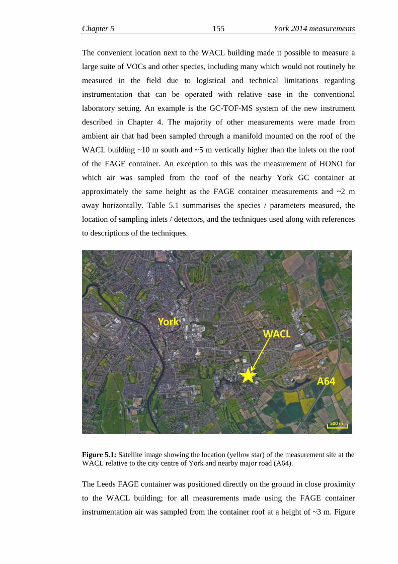
Chapter 5 155 York 2014 measurements
The convenient location next to the WACL building made it possible to measure a
large suite of VOCs and other species, including many which would not routinely be
measured in the field due to logistical and technical limitations regarding
instrumentation that can be operated with relative ease in the conventional
laboratory setting. An example is the GC-TOF-MS system of the new instrument
described in Chapter 4. The majority of other measurements were made from
ambient air that had been sampled through a manifold mounted on the roof of the
WACL building ~10 m south and ~5 m vertically higher than the inlets on the roof
of the FAGE container. An exception to this was the measurement of HONO for
which air was sampled from the roof of the nearby York GC container at
approximately the same height as the FAGE container measurements and ~2 m
away horizontally. Table 5.1 summarises the species / parameters measured, the
location of sampling inlets / detectors, and the techniques used along with references
to descriptions of the techniques.
Figure 5.1: Satellite image showing the location (yellow star) of the measurement site at theWACL relative to the city centre of York and nearby major road (A64).
The Leeds FAGE container was positioned directly on the ground in close proximity
to the WACL building; for all measurements made using the FAGE container
instrumentation air was sampled from the container roof at a height of ~3 m. Figure

Chapter 5 156 York 2014 measurements
5.2 shows a photograph of the FAGE container at the measurement site during the
campaign with the approximate locations of inlets / measurement points labelled.
Figure 5.2: Photograph of the Leeds FAGE container during the York 2014 ‘missing’ OHreactivity campaign. Labels show the approximate locations of sampling inlets and points ofmeasurement.
The weather conditions were dry for the majority of the campaign with periods of
rainfall typically lasting no longer than a few hours. The average temperature was
14.9 ˚C and ranged from 6.7 to 24.9 ˚C with an average relative humidity of 43 %
which ranged from 14 to 79 %. The wind speed did not exceed 2.2 m s-1 during the
measurement period and the modal value recorded by the meteorological station was
0 m s-1, indicating that air sampled at the various sampling locations could have
been poorly mixed.
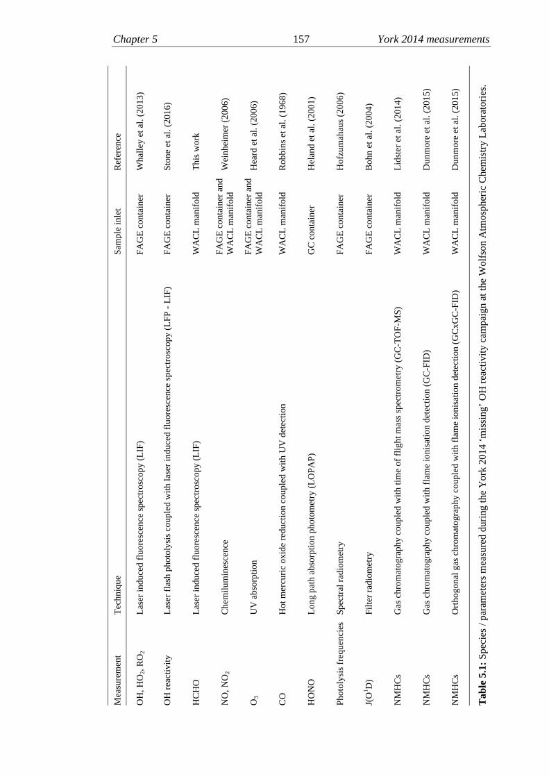
Chapter 5 157 York 2014 measurements
Ref
eren
ce
Wh
alle
yet
al.
(20
13)
Sto
ne
etal
.(2
016
)
Th
isw
ork
Wei
nh
eim
er(2
006
)
Hea
rdet
al.
(20
06)
Ro
bb
ins
etal
.(1
968
)
Hel
and
etal
.(2
00
1)
Ho
fzu
mah
aus
(200
6)
Bo
hn
etal
.(2
00
4)
Lid
ster
etal
.(2
014
)
Du
nm
ore
etal
.(20
15
)
Du
nm
ore
etal
.(20
15
)
Ta
ble
5.1
:S
pec
ies
/p
aram
eter
sm
easu
red
dur
ing
the
Yo
rk2
01
4‘m
issi
ng’
OH
reac
tiv
ity
cam
pai
gn
atth
eW
olf
son
Atm
osp
her
icC
hem
istr
yL
abor
ato
ries
.
Sam
ple
inle
t
FA
GE
con
tain
er
FA
GE
con
tain
er
WA
CL
man
ifo
ld
FA
GE
con
tain
eran
dW
AC
Lm
anif
old
FA
GE
con
tain
eran
dW
AC
Lm
anif
old
WA
CL
man
ifo
ld
GC
con
tain
er
FA
GE
con
tain
er
FA
GE
con
tain
er
WA
CL
man
ifo
ld
WA
CL
man
ifo
ld
WA
CL
man
ifo
ld
Tec
hn
iqu
e
Las
erin
du
ced
flu
ore
scen
cesp
ectr
osc
op
y(L
IF)
Las
erfl
ash
ph
oto
lysi
sco
up
led
wit
hla
ser
ind
uce
dfl
uo
resc
ence
spec
tro
sco
py
(LF
P-
LIF
)
Las
erin
du
ced
flu
ore
scen
cesp
ectr
osc
op
y(L
IF)
Ch
emil
um
ines
cen
ce
UV
abso
rpti
on
Ho
tm
ercu
ric
ox
ide
red
uct
ion
cou
ple
dw
ith
UV
det
ecti
on
Lo
ng
pat
hab
sorp
tio
np
ho
tom
etry
(LO
PA
P)
Sp
ectr
alra
dio
met
ry
Fil
ter
rad
iom
etry
Gas
chro
mat
og
rap
hy
coup
led
wit
hti
me
of
flig
ht
mas
ssp
ectr
om
etry
(GC
-TO
F-M
S)
Gas
chro
mat
og
rap
hy
coup
led
wit
hfl
ame
ion
isat
ion
det
ecti
on(G
C-F
ID)
Ort
ho
gon
alg
asch
rom
ato
grap
hy
coup
led
wit
hfl
ame
ion
isat
ion
det
ecti
on
(GC
xG
C-F
ID)
Mea
sure
men
t
OH
,H
O2,
RO
2
OH
reac
tiv
ity
HC
HO
NO
,N
O2
O3
CO
HO
NO
Ph
oto
lysi
sfr
equ
enci
es
J(O
1 D)
NM
HC
s
NM
HC
s
NM
HC
s

Chapter 5 158 York 2014 measurements
5.4 OH reactivity
5.4.1 OH reactivity observations
The Leeds laser flash photolysis instrument for the measurement of OH reactivity
was situated ~3 m above ground on the roof of the Leeds FAGE container for the
duration of the measurement period. Measurements were made with the instrument
in configuration 1 as described in Section 2.1.6. Figure 5.3 shows a photograph of
the instrument at the measurement site whilst sampling ambient air.
Figure 5.3: Image of the laser flash photolysis OH reactivity instrument whilst makingmeasurements in ambient air during the York 2014 ‘missing’ OH reactivity campaign, keyfeatures are labelled.
The scroll pump, photolysis laser control unit and the majority of the other
electronic components of the instrument were housed inside the FAGE container.
They were connected to the apparatus on the roof via long cables and tubing that
were routed through a waterproof enclosure which housed the ROx detection cells. A

Chapter 5 159 York 2014 measurements
10 m optical fibre was also routed through this enclosure to deliver 308 nm light for
the detection of OH in the FAGE cell of the OH reactivity instrument.
Ambient levels of O3 (15 – 30 ppb during the day) and water vapour (14 – 79 %)
were high enough to form sufficient [OH] via photolysis of O3 for a decay signal to
be observed within ~1 minute. It was not necessary to add either O3 or water vapour
to the instrument for the duration of the campaign.
In order to extract a value for k’OH(raw) from OH decays observed whilst the
instrument was in configuration 1 (as described in Section 2.2.7), a bi-exponential
decay function (E2.2) was fitted to each decay. Following this, k’OH(physical), the loss
rate of OH due to physical processes (diffusion and wall loss) in the flow tube was
subtracted from each k’OH(raw) value. The value of k’OH(physcal) used was 1.25 s-1 and
details of the determination of this value are reported in Section 2.1.8. The pressure
within the flow tube of the OH reactivity instrument was slightly sub-ambient (by ~
30 Torr) for the duration of the campaign, this meant that the concentration of OH
sinks (in molecule cm-3) in the flow tube were slightly lower than in the ambient air
sampled. The result was that the OH loss rates, k’OH(raw) - k’OH(physical), were slightly
lower than the actual loss rate of OH present in the ambient air sampled. To correct
for this each k’OH(raw) - k’OH(physical) was multiplied by the ratio of the pressure of the
ambient air sampled (PAmb) to the pressure within the flow tube (PFT), E5.1.
′ைு = (ᇱைு(௪ ) − ′ைு(௬௦)) ×
ி E5.1
The laser flash photolysis OH reactivity instrument operated as intended for the
majority of the campaign. The majority of gaps in the data recorded were as a result
of intentionally switching off the instrument during planned breaks in the
measurements.
OH reactivity was measured from 19/05/2014 to 16/06/2014 and all observations are
displayed in the plots shown in Figure 5.4. Figure 5.4a shows the time series of OH
reactivity plotted with error bars which represent the 1σ uncertainty (~±0.6 s-1 on
average) determined through combining the uncertainties on the OH decay fits, the
determination of k’(physical) and the correction for pressure described above. The
measurements are re-plotted in Figure 5.4b with the omission of error bars for
clarity. Values ranged from 2.8 to 17.4 s-1 and the mean average k’OH was 6.3 s-1.

Chapter 5 160 York 2014 measurements
Fig
ure
5.4
:T
ime
seri
eso
fm
easu
red
OH
reac
tivi
tyd
uri
ng
the
Yo
rk2
01
4‘m
issi
ng’
OH
reac
tiv
ity
cam
pai
gn
.(a
)D
ata
plo
tted
wit
her
ror
bars
rep
rese
nta
tiv
eof
1σ
det
erm
ined
th
rou
gh
co
mbi
nin
g t
he
un
cert
aint
ies
from
the
dec
ay f
its,
th
e d
eter
min
atio
n o
f k’
OH
(zer
o)an
da
corr
ecti
onfo
rp
ress
ure.
(b)
data
plo
tted
wit
ho
uter
ror
bar
sfo
rcl
arit
y.

Chapter 5 161 York 2014 measurements
5.4.2 Interpretation of OH reactivity observations
5.4.2.1 Diurnal behaviour
Owing to the location of the measurement site used for the York 2014 ‘missing’ OH
reactivity campaign being on a university campus, in close proximity to buildings
and small roads, it is likely that locally emitted OH sinks would have momentarily
affected the measured values of OH reactivity. Such species may not have accounted
for a significant portion of the OH sink for the whole campaign, but may have done
for a short period of time. In order to broadly examine nature of the OH sinks at the
site, a diurnal profile for the ‘average day’ has been generated. All measurements of
OH reactivity were averaged into 96 time bins with a mean value every 15 minutes
using the ‘timeAverage’ function of the openair package in R (Carslaw and Ropkins,
2012, Carslaw, 2015), these data are plotted in Figure 5.5.
Figure 5.5: Diurnal profile of OH reactivity observed during the York 2014 ‘missing’ OHreactivity campaign in 15 minute time bins. Error bars represent ± 1 σ standard deviation from the mean observation.

Chapter 5 162 York 2014 measurements
The profile of Figure 5.5 shows a rise in OH reactivity through the morning hours,
starting at around 06:00 and reaching a maximum of ~8 s-1. This is a typical feature
of OH reactivity observations from environments where the air mass is significantly
influenced by anthropogenic emissions at urban and urban background sites, in
particular vehicular emissions. Diurnal morning rush hour peaks in OH reactivity
were reported for measurements made in Mexico City (~120 s-1), New York (~25 s-
1), Tokyo (~50 s-1), Paris (~30 s-1) and London (~27 s-1) (Shirley et al., 2006, Ren et
al., 2006a, Chatani et al., 2009, Dolgorouky et al., 2012, Whalley et al., 2016). In
addition to diurnal morning rush hour peaks, evening rush hour peaks have also been
reported. Strong diurnal evening rush hour peaks were reported for measurements in
New York (~40 s-1) and Tokyo (~35 s-1) (Ren et al., 2006b, Chatani et al., 2009).
Figure 5.5 shows a slight rise in OH reactivity from the afternoon into the night
however there is no evidence of such a diurnal evening rush hour peak in the diurnal
profile or in the data for individual days.
The maximum OH reactivity in the diurnal morning rush hour peak for the York
measurements shown in Figure 5.5 is significantly lower than what has been
reported at other locations listed above. York is a much smaller city than all of these,
and the measurements were made on a University Campus near small roads which
are less prone to morning congestion, this was most likely the main reason for the
lower values measured. The close proximity of agricultural land also means that the
cleaner less polluted air will have influenced the site more than if measurements
were made closer to the city centre.
Brune et al. (2016) recently reported measurements of OH reactivity from the
CalNex campaign at an urban background site in Bakersfield, CA, US. The site
shared a number of similarities to the site at the WACL; both were car parks situated
in close proximity to major roads (York ~2 km, CalNex ~0.8 km), and both were
situated on the edge of cities in close proximity to agricultural land. The diurnal
profile of the CalNex measurements did not show an evening rush hour peak.
However, the values rose steadily through the night time hours (similar to those
presented here) and stabilised in the early morning before steadily decreasing again
through the daytime hours. This behaviour was attributed to differences in the height
of the boundary layer between day time and night time. It is likely that the evening
rise in diurnal OH reactivity observed in York was influenced by changes in the
boundary layer height.

Chapter 5 163 York 2014 measurements
5.4.2.2 Correlations with other measurements
To further investigate the shape of the diurnal profile presented in Section 5.3.2.1,
and the potential sources of sinks that influenced it, correlations between OH
reactivity and other species measured were investigated. All correlations presented
in this section were produced considering only measurements that were made from
31/05/2014 00:00:00 to 15/06/2014 07:45:00; from here on referred to as the
comparison period. All measurements made during the campaign in York were
merged into a single data set by Dr. Jenny Young so that a common time base was
shared, with a measurement every 15 minutes during the comparison period. For
species that were measured using GC techniques data were reported hourly. It
followed that it was not possible to calculate concentrations for the 15 minute bins
between the times at which data for GC measured species were reported. These data
were estimated through linear interpolation between the 15 minute concentrations
that were able to be determined. All of the correlations presented in this section were
plotted using the merged data for the comparison period.
It was postulated in Section 5.3.2.1 that the diurnal morning peak in OH reactivity
was a result of the morning ‘rush hour’ in traffic, which would indicate that
vehicular emissions such as NOx would have played a major role in influencing OH
reactivity. NOx observations from York are presented in Figure 4.6 and show that
the levels of each species were often highest during the morning hours of each day.
NO is shown to frequently rise to ~5 ppb and NO2 is shown to frequently rise as
high as 10 ppb. The correlation between OH reactivity and NOx was investigated
and the resulting plots are displayed in Figure 5.7.
Figure 5.6: Observations of NO (red line) and NO2 (grey dashed line) for the comparisonperiod of the York 2014 ‘missing’ OH reactivity campaign. Data are plotted at 15 minutetime intervals.

Chapter 5 164 York 2014 measurements
Figure 5.7: Plots of OH reactivity against both [NO] and [NO2]. Data shown are 15 minutebinned mean averages from measurements taken between 31/05/2014 00:00:00 –15/06/2014 07:45:00 of the York 2014 ‘missing’ OH reactivity campaign. The shaded areasrepresent the 95% confidence intervals from the linear fits (least squares).
It is shown that the correlation between OH reactivity and [NO2] is stronger than it
is with [NO] (R2: 0.49 and 0.092, respectively). This difference in correlation
strength is consistent with other observations of OH reactivity in atmospheres that
are influenced by vehicular emissions. On average NO2 often contributes more to
OH reactivity than NO, and also is more dominant at driving change in OH
reactivity. Two examples of this are measurements reported from Tokyo and
London (Yoshino et al., 2006, Whalley et al., 2016). It follows from this that a
stronger correlation between NO2 and OH reactivity would be expected.
In addition to NOx, correlations were examined for all other species that were
measured. Figure 5.8 shows some examples for species where reasonable
correlations were found. Correlations are shown for ethane, propane, propene and
toluene; all of which are known vehicular emissions (Nakashima et al., 2012). The
presence of these correlations further supports the hypothesis that vehicular
emissions accounted for a significant portion of the OH sink in York.

Chapter 5 165 York 2014 measurements
Figure 5.8: Plots of OH reactivity against [ethene], [propane], [propene] and [toluene]. Datashown are 15 minute binned mean averages from measurements taken between 31/05/201400:00:00 – 15/06/2014 07:45:00 of the York 2014 ‘missing’ OH reactivity campaign. Datawhere VOC concentrations were estimated through linear interpolation have been excluded..The shaded areas represent the 95% confidence intervals from the linear fits (least squares).
Chapter 5 166 York 2014 measurements
5.4.2.3 Calculation of OH reactivity
To examine the extent of the completeness of the suite of sinks measured during the
campaign, the OH reactivity was calculated using the measured concentrations of
sinks and corresponding bimolecular rate coefficients as in E1.3 (reproduced below).
Sink concentrations in the merged 15 minute data set for the comparison period
(described in Section 5.3.2.2) were used for this.
′ைு() = ைுା
[ܣ] E1.3
The sinks which were used to calculate OH reactivity for the York 2014 ‘missing’
OH reactivity campaign are summarise in Table 5.2. Each sink was also assigned to
a class according to its functionality so that grouped contributions to calculated OH
reactivity could be determined, these are also listed with their campaign average
contributions. Details of the instrument used to measure each species are provided in
addition to bimolecular rate coefficients. The values shown are those calculated at a
temperature of 298 K and a pressure of 1 atmosphere. For the calculation of OH
reactivity, the values used were determined using the temperature and pressure
dependencies in conjunction with measured temperatures and pressures by the
meteorological station that was positioned on the roof of the FAGE container. All
expressions for rate coefficients were IUPAC recommended values taken from the
Master Chemical Mechanism (MCM) v3.3 (Jenkin et al., 1997, Saunders et al.,
2003) with the exception of 8 species (Cyclopentane, Isopentane, 2,2,4-
Trimethylpentane, 4-Isopropyltoluene, Indane, t-Butylbenzene, 1,3-diethylbenzene,
1,4-Diethylbenzene), which were taken from the sources listed in the table caption
as there was no data available in the MCM. The calculated OH reactivity is
presented in Section 4.3.2.4 in addition to discussion of its relationship with the
measured OH reactivity.

Chapter 5 167 York 2014 measurements
Sink Class ksink + OH
(cm3 molecule-1 s-1)Contribution to OHreactivity (s-1)
Instrument
O3 O3 7.3 × 10⁻¹⁴ 0.04 Thermo 49 SeriesNO NO 9.8 × 10⁻¹² 0.38 Air Quality Design Inc.
Chemiluminescence withLED NO2 converter
NO2 NO2 9.9 × 10⁻¹² 1.41
CO CO 2.3 × 10⁻¹³ 0.79 Ametek monitorHONO NOz 6.0 × 10⁻¹² 0.03 LOPAPMethanol Alcohols 9.0 × 10⁻¹³ 0.04 GC-FIDEthane Alkanes 2.4 × 10⁻¹³ 0.55 GC-FIDPropane 1.1 × 10⁻¹² GC-FIDMethylpropane 2.2 × 10⁻¹² GC-FIDButane 2.4 × 10⁻¹² GC-FIDPentane 4.0 × 10⁻¹² GC-FID2-Methylpentane 5.3 × 10⁻¹² GC-FIDHexane 5.5 × 10⁻¹² GC-FIDHeptane 7.0 × 10⁻¹² GC-FIDOctane 8.7 × 10⁻¹² GCxGC-FIDNonane 1.0 × 10⁻¹¹ GCxGC-FIDDecane 1.1 × 10⁻¹¹ GCxGC-FIDUndecane 1.3 × 10⁻¹¹ GCxGC-FIDDodecane 1.4 × 10⁻¹¹ GCxGC-FIDCyclopentane 1 5.0 × 10⁻¹² GC-FID2-Methylbutane 2 3.7 × 10⁻¹² GC-FID2,2,4-Trimethylpentane 1 3.3 × 10⁻¹² GCxGC-FIDAcetylene Alkenes and
Alkynes7.5 × 10-13 0.19 GC-FID
Ethene 7.8 × 10⁻¹² GC-FIDPropene 2.8 × 10⁻¹¹ GC-FIDtrans-But-2-ene 6.4 × 10⁻¹¹ GC-FIDBut-1-ene 3.1 × 10⁻¹¹ GC-FID2-Methylprop-1-ene 5.1 × 10⁻¹¹ GC-FIDcis-But-2-ene 5.6 × 10⁻¹¹ GC-FIDtrans-Pent-2-ene 6.7 × 10⁻¹¹ GC-FIDcis-Pent-2-ene 6.5 × 10⁻¹¹ GC-FIDBenzene Aromatics 1.2 × 10⁻¹² 0.53 GC-FIDToluene 5.6 × 10⁻¹² GC-FIDStyrene 5.8 × 10⁻¹¹ GCxGC-FID1,3-Dimethylbenzene 2.3 × 10⁻¹¹ GCxGC-FID1,4-Dimethylbenzene 1.4 × 10⁻¹¹ GCxGC-FID1,2-Dimethylbenzene 1.4 × 10⁻¹¹ GCxGC-FIDEthylbenzene 7.0 × 10⁻¹² GCxGC-FIDIsopropylbenzene 6.3 × 10⁻¹² GCxGC-FIDPropylbenzene 5.8 × 10⁻¹² GCxGC-FID1-Ethyl-3-methylbenzene 1.9 × 10⁻¹¹ GCxGC-FID1-Ethyl-4-methylbenzene 1.2 × 10⁻¹¹ GCxGC-FID1-Ethyl-2-methylbenzene 1.2 × 10⁻¹¹ GCxGC-FID1,3,5-Trimethylbenzene 5.7 × 10⁻¹¹ GCxGC-FID1,2,3-Trimethylbenzene 5.7 × 10⁻¹¹ GCxGC-FID1,2,4-Trimethylbenzene 3.3 × 10⁻¹¹ GCxGC-FID4-isopropyltoluene 3 1.5 × 10⁻¹¹ GCxGC-FIDIndane 4 1.9 × 10⁻¹¹ GCxGC-FIDt-butyl benzene 1 4.5 × 10⁻¹² GCxGC-FID1,3-diethyl benzene 5 2.6 × 10⁻¹¹ GCxGC-FID1,4-diethyl benzene 5 1.6 × 10⁻¹¹ GCxGC-FIDα-Pinene Biogenics 5.3 × 10⁻¹¹ 0.32 GCxGC-FIDLimonene 1.6 × 10⁻¹⁰ GCxGC-FIDAcetaldehyde Carbonyls 1.5 × 10⁻¹¹ 0.65 GCxGC-FIDAcetone 1.8 × 10⁻¹³ GCxGC-FIDFormaldehyde 8.5 × 10⁻¹³ LIF1,3-Butadiene Dialkenes 6.7 × 10⁻¹¹ 0.21 GC-FIDIsoprene 1.0 × 10⁻¹⁰ GC-FID
Table 5.2: OH sinks measured in York used in the calculation of OH reactivity. Specieswere assigned classes according to their functionality. Bimolecular rate coefficients for thereaction with OH at 298 K and 1 Atmosphere are shown, however pressure and temperaturedependencies were used in the calculation of OH reactivity. Campaign averagecontributions to OH reactivity are also shown for each sink classification in addition todetails of the instrument used for the measurement of each species. 1: Atkinson (2003) 2:Wilson et al. (2006) 3: Corchnoy and Atkinson (1990) 4: Kwok et al. (1997) 5: Carter(2010).
Chapter 5 168 York 2014 measurements
5.4.2.4 Measured and calculated OH reactivity
The values calculated using the 15 minute averaged sink concentrations are plotted
in Figure 5.9, in addition to the measured values of k’OH on the same time base. It
can be seen that the profile of the calculated values tracks that of the measured
values well for the majority of the comparison period, and that the measured values
are typically slightly higher for the majority of the time. The results indicate that the
identifiable OH sink measurements made during the campaign in York accounted
for most, but not all of the OH reactivity that was measured. The correlation
between the OH reactivity measured and calculated using concentrations of
identifiable sinks, is presented in Figure 4.10. The majority of points plotted occupy
the space below the 1:1 line representing 100% agreement, and above the boundary
representing 50% underestimation by the calculation; the linear least squares
gradient is 0.73. Therefore, it can be concluded that overall for the measurements in
York, OH reactivity was under predicted when calculated using measured
concentrations of identifiable sinks.
To gain further insight into periods of the campaign where there may have been
‘missing’ OH reactivity, the agreement between the measured and calculated values
for individual days is considered. The plots in Figure 5.11 and Figure 5.12 compare
measured and calculated OH reactivity for each day of the comparison period. In
each plot the measured OH reactivity is represented by the red line and the
calculated cumulative OH reactivity is represented by the top of the stacked
structures. Each coloured band represents a contribution to calculated OH reactivity
from groups of known measured OH sinks (summarised in Table 5.2) that were
measured. The categories of OH sinks in order from the bottom of the stacked
structures were: Dialkenes, Carbonyls, Biogenics, Aromatics, Alkenes and Alkynes,
Alkanes, Alcohols, NO2, NO and CO.

Chapter 5 169 York 2014 measurements
Fig
ure
5.9
:M
easu
red
OH
reac
tivi
ty(r
edli
ne)
and
calc
ula
ted
OH
reac
tivi
ty(g
rey
das
hed
lin
e)fo
rth
eco
mpa
riso
npe
rio
dof
the
Yo
rk2
014
‘mis
sin
g’O
Hre
acti
vit
yca
mpa
ign
.D
ata
are
plo
tted
at15
min
ute
tim
ein
terv
als.

Chapter 5 170 York 2014 measurements
Figure 5.10: Correlation plot to show the relationship between measured and calculated OHreactivity during the York 2014 ‘missing’ OH reactivity campaign. The solid line represents1:1 agreement and the two dashed lines represent 50 % over or underestimation. Linear leastsquares gradient: 0.73, R2:0.36.
It can be seen from Figure 5.11 and Figure 5.12 that the profile of the measured OH
reactivity (red line) was typically higher than the calculated OH reactivity on all
days shown. The difference is typically between 1 and 3 s-1 and is greatest towards
the start of the comparison period (31/05/2014, 01/06/2014 and 02/06/2014) where
the measured values are shown to be as much as a factor of two higher than the
calculated values, e.g. late at night on 01/06/2014. The daily agreement between the
measurements and calculations is discussed in more detail below.

Chapter 5 171 York 2014 measurements
Figure 5.11: Daily comparisons (31st May -7th June 2014) of measured total OH reactivity(red line) with cumulative calculated OH reactivity (stacked coloured structures) from thecomparison period of the York 2014 ‘missing’ OH reactivity campaign. Calculatedcontributions for each OH sink classification were determined using data for all speciesmeasured that are summarised in Table 5.2.
16 16
14 14
12 12
10 10
8 8
6 6
4 4
2 2
0 0
k OH
(s-1
)
06:00 12:00 18:00Local Time (GMT + 1)
16 16
14 14
12 12
10 10
8 8
6 6
4 4
2 2
0 0
k OH
(s-1
)
06:00 12:00 18:00Local Time (GMT + 1)
16 16
14 14
12 12
10 10
8 8
6 6
4 4
2 2
0 0
k OH
(s-1
)
06:00 12:00 18:00Local Time (GMT + 1)
16 16
14 14
12 12
10 10
8 8
6 6
4 4
2 2
0 0
k OH
(s-1
)
06:00 12:00 18:00Local Time (GMT + 1)
16 16
14 14
12 12
10 10
8 8
6 6
4 4
2 2
0 0
k OH
(s-1
)
06:00 12:00 18:00Local Time (GMT + 1)
16 16
14 14
12 12
10 10
8 8
6 6
4 4
2 2
0 0
k OH
(s-1
)
06:00 12:00 18:00Local Time (GMT + 1)
16 16
14 14
12 12
10 10
8 8
6 6
4 4
2 2
0 0
k OH
(s-1
)
06:00 12:00 18:00Local Time (GMT + 1)
16 16
14 14
12 12
10 10
8 8
6 6
4 4
2 2
0 0
k OH
(s-1
)
06:00 12:00 18:00Local Time (GMT + 1)
31/05/2014 01/06/2014
02/06/2014 03/06/2014
04/06/2014 05/06/2014
06/06/2014 07/06/2014
CO NO NO2
Alkanes Alkenes & AlkynesAromatics BiogenicsCarbonyls DialkenesMeasured OH reactivity

Chapter 5 172 York 2014 measurements
Figure 5.12: Daily comparisons (8th June -15th June 2014) of measured total OH reactivity(red line) with cumulative calculated OH reactivity (stacked coloured structures) from thecomparison period of the York 2014 ‘missing’ OH reactivity campaign. Calculatedcontributions for each OH sink classification were determined using data for all speciesmeasured that are summarised in Table 5.2.
16 16
14 14
12 12
10 10
8 8
6 6
4 4
2 2
0 0
kO
H(s
-1)
06:00 12:00 18:00Local Time (GMT + 1)
16 16
14 14
12 12
10 10
8 8
6 6
4 4
2 2
0 0
kO
H(s
-1)
06:00 12:00 18:00Local Time (GMT + 1)
16 16
14 14
12 12
10 10
8 8
6 6
4 4
2 2
0 0
kO
H(s
-1)
06:00 12:00 18:00Local Time (GMT + 1)
16 16
14 14
12 12
10 10
8 8
6 6
4 4
2 2
0 0
kO
H(s
-1)
06:00 12:00 18:00Local Time (GMT + 1)
16 16
14 14
12 12
10 10
8 8
6 6
4 4
2 2
0 0
kO
H(s
-1)
06:00 12:00 18:00Local Time (GMT + 1)
16 16
14 14
12 12
10 10
8 8
6 6
4 4
2 2
0 0
kO
H(s
-1)
06:00 12:00 18:00Local Time (GMT + 1)
16 16
14 14
12 12
10 10
8 8
6 6
4 4
2 2
0 0
kO
H(s
-1)
06:00 12:00 18:00Local Time (GMT + 1)
16 16
14 14
12 12
10 10
8 8
6 6
4 4
2 2
0 0
kO
H(s
-1)
06:00 12:00 18:00Local Time (GMT + 1)
CO NO NO2
Alkanes Alkenes & AlkynesAromatics BiogenicsCarbonyls DialkenesMeasured OH reactivity
08/06/2014 09/06/2014
10/06/2014 11/06/2014
12/06/2014 13/06/2014
14/06/2014 15/06/2014

Chapter 5 173 York 2014 measurements
Data for all days shown in Figure 5.11 and Figure 5.12 demonstrate that throughout
the comparison period variations in OH reactivity were largely driven by NOx
emissions. The vertical width of the coloured bands representing NO and NO2 both
typically get wider when OH reactivity increases over a period of a few hours, and
narrower when it decreases over a period of a few hours. This relationship is
typically stronger for NO2, an example of this is shown in the plot for 31/05/2014
where the measured and calculated OH reactivity are shown to both increase from
~0600 to peak at ~0900 before decreasing again. It can also be seen that often when
there are sharp fluctuations in the contribution from NOx, the same changes are not
observed in the measured OH reactivity. Data from ~0000 – 0600 on 31/05/2014
demonstrate this as well as data at ~1200 on 03/06/2014 and 10/06/2014 where there
are sharp spikes in the contribution from NOx. As described in Section 4.2, ambient
air was sampled from the roof of the FAGE container whereas the majority of OH
sinks, such as NOx, were measured from the WACL roof manifold. It is possible that
the poor agreement between measured and calculated OH reactivity, where there are
large rapid fluctuations in the contributions from NOx, are a result of incomplete
mixing of fresh emissions into the air mass sampled at the two inlets. The rapid
fluctuations in the contribution from NOx are likely due to local vehicular emissions
from the carpark at the measurement site.
Contributions to OH reactivity from other classes of sink generally showed less
variability through each day than NOx, although on some days the contribution from
other classes of compounds varies. Where VOC contributions were relatively large
and variable, the calculated OH reactivity had a tendency to not track, be closer to,
and sometimes exceed, the measurements. The data for 03/06/2014 demonstrate this
where the contribution from biogenic species fluctuates through most of the day and
the agreement is close. The agreement is also shown to be close after ~1000 on
14/06/2014 where after a reduction in the contribution from NOx the contribution
from carbonyls fluctuates, and the measured and calculated reactivity follow
different profiles. The calculated values are shown to fluctuate by ~1.5 s-1 due to the
carbonyl contribution which is not reflected in the measurements. Closer inspection
of the data for individual species of carbonyls that were measured (acetaldehyde,
acetone and formaldehyde) show that this variation is dominated by changes in the
level of acetaldehyde. Acetaldehyde is known to be directly emitted from engine
combustion and a wide range of industrial process (Ban-Weiss et al., 2008, Zavala et
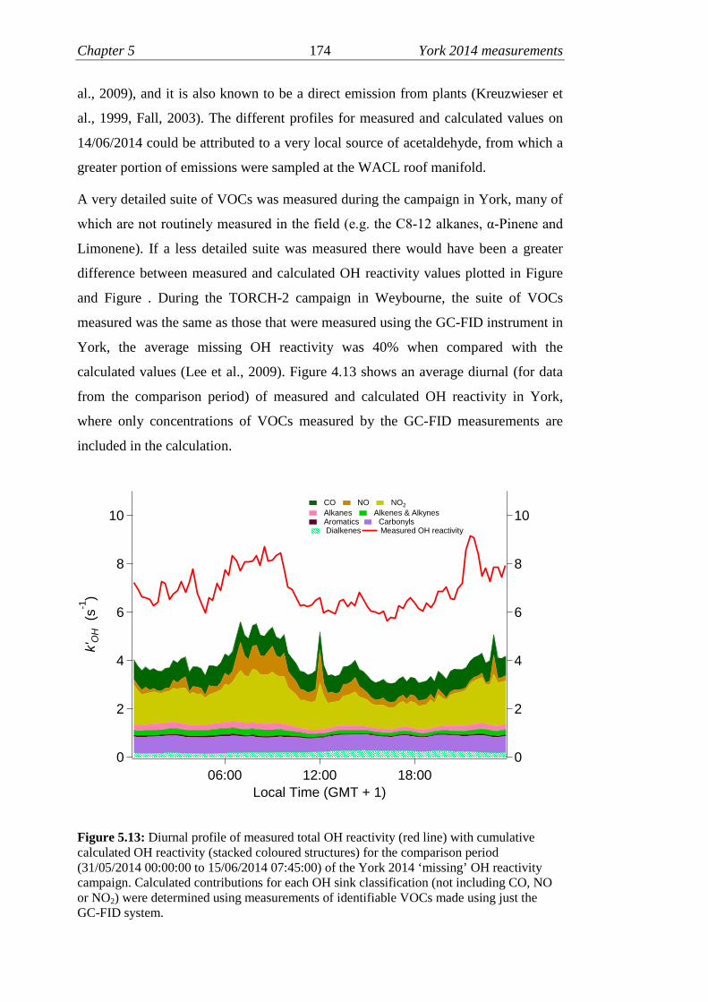
Chapter 5 174 York 2014 measurements
al., 2009), and it is also known to be a direct emission from plants (Kreuzwieser et
al., 1999, Fall, 2003). The different profiles for measured and calculated values on
14/06/2014 could be attributed to a very local source of acetaldehyde, from which a
greater portion of emissions were sampled at the WACL roof manifold.
A very detailed suite of VOCs was measured during the campaign in York, many of
which are not routinely measured in the field (e.g. the C8-12 alkanes, α-Pinene and
Limonene). If a less detailed suite was measured there would have been a greater
difference between measured and calculated OH reactivity values plotted in Figure
and Figure . During the TORCH-2 campaign in Weybourne, the suite of VOCs
measured was the same as those that were measured using the GC-FID instrument in
York, the average missing OH reactivity was 40% when compared with the
calculated values (Lee et al., 2009). Figure 4.13 shows an average diurnal (for data
from the comparison period) of measured and calculated OH reactivity in York,
where only concentrations of VOCs measured by the GC-FID measurements are
included in the calculation.
Figure 5.13: Diurnal profile of measured total OH reactivity (red line) with cumulativecalculated OH reactivity (stacked coloured structures) for the comparison period(31/05/2014 00:00:00 to 15/06/2014 07:45:00) of the York 2014 ‘missing’ OH reactivitycampaign. Calculated contributions for each OH sink classification (not including CO, NOor NO2) were determined using measurements of identifiable VOCs made using just theGC-FID system.
10 10
8 8
6 6
4 4
2 2
0 0
k' O
H(s
-1)
06:00 12:00 18:00
Local Time (GMT + 1)
CO NO NO2
Alkanes Alkenes & AlkynesAromatics CarbonylsDialkenes Measured OH reactivity

Chapter 5 175 York 2014 measurements
It is shown that there is a gap between the measured and calculated OH reactivity
typically of ~3 s-1 throughout the course of the average day when the limited set of
VOC measurements are used. The discrepancy was ~44 % of the measurements on
average and if the only VOC measurements made in York were done so using the
GC-FID system, this would have been reported as ‘missing’ OH reactivity. Also, if
the VOC measurement suite used in York was available during the TORCH-2
campaign, there would have likely been less missing OH reactivity.
During the York 2014 ‘missing’ OH reactivity campaign additional VOCs were also
measured using the GCxGC-FID technique where it was possible to measure n-
alkanes longer than n-octane up to n-dodecane and also substituted aromatics and
biogenic species such as α-pinene and limonene. These additional species which are
less regularly measured in the field, were included in the calculations of OH
reactivity that are plotted in the above figures. Figure 5.14 shows an average diurnal
(for data from the comparison period) of measured and calculated OH reactivity
where these additional species are considered in the calculation.
Figure 5.14: Diurnal profile of measured total OH reactivity (red line) with cumulativecalculated OH reactivity (stacked coloured structures) for the comparison period(31/05/2014 00:00:00 to 15/06/2014 07:45:00) of the York 2014 ‘missing’ OH reactivitycampaign. Calculated contributions for each OH sink classification (not including CO, NOor NO2) were determined using measurements of identifiable VOCs made using both theGC-FID and GCxGC-FID systems.
10 10
8 8
6 6
4 4
2 2
0 0
k' O
H(s
-1)
06:00 12:00 18:00
Local Time (GMT + 1)
CO NO NO2
Alkanes Alkenes & AlkynesAromatics BiogenicsCarbonyls DialkenesMeasured OH reactivity

Chapter 5 176 York 2014 measurements
Not surprisingly, the difference between the measured and total calculated values is
smaller here as concentrations of more sinks have been included in the calculation.
The difference is typically ~2 s-1 and is ~27% of the measurements on average,
meaning that the VOCs measured by the GCxGC-FID instrument accounted for ~17
% of the OH sink in York. Given the relatively conventional emission sources
thought to have influenced the site such as traffic pollution and agricultural land, this
observation is of wider importance.
Many studies in the literature conclude the presence of ‘missing’ OH reactivity from
measurements made in a range of environments. Measurements in urban areas often
show evidence for ‘missing’ OH reactivity, such as those reported from Nashville
(~10 % missing) (Kovacs et al., 2003) and Paris (~54 % missing) (Dolgorouky et al.,
2012). The additional VOCs that were measured by the GCxGC-FID instrument in
York were not measured in these previous studies. Whalley et al. (2016) reported
that when OH reactivity was modelled using measurements from central London,
the predicted values rose from 67 % of the measurements, to within 15 % of the
measurements with the inclusion of data for the same additional GCxGC-FID
measured VOCs. Given this and the results presented here from the campaign in
York, it is likely that if the additional species were measured in other studies in
urban environments, such as those in Nashville and Paris, the ‘missing’ OH
reactivity would have likely been significantly reduced. It should be noted that in the
study reported by Whalley et al. (2016), predictions of OH reactivity were made
using a computer model where contributions from oxidised intermediates were
estimated, in addition to contributions from the measured OH sinks.
5.4.2.5 Accounting for ‘missing’ OH reactivity
In addition to the less commonly measured n-alkanes, substituted aromatics and
biogenic species that were measured using the GCxGC-FID instrument, many
unidentifiable VOCs were also detected. Peaks for these unidentified species were
grouped according to their predicted functionality which is predicted by the space
they occupy on the chromatograms. Grouped concentrations for each class of
compound were then estimated. A detailed explanation of this process can be found
in Dunmore et al. (2015) and the classes of unidentifiable VOCs were C9 aliphatics,
C10 aliphatics, C11 aliphatics, C12 aliphatics, C13+ aliphatics, C4 substituted mono
aromatics and monoterpenes. It is likely that the unidentified species contributed to

Chapter 5 177 York 2014 measurements
the ~27 % ‘missing’ OH reactivity that was observed in York. The estimated
grouped concentrations were used in combination with estimated bimolecular rate
coefficients for their reaction with OH, summarised in Table 5.2. Figure 5.15 shows
a campaign average diurnal for measured and calculated OH reactivity where these
are considered in the calculation of OH reactivity.
Sink Class ksink + OH
(cm3 molecule-1 s-1)Contribution to OHreactivity (s-1)
Instrument
C9 aliphatics Alkanes 1.6 × 10⁻¹¹ 0.53 GCxGC-FIDC10 aliphatics 1.3 × 10⁻¹¹ GCxGC-FIDC11 apliphatics 1.3 × 10⁻¹¹ GCxGC-FIDC12 aliphatics 1.4 × 10⁻¹¹ GCxGC-FIDC13+ aliphatics 1.6 × 10⁻¹¹ GCxGC-FIDC4 substitutedmonoaromatics
Aromatics 2.4 × 10⁻¹¹ 0.09 GCxGC-FID
monoterpenes Biogenics 5.3 × 10⁻¹¹ 1.78 GCxGC-FID
Table 5.3: Unidentified groups of OH sinks measured in York. Grouped species wereassigned classes according to their predicted functionality. With the exception ofmonoterpenes bimolecular rate coefficients shown are estimates at 300 K and 1 atmospheretaken from Carter (2010). No temperature or pressure dependencies were used for thesegrouped species when calculating their contribution to OH reactivity. The bimolecular ratecoefficient shown for monoterpenes is assumed to be the same as that for α-Pinene as shown in Table 5.2. Campaign average contributions to OH reactivity are also shown foreach sink classification in addition to details of the instrument used for the measurement ofeach species.
Figure 5.15: Diurnal profile of measured total OH reactivity (red line) with cumulativecalculated OH reactivity (stacked coloured structures) for the comparison period(31/05/2014 00:00:00 to 15/06/2014 07:45:00) of the York 2014 ‘missing’ OH reactivitycampaign. Calculated contributions for each OH sink classification (not including CO, NOor NO2) were determined using measurements of identifiable VOCs made using both theGC-FID and GCxGC-FID systems, and also grouped concentrations of unidentified VOCsdetected by the GCxGC-FID system.
10 10
8 8
6 6
4 4
2 2
0 0
k' O
H(s
-1)
06:00 12:00 18:00
Local Time (GMT + 1)
CO NO NO2
Alkanes Alkenes & AlkynesAromatics BiogenicsCarbonyls DialkenesMeasured OH reactivity
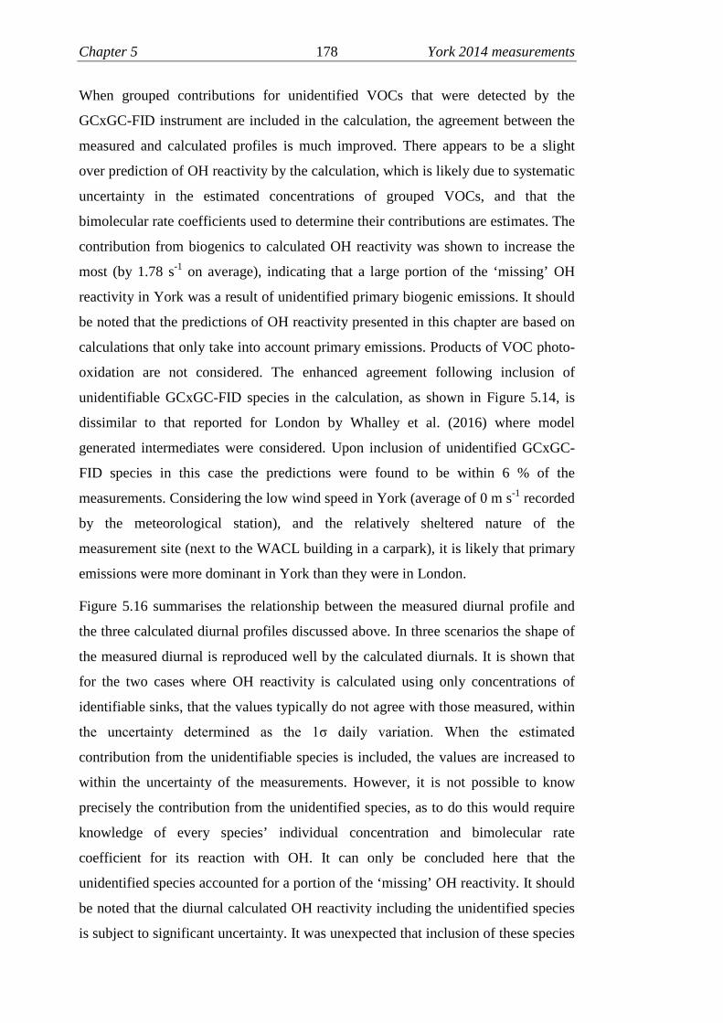
Chapter 5 178 York 2014 measurements
When grouped contributions for unidentified VOCs that were detected by the
GCxGC-FID instrument are included in the calculation, the agreement between the
measured and calculated profiles is much improved. There appears to be a slight
over prediction of OH reactivity by the calculation, which is likely due to systematic
uncertainty in the estimated concentrations of grouped VOCs, and that the
bimolecular rate coefficients used to determine their contributions are estimates. The
contribution from biogenics to calculated OH reactivity was shown to increase the
most (by 1.78 s-1 on average), indicating that a large portion of the ‘missing’ OH
reactivity in York was a result of unidentified primary biogenic emissions. It should
be noted that the predictions of OH reactivity presented in this chapter are based on
calculations that only take into account primary emissions. Products of VOC photo-
oxidation are not considered. The enhanced agreement following inclusion of
unidentifiable GCxGC-FID species in the calculation, as shown in Figure 5.14, is
dissimilar to that reported for London by Whalley et al. (2016) where model
generated intermediates were considered. Upon inclusion of unidentified GCxGC-
FID species in this case the predictions were found to be within 6 % of the
measurements. Considering the low wind speed in York (average of 0 m s-1 recorded
by the meteorological station), and the relatively sheltered nature of the
measurement site (next to the WACL building in a carpark), it is likely that primary
emissions were more dominant in York than they were in London.
Figure 5.16 summarises the relationship between the measured diurnal profile and
the three calculated diurnal profiles discussed above. In three scenarios the shape of
the measured diurnal is reproduced well by the calculated diurnals. It is shown that
for the two cases where OH reactivity is calculated using only concentrations of
identifiable sinks, that the values typically do not agree with those measured, within
the uncertainty determined as the 1σ daily variation. When the estimated
contribution from the unidentifiable species is included, the values are increased to
within the uncertainty of the measurements. However, it is not possible to know
precisely the contribution from the unidentified species, as to do this would require
knowledge of every species’ individual concentration and bimolecular rate
coefficient for its reaction with OH. It can only be concluded here that the
unidentified species accounted for a portion of the ‘missing’ OH reactivity. It should
be noted that the diurnal calculated OH reactivity including the unidentified species
is subject to significant uncertainty. It was unexpected that inclusion of these species

Chapter 5 179 York 2014 measurements
would increase the calculated reactivity so that it matched the measurements
considering that no unmeasured VOC products from the reactions of the measured
sinks have yet been considered.
Figure 5.16: Diurnal profile of measured OH reactivity (black line), error bars represent the1 σ variability of the measurements) and three scenarios for calculated OH reactivity. Blue line: calculated using VOC concentrations from GC-FID; orange line: same as for blue linewith contribution from identifiable VOCs measured by GCxGC-FID; red line: same as fororange line with estimated contribution from unidentifiable species detected by the GCxGC-FID.
Many studies of OH reactivity reported in the literature use computer models where
unmeasured products of the reactions between measured species and OH are
considered as contributors to OH reactivity. To further investigate the OH reactivity
observed during the York 2014 ‘missing’ OH reactivity campaign, a zero
dimensional chemical box modelling study was conducted by Dr. Jenny Young
using the Master Chemical Mechanism (MCM). Figure 5.17 shows some model
simulated diurnal profiles of OH reactivity alongside the measurements. For each of
the three simulated diurnal profiles the model was run using standard MCM
chemistry and unconstrained to HCHO, only measurements of OH sinks that could
be identified were included. The three simulations differed in the deposition rate that
was used for the intermediates generated. The results show that the model was
12 12
10 10
8 8
6 6
4 4
2 2
0 0
k' O
H(s
-1)
06:00 12:00 18:00
Local Time (GMT + 1)

Chapter 5 180 York 2014 measurements
sensitive to deposition rate, as this was increased the agreement between the
measured and predicted diurnals improved.
Figure 5.17: Diurnal profile of measured OH reactivity (black line), error bars represent the1 σ variability of the measurements) and three predictions from three models (all unconstrained to HCHO with standard MCM chemistry). Red line: Deposition rate extendedby 0.5 cm s-1, Yellow line: Deposition rate extended by 0.8 cm s-1, Blue line: Depositionrate extended by 1.0 cm s-1.
The shape of the model simulated diurnal profiles is similar to that of the
measurements. However there is one key difference in the relationship between the
calculation predictions and the model predictions. Figure 5.16 shows that the
difference between the measurements and the predictions is roughly constant
throughout the average day. However, Figure 5.17 shows more variation in the
discrepancy which is shown to increase following the morning rush hour peak
before decreasing again at nightfall. This may reflect uncertainties in the model
treatment of boundary layer depth which influences the lifetime of model generated
intermediates with respect to deposition.
The results presented in this section show that the missing OH reactivity observed in
York can be accounted for when unidentified VOCs are included in the calculation
of OH reactivity, and when a computer model is used to simulate OH reactivity by
taking into account products of oxidation chemistry. However, both methods are
12 12
10 10
8 8
6 6
4 4
2 2
0 0
k' O
H(s
-1)
06:00 12:00 18:00
Local Time (GMT + 1)

Chapter 5 181 York 2014 measurements
subject to significant uncertainty and may over predict the extra contributions. The
grouped concentrations of unidentifiable VOCs are estimated as are the bimolecular
rate coefficients for reaction with OH; predicted contributions from these species
could potentially be subject to a systematic positive bias. The deposition rates for
model generated intermediates, and the boundary layer depth, may not be
representative of the real conditions at the time of the measurements. Intermediate
species may be removed from the simulation too slowly resulting in their
accumulation and subsequently over predicted contribution to OH reactivity. If both
model generated intermediates and the unidentified grouped species were considered
in the simulation of OH reactivity, this would over predict the measurements by a
greater extent than is shown in Figure 5.16 and Figure 5.17.
5.5 Formaldehyde
5.5.1 Formaldehyde observations
Formaldehyde was measured during the York 2014 ‘missing’ OH reactivity
campaign using the new laser induced fluorescence instrument described in Section
2.3.6. The instrument was operated in configuration 2 and was housed inside a
ground floor laboratory of the WACL building for the duration of the measurement
period; ambient air was sampled from the roof manifold and passed through ~20 m
of half inch OD Teflon tubing before reaching the instrument. The residence time of
the gas in this tuning was ~2 s. Tests conducted by Dr. Trevor Ingham prior to
deployment of the instrument, with tubing of dimensions, showed no evidence for
loss of HCHO. Figure 5.18 shows the instrument during its deployment in York.
The York 2014 ‘missing’ OH reactivity campaign was the first deployment of the
HCHO instrument and as a safety precaution it was only operated during the
daytime so that it could be closely monitored. The instrument operated successfully
the majority of the time and near-continuous daytime measurements were recorded
on twelve days. Measurements were made with 1 s time resolution and the
instrument calibration factor, (1.46 ± 0.034) ×10-9 count s-1 mW-1 molecule-1 cm3,
determined using calibration method 1 as described in Section 2.3.7, was applied to
the 1 s LIF signal differentials which were normalised for laser power. Figure 5.19
shows all of the 1 s HCHO data that were recorded in York.

Chapter 5 182 York 2014 measurements
Figure 5.18: Photograph of the HCHO instrument set up inside the WACL building duringthe York 2014 ‘missing’ OH reactivity campaign.

Chapter 5 183 York 2014 measurements
Fig
ure
5.1
9:
Tim
ese
ries
of
1se
con
dm
easu
rem
ents
of
HC
HO
fro
mth
eY
ork
20
14‘m
issi
ng’
OH
reac
tivi
tyca
mp
aig
nfo
rda
ys.

Chapter 5 184 York 2014 measurements
The results show that the level of daytime HCHO observed did not vary
significantly from day to day, and the levels observed were typically between 0.5
and 2 ppb. The mean average level was ~1.3 ppb which is lower than other typical
levels reported for urban areas in the literature. Dasgupta et al. (2005) reported
average levels of 3.3, 7.9 and 2.3 ppb in Houston, Atlanta and Tampa, respectively.
It is not surprising that the measurements made in York were lower than these as the
measurements were not made in the city centre; the site was several miles away. The
measurements made in Houston, Atlanta and Tampa were either taken in central, or
heavily industrialised areas. High levels of HCHO are known to be emitted from
vehicles as a result of incomplete fossil fuel combustion meaning that higher levels
are to be expected in central urban and industrialised areas than in non-central urban
background areas such as the measurement site in York (Anderson et al., 1996).
Measurements reported from the Mexico City Metropolitan Area campaign
(MCMA) were also unsurprisingly higher than the measurements in from York.
Mean concentrations of ~8.2 and ~6.0 ppb were reported from two separate
locations (Volkamer et al., 2005, Garcia et al., 2006, Grutter et al., 2005). Lee et al.
(1998) also reported mean HCHO levels from 1995 measurements in Nashville to be
~4.2 ppb. Again it is not surprising that these measurements are significantly higher
than recorded in York, considering the relative sizes of the cities. Considering that
the OH reactivity reported from the MCMA campaign (~25 s-1 daytime) was also
much higher than it was in York, the presence of more HCHO is to be expected as it
is an end product of the photo-oxidative processing of VOCs (Shirley et al., 2006). It
should be noted that here that the composition of the air mass in York is expected to
be considerably different to the other locations mentioned above. All are much
closer to the equator than York and are therefore typically subject to more regular
and intense sunlight, meaning more rapid photo-chemical processing of VOCs
leading to the production of HCHO is expected.
It can be seen in the complete 1 s time series shown in Figure 5.19 that there were
sharp excursions in HCHO concentration on a number of days; the level of HCHO
reaches as high as ~5 ppb before falling again in a matter of seconds. These events
coincided with the arrival of vehicles (in most cases large trucks) to the car park at
the measurement site (for example delivery of liquid N2). Figure 5.20(a) shows all
of the 1 s HCHO measurements from 04/06/2014 and an example of this behaviour
is circled in red.

Chapter 5 185 York 2014 measurements
Figure 5.20: Observations of HCHO from 04/06/14 during the York 2014 ‘missing’ OHreactivity campaign. (a) Data plotted with y-axis maximum of 5000 ppt to show example ofa rapid excursion to high HCHO (circled in red). (b) Data plotted with y-axis maximum of2000 ppt to show slower variation in HCHO.
The presence of these excursions in the 1 s data demonstrates an advantage of
measuring atmospheric HCHO using a fast response LIF detector over other types of
instruments with a slower response time. For example, if the measurements made
during the campaign in York were made using the Hanzch Fluorimetry
methodology, where measurements are typically made every minute, this behaviour
would have not likely been observed. Figure 5.20(b) shows the same 1 s data set for
04/06/2014 as Figure 5.20(a) on a smaller scale so that more gradual changes in
[HCHO] can be observed through the course of the day.
5.5.2 Interpretation of formaldehyde observations
5.5.2.1 Diurnal behaviour
It can be seen from Figure 5.19 that on the majority of days where formaldehyde
was measured an increase was typically observed through the morning hours. An
example of this is also clearly shown in Figure 5.20(b) where levels increased by
~500 ppt between 0800 and 1200. In order to broadly examine the variations in
formaldehyde levels with respect to its chemistry, the data were processed in the
same way as the OH reactivity data in order to produce a diurnal profile for the

Chapter 5 186 York 2014 measurements
‘average day’. Measurements were averaged into 96 time bins with a mean value
every 15 minutes; Figure 5.21 shows the diurnal profile obtained from all of the 1s
data shown in Figure 5.19.
The diurnal profile shows an increase in HCHO through the morning hours which
plateaus at ~1200. This behaviour is not surprising considering that HCHO is a
major by-product of the photo oxidative processing of VOCs and can act as an
overall tracer for VOC oxidation (DiGangi et al., 2011). It is likely that this rise is a
result of an increased rate of production of OH as the sun rose leading to more rapid
processing of VOCs to form HCHO. This is a common feature of HCHO
measurements in environments with air masses characterised by a strong influence
from anthropogenic emissions. Dasgupta et al. (2005) reported this feature in diurnal
profiles resulting from measurements from Nashville, Atlanta, Philadelphia and
Tampa.
Figure 5.21: Diurnal profile of [HCHO] observed during the York 2014 ‘missing’ OHreactivity campaign in 15 minute time bins. Error bars ± 1 σ standard deviation from the mean observation, and are a measure of the variability during a 15 minute time bin.

Chapter 5 187 York 2014 measurements
The behaviour exhibited by the diurnal profile is likely to have been driven by the
photochemical processing of VOCs to produce HCHO. The change in the level of
HCHO through the course of the average day is unlikely to have been driven by
direct emissions as it does not vary in the same way as the contribution from NOx to
calculated OH reactivity. If the change was a result of direct emissions, a morning
rush hour peak similar to the NOx driven morning rush hour peak in OH reactivity
would have likely been observed. To further investigate what contributed to the
changes seen in HCHO, correlations with other species and parameters measured
were examined.
5.5.2.2 Correlations with other measurements
The relationship between the level of HCHO and other species and parameters
measured was examined to investigate any potential sources. Correlation plots to
show the relationship between HCHO and NOx are shown in Figure 5.22.
Figure 5.22: Plots of [HCHO] against both [NO] and [NO2]. Data shown are 15 minutebinned mean averages from measurements taken between 31/05/2014 00:00:00 –15/06/2014 07:45:00 of the York 2014 ‘missing’ OH reactivity campaign. The shaded areasrepresent the 95% confidence intervals from the linear fits (least squares).
It is shown that there are no correlations between HCHO and NO or NO2. This is not
surprising considering the shape of the diurnal profile which is characteristic of
secondarily sourced HCHO. If direct HCHO sources were dominant in York some
level of correlation would be expected here. The relationship between measured
HCHO and all other measured species and parameters was examined, it was only
possible to identify two weak correlations. These were with ambient air temperature,
and the photolytic O1D production rate (J(O1D)), plots are shown in Figure 5.23.

Chapter 5 188 York 2014 measurements
Figure 5.23: Plots of measured [HCHO] against both temperature and J(O1D). Data shownare 15 minute binned mean averages from measurements taken between 31/05/201400:00:00 – 15/06/2014 07:45:00 of the York 2014 ‘missing’ OH reactivity campaign. Theshaded areas represent the 95% confidence intervals from the linear fits (least squares).
It is to be expected that HCHO would correlate with both temperature and J(O1D), if
its major source was secondary production. Higher J(O1D) is typically associated
with elevated temperatures owing to there being more solar radiation available for
photolysis and to heat the air mass. When there is a higher rate of O1D production
there is more rapid production of OH which ultimately leads to more rapid photo-
oxidative processing of VOCs and subsequently more HCHO. Whilst these
correlations are present, they are by no means strong and this is likely due to there
being a contribution from locally produced HCHO and HCHO produced further
afield which was transported to the site.
Given that the only measurements which showed correlation with the HCHO
measurements were ambient air temperature and J(O1D), it can be concluded that
that the dominant source of HCHO in York was secondary production from photo-
oxidation. However, local sources of HCHO such as that from combustion engines,
did contribute to the measurement for short periods of time.
5.6 Summary and conclusions
OH reactivity and formaldehyde observations from a site subject to significant
influence from anthropogenic and biogenic emissions are presented. Measurements
were made during the York 2014 ‘missing’ OH reactivity campaign which took
place in May / June 2014 at the University of York campus. The main objective for
campaign was to test the operation of a new instrument for the identification of

Chapter 5 189 York 2014 measurements
species that contribute to ‘missing’ OH reactivity, alongside the laser flash
photolysis instrument for the measurement of OH reactivity. Details of the new
instrument are presented in Chapter 4. An additional aim was to field-test the Leeds
LIF instrument for the measurement of formaldehyde; the ambient measurements
presented here were the first to be made by it. Both instruments for the measurement
of OH reactivity, and for the measurement of formaldehyde performed well for the
majority of the campaign and there are few unplanned gaps in either set of data.
The mean average OH reactivity recorded was 6.3 s-1 which is lower than what has
been reported in the literature for other studies where the air mass is largely
characterised by anthropogenic emissions. It is concluded that the reason for the
lower OH reactivity measurements presented here is that the site in York is roughly
in as close proximity to agricultural land as it was to York city centre, meaning that
less polluted air would have had a stronger influence, compared to studies where
measurement sites were completely surrounded by urban development. OH
reactivity was found to correlate well with NOx and other anthropogenic emissions
typical of vehicular exhaust.
OH reactivity was calculated using concentrations of known OH sinks that were
measured at the same time. When concentrations for all of the identifiable sinks
were included in the calculation, it was found that the values were typically lower
than those measured by ~1 - 3 s-1. On average for the comparison period of the
campaign there was ~27 % ‘missing’ OH reactivity, with all measured identifiable
OH sinks considered. A very detailed suite of VOCs were measured in York. When
OH reactivity was calculated using only measured concentrations of VOCs which
are routinely measured in the field (using GC-FID), the gap between the measured
and calculated OH reactivity was significantly greater. If a typical set of VOC
measurements were made in York it would have been concluded that on average
there was 44 % ‘missing’ OH reactivity. The results from this study demonstrate the
importance of measuring longer n-alkanes, substituted aromatics and biogenic
species in this environment.
Discussion is given on the potential cause of the ‘missing’ OH reactivity. It was
found that when a contribution to the calculated OH reactivity is estimated for
grouped concentrations of unidentifiable species detected by the GCxGC-FID
instrument, the two data sets are in close agreement. A zero-dimensional chemical

Chapter 5 190 York 2014 measurements
box modelling study also showed that the ‘missing’ OH reactivity could be
accounted for by model-generated intermediates when the deposition rate is
sufficient. However there is great uncertainty associated with both of these
approaches. For the unidentified species both the concentrations and the rate
coefficients are estimated and the model was shown to be sensitive to deposition
rate. A portion of the ‘missing’ OH reactivity can likely be attributed to a
combination of both the unidentified species, and products of photo-oxidation that
were considered in the model. In addition to this it is possible that some currently
unidentified species that were detected by the GC-TOF-MS system of the new
instrument described in Chapter 4 could have also contributed. However, data from
this instrument has not yet been analysed to quantify and identify any of these
species.
The mean average level of formaldehyde observed was ~1.3 ppb which is lower than
much of the literature based on studies in environments characterised by significant
anthropogenic influence. Measurements were made only during the daytime owing
to the need to closely monitor the instrument on its first deployment. The day time
diurnal profile follows that typical of an environment where the dominant source is
secondary formation from photo-oxidation of VOCs with a rise through the morning
hours as the sun rises. Correlations of HCHO with temperature and J(O1D) support
this and HCHO was not found to correlate with any other species or parameter
measured. The advantage of the LIF technique for HCHO measurement is
demonstrated by the presence of rapid excursions in the measurements that were
synchronous with large vehicles entering the car park at the measurement site.
5.7 References
ANDERSON, L. G., LANNING, J. A., BARRELL, R., MIYAGISHIMA, J.,JONES, R. H. & WOLFE, P. 1996. Sources and sinks of formaldehyde andacetaldehyde: An analysis of Denver's ambient concentration data.Atmospheric Environment, 30, 2113-2123.
ATKINSON, R. 2003. Kinetics of the gas-phase reactions of OH radicals withalkanes and cycloalkanes. Atmos. Chem. Phys., 3, 2233-2307.
BAN-WEISS, G. A., MCLAUGHLIN, J. P., HARLEY, R. A., KEAN, A. J.,GROSJEAN, E. & GROSJEAN, D. 2008. Carbonyl and Nitrogen DioxideEmissions From Gasoline- and Diesel-Powered Motor Vehicles.Environmental Science & Technology, 42, 3944-3950.
BOHN, B., KRAUS, A., MÜLLER, M. & HOFZUMAHAUS, A. 2004.Measurement of atmospheric O3 → O(1D) photolysis frequencies using

Chapter 5 191 York 2014 measurements
filterradiometry. Journal of Geophysical Research: Atmospheres, 109,D10S90.
BRUNE, W. H., BAIER, B. C., THOMAS, J., REN, X., COHEN, R. C., PUSEDE,S. E., BROWNE, E. C., GOLDSTEIN, A. H., GENTNER, D. R.,KEUTSCH, F. N., THORNTON, J. A., HARROLD, S., LOPEZ-HILFIKER,F. D. & WENNBERG, P. O. 2016. Ozone production chemistry in thepresence of urban plumes. Faraday Discussions, 189, 169-189.
CARSLAW, D. C. 2015. The openair manual - open-source tools for analysing airpollution data. Manual for version 1.1-4, King's College London.
CARSLAW, D. C. & ROPKINS, K. 2012. openair - an R package for air qualitydata analysis. Environmental Modelling and Software, 27-28, 52-61.
CARTER, W. P. L. 2010. Development of the SAPRC-07 chemical mechanism.Atmospheric Environment, 44, 5324-5335.
CHATANI, S., SHIMO, N., MATSUNAGA, S., KAJII, Y., KATO, S.,NAKASHIMA, Y., MIYAZAKI, K., ISHII, K. & UENO, H. 2009.Sensitivity analyses of OH missing sinks over Tokyo metropolitan area inthe summer of 2007. Atmos. Chem. Phys., 9, 8975-8986.
CORCHNOY, S. B. & ATKINSON, R. 1990. Kinetics of the gas-phase reactions ofhydroxyl and nitrogen oxide (NO3) radicals with 2-carene, 1,8-cineole, p-cymene, and terpinolene. Environmental Science & Technology, 24, 1497-1502.
DASGUPTA, P. K., LI, J., ZHANG, G., LUKE, W. T., MCCLENNY, W. A.,STUTZ, J. & FRIED, A. 2005. Summertime Ambient Formaldehyde in FiveU.S. Metropolitan Areas: Nashville, Atlanta, Houston, Philadelphia, and Tampa. Environmental Science & Technology, 39, 4767-4783.
DIGANGI, J. P., BOYLE, E. S., KARL, T., HARLEY, P., TURNIPSEED, A., KIM,S., CANTRELL, C., MAUDLIN III, R. L., ZHENG, W., FLOCKE, F.,HALL, S. R., ULLMANN, K., NAKASHIMA, Y., PAUL, J. B., WOLFE,G. M., DESAI, A. R., KAJII, Y., GUENTHER, A. & KEUTSCH, F. N.2011. First direct measurements of formaldehyde flux via eddy covariance:implications for missing in-canopy formaldehyde sources. Atmos. Chem.Phys., 11, 10565-10578.
DOLGOROUKY, C., GROS, V., SARDA-ESTEVE, R., SINHA, V., WILLIAMS,J., MARCHAND, N., SAUVAGE, S., POULAIN, L., SCIARE, J. &BONSANG, B. 2012. Total OH reactivity measurements in Paris during the2010 MEGAPOLI winter campaign. Atmos. Chem. Phys., 12, 9593-9612.
DUNMORE, R. E., HOPKINS, J. R., LIDSTER, R. T., LEE, J. D., EVANS, M. J.,RICKARD, A. R., LEWIS, A. C. & HAMILTON, J. F. 2015. Diesel-relatedhydrocarbons can dominate gas phase reactive carbon in megacities. Atmos.Chem. Phys., 15, 9983-9996.
EDWARDS, P. M., EVANS, M. J., FURNEAUX, K. L., HOPKINS, J., INGHAM,T., JONES, C., LEE, J. D., LEWIS, A. C., MOLLER, S. J., STONE, D.,WHALLEY, L. K. & HEARD, D. E. 2013. OH reactivity in a South EastAsian tropical rainforest during the Oxidant and Particle PhotochemicalProcesses (OP3) project. Atmos. Chem. Phys., 13, 9497-9514.
FALL, R. 2003. Abundant Oxygenates in the Atmosphere: A Biochemical Perspective. Chemical Reviews, 103, 4941-4952.
GARCIA, A. R., VOLKAMER, R., MOLINA, L. T., MOLINA, M. J.,SAMUELSON, J., MELLQVIST, J., GALLE, B., HERNDON, S. C. &KOLB, C. E. 2006. Separation of emitted and photochemical formaldehyde

Chapter 5 192 York 2014 measurements
in Mexico City using a statistical analysis and a new pair of gas-phasetracers. Atmos. Chem. Phys., 6, 4545-4557.
GRUTTER, M., FLORES, E., ANDRACA-AYALA, G. & BÁEZ, A. 2005.Formaldehyde levels in downtown Mexico City during 2003. AtmosphericEnvironment, 39, 1027-1034.
HEARD, D. E., READ, K. A., METHVEN, J., AL-HAIDER, S., BLOSS, W. J.,JOHNSON, G. P., PILLING, M. J., SEAKINS, P. W., SMITH, S. C.,SOMMARIVA, R., STANTON, J. C., STILL, T. J., INGHAM, T.,BROOKS, B., DE LEEUW, G., JACKSON, A. V., MCQUAID, J. B.,MORGAN, R., SMITH, M. H., CARPENTER, L. J., CARSLAW, N.,HAMILTON, J., HOPKINS, J. R., LEE, J. D., LEWIS, A. C., PURVIS, R.M., WEVILL, D. J., BROUGH, N., GREEN, T., MILLS, G., PENKETT, S.A., PLANE, J. M. C., SAIZ-LOPEZ, A., WORTON, D., MONKS, P. S.,FLEMING, Z., RICKARD, A. R., ALFARRA, M. R., ALLAN, J. D.,BOWER, K., COE, H., CUBISON, M., FLYNN, M., MCFIGGANS, G.,GALLAGHER, M., NORTON, E. G., O'DOWD, C. D., SHILLITO, J.,TOPPING, D., VAUGHAN, G., WILLIAMS, P., BITTER, M., BALL, S.M., JONES, R. L., POVEY, I. M., O'DOHERTY, S., SIMMONDS, P. G.,ALLEN, A., KINNERSLEY, R. P., BEDDOWS, D. C. S., DALL'OSTO, M.,HARRISON, R. M., DONOVAN, R. J., HEAL, M. R., JENNINGS, S. G.,NOONE, C. & SPAIN, G. 2006. The North Atlantic Marine Boundary LayerExperiment(NAMBLEX). Overview of the campaign held at Mace Head,Ireland, in summer 2002. Atmos. Chem. Phys., 6, 2241-2272.
HELAND, J., KLEFFMANN, J., KURTENBACH, R. & WIESEN, P. 2001. A NewInstrument To Measure Gaseous Nitrous Acid (HONO) in the Atmosphere.Environmental Science & Technology, 35, 3207-3212.
HOFZUMAHAUS, A. 2006. Measurement of Photolysis Frequencies in theAtmosphere. In: HEARD, D. (ed.) Analytical Techniques for AtmosphericMeasurement. Blackwell Publishing Ltd.
JENKIN, M. E., SAUNDERS, S. M. & PILLING, M. J. 1997. The troposphericdegradation of volatile organic compounds: a protocol for mechanismdevelopment. Atmospheric Environment, 31, 81-104.
KAISER, J., WOLFE, G. M., BOHN, B., BROCH, S., FUCHS, H., GANZEVELD,L. N., GOMM, S., HÄSELER, R., HOFZUMAHAUS, A., HOLLAND, F.,JÄGER, J., LI, X., LOHSE, I., LU, K., PRÉVÔT, A. S. H., ROHRER, F.,WEGENER, R., WOLF, R., MENTEL, T. F., KIENDLER-SCHARR, A.,WAHNER, A. & KEUTSCH, F. N. 2015. Evidence for an unidentified non-photochemical ground-level source of formaldehyde in the Po Valley withpotential implications for ozone production. Atmos. Chem. Phys., 15, 1289-1298.
KATO, S., SATO, T. & KAJII, Y. 2011. A method to estimate the contribution ofunidentified VOCs to OH reactivity. Atmospheric Environment, 45, 5531-5539.
KOVACS, T. A., BRUNE, W. H., HARDER, H., MARTINEZ, M., SIMPAS, J. B.,FROST, G. J., WILLIAMS, E., JOBSON, T., STROUD, C., YOUNG, V.,FRIED, A. & WERT, B. 2003. Direct measurements of urban OH reactivityduring Nashville SOS in summer 1999. J. Environ. Monit., 5, 68-74.
KREUZWIESER, J., SCHNITZLER, J. P. & STEINBRECHER, R. 1999.Biosynthesis of Organic Compounds Emitted by Plants. Plant Biology, 1,149-159.

Chapter 5 193 York 2014 measurements
KWOK, E. S. C., ATKINSON, R. & AREY, J. 1997. Kinetics of the gas-phasereactions of indan, indene, fluorene, and 9,10-dihydroanthracene with OHradicals, NO3 radicals, and O3. International Journal of Chemical Kinetics,29, 299-309.
LEE, J. D., YOUNG, J. C., READ, K. A., HAMILTON, J. F., HOPKINS, J. R.,LEWIS, A. C., BANDY, B. J., DAVEY, J., EDWARDS, P., INGHAM, T.,SELF, D. E., SMITH, S. C., PILLING, M. J. & HEARD, D. E. 2009.Measurement and calculation of OH reactivity at a United Kingdom coastalsite. Journal of atmospheric chemistry, 64, 53-76.
LEE, Y. N., ZHOU, X., KLEINMAN, L. I., NUNNERMACKER, L. J.,SPRINGSTON, S. R., DAUM, P. H., NEWMAN, L., KEIGLEY, W. G.,HOLDREN, M. W., SPICER, C. W., YOUNG, V., FU, B., PARRISH, D.D., HOLLOWAY, J., WILLIAMS, J., ROBERTS, J. M., RYERSON, T. B.& FEHSENFELD, F. C. 1998. Atmospheric chemistry and distribution offormaldehyde and several multioxygenated carbonyl compounds during the1995 Nashville/Middle Tennessee Ozone Study. Journal of GeophysicalResearch: Atmospheres, 103, 22449-22462.
LIDSTER, R. T., HAMILTON, J. F., LEE, J. D., LEWIS, A. C., HOPKINS, J. R.,PUNJABI, S., RICKARD, A. R. & YOUNG, J. C. 2014. The impact ofmonoaromatic hydrocarbons on OH reactivity in the coastal UK boundarylayer and free troposphere. Atmos. Chem. Phys., 14, 6677-6693.
NAKASHIMA, Y., TSURUMARU, H., IMAMURA, T., BEJAN, I., WENGER, J.C. & KAJII, Y. 2012. Total OH reactivity measurements in laboratorystudies of the photooxidation of isoprene. Atmospheric Environment, 62,243-247.
REN, X., BRUNE, W. H., MAO, J., MITCHELL, M. J., LESHER, R. L., SIMPAS,J. B., METCALF, A. R., SCHWAB, J. J., CAI, C., LI, Y., DEMERJIAN, K.L., FELTON, H. D., BOYNTON, G., ADAMS, A., PERRY, J., HE, Y.,ZHOU, X. & HOU, J. 2006a. Behavior of OH and HO2 in the winteratmosphere in New York City. Atmospheric Environment, 40, Supplement 2,252-263.
REN, X., BRUNE, W. H., OLIGER, A., METCALF, A. R., SIMPAS, J. B.,SHIRLEY, T., SCHWAB, J. J., BAI, C., ROYCHOWDHURY, U., LI, Y.,CAI, C., DEMERJIAN, K. L., HE, Y., ZHOU, X., GAO, H. & HOU, J.2006b. OH, HO2, and OH reactivity during the PMTACS-NY WhitefaceMountain 2002 campaign: Observations and model comparison. J. Geophys.Res, 111, D10S03.
ROBBINS, R. C., BORG, K. M. & ROBINSON, E. 1968. Carbon Monoxide in theAtmosphere. Journal of the Air Pollution Control Association, 18, 106-110.
SAUNDERS, S. M., JENKIN, M. E., DERWENT, R. G. & PILLING, M. J. 2003.Protocol for the development of the Master Chemical Mechanism, MCM v3(Part A): tropospheric degradation of non-aromatic volatile organiccompounds. Atmospheric Chemistry and Physics, 3, 161-180.
SHIRLEY, T. R., BRUNE, W. H., REN, X., MAO, J., LESHER, R., CARDENAS,B., VOLKAMER, R., MOLINA, L. T., MOLINA, M. J., LAMB, B.,VELASCO, E., JOBSON, T. & ALEXANDER, M. 2006. Atmosphericoxidation in the Mexico City metropolitan area (MCMA) during April 2003.Atmospheric Chemistry and Physics, 6, 2753-2765.
STONE, D., WHALLEY, L. K., INGHAM, T., EDWARDS, P. M., CRYER, D. R.,BRUMBY, C. A., SEAKINS, P. W. & HEARD, D. E. 2016. Measurement

Chapter 5 194 York 2014 measurements
of OH reactivity by laser flash photolysis coupled with laser-inducedfluorescence spectroscopy. Atmos. Meas. Tech., 9, 2827-2844.
VOLKAMER, R., MOLINA, L. T., MOLINA, M. J., SHIRLEY, T. & BRUNE, W.H. 2005. DOAS measurement of glyoxal as an indicator for fast VOCchemistry in urban air. Geophysical Research Letters, 32, L08806.
WEINHEIMER, A. J. 2006. Chemical Methods: Chemiluminescence, ChemicalAmplification, Electrochemistry, and Derivitization. In: HEARD, D. (ed.)Analytical Techniques for Atmospheric Measurement. Blackwell PublishingLtd.
WHALLEY, L. K., BLITZ, M. A., DESSERVETTAZ, M., SEAKINS, P. W. &HEARD, D. E. 2013. Reporting the sensitivity of laser-induced fluorescenceinstruments used for HO2 detection to an interference from RO2 radicals andintroducing a novel approach that enables HO2 and certain RO2 types to beselectively measured. Atmos. Meas. Tech., 6, 3425-3440.
WHALLEY, L. K., STONE, D., BANDY, B., DUNMORE, R., HAMILTON, J. F.,HOPKINS, J., LEE, J. D., LEWIS, A. C. & HEARD, D. E. 2016.Atmospheric OH reactivity in central London: observations, modelpredictions and estimates of in situ ozone production. Atmos. Chem. Phys.,16, 2109-2122.
WILSON, E. W., HAMILTON, W. A., KENNINGTON, H. R., EVANS, B.,SCOTT, N. W. & DEMORE, W. B. 2006. Measurement and Estimation ofRate Constants for the Reactions of Hydroxyl Radical with Several Alkanesand Cycloalkanes. The Journal of Physical Chemistry A, 110, 3593-3604.
YOSHINO, A., NAKASHIMA, Y., MIYAZAKI, K., KATO, S., SUTHAWAREE,J., SHIMO, N., MATSUNAGA, S., CHATANI, S., APEL, E.,GREENBERG, J., GUENTHER, A., UENO, H., SASAKI, H., HOSHI, J.-Y., YOKOTA, H., ISHII, K. & KAJII, Y. 2012. Air quality diagnosis fromcomprehensive observations of total OH reactivity and reactive trace speciesin urban central Tokyo. Atmospheric Environment, 49, 51-59.
YOSHINO, A., SADANAGA, Y., WATANABE, K., KATO, S., MIYAKAWA, Y.,MATSUMOTO, J. & KAJII, Y. 2006. Measurement of total OH reactivityby laser-induced pump and probe technique - comprehensive observations inthe urban atmosphere of Tokyo. Atmospheric Environment, 40, 7869-7881.
ZAVALA, M., HERNDON, S. C., WOOD, E. C., JAYNE, J. T., NELSON, D. D.,TRIMBORN, A. M., DUNLEA, E., KNIGHTON, W. B., MENDOZA, A.,ALLEN, D. T., KOLB, C. E., MOLINA, M. J. & MOLINA, L. T. 2009.Comparison of emissions from on-road sources using a mobile laboratoryunder various driving and operational sampling modes. Atmos. Chem. Phys.,9, 1-14.

195
Chapter 6 - Integrated Chemistry of
Ozone in the Atmosphere campaign
6.1 Background to the ICOZA project
The atmospheric chemistry of ozone in the troposphere plays a key role in numerous
processes relating to air quality and climate change as it is both a pollutant and a
greenhouse gas. O3 is a major constituent of photochemical smog and is a known
respiratory irritant, exposure to excessive levels has been shown to be linked with
increased mortality rates in a number of European cities; daily deaths have been
shown to increase by 0.3 % per every ~5 ppb increase in O3 exposure (World Health
Organisation, 2005). In addition to this, tropospheric O3 is damaging to crops; it can
harm yields and reduce quality (Krupa et al., 1998). Tropospheric O3 is often
produced as a product from the photo-oxidative processing of VOCs in the presence
of NOx through the reaction of O(3P) with O2, where O(3P) was formed from the
photolysis of NO2 that resulted from the reaction between NO and RO2, or HO2.
This chapter focusses on the Integrated Chemistry of Ozone in the Atmosphere
(ICOZA) campaign which took place at a site on the North Norfolk Coast, UK, in
the summer of 2016. The focus of the ICOZA project was investigate O3 production,
through both its direct measurement, and the measurement of other species and
parameters that relate to it.
6.2 Aims
Indirect approaches to determining the O3 production regime and calculating O3
production rate, such as those described Section 1.3, require accurate measurements
of various species (NOy, ROx, VOCs), and good knowledge of physical parameters
such as rate coefficients. This results in the indirect approaches being subject to
significant uncertainty. The main aim of the ICOZA campaign was to directly

Chapter 6 196 ICOZA measurements
measure the O3 production rate, and its response to changes in NOx, and VOC
levels, using a newly developed instrument deployed to a UK coastal site which is
known to be regularly subject to the pollution outflow from London and continental
Europe.
The new instrument was developed by the research group of Prof. William Bloss at
the University of Birmingham and utilised a methodology known as the Perturbed
Ozone Production Rate (POPR) approach. In this method ambient air is drawn into
two transparent flow reactors, one of which transmits all wavelengths of UV-visible
solar radiation that reach the earths surface (to allow photochemistry) and one which
absorbs below ~400 nm (to stop photochemistry of NO2). O3 is measured in the flow
from each reactor and is used to calculate the rate of in situ O3 production by taking
into account the residence time of the ambient air in the reactors. The measured O3
production rate is perturbed by the addition of NOx or VOCs before entry to the
reactors to enable responses to be examined. A detailed description of the method
can be found in Cazorla and Brune (2010).
An extensive suite of other species and parameters were co-measured to enable
interpretation of the O3 production rate. This chapter focusses on measurements of
OH reactivity and HCHO that were made using the laser flash photolysis instrument
and LIF instrument, respectively that are both described in Chapter 2.
6.3 Site description, measurement suite and conditions
During the ICOZA campaign all measurements were made at the University of East
Anglia (UEA) managed Weybourne Atmospheric Observatory (WAO) on the North
Norfolk coast, UK (52° 57' N, 1° 07' E). The main building at the observatory is a
decommissioned second world war ammunitions store and houses a laboratory
containing a variety of instrumentation for atmospheric measurement. It is built on
land 16 m above sea level that declines gently towards a pebble beach that faces
North. A detailed description of the WAO can be found in Penkett et al. (1999) and
the geographical location of the site is shown by the satellite image in Figure 6.1.

Chapter 6 197 ICOZA measurements
Figure 6.1: Satellite image showing the location (yellow star) of the measurement site at theWeybourne Atmospheric Observatory during the ICOZA campaign.
The WAO was chosen for the ICOZA campaign owing to the variation in air masses
it is regularly subjected to. It provided a strong opportunity to field test the
University of Birmingham developed POPR instrument and to measure the in situ
ozone production rates in polluted air masses subjected to varying degrees of
photochemical ages and pollutant loadings. Previous measurement campaigns at the
WAO have received photochemically aged air masses containing pollution from
continental Europe in addition to lesser aged air masses from London and the rest of
the UK, cleaner marine air from the North Sea also regularly reaches the site (Lee et
al., 2009).
A large concreted area on the land adjacent to the WAO building provided ample
space for the deployment of mobile laboratories from which measurements were
also made during ICOZA. A van belonging to the University of Birmingham, the
Leeds FAGE container and the Leicester container were deployed. The photograph
in Figure 6.2 shows the positioning of the mobile laboratories relative to the WAO
building. Table 6.1 summarises all of the measurements that were made during
ICOZA, the locations of the inlets / measurement points and the techniques used.

Chapter 6 198 ICOZA measurements
Figure 6.2: Photograph of the measurement site at the WAO where the Leeds FAGEcontainer was situated for the ICOZA campaign.
For measurements that were made from the laboratory inside the WAO building,
ambient air was either sampled via ~5 m of ¼” OD Teflon tubing from the roof or
from a tower ~10 m above the roof. From the top of which, a glass manifold was
used to circulate ambient air to the laboratory; this enabled subsequent samples of
ambient air to taken by instruments.

Chapter 6 199 ICOZA measurements
Ref
eren
ce
Wh
alle
yet
al.(
2013
)
Sto
ne
etal
.(2
016
)
Th
isw
ork
Caz
orl
aan
dB
run
e(2
010
)
Wei
nh
eim
er(2
006
)
Lan
gri
dg
eet
al.(
2006
)
Hea
rdet
al.
(20
06)
Ro
bbi
ns
etal
.(19
68)
Hel
and
etal
.(2
001
)
Ban
nan
etal
.(20
15)
Ho
fzu
mah
aus
(20
06)
Bo
hn
etal
.(2
004
)
- Mu
rph
yet
al.
(201
0)
Ta
ble
6.1
:S
pec
ies
/p
aram
eter
sm
easu
red
dur
ing
the
ICO
ZA
cam
pai
gn
atth
eW
eyb
ou
rne
Atm
osp
her
icO
bser
vat
ory
(WA
O)
Sam
ple
inle
t
FA
GE
con
tain
er
FA
GE
con
tain
er
WA
Om
anif
old
Bir
min
gh
amv
an
WA
Oro
of
Lei
cest
erco
nta
iner
WA
Om
anif
old
WA
Om
anif
old
Bir
min
gh
amv
an
Lei
cest
erco
nta
iner
FA
GE
con
tain
eran
dL
eice
ster
con
tain
er
FA
GE
con
tain
er
WA
Oro
of
WA
Oro
of
Tec
hn
iqu
e
Las
erin
du
ced
fluo
resc
ence
spec
tro
sco
py(L
IF)
Las
erfl
ash
pho
toly
sis
cou
ple
dw
ith
lase
rin
du
ced
fluo
resc
ence
spec
tro
sco
py
(LF
P-
LIF
)
Las
erin
du
ced
fluo
resc
ence
spec
tro
sco
py(L
IF)
Per
turb
edo
zon
ep
rodu
ctio
nra
te(P
OP
R)
Ch
emil
um
ines
cen
ce
(CR
DS
)
UV
abso
rpti
on
Ho
tm
ercu
ric
oxi
de
redu
ctio
nco
uple
dw
ith
UV
det
ecti
on
Lo
ngp
ath
abso
rpti
on
pho
tom
etry
(LO
PA
P)
Ch
emic
alIo
nis
atio
nm
ass
spec
trom
etry
(CIM
S)
Sp
ectr
alra
dio
met
ry
Fil
ter
rad
iom
etry
Gas
chro
mat
og
raph
yco
uple
dw
ith
flam
eio
nisa
tio
nd
etec
tor
(GC
-FID
)
Pro
ton
tran
sfer
mas
ssp
ectr
om
eter
(PT
R-M
S)
Mea
sure
men
t
OH
,H
O2,
RO
2
OH
reac
tiv
ity
HC
HO
Ozo
ne
pro
duct
ion
rate
NO
,N
O2
NO
2
O3
CO
HO
NO
ClN
O2
Ph
oto
lysi
sfr
equ
enci
es
J(O
1 D)
NM
HC
s
NM
HC
s

Chapter 6 200 ICOZA measurements
Figure 6.3: Photograph of the ~10m tower at the WAO where ambient air was sampled viaa glass manifold (shown) to the laboratory for analysis.

Chapter 6 201 ICOZA measurements
The weather was very variable during the ICOZA campaign and ranged from a heat
wave on 01/07/2015 to colder wetter days and night time thunderstorms. The
average temperature was 16.3 ˚C and ranged from 9.4 to 29 ˚C with an average
relative humidity of 75 % which ranged from 38 to 98 %. For most of the campaign
the wind speed was typically below 10 m s-1 with a minimum of 0.3. m s-1, higher
wind speeds (18.3 m s-1 maximum) were observed on 25/07/2015 during and
following a heavy thunderstorm. Figure 6.4 shows the variations in temperature,
relative humidity and wind speed that were observed during the ICOZA campaign.
Figure 6.4: Time series of key meteorological parameters recorded by the WeybourneAtmospheric Observatory (WAO) meteorological station positioned at the top of thesampling tower. Key events are labelled.

Chapter 6 202 ICOZA measurements
6.4 OH reactivity
6.4.1 OH reactivity observations
The Leeds laser flash photolysis instrument for the measurement of OH reactivity
was positioned ~3 m above ground on the roof of the Leeds FAGE container in a
similar manner to during the York 2014 ‘missing’ OH reactivity campaign (Chapter
4). The instrument was operated in configuration 2 as described in Section 2.2.7.
The instrument operated well for the majority of the campaign with few unplanned
gaps in the data. However, it was not possible to make measurements of OH
reactivity during the final week of the campaign owing to problems encountered
with the reference cell used to tune the wavelength of the 308 nm probe laser. Figure
6.5 shows the instrument whilst sampling ambient air during ICOZA with some key
features labelled.
Figure 6.5: Photograph of the laser flash photolysis OH reactivity instrument whilst makingmeasurements in ambient air during the ICOZA campaign at the Weybourne AtmosphericObservatory (WAO), key features are labelled.

Chapter 6 203 ICOZA measurements
Ambient levels of ozone (typically 30 – 50 ppb during the day) and water vapour
(RH 38 – 98 %) were sufficiently large through the course of the campaign to
achieve OH decays with good signal-to-noise during the set period when the FAGE
apparatus recorded an online fluorescence signal which was typically 75s. It was not
necessary to add additional ozone or water vapour to the OH reactivity instrument at
any point during ICOZA. It was not necessary to correct the measurements to
account for a difference in pressure between the flow tube of the instrument and
ambient as was the case for the campaign in York (when the instrument was
operated in configuration 1). This is because the use of a wider sampling line during
ICOZA (when the instrument was operated in configuration 2) resulted in this
pressure difference being negligible (<1 Torr).
OH reactivity was measured from 29/06/2015 to 22/07/2015 and all measurements
made are displayed in Figure 6.6. Figure 6.6(a) shows the time series of OH
reactivity plotted with error bars which represent the 1σ uncertainty (~±0.2 s-1 on
average) determined through the uncertainties on the OH decay fits and the
determination of k’(zero). The measurements are re-plotted in Figure 6.6(b) with the
omission of error bars for clarity. Values ranged from 1.7 to 27.7 s-1 and the mean
average k’OH was 5.1 s-1 which is close to the 4.9 s-1 average OH reactivity reported
by Lee et al. (2009) for the TORCH-2 campaign which took place at the WAO in
May 2004. The plots were constructed using the mid-point of the period during
which OH decay signals were summed (i.e. when the fluorescence signal was
recorded by the FAGE instrument).
Higher OH reactivity was typically observed towards the start of the campaign on
01/07/2015 and 02/07/2015 which coincided with the heat wave. An event of
particular importance occurred on 01/07/2015 where a rapid change in wind
direction occurred which gave rise to a ~10 ˚C increase in temperature and not long
after this OH reactivity was shown to increase. Following this the OH reactivity
decreased on a longer time scale and this is described further in context of air mass
origin according to back trajectories in Section 6.3.2.3. The OH reactivity data are
examined for evidence of diurnal behaviour in Section 6.3.2.1, and correlations with
other species / parameters measured are presented and discussed in Section 6.3.2.2.

Chapter 6 204 ICOZA measurements
Fig
ure
6.6
:T
ime
seri
eso
fm
easu
red
OH
reac
tivi
tyd
uri
ng
the
ICO
ZA
cam
pai
gn
.(a
)D
ata
plo
tted
wit
her
ror
bars
repr
esen
tati
ve
ofth
e1σ
un
cert
ain
tyd
eter
min
edth
rou
gh
com
bin
ing
the
un
cert
ain
ties
ofth
ed
ecay
fits
and
the
det
erm
inat
ion
of
k’O
H(Z
ER
O).
(b)
Dat
apl
otte
dw
ith
out
erro
rb
ars
for
clar
ity
.

Chapter 6 205 ICOZA measurements
6.4.2 Interpretation of OH reactivity observations
6.4.2.1 Diurnal behaviour
It is often the case that where there are sources of OH reactive species that vary in a
similar manner each day that a diurnal change in OH reactivity will be observed.
Examples of this are morning rush hour peak at sites with strong anthropogenic
influences such as that shown in Chapter 5 for the measurements made during the
York 2014 ‘missing’ OH reactivity campaign. Another example is measurements in
forests such as those reported by Ren et al. (2006) from the PMTACS-NY
Whiteface Mountain campaign where OH reactivity was typically higher during the
day owing to the rate of biogenic VOC emission varying with the intensity of
sunlight. To test whether there was any such source of OH reactive species acting on
the air reaching the WAO during ICOZA, all OH reactivity measurements were
averaged into 96 time bins with a mean value every 15 minutes using the
timeAverage function of the openair package in R (Carslaw and Ropkins, 2012,
Carslaw, 2015). These data are plotted in Figure 6.7.
Figure 6.7: Diurnal profile of OH reactivity observed during the ICOZA campaign in 15minute time bins. Error bars represent ± 1 σ standard deviation from the mean observation, and are a measure of the variability during a 15 minute time bin.

Chapter 6 206 ICOZA measurements
It can be seen that there is no clear structure in the points plotted indicating that
there were no sources of OH reactive species that influenced the OH reactivity in a
consistent manner daily. This was to be expected as the WAO campaign was chosen
for the ICOZA campaign because it is subject to a wide variety of air masses; the
lack of structure is likely a result of OH sinks from different sources reaching the
site for varying periods of time each day. Previous measurements of OH reactivity at
the WAO during the TORCH-2 campaign also showed no evidence of a diurnal
trend. The absence of a diurnal trend in Figure 6.7 means it cannot be used to draw
conclusions as to the ‘average’ behaviour of likely sources of OH reactive species
(e.g. anthropogenic or biogenic VOCs). Correlations between OH reactivity and
other species and parameters measured during ICOZA are presented and discussed
in Section 6.3.2.2.
6.4.2.2 Correlations with other measurements
For the purpose of all analyses to examine the relationships between various species
/ parameters that were measured, all measurements were merged so that a common
time base was shared. This was achieved using the timeAverage function of the
openair package for R. Measurements of OH reactivity, individual OH sinks and
meteorological parameters from the WAO tower were merged. Measurements
recorded from 01/07/2015 13:00:00 – 25/07/2015 02:00:00 (UTC) were averaged
into 15 minute bins. For the OH sinks measured using the GC-FID instrument,
values were only recorded every ~90 minutes owing to the length of analysis time.
Following the use of the timeAverage function on these data sets, gaps were filled
by estimates obtained through linear interpolation between measurements.
The OH reactivity measured at the WAO during the TORCH-2 campaign was found
to include a significant portion resulting from the presence of NOx; NO and NO2
contributed 0.087 s-1 and 0.722 s-1, respectively, on average for the campaign (Lee et
al., 2009). Correlations for measured OH reactivity with measured NO and NO2
during ICOZA are presented in Figure 6.8.

Chapter 6 207 ICOZA measurements
Figure 6.8: Plots of OH reactivity against both [NO] and [NO2]. Data shown are 15 minutebinned mean averages from measurements taken between 01/07/2015 13:00:00 –25/07/2015 02:00:00 (UTC) during the ICOZA campaign. The shaded areas represent the95% confidence intervals from the linear fits (least squares). NO and NO2 data weresupplied by Dr. James Lee, University of York.
There was no correlation between OH reactivity and NO during ICOZA indicating
that NO was a minor contributor to the OH sink. The correlation with NO2 is much
stronger (R2 = 0.54 compared with 0.016) and this indicates that NO2 played a more
dominant role in driving changes in OH reactivity that were observed, as was the
case during TORCH-2. The strong correlation with NO2 indicates that air masses
containing pollution of anthropogenic origin were transported to the site as NO2 is a
secondary pollutant formed from the photo-oxidative processing of VOCs in the
presence of NO (Wayne, 2000).
Also during TORCH-2 strong contributions to OH reactivity from alkenes and also
OVOCs were reported, the campaign averages 0.262 s-1 and 0.563 s-1. Correlations
are shown in Figure 6.9 for measured OH reactivity with measured ethene (as an
example alkene) and also the summed concentrations of measured MVK and MACR
(as example OVOCs).
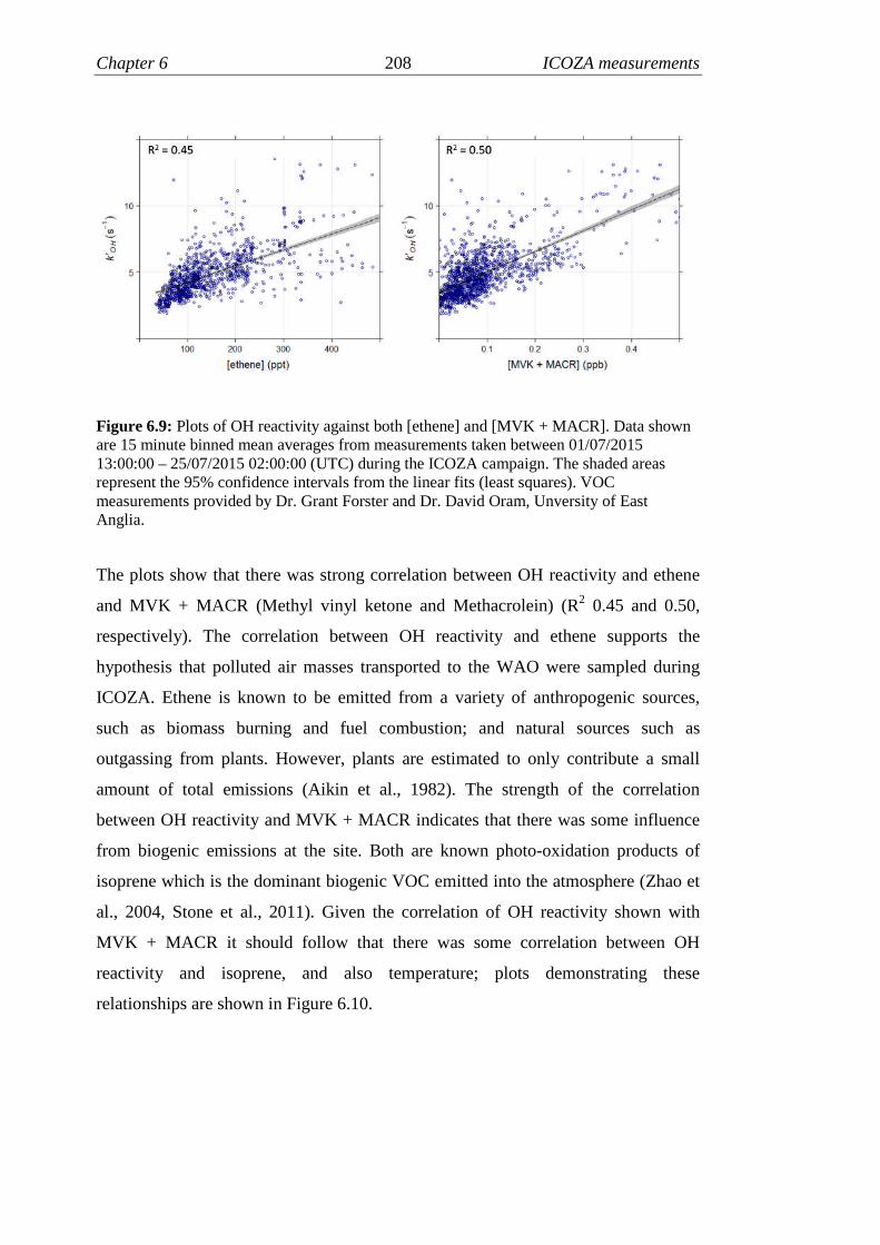
Chapter 6 208 ICOZA measurements
Figure 6.9: Plots of OH reactivity against both [ethene] and [MVK + MACR]. Data shownare 15 minute binned mean averages from measurements taken between 01/07/201513:00:00 – 25/07/2015 02:00:00 (UTC) during the ICOZA campaign. The shaded areasrepresent the 95% confidence intervals from the linear fits (least squares). VOCmeasurements provided by Dr. Grant Forster and Dr. David Oram, Unversity of EastAnglia.
The plots show that there was strong correlation between OH reactivity and ethene
and MVK + MACR (Methyl vinyl ketone and Methacrolein) (R2 0.45 and 0.50,
respectively). The correlation between OH reactivity and ethene supports the
hypothesis that polluted air masses transported to the WAO were sampled during
ICOZA. Ethene is known to be emitted from a variety of anthropogenic sources,
such as biomass burning and fuel combustion; and natural sources such as
outgassing from plants. However, plants are estimated to only contribute a small
amount of total emissions (Aikin et al., 1982). The strength of the correlation
between OH reactivity and MVK + MACR indicates that there was some influence
from biogenic emissions at the site. Both are known photo-oxidation products of
isoprene which is the dominant biogenic VOC emitted into the atmosphere (Zhao et
al., 2004, Stone et al., 2011). Given the correlation of OH reactivity shown with
MVK + MACR it should follow that there was some correlation between OH
reactivity and isoprene, and also temperature; plots demonstrating these
relationships are shown in Figure 6.10.

Chapter 6 209 ICOZA measurements
Figure 6.10: Plots of OH reactivity against both temperature in degrees C and [isoprene].Data shown are 15 minute binned mean averages from measurements taken between01/07/2015 13:00:00 – 25/07/2015 02:00:00 (UTC) during the ICOZA campaign. Theshaded areas represent the 95% confidence intervals from the linear fits (least squares).
It is shown that there are moderate correlations between OH reactivity and both
isoprene and temperature (R2 = 0.36 and 0.26, respectively). The correlation with
isoprene provides confirmation that biogenic emissions played some role in driving
changes seen in OH reactivity during ICOZA. Biogenic emissions such as isoprene
are known to increase with temperature (Di Carlo et al., 2004, Hansen et al., 2014).
It is likely the correlation observed here is partly due to increased biogenic
emissions. A full analysis of the potential drivers of changes in OH reactivity is
given in the remaining subsections of Section 6.3.2.
6.4.2.3 Relationship with wind direction and air mass origin
To gain further insight into the sources of the varying levels measured of OH
reactivity during ICOZA, the relationship with wind direction was examined and the
percentileRose function of the openair R package was used for this. The 15 minute
OH reactivity measurements, and wind directions measured at the top of the WAO
tower in the merged data set described in Section 6.3.2.2 were used. A wind rose is
shown in Figure 6.11(b) summarises the relationship between OH reactivity and
wind direction during ICOZA.

Chapter 6 210 ICOZA measurements
Fig
ure
6.1
1:
(a)
Map
tosh
ow
the
loca
tio
nal
rela
tio
nsh
ipb
etw
een
the
Wey
bo
urn
eA
tmos
ph
eric
Ob
serv
ato
ry(W
AO
)an
dth
eci
tyof
No
rwic
h.
(b)
Win
dro
seto
dem
ons
trat
eth
ede
pen
den
ceo
fm
easu
red
OH
reac
tivi
tyo
nw
ind
dir
ecti
ond
uri
ng
the
ICO
ZA
cam
pai
gn
.T
he
bla
ckli
ne
repr
esen
tsth
em
ean
ob
serv
edv
alu
efo
ra
giv
enw
ind
sect
or.
Co
lou
red
area
sre
pres
ent
the
per
cen
tile
lev
els
for
agi
ven
win
dse
cto
r.

Chapter 6 211 ICOZA measurements
During ICOZA the OH reactivity varied with wind direction, the black line in Figure
6.11(a) represents the mean values for the different wind sectors and shows that
measurements were typically higher on average (~6-9 s-1) when winds were
southerly to south easterly. This is unsurprising considering that these winds blew
from the land towards the sea and would have been expected to be more polluted
and have a higher loading of OH sinks. A satellite image in Figure 6.11(b) illustrates
the location of the city of Norwich relative to the WAO; Norwich is shown to be
south-southeast of the WAO. It is concluded that the higher mean OH reactivity
recorded when the wind was southerly to south easterly was likely a result of VOCs
and other OH reactive pollutants transported from Norwich. Figure 5.11(b) also
shows that on average for the campaign, the wind sectors with the lowest mean
values were typically between easterly, northerly and westerly. This comes as no
surprise considering that the air reaching the site in this case would be typically be
less polluted as it is of marine origin.
Whilst Figure 6.11 shows evidence for a dependency of OH reactivity observations
on wind direction, there are limitations to such an approach, as only speculative
conclusions can be made as to the location of sink sources. To investigate the
possible sources of sinks that contributed to OH reactivity during ICOZA, the
measurements were examined in the context of their origin as determined through
the calculation of the back trajectories of the ambient air that was sampled. The
Hybrid Single Particle Lagrangian Integrated Trajectory Model (HYSPLIT) was
used to calculate back trajectories using archived meteorological data provided by
the National Oceanic and Atmospheric Administration (NOAA) for air reaching the
WAO. The history of the air mass reaching the WAO was calculated for the
previous four days at a starting height of 10 m every three hours for July 2015. It
should be noted that whilst the back trajectories started at a height of 10 m, changes
in altitude of the air during transport to the measurement site are not considered.
Analyses which utilised back trajectories presented in this chapter should be
considered as preliminary. Future work should include a detailed assessment of the
impact variations in altitude could have on the results presented here.
Following the computation of back trajectories as described above, the openair
trajPlot function was used to examine the relationship between various back
trajectories, and the observed levels of OH reactivity. The results from such analysis

Chapter 6 212 ICOZA measurements
for 01/07/2014 and 02/07/2014 during the heat wave at the beginning of the
campaign where high OH reactivity was recorded are summarised in Figure 6.12.
Figure 6.12: Four day back trajectories calculated using HYSPLIT (10 m startingheight) for air reaching the WAO every three hours during ICOZA from 01/07/201513:00:00 to 02/07/2015 21:00:00. The colour of each back trajectory represents the meanOH reactivity for the hour.
From the afternoon to the end of 01/07/2015 the back trajectories show that the air
mass had spent considerable time over the UK and continental Europe. During this
time the three hour average OH reactivity measured ranged between ~10 – 12 s-1
which were the highest levels measured during the campaign. Following this in the
early hours of 02/07/2015 the origin of the air mass transitioned so that the air
reaching the WAO has spent less time passing over continental Europe. By the
afternoon the back trajectories show that the air mass reaching the WAO had spent
minimal time passing over continental Europe in the four days prior to arrival.
Through the course of this change in air mass the measured OH reactivity is shown
to drop to between 6 - 8 s-1.
To broadly investigate the origin of the sinks that contributed to the OH reactivity
measured at the site all of the back trajectories that were calculated for July 2014
were classified according to their profile using a cluster analysis, the openair
trajCluster function was used for this to assign clusters based on the Euclidian

Chapter 6 213 ICOZA measurements
(straight line) distances between each pair of back trajectories. This analysis showed
that the four day back trajectories for the air reaching the WAO during ICOZA fell
into three distinct categories. These are defined as Local, Northerly and Westerly;
they are summarised in Figure 6.13.
Figure 6.13: Clustered four day back trajectories determined using the openair trajClusterfunction to analyse back trajectories calculated every 3 three hours during ICOZA from01/07/2015 13:00:00 – 25/07/2015 02:00:00 (UTC). The blue line represents the path ofLocal air, the red line represents the path of Northerly air and the green line represents thepath of Westerly air.
The OH reactivity measurements were grouped according to the classification of air
mass that was sampled. Figure 6.14 shows daily averages of OH reactivity, the
heights of the bars are split according to the proportion of time each air mass type
reached the site.

Chapter 6 214 ICOZA measurements
Figure 6.14: Bar chart to show the average daily OH reactivities recorded during ICOZA.Averages were calculated using data from 01/07/2015 13:00:00 – 25/07/2015 02:00:00(UTC) and the height of each bar represents the portion of time that air of each classificationreached the site. See Figure 5.14 for definition of air mass.
It is shown that for most of the campaign, air of Westerly origin was dominant, air
masses of Local and Northerly origin reached the site less frequently. The highest
average daily OH reactivity was recorded at the beginning of the campaign during
the heat wave and further details regarding the variation in the origin of the air mass
at this time are described above. The origin of the air mass transitioned from Local
to Westerly. Following the heat wave Local air masses were only sampled twice
again on 11/07/2016 and 16/07/2016. On these occasions the OH reactivity sampled
did not reach the daily average levels that were recorded during the heatwave, it is
likely that the high OH reactivity recorded during the heatwave included a greater
contribution from products of VOC photo-oxidation, or temperature enhanced
emissions. When the air reaching the WAO was of Northerly origin OH reactivity
was typically lower and this is likely due to the predominantly oceanic and so less
polluted nature of the back trajectory for this classification. Whilst the cluster
analysis of the back trajectories can give indications as to the location of potential
sink sources, it is not possible to draw conclusions on the specific locations of
sources that contributed to OH reactivity as these could have been anywhere in the
path of the back trajectory. To gain further insight into the specific locations of sink
sources during ICOZA, the Concentration Weighted Trajectory (CWT) approach
was utilised using the openair trajLevel function. Figure 6.15 shows the CWT mean

Chapter 6 215 ICOZA measurements
average levels of OH reactivity that contributed to the observations at the WAO
during ICOZA.
Figure 6.15: Concentration Weighted Trajectory (CWT) mean contribution to OH reactivitymeasured at the WAO during ICOZA. Values were determined based on 15 minute OHreactivity data and three hourly back trajectories during ICOZA from 01/07/2015 13:00:00 –25/07/2015 02:00:00 (UTC).
The choropleth map represents the CWT mean contribution to the OH reactivity that
was measured at the WAO during the whole of ICOZA. The areas which likely
contributed the most to OH reactivity are darker whereas the lighter areas likely
contributed less. It is shown that the biggest contributions to the measurements
originated from the coastal area to the north of the Netherlands and also central
Germany, and the coastal area near the Belgium-Netherlands boarder where the port
of Rotterdam is situated. The contribution from the northern Netherlands coast is to
be expected as there are high volumes of shipping in this area as there are a number
of ports here and many vessels pass through these waters on their way to the
German port of Hamburg. Also, the port of Rotterdam is the largest in Europe so it
is so it is to be expected that shipping emissions originating from here contributed to

Chapter 6 216 ICOZA measurements
the measured OH reactivity when air was transported from here to the WAO. The
high CWT mean contribution shown over central Germany lies over the city of
Hanover which is home to many factories and other industrial developments which
are all likely to emit pollutants that could have contributed to the OH reactivity
measured. During the heat wave on 01/07/2015 the back trajectories passed over all
three of the areas described above, as shown in Figure 6.12. It is possible that had
there not been a heatwave at this time the CWT mean contributions for these areas
would not have been as high as those shown in Figure 6.15 if a large portion of the
reactivity measured at this time was accounted for by products of photo-oxidation. It
can also be seen from Figure 6.15 that the CWT mean contribution was higher over
England, Wales and surrounding waters than over Scotland and its surrounding
waters. The results of the cluster analysis discussed above support this by showing
that air originating from the North Sea, which may or may not have passed over
Scotland, reached the WAO for only a small portion of ICOZA. Figure 6.14 showed
that lowest daily average OH reactivities recorded were subject to air originating
from the North Sea. In order to further understand the nature of the OH reactivity
measured it was calculated using concentrations of co-measured sinks. Section
6.3.2.4 describes the method for this calculation and Section 6.3.2.5 compares and
discussed the measured and calculated values.
6.4.2.4 Calculation of OH reactivity
The merged 15 minute data set described in Section 6.3.2.2 was used for the
calculation of OH reactivity. Mixing ratios of OH sinks were converted to
concentrations using the temperatures and pressures contained within the
meteorological data. The resulting OH sink concentrations were used in conjunction
with corresponding bimolecular rate coefficients for the reaction between each sink
and OH as in E1.3 (reproduced below) to calculate a value of OH reactivity for each
15 minute bin. The sinks which were used to calculate OH reactivity for the ICOZA
campaign are listed in Table 6.2.
′ைு() = ைுା
[ܣ] E1.3

Chapter 6 217 ICOZA measurements
Sink Class ksink + OH
(cm3 molecule-1 s-1)Contribution toOH reactivity(s-1)
Instrument
O3 O3 7.3 × 10⁻¹⁴ 0.06 Thermo 49 SeriesNO NO 9.8 × 10⁻¹² 0.11 Air Quality Design Inc.
Chemiluminescence withLED NO2 converter
NO2 NO2 9.9 × 10⁻¹² 0.84
CO CO 2.3 × 10⁻¹³ 0.66 Ametek monitorHONO NOz 6.0 × 10⁻¹² 0.01 LOPAPMethanol Alcohol 9.0 × 10⁻¹³ 0.06 PTR-TOF-MSEthane Alkane 2.4 × 10⁻¹³ 0.07 GC-FIDPropane 1.1 × 10⁻¹² GC-FIDMethylpropane 2.2 × 10⁻¹² GC-FIDButane 2.4 × 10⁻¹² GC-FID2-Methylbutane 3.7 × 10⁻¹² GC-FIDPentane 4.0 × 10⁻¹² GC-FID2-Methylpentane 5.3 × 10⁻¹² GC-FIDHexane 5.5 × 10⁻¹² GC-FIDAcetylene Alkene and
Alkyne7.5 × 10-13 0.12 GC-FID
Ethene 7.8 × 10⁻¹² GC-FIDPropene 2.8 × 10⁻¹¹ GC-FIDtrans-But-2-ene 6.4 × 10⁻¹¹ GC-FIDBut-1-ene 3.1 × 10⁻¹¹ GC-FIDcis-But-2-ene 5.6 × 10⁻¹¹ GC-FIDBenzene Aromatic 1.2 × 10⁻¹² 0.01 PTR-TOF-MSToluene 5.6 × 10⁻¹² PTR-TOF-MSFormaldehyde Carbonyl 8.5 × 10⁻¹² 0.40 LIFAcetaldehyde 1.5 × 10⁻¹¹ PTR-TOF-MSAcetone 1.8 × 10⁻¹³ PTR-TOF-MSMethacrolein 2.9 × 10⁻¹¹ PTR-TOF-MSMethyl vinyl ketone 2.0 × 10⁻¹¹ PTR-TOF-MSMethyl ethyl ketone 1.1 × 10⁻¹² PTR-TOF-MS1,3-Butadiene Dialkene 6.7 × 10⁻¹¹ 0.33 GC-FIDIsoprene 1.0 × 10⁻¹⁰ PTR-TOF-MSAcetonitrile Unclassified 2.2 × 10⁻¹⁴ 0.05 PTR-TOF-MSDimethyl Sulfide 7.0 × 10⁻¹² PTR-TOF-MSSO2 8.9 × 10⁻¹³ Thermo 43 Series
Table 6.2: OH sinks measured during the ICOZA campaign used in the calculation of OHreactivity. Species were assigned classes according to their functionality. Bimolecular ratecoefficients for the reaction with OH at 298 K and 1 Atmosphere are shown howeverpressure and temperature dependencies were used in the calculation of OH reactivity.Campaign average contributions to OH reactivity are also shown for each sink classificationin addition to details of the instrument used for the measurement of each species.
Each sink was assigned to a class according to its functionality, so that grouped
contributions to calculated OH reactivity could be determined, these are also listed
with their campaign average contributions. Details of the instrument used to measure
each species are provided in addition to bimolecular rate coefficients for reaction
with OH. The values shown are those calculated at a temperature of 298 K and
pressure of 1 Atmosphere. For the calculation of OH reactivity, the values used were
determined using the temperature and pressure dependencies in conjunction with
measured temperatures and pressures by the WAO meteorological station. All
expressions for rate coefficients were IUPAC recommended values taken from the
Master Chemical Mechanism (MCM) v3.3 (Jenkin et al., 1997, Saunders et al.,
2003), with the exception of acetonitrile which was taken from directly from IUPAC
owing to it being absent from the MCM. The measured OH reactivity is presented in

Chapter 6 218 ICOZA measurements
Section 6.3.2.5 in addition to discussion of its relationship with the measured OH
reactivity.
6.4.2.5 Measured and calculated OH reactivity
The method for the calculation of OH reactivity using data from co-measurements of
OH sinks was described in Section 6.3.2.4. The resulting values are plotted in Figure
6.17 along with the measured values for comparison. The measured values are
significantly higher than the calculated values for the majority of the campaign,
implying the presence of ‘missing’ OH reactivity. The mean average measured OH
reactivity was 4.8 s-1 and the mean average of the calculated values, determined
where there was a corresponding measured value, was 2.7 s-1. The ‘missing’ OH
reactivity was 44 % on average for the campaign which is close to that determined
by Lee et al. (2009) for TORCH-2 (40 %, when a similar suite of VOCs were
measured at the WAO) when only measured species were used to calculate OH
reactivity. The correlation between measured and calculated OH reactivity is
presented in Figure 6.16. The majority of points typically occupy space around and
just above the line representing 50% underestimation by the calculation of OH
reactivity, which is not surprising considering that the ‘missing’ OH reactivity is 44
%. The linear least squares gradient is 0.56.
To gain further insight into factors which may have influenced the level of ‘missing’
OH reactivity, the agreements between the measured and calculated values for
individual days are considered. The plots in Figure 6.18, Figure 6.19 and Figure 6.20
compare measured and calculated OH reactivity for each day. In each plot the
measured OH reactivity is represented by the red line and the cumulative calculated
OH reactivity is represented by the top of the stacked structures. Each coloured band
represents a contribution to calculated OH reactivity from groups of measured OH
sinks (summarised in Table 5.2) that were measured. The categories of OH sinks in
order from the bottom of the stacked structures were: Dialkenes, Carbonyls, Alkenes
and Alkynes, Alkanes, NO2, NO and CO. To aid clarity, OH sink categories with an
average contribution of less than 0.1 s-1 have been omitted unless they were found to
contribute significantly (>0.5 s-1) at any point. The daily comparisons show that
there is significant variation in the discrepancy between the measured and calculated
OH reactivity. The greatest differences (as high as ~70 %) are shown for 01/07/2015
and 02/07/2015 which coincided with elevated temperatures during the heatwave
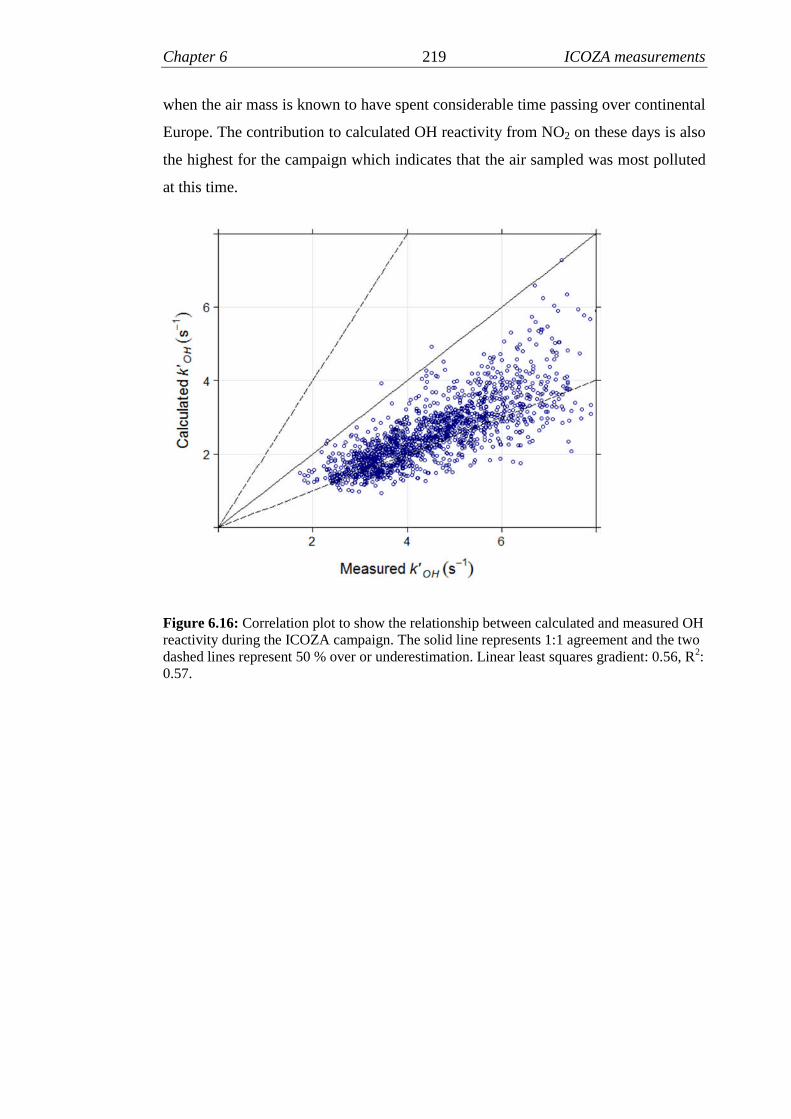
Chapter 6 219 ICOZA measurements
when the air mass is known to have spent considerable time passing over continental
Europe. The contribution to calculated OH reactivity from NO2 on these days is also
the highest for the campaign which indicates that the air sampled was most polluted
at this time.
Figure 6.16: Correlation plot to show the relationship between calculated and measured OHreactivity during the ICOZA campaign. The solid line represents 1:1 agreement and the twodashed lines represent 50 % over or underestimation. Linear least squares gradient: 0.56, R2:0.57.

Chapter 6 220 ICOZA measurements
Fig
ure
6.1
7:M
easu
red
OH
reac
tiv
ity
(red
lin
e)an
dca
lcu
late
dO
Hre
acti
vit
y(g
rey
das
hed
lin
e)fo
rth
eIC
OZ
Aca
mpa
ign
.D
ata
are
plo
tted
at1
5m
inut
eti
me
inte
rval
s.

Chapter 6 221 ICOZA measurements
Figure 6.18: Daily comparisons (1st July – 8th July 2015) of measured total OH reactivity(red line) with cumulative calculated OH reactivity (stacked coloured structures) from theICOZA campaign. Calculated contributions for each OH sink classification were determinedusing data for all species measured that are summarised in Table 6.2.
16 16
14 14
12 12
10 10
8 8
6 6
4 4
2 2
0 0
kO
H(s
-1)
06:00 12:00 18:00Time of Day (UTC)16 16
14 14
12 12
10 10
8 8
6 6
4 4
2 2
0 0
kO
H(s
-1)
06:00 12:00 18:00Time of Day (UTC)
16 16
14 14
12 12
10 10
8 8
6 6
4 4
2 2
0 0
kO
H(s
-1)
06:00 12:00 18:00Time of Day (UTC)
16 16
14 14
12 12
10 10
8 8
6 6
4 4
2 2
0 0
kO
H(s
-1)
06:00 12:00 18:00Time of Day (UTC)
16 16
14 14
12 12
10 10
8 8
6 6
4 4
2 2
0 0
kO
H(s
-1)
06:00 12:00 18:00Time of Day (UTC)
16 16
14 14
12 12
10 10
8 8
6 6
4 4
2 2
0 0
kO
H(s
-1)
06:00 12:00 18:00Time of Day (UTC)
16 16
14 14
12 12
10 10
8 8
6 6
4 4
2 2
0 0
kO
H(s
-1)
06:00 12:00 18:00Time of Day (UTC)
01/07/2015 02/07/2015
03/07/2015 04/07/2015
05/07/2015 06/07/2015
07/07/2015 08/07/2015
CO NO NO2 Alkanes
Alkenes & Alkynes CarbonylsDialkenes Measured OH reactivity
16 16
14 14
12 12
10 10
8 8
6 6
4 4
2 2
0 0
kO
H(s
-1)
06:00 12:00 18:00Time of Day (UTC)

Chapter 6 222 ICOZA measurements
Figure 6.19: Daily comparisons (9th July – 16th July 2015) of measured total OH reactivity(red line) with cumulative calculated OH reactivity (stacked coloured structures) from theICOZA campaign. Calculated contributions for each OH sink classification were determinedusing data for all species measured that are summarised in Table 6.2.
16 16
14 14
12 12
10 10
8 8
6 6
4 4
2 2
0 0
kO
H(s
-1)
06:00 12:00 18:00Time of Day (UTC)
16 16
14 14
12 12
10 10
8 8
6 6
4 4
2 2
0 0
kO
H(s
-1)
06:00 12:00 18:00Time of Day (UTC)
16 16
14 14
12 12
10 10
8 8
6 6
4 4
2 2
0 0
kO
H(s
-1)
06:00 12:00 18:00Time of Day (UTC)
16 16
14 14
12 12
10 10
8 8
6 6
4 4
2 2
0 0
kO
H(s
-1)
06:00 12:00 18:00Time of Day (UTC)
16 16
14 14
12 12
10 10
8 8
6 6
4 4
2 2
0 0
kO
H(s
-1)
06:00 12:00 18:00Time of Day (UTC)
16 16
14 14
12 12
10 10
8 8
6 6
4 4
2 2
0 0
kO
H(s
-1)
06:00 12:00 18:00Time of Day (UTC)
16 16
14 14
12 12
10 10
8 8
6 6
4 4
2 2
0 0
kO
H(s
-1)
06:00 12:00 18:00Time of Day (UTC)16 16
14 14
12 12
10 10
8 8
6 6
4 4
2 2
0 0
kO
H(s
-1)
06:00 12:00 18:00Time of Day (UTC)
09/07/2015 10/07/2015
11/07/2015 12/07/2015
13/07/2015 14/07/2015
15/07/2015 16/07/2015
CO NO NO2 Alkanes
Alkenes & Alkynes CarbonylsDialkenes Measured OH reactivity

Chapter 6 223 ICOZA measurements
Figure 6.20: Daily comparisons (17th July – 24th July 2015) of measured total OH reactivity(red line) with cumulative calculated OH reactivity (stacked coloured structures) from theICOZA campaign. Calculated contributions for each OH sink classification were determinedusing data for all species measured that are summarised in Table 6.2.
16 16
14 14
12 12
10 10
8 8
6 6
4 4
2 2
0 0
kO
H(s
-1)
06:00 12:00 18:00Time of Day (UTC)
16 16
14 14
12 12
10 10
8 8
6 6
4 4
2 2
0 0
kO
H(s
-1)
06:00 12:00 18:00Time of Day (UTC)
16 16
14 14
12 12
10 10
8 8
6 6
4 4
2 2
0 0
kO
H(s
-1)
06:00 12:00 18:00Time of Day (UTC)
16 16
14 14
12 12
10 10
8 8
6 6
4 4
2 2
0 0
kO
H(s
-1)
06:00 12:00 18:00Time of Day (UTC)
16 16
14 14
12 12
10 10
8 8
6 6
4 4
2 2
0 0
kO
H(s
-1)
06:00 12:00 18:00Time of Day (UTC)
16 16
14 14
12 12
10 10
8 8
6 6
4 4
2 2
0 0
kO
H(s
-1)
06:00 12:00 18:00Time of Day (UTC)
16 16
14 14
12 12
10 10
8 8
6 6
4 4
2 2
0 0
kO
H(s
-1)
06:00 12:00 18:00Time of Day (UTC)
16 16
14 14
12 12
10 10
8 8
6 6
4 4
2 2
0 0
kO
H(s
-1)
06:00 12:00 18:00Time of Day (UTC)
17/07/2015 18/07/2015
19/07/2015 20/07/2015
21/07/2015 22/07/2015
23/07/2015 24/07/2015
CO NO NO2 Alkanes
Alkenes & Alkynes CarbonylsDialkenes Measured OH reactivity

Chapter 6 224 ICOZA measurements
The plots for individual days demonstrate how the measured OH reactivity varies
typically in the same way as the calculated values. However, there are periods of
time where the profile of the measured values does not track that of the calculated.
For example the spikes in measured OH reactivity just before 1200 on 02/07/2015
and 05/07/2015. It is likely that these are the result of a short lived elevated
concentration of an OH sink that either was not measured, or was measured but rose
and fell in concentration during the time where, for example, GC-FID measurements
were linearly interpolated to achieve 15 minute time resolution.
The contribution from NO2 to the calculated values is significantly more variable
than those for other classifications of OH sink, and that changes in measured OH
reactivity were almost always accompanied by a change in the calculated
contribution from NO2. This is expected considering the strength of the correlation
with NO2 presented in Section 6.3.2.2 and indicates that for the majority of ICOZA
anthropogenic emissions drove the observed changes in OH reactivity.
Contributions from classes of OH sink other than NO2 do not vary to the same
extent on most days for which data are shown in Figure 6.18, Figure 6.19 and Figure
6.20. The class that showed the most variation after NO2 is the dialkenes which
includes contributions from isoprene and butadiene. These were shown to contribute
the most to OH reactivity on 01/07/2015 and 02/07/2015 during and following the
heat wave. This contribution from dialkenes at this time was almost exclusively
driven by isoprene, which accounted for 91 % on 01/07/2015 and 99 % on
02/07/2015. This indicates that biogenic emissions, and their photo-oxidation
products contributed to the OH reactivity measured during the heat wave as well as
anthropogenic emissions.
On 01/07/2015 the daily average contribution from carbonyls to calculated OH
reactivity (0.86 s-1) was the highest recorded during the campaign. The largest
contributor was acetaldehyde (50 %) followed by MVK + MACR (23 %) and
formaldehyde (24 %). The largest atmospheric acetaldehyde source is thought to be
the photochemical degradation of VOCs such as small alkanes and alkenes
(Atkinson et al., 2006). The campaign average contribution from acetaldehyde to the
carbonyl class was 31 % which is significantly lower than it was on 01/07/2015.
This supports the hypothesis that a large portion of the OH reactivity during the heat
wave could be attributed to increased photo-chemical processing of anthropogenic

Chapter 6 225 ICOZA measurements
VOCs, such as those from vehicles. Small alkanes and alkenes such as ethane,
propane and propene are known to be directly emitted from combustion engines and
these could have been processed more rapidly (Nakashima et al., 2012).
Acetaldehyde is also known to be emitted from sea water as a result of
photochemical degradation of dissolved organic matter, a source which has been
postulated to be the second largest globally (Millet et al., 2010, Kieber et al., 1990).
The campaign average contribution from MVK + MACR was 12 % which, similarly
to acetaldehyde, is lower than it was on 01/07/2015. This observation further
supports the hypothesis that biogenic emissions could have played a significant role
in driving changes in OH reactivity during the start of campaign heat wave. It should
be noted here that the contribution from formaldehyde to the carbonyl class is an
estimate based on the average level measured from 08/07/2015 – 24/07/2015. This
was necessary due to problems encountered with the HCHO LIF instrument at the
beginning of the campaign. The contribution from HCHO here could have been far
greater considering that the high temperatures that would have likely resulted in the
most rapid photo-chemical processing of VOCs during the campaign.
As discussed above the discrepancy between the measured and calculated OH
reactivity during ICOZA was greatest during the heatwave and a significant portion
could be accounted for by a combination of anthropogenic and biogenic emissions,
and their photo-oxidation products. Lee et al. (2009) reported that during the
TORCH-2 campaign when a model was used to simulate the production of photo-
oxidation products (which were not measured), the ’missing’ reactivity was reduced
from 40 % to 30 %. The use of a zero dimensional chemical box model to calculate
the OH reactivity during ICOZA would also reduce the ‘missing’ OH reactivity.
This should form the basis of future work on the study of OH reactivity during
ICOZA.
Whalley et al. (2016) reported that a steady state concentration of RO2 ([RO2]ss) can
be calculated using E6.1, when it is assumed that the reaction between OH and NO
to form HONO is a temporary radical sink, and that the reaction between OH and
NO2 is a permanent radical sink. It was also reported that the [RO2]ss can be used to
estimate the rate of ozone production (P(O3)) from the reaction of RO2 with NO (to
form NO2 which is subsequently photolysed leading to O3 production) minus a
correction to account for reaction of NO2 with OH (which makes it unavailable for
O3 production), E6.2.

Chapter 6 226 ICOZA measurements
[ROଶ]ୱୱ = (ᇱୌ
− ൫ ୌାమ[NOଶ] + ୌା [NO] + ୌାయ
[Oଷ] + ୌାେ[CO]
+ ୌାୌେୌ [HCHO]൯[OH]) / ( మା[NO])
E6.1
(Oଷ) = మା[ROଶ]ୱୱ[NO] − ୌାమ[OH][NOଶ] E6.2
The average daytime (from 0600 – 2000 UTC) OH reactivity measured during
ICOZA was 4.75 s-1. This was used in conjunction with average daytime values of
[NO2], [NO], [O3], [HCHO], and preliminary daytime average [OH] (5 × 10⁶
molecule cm-3) as in E6.1. [RO2]ss was found to be equal to 4.3 × 10⁸ molecule cm-3
for ICOZA, this corresponded to a daily average estimated P(O3) value of ~39 ppb
d-1 as calculated using E6.2. In both calculations rate coefficients used were those
shown in Table 6.2 with the exception of మାthat was assumed to be equal to
େమୌఱା� at 298 K (2.6 × 10⁻¹² cm3 molecule-1 s-1, DeMore et al. (1997)). When
the average daytime calculated OH reactivity is used in E6.1, in place of the
measured OH reactivity, the value of [RO2]ss determined is 2.0 × 10⁸ molecule cm-3
(a 53 % reduction) and corresponds to a daily average estimated P(O3) value of ~12
ppb. This analysis means that ~27 ppb d-1 (~69 %) of the daily average O3
production during ICOZA could have resulted from photo-oxidative processing of
VOCs that were not measured (assuming that the missing OH reactivity was
attributable to VOCs) and demonstrates the value of OH reactivity as a
measurement. If the method reported by Ehlers et al. (2016) had been used to
calculate O3 production rates for ICOZA, using the calculated OH reactivity
attributable to measured VOCs, and the calculated OH reactivity that is attributable
to measured NO2 with a computer model simulation, O3 production would have
been severely underestimated. Based on the assumption that ‘missing’ OH reactivity
reported for ICOZA was exclusively due to unmeasured VOCs, the average daily
production rate would be underestimated by ~69 %. However, it is likely that a
significant portion of the discrepancy could be accounted for by unmeasured
products of photo-oxidation. As mentioned above, future work should include a
computer modelling study to assess the contribution from unmeasured photo-
oxidation products, of measured VOCs, to the measured OH reactivity during
ICOZA. The estimation of a third daily average O3 production rate, using the OH
reactivity predicted by the model, should be compared with the estimates above to
further investigate sources of O3. Further to this, the estimated production rates

Chapter 6 227 ICOZA measurements
should be compared with those directly measured by the POPR instrument
(University of Birmingham).
6.5 Formaldehyde
6.5.1 Formaldehyde observations
The LIF instrument for the measurement of HCHO was deployed for the ICOZA
campaign and was operated in configuration 3 as described in Section 2.3.6. The
instrument was placed inside the WAO laboratory and measurements were made
from a glass manifold which sampled ambient air from the top of the tower
(described in Section 6.2). It was not possible to measure HCHO at the beginning of
the campaign owing to problems encountered with communication between the
instrument computer and the photon counting card, and also low laser power
resulting from an electronic fault within the control unit of the fibre laser. Both of
these problems were resolved by 08/07/2015 and measurements were made near
continuously following this. The only unplanned gap in the data arose from a run
down battery in the photodiode which meant it was not possible to normalise the
LIF signal for laser power for some time on 14/07/2015 and 15/07/2015. The
photograph in Figure 6 shows the instrument inside the WAO laboratory during the
ICOZA campaign.
The levels of HCHO observed were found to vary significantly during the course of
the ICOZA campaign; the observed levels were typically between 500 and 2000 ppt
with a mean average of ~990 ppt. A complete time series for the ICOZA
measurements is shown in Figure 6.21. The daily trend in HCHO levels was largely
consistent through the campaign; increases were typically seen through the late
morning and daytime hours and decreases were typically seen through the night time
and early morning hours. The diurnal behaviour is discussed in detail in Section
6.4.2.1.

Chapter 6 228 ICOZA measurements
Figure 66.21: Photograph of the LIF HCHO instrument inside the WAO laboratory duringthe ICOZA campaign.
On the 08/07/2015 and 09/07/2015 HCHO was typically less than 1000 ppt before
increasing on the 10/07/2015 where levels were typically higher than 1000 ppt and
showed greater variation through the course of each day (~1000 ppt to ~ 2000 ppt).
From the 21/07/2015 the measurements were typically lower until the end of the
campaign. An exception to this is a period where large rapid excursions are shown
during the early hours of the 25/07/2015 which coincided with a heavy
thunderstorm. These data are plotted in Figure 6.22 to enable closer inspection.
During the storm the level of HCHO was shown to fluctuate by as much as ~1000
ppt on an order of minutes. The storm is known to have started at ~2200 on
24/07/2015 and ended at ~0600 on 25/07/2015. Figure 6.22 shows that HCHO levels
behaved in a similar manner from ~0600 - ~1200 on 25/07/2015. The mean level of
HCHO for ICOZA was ~985 ppt when the data from the storm were not considered.
A more detailed discussion of the HCHO observed during and following the storm is
given in Section 6.4.2.3.

Chapter 6 229 ICOZA measurements
Fig
ure
6.2
1:
Tim
ese
ries
of
mea
sure
d[H
CH
O]
duri
ng
the
ICO
ZA
cam
pai
gn
.D
ata
are
plot
ted
wit
h1
min
ute
tim
ere
sult
ion
.T
he
un
usu
albe
hav
iou
ro
nJu
ly2
5th
coin
cid
edw
ith
ath
und
erst
orm
atth
esi
te.

Chapter 6 230 ICOZA measurements
Figure 6.22: HCHO measurements plotted at 1 minute time intervals for 17:00:0024/07/2015 – 14:00:00 25/07/2015 during the storm.
6.5.2 Interpretation of formaldehyde observations
6.5.2.1 Diurnal behaviour
The time series of HCHO measurements made during the ICOZA campaign
presented in Section 6.4.1 showed that the daily trend was fairly similar on most
days of the campaign where measurements were made. To enable a broad
examination of the major drivers of the HCHO levels observed with respect to its
chemistry, a diurnal profile was calculated for the ‘average day’. Measurements
were averaged into 96 time bins with a mean value every 15 minutes; Figure 6.23
shows the resulting diurnal profile.

Chapter 6 231 ICOZA measurements
Figure 6.23: Diurnal profile of [HCHO] observed during the ICOZA campaign in 15minute time bins. Error bars ± 1 σ standard deviation from the mean observation, and are a measure of the variability of HCHO levels during a 15 minute time bin.
Formaldehyde levels demonstrated clear diurnal behaviour during ICOZA and the
profile is very typical of that for an environment where formaldehyde production is
largely driven by photo-oxidation of VOCs. For example, the shape is very similar
to that reported in the literature for clean marine environments. Ayers et al. (1997)
reported a diurnal profile in 1993 measurements made in Cape Grim, Tasmania, and
is consistent with there being net photochemical production during the daylight
hours with more or less continuous loss to deposition which led to net loss in the
night time hours. The level of HCHO is shown to increase from ~0600 and continue
to rise until it plateaued towards a maximum at ~1600 when the sunlight driving the
photochemical source would have been less intense. Following this a decrease is
seen through the night until sunrise.

Chapter 6 232 ICOZA measurements
6.5.2.2 Correlations with other species measured
The relationship between the observed levels of HCHO and other species /
parameters measured was examined to further investigate the nature of potential
sources. The shape of the diurnal profile in Figure 6.26 indicates that the dominant
source of HCHO during ICOZA was photochemical rather than direct emissions,
e.g. those from engine combustion, industrial processes or the ocean. To assess the
likelihood as to whether or not a such a direct emission source significantly
impacted the HCHO measurements the relationship with NOx was assessed.
Correlation plots to demonstrate these relationships are shown in Figure 6.24.
Figure 6.24: Plots of measured [HCHO] against both [NO] and [NO2]. Data shown are 15minute binned mean averages from measurements taken between 01/07/2015 13:00:00 –25/07/2015 02:00:00 (UTC) during the ICOZA campaign. The shaded areas represent the95% confidence intervals from the linear fits (least squares).[NO] and [NO2] measurementswere provided by Dr. James Lee, University of York.
Measured HCHO did not correlate with either NO or NO2 during ICOZA,
supporting the conclusion that the main source and driver of change in the HCHO
observed was photochemical in origin. If a strong direct emission source impacted
the measurements, some level of correlation would have been expected, as NOx,
similar to HCHO is a major by-product of fuel combustion and many industrial
processes. To further investigate the photolytic HCHO source, the relationships with
temperature and J(O1D) were examined. Correlation plots to demonstrate these
relationships are shown in Figure 6.25.

Chapter 6 233 ICOZA measurements
Figure 6.25: Plots of measured [HCHO] against both temperature and J(O1D). Data shownare 15 minute binned mean averages from measurements taken between 01/07/201513:00:00 – 25/07/2015 02:00:00 (UTC) during the ICOZA campaign. The shaded areasrepresent the 95% confidence intervals from the linear fits (least squares).
A clear correlation is shown between the level HCHO and the temperature of
ambient air (R2 = 0.40). This supports the conclusion that a large portion of the
HCHO source during ICOZA was photochemical, as higher temperatures typically
coincide with with more rapid photo-oxidation of VOCs. However, it is possible that
to some extent that the correlation was influenced by direct biogenic emissions of
HCHO as the comparison of OH reactivity and individually measured sinks (Section
6.3.2.2) showed evidence that there was some biogenic influence. It has been
reported that direct HCHO emissions from plants have a positive temperature
dependency (DiGangi et al., 2011). It is also shown that there was no correlation
between the level of HCHO observed and the photolytic production rate of O1D,
J(O1D), which at first is surprising. However, it must be considered that the WAO is
regularly subjected to air masses which are transported from considerable distances
and that HCHO would be formed photochemically during this transport. HCHO
typically has an atmospheric lifetime of a few hours (Jones et al., 2009) and so could
be present in an air mass reaching the site having been produced a considerable
distance away. If the air mass had been static during ICOZA, some level of
correlation with J(O1D) would be expected. During the York 2014 ‘missing’ OH
reactivity campaign a reasonably strong correlation (R2 = 0.32) was reported
(Chapter 5). During this campaign wind speeds were much lower (0.35 m s-1
compared with 5.6 m s-1) and so a greater portion of the photochemically produced

Chapter 6 234 ICOZA measurements
HCHO would have been formed locally through reactions involving locally
produced O1D.
Unfortunately, numerous instruments failed during the thunder storm between 24-
25th July. Data that were available (NOy, CO, metorological and PTR measured
species) were used to investigate any possible relationship with HCHO. No
correlations could be identified for this period. Although the temporal resolution is
remarkable, it is not possible to draw conclusions here on potential sources of
HCHO during the storm. A discussion of the possible cause of the HCHO during the
storm is presented in Section 6.4.2.3 in the context of the origin of air mass as
determined by the calculations of back trajectories.
6.5.2.3 Relationship with wind direction and air mass origin
During TORCH-2 HCHO was reported to be dependent on wind direction (Lee et
al., 2009). It was found that HCHO was typically higher when the wind blew from
the land than from the sea. When the wind was westerly to southerly to easterly the
level of HCHO reported was ~750 – 1100 ppt. Whereas when the wind was westerly
to northerly to easterly the levels were typically ~500 – 750 ppt. To investigate the
relationship between HCHO and wind direction during ICOZA, the openair
percentileRose function used. The 15 minute HCHO measurements, and the wind
directions measured at the top of the WAO tower in the merged data set described in
Section 6.3.2.2 were used. Figure 6.26 shows a wind rose for the HCHO measured
during ICOZA and a map to show the location of the WAO. Data recorded during
the storm were not included in this analysis.
It is shown that the highest (~1000 – 1500 ppt) mean HCHO was recorded when the
wind was southerly to south westerly and similar to TORCH-2 the wind sector mean
values were all greater than 500 ppt from westerly to southerly to easterly. The
lowest mean values were observed for wind sectors from northerly to easterly which
was also the case during TORCH-2. The dependence of HCHO levels on wind
direction varies from that observed for OH reactivity where the highest mean values
were shown to be for south easterly air, caused by higher values that were recorded
during the heatwave at the beginning of the campaign. This is not reflected for
HCHO in Figure 6.27 because measurements did not start until after the heatwave.

Chapter 6 235 ICOZA measurements
Fig
ure
6.2
6:
Win
dro
seto
dem
ons
trat
eth
ede
pen
den
ceo
fm
easu
red
[HC
HO
]on
win
dd
irec
tio
nd
urin
gth
eIC
OZ
Aca
mp
aig
n.
Th
ebl
ack
line
rep
rese
nts
the
mea
no
bse
rved
val
ue
for
ag
iven
win
dse
cto
r.C
olo
ured
area
sre
pre
sen
tth
epe
rcen
tile
lev
els
for
agi
ven
win
dse
cto
r.

Chapter 6 236 ICOZA measurements
It was not possible to conduct a similar analysis as conducted for OH reactivity
using back trajectories to identify possible source locations for HCHO for the whole
of ICOZA. As stated above, the majority of the HCHO observed is thought to have
been photo chemically produced and so would have been produced in situ during
transport to the WAO. An exception to this was the 24-25/07/2015 storm which
occurred during the night when there would have been no photochemical source.
Figure 6 shows how the level of HCHO observed changed with the course of the
back trajectory of the air reaching the WAO during the storm. The back trajectories
were calculated as described in Section 6.3.2.3.
Figure 66.28: Four day back trajectories calculated using HYSPLIT (10 m starting height)for air reaching the WAO every three hours during ICOZA from 24/07/2015 00:00:00 to25/07/2015 21:00:00 (UTC). The colour of each back trajectory represents the mean[HCHO] for the hour. Thundersorm onset was at ~2200 on 24/07/2015.
The back trajectories show a change in air mass simultaneous with the onset of the
storm. Prior to the storm air of Atlantic origin was transported across southern
England to the North Norfolk coast. As the storm began at ~2100 on 24/07/2015 the

Chapter 6 237 ICOZA measurements
back trajectories show that the air sampled had a brief excursion over the North Sea
before returning to the coast where it was sampled at the WAO. It is not possible to
draw any conclusions here as to the cause of the behaviour of HCHO during the
night time storm. Following cessation of the storm at ~0600 on 25/07/2015 the back
trajectories show that the path travelled changed so that it no longer passed over
Southern England. It passed from the North Atlantic over Scotland into the North
Sea before taking a sharp change in course to reach the WAO. At ~1200 on
25/07/2015 it is shown that the path travelled changed again so that transport into
the North Sea did not occur and a more direct path was taken from the North
Atlantic.
Figure 6.22 showed a pause in the rapid fluctuations of HCHO observed at ~0600 on
25/07/2015 when the storm ended. Following this the HCHO measurements started
to behave in a similar manner to during the night-time storm until ~1200 when the
profile of and level of HCHO returned to that typical for the rest of the campaign.
On the morning of 25/07/2015 before ~1200 the waves in the North Sea near the
WAO were the biggest observed and the water was visibly the most turbulent during
the whole of the ICOZA campaign, the sunlight was also intense at this time. It is
possible the HCHO fluctuations on the morning after the storm were due to a
combination of the rougher sea and increased irradiation as the sun rose. Dissolved
organic matter in sea water is known to make HCHO when irradiated with sunlight
and more of this matter may have been available for photolytic degradation when
the sea was more turbulent (Kieber et al., 1990).
It should be stressed that the possible reasons given for the unusual HCHO
behaviour observed during the storm are not conclusive. To the knowledge of the
author there are no other examples of such behaviour reported in the literature.
Unfortunately due to the failure of other instruments during the storm only a limited
analysis in the context of other observations could be conducted. It is suggested that
laboratory experiments are conducted where sea water disturbed and irradiated with
a lamp of similar spectral output to that of the sun whilst HCHO is measured in the
headspace. This would allow the hypothesis that photodegradation of organic matter
was a source of HCHO that contributed to unusual behaviour following the storm to
be tested. Further to investigation of the cause of the unusual behaviour of HCHO
observed during the thunder storm, it is suggested that a zero-dimensional chemical

Chapter 6 238 ICOZA measurements
box modelling study is conducted, using the MCM, to further investigate the HCHO
budget during ICOZA.
6.6 Summary and conclusions
Measurements of OH reactivity and formaldehyde are presented from the ICOZA
campaign which took place at the WAO on the North Norfolk Coast in July 2015.
The campaign formed as a collaboration between researchers at the University of
Leeds, University of Birmingham, University of York, University of East Anglia
and University of Leicester.
OH reactivity was measured near continuously from 29/06/2015 to 22/07/2015 with
few unplanned gaps in the data coverage. Measurements stopped on 22/07/2015 due
to a problem encountered with the signal of the reference cell used to tune the
wavelength of the 308 nm probe laser for the detection of OH. Formaldehyde was
measured near continuously from 08/07/2015 – 31/07/2015. It was not possible to
measure formaldehyde at the beginning of the campaign due to problems
encountered with the computer used to control the LIF instrument and also a
problem with low laser power from the fibre laser.
The mean OH reactivity measured was 5.1 s-1 and individual measurements were
shown to vary between 1.7 and 27.7 s-1. The mean was similar to that reported
previously at the WAO during TORCH-2 (4.8 s-1). Some of the highest
measurements were made during a heatwave at the beginning of the campaign when
the maximum temperature recorded was ~29 ˚C on 01/07/2015. At this time back
trajectory analysis showed that the air in which OH reactivity was measured had
spent a considerable amount of time being transported over both the UK and
continental Europe in the four days prior to arrival at the WAO. A cluster analysis of
the back trajectories concluded that the air masses sampled during ICOZA could be
assigned one of three distinct classifications. These were Atlantic, North Sea and
Local European. Atlantic air masses, where the air had passed over Southern
England, were found to dominate the majority of the campaign. Back trajectories
were used to calculate CWT mean OH reactivities to investigate the locations of
potential sources of OH reactivity. It was shown that the greatest sources of OH
sinks were likely to be along the coast of the Netherlands, and central Germany. OH
reactivity was calculated using the concentrations of co-measured identifiable OH
sinks for 01/07/2015 – 22/07/2015. The average calculated OH reactivity for this

Chapter 6 239 ICOZA measurements
period was 2.7 s-1, the ‘missing’ OH reactivity was 44 % which was comparable to
that reported for TORCH-2 where 40 % was reported to be ‘missing’. It was
concluded that changes in the OH reactivity measured were largely driven by NOx
emissions and that the missing OH reactivity was likely due to a combination of
primary and secondary unmeasured anthropogenic and biogenic VOCs. The
measured OH reactivity and that calculated using concentrations of OH sinks, were
each used to estimate a daily average production rate of O3 through calculation of a
steady state concentration of RO2. When the measured OH reactivity was used, this
was estimated at ~39 ppb d-1, whereas when the calculated OH reactivity was used it
was estimated at ~12 ppb d-1 (69 % lower). It is not known at present what portion
of this difference could be reconciled by taking into account products of photo
oxidation in the prediction of OH reactivity, using a computer model. It is suggested
that further work relating to the OH reactivity measurements includes a modelling
study to assess the magnitude of the contribution from products of the photo
oxidation of measured species that may have contributed to OH reactivity.
Following this the daily average O3 production rate should be estimated using the
model predicted OH reactivity to assess what portion of the 69 % discrepancy is
accounted for by model generated intermediates. The estimated ozone production
rates should also be compared with direct measurements made using the University
of Birmingham POPR instrument.
The mean level of formaldehyde observed during ICOZA was ~990 ppt and was
found to vary by ~1000 – 2000 ppt through the course of each day. Clear diurnal
behaviour was observed and was consistent with what has been previously reported
in the literature, for an environment where the dominant source of formaldehyde is
the photochemical processing of VOCs. The dependence of measured formaldehyde
levels on wind direction was roughly in line with what was reported at the WAO
during TORCH-2. An interesting observation of formaldehyde during ICOZA was
that which occurred during, and after a storm on 24-25/07/2015 where the
concentration was seen to rapidly (on an order of minutes) fluctuate by up to ~1000
ppt. No correlation between formaldehyde and any other measurement could be
found for this time period and many instruments failed during the storm. It was
concluded that a possible source of some of the formaldehyde following the storm
could have been due an increased flux from the sea. Formaldehyde formed from
photo degradation of dissolved organic matter could have been a greater source at

Chapter 6 240 ICOZA measurements
this time due to the high swell of the sea. It is suggested that future work to further
rationalise these observations takes the form of a laboratory experiment to try and
simulate these conditions in a controlled setting whilst formaldehyde is measured.
6.7 References
AIKIN, A. C., HERMAN, J. R., MAIER, E. J. & MCQUILLAN, C. J. 1982.Atmospheric chemistry of ethane and ethylene. Journal of GeophysicalResearch: Oceans, 87, 3105-3118.
ATKINSON, R., BAULCH, D. L., COX, R. A., CROWLEY, J. N., HAMPSON, R.F., HYNES, R. G., JENKIN, M. E., ROSSI, M. J., TROE, J. &SUBCOMMITTEE, I. 2006. Evaluated kinetic and photochemical data foratmospheric chemistry: Volume II – gas phase reactions of organicspecies. Atmos. Chem. Phys., 6, 3625-4055.
AYERS, G. P., GILLETT, R. W., GRANEK, H., DE SERVES, C. & COX, R. A.1997. Formaldehyde production in clean marine air. Geophysical ResearchLetters, 24, 401-404.
BANNAN, T. J., BOOTH, A. M., BACAK, A., MULLER, J. B. A., LEATHER, K.E., LE BRETON, M., JONES, B., YOUNG, D., COE, H., ALLAN, J.,VISSER, S., SLOWIK, J. G., FURGER, M., PRÉVÔT, A. S. H., LEE, J.,DUNMORE, R. E., HOPKINS, J. R., HAMILTON, J. F., LEWIS, A. C.,WHALLEY, L. K., SHARP, T., STONE, D., HEARD, D. E., FLEMING, Z.L., LEIGH, R., SHALLCROSS, D. E. & PERCIVAL, C. J. 2015. The firstUK measurements of nitryl chloride using a chemical ionization massspectrometer in central London in the summer of 2012, and an investigationof the role of Cl atom oxidation. Journal of Geophysical Research:Atmospheres, 120, 5638-5657.
BOHN, B., KRAUS, A., MÜLLER, M. & HOFZUMAHAUS, A. 2004.Measurement of atmospheric O3 → O(1D) photolysis frequencies using filterradiometry. Journal of Geophysical Research: Atmospheres, 109,D10S90.
CARSLAW, D. C. 2015. The openair manual - open-source tools for analysing airpollution data. Manual for version 1.1-4, King's College London.
CARSLAW, D. C. & ROPKINS, K. 2012. openair - an R package for air qualitydata analysis. Environmental Modelling and Software, 27-28, 52-61.
CAZORLA, M. & BRUNE, W. H. 2010. Measurement of Ozone Production Sensor.Atmos. Meas. Tech., 3, 545-555.
DEMORE, W. B., SANDER, S. P., GOLDEN, D. M., HAMPSON, R. F.,KURYLO, M. J., HOWARD, C. J., RAVISHANKARA, A. R., KOLB, C. E.& MOLINA, M. J. 1997. Chemical kinetics and photochemical data for usein stratospheric modeling. JPL Publication, 4.
DI CARLO, P., BRUNE, W. H., MARTINEZ, M., HARDER, H., LESHER, R.,REN, X., THORNBERRY, T., CARROLL, M. A., YOUNG, V., SHEPSON,P. B., RIEMER, D., APEL, E. & CAMPBELL, C. 2004. Missing OHReactivity in a Forest: Evidence for Unknown Reactive Biogenic VOCs.Science, 304, 722-725.

Chapter 6 241 ICOZA measurements
DIGANGI, J. P., BOYLE, E. S., KARL, T., HARLEY, P., TURNIPSEED, A., KIM,S., CANTRELL, C., MAUDLIN III, R. L., ZHENG, W., FLOCKE, F.,HALL, S. R., ULLMANN, K., NAKASHIMA, Y., PAUL, J. B., WOLFE,G. M., DESAI, A. R., KAJII, Y., GUENTHER, A. & KEUTSCH, F. N.2011. First direct measurements of formaldehyde flux via eddy covariance:implications for missing in-canopy formaldehyde sources. Atmos. Chem.Phys., 11, 10565-10578.
EHLERS, C., KLEMP, D., ROHRER, F., MIHELCIC, D., WEGENER, R.,KIENDLER-SCHARR, A. & WAHNER, A. 2016. Twenty years of ambientobservations of nitrogen oxides and specified hydrocarbons in air massesdominated by traffic emissions in Germany. Faraday Discussions, 189, 407-437.
HANSEN, R. F., GRIFFITH, S. M., DUSANTER, S., RICKLY, P. S., STEVENS,P. S., BERTMAN, S. B., CARROLL, M. A., ERICKSON, M. H., FLYNN,J. H., GROSSBERG, N., JOBSON, B. T., LEFER, B. L. & WALLACE, H.W. 2014. Measurements of total hydroxyl radical reactivity duringCABINEX 2009 – Part 1: field measurements. Atmos. Chem. Phys.,14, 2923-2937.
HEARD, D. E., READ, K. A., METHVEN, J., AL-HAIDER, S., BLOSS, W. J.,JOHNSON, G. P., PILLING, M. J., SEAKINS, P. W., SMITH, S. C.,SOMMARIVA, R., STANTON, J. C., STILL, T. J., INGHAM, T.,BROOKS, B., DE LEEUW, G., JACKSON, A. V., MCQUAID, J. B.,MORGAN, R., SMITH, M. H., CARPENTER, L. J., CARSLAW, N.,HAMILTON, J., HOPKINS, J. R., LEE, J. D., LEWIS, A. C., PURVIS, R.M., WEVILL, D. J., BROUGH, N., GREEN, T., MILLS, G., PENKETT, S.A., PLANE, J. M. C., SAIZ-LOPEZ, A., WORTON, D., MONKS, P. S.,FLEMING, Z., RICKARD, A. R., ALFARRA, M. R., ALLAN, J. D.,BOWER, K., COE, H., CUBISON, M., FLYNN, M., MCFIGGANS, G.,GALLAGHER, M., NORTON, E. G., O'DOWD, C. D., SHILLITO, J.,TOPPING, D., VAUGHAN, G., WILLIAMS, P., BITTER, M., BALL, S.M., JONES, R. L., POVEY, I. M., O'DOHERTY, S., SIMMONDS, P. G.,ALLEN, A., KINNERSLEY, R. P., BEDDOWS, D. C. S., DALL'OSTO, M.,HARRISON, R. M., DONOVAN, R. J., HEAL, M. R., JENNINGS, S. G.,NOONE, C. & SPAIN, G. 2006. The North Atlantic Marine Boundary LayerExperiment(NAMBLEX). Overview of the campaign held at Mace Head,Ireland, in summer 2002. Atmos. Chem. Phys., 6, 2241-2272.
HELAND, J., KLEFFMANN, J., KURTENBACH, R. & WIESEN, P. 2001. A NewInstrument To Measure Gaseous Nitrous Acid (HONO) in the Atmosphere.Environmental Science & Technology, 35, 3207-3212.
HOFZUMAHAUS, A. 2006. Measurement of Photolysis Frequencies in theAtmosphere. In: HEARD, D. (ed.) Analytical Techniques for AtmosphericMeasurement. Blackwell Publishing Ltd.
JENKIN, M. E., SAUNDERS, S. M. & PILLING, M. J. 1997. The troposphericdegradation of volatile organic compounds: a protocol for mechanismdevelopment. Atmospheric Environment, 31, 81-104.
JONES, N. B., RIEDEL, K., ALLAN, W., WOOD, S., PALMER, P. I., CHANCE,K. & NOTHOLT, J. 2009. Long-term tropospheric formaldehyde

Chapter 6 242 ICOZA measurements
concentrations deduced from ground-based fourier transform solar infraredmeasurements. Atmos. Chem. Phys., 9, 7131-7142.
KIEBER, R. J., ZHOU, X. & MOPPER, K. 1990. Formation of carbonylcompounds from UV-induced photodegradation of humic substances innatural waters: Fate of riverine carbon in the sea. Limnology andOceanography, 35, 1503-1515.
KRUPA, S. V., NOSAL, M. & LEGGE, A. H. 1998. A numerical analysis of thecombined open-top chamber data from the USA and Europe on ambientozone and negative crop responses. Environmental Pollution, 101, 157-160.
LANGRIDGE, J. M., BALL, S. M. & JONES, R. L. 2006. A compact broadbandcavity enhanced absorption spectrometer for detection of atmospheric NO(2)using light emitting diodes. Analyst, 131, 916-22.
LEE, J. D., YOUNG, J. C., READ, K. A., HAMILTON, J. F., HOPKINS, J. R.,LEWIS, A. C., BANDY, B. J., DAVEY, J., EDWARDS, P., INGHAM, T.,SELF, D. E., SMITH, S. C., PILLING, M. J. & HEARD, D. E. 2009.Measurement and calculation of OH reactivity at a United Kingdom coastalsite. Journal of atmospheric chemistry, 64, 53-76.
MILLET, D. B., GUENTHER, A., SIEGEL, D. A., NELSON, N. B., SINGH, H. B.,DE GOUW, J. A., WARNEKE, C., WILLIAMS, J., EERDEKENS, G.,SINHA, V., KARL, T., FLOCKE, F., APEL, E., RIEMER, D. D., PALMER,P. I. & BARKLEY, M. 2010. Global atmospheric budget of acetaldehyde: 3-D model analysis and constraints from in-situ and satellite observations.Atmos. Chem. Phys., 10, 3405-3425.
MURPHY, J. G., ORAM, D. E. & REEVES, C. E. 2010. Measurements of volatileorganic compounds over West Africa. Atmos. Chem. Phys., 10, 5281-5294.
NAKASHIMA, Y., TSURUMARU, H., IMAMURA, T., BEJAN, I., WENGER, J.C. & KAJII, Y. 2012. Total OH reactivity measurements in laboratorystudies of the photooxidation of isoprene. Atmospheric Environment, 62,243-247.
PENKETT, S. A., PLANE, J. M. C., COMES, F. J., CLEMITSHAW, K. C. & COE,H. 1999. The Weybourne Atmospheric Observatory. Journal of AtmosphericChemistry, 33, 107-110.
REN, X., BRUNE, W. H., OLIGER, A., METCALF, A. R., SIMPAS, J. B.,SHIRLEY, T., SCHWAB, J. J., BAI, C., ROYCHOWDHURY, U., LI, Y.,CAI, C., DEMERJIAN, K. L., HE, Y., ZHOU, X., GAO, H. & HOU, J.2006. OH, HO2, and OH reactivity during the PMTACS-NY WhitefaceMountain 2002 campaign: Observations and model comparison. J. Geophys.Res, 111, D10S03.
ROBBINS, R. C., BORG, K. M. & ROBINSON, E. 1968. Carbon Monoxide in theAtmosphere. Journal of the Air Pollution Control Association, 18, 106-110.
SAUNDERS, S. M., JENKIN, M. E., DERWENT, R. G. & PILLING, M. J. 2003.Protocol for the development of the Master Chemical Mechanism, MCM v3(Part A): tropospheric degradation of non-aromatic volatile organiccompounds. Atmospheric Chemistry and Physics, 3, 161-180.
STONE, D., EVANS, M. J., EDWARDS, P. M., COMMANE, R., INGHAM, T.,RICKARD, A. R., BROOKES, D. M., HOPKINS, J., LEIGH, R. J., LEWIS,

Chapter 6 243 ICOZA measurements
A. C., MONKS, P. S., ORAM, D., REEVES, C. E., STEWART, D. &HEARD, D. E. 2011. Isoprene oxidation mechanisms: measurements andmodelling of OH and HO<sub>2</sub> over a South-East Asian tropicalrainforest during the OP3 field campaign. Atmos. Chem. Phys., 11, 6749-6771.
STONE, D., WHALLEY, L. K., INGHAM, T., EDWARDS, P. M., CRYER, D. R.,BRUMBY, C. A., SEAKINS, P. W. & HEARD, D. E. 2016. Measurementof OH reactivity by laser flash photolysis coupled with laser-inducedfluorescence spectroscopy. Atmos. Meas. Tech., 9, 2827-2844.
WAYNE, R. P. 2000. Chemistry of Atmospheres, New York, Oxford UniversityPress.
WEINHEIMER, A. J. 2006. Chemical Methods: Chemiluminescence, ChemicalAmplification, Electrochemistry, and Derivitization. In: HEARD, D. (ed.)Analytical Techniques for Atmospheric Measurement. Blackwell PublishingLtd.
WHALLEY, L. K., BLITZ, M. A., DESSERVETTAZ, M., SEAKINS, P. W. &HEARD, D. E. 2013. Reporting the sensitivity of laser-induced fluorescenceinstruments used for HO2 detection to an interference from RO2 radicals andintroducing a novel approach that enables HO2 and certain RO2 types to beselectively measured. Atmos. Meas. Tech., 6, 3425-3440.
WHALLEY, L. K., STONE, D., BANDY, B., DUNMORE, R., HAMILTON, J. F.,HOPKINS, J., LEE, J. D., LEWIS, A. C. & HEARD, D. E. 2016.Atmospheric OH reactivity in central London: observations, modelpredictions and estimates of in situ ozone production. Atmos. Chem. Phys.,16, 2109-2122.
WORLD HEALTH ORGANISATION, W. 2005. Air Quality Guidelines GlobalUpdate 2005.
ZHAO, J., ZHANG, R., FORTNER, E. C. & NORTH, S. W. 2004. Quantificationof Hydroxycarbonyls from OH−Isoprene Reactions. Journal of the AmericanChemical Society, 126, 2686-2687.

244
Chapter 7 - Summary and future work
7.1 Summary
In Chapter 1 of this thesis the importance of measuring OH reactivity and HCHO in
the atmosphere is highlighted. Measurement techniques available for the
measurement of each of these parameters are summarised in addition to a discussion
of field observations that have been reported in the literature. In Chapter 2 details
are provided of the two instruments used to make measurements of OH reactivity
and HCHO for this thesis. The operating principles are described in addition to
details regarding the key components and methods for data acquisition utilised by
each instrument.
In Chapter 3 of this thesis an intercomparison is described for OH reactivity
instrumentation that took part at the SAPHIR chamber at Jülich Forschungszentrum,
Germany in late autumn 2015. Measurements of OH reactivity made using the
Leeds LFP-LIF instrument are compared with anonymised measurements made
using eight other instruments. Results were shown for three experiments out of a
total of ten that took place during the intercomparison. In these three experiments
the measurements made using the Leeds instrument agreed well with calculated
values and measurements made using other LIF type instruments. However, in some
cases the Leeds measurements showed a slight positive bias probably caused due to
contaminants in the Leeds sampling line, or in the system that was used to supply O3
to the instrument flow tube during some experiments. A full analysis of the data
reported from all participating instruments of the intercomparison study, in addition
to discussion of the agreement of data will be form the basis of a future publication.
In Chapter 4 the laboratory characterisation is described for an OH flow reactor
which was successfully coupled with a GC-TOF-MS system at the University of
York to form a new instrument for the identification of ‘missing’ OH reactivity.
Some preliminary observations in ambient air made using this instrument are

Chapter 7 245 Summary and conclusions
presented from the York 2014 ‘missing’ OH reactivity campaign which took place at
an urban background site.
Measurements of OH reactivity and HCHO from the York 2014 ‘missing’ OH
reactivity campaign are presented in Chapter 5. The mean OH reactivity was ~6.3 s-1
and measurements ranged from 2.8 – 17.4 s-1. Diurnal behaviour in OH reactivity
showed evidence that the site was influenced by morning ‘rush hour’ vehicular
emissions. A diurnal morning peak was observed at ~8 s-1. OH reactivity was
calculated using measured concentrations of a very detailed suite of OH sinks, for
example several classes of VOCs. The campaign average ‘missing’ OH reactivity
was ~27 % when the measurements were compared with predictions made with a
calculation that used measured concentrations of identifiable OH sinks. It was
concluded that the cause of ‘missing’ OH reactivity was likely a combination of
unidentified primary VOCs and products of VOC photo-oxidation that were not
measured. Data collected using the new instrument described in Chapter 4 have the
potential to chemically identify some of the species that contributed to the ‘missing’
OH reactivity. The York 2014 ‘missing’ OH reactivity campaign was the first field
deployment of the HCHO LIF instrument (described in Chapter 2). The average
level of HCHO observed was ~1.3 ppb and measurements were typically in the
range 0.5 – 2.0 ppb. The measurements demonstrated the value of using the LIF
technique for the measurement of HCHO with high time resolution (1 sercond) as
rapid HCHO fluctuations (on the order of a few seconds) were observed that would
likely be missed if another technique with lower time resolution was used. Some
evidence of a diurnal profile was observed for HCHO in York that indicated the
biggest source of HCHO was photo-chemical, a steady rise was observed through
the daytime hours. However, it was only possible to examine data for daytime
HCHO as the instrument was switched off overnight throughout the campaign.
Further field measurements of OH reactivity and HCHO are presented in Chapter 6
from the WAO situated on the North Norfolk Coast during the ICOZA campaign.
OH reactivity was calculated using the concentrations of measured OH sinks and
compared with the observations. The mean OH reactivity was ~5.1 s-1 and
measurements ranged from 1.7 – 27.7 s-1. The average ‘missing’ OH reactivity was
~44 % which is comparable with what has been determined previously at the same
site. The biggest discrepancies (as high as ~70 %) were observed during a heat wave
(29 ˚C maximum temperature) indicating a greater contribution from products of

Chapter 7 246 Summary and conclusions
VOC photo-oxidation. The measured and calculated OH reactivity were used to
estimate a daily average O3 production rates of ~39 ppb d-1 and ~12 ppb d-1,
respectively. The ~69 % difference between these values demonstrates the value of
measuring OH reactivity when studying in situ O3 production. This observation
demonstrates that production rates could be substantially underestimated if the suite
of VOCs measured is not representative of the composition of the air mass. The
average level of HCHO observed was ~1.0 ppb and measurements were typically in
the range 0.5 – 2.0 ppb. Strong diurnal behaviour of HCHO was observed at
Weybourne that was consistent with what has been reported in the literature for
similar environments where the dominant source is photo-chemical. An interesting
feature of the HCHO measurements was the behaviour that was observed during a
heavy thunderstorm at the end of the campaign. Sharp fluctuations (~1 ppb) were
observed on the order of minutes. However, it was not possible to fully investigate
the cause of this in the context of other species and parameters measured due to the
failure of most other instrumentation during the storm.
7.2 Future work
A summary of the research, key results and conclusions that are presented in this
thesis is given in the previous section. The purpose of this final section is to suggest
what should be considered for future work with regard to continuation of the
research presented here.
The work from the OH reactivity intercomparison at the SAPHIR chamber,
discussed in Chapter 3 is currently in preparation for publication. The proposed
publication will present results from each experiment that was conducted, and will
also include a detailed discussion of the agreement of data that were recorded by all
participating instrumentation. Much of the analysis of data required for completion
of this publication is still in progress and as such it is not possible to provide
detailed suggestions for future work here.
Chapter 4 details the design, development and characterisation of an OH flow
reactor as part of a new instrumentation for the identification of 'missing' OH
reactivity through the analysis of ambient air. Preliminary results are presented from
the York 2014 'missing' OH reactivity campaign (described in Chapter 5). However,
these are only for a small period of the measurement campaign (~2 days out of ~1
month). Future work relating to Chapter 4 should include a complete analysis of all

Chapter 7 247 Summary and conclusions
of the data that were acquired by the new instrument in York. All identifiable
species in the air that was sampled by the system should be quantified where the
sample had, and had not been exposed to OH in the flow reactor. These data should
then be used to re-quantify as accurately as possible, the relationship between the
change in instrument response for OH reactive species identified, and the
bimolecular rate coefficients for their reaction with OH. Further to this, the chemical
identity of species that were not immediately identifiable, should be investigated
through thorough analysis of the large library of mass spectral data that was
acquired. Any such species should then be accounted for in the prediction of OH
reactiivity (as in Chapter 5), through calculation and model simulation, to assess
their significance as an OH sink. The new instrument discussed here has shown
potential as a valuable tool for investigating the source of 'missing' OH reactivity.
Future deployment of this instrument should be considered to environments with
atmospheres for which significant 'missing' OH reactivity has been reported, such as
a forest. However, before this can happen the system should be re-engineered as a
portable field instrument. The measurements made in York were only logistically
possible because the instrument was housed within a well equipped laboratory in a
space much larger than what is typically available in the field.
In Chapter 6 measurements of OH reactivity and HCHO are presented from the
ICOZA campaign in Weybourne. OH reactivity was measured and predicted
through calculation using the concentrations of co-measured identifiable sinks.
Products of VOC photo-oxidation have not yet been considered in the prediction of
OH reactivity for ICOZA. Future work should include a computer modelling study
using the MCM to simulate OH reactivity for ICOZA, so that the contribution to OH
reactivity from products of photo-oxidation of the measured primary sinks can be
assessed, the missing OH reactivity should also be re-quantified. Further to this,
daily ozone production rates should be re-calculated, using the steady state
approximation for RO2, to estimate the portion of daily ozone production in
Weybourne that was attributable to the processing of OH sinks not accounted for in
the model simulation. This calculation, and those presented in Chapter 6 should be
repeated using a revised average daytime OH concentration as at the time of writing
only a preliinary value was available. Future work relating to HCHO for ICOZA
should include a computer modelling study using the MCM where levels are
simulated and compared with the measurements. Unfortunately, due to technical

Chapter 7 248 Summary and conclusions
challeges with many instruments during the thunderstorm at end of ICOZA, it was
not possible to fully investigate the cause of rapid flutuations in HCHO that were
observed. In future the hypothesis that that the HCHO source was oceanic should be
tested through laboratory experiments where the headspace of some seawater, under
various simulated atmospheric conditions, is sampled by the HCHO LIF instrument.
Numerous analyses are presented in Chapter 6 which utilise back trajectories that
were calculated using the HYSPLIT model, whilst the starting height for the back
trajectories calculated was set at 10 m, these analyses do not take into account
variations in the altitude of air during transport to the site. Future work should
include a detailed assessment of the variation in altitude through the course of each
back trajectory calculated to determine the relevance of the preliminary conclusions
relating to the origin of species contributing to OH reactivity during ICOZA.