MEASUREMENT OF TIME-DEPENDENT CP VIOLATION IN B → η K ...
153
University of Ljubljana F aculty of Mathematics and Physics Department of Physics Luka Šantelj MEASUREMENT OF TIME-DEPENDENT CP VIOLATION IN B → η 0 K 0 S DECAYS Doctoral thesis advisor: prof. Boštjan Golob Ljubljana, 2013
-
Upload
khangminh22 -
Category
Documents
-
view
2 -
download
0
Transcript of MEASUREMENT OF TIME-DEPENDENT CP VIOLATION IN B → η K ...
University of Ljubljana
Faculty of Mathematics and Physics
Department of Physics
Luka Šantelj
MEASUREMENT OF TIME-DEPENDENTCP VIOLATION IN B→ η′K0
S DECAYS
Doctoral thesis
advisor: prof. Boštjan Golob
Ljubljana, 2013

Univerza v Ljubljani
Fakulteta za matematiko in fiziko
Oddelek za fiziko
Luka Šantelj
MERITEV CASOVNO ODVISNE KRŠITVESIMETRIJE CP V RAZPADU B→ η′K0
S
Doktorska disertacija
mentor: prof. Boštjan Golob
Ljubljana, 2013

Abstract
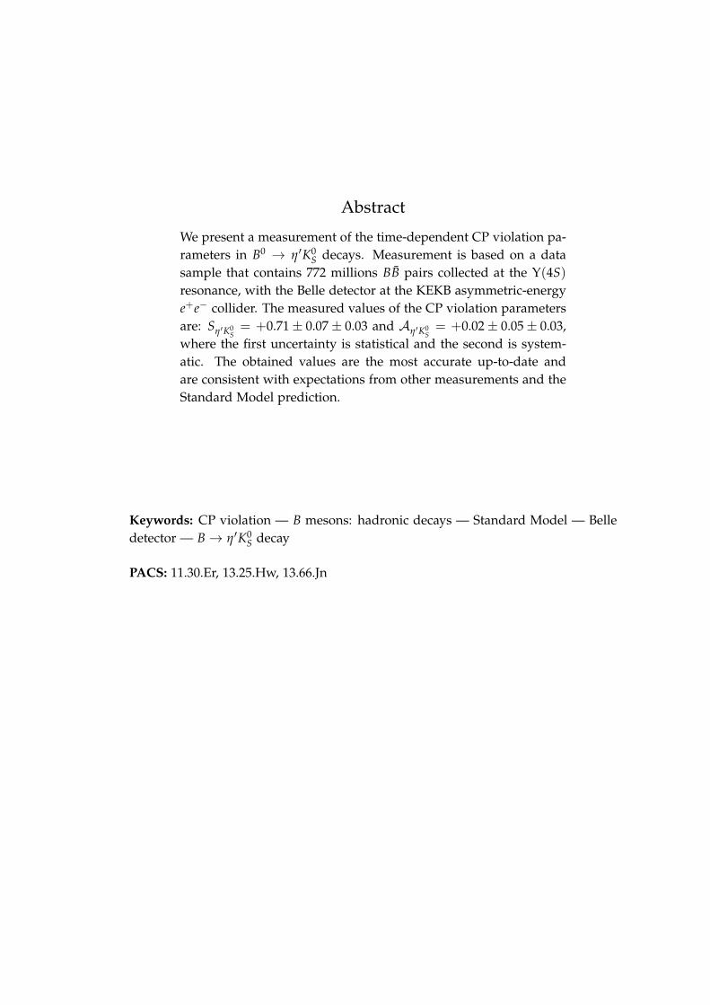
We present a measurement of the time-dependent CP violation pa-rameters in B0 → η′K0
S decays. Measurement is based on a datasample that contains 772 millions BB pairs collected at the Υ(4S)resonance, with the Belle detector at the KEKB asymmetric-energye+e− collider. The measured values of the CP violation parametersare: Sη′K0
S= +0.71± 0.07± 0.03 and Aη′K0
S= +0.02± 0.05± 0.03,
where the first uncertainty is statistical and the second is system-atic. The obtained values are the most accurate up-to-date andare consistent with expectations from other measurements and theStandard Model prediction.
Keywords: CP violation — B mesons: hadronic decays — Standard Model — Belledetector — B→ η′K0
S decay
PACS: 11.30.Er, 13.25.Hw, 13.66.Jn

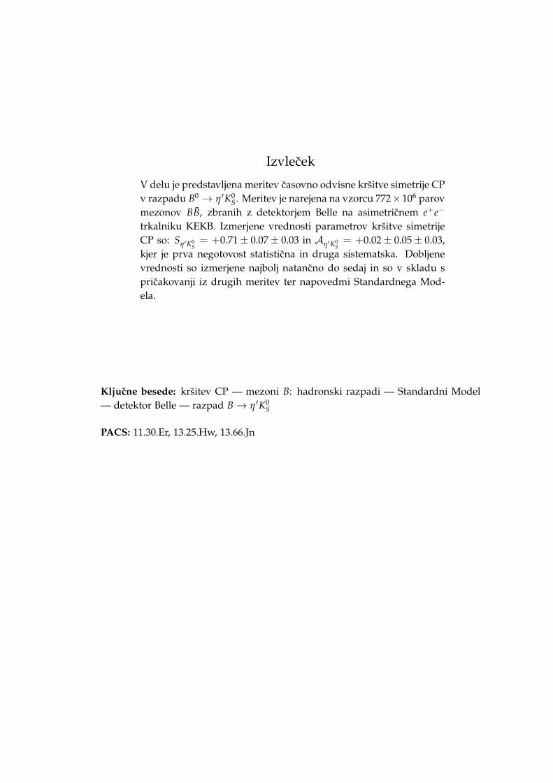
Izvlecek
V delu je predstavljena meritev casovno odvisne kršitve simetrije CPv razpadu B0 → η′K0
S. Meritev je narejena na vzorcu 772× 106 parovmezonov BB, zbranih z detektorjem Belle na asimetricnem e+e−
trkalniku KEKB. Izmerjene vrednosti parametrov kršitve simetrijeCP so: Sη′K0
S= +0.71± 0.07± 0.03 in Aη′K0
S= +0.02± 0.05± 0.03,
kjer je prva negotovost statisticna in druga sistematska. Dobljenevrednosti so izmerjene najbolj natancno do sedaj in so v skladu spricakovanji iz drugih meritev ter napovedmi Standardnega Mod-ela.
Kljucne besede: kršitev CP — mezoni B: hadronski razpadi — Standardni Model— detektor Belle — razpad B→ η′K0
S
PACS: 11.30.Er, 13.25.Hw, 13.66.Jn


Acknowledgments
I would like to thank to my advisor Prof. Boštjan Golob for all his help and effortto make this thesis better. I am grateful to him and to Prof. Peter Križan, for theirguidance and continuous support of my Ph.D study and research. My thanks alsogo to all members of the Ljubljana Belle group for their contribution to this work,and for a great research atmosphere.
I am grateful to all my closest friends for not allowing me to work as hard asmy advisors would like me to. Finally, I would like to thank to my family for theirendless support on every step of my way.

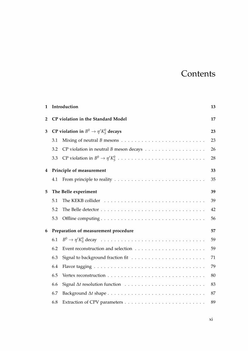
Contents
1 Introduction 13
2 CP violation in the Standard Model 17
3 CP violation in B0 → η′K0S decays 23
3.1 Mixing of neutral B mesons . . . . . . . . . . . . . . . . . . . . . . . . . 23
3.2 CP violation in neutral B meson decays . . . . . . . . . . . . . . . . . . 26
3.3 CP violation in B0 → η′K0S . . . . . . . . . . . . . . . . . . . . . . . . . . 28
4 Principle of measurement 33
4.1 From principle to reality . . . . . . . . . . . . . . . . . . . . . . . . . . . 35
5 The Belle experiment 39
5.1 The KEKB collider . . . . . . . . . . . . . . . . . . . . . . . . . . . . . . 39
5.2 The Belle detector . . . . . . . . . . . . . . . . . . . . . . . . . . . . . . . 42
5.3 Offline computing . . . . . . . . . . . . . . . . . . . . . . . . . . . . . . . 56
6 Preparation of measurement procedure 57
6.1 B0 → η′K0S decay . . . . . . . . . . . . . . . . . . . . . . . . . . . . . . . 59
6.2 Event reconstruction and selection . . . . . . . . . . . . . . . . . . . . . 59
6.3 Signal to background fraction fit . . . . . . . . . . . . . . . . . . . . . . 71
6.4 Flavor tagging . . . . . . . . . . . . . . . . . . . . . . . . . . . . . . . . . 79
6.5 Vertex reconstruction . . . . . . . . . . . . . . . . . . . . . . . . . . . . . 80
6.6 Signal ∆t resolution function . . . . . . . . . . . . . . . . . . . . . . . . 83
6.7 Background ∆t shape . . . . . . . . . . . . . . . . . . . . . . . . . . . . . 87
6.8 Extraction of CPV parameters . . . . . . . . . . . . . . . . . . . . . . . . 89
xi
CONTENTS
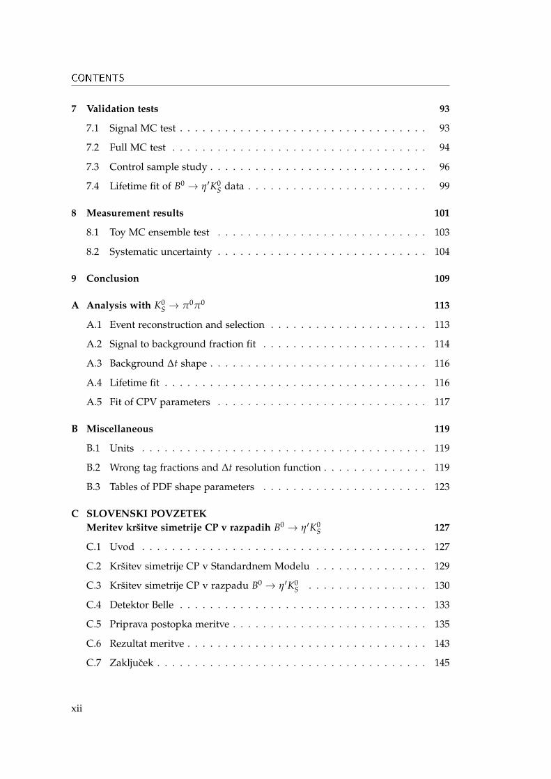
7 Validation tests 93
7.1 Signal MC test . . . . . . . . . . . . . . . . . . . . . . . . . . . . . . . . . 93
7.2 Full MC test . . . . . . . . . . . . . . . . . . . . . . . . . . . . . . . . . . 94
7.3 Control sample study . . . . . . . . . . . . . . . . . . . . . . . . . . . . . 96
7.4 Lifetime fit of B0 → η′K0S data . . . . . . . . . . . . . . . . . . . . . . . . 99
8 Measurement results 101
8.1 Toy MC ensemble test . . . . . . . . . . . . . . . . . . . . . . . . . . . . 103
8.2 Systematic uncertainty . . . . . . . . . . . . . . . . . . . . . . . . . . . . 104
9 Conclusion 109
A Analysis with K0S → π0π0 113
A.1 Event reconstruction and selection . . . . . . . . . . . . . . . . . . . . . 113
A.2 Signal to background fraction fit . . . . . . . . . . . . . . . . . . . . . . 114
A.3 Background ∆t shape . . . . . . . . . . . . . . . . . . . . . . . . . . . . . 116
A.4 Lifetime fit . . . . . . . . . . . . . . . . . . . . . . . . . . . . . . . . . . . 116
A.5 Fit of CPV parameters . . . . . . . . . . . . . . . . . . . . . . . . . . . . 117
B Miscellaneous 119
B.1 Units . . . . . . . . . . . . . . . . . . . . . . . . . . . . . . . . . . . . . . 119
B.2 Wrong tag fractions and ∆t resolution function . . . . . . . . . . . . . . 119
B.3 Tables of PDF shape parameters . . . . . . . . . . . . . . . . . . . . . . 123
C SLOVENSKI POVZETEKMeritev kršitve simetrije CP v razpadih B0 → η′K0
S 127
C.1 Uvod . . . . . . . . . . . . . . . . . . . . . . . . . . . . . . . . . . . . . . 127
C.2 Kršitev simetrije CP v Standardnem Modelu . . . . . . . . . . . . . . . 129
C.3 Kršitev simetrije CP v razpadu B0 → η′K0S . . . . . . . . . . . . . . . . 130
C.4 Detektor Belle . . . . . . . . . . . . . . . . . . . . . . . . . . . . . . . . . 133
C.5 Priprava postopka meritve . . . . . . . . . . . . . . . . . . . . . . . . . . 135
C.6 Rezultat meritve . . . . . . . . . . . . . . . . . . . . . . . . . . . . . . . . 143
C.7 Zakljucek . . . . . . . . . . . . . . . . . . . . . . . . . . . . . . . . . . . . 145
xii
1Introduction
Symmetries are not only important in everyday life but also in science. Consideringthe symmetries of physical laws, we attempt to understand the dynamics of variousphysical systems. Especially important are the transformations under which certainphysics phenomena are invariant. We say that such phenomena observe a givensymmetry, or that they are symmetry invariant. The subject of this work is related totwo discrete symmetries, parity P and charge conjugation C, that are of fundamentalimportance in modern physics. Assuming them to be exact symmetries of nature,the universe in which
• everything is replaced with its mirror image, P: ~r → −~r, or
• every particle is replaced with its antiparticle, C: x → x,
would be indistinguishable from the actual universe and would follow exactly thesame physical laws. Intuitively it seems natural that parity is conserved, or in otherwords, that nature has no preference about left or right. As it was known to be re-spected by gravitation, electromagnetic and the strong interaction, the conservationof parity was assumed to be a universal law. However, in the mid 1950s Chen NingYang and Tsung-Dao Lee suggested that the fourth of the fundamental interactionsof nature, the weak interaction, might violate this law [1]. Indeed, parity violation ofthe weak interaction was confirmed in the famous 60Co experiment by Chien ShiungWu and collaborators [2], earning Yang and Lee the 1957 Nobel Prize in Physics.This and further experiments showed that only left (right) handed neutrinos (anti-neutrinos) exist (or more exactly, only those participate in the weak interaction).Since the neutrinos are (almost) massless, handedness coincides with helicity, i.e.
13
CHAPTER 1. INTRODUCTION
the projection of spin on the particle’s momentum. Hence both, C and P, are vio-lated maximally by the weak interaction. Soon after this discovery, the combinedCP symmetry was proposed as the exact symmetry of nature, representing the truesymmetry between matter and antimatter. Taking the mirror image of a physicalsystem and replacing every particle with its antiparticle would result in exactly thesame phenomena as in the original setting. The weak interaction seemed to vio-late P and C in a way that combined CP is conserved. However, in the mid 1960sthe second great surprise came. James Cronin, Val Fitch and coworkers providedan experimental demonstration that also CP symmetry is violated in certain weakprocesses [3], in particular, in decays of neutral kaons1. Beside the discovery thatCP symmetry, which by then became widely believed to be exact, is violated, alsothe smallness of the observed violation was intriguing. It took nearly ten years forthe breakthrough in understanding how the observed CP violation can be connectedwith at that time emerging structure of the Standard Model (SM) of particle physics.In 1973 Makoto Kobayashi and Toshihide Maskawa pointed out that in the case ofthree quark generations the number of degrees of freedom in the SM naturally givesrise to the CP violating complex phase in the 3× 3 quark mixing matrix, now knownas the Cabibbo–Kobayashi–Maskawa (CKM) matrix [4] (note that in 1973 only the u, d, squarks were known). Indeed, two new quarks were discovered soon after, c (1974)and b (1977), and finally also t in 1995. The CKM matrix has four free parameters(three angles and one complex phase) and in an elegant way encodes informationon the relative strength of flavor changing weak decays, predicting correlations be-tween different quark decays and CP violating observables. The predicted large CPviolation in the B meson system was the main motivation for construction of twoso-called B factory experiments, Belle [5] and BaBar [6]. Already in the first years ofoperation, in 2001, these two experiments observed decay time dependent CP viola-tion by analyzing decays of neutral B mesons to J/ψK0
S. This represented the firstobservation of CP violation outside the kaon system [7, 8]. In the past decade Belleand BaBar have measured CP violating observables in many decays2 of B mesons,in some with only a few percent experimental uncertainty, and confirmed the singlecomplex phase of the CKM matrix as the main source of CP violation. After the ex-perimental confirmation of their predictions Kobayashi and Maskawa were awardedthe 2008 Nobel Prize in Physics.
So far the SM, a theory of electromagnetic, weak, and strong interaction with theCKM paradigm at the heart of its flavor sector, has proven to be a good descriptionof Nature up to energies of nearly 1 TeV. Apart from the non-zero neutrino massesno significant deviations from the SM predictions, induced by possible new physicsprocesses at some higher energy scale, were yet experimentally observed. However,the existence of new physics is assured at least by the fact the SM does not include
1Cronin and Fitch won the 1980 Nobel Prize in Physics for this discovery.2CP violation is observed in about 20 different decay modes with more than 3σ significance.
14
gravity, and also by non-zero neutrino masses. This makes us consider the SM asa low energy effective theory, valid up to some new physics energy scale Λ. Con-cerning the SM flavor sector, two intriguing facts in addition stimulate the thinkingabout new physics. First, the CKM matrix is almost a unit matrix. The origin of thishierarchy is unknown (as the elements of CKM matrix are free parameters of theSM) and indicates the presence of some new flavor symmetry at higher energy scale.Second, CP violation is one of the necessary conditions for the observed dominanceof matter over antimatter in the present Universe [9], but the CP violating phase ofCKM matrix fails by many orders of magnitude to explain the observed asymme-try [10]. Therefore, yet unknown additional CP violating phases must exist from thecosmological point of view.
The energy frontier experiments at the Large Hadron Collider have in recentyears started to probe physics at the TeV energy scale. This research is stimulated bythe well known fine tuning problem of the Higgs mass within the SM (the so-calledhierarchy problem) implying the energy scale of new physics (i.e. Λ ∼ TeV). Strictlyspeaking, so far no deviations from the SM predictions were observed, although thelong awaited discovery of the Higgs-like boson [11, 12] has not yet been decisivelyconfirmed to be of the SM origin. On the other hand, the flavor physics, mainly sup-ported by B physics measurements at B factories, already provides strong constraintson the flavor structure of new physics models at this energy scale. New physics, ifpresent at the TeV scale, must most probably have a non-generic flavor structurein order to suppress the Flavor-Changing Neutral Current (FCNC) processes, whichwould otherwise violate current experimental limits. Despite a necessary mechanismof FCNC suppression, new flavor mixing and CP violating phases almost inevitablyarise in a large class of new physics scenarios at TeV energies [13]. This gives themotivation for search of new physics effects in the wide range of FCNC processesavailable in B meson decays. Because FCNC processes can, within the SM, proceedonly through the so-called penguin diagrams, one can investigate the effects of pos-sible new heavy particles in quantum loops of these diagrams. At many points inthe history of particle physics this approach turned out to be very fruitful, leadingto several important breakthroughs3.
In this work we present a measurement of time-dependent CP violation in B0 →η′K0
S decays. This decay is mediated by the b → sqq quark transition, which is anexample of FCNC process induced by a penguin diagram, and as such sensitiveto possible new CP violating phases. The decay final state η′K0
S is a CP eigenstateinto which both B0 and its antiparticle B0 meson can decay. The SM predicts theasymmetry in time-dependent decay rates of B0 and B0 mesons into η′K0
S to be veryclose (at few % level [15–21]) to the asymmetry in B0 → J/ψK0
S decay. However,
3The existence of the charm quark was postulated to explain the smallness of FCNC (GIM mecha-nism [14]), observation of CP violation led to the prediction of third generation of quarks [4], the topquark mass was predicted based on the B0 mixing measurements.
15
CHAPTER 1. INTRODUCTION
the presence of new CP violating phases can potentially induce a large deviationbetween the asymmetries in these two decays. While the penguin dominated de-cay B → η′K0
S, can recieve sizable contributions from such phases, the tree diagramdominated B0 → J/ψK0
S decay, is relatively insensitive to those phases. The verywell measured CP asymmetry in the latter decay and a relatively clean SM predic-tion make CP violation in B0 → η′K0
S decays one of the gold-plated observables forpossible new CP violating phases.
The measurement presented here is based on a data sample that contains 772million BB pairs, collected with the Belle detector during the years of its operation(1999-2010). We start with a brief introduction to CP violation in the SM (chapter 2),which is followed by a description of possible manifestations of CP violation in theB meson system, and in particular in B0 → η′K0
S decays, and a summary of previousexperimental results, in chapter 3. Next, in chapter 4, we present the basic principlesof time-dependent CP violation measurements at B factories, and describe the KEKBcollider and Belle detector in chapter 5. After these introductory chapters we moveto the performed measurement. In the main part of the work we describe the methodof measurement (chapter 6) and its validation tests (chapter 7) in some detail. Theresults and the estimation of the systematic uncertainty of the method are presentedin chapter 8. Finally we conclude in chapter 9 with some future prospects.
16
2CP violation in the Standard Model
The Standard Model is a theory that describes the dynamics of the known subatomicparticles, driven by the electromagnetic, weak and strong interaction. Mathemati-cally, it is formulated as a gauge field theory with the local SU(3)C × SU(2)L ×U(1)gauge symmetry, and this internal symmetry essentially defines it. Usually we di-vide the SM into two sectors, one being the quantum chromodynamics with the SU(3)C
as a gauge symmetry that describes the strong interaction, and the other being theelectroweak theory with the SU(2)L ×U(1) symmetry that describes the unified elec-troweak interaction. Since CP violation resides in the latter part we briefly introduceits structure.
In the SU(2)L × U(1) gauge symmetry, the SU(2)L represents the weak isospinand the U(1) represents the weak hypercharge. The subscript L indicates that only lefthanded fermions transform non-trivially under isospin, they belong to an isodoublet,while right handed fermions belong to an isosinglet. In the SM fermions come inthree generations
leptons: lL =
((νe
e
)L
,
(νµµ
)L
,
(ντ
τ
)L
), eR,µR, τR (2.1)
quarks: qL =
((ud
)L
,
(cs
)L
,
(tb
)L
), uR, dR, cR, sR, tR, bR. (2.2)
In the following text the notation ~e = (e,µ, τ), ~ν = (νe, νµ, ντ), ~u = (u, c, t) and~d = (d, s, b) is also used. Hypercharge is also assigned to each of the degrees offreedom given above. To satisfy the SU(2)L × U(1) invariance, four gauge bosonfields have to be introduced. After the electroweak symmetry breaking, these fields
17
CHAPTER 2. CP VIOLATION IN THE STANDARD MODEL
result in the W+, W− and Z0 gauge bosons of the weak interaction and the photonA, a gauge boson of the electromagnetic interaction. A gauge invariant Lagrangiandescribing the interaction between the gauge bosons and fermions is given by
Lint =g√2
(J+µ W¯µ + J−µ W+µ
)+ eJem
µ Aµ +g
cos θW
(J3µ − sin2 θW Jem
µ
)Zµ, (2.3)
where
J+µ = uiLγµdL,i + νi
LγµeL,i is the charged weak current,
J3µ =
12
(ui
LγµuL,i − diLγµdL,i + νi
LγµνL,i − eiLγµeL,i
)is the neutral weak current,
Jemµ =
23
uiLγµuL,i −
13
diLγµdL,i − ei
LγµeL,i is the electromagnetic current, (2.4)
g and e are the coupling constants, θW is the Weinberg angle, and the summation overgeneration index i = 1, 2, 3 is assumed. As will be shown shortly, the CP violationmanifests itself in Lint introduced above, but its origin is actually in another part ofthe SM Lagrangian, namely in the couplings of the SU(2) doublet of the Higgs fieldsφ with fermions
−LHF = f iju qL,i
(φ0
−φ−
)uR,j + f ij
d qL,i
(φ+
φ0
)dR,j + f ij
e lL,i
(φ0
−φ−
)eR,j, (2.5)
where fu, fd, fe are the generational coupling matrices. After the spontaneous sym-metry breaking, the neutral Higgs field acquires the vacuum expectation value 〈φ0〉 =v, giving rise to the fermion mass terms, with the mass matrices Mα = v fα (α =
u, d, e). Since, within the SM, there is no prescription or symmetry constraining thecontent of fα, the mass matrices Mα are in general non-diagonal. Therefore, thefermions introduced in (2.2) and used in Lint are not mass eigenstates of the theory.To obtain the latter, we diagonalize each of the mass matrices with the help of twounitary matrices
SαLMαSα†
R = Mdiagα (α = u, d, e), (2.6)
and obtain the mass eigenstates as
umL(R) = Su
L(R)uL(R), dmL(R) = Sd
L(R)dL(R), emL(R) = Se
L(R)eL(R). (2.7)
If we were to rewrite the Lagrangian Lint given in (2.3) in the mass basis, we wouldfind that the change of the basis has no effect on the electromagnetic, neutral andleptonic charged current1. For the quark charged current the situation is different.We have
J+µ (qk) = uiLγµdL,i = um,i
L γµSu†L,ijS
d,jkL dm
L,k = um,iL γµVijdm
L,j, (2.8)
1For the electromagnetic and neutral current the reason is simple, the matrices S are unitary andtherefore SS† = 1. For the leptonic charged current the reason is different, it is due to the fact thatwithin the SM the neutrinos are massless and as such mass degenerate. This allows for the flavoreigenstates to coincide with the mass eigenstates.
18
where we introduce the Cabibbo-Kobayashi-Maskawa (CKM) matrix V, a unitary ma-trix that by convention mixes down-type quark mass states to obtain quark statesparticipating in the weak interaction
V ≡ Su†L Sd
L =
Vud Vus Vub
Vcd Vcs Vcb
Vtd Vts Vtb
. (2.9)
Although a general 3 × 3 unitary matrix has 9 real valued parameters, 3 anglesand 6 phases, in the CKM matrix besides the angles only one phase is of physicalsignificance2. This irreducible phase introduces CP violation in the SM [4]. Usuallyit is called the Kobayashi-Maskawa (KM) phase, and as experimentally confirmed,is responsible for all the CP violating phenomena observed so far (or at least itis the main source). By performing CP transformation on Lint one can show that(CP)Lint(CP)† = L†
int, concluding that CP is conserved if Lint = L†int. In the presence
of a complex phase in the CKM matrix this condition does not hold, and thereforeCP is violated.
The mechanism described above is one of the two possible ways of breakingCP symmetry within the SM. There are natural terms in the QCD Lagrangian thatare able to break CP symmetry. By natural we mean that they are gauge invariantand renormalizable, and that there is no known principle prohibiting their presence.However, experiments do not indicate any CP violation in the QCD sector, limitingthe presence of such terms to "unnaturally" tiny values. Why there is no CP violationin the QCD is an open problem, usually referred to as the strong CP problem [22].
2.0.1 Wolfenstein parametrization
There is no unique parametrization of the CKM matrix in terms of the three rotationangles and one phase. Any scheme that is consistently employed leads to the samephysics observables. On the phenomenological grounds the Wolfenstein parametriza-tion is particularly useful [23]. It incorporates the experimentally observed hierarchy|Vub|2 � |Vcb|2 � |Vus|2 � 1 . We define λ ≡ |Vus| ' 0.22, and expand the elementsof the CKM matrix in powers of λ as
V =
1− λ2/2 λ λ3A(ρ− iη)−λ 1− λ2/2 λ2A
λ3A(1− ρ− iη) −λ2A 1
, (2.10)
where the real valued parameters A, ρ and η are required to be of the order unity,and the non-zero η introduces the CP violation. Their current experimental values
2Five phases can be removed by re-phasing the quark fields.
19
CHAPTER 2. CP VIOLATION IN THE STANDARD MODEL
are [24]:
λ = 0.22535± 0.00065, A = 0.811+0.022−0.012
ρ = 0.131+0.026−0.013, η = 0.345+0.013
−0.014. (2.11)
Since the elements of the CKM matrix are free parameters of the SM, it is veryintriguing that such an obvious hierarchy is found. It shows that some, yet unknown,mechanism from physics beyond the SM must be at work.
2.0.2 Unitarity triangle
As it was already pointed out, the CKM matrix is unitary. This imposes the con-ditions ∑i VijV∗ik = δjk and ∑j VijV∗kj = δik on its elements. The six of the vanishingrelations can be presented as triangles in the complex plane, called the unitarity tri-angles. It can be seen from (2.10) that two of these have all three sides of the orderλ3, potentially having all three of their angles large. In this case, the relative weakphases in the quark transitions are of the order unity, inducing large CP asymmetriesin some decays. The triangle that is usually used is obtained from
VudV∗ub + VcdV∗cb + VtdV∗tb = 0, (2.12)
by dividing it with VcdV∗cb. This results in the triangle with the vertices at (0, 0),(1, 0)and (ρ, η), where ρ = ρ(1− λ2/2) and η = η(1− λ2/2). The sketch of the unitarytriangle, with the defined sides and angles, is given in figure 2.1. The angles areexpressed with the CKM matrix elements by
φ1 = arg[−
VcdV∗cbVtdV∗tb
], φ2 = arg
[−
VtdV∗tbVudV∗ub
], φ3 = arg
[−
VudV∗ubVcdV∗cb
]. (2.13)
The parameters (sides, angles) of the described triangle can be obtained mainly fromthe measurements of decay rates and CP asymmetries in the B meson system. Thesemeasurements are of great importance for three reasons: they are measurements ofthe SM free parameters, they provide an experimental test of CP violation mech-anism and the flavor structure of the SM, and some decay modes are sensitive tonew physics contributions and provide a way to discover new physics, or at leastconstrain theoretical models of it.
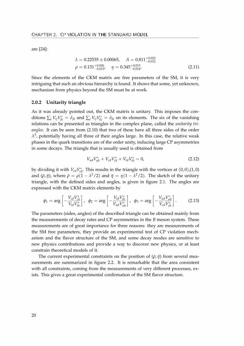
The current experimental constraints on the position of (ρ, η) from several mea-surements are summarized in figure 2.2. It is remarkable that the area consistentwith all constraints, coming from the measurements of very different processes, ex-ists. This gives a great experimental confirmation of the SM flavor structure.
20
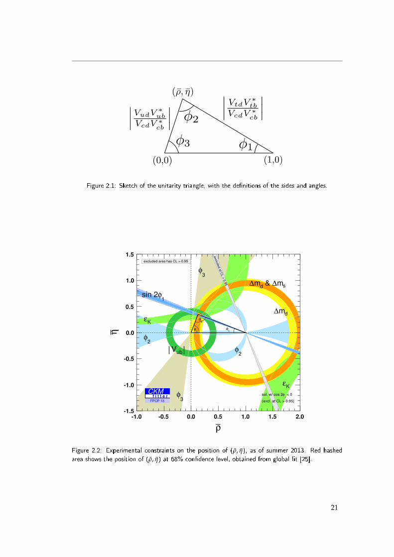
Figure 2.1: Sketch of the unitarity triangle, with the de�nitions of the sides and angles.
3φ
3φ
2φ
2φ
dm∆
Kε
Kε
sm∆ & dm∆
ubV
1φsin 2
(excl. at CL > 0.95)
< 01
φsol. w/ cos 2
exc
luded a
t CL >
0.9
5
2φ
1φ
3φ
ρ
1.0 0.5 0.0 0.5 1.0 1.5 2.0
η
1.5
1.0
0.5
0.0
0.5
1.0
1.5
excluded area has CL > 0.95
FPCP 13
CKMf i t t e r
Figure 2.2: Experimental constraints on the position of (ρ, η), as of summer 2013. Red hashedarea shows the position of (ρ, η) at 68% con�dence level, obtained from global �t [25].
21

3CP violation in B0 → η′K0
S decays
In this chapter we present how CP violation can be observed in the decays of neutralB mesons into η′ and K0
S mesons. First we give a brief introduction into the mixingof neutral B mesons and describe how CP violation can manifest itself in B mesondecays. We then estimate the size of CP violation in the B0 → η′K0
S decay withinthe SM, and discuss the connection with new physics. Finally, we conclude with thesummary of the past experimental results.
3.1 Mixing of neutral B mesons
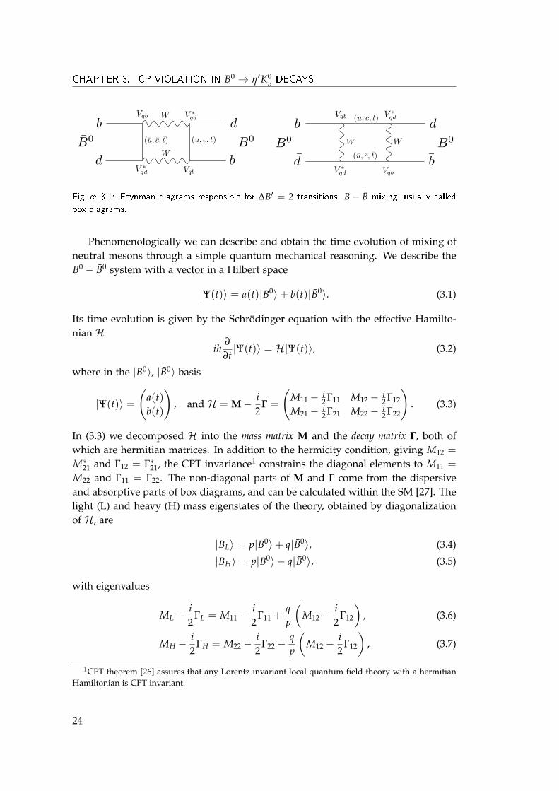
Unlike the π0 meson, which is its own anti-particle, the neutral B meson carriesan additional quantum number called bottomness, allowing a distinction betweenthe B0 meson and its anti-particle, B0. Bottomness is a flavor quantum number,defined as B′ = −(nb − nb), where nb stands for the number of bottom quarks, andnb for the number of bottom anti-quarks. B0 (db) meson has B′ = 1, and B0 (db)meson has B′ = −1. As other flavor quantum numbers, bottomness is conserved bythe electromagnetic and strong interaction, while the weak interaction varies it for∆B′ = ±1 (in 1st order processes, i.e. processes involving a single quark). However,in processes of the 2nd order in the weak interaction, there is also a possibility oftransitions with ∆B′ = ±2. In the SM these transitions are in the lowest order givenby so-called box diagrams, as shown in figure 3.1. These diagrams connect the B0 andB0 states, and give rise to the phenomenon called B0− B0 mixing. If, for example, weproduce a pure B0 state, as this state propagates in time, it will gain a component ofthe B0 state.
23
CHAPTER 3. CP VIOLATION IN B0 → η′K0S DECAYS
Figure 3.1: Feynman diagrams responsible for ∆B′ = 2 transitions, B− B mixing, usually calledbox diagrams.
Phenomenologically we can describe and obtain the time evolution of mixing ofneutral mesons through a simple quantum mechanical reasoning. We describe theB0 − B0 system with a vector in a Hilbert space
|Ψ(t)〉 = a(t)|B0〉+ b(t)|B0〉. (3.1)
Its time evolution is given by the Schrödinger equation with the effective Hamilto-nian H
ih∂
∂t|Ψ(t)〉 = H|Ψ(t)〉, (3.2)
where in the |B0〉, |B0〉 basis
|Ψ(t)〉 =(
a(t)b(t)
), and H = M− i
2Γ =
(M11 − i
2 Γ11 M12 − i2 Γ12
M21 − i2 Γ21 M22 − i
2 Γ22
). (3.3)
In (3.3) we decomposed H into the mass matrix M and the decay matrix Γ, both ofwhich are hermitian matrices. In addition to the hermicity condition, giving M12 =
M∗21 and Γ12 = Γ∗21, the CPT invariance1 constrains the diagonal elements to M11 =
M22 and Γ11 = Γ22. The non-diagonal parts of M and Γ come from the dispersiveand absorptive parts of box diagrams, and can be calculated within the SM [27]. Thelight (L) and heavy (H) mass eigenstates of the theory, obtained by diagonalizationof H, are
|BL〉 = p|B0〉+ q|B0〉, (3.4)
|BH〉 = p|B0〉 − q|B0〉, (3.5)
with eigenvalues
ML −i2
ΓL = M11 −i2
Γ11 +qp
(M12 −
i2
Γ12
), (3.6)
MH −i2
ΓH = M22 −i2
Γ22 −qp
(M12 −
i2
Γ12
), (3.7)
1CPT theorem [26] assures that any Lorentz invariant local quantum field theory with a hermitianHamiltonian is CPT invariant.
24
where q/p is given by
qp=
√M∗12 −
i2 Γ∗12
M12 − i2 Γ12
. (3.8)
In the SM, the quantity |Γ12/M12| ∼ O(m2b/m2
t ) is very small (. O(10−3) [28]) andM12 ∝ V∗tdVtb [27], resulting in
qp'
V∗tdVtb
VtdV∗tb, and therefore
∣∣∣∣ qp
∣∣∣∣ ' 1. (3.9)
Knowing the time evolution of the mass eigenstates |BL〉 and |BH〉 (i.e. |BL,H(t)〉 =|BL,H〉e−i(ML,H−iΓL,H/2)t), and taking into account (3.5), one can easily obtain how aninitially produced pure B0 (B0) state, denoted as |B0(t)〉 (|B0(t)〉), evolves in time
|B0(t)〉 = f+(t)|B0〉+ qp
f−(t)|B0〉, (3.10)
|B0(t)〉 = f+(t)|B0〉+ pq
f−(t)|B0〉. (3.11)
Here we introduced
f±(t) =12
e−iMt− 12 Γt[1± e−i∆Mt+ 1
2 ∆Γt]
, (3.12)
with the B meson mass M ≡ (ML + MH)/2, decay width Γ ≡ (ΓL + ΓH)/2, mixingfrequency ∆M ≡ MH −ML, and the width difference ∆Γ = ΓL − ΓH. As the initialB0 (or B0) state evolves in time, it oscillates between the B0 and B0 states with thefrequency ∆M. Luckily, the value of the mixing parameter x = ∆M/Γ (giving thenumber of oscillations in a lifetime) is of order unity in the B meson system (exp. x =
0.77± 0.01 [29]), allowing the oscillations to be experimentally observed. In addition,it can be seen from (3.6) and (3.7) that ∆Γ � ∆M, since |Γ12/M12| . O(10−3), andfrom ∆M/Γ ∼ 1 it follows that ∆Γ� Γ. Unlike in the kaon system, the decay widthdifference between the two mass states is very small here.
3.1.1 Decay rates
What we can measure in the experiments are the decay rates. Therefore we askourselves at which rate an initially produced B0 (or B0) state decays into some finalstate f . Clearly the decay rate Γ(B0(t) → f ) is time dependent, since the B0(t) stateis a time dependent superposition of the B0 and B0 states. We denote the decayamplitudes of flavor eigenstates B0 and B0 decaying into f with A f = 〈 f |B0〉 andA f = 〈 f |B0〉, and define the parameter
λ f ≡1
λ f≡ q
pA f
A f. (3.13)
25
CHAPTER 3. CP VIOLATION IN B0 → η′K0S DECAYS
The decay rates can be obtained from the equations (3.10) and (3.11) by Γ(B0(t) →f ) = |〈 f |B0(t)〉|2, yielding
Γ(B0(t)→ f ) ∝ e−Γt|A f |2[K+(t) + K−(t)|λ f |2 + 2Re
(L(t)λ f
)], (3.14)
Γ(B0(t)→ f ) ∝ e−Γt|A f |2[K+(t) + K−(t)|λ f |2 + 2Re
(L(t)λ f
)], (3.15)
with
K±(t) = 1 + e∆Γt ± 2e12 ∆Γt cos ∆Mt, (3.16)
L(t) = 1− e∆Γt + 2ie12 ∆Γt sin ∆Mt. (3.17)
From (3.14) and (3.15) one can see that in the case when both B0 and B0, can decayinto the same final state f (i.e. λ f , λ f 6= 0), the decay rate consists of three terms. Thefirst one representing a decay of B0, second one a decay of the B0 component arisingthrough mixing, and the third one representing the interference between these twopossible decays.
3.2 CP violation in neutral B meson decays
To measure CP violation, we measure the asymmetry between the decays of B0(t)and B0(t) into the CP conjugated final states, f and f . Since the decay rates of theneutral B mesons are time dependent, the asymmetry also depends on time, and isdefined by
a f (t) ≡Γ(B0(t)→ f )− Γ(B0(t)→ f )Γ(B0(t)→ f ) + Γ(B0(t)→ f )
. (3.18)
By carefully examining the equations (3.14) and (3.15) one can find three extremecases in which a f differs from zero, but for different reasons [30]. In general, allthree of them can contribute, depending on the decay final state f .
• CP is most obviously violated if |A f | 6= |A f |, and therefore Γ(B0(t) → f ) 6=Γ(B0(t)→ f ). This is called direct CP violation. It is independent of the B0− B0
mixing effects and can also be observed in the decays of charged B mesons.
• Another possibility is found by studying flavor specific decays, i.e. decays withsuch final state f ( f ), that only the B0 (B0) flavor eigenstate can decay into. Themost prominent examples of these are semileptonic decays. In this case A f = 0and A f = 0. If, in addition, we demand that there is no direct CP violationin the selected decay (|A f | = |A f |), the equations (3.14) and (3.15) yield theasymmetry
a f =1− |p/q|41 + |p/q|4 , (3.19)
26
which is time independent and differs from zero if | pq | 6= 1. However, as givenin (3.9), q
p is in close approximation a pure phase, making this asymmetrytoo small to be experimentally observed so far. Its current experimental valuefrom semileptonic B decays is aSL = (−3.3± 3.3)× 10−3 [24]. This type of CPviolation is called CP violation in mixing.
• The third way in which CP violation can manifest itself, can be observed indecays into flavor non-specific final states, i.e. states into which both B0 andB0 can decay. Decays into CP eigenstates are obviously of this type ( f = f ).Beginning with a general case, we allow for the B0 and B0 to have differentamplitudes to decay into f (|A f | 6= |A f |). First we can simplify the decayrates, as given in (3.14) and (3.15), by taking into account that ∆Γ � Γ and thedefinition of λ f and λ f (3.13)
Γ(B0(t)→ f ) ∝ e−Γt|A f |2[
1 +1− |λ f |2
1 + |λ f |2cos ∆Mt−
2Imλ f
1 + |λ f |2sin ∆Mt
](3.20)
Γ(B0(t)→ f ) ∝ e−Γt|A f |2[
1−1− |λ f |2
1 + |λ f |2cos ∆Mt +
2Imλ f
1 + |λ f |2sin ∆Mt
].
(3.21)
From this and the definition of asymmetry a f (t) (3.18) we then obtain
a f (t) = A f cos ∆Mt + S f sin ∆Mt, (3.22)
where we have introduced two so-called CP violation parameters (commonly wewill use "CPV parameters" notation) given by
A f =|λ f |2 − 1|λ f |2 + 1
, S f =2Imλ f
1 + |λ f |2. (3.23)
Remembering that λ f = qp
A fA f
and∣∣∣ q
p
∣∣∣ ' 1, we can see that the first term in
(3.22) is due to direct CP violation, since A f 6= 0 only if |A f | 6= |A f |. However,the second term in (3.22) is something new and represents CP violation inthe interference between the direct B0 → f and mixed B0 → B0 → f decay.This second term can be non-zero even in the case when |q/p| = 1 and also|A f | = |A f | holds, as then S f = sin[arg(q/p) + arg(A f /A f )]. Measuring theasymmetry (3.22), and consequently the parameter S f , therefore allows us tomeasure a sum of CP violating phases in mixing and decay.
27
CHAPTER 3. CP VIOLATION IN B0 → η′K0S DECAYS
3.3 CP violation in B0 → η′K0S
Neutral B0 and B0 meson can both decay into η′K0S final state, since this state is a
CP eigenstate (if a tiny CP odd component of K0S is neglected). Strictly speaking, in
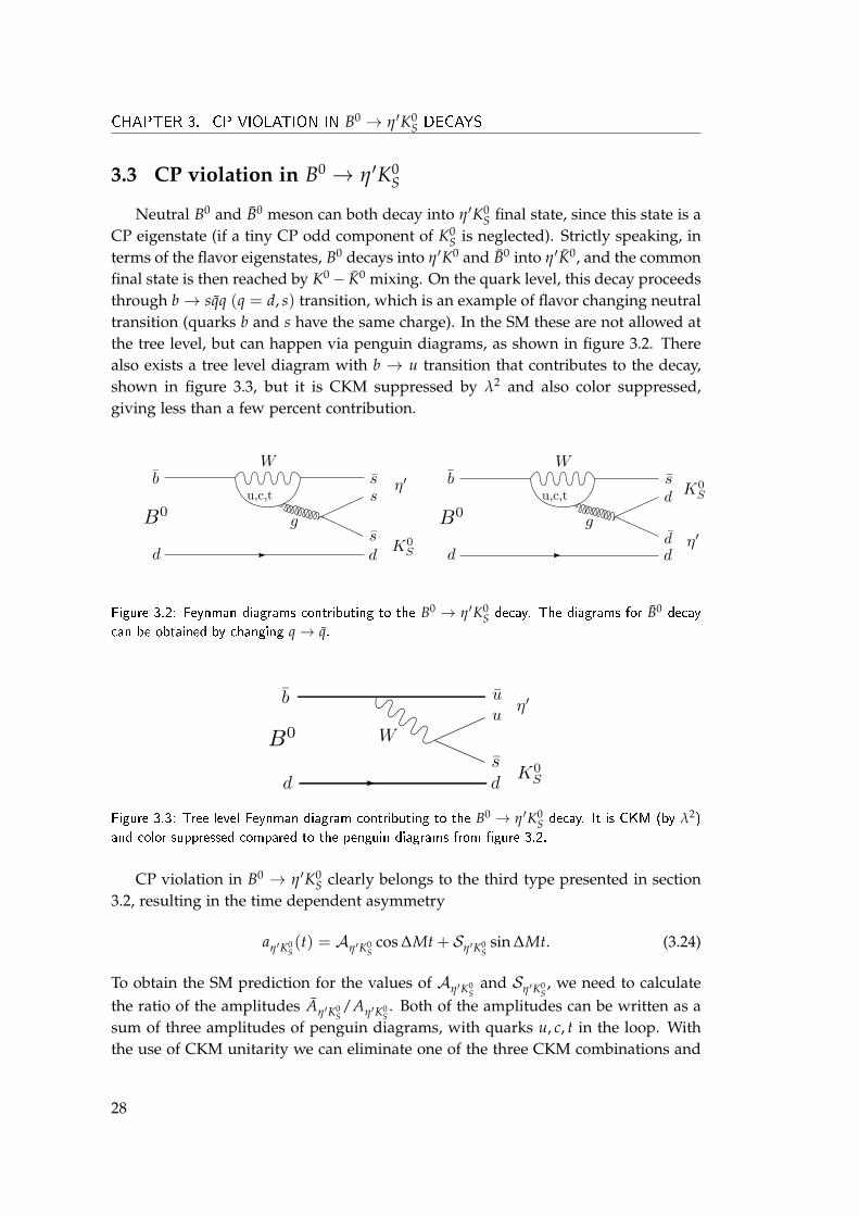
terms of the flavor eigenstates, B0 decays into η′K0 and B0 into η′K0, and the commonfinal state is then reached by K0− K0 mixing. On the quark level, this decay proceedsthrough b→ sqq (q = d, s) transition, which is an example of flavor changing neutraltransition (quarks b and s have the same charge). In the SM these are not allowed atthe tree level, but can happen via penguin diagrams, as shown in figure 3.2. Therealso exists a tree level diagram with b → u transition that contributes to the decay,shown in figure 3.3, but it is CKM suppressed by λ2 and also color suppressed,giving less than a few percent contribution.
Figure 3.2: Feynman diagrams contributing to the B0 → η′K0S decay. The diagrams for B0 decay
can be obtained by changing q→ q.
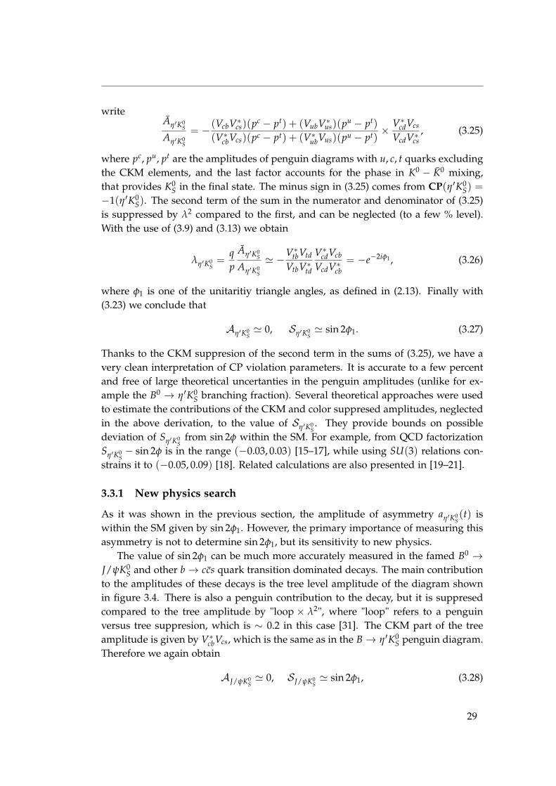
Figure 3.3: Tree level Feynman diagram contributing to the B0 → η′K0S decay. It is CKM (by λ2)
and color suppressed compared to the penguin diagrams from �gure 3.2.
CP violation in B0 → η′K0S clearly belongs to the third type presented in section
3.2, resulting in the time dependent asymmetry
aη′K0S(t) = Aη′K0
Scos ∆Mt + Sη′K0
Ssin ∆Mt. (3.24)
To obtain the SM prediction for the values of Aη′K0S
and Sη′K0S, we need to calculate
the ratio of the amplitudes Aη′K0S/Aη′K0
S. Both of the amplitudes can be written as a
sum of three amplitudes of penguin diagrams, with quarks u, c, t in the loop. Withthe use of CKM unitarity we can eliminate one of the three CKM combinations and
28
writeAη′K0
S
Aη′K0S
= − (VcbV∗cs)(pc − pt) + (VubV∗us)(pu − pt)
(V∗cbVcs)(pc − pt) + (V∗ubVus)(pu − pt)×
V∗cdVcs
VcdV∗cs, (3.25)
where pc, pu, pt are the amplitudes of penguin diagrams with u, c, t quarks excludingthe CKM elements, and the last factor accounts for the phase in K0 − K0 mixing,that provides K0
S in the final state. The minus sign in (3.25) comes from CP(η′K0S) =
−1(η′K0S). The second term of the sum in the numerator and denominator of (3.25)
is suppressed by λ2 compared to the first, and can be neglected (to a few % level).With the use of (3.9) and (3.13) we obtain
λη′K0S=
qp
Aη′K0S
Aη′K0S
' −V∗tbVtd
VtbV∗td
V∗cdVcb
VcdV∗cb= −e−2iφ1 , (3.26)
where φ1 is one of the unitaritiy triangle angles, as defined in (2.13). Finally with(3.23) we conclude that
Aη′K0S' 0, Sη′K0
S' sin 2φ1. (3.27)
Thanks to the CKM suppresion of the second term in the sums of (3.25), we have avery clean interpretation of CP violation parameters. It is accurate to a few percentand free of large theoretical uncertanties in the penguin amplitudes (unlike for ex-ample the B0 → η′K0
S branching fraction). Several theoretical approaches were usedto estimate the contributions of the CKM and color suppresed amplitudes, neglectedin the above derivation, to the value of Sη′K0
S. They provide bounds on possible
deviation of Sη′K0S
from sin 2φ within the SM. For example, from QCD factorizationSη′K0
S− sin 2φ is in the range (−0.03, 0.03) [15–17], while using SU(3) relations con-
strains it to (−0.05, 0.09) [18]. Related calculations are also presented in [19–21].
3.3.1 New physics search
As it was shown in the previous section, the amplitude of asymmetry aη′K0S(t) is
within the SM given by sin 2φ1. However, the primary importance of measuring thisasymmetry is not to determine sin 2φ1, but its sensitivity to new physics.
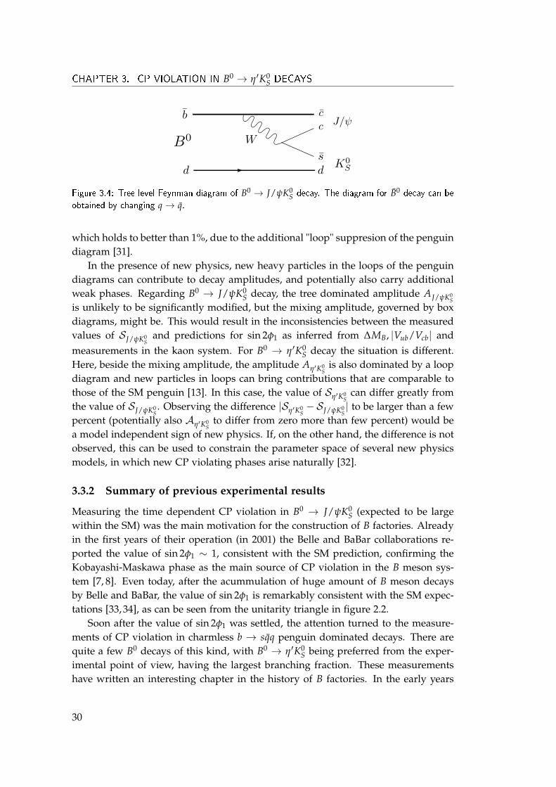
The value of sin 2φ1 can be much more accurately measured in the famed B0 →J/ψK0
S and other b→ ccs quark transition dominated decays. The main contributionto the amplitudes of these decays is the tree level amplitude of the diagram shownin figure 3.4. There is also a penguin contribution to the decay, but it is suppresedcompared to the tree amplitude by "loop × λ2", where "loop" refers to a penguinversus tree suppresion, which is ∼ 0.2 in this case [31]. The CKM part of the treeamplitude is given by V∗cbVcs, which is the same as in the B→ η′K0
S penguin diagram.Therefore we again obtain
AJ/ψK0S' 0, SJ/ψK0
S' sin 2φ1, (3.28)
29
CHAPTER 3. CP VIOLATION IN B0 → η′K0S DECAYS
Figure 3.4: Tree level Feynman diagram of B0 → J/ψK0S decay. The diagram for B0 decay can be
obtained by changing q→ q.
which holds to better than 1%, due to the additional "loop" suppresion of the penguindiagram [31].
In the presence of new physics, new heavy particles in the loops of the penguindiagrams can contribute to decay amplitudes, and potentially also carry additionalweak phases. Regarding B0 → J/ψK0
S decay, the tree dominated amplitude AJ/ψK0S
is unlikely to be significantly modified, but the mixing amplitude, governed by boxdiagrams, might be. This would result in the inconsistencies between the measuredvalues of SJ/ψK0
Sand predictions for sin 2φ1 as inferred from ∆MB, |Vub/Vcb| and
measurements in the kaon system. For B0 → η′K0S decay the situation is different.
Here, beside the mixing amplitude, the amplitude Aη′K0S
is also dominated by a loopdiagram and new particles in loops can bring contributions that are comparable tothose of the SM penguin [13]. In this case, the value of Sη′K0
Scan differ greatly from
the value of SJ/ψK0S. Observing the difference |Sη′K0
S−SJ/ψK0
S| to be larger than a few
percent (potentially also Aη′K0S
to differ from zero more than few percent) would bea model independent sign of new physics. If, on the other hand, the difference is notobserved, this can be used to constrain the parameter space of several new physicsmodels, in which new CP violating phases arise naturally [32].
3.3.2 Summary of previous experimental results
Measuring the time dependent CP violation in B0 → J/ψK0S (expected to be large
within the SM) was the main motivation for the construction of B factories. Alreadyin the first years of their operation (in 2001) the Belle and BaBar collaborations re-ported the value of sin 2φ1 ∼ 1, consistent with the SM prediction, confirming theKobayashi-Maskawa phase as the main source of CP violation in the B meson sys-tem [7, 8]. Even today, after the acummulation of huge amount of B meson decaysby Belle and BaBar, the value of sin 2φ1 is remarkably consistent with the SM expec-tations [33, 34], as can be seen from the unitarity triangle in figure 2.2.
Soon after the value of sin 2φ1 was settled, the attention turned to the measure-ments of CP violation in charmless b → sqq penguin dominated decays. There arequite a few B0 decays of this kind, with B0 → η′K0
S being preferred from the exper-imental point of view, having the largest branching fraction. These measurementshave written an interesting chapter in the history of B factories. In the early years
30
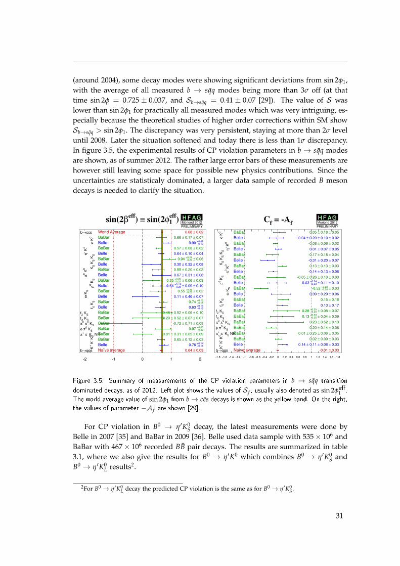
(around 2004), some decay modes were showing significant deviations from sin 2φ1,with the average of all measured b → sqq modes being more than 3σ off (at thattime sin 2φ = 0.725 ± 0.037, and Sb→sqq = 0.41 ± 0.07 [29]). The value of S waslower than sin 2φ1 for practically all measured modes which was very intriguing, es-pecially because the theoretical studies of higher order corrections within SM showSb→sqq > sin 2φ1. The discrepancy was very persistent, staying at more than 2σ leveluntil 2008. Later the situation softened and today there is less than 1σ discrepancy.In figure 3.5, the experimental results of CP violation parameters in b → sqq modesare shown, as of summer 2012. The rather large error bars of these measurements arehowever still leaving some space for possible new physics contributions. Since theuncertainties are statisticaly dominated, a larger data sample of recorded B mesondecays is needed to clarify the situation.
sin(2βeff
) ≡ sin(2φe1ff)
b→ccs
φ K
0
η′ K
0
KS K
S K
S
π0 K
0
ρ0 K
S
ω K
S
f 0 K
S
f2 KS
fX KS
π0 π
0 KS
φ π0 KS
π+ π
- KS NR
K+ K
- K0
b→qqs
-2 -1 0 1 2
World Average 0.68 ± 0.02
BaBar 0.66 ± 0.17 ± 0.07
Belle 0.90 +-00..0199
BaBar 0.57 ± 0.08 ± 0.02
Belle 0.64 ± 0.10 ± 0.04
BaBar 0.94 +-00..2214 ± 0.06
Belle 0.30 ± 0.32 ± 0.08
BaBar 0.55 ± 0.20 ± 0.03
Belle 0.67 ± 0.31 ± 0.08
BaBar 0.35 +-00..2361 ± 0.06 ± 0.03
Belle 0.64 +-00..1295 ± 0.09 ± 0.10
BaBar 0.55 +-00..2269 ± 0.02
Belle 0.11 ± 0.46 ± 0.07
BaBar 0.74 +-00..1125
Belle 0.63 +-00..1169
BaBar 0.48 ± 0.52 ± 0.06 ± 0.10
BaBar 0.20 ± 0.52 ± 0.07 ± 0.07
BaBar -0.72 ± 0.71 ± 0.08
BaBar 0.97 +-00..0532
BaBar 0.01 ± 0.31 ± 0.05 ± 0.09
BaBar 0.65 ± 0.12 ± 0.03
Belle 0.76 +-00..1148
Naïve average 0.64 ± 0.03
H F A GH F A GMoriond 2012
PRELIMINARY
Cf = -A
fφ K
0
η′ K
0
KS K
S K
S
π0 K
0
ρ0 K
S
ω K
S
f 0 K
S
f2 KS
fX KS
π0 π
0 KS
φ π0 KS
π+ π
- KS NR
K+ K
- K0
b→qqs
-1.8 -1.6 -1.4 -1.2 -1 -0.8 -0.6 -0.4 -0.2 0 0.2 0.4 0.6 0.8 1 1.2 1.4 1.6 1.8
BaBar 0.05 ± 0.18 ± 0.05
Belle -0.04 ± 0.20 ± 0.10 ± 0.02
BaBar -0.08 ± 0.06 ± 0.02
Belle 0.01 ± 0.07 ± 0.05
BaBar -0.17 ± 0.18 ± 0.04
Belle -0.31 ± 0.20 ± 0.07
BaBar 0.13 ± 0.13 ± 0.03
Belle -0.14 ± 0.13 ± 0.06
BaBar -0.05 ± 0.26 ± 0.10 ± 0.03
Belle -0.03 +-00..2243 ± 0.11 ± 0.10
BaBar -0.52 +-00..2220 ± 0.03
Belle 0.09 ± 0.29 ± 0.06
BaBar 0.15 ± 0.16
Belle 0.13 ± 0.17
BaBar 0.28 +-00..3450 ± 0.08 ± 0.07
BaBar 0.13 +-00..3335 ± 0.04 ± 0.09
BaBar 0.23 ± 0.52 ± 0.13
BaBar -0.20 ± 0.14 ± 0.06
BaBar 0.01 ± 0.25 ± 0.06 ± 0.05
BaBar 0.02 ± 0.09 ± 0.03
Belle 0.14 ± 0.11 ± 0.08 ± 0.03
Naïve average -0.01 ± 0.03
H F A GH F A GMoriond 2012
PRELIMINARY
Figure 3.5: Summary of measurements of the CP violation parameters in b → sqq transition
dominated decays, as of 2012. Left plot shows the values of S f , usually also denoted as sin 2φe�1 .The world average value of sin 2φ1 from b→ ccs decays is shown as the yellow band. On the right,the values of parameter −A f are shown [29].
For CP violation in B0 → η′K0S decay, the latest measurements were done by
Belle in 2007 [35] and BaBar in 2009 [36]. Belle used data sample with 535× 106 andBaBar with 467× 106 recorded BB pair decays. The results are summarized in table3.1, where we also give the results for B0 → η′K0 which combines B0 → η′K0
S andB0 → η′K0
L results2.
2For B0 → η′K0L decay the predicted CP violation is the same as for B0 → η′K0
S.
31

CHAPTER 3. CP VIOLATION IN B0 → η′K0S DECAYS
S AB→ η′K0
SBelle 0.67± 0.11± 0.04 −0.03± 0.07± 0.05BaBar 0.53± 0.08± 0.02 +0.11± 0.06± 0.02B→ η′K0
Belle 0.64± 0.10± 0.04 −0.01± 0.07± 0.05BaBar 0.57± 0.08± 0.02 +0.08± 0.06± 0.02Average 0.60± 0.07 +0.05± 0.05B→ ccK0
S 0.68± 0.02 −0.01± 0.02
Table 3.1: Current experimental values of CP violation parameters in B0 → η′K0S. The �rst
uncertainties are statistical and the second are systematic. Also the values for combined �t ofB0 → η′K0
S and B0 → η′K0L data are given, and the world average value of sin 2φ1 [29, 35,36].
32
4Principle of measurement
In this chapter we present the basic principles of measuring time dependent CPasymmetry at B factories.
To obtain the asymmetry aη′K0S(t) as given in (3.18), we need to measure the
difference between the time dependent decay rates of states B0(t) and B0(t) intothe final state η′K0
S. This means that we need to select B mesons that were in pureflavor eigenstate at time t = 0, determine their flavor at that time (B0 or B0), andmeasure the time distribution of their decays into η′K0
S. The difference between thedistributions of the inital B0 and B0 states gives the asymmetry aη′K0
S(t), that allows
us to extract the values of Aη′K0S
and Sη′K0S.
After many conceptual insights it was realized by the late 1980s that measur-ing the time dependent asymmetries, as described above, is experimentally possible.This resulted in the construction of two novel experiments, so-called B factories, inthe 1990s. One being the KEKB/Belle [5, 37] and the other PEP-II/BaBar [6] accel-erator and detector complexes. In the following we describe four main principlesutilized by B factories, that have enabled to perform such measurements.
• Collisions of electrons and positrons provide a clean enviroment for studyingB physics. At B factories, the center of mass energy of colliding electron andpositron beams is tuned to the mass1 of Υ(4S) resonance (10.58 GeV), which isjust above the threshold for BB (B0B0 or B+B−) pair production. It decays inalmost 100% to a BB pair, and this pair is practically at rest in the Υ(4S) centerof mass system (CMS). Due to almost equal mass of charged and neutral Bmesons they are produced in almost equal measure.
1Throughout this work we use a system of natural units, with c set to 1. See appendix B.1.
33
CHAPTER 4. PRINCIPLE OF MEASUREMENT
• The BB meson pair from Υ(4S) decay is produced in a quantum coherent state.The mesons then undergo B0 − B0 mixing and both gain a component of theopposite flavor, but the coherence between the two is preserved until one me-son decays. If we observe one of them, lets call it Btag, to decay into a flavorspecific final state (i.e. a final state into which only B0 or B0 can decay) atsome time ttag, this means that at this time its wave function collapsed into aflavor eigenstate. By quantum coherence we know that the other B meson ofa pair, lets call it BCP, was in the opposite flavor eigenstate at time ttag. Fromthen on, BCP evolves as B0(t− ttag) if Btag decayed into B0 specific state, andas B0(t− ttag) if Btag decayed into B0 specific state. One then reconstructs BCP
decay into η′K0S at time ttag + ∆t, and since its flavor at ttag is known, we are
able to obtain the decay rates Γ(B0(∆t) → η′K0S) and Γ(B0(∆t) → η′K0
S), asgiven in (3.20) and (3.21). We are therefore also able to obtain the asymmetryaηK0
S(∆t). Note that the same expressions for the decay rates (3.20),(3.21) can
be applied also when BCP decays at time ∆t before Btag decays, resulting in anegative ∆t.
• The use of asymmetric beam energies at B factories allows to infer ∆t fromthe spatial distance between the decay vertices of Btag and BCP. At the KEKBcollider, the electron beam energy is 8 GeV, while the positron beam energy is3.5 GeV. The resulting Υ(4S) resonance is boosted along the beam directionwith the boost factor γβ = 0.425. The already mentioned fact that a B mesonpair is practically at rest in the Υ(4S) CMS, gives an easy conversion betweenthe spatial and temporal distance between the decay vertices
∆t ' ∆zγβc
, (4.1)
where ∆z is the distance between the vertices in the beam direction2. With theB meson lifetime τB0 ∼ 1.5 ps, |∆z| = γβcτB is about 200 µm. To measure thetime dependent CP violation ∆z has to be determined with the resolution ofabout 200 µm, or better.
• To measure the time dependent asymmetries in decays with the branchingfraction O(10−5), a large number of B mesons is needed. For this reason, theB factories were designed as very high luminosity machines, with the KEKBholding world record at peak luminosity of 2× 1034 s−1cm−2.
2The distance traveled by B meson in a plane perpendicular to the beam direction is small and takeninto account in the resolution function as described later.
34
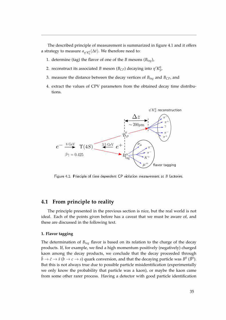
The described principle of measurement is summarized in figure 4.1 and it offersa strategy to measure aη′K0
S(∆t). We therefore need to:
1. determine (tag) the flavor of one of the B mesons (Btag),
2. reconstruct its associated B meson (BCP) decaying into η′K0S,
3. measure the distance between the decay vertices of Btag and BCP, and
4. extract the values of CPV parameters from the obtained decay time distribu-tions.
Figure 4.1: Principle of time dependent CP violation measurement at B factories.
4.1 From principle to reality
The principle presented in the previous section is nice, but the real world is notideal. Each of the points given before has a caveat that we must be aware of, andthese are discussed in the following text.
1. Flavor tagging
The determination of Btag flavor is based on its relation to the charge of the decayproducts. If, for example, we find a high momentum positively (negatively) chargedkaon among the decay products, we conclude that the decay proceeded throughb→ c→ s (b→ c→ s) quark conversion, and that the decaying particle was B0 (B0).But this is not always true due to possible particle misidentification (experimentallywe only know the probability that particle was a kaon), or maybe the kaon camefrom some other rarer process. Having a detector with good particle identification
35
CHAPTER 4. PRINCIPLE OF MEASUREMENT
systems is crucial for efficient flavor tagging. Presence of wrongly tagged B mesonsdilutes the asymmetry aη′K0
S, as given in (3.24), to
awtη′K0
S(∆t) = (1− 2w)aη′K0
S(∆t)− ∆w, (4.2)
where w = (wB0 + wB0)/2 and ∆w = wB0 − wB0 , with wB0 (wB0) being the fraction ofwrongly tagged B0 (B0) mesons.
2. Decay reconstruction
Experimentally, we can only detect particles that live long enough to produce signalsin tracking detectors (charged particles) or calorimeters (neutral particles). For B →η′K0
S decay these particles are charged pions and photons. They come either from thedecay of η′, that decays immediately at the interaction point3, or from the K0
S decay,which can happen a few cm from the interaction point due to relatively long lifetimeof K0
S (∼ 10−10 s). To reconstruct the B → η′K0S decay, we take the decay final state
particles and combine them to first obtain the intermediate states and finally the Bmeson candidate. Several conditions are imposed in the reconstruction to select asmany signal candidates as possible (i.e. B0 mesons that have actually decayed intoη′K0
S), while keeping the amout of background candidates (all non signal candidates)as low as possible. But since we always have some irreducible fraction of backgroundcandidates, this dilutes the asymmetry aη′K0
Sto
abgη′K0
S(∆t) = fsigaη′K0
S(∆t), (4.3)
where fsig is the fraction of signal candidates among all reconstructed candidates(and we assume that background candidates posses no asymmetry).
3. Decay vertex reconstruction
In reality, we can only determine the time difference ∆t with finite precision. Thedecay vertex position is mainly determined by the number and position of chargedparticle hits (in our case pions from η′ decay) in the detector closest to the interactionpoint. The detector has finite granularity and is placed at some distance from theinteraction point. The fact that a B meson pair is only approximately at rest inthe Υ(4S) CMS also limits the precision of determining ∆t. The effect of finite ∆tresolution on the asymmetry aη′K0
Scan be written as
ar fη′K0
S(∆t) = aη′K0
S(∆t)⊗R(∆t), (4.4)
where R(∆t) is the detector ∆t resolution function, and ⊗ denotes convolution.
3Lifetime of η′ is about 10−21 s.
36
4. Extraction of CP violating parameters
Neglecting the discussed experimental effects, we are able extract the values of theCPV parameters, Aη′K0
Sand Sη′K0
S, by fitting the following probability density func-
tion (PDF), obtained form the rates (3.20) and (3.21), to the measured decay rates
P(∆t, q) =e−|∆t|/τB0
4τB0
[1 + q
(Aη′K0
Scos ∆M∆t + Sη′K0
Ssin ∆M∆t
)], (4.5)
where q = +1 when Btag = B0 and q = −1 when Btag = B0 mesons4. As we haveseen, the measured decay rates differ from this PDF. To be still able to obtain thecorrect values of Aη′K0
Sand Sη′K0
S, we have to include the experimental effects in
P(∆t, q). The PDF that includes all three effects presented in the previous points isgiven by
P(∆t, q) =
fsige−|∆t|/τB0
4τB0
[1− q∆w + (1− 2w)q
(Aη′K0
Scos ∆M∆t + Sη′K0
Ssin ∆M∆t
)]⊗Rsig(∆t)
+ (1− fsig)Pbkg(∆t)⊗Rbkg(∆t), (4.6)
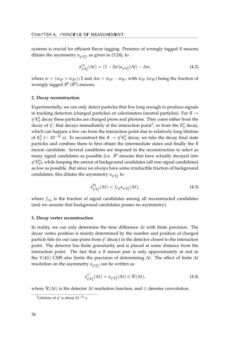
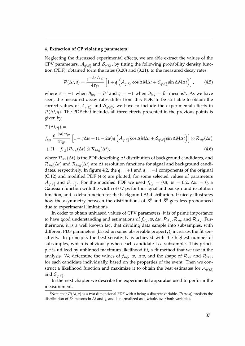
where Pbkg(∆t) is the PDF describing ∆t distribution of background candidates, andRsig(∆t) and Rbkg(∆t) are ∆t resolution functions for signal and background candi-dates, respectively. In figure 4.2, the q = +1 and q = −1 components of the original(C.12) and modified PDF (4.6) are plotted, for some selected values of parametersAη′K0
Sand Sη′K0
S. For the modified PDF we used fsig = 0.8, w = 0.2, ∆w = 0, a
Gaussian function with the width of 0.7 ps for the signal and background resolutionfunction, and a delta function for the backgound ∆t distribution. It nicely illustrateshow the asymmetry between the distributions of B0 and B0 gets less pronounceddue to experimental limitations.
In order to obtain unbiased values of CPV parameters, it is of prime importanceto have good understanding and estimations of fsig, w, ∆w,Pbkg,Rsig and Rbkg. Fur-thermore, it is a well known fact that dividing data sample into subsamples, withdifferent PDF parameters (based on some observable property), increases the fit sen-sitivity. In principle, the best sensitivity is achieved with the highest number ofsubsamples, which is obviously when each candidate is a subsample. This princi-ple is utilized by unbinned maximum likelihood fit, a fit method that we use in theanalysis. We determine the values of fsig, w, ∆w, and the shape of Rsig and Rbkg,for each candidate individually, based on the properties of the event. Then we con-struct a likelihood function and maximize it to obtain the best estimates for Aη′K0
Sand Sη′K0
S.
In the next chapter we describe the experimental apparatus used to perform themeasurement.
4Note that P(∆t, q) is a two dimensional PDF with q being a discrete variable. P(∆t, q) predicts thedistribution of B0 mesons in ∆t and q, and is normalized as a whole, over both variables.
37
CHAPTER 4. PRINCIPLE OF MEASUREMENT
-6 -4 -2 0 2 4 6
deca
yra
te
0
0.01
0.02
0.03
0.04
-6 -4 -2 0 2 4 6
deca
yra
te0
0.01
0.02
0.03
0.04
0.05
-6 -4 -2 0 2 4 6
deca
yra
te
0
0.01
0.02
0.03
0.04
-6 -4 -2 0 2 4 6
deca
yra
te
0
0.01
0.02
0.03
Figure 4.2: Time dependent decay rates of B0 and B0 mesons in the case of Sη′K0S= 0.68 and
Aη′K0S= 0.0 on the left, and in the case of Sη′K0
S= 0.68 and Aη′K0
S= 0.3 on the right. The top
two plots show decay rates as theoretically predicted, and the bottom two plots show the decayrates modi�ed by experimental limitations (presence of background ( fsig = 0.8) and wrongly taggedcandidates (w = 0.2), �nite detector resolution (σt = 0.7 ps)).
38
5The Belle experiment
The Belle experiment is one of the world’s two experiments operating on the so-called B factories. It is located in KEK, High Energy Accelerator Research Organiza-tion center in Tsukuba, Japan. It was designed in the 1990s, to exploit the propertiesof B mesons produced in e+e− collisions at the KEKB collider. The Belle collabora-tion consists of about 440 people from over 70 institutes, working on the experiment.In this chapter we describe in short the KEKB accelerator and the Belle detector, theexperimental apparatus used to record B meson decays 1.
5.1 The KEKB collider
The KEKB collider is an asymmetric energy e+e− collider [37], designed to pro-duce a large number of BB pairs. The energies of electron and positron beams are8 GeV and 3.5 GeV, respectively. The electrons and positrons are first acceleratedto their final energies in a linear accelerator (linac) and then injected into two sepa-rate storage rings of about 3 km in circumference, residing in a tunnel 11 m underground. There are about 1000 bunches of electrons and positrons in each ring, core-sponding to the distance of about 3 m between them. The two rings intersect ata single point on the orbital trajectory, called the interaction point (IP), where thebunches collide and where the Belle detector is placed. The electron and positronbeams collide at a finite angle of ±11 mrad, to avoid parasitic collisions. On average
1The other B factory experiment is BaBar at the PEPII collider at Stanford Linear Accelerator Labo-ratory (SLAC).
39
CHAPTER 5. THE BELLE EXPERIMENT
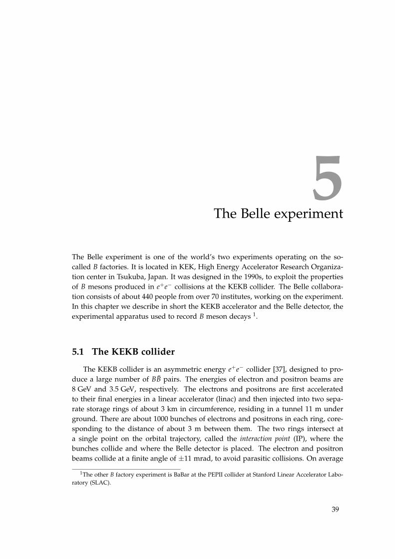
on approximately every 105 bunch collisions an e+e− interaction occurs, resulting inan outflow of particles produced in the collision, which are then detected in the Belledetector (in jargon we call this simply an event). The figure 5.1 illustrates the KEKBconfiguration.
positron target
wig
gler
wiggler
LER
HER
IP
Belle
Figure 5.1: Con�guration of the KEKB collider and the Belle detector.
The energy of the colliding beams is such, that the available energy in the CMSis equal to the mass of Υ(4S) resonance, which is a bound state of a b and b quark.However, in most events instead of the Υ(4S) production, a lighter pair of quarksis produced in e+e− → qq, where q stands for u, d, s, c. In the studies of B mesonsthese events represent the background component. On the other hand, when theΥ(4S) resonance is produced, it immediatelly decays into a BB pair. As alreadyargued in the previous chapter, this pair is approximatelly at rest in the CMS, since2MB = 10.56 GeV and MΥ(4S) = 10.58 GeV. In combination with asymmetric beamenergies this simplifies the kinematics of a BB pair to a single dimension, makesthe B meson flight distance measurable (∼ 200 µm), and therefore allows for timedependent studies.
Beside asymmetric beam energies, a high luminosity is another property defininga B factory. To perform precision measurments it is crucial to collect a large sampleof B decays. The design luminosity of the KEKB collider was L = 1.0× 1034 cm−2s−1.By the end of its operation in 2010 the peak luminosity reached the record value ofL = 2.1× 1034 cm−2s−1, well exceeding the design value. The evolution of the KEKBluminosity, as well as its time integrated value, are shown in figure 5.2. From the
40
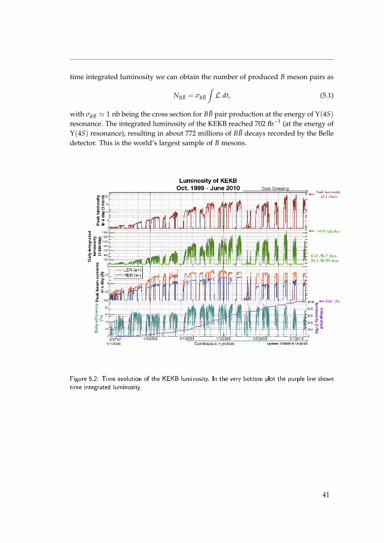
time integrated luminosity we can obtain the number of produced B meson pairs as
NBB = σBB
∫L dt, (5.1)
with σBB ' 1 nb being the cross section for BB pair production at the energy of Υ(4S)resonance. The integrated luminosity of the KEKB reached 702 fb−1 (at the energy ofΥ(4S) resonance), resulting in about 772 millions of BB decays recorded by the Belledetector. This is the world’s largest sample of B mesons.
Figure 5.2: Time evolution of the KEKB luminosity. In the very bottom plot the purple line showstime integrated luminosity.
41

CHAPTER 5. THE BELLE EXPERIMENT
5.2 The Belle detector
The Belle detector is a large-solid-angle magnetic spectrometer that is able todetect long-lived particles produced in e+e− collisions. These are
Charged particles: e±,µ±, π±, K±, p±
Neutral particles: γ, K0L.
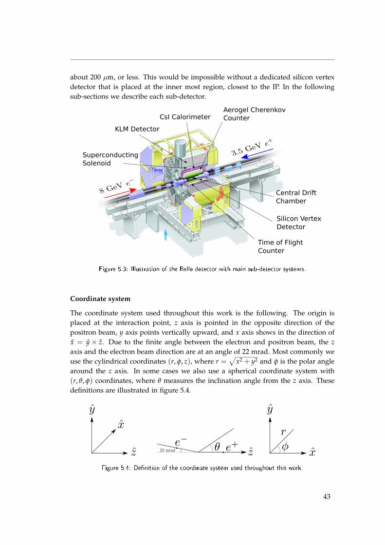
These particles are commonly produced in decays of heavier particles, such as B or Dmesons, or other short-lived hadrons, that decay practically at the interaction pointand cannot be directly detected. From these long-lived remnants the decay has to bereconstructed, to explore the underlying physical processes. The basic demand forthe detector is therefore to detect, measure the momentum, and determine the iden-tity of mentioned particles with high efficiency. In addition to this, a good precisionat determining the position of the decay vertex is crucial for time dependent studies.The Belle detector consists of several sub-detectors placed in cylindrically symmetricconfiguration around the IP, with some forward-backward asymmetries, followingthe asymmetry of e+e− collisions. The configuration of sub-detectors is illustratedin figure 5.3. We now briefly summarize how the information from each of them isutilized to fullfil the above demands, while more technical description is given in thefollowing subsections.
In its essence the Belle detector is a magnetic spectrometer, allowing to measurecharged particle momentum from the radius of curvature of its helix in a magneticfield. Large part of the Belle detector is inside the large superconducting solenoid,producing a homogeneous magnetic field of 1.5 T. Particle’s helix is tracked in thecentral drift chamber through the ionisation of gas that it is filled with. In additionto momentum, the particle’s charge is determined from the orientation of its helix.The information about identity of low momentum particles (< 1 GeV) can also beobtained from the central drift chamber, by measuring their energy loss due to ion-isation. Sub-detectors on the outer side of the drift chamber are used to provide anadditional information on particle identity. Two main principles are used. Measur-ing the velocity of the particle, and the nature of its interaction with the material.By measuring the velocity and knowing the momentum one can determine particle’smass, as they are related with p = γmv, and therefore its identity. The velocityis measured by aerogel Cherenkov counters, providing a good separation betweenhigh momentum (∼ 1.2− 3.5 GeV) pions and kaons, and by time of flight detectorfor separation at lower momenta. The nature of the interaction with the materialis used in two calorimeters, the electromagnetic calorimeter to detect photons andidentify electrons, and the KLM detector that is used to detect neutral kaons K0
L andidentify muons.
As it was argued in the previous chapter, for studies of time dependent asym-metries the decay vertex of B meson needs to be determined with the resolution of
42
about 200 µm, or less. This would be impossible without a dedicated silicon vertexdetector that is placed at the inner most region, closest to the IP. In the followingsub-sections we describe each sub-detector.
Silicon Vertex
Detector
Central Drift
Chamber
Aerogel Cherenkov
Counter
Time of Flight
Counter
CsI Calorimeter
KLM Detector
Superconducting
Solenoid
Figure 5.3: Illustration of the Belle detector with main sub-detector systems.
Coordinate system
The coordinate system used throughout this work is the following. The origin isplaced at the interaction point, z axis is pointed in the opposite direction of thepositron beam, y axis points vertically upward, and x axis shows in the direction ofx = y × z. Due to the finite angle between the electron and positron beam, the zaxis and the electron beam direction are at an angle of 22 mrad. Most commonly weuse the cylindrical coordinates (r, φ, z), where r =
√x2 + y2 and φ is the polar angle
around the z axis. In some cases we also use a spherical coordinate system with(r, θ, φ) coordinates, where θ measures the inclination angle from the z axis. Thesedefinitions are illustrated in figure 5.4.
Figure 5.4: De�nition of the coordinate system used throughout this work.
43
CHAPTER 5. THE BELLE EXPERIMENT
5.2.1 Silicon Vertex Detector
The Silicon Vertex Detector (SVD) plays a central role in measurements of time de-pendent CP violation, as it provides a precise measurements of B meson decay vertexposition. Besides a good spatial resolution, it is also important for this sub-detectorthat the amount of material placed inside the detector acceptance is kept sufficientlylow (to reduce the multiple scattering of particles). The most natural choice thatmeets this criteria is the use of double-sided silicon strip detectors (DSSDs).
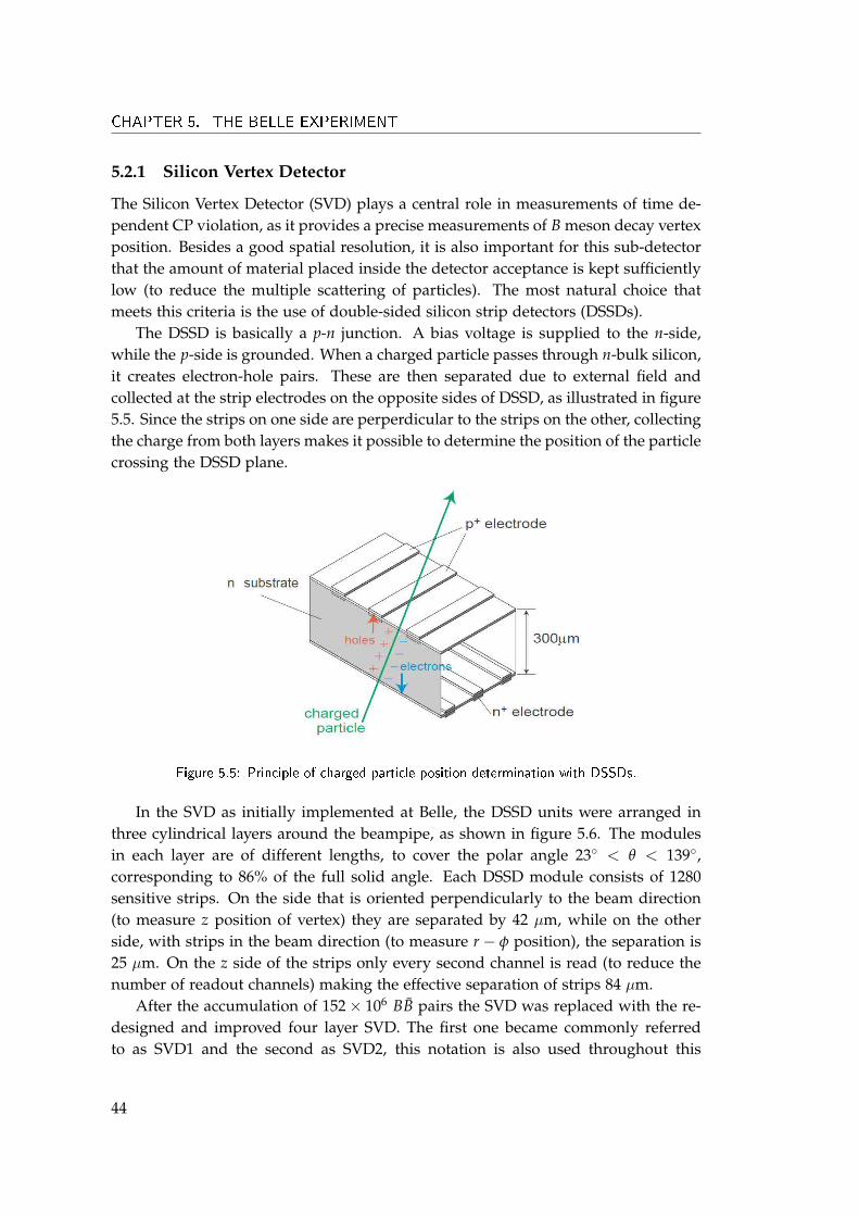
The DSSD is basically a p-n junction. A bias voltage is supplied to the n-side,while the p-side is grounded. When a charged particle passes through n-bulk silicon,it creates electron-hole pairs. These are then separated due to external field andcollected at the strip electrodes on the opposite sides of DSSD, as illustrated in figure5.5. Since the strips on one side are perperdicular to the strips on the other, collectingthe charge from both layers makes it possible to determine the position of the particlecrossing the DSSD plane.
Figure 5.5: Principle of charged particle position determination with DSSDs.
In the SVD as initially implemented at Belle, the DSSD units were arranged inthree cylindrical layers around the beampipe, as shown in figure 5.6. The modulesin each layer are of different lengths, to cover the polar angle 23◦ < θ < 139◦,corresponding to 86% of the full solid angle. Each DSSD module consists of 1280sensitive strips. On the side that is oriented perpendicularly to the beam direction(to measure z position of vertex) they are separated by 42 µm, while on the otherside, with strips in the beam direction (to measure r− φ position), the separation is25 µm. On the z side of the strips only every second channel is read (to reduce thenumber of readout channels) making the effective separation of strips 84 µm.
After the accumulation of 152× 106 BB pairs the SVD was replaced with the re-designed and improved four layer SVD. The first one became commonly referredto as SVD1 and the second as SVD2, this notation is also used throughout this
44
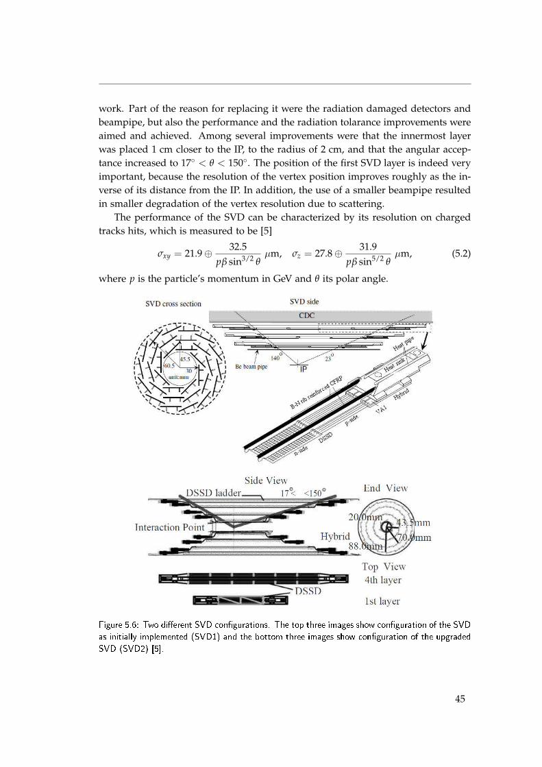
work. Part of the reason for replacing it were the radiation damaged detectors andbeampipe, but also the performance and the radiation tolarance improvements wereaimed and achieved. Among several improvements were that the innermost layerwas placed 1 cm closer to the IP, to the radius of 2 cm, and that the angular accep-tance increased to 17◦ < θ < 150◦. The position of the first SVD layer is indeed veryimportant, because the resolution of the vertex position improves roughly as the in-verse of its distance from the IP. In addition, the use of a smaller beampipe resultedin smaller degradation of the vertex resolution due to scattering.
The performance of the SVD can be characterized by its resolution on chargedtracks hits, which is measured to be [5]
σxy = 21.9⊕ 32.5pβ sin3/2 θ
µm, σz = 27.8⊕ 31.9pβ sin5/2 θ
µm, (5.2)
where p is the particle’s momentum in GeV and θ its polar angle.
Figure 5.6: Two di�erent SVD con�gurations. The top three images show con�guration of the SVDas initially implemented (SVD1) and the bottom three images show con�guration of the upgradedSVD (SVD2) [5].
45
CHAPTER 5. THE BELLE EXPERIMENT
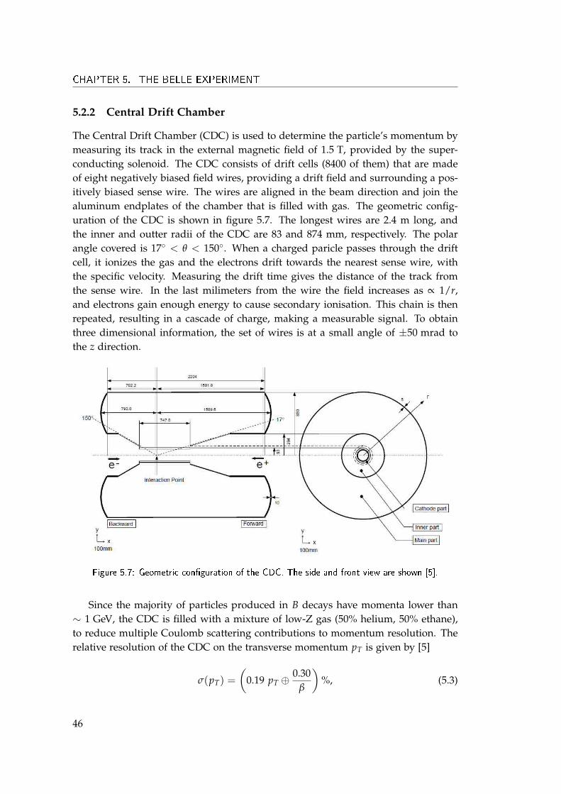
5.2.2 Central Drift Chamber
The Central Drift Chamber (CDC) is used to determine the particle’s momentum bymeasuring its track in the external magnetic field of 1.5 T, provided by the super-conducting solenoid. The CDC consists of drift cells (8400 of them) that are madeof eight negatively biased field wires, providing a drift field and surrounding a pos-itively biased sense wire. The wires are aligned in the beam direction and join thealuminum endplates of the chamber that is filled with gas. The geometric config-uration of the CDC is shown in figure 5.7. The longest wires are 2.4 m long, andthe inner and outter radii of the CDC are 83 and 874 mm, respectively. The polarangle covered is 17◦ < θ < 150◦. When a charged paricle passes through the driftcell, it ionizes the gas and the electrons drift towards the nearest sense wire, withthe specific velocity. Measuring the drift time gives the distance of the track fromthe sense wire. In the last milimeters from the wire the field increases as ∝ 1/r,and electrons gain enough energy to cause secondary ionisation. This chain is thenrepeated, resulting in a cascade of charge, making a measurable signal. To obtainthree dimensional information, the set of wires is at a small angle of ±50 mrad tothe z direction.
Figure 5.7: Geometric con�guration of the CDC. The side and front view are shown [5].
Since the majority of particles produced in B decays have momenta lower than∼ 1 GeV, the CDC is filled with a mixture of low-Z gas (50% helium, 50% ethane),to reduce multiple Coulomb scattering contributions to momentum resolution. Therelative resolution of the CDC on the transverse momentum pT is given by [5]
σ(pT) =
(0.19 pT ⊕
0.30β
)%, (5.3)
46
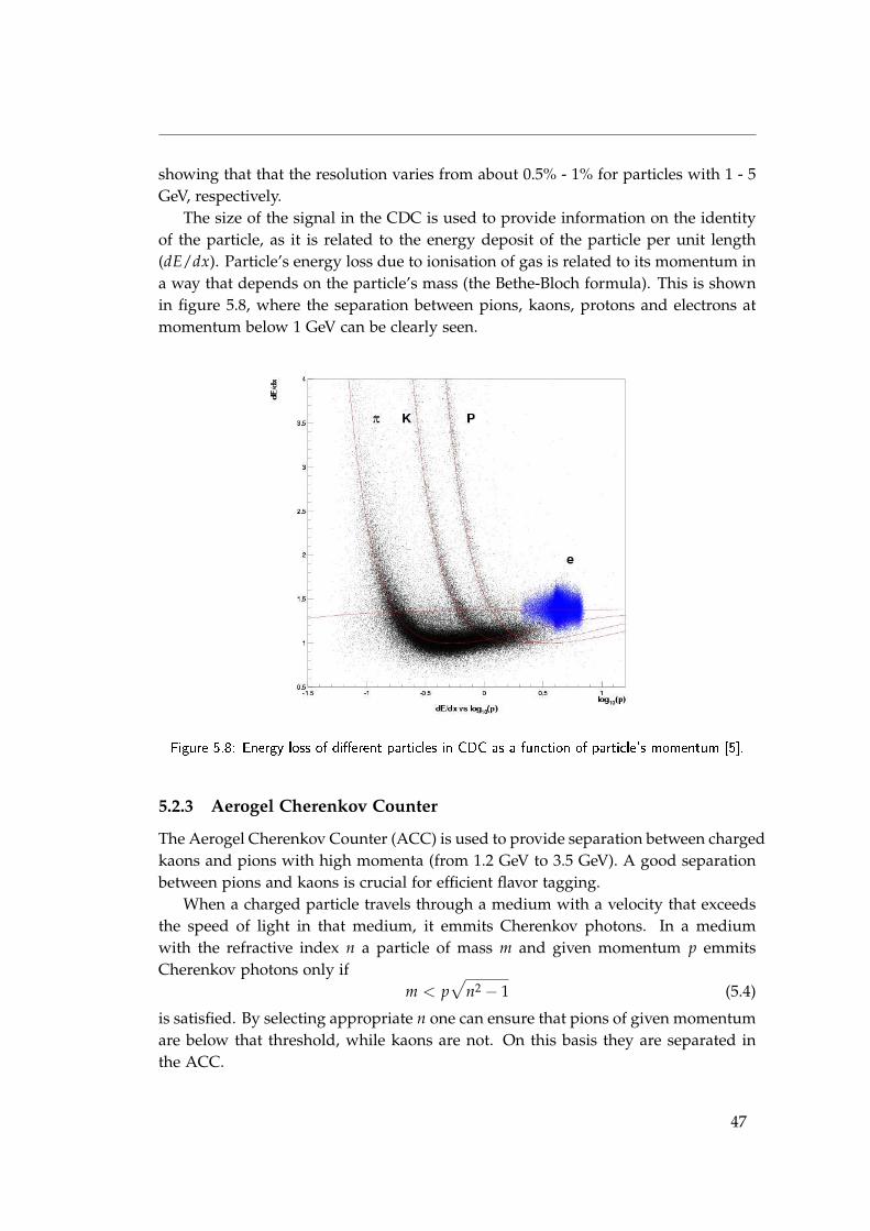
showing that that the resolution varies from about 0.5% - 1% for particles with 1 - 5GeV, respectively.
The size of the signal in the CDC is used to provide information on the identityof the particle, as it is related to the energy deposit of the particle per unit length(dE/dx). Particle’s energy loss due to ionisation of gas is related to its momentum ina way that depends on the particle’s mass (the Bethe-Bloch formula). This is shownin figure 5.8, where the separation between pions, kaons, protons and electrons atmomentum below 1 GeV can be clearly seen.
Figure 5.8: Energy loss of di�erent particles in CDC as a function of particle's momentum [5].
5.2.3 Aerogel Cherenkov Counter
The Aerogel Cherenkov Counter (ACC) is used to provide separation between chargedkaons and pions with high momenta (from 1.2 GeV to 3.5 GeV). A good separationbetween pions and kaons is crucial for efficient flavor tagging.
When a charged particle travels through a medium with a velocity that exceedsthe speed of light in that medium, it emmits Cherenkov photons. In a mediumwith the refractive index n a particle of mass m and given momentum p emmitsCherenkov photons only if
m < p√
n2 − 1 (5.4)
is satisfied. By selecting appropriate n one can ensure that pions of given momentumare below that threshold, while kaons are not. On this basis they are separated inthe ACC.
47
CHAPTER 5. THE BELLE EXPERIMENT
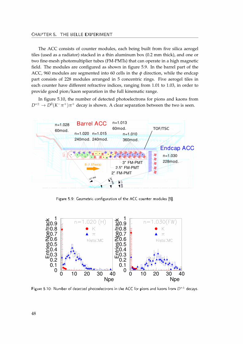
The ACC consists of counter modules, each being built from five silica aerogeltiles (used as a radiator) stacked in a thin aluminum box (0.2 mm thick), and one ortwo fine-mesh photomultiplier tubes (FM-PMTs) that can operate in a high magneticfield. The modules are configured as shown in figure 5.9. In the barrel part of theACC, 960 modules are segmented into 60 cells in the φ direction, while the endcappart consists of 228 modules arranged in 5 concentric rings. Five aerogel tiles ineach counter have different refractive indices, ranging from 1.01 to 1.03, in order toprovide good pion/kaon separation in the full kinematic range.
In figure 5.10, the number of detected photoelectrons for pions and kaons fromD∗± → D0(K−π+)π+ decay is shown. A clear separation between the two is seen.
B (1.5Tesla) 3" FM-PMT2.5" FM-PMT
2" FM-PMT
17deg
127deg 34
deg
Endcap ACC
885
R(BACC/inner)
1145
R(EACC/outer)
1622 (BACC)
1670 (EACC/inside)
854 (BACC)
1165
R(BACC/outer)
n=1.02860mod.
n=1.020240mod.
n=1.015240mod.
n=1.01360mod.
n=1.010360mod.
Barrel ACC
n=1.030228mod.
TOF/TSC
Figure 5.9: Geometric con�guration of the ACC counter modules [5].
Npe
00.10.20.30.40.50.60.70.80.9
1
0 10 20 30 40
Ent
ries/
Npe
/trac
k
00.10.20.30.40.50.60.70.80.9
1
0 10 20 30 40
Ent
ries/
Npe
/trac
k
Npe
Figure 5.10: Number of detected photoelectrons in the ACC for pions and kaons from D∗± decays.
48

5.2.4 Time of Flight Counter
The Time of Flight Counter (TOF) gives particle identification information in orderto separate charged pions and kaons with low momenta, below 1.2 GeV.
By measuring the time T that particle needs from the IP to the TOF (∼ 1.2 m),and knowing its momentum p, particle’s mass can be inferred by
m = p
√c2TL2 − 1. (5.5)
Basic building blocks of the TOF are photomultiplier tubes with attached plasticscintillation counters. They provide a timing resolution of 100 ps, allowing the sep-aration between kaons and pions at 1.0 GeV with 3σ significance. The TOF alsoprovides fast timing signals for the data acquisition trigger system. For this pur-pose, a thin trigger scintillation counter (TSC) is placed directly in front of two basicunits to form a TOF module. The geometric configuration of a TOF module is shownin figure 5.11. In total there are 64 TOF modules placed in the barrel region at theradius of 1.2 m from the IP. The polar angle covered is 34◦ < θ < 120◦.
TSC 0.5 t x 12.0 W x 263.0 L
PMT122.0
182. 5 190. 5
R= 117. 5
R= 122. 0R=120. 05
R= 117. 5R=117. 5
PMT PMT
- 72.5- 80.5- 91.5
Light guide
TOF 4.0 t x 6.0 W x 255.0 L
1. 0
PMTPMT
ForwardBackward
4. 0
282. 0287. 0
I.P (Z=0)
1. 5
Figure 5.11: Geometric con�guration of a TOF module [5]. All dimensions are in cm.
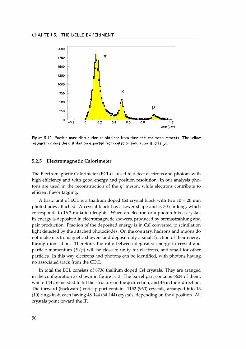
Figure 5.12 shows the mass distribution of particles with momentum below 1.2GeV, as obtained from the TOF measurements. Separated peaks at masses of kaon,pion, and proton can be seen. Also the expected distribution obtained from thedetector simulation is shown, and matches the measured data well.
49
CHAPTER 5. THE BELLE EXPERIMENT
Figure 5.12: Particle mass distribution as obtained from time of �ight measurements. The yellowhistogram shows the distribution expected from detector simulation studies [5].
5.2.5 Electromagnetic Calorimeter
The Electromagnetic Calorimeter (ECL) is used to detect electrons and photons withhigh efficiency and with good energy and position resolution. In our analysis pho-tons are used in the reconstruction of the η′ meson, while electrons contribute toefficient flavor tagging.
A basic unit of ECL is a thallium doped CsI crystal block with two 10× 20 mmphotodiodes attached. A crystal block has a tower shape and is 30 cm long, whichcorresponds to 16.2 radiation lenghts. When an electron or a photon hits a crystal,its energy is deposited in electromagnetic showers, produced by bremsstrahlung andpair production. Fraction of the deposited energy is in CsI converted to scintilationlight detected by the attached photodiodes. On the contrary, hadrons and muons donot make electromagnetic showers and deposit only a small fraction of their energythrough ionisation. Therefore, the ratio between deposited energy in crystal andparticle momentum (E/p) will be close to unity for electrons, and small for otherparticles. In this way electrons and photons can be identified, with photons havingno associated track from the CDC.
In total the ECL consists of 8736 thallium doped CsI crystals. They are arangedin the configuration as shown in figure 5.13. The barrel part contains 6624 of them,where 144 are needed to fill the structure in the φ direction, and 46 in the θ direction.The forward (backward) endcap part contains 1152 (960) crystals, arranged into 13(10) rings in φ, each having 48-144 (64-144) crystals, depending on the θ position. Allcrystals point toward the IP.
50
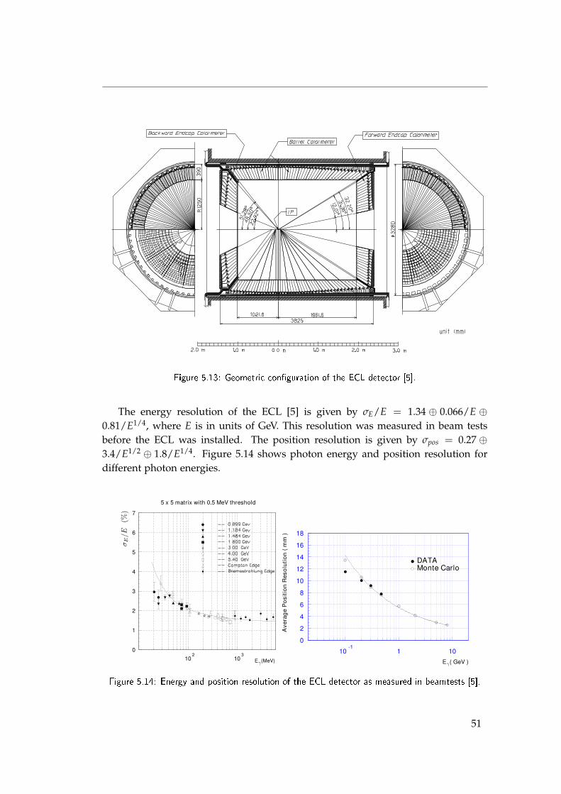
Figure 5.13: Geometric con�guration of the ECL detector [5].
The energy resolution of the ECL [5] is given by σE/E = 1.34 ⊕ 0.066/E ⊕0.81/E1/4, where E is in units of GeV. This resolution was measured in beam testsbefore the ECL was installed. The position resolution is given by σpos = 0.27 ⊕3.4/E1/2 ⊕ 1.8/E1/4. Figure 5.14 shows photon energy and position resolution fordifferent photon energies.
5 x 5 matrix with 0.5 MeV threshold
0
1
2
3
4
5
6
7
102
103
E (MeV)
0
2
4
6
8
10
12
14
16
18
10-1
1 10
E ( GeV )
Ave
rage
Pos
ition
Res
olution(m
m)
Monte CarloDATA
Figure 5.14: Energy and position resolution of the ECL detector as measured in beamtests [5].
51
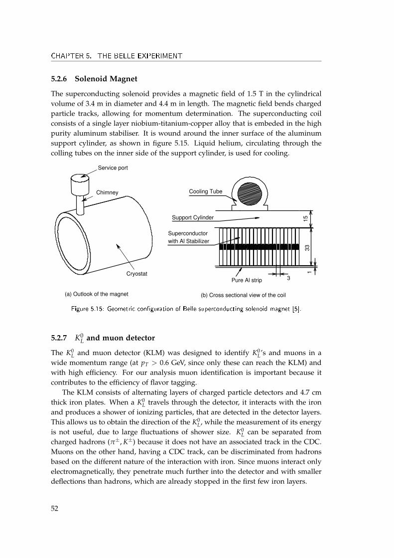
CHAPTER 5. THE BELLE EXPERIMENT
5.2.6 Solenoid Magnet
The superconducting solenoid provides a magnetic field of 1.5 T in the cylindricalvolume of 3.4 m in diameter and 4.4 m in length. The magnetic field bends chargedparticle tracks, allowing for momentum determination. The superconducting coilconsists of a single layer niobium-titanium-copper alloy that is embeded in the highpurity aluminum stabiliser. It is wound around the inner surface of the aluminumsupport cylinder, as shown in figure 5.15. Liquid helium, circulating through thecolling tubes on the inner side of the support cylinder, is used for cooling.
Pure Al strip
Superconductorwith Al Stabilizer
Support Cylinder
Cooling Tube
3
133
15
Chimney
Cryostat
Service port
(a) Outlook of the magnet (b) Cross sectional view of the coil
Figure 5.15: Geometric con�guration of Belle superconducting solenoid magnet [5].
5.2.7 K0L and muon detector
The K0L and muon detector (KLM) was designed to identify K0
L’s and muons in awide momentum range (at pT > 0.6 GeV, since only these can reach the KLM) andwith high efficiency. For our analysis muon identification is important because itcontributes to the efficiency of flavor tagging.
The KLM consists of alternating layers of charged particle detectors and 4.7 cmthick iron plates. When a K0
L travels through the detector, it interacts with the ironand produces a shower of ionizing particles, that are detected in the detector layers.This allows us to obtain the direction of the K0
L, while the measurement of its energyis not useful, due to large fluctuations of shower size. K0
L can be separated fromcharged hadrons (π±, K±) because it does not have an associated track in the CDC.Muons on the other hand, having a CDC track, can be discriminated from hadronsbased on the different nature of the interaction with iron. Since muons interact onlyelectromagnetically, they penetrate much further into the detector and with smallerdeflections than hadrons, which are already stopped in the first few iron layers.
52
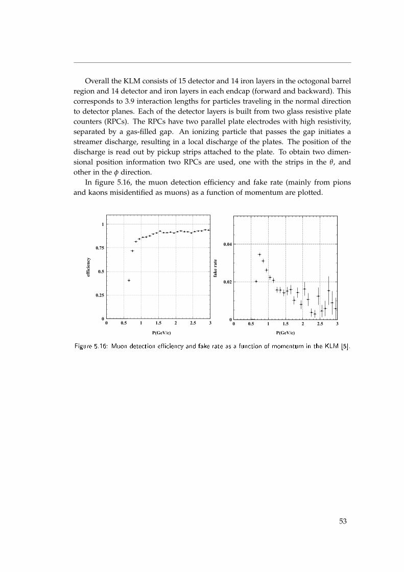
Overall the KLM consists of 15 detector and 14 iron layers in the octogonal barrelregion and 14 detector and iron layers in each endcap (forward and backward). Thiscorresponds to 3.9 interaction lengths for particles traveling in the normal directionto detector planes. Each of the detector layers is built from two glass resistive platecounters (RPCs). The RPCs have two parallel plate electrodes with high resistivity,separated by a gas-filled gap. An ionizing particle that passes the gap initiates astreamer discharge, resulting in a local discharge of the plates. The position of thedischarge is read out by pickup strips attached to the plate. To obtain two dimen-sional position information two RPCs are used, one with the strips in the θ, andother in the φ direction.
In figure 5.16, the muon detection efficiency and fake rate (mainly from pionsand kaons misidentified as muons) as a function of momentum are plotted.
0
0.25
0.5
0.75
1
0 0.5 1 1.5 2 2.5 3
P(GeV/c)
efficiency
0
0.02
0.04
0 0.5 1 1.5 2 2.5 3
P(GeV/c)
fakerate
Figure 5.16: Muon detection e�ciency and fake rate as a function of momentum in the KLM [5].
53
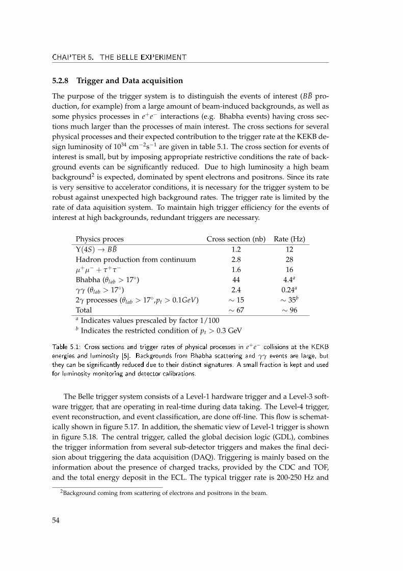
CHAPTER 5. THE BELLE EXPERIMENT
5.2.8 Trigger and Data acquisition
The purpose of the trigger system is to distinguish the events of interest (BB pro-duction, for example) from a large amount of beam-induced backgrounds, as well assome physics processes in e+e− interactions (e.g. Bhabha events) having cross sec-tions much larger than the processes of main interest. The cross sections for severalphysical processes and their expected contribution to the trigger rate at the KEKB de-sign luminosity of 1034 cm−2s−1 are given in table 5.1. The cross section for events ofinterest is small, but by imposing appropriate restrictive conditions the rate of back-ground events can be significantly reduced. Due to high luminosity a high beambackground2 is expected, dominated by spent electrons and positrons. Since its rateis very sensitive to accelerator conditions, it is necessary for the trigger system to berobust against unexpected high background rates. The trigger rate is limited by therate of data aquisition system. To maintain high trigger efficiency for the events ofinterest at high backgrounds, redundant triggers are necessary.
Physics proces Cross section (nb) Rate (Hz)Υ(4S)→ BB 1.2 12Hadron production from continuum 2.8 28µ+µ− + τ+τ− 1.6 16Bhabha (θlab > 17◦) 44 4.4a
γγ (θlab > 17◦) 2.4 0.24a
2γ processes (θlab > 17◦,pt > 0.1GeV) ∼ 15 ∼ 35b
Total ∼ 67 ∼ 96a Indicates values prescaled by factor 1/100b Indicates the restricted condition of pt > 0.3 GeV
Table 5.1: Cross sections and trigger rates of physical processes in e+e− collisions at the KEKBenergies and luminosity [5]. Backgrounds from Bhabha scattering and γγ events are large, butthey can be signi�cantly reduced due to their distinct signatures. A small fraction is kept and usedfor luminosity monitoring and detector calibrations.
The Belle trigger system consists of a Level-1 hardware trigger and a Level-3 soft-ware trigger, that are operating in real-time during data taking. The Level-4 trigger,event reconstruction, and event classification, are done off-line. This flow is schemat-ically shown in figure 5.17. In addition, the shematic view of Level-1 trigger is shownin figure 5.18. The central trigger, called the global decision logic (GDL), combinesthe trigger information from several sub-detector triggers and makes the final deci-sion about triggering the data acquisition (DAQ). Triggering is mainly based on theinformation about the presence of charged tracks, provided by the CDC and TOF,and the total energy deposit in the ECL. The typical trigger rate is 200-250 Hz and
2Background coming from scattering of electrons and positrons in the beam.
54
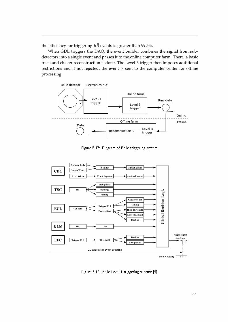
the efficiency for triggering BB events is greater than 99.5%.When GDL triggers the DAQ, the event builder combines the signal from sub-
detectors into a single event and passes it to the online computer farm. There, a basictrack and cluster reconstruction is done. The Level-3 trigger then imposes additionalrestrictions and if not rejected, the event is sent to the computer center for offlineprocessing.
Level-1trigger
Level-3trigger
Level-4triggerReconsrtuction
Belle detecor
Online farm
Electronics hut
Raw data
Online
OfflineOffline farmData
Figure 5.17: Diagram of Belle triggering system.
GlobalDecisionLogic
CDC
EFC
TSC
KLM
ECL
Cathode Pads
Stereo Wires
Axial Wires Track Segment
z track count
r- track count
Z finder
High Threshold
Trigger Cell ThresholdBhabha
Two photon
Hit
multiplicity
topology
timing
Hit hit
4x4 SumTrigger Cell
Energy Sum
Cluster count
Timing
Low Threshold
Bhabha
Trigger Signal
Gate/Stop
Beam Crossing
2.2 sec after event crossing�
�
�
Figure 5.18: Belle Level-1 triggering scheme [5].
55
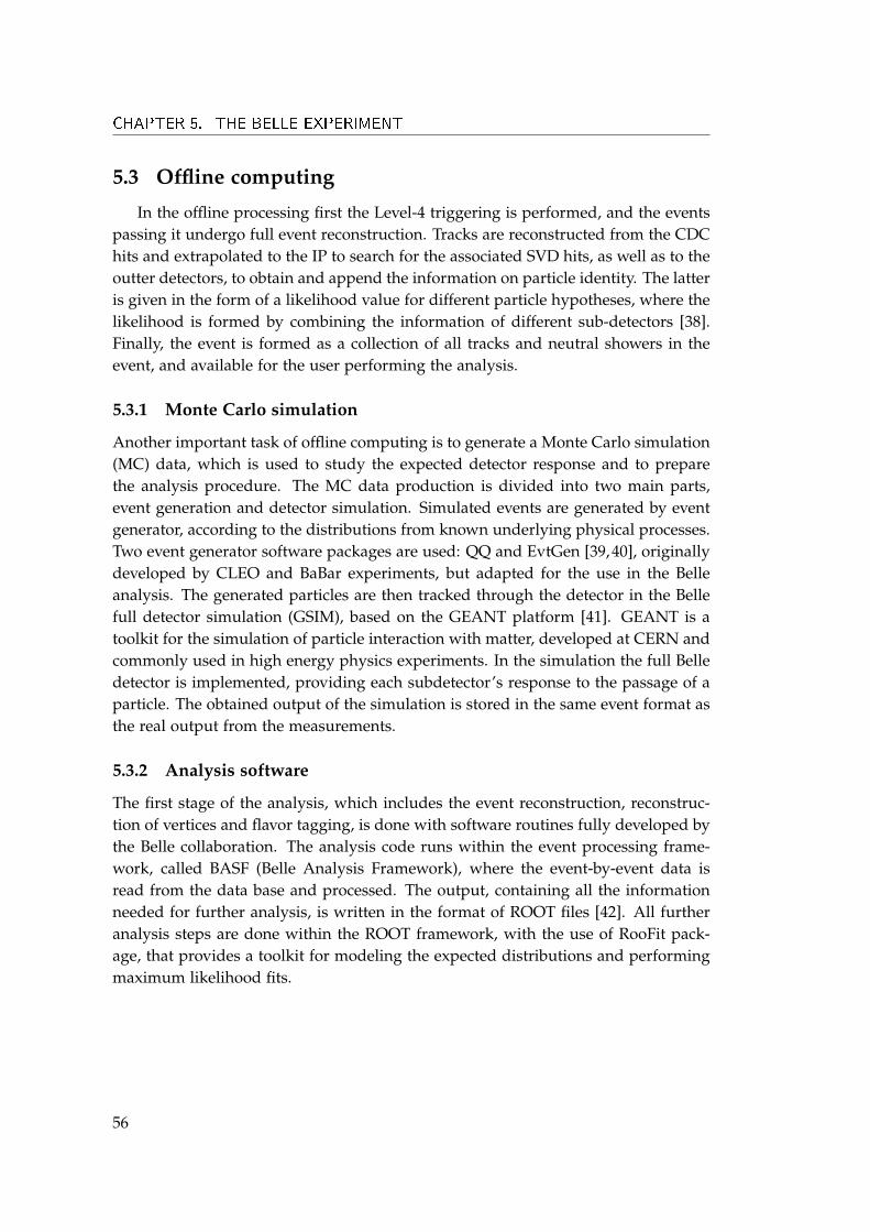
CHAPTER 5. THE BELLE EXPERIMENT
5.3 Offline computing
In the offline processing first the Level-4 triggering is performed, and the eventspassing it undergo full event reconstruction. Tracks are reconstructed from the CDChits and extrapolated to the IP to search for the associated SVD hits, as well as to theoutter detectors, to obtain and append the information on particle identity. The latteris given in the form of a likelihood value for different particle hypotheses, where thelikelihood is formed by combining the information of different sub-detectors [38].Finally, the event is formed as a collection of all tracks and neutral showers in theevent, and available for the user performing the analysis.
5.3.1 Monte Carlo simulation
Another important task of offline computing is to generate a Monte Carlo simulation(MC) data, which is used to study the expected detector response and to preparethe analysis procedure. The MC data production is divided into two main parts,event generation and detector simulation. Simulated events are generated by eventgenerator, according to the distributions from known underlying physical processes.Two event generator software packages are used: QQ and EvtGen [39,40], originallydeveloped by CLEO and BaBar experiments, but adapted for the use in the Belleanalysis. The generated particles are then tracked through the detector in the Bellefull detector simulation (GSIM), based on the GEANT platform [41]. GEANT is atoolkit for the simulation of particle interaction with matter, developed at CERN andcommonly used in high energy physics experiments. In the simulation the full Belledetector is implemented, providing each subdetector’s response to the passage of aparticle. The obtained output of the simulation is stored in the same event format asthe real output from the measurements.
5.3.2 Analysis software
The first stage of the analysis, which includes the event reconstruction, reconstruc-tion of vertices and flavor tagging, is done with software routines fully developed bythe Belle collaboration. The analysis code runs within the event processing frame-work, called BASF (Belle Analysis Framework), where the event-by-event data isread from the data base and processed. The output, containing all the informationneeded for further analysis, is written in the format of ROOT files [42]. All furtheranalysis steps are done within the ROOT framework, with the use of RooFit pack-age, that provides a toolkit for modeling the expected distributions and performingmaximum likelihood fits.
56
6Preparation of measurement procedure
In this chapter we describe the analysis procedure in detail. To prepare and validatethe pocedure a large dataset of simulated events is used, beside the nominal datasetof the measured events. On both datasets we reconstruct B candidates from theB0 → η′K0
S and B+ → η′K+ decays. The candidates from the latter are used as thecontrol sample. During the preparation of the analysis procedure we blind the flavorinformation of B0 candidates reconstruced from the measured events. Only when theanalysis procedure is fully prepared and validated by studying the simulated dataand the control sample, we unblind the flavor information, and use the preparedprocedure to extract the CPV parameters from the candidates reconstructed fromthe measured events. This so-called blind analysis technique is applied in order not tobias the results of the measurement which could arise, for example, by determinationof the selection criteria and other details of the method using measured data, or bythe subjective observer induced biases.
The basic idea of the measurement procedure was already presented in chapter4. The values of the CPV parameters can be extracted from the ∆t, q distribution ofreconstructed B candidates by fitting the PDF
P(∆t, q) =
fsige−∆t/τB0
4π
[1− q∆w + (1− 2w)q
(Aη′K0
Scos ∆M∆t + Sη′K0
Ssin ∆M∆t
)]⊗Rsig(∆t)
+ (1− fsig)Pbkg(∆t)⊗Rbkg(∆t), (6.1)
to the measured ∆t, q distribution. To be able to perform this fit, and obtain unbiased
57
CHAPTER 6. PREPARATION OF MEASUREMENT PROCEDURE
values of the CPV parameters, the following points have to be done first:
1. B0 meson candidates decaying into η′K0S final state have to be reconstructed
from a set of events.
2. Selection criteria need to be applied to reduce the number of B0 candidatescoming from background events (events not containing B0 → η′K0
S decay).
3. The fraction of candidates from signal events ( fsig), among all the candidatessurviving selection criteria, needs to be estimated.
4. The flavor of each B0 candidate needs to be determined (q = +1 or q = −1).
5. The ∆t has to be determined by measuring a spatial distance between the decayvertices of both B mesons in the event.
6. The ∆t resolution function of the signal candidates (Rsig(∆t)) has to be deter-mined.
7. The ∆t distribution of the candidates from the background events has to bestudied to obtain Pbkg(∆t)⊗Rbkg(∆t).
8. Finally, the CPV parameters can be extracted by fitting the PDF (6.1) to the ∆t, qdistribution of the reconstructed B0 candidates.
In this chapter each of the points given above is described in its own section, follow-ing the same order.
We now name and describe different datasets that are used to prepare the analy-sis procedure. The terminology given is used throught this work.
DatasetsSignal MC: dataset of simulated signal events. Signal events contain e+e¯ →Υ(4S)→ B0B0 process, with one B meson of a pair decaying into η′K0
S and the otherdecaying generically, according to all known and measured branching fractions.
Generic BB MC: dataset of simulated events containing e+e¯ → Υ(4S) → B+B−
or B0B0 process, with both B mesons decaying generically, but excluding our signaldecay. These events represent background for our analysis.
Continuum MC: dataset of simulated e+e− → qq (q = u, d, s, c) events. No B mesonsare produced in these events and they represent background for our analysis.
Measured data: our nominal dataset of measured events from the Belle detector.This is the Belle final dataset, accumulated during the years of its operation (1999-2010). It contains about 772 millions BB events, half of them being B+B− and halfB0B0 events.
58
Full MC: dataset of simulated events obtained by merging signal MC, generic BBMC, and continuum MC, with the fractions as expected in the measured data. Itcontains a signal and all expected backgrounds, so this set is equivalent to the mea-sured data.
To express the number of events contained in a dataset, we usually compare it withthe expected number of events of specified type in the measured data. A term streamis used for the latter. For example, if we state that some study was done on 2 streamsof signal MC, this means that the number of signal events in the dataset used wastwice the number of signal events expected in the measured data.
6.1 B0 → η′K0S decay
Here we trace the B0 → η′K0S decay to the final state long-lived particles, that
can be detected with the Belle detector. The neutral B meson decays into η′ and K0
meson with the branching fraction of [24]
B(B0 → η′K0) = (6.6± 0.4)× 10−5. (6.2)
After the decay, K0 undergoes K0 − K0 mixing and in 50% of cases decays as K0S and
in other 50% as K0L. In this analysis only the K0
S is used1. K0S decays into π0π0 in
roughly 30%, and into π+π− in roughly 70% of the cases. A neutral pion decays intotwo photons, while charged pions are long-lived (compared to the time they need tocross the detector).
The η′ meson has three relevant decay modes, with the branching fraction largerthan 3%. Two of them contain the intermediate η meson, which further decays intostates of three pions or two photons, and one contains the intermediate ρ0 meson,which decays into two charged pions. The branching fractions of all decays in thischain are summarized in table 6.1. In table 6.2 we give some basic properties of theparticles involved.
6.2 Event reconstruction and selection
In this section we describe how the B0 → η′K0S decay is reconstructed, and the
criteria used to reduce the number of B candidates coming from the backgroundevents.
To reconstruct the B0 → η′K0S decay we use two η′ decay modes, η′ → ρ0γ
and η′ → π+π−η, and both K0S decay modes, K0
S → π+π− and K0S → π0π0. To
1Reconstruction of K0L demands quite a different technique, as K0
L leaves no traces in the CDC. Themeasurement of B→ η′K0
L is a subject of another study.
59
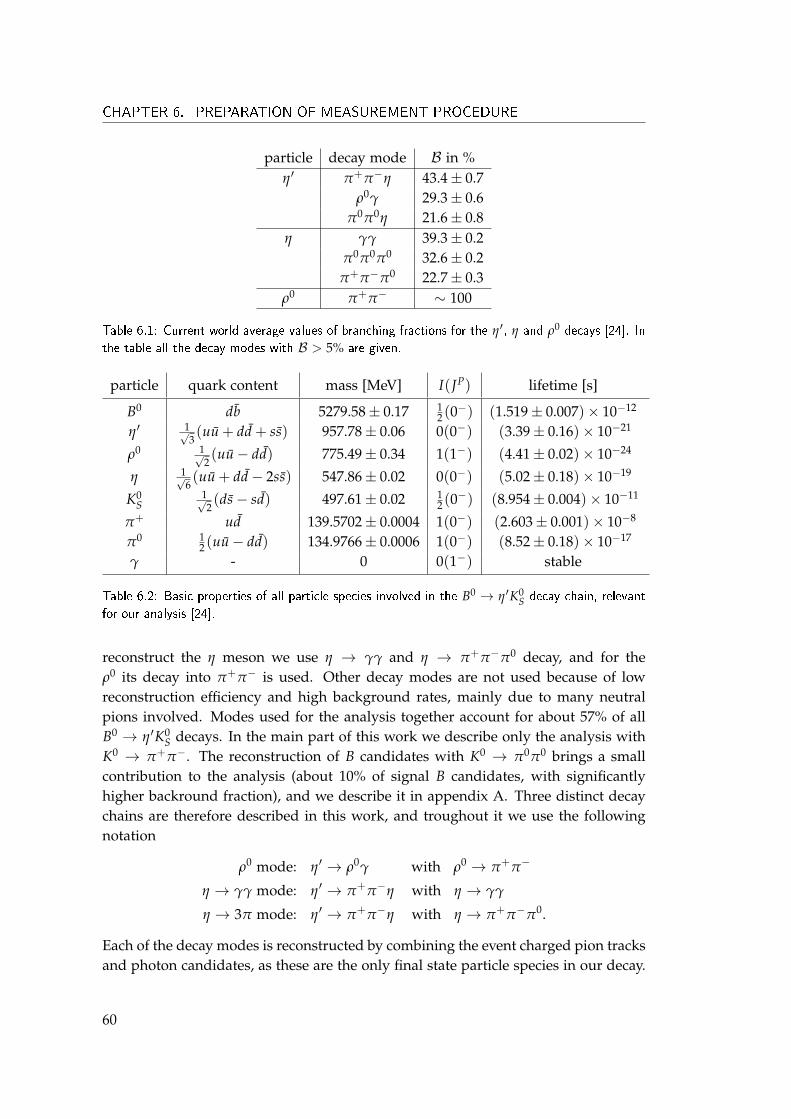
CHAPTER 6. PREPARATION OF MEASUREMENT PROCEDURE
particle decay mode B in %η′ π+π−η 43.4± 0.7
ρ0γ 29.3± 0.6π0π0η 21.6± 0.8
η γγ 39.3± 0.2π0π0π0 32.6± 0.2π+π−π0 22.7± 0.3
ρ0 π+π− ∼ 100
Table 6.1: Current world average values of branching fractions for the η′, η and ρ0 decays [24]. Inthe table all the decay modes with B > 5% are given.
particle quark content mass [MeV] I(JP) lifetime [s]
B0 db 5279.58± 0.17 12 (0−) (1.519± 0.007)× 10−12
η′ 1√3(uu + dd + ss) 957.78± 0.06 0(0−) (3.39± 0.16)× 10−21
ρ0 1√2(uu− dd) 775.49± 0.34 1(1−) (4.41± 0.02)× 10−24
η 1√6(uu + dd− 2ss) 547.86± 0.02 0(0−) (5.02± 0.18)× 10−19
K0S
1√2(ds− sd) 497.61± 0.02 1
2 (0−) (8.954± 0.004)× 10−11
π+ ud 139.5702± 0.0004 1(0−) (2.603± 0.001)× 10−8
π0 12 (uu− dd) 134.9766± 0.0006 1(0−) (8.52± 0.18)× 10−17
γ - 0 0(1−) stable
Table 6.2: Basic properties of all particle species involved in the B0 → η′K0S decay chain, relevant
for our analysis [24].
reconstruct the η meson we use η → γγ and η → π+π−π0 decay, and for theρ0 its decay into π+π− is used. Other decay modes are not used because of lowreconstruction efficiency and high background rates, mainly due to many neutralpions involved. Modes used for the analysis together account for about 57% of allB0 → η′K0
S decays. In the main part of this work we describe only the analysis withK0 → π+π−. The reconstruction of B candidates with K0 → π0π0 brings a smallcontribution to the analysis (about 10% of signal B candidates, with significantlyhigher backround fraction), and we describe it in appendix A. Three distinct decaychains are therefore described in this work, and troughout it we use the followingnotation
ρ0 mode: η′ → ρ0γ with ρ0 → π+π−
η → γγ mode: η′ → π+π−η with η → γγ
η → 3π mode: η′ → π+π−η with η → π+π−π0.
Each of the decay modes is reconstructed by combining the event charged pion tracksand photon candidates, as these are the only final state particle species in our decay.
60
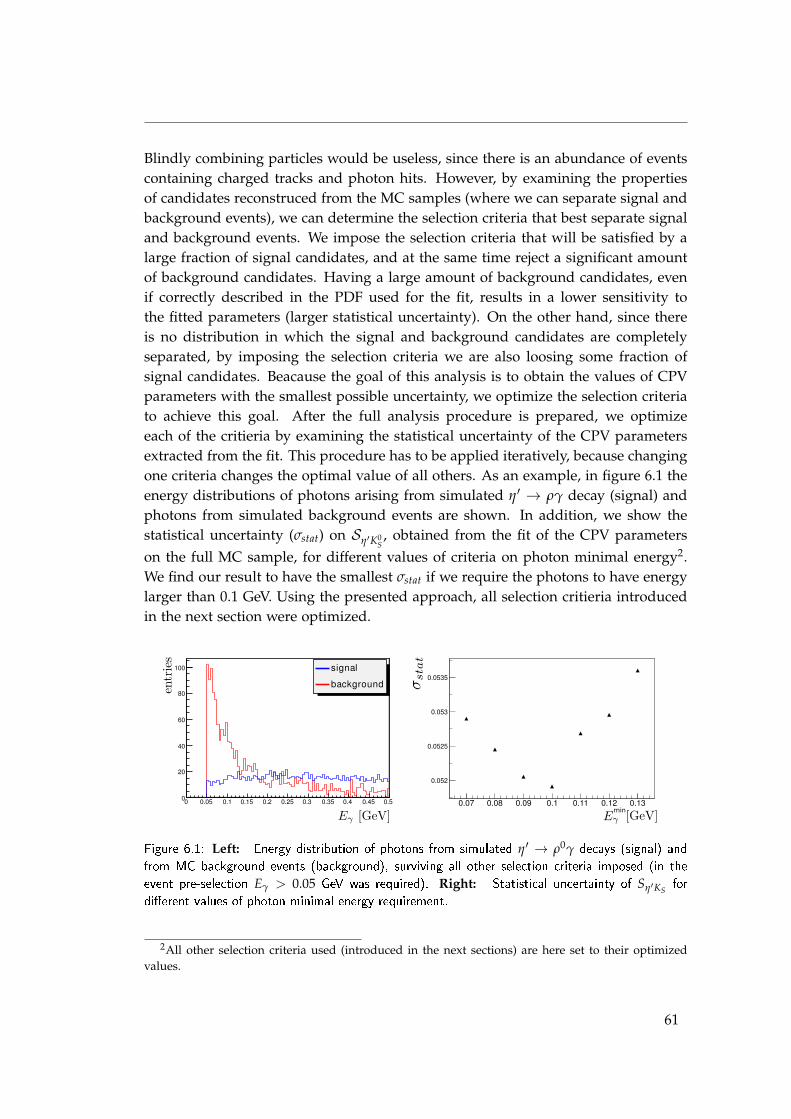
Blindly combining particles would be useless, since there is an abundance of eventscontaining charged tracks and photon hits. However, by examining the propertiesof candidates reconstruced from the MC samples (where we can separate signal andbackground events), we can determine the selection criteria that best separate signaland background events. We impose the selection criteria that will be satisfied by alarge fraction of signal candidates, and at the same time reject a significant amountof background candidates. Having a large amount of background candidates, evenif correctly described in the PDF used for the fit, results in a lower sensitivity tothe fitted parameters (larger statistical uncertainty). On the other hand, since thereis no distribution in which the signal and background candidates are completelyseparated, by imposing the selection criteria we are also loosing some fraction ofsignal candidates. Beacause the goal of this analysis is to obtain the values of CPVparameters with the smallest possible uncertainty, we optimize the selection criteriato achieve this goal. After the full analysis procedure is prepared, we optimizeeach of the critieria by examining the statistical uncertainty of the CPV parametersextracted from the fit. This procedure has to be applied iteratively, because changingone criteria changes the optimal value of all others. As an example, in figure 6.1 theenergy distributions of photons arising from simulated η′ → ργ decay (signal) andphotons from simulated background events are shown. In addition, we show thestatistical uncertainty (σstat) on Sη′K0
S, obtained from the fit of the CPV parameters
on the full MC sample, for different values of criteria on photon minimal energy2.We find our result to have the smallest σstat if we require the photons to have energylarger than 0.1 GeV. Using the presented approach, all selection critieria introducedin the next section were optimized.
0 0.05 0.1 0.15 0.2 0.25 0.3 0.35 0.4 0.45 0.50
20
40
60
80
100 signal
background
0.07 0.08 0.09 0.1 0.11 0.12 0.13
0.052
0.0525
0.053
0.0535
min
Figure 6.1: Left: Energy distribution of photons from simulated η′ → ρ0γ decays (signal) andfrom MC background events (background), surviving all other selection criteria imposed (in theevent pre-selection Eγ > 0.05 GeV was required). Right: Statistical uncertainty of Sη′KS
fordi�erent values of photon minimal energy requirement.
2All other selection criteria used (introduced in the next sections) are here set to their optimizedvalues.
61
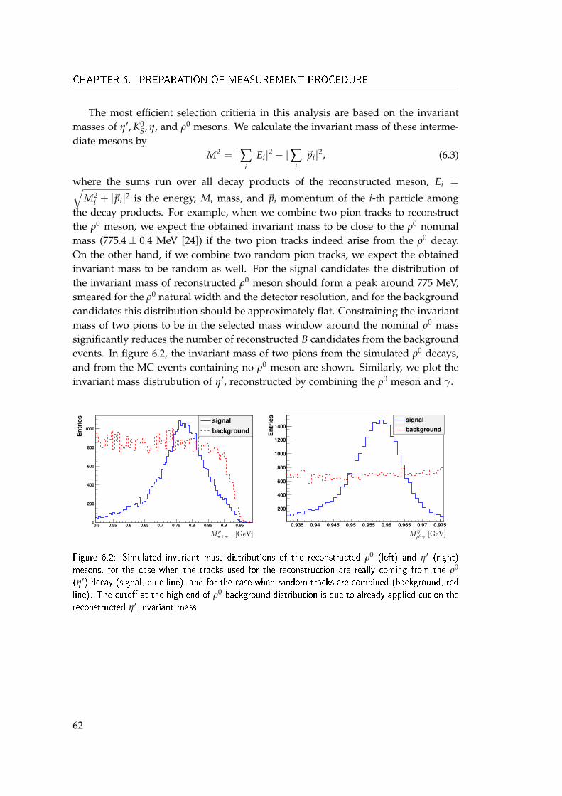
CHAPTER 6. PREPARATION OF MEASUREMENT PROCEDURE
The most efficient selection critieria in this analysis are based on the invariantmasses of η′, K0
S, η, and ρ0 mesons. We calculate the invariant mass of these interme-diate mesons by
M2 = |∑i
Ei|2 − |∑i~pi|2, (6.3)
where the sums run over all decay products of the reconstructed meson, Ei =√M2
i + |~pi|2 is the energy, Mi mass, and ~pi momentum of the i-th particle amongthe decay products. For example, when we combine two pion tracks to reconstructthe ρ0 meson, we expect the obtained invariant mass to be close to the ρ0 nominalmass (775.4± 0.4 MeV [24]) if the two pion tracks indeed arise from the ρ0 decay.On the other hand, if we combine two random pion tracks, we expect the obtainedinvariant mass to be random as well. For the signal candidates the distribution ofthe invariant mass of reconstructed ρ0 meson should form a peak around 775 MeV,smeared for the ρ0 natural width and the detector resolution, and for the backgroundcandidates this distribution should be approximately flat. Constraining the invariantmass of two pions to be in the selected mass window around the nominal ρ0 masssignificantly reduces the number of reconstructed B candidates from the backgroundevents. In figure 6.2, the invariant mass of two pions from the simulated ρ0 decays,and from the MC events containing no ρ0 meson are shown. Similarly, we plot theinvariant mass distrubution of η′, reconstructed by combining the ρ0 meson and γ.
-
0.5 0.55 0.6 0.65 0.7 0.75 0.8 0.85 0.9 0.95
Entries
0
200
400
600
800
1000
signalbackground
0.935 0.94 0.945 0.95 0.955 0.96 0.965 0.97 0.975
Entries
200
400
600
800
1000
1200
1400signalbackground
Figure 6.2: Simulated invariant mass distributions of the reconstructed ρ0 (left) and η′ (right)mesons, for the case when the tracks used for the reconstruction are really coming from the ρ0
(η′) decay (signal, blue line), and for the case when random tracks are combined (background, redline). The cuto� at the high end of ρ0 background distribution is due to already applied cut on thereconstructed η′ invariant mass.
62
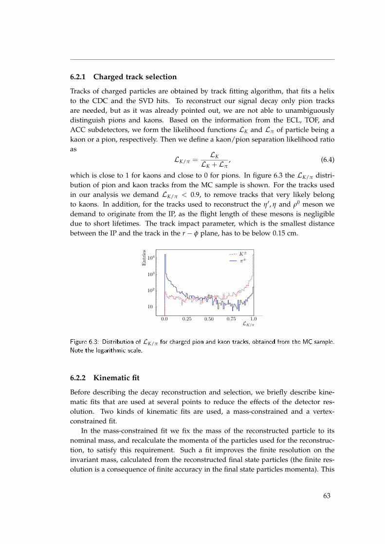
6.2.1 Charged track selection
Tracks of charged particles are obtained by track fitting algorithm, that fits a helixto the CDC and the SVD hits. To reconstruct our signal decay only pion tracksare needed, but as it was already pointed out, we are not able to unambiguouslydistinguish pions and kaons. Based on the information from the ECL, TOF, andACC subdetectors, we form the likelihood functions LK and Lπ of particle being akaon or a pion, respectively. Then we define a kaon/pion separation likelihood ratioas
LK/π =LK
LK + Lπ, (6.4)
which is close to 1 for kaons and close to 0 for pions. In figure 6.3 the LK/π distri-bution of pion and kaon tracks from the MC sample is shown. For the tracks usedin our analysis we demand LK/π < 0.9, to remove tracks that very likely belongto kaons. In addition, for the tracks used to reconstruct the η′, η and ρ0 meson wedemand to originate from the IP, as the flight length of these mesons is negligibledue to short lifetimes. The track impact parameter, which is the smallest distancebetween the IP and the track in the r− φ plane, has to be below 0.15 cm.
Figure 6.3: Distribution of LK/π for charged pion and kaon tracks, obtained from the MC sample.Note the logarithmic scale.
6.2.2 Kinematic fit
Before describing the decay reconstruction and selection, we briefly describe kine-matic fits that are used at several points to reduce the effects of the detector res-olution. Two kinds of kinematic fits are used, a mass-constrained and a vertex-constrained fit.
In the mass-constrained fit we fix the mass of the reconstructed particle to itsnominal mass, and recalculate the momenta of the particles used for the reconstruc-tion, to satisfy this requirement. Such a fit improves the finite resolution on theinvariant mass, calculated from the reconstructed final state particles (the finite res-olution is a consequence of finite accuracy in the final state particles momenta). This
63
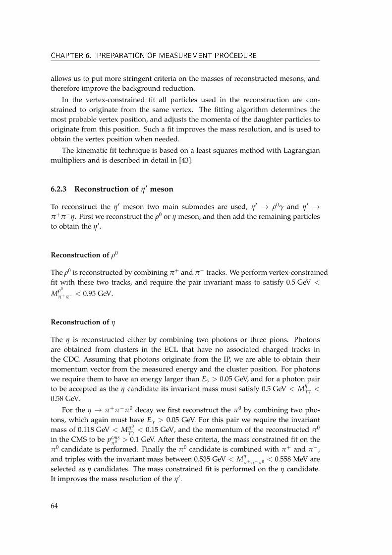
CHAPTER 6. PREPARATION OF MEASUREMENT PROCEDURE
allows us to put more stringent criteria on the masses of reconstructed mesons, andtherefore improve the background reduction.
In the vertex-constrained fit all particles used in the reconstruction are con-strained to originate from the same vertex. The fitting algorithm determines themost probable vertex position, and adjusts the momenta of the daughter particles tooriginate from this position. Such a fit improves the mass resolution, and is used toobtain the vertex position when needed.
The kinematic fit technique is based on a least squares method with Lagrangianmultipliers and is described in detail in [43].
6.2.3 Reconstruction of η′ meson
To reconstruct the η′ meson two main submodes are used, η′ → ρ0γ and η′ →π+π−η. First we reconstruct the ρ0 or η meson, and then add the remaining particlesto obtain the η′.
Reconstruction of ρ0
The ρ0 is reconstructed by combining π+ and π− tracks. We perform vertex-constrainedfit with these two tracks, and require the pair invariant mass to satisfy 0.5 GeV <
Mρ0
π+π− < 0.95 GeV.
Reconstruction of η
The η is reconstructed either by combining two photons or three pions. Photonsare obtained from clusters in the ECL that have no associated charged tracks inthe CDC. Assuming that photons originate from the IP, we are able to obtain theirmomentum vector from the measured energy and the cluster position. For photonswe require them to have an energy larger than Eγ > 0.05 GeV, and for a photon pairto be accepted as the η candidate its invariant mass must satisfy 0.5 GeV < Mη
γγ <
0.58 GeV.
For the η → π+π−π0 decay we first reconstruct the π0 by combining two pho-tons, which again must have Eγ > 0.05 GeV. For this pair we require the invariantmass of 0.118 GeV < Mπ0
γγ < 0.15 GeV, and the momentum of the reconstructed π0
in the CMS to be pcmsπ0 > 0.1 GeV. After these criteria, the mass constrained fit on the
π0 candidate is performed. Finally the π0 candidate is combined with π+ and π−,and triples with the invariant mass between 0.535 GeV < Mη
π+π−π0 < 0.558 MeV areselected as η candidates. The mass constrained fit is performed on the η candidate.It improves the mass resolution of the η′.
64
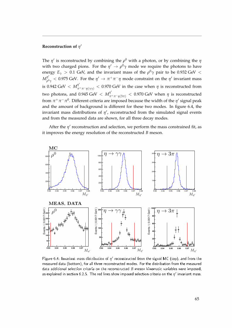
Reconstruction of η′
The η′ is reconstructed by combining the ρ0 with a photon, or by combining the η
with two charged pions. For the η′ → ρ0γ mode we require the photons to haveenergy Eγ > 0.1 GeV, and the invariant mass of the ρ0γ pair to be 0.932 GeV <
Mη′
ρ0γ< 0.975 GeV. For the η′ → π+π−η mode constraint on the η′ invariant mass
is 0.942 GeV < Mη′
π+π−η(γγ)< 0.970 GeV in the case when η is reconstructed from
two photons, and 0.945 GeV < Mη′
π+π−η(3π)< 0.970 GeV when η is reconstructed
from π+π−π0. Different criteria are imposed because the width of the η′ signal peakand the amount of background is different for these two modes. In figure 6.4, theinvariant mass distributions of η′, reconstructed from the simulated signal eventsand from the measured data are shown, for all three decay modes.
After the η′ reconstruction and selection, we perform the mass constrained fit, asit improves the energy resolution of the reconstructed B meson.
0.93 0.94 0.95 0.96 0.97 0.980
200
400
600
800
0.93 0.94 0.95 0.96 0.97 0.980
200
400
600
800
1000
0.93 0.94 0.95 0.96 0.97 0.980
100
200
300
400
0.93 0.94 0.95 0.96 0.97
Eve
nts
/(0.
0017
GeV
)
0
50
100
150
200
250
300
0
50
100
150
200
0
20
40
60
80
100
Eve
nts
/(0.
0017
GeV
)
Eve
nts
/(0.
0017
GeV
)
0.93 0.94 0.95 0.96 0.97 0.93 0.94 0.95 0.96 0.97
Figure 6.4: Invariant mass distribution of η′ reconstructed from the signal MC (top), and from themeasured data (bottom), for all three reconstructed modes. For the distribution from the measureddata additional selection criteria on the reconstructed B meson kinematic variables were imposed,as explained in section 6.2.5. The red lines show imposed selection criteria on the η′ invariant mass.
65
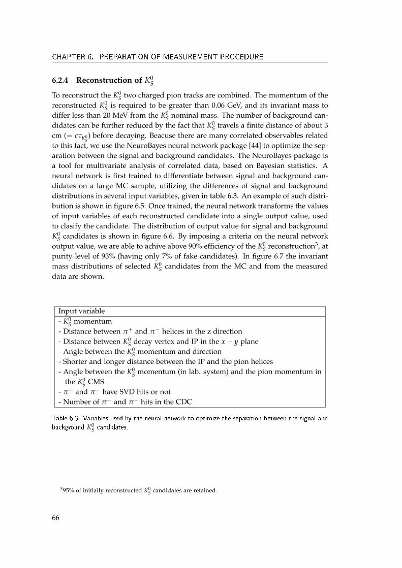
CHAPTER 6. PREPARATION OF MEASUREMENT PROCEDURE
6.2.4 Reconstruction of K0S
To reconstruct the K0S two charged pion tracks are combined. The momentum of the
reconstructed K0S is required to be greater than 0.06 GeV, and its invariant mass to
differ less than 20 MeV from the K0S nominal mass. The number of background can-
didates can be further reduced by the fact that K0S travels a finite distance of about 3
cm (= cτK0S) before decaying. Beacuse there are many correlated observables related
to this fact, we use the NeuroBayes neural network package [44] to optimize the sep-aration between the signal and background candidates. The NeuroBayes package isa tool for multivariate analysis of correlated data, based on Bayesian statistics. Aneural network is first trained to differentiate between signal and background can-didates on a large MC sample, utilizing the differences of signal and backgrounddistributions in several input variables, given in table 6.3. An example of such distri-bution is shown in figure 6.5. Once trained, the neural network transforms the valuesof input variables of each reconstructed candidate into a single output value, usedto clasify the candidate. The distribution of output value for signal and backgroundK0
S candidates is shown in figure 6.6. By imposing a criteria on the neural networkoutput value, we are able to achive above 90% efficiency of the K0
S reconstruction3, atpurity level of 93% (having only 7% of fake candidates). In figure 6.7 the invariantmass distributions of selected K0
S candidates from the MC and from the measureddata are shown.
Input variable- K0
S momentum- Distance between π+ and π− helices in the z direction- Distance between K0
S decay vertex and IP in the x− y plane- Angle between the K0
S momentum and direction- Shorter and longer distance between the IP and the pion helices- Angle between the K0
S momentum (in lab. system) and the pion momentum inthe K0
S CMS- π+ and π− have SVD hits or not- Number of π+ and π− hits in the CDC
Table 6.3: Variables used by the neural network to optimize the separation between the signal andbackground K0
S candidates.
395% of initially reconstructed K0S candidates are retained.
66
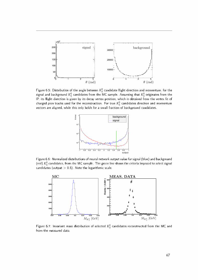
Figure 6.5: Distribution of the angle between K0S candidate �ight direction and momentum, for the
signal and background K0S candidates from the MC sample. Assuming that K0
S originates from theIP, its �ight direction is given by its decay vertex position, which is obtained from the vertex �t ofcharged pion tracks used for the reconstruction. For true K0
S candidates direction and momentumvectors are aligned, while this only holds for a small fraction of background candidates.
output-1 -0.8 -0.6 -0.4 -0.2 0 0.2 0.4 0.6 0.8 1
Ent
ries
-310
-210
-110
1 backgroundsignal
Figure 6.6: Normalized distributions of neural network output value for signal (blue) and background(red) K0
S candidates, from the MC sample. The green line shows the criteria imposed to select signalcandidates (output > 0.5). Note the logarithmic scale.
0.47 0.48 0.49 0.5 0.51 0.52 0.53
Eve
nts/(
0.00
1)
0
200
400
600
800
0.47 0.48 0.49 0.5 0.51 0.52 0.530
1000
2000
3000
4000
5000
Figure 6.7: Invariant mass distribution of selected K0S candidates reconstructed from the MC and
from the measured data.
67
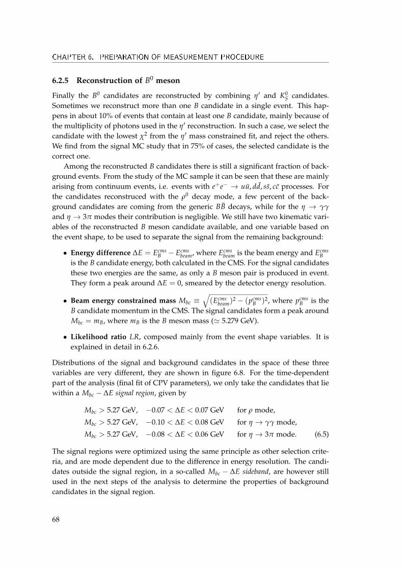
CHAPTER 6. PREPARATION OF MEASUREMENT PROCEDURE
6.2.5 Reconstruction of B0 meson
Finally the B0 candidates are reconstructed by combining η′ and K0S candidates.
Sometimes we reconstruct more than one B candidate in a single event. This hap-pens in about 10% of events that contain at least one B candidate, mainly because ofthe multiplicity of photons used in the η′ reconstruction. In such a case, we select thecandidate with the lowest χ2 from the η′ mass constrained fit, and reject the others.We find from the signal MC study that in 75% of cases, the selected candidate is thecorrect one.
Among the reconstructed B candidates there is still a significant fraction of back-ground events. From the study of the MC sample it can be seen that these are mainlyarising from continuum events, i.e. events with e+e− → uu, dd, ss, cc processes. Forthe candidates reconstruced with the ρ0 decay mode, a few percent of the back-ground candidates are coming from the generic BB decays, while for the η → γγ
and η → 3π modes their contribution is negligible. We still have two kinematic vari-ables of the reconstructed B meson candidate available, and one variable based onthe event shape, to be used to separate the signal from the remaining background:
• Energy difference ∆E = EcmsB − Ecms
beam, where Ecmsbeam is the beam energy and Ecms
Bis the B candidate energy, both calculated in the CMS. For the signal candidatesthese two energies are the same, as only a B meson pair is produced in event.They form a peak around ∆E = 0, smeared by the detector energy resolution.
• Beam energy constrained mass Mbc ≡√(Ecms
beam)2 − (pcms
B )2, where pcmsB is the
B candidate momentum in the CMS. The signal candidates form a peak aroundMbc = mB, where mB is the B meson mass (' 5.279 GeV).
• Likelihood ratio LR, composed mainly from the event shape variables. It isexplained in detail in 6.2.6.
Distributions of the signal and background candidates in the space of these threevariables are very different, they are shown in figure 6.8. For the time-dependentpart of the analysis (final fit of CPV parameters), we only take the candidates that liewithin a Mbc − ∆E signal region, given by
Mbc > 5.27 GeV, −0.07 < ∆E < 0.07 GeV for ρ mode,
Mbc > 5.27 GeV, −0.10 < ∆E < 0.08 GeV for η → γγ mode,
Mbc > 5.27 GeV, −0.08 < ∆E < 0.06 GeV for η → 3π mode. (6.5)
The signal regions were optimized using the same principle as other selection crite-ria, and are mode dependent due to the difference in energy resolution. The candi-dates outside the signal region, in a so-called Mbc − ∆E sideband, are however stillused in the next steps of the analysis to determine the properties of backgroundcandidates in the signal region.
68
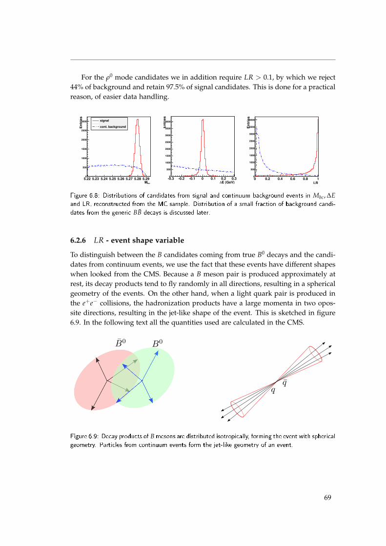
For the ρ0 mode candidates we in addition require LR > 0.1, by which we reject44% of background and retain 97.5% of signal candidates. This is done for a practicalreason, of easier data handling.
bcM5.22 5.23 5.24 5.25 5.26 5.27 5.28 5.29
En
trie
s
0
500
1000
1500
2000
2500
3000 signal
cont. background
E (GeV)∆
0.3 0.2 0.1 0 0.1 0.2 0.3
En
trie
s
0
500
1000
1500
2000
2500
3000
3500
4000
LR0 0.2 0.4 0.6 0.8 1
En
trie
s
0
500
1000
1500
2000
2500
3000
3500
4000
Figure 6.8: Distributions of candidates from signal and continuum background events in Mbc, ∆Eand LR, reconstructed from the MC sample. Distribution of a small fraction of background candi-dates from the generic BB decays is discussed later.
6.2.6 LR - event shape variable
To distinguish between the B candidates coming from true B0 decays and the candi-dates from continuum events, we use the fact that these events have different shapeswhen looked from the CMS. Because a B meson pair is produced approximately atrest, its decay products tend to fly randomly in all directions, resulting in a sphericalgeometry of the events. On the other hand, when a light quark pair is produced inthe e+e− collisions, the hadronization products have a large momenta in two opos-site directions, resulting in the jet-like shape of the event. This is sketched in figure6.9. In the following text all the quantities used are calculated in the CMS.
Figure 6.9: Decay products of B mesons are distributed isotropically, forming the event with sphericalgeometry. Particles from continuum events form the jet-like geometry of an event.
69
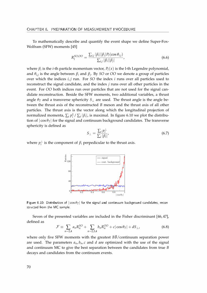
CHAPTER 6. PREPARATION OF MEASUREMENT PROCEDURE
To mathematically describe and quantify the event shape we define Super-Fox-Wolfram (SFW) moments [45]
RSO,OOl =
∑i,j |~pi||~pj|Pl(cos θi,j)
∑i,j |~pi||~pj|, (6.6)
where ~pi is the i-th particle momentum vector, Pl(x) is the l-th Legendre polynomial,and θi,j is the angle between ~pi and ~pj. By SO or OO we denote a group of particlesover which the indices i, j run. For SO the index i runs over all particles used toreconstruct the signal candidate, and the index j runs over all other particles in theevent. For OO both indices run over particles that are not used for the signal can-didate reconstruction. Beside the SFW moments, two additional variables, a thrustangle θT and a transverse sphericity S⊥ are used. The thrust angle is the angle be-tween the thrust axis of the reconstructed B meson and the thrust axis of all otherparticles. The thrust axis is the vector along which the longitudinal projection ofnormalized momenta, ∑i pL
i / ∑i |~pi|, is maximal. In figure 6.10 we plot the distribu-tion of | cos θT| for the signal and continuum background candidates. The transversesphericity is defined as
S⊥ =∑i p⊥i∑i |~pi|
, (6.7)
where p⊥i is the component of ~pi perpedicular to the thrust axis.
Figure 6.10: Distribution of | cos θT | for the signal and continuum background candidates, recon-structed from the MC sample.
Seven of the presented variables are included in the Fisher discriminant [46, 47],defined as
F ≡ ∑n=2,4
anRSOn + ∑
n=2,3,4bnROO
n + c| cos θT|+ dS⊥, (6.8)
where only five SFW moments with the greatest BB/continuum separation powerare used. The parameters an, bn, c and d are optimized with the use of the signaland continuum MC to give the best separation between the candidates from true Bdecays and candidates from the continuum events.
70
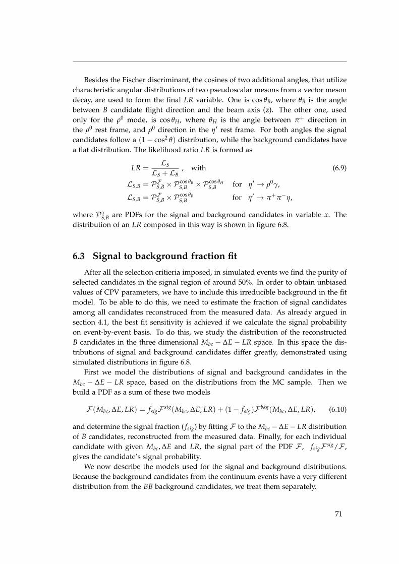
Besides the Fischer discriminant, the cosines of two additional angles, that utilizecharacteristic angular distributions of two pseudoscalar mesons from a vector mesondecay, are used to form the final LR variable. One is cos θB, where θB is the anglebetween B candidate flight direction and the beam axis (z). The other one, usedonly for the ρ0 mode, is cos θH, where θH is the angle between π+ direction inthe ρ0 rest frame, and ρ0 direction in the η′ rest frame. For both angles the signalcandidates follow a (1− cos2 θ) distribution, while the background candidates havea flat distribution. The likelihood ratio LR is formed as
LR =LS
LS + LB, with (6.9)
LS,B = PFS,B ×Pcos θBS,B ×Pcos θH
S,B for η′ → ρ0γ,
LS,B = PFS,B ×Pcos θBS,B for η′ → π+π−η,
where P xS,B are PDFs for the signal and background candidates in variable x. The
distribution of an LR composed in this way is shown in figure 6.8.
6.3 Signal to background fraction fit
After all the selection critieria imposed, in simulated events we find the purity ofselected candidates in the signal region of around 50%. In order to obtain unbiasedvalues of CPV parameters, we have to include this irreducible background in the fitmodel. To be able to do this, we need to estimate the fraction of signal candidatesamong all candidates reconstruced from the measured data. As already argued insection 4.1, the best fit sensitivity is achieved if we calculate the signal probabilityon event-by-event basis. To do this, we study the distribution of the reconstructedB candidates in the three dimensional Mbc − ∆E− LR space. In this space the dis-tributions of signal and background candidates differ greatly, demonstrated usingsimulated distributions in figure 6.8.
First we model the distributions of signal and background candidates in theMbc − ∆E − LR space, based on the distributions from the MC sample. Then webuild a PDF as a sum of these two models
F (Mbc, ∆E, LR) = fsigF sig(Mbc, ∆E, LR) + (1− fsig)F bkg(Mbc, ∆E, LR), (6.10)
and determine the signal fraction ( fsig) by fitting F to the Mbc−∆E− LR distributionof B candidates, reconstructed from the measured data. Finally, for each individualcandidate with given Mbc, ∆E and LR, the signal part of the PDF F , fsigF sig/F ,gives the candidate’s signal probability.
We now describe the models used for the signal and background distributions.Because the background candidates from the continuum events have a very differentdistribution from the BB background candidates, we treat them separately.
71
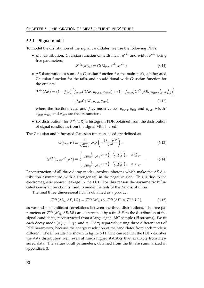
CHAPTER 6. PREPARATION OF MEASUREMENT PROCEDURE
6.3.1 Signal model
To model the distribution of the signal candidates, we use the following PDFs:
• Mbc distribution: Gaussian function G, with mean µmbc and width σmbc beingfree parameters,
F sig(Mbc) = G(Mbc,µmbc, σmbc) (6.11)
• ∆E distribution: a sum of a Gaussian function for the main peak, a bifurcatedGaussian function for the tails, and an additional wide Gaussian function forthe outliers,
F sig(∆E) = (1− fout)[
fmainG(∆E,µmain, σmain) + (1− fmain)Gbi f (∆E,µtail , σLtail , σR
tail)]
+ foutG(∆E,µout, σout), (6.12)
where the fractions fmain and fout, mean values µmain,µtail and µout, widthsσmain, σtail and σout, are free parameters.
• LR distribution: for F sig(LR) a histogram PDF, obtained from the distributionof signal candidates from the signal MC, is used.
The Gaussian and bifurcated Gaussian functions used are defined as
G(x,µ, σ) ≡ 1√2πσ
exp(− (x− µ)2
2σ2
), (6.13)
Gbi f (x,µ, σL, σR) ≡
2√
2π(σL+σR)exp
(− (x−µ)2
2(σL)2
), x ≤ µ
2√2π(σL+σR)
exp(− (x−µ)2
2(σR)2
), x > µ
. (6.14)
Reconstruction of all three decay modes involves photons which make the ∆E dis-tribution asymmetric, with a stronger tail in the negative side. This is due to theelectromagnetic shower leakage in the ECL. For this reason the asymmetric bifur-cated Gaussian function is used to model the tails of the ∆E distribution.
The final three dimensional PDF is obtained as a product
F sig(Mbc, ∆E, LR) = F sig(Mbc)×F sig(∆E)×F sig(LR), (6.15)
as we find no significant correlations between the three distributions. The free pa-rameters of F sig(Mbc, ∆E, LR) are determined by a fit of F to the distribution of thesignal candidates, reconstructed from a large signal MC sample (15 streams). We fiteach decay mode (ρ0, η → γγ and η → 3π) separately, using three different sets ofPDF parameters, because the energy resolution of the candidates from each mode isdifferent. The fit results are shown in figure 6.11. One can see that the PDF describesthe data distribution well, even at much higher statistics than available from mea-sured data. The values of all parameters, obtained from the fit, are summarized inappendix B.3.
72
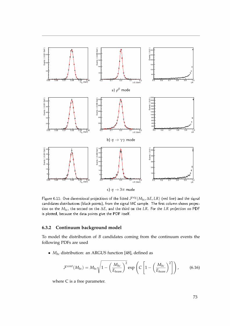
(GeV)bc
m5.25 5.26 5.27 5.28 5.29 5.30
Events
/ (
0.0
01 G
eV
)
0
500
1000
1500
E (GeV)∆
0.2 0.1 0.0 0.1 0.2
Events
/ (
0.0
08 G
eV
)
0
500
1000
1500
2000
LR0.5 0.6 0.7 0.8 0.9 1.0
Events
/ (
0.0
1 )
0
500
1000
1500
2000
2500
3000
a) ρ0 mode
(GeV)bc
m5.25 5.26 5.27 5.28 5.29 5.30
Eve
nts
/ (
0.0
01
Ge
V )
0
200
400
600
800
1000
E (GeV)∆
0.2 0.1 0.0 0.1 0.2
Eve
nts
/ (
0.0
08
Ge
V )
0
200
400
600
800
1000
LR0.5 0.6 0.7 0.8 0.9 1.0
Eve
nts
/ (
0.0
1 )
0
200
400
600
800
1000
1200
1400
1600
1800
2000
2200
b) η → γγ mode
(GeV)bc
m5.25 5.26 5.27 5.28 5.29 5.30
Events
/ (
0.0
01 G
eV
)
0
50
100
150
200
250
300
E (GeV)∆
0.2 0.1 0.0 0.1 0.2
Events
/ (
0.0
08 G
eV
)
0
50
100
150
200
250
300
350
LR0.5 0.6 0.7 0.8 0.9 1.0
Events
/ (
0.0
1 )
0
100
200
300
400
500
c) η → 3π mode
Figure 6.11: One dimensional projections of the �tted F sig(Mbc, ∆E, LR) (red line) and the signalcandidates distributions (black points), from the signal MC sample. The �rst column shows projec-tion on the Mbc, the second on the ∆E, and the third on the LR. For the LR projection no PDFis plotted, because the data points give the PDF itself.
6.3.2 Continuum background model
To model the distribution of B candidates coming from the continuum events thefollowing PDFs are used
• Mbc distribution: an ARGUS function [48], defined as
F cont(Mbc) = Mbc
√1−
(Mbc
Ebeam
)2
exp
(C
[1−
(Mbc
Ebeam
)2])
, (6.16)
where C is a free parameter.
73
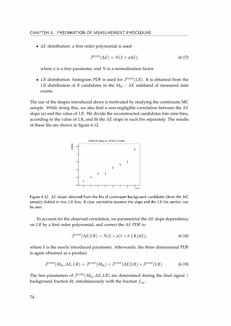
CHAPTER 6. PREPARATION OF MEASUREMENT PROCEDURE
• ∆E distribution: a first order polynomial is used
F cont(∆E) = N(1 + a∆E), (6.17)
where a is a free parameter, and N is a normalization factor.
• LR distribution: histogram PDF is used for F cont(LR). It is obtained from theLR distribution of B candidates in the Mbc − ∆E sideband of measured dataevents.
The use of the shapes introduced above is motivated by studying the continuum MCsample. While doing this, we also find a non-negligible correlation between the ∆Eslope (a) and the value of LR. We divide the reconstructed candidates into nine bins,according to the value of LR, and fit the ∆E slope in each bin separately. The resultsof these fits are shown in figure 6.12.
LR bin2 3 4 5 6 7 8 9
slo
pe
1.8
1.6
1.4
1.2
1
0.8
mode)ρE slope vs. LR bin (∆Fitted
Figure 6.12: ∆E slopes obtained from the �ts of continuum background candidates (from the MCsample) divided in nine LR bins. A clear correlation between the slope and the LR bin number canbe seen.
To account for the observed correlation, we parametrize the ∆E slope dependencyon LR by a first order polynomial, and correct the ∆E PDF to
F cont(∆E|LR) = N(1 + a(1 + b LR)∆E), (6.18)
where b is the newly introduced parameter. Afterwards, the three dimensional PDFis again obtained as a product
F cont(Mbc, ∆E, LR) = F cont(Mbc)×F cont(∆E|LR)×F cont(LR). (6.19)
The free parameters of F cont(Mbc, ∆E, LR) are determined during the final signal /background fraction fit, simultaneously with the fraction fsig.
74

6.3.3 BB background model
The Mbc × ∆E× LR distribution of background candidates coming from the genericBB decays does not follow any simple function. The distribution of B candidatesreconstructed from the 10 streams of BB MC sample is shown in figure 6.13. Wedo not parametrize this distribution, but rather take the tree dimensional histogramfrom the MC sample for F BB(Mbc, ∆E, LR). Since the number of these candidates isvery small for the η → γγ and η → 3π modes (even in the 10 streams of the MCsample), the same PDF is used for all three reconstructed modes.
(GeV)bc
m5.22
5.245.26
5.285.3
-0.2-0.1
00.10.2
Eve
nts
/(0.
004
GeV
x0.
025
GeV
)
0
50
100
150
200
250
300
350
-0.2 -0.1 0 0.1 0.2LR
0.50.6
0.70.8
0.91E
vent
s/(
0.02
5G
eVx
0.02
5)
0100200
300400500600
700
Figure 6.13: Distributions of BB background candidates in the Mbc − ∆E (left) and in the LR−∆E plane (right), obtained from the 10 streams of generic BB MC sample. The plots show thedistribution of candidates combined from all three reconstructed decay modes.
6.3.4 Fit procedure
To perform the signal/background fraction fit we divide the reconstructed B can-didates into seven bins (r bins), according to the quality of the flavor tagging in-formation. In the first r bin are the candidates with no flavor information, and inthe seventh are the candidates with almost unambiguously determined flavor. Thedetails of this binning are described in the flavor tagging section 6.4. As one mightexpect, a fraction of the signal candidates differs from bin to bin, since the eventscontaining a BB pair are preferred to have good flavor tagging information, com-pared to the continuum events. We fit the (Mbc, ∆E, LR) distribution of candidates ineach bin separately, and by this gain in the sensitivity for the price of increased fitcomplexity.
The PDF for the signal/background fraction fit is build as a sum of the signal,continuum background, and BB background contributions
F i = f isigF sig,i + (1− f i
sig)[
f iBBF BB + (1− f i
BB)F cont]
, (6.20)
where f isig is the fraction of the signal candidates among all candidates in the i-th
bin, and fBB is the fraction of the candidates that come from the generic BB decays,
75
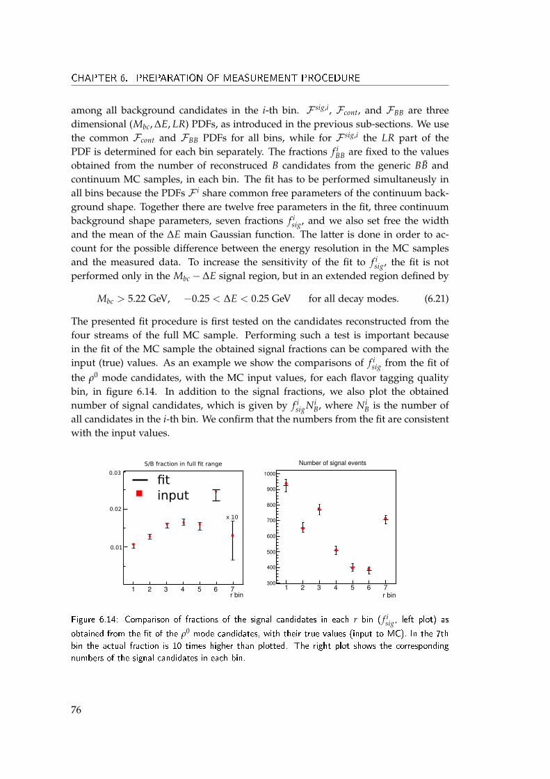
CHAPTER 6. PREPARATION OF MEASUREMENT PROCEDURE
among all background candidates in the i-th bin. F sig,i, Fcont, and FBB are threedimensional (Mbc, ∆E, LR) PDFs, as introduced in the previous sub-sections. We usethe common Fcont and FBB PDFs for all bins, while for F sig,i the LR part of thePDF is determined for each bin separately. The fractions f i
BB are fixed to the valuesobtained from the number of reconstruced B candidates from the generic BB andcontinuum MC samples, in each bin. The fit has to be performed simultaneusly inall bins because the PDFs F i share common free parameters of the continuum back-ground shape. Together there are twelve free parameters in the fit, three continuumbackground shape parameters, seven fractions f i
sig, and we also set free the widthand the mean of the ∆E main Gaussian function. The latter is done in order to ac-count for the possible difference between the energy resolution in the MC samplesand the measured data. To increase the sensitivity of the fit to f i
sig, the fit is notperformed only in the Mbc − ∆E signal region, but in an extended region defined by
Mbc > 5.22 GeV, −0.25 < ∆E < 0.25 GeV for all decay modes. (6.21)
The presented fit procedure is first tested on the candidates reconstructed from thefour streams of the full MC sample. Performing such a test is important becausein the fit of the MC sample the obtained signal fractions can be compared with theinput (true) values. As an example we show the comparisons of f i
sig from the fit ofthe ρ0 mode candidates, with the MC input values, for each flavor tagging qualitybin, in figure 6.14. In addition to the signal fractions, we also plot the obtainednumber of signal candidates, which is given by f i
sigNiB, where Ni
B is the number ofall candidates in the i-th bin. We confirm that the numbers from the fit are consistentwith the input values.
1 2 3 4 5 6 7r bin
1 2 3 4 5 6 7300
400
500
600
700
800
900
1000
Number of signal eventsNumber of signal events
0.01
0.02
0.03
r bin
x 10
fitinput
S/B fraction in full fit range
Figure 6.14: Comparison of fractions of the signal candidates in each r bin ( f isig, left plot) as
obtained from the �t of the ρ0 mode candidates, with their true values (input to MC). In the 7thbin the actual fraction is 10 times higher than plotted. The right plot shows the correspondingnumbers of the signal candidates in each bin.
76
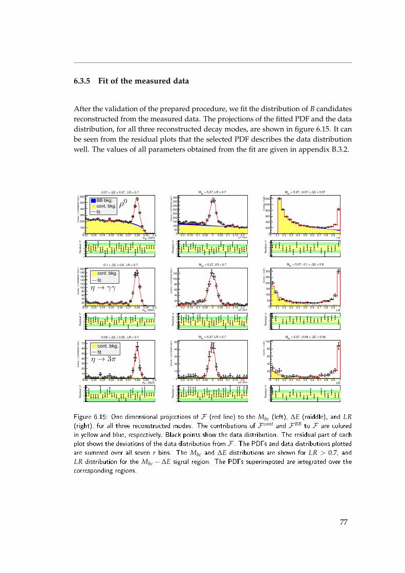
6.3.5 Fit of the measured data
After the validation of the prepared procedure, we fit the distribution of B candidatesreconstructed from the measured data. The projections of the fitted PDF and the datadistribution, for all three reconstructed decay modes, are shown in figure 6.15. It canbe seen from the residual plots that the selected PDF describes the data distributionwell. The values of all parameters obtained from the fit are given in appendix B.3.2.
5.22 5.23 5.24 5.25 5.26 5.27 5.28 5.29 5.3
Events/(
0.0026
6667
GeV
)
0
100
200
300
400
500
600
E < 0.07 , LR > 0.7-0.07 <
BB bkg.cont. bkg.fit
Residua
l/
-3-2
-101
2
E (GeV)-0.2 -0.15 -0.1 -0.05 0 0.05 0.1 0.15 0.2
Events/(
0.0153
333GeV
)
050100
150200
250300350
400450
> 5.27, LR > 0.7bcM
Residua
l/
-3-2-10123
0 0.1 0.2 0.3 0.4 0.5 0.6 0.7 0.8 0.9 1
Events/(
0.05
)
0
200
400
600
800
1000
1200
E < 0.07> 5.27, -0.07 <bcM
Residua
l/
-3-2-1012
5.22 5.23 5.24 5.25 5.26 5.27 5.28 5.29 5.3
Events/(
0.0026
6667
GeV
)
020406080100120140160180200
E < 0.8 , LR > 0.7-0.1 <
cont. bkg.
fit
Residua
l/
-3-2-10123
E (GeV)-0.2 -0.15 -0.1 -0.05 0 0.05 0.1 0.15 0.2
Events/(
0.0153
333GeV
)
0
20
40
60
80
100
120
> 5.27, LR > 0.7bcM
Residua
l/
-2
-10
1
23
0 0.1 0.2 0.3 0.4 0.5 0.6 0.7 0.8 0.9 1
Events/(
0.05
)
0
50
100
150
200
250
300
E < 0.8> 5.27, -0.1 <bcMResidua
l/
-4-3-2-10123
5.22 5.23 5.24 5.25 5.26 5.27 5.28 5.29 5.3
Events/(
0.0026
6667
GeV
)
0
10
20
30
40
50
60
70
E < 0.06 , LR > 0.7-0.08 <
cont. bkg.fit
Residua
l/
-2-1
0123
E (GeV)-0.2 -0.15 -0.1 -0.05 0 0.05 0.1 0.15 0.2
Events/(
0.0153
333GeV
)
0
10
20
30
40
50
> 5.27, LR > 0.7bcM
Residua
l/
-2
-1
0
12
3
0 0.1 0.2 0.3 0.4 0.5 0.6 0.7 0.8 0.9 1
Events/(
0.05
)
0
20
40
60
80
100
E < 0.06> 5.27, -0.08 <bcM
Residua
l/
-2-10123
LR
LR
LR
(GeV)bcm
(GeV)bcm
(GeV)bcm
Figure 6.15: One dimensional projections of F (red line) to the Mbc (left), ∆E (middle), and LR(right), for all three reconstructed modes. The contributions of F cont and F BB to F are coloredin yellow and blue, respectively. Black points show the data distribution. The residual part of eachplot shows the deviations of the data distribution from F . The PDFs and data distributions plottedare summed over all seven r bins. The Mbc and ∆E distributions are shown for LR > 0.7, andLR distribution for the Mbc − ∆E signal region. The PDFs superimposed are integrated over thecorresponding regions.
77
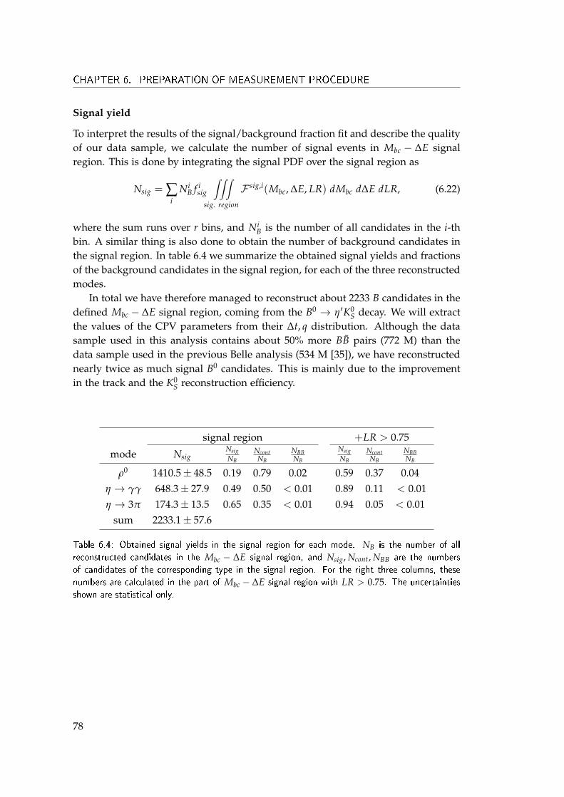
CHAPTER 6. PREPARATION OF MEASUREMENT PROCEDURE
Signal yield
To interpret the results of the signal/background fraction fit and describe the qualityof our data sample, we calculate the number of signal events in Mbc − ∆E signalregion. This is done by integrating the signal PDF over the signal region as
Nsig = ∑i
NiB f i
sig
∫∫∫sig. region
F sig,i(Mbc, ∆E, LR) dMbc d∆E dLR, (6.22)
where the sum runs over r bins, and NiB is the number of all candidates in the i-th
bin. A similar thing is also done to obtain the number of background candidates inthe signal region. In table 6.4 we summarize the obtained signal yields and fractionsof the background candidates in the signal region, for each of the three reconstructedmodes.
In total we have therefore managed to reconstruct about 2233 B candidates in thedefined Mbc − ∆E signal region, coming from the B0 → η′K0
S decay. We will extractthe values of the CPV parameters from their ∆t, q distribution. Although the datasample used in this analysis contains about 50% more BB pairs (772 M) than thedata sample used in the previous Belle analysis (534 M [35]), we have reconstructednearly twice as much signal B0 candidates. This is mainly due to the improvementin the track and the K0
S reconstruction efficiency.
signal region +LR > 0.75
mode NsigNsigNB
NcontNB
NBBNB
NsigNB
NcontNB
NBBNB
ρ0 1410.5± 48.5 0.19 0.79 0.02 0.59 0.37 0.04η → γγ 648.3± 27.9 0.49 0.50 < 0.01 0.89 0.11 < 0.01η → 3π 174.3± 13.5 0.65 0.35 < 0.01 0.94 0.05 < 0.01
sum 2233.1± 57.6
Table 6.4: Obtained signal yields in the signal region for each mode. NB is the number of allreconstructed candidates in the Mbc − ∆E signal region, and Nsig, Ncont, NBB are the numbersof candidates of the corresponding type in the signal region. For the right three columns, thesenumbers are calculated in the part of Mbc − ∆E signal region with LR > 0.75. The uncertaintiesshown are statistical only.
78
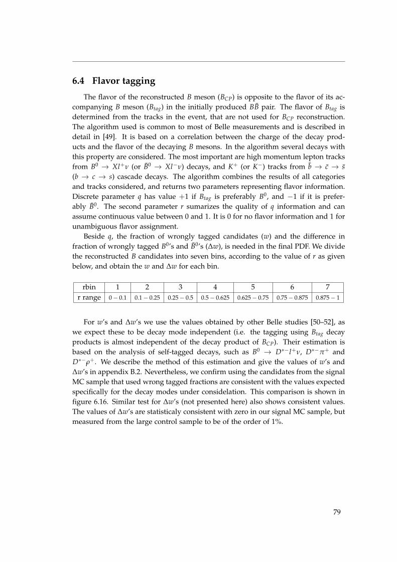
6.4 Flavor tagging
The flavor of the reconstructed B meson (BCP) is opposite to the flavor of its ac-companying B meson (Btag) in the initially produced BB pair. The flavor of Btag isdetermined from the tracks in the event, that are not used for BCP reconstruction.The algorithm used is common to most of Belle measurements and is described indetail in [49]. It is based on a correlation between the charge of the decay prod-ucts and the flavor of the decaying B mesons. In the algorithm several decays withthis property are considered. The most important are high momentum lepton tracksfrom B0 → Xl+ν (or B0 → Xl−ν) decays, and K+ (or K−) tracks from b → c → s(b → c → s) cascade decays. The algorithm combines the results of all categoriesand tracks considered, and returns two parameters representing flavor information.Discrete parameter q has value +1 if Btag is preferably B0, and −1 if it is prefer-ably B0. The second parameter r sumarizes the quality of q information and canassume continuous value between 0 and 1. It is 0 for no flavor information and 1 forunambiguous flavor assignment.
Beside q, the fraction of wrongly tagged candidates (w) and the difference infraction of wrongly tagged B0’s and B0’s (∆w), is needed in the final PDF. We dividethe reconstructed B candidates into seven bins, according to the value of r as givenbelow, and obtain the w and ∆w for each bin.
rbin 1 2 3 4 5 6 7r range 0− 0.1 0.1− 0.25 0.25− 0.5 0.5− 0.625 0.625− 0.75 0.75− 0.875 0.875− 1
For w’s and ∆w’s we use the values obtained by other Belle studies [50–52], aswe expect these to be decay mode independent (i.e. the tagging using Btag decayproducts is almost independent of the decay product of BCP). Their estimation isbased on the analysis of self-tagged decays, such as B0 → D∗−l+ν, D∗−π+ andD∗−ρ+. We describe the method of this estimation and give the values of w’s and∆w’s in appendix B.2. Nevertheless, we confirm using the candidates from the signalMC sample that used wrong tagged fractions are consistent with the values expectedspecifically for the decay modes under considelation. This comparison is shown infigure 6.16. Similar test for ∆w’s (not presented here) also shows consistent values.The values of ∆w’s are statisticaly consistent with zero in our signal MC sample, butmeasured from the large control sample to be of the order of 1%.
79
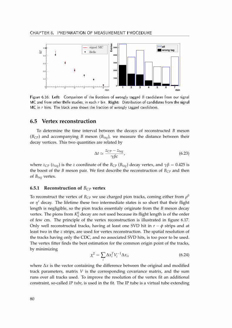
CHAPTER 6. PREPARATION OF MEASUREMENT PROCEDURE
rbin0 1 2 3 4 5 60
0.1
0.2
0.3
0.4
0.5
rbin1 2 3 4 5 6 7
Entries
0
1000
2000
3000
4000
5000 allwrong tag
Figure 6.16: Left: Comparison of the fractions of wrongly tagged B candidates from our signalMC and from other Belle studies, in each r bin. Right: Distribution of candidates from the signalMC in r bins. The black area shows the fraction of wrongly tagged candidates.
6.5 Vertex reconstruction
To determine the time interval between the decays of reconstructed B meson(BCP) and accompanying B meson (Btag), we measure the distance between theirdecay vertices. This two quantities are related by
∆t 'zCP − ztag
γβc, (6.23)
where zCP (ztag) is the z coordinate of the BCP (Btag) decay vertex, and γβ = 0.425 isthe boost of the B meson pair. We first describe the reconstruction of BCP and thenof Btag vertex.
6.5.1 Reconstruction of BCP vertex
To reconstruct the vertex of BCP we use charged pion tracks, coming either from ρ0
or η′ decay. The lifetime these two intermediate states is so short that their flightlength is negligible, so the pion tracks essentialy originate from the B meson decayvertex. The pions from K0
S decay are not used because its flight length is of the orderof few cm. The principle of the vertex reconstruction is illustrated in figure 6.17.Only well reconstructed tracks, having at least one SVD hit in r − φ strips and atleast two in the z strips, are used for vertex reconstruction. The spatial resolution ofthe tracks having only the CDC, and no associated SVD hits, is too poor to be used.The vertex fitter finds the best estimation for the common origin point of the tracks,by minimizing
χ2 = ∑i
∆xTi V−1
i ∆xi, (6.24)
where ∆x is the vector containing the difference between the original and modifiedtrack parameters, matrix V is the corresponding covariance matrix, and the sumruns over all tracks used. To improve the resolution of the vertex fit an additionalconstraint, so-called IP tube, is used in the fit. The IP tube is a virtual tube extending
80
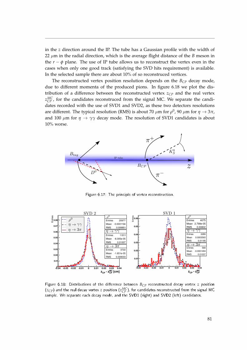
in the z direction around the IP. The tube has a Gaussian profile with the width of22 µm in the radial direction, which is the average flight distance of the B meson inthe r − φ plane. The use of IP tube allows us to reconstruct the vertex even in thecases when only one good track (satisfying the SVD hits requirement) is available.In the selected sample there are about 10% of so reconstruced vertices.
The reconstructed vertex position resolution depends on the BCP decay mode,due to different momenta of the produced pions. In figure 6.18 we plot the dis-tribution of a difference between the reconstructed vertex zCP and the real vertexzMC
CP , for the candidates reconstruced from the signal MC. We separate the candi-dates recorded with the use of SVD1 and SVD2, as these two detectors resolutionsare different. The typical resolution (RMS) is about 70 µm for ρ0, 90 µm for η → 3π,and 100 µm for η → γγ decay mode. The resolution of SVD1 candidates is about10% worse.
Figure 6.17: The principle of vertex reconstruction.
h11Entries 20977Mean -0.0001194RMS 0.006851
[cm]CPMC- zCPz
-0.04 -0.03 -0.02 -0.01 0 0.01 0.02 0.03 0.04
Ent
ries
0
0.01
0.02
0.03
0.04
0.05
0.06
0.07
0.08 Entries 20977Mean -0.0001194RMS 0.006851
h21Entries 11811Mean -8.305e-05RMS 0.01007
Entries 11811Mean -8.305e-05RMS 0.01007
h31Entries 3722Mean -1.651e-05RMS 0.009033
Entries 3722Mean -1.651e-05RMS 0.009033
h1Entries 4075Mean 2.799e-05RMS 0.00802
CPMC- zCPz
-0.04 -0.03 -0.02 -0.01 0 0.01 0.02 0.03 0.04
Ent
ries
0
0.01
0.02
0.03
0.04
0.05
0.06Entries 4075Mean 2.799e-05RMS 0.00802
h2Entries 2289Mean 0.0003593RMS 0.01185
Entries 2289Mean 0.0003593RMS 0.01185
h3Entries 568Mean -0.0001494RMS 0.01037
Entries 568Mean -0.0001494RMS 0.01037
Figure 6.18: Distributions of the di�erence between BCP reconstructed decay vertex z position(zCP) and the real decay vertex z position (zMC
CP ), for candidates reconstructed from the signal MCsample. We separate each decay mode, and the SVD1 (right) and SVD2 (left) candidates.
81
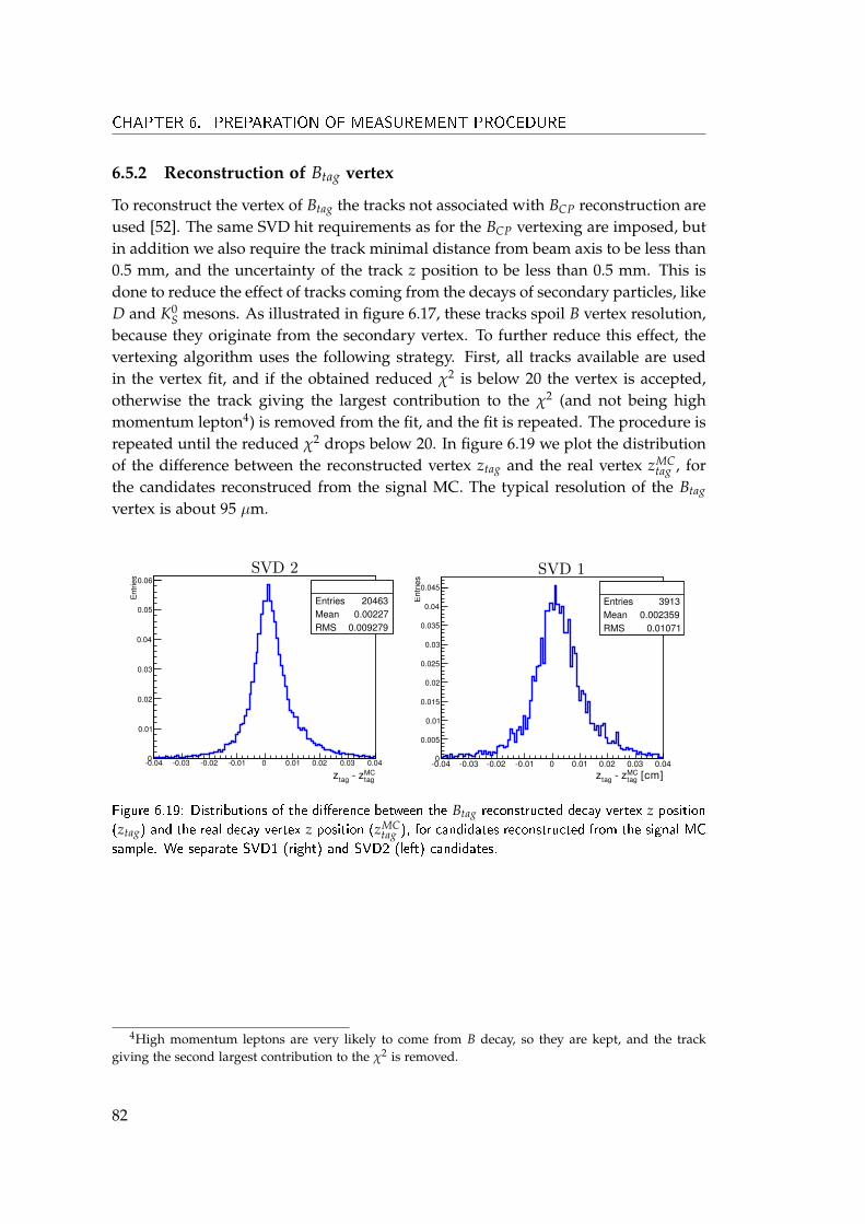
CHAPTER 6. PREPARATION OF MEASUREMENT PROCEDURE
6.5.2 Reconstruction of Btag vertex
To reconstruct the vertex of Btag the tracks not associated with BCP reconstruction areused [52]. The same SVD hit requirements as for the BCP vertexing are imposed, butin addition we also require the track minimal distance from beam axis to be less than0.5 mm, and the uncertainty of the track z position to be less than 0.5 mm. This isdone to reduce the effect of tracks coming from the decays of secondary particles, likeD and K0
S mesons. As illustrated in figure 6.17, these tracks spoil B vertex resolution,because they originate from the secondary vertex. To further reduce this effect, thevertexing algorithm uses the following strategy. First, all tracks available are usedin the vertex fit, and if the obtained reduced χ2 is below 20 the vertex is accepted,otherwise the track giving the largest contribution to the χ2 (and not being highmomentum lepton4) is removed from the fit, and the fit is repeated. The procedure isrepeated until the reduced χ2 drops below 20. In figure 6.19 we plot the distributionof the difference between the reconstructed vertex ztag and the real vertex zMC
tag , forthe candidates reconstruced from the signal MC. The typical resolution of the Btag
vertex is about 95 µm.
h1Entries 20463Mean 0.00227RMS 0.009279
tagMC- ztagz
-0.04 -0.03 -0.02 -0.01 0 0.01 0.02 0.03 0.04
Ent
ries
0
0.01
0.02
0.03
0.04
0.05
0.06
Entries 20463Mean 0.00227RMS 0.009279
h11Entries 3913Mean 0.002359RMS 0.01071
[cm]tagMC- ztagz
-0.04 -0.03 -0.02 -0.01 0 0.01 0.02 0.03 0.04
Ent
ries
0
0.005
0.01
0.015
0.02
0.025
0.03
0.035
0.04
0.045
Entries 3913Mean 0.002359RMS 0.01071
Figure 6.19: Distributions of the di�erence between the Btag reconstructed decay vertex z position(ztag) and the real decay vertex z position (zMC
tag ), for candidates reconstructed from the signal MCsample. We separate SVD1 (right) and SVD2 (left) candidates.
4High momentum leptons are very likely to come from B decay, so they are kept, and the trackgiving the second largest contribution to the χ2 is removed.
82
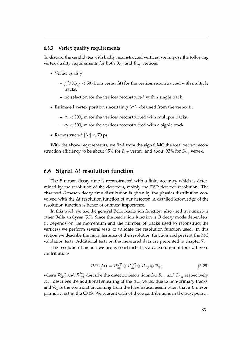
6.5.3 Vertex quality requirements
To discard the candidates with badly reconstructed vertices, we impose the followingvertex quality requirements for both BCP and Btag vertices:
• Vertex quality
– χ2/Ndo f < 50 (from vertex fit) for the vertices reconstructed with multipletracks.
– no selection for the vertices reconstruced with a single track.
• Estimated vertex position uncertainty (σz), obtained from the vertex fit
– σz < 200µm for the vertices reconstructed with multiple tracks.
– σz < 500µm for the vertices reconstructed with a signle track.
• Reconstructed |∆t| < 70 ps.
With the above requirements, we find from the signal MC the total vertex recon-struction efficiency to be about 95% for BCP vertex, and about 93% for Btag vertex.
6.6 Signal ∆t resolution function
The B meson decay time is reconstructed with a finite accuracy which is deter-mined by the resolution of the detectors, mainly the SVD detector resolution. Theobserved B meson decay time distribution is given by the physics distribution con-volved with the ∆t resolution function of our detector. A detailed knowledge of theresolution function is hence of outmost importance.
In this work we use the general Belle resolution function, also used in numerousother Belle analyses [53]. Since the resolution function is B decay mode dependent(it depends on the momentum and the number of tracks used to reconstruct thevertices) we perform several tests to validate the resolution function used. In thissection we describe the main features of the resolution function and present the MCvalidation tests. Additional tests on the measured data are presented in chapter 7.
The resolution function we use is constructed as a convolution of four differentcontributions
Rsig(∆t) = RCPdet ⊗R
tagdet ⊗Rnp ⊗Rk, (6.25)
where RCPdet and Rtag
det describe the detector resolutions for BCP and Btag respectively,Rnp describes the additional smearing of the Btag vertex due to non-primary tracks,and Rk is the contribution coming from the kinematical assumption that a B mesonpair is at rest in the CMS. We present each of these contributions in the next points.
83
CHAPTER 6. PREPARATION OF MEASUREMENT PROCEDURE
Detector resolution
RCPdet and Rtag
det describe the resolution of the reconstructed zCP and ztag. The vertexposition resolution is actually event dependent, because it depends on many eventparameters, such as the number of SVD hits, momentum of the tracks, and the direc-tion of the tracks. This motivates the use of event dependent resolution function, thatis parametrized as a function of the vertex position uncertainty (σz), obtained fromthe vertex fit. If σz would be the correct uncertainty estimator, a simple Gaussianfunction with the width σz would describe the resolution function. It turns out thatthis description is not sufficient, so the detector resolution function used is given by
Radet(x) = G(x; 0, [s0
a + s1ah]σz) (a = CP, tag), (6.26)
where h ≡ χ2/Ndo f is obtained from the vertex fit, and where we have introducedtwo scale factors s0
a and s1a. The scale factors are determined from a lifetime fit5,
using the measured ∆t distribution of candidates from a large control sample. Insuch a fit, the full resolution function as given in (6.25) has to be used, but some ofits parameters are set free and optimized to correctly describe the data. Differentsets of scale factors are used for the resolution functions of candidates recorded withthe SVD1 and SVD2 detectors. For the vertices reconstruced with a single track, aslightly modified resolution function is used. It is described in appendix B.2, wherealso the values of all resolution function parameters are given.
Non-primary track smearing
The resolution function Rnp is introduced in order to describe the smearing of ztag,due to tracks that originate from a point displaced from the Btag vertex. It consistsof a prompt component, described by Dirac delta fucnction, and a smeared part.The functional form of the smeared part is obtained from the difference between ztag
reconstructed from the usual MC and a special MC sample, in which the lifetime ofall charm and K0
S mesons is set to zero. The shape used is given by a sum of Diracdelta function and two exponential components, for positive and negative ∆t side,
Rnp(x) = fδ δ(x) + (1− fδ)[(1− fn)Ep(x; τ
pnp) + fnEn(x; τn
np)]
, (6.27)
where
Ep(n)(x; τ) ≡ 1τ
exp(−(+)
xτ
), for x > 0 (x ≤ 0) and 0 otherwise, (6.28)
fδ and fn are shape parameters. The effective lifetimes, τpnp and τn
np , are parametrized
as functions of σtagz and h from the vertex fit
τp(n)np = τ0
p(n) + τhp(n)h + (τs
p(n) + τshp(n)h)σ
tagz /(cβγ), (6.29)
5The lifetime fit is described in detail in section 7.3.
84
where s0tag and s1
tag are the scale factors introduced in the previous point, and wehave introduce eight additional shape parameters, τ0
p(n), τhp(n), τs
p(n), τshp(n). The shape
parameters of Rnp are determined by fitting the distribution of the difference be-tween the mentioned MC samples. Again, different sets of parameters are used forthe SVD1 and SVD2 candidates, and we show their values in the appendix B.2.
Kinematic approximation
We calculate the time difference between the decays of BCP and Btag by measuringthe distance between the decay vertices, and assuming that B mesons are at rest inthe CMS. As this is not exactly true, the value of ∆t calculated this way is smearedaround its true value ∆ttrue. From the kinematics of Υ(4S) → BB decay and knownbeam energies, one can obtain
∆ttrue ∼ ∆t− 0.165 cos θcmsB (tCP + ttag), (6.30)
where θcmsB is the polar angle of BCP in the CMS, and tCP (ttag) is the decay time of BCP
( Btag). With some more effort the analytic formula for Rk [53], which describes thissmearing, can be obtained as a conditional probability of obtaining x given ∆ttrue,
Rk(x) =
Ep(n)
(x−
[(
EcmsB
mB− 1)∆ttrue +
pcmsB cos θcms
BβmB
|∆ttrue|])
, cos θcmsB > 0 (< 0)
δdirac(
x− (Ecms
BmB− 1)∆ttrue
)(6.31)
where mB = 5.279 GeV, EcmsB = 5.292 GeV, and pcms
B = 0.340 GeV are B mesonmass, energy and momentum in the CMS. Having the physical PDF P phys(∆ttrue),we obtain the PDF of the measured distribution by convolution
Pmeas(∆t) =∫P phys(∆ttrue)Rk(∆t− ∆ttrue) d∆ttrue, (6.32)
which can be for the case of P phys as given in (C.12) calculated analitically.
6.6.1 MC validation test
By its definition the resolution function Rsig should describe the distribution of thedifference between the reconstructed ∆t and its true value. This can easily be checkedon the MC sample, where the information about generated ∆t is available. We use∆tMC to denote the generated ∆t value. In figure 6.20 the distribution of ∆t−∆tMC isploted for the candidates recnstructed from the 15 streams of signal MC. We separatethe distributions of the SVD1 and SVD2 candidates. We superimpose the resolutionfunction Rsig on the simulated data distributions. From the residual plots beloweach distribution one can see that Rsig describes the data very well. Note that the
85
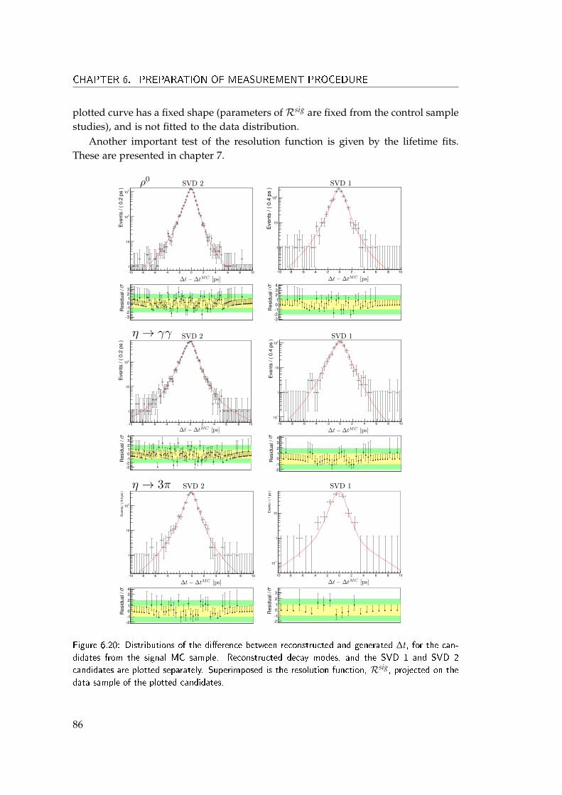
CHAPTER 6. PREPARATION OF MEASUREMENT PROCEDURE
plotted curve has a fixed shape (parameters ofRsig are fixed from the control samplestudies), and is not fitted to the data distribution.
Another important test of the resolution function is given by the lifetime fits.These are presented in chapter 7.
-10 -8 -6 -4 -2 0 2 4 6 8 10
Eve
nts
/(0.
2ps
)
1
10
210
310
Res
idua
l/
-3-2-10123
-10 -8 -6 -4 -2 0 2 4 6 8 10E
vent
s/(
0.4
ps)
1
10
210
Res
idua
l/
-3-2-101234
-10 -8 -6 -4 -2 0 2 4 6 8 10
Eve
nts
/(0.
2ps
)
1
10
210
Res
idua
l/
-3-2-101234
-10 -8 -6 -4 -2 0 2 4 6 8 10
Eve
nts
/(0.
4ps
)
-110
1
10
210
Res
idua
l/
-2-101234
-10 -8 -6 -4 -2 0 2 4 6 8 10
Eve
nts
/(0.
4ps
)
1
10
210
Res
idua
l/
-2-101234
-10 -8 -6 -4 -2 0 2 4 6 8 10
Eve
nts
/(1
ps)
-110
1
10
Res
idua
l/
-2-10123
Figure 6.20: Distributions of the di�erence between reconstructed and generated ∆t, for the can-didates from the signal MC sample. Reconstructed decay modes, and the SVD 1 and SVD 2candidates are plotted separately. Superimposed is the resolution function, Rsig, projected on thedata sample of the plotted candidates.
86
Plotting a conditional PDF
The shape of Rsig is determined on the event-by-event basis, because it depends onseveral candidate parameters, such as σCP
z and σtagz . The resolution function plotted
in figure 6.20 has to be obtained as a sum of normalized resolution functions of eachcandidate
Rplot(∆t− ∆tMC) = ∑iRsig(∆t− ∆tMC | (σCP
z , hCP, σtagz , htag)i), (6.33)
where the sum runs over all candidates. More formally we say that Rsig is a con-ditional PDF, depending on the candidate parameters, and normalized for each setof the parameters. When such a PDF is compared with the data distribution (as infigure 6.20) it is obtained as given in (6.33), and we say that it is projected on the datasample.
Basically all PDFs used in this analysis are of this type, and the above procedureis used for all.
6.7 Background ∆t shape
As described in section 6.3, there are three types of B candidates in the Mbc − ∆Esignal region. Some are signal candidates, but there are also background candidatescoming from the continuum and generic BB events. To obtain the correct ∆t dis-tribution of the signal candidates (and consequently the correct values of the CPVparameters) we have to know the fraction of background candidates (see section 6.3),as well as their ∆t distribution. The determination of the latter is described in thefollowing.
We compose the PDF to describe the background ∆t distribution as a convolutionof the physics-like part and the resolution function, P bkg = P bkg
phys ⊗Rbkg. For thephysics-like part we use a sum of the prompt component and the component with afinite (effective) lifetime
P bkgphys(∆t) = fδδ(∆t− µδ) + (1− fδ) exp
(−|∆t− µτ|
τbkg
), (6.34)
where the fraction fδ, the mean of two components µδ and µτ, and the effective life-time τbkg, are the shape parameters. The prompt part describes the candidates fromevents with charged tracks originating from the IP, and the lifetime part describes thecandidates from events containing some intermediate meson states with the effectivelifetime τbkg. For the resolution function of the background candidates we use a sumof three Gaussian functions
Rbkg(∆t) = (1− fout) [(1− ftail)G(∆t, 0, smainσt) + ftailG(∆t, 0, stailσt)]
+ foutG(∆t, 0, soutσt), (6.35)
87
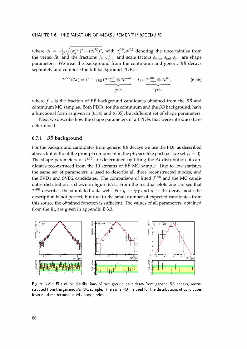
CHAPTER 6. PREPARATION OF MEASUREMENT PROCEDURE
where σt = 1βγc
√(σCP
z )2 + (σtagz )2, with σCP
z , σtagz denoting the uncertainties from
the vertex fit, and the fractions ftail , fout and scale factors smain, stail , sout are shapeparameters. We treat the background from the continuum and generic BB decaysseparately and compose the full background PDF as
P bkg(∆t) = (1− fBB)P contphys ⊗Rcont︸ ︷︷ ︸+ fBB PBB
phys ⊗RBB︸ ︷︷ ︸, (6.36)
P cont PBB
where fBB is the fraction of BB background candidates obtained from the BB andcontinuum MC samples. Both PDFs, for the continuum and the BB background, havea functional form as given in (6.34) and (6.35), but different set of shape parameters.
Next we describe how the shape parameters of all PDFs that were introduced aredetermined.
6.7.1 BB background
For the background candidates from generic BB decays we use the PDF as describedabove, but without the prompt component in the physics-like part (i.e. we set fδ = 0).The shape parameters of PBB are determined by fitting the ∆t distribution of can-didates reconstruced from the 10 streams of BB MC sample. Due to low statisticsthe same set of parameters is used to describe all three reconstructed modes, andthe SVD1 and SVD2 candidates. The comparison of fitted PBB and the MC candi-dates distribution is shown in figure 6.21. From the residual plots one can see thatPBB describes the simulated data well. For η → γγ and η → 3π decay mode thedescription is not perfect, but due to the small number of expected candidates fromthis source the obtained function is sufficient. The values of all parameters, obtainedfrom the fit, are given in appendix B.3.3.
-8 -4 0 4 8
Eve
nts
/(0.
25ps
)
1
10
210
Res
idua
l/
-3-2-10123
Eve
nts
/(1
ps)
-110
1
10
210
Res
idua
l/
-3-2-101234
Eve
nts
/(2
ps)
-110
1
10
Res
idua
l/
-2-10123
-8 -4 0 4 8 -8 -4 0 4 8
Figure 6.21: Fits of ∆t distributions of background candidates from generic BB decays, recon-structed from the generic BB MC sample. The same PDF is used for the distributions of candidatesfrom all three reconstructed decay modes.
88
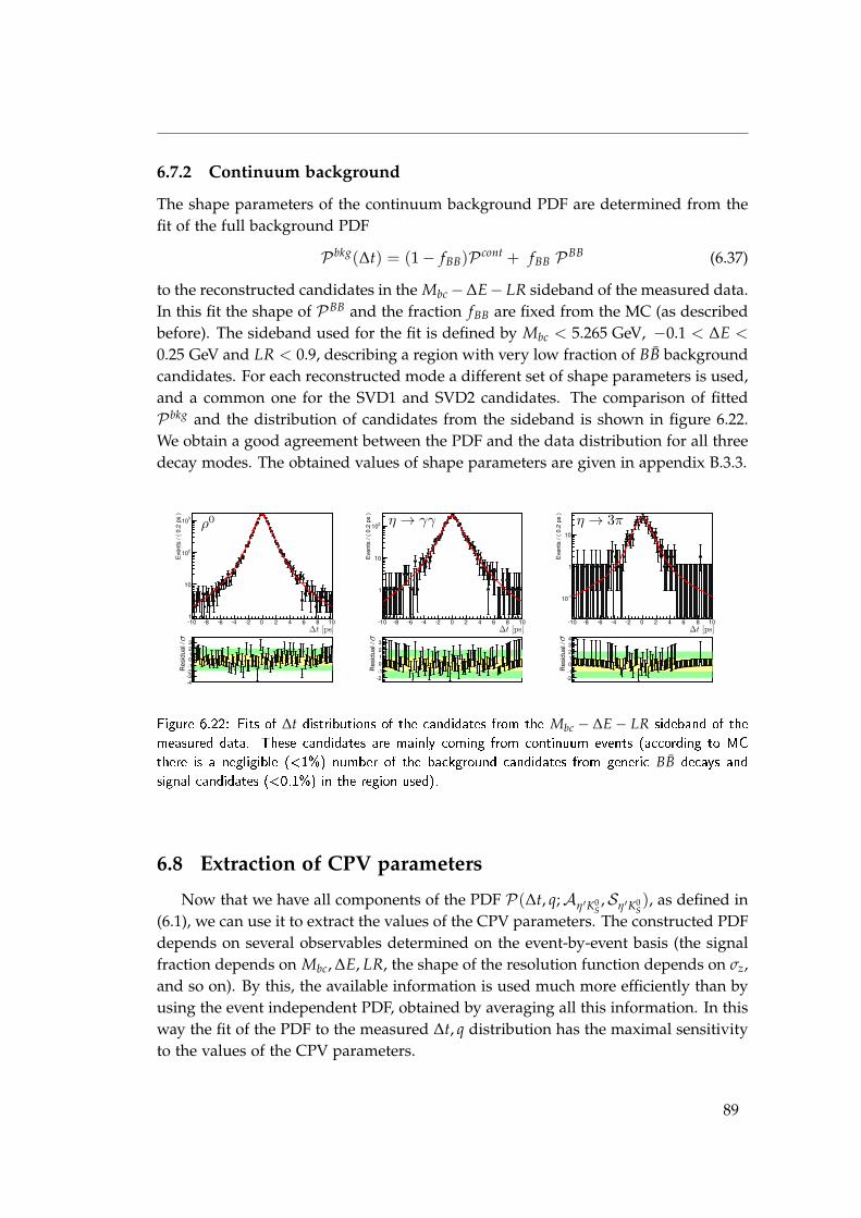
6.7.2 Continuum background
The shape parameters of the continuum background PDF are determined from thefit of the full background PDF
P bkg(∆t) = (1− fBB)P cont + fBB PBB (6.37)
to the reconstructed candidates in the Mbc−∆E− LR sideband of the measured data.In this fit the shape of PBB and the fraction fBB are fixed from the MC (as describedbefore). The sideband used for the fit is defined by Mbc < 5.265 GeV, −0.1 < ∆E <
0.25 GeV and LR < 0.9, describing a region with very low fraction of BB backgroundcandidates. For each reconstructed mode a different set of shape parameters is used,and a common one for the SVD1 and SVD2 candidates. The comparison of fittedP bkg and the distribution of candidates from the sideband is shown in figure 6.22.We obtain a good agreement between the PDF and the data distribution for all threedecay modes. The obtained values of shape parameters are given in appendix B.3.3.
-10 -8 -6 -4 -2 0 2 4 6 8 10
Eve
nts
/(0.
2ps
)
1
10
210
310
Res
idua
l/
-4-3-2-10123
-10 -8 -6 -4 -2 0 2 4 6 8 10
Eve
nts
/(0.
2ps
)
1
10
210
Res
idua
l/
-2-10123
-10 -8 -6 -4 -2 0 2 4 6 8 10
Eve
nts
/(0.
2ps
)
-110
1
10
Res
idua
l/
-2-101234
Figure 6.22: Fits of ∆t distributions of the candidates from the Mbc − ∆E− LR sideband of themeasured data. These candidates are mainly coming from continuum events (according to MCthere is a negligible (<1%) number of the background candidates from generic BB decays andsignal candidates (<0.1%) in the region used).
6.8 Extraction of CPV parameters
Now that we have all components of the PDF P(∆t, q;Aη′K0S,Sη′K0
S), as defined in
(6.1), we can use it to extract the values of the CPV parameters. The constructed PDFdepends on several observables determined on the event-by-event basis (the signalfraction depends on Mbc, ∆E, LR, the shape of the resolution function depends on σz,and so on). By this, the available information is used much more efficiently than byusing the event independent PDF, obtained by averaging all this information. In thisway the fit of the PDF to the measured ∆t, q distribution has the maximal sensitivityto the values of the CPV parameters.
89
CHAPTER 6. PREPARATION OF MEASUREMENT PROCEDURE
The PDF P(∆t, q;Aη′K0S,Sη′K0
S) gives the probability of obtaining ∆t and q, for
given Aη′K0S
and Sη′K0S. However, now we need the opposite. We ask, what are the
most likely values of Aη′K0S
and Sη′K0S, given the measured distribution of ∆t and q.
To answer this question we construct a likelihood function as
L(Aη′K0S,Sη′K0
S; {∆ti, qi}) = ∏
iP i(∆ti, qi;Aη′K0
S,Sη′K0
S), (6.38)
where {∆ti, qi} is the set of all reconstructed B candidates’ ∆t, q values, and theproduct runs over this set. With i on P i we stress that the shape of P dependson candidate properties. The values of Aη′K0
Sand Sη′K0
Sfor which the likelihood
function L is maximal, are best estimates for the values of these two parameters. Inother words, for these values the probability of observing the measured distibutionis maximized.
In practice it is usually more convinient to work with so-called log-likelihood,which is obtained as −2 lnL, turning the product in (6.38) into a sum. To mini-mize the log-likelihood function we use MIGRAD algorithm [54], commonly used inhigh energy physics experiments. Besides the estimated best values of the param-eters, the minimizer also returns the statistical uncertainty of the estimation. It iscalculated as a difference between the parameter value at minimum and the value atwhich −2 lnL is increased by one unit. In the limit of a large number of candidates,the likelihood function L has a Gaussian shape in the vicinity of the minimum, andthe uncertainty corresponds to the width (one standard deviation) of this Gaussianfunction.
6.8.1 Full PDF
In this subsection we summarize the full PDF that is used to extract the CPV param-eters. Based on the PDF given in (6.1), and things introduced in this chapter, we canwrite
P(∆t, q;Aη′K0S,Sη′K0
S) = fsig F sig P sig(∆t, q;Aη′K0
S,Sη′K0
S)⊗Rsig(∆t)
+ (1− fsig)[
fBBF BBPBB(∆t) + (1− fBB)F contP cont(∆t)]
,
(6.39)
where fsig is obtained from the signal/background fraction fit, fBB is fixed from theMC sample, and all PDFs used were introduced in this chapter. Background PDFsPBB and P cont, defined in (6.36), already include the ∆t resolution function, so itis not written explicitly. The PDF P sig contains two additional physical parametersbeside Aη′K0
Sand Sη′K0
S, namely B0 meson lifetime τB0 , and the mass difference ∆M.
In the fit of the CPV parameters we fix the values of these two parameters to theirworld average values [24], τ0
B = 1.519 ps and ∆M = 507 ps−1.
90

The components of the PDF (6.39) depend on the following candidate parameters(excluding ∆t, q)
fsig(r bin, mode), fBB(r bin, mode), F sig(cont,BB)(Mbc, ∆E, LR, r bin, mode), (6.40)
P sig(w), Rsig(σCPz , σ
tagz , hCP, htag, cos θB, SVD#), P cont(BB)(σCP
z , σtagz ).
When studying the large sample of MC events, a very small fraction (O(10−4))of candidates that cannot be described with the PDF (6.39) is observed. They forma very wide tail in the ∆t distribution (with σ ∼ 40 ps). We describe these byadding the outlier term Pol to the PDF (6.39), given by a simple Gaussian functionG(∆t; 0, σol). These outlying candidates arise from badly reconstructed tracks, so weassume an equal fraction of them, fol , for the signal and background distributions.The final PDF used in the fit becomes
P f ull(∆t, q;Aη′K0S,Sη′K0
S) = (1− fol)P(∆t, q;Aη′K0
S,Sη′K0
S) + folPol(∆t). (6.41)
The fraction fol and the width σol are determined by the lifetime fit of a large controlsample. The only free parameters of the PDF (6.41) are the CPV parameters Aη′K0
Sand Sη′K0
S.
In next chapter we present the tests used to validate the described fit method.
91

7Validation tests
Before unblinding the flavor of the candidates reconstructed and selected from themeasured dataset of events, we perform several tests of the prepared procedure.These are necessary in order to make sure that the values of the CPV parametersobtained from the fit are unbiased. We use two kinds of tests. First we test theprocedure on the MC sample, where the values of the measured CPV parameterscan be compared with the generated (true) values. However, due to the possibledifferences between the simulated and the measured data, it is even more importantto test the procedure on the measured data sample. For this purpose we use thecontrol sample and our nominal measured data sample, still being blind to flavorinformation. In this chapter we first present the tests done on the MC samples andlater on the measured datasets.
7.1 Signal MC test
We generate six large samples of signal events with different values of generatedS gen
η′K0S= (0.0, 0.3, 0.56, 0.67, 0.93, 0.97), and all with Agen
η′K0S= 0.0. Each sample contains
15 streams of events. After the reconstruction of B candidates, flavor tagging andvertices reconstruction, we perform the maximum likelihood fit of the signal PDFP sig ⊗Rsig to the obtained ∆t, q distribution. We fit the candidates from each decaymode separately and also simultaneously. In figure 7.1, a comparison of the fittedPDF and the candidates distribution in the case of S gen
η′K0S= 0.67 (which the value
obtained from the previous Belle analyis [35]) is shown, for each decay mode. The∆t distribution of the reconstructed candidates with q = +1 and q = −1 is plotted
93
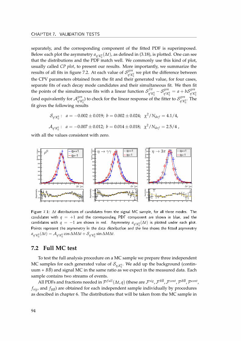
CHAPTER 7. VALIDATION TESTS
separately, and the corresponding component of the fitted PDF is superimposed.Below each plot the asymmetry aη′K0
S(∆t), as defined in (3.18), is plotted. One can see
that the distributions and the PDF match well. We commonly use this kind of plot,usually called CP plot, to present our results. More importantly, we summarize theresults of all fits in figure 7.2. At each value of S gen
η′K0S
we plot the difference betweenthe CPV parameters obtained from the fit and their generated value, for four cases,separate fits of each decay mode candidates and their simultaneous fit. We then fitthe points of the simultaneous fits with a linear function S f it
η′K0S− S gen
η′K0S= a + bS gen
η′K0S
(and equivalently for Agenη′K0
S) to check for the linear response of the fitter to S gen
η′K0S. The
fit gives the following results
Sη′K0S
: a = −0.002± 0.019; b = 0.002± 0.024; χ2/Ndo f = 4.1/4,
Aη′K0S
: a = −0.007± 0.012; b = 0.014± 0.018; χ2/Ndo f = 2.5/4 ,
with all the values consistent with zero.
-10 -8 -6 -4 -2 0 2 4 6 8 10
Eve
nts
/(0.
5ps
)
0
100
200
300
400
500
600
700
800 q=+1q=-1
-10 -8 -6 -4 -2 0 2 4 6 8 10
Asy
mm
etry
-0.5
0
0.5
-10 -8 -6 -4 -2 0 2 4 6 8 10
Eve
nts
/(0.
5ps
)
0
50
100
150
200
250
300
350
400
450 q=+1q=-1
-10 -8 -6 -4 -2 0 2 4 6 8 10
Asy
mm
etry
-1
-0.5
0
0.5
-10 -8 -6 -4 -2 0 2 4 6 8 10
Eve
nts
/(1
ps)
0
20
40
60
80
100
120
140
160
180
200
220
q=+1q=-1
-10 -8 -6 -4 -2 0 2 4 6 8 10
Asy
mm
etry
-0.5
0
0.5
1
Figure 7.1: ∆t distributions of candidates from the signal MC sample, for all three modes. Thecandidates with q = +1 and the corresponding PDF component are shown in blue, and thecandidates with q = −1 are shown in red. Asymmetry aη′K0
S(∆t) is plotted under each plot.
Points represent the asymmetry in the data distribution and the line shows the �tted asymmetryaη′K0
S(∆t) = Aη′K0
Scos ∆M∆t + Sη′K0
Ssin ∆M∆t.
7.2 Full MC test
To test the full analysis procedure on a MC sample we prepare three independentMC samples for each generated value of Sη,K0
S. We add up the background (contin-
uum + BB) and signal MC in the same ratio as we expect in the measured data. Eachsample contains two streams of events.
All PDFs and fractions needed in P f ull(∆t, q) (these are F sig,F BB,F cont,PBB,P cont,fsig, and fBB) are obtained for each independent sample individually by proceduresas descibed in chapter 6. The distributions that will be taken from the MC sample in
94
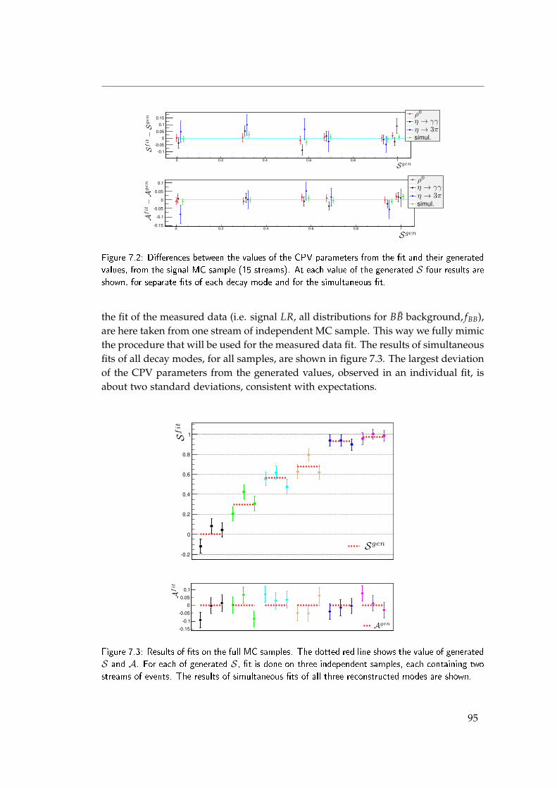
0 0.2 0.4 0.6 0.8 1
-0.1
-0.05
0
0.05
0.1
0.15
simul.
0 0.2 0.4 0.6 0.8 1-0.15
-0.1
-0.05
0
0.05
0.1
simul.
Figure 7.2: Di�erences between the values of the CPV parameters from the �t and their generatedvalues, from the signal MC sample (15 streams). At each value of the generated S four results areshown, for separate �ts of each decay mode and for the simultaneous �t.
the fit of the measured data (i.e. signal LR, all distributions for BB background, fBB),are here taken from one stream of independent MC sample. This way we fully mimicthe procedure that will be used for the measured data fit. The results of simultaneousfits of all decay modes, for all samples, are shown in figure 7.3. The largest deviationof the CPV parameters from the generated values, observed in an individual fit, isabout two standard deviations, consistent with expectations.
-0.2
0
0.2
0.4
0.6
0.8
1
-0.15
-0.1
-0.05
0
0.05
0.1
Figure 7.3: Results of �ts on the full MC samples. The dotted red line shows the value of generatedS and A. For each of generated S , �t is done on three independent samples, each containing twostreams of events. The results of simultaneous �ts of all three reconstructed modes are shown.
95
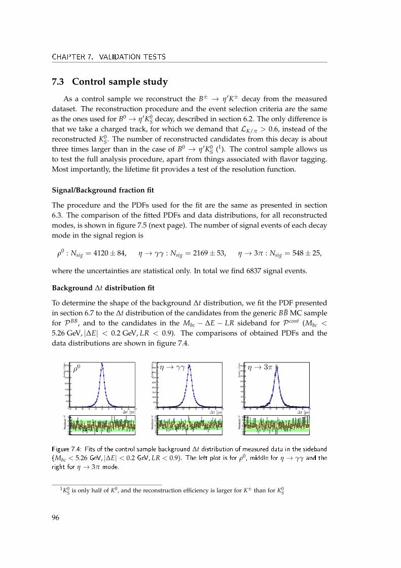
CHAPTER 7. VALIDATION TESTS
7.3 Control sample study
As a control sample we reconstruct the B± → η′K± decay from the measureddataset. The reconstruction procedure and the event selection criteria are the sameas the ones used for B0 → η′K0
S decay, described in section 6.2. The only difference isthat we take a charged track, for which we demand that LK/π > 0.6, instead of thereconstructed K0
S. The number of reconstructed candidates from this decay is aboutthree times larger than in the case of B0 → η′K0
S (1). The control sample allows usto test the full analysis procedure, apart from things associated with flavor tagging.Most importantly, the lifetime fit provides a test of the resolution function.
Signal/Background fraction fit
The procedure and the PDFs used for the fit are the same as presented in section6.3. The comparison of the fitted PDFs and data distributions, for all reconstructedmodes, is shown in figure 7.5 (next page). The number of signal events of each decaymode in the signal region is
ρ0 : Nsig = 4120± 84, η → γγ : Nsig = 2169± 53, η → 3π : Nsig = 548± 25,
where the uncertainties are statistical only. In total we find 6837 signal events.
Background ∆t distribution fit
To determine the shape of the background ∆t distribution, we fit the PDF presentedin section 6.7 to the ∆t distribution of the candidates from the generic BB MC samplefor PBB, and to the candidates in the Mbc − ∆E − LR sideband for P cont (Mbc <
5.26 GeV, |∆E| < 0.2 GeV, LR < 0.9). The comparisons of obtained PDFs and thedata distributions are shown in figure 7.4.
Figure 7.4: Fits of the control sample background ∆t distribution of measured data in the sideband(Mbc < 5.26 GeV, |∆E| < 0.2 GeV, LR < 0.9). The left plot is for ρ0, middle for η → γγ and theright for η → 3π mode.
1K0S is only half of K0, and the reconstruction efficiency is larger for K± than for K0
S
96
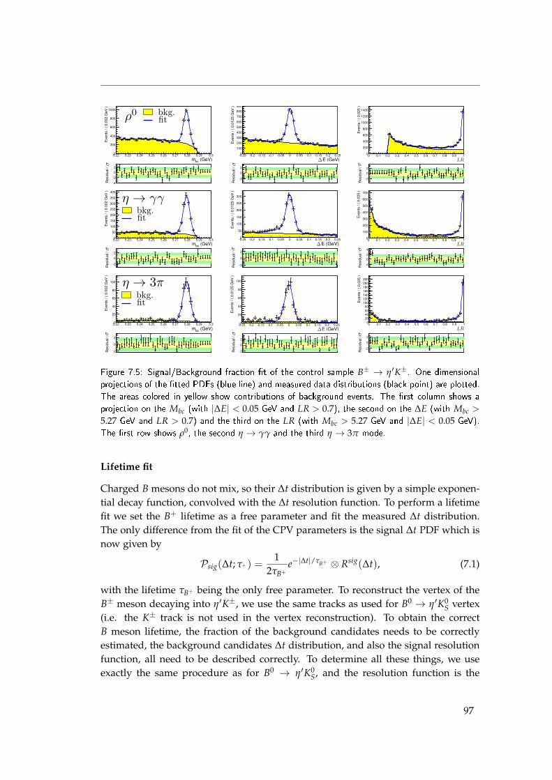
5.22 5.23 5.24 5.25 5.26 5.27 5.28 5.29 5.3
Events/(0.002GeV)
0
200
400
600
800
1000Residual/
-4
-2
0
2
E (GeV)-0.25 -0.2 -0.15 -0.1 -0.05 0 0.05 0.1 0.15 0.2 0.25
Events/(0.0125GeV)
0
100
200
300
400
500
600
700
800
900
Residual/
-2
0
2
0 0.1 0.2 0.3 0.4 0.5 0.6 0.7 0.8 0.9 1
Events/(0.025)
0
200
400
600
800
1000
1200
1400
Residual/
-2
0
2
5.22 5.23 5.24 5.25 5.26 5.27 5.28 5.29 5.3
Events/(0.002GeV)
0
50
100
150
200
250
300
350
400
Residual/
-2
0
2
E (GeV)-0.25 -0.2 -0.15 -0.1 -0.05 0 0.05 0.1 0.15 0.2 0.25
Events/(0.0125GeV)
0
50
100
150
200
250
300
Residual/
-2
0
2
0 0.1 0.2 0.3 0.4 0.5 0.6 0.7 0.8 0.9 1
Events/(0.025)
0
100
200
300
400
500
600
700
Residual/
-2
02
4
5.22 5.23 5.24 5.25 5.26 5.27 5.28 5.29 5.3
Events/(0.002GeV)
0
20
40
60
80
100
Residual/
-2
0
2
E (GeV)-0.25 -0.2 -0.15 -0.1 -0.05 0 0.05 0.1 0.15 0.2 0.25
Events/(0.0125GeV)
0
20
40
60
80
100
Residual/
-2
0
2
0 0.1 0.2 0.3 0.4 0.5 0.6 0.7 0.8 0.9 1
Events/(0.025)
020406080100120140160180200220
Residual/
-2
0
2
(GeV)bcm
(GeV)bcm
(GeV)bcm
Figure 7.5: Signal/Background fraction �t of the control sample B± → η′K±. One dimensionalprojections of the �tted PDFs (blue line) and measured data distributions (black point) are plotted.The areas colored in yellow show contributions of background events. The �rst column shows aprojection on the Mbc (with |∆E| < 0.05 GeV and LR > 0.7), the second on the ∆E (with Mbc >
5.27 GeV and LR > 0.7) and the third on the LR (with Mbc > 5.27 GeV and |∆E| < 0.05 GeV).The �rst row shows ρ0, the second η → γγ and the third η → 3π mode.
Lifetime fit
Charged B mesons do not mix, so their ∆t distribution is given by a simple exponen-tial decay function, convolved with the ∆t resolution function. To perform a lifetimefit we set the B+ lifetime as a free parameter and fit the measured ∆t distribution.The only difference from the fit of the CPV parameters is the signal ∆t PDF which isnow given by
Psig(∆t; τ+) =1
2τB+e−|∆t|/τB+ ⊗ Rsig(∆t), (7.1)
with the lifetime τB+ being the only free parameter. To reconstruct the vertex of theB± meson decaying into η′K±, we use the same tracks as used for B0 → η′K0
S vertex(i.e. the K± track is not used in the vertex reconstruction). To obtain the correctB meson lifetime, the fraction of the background candidates needs to be correctlyestimated, the background candidates ∆t distribution, and also the signal resolutionfunction, all need to be described correctly. To determine all these things, we useexactly the same procedure as for B0 → η′K0
S, and the resolution function is the
97
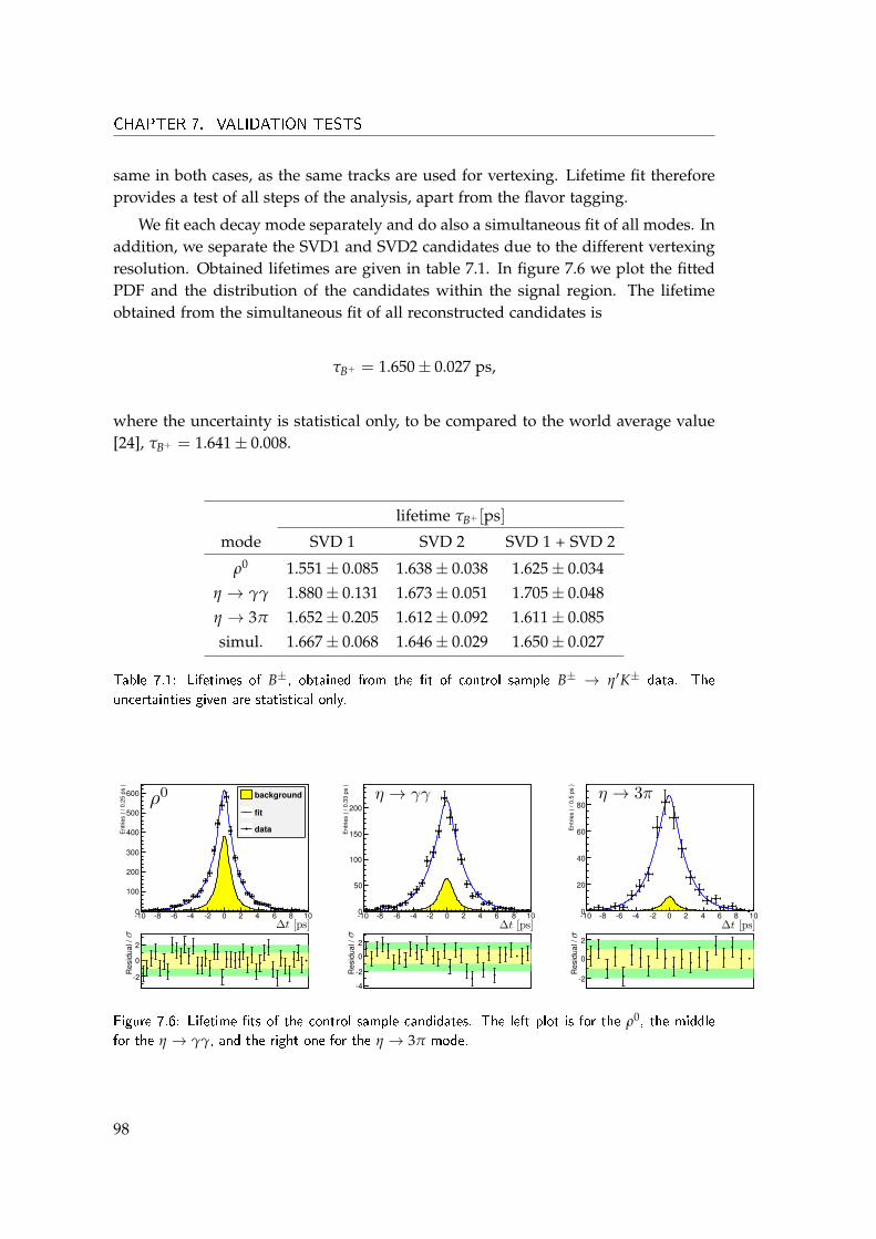
CHAPTER 7. VALIDATION TESTS
same in both cases, as the same tracks are used for vertexing. Lifetime fit thereforeprovides a test of all steps of the analysis, apart from the flavor tagging.
We fit each decay mode separately and do also a simultaneous fit of all modes. Inaddition, we separate the SVD1 and SVD2 candidates due to the different vertexingresolution. Obtained lifetimes are given in table 7.1. In figure 7.6 we plot the fittedPDF and the distribution of the candidates within the signal region. The lifetimeobtained from the simultaneous fit of all reconstructed candidates is
τB+ = 1.650± 0.027 ps,
where the uncertainty is statistical only, to be compared to the world average value[24], τB+ = 1.641± 0.008.
lifetime τB+ [ps]
mode SVD 1 SVD 2 SVD 1 + SVD 2
ρ0 1.551± 0.085 1.638± 0.038 1.625± 0.034η → γγ 1.880± 0.131 1.673± 0.051 1.705± 0.048η → 3π 1.652± 0.205 1.612± 0.092 1.611± 0.085simul. 1.667± 0.068 1.646± 0.029 1.650± 0.027
Table 7.1: Lifetimes of B±, obtained from the �t of control sample B± → η′K± data. Theuncertainties given are statistical only.
-10 -8 -6 -4 -2 0 2 4 6 8 10
Ent
ries
(/0.
25ps
)
0
100
200
300
400
500
600 background
fit
data
Res
idua
l/
-2
0
2
-10 -8 -6 -4 -2 0 2 4 6 8 10
Ent
ries
(/0.
33ps
)
0
50
100
150
200
Res
idua
l/
-4
-2
0
2
-10 -8 -6 -4 -2 0 2 4 6 8 10
Ent
ries
(/0.
5ps
)
0
20
40
60
80
Res
idua
l/
-2
0
2
Figure 7.6: Lifetime �ts of the control sample candidates. The left plot is for the ρ0, the middlefor the η → γγ, and the right one for the η → 3π mode.
98
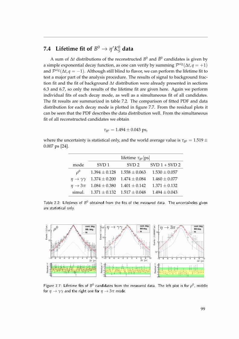
7.4 Lifetime fit of B0 → η′K0S data
A sum of ∆t distributions of the reconstructed B0 and B0 candidates is given bya simple exponential decay function, as one can verify by summing P sig(∆t, q = +1)and P sig(∆t, q = −1). Although still blind to flavor, we can perform the lifetime fit totest a major part of the analysis procedure. The results of signal to background frac-tion fit and the fit of background ∆t distribution were already presented in sections6.3 and 6.7, so only the results of the lifetime fit are given here. Again we performindividual fits of each decay mode, as well as a simultaneous fit of all candidates.The fit results are summarized in table 7.2. The comparison of fitted PDF and datadistribution for each decay mode is plotted in figure 7.7. From the residual plots itcan be seen that the PDF describes the data distribution well. From the simultaneousfit of all reconstructed candidates we obtain
τB0 = 1.494± 0.043 ps,
where the uncertainty is statistical only, and the world average value is τB0 = 1.519±0.007 ps [24].
lifetime τB0 [ps]
mode SVD 1 SVD 2 SVD 1 + SVD 2
ρ0 1.394± 0.128 1.558± 0.063 1.530± 0.057η → γγ 1.374± 0.200 1.474± 0.084 1.460± 0.077η → 3π 1.084± 0.380 1.401± 0.142 1.371± 0.132simul. 1.371± 0.132 1.517± 0.048 1.494± 0.043
Table 7.2: Lifetimes of B0 obtained from the �ts of the measured data. The uncertainties givenare statistical only.
-10 -8 -6 -4 -2 0 2 4 6 8 10
Eve
nts
/(0.
2ps
)
1
10
210
cont. bkg.BB. bkg.fit
Res
idua
l/
-3-2-10123
-10 -8 -6 -4 -2 0 2 4 6 8 10
Eve
nts
/(0.
4ps
)
-110
1
10
210cont. bkg.BB bkg.fit
Res
idua
l/
-3-2-10123
-10 -8 -6 -4 -2 0 2 4 6 8 10
Eve
nts
/(0.
6666
67ps
)
-110
1
10
cont. bkgBB bkg.fit
Res
idua
l/
-2-10123
Figure 7.7: Lifetime �ts of B0 candidates from the measured data. The left plot is for ρ0, middlefor η → γγ and the right one for η → 3π mode.
99

CHAPTER 7. VALIDATION TESTS
Having done all the tests presented in this chapter, and finding all results con-sistent with expectations, we are ready perform a fit of the CPV parameters on thecandidates recontructed from the measured data. We present the results in the nextchapter.
100
8Measurement results
In chapter 6 we have presented the method that allows us to extract the values ofthe CPV parameters from the ∆t, q distribution of reconstructed B candidates inB0 → η′K0
S decay. After the extensive validation tests, described in chapter 7, wefix the analysis procedure and apply it to the candidates reconstructed from theBelle final data sample, containing 772 millions BB pairs. As shown in table 6.4, wereconstruct 2233± 90 signal candidates (stat. error only). First we fit the candidatesof each mode separately, to check the results consistency between the subsamples,and then the simultaneous fit to all candidates is performed. From the simultaneousfit we obtain
Sη′K0S(π
+π−) = +0.728± 0.079,
Aη′K0S(π
+π−) = −0.002± 0.054,
where (π+π−) subscript denotes that K0S was reconstructed from π+π− pair only.
The uncertainties shown are statistical only. We also reconstruct the candidates withK0
S → π0π0 and include them into the analysis. Details of this addition are givenin appendix A. After the reconstruction, the analysis procedure is basically thesame as the one used for the candidates with K0
S → π+π−, except that we do notreconstruct η → 3π decay mode (due to low statistics). In total we reconstruct272 signal candidates with K0
S → π0π0, representing about 10% of all reconstructedsignal candidates.
101
CHAPTER 8. MEASUREMENT RESULTS
The values of the CPV parameters extracted only from K0S → π0π0 candidates
are
Sη′K0S(π
0π0) = +0.576± 0.206,
Aη′K0S(π
0π0) = +0.284± 0.180.
Finally, we perform the fit to all K0S → π+π+ and K0
S → π0π0 candidates simul-taneously, to extract the values of the CPV parameters in B0 → η′K0
S decay, andobtain
Sη′K0S= +0.71± 0.07,
Aη′K0S= +0.02± 0.05,
where the uncertainties given are statistical only. Estimation of systematic uncer-tainty is described in section 8.2. In figure 8.1 the background subtracted ∆t distru-butions of the reconstructed B candidates with q = +1 and q = −1 are shown, withsuperimposed signal PDF P sig(∆t, q). Below the plot, the resulting asymmetry in thedistributions, aη′K0
S(∆t), is shown. We summarize the results of all performed fits in
table 8.1.
772 M BBmode Sη′K0 Aη′K0
B0 → η′K0S 0.711± 0.074 +0.021± 0.052
K0S → π+π− 0.728± 0.079 −0.002± 0.054
ρ0 0.718± 0.098 −0.071± 0.069η → γγ 0.724± 0.151 +0.161± 0.098η → 3π 0.800± 0.259 −0.058± 0.181
K0S → π0π0 0.576± 0.206 +0.284± 0.180
B0 → η′K0L 0.458± 0.213 +0.088± 0.139
B0 → η′K0 0.682± 0.070 +0.029± 0.049
Table 8.1: The results of the CPV parameters �ts in B0 → η′K0S decay. The results of individual
decay modes and simultaneous �ts are given. Beside our results we show also the result fromB0 → η′K0
L analysis, done by other authors [56]. Expected values of the CPV parameters in thisdecay are the same as in our analysis, so we combine all the candidates reconstructed with K0
S andK0
L, and perform the simultaneous �t. We state this result as the values of the CPV parameters inB0 → η′K0 decays. The uncertainties given are statistical only.
102
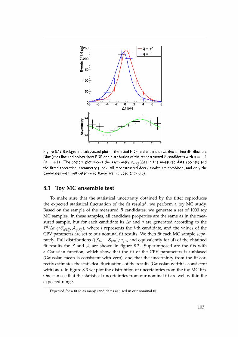
t [ps]-8 -6 -4 -2 0 2 4 6 8
Eve
nts(/
1.6ps
)
0
50
100
150
200
250 q = +1q = -1
-8 -6 -4 -2 0 2 4 6 8
Asy
mmetry
-0.5
0
0.5
Figure 8.1: Background subtracted plot of the �tted PDF and B candidates decay time distribution.Blue (red) line and points show PDF and distribution of the reconstructed B candidates with q = −1(q = +1). The bottom plot shows the asymmetry aη′K0
S(∆t) in the measured data (points) and
the �tted theoretical asymmetry (line). All reconstructed decay modes are combined, and only thecandidates with well determined �avor are included (r > 0.5).
8.1 Toy MC ensemble test
To make sure that the statistical uncertanty obtained by the fitter reproducesthe expected statistical fluctuation of the fit results1, we perform a toy MC study.Based on the sample of the measured B candidates, we generate a set of 1000 toyMC samples. In these samples, all candidate properties are the same as in the mea-sured sample, but for each candidate its ∆t and q are generated according to theP i(∆t, q;Sη′K0
S,Aη′K0
S), where i represents the i-th candidate, and the values of the
CPV parametrs are set to our nominal fit results. We then fit each MC sample sepa-rately. Pull distributions ((S f it − Sgen)/σf it, and equivalently for A) of the obtainedfit results for S and A are shown in figure 8.2. Superimposed are the fits witha Gaussian function, which show that the fit of the CPV parameters is unbiased(Gaussian mean is consistent with zero), and that the uncertainty from the fit cor-rectly estimates the statistical fluctuations of the results (Gaussian width is consistentwith one). In figure 8.3 we plot the distrubtion of uncertainties from the toy MC fits.One can see that the statistical uncertainties from our nominal fit are well within theexpected range.
1Expected for a fit to as many candidates as used in our nominal fit.
103
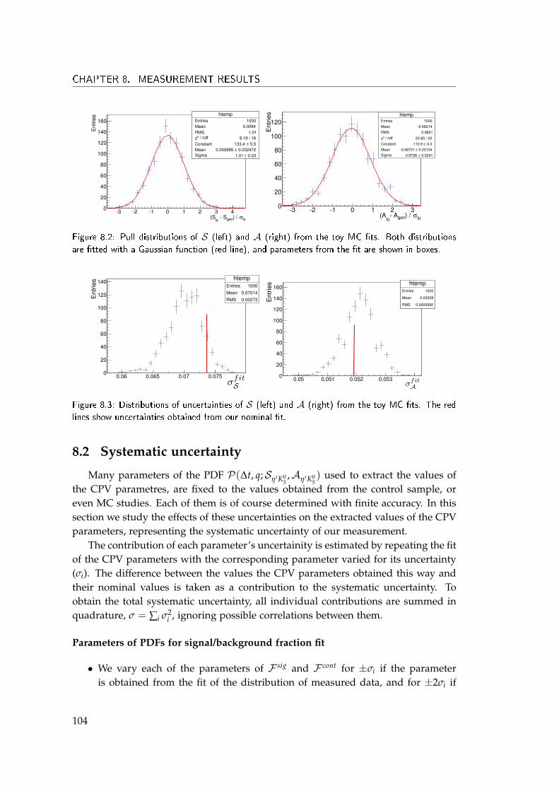
CHAPTER 8. MEASUREMENT RESULTS
htemp
Entries 1000
Mean 0.0094
RMS 1.01
/ ndf 2χ 9.19 / 16
Constant 5.5± 133.4
Mean 0.032472± 0.000995
Sigma 0.03± 1.01
fitσ) / gen Sfit
(S3 2 1 0 1 2 3 4
En
trie
s
0
20
40
60
80
100
120
140
160
htemp
Entries 1000
Mean 0.0094
RMS 1.01
/ ndf 2χ 9.19 / 16
Constant 5.5± 133.4
Mean 0.032472± 0.000995
Sigma 0.03± 1.01
htempEntries 1000
Mean 0.06214
RMS 0.9931
/ ndf 2χ 20.65 / 20
Constant 4.5± 110.9
Mean 0.03134± 0.06721
Sigma 0.0241± 0.9738
fitσ) / gen A
fit(A
3 2 1 0 1 2 3
En
trie
s
0
20
40
60
80
100
120
htempEntries 1000
Mean 0.06214
RMS 0.9931
/ ndf 2χ 20.65 / 20
Constant 4.5± 110.9
Mean 0.03134± 0.06721
Sigma 0.0241± 0.9738
Figure 8.2: Pull distributions of S (left) and A (right) from the toy MC �ts. Both distributionsare �tted with a Gaussian function (red line), and parameters from the �t are shown in boxes.
htempEntries 1000
Mean 0.07014
RMS 0.00273
0.06 0.065 0.07 0.075
Ent
ries
0
20
40
60
80
100
120
140htemp
Entries 1000
Mean 0.07014
RMS 0.00273
htempEntries 1000
Mean 0.05208
RMS 0.0005592
0.05 0.051 0.052 0.053
Ent
ries
0
20
40
60
80
100
120
140
160htemp
Entries 1000
Mean 0.05208
RMS 0.0005592
Figure 8.3: Distributions of uncertainties of S (left) and A (right) from the toy MC �ts. The redlines show uncertainties obtained from our nominal �t.
8.2 Systematic uncertainty
Many parameters of the PDF P(∆t, q;Sη′K0S,Aη′K0
S) used to extract the values of
the CPV parametres, are fixed to the values obtained from the control sample, oreven MC studies. Each of them is of course determined with finite accuracy. In thissection we study the effects of these uncertainties on the extracted values of the CPVparameters, representing the systematic uncertainty of our measurement.
The contribution of each parameter’s uncertainity is estimated by repeating the fitof the CPV parameters with the corresponding parameter varied for its uncertainty(σi). The difference between the values the CPV parameters obtained this way andtheir nominal values is taken as a contribution to the systematic uncertainty. Toobtain the total systematic uncertainty, all individual contributions are summed inquadrature, σ = ∑i σ2
i , ignoring possible correlations between them.
Parameters of PDFs for signal/background fraction fit
• We vary each of the parameters of F sig and F cont for ±σi if the parameteris obtained from the fit of the distribution of measured data, and for ±2σi if
104
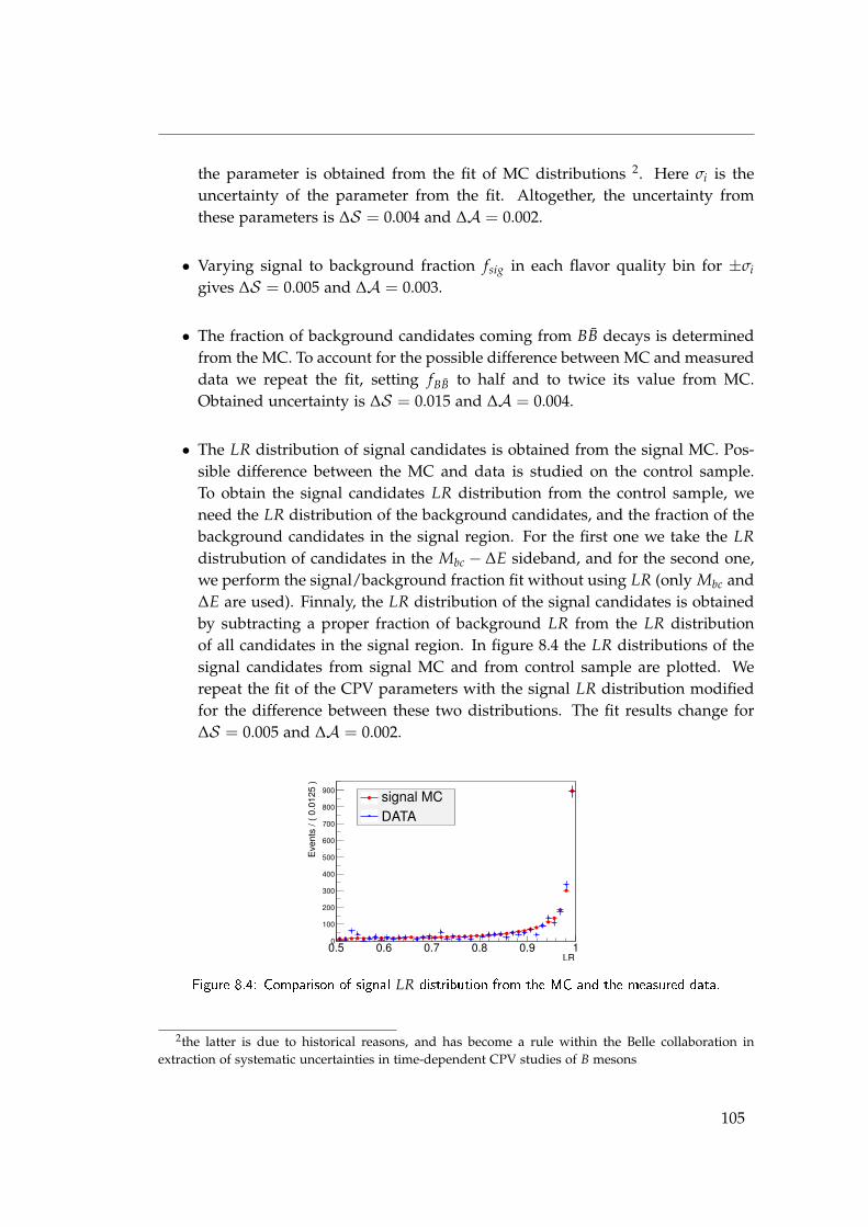
the parameter is obtained from the fit of MC distributions 2. Here σi is theuncertainty of the parameter from the fit. Altogether, the uncertainty fromthese parameters is ∆S = 0.004 and ∆A = 0.002.
• Varying signal to background fraction fsig in each flavor quality bin for ±σi
gives ∆S = 0.005 and ∆A = 0.003.
• The fraction of background candidates coming from BB decays is determinedfrom the MC. To account for the possible difference between MC and measureddata we repeat the fit, setting fBB to half and to twice its value from MC.Obtained uncertainty is ∆S = 0.015 and ∆A = 0.004.
• The LR distribution of signal candidates is obtained from the signal MC. Pos-sible difference between the MC and data is studied on the control sample.To obtain the signal candidates LR distribution from the control sample, weneed the LR distribution of the background candidates, and the fraction of thebackground candidates in the signal region. For the first one we take the LRdistrubution of candidates in the Mbc − ∆E sideband, and for the second one,we perform the signal/background fraction fit without using LR (only Mbc and∆E are used). Finnaly, the LR distribution of the signal candidates is obtainedby subtracting a proper fraction of background LR from the LR distributionof all candidates in the signal region. In figure 8.4 the LR distributions of thesignal candidates from signal MC and from control sample are plotted. Werepeat the fit of the CPV parameters with the signal LR distribution modifiedfor the difference between these two distributions. The fit results change for∆S = 0.005 and ∆A = 0.002.
LR0.5 0.6 0.7 0.8 0.9 1
Events
/ (
0.0
125 )
0
100
200
300
400
500
600
700
800
900signal MC
DATA
Figure 8.4: Comparison of signal LR distribution from the MC and the measured data.
2the latter is due to historical reasons, and has become a rule within the Belle collaboration inextraction of systematic uncertainties in time-dependent CPV studies of B mesons
105

CHAPTER 8. MEASUREMENT RESULTS
Background ∆t PDF
We vary each prameter of P cont(∆t) and PBB(∆t) for ±σi, where σi is the uncertaintyof the parameter from the background shape fit. Obtained uncertainty is ∆S = 0.002and ∆A = 0.001.
∆t resolution function
We vary each parameter of Rsig for ±1σi if it is determined from the measureddata study, and for ±2σi if determined from the MC study. Here σi is the uncertaintyof the parameter from the fit of the control sample or MC, and includes its statisticaland systematic error. Obtained difference is ∆S = 0.020 and ∆A = 0.006.
Flavor tagging
We vary w and ∆w in each of the tagging quality bins separately for ±σi. Hereσi is the uncertainty of each fraction, obtained from the fit of the control sample usedto determine w and ∆w. Contribution to the systematic uncertainty is ∆S = 0.006and ∆A = 0.005.
Physics parameters
We vary the physics parameters that are fixed in our analysis, namely τB0 and ∆mB,for their uncertainties taken from PDG [24]. Obtained uncertainty is ∆S = 0.002 and∆A = 0.001.
Vertex reconstruction
• Poor quality vertex rejection: we change the criteria on the vertex fit χ2/Ndo f <
50 to χ2/Ndo f < 25 and χ2/Ndo f < 100, and the criteria on the uncertainty ofvertex z position from zerr < 0.02 cm to no criteria. Obtained uncertainty is∆S = 0.010 and ∆A = 0.007.
• We change ∆t fit range from |∆t| < 70 ps to |∆t| < 40 ps and |∆t| < 100 ps.Obtained uncertainty is ∆S < 0.001 and ∆A < 0.001.
• We change the radial smearing (in r− φ plane) of the IP tube used in the vertexfit from 21 µm to 11 µm and 41 µm. Obtained uncertainty is ∆S = 0.003 andA = 0.002.
• We change the track rejection criteria for Btag vertex reconstruction from dr <0.05 cm to dr < 0.04 cm and dr = 0.06 cm, and from σz < 0.05 cm to σz < 0.04cm and σz < 0.06 cm. Obtained difference in fit results is ∆S = 0.003 andA = 0.001.
106

• As an estimation of uncertainty due to imperfect SVD alignment we use theresult of other Belle studies. This uncertainty is expected to be decay modeindependent. It is obtained from a special MC sample, with the modified SVDalignment. We set ∆S = 0.006 and A = 0.004.
• Small biases are observed in ∆z measurements in e+e− → µ+µ− and controlsamples. To account for the possible systematic uncertainty from this sourcewe use the uncertainty obtained from other Belle studies. This uncertaintywas estimated by applying special ∆z correction functions, repeating the fit,and comparing the obtained results. Obtained values are ∆S = 0.005 andA = 0.007.
Tag side interference
The interference between CKM-favored b → cud and doubly CKM suppresed b →ucd amplitudes in the tagging side B can effect time dependent CPV measure-ments [55]. It introduces a small correction to the signal ∆t PDF, which was neglectedin P sig. To estimate the effect of this correction, we generate a large sample of toyMC pseudo-experiments with the corrected PDF. Then we fit the obtained ∆t, q dis-tributions with non-corrected PDF (same as used in nominal fit), and check for thedifference between the generated and fitted values of the CPV parameters. This waywe obtain ∆S = 0.002 and ∆A = 0.020.
All above presented contibutions are summarized in table 8.2. Summing all contri-butions in quadrature we obtain
∆S syst = 0.031 and ∆Asyst = 0.027, (8.1)
which we state as the systematic uncertainty of our measurement.
107

CHAPTER 8. MEASUREMENT RESULTS
source ∆S ∆AF sig,F cont parameters 0.004 0.002fractions f i
sig 0.005 0.003fractions f i
BB 0.015 0.004signal LR PDF 0.005 0.002background ∆t PDF 0.002 0.001∆t resolution 0.020 0.006flavor tagging 0.006 0.005physics parameters 0.002 0.001poor quality vertex rej. 0.010 0.007∆t range < 0.001 < 0.001IP tube 0.003 0.002Btag track rej. 0.003 0.001SVD missalignment 0.006 0.004∆z bias 0.005 0.007tag-side interference 0.002 0.020TOTAL 0.031 0.027
Table 8.2: Summary of systematic uncertainty contributions from di�erent sources.
108

9Conclusion
We measured the values of the CPV parameters in B0 → η′K0S decays. The results
were obtained from the Belle final data sample, containing 772× 106 BB pairs col-lected at the Υ(4S) resonance with the Belle detector at the KEKB asymmetric e+e−
collider. The final result of the measurement is
Sη′K0S= +0.71± 0.07(stat)± 0.03(syst),
Aη′K0S= +0.02± 0.05(stat)± 0.03(syst),
including statistical and systematic uncertainty. Our measurement gives the world’smost precise values of Sη′K0
Sand Aη′K0
Sto date, which are also the most precisely
determined values of the CPV parameters among all b → sqq penguin dominateddecay modes of B0 mesons. In figure 9.1 we compare the above result with the previ-ous Belle and BaBar measurement results, and the world average values of the CPVparameters in B0 → ccK0 decays. We find our result consistent with the previousBelle and BaBar measurements. There is no statistically significant deviation fromthe values of the CPV parameters in B → ccK0 decays, which is consistent with theSM predictions for Sη′K0
Sand Aη′K0
S.
Future prospects
In the past decade the KM mechanism, with a single irreducible CP violating com-plex phase, was experimentally firmly established as the main source of CP viola-tion. After the great excitement in the early years of B factories operation, whensome large deviations of the CPV parameters in b → sqq dominated modes from
109

CHAPTER 9. CONCLUSION
Figure 9.1: Comparison of our measurement result with the previous Belle [35] and BaBar [36]measurements. In addition we plot the value of the CPV parameters in charmed B→ ccK0 decays,representing the SM expectation value for our result.
the predicted values were observed, we find today the former statement true notonly for the tree dominated B0 decays, but also for these, to new physics sensitivedecay modes. However, relatively large experimental uncertainties on the values ofthe CPV parameters in b → sqq modes still leave space for sizable new physics con-tributions. Beside the fact that in many models of new physics such contributionsarise naturally at the few percent level, they are also necessary to explain the matter-antimatter asymmetry of the universe. This motivates further measurements of theCPV parameters in these modes, with the difference ∆S = Sb→sqq − SJ/ψK0 as oneof gold-plated observables to search for new CP violating phases, also at the futureSuperKEKB collider and Belle II detector [57,58]. The SuperKEKB/Belle II (upgradeof the KEKB collider and the Belle detector) plan to start the operation in 2016, andachieve the integrated luminosity of 50 ab−1 by 2023. The planned peak and in-tegrated luminosity curves are shown in figure 9.2. The uncertainties of the CPVparameters in most of the b → sqq decay modes are dominated by statistical uncer-tainties, so the luminosity increase is the only way to clarify the current experimentalsituation, either by discovering new CP violating phases, or further constraining andpossibly rule out some new physics models. In figure 9.3 the projected ∆S uncer-tainty as a function of integrated luminosity is shown, for B0 → η′K0, φK0, K0
SK0SK0
Sdecay modes [59]. With an integrated luminosity of 50 ab−1 the ∆S in η′K0
S can be
110
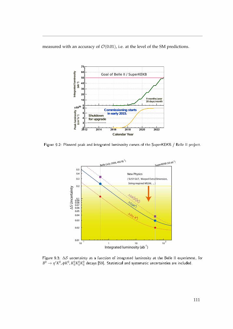
measured with an accuracy of O(0.01), i.e. at the level of the SM predictions.
Goal of Belle II / SuperKEKB
9months/year20days/month
Commissioningstartsinearly2015.
Shutdownforupgrade
Inte
gra
tedluminosity
(ab
-1)
Pea
kluminosity
(cm
-2s-
1 )
CalendarYear
Figure 9.2: Planned peak and integrated luminosity curves of the SuperKEKB / Belle II project.
Figure 9.3: ∆S uncertainty as a function of integrated luminosity at the Belle II experiment, forB0 → η′K0, φK0, K0
SK0SK0
S decays [59]. Statistical and systematic uncertainties are included.
111

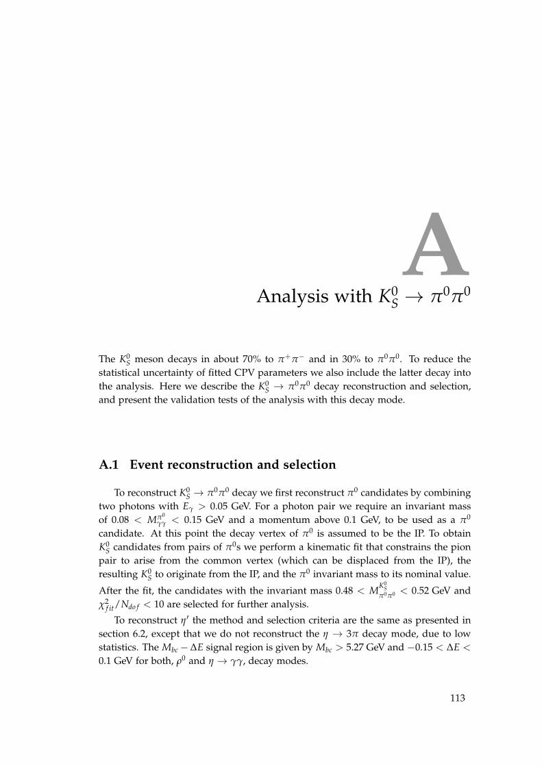
AAnalysis with K0
S → π0π0
The K0S meson decays in about 70% to π+π− and in 30% to π0π0. To reduce the
statistical uncertainty of fitted CPV parameters we also include the latter decay intothe analysis. Here we describe the K0
S → π0π0 decay reconstruction and selection,and present the validation tests of the analysis with this decay mode.
A.1 Event reconstruction and selection
To reconstruct K0S → π0π0 decay we first reconstruct π0 candidates by combining
two photons with Eγ > 0.05 GeV. For a photon pair we require an invariant massof 0.08 < Mπ0
γγ < 0.15 GeV and a momentum above 0.1 GeV, to be used as a π0
candidate. At this point the decay vertex of π0 is assumed to be the IP. To obtainK0
S candidates from pairs of π0s we perform a kinematic fit that constrains the pionpair to arise from the common vertex (which can be displaced from the IP), theresulting K0
S to originate from the IP, and the π0 invariant mass to its nominal value.
After the fit, the candidates with the invariant mass 0.48 < MK0S
π0π0 < 0.52 GeV andχ2
f it/Ndo f < 10 are selected for further analysis.
To reconstruct η′ the method and selection criteria are the same as presented insection 6.2, except that we do not reconstruct the η → 3π decay mode, due to lowstatistics. The Mbc−∆E signal region is given by Mbc > 5.27 GeV and −0.15 < ∆E <
0.1 GeV for both, ρ0 and η → γγ, decay modes.
113
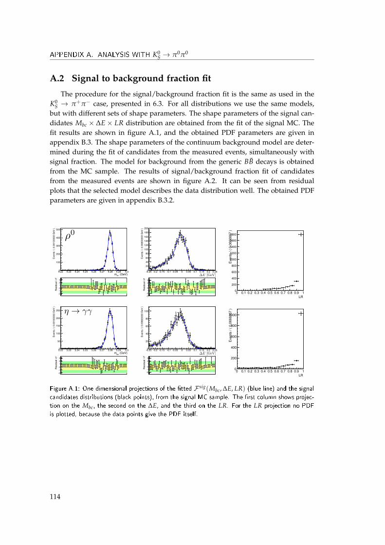
APPENDIX A. ANALYSIS WITH K0S → π0π0
A.2 Signal to background fraction fit
The procedure for the signal/background fraction fit is the same as used in theK0
S → π+π− case, presented in 6.3. For all distributions we use the same models,but with different sets of shape parameters. The shape parameters of the signal can-didates Mbc × ∆E× LR distribution are obtained from the fit of the signal MC. Thefit results are shown in figure A.1, and the obtained PDF parameters are given inappendix B.3. The shape parameters of the continuum background model are deter-mined during the fit of candidates from the measured events, simultaneously withsignal fraction. The model for background from the generic BB decays is obtainedfrom the MC sample. The results of signal/background fraction fit of candidatesfrom the measured events are shown in figure A.2. It can be seen from residualplots that the selected model describes the data distribution well. The obtained PDFparameters are given in appendix B.3.2.
5.22 5.23 5.24 5.25 5.26 5.27 5.28 5.29 5.3
Eve
nts/(
0.00
1333
33GeV
)
0
100
200
300
400
500
Res
idua
l/
-2-10123
-0.25 -0.2 -0.15 -0.1 -0.05 0 0.05 0.1 0.15 0.2 0.25
Eve
nts/(
0.00
8333
33GeV
)
0
20
40
60
80
100
120
140
160
180
200
Res
idua
l/
-3-2-10123
LR0 0.1 0.2 0.3 0.4 0.5 0.6 0.7 0.8 0.9 1
Eve
nts/(
0.06
6666
7)
0
200
400
600
800
1000
1200
1400
1600
1800
5.22 5.23 5.24 5.25 5.26 5.27 5.28 5.29 5.3
Eve
nts/(
0.00
1333
33GeV
)
0
50
100
150
200
250
Res
idua
l/
-2-10123
-0.25 -0.2 -0.15 -0.1 -0.05 0 0.05 0.1 0.15 0.2 0.25
Eve
nts/(
0.00
8333
33GeV
)
0
20
40
60
80
100
Res
idua
l/
-2-10123
LR0 0.1 0.2 0.3 0.4 0.5 0.6 0.7 0.8 0.9 1
Eve
nts/(
0.06
6666
7)
0
200
400
600
800
1000
(GeV)bcm
(GeV)bcm
Figure A.1: One dimensional projections of the �tted F sig(Mbc, ∆E, LR) (blue line) and the signalcandidates distributions (black points), from the signal MC sample. The �rst column shows projec-tion on the Mbc, the second on the ∆E, and the third on the LR. For the LR projection no PDFis plotted, because the data points give the PDF itself.
114
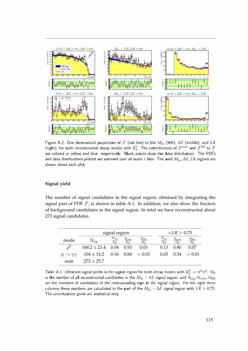
Figure A.2: One dimensional projections of F (red line) to the Mbc (left), ∆E (middle), and LR(right), for both reconstructed decay modes with K0
S. The contributions of F cont and F BB to Fare colored in yellow and blue, respectively. Black points show the data distribution. The PDFsand data distributions plotted are summed over all seven r bins. The used Mbc, ∆E, LR regions areshown above each plot.
Signal yield
The number of signal candidates in the signal region, obtained by integrating thesignal part of PDF F , is shown in table A.1. In addition, we also show the fractionof background candidates in the signal region. In total we have reconstructed about272 signal candidates.
signal region +LR > 0.75
mode NsigNsigNB
NcontNB
NBBNB
NsigNB
NcontNB
NBBNB
ρ0 168.2± 21.4 0.04 0.93 0.03 0.13 0.80 0.07η → γγ 104± 14.2 0.16 0.84 < 0.01 0.65 0.34 < 0.01
sum 272± 25.7
Table A.1: Obtained signal yields in the signal region for both decay modes with K0S → π0π0. NB
is the number of all reconstructed candidates in the Mbc − ∆E signal region, and Nsig, Ncont, NBBare the numbers of candidates of the corresponding type in the signal region. For the right threecolumns these numbers are calculated in the part of the Mbc − ∆E signal region with LR > 0.75.The uncertainties given are statistical only.
115
APPENDIX A. ANALYSIS WITH K0S → π0π0
A.3 Background ∆t shape
To model the background ∆t shape the same PDFs as introduced in section 6.7are used. To determine the shape parameters of the background from BB decays, wefit the ∆t distribution of candidates from the generic BB MC, and for the continuumbackground we fit the distribution of the candidates in Mbc − ∆E− LR sideband ofmeasured events. The fit results are shown in figure A.3, and the obtained shapeparameters are given in appendix B.3.3.
-10 -8 -6 -4 -2 0 2 4 6 8 10
Eve
nts
/(0.
2ps
)
1
10
210
310
Res
idua
l/
-3-2-10123
-10 -8 -6 -4 -2 0 2 4 6 8 10
Eve
nts
/(0.
2ps
)
1
10
210
Res
idua
l/
-3-2-10123
-10 -8 -6 -4 -2 0 2 4 6 8 10
Eve
nts
/(0.
2ps
)
1
10
210
Res
idua
l/
-3-2-10123
Figure A.3: Fits of background ∆t distribution. The left two plots show �ts of the candidates in theMbc − ∆E− LR sideband of measured data, and the right plot shows �t of background candidatesfrom BB MC sample.
A.4 Lifetime fit
We use the same signal ∆t resolution function as for K0S → π+π− decay mode.
Pions from K0S are not used in the vertex reconstruction, so the resolution is inde-
pendent of the K0S decay mode. We perform the lifetime fit as it also provides a test
of the signal/background fraction fit and the background ∆t distribution. Fit resultsare ploted in figure A.4 and obtained lifetimes from both reconstructed modes andsimultaneous fit are:
ρ0 : τB0 = 1.316± 0.180 ps
η → γγ : τB0 = 1.786± 0.152 ps
simul.: τB0 = 1.510± 0.122 ps,
where the uncertainties given are statistical only. The results are to be comparedwith the world average value of τB0 = 1.519± 0.007 ps [24].
116
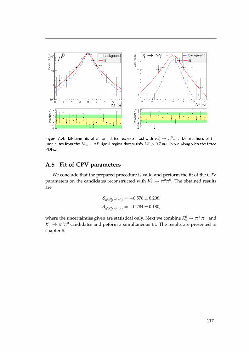
-8 -6 -4 -2 0 2 4 6 8
Eve
nts
/(0.
8ps
)
-110
1
10
210 backgoundfit
�R
esid
ual/
-2-10123
-6 -4 -2 0 2 4 6
Events/(
0.8ps
)
1
10
background
fit
�Residua
l/
-4-3-2-10123
Figure A.4: Lifetime �ts of B candidates reconstructed with K0S → π0π0. Distributions of the
candidates from the Mbc − ∆E signal region that satisfy LR > 0.7 are shown along with the �ttedPDFs.
A.5 Fit of CPV parameters
We conclude that the prepared procedure is valid and perform the fit of the CPVparameters on the candidates reconstructed with K0
S → π0π0. The obtained resultsare
Sη′K0S(π
0π0) = +0.576± 0.206,
Aη′K0S(π
0π0) = +0.284± 0.180,
where the uncertainties given are statistical only. Next we combine K0S → π+π− and
K0S → π0π0 candidates and peform a simultaneous fit. The results are presented in
chapter 8.
117

BMiscellaneous
B.1 Units
In this work we use units that are commonly used in high energy physics. Asa unit of energy electron volt (eV) is used, most commonly with a prefix giga,GeV, which is the energy scale of processes of our interest. To make easier use ofE2 = p2c2 + m2c4 relation the same unit (GeV) is used to express also mass and mo-mentum. Although formally m [GeV/c2] and p [GeV/c] a system of natural units,with c set to 1, is used for the sake of simplicity.
B.2 Wrong tag fractions and ∆t resolution function
To determine the fraction of B candidates with wrongly assigned flavor (wrongtag) and the parameters of the ∆t resolution function on the measured events, thefollowing flavor specific decays are studied: B0 → D+π−, D∗+π−, D∗+ρ−, D∗+l−νl
and B+ → D0π+, D∗0π+. After the reconstruction, event selection, and signal tobackground fraction fit of each decay mode, a simultaneous fit to ∆t distribution isperformed. The PDF used for the fit is given by
P(∆t) = (1− fol)[
fsigP sig + (1− fsig)P bkg(∆t)]+ folP ol(∆t), (B.1)
where fsig and P bkg depend on the decay mode, and outlier fraction and shape( fol ,P ol) are common to all decay modes. The signal PDF, P sig, is obtained as aconvolution of the physical part and the resolution function, P sig = P sig
phys ⊗Rsig.
119
APPENDIX B. MISCELLANEOUS
For the self tagged B0 decay modes the B0 − B0 mixing has to be taken into account,and from the decay rates given in (3.20) and (3.21), we can write
P sigphys(∆t)OF,SF =
14τB0
exp(−|∆t|
τB0
)[1± (1− 2w) cos ∆M∆t] , (B.2)
where OF (SF), with + (−) in the bracket, are used for the reconstructed B candidatesdecaying into the final state specific for the flavor opposite to (same as) the associatedB meson flavor, determined by flavor tagging algorithm. B0 candidates are dividedinto seven bins according to the flavor tagging information quality (r), and for eachbin a different w is used. For B± candidates the ∆t PDF is given by the exponentialfunction P sig
phys =1
2τB+exp(−|∆t|/τB+).
In the fit of the ∆t distribution, ∆t resolution function parameters, wrong tagfractions, lifetimes τB0 and τB+ , and mixing parameter ∆M, are free parameters. Theobtained lifetimes and ∆M are
τB+ = 1.6261± 0.0038 ps, (B.3)
τB0 = 1.5299± 0.0029 ps, (B.4)
∆M = 0.5088± 0.0019 ps−1, (B.5)
where the uncertainties are statistical only. The results are consistent with the worldaverage values [24], τB+ = 1.641± 0.008 ps, τB0 = 1.519± 0.007 ps and ∆M = 507±0.004ps−1. This validates the reslution function used. To obtain the final valuesof wrong tag fractions and resolution function parameters, the fit is repeated withτB+ , τB0 and ∆M fixed to the world average values, since these are also fixed in thefit to extract the CPV parameters. The obtained wrong tag fractions are summarizedin table B.1.
∆t Resolution function
In section 6.6 we only described the resolution function used for vertices recon-struced with multiple tracks. In the case of single track vertex reconstruction adifferent resolution function is used, because for these vertices χ2, as given in eq.(6.24), cannot be calculated. The detector resolution function used is given by
Radet(x) = (1− ftail)G(x; 0, smain
a σz) + ftailG(x, staila σz) (a = CP, tag), (B.6)
where the scale factors smain, stail and fraction ftail are shape parameters, and σz isobtained from the vertex fit. For the resolution function describing smearing dueto non-primary tracks the same function as given in (6.27) is used, but with thefollowing parametrization of effective lifetimes
τp,n = τ0,singp,n + τ
1,singp,n σz, (B.7)
and the fractions f singδ , f sing
n being constants.The values of all resolution function parameters obtained from the fit of the con-
trol sample are summarized in table B.2
120

SVD1 SVD2w σ+ σ− w σ+ σ−
r-bin [×10−3] [×10−3] [×10−3] [×10−3]
0 0.50 0.51 0.4188 7.23 6.00 0.4188 4.15 3.572 0.3298 7.12 6.43 0.3193 3.24 2.803 0.2338 7.41 7.69 0.2229 3.72 3.4864 0.1706 6.88 6.41 0.1631 3.31 4.245 0.0997 6.76 8.80 0.1040 3.18 3.696 0.0228 4.33 4.58 0.0251 2.17 3.07
r-bin ∆w ∆w0 0.0 0.01 0.0569 8.92 9.16 -0.0087 3.96 3.922 0.0126 9.18 9.14 0.0103 3.54 3.693 -0.0147 10.0 9.98 -0.0109 4.12 4.174 -0.0005 9.02 8.87 -0.0186 4.16 4.605 0.0088 9.30 9.29 0.0016 3.99 3.916 0.0046 5.69 5.78 -0.0036 2.43 2.36
Table B.1: Wrong tag fractions obtained from the �t of SVD1 and SVD2 control sample. Besidethe mean values also the positive (σ+) and negative (σ−) uncertainties are shown (statistical +systematic).
121
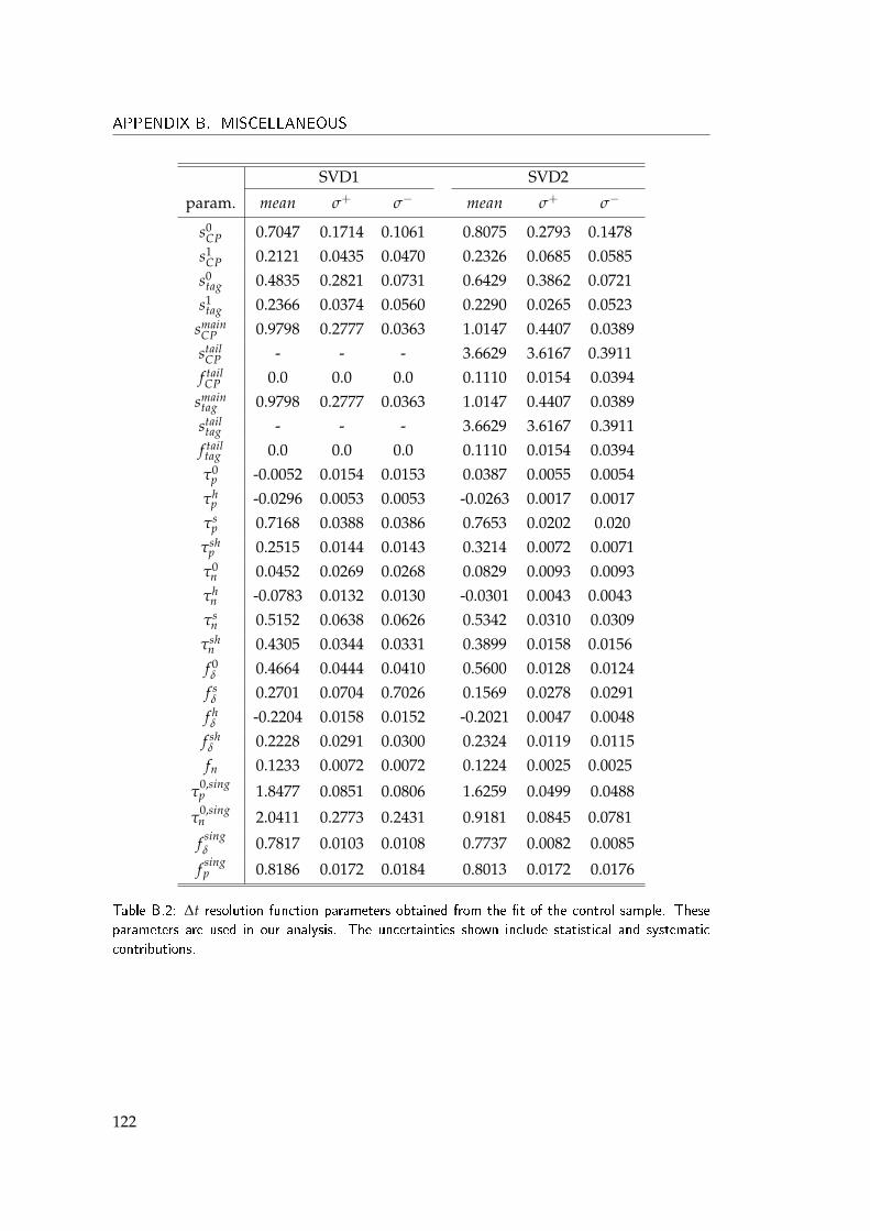
APPENDIX B. MISCELLANEOUS
SVD1 SVD2
param. mean σ+ σ− mean σ+ σ−
s0CP 0.7047 0.1714 0.1061 0.8075 0.2793 0.1478
s1CP 0.2121 0.0435 0.0470 0.2326 0.0685 0.0585
s0tag 0.4835 0.2821 0.0731 0.6429 0.3862 0.0721
s1tag 0.2366 0.0374 0.0560 0.2290 0.0265 0.0523
smainCP 0.9798 0.2777 0.0363 1.0147 0.4407 0.0389stail
CP - - - 3.6629 3.6167 0.3911f tailCP 0.0 0.0 0.0 0.1110 0.0154 0.0394
smaintag 0.9798 0.2777 0.0363 1.0147 0.4407 0.0389stail
tag - - - 3.6629 3.6167 0.3911f tailtag 0.0 0.0 0.0 0.1110 0.0154 0.0394τ0
p -0.0052 0.0154 0.0153 0.0387 0.0055 0.0054τh
p -0.0296 0.0053 0.0053 -0.0263 0.0017 0.0017τs
p 0.7168 0.0388 0.0386 0.7653 0.0202 0.020τsh
p 0.2515 0.0144 0.0143 0.3214 0.0072 0.0071τ0
n 0.0452 0.0269 0.0268 0.0829 0.0093 0.0093τh
n -0.0783 0.0132 0.0130 -0.0301 0.0043 0.0043τs
n 0.5152 0.0638 0.0626 0.5342 0.0310 0.0309τsh
n 0.4305 0.0344 0.0331 0.3899 0.0158 0.0156f 0δ 0.4664 0.0444 0.0410 0.5600 0.0128 0.0124
f sδ 0.2701 0.0704 0.7026 0.1569 0.0278 0.0291
f hδ -0.2204 0.0158 0.0152 -0.2021 0.0047 0.0048
f shδ 0.2228 0.0291 0.0300 0.2324 0.0119 0.0115fn 0.1233 0.0072 0.0072 0.1224 0.0025 0.0025
τ0,singp 1.8477 0.0851 0.0806 1.6259 0.0499 0.0488
τ0,singn 2.0411 0.2773 0.2431 0.9181 0.0845 0.0781
f singδ 0.7817 0.0103 0.0108 0.7737 0.0082 0.0085
f singp 0.8186 0.0172 0.0184 0.8013 0.0172 0.0176
Table B.2: ∆t resolution function parameters obtained from the �t of the control sample. Theseparameters are used in our analysis. The uncertainties shown include statistical and systematiccontributions.
122
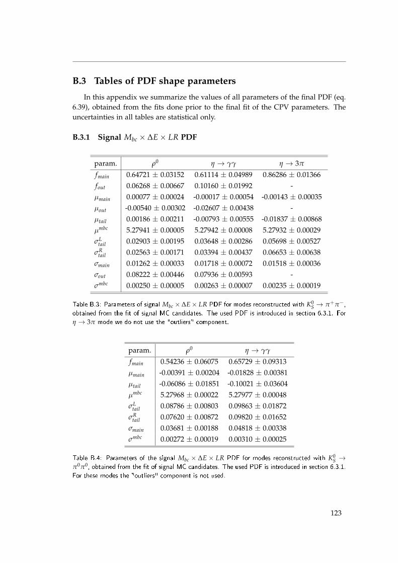
B.3 Tables of PDF shape parameters
In this appendix we summarize the values of all parameters of the final PDF (eq.6.39), obtained from the fits done prior to the final fit of the CPV parameters. Theuncertainties in all tables are statistical only.
B.3.1 Signal Mbc × ∆E× LR PDF
param. ρ0 η → γγ η → 3π
fmain 0.64721 ± 0.03152 0.61114 ± 0.04989 0.86286 ± 0.01366fout 0.06268 ± 0.00667 0.10160 ± 0.01992 -µmain 0.00077 ± 0.00024 -0.00017 ± 0.00054 -0.00143 ± 0.00035µout -0.00540 ± 0.00302 -0.02607 ± 0.00438 -µtail 0.00186 ± 0.00211 -0.00793 ± 0.00555 -0.01837 ± 0.00868µmbc 5.27941 ± 0.00005 5.27942 ± 0.00008 5.27932 ± 0.00029σL
tail 0.02903 ± 0.00195 0.03648 ± 0.00286 0.05698 ± 0.00527σR
tail 0.02563 ± 0.00171 0.03394 ± 0.00437 0.06653 ± 0.00638σmain 0.01262 ± 0.00033 0.01718 ± 0.00072 0.01518 ± 0.00036σout 0.08222 ± 0.00446 0.07936 ± 0.00593 -σmbc 0.00250 ± 0.00005 0.00263 ± 0.00007 0.00235 ± 0.00019
Table B.3: Parameters of signal Mbc ×∆E× LR PDF for modes reconstructed with K0S → π+π−,
obtained from the �t of signal MC candidates. The used PDF is introduced in section 6.3.1. Forη → 3π mode we do not use the "outliers" component.
param. ρ0 η → γγ
fmain 0.54236 ± 0.06075 0.65729 ± 0.09313µmain -0.00391 ± 0.00204 -0.01828 ± 0.00381µtail -0.06086 ± 0.01851 -0.10021 ± 0.03604µmbc 5.27968 ± 0.00022 5.27977 ± 0.00048σL
tail 0.08786 ± 0.00803 0.09863 ± 0.01872σR
tail 0.07620 ± 0.00872 0.09820 ± 0.01652σmain 0.03681 ± 0.00188 0.04818 ± 0.00338σmbc 0.00272 ± 0.00019 0.00310 ± 0.00025
Table B.4: Parameters of the signal Mbc × ∆E × LR PDF for modes reconstructed with K0S →
π0π0, obtained from the �t of signal MC candidates. The used PDF is introduced in section 6.3.1.For these modes the "outliers" component is not used.
123
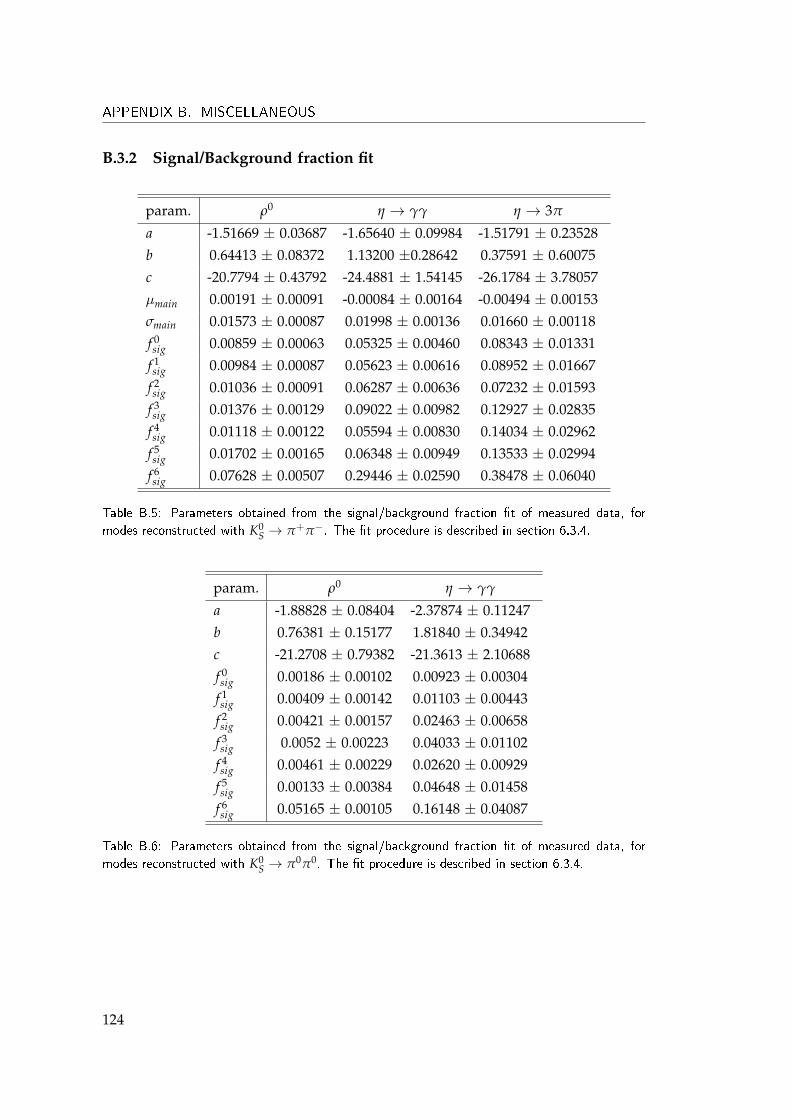
APPENDIX B. MISCELLANEOUS
B.3.2 Signal/Background fraction fit
param. ρ0 η → γγ η → 3π
a -1.51669 ± 0.03687 -1.65640 ± 0.09984 -1.51791 ± 0.23528b 0.64413 ± 0.08372 1.13200 ±0.28642 0.37591 ± 0.60075c -20.7794 ± 0.43792 -24.4881 ± 1.54145 -26.1784 ± 3.78057µmain 0.00191 ± 0.00091 -0.00084 ± 0.00164 -0.00494 ± 0.00153σmain 0.01573 ± 0.00087 0.01998 ± 0.00136 0.01660 ± 0.00118f 0sig 0.00859 ± 0.00063 0.05325 ± 0.00460 0.08343 ± 0.01331
f 1sig 0.00984 ± 0.00087 0.05623 ± 0.00616 0.08952 ± 0.01667
f 2sig 0.01036 ± 0.00091 0.06287 ± 0.00636 0.07232 ± 0.01593
f 3sig 0.01376 ± 0.00129 0.09022 ± 0.00982 0.12927 ± 0.02835
f 4sig 0.01118 ± 0.00122 0.05594 ± 0.00830 0.14034 ± 0.02962
f 5sig 0.01702 ± 0.00165 0.06348 ± 0.00949 0.13533 ± 0.02994
f 6sig 0.07628 ± 0.00507 0.29446 ± 0.02590 0.38478 ± 0.06040
Table B.5: Parameters obtained from the signal/background fraction �t of measured data, formodes reconstructed with K0
S → π+π−. The �t procedure is described in section 6.3.4.
param. ρ0 η → γγ
a -1.88828 ± 0.08404 -2.37874 ± 0.11247b 0.76381 ± 0.15177 1.81840 ± 0.34942c -21.2708 ± 0.79382 -21.3613 ± 2.10688f 0sig 0.00186 ± 0.00102 0.00923 ± 0.00304
f 1sig 0.00409 ± 0.00142 0.01103 ± 0.00443
f 2sig 0.00421 ± 0.00157 0.02463 ± 0.00658
f 3sig 0.0052 ± 0.00223 0.04033 ± 0.01102
f 4sig 0.00461 ± 0.00229 0.02620 ± 0.00929
f 5sig 0.00133 ± 0.00384 0.04648 ± 0.01458
f 6sig 0.05165 ± 0.00105 0.16148 ± 0.04087
Table B.6: Parameters obtained from the signal/background fraction �t of measured data, formodes reconstructed with K0
S → π0π0. The �t procedure is described in section 6.3.4.
124

param. ρ0 η → γγ η → 3π
f 0BB 0.01101 0.00173 0.00233
f 1BB 0.01431 0.00137 0.00310
f 2BB 0.01612 0.00240 0.00240
f 3BB 0.01678 0.00325 0.00449
f 4BB 0.01417 0.00237 0.00358
f 5BB 0.01819 0.00225 0.00221
f 6BB 0.05032 0.00581 0.00311
Table B.7: Fractions of background candidates from generic BB decays, for all r bins, for modesreconstructed with K0
S → π+π−. The Mbc − ∆E region used is given in (6.21).
param. ρ0 η → γγ
f 0BB 0.01458 0.00227
f 1BB 0.01962 0.00368
f 2BB 0.02591 0.00398
f 3BB 0.02712 0.00309
f 4BB 0.02497 0.00487
f 5BB 0.03020 0.00719
f 6BB 0.07251 0.01408
Table B.8: Fractions of background candidates from generic BB decays, for all r bins, for modesreconstructed with K0
S → π0π0. The Mbc − ∆E region used is given in (6.21).
B.3.3 Background ∆t shape parameters
param. ρ0 η → γγ η → 3π
σmain 1.14058 ± 0.01198 1.13537 ± 0.03964 1.17198 ± 0.09678σout 27.6202 ± 1.26978 30.3102 ± 4.03072 10.6445 ± 7.38035σtail 3.84347 ± 0.09462 3.84401 ± 0.31426 5.97836 ± 1.26626fδ 0.46549 ± 0.02542 0.47245 ± 0.09446 0.39168 ± 0.12857fout 0.01236 ± 0.00072 0.01259 ± 0.00242 0.00953 ± 0.02552ftail 0.14653 ± 0.00777 0.15981 ± 0.02768 0.08809 ± 0.03885µδ -0.01317 ± 0.01052 -0.01840 ± 0.04991 -0.06207 ± 0.08989µτ 0.04602 ± 0.01356 0.06805 ± 0.06132 0.07247 ± 0.09904τbkg 0.57528 ± 0.02216 0.63783 ± 0.09045 0.78553 ± 0.13529
Table B.9: Parameters of the background ∆t PDF, obtained from the �t of measured data sideband,for modes reconstructed with K0
S → π+π−. The �t procedure is described in section 6.7.
125

APPENDIX B. MISCELLANEOUS
param. ρ0 η → γγ
σmain 1.04506 ± 0.02290 1.13098 ± 0.04738σout 17.2121 ± 1.37908 27.5123 ± 6.37009σtail 3.14152 ± 0.12165 3.79134 ± 0.35678fδ 0.43964 ± 0.06147 0.37833 ± 0.17060fout 0.01353 ± 0.00165 0.00887 ± 0.00269ftail 0.19884 ± 0.01773 0.13620 ± 0.02761µδ 0.03108 ± 0.022648 0.04465 ± 0.09347µτ -0.00643 ± 0.024181 0.02312 ± 0.07239τbkg 0.47569 ± 0.04299 0.50141 ± 0.10140
Table B.10: Parameters of the background ∆t PDF, obtained from the �t of measured data side-band, for modes reconstructed with K0
S → π0π0. The �t procedure and used PDF are describedin section 6.7.
param. K0S → π+π− K0
S → π0π0
σmain 5.75214 ± 0.69209 8.19295 ± 1.28161σout 0.98858 ± 0.05385 0.94660 ± 0.01376σtail 38.6135 ± 5.94849 41.2452 ± 10.2304fout 0.93586 ± 0.01567 0.91483 ± 0.02779ftail 0.05668 ± 0.01659 0.06993 ± 0.02779µl -0.17100 ± 0.01511 -0.13662 ± 0.01892τbkg 1.44578 ± 0.02150 1.24238 ± 0.03181
Table B.11: Parameters of the ∆t PDF of background candidates from generic BB decays, obtainedfrom the �t of BB MC sample. The �t procedure and used PDF are described in section 6.7.
126
CSLOVENSKI POVZETEKMeritev kršitve simetrije CP v razpadih
B0 → η′K0S
C.1 Uvod
Simetrije imajo pomembno vlogo tako v vsakdanjem življenju kot v sodobniznanosti. Ko se sprašujemo o simetrijah fizikalnih zakonov, nas zanimajo transforma-cije fizikalnih sistemov, ki ne spremenijo dinamike sistema. Ce taka transformacijaobstaja, pravimo, da je sistem, oziroma fizikalni zakon, ki opisuje njegovo dinamiko,invarianten ali simetricen glede na izbrano transformacijo. Tema pricujocega dela,simetrija CP, je invariantnost na produkt dveh transformacij: konjugacijo naboja C, kipretvori delec v antidelec (Q → Q) in parnost P, ki prezrcali prostorske koordinate(~x → −~x). Tako se na primer levorocni elektron e−L pri transformaciji CP preslikav desnorocni pozitron e+R . Vecina pojavov v naravi je C in P simetricnih (torej tudiCP). Pravzaprav so taki vsi pojavi, ki so povezani z elektromagnetno, mocno jedrskoin gravitacijsko silo. Na drugi strani šibka jedrska sila ocitno in mocno krši C inP simetrijo, saj sklaplja le levorocne fermione in desnorocne antifermione. Kljubtemu obstaja precej procesov preko šibke interakcije, ki so simetricni na produktobeh transformacij, CP. Simetrija CP je do sredine prejšnjega stoletja veljala za eksak-tno simetrijo narave, simetrijo med materijo in antimaterijo. Da to ne drži povsem,se je eksperimentalno prvic pokazalo pri meritvah razpadov nevtralnih kaonov leta1964 [3], do preboja v teoreticnem opisu opažene kršitve simetrije CP pa je prišloslabih 10 let pozneje. Leta 1973 sta M. Kobayashi in T. Maskawa pokazala kakokršitev CP vstopa v takrat nastajajoco teorijo osnovnih delcev, Standardni Model(SM) [4]. Opazila sta, da je kršitev simetrije CP v SM naravno prisotna, ce le obsta-
127
APPENDIX C. SLOVENSKI POVZETEK
MERITEV KR�ITVE SIMETRIJE CP V RAZPADIH B0 → η′K0S
jajo vsaj tri družine kvarkov (leta 1973 so bili znani le kvarki u, d, s). V tem primerukvarkovska mešalna matrika, t.i. matrika Cabibbo-Kobayashi-Maskawa, krajše ma-trika CKM, ki podaja relativne jakosti sklopitev nabitih šibkih bozonov s kvarki ra-zlicnih okusov, vsebuje kompleksno fazo, ki je vir kršitve simetrije CP v SM. Kmaluzatem sta bila odkrita kvarka c (1974) in b (1977), in koncno leta 1995 še kvark t.
Da bi preverili konsistentnost t.i. Kobayashi-Maskawa (KM) mehanizma kršitvesimetrije CP, z eno kompleksno fazo v matriki CKM, so nujne meritve kršitve simetrijeCP v sistemu mezonov B (mezonov, ki vsebujejo kvark b), v katerem mehanizem KMnapove relativno velike kršitve simetrije CP. V ta namen sta bili v devetdesetih letihprejšnjega stoletja zgrajeni dve tovarni mezonov B, KEKB in PEP-II, z eksperimen-toma Belle [5] in BaBar [6]. Leta 2001 sta oba eksperimenta potrdila kršitev simetrijeCP v razpadih nevtralnih mezonov B v J/ψK0
S [7, 8]. To je bila prva opažena kršitevsimetrije CP izven sistema kaonov. V naslednjem desetletju so pri Belle in BaBarizmerili kršitev CP še v številnih drugih razpadih mezonov B, v vseh v skladu znapovedmi SM, in potrdili kompleksno fazo matrike CKM kot glavni vir kršitvesimetrije CP. Eksperimentalna potrditev napovedi Kobayashija in Maskawe jima jeprinesla Nobelovo nagrado za fiziko v letu 2008.
Kljub vsem potrditvam mehanizma KM, je na mestu vprašanje, ali je kompleksnafaza matrike CKM edini vir kršitve simetrije CP. Misel, da temu ni tako, spodbujatavsaj dva argumenta. Prvic, prisotnost novih kompleksnih faz, ki kršijo simetrijoCP, se zdi neizogibna v vecini modelov razširitve SM (t.i. nove fizike). Drugic,kršitev simetrije CP je nujni pogoj za razlago dominance materije nad antimaterijov opazljivem vesolju, toda ta kršitev je v SM mnogo premajhna, da bi pojasnilaopaženo asimetrijo. Prisotnost novih virov kršitve simetrije CP je tako nujna tudi skozmološkega vidika.
V sistemu mezonov B so na morebitno prisotnost novih faz, ki kršijo simetrijoCP, posebej obcutljivi razpadi pri katerih se kvark b pretvori v kvark s in še dvakvarka (b → sqq). Taki razpadi v SM potekajo le preko diagramov z zankami, vkaterih lahko prisotnost težkih, še neodkritih delcev, spremeni vrednosti nekaterihopazljivih kolicin. V primeru razpadov b → sqq je ta opazljiva kolicina casovnoodvisna kršitev simetrije CP. Meritev njene vrednosti in primerjava z napovedjo SMtorej ponuja možnost detekcije nove fizike.
V pricujocem delu predstavimo meritev casovno odvisne kršitve simetrije CP vrazpadih B0 → η′K0
S, ki potekajo preko omenjenega procesa b→ sqq. Meritev je bilaopravljena na vzorcu 772 milijonov razpadov parov BB, zbranih z detektorjem Bellev casu njegovega delovanja (1999-2010). V delu najprej predstavimo izvor kršitvesimetrije CP v SM (poglavje C.2), nato pa v njegovem okviru izracunamo napovedvrednosti parametrov kršitve CP v razpadu B0 → η′K0
S in jih primerjamo z rezul-tati dosedanjih meritev (poglavje C.3). V poglavju C.4 predstavimo detektor Belle.Sledi opis postopka meritve (poglavje C.5) in koncno rezultat meritve (poglavje C.6).Zakljucimo s pogledom v prihodnost, v poglavju C.7.
128
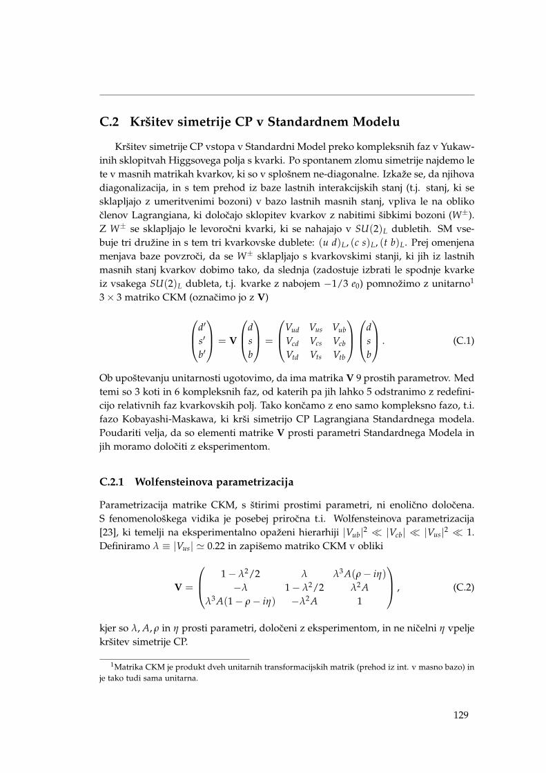
C.2 Kršitev simetrije CP v Standardnem Modelu
Kršitev simetrije CP vstopa v Standardni Model preko kompleksnih faz v Yukaw-inih sklopitvah Higgsovega polja s kvarki. Po spontanem zlomu simetrije najdemo lete v masnih matrikah kvarkov, ki so v splošnem ne-diagonalne. Izkaže se, da njihovadiagonalizacija, in s tem prehod iz baze lastnih interakcijskih stanj (t.j. stanj, ki sesklapljajo z umeritvenimi bozoni) v bazo lastnih masnih stanj, vpliva le na oblikoclenov Lagrangiana, ki dolocajo sklopitev kvarkov z nabitimi šibkimi bozoni (W±).Z W± se sklapljajo le levorocni kvarki, ki se nahajajo v SU(2)L dubletih. SM vse-buje tri družine in s tem tri kvarkovske dublete: (u d)L, (c s)L, (t b)L. Prej omenjenamenjava baze povzroci, da se W± sklapljajo s kvarkovskimi stanji, ki jih iz lastnihmasnih stanj kvarkov dobimo tako, da slednja (zadostuje izbrati le spodnje kvarkeiz vsakega SU(2)L dubleta, t.j. kvarke z nabojem −1/3 e0) pomnožimo z unitarno1
3× 3 matriko CKM (oznacimo jo z V)
d′
s′
b′
= V
dsb
=
Vud Vus Vub
Vcd Vcs Vcb
Vtd Vts Vtb
d
sb
. (C.1)
Ob upoštevanju unitarnosti ugotovimo, da ima matrika V 9 prostih parametrov. Medtemi so 3 koti in 6 kompleksnih faz, od katerih pa jih lahko 5 odstranimo z redefini-cijo relativnih faz kvarkovskih polj. Tako koncamo z eno samo kompleksno fazo, t.i.fazo Kobayashi-Maskawa, ki krši simetrijo CP Lagrangiana Standardnega modela.Poudariti velja, da so elementi matrike V prosti parametri Standardnega Modela injih moramo dolociti z eksperimentom.
C.2.1 Wolfensteinova parametrizacija
Parametrizacija matrike CKM, s štirimi prostimi parametri, ni enolicno dolocena.S fenomenološkega vidika je posebej prirocna t.i. Wolfensteinova parametrizacija[23], ki temelji na eksperimentalno opaženi hierarhiji |Vub|2 � |Vcb| � |Vus|2 � 1.Definiramo λ ≡ |Vus| ' 0.22 in zapišemo matriko CKM v obliki
V =
1− λ2/2 λ λ3A(ρ− iη)−λ 1− λ2/2 λ2A
λ3A(1− ρ− iη) −λ2A 1
, (C.2)
kjer so λ, A, ρ in η prosti parametri, doloceni z eksperimentom, in ne nicelni η vpeljekršitev simetrije CP.
1Matrika CKM je produkt dveh unitarnih transformacijskih matrik (prehod iz int. v masno bazo) inje tako tudi sama unitarna.
129

APPENDIX C. SLOVENSKI POVZETEK
MERITEV KR�ITVE SIMETRIJE CP V RAZPADIH B0 → η′K0S
C.2.2 Unitarni trikotnik
Ker je matrika CKM unitarna, morajo njeni elementi zadošcati zvezam ∑k VkiV∗kj =
δij. Ce produkte VkiV∗kj predstavimo kot vektorje v kompleksni ravnini, tri izmedomenjenih vsot (z i 6= j) tvorijo t.i. unitarni trikotnik. Najzanimivejši trikotnik, vkaterem so dolžine vseh treh stranic velikostnega reda λ3 (in posledicno vsi kotiveliki), daje zveza VudV∗ub + VcdV∗cb + VtdV∗tb = 0. Ce to še delimo z VcdV∗cb, dobimotrikotnik z oglišci (0,0), (1,0) in (ρ, η), kjer je ρ = ρ(1− λ2/2) in η = η(1− λ2/2).Trikotnik je skiciran na sliki C.1. Z elementi matrike CKM se koti unitarnega trikot-nika zapišejo kot
φ1 = arg[−
VcdV∗cbVtdV∗tb
], φ2 = arg
[−
VtdV∗tbVudV∗ub
], φ3 = arg
[−
VudV∗ubVcdV∗cb
]. (C.3)
Parametri (stranice in koti) unitarnega trikotnika so v veliki meri doloceni z merit-vami razpadnih širin in asimetrij CP v sistemu mezonov B. Te meritve predstavljajotest konsistentnosti SM, nekateri razpadni kanali pa so, kot že omenjeno v uvodu,obcutljivi na morebitne prispevke nove fizike.
Slika C.1: Skica unitarnega trikotnika, z de�nicijami kotov in stranic.
C.3 Kršitev simetrije CP v razpadu B0 → η′K0S
Nevtralni mezon B0 je vezano stanje kvarkov d in b (njegov antidelec B0 pakvarkov d in b). Ker stanji B0 in B0, z dobro definirano kvarkovsko vsebino (lastnistanji okusa), nista masni lastni stanji (s katerimi opisujemo razvoj stanja v casu),pride v casovnem razvoju mezona B0 (B0) do t.i. mešanja, pri katerem ta pridobikomponento mezona nasprotnega okusa, B0 (B0). V SM mešanje poteka prekoprocesa prikazanega na sliki C.2.
Fenomenološko proces mešanja opišemo s Schrödingerjevo enacbo z efektivnimHamiltonianom. S krajšim racunom lahko izpeljemo casovno odvisnost verjetnosti
130
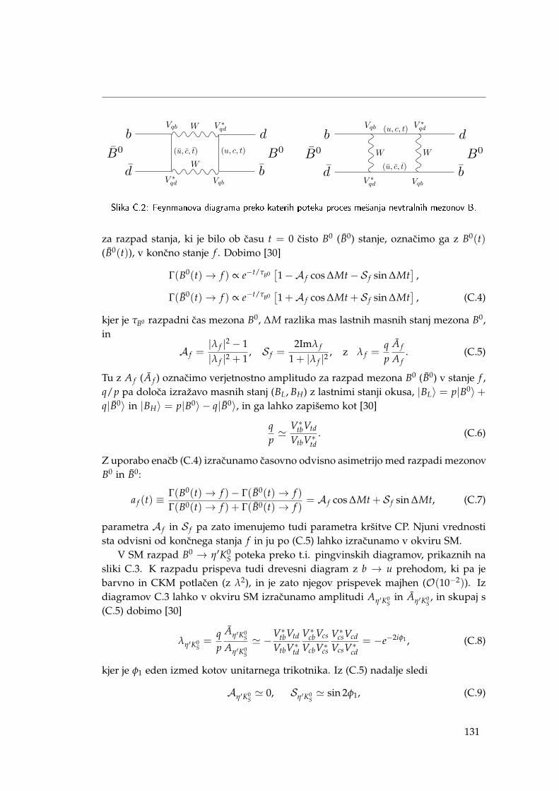
Slika C.2: Feynmanova diagrama preko katerih poteka proces me²anja nevtralnih mezonov B.
za razpad stanja, ki je bilo ob casu t = 0 cisto B0 (B0) stanje, oznacimo ga z B0(t)(B0(t)), v koncno stanje f . Dobimo [30]
Γ(B0(t)→ f ) ∝ e−t/τB0[1−A f cos ∆Mt− S f sin ∆Mt
],
Γ(B0(t)→ f ) ∝ e−t/τB0[1 +A f cos ∆Mt + S f sin ∆Mt
], (C.4)
kjer je τB0 razpadni cas mezona B0, ∆M razlika mas lastnih masnih stanj mezona B0,in
A f =|λ f |2 − 1|λ f |2 + 1
, S f =2Imλ f
1 + |λ f |2, z λ f =
qp
A f
A f. (C.5)
Tu z A f (A f ) oznacimo verjetnostno amplitudo za razpad mezona B0 (B0) v stanje f ,q/p pa doloca izražavo masnih stanj (BL, BH) z lastnimi stanji okusa, |BL〉 = p|B0〉+q|B0〉 in |BH〉 = p|B0〉 − q|B0〉, in ga lahko zapišemo kot [30]
qp'
V∗tbVtd
VtbV∗td. (C.6)
Z uporabo enacb (C.4) izracunamo casovno odvisno asimetrijo med razpadi mezonovB0 in B0:
a f (t) ≡Γ(B0(t)→ f )− Γ(B0(t)→ f )Γ(B0(t)→ f ) + Γ(B0(t)→ f )
= A f cos ∆Mt + S f sin ∆Mt, (C.7)
parametra A f in S f pa zato imenujemo tudi parametra kršitve CP. Njuni vrednostista odvisni od koncnega stanja f in ju po (C.5) lahko izracunamo v okviru SM.
V SM razpad B0 → η′K0S poteka preko t.i. pingvinskih diagramov, prikaznih na
sliki C.3. K razpadu prispeva tudi drevesni diagram z b → u prehodom, ki pa jebarvno in CKM potlacen (z λ2), in je zato njegov prispevek majhen (O(10−2)). Izdiagramov C.3 lahko v okviru SM izracunamo amplitudi Aη′K0
Sin Aη′K0
S, in skupaj s
(C.5) dobimo [30]
λη′K0S=
qp
Aη′K0S
Aη′K0S
' −V∗tbVtd
VtbV∗td
V∗cbVcs
VcbV∗cs
V∗csVcd
VcsV∗cd= −e−2iφ1 , (C.8)
kjer je φ1 eden izmed kotov unitarnega trikotnika. Iz (C.5) nadalje sledi
Aη′K0S' 0, Sη′K0
S' sin 2φ1, (C.9)
131
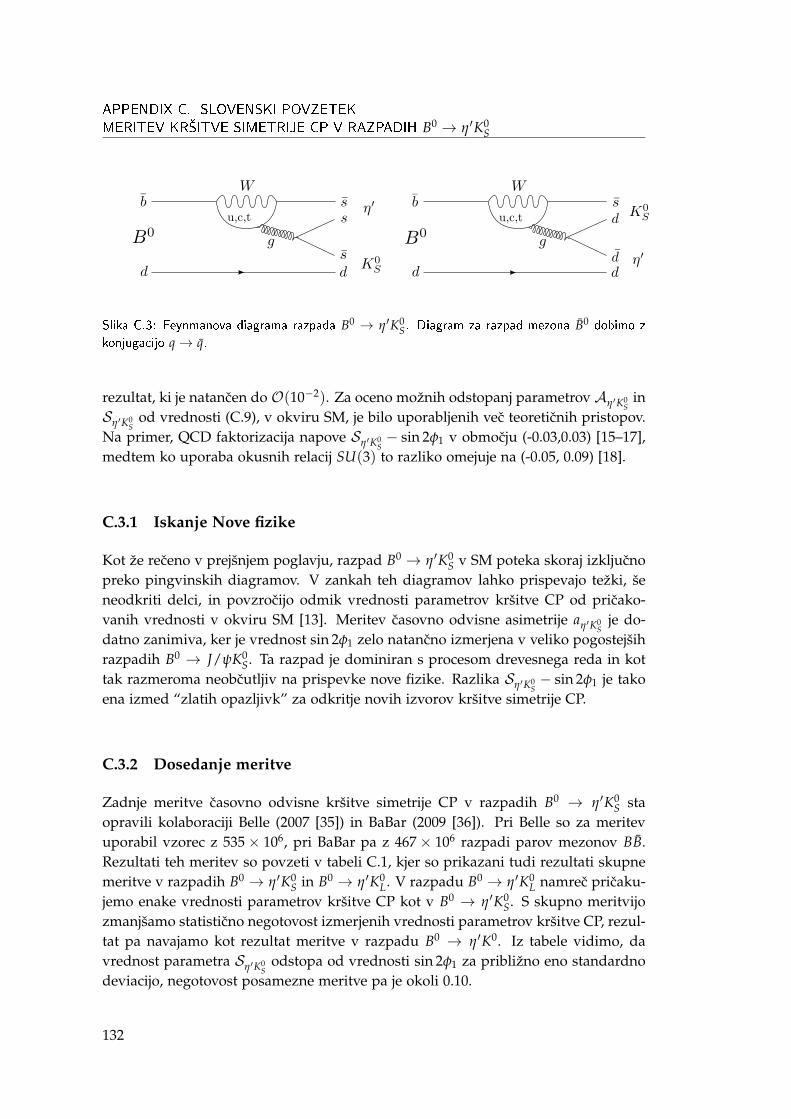
APPENDIX C. SLOVENSKI POVZETEK
MERITEV KR�ITVE SIMETRIJE CP V RAZPADIH B0 → η′K0S
Slika C.3: Feynmanova diagrama razpada B0 → η′K0S. Diagram za razpad mezona B0 dobimo z
konjugacijo q→ q.
rezultat, ki je natancen do O(10−2). Za oceno možnih odstopanj parametrov Aη′K0S
inSη′K0
Sod vrednosti (C.9), v okviru SM, je bilo uporabljenih vec teoreticnih pristopov.
Na primer, QCD faktorizacija napove Sη′K0S− sin 2φ1 v obmocju (-0.03,0.03) [15–17],
medtem ko uporaba okusnih relacij SU(3) to razliko omejuje na (-0.05, 0.09) [18].
C.3.1 Iskanje Nove fizike
Kot že receno v prejšnjem poglavju, razpad B0 → η′K0S v SM poteka skoraj izkljucno
preko pingvinskih diagramov. V zankah teh diagramov lahko prispevajo težki, šeneodkriti delci, in povzrocijo odmik vrednosti parametrov kršitve CP od pricako-vanih vrednosti v okviru SM [13]. Meritev casovno odvisne asimetrije aη′K0
Sje do-
datno zanimiva, ker je vrednost sin 2φ1 zelo natancno izmerjena v veliko pogostejšihrazpadih B0 → J/ψK0
S. Ta razpad je dominiran s procesom drevesnega reda in kottak razmeroma neobcutljiv na prispevke nove fizike. Razlika Sη′K0
S− sin 2φ1 je tako
ena izmed “zlatih opazljivk” za odkritje novih izvorov kršitve simetrije CP.
C.3.2 Dosedanje meritve
Zadnje meritve casovno odvisne kršitve simetrije CP v razpadih B0 → η′K0S sta
opravili kolaboraciji Belle (2007 [35]) in BaBar (2009 [36]). Pri Belle so za meritevuporabil vzorec z 535× 106, pri BaBar pa z 467× 106 razpadi parov mezonov BB.Rezultati teh meritev so povzeti v tabeli C.1, kjer so prikazani tudi rezultati skupnemeritve v razpadih B0 → η′K0
S in B0 → η′K0L. V razpadu B0 → η′K0
L namrec pricaku-jemo enake vrednosti parametrov kršitve CP kot v B0 → η′K0
S. S skupno meritvijozmanjšamo statisticno negotovost izmerjenih vrednosti parametrov kršitve CP, rezul-tat pa navajamo kot rezultat meritve v razpadu B0 → η′K0. Iz tabele vidimo, davrednost parametra Sη′K0
Sodstopa od vrednosti sin 2φ1 za približno eno standardno
deviacijo, negotovost posamezne meritve pa je okoli 0.10.
132
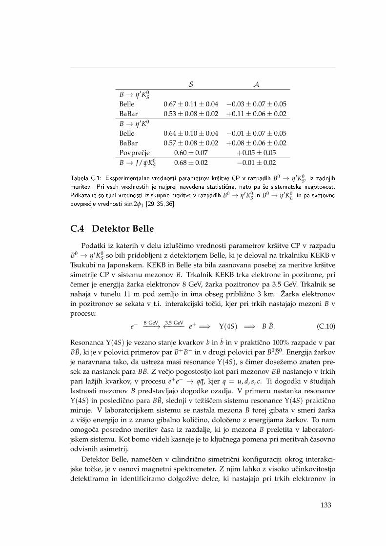
S AB→ η′K0
SBelle 0.67± 0.11± 0.04 −0.03± 0.07± 0.05BaBar 0.53± 0.08± 0.02 +0.11± 0.06± 0.02B→ η′K0
Belle 0.64± 0.10± 0.04 −0.01± 0.07± 0.05BaBar 0.57± 0.08± 0.02 +0.08± 0.06± 0.02Povprecje 0.60± 0.07 +0.05± 0.05B→ J/ψK0
S 0.68± 0.02 −0.01± 0.02
Tabela C.1: Eksperimentalne vrednosti parametrov kr²itve CP v razpadih B0 → η′K0S, iz zadnjih
meritev. Pri vseh vrednostih je najprej navedena statisti£na, nato pa ²e sistematska negotovost.Prikazane so tudi vrednosti iz skupne meritve v razpadih B0 → η′K0
S in B0 → η′K0L, in pa svetovno
povpre£je vrednosti sin 2φ1 [29, 35,36].
C.4 Detektor Belle
Podatki iz katerih v delu izlušcimo vrednosti parametrov kršitve CP v razpaduB0 → η′K0
S so bili pridobljeni z detektorjem Belle, ki je deloval na trkalniku KEKB vTsukubi na Japonskem. KEKB in Belle sta bila zasnovana posebej za meritve kršitvesimetrije CP v sistemu mezonov B. Trkalnik KEKB trka elektrone in pozitrone, pricemer je energija žarka elektronov 8 GeV, žarka pozitronov pa 3.5 GeV. Trkalnik senahaja v tunelu 11 m pod zemljo in ima obseg približno 3 km. Žarka elektronovin pozitronov se sekata v t.i. interakcijski tocki, kjer pri trkih nastajajo mezoni B vprocesu:
e− 8 GeV−−−→ 3.5 GeV←−−−− e+ =⇒ Υ(4S) =⇒ B B. (C.10)
Resonanca Υ(4S) je vezano stanje kvarkov b in b in v prakticno 100% razpade v parBB, ki je v polovici primerov par B+B− in v drugi polovici par B0B0. Energija žarkovje naravnana tako, da ustreza masi resonance Υ(4S), s cimer dosežemo znaten pre-sek za nastanek para BB. Z vecjo pogostostjo kot pari mezonov BB nastanejo v trkihpari lažjih kvarkov, v procesu e+e− → qq, kjer q = u, d, s, c. Ti dogodki v študijahlastnosti mezonov B predstavljajo dogodke ozadja. V primeru nastanka resonanceΥ(4S) in posledicno para BB, slednji v težišcem sistemu resonance Υ(4S) prakticnomiruje. V laboratorijskem sistemu se nastala mezona B torej gibata v smeri žarkaz višjo energijo in z znano gibalno kolicino, doloceno z energijama žarkov. To namomogoca posredno meritev casa iz razdalje, ki jo mezona B preletita v laboratori-jskem sistemu. Kot bomo videli kasneje je to kljucnega pomena pri meritvah casovnoodvisnih asimetrij.
Detektor Belle, namešcen v cilindricno simetricni konfiguraciji okrog interakci-jske tocke, je v osnovi magnetni spektrometer. Z njim lahko z visoko ucinkovitostjodetektiramo in identificiramo dolgožive delce, ki nastajajo pri trkih elektronov in
133
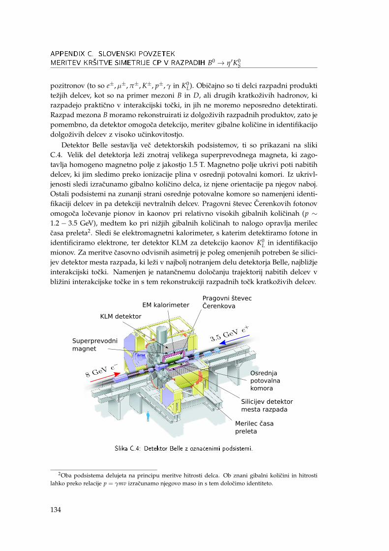
APPENDIX C. SLOVENSKI POVZETEK
MERITEV KR�ITVE SIMETRIJE CP V RAZPADIH B0 → η′K0S
pozitronov (to so e±,µ±, π±, K±, p±, γ in K0L). Obicajno so ti delci razpadni produkti
težjih delcev, kot so na primer mezoni B in D, ali drugih kratkoživih hadronov, kirazpadejo prakticno v interakcijski tocki, in jih ne moremo neposredno detektirati.Razpad mezona B moramo rekonstruirati iz dolgoživih razpadnih produktov, zato jepomembno, da detektor omogoca detekcijo, meritev gibalne kolicine in identifikacijodolgoživih delcev z visoko ucinkovitostjo.
Detektor Belle sestavlja vec detektorskih podsistemov, ti so prikazani na slikiC.4. Velik del detektorja leži znotraj velikega superprevodnega magneta, ki zago-tavlja homogeno magnetno polje z jakostjo 1.5 T. Magnetno polje ukrivi poti nabitihdelcev, ki jim sledimo preko ionizacije plina v osrednji potovalni komori. Iz ukrivl-jenosti sledi izracunamo gibalno kolicino delca, iz njene orientacije pa njegov naboj.Ostali podsistemi na zunanji strani osrednje potovalne komore so namenjeni identi-fikaciji delcev in pa detekciji nevtralnih delcev. Pragovni števec Cerenkovih fotonovomogoca locevanje pionov in kaonov pri relativno visokih gibalnih kolicinah (p ∼1.2− 3.5 GeV), medtem ko pri nižjih gibalnih kolicinah to nalogo opravlja merileccasa preleta2. Sledi še elektromagnetni kalorimeter, s katerim detektiramo fotone inidentificiramo elektrone, ter detektor KLM za detekcijo kaonov K0
L in identifikacijomionov. Za meritve casovno odvisnih asimetrij je poleg omenjenih potreben še silici-jev detektor mesta razpada, ki leži v najbolj notranjem delu detektorja Belle, najbližjeinterakcijski tocki. Namenjen je natancnemu dolocanju trajektorij nabitih delcev vbližini interakcijske tocke in s tem rekonstrukciji razpadnih tock kratkoživih delcev.
Silicijev detektormesta razpada
Pragovni števecČerenkova
Merilec časapreleta
EM kalorimeter
KLM detektor
Superprevodnimagnet
Osrednjapotovalna komora
Slika C.4: Detektor Belle z ozna£enimi podsistemi.
2Oba podsistema delujeta na principu meritve hitrosti delca. Ob znani gibalni kolicini in hitrostilahko preko relacije p = γmv izracunamo njegovo maso in s tem dolocimo identiteto.
134
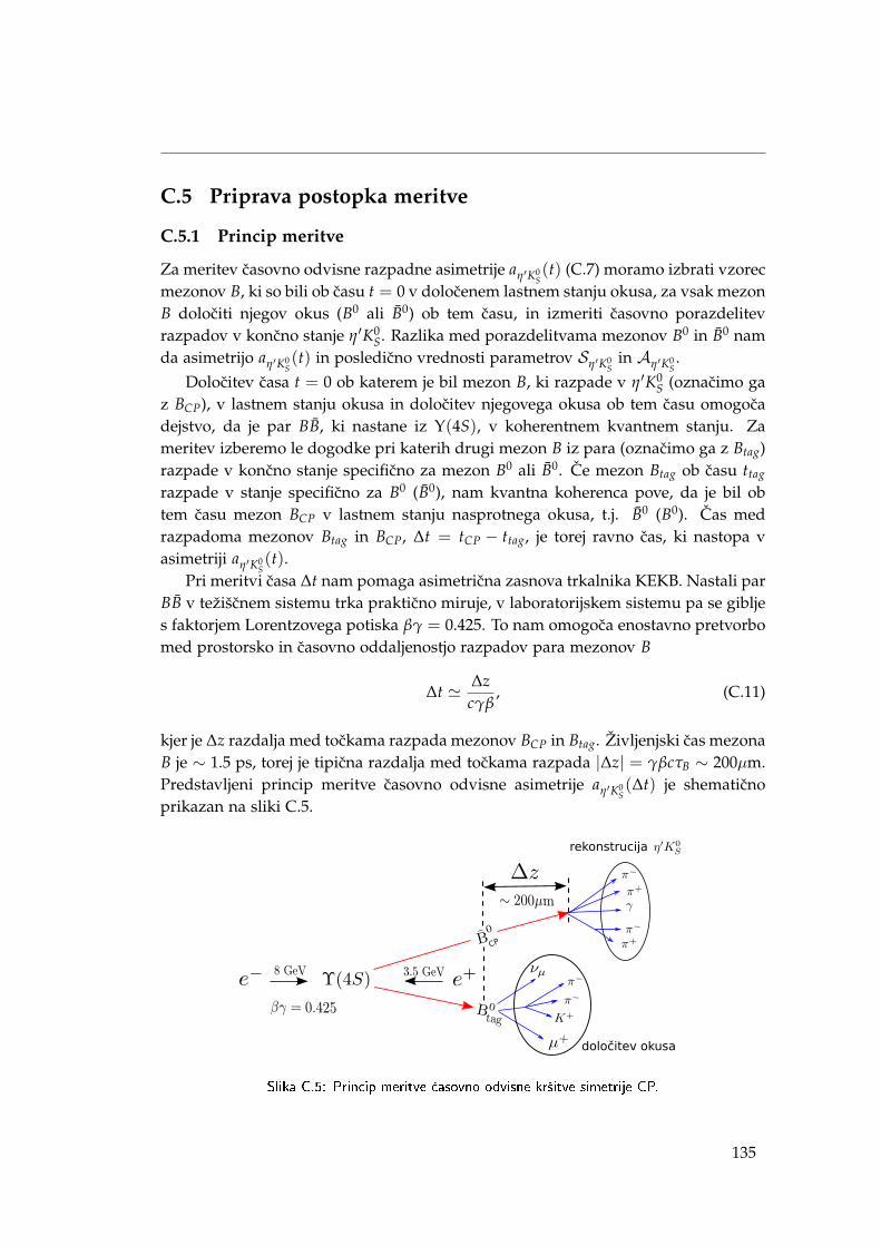
C.5 Priprava postopka meritve
C.5.1 Princip meritve
Za meritev casovno odvisne razpadne asimetrije aη′K0S(t) (C.7) moramo izbrati vzorec
mezonov B, ki so bili ob casu t = 0 v dolocenem lastnem stanju okusa, za vsak mezonB dolociti njegov okus (B0 ali B0) ob tem casu, in izmeriti casovno porazdelitevrazpadov v koncno stanje η′K0
S. Razlika med porazdelitvama mezonov B0 in B0 namda asimetrijo aη′K0
S(t) in posledicno vrednosti parametrov Sη′K0
Sin Aη′K0
S.
Dolocitev casa t = 0 ob katerem je bil mezon B, ki razpade v η′K0S (oznacimo ga
z BCP), v lastnem stanju okusa in dolocitev njegovega okusa ob tem casu omogocadejstvo, da je par BB, ki nastane iz Υ(4S), v koherentnem kvantnem stanju. Zameritev izberemo le dogodke pri katerih drugi mezon B iz para (oznacimo ga z Btag)razpade v koncno stanje specificno za mezon B0 ali B0. Ce mezon Btag ob casu ttag
razpade v stanje specificno za B0 (B0), nam kvantna koherenca pove, da je bil obtem casu mezon BCP v lastnem stanju nasprotnega okusa, t.j. B0 (B0). Cas medrazpadoma mezonov Btag in BCP, ∆t = tCP − ttag, je torej ravno cas, ki nastopa vasimetriji aη′K0
S(t).
Pri meritvi casa ∆t nam pomaga asimetricna zasnova trkalnika KEKB. Nastali parBB v težišcnem sistemu trka prakticno miruje, v laboratorijskem sistemu pa se gibljes faktorjem Lorentzovega potiska βγ = 0.425. To nam omogoca enostavno pretvorbomed prostorsko in casovno oddaljenostjo razpadov para mezonov B
∆t ' ∆zcγβ
, (C.11)
kjer je ∆z razdalja med tockama razpada mezonov BCP in Btag. Življenjski cas mezonaB je ∼ 1.5 ps, torej je tipicna razdalja med tockama razpada |∆z| = γβcτB ∼ 200µm.Predstavljeni princip meritve casovno odvisne asimetrije aη′K0
S(∆t) je shematicno
prikazan na sliki C.5.
rekonstrucija
določitev okusa
Slika C.5: Princip meritve £asovno odvisne kr²itve simetrije CP.
135
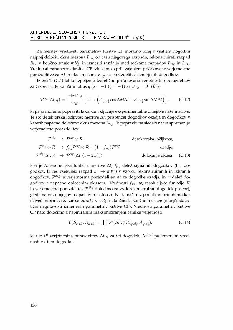
APPENDIX C. SLOVENSKI POVZETEK
MERITEV KR�ITVE SIMETRIJE CP V RAZPADIH B0 → η′K0S
Za meritev vrednosti parametrov kršitve CP moramo torej v vsakem dogodkunajprej dolociti okus mezona Btag ob casu njegovega razpada, rekonstruirati razpadBCP v koncno stanje η′K0
S, in izmeriti razdaljo med tockama razpadov Btag in BCP.Vrednosti parametrov kršitve CP izlušcimo s prilagajanjem pricakovane verjetnostneporazdelitve za ∆t in okus mezona Btag na porazdelitev izmerjenih dogodkov.
Iz enacb (C.4) lahko izpeljemo teoreticno pricakovano verjetnostno porazdelitevza casovni interval ∆t in okus q (q = +1 (q = −1) za Btag = B0 (B0))
P sig(∆t, q) =e−|∆t|/τB0
4τB0
[1 + q
(Aη′K0
Scos ∆M∆t + Sη′K0
Ssin ∆M∆t
)], (C.12)
ki pa jo moramo popraviti tako, da vkljucuje eksperimentalne omejitve naše meritve.Te so: detektorska locljivost meritve ∆t, prisotnost dogodkov ozadja in dogodkov vkaterih napacno dolocimo okus mezona Btag. Ti popravki na sledeci nacin spremenijoverjetnostno porazdelitev
P sig → P sig ⊗R detektorska locljivost,
P sig ⊗R → fsigP sig ⊗R+ (1− fsig)P bkg ozadje,
P sig(∆t, q) → P sig(∆t, (1− 2w)q) dolocanje okusa, (C.13)
kjer je R resolucijska funkcija meritve ∆t, fsig delež signalnih dogodkov (t.j. do-godkov, ki res vsebujejo razpad B0 → η′K0
S) v vzorcu rekonstruiranih in izbranihdogodkov, P bkg je verjetnostna porazdelitev ∆t za dogodke ozadja, in w delež do-godkov z napacno dolocenim okusom. Vrednosti fsig, w, resolucijsko funkcijo Rin verjetnostno porazdelitev P bkg dolocimo za vsak rekonstruiran dogodek posebej,glede na vrsto njegovih opazljivih lastnosti. Na ta nacin iz podatkov pridobimo karnajvec informacije, kar se odraža v vecji natancnosti koncne meritve (manjši statis-ticni negotovosti izmerjenih parametrov kršitve CP). Vrednosti parametrov kršitveCP nato dolocimo z nebiniranim maksimiziranjem cenilke verjetnosti
L(Sη′K0S,Aη′K0
S) = ∏
iP i(∆ti, qi;Sη′K0
S,Aη′K0
S), (C.14)
kjer je P i verjetnostna porazdelitev ∆t, q za i-ti dogodek, ∆ti, qi pa izmerjeni vred-nosti v i-tem dogodku.
136
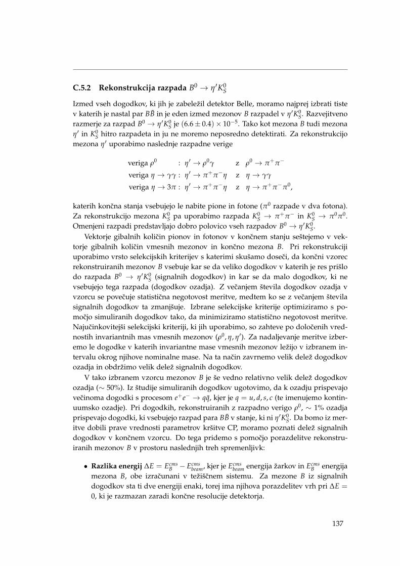
C.5.2 Rekonstrukcija razpada B0 → η′K0S
Izmed vseh dogodkov, ki jih je zabeležil detektor Belle, moramo najprej izbrati tistev katerih je nastal par BB in je eden izmed mezonov B razpadel v η′K0
S. Razvejitvenorazmerje za razpad B0 → η′K0
S je (6.6± 0.4)× 10−5. Tako kot mezona B tudi mezonaη′ in K0
S hitro razpadeta in ju ne moremo neposredno detektirati. Za rekonstrukcijomezona η′ uporabimo naslednje razpadne verige
veriga ρ0 : η′ → ρ0γ z ρ0 → π+π−
veriga η → γγ : η′ → π+π−η z η → γγ
veriga η → 3π : η′ → π+π−η z η → π+π−π0,
katerih koncna stanja vsebujejo le nabite pione in fotone (π0 razpade v dva fotona).Za rekonstrukcijo mezona K0
S pa uporabimo razpada K0S → π+π− in K0
S → π0π0.Omenjeni razpadi predstavljajo dobro polovico vseh razpadov B0 → η′K0
S.Vektorje gibalnih kolicin pionov in fotonov v koncnem stanju seštejemo v vek-
torje gibalnih kolicin vmesnih mezonov in koncno mezona B. Pri rekonstrukcijiuporabimo vrsto selekcijskih kriterijev s katerimi skušamo doseci, da koncni vzorecrekonstruiranih mezonov B vsebuje kar se da veliko dogodkov v katerih je res prišlodo razpada B0 → η′K0
S (signalnih dogodkov) in kar se da malo dogodkov, ki nevsebujejo tega razpada (dogodkov ozadja). Z vecanjem števila dogodkov ozadja vvzorcu se povecuje statisticna negotovost meritve, medtem ko se z vecanjem številasignalnih dogodkov ta zmanjšuje. Izbrane selekcijske kriterije optimiziramo s po-mocjo simuliranih dogodkov tako, da minimiziramo statisticno negotovost meritve.Najucinkovitejši selekcijski kriteriji, ki jih uporabimo, so zahteve po dolocenih vred-nostih invariantnih mas vmesnih mezonov (ρ0, η, η′). Za nadaljevanje meritve izber-emo le dogodke v katerih invariantne mase vmesnih mezonov ležijo v izbranem in-tervalu okrog njihove nominalne mase. Na ta nacin zavrnemo velik delež dogodkovozadja in obdržimo velik delež signalnih dogodkov.
V tako izbranem vzorcu mezonov B je še vedno relativno velik delež dogodkovozadja (∼ 50%). Iz študije simuliranih dogodkov ugotovimo, da k ozadju prispevajovecinoma dogodki s procesom e+e− → qq, kjer je q = u, d, s, c (te imenujemo kontin-uumsko ozadje). Pri dogodkih, rekonstruiranih z razpadno verigo ρ0, ∼ 1% ozadjaprispevajo dogodki, ki vsebujejo razpad para BB v stanje, ki ni η′K0
S. Da bomo iz mer-itve dobili prave vrednosti parametrov kršitve CP, moramo poznati delež signalnihdogodkov v koncnem vzorcu. Do tega pridemo s pomocjo porazdelitve rekonstru-iranih mezonov B v prostoru naslednjih treh spremenljivk:
• Razlika energij ∆E = EcmsB − Ecms
beam, kjer je Ecmsbeam energija žarkov in Ecms
B energijamezona B, obe izracunani v težišcnem sistemu. Za mezone B iz signalnihdogodkov sta ti dve energiji enaki, torej ima njihova porazdelitev vrh pri ∆E =
0, ki je razmazan zaradi koncne resolucije detektorja.
137
APPENDIX C. SLOVENSKI POVZETEK
MERITEV KR�ITVE SIMETRIJE CP V RAZPADIH B0 → η′K0S
• Invariantna masa Mbc ≡√(Ecms
beam)2 − (pcms
B )2, kjer je pcmsB gibalna kolicina
mezona B v težišcnem sistemu. Porazdelitev mezonov B iz signalnih dogodkovima vrh pri Mbc = mB, kjer je mB masa mezona B0 (' 5.279 GeV).
• Spremenljivka oblike dogodka LR sestavljena iz vecih spremenljivk, ki naosnovi razlicne prostorske porazdelitve gibalnih kolicin razpadnih produktovv težišcnem sistemu omogocajo razlikovanje med dogodki, ki vsebujejo par BB(sfericno porazdeljeni razpadni produkti) in dogodki kontinuumskega ozadja(razpadni produkti letijo v dve nasprotni strani).
S pomocjo simuliranih signalnih dogodkov in dogodkov ozadja pripravimo model,ki opisuje porazdelitev prvih (P sig) in drugih (P bkg) v prostoru Mbc − ∆E − LR. Sprilagajanjem vsote obeh modelov
F (Mbc, ∆E, LR) = fsigF sig + (1− fsig)F bkg, (C.15)
na porazdelitev izbranih razpadov, dolocimo delež signalnih dogodkov v vzorcu( fsig). Rezultati prilagajanja so prikazani na sliki C.6. Iz grafov vidimo, da izbranaverjetnostna porazdelitev F dobro opiše porazdelitev podatkov. Ko poznamo vred-nost fsig, s pomocjo signalnega dela verjetnostne porazdelitve (C.15), fsigF sig/F ,dolocimo verjetnost, da je posamezni rekonstruiran dogodek signalni dogodek (gledena specificne vrednosti Mbc, ∆E in LR v tem dogodku).
Za nadaljevanje meritve izberemo le dogodke v katerih Mbc in ∆E mezona Bležita v t.i. signalnem obmocju, definiranem z Mbc > 5.27 GeV in −0.08 < ∆E < 0.08GeV. Z integralom signalnega dela verjetnostne porazdelitve izracunamo, da v sig-nalnem obmocju leži 2505± 94 signalnih dogodkov (kjer je negotovost le statisticna).
C.5.3 Dolocitev okusa mezona Btag
Okus mezona Btag dolocimo na podlagi vrste okusno znacilnih razpadov mezonovB. Taki so na primer semileptonski razpadi B0 → Xl+ν (ali B0 → Xl−ν), pri katerihiz pozitivnega (negativnega) naboja visoko energijskega leptona sklepamo, da je Btag
razpadel kot B0 (B0). Algoritem, ki ga uporabimo za dolocitev okusa je uporabljentudi v drugih meritvah kolaboracije Belle in je podrobno opisan v [49]. Upoštevavrsto razlicnih okusno znacilnih razpadov in za vsak dogodek vrne vrednost q (+1ali -1) ter vrednost parametra r, ki podaja kvaliteto informacije okusa (r ' 1 za do-godke s skoraj enolicno dolocenim okusom in r ' 0 za dogodke pri katerih nimamoprakticno nobene informacije o okusu). Dogodke razporedimo v 7 razdelkov gledena vrednost r. V vsakem razdelku že pred tem, s pomocjo velikega kontrolnegavzorca okusno znacilnih razpadov mezonov Bsig (3), izmerimo delež dogodkov znapacno dolocenim okusom (w). Razdelki in izmerjene vrednosti w so prikazani vtabeli C.2.
3Tu Btag uporabimo za dolocitev okusa, drug mezon B iz para (Bsig) pa rekonstruiramo v okusnoznacilno koncno stanje. Postopek je podrobneje opisan v dodatku B.2.
138

5.22 5.23 5.24 5.25 5.26 5.27 5.28 5.29 5.3
Events/(
0.0026
6667
GeV
)
0
100
200
300
400
500
600
E < 0.07 , LR > 0.7-0.07 <
BB bkg.cont. bkg.fit
Residual/
-3-2
-101
2
E (GeV)-0.2 -0.15 -0.1 -0.05 0 0.05 0.1 0.15 0.2
Events/(
0.0153
333GeV
)
050100
150200
250300350
400450
> 5.27, LR > 0.7bcM
Residual/
-3-2-10123
0 0.1 0.2 0.3 0.4 0.5 0.6 0.7 0.8 0.9 1
Events/(
0.05
)
0
200
400
600
800
1000
1200
E < 0.07> 5.27, -0.07 <bcM
Residual/
-3-2-1012
5.22 5.23 5.24 5.25 5.26 5.27 5.28 5.29 5.3
Events/(
0.0026
6667
GeV
)
020406080100120140160180200
E < 0.8 , LR > 0.7-0.1 <
cont. bkg.
fit
Residual/
-3-2-10123
E (GeV)-0.2 -0.15 -0.1 -0.05 0 0.05 0.1 0.15 0.2
Events/(
0.0153
333GeV
)
0
20
40
60
80
100
120
> 5.27, LR > 0.7bcM
Residual/
-2
-10
1
23
0 0.1 0.2 0.3 0.4 0.5 0.6 0.7 0.8 0.9 1
Events/(
0.05
)
0
50
100
150
200
250
300
E < 0.8> 5.27, -0.1 <bcM
Residual/
-4-3-2-10123
5.22 5.23 5.24 5.25 5.26 5.27 5.28 5.29 5.3
Events/(
0.0026
6667
GeV
)
0
10
20
30
40
50
60
70
E < 0.06 , LR > 0.7-0.08 <
cont. bkg.fit
Residual/
-2-1
0123
E (GeV)-0.2 -0.15 -0.1 -0.05 0 0.05 0.1 0.15 0.2
Events/(
0.0153
333GeV
)
0
10
20
30
40
50
> 5.27, LR > 0.7bcM
Residual/
-2
-1
0
12
3
0 0.1 0.2 0.3 0.4 0.5 0.6 0.7 0.8 0.9 1
Events/(
0.05
)
0
20
40
60
80
100
E < 0.06> 5.27, -0.08 <bcM
Residual/
-2-10123
LR
LR
LR
(GeV)bcm
(GeV)bcm
(GeV)bcm
Slika C.6: Enodimenzionalne projekcije verjetnostne porazdelitve F (rde£a £rta) na Mbc (levo),∆E (sredina) in LR (desno), za vse tri rekonstruirane verige η′ in K0
S → π+π−. Prispevkakontinuumskega ozadja in ozadja iz dogodkov BB sta prikazana v rumeni in modri barvi. �rneto£ke prikazujejo porazdelitev podatkov. Pod vsakim grafom je prikazano odstopanje porazdelitvepodatkov od prilagajane funkcije F . Obmo£je v prostoru Mbc−∆E− LR, ki ga izberemo za prikazposamezne porazdelitve, je podano nad gra�.
razdelek 1 2 3 4 5 6 7r 0− 0.1 0.1− 0.25 0.25− 0.5 0.5− 0.625 0.625− 0.75 0.75− 0.875 0.875− 1
w 0.5 0.42 0.32 0.22 0.16 0.10 0.03
Tabela C.2: Razdelki glede na vrednosti r in izmerjeni deleºi dogodkov z napa£no dolo£enim okusomBtag v vsakem razdelku.
139
APPENDIX C. SLOVENSKI POVZETEK
MERITEV KR�ITVE SIMETRIJE CP V RAZPADIH B0 → η′K0S
C.5.4 Rekonstrukcija mesta razpada in resolucijska funkcija za ∆t
Položaj razpada mezona BCP dolocimo z ekstrapolacijo sledi π+ in π−, iz razpadamezona ρ0 ali η (4), v skupno tocko razpada. Pri tem uporabimo le sledi, ki imajopoleg zadetkov v osrednji potovalni komori vsaj tri pripadajoce zadetke v silicijevemdetektorju. Najboljšo oceno mesta razpada dobimo z minimizacijo vrednosti
χ2 = ∑i
∆xTi V−1
i ∆xi,
kjer vektor ∆xi vsebuje razliko vrednosti parametrov i-te uporabljene sledi pred inpo ekstrapolaciji vseh sledi v skupno tocko, matrika Vi pa je pripadajoca kovariancnamatrika. Iz simuliranih dogodkov ocenimo, da je natancnost tako dolocenega mestarazpada ∼ 100 µm.
Položaj razpada mezona Btag dolocimo z algoritmom, ki je podrobneje opisanv [52]. Algoritem z minimizacijo vrednosti χ2 ekstrapolira vse preostale sledi vdogodku (ki jih ne uporabimo pri rekonstrukciji mezona BCP) v skupno izhodišcnotocko. Pri tem zavrže sledi z zelo velikim prispevkov k χ2, saj te v mnogo primerihizvirajo iz razpadov vmesnih dolgoživih stanj (D ali K0
S mezonov), ki preletijo znatnorazdaljo preden razpadejo. S tem pristopom lahko tudi mesto razpada mezona Btag
dolocimo z natancnostjo ∼ 100 µm.Iz meritve mesta razpada BCP in Btag po enacbi (C.11) dolocimo cas ∆t. Koncno
locljivost dolocitve slednjega opišemo z resolucijsko funkcijo Rsig, ki jo sestavimokot konvolucijo štirih prispevkov
Rsig(∆t) = RCPdet ⊗R
tagdet ⊗Rnp ⊗Rkin.
Prva dva opisujeta detektorsko locljivost meritve mesta razpada mezona BCP inBtag, tretji opisuje razmazanost mesta razpada Btag zaradi sledi, ki izvirajo iz raz-padov vmesnih stanj, cetrti prispevek pa opisuje razmazanost ∆t, do katere pridezaradi predpostavke, da mezona B v težišcnem sistemu mirujeta. Natancen opisresolucijske funkcije Rsig je podan v [53]. Povejmo le, da resolucijsko funkcijoparametriziramo kot funkcijo negotovosti meritve mesta razpada (σz) in vrednostiχ2, ki ju dobimo iz procesa rekonstrukcije mesta razpada.
C.5.5 Porazdelitev ∆t za dogodke ozadja
Da bi iz meritve dobili nepristranske vrednosti parametrov kršitve CP, moramo polegdeleža signalnih dogodkov v vzorcu poznati tudi porazdelitev ∆t za dogodke ozadja.Slednjo opišemo z verjetnostno porazdelitvijo
P bkgphys(∆t) = fδδ(∆t− µδ) + (1− fδ) exp
(−|∆t− µτ|
τbkg
), (C.16)
4Razpadni cas mezonov ρ0 in η je tako kratek, da razpadeta prakticno na mestu razpada mezona B
140
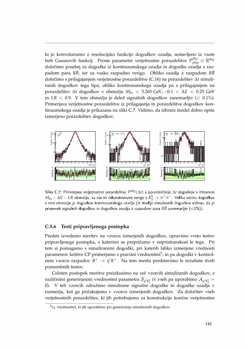
ki jo konvoluiramo z resolucijsko funkcijo dogodkov ozadja, sestavljeno iz vsotetreh Gaussovih funkcij. Proste parametre verjetnostne porazdelitve P bkg
phys ⊗ Rbkg
dolocimo posebej za dogodke iz kontinuumskega ozadja in dogodke ozadja z raz-padom para BB, ter za vsako razpadno verigo. Obliko ozadja z razpadom BBdolocimo s prilagajanjem verjetnostne porazdelitve (C.16) na porazdelitev ∆t simuli-ranih dogodkov tega tipa, obliko kontinuumskega ozadja pa s prilagajanjem naporazdelitev ∆t dogodkov v obmocju Mbc < 5.265 GeV,−0.1 < ∆E < 0.25 GeVin LR < 0.9. V tem obmocju je delež signalnih dogodkov zanemarljiv (< 0.1%).Primerjava verjetnostne porazdelitve iz prilagajanja in porazdelitve dogodkov kon-tinuumskega ozadja je prikazana na sliki C.7. Vidimo, da izbrani model dobro opišeizmerjeno porazdelitev dogodkov.
-10 -8 -6 -4 -2 0 2 4 6 8 10
Eve
nts
/(0.
2ps
)
1
10
210
310
Res
idua
l/
-4-3-2-10123
-10 -8 -6 -4 -2 0 2 4 6 8 10
Eve
nts
/(0.
2ps
)
1
10
210
Res
idua
l/
-2-10123
-10 -8 -6 -4 -2 0 2 4 6 8 10
Eve
nts
/(0.
2ps
)
-110
1
10
Res
idua
l/
-2-101234
Slika C.7: Primerjava verjetnostne porazdelitve P bkg(∆t) s porazdelitvijo ∆t dogodkov v izbranemMbc − ∆E− LR obmo£ju, za vse tri rekonstruirane verige z K0
S → π+π−. Velika ve£ina dogodkovv tem obmo£ju je dogodkov kontinuumskega ozadja (iz ²tudije simuliranih dogodkov vidimo, da jeprispevek signalnih dogodkov in dogodkov ozadja z razpadom para BB zanemarljiv (<1%)).
C.5.6 Testi pripravljenega postopka
Preden izvedemo meritev na vzorcu izmerjenih dogodkov, opravimo vrsto testovpripravljenega postopka, s katerimi se prepricamo v nepristranskost le tega. Pritem si pomagamo s simuliranimi dogodki, pri katerih lahko izmerjene vrednostiparametrov kršitve CP primerjamo s pravimi vrednostmi5, in pa dogodki v kontrol-nem vzorcu razpadov B+ → η′K+. Na tem mestu predstavimo le rezultate dvehpomembnih testov.
Celoten postopek meritve preizkusimo na vec vzorcih simuliranih dogodkov, zrazlicnimi generiranimi vrednostmi parametra Sη′K0
S(v vseh pa uporabimo Aη′K0
S=
0). V teh vzorcih združimo simulirane signalne dogodke in dogodke ozadja vrazmerju, kot ga pricakujemo v vzorcu izmerjenih dogodkov. Za dolocitev vsehverjetnostnih porazdelitev, ki jih potrebujemo za konstrukcijo koncne verjetnostne
5t.j. vrednostmi, ki jih uporabimo pri generiranju simuliranih dogodkov.
141
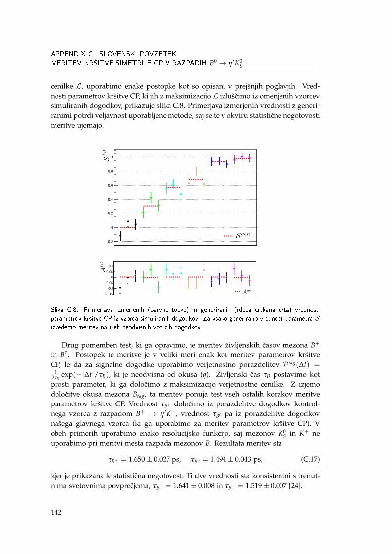
APPENDIX C. SLOVENSKI POVZETEK
MERITEV KR�ITVE SIMETRIJE CP V RAZPADIH B0 → η′K0S
cenilke L, uporabimo enake postopke kot so opisani v prejšnjih poglavjih. Vred-nosti parametrov kršitve CP, ki jih z maksimizacijo L izlušcimo iz omenjenih vzorcevsimuliranih dogodkov, prikazuje slika C.8. Primerjava izmerjenih vrednosti z generi-ranimi potrdi veljavnost uporabljene metode, saj se te v okviru statisticne negotovostimeritve ujemajo.
-0.2
0
0.2
0.4
0.6
0.8
1
-0.15
-0.1
-0.05
0
0.05
0.1
Slika C.8: Primerjava izmerjenih (barvne to£ke) in generiranih (rde£a £rtkana £rta) vrednostiparametrov kr²itve CP iz vzorca simuliranih dogodkov. Za vsako generirano vrednost parametra Sizvedemo meritev na treh neodvisnih vzorcih dogodkov.
Drug pomemben test, ki ga opravimo, je meritev življenskih casov mezona B+
in B0. Postopek te meritve je v veliki meri enak kot meritev parametrov kršitveCP, le da za signalne dogodke uporabimo verjetnostno porazdelitev P sig(∆t) =
12τB
exp(−|∆t|/τB), ki je neodvisna od okusa (q). Življenski cas τB postavimo kotprosti parameter, ki ga dolocimo z maksimizacijo verjetnostne cenilke. Z izjemodolocitve okusa mezona Btag, ta meritev ponuja test vseh ostalih korakov meritveparametrov kršitve CP. Vrednost τB+ dolocimo iz porazdelitve dogodkov kontrol-nega vzorca z razpadom B+ → η′K+, vrednost τB0 pa iz porazdelitve dogodkovnašega glavnega vzorca (ki ga uporabimo za meritev parametrov kršitve CP). Vobeh primerih uporabimo enako resolucijsko funkcijo, saj mezonov K0
S in K+ neuporabimo pri meritvi mesta razpada mezonov B. Rezultata meritev sta
τB+ = 1.650± 0.027 ps, τB0 = 1.494± 0.043 ps, (C.17)
kjer je prikazana le statisticna negotovost. Ti dve vrednosti sta konsistentni s trenut-nima svetovnima povprecjema, τB+ = 1.641± 0.008 in τB+ = 1.519± 0.007 [24].
142
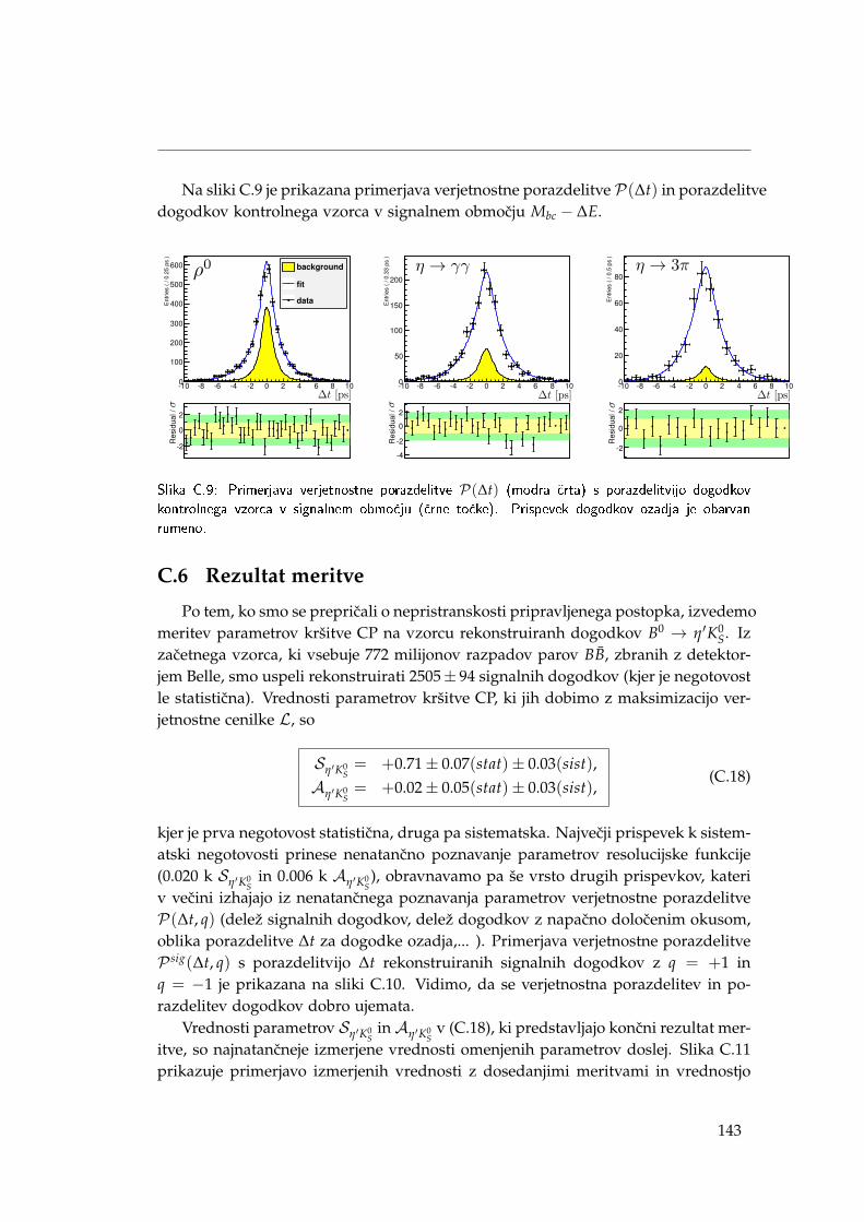
Na sliki C.9 je prikazana primerjava verjetnostne porazdelitve P(∆t) in porazdelitvedogodkov kontrolnega vzorca v signalnem obmocju Mbc − ∆E.
-10 -8 -6 -4 -2 0 2 4 6 8 10
Ent
ries
(/0.
25ps
)
0
100
200
300
400
500
600 background
fit
data
Res
idua
l/
-2
0
2
-10 -8 -6 -4 -2 0 2 4 6 8 10E
ntrie
s(/
0.33
ps)
0
50
100
150
200
Res
idua
l/
-4
-2
0
2
-10 -8 -6 -4 -2 0 2 4 6 8 10
Ent
ries
(/0.
5ps
)
0
20
40
60
80
Res
idua
l/
-2
0
2
Slika C.9: Primerjava verjetnostne porazdelitve P(∆t) (modra £rta) s porazdelitvijo dogodkovkontrolnega vzorca v signalnem obmo£ju (£rne to£ke). Prispevek dogodkov ozadja je obarvanrumeno.
C.6 Rezultat meritve
Po tem, ko smo se prepricali o nepristranskosti pripravljenega postopka, izvedemomeritev parametrov kršitve CP na vzorcu rekonstruiranh dogodkov B0 → η′K0
S. Izzacetnega vzorca, ki vsebuje 772 milijonov razpadov parov BB, zbranih z detektor-jem Belle, smo uspeli rekonstruirati 2505± 94 signalnih dogodkov (kjer je negotovostle statisticna). Vrednosti parametrov kršitve CP, ki jih dobimo z maksimizacijo ver-jetnostne cenilke L, so
Sη′K0S= +0.71± 0.07(stat)± 0.03(sist),
Aη′K0S= +0.02± 0.05(stat)± 0.03(sist),
(C.18)
kjer je prva negotovost statisticna, druga pa sistematska. Najvecji prispevek k sistem-atski negotovosti prinese nenatancno poznavanje parametrov resolucijske funkcije(0.020 k Sη′K0
Sin 0.006 k Aη′K0
S), obravnavamo pa še vrsto drugih prispevkov, kateri
v vecini izhajajo iz nenatancnega poznavanja parametrov verjetnostne porazdelitveP(∆t, q) (delež signalnih dogodkov, delež dogodkov z napacno dolocenim okusom,oblika porazdelitve ∆t za dogodke ozadja,... ). Primerjava verjetnostne porazdelitveP sig(∆t, q) s porazdelitvijo ∆t rekonstruiranih signalnih dogodkov z q = +1 inq = −1 je prikazana na sliki C.10. Vidimo, da se verjetnostna porazdelitev in po-razdelitev dogodkov dobro ujemata.
Vrednosti parametrov Sη′K0S
inAη′K0S
v (C.18), ki predstavljajo koncni rezultat mer-itve, so najnatancneje izmerjene vrednosti omenjenih parametrov doslej. Slika C.11prikazuje primerjavo izmerjenih vrednosti z dosedanjimi meritvami in vrednostjo
143
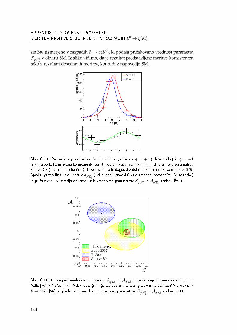
APPENDIX C. SLOVENSKI POVZETEK
MERITEV KR�ITVE SIMETRIJE CP V RAZPADIH B0 → η′K0S
sin 2φ1 (izmerjeno v razpadih B→ ccK0), ki podaja pricakovano vrednost parametraSη′K0
Sv okviru SM. Iz slike vidimo, da je rezultat predstavljene meritve konsistenten
tako z rezultati dosedanjih meritev, kot tudi z napovedjo SM.
t [ps]-8 -6 -4 -2 0 2 4 6 8
Eve
nts(/
1.6ps
)
0
50
100
150
200
250 q = +1q = -1
-8 -6 -4 -2 0 2 4 6 8
Asy
mmetry
-0.5
0
0.5
Slika C.10: Primerjava porazdelitve ∆t signalnih dogodkov z q = +1 (rde£e to£ke) in q = −1(modre to£ke) z ustrezno komponento verjetnostne porazdelitve, ki jo nam da vrednosti parametrovkr²itve CP (rde£a in modra £rta). Upo²tevani so le dogodki z dobro dolo£enim okusom (z r > 0.5).Spodnji graf prikazuje asimetrijo aη′K0
S(de�nirano v ena£bi C.7) v izmerjeni porazdelitvi (£rne to£ke)
in pri£akovano asimetrijo ob izmerjenih vrednostih parametrov Sη′K0Sin Aη′K0
S(zelena £rta).
Slika C.11: Primerjava vrednosti parametrov Sη′K0Sin Aη′K0
Siz te in prej²njih meritev kolaboracij
Belle [35] in BaBar [36]. Poleg omenjenih je podana ²e vrednost parametrov kr²itve CP v razpadihB→ ccK0 [29], ki predstavlja pri£akovano vrednost parametrov Sη′K0
Sin Aη′K0
Sv okviru SM.
144
C.7 Zakljucek
V delu smo predstavili meritev prametrov kršitve simetrije CP v razpadu B0 →η′K0
S. Meritev je bila opravljena na vzorcu 772 milijonov parov BB, zbranih z detek-torjem Belle v casu njegovega delovanja (1999-2010). Izmerjene vrednosti
Sη′K0S=+ 0.71± 0.07(stat)± 0.03(sist),
Aη′K0S=+ 0.02± 0.05(stat)± 0.03(sist),
so konsistentne z rezultati dosedanjih meritev in napovedjo SM.Za konec se ozrimo še nekoliko v prihodnost te in podobnih meritev. Izmerjene
vrednosti parametrov kršitve CP v razpadih, ki potekajo preko procesa b → sqq, kije dominiran s pingvinskimi diagrami, in so kot taki obcutljivi na prispevke novihizvorov kršitve CP, so v vseh primerih konsistentne z napovedmi SM. Trenutnodosežena natancnost teh meritev pa še vedno dopušca znatne prispevke kršitve CPiz izvorov onkraj SM. Ti so naravno prisotni v vecini modelov nove fizike in nujnitudi s kozmološkega vidika (razlaga ocitne asimetrije med materijo in antimaterijo vvesolju). Ker je eksperimentalna natancnost meritev v vecini razpadov omenjenegatipa dominirana s statisticno negotovostjo, lahko do natancnejših meritev pridemole z vecjim vzorcem mezonov B. To možnost bo ponudil trkalnik SuperKEKB zdetektorjem Belle II [57, 58](nadgradnja trkalnika KEKB in detektorja Belle), ki bozacel delovati v letu 2016. Z detektorjem Belle II nameravamo do leta 2023 zabeležiti∼ 50-krat vec razpadov mezonov B, kot jih je zabeležil Belle. To bo omogocilo mer-itve parametrov kršitve CP z natancnostjo nekaj 10−2 (npr. za Sη′K0
Spricakujemo
negotovost ' 0.02 [59]) in morda vodilo do detekcije novih izvorov kršitve simetrijeCP. Ce slednjih ne bomo opazili, bo to postavilo mocne omejitve na možno strukturo(predvsem okusnega dela) modelov nove fizike.
145

Bibliography
[1] T.D. Lee, C. N. Yang, Phys. Rev. 104 (1), 254 (1956)
[2] C.S. Wu, E. Ambler et. al, Phys. Rev. 105 (4), 1413 (1957)
[3] J.W. Coronin, V.L. Fitch, Phys. Rev. Lett. 13, 138 (1964)
[4] M. Kobayashi and T. Maskawa, Prog. Theor. Phys. 49, 652 (1973)
[5] A. Abashian et al. (Belle Collaboration), Nucl. Instrum. Methods Phys. Res. A479, 117 (2002).
[6] BaBar Collaboration, Nucl. Instrum. Meth. A 479, 1 (2002)
[7] K. Abe et al. (Belle Collaboration), Phys. Rev. Lett. 87, 091802 (2001)
[8] B. Aubert et al. (BaBar Collaboration), Phys. Rev. Lett. 87, 091801 (2001)
[9] A.D. Sakharov, Pis’ma Zh. Eksp. Teor. Fiz. 5, 32 (1967) [JETP Lett. 5, 24 (1967)].
[10] M. B. Gavela et al., Nucl. Phys. B 430, 382 (1994)
[11] Atlas Collaboration, Phys. Lett. B 716, 1 (2012)
[12] CMS collaboration, Phys. Lett. B 716, 30 (2012)
[13] Y. Grossman and M. P. Worah, Phys. Lett. B 395, 241 (1997); D. Atwood andA. Soni, Phys. Lett. B 405, 150 (1997); M. Ciuchini et al., Phys. Rev. Lett. 79, 978(1997).
[14] S.L Glashow, J. Iliopoulos, L. Maiani, Phys. Rev. D 2, 1285 (1970)
[15] M. Beneke, Phys. Lett. B 620, 143 (2005).
[16] A. R.Williamson and J. Zupan, Phys. Rev. D 74, 014003 (2006)
[17] H-Y. Cheng, C-K. Chua, and A. Soni, Phys. Rev. D 72, 014006 (2005).
[18] M. Gronau, J. L. Rosner, and J. Zupan, Phys. Rev. D 74, 093003 (2006)
[19] M. Beneke and M. Neubert, Nucl. Phys. A 675, 333 (2003)
147
BIBLIOGRAPHY
[20] M. Gronau, J. L. Rosner, and J. Zupan, Phys. Lett. B 596, 107 (2004).
[21] Y. Grossman, Z. Ligeti, Y. Nir, and H. Quinn, Phys. Rev. D 68, 015004 (2003)
[22] J. E. Kim and G. Carosi, Rev. Mod. Phys. 82, 557(2010)
[23] L. Wolfenstein, Phys. Rev. Lett. 51, 21 (1983)
[24] J. Beringer et al. (Particle Data Group), Phys. Rev. D 86, 010001 (2012) and 2013partial update for the 2014 edition.
[25] J. Charles et al. (CKMfitter Group), Eur. Phys. J. C 41, 1-131(2005) [hep-ph/0406184], updated results and plots available at:http://ckmfitter.in2p3.fr
[26] R. Jost, Hel. Phys. Acta 30 , 409 (1957)
[27] A.J. Buras, W. Slominski, and H. Steger, Nucl. Phys. B 245, 369 (1984).
[28] I. I. Bigi et al., in "CP violation", ed. C. Jarlskog, Signapore World Scientific (1989)
[29] D. Asner et al. (HFAG), arXiv:1010.1589v3 [hep-ex] (2001), updated resultsand plots available at: http://www.slac.stanford.edu/xorg/hfag
[30] I.I. Bigi and A.I. Sanda, "CP violation", Cambridge Univ. Press (2000)
[31] A. B. Carter and A. I. Sanda, Phys. Rev. D 23, 1567 (1981); I. I. Bigi and A. I.Sanda, Nucl. Phys. B 193, 85 (1981).
[32] L. Silvestrini, Ann. Rev. Nucl. Part. Sci. 57, 405 (2007)
[33] I. Adachi et al. (Belle Collaboration), Phys. Rev. Lett. 108, 171802 (2012)
[34] B. Aubert et. al (BaBar Collaboration), Phys. Rev. D 79, 052005 (2009)
[35] K.-F. Chen et al. (Belle Collaboration), Phys. Rev. Lett. 98, 031802 (2007)
[36] B. Aubert et al. (BaBar Collaboration), Phys. Rev. D 79, 052003 (2009)
[37] S. Kurokawa and E. Kikutani, Nucl. Instrum. Methods Phys. Res. A 499, 1 (2003)
[38] T. Iijima, B PHYSICS AND CP VIOLATION: Proceedings. Edited by H.-Y.Cheng and W.-S. Hou. Singapore, World Scientific, 29 (2000)
[39] D. J. Lange et al., Nucl. Instrum. Methods Phys. Res. A 462, 152 (2001).
[40] QQ - The CLEO Event Generator, http://www.lns.cornell.edu/public/CLEO/soft/QQ(unpublished)
[41] R. Brun et al., GEANT 3.21, CERN DD/EE/84-1 (1984).
148
[42] Rene Brun and Fons Rademakers, Nucl. Instrum. Methods Phys. Res. A 389, 81(1997). See also http://root.cern.ch/.
[43] J. Tanaka, Development of the Low Momentum Track Reconstruction Program and theKinematic Fitter for the Belle Experiment, M.Sc. thesis, University of Tokyo (1999).
[44] M. Feindt and U. Kerzel, Nucl. Instrum. Meth. A 559, 190 (2006).
[45] K. Abe et al. (Belle Collaboration), Phys. Rev. Lett. 87,101801 (2001).
[46] R. A. Fisher, Annals Eugen. 7, 179 (1936).
[47] K. Abe et al. (Belle Collaboration), Phys. Rev. Lett. 91, 261801 (2003).
[48] H. Albrecht et al. (ARGUS collaboration ), Phys. Lett. B 241, 278 (1900).
[49] H. Kakuno et al. (Belle Collaboration), Nucl.Instrum.Meth. A 533, 516 (2004).
[50] K. Abe et al. (Belle Collaboration), Phys. Rev. D 71, 072003 (2005).
[51] H. Sahoo et al. (Belle Collaboration), Phys. Rev. D 77, 091103 (2008).
[52] K. F. Chen et al. (Belle Collaboration), Phys. Rev. D 72, 012004 (2005).
[53] H. Tajima et al., Nucl. Instrum. Meth. A 533, 370 (2004).
[54] F. James, MINUIT - Function Minimization and Error Analysis - Reference Man-ual (2000).
[55] O. Long et al., Phys. Rev. D 68, 034010 (2003)
[56] Y. Yusa, Belle Collaboration internal note #1300.
[57] “Super-KEKB Letter of Intent (LoI)”, KEK Report 04-4 (2004), available fromhttp://www-superkekb.kek.jp
[58] Belle II Collaboration, KEK Report 2010-1, arXiv:1011.0352[physics.ins-det] (2010)
[59] Belle II Collaboration, KEK Report 2009-12, arXiv:1002.5012 [hep-ex] (2009)
149


Izjava o avtorstvu
Izjavljam, da je predložena disertacija rezultat lastnega znanstveno-raziskovalnegadela.
Ljubljana, 16. 9. 2013 Luka Šantelj