Holzforschung, Vol. 67, pp. 59–65, 2013 • Copyright © by Walter de Gruyter • Berlin • Boston. DOI 10.1515/hf-2011-0258

Measurement of intra-ring wood density by means of imaging VIS/NIR spectroscopy (hyperspectral imaging)

Armando Fernandes *, Jos é Lousada, Jos é Morais, Jos é Xavier, Jo ã o Pereira and Pedro Melo-Pinto

CITAB – Centre for the Research and Technology of Agro-Environmental and Biological Sciences , University of Tr á s-os-Montes e Alto Douro, Apartado 1013, 5001-801 Vila Real , Portugal

* Corresponding author. CITAB – Centre for the Research and Technology of Agro-Environmental and Biological Sciences, University of Tr á s-os-Montes e Alto Douro, Apartado 1013, 5001-801 Vila Real, PortugalE-mail: arm.fernandes@gmail.com

Abstract

This paper reports a novel application of hyperspectral imag-ing (a spectroscopic technique) for measuring wood density profi les at the growth ring scale. The measurements were performed with a spatial resolution of 79 μm. In the present case, hyperspectral imaging was used to measure wood sam-ple refl ectance for light in the wavelength range between 380 and 1028 nm, with a resolution of approximately 0.6 nm. The work was performed with 34 samples collected from 34 trees of Pinus pinea . A total of 34,093 density points were used to create and validate a partial least-squares (PLS) regression that converts spectroscopic refl ectance data into density val-ues. The coeffi cient of determination value between the pres-ent method and X-ray microdensitometry is 0.810 with a root mean squared error of 6.54 × 10 -2 g.cm -3 .

Keywords: density; hyperspectral imaging; partial least-squares (PLS); VIS/NIR imaging spectroscopy; wood.

Introduction

In the present work, studying wood density with high resolu-tion was in focus; more precisely the hyperspectral imaging technique [visible (VIS) and near-infrared (NIR) spectro-scopic imaging] was applied (Gowen et al. 2007; Meder et al. 2010; Thumm et al. 2010; Mora et al. 2011). By means of this technique, wood density profi les can be recorded within individual annual growth rings. The interaction of electro-magnetic waves with the material is observed via refl ectance, which is the percentage of light refl ected by the wood rela-tive to the incident light . The technique combined with the partial least-squares (PLS) regression algorithm (Geladi and Kowalski 1986 ) permits calibrations in terms of wood den-sity data. As many as 1040 wavelengths can be used at the same time, and therefore, the calibration quality is high. This

improved methodology could substitute the established X-ray microdensitometry, which is time consuming and expensive.

The present work contains several innovations when com-pared to previously published works in wood density deter-mination by spectroscopic means. In previous works, only average density data composed of earlywood (EW) and late-wood (LW) was measured with a few mm resolution, and the spectroscopic data was collected point-to-point for wave-lengths > 1000 nm (Thygesen 1994 ; Hoffmeyer and Pedersen 1995 ; Schimleck et al. 2001a,b, 2002, 2003, 2009 ; Schimleck and Evans 2003 ; Jones et al. 2005, 2007, 2008 ; Via et al. 2005 ; Zhu et al. 2009 ; Mora and Schimleck 2010 ; Kothiyal and Raturi 2011 ; Alves et al. 2012 ).

First of all, in the present work, the spatial resolution will be lowered to 79 μ m, a value, which is in the order of magnitude of the average transverse dimension of coniferous EW cells. Though the cells are not resolved, the growth ring density val-ues can be measured with high precision. The second innova-tion is the consideration of the spectral range 380 – 1028 nm; less expensive cameras are needed for the observation of this range than for the typical spectral range > 1000 nm. However, a few authors also tried to explore the range around or slightly below 1000 nm (Jones et al. 2008 ; Zhu et al. 2009 ; Kothiyal and Raturi 2011 ). The third novelty is the improved spectro-scope utilized, which is a camera able to collect spectra of 1392 points simultaneously (in contrast to point to point mea-surements). In the experiments of Mora et al. (2011) , the data of the hyperspectral imaging system was averaged within a certain spatial region of interest.

In a previous study, the authors already showed the fea-sibility of the current approach (Fernandes et al. 2011 ). The present paper enlarges the data basis of the technique by analyzing more samples collected from several Pinus pinea trees.

Materials and methods

The experimental setup

The experimental setup comprised a hyperspectral (VIS/NIR) cam-era, a lamp holder for sample illumination, and a spectralon refer-ence (Springsteen 1999 ) as shown in Figure 1 a. The white spectralon (a fl uoropolymer, which has the highest diffuse refl ectance of any known material or coating over the UV, VIS and NIR regions of the spectrum) has the theoretic ability to refl ect 100 % of the light reaching its surface. The hyperspectral camera is a combination of a Specim (Oulu, Finland) Imspector V10E spectrograph and a JAI (Denmark, Germany, Japan, UK and USA) Pulnix black and white camera. Image resolution: 1040 × 1392 pixels, where the 1040 pixels correspond to 1040 channels that collect light of different

Brought to you by | Instituto Nacional de Investigación y Tecnología Agraria y Alimentaria INIAAuthenticated | 193.144.96.41

Download Date | 1/18/13 1:35 PM

60 A. Fernandes et al.

wavelengths between 380 and 1028 nm at approximately 0.6 nm spectral resolution, while the 1392 pixels correspond to a line length 110 mm along the sample, which corresponds to a spatial resolution of 79 μ m. For each tree, the 110 mm segment closer to the pith was measured, as depicted in Figure 1b. The camera accumulates 64 im-ages within approximately 8 s. The images were acquired by means of Coyote software provided by the B&W camera builders, JAI. The lamp holder contained four 20 W, 12 V halogen lamps and two 40 W, 220 V spotline refl ector lamps from Philips that provide proper illumination over the wavelength operation range of the camera. The lamps were powered by a continuous current supply. The spotline refl ector lamp was powered by a 110 V power supply to reduce its lighting intensity. This lamp improves lighting in the NIR region in comparison to the utilization of halogen lamps. The lamp holder size was 300 × 300 × 175 mm 3 (length × width × height). The distance be-tween the camera and the sample was 420 mm. The wood sample was placed over the spectralon in such a way that the light was refl ected to the camera. The light intensity refl ected from the spectralon or the sample did not saturate the camera charge-coupled device (CCD). Light uniformity was adjusted by changing the position of the lamps. The camera focus was adjusted to the sample position based on a black and white contrast target. The camera spectral calibration was done with an Osram Dulux fl uorescent lamp, following the procedure recommended by the manufacturer (EHE 2006 ). The setup vertical axis corresponded to the longitudinal direction of the sample.

Samples

A total of 34 samples were collected in the radial direction and at a height of 1.3 m from 34 different Pinus pinea trees grown in several sites at the Northern and Central regions of Portugal. The samples were taken from discs of felled trees. The width (tangential direction)

of the samples was 5 mm, and their thickness (longitudinal direc-tion) was 3 mm, as shown in Figure 1b. The total sample length was variable, depending on the age of the tree and the width of the an-nual growth rings. The strips were produced with a double circular saw with thin teeth without edge, operating at 10 000 rpm, which provides good and uniform surfaces. The age of the 34 trees was between 3 and 44 years with an average of 19 years. The images were recorded uniformly from samples of 110 mm length, and the samples comprised the annual growth rings close to the pith. Accordingly, different ring numbers were imaged per tree, because the growth ring size was highly variable. In addition, the variation in the number of points per tree available for calibration was lower compared to the full sample length imaging. This method prevented the older trees from having a signifi cantly larger weight in the calibrations than the younger trees. The imaged growth rings included both sapwood and heartwood.

Refl ectance determination

Refl ectance is the ratio between the intensities of refl ected and irradi-ated light [Eq. (1)]:

( , )- ( , )( , ) .

( , )- ( , )

WI x D xR x

S x D x

λ λλ

λ λ=

(1)

where x is the sample position at each wavelength λ . WI is the re-fl ected light intensity, S is the light intensity from the spectralon target, and D is the camera dark current. S corresponds to the total light reaching the wood sample, i.e., it is the reference for refl ec-tance determination. D corresponds to noise from the electronics and is measured with the camera lens covered. This data must be discounted from both WI and S ; if not, the sample refl ectance is dis-torted. The values for WI , S and D were calculated by adding 64 hyperspectral images to reduce measurement noise. The experiments were performed in a dark room at approximately 20 ° C. Figure 2 a shows the refl ectance image for one tree sample. Figure 3 is the

Pith Bark

Spectralon

Lampholder

Halogenlamp

Spotlinelamp

Lens

Spectrograph

Black & whitecamera

Hyperspectralcamera

Line ofscan 5 mm width

3 mm thickness

Radial

TangentialLongitudinal

Imaged length – 110 mm(contains a variable number of rings)

b

a

Figure 1 Experimental setup (a) and sample size and orientation (b) line of scan is both for the X-ray microdensitometry and for the hyperspectral imaging.

0

1.1

1.0

0.90.8

0.7

0.60.5

10 20 30 40 50 60 70Position (mm)

Den

sity

(g.c

m-3

)W

avel

engt

h (n

m)

80 90 100

0

500

600

700

800

900

1000

10 20 30 40 50 60 70 80 90 100

0.2

0.3

0.4

0.5

R

0.6

0.7

0.8

b

a

Figure 2 Refl ectance ( R ) along a wood sample obtained by hyper-spectroscopy (a) and the corresponding density values measured by X-ray microdensitometry (b).

Brought to you by | Instituto Nacional de Investigación y Tecnología Agraria y Alimentaria INIAAuthenticated | 193.144.96.41

Download Date | 1/18/13 1:35 PM

VIS/NIR spectroscopic imaging of wood density 61

average refl ectance spectrum for all available samples, which also illustrates the standard deviation accounting for 95 % of the samples.

X-ray microdensitometry

Equipment: Joyce Loebl MK3 double-beam microdensitometer equipped with a Seifert ISO-Debyefl ex 1001 X-ray generator. The strips were conditioned at 12 % MC. These radial samples were X-rayed along the sample longitudinal direction; for details see Polge (1978) and Louzada and Fonseca (2002) . The exposure time to radiation was 350 s at an intensity of 18 mA; an accelerating ten-sion of 12 kV was applied with a 2.5 m distance between the X-ray source and the fi lm. The density was recorded every 100 μ m along the radial strip with a slit height (tangential direction) of 455 μ m. The samples density distribution is presented in Figure 4 , where the minimum, maximum and mean micro densities are 0.400, 1.18, and 0.774 g.cm -3 , respectively. The error of the microdensitometry measurements is 8 × 10 -4 g cm -3 . The X-ray microdensitometry val-ues and the hyperspectral refl ectance values were both measured along the central (scan) line of the wood sample, which allowed matching of the two measurements as shown in Figure 2. The X-ray microdensitometry data were interpolated to obtain values at a higher spatial resolution than 100 μ m, so that the spatial resolution of the hyperspectral images was matched. A total of 34 093 measurements

of hyperspectral refl ectance and corresponding X-ray densitometry data were created for the PLS based calibrations.

Partial least-squares regression (PLSR)

PLSR was applied (Geladi and Kowalski 1986 ) for data evaluation, in which the dependent variable is wood density and the independent variables are the refl ectance values obtained at various wavelengths. PLSR projects both variables to new directions that decompose these variables in such a way that the decomposition explains the best co-variance between the two variables. In the regression step, the de-composition of the independent variables in the new directions (also called PLS components) is used to predict the dependent variable. The number of PLS components was varied between 1 and 40. The lowest root mean squared error ( RMSE) in the validation set was provided by the optimal number of PLS components for each calibra-tion. Software: statistical toolbox from Matlab, which implements PLS with the SIMPLS algorithm; no outlier detection was used.

Validation method

The data set for validation must not include data from the calibration data set. Frequently, the ‘ hold-out or leave-out ’ method is applied (Bishop 1995 ). The ‘ leave-one-out ’ validation method did not seem appropriate for the present work, due to the large number of points available per tree. This method could have created more complex data sets than necessary, which could have led to over-fi tting. Over-fi tting means that the calibration provides good results for the train-ing set, but not for the validation set. This problem was analyzed by several authors (Xu et al. 2004 ; Alves et al. 2012 ).

In the present work, 50 % of the trees were used for calibration (training) and 50 % for validation. All available refl ectance spectra, even from adjacent sample positions, were included in the training and validation sets. The data of a certain tree were included either in the training or in the validation set, but never in both simultane-ously. This assures that training and validation sets spectra are from individuals with different genetics, which prevents erroneous valida-tion results due to a strong covariance between the spectra compos-ing the two sets. However, validation sets containing different trees yielded different validation results. To minimize this problem, the training and validation operations were repeated 20 times, with dif-ferent training and validation sets containing trees selected randomly. Due to the random selection, the distribution and range of density values included in the training and validation sets were similar to the distribution and range for all the trees that is shown in Figure 4. The overall performance value reported for the PLS calibration cor-responds to the mean result of the 20 different validation sets. By ave-raging the results of the 20 calibrations, a reliable characterization of the quality of the PLS calibrations is obtained.

Results and discussion

The 20 different PLS calibrations were created using dif-ferent training and validation sets, with each set containing the density values of 17 trees selected randomly. The RMSE and coeffi cient of determination ( r 2 ) abbreviations refer to the comparison between the PLS calibrations and X-ray microdensitometry measurements. The error of the RMSE and r 2 mean values over 20 calibrations were 2.70 % and 1.12 % for 95 % confi dence intervals, which were low enough so that no more than 20 calibrations were needed. The variability of

400 500 600 700 800 900 1000

0.1

0.2

0.3

0.4

0.5

0.6

0.7

0.8

0.9

1.0R

efle

ctan

ce

Wavelength (nm)

2*Standard deviation Mean value

Figure 3 Average refl ectance spectrum and the standard deviations for 34,093 points measured.

0.3 0.4 0.5 0.6 0.7 0.8 0.9 1.0 1.1 1.20

200

400

600

800

1000

1200

Freq

uenc

y

Density (g.cm-3)

Figure 4 Distribution of sample density values measured by X-ray microdensitometry.

Brought to you by | Instituto Nacional de Investigación y Tecnología Agraria y Alimentaria INIAAuthenticated | 193.144.96.41

Download Date | 1/18/13 1:35 PM

62 A. Fernandes et al.

correct values for trees not employed in training. However, these concerns may be put aside, as the validation results are good and the standard deviations of both the RMSE and r 2 for the training and validation sets are similar. If the calibrations were unstable, the variation in validation results would origi-nate larger standard deviation values.

These results cannot be directly compared to those of pre-vious works published in scientifi c literature, because of the innovations introduced by the present work and stated in the introduction. However, the mean RMSE of 6.54 × 10 -2 g.cm -3 has the same order of magnitude as the RMSE values reported for the great majority of works analyzed in the review of Alves et al. (2012) . In this review, the RMSE values for the validation sets vary between 2.8 × 10 -2 and 15.6 × 10 -2 g.cm -3 . Because of the correspondence of these extreme values to the measurement of average densities at a spatial resolution of several mm, one may conclude that it is possible to increase the spatial resolution of the hyperspectral measurements to approximately 80 μ m, without losing accuracy in the density values obtained from these measurements.

The calibration resulting in RMSE and r 2 values with the smallest difference to the mean values for the 20 calibrations is number 17, with an RMSE of 6.45 × 10 -2 g.cm -3 and an r 2 of 0.814. For this reason, this calibration was used to illustrate the PLS calibration results. Figure 6 depicts results concern-ing the components of the PLS regression for calibration 17. Up to three and four PLS components for refl ectance and density, respectively, the percentage of variance explained

the results allows the characterization of the sensitivity of the calibrations to the tree sampling.

Figure 5 plots the RMSE, r 2 and optimal number of PLS components for the 20 calibrations. The values are also shown in Table 1 . These values were calculated considering all the trees composing each validation set. The results for the train-ing set are better than those for the validation set, confi rming the necessity of a validation set. One may also observe that the RMSE varies between 6.12 × 10 -2 and 7.75 × 10 -2 g.cm -3 and that the r 2 varies between 0.751 and 0.831 for the vali-dation set, with mean values of 6.54 × 10 -2 g.cm -3 and 0.810, respectively. Large fl uctuations in the optimum number of PLS components exist between calibrations. The number of PLS components may seem too large when compared to the number of tree samples, which raises concerns that calibra-tions may not be stable in order to generalize well, i.e., provide

Training set

Validation set

8.0a

b

c

7.5

7.0

6.5

6.0

5.5

5.0

4.5

0.90

0.88

0.86

0.84

0.82

0.80

0.78

0.76

0.74

22

20

18

16

14

12

10

8

61 3 5 7 9 11

Calibration

Num

ber o

f PLS

com

pone

nts

RM

SE

(×10

-2 g

.cm

-3)

Coe

ffici

ent o

f det

erm

inat

ion

(r2 )

13 15 17 19

1 3 5 7 9 11 13 15 17 19

1 3 5 7 9 11 13 15 17 19

Figure 5 Statistical data of 20 different PLS calibrations between hyperspectroscopy and X-ray microdensitometry measurements. The horizontal lines are mean values.

Table 1 Values of root mean squared error (RMSE) and coeffi cient of determination ( r 2 ) for the training and validation sets of the 20 calibrations from Figure 5. Optimum number of PLS components for the same calibrations.

Calibration Validation

Calibr. # RMSE* r 2 RMSE* r 2 PLS component

1 5.38 0.872 6.26 0.820 19 2 5.15 0.880 6.45 0.819 17 3 5.79 0.844 7.75 0.751 8 4 5.02 0.875 6.33 0.830 20 5 5.92 0.845 6.30 0.812 9 6 6.04 0.846 6.95 0.803 8 7 5.16 0.878 6.22 0.825 17 8 5.26 0.873 6.32 0.828 17 9 4.87 0.888 6.94 0.785 2110 5.36 0.868 6.16 0.831 1911 4.87 0.893 7.09 0.781 2012 5.23 0.881 6.71 0.799 1513 5.01 0.878 6.44 0.822 1914 5.02 0.880 6.73 0.803 1715 5.33 0.870 6.22 0.828 1716 6.48 0.814 6.40 0.815 717 5.75 0.848 6.45 0.814 1018 5.09 0.883 6.77 0.791 1619 5.45 0.871 6.29 0.823 1520 5.34 0.872 6.12 0.828 19Mean 5.38 0.868 6.54 0.810 –

*( × 10 -2 g cm -3 ).

Brought to you by | Instituto Nacional de Investigación y Tecnología Agraria y Alimentaria INIAAuthenticated | 193.144.96.41

Download Date | 1/18/13 1:35 PM

VIS/NIR spectroscopic imaging of wood density 63

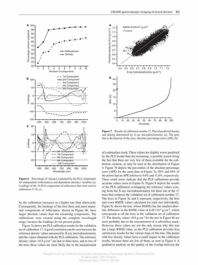
by the calibration increases at a higher rate than afterwards. Consequently, the loadings of the fi rst three and most impor-tant components of refl ectance, shown in Figure 6b, have larger absolute values than the remaining components. The calibrations were created using the complete wavelength range, because the loadings do not present peaks.

Figure 7 a shows the PLS calibration results for the validation set of calibration 17. A good correlation can be seen between the reference density values measured by X-ray microdensitometry and the values obtained with the PLS calibration. The reference density values < 0.5 g.cm -3 are due to three trees, and in two of the trees these values are most likely due to the measurement

100

95

90

85

80

75

70

65

60

55

50

100

50

0

-50

-100

-150

30

15

-15

-30

400 500 600 700 800 900 1000

400 500

1 2 3 4 5 6 7 8 9 10

600 700 800 900 1000

Wavelength (nm)

6th Component7th Component8th Component9th Component10th Component

1st Component

ReflectancesDensity

Number of components

2nd Component3rd Component4th Component5th Component

0

Load

ings

Load

ings

Per

cent

age

varia

nce

expl

aine

da

b

c

Figure 6 Percentage of variance explained by the PLS components for independent (refl ectances) and dependent (density) variables (a). Loadings of the 10 PLS components of refl ectance that were used in calibration 17 (b, c).

0.4 0.5 0.6 0.7 0.8 0.9 1.0 1.1 1.2

0.4

0.5

0.6

0.7

0.8

0.9

1.0

1.1

1.2a

Pre

dict

ed d

ensi

ty b

y P

LS (g

.cm

-3)

X-ray microdensitometry (g.cm-3)

RMSE=6.45x10-2 g.cm-3

r 2=0.814

0 10 20 30 40 50 60 70 80 90 1000

5

10

15

20

40

60b

AP

E (%

)

Percentile

Figure 7 Results of calibration number 17. Plot of predicted density and density determined by X-ray microdensitometry (a). The gray line is the bisector of the axes. Absolute percentage error (APE) (b).

of a subsurface crack. These values are slightly worse predicted by the PLS model than the remaining, a possible reason being the fact that there are very few of them available for the cali-bration creation, as may be seen in the distribution of Figure 4. Figure 7b depicts the percentiles of the absolute percentage error (APE) for the same data of Figure 7a; 50 % and 85 % of the points had an APE inferior to 5.6 % and 11.6 % , respectively. These small errors indicate that the PLS calibrations provide accurate values (seen in Figure 8 ). Figure 8 depicts the results of the PLS calibration overlapping the reference values com-ing from the X-ray microdensitometry for three out of the 17 trees that compose the validation set of calibration number 17. The trees in Figure 8a and b represent, respectively, the best and worst RMSE values calculated for each tree individually. Figure 8c shows the tree, whose RMSEs has the smallest abso-lute difference to the RMSE value of 6.45 × 10 -2 g.cm -3 , which corresponds to all the trees in the validation set of calibration 17. The density values < 0.6 g.cm -3 for the tree in Figure 8b are most probably due to the measurement of a subsurface crack. However, these values are not the only reason why this tree has a large RMSE value, as the PLS calibration provides less satisfactory results for the various rings of this tree. The points with low density values have a small impact in the calibration results, because there are few of them, as seen in Figure 4. A qualitative analysis on the quality of the overlap between the

Brought to you by | Instituto Nacional de Investigación y Tecnología Agraria y Alimentaria INIAAuthenticated | 193.144.96.41

Download Date | 1/18/13 1:35 PM

64 A. Fernandes et al.

PLS calibration and the reference density values, did not reveal any major differences between regions of sapwood or heart-wood, or containing extractives or resin ducts. The samples did not have reaction wood. In Figure 8, at fi rst sight, the narrower rings have a better overlap than the wider rings, but a closer analysis shows that the PLS calibration reproduces equally well the largest and smallest density data of the narrow and of the wide rings.

The RMSE and r 2 values are signifi cantly different between validation trees of calibration 17. RMSE varies

0.5

0.6

0.7

0.8

0.9

1.0r2=0.913

r2=0.680

r2=0.822

ReferencePLS model

Den

sity

(g.c

m-3

)D

ensi

ty (g

.cm

-3)

Den

sity

(g.c

m-3

)

0 10 20 30 40 50 60 70 80 900.4

0.5

0.6

0.7

0.8

0.9

1.0

1.1

1.2 RMSE=9.09×10-2 g.cm-3

Reference PLS model

0 10 20 30 40 50 60 70 80 90 1000.5

0.6

0.7

0.8

0.9

1.0

1.1

1.2 RMSE=6.41×10-2 g.cm-3 ReferencePLS model

Position (mm)

0 10 20 30 40 50 60

RMSE=4.96×10-2 g.cm-3a

b

c

Figure 8 Comparison between the density values obtained by PLS calibration number 17 and X-ray microdensitometry reference measurements for individual trees in the validation set. Best (a) and worst (b) RMSEs for individual trees. Tree with the smallest absolute difference to the RMSE of the whole validation set (c).

between 4.96 × 10 -2 and 9.09 × 10 -2 g.cm -3 , and r 2 varies between 0.680 and 0.913. Most trees have RMSE and r 2 values that vary slightly around 5.5 × 10 -2 g.cm -3 and 0.875. The variation in the tree results is the cause of the varia-tions observed in the results of the 20 calibrations plotted in Figure 5. The most plausible explanation for the varia-tion of the results between trees is the natural variability between trees. The variation in calibration results cannot be attributed to the variation in the optimum number of PLS, or in the number of points comprising the training and vali-dation sets. This is because the coeffi cient of determination between these numbers and the RMSE or r 2 is smaller than 0.09. The number of points in the sets is different for the 20 calibrations, because the number of points available per tree varies.

Conclusions

The present study demonstrates that a PLS calibration of hyperspectral imaging (a spectroscopic technique) data allows the accurate measurement of the intra growth ring density values at a spatial resolution of 79 μ m for Pinus pinea samples. This is the fi rst time, besides an exploratory work by the authors, that wood density was determined with such a high resolution by spectroscopic methods. It was also demon-strated that this can be done in the atypical wavelength range of 400 – 1000 nm.

The mean values of the r 2 and RMSE results of PLS cali-brations relative to the X-ray microdensitometry reference values are 0.810 and 6.54 × 10 -2 g.cm -3 , respectively. A sig-nifi cant variation was found between the trees. Further work will focus on improving the r 2 and RMSE values reported in the present article.

Acknowledgments

Armando Fernandes and Jos é Xavier acknowledge an Auxiliary Researcher contract from program “ Ci ê ncia 2008 ” .

References

Alves, A., Santos, A., Rozenberg, P., P â ques, L., Charpentier, J.-P., Schwanninger, M., Rodrigues, J. (2012) A common near infrared based partial least squares regression model for the prediction of wood density of Pinus pinaster and Larix x eurolepis . Wood Sci. Technol. 46:157 – 175.

Bishop, C.M. Neural networks for pattern recognition, Clarendon Press, Oxford University Press, Oxford, New York, 1995.

EHE (2006) Spectral calibration with Osram Dulux Mobil fl uores-cence lamp, SPECIM – Spectral Imaging Ltd. – Technical Note TN-0014.

Fernandes, A., Lousada, J., Morais, J., Xavier, J., Pereira, J., Melo-Pinto, P. High Spatial Resolution Measurement of Wood Density Using Hyperspectral Imaging and Neural Networks. COST Action FP0802 “Mixed numerical and experimental methods applied to the mechanical characterization of bio-based materials “ materials ” , UTAD, Vila Real, Portugal, 2011.

Brought to you by | Instituto Nacional de Investigación y Tecnología Agraria y Alimentaria INIAAuthenticated | 193.144.96.41

Download Date | 1/18/13 1:35 PM

VIS/NIR spectroscopic imaging of wood density 65

Geladi, P., Kowalski, B.R. (1986) Partial least-squares regression – A tutorial. Anal. Chim. Acta 185:1 – 17.

Gowen, A.A., O ’ Donnell, C.P., Cullen, P.J., Downey, G., Frias, J.M. (2007) Hyperspectral imaging – an emerging process analytical tool for food quality and safety control. Trends Food Sci. Tech. 18:590 – 598.

Hoffmeyer, P., Pedersen, J. (1995) Evaluation of density and strength of Norway spruce wood by near infrared refl ectance spectro-scopy. Eur. J. Wood Wood Prod. 53:165 – 170.

Jones, P., Schimleck, L., Daniels, R., Clark, A., Purnell, R. (2008) Comparison of Pinus taeda L. whole-tree wood property calibrations using diffuse refl ectance near infrared spectra obtained using a variety of sampling options. Wood Sci. Technol. 42:385 – 400.

Jones, P.D., Schimleck, L.R., Peter, G.F., Daniels, R.F., Clark III, A. (2005) Nondestructive estimation of Pinus taeda L. wood prop-erties for samples from a wide range of sites in Georgia. Can. J. Forest Res. 35:85 – 92.

Jones, P.D., Schimleck, L.R., So, C.L., Clark, A., Daniels, R.F. (2007) High resolution scanning of radial strips cut from increment cores by near infrared spectroscopy. IAWA J. 28:473 – 484.

Kothiyal, V., Raturi, A. (2011) Estimating mechanical properties and specifi c gravity for fi ve-year-old Eucalyptus tereticornis having broad moisture content range by NIR spectroscopy. Holzforschung 65:757 – 762.

Louzada, J.L.P.C., Fonseca, F.M.A. (2002) The heritability of wood density components in Pinus pinaster Ait. and implications for tree breeding. Ann. For. Sci. 59:867 – 873.

Meder, R., Marston, D., Ebdon, N., Evans, R. (2010) Spatially-resolved radial scanning of tree increment cores for near infrared prediction of microfi bril angle and chemical composition. J. Near Infrared Spec. 18:499 – 505.

Mora, C., Schimleck, L. (2010) Kernel regression methods for the prediction of wood properties of Pinus taeda using near infrared spectroscopy. Wood Sci. Technol. 44:561 – 578.

Mora, C.R., Schimleck, L.R., Yoon, S.C., Thai, C.N. (2011) Determination of basic density and moisture content of loblolly pine wood disks using a near infrared hyperspectral imaging system. J. Near Infrared Spec. 19:401 – 409.

Polge, H. (1978) Fifteen years of wood radiation densitometry. Wood Sci. Technol. 12:187 – 196.

Schimleck, L., Evans, R., Ilic, J. (2003) Application of near infrared spectroscopy to the extracted wood of a diverse range of species. IAWA J. 24:429 – 438.

Schimleck, L.R., Espey, C., Mora, C.R., Evans, R., Taylor, A., Muniz, G. (2009) Characterization of the wood quality of pernam-buco ( Caesalpinia echinata Lam) by measurements of density, extractives content, microfi bril angle, stiffness, color, and NIR spectroscopy. Holzforschung 63:457 – 463.

Schimleck, L.R., Evans, R. (2003) Estimation of air-dry density of incre-ment cores by near infrared spectroscopy. Appita J. 56:312 – 317.

Schimleck, L.R., Evans, R., Ilic, J. (2001a) Application of near infra-red spectroscopy to a diverse range of species demonstrating wide density and stiffness variation. IAWA J. 22:415 – 429.

Schimleck, L.R., Evans, R., Ilic, J. (2001b) Estimation of Eucalyptus delegatensis wood properties by near infrared spectroscopy. Can. J. Forest Res. 31:1671 – 1675.

Schimleck, L.R., Evans, R., Matheson, A.C. (2002) Estimation of Pinus radiata D. Don clear wood properties by near-infrared spectroscopy. J. Wood Sci. 48:132 – 137.

Springsteen, A. (1999) Standards for the measurement of diffuse refl ectance – an overview of available materials and measure-ment laboratories, Anal. Chim. Acta 380:379 – 390.

Thumm, A., Riddell, M., Nanayakkara, B., Harrington, J., Meder, R. (2010) Near infrared hyperspectral imaging applied to mapping chemical composition in wood samples. J. Near Infrared Spec. 18:507 – 515.

Thygesen, L. (1994) Determination of dry matter content and basic density of Norway spruce by near infrared refl ectance and trans-mittance spectroscopy. J. Near Infrared Spectrosc. 2:127 – 135.

Via, B.K., So, C.L., Shupe, T.F., Stine, M., Groom, L.H. (2005) Ability of near infrared spectroscopy to monitor air-dry density distribu-tion and variation of wood. Wood Fiber Sci. 37:394 – 402.

Xu, Q.S., Liang, Y.Z., Du, Y.P. (2004) Monte Carlo cross-validation for selecting a model and estimating the prediction error in multivariate calibration, J. Chemometr. 18:112 – 120.

Zhu, X.R., Shan, Y., Li, G.Y., Huang, A. M., Zhang, Z. Y. (2009) Prediction of wood property in Chinese Fir based on visible/near-infrared spectroscopy and least square-support vector machine. Spectrochim. Acta A. 74:344 – 348.

Received December 15, 2011 . Accepted July 30, 2012. Previously published online September 4, 2012.

Brought to you by | Instituto Nacional de Investigación y Tecnología Agraria y Alimentaria INIAAuthenticated | 193.144.96.41

Download Date | 1/18/13 1:35 PM