Maximum Spectral Demands in the Near-Fault Region

Yin-Nan Huang,a)M.EERI, Andrew S. Whittaker,a)

M.EERI, and Nicolas Luco,b)M.EERI

The Next Generation Attenuation (NGA) relationships for shallow crustalearthquakes in the western United States predict a rotated geometric mean ofhorizontal spectral demand, termed GMRotI50, and not maximum spectraldemand. Differences between strike-normal, strike-parallel, geometric-mean,and maximum spectral demands in the near-fault region are investigated using147 pairs of records selected from the NGA strong motion database. Theselected records are for earthquakes with moment magnitude greater than 6.5and for closest site-to-fault distance less than 15 km. Ratios of maximumspectral demand to NGA-predicted GMRotI50 for each pair of groundmotions are presented. The ratio shows a clear dependence on period and theSomerville directivity parameters. Maximum demands can substantiallyexceed NGA-predicted GMRotI50 demands in the near-fault region, whichhas significant implications for seismic design, seismic performanceassessment, and the next-generation seismic design maps. Strike-normalspectral demands are a significantly unconservative surrogate for maximumspectral demands for closest distance greater than 3 to 5 km. Scale factors thattransform NGA-predicted GMRotI50 to a maximum spectral demand in thenear-fault region are proposed. �DOI: 10.1193/1.2830435�

NEXT GENERATION ATTENUATION RELATIONSHIPS AND GMROTI50

The United States Geological Survey (USGS) is using three Next Generation Attenu-ation (NGA) relationships to generate the 2007 seismic hazard maps for the WesternUnited States: 1) Boore and Atkinson (2008), 2) Campbell and Bozorgnia (2008), and 3)Chiou and Youngs (2008). The same three relationships are being used to update theseismic design maps for the 2009 NEHRP Recommended Provisions for Seismic Regu-lations for New Buildings and Other Structures. More specifically, the NGA relation-ships will be used to perform probabilistic seismic hazard analysis and to establish de-terministic limits on seismic demand in near-fault regions. The ground-motion recordsused to develop these relationships are available from the PEER NGA database(http://peer.berkeley.edu/nga/), which includes more than 3,500 sets of recordings from173 earthquakes. Importantly, the database includes a significant number of near-faultrecordings.

The output of the NGA relationships is a geometric-mean (termed geomean

a) University at Buffalo, 212 Ketter Hall, Buffalo, NY 14260b)

U.S. Geological Survey, 1711 Illinois St., Room 426, Golden, CO 8022

319Earthquake Spectra, Volume 24, No. 1, pages 319–341, February 2008; © 2008, Earthquake Engineering Research Institute

320 Y. HUANG, A. S.WHITTAKER, AND N. LUCO

hereafter)1 spectral demand for two orthogonal horizontal components of ground mo-tion; maximum spectral demand is not predicted. The value of the geomean demand at agiven station will depend on the orientation of the sensors recording the earthquakeshaking. To provide a consistent basis for developing the NGA relationships, Boore et al.(2006) defined a rotated geomean, GMRotI50, that is independent of sensor orientation.They showed that the average effect on geomean spectral demand of rotating the pair ofground motions from the recorded orientation was less than 3%. In this paper, the ro-tated geomean demand predicted by the NGA relationships is termed NGA-predictedGMRotI50 and the rotated geomean computed from a pair of earthquake records istermed GMRotI50.

Rupture directivity effects were observed in the Pacoima Dam record of the 1971San Fernando earthquake and many have subsequently reported the difference in fault-strike-normal (SN) and strike-parallel (SP) spectral demands. The observed differencebetween SN and SP spectral demands provided clear evidence that maximum spectraldemands could substantially exceed geomean spectral demands. In the mid-1990s, Som-erville et al. (1997) developed a rupture directivity model to characterize the geomean,SN, and SP spectral demands in the near-fault region. Somerville’s model utilized alength ratio for strike-slip faults, X; a width ratio for dip-slip faults, Y; an azimuth anglebetween the fault plane and ray path to site for strike-slip faults, �; and a zenith anglebetween the fault plane and ray path to the site for dip-slip faults, �. Figure 1 identifiesthese variables. Two parameters were used to characterize directivity effects: X cos � forstrike-slip faults and Y cos � for dip-slip faults. Somerville et al. observed that 1) formoment magnitude greater than 6.5, period greater than 0.6 second, and X cos � orY cos � greater than about 0.5, the geomean spectral demand was on average greaterthan the geomean spectral demand predicted by the widely used attenuation relationshipof Abrahamson and Silva (1997); and 2) for moment magnitude greater than 6, period

1

Figure 1. Somerville directivity parameters, after Somerville et al. (1997).

The geomean demand is computed as the square root of the product of the two orthogonal spectral demands.

MAXIMUM SPECTRAL DEMANDS IN THE NEAR-FAULT REGION 321

greater than 0.5 second, and � or � smaller than about 45°, the SN spectral demand wason average greater than the SP spectral demand and the geomean of SN and SP spectraldemand.

Howard et al. (2005) characterized directivity effects using a spectral intensity indexthat integrates spectral acceleration over a period range from 0.5 to 3 seconds. A polarityazimuth range is identified for a pair of ground motions using the velocity orbit of thepair. The time series is then rotated within this azimuth range until one component pro-duces the greatest spectral intensity measured by the integration of spectral accelerationfor the component over a period range of 0.5 to 3 seconds. The orientation and spectraldemand for this component, termed the SAMAX component, were compared with thosefor the SN component using 29 pairs of near-fault ground motions. They concluded that1) the SN spectral demand estimated by Somerville et al. (1997) and modified by Abra-hamson (2000) adequately predicted the average spectral demand for the SAMAX com-ponent for sites within 5 km of a strike-skip fault, and 2) the average spectral demandfor the SAMAX component exceeded the predictions of Somerville et al. (1997) andAbrahamson (2000) for the SN component by a factor between 1.7 and 2 for reversefaults.

Beyer and Bommer (2006) investigated the ratio of the maximum to recordedgeomean spectral demands using 949 earthquake records with moment magnitude rang-ing between 4.2 and 7.9, and hypocentral distance ranging between 5 and 200 km. Theyreported that the median of the ratio varied between 1.2 and 1.3, depending on the pe-riod. Campbell and Bozorgnia (2008) computed the ratio of the greater spectral demandfor a pair of recorded ground motions to GMRotI50 for the pair using 1,561 recordswith magnitudes and distances similar to those of Beyer and Bommer. The median of theratio varied between 1.11 and 1.2.

The Beyer and Bommer study of maximum and geomean spectral demands used adatabase composed of far-field and near-fault ground motions together. This paper fo-cuses solely on recorded near-fault ground motions and addresses the following fourquestions:

1. Can SN spectral demand be used as a surrogate for maximum demand in thenear-fault region?

2. Is maximum demand in the near-fault region substantially greater thanmaximum-minimum geomean (MMgm) demand2? If so, how much greater?

3. Does NGA-predicted GMRotI50 demand accurately estimate MMgm demandin the near-fault region?

4. What is the relationship between maximum demand and NGA-predicted GM-RotI50 in the near-fault region? Can bias factors be developed to transformNGA-predicted GMRotI50 to expected maximum spectral demand?

The answers to these questions can be used in establishing deterministic limits on the

2 MMgm is the geomean of the maximum and minimum spectral demands for a pair of ground motions, as

defined in the next section of the paper.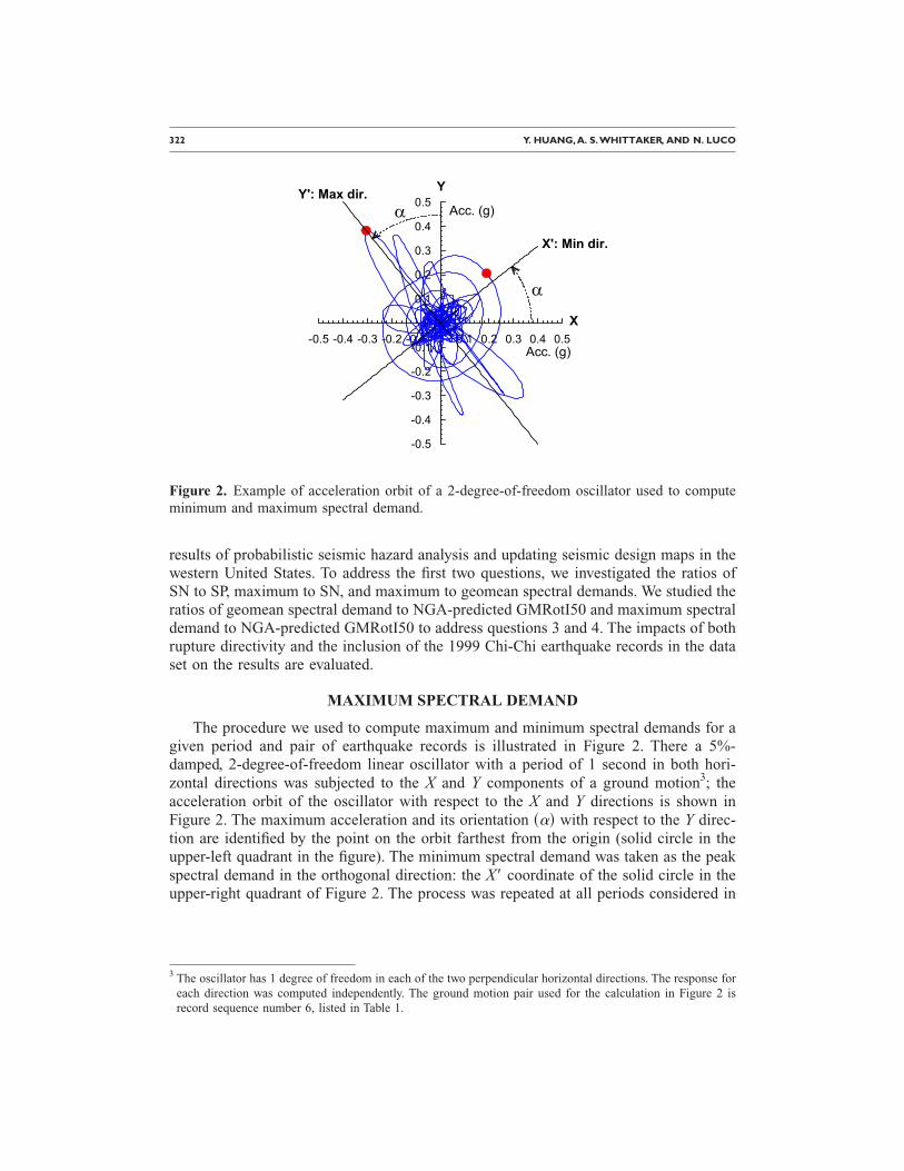

322 Y. HUANG, A. S.WHITTAKER, AND N. LUCO

results of probabilistic seismic hazard analysis and updating seismic design maps in thewestern United States. To address the first two questions, we investigated the ratios ofSN to SP, maximum to SN, and maximum to geomean spectral demands. We studied theratios of geomean spectral demand to NGA-predicted GMRotI50 and maximum spectraldemand to NGA-predicted GMRotI50 to address questions 3 and 4. The impacts of bothrupture directivity and the inclusion of the 1999 Chi-Chi earthquake records in the dataset on the results are evaluated.

MAXIMUM SPECTRAL DEMAND

The procedure we used to compute maximum and minimum spectral demands for agiven period and pair of earthquake records is illustrated in Figure 2. There a 5%-damped, 2-degree-of-freedom linear oscillator with a period of 1 second in both hori-zontal directions was subjected to the X and Y components of a ground motion3; theacceleration orbit of the oscillator with respect to the X and Y directions is shown inFigure 2. The maximum acceleration and its orientation ��� with respect to the Y direc-tion are identified by the point on the orbit farthest from the origin (solid circle in theupper-left quadrant in the figure). The minimum spectral demand was taken as the peakspectral demand in the orthogonal direction: the X� coordinate of the solid circle in theupper-right quadrant of Figure 2. The process was repeated at all periods considered in

3 The oscillator has 1 degree of freedom in each of the two perpendicular horizontal directions. The response foreach direction was computed independently. The ground motion pair used for the calculation in Figure 2 is

-0.5 -0.4 -0.3 -0.2 -0.1 0 0.1 0.2 0.3 0.4 0.5

-0.5

-0.4

-0.3

-0.2

-0.1

0

0.1

0.2

0.3

0.4

0.5

Acc. (g)

X': Min dir.

Y': Max dir.Acc. (g)

X

Y

�

�

Figure 2. Example of acceleration orbit of a 2-degree-of-freedom oscillator used to computeminimum and maximum spectral demand.

record sequence number 6, listed in Table 1.

MAXIMUM SPECTRAL DEMANDS IN THE NEAR-FAULT REGION 323

the analysis, from 0 to 4 seconds, to construct the maximum spectrum for the ground-motion pair. For a given ground-motion pair, � varies as a function of period. This defi-nition of maximum spectral demand is termed MaxD by Beyer and Bommer (2006).

STRONG MOTION DATA SET

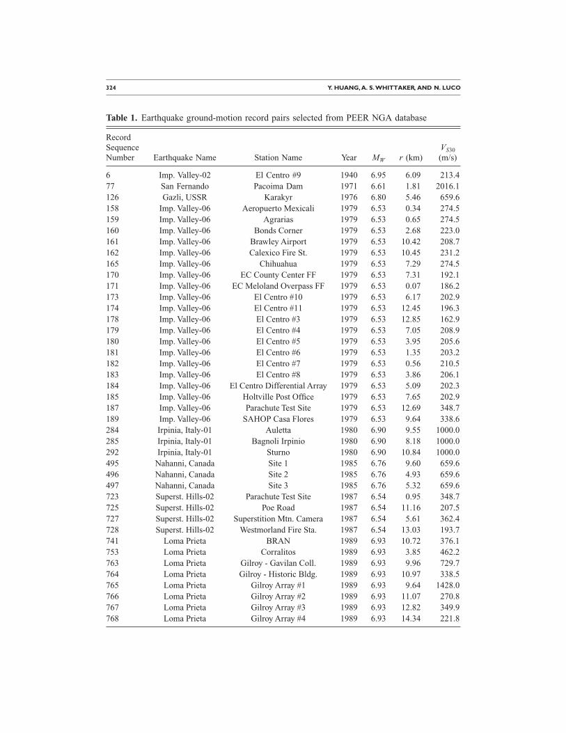
The data set used in this study is a subset of that described in the PEER NGA Da-tabase Flatfile (see http://peer.berkeley.edu/products/nga_flatfiles_dev.html). Each pair oftime series referred to in the Flatfile was rotated to be SN and SP to the causative faultby members of the NGA project team. Since the focus of our work is strong near-faultshaking, we include in our data set all pairs of ground motions from earthquakes withmoment magnitude �MW� of 6.5 and greater, and with closest distance from the record-ing site to the ruptured area �r� of 15 km and less. The 147 ground-motion pairs in ourdata set are listed in Table 1.

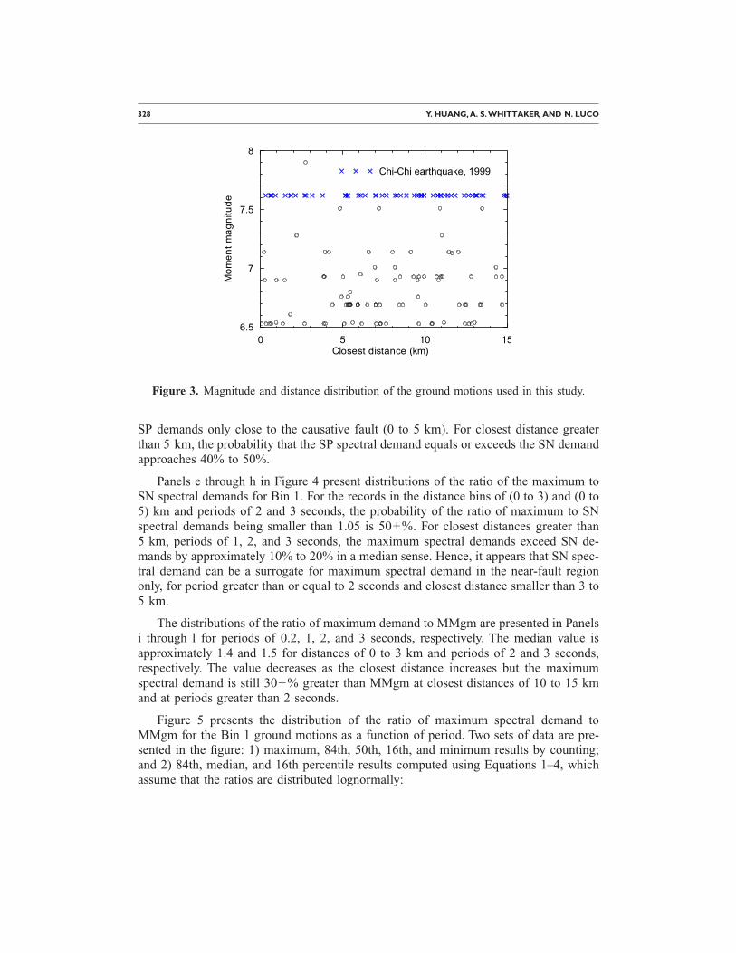
Figure 3 presents the distribution of the 147 ground-motion pairs as a function ofMW and r. Of the 147 pairs of motions, 46 are associated with strike-slip faulting and101 with dip-slip faulting4; 3, 7, 78, 58, and 1 pairs of motions are associated with SiteClasses A through E, respectively, per the site classification of the 2003 NEHRP Rec-ommended Provisions (FEMA 2004); 56 pairs of motions are from the 1999 Chi-Chiearthquake in Taiwan.

Three bins of ground motions, termed Bins 1, 2, and 3, were prepared for this study.Bin 1 includes all 147 ground-motion pairs in the data set. Bin 2 includes all ground-motion pairs in the data set except those of the 1999 Chi-Chi earthquake. Bin 2 wasprepared to determine whether the preponderance (56 of 147) of Chi-Chi ground-motionhistories in the data set distorted the analysis results. Bin 3 includes all records in thedata set with X cos � or Y cos � greater than or equal to 0.5 (forward-directivity region5)and was assembled to study the impact of rupture directivity on spectral demand. Fiftypairs of records in the bin have � or � smaller than 45°. The values of Y cos � for all ofthe Chi-Chi records are smaller than 0.5 and as such there are no Chi-Chi records inBin 3.

RELATIONSHIPS BETWEEN STRIKE-NORMAL, STRIKE-PARALLEL,GEOMEAN, AND MAXIMUM SPECTRAL DEMANDS

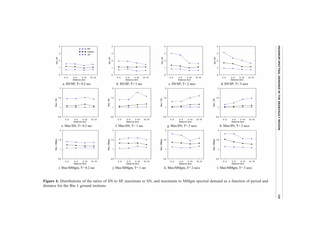
Figure 4 presents information on maximum, MMgm, SN, and SP spectral demandsfor the Bin 1 ground motions as a function of period and the closest distance from thesite to the ruptured fault. Panels a through d present the median (50th), 16th, and 84thpercentile ratios of SN to SP shaking for distances between 0 and 15 km and periods of0.2, 1, 2, and 3 seconds. The percentile values were established by sorting the values ofthe ratio in ascending order and counting. Closest distance is binned as (0 to 3), (0 to 5),(5 to 10), and (10 to 15) km. The numbers of ground-motion pairs in each distance bin

4 The 101 pairs of motions from dip-slip faults include 30 recordings off the ends of the faults.5 We recognize that X cos � and Y cos � are not perfect parameterizations of directivity and that other directivity

parameters could result in different bins of forward-directivity records.

324 Y. HUANG, A. S.WHITTAKER, AND N. LUCO

Table 1. Earthquake ground-motion record pairs selected from PEER NGA database

RecordSequenceNumber Earthquake Name Station Name Year MW r (km)

VS30

(m/s)

6 Imp. Valley-02 El Centro #9 1940 6.95 6.09 213.477 San Fernando Pacoima Dam 1971 6.61 1.81 2016.1126 Gazli, USSR Karakyr 1976 6.80 5.46 659.6158 Imp. Valley-06 Aeropuerto Mexicali 1979 6.53 0.34 274.5159 Imp. Valley-06 Agrarias 1979 6.53 0.65 274.5160 Imp. Valley-06 Bonds Corner 1979 6.53 2.68 223.0161 Imp. Valley-06 Brawley Airport 1979 6.53 10.42 208.7162 Imp. Valley-06 Calexico Fire St. 1979 6.53 10.45 231.2165 Imp. Valley-06 Chihuahua 1979 6.53 7.29 274.5170 Imp. Valley-06 EC County Center FF 1979 6.53 7.31 192.1171 Imp. Valley-06 EC Meloland Overpass FF 1979 6.53 0.07 186.2173 Imp. Valley-06 El Centro #10 1979 6.53 6.17 202.9174 Imp. Valley-06 El Centro #11 1979 6.53 12.45 196.3178 Imp. Valley-06 El Centro #3 1979 6.53 12.85 162.9179 Imp. Valley-06 El Centro #4 1979 6.53 7.05 208.9180 Imp. Valley-06 El Centro #5 1979 6.53 3.95 205.6181 Imp. Valley-06 El Centro #6 1979 6.53 1.35 203.2182 Imp. Valley-06 El Centro #7 1979 6.53 0.56 210.5183 Imp. Valley-06 El Centro #8 1979 6.53 3.86 206.1184 Imp. Valley-06 El Centro Differential Array 1979 6.53 5.09 202.3185 Imp. Valley-06 Holtville Post Office 1979 6.53 7.65 202.9187 Imp. Valley-06 Parachute Test Site 1979 6.53 12.69 348.7189 Imp. Valley-06 SAHOP Casa Flores 1979 6.53 9.64 338.6284 Irpinia, Italy-01 Auletta 1980 6.90 9.55 1000.0285 Irpinia, Italy-01 Bagnoli Irpinio 1980 6.90 8.18 1000.0292 Irpinia, Italy-01 Sturno 1980 6.90 10.84 1000.0495 Nahanni, Canada Site 1 1985 6.76 9.60 659.6496 Nahanni, Canada Site 2 1985 6.76 4.93 659.6497 Nahanni, Canada Site 3 1985 6.76 5.32 659.6723 Superst. Hills-02 Parachute Test Site 1987 6.54 0.95 348.7725 Superst. Hills-02 Poe Road 1987 6.54 11.16 207.5727 Superst. Hills-02 Superstition Mtn. Camera 1987 6.54 5.61 362.4728 Superst. Hills-02 Westmorland Fire Sta. 1987 6.54 13.03 193.7741 Loma Prieta BRAN 1989 6.93 10.72 376.1753 Loma Prieta Corralitos 1989 6.93 3.85 462.2763 Loma Prieta Gilroy - Gavilan Coll. 1989 6.93 9.96 729.7764 Loma Prieta Gilroy - Historic Bldg. 1989 6.93 10.97 338.5765 Loma Prieta Gilroy Array #1 1989 6.93 9.64 1428.0766 Loma Prieta Gilroy Array #2 1989 6.93 11.07 270.8767 Loma Prieta Gilroy Array #3 1989 6.93 12.82 349.9768 Loma Prieta Gilroy Array #4 1989 6.93 14.34 221.8

MAXIMUM SPECTRAL DEMANDS IN THE NEAR-FAULT REGION 325

Table 1. (cont.)

RecordSequenceNumber Earthquake Name Station Name Year MW r (km)

VS30

(m/s)

779 Loma Prieta LGPC 1989 6.93 3.88 477.7801 Loma Prieta San Jose - Santa Teresa Hills 1989 6.93 14.69 671.8802 Loma Prieta Saratoga - Aloha Ave 1989 6.93 8.50 370.8803 Loma Prieta Saratoga – W. Valley Coll. 1989 6.93 9.31 370.8821 Erzincan, Turkey Erzincan 1992 6.69 4.38 274.5825 Cape Mendocino Cape Mendocino 1992 7.01 6.96 513.7828 Cape Mendocino Petrolia 1992 7.01 8.18 712.8829 Cape Mendocino Rio Dell Overpass - FF 1992 7.01 14.33 311.8864 Landers Joshua Tree 1992 7.28 11.03 379.3879 Landers Lucerne 1992 7.28 2.19 684.9949 Northridge-01 Arleta - Nordhoff Fire Sta. 1994 6.69 8.66 297.7959 Northridge-01 Canoga Park - Topanga Can 1994 6.69 14.70 267.5960 Northridge-01 Canyon Country – W. Lost

Cany.1994 6.69 12.44 308.6

982 Northridge-01 Jensen Filter Plant 1994 6.69 5.43 373.1983 Northridge-01 Jensen Filter Plant

Generator1994 6.69 5.43 525.8

1004 Northridge-01 LA - Sepulveda VA Hospital 1994 6.69 8.44 380.11013 Northridge-01 LA Dam 1994 6.69 5.92 629.01042 Northridge-01 N. Hollywood - Coldwater

Can.1994 6.69 12.51 446.0

1044 Northridge-01 Newhall - Fire Sta. 1994 6.69 5.92 269.11045 Northridge-01 Newhall – W. Pico Canyon

Rd.1994 6.69 5.48 285.9

1048 Northridge-01 Northridge - 17645 SaticoySt.

1994 6.69 12.09 280.9

1050 Northridge-01 Pacoima Dam (downstr.) 1994 6.69 7.01 2016.11051 Northridge-01 Pacoima Dam (upper left) 1994 6.69 7.01 2016.11052 Northridge-01 Pacoima Kagel Canyon 1994 6.69 7.26 508.11063 Northridge-01 Rinaldi Receiving Sta. 1994 6.69 6.50 282.31080 Northridge-01 Simi Valley - Katherine Rd. 1994 6.69 13.42 557.41082 Northridge-01 Sun Valley - Roscoe Blvd. 1994 6.69 10.05 308.61083 Northridge-01 Sunland – Mt. Gleason Ave. 1994 6.69 13.35 446.01084 Northridge-01 Sylmar - Converter Sta. 1994 6.69 5.35 251.21085 Northridge-01 Sylmar - Converter Sta. East 1994 6.69 5.19 370.51086 Northridge-01 Sylmar - Olive View Med

FF1994 6.69 5.30 440.5

1106 Kobe, Japan KJMA 1995 6.90 0.96 312.01111 Kobe, Japan Nishi-Akashi 1995 6.90 7.08 609.01119 Kobe, Japan Takarazuka 1995 6.90 0.27 312.01120 Kobe, Japan Takatori 1995 6.90 1.47 256.0

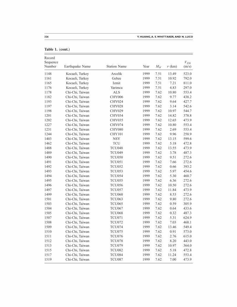
326 Y. HUANG, A. S.WHITTAKER, AND N. LUCO

Table 1. (cont.)

RecordSequenceNumber Earthquake Name Station Name Year MW r (km)

VS30

(m/s)

1148 Kocaeli, Turkey Arcelik 1999 7.51 13.49 523.01161 Kocaeli, Turkey Gebze 1999 7.51 10.92 792.01165 Kocaeli, Turkey Izmit 1999 7.51 7.21 811.01176 Kocaeli, Turkey Yarimca 1999 7.51 4.83 297.01178 Chi-Chi, Taiwan ALS 1999 7.62 10.80 553.41182 Chi-Chi, Taiwan CHY006 1999 7.62 9.77 438.21193 Chi-Chi, Taiwan CHY024 1999 7.62 9.64 427.71197 Chi-Chi, Taiwan CHY028 1999 7.62 3.14 542.61198 Chi-Chi, Taiwan CHY029 1999 7.62 10.97 544.71201 Chi-Chi, Taiwan CHY034 1999 7.62 14.82 378.81202 Chi-Chi, Taiwan CHY035 1999 7.62 12.65 473.91227 Chi-Chi, Taiwan CHY074 1999 7.62 10.80 553.41231 Chi-Chi, Taiwan CHY080 1999 7.62 2.69 553.41244 Chi-Chi, Taiwan CHY101 1999 7.62 9.96 258.91403 Chi-Chi, Taiwan NSY 1999 7.62 13.15 599.61462 Chi-Chi, Taiwan TCU 1999 7.62 5.18 472.81488 Chi-Chi, Taiwan TCU048 1999 7.62 13.55 473.91489 Chi-Chi, Taiwan TCU049 1999 7.62 3.78 487.31490 Chi-Chi, Taiwan TCU050 1999 7.62 9.51 272.61491 Chi-Chi, Taiwan TCU051 1999 7.62 7.66 272.61492 Chi-Chi, Taiwan TCU052 1999 7.62 0.66 393.21493 Chi-Chi, Taiwan TCU053 1999 7.62 5.97 454.61494 Chi-Chi, Taiwan TCU054 1999 7.62 5.30 460.71495 Chi-Chi, Taiwan TCU055 1999 7.62 6.36 272.61496 Chi-Chi, Taiwan TCU056 1999 7.62 10.50 272.61497 Chi-Chi, Taiwan TCU057 1999 7.62 11.84 473.91499 Chi-Chi, Taiwan TCU060 1999 7.62 8.53 272.61501 Chi-Chi, Taiwan TCU063 1999 7.62 9.80 272.61503 Chi-Chi, Taiwan TCU065 1999 7.62 0.59 305.91504 Chi-Chi, Taiwan TCU067 1999 7.62 0.64 433.61505 Chi-Chi, Taiwan TCU068 1999 7.62 0.32 487.31507 Chi-Chi, Taiwan TCU071 1999 7.62 5.31 624.91508 Chi-Chi, Taiwan TCU072 1999 7.62 7.03 468.11509 Chi-Chi, Taiwan TCU074 1999 7.62 13.46 549.41510 Chi-Chi, Taiwan TCU075 1999 7.62 0.91 573.01511 Chi-Chi, Taiwan TCU076 1999 7.62 2.76 615.01512 Chi-Chi, Taiwan TCU078 1999 7.62 8.20 443.01513 Chi-Chi, Taiwan TCU079 1999 7.62 10.97 364.01515 Chi-Chi, Taiwan TCU082 1999 7.62 5.18 472.81517 Chi-Chi, Taiwan TCU084 1999 7.62 11.24 553.41519 Chi-Chi, Taiwan TCU087 1999 7.62 7.00 473.9

MAXIMUM SPECTRAL DEMANDS IN THE NEAR-FAULT REGION 327

are 25, 36, 63, and 48, respectively. The (0 to 3) km bin is dominated by the 1979 Im-perial Valley earthquake (6 records), 1995 Kobe earthquake (3 records), and 1999 Chi-Chi earthquake (11 records). Generally, the median ratio increases with period and re-duces with distance, especially for closest distances smaller than 10 km. At very smallclosest distances (0 to 3 km) and a period of 3 seconds, the median ratio is 1.71 and the84th percentile value is 3.15. Setting aside the ratio for T=0.2 and 1 second, becausedirectivity effects are expected to be modest at these periods per Somerville et al.(1997), our near-fault data set indicates that SN demands are systematically larger than

Table 1. (cont.)

RecordSequenceNumber Earthquake Name Station Name Year MW r (km)

VS30

(m/s)

1521 Chi-Chi, Taiwan TCU089 1999 7.62 8.88 553.41527 Chi-Chi,Taiwan TCU100 1999 7.62 11.39 473.91528 Chi-Chi, Taiwan TCU101 1999 7.62 2.13 272.61529 Chi-Chi, Taiwan TCU102 1999 7.62 1.51 714.31530 Chi-Chi, Taiwan TCU103 1999 7.62 6.10 494.11531 Chi-Chi, Taiwan TCU104 1999 7.62 12.89 473.91533 Chi-Chi, Taiwan TCU106 1999 7.62 14.99 473.91535 Chi-Chi, Taiwan TCU109 1999 7.62 13.08 473.91536 Chi-Chi, Taiwan TCU110 1999 7.62 11.60 212.71541 Chi-Chi, Taiwan TCU116 1999 7.62 12.40 493.11545 Chi-Chi, Taiwan TCU120 1999 7.62 7.41 459.31546 Chi-Chi, Taiwan TCU122 1999 7.62 9.35 475.51547 Chi-Chi, Taiwan TCU123 1999 7.62 14.93 272.61548 Chi-Chi, Taiwan TCU128 1999 7.62 13.15 599.61549 Chi-Chi, Taiwan TCU129 1999 7.62 1.84 664.41550 Chi-Chi, Taiwan TCU136 1999 7.62 8.29 473.91551 Chi-Chi, Taiwan TCU138 1999 7.62 9.79 652.91595 Chi-Chi, Taiwan WGK 1999 7.62 9.96 258.91596 Chi-Chi, Taiwan WNT 1999 7.62 1.84 664.41602 Düzce, Turkey Bolu 1999 7.14 12.04 326.01605 Düzce, Turkey Düzce 1999 7.14 6.58 276.01611 Düzce, Turkey Lamont 1058 1999 7.14 0.21 424.81612 Düzce, Turkey Lamont 1059 1999 7.14 4.17 424.81614 Düzce, Turkey Lamont 1061 1999 7.14 11.46 481.01615 Düzce, Turkey Lamont 1062 1999 7.14 9.15 338.01617 Düzce, Turkey Lamont 375 1999 7.14 3.93 424.81618 Düzce, Turkey Lamont 531 1999 7.14 8.03 659.61787 Hector Mine Hector 1999 7.13 11.66 684.92114 Denali, Alaska TAPS Pump Station #10 2002 7.90 2.74 329.43548 Loma Prieta Los Gatos-Lexington Dam 1989 6.93 5.02 1070.3

328 Y. HUANG, A. S.WHITTAKER, AND N. LUCO

SP demands only close to the causative fault (0 to 5 km). For closest distance greaterthan 5 km, the probability that the SP spectral demand equals or exceeds the SN demandapproaches 40% to 50%.

Panels e through h in Figure 4 present distributions of the ratio of the maximum toSN spectral demands for Bin 1. For the records in the distance bins of (0 to 3) and (0 to5) km and periods of 2 and 3 seconds, the probability of the ratio of maximum to SNspectral demands being smaller than 1.05 is 50+%. For closest distances greater than5 km, periods of 1, 2, and 3 seconds, the maximum spectral demands exceed SN de-mands by approximately 10% to 20% in a median sense. Hence, it appears that SN spec-tral demand can be a surrogate for maximum spectral demand in the near-fault regiononly, for period greater than or equal to 2 seconds and closest distance smaller than 3 to5 km.

The distributions of the ratio of maximum demand to MMgm are presented in Panelsi through l for periods of 0.2, 1, 2, and 3 seconds, respectively. The median value isapproximately 1.4 and 1.5 for distances of 0 to 3 km and periods of 2 and 3 seconds,respectively. The value decreases as the closest distance increases but the maximumspectral demand is still 30+% greater than MMgm at closest distances of 10 to 15 kmand at periods greater than 2 seconds.

Figure 5 presents the distribution of the ratio of maximum spectral demand toMMgm for the Bin 1 ground motions as a function of period. Two sets of data are pre-sented in the figure: 1) maximum, 84th, 50th, 16th, and minimum results by counting;and 2) 84th, median, and 16th percentile results computed using Equations 1–4, whichassume that the ratios are distributed lognormally:

0 5 10 15Closest distance (km)

6.5

7

7.5

8

Momentmagnitude

Chi-Chi earthquake, 1999

Figure 3. Magnitude and distance distribution of the ground motions used in this study.

0 -3 0 -5 5 -10 10 -15Distance (km)

0

1

2

3

4

SN/SP

84th

median16th

0 -3 0 -5 5 -10 10 -15Distance (km)

0

1

2

3

4

SN/SP

0 -3 0 -5 5 -10 10 -15Distance (km)

0

1

2

3

4

SN/SP

0 -3 0 -5 5 -10 10 -15Distance (km)

0

1

2

3

4

SN/SP

a. SN/SP, T= 0.2 sec b. SN/SP, T= 1 sec c. SN/SP, T= 2 secs d. SN/SP, T= 3 secs

0 -3 0 -5 5 -10 10 -15Distance (km)

0.5

1

1.5

2

Max/SN

0 -3 0 -5 5 -10 10 -15Distance (km)

0.5

1

1.5

2

Max/SN

0 -3 0 -5 5 -10 10 -15Distance (km)

0.5

1

1.5

2

Max/SN

0 -3 0 -5 5 -10 10 -15Distance (km)

0.5

1

1.5

2

Max/SN

e. Max/SN, T= 0.2 sec f. Max/SN, T= 1 sec g. Max/SN, T= 2 secs h. Max/SN, T= 3 secs

0 -3 0 -5 5 -10 10 -15Distance (km)

0.5

1

1.5

2

Max/MMgm

0 -3 0 -5 5 -10 10 -15Distance (km)

0.5

1

1.5

2

Max/MMgm

0 -3 0 -5 5 -10 10 -15Distance (km)

0.5

1

1.5

2

Max/MMgm

0 -3 0 -5 5 -10 10 -15Distance (km)

0.5

1

1.5

2

Max/MMgm

i. Max/MMgm, T= 0.2 sec j. Max/MMgm, T= 1 sec k. Max/MMgm, T= 2 secs l. Max/MMgm, T= 3 secs

Figure 4. Distributions of the ratios of SN to SP, maximum to SN, and maximum to MMgm spectral demand as a function of period anddistance for the Bin 1 ground motions.

MA

XIM

UM

SP

EC

TR

AL

DE

MA

ND

SIN

TH

EN

EA

R-FA

UL

TR

EG

ION

329

330 Y. HUANG, A. S.WHITTAKER, AND N. LUCO

�Y = exp�1

n�i=1

n

ln yi� �1�

�Y =� 1

n − 1�i=1

n

�ln yi − ln �Y�2 �2�

y16th = �Y · e−�Y �3�

y84th = �Y · e�Y �4�

where yi is the ratio of maximum spectral demand to MMgm for the ith ground-motionpair and �Y, �Y, y16th, and y84th are the median, logarithmic standard deviation, and 16thand 84th percentiles of the ratio, respectively. Counted percentiles agree well with thosebased on the lognormal assumption except for the median values in the long-periodrange, where the ratio based on counting is about 5% (or less) less than that based on thelognormal assumption6. The median values of the ratio for periods smaller than 0.2 sec-ond are about 1.2 and increase to about 1.5 at 4 seconds. The median values for the ratioin the long-period range are higher than those reported by Beyer and Bommer.

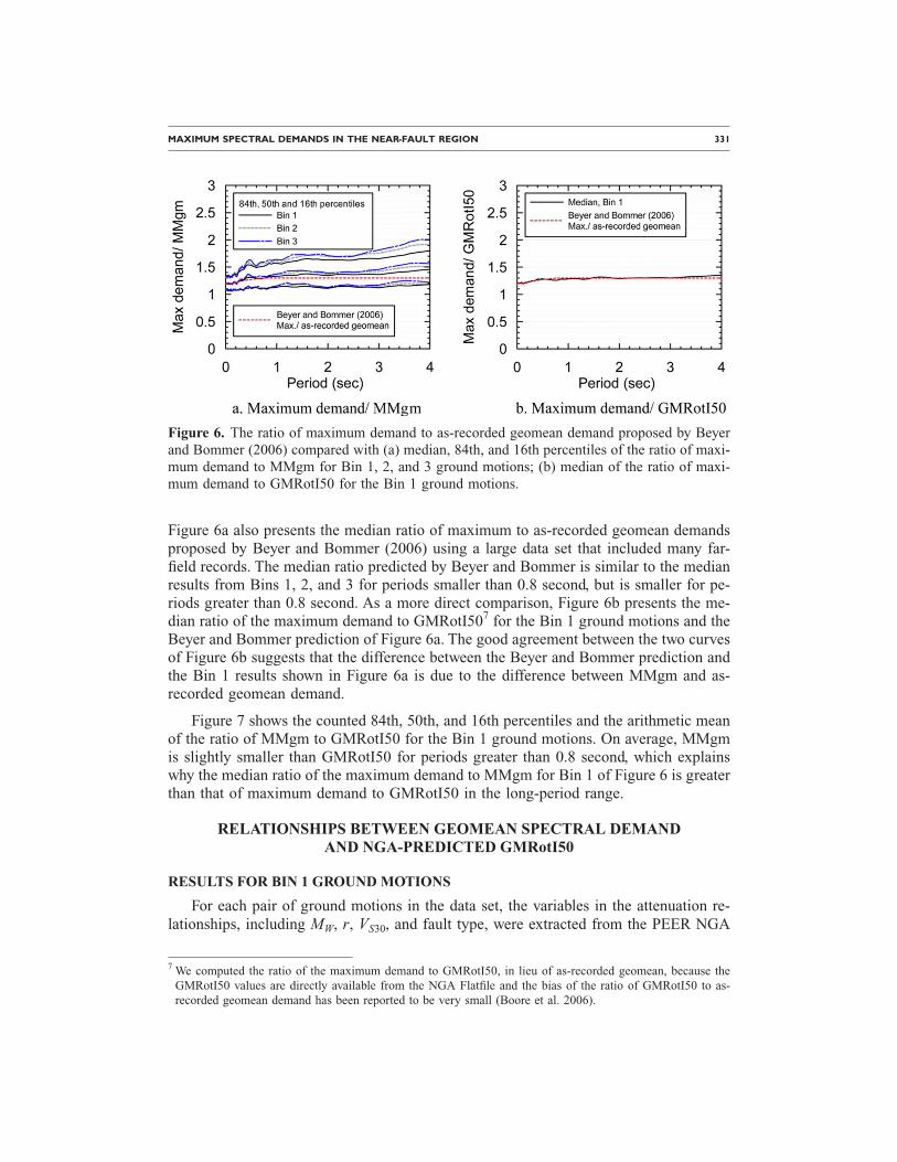
Figure 6a presents the median, 84th, and 16th percentile results computed usingEquations 1–4 for all three bins of ground motions. The ratio of maximum demand toMMgm demand is maximized when forward-directivity motions are considered and forlonger periods although the ratios at each of the percentiles are similar for all three bins.

6 Despite the obvious fact that the ratio of maximum to MMgm spectral demand must be greater than unitywhereas a lognormal distribution includes values less than unity, a similar conclusion was drawn by Beyer andBommer (2006), who studied the distribution of the ratio of maximum to GMxy demand, where GMxy is thegeomean demand for the pair of recorded ground motions. They reported that the use of the lognormal distri-

Figure 5. Maximum, minimum, median, and 84th and 16th percentiles of the ratio of maxi-mum spectral demand to MMgm as a function of period for the Bin 1 ground motions.

bution for the ratio of maximum to GMxy demand is “not exact but a reasonable approximation.”

MAXIMUM SPECTRAL DEMANDS IN THE NEAR-FAULT REGION 331

Figure 6a also presents the median ratio of maximum to as-recorded geomean demandsproposed by Beyer and Bommer (2006) using a large data set that included many far-field records. The median ratio predicted by Beyer and Bommer is similar to the medianresults from Bins 1, 2, and 3 for periods smaller than 0.8 second, but is smaller for pe-riods greater than 0.8 second. As a more direct comparison, Figure 6b presents the me-dian ratio of the maximum demand to GMRotI507 for the Bin 1 ground motions and theBeyer and Bommer prediction of Figure 6a. The good agreement between the two curvesof Figure 6b suggests that the difference between the Beyer and Bommer prediction andthe Bin 1 results shown in Figure 6a is due to the difference between MMgm and as-recorded geomean demand.

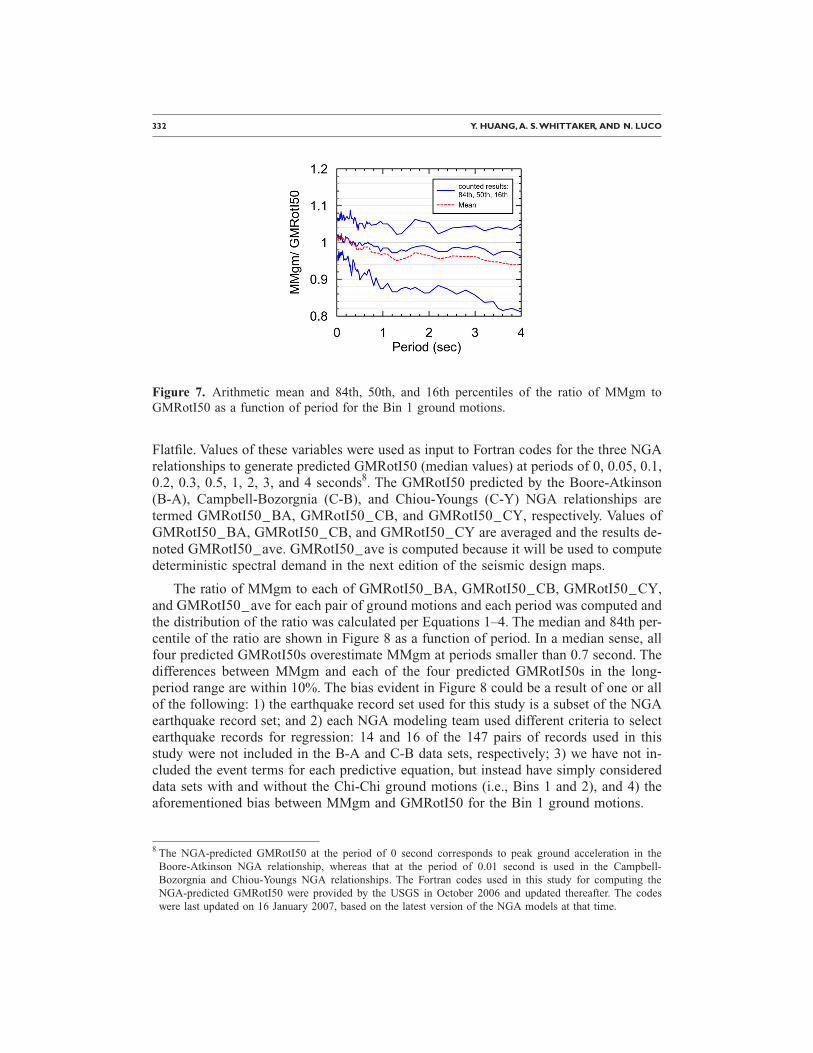
Figure 7 shows the counted 84th, 50th, and 16th percentiles and the arithmetic meanof the ratio of MMgm to GMRotI50 for the Bin 1 ground motions. On average, MMgmis slightly smaller than GMRotI50 for periods greater than 0.8 second, which explainswhy the median ratio of the maximum demand to MMgm for Bin 1 of Figure 6 is greaterthan that of maximum demand to GMRotI50 in the long-period range.

RELATIONSHIPS BETWEEN GEOMEAN SPECTRAL DEMANDAND NGA-PREDICTED GMRotI50

RESULTS FOR BIN 1 GROUND MOTIONS

For each pair of ground motions in the data set, the variables in the attenuation re-lationships, including MW, r, VS30, and fault type, were extracted from the PEER NGA

7 We computed the ratio of the maximum demand to GMRotI50, in lieu of as-recorded geomean, because theGMRotI50 values are directly available from the NGA Flatfile and the bias of the ratio of GMRotI50 to as-

Figure 6. The ratio of maximum demand to as-recorded geomean demand proposed by Beyerand Bommer (2006) compared with (a) median, 84th, and 16th percentiles of the ratio of maxi-mum demand to MMgm for Bin 1, 2, and 3 ground motions; (b) median of the ratio of maxi-mum demand to GMRotI50 for the Bin 1 ground motions.

recorded geomean demand has been reported to be very small (Boore et al. 2006).

332 Y. HUANG, A. S.WHITTAKER, AND N. LUCO

Flatfile. Values of these variables were used as input to Fortran codes for the three NGArelationships to generate predicted GMRotI50 (median values) at periods of 0, 0.05, 0.1,0.2, 0.3, 0.5, 1, 2, 3, and 4 seconds8. The GMRotI50 predicted by the Boore-Atkinson(B-A), Campbell-Bozorgnia (C-B), and Chiou-Youngs (C-Y) NGA relationships aretermed GMRotI50_BA, GMRotI50_CB, and GMRotI50_CY, respectively. Values ofGMRotI50_BA, GMRotI50_CB, and GMRotI50_CY are averaged and the results de-noted GMRotI50_ave. GMRotI50_ave is computed because it will be used to computedeterministic spectral demand in the next edition of the seismic design maps.

The ratio of MMgm to each of GMRotI50_BA, GMRotI50_CB, GMRotI50_CY,and GMRotI50_ave for each pair of ground motions and each period was computed andthe distribution of the ratio was calculated per Equations 1–4. The median and 84th per-centile of the ratio are shown in Figure 8 as a function of period. In a median sense, allfour predicted GMRotI50s overestimate MMgm at periods smaller than 0.7 second. Thedifferences between MMgm and each of the four predicted GMRotI50s in the long-period range are within 10%. The bias evident in Figure 8 could be a result of one or allof the following: 1) the earthquake record set used for this study is a subset of the NGAearthquake record set; and 2) each NGA modeling team used different criteria to selectearthquake records for regression: 14 and 16 of the 147 pairs of records used in thisstudy were not included in the B-A and C-B data sets, respectively; 3) we have not in-cluded the event terms for each predictive equation, but instead have simply considereddata sets with and without the Chi-Chi ground motions (i.e., Bins 1 and 2), and 4) theaforementioned bias between MMgm and GMRotI50 for the Bin 1 ground motions.

8 The NGA-predicted GMRotI50 at the period of 0 second corresponds to peak ground acceleration in theBoore-Atkinson NGA relationship, whereas that at the period of 0.01 second is used in the Campbell-Bozorgnia and Chiou-Youngs NGA relationships. The Fortran codes used in this study for computing theNGA-predicted GMRotI50 were provided by the USGS in October 2006 and updated thereafter. The codes

Figure 7. Arithmetic mean and 84th, 50th, and 16th percentiles of the ratio of MMgm toGMRotI50 as a function of period for the Bin 1 ground motions.

were last updated on 16 January 2007, based on the latest version of the NGA models at that time.

MAXIMUM SPECTRAL DEMANDS IN THE NEAR-FAULT REGION 333

To evaluate the impact of the bias between MMgm and GMRotI50, we computed thedistribution of the ratio of GMRotI50 to GMRotI50_ave per Equations 1–4. Results arepresented in Figure 9. The median result for Bin 1 in Figure 9 is almost identical to thatin Figure 8d at periods smaller than 1 second and slightly greater for periods greaterthan 1 second. At a period of 4 seconds, the median value for the Bin 1 ground motionsin Figures 8d and 9 are 0.97 and 1.05, respectively. Since the differences betweenMMgm and GMRotI50 are small in the short-period range per Figure 7, the cause of the

0 1 2 3 4Period (sec)

0

0.5

1

1.5

2

2.5MMgm/GMRotI50_BA

0 1 2 3 4Period (sec)

0

0.5

1

1.5

2

2.5

MMgm/GMRotI50_CB

a. B-A relationship b. C-B relationship

0 1 2 3 4Period (sec)

0

0.5

1

1.5

2

2.5

MMgm/GMRotI50_CY

0 1 2 3 4Period (sec)

0

0.5

1

1.5

2

2.5

MMgm/GMRotI50_ave

c. C-Y relationship d. average of B-A, C-B and C-Y relationships

median, Bin 1 (all 147 records)median, Bin 2 (all records except Chi-Chi)median, Bin 3 (forward dir. records)84th, Bin 1 (all 147 records)84th, Bin 2 (all records except Chi-Chi)84th, Bin 3 (forward dir. records)

e. legend

Figure 8. Median and 84th percentile of the ratio of MMgm to NGA-predicted GMRotI50 forthe Bin 1, 2, and 3 ground motions.

334 Y. HUANG, A. S.WHITTAKER, AND N. LUCO

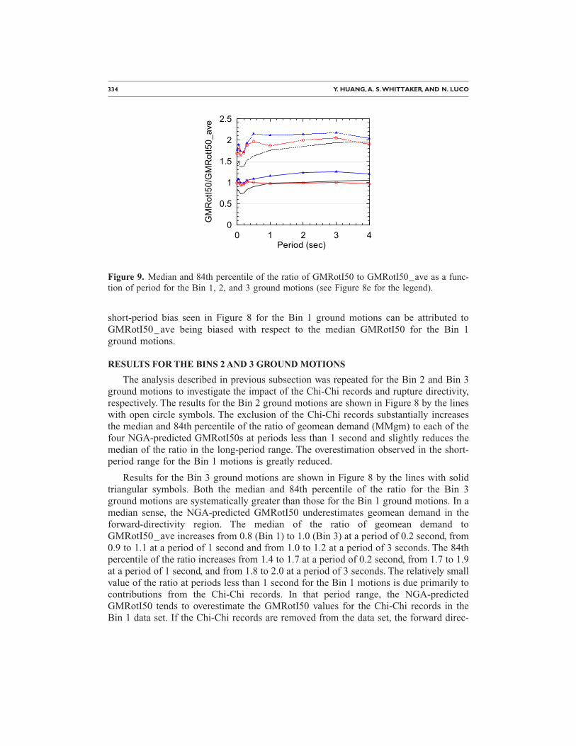
short-period bias seen in Figure 8 for the Bin 1 ground motions can be attributed toGMRotI50_ave being biased with respect to the median GMRotI50 for the Bin 1ground motions.

RESULTS FOR THE BINS 2 AND 3 GROUND MOTIONS

The analysis described in previous subsection was repeated for the Bin 2 and Bin 3ground motions to investigate the impact of the Chi-Chi records and rupture directivity,respectively. The results for the Bin 2 ground motions are shown in Figure 8 by the lineswith open circle symbols. The exclusion of the Chi-Chi records substantially increasesthe median and 84th percentile of the ratio of geomean demand (MMgm) to each of thefour NGA-predicted GMRotI50s at periods less than 1 second and slightly reduces themedian of the ratio in the long-period range. The overestimation observed in the short-period range for the Bin 1 motions is greatly reduced.

Results for the Bin 3 ground motions are shown in Figure 8 by the lines with solidtriangular symbols. Both the median and 84th percentile of the ratio for the Bin 3ground motions are systematically greater than those for the Bin 1 ground motions. In amedian sense, the NGA-predicted GMRotI50 underestimates geomean demand in theforward-directivity region. The median of the ratio of geomean demand toGMRotI50_ave increases from 0.8 (Bin 1) to 1.0 (Bin 3) at a period of 0.2 second, from0.9 to 1.1 at a period of 1 second and from 1.0 to 1.2 at a period of 3 seconds. The 84thpercentile of the ratio increases from 1.4 to 1.7 at a period of 0.2 second, from 1.7 to 1.9at a period of 1 second, and from 1.8 to 2.0 at a period of 3 seconds. The relatively smallvalue of the ratio at periods less than 1 second for the Bin 1 motions is due primarily tocontributions from the Chi-Chi records. In that period range, the NGA-predictedGMRotI50 tends to overestimate the GMRotI50 values for the Chi-Chi records in theBin 1 data set. If the Chi-Chi records are removed from the data set, the forward direc-

0 1 2 3 4Period (sec)

0

0.5

1

1.5

2

2.5

GMRotI50/GMRotI50_ave

Figure 9. Median and 84th percentile of the ratio of GMRotI50 to GMRotI50_ave as a func-tion of period for the Bin 1, 2, and 3 ground motions (see Figure 8e for the legend).

MAXIMUM SPECTRAL DEMANDS IN THE NEAR-FAULT REGION 335

tivity effects are small in the short-period range but still considerable in the long-periodrange. Similar trends are observed in Figure 9 for the ratio of GMRotI50 toGMRotI50_ave and the ground motions of Bins 2 and 3.

RELATIONSHIPS BETWEEN MAXIMUM SPECTRAL DEMANDAND NGA-PREDICTED GMRotI50

RESULTS FOR BINS 1, 2, AND 3 GROUND MOTIONS

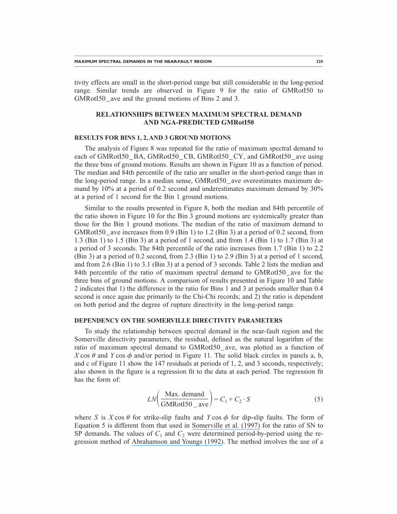
The analysis of Figure 8 was repeated for the ratio of maximum spectral demand toeach of GMRotI50_BA, GMRotI50_CB, GMRotI50_CY, and GMRotI50_ave usingthe three bins of ground motions. Results are shown in Figure 10 as a function of period.The median and 84th percentile of the ratio are smaller in the short-period range than inthe long-period range. In a median sense, GMRotI50_ave overestimates maximum de-mand by 10% at a period of 0.2 second and underestimates maximum demand by 30%at a period of 1 second for the Bin 1 ground motions.

Similar to the results presented in Figure 8, both the median and 84th percentile ofthe ratio shown in Figure 10 for the Bin 3 ground motions are systemically greater thanthose for the Bin 1 ground motions. The median of the ratio of maximum demand toGMRotI50_ave increases from 0.9 (Bin 1) to 1.2 (Bin 3) at a period of 0.2 second, from1.3 (Bin 1) to 1.5 (Bin 3) at a period of 1 second, and from 1.4 (Bin 1) to 1.7 (Bin 3) ata period of 3 seconds. The 84th percentile of the ratio increases from 1.7 (Bin 1) to 2.2(Bin 3) at a period of 0.2 second, from 2.3 (Bin 1) to 2.9 (Bin 3) at a period of 1 second,and from 2.6 (Bin 1) to 3.1 (Bin 3) at a period of 3 seconds. Table 2 lists the median and84th percentile of the ratio of maximum spectral demand to GMRotI50_ave for thethree bins of ground motions. A comparison of results presented in Figure 10 and Table2 indicates that 1) the difference in the ratio for Bins 1 and 3 at periods smaller than 0.4second is once again due primarily to the Chi-Chi records; and 2) the ratio is dependenton both period and the degree of rupture directivity in the long-period range.

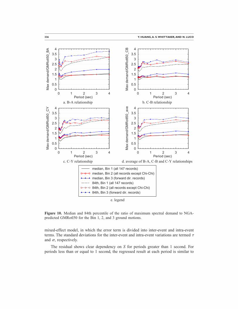
DEPENDENCY ON THE SOMERVILLE DIRECTIVITY PARAMETERS

To study the relationship between spectral demand in the near-fault region and theSomerville directivity parameters, the residual, defined as the natural logarithm of theratio of maximum spectral demand to GMRotI50_ave, was plotted as a function ofX cos � and Y cos � and/or period in Figure 11. The solid black circles in panels a, b,and c of Figure 11 show the 147 residuals at periods of 1, 2, and 3 seconds, respectively;also shown in the figure is a regression fit to the data at each period. The regression fithas the form of:

LN� Max. demand

GMRotI50 _ ave� = C1 + C2 · S �5�

where S is X cos � for strike-slip faults and Y cos � for dip-slip faults. The form ofEquation 5 is different from that used in Somerville et al. (1997) for the ratio of SN toSP demands. The values of C1 and C2 were determined period-by-period using the re-gression method of Abrahamson and Youngs (1992). The method involves the use of a

336 Y. HUANG, A. S.WHITTAKER, AND N. LUCO

mixed-effect model, in which the error term is divided into inter-event and intra-eventterms. The standard deviations for the inter-event and intra-event variations are termed �and �, respectively.

The residual shows clear dependency on S for periods greater than 1 second. Forperiods less than or equal to 1 second, the regressed result at each period is similar to

0 1 2 3 4Period (sec)

00.51

1.52

2.53

3.54

Maxdemand/GMRotI50_BA

0 1 2 3 4Period (sec)

00.51

1.52

2.53

3.54

Maxdemand/GMRotI50_CB

a. B-A relationship b. C-B relationship

0 1 2 3 4Period (sec)

00.51

1.52

2.53

3.54

Maxdemand/GMRotI50_CY

0 1 2 3 4Period (sec)

00.51

1.52

2.53

3.54

Maxdemand/GMRotI50_ave

c. C-Y relationship d. average of B-A, C-B and C-Y relationships

median, Bin 1 (all 147 records)median, Bin 2 (all records except Chi-Chi)median, Bin 3 (forward dir. records)84th, Bin 1 (all 147 records)84th, Bin 2 (all records except Chi-Chi)84th, Bin 3 (forward dir. records)

e. legend

Figure 10. Median and 84th percentile of the ratio of maximum spectral demand to NGA-predicted GMRotI50 for the Bin 1, 2, and 3 ground motions.

MAXIMUM SPECTRAL DEMANDS IN THE NEAR-FAULT REGION 337

that presented in the second column of Table 2 (Bin 1, median) and doesn’t show cleardependency on S. Values for C1, C2, �, and � are presented in Table 3 for periods of 1,2, 3, and 4 seconds.

Figure 11d shows the exponential values of the regression fits (equivalent to the ratioof maximum demand to GMRotI50_ave) at periods of 1, 2, 3, and 4 seconds to identifythe effect of period on the residuals. The slope of the curve increases as the period in-creases. For a period of 4 seconds and S equal to 1, the regressed ratio of maximumdemand to GMRotI50_ave is 2.4.

ESTIMATING MAXIMUM SPECTRAL DEMANDS GIVEN GMRotI50

In near-fault regions in coastal California, the ordinates of the Maximum ConsideredEarthquake spectrum (FEMA 2004) are established by probabilistic seismic hazardanalysis subject to a deterministic limit of 150% of the median geomean demand of acharacteristic or maximum-magnitude earthquake. If maximum demand rather thanGMRotI50 demand is to be used as the basis for the deterministic limit, the medianmaximum spectral demand can be estimated by increasing the prediction forGMRotI50_ave by the factors presented in either column 2 of Table 2 (Bin 1, median)for average-directivity demand or column 6 of Table 2 (Bin 3, median) for forward-directivity demand. For a structure with a period greater than 1 second located at a near-fault site with a potential value of X cos � or Y cos � close to 1 (which presumes a prioriknowledge of the epicenter), the median value for the ratio of maximum spectral de-mand to GMRotI50_ave will be greater than that proposed in column 2 of Table 2;Equation 5 can be used to estimate the maximum spectral demand for this case.

Beyond the deterministic regions of the seismic hazard maps, where probabilistic

Table 2. Median and 84th percentile of the ratio of maximum spectral demand toGMRotI50_ave demand for the Bin 1, 2, and 3 ground motions

Bin 1(All Earthquake

Records)

Bin 2(No Chi-Chi

Earthquake Records)

Bin 3(Forward-DirectivityEarthquake Records)

Period(Seconds) Median

84thPercentile Median

84thPercentile Median

84thPercentile

0 1.0 1.8 1.2 2.1 1.3 2.20.05 1.0 1.8 1.2 2.2 1.3 2.30.1 0.9 1.7 1.1 2.0 1.2 2.10.2 0.9 1.7 1.2 2.1 1.2 2.20.3 1.0 1.9 1.3 2.4 1.3 2.50.5 1.2 2.1 1.3 2.6 1.4 2.81 1.3 2.3 1.3 2.5 1.5 2.92 1.3 2.5 1.3 2.7 1.6 2.93 1.4 2.6 1.3 2.9 1.7 3.14 1.4 2.7 1.3 2.7 1.7 3.0

rameters for the Bin 1 ground motions.

338 Y. HUANG, A. S.WHITTAKER, AND N. LUCO

Table 3. Coefficients for Equation 5 relating the ratioof maximum spectral demand over GMRotI50_aveto the Somerville et al. (1997) directivity parameter

Period(Seconds) C1 C2 � �

1 0.21 0.04 0.51 0.412 0.08 0.39 0.53 0.453 0.00 0.69 0.53 0.414 −0.07 0.95 0.53 0.39

0 0.2 0.4 0.6 0.8 1Xcos� or Ycos�

-3

-2

-1

0

1

2

3LN(Max/GMRotI50_ave)

Regression result

0 0.2 0.4 0.6 0.8 1Xcos� or Ycos�

-3

-2

-1

0

1

2

3

LN(Max/GMRotI50_ave)

a. T= 1 second b. T= 2 seconds

0 0.2 0.4 0.6 0.8 1Xcos� or Ycos�

-3

-2

-1

0

1

2

3

LN(Max/GMRotI50_ave)

0 0.2 0.4 0.6 0.8 1Xcos� or Ycos�

0

0.5

1

1.5

2

2.5

3

Max/GMRotI50_ave

1 sec2 secs3 secs4 secs

c. T= 3 seconds d. regression results

Figure 11. Ratios of maximum spectral demand to GMRotI50_ave at periods of 1, 2, and 3seconds, and the regression results as a function of period and the Somerville directivity pa-

MAXIMUM SPECTRAL DEMANDS IN THE NEAR-FAULT REGION 339

seismic hazard analysis (PSHA) is used to characterize spectral demands, maximumspectral demand should be computed using attenuation functions that predict maximumdemand. However, such functions do not exist at this time. As an interim measure, maxi-mum spectral demand for a given return period could be estimated by increasing thePSHA-based predictions for GMRotI50 by the factors described above. However, wenote that this straightforward procedure will not be exact unless: 1) the ratio of maxi-mum to NGA-predicted GMRotI50 spectral demand is independent of moment magni-tude, distance, and all other variables used in the attenuation relationships; and 2) thedispersion in the maximum spectral demand is equal to that in GMRotI50.

CONCLUSIONS

One hundred and forty-seven pairs of ground-motion records with MW greater than6.5 and r smaller than 15 km were selected from the PEER NGA database and analyzedto investigate the relationships between maximum, MMgm, SN and SP, GMRotI50, andNGA-predicted GMRotI50 spectral demand for periods from 0 to 4 seconds in the near-fault region. The following conclusions can be drawn from the study:

1. For periods greater than or equal to 2 seconds and closest site-to-fault distancesless than 3 to 5 km, the probability of the ratio of maximum to SN spectral de-mands being less than 1.05 is 50+%. For all other periods and distances, SNspectral demands should not be used to represent maximum demand.

2. The median of the ratio of the maximum spectral demand to MMgm rangesfrom 1.2 to 1.45 and that of maximum demand to GMRotI50 ranges from 1.2 to1.3 in the period range from 0 to 4 seconds. The results for the latter ratio agreewell with that of Beyer and Bommer (2006).

3. Based on analysis using all of the records in our near-fault data set, in a mediansense the NGA-predicted GMRotI50 overestimates MMgm and GMRotI50 inthe short-period range and estimates geomean demand with less than 10% errorin the long-period range. For our forward-directivity subset of records, theNGA-predicted GMRotI50 underestimates MMgm and GMRotI50 in the long-period range, again in a median sense.

4. The median of the ratio of maximum spectral demand to the average NGA-predicted GMRotI50 �GMRotI50_ave� in the near-fault region is dependent onperiod and the Somerville directivity parameters. For X cos � �Y cos �� greaterthan 0.3 and period greater than 1 second, this ratio increases with both periodand X cos � �Y cos ��.

5. Scale factors have been developed in this study to transform GMRotI50_ave tomaximum demand in the near-fault region for average directivity, forward di-rectivity, and furthermore, for worst-case directivity. At periods of 0.2, 1.0, and3.0 seconds, the scale factors are (0.9, 1.3, 1.4) for average directivity, (1.2, 1.5,1.7) for forward directivity, and (1.2, 1.5, and 2.0) for worst-case directivity.

340 Y. HUANG, A. S.WHITTAKER, AND N. LUCO

ACKNOWLEDGMENTS

The original Fortran codes for the three NGA relationships were provided byStephen Harmsen of the USGS. The authors acknowledge this important contribution tothis study and his review of an early draft of this manuscript. The authors thank DavidWald of the USGS and the anomymous reviewers for their thoughtful comments on thedraft manuscript.

NOTATIONC1 = Period-dependent translation coefficient in Equation 5C2 = Period-dependent transformation coefficient in Equation 5GMRotI50 = Rotated geomean spectral demand per Boore et al. (2006)MMgm = Geometric mean of the maximum and minimum spectral demands for a

rotated pair of ground motionsMW = Moment magnituder = Closest distance from the recording site to the ruptured fault areaS = Directivity parameter in Equation 5SN = Strike normalSP = Strike parallelV30 = Shear wave velocity in the upper 30 m of a soil columnX = Rupture directivity length ratio a la Somerville et al. (1997)Y = Rupture directivity width ratio a la Somerville et al. (1997)y16th = 16th percentile of a ratio of spectral demands, also denoted Yy84th = 84th percentile of the ratio of spectral demands�Y = Logarithmic standard deviation of the ratio of spectral demands� = Zenith angle between the fault plane and the ray path to the site for dip-

slip faults, a la Somerville et al. (1997)� = Azimuth angle between the fault plane and the ray path to the site for

strike-slip faults, a la Somerville et al. (1997)�Y = Median of the previously mentioned ratio of spectral demands� = Standard deviation for the intra-event variation in a mixed-effect model� = Standard deviation for the inter-event variation in a mixed-effect model

REFERENCES

Abrahamson, N. A., 2000. Effects of rupture directivity on probabilistic seismic hazard analy-sis, Proceedings, 6th International Conference on Seismic Zonation, Palm Springs, CA.

Abrahamson, N. A., and Silva, W. J., 1997. Empirical response spectral attenuation relations forshallow crustal earthquakes, Seismol. Res. Lett. 68, 94–127.

Abrahamson, N. A., and Youngs, R. R., 1992. A stable algorithm for regression analyses usingthe random effects model, Bull. Seismol. Soc. Am. 82, 505–510.

Beyer, K., and Bommer, J. J., 2006. Relationships between median values and between aleatoryvariabilities for different definitions of the horizontal component of motion, Bull. Seismol.Soc. Am. 96, 1512–1522.

Boore, D. M., and Atkinson, G. M., 2008. Ground-motion prediction equations for the average

MAXIMUM SPECTRAL DEMANDS IN THE NEAR-FAULT REGION 341

horizontal component of PGA, PGV, and 5%-damped PSA at spectral periods between 0.01s and 10.0 s, Earthquake Spectra 24, 99–138.

Boore, D. M., Watson-Lamprey, J., and Abrahamson, N. A., 2006. Orientation-independentmeasures of ground motion, Bull. Seismol. Soc. Am. 96, 1502–1511.

Campbell, K. W., and Bozorgnia, Y., 2008. NGA ground motion model for the geometric meanhorizontal component of PGA, PGV, PGD, and 5% damped linear elastic response spectrafor periods ranging from 0.01 to 10 s, Earthquake Spectra 24, 139–171.

Chiou, B. S.-J., and Youngs, R. R., 2008. An NGA model for the average horizontal componentof peak ground motion and response spectra, Earthquake Spectra 24, 173–215.

Federal Emergency Management Agency (FEMA), 2004. NEHRP recommended provisions forseismic regulations for new buildings and other structures: Provisions and Commentary, Re-port No. 450-1 and 450-2, Washington, D.C.

Howard, J. K., Tracy, C. A., and Burns, R. G., 2005. Comparing observed and predicted direc-tivity in near-source ground motion, Earthquake Spectra 21, 1063–1092.

Somerville, P. G., Smith, N. F., and Graves, R. W., 1997. Modification of empirical strongground motion attenuation relations to include the amplitude and duration effects of rupturedirectivity, Seismol. Res. Lett. 68, 94–127.

(Received 30 June 2007; accepted 15 November 2007�