Maximizing the profitability of forestry projects under the Clean Development Mechanism using a...

Maximizing the profitability of forestry projects under the Clean

Development Mechanism using a forest management optimization model

Vıctor Hugo Gutierrez *, Mauricio Zapata, Carlos Sierra,William Laguado, Alı Santacruz

Research Center on Ecosystems and Global Change, Carbono & Bosques (C&B),

Calle 51 # 72-07, Int. 708, Medellın, Colombia

Received 14 September 2005; received in revised form 3 February 2006; accepted 3 February 2006

Abstract

Forestry projects under the Clean Development Mechanism (CDM) may provide several benefits for developing countries. Under the current

rules, these projects can participate in both timber and carbon markets. Thus, project developers need to know what the optimal forest management

design would be to maximize their revenues according to timber and carbon market expectations while at the same time complying with

international rules adopted for carbon sequestration projects under the CDM.

We developed Carbomax, a management optimization model that simulates forest growth under different forest management regimes (intensity

and frequency of thinnings and rotation lengths). A genetic algorithm was used to find the management regime that maximizes the Annual

Equivalent Value (AEV) of projects under different market scenarios.

We tested our model under a wide variety of possible scenarios for forestry projects. Five tropical plantation species (Alnus jorullensis, Cordia

alliodora, Pinus patula, Cupressus lusitanica and Eucalyptus grandis) were evaluated, at discount rates of 4, 7 and 10%, and certified emissions

reduction (CER) prices of US$3, 7, 10 and 13. Temporary CERs (tCERs) and long-term CERs (lCERs) prices were considered in the evaluation and

were calculated as a variable proportion of CER price.

Results showed that optimal forest management is sensible to carbon and timber market conditions. Under each discount rate, as CER price

increased, frequency and intensity of thinnings tended to decrease and optimal thinnings and rotation lengths tended to be reached at older ages.

The largest AEV were obtained with discount rates of 10%, CER prices of US$13 and rotation lengths of 40 years for all species. For those species

with higher timber prices, thinnings tended to be more frequent and at early ages of the plantation. For all species optimal thinnings were found at

35 years of plantation age. tCERs was selected by the model as the best choice to maximize the profitability of the projects.

# 2006 Elsevier B.V. All rights reserved.

Keywords: Forest management; Simulation; Profitability; Optimization; lCERs; tCERs; Genetic algorithm; CDM; Growth equations; Carbon sequestration

www.elsevier.com/locate/foreco

Forest Ecology and Management 226 (2006) 341–350

1. Introduction

According to the Kyoto Protocol, projects under the Clean

Development Mechanism (CDM) have to be designed to

promote sustainable development in developing countries

while at the same time can be used to assist developed

countries to reach their emission reduction targets (UNFCCC,

1997). Forestry activities can help to achieve these objectives

because well-designed projects generate important environ-

mental and social collateral benefits like water regulation,

erosion amelioration, habitat improvement and employment

* Corresponding author. Tel.: +57 4 230 08 76; fax: +57 4 230 08 76.

E-mail address: [email protected] (V.H. Gutierrez).

0378-1127/$ – see front matter # 2006 Elsevier B.V. All rights reserved.

doi:10.1016/j.foreco.2006.02.002

generation, among others (Ji and Junfeng, 2000; Garcia et al.,

2005; IUCN, 2006).

However, forest activities have detractors because CO2

absorbed by forests is not permanently sequestered. This

‘‘crunch’’ issue was addressed in the ninth Conference of the

Parties (COP9), in which modalities and procedures for forestry

projects under the CDM were approved. According to COP9

rules, forestry credits are issued for a limited period of time, at

the end of which, they have to be renewed or replaced for other

valid units (AAUs, CERs, ERUs and RMUs) before their expiry

date (UNFCCC, 2003).

Decisions adopted about non-permanence in COP9 allow

forestry projects to obtain revenues from both certified

emission reductions (CERs) and timber. Nevertheless, timber

and CERs prices will be variable and, as it will be shown below,

mailto:[email protected]

http://dx.doi.org/10.1016/j.foreco.2006.02.002

V.H. Gutierrez et al. / Forest Ecology and Management 226 (2006) 341–350342

decisions made in forest management to favor revenues from

one of these two sources of incomes, will affect negatively the

incomes received from the other. This is the reason why project

developers need appropriate tools to know what could be the

forest management regime (frequency and intensity of

thinnings and rotation lengths) to maximize their revenues

from these two sources of incomes.

We developed Carbomax as a management optimization

model for forestry projects under the CDM. Carbomax

simulates different management regimes and finds the one

that maximize the profitability of projects, depending on

carbon sequestration and timber production capacity of the

species considered and expectancies about carbon and timber

markets.

The first part of this paper describes the general structure of

the model. In the second part, the following two basic

hypotheses were tested through its application to a case study in

Colombia: (1) optimal forest management is strongly

influenced by carbon and timber market scenarios. (2) tCERs

will be more profitable for forestry projects under the CDM

because they give more flexibility to forest management.

2. Model structure

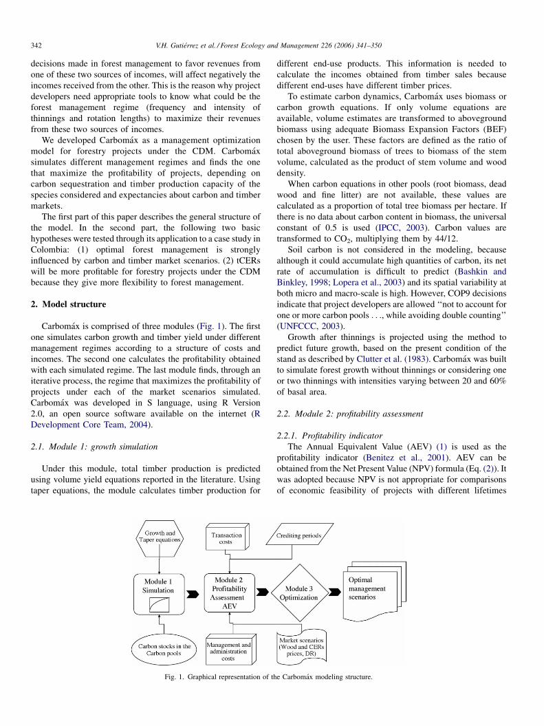
Carbomax is comprised of three modules (Fig. 1). The first

one simulates carbon growth and timber yield under different

management regimes according to a structure of costs and

incomes. The second one calculates the profitability obtained

with each simulated regime. The last module finds, through an

iterative process, the regime that maximizes the profitability of

projects under each of the market scenarios simulated.

Carbomax was developed in S language, using R Version

2.0, an open source software available on the internet (R

Development Core Team, 2004).

2.1. Module 1: growth simulation

Under this module, total timber production is predicted

using volume yield equations reported in the literature. Using

taper equations, the module calculates timber production for

Fig. 1. Graphical representation of th

different end-use products. This information is needed to

calculate the incomes obtained from timber sales because

different end-uses have different timber prices.

To estimate carbon dynamics, Carbomax uses biomass or

carbon growth equations. If only volume equations are

available, volume estimates are transformed to aboveground

biomass using adequate Biomass Expansion Factors (BEF)

chosen by the user. These factors are defined as the ratio of

total aboveground biomass of trees to biomass of the stem

volume, calculated as the product of stem volume and wood

density.

When carbon equations in other pools (root biomass, dead

wood and fine litter) are not available, these values are

calculated as a proportion of total tree biomass per hectare. If

there is no data about carbon content in biomass, the universal

constant of 0.5 is used (IPCC, 2003). Carbon values are

transformed to CO2, multiplying them by 44/12.

Soil carbon is not considered in the modeling, because

although it could accumulate high quantities of carbon, its net

rate of accumulation is difficult to predict (Bashkin and

Binkley, 1998; Lopera et al., 2003) and its spatial variability at

both micro and macro-scale is high. However, COP9 decisions

indicate that project developers are allowed ‘‘not to account for

one or more carbon pools . . ., while avoiding double counting’’

(UNFCCC, 2003).

Growth after thinnings is projected using the method to

predict future growth, based on the present condition of the

stand as described by Clutter et al. (1983). Carbomax was built

to simulate forest growth without thinnings or considering one

or two thinnings with intensities varying between 20 and 60%

of basal area.

2.2. Module 2: profitability assessment

2.2.1. Profitability indicator

The Annual Equivalent Value (AEV) (1) is used as the

profitability indicator (Benitez et al., 2001). AEV can be

obtained from the Net Present Value (NPV) formula (Eq. (2)). It

was adopted because NPV is not appropriate for comparisons

of economic feasibility of projects with different lifetimes

e Carbomax modeling structure.

V.H. Gutierrez et al. / Forest Ecology and Management 226 (2006) 341–350 343

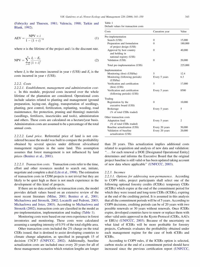
Table 1

Default values for transaction costs

Costs Causation year Value

Pre-implementation

Search (US$) 0 15,000

Preparation and formulation

of project design (US$)

0 180,000

Approval by host country

and holding in

national registry (US$)

0 40,000

Validation (US$) 0 20,000

Total pre-implementation (US$) 225,000

Implementation

Monitoring (first) (US$/ha) 5 12.4

Monitoring (following periods)

(US$/ha)

Every 5 years 6.3

Verification and certification

(first) (US$)

5 17,000

Verification and certification

(following periods) (US$)

Every 5 years 8500

Trading

Registration by the

executive board (US$)

0 10,000

Brokerage

(% of total CERs traded)

Every 5 years 5

Other transaction costs

Adaptation fund

(% of total CERs traded)

Every 5 years 2

Baseline actualization (US$) Every 20 years 50,000

Validation of baseline

actualization (US$)

Every 20 years 20,000

(Fabrycky and Thuesen, 1981; Valencia, 1988; Tarkin and

Blank, 1992).

AEV ¼ NPV� i

1� ð1þ iÞ�n (1)

where n is the lifetime of the project and i is the discount rate.

NPV ¼Xn

t¼0

It � Et

ð1þ iÞt(2)

where It is the incomes incurred in year t (US$) and Et is the

costs incurred in year t (US$).

2.2.2. Costs

2.2.2.1. Establishment, management and administration cost-

s. In this module, projected costs incurred over the whole

lifetime of the plantation are considered. Operational costs

include salaries related to planting and management (ground

preparation, laying-out, digging, transportation of seedlings,

planting, pest control, fertilization, replanting, weeding, road

maintenance, fire protection, pruning and thinning) materials

(seedlings, fertilizers, insecticides and tools), administration

and others. These costs are calculated on a hectare/year basis.

Administration costs are assumed to be a percentage of the total

annual costs.

2.2.2.2. Land price. Referential price of land is not con-

sidered because the model was built to compare the profitability

obtained by several species under different silvicultural

management regimes in the same land. This assumption

assumes that forest management is not influenced by land

prices (Benitez et al., 2001).

2.2.2.3. Transaction costs. Transaction costs refer to the time,

effort and other resources needed to search out, initiate,

negotiate and complete a deal (Lile et al., 1998). The estimation

of transaction costs in CDM projects is not trivial but they are

likely to be quiet high as there is not much experience in the

development of this kind of projects.

If there are no data available on transaction costs, the model

provides default values based on an extensive review of the

most recent literature (Milne, 2001; Benitez et al., 2001;

Michaelowa and Stronzik, 2002; Locatelli and Pedroni, 2003;

Michaelowa and Jotzo, 2003). According to Michaelowa and

Stronzik (2002), transaction costs are classified in the model as

pre-implementation, implementation and trading (Table 1).

Monitoring costs were based on our own experience in forest

inventories and monitoring. These costs were calculated

assuming a sampling intensity of 0.5% of the total eligible area.

Other transaction costs included the 2% charge on the total

CERs issued, that is destined to assist developing countries to

climate change adaptation, as specified in paragraph 15 of

decision 17/CP.7 (UNFCCC, 2002). Additionally, baseline

actualization costs are included once every 20 years for all of

those management scenarios which rotation lengths are longer

than 20 years. This actualization implies additional costs

related to acquisition and analysis of new data and validation:

‘‘. . . for each renewal a DOE [Designated Operational Entity]

determines and informs the Executive Board that the original

project baseline is still valid or has been updated taking account

of new data where applicable’’ (UNFCCC, 2003).

2.2.3. Incomes

2.2.3.1. Options for addressing non-permanence. According

to COP9 rules, project participants shall select one of the

following optional forestry credits (fCERs): temporary CERs

(tCERs) which expire at the end of the commitment period for

which they were issued and long-term CERs (lCERs), expiring

at the end of the crediting period. It is assumed in this analysis

that all the commitment periods will be of 5 years. According to

COP9 decisions, crediting periods can be of 20 years with two

possible renewals or 30 years without renewals. Once fCERs

expire, developed countries have to renew or replace them with

other valid units approved in the Kyoto Protocol (CERs, AAUs

or ERUs) (UNFCCC, 2003). Because of the uncertainty on

what kind of fCERs will be more profitable for forestry

projects, Carbomax evaluates the profitability obtained under

each management regime for the case of both tCERs and

lCERs.

According to COP9 rules, if the lCERs option is selected,

carbon stocks at the end of a commitment period should have

increased since the previous certification report (UNFCCC,


2003). Carbomax introduces this rule as a restriction in this

module. If any management regime does not guarantee this

condition, the solution is discarded by the model.

2.2.3.2. fCERs valuation. Current approaches concerning

fCERs values are based on expectancies about future price

of permanent CERs (Dutschke and Schlamadinger, 2003;

Locatelli and Pedroni, 2003; Dutschke et al., 2004). Depending

on the expected discount rate and the value of a fCER, incomes

expected from 1 t of CO2 stored in vegetation at the end of the

commitment period i + 1 are calculated as follows:

fCERiþ1 ¼CERi

ð1þ IiÞi� CERed

ð1þ IedÞed(3)

where ed is the expiring date of the credits. For tCERs, ed is

equal to i + 1. For lCERs, ed is equal to the crediting period for

which fCERs will be issued (20 which may be renewed at twice

or 30 years without renewals).

Carbomax gives the option to assume constant or variable

CER prices, according to market tendencies. Also, it is possible

to discount a percentage of the CERs issued attributable to

leakage.

Discount rate employed for fCERs valuation ‘‘expresses

price expectances of the market participants. It is influenced by

the interest rate as well as expectations on the stringency of

future emission-limitation commitments’’ (Dutschke and

Schlamadinger, 2003). Under this model, it is possible to

assume constant or dynamic discount rates, according to market

tendencies.

To calculate revenues from timber, Carbomax requires timber

prices for different end-uses (lumber, pulpwood, etc.) for each

one of the species considered. This value can be constant or

dynamic over time, depending upon market expectances.

2.3. Module 3: optimization

This module uses a genetic algorithm to optimize forest

management. This is an adaptive, stochastic model which

incorporates principia of natural selection to find optimal

solutions. It is very useful to solve large optimization problems

with multiple local optima (Ansari and Hou, 1997; Fouskakis

and Draper, 2002).

In this case, solutions from the previous two modules are

evaluated by a fitness function, defined in this case as the AEV

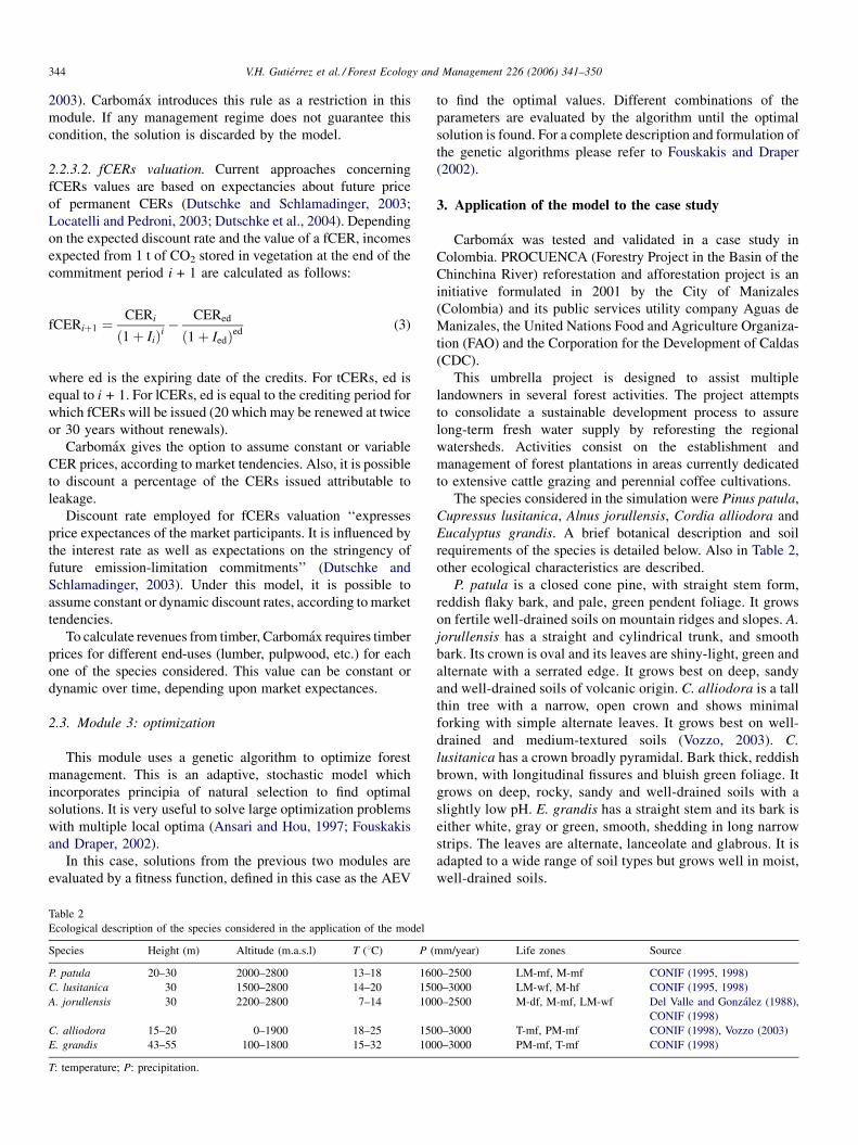
Table 2

Ecological description of the species considered in the application of the model

Species Height (m) Altitude (m.a.s.l) T (8C) P (

P. patula 20–30 2000–2800 13–18 160

C. lusitanica 30 1500–2800 14–20 150

A. jorullensis 30 2200–2800 7–14 100

C. alliodora 15–20 0–1900 18–25 150

E. grandis 43–55 100–1800 15–32 100

T: temperature; P: precipitation.

to find the optimal values. Different combinations of the

parameters are evaluated by the algorithm until the optimal

solution is found. For a complete description and formulation of

the genetic algorithms please refer to Fouskakis and Draper

(2002).

3. Application of the model to the case study

Carbomax was tested and validated in a case study in

Colombia. PROCUENCA (Forestry Project in the Basin of the

Chinchina River) reforestation and afforestation project is an

initiative formulated in 2001 by the City of Manizales

(Colombia) and its public services utility company Aguas de

Manizales, the United Nations Food and Agriculture Organiza-

tion (FAO) and the Corporation for the Development of Caldas

(CDC).

This umbrella project is designed to assist multiple

landowners in several forest activities. The project attempts

to consolidate a sustainable development process to assure

long-term fresh water supply by reforesting the regional

watersheds. Activities consist on the establishment and

management of forest plantations in areas currently dedicated

to extensive cattle grazing and perennial coffee cultivations.

The species considered in the simulation were Pinus patula,

Cupressus lusitanica, Alnus jorullensis, Cordia alliodora and

Eucalyptus grandis. A brief botanical description and soil

requirements of the species is detailed below. Also in Table 2,

other ecological characteristics are described.

P. patula is a closed cone pine, with straight stem form,

reddish flaky bark, and pale, green pendent foliage. It grows

on fertile well-drained soils on mountain ridges and slopes. A.

jorullensis has a straight and cylindrical trunk, and smooth

bark. Its crown is oval and its leaves are shiny-light, green and

alternate with a serrated edge. It grows best on deep, sandy

and well-drained soils of volcanic origin. C. alliodora is a tall

thin tree with a narrow, open crown and shows minimal

forking with simple alternate leaves. It grows best on well-

drained and medium-textured soils (Vozzo, 2003). C.

lusitanica has a crown broadly pyramidal. Bark thick, reddish

brown, with longitudinal fissures and bluish green foliage. It

grows on deep, rocky, sandy and well-drained soils with a

slightly low pH. E. grandis has a straight stem and its bark is

either white, gray or green, smooth, shedding in long narrow

strips. The leaves are alternate, lanceolate and glabrous. It is

adapted to a wide range of soil types but grows well in moist,

well-drained soils.

mm/year) Life zones Source

0–2500 LM-mf, M-mf CONIF (1995, 1998)

0–3000 LM-wf, M-hf CONIF (1995, 1998)

0–2500 M-df, M-mf, LM-wf Del Valle and Gonzalez (1988),

CONIF (1998)

0–3000 T-mf, PM-mf CONIF (1998), Vozzo (2003)

0–3000 PM-mf, T-mf CONIF (1998)


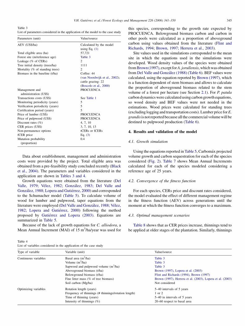
Table 3

List of parameters considered in the application of the model to the case study

Parameters (unit) Value/source

AEV (US$/ha) Calculated by the model

using Eq. (1)

Total eligible area (ha) 57,721

Forest site (m/reference age) Table 3

Leakage (% of CERs) 2

Tree initial density (trees/ha) 1111

Mortality (% of standing trees) 2

Biomass in the baseline (t/ha) Coffee: 44

(van Noordwijk et al., 2002);

cattle grazing: 22

(Boscolo et al., 2000)

Management and

administration (US$)

PROCUENCA

Transactions costs (US$) See Table 1

Monitoring periodicity (years) 5

Verification periodicity (years) 5

Certification period (years) 5

Price of lumber (US$) PROCUENCA

Price of pulpwood (US$) PROCUENCA

Discount rates (%) 4, 7, 10

CER prices (US$) 3, 7, 10, 13

Non-permanence options tCERs or lCERs

fCER price Eq. (3)

Mutation probability

(proportion)

0.4

Data about establishment, management and administration

costs were provided by the project. Total eligible area was

obtained from a pre-feasibility study concluded recently (Black

et al., 2004). The parameters and variables considered in the

application are shown in Tables 3 and 4.

Growth equations were obtained from the literature (Del

Valle, 1979; Velez, 1982; Gonzalez, 1983; Del Valle and

Gonzalez, 1988; Lopera and Gutierrez, 2000) and corresponded

to the Schumacher model (Table 5). To calculate volume of

wood for lumber and pulpwood, taper equations from the

literature were employed (Del Valle and Gonzalez, 1988; Velez,

1982; Lopera and Gutierrez, 2000) following the method

proposed by Gutierrez and Lopera (2003). Equations are

summarized in Table 5.

Because of the lack of growth equations for C. alliodora, a

Mean Annual Increment (MAI) of 15 m3/ha/year was used for

Table 4

List of variables considered in the application of the case study

Type of variable Variable (unit)

Continuous variables Basal area (m2/ha)

Volume (m3/ha)

Sapwood and pulpwood volume (m3/ha)

Aboveground biomass (t/ha)

Belowground biomass (t/ha)

Fine litter mass (% of tree biomass)

Soil carbon (Mg/ha)

Optimizing variables Rotation length (years)

Frequency of thinnings (# thinnings/rotation le

Time of thinning (years)

Intensity of thinnings (%)

this species, corresponding to the growth rate expected by

PROCUENCA. Belowground biomass carbon and carbon in

other pools were calculated as a proportion of aboveground

carbon using values obtained from the literature (Flint and

Richards, 1994; Brown, 1997; Herrera et al., 2003).

Site values used in the simulations corresponded to the mean

site in which the equations used in the simulations were

developed. Wood density values of the species were obtained

from Brown (1997), except for A. jorullensis, which was obtained

from Del Valle and Gonzalez (1988) (Table 6). BEF values were

calculated, using the equation reported by Brown (1997), which

is a function dependent of stem biomass and allows to calculate

the proportion of aboveground biomass related to the stem

volume of a forest per hectare (see Section 2.1). For P. patula

carbon dynamics were calculated using carbon growth equations,

so wood density and BEF values were not needed in the

estimations. Wood prices were calculated for standing trees

(excluding logging and transportation costs). Lumber price for E.

grandis is not reported because all the commercial volumewill be

destined to pulpwood production (Table 6).

4. Results and validation of the model

4.1. Growth simulation

Using the equations reported in Table 5, Carbomax projected

volume growth and carbon sequestration for each of the species

considered (Fig. 2). Table 7 shows Mean Annual Increments

calculated for each of the species modeled considering a

reference age of 25 years.

4.2. Convergence of the fitness function

For each species, CERs price and discount rates considered,

the model evaluated the effect of different management regime

in the fitness function (AEV) across generations until the

moment at which the fitness function converges to a maximum.

4.3. Optimal management scenarios

Table 8 shows that as CER prices increase, thinnings tend to

be applied at older stages of the plantation. Similarly, thinnings

Value/source

Table 3

Table 3

Table 3

Brown (1997), Lopera et al. (2003)

Flint and Richards (1994), Brown (1997)

Brown (1997), Herrera et al. (2003), Lopera et al. (2003)

Not considered

5–40 intervals of 5 years

ngth) 1 or 2

5–40 in intervals of 5 years

20–60 respect to basal area


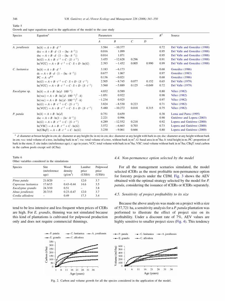
Table 5

Growth and taper equations used in the application of the model to the case study

Species Equationa Parameters R2 Source

A B C D

A. jorullensis lnðhÞ ¼ Aþ B � d�1 3.584 �10.377 0.72 Del Valle and Gonzalez (1988)

dcc ¼ Aþ B � d � ð1� ðhc � h�1ÞÞ 0.016 1.099 0.95 Del Valle and Gonzalez (1988)

dsc ¼ Aþ B � d � ð1� ðhc � h�1ÞÞ 0.014 1.071 0.95 Del Valle and Gonzalez (1988)

lnðGÞ ¼ Aþ B � t�1 þ C � ðS � t�1Þ 3.455 �12.628 0.296 0.91 Del Valle and Gonzalez (1988)

lnðVCCÞ ¼ Aþ B � t�1 þ C � Sþ D � lnðGÞ 2.393 �1.452 0.005 0.990 0.99 Del Valle and Gonzalez (1988)

C. lusitanica lnðhÞ ¼ Aþ B � d�1 3.183 �6.173 0.68 Gonzalez (1986)

dc ¼ Aþ B � d � ð1� ðhc � h�1ÞÞ 0.677 1.067 0.97 Gonzalez (1983)

PC ¼ A � eB�d 0.136 �0.021 0.68 Gonzalez (1986)

lnðGÞ ¼ Aþ B � t�1 þ C � Sþ D � ðS � t�1Þ 2.505 �8.745 0.077 0.152 0.65 Del Valle (1979)

lnðVCCÞ ¼ Aþ B � t�1 þ C � Sþ D � ðS � t�1Þ 3.560 �5.889 0.125 �0.049 0.72 Del Valle (1979)

Eucalyptus sp. lnðhÞ ¼ Aþ B � lnðd � 100�1Þ 4.032 0.589 0.80 Velez (1982)

lnðvccÞ ¼ Aþ B � lnððd � 100�1Þ2 � hÞ �1.051 0.922 0.98 Velez (1982)

lnðvscÞ ¼ Aþ B � lnððd � 100�1Þ2 � hÞ �1.234 0.925 0.97 Velez (1982)

lnðGÞ ¼ Aþ B � t�1 þ C � ðS � t�1Þ 3.824 �8.530 0.223 0.71 Velez (1982)

lnðVCCÞ ¼ Aþ B � t�1 þ C � Sþ D � ðS � t�1Þ 5.480 �10.272 0.018 0.315 0.75 Velez (1982)

P. patula lnðhÞ ¼ Aþ B � lnðdÞ 0.751 0.659 0.38 Lema and Parra (1995)

dsc ¼ Aþ B � lnð1� ðhc � h�1ÞÞ 2.221 0.996 0.90 Gutierrez and Lopera (2003)

lnðGÞ ¼ Aþ B � t�1 þ C � ðS � t�1Þ 4.289 �12.552 0.218 0.92 Lopera and Gutierrez (2000)

lnðVSCÞ ¼ Aþ B � t�1 þ C � lnðGÞ 3.572 �6.663 0.703 0.73 Lopera and Gutierrez (2000)

lnðCBqTÞ ¼ Aþ B � t�1 þ C � lnðGÞ 3.230 �9.061 0.666 0.80 Lopera and Gutierrez (2000)

a d: diameter at breast height in cm; dc: diameter at any height (hc in m) in cm; dcc: diameter at any height with bark in cm; dsc: diameter at any height without bark

in cm; vcc: total volume of a tree, including bark in m3; vsc: total volume of a tree, without bark in m3; G: basal area in m2/ha; h: total height in m; PC: proportion of

bark in the stem; S: site index (m/reference age); t: age in years; VCC: total volume with bark in m3/ha; VSC: total volume without bark in m3/ha; CBqT: total carbon

in the carbon pools except soil (tC/ha).

Table 6

Other variables considered in the simulations

Species Site

(m/reference

age)

Wood

density

(g/cm3)

Lumber

price

(US$/t)

Pulpwood

price

(US$/t)

Pinus patula 21.0/20 – 12.0 3.7

Cupressus lusitanica 17.6/15 0.43–0.44 14.6 3.5

Eucalyptus grandis 24.3/10 0.51 – 3.8

Alnus jorullensis 20.7/15 0.23–0.47 12.0 3.7

Cordia alliodora – 0.49 17.3 3.4

tend to be less intensive and less frequent when prices of CERs

are high. For E. grandis, thinning was not simulated because

this kind of plantations is cultivated for pulpwood production

only and does not require commercial thinnings.

Fig. 2. Carbon and volume growth for all the spec

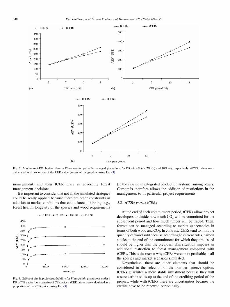
4.4. Non-permanence option selected by the model

For all the management scenarios simulated, the model

selected tCERs as the most profitable non-permanence option

for forestry projects under the CDM. Fig. 3 shows the AEV

obtained with the optimal strategy selected by the model for P.

patula, considering the issuance of tCERs or lCERs separately.

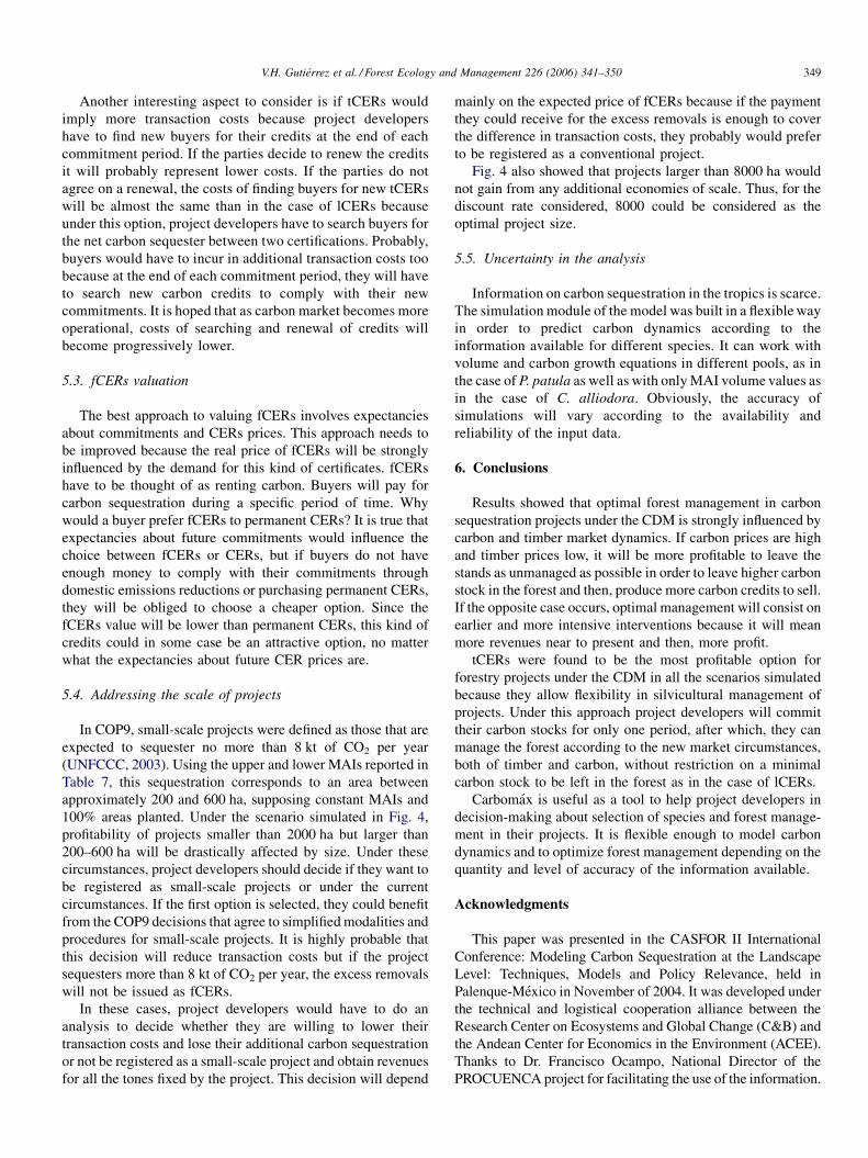
4.5. Sensitivity of project profitability to its size

Because the above analysis was made on a project with a size

of 57,721 ha, a sensitivity analysis for a P. patula plantation was

performed to illustrate the effect of project size on its

profitability. Under a discount rate of 7%, AEV values are

highly sensitive to smaller project sizes (Fig. 4). This tendency

ies considered in the application of the model.


Table 7

Mean Annual Increments (MAIs) in volume and carbon calculated for the

species considered considering a reference age of 25 years

Species MAI V (m3/ha/year) MAI C (t/ha/year)

A. jorullensis 11.54 5.73

C. alliodora 15.00 8.37

C. lusitanica 8.90 3.63

Eucalyptus sp. 13.39 8.07

P. patula 17.81 9.93

Mean 12.89 7.14

is more acute when project size is less than 2000 ha. As eligible

area increases, project profitability tends to an asymptote. For

project sizes above 8000 ha, the influence of area on project

profitability is low, with AEV values corresponding to 96–99%

of the maximum AEV depending on the CER prices simulated.

5. Discussion

5.1. Optimal forest management scenarios

Profitability of forestry projects under the CDM is influenced

by timber and fCER prices. Incomes obtained from one of these

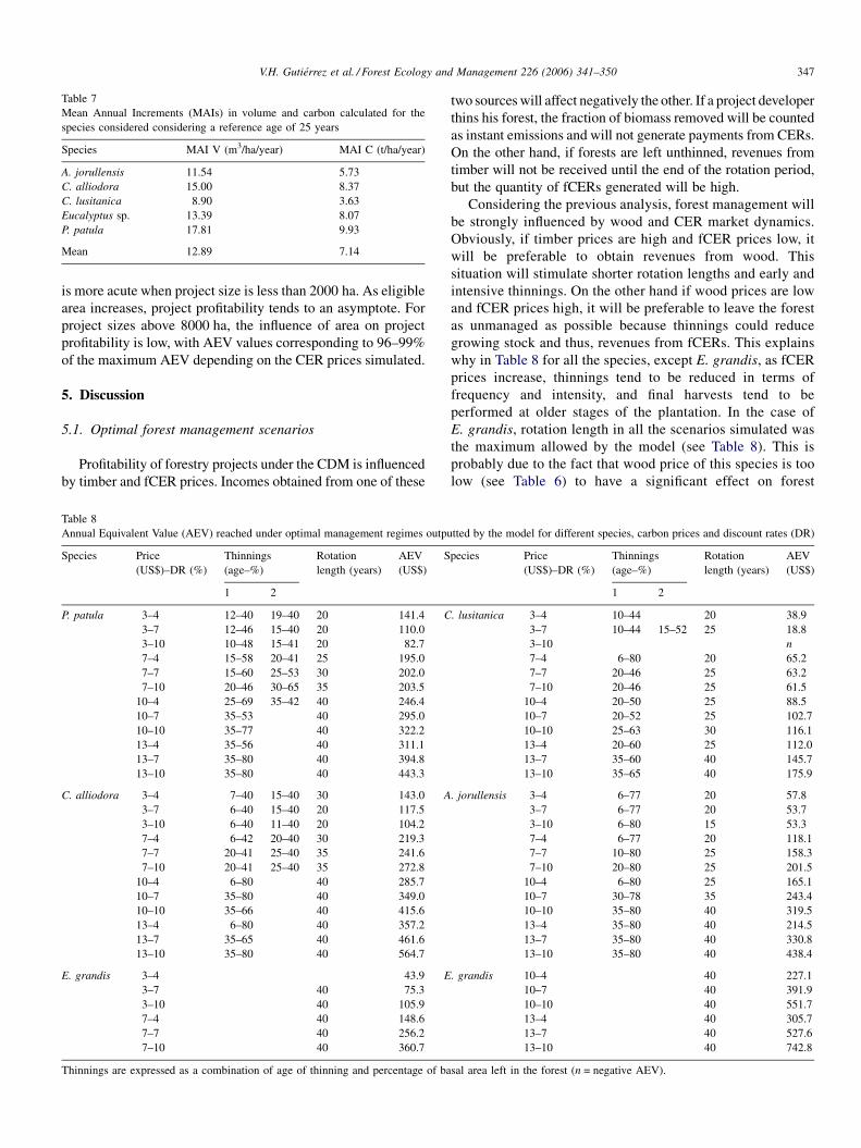
Table 8

Annual Equivalent Value (AEV) reached under optimal management regimes outpu

Species Price

(US$)–DR (%)

Thinnings

(age–%)

Rotation

length (years)

AEV

(US$)

S

1 2

P. patula 3–4 12–40 19–40 20 141.4 C

3–7 12–46 15–40 20 110.0

3–10 10–48 15–41 20 82.7

7–4 15–58 20–41 25 195.0

7–7 15–60 25–53 30 202.0

7–10 20–46 30–65 35 203.5

10–4 25–69 35–42 40 246.4

10–7 35–53 40 295.0

10–10 35–77 40 322.2

13–4 35–56 40 311.1

13–7 35–80 40 394.8

13–10 35–80 40 443.3

C. alliodora 3–4 7–40 15–40 30 143.0 A

3–7 6–40 15–40 20 117.5

3–10 6–40 11–40 20 104.2

7–4 6–42 20–40 30 219.3

7–7 20–41 25–40 35 241.6

7–10 20–41 25–40 35 272.8

10–4 6–80 40 285.7

10–7 35–80 40 349.0

10–10 35–66 40 415.6

13–4 6–80 40 357.2

13–7 35–65 40 461.6

13–10 35–80 40 564.7

E. grandis 3–4 43.9 E

3–7 40 75.3

3–10 40 105.9

7–4 40 148.6

7–7 40 256.2

7–10 40 360.7

Thinnings are expressed as a combination of age of thinning and percentage of ba

two sources will affect negatively the other. If a project developer

thins his forest, the fraction of biomass removed will be counted

as instant emissions and will not generate payments from CERs.

On the other hand, if forests are left unthinned, revenues from

timber will not be received until the end of the rotation period,

but the quantity of fCERs generated will be high.

Considering the previous analysis, forest management will

be strongly influenced by wood and CER market dynamics.

Obviously, if timber prices are high and fCER prices low, it

will be preferable to obtain revenues from wood. This

situation will stimulate shorter rotation lengths and early and

intensive thinnings. On the other hand if wood prices are low

and fCER prices high, it will be preferable to leave the forest

as unmanaged as possible because thinnings could reduce

growing stock and thus, revenues from fCERs. This explains

why in Table 8 for all the species, except E. grandis, as fCER

prices increase, thinnings tend to be reduced in terms of

frequency and intensity, and final harvests tend to be

performed at older stages of the plantation. In the case of

E. grandis, rotation length in all the scenarios simulated was

the maximum allowed by the model (see Table 8). This is

probably due to the fact that wood price of this species is too

low (see Table 6) to have a significant effect on forest

tted by the model for different species, carbon prices and discount rates (DR)

pecies Price

(US$)–DR (%)

Thinnings

(age–%)

Rotation

length (years)

AEV

(US$)

1 2

. lusitanica 3–4 10–44 20 38.9

3–7 10–44 15–52 25 18.8

3–10 n

7–4 6–80 20 65.2

7–7 20–46 25 63.2

7–10 20–46 25 61.5

10–4 20–50 25 88.5

10–7 20–52 25 102.7

10–10 25–63 30 116.1

13–4 20–60 25 112.0

13–7 35–60 40 145.7

13–10 35–65 40 175.9

. jorullensis 3–4 6–77 20 57.8

3–7 6–77 20 53.7

3–10 6–80 15 53.3

7–4 6–77 20 118.1

7–7 10–80 25 158.3

7–10 20–80 25 201.5

10–4 6–80 25 165.1

10–7 30–78 35 243.4

10–10 35–80 40 319.5

13–4 35–80 40 214.5

13–7 35–80 40 330.8

13–10 35–80 40 438.4

. grandis 10–4 40 227.1

10–7 40 391.9

10–10 40 551.7

13–4 40 305.7

13–7 40 527.6

13–10 40 742.8

sal area left in the forest (n = negative AEV).


Fig. 3. Maximum AEV obtained from a Pinus patula optimally managed plantations for DR of: 4% (a), 7% (b) and 10% (c), respectively. t/lCER prices were

calculated as a proportion of the CER value (x-axis of the graphs), using Eq. (3).

management, and then fCER price is governing forest

management decisions.

It is important to consider that not all the simulated strategies

could be really applied because there are other constraints in

addition to market conditions that could force a thinning, e.g.,

forest health, longevity of the species and wood requirements

Fig. 4. Effect of size in project profitability for Pinus patula plantations under a

DR of 7% under four scenarios of CER prices. tCER prices were calculated as a

proportion of the CER price, using Eq. (3).

(in the case of an integrated production system), among others.

Carbomax therefore allows the addition of restrictions in the

management to fit particular project requirements.

5.2. tCERs versus lCERs

At the end of each commitment period, tCERs allow project

developers to decide how much CO2 will be committed for the

subsequent period and how much timber will be traded. Then,

forests can be managed according to market expectancies in

terms of both wood and CO2. In contrast, lCERs tend to limit the

quantity of wood sold because according to current rules, carbon

stocks at the end of the commitment for which they are issued

should be higher than the previous. This situation imposes an

additional restriction to forest management compared with

tCERs. This is the reason why tCERs were more profitable in all

the species and market scenarios simulated.

Nevertheless, there are other elements that should be

considered in the selection of the non-permanence option.

lCERs guarantee a more stable investment because they will

assure carbon sales up to the end of the crediting period of the

project, while with tCERs there are uncertainties because the

credits have to be renewed periodically.


Another interesting aspect to consider is if tCERs would

imply more transaction costs because project developers

have to find new buyers for their credits at the end of each

commitment period. If the parties decide to renew the credits

it will probably represent lower costs. If the parties do not

agree on a renewal, the costs of finding buyers for new tCERs

will be almost the same than in the case of lCERs because

under this option, project developers have to search buyers for

the net carbon sequester between two certifications. Probably,

buyers would have to incur in additional transaction costs too

because at the end of each commitment period, they will have

to search new carbon credits to comply with their new

commitments. It is hoped that as carbon market becomes more

operational, costs of searching and renewal of credits will

become progressively lower.

5.3. fCERs valuation

The best approach to valuing fCERs involves expectancies

about commitments and CERs prices. This approach needs to

be improved because the real price of fCERs will be strongly

influenced by the demand for this kind of certificates. fCERs

have to be thought of as renting carbon. Buyers will pay for

carbon sequestration during a specific period of time. Why

would a buyer prefer fCERs to permanent CERs? It is true that

expectancies about future commitments would influence the

choice between fCERs or CERs, but if buyers do not have

enough money to comply with their commitments through

domestic emissions reductions or purchasing permanent CERs,

they will be obliged to choose a cheaper option. Since the

fCERs value will be lower than permanent CERs, this kind of

credits could in some case be an attractive option, no matter

what the expectancies about future CER prices are.

5.4. Addressing the scale of projects

In COP9, small-scale projects were defined as those that are

expected to sequester no more than 8 kt of CO2 per year

(UNFCCC, 2003). Using the upper and lower MAIs reported in

Table 7, this sequestration corresponds to an area between

approximately 200 and 600 ha, supposing constant MAIs and

100% areas planted. Under the scenario simulated in Fig. 4,

profitability of projects smaller than 2000 ha but larger than

200–600 ha will be drastically affected by size. Under these

circumstances, project developers should decide if they want to

be registered as small-scale projects or under the current

circumstances. If the first option is selected, they could benefit

from the COP9 decisions that agree to simplified modalities and

procedures for small-scale projects. It is highly probable that

this decision will reduce transaction costs but if the project

sequesters more than 8 kt of CO2 per year, the excess removals

will not be issued as fCERs.

In these cases, project developers would have to do an

analysis to decide whether they are willing to lower their

transaction costs and lose their additional carbon sequestration

or not be registered as a small-scale project and obtain revenues

for all the tones fixed by the project. This decision will depend

mainly on the expected price of fCERs because if the payment

they could receive for the excess removals is enough to cover

the difference in transaction costs, they probably would prefer

to be registered as a conventional project.

Fig. 4 also showed that projects larger than 8000 ha would

not gain from any additional economies of scale. Thus, for the

discount rate considered, 8000 could be considered as the

optimal project size.

5.5. Uncertainty in the analysis

Information on carbon sequestration in the tropics is scarce.

The simulation module of the model was built in a flexible way

in order to predict carbon dynamics according to the

information available for different species. It can work with

volume and carbon growth equations in different pools, as in

the case of P. patula as well as with only MAI volume values as

in the case of C. alliodora. Obviously, the accuracy of

simulations will vary according to the availability and

reliability of the input data.

6. Conclusions

Results showed that optimal forest management in carbon

sequestration projects under the CDM is strongly influenced by

carbon and timber market dynamics. If carbon prices are high

and timber prices low, it will be more profitable to leave the

stands as unmanaged as possible in order to leave higher carbon

stock in the forest and then, produce more carbon credits to sell.

If the opposite case occurs, optimal management will consist on

earlier and more intensive interventions because it will mean

more revenues near to present and then, more profit.

tCERs were found to be the most profitable option for

forestry projects under the CDM in all the scenarios simulated

because they allow flexibility in silvicultural management of

projects. Under this approach project developers will commit

their carbon stocks for only one period, after which, they can

manage the forest according to the new market circumstances,

both of timber and carbon, without restriction on a minimal

carbon stock to be left in the forest as in the case of lCERs.

Carbomax is useful as a tool to help project developers in

decision-making about selection of species and forest manage-

ment in their projects. It is flexible enough to model carbon

dynamics and to optimize forest management depending on the

quantity and level of accuracy of the information available.

Acknowledgments

This paper was presented in the CASFOR II International

Conference: Modeling Carbon Sequestration at the Landscape

Level: Techniques, Models and Policy Relevance, held in

Palenque-Mexico in November of 2004. It was developed under

the technical and logistical cooperation alliance between the

Research Center on Ecosystems and Global Change (C&B) and

the Andean Center for Economics in the Environment (ACEE).

Thanks to Dr. Francisco Ocampo, National Director of the

PROCUENCA project for facilitating the use of the information.


We would also thanks to Dr. Sandra Brown, Dr. Margaret Skutsch

and Professor Alvaro Lema for revisions and comments and to

the two anonymous reviewers of this paper for their suggestions

and recommendations.

References

Ansari, N., Hou, E., 1997. Computational Intelligence for Optimization. Kluwer

Academic Publishers, Norwell.

Bashkin, M., Binkley, D., 1998. Changes in soil carbon following afforestation

in Hawai. Ecology 79 (3), 828–833.

Benitez, P., Olschewski, R., de Koning, F., Lopez, M., 2001. Investigacion de

Bosques Tropicales: Analisis Costo Beneficio de Usos del Suelo y Fijacion

de Carbono en Sistemas Forestales de Ecuador Noroccidental. Begleitpro-

gramm Tropenokologie (TOB) – Deutsche Gelleschaft fur Technische

Zusammenarbeit (GTZ). Eschborn.

Black, T., Gutierrez, V., Zapata, M., Gomez, A., Laguado, W., Santacruz, A.,

2004. Estudio de prefactibilidad para implementar el Mecanismo de Desar-

rollo Limpio (MDL) en el proyecto PROCUENCA. Centro Andino para la

Economıa en el Medio Ambiente (CAEMA) – Centro de Investigacion en

Ecosistemas y Cambio Global – Carbono & Bosques (C&B), Bogota.

Boscolo, M., Buongiorno, J., Condit, R., 2000. A model to predict biomass

recovery and economic potential of a tropical forest. Development discus-

sion paper No. 743. Harvard Institute for International Development,

Harvard University.

Brown, S., 1997. Estimating biomass and biomass change of tropical forests.

FAO forestry paper 134. FAO, Rome.

Clutter, J., Forston, J., Pienaar, L., Brister, G., Bailey, R., 1983. Timber

Management: A Quantitative Approach. John Wiley & Sons, New York.

CONIF, 1995. Coniferas. Corporacion Nacional de Investigacion y fomento

Forestal. Bogota.

CONIF, 1998. Guıa para plantaciones forestales comerciales en la Orinoquia.

Corporacion Nacional de Investigacion y fomento Forestal, serie de doc-

umentacion numero 38. Bogota.

Del Valle, J., 1979. Rendimiento y crecimiento de Cupressus lusitanica en

Antioquia, Colombia. Cronica Forestal y del Medio Ambiente 1 (2), 1–42.

Del Valle, J., Gonzalez, H., 1988. Rendimiento y crecimiento del cerezo (Alnus

jorullensis) en la region central andina, Colombia. Facultad Nacional de

Agronomıa 41 (1), 61–91.

Dutschke, M., Schlamadinger, B., 2003. Practical issues concerning temporary

carbon credits in the CDM. HWWA discussion paper 227. Hamburguisches

Welt-Wirtschafts-Archiv (HWWA), Hamburg.

Dutschke, M., Schlamadinger, B., Wong, J., Rumberg, M., 2004. Value and risks

of expiring carbon credits form CDM afforestation and reforestation.

HWWA discussion paper 290. Hamburguisches Welt-Wirtschafts-Archiv

(HWWA), Hamburg.

Fabrycky, W., Thuesen, G., 1981. Decisiones economicas: analisis y proyectos.

Prentice Hall, Colombia.

Flint, E., Richards, J., 1994. Trends in carbon content of vegetation in south and

southeast Asia associated with changes in land use. In: Dale, V. (Ed.),

Effects of Land-Use Changes on Atmospheric Concentrations. South and

Southeast Asia as a Case Study. Springer-Verlag, New York, pp. 201–299.

Fouskakis, D., Draper, D., 2002. Stochastic optimization: a review. Int. Stat.

Rev. 70 (3), 315–349.

Garcia, J., Deckmyn, G., Moons, E., Proost, S., Ceulemans, R., Muys, B., 2005.

An integrated decision support framework for the prediction and evaluation

of efficiency, environmental impact and total social cost of domestic and

international forestry projects for greenhouse gas mitigation: description

and case studies. For. Ecol. Manage. 207, 245–262.

Gonzalez, C., 1986. La conicidad del cipres (Cupressus lusitanica M) en el

departamento de Antioquia. Thesis. Universidad Nacional de Colombia,

Medellın.

Gonzalez, H., 1983. Cuantificacion y calificacion de la conicidad del cipres

(Cupressus lusitanica M). Research Report. Universidad Nacional de

Colombia, Medellın.

Gutierrez, V., Lopera, G., 2003. El arbol de area basal promedia como predictor

del volumen por usos del rodal. Revista de la Facultad Nacional de

Agronomıa 55 (2), 1683–1693.

Herrera, M., Del Valle, J., Orrego, S., 2003. Biomasa de la vegetacion herbacea

y lenosa pequena y necromasa en bosques primarios intervenidos y secun-

darios. In: Orrego, S., Del Valle, J., Moreno, F. (Eds.), Existencias y flujos de

carbono en ecosistemas forestales tropicales de Colombia. Universidad

Nacional de Colombia, Centro Andino para la Economıa en el Medio

Ambiente, Bogota.

Intergovernmental Panel on Climate Change (IPCC), 2003. Good Practice

Guidance for Land Use, Land-Use Change and Forestry. Institute for Global

Environmental Strategies (IGES), Hayama.

IUCN, 2006. The World Conservation Union, http://www.iucn.org/themes/

carbon/knowcdm/dc_opps.htm (online).

Ji, Z., Junfeng, L., 2000. China: CDM opportunities and benefits. In: Austin,

D., Faeth, P. (Eds.), Financing Sustainable Development with the Clean

Development Mechanism. World Resources Institute, Washington DC.

Lema, A., Parra, R., 1995. Ecuaciones de crecimiento, conicidad y de volumen

para las plantaciones de las Empresas Publicas de Medellın. Universidad

Nacional de Colombia, Medellın.

Lile, R., Powell, M., Toman, M., 1998. Implementing the Clean Development

Mechanism: lessons from U.S. private sector participation in activities

implemented jointly. Discussion paper 99-08. Resources for the Future,

Washington, DC.

Locatelli, B., Pedroni, L., 2003. Accounting methods for carbon credits:

impacts on the minimum size of CDM forestry projects. Working paper.

Global Change Group, CATIE, Turrialba.

Lopera, G., Gutierrez, V., Lema, A., 2003. Fijacion de carbono en plantaciones

tropicales de Pinus patula. In: Orrego, S., Del Valle, J., Moreno, F. (Eds.),

Existencias y flujos de carbono en ecosistemas forestales tropicales de

Colombia. Universidad Nacional de Colombia, Centro Andino para la

Economıa en el Medio Ambiente, Bogota.

Lopera, G., Gutierrez, V., 2000. Viabilidad tecnica y economica de la utilizacion

de plantaciones de Pinus patula como sumideros de CO2. Thesis. Uni-

versidad Nacional, Medellın.

Michaelowa, A., Jotzo, F., 2003. Impacts of transaction costs and institutional

rigidities on the share of the clean development mechanism in the global

greenhouse gas market. Paper fur die Sitzung des Ausschusses Umwelto-

konomie im Verein fur Socialpolitik, Rostock.

Michaelowa, A., Stronzik, M., 2002. Transaction costs of the Kyoto Protocol.

HWWA discussion paper 175. Hamburguisches Welt-Wirtschafts-Archiv

(HWWA), Hamburg.

Milne, M., 2001. Transaction Costs of Forest Carbon Projects. Working paper

CC05. Center for International Forestry Research (CIFOR), Bogor.

van Noordwijk, M., Rahayu, S., Hairiah, K., Wulan, Y.C., Farida, A.,

Verbist, B., 2002. Carbon stock assessment for a forest-to-coffee con-

version landscape in Sumber-Jaya (Lampung, Indonesia): from allo-

metric equations to land use change analysis. Science in China: Series C

45 supp.

R Development Core Team, 2005. R: A Language and Environment for

Statistical Computing. R Foundation for Statistical Computing, Vienna.

Tarkin, A., Blank, L., 1992. Ingenierıa economica. McGraw Hill, Mexico.

UNFCCC, 2003. Report of the Conference of the Parties on its Ninth Session,

held at Milan from 1 to 12 December 2003. FCCC/CP/2003/6/Add.2.

UNFCCC, 2002. Report of the Conference of the Parties on its Seventh Session,

held at Marrakesh from 29 October to 10 November 2001. FCCC/CP/2001/

13/Add.2.

UNFCCC, 1997. Kyoto Protocol to the United Nations Framework Convention

on Climate Change. FCCC/CP/L.7/Add.1.

Valencia, E., 1988. Decisiones economicas en la ingenierıa. Ingenierıa eco-

nomica. Universidad Nacional de Colombia, Medellın.

Velez, G., 1982. Indice de sitio, estimacion edafica y rendimiento del Euca-

lyptus saligna en Antioquia. Thesis. Universidad Nacional de Colombia,

Medellın.

Vozzo, J., 2003. Tropical Tree Seed Manual. United States Department of

Agriculture Forest Service.



Maximizing the profitability of forestry projects under the Clean Development Mechanism using a...

Documents

Transcript of Maximizing the profitability of forestry projects under the Clean Development Mechanism using a...