MATHEMATICS AND MONUMENTS CONSERVATION:

FREE BOUNDARY MODELS OF MARBLE SULPHATION

FABRIZIO CLARELLI, ANTONIO FASANO, AND ROBERTO NATALINI

A. We introduce some free boundary problems which describe

the evolution of calcium carbonate stones under the attack of atmospheric

SO2, taking into account both swelling of the external gypsum layer and

the influence of humidity. Different behaviors are described according to

the relative humidity of the environment, and in all cases reliable explicit

quasi steady approximations are introduced under reasonable assump-

tions on the data. Some numerical simulations are also performed to

describe gypsum formation using experimental data, which show a good

agreement with the quasi steady solutions. The influence of the cleaning

the crust and of the change in concentration of pollution is evaluated and

discussed.

1. I

Deterioration of stones is a complex problem and one of the main concernfor people working in the field of conservation and restoration of culturalheritage. It is extremely difficult to isolate a single factor in this kind ofprocesses, which are the results of the interaction of various mechanisms,many of which also occur in natural weathering, but atmospheric pollutioncan certainly be considered as one of the most important factor of damage.In this paper we shall introduce some free boundary models to describedamage induced by pollution.

Although in recent years air pollution in European urban areas has de-creased considerably, we have still concentrations of pollutants such assulfur dioxide (SO2) from combustion of fossil fuels, and nitrogen oxides(NOx) from combustion engines, the former being the most important fac-tor in the deterioration of stones. Indeed SO2 can react with any calcareouscomponent in the stone, producing an external layer of gypsum, whichmay be drained away by rain or form crusts, that eventually exfoliate. Thisprocess greatly depends on the nature of the stone and on the presence ofmoisture. Since the stone is a porous material, condensation of moisturemay occur within its pores deeply in the material, and it is critical to its re-activity to pollutant. Despite the intense experimental research performedin this area (see [5] for a large review), further studies are necessary in orderto provide a predictive tool.

The present paper will be concerned with the so called dry deposition ofSO2 on calcium carbonate stones. Many experimental investigations, see for

2000 Mathematics Subject Classification. Primary: 76S05; Secondary: 35R35.Key words and phrases. Free boundary problems, chemical damage, porous media,

swelling, influence of humidity, damage of cultural heritage.

1

instance [6, 5], have shown that this process, which is mainly influenced byshort range transport of pollutants from local sources, is the main source ofdamage in stones, and more precisely very compact stones like high qualitymarbles. Wet deposition, in which pollutants are dissolved in moisturedroplets and rain, is actually considered as secondary, even if, in areaswhere buildings and monuments remain wet for a long time, it may becomeimportant.

For dry deposition the path of reaction of SO2 with calcium carbonate isrevealed by the X-Ray diffraction counts, which suggest that the reactioncan be approximated by the following simplified one-step reaction [2, 6]:

(1) CaCO3 + SO2 +1

2O2 + 2H2O→ CaSO4 · 2H2O + CO2.

Namely, one mole of calcium carbonate and one mole of sulfur dioxide,combined with two moles of water, produce one mole of calcium sulfatedihydrate (gypsum) CaSO4 · 2H2O and one of carbon dioxide CO2. In thefollowing we will use the fact that, on the typical time scale of the wholeprocess, which will be one year, not only we may neglect the intermedi-ate steps leading to 1, but we may consider this reaction instantaneous,so producing a sharp free boundary between gypsum and the unreactedcalcium carbonate. In stones with very low porosity, the appearance of asharp gypsum-marble interface has been experimentally observed in [6, 4],see Fig. 1. Moreover, according to the results in [7], this is an excellent

F 1. SEM-EDS map of the chemical elements on thesample surface exposed for 144 hours (Calcium Carbonate:right Gypsum: left), as obtained in the laboratory test in [4].

approximation of the finite rate regime.In our model we will consider only a one-dimensional geometry. Actu-

ally, since the typical thickness of the gypsum layer produced in one yearin standard conditions is 20 µm, if the gypsum layer is not removed, forsurfaces with no too high curvature a one-dimensional model is fully appro-priate. However, a peculiar feature of the process is that, the advancementof the sulfation front depends on factors that can change several hundredsof times during the same timescale. Such factors may be influenced verymuch by local conditions with the consequence that monuments made of

2

the same material, having the same age and located in the same city, not farfrom each other, can have a very different state of preservation. Thus, evenif we consider a small number of influencing factors, the resulting pictureis not simple and requires a rather detailed knowledge of data concerningnot only the regional climatic conditions, but also the local environment.

Some more comment about reaction (1) is in order. As a matter of fact,in real processes, also calcium sulfite is produced, according to the reactionpath

CaCO3 + SO2 +1

2H2O→ CaSO3 ·

1

2H2O + CO2.

In this regard, it has been shown that the proportion of CaSO4 and CaSO3

in a sulfation process can be affected to a great extent not only by relativehumidity, but also by the presence of other substances like CaCl2, MnCl2,CuCl2, FeCl3 acting as catalysts which favour one of the two reactions [6, 9].The two reactions generally occur simultaneously and the resulting mixedlayer can have properties (e.g. porosity, permeability, etc.) depending onthe volume fractions of the two substances, and calcium sulfite may beconverted to calcium sulfate

CaSO3 ·1

2H2O +

1

2O2 +

3

2H2O→ CaSO4 · 2H2O,

so that the process, including the two reactions, is considerably more com-plicated. However, even if laboratory tests show that calcium sulfite is theprimary product of the reaction, in situ analysis reveals only the presenceof calcium sulfate, which can be considered as the final state reached by thewhole reaction.

In this paper we present some free boundary models, which includeimportant phenomena, not considered in the previous mathematical paperson the subject [3, 1]: swelling and relative humidity. As we can see inthe following, these two factors have a deep influence in the evolution ofsulfation, and need for a specific consideration. Using dimensional scalingwe are able to build almost explicit approximations of these models, whichwill be very useful in their calibration and qualitative study. Differentregimes are determined, according to the presence of relative humidity nearthe stones. We also introduce some finite differences schemes to comparethe results of our asymptotic analysis and the real behavior of the solutions.A good agreement is found in all cases, even if on the scale of 10 years thenumerical schemes should be preferred. Simulations are finally performedalso utilizing real data, which were kindly provided by Arpalazio, the Romeregional authority for monitoring pollution. Useful indications are derivedby our elaboration of these data.

2. S

The transformation of marble into gypsum is accompanied by a volumechange. The swelling rate can be calculated easily because the molar ratioin equation (1) between CaCO3 and CaSO4 is 1 : 1. Thus, on the unitsurface of the reaction front the consumption rate of CaCO3 moles equalsthe production rate of CaSO4 moles. If x = σ(t) denotes the sulfation front

3

and x = σ0(t) is the gypsum surface exposed to air ( the frame of referenceis chosen so that unreacted marble is at ret, the equality above is expressedby µmσ = µs|σ0|, where µm is the molar density ( # moles/cm3) of CaCO3 inthe marble and µs is the analogous quantity for CaSO4 in the gypsum. Thuswe obtain

(2) σ0 = −ωσ,

where ω =µm

µs. We are supposing that µm is constant (i.e. the marble is a

F 2. Growth of the internal and external free boundaries.

homogeneous material) and that µs is also constant, meaning that gypsumis formed with some standard structure, independently of its productionrate. Under this assumption, if σ0(0) = σ(0) = 0, we may conclude that (fig.2)

(3) σ0(t) = −ωσ(t),

so that the thickness of the gypsum layer at time t is

(4) h(t) = (1 + ω)σ(t).

Otherwise if σ(0) > 0 and σ0(0) > 0, we obtain

(5) σ0(t) − σ0(0) = −ω (σ(t) − σ(0)) .

Swelling is an important phenomenon. First of all it is not small. Althoughthe determination of µs is not easy, it is reasonable to say that the swellingrate ω may vary between 2 and 3. The motion of gypsum influences theflow of the air and of the other gaseous components present in the pores.We concentrate our attention on SO2 and water vapour. As we shall see inSection 8, on the length and time scales typical of the process, air can beconsidered to move with the same speed as gypsum, i.e.

(6) va = σ0.4

3. S: -

Experimentalists know that relative humidity has a key role in regulatingthe speed of marble sulfation. One could think that since SO2 is by far themost diluted among the reactants in (1), it has to play a limiting role.On the contrary, this role is taken up by H2O. Indeed it is observed thatwhen relative humidity exceeds some threshold, then SO2 reacts completely.Below that threshold (which is around 75%) there is another range (downto 45%) in which the reaction slows down and stops completely for evenlower values. We can interpret this phenomenon as follows.According to (1) a molecule of SO2 coming in contact with CaCO3 reactsif two molecules of H2O are available at the same point (we suppose thatthere is always enough O2). Such a multiple encounter has a negligiblysmall probability to occur, if H2O is just in the gaseous form. To makethe reaction proceed at full speed it is necessary that H2O is permanentlyavailable. This is true only if vapour condenses on the unreacted marblesurface forming a liquid film.Condensation is made possible by the fact that marble is hygroscopic andit will be the result of a sorption-desorption process, which we assume togo through equilibrium states. Therefore, we may interpret the limitingrole of H2O saying that the liquid film is present if the relative humidityis above the 75% threshold, while in the range 45%-75% there will be justhumid spots on which the reaction takes place. Accordingly only a fractionof the SO2 arriving to the front will be employed in the reaction. For relativehumidity below 45% no liquid water is present and the reaction stops.

The two sulfation regimes (full and reduced speed) have different bound-ary conditions on the unreacted marble surface. We will examine themseparately.

4. F

If temperature T and pressure p are prescribed, the condition for fullreaction speed is that the concentration of H2O in air exceeds some valuew0(T, p).

Let s denote the concentration of SO2 in the pores of gypsum. The flow ofSO2 relative to air is governed by Fick’s law. Thus in the frame of referencewhere marble is at rest the SO2 flux has the expression

(7) js = ng

(− ds∂s

∂x− sωσ

),

ng denoting gypsum porosity and ds the diffusivity of SO2 in air.We have used (6) and (2). Consistently with the assumption µs =

constant, we suppose also ng = constant.Thus the SO2 mass balance in the gypsum layer σ0(t) < x < σ(t) is

expressed by

(8)∂s

∂t− ds∂2s

∂x2− ωσ ∂s

∂x= 0.

5

The value of s at the external boundary is some known function of time 1

(9) s(σ0(t), t) = sa(t).

When SO2 reacts totally at the front we have

(10) s(σ(t), t) = 0,

implying that the flux of SO2 at the front is purely diffusive. Hence themass balance in the reaction is

(11) −ngds

Ms

∂s

∂x=ρm

Mmσ,

where Ms, Mm are the molar weights of SO2 and of CaCO3, respectively,

and ρm is the density of the pristine marble (the ratioρm

Mmis nothing but the

molar density µm we have already introduced).Thus in this region the problem for the pair (s, σ) can be formulated

independently of the evolution of other quantities.Although the water vapour concentration w plays no role during this

time, it is important to monitor its evolution in view of the possible transitionto the other regime, since the constraint

(12) w(σ(t), t) ≥ w0(T, p)

must be satisfied during this stage.The water vapour flux is

(13) jw = ng

(− dw

∂w

∂x− wωσ

)

(dw is the diffusivity of H2O in air), thus the H2O mass balance is

(14)∂w

∂t− dw

∂2w

∂x2− ωσ∂w

∂x= 0.

At the outer surface w equals the external concentration (see the commentabout (9)).

(15) w(σ0(t), t) = wa(t).

On the free boundary

(16) −ngdw

Mw

∂w

∂x= 2ρm

Mmσ + ng(1 + ω)

w

Mwσ

(Mw molar weight of H2O), since two moles of H2O react with one mole ofCaCO3.

The validity of (12) must be checked at all times. The system (8)-(11) canbe reduced to a standard Stefan problem, as we shall see, and once σ(t) isknown, problem (14)-(16) presents no difficulties.

1here we are assuming that there is no jump of pressure passing from the gypsum to air(see Sect. 9)

6

Remark 4.1. The balance in equation (16) contains some implicit assump-tions. As we said, in order to trigger the reaction, water must condense as aliquid film. The production of CaSO4 is the result of intermediate reactionsoccurring in the film and producing H2SO4, which eventually reacts withCaCO3. In writing (16) we neglected the film thickness and we neglectedthe moisture content in the pristine marble. Strictly speaking, the l.h.s.in (16) must be interpreted as the feeding rate of the water film, whosethickness we suppose to be very small in comparison with the typical scalelength of the process and constant. The first term on the r.h.s. of (16) is thewater moles consumption rate in the reaction per unit surface. However,if the pores of the pristine marble contain some water, this would enter the

balance with a term nmσwm

Mw(nm marble porosity, wm water concentration

in marble pores).If by chance marble is saturated by liquid water (wm = liquid water density)this term may not be negligible. Moreover, the water within the marble maycontribute to keep a sufficiently high relative humidity in the gypsum forsome time, even when the relative humidity in air drops below the fullspeed threshold. In any case the fact that marble is hygroscopic is going toaffect the water vapour flow within the marble. We will not deal with theseaspects, which however could be easily included in the model.

5. R

We have now w between two thresholds

(17) w1(T, p) ≤ w(σ(t), t) ≤ w0(T, p).

The governing differential equations for s, w remain unchanged (i.e. (8),(14)), as well as the conditions on the external boundary (9), (15). A deepmodification intervenes on the free boundary, since the CaCO3 front is notcoated by a continuous water film, but rather covered by humid spots. Wecan define an efficiency factor α(w,T, p) (which for simplicity we denoteα(w)) for the chemical reaction, which increases from 0 to∞ as w goes fromw1 (the no-reaction threshold) to w0 (the full reaction threshold). The twofree boundary conditions (10), (11) are now replaced by

(18)js

Ms=ρm

Mmσ + ng

s

Msσ,

(19)ρm

Mmσ = ngα(w)

s

Ms.

The first equation expresses the total molar balance of SO2, including theloss rate due to the reaction and the advective flux due to the transport ofthe residual SO2 by the moving front. The second condition contains thefactor α(w) specifying the reaction efficiency (α is dimensionally a velocity).When α goes to +∞, s(σ(t), t) is forced to tend to zero and we are back tothe full speed regime. When α vanishes the front stops and the SO2 flux

vanishes too, yielding∂s

∂x= 0.

7

6. L

Before we deal with the flow of air, it is convenient to adopt a frame ofreference (ξ, t) moving with the gypsum. In the frame (x, t) we have usedso far the marble is at rest.

Let us consider a gypsum particle which is formed at the point x = ξ at atime τ(ξ). Following its motion up to the time t, we find it at the location

(20) x = ξ +

∫ t

τ(ξ)σ0(ϑ)dϑ = ξ − ω[σ(t) − σ(τ(ξ)))] = (1 + ω)ξ − ωσ(t),

since by definition σ(τ(ξ)) = ξ. Thus ξ plays the role of a Lagrangiancoordinate. Inverting (20) we find

(21) ξ =1

1 + ωx +

ω

1 + ωσ(t)

and of course x = ξ = σ(t) on the free boundary. We define

(22) S(ξ, t) = s(x, t),

so that the domain σ0(t) < x < σ(t), t > 0 is mapped to 0 < ξ < σ(t), t > 0and (8)-(11) transform to

(23)∂S

∂t− ds

(1 + ω)2

∂2S

∂ξ2= 0,

(24) S(0, t) = sa(t),

(25) S(σ(t), t) = 0,

(26) −ngds

Ms

1

1 + ω

∂S

∂ξ=ρm

Mmσ.

Similarly, we introduce

(27) W(ξ, t) = w(x, t)

and (14)-(16) become

(28)∂W

∂t− dw

(1 + ω)2

∂2W

∂ξ2= 0,

(29) W(0, t) = wa(t),

(30) −ngdw

Mw

1

1 + ω

∂W

∂ξ= 2ρm

Mmσ + ng(1 + ω)

W

Mwσ.

The free boundary conditions (18), (19) for the reduced speed regime takethe form

(31) − 1

Ms

( ds

1 + ω

∂S

∂ξ+ ngωσS

)=

( ρm

Mm+ ng

S

Ms

)σ,

(32)ρm

Mmσ = ngα(W)

S

Ms.

8

7. T

So far we have used the approximation (6), that has still to be justified,studying the flow of air through gypsum. In this section we will use directlythe Lagrangian coordinates, introducing the air pressure p(x, t) = P(ξ, t). Inisothermal conditions the air density ρa(ξ, t) is a known function of pressurethat we can linearize around a reference pressure P0 (typically 1 Atm.):

(33) ρa = ρ0 + λ(P − P0)

(ρ0 = ρa(P0)). The volumetric flow of air relative to gypsum can be describedby Darcy’s law

(34) ngvRa = −ka

1

1 + ω

∂P

∂ξ,

where vRa is the average molecular velocity in the Lagrangian reference

frame, and for hydraulic conductivity of air we take the linear approxima-tion ka = k0 + χ(P − P0).

In this same frame the air mass balance writes

(35)∂ρa

∂t+

1

1 + ω

∂

∂ξ(vR

a ρa) = 0,

yielding the equation governing the evolution of pressure

(36)

λ∂P∂t −1

(1+ω)2 [k0ρ0 + (k0λ + ρ0χ)(P − P0)]∂2P∂ξ2

− 1(1+ω)2 λ[k0 + χ(P − P0)] + χ[ρ0 + λ(P − P0)]

(∂P∂ξ

)2= 0,

where we have neglected the terms with (P − P0)2, consistently with thelinearization already performed.

In conditions of still external air the value of P at ξ = 0 can be set equal tothe value in atmosphere (the wind can alter the air pressure at the gypsumsurface):

(37) P(0, t) = Pa(t).

In order to write down the mass balance of air on the reaction front ξ = σ(t),we suppose that marble pores are filled with air having a prescribed densityρ0 (for instance ρ0 = ρ0) and we impose that the air flux supplies the amountof air (ngρa − nmρ0)σ per unit time and unit surface of the front (nm is themarble porosity). Performing the usual linearization we obtain

(38) − 1

1 + ω[k0ρ0 + (k0λ + ρ0χ)(P − P0)]

∂P

∂ξ=

= ng[ρ0 + λ(P − P0)](1 + ω)σ − nmρ0σ.

The justification of (6) comes now from rescaling, as we are going to see inthe next section.

9

8. R

Let σ∗, t∗ be suitable length and time scales. We put

η = ξ/σ∗, ϑ = t/t∗, δ(ϑ) = σ(t∗ϑ)/σ∗,

moreover we define

S(η, ϑ) = S(ξ, t)/s∗, W(η, ϑ) =W(ξ, t)/w∗, P(η, ϑ) = P(ξ, t)/P0.

To be specific, we take t∗ = 1 year ≃ 3.15 · 107 sec and σ∗ = 2 · 10−3 cm. Thenwe take s∗ = 14.3 ·10−12g · cm−3 as a typical yearly average of SO2 concentra-tion in air, and w∗ = 13·10−6g·cm−3 as the H2O concentration coinciding withthe threshold w0 corresponding to P0 and to a fixed temperature T = 20o

Celsius.

8.1. Rescaling the air flow problem. In the new variables equation (36) iswritten as follows

(39)∂P

∂ϑ− 1

(1 + ω)2[1 + (A + B)(P − 1)]Ka

∂2P

∂η2+

− 1

(1 + ω)2[A + B + 2AB(P − 1)]Ka

(∂P∂η

)2= 0,

containing the nondimensional coefficients

A = P0λ

ρ0, B = P0

χ

k0, Ka =

t∗k0ρ0

λσ∗2.

We remark thatt0 = k0ρ0

has the dimension of time and that

λ−1/2 = vλ

is the reference value of sound speed in air (340 m/sec). Thus the constantKa can be interpreted as

(40) Ka =v2λ

v∗2t0

t∗,

with v∗ =σ∗

t∗representing a typical mean velocity of the reaction front.

Let us derive the nondimensional version of the balance equation (38),

noting that σ =σ∗

t∗dδ

dϑ= v∗

dδ

dϑand that

P0t0

ρ0v∗σ∗= AKa:

(41) − 1

(1 + ω)2[1 + (A + B)(P − 1)]AKa

∂P

∂η=

= ngdδ

dϑ

[1 + A(P − 1) − 1

1 + ω

nm

ng

ρ0

ρ0

].

Since A ≃ 1, if Ka ≫ 1 the air motion is quasi steady and Q =∂P

∂ηobeys

[1 + (A + B)(P − 1)]∂Q

∂η+ [A + B + 2AB(P − 1)]Q2 = 0

10

with the condition Q(δ(ϑ)) ≃ 0, implying

(42)∂P

∂η≃ 0

throughout the gypsum.Therefore, if Ka ≫ 1, the pressure field is flat. To check this property,

we observe that v2λ≃ (3.4 · 104cm · sec−1)2, v∗2 =

( 2 · 10−3cm

3.15 · 107sec

)2hence

v2λ

v∗2≃ 2.5·1028, t0 ≃ 10−13sec since k0 ≃ 10−10g−1cm3sec andρ0 ≃ 10−3g·cm−3,

thust0

t∗≃ 10−20

3. So finally Ka ≃ 108 and formula (6) is largely justified.

8.2. Rescaling the SO2 flow problem. The system (23)-(26) rescales to

(43)∂S

∂ϑ− 1

(1 + ω)2Ks∂2S

∂η2= 0,

(44) S(0, ϑ) = sa(ϑ),

(45) S(δ(ϑ), ϑ) = 0,

(46) −ngKs1

1 + ω

s∗

Ms

Mm

ρm

∂S

∂η=

dδ

dϑ,

where sa(ϑ) = sa(t∗σ)/s∗, Ks =t∗ds

σ∗2, and ds = 0.1cm2sec−1. With ω ≃ 2 we

have Ks

(1+ω)2 ≃ 9 · 1010 ≫ 1 and here too (43) simplifies to∂2S

∂η2≃ 0. With

ng = 0.3, the coefficient of∂S

∂ηin (46) is

(47) Ωs =ng

1 + ω

s∗Mm

MsρmKs ≃ 0.286

Thus we may say that at each time S(η, ϑ) is very well approximated by alinear function of η:

(48) S(η, ϑ) = sa(ϑ) − γ(ϑ)η

satisfying the conditions

γ(ϑ)δ(ϑ) = sa(ϑ), Ωsγ(ϑ) = δ′(ϑ).

Hence we obtain

(49) δ(ϑ) =[2Ωs

∫ ϑ

0

sa(τ)dτ]1/2

and

(50) S(η, ϑ) = sa(ϑ)[1 −

η

δ(ϑ)

].

11

The procedure of approximating S as in (48) is justified as long as∂S

∂ϑis

not singular, or more precisely as long as

(51)∂S

∂ϑ· 10−11 << 1

in our setting. However, if sa(0) is not zero we know that (43)-(46) has an

explicit solution withdδ

dϑ≈ 1√

ϑand

∂S

∂ϑ≈ 1

ϑ, which could make approxi-

mation not applicable. Let us investigate more carefully this points. Let usconsider the case

(52) sa(ϑ) = S0 > 0.

For simplicity we define A =Ks

(1 + ω)2. The explicit solution of (43)-(46) is

(53) S(η, ϑ) =A

Ωs2γeγ

2

∫ γ

η

2√

Aϑ

e−ξ2dξ,

(54) δ(ϑ) = 2γ√

Aϑ,

where γ is the unique solution of

(55)Ωs

AS0 = 2γeγ

2

∫ γ

0

e−ξ2dξ.

Now, we notice that Ωs/A ≈ 3 · 10−11 implying that γ << 1. Therefore,

setting F(γ) = 2γeγ2∫ γ

0e−ξ

2dξ, since F(0) = F′(0) = 0 and F′′(0) = 4 we may

approximate the r.h.s. of (55) as F(γ) ≃ 2γ2, hence

(56) γ ≃(S0Ωs

2A

)1/2 [≃ 4 · 10−6

],

concluding that

(57) δ(ϑ) ≃√

2ΩsS0ϑ.

This is precisely formula (49), which is therefore justified even for small ϑ.At the same time we conclude that

(58) S(η, ϑ) = S0

1 −

η√

2ΩsϑS0

, 0 < η <

√2ΩsϑS0.

8.3. Rescaling the H2O flow problem. The system (28)-(30) rescales to

(59)∂W

∂ϑ− Kw

(1 + ω)2

∂2W

∂η2= 0, Kw =

t∗dw

σ∗2= Ks

dw

ds>> 1,

(60) W(0, ϑ) = wa(ϑ) = wa(t∗ϑ)/w∗,

(61) −Ωw∂W

∂η=

[1 +

1

2ng(1 + ω)

w∗MmW

Mwρm

] dδ

dϑ,

12

with

Ωw =1

2

ng

1 + ω

dww∗t∗

Mwσ∗2Mm

ρm=

=1

2

ng

1 + ω

w∗Mm

MwρmKw =

1

2

w∗

s∗Ms

Mw

dw

dsΩs.

Due to the smallness of the ratiow∗

ρm, condition (61) can be simplified to

(62) −Ωw∂W

∂η=

dδ

dϑ.

Then, according to the approximation Wηη = 0:

(63) W(η, ϑ) = wa(ϑ) − β(ϑ)η,

where β = −Wη = δ/Ωw =Ωs

Ωw

sa(ϑ)

δ(ϑ). Then

(64) W(η, ϑ) = wa(ϑ) − Ωs

Ωw

sa(ϑ)

δ(ϑ)η.

It is useful observing that the different order of magnitude of Ωs = 0.286

andΩw ≃ 3 ·106, related to the ratiow∗

s∗, yields a strong qualitative difference

between the transport of SO2 and H2O within gypsum.

8.4. Rescaling the SO2 and H2O flow in the reduced speed regime. Therescaled version of (31), (32) is

(65) −Ωs∂S

∂η=

dδ

dϑ

[1 + ng

s∗MmS

ρmMs(1 + ω)

],

(66)dδ

dϑ= ng

s∗Mm

Msρmα(W)S = λ1α(W)S, α =

α

v∗.

Again we may simplify (65) to

(67) −Ωs∂S

∂η=

dδ

dϑ.

The solution (48) on the boundary η = δ(ϑ) is

(68) S(δ, ϑ) = sa(ϑ) − δ′(ϑ)

Ωsδ(ϑ),

substituting equation (66) in (68), we get

(69) S(δ, ϑ) =sa(ϑ)(

1 +λ1

Ωsαδ(ϑ)

) .

Then, using (69) in (66) we have

(70) δ′(ϑ) = λ1αsa(ϑ)(

1 +λ1

Ωsαδ(ϑ)

) ;

13

finally, from (48) and (63)

(71) S(η, ϑ) = sa(ϑ) − δ′

Ωsη,

(72) W(η, ϑ) = wa(ϑ) − δ′

Ωwη.

The initial condition depends on when the reduced speed regime isstarted. Note that, when α becomes large (70), reduces to δ′δ = Ωssa(ϑ), i.e.the full speed law of advancement.

Remark 8.1. A possible variation in time of the water film thickness wouldimply an additional term. This is not a trivial change. Suppose for instancethat the water film thickness is ε(w) with ε = 0 below the lower threshold,ε = εmax above the upper threshold, and ε′(w) > 0 in between. In the rangeof w where ε varies the additional water molar flux created by the variation

of the water film thickness is ngdε

dt

ρw

Mw, where ρw is the density of liquid

water. It means that the term to be added on the r.h.s. of (16) is

ngρw

Mwε′(w)

(∂w∂t+ σ∂w

∂x

),

which makes the problem of finding w much more difficult. However wepoint our that performing the rescaling so far adopted, the influence of thiseffet can be neglected.

9. T

If you want to study the sulfation process for a monument placed inthe exterior, the assumption of constant temperature cannot hold duringexposure times of the order of one year. The main influence of temperaturedistribution within the monument is on the determination of the relativehumidity on the sulfation front, which may differ considerably from itsvalue in air. For a monument not exposed to sunlight, the assumptions thatthe relative humidity in the marble can be identified with the value in air ispractically acceptable and we will confine our numerical simulation to thiscase. Nevertheless, for the sake of completeness, we add some remarks onthe difficulties that may arise when the thermal inertia of the monument istaken into account. Of course the heat conduction problem is standard, butit can be complicated by several factors.

First of all the geometry. Having taken a one-dimensional setting forthe sulfation model is largely justified by the fact that only an extremelythin layer is affected. The real shape of the monument is on the contraryimportant when we want to know how the superficial temperature evolves.

The boundary conditions are also non-trivial, even if -again- we neglectthe action of the wind. We have several different situations, for instance:

• the vicinity of other heat radiating surfaces• direct exposition to sunlight• nocturnal boundary conditions are different on those parts of the

surface facing the sky14

• rain can have important temporary influence, also because of theabsorption of latent heat of vaporization on the wet surface of themonument; rain can produce a temporary increase of the SO2 con-centration on the surface, while on the other hand it can lower theconcentration in air• the accumulation of frost• on the external boundary, when the gypsum temperature is not

equal to the air temperature, instead of continuity of concentrations,passing from the gypsum pores to atmosphere, we must imposecontinuity of partial pressures.

All such phenomena may indeed occur during the time examined. There-fore reconstructing the history of the sulfation front needs the knowledgeof metereological data as close as possible to the local climatic conditions.

Thus the heat equation

(73) ρmcm∂T

∂t− km∇2T = 0

must be solved in the domain occupied by the monument (cm = specific heat,km = thermal conductivity of marble) with boundary conditions which canbe of different types. For instance, during the daytime

(74) −km∂T

∂n= h(Tair − T) + qsol(~x, t) + qenv(~x, t)

where∂

∂nis the derivative in the outward normal direction, h is the coeffi-

cient regulating the heat transfer rate with air, qsol is the absorbed fractionof solar radiation, qenv is the heat exchanged by radiative transfer withsurrounding bodies (or even other parts of the same body).

After sunset qsol must be replaced with −qsky, the radiative loss rate,depending on the exposition to the sky. Of course the presence of cloudsdeeply modifies both qsol and qsky. Following the detailed evolution of theboundary conditions is virtually impossible. Thus a reasonable target ofsimulations must refer to some suitably interpolated meteorological data.

The thermal problem must not be solved using the time and lengthscale of the sulfation problem. The surface temperature must be used fornumerical computation at each time step of the sulfation problem in orderto update the value of relative humidity and the boundary conditions.

10. N

As we have seen, the quasi steady approximations provides a simpleway of constructing solutions, however it is advisable to set up a numericalscheme able to deal with the complete equations (i.e. including the inertiaterms). The reason is twofold:

(1) Although we have limited our attention to a one year period (whichis the time for which data were available to us), in practical cases onecould be interested in predictions extended to a period of ten years ormore. We will see that for the cases here examined the discrepancybetween the full model and the quasi steady approximation rangesbetween 2 − 4%, but errors may accumulate over the years.

15

(2) It may happen that the SO2 concentration and/or relative humidityundergo sudden changes (for instance due to a massive air replace-ment in the region where the monument is situated). This eventmay not be correctly described on the basis of the quasi steady ap-proximation.

These arguments motivate the numerical scheme we are going to presentin this section. The quasi steady approximation will be anyway useful toprovide a reliable starting point.

Consider equations (43), (44), (45), (46), (59), (60), (62) and (66). This isa problem with a moving boundary given by δ(ϑ). We prefer to changecoordinates, so to obtain a fixed boundary. To this purpose, we introduce(y, τ

)such that y = η/δ(ϑ) and τ = ϑ, the domain changes to 0 ≤ y ≤ 1,

supposing δ(0) > 0.Equations change to

(75)∂S

∂τ−

yδ′(τ)

δ(τ)

∂(S)

∂y− 1

(1 + ω)2(δ(τ))2Ks∂2S

∂y2= 0.

(76) S(y = 0, τ) = sa(τ),

(77) −Ωs1

δ(τ)

∂S

∂y=

dδ

dτat y = 1.

(78) S(y = 1, τ) = 0, ( f ull speed)

or

(79)dδ

dτ= ng

s∗Mm

Msρmα(W)S, α =

α

v∗(red. speed).

(80)∂W

∂τ−

yδ′(τ)

(δ(τ))2

W

∂y− Kw

(1 + ω)2δ(τ)2

∂2W

∂y2= 0,

(81) W(y = 0, τ) = wa(τ),

(82) − Ωw

δ(τ)

∂W

∂y= [1 +

1

2ng(1 + ω)

w∗MmW

Mwρm]dδ

dτ≈ dδ

dτ.

10.1. Finite difference scheme. From now on, for the sake of simplicity,we write all symbols without hat.

Consider equations (75) and (80). We note that the diffusion coefficientsare Ki/(1 + ω)2 ≈ 1011, where i = s,w, and δ ≈ 1. For this reason we use animplicit numerical scheme, which is stable and monotone even using largetime steps, to solve our system.

16

10.1.1. Full speed case. We assume that j = 1, ..., J (space index) and n =1, ...,N (time index). We write equation (75) as follows

(83)Sn+1

j− Sn

j

∆τ= y jδ′n

δn

Snj+1− Sn

j−1

2∆y+

Ks

(1 + ω)2(δn)2

Sn+1j+1− 2Sn+1

j+ Sn+1

j−1

(∆y)2,

where y j = ∆y( j − 1). From the (77), we get

(84)δn+1 − δn

∆τ= −Ωs

δn

3SnJ− 4Sn

J−1+ Sn

J−2

2∆y,

the boundary conditions are given by (76)

(85) Sn1 = sn

a ,

and (78)

(86) SnJ = 0.

To solve the system (83), we put βs =∆τKs

∆y2(1+ω)2 , and we get

(87) Sn+1j −

βs

(δn)2

(Sn+1

j+1 − 2Sn+1j + Sn+1

j−1

)= Sn

j + ∆τy jδn

δn

Snj+1− Sn

j−1

2∆y.

This way, we have

(88) M1Sn+1 = pn,

where Sn+1 is the vector of unknowns Sn+1 = (Sn+12, ...,Sn+1

J−1), Pn is the vector

of explicit part

(89) pnj = Sn

j + ∆τy jδn

δn

Snj+1− Sn

j−1

2∆y, f or j = 3, .., J − 1,

and the tridiagonal (J − 2) × (J − 2)-matrixM1 is given by

(90) M1 =

1 +2βs

(δn+1)2 − βs

(δn+1)2 0 ... 0

− βs

(δn+1)2 1 +2βs

(δn+1)2 − βs

(δn+1)2 ... 0

.... ... .... .... ....

0 ... − βs

(δn+1)2 1 +2βs

(δn+1)2 − βs

(δn+1)2

0 ... 0 − βs

(δn+1)2 1 +2βs

(δn+1)2

.

pn2

is given by

(91) pn2 = Sn

2 + ∆τy2δ′n

δn

Sn3− Sn

1

2∆y+

βs

(δn+1)2Sn+1

1 .

Solving the algebraic system (88), we obtain Sn+1, in the full speed case.In the same way we solve problem (80), by the scheme

(92)Wn+1

j−Wn

j

∆τ= y jδ′n

δn

Wnj+1−Wn

j−1

2∆y+

Kw

(1 + ω)2(δn)2

Wn+1j+1− 2Wn+1

j+Wn+1

j−1

(∆y)2,

with

(93) Wn+11 =Wn

a .17

From (82) and (77), we get

(94) Wn+1J =

4

3Wn+1

J−1 −1

3Wn+1

J−2 +Ωs

Ωw

(3Sn+1

J − 4Sn+1J−1 + Sn+1

J−2

).

This yields another algebraic system

(95) M2Wn+1 = Qn,

where

(96) M2 =

1 +2βw

(δn+1)2 − βs

(δn+1)2 0 ... 0

− βw

(δn+1)2 1 +2βw

(δn+1)2 − βw

(δn+1)2 ... 0

.... ... .... .... ....

0 ... − βw

(δn+1)2 1 +2βw

(δn+1)2 − βw

(δn+1)2

0 ... 0 − 2βw

3(δn+1)2 1 +2βw

3(δn+1)2

,

and βw =∆τKw

∆y2(1+ω)2 . The vector Qn =(qn

2, ..., qn

J−1

)is given by

(97) qnj =Wn

j + ∆τy jδn

δn

Wnj+1−Wn

j−1

2∆y, f or j = 3, .., J − 2.

The first term is given by

(98) qn2 =Wn

2 + ∆τy2δn

δn

Wn3−Wn

1

2∆y+βw

(δn+1)2Wn+1

1 ,

while the last one is(99)

qnJ−1 =Wn

J−1 + ∆τyJ−1δn

δn

WnJ−Wn

J−2

2∆y+βw

(δn+1)2

Ωs

Ωw

(−4/3Wn+1

J−1 + 1/3Wn+1J−2

).

So, we have obtained Wn+1j

.

10.1.2. Reduced speed case. If we are in the reduced speed case, we havedifferent boundary conditions for S, see (77) and (79). This means that wehave

(100) α =t∗

σ∗

1

W0 −WnJ

− 1

W0 −W1

,

and we obtain

(101) δn+1 = δn + ∆τngMmS∗

ρmMsαSn

J .

Now the matrixM1 is changed to

(102) M1 =

1 +2βs

(δn+1)2 − βs

(δn+1)2 0 ... 0

− βs

(δn+1)2 1 +2βs

(δn+1)2 − βs

(δn+1)2 ... 0

.... ... .... .... ....

0 ... − βs

(δn+1)2 1 +2βs

(δn+1)2 − βs

(δn+1)2

0 ... 0 Γ2 Γ1

,

18

where

(103) Γ2 = −βs

(δn+1)2+

βs

3(δn+1)2

1

1 + 23Ωs∆y

(δn+1

)2ng

Mms∗

Msρmα,

and

(104) Γ1 = 1 + 2βs

(δn+1)2−

4βs

3(δn+1)2

1

1 + 23Ωsδy(δn+1)2ng

Mms∗

Msρmα.

The we have to solve the algebraic system

M1Sn+1 = Pn,

where the vector Pn = (pn2, ..., pn

J−1) is given by the (89), for j = 3, ..., J− 1, and

p2 is given by (91). Finally, the integration of W proceeds the same way asin the full speed case.

10.2. Initial Conditions. Our numerical procedure requires δ(0) , 0. If wehave to deal with the case δ(0) = 0, then we can obtain a quite reasonableguess of the location of the interface and of the SO2 distribution in thegypsum at some sufficiently small time ∆t proceedings as follows. Wedistinguish two cases: (a) Sa(0) > 0; (b) Sa(0) = S0

a = 0.

a: From formulas (57), (58) we know that δ(∆t) =√

2ΩsS0a∆t,

S(η,∆t) = Sa

(1 − η

∆t

).

b: Here we assume that S′a(0) = c > 0. Then the slope of the freeboundary will be finite and can be obtained from the continuity ofSη, Sϑ in the origin and the equations

−ΩsSη(δ, t) = δ′, Sηδ

′ + Sϑ = 0.

For t ↓ 0 and Sϑ → c we derive

δ′(0) =√Ωsc.

Hence we may take

δ(∆t) ≃√Ωsc∆t.

S(η,∆t) ≃ c

(1 −

η

δ(∆t)

)∆t.

In a realistic situation case (a) is the one of interest. Then, we use as initialconditions the solutions of quasi steady case (50) and (64) obtained for atime period of one day.

We can note that for each initial condition S(x, 0) and W(x, 0) chosen, theseconditions have a completely negligible influence on our solutions after 1year of simulations.

11. N S

In this section we simulate two cases:

• In the first one, we use SO2 data detected during all year 2005 at"Piazzale Fermi" in Rome, Italy, but with temperature and humiditydata taken by adapting the values detected in Rome during 2005,since such quantities had not been recorded at Piazzale Fermi.

19

• In the second one, we use SO2, humidity and temperature experi-mental data detected by the same device every hour during all year2006 at "Villa Ada" in Rome, Italy, by Arpalazio, the Roman RegionalAuthority for air monitoring.

We note that "Piazzale Fermi" is a high traffic density region, while "VillaAda" is a public park. Let us also notice that although we simulated thegrowth of the gypsum crust by our model, we have no experimental data onthe real behavior of marble in the same time and under the same conditions.This comparison is beyond the aims of the present work, and will be theobject of a future work. However, we do have a full agreement betweenour results and the laboratory tests in [4, 6].

11.1. Case 1: Piazzale Fermi. Here we want to make simulation corre-sponding to one year. To know the initial condition of σ(0), we follow theindications of section 10.2 Initial Conditions.

For Piazzale Fermi, we had only the SO2 data, so we used averagedhumidity and temperature data for the city of Rome during the year 2005.We show the behavior of temperature in figure 3, reconstructed on thebasis of monthly averages with superimposed daily oscillations betweenthe minimum and the maximum. The relative humidity is in figure 4.

Jan Feb Mar Apr May Jun Jul Aug Sep Oct Nov Dec −5

0

5

10

15

20

25

30

35

40

Tem

pera

ture

[o C]

F 3. Averaged temperature measured during the year 2005 in Rome.

20

Jan Feb Mar Apr May Jun Jul Aug Sep Oct Nov Dec 0

10%

20%

30%

40%

50%

60%

70%

80%

90%

100%Re

lativ

e hu

mid

ity in

air

F 4. Relative humidity measured during the year 2005 in Rome.

We get the saturated vapor density (SVD in [g/m3]) as function of tem-perature T [oC] using the following relation [8]:

(105) SVD(T) = 5.018 + 0.32321T + 8.184710−3T2 + 3.1243 ∗ 10−4T3.

Changing the unit of measure of SVD in [g/cm3], we show SVD in figure 5.

Jan Feb Mar Apr May Jun Jul Aug Sep Oct Nov Dec 0

0.5

1

1.5

2

2.5

3

3.5

4

4.5

5x 10

−5

SVD

[g/cm

3 ]

F 5. Saturated vapor density during the year 2005 in Rome.

At this point, we can obtain the density of vapor in [g/cm3] (see figure 6)from the relative humidity data.

21

Jan Feb Mar Apr May Jun Jul Aug Sep Oct Nov Dec 0

0.5

1

1.5

2

2.5

3

3.5

4

4.5

5x 10

−5Va

por d

ensit

y [g/c

m3 ]

F 6. Vapor density of 2005 in Rome.

The SO2 data are given by a detector placed in "Piazzale Fermi" byArpalazio, and that are shown in figure 7.

Jan May Sep 0

1

2

3

4

5

6x 10

−11

SO2 m

ass d

ensit

y [g/c

m3 ]

F 7. SO2 values during 2005 at P. Fermi in Rome.

We show in figure 8 the front advancement in the marble.The gypsum evolution during the year 2005 is in figure 9.

22

F 8. σ(t) [νm], front advancement in the marble.

F 9. Evolution of gypsum in 2005 at Piazzale Fermi, Rome.

11.1.1. One year evolution with one intervention of gypsum removal. Here weassume to have the same previous conditions, but we suppose to remove

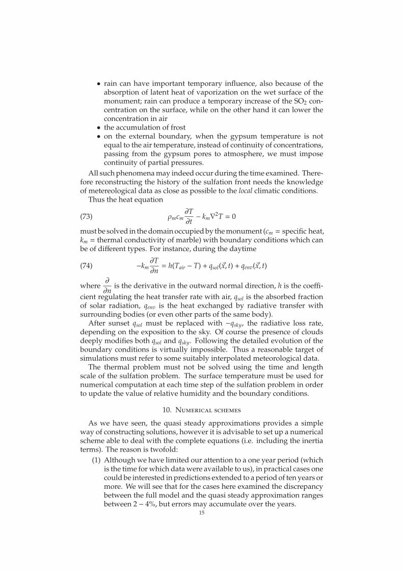
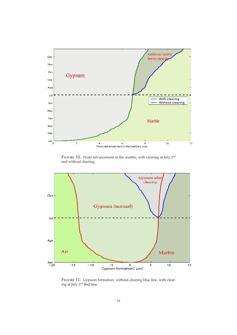
the gypsum on July 2nd. We obtain the following front advancement inthe marble with and without clearing, shown in figure 10. The gypsumdevelopment (with and without clearing) is in figure 11.

23

F 10. Front advancement in the marble, with clearing at July 2nd

and without clearing.

F 11. Gypsum formation: without clearing blue line, with clear-ing at July 2nd Red line.

24

11.2. Simulations: Rome, Villa Ada. For the location of Villa Ada, wehave obtained from Arpalazio a complete record of SO2, humidity andtemperature data detected by a pollution detector placed in "Villa Ada" inRome during the year 2006, with data taken by a one-hour frequency.

The temperature is in figure 12 and the relative humidity is shown in fig-ure 13. The distribution of pollutant SO2 detected at Villa Ada is representedin figure 14.

Jan Feb Mar Apr May Jun Jul Aug Sep Oct Nov Dec −10

−5

0

5

10

15

20

25

30

35

Time

o Cels

ius

F 12. Temperature during 2006.

Jan Feb Mar Apr May Jun Jul Aug Sep Oct Nov Dec 0

20 %

40 %

60 %

80 %

100 %

Relat

ive H

umidi

ty

F 13. Relative humidity during 2006.

25

Jan Feb Mar Apr May Jun Jul Aug Sep Oct Nov Dec 0

0.5

1

1.5

2

2.5

3

3.5

4x 10

−11SO

2 mas

s den

sity [

g/cm3 ]

F 14. SO2 during 2006.

Now, under the conditions detected during 2006 at Villa Ada, we computemarble degradation, starting with σ0 = 0. Using our mathematical modelwith ∆t = 10−5 and ∆x = 10−1, we have that at the end of 2006 the frontadvancement is shown in figure 15, and the total thickness of gypsum isshown in figure 16.

F 15. Front advancement in the marble at Villa Ada during 2006.

26

F 16. Gypsum evolution.

11.2.1. One year evolution with one intervention of gypsum removal. As done

in the previous case, we suppose to remove the gypsum on July 2nd. Weobtain the following gypsum development with clearing (blu line) andwithout clearing (red line) shown in figure 17.

F 17. Gypsum formation, with clearing (blu line) and withoutclearing (red line).

27

12. Q

Here, we want to see what happens using quasi steady solutions, moti-vated by the fact that the coefficients Ks, Kw are very large. If we assume tohave S(0, t) = Sa = const. and W(0, t) = Wa = const., we can observe that thesolutions S(x, t) and W(x, t) can be approximated very well by a functionslinear in x. For this reason, if the fluctuations of boundary values are suf-ficiently slow, then we can approximate our model by stationary solutions.Here, we want to estimate the error between numerical solutions of the fullmodel and the quasi steady approximations.

In the full-speed case, the system is given by (49), (45) (50), (62) and (64).We introduce a new space variable y = η/δ, where y ∈ [0, 1], we obtain

(106) δ = Sa(ϑ)Ωs

δ(ϑ),

(107) S(η, ϑ) = Sa(ϑ)(1 − y

),

(108) W(η, ϑ) =Wa(ϑ) − Ωs

ΩwSa(ϑ)y.

In the reduced-speed case, we obtain the following equations:

(109) δ(τ) = λ1αSa(τ)(

1 +λ1

Ωsαδ(τ)

) ,

(110) S(y, τ) = Sa(τ) − δ(τ)Ωs

yδ(τ),

(111) W(y, τ) =Wa(τ) − δ(τ)Ωw

yδ(τ).

To have a quantitative idea of the difference between stationary solutionsand numerical solutions, we use the experimetal data of case 2, "Villa Ada".We obtain the behavior of the two fronts of advancement (full model andstationary solutions) in figure 18. We note that the maximum relative error(σ−σsteady

σ

)obtained is about 2.2%. Therefore this is a case in which it would

have been safe to use directly the quasi steady approximation.

28

F 18. Comparison between steady and numerical solutions atVilla Ada.

Now, we show two fronts advancement (full model and stationary solu-tions) using the data of case 1: "P. Fermi", see figure 19.

F 19. Comparison between steady and numerical solutions (P. Fermi).

In this case the relative error(σ−σsteady

σ

)obtained is about 4%, thus almost

twice the one obtained for Villa Ada. Next we have increased (4 times)SO2 data of "P. Fermi", so to highlight the contribution of pollutant (and"its" oscillations) to the relative error with respect to the steady solution.

We found (see figure 20) that(σ−σsteady

σ

)is about 6%. We point out that the

estimated numerical error is much smaller (see Sect. 13).

29

F 20. Comparison between steady and numerical solutions (P.Fermi) during 2005 using SO2 data (4x) increased.

13. C

13.1. Front advancement as function of SO2. On the wake of the lattercalculation we decided to investigate the influence of SO2 by a factor c,that is to say, we replace S(0, t) by cS(0, t), where c is a given constant. Weused "Villa Ada" data, and we have multiplied the SO2 concentration byc = 1/9, 1/4, 1, 2, 4, 6, 9. We can see the result in figure 21. The results

0 2 4 6 8 10 12 14Jan

May

Sep

Front advancement [µm]

(1/16x) S(1/4x) S(1x) S(2x) S(4x) S(6x) S(9x) S

Marble

F 21. Front advancement as function of SO2 data.

obtained show that the thickness of the front σ, after one year, varies as√c: In order to better visualize this fact, in figure 22 we have reported

30

σ = σ(√

c), obtaining a clearly linear graph, consistently with the nature ofthe quasi-steady approximation.

F 22. Marble wasted after one year, for different values of√

c.

13.2. Front advancement as function of time. For the same reason the av-erage growth of σ is close to a

√t behavior, strengthening the conclusion

reported in [3]. We used Villa Ada data, and we have repeated the experi-mental data of the first year (2006) for the next 8 years. This way, we haveobtained σ(1 year) ≈ 4µm, after 4 years σ(4 years) ≈ 8.2µm and after 9 yearsσ(9 years) ≈ 12.5µm. Fig. 23 show oscillations around a parabolic behavior.

F 23. Front advancement in 9 years, at Villa Ada.

31

13.3. Order of accuracy of numerical schemes and extrapolation results.Since we do not have the exact solution of the problem, we give an ap-proximate estimate the order of the numerical method using the followingstandard relations:

(1) accuracy in L1 norm:

(112) γ1 = log2

(‖u(h) − u(h/2)‖1‖u(h/2) − u(h/4)‖1

),

(2) accuracy in L∞ norm:

(113) γ∞ = log2

(maxx |u(h) − u(h/2)|

maxx |u(h/2) − u(h/4)|

),

Using the simulations of "Villa Ada" case, with h = 0.1, we obtain the resultsin table 1, which are in good agreement with the formal truncation errorof the implicit scheme, which is just order 1. Finally further consideration

Norm γs γw

L1 0.89 0.84L∞ 0.90 0.84

T 1. Approximate order of accuracy of the numerical schemes.

can be done regarding σ obtained after 1 year at Villa Ada. Using h∗ = 0.1we found σh∗ = 3.960 µm, with h∗/2, σh∗/2 = 3.971 µm and with h∗/4, σh∗/4 =

3.977 µm. Making an extrapolation as h → 0, we obtained an estimate forthe real value, namely σexact = 3.983. This way we can estimate that ournumerical relative error, in terms of the gypsum front, is about 0.5%.

14. C

We have proposed a quantitative model to predict the growth of thegypsum crust on marble stones, by using environmental data, as temper-ature, relative humidity and pollution concentration. For this model wehave identified a quasi steady asymptotic regime, in good agreement withlaboratory data [4, 6] and numerical simulations. Thanks to this model weare now able to quantify how influence the evolution of local conditions, oreven the cleaning of the stone surface, can change the thickness of the crust,and so the total waste of marble. These results will be useful in the optimaldesign of future conservation strategies.

A

The authors thank the Roman Regional Authority for environment Arpalazio,http://www.arpalazio.it/, Agenzia Regionale per la Protezione Ambientaledel Lazio, for all the in situ data used in this paper. Also we want tothank Deepika Ghai for the work done on this problem during her summerinternship in 2006 at Istituto per le Applicazioni del Calcolo in Rome.

32

R

[1] G. Alì , V. Furuholt, R. Natalini, I. Torcicollo. A mathematical model of sulphite chemicalaggression of limestones with high permeability. Part I: Presentation of the model andqualitative analysis; Transport in Porous Media; online from November 03, 2006; DOI:10.1007/s11242-006-9067-2; http://www.springerlink.com/content/p41049831n308139

[2] G. G. Amoroso, V. Fassina, Stone decay and conservation - Atmospheric Pollution, Cleaning,Consolidation and Protection. Amsterdam: Elsevier Science Publishers, 1983.

[3] D. Aregba-Driollet, F. Diele, R. Natalini, A mathematical model for the SO2 aggres-sion to calcium carbonate stones: numerical approximation and asymptotic analysis, SIAMJ.Appl.Math., 64, (2004), 1636-1667.

[4] E. Borrelli, C. Giavarini, M. Incitti, M. L. Santarelli, R. Natalini, A material model forthe evolution of gypsum crusts: numerical and experimental results, in Proceedings ofthe “10th International Congress on Deterioration and Conservation of Stone”, Eds. D.Kwiatkowski and R. Löfvendahl, p. 35-42, Vol. I, Stockholm, Sweden (2004)

[5] E.A. Charola, Acidic deposition on stone. US/ICOMOS Scientific Journal 3, (2001),19-58.

[6] K. Lal Gauri, J.K. Bandyopadhyay, Carbonate Stone, Chemical Behaviour Durability andConservation, John Wiley & Sons, Inc. (1999).

[7] F. R. Guarguaglini and R. Natalini, Fast reaction limit and large time behavior ofsolutions to a nonlinear model of sulphation phenomena, Commun. Partial Differ.Equations 32 (2007), 163-189

[8] http : //hyperphysics.phy− astr.gsu.edu/hbase/h f rame.html of "Georgia State University".[9] J.L. Pérez Bernal, M.A. Bello, Modeling sulfur dioxide deposition on calcium carbonate, Ind.

Eng. Chem. Res. 42 (2003), 1028–1034.

I A C “M. P”, C N R, V P 137, I–00161 R, I

E-mail address: clarellif@gmail.com

D M "U D" - U S F, VM 67/A, I-50134 F, I

E-mail address: fasano@math.unifi.it

I A C “M. P”, C N R, V P 137, I–00161 R, I

E-mail address: r.natalini@iac.cnr.it

33