
MATHEMATICAL MODELING OF WATER MANAGEMENT ...
128
MATHEMATICAL MODELING OF WATER MANAGEMENT STRATEGIES IN URBANIZING RIVER BASINS by Wynn R. Walker Gaylord V. Skogerboe June 1973 Colorado Water Resources Research Institute Completion Report No. 45
-
Upload
khangminh22 -
Category
Documents
-
view
3 -
download
0
Transcript of MATHEMATICAL MODELING OF WATER MANAGEMENT ...
MATHEMATICAL MODELING OF WATER MANAGEMENT
STRATEGIES IN URBANIZING RIVER BASINS
by
Wynn R. WalkerGaylord V. Skogerboe
June 1973
Colorado Water Resources Research InstituteCompletion Report No. 45
MATHEMATICAL MODELING OF WATER MANAGEMENTSTRATEGIES IN URBANIZING RIVER BASINS
Completion ReportOWRR Project No. B-071-COLO
by
Wynn R. WalkerGaylord V. Skogerboe
submitted to
Office of Water Resources ResearchUnited States Department of the Interior
Washington, D. C. 20240
June 1973
The work upon which this report is based was supported (in part) byfunds provided by the United States Department of the Interior, Officeof Water Resources Research, as authorized by the Water ResourcesResearch Act of 1964, and pursuant to Grant Agreement No. 14-31-0001-3567.
Colorado Water Resources Research InstituteColorado State University
Fort Collins, Colorado 80521
Norman A. Evans, Director
AER72-73WRW-GVS25
ABSTRACT
MATHEMATICAL MODELING OF WATER MANAGEMENT
STRATEGIES IN URBANIZING RIVER BASINS
Water management in arid urbanizing regions requirescareful evaluation of the alternative strategies for supplyplying future demands and control of water quality. Mathematical models were formulated to study the interrelationships that exist among various institutional factorsin order to delineate the requirements for implementingoptimal policies. Two study areas were selected on whichto test the utility of the models. Denver, Colorado, waschosen as an area representing conditions of water scarcityand increasingly stringent water quality standards. TheUtah Lake drainage area in central Utah presented conditions where water quality management is necessary to insurethe continued use of water in the downstream populationcenter of the state. Together these models produce resultsuseful in determining the optimal strategies for watermanagement in arid urbanizing areas.
Walker, Wynn R., and Skogerboe, Gaylord V. MATHEMATICAL MODELING OF WATER MANAGEMENT STRATEGIES IN URBANIZINGRIVER BASINS. Technical Completion Report to ,the Office ofWater Resources Research, U.S. Department of the Interior.Report AER72-73WRW-GVS25,Environm~ntalResources Center,Colorado State University, Fort Collins, Colorado. June1973.
KEYWORDS - agricultural wastes, institutional constraints, mathematical models, optimization, systems analysis, urbanization, wastewater treatment, water management(applied), water quality, water supply.
ii
TABLE OF CONTENTS
LIST OF TABLES .
LIST OF FIGURES . . . . . . . . . . . . vi
NOMENCLATURE . .
SECTION
• viii
I
II
III
INTRODUCTIONPurpose • • •Scope • • •
OPTIMIZATION CRITERIONIntroduction • • • • • • •Economic Nature of Water Resource Systems •Optimizing Criterion • • • . • • •
JACOBIAN DIFFERENTIAL ALGORITHMIntroduction • • • • • • • .Theoretical Development . • •
Elimination Procedure • • •Kuhn-Tucker Conditions • • .Evaluation of Optimal Direction • • •Determining the Step Size •
The Computer Code • • • • • • • • • • • • •Subroutine DIFALGO • • •Subroutine REORGA • • • • • • • . • • • •Subroutine NEWTSIMSubroutine DECDJ . • • •
112
5557
111113141719222831343637
IV URBAN WASTEWATER TREATMENT AND RECLAMATIONMODEL • . • • • . • . • .Introduction • • • • . • • • • • • • • . .Formulation of Wastewater Treatment Model .Model Components . • • • • . • • •
Primary Treatment • . • •• . •.Secondary Treatment • • • • • . • • . . •Tertiary Treatment • • • • • • •De~alting • • • • • • • • • • • . • • • •
Operation of Wastewater Treatment Model • •
424243474749505253
v THE URBAN WATER SYSTEM MODEL • • •Introduction • • • • • • • • •Water Sources • . . • • . • •
Stream Flows • • • • • • •Interbasin Transfers • • •Agricultural Water TransfersGroundwater • • • • • • • • • • • •
iii
62626565666869
Water Distribution Network • • • • •Domestic Water Uses • • • _ • • • • • • •Municipal Water Uses • • • _ . _ • • • • •Industrial Water Uses • • • • .• . •
Model Formulation _ • _ • •Model ConstraintsObjective Function • • • •
TABLE OF CONTENTS (Continued)
SECTION Page
71727374757577
VI
VII
VIII
COORDINATION OF AGRICULTURAL AND URBAN WATERQUALITY MANAGEMENT .Introduction • • •• _....... _ •Model Description _ • _ • • • •
Improved Practices • • • .structural Improvements • • •
Model Formulation . • .Objective Function • _ • •Model Constraints ••••
OPTIMIZING REGIONAL WATER QUALITY ~1ANAGEMENT
STRATEGIES • • •• •••••••Introduction • • • • • • _ • _ • • • • • • •Model Description • • • • • • • • • • • • •
District Water Quality Management • • • •Lake Diking • • •Desalting • • • - • • • • • •
Model Formulation _ • • • • _ • • - • • • Model Objective Functions • • • • • •Model Constraints • . . . . . . . . .
Mf'l1101 nl·o'~f lrlH
SUMMARY AND CONCLUSIONS • • ._Introduction • - • • • • • •S\1Il\It\ary • • • - • • • • • -Conclusions
8181838588919195
979799
1011011021031041071 n7
110110110114
REFERENCES . . . . . . . . . .
iv
116
LIST OF TABLES
Table
1 Definition of subroutine functions • • • • • • . 30
v
Figure
1
2
3
4
5
6
7
8
9
10
11
12
LIST OF FIGURES
Differential system expressing the linearized objective function, active constraints,and inactive constraints • • • • ••••
Algebraic formulas for computing the statevariable constrained derivatives with respect to the particular decision or slackvariables •• • • • • • • • • • • • • • • •
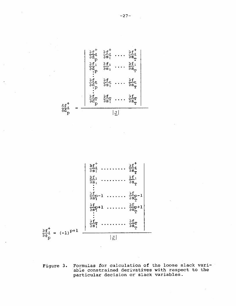
Formulas for calculation of the loose slackvariable constrained derivatives with respect to the particular decision or slackvariables • • • . • • •• • . . . • • •
Illustrative flow chart of the subroutineDIFALGO • • • • . •• •••••••
Illustrative flow chart of the subroutineREORGA • • • • • • • • • • • • • • • • • • •
Flow chart of the subroutine NEWTSIM used tosolve systems of non-linear equations •••
Illustrative flow chart of the subroutineDECDJ • • • • • • •• • • • • • • • • •
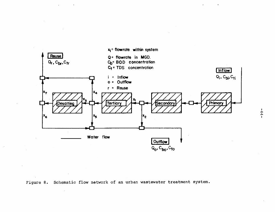
Schematic flow network of an urban wastewater treatment system • • • • . • • • •
Unit costs of recycled wastewater undervarying water quality standards . • • •
Effects of varying water quality standardson the unit costs and economies of scale ofrecycled wastewater •. • • • • . • • .
Average unit costs for reused wastewater fora BOD limit on the urban effluent, CBO, of35 mg/l and various levels of effluent TDS,eTO • • . • • •• ••••.•••.
Average unit costs ofr reused wastewater fora BOD limit on the urban effluent, CBO, of5 mg/l and various levels of effluent TDS,eTO • • • • • • . • . • • • • • • • • • • •
vi
23
24
27
33
35
38
39
44
55
57
59
60
Figures
13
14
15
16
LIST OF FIGURES (Continued)
Schematic diagram of the urban water supply and distribution system model •
Utah Lake district model
Cost-effectiveness relationships for TDSreductions in agricultural return flows inthe Utah Lake drainage area • • • . • .
Utah Lake area water quality managementmodel . . • • • • • • • • • • • • • • •
vii
64
84
89
100
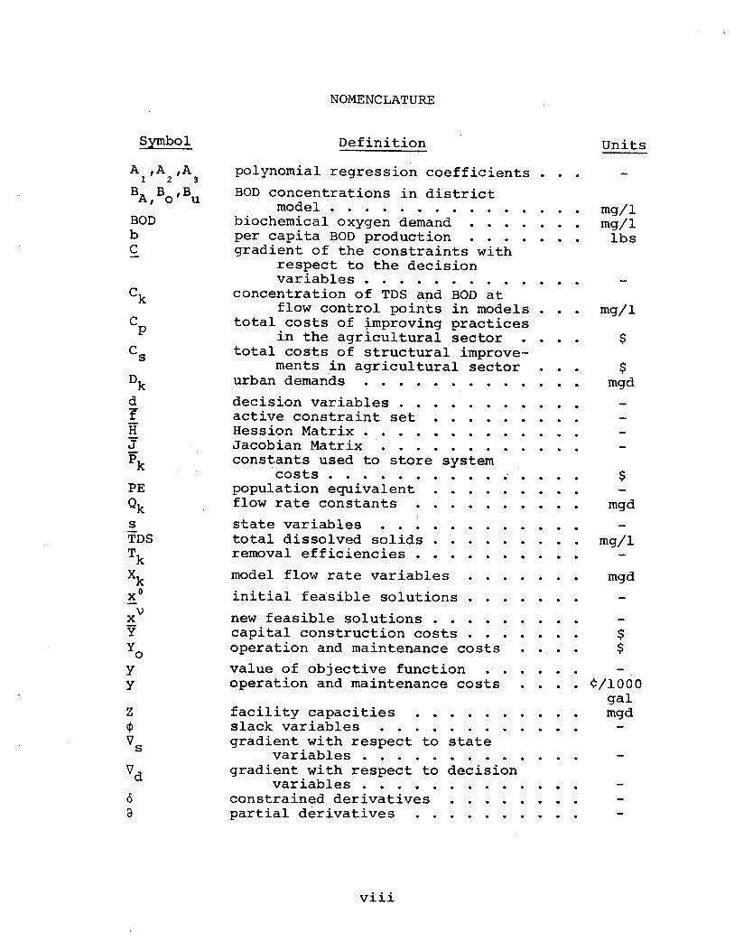
NOMENCLATURE
Symbol Definition Units
model flow rate variables
initial feasible solutions
state variables • • • •total dissolved solids •removal efficiencies • • • .
new feasible solutions • • • • • . • • •capital construction costs .operation and maintenance costs . • • •
value of object~ve functionoperation and maintenance costs
mgd
mgd
$$
$
$mgd
$
mg/l
mg/lmg/l
Ibs
mg/l
¢/lOOOgalmgd
· . . . . . . .· . . . . . . .
· . . . . . . .
decision
state
decision variables . • • • •active constraint set • • •Hession Matrix • • .• .••.Jacobian Matrix • • . •••constants used to store system
'costs • . • • •• ••.population equivalent • • •flow rate constants . • • •
polynomial regression coefficients • • •
BOD concentrations in districtmodel . • . • . . . . . • .
biochemical oxygen demandper capita BOD production . . •gradient of the constraints with
respect to the decisionvariables • . • .• .•••
concentration of TDS and BOD atflow control points in models •
total costs of ~mproving practicesin the agricultural sector
total costs of structural improvements in agricultural sector • • •
urban demands • . • . . • • •
facility capacitiesslack variablesgradient with respect to
variables . • . • •gradient with respect to
variables • • . • •constrained derivativespartial derivatives
BODbC
A ,A ,A1 2 3
BA
B ,B, 0 u
DkdfHJPk
PEQksTDSTkXkXO
xVy
YO
YY
viii
SECTION I
INTRODUCTION
Purpose
An essential requirement for advancing civilizations
has been to increase agricultural production. A few cen
turies ago a single farmer could barely support his family,
but modern agriculturalists are capable of supplying food
and fibre for many. The evolution of the agricultural
enterprise from the individualistic subsistance farming to
the corporate business has also reduced the number of peo
ple necessary to satisfy agricultural demands. Consequent
ly, with fewer opportunities in the agricultural industry,
people have aggregrated in metropolitan environments to
work in government administration, support services, and
manufacturing to note only a few. A basic shift has thus
occurred from rural to urban living.
Regional urbanization has been accompanied by new
problems in administering natural resources such as water.
First, the demands for water of suitable quality have
greatly affected the usefulness of water supplies in
several areas. As a result, new sources have been actively
sought and the feasibility of employing technological ad
vances to amend marginal supplies have been investigated.
Secondly, the concentration of water use in conjunction
with the growing demands have created serious water quality
-2-
degradation by far exceeding the natural assimilative
capacity of rivers and lakes. And finally, the institu
tional mechanisms developed to allocate and manage the
water resource have not been altered sufficiently to effec
tively meet the requirements of rapid urbanization.
The purpose of this study is to investigate the fea
sibility of alternative water management strategies which
could be implemented to alleviate the mounting problems of
water shortage and water quality deterioration. At this
level of interest, the factors especially requiring evalua
tion are the institutional requirements for accomplishing
efficient operation of water use systems. The objective
therefore is to model alternative water management strate
gies to test the effects of various institutional factors
in accomplishing more effective water use.
Scope
Administering water resource utilization in rapidly
urbanizing areas encompasses numerous individual aspects of
significant importance. Two of these have been selected
for this study:
(1) coordination of the supply, distribution, and
treatment of water in the metropolitan setting;
and
(2) regional integration of agricultural and urban
water pollution control.

-3-
Since the first topic is an important subproblem of the
second, consideration of these two problems allows this
study to evaluate the specific institutional requirements
for optimizing water management decisions in urbanizing
areas.
Two regions where the conditions are particularly
suitable to the objectives of this study are the Denver,
Colorado metropolitan area and the Utah Lake Drainage area
in central Utah.
The Denver, Colorado, area is a water-short, rapidly
expanding urban center facing rigid water quality controls.
Water supplies for the area are primarily obtained from
sources in both the headwaters of the South Platte River
Basin and the headwaters of the nearby Colorado River Basin.
It appears reasonable to conclude from previous develop
ments, that diverting more water resources from these
watersheds to supply the expanding needs will induce ex
tensive legal, social, and political controversy. A need
therefore exists to evaluate the feasibility of alternative
management strategies in this area and determine the nature
and expense of the institutional constraints which may
hinder implementation of more effective policies.
The Utah Lake Drainage area does not face serious
water supply problems, but it does contribute significantly
to a critical water quality problem in its downstream
reaches. This region is the headwaters of the Jordan River,
which is a major water source for three-fourths of Utah's
-4-
population located along an area known as the "Wasatch
Front." The water demands a.long the Wasatch Front are com
prised mainly of municipal and industrial uses, which re
quire not only a sufficient supply but an acceptable
quali.ty as well. Efforts to minimize water pollution must
therefore be regional in scope, which necessitates examina
tion of practices and potential treatments in the Utah
Lake Drainage area. This study is thus concerned with the
levels of water quality control achievable in the area and
the optimal policies to accomplish such control.
In order to present the results of this study, four
reports have been prepared. This effort is the first of
the series and covers the modeling procedures employed in
the study. The first segment of this report, encompassing
SECTIONS II and III, deal with the mechanics of the optimi
zation processes used to evaluate alternative strategies.
Next, the urban water management model is formulated in
SECTIONS IV and V, which expresses the scope of the in
vestigation in the Denver metropolitan area. Next, the
Utah Lake modeling techniques are illustrated in SECTIONS
VI and VII. Finally, SECTION VIII summarizes the modeling
efforts and recommends additional research, as well as sug
gestions for improving these models.
SECTION II
OPTIMIZATION CRITERION
Introduction
Alternative measures for meeting the requirements of
water management problems in areas of urbanization need to
be evaluated for feasibility in the context of both long
and short range objectives. In order to facilitate such
comparisons necessitates a criterion upon which a common
link between alternatives can be developed. This Section
presents some general comment and support from other
investigators for the optimization criterion selected for
this study.
Economic Nature of Water Resource Systems
There is probably no other means as commonly used or
as widely accepted for evaluating the merits of water re
source systems as is economics. While environmental con
cerns have been mounting and engineering designs have
become more sophisticated, the central character in eval
uating projects is the economic analysis. Not all of these
economic considerations have been made by economists, but
those making the studies have of necessity relied upon the
discipline to provide new and better techniques for in
investigation.
-6-
Although water resources can be classified primarily
as public commodities, significant influences on pricing
and management are due to water uses in the private market.
In most states, water is not legally "owned" by an indi
vidual other than the state, but rights can be obtained for
the use of water by individuals. However, when the legal
interpretation implies that the water is tied to the land
and cannot be transferred, then the value of the land is
enhanced by its water right. These cases give water a
market value obtainable by a right holder even when the
resource is administered as public property. As in the
case of grazing privileges on public lands, the pricing is
usually lower than that obtainable in the private economy.
As a consequence, right holders are often reluctant to
accept changes which may reduce their water supply.
Reservoirs, diversion works, and distribution systems
aid management of water resources which tend to remain
fixed in spatial distribution and random in time distribu
tion. These characteristics which would otherwise con
strain water supplies to local utilization, allow wider
water use between adjoining watersheds and along a river
system. However, the diversion of waters from one basin
to another, or the transfer of water usage to another
location in the river network, creates exteralities which
are usually not considered by local planners. Thus, maxi
mum economic efficiencies are only achieved when the
economic evaluations assume a regional interpretation.
-7-
Finally, the inefficiencies existing in current water
use practices can be traced to a large extent to those
social, legal, and political institutions responsible for
distribution of water among demands. These limitations
have not been severe until water resources have become
scarce. However, when expansions in urban needs occur, the
water resources that could be better utilized in a new use
may be tied to an old use without means for making a
conversion. As a result, the optimal water management pol
icies which suggest that water be transferred from one use
to another, such as transferring agricultural water to
municipal uses, have been difficult to date because of the
institutional constraints (Hartman and Seastone, 1972).
Although such constraints hinder efficient use of water,
they have nevertheless become the tools which substitute
for the free market economic system.
Optimizing Criterion
Optimization is generally a maximization or a minimi
zation of concise numerical quantities reflecting the rela
tive importance of the goals and purposes contained in
alternative decisions. Of themselves, neither the goals or
purposes directly yield the precise quantitative statements
required by systems analysis procedures •. Therefore, the
objectives to be accomplished must first be stated by a
quantit~tive measure from which alternative policies can be
mathematically compared (Hall and Dracup, 1970).
-8-
Presumably, such a comparison would permit a ranking of
these policies as a basis for decision making. The speci
ficmeasure to facilitate this examination can be defined
as the optimizing criterion.
The central problem facing engineers is to link the
descriptions of the physical environment via mathematical
models with the social and political environment (Thomann,
1972). Probably the most commonly used ~nd widely accepted
"indicators" are found among the many economic objective
functions. However, considerable controversy exists as to
the most realistic of these tools. If all human desires
could be priced in an idealized free market monetary ex
change, the forces that operated would insure that every
individual's marginal costs equalled his marginal gains,
thereby insuring maximum economic efficiency. In fact,
such a condition would reduce the need for optimization
methodologies to aid decision making. In the absence of
this ideal situation, goals cannot be quantified with a
high degree of accuracy and the optimizing c~iterion in
any case is at best an indicator of the particular
alternative.
Among the more adaptable economic indicators are
maximization of net benefits, minimum costs, maintaining
the economy, and economic development. The use of each de
pends on the ability to adequately define tangible and
intangible direct or indirect costs and benefits. In
water resource development and water quality management
-9-
specifically, the economic incentives for more effective
resource utj.lization are negative in nature (Kneese, 1964).
A large part of this problem stems from the fact that water
pollution is a cost passed on by the polluter to the down
stream user. Consequently, the inability of the existing
economic systems to adequately value costs and benefits has
resulted in the establishment of water quality standards,
however inefficient these may be economically (Hall and
Dracup, 1970). The immediate objective of water resource
planners is thus to devise and analyze the alternatives for
achieving these quality restrictions at minimum cost
(Thomann, 1972) and is the criteria chosen for this study.
SECTION III
JACOBIAN DIFFERENTIAL ALGORITHM
Introduction
The search for an optimizing technique to evaluate the
relative merits of an array of alternative~ depends largely
upon the form of the problem and its constraints. While the
allegorical Chinese maxim cited by Wilde and Beightler (l967)
stating, "There are many paths to the top of the mountain,
but the view there is always the same," is also true in this
case; not every method can be applied with the same ease.
Each optimization scheme has its unique properties making it
adaptable to specific problems, although many techniques
when sufficiently understood can be modified to extend their
applicability. Successful modifications of this nature are
prevalent in current engineering practice but requires some
experience in using these methods.
Most conditions encountered in the field of water re
sources, urban water systems specifically, involve mathemati
cal formulations which are non-linear in both the objective
function and the constraints. Furthermore, the constraining
functions may be mixtures of linear and non-linear equalities
and inequalities. Without simplifying these problems or rad
ically changing existing optimization techniques, it ispos
sible to derive solutions based upon what Wilde and Beightler
(1967) describe as the "differential appraoch."
-11-
Most techniques for selecting the optimal policy do so
by successively improving a previous estimate until no
betterment is possible. These may be classified as direct
or indirect methods depending on whether they start at a
feasible point and stepwise move toward the optimum or solve
a set of equations which contain the optimum as a root." In
a majority of cases, the differential approach can be used
to describe the method. Thus, it is possible to understand
a wide variety of procedures by knowing one basic mathemati-
cal approach.
Numerous applications of one form or another of the
basic differential appro~ch have been made in the field of
engineering (Monarchi, 1972). Because of the considerable
difficulty in progranuning "generality," nearly all of these
applications have been somewhat specialized toward the spe
cific geometry of the problem. The research project respon
sible for this development necessitates two entirely differ
ent optimization analyses. Consequently, to avoid develop
ing two models, it was decided to attempt to program a gen
eral differential algorithm. A class entitled "Foundations
of Engineering Optimization" taught by Dr. H. J. Morel
Seytoux, Professor of Civil Engineering at Colorado State
University provided the theoretical basis for the model.
This writer, a student in the class, coded the algorithm
for use on the digital computer facilities at the Universit~
The optimizing technique is called in this writing
the "Jacobian Differential Algorithm." Theoretically,
.:..12-
it is a generalized eliminating procedure which is com
putationally feasible under a wide variety of conditions.
The characteristics of convexity are assumed and since
the maximization problem is simply the negative of a
minimization one, the succeeding discussion will be limit
ed to the latter case. As in all direct minimizing
procedures, the algorithm involves four steps:
1. Evaluate a first feasible solution, xo which
satisfies the problemconstraintsw The under
bar indicates vector notation and the super
script 0 is used to describe the "old" or
initial points.
2. Determine the direction in which to move
such that the objective function, y, is
decreased the most rapidly. This re
quires a move from xo to the new point,
xV in which the superscript v represents
the new point notation.
3. Find the distance that can be moved with-
out violating any of the problem constraints.
4. ,Stop when the optimum is reached.
While the procedure yields the requirements for steps 2 and
3, the user is left with providing the first feasible solu
tion, step 1. This may seem to be a drawback for the prob
lem, but in real situations a feasible solution already
exists as a current policy. Step 4 is accomplished by an
examination of what are now referred to as the "Kuhn-Tucker
-13-
conditions." These criteria do not indicate whether the
procedure has reached a local or global optimum; conse-
quently, it is necessary to derive a means for checking.
This is not usually a difficult process.
Theoretical Development
Consider the problem in which the minimum value of the
objective function is sought subject to a set of constrain
ing functions. Writing this problem mathematically,
minx {y = y (~) } (I)
subject to,
(2)
where the notation y(~) denotes "as a functi'.Jn of the vec-
tor x." The number of'x variables is defined as N and theI
number of constraints as K. The method of analysis depends
largely upon the structure of the constraints. When all
the constraints are inequalities and "loose" or "inactive"
(strictly» at the initial feasible point xo, the problem
is "unconstrained." In the other case when either some of
these functions are strict equalities or when some of the
inequalities are "tight" or "active," the problem is re-
ferred to as "constrained. 1I Although both of the conditions
may occur in the solution of a problem, they require some-
what different approaches as the algorithm progresses toward
the optimum.
-14-
Elimination Procedure
The elimination nature of the technique is derived
from the fact that it is at least conceptually possible to
employ only the currently active constraints to eliminate
some of the x's from the problem, making it temporarily
unconstrained. To begin, define the number of active con
straints as T and reorder the constraint set so that the
first Tare the'active constraints with index t = 1, 2,
... , T. Further, introduce "slack" variables to the
active constraints so they take the form,
f(~) - ! = Q (3)
and become strict equalities, where! is the vector of slack
variables. Later in the development, slack variables will
also be added to the inactive constraints. The purpose of
this transformation is that by continual observation of the
slack values, the distinction between active and inactive
functions can be determined, since active slack variables
are equal to zero and inactive slacks are always greater
than zero. The problem now contains N original variables
plus T slack variables which are related by T active con
straints. If the constraints are linear, T of the vari
ables can be eliminated from the objective function by the
constraint expressions, making the problem unconstrained.
However, in the general situation, the constraints are non
linear, and it is not directly possible to substitute for
the dependent variables. It is necessary in the general
case to first linearize the functions by taking the first

-15-
partial derivatives with respect to the x variables. Even
though the non-linearity may still exist due to the nature
of the terms in the constraints, if it is assumed that the
changes toward the optimum point are sufficiently small,I
then only a small deviation is introduced. The elimination
procedure takes place by partitioning the variable set into
"states" and "decisions." The state variables are the se-
lected variables which are to be eliminated by the T active
constraints. The decision variables are the remaining in-
dependent variables which will be employed to seek the min-
imum value of the objective function. The criteria for the
partition include two aspects:
1. All slack variables are taken as decisions
unless no other x-variable is available to
be a state variable. Since all ~t are
identically equal to zero, when the algo-
. h f h ld . 0 hr1t m moves rom teo p01nt ~ to t e new
one xV in its search for the minirnwn, there
is a 50 percent chance that the ~t will be
come negative. This is a violation of the
problem constraints.
2. Since the same basic reasoning applies to the
x-variables, the largest absolute valued
variables are best suited to be state variables.
In the computer code of the algorithm, the selection of
states and decisions is much more complex, but to describe

-16-
all the partitioning difficulties at this point would be
confusing.
After partitioning the x-vector into state and deci-
sion variables, the variables can be relabeled s for states
and d for decisions. Equation 1 at the initial point x O
can then be written,
m~n y:: y (s 1 ' S 2 ,. • ., S"T ' d 1 ' d 2 ,. • ., d D ) ( 4 )
in which D is the number of decision variables and equals
(N - T). In addition, the constraints listed in Equation
3 can be rewritten as:
( 5)
The next step is to employ the chain rule of calculating
the total differential of y. In vector notation,
ay = (V sY) a~ + (Vdy) a~ (6)
where the symbol ay is used to denote the total differen-
tial rather than the standard notation of dye This modifi-
cation is made so that the d can be reserved to denote the
decision variables.
The derivatives of the constraining functions can
also be written in vector form,
(7)
where the gradient, (V f), is called the Jacobian Matrix,s-
~, and the matrix (Vdf) can be relabeled as C. Employing
these variables in Equation 7 and rearranging terms:
Jas = -Cad + at
If the Jacobian matrix is always taken non-singular, the
vector as can be solved for.
(8 )
-17-
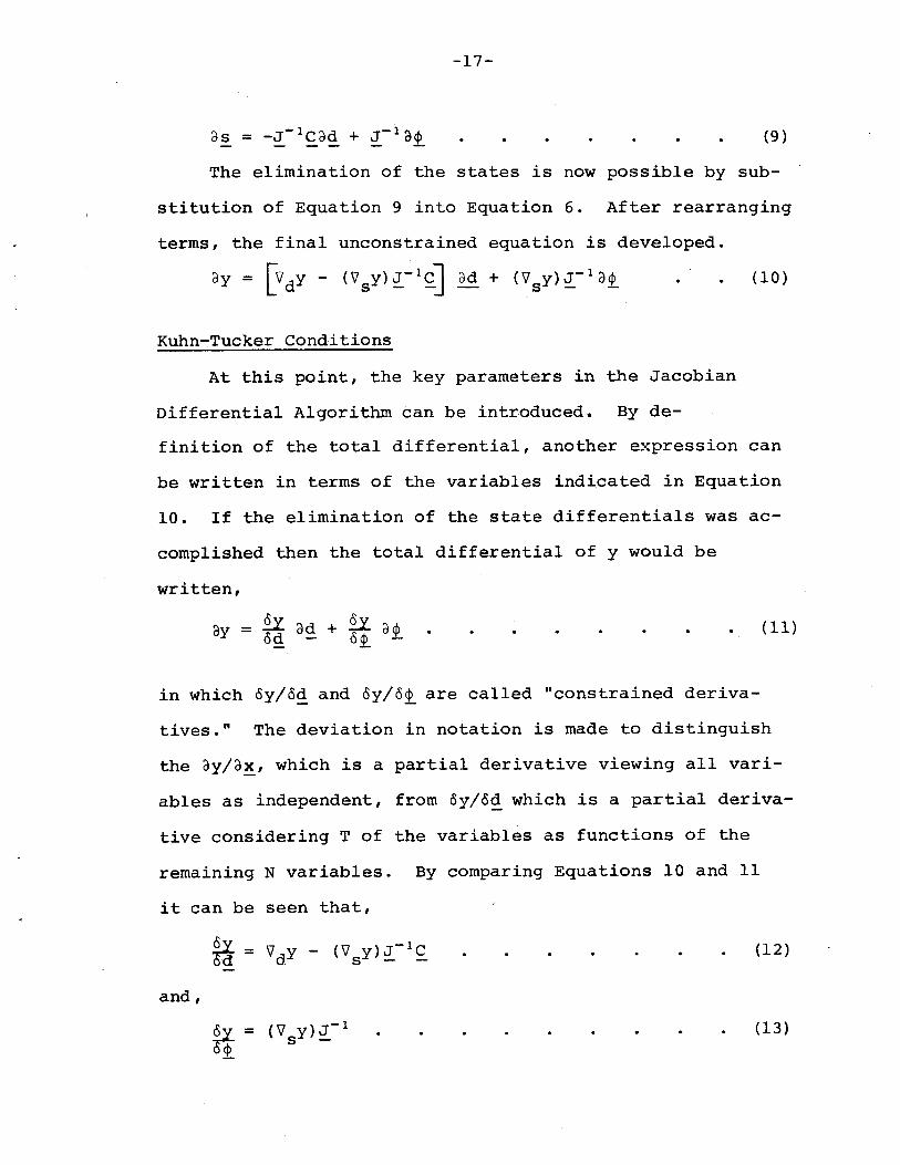
(9 )
The elimination of the states is now possible by sub
stitution of Equation 9 into Equation 6. After rearranging
terms, the final unconstrained equation is developed.
ay = [VdY - (Vsy)~-l~J ad + (Vsy)~-lat
Kuhn~Tucker Cond~tions
At this point, the key parameters in the Jacobian
Differential Algorithm can be introduced. By de-
(10)
finition of the total differential, another expression can
be written in terms of the variables indipated in Equation
10. If the elimination of the state differentials was ac-
complished then the total differential of y would be
written,
(11)
in which oy/o~ and oy/o1 are called "constrained deriva-
tives. tI The deviation in notation is made to distinguish
the ay/a~, which is a partial derivative viewing all vari
ables as independent, from oy/o~ which is a partial deriva
tive considering T of the variables as functions of the
remaining N variables. By comparing Equations 10 and 11
it can be seen that,
a= 'Vdy - {V y)J-1CS - -
and,
q = (V y)J- 1
S -
(12)
(l3)
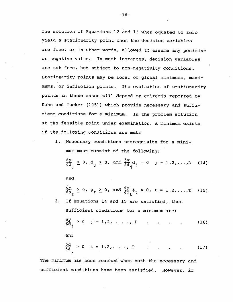
-18-
The solution of Equations 12 and 13 when equated to zero
yield a stationarity point when the decision variables
are free, or in other words, allowed to assume any positive
or negative value. In most instances, decision variables
are not free, but sUbject to non-negativity conditions.
stationarity points may be local or global minimums, maxi-
mums, or inflection points. The evaluation of stationarity
points in these cases will depend on criteria reported by
Kuhn and Tucker (1951) which provide necessary and suffi-
cient conditions for a minimum. In the problem solution
at the feasible point under examination, a minimum exists
if the following conditions are met:
1. Necessary conditions prerequisite for a mini-
mum must consist of the following:
*. > 0, d j > 0, and *.d j = 0 j = 1,2, ••• ,D (14)J J
and
~ ~ 0, <P t ~ 0, and ~<P t = 0, t =. 1 ,2, .•• , T (15)t t
2. If Equations 14 and 15 are satisfied, then
sufficient conditions for a minimum are:*. > 0 j = 1,2, ... , DJ
and
<Sd > 0 t = 1, 2 ,. • ., Toept
The minimum has been reached when both the necessary and
sufficient conditions have been satisfied. However, if
(16)
(17)
-19-
for example, oy/cd. equals zero and d. > 0, the tests are) J -
inconclusive since the sufficient conditions have not been
met. In this case, it is necessary to take the second de-
rivatives of the objective function with respect to the x-
vector. This analysis yields a square matrix of second
order partial derivatives called the Hessian matrix written
mathematically as:
(18)
In order for the stationarity point to be a minimum (local
or global) the value of the Hessian matrix must be positive-
definite, and since the properties of positive-definite ma-
trices can be found in most texts on linear algebra, no
further description will be given here.
Evaluation of Optimal Direction
In addition to the description of the fundamental elim-
ination technique of this optimizing t~chnique, the preced-
ing sections also provided the definition of the constrained
derivatives of the objective function in terms of the de-
cision and slack variables. Furthermore, criteria were
given with which these parameters can also be evaluated to
see when the minimum is achieved. In this section, these
same derivatives will be used to determine the direction a
particular decision variable, d or <t> , must be "moved" inp p
order to create the maximum reduction in the value of the
objective function during each iterative step.
-20-
Among the non-linear progranuning techniques for optimi-
zation several essentially alter all of the decision vari-
abIes at each iteration. In the Jacobian Differential Al-
gorithm, one decision variable Cd or ~ ) is selected fromp p
among the set which when moved will result in the most prog-
ress toward the minimum. If an individual term from Equa-
tion 11 is written in discrete element form, the new value
of the decision variable (or slack variable) can be
determined,
yV _ yO =(~JO (d/ - di
O)
or,
(19 )
<f> \)
t(20)
where the reader is reminded that the superscripts 0 and v
refer to the functional evaluations made at the old and new
feasible solutions. It may also be worth mentioning that
<P t can only be ~ncreased whereas d i can be also decreased
(assuming the non-negativity constraints are not violated) •
As a result, the increase in a slack variable is in reality
a loosening of an active constraint.
The choice of the decision variable or the slack
variable to be modified is primarily made on the basis of
largest absolute value among the respective constrained
derivatives. Three general categories are examined. To
begin with, the largest positive valued derivative with
which the associated decision variable is greater than
zero is determined and the Kuhn-Tucker Conditions are
-21-
checked according to the previous section. Mathematica
lly, this first alternative can be written,
(21)
where the notation Idi > 0 means "subject to the value of
d. being positive."1
The second alternative selection for the step direc-
tion is in the negative constrained derivatives. In this
case, the specific decision variable ~ill be increased and
unless an upper bound on the variable is imposed, no exam-
ination of the decision need be made. Symbolically then,
find: mini
[~i < 0, i = 1,2,. • ., 0 1· (22)
Finally, the largest reduction in the objective func-
tion may be facilitated by loosening a particular active
constraint. Unless the constrained derivative of y with
respect to the slack variable is negative, the Kuhn-Tucker
Conditions are satisfied. Therefore, this solution can be
expressed as:
minfind: t [at > 0, t= 1,2,. . ., T ] ( 23)
Once these maximum and minimums have been selected, the
next item is to compare them with each other and select the
largest absolute valued one. After having made the choice,
the index on the specified decision or slack variable is
now denoted by a lip", and these vari'abl'es now become d p or
~ depending on the decision among alternatives.p
-22-
Determining the Step Size
The analysis in the previous section paved the way to
compute the direction in which the decision and slack vari
ables are to be moved for a maximum decrease in the objec
tive function. This section is presented to find how much
the procedure can move in the appropriate direction without
violating the constraints. In order to accomplish this,
four new constrained derivatives must be developed. To
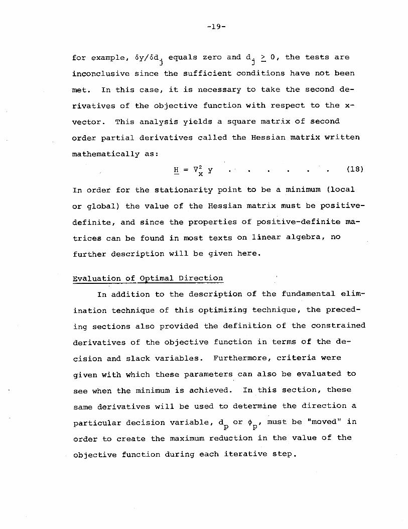
begin, it is useful to rewrite Equations 6 and 7 as a com
plete differential system. In addition, the slack varia
bles (~+) may be added to the inactive constraints (f+) and
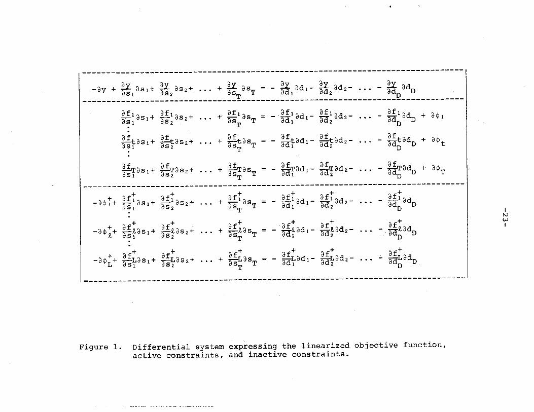
included in the differential system. The complete three
part system has been included in Figure 1.
Because the particular decision variable or slack vari
able to be modified has been selected, the remaining deci
sions and slacks will remain constant and can therefore be
temporarily ignored. The next computation necessary is to
determine which of the boundaries of the problem are ap
proached first. If the non-negativity constraints on the
variables are in effect, one consideration is how far a
decision or slack variable can be moved without forcing a
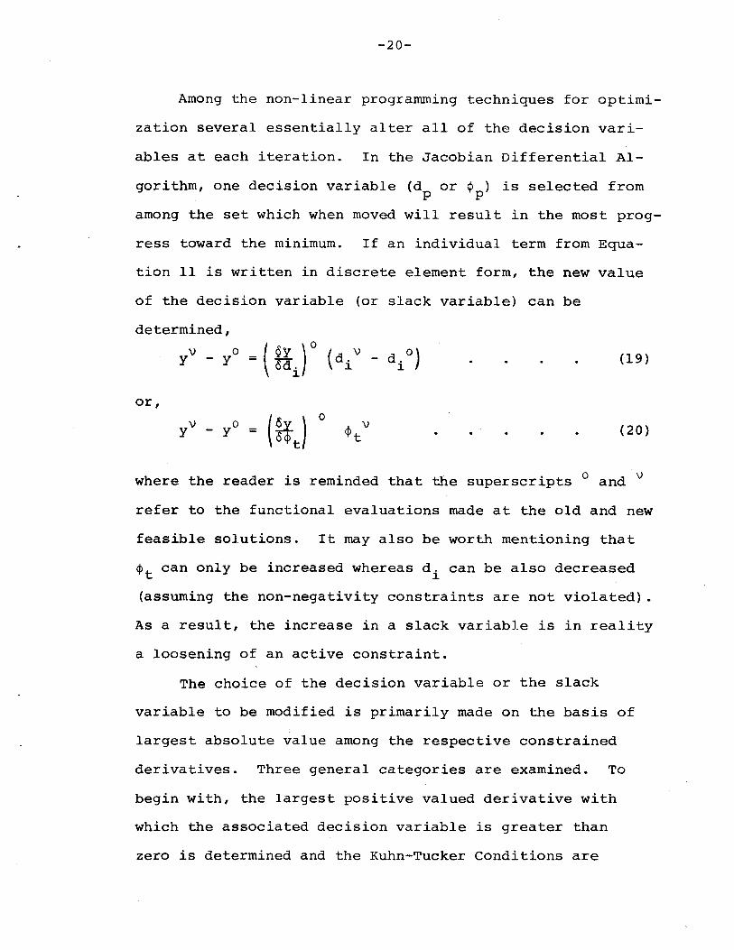
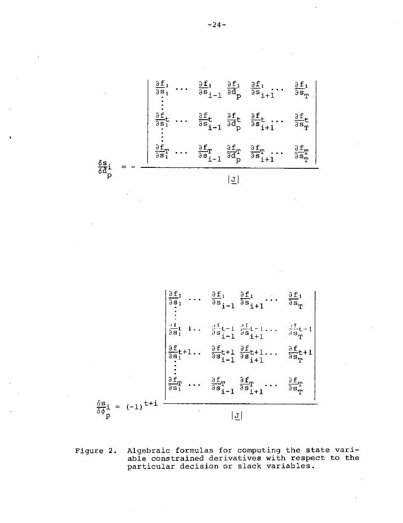
state variable to become negative. In order to accomplish
this, the constrained derivatives of each state variable
with respect to the particular decision or slack variable
are computed. The representation of these values is ·com
puted from the formulas shown in Figure 2 in which the use
of Cramer's rule was applied to the system in Figure 1.
~ ~ ~ ~ ~ ~
--=~~_:_~::~:~:_~::~:~:_~~~_:_~:!~::_:_=-~~:~~~=-~~:~~~=-~~~-=-~~Q~~~----------+ a<p1
+ a<P t
af1adad D
D
~tadD- adD
~ladl- ~lad2-ad 1 ad2
af af- --tadl- --tad2-ad 1 ad 2• •• +
+ ~lasT• • · aST
~tas =as TT
afl afl~ a5l+ ;s- as 2 +051 052
af af;s-tas l + ~taS2+051 052
af af af af of of~aS1+ OS~OS2+ ..• + as~osT = - odi odl - ad~od2- ••• - ad;odD + o¢T
af+ of+= - --Lodl- -Lod2-ad l od2
ItvWI
af+- 1aodD dD
of+- .. aa~3dD
3f+- adLod
D D
+ +~1 ad 1- 2..£1 ad 2 -ad 1 ad 2
af+ af+acr~ ad 1 - ad~ ad 2 -
- -
+~asTaST
+afl asas TT
+~R,as =as T
T
· •• +
· •• +
· .• ++ +
"\ + af l af 1- a <P 1 + -- as 1 + _. as 2 +oS! aS 2
+ af+ of+-o<P L+ ~LaSl+ ~LaS2+
aSl 052
+ af+ af+-3<Po+ ~R,3S1+ ~R,aS2+
JV dS1 dS2
--------------_._------------------------------~--------------------------------
Figure 1. Differential system expressing the linearized objective function,active constraints, and inactive constraints.
-24- -
£!.l E..fl af l af l £1.1aS l as. 1 adp a5i +i · . aST. J.-
gt 2.!t ~t af ~tat ..•qSl as. 1 ad si+l aSTJ.- p
2.!.T ~ afT af afTaT •••aSl as. 1 ad Si+l aSTos. ~- pod~ =
P I~I
££1 E.fl a f 1 af laSl as. 1 a5i +l
. .. aST. ~-
II r ,I r ,I r .1 ras~--l .. ;------t-1
as-~~~· .. :----l-- 1Js. 1 ;)sT -
1-
af £.!.t+l af af t +la-t +l .. ag-t+l ...Sl as. 1 i+l aST1-
afT ~ ~ ~aSl as. 1 aS i +l aST~-
os. (_l)t+i8'¢J. =
p I~I
Figure 2. Algebraic formulas for computing the state variable constrained derivatives with respect to theparticular decision or slack variables.
-25-
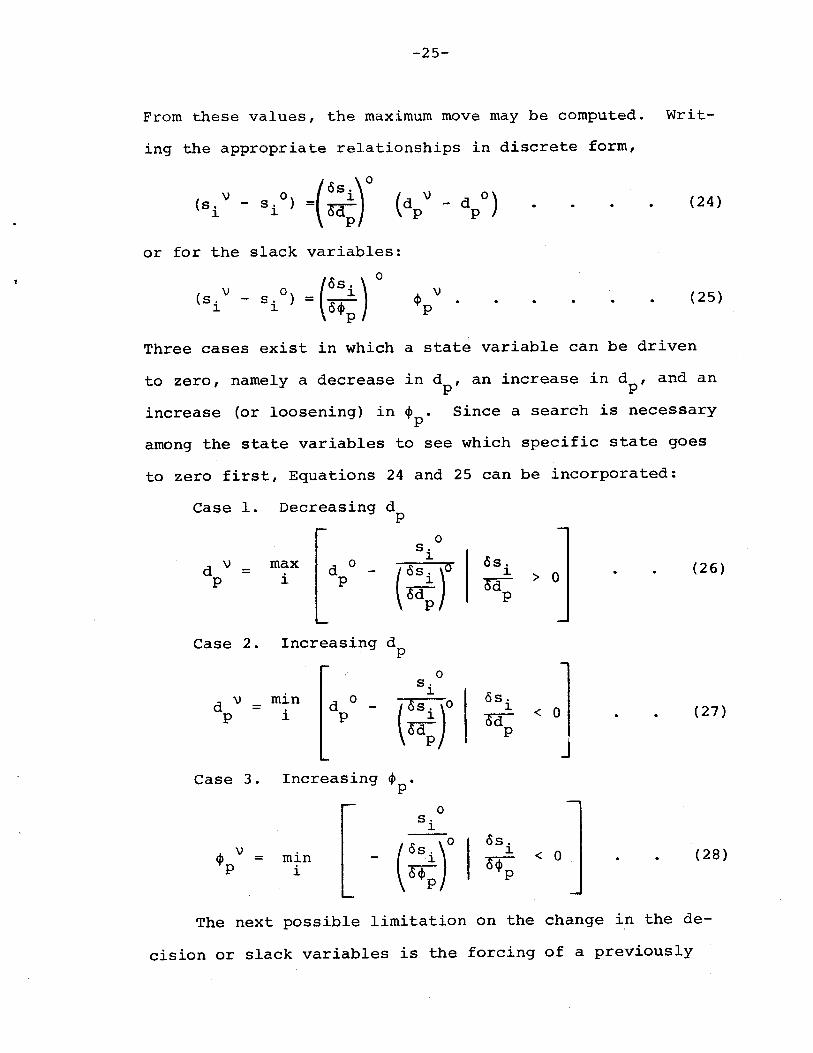
From these values, the maximum move may be computed. Writ-
ing the appropriate relationships in discrete form,
or for the slack variables:
(24)
4> \) ·P
(25)
Three cases exist in which a state variable can be driven
to zero, namely a decrease in d , an increase in d , and anp p
increase (or loosening) in 4>. Since a search is necessaryp
among the state variables to see which specific state goes
to zero first, Equations 24 and 25 can be incorporated:
Case 1. Decreasing dp
0s.d \) d 0
1 os.max
(~r(26 )= i 1
P P Od > 0p
Case 2. Increasing d p
0
01s.
min 1 os.d \) = d 0
t::~r1 (27)P i p ocr- <p
JCase 3. Increasing 4> •p
0S.
1
(::~ros.
<P \) min J. < 0 (28)P i OCPp
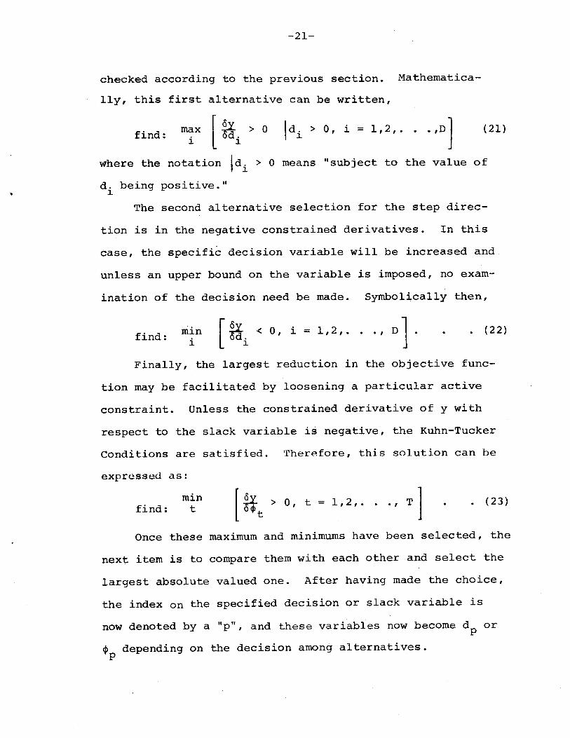
The next possible limitation on the change in the de
cision or slack variables is the forcing of a previously
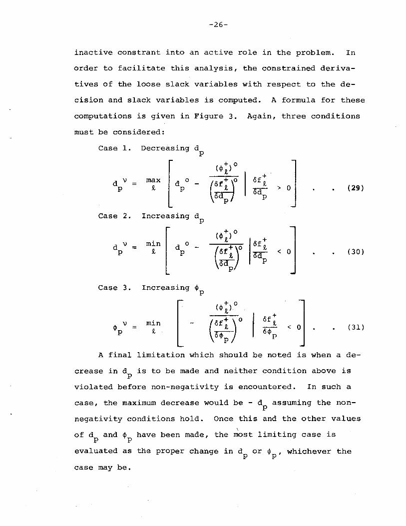
-26-
inactive constrant into an active role in the problem. In
order to facilitate this analysis, the constrained deriva-
tives of the loose slack variables with respect to the de-
cision and slack variables is computed. A formula for these
computations is given in Figure 3. Again, three conditions
must be considered:
Case 1. Decreasing dp
\) maxd =
P td 0
P > 0 (29)
Case 2. Increasing dp
d \> =P
mint
d 0P < 0 (30)
Case 3. Increasing ~p
~ \) =P
minR. < 0 (31)
A final limitation which should be noted is when a de-
crease in d is to be made and neither condition above isp
violated before non-negativity is encountered. In such a
case, the maximum decrease would be - dp assuming the non
negativity conditions hold. Once this and the other values\
of dp
and ~p have been made, the most limiting case is
evaluated as the proper change in d or $ , whichever thep p
case may be.
-27-
af+ af+ af+ad t as~ ag-t
p Tafl a f 1 aflad asl aST.p
~t af ~t-tad aS l aST.p.~ ~ .... ~ad aS l aSTcSf+ p
cd t =p I~I
(-1) p+l
af+-taS I
aflas l
af 1m-at +1m
af 1asP-T
at +1asPT
Figure 3. Formulas for calculation of the loose slack variable constrained derivatives with respect to theparticular decision or slack variables.
-28-
Before this section is concluded, a few notes should
be made. The first of these is that the number of state
variables depends only on the number of active constraints.
If by varying a slack or decision variable, a state is
driven to zero, a decision variable must be selected to
trade positions with the state because of the rick
of zero valued state variables. The second point to make
is that when a loose constraint is tightened, a new state
variable must be selected from the rest of the decision
variables. The exception to this is when a loose constraint
is tightened by loosening a currently active constraint.
In any event, there are so many functions and variables to
keep track of, and so many possible alternatives to con
sider, that the most difficult aspect of this algorithm is
the "bookkeeping" that is necessary. This will be demon
strated in the discussion of the computer code.
The Computer Code
Although the theory encompassing this optimization
"technique is a very powerful one, the computer code of the
method has certain inherent limitations. This is not a
fault of this particular program, but rather a characteristic
of nearly all programs with any degree of sophistication.
The utility of any optimum seeking procedure in engineering
applications is largely dependent on the economy of use and
-29-
its generality. It is primarily the latter aspect that
limits the subsequent use by an individual unfamilar with
the mechanics of the programs' operation. Very few large
computer programs are general enough to be used with little
or no knowledge of their structure and weak points. The
computer code developed. in this section is not among these
very few, but a great deal of time and effor.t has been spent
in maximizing the generality of the program.
One of the most efficient uses of coding technology is
to provide the means whereby segments of programs can be
easily modified and used successively for other purposes.
In order to facilitate future use of this program, each
functional element in the procedure has been identified in
a subroutine format. This type of program structure has
several important advantages including the ease in which
the program can be debugged. In addition, whatever modifi
cations become desirable can be made within the framework of
the subroutine without detailed consideration to the remain
der of the program. Another advantageous characteristic of
the program is that most of the variables are placed in a
common storage, thereby making their values accessable from
throughout the program.
The Jacobian Differential Algorithm consists of 25 sub-
routines which have been defined in Table 1. The entire
system can be subdivided into seven groups acoording to
their role in the optimizing technique:
1. Problem definition is accomplished in
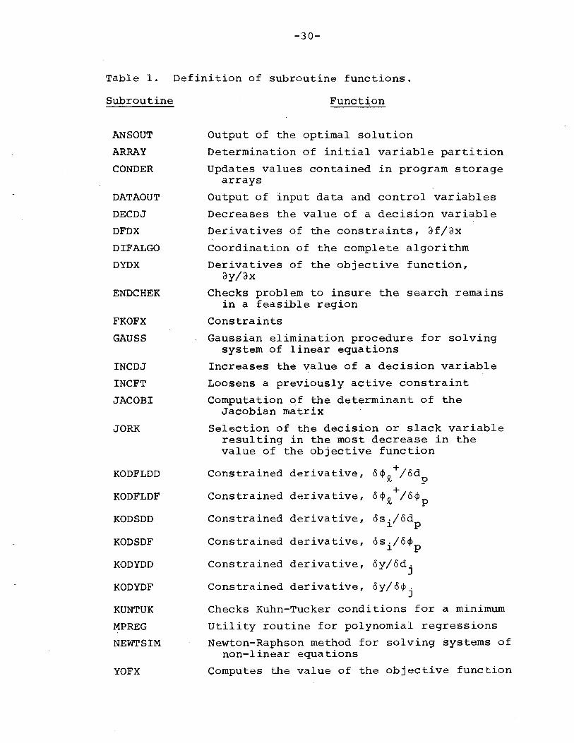
Table 1.
-30-
Definition of subroutine functions.
Subroutine
ANSOUT
ARRAY
CONDER
DATAOUT
DECDJ
DFDX
DIFALGO
DYDX
ENDCHEK
FKOFX
GAUSS
INCDJ
INCFT
JACOBI
JORK
KODFLDD
KODFLDF
KODSDD
KODSDF
KODYDD
KODYDF
KUNTUK
MPREG
NEWTSIM
YOFX
Function
Output of the optimal solution
Determination of initial variable partition
Updates values contained in program storagearrays
Output of input data and control variables
Decreases the value of a decision variable
Derivatives of the constraints, af/ax
Coordination of the complete algorithm
Derivatives of the objective function,ay/ax
Checks problem to insure the search remainsin a feasible region
Constraints
Gaussian elimination procedure for solvingsystem of linear equations
Increases the value of a decision variable
Loosens a previously active constraint
Computation of the determinant of theJacobian matrix
Selection of the decision or slack variableresulting in the most decrease in thevalue of the objective function
Constrained derivative, o<Pt+/ odp
Constrained derivative, o<Pt+/o<P p
Constrained derivative, os./od.1. p
Constrained derivative, os./ocl>.1. p
Constrained derivative, oy/od.J
Constrained derivative, oy/o¢.J
Checks Kuhn-Tucker conditions for a minimum
Utility routine for polynomial regressions
Newton-Raphson method for solving systems ofnon-linear equations
Computes the value of the objective function
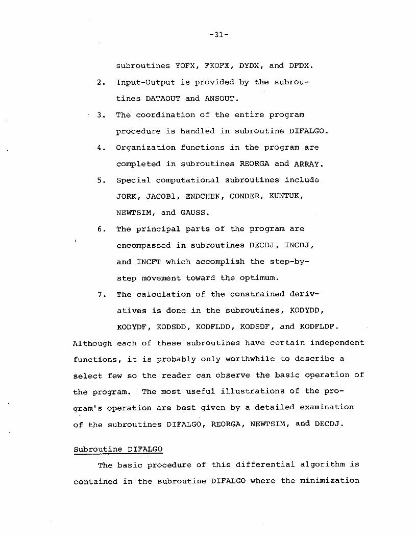
-31-
subroutines YOFX, FKOFX, DYDX, and DFDX.
2. Input-Output is provided by the subrou
tines DATAOUT and ANSOUT.
3. The coordination of the entire program
procedure is handled in subroutine DIFALGO.
4. Organization functions in the program are
completed in subroutines REORGA and ARRAY.
5. Special computational subroutines include
JORK, JACOBI, ENDCHEK, CONDER, KUNTUK,
NEWTSIM, and GAUSS.
6. The principal parts of the program are
encompassed in subroutines DECDJ, INCDJ,
and INCFT which accomplish the step-by
step movement toward the optimum.
7. The calculation of the constrained deriv
atives is done in the subroutines, KODYDD,
KODYDF, KODSDD, KODFLDD, KODSDF, and KODFLDF.
Although each of these subroutines have certain independent
functions, it is probably only worthwhile to describe a
select few so the reader can observe the basic operation of
the program. The most useful illustrations of the pro
gram's operation are best given by a detailed examination
of the subroutines DIFALGO, REORGA, NEWTSIM, and DECDJ.
Subroutine DIFALGO
The basic procedure of this differential algorithm is
contained in the subroutine DIFALGO where the minimization
-32-
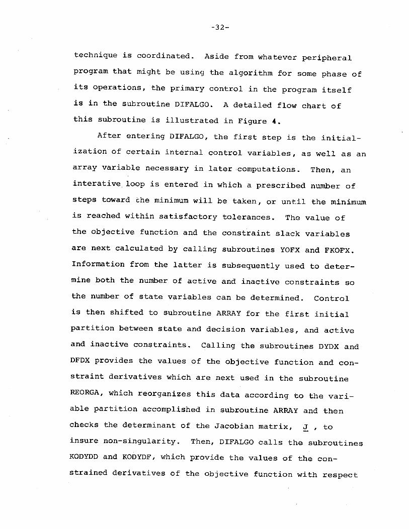
technique is coordinated. Aside from whatever peripheral
program that might be using the algorithm for some phase of
its operations, the primary control in the program itself
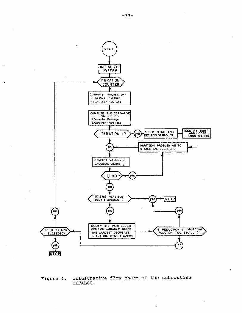
is in the subroutine DIFALGO. A detailed flow chart of
this subroutine is illustrated in Figure 4.
After entering DIFALGO, the first step is the initial
ization of certain internal control variables, as well as an
array variable necessary in later ;computations. Then, an
interative loop is entered in which a prescribed number of
steps toward t.he minimum will be taken, or until the minimum
is reached within satisfactory tolerances. The value of
the objective function and the constraint slack variables
are next calculated by calling subroutines YOFX and FKOFX.
Information from the latter is subsequently used to deter
mine both the number of active and inactive constraints so
the number of state variables can be determined. Control
is then shifted to subroutine ARRAY for the first initial
partition between state and decision variables, and active
and inactive constraints. Calling the subroutines DYDX and
DFDX provides the values of the objective function and con
straint derivatives which are next used in the subroutine
REORGA, which reorganizes this data according to the vari
able partition accomplished in subroutine ARRAY and then
checks the determinant of the Jacobian matrix, ~, to
insure non-singularity. Then, DIFALGO calls the subroutines
KODYDD and KODYDF, which provide the values of the con
strained derivatives of the objective function with respect
-33-
COMPUTE VALUES OFI.Objectille Function
2. Constraint Functions
COMPUTE THE DERIVATIVEVALUES OF'
I. Objective Function2.ConSffoint Function,
IS REDUCTION IN OBJECTIVEFUNCTION TOO S MAL L ?
PARTITION PROBLEM AS TO....I-----......f STATES AND DECISiONS
MODIFY TH E PARTlCUlA HDECISION VARIABLE GIVINGTHE LARGEST DECREASEIN THE OBJECTIVE FUNCTION
Figure 4. Illustrative flow chart of the subroutineDIFALGO.
-34-
to the decision and slack variables. These values are then
used in subroutine JORK to determine which decision or
slack variable is to be modified. The Kuhn-Tucker condi-
tions are next checked; if they are satisfied, the proce-
dure succeeded. Control is then passed to the appropriate
change function (decrease d , DECDJ, increase d , INCDJ, orp p
loosen a tight constraint, INCFT) where the step toward the
optimum is taken and all problem boundaries are checked for
violations. Finally, the program returns to the next
iteration.
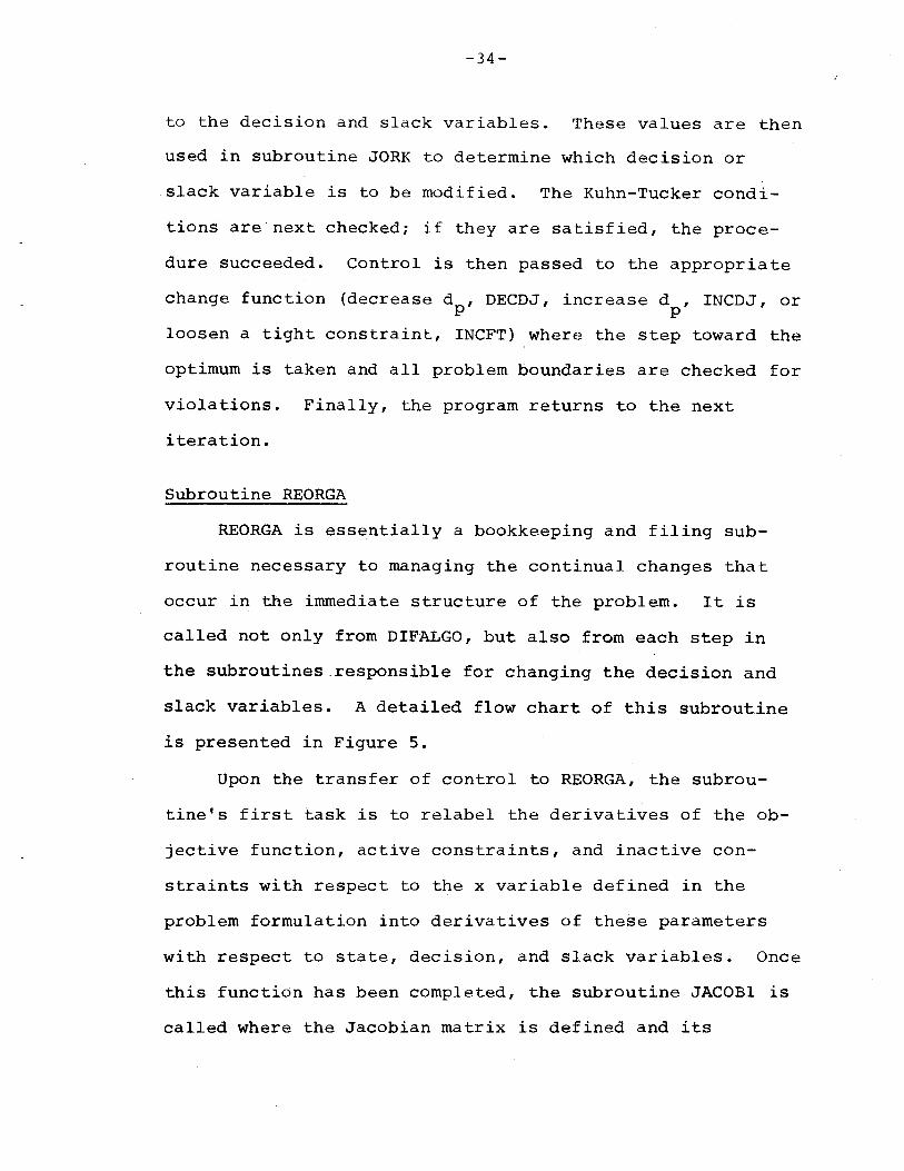
Subroutine REORGA
REORGA is essentially a bookkeeping and filing sub-
routine necessary to managing the continual changes that
occur in the immediate structure of the problem. It is
called not only from DIFALGO, but also from each step in
the subroutines ,responsible for changing the decision and
slack variables. A detailed flow chart of this subroutine
is presented in Figure 5.
Upon the transfer of control to REORGA, the subrou-
tine's first task is to relabel the derivatives of the ob-
jective function, active constraints, and inactive con-
straints with respect to the x variable defined in the
problem formulation into derivatives of these parameters
with respect to state, decision, and slack variables. Once
this function has been completed, the subroutine JACOBI is
called where the Jacobian matrix is defined and its
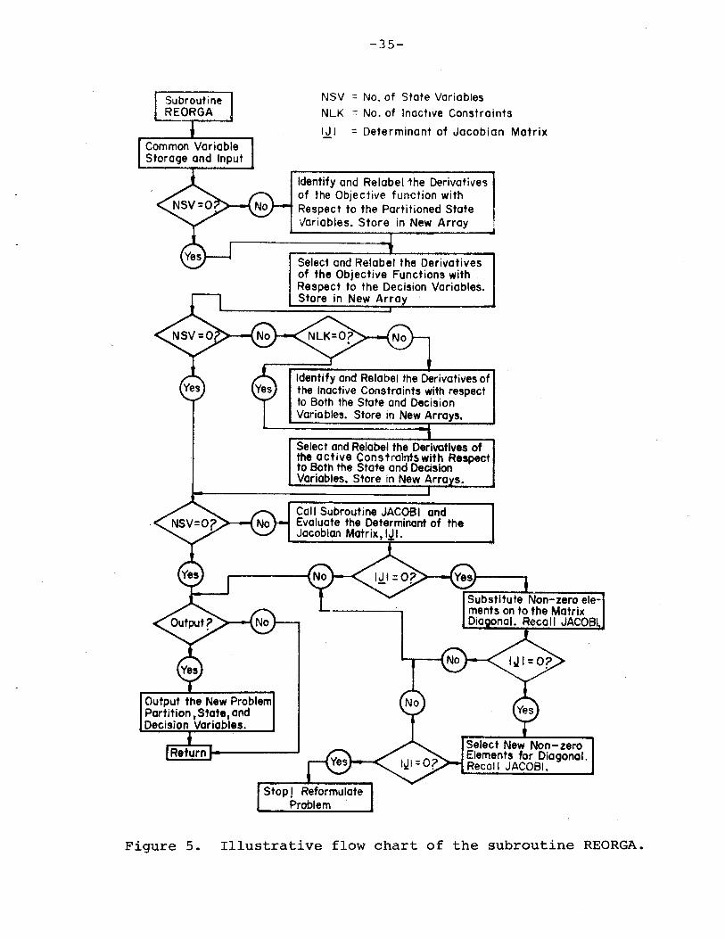
-35-
Identify and Relabel the Derivatives ofthe Inactive Constraints with respectto Both the State and DecisionVaria bles. Store in New Arrays.
NSV = No. of State VariablesNLK = No. of Inactive Constraints
III = Determinant of Jacobian Matrix
Select and Relabel the .Derivativesof the Objective Functions with ,Respect to the Decision Variables.Store in New Arra
Identify and Relabel1he Derivativesof the Objective function withRespect to the Partitioned StateVariables. Store in New Array
Select and Relabel the Derivatives ofthe active Constraints with Respectto Both the State and DecisionVariables. Store in New Arra s.
Return ...----~
Output the New ProblemPartition,Stat., andDecision Variables.
Call Subroutine JACOBI andEvaluate the Determinant of theJacobian Matrix.I~I.
Select New Non-zeroElements for Diagonal.Recall JACOBI.
Figure 5. Illustrative flow chart of the subroutine REORGA.
-36-
determinant is evaluated. If this value is not zero, then
REORGA concludes its function and control is returned.
However, if for some reason the current partition between
states and decisions yields a singular value for the Jac-
obian matrix, REORGA attempts to restructure the partition
into a non-singular condition. In problems with many state
variables, this may be an almost impossible requirement be-
cause of the enormous number of variable combinations pos-
sible. In REORGA, the best plan that could be thought of
was one of trying to make all diagonal values in the matrix
non-zero. Unfortunately, cases have been found where this
is insufficient in which the problem definition needs to be
re-evaluated. Generally, the diagonalization will provide
a non-singular Jacobian matrix.
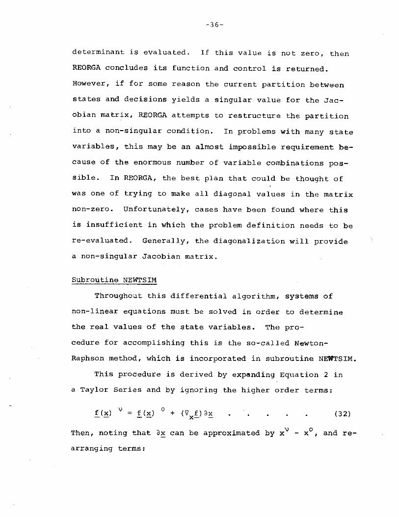
Subroutine NEWTSIM
Throughoat this differential algorithm, systems of
non-linear equations must be solved in order to determine
the real values of the state variables. The pro-
cedure for accomplishing this is the so-called Newton-
Raphson method, which is incorporated in subroutine NEWTSIM.
This procedure is derived by expanding Equation 2 in
a Taylor Series and by ignoring the higher order terms:
+ ('V f)dXx- - (32)
Then, noting that ax can be approximated by xV - xc, and re-
arranging terms:

-37-
xV = xO - (V f)-l f(x) 0x- - - (33)
This recursive equation can then be used to solve the non-
linear equations.
There are several problems with the Newton-Raphson
method which demand attention in NEWTSIM. Occasionally,
the system of equations being solved represent functions
with several inflection points or!nodules. In these situa-
tions, if the step size in a decision variable is too large,
the procedure may converge on meaningless points. To com-
bat this occurrence (which is often), the NEWTSIM subrou-
tine is able to back up until a proper solution is obtained.
An illustrative flow chart of this subroutine is shown in
Fig. 6. In some cases, the procedure simply will not con-
verge on a solution. Generally, this means a poor problem
formulation, but if it occurs, the output subroutines are
called and the program will stop.
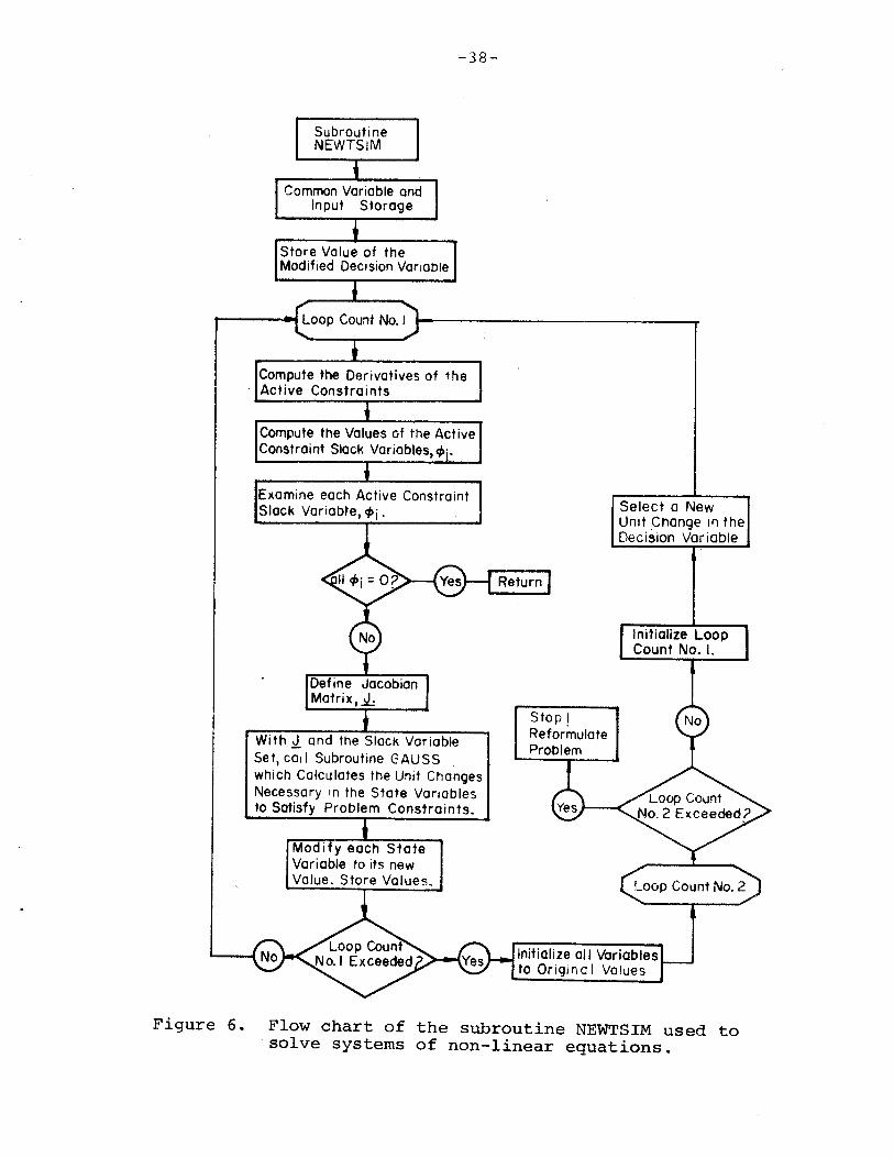
Subroutine DECDJ
DECDJ is the subroutine in which the particular deci-
sian variable, d p ' is decreased. It, along with INCDJ and
INCFT, is the basic component in this optimizing method,
and it is by far the most complex. This subroutine has
been flowcharted in Figure 7.
The first operation of DECDJ is to store the entering
values of the decision variable, d , and the constrainedp
derivative of the objective function, oy/6d. Then, subp
routines calculating the constrained derivatives, os./&d- 1 P
-38-
Compute the Deriva1ives of theActive Constraints
Compute the Values of the ActiveConstraint Slack Variables, ~'.
Examine each Active ConstraintSlack Variabte, c#lj •
With.J. and the Slack VariableSet, coil Subroutine GAUSSwhich Calculates the Unit ChangesNecessary in the State Vanablesto Satisfy Problem Constraints.
Modify each StateVariable to its newValue. Store Values.
Select a NewUntt Change in theDecision Variable
Initialize LoopCount No. I.
Initialize all Variablesto Origi Ij a I Values
Figure 6. Flow chart of the subroutine NEWTSIM used tosolve systems of non-linear equations.
-39-
Compute the Constrained Deril/ativesof all State Variables with Respectto the Decision Variable, dp.
Find the Maximum Decrease in theValue of dp which First Forces aState Variabe t" Zero. Label thisDecrease ~d "
Compute tM Constrained Derivatillesof all Loose Slack Variables withRespect to the DecIsion Venable, dp.
Find the Moximum Decrease in theValues of dp which First Forcesan Inactive Constant to be Active.~_abel this Decreas·e 6d j .
Set the State VariableFirst Driven to ZeroEqual to Zero
Interchange the ZeroValued State VonobleWith the DecI510n Vanabledp .
Compare the Values of ~di, and ~dj
wIth the Decrease Necessary to makethe Decision Variable Zero,6dk-'
Call Subroutine CONDERto Compute the Constrained Derivative of theObjective Function withRespect to the DecisionVanable. 8y/8dp
Add the Activated Constraint tothe Active set. Select LargestValued Decision Variable to beNew State Variable
Call Subrout ine ENDCHEK tomake sure thiS Solution is Feasible'
• Note !hot at I ~d arenegative so maximumsare the smallest inabsolute value.
Using 0 WeightedAverage IterativeTechnique, Increasethe Value of theDecision VariableUntil 8y/8d zOo
Figure 7. Illustrativ~ flow chart of the subroutine DECDJ.
-40-
and 8f~+/8dp are called. Next, the most limiting condition
affecting the magnitude of the decrease in d is evaluated.p
Based upon this determination, the appropriate change in the
decision variables is made and a new value for 8y/odp is
calculated. If this value has become negative, the de
crease has been too large and the procedure progressed
past the minimum. When this occurs, the inj.tial and new
values of d and oy/od are used for a weighted average it-p P
erative procedure to adjust d to a value that 'results inp
oy/od being equal to zero. On the other hand, if thesep
constrained derivatives of the objective function remain
positive, the program continues. Three conditions occur:
1. dp
can be decreased to zero and no changes
in the problem structure are necessary.
2. The decrease in the decision variable can
force a state variable to zero. The par-
ticular state going to zero is already known,
so the largest valued decision varictble
is interchanged with the state. Then, with
the old state variable equal to zero, the
new set of equations can be solved.
3. The decrease in d may result in a prevp
iously inactive constraint being tightened.
In this situation, the number of state
variables must be increased by one and a
new variable and constraint partition
determined.

-41-
At the conclusion of these adjustments, the subroutine
ENDCHEK is called to make sure the new problem structure is
a realistic one. If so, the control is passed first back
to DECDJ and then to DIFALGO for a new iteration. If not,
ENDCHEK redefines the structure and partition until they
are satisfactory.
SECTION IV
URBAN WASTEWATER AND
RECLAMATION MODEL
Introduction
The urban wastewater treatment and reclamation system
is a complex network of unit operations, flow control
points, and water quality objectives. Associated with each
unit of treatment are the capital costs of construction and
the costs of operating and maintaining these facilities.
An analysis of these costs by Deredec (1972) indicates that
these facilities exhibit significant economies of scale,t~i.e., the marginal costs decrease with capacity. In a re-
view of several sources of information, Deredec (1972)
summarized the costs of these facilities into useable
cost functions and then compares the predicted values using
these relationships to actual installations. These results
indicated an accuracy of within about 10-20%. This accu-
racy is also sufficient for the purposes of this
investigation.
In the model of the wastewater treatment system
developed in this section, these relationships are used to
reflect the costs of treating and reclaiming wastewater for
recycling and achieving the standards set for urban
effluents.
-43-
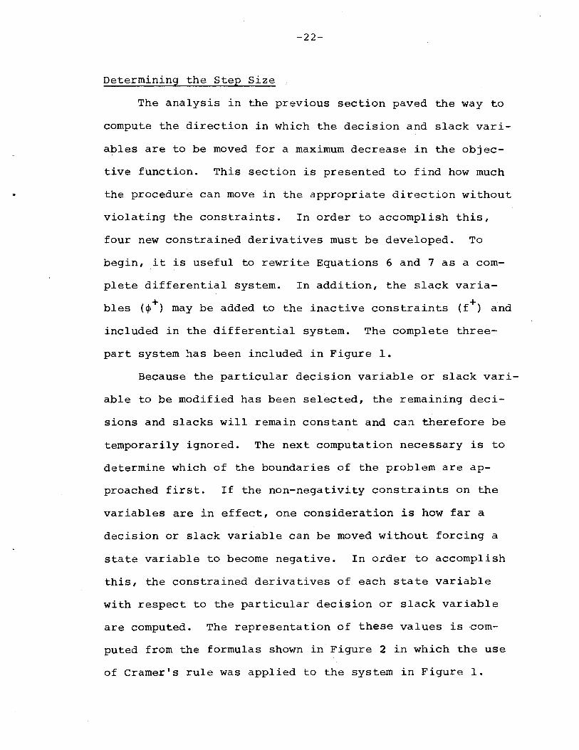
Formulation of Wastewater Treatment Model
The intent of the wastewater treatment model, illus
trated in Figure 8, is to minimize the costs of the facil
ities subject to the water quality standards placed on the
urban effluent and the water being recycled. The costs of
recycled water are determined as the unit difference bet
ween the total system costs with and without recycling.
Thus, by dividing the difference in these costs by the
quantity of water to be reused, an average cost, or unit
cost, for this water can be determined. The optimization
of the wastewater treatment system minimizes the unit
costs of recycled water, as well as the costs of achieving
certain levels of pollutants in the released effluent.
For the purposes of this study, the water quality
vector will be limited to two parameters: (1) the inor
ganic concentration of total dissolved solids, TDS; and
(2) the commonly cited S-day Biochemical Oxygen Demand,
BOD. However, the cost functions represent treatment
facilities which remove suspended solid~, nitrates, phos
phates, and other pollutants restricted by water pollu
tion guidelines, as set by the regulatory agencies. The
consideration of only two of these parameters by no means
assumes that other quality criteria are unimportant. In
stead, the intent of this limitation is to select two
parameters that best characterize the overall quality of
water. The evaluation of water management policies in the
IReuse IOr, Cbr.Ctr
X6
Xi = flowrate .ithin system
Q= flowrate in MGD.Cb= BO 0 concentrationCt =TDS concentration
i =o =
I Inflow IOJ, Cbi,Cti
I~
~
I
Water flow IOutflow IQo' cbo,Cto
Figure 8. Schematic flow network of an urban wastewater treatment system.

-45-
urban environment requires that the interdependence bet-
ween the sectors of the model be properly defined. As a
result, TDS and BOD were selected as "indicators" of the
effects that water quality in one part of the model have on
the others. These variables are also widely used in de
sign and monitoring and therefore are commonly measured.
Wastewater from the\ urban area is collected and sent
first to the primary treatment.. The quantity of these
flows is defined as Qi while their associated TOS and BOD
concentrations are Cti and Cbi , respectively. The primary
effluent then becomes the influent to the secondary treat
ment phase. Upon concluding secondary treatment, the BOD
levels are usually low enough to satisfy the 80% removal
specified by present water quality standards (Nichols,
Skogerboe, and Ward, 1972). However, as the water quality
standards become more rigid, further treatment is neces-
sary. Consequently, a decision must be made at this point
as to how much water should be spilled into the effluent
channels, X , and how much should be sent through tertiary2
treatment, X , in order to achieve a mix with a given level1
of BOD in the final urban effluent, Cbo • After tertiary.
treatment, three additional flow parameters must be decided
upon: (1) the quantity of water released to the outflow,
X , (2) the ,quantities released to the reuse system! X ,5 ~
and (3) the flows needing desalinization, X , to satisfy. 3
specified levels of TOS in both the outflow and the recycl-
ed water. The TOS constraints on the reuse system and
-46-
outflows are defined as Ctr and Cto ' respectLvely, which
are met by mixing flows passing through the desalting pro
cess (X and X ), with the other flows. The flows in the6 7
wastewater model are regulated according to the water
quality standards, physical system at each junction, and
the quantities of outflow, 00' and reuse, Qr.·
The water quality objectives in this model function
as constraints on the optimization procedure. Two con-
straints on the effluent water quality thus describe the
restriction~ on the two quality parameters, TDS and BOD.
The functions can be written as,
X T + (X + X )Cb < Q Cb21 5 6 r- 00
and,
(34)
( 35)(X + X )Ct , + X T Ct , < Q Ct2 5 ~ 62 ~- 00
in which T is the BOD concentration after secondary treat-
ment in mg/l,T is the removal efficiency for the desalt-
ing process, in mg/l and Cbr is the BOD concentration from
tertiary treatment. The water quality constraints for the
reuse segment can be written as,
X4Cti + X
7T
2Cti ~ 0rCtr (36)
representing only the concentrations of TDS since it is
practical to assume that BOD levels after tertiary treat-
ment would generally satisfy criteria for raw water
supplies.
The interaction of flow rates and water quality, ex-
tends the mathematical non-linearity to the constraints
of the preceding paragraph. Therefore, it is necessary
-47-
to add physical flow constraints to the model to avoid
unusual flows in the network. To begin, consider the
outflow,
x + X + X = Q2 560
and also the reuse phase:
X + X =' Q4 7 r
.,
(37)
(38 )
In addition, the flow system must also be feasible at each
decision junction in the model:
X + X = Q. (39)1 2 ~
X - X - X - X = 0 (40)1 3 4 5
X - X - X = 0 (41)3 6 7
The cost functions for each treatment process, along
with these constraints, form the optimizing model of the
wastewater treatment system.
Model Components
Primary Treatment
The first component of urban wastewater renovation,
primary treatment, consists primarily of screening, grit
removal, and primary clarification. Although these proces-
ses are quite often incorporated with secondary treatment,
sufficient cost information exists in the literature to
make the distinction.
Capital construction cost estimates for primary treat-
ment facilities have been reported by several researchers.
These estimating functions are helpful .not only in
-48-
establishing the costs of water quality control, but also
in the planning of treatment plants themselves. Typically,
these relationships have the form,
Y = aZm (42)
in which Y is the capital cost in millions of dollars and
z is the plant capacity in million gallons per day (mgd).
Primary treatment as a whole is relatively subject to eco-
nomics of scale as the exponential coefficient, m, usually
ranges between 0.7 to 0.6. Smith (1968) states that in
terms of 1967 dollars,
Y = 0.3l6Zo. 71 • (43 )
while Shah and Reid (1970) propose a 1959 dollar value ex-
pression of:
(44 )
The operation and maintenance costs have also been of
interest to managers, builders, and planners of wastewater
treatment systems. The formulas which have been proposed
by several investigators have the same general format as
expressed in Equation 42. Michel (1970), for example, in-
dicates that in 1967 dollars, the operation and maintenance
costs are,
Y = 21,8800°·59o
(45)
where Yo is the total annual operation and maintenance
costs and Q is the average daily flow in mgd. However,
these costs are more commonly expressed as costs per 1000
gallons treated, such as the work by Smith (1968) which
uses 1967 dollars,
-49-
y = 4.47Z-0. 17 (46)
in which y is the operation and maintenance costs in cents
per 1000 gallons.
Secondary Treatment
The principal components of the secondary treatment
are most commonly either activiated sludge, rapid rate
trickling filt~rs, or slow rate trickling filters. For
the purpose of this' writing, the activated sludge process
was selected primarily for its flexibility with respect to
varying removal efficiencies. Although activated sludge
appears to achieve greater removal efficiencies and more
design flexibility than the other two, the costs are
also somewhat higher. In a design context, the respective
choice would be based on a more comprehensive analysis than
is appropriate here.
The capital construction costs of building secondary
treatment plants, while not indicating as large an economy
with scale as encountered in the primary treatment plants,
do nevertheless exhibit costs relationships with declining
marginal costs with increased capacity. Shah and Reid
(1970) state that in equivalents of 1959 dollars, the capi
tal construction costs for these plants can be estimated
from the following relationship,
Y = 2.48 X 10- 4 (PE)O.47 ZO.22 • (47)
where PE is the Population Equivalent of the organic load
ing expressed as,
PE =8.34 QCbi
b
-50-
:(48)
in which Q is the average daily flow in mgd, Cb
, is the. ~
Biochemical Oxygen Demand (BOD) concentration of the flows
.in mg(l, and b is a constant, usually 0.17 lb of BOD per
capita per day. Smith (1968) also presents an estimate of
activated sludge plant costs:
Y = 0.58 ZO.80 (49)
Of some additional interest is Shah and Reids' (1970) esti-
mate of the costs of the activated sludge unit itself.
This relationship, having the same format as Equation 47,
is given in 1959 dollars as:
Y = 5.1 X 10- 3 PEO.~6 ZO.36 • (50)
The costs associated with operating and maintaining
secondary treatment plants are listed in several sources.
For example, Michel (1970) suggests three relationships
for these costs:
Yo = 3.16 X 10 4 QO.73 (51)
Y = 28.2 PEO. 75 (52)0
Y = 9.02 Z-O.107 (53)
Tertiary Treatment
Advances in wastewater treatment have led to several
demonstrations of the feasibility of adding tertiary treat-
ment to existing primary, secondary treatment facilities
for further removal of waterborne contaminants (Evans and
Wilson, 1972). Such advances have been prompted by several
-51-
mounting crises. First, the need for water by municipali
ties, industries, and agriculture is outstripping the sup
plies of natural waters under existing inefficient prac
tices. Secondly, 90% removal of BOD, for example, is not
considered satisfactory to continually insure pUblic
safety and palatability (Fair, Geyer, and Okun, 1968). And
finally, the advent of new pollutants in conjunction with
mans' increasing life span subjects him to extended expo
sures to chemicals with yet uncertain results (Civil Engi
neering,1972). Since very few if any existing primary
secondary wastewater treatment facilities can meet reduced
pollution levels, or support a "zero level pollution"
philosophy for urban effluents, tertiary treatment will be
come as necessary in the near future as secondary treatment
is now.
In this writing, tertiary treatment will consist of
flocculation, lime treatment, and sedimentation; granular
carbon adsorption; and ammonia stripping. Although terti
ary treatment has found only limited application to date,
sufficient testi.ng has been completed to generate general
cost functions.
The capital costs,of tertiary treatment can be found
in several sources. Smith (1968) suggests that in terms of
1967 dollars, the following relationships can be employed:
Y = 0.05 ZO.89 (54)
for flocculation, lime treatment, and sedimentation,
Y = .398 ZO.65 (55)
-52-
for grannular carbon adsorption and,
Y = .0398 ZO.90 (56)
(60 )
(59 )
for ammonia stripping. Barnard and Eckenfelder (1970) also
give an estimating formula for granular carbon adsorption
in 1959 dollars which will be included here for comparison:
Y = 0.20 ZO.86 (57)
The costs of operating and maintaining tertiary plants
are also listed by Smith (1968) in terms of 1967 dollars:
y = 2.99 Z-O.03~ • (58)
for flocculation, lime treatment. and sedimentation,
y = 10 Z-O.28 •
for granular carbon adsorption and,
y = 11.58 Z-O.3 Z < 3 mgd
y = 1.2 Z-O.04 Z > 3 mgd
for ammonia stripping.
Desalting
The removal of salts from seawater and brackish waters
has been under close examination for some time as a source
for supplemental water supplies (White, 1971). The limit
ing factor to date has been the high costs as compared to
other water sources. Among the promising techniques that
have been developed, either electrodialysis, reverse
osmosis, or a combination of these two methods seems to be
the best suited for reclamation of urban wastewater
(Dykstra, 1968). Again the flexibility with regards to
-53-
removal efficiencies prompted the selection of electrodial
ysis for this model.
The capital construction costs for desalting plants
has been suggested by Smith (1968) to be,
Y = 0.51 ZO.67 (61)
and by Rambow (Cited by Deredec, 1972),
Y = 0.219 ZO.66 • (62)
which are also in terms of 1967 dollars. The first equa
tion is for a 90% TDS removal and the second is for a re
moval of 500mg/l.
The same two sources supplying capital cost informa
tion also suggest the following operation and maintenance
costs:
Smith (1968)
Rambow
y = 47.94 Z-·21
Y = 10.2 Z-0.12
(63)
(64 )
indicating significant variation.
A single-stage electrodialysis process applied in this
model is assumed to have a removal efficiency of about 40%.
Therefore, the costs suggested by Smith (1968) would be for
a four-stage demineralization system.
Operation of Wastewater Treatment Model
In order to provide the reader with a clearer under
standing of the urban wastewater treatment model and illus
trate its use in evaluating optimal policies in the overall
urban water system, it is useful to examine some of the
-54-
types of results generated by the wastewater treatment
model.
The cost functions presented in Equations 34 to 64 are
in the present-worth dollar value set by the original
authors. These relationships were multiplied by an ad
justment factor to convert all of them to 1970 dollar
values and then a set of results were generated to deline
ate the basic characteristics of the system.
The first characteristic of interest is the effects
varying effluent quality standards have on the unit costs
of recycled water. An illustration of this influence,
shown in Figure 9, represents a system with a reuse capa
city (Qr) of 30 mgd, and a fixed effluent TDS standard
(eto ) of 600 mg/l. The unit costs (present-worth) are
shown as a function of BOD standards on the outflows (Cbo )
with four levels of TDS concentrations in the recycled
flows. It i~ interesting to observe the curves at an
abcissa value of about 10 mg/l. At this point, the unit
costs for the higher limits of TDS in the reuse become
negative. This characteristic illustrates that when water
quality standards on the outflow are sufficiently restric
tive, the capacity of the desalting plant (and therefore
the costs) is larger than if the system would permit some
flows to be diverted to reuse at a poorer quality. The
effect therefbre of increasingly stringent standards on
urban effluents is to substantially enhance the feasibility
of reclaiming and reusing wastewaters.

1.5 ... QR=30mgdCTO=500mg/l
ICtJ)
0
8 1.0"'-~
en
~ I //~~I
U1U1
:!:05I
c:::::>
OD
-050 5 to 15 20 25 30ceo mg/I
Figure 9. Unit costs of recycled wastewater under varying water quality standards.
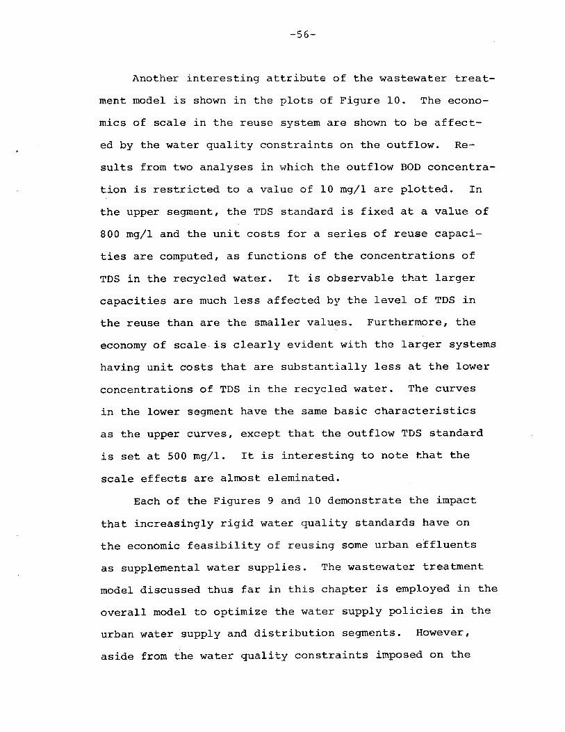
-56-
Another interesting attribute of the wastewater treat
ment model is shown in the plots of Figure 10. The econo
mics of scale in the reuse system are shown to be affect
ed by the water quality constraints on the outflow. Re
sults from two analyses in which the outflow BOD concentra
tion is restricted to a value of 10 mg/l are plotted. In
the upper segment, the TDS standard is fixed at a value of
800 mg/l and the unit costs for a series of reuse capaci
ties are computed, as functions of the concentrations of
TDS in the recycled water. It is observable that larger
capacities are much less affected by the level of TDS in
the reuse than are the smaller values. Furthermore, the
economy of scale· is clearly evident with the larger systems
having unit costs that are substantially less a~ the lower
concentrations of TDS in the recycled water. The curves
in the lower segment have the same basic characteristics
as the upper curves, except that the outflow TDS standard
is set at 500 mg/l. It is interesting to note that the
scale effects are almost eleminated.
Each of the Figures 9 and 10 demonstrate the impact
that increasingly rigid water quality standards have on
the economic feasibility of reusing some urban effluents
as supplemental water supplies. The wastewater treatment
model discussed thus far in this chapter is employed in the
overall model to optimize the water supply policies in the
urban water supply and distribution segments. However,
aside from the water quality constraints imposed on the

-57-
2.5
C80= IOmg/1CTO=800mg/1
2.0
0 1.5CJ)
0
8"""tit.. 1.0f/)...f/)00...c:~ CBO=IOmg/1
0.5 CTO=500mg/l
Reuse \/01uf1)e I
40 f1) drngd
0.0
-0.5500 600 700
TDS in Reuse. mg / I
I
800
Figure lO~ Effects of varying water quality standards ont~e unit costs and economies of scale 'of re-cycled wastewater.
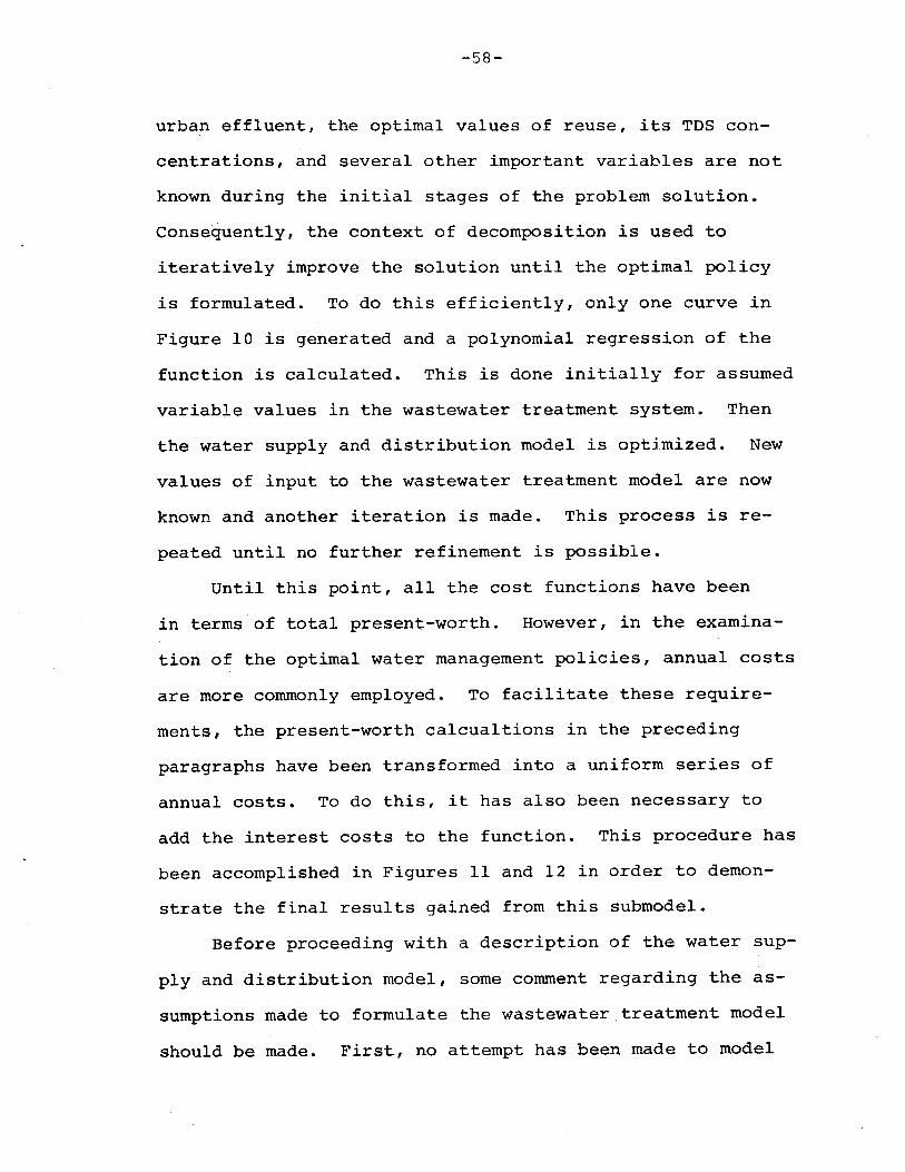
-58-
urban effluent, the optimal values of reuse, its TDS con
centrations, and several other important variables are not
known during the initial stages of the problem solution.
Consequently, the context of decomposition is used to
iteratively improve the solution until the optimal policy
is formulated. To do this efficiently, only one curve in
Figure 10 is generated and a polynomial regression of the
function is calculated. This is done initially for assumed
variab~e values in the wastewater treatment system. Then
the water supply and distribution model is optimized. New
values of input to the wastewater treatment model are now
known and another iteration is made. This process is re
peated until no further refinement is possible.
Until this point, all the cost functions have been
in terms of total present-worth. However, in the examina
tion of the optimal water management policies, annual costs
are more commonly employed. To facilitate these require
ments, the present-worth calcualtions in the preceding
paragraphs have been transformed into a uniform series of
annual costs. To do this, it has also been necessary to
add the interest costs to the function. This procedure has
been accomplished in Figures 11 and 12 in order to demon
strate the final results gained from this submodel.
Before proceeding with a description of the water sup
ply and distribution model, some comment regarding the as
sumptions made to formulate the wastewater;tr~atmentmodel
should be made. First, no attempt has been made to model
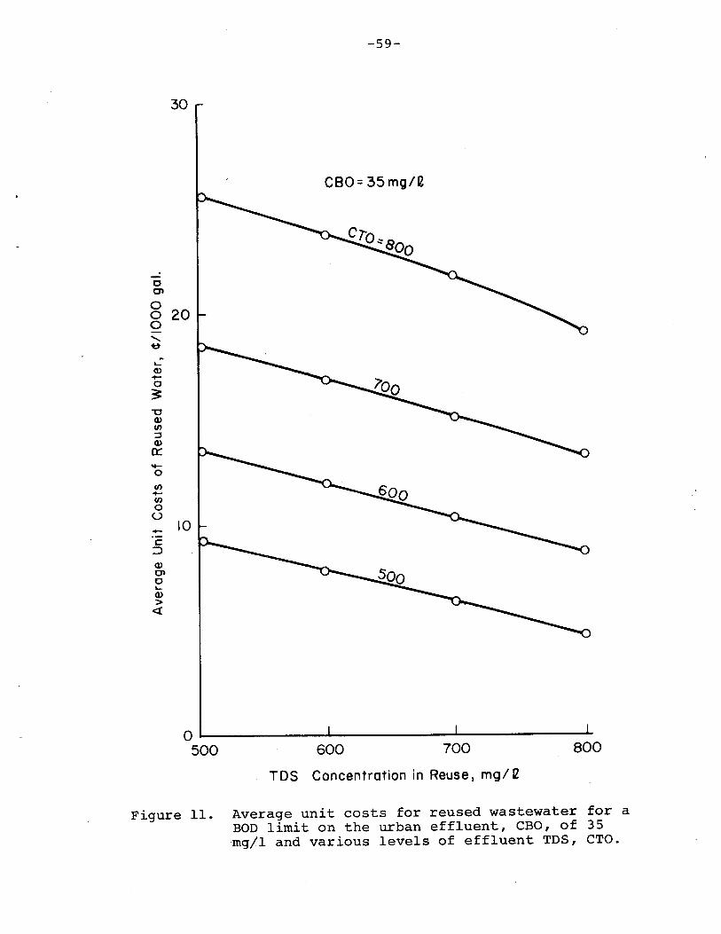
-59-
30
ceo= 35mg/2
-00'
00 200.........~
'-Q)-03:-0Q)fJ)
::sQ)
0.:::'+-0
fJ)-fJ)
00- 10c
::>Q)C'0'-Q)>~
800700600o------------------.......-------~500
TDS Concentration in Reuse J mg / e
Figure 11. Average unit costs for reused wastewater for aBOD limit on the urban effluent, CBO, of 35mg/l and various levels of effluent TDS, CTO.
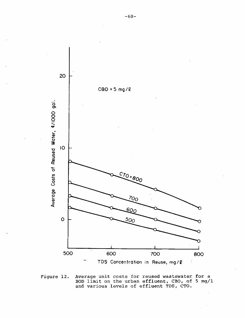
-60-
20
CSO =5 mg/rl
-0D'
000........~
.....'"Q)-0~
"0 10Q)(/)
:::sQ)
a:.....0
(/)-(/)0uQ)0'0.....Q)
>~
0
500 600 700
TDS Concentration in Reuse, mg/2
800
Figure 12. Average unit costs for reused wastewater for aBOD limit on the urban effluent, CBO,of 5 mg/land various levels of effluent TDS, CTO.
-61-
the numerous alternative treatment schemes which may im
prove the cost-effectiveness of this system. For example,
the use of polymers in primary treatment have been shown to
significantly improve the primary removal efficiency in
certain circumstances (Henningson, et. aI, 1970). Justifi
cation for this assumption is because cost information is
not accessible at this time in the general literature
from which cost functions could be formulated for inclu
sion in this section.
•
SECTION V
THE URBAN WATER SYSTEM MODEL
Introduction
In the preceding section, the urban wastewater treat-
ment and reclamation system model was developed prepatory
to its use here. The water supply and distribution system
model, defined in this section, focuses on the analysis of
water supply alternatives. However, because recycling is
an integral part of urban water supply, the linkage be
tween the two systems is brought to light.
The scope and format of the urban water system model
derived and explained in this section follows the "limited
purpose model" concept. The intent of this development is,.
to provide the mathematical description of the broad and
macroscopic characteristics of urban water systems and
evaluate the effects of changing institutional constraints,
such as water quality goals, on the optimal water manage-
ment policies. Consequently, the model is less useful as
a design or capacity determining tool as ~t is for deline-
ating and comparing various planning and management al-
ternatives. By limiting the scope of the model in this
manner, and avoiding the entangling detail of the exact na-
ture. of the flow networks, the model can be general in
nature and adopted to other areas with a minimum of
modification.
-63-
The basic nature of the model as it is operated begins
by combining the water supply alternatives with the distri-.
bution system, leading to the individual urban demands, as
illustrated in Figure 13. This leaves the urban water
system model in two distinct components which are then
conjunctively solved to optimize the complete network.
The procedure involves the following three steps:
(1) A quantity and quality of water needed for
reuse from the reclaimed wastewater treat
ment system is assumed and unit costs for
this water are computed for a range of TDS
concentrations. Then a polynomial regres
sion of these data points is computed giv
ing the unit costs of recycled water as a
function of its TDS concentrations.
(2) Using the unit costs previously deter
mined for recycled water, the model op
timizes the water supply and distribution
subsystem to evaluate the optimal water
management policy.
(3) The assumed values of reuse are contrasted
with the quantities actually employed in
the optimal plan. If these values differ
markedly, new values of reuse parameters
are assumed and the process repeated.
In addition to recycling wastewater, alternative
water supplies such as interbasin water transfers,
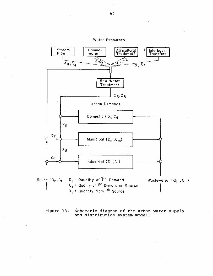
64
Water Resources
Urban Demands
Reuse (Qr 1 Cr
" ,
Industrial (Dj ,Cj)
OJ = Qua nti t y of "jth Demo nd
Cj = Quality of jth Demond or Source
Xj = Quantity from jth Source
Wastewater (OJ 1 Cj )
Figure 13. Schematic diagram of the urban water supplyand distribution system model.
-65-
groundwater, agricultural right aquisition and transfer,
and, of course, in-basin stream flows are available. The
characteristi~s of these resources are complex, but have
been extensively investigated. Although a thorough review
of such characteristics is infeasible, some general com
ments are helpful in realizing the potential uses and ex
tensions of the urban water system model.
Water Sources
Stream Flows
Water 'resources generated within the hydrologic unit
encompassing the urban demand consist primarily of stream
flows. Reservoirs, diversion works, and conveyance systems
transform the stochastic variations in these flows into de
mand frequency water supplies. Such supplies were develop
ed in competition with other interests, such as the agri
cultural and mining enterprises. Because urban areas have
generally been junior appropriators, they have been forced
to develop additional alternative water sources to meet
growing needs •.
The competitive characteristic of over-appropriated
water supplies has prompted numerous attempts to impart
an economic value or price to the flows. Such studies
seem to indicate that water values are higher than exist
ing prices because of the protective influence of the water
right system. In order to avoid the surrounding
-66-
controversy regarding the planning values these resources
should assume, existing rights are valued at estimated cur
rent costs. Then, in the model operation to be described
later, an attempt is made to indirectly value additional
stream flows according to actual worth. A more specific
description ~f this analysis will be deferred until later
in this.writing.
Interbasin Transfers
Transferring water resources from one river basin to
another is among the most feasible alternatives for sup
plying the needs of water-short areas. However, most
proposals for these transfers in the West have resulted in
political conflict because of the high value of the scarce
resource. Such conflicts have been observed in both the
Congress and State legislatures, in the Federal agencies,
in the association of Federal and State governments, in the
courts, and even on the canal or reservoir banks (National
Water Commission, 1972). The conflicts have also extended
to various interest groups, such as conservationists and
the large urban centers.
The costs of interbasin transfers are three dimension
al in nature. First, the capital outlays for construction
of the necessary facilities to import the water are very
large. However, unlike the water treatment plants, these
facilities are relatively permanent in nature. For
example, the structures involved may include reservoirs,
-67-
tunnels, canals, and diversion and control structures.
Since the expected life of these facilities extend beyond
the planning horizon, they may be easily financed for as
much as 50 years or more, which substantially reduces the
annual costs. The second economic consideration regarding
interbasin transfers is the operation and maintenance
costs. Again, the permanent nature of the system is char
acterized by a relative freedom from maintenance and thus
have low operation and maintenance costs. And finally,
the third dimension of costs associated with water importa
tion is the externalities, or costs to downstream water
users as a result of the water transfer. Externalities
are difficult to quantify and require a more specific
analysis than is permissible here.
External costs cannot be ignored in regional water
resource management, but are difficult to incorporate into
local planning efforts. It would appear plausible there
fore, to suggest further investigations regarding the ex
ternal effects of the importations and coordinate water
developments on a state level.
Because interbasin transfers are being considered on
such a large scale in the western states, it would be
helpful for the cost versus capacity relationship to be in
corporated in a model such as this. However, such an
analysis has not heretofore been completed in sufficient
detail to include in this description. Thus, the model
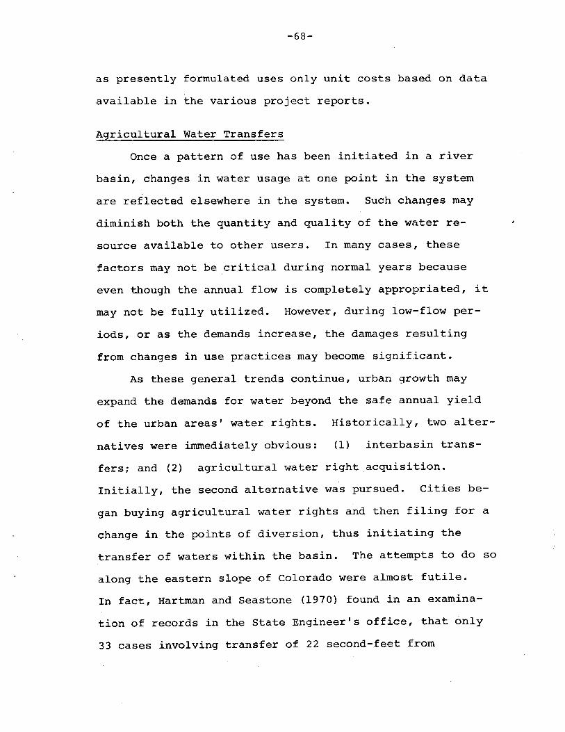
-68-
as presently formulated uses only unit costs based on data
available in the various project reports.
Agricultural Water Transfers
Once a pattern of use has been initiated in a river
basin, changes in water usage at one point in the system
are reflected elsewhere in the system. Such changes may
diminish both the quantity and quality of the water re
source available to other users. In many cases, these
factors may not be critical during normal years because
even though the annual flow is completely appropriated, it
may not be fully utilized. However, during low-flow per
iods, or as the demands increase, the damages resulting
from changes in use practices may become significant.
As these general trends continue, urban growth may
expand the demands for water beyond the safe annual yield
of the urban areas' water rights. Historically, two alter
natives were immediately obvious: (1) interbasin trans
fers; and (2) agricultural water right ,acquisition.
Initially, the second alternative was pursued. Cities be
gan buying agricultural water rights and then filing for a
change in the points of diversion, thus initiating the
transfer of waters within the basin. The attempts to do so
along the eastern slope of Colorado were almost futile.
In fact, Hartman and Seastone (1970) found in ,an examina
tion of records in the State Engineer's office, that only
33 cases involving transfer of 22 second-feet from
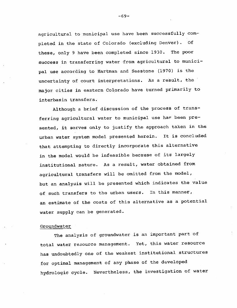
-69-
agricultural to municipal use have been successfully com
pleted in the state of Colorado (excluding Denver). Of
these, only 9 have been completed since 1930. The poor
success in transferring water ,from agricultural to munici
pal use according to Hartman and Seastone (1970) is the
uncertainty of court interpretations. As a result, the
major cities in eastern Colorado have turned primarily to
interbasin transfers.
Although a brief discussion of the process of trans
ferring agricultural water to municipal use hap been pre
sented, it serves only to justify the approach taken in the
urban water system model presented herein. It is concluded
that attempting to directly incorporate this alternative
in the model would be infeasible because of its largely
institutional nature. As a result, water obtained from
agricultural ~ransfers will be omitted from the model,
but an analysis will·be presented.which indicates the value
of such transfers to the urban users. In this manner,
an estimate of the costs of this alternative as a potential
water supply can be generated.
Groundwater
The analysis of groundwater .is an important part of
total water re30urce management. Yet, this water resource
has undoubtedly one of. the weakest institutional structures
for optimal management of any phase of the developed
hydrologic cycle. Nevertheless, the investigation of water
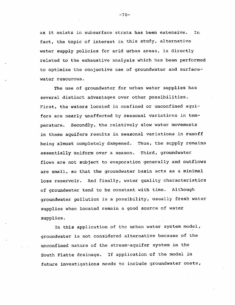
-70-
as it exists in subsurface strata has been extensive. In
fact, the topic of interest in this study, alternative
water supply policies for arid urban areas, is directly
related to the exhaustive analysis which has been performed
to optimize the conjuctive use of groundwater and surface
water resources.
The use of groundwater for urban water supplies has
several distinct advantages over other possibilities.
First, the waters located in confined or unconfined aqui
fers are nearly unaffected by seasonal variations in tem
perature. Secondly, the relatively slow water movements
in these aquifers results in seasonal variations in runoff
being almost completely dampened. Thus, the supply remains
essentially uniform over a season. Third, groundwater
flows are not subject to evaporation generally and outflows
are small, so that the groundwater basin acts as a minimal
loss reservoir. And finally, water quality characteristics
of groundwater tend to be constant with time. Although
groundwater pollution is a possibility, usually fresh water
supplies when located remain a good source of water
supplies.
In this application of the urban water system model,
groundwater is not considered alternative because of the
unconfined nature of the stream-aquifer system in the
South Platte drainage. If application of the model in
future investigations needs to include groundwater costs,
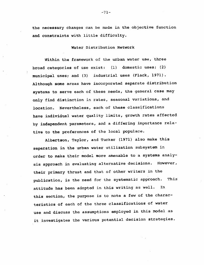
-71-
the necessary changes can be made in the objective function
and constraints with little difficulty.
Water Distribution Network
Within the framework of the urban water use, three
broad categories of use exist: (1) domestic uses; (2)
municipal u~eSi and (3) industrial uses (Flack, 1971).
Although some areas have incorporated separate distribution
systems to serve each of these needs, the general case may
only find distinction in rates, seasonal variations, and
location. Nevertheless, each of these class~fications
have individual water quality limits, growth rates affected
by independent parameters, and a differing importance rela
tive to the preferences of the local populace.
Albertson, Taylor, and Tucker (1971) also make this
separation in the urban water utilization subsystem in
order to make their model more amenable to a systems analy
sis approach in evaluating alternative decisions. However,
their primary thrust and that of other writers in the
publication, is the need for the systematic approach. This
attitude has been adopted in this writing as well. In
this section, the purpose is to note a few of the charac
teristics of each of the three classifications of water
use and discuss the assumptions employed in this model as
it investigates the various potential decision strategies.

-72-
Domestic Watel.· Uses
The first objective of a municipal water supply sys
tem is to serve the immediate needs of the population.
When water supplies are insufficient to meet all potential
demands, one after another of the less important uses may
be restricted. In the ultimate limitation, water would
only be available for such things as drinking, bathing, and
cooking. Thus, the domestic water uses are the first
priorities of the urban water system.
It has been traditional to lump outside-the-house
uses such as lawn or tree watering with the other domestic
uses. However, these uses are also subject to rationing
during critical periods. Consequently, lawn and tree
watering have been deleted from the domestic category
and placed with those considered as municipal uses. Such
an assumption may be infeasible due to the physical struc
ture of the distribution system. Nevertheless, it does
represent the extreme limit of separation between the two
uses, and it is, therefore, of interest in this analysis.
Domestic water uses not only maintain first priority
on the water supply, but its water quality as well. Many
other uses may be restricted by the concentration of
total dissolved solids, suspended solids, phosphates, nit
rates, heavey metals, or organisms, to name only a few.
Domestic water uses have limits on nearly every water qual
ity parameter currently used. As a result, tre~tment for
such uses must be more extensive. In the model proposed
~ ...._. ~~-.-
-73-
herein, the philosophy has been adopted to maintain water
quality limi~s for the domestic use at their present level,
even though these levels may not be as high as the toler
able limits. The basis on which such an assumption is
based is the fact that drinking water standards are upper
limits and not desirable if reduced water pollutants can
be maintained.
Municipal Water Uses
Although the fire protection water needs may be nearly
as important in an urban area as the domestic needs from
purely a survival viewpoint, other municipal water uses
such as park, golf course, lawn, and tree irrigations may
be important to the living environment. Such uses are
generally regarded as supplemental to the enjoyment of
living in the urban area.
A great deal has been said concerning the difficult
decisions to be made during periods of water shortage, but
the cause of the shortage has not been stated. Certainly
a man stranded in a life raft in the middle of the ocean is
as water short as another lost in the Sahara Desert. It
can therefore be concluded that an important method of
extending water supplies by more efficient use would be to
rearrange the urban water system in such a manner as to
distribute water on the basis of quality needs rather than
quantity asp~cts alone. By dividing the urban water use
and extracting municipal uses to be served by a poorer
-74-
quality water, especially with regards to reuse, more water
is available to the needs with more restrictive quality
characteristics.
Industrial water Uses
Industrinl water use, or commercial use, is defined
somewhat differently in this study than its real meaning.
For the purposes of this study, industrial uses are those
being filled by the urban water system. Fair, Geyer, and
Okun (1968) states that more than 60% of the industrial
needs in the United States are met by internal reuse.
Thus, only 40t of the industrial requirements are on the
average served by the metropolitan water system.
If domestic needs exist because people need water to
survive, and municipal needs exist because people demand an
enjoyable living environment, then industrial needs exists
because people are in the urban area to work in the direct
and indirect needs of industry. In other words, people
live in cities because of industrial concentzation and the
needs to support industrial jobs with services. Therefore,
the priority on industrial water is second to the domestic
uses.
The water quality constraints on industrial water use
are as varied as the nature of the industries themselves.
In this investigation, industrial quality requirements have
been limited to the maximum suggested for public potable
supplies.
-75-
Model Formulation
The model proposed in this thesis has been formulated
in the context of long range planning, but from a unique
viewpoint. By simplifying and generalizing the model be
yond the intricate details of either physical or institu
tional structures of any specific location, two central
advantages are gained:
(1) The optimal policies derived and the alter
natives evaluated indicate decision making on
the scale of planning alternatives of water
supplies.
(2) Only those institutional constraints violated
by cptimal strategies are identified. Thus,
those which effect future decisions are valued
in the sense that they can be priced by com
paring with and without analyses.
Model Constraints
The urban water supply and distribution system model
is bounded and operated by two major types of constraints:
(1) water quality constraints; and (2) water flow con
straints. The water quality constraints in effect place an
upper limit on the quality flows diverted to each of the
three use categories. It has been assumed that tertiary
treatment would be necessary for any quantities of water
recycled since public contact, occurring in all use cate
gories, would forbid objectionable odors and potential
-76-
health hazards resulting from the higher levels of BOD. In
addition, it is unlikely that desalting could be feasibly
accomplished if the suspended solids were limited only by
primary and secondary wastewater treatment.
To begin, the quantity of water treated in the munici-
pal raw water treatment system and its associated quality
are defined,
4X = E X. + (Qr - X - X )
5 j=l J 7 9
4E X.C. + (Qr - X - X 9) (Ctr )
j=l J J 7
C =5 Dd + X
.6
in which:
( 65)
( 66)
X. = quantity of water from source jJ
X , & X = quantities of water recycled directly to7 9 municipal and industrial uses
= total quantity of water from reclaimed wastewater
= associated water quality (TDS) from respectivesources
= the TDS concentrations in the reuse water
= domestic demand
Then for each water use, an upper limit on TDS can be
defined,
(67)
C. 1
tC + X Ct j6 5 7 r > 0 (68)D + X -m 8
tC + X Ctrj8 5 9 > 0 (69)D. -
1
where
-77-
= ¢ (Cd' C , C.)m ~(70)
Cd' C , C. = maximum allowable TDS for domestic,m ~ municipal, and industrial uses.
Cti = water quality of wastewater as a function of thewater quality supplied to the demands.
Dm and Di = municipal and industrial demands.
These constraints can be varied over an applicable range to
determine the costs associated with delivering water to
users of various quality.
The physical flow constraints become necessary not
only to insure each demand is satisfied, but also to main-
tain feasible solutions. Because the model operates in
an optimization format, it is necessary to p~ovide for
. realistic solutions as the model minimizes costs. These
constraints on the system can be written:
4Dd + D + D. = E X. + Qrm ~ j=l ~
D + X - X - X = 0m 8 6 7
D. - X - X = 0~ 8 9
and,
Q. = <P (Dd' Dm, D. )1 .1.
where Q. is the discharge of urban effluent, mgd.~
(71 )
(72)
(73)
(74 )
Objective Function
Employing the minimum cost criterion described in
S~ction II, and the cost functions described in the

-78-
previous paragraphs, the objective function can be formu-
lated. The objective function consists of three basic seg-
mentsi (1) cost of water supplies available at the raw
water treatment intake; (2) the costs of raw water treat-
menti and (3) the costs of recycling wastewater directly
to the municipal and urban demands.
If P i-s defined as the water supply cost, then1
4p = E c.X. + (Or - X - X
g) C r1 j=l J J 1
(75)
in which c. is the unit costs of the jth water source, X.J J
is the 'quantity selected from the jth source, and c isr
the costs of reused water, derived from the regression
with values of TDS in the flows. The polynomial expression
for c will be in the following form,r
c = A + A Ct + A C2r 1 2 r 3 tr
where Ai are the regression coefficients.
(76)
The variable
Ctr is the coordinating link between the urban wastewater
reclamation system and the urban water supply and distri-
bution syste:n.
The Illinois State Water Survey (1968) indicated that
in terms of 1964 dollar value, the capital construction
costs for raw water treatment facilities, including screen-
ing, flocculation, clarification, rapid sand filtration,
and chlorination, could be expressed as:
Y = 0.323 ZO.65 •
In addition, this source also showed the operation and
maintenance costs could be determined by:
(77 )
y = 1.21 Z-O.35
-79-
(78 )
where y is the costs of the treated water in $/1000 gal and
Z is the capacity of the treatment facilities in mgd. If
these costs are evaluated at their present-worth, added to
the interest costs, and extended in a uniform series over
a design life of 30 years with a discount rate of 5%, then
the total annual costs, in terms of 1964 dollars, can be
written as,
(79)
where P represents the total annual costs in dollars per2
million gallons treated.
The final component of the objective function is the
costs of the ~ecycled water which is sent directly to
municipal and industrial demands. From the preceding de-
finitions, P can be representative of the costs and3
written as,
P = (X + X )c3 7 9 r
or more completely:
P = (X + X ) (A + A Ct + A Ct2
)3 7 9 1 2 r 3 r
(80 )
( 81)
The complete objective function can now be expressed:
y = mini
3l:
i=lP.
1.(82)
These previous functions do not include several of the
costs encoun"tered in supplying water to urban demands. For
example, the costs of the distribution system, pumping, and
storage are not included since they are assumed to be
-80-
common to all aspects of the model. In addition, the func
tions were developed on the basis of differing dollar
values which can be corrected by applying an adjustment
factor taken from published cost indexes.
SECTION VI
COORDINATION OF AGRICULTURAL AND URBAN
WATER QUALITY MANAGEMENT
Introduction
The interrelated and competing uses of water often
result in co~plex problems in areas where water resources
are inadequate to meet the needs of potential interests.
The seriousness of these problems depends on the viewpoint
of the observer and efforts are necessary to arbitrate the
differences between those responsible for the problems and
those adversely affected. One of the most difficult of
these problems to resolve because of its widespread occur
rance is water quality degradation. The distinction bet
ween water supplies and wastewater return flows is slight
since many instances exist in which one individual's
effluent is another's supply. The ultimate objective is
therefore to maximize the utility of the resource on a
regional scale.
In order to insure equitable allocation of a resource
extending beyond local boundaries, the administrative
. structure of the water right was formulated. Along with
the concept of a water right, other institutional factors
have been implemented to control the flow and use of water.
Although such factors promoted optimal water use when first
implemented, no efficient means of updating these criteria
-82-
for later water resource allocation were included. The
institutional structures constructed in one era may thus
become barriers at a later date to optimization of water
resource use. When such conditions are encountered, in
vestigation into the feasibility of alternative courses of
action is initiated.
In arid and urbanizing areas like the Utah Lake re
gion, the best policy for water quality management usually
lies between the alternatives of complete emphasis on urban
pollution or on agricultural pollutiori. Water quality
management programs, instituted to insure the continued
use of the resource elsewhere, must consider which com
bination of treatments is the most efficient, (e.g., the
strategy with the greatest cost-effectiveness). As a re
sult, an important question to be addressed is the optimal
policies of coordinated water quality management between
agricultural and urban users. One method which is common
ly employed for evaluating such decisions is to model the
water use system at a level of detail that will yield the
solutions to the problem.
This section is presented to discuss the formulation
and application of a model designed to facilitate this type
of investigatiun. In the Utah Lake area, four major divi
sions in the region surrounding the lake have been made
(Huntzinger,197l): (1) American Fork-Lehi District;
(2) Provo District; (3) Spanish Fork District; and (4)
Elberta-Goshen District. The bulk of both agricultural
-83-
and urban deme.nds in the basin are contained wi thin these
districts. Consequently, the model developed in this sec
tion is intended to represent the water quality management
decisions on this district level.
Model Description
The coordination of agricultural and urban wate~ qual
ity controls is a necessary requirement for such pollutants
as total dissolved solids (TDS), often referred to as
salinity. However, the costs of urban salinity control
were shown i~ SECTION IV to be somewhat dependent on re
ductions in Biochemical Oxygen Demand (BOD), as well.
The urban wastewater treatment segment of this model
is equivalent to the model described in SECTION IV when the
levels of reuse are zero. Relying on that previous dis
cussion to sufficiently acquaint the reader, the emphasis
in the following paragraphs will be on the agricultural
segment of the model.
A management level model of an area consisting of both
agricultural and urban water uses can be conceptually or
ganized as shown in Figure 14. Such a model assumes that
diversions to the sectors are independent in nature and
thus does not allow for the subsequent use of effluents by
another use •. This type of operation is prevalant in the
Utah Lake study area, but can be modified easily to repre
sent the more general situation.
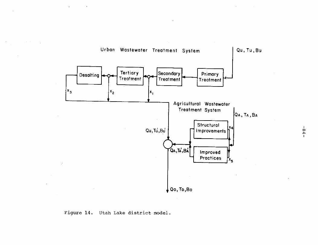
Urban Wastewater Treatment System QU,Tu,Bu
....--. Desaltin ~ Tertiary 1--.- - 1SecondaryH Primary ~g Treatment I'rl Treatment Treatment
X3,
X2 XI
Agricultural WastewaterTreat ment System
QA,TA,BA
Structural LX4
~ ImprovementsI
00~
I
ItImproved
I Pract ices Ix5
--QA ~I 8 11 .•--
,lA, A
•Qu, Tu ,au
• Qo, TO,Bo
Figure 14. Utah Lake district model.
-85-
The agricultural segment of the model is divided into
two treatments for reducing TDS concentration in the return
flows: (1) improving the water use practices in the dis
tricts; and (2) rehabilitating the structural elements of
the system. In the following paragraphs, these two mea
sures will be described in detail.
Improved Practices
Water diverted for agricultural purposes, in the west
ern United St~tes is used primarily for irrigation of crop
land to supplement insufficient natural precipitation. The
individual network of flows in the agricultural area can
be broadly divided into a groundwater subsystem, a root
zone subsystem, and a surface subsystem, each of which are
intricately interrelated with one another.
The surface subsystem begins with the diversion of
water from rivers, streams, or reservoirs into a conveyance
system consisting of either canals, ditches, or conduits.
From these conveyance networks, water is transmitted to the
areas of cropland to be irrigated, but in route some of the
flows are lost by seepage into the groundwater subsystem
and evaporation to the atmosphere. The remainder of the
diversions are applied to the croplands and enter the root
zone subsystem. Some of the water applied to the cropland,
however, may result in field tailwater which then returns
to the natural surface system for conveyance downstream.
-86-
'Flows entering the root zone subsystem by way of the
soil surface are usually the largest percentage -of the
total diversions~ From here, plants draw water through
their roots up into the leaves where it transpires into the
atmosphere. In addition, some moisture may evaporate
directly from exposed soil surfaces or percolate into the
groundwater.
Finally, water from seepage, percolation, subsurface
inflows from adjacent areas, and water naturally occurring
in the area are collected in the groundwater subsystem. In
most areas, the storage capacity in this subsystem is ex
tensive, which is useful in several ways as noted in SEC
TION V. Flows in th~ groundwater basin are partially
interactive with the other subsystems via drainage inter
ception and capillary water rise.
Associated with each of the components in the water
flow system is a TDS concentration. These concentrations
are affected by the concentrating effects of evaporation
and the loading effects derived from the contact with dis
solvable materials. If a particular segment in the flow
network is eHpecially detrimental with regards to these
quality criteria, then practices which introduce excessive
water into such areas should be alleviated, or improved.
The effective treatment of conditions which concen
trate salts is generally a matter of correcting the effects
of poor water management practices. For example, the
eradication of phreatophytes and the minimization of water
-87-
surface areas by eliminating unnecessary ponds and marshes,
are often feasible methods of salinity control. utah Lake
is the largest concentrator of salts in the study area with
the salt concentration being more than doubled. As a re
sult, lake diking to reduce the surface area of Utah Lake
is currently under serious consideration as part of the
Bureau of Reclamation's Central Utah Project (Skogerboe
and Huntzinger, 1972).
The contact of deep percolating water with soils and
groundwater aquifers results in a leaching of salts from
these materials, or the dissolving of mineral constituents
which are taken into solution. This salt loading effect,
often called "salt pickup," is observable in most areas,
but the rate of salt pickup varies widely depending upon
geologic characteristics and the previous effects of irri
gation. Salt pickup is generally minimized when efficient
irrigation practices are used. Total control is usually
not possible since some leaching is necessary to maintain
a salt balance in the root zone region of the soil to in
sure agricultural productivity.
The reduction of TOS concentrations in irrigation re
turn flows can be accomplished by improving the efficiency
of the irrigation practices. The term "irrigation effi
ciency" has been defined differently throughout the techni
cal literature, but is intended to denote the percentage of
the total agricultural diversions that is beneficially
used. To increase this efficiency, radical departures
-88-
from existing practices may be necessary. For example,
tighter control of water in the conveyance systems reduces
seepage and dumping of surplus flows into natu~al waste
ways, both of which cause salinity problems. In addition,
different irrigation methods may achieve higher levels of
application efficiency, which is the percentage of water
applied to the cropland that is consumptively used by the
plants. These improved methods control salinity by re
ducing the quantities of deep percolation losses.
Since significant variations in irrigation efficien
cies have been shown among individual farmers, improvements
in irrigation practices can be made in such a manner as to
correct the most inefficient first. This assumption yields
cost functions which have the characteristic of increasing
marginal costs with the percentage of the area treated.
The relationship derived for this study is shown in Figure
15, along with a similar curve for the structural improve
ments to be Jescribed next. These cost-effectiveness func
tions were generated from previous research experience in
the area, as well as feasibility studies conducted to eval
uate the potential for such improvements.
Structural Improvements
Many methods and structures which have been developed
for irrigating land provide considerable flexibility in
selecting the proper system for individual farm needs.
In these systems, the following functions should be
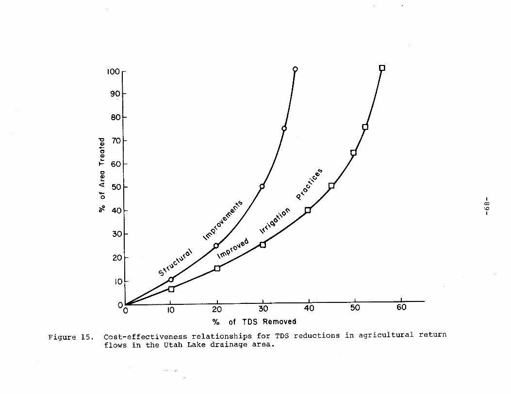
100
90
80
"C 70Q)-0Q)
~ 600Q)'-<t 50~
0
~ 40
30
20
10
00
<..()\v\~
\'(~G.>
10
,,,flJ~
flJ~o~
~<..,~
20 30
(be,.~
,-'o~
~...
40 50 60
Ico\0I
0/0 of TDS Removed
Figure 15. Cost-effectiveness relationships for TDS reductions in agricultural returnflows in the utah Lake drainage area.
-90-
efficiently employed: (l) water should be delivered to
the fields when needed and in amounts necessary to meet the
crop demands; (2) complete control of the water should be
provided and accurate measuring techniques practiced; (3)
water should be distributed evenly into the soil of each
field with adequate disposal of wastewater or the capabil
ity of reuse if desired; and (4) allow easy movement of
farm and maintenance machinery. When any of these cate
gories are not effectively fulfilled by the system, water
quality deterioration can be expected from excession see
page, deep percolation, poor drainage, phreatophytes, and
high evaporation losses.
At the present, many irrigation systems are in poor
condition because little or no need has existed for im
proved water management. With few exceptions, water sup
plies for agricultural lands have been abundant, thus lead
ing to low costs for water, and excessive uses. These
conditions have resulted in a significant deterioration in
water quality in many areas of the western United States.
The structural costs to alleviate these conditions,
which are shown in Figure 15, also exhibit increasing
marginal costs with increasing scale. However, the effec
tiveness of structural improvements is not expected to be
as great as the effectiveness of improved irrigation prac
tices, but structural irnprovementsmust be implemented in
order to achieve higher levels of irrigation efficiency.
-91-
Model Formulation
In order to operate the model in a manner which eval-
uates alterliative water quality control decisions, it is
necessary to formulate the mathematical description in an
optimizational format. Optimization requires three essen-
tial parts: (1) a criterion upon which alternatives are
ranked; (2) an objective function relating the criterion
to the alternatives; and (3) an array of constraints which
limits the se~rch for the best alternative to a specified
feasible region. The model constraints are not always
necessary if the search is assumed to be unbounded. Since
this is not a general condition, constraints are usually
considered as part of the model.
The optimization criterion has been selected and dis-
cussed in SECTION II, where cost minimization was shown
to be the most realistic parameter for this study. In the
following segments, the discussion will emph3.size first the
objective function and then the model constraints.
Objective Function
Beginning first with the urban sector of the model, it
may be worth repeating the functions derived in SECTION IV.
Recalling Equation 34, the cost functions have the typical
form,
mY = aZ . ( 34a)
where Y is the cost in millions of dollars annually, a is
a coefficient, Z is the capacity of the facility in
-92-
millions of g3110ns per day (mgd), and m is an exponent
usually less than 1.0. The costs of construction, as well
as operation and maintenance, were then outlined for each
of the treatment operations; namely, primary, secondary,
tertiary, and desalting. A summary of these will be omit-
ted here; but let P , P , P , and P be the variable unit123 4
costs for prbnary, secondary, tertiary, and desalting
plants, respectively. Referring to Figure 14, the annual
costs of urban wastewater treatment in a particular ag-
gregated district can be written,
Y = Q (P +P ) + (X +X)P + X Pu U 12 233 34
(83 )
in which Yu is the total annual costs in $ million, Qu is
the average daily outflow from the urban sector in mgd, and
x , X , X are the mixing flows released from each phase of123
the treatment to meet a specified level of water quality
in the effluents. In this model, it is assumed that ter-
tiary treatment is necessary for all flows to be desalted,
and BOD remo7al efficiencies in this model have been fixed
at 85% for the combined primary-secondary treatment and 99%
for the tertiary treatment facility, while the TDS removal
efficiency of the electrodialysis desalting plant is 90%.
Consequently, to achieve any particular value of either
TDS or BOD concentration in the effluents, only the capaci-
ties are chauged.
The agricultural water quality management costs are
quite different than the urban costs. In this sector of
the model, the salts which can be removed are only those
-93-
actually being picked up in the area. In addition, a small
reduction in TOS concentrations can be achieved by minimiz-
ing phreatophytes and evaporation from open water surfaces.
As a result, a minimum TOS concentration in agricultural
return flows, accomplished when 100% of the district has
been structurally rehabilitated and modified to exhibit
the most effective irrigation practices, is a function only
of the portion of the salts in the flows added by the dis-
trict. It may be worth noting in Figure 15 that if all
the area is treated, the maximum effect is approximately
90%.' This is to account for the small fraction of the
problem which must be left unresolved because of the leach-
ing requirements in the root zone.
For any intermediate reduction in TOS concentrations
in agricultural return flows, it is necessary to select
the optimal balance between structural and practice im-
provements. Consequently, in each optimization between the
agricultural and urban sectors, a sub-optimization is
necessary in the agricultural sector. To formulate this
problem, it is necessary to define the total annual ,struc-
tural cost in a district as Cs and the total annual prac-
tice improvement cost as C . Then let X and X be thep It 5
fraction of the expected TOS reduction accomplished by
each alternative measure. Thus, if a level of TOS of T'A
is desired in the return flows, the costs of doing so can
be written,
(84 )
(85)
-94-
in which Ya is the total annual costs in $ million, and
~s and ~p are the respective functions in Figure 15. If
the percentage of salts to be removed is defined as,
. ~T' - T ~CT = 1. 0 _ A minTA - Tmin
.J
where CT is the fraction removed, T' is the concentrationA
desired in the return flows, T. is the minimum achievablem1n
in the district, and TA is the initial concentrations in
the effluents, then;
CT = X + X4 5
(86 )
(87 )
The optimal choice of values for X and X is thus deter-4 5
mined by minimizing Equation 84, subject to the constraints
expressed in Equations 85 and 86.
Once the minimum costs for the urban wastewater treat-
ment, Yu ' have been determined and also the agricultural
costs, Ya , th~ objective function for each district can be
written;
Y= min [Yu + Ya]
The optimization thus attempts to find the best policy for
allocating water quality management responsibilites bet-
ween the agricultural and urban water user. This solution
is achieved in two levels; by first optimizing each in-
dividual sector and then secondly, optimization of the two
sectors together.

-9S-
Model Constra~nts
In order to insure that the solution to this problem
is both realistic and feasible, it is necessary to impose
constraints on the model. Again, beginning with the urban
wastewater treatment system, assume that a TDS constraint
on the district effluent has been set at To' and further
assume that the corresponding BOD constraint is set at B •o
If by some means it was previously determined that the ?p-
timal level of urban effluent TDS and BOD concentrations
were T' and B r then this sector's constraints could beu u'
written as,
and
X (O.lS·B ) + (X +X ) (0.01) (O.lS-B )1 . U 2 3 U
QU
< B'u (88)
(X +X ) T + X (0.1) (T )1 2 U 3 U
QU
< T'u
(89)
where Qu ' Tu ' and Bu are the initial effluent flows, TDS,
and BOD, res~ectively; and
x + X + X == Q1 2 3 U
In a similar manner, if the predetermined optimal
(90 )
water quality characteristics for the agricultural sector
were TAand BA, then these constraints could be written as
indicated previously in Equations 86 and 87.
Since the variables T~, B~, TA, and BAare in reality
the main interest in this model, then an overall set of
constraints must be imposed; namely,
-96-
SECTION VII
OPTIMIZING REGIONAL WATER QUALITY
MANAGEMENT STRATEGIES
Introduction
During recent decades, improvements in hydraulic de
sign, equipment, and construction methods have increased
the feasibility of transporting large quantities of water.
For this reason, the development and transfer of water re
sources in areas with abundant supplies to areas encounter
ing shortages has become widely practiced. Rapid growth
and concentr~tion of urban demands have often been met with
interbasin transfers because of their high quality and
economic feasibility. Other alternatives, such as the
acquisition and transfer of agricultural water rights,
have been used to a lesser degree because of the complex
and often discouraging legal procedures. In addition, the
reclamation and reuse of wastewater has previously been
prohibitive because of high costs.
The decision to import water in each instance has
been a local rather than a regional optimum. These di
versions are not without some inherent disadvantages, one
of which is of primary concern in this section; namely,
water qualit~' deterioration. As a consequence of these
limited considerations, at least two major water quality
problems are manifested. First, the export of good
-98-
quality water from a watershed reduces the dilution capa
city of that system to assimilate and transport the waste
materials occurring therein. This condition is a major
argument against interbasin water transfers, since they
tend to restrict economic growth in the basins of origin.
The second problem is felt downstream from the local area
when the effect of the effluents overwhelms the existing
assimilative capacities in the remaining flows. When this
occurs, the downstream uses are restricted to the more in
sensitive applications, thereby again being economically
penalized. The resolution of the first problem is yet to
be evaluated, but the second condition is of particular
interest in this study.
The purpose of this section is to formulate a model
of the basin wide water quality management decisions for
areas involving both urban and agricultural water quality
problems. In the previous section, the model presented
represented individual subsystems in a region and was
shown to be relatively general in nature. The model to be
formulated in this section was designed specifically for
the Utah Lake drainage area and is therefore less applica
ble to other areas. The basic principles of the model are
general, however, so that application to othAr problems
can be facilitated by modifying the geometry of this model
to fit the characteristics encountered in another area.

-99-
Model Description
Some of the flows within the Utah .Lake drainage area
are used for municipal and industrial demands in Utah
Valley and the Salt Lake City metropolitan area. These
uses require careful examination of a number of water
quality parameters, but the most important is probably
the concentrations of TOS. Municipal and industrial water
supplies presently derived from the area have e;ccellent
quality, while the return flows from Utah Valley, which
are collected in Utah Lake, create a salinity problem; how
ever, there is not a significant BOD problem in Utah Lake
at the present time. Thus, TDS was selected in this model
to indicate the effects of alternative water management
strategies in the region.
The model proposed in this section is subdivided into
three major measures of salinity control. The first is the
management of salts in the return flows from the lands sur
rounding Utah Lake. In SECTION VI, these inflows were de
noted as district effluents and consequently this alter
native can be defined as district management. The reduc
tion of lake evaporation is the second salinity control
measure investigated in the model. Finally, exposing a
fraction of the flows leaving the region (Jordan River) to
desalination is considered. When these alternatives are
coordinated in a management level model, such as shown in
Figure 16, questions concerning optimal water quality
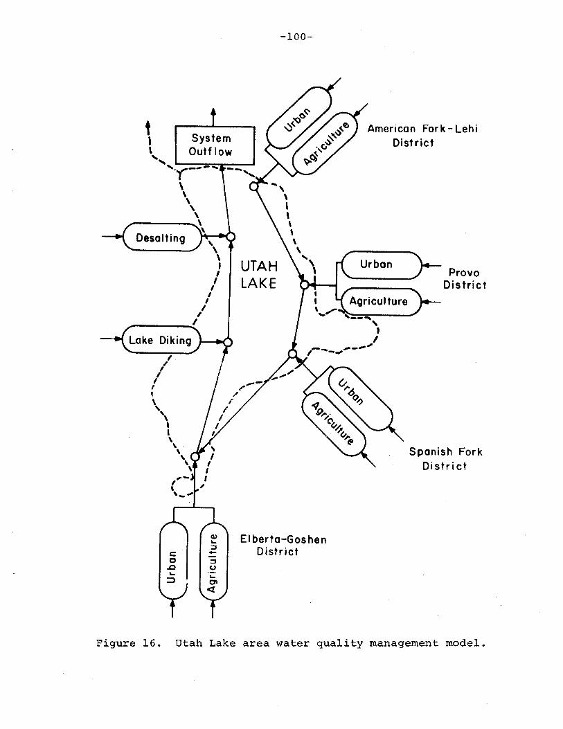
-100-
ProvoDistrict
Spanish ForkDistrict
American Fork - LehiDist rief
Urban
SystemOutflow
Desalting
I
"III~
\
'\I,\
\\ ,
\\
,-I,,-.,
Lake
t1,"
'<~----
\\,"
"...----.\\
::JCo)
EI berto-GoshenDistrict
Figure 16. utah Lake area water quality management model.
-101-
management can be addressed. A more detailed description
of these model components, which is presented in the fol
lowing paragraphs, is helpful in developing an understand
ing of the system.
District Water Quality Management
In the previous section of this report, a district
model was pr~sented which describes the interaction of ur
ban and agricultural water quality management. At the next
level of investigation, it is interesting to determine the
optimal strategy for controlling water pollution by coordi
nated operation among the districts. To accomplish this
task, the district models can be implemented into an over
all search for such an optimum. The technique used in this
segment of the model is a dynamic programming philosophy.
In previous studies, the major districts were called
collectively Utah Valley (Hyatt, Skogerboe" Haws, and
Austin, 1967, and Huntzinger, 1971). Following this lead,
the segment of the regional model describing the Utah"-,
Valley area operates by finding the minimum cost policy
for achieving a predetermined aggregate TDS concentration
in the flows entering the lake.
Lake Diking
As the Utah Lake evaporates approximately one-half of
the flows which enter it, the concentrations of salts are
correspondingly doubled. (Hyatt, Skogerboe, Haws, and
Austin, 1967). As a result of this action, the effect of
-102-
the lake far su~passes any other single cause of salinity
in the area. This realization has been incorporated into
the Bureau of Reclamation's massive Central Utah Project.'
Dikes are planned to separate both Goshen and Provo Bays
from the lake. From the estimated costs of the dikes, a
function with increasing marginal costs with scale was de
rived, which will be presented-in a following report.
This function allows the model to evaluate various diking
alternatives and test their feasibility in light of the
objective of regional water pollution control.
Desalting
A great deal of research has been undertaken to deter
mine the feasibility of reclaiming and reusing water which
was otherwise unfit for use because of poor water quality.
Among the pollutants of most concern, the inorganic salts
are the most significant. Investigations involving the
application of desalting technology have been undertaken
in numerous areas. In 1968, the Utah Division of Natural
Resources, as part of the long range state water plan,
joined with ~he Office of Saline Water of the Department of
the Interior and the u.s. Atomic Energy Commission to test
the feasibility of a multipurpose desalting, steam pro
duction, and electric power generation facility in the
Utah Lake area which would supply some of the metropolitan
needs of Utah (Haycock, Shiozawa, and Roberts, 1968).
The recommendations were generally positive regarding
-103-
desalting, st«ting that " ... desalting should be consid
ered a potential 'source of water supply to meet the State's
growing water needs. II
The scope of this model does not consider desalting
as a "source" of water, but rather an amendment to make
existing resources usable. This is admittedly a fine
distinction tu make. However, the view taken here is one
of water quality management in the total resources of a
large drainage basin.
The alternative methods suggested by the Utah study
center primarily on electrodialysis, which is also utilized
in this model. This, of course, simplified much of the
modeling, since this method has received close scrutiny
in a prior section of this report.
Model Formulation
The time interval used in this model was set as one
year in this study. The data requirements are thus annual
averages expressed on a daily basis. The scope of the
model is similar to those previously developed in that it
is in an optimization structure. Consequently, the major
divisions in this phase of the section can be divided into
a discussion of the objective function, which compares
alternatives 1 and the constraints which control the search
for the optimal solution.
-104-
Model Objecti,,'e Functions
The cost of achieving a specified reduction in the
TDS levels in the area outflow consists of the costs at-
tributable to management in Utah Valley, lake diking, and
desalting. The first consideration in this serial system
is the Utah Valley segment. Assume initially that th~ TDS
concentration in the valley effluents under a predetermined
policy are known and defined as C.1.n
In order to accomp-
lish this objective, it would be necessary fOL each dis-
trict effluent to be treated sufficiently to make the net
effect equal to the standard. This, of course, requires an
input to each area according to an optimal policy. It is
this allocation of costs among the districts that is of
interest.
Suppose from the district model previously formulated,
the minimum costs for achieving a TDS level in the i th dis-
trict were represented by Pi. Then, the costs of water
quality management in all Utah Valley would be the sum of
the costs in the districts,
(94)
where Y is the total annual costs.v
The next aspect in the objective function formulation
is to link the diking alternative with treatments in utah
Valley. Let Q be defined as the daily average outflowo
from the lake, thus
(95)
-105-
in whichQi is the inflow from the i th district in mgd;
and Q1 is the average dail~ lake surface net evaporation,
in mgd. The concentration of TDS entering the lake, C. ,~n
can be written in terms of these variables as:
i i1: Q.C. 1: Q.C.
C. ~ ~ ~ ~
(96 )= =~n i Qo + QlE Q.
~
The concentration of TDS in the lake outflow can similarily
be written,
C =o
i1: Q.C.
~ ~
°0(97)
If Equation 96 is subtracted from Equation 97, the rela-
tionship between the inflow concentration and that for the
outflow is determined,
which reduces to:
iC. 1: Q ..~n ..= '--0
0--
(98 )
(99)
This expression can then be used to evaluate the costs of
lake diking as a function of salinity reductions. To be
consistant, however, it is helpful to express the costs of
the lake diking measure in terms of a percent reduction.
As a result, it is possible to define this fraction as,
n = (100 )
-106-
where n is the decimal fraction and C is present concen-. p
trations. The cost-effectiveness function for lake diking
is similar in shape to the curves of Figure 15. Thus, the
costs of lake diking can be written as,
• (l 01)
in which a and m are the functional constants.
Finally, the costs of the desalting alternative can
be added to the objective function. Assuming the TDS re-
moval efficiency is fixed, the degree of desalting neces-
sary for the outflows to meet any specified standard can
be calculated. If the final effluent quality is defined
as Cn , a simple dilution equation reveals that:o
Q e" - Q"CQ' = 0 0 0 0
o C'o
(102)
where Q~ is the desalting plant capacity in mgd, C~ is the
quality of the desalted flows in mg/l, and Qn is the flowso
passing by the desalting plant in mgd. Thus, the costs of
the desalting can be determined as illustrated in SECTION
IV, which ca~ be denoted by Yd.
By properly selecting the amount of salts to be re-
moved in the districts according to an optimal allocation
among the districts, the degree of lake diking, and the de-
salting capacity, a minimum cost can be computed for ac-
complishing an effluent standard,
function is:
Y = min [Yu + Yl + Yd]
e"o· Thus, the objective
(103 )
-107-
Model Constraints
Beginning with the Utah Valley phase of the model, as-
surne that the degree of treatment for the entire valley has
been set at a TDS concentration of C. as noted before.~n
Then, a water quality constraint on the valley must be
written to insure this goal is reached:
il: Q.C.
J. ~. < C.J. J.nl: Qi
(l04 )
A constraint is also necessary in order to achieve co-
ordination of the three types of salinity control measures
taken together. This function can be written as the solu-
tion for e" in Equation 102:0
Q'C' + Q"CC" o 0 o 0 (102a)=0 Qo
These constraints link the model proposed in this section
together and allow the model to optimize the water quality
management strategies for the area.
Model Operation
This model operates in four basic levels:
(l) Optimization of urban and agricultural waste-
water treatment scheme on an individual basis as
outlined in the previous section;
(2) Optimal coordination of urban and agricultural
salin~ty control on a district scale, which was
also discussed in the previous section;
-108-
(3) Optimization of water quality strategies among
districts; and
(4) Optimization of salinity control including utah
Valley, Utah Lake diking, and desalting.
Because the model involves four levels of optimization, it
is helpful to explain the model operation in detail in or
der to understand the evaluation presented in this section.
Suppose the concentration of dissolved s~lts in the
outflows from the Utah Lake area were to be reduced by
100 mg/l and it was of interest to know the le~st cost
policy for achieving this objective. The first step would
consist of making an intelligent "guess." The first feas
ible solution would thus specify the reductions in TDS con
centrations necessary in the return flows from Utah Valley,
the amount of diking to be constructed, and the capacity
of the regional desalting plant. The total costs, as well
as the marginal costs (constrained derivatives), for both
desalting and lake diking can be immediately calculated
since they are represented by single-cost functions. The
costs for the Utah Valley segment, however, must be
determined.
With the value of the composite TDS concentration for
the return flows from Utah Valley specified, the next step
is to assume an initial distribution of salinity reductions
throughout the districts. Having accomplished this step,
the model developed in the previous section is used to
optimize the urban and agricultural water quality control
-109-
within the cistricts. Then, these solutions are used to
calculate the constrained derivatives from which the\
solution can be tested for a minimum. If such is not the
case, the allocation among districts is modified to reflect
another solution which is close to the minimum. This
procedure is repeated until the salinity control in Utah
Valley is represented by a minimum cost solution.
At this point, the marginal costs for the Utah Valley
segment is compared to those of the other two salinity
measures to check for a model optimum. If the solution is
not optimal, another solution is computed and this entire
process is repeated. When the minimum cost solution for
the entire Utah Lake drainage area is found, a complete and
comprehensive strategy for salinity control has been
outlined.
SECTION VIII
SUMMARY AND CONCLUSIONS
Introduction
Water management in arid urbanizing regions is a prob
lem requiring careful decision making supported by exten
sive investigation into all alternative actions having
particular merit. The most commonly employed tool for ac
complishing such comprehensive studies is the formulation
of mathematical models of the water use systems in these
regions. Such models are useful in not only determining
optimal courses of action to meet the changing needs, but
also produce valuable information concerning the operation~
al aspects of large and complex water use systems.
This report is the first in a series addrassing the
questions of water management in metropolitan areas and
their surrounding watersheds. In this writing, the model
formulations which accomplish these objectives are present
ed, with this section summarizing the results of the
modeling developments.
Sununary
As a means of testing the value of the models develop
ed in this report, two case studies will be presented in
subsequent reports. The first area selected for study was
the Denver metropolitan area, which is characteristic of

-111-
arid urban centers facing critical water shortages and in
creasingly stringent controls on the area's effluent water
quality. The Utah Lake drainage area in central Utah was
chosen as an area where a large scale regional water qual
ity study could be made. In this area, downstream water
uses are severely affected by high TDS levels resulting
from salts acquired in the Utah Valley (both agricultural
and municipal) surrounding the Utah Lake, as well as the
concentrating effect of evaporation from the lake. To
gether, these two areas typify water quality management
problems often encountered in the western United States.
The comparison of alternative strategies for water
management implicitly assumes an optimizational format.
As a result, the initial sections of this report describe
the optimization criterion employed in the study and the
principal optimization-technique developed. A minimum cost
criterion was selected from among the available economic
indicators because of the generally restricted nature of
water resources. State systems for allocation of water re
sources and federal policies for water quality control
tend to isolate individual water uses from each other at
'the management level. Consequently, much of the decision
processes in these areas center around meeting the demand
and water quality restrictions at minimum public cost.
The technique developed for minimizing costs in this
study is a general differential algorithm derived from the
basic mathematical approach to the derivation that added
-112-
generality to the method, thereby making it applicable to
problems which may be linear, quadratic, or geometric in
nature, as well as non-integer non-linearities. The method
is also gener~l in that it allows linear or non-linear con
straint functions of either the equality or mixed in
equality type.
Four individual mathematical descriptions were prepar
ed for different aspects of regional water quality manage
ment. The first application was made to the typical urban
wastewater coJlection and treatment system. A model con
sisting of the essential elements of primary, secondary,
tertiary, and desalting treatments were form~lated together
in a mixing model. The costs of the facilities, as well
as operation and maintenance costs, are minimized subject
to the criteria established for the effluents. Water which
is to be recycled is priced by computing unit differences
between the optimized system costs with no reuse and those
with a specified level of recycled diversions. Each of the
wastewater treatment costs exhibit decreasing marginal
costs with scale, thereby encouraging system consolidation.
The remaining two aspects of urban water management;
namely water supply and distribution, were next modeled and
then coupled with the wastewater treatment model via reuse
to represent the complete urban water system. The alter
natives for water supply include stream flows, interbasin
transfers, agricultural water right acquisition and trans
fer, groundwater, and of course, reused wastewater. The

-113-
costs of these supplies were assumed to be linear, making
the decisions in the model primarily functions of the ef
fluent standards on the wastewater, since the relative
feasibility of the recycled flows was the basic variable in
this regard. From the sources of water, the flows pro
ceed through the raw water treatment to the individual
urban demands. In this model, a distinction was made in
these uses on the basis of both a priority for quantity and
quality. Domestic uses which are typically defined as
household demands, as well as those demands which are most
sensitive to water quality, were delineated. In addition,
the municipal demands consisting of vegetative needs, fire
protection, and other uses were also delineated; as were
the host of industrial type needs. The model allows recy
cling to either be accomplished through the existing raw
water facilities or directly to both municipal and indus
trial demanas. This characteristic provides a great deal
of flexibility in evaluating alternative policies in the
urban system.
These previously noted models were designed specifi
cally for the urban area. Also of interest in this study
was the interaction of agricultural and urban water qual
ity problems. To study this question, a model was develop
ed to describe first individual agricultural and urban
wastewater treatment functions and secondly to coordinate
them together as a means of optimizing water quality man
agement from'a locality. The model (termed a district
-114-
model) is general in nature and is applicable to similar
problems in other areas.
Finally, the district level model was incorporated
into a regional or basinwide water quality management
model of the Utah Lake drainage area. This model also
consisted of 6esalting and lake diking measures for evalu
ating salinity control strategy for the area. By optimiz
ing the levels of salinity control responsibility among
the various alternatives, a comprehensive strategy is
generated for water quality management.
These models are multidimensional descriptions of the
basic water management strategies in urbanizing areas.
They answer questions of concern for planners and officials
of local, state, and national government by e~aluating man
agement policies. The scope of these models is, however,
most useful in testing the effects of the legali social,
and politica~ structures which have emerged to regulate
and allocate water resources.
Conclusions
The primary conclusions developed from this portion
of the study involve mainly the philosophy of modeling.
The water re~ources system is already complex without add~
ing the immense details of an urban structure. Therefore,
a temptation exists to create models which are detailed and
eXhau~tive. The authors feel that such a direction does
-115-
not facilitate decision-making, but rather clouds the
issues.
Because of the interrelated nature of water management
decisions, it is more feasible to limit models to either of
two purposes. First, it is helpful to provide models to
planners and operators of water systems which aid their
decision making. Such models must be designed to answer
specific questions of interest and should be as simple as
possible. The second aspect deals with questions involving
the integration of several levels of decision-making.
These models should be composed of simple unipurpose sub
models coordinated by a more sophisticated modeling
philosophy. The advantages of this stance is obvious.
Each segment of the 'complex system is best known to its
operators. Thus, a model of these components can be more
realistically detailed, thereby resulting in more repre
sentative r~sponses.

REFERENCES
Albertson, M. L., Tucker, L. S., and Taylor, D. C. 1971.Summary--The Urban Water System. Section XII, TreatiseOn Urban Water 'Systems, Ed. by M. L. Alhertson,L. S. Tucker, and D. C. Taylor. Colorado State University, Fort Collins, Colorado. J~ly.
Barnard, J. L., and Eckenfelder, W. W. 1970. TreatmentCost Relationships for Organic Industrial Wastes.Paper presented at the Fifth International Water Pollution Research Conference. August.
Civil Engineering. 1972. Reuse of Treated Wastewater asPotable Water. Summary from Papers presented at 1972Environmental Meeting, ASCE~ December.
Clark, J. W., Viesmann, W., and Hammer, M. J. 1971.Water Supply and Pollution Control. InternationalTextbook Company. Scranton, Pennsylvania.
Deredec, A. 1972. A Systematic Approach to the WaterSupply of a Large Urban Area. M.S. Thesis, CivilEngineering Department, Colorado State university,Fort Collins, Colorado. May.
Dykstra, 0.1. 1968. Status of Office of Saline WaterDevelopment in Brackish Water Conversion. "Water1968," Vol. 64, No. 90. American Institute of Chemical Engineers.
Evans, D. R., and Wilson, J. C. 1972. Capital and Operating Costs--Advanced Wastewater Treatment. Journalof the Water Pollution Control Federation. Vol. 44,No.1. January.
Fair, G. M., Geyer, J. C. , and Okun, D. A. 1968. Waterand Wastewater Engineering. Vol. 2, Water Purification and Wastewater Treatment and Disposal~ JohnWiley & Sons, Inc. New York, N. Y.
Flack, J. E. 1971. Allocation of Resources With a CaseStudy of the Water Management Game. Section V,Treatise On Urban Water Systems, Ed. by M. L. Albertson, L~ S. Tucker, and D. C. Taylor. Colorado StateUniversity, Fort Collins, Colorado. July.
Hall, W. A., and Dracup, J. A. 1971. Water ResourcesSystems Engineering. MaGraw-Hil1, Inc. New York,N. Y.
-117-
Hartman, L. M., and Seastone, D. 1970. Water Transfers,Economic Efficiency and Alternative Institutions.The Johns Hopkins.press, Baltimore, Maryland.
Haycock, E. B., Shiozawa, S., and Roberts, J. o. 1968.Utah Desalting Study, Preliminary Assessment of Desalting and Electric Power and Process Stearn Productionfor the Wasatch Front Area. Utah Department of NaturalResources, Office of Saline Water (USDI), and U'. S.Atomic Energy Commission. Salt Lake City, Utah.December.
Henningson, Durham, and Richardson - Consultants. 1970.Area Wide Sewerage Master Plan Report for the DenverMetropolitan Area, Phase I. Submitted to DenverRegional Council of Governments, Denve~'( Colorado.March.
Huntzinger, T. L. 1971. Future Water Use Model of UtahValley. M.S. Thesis, Agricultural Engineering Department, Colorado State University~ Fort Collins, Colorado. December.
Hyatt, M. L., Skogerboe, G. V., Haws, F. W., and Austin,L. H. 1969. Hydrologic Inventory of the Utah LakeDrainage Area. Report WG40-3. Utah Water ResearchLaboratory, Utah State University, Logan, Utah.November.
Illinois State Water Survey. Cost of Water Treatment inIllinois. October. (Cited by Deredec, 1972).
Kneese, A. V. 1964. The Economics of Regional WaterQuality Management. The Johns Hopkins Press, Baltimore, Maryland.
Kuhn, H. W., and Tucker, A. W. 1951. Non-linear Programming. Proceedings of the Second Berkeley Symposiumon Mathematics, Statistics, and Probability. J.Neyman, Ed. University of California Press, Berkeley,California.
McGauhey, P. H. 1966. Quality Aspects of Ground WaterUse and Management. proceedings of 1965 BiennialConference on Groundwater Recharge, Development, andManageroent. Fresno Field Station, Agricultural Research S~rvice, u.s. Department of Agriculture.January.
Michel, R. L. 1970. Costs and Manpower for MunicipalWaste Water Treatment Plant Operation and Maintenance,1965-1968. Journal of the Water Pollution ControlFederation, Vol. 42, No. 11, November.
-118-
Monarchi, D. 1972. Interactive Algorithm for MultipleObjective Decision Making. Technical Report No.6,Technical" Reports on Hydrology and Water Resources.The University of Arizona, Tucson, Arizona. June.
National Water Comnlission. 1972. Interbasin Water Transfers - A Political and Institutional Analysis. National Technical Information Service, u.S. Departmentof Commerce. Springfield, Virginia. March.
Nichols, S. R., Skogerboe, G. V., and Ward, R. C. 1972.Water Quality Management Decisions in Colorado. Completion Report Series, No. 38, Environmental ResourcesCenter, Colorado State University, Fort Collins, Colo-rado. June. .
Rambow, C. A. Industrial Wastewater Reclamation. Paperpresented at 23rd Purdue Industrial Waste Conference,Lafayette, Indiana. (Cited by Deredec, 1972).
Shah, K. L.,and Reid, G. W. 1970. Techniques for E~ti
mating Construction Costs of Waste-Treatment Plants.Journal of the Water Pollution Control Federation,Vol. 42, No.5. May.
Skogerboe,G. V., and Huntzinger, T. L. 1971. Effects ofInterbasin Transfers Upon Water Management Alternatives in Central Utah. American Water Resources Association. Water Resources Bulletin, Vol. 7, No.5.October.
Smith, R. 1968. Cost of Conventional and AdvancedTreatment of Wastewater. Journal of the Water Pollution Control Federation, Vol. 40, No.9. September.
Thomann, R. V. 1972. Systems Analysis and Wa~er QualityManagement. Environmental Science Services Division,Environmental Research and Applications, Inc. NewYork, N.Y.
Todd, D. K. 1960.& Sons, Inc.
Ground Water Hydrology.New York, N.Y.
John Wiley
U.S. Environmental Protection Agency. 1972. Conference inthe Matter of Pollution of the Interstate Waters ofthe Colorado River and Its Tributaries - Colorado, .New Mexico, Arizona, California, Nevada, wyoming,Utah. Proceedings of the Reconvened Seventh Session.Denver, Colorado. April.
White, K. R. 1971. Improving Municipal Water Supplies byDesalting. Prepared for Colorado Water ConservationBoard and Office of Saline Water, USDI. Denver,Colorad~. April.
-119-
Wilde, D. J., and Beightler, c. s. 1967. Foundations ofOptimization. Prentice-Hall, Inc. Englewood cliffs,New Jersey.