
Mathematical Analysis of Vaccination Models for the ... - MSpace
203
Mathematical Analysis of Vaccination Models for the Transmission Dynamics of Oncogenic and Warts-causing HPV Types by Aliya Ali Alsaleh A Thesis submitted to the Faculty of Graduate Studies of the University of Manitoba in partial fulfilment of the requirements of the degree of MASTER OF SCIENCE Department of Mathematics University of Manitoba Winnipeg Copyright c 2013 by Aliya Ali Alsaleh
-
Upload
khangminh22 -
Category
Documents
-
view
2 -
download
0
Transcript of Mathematical Analysis of Vaccination Models for the ... - MSpace
Mathematical Analysis of Vaccination Models for the Transmission
Dynamics of Oncogenic and Warts-causing HPV Types
by
Aliya Ali Alsaleh
A Thesis submitted to the Faculty of Graduate Studies of
the University of Manitoba in partial fulfilment of the requirements of the degree of
MASTER OF SCIENCE
Department of Mathematics
University of Manitoba
Winnipeg
Copyright c� 2013 by Aliya Ali Alsaleh
Abstract
The thesis uses mathematical modeling and analysis to provide insights into the transmission
dynamics of Human papillomavirus (HPV), and associated cancers and warts, in a commu-
nity. A new deterministic model is designed and used to assess the community-wide impact
of mass vaccination of new sexually-active susceptible females with the anti-HPV Gardasil
vaccine. Conditions for the existence and asymptotic stability of the associated equilibria
are derived. Numerical simulations show that the use of Gardasil vaccine could lead to
the effective control of the spread of HPV in the community if the vaccine coverage is at
least 78%. The model is extended to include the dynamics of the low- and high-risk HPV
types and the combined use of the Gardasil and Cervarix anti-HPV vaccines. Overall, this
study shows that the prospect of the effective community-wide control of HPV using the
currently-available anti-HPV vaccines are encouraging.
i

Acknowledgements
I would like to express my gratitude to my supervisor, Professor Abba B. Gumel (Department
of Mathematics), whose expertise, understanding, and patience, added considerably to my
graduate experience. I appreciate his valuable guidance and encouragement. He taught me
that the word ”impossible” does not exist anymore and how I should always take the failure
stage as the beginning for my success. I gratefully acknowledge all the financial assistance
and encouragement to continue my studies in Canada from the Royal Embassy of High
Education of Saudi Arabia. I am very grateful to Professors J. J. Williams and S. Portet for
their kindness and support. I am thankful to members of our research group, notably Dr. T.
Malik, Ms. F. Forouzannia, Ms. F. Nazari and Mr. A. Javame, for their helpful discussions.
I am very grateful to Dr. E. H. Elbasha (Merck Inc., USA) for answering many questions
on HPV, and for sharing some important references. I am grateful to my Thesis Committee
members, namely Professors S. H. Lui (Department of Mathematics) and Witold Kinsner
(Department of Electrical and Computer Engineering). I am thankful to the employees of
Mcdonald’s outlet (3045 Bairdmore Blvd), for their kindness during the many hours I spent
there working on my thesis (sometimes alongside my supervisor).
Finally, I would like to express my profound gratitude to my father, Ali Alsaleh (I have
inherited his smile), my mother, Laila Alhanfoush (I have inherited her patience), and my
brother Hussain Alsaleh (I have inherited his strength), for their unflinching support, en-
couragement, love, warmth and sacrifices. This will not be possible without them. I am
also grateful to my lovely other siblings, Afrah, Yaser, Ahmed, Fatimah, Duaa, Lamya and
ii

Mohammad Alsaleh, for always been there for me. I owe thanks to my grandfathers, grand-
mothers, uncles, aunts, cousins, nieces and nephews for their emotional care. The love and
support of my friends (F. Albinsaeed, J. Reimer, S. Alhelal, S. Albalooshi, S. Ibrahim, M.
Alsubait, F. Alhelal and S. Alrabeeh) have been greatly appreciated.
iii

Dedication
To my lovely parents, Ali Alsaleh and Laila Alhanfoush, and my brother Hussain Alsaleh.
iv
Contents
Abstract i
Acknowledgements ii
Dedication iv
Contents viii
List of Tables ix
List of Figures xv
Glossary xv
1 Introduction 1
1.1 Human Papillomavirus (HPV) . . . . . . . . . . . . . . . . . . . . . . . . . . 1
1.2 Control Strategies . . . . . . . . . . . . . . . . . . . . . . . . . . . . . . . . . 7
1.2.1 Treatment . . . . . . . . . . . . . . . . . . . . . . . . . . . . . . . . . 8
1.2.2 Pap screening . . . . . . . . . . . . . . . . . . . . . . . . . . . . . . . 8
1.2.3 HPV Vaccine . . . . . . . . . . . . . . . . . . . . . . . . . . . . . . . 9
1.3 Reproduction Number and Bifurcations . . . . . . . . . . . . . . . . . . . . . 9
1.4 Thesis Outline . . . . . . . . . . . . . . . . . . . . . . . . . . . . . . . . . . . 11
v
2 Mathematical Preliminaries 13
2.1 Equilibria of Autonomous Ordinary Differential Equations (ODEs) . . . . . . 13
2.2 Hartman-Grobman Theorem . . . . . . . . . . . . . . . . . . . . . . . . . . . 14
2.3 Stability Theory . . . . . . . . . . . . . . . . . . . . . . . . . . . . . . . . . . 15
2.3.1 Standard linearization . . . . . . . . . . . . . . . . . . . . . . . . . . 16
2.3.2 The next generation operator method and R0 . . . . . . . . . . . . . 16
2.3.3 Krasnoselskii sub-linearity argument . . . . . . . . . . . . . . . . . . 18
2.4 Center Manifold Theory . . . . . . . . . . . . . . . . . . . . . . . . . . . . . 18
2.5 Bifurcation Theory . . . . . . . . . . . . . . . . . . . . . . . . . . . . . . . . 21
2.6 Lyapunov Function Theory . . . . . . . . . . . . . . . . . . . . . . . . . . . . 23
2.7 Comparison Theorem . . . . . . . . . . . . . . . . . . . . . . . . . . . . . . . 25
3 HPV Model Using the Gardasil Vaccine for Females 27
3.1 Introduction . . . . . . . . . . . . . . . . . . . . . . . . . . . . . . . . . . . . 27
3.2 Model Formulation . . . . . . . . . . . . . . . . . . . . . . . . . . . . . . . . 28
3.2.1 Basic properties . . . . . . . . . . . . . . . . . . . . . . . . . . . . . . 37
3.3 Analysis of Vaccination-free Model . . . . . . . . . . . . . . . . . . . . . . . 38
3.3.1 Local asymptotic stability of disease-free equilibrium (DFE) . . . . . 40
3.3.2 Interpretation of the basic reproduction number (R0) . . . . . . . . . 42
3.3.3 Existence and local asymptotic stability of endemic equilibrium point
(EEP) . . . . . . . . . . . . . . . . . . . . . . . . . . . . . . . . . . . 44
3.3.4 Backward bifurcation analysis . . . . . . . . . . . . . . . . . . . . . . 47
3.3.5 Global asymptotic stability of DFE (special case) . . . . . . . . . . . 49
3.4 Analysis of Vaccination Model . . . . . . . . . . . . . . . . . . . . . . . . . . 50
3.4.1 Local asymptotic stability of DFE . . . . . . . . . . . . . . . . . . . . 50
3.4.2 Existence and local asymptotic stability of EEP . . . . . . . . . . . . 52
3.4.3 Global asymptotic stability of DFE (special case) . . . . . . . . . . . 55
3.5 Qualitative Assessment of Vaccine Impact . . . . . . . . . . . . . . . . . . . 56
vi
3.6 Numerical Simulations . . . . . . . . . . . . . . . . . . . . . . . . . . . . . . 57
3.7 Summary of the Chapter . . . . . . . . . . . . . . . . . . . . . . . . . . . . . 59
4 Risk-structured HPV Model with the Gardasil and Cervarix Vaccines 71
4.1 Introduction . . . . . . . . . . . . . . . . . . . . . . . . . . . . . . . . . . . . 71
4.2 Model Formulation . . . . . . . . . . . . . . . . . . . . . . . . . . . . . . . . 73
4.2.1 Basic properties . . . . . . . . . . . . . . . . . . . . . . . . . . . . . . 89
4.3 Existence and Stability of Equilibria . . . . . . . . . . . . . . . . . . . . . . 90
4.3.1 Local asymptotic stability of DFE . . . . . . . . . . . . . . . . . . . . 90
4.3.2 Existence and local stability of boundary equilibria . . . . . . . . . . 96
4.3.3 Existence of backward bifurcation . . . . . . . . . . . . . . . . . . . . 102
4.3.4 Global asymptotic stability of DFE (special case) . . . . . . . . . . . 103
4.4 Numerical Simulations . . . . . . . . . . . . . . . . . . . . . . . . . . . . . . 105
4.5 Summary of the Chapter . . . . . . . . . . . . . . . . . . . . . . . . . . . . . 107
5 Contributions of the Thesis and Future Work 122
5.1 Model Formulation . . . . . . . . . . . . . . . . . . . . . . . . . . . . . . . . 123
5.2 Mathematical Analysis . . . . . . . . . . . . . . . . . . . . . . . . . . . . . . 124
5.2.1 Chapter 3 . . . . . . . . . . . . . . . . . . . . . . . . . . . . . . . . . 124
5.2.2 Chapter 4 . . . . . . . . . . . . . . . . . . . . . . . . . . . . . . . . . 125
5.3 Public Health . . . . . . . . . . . . . . . . . . . . . . . . . . . . . . . . . . . 126
5.4 Future Work . . . . . . . . . . . . . . . . . . . . . . . . . . . . . . . . . . . . 127
APPENDICES 128
A Proof of Theorem 3.1 129
B Proof of Theorem 3.5 131
vii
C Proof of Theorem 3.6 139
C.1 Effect of Re-infection of Recovered Individuals on Backward Bifurcation . . . 145
D Proof of Theorem 3.7 148
E Proof of Theorem 3.10 151
E.1 Non-existence of Backward Bifurcation . . . . . . . . . . . . . . . . . . . . . 153
F Proof of Theorem 3.11 155
G Positivity of Rfl,Rml,Rfh and Rmh 158
H Coefficients of the Polynomial (4.42) 161
I Proof of Theorem 4.4 163
J Proof of Theorem 4.6 170
BIBLIOGRAPHY 177
viii
List of Tables
1.1 Incidence and mortality of cervical cancer by region for the year 2008 [100]. . 2
1.2 Estimates of new cases of cervical cancer by province in Canada for 2009 [76]. 4
3.1 Description of variables and parameters of the vaccination model (3.19). . . . 62
3.2 Number of possible positive real roots of (3.34) for R0 < 1 and R0 > 1. . . . 64
3.3 Number of possible positive real roots of (3.41) for Rv < 1 and Rv > 1. . . . 67
4.1 Description of state variables of the model (4.34). . . . . . . . . . . . . . . . 111
4.2 Description of the parameters of the model (4.34), where l and h represent
the low-risk and high-risk HPV types, respectively. . . . . . . . . . . . . . . 112
4.3 Number of possible positive real roots of (4.42) for Rl0 < 1 and Rl
0 > 1. . . . 115
ix
List of Figures
1.1 World age-standardized∗ incidence rates of cervical cancer for the year 2008
[100]. ∗ ”age-standardized” rate (ASR) is a method of adjusting the crude (with
respect to incidence and mortality) rate to eliminate the effect of differences
in population age structures when comparing crude (with respect to incidence
and mortality) rates for different periods of time, different geographic areas
and/or different population sub-groups [4]. . . . . . . . . . . . . . . . . . . . 3
1.2 World age-standardized mortality rates of cervical cancer for the year 2008
[100]. . . . . . . . . . . . . . . . . . . . . . . . . . . . . . . . . . . . . . . . . 3
1.3 A diagram for the transition of high-risk HPV types through the various stages
of cervical dysplasia (CIN1, CIN2 and CIN3), cervical cancer, and associated
regression [39]. . . . . . . . . . . . . . . . . . . . . . . . . . . . . . . . . . . 6
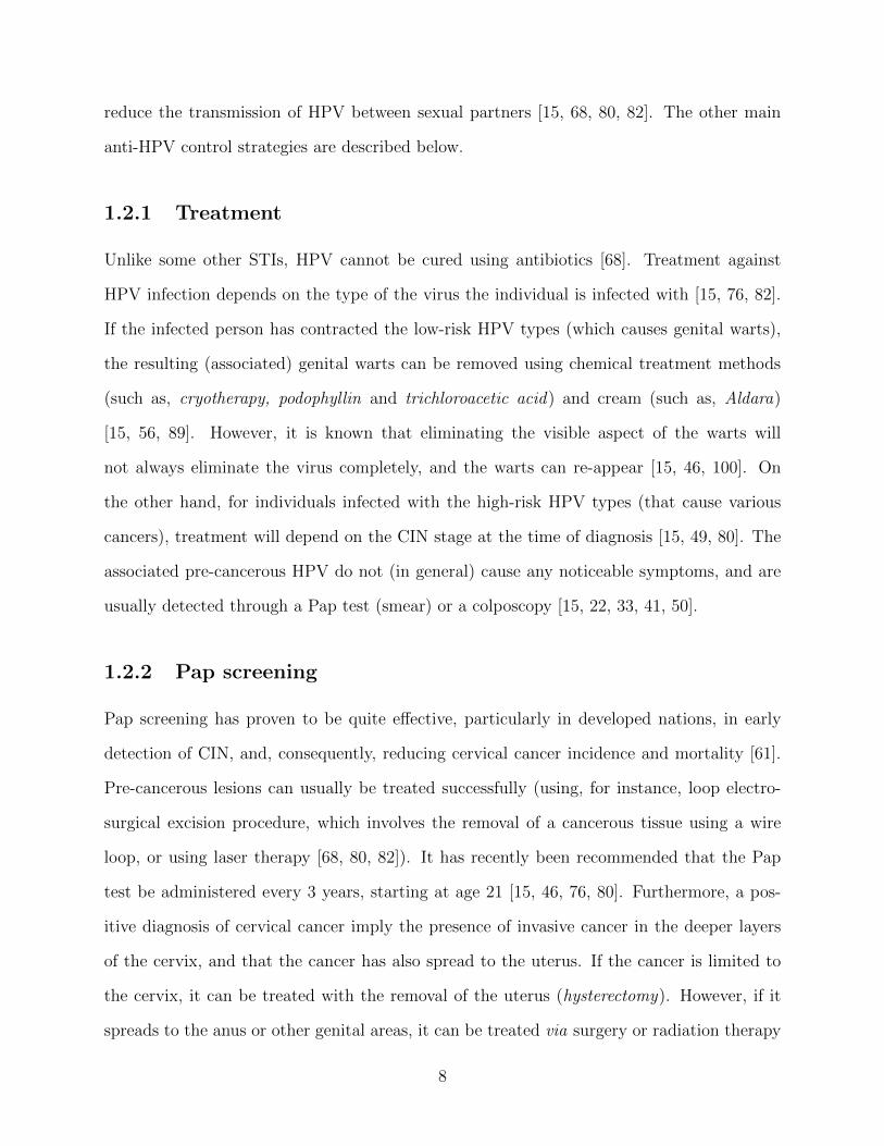
1.4 HPV infection in women [69]. . . . . . . . . . . . . . . . . . . . . . . . . . . 7
1.5 Forward bifurcation diagram (where λ is the infection rate). . . . . . . . . . 10
1.6 Backward bifurcation diagram, showing co-existence of a stable DFE and two
branches of endemic equilibria (stable and unstable branch). . . . . . . . . . 11
3.1 Flow diagram of the vaccination model (3.19). . . . . . . . . . . . . . . . . . 61
x
3.2 Simulations of the vaccination-free model (3.21), showing the total number of
infected individuals (females and males) as a function of time using various
initial conditions. Parameter values used are as given in Table 3.1, with
ρf = ρm = 0, ξf = ξm = 0.0012, πf = πm = 400, βf = 0.8, βm = 0.9, κf = 0.7,
αf = 0.5, σf = σm = 0.5, ψf = ψm = 0.5 and ηf = ηm = 0.8 (so that,
R0 = 6.4887 > 1). . . . . . . . . . . . . . . . . . . . . . . . . . . . . . . . . . 64
3.3 Backward bifurcation diagram for the vaccination-free model (3.21), showing
the total number of infected individuals (females and males) as a function of
the backward bifurcation parameter, β∗. Parameter values used are as given
in Table 3.1, with ξf = ξm = 0.0012, ρf = 1.2, ρm = 0.9855, πf = πm = 100,
βm = 0.35, cm = cf = 15, µf = µm = 175 , κf = 0.895, αf = 0.878, σf = σm =
0.75, ψf = ψm = 0.8, θp = 0.95 and ηf = ηm = 0.9 (so that, R0 = 1). . . . . . 65
3.4 Simulations of the vaccination-free model (3.21), showing the total number of
infected individuals (females and males) as a function of time using various
initial conditions. Parameter values used are as given in Table 3.1, with
ξf = ξm = 0.1, ρf = ρm = 0, πf = πm = 400, βf = βm = 0.05, κf = 0.7,
γf = 0.22, αf = 0.5, σf = σm = 0.5, ψf = ψm = 0.5 and ηf = ηm = 0.8 (so
that, R0 = 0.3823 < 1). . . . . . . . . . . . . . . . . . . . . . . . . . . . . . . 66
3.5 Simulations of the vaccination model (3.19), showing a contour plot of Rv
as a function of vaccine efficacy (εv) and the fraction of new sexually-active
females vaccinated at steady-state (ϕf ). Parameter values used are as given
in Table 3.1, with ξf = ξm = 0.01, ρf = ρm = 0, κf = 0.895, αf = 0.878,
rf = 0.887, γf = 0.22, σf = σm = 0.85 and ηf = ηm = 0.8 and various values
of εv and ϕf (with 0 ≤ εv,ϕf ≤ 1). . . . . . . . . . . . . . . . . . . . . . . . 68
xi
3.6 Simulation of the vaccination-free model (3.21), showing the cumulative num-
ber of cervical cancer cases as a function of time. Parameter values used are as
given in Table 3.1, with ξf = ξm = 0.012, ρf = ρm = 0.3, κf = 0.7, αf = 0.42,
σf = σm = ψf = ψm = 0.5, θp = 0.9, ηf = ηm = 0.85 and δf = 0.001. . . . . . 69
3.7 Simulation of the vaccination-free model (3.19), showing the cumulative cer-
vical cancer-related mortality as a function of time. Parameter values used
are as given in Table 3.1, with ξf = ξm = 0.012, ρf = ρm = 0.3, κf = 0.7,
αf = 0.42, σf = σm = ψf = ψm = 0.5, θp = 0.9, ηf = ηm = 0.85 and δf = 0.01. 69
3.8 Simulation of the vaccination model (3.19), showing the cumulative number of
cervical cancer cases as a function of time for various vaccine efficacy levels.
Parameter values used are as given in Table 3.1, with ξf = ξm = 0.012,
ρf = ρm = 0.3, κf = 0.7, αf = 0.42, σf = σm = ψf = ψm = 0.5, θp = 0.9,
ηf = ηm = 0.85 and δf = 0.001. . . . . . . . . . . . . . . . . . . . . . . . . . 70
3.9 Simulation of the vaccination model (3.19), showing the cumulative cervical
cancer-related mortality as a function of time for various vaccine efficacy levels.
Parameter values used are as given in Table 3.1, with ξf = ξm = 0.012,
ρf = ρm = 0.3, κf = 0.7, αf = 0.42, σf = σm = ψf = ψm = 0.5, θp = 0.9,
ηf = ηm = 0.85 and δf = 0.01. . . . . . . . . . . . . . . . . . . . . . . . . . . 70
4.1 Flow diagram of the female component of the model (4.34). . . . . . . . . . . 109
4.2 Flow diagram of the male component of the model (4.34). . . . . . . . . . . 110
xii
4.3 HPV prevalence as a function of time for the model (4.34) using various initial
conditions. Parameter values used are as given in Table 4.2. (A) Rl < 1 < Rh
(here, ρlf = ρlm = 0.2, ρhf = ρhm = 0.0001, βlm = βl
f = 0.005, βhm = 0.9,
βhf = 0.95875, cf = 32, γf = γm = 0.22, ψl
f = σlf = 0.1, kh
f = khm = 0.7,
ηlf = ηlm = 0.8, ηhf = ηhm = 0.9, θlf = θlm = 0.9 and θhf = θhm = 0.95; so that
0.1781 = Rl < 1 < Rh = 10.5770 and Rr0 = 3.2522). (B) Rh < 1 < Rl
(here, ρhf = ρhm = 0.2, ρlf = ρlm = 0.0001, βlm = 0.9,βl
f = 0.8, βhm = 0.05,
βhf = 0.003, cf = 32, γf = γm = 0.22, ψl
f = σlf = 0.1, kh
f = khm = 0.7,
ηlf = ηlm = 0.8, ηhf = ηhm = 0.9, θlf = θlm = 0.9 and θhf = θhm = 0.95; so that
0.0310 = Rh < 1 < Rl = 5.718 and Rr0 = 2.3899). . . . . . . . . . . . . . . . 116
4.4 HPV prevalence as a function of time for the model (4.34) using various initial
conditions. Parameter values used are as given in Table 4.2. (A) Rl > Rh > 1
(here, ρlf = ρlm = 0.001, ρhf = ρhm = 0.03, βlm = 0.058, βl
f = 0.28, βhm = 0.45,
βhf = 0.27, cf = 8, γf = 0.7, γm = 0.5, ψl
m = ψhm = σh
m = 0.4, σlf = 0.1,
khf = kh
m = 0.7, ηlf = ηlm = 0.8, ηhf = ηhm = 0.8, θlf = θlm = 0.9, zf = zm = 3,
wf = wm = 0.9, df = dm = 0.6, uf = um = 2, and θhf = θhm = 0.95; so that
10.1328 = Rl > Rh = 6.3261 > 1 and Rr0 = 3.1832). (B) Rh > Rl > 1 (here,
ρhf = ρhm = 0.03, ρlf = ρlm = 0.0001, βlm = 0.45,βl
f = 0.03, βhm = 0.7, βh
f = 0.3,
cf = 8, ψlf = σl
f = 0.1, khf = kh
m = 0.7, ηlf = ηlm = 0.8, ηhf = ηhm = 0.9,
θlf = θlm = 0.9, ψhf = ψh
m = 0.5 and θhf = θhm = 0.9; so that 16.8274 = Rh >
Rl = 10.9341 and Rr0 = 4.1021). . . . . . . . . . . . . . . . . . . . . . . . . . 117
4.5 HPV prevalence as a function of time for the model (4.34) using various initial
conditions. Parameter values used are as given in Table 4.2, with ρlf = ρlm =
ρhf = ρhm = δm = 0, βlm = βl
f = 0.05, βhm = 0.5, βh
f = 0.4, ηlf = ηlm = 0.7,
ηhf = ηhm = 0.8, θlf = θlm = 0.9 and θhf = θhm = 0.95 (so that, 0.005 = Rl <
Rh = 0.2253 < 1 and Rr01 = 0.4747 < 1). . . . . . . . . . . . . . . . . . . . . 118
xiii
4.6 Simulation of the model (4.34) using Gardasil vaccine. Parameter values used
are as given in Table 4.2. (A) Showing the cumulative number of HPV-related
cancer cases in both females and males as a function of time for females only
vaccinated and both females and males vaccinated (here, ρhf = ρhm = ρlf =
ρlm = 0.0012, βlm = 0.8, βl
f = 0.9, βhm = 0.7, βh
f = 0.9, khf = kh
m = 0.2, ηlf =
ηlm = 0.7, ηhf = ηhm = 0.8, θlf = θlm = 0.9, αlf = αl
m = 1.4, αhf = αh
m = 11.75
and θhf = θhm = 0.9). (B) Showing the cumulative number of mortality as
a function of time for females only vaccinated and both females and males
vaccinated (here, ρhf = ρhm = ρlf = ρlm = 0.0012, βlm = 0.8, βl
f = 0.9, βhm = 0.7,
βhf = 0.9,kh
f = khm = 0.2, ηlf = ηlm = 0.8, ηhf = ηhm = 0.9, θlf = θlm = 0.9 and
θhf = θhm = 0.9). . . . . . . . . . . . . . . . . . . . . . . . . . . . . . . . . . . 119
4.7 Simulations of the model (4.34). Parameter values used are as given in Table
4.2. (A) showing a contour plot of Rr01 as a function of the Gardasil vaccine
efficacy (εq) and the fraction of new sexually-active females vaccinated at
steady-state (ϕqf ) with ρlf = ρlm = ρhf = ρhm = δm = 0, βl
m = βlf = 0.05,
βhm = 0.5, βh
f = 0.4, rlf = rlm = 0.887, ϕqm = 0, ηlf = ηlm = ηhf = ηhm = 0.8 and
θlf = θlm = θhf = θhm = 0.9. (B) showing a contour plot of Rr01 as a function
of the fraction of new sexually-active females vaccinated with Gardasil (ϕqf )
and Cervarix (ϕbf ) at steady-state with ρlf = ρlm = ρhf = ρhm = δm = 0,
βlm = βl
f = 0.05, βhm = 0.5, βh
f = 0.04, rlf = rlm = 0.887, ϕqm = 0, ηlf = ηlm =
ηhf = ηhm = 0.8 and θlf = θlm = θhf = θhm = 0.9. . . . . . . . . . . . . . . . . . . 120
4.8 Simulations of the model (4.34). Parameter values used are as given in Table
4.2, showing a contour plot of Rr01 as a function the fraction of new sexually-
active females vaccinated at steady-state (ϕqf ) and the fraction of new sexually-
active males vaccinated at steady-state (ϕqm) with ρlf = ρlm = ρhf = ρhm = δm =
0, βlm = βl
f = 0.05, βhm = 0.5, βh
f = 0.04, rlf = rlm = 0.887, σlm = σl
f = 0.85,
ηlf = ηlm = ηhf = ηhm = 0.8 and θlf = θlm = θhf = θhm = 0.9. . . . . . . . . . . . . 121
xiv
Glossary
Abbreviation Meaning
CIN Cervical intraepithelial neoplasia
DFE Disease-free equilibrium
EEP Endemic equilibrium point
GAS Globally-asymptotically stable
HPV Human papillomavirus
INM HPV-related intraepithelial neoplasia in males
LAS Locally-asymptotically stable
ODE Ordinary differential equation
STI Sexually-transmitted infection
xv
Chapter 1
Introduction
This chapter provides a review of some of the key biological and epidemiological features of
HPV disease, as well as the associated cancers and warts.
1.1 Human Papillomavirus (HPV)
Human papillomavirus (HPV) is a major sexually-transmitted infection (STI) that continues
to inflict significant public health burden globally (see, for example, [27, 45, 51, 72, 100]).
Genital HPV infection is the commonest STI in Canada and the USA [35, 45, 80, 82].
Currently, 79 million Americans are infected with HPV, and 14 million new HPV infections
are recorded in the USA annually [15]. HPV prevalence is higher in women than in men
[50, 68, 71, 100], and it is estimated that as many as 75% of sexually-active men and women
will have at least one HPV infection in their lifetime [45, 49, 56, 100]. HPV was identified,
in 1983, as the causative agent of cervical cancer [45, 46].
Cervical cancer is currently the second most common malignancy among women, and
a leading cause of cancer-related death globally [24, 45, 72, 100]. Data shows that up to
250,000 cervical cancer related deaths are recorded globally every year [33, 46], and that
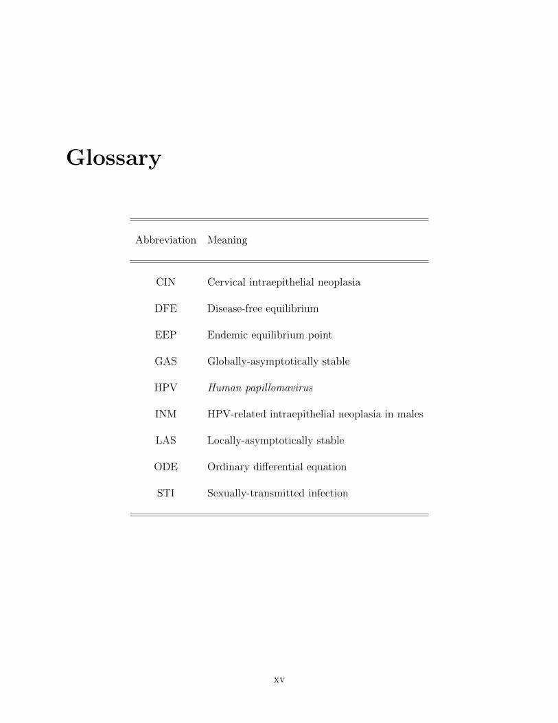
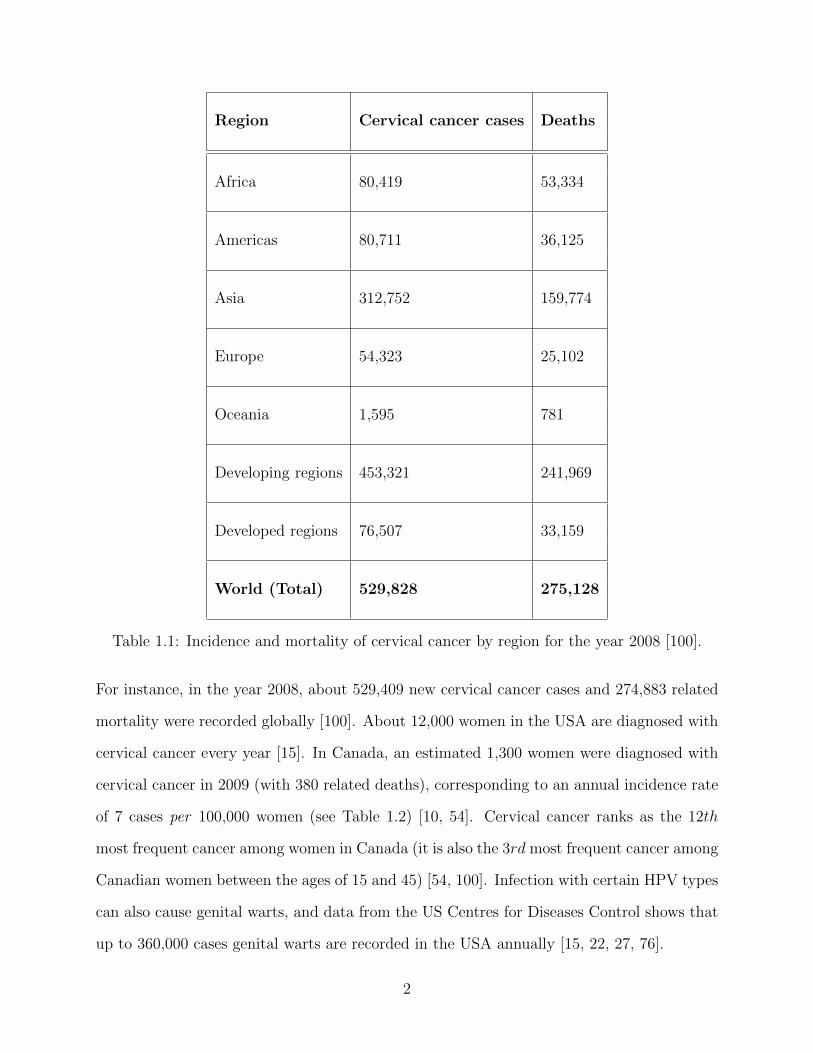
about 86% of cervical cancer cases occur in developing countries [100] (see also Table 1.1
and Figures 1.1 and 1.2).
1
Region Cervical cancer cases Deaths
Africa 80,419 53,334
Americas 80,711 36,125
Asia 312,752 159,774
Europe 54,323 25,102
Oceania 1,595 781
Developing regions 453,321 241,969
Developed regions 76,507 33,159
World (Total) 529,828 275,128
Table 1.1: Incidence and mortality of cervical cancer by region for the year 2008 [100].
For instance, in the year 2008, about 529,409 new cervical cancer cases and 274,883 related
mortality were recorded globally [100]. About 12,000 women in the USA are diagnosed with
cervical cancer every year [15]. In Canada, an estimated 1,300 women were diagnosed with
cervical cancer in 2009 (with 380 related deaths), corresponding to an annual incidence rate
of 7 cases per 100,000 women (see Table 1.2) [10, 54]. Cervical cancer ranks as the 12th
most frequent cancer among women in Canada (it is also the 3rd most frequent cancer among
Canadian women between the ages of 15 and 45) [54, 100]. Infection with certain HPV types
can also cause genital warts, and data from the US Centres for Diseases Control shows that
up to 360,000 cases genital warts are recorded in the USA annually [15, 22, 27, 76].
2
Figure 1.1: World age-standardized∗ incidence rates of cervical cancer for the year 2008 [100].
∗ ”age-standardized” rate (ASR) is a method of adjusting the crude (with respect toincidence and mortality) rate to eliminate the effect of differences in population agestructures when comparing crude (with respect to incidence and mortality) rates for differentperiods of time, different geographic areas and/or different population sub-groups [4].
Figure 1.2: World age-standardized mortality rates of cervical cancer for the year 2008 [100].
HPV is caused by over 120 different serotypes [15, 27, 76]. While some of these types
cause genital warts only, others can cause diverse cancers [15, 27, 76]. HPV infects squamous
3
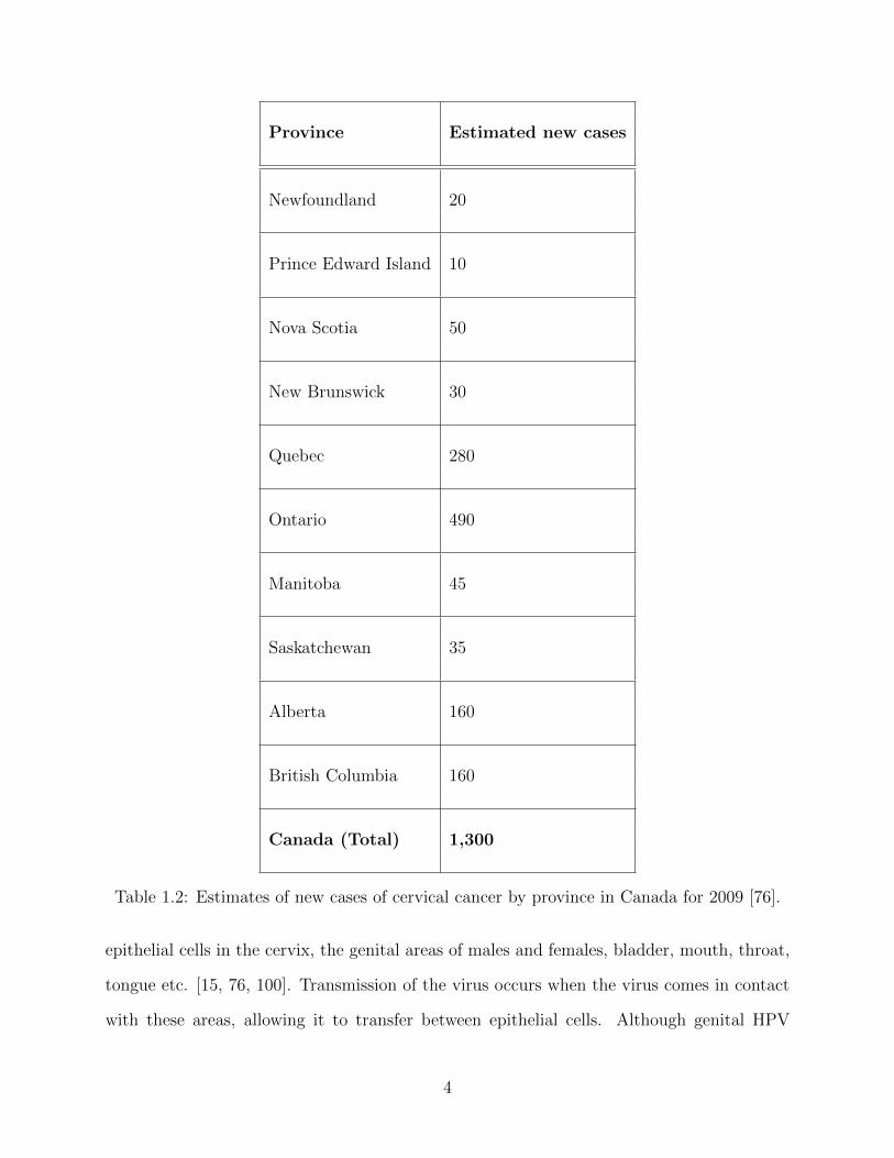
Province Estimated new cases
Newfoundland 20
Prince Edward Island 10
Nova Scotia 50
New Brunswick 30
Quebec 280
Ontario 490
Manitoba 45
Saskatchewan 35
Alberta 160
British Columbia 160
Canada (Total) 1,300
Table 1.2: Estimates of new cases of cervical cancer by province in Canada for 2009 [76].
epithelial cells in the cervix, the genital areas of males and females, bladder, mouth, throat,
tongue etc. [15, 76, 100]. Transmission of the virus occurs when the virus comes in contact
with these areas, allowing it to transfer between epithelial cells. Although genital HPV
4
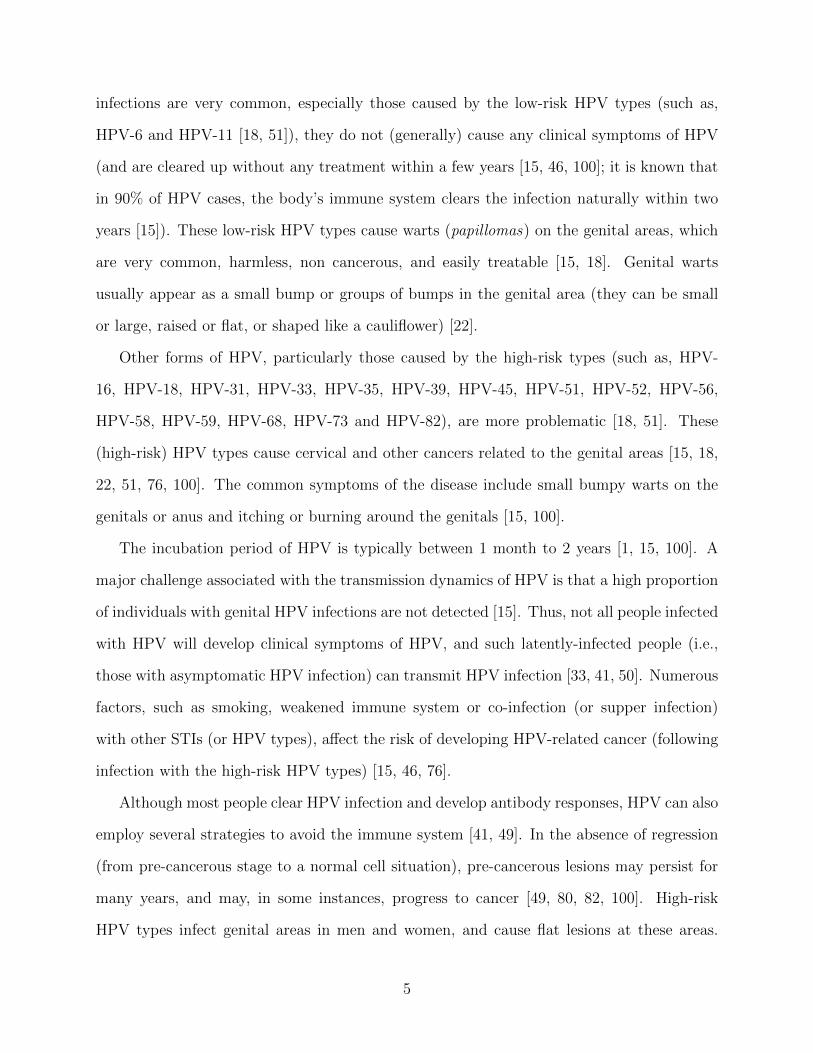
infections are very common, especially those caused by the low-risk HPV types (such as,
HPV-6 and HPV-11 [18, 51]), they do not (generally) cause any clinical symptoms of HPV
(and are cleared up without any treatment within a few years [15, 46, 100]; it is known that
in 90% of HPV cases, the body’s immune system clears the infection naturally within two
years [15]). These low-risk HPV types cause warts (papillomas) on the genital areas, which
are very common, harmless, non cancerous, and easily treatable [15, 18]. Genital warts
usually appear as a small bump or groups of bumps in the genital area (they can be small
or large, raised or flat, or shaped like a cauliflower) [22].
Other forms of HPV, particularly those caused by the high-risk types (such as, HPV-
16, HPV-18, HPV-31, HPV-33, HPV-35, HPV-39, HPV-45, HPV-51, HPV-52, HPV-56,
HPV-58, HPV-59, HPV-68, HPV-73 and HPV-82), are more problematic [18, 51]. These
(high-risk) HPV types cause cervical and other cancers related to the genital areas [15, 18,
22, 51, 76, 100]. The common symptoms of the disease include small bumpy warts on the
genitals or anus and itching or burning around the genitals [15, 100].
The incubation period of HPV is typically between 1 month to 2 years [1, 15, 100]. A
major challenge associated with the transmission dynamics of HPV is that a high proportion
of individuals with genital HPV infections are not detected [15]. Thus, not all people infected
with HPV will develop clinical symptoms of HPV, and such latently-infected people (i.e.,
those with asymptomatic HPV infection) can transmit HPV infection [33, 41, 50]. Numerous
factors, such as smoking, weakened immune system or co-infection (or supper infection)
with other STIs (or HPV types), affect the risk of developing HPV-related cancer (following
infection with the high-risk HPV types) [15, 46, 76].
Although most people clear HPV infection and develop antibody responses, HPV can also
employ several strategies to avoid the immune system [41, 49]. In the absence of regression
(from pre-cancerous stage to a normal cell situation), pre-cancerous lesions may persist for
many years, and may, in some instances, progress to cancer [49, 80, 82, 100]. High-risk
HPV types infect genital areas in men and women, and cause flat lesions at these areas.
5
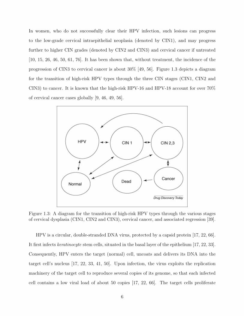
In women, who do not successfully clear their HPV infection, such lesions can progress
to the low-grade cervical intraepithelial neoplasia (denoted by CIN1), and may progress
further to higher CIN grades (denoted by CIN2 and CIN3) and cervical cancer if untreated
[10, 15, 26, 46, 50, 61, 76]. It has been shown that, without treatment, the incidence of the
progression of CIN3 to cervical cancer is about 30% [49, 56]. Figure 1.3 depicts a diagram
for the transition of high-risk HPV types through the three CIN stages (CIN1, CIN2 and
CIN3) to cancer. It is known that the high-risk HPV-16 and HPV-18 account for over 70%
of cervical cancer cases globally [9, 46, 49, 56].
Figure 1.3: A diagram for the transition of high-risk HPV types through the various stagesof cervical dysplasia (CIN1, CIN2 and CIN3), cervical cancer, and associated regression [39].
HPV is a circular, double-stranded DNA virus, protected by a capsid protein [17, 22, 66].
It first infects keratinocyte stem cells, situated in the basal layer of the epithelium [17, 22, 33].
Consequently, HPV enters the target (normal) cell, uncoats and delivers its DNA into the
target cell’s nucleus [17, 22, 33, 41, 50]. Upon infection, the virus exploits the replication
machinery of the target cell to reproduce several copies of its genome, so that each infected
cell contains a low viral load of about 50 copies [17, 22, 66]. The target cells proliferate
6
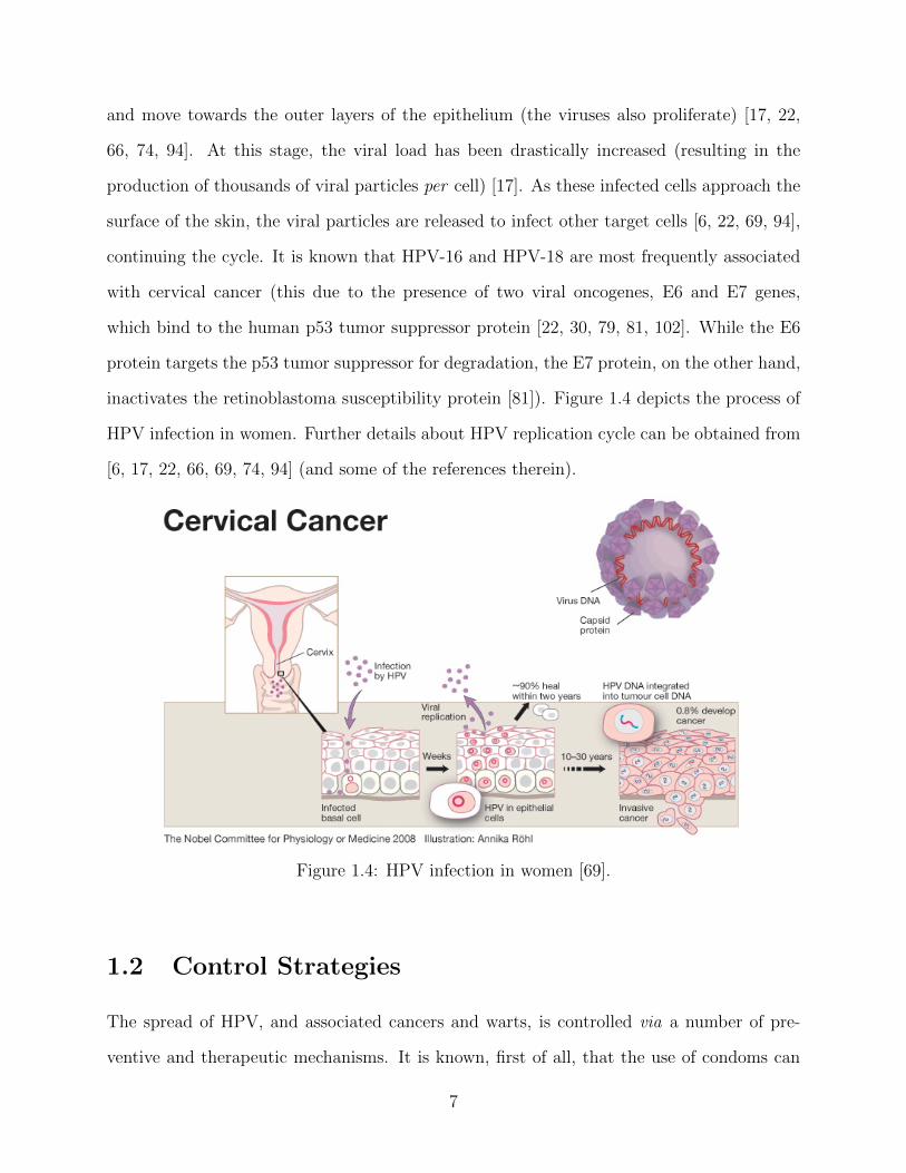
and move towards the outer layers of the epithelium (the viruses also proliferate) [17, 22,
66, 74, 94]. At this stage, the viral load has been drastically increased (resulting in the
production of thousands of viral particles per cell) [17]. As these infected cells approach the
surface of the skin, the viral particles are released to infect other target cells [6, 22, 69, 94],
continuing the cycle. It is known that HPV-16 and HPV-18 are most frequently associated
with cervical cancer (this due to the presence of two viral oncogenes, E6 and E7 genes,
which bind to the human p53 tumor suppressor protein [22, 30, 79, 81, 102]. While the E6
protein targets the p53 tumor suppressor for degradation, the E7 protein, on the other hand,
inactivates the retinoblastoma susceptibility protein [81]). Figure 1.4 depicts the process of
HPV infection in women. Further details about HPV replication cycle can be obtained from
[6, 17, 22, 66, 69, 74, 94] (and some of the references therein).
Figure 1.4: HPV infection in women [69].
1.2 Control Strategies
The spread of HPV, and associated cancers and warts, is controlled via a number of pre-
ventive and therapeutic mechanisms. It is known, first of all, that the use of condoms can
7
reduce the transmission of HPV between sexual partners [15, 68, 80, 82]. The other main
anti-HPV control strategies are described below.
1.2.1 Treatment
Unlike some other STIs, HPV cannot be cured using antibiotics [68]. Treatment against
HPV infection depends on the type of the virus the individual is infected with [15, 76, 82].
If the infected person has contracted the low-risk HPV types (which causes genital warts),
the resulting (associated) genital warts can be removed using chemical treatment methods
(such as, cryotherapy, podophyllin and trichloroacetic acid) and cream (such as, Aldara)
[15, 56, 89]. However, it is known that eliminating the visible aspect of the warts will
not always eliminate the virus completely, and the warts can re-appear [15, 46, 100]. On
the other hand, for individuals infected with the high-risk HPV types (that cause various
cancers), treatment will depend on the CIN stage at the time of diagnosis [15, 49, 80]. The
associated pre-cancerous HPV do not (in general) cause any noticeable symptoms, and are
usually detected through a Pap test (smear) or a colposcopy [15, 22, 33, 41, 50].
1.2.2 Pap screening
Pap screening has proven to be quite effective, particularly in developed nations, in early
detection of CIN, and, consequently, reducing cervical cancer incidence and mortality [61].
Pre-cancerous lesions can usually be treated successfully (using, for instance, loop electro-
surgical excision procedure, which involves the removal of a cancerous tissue using a wire
loop, or using laser therapy [68, 80, 82]). It has recently been recommended that the Pap
test be administered every 3 years, starting at age 21 [15, 46, 76, 80]. Furthermore, a pos-
itive diagnosis of cervical cancer imply the presence of invasive cancer in the deeper layers
of the cervix, and that the cancer has also spread to the uterus. If the cancer is limited to
the cervix, it can be treated with the removal of the uterus (hysterectomy). However, if it
spreads to the anus or other genital areas, it can be treated via surgery or radiation therapy
8
[15, 34, 56, 100].
1.2.3 HPV Vaccine
Two anti-HPV vaccines, namely Cervarix and Gardasil, have been approved for use to
protect new sexually-active males and females against some of the most common HPV types
[15, 34, 46, 56, 76]. The Gardasil quadrivalent vaccine, produced by Merck Inc., protects
against four HPV types (namely, HPV-6, HPV-11, HPV-16 and HPV-18; these are the four
commonest HPV types). The Cervarix bivalent vaccine, produced by GlaxoSmithKline,
targets two high-risk HPV types (namely, HPV-16 and HPV-18 ) [10, 77]. The two vaccines,
administered in a series of three doses over a period of 6 months, are 90-100% effective in
preventing HPV infection against the respective HPV types [9, 27, 46, 50, 61, 76, 100]. Both
vaccines have been licensed by the Food and Drug Administration of the USA, and the retail
price of either vaccine is about USD $130 per dose (that is, USD $390 for full series) [15, 34].
It has been reported that both vaccines have side effects, including pain (at the body location
where the vaccine is given), fever, dizziness, and nausea [15, 34, 76, 100]. While the Gardasil
vaccine is approved for both females and males, the Cervarix vaccine is only approved for
females [76, 77, 100].
1.3 Reproduction Number and Bifurcations
Compartmental mathematical models have been widely used to gain insights into the spread
and control of emerging and re-emerging diseases of public health importance, dating back
to the pioneering works of Bernoulli in 1760 (see, for instance, [2, 3, 5, 21, 47] and the
references therein). The dynamics of these models is typically characterized by a threshold
quantity, known as the basic reproduction number (denoted by R0), which measures the
average number of new cases a typical infectious individual can generate in a completely-
susceptible population [3, 20, 47]. In general, the disease dies out in time if R0 < 1, and
9
persists in the community if R0 > 1. This phenomenon, where the disease-free equilibrium
(DFE) and an endemic equilibrium point (EEP) of the model exchange their stability atR0 =
1, is known as forward bifurcation [12, 14, 42, 47, 48, 86]. The epidemiological meaning of
the forward bifurcation phenomenon is that the requirement R0 < 1 is (in general) necessary
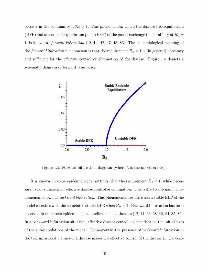
and sufficient for the effective control or elimination of the disease. Figure 1.5 depicts a
schematic diagram of forward bifurcation.
Figure 1.5: Forward bifurcation diagram (where λ is the infection rate).
It is known, in some epidemiological settings, that the requirement R0 < 1, while neces-
sary, is not sufficient for effective disease control or elimination. This is due to a dynamic phe-
nomenon, known as backward bifurcation. This phenomenon results when a stable EEP of the
model co-exists with the associated stable DFE whenR0 < 1. Backward bifurcation has been
observed in numerous epidemiological studies, such as those in [12, 14, 23, 28, 42, 84, 85, 86].
In a backward bifurcation situation, effective disease control is dependent on the initial sizes
of the sub-populations of the model. Consequently, the presence of backward bifurcation in
the transmission dynamics of a disease makes the effective control of the disease (in the com-
10
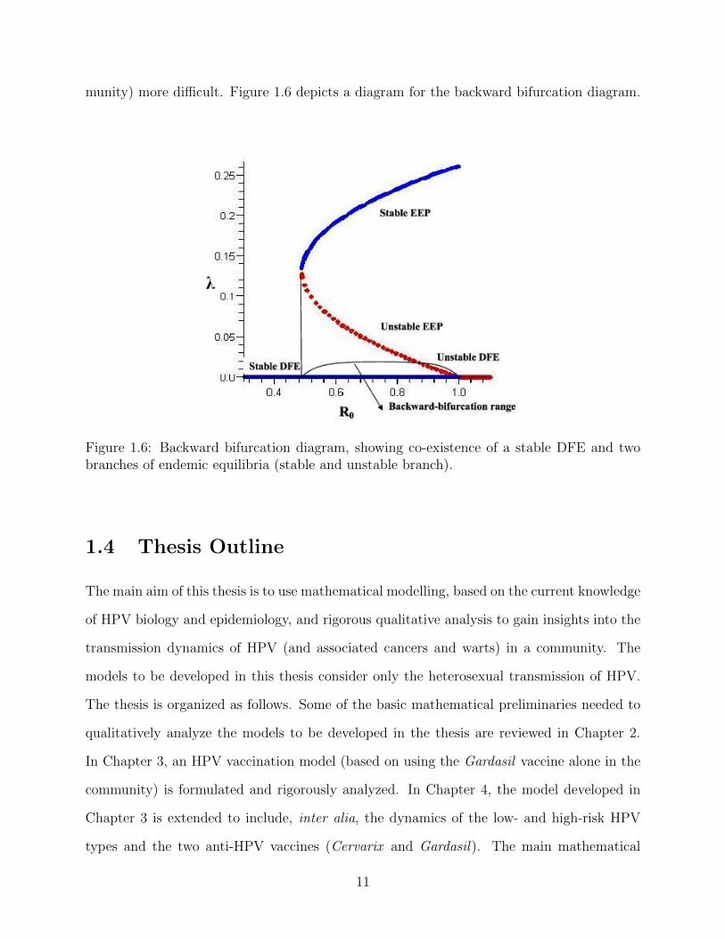
munity) more difficult. Figure 1.6 depicts a diagram for the backward bifurcation diagram.
Figure 1.6: Backward bifurcation diagram, showing co-existence of a stable DFE and twobranches of endemic equilibria (stable and unstable branch).
1.4 Thesis Outline
The main aim of this thesis is to use mathematical modelling, based on the current knowledge
of HPV biology and epidemiology, and rigorous qualitative analysis to gain insights into the
transmission dynamics of HPV (and associated cancers and warts) in a community. The
models to be developed in this thesis consider only the heterosexual transmission of HPV.
The thesis is organized as follows. Some of the basic mathematical preliminaries needed to
qualitatively analyze the models to be developed in the thesis are reviewed in Chapter 2.
In Chapter 3, an HPV vaccination model (based on using the Gardasil vaccine alone in the
community) is formulated and rigorously analyzed. In Chapter 4, the model developed in
Chapter 3 is extended to include, inter alia, the dynamics of the low- and high-risk HPV
types and the two anti-HPV vaccines (Cervarix and Gardasil). The main mathematical
11
and epidemiological contributions of the thesis, including some areas for future work, are
enumerated in Chapter 5.
Some of the main questions to be addressed in the thesis are:
i) What are the main qualitative features of realistic models for the transmission dynam-
ics of HPV (and associated cancers and warts) in a community, in the presence of a
mass vaccination program (using the currently-available Cervarix and Gardasil vac-
cines) against HPV? In particular, emphasis will be on determining conditions for the
existence and asymptotic (both local and global) stability of the associated equilibria
of the models, as well as to characterize the various bifurcation types the models may
undergo.
ii) Can the singular use of the Gardasil vaccine for new sexually-active susceptible women
lead to the effective control or elimination of HPV from the community? If yes, what
percentage of the new sexually-active susceptible women need to be vaccinated to
achieve this result?
iii) What are the qualitative features of a vaccination model for HPV that stratifies the
total population in terms of the risk of transmitting infection with the low- and high-
risk HPV types?
iv) Does the vaccination of new sexually-active susceptible males have a quantifiable
community-wide impact in reducing HPV (and HPV-related) burden?
v) What is the community-wide impact of the combined use of the two anti-HPV vaccines,
Cervarix and Gardasil (for new sexually-active susceptible women)?
12
Chapter 2
Mathematical Preliminaries
This chapter introduces some of the basis mathematical theories and methodologies relevant
to the thesis.
2.1 Equilibria of Autonomous Ordinary Differential Equa-
tions (ODEs)
In this thesis, only the systems of autonomous ODEs, given by
x = f(x), x ∈ Rn, (2.1)
are considered. That is, non-autonomous ODE systems, of the form
x = f(x, t), x ∈ Rn, and t ∈ R, (2.2)
where f can depend on the independent variable t, are not considered in this thesis.
In both equations (2.1) and (2.2), and throughout this thesis, the over dot represents
differentiation with respect to time ( ddt), and the right-hand side function, f ∈ Cr with
r ≥ 1, is called a vector field [73].
13
Definition 2.1. A point x ∈ Rn is called an equilibrium point of the autonomous system
(2.1) if f(x) = 0.
Theorem 2.1. (Fundamental Existence- Uniqueness Theorem [73]). Let E be an open subset
of Rn containing x0 and assume that f ∈ C1(E). Then, there exists an a > 0 such that the
initial value problem:
x = f(x), x(0) = x0,
has a unique solution x(t) on the interval [−a, a].
Definition 2.2. The Jacobian matrix of f at the equilibrium x, denoted by Df(x), is the
matrix,
J(x) =
∂f1∂x1
(x) · · ·∂f1∂xn
(x)
......
...
∂fn∂x1
(x) · · ·∂fn∂xn
(x)
,
of partial derivatives of f evaluated at x.
Definition 2.3. The linear system x = Ax, with the matrix A = Df(x), is called the
linearization of the system (2.1) at the equilibrium x.
Definition 2.4. An equilibrium point x of the system (2.1) is called hyperbolic if none of
the eigenvalues of Df(x) has zero real part.
Definition 2.5. An equilibrium point that is not hyperbolic is called non-hyperbolic.
2.2 Hartman-Grobman Theorem
Consider the dynamical system:
x = f(x), x ∈ Rn, (2.3)
y = g(y), y ∈ Rn,
14
where f(x) and g(x) are two Cr (r ≥ 1) vector fields on Rn.
Definition 2.6. [98]. The dynamics generated by the vector fields f and g, of the system
(2.3), are said to be locally Ck-conjugate (k ≤ r) if there exists a Ck diffeomorphisim h
which takes the orbits of the flow generated by f , φ(t, x), to the orbits of the flow generated
by g, ψ(t, y), preserving orientation and parameterization by time.
Theorem 2.2. (Hartman-Grobman Theorem [98]). Consider the Cr(r ≥ 1) system
x = f(x), x ∈ Rn, (2.4)
with domain of f to be a large open subset of Rn. Suppose also that the system (2.4) has
equilibrium solutions which are hyperbolic. Consider the associated linear system
ξ = Df(x)ξ, ξ ∈ Rn. (2.5)
Then, the flow generated by the system (2.4) is C0-conjugate to the flow generated by the
linearized system (2.5) in a neighborhood of the equilibrium point x = x.
It should be stated that the Hartman-Grobman Theorem guarantees a homeomorphism
between the flow of the non-linear ODE and that of its linearization. In general, near a
hyperbolic equilibrium point x, the non-linear system x = f(x) has the same qualitative
structure as the linear system x = Ax, with A = Df(x) [73].
2.3 Stability Theory
Definition 2.7. [98]. The equilibrium x, of the system (2.1), is said to be stable if, given
� > 0, there exists a δ = δ(�) > 0 such that, for any solution y(t) of the system (2.1)
satisfying |x− y(t0)| < δ, |x− y(t)| < � for t > t0 where t0 ∈ R.
15

Definition 2.8. [98]. The equilibrium x, of the system (2.1), is said to be asymptotically-
stable if it is stable and there exists a constant c > 0 such that, for any solution y(t) of the
system (2.1) satisfying |x− y(t0)| < c, limt→∞
|x− y(t)| = 0.
Definition 2.9. An equilibrium solution which is not stable is said to be unstable.
The main standard methods for analyzing the stability of the equilibria of the disease trans-
mission models are described below.
2.3.1 Standard linearization
Theorem 2.3. [98]. Suppose all the eigenvalues of Df(x) have negative real parts. Then,
the equilibrium solution x = x, of the system (2.1), is locally-asymptotically stable (LAS). It
is unstable if at least one of the eigenvalues has positive real part.
2.3.2 The next generation operator method and R0
The next generation operator method [19, 95] is used to establish the local asymptotic
stability of the disease-free equilibrium (DFE) of a disease transmission model. The notation
in [95] is used in this thesis. Suppose the given disease transmission model, with non-negative
initial conditions, can be written in terms of the following system:
xi = f(x) = Fi(x)− Vi(x), i = 1, ..., n, (2.6)
where Vi = V −i − V +
i and the functions satisfy Axioms (A1)-(A5) below.
The function Fi(x) represents the rate of appearance of new infections in compartment
i, V +i (x) represents the rate of transfer of individuals into compartment i, and V −
i (x)
represents the rate of transfer of individuals out of compartment i. Furthermore, the
number of individuals in each compartment is given by x = (x1, ..., xn)t, xi ≥ 0, and
Xs = {x ≥ 0 | xi = 0, i = 1, ...,m} is defined as the disease-free states (non-infected
variables of the model).
16
(A1) If x ≥ 0, then Fi, V+i , V −
i ≥ 0 for i = 1, ...,m;
(A2) if xi = 0, then V −i = 0. In particular, if x ∈ Xs then V −
i = 0 for i = 1, ...,m;
(A3) Fi = 0 if i > m;
(A4) if x ∈ Xs then Fi(x) = 0 and V +i = 0 for i = 1, ...,m;
(A5) if F (x) is set to zero, then all eigenvalues of Df(x0) have negative real parts.
Definition 2.10. (M-Matrix). An n×n matrix A is called an M-matrix if and only if every
off-diagonal entry of the matrix A is non-positive and the diagonal entries are all positive.
Lemma 2.1. (van den Driessche and Watmough [95]). If x is a DFE of (2.6) and fi(x)
satisfy (A1)-(A5), then the derivatives DF (x) and DV (x) are partitioned as
DF (x) =
F 0
0 0
, DV (x) =
V 0
J3 J4
,
where F and V are the m×m matrices defined by,
F =
�∂Fi
∂xj(x)
�and V =
�∂Vi
∂xj(x)
�with 1 ≤ i, j ≤ m.
Further, F is a non-negative matrix, V is a non-singular M-matrix and J3, J4 are matrices
associated with the transition terms of the model, and all eigenvalues of J4 have positive real
parts.
Theorem 2.4. (van den Driessche and Watmough [95]). Consider the disease transmission
model given by (2.6) with f(x) satisfying Axioms (A1)-(A5). If x is a DFE of the model,
then x is LAS if R0 = ρ(FV −1) < 1 (where ρ is spectral radius), but unstable if R0 > 1.
17
2.3.3 Krasnoselskii sub-linearity argument
The central idea of the Krasnoselskii sub-linearity argument is to show that the linearized
version of the non-linear system x = f(x), given by (where x is an equilibrium solution of
the non-linear system)
Z(t) = Df(x)Z,
has no solution of the form
Z(t) = Z0eωt,
with Z0 ∈ Cn, ω ∈ C and Re(ω) ≥ 0, where C denotes the complex number (further details
about the application of the Krasnoselskii sub-linearity argument to prove the asymptotic
stability of an equilibrium of a disease transmission model are available in [31, 32, 91]).
2.4 Center Manifold Theory
An effective way to analyse the qualitative properties of some dynamical systems is to re-
duce their dimensionality. The Centre Manifold Theory offers a mathematical technique for
making such reduction (near an equilibrium point) possible.
Consider the non-linear system (2.1). Further, let,
x = Ax, (2.7)
be the corresponding linearized system, with A = Df(x), near a hyperbolic equilibrium
point x.
Definition 2.11. [73]. The stable, unstable, and centre subspaces; respectively, of the linear
18
system (2.7) are defined by (where A ∈ Mnn(R))
Es = span {uj, vj; aj < 0} ,
Eu = span {uj, vj; aj > 0} ,
Ec = span {uj, vj; aj = 0} ,
where wj = uj ± ivj are eigenvectors corresponding to the eigenvalues λj = aj ± ibj.
Remark 2.1. For a hyperbolic flow of a linear system, Rn = Es ⊕ Eu. These subspaces
become manifolds for non-linear ODEs.
Theorem 2.5. (Stable Manifold Theory [73]). Let f ∈ C1(E), where E is an open subset
of Rn containing the origin, and let φt be the flow of non-linear system (2.1). Suppose that
f(0) = 0 and D(0) has k eigenvalues with negative real parts, and q = n−k eigenvalues with
positive real parts. Then, there exists a k-dimensional differentiable manifold S tangent to
the stable subspace Es of the linear system (2.7) at 0 such that for all t ≥ 0,φt(S) ⊂ S and
for all x0 ∈ S,
limt→∞
φt(x0) = 0,
and there exists a q-dimensional differentiable manifold U tangent to the unstable subspace
Eu of the linear system (2.7) at 0 such that for all t ≥ 0,φt(U) ⊂ U and for all x0 ∈ U ,
limt→−∞
φt(x0) = 0.
Definition 2.12. [73]. Let φt be the flow of non-linear system (2.1). The global stable and
unstable manifolds of (2.7) at 0 are defined, respectively, by
W s(0) =�
t≤0
φt(S),
19
and,
W u(0) =�
t≥0
φt(U).
Theorem 2.6. [73]. Let f ∈ Cr(E), where E is an open subset of Rn containing the origin
and r ≥ 1. Suppose that f(0) = 0 and that Df(0) has k eigenvalues with negative real parts,
j eigenvalues with positive real parts, and m = n − k − j eigenvalues with zero real parts.
Then, there exists an m− dimensional centre manifold W c(0) of class Cr tangent to centre
subspace Ec of (2.7) which is invariant under the flow φt of (2.1).
Lemma 2.2. The local centre manifold of the system (2.1) at 0,
W cloc(0) = {(x, y) ∈ Rm
× Rk| y = h(x) for |x| < δ}, (2.8)
for some δ > 0, where h ∈ Cr(Nδ(0)), h(0) = 0 and Dh(0) = O since W c(0) is tangent to
the centre subspace
Ec = {(x, y) ∈ Rm× Rk
| y = 0},
at the origin.
Theorem 2.7. (Center Manifold Theory [73]). Let f ∈ Cr(E) where E is an open subset of
Rn containing the origin and r ≥ 1. Suppose that f(0) = 0 and that Df(0) has m eigenvalues
with zero real parts and k eigenvalues with negative real parts, where m+k = n. The system
(2.1) then can be written in diagonal form
x = Cx+ F (x, y),
y = Py +G(x, y),
where (x, y) ∈ Rm × Rk, C is a square matrix with m eigenvalues having zero real parts,
P is a square matrix with k eigenvalues with negative real parts, and F (0) = G(0) = 0,
DF (0) = DG(0) = O. Furthermore, there exists a δ > 0 and a function h ∈ Cr(Nδ(0)) that
20
defines the local centre manifold (2.8) and satisfies
Dh(x)[Cx+ F (x, h(x))]− Ph(x)−G(x, h(x)) = 0,
for |x| < δ; and the flow on the centre manifold W c(0) is defined by the system of differential
equations
x = Cx+ F (x, h(x)),
for all x ∈ Rmwith |x| < δ.
Theorem 2.7 can be used to determine the flow near non-hyperbolic equilibrium points [73].
2.5 Bifurcation Theory
Bifurcation theory plays an important role in providing deeper insight into the qualitative
dynamics of many phenomena arising in the natural and engineering sciences.
Consider the non-linear autonomous ODE system
x = f(x, µ), x ∈ Rn, (2.9)
where f is a function of time and µ is a scalar parameter.
Definition 2.13. Bifurcation is defined as a change in the qualitative behaviour of a given
dynamical system when an associated parameter is varied.
Definition 2.14. The parameter values where bifurcation occurs are called bifurcation values
(or bifurcation points).
There are numerous types of bifurcations, including saddle-node, transcritical, pitchfork,
Hopf, and backward bifurcation [44, 47, 73, 98]. The following theorem, which uses Centre
Manifold Theory, is used to establish the existence of backward bifurcation phenomenon (for
the models in Chapters 3 and 4 of the thesis).
21
Theorem 2.8. (Castillo-Chavez & Song [11, 14]). Consider the following general system of
ordinary differential equations with a parameter φ
dx
dt= f(x,φ), f : Rn
× R → Rand f ∈ C2 (Rn× R) , (2.10)
where 0 is an equilibrium point of the system (that is, f(0,φ) ≡ 0 for all φ) and assume
A.1) A = Dxf(0, 0) =�
∂fi∂xj
(0, 0)�
is the linearization matrix of the system (2.10) around
the equilibrium 0 with φ evaluated at 0. Zero is a simple eigenvalue of A and other
eigenvalues of A have negative real parts;
A.2) Matrix A has a right eigenvector w and a left eigenvector v (each corresponding to the
zero eigenvalue).
Let fk be the k-th component of f and
a =n�
k,i,j=1
vkwiwj∂2fk
∂xi∂xj(0, 0),
b =n�
k,i=1
vkwi∂2fk∂xi∂φ
(0, 0).
The local dynamics of the system around 0 is totally determined by the signs of a and b.
i) a > 0, b > 0. When φ < 0 with |φ| � 1, 0 is locally asymptotically stable and there
exists a positive unstable equilibrium; when 0 < φ � 1, 0 is unstable and there exists a
negative, locally asymptotically stable equilibrium;
ii) a < 0, b < 0. When φ < 0 with |φ| � 1, 0 is unstable; when 0 < φ � 1, 0 is locally
asymptotically stable equilibrium, and there exists a positive unstable equilibrium;
iii) a > 0, b < 0. When φ < 0 with |φ| � 1, 0 is unstable, and there exists a locally
asymptotically stable negative equilibrium; when 0 < φ � 1, 0 is stable, and a positive
unstable equilibrium appears;
22
iv) a < 0, b > 0. When φ changes from negative to positive, 0 changes its stability from
stable to unstable. Correspondingly a negative unstable equilibrium becomes positive
and locally asymptotically stable.
Particularly, if a > 0 and b > 0, then a backward bifurcation occurs at φ = 0.
2.6 Lyapunov Function Theory
A powerful method for analyzing the stability of an equilibrium point is based on the use of
Lyapunov functions.
Definition 2.15. [73]. A point x0 ∈ Rn is called an ω−limit point of x ∈ Rn, denoted by
ω(x), if there exists a sequence {ti} such that
φ(ti, x) → x0 as ti → ∞.
Definition 2.16. [73]. A point x0 ∈ Rn is called an α−limit point of x ∈ Rn, denoted by
α(x), if there exists a sequence {ti} such that
φ(ti, x) → x0 as ti → −∞.
Definition 2.17. [73]. The set of all ω−limit points of a flow is called the ω−limit set.
Similarly, The set of all α−limit points of a flow is called the α−limit set.
Definition 2.18. [98]. Let S ⊂ Rn be a set. Then, S is said to be invariant under the flow
generated by x = f(x) if for any x0 ∈ S we have φ(t, x0) ∈ S for all t ∈ R.
Lemma 2.3. [98]. A set S ⊂ Rn is positively-invariant if, for every x0 ∈ S, φ(t, x0) ∈ S, ∀
t ≥ 0.
Definition 2.19. [98]. A function V : Rn → R is said to be positive-definite if:
23
• V (x) > 0 for all x �= 0,
• V (x) = 0 if and only if x = 0.
Definition 2.20. [98]. Consider the system (2.1). Let x be an equilibrium solution of the
system (2.1), and let V : U → R be a C1 function defined on some neighbourhood U of x
such that
i) V is positive-definite,
ii) V (x) ≤ 0 in U \ {x}.
Definition 2.21. [98]. Any function, V , that satisfies the conditions (i) and (ii) in Definition
2.20 is called a Lyapunov function.
Theorem 2.9. (LaSalle’s Invariance Principle [44]). Consider the system (2.1). Let,
S = {x ∈ U : V (x) = 0} (2.11)
and M be the largest positive invariant set of the system (2.1) in S. If V is a Lyapunov
function on U and γ+(x0) is a bounded orbit of the system (2.1) which lies in S, then the
ω−limit set of γ+(x0) belongs to M ; that is, x(t, x0) → M as t → ∞.
Corollary 2.1. If V (x) → ∞ as |x| → ∞ and V ≤ 0 on Rn, then every solution of the
system (2.1) is bounded and approaches the largest invariant set M of (2.1) in the set where
V = 0. In particular, if M = {0}, then the solution x = 0 is globally-asymptotically stable
(GAS).
24
2.7 Comparison Theorem
Comparison Theorem is sometimes used to prove the global asymptotic stability of equilibria
of dynamical systems. The general idea is to compare the solutions of the non-linear system
x = f(t, x), (2.12)
with those of the differential inequality system
z ≤ f(t, z), (2.13)
or,
y ≥ f(t, y), (2.14)
on an interval. The technique requires that the system (2.12) has a unique solution. Consider
the autonomous system (2.12), where f is a continuously-differentiable function on an open
subset D ⊂ Rn. Let φt(x) denote the solution of the system (2.12) with initial value x.
Definition 2.22. [87]. f is said to be of Type K in D if for each i, fi(a) ≤ fi(b) for any
two points, a and b, in D satisfying a ≤ b and ai = bi.
Definition 2.23. [87]. The subset D is p-convex if tx + (1 − t)y ∈ D for all t ∈ [0, 1]
whenever x, y ∈ D and x ≤ y.
Thus, if D is a convex set, then it is also p-convex. If D is a p-convex subset of Rn and
∂fi∂xj
≥ 0, i �= j, x ∈ D, (2.15)
then f is of Type K in D (i.e., the Type K condition can be identified from the sign structure
of the Jacobian matrix of the system (2.12) [87]).
Theorem 2.10. (Comparison Theorem [88]). Let f be continuous on R × D and of Type
K. Let x(t) be a solution of (2.12) defined on [a, b]. If z(t) is a continuous function on [a, b]
25

satisfying (2.13) on (a, b), with z(a) ≤ x(a), then z(t) ≤ x(t) for all t in [a, b]. If y(t) is a
continuous on [a, b] satisfying (2.14) on (a, b), with y(a) ≥ x(a), then y(t) ≥ x(t) for all t in
[a, b].
26
Chapter 3
HPV Model Using the Gardasil
Vaccine for Females
3.1 Introduction
As stated in Chapter 1, two anti-HPV vaccines are currently available in the market [15,
46, 68, 76, 93, 96]. These vaccines, which are highly-effective against HPV infection (with
efficacy of about 90-100% [15, 76, 93, 96]), have been approved for use in a number of
countries, including Australia, Canada, USA and some European countries [1, 76, 100]. In
this chapter, the quadrivalent Gardasil vaccine (which targets the four vaccine-preventable
HPV types, namely HPV-6, HPV-11, HPV-16 and HPV-18) will be considered. The vaccine
is recommended for females between 9 and 13 years of age (as this is the age range before
the onset of sexual activity for most females; the vaccine should be administered to females
before they become sexually-active in order to ensure maximum benefit [10, 15, 76]).
In other words, the objective of this chapter is to qualitatively assess the community-wide
impact of mass vaccination, of new sexually-active susceptible females using the quadriva-
lent Garadsil vaccine, on the transmission dynamics of the aforementioned four vaccine-
preventable HPV types in a community. To achieve this objective, a new deterministic
27
model, for the heterosexual transmission of HPV community, will be formulated and rigor-
ously analysed, as below.
Although there are many types of cancers associated with HPV infection [10, 15, 26, 46,
50, 76], this chapter considers only cervical cancer (because it is the more predominant of all
the HPV-related cancers [10, 15, 33, 34, 35, 45, 46, 50, 76, 77, 97]). Furthermore, it is worth
mentioning that a sizeable percentage of HPV-infected females (particularly those who are
untreated) develop persistent HPV infection, and become at the greatest risk of developing
cervical cancer precursor lesions, causing cell abnormalities (known as cervical intraepithelial
neoplasia (CIN)) and cervical cancer [10, 15, 26, 35, 45, 46, 50, 61, 68, 77].
HPV infection affects men as well, causing serious cancers including throat and penile
cancers (albeit they are less common) [71, 76]. Although some researchers suggest that
both females and males should be vaccinated against HPV [46, 76, 77] (while others suggest
vaccinating females only is more effective than vaccinating both males and females [9, 40, 41,
68]), this chapter considers the vaccination of females only (in line with the studies reported
in [9, 24, 25, 26, 61]). This assumption (of vaccinating only females) is relaxed in Chapter
4, where both new sexually-active susceptible males and females are vaccinated.
3.2 Model Formulation
The model to be constructed is based on the heterosexual transmission dynamics of HPV
in a community, subject to the use of mass vaccination of new sexually-active susceptible
females (of ages 9 to 13) using the quadrivalent Gardasil vaccine. The model assumes
homogenous mixing of the sexually-active female and male populations. The total sexually-
active population at time t, denoted by N(t), is sub-divided into two gender groups, namely
the total female population at time t (denoted by Nf (t)) and the total male population at
time t (denoted by Nm(t)). The total sexually-active female population (Nf (t)) is further
sub-divided into eight mutually-exclusive compartments of unvaccinated susceptible females
28
(Sf (t)), new sexually-active susceptible females vaccinated with the Gardasil vaccine (Vf (t)),
exposed (i.e., latently-infected, and show no clinical symptoms of HPV) females (Ef (t)),
infected females with clinical symptoms (symptomatic) of HPV (If (t)), infected females
with persistent HPV infection (P (t)), infected females with cervical cancer (C(t)), infected
females who recovered from cervical cancer (Rc(t)), and infected females who recovered from
infection without developing cervical cancer (Rf (t)).
Furthermore, the total sexually-active male population at time t (Nm(t)) is sub-divided
into susceptible (Sm(t)), exposed (Em(t)), infected with clinical symptoms of HPV (Im(t))
and recovered (Rm(t)) males. Thus,
N(t) = Nf (t) +Nm(t),
where,
Nf (t) = Sf (t) + Vf (t) + Ef + If (t) + P (t) + C(t) +Rc(t) +Rf (t),
and,
Nm(t) = Sm(t) + Em + Im(t) +Rm(t).
It should be emphasized that, in this thesis, individuals in the exposed (Ef and Em) and
persistent (P ) classes are infected with HPV, and can transmit HPV to susceptible individ-
uals.
The population of unvaccinated susceptible females (Sf ) is increased by the recruitment
of new sexually-active females at a rate πf (1-ϕf ), where 0 < ϕf ≤ 1 is the fraction of
newly-recruited sexually-active females (typically of ages 9 to 13 years [10, 15, 76]) who are
vaccinated with the Gardasil vaccine. This population is further increased by the loss of
infection-acquired immunity by recovered females who did not develop cervical cancer (at a
rate ξf ). Unvaccinated susceptible females acquire HPV infection, following effective contact
29
with infected males (i.e., those in the Em and Im classes), at a rate λm, where
λm =βmcf (Nm, Nf ) (ηmEm + Im)
Nm. (3.1)
In (3.1), βm is the probability of infection from males to females per contact, and cf (Nm, Nf )
is the average number of female partners per male per unit time. Thus, βmcf (Nm, Nf ) is
the effective contact rate (i.e., contact capable of leading to infection) for male-to-female
transmission of HPV. Furthermore, ηm (with 0 ≤ ηm < 1) is the modification parameter
accounting for the assumption that exposed males are less infectious than symptomatically-
infected males (in other words, unlike in many other HPV transmission modelling studies
(such as those in [9, 24, 25, 26, 61]), the model to be developed in this chapter assumes HPV
transmission by exposed individuals). It should be emphasized that a standard incidence
formulation is used in (3.1), where the contact rate is assumed to be constant, unlike in the
case of the mass action incidence (where the contact rate increases linearly with the total
size of the population [47]). It has been shown that using standard incidence function is
more suited for modelling human diseases than mass action incidence [58]. The population
of unvaccinated susceptible females is further decreased by natural death at a rate µf (it is
assumed that females in all epidemiological compartments suffer natural death at the rate
µf ). Thus,dSf
dt= πf (1− ϕf ) + ξfRf − λmSf − µfSf . (3.2)
The population of vaccinated new sexually-active susceptible females with the Gardasil
vaccine (Vf ) is generated by the vaccination of unvaccinated susceptible females (at the
rate πfϕf ), and is decreased by HPV infection (at the reduced rate λm(1 − εv), where
0 < εv ≤ 1 represents the vaccine efficacy against HPV infection) and natural death. As in
[10, 15, 46, 76, 77], it is assumed that the Gardasil vaccine does not wane for the duration
of the HPV dynamics considered (to our knowledge, no evidence of waning Gardasil vaccine
30
protection has been shown in the literature). Thus,
dVf
dt= πfϕf − (1− εv)λmVf − µfVf . (3.3)
The population of exposed females (Ef ) is generated by the infection of unvaccinated and
vaccinated susceptible females. This population is further increased by the re-infection of
recovered females (at a rate ρfλm, where 0 ≤ ρf < 1 accounts for the assumption that
the re-infection of recovered females occur at a rate lower than the primary infection of
unvaccinated susceptible females). It is assumed, unlike in some other modelling studies
of HPV transmission dynamics (such as those in [9, 24, 25, 26, 61]), that HPV infection
does not confer permanent immunity against re-infection. Exposed females develop clinical
symptoms of HPV (at a rate σf ) and suffer natural death. Thus,
dEf
dt= λm [Sf + (1− εv)Vf ] + ρfλmRf − (σf + µf )Ef . (3.4)
The population of infected females with clinical symptoms of HPV (If ) is generated at the
rate σf . This population is decreased by recovery (at a rate ψf ) and natural death. Hence,
dIfdt
= σfEf − (ψf + µf )If . (3.5)
The population of infected females with persistent HPV infection (P ) is generated when
infected females with clinical symptoms of HPV develop persistent HPV infection (at a rate
ψf (1−rf ), where 0 < rf ≤ 1 is the fraction of infected females with clinical symptoms of HPV
who recover naturally from HPV infection without developing persistent HPV infection).
Females with persistent HPV infection move out of this epidemiological class (either through
recovery or development of cervical cancer) at a rate αf , and suffer natural death. Thus,
dP
dt= ψf (1− rf )If − (αf + µf )P. (3.6)
31
It should be mentioned that the model to be developed in this chapter does not not explicitly
account for the pre-cancerous CIN stages (albeit the P class is assumed to also contain
individuals in the CIN stages; individuals in the CIN stages are typically detected using Pap
screening [61], which is also not explicitly incorporated in the model to be developed in this
chapter, although it is, intuitively, the reason individuals in the persistent infection class
are moved to the cancer class). The dynamics of the CIN stages is explicitly modelled in
Chapter 4.
The population of females with cervical cancer (C) is generated by the development of
cervical cancer by infected females with persistent HPV infection (at a rate αf (1−κf ), where
0 < κf ≤ 1 is the fraction of infected females with persistent HPV infection who recovered
from HPV infection). This population decreases due to recovery (at a rate γf ), natural death
and disease-induced death (at a rate δf ). Hence,
dC
dt= αf (1− κf )P − (γf + µf + δf )C. (3.7)
The class of infected females who recovered from cervical cancer (Rc) is generated at the
rate γf , and decreases by natural death, so that
dRc
dt= γfC − µfRc. (3.8)
The population of infected females who recovered from infection without developing cervical
cancer (Rf ) is generated at the rates ψfrf and αfκf , respectively. Recovered females acquire
HPV re-infection at the rate ρfλm. This population is further decreased by the loss of
infection-acquired immunity (at the rate ξf ) and natural death. This gives:
dRf
dt= ψfrfIf + αfκfP − (ρfλm + ξf + µf )Rf . (3.9)
The population of susceptible males (Sm) is generated by the recruitment of new sexually-
32
active males (at a rate πf ). It is further increased by the loss of infection-acquired immunity
by recovered males (at a rate ξm). This population is diminished by infection, following
effective contact with infected females, at a rate λf , where
λf =βfcm (Nm, Nf ) (ηfEf + If + θpP )
Nf. (3.10)
In (3.10), βf is the probability of infection from females to males per contact, cm (Nm, Nf )
is the average number of male partners per female per unit time, ηf (0 ≤ ηf < 1) is the
modification parameter accounting for the assumption that exposed females (i.e., those in
the Ef class) are less infectious than symptomatically-infected females (i.e., those in the If
class), and θp > 0 is the modification parameter accounting for the assumption that infected
females with persistent HPV infection transmit HPV at a different rate compared to infected
females in the If class. This population is further decreased by natural death (at a rate µm;
it is assumed that males in all epidemiological compartments suffer natural death at this
rate, µm). Thus,dSm
dt= πm + ξmRm − λfSm − µmSm. (3.11)
The population of exposed males (Em) is generated by the infection of susceptible males (at
the rate λf ) and by the re-infection of recovered males (at a rate ρmλf , where 0 ≤ ρm < 1
accounts for the assumption that the re-infection of recovered males occur at a rate lower
than the primary infection of susceptible males). Exposed males develop clinical symptoms
of HPV (at a rate σm) and suffer natural death. Thus,
dEm
dt= λfSm + ρmλfRm − (σm + µm)Em. (3.12)
The population of infected males with clinical symptoms of HPV (Im) is generated at the
33
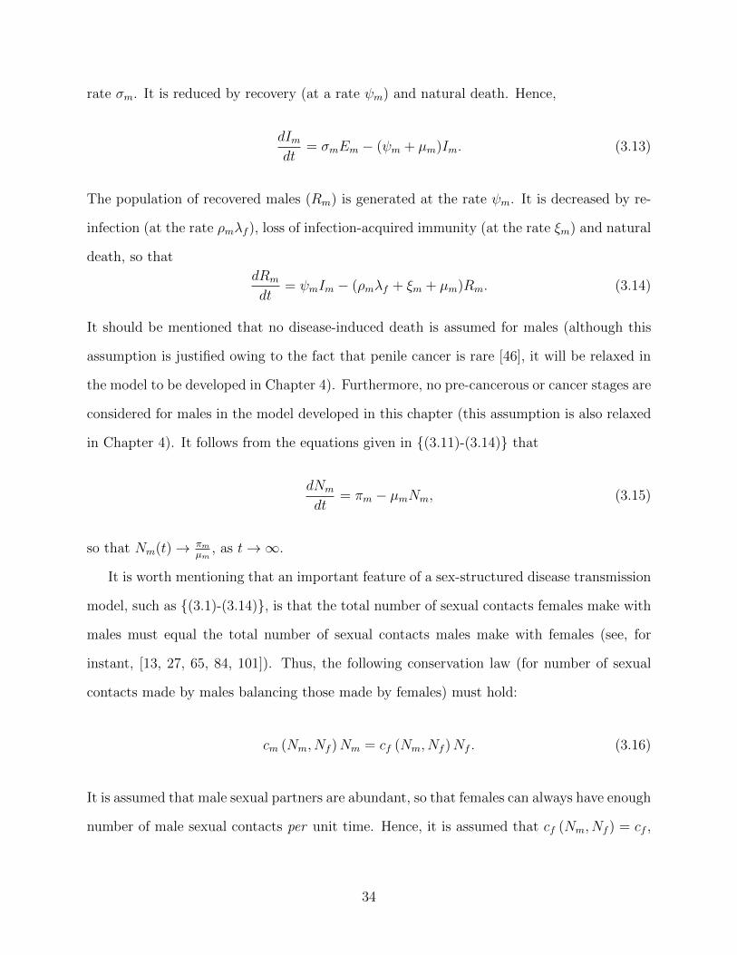
rate σm. It is reduced by recovery (at a rate ψm) and natural death. Hence,
dImdt
= σmEm − (ψm + µm)Im. (3.13)
The population of recovered males (Rm) is generated at the rate ψm. It is decreased by re-
infection (at the rate ρmλf ), loss of infection-acquired immunity (at the rate ξm) and natural
death, so thatdRm
dt= ψmIm − (ρmλf + ξm + µm)Rm. (3.14)
It should be mentioned that no disease-induced death is assumed for males (although this
assumption is justified owing to the fact that penile cancer is rare [46], it will be relaxed in
the model to be developed in Chapter 4). Furthermore, no pre-cancerous or cancer stages are
considered for males in the model developed in this chapter (this assumption is also relaxed
in Chapter 4). It follows from the equations given in {(3.11)-(3.14)} that
dNm
dt= πm − µmNm, (3.15)
so that Nm(t) →πmµm
, as t → ∞.
It is worth mentioning that an important feature of a sex-structured disease transmission
model, such as {(3.1)-(3.14)}, is that the total number of sexual contacts females make with
males must equal the total number of sexual contacts males make with females (see, for
instant, [13, 27, 65, 84, 101]). Thus, the following conservation law (for number of sexual
contacts made by males balancing those made by females) must hold:
cm (Nm, Nf )Nm = cf (Nm, Nf )Nf . (3.16)
It is assumed that male sexual partners are abundant, so that females can always have enough
number of male sexual contacts per unit time. Hence, it is assumed that cf (Nm, Nf ) = cf ,
34
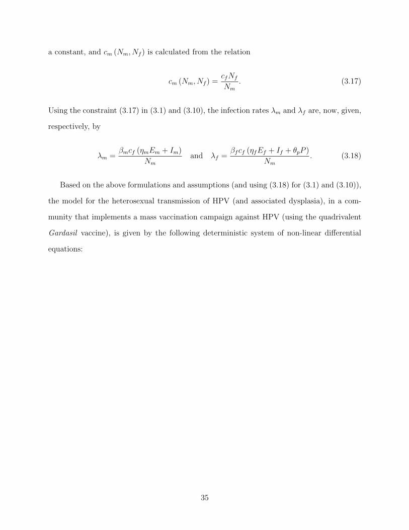
a constant, and cm (Nm, Nf ) is calculated from the relation
cm (Nm, Nf ) =cfNf
Nm. (3.17)
Using the constraint (3.17) in (3.1) and (3.10), the infection rates λm and λf are, now, given,
respectively, by
λm =βmcf (ηmEm + Im)
Nmand λf =
βfcf (ηfEf + If + θpP )
Nm. (3.18)
Based on the above formulations and assumptions (and using (3.18) for (3.1) and (3.10)),
the model for the heterosexual transmission of HPV (and associated dysplasia), in a com-
munity that implements a mass vaccination campaign against HPV (using the quadrivalent
Gardasil vaccine), is given by the following deterministic system of non-linear differential
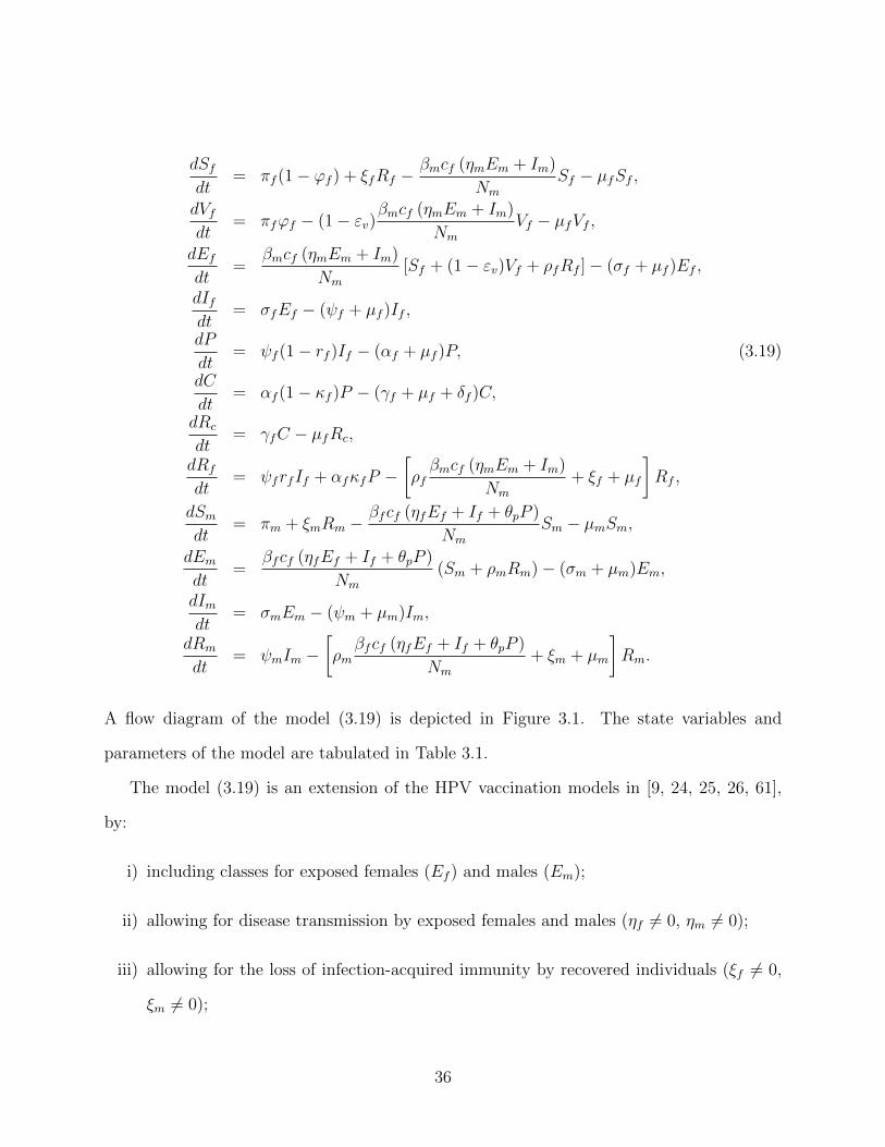
equations:
35
dSf
dt= πf (1− ϕf ) + ξfRf −
βmcf (ηmEm + Im)
NmSf − µfSf ,
dVf
dt= πfϕf − (1− εv)
βmcf (ηmEm + Im)
NmVf − µfVf ,
dEf
dt=
βmcf (ηmEm + Im)
Nm[Sf + (1− εv)Vf + ρfRf ]− (σf + µf )Ef ,
dIfdt
= σfEf − (ψf + µf )If ,
dP
dt= ψf (1− rf )If − (αf + µf )P, (3.19)
dC
dt= αf (1− κf )P − (γf + µf + δf )C,
dRc
dt= γfC − µfRc,
dRf
dt= ψfrfIf + αfκfP −
�ρf
βmcf (ηmEm + Im)
Nm+ ξf + µf
�Rf ,
dSm
dt= πm + ξmRm −
βfcf (ηfEf + If + θpP )
NmSm − µmSm,
dEm
dt=
βfcf (ηfEf + If + θpP )
Nm(Sm + ρmRm)− (σm + µm)Em,
dImdt
= σmEm − (ψm + µm)Im,
dRm
dt= ψmIm −
�ρm
βfcf (ηfEf + If + θpP )
Nm+ ξm + µm
�Rm.
A flow diagram of the model (3.19) is depicted in Figure 3.1. The state variables and
parameters of the model are tabulated in Table 3.1.
The model (3.19) is an extension of the HPV vaccination models in [9, 24, 25, 26, 61],
by:
i) including classes for exposed females (Ef ) and males (Em);
ii) allowing for disease transmission by exposed females and males (ηf �= 0, ηm �= 0);
iii) allowing for the loss of infection-acquired immunity by recovered individuals (ξf �= 0,
ξm �= 0);
36
iv) allowing for the re-infection of recovered individuals (ρf �= 0, ρm �= 0).
Furthermore, the model (3.19) extends the vaccination models in [9, 26] by, in addition to
Items (i)-(iii) above, including disease-induced mortality (δf �= 0) and a compartment for
females with persistent HPV infection (P ).
3.2.1 Basic properties
The basic qualitative features of the basic HPV vaccination model (3.19) will be explored.
First of all, for the vaccination model (3.19) to be epidemiologically meaningful, it is impor-
tant to show that all its state variables are non-negative for all time t > 0 (i.e., the solutions
of the vaccination model (3.19) with non-negative initial data must remain non-negative for
all t > 0).
Theorem 3.1. Let the initial data for the vaccination model (3.19) be Sf (0) > 0, Vf (0) >
0, Ef (0) ≥ 0, If (0) ≥ 0, P (0) ≥ 0, C(0) ≥ 0, Rc(0) ≥ 0, Rf (0) ≥ 0, Sm(0) > 0, Em(0) ≥
0, Im(0) ≥ 0, and Rm(0) ≥ 0. Then, the solutions (Sf (t), Vf (t), Ef (t), If (t), P (t), C(t), Rc(t),
Rf (t), Sm(t), Em(t), Im(t), Rm(t)) of the model with positive initial data, will remain positive
for all time t > 0.
The proof of Theorem 3.1 is given in Appendix A.
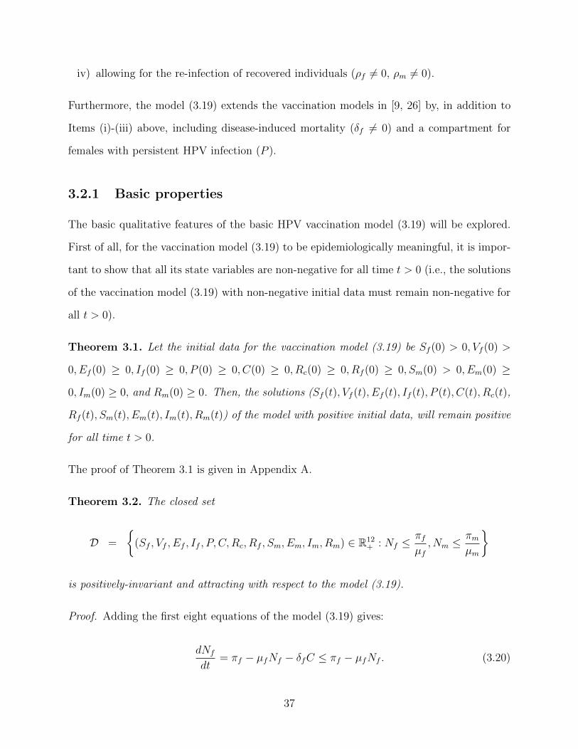
Theorem 3.2. The closed set
D =
�(Sf , Vf , Ef , If , P, C,Rc, Rf , Sm, Em, Im, Rm) ∈ R12
+ : Nf ≤πf
µf, Nm ≤
πm
µm
�
is positively-invariant and attracting with respect to the model (3.19).
Proof. Adding the first eight equations of the model (3.19) gives:
dNf
dt= πf − µfNf − δfC ≤ πf − µfNf . (3.20)
37
It follows from (3.20) that dNf
dt < 0 if Nf (t) > πf
µf. Thus, using a standard Comparison
Theorem (Theorem 2.10; see also [58]),
Nf (t) ≤ Nf (0)e−µf t +
πf
µf(1− e−µf t).
Therefore, Nf (t) ≤πf
µfif Nf (0) ≤
πf
µf. Similarly, it follows from (3.15) that
Nm(t) = Nm(0)e−µmt +
πm
µm(1− e−µmt).
Hence, Nm(t) ≤πmµm
if Nm(0) ≤πmµm
. Thus, D is positively-invariant. Furthermore, if Nf (t) >
πf
µfand Nm(t) >
πmµm
; then either the solution enters D in finite time, or Nf (t) approachesπf
µf
and Nm(t) approachesπmµm
, and the state variables associated with the infected classes of the
model approach zero. Hence, D attracts all solutions in R12+ .
In the region D, the model (3.19) can be considered as epidemiologically and mathematically
well-posed [47].
3.3 Analysis of Vaccination-free Model
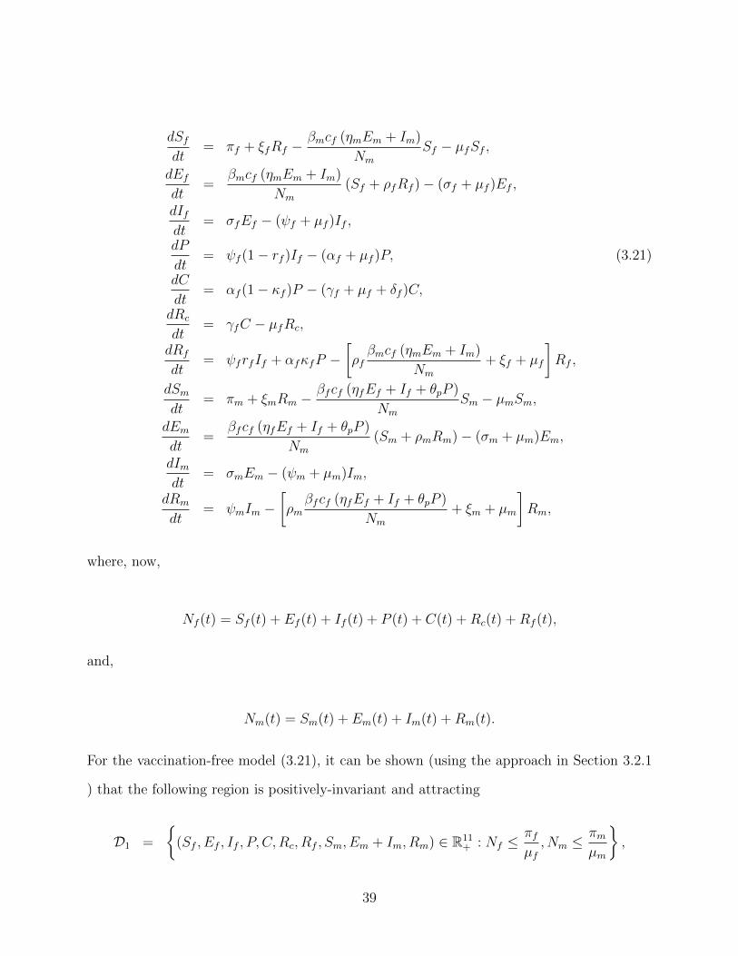
Before analyzing the vaccination model (3.19), it is instructive to gain insight into the dynam-
ics of the model (3.19) in the absence of vaccination (i.e., the model (3.19) with ϕf = Vf = 0).
The resulting vaccination-free model is given by
38
dSf
dt= πf + ξfRf −
βmcf (ηmEm + Im)
NmSf − µfSf ,
dEf
dt=
βmcf (ηmEm + Im)
Nm(Sf + ρfRf )− (σf + µf )Ef ,
dIfdt
= σfEf − (ψf + µf )If ,
dP
dt= ψf (1− rf )If − (αf + µf )P, (3.21)
dC
dt= αf (1− κf )P − (γf + µf + δf )C,
dRc
dt= γfC − µfRc,
dRf
dt= ψfrfIf + αfκfP −
�ρf
βmcf (ηmEm + Im)
Nm+ ξf + µf
�Rf ,
dSm
dt= πm + ξmRm −
βfcf (ηfEf + If + θpP )
NmSm − µmSm,
dEm
dt=
βfcf (ηfEf + If + θpP )
Nm(Sm + ρmRm)− (σm + µm)Em,
dImdt
= σmEm − (ψm + µm)Im,
dRm
dt= ψmIm −
�ρm
βfcf (ηfEf + If + θpP )
Nm+ ξm + µm
�Rm,
where, now,
Nf (t) = Sf (t) + Ef (t) + If (t) + P (t) + C(t) +Rc(t) +Rf (t),
and,
Nm(t) = Sm(t) + Em(t) + Im(t) +Rm(t).
For the vaccination-free model (3.21), it can be shown (using the approach in Section 3.2.1
) that the following region is positively-invariant and attracting
D1 =
�(Sf , Ef , If , P, C,Rc, Rf , Sm, Em + Im, Rm) ∈ R11
+ : Nf ≤πf
µf, Nm ≤
πm
µm
�,
39
so that it is sufficient to consider the dynamics of the vaccination-free model (3.21) in D1.
It is worth noting from (3.15) that Nm(t) →πmµm
as t → ∞. Consequently, from now on,
the total male population at time t (given by Nm(t)) will be replaced by its limiting value,
πmµm
(since Nm(t) →πmµm
, as t → ∞). In other words, the rest of the analyses in this chapter
will be carried out with Nm(t), in (3.19) and (3.21), replaced by its limiting value, N∗m = πm
µm.
3.3.1 Local asymptotic stability of disease-free equilibrium (DFE)
The vaccination-free model (3.21) has a DFE, obtained by setting the right-hand sides of
the equations in the model (3.21) to zero, given by
E0 = (S∗f , E
∗f , I
∗f , P
∗, C∗, R∗c , R
∗f , S
∗m, E
∗m, I
∗m, R
∗m) =
�πf
µf, 0, 0, 0, 0, 0,
πm
µm, 0, 0
�. (3.22)
with,
N∗f = S∗
f =πf
µfand N∗
m = S∗m =
πm
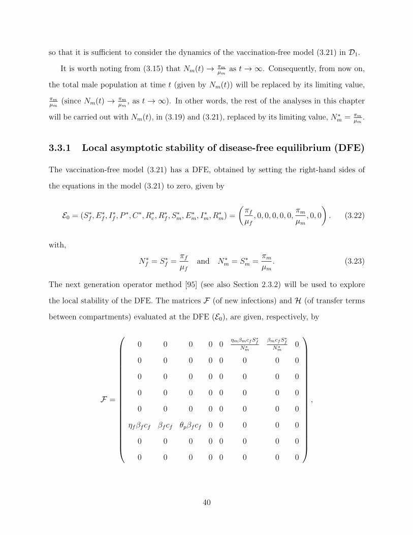
µm. (3.23)
The next generation operator method [95] (see also Section 2.3.2) will be used to explore
the local stability of the DFE. The matrices F (of new infections) and H (of transfer terms
between compartments) evaluated at the DFE (E0), are given, respectively, by
F =
0 0 0 0 0ηmβmcfS∗
f
N∗m
βmcfS∗f
N∗m
0
0 0 0 0 0 0 0 0
0 0 0 0 0 0 0 0
0 0 0 0 0 0 0 0
0 0 0 0 0 0 0 0
ηfβfcf βfcf θpβfcf 0 0 0 0 0
0 0 0 0 0 0 0 0
0 0 0 0 0 0 0 0
,
40
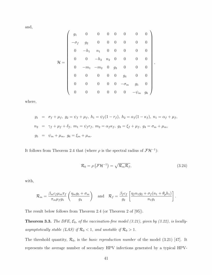
and,
H =
g1 0 0 0 0 0 0 0
−σf g2 0 0 0 0 0 0
0 −h1 n1 0 0 0 0 0
0 0 −h2 n2 0 0 0 0
0 −m1 −m2 0 g3 0 0 0
0 0 0 0 0 g4 0 0
0 0 0 0 0 −σm g5 0
0 0 0 0 0 0 −ψm g6
,
where,
g1 = σf + µf , g2 = ψf + µf , h1 = ψf (1− rf ), h2 = αf (1− κf ), n1 = αf + µf ,
n2 = γf + µf + δf , m1 = ψfrf , m2 = αfκf , g3 = ξf + µf , g4 = σm + µm,
g5 = ψm + µm, g6 = ξm + µm.
It follows from Theorem 2.4 that (where ρ is the spectral radius of FH−1):
R0 = ρ�FH
−1�=
�RmRf , (3.24)
with,
Rm =βmcfµmπf
πmµfg5
�ηmg5 + σm
g4
�and Rf =
βfcfg2
�ηfn1g2 + σf (n1 + θph1)
n1g1
�.
The result below follows from Theorem 2.4 (or Theorem 2 of [95]).
Theorem 3.3. The DFE, E0, of the vaccination-free model (3.21), given by (3.22), is locally-
asymptotically stable (LAS) if R0 < 1, and unstable if R0 > 1.
The threshold quantity, R0, is the basic reproduction number of the model (3.21) [47]. It
represents the average number of secondary HPV infections generated by a typical HPV-
41
infected person if introduced into a completely-susceptible sexually-active population (or
community). It is worth noting that R0 is an aggregate product of the average number of
new HPV cases generated by females (denoted by Rf ) and males (denoted by Rm).
Epidemiologically speaking, Theorem 3.3 states that a small influx of infected individuals
(males or females) will not generate large HPV outbreaks in the community if R0 < 1 (in
other words, HPV can be effectively controlled in the community if the initial sizes of the
sub-populations of the model (3.21) are in the basin of attraction of the DFE, E0, of the model
(3.21)). However, in order for such effective control (or elimination) to be independent of
the initial sizes of the sub-populations of the vaccination-free model (3.21), it is necessary
to show that the DFE (E0), of the model (3.21), is globally-asymptotically stable (GAS) if
R0 < 1. This is explored, for a special case, in Section 3.3.5.
3.3.2 Interpretation of the basic reproduction number (R0)
The reproduction threshold (R0) can be interpreted as follows. Susceptible females can
acquire infection, following effective contacts with either exposed (Em) or symptomatic males
(Im). The number of female infections generated by exposed males (near the DFE) is given
by the product of the infection rate of exposed males�
βmcfηmS∗f
N∗m
�and the average duration
in the exposed (Em) class�
1σm+µm
= 1g4
�. Furthermore, the number of female infections
generated by symptomatic males (near the DFE) is given by the product of the infection
rate of symptomatic males�
βmcfS∗f
N∗m
�, the probability that an exposed male survives the
exposed stage and move to the symptomatic stage�
σmσm+µm
= σmg4
�and the average duration
in the symptomatic (Im) class�
1ψm+µm
= 1g5
�. Thus, the average number of new female
infections generated by infected males (exposed or symptomatic) is given by (noting that
S∗f = πf
µfand N∗
m = πmµm
),
�βmcfηmµm
πmg4+
βmcfµmσm
πmg4g5
�S∗f =
βmcfµmπf
πmµf
�ηmg5 + σm
g4g5
�. (3.25)
42
The two terms in the left-hand side (LHS) of (3.25), represent the number of new female in-
fections generated by exposed males (Em) and the number of new female infections generated
by symptomatic males (Im), respectively.
Similarly, susceptible males acquire HPV infection, following effective contacts with either
exposed females (Ef ), symptomatic females (If ) or females with persistent HPV infection
(P ). The number of male infections generated by exposed females (near the DFE) is the
product of the infection rate of exposed females�
βf cfηfS∗m
N∗m
�and the average duration in the
exposed (Ef ) class�
1σf+µf
= 1g1
�. The number of male infections generated by symptomatic
females is the product of the infection rate of symptomatic females�
βf cfS∗m
N∗m
�, the probabil-
ity that an exposed female survives the exposed class and move to the symptomatic stage�
σf
σf+µf= σf
g1
�and the average duration in the symptomatic (If ) class
�1
ψf+µf= 1
g2
�. Fur-
thermore, the number of male infections generated by females with persistent HPV infection
is the product of the infection rate of females with persistent HPV infection�
βf cf θpS∗m
N∗m
�, the
probability that an exposed female survives the exposed class and move to the symptomatic
stage�
σf
σf+µf= σf
g1
�, the proportion of symptomatic females that move to the persistent
infection class�
ψf (1−rf )ψf+µf
= h1g2
�and the average duration in the persistent infection class
�1
αf+µf= 1
n1
�. Thus, the average number of new male infections generated by infected fe-
males (exposed, symptomatic or those with persistent HPV infection) is given by (noting
that S∗m = πm
µm)
�βfcfηfµm
πmg1+
βfcfµmσf
πmg1g2+
βfcfσfθpµmh1
πmn1g1g2
�S∗m = βfcf
�ηfn1g2 + σfn1 + σfθph1
n1g1g2
�. (3.26)
The terms in LHS of (3.26), represent the number of new male infections generated by
exposed females (Ef ), symptomatic (If ) and females with persistent HPV infection (P ).
Since two generations are needed in the female-male-female HPV transmission cycle, the
geometric mean of (3.25) and (3.26) gives the basic reproduction number, R0 (interpretation
for R0 is also given in [16, 37, 43] for other epidemiological settings).
43
3.3.3 Existence and local asymptotic stability of endemic equilib-
rium point (EEP)
It is instructive to determine the number of possible equilibrium solutions the vaccination-
free model (3.21) can have. It is convenient to let
E1 = (S∗∗f , E∗∗
f , I∗∗f , P ∗∗, C∗∗, R∗∗c , R∗∗
f , S∗∗m , E∗∗
m , I∗∗m , R∗∗m ), (3.27)
be an arbitrary endemic equilibrium of the model (3.21) (an equilibrium where all the infected
components of the model are non-zero). Furthermore, let (it should be emphasized that Nm,
in (3.21), is now replaced by πmµm
)
λ∗∗m =
βmcfµm (ηmE∗∗m + I∗∗m )
πm, (3.28)
and,
λ∗∗f =
βfcfµm
�ηfE∗∗
f + I∗∗f + θpP ∗∗�
πm, (3.29)
be the force of infection for males and females at steady- state, respectively.
Solving the equations of the vaccination-free (3.21) at the endemic steady-state gives:
S∗∗f =
πf + ξfR∗∗f
λ∗∗m + µf
, E∗∗f =
λ∗∗m
�S∗∗f + ρfR∗∗
f
�
g1, I∗∗f =
σfE∗∗f
g2,
P ∗∗ =h1I∗∗fn1
, C∗∗ =h2P ∗∗
n2, R∗∗
c =γfC∗∗
µf, R∗∗
f =m1I∗∗f +m2P ∗∗
ρfλ∗∗m + g3
, (3.30)
S∗∗m =
πm + ξmR∗∗m
λ∗∗f + µm
, E∗∗m =
λ∗∗f (S∗∗
m + ρmR∗∗m )
g4, I∗∗m =
σmE∗∗m
g5,
R∗∗m =
ψmI∗∗mρmλ∗∗
f + g6.
44
Substituting the expressions in (3.30) into (3.28) and (3.29) gives
λ∗∗m =
λ∗∗f z11
�g6 + λ∗∗
f t12�
�λ∗∗f
�2z12 + λ∗∗
f z13 + z14, (3.31)
λ∗∗f =
λ∗∗mz21 (g3 + λ∗∗
m t22)
(λ∗∗m )2 z22 + λ∗∗
mz23 + z24, (3.32)
with,
z11 = βmcfµm (ηmg5 + σm) , t12 = ρm, z12 = t12 (g4g5 − σmψm) ,
z13 = g4g5 (g6 + µmt12)− σmψm (ξm + µmt12) , z14 = g4g5g6µm, (3.33)
z21 =βfcfπfµm
πm(ηfn1g2 + n1σf + θph1σf ) , t22 = ρf , z22 = t22 [n1g1g2 − σf (n1m1 + h1m2)] ,
z23 = n1g1g2 (g3 + µf t22)− σf (n1m1 + h1m2) (ξf + µf t22) , z24 = n1g1g2g3µf .
The expressions in (3.33) can be simplified to
z12 = t12µm (σm + ψm + µm) > 0,
z13 = µm [(σm + ψm + µm) (ξm + µmt12) + (σm + µm) (ψm + µm)] > 0,
z22 = t22µf (σf + ψf + µf ) (µf + αf ) + σfψf (1− rf ) [µf + αf (1 + κf )] > 0,
z23 = σfψf (1− rf ) {ξf [µf + αf (1− κf )] + t22µf (αf + µf )}
+ µf
�µ2f (ξf + µf ) + σfξf (αf + µf )
�+ µf (σf + ξf + µf ) [αf (ψf + µf ) + µfψf ]
+ t22µ2f (σf + ψf + µf ) (αf + µf ) > 0.
By substituting (3.32) into (3.31), and simplifying, it follows that the endemic equilibria of
the vaccination-free model (3.21) satisfy the following polynomial (in terms of λ∗∗m ),
a0 (λ∗∗m )4 + b0 (λ
∗∗m )3 + c0 (λ
∗∗m )2 + d0λ
∗∗m + e0 = 0, (3.34)
45
where,
a0 = t22z21 (t22z21z12 + z13z22) + z14z222,
b0 = 2t22g3z12z221 + z22 (z14z23 + g3z13z21) + z22 (z14z23 − g6g3z11z21)
+ t22z21 (z13z23 − t12t22z11z21) ,
c0 = z22z14z24�2−R
20
�+ g3z13z21z23 + g3z21 (g3z21z12 − t12t22z11z21) (3.35)
+ t22z21 (z13z23 − t12g3z11z21) + z13 (z14z23 − g6t22z11z21) ,
d0 = z23z14z24�1−R
20
�+ z24 (g3z13z21 − g6t22z11z21) + g3z21 (z24z13 − t12g3z11z21) ,
e0 = z11z224
�1−R
20
�.
It follows from (3.35) that the coefficient, a0, of the quartic (3.34), is always positive (since all
the parameters of the model (3.21) are positive). Furthermore, the coefficient, e0, is positive
(negative) if R0 is less than (greater than) unity. Thus, the number of possible positive real
roots the polynomial (3.34) can have depends on the signs of b0, c0, and d0. This can be
analysed using the Descartes Rule of Sign for the quartic (3.34). The various possibilities
for the number of positive real roots of (3.34) are tabulated in Table 3.2, from which the
following result is obtained:
Theorem 3.4. The vaccination-free model (3.21),
i) has a unique endemic equilibrium if R0 > 1 and Cases 1,2,3 and 6 of Table 3.2 hold;
ii) could have more than one endemic equilibria if R0 > 1 and Cases 4,5,7 and 8 of Table
3.2 hold;
46
iii) could have two or more endemic equilibria if R0 < 1 and Cases 2,3,4,5,6,7 and 8 of
Table 3.2 hold.
We claim the following result, for the local asymptotic stability of a special case of the EEP
(E1) of the model (3.21).
Theorem 3.5. Consider the vaccination-free model (3.21) with ρf = ρm = 0 and that
Item (i) of Theorem 3.4 holds. Then, the associated unique endemic equilibrium, E1, of the
resulting reduced model, is LAS whenever R0 > 1.
The proof of Theorem 3.5, based on using a Krasnoselskii sub-linearity argument [31, 32, 91],
is given in Appendix B. The result of Theorem 3.5 is numerically illustrated by simulating the
model (3.21), using numerous initial conditions and parameter values such that R0 = 6.4887.
The results obtained, depicted in Figure 3.2, show convergence of the solutions to the unique
endemic equilibrium, E1 (in line with Theorem 3.5). The epidemiological implication of
this result is that, for this special case (of the model (3.21) with ρf = ρm = 0), HPV will
establish itself in the population, when R0 > 1, if the initial sizes of the sub-populations
of the vaccination-free model (3.21) are in the basin of attraction of the unique endemic
equilibrium (E1).
3.3.4 Backward bifurcation analysis
The presence of multiple endemic equilibria of the vaccination-free model (3.21) whenR0 < 1
(as shown in Theorem 3.4 and Table 3.2) suggests the possibility of backward bifurcation,
where, typically, the stable DFE (E0) co-exists with a stable endemic equilibrium (E1), when
the associated basic reproduction number (R0) is less than unity. The phenomenon of
backward bifurcation has been observed in numerous disease transmission models, such as
those with imperfect vaccine and exogenous re-infection (see, for instance, [14, 28, 83, 84, 85,
86, 103] and some of the references therein), vector-borne diseases [37] and treatment [104].
47
We claim the following result (the proof, based on using Centre Manifold Theory, as
described in [14], is given in Appendix C).
Theorem 3.6. The vaccination-free model (3.21) undergoes backward bifurcation at R0 = 1
if the inequality ρf > ρcf , given by (C.6) in Appendix C, holds.
The backward bifurcation phenomenon is illustrated by simulating the vaccination-free
model (3.21) with the following set of parameter values: δf = 0.0001, ξf = ξm = 0.0012, ρf =
1.2, ρm = 0.9855, πf = πm = 100, βm = 0.35, cm = cf = 15, µf = µm = 175 , κf =
0.895, αf = 0.878, σf = σm = 0.75, ψf = ψm = 0.8, θp = 0.95 and ηf = ηm = 0.9.
With this set of parameter values, the associated bifurcation coefficients, a and b (defined in
Appendix C), take the values a = 0.0182183226 > 0 and b = 359.2293164 > 0.
It should be mentioned that the aforementioned parameter values are chosen only to
illustrate the backward bifurcation phenomenon property of the vaccination-free model (and
they may not all be realistic epidemiologically; in particular, the parameter ρf has to be
chosen outside its realistic range 0 ≤ ρf ≤ 1). As noted by Lipsitch and Murray [60], it is, in
general, difficult to illustrate the phenomenon of backward bifurcation using a realistic set of
parameter values. Nonetheless, the analyses in Appendix C show that the vaccination-free
model (3.21) will undergo backward bifurcation R0 = 1 if the re-infection parameter for
females (ρf ) exceeds a certain threshold (ρcf ). The resulting backward bifurcation diagram
is depicted in Figure 3.3.
The epidemiological consequence of the backward bifurcation phenomenon of the vaccination-
free model (3.21) is that the effective control of HPV spread in the population (when R0 < 1)
is dependent on the initial sizes of the sub-populations of the model. In other words, the
presence of backward bifurcation in the vaccination-free model (3.21) makes the effort to
effectively control (or eliminate) HPV spread in the population difficult.
Furthermore, it follows from the analyses in Appendix C that the vaccination-free model
(3.21) does not undergo backward bifurcation if recovered females and males do not acquire
HPV re-infection (i.e., if ρm = ρf = 0). In such a scenario (i.e., the model (3.21) with
48
ρm = ρf = 0 and, for computational convenience, ξf = ξm = 0), the backward bifurcation
coefficient, a (given by (C.7) in Appendix C), is negative (which excludes backward bifurca-
tion in line with Item (iv) of Theorem 2.8 in Chapter 2). Thus, the analyses in Appendix
C suggest that the DFE (E0), of the vaccination-free model (3.21), is GAS if R0 < 1 and
ρm = ρf = 0. This claim is explored below.
3.3.5 Global asymptotic stability of DFE (special case)
To further confirm the absence of backward bifurcation in the vaccination-free model (3.21),
for the scenario when ρm = ρf = 0, the global asymptotic stability property of its DFE (E0),
is established below for this special case.
Theorem 3.7. The DFE, E0, of the vaccination-free model (3.21), with ρf = ρm = 0, is
GAS in D1 if R0 < 1.
The proof of Theorem 3.7, based on using a Comparison Theorem [58], is given in Appendix
D. This result is illustrated numerically in Figure 3.4, by simulating the vaccination-free
model (3.21) using multiple initial conditions and parameter values such that R0 = 0.3823
(so that, by Theorem 3.7, the DFE, E0, of the model (3.21) is GAS). Figure 3.4 shows
convergence of the solution profiles to the DFE (in accordance with Theorem 3.7). The
epidemiological implication of Theorem 3.7 is that the classical epidemiological requirement
of having the associated reproduction number (R0) less than unity is necessary and sufficient
for the elimination of HPV from the community.
In summary, the vaccination-free model (3.21) has the following dynamical features:
i) The model has a LAS DFE whenever R0 < 1;
ii) The model can have a unique or multiple endemic equilibria when the associated re-
production number (R0) exceeds unity. For the special case when the model has a
unique endemic equilibrium point, this equilibrium is shown to be LAS;
49
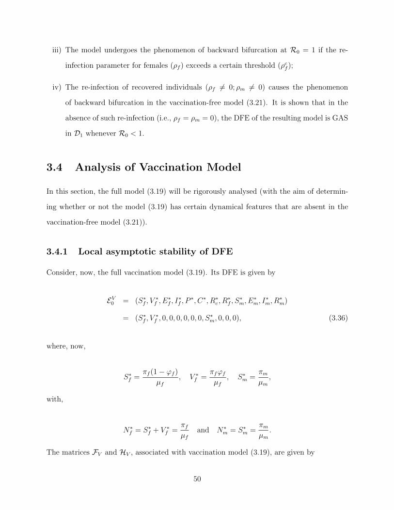
iii) The model undergoes the phenomenon of backward bifurcation at R0 = 1 if the re-
infection parameter for females (ρf ) exceeds a certain threshold (ρcf );
iv) The re-infection of recovered individuals (ρf �= 0; ρm �= 0) causes the phenomenon
of backward bifurcation in the vaccination-free model (3.21). It is shown that in the
absence of such re-infection (i.e., ρf = ρm = 0), the DFE of the resulting model is GAS
in D1 whenever R0 < 1.
3.4 Analysis of Vaccination Model
In this section, the full model (3.19) will be rigorously analysed (with the aim of determin-
ing whether or not the model (3.19) has certain dynamical features that are absent in the
vaccination-free model (3.21)).
3.4.1 Local asymptotic stability of DFE
Consider, now, the full vaccination model (3.19). Its DFE is given by
EV0 = (S∗
f , V∗f , E
∗f , I
∗f , P
∗, C∗, R∗c , R
∗f , S
∗m, E
∗m, I
∗m, R
∗m)
= (S∗f , V
∗f , 0, 0, 0, 0, 0, 0, S
∗m, 0, 0, 0), (3.36)
where, now,
S∗f =
πf (1− ϕf )
µf, V ∗
f =πfϕf
µf, S∗
m =πm
µm,
with,
N∗f = S∗
f + V ∗f =
πf
µfand N∗
m = S∗m =
πm
µm.
The matrices FV and HV , associated with vaccination model (3.19), are given by
50
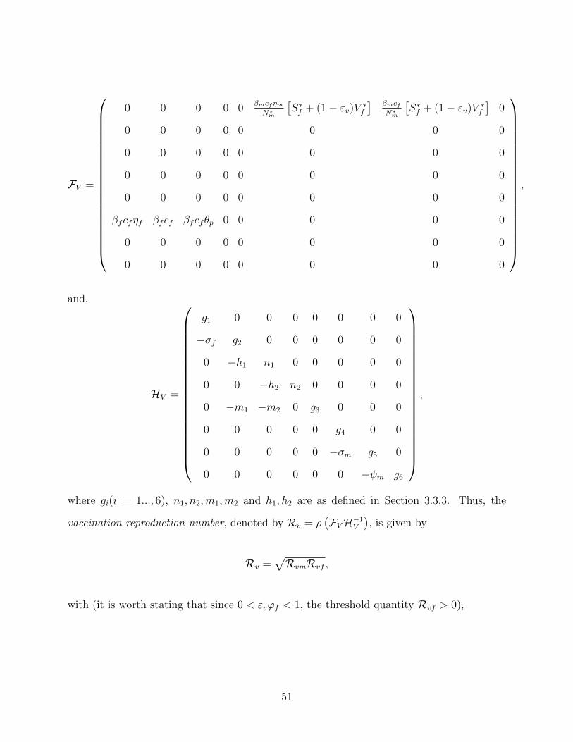
FV =
0 0 0 0 0 βmcfηmN∗
m
�S∗f + (1− εv)V ∗
f
� βmcfN∗
m
�S∗f + (1− εv)V ∗
f
�0
0 0 0 0 0 0 0 0
0 0 0 0 0 0 0 0
0 0 0 0 0 0 0 0
0 0 0 0 0 0 0 0
βfcfηf βfcf βfcfθp 0 0 0 0 0
0 0 0 0 0 0 0 0
0 0 0 0 0 0 0 0
,
and,
HV =
g1 0 0 0 0 0 0 0
−σf g2 0 0 0 0 0 0
0 −h1 n1 0 0 0 0 0
0 0 −h2 n2 0 0 0 0
0 −m1 −m2 0 g3 0 0 0
0 0 0 0 0 g4 0 0
0 0 0 0 0 −σm g5 0
0 0 0 0 0 0 −ψm g6
,
where gi(i = 1..., 6), n1, n2,m1,m2 and h1, h2 are as defined in Section 3.3.3. Thus, the
vaccination reproduction number, denoted by Rv = ρ�FVH
−1V
�, is given by
Rv =�RvmRvf ,
with (it is worth stating that since 0 < εvϕf < 1, the threshold quantity Rvf > 0),
51
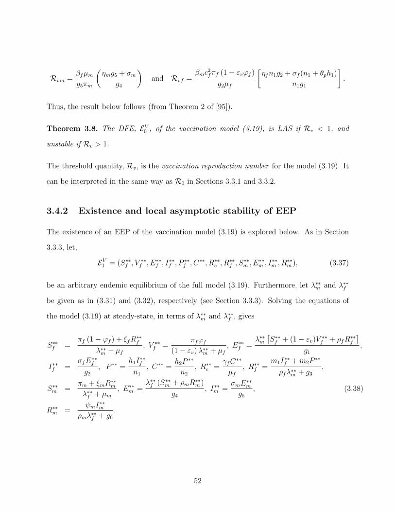
Rvm =βfµm
g5πm
�ηmg5 + σm
g4
�and Rvf =
βmc2fπf (1− εvϕf )
g2µf
�ηfn1g2 + σf (n1 + θph1)
n1g1
�.
Thus, the result below follows (from Theorem 2 of [95]).
Theorem 3.8. The DFE, EV0 , of the vaccination model (3.19), is LAS if Rv < 1, and
unstable if Rv > 1.
The threshold quantity, Rv, is the vaccination reproduction number for the model (3.19). It
can be interpreted in the same way as R0 in Sections 3.3.1 and 3.3.2.
3.4.2 Existence and local asymptotic stability of EEP
The existence of an EEP of the vaccination model (3.19) is explored below. As in Section
3.3.3, let,
EV1 = (S∗∗
f , V ∗∗f , E∗∗
f , I∗∗f , P ∗∗f , C∗∗, R∗∗
c , R∗∗f , S∗∗
m , E∗∗m , I∗∗m , R∗∗
m ), (3.37)
be an arbitrary endemic equilibrium of the full model (3.19). Furthermore, let λ∗∗m and λ∗∗
f
be given as in (3.31) and (3.32), respectively (see Section 3.3.3). Solving the equations of
the model (3.19) at steady-state, in terms of λ∗∗m and λ∗∗
f , gives
S∗∗f =
πf (1− ϕf ) + ξfR∗∗f
λ∗∗m + µf
, V ∗∗f =
πfϕf
(1− εv)λ∗∗m + µf
, E∗∗f =
λ∗∗m
�S∗∗f + (1− εv)V ∗∗
f + ρfR∗∗f
�
g1,
I∗∗f =σfE∗∗
f
g2, P ∗∗ =
h1I∗∗fn1
, C∗∗ =h2P ∗∗
n2, R∗∗
c =γfC∗∗
µf, R∗∗
f =m1I∗∗f +m2P ∗∗
ρfλ∗∗m + g3
,
S∗∗m =
πm + ξmR∗∗m
λ∗∗f + µm
, E∗∗m =
λ∗∗f (S∗∗
m + ρmR∗∗m )
g4, I∗∗m =
σmE∗∗m
g5, (3.38)
R∗∗m =
ψmI∗∗mρmλ∗∗
f + g6.
52
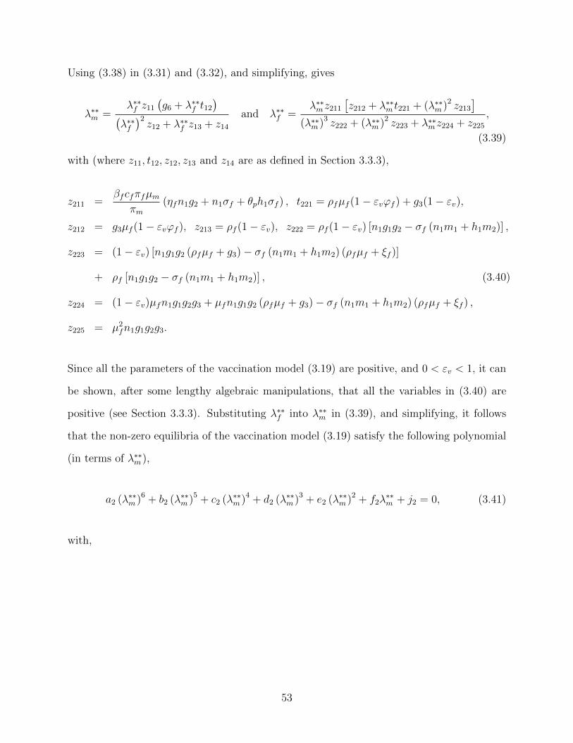
Using (3.38) in (3.31) and (3.32), and simplifying, gives
λ∗∗m =
λ∗∗f z11
�g6 + λ∗∗
f t12�
�λ∗∗f
�2z12 + λ∗∗
f z13 + z14and λ∗∗
f =λ∗∗mz211
�z212 + λ∗∗
m t221 + (λ∗∗m )2 z213
�
(λ∗∗m )3 z222 + (λ∗∗
m )2 z223 + λ∗∗mz224 + z225
,
(3.39)
with (where z11, t12, z12, z13 and z14 are as defined in Section 3.3.3),
z211 =βfcfπfµm
πm(ηfn1g2 + n1σf + θph1σf ) , t221 = ρfµf (1− εvϕf ) + g3(1− εv),
z212 = g3µf (1− εvϕf ), z213 = ρf (1− εv), z222 = ρf (1− εv) [n1g1g2 − σf (n1m1 + h1m2)] ,
z223 = (1− εv) [n1g1g2 (ρfµf + g3)− σf (n1m1 + h1m2) (ρfµf + ξf )]
+ ρf [n1g1g2 − σf (n1m1 + h1m2)] , (3.40)
z224 = (1− εv)µfn1g1g2g3 + µfn1g1g2 (ρfµf + g3)− σf (n1m1 + h1m2) (ρfµf + ξf ) ,
z225 = µ2fn1g1g2g3.
Since all the parameters of the vaccination model (3.19) are positive, and 0 < εv < 1, it can
be shown, after some lengthy algebraic manipulations, that all the variables in (3.40) are
positive (see Section 3.3.3). Substituting λ∗∗f into λ∗∗
m in (3.39), and simplifying, it follows
that the non-zero equilibria of the vaccination model (3.19) satisfy the following polynomial
(in terms of λ∗∗m ),
a2 (λ∗∗m )6 + b2 (λ
∗∗m )5 + c2 (λ
∗∗m )4 + d2 (λ
∗∗m )3 + e2 (λ
∗∗m )2 + f2λ
∗∗m + j2 = 0, (3.41)
with,
53
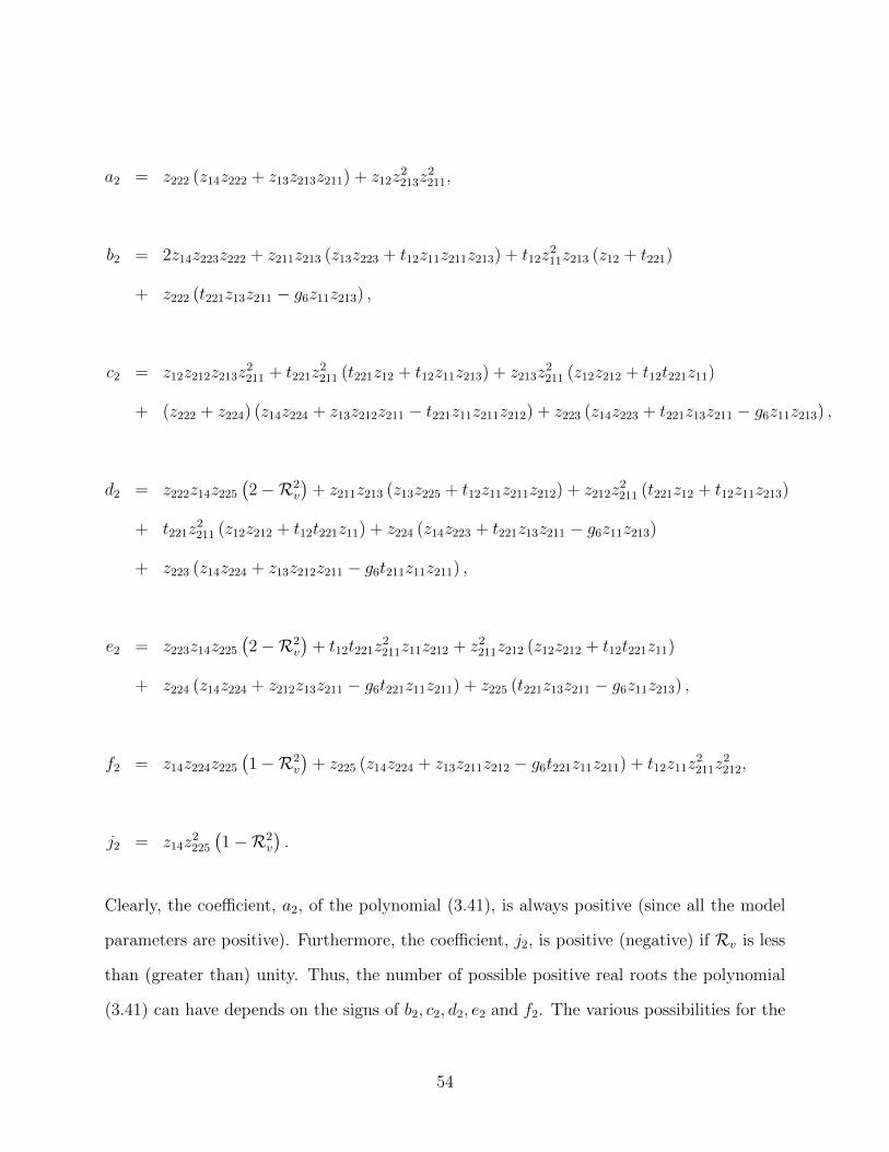
a2 = z222 (z14z222 + z13z213z211) + z12z2213z
2211,
b2 = 2z14z223z222 + z211z213 (z13z223 + t12z11z211z213) + t12z211z213 (z12 + t221)
+ z222 (t221z13z211 − g6z11z213) ,
c2 = z12z212z213z2211 + t221z
2211 (t221z12 + t12z11z213) + z213z
2211 (z12z212 + t12t221z11)
+ (z222 + z224) (z14z224 + z13z212z211 − t221z11z211z212) + z223 (z14z223 + t221z13z211 − g6z11z213) ,
d2 = z222z14z225�2−R
2v
�+ z211z213 (z13z225 + t12z11z211z212) + z212z
2211 (t221z12 + t12z11z213)
+ t221z2211 (z12z212 + t12t221z11) + z224 (z14z223 + t221z13z211 − g6z11z213)
+ z223 (z14z224 + z13z212z211 − g6t211z11z211) ,
e2 = z223z14z225�2−R
2v
�+ t12t221z
2211z11z212 + z2211z212 (z12z212 + t12t221z11)
+ z224 (z14z224 + z212z13z211 − g6t221z11z211) + z225 (t221z13z211 − g6z11z213) ,
f2 = z14z224z225�1−R
2v
�+ z225 (z14z224 + z13z211z212 − g6t221z11z211) + t12z11z
2211z
2212,
j2 = z14z2225
�1−R
2v
�.
Clearly, the coefficient, a2, of the polynomial (3.41), is always positive (since all the model
parameters are positive). Furthermore, the coefficient, j2, is positive (negative) if Rv is less
than (greater than) unity. Thus, the number of possible positive real roots the polynomial
(3.41) can have depends on the signs of b2, c2, d2, e2 and f2. The various possibilities for the
54
roots of (3.34) are tabulated in Table 3.3.
Theorem 3.9. The vaccination model (3.19),
i) has a unique endemic equilibrium if Rv > 1 and whenever Cases 1,2,3 and 6 of Table
3.3 hold;
ii) could have more than one endemic equilibrium if Rv > 1 and whenever Cases 4,5,7,8,11
and 12 of Table 3.3 hold;
iii) could have two or more endemic equilibrium if Rv < 1 and whenever Cases 2-12 of
Table 3.3 hold.
Furthermore, as in the case of the vaccination-free model (3.21), the vaccination model
(3.19) also undergoes backward bifurcation, as below.
Theorem 3.10. The vaccination model (3.19) undergoes backward bifurcation at Rv = 1
whenever the inequality (E.3), given in Appendix E, is satisfied.
The proof, based on using Centre Manifold Theory, is given in Appendix E. Here, too, the
backward bifurcation property of the vaccination model (3.19) can be removed whenever the
re-infection of recovered individuals does not occur (i.e., ρf = ρm = 0). The GAS property
of the DFE, EV0 , of the vaccination model (3.19), is established for this case in Section 3.4.3.
3.4.3 Global asymptotic stability of DFE (special case)
The global asymptotic stability of the DFE, EV0 , of the vaccination model (3.19) is established
for the special case where the re-infection of recovered individuals does not occur (i.e., ρf =
ρm = 0).
Theorem 3.11. The DFE, EV0 , of the vaccination model (3.19), with ρf = ρm = 0, is GAS
in D if Rv < 1.
The proof of Theorem 3.11, based on using a Lyapunov function, is given in Appendix F.
55
3.5 Qualitative Assessment of Vaccine Impact
The population-level impact of the anti-HPV mass vaccination program, using the Gardasil
vaccine, in the community is assessed for the special case of the vaccination model (3.19)
with ρf = ρm = 0 (so that the DFE of the resulting model is GAS, in line with Theorem
3.11). It is convenient to re-write the associated vaccination reproduction number, Rv, as
R2v = R
20 (1− εvϕf ) , (3.42)
where ϕf represents the fraction of females vaccinated at steady-state, εv is the vaccine
efficacy, and R0 is basic reproduction number for the vaccination-free model (3.21) with
ρf = ρm = 0. Thus (noting that gi(i = 1..., 6), n1, n2,m1,m2 and h1, h2 are as defined in
Section 3.3.3),
R20 = R
2v |ϕf=0=
βfcmβmcf (ηmg5 + σm) (ηfn1g2 + σfn1 + σfθph1)
n1g1g2g4g5.
It can be shown from (3.42), by writing Rv = Rv (ϕf ), that
Rv (ϕf ) = R0
�1− εvϕf , (3.43)
so that,
∂Rv
∂ϕf= −
εvR0
2�
1− εvϕf
.
Since 0 < εv < 1, it follows that Rv(ϕf ) is a decreasing function of ϕf . Furthermore, there
is a unique ϕcf , such that Rv
�ϕcf
�= 1, given by
ϕcf =
1
εv
�1−
1
R20
�.
Lemma 3.1. The DFE, EV0 , of the vaccination model (3.19), with ρf = ρm = 0, is GAS in
56
D if ϕf > ϕcf , and unstable if ϕf < ϕc
f .
Proof. Consider the vaccination model (3.19) with ρf = ρm = 0. Let ϕf > ϕcf . Then, it
follows from (3.42) that Rv < 1. Hence, the result follows from Theorem 3.11 that the DFE,
EV0 of (3.19) with ρf = ρm = 0, is GAS in D for this case (ϕf > ϕc
f ).
Figure 3.5 depicts a contour plot of Rv, as a function of the vaccine efficacy (εv) and coverage
(ϕf ). It follows from Figure 3.5 that, with the assumed 90% efficacy of the Gardasil vaccine
[7, 15, 76, 93, 96], HPV can be effectively controlled or eliminated from the community if
at least 78% of the new sexually-active susceptible females in the community are vaccinated
(with Gardasil) at steady-state.
3.6 Numerical Simulations
The vaccination-free model (3.21) is simulated, first of all, using the parameter values given
in Table 3.1 (unless otherwise stated). The following initial conditions were used in the
simulations: Sf (0) = 15, 000, Vf (0) = 35, 000, Ef (0) + If (0) + P (0) = 5, 000, C(0) = 1, 300,
Sm(0) = 50, 000, Em(0) + Im(0) = 500 and Rc(0) = Rf (0) = Rm(0) = 0. Figure 3.6 depicts
the cumulative number of new cervical cancer cases as a function of time in the absence of
vaccination (i.e., Vf = ϕf = 0). This figure (which represents the worst-case scenario of
HPV transmission in the community in the absence of mass vaccination) shows that about
1, 700 cervical cancer cases will be recorded over 5 years. Furthermore, up to 262 infected
people will die over the same time period (Figure 3.7).
The vaccination model (3.19) is then simulated to determine the impact of mass vaccina-
tion of new sexually-active females (using the Gardasil vaccine) on the cumulative number
of new cervical cancer cases in the community. Figure 3.8 shows a marked decrease in the
cumulative number of cases (from 1, 700 in Figure 3.6 to about 907) if the Gardasil vaccine
efficacy is assumed to be 80%. This number further reduces to only 3 cases if the vaccine
efficacy is 99% (it should be recalled that the efficacy of the Gardasil vaccine is in the range
57
90 − 100% [15, 76, 93, 96]; so that the assumption for 80% and 99% efficacy is within a
realistic range). The cumulative number of cervical cancer mortality, for various Gardasil
efficacy, for this case is depicted in Figure 3.9. This figure shows that with an assumed
vaccine efficacy of 80%, the cumulative mortality, over 5 years, reduces (in comparison to
the worst-case scenario) to about 23 deaths (this number further reduces to 16 deaths if
the vaccine efficacy is 99%). It is worth mentioning that the simulations carried out in this
chapter are subject to uncertainties in the estimates of the parameter values given in Table
3.1 (the effect of such uncertainties can be assessed by using a sampling technique, such as
Latin hypercube sampling, as described in [8, 63]).
In summary, the vaccination model (3.19) has the following dynamical features:
i) The model has a LAS DFE whenever Rv < 1;
ii) The model can have a unique or multiple endemic equilibria when the associated re-
production number (Rv) exceeds unity. For the special case when the model has a
unique endemic equilibrium point, this equilibrium is shown to be LAS;
iii) The model undergoes the phenomenon of backward bifurcation at Rv = 1 if the in-
equality (E.3) holds. It is shown that the re-infection of recovered males and females
causes the backward bifurcation phenomenon in this model. In the absence of re-
infection of recovered individuals (i.e., ρf = ρm = 0), the DFE of the resulting model
was shown to be GAS in D whenever Rv < 1.
These results show that the vaccination model (3.19) exhibits essentially the same qualitative
dynamics (with respect to the existence and stability of the associated equilibria, as well as
with respect to the backward bifurcation property) as the vaccination-free model (3.21).
58
3.7 Summary of the Chapter
A new deterministic model for the transmission dynamics of HPV in a community, where a
mass vaccination program using Gardasil is administrated for new sexually-active susceptible
females, is designed. An essential feature of the resulting HPV vaccination model is that
it incorporates the re-infection of, as well as the loss of infection-acquired immunity by,
recovered individuals. Both the vaccination-free and vaccination models were rigorously
analysed to gain insight into their dynamical features. Some of the main theoretical and
epidemiological findings of this chapter are as follows:
i) both the vaccination-free model (3.21) and the vaccination model (3.19) have a globally-
asymptotically stable DFE whenever their associated reproduction number is less than
unity and no re-infection of recovered individuals occurs (i.e., ρf = ρm = 0);
ii) both models have at least one locally-asymptotically stable EEP whenever their re-
spective reproduction numbers exceed unity for the special case with ρf = ρm = 0;
iii) both models exhibit the phenomenon of backward bifurcation under certain conditions.
It is shown that the backward bifurcation phenomenon is caused by the re-infection of
recovered individuals;
iv) the cumulative number of cervical cancer cases in the absence of vaccination, which
represents the worst-case scenario of HPV transmission in the community, shows that
about 1, 700 cervical cancer cases will be recorded over 5 years. Furthermore, up to
262 infected females will die of cervical cancer over the same time period;
v) the impact of mass vaccination of new sexually-active susceptible females (using the
Gardasil vaccine) on the cumulative number of new cervical cancer cases in the com-
munity shows a marked decrease in the number of cases (from 1, 700 in to about 907)
if theGardasil vaccine efficacy is assumed to be 80%. This number further reduces to
only 3 cases if the Gardasil vaccine efficacy is assumed to be 99%;
59
vi) the cumulative number of cervical cancer mortality shows that with an assumed Gar-
dasil vaccine efficacy of 80%, the cumulative mortality, over 5 years, reduces (in com-
parison to the worst-case scenario) to about 23 deaths (this number further reduces to
16 deaths if the efficacy of the vaccine is assumed to be 99%);
vii) numerical simulations of the vaccination model (3.19) show that the use of the Gar-
dasil vaccine (with the assumed efficacy of 90%) can lead to the effective control (or
elimination) of the four HPV types (HPV-6, HPV-11, HPV-16 and HPV-18) in the
community if at least 78% of the new sexually-active susceptible females are vacci-
nated at steady-state.
60
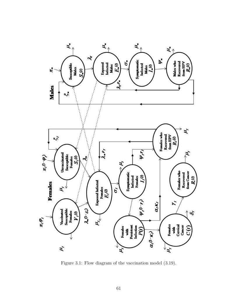
Figure 3.1: Flow diagram of the vaccination model (3.19).
61
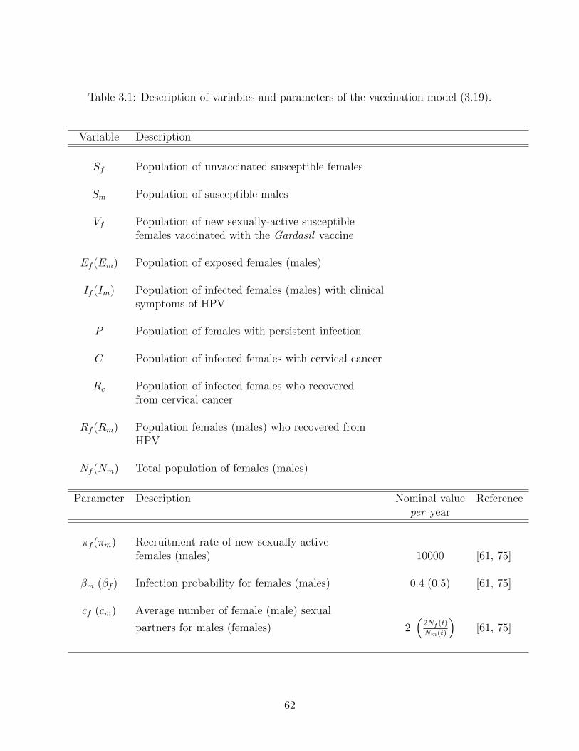
Table 3.1: Description of variables and parameters of the vaccination model (3.19).
Variable Description
Sf Population of unvaccinated susceptible females
Sm Population of susceptible males
Vf Population of new sexually-active susceptiblefemales vaccinated with the Gardasil vaccine
Ef (Em) Population of exposed females (males)
If (Im) Population of infected females (males) with clinicalsymptoms of HPV
P Population of females with persistent infection
C Population of infected females with cervical cancer
Rc Population of infected females who recoveredfrom cervical cancer
Rf (Rm) Population females (males) who recovered fromHPV
Nf (Nm) Total population of females (males)
Parameter Description Nominal value Referenceper year
πf (πm) Recruitment rate of new sexually-activefemales (males) 10000 [61, 75]
βm (βf ) Infection probability for females (males) 0.4 (0.5) [61, 75]
cf (cm) Average number of female (male) sexual
partners for males (females) 2�
2Nf (t)Nm(t)
�[61, 75]
62
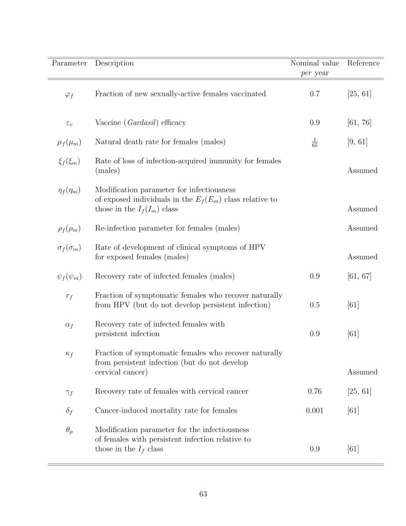
Parameter Description Nominal value Referenceper year
ϕf Fraction of new sexually-active females vaccinated 0.7 [25, 61]
εv Vaccine (Gardasil) efficacy 0.9 [61, 76]
µf (µm) Natural death rate for females (males) 165 [9, 61]
ξf (ξm) Rate of loss of infection-acquired immunity for females(males) Assumed
ηf (ηm) Modification parameter for infectiousnessof exposed individuals in the Ef (Em) class relative tothose in the If (Im) class Assumed
ρf (ρm) Re-infection parameter for females (males) Assumed
σf (σm) Rate of development of clinical symptoms of HPVfor exposed females (males) Assumed
ψf (ψm) Recovery rate of infected females (males) 0.9 [61, 67]
rf Fraction of symptomatic females who recover naturallyfrom HPV (but do not develop persistent infection) 0.5 [61]
αf Recovery rate of infected females withpersistent infection 0.9 [61]
κf Fraction of symptomatic females who recover naturallyfrom persistent infection (but do not developcervical cancer) Assumed
γf Recovery rate of females with cervical cancer 0.76 [25, 61]
δf Cancer-induced mortality rate for females 0.001 [61]
θp Modification parameter for the infectiousnessof females with persistent infection relative tothose in the If class 0.9 [61]
63
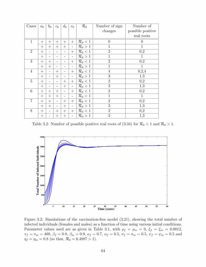
Cases a0 b0 c0 d0 e0 R0 Number of signchanges
Number ofpossible positive
real roots
1 + + + + + R0 < 1 0 0+ + + + - R0 > 1 1 1
2 + - - - + R0 < 1 2 0,2+ - - - - R0 > 1 1 1
3 + + - - + R0 < 1 2 0,2+ + - - - R0 > 1 1 1
4 + - + - + R0 < 1 4 0,2,4+ - + - - R0 > 1 3 1,3
5 + - - + + R0 < 1 2 0,2+ - - + - R0 > 1 3 1,3
6 + + + - + R0 < 1 2 0,2+ + + - - R0 > 1 1 1
7 + + - + + R0 < 1 2 0,2+ + - + - R0 > 1 3 1,3
8 + - + + + R0 < 1 2 0,2+ - + + - R0 > 1 3 1,3
Table 3.2: Number of possible positive real roots of (3.34) for R0 < 1 and R0 > 1.
5 10 15 20 25 30 35 40 45 50 55 600
500
1000
1500
2000
2500
3000
3500
Time (years)
Tota
l N
um
ber
of
Infe
cted
In
div
idu
als
Figure 3.2: Simulations of the vaccination-free model (3.21), showing the total number ofinfected individuals (females and males) as a function of time using various initial conditions.Parameter values used are as given in Table 3.1, with ρf = ρm = 0, ξf = ξm = 0.0012,πf = πm = 400, βf = 0.8, βm = 0.9, κf = 0.7, αf = 0.5, σf = σm = 0.5, ψf = ψm = 0.5 andηf = ηm = 0.8 (so that, R0 = 6.4887 > 1).
64
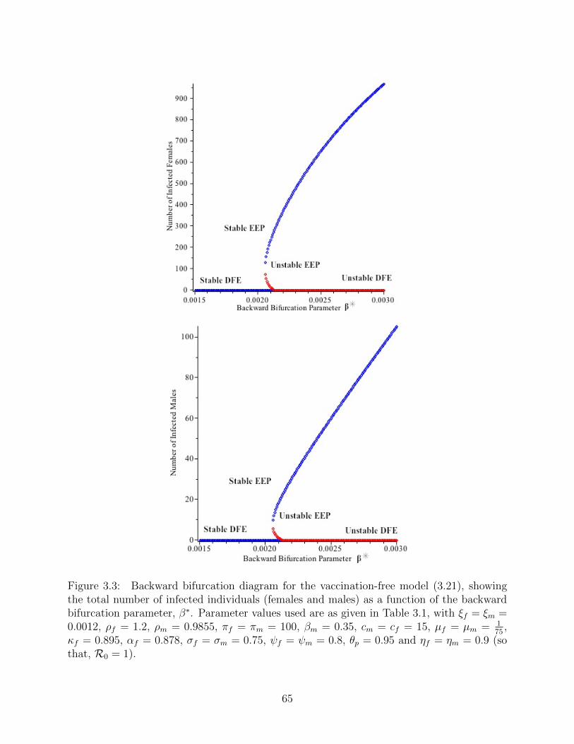
Figure 3.3: Backward bifurcation diagram for the vaccination-free model (3.21), showingthe total number of infected individuals (females and males) as a function of the backwardbifurcation parameter, β∗. Parameter values used are as given in Table 3.1, with ξf = ξm =0.0012, ρf = 1.2, ρm = 0.9855, πf = πm = 100, βm = 0.35, cm = cf = 15, µf = µm = 1
75 ,κf = 0.895, αf = 0.878, σf = σm = 0.75, ψf = ψm = 0.8, θp = 0.95 and ηf = ηm = 0.9 (sothat, R0 = 1).
65
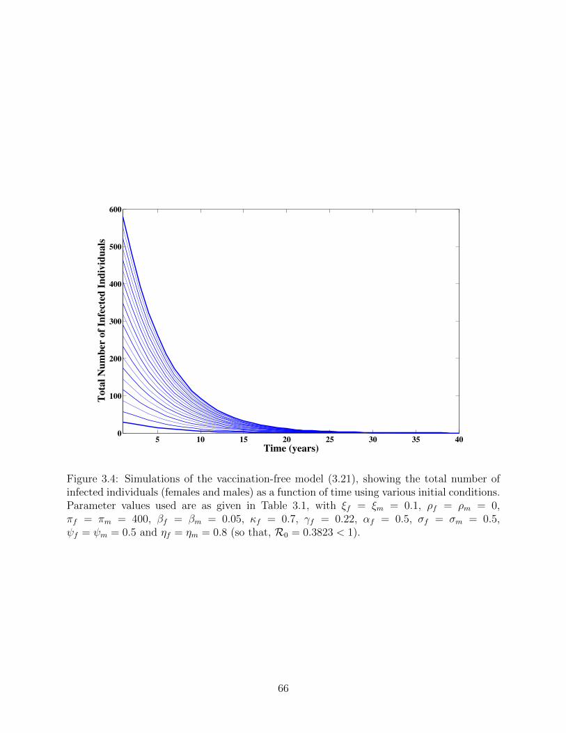
5 10 15 20 25 30 35 400
100
200
300
400
500
600
Time (years)
Tota
l N
um
ber
of
Infe
cted
In
div
idu
als
Figure 3.4: Simulations of the vaccination-free model (3.21), showing the total number ofinfected individuals (females and males) as a function of time using various initial conditions.Parameter values used are as given in Table 3.1, with ξf = ξm = 0.1, ρf = ρm = 0,πf = πm = 400, βf = βm = 0.05, κf = 0.7, γf = 0.22, αf = 0.5, σf = σm = 0.5,ψf = ψm = 0.5 and ηf = ηm = 0.8 (so that, R0 = 0.3823 < 1).
66
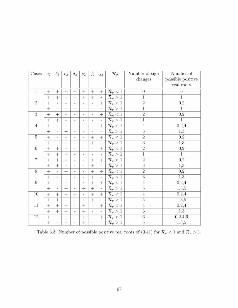
Cases a2 b2 c2 d2 e2 f2 j2 Rv Number of signchanges
Number ofpossible positive
real roots
1 + + + + + + + Rv < 1 0 0+ + + + + + - Rv > 1 1 1
2 + - - - - - + Rv < 1 2 0,2+ - - - - - - Rv > 1 1 1
3 + + - - - - + Rv < 1 2 0,2+ + - - - - - Rv > 1 1 1
4 + - + - - - + Rv < 1 4 0,2,4+ - + - - - - Rv > 1 3 1,3
5 + - - - - + + Rv < 1 2 0,2+ - - - - + - Rv > 1 3 1,3
6 + + + - - - + Rv < 1 2 0,2+ + + - - - - Rv > 1 1 1
7 + + - - - + + Rv < 1 2 0,2+ + - - - + - Rv > 1 3 1,3
8 + - + - - + + Rv < 1 2 0,2+ - + - - + - Rv > 1 3 1,3
9 + - + - + + + Rv < 1 4 0,2,4+ - + - + + - Rv > 1 5 1,3,5
10 + + - + - + + Rv < 1 4 0,2,4+ + - + - + - Rv > 1 5 1,3,5
11 + + + - + - + Rv < 1 4 0,2,4+ + + - + - - Rv > 1 3 1,3
12 + - + - + - + Rv < 1 6 0,2,4,6+ - + - + - - Rv > 1 5 1,3,5
Table 3.3: Number of possible positive real roots of (3.41) for Rv < 1 and Rv > 1.
67
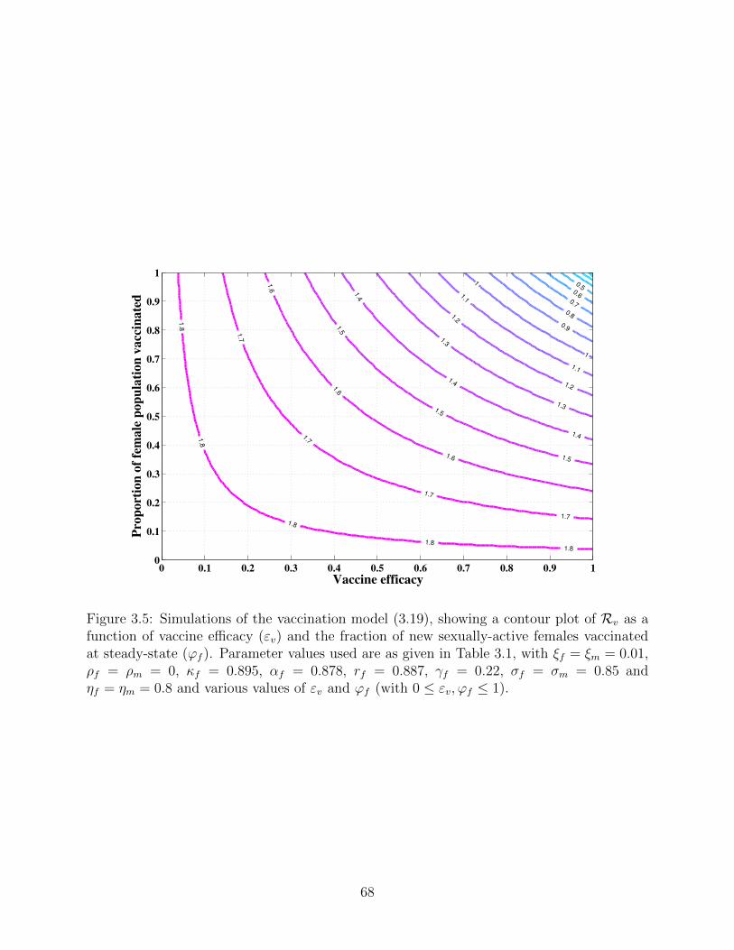
0.50.6
0.7
0.8
0.9
1
1
1.1
1.1
1.2
1.2
1.3
1.3
1.4
1.4
1.4
1.5
1.5
1.51.6
1.6
1.6
1.7
1.7
1.7
1.7
1.8
1.8
1.8
1.81.8
Vaccine efficacy
Pro
po
rtio
n o
f fe
ma
le p
op
ula
tio
n v
acc
ina
ted
0 0.1 0.2 0.3 0.4 0.5 0.6 0.7 0.8 0.9 10
0.1
0.2
0.3
0.4
0.5
0.6
0.7
0.8
0.9
1
Figure 3.5: Simulations of the vaccination model (3.19), showing a contour plot of Rv as afunction of vaccine efficacy (εv) and the fraction of new sexually-active females vaccinatedat steady-state (ϕf ). Parameter values used are as given in Table 3.1, with ξf = ξm = 0.01,ρf = ρm = 0, κf = 0.895, αf = 0.878, rf = 0.887, γf = 0.22, σf = σm = 0.85 andηf = ηm = 0.8 and various values of εv and ϕf (with 0 ≤ εv,ϕf ≤ 1).
68
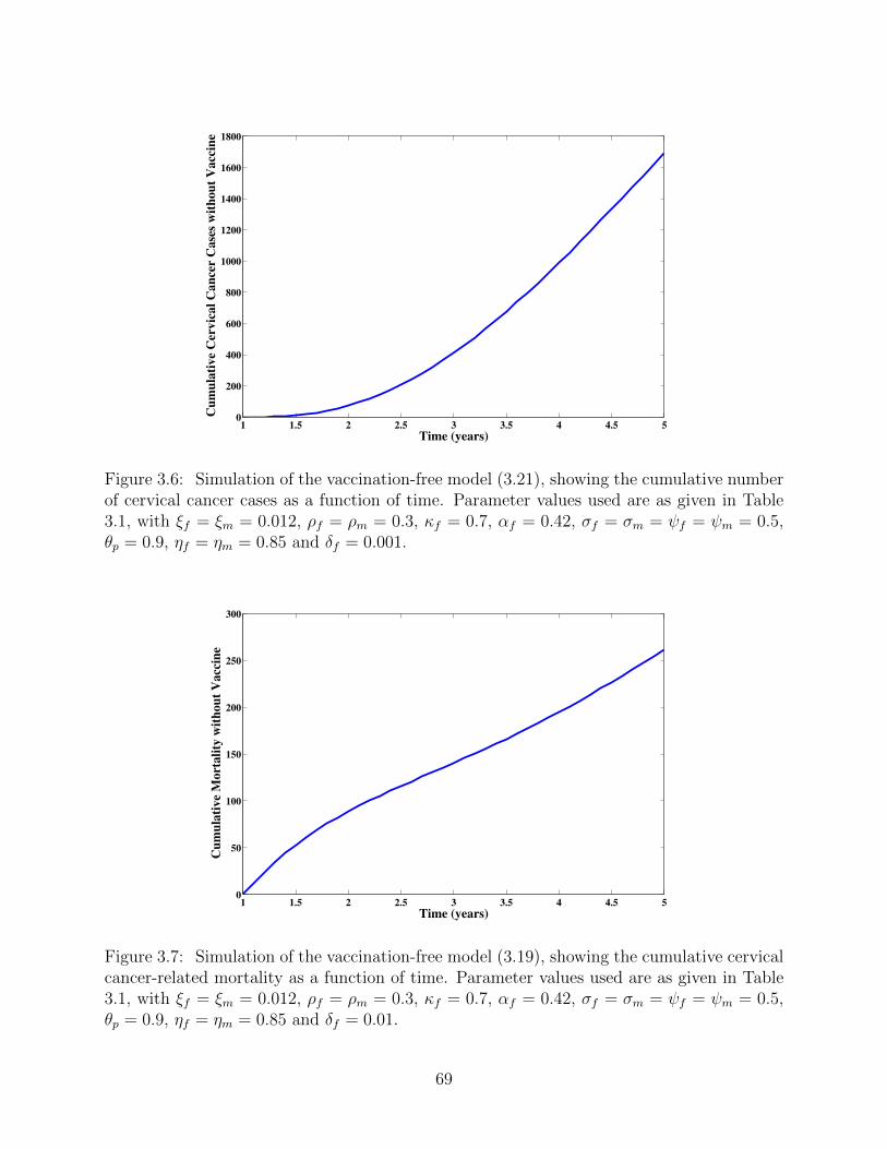
1 1.5 2 2.5 3 3.5 4 4.5 50
200
400
600
800
1000
1200
1400
1600
1800
Time (years)
Cu
mu
lati
ve
Cer
vic
al
Can
cer
Case
s w
ith
ou
t V
acc
ine
Figure 3.6: Simulation of the vaccination-free model (3.21), showing the cumulative numberof cervical cancer cases as a function of time. Parameter values used are as given in Table3.1, with ξf = ξm = 0.012, ρf = ρm = 0.3, κf = 0.7, αf = 0.42, σf = σm = ψf = ψm = 0.5,θp = 0.9, ηf = ηm = 0.85 and δf = 0.001.
1 1.5 2 2.5 3 3.5 4 4.5 50
50
100
150
200
250
300
Time (years)
Cu
mu
lati
ve
Mo
rta
lity
wit
ho
ut
Vacc
ine
Figure 3.7: Simulation of the vaccination-free model (3.19), showing the cumulative cervicalcancer-related mortality as a function of time. Parameter values used are as given in Table3.1, with ξf = ξm = 0.012, ρf = ρm = 0.3, κf = 0.7, αf = 0.42, σf = σm = ψf = ψm = 0.5,θp = 0.9, ηf = ηm = 0.85 and δf = 0.01.
69
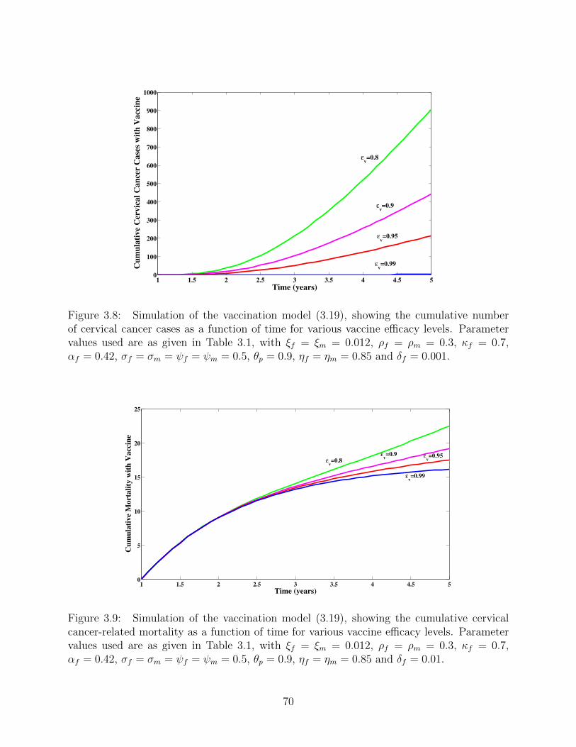
1 1.5 2 2.5 3 3.5 4 4.5 50
100
200
300
400
500
600
700
800
900
1000
Time (years)
Cu
mu
lati
ve
Cer
vic
al
Can
cer
Case
s w
ith
Vacc
ine
!v=0.9
!v=0.95
!v=0.99
!v=0.8
Figure 3.8: Simulation of the vaccination model (3.19), showing the cumulative numberof cervical cancer cases as a function of time for various vaccine efficacy levels. Parametervalues used are as given in Table 3.1, with ξf = ξm = 0.012, ρf = ρm = 0.3, κf = 0.7,αf = 0.42, σf = σm = ψf = ψm = 0.5, θp = 0.9, ηf = ηm = 0.85 and δf = 0.001.
1 1.5 2 2.5 3 3.5 4 4.5 50
5
10
15
20
25
Time (years)
Cu
mu
lati
ve
Mo
rta
lity
wit
h V
acc
ine
!v=0.9 !
v=0.95
!v=0.99
!v=0.8
Figure 3.9: Simulation of the vaccination model (3.19), showing the cumulative cervicalcancer-related mortality as a function of time for various vaccine efficacy levels. Parametervalues used are as given in Table 3.1, with ξf = ξm = 0.012, ρf = ρm = 0.3, κf = 0.7,αf = 0.42, σf = σm = ψf = ψm = 0.5, θp = 0.9, ηf = ηm = 0.85 and δf = 0.01.
70
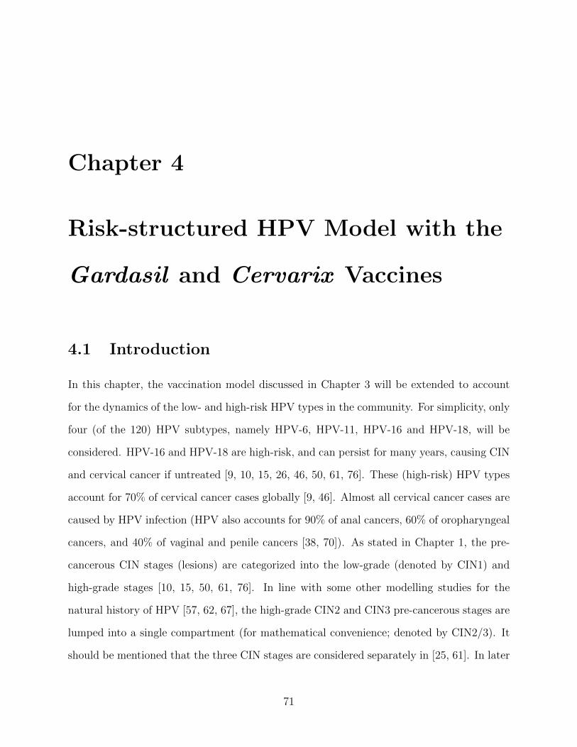
Chapter 4
Risk-structured HPV Model with the
Gardasil and Cervarix Vaccines
4.1 Introduction
In this chapter, the vaccination model discussed in Chapter 3 will be extended to account
for the dynamics of the low- and high-risk HPV types in the community. For simplicity, only
four (of the 120) HPV subtypes, namely HPV-6, HPV-11, HPV-16 and HPV-18, will be
considered. HPV-16 and HPV-18 are high-risk, and can persist for many years, causing CIN
and cervical cancer if untreated [9, 10, 15, 26, 46, 50, 61, 76]. These (high-risk) HPV types
account for 70% of cervical cancer cases globally [9, 46]. Almost all cervical cancer cases are
caused by HPV infection (HPV also accounts for 90% of anal cancers, 60% of oropharyngeal
cancers, and 40% of vaginal and penile cancers [38, 70]). As stated in Chapter 1, the pre-
cancerous CIN stages (lesions) are categorized into the low-grade (denoted by CIN1) and
high-grade stages [10, 15, 50, 61, 76]. In line with some other modelling studies for the
natural history of HPV [57, 62, 67], the high-grade CIN2 and CIN3 pre-cancerous stages are
lumped into a single compartment (for mathematical convenience; denoted by CIN2/3). It
should be mentioned that the three CIN stages are considered separately in [25, 61]. In later
71
stages, the original cancer may spread to areas surrounding the uterus and cervix or near
organs such as the bladder or rectum. It may also spread to distant sites in the body through
the bloodstream or the lymph nodes [76, 100]. Furthermore, the high-risk HPV types cause
pre-cancerous intraepithelial neoplasia in males (also divided into three grades according to
severity of the lesions, denoted by INM1 and INM2/3), resulting in various cancers in males
(such as anal and penile cancers [29]). The currently-available HPV vaccines (Gardasil and
Cervarix ) target these high-risk HPV types.
On the other hand, HPV-6 and HPV-11 are considered low-risk HPV types (since they
do not cause cervical cancer; although they do cause genital warts [76, 77]). As stated in
Chapter 1, while the bivalent (Cervarix ) vaccine exclusively targets the high-risk HPV types
(HPV-16 and HPV-18), the quadrivalent (Gardasil) vaccine targets both the low-risk (HPV-
6 and HPV-11) and the high-risk (HPV-16 and HPV-18) HPV types. As stated in Chapter
1, it should be emphasized that the Cervarix vaccine is approved for use in females only,
while the Gardasil vaccine is approved for use in both females and males [76, 77, 100].
Unlike in Chapter 3 (where only the Gardasil vaccine is used), both Gardasil and Cervarix
will be used in this chapter. In other words, susceptible females have the option to choose
between the Gardasil and Cervarix vaccines (while susceptible males only have the Gardasil
vaccine option). Furthermore, in line with the recent recommendations by some Public
Health Agencies [46, 76, 77], both females and males will be vaccinated (only females are
vaccinated in the model developed in Chapter 3). As in Chapter 3, the vaccines will be
given to children of ages 9 to 13 [10, 15, 76] (it should be stated that males and females of
ages 13 to 26, who were not vaccinated before, are also be vaccinated [46, 76]). It is worth
mentioning that, unlike in [25, 29], no co-infection of HPV types is assumed in this study.
72
4.2 Model Formulation
To formulate the model for the transmission dynamics of the low- and high-risk HPV sub-
types in a community, in the presence of mass vaccination (using the Cervarix and Gar-
dasil vaccines), the total sexually-active female population at time t (denoted by Nf (t))
is sub-divided into mutually-exclusive compartments of unvaccinated susceptible females
(Sf (t)), new sexually-active susceptible females vaccinated with the bivalent Cervarix vaccine
(V bf (t)), new sexually-active susceptible females vaccinated with the quadrivalent Gardasil
vaccine (V qf (t)), exposed (latently-infected) females with the low-risk HPV types (El
f (t)), ex-
posed females with the high-risk HPV types (Ehf (t)), infected females with clinical symptoms
of the low-risk HPV types (I lf (t)), infected females with clinical symptoms of the high-risk
HPV types (I lf (t)), infected females with persistent infection with the low-risk HPV types
(P lf (t)), infected females with persistent infection with the high-risk HPV types (P h
f (t)),
infected females in the (low-grade) CIN1 stage (Gfl(t)), infected females in the (high-grade)
CIN2/3 stage (Gfh(t)), infected females with genital warts (Wf (t)), infected females with
cervical cancer (Ccf (t)), infected females who recovered from cervical cancer (Rc
f (t)) and
infected females who recovered from HPV infection (and genital warts) without develop-
ing cervical cancer (Rf (t)), so that (where the indices l and h in Gfl and Gfh represent,
respectively, low- and high-grade CIN, and not low- and high-risk HPV types),
Nf (t) = Sf (t) + V bf (t) + V q
f (t) + Eif (t) + I if (t) + P i
f (t) +Wf (t) +Gfl(t) +Gfh(t)
+ Ccf (t) +Rc
f (t) +Rf (t), i ∈ {l, h}, (4.1)
where the indices l and h (with exception of those in Gfl and Gfh) represent low- and high-
risk HPV types, respectively. In this study, HPV-6 and HPV-11 are the low-risk HPV types
considered, while HPV-16 and HPV-18 are the high-risk HPV types. These HPV types are
preventable using the Cervarix and Gardasil vaccines.
Furthermore, the total sexually-active male population at time t, denoted by Nm(t), is
73
sub-divided into mutually-exclusive compartments of unvaccinated susceptible males (Sm(t)),
new sexually-active susceptible males vaccinated with the quadrivalent Gardasil vaccine
(V qm(t)), exposed males with the low-risk HPV types (El
m(t)), exposed males with the high-
risk HPV types (Ehm(t)), infected males with clinical symptoms of the low-risk HPV types
(I lm(t)), infected males with clinical symptoms of the high-risk HPV types (Ihm(t)), infected
males with persistent infection with the low-risk HPV types (P lm(t)), infected males with
persistent infection with the high-risk HPV types (P hm(t)), infected males with genital warts
(Wm(t)), infected males in the low-grade HPV-related intraepithelial neoplasia INM1 stage
(Gml(t)), infected males in the high-grade HPV-related intraepithelial neoplasia INM2/3
stage (Gmh(t)), infected males with HPV-related cancers (Crm(t)), infected males who recov-
ered from HPV-related cancers (Rcm(t)) and infected males who recovered from HPV (and
genital warts) without developing HPV-related cancers (Rm(t)). Thus (noting that the in-
dices l and h in Gml and Gmh represent, respectively, low- and high-grade INM for males,
and not low- and high-risk HPV type),
Nm(t) = Sm(t) + V qm(t) + Ei
m(t) + I im(t) + P im(t) +Wm(t) +Gml(t) +Gmh(t)
+ Crm(t) +Rc
m(t) +Rm(t), i ∈ {l, h}. (4.2)
It follows from (4.1) and (4.2) that the total sexually-active (heterosexual) population, at
time t, is given by
N(t) = Nf (t) +Nm(t).
It should be emphasized that, in this chapter, individuals in the exposed (Eif and Ei
m) and
persistent (P if and P i
m) classes, with i ∈ {l, h}, are infected with HPV, and can transmit
HPV to susceptible individuals.
The population of unvaccinated susceptible females (Sf ) is increased by the recruitment
of new sexually-active females at a rate πf (a fraction, 1−ϕbf −ϕq
f , with 0 < ϕbf +ϕq
f ≤ 1, of
which, is vaccinated; where, ϕbf is the fraction of unvaccinated susceptible females vaccinated
74
with the Cervarix vaccine, and ϕqf is the fraction vaccinated with the Gardasil vaccine). This
population is further increased by the loss of infection-acquired immunity by infected females
who recovered without developing cervical cancer (at a rate ξf ). The population is decreased
by infection, following effective contacts with males infected with the high-risk and the low-
risk HPV types (i.e., those in the Elm, E
hm, I
lm, I
hm, P
lm and P h
m classes), at the rates λlm and
λhm, given, respectively, by:
λlm =
βlmcf (Nm, Nf )
�ηlmE
lm + I lm + θlmP
lm
�
Nm, (4.3)
λhm =
βhmcf (Nm, Nf )
�ηhmE
hm + Ihm + θhmP
hm
�
Nm. (4.4)
In (4.3), βlm is the probability of transmission of HPV infection from infected males (with
the low-risk HPV types) to susceptible females per contact, and cf (Nm, Nf ) is the average
number of female partners per male per unit time. Thus, βlmcf (Nm, Nf ) is the effective
contact rate for male-to-female transmission of the low-risk HPV types. Furthermore, ηlm
(with 0 ≤ ηlm < 1) is the modification parameter accounting for the assumption that exposed
males with the low-risk HPV types are less infectious than symptomatically-infected males
with the low-risk HPV types. Similarly, in (4.4), βhm is the probability of transmission of
HPV infection from infected males (with the high-risk HPV types) to susceptible females per
contact, and βhmcf (Nm, Nf ) is the effective contact rate for male-to-female transmission of
the high-risk HPV types. The parameter ηhm (with 0 ≤ ηhm < 1) accounts for the assumption
that exposed males with the high-risk HPV types are less infectious than symptomatically-
infected males with the high-risk HPV types, and θlm(θhm) > 0 is the modification parameter
accounting for the assumption that infected males with persistent infection with the low-
risk (high-risk) HPV types transmit HPV at a different rate compared to infected males
in the other infected classes (Elm, I
lm(E
hm, I
hm)). The population of unvaccinated susceptible
females is further decreased by natural death (at a rate µf ; it is assumed that females in all
epidemiological compartments suffer natural death at the rate µf ). Thus,
75
dSf
dt= (1− ϕb
f − ϕqf )πf + ξfRf −
�λlm + λh
m
�Sf − µfSf . (4.5)
The population of new sexually-active susceptible females vaccinated with the bivalent Cer-
varix vaccine (V bf ) is generated by the vaccination of a fraction, ϕb
f , of unvaccinated suscep-
tible females with the Cervarix vaccine (at the rate πfϕbf ). It is decreased by HPV infection,
following effective contacts with males infected with high-risk HPV types (at the reduced
rate (1 − εb)λhm, where 0 < εb ≤ 1 represents the efficacy of the Cervarix vaccine against
infection with the high-risk HPV types) and males infected with the low-risk HPV types
(at the rate λlm; it should be emphasized that the Cervarix vaccine has no efficacy against
the low-risk HPV types, HPV-6 and HPV-11 [46, 76, 77]). This population is decreased by
natural death. Since there is currently no evidence to the contrary, it is assumed that this
vaccine (as well as Gardasil) does not wane [10, 15, 46, 76, 77]. Hence,
dV bf
dt= ϕb
fπf − (1− εb)λhmV
bf − λl
mVbf − µfV
bf . (4.6)
The population of new sexually-active susceptible females vaccinated with the quadrivalent
Gardasil vaccine (V qf ) is generated by the vaccination of a fraction, ϕq
f , of unvaccinated
susceptible females with the Gardasil vaccine (at the rate πfϕqf ). It is decreased by HPV
infection, following effective contacts with males infected with the low- and high-risk HPV
types (at a reduced rate (1 − εq)�λlm + λh
m
�, where 0 < εq ≤ 1 represents the efficacy
of Gardasil vaccine against infection with HPV-6, HPV-11, HPV-16 and HPV-18). This
population is decreased by natural death. Thus,
dV qf
dt= ϕq
fπf − (1− εq)�λhm + λl
m
�V qf − µfV
qf . (4.7)
The population of exposed females with the low-risk (high-risk) HPV types (Elf (E
hf )) is
generated by the infection of unvaccinated and vaccinated susceptible females with the low-
76
risk HPV types (at the rate λlm(λ
hm)). This population is further increased by the re-infection
of recovered females with the low-risk (high-risk) HPV types (at a rate ρlfλlm(ρ
hfλ
hm), where
0 ≤ ρlf (ρhf ) < 1 accounts for the assumption that the re-infection of recovered females with
low-risk (high-risk) HPV types occurs at a rate lower than the rate for primary infection of
susceptible females). Exposed females develop clinical symptoms of the low-risk (high-risk)
HPV types (at a rate σlf (σ
hf )) and suffer natural death. Thus,
dElf
dt= [Sf + Vb + (1− εq)Vq]λ
lm + ρlfλ
lmRf − (σl
f + µf )Elf ,
dEhf
dt= [Sf + (1− εb)Vb + (1− εq)Vq]λ
hm + ρhfλ
hmRf − (σh
f + µf )Ehf . (4.8)
The population of infected females with clinical symptoms of the low-risk (high-risk) HPV
types (I lf (Ihf )) is generated at the rate σl
f (σhf ). This population is decreased by recovery (at
a rate ψlf (ψ
hf )) and natural death. Hence,
dI lfdt
= σlfE
lf − (ψl
f + µf )Ilf ,
dIhfdt
= σhfE
hf − (ψh
f + µf )Ihf . (4.9)
The population of females with persistent infection with the low-risk HPV types (P lf ) is
generated by the development of persistent infection, with the low-risk HPV types, by symp-
tomatic females with the low-risk HPV types (at a rate (1 − rlf )ψlf , where 0 < rlf ≤ 1 is
the fraction of symptomatic females with the low-risk HPV types who recovered from HPV
infection without developing genital warts; it is assumed that individuals infected with the
low-risk HPV types do not progress to the CIN stages and/or develop cancer [10, 15, 76, 77]).
Females with persistent infection with the low-risk HPV types move out of this epidemiolog-
ical class (either through recovery or development of genital warts) at a rate αlf , and suffer
natural death. Thus,dP l
f
dt= (1− rlf )ψ
lfI
lf − (αl
f + µf )Plf . (4.10)
77
The population of females with persistent infection with the high-risk HPV types (P hf ) is
generated at a rate (1 − rhf )ψhf , where 0 < rhf ≤ 1 is the fraction of symptomatic females
with the high-risk HPV types who recovered from HPV without progressing to the low-
grade CIN1 stage, and by a fraction, 1 − (s1f + s2f ), of infected females in the high-grade
CIN2/3 stage who develop persistent infection (at a rate [1− (s1f + s2f )] zf , where s1f and
s2f , with 0 ≤ s1f + s2f ≤ 1, are the fractions of infected females in the high-grade CIN2/3
stage who naturally recovered from HPV infection, and of infected females in the high-grade
CIN2/3 stage who revert to the low-grade CIN1 stage, respectively). Females with persistent
infection with the high-risk HPV types move out of this epidemiological class (either through
recovery or development of pre-cancerous CIN lesions) at a rate αhf , and suffer natural death.
Hence,
dP hf
dt= (1− rhf )ψ
hf I
hf + [1− (s1f + s2f )] zfGfh − (αh
f + µf )Phf .
The population of females with genital warts (Wf ) is generated when infected females with
persistent infection with the low-risk HPV types develop genital warts (at a rate (1− klf )α
lf ,
where 0 < klf ≤ 1 is the fraction of infected females with persistent low-risk HPV types
who recovered from HPV infection). Since genital warts do not cause cervical cancer (or any
other type of cancer [76, 100]), it is assumed that genital warts do not cause death in females
and males. This population decreases due to recovery (at a rate nf ) and natural death, so
that,dWf
dt= (1− kl
f )αlfP
lf − (nf + µf )Wf . (4.11)
The population of females with the low-grade CIN1 (Gfl) is generated when infected females
with persistent infection with the high-risk HPV types develop pre-cancerous CIN lesions
(at a rate (1 − khf )α
hf , where 0 < kh
f ≤ 1 is the fraction of infected females with persistent
infection with the high-risk HPV types who recovered from HPV infection). This population
is further increased by the reversion (or regression) of individuals in the high-grade CIN2/3
78
stage into the low-grade CIN1 stage (at a rate s2fzf ). Individuals move out of this class
at a rate uf (due to progression to the high-grade CIN2/3 stage [25, 29, 61, 100], at a rate
(1− df )uf , or recovery, at a rate dfuf ). It is assumed that individuals in the CIN stages do
not suffer disease-induced death (until they develop cervical cancer). Thus,
dGfl
dt= (1− kh
f )αhfP
hf + s2fzfGfh − (uf + µf )Gfl. (4.12)
The population of females in the high-grade CIN2/3 stage (Gfh) is generated by the pro-
gression of infected females with low-grade CIN1 (at the rate (1− df )uf , where 0 ≤ df ≤ 1
is the fraction of infected females in the low-grade CIN1 stage who naturally recovered from
HPV infection). Transition out of this class occurs at a rate zf (where a fraction, s1fzf ,
recovers; another fraction, s2fzf , reverts to the low-grade CIN1 stage and the remaining
fraction, 1− (s1f + s2f ), develops persistent infection). This population is decreased by the
development of cervical cancer (at a rate ωf ) and natural death. Hence,
dGfh
dt= (1− df )ufGfl − (zf + ωf + µf )Gfh. (4.13)
The population of females with cervical cancer (Ccf ) is generated by the development of
cervical cancer by infected females in the high-grade CIN2/3 stage (at the rate ωf ). This
population decreases due to recovery (at a rate γf ), natural death and cancer-induced death
(at a rate δf ), so thatdCc
f
dt= ωfGfh − (γf + µf + δf )C
cf . (4.14)
The population of infected females who recovered from cervical cancer (Rcf ) is generated at
the rate γf , and decreases by natural death. As in [61], it is assumed that individuals in this
class do not acquire HPV infection again (since these individuals require treatment/surgery,
which, typically, result in the removal or damage to the cervix and some other normal tissues
79
around it [68]). Thus,dRc
f
dt= γfC
cf − µfR
cf . (4.15)
The population of infected females who recovered from HPV infection (and genital warts)
without developing cervical cancer (Rf ) is generated at the rates rlfψlf , r
lfhψ
hf , k
lfα
lf , k
hfα
hf ,
nf , dfuf and s1fzf , respectively. Recovered females acquire re-infection at the rates ρlfλlm
and ρhfλhm. This population is further decreased by the loss of infection-acquired immunity
(at the rate ξf ) and natural death. This gives:
dRf
dt= rlfψ
lfI
lf + rhfψ
hf I
hf + kl
fαlfP
lf + kh
fαhfP
hf + nfWf + dfufGfl + s1fzfGfh
−�ρhfλ
hm + ρlfλ
lm
�Rf − (ξf + µf )Rf . (4.16)
The population of unvaccinated susceptible males (Sm) is generated by the recruitment
of new sexually-active males at a rate πm (a fraction, ϕqm, of which, is vaccinated with the
Gardasil vaccine; it is assumed that males are not vaccinated with the Cervarix vaccine
[76, 77, 100]). It is further increased by the loss of infection-acquired immunity by recovered
males (at a rate ξm). This population is diminished by infection, following effective contacts
with infected females (with both the low-risk and high-risk HPV types), at rates λlf and λh
f ,
where
λlf =
βlfcm (Nm, Nf )
�ηlfE
lf + I lf + θlfP
lf
�
Nf, (4.17)
λhf =
βhf cm (Nm, Nf )
�ηhfE
hf + Ihf + θhfP
hf
�
Nf. (4.18)
In (4.17) and (4.18), βlf (β
hf ) is the probability of transmission of HPV infection from infected
females with the low-risk (high-risk) HPV types to males per contact and cm (Nm, Nf ) is the
average number of male partners per female per unit time. Furthermore, ηlf (ηhf ) (with
0 ≤ ηlf (ηhf ) < 1) is the modification parameter accounting for the assumption that exposed
females with the ow-risk (high-risk) HPV types (i.e., those in the Elf (E
hf ) class) are less
80
infectious than symptomatically-infected females (i.e., those in the I lf (Ihf ) class), and θlf (θ
hf ) >
0 is the modification parameter accounting for the assumption that infected females with
persistent infection with the low-risk (high-risk) HPV types transmit HPV at a different
rate compared to infected females in the Elf , I
lf (E
hf , I
hf ) classes. This population is further
decreased by natural death (at a rate µm; it is assumed that males in all epidemiological
compartments suffer natural death at this rate, µm). Thus,
dSm
dt= (1− ϕq
m) πm + ξmRm −�λhf + λl
f
�Sm − µmSm. (4.19)
The population of new sexually-active susceptible males vaccinated with the Gardasil vaccine
(V qm) is generated by the vaccination of the fraction, ϕq
m, of unvaccinated susceptible males (at
the rate πmϕqm). It is decreased by HPV infection, following effective contacts with females
infected with the high-risk HPV types (at a reduced rate (1− εq)λhf , where 0 < εq ≤ 1 is the
efficacy of the Gardasil vaccine) and females infected with the low-risk HPV types (at the
rate (1− εq)λlf ). This population is reduced by natural death. Hence,
dV qm
dt= ϕq
mπm − (1− εq)�λhf + λl
f
�V qm − µmV
qm. (4.20)
The population of exposed males with the low-risk (high-risk) HPV types (Elm(E
hm)) is
generated by the infection of unvaccinated and vaccinated susceptible males with the low-
risk (high-risk) HPV types (at the rate λlf (λ
hf )). This population is further increased by the
re-infection of recovered males (at a rate ρlmλlf (ρ
hmλ
hf ), where 0 ≤ ρlm(ρ
hm) < 1 also accounts
for the assumption that re-infection of recovered females occurs at a rate lower than the
primary infection). Exposed males develop clinical symptoms of the low-risk (high-risk)
HPV types (at a rate σlm(σ
hm)) and suffer natural death. Hence,
dElm
dt= [Sm + (1− εq)V
qm]λ
lf + ρlmλ
lfRm − (σl
m + µm)Elm, (4.21)
dEhm
dt= [Sm + (1− εq)V
qm]λ
hf + ρhmλ
hfRm − (σh
m + µm)Ehm. (4.22)
81
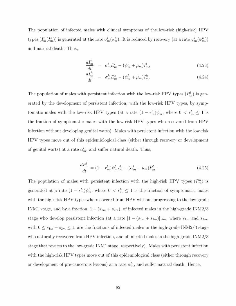
The population of infected males with clinical symptoms of the low-risk (high-risk) HPV
types (I lm(Ihm)) is generated at the rate σl
m(σhm). It is reduced by recovery (at a rate ψl
m(ψhm))
and natural death. Thus,
dI lmdt
= σlmE
lm − (ψl
m + µm)Ilm, (4.23)
dIhmdt
= σhmE
hm − (ψh
m + µm)Ihm. (4.24)
The population of males with persistent infection with the low-risk HPV types (P lm) is gen-
erated by the development of persistent infection, with the low-risk HPV types, by symp-
tomatic males with the low-risk HPV types (at a rate (1 − rlm)ψlm, where 0 < rlm ≤ 1 is
the fraction of symptomatic males with the low-risk HPV types who recovered from HPV
infection without developing genital warts). Males with persistent infection with the low-risk
HPV types move out of this epidemiological class (either through recovery or development
of genital warts) at a rate αlm, and suffer natural death. Thus,
dP lm
dt= (1− rlm)ψ
lmI
lm − (αl
m + µm)Plm. (4.25)
The population of males with persistent infection with the high-risk HPV types (P hm) is
generated at a rate (1 − rhm)ψhm, where 0 < rhm ≤ 1 is the fraction of symptomatic males
with the high-risk HPV types who recovered from HPV without progressing to the low-grade
INM1 stage, and by a fraction, 1− (s1m + s2m), of infected males in the high-grade INM2/3
stage who develop persistent infection (at a rate [1− (s1m + s2m)] zm, where s1m and s2m,
with 0 ≤ s1m + s2m ≤ 1, are the fractions of infected males in the high-grade INM2/3 stage
who naturally recovered from HPV infection, and of infected males in the high-grade INM2/3
stage that reverts to the low-grade INM1 stage, respectively). Males with persistent infection
with the high-risk HPV types move out of this epidemiological class (either through recovery
or development of pre-cancerous lesions) at a rate αhm, and suffer natural death. Hence,
82
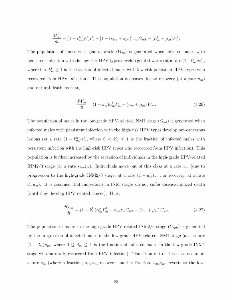
dP hm
dt= (1− rhm)ψ
hmI
hm + [1− (s1m + s2m)] zmGmh − (αh
m + µm)Phm.
The population of males with genital warts (Wm) is generated when infected males with
persistent infection with the low-risk HPV types develop genital warts (at a rate (1−klm)α
lm,
where 0 < klm ≤ 1 is the fraction of infected males with low-risk persistent HPV types who
recovered from HPV infection). This population decreases due to recovery (at a rate nm)
and natural death, so that,
dWm
dt= (1− kl
m)αlmP
lm − (nm + µm)Wm. (4.26)
The population of males in the low-grade HPV-related INM1 stage (Gml) is generated when
infected males with persistent infection with the high-risk HPV types develop pre-cancerous
lesions (at a rate (1 − khm)α
hm, where 0 < kh
m ≤ 1 is the fraction of infected males with
persistent infection with the high-risk HPV types who recovered from HPV infection). This
population is further increased by the reversion of individuals in the high-grade HPV-related
INM2/3 stage (at a rate s2mzm). Individuals move out of this class at a rate um (due to
progression to the high-grade INM2/3 stage, at a rate (1 − dm)um, or recovery, at a rate
dmum). It is assumed that individuals in INM stages do not suffer disease-induced death
(until they develop HPV-related cancer). Thus,
dGml
dt= (1− kh
m)αhmP
hm + s2mzmGmh − (um + µm)Gml. (4.27)
The population of males in the high-grade HPV-related INM2/3 stage (Gmh) is generated
by the progression of infected males in the low-grade HPV-related INM1 stage (at the rate
(1 − dm)um, where 0 ≤ dm ≤ 1 is the fraction of infected males in the low-grade INM1
stage who naturally recovered from HPV infection). Transition out of this class occurs at
a rate zm (where a fraction, s1mzm, recovers; another fraction, s2mzm, reverts to the low-
83
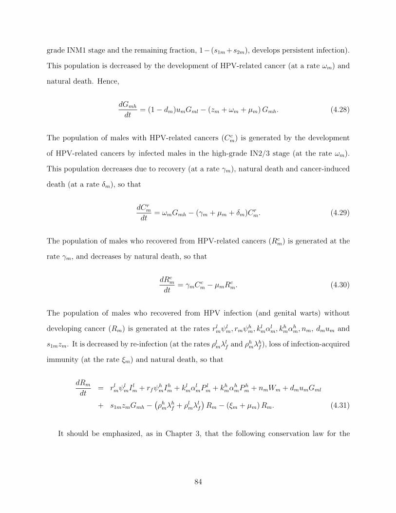
grade INM1 stage and the remaining fraction, 1− (s1m+s2m), develops persistent infection).
This population is decreased by the development of HPV-related cancer (at a rate ωm) and
natural death. Hence,
dGmh
dt= (1− dm)umGml − (zm + ωm + µm)Gmh. (4.28)
The population of males with HPV-related cancers (Ccm) is generated by the development
of HPV-related cancers by infected males in the high-grade IN2/3 stage (at the rate ωm).
This population decreases due to recovery (at a rate γm), natural death and cancer-induced
death (at a rate δm), so that
dCrm
dt= ωmGmh − (γm + µm + δm)C
rm. (4.29)
The population of males who recovered from HPV-related cancers (Rcm) is generated at the
rate γm, and decreases by natural death, so that
dRcm
dt= γmC
cm − µmR
cm. (4.30)
The population of males who recovered from HPV infection (and genital warts) without
developing cancer (Rm) is generated at the rates rlmψlm, rmψ
hm, k
lmα
lm, k
hmα
hm, nm, dmum and
s1mzm. It is decreased by re-infection (at the rates ρlmλlf and ρhmλ
hf ), loss of infection-acquired
immunity (at the rate ξm) and natural death, so that
dRm
dt= rlmψ
lmI
lm + rfψ
hmI
hm + kl
mαlmP
lm + kh
mαhmP
hm + nmWm + dmumGml
+ s1mzmGmh −�ρhmλ
hf + ρlmλ
lf
�Rm − (ξm + µm)Rm. (4.31)
It should be emphasized, as in Chapter 3, that the following conservation law for the
84
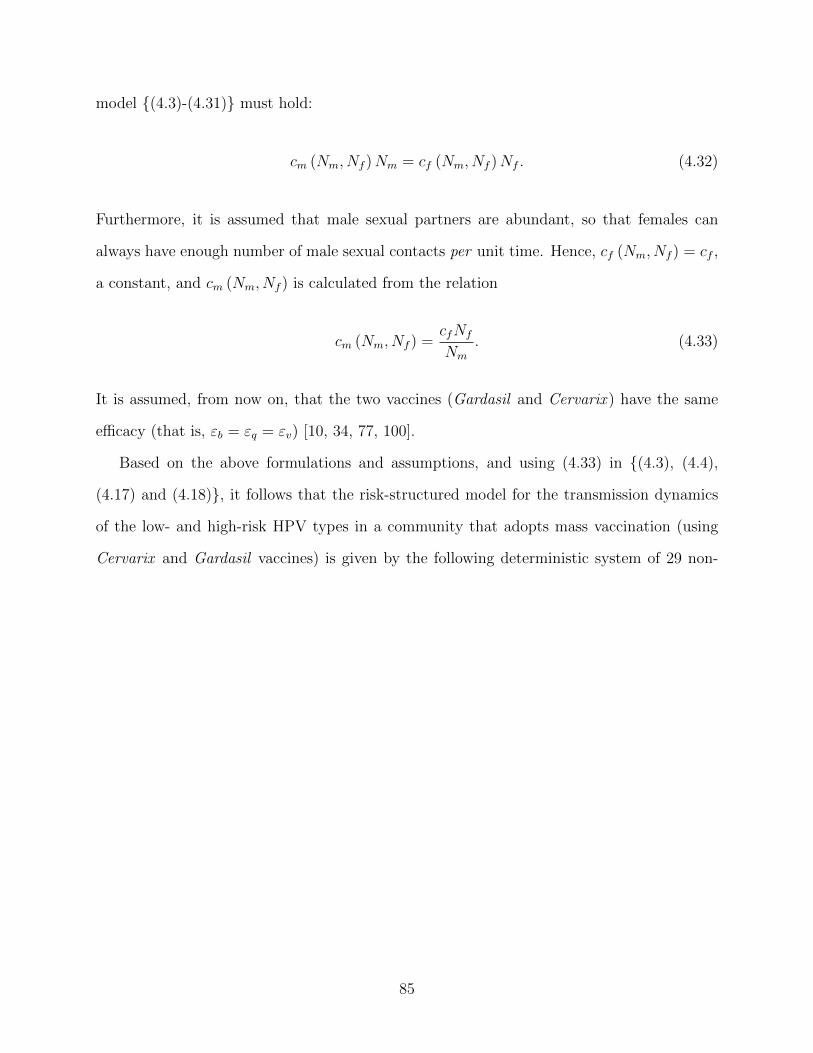
model {(4.3)-(4.31)} must hold:
cm (Nm, Nf )Nm = cf (Nm, Nf )Nf . (4.32)
Furthermore, it is assumed that male sexual partners are abundant, so that females can
always have enough number of male sexual contacts per unit time. Hence, cf (Nm, Nf ) = cf ,
a constant, and cm (Nm, Nf ) is calculated from the relation
cm (Nm, Nf ) =cfNf
Nm. (4.33)
It is assumed, from now on, that the two vaccines (Gardasil and Cervarix ) have the same
efficacy (that is, εb = εq = εv) [10, 34, 77, 100].
Based on the above formulations and assumptions, and using (4.33) in {(4.3), (4.4),
(4.17) and (4.18)}, it follows that the risk-structured model for the transmission dynamics
of the low- and high-risk HPV types in a community that adopts mass vaccination (using
Cervarix and Gardasil vaccines) is given by the following deterministic system of 29 non-
85
linear differential equations:
dSf
dt= (1− ϕb
f − ϕqf )πf + ξfRf −
�λhm + λl
m
�Sf − µfSf ,
dV bf
dt= ϕb
fπf − (1− εv)λhmV
bf − λl
mVbf − µfV
bf ,
dV qf
dt= ϕq
fπf − (1− εv)�λhm + λl
m
�V qf − µfV
qf ,
dElf
dt=
�Sf + V b
f + (1− εv)Vqf
�λlm + ρlfλ
lmRf − (σl
f + µf )Elf ,
dEhf
dt=
�Sf + (1− εv)V
bf + (1− εv)V
qf
�λhm + ρhfλ
hmRf − (σh
f + µf )Ehf ,
dI lfdt
= σlfE
lf − (ψl
f + µf )Ilf ,
dIhfdt
= σhfE
hf − (ψh
f + µf )Ihf ,
dP lf
dt= (1− rlf )ψ
lfI
lf − (αl
f + µf )Plf ,
dP hf
dt= (1− rhf )ψ
hf I
hf + [1− (s1f + s2f )] zfGfh − (αh
f + µf )Phf , (4.34)
dWf
dt= (1− kl
f )αlfP
lf − (nf + µf )Wf ,
dGfl
dt= (1− kh
f )αhfP
hf + s2fzfGfh − (uf + µf )Gfl,
dGfh
dt= (1− df )ufGfl − (zf + ωf + µf )Gfh,
dCcf
dt= ωfGfh − (γf + µf + δf )C
cf ,
dRcf
dt= γfC
cf − µfR
cf ,
dRf
dt= rlfψ
lfI
lf + rhfψ
hf I
hf + kl
fαlfP
lf + kh
fαhfP
hf + nfWf + dfufGfl
+ s1fzfGfh −�ρhfλ
hm + ρlfλ
lm
�Rf − (ξf + µf )Rf ,
86
dSm
dt= (1− ϕq
m) πm + ξmRm −�λhf + λl
f
�Sm − µmSm,
dV qm
dt= ϕq
mπm − (1− εv)�λhf + λl
f
�V qm − µmV
qm,
dElm
dt= [Sm + (1− εv)V
qm]λ
lf + ρlmλ
lfRm − (σl
m + µm)Elm,
dEhm
dt= [Sm + (1− εv)V
qm]λ
hf + ρhmλ
hfRm − (σh
m + µm)Ehm,
dI lmdt
= σlmE
lm − (ψl
m + µm)Ilm,
dIhmdt
= σhmE
hm − (ψh
m + µm)Ihm,
dP lm
dt= (1− rlm)ψ
lmI
lm − (αl
m + µm)Plm,
dP hm
dt= (1− rhm)ψ
hmI
hm + [1− (s1m + s2m)] zmGmh − (αh
m + µm)Phm,
dWm
dt= (1− kl
m)αlmP
lm − (nm + µm)Wm,
dGml
dt= (1− kh
m)αhmP
hm + s2mzmGmh − (um + µm)Gml,
dGmh
dt= (1− dm)umGml − (zm + ωm + µm)Gmh,
dCrm
dt= ωmGmh − (γm + µm + δm)C
rm,
dRcm
dt= γmC
cm − µmR
cm,
dRm
dt= rlmψ
lmI
lm + rhmψ
hmI
hm + kl
mαlmP
lm + kh
mαhmP
hm + nmWm + dmumGml
+ s1mzmGmh −�ρhmλ
hf + ρlmλ
lf
�Rm − (ξm + µm)Rm.
A flow diagram of the model (4.34) is depicted in Figures 4.1 and 4.2. The state variables
and parameters of the model are tabulated in Tables 4.1 and 4.2.
It should be mentioned that there is no biological or epidemiological relationship (such
as back-and-forth transition or evolution) between the low- and high-risk HPV types. That
is, the two HPV risk types (low and high) are independent, and the reason for stratifying the
infected population according to the two risk types is to account for the fact that infection
87
with the low-risk HPV types causes genital warts only, while infection with the high-risk
HPV types causes cancers. In other words, the purpose of the risk structure in this study
is to account for the heterogeneity of outcomes (cancers or warts) associated with infection
with the low- or high-risk HPV types. Another advantage of stratifying the infected popu-
lation in terms of infection with the low- and high-risk HPV types is that it allows for the
realistic assessment of the community-wide impact of the currently-available vaccines (since,
for example, the Cervarix vaccine only targets the high-risk, HPV-16 and HPV-18, types
while the Gardasil vaccine targets all the four HPV types considered in this study). Further-
more, it should be emphasized that the risk-structure in this study is not associated with
human behaviour (i.e., risky sexual practices), so that there is no back-and-forth transition
between the two risk HPV types based on changes in human behaviour.
The 29-dimensional model (4.34) extends the 12-dimensional model (3.19) developed in
Chapter 3 by (inter alia):
i) stratifying the total population in terms of the dynamics of the low- and high-risk HPV
types;
ii) incorporating two anti-HPV vaccines (Cervarix and Gardasil); only the Gardasil vac-
cine is considered in Chapter 3;
iii) vaccinating both new sexually-active susceptible females and males (only females are
vaccinated in Chapter 3);
iv) including the dynamics of individuals with genital warts (Wf ,Wm);
v) including the dynamics of individuals in the low- and high-grade pre-cancer (CIN and
INM) stages for females and males (Gfl, Gml, Gfh, Gmh);
vi) including the dynamics of infected males with HPV-related cancers (Crm), cancer-
induced mortality for males (δm �= 0), infected males who recovered from HPV-related
cancers (Rcm) and a compartment for males with persistent HPV infection (Pm).
88
4.2.1 Basic properties
As in Section 3.2.1, the following result holds for the low- and high-risk HPV model (4.34).
Theorem 4.1. Let the initial data for the model (4.34) be Sf (0) > 0, V bf (0) > 0, V q
f (0) >
0, Elf (0) ≥ 0, Eh
f (0) ≥ 0, I lf (0) ≥ 0, Ihf (0) ≥ 0, P lf (0) ≥ 0, P h
f (0) ≥ 0,Wf (0) ≥ 0, Gfl(0) ≥
0, Gfh(0) ≥ 0, Ccf (0) ≥ 0, Rc
f (0) ≥ 0, Rf (0) ≥ 0, Sm(0) > 0, V qm(0) > 0, El
m(0) ≥ 0, Ehm(0) ≥
0, I lm(0) ≥ 0, Ihm(0) ≥ 0, P lm(0) ≥ 0, P h
m(0) ≥ 0,Wm(0) ≥ 0, Gml(0) ≥ 0, Gmh(0) ≥ 0, Crm(0) ≥
0, Rcm(0) ≥ 0 and Rm(0) ≥ 0. Then, the solutions (Sf (t), V b
f (t), Vqf (t), E
lf (t), E
hf (t), I
lf (t), I
hf (t),
P lf (t), P
hf (t),Wf (t), Gfl(t), Gfh(t), Cc
f (t), Rcf (t), Rf (t), Sm(t), V q
m(t), Elm(t), E
hm(t), I
lm(t), I
hm(t),
P lm(t), P
hm(t),Wm(t), Gml(t), Gmh(t), Cr
m(t), Rcm(t), Rm(t)) of the model with positive initial
data, will remain positive for all time t > 0.
Theorem 4.1 can be proved using the approach in Appendix A (and the proof is not repeated
here). Consider, next, the feasible region
Dr = Df ∪Dm ⊂ R15+ × R14
+ ,
with,
Df =
��Sf , V
bf , V
qf , E
lf , E
hf , I
lf , I
hf , P
lf , P
hf ,Wf , Gfl, Gfh, C
cf , R
cf , Rf
�∈ R15
+ : Nf ≤πf
µf
�,
and,
Dm =
��Sm, V
qm, E
lm, E
hm, I
lm, I
hm, P
lm, P
hm,Wm, Gml, Gmh, C
cm, R
cm, Rm
�∈ R14
+ : Nm ≤πm
µm
�.
Using the method described in Section 3.2.1, it can be shown that the region Dr is positively-
invariant and attracting for the model (4.34), so that it is sufficient to consider the dynamics
of the model in Dr. This result is summarized below.
89
Lemma 4.1. The region Dr = Df ∪ Dm ⊂ R15+ × R14
+ is positively-invariant for the model
(4.34) with initial conditions in R29+ .
4.3 Existence and Stability of Equilibria
4.3.1 Local asymptotic stability of DFE
The DFE of the model (4.34) is given by
Er0 = (S∗
f , Vb∗
f , V q∗
f , El∗
f , Eh∗
f , I l∗
f , Ih∗
f , P l∗
f , P h∗
f ,W ∗f , G
∗fl, G
∗fh, C
c∗
f , Rc∗
f , R∗f , S
∗m,
V q∗
m , El∗
m, Eh∗
m , I l∗
m, Ih∗
m , P l∗
m , P h∗
m ,W ∗m, G
∗ml, G
∗mh, C
r∗
m , Rc∗
m , R∗m)
= (S∗f , V
b∗
f , V q∗
f , 0, 0, 0, 0, 0, 0, 0, 0, 0, 0, 0, 0, S∗m, V
q∗
m , 0, 0, 0, 0, 0, 0, 0, 0,
0, 0, 0, 0), (4.35)
with (noting that ϕbf + ϕq
f ≤ 1, so that S∗f > 0),
S∗f =
πf
�1− ϕb
f − ϕqf
�
µf, V b∗
f =πfϕb
f
µf, V q∗
f =πfϕ
qf
µf,
S∗m =
πm (1− ϕqm)
µm, V q∗
m =πmϕq
m
µf,
and,
N∗f = S∗
f + V b∗
f + V q∗
f =πf
µfand N∗
m = S∗m + V q∗
m =πm
µm.
The associated next generation matrices, Fr and Hr (for the new infection terms and the
remaining transfer terms in the model (4.34)) are, respectively, given by (it should be
mentioned that, for the purpose of the computations in this section, the infected classes
of the model (4.34) are ordered as follows: Elf , I
lf , P l
f ,Wf , Ehf , I
hf , P h
f , Gfl, Gfh, Ccf ,
90
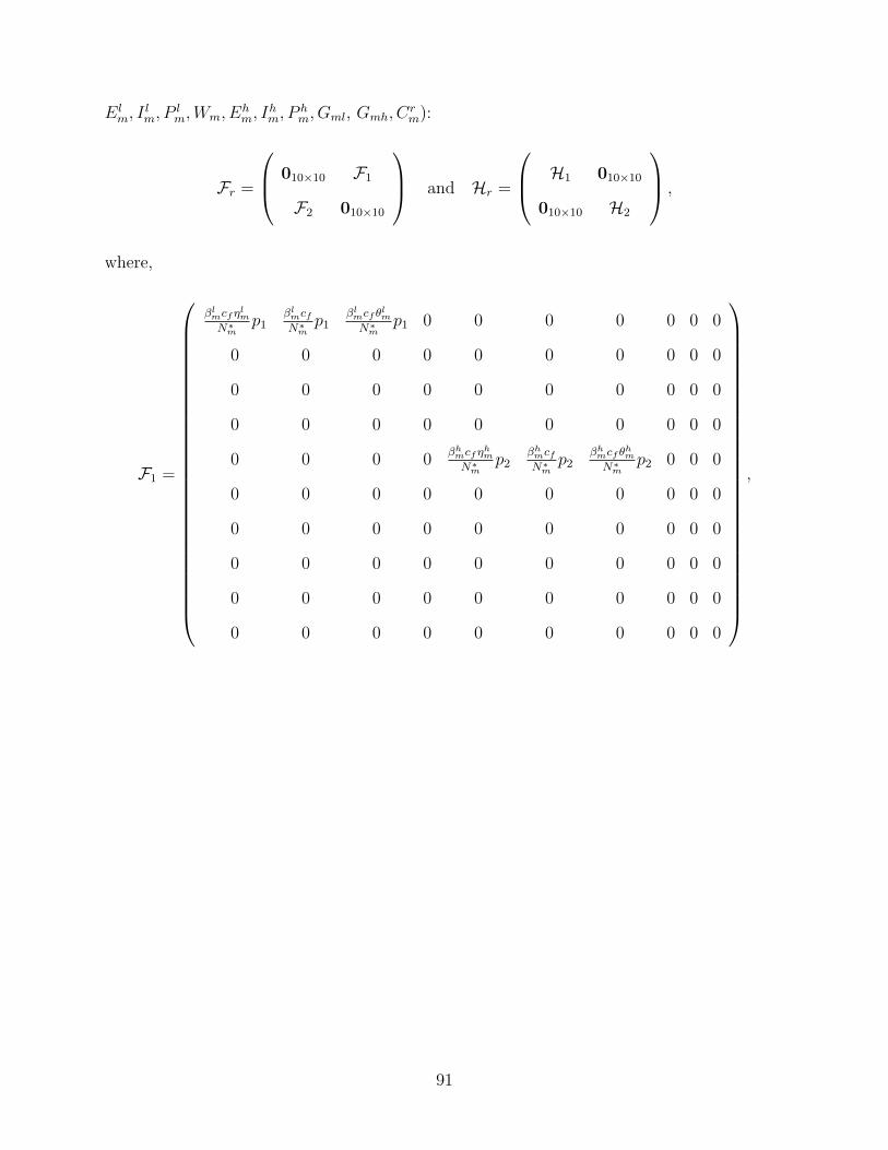
Elm, I
lm, P
lm,Wm, Eh
m, Ihm, P
hm, Gml, Gmh, Cr
m):
Fr =
010×10 F1
F2 010×10
and Hr =
H1 010×10
010×10 H2
,
where,
F1 =
βlmcfηlmN∗
mp1
βlmcfN∗
mp1
βlmcf θlmN∗
mp1 0 0 0 0 0 0 0
0 0 0 0 0 0 0 0 0 0
0 0 0 0 0 0 0 0 0 0
0 0 0 0 0 0 0 0 0 0
0 0 0 0 βhmcfηhmN∗
mp2
βhmcfN∗
mp2
βhmcf θhmN∗
mp2 0 0 0
0 0 0 0 0 0 0 0 0 0
0 0 0 0 0 0 0 0 0 0
0 0 0 0 0 0 0 0 0 0
0 0 0 0 0 0 0 0 0 0
0 0 0 0 0 0 0 0 0 0
,
91
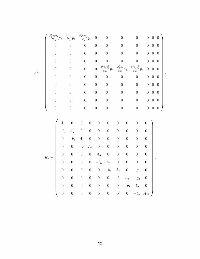
F2 =
βlf cfη
lf
N∗m
p3βlf cfN∗
mp3
βlf cf θ
lf
N∗m
p3 0 0 0 0 0 0 0
0 0 0 0 0 0 0 0 0 0
0 0 0 0 0 0 0 0 0 0
0 0 0 0 0 0 0 0 0 0
0 0 0 0βhf cfη
hf
N∗m
p4βhf cfN∗
mp4
βhf cf θ
hf
N∗m
p4 0 0 0
0 0 0 0 0 0 0 0 0 0
0 0 0 0 0 0 0 0 0 0
0 0 0 0 0 0 0 0 0 0
0 0 0 0 0 0 0 0 0 0
0 0 0 0 0 0 0 0 0 0
,
H1 =
A1 0 0 0 0 0 0 0 0 0
−b1 A2 0 0 0 0 0 0 0 0
0 −b2 A3 0 0 0 0 0 0 0
0 0 −b3 A4 0 0 0 0 0 0
0 0 0 0 A5 0 0 0 0 0
0 0 0 0 −b5 A6 0 0 0 0
0 0 0 0 0 −b6 A7 0 −g1 0
0 0 0 0 0 0 −b7 A8 −g2 0
0 0 0 0 0 0 0 −b8 A9 0
0 0 0 0 0 0 0 0 −b9 A10
,
92
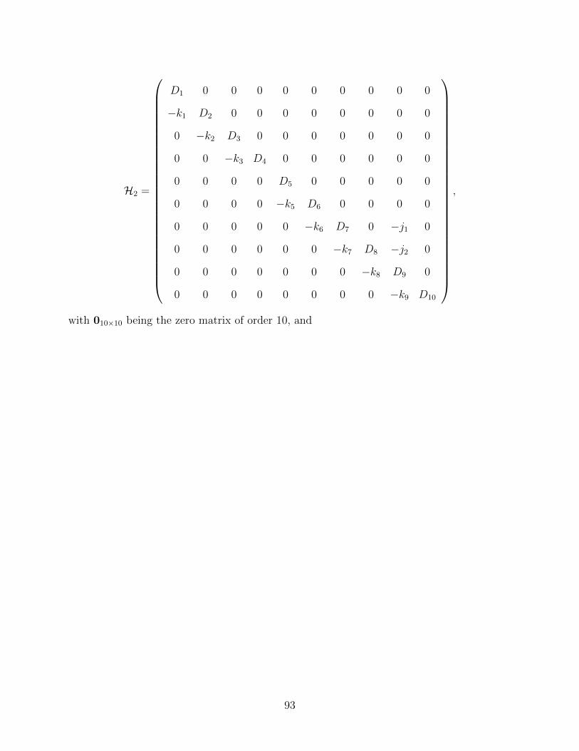
H2 =
D1 0 0 0 0 0 0 0 0 0
−k1 D2 0 0 0 0 0 0 0 0
0 −k2 D3 0 0 0 0 0 0 0
0 0 −k3 D4 0 0 0 0 0 0
0 0 0 0 D5 0 0 0 0 0
0 0 0 0 −k5 D6 0 0 0 0
0 0 0 0 0 −k6 D7 0 −j1 0
0 0 0 0 0 0 −k7 D8 −j2 0
0 0 0 0 0 0 0 −k8 D9 0
0 0 0 0 0 0 0 0 −k9 D10
,
with 010×10 being the zero matrix of order 10, and
93
p1 =�S∗f + V b∗
f + (1− εv)Vq∗
f
�=
πf
�1− εvϕ
qf
�
µf,
p2 =�S∗f + (1− εv)V
b∗
f + (1− εv)Vq∗
f
�=
πf
�1− εv
�ϕbf + ϕq
f
��
µf,
p3 =�S∗m + V b∗
m + (1− εv)Vq∗
m
�=
πm (1− εvϕqm)
µm,
p4 =�S∗m + (1− εv)V
b∗
m + (1− εv)Vq∗
m
�=
πm (1− εvϕqm)
µm,
A1 = σlf + µf , b1 = σl
f , A2 = ψlf + µf , b2 =
�1− rlf
�ψlf , A3 = αl
f + µf ,
b3 =�1− kl
f
�αlf , A4 = nf + µf , A5 = σh
f + µf , b5 = σhf , A6 = ψh
f + µf ,
b6 =�1− rhf
�ψhf , A7 = αh
f + µf , g1 = [1− (s1f + s2f )] zf , b7 =�1− kh
f
�αhf ,
A8 = uf + µf , g2 = s2fzf , b8 = (1− df ) uf , A9 = zf + ωf + µf , b9 = ωf ,
A10 = γf + µf + δf , D1 = σlm + µm, k1 = σl
m, D2 = ψlm + µm,
k2 =�1− rlm
�ψlm, D3 = αl
m + µm, k3 =�1− kl
m
�αlm, D4 = nm + µm,
D5 = σhm + µm, k5 = σh
m, D6 = ψhm + µm, k6 =
�1− rhm
�ψhm, D7 = αh
m + µm,
j1 = [1− (s1m + s2m)] zm, k7 =�1− kh
m
�αhm, D8 = um + µm, j2 = s2mzm,
k8 = (1− dm) um, D9 = zm + ωm + µm, k9 = ωm, D10 = γm + µm + δm.
Thus, it follows from [95] that
Rr0 = ρ
�FrH
−1r
�=
�RrfRrm, (4.36)
where,
Rrf = ρ�F1H
−12
�= max{Rfl,Rfh} and Rrm = ρ
�F2H
−11
�= max{Rml,Rmh},
94
with,
Rfl =βlmcfπfµm
�1− εvϕ
qf
�B1
µfπm
3�i=1
Di
, Rfh =βhmcfπfµm
�1− εv
�ϕbf + ϕq
f
��(Q1 +Q2 +Q3)
µfπmD5D6Q4,
Rml =βlfcf (1− εvϕq
m)B2
3�i=1
Ai
, Rmh =βhf cf (1− εvϕq
m) (Q5 +Q6 +Q7)
A5A6Q8,
and,
B1 = ηlmD3D2 + k1D3 + θlmk2k1, Q1 = ηhm (D6D7D8D9 − k8j2D6D7 − k8k7j1D6) ,
Q2 = k5D7D8D9 − k5k8j2D7 − k5k7k8j1, Q3 = θhm (k5k6D8D9 − k5k6k8j2) ,
Q4 = D7D8D9 − k8j2D7 − k7k8j1, B2 = ηlfA3A2 + b1A3 + θlfb2b1,
Q5 = ηhf (A6A7A8A9 − b8g2A6A7 − b8b7g1A6) , Q6 = b5A7A8A9 − b5b8g2A7 − b5b7b8g1,
Q7 = θhf (b5b6A8A9 − b5b6b8g2) , Q8 = A7A8A9 − b8g2A7 − b7b8g1.
It can be shown that the quantities Rfl,Rml,Rfh and Rmh are positive (see Appendix G), so
that the reproduction thresholds, Rrf and Rrm are positive. For mathematical convenience,
let (where Rl = RflRml and Rh = RfhRmh)
Rr0 =
�max{Rl,Rh}.
Consequently, the result below follows from Theorem 2 of [95].
Theorem 4.2. The DFE, Er0 , of the model (4.34), given by (4.35), is LAS if Rr
0 < 1, and
unstable if Rr0 > 1.
The threshold quantity, Rr0, is the basic reproduction number [47] for the model (4.34). It
represents the average number of secondary HPV infections generated by a typical HPV-
infected person if introduced into a susceptible sexually-active population (or community)
95
where a certain fraction of the new sexually-active individuals is vaccinated. It is worth
noting that Rr0 is an aggregate product of the average number of new HPV cases generated
by females (denoted by Rrf ) and males (denoted by Rrm) in a community.
Epidemiologically speaking, Theorem 4.2 states that a small influx of infected individuals
(females or males) will not generate large outbreaks of the low- and high-risk HPV types in
the community if Rr0 < 1 (in other words, the two HPV types can be effectively controlled
in the community if the initial sizes of the sub-populations of the model (4.34) are in the
basin of attraction of the DFE, Er0 , of the model (4.34)). However, in order for such effective
control (or elimination) to be independent of the initial sizes of the sub-populations of the
model (4.34), it is necessary to show that the DFE (Er0 ), of the model (4.34), is globally-
asymptotically stable (GAS) if Rr0 < 1. This is explored, for a special case, in Section
4.3.4.
4.3.2 Existence and local stability of boundary equilibria
The possible non-trivial equilibria of the model (4.34) are:
i) low-risk-only boundary equilibrium (an equilibrium of the model (4.34) with no high-
risk HPV types), denoted by E l1;
ii) high-risk-only boundary equilibrium (an equilibrium of the model (4.34) with no low-
risk HPV types), denoted by Eh1 ;
iii) co-existence equilibria (equilibria of the model (4.34) where both the low- and high-risk
HPV types co-exist), denoted by Er1 .
Consider the model (4.34) in the absence of the high-risk HPV types (i.e., the model (4.34)
with V bf = Eh
f = Ihf = P hf = Gfl = Gfh = Cc
f = V bm = Eh
m = Ihm = P hm = Gml = Gmh = Cr
m =
0). Furthermore, for computational convenience, let ηlm = ηlf = θlm = θlf = ξf = ξm = 0
in the model (4.34). The resulting low-risk-only model is given by (it should be noted that
Nm, in the model (4.34), is now replaced by its limiting value, πmµm
, since individuals infected
96
with the low-risk HPV types do not develop or suffer cancer-induced mortality, so that the
total male population, Nm(t), remains constant):
dSf
dt= (1− ϕq
f )πf −βlmcfµmI lm
πmSf − µfSf ,
dV qf
dt= ϕq
fπf − (1− εv)βlmµmcfI lm
πmV qf − µfV
qf ,
dElf
dt=
�Sf + (1− εv)V
qf
� βlmcfµmI lm
πm+ ρlf
βlmcfµmI lm
πmRf − (σl
f + µf )Elf ,
dI lfdt
= σlfE
lf − (ψl
f + µf )Ilf ,
dP lf
dt= (1− rlf )ψ
lfI
lf − (αl
f + µf )Plf , (4.37)
dWf
dt= (1− kl
f )αlfP
lf − (nf + µf )Wf ,
dRf
dt= rlfψ
lfI
lf + kl
fαlfP
lf + nfWf − ρlf
βlmcfµmI lm
πmRf − µfRf ,
dSm
dt= (1− ϕq
m) πm −βlfcfµmI lfπm
Sm − µmSm,
dV qm
dt= ϕq
mπm − (1− εv)βlfcfµmI lfπm
V qm − µmV
qm,
dElm
dt= [Sm + (1− εv)V
qm]
βlfcfµmI lfπm
+ ρlmβlfcfµmI lfπm
Rm − (σlm + µm)E
lm,
dI lmdt
= σlmE
lm − (ψl
m + µm)Ilm,
dP lm
dt= (1− rlm)ψ
lmI
lm − (αl
m + µm)Plm,
dWm
dt= (1− kl
m)αlmP
lm − (nm + µm)Wm,
dRm
dt= rlmψ
lmI
lm + kl
mαlmP
lm + nmWm − ρlm
βlfcfµmI lfπm
Rm − µmRm.
It is convenient to let (with A1, A2, D1, D2, b1 and k1 as defined in Section 4.3.1)
Rl0 = R
r0 |Rfh=Rmh=ηlm=ηlf=θlm=θlf=ξf=ξm=0=
�βlmc
2fπfµmβl
fb1k1�1− εvϕ
qf
�(1− εvϕ
qm)
πmµfA1A2D1D2.
97
Furthermore, let
El1 = (S∗∗
f , V q∗∗
f , El∗∗
f , I l∗∗
f , P l∗∗
f ,W ∗∗f , R∗∗
f , S∗∗m , V q∗∗
m , El∗∗
m , I l∗∗
m , P l∗∗
m ,W ∗∗m , R∗∗
m ),
represents any arbitrary endemic equilibrium of the low-risk-only model (4.37). Define
λl∗∗
m =βlmcfµmI l
∗∗m
πmand λl∗∗
f =βlfcfµmI l
∗∗f
πm. (4.38)
Setting the right-hand sides of the low-risk-only model (4.37) to zero gives the following
steady-state expressions:
S∗∗f =
πf
�1− ϕq
f
�
λl∗∗m + µf
, V q∗∗
f =πfϕ
qf
(1− εv)λl∗∗m + µf
,
El∗∗
f =
�S∗∗f + (1− εv)V
q∗∗
f
�λl∗∗m + ρlfλ
l∗∗m R∗∗
f
A1, I l
∗∗
f =b1El∗∗
f
A2, P l∗∗
f =b2I l
∗∗f
A3, (4.39)
W ∗∗f =
b3P l∗∗f
A4, R∗∗
f =m1I l
∗∗f +m2P l∗∗
f + nfW ∗∗f
ρlfλl∗∗m +m3
, S∗∗m =
πm (1− ϕqm)
λl∗∗f + µm
,
V q∗∗
m =πmϕq
m
(1− εv)λl∗∗f + µm
, El∗∗
m =
�S∗∗m + (1− εv)V q∗∗
m
�λl∗∗f + ρlmλ
l∗∗f R∗∗
m
D1,
I l∗∗
m =k1El∗∗
m
D2, P l∗∗
m =k2I l
∗∗m
D3, W ∗∗
m =k3P l∗∗
m
D4, R∗∗
m =m4I l
∗∗m +m5P l∗∗
m + nmW ∗∗m
ρlmλl∗∗f +m6
,
where (with Ai, Di (i = 1, ..., 4), b1, b2, b3, k1, k2 and k3 as defined in Section 4.3.1),
m1 = rlfψlf , m2 = kl
fαlf , m4 = rlmψ
lm and m5 = kl
mαlm.
98
Substituting (4.39) into the expression for λl∗∗m and λl∗∗
f in (4.38) gives,
λl∗∗
m =λl∗∗f
�a02
�λl∗∗f
�2+ a01λl∗∗
f + a0�
a33�λl∗∗f
�3+ a22
�λl∗∗f
�2+ a11λl∗∗
f + a00, λl∗∗
f =λl∗∗m
�b02
�λl∗∗m
�2+ b01λl∗∗
m + b0�
b33 (λl∗∗m )3 + b22 (λl∗∗
m )2 + b11λl∗∗m + b00
,
(4.40)
99
where,
a02 =µmβl
mcfk1ρlm (1− εv)
2�i=1
Di
, a01 =µ2mβ
lmcfk1
�(1− εv) + ρlm (1− εqϕq
m)�
2�i=1
Di
,
a0 =µ3mβ
lmcfk1 (1− εvϕq
m)2�
i=1Di
, a33 =
(1− εv) ρlm
�4�
i=1Di − k1 (m4D3D4 +m5D4k2 + nmk3k2)
�
4�i=1
Di
,
a22 =
µm
�(1− εv)
4�i=1
Di + ρlm (2− εv)
�4�
i=1Di − k1 (m4D3D4 +m5D4k2 + nmk3k2)
��
4�i=1
Di
,
a11 =
µ2m
�(2− εv)
4�i=1
Di + ρlm
�4�
i=1Di − k1 (m4D3D4 +m5D4k2 + nmk3k2)
��
4�i=1
Di
, (4.41)
a00 = µ3m, b02 =
µmπfβlfcfb1ρ
lf (1− εv)
πm
2�i=1
Ai
, b01 =µmµfπfβl
fcfb1�(1− εv) + ρlf
�1− εvϕ
qf
��
πm
2�i=1
Ai
,
b0 =µmµ2
fπfβlfcfb1
�1− εvϕ
qf
�
πm
2�i=1
Ai
, b33 =
(1− εv) ρlf
�4�
i=1Ai − b1 (m1A3A4 +m2A4b2 + nfb3b2)
�
4�i=1
Ai
,
b22 =
µf
�(1− εv)
4�i=1
Ai + ρlf (2− εv)
�4�
i=1Ai − b1 (m1A3A4 +m2A2b2 + nfb3b2)
��
4�i=1
Ai
,
b11 =
µ2f
�(2− εv)
4�i=1
Ai + ρlf
�4�
i=1Ai − b1 (m1A3A4 +m2A4b2 + nfb3b2)
��
4�i=1
Ai
, b00 = µ3f .
Since all the parameters of the low-risk-only model (4.37) are positive, and 0 < εv,ϕqm,ϕ
qf ≤
1, it can be shown, after some lengthy algebraic manipulations, that all the expressions in
(4.41) (namely, a02, a01, a0, a33, a22, a11, a00, b02, b01, b0, b33, b22, b11, b00) are positive. It follows,
100
by substituting λl∗∗f into λl∗∗
m in (4.40), and simplifying, that the non-zero (endemic) equilibria
of the low-risk-only model (4.37) satisfy the following polynomial (in terms of λl∗∗m ):
9�
i=0
Yi
�λl∗∗
m
�9−i= 0, (4.42)
with Yi (i = 0, ..., 9) given in Appendix H. Since all the parameters of the low-risk-only model
(4.37) are non-negative, it follows from the expressions for Yi (i = 0, ..., 9) in Appendix H
that Y0 > 0 and Y9 > 0 whenever Rl0 < 1. Thus, the number of possible positive real
roots the polynomial (4.42) can have depends on the signs of Yi (i = 1, ..., 8). The various
possibilities (using the Descartes Rule of Signs) for the number of positive real roots of (4.42)
are tabulated in Table 4.3, from which the following result is obtained.
Theorem 4.3. The low-risk-only model (4.37) could have 2 or more endemic equilibria if
Rl0 < 1, and at least one positive endemic equilibrium whenever Rl
0 > 1.
Similar result can be established if the high-risk-only component of the model (4.34) is
considered. Consequently, we offer the following conjecture:
Conjecture 4.1. The model (4.34) could have 2 or more endemic equilibria if Rr0 < 1, and
at least one positive endemic equilibrium whenever Rr0 > 1.
The presence of multiple endemic equilibria in the low-risk-only model (4.37) (and, by ex-
tension, the risk-structured model (4.34)) when Rl0 < 1 suggests the possibility of backward
bifurcation in the model (4.34). This is explored in Section 4.3.3.
Extensive numerical simulations of the model (4.34), using the parameter values in Table
4.2 (unless otherwise stated), were carried out to quantitatively assess the dynamics of the
low- and high-risk HPV types in the community, for various scenarios (of the associated
reproduction numbers, Rl and Rh). It should be mentioned that these numerical simulations
have to be ran for extended periods of time to reach steady-state (as is evident in some of the
plots). Figure 4.3 depicts the simulation results obtained for the case when the reproduction
101
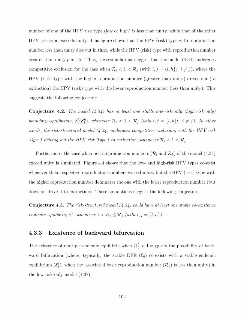
number of one of the HPV risk type (low or high) is less than unity, while that of the other
HPV risk type exceeds unity. This figure shows that the HPV (risk) type with reproduction
number less than unity dies out in time, while the HPV (risk) type with reproduction number
greater than unity persists. Thus, these simulations suggest that the model (4.34) undergoes
competitive exclusion for the case when Ri < 1 < Rj (with i, j = {l, h}; i �= j), where the
HPV (risk) type with the higher reproduction number (greater than unity) drives out (to
extinction) the HPV (risk) type with the lower reproduction number (less than unity). This
suggests the following conjecture:
Conjecture 4.2. The model (4.34) has at least one stable low-risk-only (high-risk-only)
boundary equilibrium, E l1(E
h1 ), whenever Ri < 1 < Rj (with i, j = {l, h}; i �= j). In other
words, the risk-structured model (4.34) undergoes competitive exclusion, with the HPV risk
Type j driving out the HPV risk Type i to extinction, whenever Ri < 1 < Rj.
Furthermore, the case when both reproduction numbers (Rl and Rh) of the model (4.34)
exceed unity is simulated. Figure 4.4 shows that the low- and high-risk HPV types co-exist
whenever their respective reproduction numbers exceed unity, but the HPV (risk) type with
the higher reproduction number dominates the one with the lower reproduction number (but
does not drive it to extinction). These simulations suggest the following conjecture:
Conjecture 4.3. The risk-structured model (4.34) could have at least one stable co-existence
endemic equilibria, Er1 , whenever 1 < Ri ≤ Rj (with i, j = {l, h}).
4.3.3 Existence of backward bifurcation
The existence of multiple endemic equilibria when Rl0 < 1 suggests the possibility of back-
ward bifurcation (where, typically, the stable DFE (E0) co-exists with a stable endemic
equilibrium (E l1), when the associated basic reproduction number (Rl
0) is less than unity) in
the low-risk-only model (4.37).
102
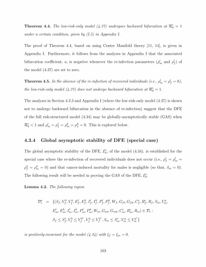
Theorem 4.4. The low-risk-only model (4.37) undergoes backward bifurcation at Rl0 = 1
under a certain condition, given by (I.5) in Appendix I.
The proof of Theorem 4.4, based on using Centre Manifold theory [11, 14], is given in
Appendix I. Furthermore, it follows from the analyses in Appendix I that the associated
bifurcation coefficient, a, is negative whenever the re-infection parameters (ρlm and ρlf ) of
the model (4.37) are set to zero.
Theorem 4.5. In the absence of the re-infection of recovered individuals (i.e., ρlm = ρlf = 0),
the low-risk-only model (4.37) does not undergo backward bifurcation at Rl0 = 1.
The analyses in Section 4.3.3 and Appendix I (where the low-risk-only model (4.37) is shown
not to undergo backward bifurcation in the absence of re-infection) suggest that the DFE
of the full risk-structured model (4.34) may be globally-asymptotically stable (GAS) when
Rr0 < 1 and ρlm = ρlf = ρhm = ρhf = 0. This is explored below.
4.3.4 Global asymptotic stability of DFE (special case)
The global asymptotic stability of the DFE, Er0 , of the model (4.34), is established for the
special case where the re-infection of recovered individuals does not occur (i.e., ρlf = ρlm =
ρhf = ρhm = 0) and that cancer-induced mortality for males is negligible (so that, δm = 0).
The following result will be needed in proving the GAS of the DFE, Er0 .
Lemma 4.2. The following region
D∗r = {(Sf , V
bf , V
qf , E
lf , E
hf , I
lf , I
hf , P
lf , P
hf ,Wf , Gfl, Gfh, C
cf , R
cf , Rf , Sm, V
qm,
Elm, E
hm, I
lm, I
hm, P
lm, P
hm,Wm, Gml, Gmh, C
rm, R
cm, Rm) ∈ Dr :
Sf ≤ S∗f , V
bf ≤ V b∗
f , V qf ≤ V q∗
f , Sm ≤ S∗m, V
qm ≤ V q∗
m }
is positively-invariant for the model (4.34) with ξf = ξm = 0.
103
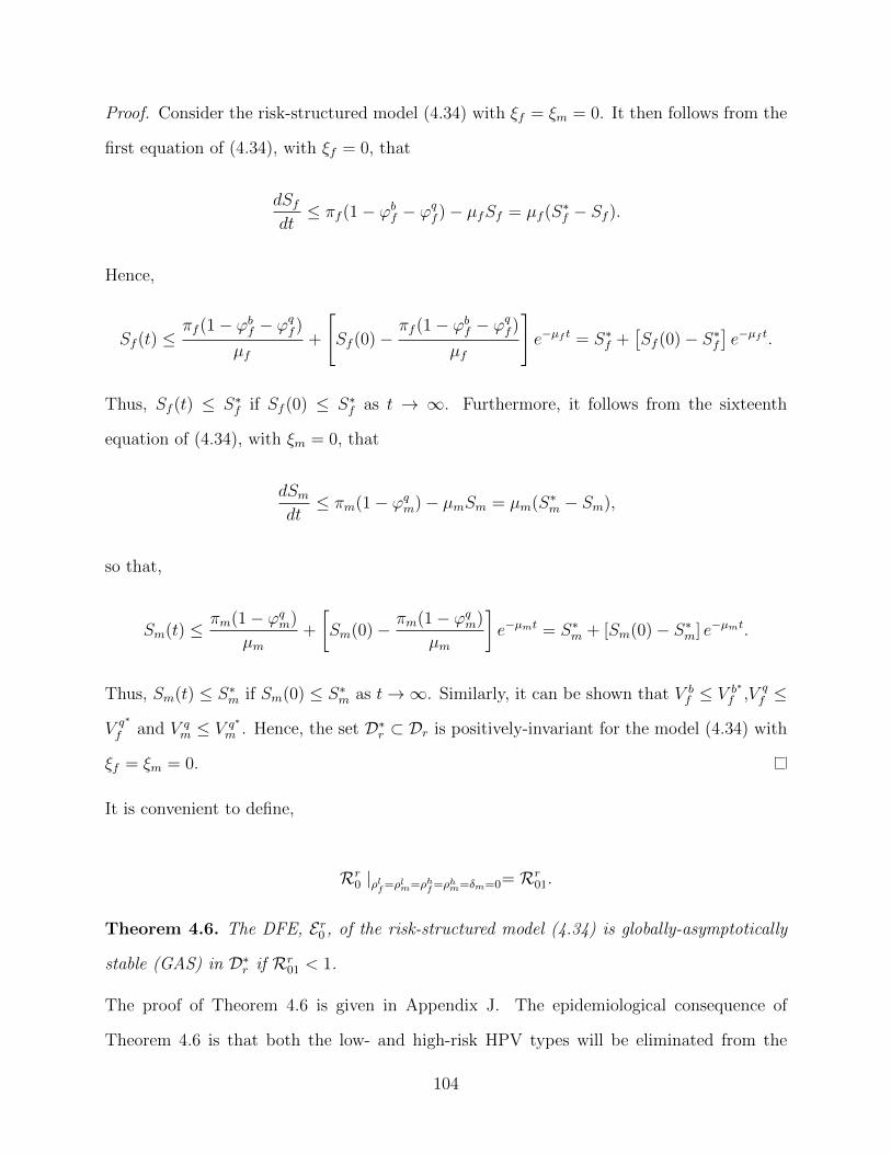
Proof. Consider the risk-structured model (4.34) with ξf = ξm = 0. It then follows from the
first equation of (4.34), with ξf = 0, that
dSf
dt≤ πf (1− ϕb
f − ϕqf )− µfSf = µf (S
∗f − Sf ).
Hence,
Sf (t) ≤πf (1− ϕb
f − ϕqf )
µf+
�Sf (0)−
πf (1− ϕbf − ϕq
f )
µf
�e−µf t = S∗
f +�Sf (0)− S∗
f
�e−µf t.
Thus, Sf (t) ≤ S∗f if Sf (0) ≤ S∗
f as t → ∞. Furthermore, it follows from the sixteenth
equation of (4.34), with ξm = 0, that
dSm
dt≤ πm(1− ϕq
m)− µmSm = µm(S∗m − Sm),
so that,
Sm(t) ≤πm(1− ϕq
m)
µm+
�Sm(0)−
πm(1− ϕqm)
µm
�e−µmt = S∗
m + [Sm(0)− S∗m] e
−µmt.
Thus, Sm(t) ≤ S∗m if Sm(0) ≤ S∗
m as t → ∞. Similarly, it can be shown that V bf ≤ V b∗
f ,V qf ≤
V q∗
f and V qm ≤ V q∗
m . Hence, the set D∗r ⊂ Dr is positively-invariant for the model (4.34) with
ξf = ξm = 0.
It is convenient to define,
Rr0 |ρlf=ρlm=ρhf=ρhm=δm=0= R
r01.
Theorem 4.6. The DFE, Er0 , of the risk-structured model (4.34) is globally-asymptotically
stable (GAS) in D∗r if Rr
01 < 1.
The proof of Theorem 4.6 is given in Appendix J. The epidemiological consequence of
Theorem 4.6 is that both the low- and high-risk HPV types will be eliminated from the
104
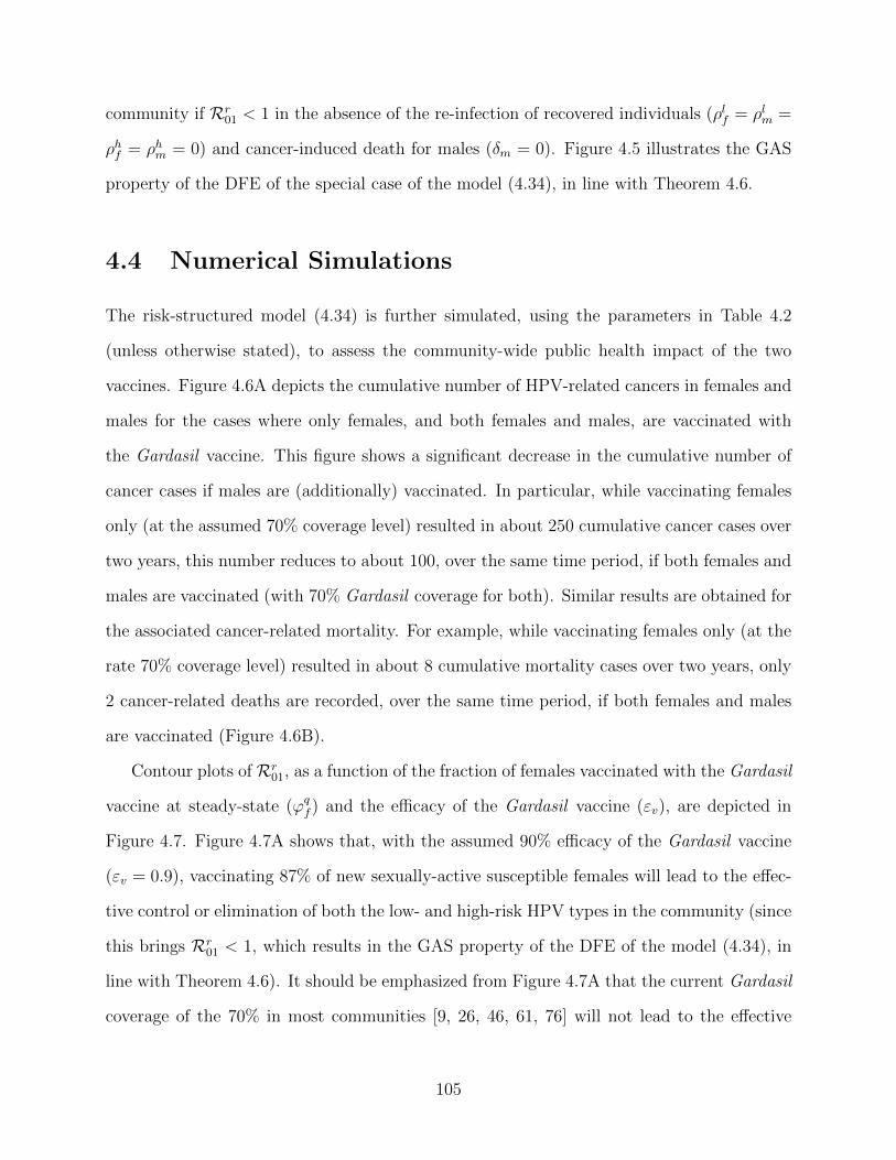
community if Rr01 < 1 in the absence of the re-infection of recovered individuals (ρlf = ρlm =
ρhf = ρhm = 0) and cancer-induced death for males (δm = 0). Figure 4.5 illustrates the GAS
property of the DFE of the special case of the model (4.34), in line with Theorem 4.6.
4.4 Numerical Simulations
The risk-structured model (4.34) is further simulated, using the parameters in Table 4.2
(unless otherwise stated), to assess the community-wide public health impact of the two
vaccines. Figure 4.6A depicts the cumulative number of HPV-related cancers in females and
males for the cases where only females, and both females and males, are vaccinated with
the Gardasil vaccine. This figure shows a significant decrease in the cumulative number of
cancer cases if males are (additionally) vaccinated. In particular, while vaccinating females
only (at the assumed 70% coverage level) resulted in about 250 cumulative cancer cases over
two years, this number reduces to about 100, over the same time period, if both females and
males are vaccinated (with 70% Gardasil coverage for both). Similar results are obtained for
the associated cancer-related mortality. For example, while vaccinating females only (at the
rate 70% coverage level) resulted in about 8 cumulative mortality cases over two years, only
2 cancer-related deaths are recorded, over the same time period, if both females and males
are vaccinated (Figure 4.6B).
Contour plots of Rr01, as a function of the fraction of females vaccinated with the Gardasil
vaccine at steady-state (ϕqf ) and the efficacy of the Gardasil vaccine (εv), are depicted in
Figure 4.7. Figure 4.7A shows that, with the assumed 90% efficacy of the Gardasil vaccine
(εv = 0.9), vaccinating 87% of new sexually-active susceptible females will lead to the effec-
tive control or elimination of both the low- and high-risk HPV types in the community (since
this brings Rr01 < 1, which results in the GAS property of the DFE of the model (4.34), in
line with Theorem 4.6). It should be emphasized from Figure 4.7A that the current Gardasil
coverage of the 70% in most communities [9, 26, 46, 61, 76] will not lead to the effective
105
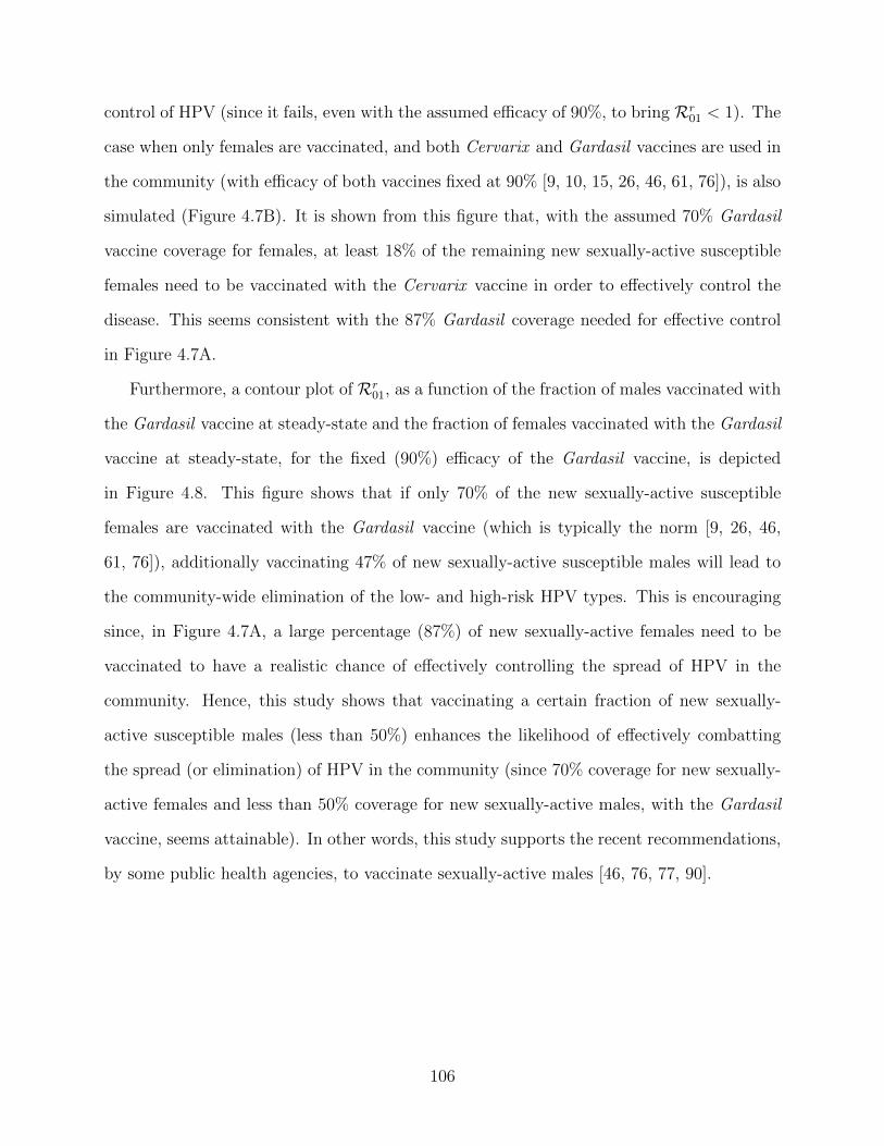
control of HPV (since it fails, even with the assumed efficacy of 90%, to bring Rr01 < 1). The
case when only females are vaccinated, and both Cervarix and Gardasil vaccines are used in
the community (with efficacy of both vaccines fixed at 90% [9, 10, 15, 26, 46, 61, 76]), is also
simulated (Figure 4.7B). It is shown from this figure that, with the assumed 70% Gardasil
vaccine coverage for females, at least 18% of the remaining new sexually-active susceptible
females need to be vaccinated with the Cervarix vaccine in order to effectively control the
disease. This seems consistent with the 87% Gardasil coverage needed for effective control
in Figure 4.7A.
Furthermore, a contour plot of Rr01, as a function of the fraction of males vaccinated with
the Gardasil vaccine at steady-state and the fraction of females vaccinated with the Gardasil
vaccine at steady-state, for the fixed (90%) efficacy of the Gardasil vaccine, is depicted
in Figure 4.8. This figure shows that if only 70% of the new sexually-active susceptible
females are vaccinated with the Gardasil vaccine (which is typically the norm [9, 26, 46,
61, 76]), additionally vaccinating 47% of new sexually-active susceptible males will lead to
the community-wide elimination of the low- and high-risk HPV types. This is encouraging
since, in Figure 4.7A, a large percentage (87%) of new sexually-active females need to be
vaccinated to have a realistic chance of effectively controlling the spread of HPV in the
community. Hence, this study shows that vaccinating a certain fraction of new sexually-
active susceptible males (less than 50%) enhances the likelihood of effectively combatting
the spread (or elimination) of HPV in the community (since 70% coverage for new sexually-
active females and less than 50% coverage for new sexually-active males, with the Gardasil
vaccine, seems attainable). In other words, this study supports the recent recommendations,
by some public health agencies, to vaccinate sexually-active males [46, 76, 77, 90].
106
4.5 Summary of the Chapter
A new risk-structured deterministic model for the transmission dynamics of HPV in a pop-
ulation, in the presence of the Cervarix and Gardasil vaccines (that target the four low-
and high-risk HPV types considered in this chapter), is designed. The main theoretical and
numerical results obtained are summarized below.
i) the risk-structured model (4.34) has a LAS DFE whenever Rr0 < 1;
ii) the low-risk-only model (4.37) undergoes the phenomenon of backward bifurcation
at Rl0 = 1 if Inequality (I.5) holds. It is shown that the re-infection of recovered
individuals causes the backward bifurcation property in the model. The low-risk-only
model could have one or more endemic equilibria when the associated reproduction
number (Rl0) exceeds unity;
iii) in the absence of the re-infection of recovered individuals (i.e., ρlf = ρlm = ρhf = ρhm = 0)
and cancer-induced death in males (i.e., δm = 0), the DFE of the risk-structured model
(4.34) is GAS in D∗r whenever Rr
01 < 1;
iv) with the assumed 90% efficacy of the Gardasil vaccine, at least 87% of the new sexually-
active females need to be vaccinated to have a realistic chance of effectively controlling
the spread of the low- and high-risk HPV types in the community;
v) it is shown that, with the assumed 70% Gardasil vaccine coverage for females, at least
18% of the remaining new sexually-active susceptible females need to be vaccinated
with the Cervarix vaccine in order to effectively control the spread of the low- and
high-risk HPV types in the community;
vi) vaccinating a fraction of new sexually-active susceptible males offers beneficial community-
wide public health impact. In particular, simulations show that while vaccinating new
sexually-active susceptible females only (at the assumed 70% vaccine coverage) re-
sulted in about 250 cumulative cancer cases (in both females and males) over two
107
years, this number reduces to about 100, over the same time period, if both new
sexually-active susceptible males (with 70% Gardasil coverage level) and females are
vaccinated. Furthermore, while vaccinating females only with the Gardasil vaccine (at
the 70% coverage level) resulted in about 8 cumulative cancer-related mortality cases
over two years, only 2 such deaths are recorded, over the same time period, if both
males and females are vaccinated;
vii) if only 70% of the new sexually-active susceptible females are vaccinated with the
Gardasil vaccine, additionally vaccinating 47% of the new sexually-active susceptible
males will lead to the effective community-wide control, or elimination, of the low- and
high-risk HPV types. Thus, this study supports the recent recommendations by some
public health agencies to vaccine sexually-active males (since doing so offers additional
community-wide benefit, vis-a-vis the control of the two (risk) HPV types).
108
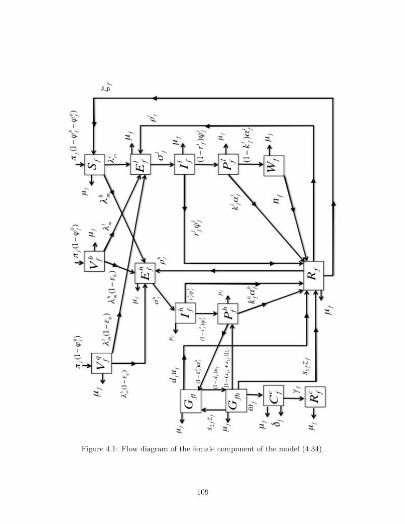
Figure 4.1: Flow diagram of the female component of the model (4.34).
109
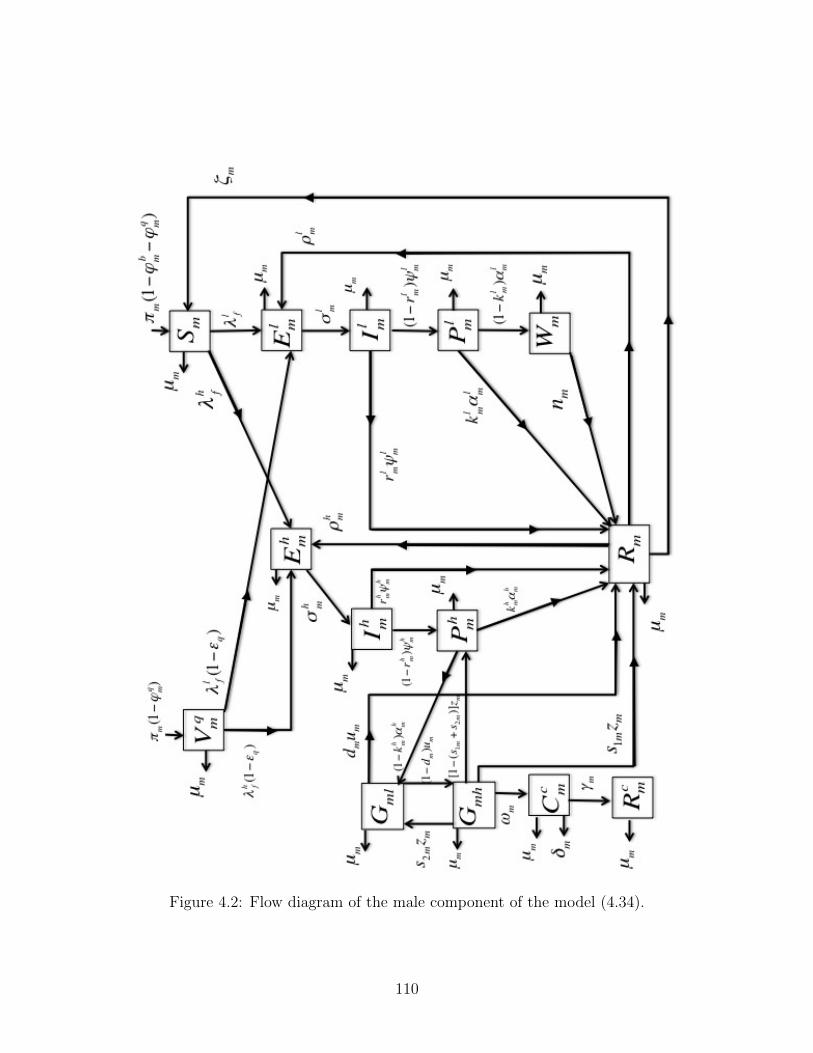
Figure 4.2: Flow diagram of the male component of the model (4.34).
110
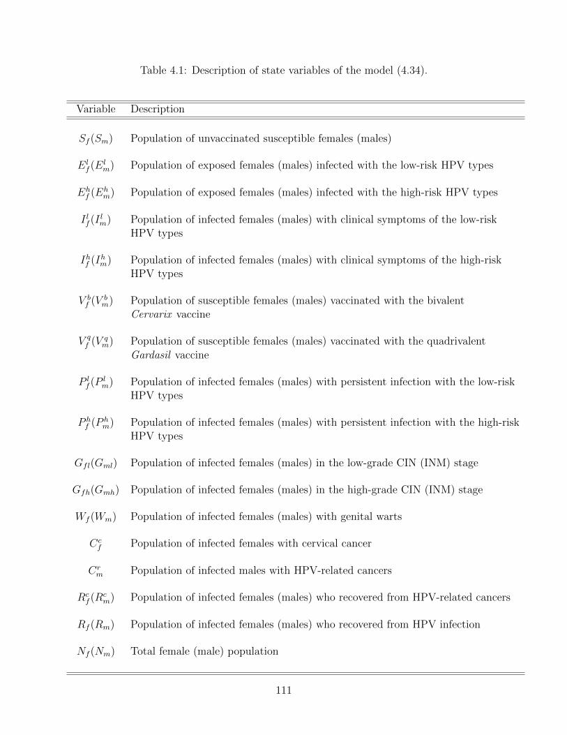
Table 4.1: Description of state variables of the model (4.34).
Variable Description
Sf (Sm) Population of unvaccinated susceptible females (males)
Elf (E
lm) Population of exposed females (males) infected with the low-risk HPV types
Ehf (E
hm) Population of exposed females (males) infected with the high-risk HPV types
I lf (Ilm) Population of infected females (males) with clinical symptoms of the low-risk
HPV types
Ihf (Ihm) Population of infected females (males) with clinical symptoms of the high-risk
HPV types
V bf (V
bm) Population of susceptible females (males) vaccinated with the bivalent
Cervarix vaccine
V qf (V
qm) Population of susceptible females (males) vaccinated with the quadrivalent
Gardasil vaccine
P lf (P
lm) Population of infected females (males) with persistent infection with the low-risk
HPV types
P hf (P
hm) Population of infected females (males) with persistent infection with the high-risk
HPV types
Gfl(Gml) Population of infected females (males) in the low-grade CIN (INM) stage
Gfh(Gmh) Population of infected females (males) in the high-grade CIN (INM) stage
Wf (Wm) Population of infected females (males) with genital warts
Ccf Population of infected females with cervical cancer
Crm Population of infected males with HPV-related cancers
Rcf (R
cm) Population of infected females (males) who recovered from HPV-related cancers
Rf (Rm) Population of infected females (males) who recovered from HPV infection
Nf (Nm) Total female (male) population
111
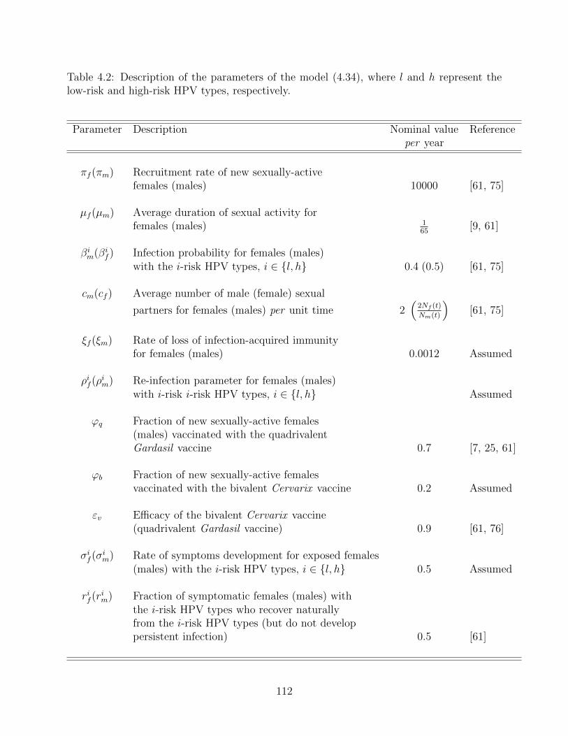
Table 4.2: Description of the parameters of the model (4.34), where l and h represent thelow-risk and high-risk HPV types, respectively.
Parameter Description Nominal value Referenceper year
πf (πm) Recruitment rate of new sexually-activefemales (males) 10000 [61, 75]
µf (µm) Average duration of sexual activity forfemales (males) 1
65 [9, 61]
βim(β
if ) Infection probability for females (males)
with the i-risk HPV types, i ∈ {l, h} 0.4 (0.5) [61, 75]
cm(cf ) Average number of male (female) sexual
partners for females (males) per unit time 2�
2Nf (t)Nm(t)
�[61, 75]
ξf (ξm) Rate of loss of infection-acquired immunityfor females (males) 0.0012 Assumed
ρif (ρim) Re-infection parameter for females (males)
with i-risk i-risk HPV types, i ∈ {l, h} Assumed
ϕq Fraction of new sexually-active females(males) vaccinated with the quadrivalentGardasil vaccine 0.7 [7, 25, 61]
ϕb Fraction of new sexually-active femalesvaccinated with the bivalent Cervarix vaccine 0.2 Assumed
εv Efficacy of the bivalent Cervarix vaccine(quadrivalent Gardasil vaccine) 0.9 [61, 76]
σif (σ
im) Rate of symptoms development for exposed females
(males) with the i-risk HPV types, i ∈ {l, h} 0.5 Assumed
rif (rim) Fraction of symptomatic females (males) with
the i-risk HPV types who recover naturallyfrom the i-risk HPV types (but do not developpersistent infection) 0.5 [61]
112
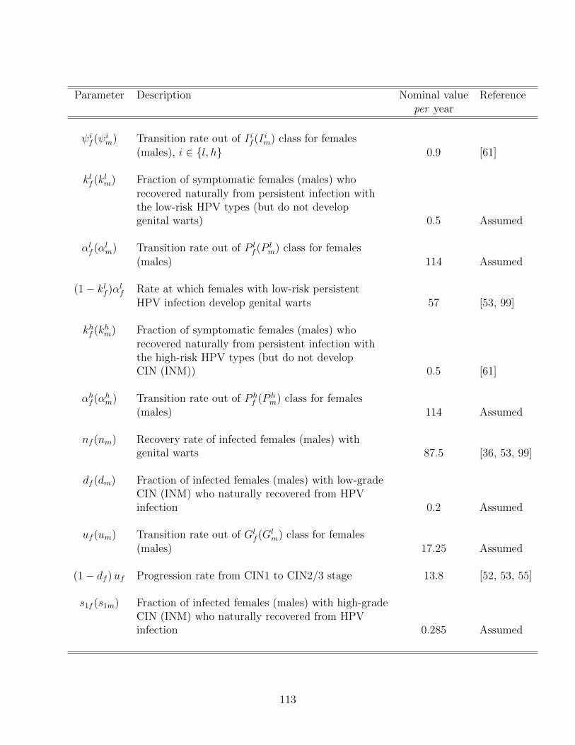
Parameter Description Nominal value Referenceper year
ψif (ψ
im) Transition rate out of I if (I
im) class for females
(males), i ∈ {l, h} 0.9 [61]
klf (k
lm) Fraction of symptomatic females (males) who
recovered naturally from persistent infection withthe low-risk HPV types (but do not developgenital warts) 0.5 Assumed
αlf (α
lm) Transition rate out of P l
f (Plm) class for females
(males) 114 Assumed
(1− klf )α
lf Rate at which females with low-risk persistent
HPV infection develop genital warts 57 [53, 99]
khf (k
hm) Fraction of symptomatic females (males) who
recovered naturally from persistent infection withthe high-risk HPV types (but do not developCIN (INM)) 0.5 [61]
αhf (α
hm) Transition rate out of P h
f (Phm) class for females
(males) 114 Assumed
nf (nm) Recovery rate of infected females (males) withgenital warts 87.5 [36, 53, 99]
df (dm) Fraction of infected females (males) with low-gradeCIN (INM) who naturally recovered from HPVinfection 0.2 Assumed
uf (um) Transition rate out of Glf (G
lm) class for females
(males) 17.25 Assumed
(1− df ) uf Progression rate from CIN1 to CIN2/3 stage 13.8 [52, 53, 55]
s1f (s1m) Fraction of infected females (males) with high-gradeCIN (INM) who naturally recovered from HPVinfection 0.285 Assumed
113
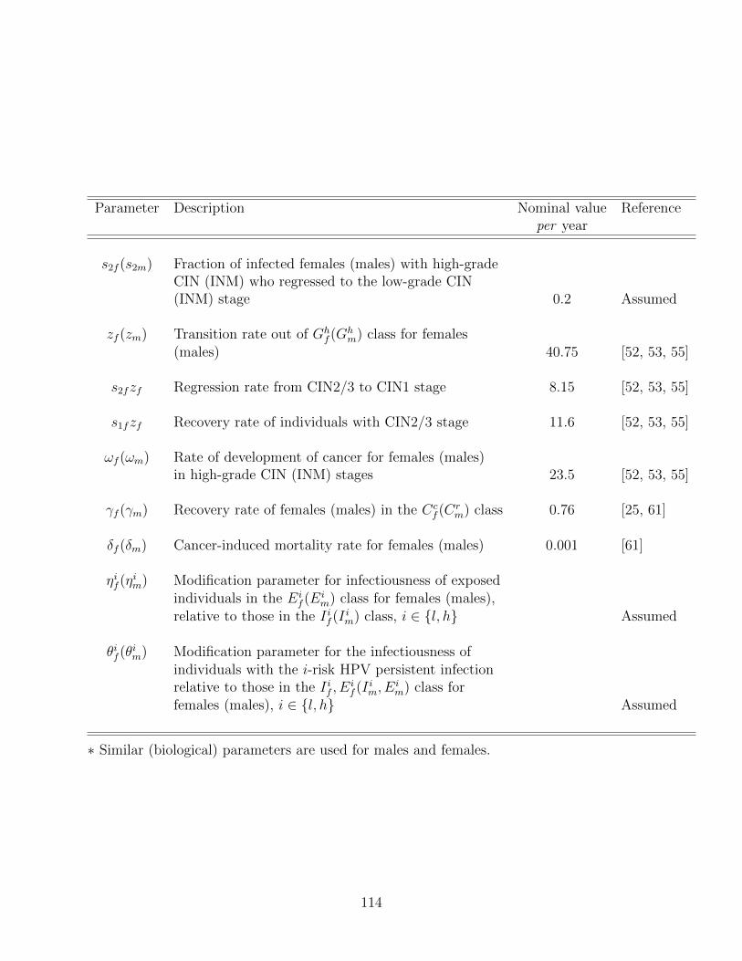
Parameter Description Nominal value Referenceper year
s2f (s2m) Fraction of infected females (males) with high-gradeCIN (INM) who regressed to the low-grade CIN(INM) stage 0.2 Assumed
zf (zm) Transition rate out of Ghf (G
hm) class for females
(males) 40.75 [52, 53, 55]
s2fzf Regression rate from CIN2/3 to CIN1 stage 8.15 [52, 53, 55]
s1fzf Recovery rate of individuals with CIN2/3 stage 11.6 [52, 53, 55]
ωf (ωm) Rate of development of cancer for females (males)in high-grade CIN (INM) stages 23.5 [52, 53, 55]
γf (γm) Recovery rate of females (males) in the Ccf (C
rm) class 0.76 [25, 61]
δf (δm) Cancer-induced mortality rate for females (males) 0.001 [61]
ηif (ηim) Modification parameter for infectiousness of exposed
individuals in the Eif (E
im) class for females (males),
relative to those in the I if (Iim) class, i ∈ {l, h} Assumed
θif (θim) Modification parameter for the infectiousness of
individuals with the i-risk HPV persistent infectionrelative to those in the I if , E
if (I
im, E
im) class for
females (males), i ∈ {l, h} Assumed
∗ Similar (biological) parameters are used for males and females.
114
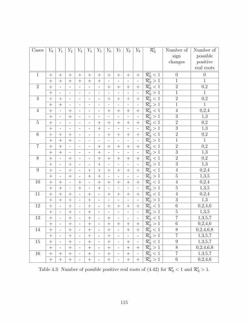
Cases Y0 Y1 Y2 Y3 Y4 Y5 Y6 Y7 Y8 Y9 Rl0 Number of
signchanges
Number ofpossiblepositivereal roots
1 + + + + + + + + + + Rl0 < 1 0 0
+ + + + + + - - - - Rl0 > 1 1 1
2 + - - - - - + + + + Rl0 < 1 2 0,2
+ - - - - - - - - - Rl0 > 1 1 1
3 + + - - - - + + + + Rl0 < 1 2 0,2
+ + - - - - - - - - Rl0 > 1 1 1
4 + - + - - - + + + + Rl0 < 1 4 0,2,4
+ - + - - - - - - - Rl0 > 1 3 1,3
5 + - - - - + + + + + Rl0 < 1 2 0,2
+ - - - - + - - - - Rl0 > 1 3 1,3
6 + + + - - - + + + + Rl0 < 1 2 0,2
+ + + - - - - - - - Rl0 > 1 1 1
7 + + - - - + + + + + Rl0 < 1 2 0,2
+ + - - - + - - - - Rl0 > 1 3 1,3
8 + - + - - + + + + + Rl0 < 1 2 0,2
+ - + - - + - - - - Rl0 > 1 3 1,3
9 + - + - + + + + + + Rl0 < 1 4 0,2,4
+ - + - + + - - - - Rl0 > 1 5 1,3,5
10 + + - + - + + + + + Rl0 < 1 4 0,2,4
+ + - + - + - - - - Rl0 > 1 5 1,3,5
11 + + + - + - + + + + Rl0 < 1 4 0,2,4
+ + + - + - - - - - Rl0 > 1 3 1,3
12 + - + - + - + + + + Rl0 < 1 6 0,2,4,6
+ - + - + - - - - - Rl0 > 1 5 1,3,5
13 + - + - + - + - - - Rl0 < 1 7 1,3,5,7
+ - + - + - + + + + Rl0 > 1 6 0,2,4,6
14 + - + - + - + - + + Rl0 < 1 8 0,2,4,6,8
+ - + - + - + - - - Rl0 > 1 7 1,3,5,7
15 + - + - + - + - + - Rl0 < 1 9 1,3,5,7
+ - + - + - + - + + Rl0 > 1 8 0,2,4,6,8
16 + + + - + - + - + - Rl0 < 1 7 1,3,5,7
+ + + - + - + - + + Rl0 > 1 6 0,2,4,6
Table 4.3: Number of possible positive real roots of (4.42) for Rl0 < 1 and Rl
0 > 1.
115
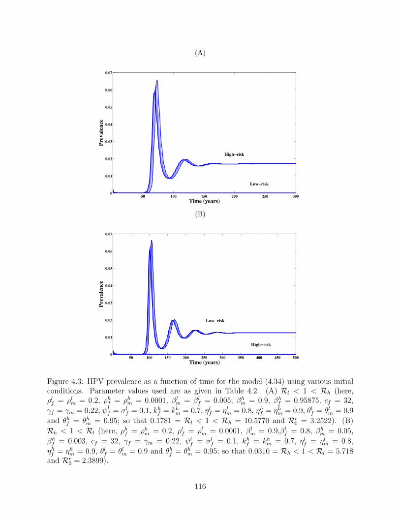
(A)
50 100 150 200 250 3000
0.01
0.02
0.03
0.04
0.05
0.06
0.07
Time (years)
Pre
va
len
ce
High!risk
Low!risk
(B)
50 100 150 200 250 300 350 400 450 5000
0.01
0.02
0.03
0.04
0.05
0.06
0.07
Time (years)
Pre
va
len
ce
Low!risk
High!risk
Figure 4.3: HPV prevalence as a function of time for the model (4.34) using various initialconditions. Parameter values used are as given in Table 4.2. (A) Rl < 1 < Rh (here,ρlf = ρlm = 0.2, ρhf = ρhm = 0.0001, βl
m = βlf = 0.005, βh
m = 0.9, βhf = 0.95875, cf = 32,
γf = γm = 0.22, ψlf = σl
f = 0.1, khf = kh
m = 0.7, ηlf = ηlm = 0.8, ηhf = ηhm = 0.9, θlf = θlm = 0.9and θhf = θhm = 0.95; so that 0.1781 = Rl < 1 < Rh = 10.5770 and Rr
0 = 3.2522). (B)Rh < 1 < Rl (here, ρhf = ρhm = 0.2, ρlf = ρlm = 0.0001, βl
m = 0.9,βlf = 0.8, βh
m = 0.05,βhf = 0.003, cf = 32, γf = γm = 0.22, ψl
f = σlf = 0.1, kh
f = khm = 0.7, ηlf = ηlm = 0.8,
ηhf = ηhm = 0.9, θlf = θlm = 0.9 and θhf = θhm = 0.95; so that 0.0310 = Rh < 1 < Rl = 5.718and Rr
0 = 2.3899).
116
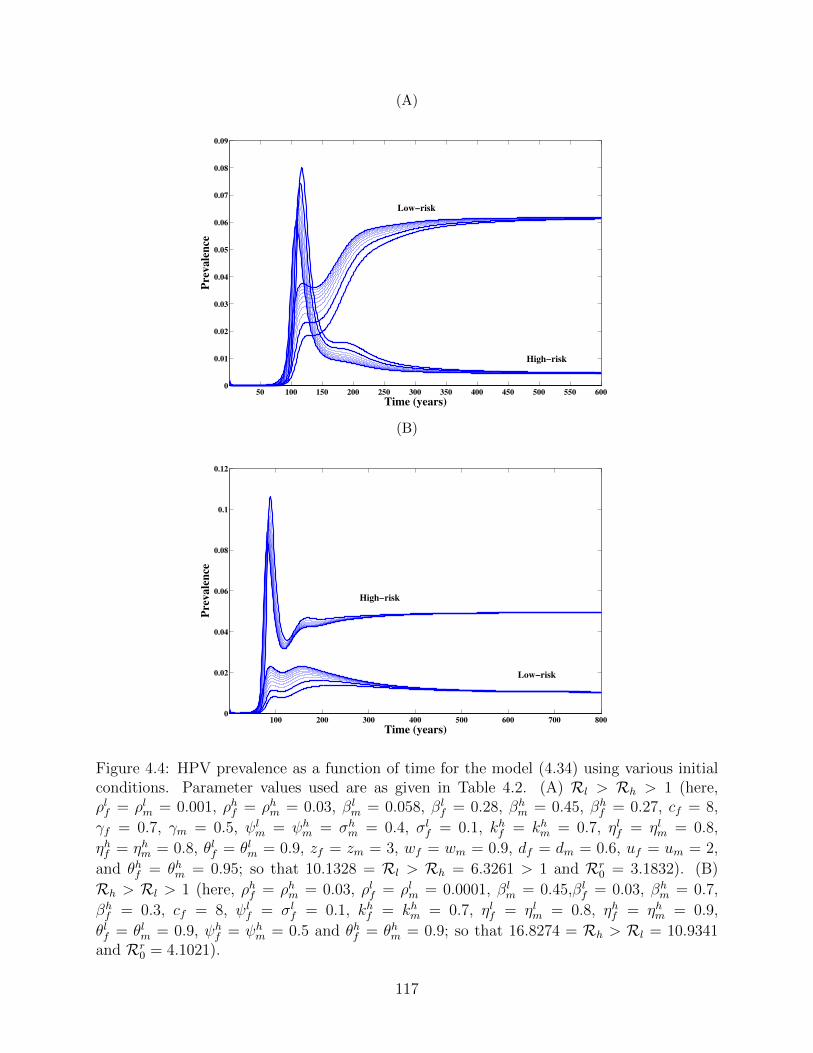
(A)
50 100 150 200 250 300 350 400 450 500 550 6000
0.01
0.02
0.03
0.04
0.05
0.06
0.07
0.08
0.09
Time (years)
Pre
va
len
ceLow!risk
High!risk
(B)
100 200 300 400 500 600 700 8000
0.02
0.04
0.06
0.08
0.1
0.12
Time (years)
Pre
va
len
ce
High!risk
Low!risk
Figure 4.4: HPV prevalence as a function of time for the model (4.34) using various initialconditions. Parameter values used are as given in Table 4.2. (A) Rl > Rh > 1 (here,ρlf = ρlm = 0.001, ρhf = ρhm = 0.03, βl
m = 0.058, βlf = 0.28, βh
m = 0.45, βhf = 0.27, cf = 8,
γf = 0.7, γm = 0.5, ψlm = ψh
m = σhm = 0.4, σl
f = 0.1, khf = kh
m = 0.7, ηlf = ηlm = 0.8,ηhf = ηhm = 0.8, θlf = θlm = 0.9, zf = zm = 3, wf = wm = 0.9, df = dm = 0.6, uf = um = 2,and θhf = θhm = 0.95; so that 10.1328 = Rl > Rh = 6.3261 > 1 and Rr
0 = 3.1832). (B)Rh > Rl > 1 (here, ρhf = ρhm = 0.03, ρlf = ρlm = 0.0001, βl
m = 0.45,βlf = 0.03, βh
m = 0.7,βhf = 0.3, cf = 8, ψl
f = σlf = 0.1, kh
f = khm = 0.7, ηlf = ηlm = 0.8, ηhf = ηhm = 0.9,
θlf = θlm = 0.9, ψhf = ψh
m = 0.5 and θhf = θhm = 0.9; so that 16.8274 = Rh > Rl = 10.9341and Rr
0 = 4.1021).
117
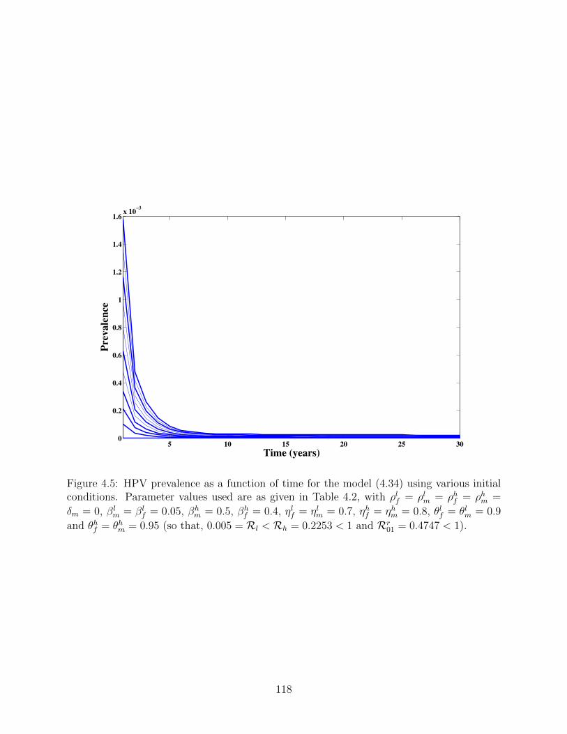
5 10 15 20 25 300
0.2
0.4
0.6
0.8
1
1.2
1.4
1.6x 10
!3
Time (years)
Pre
vale
nce
Figure 4.5: HPV prevalence as a function of time for the model (4.34) using various initialconditions. Parameter values used are as given in Table 4.2, with ρlf = ρlm = ρhf = ρhm =δm = 0, βl
m = βlf = 0.05, βh
m = 0.5, βhf = 0.4, ηlf = ηlm = 0.7, ηhf = ηhm = 0.8, θlf = θlm = 0.9
and θhf = θhm = 0.95 (so that, 0.005 = Rl < Rh = 0.2253 < 1 and Rr01 = 0.4747 < 1).
118
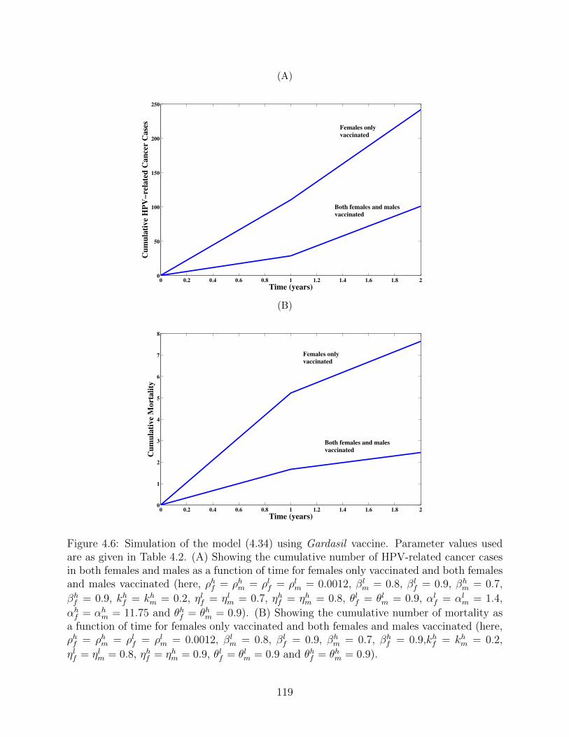
(A)
0 0.2 0.4 0.6 0.8 1 1.2 1.4 1.6 1.8 20
50
100
150
200
250
Time (years)
Cu
mu
lati
ve
HP
V!
rela
ted
Ca
nce
r C
ase
s
Both females and malesvaccinated
Females onlyvaccinated
(B)
0 0.2 0.4 0.6 0.8 1 1.2 1.4 1.6 1.8 20
1
2
3
4
5
6
7
8
Time (years)
Cu
mu
lati
ve
Mo
rta
lity
Females onlyvaccinated
Both females and malesvaccinated
Figure 4.6: Simulation of the model (4.34) using Gardasil vaccine. Parameter values usedare as given in Table 4.2. (A) Showing the cumulative number of HPV-related cancer casesin both females and males as a function of time for females only vaccinated and both femalesand males vaccinated (here, ρhf = ρhm = ρlf = ρlm = 0.0012, βl
m = 0.8, βlf = 0.9, βh
m = 0.7,βhf = 0.9, kh
f = khm = 0.2, ηlf = ηlm = 0.7, ηhf = ηhm = 0.8, θlf = θlm = 0.9, αl
f = αlm = 1.4,
αhf = αh
m = 11.75 and θhf = θhm = 0.9). (B) Showing the cumulative number of mortality asa function of time for females only vaccinated and both females and males vaccinated (here,ρhf = ρhm = ρlf = ρlm = 0.0012, βl
m = 0.8, βlf = 0.9, βh
m = 0.7, βhf = 0.9,kh
f = khm = 0.2,
ηlf = ηlm = 0.8, ηhf = ηhm = 0.9, θlf = θlm = 0.9 and θhf = θhm = 0.9).
119
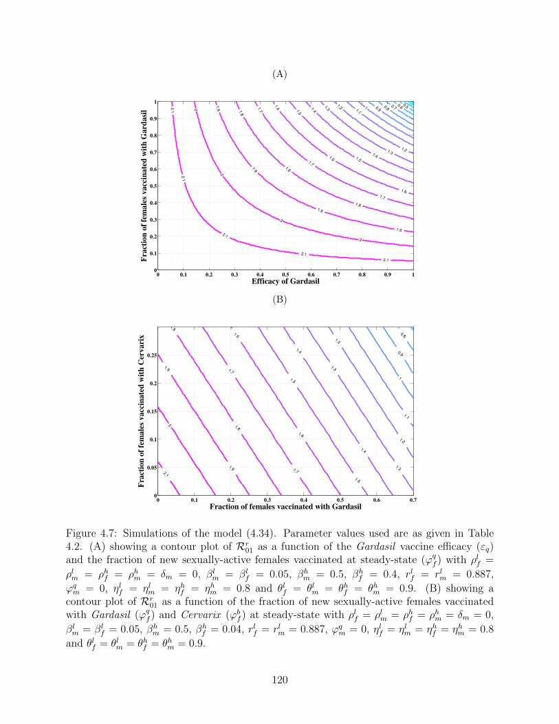
(A)
0.50.60.70.80.9
11.1
1.2
1.2
1.3
1.3
1.4
1.4
1.5
1.5
1.6
1.6
1.6
1.7
1.7
1.7
1.8
1.8
1.8
1.9
1.9
1.9
1.9
2
2
2
2
2.1
2.1
2.1
2.1
2.1
Efficacy of Gardasil
Fra
ctio
n o
f fe
ma
les
va
ccin
ate
d w
ith
Ga
rda
sil
0 0.1 0.2 0.3 0.4 0.5 0.6 0.7 0.8 0.9 10
0.1
0.2
0.3
0.4
0.5
0.6
0.7
0.8
0.9
1
(B)
0.8
0.9
1
1.1
1.2
1.2
1.3
1.3
1.4
1.4
1.5
1.5
1.6
1.6
1.7
1.7
1.8
1.8
1.9
1.9
2
2.1
Fraction of females vaccinated with Gardasil
Fra
cti
on
of
fem
ale
s v
accin
ate
d w
ith
Cerv
arix
0 0.1 0.2 0.3 0.4 0.5 0.6 0.70
0.05
0.1
0.15
0.2
0.25
Figure 4.7: Simulations of the model (4.34). Parameter values used are as given in Table4.2. (A) showing a contour plot of Rr
01 as a function of the Gardasil vaccine efficacy (εq)and the fraction of new sexually-active females vaccinated at steady-state (ϕq
f ) with ρlf =ρlm = ρhf = ρhm = δm = 0, βl
m = βlf = 0.05, βh
m = 0.5, βhf = 0.4, rlf = rlm = 0.887,
ϕqm = 0, ηlf = ηlm = ηhf = ηhm = 0.8 and θlf = θlm = θhf = θhm = 0.9. (B) showing a
contour plot of Rr01 as a function of the fraction of new sexually-active females vaccinated
with Gardasil (ϕqf ) and Cervarix (ϕb
f ) at steady-state with ρlf = ρlm = ρhf = ρhm = δm = 0,βlm = βl
f = 0.05, βhm = 0.5, βh
f = 0.04, rlf = rlm = 0.887, ϕqm = 0, ηlf = ηlm = ηhf = ηhm = 0.8
and θlf = θlm = θhf = θhm = 0.9.
120
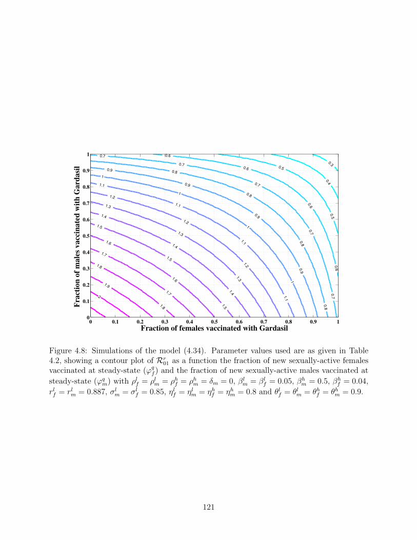
0.3
0.4
0.5
0.5
0.6
0.6
0.6
0.6
0.7
0.7
0.7
0.7
0.7
0.8
0.8
0.8
0.8
0.9
0.9
0.9
0.9
1
1
1
1
1.1
1.1
1.1
1.1
1.2
1.2
1.2
1.3
1.3
1.3
1.4
1.4
1.4
1.5
1.5
1.5
1.6
1.6
1.7
1.71.8
1.8
1.9
2
Fraction of females vaccinated with Gardasil
Fracti
on
of
male
s v
accin
ate
d w
ith
Gard
asil
0 0.1 0.2 0.3 0.4 0.5 0.6 0.7 0.8 0.9 10
0.1
0.2
0.3
0.4
0.5
0.6
0.7
0.8
0.9
1
Figure 4.8: Simulations of the model (4.34). Parameter values used are as given in Table4.2, showing a contour plot of Rr
01 as a function the fraction of new sexually-active femalesvaccinated at steady-state (ϕq
f ) and the fraction of new sexually-active males vaccinated atsteady-state (ϕq
m) with ρlf = ρlm = ρhf = ρhm = δm = 0, βlm = βl
f = 0.05, βhm = 0.5, βh
f = 0.04,rlf = rlm = 0.887, σl
m = σlf = 0.85, ηlf = ηlm = ηhf = ηhm = 0.8 and θlf = θlm = θhf = θhm = 0.9.
121

Chapter 5
Contributions of the Thesis and
Future Work
The thesis contributes in three main categories, namely:
i) model formulation: formulation of novel anti-HPV vaccination models, of the form
of deterministic systems of non-linear differential equations, for the transmission dy-
namics of HPV, and the associated cancers and warts, in a community;
ii) mathematical analysis: carrying out detailed qualitative (mathematical) analysis of
the models developed in the thesis (in particular, finding conditions for the existence
and asymptotic stability of the associated equilibria);
iii) public health: using the models developed in the thesis to evaluate the impact of the
anti-HPV Cervarix and Gardasil vaccines in combatting the spread of the four chosen
HPV-types (HPV-6, HPV-11, HPV-16 and HPV-18).
The specific contributions of the thesis are summarized below.
122
5.1 Model Formulation
The thesis consists of two new models for HPV transmission dynamics (and the associated
cancers and warts) in a community.
i) The first model, given by (3.19), is for the transmission dynamics of HPV (and the
associated cancers in females) in a population, in the presence of the Gardasil vaccine
(which targets the four HPV types, HPV-6, HPV-11, HPV-16 and HPV-18) for new
sexually-active susceptible females. Some of the novelties of this model (in relation to
the many other HPV transmission models in the literature, including those in [9, 24,
25, 26, 61]) is that it:
a) includes the dynamics of the exposed (i.e., latently-infected) individuals;
b) allows for the transmission of HPV by exposed individuals;
c) allows for the loss of infection-acquired immunity by recovered individuals;
d) allows for the re-infection of recovered individuals.
Furthermore, the model (3.19) extends the models in [9, 26] by, additionally, including
cancer-induced mortality in females and the dynamics of females with persistent HPV
infection.
ii) The second model, given by (4.34), is based on extending the model developed in
Chapter 3 to study the transmission dynamics of the low- and high-risk HPV types in
the presence of the Cervarix and Gardasil vaccines. Some of the notable new features
of the model (4.34), in relation to the model (3.19), are:
a) stratifying the entire population in terms of the risk of transmitting either the low-
risk (HPV-6 and HPV-11) or the high-risk (HPV-16 and HPV-18) HPV types;
b) incorporating two anti-HPV vaccines (Cervarix and Gardasil);
123
c) allowing for mass vaccination of new sexually-active susceptible males (with the
Gardasil vaccine);
d) including the dynamics of infected individuals with genital warts;
e) including the dynamics of individuals in the low-grade and high-grade pre-cancer
stages (CIN for females and INM for males);
f) including the dynamics of infected males:
1) with HPV-related cancers;
2) cancer-induced mortality for males;
3) infected males who recovered from HPV-related cancers;
4) a compartment for males with persistent HPV infection.
5.2 Mathematical Analysis
A major contribution of the thesis is the detailed qualitative analyses of (the two models) it
contains. Some of the main mathematical results obtained are summarized below.
5.2.1 Chapter 3
The model (3.19), and its vaccination-free version (3.21), are qualitatively analysed. The
leading following theoretical results were obtained:
i) it is shown, using the next generation operator method, that each of the two models
has a locally-asymptotically stable disease-free equilibrium whenever its associated
reproduction number is less than unity;
ii) each of the two models has at least one endemic equilibrium whenever its associated
reproduction threshold exceeds unity. For the case when the models have a unique
endemic equilibrium, it is shown, using a Krasnoselskii sub-linearity argument, that
the unique endemic equilibrium is locally-asymptotically stable;
124

iii) the two models undergo the phenomenon of backward bifurcation under certain condi-
tions. The backward bifurcation phenomenon, proved using Centre Manifold Theory,
is shown to arise due to the re-infection of recovered individuals;
iv) in the absence of the re-infection of recovered individuals, it is shown, using Comparison
Theorem and Lyapunov Function theory, that the associated disease-free equilibrium
of the two models are globally-asymptotically stable whenever the respective associated
reproduction threshold is less than unity;
v) overall, it is shown that the two models (vaccination and vaccination-free models)
developed in Chapter 3 have essentially the same qualitative features. Thus, this
study shows that adding vaccination to the vaccination-free model (3.21) does not alter
its qualitative dynamics with respect to the existence and stability of its associated
equilibria, as well as with respect to its backward bifurcation property.
5.2.2 Chapter 4
The model (4.34), and the low-risk-only version (4.37), are qualitatively analysed.
i) Each of the two models has a locally-asymptotically stable disease-free equilibrium
whenever its associated reproduction threshold is less than unity;
ii) it is shown that both models have at least one endemic equilibrium whenever the
reproduction threshold exceeds unity;
iii) it is shown that the low-risk-only model (4.37) undergoes a re-infection-induced back-
ward bifurcation under certain conditions;
iv) in the absence of the re-infection of recovered individuals and cancer-induced mortality
in males, it is shown that the disease-free equilibrium of the model (4.34) is globally-
asymptotically stable whenever the associated reproduction threshold is less than unity.
125
5.3 Public Health
The models developed in this thesis are simulated, using the parameter values in Tables 3.1
and 4.2, to gain quantitative insight into the transmission dynamics of HPV (and related
cancers and warts) in a community. Some of the main public health contributions of the
thesis, derived from these simulations, are summarized below:
i) the vaccination model in Chapter 3 shows that the mass vaccination of new sexually-
active females only, using the Gardasil vaccine (with the assumed efficacy of 90%), can
lead to effective community-wide control (or elimination) of HPV if at least 78% of the
new sexually-active susceptible female population is vaccinated at steady-state. How-
ever, the model in Chapter 4 shows that vaccinating new sexually-active susceptible
females alone (with the Gardasil vaccine) can lead to effective control, or elimination,
of HPV from the community if at least 87% of the new sexually-active susceptible
females are vaccinated. Unfortunately, however, since the current Gardasil coverage
in most communities is about 70% [9, 26, 46, 61, 76], this study shows that the sin-
gular use of Gardasil (with the 70% coverage) is inadequate to lead to the effective
control of HPV (since it fails to bring the associated reproduction threshold of the two
vaccination models, (3.19) and (4.34), to be less than unity);
ii) vaccinating new sexually-active susceptible males offers beneficial community-wide im-
pact. In particular, simulations show that while vaccinating new sexually-active suscep-
tible females only (at the assumed 70% coverage rate) resulted in about 250 cumulative
cancer cases over two years, this number reduces to about 100, over the same time pe-
riod, if both new sexually-active males (with 70% Gardasil coverage) and females are
vaccinated. Furthermore, while vaccinating new sexually-active females only with the
Gardasil vaccine (at the 70% coverage level) resulted in about 8 cumulative mortality
cases over two years, only 2 cancer-related deaths are recorded, over the same time
period, if both new sexually-active males and females are vaccinated;
126
iii) if only 70% of the new sexually-active susceptible females are vaccinated with the
Gardasil vaccine, additionally vaccinating 47% of new sexually-active susceptible males
will lead to the community-wide elimination of the low- and high-risk HPV types;
iv) it is shown that, with the assumed 70% Gardasil vaccine coverage for new sexually-
active females, at least 18% of the remaining unvaccinated susceptible females need to
be vaccinated with the Cervarix vaccine in order to effectively control the disease.
5.4 Future Work
The work in this thesis can be extended in several directions (in terms of model construction
and associated mathematical analyses), such as:
i) including age-structure (since both vaccines are recommended to be administered to
individuals in certain age groups [15, 76, 93, 96]);
ii) including other anti-HPV intervention strategies (such as condom use and Pap screen-
ing, which are also considered as standard anti-HPV control strategies [15, 27, 61, 76]);
iii) explicitly incorporating the effect of co-infection (of multiple HPV types and/or with
other STIs);
iv) carrying out a cost-benefit analysis of implementing the mass vaccination program in
a community;
v) vaccination of older susceptible men and women (outside the 9-26 age bracket). The ob-
jective is to determine whether vaccinating this age group offers beneficial community-
wide impact;
vi) incorporate the homosexual transmission of HPV. This is crucial since HPV can also
be transmitted via this route. This aspect of HPV transmission dynamics has not yet
been addressed in the literature;
127
vii) modelling the in-host dynamics of HPV;
viii) establishing the global asymptotic stability of the endemic and/or boundary equilibria
of the models (mathematical interest). Establishing the global asymptotic stability of
a relatively large dynamical system, such as the 29-dimensional model in Chapter 4,
is always of significant mathematical interest (since one key objective of mathematical
biology research is to develop new mathematical techniques and theories for analysing
relatively large systems of non-linear differential equations).
128
Appendix A
Proof of Theorem 3.1
Proof. Let t1 = sup{t > 0 : Sf (t) > 0, Vf (t) > 0, Ef (t) > 0, If (t) > 0, P (t) > 0, C(t) >
0, Rc(t) > 0, Rf (t) > 0, Sm(t) > 0, Em(t) > 0, Im(t) > 0, Rm(t) > 0} > 0. It follows from the
first equation of the vaccination model (3.19) that
dSf
dt= πf (1− ϕf ) + ξfRf (t)− λm(t)Sf (t)− µfSf (t) ≥ πf (1− ϕf )− [λm(t) + µf ]Sf (t),
which can be re-written as,
d
dt
�Sf (t) exp
�µf t+
� t
0
λm(τ) dτ
��≥ πf (1− ϕf ) exp
�µf t+
� t
0
λm(τ) dτ
�.
Hence,
Sf (t1) exp
�µf t1 +
� t1
0
λm(τ) dτ
�− Sf (0) ≥
� t1
0
πf (1− ϕf ) exp
�µfy +
� y
0
λm(τ) dτ
�dy,
so that,
129
Sf (t1) ≥ Sf (0) exp
�−µf t1 −
� t1
0
λm(τ) dτ
�
+
�exp
�−µf t1 −
� t1
0
λm(τ) dτ
��� t1
0
πf (1− ϕf ) exp
�µfy +
� y
0
λm(τ) dτ
�dy > 0.
Similarly, it can be shown that Vf (t) > 0, Ef (t) ≥ 0, If (t) ≥ 0, P (t) ≥ 0, C(t) ≥ 0, Rc(t) ≥
0, Rf (t) ≥ 0, Sm(t) ≥ 0, Em(t) ≥ 0, Im(t) ≥ 0, and Rm(t) ≥ 0 for all time t > 0. Hence, all
solutions remain positive for all non-negative initial conditions.
Theorem 3.1 can also be proved using the approach given in Appendix A of [92].
130
Appendix B
Proof of Theorem 3.5
Proof. Consider the vaccination-free model (3.21) with ρf = ρm = 0. The proof of Theorem
3.5 is based on using a Krasnoselskii sub-linearity trick, as given in [91] (see also [31, 32]).
The method essentially entails proving that the linearization of the model system (3.21),
around the EEP (E1) of the vaccination-free model (3.21), has no solutions of the form
Z(t) = Z0eωt, (B.1)
with,
Z0 = (Z1, Z2, Z3, Z4, Z5, Z6, Z7, Z8, Z9, Z10, Z11) , Zi ∈ C, ω ∈ C, and Re(ω) ≥ 0.
This implies that the eigenvalues of the characteristic polynomial associated with the lin-
earized equations have negative real part (i.e., Re (ω) < 0). Then the EEP, E1, is locally
asymptotically stable. For simplicity, consider the special case of the vaccination-free model
(3.21) with the probability of re-infection set to zero (so that, ρm = ρf = 0 in (3.21)). The
linearized system of (3.21), around the EEP E1 (with ρm = ρf = 0), gives the following
system of linear equations
131
ωZ1 = −
�βmcfµm (ηmE∗∗
m + I∗∗m )
πm+ µf
�Z1 + ξfZ7 −
βmcfµmηmS∗∗f
πmZ9 −
βmcfµmS∗∗f
πmZ10,
ωZ2 =βmcfµm (ηmE∗∗
m + I∗∗m )
πmZ1 − g1Z2 +
βmcfµmηmS∗∗f
πmZ9 +
βmcfµmS∗∗f
πmZ10,
ωZ3 = σfZ2 − g2Z3,
ωZ4 = h1Z3 − n1Z4,
ωZ5 = h2Z4 − n2Z5,
ωZ6 = γfZ5 − µfZ6, (B.2)
ωZ7 = m1Z3 +m2Z4 − g3Z7,
ωZ8 = −βfcfµmηfS∗∗
m
πmZ2 −
βfcfµmS∗∗m
πmZ3 −
βfcfµmθpS∗∗m
πmZ4
−
�βfcfµm
�ηfE∗∗
f + I∗∗f + θpP ∗∗�
πm+ µm
�Z8 + ξmZ11,
ωZ9 =βfcfµmηfS∗∗
m
πmZ2 +
βfcfµmS∗∗m
πmZ3 +
βfcfµmθpS∗∗m
πmZ4 +
βfcfµm
�ηfE∗∗
f + I∗∗f + θpP ∗∗�
πmZ8
− g4Z9,
ωZ10 = σmZ9 − g5Z10,
ωZ11 = ψmZ10 − g6Z11,
132
which is equivalent to the system
�1 +
1
µf
�ω +
βmcfµm (ηmE∗∗m + I∗∗m )
πm
��Z1 =
ξfµf
Z7 −βmcfµmηmS∗∗
f
µfπmZ9
−βmcfµmS∗∗
f
µfπmZ10,
�1 +
ω
g1
�Z2 =
βmcfµm (ηmE∗∗m + I∗∗m )
g1πmZ1
+βmcfµmηmS∗∗
f
g1πmZ9 +
βmcfµmS∗∗f
g1πmZ10,
�1 +
ω
g2
�Z3 =
σf
g2Z2,
�1 +
ω
n1
�Z4 =
h1
n1Z3,
�1 +
ω
n2
�Z5 =
h2
n2Z4,
�1 +
ω
µf
�Z6 =
γfµf
Z5, (B.3)
�1 +
ω
g3
�Z7 =
m1
g3Z3 +
m2
g3Z4,
�1 +
1
µm
�ω +
βfcfµm
�ηfE∗∗
f + I∗∗f + θpP ∗∗�
πm
��Z8 = −
βfcfηfS∗∗m
πmZ2 −
βfcfS∗∗m
πmZ3
−βfcfθpS∗∗
m
πmZ4 +
ξmµm
Z11,�1 +
ω
g4
�Z9 =
βfcfµmηfS∗∗m
g4πmZ2 +
βfcfµmS∗∗m
g4πmZ3
+βfcfµmθpS∗∗
m
g4πmZ4
+βfcfµm
�ηfE∗∗
f + I∗∗f + θpP ∗∗�
g4πmZ8,
�1 +
ω
g5
�Z10 =
σm
g5Z9,
�1 +
ω
g6
�Z11 =
ψm
g6Z10.
Adding the first, ninth, and tenth equations of (B.3), and then adding the second, third,
fourth, and eighth equations of (B.3), and finally moving all the negative terms to the left-
133
hand side (and simplifying) gives the following system:
[1 + F1 (ω)]Z1 + [1 + F9 (ω)]Z9 + [1 + F10 (ω)]Z10 =�HZ
�1+�HZ
�9
+�HZ
�10,
[1 + F2 (ω)]Z2 + [1 + F3 (ω)]Z3 + [1 + F4 (ω)]Z4 + [1 + F8 (ω)]Z8 =�HZ
�2+�HZ
�3
+�HZ
�4+�HZ
�8,
[1 + F5 (ω)]Z5 =�HZ
�5, (B.4)
[1 + F6 (ω)]Z6 =�HZ
�6,
[1 + F7 (ω)]Z7 =�HZ
�7,
[1 + F11 (ω)]Z11 =�HZ
�11,
134
where,
F1 (ω) =1
µf
�ω +
βmcfµm (ηmE∗∗m + I∗∗m )
πm
�,
F2 (ω) =1
g1
�ω +
g1βfcfηfS∗∗m
πm
�,
F3 (ω) =1
g2
�ω +
g2βfcfS∗∗m
πm
�,
F4 (ω) =1
n1
�ω +
n1βfcfθpS∗∗m
πm
�,
F5 (ω) =ω
n2,
F6 (ω) =ω
µf,
F7 (ω) =ω
g3,
F8 (ω) =1
µm
�ω +
βfcfµm
�ηfE∗∗
f + I∗∗f + θpP ∗∗�
πm
�,
F9 (ω) =1
g4
�ω +
g3βmcfµmηmS∗∗f
µfπm
�,
F10 (ω) =1
g5
�ω +
g4βmcfµmS∗∗f
µfπm
�,
F11 (ω) =ω
g6,
135
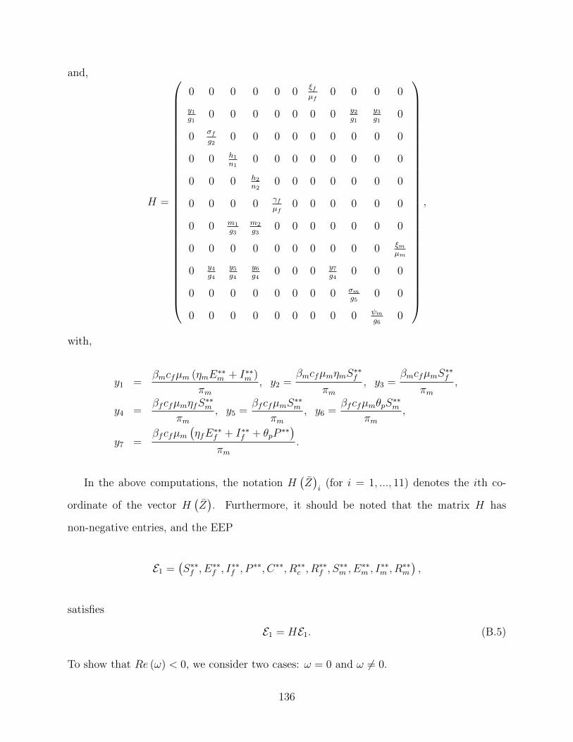
and,
H =
0 0 0 0 0 0 ξfµf
0 0 0 0
y1g1
0 0 0 0 0 0 0 y2g1
y3g1
0
0 σf
g20 0 0 0 0 0 0 0 0
0 0 h1n1
0 0 0 0 0 0 0 0
0 0 0 h2n2
0 0 0 0 0 0 0
0 0 0 0 γfµf
0 0 0 0 0 0
0 0 m1g3
m2g3
0 0 0 0 0 0 0
0 0 0 0 0 0 0 0 0 0 ξmµm
0 y4g4
y5g4
y6g4
0 0 0 y7g4
0 0 0
0 0 0 0 0 0 0 0 σmg5
0 0
0 0 0 0 0 0 0 0 0 ψm
g60
,
with,
y1 =βmcfµm (ηmE∗∗
m + I∗∗m )
πm, y2 =
βmcfµmηmS∗∗f
πm, y3 =
βmcfµmS∗∗f
πm,
y4 =βfcfµmηfS∗∗
m
πm, y5 =
βfcfµmS∗∗m
πm, y6 =
βfcfµmθpS∗∗m
πm,
y7 =βfcfµm
�ηfE∗∗
f + I∗∗f + θpP ∗∗�
πm.
In the above computations, the notation H�Z�i(for i = 1, ..., 11) denotes the ith co-
ordinate of the vector H�Z�. Furthermore, it should be noted that the matrix H has
non-negative entries, and the EEP
E1 =�S∗∗f , E∗∗
f , I∗∗f , P ∗∗, C∗∗, R∗∗c , R∗∗
f , S∗∗m , E∗∗
m , I∗∗m , R∗∗m
�,
satisfies
E1 = HE1. (B.5)
To show that Re (ω) < 0, we consider two cases: ω = 0 and ω �= 0.
136
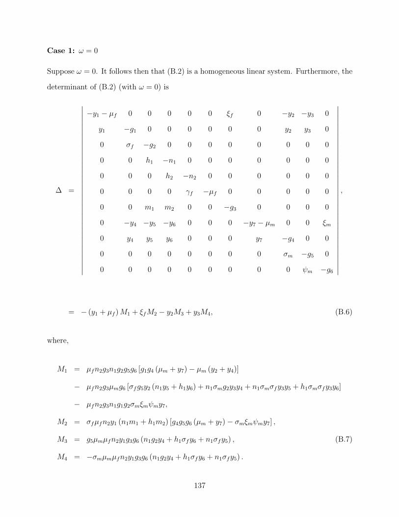
Case 1: ω = 0
Suppose ω = 0. It follows then that (B.2) is a homogeneous linear system. Furthermore, the
determinant of (B.2) (with ω = 0) is
∆ =
������������������������������������
−y1 − µf 0 0 0 0 0 ξf 0 −y2 −y3 0
y1 −g1 0 0 0 0 0 0 y2 y3 0
0 σf −g2 0 0 0 0 0 0 0 0
0 0 h1 −n1 0 0 0 0 0 0 0
0 0 0 h2 −n2 0 0 0 0 0 0
0 0 0 0 γf −µf 0 0 0 0 0
0 0 m1 m2 0 0 −g3 0 0 0 0
0 −y4 −y5 −y6 0 0 0 −y7 − µm 0 0 ξm
0 y4 y5 y6 0 0 0 y7 −g4 0 0
0 0 0 0 0 0 0 0 σm −g5 0
0 0 0 0 0 0 0 0 0 ψm −g6
������������������������������������
,
= − (y1 + µf )M1 + ξfM2 − y2M3 + y3M4, (B.6)
where,
M1 = µfn2g3n1g2g5g6 [g1g4 (µm + y7)− µm (y2 + y4)]
− µfn2g3µmg6 [σfg5y2 (n1y5 + h1y6) + n1σmg2y3y4 + n1σmσfy3y5 + h1σmσfy3y6]
− µfn2g3n1g1g2σmξmψmy7,
M2 = σfµfn2y1 (n1m1 + h1m2) [g4g5g6 (µm + y7)− σmξmψmy7] ,
M3 = g5µmµfn2y1g3g6 (n1g2y4 + h1σfy6 + n1σfy5) , (B.7)
M4 = −σmµmµfn2y1g3g6 (n1g2y4 + h1σfy6 + n1σfy5) .
137
It can be shown, by simplifying (B.6) with (B.7), that the determinant, ∆, is non-zero.
Hence, for the case that ω = 0, the linear system (B.2) has only the trivial solution Z = 0.
This implies that ω �= 0.
Case 2: ω �= 0
Now assume that ω �= 0 and Re (ω) ≥ 0 (assume the contrary to show that Re (ω) < 0). Let
F (ω) = min {|1 + Fi (ω)| , i = 1, 2, 3, ..., 11}. It can be shown from (B.4) that |1 + Fi (ω)| > 1
for all i. Hence, F (ω) > 1. On the other hand, since the coordinates of E1 are positive, if Z
is any solution of (B.4), then there exists a minimal positive real number s such that
��Z�� ≤ sE1,
where��Z
�� = (|Z1| , |Z2| , |Z3| , |Z4| , ..., |Z11|) and |.| is the norm in C. Therefore, sF (ω) < s and
the minimality of s implies that��Z
�� > sF (ω)E1. Since s is the minimal positive real number
such that
|Z11| ≤ sR∗∗m , (B.8)
Taking norms on both side of last equation of (B.4), and using (B.5), (B.8) and the fact that
H is nonnegative, gives
F (ω) |Z11| ≤ H (|Z|)11 ≤ sR∗∗m ,
so that,
|Z11| ≤s
F (ω)R∗∗
m < sR∗∗m ,
which contradicts the minimality of s. Hence, Re (ω) < 0. This concludes the proof.
138
Appendix C
Proof of Theorem 3.6
Proof. The Centre Manifold Theory, as described in [14], will be used to prove Theorem 3.6.
It is convenient to, first of all, make the following changes of variables. Let,
Sf = x1, Ef = x2, If = x3, P = x4, C = x5, Rc = x6, Rf = x7,
and,
Sm = x8, Em = x9, Im = x10, Rm = x11.
Furthermore, it should be noted that the total male population, now given by Nm = x8 +
x9+x10+x11 is replaced by its limiting value πmµm
. Hence, the model (3.19) can be re-written
in the form:
139
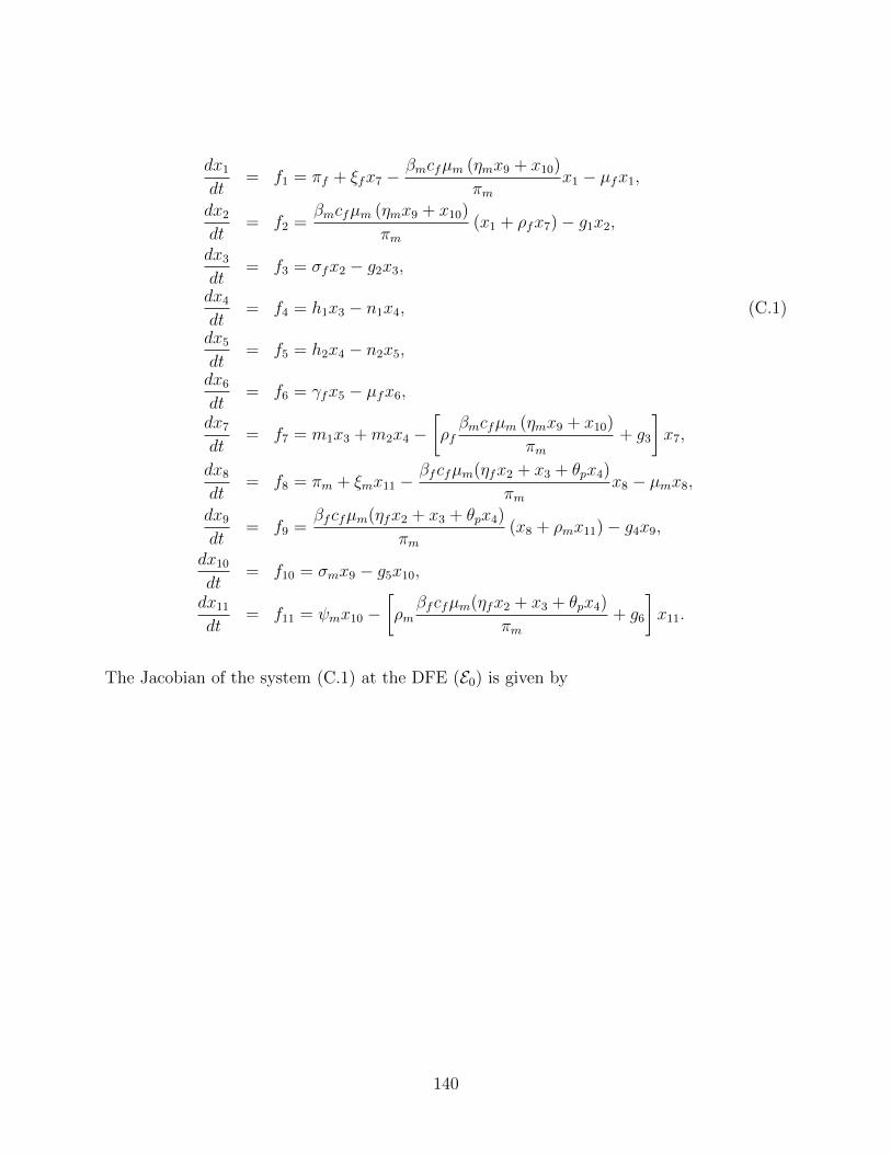
dx1
dt= f1 = πf + ξfx7 −
βmcfµm (ηmx9 + x10)
πmx1 − µfx1,
dx2
dt= f2 =
βmcfµm (ηmx9 + x10)
πm(x1 + ρfx7)− g1x2,
dx3
dt= f3 = σfx2 − g2x3,
dx4
dt= f4 = h1x3 − n1x4, (C.1)
dx5
dt= f5 = h2x4 − n2x5,
dx6
dt= f6 = γfx5 − µfx6,
dx7
dt= f7 = m1x3 +m2x4 −
�ρf
βmcfµm (ηmx9 + x10)
πm+ g3
�x7,
dx8
dt= f8 = πm + ξmx11 −
βfcfµm(ηfx2 + x3 + θpx4)
πmx8 − µmx8,
dx9
dt= f9 =
βfcfµm(ηfx2 + x3 + θpx4)
πm(x8 + ρmx11)− g4x9,
dx10
dt= f10 = σmx9 − g5x10,
dx11
dt= f11 = ψmx10 −
�ρm
βfcfµm(ηfx2 + x3 + θpx4)
πm+ g6
�x11.
The Jacobian of the system (C.1) at the DFE (E0) is given by
140
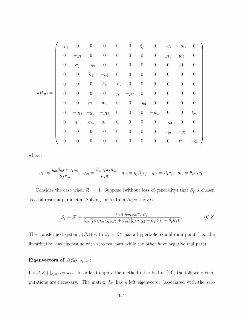
J(E0) =
−µf 0 0 0 0 0 ξf 0 −g11 −g12 0
0 −g1 0 0 0 0 0 0 g11 g12 0
0 σf −g2 0 0 0 0 0 0 0 0
0 0 h1 −n1 0 0 0 0 0 0 0
0 0 0 h2 −n2 0 0 0 0 0 0
0 0 0 0 γf −µf 0 0 0 0 0
0 0 m1 m2 0 0 −g3 0 0 0 0
0 −g13 −g14 −g15 0 0 0 −µm 0 0 ξm
0 g13 g14 g15 0 0 0 0 −g4 0 0
0 0 0 0 0 0 0 0 σm −g5 0
0 0 0 0 0 0 0 0 0 ψm −g6
,
where,
g11 =ηmβmcfπfµm
µfπm, g12 =
βmcfπfµm
µfπm, g13 = ηfβfcf , g14 = βfcf , g15 = θpβfcf .
Consider the case when R0 = 1. Suppose (without loss of generality) that βf is chosen
as a bifurcation parameter. Solving for βf from R0 = 1 gives
βf = β∗ =n1g1g2g4g5πmµf
βmc2fπfµm (ηmg5 + σm) [ηfn1g2 + σf (n1 + θph1)]. (C.2)
The transformed system, (C.1) with βf = β∗, has a hyperbolic equilibrium point (i.e., the
linearization has eigenvalue with zero real part while the other have negative real part).
Eigenvectors of J(E0) |βf=β∗:
Let J(E0) |βf=β∗= Jβ∗ . In order to apply the method described in [14], the following com-
putations are necessary. The matrix Jβ∗ has a left eigenvector (associated with the zero
141
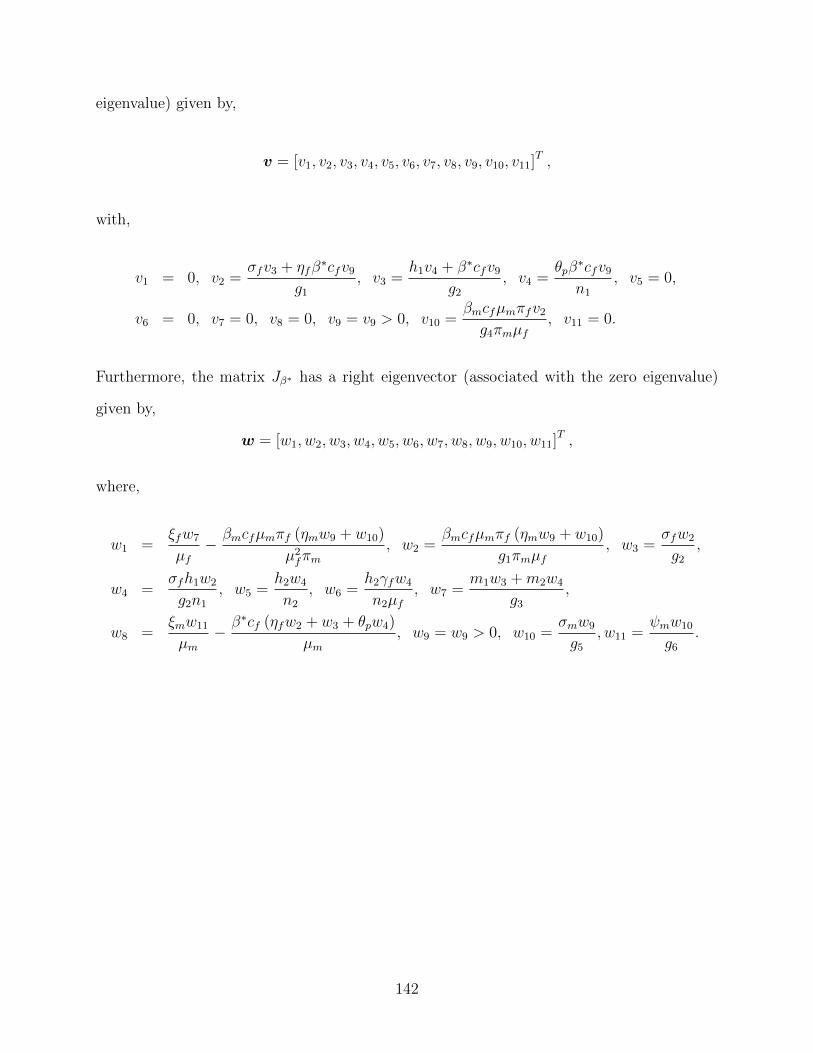
eigenvalue) given by,
v = [v1, v2, v3, v4, v5, v6, v7, v8, v9, v10, v11]T ,
with,
v1 = 0, v2 =σfv3 + ηfβ∗cfv9
g1, v3 =
h1v4 + β∗cfv9g2
, v4 =θpβ∗cfv9
n1, v5 = 0,
v6 = 0, v7 = 0, v8 = 0, v9 = v9 > 0, v10 =βmcfµmπfv2
g4πmµf, v11 = 0.
Furthermore, the matrix Jβ∗ has a right eigenvector (associated with the zero eigenvalue)
given by,
w = [w1, w2, w3, w4, w5, w6, w7, w8, w9, w10, w11]T ,
where,
w1 =ξfw7
µf−
βmcfµmπf (ηmw9 + w10)
µ2fπm
, w2 =βmcfµmπf (ηmw9 + w10)
g1πmµf, w3 =
σfw2
g2,
w4 =σfh1w2
g2n1, w5 =
h2w4
n2, w6 =
h2γfw4
n2µf, w7 =
m1w3 +m2w4
g3,
w8 =ξmw11
µm−
β∗cf (ηfw2 + w3 + θpw4)
µm, w9 = w9 > 0, w10 =
σmw9
g5, w11 =
ψmw10
g6.
142
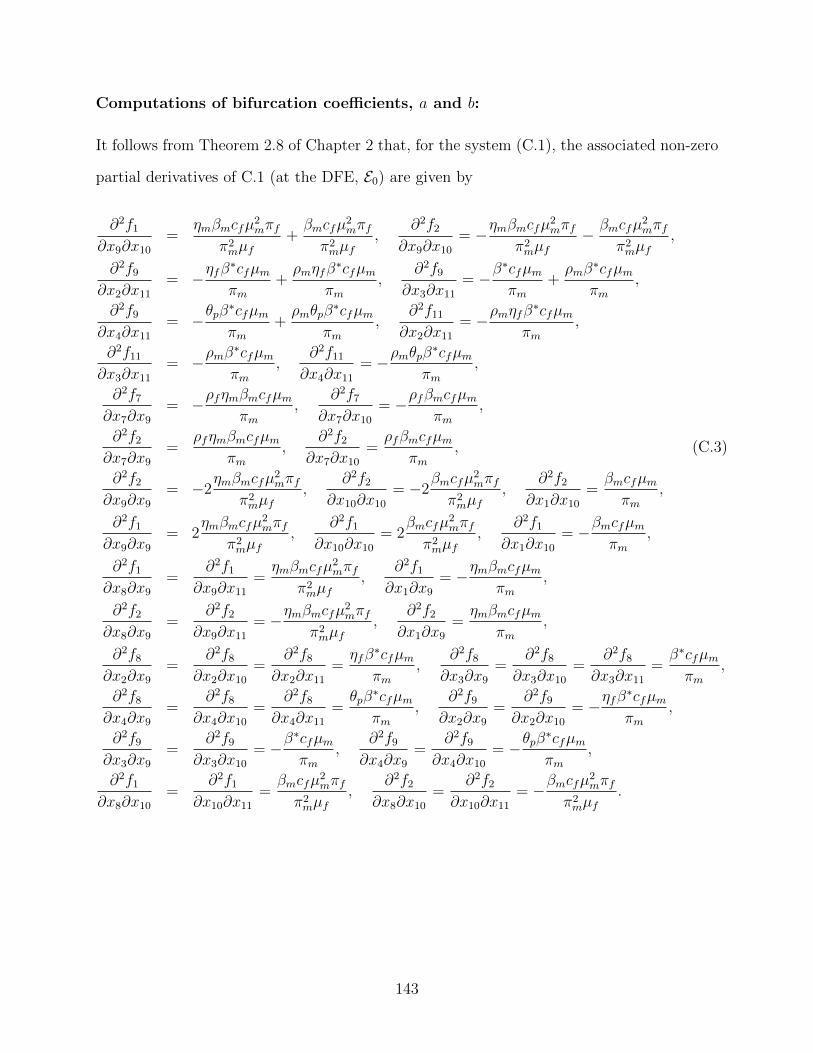
Computations of bifurcation coefficients, a and b:
It follows from Theorem 2.8 of Chapter 2 that, for the system (C.1), the associated non-zero
partial derivatives of C.1 (at the DFE, E0) are given by
∂2f1∂x9∂x10
=ηmβmcfµ2
mπf
π2mµf
+βmcfµ2
mπf
π2mµf
,∂2f2
∂x9∂x10= −
ηmβmcfµ2mπf
π2mµf
−βmcfµ2
mπf
π2mµf
,
∂2f9∂x2∂x11
= −ηfβ∗cfµm
πm+
ρmηfβ∗cfµm
πm,
∂2f9∂x3∂x11
= −β∗cfµm
πm+
ρmβ∗cfµm
πm,
∂2f9∂x4∂x11
= −θpβ∗cfµm
πm+
ρmθpβ∗cfµm
πm,
∂2f11∂x2∂x11
= −ρmηfβ∗cfµm
πm,
∂2f11∂x3∂x11
= −ρmβ∗cfµm
πm,
∂2f11∂x4∂x11
= −ρmθpβ∗cfµm
πm,
∂2f7∂x7∂x9
= −ρfηmβmcfµm
πm,
∂2f7∂x7∂x10
= −ρfβmcfµm
πm,
∂2f2∂x7∂x9
=ρfηmβmcfµm
πm,
∂2f2∂x7∂x10
=ρfβmcfµm
πm, (C.3)
∂2f2∂x9∂x9
= −2ηmβmcfµ2
mπf
π2mµf
,∂2f2
∂x10∂x10= −2
βmcfµ2mπf
π2mµf
,∂2f2
∂x1∂x10=
βmcfµm
πm,
∂2f1∂x9∂x9
= 2ηmβmcfµ2
mπf
π2mµf
,∂2f1
∂x10∂x10= 2
βmcfµ2mπf
π2mµf
,∂2f1
∂x1∂x10= −
βmcfµm
πm,
∂2f1∂x8∂x9
=∂2f1
∂x9∂x11=
ηmβmcfµ2mπf
π2mµf
,∂2f1
∂x1∂x9= −
ηmβmcfµm
πm,
∂2f2∂x8∂x9
=∂2f2
∂x9∂x11= −
ηmβmcfµ2mπf
π2mµf
,∂2f2
∂x1∂x9=
ηmβmcfµm
πm,
∂2f8∂x2∂x9
=∂2f8
∂x2∂x10=
∂2f8∂x2∂x11
=ηfβ∗cfµm
πm,
∂2f8∂x3∂x9
=∂2f8
∂x3∂x10=
∂2f8∂x3∂x11
=β∗cfµm
πm,
∂2f8∂x4∂x9
=∂2f8
∂x4∂x10=
∂2f8∂x4∂x11
=θpβ∗cfµm
πm,
∂2f9∂x2∂x9
=∂2f9
∂x2∂x10= −
ηfβ∗cfµm
πm,
∂2f9∂x3∂x9
=∂2f9
∂x3∂x10= −
β∗cfµm
πm,
∂2f9∂x4∂x9
=∂2f9
∂x4∂x10= −
θpβ∗cfµm
πm,
∂2f1∂x8∂x10
=∂2f1
∂x10∂x11=
βmcfµ2mπf
π2mµf
,∂2f2
∂x8∂x10=
∂2f2∂x10∂x11
= −βmcfµ2
mπf
π2mµf
.
143
It follows from the expressions in (C.3), and Theorem 2.8 of Chapter 2, that
a =11�
k,i,j=1
vkwiwj∂2fk
∂xi∂xj(0, 0),
=2cfµm
µ2fπ
2m
[A1v2 (ηmw9 + w10) + A2v9 (ηfw2 + w3 + θpw4)] (C.4)
−2cfµm
µ2fπ
2m
[B1v2 (ηmw9 + w10) + B2v9 (ηfw2 + w3 + θpw4) + B3] ,
with,
A1 = βm [πmµf (ξf + µfρf )w7 + β∗πfµfcf (ηfw2 + w3 + θpw4)] ,
A2 = β∗πmµ2fρmw11,
B1 = βmπf [µf (ξmw11 + µm (w9 + w11)) + cfµm (ηmw9 + w10)] ,
B2 = β∗πmµ2f (w9 + w10 + w11) ,
B3 = βmπfµmµfv2w10 (w9 + w10) ,
and,
b =11�
k,i=1
vkwi∂2fk
∂xi∂β∗ (0, 0) = cfv9 (ηfw2 + w3 + θpw4) > 0.
It is evident from (C.4) that the bifurcation coefficient, a, is positive whenever
Q1 > Q2, (C.5)
where,
Q1 = A1v2 (ηmw9 + w10) + A2v9 (ηfw2 + w3 + θpw4) ,
Q2 = B1v2 (ηmw9 + w10) + B2v9 (ηfw2 + w3 + θpw4) + B3.
144
Thus, it follows from Theorem 2.8, that the vaccination-free model (3.21) undergoes back-
ward bifurcation whenever Inequality (C.5) holds.
The inequality (C.5) can be expressed in terms of the re-infection parameter for recovered
females, ρf , as
ρf > ρcf , (C.6)
where,
ρcf =B1
βmπmµ2f
+B2v9 (ηfw2 + w3 + θpw4)
v2 (ηmw9 + w10) βmπmµ2f
+B3
v2 (ηmw9 + w10) βmπmµ2f
−A2v9 (ηfw2 + w3 + θpw4)
v2 (ηmw9 + w10) βmπmµ2f
−β∗πfcf (ηfw2 + w3 + θpw4)
πmµf−
ξfµf
> 0.
Thus, this study shows that the vaccination-free model (3.21) undergoes backward bi-
furcation whenever the re-infection parameter for females (ρf ) exceeds a certain threshold
(ρcf ). Models with re-infection, such as those for the transmission dynamics of mycobacterium
tuberculosis [14, 60, 86], are known to undergo backward bifurcation. It is instructive, there-
fore, to check whether or not the re-infection of recovered individuals in the model (3.21)
induces the phenomenon of backward bifurcation in the model. This is explored below.
C.1 Effect of Re-infection of Recovered Individuals on
Backward Bifurcation
It is worth exploring the possible effect the re-infection of recovered individuals may have on
the backward bifurcation property of the vaccination-free model (3.21). Setting ρf = ρm = 0
(and, for computational convenience, ξf = ξm = 0) in (C.5) shows that
a =2cfµm
µ2fπ
2m
[(A11 − B11) v2 − B22v9 (ηfw2 + w3 + θpw4)] , (C.7)
145
with,
A11 = β∗µfβmπfcf (ηfw2 + w3 + θpw4) (ηmw9 + w10) ,
B11 = β∗πfµm [(ηmw9 + w10) (β∗cf (ηmw9 + w10) + µf (w9 + w10)) + µfw10w11] ,
B22 = µ2fπmβ
∗ (w9 + w10 + w11) .
Using the value of β∗ from (C.2) gives (here the eigenvectors v9 and w9 are given the value
unity)
A11 − B11 = −π2fµm (σm + µm)
πmcfµf (ψm + µm) (ηmψm + ηmµm + σm)[ηmµfψm
�µmψm + 2µ2
m + 2βmcfσm
�
+ βmcfηmψmµm (2ηmµm + ηmψm + 2σm) + ηmµ2m (βmcfµmηm + µmµf + 2βmcfσm)
+ σm
�βmcfµmσm + 2µfσmψm + ηmµmµfψm + µmµfψm + µfµ
2m
�] < 0,
B22 =π2fµm (σm + µm)
2
πmcf> 0. (C.8)
Hence, it follows from (C.7), with (C.8), that the bifurcation coefficient a < 0 for the
vaccination-free model (3.21) with ρf = ρm = ξf = ξm = 0. Thus, it follows from Item
(iv) of Theorem 2.8 of Chapter 2 that the vaccination-free model (3.21) does not undergo
backward bifurcation in the absence of re-infection and loss of infection-acquired immunity
(ρf = ρm = ξf = ξm = 0). This fact can further be illustrated by substituting ρf = ρm = 0
in the quartic (3.34) in Section 3.4.2. Doing so shows that the non-zero equilibria of the
model (3.21), with ρf = ρm = 0, reduces to
a1λ∗∗m − b1 = 0, (C.9)
146
where,
a1 =βfcfπfµm
πm(ηfn1g2 + n1σf + θph1σf ) g3µm [(σm + ψm + µm) ξm + (σm + µm) (ψm + µm)]
+ µmg4g5g6ξfσfψf (1− rf ) [µf + αf (1− κf )] + µf
�µ2f (ξf + µf ) + σfξf (αf + µf )
�
+ µf (σf + ξf + µf ) [αf (ψf + µf ) + µfψf ] ,
b1 = µfµmn1g1g2g3g4g5g6�R
20 − 1
�.
It is clear from (C.9) that the coefficient a1 > 0 and b1 > 0 for R0 > 1 (furthermore, b1 < 0
if R0 < 1). Thus, the linear system (C.9) has a unique positive solution, given by λ∗∗m = b1
a1,
whenever R0 > 1 (the linear system has no positive endemic equilibrium when R0 < 1).
Lemma C.1. The vaccination-free model (3.21), with ρf = ρm = 0, has a unique endemic
equilibrium whenever R0 > 1, and no endemic equilibrium whenever R0 < 1.
The absence of endemic equilibria in (C.9) when R0 < 1 suggests that the phenomenon
backward bifurcation is not possible in the vaccination-free model (3.21), when ρf = ρm =
0 (since backward bifurcation requires the existences of multiple endemic equilibria when
R0 < 1). Thus, it can be concluded from the analyses in this Appendix (and Theorem 3.7)
that the backward bifurcation property of the vaccination-free model (3.21) is caused by the
re-infection of recovered individuals.
147
Appendix D
Proof of Theorem 3.7
Proof. Consider the vaccination-free model (3.21) in the absence of re-infection (i.e., ρf =
ρm = 0). The proof is based on using a Comparison Theorem (see Theorem 2.10). The
equations for the infected components of the vaccination-free model (3.21), with ρf = ρm = 0,
can be re-written as (it should be noted the system (D.1) satisfies the Type K condition [87],
as discussed in Section 2.7):
d
dt
Ef (t)
If (t)
P (t)
C(t)
Rf (t)
Em(t)
Im(t)
Rm(t)
= (F −H)
Ef (t)
If (t)
P (t)
C(t)
Rf (t)
Em(t)
Im(t)
Rm(t)
− J
Ef (t)
If (t)
P (t)
C(t)
Rf (t)
Em(t)
Im(t)
Rm(t)
, (D.1)
where the matrices F and H are as defined in Section 3.3.1, and
J =
�1−
µfSf (t)
πf
�J1 +
�1−
µmSm(t)
πm
�J2,
148
with,
J1 =
0 0 0 0 0 ηmβmcfπfµm
µfπm
βmcfπfµm
µfπm0
0 0 0 0 0 0 0 0
0 0 0 0 0 0 0 0
0 0 0 0 0 0 0 0
0 0 0 0 0 0 0 0
0 0 0 0 0 0 0 0
0 0 0 0 0 0 0 0
,
and,
J2 =
0 0 0 0 0 0 0 0
0 0 0 0 0 0 0 0
0 0 0 0 0 0 0 0
0 0 0 0 0 0 0 0
0 0 0 0 0 0 0 0
ηfβfcf βfcf θpβfcf 0 0 0 0 0
0 0 0 0 0 0 0 0
0 0 0 0 0 0 0 0
.
It should be noted that J1 and J2 are non-negative matrices. Furthermore, since,
Sf (t) ≤ Nf (t) ≤πf
µfand Sm(t) ≤ Nm(t) ≤
πm
µm(for all t ≥ 0 in D1),
it follows that,µfSf (t)
πf≤ 1 and
µmSm(t)
πm≤ 1,
149
so that J is a non-negative matrix. It follows from (D.1) that
d
dt
Ef (t)
If (t)
P (t)
C(t)
Rf (t)
Em(t)
Im(t)
Rm(t)
≤ (F −H)
Ef (t)
If (t)
P (t)
C(t)
Rf (t)
Em(t)
Im(t)
Rm(t)
. (D.2)
Using the fact that the eigenvalues of the matrix F − H all have negative real parts (see
local stability result in Section 3.3.1, where ρ(FH−1) < 1 if R0 < 1, which is equivalent
to F − H having eigenvalues with negative real parts when R0 < 1), it follows that the
linearized differential inequality system (D.2) is stable whenever R0 < 1. Thus, it follows,
by Comparison Theorem [58] (see also Theorem 2.10), that
limt→∞
(Ef (t), If (t), P (t), C(t), Em(t), Im(t)) → (0, 0, 0, 0, 0, 0) .
Substituting Ef = If = P = C = Im = Em = 0 into the first and eighth equations of the
vaccination-free model (3.21) gives Sf (t) → S∗f and Sm(t) → S∗
m as t → ∞ for R0 < 1.
Thus,
limt→∞
(Sf (t), Ef (t), If (t), P (t), C(t), Rc(t), Rf (t), Sm(t), Em(t), Im(t), Rm(t)) = E0,
so that the DFE, E0, of the vaccination-free model (3.21) is GAS in D1 whenever R0 < 1
and ρf = ρm = 0.
150
Appendix E
Proof of Theorem 3.10
Proof. The proof of Theorem 3.10 is also based on using Centre Manifold Theory, as shown
in Appendix C. Solving for βf from Rv = 1 gives
βf = β∗ =n1g1g2g4g5πmµf
βmc2fπfµm (ηmg5 + σm) [ηfn1g2 + σf (n1 + θph1)] (1− εvϕf ). (E.1)
Eigenvectors of J(EV0 ) |βf=β∗:
For the system (3.19), it can be shown that the associated matrix J(EV0 ) |βf=β∗= JV
β∗ has a
left eigenvector (associated with the zero eigenvalue) given by,
v = [v1, v2, v3, v4, v5, v6, v7, v8, v9, v10, v11, v12]T ,
with,
v1 = 0, v2 = 0, v3 =β∗cf (σfn1 + σfh1θp + n1g2ηf ) v10
n1g1g2, v4 =
β∗cf (n1 + θph1)v10n1g2
,
v5 =θpβ∗cfv10
n1, v6 = 0, v7 = 0, v8 = 0, v9 = 0, v10 = v10 > 0,
v11 =βmcfµmπf (1− εvϕf )v3
g5πmµf, v12 = 0.
151
Furthermore, JVβ∗ has a right eigenvector (associated with the zero eigenvalue) given by,
w = [w1, w2, w3, w4, w5, w6, w7, w8, w9, w10, w11, w12]T ,
where,
w1 =ξfw8
µf−
βmcfµmπf (1− ϕf ) (ηmw10 + w11)
µ2fπm
, w2 = −βmcfµmπfϕf (1− εv) (ηmw10 + w11)
µ2fπm
,
w3 =βmcfµmπf (σm + ηmg5)(1− εvϕf )w10
µfπmg1g5, w4 =
σfw3
g2, w5 =
h1w4
n1, w6 =
h1h2w4
n1n2,
w7 =γfw6
µf, w8 =
m1w4 +m2w5
g3, w9 =
ξmw12
µm−
β∗cf (ηfw3 + w4 + θpw5)
µm,
w10 = w10 > 0, w11 =σmw10
g5, w12 =
ψmw11
g6.
Computations of bifurcation coefficients, a and b:
For the model (3.19), it can be shown that the associated bifurcation coefficients, a and b
are given, respectively, by
a =12�
k,i,j=1
vkwiwj∂2fk
∂xi∂xj(0, 0),
=2cfµm
µ2fπ
2m
[A111v3 (ηmw10 + w11) + A222v10 (ηfw3 + w4 + θpw5)] , (E.2)
−2cfµm
µ2fπ
2m
[B111v3 (ηmw10 + w11) + B222v10 (ηfw3 + w4 + θpw5)] ,
and,
b =12�
k,i=1
vkwi∂2fk
∂xi∂β∗ (0, 0) = cfv10 (ηfw3 + w4 + θpw5) > 0.
152
In (E.2),
A111 = βm [πmµf (ξf + µfρf )w8 + β∗µfcfπf (1− εvϕf ) (ηfw3 + w4 + θpw5)]
+ β2mcfµmπfϕf (ηmw10 + w11) ,
A222 = β∗πmµ2fρmw12,
B111 = βmµfπf (1− εvϕf ) [ξmw12 + µm (w10 + w11 + w12)] + β2mcfµmπf (ηmw9 + w10) ,
B222 = β∗πmµ2f (w10 + w11 + w12) .
Hence, it follows from Theorem 2.8 that the vaccination model (3.19) undergoes backward
bifurcation at Rv = 1 if the bifurcation parameter a, given in (E.2), is positive. It is evident
from (E.2) that a > 0 whenever
Q3 > Q4, (E.3)
where,
Q3 = A111v3 (ηmw10 + w11) + A222v10 (ηfw3 + w4 + θpw5) ,
Q4 = B111v3 (ηmw10 + w11) + B222v10 (ηfw3 + w4 + θpw5) .
E.1 Non-existence of Backward Bifurcation
Consider the vaccination model (3.19) in the absence of re-infection (ρf = ρm = 0). Setting
ρf = ρm = 0 (and, for simplicity, ξf = ξm = 0) into the expression for the bifurcation
coefficient, a in (E.2), and using β∗ for βf in (E.1), shows that (here, the eigenvectors v10
153
and w10 are given the value unity)
a = −2βmcfµm (σm + µm) (ηmψm + ηmµm + σm) [1− εvϕf (2− εv)]
πmµf (µm + ψm) (1− εvϕf )−
2 (σm + µm)2
πm< 0.
(E.4)
It should be stated that, in (E.4), 0 ≤ εv,ϕf ≤ 1. Hence, it follows from (E.4), that the
bifurcation coefficient, a < 0, for the vaccination model (3.19) with ρf = ρm = ξf = ξm = 0.
Thus, it follows from Item (iv) of Theorem 2.8 that the vaccination model (3.19) does not
undergo backward bifurcation in the absence of re-infection.
154
Appendix F
Proof of Theorem 3.11
Proof. Consider the vaccination model (3.19) with ρf = ρm = 0 and Rv < 1. Furthermore,
consider the following Lyapunov function (where g1, g2, g4, g5, n1 and h1 are as defined in
Section 3.3.3):
L =βfcf (ηfn1g2 + σfn1 + θpσfh1) (ηmg5 + σm)
n1g1g2g4R2v
Ef +βfcf (n1 + θph1) (ηmg5 + σm)
n1g2g4R2v
If
+βfcfθp (ηmg5 + σm)
n1g4P +
(ηmg5 + σm)
g4Em + Im,
with Lyapunov derivative (where, as in Chapter 2, the dot denotes the differentiation with
respect to t) given by
L =βfcf (ηfn1g2 + σfn1 + θpσfh1) (ηmg5 + σm)
n1g1g2g4R2v
Ef +βfcf (n1 + θph1) (ηmg5 + σm)
n1g2g4R2v
If
+βfcfθp (ηmg5 + σm)
n1g4P +
(ηmg5 + σm)
g4Em + ˙Im,
155
so that,
L =βfcf (ηfn1g2 + σfn1 + θpσfh1) (ηmg5 + σm)
n1g1g2g4R2v
�βmcf (ηmEm + Im)
Nm[Sf + (1− εv)Vf ]− g1Ef
�
+βfcf (n1 + θph1) (ηmg5 + σm)
n1g2g4R2v
(σfEf − g2If ) +βfcfθp (ηmg5 + σm)
n1g4(h1If − n1P )
+(ηmg5 + σm)
g4
�βfcf (ηfEf + If + θpP )
NmSm − g4Em
�+ (σmEm − g5Im) .
Since Sf (t) + Vf (t) ≤ Nf (t) ≤πf
µf, Sm(t) ≤ Nm(t) ≤
πmµm
for all t in D, and 0 < εv < 1, it
follows that
L ≤
�−βfcf (ηfn1g2 + σfn1 + θpσfh1) (ηmg5 + σm)
n1g1g2g4R2v
g1 +βfcf (n1 + θph1) (ηmg5 + σm)
n1g2g4R2v
σf
�Ef
+
�−βfcf (n1 + θph1) (ηmg5 + σm)
n1g2g4R2v
g2 +βfcfθp (ηmg5 + σm)
n1g4h1
�If
+
�−βfcf (ηmg5 + σm)
g4+
βfcf (ηmg5 + σm)
g4R2v
�(ηfEf + If )
+
�−g5 +
βmc2fπfµm (ηmg5 + σm) (ηfn1g2 + σfn1 + σfθph1) (1− εvϕf )
n1g1g2g4πmµfR2v
�(ηmEm + Im)
+
�−βfcfθp (ηmg5 + σm)
n1g4n1 +
βfcfθp (ηmg5 + σm)
g4
�P,
156
L =ηfβfcf (ηmg5 + σm)
g4R2v
�R
2v − 1
�Ef +
βfcf (ηmg5 + σm) (n1 + θph1)
n1g4R2v
�R
2v − 1
�If
+ g5�R
2v − 1
�(ηmEm + Im) < 0 for R
2v < 1.
Since all the model parameters are non-negative, it follows that L < 0 if R2v < 1. Hence,
it follows from the LaSalle’s Invariance Principle [59] that every solution of the vaccination
model (3.19), with ρf = ρm = 0 and initial conditions in D, converges to the DFE, EV0 ,
as t → ∞. That is, (Ef (t), If (t), P (t), C(t), Em(t), Im(t)) → (0, 0, 0, 0, 0, 0) as t → ∞.
Substituting Ef = If = P = C = Im = Em = 0 in the first, second and ninth equations of
the vaccination model (3.19) gives Sf (t) → S∗f , Vf (t) → V ∗
f and Sm(t) → S∗m as t → ∞ for
Rv < 1. Thus,
limt→∞
(Sf (t), Vf (t), Ef (t), If (t), P (t), C(t), Rc(t), Rf (t), Sm(t), Em(t), Im(t), Rm(t)) = EV0 ,
so that, the DFE, EV0 , of the vaccination model (3.19) is GAS in D whenever Rv < 1 and
ρf = ρm = 0.
157
Appendix G
Positivity of Rfl,Rml,Rfh and Rmh
Recall from Section 4.3.1 (with all the associated variables as defined in Section 4.3.1) that
Rfl =βlmcfπfµm
�1− εvϕ
qf
�B1
µfπmD1D2D3, Rfh =
βhmcfπfµm
�1− εv
�ϕbf + ϕq
f
��(Q1 +Q2 +Q3)
µfπmD5D6Q4,
Rml =βlfcf (1− εvϕq
m)B2
A1A2A3, Rmh =
βhf cf (1− εqϕq
m) (Q5 +Q6 +Q7)
A5A6Q8.
The following steps are taken to prove that the quantities above are positive. It can be
shown that:
B1 = ηlmD3D2 + k1D3 + θlmk2k1 > 0,
Q1 = ηhm (D6D7D8D9 − k8j2D6D7 − k8k7j1D6)
= ηhmD6 (ωm + µm) (um + µm)�αhm + µm
�
+ ηhmD6zmµm
�αhm + µm
�+ ηhmD6dmumzm
�αhm + s2mµm
�+ ηhmD6umzmµm (1− s2m)
+ ηhmD6umzm (1− dm)αhm
�s1m
�1− kh
m
�+ kh
m (1− s2m)�> 0,
158
Q2 = k5D7D8D9 − k5k8j2D7 − k5k7k8j1 = k5 (ωm + µm) (um + µm)�αhm + µm
�
+ k5zmµm
�αhm + µm
�+ k5dmumzm
�αhm + s2mµm
�+ k5umzmµm (1− s2m)
+ k5umzm (1− dm)αhm
�s1m
�1− kh
m
�+ kh
m (1− s2m)�> 0,
Q3 = θhm (k5k6D8D9 − k5k6k8j2)
= θhmk5k6 (ωm + µm) (um + µm) + θhmk5k6zmum (1− s2m)
+ θhmk5k6zm (dmums2m + µm) > 0,
Q4 = D7D8D9 − k8j2D7 − k7k8j1
= (ωm + µm) (um + µm)�αhm + µm
�+ zmµm
�αhm + µm
�
+ dmumzm�αhm + s2mµm
�+ umzmµm (1− s2m)
+ umzm (1− dm)αhm
�s1m
�1− kh
m
�+ kh
m (1− s2m)�> 0,
B2 = ηlfA3A2 + b1A3 + θlfb2b1 > 0,
Q5 = ηhf (A6A7A8A9 − b8g2A6A7 − b8b7g1A6)
= ηhfA6 (ωf + µf ) (uf + µf )�αhf + µf
�
+ ηhfA6zfµf
�αhf + µf
�+ ηhfA6dfufzf
�αhf + s2fµf
�+ ηhfA6ufzfµf (1− s2f )
+ ηhfA6ufzf (1− df )αhf
�s1f
�1− kh
f
�+ kh
f (1− s2f )�> 0,
159
Q6 = b5A7A8A9 − b5b8g2A7 − b5b7b8g1
= b5 (ωf + µf ) (uf + µf )�αhf + µf
�
+ b5zfµf
�αhf + µf
�+ b5dfufzf
�αhf + s2fµf
�+ b5ufzfµf (1− s2f )
+ b5ufzf (1− df )αhf
�s1f
�1− kh
f
�+ kh
f (1− s2f )�> 0,
Q7 = θhf (b5b6A8A9 − b5b6b8g2)
= θhf b5b6 (ωf + µf ) (uf + µf ) + θhf b5b6zfuf (1− s2f )
+ θhf b5b6zf (dfufs2f + µf ) > 0,
Q8 = A7A8A9 − b8g2A7 − b7b8g1
= (ωf + µf ) (uf + µf )�αhf + µf
�+ zfµf
�αhf + µf
�
+ dfufzf�αhf + s2fµf
�+ ufzfµf (1− s2f )
+ ufzf (1− df )αhf
�s1f
�1− kh
f
�+ kh
f (1− s2f )�> 0.
Thus,
Rfl > 0, Rml > 0, Rfh > 0 and Rmh > 0.
160
Appendix H
Coefficients of the Polynomial (4.42)
Y0 = b302a33 + a02a22b02b33 + b333a00 + b233b02a11 > 0,
Y1 = 2b22b33 (a00b33 + a11b02) + b233 (b22a00 − b02a0 + b01a11) + a02a22 (b02b22 + b01b33) + 2b202b01a33
+ b02b33 (b01a22 − b02a01) + b202 (b01a33 − b02a02) ,
Y2 = b202 (b0a33 − b01a02) + 2b02b01 (b01b33 − b02a02) + b02b33�2b0b02 + b201
�+ b02b33 (b0a22 − b01a01)
+ a02a22 (b02b11 + b01b22 + b0b33) + (b02b22 + b01b33) (b01a22 − b02a01)
+�2b11b33 + b222
�(a00b33 + a11b02) + 2b33b22 (b22a00 − b02a0 + b01a11)
+ b233 (b11a00 + b0a11 − b01a0) ,
Y3 = −b202b0a02 + 2b02b01 (b0a33 − b01a02) +�b02b0 + b201 + b0b02
�(b01a33 − b02a02)− a01b0b02b33
+ 2b0b01b02a33 + a02a22 (b02b00 + b01b11 + b0b22) + 2b22b33 (a11b0 + a00b11 − b01a0)
+ (b01a22 − b02a01) (b02b11 + b01b22 + b0b33) + (a00b33 + a11b02) (2b33b00 + 2b22b11)
+ (b0a22 − b01a01) (b02b22 + b01b33) + (b22a00 − b02a0 + b01a11)�2b33b11 + b222
�
+ b233 (a00b00 − a0b0) ,
161
Y4 = −2b0a02b02b01 +�2b0b02 + b201
�(b0a33 − b01a02) + 2b0b01 (b01a33 − a02b02) + a02a22b01b00
+ a02a22b0b11 + (b01a22 − b02a01) (b02b00 + b01b11 + b0b22)− a01b0 (b02b22 + b01b33)
+ (b0a22 − b01a01) (b02b11 + b01b22 + b0b33) + (a00b33 + a11b02)�2b22b00 + b211
�
+ (b22a00 − a0b02) (2b22b11 + 2b33b00) + (a11b0 + a00b11 − b01a0)�2b11b33 + b222
�
+ 2b22b33 (a00b00 − a0b0) ,
Y5 = −2b0a02�2b0b02 + b201
�+ b201 (b01a33 − a02b02) + 2b0b01 (b0a33 − b01a02) + 2b00b11a00b33
+ 2b00b11a11b02 + (b01a22 − b02a01) (b01b00 + b0b11)− a01b0 (b02b11 + b01b22 + b0b33)
+ (b22a00 − a0b02 + b01a11)�2b00b22 + b211
�+ (b0a22 − b01a01) (b02b00 + b01b11 + b0b22)
+ (a11b0 + a00b11 − b01a0) (2b00b33 + 2b22b11) + (a00b00 − a0b0)�2b11b33 + b222
�,
Y6 = −2b20b01a02 + b201 (b0a33 − b01a02) + b0b00 (b01a22 − b02a01) + (b0a22 − b01a01) (b01b00 + b0b11)
+ 2b00b11 (b22a00 − a0b02 + b01a11) + b200 (a00b33 + a11b02)− b20a01b00 − b01a0�2b22b00 + b211
�
+ (a11b0 + b11a00)�2b22b00 + b211
�+ (a00b00 − a0b0) (2b33b00 + 2b22b11) ,
Y7 = −b0a02b201 + b0b00 (b0a22 − b01a01)− a01b0 (b01b00 + b0b11) + 2b00b11 (a00b11 − b01a0 + a11b0)
+ b200 (b22a00 − a0b02 + b01a11) + (a00b00 − a0b0)�2b22b00 + b211
�,
Y8 = −a01b20b00 + b200 (a11b0 + a00b11 − a0b01) + 2b00b11 (a00b00 − a0b0) ,
Y9 = b300a00�1−
�R
l0
�2�> 0
�if R
l0 < 1
�.
162
Appendix I
Proof of Theorem 4.4
Proof. The Centre Manifold Theory, as described in [14], will be used to prove Theorem 4.4.
It is convenient to use the change of variables:
Sf = x1, V qf = x2, El
f = x3, I lf = x4, P lf = x5, Wf = x6, Rf = x7, Sm = x8,
V qm = x9, El
m = x10, I lm = x11, P lm = x12, Wm = x13, Rm = x14. (I.1)
Let f = [f1, ..., f14] denote the vector field of the low-risk-only model (4.37) in the notation
(I.1), so that the low-risk-only model (4.37) is re-written in the form:
163
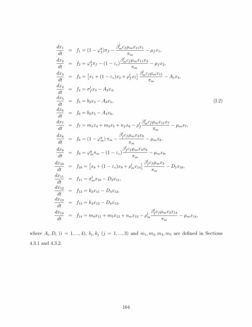
dx1
dt= f1 = (1− ϕq
f )πf −βlmcfµmx11x1
πm− µfx1,
dx2
dt= f2 = ϕq
fπf − (1− εv)βlmcfµmx11x2
πm− µfx2,
dx3
dt= f3 =
�x1 + (1− εv)x2 + ρlfx7
� βlmcfµmx11
πm− A1x3,
dx4
dt= f4 = σl
fx3 − A2x4,
dx5
dt= f5 = b2x4 − A3x5, (I.2)
dx6
dt= f6 = b3x5 − A4x6,
dx7
dt= f7 = m1x4 +m2x5 + nfx6 − ρlf
βlmcfµmx11x7
πm− µmx7,
dx8
dt= f8 = (1− ϕq
m) πm −βlfcfµmx3x8
πm− µmx8,
dx9
dt= f9 = ϕq
mπm − (1− εv)βlfcfµmx3x9
πm− µmx9,
dx10
dt= f10 =
�x8 + (1− εv)x9 + ρlmx14
� βlfcfµmx3
πm−D1x10,
dx11
dt= f11 = σl
mx10 −D2x11,
dx12
dt= f12 = k2x11 −D3x12,
dx13
dt= f13 = k3x13 −D4x13,
dx14
dt= f14 = m4x11 +m5x12 + nmx13 − ρlm
βlfcfµmx3x14
πm− µmx14,
where Ai, Di (i = 1, ..., 4), bj, kj (j = 1, ..., 3) and m1,m2,m4,m5 are defined in Sections
4.3.1 and 4.3.2.
164
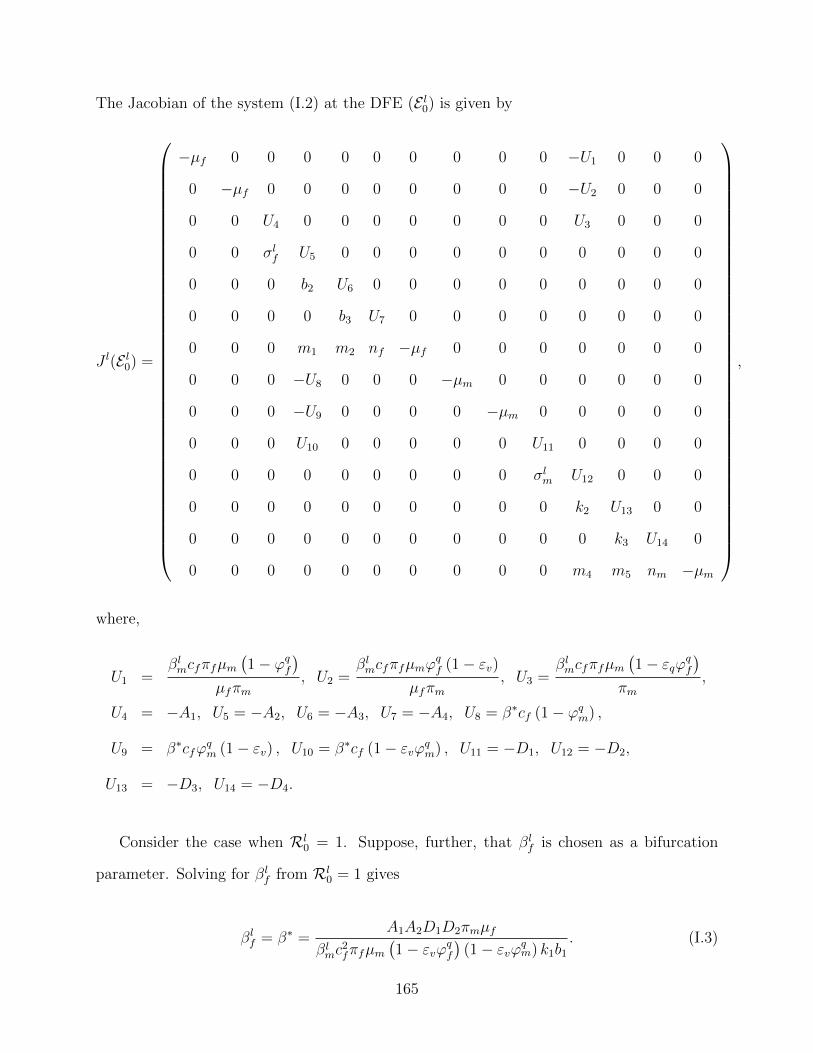
The Jacobian of the system (I.2) at the DFE (E l0) is given by
J l(E l0) =
−µf 0 0 0 0 0 0 0 0 0 −U1 0 0 0
0 −µf 0 0 0 0 0 0 0 0 −U2 0 0 0
0 0 U4 0 0 0 0 0 0 0 U3 0 0 0
0 0 σlf U5 0 0 0 0 0 0 0 0 0 0
0 0 0 b2 U6 0 0 0 0 0 0 0 0 0
0 0 0 0 b3 U7 0 0 0 0 0 0 0 0
0 0 0 m1 m2 nf −µf 0 0 0 0 0 0 0
0 0 0 −U8 0 0 0 −µm 0 0 0 0 0 0
0 0 0 −U9 0 0 0 0 −µm 0 0 0 0 0
0 0 0 U10 0 0 0 0 0 U11 0 0 0 0
0 0 0 0 0 0 0 0 0 σlm U12 0 0 0
0 0 0 0 0 0 0 0 0 0 k2 U13 0 0
0 0 0 0 0 0 0 0 0 0 0 k3 U14 0
0 0 0 0 0 0 0 0 0 0 m4 m5 nm −µm
,
where,
U1 =βlmcfπfµm
�1− ϕq
f
�
µfπm, U2 =
βlmcfπfµmϕ
qf (1− εv)
µfπm, U3 =
βlmcfπfµm
�1− εqϕ
qf
�
πm,
U4 = −A1, U5 = −A2, U6 = −A3, U7 = −A4, U8 = β∗cf (1− ϕqm) ,
U9 = β∗cfϕqm (1− εv) , U10 = β∗cf (1− εvϕ
qm) , U11 = −D1, U12 = −D2,
U13 = −D3, U14 = −D4.
Consider the case when Rl0 = 1. Suppose, further, that βl
f is chosen as a bifurcation
parameter. Solving for βlf from Rl
0 = 1 gives
βlf = β∗ =
A1A2D1D2πmµf
βlmc
2fπfµm
�1− εvϕ
qf
�(1− εvϕ
qm) k1b1
. (I.3)
165
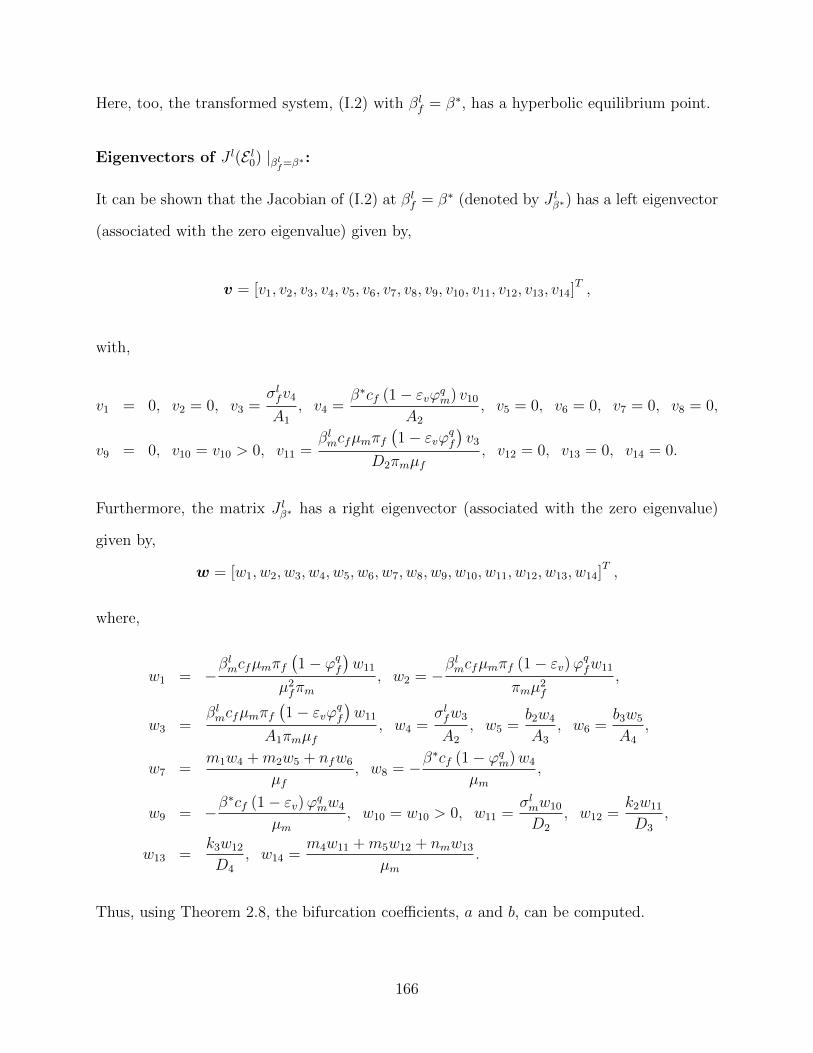
Here, too, the transformed system, (I.2) with βlf = β∗, has a hyperbolic equilibrium point.
Eigenvectors of J l(E l0) |βl
f=β∗:
It can be shown that the Jacobian of (I.2) at βlf = β∗ (denoted by J l
β∗) has a left eigenvector
(associated with the zero eigenvalue) given by,
v = [v1, v2, v3, v4, v5, v6, v7, v8, v9, v10, v11, v12, v13, v14]T ,
with,
v1 = 0, v2 = 0, v3 =σlfv4A1
, v4 =β∗cf (1− εvϕq
m) v10A2
, v5 = 0, v6 = 0, v7 = 0, v8 = 0,
v9 = 0, v10 = v10 > 0, v11 =βlmcfµmπf
�1− εvϕ
qf
�v3
D2πmµf, v12 = 0, v13 = 0, v14 = 0.
Furthermore, the matrix J lβ∗ has a right eigenvector (associated with the zero eigenvalue)
given by,
w = [w1, w2, w3, w4, w5, w6, w7, w8, w9, w10, w11, w12, w13, w14]T ,
where,
w1 = −βlmcfµmπf
�1− ϕq
f
�w11
µ2fπm
, w2 = −βlmcfµmπf (1− εv)ϕ
qfw11
πmµ2f
,
w3 =βlmcfµmπf
�1− εvϕ
qf
�w11
A1πmµf, w4 =
σlfw3
A2, w5 =
b2w4
A3, w6 =
b3w5
A4,
w7 =m1w4 +m2w5 + nfw6
µf, w8 = −
β∗cf (1− ϕqm)w4
µm,
w9 = −β∗cf (1− εv)ϕq
mw4
µm, w10 = w10 > 0, w11 =
σlmw10
D2, w12 =
k2w11
D3,
w13 =k3w12
D4, w14 =
m4w11 +m5w12 + nmw13
µm.
Thus, using Theorem 2.8, the bifurcation coefficients, a and b, can be computed.
166
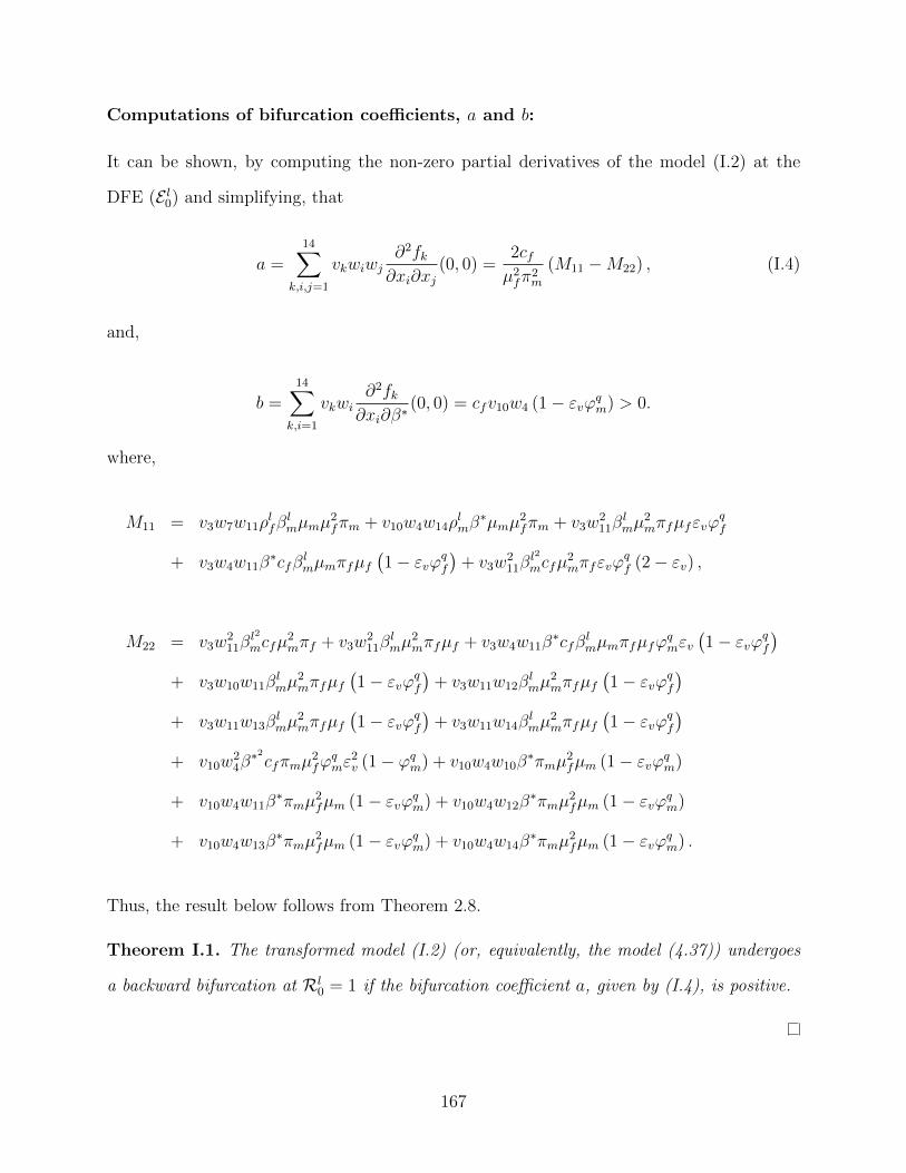
Computations of bifurcation coefficients, a and b:
It can be shown, by computing the non-zero partial derivatives of the model (I.2) at the
DFE (E l0) and simplifying, that
a =14�
k,i,j=1
vkwiwj∂2fk
∂xi∂xj(0, 0) =
2cfµ2fπ
2m
(M11 −M22) , (I.4)
and,
b =14�
k,i=1
vkwi∂2fk
∂xi∂β∗ (0, 0) = cfv10w4 (1− εvϕqm) > 0.
where,
M11 = v3w7w11ρlfβ
lmµmµ
2fπm + v10w4w14ρ
lmβ
∗µmµ2fπm + v3w
211β
lmµ
2mπfµfεvϕ
qf
+ v3w4w11β∗cfβ
lmµmπfµf
�1− εvϕ
qf
�+ v3w
211β
l2
mcfµ2mπfεvϕ
qf (2− εv) ,
M22 = v3w211β
l2
mcfµ2mπf + v3w
211β
lmµ
2mπfµf + v3w4w11β
∗cfβlmµmπfµfϕ
qmεv
�1− εvϕ
qf
�
+ v3w10w11βlmµ
2mπfµf
�1− εvϕ
qf
�+ v3w11w12β
lmµ
2mπfµf
�1− εvϕ
qf
�
+ v3w11w13βlmµ
2mπfµf
�1− εvϕ
qf
�+ v3w11w14β
lmµ
2mπfµf
�1− εvϕ
qf
�
+ v10w24β
∗2cfπmµ2fϕ
qmε
2v (1− ϕq
m) + v10w4w10β∗πmµ
2fµm (1− εvϕ
qm)
+ v10w4w11β∗πmµ
2fµm (1− εvϕ
qm) + v10w4w12β
∗πmµ2fµm (1− εvϕ
qm)
+ v10w4w13β∗πmµ
2fµm (1− εvϕ
qm) + v10w4w14β
∗πmµ2fµm (1− εvϕ
qm) .
Thus, the result below follows from Theorem 2.8.
Theorem I.1. The transformed model (I.2) (or, equivalently, the model (4.37)) undergoes
a backward bifurcation at Rl0 = 1 if the bifurcation coefficient a, given by (I.4), is positive.
167
It is clear from the expression for the bifurcation coefficient, a, given by (I.4), that a > 0
whenever (since all the low-risk-only model parameters are positive)
M11 > M22. (I.5)
Furthermore, consider the low-risk-only model (4.37) in the absence of re-infection (ρlf =
ρlm = 0). Setting ρlf = ρlm = 0 into the expression for the bifurcation coefficient, a in (I.4),
and using β∗ for βlf in (I.3), shows that (here, the eigenvectors v10 and w10 are given the
value unity)
168
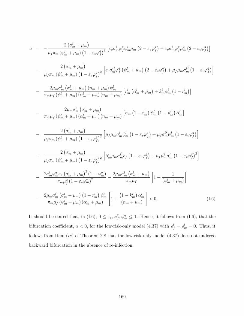
a = −2�σlm + µm
�
µfπm (ψlm + µm)
�1− εvϕ
qf
�2�εvσ
lmϕ
qfψ
lmµm
�2− εvϕ
qf
�+ εvσ
lmϕ
qfµ
2m
�2− εvϕ
qf
��
−2�σlm + µm
�
µfπm (ψlm + µm)
�1− εvϕ
qf
�2�εvσ
l2
mϕqf
�ψlm + µm
� �2− εvϕ
qf
�+ µfµmσ
l2
m
�1− εvϕ
qf
��
−2µmσl
m
�σlm + µm
�(nm + µm)ψl
m
πmµf (ψlm + µm) (αl
m + µm) (nm + µm)
�rlm
�αlm + µm
�+ kl
mαlm
�1− rlm
��
−2µmσl
m
�σlm + µm
�
πmµf (ψlm + µm) (αl
m + µm) (nm + µm)
�nm
�1− rlm
�ψlm
�1− kl
m
�αlm
�
−2�σlm + µm
�
µfπm (ψlm + µm)
�1− εvϕ
qf
�2�µfµmσ
lmψ
lm
�1− εvϕ
qf
�+ µfσ
l2
mψlm
�1− εvϕ
qf
��
−2�σlm + µm
�
µfπm (ψlm + µm)
�1− εvϕ
qf
�2�βlmµmσ
l2
mcf�1− εvϕ
qf
�+ µfµ
2mσ
lm
�1− εvϕ
qf
�2�
−2σl
mϕqmεv
�σlm + µm
�2(1− ϕq
m)
πmµ2f (1− εvϕ
qm)
2 −2µmσl
m
�σlm + µm
�
πmµf
�1 +
1
(ψlm + µm)
�
−2µmσl
m
�σlm + µm
� �1− rlm
�ψlm
πmµf (ψlm + µm) (αl
m + µm)
�1 +
�1− kl
m
�αlm
(nm + µm)
�< 0. (I.6)
It should be stated that, in (I.6), 0 ≤ εv,ϕqf ,ϕ
qm ≤ 1. Hence, it follows from (I.6), that the
bifurcation coefficient, a < 0, for the low-risk-only model (4.37) with ρlf = ρlm = 0. Thus, it
follows from Item (iv) of Theorem 2.8 that the low-risk-only model (4.37) does not undergo
backward bifurcation in the absence of re-infection.
169
Appendix J
Proof of Theorem 4.6
Proof. Consider the model (4.34) with ρlf = ρlm = ρhf = ρhm = δm = 0. The proof is based
on using a Comparison Theorem. The equations for the infected components of the model
(4.34) can be written as (it should be mentioned that system (J.1) satisfies the Type K
condition discussed in Chapter 2):
170
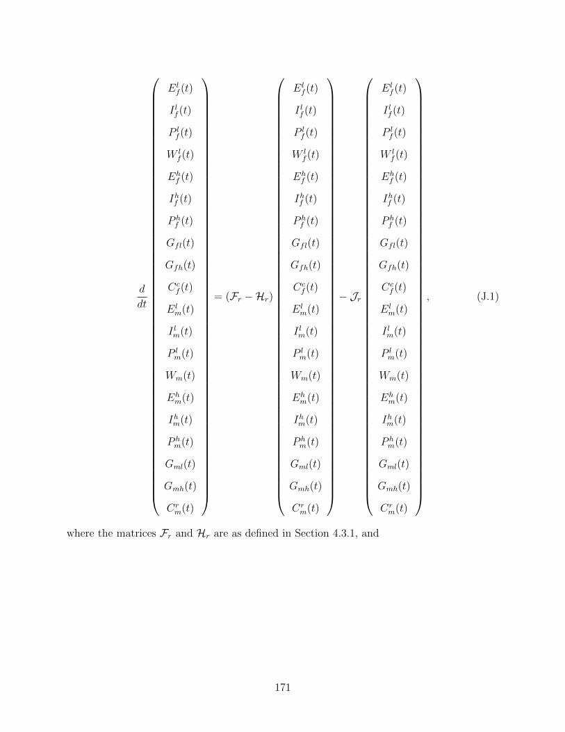
d
dt
Elf (t)
I lf (t)
P lf (t)
W lf (t)
Ehf (t)
Ihf (t)
P hf (t)
Gfl(t)
Gfh(t)
Ccf (t)
Elm(t)
I lm(t)
P lm(t)
Wm(t)
Ehm(t)
Ihm(t)
P hm(t)
Gml(t)
Gmh(t)
Crm(t)
= (Fr −Hr)
Elf (t)
I lf (t)
P lf (t)
W lf (t)
Ehf (t)
Ihf (t)
P hf (t)
Gfl(t)
Gfh(t)
Ccf (t)
Elm(t)
I lm(t)
P lm(t)
Wm(t)
Ehm(t)
Ihm(t)
P hm(t)
Gml(t)
Gmh(t)
Crm(t)
− Jr
Elf (t)
I lf (t)
P lf (t)
W lf (t)
Ehf (t)
Ihf (t)
P hf (t)
Gfl(t)
Gfh(t)
Ccf (t)
Elm(t)
I lm(t)
P lm(t)
Wm(t)
Ehm(t)
Ihm(t)
P hm(t)
Gml(t)
Gmh(t)
Crm(t)
, (J.1)
where the matrices Fr and Hr are as defined in Section 4.3.1, and
171
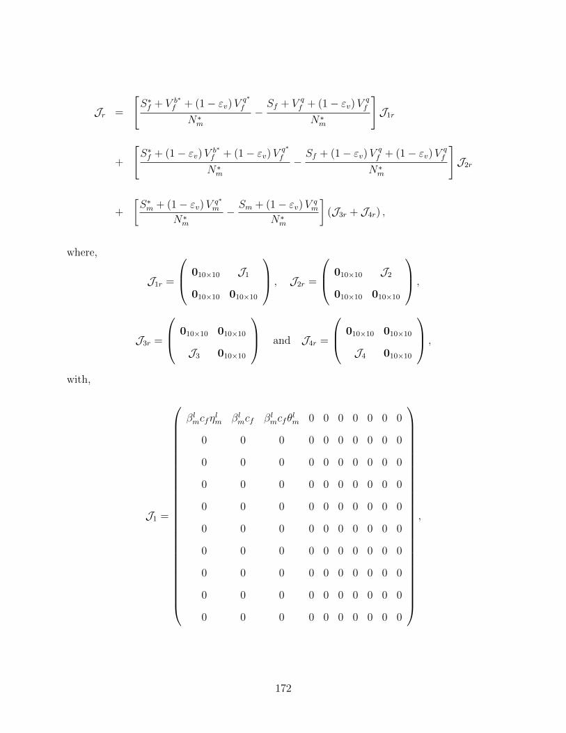
Jr =
�S∗f + V b∗
f + (1− εv)Vq∗
f
N∗m
−Sf + V q
f + (1− εv)Vqf
N∗m
�J1r
+
�S∗f + (1− εv)V b∗
f + (1− εv)Vq∗
f
N∗m
−Sf + (1− εv)V
qf + (1− εv)V
qf
N∗m
�J2r
+
�S∗m + (1− εv)V q∗
m
N∗m
−Sm + (1− εv)V q
m
N∗m
�(J3r + J4r) ,
where,
J1r =
010×10 J1
010×10 010×10
, J2r =
010×10 J2
010×10 010×10
,
J3r =
010×10 010×10
J3 010×10
and J4r =
010×10 010×10
J4 010×10
,
with,
J1 =
βlmcfη
lm βl
mcf βlmcfθ
lm 0 0 0 0 0 0 0
0 0 0 0 0 0 0 0 0 0
0 0 0 0 0 0 0 0 0 0
0 0 0 0 0 0 0 0 0 0
0 0 0 0 0 0 0 0 0 0
0 0 0 0 0 0 0 0 0 0
0 0 0 0 0 0 0 0 0 0
0 0 0 0 0 0 0 0 0 0
0 0 0 0 0 0 0 0 0 0
0 0 0 0 0 0 0 0 0 0
,
172
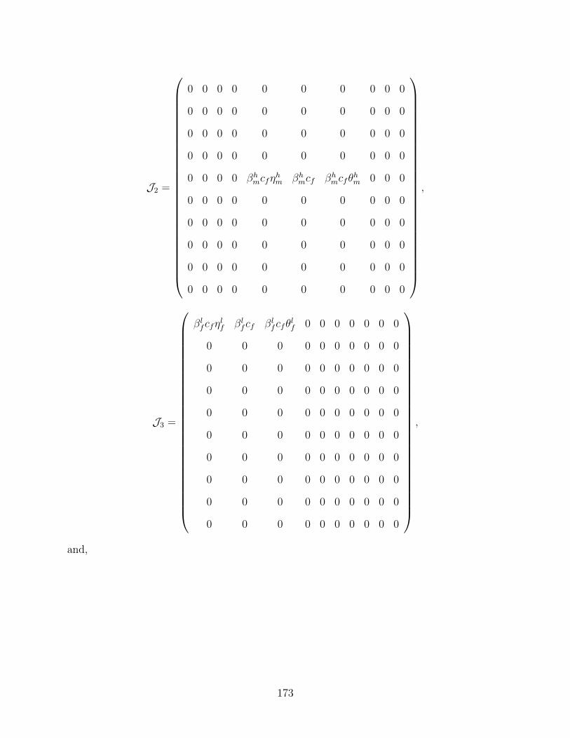
J2 =
0 0 0 0 0 0 0 0 0 0
0 0 0 0 0 0 0 0 0 0
0 0 0 0 0 0 0 0 0 0
0 0 0 0 0 0 0 0 0 0
0 0 0 0 βhmcfη
hm βh
mcf βhmcfθ
hm 0 0 0
0 0 0 0 0 0 0 0 0 0
0 0 0 0 0 0 0 0 0 0
0 0 0 0 0 0 0 0 0 0
0 0 0 0 0 0 0 0 0 0
0 0 0 0 0 0 0 0 0 0
,
J3 =
βlfcfη
lf βl
fcf βlfcfθ
lf 0 0 0 0 0 0 0
0 0 0 0 0 0 0 0 0 0
0 0 0 0 0 0 0 0 0 0
0 0 0 0 0 0 0 0 0 0
0 0 0 0 0 0 0 0 0 0
0 0 0 0 0 0 0 0 0 0
0 0 0 0 0 0 0 0 0 0
0 0 0 0 0 0 0 0 0 0
0 0 0 0 0 0 0 0 0 0
0 0 0 0 0 0 0 0 0 0
,
and,
173
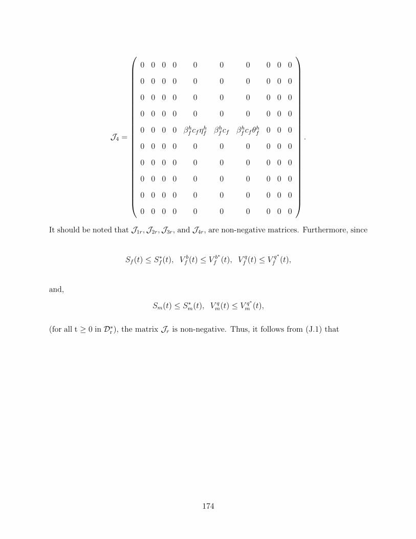
J4 =
0 0 0 0 0 0 0 0 0 0
0 0 0 0 0 0 0 0 0 0
0 0 0 0 0 0 0 0 0 0
0 0 0 0 0 0 0 0 0 0
0 0 0 0 βhf cfη
hf βh
f cf βhf cfθ
hf 0 0 0
0 0 0 0 0 0 0 0 0 0
0 0 0 0 0 0 0 0 0 0
0 0 0 0 0 0 0 0 0 0
0 0 0 0 0 0 0 0 0 0
0 0 0 0 0 0 0 0 0 0
.
It should be noted that J1r,J2r,J3r, and J4r, are non-negative matrices. Furthermore, since
Sf (t) ≤ S∗f (t), V b
f (t) ≤ V b∗
f (t), V qf (t) ≤ V q∗
f (t),
and,
Sm(t) ≤ S∗m(t), V q
m(t) ≤ V q∗
m (t),
(for all t ≥ 0 in D∗r ), the matrix Jr is non-negative. Thus, it follows from (J.1) that
174
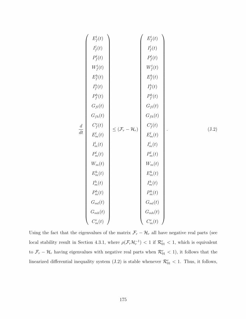
d
dt
Elf (t)
I lf (t)
P lf (t)
W lf (t)
Ehf (t)
Ihf (t)
P hf (t)
Gfl(t)
Gfh(t)
Ccf (t)
Elm(t)
I lm(t)
P lm(t)
Wm(t)
Ehm(t)
Ihm(t)
P hm(t)
Gml(t)
Gmh(t)
Crm(t)
≤ (Fr −Hr)
Elf (t)
I lf (t)
P lf (t)
W lf (t)
Ehf (t)
Ihf (t)
P hf (t)
Gfl(t)
Gfh(t)
Ccf (t)
Elm(t)
I lm(t)
P lm(t)
Wm(t)
Ehm(t)
Ihm(t)
P hm(t)
Gml(t)
Gmh(t)
Crm(t)
. (J.2)
Using the fact that the eigenvalues of the matrix Fr −Hr all have negative real parts (see
local stability result in Section 4.3.1, where ρ(FrH−1r ) < 1 if Rr
01 < 1, which is equivalent
to Fr − Hr having eigenvalues with negative real parts when Rr01 < 1), it follows that the
linearized differential inequality system (J.2) is stable whenever Rr01 < 1. Thus, it follows,
175
by Comparison Theorem [58] (see also Theorem 2.10), that
limt→∞
(Elf (t), I
lf (t), P
lf (t),W
lf (t), E
hf (t), I
hf (t), P
hf (t), Gfl(t), Gfh(t), C
cf (t), E
lm(t),
I lm(t), Plm(t),Wm(t), E
hm(t), I
hm(t), P
hm(t), Gml(t), Gmh(t), C
rm(t))
= (0, 0, 0, 0, 0, 0, 0, 0, 0, 0, 0, 0, 0, 0, 0, 0, 0, 0, 0, 0).
Substituting Elf = I lf = P l
f =W lf = Eh
f = Ihf = P hf =Gfl = Gfh = Cc
f = Elm=I lm = P l
m =
Wm =Ehm = Ihm = P h
m = Gml = Gmh = Crm = 0 into the equations of the model (4.34)
gives Sf (t) → S∗f , V
bf (t) → V b∗
f , V qf (t) → V q∗
f , Sm(t) → S∗m and V q
m(t) → V q∗m , as t → ∞ for
Rr01 < 1. Thus,
limt→∞
(Sf (t), Vbf (t), V
qf (t), E
lf (t), I
lf (t), P
lf (t),W
lf (t), E
hf (t), I
hf (t), P
hf (t), Gfl(t),
Gfh(t), Ccf (t), Sm(t), V
qm(t), E
lm(t), I
lm(t), P
lm(t),Wm(t), E
hm(t),
Ihm(t), Phm(t), Gml(t), Gmh(t), C
rm(t)) = E
r0 ,
so that the DFE, Er0 , of the model (4.34) is GAS in D∗
r whenever Rr01 < 1.
176
Bibliography
[1] American University. (2011). Sexually Transmitted Diseases (STDs). www.american.ca.
Accessed: 15 January 2013.
[2] Anderson, R. M., & May, R. M., eds. (1982). Population of Biology of Infectious Diseases.
Springer-Verlage, Berlin, Heidelberg: New York.
[3] Anderson, R. M., & May, R. M., eds. (1991). Infectious Diseases of Humans: Dynamics
and Control. Oxford Univ, Press, London: New York.
[4] Australian Institute of Health and Welfare. (2013). http://www.aihw.gov.au. Accessed:
20 March 2013.
[5] Bernoulli, D. (1766). Essai D’une Nouvelle Analyse De La Mortalite Causee Par La Petite
Verole. Mem. Math. Phys. Acad. Roy. Sci., Paris.
[6] Bellanger, S., Tan, C. L., Xue, Y. Z., Teissier, S., & Thierry, F. (2011). Tumor Suppressor
or Oncogene? A critical Role of the Human Papillomavirus (HPV) E2 Protein in Cervical
Cancer Progression. Am J Cancer Res., 1(3): 373-389.
[7] Brisson, M., Van de Velde, N. & Boily, M. C. (2011). Different Population-level Vaccina-
tion Effectiveness for HPV Types 16, 18, 6 and 11. Sex. Transm. Infect., 87: 41-43.
[8] Blower, S. M., & Dowlatabadi, H. (1994). Sensitivity and Uncertainty Analysis of Com-
plex Models of Disease Transmission: An HIV Model, As An Example. Int. Stat. Rev.,
62: 229-243.
177

[9] Brown, V. L., & White, K. A. J. (2011). The Role of Optimal Control in Assessing the
Most Cost-effective Implementation of a Vaccination Programme: HPV as a Case Study.
Math. Biosci., 231: 126-134.
[10] Canadian Cancer Society. (2010). http://www.cancer.ca. Accessed: 10 September 2012.
[11] Carr, J. (1981). Applications of Centre Manifold Theory. Springer-Verlag, New York.
[12] Castillo-Chavez, C., Cooke, K., Huang, W., & Levin, S. A. (1989). Results on the
Dynamics for Models for the Sexual Transmission of the Human Immunodeficiency Virus.
Appl. Math. Letters, 2: 327-331.
[13] Castillo-Chavez, C., Huang, W., & Li, J. (1997). The Effects of Females’ Susceptibility
on the Co-existence of Multiple Pathogen Strains of Sexually Transmitted Diseases. J.
Math. Biol., 35: 503-522.
[14] Castillo-Chavez, C., & Song, B. (2004). Dynamical Models of Tuberculosis and Their
Applications. Math. Biosci. Engrg., 1(2): 361-404.
[15] Centres for Disease Control and Prevention. (2012). Sexually Transmitted Diseases
(STDs). http://www.cdc.gov. Accessed: 15 November 2012.
[16] Chowell, G., Diaz-Duenas, P., Miller, J. C., Alcazar-Velazco, A., Hyman, J. M., Fen-
imore, P. W., & Castillo Chavez, C. (2007). Estimation of the Reproduction Number of
Dengue Fever from Spatial Epidemic Data. Mathematical Biosciences, 208(2): 571-589.
[17] Davidson College. (2006). http://www.bio.davidson.edu. Accessed: 23 March 2013.
[18] de Villiers, E.-M., Fauquet, C., Broker, T. R., Bernard, H.-V. & zur Hausen, H. (2004).
Classification of Papillomaviruses. Virology. 324: 17-27.
[19] Diekmann, O., Heesterbeek, J. A. P., & Metz, J. A. J. (1990). On the Definition and
the Computation of the Basic Reproduction Ratio R0 in Models for Infectious Diseases
in Heterogeneous Populations. J. Math. Biol., 28(4): 365-382.
178
[20] Dietz, K. (1975). Transmission and Control of Arboviurs Disease, In Epidemiology, K.
L. Cook, ed. SIAM, Philadelphia.
[21] Dietz, K., & Heesterbeek, J. A. P. (2002). Daniel Bernoulli’s Epidemiological Model
Revisited. Mathematical Biosciences, 180: 1-21.
[22] Doorbar, J. (2005). The Papillomavirus Life Cycle. Review. Virology, 32: 7-15.
[23] Dushoff, J., Wenzhang, H., & Castillo-Chavez, C. (1998). Backwards Bifurcations and
Catastrophe in Simple Models of Fatal Diseases. J. Math. Biol., 36: 227-248.
[24] Elbasha, E. H., Dasbach, E. J., & Insinga, R. P. (2008). A Multi-Type HPV Transmis-
sion Model. Bull. Math. Biol., 70(8): 2126-2176.
[25] Elbasha, E. H., Dasbach, E. J., & Insinga, R. P. (2007). Model For Assessing Human
Papilomavirus Vaccination Strategies. Emerg Infect Dis., 13(1): 28- 41.
[26] Elbasha, E. H., & Galvani, A. P. (2005). Vaccination Against Multiple HPV Types.
Math. Biosci., 197(1): 88-117.
[27] Elbasha, E. H. (2008). Global Stability of Equilibria in a Two-Sex HPV Vaccination
Model. Bull. Math. Biol., 70: 894-909.
[28] Elbasha, E. H., & Gumel, A. B. (2006). Theoretical Assessment of Public Health Impact
of Imperfect Prophylactic HIV-1 Vaccines with Therapeutic Benefits. Bull. Math. Biol.,
68: 577-614.
[29] Elbasha, E. H., & Dasbach, E. J. (2010). Impact of Vaccinating Boys and Men Against
HPV in the United States. Vaccine, 28 : 6858-6867.
[30] Escobar Ospina, M. E., & Perdomo, J. G. (2012). A growth Model of Human Papil-
lomavirus Type 16 Designed From Cellular Automata and Agent-based Models. Artif.
Intell. Med., 57(1):31-47.
179
[31] Esteva, L., Gumel, A. B., & de Leon, C. V. (2009). Qualitative Study of Transmission
Dynamics of Drug-Resistant Malaria. Math. Comput. Modelling, 50: 611-630.
[32] Esteva, L., & Vergas, C. (2000). Influence of Vertical and Mechanical Transmission on
the Dynamics of Dengue Disease. Math Biosci., 167: 51-64.
[33] Ferlay, J., Shin, H. R., Bray, F., Forman, D., Mathers, C., & Parkin, D. M. (2010).
Estimates of Worldwide Burden of Cancer in 2008: GLOBOCAN 2008. Int. J. Cancer,
127(12): 2893-2917.
[34] Food and Drug Administration. (2010). FDA Approves New Vaccine for Prevention of
Cervical Cancer. http://www.fda.gov. Accessed: 5 December 2012.
[35] Franco, E. L., Duarte-Franco, E. & Ferenczy, A. (2001). Cervical Cancer: Epidemiology,
Prevention and The Role of Human Papillomavirus Infection. CMAJ., 164(7): 1017-1025.
[36] Friedman-Kien, A. (1995). Management of Condylomata Acuminata with Alferon N
Injection, Interferon Alfa-n3 (Human Leukocyte Derived). Am J Obstet Gynecol., 172:
1359-1368.
[37] Garba, S. M., Gumel, A. B., & Abu Bakar, M. R. (2008). Backward Bifurcations in
Dengue Transmission Dynamics. Math. Biosci., 215: 11-25.
[38] Gillison, M. L., Chaturvedi, A. K., &Lowy, D. R. (2008). HPV Prophylactic Vaccines
and the Potential Prevention of Noncervical Cancers in Both Men and Women. Cancer,
113(10): 3036-3046.
[39] Goldberg Arnold, R. J. (2007). Cost-effectiveness Analysis: Should It Be Required for
Drug Registration and Beyond? Drug Discovery Today, 12(22): 960-965.
[40] Goldie, S. J., Goldhaber-Fiebert, J. D., & Garnett, G. P. (2006) Chapter 18: Public
Health Policy for Cervical Cancer Prevention; the Role of Decision Science, Economic
Evaluation and Mathematical Modelling. Vaccine, 24(3): 155-163
180
[41] Goldie, S. J., Kim, J. J., & Myers, E. (2006) Chapter 19: Cost-effectiveness of Cervical
Cancer Screening. Vaccine, 24(3): 164-170.
[42] Gumel, A. B. (2012). Causes of Backward Bifurcations in Some Epidemiological Models.
J. Math. Anal. Appl., 395(1): 355-365.
[43] Gumel, A. B., McCluskey, Connell C., & van den Driessche, P. (2006). Mathematical
Study of a Staged-progression HIV Model with Imperfect Vaccine. Bull. Math. Biol., 68
(8): 2105-2128.
[44] Hale, J. K. (1969). Ordinary Differential Equations. New York: John Wiley and Sons.
[45] Hausen, H. (2002). Papillomaviruses and Cancer: From Basic Studies to Clinical Ap-
plication. Nature Publishing Group, 2: 342-350.
[46] Health Canada. (2010). http://www.hc-sc.gc.ca. Accessed: 19 July 2012.
[47] Hethcote, H. W. (2000). The Mathematics of Infectious Diseases. SIAM Review, 42(4):
599-653.
[48] Hethcote, H. W., & van Ark, J. W. (1987). Epidemiology Models for Heterogeneous Pop-
ulation: Proportionate Mixing, Parameter Estimation, and Immunization Programs.Math.
Biosci., 84: 85-118.
[49] Holowaty, P., Miller, A. B., Rohan, T., & To, T. (1999). Natural History of Dysplasia
of the Uterine Cervix. J Natl Cancer Inst., 91: 252-258.
[50] IARC Working Group. (2007). Human Papillomaviruses: IARC Monographs on the
Evaluation of the Carcinogenic Risks to Humans. Lyon, France: International Agency for
Research on Cancer, 90: 23-476.
[51] Insinga, R., Glass, A. & Rush, B. (2004). The Healthcare Costs of Cervical Human
Papillomavirus-related Disease. Am. J. Obstet. Gynecol., 191: 114-120.
181
[52] Insinga, R. P. (2007). The Natural History of Low-grade Cervical Intraepithelial Neo-
plasia. Manuscript in preparation.
[53] Insinga, R. P., Dasbach, E. J., & Elbasha, E. H. (2009). Epidemiologic Natural History
and Clinical Management of Human Papillomavirus (HPV) Disease: a Critical and Sys-
tematic Review of the Literature in the Development of an HPV Dynamic Transmission
Model. BMC Infectious Diseases, 9(119): 1-26.
[54] Institute of Health Economics. (2009). Human Papillomavirus (HPV): Testing in Al-
berta. http://www.ihe.ca. Accessed: 2 January 2013.
[55] Kataja, V., Syrjanen, K., Mantyjarvi, R., et al. (1989). Prospective Follow-up of Cervical
HPV Infections: Life Table Analysis of Histopathological, Cytological and Colposcopic
Data. Eur. J. Epidemiol., 5: 1-7.
[56] Kei, K., Katsuyuki, A., Satoko, K., Shiro, K., & Tomoyuki, F. (2012). Therapeutic
Human Papillomavirus (HPV) Vaccines: A Novel Approach. Virol J., 6: 264-269.
[57] Kim, J. J., Wright, T. C., & Goldie, S. J. (2002). Cost-effectiveness of Alternative Triage
Strategies for Atypical Squamous Cells of Undetermined Significance. JAMA, 287:2382-
2390.
[58] Lakshmikantham, V., Leela, S., & Martynyuk, A. A. (1989). Stability Analysis of Non-
linear Systems. Marcel Dekker Inc.: New York and Basel.
[59] LaSalle, J. P. (1976). The stability of dynamical systems. Regional Conference Series in
Applied Mathematics, SIAM, Philadelphia.
[60] Lipsitch, M. & Murray, M. B. (2003). Multiple Equilibria: Tuberculosis Transmission
Require Unrealistic Assumption. Theor. Popul. Biol., 63(2): 169-170.
[61] Malik, M. T., Reimer, J., Gumel, A. B., Elbasha, E. H., & Mahmud, S. M. (2013).
The Impact of an Imperfect Vaccine and Pap Cytology Screening on the Transmission
182
of Human Papillomavirus and Occurrence of Associated Cervical Dysplasia and Cancer.
Math. Biosci. Engrg. To appear.
[62] Mandelblatt, J. S., Lawrence, W. F., Womack, S. M., et al. (2002). Benefits and Costs
of Using HPV Testing to Screen for Cervical Cancer. JAMA, 287:2372-2381.
[63] McLeod, R. G., Brewster, J. F., Gumel, A. B., & Slonowsky, D. A. (2006). Sensitivity
and Uncertainty Analyses for a SARS Model With Time-varying Inputs and Outputs.
Math. Biosci. Eng., 3(3): 527-544.
[64] MicrobiologyBytes. (2009). http://www.microbiologybytes.com/virology. Accessed: 13
March 2013.
[65] Mukandavire, Z., & Garira, W. (2007). Age and Sex Structured Model for Assessing the
Demographic Impact of Mother-to-child Transmission of HIV/AIDS. Bull. Math. Biol.,
69(6): 2061-2092.
[66] Muller, M., & Demeret, C. (2012). The HPV E2-Host Protein-Protein Interactions: A
Complex Hijacking of the Cellular Network. Virol J., 6: 173-189.
[67] Myers, E. R. et al. (2000). Mathematical Model for the Natural History of Human
Papillomavirus Infection and Cervical Carcinogenesis. Am. J. Epidemiol., 151(12): 1158-
1171.
[68] National Cancer Institute. (2011). Human Papillomavirus (HPV) Vaccines.
http://www.cancer.gov. Accessed: 19 December 2012.
[69] Onco Health Corp. (2013). http://oncohealthcorp.com/technology. Accessed: 13 March
2013.
[70] Oxford Journals. (2012). Annual Report to the Nation on the Status of Cancer,1975-
2009, Featuring the Burden and Trends in Human Papillomavirus (HPV)-Associated Can-
183
cers and HPV Vaccination Coverage Levels. http://jnci.oxfordjournals.org. Accessed: 18
February 2013.
[71] Palefsky, J. M. (2010). Human Papillomavirus-Related Disease in Men: Not Just a
Women Issue. Journal of Adolescent Health, 46: 12-19.
[72] Parkin, D., Bray, F., Ferlay, J. & Pisani, P. (2005). Global Cancer Statistics. Cancer J.
Clin., 55: 74-108.
[73] Perko, L. (2001). Differential Equations and Dynamical Systems. New York: Springer.
[74] Physicians’ Research Network, Inc. (2013). http://www.prn.org. Accessed: 10 March
2013.
[75] Podder, C. N., & Gumel, A. B. (2009). Transmission Dynamics of a Two-sex Model for
Herpes Simplex Virus Type2. Can. Math. Quarterly., 17(2): 339-386.
[76] Public Health Agency of Canada. (2010). Human Papillomavirus. HPV Purple Paper
(bds). http://www.phac-aspc.gc.ca/std-mts/hpv-vph/fact-faits-eng.php. Accessed: 11 Oc-
tober 2012.
[77] Public Health Agency of Canada. (2007). Statement on Human Papillomavirus Vaccine.
http://www.publichealth.gc.ca. Accessed: 5 December 2012.
[78] Roche Molecular Systems Inc. (2013). http://www.hpv16and18.com. Accessed: 15
March 2013.
[79] Spangle, J. M., & Munger, K. (2013). The HPV16 E6 Oncoprotein Causes Prolonged
Receptor Protein Tyrosine Kinase Signaling and Enhances Internalization of Phosphory-
lated Receptor Species. PLoS. Pathog., 9(3): e1003237. doi: 10.1371/journal.ppat.1003237
[80] Saslow, D. et al. (2012). American Cancer Society, American Society for Colposcopy and
Cervical Pathology, and American Society for Clinical Pathology Screening Guidelines for
184
the Prevention and Early Detection of Cervical Cancer. Am. J. Clin. Pathol., 137: 516-
542.
[81] Seavey, S. E., Holubar, M., Saucedo, L. J., & Perry, M. E. (1999). The E7 Oncoprotein
of Human Papillomavirus Type 16 Stabilizes p53 through a Mechanism Independent of
p19ARF. J. Virol., 73(9): 7590-7598.
[82] Severini, A., Jiang, Y., Brassard, P., Morrison, H., Demers, A. A., Oguntuase, E.,
Al-Rushdi, M., Preston, F., Ratnam, S., & Mao, Y. (2013). Type-specific Prevalence of
Human Papillomavirus in Women Screened for Cervical Cancer in Labrador, Canada. Int
J Circumpolar Health, 72: doi: 10.3402/ijch.v72i0.19743.
[83] Sharomi, O., & Gumel, A. B. (2011). Mathematical Dynamical Analysis of a Sex-
Structured Chlamydia Trachomatis Transmission Model with Time Delay. Nonlinear Anal.
Real World Appl., 12(2): 837-866.
[84] Sharomi, O., & Gumel, A. B. (2009). Re-infection-induced Backward Bifurcation in the
Transmission Dynamics of Chlamydia Trachomatis. Journal of Mathematical Analysis and
Applications, 356(1): 96-118.
[85] Sharomi, O., Podder, C. N., Gumel, A. B., Elbasha, E. H., & Watmough. J. (2007).
Role of Incidence Function in Vaccine-induced Backward Bifurcation in Some HIV Models.
Bull. Math. Biol., 210(2): 436-463.
[86] Sharomi, O., Podder, C. N., Gumel, A. B., & Song, B. (2008). Mathematical Analysis of
the Transmission Dynamics of HIV/TB Co-infection in the Presence of Treatment. Math.
Biosci. Engg., 5(1): 145-174.
[87] Smith, H. L. (1995). Monotone Dynamical Systems: An Introduction to the Theory of
Competitive and Cooperative Systems. Mathematical Surveys and Monographs. American
Mathematical Society; Providence. 41.
185
[88] Smith, H. L., & Waltman, P. (1995). The Theory of the Chemostat. Cambridge Univer-
sity Press.
[89] Stanford University. (2005). http://www.stanford.edu. Accessed: 14 March 2013.
[90] Statistics Canada. (2012). www.statcan.gc.ca. Accessed: 20 January 2013.
[91] Thieme, H. R., & Hethcote, H. W. (1985). Stability of the Endemic Equilibrium in
Epidemic Models with Subpopulations. Math. Biosci., 75: 205-227.
[92] Thieme, H.R. (2003). Mathematics in Population Biology. Princeton University Press;
Princeton, NJ.
[93] The GlaxoSmithKline Vaccine HPV-007 Study Group. (2009). Sustained Efficacy and
Immunogenicity of the Human Papillomavirus (HPV)-16/17 ASO4-adjuvanted Vaccine:
Analysis of a Randomised Placebo-controlled Trial up to 6.4 Years. Lancet, 374: 1975-
1985.
[94] University of Bristol. (2006). http://www.bristol.ac.uk. Accessed: 1 March 2013.
[95] van den Driessche, P., & Watmough, J. (2005). Reproduction Numbers and Sub-
Threshold Endemic Equilibria for Compartmental Models of Disease Transmission. Math.
Biosci. 180: 29-48.
[96] Villa, L. L., Costa, R. L., Petta, C. A., Andrade, R. P., Paavonen, J., & Iversen, O-E., et
al. (2006). High Sustained Efficacy of a Prophylactic Quadrivalent Human Papillomavirus
Types 6/11/16/18 virus-like Particle Vaccine Through 5 Years of Follow-up. British Jour-
nal of Cancer, 95(11): 1459-1466.
[97] Walboomers, J. M. M., Jacobs, M. V., & Manos, M. M. et al. (1999). Human Papillo-
mavirus is a Necessary Cause of Invasive Cervical Cancer Worldwide. J. Pathol., 189(1):
12-19.
186
[98] Wiggins, S. (1983). Introduction to Applied Nonlinear Dynamical Systems and Chaos.
New York: Springer- Verlag.
[99] Winer, R. L., Kiviat, N. B., Hughes, J. P., et al. (2005). Development and Duration of
Human Papillomavirus Lesions, After Initial Infection. J Infect Dis., 191: 731-738.
[100] World Health Organization. (2009). Accessed: 11 January 2013.
[101] Xiaodong, L., Hethcote, H. W., & van den Driessche, P. (1993). An Epidemiological
Model for HIV/AIDS with Proportional Recruitment. Math. Biosci., 118: 181-195.
[102] Yew, C. W., Lee, P., Chan, W. K., Lim, V. K., Tay, S. K., Tan, T. M., & Deng, L. W.
(2011). A Novel MLL5 Isoform That Is Essential to Activate E6 and E7 Transcription in
HPV16/18-associated Cervical Cancers. Cancer Res., 71(21): 6696-6707.
[103] Zhang, X. & Liu, X. (2009). Backward Bifurcation and Global Dynamics of an SIS
Epidemic Model with General Incidence Rate and Treatment. Nonlinear Anal: Real World
Appl., 10: 565-575.
[104] Zhang, X. & Liu, X. (2008). Backward Bifurcation of an Epidemic Model with Satu-
rated Treatment Function. J. Math. Anal. Appl., 348: 433-443.
187