A CAPACITY PLANMNG MODEL

FOR

CANADIAN MILITARY AIRLIFT REQTJESTS

BY

LIEUTENANT-COI,ONEL BARRY À. STANNARD

A ThesisSubmitted to the Faculty of Graduate Studies

in Partial Fulfillment of the Requirementsfor the Degree of

MASTER OF SCIENCE

Department of Actuarial and Management ScienceUniversity of Manitoba

Winnipeg, Manitoba

(c) August, 1993

P*! |,*î3'o:o'""Acqu¡sitions andBibliographic Serv¡ces Branch

395 Weliington SlreelOttawa, OnlarioK1A ON4

Bibliothèque nationaledu Canada

Direction des acquis¡lions etdes serv¡ces bibliographiques

395, rue WellinglonOtlawa (Ontario)KlA ON4

The author has granted anirrevocable non-exclusive licenceallowing the National Library ofCanada to reproduce, loan,distribute or sell copies ofhis/her thesis by any means andin any form or format, makingthis thesis available to interestedpersons.

The author retains ownership ofthe copyright in his/her thesis.Neither the thesis nor substantialextracts from it may be printed orotherwise reproduced withouthis/her permission.

rsBN 0-315-86079-0

L'auteur a accordé une licenceirrévocable et non exclusivepermettant à la Bibliothèquenationale du Canada dereproduire, prêter, distribuer ouvendre des copies de sa thèsede quelque manière et sousquelque forme que ce soit pourmettre des exemplaires de cettethèse à la disposition despersonnes intéressées.

L'auteur conserve la propriété dudroit d'auteur qui protège sathèse. Ni la thèse ni des extraitssubstantiels de celle-ci nedoivent être imprimés ouautrement reproduits sans sonautorisation.

Canadä

rd, generol subiecl cotegories. Pleose selecl Èe one subiect which mosllhe corresponding fourdigit code in the spoces provided.

olæ,t'f,onts ,(¿sa*¿ct WVW U'h4'lSU8JECI T[RM

Subiect Cotegories

Î*lE ¡{UmArd¡flES Afi¡B s@€¡At E€¡Ehl€Es

SUBJECf CODE

rÂRTH S(lEN(15Biôôdhemkrrv ..........0425Ge&hemitry .'..........................0996

Disserlolion Abslrqcts lnlernolionol esl orgonisé en colégories de sujets. Veuillez s,v.p. choisir ìe suiet qui décril le mieux volrethèse el inscrivez le code numérique opproprié dons l'espoce réservé ci-dessous.

ITT-N U.N4.ICODE DE SUJET

t€{ture .................................. ..0535Morhémo|iques ......................... 0280Musious...................................0522Ori€ntolion et consultotion ......... O5l9lhilosophiede I educoriôn........0??9Phvsrouê ..........-....-.... 0523P¡óqrommes d'éhrdes et

en3eionemenl....-....... 0727PsvcholËoie............. o52sùcrences.,...,,............................u/ I 4Sciences socio|es.......................0534Sociôlooie de l'édùcorion o3¿0Techno|ogie............................ 0710

IÄNGUI, tITIiRÄTURI IÌuNcu¡s 0uI

uoterne's...Litléroture

Gênérolilés .........................0¿01Anciennes.... .............. . .....0294ComDdrée................... 0295Mêdiévo|e...........................0297Moderne... ............ ...... .....0298Africoíne ............................031óAmérico'ne.........................0591Andlõise .......................0s93

Co¡oJienne lA¡oloise) .... . .0352Conod enne flro¡çorsej ......03J¡Germoniquê .......................031 ìLorino.omé¡icoine........... .. .0312Moven-orieñrdlê... .... ..0315

Slove el esl.eu¡opéenne ....... 031 I

Psvcholoóie exoerimenrdleP.í.h"1;i. i"å,'d.i.ì1.Psícholoãie ohvsioløiooePs;choloËie ir;iole : :Psi,chomÈtrie ..................

.....0621

.....0625

.....03¿9

.....0ô22....0384r ..0ó20.....0623.....0624....0989.....0451.....0632

@

Scie¡ce véìérinoire ..... ........0778Zooløie OÁ72

SiophysiqieGéñé¡ôlirés . . .. .... .. .. .O78óMedicole ............................07ó0

A CÄPACITY PI,ANNING MODBI, FOR

CÄNADIAN I.TILITARY AIFRT.IFT RNQI]ESTS

BY

LIEUTENANT-COLONEL BÂR¡.Y A. STANNARD

A Thesis submitted to the Faculty of G¡aduate Studies of the University of Mùdtoba in partial

fulfillment of the require-arents for the degree of

HASTER OF SCIENCE

@ 1993

le¡:nission h¡s been g¡anied b ihe LIBR {-RY OF THE TNTVERSITY OF MAr\TTOB A to lend or

sell copies of this thesis, b the NATION¡{,L IJBRåRY OF Cå¡¡ÅDA to miqoÊtm this thesis and

to lend or sell copies of the 6.1m, and LINTITERSITY MIG,OEILIÍÍi to pubüsh a.Il åbsEact of this

thegis

The author ¡ese¡'¡es other publications riglts, end neii¡e! the thesis no! extensive exFac€ -from itmay be printed or otherwise reproduced rithout the auiho/s pe¡:r issiorl

TABLE OF CONTENTS

TABLEOFCONTENTS .... ,,..... i

ABSTRACT .......iii

ACKNOWLEDGEMENTS

LIST OF FIGURES

LIST OF TABLES

1V

vt

CHAPTER ONEDESCRIPTION OF THE RESEARCH PROBLEM

INTRODUCTION....BACKGROUNDTHESIS OBJECTIVE AND OUTLINE

CHAPTERTWO. ........11OPERATIONALRESEARCH AND THE MILITARY 11

THEBEGINNING OFOPERATIONALRESEARCH . . . . ., . 11

OPERATIONAL RESEARCH COMES OF AGE IN WORLDWAR II L3

OPERATIONAL RESEARCH AND CANADIAN MILITARY . . 1,6

CHAPTERTHREE ........19MTSSION WORTH ASSESSMENT USING

ANALYTIC HIERARCHY PROCESS T9INTRODUCTION.... 19scoPE . .....21MODELSTRUCTURE ........21RANKREVERSAL.. ...34SUMMARY ... 40

CHAPTERFOUR. ........41AIRCRAFTAVAILABILITYMODEI^S ........41

INTRODUCTION.... ........47scoPE . ..... 43AVAILABLEDATA. ...43SAMPLING ...44DESTGN ......45DATACOLLECTION. ........47DATAMAMPULATION ...,.,.48IMTIALDATAANALYSIS.,. ...,,,,. 50

RESEARCHED MEANS MODELMARKOV MODEI-SMARKOV STEADY STATE MODEL . , . .

MARKOV TRANSITION PREDICTION MODELFINDINGSLIMITATIONSCONCLUDING REMARKS

CHAPTER FIVE .

A SEQUENTIAL LINEAR PROGRAMMING MODELFOR AIRLIF'T MISSION REQUEST ALLOCATION

WHATMUSTTHE MODEL DO? . .

GENERAL MATHEMATICAL MODELMODEL APPLIED TO REPRESENTATIVE SCENARIO . . . . .

PROTOTYPE MODEL USAGECOMPUTATIONAL SPEEDPROTOTYPE MODEL SUMMARY

CHAPTER SIX . .

CONCLUSIONS, LIMITATIONS AND RECOMMENDATIONS . . . . .

CONCLUSIONS...,LIMITATIONSRECOMMENDATIONS

REFERENCES

5557606I626566

68

68686871

768081

82828283

84

85

ABSTRACT

This thesis ¡esearch was motivated by capacity pla:rning problems encountered

by the Canadian Forces Air Transport Group airlift planners who usually have more

airlift mission requests than can be satisfied with the resources available. The

problem is the constrained assignment of n variable length tasks (missions),

integrating many airlift requests from 13 users with eight priorities, to m parallel

machines (CC130 "Hercules" airframes). A general mathematical model was

developed which is suitable for assisting airlift planners in deciding which ai¡lift

mission requests to accept. The model, which can be implemented on a micro

computer, is essentially a computational sub¡outine for a larger Decision Support

System.

A high quality airlift capacity plan resulted from the application of a group of

management science techniques. Analytic Hierarchy Process was used to quantify

each mission request. A sequential linear programming model proved to be a

computationally efficient approach for producing an automated planning aid to assist

the airlift capacity planners. The model is flexible, computationally quick and

accurate. It handles linked missions, either as a pair or as a minimum out of an

optimal number. User hour and fleet flying hour constraints are modelled and

missions can be added, deleted or modified. While the model has been developed for

the Canadian Forces it can be adapted fo¡ other simila¡ military and civilian

situations.

llt

ACKNOWLEDGEMENTS

The autho¡ is sincerely grateful to the following people:

a. Doctor E.S. Rosenbloom, who unfailingly and willingly made

considerable time available, for his wisdom, patience, friendship and

motivation as my thesis supervisor;

b. Doctor N.S. Bruning for providing editorial advice as a committee

member and for her significant help with the statistical content;

c. Professor H.J. Boom for his exhaustive, extremely helpful editorial

advice as a committee member;

d, Doctor S.K. Bhatt for his service as a committee membe¡ and for his

assistance in developing an early version of the mathematical model;

e. Doctor C.R. Bector for his encouragement and for exposing a number

of mathematical models from which the cruciai modelling approach

h.

sprang;

Mr. Ivan Taylor, Operational Research Advisor to the Commañder of

Air Transport Group, for his encouragement and for having provided

virtually all the required data;

Mr. Peter Hypher, former OR Adviso¡ to Commander Air Transport

Group, who was instrumental in encouraging pursuit of this goal; and

Mavis, my wife, Katherine and Anthony, our children, for their

patience and support without which this would not have been possible.

1V

o

LIST OF FIGIIRES

Figure l. Decision Hierarchy .......22

Figure 2. Eigenvector Calculation of Attribute Weights. 24

Figure 3. Sensitivity Plot for Decision Attribute Values. . 32

Figure 4. Spreadsheet Representation. ........ 48

Figure 5. 1989 Edmonton Aircraft States. . ..... 5i

Figure 6. 1989 Trenton Aircraft States. . ......52

Figure 7. P Chart for Edmonton Serviceability 1987 -1989. ....... 54

Figure 8. P Chart fo¡ Trenton Serviceability 1987-1989. 55

LIST OF TABLES

Table 1 Pairwise Comparison - Decision Attributes 22

Table 2. Interpretâtion of Entries in a Pairwise Comparison Matrix . ....... 23

Table 3. Spreadsheet Decision Attribute Matrix Caiculations . . 25

Table 4. Pairwise Comparison - Training Value Attribute 26

Table 5. Pairwise Comparison - User Category Attribute 27

Table 6. Pairwise Comparison - Effective Use Attribute 28

Table 7. All Possible Mission Attribute Combinations 29

Table 8. Sensitivity to Decision Attribute Importance Values. . 31

Table 9. Ranking of Missions Representative of Peacetime Conditions 33

Table 10. Fimonton and Trenton Transition Matrices 49

Table I 1. Edmonton and Trenton Transition Matrices Without State 4 50

Table i2. Summary of Means and Standard Deviations 56

Table 13. Summary of Statistical Tests . . ...... 56

Table 14. Mean First Passage Times for Trenton . 60

Table 15. Mean First Passage Times for Edmonton 60

Table 16. Ma¡kov Steady State P¡obabilities . . . . 61

Table 17. MFEand MAD Comparisons - High InitialServiceability. . . . . . . . 63

Table 18. MFE and MAD Comparisons - l,ow Initiai Serviceability ........ 63

Table 19. Inputs to Prototype Sequential Linea¡ Model 77

Table 20. Outputs of Various Runs of the Prototype Se4uential Linea¡ Model. 79

CHAP'IER ONE

DESCRIPTION OF THE RNSEARCH PROBLEM

INTRODUCTION

Militâry airlift planners usually have more airlift mission requests than can be

satisfied with the resources available. This thesis proposes an operational Research

model which can assist military airlift planners in deciding which airlift mission

requests to accept. This model car be implemented on a micro computer. The

resea¡ch was motivated by scheduling problems encountered by the canadian Forces

Air Transport Group airlift planners. The model in this thesis is developed for the

canadian Forces but can be generalised to other military and civilian situations. The

purpose of this chapter is to desc¡ibe the Ca¡adian Forces airlift capacity planning

problem. The background section provides an overview of the planning envi¡onment

followed by a stâtement of the thesis objective and an outline of its presentation.

BACKGROIIND

Air Transport Group (ATG) is the primary national military air transp'ort

formation that is tasked to provide operationally ready air transpo¡t including strategic

airlift, air-to-air refuelling, tactical airlift, as well as very important person transport

and utility airlift. In addition, ATG provides air sea¡ch and Rescue (sAR) forces for

the Canadian SAR Regions and conducts SAR operations in the Trenton and

Edmonton SAR regions. Air Transport Group, with headquarters in Trenton,

ontario, is a subordinate formation of Air command which, in turn, is a subordinate

fo¡mation of the Department of National Defence. Air command Headquarters is

located in Winnipeg and National Defence Heâdquarters in Ottawa.

Air Transport Group consists of four bases, ten squadrons and 14 units. It has

5000 military a¡d 2000 civilian personnei in locations from Comox, B.C. to I-ahr,

Germany. ATG's airc¡aft and personnel regularly operate worldwide. The main

airlift operating bases are Trenton, Ottawa and Edmonton. To illustrate a typical

yearly workload, in fiscal year l99ll92l1l, ATG squadrons flew 9,805 flights that

ca¡ned 229,969 passengers and airlifted 31,742,653 pounds of freight, baggage and

mail. ATG's 84 aircraft of seven diffe¡ent types flew 65,761 hours. The 31 CC130

Hercules aircraft comprise the largest component of the ATG fleet logging 33,831

hours of that total.

The 31 CC130 aircraft are based at Trenton (19), Edmonton (10) and

Greenwood (2). As the two based at G¡eenwood are essentially SAR resources and

are currently rarely tasked for transport missions, their planning and scheduling will

not be included in this discussion. The remaining 29 airframes vary somewhat in

their configurations due to acquisition of different CC130 models over a span of more

than 25 years and to subsequent modifications. For example, only the five acquired

in 1991 wili be capable of air-to-air refuelling, Others embody differences in

electronics while others have certain airframe differences. About two thirds of the

fleet are older "E" models and have engines with different operating characteristics

that, under certain operating conditions, can affe¿t the efficiency of airlift. However,

as far as strategic (generally longer range hauling) and certain tactical missions are

concerned, all CCi30 airframes are equally taskable. Tactical missions in certain

hostile operations could be airframe dependent.

Air Transport Group identifies 13 airlift wers[2]. As the Govemment of

Canada or the Department of National Defence evoives, the following list could

change:

I - NDHQ/Dire.ctor General Transport @GT) scheduled flights

2 - NDHQ/Director General Transport forecast special flights

3 - NDHQ contingency reserve

4 - Air Command (except ATG)

5 - Air Transport Group

6 - Force Mobile Command (FMC)

7 - Maritime Commard O{ARCOM)

I - Rescue Coordination Centre (RCC) for SAR

9 - Northern Region Headquarters (NRHQ)

10 - Canadian Forces Support Unit (CFSU) Colorado Springs

11 - Canadian Forces Communications Commard (CFCC)

12 - Canadian Forces Europe (CFE)

13 - United Nations.

As requests for airlift resources normally exceed capabilities, the following

order of prioritj¿s has been established for tasking the airlift resources of Air

Transport Group:

I - emergency and code 1 VIP flights

2 - ATG conversion and continuation training including the route training

programme (for aircrew) and one 12 plane CC130 formation exercise

per year

3 - scheduled northem and deployed peacekeeping forces resupply flights

4 - CF exercises approved by NDHQ which evaluate portions of the

national contingency plan

5 - joint exercises (includes Mobile Command/Maritime

Command/Communications Command/Air Command)

6 - scheduled passenger flights

7 - scheduled freight flights

8 - special flights, including command exercises not covered under

priority 4 or 5.

Annual demand for airlift support has always been greåter than the military

airlift system has been able to provide. Therefore, equitable allocation of sca¡ce

airlift resources has been the focus of multi-level iterative planning striving to

maximize use of resources to meet as much of the demand as possible within'the

constrained availability of airframe types, personnel, funding and infrastructure. For

many years airlift planning has used a yearly fo¡ecast, updated and republished

quarterly to all involved. Planning has been in the domain of Air Transport Group

Headquarters and higher headquarters, while the actual scheduling of the airframes

has been done at the Base level.

Following orders and set procedures, users identify airlift requirements in

terms of the amount of freight or passengers to be moved from a departure point to a

destination on a specific date or within a specihc time window. Air Transport Group

staff office¡s distil the request into an itinerary for one or more aircraft to accomplish

the task. These itinera¡ies, as well as the aircrew training missions, are an input to

the production of the airlift capacity plan. Some of the elements affecting airlift

capacity are: priority of user re4uest, enroute time estimates, amount of required

airlift in hours by aircraft type, amount of hours available to user, planned operating

hours and maximum traffic handling capabilities of airports to be used, maximum

number of aircraft available for tasking by Base and type, specific requirements of

foreign countries affecting overflight clearances, and contract maintenance of specific

aircraft requiring signif,rcant downtirne.

In spite of a multitude of factors such as the changeability of user demand

including: additional airlift requests, the lack of suitable computer support to the

personnel involved, and the rotation of staff every three to four yeårs, the current

system has worked reasonably well. It is, however, very labour intensive. Further,

the time and personnel constraints of the current system have not permitted

comparisons to alternative possible plans. Thus, the quality of the rnanually

developed plan has not been quantitatively assessed.

The airlift plan is designed to do valuable wo¡k and keep the entire airlift

system operationally current while awaiting the development of emergency situations.

These are usually humanitarian relief flights, UN peacekeeping tasks and missions

associated with military necessity like the Gulf Crisis. When these events occur,

much of the preplanned airlift is cancelled and it is necessary to ¡ework the airlift

plan to do as much as cân be done with the resources left and then be ready to pick

up immediately after the emergency is over.

Flexibility and timeliness depend totally upon the knowledge and dedication of

the staff officers involved. They do this process by hand using pencil, paper and

erase¡. The results are displayed on magnetic boards. The two officers who actuaily

do the CCl30 planning are Staff Officer Operations Planning (SOOPSP-5) and Staff

Officer Airlift Programs (SOAP-3) located at Air Transport Group Headquarters.

Both exercise their judgement and operate within the framework of a set of decision

rules concerning their work.

The output of the cur¡ent Air Transport Group Headquarters planning method

is a Gantt chart-like-matrix with rows being CC130s (on1y 10 "lines" per day to

Trenton, 7 to Edmonton and 2 to Greenwood) and columns being the days of the

year. Airlift tåsks are manually scheduled into the grid integrating ai¡lift mission

requests from the 13 users ranging over the 8 priority levels. The sheer size and

complexity of the resultant matrix for the CCl30 airlift plan makes changes difficult

and very labour intensive. The emphasis is on finding a feasible schedule.

Each Base has a given allocation of ai¡craft and Air Transport Group

Headquarters does not concern itself with the specific aircraft which actually carries

out a task assigned to a Base. Since Air Transport Group Headquarters usually only

rasks 70% or less of a Base's aircraft inventory per day, rnany of the considerations

that would otherwise complicate the planning issue are avoided. Some of these

considerations are: numbe¡ of hours left on each airframe before the next required

inspection, time fo¡ required aircraft maintenance, maintenance capability, aircraft

configuration and reconfiguration times, maximum number of crew available for

tasking by squadron, time on ramp for loading, time on ramp for refuelling and time

on ramp for crew preflight checks.

Assignment of a specif,rc airframe to a mission is a function of Base Operations

(an organisation responsible for coordinating all aspects of a Base's daily flying

activities). One of their objectives is to maximise the number of fleet flying hours

available to provide maximum airlift capability at any point in time specifically

keeping in mind the number of flying hours remaining to required major airframe

maintenance. When a Base receives a tâsking from Air Transport Group

Headquarters a scheduling officer (an experienced aircrew officer) assigns a specific

airframe (or airframes) by tail number. Developing the best scheduling plan

incorporating the tåsk again depends entirely upon the knowledge of the scheduling

off,rcer and the hours available to do thejob. Response to last minute changes in

previously scheduled missions, aircraft unserviceabilities or emergency tasking can

precipitate a scheduling situation that does not result in a better solution due to the

finite number of hours available for manually integrating all the factors required to

produce an amended schedule. The full benefit of the scheduling officer's knowiedge

may not be realised, neither may the fleet hour allocation be the best it could be. At

present the schedulers display the results on a large magnetic matrix boatd with

airframe tail numbers as rows and days of the year as columns. The missions are

represented on magnetic strips placed on the grid resulting in a picture of the

day-to-day disposition of the aircraft in each Base's fleet. It would be a complex and

a labour intensive procedure to test the different available patterns of possible

airframe assignments for the best possible fit. While the first schedule produced may

be reasonable, subsequent rapid or major disruptions often result in less than efficient

but still workable solutions.

The current system does have some negative human factors. For example, all

scheduling officers are highly paid experienced pilot or navigator aircrew off,rcers.

As such, they virtually all see "ground tours" such as these planning and scheduling

jobs, although recognised and responded to as very important, in a lesser light than

"flying tours". This is compounded by a lack of modern technology with which to do

thejob. At a handover briefing between the outgoing and incoming planning officers

very specific direction was given as to precisely which type of eraser was best for the

job. At one of the Base airframe scheduling desks I was once told that some days all

that could be expected was production of a workable solution rather than the best

possible one, strictly due to the pressure of time. This same situation occurs for HQ

planners as well.

In summary, the problem is the constrained assignment of n variable length

(possibly airframe type dependent) tasks (missions), integrating hundreds of airlift

requests from 13 users with eight priorities, to m CC130 airframes of different

variants located at two geographically widely separated sites (Bases). Given the

realities faced by Air Transport Group, it must be possible to implement this solution

using microprocesso¡s at modest cost. The solution must be suff,rciently time-

sensitive. Staff Officer Operations Planning-5, Staff Officer Airlift Programs-3, and

Base schedulers need solutions in near ¡eal time.

THESIS OBJECTTVE AND OUTLINE

Operations Research Advisor to the Commander of Air Transport Group, Ivan

Taylor, proposed this area of resea¡ch to meet a long standing need. The Senior Stâff

Officer Operations (SSOOPS), who is responsible to the Commander fo¡ airlift

operations including airlift programs, is the officer of primary interest (OPI) for this

command and control project. It is his staff who would use a system fully developed

from a prototype. It should be noted that some researchers at the Royat Military

College are using an Expert Systems approach to the same problem.

For the purposes of this thesis, only CC130 "Hercules" fleet planning is

considered. However, it is fully expected that the results will be applicable to the

other smaller fleets as well. Further, the thesis is limited to ATG Headquafiers (HQ)

planning only. Due to time constraints, the additional complexity of Base level

scheduling is beyond the scope of this ¡esearch. Information used in this theiis is

dateÅ 1992 or earlier.

The prototype planning model for planning officers to be developed in this

thesis should:

a. develop an ai¡lift plan including linked mission requests,

b. respond to user requested changes to the original airlift plan including

mission request additions, deletions and modifications,

d. respond to changes in system constraints such as the number of

airframes that can be tasked on a given day, the number of flying hours

available to each user, and the total fleet yearly flying rate hours,

e. improve the quality of work life for those involved in the planning

process and

f. improve the quality and timeliness of the information available to those

in command and control positions.

This prototype model is to be imbedded in a larger command and control

system which, at a minimum, incorporates:

a. a user request database for airlift missions in terms of user identity,

dates of a specific request, hours of airframe usage per mission,

priority and category of a request, linkage to any other missions;

b. a system constraint database including fleet flying hour limitations,

maximum number of taskable aircraft by type and Base; and

c. an appropriate user inpuloutput interface.

The thesis is developed in the foliowing outline by chapter. Chapter two

develops the relationship between operational research (OR) and the milita¡y. The

Analytic Hierarchy Process, a method for discriminating between competing

altematives, is presented in chapter three. Chapter four investigates methods of

forecasting the number of aircraft available to task each day. Chapter five presents

the use of the mathematical planning model. Chapter six contains the conclusions,

re¿ommendations and limitations.

t0

CHAPTER TWO

OPERATIONAL RESEARCH AND THE MILITARY

THE BEGINNING OF OPERATIONAL RF,SEARCTI

Operational Research, like much else, was bo¡n out of necessity. The purpose

of this chapter is to describe its historical beginnings as well as its current connection

to the military.

The application of the methods and terhniques of science to decision making is

known as Operational Research (a.k.a. as Operations Research), in military circles

and as Management Science in civilian organizations. Several definitions of

Operational Research or Management Science (OR./MS) exist. F¡om one point of

view, Cook and Russell[3] note that it is an interdisciplinary field, comprising

elements of mathematics, economics, computer science and engineering, devoted to

studying and developing procedures to help in the process of decision making. From

another, Woolsey[4] states "operations research is the application of logic and

mathematics to real world problems in such a way that the method doesn't get in the

way of common sense". Further, he emphasises that applicational success is the only

proper measure of the profession. Whatever the view point, the hallma¡k of

operational reseårch is the application of the scientific method to management

problems so as to enable better decisions for successful implementation.

During the latter parts of the previous century and throughout this century

there has been an ever increasing effort to apply scientific techniques to management.

Cook and Russell[3] give a brief review of the early days. They note that Charles

Babbage, a brillia¡t English mathematician and mechanical inventor, wrote a "seminal

treatise titled On Economy of Machines and Manufactures (1832)"[3]. In it he

discussed relevant management science issues such as skill-related differentials in

wages and concepts of industrial engineering. I-åter, the American engineer

Frederick Taylor[3] postulated that there was one best or most eff,rcient way to

accomplish a given task. He used time studies to rate worker performance and

examine work methods. At the same time, Henry L. Gantt[3] brought the

consideration of the human factor into management's attitude towards labour,

championing the impo¡tânce of a personnel department to the scientific approach to

management. Most importânt is that his development of a method for scheduling jobs

on machines endures today. His Gantt chart method, essentially a manual recording

system, facilitated minimising job completion delays permitting machine loadings to

be planned months in advance. These developments were concentrated on the

working levels of organizations and were significant advances ât the time.

Mathematical modelling of decision problems was apparent by 19L4. '

Frederick W. Lanchester[3] attempted to predict the outcome of military battles based

on numerical personnel strength and weaponry. Development of a simple lot-sized

formula by Ford W. Harris[3] followed and it remains in use today. Amongst other

work, A. K. Erlang[3], a Danish mathematician, founded queueing theory which

includes mathematical formulas to predict waiting times for callers using automatic

telephone systems. World War II saw the emergence of operational resea¡ch as a

recognised discipline.

OPERATIONAL RESEA.RCH COMF,S OF AGE IN WORLD \ryAR tr

As one of the people involved, Harold I¿rnder, past president of the Canadian

Operationai Research Society, provides a superb look at Th¿ Origín of Operationnl

Researchf'l. The following is a summary with quoted excerpts. F¡om i933 to 1939,

Hitler's goal was to create a Luftwaffe equal in power to the combined air forces of

Britain and France. Britain was determined to create an air defence that could resist

ân attack on the British Isles. Through 1933 and i934, no solution to this problem

could be seen. The Committee for the Scientific Survey of Air Defence was

established in Britain to consider "how far recent advances in scientific and technic¿l

knowledge can be used to strengthen the present methods against hostile aircraft". In

1935 the Cornmittee asked Robert Watson-Watt to see if a "death ray" might be

developed to kill or incapacitate the pilot or disable the aircraft. Watson-Watt and his

team found that the essential problem was iocating the incoming aircraft. Further,

although a "death ray" was beyond the technology of the time, Watson-Watt was able

to demonstrate that he could locate an aircraft by radio. In 1937, the first májor air

defence exercise was held. Radar results were encouraging but obvious command and

control problems arose. After these finding were confi¡med by another exercise in

1938, A.P. Rowe proposed that rese¿rch be carried out into the operational aspects of

the system. I-amder notes that the term "Operational Resea¡ch " was coined to name

this new branch of applied science. The results were so effective that Air Chief

Marshall Sir Hugh Dowding, then Air Office¡ Commanding-in-Chief Royal Air Force

Fighter Command, ensured that the resea¡ch teams be attached to his headquarters.

t3

Under the direction of Harold Larnder, the Operational Research Section was

formalised in 1939.

From i939 onwards, every failure in intercepting a daylight raid was analysed.

This resulted in high air defence system efficiency. In addition, resea¡ch was

extended beyond warning and control systems to the deployment and handling of air

defence f,rghters. Further, noting that enemy mine-laying aircraft left fragmentary

radar tracks due to 1ow altitude flying, the section postulated that when the targets

disappeared they were often laying mines. Given the subsequent positions, the navy

was able to take appropriate action. So, the early operational research work was

intertwined with radar. However, this was only the beginning.

In 1940, the RAF was fighting on the continent and suffering significant

losses. Dowding, facrÅ with this high loss rate and Churchill's impending

deployment of yet another ten squadrons to support the French, was determined to

keep the aircraft in Britain. Here starts one of the best known of all operational

research war stories. On the morning of 15 May 1940, Dowding asked I_¿rnäer ,'is

there anything you scientists cax suggest bearing on this matter?".

Only two hours were available before the War Cabinet meeting. I¿rnder

recounts "at the suggestion of E.C. Williams, a rapid study was carried out based on

current daily losses and replacement rates to show how rapidly the Command's

strength was being sapped and how much more rapid this would become if its losses

were to be doubled while the replacement rate remained constant. For ease of display

and understanding the findings were presented in graphical form,'. The meeting

1,4

ensues. According to I-amder, quoting Collier (1957), Dowding sensed the need for

more persuasion and walked around to Churchill saying "if the present rate of wastage

continues fo¡ another fortnight, we shail not have a single Hurricare left in France or

in this country". Laying down the graphs won the day. Not only was the

deployment cancelled but the aircraft on the continent were recalled. Larnder notes

that the important lesson he¡e was in providing the Commander-in-Chief with

information in a form (graphs) that would give Dowding the means to oppose what he

knew would have been a fatal decision.

The winning of the Battle of Britain was crucial to the outcome of World Wa¡

II. l¿rnder notes "there seems little doubt that, had Dowding not won his battle with

Chu¡chill in May, he would almost have lost the Battle of Britain in September,,.

Historian William L. Shirer[6] quotes Adolph Galland, the famous German fighter

ace: "We realised that the RAF fighter squadrons must be controlled from the ground

by some new procedure because we heard commands skilfully and accurately

directing Spitfires and Hurricanes on to German formations.. . For us this radai and

fighter control was a surprise and a very bitter one." l¿rnder notes that operational

research contributions were significant. When Sir Hugh Dowding turned over his

Command he responded to Larnder: "Thanks. This war will be won by science

thoughtfully applied to operational needs. "

Cook and Russell[3] note that other major problem a¡eas studied in World War

II were: guidance systems for long range bombing, antisubmarine warfare weapon

systems and methods as well as civilian defence and the optimal deployment of

t5

convoy escort vessels. Further, the multidisciplinary teams formed have become

"cha¡acteristic of operational research/management science".

Cook and Russell[3] observe that the successes of the British operational

research teams convinced the United States mititary to include ',operations analysis,'

groups. These were comprised of mathematicians, statisticians, probability theorists

and computer experts. John Von Neumann[3] made huge contributions in the area of

game and utility theory. George Dantzig[3] worked on the simplex method of line¿r

programming, a technique that uses linear algebra to determine the optimal allocation

of sca¡ce resources. At the end of the 1950's, the major tools of operational research

were fairly well developed. These included linear programming, dynamic

programming, inventory control theory and queueing theory. In the 1960s, decision

analysis was initiated for dealing with decisions under uncertainty. Goal

programming and multiobjertive linea¡ programming were int¡oduced to solve

decision problems with multiple or conflicting goals.

One of the most crucial developments in support of operational ¡esearch

activities has been the maturing of computer technology, methods and software.

Much of what operational resea¡ch professionals do requires powerful computational

ability. Development of mathematical models such as those used in this thesis would

have been much more difhcult without digital computers a¡d associated software.

OPERATIONAL RESEARCH AND CANADIAN MILITARY

Operational research was formally established in Ca¡ada as the Defence

Research Boa¡d in the iate 1950s. currently there are operational research sections in

16

National Defence Headquarters, Air Command Headquarters, Fighter Group,

Maritime Air Group and Transport Group Headquarters. Within Air Transport, the

position of operational research advisor to the Commander was set up in the mid

1960s. It was f,irst staffed by the multitalented Peter Hypher who inspired the

author, while seconded to his staff in 1982, to seek professional development in the

operational research community.

Throughout the yeffs in Air Transport Group, the Operational Research

section has developed automated tools to assist in airlift load planning, airlift itinerary

generation for multiple ai¡craft and crews, and airlift simulation. They continually

carry out detailed post-operation analysis of major airlifts. As a resuit of their

research, they have published general planning guidelines for airlift planners.

Moreover, significant studies have been done concerning the Search and Rescue

system, the transport aircrew training system, replacement ai¡craft selection,

operational characteristics of the various aircraft fleets, and aircrew experience levels,

to name but a few.

Air Transport Group was heavily involved in the Gulf crisis. One of the

consequences was the observation "the [Commander's] Command and Control system

needs 'user-friendly', fast, reliable and deployable automated airlift planning

tools"[7]. The prototype models developed in this thesis are expected to be of some

use in this area.

In closing this chapter it is worthwhile to note that, in the military context,

work as an Operational Research professional is a staff, as opposed to line, function.

t7

Simply put, this means Operational Research personnel do not command, they advise

those military officers who do command. Thus, the objective must be to provide the

milit¿ry commander with the best possible advice to enable that off,rcer to make the

best possible de¡ision. In doing this, one should remember Woolsey's primary law,

"People would rather live with a problem they cannot solve than accept a solution

they cannot understand"[8].

Penultimately, to practise military operational research one must be mindful of

the simple but sometimes forgotten fact that the military environment functions under

particular laws and ethics germane only to the military. Thus, what may be a most

suitable model in business or other civilian disciplines must be carefully scrutinised

for acceptability.

Finally, given the ever continuing spiral of decreasing resources made

available to the military and the high expectations of government and miliary

leadership, it seems reasonable that operational research professionals will not be

sho¡t of work. Analysis and modelling of systems with scarce resources to þrovide

acceptable options will become eve¡ more necessary.

18

CH,A.PrTER TIIREE

MISSION WORTTI ,A,SSESSMENT USING

ANALYTIC HIERARCHY PROCESS

INTRODUCTION

A means of describing an airlift mission request numerically is required in

order to quantitatively and selectively discriminate amongst competing alternatives.

This becomes challenging when a number of categorical mission criteria, such as

importance to a user, training value, and effective aircraft use, are used to identify a

mission. In chapter five, an algorithm involving linear programming is developed

for fleet capacity planning. The algorithm requires the numerical values calculated

here as the objective function coefficients. Parts of this chapter were inspired by a

joint course project[9].

Thomas Saaty's Analytic Hierarchy Process (AHP)[i0], first proposed in the

late 1970s, is a powerful tool suited to this type of multiple criteria decision problem.

As the criteria meâsurement is not probabilistic, an alternative such as Multi-Attribute

Utility Theory (MAUT) is not appropriate. Saaty notes that AHP is a systematic

procedure for representing the elements of any hierarchic structure. It organises one's

basic reasoning disposition by breaking down the structure into its smalle¡ constituent

parts and then calls for simple pairwise comparison judgements to develop the

priorities in each hierarchy. Schoner[11] observes that AHP involves three ståges:

first, decomposition of the problem into a hierarchy; second, paired comparisons of

items on any hierarchical level relative to their contribution towards the immediately

t9

higher ievel; and third, composition of the resulting local priorities, known as

importance weights, into ratio-scaled composite values that reflect the overall

importance of each objective. Application of AHP to the numerical description of

airlift mission requests is the aim of this chapte¡; a more detailed explanation of AHP

is incorporated.

Currently, the only means of differentiating betwe€n airlift support requests in

a given priority level, as described in chapter one, is assigning one of three following

categoriesflZl.

Category A - missions in direct support of planned operations, such as

personnel rotations and exercise reconnaissance.

Category B - missions in support of the day to day functioning of the

Department of National Defence, such as staff liaison visits and

the movement of personnel as part of a formalised Canadian

Forces course.

Category C - missions in support of other activities such as parades,

ceremonies and official sports competitions.

Thus, the worth of a mission in a given priority could be represented

mathematically by simple weighting factors such as 0.6 for category A, 0.3 for B and

0.1 for C. The priority and category capture the user's measure of importance of a

mission. However, there are other significant aspects of an airlift mission that could

aid in the discrimination if incorporated with category, such as system training value

a¡d effective use of the aircraft.

20

With an input assessment of the training, category and effective use decision

attributes, the Analytic Hierarchy Process (AHP) can be used to produce a ranking of

airlift requests. AHP is well suited to "converting subjective assessments of relative

importålce into a linear set of weights which can be used to rank alternatives or to

serve as an objective function in other techniques" [13].

SCOPE

As a matter of Departmentâl policy, the order of priority is virtually absolute.

A priority 3 mission should not be planned at the expense of a priority 2 mission.

Operational exigencies can cause senior departmentat off,rcials to override this

limitation but this is rarely done. For the purposes of this paper, priority is

overriding and therefore has not been included in the AHP. Rather, AHP will be

used to rank requests within a given priority.

AHP MODEL STRUCTURE

Ranking of airlift support requests implies that some value must be calculated

for each request. The only currently documented factor in addition to priority is user

category. Many years of experience and discussions with several decision makers

within ATG made it clear that more than just priority and user category is involved in

a mission's value. Particula¡ly in peacetime, a major component of the value of a

mission to ATG is the amount of training it provides. Further, the effective use of

the aircraft related to other requests has a value. While these attributes are only

representative and others may be deemed significant by other decision make¡s at other

points in time, they are assessed to find the relative worth of a mission for the

21

prototype model. The resultant AHP hierarchical structure is presented in Figure

and represents the first step in the AHP.

Msn 01Msn 02

Msn 2'l

Msn 01Msn 02

ll4sn 2'l

Usn 01Msn 02

:Msn 27

Figure 1. Decision Hierarchy

The next step is to assess the relative importance of the decision attributes

using pairwise comparisons of relative importance as shown in Table 1.

Mission Attribute Training Value User Category Effective Use

Training Value 3 7

User Categorv U3 4

Effective Use Lt7 t/4 I

Table 1. Pairwise Comparison - Decision Attributes.

Table i is representâtive of the type of management assessment that puts a

higher importance on training value more typical of a peacetime scenario. Like all

othe¡ such comparisons in this project, the accuraôy of the àssessments depends on a

particular point of view. Therefore, sensitivity analysis of this matrix is important

and various management "importance" assessments are developed later in this section.

22

Standard AHP "importance" comparisons have been used where the decision attributes

are compared pairwise to determine the ¡elative importance based on a scale of 1-9 as

per Table 2.

Table 2. Interpretâtion of Entries in a Pai¡wise Comparison Matrix.

The preferred method of computing AHP values is to use an eigenvector based

method such as Expert Choice, a licensed software product not available to the

author. As an alternative, the spreadsheet technique described by Winston[l4] was

used with ¡ecent verif,rcation using MathCad[15], see Figure 2. As shown in Table 3,

the pairwise comparison matrix has been normalised and from this normalised matrix,

the weights for each attribute have been determined. Part of the AHp is a consistency

check to ensure that the decision makers' comparisons of importance between the

decision attributes are consistent. Referring to Table 3, the measure of consistency

(CI/RI) is 0.028 which is well within the maximum limit of 0. 10.

Value of a', Intelpretâtion

Attribute i and j are of equal importance.

3 Attribute i is weakly more importânt than j

5Experience and judgement indicate that attribute iis strongly more important than attribute j.

7 Attribute i is very strongly or demonstrably moreimportânt than attribute j.

9 Attribute i is absolutely more important than j2,4,6,8 Intermediate values - ie. a value of 2 indicates that attribute i

is midway between equal and weakly more important than j.

/.J

Ir.o 3.0 z.û I

lr ,n rnl¡:=l S I

[+ + "]c := eigeïv¿ls( À )

t 3.D321 \

"= f-o.orez - o.rrr' I

\-o.otrr . o.rlrr' /

v := eiqealeec(À, c0)/ o.s23z\

u= I o-sssr I

\ o.ttori lul =1 sr=Zq s= l-,1016

T:= u r = 0'658GJ

u:=l o = 0.2628s

E:== E = 0.078Ët

:=T+ 0+ f l{ = 1

Cheok

/ 2.zss4\a." = | t.ttse

I

\ o.se+r /

/ 2.7ss{1

.0." = [ r.rrse J

\ 0.331r /

Figure 2. Eigenvector Calculation of Attribute Weights.

Comparing the W_MAX values for training, user and effectiveness from Table

3 and the T, U and E values from Figure 2 show that the maximum diffe¡ence is .003

(for the training value attribute). As shown in Table 9, further analysis of the effect

of the eigenve¿tor values on the overall ranking of mission requests has reveåled that

the ranking o¡der did not change nor was any difference gre¿ter than .0002. Thus,

the approximation is sufficiently accurate for this prototype model. The eigenvector

method, however, is recommended for an operational implementation.

Like most military personnel, those in ATG experience three to four year

posting cycles. The effect of this is lhat U4 to 1/3 of a military unit's personnel

posting cycles. The effect of this is that 1/4 to 1/3 of a military unit's personnel

PAIRW]SE COMPARISON MATRIX

COMPARE TRG USER EFFECT

TRG VAL 1.0000 3.0000 7.0000

USER CAT 0.333 3 1.0000 4.0000

EFFECT o.1429 0.2500 1.0000

COL SUM 1.4762 4.2500 12.0000

NORMALISE TRG USER EFFECT W MAX

TRG VAL o.6774 0.7059 0.5833 2.007 5 0.6555

USER CAT o.2258 o.2353 0.3 333 0.8019 o.2648

EFFECT 0.0968 0.0588 0.0833 0.2395 0.o796

CONSISTENCY INDEX CALCULATIONS

3.0623 CI: 0.0163

3.0282 sUM/3 = 3.0325 RI: 0.58

3.0071 CIlRI= 0.0280

Table 3. Spreadsheet Decision Attribute Matrix Calculations.

require training to some degree every year to accomplish the tasks associated. with

their new positions. Further, due to the necessarily very high performance standards,

personnel undergo training and evaluation to varying degrees every year. In order for

ATG to meet its mandate of being operationally reådy, the entire system must provide

those necessary training opportunities. Therefore it is reasonable to include Training

Value as an AHP attribute. In relation to the other two attributes, ATG decision

makers feel that Training Value is more important. When comparing the Training

Value offered by various missions, it was felt that a subjective rating system of High

(H), Average (V) and lnw (L) could be implemented. For example, a transoceanic

25

flight from Canada to Europe with a freight load would be considered to have a high

ATG Training Value. A fly past for an air display would have a relatively low

system training value. Routine passenger or freight flights in southern Canada would

be rated as average. Although some point-scoring method for given missions would

provide better discrimination, the ¡esources to do this are not currently available.

Table 4 shows a typical baseline pairwise comparison matrix to assist in assessing

airlift support requests, given that the decision maker can accomplish a three point

assessment.

Training Value High Average Low

High 1 3 5

Average t/3 I 3

Low t/5 t/3 1

Table 4. Pairwise Comparison - Training Value Attribute.

The Canadian Forces Administration Orders(CFAO)[12] directs that airlift

users thoroughly screen and categorise airlift requests in accordance with the A,B, or

C category system, so that the users can indicate relative importance of their mission

requests. Because there are 13 users, consistency is an important issue. Should the

model be adopted it may be necessary to amplify this CFAO to provide better

guidance to avoid over-rating in the user câtegory. Table 5 shows a probable baseline

pairwise comparison matrix for the user câtegory attribute to assist in assessing airlift

support requests.

26

Category A B C

A 5 9

B L/5 I 5

c 1/9 t/5 I

Table 5. Pairwise Comparison - User Category Attribute.

In the past, decision makers involved in the airlift system have expressed a

desire to assess the effective use of airlift. This, however, is a complex issue due to

the influence of many absolute factors such as aircraft maximum load bearing

capacity, maximum volume, maximum seating, and maximum all-up-weight. These

constraints a¡e affected by the range-payload dichotomy. The weight of the aircraft

when empty combined with the weight of fuel required and the weight of the freight

or passengers cannot exceed the maximum all-up-weight for takeoff. Therefore, the

actual usable "maxima" for a given flight over a given range are often less than the

absolute maxima. An additional important factor for effective use assessment is the

average number of flying hours used per day during the mission. For example,

Service Flight 85/86 between Trenton and Alert typically uses 19 hours in 2 days for

an average of 8.5 hours per day, while a passenger airlift mission for an essential

training course has used 35 hours in 14 days for 2.5 hours per day. The former is a

much more effective use of the aircraft than the latter. Both would likely be full to

capacity and the decision maker would have to weight both aspects in judging the

relative worth of the two missions. Again, a three point High (H), Average (V) and

I-ow (L) assessment of relative effective use can be instituted. For example, if the

2'7

airlift support request will clearly fill the capacity of the cargo compartment in ary of

weight, volume or seating factors, the mission would be rated as High. Likewise, if

it is a long range flight and again the cargo compartment is filled to the maximum fo¡

that given mission, a rating of High would be appropriate. Arbitrarily, greâter than

75% colld be considered High, less Than 25Vo could be considered low with Average

Iying in between. Table 6 shows a baseline pairwise comparison matrix for the

Effective Use attribute to assist in assessing airlift support requests.

Effective Use Hieh Average l-ow

High I 3 5

Average U3 i 3

I-ow 1/5 1/3

Table 6. Pairwise Comparison - Effective Use Attribute.

Once the relative weights of the attributes have been decided upon, the mission

requests are similarly compared pairwise to determine their relative importance with

respert to each attribute. Finally, the weights for each decision attribute a¡e .

combined with the weights for each alternative with respect to that attribute and a

final weight is produced for each mission request. The end result is a comparative

rank for each triplet of mission attributes amongst the possible attribute combinations.

Given the three decision attributes of training value, category and effective use, only

27 possible combinations exist (see Table 7)

Attribute Combinations

Mission # TrainingValue

UserCategory

Effective Use

I H H

2 H

3 H L

4 H B H

5 H B

6 H B L,1 H c H

8 H c

9 H c L

10 H

11

t2 A L

13 B H

t4 B

15 L

t6 c H

t7 c

t8 c L

19 L H

20 L

21 L L

z? L B H

23 L B

L B L

25 L c H

26 L c

27 L c L

29

nat10ns.

One of the most important steps for gaining management acceptance of the

proposed model is demonstrating the robustness of this approach. In addition to the

1-3-7 baseline calculations, three other sets have been produced (see Table 8). To

differentiate between the four sets of calculations, the second row of Table 8 refers to

management's importånce ratings on the associated upper row of the pairwise decision

attribute comparison matrix. Comparing the mission number (MSN #) sequence (1-

27) of all possible options from Table 7 , one can se€ in Table 8 that fo¡ each decision

attribute comparison matrix, a new sequence of mission numbe¡s results. This occurs

as the AHP produces a new set of values for ranking the 27 combinations for each

additional set. Set four, for example, shows the results of management postulating

that the training value a¡d user category are of equal importânce, thus allowing

effective use of the aircraft to be the discriminating attribute for ranking the mission

requests. The AHP-computed values for each set of calculations are shown in Figure

-t -

30

SET I ATTRIB SET 2 ATIRIB SET 3 ATTRIB SET 4 ATTRIB

MSN # t-3-'t MSN # t -3-9 MSN # 1-2-5 MSN # t-1-5

HAH HAH i I]ATI I HAH

2 HAV 2 HAV 2 HAV 2 HAV

3 HAL 3 HAL 3 HAL 3 HA]-

4 HBH 4 HBH 4 HBH 10 vAl]

5 HBV 5 HBV 5 HBV 1l

7 HCH 6 HBL 7 HCH 4 HBH

6 IIBL '1 HCH 6 HBL 12 VAL

8 HCV 8 HCV 10 VAH 19 LAH

9 HCL 9 HCL 8 HCV 5 HBV

l0 VAH 10 VAH lt 6 HBL

ti 11 9 HCL 20 LAV

12 VAL tz VAL t2 vAl 7 HCH

T9 LAH t9 LAH t9 LAH 2t LAL

20 LAV 20 LAV 20 LAV 8 HCV

t3 VBH 21 LAL 2t LAL 9 HCL

2l LAL 13 VBH 13 VBH l3 VBH

t4 VBV 14 VBV l4 VBV L4 vBv

l6 VCH t5 VBL t6 vcH l5 VBL

t5 VBL l6 vcH t5 VBL i6 VCH

t't vcv t7 vcv t7 vcv 22 LBH

18 VCL f8 VCL 22 LBH t7 vcv22 LBH 22 LBH 18 VCL 23 LBV

23 LBV 23 LBV LBV l8 vcL25 LCH 24 LBL 25 LCH 24 LBL

24 LBL 25 LCH 24 LBL 25 LCH

26 LCV 26 LCV 26 LCV 26 LCV

27 LCL 2'7 LCL LCL 27 LCL

Table 8. Sensitivity to Decision Attribute Importance Values.

31

The x-axis mission numbers of the graph refer to the original mission numbers

from Table 7. As expected, the airlift mission requests with the absolute highest and

lowest decision attribute values (HAH and LCL) always appear highest and lowest

respectively with the reåffaxgement due to AHP value calculations occurring in

between.

SENS IT IV ITY PLOTfOF ÀIIEIOUIE Y^I UES

Figure 3. Sensitivity Plot for Decision Att¡ibute Values.

The senio¡ officers in the ATG hierarchy would have positive control over the

particular importance values for the decision attribute comparison matrix. They could

direct the use of certain set matrices for given military circumstances. The results for

the planners are shown in Table 9 which is representative of peacetime operations.

32

SELECTIONSEQUENCE

MISSIONNUMBER

MISSIONREQUEST

ATTRIBUTES

AHPVALUEl.otus

AHPVALUEMathCad

1 HAH 0.0730 0.0730

2 2 HAV 0.0697 0.0697

3 3 HAL 0.0683 0.0684

4 4 HBH 0.058r 0.0582

5 5 HBV 0.0548 0.0549

6 7 HCH 0.0535 0.0537

7 6 HBL 0.0534 0.0536

I 8 HCV 0.0502 0.0504

9 9 HCL 0.0489 0.0491

l0 10 VAH 0.0459 o.0457

t1 o.0426 0.0425

2 T2 VAL 0.0412 0.0411

3 t9 LAH 0.0346 o.o344

14 20 LAV 0.0313 0.0312

15 t3 VBH 0.0309 0.0309

16 21 LAL 0.0299 0.0298

t7 t4 VBV o.o276 o.o2'16

t8 l6 vcH 0.0264 0.0264

t9 t5 VBL o.0263 0.0263

20 1'1 vcv 0.023 r 0.0231

2l 18 VCL o.o2r'1 0,0218

22 LBH 0.0197 0.0196

23 23 LBV 0.0164 0.0163

24 25 LCH 0.0151 0.0151

25 24 LBL 0.0150 0.0150

26 zo LCV 0.01t8 0.01 18

27 LCL 0.0105 0.0105

Table 9, Ranking of Missions Representative of Peacetime Conditions.

RANK REVERSAL

The AHP produces an ordered set f¡om a set of choices. Sometimes, when an

alternative is added or deleted from the choice set, the order for the choices in the

new set may change. If it does, this is known as rank reversal. For example, from a

choice set of four items, suppose the initial ordered set from the AHP was items 1,2,4

and 3. If item 2 is removed from the choice set, one expects the order to be 1,4 and

3. If the AHP produces an ordered set of 1,3 and 4, rank reve¡sal has occurred.

Invariably questions are asked about rank reversal when the AHP is used. In

this case, is rank reversal a threåt to the model? First, we review the academic

argument between proponents and opponents of the Analytic Hierarchy Process (AHp)

in its conventional form. Then, a discussion of the AHP and the proposed use of the

model specifically.

Dyer[l6] states "the Analytic Hierarchy Process (AHP) is flawed as a

procedure for ranking alternatives in that the rankings produced by this procedure are

arbitrary". Howard[l7], using a religious metaphor, claims that those who embrace

AHP (and fuzzy set theory) are "heathens". Schoner[l1] claims "the case against

conventional AHP is ironclad".

. The phenomenon of rank reversal is identified by Dyer as the most

controversial aspect of AHP. Under certain circumstances, rank reversal can occur

when another alternative is added to a group of alternatives previously ranked by

AHP. He concludes that "rank reversal is a symptom of a much more profound

problem with AHP: the rankings provided by the methodology are arbitrary',. Dyer

34

attributes the problem to the AHP principle of "hierarchic composition" (the weights

assigned to the criteria (decision attributes) do not depend on the alternatives under

consideration). He further argues that this principle is always violated when

evaluating alternatives on multiple criteria. Dyer concludes that the solution lies in a

synthesis of AHP and Multi-Aftribute Uriliry Theory (MAUT).

Howa¡d is biased toward the Utility Theory view held by what, to extend

Howa¡d's religious metaphor, might be called the "true believers,'. He def,rnes

"heathens" as those who are external challengers to the "usual axiomatic structure,' of

decision analysis and includes proponents of AHP in this group. His main reason for

rejecting AHP is that it does not measure up to his self-defined "warranties,,[criteria].

He also, but without the rigour of Dyer, identifies the possibility of rank reversal as

"particularly bothe¡some". Howard does not propose any remedial fixes. It appeârs

celibacy may reflect his approach to AHP.

Schoner has been actively involved in the discussions on AHp. The following

is from his article Corrccting the Analytic Hierarchy Processllll. He notes that

Watson and Freeling (1982) identifred the manne¡ in which criteria weights are

assigned as the cause of rank reversal. He further notes that an example of protection

against rank reversal by Saaty, Vargas and Wendell (i983), required that the criteria

decision attribute weights be constrained so that "the ratio of the weights of two

criteria equalled the ratio of the sum (or average) of the measurements of the

altematives on each of the cdteria". In 1988, Schone¡ and Wedley coined the term

"Mean Referenced condition" for this concept and showed that the Meån Refe¡enced

35

Condition is essential. If it is violated, "the estimated composite priorities of ali

alternatives are incorrect". While conventional AHP axioms state that the higher

levels are not dependent on the lower levels in the hierarchy, Schoner notes the Meån

Referenced Condition "makes criteria weights completely dependent on the

altematives in the choice set". Schoner concludes by stating that the AHP should be

modified to overcome the identified def,rciencies and retain its positive features. He

suggests a Vertical Linking Pins model, discussed below.

Saaty[l8], responding to Dyer, notes "there is good reason, even a need, for

rank reversal in the relative meåsurement mode of AHP for which there is no parallel

in utility theory. This is an advantage of relative meâsurement, rather than being

flawed... ". Harker and Vargas[l9] state that Dyer's "criticism arises out of a lack of

understanding of the theory of AHP". Thus, between the two camps, we have a¡

ongoing strenuous argument.

Saaty[20] goes to great lengths to respond to Dyer's criticism. He points out

that AHP is a "different and independent theory of decision making from utilíty

theory". Utility theory is a normative process while AHP is a descriptive process

capable of dealing with "outcomes not accounted for by the demanding assumptions of

a normative theory". Further, and apparently to remind the reader, Saaty notes that

the utility theory rival also makes some "unrealistic assumptions about transitivity,

consistency of preferences and the difficutt use of lotteries leaving a long trail of

paradoxes behind that diminish its validity and relevance". It appeffs that Saaty's

point is that utility theory is also "flawed" so direct comparisons to it are not

necessarily valid.

The main point made by Saaty is that addition or deletion of an alternative

changes the fundamental nature of the decision to be made. The change is one of

information concerning the dominance of one altemative over another. He uses the

analogy of adding or deleting variables to a linear program from which a new optimal

solution does not usually coincide with the previous one for some of the variables.

Saaty notes "this is not like anything encountered in utility theory. It is new and

iogical, but certainly not arbitrary" as suggested by Dyer. Further, Saaty indicates

that relative measurements based on ratios, as used in AHP, involve a kind of

dependence among alternatives that is not encountered in absolute measurement nor in

utility theory. Saaty also agrees that the addition of an exact copy of one of the

altematives in relative AHP measu¡ement can change the rank of alternatives, but

argues that this is because what appears to be a copy using absolute meâsurement may

not be so under the AHP relative measurement paradigm. Saaty dismisses Dyer's

MAUT hx by again marshalling the inadequacies of utility theory, with exaniples to

conclude that Dyer's fix produces no better decision than the conventional AHp.

Dyer had ¡easoned that AHP does not have an independence axiom and

concluded AHP yields arbitrary rankings. Harker and Vargas[21] point out that AHp

Axiom 3 "states very clearly what independence means in the context of AHp,'. They

also point out that the example used by Dyer does not comply with Axiom 3 and is

therefore invalid. Fu¡ther, they go on to show by example that Dyer's proposed

MAUT fix doesn't work. Harker and Vargas suppo¡t Saaty by concluding ,,the

3t

reâson why rank can reverse in the AHP with relative meåsurement is clear. It is

be¡ause the alternatives depend on what alternatives are considered, hence, adding or

deleting altematives can leâd to change in the final rank". They sign off by firing a

broadside: "utility theorists should direct their energy to preserving rank in their

theory in a mathematically justifiable way rather than banning rank reversals from the

domain of what constitutes rational behaviour. "

We left Schoner above with a promise to discuss Vertical Linking Pins.

Schoner[l 1] shows why the Meån Referenced Condition is necessary with respect to

conventional AHP and notes that, in his experience, it is "extremely difficult to

implement". This led Schoner, Vr'edley and ChooQ2l to develop a class of AHp

methods involving Vertical Linking Pins to overcome the view that "AHP is not

consistent with the principle of the independence of i¡¡elevant alternatives,,. They

discuss th¡ee approaches that are consistent: referenced AHP, normalisation to the

maximum entry, and normalisation to the minimum entry. They then present an

approach that unifies all three and continue to compare their approach to Saaiy's

supermatrix approach. All give the same answer to a test case. Furthermore, their

approach does not require implementation of the Meãì Referenced Condition. The

reader is directed to Schoner et al. for a complete description but, briefly, ,,local

priorities of attributes are normalised so that one entry in each vector of local

priorities is assigned a value of unity, and comparing the importance weights of

criteria consists of comparing the corresponding values of the alternatives assigned

unity. For example, if the styling of car 1 in the vector of locai priorities under

38

styling, and the engineering of cat 2 in the vector of local priorities under engineering

were each assigned values of one, the appropriate question to assess criteria

importånce would be 'Which is more important, the styling of ca¡ 1 or the

engineering of car 2, and by how many times?"[l1]. Schoner et al. also note that

their method is essentially a simple but effe¡tive subset of Saaty's supermatrix

approach requiring many fewer estimates by the decision maker.

It is clea¡ that care needs to be taken with the AHP concerning possible rank

reversals. Use of the Mean Referenced Condition and Vertical Linking Pins offers a

more defensively robust option to conventional AHP when needed.

As has been shown above, the purpose of the AHP model constructed in this

thesis is to quantitatively describe the entire set of possible qualitâtive descriptions of

airlift missions within the constraints of the three decision attributes presented. The

AHP quantitâtive value associated with eåch mission description becomes the

weighting factor for a unique mission variable indicating the wofth of a specific

mission when compared against the worth of another mission at the same priórity

level. With three decision attributes, each with three possible values, only 27

alternatives are possible. Rank reversal occurs when a change to the list of

alternatives is introduced. This will not occur within the context of this paper.

Should the number or type of factors within the decision attributes be changed, then a

new set of quantitative values to describe the wofth of a mission could be generated

for use within the linear program.

39

SUMMARY

In summary, we hâve shown that the AHP process can be used to produce a

ranking of airlift missions within a given priority. Further, management can change

the "importance" values of the decision attribute matrix to reflect the military situation

be it peacetime or otherwise. Moreover, rank reversal is not a factor within the

model constraints.

40

CHAPTER FO[]R

AIRCRAFT AVAILABILITY MODEIS

INTRODUCTION

The linea¡ programming model developed in chapter five contains one ai¡craft

availability constraint for each day of the period under consideration. Air Transport

Group currently plans day-to-day tasking of the CC130 Hercules fleet at a rate of

70%. This means that a Base with 10 aircraft is expected to have 7 available for

tasking of various sorts. The purpose of this chapter is to assess the validity of the

stândard 10% lorerasting model and to investigate whether there are other, possibly

better, forecast models The results of this research define the form of the availability

constraints. Portions of this chapter result from joint course project workt23l[24].

The future state of a pool of resources is often unknown to those who plan the

optimal allocation of those resources. Accurate planning of the pool fo¡ future use is

time consuming and diff,rcult if the projected availability of the resources is not known

with appropriate precision. The CCi30 aircraft fleet represents such a pool tif

resources which must be allocated to specific tasks ahead of time.

The decision makers (DM) are the planning staff officers at Air Transport

Group Headquarters. The planners currently assume that 70Vo of the aircraft will be

serviceable on any given day in the future and task Bases to fly missions based on this

assumption. The remaining 30% of aftcraft are experted to be in an unavailable

state. Upon occasion, Air Transport Group planners, by consensus, do task a Base to

provide more than the normal 70%. Optimal planning requires this flexibility.

41

The operational research office of Air Transport Group has studied the

operational characteristics of the CC130 fleet. One area of interest has been the

utilisation rate of the fleet both in day-to-day operations and during emergency airlift.

The 70% standard for day-to-day tasking appears to have existed for many years.

Funding personnel and infrastructure have been provided to accomplish this objective.

Taylor[25] believes that queueing theory applies to the provision of air transport

services. He notes that, fo¡ large fleets, a70% standard provides a small cancellation

rate.

Few detailed studies have been undertaken to determine to what degree and

how well this level of utilisation is being achieved. Further, it appears that no

dynamic mathematical model has been developed to predict the operational state of the

CC130 fleet.

Individual aircraft can be found in various states of serviceability and

unserviceability. The transition from one state to another does not appear to depend

on history. Therefore, a Markov Transition Mat¡ix is a natural tool for modèlling the

availability of CC130 aircraft. Knowledge of the mean and stândard deviation of

flyable (serviceable) aircraft availability and the Markov transition matrices for fleet

status are essential for furthe¡ development of a microcomputer based capacity

planning model for the CC130 fleet. The major benefit of a mo¡e accurate

availability fo¡ecast would be an airlift capacity plan with improved user (customer)

satisfaction resulting from making constraints on the daily number of taskable aircraft

more accurate and responsive to the planner's needs. Thus, the purpose of this

42

chapter is to develop and examine, in comparison to the current 7070 standard, the

application of the following fore¿ast models to the CC130 aircraft fleet:

a. researched statisticåI meâns,

b. Markov steady state probabilities,

c. Markov chain prediction.

Specifically, the aim is to ascerlain the best model fo¡ predicting the number of

aircraft available to task.

SCOPE

During the period of this study, the main fleet of CC130 aircraft was situated

at Canadian Forces Base (CFB) Edmonton, Alberta and CFB Trenton, Ontario

(CC130 aircraft at Winnipeg have been excluded from the study). The study

examined each location as a separate entity since the unique characteristics of each

Base make aggregation into a single fleet un¡easonable.

AVAILABLE DATA

Military maintenance personnel track the status of individual aircraft hour by

hour using a "Rainbow" sheet. Four and a half years of these raw datâ were obtained

from Air Transport Group Headquarters in Trenton, Ontario. It is colour-coded

according to aircraft state by hour for each day of the year for each airplane based at

Edmonton and Trenton. Aithough the sheets code only f,ive states, the yellow state

was b¡oken into two states as defined below. This decision was made to avoid a

possible confounding variable arising from interaction between routine inspections and

long-term contractor inspections. Each of the approximately 25 airplanes was in one

43

of six states. These were:

(1) RED - unserviceable, needs repair,Ø BROWN - unserviceable, awaiting parts,(3) YELLOW 1 - undergoing routine inspection,(4) YELLOW 2 - undergoing long term contractor inspections(5) GREEN - serviceable, not flying,(6) BLUE - serviceable, flying.

RED, BROWN, and YELLOW collectively meån that the airplane was not available

for flying operations, while GREEN and BLUE collectively meân that the airplane

was available for flying operations. The probability of a plane moving between the

states was the transition probability to be determined fo¡ Markov modelling.

SAMPLING

The two main bases for the CC130s are Trenton and Edmonton; they account

for most of the CC130 airlift missions. Several years of daily airplane activity data

have been recorded by the two Air Command bases but it has not been analysed to

verify the level of airc¡aft availability. The complete years, 1987 to 1990 inclusive,

were made available. The Persian Gulf crisis in 1990 ¡esulted in a decision to discard

that year's data because this thesis was intended to focus on the level of serviceability

in peacetime service only and the crisis altered the tasking of the planes. Given the

objectives and the type of data being used, the study dealt with inference for count

data. A simple random sample size was selected for a desired confidence level and

set confidence interval width according to the formula[26]:

44

¡ : ¡(22. o) I wlz(p.)(r _p)

where: z': the upper o/2 normal criticalvalue

ø = standard deviationw : confidence interval widthp': the guessed value of the true

proportion.

Fo¡ a confidence level of 95V0, a desired confidence interval of 0.1 and a highly

probable estimate of p : 9.7 for the true pfoportion, the sample size would be 332.

This study dealt with dat¿ where the independent variable was time and the possibility

of trends and seasonality were explored conceming the aircraft state as the dependent

variable. Fo¡ the Markov transition matrix, however, sequential pairs of days were

needed fo¡ the calculation of the Markov transition probabilities. After pairing the

random sample days, difficulty was encountered in processing the data. As the

sample days numbered approximately two-thirds of the year, putting in the other third

of the sample days simpiified the processing. Thus, a census of the 1989 data, being

the most recent peåcetime data, was used.

DESIGN

This section provides the ¡ationale for using a formal descriptive design. Air

Transport Group Headquarters has set a sta¡dard of 70Vo urcraft utilisation at eåch

base as appropriate to meet peacetime needs. It is possible to ascertain if the two

bases have actually met this level. Given the standæd desired by Air Transport

Group, further exploratory resea¡ch to determine the appropriate desired level was

not needed. Therefore, the study was a formal one, whereby the hypothesis of actual

versus standard utilisation was tested:

Ho: P : 6.7Ha:p+0.7 lHa: p > 0.7 ! asapplicable.

fHa:p<0.7 )

By using the previously collected data, the study has been observational, rather

than interrogative. The objective of confirmation of fhe 70% standard with

hypothesis testing and the development of the Markov model for state transitions

makes this study descriptive, rather than causal. The objective was not to determine

why the actual utiliz¿tion may or may not differ from the standard utilization.

Other than ensuring the accuracy of data entry, no control was exercised over

the data variables collected by each base. The study design was ex post facto, rather

than experimental. The aircrews and maintenance crews were aware of the data

coliection but not of its use in this study. The data collection was unlikely to have

affected their actions as it is used primarily as a record of e¿ch aircraft's activities.

The dete¡mination of whether seasonality affects aircraft availability required a

longitudinal study and thre€ years of data were selected. Since a plane may have its

avaiiability stâtus changed during the day, analysing every status change would have

been extraordinarily time consuming. Discussion with airlift planners and review of

an Air Transport Group draft study of mission departure times has indicated that the

highest frequency of departures occurs at 0900 hours locai for both bases. Each

airplane is generally prepared for a day's flying three hours befo¡e take-off.

Therefore, a sample taken daily at 0600 hours would be appropriate.

Given the amount of datå, a statistical study to capture the breadth of airc¡aft

46

availability was appropriate. By using the sample, the statistics generated from it

should exhibit the characteristics of each base's activities over the three year period.

DATA COLLECTION

Each day of the three year period (1987-89) was assigned a sequential number,

with January 1, 1987 and December 31, 1989 being assigned number i and number

1095 respectively. A random sample of 332 from the 1095 days was generated in

Lotus using the random number generator. With the sample set, the corresponding

data 1^, 3690 items) were tabulated fo¡ those days to sample actual availability. To

establish the Markov transition matrices, the Rainbow sheets for the entire 1989

calendar year were used. A census of the fle€t's availability was taken from the data

for both Edmonton and Trenton with the 9 aircraft at Edmonton and 15 aircraft at

Trenton accounting for more than 9,000 trarsitions. As the stâte of an aircraft was

recorded at 0600 hours local time every day, the 24 hour period was used as the

Markov period / for extracting the stâte of both bases' fleets. The condition of the

plare at this time was ¡ecorded as indicative of the stâte for the period. The States of

I to 6, as discussed earlier were used as the primary classification. Other

classifrcation ståtes used were:

State 8

State 9

States 1 1 to 16 -

Airplane crashed

Airplane data missing

The first digit, the "1", designates a Trenton airplane atthe Edmonton base and the second number denotes itsstate (" 16" meâns a Trenton airplare at Edmonton instate 6).

States 21 to 26 - The first digit, the "2", designates an Edmonton airplaneat the Trenton base and the second number denotes itsstate.

DATA MANIPULATION

Datâ entry and initial processing was accomplished by constructing a detailed

spreadsheet fo¡ both klmonton and Trenton. Figure 4 shows the layout.

I-otus was used to record the

visually extracted input data and

two macros were developed to

first calculate the number of

airplanes in eåch state daily and

then calculate the probability of

an airplane moving from one

.A.ircraft States - [rput trilt lï"""r!"r t

I state rra¡'iti"n cou¡r* I I u"u""' I

Figure 4. Spreadsheet Representation.

state to another. The fi¡st macro counted the number of airplanes in each state and

tabulated the total for each stâte every sample day. The purpose of the se¡ond mac¡o

was to count the number of transitions from one state at time, to another, including

the originai state, at time /+1. The combined count for each state i to j for j = I to

6 was divided into the count for each state ij. This was repeated for all i : I to 6.

Finally, the Ma¡kov transition matrices for Edmonton and Trenton were calculated

from the state transition counts for the 1989 census data only. Table 10 illustrates

the transition matrices for Edmonton and Trenton.

48

EDMONTON TRANSITION MATRIX

STATE 2 3 4 5 6 SUM

1 o.294 0.057 0.011 0.003 o.529 0.106 1.0

z 0.I53 0.389 0.014 0.014 0.431 0.000 1.0

0.039 0.000 o.872 0,010 0.074 0.005 1.0

0.01 1 0.000 0.000 o.973 0.011 0.005 1.0

5 0.087 0.014 0.010 0.002 0.750 o.137 i.0

6 0.098 0.004 0.005 0.002 o.127 o.'164 l.o

TRENTON TRANSMION MATRIX

STATE 2 I 4 5 6

0.406 0.034 o.026 0.000 0.409 o.t24 1.0

2 0.191 o.649 0.053 0.000 0.106 0.000 1.0

3 0.046 0.007 0.889 0.000 0.054 0.004 i.0

4 0.008 0.000 0.002 0.984 0.006 0.000 1.0

5 0.119 0.004 0.006 0.005 0.580 0.285 1.0

ó 0.136 0.003 0.001 0.001 o.124 o.735 1.0

Table 10. Edmonton and Trenton Transition Matrices.

. Table i 1 displays the minimal effect of ¡emoving stâte 4 from the matrices.

This was done to see if the other states would be affected by removing a stâte which

had such a comparatively long duration and could be argued as being somewhat

detorÍninistic. Since the effect appeared minimai it was decided to proceed with the

original six states.

49

EDMONTON WITH STATE 4 REMOVED

STATE I 2 3 5 6 Sum

o.295 o.o57 0.011 0.530 0.106 1.0

2 0. 155 0_394 0.014 o.437 0.000 1.0

3 0.o40 0.000 0.8 8l 0.075 0.005 1.0

5 0.087 0.014 0.010 o.'152 o.137 f_0

6 0.098 0.004 0.005 o.128 o.766 1.0

TRENTON WITH STATE 4 REMOVED

STATE I 2 3 5 6 Sum

0.406 0.034 o.026 0.409 o,124 1.0

2 0.191 o.649 0.053 0. i06 o.000 1.0

3 0.046 0.007 0.889 0.054 0.004 1.0

5 0.120 0.004 0.006 0.583 0.287 1.0

6 0.136 0.003 0.00t 0.124 o.736 1.0

ton

IMTIAL DATA ANALYSIS

An initial overview of the data was obtained using l¡tus pie charts that

showed the percentage of aircraft in each of the states for each base. For example,

using the census 1989 data and observing the two sectors Flyable at Base and Fiyable

Away, the Edmonton fleet pie chart in Figure 5 indicates that the 70Vo standard was

slightly exceeded with the serviceable total being 71.0%. The Trenton fleet pie chart

in Figure 6 indicates thal The 70% standard was not met, with the tolø,l being 63.0% .

Pie charts for Edmonton and Trenton covering the years 1987-1989 are similar.

50

4 rq (Þ tÀ \o oo \o ñ :J o o c) Þ v) Þ o ?

ED

N/O

NT

ON

CC

13O

AIR

CR

AF

T S

TA

TE

S

1989 F

LYA

ELE

.BA

SE

(42

.0*]

oa ã (Þ o\ \o co \o FI o ô c) (t') s o

¡.)

IRE

NT

ON

CC

13O

AIR

CR

AF

T

198!

FLY

AB

TE

-AW

AY

( 35

.5X

l FL

fAB

LE.E

AS

E (

27.

59)

s S

UP

PLY

(2.

3X)

SC

HE

D M

A tN

T (

6.9X

)

PS

r /

CoN

TR

AC

.T (

13.2

X)

The datå used in this study were classified into ståtes by counts and

proportion. This is refened to as classihcation by attribute in control chart theory.

At each Base, the sample size is common (well within the + 25% variation allowed)

to all daily samples and thus a P chart[27] was appropriate for an initial longitudinal

overview of the datâ. The essential chart structure consists of a centreline (CL) and

upper axd lower control limits (UCL and LCL). In the P chart, the CL usualiy

represents the fraction defective p but in this case it represents the fraction of aircraft

serviceable (combined flying and ready{o-fly). The sampling distribution of the

fraction serviceable in a¡ infinite frame is defined[28] in terms ofp and sample size n

as

v=p op =

A certain proportion of the data will tend to fall within one, two or three standard

er¡ors from the mean ¡r of the process, also the CL. The UCL and LCL repiesent *3 standard errors. Although application of interpretation rules can define whether or

not a process is stable, it was not the objective of this study to do so. Rather, the p

chart has been used to show the variability of the fraction serviceable and give the

¡eader a clear picture of the sample being studied.

The P charts for Edmonton and Trenton, covering the years 1987-1989,

summa¡ise the proportion serviceable against mean proportion and the upper and

lower control limits for the data. The key finding from the p charts is that the actual

53

serviceable rate is highly variable. The P chart for the Edmonton fleet, as shown in

Figure 7, shows variability between approximately .33 and 1.00, with several sample

P CHARTEDtofit0il ccÚ0 l tRcR^f I

;

9

0l.J¿r'Bt lt! Jul 0¡ 179.,r¡r.ll lr¡.^rq !3 l¡3 JÀr.t9 | 10.5!p.39

OAI€

O SerY¡.e¡ùr¿ UCt

-

tct

Figure 7. P Cha¡t for Edmonton Serviceability 1987-1989.

days at the upper control limit. No quarterly trends or seasonality seem to exist for

the Edmonton data.

The P chaf for Trenton, as shown in Figure 8, exhibits the same high

variability as Edmonton, between approximately .30 and .95. No quarterly trends or

seasonality seems to exist for the Trenton data, although here a large number of the

sample days are clustered closer to the centre line than in Edmonton. As the process

appeãs to be highly variable, one might expect that forecasting the availability of

aircraft using the same proportion for e¿ch day may not be the best approach.

54

P CHARTIREIr0N CCrl! ftEEr

9

0l.JÂi.3t | 16.,J!1.¡l l ?9.J!¡.¡¡ | lt-À!q 3t l ¿¡.JÀ¡-¡l | 10.sep.89

0^rto s!¡fi¡¿¡bt€ + tct o ct a uct

Figure 8. P Chart for Trenton Serviceability 1987-1989.

RF,SEARCIIED MEANS MODEL

Statisticål Processing fo¡ the Social Sciences (SPSS) was used to obtaih the

descriptive statistics including the mean number of aircraft serviceable for each base,

staxdard deviation, maximum and minimum of aircraft serviceable and unserviceable.

Histogram plots were generated to give a visual representation of the data. Recoding

was done where needed. The mean number of aircraft serviceable and unservice¿ble

and the standard deviation for the two bases are shown in 'lable 12. These means,

converted to %, are refer¡ed to as the Reseårched Means for comparison with the

70% standud.

55

BASE Edmonton Trenton

STATE Mean Std Dev Mean Std Dev

Serviceable 6.65 r.26 8.70 1.58

Unserviceable 2.63 1.34 4.30 i.58

Table 12. Summary of Me¿ns and Standa¡d Deviations.

Hypothesis tests were performed on each base's fleets to dete¡mine if there

was a statistically significant difference between the actual utilisation and the 70To

standa¡d (Ho: p:9.7¡. Also, testing was done to see if there was a statistical

difference between the Bases (Ho: pr=pz ). Testing was conducted using both 95%

utd 99% confidence intervals. The ¡esults are shown in Table 13.

STATS

BASE

F{o Ha Zcnta =.05c¿:.01

Zstata:.05a=.01

RejectHo

a=.05?

Rej ectHo

a:.01?

EDMONTON P:0.7 p>0.71,.645 2.028 Yes

2.330 2.028 No

TRENTON p:0.7 p<0.71.645 -4.435 Yes

-2.330 -4.435 Yes

TRENTONSAME AS

EDMONTONPr:Pz Pr <Þ

1.645 -4.396 Yes

-2.330 4.396 Yes

Table 13. Summary of Statistical Tests.

Statistically, given an cy = 0.05, it appears that Edmonton exceeds the goal

while Trenton does not. Trenton and Edmonton do not appear equal in terms of

fraction of CC130 fleet serviceable.

56

MARKOV MODEI.S

It is possible to create a CC130 aircraft state forecast model using Markov

theory. Referring to the Markov transition matrices shown in Table 10, the matrix

elements identify the probability of an aircraft moving from one stâte to another in

one time period. For example, using the Trenton state matrix, the probability of

going from state 1 (unserviceable - maintenance) to state 5 (serviceable at Base) in

one day is 0.409.

Several conditions must be satisfled to allow application of a Markov chain

model to the airlift system. The first property that the model must display is that

there is a frnite number of states. The state space consists of six unique states which

an individual aircraft ca¡ occupy. The states are as follows:

1) Unserviceable - needs repair. The ai¡craft cannot be flown until repairs are

made. The aircraft is usually in this state for a short periods only.

2) Unserviceable - awaiting parts. The aircraft cannot be flown until

replacement parts are received and installed. Typically the plane is in this

stâte for reasonably short periods.

3) Unserviceable - routine inspection. An inspection by Caradian Forces

personnel is in progress and the aircraft cannot be flown. The aircraft is

typically unserviceable for a few days to weeks.

4) Unserviceable - long-term contractor maintenance. The aircraft is being

¡efurbished by a private contractor and is unserviceable in this sate for a few

months.

57

5) Serviceable - not flying. The aircraft is in flying condition but is on the

ground.

6) Serviceable - flying. The aircraft is in on a mission and expected to be

serviceable.

(Ihe current planning model uses a70% standard to represent those aircraft in

states 5 and 6.)

The modei must also display the Markov property. If we consider the state of

each aircraft at a specific point in time to be a ra¡dom variable then the availability of

a CC130 aircraft is a discrete time stochastic process. It is re¿sonable to assume that

the probability distribution of the state j at time t* 1 depends on state i at time t and

does not depend on the states the aircraft passed through on the way to state i at time

t, so P(x,*, : j lxr =Ð = Prj.

The process must also be stationary if a Ma¡kov chain model is to be applied.

The model is stationary if the probability of going from state i to state j is

independent of the time at which the transition is made. Based on a historical

perspective, it is reasonable to assume that the probability of ar aircraft changing

f¡om one state to another is independent of time. The serviceability of the fleet does

not appeâr to display seasonal fluctuations. The occurrence of states I,2,3, 5 and 6

is random. State 4 is somewhat less random than the other states as airc¡aft are

scheduled for long-term maintenance far in advance.

The aircraft in the fleet must also be homogeneous if the transition matrices

58

for each separate aircraft are to be combined to form the fleet transition matrix. The

assumption that all ai¡craft are homogeneous is valid. First, all aircraft a¡e the same

type, CC130s. Second, although the aircraft are of different variants and ages, each

aircraft in the fleet is maintained and operated under the same rules.

In summary, the modelling of the aircraft s[ates as a Markov chain is valid

since the underlying conditions for such a model are satisfied.

The Markov chain modelled is ergodic as all states are recuffent, aperiodic,

and communicate with each other. A state is said to be recurrent if it is not transient.

Transient implies that once a state is exited it can never be entered again. All states

in the model may be re-entered at some time in the future so they are recurrent. All

stâtes are aperiodic because there is no cyclical period k which le¿ds from state i back

to state i. Finally, all slates can be reached from all others, so they are said to

communicate with each other. The ergodic nature of the aircraft states will allow

meån first passage times to be calculated from each state i to each state j.

A PL/1 program was used to solve a system of 36 linear equations with 36

unknowns to produce the mean first passage times. Tables 14 and 15 show the results

for Trenton and Edmonton. Although further detailed analysis was not required in

this thesis, these results have been recorded to provide a more complete picture and to

enable future assessment.

59

STATES 1 t 3 4 -l 6

1 6.5 120.9 123.5 508.6 3,8 6.7

) 7.8 44.2 109.1 5tt.6 6.6 10.4

3 14.3 Í25.3 14.9 516.2 lt .2 i5.1

4 67.8 186. 1 172.4 9.1 65.8 69.8

9.3 t26.6 128.3 505.3 3.6 5.4

6 8.5 126.3 t29.1 509.0 6.1 2.7ues fepresent ays) to get lrom state I to

state j on average.)Table 14. Meån First Passage Times for Trenton.

STATES n 3 4 6

I 9.7 71.1 128.4 345.0 3.0 9.81 tt.7 46.9 128.1 338.9 3.6 t2.1

3 18.8 84.6 t7.8 326.4 12.0 t9.6

4 44.2 110.9 165.9 10.3 39.4 44.8

1)) 75.1 t28.6 345.9 2.3 9.2

6 t 1.8 76.9 130.4 346.3 6. 1 3.4

Table 15. Mean First Passage Times for Edmonton.

The model does not include any absorbing states (the ergodic property would

be lost). A crashed aircraft would b" ,.pr.r.nr.tiue of an absorbing state. Since the

frequency of crashes is minirnal they will not be included in the model.

MARKOV STEADY STATE MODEL

An Ergodic Markov chain will converge to a steady-state or equilibrium, that

is, as the number of periods grows larger the state values tend to stabilise at a steådy-

OU

state independent of the initial state. Quantitative Systems for Business Plus was

used to calculate the Markov Steådy State probabilities from the transition matrices.

(see Table 16). States five and six were combined to get an estimate of serviceability

for each Base and used as one of the forecast methods,

STATE / BASE EDMONTON TRENTON

STATE 1 0.1029 0.1541

STATE 2 0.0213 0.0226

STATE 3 0.0561 0.0671

STATE 4 0.0968 0. 1095

STATE 5 0.426t 0.2763

STATE 6 0.2968 0.3703

TOTALITERATIONS

258 380

Table 1ó. Markov Steady State Probabilities.

MARKOV TRANSITION PREDICTION MODEL

A useful application of the Markov tra¡sition probabilities is that it enables the

prediction of future states. To predict a future stâte, one needs to know the initial

state of the system and the transition probabilities. The successive future stâtes of a

Markov process are called chains. Exhibit i shows the n-step Íansition calculations

used to predict the future state of the fleet. The initial starting days were selected to

ensure that the effect of high and low initial serviceability states could be observed.

These represent the extremes of the system.

61

FINDINGS

The P charts in Figures 7 and 8 show considerable variability of the fraction of

aircraft serviceable at both Edmonton and Trenton. This leads one to suspect that a

linear forecast model may not be the most appropriate; any modei of the system must

take this variability into account.

A way of comparing the four forecast methods was ne¡ded. To observe the

relative effectiveness of the cur¡ent 70Vo linezr standa¡d against the values produced

by this research, Mean Forecast Error (MFE) and Mea¡ Absolute Deviation

techniques were employed; they are complementary mea¡s of comparison. MFE was

selected as it produces a measure of comparability with a directional component which

reveals the under- or over-forecasting tendency of a forecast model. MAD gives a

better sense of the accuracy of the forecast model as the positive and negative

deviations do not cancel out and produce a more optimistic me¿sure of accuracy as is

the case with MFE . Statistical Processing for the Social Sciences was used for

detailed analysis of the forecast methods.

Tables 17 and 18 present a summary of Exhibit 2, MFE and MAD

calculations. Fo¡ Edmonton samples it was found that, following an initial high

serviceability stâte, the Markov P¡ediction appeared best, using either MFE or MAD.

However, for similar Trenton samples, the current 70% s¡andard appeared best.

Thus, for these conditions, there is no dominant method. It was found that, for both

Edmonton and Trenton samples following an initial low serviceability state, the

Ma¡kov Prediction appeared best using either MFE or MAD. As the initial condition

62

of low serviceability is operationally more critical, these results are considered more

important. However, it is not clear whether or not these are statistically different.

EDMONTON TRENTON

METHOD MFE MAD MFE MAD

70% STANDARD 1.400 1.563 -0.038 o.713

RESEARCH t.253 1.43s 0.366 0.839

STEADY STATE t.202 1.391 0.6s7 0.985

PREDICTION 0.2r3 0.855 0.751 1.040

Note. Values closer to zero are better.

Table 17. MFE and MAD Comparisons - High Initial Serviceability.

EDMONTON TRENTON

METHOD MFE MAD MFE MAD

70% STANDARD -0.98r 1.094 1.538 1.537

RESEARCH t.t63 t.205 1. 135 t.324

STEADY STATE 1.226 t.244 -0.843 1.215

PREDICTION -0.r44 0.824 -0.397 1. 190

Note. Values closer to zero are better.

Tal¡le 18. MFE and MAD Comparisons - Low Initial Serviceability.

Exhibit 3 comprises the Statistical Processing for the Social Sciences (SPSS)

statistical output. The sample forecasts were grouped by Method and Base,

differentiating the high and low initial serviceability conditions. Taking starting states

from extreme values, limited samples of days with high and low actual serviceability

OJ

levels were selected to capture the extremes of the systems. This was possible by

taking the sample forecasts and grouping them by Method (1 = 70% standa¡d and,2

: meâns researched) and Base (1 = high serviceability Flmonton, 2 : high

serviceability Trenton, 3 : low serviceability Edmonton, 4 : low serviceability

Trenton). First, the Differences @IFF) were calculated by subtracting Forecâst

(FORESCT) from Actual (ACTUAL). Starting at page 5 of Exhibit 3, the

Differences were examined for normality to ascertain the need for parametric or non-

parametric tests. The results, including the Lilliefors significance > 0.2, indicated

that parametric tests should be acceptable. However, where possible, equivalent

non-parametric tests were run to ensure accuracy. The boxplot on page 9 confirms

the similarity of all methods as seen previously. The null hypothesis is that the

population means for the four methods are equal, the alternative being that at leâst

one is not equa1. A ONEWAY ANOVA was run with the results þage 11) showing

that "No two groups are significantly different at the 0.05 a level". This was

confirmed by the NPAR /KRUSKAL-WALLIS test on page 11. This did not change

at the 0. 10 o ievel as shown on page 12. The ANOVA (page 20) shows a significant

inte¡action effect between Method and Base. To find out the source of the interaction

a new variable INTER was defined to facilitate a ONEWAY ANOVA þage 20).

This enabled assessment of INTER pairs. The results "*" (page 22) show that

INTER Grp values 1 to 8 (representing the samples from a high initial serviceability

state) are signif,rcantly diffe¡ent from values 9 to 16 (representing the samples from an

initial low serviceability state). There is no statistical support to reject the null

64

hypothesis that the meåns of the four methods are the same. However, the

conclusion is that all testing methods have proved the Markov Steådy State and

Ma¡kov P¡ediction at least as effective as the current 70% standard or the newly

resea¡ched values.

LIMITATIONS

The decision to use 0600 hours local time for the sampling time for each day

may not represent the actual daily condition of the fleet with the best accuracy. The

distribution of.departure times led to picking 0600 hours but the departure times are

spread over approximately six hours. Conside¡âtion was given to using a window of

time but Markov chain models require equal time intervals for calculation of the

transition probabilities. Another approach, considered but not used, would be to

divide the day into equal time periods and selert the period that covers the majority of

a Base's departures to bette¡ asceriain the status of the fleet.

The data were collected by maintenance personnel. There is no way to

ensure that bias has not been injected into the record keeping. However, givên the

professionalism of the personnel involved, bias is not expected. Only one day in

1989 was missed for one base. This day had no effect on the three year sample. It

was coded as missing datå for the Markov transition calculation.

Historic¿l trends are not reliably indicative of the future. The results from the

data used are applicable to the system as it existed during the period of the study.

Since the curent fleet size, the dist¡ibution of aircraft, and the distribution of types of

missions have changed, these results are less applicable to the current system.

65

However, the methods used in the study can be appiied to the present system to obtain

current results. Time did not permit the analysis of the system using the transition

matrices with state four removed. This could be pursued to see if a bette¡ solution

will result.

The fleet sizes at both Edmonton and Trenton are relatively small. To change

the expected number of taskable aircraft per day using a % standañ would require

that the cur¡ent 70% be found inaccurate by about 5% for Edmonton and about 8%

for Trenton for the 1989 year. For example, suppose a fleet size of 10 at Fdmonton

which results in 7 aircraft being tasked. To change this to 6 or 8 aircraft would

require a goal of less than 65% or greater Than 75Vo respectively. This concept must

be considered in operationally assessing the significance of any similar statistical

analysis.

CONCLTJDING REMARKS

Statistically Trenton did not achieve the standard serviceability of 70% while

Edmonton exceeded the standard. However, the 70% standard for tasking míssions

for both Bases remains usable as these findings are not operationally significant.

Second, the serviceability fraction is highly variable and it is therefore re¡ommended

that further rese¿rch be pursued on a non-linear prediction model for availability

forecasting. The Ma¡kov state transition matrices provided are the first step towaids

building Ma¡kov steady stâte and prediction models for a micro-computer based

optimised decision support system.

66

Given the limitations of this study, it is concluded that all four forecast

methods can be considered statisticaily equivalent across both bases and initial system

states.

It is recommended that the curent 70Vo linear standard be maintained for

capacity planning because it i¡ simple and easiiy understood. Further, because of the

inherent variability in the system, another study should be undertaken with cunent

fleet data, to model and more thoroughly test the Markov Prediction Model. As

shown by this study, in the MAD and MFE detailed calculations, there is potential for

use in near term capacity planning. The accuracy period for the resultant Ma¡kov

model should be established by statistical testing. Finally, any mathematical planning

model, developed for capacity planning, must take into account the need to

accommodate the highly variable availability of airc¡aft at both Bases.

67

CHAPTER FIVE

A SEQUENTIAL LINEAR PROGRAMMING MODEL

FOR AIRLIFT MISSION REQTJEST ÄLIOCATION

WHAT MUST THE MODEL DO?

The model must support two planning officers with different needs. The Staff

Officer Operations Planning (SOOPSP-S) requires a model that will identify the airlift

missions to select in accordance with the priority of the mission, the category or other

mission discrimination features, the limit of taskable aircraft by Base, the user flying

hours budget, missions that are linked together, and the fleet flying hour limit. The

Staff Officer Airlift Programs (SOAP 3) requirements are the same, with the addition

of the ability to enable overtasking of a Base for a specif,rc number of aircraft fo¡

specific days. Both require an ability to add, delete and modify airlift requests. Both

require near reai time response. Most important is that the priority criteria must not

be violated (a lower priority mission must not unthinkingly be selected at the expense

of a higher priority mission)

GENERAL MATHEMATICAL MODEL

The fact that the airlift missions are partitioned into a number of priority levels

suggests a pre-emptive goal programming like approach. Since the system priority

levels are stated in terms of ordinal measurement, pre-emptive versus archimedean

goal programming is pertinent. Goal programming operates in such a way that lower

priority goals a¡e addressed only after higher priority goals have been satisfied as well

68

as possible. While linea¡ programming yields the solution that optimises a single

objective, goal programming identifies the overall solution that best satisfies all

problem goals at the cost of sacrificing some individuat ones. This is called

saüsrtcing,

Unfortunately there are no a priori target levels fo¡ each priority. Therefore,

formulating the problem as a goal programme where goal j is the total value of

priority j missions selected is inconsistent with the satisfictng philosophy of goal

programming, since solving such a goal p¡ogram would almost certainly result in

ignoring the lower priority goals. While the priority criteria for airlift mission

selection must not be automatically compromised, a selection of lower priority

missions should be made given that the resources are available.

A sequential linear program approach is suggested for multi-objective

problems withou| a priori target levels. Such an approach can be applied to the

problem described below. The decision variabies are 0-1 integers Xr,X2,...,X".

There are k goals (i=1,...,k), one for each priority level, numbered so that goal j has

a higher priority than goal j+1 (i:1,...,k-1) The objective function of goal j and

the linear constraints are represented by

Maximize E c,.x,i

IJ J

AX<b

Aithough goal j represents a more important priority than goal j * 1, the

decision maker wouid prefer a solution with the highest possible value for priority

69

j + i if the conesponding value for priority j is at least a fraction ? of the highest

possible value for priority j. A solution ¡ = {X,,X2,...,X"} is defined to be 7,

preferable if it maximises priority t subject to the constrâints that it is at least a

fraction 7 of the highest possible values for priorities 1,...,t-1. This relaxation may

make it possible to select more missions.

A sequential linear programming approach involves solving a se4uence of

linear programs LP,, LP2,. . . ,LPr, formulated as follows:

for j : i

.LLPr:MaxZr=1Ci1Xi-t

d tTl

AX<bcir>o

Xt=0 ' L

and for j : 2,...,k

JLLPíi Max zr = L CtrxiJ J i 'J

ù, t.AX<b

) crrx, > yz, t=!,...,j-1I

Xi=0 , L

ci¡>o

70

The optimal solution to LP* would be 7* preferable. If 7 equals l, the

problem is reduced to pre-emptive goal programming. Choosing 'y less than 1, say

0.95, gives a ?k solution which scores close to the highest possible value for the more

importânt goals but enables more missions to possibly be selected at the lower

priorities.

MODEL APPLIED TO REPRESENTATIVE SCENARIO

The following application of the general model to the mission request scenario

is amplified by reference to Exhibit 4 which displays the last of five passes for the

initiai run of a prototype model demonstration. The decision va¡iables are 0-1

integers Xt,Xr,...X". If Xi : l, mission i is accepted. If X, : ç, then mission i is

not accepted. C', is the AHP value of mission i on priority j. The linear program Lp,

is run once for each priority level j, with the objective function Z, maximising the

worth C'., of the missions Xi at that specif,rc priority level. The .y fraction chosen for

the test runs was 1.0, thus the model was one of preemptive goal programming.

Taskable Aircraft Constraints

The major system constraint is TAC, the total number of aircraft available to

task each day. For each Base there is a target represented by the parameter TAC.

For every day d (1-30 for the prototype), the sum of all missions X, selected for that

day, plus the number of undertaskings (.\M) minus the number of overtaskings (Aop)

must equal TAC. l,et a,o : 1, if mission i uses day d and 0 otherwise, then we must

have

7T

Ð a,o x, + AaM - AdP = TAC, 'd'

These constraints are shown in lines 2 to 31 of Exhibit 4. Note that TAC has been

set to 6 for this model. This represents a Base with ten aircraft whose 70Vo standard

expected availability is seven. As one tasking line is permanently assigned to Sea¡ch

and Rescue missions only six tasking lines are left.

Overtasking Constraints

The use of the deviational variables AoM and AoP provides flexibility to the

model. As previously seen, the actual 1evel of serviceability is highly variable. In

the short term this can affect the number of tasking lines available at a Base. Further,

the SOAP 3 planner sometimes coordinates the deliberate overtasking of a Base. Both

planners need to know the number of aircraft tasking lines available on any given day.

The use of a deviational variable handles these variations. For example, the AoM

value for day d shows the number of aircraft lines still available to task undei normal

conditions (that is, less than the value of TAC). Obsewing the AoP values indicates

on which days overtasking is required and by how many aircraft lines. Overtasking

may be constrained in terms of the number of days a Base can be overtasked (OT)

during the period. Line 32 of Exhibit 4 shows that overtâsking is disabled by setting

the constraint equal to zero. More likely, the planner would choose which days to

overtask and by how many aircraft by setting the right hand side values (HMJ of the

specific AoPs. Such is the case as shown in lines 33 to 62 of Exhibit 7. The generai

72

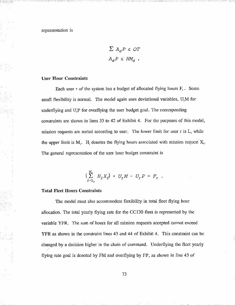
representation is

Eeoe<orAdP < HMd .

User Hour Co¡straints

Each user r of the system has a budget of allocated flying hours F,. Some

small flexibility is normal. The model again uses deviational variables, U.lr4 for

underflying ard Uf for overflying the user budget goal. The corresponding

constraints are shown in lines 33 to 42 of Exhibit 4. For the purposes of this model,

mission requests are sorted according to user. The lower limit fo¡ user r is L, while

the upper limit is M,. H' denotes the flying hours associated with mission request Xi.

The general representation of the user hour budget constraint is

M

{E nrxr\ + [J,M - u,P = F, ,i=Lr

Total Fleet Hours Constlaints

The model must also accommodate flexibility in total fieet flying hour

alloc¿tion. The total yearly flying rate for the CC130 fleet is represented by the

variable YFR. The sum of hours for all mission tequests accepted cannot exceed

YFR as shown in the constraint lines 43 and 44 of Exhibit 4. This constraint can be

changed by a decision higher in the chain of command. Underflying the fleet yearly

flying rate goai is denoted by FM and overflying by FP, as shown in line 43 of

t)

Exhibit 4. The generalised constraint is

r$\¿- Hixil + FM - FP = YFR

Linked Mission Constraints

Certain missions are operationally linked to other missions. If one is selected

then all must be selected; if one is not selected then none a¡e selected. The constraint

for a pair of missions is quite simple; just equate one X, to the other X, as shown in

line 45 of Exhibit 4 which links missions 17 and 19. The constraint for more tha¡

two can be modelled using the standard "either or" pattern of 0-i integer

programming. This involves the introduction of a 0-1 variable, say Y, and M, an

arbitrarily large value. As an example, suppose out of five missions

6.2t,X22,){.,,Xz4,X2j) at least four must be selected as demonstrated in lines 46 and

47. Then we wish one of the two following constraints to be¿ome relevant.

Re-writing,

x2t+x22+x8+x24+x2s > 4

X'+X2'+XB+ Xr4 +X2j = 0.

4 - X2fX22-X8-Xro-Xr' < 0

x2t+x22+x2j+ x24 + x2s < 0.

Then, introducing M and Y, 4 - Xu-X2z-Xß-Xro-Xr, < 0 + MY

x2t+x22+x8+x24+x2s < 0 + M(l-Y).

Then, usingM = 1000 4-Xz1-X22-XB-Xu-Xzs S 0 + 1000Y

x^+x22+xß+x24+x25 < 0 + i000(1-y).

74

Finally, rewriting (A) 1000Y+ X2r+ X2z+X,.+ X24+X zs à 4

(B) 1000y+xil+x22+x,3+x24+x2s < 1000.

These constraints are interpreted as follows. If mission requests

X2t,Xzz,X21,X24 and X¡ take on a total value of 4 or 5, the 0-i variable Y in

constraint A becomes 0. This causes constraint A to be relevant and B to be¡ome

redundant. If these missions take on a total value of three or less, Y is forced to be

1 due to constraint A. In turn, this makes constraint B releva.nt ard forces the values

of Xz1,X22,XB,Xro and Xr5 to become 0.

Previous Goal Co¡utraints

In all passes of the linear program, except the f,irst, it is necessary to introduce

an additional constraint to reflect the solution attained at the previous priority level.

For example, if the frrst pass for priority 1 is solved with missions X,, Xr, and Xu

being selected with an objective function value (Z¡) of 0.1408, then this must be

introduced into the next pass for prionTy 2 (see line 48). Lines 49 to 51 similarly

represent passes for priority 2 to 4. The general formulation is as follows.

D crx, I ieeriority t > yz,

This constraint ensures that each subsequent pass maintains at least as good a

solution for the previous passes. In the event that there are alternative optima

(different sets of missions that have the same Z¡) at a specifrrc priority level, this

formulation allows the selection of the missions forming that particular altemative.

75

PROTOTYPE MODEL USAGE

To demonstrate the use of the model, a representâtive set of 33 mission

requests from users 2,4,5,6 a¡d 7 was developed as test data (see Table 19) and a

hypothetical, abridged airlift planning process was used to develop the sequence of

model applications. Note that mission requests 1 to 31 represent what the SOOpSp-5

planner might initially be faced with for one month for one Base. Mission 32

represents additional missions for SOOPSP-5. Likewise, mission 33 is a new request

to SOAP-3. The runs of the model presented here approximate the type of processing

done by both planners; SOOPSP in the long term and SOAP in the nearer term (90

days). A1l model calculations were made using Hyper LINDOI29I.

Consider the SOOPSP-S task of initially forming an airlift mission capacity

plan for missions 1 to 3i. Exhibit 4 is the edited output of the fifth pass of iniriaJ

SOOPSP-5 planning, representing priority 5. Recall that the variable values for X1 to

X31 equal 1 if the mission was selected and 0 if not. Like further runs of the model,

the results are summarised in Table 20. The algorithm co¡rectly did not select

mission 4 be¿ause user 2 had insuff,rcient hours. Missions 14, 16,25,29 and 31 were

not selected due to lack of aircraft tasking lines.

Although the weighting system used in these particula¡ model runs is taken

from the ouþut of the AHP analysis in chapter 3, any weighting could have been

used. For example, cuûently the attribute category is used to discriminate amongst

missions at a given priority level and categories A,B and C were allocated weights

76

M¡SSIONREQIJEST

DÀTE5(INCL)

PRIOR¡TY USER'IOUR¡

ATTRIBT'TFS

1.2 0,o313

l¡o 0.o¡19

58 þ AIt 0.058t

trtl t8 vslt 0,0309

l*l) t0 0,0.1!2

72-2ó l4 HL o.0ó&l

u

5 t9 0,03t3

5 vcH o.ù26t

t0 t.8 5 Ã HBL 0,053,¡

t¡ 9ll 5 t2 0,u26

t2 35 0.0459

t3 3 LSL 0.otlo

t4 5 45 HBII

II 2 5 0.03¡ó

t6 l 2 5 Ð vB 0,0309

t1 3.5 2 5 0.u7ó

t8 2 HCV oþ5o2

t9 2t-23 2 5 l6 o,0216

Ø t.t3 90 0.0643

2t .21 6

22 .7t 6 @

73 |.21 0.ú91

t|.zl 0.0ó97

25 |-2t 6

7Á 23-30 ó 50 H.1L 0.0643

n 2t-24 4t HAV 0,05¡E

a 23-n 35 HCV 0,0502

z, 23-21 l6

30 2+24 t1 HBL o.0534

¡t 75.24 3 n 0,04ø

32 3 Á 0,on6

33 2/-26 t2

Table 19. Inputs to Prototype Sequential Linea¡ Model.

77

0.6, 0.3, and 0.1 respectively. The output of this model run is summarised in Table

20 under the heading SOOPSP CATEGORY. The results have been manually

confirmed.

Note the values of the AoM and AoP variables, paficula_rly AuM to ArM.

They show that 1,1,I and 2 arcraft tasking lines are available on days 6 to 9. Note

also that only four of the f,rve missions X21,X2',XB,X24,Xr5 were selected on days 1l

to 21. Inspection of the associated AoMs reveals that only on days il and 2i no

aircraft is available. Suppose SOOPSP-s, in consultation, decides to tâsk the fifth

aircraft now from day 12 to 20. Suppose also that user 4 calls with a request to add

mission 32 which requires an ai¡craft for days 6 to 9 and 24 flying hours. SOOpSp-5

already knows that an âircraft is available and only needs to confirm that user 4 has

sufficient hours available. Variable U4M shows that user 4 has sufficient hours.

Thus the planner is able to confirm immediately that user 4 can have the requested

mission. Exhibit 5 is the output of the SOOpSp run which represents the stâte of the

airlift plan when SOOPSP-5 hands it over to SOAP-3

User 7 has not given up on the request for mission 31 which did not get

selected in the airlift plan (see va¡iable value for X31 in Exhibit 5). SOAP notes rhat,

if this mission could be shifted to stârt on the 2?ú instead of the 25ú, resources are

available and user 7 agrees to this f,rx. User 7 also introduces mission 33 as another

request. SOAP knows that aircraft are not available without cancelling another

already programmed mission. Exhibit 6 shows the edited output of the subsequent

soAP model run as the planning officer establishes the effect of introducing this new

78

MISSIONREQUFJT

DATESflNCLI

PRIORNY sooPsPCATECtoRY

sooPsPNITIAL

sooPsP[TOD¡F¡ED o!¡ÊRT^SK

I,lo

J-3

t2-t7 0 o

l9-22

6 z2-

I

0

to l-3 5

ll 5

t2

¡3 27-X 1

t4 ¡l-10 5 0 0

t5 '2 2

!6 ¡,3 2 0 o

l7

t8 72.)5 0

t9

n t.¡3

21 lt.2t

22 |-71

23 ì1.2¡

2A .21

25 t|.2t 0

u 21-3¡

¿l 2)A 3

a

8 't 0 0

30 2+2ß 0

3l 25.2A 1 0

32 ó9 t

l3 2426

Note. I means mission is selected, 0 not selected.

Table 20. Outputs of Various Runs of the Prototype Sequential Linear Model.

mission. Note that mission 31 is selected on its new dates and that mission 33 is also

selected but at the expense of mission 28. Mission 28 is another priority 3 mission

belonging to user 6 who would not be pleased if it were cancelled for a priority three

mission for user 7 even if it is judged to be worth more to the system. This decision

could be taken but an unhappy customer would be a negative ¡esult. Thus SOAP

investigates the possibility of overtasking and notes that if the Base could provide an

extra aircraft for days 24 and 25, both could be satisfied. Exhibit 7 shows the

resultant airlift model with overtasking enabled for the two days. Line 32 controls

the total amount of overtasking allowed while lines 56 and 57 control the specific

days for this scenario.

COMPUTATIONAL SPEED

All models were constructed and run on a 386DX33 IBM compatible PC with

a math coprocessor. Each of the model runs consists of five sequential submissions to

LINDO which will accept ASCII hles. Although the software does not identify the

amount of time used for each run, personal observation revealed that no single pass

took mo¡e than 10 seconds with most being around 5. Thus it is reasonable to

assume that the totâl processing time for a model run is on the o¡der of 25 to 50

seconds. It is also reasonable to expect that dedicated softwa¡e on a higher speed

processor would reduce this interval. The total time needed for an operational system

will need to be determined but the speed results of this prototype are promising.

80

PROTOTYPE MODEL SI]MMARY

The prototype model was developed to provide direct computational support to

the two planning officers as they currently do their work. The individuai mission

weighting values used can be taken from any system that will provide discrimination

amongst missions at a given priority level. The prototype model has demonstrated

flexibility and accuracy.

81

CHÀPTER SIX

coNcLUsIoNS, LIMITATIONS AND RECOMMENDATIONS

CONCLUSIONS

Operational Research and the military have a historical connection. Indeed,

for many years OR professionals have carried out many effective studies centred on

military airlift in Canada and other countries. The problem, addressed in this thesis,

of ranking many airlift mission requests from several users with a constrained number

of taskable aircraft in order of priority to produce of a high quality airlift capacity

plan was made tractable by the application of a group of management science

techniques.

To create a mathematical model of the problem, a meâns was required to

numerically describe an airlift mission request. The category method of

discriminating amongst missions at a given priority level provides a workable, if

qualitatively and quantitatively rudimentary approach. We have seen that the Analytic

Hierarchy Process can numerically integrate the assessment of a mission's category

with other important mission attributes such as system training value and effective use

of the aircraft to provide better discrimination. The 27 numerical values produced by

the Analytical Hierarchy Process, compared to the three values resulting from using

the category attribute alone, result in a more differentiated airlift plan. Further, the

Analytic Hierarchy Process approach provides the decision makers with a flexible,

robust way of reflecting the importance of certain type of missions dependent upon

the prevailing military situation.

82

The detailed study of aircraft availability assessed four forecast models. The

aim was to validate the current 70% planning standard. All four models were found

to be statistically equivalent and we conclude that the 70% sranda¡d should be

maintained for capacity planning because it is simple and easily understood. The

analysis also showed a high variability of flyable aircraft on any given day. Potential

exists for the development of a more reflrned Markov prediction model and, if a

suitable cunent database is available, this should be pursued. The most important

conclusion from the ¡esearch 'was that any mathematical model of the planning system

must allow for the highly variable availability. While this is less applicable for that

portion of the model used by SOOPSP-5 in generating the long range airlift capacity

plan, it is important to SOAP-3 modelling.

The prototype sequential linear programming model meets the objective of the

thesis. The model is flexible and accurate. The model appears to be computationally

quick, it does not violate the priority criteria and it handles the selection of multiple

priorised mission requests from multiple users. It also handles iinked rnissions, either

as a pair or as a minimum out of an optimal number. User hour and fleet flying hour

constraints a¡e modelled and missions can be added, deleted or modified. In short, a

computationally efficient approach has been found to produce an automated planning

aid to assist the airlift capacity planners.

LIMITATIONS

Currently, the main limitation of the model is that it does not support a sliding

time window for departure dates. Still, this can be done manually by generating

83

another input f,rle based on a planner's decision as to which date to try. To automate

this feature, further development of the model is necessary.

The model is essentially a computational subroutine for a larger Air Transport

Group Decision Support System. Although it is possible to construct the necessary

file to pass to LINDO using commonly available word processing packages, this

would require extensive training for the planners to use the model operationally.

Appropriate database, processing and interface software needs to be developed.

The model does not currently support more than one Base per model run. It

requires a separate run for each of two or more Bases. Further development needs to

be done if the model is to identify surplus capacity at one Base that can be used to

make up for a shortage at another. Given the current development of the model, this

must be done manually and a new file submitted for processing.

The model does not support the needs of the Base level scheduler who must

match missions to aircraft tail numbers. Further development is required to enable a

combined planning and scheduling package.

RECOMMENDATIONS

The prototype model only shows that the approach merits serious consideration

for full operational deveiopment. It is strongly recommended that this approach be

incorporated in the current development of the Decision Suppoft System for Air

Transport Group.

84

REFERENCF,S

t1l. 1326-1 (Comd) 26 Mar 92 - Air Transport Group Annual Historical Report

Í21. Canadian Forces Administration Order (CFAO) 20-22.

t3l. Thomas M. Cook and Robert A. Russell, Introduction to Management Science, (PrenticeHail: Englewood Cliffs, New Jersey, 1989) 3-5.

t4l. Robert E.D. Woolsey, Operations Research for Immediate Application: A Ouick andDirty Manual, (Harper and Row Publishers: New York, N.Y., 1969) xiv.

l5l. Harold I-arnder, "The Origin of Operational Research", Proceedinqs of the EighthIFORS International Conference on Operational Research, Toronto, 1978, ed. K.B.Haley, (North Holland Publishing Company: New York, 1979) 3-12.

t6l. William L. Shirer, The Rise and Fall of the Third Reich, (Simon and Schuster: NewYork, 1960) 776.

l7l. Taylor, Ivan; Ooerational Support to Air Transport Group During Operation Friction,ATGOR Internal Working Paper 5/91, August 1991.

t8l. Woolsey, 169.

t9l. Danielson and Stannard, "A Developmental Model Using Analytic Hierarchy Process forRanking Military Airlift Support Requests", Unpublished Project Report, i4 December1992.

t101. Thomas L Saaty, "A Natural Way to Make Momentous De¿isions", Journal of Scientificand Industrial Research, Vol.51, August-September (1992): 56I-571.

tl1j. Bertram Schoner, "Correcting the Analytic Hierarchy Process", Proceedings ofAdministration Sciences Association of Canada (1992) Quebec, 62-68.

Í121. Canadian Forces Administration Order (CFAO) 20-22, pg 9, para 14 Note.

t131. D.L. Olson and J.F. Courtney Jr., Decision Support Models and Expert Systems,(MacMillan Publishing Company, New York, N.Y., 1992) 35.

t141. Wayne L. Winston, Operations Research: Applications and Algorithms (PWS-KentPublishing Company, Boston, 1991) 753-760.

t151. MathCad, computer software, MathSoft Inc., Cambridge, MA, USA, 1992.

85

1161. James S. Dyer, "Remarks on the Analytic Hierarchy Process", Management ScienceVol.36, No.3, March (1990): 249-258.

1171. Ronald A. Howard, "Heathens, Heretics, and Cults: The Religious Spectrum of DecisionAiding", Interfaces 22: 6, November-December (1992): 15 -27 .

1181. Thomas L Saaty, "An Exposition of the AHP in Reply to the Paper 'Remarks on theAnalytic Hierarchy Process"', Management Science, Voi.36, No.3, March(1990): 261.

t191. Patrick T. Harker and Luis G. Vargas, "Reply to'Remarks on the Analytic HierarchyProcess"', Management Science, Vol.36, N0.3, Ma¡ch (1990):269.

1201. Snty, 259-268.

Í211. Harker and Yargas,27L.

1221. Bertram Schoner, William C. Wedley, and Eng Ung Choo, "A Unified Approach toAHP with Linking Pins", European Journal of Operational Research,6a Q993)38 492.

t231. Stannard and Wong, "The Accuracy of the 70% Heuristic for Airlift Availability",Unpublished Project Report, 15 April i993.

1241. Kummen and Stannard, "Markov Model of CC130 Aircraft Fleet States", UnpublishedProject Report, 15 April 1993.

1251. Ivan Taylor and Kevin Naismith, "The Theory of Tasking: A Discussion Paper", AirTransport Group Headquarters, October, 1992.

t261. D.S. Moore and G.P. McCabe, Introduction to the Practise of Statistics @reeman: NewYork,1989) 587-588.

1271. Gitlow, Gitlow, Oppenheim and Oppenheim,of Ouality, (rwin: Homewood, 1989) 223-233.

1281. Gitlow et al.,145.

1291. H]¡per LINDO, computer software, LINDO Systems Inc., Chicago, IL, USA.

86

EXHIBIT 1 - N.STEP TRANSITION CALCTJLATIONS

EDMOIYTON - HIGH SE.RVICEABILITY

On 22 Janrary 1989 the number of aircraft in states I to 6 was 2 ,0 ,0 ,0 ,3

ald 4 reqpectively. Given the transition matrix (TM) for Etlmonton and using

MathCad, the transition states (TJ for subsequent days 1 to 14 ,21 and 28 were

calculated using the formula: T, = v.TM'

Table I shows the results with the cell values rrpresenting the predicted aircraft ineach state for each T,

Table 1. Edmonton State Prcdictions - High Initial Serviceability.

EX 1-1

22Jan89 STATES SUM

T" t 2 J 4 5 6 s5+s6

Tr 1.241 0.t72 0.072 0.020 3.816 3.679 7.495

T2 1.087 0.206 0.135 0.041 4.065 3.466 7 -531

T, 1,050 o.2t3 0.191 0.063 4.t63 3.321 7.484

T. 1.037 0.214 0.239 0.084 4.206 3.220 7.426

T5 1.029 0.214 0.281 0.105 4.223 3.148 7.371

T. t.023 0.214 0.317 0.t26 4.226 3.095 :7.321

T7 1.018 0.213 0.349 0.146 4.221 3.054 7.275

TE 1.014 0.212 0.376 0.167 4.2t1 3.022 7.233

T" 1.010 0.ztt 0.399 0.186 4.200 2.996 7.196

Tro 1.006 0.2t1 0.419 0.206 4.187 2.974 7.t6tT,, 1.002 0.210 0.436 o.225 4.174 2.956 7.130

T,, 0.999 0.209 0.451 0.243 4.16t 2.939 7.t00

T 0.996 0.208 0.463 0.261 4.149 2.925 7.074

Tro 0.993 0.208 0.474" 0.279 4.137 2.9t2 7.M9

T", 0.978 0.2M 0.515 0.390 4.069 2.849 6.918

T2s 0.967 0.201 0.525 0.482 4.021 2.809 6.830

EDMONTON - LOlry SER.VICEABILTIY

Similarly, on 3 October 1989, the ståte vector was 4, 1, 0,2,0,3. The state

transitions are shown in Table 2.

3Oct89 STATES SUM

T" I 2 5 4 5 6 55+56

T, 1-645 0.629 0.073 1.978 2.950 2.726 s.676

12 1.t28 0.391 0. r34 f .9s0 3.727 2.671 6.398

T. 1.004 0.279 0.185 1.921 3.93r 2.682 6.613

T, 0.971 0.232 0.229 1.891 3.975 2.7M 6.679

T. 0.962 0.212 0.267 1.862 3.976 2.724 6.700

"r. 0.959 0.204 0.300 L833 3.968 2.739 6.707

T, 0.959 0.200 0.328 1.806 3.962 2.748 6.710

T* 0.959 0.199 0.353 r.780 3.9s8 2.755 6.713

T" 0.960 0.199 o.374 1.754 3.957 2.759 6.716

Tro 0.961 0.198 0.393 1.730 3.959 2.763 6.722

T o.962 0.198 0.410 1.706 3.962 2.765 6.727

T 0.964 0.199 0.424 1.683 3.966 2.768 à.tz+Tr. 0.96s 0.199 0.437 1.661 3.972 2.771 6.743

Tto 0.967 0. r99 0.448 1.640 3.977 2.774 6.751

T", 0.977 0.20r 0.496 r.509 4.023 2.799 6.822

T2s 0.986 0.230 0.519 t.4M 4.067 2.828 ó.895

Table 2. Edmonton State predictions - Low Initiat Serviceability.

EX l-2

IREI{TON EIGE SER,VICEABILTTY

Using the Trenton transition matrix, the calculations were repeated for a low

initial serviceability state. Table 3 shows the rcsults for a starting ve*tor of 2, 0,2,

L, 4, 4 on24 luly 1989.

24lt¡189 STÀTES SUM

T. 2 5 4 5 6 55+56

T, 1.932 0.110 1.860 1.008 3.748 4.336 8.084

T, 1.93s 0.178 1.738 1.015 3.620 4.502 8.122

T" 1.951 0.222 1.633 t.021 3.568 4.588 8.156

T. 1.966 0.250 t.543 1.027 3.554 4.637 8.191

T, 1.979 0.268 1.464 1.033 3.556 4.671 8.227

T" 1.989 0.280 1.395 1.039 3.565 4.698 8.263

"I7 1.996 o.287 1.335 1.045 3.575 4.721 8.296

T, 2.003 0.292 1.282 1.051 3.584 4.742 8.326

T, 2.008 0.295 1.236 1.057 3.592 4.760 8.352

Tto 2.012 0.297 1. 195 1.063 3.599 4.176 8.375

T,, 2.015 0.298 l. 159 1.068 3.605 4.791 8.396

T," 2.017 0.299 r.127 1.074 3.610 4.803 8.413

Tß 2.019 0.299 1.099 1.080 3.613 4.814 8AnTro 2.021 0.300 1.074 1.085 3.616 4.823 8.439

T"t 2.022 0.298 0.963 1.123 3.619 4.851 8.470

T2s 2.016 0.297 0.9r3 1.156 3.608 4.845 8.453

Table 3. Tienton State P¡edictions - High Initial Serviceability.

EX 1-3

ÏREIYTON LOW SF,RVICEABILTY

The initial state vector for Trenton in a high serviceability state was

6, L, 0,2,2,2 on 5 Feb 1989. The subsequent tra¡sition states are shown in

Table 4.

5Feb89 STATES SUM

T" 2 3 4 6 s5+s6

Tr 3.153 0.867 0.227 1.980 3.980 2.784 6.7&T2 2.324 0.696 0.36 1.971 4.059 3.572 7.63t

T" 2.078 0.560 0.450 1.963 3.853 4.072 7.925

T. r.999 0.465 0.514 1.955 3.685 4.351 8.036

T, 1.970 0.401 0.564 1.947 3.583 4.498 8.08 r

T. 1.956 0.3s9 0.604 1.938 3.526 4.574 8.1@

T7 t.948 0.332 0.637 t.929 3.495 4.612 8.107

Ts t.942 0-3r4 0.664 t.920 3.477 4.630 8.107

Te f .938 0.302 0.686 r.9t2 3.465 4.637 8.r02

T,o 1.934 0.294 0.706 1.903 3.458 4.639 8.097

T,, 1.932 0.290 0.723 1.895 3.453 4.638 8.091

T 1.930 0.286 0.737 1.886 3.449 4.635 8.084

Tt. 1.928 0.284 0.750 1.878 3.446 4.632 8.078

T,o t.926 0.283 0.761 1.870 3.443 4.629 8.072

T,, 1.922 0.28i 0.808 1.816 3.435 4.611 8.046

Tr¡ 1.920 0.281 0.828 1.767 3.432 4.604 8.036

Table 4. Trenton State Predictions - I¡w Initial Serviceability.

EX 14

EX 2-1

EoM

ON

IoN

l+

0 ti

22 J

.ñu.

ry 1

9s9

CU

ÊR

EN

I H

EU

FIS

lIClll

9lfr

ac

rval

F

oFE

CA

ST

D

EV

ÌAIO

NoN

sas

E

1+O

7

_9

I 9

6,3

2..'

1O21

O73

939ô

.32.

79

4 s6

.3

1.7

9 5

aô.3

1,

'9ô

96.3

2.1

9776

.3o.

748

75.ô

t.4B

9

f a.

B

1.4

9 10

7

5.6

r.4

9 11

7

a.6

1.4

I 12

ô

5.ô

0.4

9t3'

65.ô

0.4

9 14

7

t.6

1-4

? 21

5

6.s

-r.g

92S

r63O

.'lo

l^t

22.4

MF

E -

1.

4

TÂ

ÊN

loN

T

o t¡

24

Jùty

19a

9rr

I X t) ¡.J

ON

BÁ

SË 13 13 13 13 13 13 13 l3 13 13 t3

ñES

€ÀF

CH

EO

ME

AN

Âcl

u^L

FO

R€C

AS

T O

EV

tÀ.fi

ON

I t06,

453

2.54

77,

17

2,83

6.45

3 2.

547

6.45

3 1,

347

ô.45

3 1.

a47

ô.45

3 2.

a47

6.43

3 O

,a4'

4,73

6 1.

2lJ4

4,13

0 1.

264

5.73

0 1.

264

4,73

6 1.

284

5.73

6 O

.2C

45.

73a

0.26

4s,

r36

t.264

6.4!

3 .t.

453

6.45

3 0,

54'

MF

E -

.0.0

375

FO

FE

CA

Sl

AC

CT

JRA

CY

C

OM

PA

ÂIS

ON

T

AS

LË

ÊD

MO

NT

ON

IF

ÈN

ÌôÑ

ME

TH

OO

HE

IJÀ

lSllC

t.¿

tOO

þ.

O3,

RE

Sea

FcH

1,

2a3

0.36

6S

TÊ

AD

Y S

tÂÎE

1.

202

0.65

7P

RE

otC

not\¡

0,

21i3

0.

731

MA

F(O

V

SI!À

DY

SIA

ÎEA

CIU

AL

FO

FE

CA

SI

OÊ

VIA

ÎON

MF

É _

1,2

5337

5

FÉ

SE

AÊ

CH

EO

M

EA

NA

CIU

AL

FO

FÊ

CA

SÎÞ

EM

A¡O

N

9 6.

50õt

2.4

93!

10

7,22

È 2

.771

9 ô.

!0ôr

2_4

9a9

a 6.

5061

1.a

930

â 6.

aoô1

1.4

939

I 6.

5061

2.4

939

7 tt.

506t

0.4

930

, a,

7832

1.2

160

7 a.

7æ2

1-21

6ø',

a,7s

32 1

.21a

87

a,rø

32 1

.216

Aô

5.t0

32 0

.2t6

Aô

!.ta3

2 0.

216s

t 3.

7æ2

1.21

6ø5

!.50ô

1 -1

.toót

7 6,

!O6i

0.4

939

ÎoT

AL

19.2

390

10

6.69

7 1.

303

10

6.69

7 1.

303

10

a.69

7 r3

o310

a.

697

1.30

3a

8.69

t -0

.697

9 s.

697

0.30

39

6.69

7 0.

303

I a,

697

.0.ô

977

8.69

t -1

.697

9 A

.697

0.

303

9 e,

ô97

0.30

33

3.69

7 -0

_697

I 3.

69t

0.30

3ro

s,

û97

r3o3

10

a,69

7 r3

o39

3.69

7 0.

303

lota

L 5.

84A

MÀ

ÂK

OV

P

ñEO

ICT

ION

ÀC

ÌUA

LFO

FE

CA

ST

OE

VIA

îON

MF

Ê -

i,202

4aa

MA

RK

OV

S

IIAD

Y S

ÎAT

EÂ

ctua

L F

oFE

CA

SI0

EV

tAt¡

oN

10

â.40

5ô 1

.t042

t0

9.40

5s t

,594

2fo

a.

/ro!

ã 1.

5942

10

â.40

t8

1,a9

42s

3.40

3ã .0

.405

¿I

A.4

05A

0.!9

429

A.4

o5B

O.a

942

3 0.

4059

4.4

05¡

7 A

.40s

8 -i.

4o5s

9 0,

4058

0,!9

429

a.40

5a o

.a9¡

t2s

3.¡1

058

4.40

58I

S,4

o5A

0.!9

4210

a,

4o5a

t.5

942

10

a.40

56 1

.594

29

9.40

56 0

.594

2T

OÍÁ

L 10

.507

2

MF

€ -

o.36

s5

l! 2, ¡:l o Þ

d c) Þ (t)

Þl

Þd {X E'J

Xx¡

V) lã È o FJ Þ F Fl

MF

Ê -

0.ô5

!7

€DM

ON

TO

N l+

O ¡

, 3

Ocr

obôr

1gs

oA

ISC

RA

FI

CU

Â8.

EN

T.H

EU

R]S

TIC

R

ES

EA

RC

HÊ

D I¡

ÊA

N

MA

RK

OV

S

TE

AD

Y A

TA

ÌE

MA

RK

OV

P

RE

DIC

TIO

NoN

BA

SE

r+

o ac

ruÀ

L F

oRE

cAsr

oE

vr^r

roN

¡cr

u¡L

ìiàÊ

ðiüi

ev,¡

rp¡r

¡cr

ueL

Ëór

iÈãr

ii i,?

ü^ír

ijr,¡

- A

cruA

L F

oRE

cAsr

DE

vr^r

oNto

1

6 7_

1

€ 7,

17

1t-1

e

7.22

ø

1.22

ø

o õ.

076

0.32

410

2

7 !

o z;

'.;1

9.!

, r.

.ri;

ó:ñ

z r.

3ss

0.60

2ro

37!o

ii.;i9

..!Z

;;..i;

;,ó:;;

;7€.

ôr3o

.sa.

104"

Ziå

r'.iil

.l_ei

..àió

;:;;;o

ô.!7

eo.ô

7ero

6

6 -7

r

ã i.ì

t j:1

7 I

;:ãió

;.;;

ä 6

ô.7

o.7

i1

I 7

7_.7

- o.

j j

zlàà

i 9.9

9?

i r.

rjiîõ

o..r

iÉîõ

7

6..¡

07 0

.203

11

7 "

2.7

o.s

à i.;

ät

9.1!

9 e

i.ããi

ã õ:

ð;ói

I

o.7r

1.

2ør

8 È

!.7

2.

7 á

i.;;i

?.99

1 ;

;:õi;

;:ãÈ

ió

E

..7,3

r.

7r3

r r

e I

7_.7

- i.i

á

i..ä;

i 1.

997-

6

;Ëi;

ffii;

s a.

71c

0.71

61r

ro

s

7_.j-

1.7

á

i.;;t

1.9!

Z

I ;:ü

i; ;ã

;,i;

o ..7

22 0

.722

11

l't

" !.2

o.

g ;

i.åäi

9.1

19

s t.ã

'i; ó

:ó;å

i a

..72t

1.

2.,s

11

12

" !.7

_ o.

3 á

;.;;i

9.!1

9 ã

,.ðÈ

iõ ;f

fii

a a.

734

r.26

ar

13

s j_

.2_

.t.7

à ï.;

,;;

I gg

7-

å ;.õ

i; ;ö

; I

6.74

3 0.

743

i1

14

u 7,

.! 1.

7 'B

t.á

;i | 9

e,7-

o

,;6iõ

i.ü

i; 6

6.76

r 0.

76r

11

21

u 2.

7_

1.7

à ï.;

ái

1.9s

7 e

z.õs

ìõ i:

;i;

6 8.

a22

o.a2

211

2a

B

' ,l:

7 i.7

á

;.;;i

_1.9

92

a ;:f

ii;

iËi;

6 8.

se6

0.8s

6ro

r¡L

17.6

ro

r^L

1e.2

86

ïõin

i ró

.õði

Ë

ror L

13.,1

7s

û X t.)

AIR

CR

AF

TO

N B

AS

E

TR

EN

TO

N

T+

O ii

5 F

àbru

.rv

1989

13

T+

O

132

13

a13

413

5

13

613

713

I

13

913

to

13

tl13

12

t3

t313

t4

13

21t3

28

CU

RR

EN

T H

EU

RIS

I¡C

R

ES

EA

RC

HE

O M

EA

N

MA

RK

OV

Iac

rurl

¡on¡

c¡si

óË

viÀ

iror

Acr

uAr-

FoR

EcA

sr D

EV

raro

N ^"

r,^,

."*"

"åt,i

PJ^

:Ilit

._-.

,^,

MA

RK

ov pl

ED

rcïo

N

MA

o i

1.09

376

9.1

t.19-

1 0.

19.

1 l.t

9.t

3.t

9.1

1.1

9.1

4.1

9.t

o.t

9.1

t.19.

1 t.1

1.1

0.1

9,t

o,t

g.r

3.1

9.1

4.1

g.l

t.l9.

1 0.

1t.l

3.

1T

OT

AL

24.A

MA

D -

t.6

g75

FO

RÊ

CA

ST

AC

CU

RA

CY

C

OM

PA

RIS

ON

T

AB

TE

ÊD

MO

NT

ON

IR

EN

TO

NM

ÊT

HO

DH

€Uß

IST

ICR

ES

EA

RC

HS

TE

AD

Y S

IAIE

P8Ê

Dtc

lroñ

MA

o -

'1.2

0631

3

8.69

7 0.

697

4.09

7 0.

303

8.09

7 0.

897

9.09

7 2.

697

8.69

7 0.

a97

8.69

7 3.

€97

8.88

7 0.

303

8.09

7 0.

ô97

8.€9

7 0.

897

8.89

7 0.

303

8,69

7 0.

303

8.69

7 2.

ø97

8.89

7 3.

897

8.09

7 0.

€97

B.€

97

0,30

38.

897

2.ø

97T

OT

ÄL

21.1

A2

DE

Vra

roN

¡cr

u¡r

¡one

c¡sr

ó¡v

Àiö

ü -

¡cru

¡r-'i

ãËË

liï."

,iri/i

íi o"

t.094

1.

537

1.20

5 1.

324

1.24

4 1.

216

0.42

4 1.

190

MA

O -

1.

2440

31

MA

D -

0.

9296

8.40

68 0

.406

88.

4058

0.6

042

8.40

58 0

.406

88.

4068

2.4

088

8.40

õ8 0

.405

88.

4088

3.4

068

8.40

ß8

0,59

428.

406A

0.4

068

8.¿

1068

0.4

058

8.40

68 0

.694

29.

4058

0.8

942

8.40

68 2

.406

88.

4068

3.4

058

8.40

58 0

.406

88.

4068

0.5

942

8.40

68 2

.406

8T

OT

AL

19.4

348

rì Èt z Þ u, v) t'i c '.J f! F' È ¡

¡tÞ

XoË z1 ¡v v) E

I F êJ Þ F Fl

MA

D t

1.

323S

75

ô.76

4 1.

238

7.63

1 t.3

ôg7.

s26

0.07

68.

036

2.03

88.

081

o.o8

tO

.l 3.

18.

ro7

0.8s

39,

107

o.to

7€.

102

0.10

28.

097

0,00

38.

09t

0.90

90.

084

2.O

A4

8.07

8 3.

078

8.07

2 0.

072

8.04

0 0.

854

8.03

8 2.

038

ÎoT

AL

.tg.o

36

MA

D -

1.21

4076

MA

D -

1.

'189

8876

? lrl Þ 2 U) F c rl lrl HN

ZY

nÊ ¡rr

N)

CI

a) Irl ñ o lal Þ F Ê

MA

RK

OV

PR

EO

ICT

ION

AC

TU

ÂI

FO

ÂE

CA

SÌ

OE

V1A

ÌION

9 7.

/t95

1.50

5to

7.

531

2.46

9I

7.aa

4 t.a

16a

,,126

0.

57¿

1ø

7.

371

o.ô2

9ø

7,

321

1.ôt

97

7,21

3 0.

275

, ,,2

33

0.23

37

7.19

6 0,

t96

7 7.

161

0.1ô

l7

7,13

0.

f3!

7.t

1.1

6 7.

Or4

1.

O74

7 ',O

49

0.04

95

ô,91

a 1.

eta

7 6.

A3

0.1t

IoT

AL

t3,o

7o

MF

E -

0-3t

4a?5

MÀ

FK

OV

PS

ED

ICÎO

NÁ

CT

IAL

FO

F€C

AS

Í D

ÊIIA

'¡IO

N

MA

ÈK

OV

S

IËA

DY

SIA

IEA

C'T

UA

L F

OF

ÊC

AS

'T

OÈ

V¡A

IION

ô.30

61 2

.493

97.

229

2-77

1ô,

30ô1

2.4

939

6.to

ô1

t.493

9ô.

!061

r.

4939

6.50

ô1 2

.493

9!.5

061

0.3t

939

5.76

32 1

.21a

85.

7432

t.2

r!s

5.7A

32 1

.2t6

A5.

7A32

1.2

18A

5.7t

32

0,21

6a5,

7A32

0.2

16A

5.fa

32

1.27

6Aô.

t06t

t.5

06t

ô.80

ôt

o./t0

3e.lo

raL

22.2

a2

10

A.0

64

t,9r

ô10

s.

t22

r.a7

g1o

a.

t!ô

1.A

4410

8.

t01

1.60

9e

a.22

7 0.

227

9 4.

2ô¡t

o.

737

0 a.

29ô

0.70

4g

s.32

6 0.

a26

t È

.a52

t.3

52t

6.97

3 0.

ô2!

I 9.

a96

0,60

4g

a.4t

3 0.

113

I ø

,42'

0.

573

10

a.a3

t 1.

561

10

â,4'

1.

539

9,45

3 0.

a47

lol

L 16

.646

MÂ

D -

1.

0403

7!

NÊ

SE

AR

CH

ÊD

M

ÊA

NA

CÎU

ÂL

ÊO

R€C

AS

Î O

EV

IAT

IOI.¡

MA

O -

1.

3907

5

MA

RK

OV

S

TE

AO

Y S

TA

ÌEF

OF

EC

AS

TÞ

ÊV

¡AN

ON

4.40

¡a

t.3Þ

424.

40¡a

t.!

9/t2

4.40

5â t

,!942

4.40

t6

1.!9

42s.

4058

0.a

o58

4.40

!s

0.59

424.

40!0

0.

5942

4.40

¡a

0.4o

la4.

4050

t.¡

o¡a

9.40

5a o

.594

24.

4058

0.5

942

a.4o

5s 0

.405

84.

4018

0.5

942

4.40

5a 1

.a94

20.

4059

t.¡

942

fola

l 15

,753

ô

MA

D -

0.

9s46

6,45

4 2,

54'

7.17

2.

s36-

453

2,54

'6.

453

1.54

'6.

453

1.a4

1ô.

453

2.a4

76.

4s3

0.54

75.

t3û

1.26

45.

736

t.264

5.73

6 r.

264

5.73

A

1.20

45.

73ô

O.2

845.

736

0.20

45,

73ô

1,2A

46,

453

t.453

ô,45

3 ô.

5¿7

TO

ÎAL

22.9

6

10 10 t0 10 0 t a 9 I a

10

EÞ

MO

NIO

N r

+O

1.2

2 J.

ñu.r

y 19

69C

UR

ÂË

NIH

EU

FIS

¡CA

CIU

AL

FO

ÂE

CA

ST

DÊ

VIA

IION

r+o

jt

9 6.

3 2.

721

ô7s

3 9

6.3

2.'

4 a

63

1,'

5aô3

1.

tô

I ô,

3 2.

77

7 6.

3 O

,7I

7 5.

6 1,

49

7 5.

6 1.

41O

7

5.0

1.4

11

7 5.

û 1,

412

6

5.6

O,4

13

6 5.

6 0.

4'1

4 7

5.6

1.4

21

I r.

3 t.3

26

7 6_

3 O

.'T

OIA

t 25

NE

SE

AF

CH

ED

M

EA

NA

CIU

AI.

FO

FE

CA

SID

EV

IAîO

N

10

a.a9

7 1.

303

lo

a.69

7 1.

303

r0

8.69

7 1.

303

10

a.ô9

7 r.

303

a a.

697

0,69

79

A.ô

97

0,30

39

S.ô

97

0.30

3s

a.69

t 0.

697

, 8,

69'

t.697

9 a.

69t

0.30

39

0,69

7 0.

303

a a.

a97

0,69

79

8.ã9

7 0.

303

lo

a.69

t 1.

303

10

a.û9

7 1,

303

9 a.

697

0,30

3lo

TÂ

t 13

.424

MA

O -

0.

639

MA

O ,

r.

5625

TF

EñÌ

ON

t0

¡.24

Jlty

i9€

9ar

Rca

^Fr

cuÂ

RE

Nl

HÊ

|JR

|S¡C

ON

SA

SE

A

CT

UÁ

L F

ôñÊ

CA

ST

DE

VIA

ÎION

ln

t3

r+0

aV

13

't

ro

9.1

o.9

13

2 to

9.

1 0.

9tJ

13

3

10

s.1

0.9

¡.

13

4 10

9.

r o.

913

aa9.

f1,t

13

6 99

.1

o.1

13

7 99

.1

O.1

l3

s a9

.1

t.1t3

979.

i2,1

13

10

9 ',t

o.

t13

11

9

9.1

O.1

13

12

a 9.

1 1_

1t3

t3

9

9.1

0.1

13

14

to

9.r

o.9

13

21

to

9.1

O.9

13

28

I 9.

't o.

1lo

laL

I1.4

ON

BA

SE

9

MA

D -

0.

7125

FO

RË

CA

ST

ÂC

CU

FA

CY

C

OM

PA

BIS

ON

IA

BLE

EO

MO

NIO

N T

FE

ÑIO

N

1,56

3 0,

r'12

1.43

5 0,

a39

1.39

i 0.

9a5

0.45

5 1.

040

MÊ

IHO

OH

EU

ÂIS

IICR

ES

EA

RC

HS

IEA

OY

SIA

TE

PF

EO

IClIO

N

EXHIBIT 3 - SPSS EDITED OTJTPT]T

SPSS/PC+ Studentlrare+ for ¡Bü pC 4/10/93

The SPSS/SLI+ system fite is rêâd f.oitìfi tê proj750.sys

lhe file ras creâted on 4/10/93 àt Ot12tO1ênd is titl.ed SPSS/PC+ Studenttâfe+The SPSS/SI+¡ system file contâins

25ó cases, each co¡sisting of7 variables (ihctuding system variêbtes).7 vârisbles Hitt be used in this session.

This procedure Hâs coflpletd ât 10:0ó:52Co+IPUTE DIFF = ACT0AL-toREcST.LI ST.The ¡sH dêta or transfo¡nåtíon p¿ss is p.oceeding

25ó c6ses are H.itten to the cuçreàsed ¿ctiie fil,e.

MSE I€TIITD ACruÀL FæECST

1,0 1.0 9.0 ó.31.0 1.0 10.0 7.01.0 1.0 9.0 6.31.0 1,0 8,0 6.31.0 1.0 8.0 ó.31.0 1.0 9.0 6.3t ,0 1 ,0 7,0 6.31 .0 1 .0 7.0 5.ó1 .0 I .0 7.0 5.ó1.0 1.0 7.0 5,6't.0 1.0 7.0 5.61 .0 1.0 6.0 5.61 .0 1 .0 ó.0 5,61.0 1.0 7.0 5.ó1.0 1.0 5.0 6.31 .0 r .0 7.0 ó.31.0 2.0 9.0 6.51 .0 2.0 10.0 7.21.0 2,0 9.0 6.51.0 2.0 8.0 ó.51.0 2.0 8.0 ó.51.0 2,0 9.0 6.51 .0 2.0 7.0 ó.51.0 2.0 7.0 5.71 .0 2,0 7,0 5 -71.0 2.o 7.0 5.71.0 2.0 7,0 5,71.0 2,0 ó.0 5.71.0 2,0 ó.0 5.71 ,0 2,0 7.0 5,71.0 2.0 5.0 6.51 ,0 2,0 7.0 ó.5't.0 3.0 9.0 6.5I .0 3.0 10.0 7.21.0 3.0 9.0 ó.51.0 3.0 8.0 ó,51,0 3.0 8.0 6.51,0 3,0 9.0 6.51 .0 3,0 7.0 ó.51 .0 3.0 7,0 5.81.0 3.0 7.0 5.81.0 3.0 7,O 5.81 .0 3,0 7.0 5.81.0 ¡.0 ó.0 5.81,0 3.0 ó.0 5.8I .0 3.0 7.0 5,81.0 3.0 5.0 6.5

DIFF

2.703.002.701 .701 .702.70

.70

1 ,401.401.40

.40

.401 ,10

- 1.30.70

2.552.432.551,551.552,55

.551.261.26

1 .26.26.26

1.2ó-1.15

,552.492.772,191.191.492.49

.49

1 .221 ,22.2?

1 .22-1.51

EX 3-1

L0 3.0 7.01,0 4,0 9,0I .0 4.0 10.01 .0 4,0 9.0'1.0 4,0 8.01.0 4.0 8.01.0 t1,o 9.01.0 4.0 7.01.0 4.0 7.01 .0 4.0 7.01.0 4.0 7.01,0 4.0 7.0I .0 4.0 ó.01 .0 4.0 ó.01.0 4.0 7.01.0 4.0 5.0L0 4.0 7.02.0 I .0 10.02.0 1.0 10.02.0 1.0 10.02,0 I .0 10.02.0 't.0 8.02,O 1 .0 9.02.0 1.0 9.02.0 1,0 8.02.0 1 .0 7,02.0 1,0 9.02,0 1 .0 9.02,0 1.0 8,02.0 1.0 9.02.0 1 .0 10.02.0 1.0 '10,02,0 I .0 9.02.0 2.0 ,10.0

?,0 2.0 10.02.0 2.0 10.02.0 2.0 10.02.0 2,0 8.02,0 2.0 9.02.0 2.0 9.02,0 2.0 8.02,0 2.0 7.02,0 2.0 9.02.0 2.0 9.02.0 2.0 8.02.0 2.0 9.02.0 2.0 10.02.0 2.0 10.02,0 2.0 9.02.0 3.0 10.02.0 3.0 10.02.0 3.0 10.02,0 3.0 10.02.0 3.0 8.02,0 3,0 9.02,0 3.0 9.02.0 3.0 8.02.0 3.0 7,02.0 3,0 9.02.0 3.0 9,02,0 3,0 8.02,0 3.0 9.02.0 3.0 10.02,0 3,0 10,02.0 3,0 9.02.0 4.0 10,02,0 4,0 10.02.0 4,0 10.02,0 4.0 10.0

6.5 .t197,5 1.517.5 2.t+77.5 1.527.4 ,577.4 .637.3 1.ó87.3 -.287.2 -.2i7.2 -.207.2 -.167.1 -.137,1 - 1 .107.1 -1,077.0 -.056.9 -',t.92ó,8 ,179.1 .909.1 .909.1 .909.1 .909.1 - 1,109.1 -.'t09.1 -.109.1 - 1.109.1 -2.109.1 -.109.1 -.109,1 - 1.'t09.1 -.109.1 .909,1 .909.1 -.104.7 1 .308,7 1.308.7 1.304.7 1 .308,7 - ,70a.7 .308.7 .308.7 - .704.7 -1.704,7 .308.7 .308.7 - .708.7 .308.7 1.304.7 1 .308,7 .308.4 1.594,4 1.598.4 1.594.4 1.598.4 -.418.4 .594.4 .594,4 -,418.4 -1.418.4 .594.4 .598.4 -.418.4 .598,1 1 .598.4 1.594.1 .598.1 1.928.1 1.888.2 1 .844.2 1.8'r

EX 3-2

2,0 4.02.0 1.02.0 4.02.0 4.02.0 t4.02.0 4.02,O 4.02.0 4.02.0 4.02.0 4.02.0 1.02.0 4.03.0 1 .03.0 1 .03,0 1 .03.0 1 .03.0 1 .03.0 1 .03.0 I .03.0 1 ,03.0 1 .03,0 1 .05.0 1 ,03.0 I .03.0 1 .03.0 1 .03.0 I .03.0 1 .03,0 ?.03.0 2.03.0 2.03.0 2,O3.0 2.03,0 2.03.0 2.03.0 2.03.0 2,O3.0 ?.03.0 2.03.0 2.03.0 ?.03.0 2.03.0 2,03.0 2.03.0 3.03.0 3.03.0 3.03.0 3.05.0 3.03,0 3.03.0 3.03.0 3.03.0 3.03.0 3.03.0 3.03.0 3.03.0 3.03.0 3.03.0 3.03,0 3.03.0 4,03.0 4.03.0 4.03.0 4.03.0 4.03,0 4.03.0 4.03.0 4.03.0 4.0

8.09.09.08.07.09.09.08.09.0

10.0't 0.09.0ó,07.07.0ó.0ó.07.08.05.0ó.06.08.08.06.0ó.0ó.06.0ó.07.07.0ó.0ó.07.08.05.0ó.0ó.08.08,0ó.0ó.0ó.0ó.0ó.07.07.0ó.0ó.07.08.05.0ó.0ó.08,08.0ó.0ó,0ó.0ó.0ó.07.07.0ó.0ó.07.08.05.0ó.0

8.28.38.38.38.14.4

8.44.48.48.58.57.07.07.07.07.07.77.77,77.77.77,77.77.77.77.77.77.27.27,2

7.27.97.97,97.97.97.97,97.97.97.7,7.7.7.7,7.28.08.08.08.08.08.08.08.08.08.08.05,76.46.66.76.76.7é.76.76,7

EX 3-3

3.0 4.03.0 4.03 .0 4.03,0 1.03,0 t1.O

3.0 4.03.0 4.04.0 't.04.0 I .04.0 1 .04.0 1.04.0 1 .04.0 1.04.0 1 .04.0 1.04,0 1.04.0 1.04,0 1 .04,0 1.04.0 I .04.0 1.04,0 1.04.0 1.04.0 ?,01.0 2.04.0 2.04.0 2.04.0 2.O4.0 2.04.0 2.01.0 2.04.0 2.04.0 2.01.0 2.04.0 2.04,0 2.04.0 ?.O4.0 2.04,0 2,04.0 3.04.0 3.01.0 3,04.0 3.01.0 3.01,0 3.04.0 3.04.0 3.01.0 3.04.0 3.04.O 3.04,0 3.04.0 3.04.0 3.04.0 3.04.0 3,04.0 4.04.0 4.04.0 4,04.0 4.04,0 4.04.0 4.04.0 4.04.0 .4.04.0 .. 4.04.0 1.01,0 4.04,0 4.04.0 4,04.0 4.0

ó.0 6.7 -.728.0 6.7 1-278.0 6,7 1,27ó.0 6.7 -.71ó,0 6.8 -,75ó.0 ó.8 -.82ó.0 6.9 - .908,0 9.1 -1.109.0 9.1 -.108.0 9.1 -1.10ó.0 9.1 -3.108.0 9.1 - 1.105.0 9.1 -1.109.0 9,1 -,108.0 9.1 - 1.108.0 9.1 -1.109.0 9,1 -.109.0 9.1 -.10ó.0 9.1 -3.105.0 9.1 -4,108.0 9.1 -1.109,0 9,1 '',10ó.0 9,1 -3.108.0 8.7 -.709.0 8,7 .308.0 a.7 -.706.0 8.7 -2.708.0 8.7 - .705.0 8.7 -3.709.0 8.7 .308,0 4,7 -.708.0 a.7 - .709.0 8.7 .309.0 4.7 ,30ó.0 8.7 -2.705,0 a.7 -3,708.0 a.7 -.709.0 8.7 .30ó.0 8.7 -2-708.0 a,4 -,419.0 8.1 .598.0 8.4 -.11ó.0 a.I -2.418.0 8.4 -.415.0 8,4 -3.119,0 8.4 ,598.0 a.4 - -418.0 8.1 -.119,0 a.4 .599.0 8.4 .596.0 8.4 -2.415.0 8.4 -3.418.0 a,4 -.419.0 8.4 .59ó,0 8.4 -2,418.0 ó,8 1 ,249.0 7,6 1.378.0 7.9 .07ó.0 8,0 -2.048.0 8.1 -.085,0 8.1 -3.109.0 8.1 ,898.0 8,1 -,118.0 8.1 -.109.0 8,1 ,909.0 8.1 .91ó.0 8.I -2.085,0 8,1 -3,088.0 8.1 -,07

EX 3 -4

t .0 4.0 9.0 8.0 .954,0 1.0 ó,0 8.0 -2,04

Itunber of c6ses read = 256 Íû6er of cases listed = 256

EXA'{IIIE Æ¡FF BY XETII(I)./PLOT BOXPLOT I{PPLOT HISTOGR¡X SPREADLEVEL-

DIFT

Valid casest 256.0 Hissing cases: .0 percent nissingi .0

l'leên -.1014 Std Err .0909 Min -4.1000 SkeHness -.3ó50¡lêdìôn .0000 Variånce 2.1175 Hax 3,0000 s E SkeH .1SZz5U lri¡n -.0721 std Dev 1.4552 Rênge 7.1000 Ku.tosis -.1409

IoR ?.0000 s E Ku¡t .3033

DI FF

Frequency Bin Center

2,00 Extremes *9.00 -3.500 ****13.00 -2.500 ******46,00 _1,500 *************tr**r*****57.00 -.500 ******************!r*********69,00 .500 ********************************r*47.00 1,500 **************r********12.00 2.500 ******1.00 Exttemes

Bin Hidth : 1.000Each star¡ 2 cåse(s)

DIIF

3.00

2,00

1.00

.00

-1.00

-2.00

-3.00

.ó0

.40

.00

- ,20

-,10

-.ó0

***

.ó.00 -3.00 .00 3.00

ormê[ Pl.ot

-ó.00 -3.00 .00 3.00

Detrended l¡oll¡ã t Ptot

EX 3 -5

DI FT

K-S (Li tLiefo¡s)

3.00

,00

-3.00

-ó.00

Varìabte DI FF

tl of câses 25ó.00

syri$ot Key: * - Hediên (o) - Outl,ie¡

Eoxptot footnotes denote the foLLoringt

1) cAsE198, CASE205

(E) - Extreme

.0 Percent missing: .0-4.1000 skeHness -.22113.0000 S E skeH .29937.1000 Ku¡tosis .09232.0000 S E Kurt .5905

DIFFBy ËET @ 1.0

Valid cases:Meanüed i sn5Z Trim

DIFF8y fETtl(D

64.0 Hissing cases:-.2891 Std E.r .19ó2 üin-,1000 Vafiance 2,4635 tqax-.2ó94 Std Dev 1.5ó9ó Ranse

IOR

1.0

Frequency Bin Centet2.00 Extremes **3.00 -3.2501.00 -2,7501.00 -2.250 *ó,00 -1.750 ******13.00 _ 1.250 ********r****1.00 -.750 *

11 .00 _ .250 ***********7.00 ,250 *******8.00 .750 ******r*5.00 1.2502,00 1.750 **.00 2-250

3,00 2.750 ***1.00 Extrernes

8in Hidth : .500Each stat: 'l c8se(s)

EX 3 -6

DIFFBy XEIùCD

2.40

I .ó0

.80

.00

- ,80

-1.60

-2.10

.44

.16

.00

-.16

- ,48

-ó:oo -3:oo .óo 3.óollornâl pIot

Stêt ist i c dfK-S (LiLl.iefors) .0810 64

DIFFBy flErH(I' 2.O

Vå[id cêses: 64,0 l,{issing cases:

Hean -.1ó9ó std Err .1887 l,tínüedian .1885 Variance 2.2785 t/'ax5Z T¡im -.1470 std Dev 1.5095 Rangê

taR

-ó:oo -i:oo .öo 3.öoDetrended l¡onrìâ1, P totsigni ficancê

> ,2000

.0 Pe¡cent mÍssing: .0

-3.ó970 SkeHness -.30372.8300 S E skeH .2993ó,5270 Kurtosi s -.21582.43/10 S E Kurt .5905

DIFFBy HEIHû)

Frequency

2.004.00

t 1.0012.0018.0015.004.00

Bin ridth :Each stâri

DI FFBy

'IETH(I)

2.O

Bin Cente.

-3.500 **_2.500 ****- l .500 ***********-.500 ************.500 **********ìr*******

1,500 *************2.500 ****

1.0001câse(s)

2.0

2,40

I .ó0

.80

,00

-1.ó0

-2.10

.3ó

.24

.12

.00

-.12

- .24

- .36

-t.00 -2.50 .00 2.50

Notmê L P totStatistic

-5.00 -2.50 .00 2.50

Detrended No¡flì¿1, P totSigni f i cance

EX 3-7

K-s (Li Ll.iefors) .0818 64

DTFF8y HETH(I) 3.0

Vâlid cases¡ 64.0 ¡lissing câsesillean -,0525 std Err .1871 Hinl,ledian .1324 Variênce 2.2105 4àx5U Trin -.0239 Std Dev 1.49ó8 Ranse

¡aR

> ,2000

.0 Petcent missing: .0-3.4058 SkeHness -.350ó2.n10 S E SkeH ,2993ó.17ó8 Kurtosis - .47602.4458 S E Kurr .5905

.5:oo -z:so .òo z.ÈoDetrended Hormêt PIot

Significance>.2000

.0 Percent missing: ,0

-3.1000 SkeHness -.53112.4ó90 S E SkeH .29935.5ó90 Kurtosis .0911'1.ó548 S Ë Kurt ,5905

DIFFBy IIETH([) 3.0

Frequency2.00I .003.007.001.001.00

11.007,00

11.007.O0ó,003.001,00

D¡FF8y HEÍHû)

Bin Hidth | .500Eêch star: I cåse(s)

2.t0 .30

,10

1.60

,80

.00

- -80

-1.60

-2 -10

- .20

- .30

-5:oo -2:50 .óo z.Èol¡ornê[ P tot

stat isti c dfK-S (tiLtiefors) .0853 64

DIFFBy ¡IETH(I) 4.O

VaIid cases: 64,0 l,li ssing cåses:

¡leen .1055 std Err .1532 Hinl,ledian .1225 Variânce 1.5018 Max5.l Trim .152ó std Dev 1.2255 Ranse

roR

EX 3-8

DIFFBy TETHCD

trequêncy2.00

.003.002.003.008.00

13.005.00

13.005.009.00'l .00

8in Hidth :

Each stãr:

DIFFBy HETKþ

4.0

8in Cente.-3,250-2.n0-2,250-1.750 **-1.250-.750 ********-.250 ********r.****.250 *****.750 *************

1,250 *****1,750 ***r.*****2.250

,500l case(s)

4.O2.40

1,ó0

.80

,00

-.80

-1.ó0

-2.40

.n,50

.25

.00

- .25

-.50

- .75

-5:oo -a:50 .öo z.soo.mâl pl,ot

StatisticK-S (Líltiefors) ,0625

3.00

-: loo -zl:o .óo z-ÊoDettendêd No¡rîat ptot

df Significance61 > .2000

¡|ETHoo 1.0

of Cases ó4.00

3.0 4,0

ó4.00 ó4,00

(0) 'outtie¡ (E) - Extrerne

2.0

ó4.00

SFrbol. Key: * - ¡tedianEoxptot footnotes denote the fol,toHingl

1) cAsE198, cÀsE205

Test of honogeneity of vatianceLevenê Statisti c 1.3318

dfz si gni ficênce252 .2636

dfl3

-LT rTuti utrïïï_L(0 note 1)

EX 3-9

T-TEsl /GRCUPS l{Ell'(n (1,2) /V,IRIÀBLES D¡FF.

t-têsts for independent sâÍtrtes of HETHOO

l¡úùerVa¡iable of C6ses t{eån SD SE of Mean

DIFF

r{ETfioo 1.0 64 -.2891 1,570 .196¡rË1H0D 2,0 64 -.1696 1.509 ,189

Hean Difference = -.1194

Levene,s lest for Equatity of Vatiances: t= ,01ó p= .899

t-test for EquaLity of l,leêns 95./.Variances t-value df z-lâi L Sig SE of Diff cf for Diff€quâl -.44 126 .662 .Z7Z (-.658, .419)Unequêt -.44 125.81 .662 .Z7Z (-.ó59; .419)

ÍPAR TESTS /ürr-$ TtEy DIFF 8y t{Erfl(I) (1,2).

- - - - - l,lann-tlhitney U - Uilcoxon Rank SúnH TestDIFF

by ¡lElHoo

I'lêân Rank Cases62,67 ó4 HETHoo = 1,066.33

_ó4 üEfHoo = 2,0

'128 fotatCorrected fot Ties

U H Z z-tåi Led p1931.0 4011.0 -.5583 .5766

ot{EvÂY /VARIABLES DtFF By t{ETt{(D (1,4) ./nÂÍces BIlrxEy /sTATtsTtcs ALL.

-o¡E9ÄY---VôriãbLe DIFF By Vârisbl,e

IIETHCT)

Anatysis of Vsriance

Sun of ¡lean F FSource D.F. Squêres Squares Ratio ptob.

BetHêen Groups 3 5,4419 1.9150 .ASS7 .4647l.lithin croups 252 534.5155 2.1211Totã[ 255 539.9604

-0¡tEgAY----Stêndârd StandardGroup Count Mean Deviation Ertor 95 pct Conf fnt for l,tean

Grp 1 64 -.2891 1,5696 ,.1962 -.ógi1 To .1030crp ? 64 -.1696 1.5095 ,1382 -.5467 ro .2071Grp 3 64 -,0525 1.4968 .1871 -,4264 to .3214crp 4 64 .1055 1.ZZ5S .1532 -.200ó To ,4116

TotãI 256 -.1014 1.4552 .0909 -,2805 10 .OTn

Fixed Effects ¡todet 1.1564 .0910 -,ZBO7 fo .OT7BRãndom Effects HodeL .0910 -,39,l,l lo .1AAz

EX 3-10

UARlll¡¡G - 8êt{een conponent va.iance is negativeit ¡{as reptaced by 0.0 in coíputing åbovê tåndom effects m€asures

Randor¡ Erfects l"f"l : Ti'yî-"I å"1";"i iîry":": y":i:nï_ _ _ -.0018

Group Hinin(¡n Haxim¡n

crp 1 -4.1000 3.0000crp 2 -3.6970 2.8300crp 3 -3.4058 2.n10crp 4 -3,1000 2.1690

Totå[ -1.1000 3.0000

Tests lor Hornogêneity of Variances

Cochrans C = ¡lãx. Var i Bnce/Sqn(Va r i ances ) = .2904, P = ,592 (Approx. )Bartlett-Box F = 1.114,p= ,ZZB*-""'u:"1":": 1 :':'ï:ï';",ï0, _ .'.10- - . . _ _

Variabte DI FFBy VâriôbLe l,lET HoD

¡luttipte R6nge Test

Tukey-B Procedu¡eRånges fo¡ the .050 tevet -

3,24 3.50 3.66

The rênges åbove €re tsbte rsnges.The våtue actuatly coÍpâred Hith ¡tean(J)-Heano ) is..

1.0298 * Range * sqrt(1,/N(I) + î,/tl(J))

Lo t*o g¡or.ps are significåntly different st the .050 levet

Homogeneous subsets (subsets of gToups, rhose hishest êM loHêst meansdo not diffe. by nore thên the shortestsignificant ¡ênge for a subset of thât size)

SUBSÊT 1

Group c"g '! G¡p 2 crp 3 Crp 4Mean -.2891 -.i696 -.0525 .ìos¡

IPÀr TESTS /KRUSK L-I¡ÄLLIS DIFF By tGIft{þ (1,4) ./sT frsf¡cs z.

( ¡lêdi an)25th 50th 75thl¡ percenti Ie percenti [ê petcenti Ie

DrFr 256 -1.1000 .0000 .9000r1ETfi00 256 1.2500 2.5000 3,7500

'- - - - Kruskôl-Hãl,tis'l-Hay ANOVA

0¡ Ftby ¡lETflOo

tlean Rank Cases

1t9.04 64 t{ETHoo = l125.42 64 ttETHoo = 2

130.78 64 HETHoÒ = 3138.76 61 ¡lETtloo = 4

256 Totât

Cortectêd fot TiesCASES Chi-Square Significânce Chí-Squa¡e Significance

216 ?.1415 ,4851 2.4157 .4852

T-lESl /GR(I.PS l{ETHm (1,2) ./VÄßIAALES DtFF /CRtTERIA={I (.9).

t-tests lor indeperdent sånpLes of HETIiOO

t¡l.¡IùerVôriabl.e of Cases Hesn SD SE of üean

DIFF

r,rEïfloo 1.0 64 - -2891 1.570 _196HEÌHoo 2,0 64 -,1696 1.509 .189

tilean oifference = -.1194

Levene,s lest for Equal.ity of Varisnces! F= .01ó p= .999

t-test for Êquatity of üeans 90,ÅVâ¡iânces t-value df z-Tâil. sig sE of Diff Ct for DiffEquat -,44 126 ,662 .Z7Z (-.571, .332>t,nequal -.11 125.81 .662 .272 (-.521t, .332)

qlEVAY /VANIABLES DIFF BY I{ETIICD (1,4) /RAXGES LSD (.I).

- 0N E t/aY - - - - - - - - - -

Vari abte Dl FF

By Variêbl,e HETHOD

Analysis of Vâriânce

Sl.m of lle6n F FSource D.F. Squares Squares Ratio ptob.

BetHeen croups 3 5.1149 1,8150 .ASS7 .46!.7Hithin Groups 252 534.5155 2.1211lotal. 255 539.9694

-oraE9AY---

Variâble DIFFBy V€riabl.e LETHq)

Muttiptê Range lest

LSD PaocedureRãnges for the .100 levet -

2.33 2.33 2.33

The rãnges above 8re tâbte tanges.The vãlue åctuatty coípâred Hith lte8n(J)-t{ean(¡) is,.

1.0298 * Range * Sqrtfi/t¡(t) + i/N(J))

Io tl.o grot+s aîe signific€ntl.y different at thê .i00 têvel.

EX 3-12

Honogenêous Subsets (Subsets of groups, Hhose highest ând lowest meänsdo not differ by morê than the shortestsignificânt rangê fot a subset of that size)

st,BsET 1

Group crp ! crp 2 crp 3 G¡p 4üean -,2891 -.1696 -.0525 ,1055

Âxov /V^ßIASLES DtFF By ttETH(D (1,4) BASÈ (3,4) /ST^TrSftCS ÁIL.

*** cELL ¡{EAHS ***D¡FF

BY XEIHIÐEJtS€

TOTAL POPUTATIOII

- .93( 128)

METN0o

1231-1.26 - 1.15 -1.03 -.27

( 32) ( 32) ( 32) ( 32)

gASE

34- .88 -.98

( 64\ ( 64\

¡tEfH00I -.98 -1-5t

( 1ó) ( 16'2 -1,'t6 -'t.13

( 1ó) ( 1ó)3 -1.23 -.U

( 1ó) ( 16)4 - .14 -.40

( 1ó) ( 16)

*** AIIÀLYSIS OF VARIÁIICE ***DIFF

BY XETHTI)gÂsE

Su[ of llean signi fsoqrce of vã¡istion squa.es oF squate F of t¡lain Effects 19.579 1 4.895 3,198 .016¡{ETHm 19.261 3 6.120 1.195 .007BASE .317 1 .317 .207 .ó50

z-Hay Interactions 3.849 3 1.283 .8jB -4Zsr,tETHoD BASE 3.849 3 1.283 .838 .475

Expl.ained Z3.4ZB Z 3,347 2.1A7 .040

Residuât 183.673 120 1.53.1

Totat zoz,1o1 127 1.ó3125ó Cases Here ptocessed.128 cases ( 50.0 pcT) He¡.e missins.

EX 3-13

*** IIULTIPLE CLASSIFICATIOII AIIALYSISDIFF

8y HETHü)BASE

Grênd lleân = -.928

Vârisble + catego¡y

HETHOO

EASE

Grand lleån = -.928

Variêbte + category31

Huttipte R SquêredI'tul,tipl,e R

Unsdjustedll Dev¡n Eta

32 -.3332 -.2232 -.1132 ,66

.30

Adjusted forÂdjustedfor tndependentsIndependênts + covÉti6tesDevrn Betâ Devrn Eeta

-.33

- .11.66

.30

Adjusted forAdjusted fot Independents!ndepêndents + CovariãtesDev,n Bets Devrn Beta

.05-.05

.04

I{ULTIPLE CLASSTFICATIOT AfALYSISDIFF

By XElHmBÁSE

Unadjusted11 Dev,n Etâ

61 .0561 -.05

-u4

AXOVA /VARIABLES D¡FF BY XEIHC) (1,4) SÂSE (1I2) /SIATISTICS ÃLL.

*** cELL HEANS ***

DIFFBY I{EIHü)

BASE

TOÍAt POPUTATIOI¡

.73( 128)

IlET HOO

1

.68< 32) (

BASE

1

1 .02( ó4) (

2

32) (

2

61'

34.93 .4A32) ( 32)

EX 3-l-4

1

(2

(a

(4

(

BÂSE

1

1.101ó) (

1 ,2516) (

1.201ó) (

1ó) (

2

- .041ó).3716),661ó).7516)

^LYStS OF VARTA¡CE r**

DIFFBY IG-THC)

BÀSE

Sun ofsoq¡ce of Vãriat ion Squares

l,lâin Effects¡tETfi00BASE

2-Håy ¡nteractionsIIETHOD BASE

Exptåined

Res idua I

lotal

DtFFBy ¡ETH(D

BÂSE

crând l,lean = .726

Variâbte + category N

I'tE I0Ð132232332132

BASE

Adjusted forAdjusted for Independents

Un€djusted ¡ndependents + CovêriatesDev¿n Eta Dev'n Beta Dev,n Beta

¡lean SisnifDF Square F of F

4 3-603 5.411 ,0113 1.174 1.112 .3471 10.890 10.310 .002

3 5.518 5.253 .0023 5.518 5.253 .002

7 1.437 4.201 .000

120 1.05ó

127 1.243

- .04.08.20

' -2t

14.4123.522

10.890

16.64516.645

31 .057

126.744

157.A0125ó cases Here processed.128 Cases ( 50.0 PCI) Here missing.

**' !tuLf tpLE CLASSI F¡CAtIOI At^Lysts *rr

-.04.08,20

- .24

EX 3-15

i** HULTIPLË CLASS¡FICATtOT AIALYSIS }**

DIFFBy rETHO

BASE

crand l,le6n = .726

Va¡íabte + Cêtegory1

¡lul.tipLe R Squared¡{ul.tipte R

Adjusted forAdjustedfor fndependents

Unadjusted ¡rdeændents + covatiatesll Dev'n Etâ Dev,n Betã Devrn Beta

6t1 .29 .296t+ -.29 -.29

*+r cÈLL t{EAtS **r

.26 .26

.091

.302

Âllw ./VÂRIAELES DtFF By IETfiC) (1,4) BÀSE (1,4) ,/ST TISÍTCS ALL.

DIFFBY flETH(f}

BÂSË

TOTAL POPULAT IOII

- ,10( 256)

HETHfI)12s4-.29 - ,17 -.05 .11

64) ( 61) < 61> ( 64)(

BASE

12't.02 ,13( 61) ( 61) <

BASE

1

r,{ET H001 1.40

( 1ó) (2 1.25

( 16) (3 1.20

< 16) (4 .21( 16) (

34-.88 - - 98ó/+) ( 64)

234..04 -.98 -1.511ó) ( 1ó) ( 1ó).37 -1.16 -1.131ó) ( 16) ( 16).66 -1.23 -.84ló) ( 1ó) ( 16).75 -,14 - ,401ó) ( 16> ( 16',)

EX 3-15

r*' À¡¡^LYSIS OF VARTAICE **r

DIFFBY HEÌI{(D

BÂSE

S!¡n of ¡teên SignifSou.ce of Variation Squa¡es Dt Squãre F óf F

Hain Effects 191,711 ó 31.952 ?4,704 .O0O¡lEllloo 5.1t5 3 1.815 1.403 ,2t2sASE 186.266 3 62.089 48.004 ,000

z-Hay Inte¡actions 37.832 9 4,204 3.250 .0OlfiETfioD BASE 37.832 9 4.201 3.250 .001

ExpLained 229.513 15 15.303 i1.g3t .000

Residuât 310.417 Z1O 't.293

Totê[ 539,960 2SS 2.117

25ó Cases rere ptocessêd.0 Câses ( .0 PCT) Tere missing.

*** HlJLttpLE CL^SSIFtCATTOt AxALySIS ***DIFF

By xEIHq)BÄSE

crênd l'lean = -.101 Adjusted fo¡Adjusted for ¡ndepeMents

variabre + catesory - i:i9l'"¡:: ;ÍÎi"*;:t: ;"9?x".';:;:HElHOO

1 6t+ -.19 -.192 61 -.07 _ .073 64 .05 .054 6t+ .21 .21.10 .10

r** ¡rJLTtpLE CLASST FICÀTtOt¡ AtÂLysIs **rDTFF

By XEfH(n8ÄSE

Grênd ¡lean = -,101 Adjusted fo.Adjustêdfor lndependents

variãbre+cãteso¡y - Hï9i'"¡* ¡*:i"*;:t: ;"9îX""'å:::8ÀSE

1 61 1.12 1.12? 64 .54 ,513 61 - .78 -.781 64 -.88 _.88

üuttipte R SquarêdI'luItipl,e R

.59 .59

.355-596

EX 3-17

¡t (BASE=I AND HEIHm=1) IHTER=1-It (BÂsE=1 A D l{Eftl00=2) It11ËR=2.IF (8ASE=1 A D ¡lElH00=3) r lER=5.lF (BASE=1 A D BEltl00=4) ¡NTER=4-It (8AsE=2 A D ¡IETH00=1) INTER=5-It (BASE=2 AHD l.iETH00=2) IÍTER=ó.rF (BASE=2 AND HETHo0=3) tItÊRÈ7.It (8AsE=2 Al¡D I'tÈ1800=4) f TER=8.rF (BÂsE=3 ÂliD HEltlq)=1) tI¡TER=9-¡t (8ASE=3 A{D ¡lElHm=2) lltlER=10.lF (BASE=3 A¡¡D llETH00=3) tNfER=11.IF (8ASE=3 AltD üETHoo=4) ¡I¡TER='|2.tF (BASE=4 AND HElfioo:t) I TER=13.rF (BASE=4 AND ¡{ElH00=2) ttiTER=14.It (BASE=4 AND ttETiloo¡3) INTER=15,IF (8AsE=4 AND HET[I00=4) ¡HÌER=Ió.

OIEIAY ¡¿VAR¡ASLES D¡FF 8Y BâSÉ (I,4),/RAICES B¡1KEY ./STATTSI¡CS ALL.

ol¡E9^Y----Va¡iabte D¡FF

BÂSEBy Variablê

Analysis of vêri€nce

Sun of l{e€nSquâres Squares

F

Rsti o

ó2.088ó 14.2368

1.4036

Soutce

8êtteen ctoups

Hithin cl.oups

Totat

F

Prob.

.00003

255

186.2658

353.6946

539.9604

Group

crp Icrp 2Grp 3crp 4

lotâ[

1 ,3122.6757

- .6270-.ó020

.om

- - - -0NEHAY

Stãndatd StandatdCount llean Deviation Error 95 pct Conf tnt for lle6n

61 1.0172 1.1809 .1476 ,7ZZZ to61 .4338 .9682 .1210 .i920 lo64 -.878ó 1.0071 .'t259 -i.1302 To64 -.9782 1.50ó0 .1882 -1.3543 To

256 -.1014 1.4552 .0909 -.2805 To

Rêndom Effects Sode l. - Estimâte of BetHeen CoÍponent Variênce

tixed Effects Hodet 1,1847

Rsndon Effects Hodet

.0740 -.2473 1o .0tt4

.4925 -1.6687 Jo 1.4658

.9tß2

Grp 1

crp 2c¡p 3cnp 4

Group

----0t¡EUAY-Mininm ¡lâxifi¡un

-1.9180 3.0000-2.1000 1.9160-2,9519 1.2900-4.1000 1.3ó90

-4.1000 3.0000Total

EX 3 -18

Tests for Hornogenêity of Variances

Cochrêns C = Hax. Vêr i ance/Sun(Va r i ênces ) = .4040, p= .001 (Approx,)Bartlett-Box F ! 5.321 ,p=.OOll4axißm Våriênce / l{inin¡ Vâriånce 2.t20

-otE9^Y- - -Vsriabl.e DfFF

8y Variabte 8.AS€

Muttipte Range Test

lukey-B ProcedureRânges for the ,050 Level -

3.24 3.50 3.66

Thê ranges above are tabte rânges.The valuê 6ctua[[y co{¡parêd Hith ¡iean(J)-fieån(f) is..

.832 * Rênse * sqrt(l/t¡(I) + 1/N(J))

(*) Denotes pairs of g.oups significåntly diffe.ent at the .O5O teveL

-oltE9^Y---Variable DIFF(conti red)

GGGC¡l.rrPPPP

l{eân crot-p 13 21

-.9782 crp 4-.4786 Grp 3.4138 cîp 2

1.0172 crp I

llomogeneous Subsets (Subsets of groups, r{hose highest ênd loHest me€nsdo not diffet by [þre than thê Ehortestsignifìcant rånge for a subset of that síze)

SUBSEI 1

6roup Grp 4 Grp 3Hean - .9782 -.878ó

SUBSET 2

G¡oup crp 2Heån .4338

SUBSET 3

Group Grp IMean 1.0172

EX 3-19

ol¡El¡AY /VÁR!^BLES DIFF By ¡ITER (1,ló)/nÂ{css BrlffEy /stÄTrsTlcs ALL.

- ot Et AY - - -Variåbl.e DtFF

IIIIERgy VariãbLe

Soutce

BetNeen Croups

l.li th in croups

fotãt

Analysis of Variance

SLm of l,lêân F FSquâres Squares Rât io p¡"ob,

229.5431 15.3029 11.8315 ,0000

Count ¡{een

16 .212916 -.03751ó .365516 .6567'16 .750616 -.981216 -1.162916 -1.226016 -.144116 -1.537516 -1.131516 - .8/.3316 -.3973

256 -.'t01t,

Fixed Effects ¡{odel

310.4173

539,9601

1.1478 ,2870.9287 .2322.9287 .2322.9287 .2322.9734 .2433.9304 ,2326.9327 .2i32.9336 .2334.9227 .¿307

1.4592 .364A1.4592 .36481.4592 .36481,5188 .3872

1.4552 .0909

.8245

.4574

.8ó011,15161 .2693-.4855- .6659- ,7285

.3475

- ,3570-,0658

.4280

',2805 lo -0777

15

240

255

1,293t+

GToUP

crp 1

Grp 2crp 3

Group

Grp 4crp 5G¡P ócrp 7Gnp 86rp 9crp'I0c.pl1crp12Grpl3Crpl4crp15Grpló

Totô [

Count

161616

Standard Ståndardl{eên Devistion Erro. 95 pct Conf tnt for l,{ean

1 .4000 '1.0979 ,2745 .8150 To 1 ,98501.2534 1.0942 .2736 .6703 to i.83ó41.2025 1.0930 .2732 .ó2ol To 1.781s

- - - -0NEUAY

Standârd StandârdDeviôtion Er¡or 95 Pct Conf Int for ¡teen

RandûT Effects l,lodet

1.1373 .0711 -.2111+ ro .O3Bó

,2445 -,6226 1o .4197

RaMom Effects l,lodel. - Estimête of BetHeen Coflìconent V€riance

EX 3-20

Group

c¡p 1

crp 2crp 3crp 4crp 5crp óG¡p 7Grp IGl.p 9c rp10Grpl lcrpl2Grpl3

Group

Hinift¡n

-1.3000-1,4530-1.5061-r.9180-2.1000-1.6970- 1.4058- t.5>¿u-2,7000-2.8870-2.9519-1.7130-1.1000

l,lax i n(¡n

3.00002.83002,n102.1690

.90001.30301 .59121.91ó0

.3000

.1130

.04811 ,2900-.1000

__-_0HEt¡ÂY__

l,lininm ¡låxin(m

Grp14 -3.6970 .3030Grpl5 -3.4058 .5942Grpló -3.1000 1 .3ó90

fotê[ -4.1000 3.0000

Têsts for Ho{þgeneity of Variânces

Cochrãns C = ¡lâx, Var i snce/Sqn(Vs¡ i ances ) = .,1159, p= .29g (Approx. )Bartlett-Box F = 1.205;P= .259*-""" u:|"l"i:1:':'ï u""'"*" 2'818 '

-oIEgAY---Vari€bte DIFF

By Variãble Ifl¡ER

Mul,tiple Range Test

fukey-B ProcedureRanges for the .050 tevel -

3,85 4.12 4.28 4.39 1.48 4.55 4.61 4.66 4.70 4.744.78 4.8,1 4.U 4.87 4.A9

lhe ranges above åre tôbte r€nges.lhe vå[ue actuâtly coípâred Íith l,tean(J)-8ean(I) is..

.8042 * Ranse * Sqrt(1/H(r) + î/N(J))

EX 3 -21

(*) Derþtes pairs of gro{.Fs sigr¡ific€ntty differeit at thê .tjo Level

G G G G G GG G GGG G G G GG|.t r r r r r r r l. 1r ra î IpppPpppPPpppPppp11t1 tlt

l{ean Gm{Jp 3 1 O 4 I 5 6 Z S t+ 6 7 a 3 Z 1

-1.5375 cm13-1.?24 crptl-1.16Ð crpl0-1.195 crpl4-. 12 crp 9-.&13 crpl5-.3973 crpló-.1441 cm12-.03ã cæ 5-21æ GÎp 4.3655 crp ó.6567 Grp 7-75ú crp 8

1.2025 Grp 31.2534 crp 21.4000 c¡p I

Honogeneous Subsets

SUBSET f

**r**ilrr

Grp13- 1 .5375

crpl5-.u33

Groupl,lean

(Subsets of groups. those highest and towest meansdo not differ by Ílote thân the shortestsignificant rÊnge fo¡ I subset of that size)

Grp'|1-1.2260

Grp16- .3973

crplo crp14-1,1629 -1.13t+5crp 9- .9412

Groupl,leån

SIJBSET 2

Group crpl ll.lean -1.2260

crp10-1,16?9

Grp12-.1411

Grpl4 G¡p 9-1.1315 - ,9812

crp 5-.0375

6rp15- .4433

croup crpló¡lean -.3973

su8sÊT 3

Group crp 9Hean -,9812

G¡oup ctp 4l,tean ,2129

Gl"p15- .8433

crpló G¡p12-.3973 - -1111Grp 5- .0375

SUBSET 4

crp 5- ,0375

Gfoupl{ean

Group¡leên

crpl5- .8433

Grp ó,3655

crpló- .3973

Grpl2 crp 4.2129

EX 3-22

SUBSËT 5

Group crpló Grpl2 Crp 5 crp 4 crp óI'rean -.3973 -.i441 -.0375 ,2129 .:t655

croup crp 7 crp IMean .6567 .n06

SUBSET ó

Group crp_5 crp 4 crp q c¡p Z crp 8¡rean -.0375 .2129 .3ó55 ,¿567 ,7¡O¿

Group G.p 3 crp 2Heôn 1.2025 1.2534

SUISET 7

croup Crp_l- crp ó Grp Z Grp 8 crp 3l.leân .2129 .3ó55 ,6567 ,75O¿ 1.2025

Group Grp 2 crp 1

l,lean 1.2534 1.1000

EX 3 -23

EXHIBIT 4 - EDITED OUTPUT OF SOOPSP INITIAL RUNMAx 0.0309 x4 + 0.0313 X8 + 0.0254 x9 + 0.0534 Xlo + 0.0426 x11+ 0.0581 X14SUB,]ECT TO

2) x]. +x7 +xl.5 +xL6 +x2o +À1M_Â1p= 63) xl + X7 + X8 + X1S + X16 + x20 + À2M - À2p = 64l x2 +x7 + x8 + x9 + xl-6 + xL7 + x2o + À3M _ Â3p = 65) x2 +x1 + x8 + xLz + x14 + xl? + x2o + À4M _ À'4p = 66) X2 + X3 + X1O + X12 + x14 + XL7 + X2O + À5M _ À5p = 67) X2 +X3 + XlO + X!2 + XL4 +X2O+À6M_À6p= 68) X2 +x3 + X1O + xI2 +XLA +X2O + À?M _ À7p = 69) X2 + X3 + X10 + X12 + Xt4 +X2O + ÀBM_ ÀBp = 610) X2 +x11 + x!2 +xr( +x2O +A9M_À9p= 611) X2 +Xll +X12 +XIA +x2O + Âi.0M - À10p - 6r2l x11 + x20 + x2L + x22 + xzg + x24 + x25 + À11M _ A11p = 613) x4 + x20 + x2! + x22 + x23 + x24 + x25 +A12M _ À12p _ 6LAl x4 + x20 + x21 + X22 + x2g + x24 + x25 + .A,l.3M _ À13p = 615) x4 + X2L + X22 + XZ3 + X24 + X2S + À14M _ Âl-4p = 6L6) x4 + x2L + x22 + x23 + x24 +x25 +À15M_À15p = 611l. xA + x2L + X22 + X23 + x24 +x2S +À16M_À16p = 618) x4 + xzL + x22 + X23 + x24 + x25 + À1?M _.q,1?p = 619) x27 + x22 + x23 + x24 +x25 +À18M _ A18p = 620] x5 +x21 +x22 +x23 +x24 +x25 +A19M_À19p = 62Ll x5 +x21 + x22 +x23 +x24 +x25 +À20M _À2Op = 622\ X5 + X19 + X21 + x22 + X23 + XZ4 + X25 + À21M _ .r¡21p = 623) X5 + X6 + x1B + XL9 + A22ttt - A22p = 624) X6 +X18 + X19 + X26 + X2.t + X2B + X29 +.A23M _ .A23p = 6251 x6 + xL8 + x26 + x2.t + x28 + x2g + x3o +.A24M _ A24p = 626) x6 + x18 + x26 + x27 + x28 + x29 + x3o + x3L + À25M _ À25p

27) x6 + x26 + x27 + x28 + xzg + x30 + x31 +.e,26M _ A26p = 628) x13 + x26 + x2-1 + x28 + x29 + x3O + x31 + J{2?M _ A27p = 629) x].3 +x26 +x27 + x3O + x31 +À28M _ À28p = 630) x13 + X26 + ¡,29M - À29p = 631) XL3 + X26 + À3OM - A3Op = 632) Â,1p + Ã2p + À,3p + À4p + Â5p + A6p +.Â,7p + À8p + A9p + Alop+ Àl1p + Àt-2p + À13p + À14p + A15p + A1.6p + ¡,1?p + À18p.+ À,19p +A2OP

+.A21p + A22p + þ2,3p + A24p + Â25p + À26p + A27p + À28p + À29p +

=033l. ,-L2 xL + 41 x2 + 29 x3 + L8 x4 + 10 X5 + L4 x6 + u2M _ u2p34) 24 X'Ì + 19 X8 +?x9+20xLO+22 xtL + 35 x12 + I x13 + 45x14

+ U4M - U4p = ]-6235) 14 X15 + 20 x!6 + 11 X1? + 28 X18 + 16 X19 + 90 xzo + usM _

U5P

36) 60 X21 + 60 X22 + 60 X23 + 60 X24 + 60 X2S + SO x26 + 4r X2.t+ 35 X28 + U6M - U6p = 38337) 36 X29 + 34 X3O + 22 X3L + U7M - U?p = 8338) U2P <= 1139) U4P <= L640) Usp <= 1.641) U6P <= 3842], U?P <= I43) 12 xl + 4I x2 + 29 X3 + 18 x4 + 10 x5 + l-4 x6 +24 x7 + 19 X8+ 7 x9 + 20 x10 + 22 xlL + 35 xt2 + I xL3 + 45 xl,4 + L4 x15 + 20 xi¿+ 11 x17 + 28 xL8 + 16 XL9 + 90 xzo + 60 x21 + 60 x22 + 60 x23

EX 4-1

+ 60 x24 + 60 x2S + 50 X26 + 4! xzi + 35 XZg + 36 x29 + 34 x3O+ 22 X3L +Et4-Fp= 9OO44) FP <= 10045) x17 - x19 = O46) x2t + x22 + X23 + X24 + X25 + loOO y >: 4471 x2L + x22 + x23 + x24 + x25 + looo y <_ 1oo048) 0.0313 X1 + 0.0412 X5 + 0.0683 X6 >= 0.1408491 0.0346 XLs + O.O3o9 xL6 + 0.0426 Xl? + O.O5o2 x18 + 0.02?6

xl- 9+ 0.0683 X20 >= 0.223350) 0.0346 x7 + 0.015 X13 + 0.0683 x26 + O.O54B x21 + O.OSO2 X2B+ 0,0426 X29 + 0.0534 X3O + 0.0426 X31 >= 0.276351) 0.0459 x2 + 0.0581 x3 + 0.0459 x12 + 0.0697 x2:- + O.o6g.t x22+ 0.0697 X23 + 0.069? X24 + 0.0697 XZS >= O.42B.t

ENDlNTE x1INTE X2INTE X3INTE X4

INTE X9INTE X1OINTE X11INTE XT2

INTEINTEINTEINTE

INTEINTEINTEINTEINTE

VARTABI,Ex1

.vt

x4X5

X5x6

x8

x13x14x15xl- 6x1-1

rNTE Xl.8INTE X19rNTE X2OTNTE X21INÍE X22fNlE x23INÎE X24INTE X25

INTE X27rNTE X28INTE X29INTE X3OrNTE X31INTE YENUMER.ATION COMPLETE. BRÀNCHES= 6 p]voTs=

I¡AST TNTEGER SOI]UTTON 1S THE BEST FOUNDRE-TNSTÀTÍ.ING BEST SOLUTION. . .

OBJECTIVE EUNCTION \/ÃTUE

L) .153?00000

VAI,UE1.000000r..0000001.000000

.0000001.000000

REDUCED COST.000000.000000.000000

-.030900.000000

EX 4-2

x'tX8x9

x10x11xL2xl-3x14xl-5x16x17x18x19x20x27x22x23x24

x26x21x2ax29x30x31

YÀ1MA1.PÀ2MÀ2PÀ3MÀ3P

À4PÀ5M

À6MÃ.6 PÀ?MÀ7PÀ8MÀ8PÀ9MA9P

Ã10MÀl-0P.A11MÀ,11PÀ12MA12 PÀ13MÀ13 PA14MÀL4PÀ15MÀ15 PÀ16MÀ16PÀ17MÀL?PA18M

1.0000001.000000r..0000001.0000001.0000001.0000001,0000001.000000

.0000001.000000

.0000001.0000001.0000001.0000001.0000001.0000001,0000001.0000001.000000

.0000001.0000001.0000001,000000

.0000001.000000

,000000.000000

2.000000.000000

1.000000.000000.000000.000000.000000.000000.000000.000000

1. 0000 0 0.000000

1.000000.000000

l-.000000.000000

2.000000.000000

2. 00 000 0.000000,000000.000000

1.000000.000000

1. 000000.000000

2,000000.000000

2.000000.000000

2. 0000 0 0.000000

2. 000000.000000

2.000000

,000000.000000

-.031300- . 026400-. 0534 00-.042600

.000000

.000000-.058100

.000000

.000000,000000.000000.000000.000000.000000.000000.000000.000000.000000.000000.000000.000000.000000.000000.000000.000000.000000,000000.000000.000000.000000.000000.000000.000000.000000.000000.000000.000000.000000.000000.000000.000000,000000.000000.000000.000000.000000.000000.000000.000000.000000.000000.000000.000000.000000.000000.000000.000000.000000.000000

. .000000

EX 4-3

AISPÀ19MÀl9PÀ2 0M

A21,MA2!ÞM2MA22PÀ2 3M

A24M

A2 5MÀ25PA26MM6P?2,1MA2'lPÀ28MÀ28PÀ2 9MA29PÀ30MÀ3 0P

U2Mu2PU4MU4PU5MU5PU6MU6PU7MU7P

FMFP

.000000r.,000000

,0000001.000000

.000000

.000000

.0000002.000000

.000000

.000000

.000000

.000000

.000000

.000000,000000

1.000000.000000

1.000000.000000

2.000000,000000

4.000000.000000

4.000000.000000

6.000000.000000

43.00000016.0000002.000000

.00000017.000000

.00000049.000000

.000000100.000000

,000000

ROW SI,ACK OR SURP],US2) .0000003) .00oooo4) .0000005 ) .0000006) ,0000001) .0oooooI ) .0ooooo9) .000000

L0) .00000011) .000000L2) , ooooool-3) .00000014) .00000015) .00000016) .000000r7l .00000018) . oooo0o19) .0000002ol . oooooo2!) .0ooooo221 ,000000231 .000000

.000000

.000000

.000000

.000000

.000000

.000000

.000000

.000000

.000000

.000000

.000000

.000000

.000000

.000000

.000000

.000000

.000000

.000000

.000000

.000000

.000000

.000000

.000000

.000000

.000000

.000000

.000000

.000000,000000.000000,000000.000000.000000.000000.000000.000000.000000

DUÀjJ PRICES.000000.000000.000000.000000.000000.000000.000000.000000.000000.000000.000000.000000.000000.000000.000000.000000.000000,000000.000000.000000.000000.000000

EX 4-4

241

26)2't I28)29130)3l- )

34 )35)36)37].38)39)40)4!t42],43)4414s)46)a7l48)49)50)51)

NO. ITERÀTIONS= 198BRÀNCHES= 6 DETERM.= -l-. 0008

.000000

.000000

.000000

.000000

.000000

.000000

.000000

.000000

.000000

.000000

.000000

.000000

.000000

.00000011, 000000

.00000016.00000038. 000000

8.000000,000000

100.000000.000000.000000

996.000000.000000.000000.000000.000000

.000000

.000000,000000.000000.000000,000000.000000.000000.000000.000000.000000.000000.000000.000000.000000.000000.000000.000000.000000.000000.000000.000000.000000.000000.000000.000000.000000.000000

EX 4-5

EXHIBIT 5 - EDITED OUTPUT SOOPSP MODEL RUNMÀX 0.0309 x4 + 0.0313 X8 + 0.0264 x9 + 0,0534 Xlo + 0.0426 X11+ 0.0581 x14suBJEclì TO

2l X1 + X7 + x15 + XI6 + X2O + A1M - A1p = 63) xl + X7 + XB + X15 + X16 + X2O + A2M - A2p = 64l x2 +x7 + x8 + x9 + x16 + Xl? + x2 O + À3M _ À3p = 65) x2 +x7 + x8 + x12 + xL4 + xl? + x2o + À4M _ À4p = 66l X2 + X3 + XLo + X12 + X14 + X17 + X2O + À5M _ À5p = 67) x2 +x3 + xl-o + x!2 + x!4 +x2o +x32 +À6M_À6p = 68) X2 +x3+X10 + xLz +XL4 +X2O +X32 +A?M-À7p= 69) X2 +x3 + x10 + XI2 + x!4 +X2O +X32 +À?M_À8p= 610) x2 +x11 + x12 + X14 + x2O +x3Z + À9M _À9p = 611) x2 +X11 + x12 + x14 +X2O +À1OM-Âlop = 6f2) Xl.L + X20 + X22 + X23 + X24 +X25 +À11M-ÀlLp = 613) X4 + X20 + X21 + X22 +X23 +X24 + X25 + Àl2M - A!2p =14) X4+X20+X21 + X22 +X23 +X24 + X25 + À13M - A13p -15) X4 + XzI + X22 + X23 + X24 +X25 +A14M_A14p = 616) X4 +X21 + X22 +X23 + X24 +X25 +À15M-À1Sp = 6r1l x4 +x21 + x22 +X23 +X24 +X25 +A16M_À16p = 618) x4 +x21 +x22 +x23 +x24 +x25 +A1?M_À1?p = 619) x2! + x22 +x23 +x24+x25 +A18M _A18p _ 620) X5 +X21 +X22 + X23 +X24 +X2S +À19M-À19p = 62f) X5 +X21 + y.22 + XZ3 + X24 +X2S +A2OM-À2Op = 622) x5 + x19 + x22 + x23 + x24 +x25 +À21M _À21p = 623) x5 + x6 + X18 + X!9 + A22M - A22p = 6241 X6 + x18 + X1.9 + x26 +x27 + Xzg + X2g + ¡¿3M - À23p =25) x6 + xL8 + x26 + x27 + x28 +x2g + x3o +.A24M _ A24p =261 X6 + x18 + X26 + x2't + xz9 + x2g + X3O + À2SM -.A25p =2'1) x6 + x26 + x2't + x28 + x29 +x3o + A26M_ ^26p

= 6281 X13 + x26 + x2i + XZB + x29 + x3O + X3l. + À2?M _ A27p =29) X13+X26 +x27 + x3o + x3L + À28M _ .A28p = 630) XL3 + X26 + X3L + A29M - A2gp = 631) xl-3 + X26 + X3L + À3OM - À3Op = 632) Ã1p + A2p + À3p + À4p + À5p + À6p + À?p + À8p + À9p + À1op+ A11p + À12p + À13p + A14p + À15p + À16p + A17p +.A,18p + À19p +À20P

+ Â21p + A22p + A23p + À24p + À25p +.A,26p + A21p + A28p ; À29p +À,30P

33) 12 XL + 4!X2 + 29 X3 + 18 X4 + 10 x5 + 14 X6 + U2\'_ U2p- LLZ34') 24 X7 + l-9 X8 + 7 x9 + 20 xlo +22 xL1 + 35 X12 + I x13 + 45x14

+ 24 x32 + U4M - U4p = :-6235) L4 xl-s + 20 x16 + lL xL?. + 28 x18 + 16 x19 + 90 x2o + usM _U5P

36) 60 x21 + 60 x22 + 60 x23 + 60 x24 + 60 x25 + SO x26 + 4L X27+ 35 X28 + U6M - U6p = 39337) 36 x29 + 34 X3O + 22 X3L + U?M _ U?p = g338) v2P <= 1L39) u4P <= L640) usP <= L64rl U6P <= 4342) U7P <= 843) lzxL + 4I x2 + 29x3 + 18 X4 + 10 x5 + 14 x6 + 24 x? + L9 x8+ 7 X9 + 20 xLO + 22 XlI + 35 X12 + 8 XL3 + 45 X14 + 14 X15 + 20 X16+ Ll- x17 + 28 X18 + 16 X19 + 90 x20 + 60 x21 + 60 x22 + 60 xtt+ 60 X24 + 60 X2S + 50 X26 + 4! X2.? + 35 X2B + 36 X29 + 34 x3O

66

666

EX 5-1

+ 22X3f + 24X32 +rM-Fp= 9OO44) FP <= 10045) x17 - x19 = o46) X2! + x22 + x23 + X24 + x2S + 1OOO y >= A471 XzL + X22 + X23 + X24 + X2S + tOOo y <- 1OOO48) 0.0313 X1 + O.O4I2 x5 + O.O6e3 X6 >= O.14OB491 0.0346 x15 + o.o3o9 XL6 + 0.0426 Xl? + O.O5o2 xra + 0.0276x19

+ 0.0683 x20 >= 0.223350) 0.0346 X7 + 0.015 X13 + 0.0683 X26 + 0.0548 x27 + O.O502 X28+ 0.0426 X29 + 0.0534 x3O + 0.0426 X31 + O.02?6 X32 >= 0.346551) 0.0459 X2 + 0,0581 X3 + 0.0459 Xr2 + 0.069.7 x?L + 0.069.1 X22+ 0.069? X23 + 0.0697 X24 + O.069'i X2S >= 0.498452) -x1 -X5-X6+Nt= O53) - X15 - X16 - Xl? - X1B - X19 - X2O + N2 = O54) - X? - xL3 - x26 - x2.t - x28 _ x29 _ x3o _ x31 _ x32 +N3 =055) -X2-X3-X12 - X2r - X22 - x23 _ X2A _ X2S+N4_ O56) -X4-x8-x9-X1O-Xl1 -X14+NS= O57) - x1 - x2 - x3 - x4 - x5 - x6 _ x? _ x8 _ x9 _ xlo _xL1 _ xt2- xL3 - x14 - x15 - XL6 _ x17 _ x18 _ x19 _ x20 _ x2r _ x22 _ x23- x24 - X25 - X26 - XZ't - X2A - X2g -X3O_X31 _X32+T= O

ENDINTE X].INTE X2INTE X3rNlE x4INTE X5INTE X6INTE X7INTE X8INTE X9INTE X1OINTE X11TNTE XT2INTE X13TNTE X14fNTE X15INTE X16TNÎE XT1INTE X],8INTE X].9INTE X2OINTE X2TINTE X22INTE X23INTE X24INTE X25INTE :K26INTE X.21INTE X28rNTE y.29INTE X3OINTE X31TNTE X32INTE Y

ENUMERÂTIoN CoMP],ETE. BRÀNCHES=

I,A5T INTEGER SOLUTION IS THE BEST FOUNDRE-INSTAILING BEST SOI.UTION. . .

L PMTS= '14

EX 5-2

OB.fECTIVE FIJNCTION'VAI,UE

1) .153700000

VARIAB¡E

x3

x5

x8

x10x11

x14x15xL6X1?x18x19x20x21x22x23x24x25

x27x28x29x30x31x32

YÀ.1MÀ1PJ\2MA2PÀ3MA3PÀ4MÀ4PÀ5MÀ,5 PÀ6M

À'7MÀ7PÀ8PÀ9MÂ9P

Àt- 0MAlOP.A.11M

À12MÀ12PÀl-3M

lAl,UE1.0000001..0000001,000000

.0000001.0000001.0000001.0000001,0000001.0000001.000000L.0000001,0000001.000000

.0000001.000000

.0000001.0000001.0000001. 0000001.000000l_,0000001.0000001.0000001.0000001, 0000001.0000001.000000L.000000

.0000001.0000001.0000001.000000

.0000002.000000

.0000001.000000

.000000

.000000

.000000

.000000

.000000

.000000

.000000

.000000

.000000

.000000

.000000

.0000001. 000000

.0000002.000000

.000000

.000000

.000000

.000000

.000000,000000

REDUCED COST.000000.000000.000000

-.030900. o0 00 00.000000.000000

-.031300- . 026400-,053400- . 042600

.000000

.000000-,058100

.000000

.000000

.000000

.000000

.000000

.000000

.000000

.000000,000000.000000.000000.000000.000000.000000.000000.000000.000000. o0 00 00.000000.000000.000000.000000.000000.000000.000000.000000.000000.000000.000000.000000.000000.000000.000000.000000.000000.000000.000000.000000.000000.000000.000000.000000.000000

È;i< 5-5

À13 PÀ14MÀ14P

A15PÀ16MÀ16PA17MÀ17 PÀ18MÀ18På,19MÀ19PA2OMÀ2 0PA27þ1À21PA22r4A22PÀ2 3MÀr?ÞA24MA24PÀ2 5MÀ2 5PA2 6MA26PA27t4A27 P

A28PÞ2.9MP2,9PÀ30MA3 OP

v2M

U4MU4PU5MU5PU6MU6PU7Mv7P

rMFPN1N2N3N4N5

.0000001.000000

.0000001.000000

.0000001,000000

.0000001.000000

.000000L.000000

.000000,000000.000000.000000.000000.000000.000000

2.000000.000000.000000.000000.000000,000000.000000.000000

L.000000.000000.000000.000000

1.000000.000000

3.000000.000000

3.000000.000000

17.0000001i.. o0 00 0019.000000r.6.0000002,000000

.000000

.00000043,00000027.000000

.000000

.0000006.0000003.0000005.0000008.0000008.0000004.000000

28.000000

.000000

.000000

.000000

.000000

.000000

.000000

.000000

.000000

.000000

.000000

.000000

.000000

.000000

.000000,000000.000000.000000.000000.000000.000000.000000.000000.000000.000000.000000.000000,000000.000000.000000,000000.000000.000000.000000.000000.000000.000000.000000,000000.000000.000000.000000.000000,000000.000000.000000.000000,000000,000000.000000.000000.000000.000000.000000

ROW SI,ACK OR SURPLUS DU.A! PRICES2l .000000 .oooooo3) ,000000 .oooooo4l .000000 .oooooos) .000000 .oooooo6) .000000 .oooooo7) .000000 ..oooo00

EX 5-4

8)

10)l-1)!2)13 )r4)1s )16)L.7 I18)19)20)2rl22)23t24)25].26)

28].29)30)31)32]-

34)

36)3't I38)39)40)41)42)43 )

4s)46t4'1 )48)

50)s1)

53)54)s5 )s6)s7 )

No. ITERÀTIONS=

.000000

.000000

.000000

.000000

.000000

.000000

.000000

.000000

.000000

.000000

.000000

.000000

.000000

.000000

.000000

.000000

.000000,000000.000000.000000.000000.000000.000000.000000.000000.000000.000000.000000,000000.000000,000000.000000

16,000000.000000

8.000000.000000

94.000000,000000

1,000000995.000000

,000000.000000.000000.000000.000000.000000.000000.000000.000000.000000

94

.000000

.000000

.000000

.000000,000000.000000.000000.000000.000000.000000.000000.000000.000000.000000.000000.000000.000000.000000.000000.000000.000000.000000.000000.000000.000000.000000.000000.000000.000000.000000.000000.000000.000000.000000.000000.000000.000000.000000.000000.000000.000000.000000.000000.000000.000000.000000.000000.000000.000000.000000

BRÀNCHES= L DETERM.= L. OOOE

EXHIBIT 6 - EDITED OUTPUT SOAP MODEL RUNMiqx 0.0309 X4 + 0.0313 X9 + 0.0264 x9 + 0.0534 X1o + 0.0425 xL1+ 0,0581 x14SUB.JECT TO

2l X1 + X7 + X1S + X16 + X20 + A1M - ALp = 63) xl + x? + x8 + x15 + x16 + x2o + A2M _ À2p = 64l X2 + X't + XB + X9 + x16 + x17 + X2O + À3M _ À3p = 65) x2 + x'l +x8 + x12 + xL4 + x1? + x2o +A4M _ Â,4p = 66) x2 +x3 + x1o + x!2 +xL4 + xl? +x2o+À5M_À5p= 6'1) x2 +x3 + xl.o + x!2 + x!4 + x2o + x32 + A6M _.q,6p = 68) x2 +x3 +x10+x12+x14 +x2o +x32 +¡,7M _ À7p = 69) x2 +x3+x10+xL2+x!4 +x2o +x32 +A7M_À8p= 610) x2 +xlL +xL2+ xl_4 + x2o + x32 +À9M_À9p= 61.1) X2 +X11 +X!2 + X14 + X2O + À1OM _ AlOp - 6L2) X1l + X20 + x2Z + x23 + x24 + X25 + ÀllM _ Àj.j.p = 613) x4 + x20 + x2L +x22 +x23 + X24 + x25 + À12M _ À12p = 6L4l X4 + XzO + XZ1 + X22 +XZ3 +X24 + X2S +À13M _À13p = 615) X4 + X27 + X2Z + X23 + X24 + X25 +A14M - À,1 4p= 516) X4 +x21 + x22 +xZ3 +X24 +x2S +À1SM-Àlsp = 6L7) x4 +x21 + x22 + x23 +x24 +x25 +AL6M_À16p = 618) x4 + x2! + x22 + x23 + x24 + x25 + À17M _ À1?p = 619) x2L + x22 +x23 + x24 +x2S +.ã,18M - À1Bp = 620) x5 + x2l. + x22 + x23 + x24 +x25 +À19M_À19p = 52rl X5 +X21 + X22 + X,23 + X24 +X2S +À20M-Ã2Op = 622) X5 + X19 + XZ2 + X23 + X24 +X2S +À21M-À21p = 6231 x5 + x6 + x18 + X19 + À22M _ A22P = 624) x6 + x1g + Xl.9 + X26 + x21 + X2g + ,1,29 + A23M _ Ã23p _ 6251 x6 + x18 + x26 + x21 + a.28 +xzg + x3o + x33 + A24M _ A24p

261 x6 + x1B + x26 + x27 + x2B + X29 + X3O + x33 + À25M _ A2Sp

271 x6 + x26 + x2.7 + x2a + x29 + x3o + x33 + À26M _ A26p = 628) x13 + x26 + x27 + x28 + x2g + x3o + x31 + À2?M _ A27p = 6291 x13 +x26 +x27 + x3o + x31 +À28M _ À28p = 630) xL3 + x26 + x31 + Þ2.9M, _ A2gp = 631) x13 + X26 + X31 + A3OM - À30p = 6321 Alp + Ä2p + A3p + À4p + ASp + A6p + A?p + ÂBp + À9Þ + AlOp+ À11-p + À12p + A13p + À14p + À15p + Â16p + À17p + Ai-8p + A19p +À2 0P

+ À21p + A22p + Þ2,3p + A24p + A25p + Ã26p + A27p + À28p + À29p +A3 OP

=033) 12 x1 +4LX2+29x3+ 18X4+10x5+14x6+u2M_u2p34) 24 X't + 19 x8 + .1 x9 + 20 xto + 22 X11 + 35 X12 + I xl-3 + 45xl.4

+ 24 X32 + U4M - U4p = :-6235) L4 x15 + 20 x16 + 11 X1? + 28 X18 + 16 X19 + 90 x2o + usM _U5P

= 16136) 60 x21 + 60 x22 + 60 x23 + 60 x24 + 60 x25 + 50 x26 + 4L x27+ 35 x28 + U6M - U6p = 38337) 36 X29 + 34 X3O + 22 X3:- + 12 X33 + U?M _ UZp = 0338) uzP <= 11.39) U4P <= L640) U5P <= !641) U6P <- 4342) U?P <= I43) 12 Xl + 4! X2 + 29 x3 + 18 X4 + 10 x5 + L4 x6 + 24 x.] + LgxE+ 7 x9 + 20 x10 + 22 xr:- + 3s x12 + I X13 + 45 x14 + 14 X15 + 20 xi¿

EX 6-1

+ 11 Xl-7 + 2B x18 + 16 x19 + 90 x2o + 60 xzL + 60 x22 + 60 x23+ 60 x24 + 60 X25 + 50 x26 + 4f x27 + 35 x2B + 36 X2g + 3{ x3O+22x3L + 24x32 +12X33+FM-FP= 9oO44) FP <= 10045) Xl-? - x19 =46) X2L + X22 + X23 + X24 + XZS + 1OOO y >= 44'l') x2l + x22 + X23 + X24 + X2S + 1OOO y <= 1OOO48) 0.0313 xl + O,O4]-2 x5 + 0.0683 X6 >= O.14OB49) 0.0346 X15 + O.O3O9 X16 + 0.0426 Xj.? + O.O5O2 XlB + 0.0276

+ 0.0683 X20 >= 0.223350) 0.0346 X7 + 0.015 X13 + 0.0683 x26 + 0.0548 x2.7 + 0.0502 x28+ 0.0426 X29 + 0.0534 X30 + 0.0426 X31 + 0.02?6 x32 + 0.069? x33

51) 0.0459 x2 + 0.0581 x3 + 0,0459 x12 + 0.0697 X2L + O.O6g.t x22+ 0,0697 X23 + 0.0697 x24 + O.O69i x25 >= 0.4984ENDENUMERÀTION COMP¡ETE. BRÀNCHES=

LAST TNTEGER SOLUTION IS THE BEST ¡'OUNDRE-TNSTáLING BEST SO¡UT]ON. . .

3 PMTS= 111

OBJECTIVE EI,NCTION 1¡À¡UE

1) .153700000

vARrÀarEx1

x4x5

x8

x10x11xl2x13x1.4x15xl6x17x18x19

x2L

x24

x26

x28x29x30x31

YÀ,LM

VÀ¡UE1.0000001. 0000001.000000

.0000001.0000001.0000001.0000001.0000001,0000001.0000001.0000001.0000001.000000

.0000001.000000

.000000l-.0000001.000000L.0000001 .000000l-.0000001.0000001.0000001. 0000001.0000001,0000001.000000

.000000

.0000001. 0000001.0000001.0000001.000000

.0000002.000000

REDUCED COST.000000.000000.000000

-.030900.000000.000000.000000

-.031300- .026400-.053400-,042600

.000000

.000000-. 05 81.00

.000000

.000000

.000000

.000000

.000000,000000' .000000.000000.000000.000000.000000.000000.000000.000000.000000.000000.000000.000000.000000.000000.000000

EX 6-2

Ã1PA2MA2PA3MÀ3PA4M.A'4PÀ5MA5PÀ6MÃ.6 PÀ7MA7PÀ8PÀ9MÀ9P

Ãl-0MAl OPÄ.11MA11P.A.12MaltÞÀ13MÀl_3PÀ14MÂ14 PA15M.A.15 PÀ16MÀ16PÀ17M"p'17PÀ18MÀ18PÀ19MÀ19PÀ2 0MA2OPÀ21MA2lPÞ2,2MA22PÀ2 3MA23PA2 4MA2 4PÀ2 5MÃ25PA26MPC,6PA27MÀt?DÀ2 8MA28PÃ2 9MA29PÂ30MÀ3 0P

u2þtu2PU4MU4P

.0000001.000000

.000000

.000000

.000000

.000000

.000000

.000000

.000000

.000000

.000000

.000000

.000000

.0000001.000000

.0000002.000000

.000000

.000000

.000000

.000000

.000000

.000000

.0000001.000000

.0000001.000000

.0000001.000000

.0000001.000000

.0000001.000000

.000000

.000000

.000000,000000.000000.000000.000000

2,000000.000000

L.000000.000000.000000.000000.000000.000000

l-.000000.000000

r..000000.000000

1.000000.000000

3.000000.000000

3.000000.000000

6,000000.000000

19.00000016.000000

.000000

.000000

.000000,000000.000000.000000.000000.000000.000000.000000.000000.000000.000000.000000.000000.000000.000000.000000,000000.000000.000000.000000.000000.000000.000000.000000.000000.000000.000000.000000.000000.000000.000000.000000.000000.000000.000000.000000.000000.000000.000000.000000.000000.000000.000000.000000.000000.000000.000000.000000.000000.000000.000000.000000.000000.000000.000000.000000.000000.000000.000000.000000

EX 6-3

!MFP

U5M

U6MU6PU7MU7P

2. 000 00 0.000000,000000

8.000000L5.000000

.00000017. 000000

.000000

ROW S]JACK OR SURPÌJUS2') . oooooo3) .0000004l .0000005) . ooo0006') . 0000007l .0000008) .0000009) .000000

10) .0000001l-) .000000r2l ,00000013) .00000014, . oooooo1s) .00000016) .000000!71 .00000018) .00000019) .00000020) .0000002L) .000000221 .00000023) .00000024\ .00000025]. .00000026) .000000211 .00000028], .00000029) .00000030) .00000031) .00000032) .00000033) .00000034) .00000035) . o000oo36) .0000003?) .00000038 ) 11.00000039) .00000040) 16.00000041) 3s.00000042) 8.00000043) .00000044) 100.0000004s) .00000046) r..0000004't I 995.00000048) .00000049) .00000050) .000000s1) .000000

.000000

.000000

.000000

.000000

.000000

.000000

.000000

.000000

DU.A! PRTCES.000000.000000.000000.000000,000000.000000.000000.000000.000000.000000.000000.000000,000000.000000.000000.000000.000000.000000.000000.000000.000000.000000,000000.000000.000000,000000.000000.000000.000000.000000.000000.000000.000000.000000.000000.000000.000000.000000.000000.000000,000000.000000.000000.000000.000000.000000.000000.000000.000000.000000

EX 6-4

BRANCHES= 3 DETERM,= -1.000E

EX 6-5

EXHIBIT 7 - EDITED OUTPUT OVERTASKING MODEL RT]N

MAX 0.0309 X4 + 0.0313 X8 + 0.0264 X9 + 0.0534 X10 + 0.0425 X1t+ 0.0581 xl_4SUBJECT TO

2) X1 +X7 + X15 +X16+X20 +A1M-¡,1P = 63) Xl + X? + X8 + X15 + XL6 + X20 + À2M - A2p = 64l x2 +x7 +x8 + x9 + x16 + x1? + x2o + À3M - Ä3p = 65) x2 +x7 +x8 + x12 +X14 +xl? +X2O +À4M-À4pÈ 66) X2 +X3 + X10 + y.f2 +XIA + X1? +X20 +ÀSM-ÀSp= 67l x2 + x3 + X10 + X12 + X14 +xzl + X32 +À6M-À6p = 68) x2 + x3 + x10 + x12 + x14 + x2O + X32 + Â?M - À?p = 69) x2 + x3 + xt-o + x12 + xt4 + x2o + x32 + A?M - À8p = 610) x2 + xL! + x12 + x14 +x20 +x32 +À9M - À,9p = 61-1) x2 +X11 +X]-2 + X14 + X20 +ÀLOM - À1Op = 6I2l XL1 + x20 + x22 + x23 + X24 + X25 +.Ã,L1M - Àllp = 613) X4 + X20 + X21 + X22 + X23 + X24 + X2S + À12M - Al.2p = 614) x4 + x2o + x21 +x22 +x23 +x24 + x25 +À13M- ÀL3p = 615) X4 +X21 +x22 +X23 +x24 +X25 +À14M-À14p = 676) X4 + X2r + x22 + X23 + x24 + x25 +À15M -ÀL5p = 6r'l) X4 + X2L + X22 + X23 + X24 + X25 + À16M - A16p = 618) X4 + x2L + x22 + X23 + XZ4 + X25 +Al?M -À1?p = 619) x2A + x22 + X23 + x24 + XzS +À18M- À1gp = 620) x5 +x21 +x22 +x23 +x24 +x25 +À19M - À19p = 62Ll x5 +X21 +x22 +X23 + X24 + X25 +À2OM -À2Op = 622) XS + X19 + x22 + X23 + X24 + X2S + À21M - À2Lp = 6231. X5 + X6 + x18 + X19 + À22M - A22p = 624) X6 + X18 + x19 + X26 + X27 + x28 + x29 + A23t1 - À23p = 625't x6 + x18 + x26 + x27 + x28 + x29 + x3o + x33 +.A24M _ À24p

26]. x6 + x18 + x26 + x2'? + x28 + x29 + x3o + x33 + À25M _ ¡,25p

21) x6 + x26 + x21 + x2B + x29 + x3o + x33 + À,26M _ A26p = 628]. x13 + X26 + x27 + XZA + X29 + X3O + x31 + À2?M - A27p = 629) x13 + x26 + x21 + x3O + X31 + .A2OM - .A28p = 630) xL3 + x26 + x31 + À29M - À29P - 631) X13 + X25 + X31 + Â3OM - Â3Op = 632) À1p +.A,2p + A3p + Â4p + À5p + À6p + À?p + À8p + À9p. + ALop+ Àt1p + ÀL2p +.è,13p + À14p + À15p + À16p + A1?p + À18p + À19p +À20P

+ A2Lp + Þ2,2p + A23p + A24p + å,25p + Â26p + A2.ìp + À28p + .A29p +A3 OP

33) ÀlP <= 034) .q2 P <= 035) À.3P <= 036) À4P <= 037) AsP <= 038) À6P <= 039) À,7P <= 040) À8P <= 041) A9P <= 042) 410 <= 043 ) å.L1P <= 044) À12P <= 045) À13P <: 0461 .414 P <: 0471 À15P <= 048) À16P <= 049) A1?P <= 050) A18P <= 0

EX 7-1

51) Ã19P <: 052) À20P <= 053) A2!P <= 054) A22P <= 055) À23P <= 056) À24P <= 157) À25P <= 158) P2.6P <= 059) A27P <= 060) À28P <= 06Ll À29P <= 062) À30P <= 063) 12 x1 + 41 x2+ 29X3+18X4+10x5+14X6+Uzþt_u2p641 24 X7 + L9 X8 + 7 X9 + 20 xLO +22 Xll- + 35 x12 + 8 x13 + 4sx14

+ 24 X32 + U4M - U4p = t6265) 14 x15 + 20 xL6 + Lt x1? + 28 xL8 + t.6 x19 + 90 x2o + usM _

U5P= 16166't 60 x21, + 60 x22 + 60 x23 + 60 x24 + 60 x25 + 50 x26 + 4L x27+ 35 X28 + U6M - U6p = 3836'l) 36 x29 + 34 x3O + 22 X3! + 12 X33 + U?M _ U?p = 8368) v2p <= 1169) U4P <= 1670) U5P <= 767r) U6P <= 4372l. U?P <= I73) 12 Xl + 4r x2 + 29X3 + 18 X4 + 10 X5 + 14 X6 + 24 x7 + Lg xa+ 7 x9 + 20 x10 + 22XLr + 35 X12 + I x13 + 45 X14 + 14 xLs + 20 xi6+ 11 X1? + 28 X1B + 16 X19 + 90 X2O + 60 X21 + 60 X22 + 60 XZ3+ 60 x24 + 60 x25 + 50 x26 + 4L X2'7 + 35 x28 + 36 x2g + 34 x¡o+ 22 X3f + 24 X32 + 12 X33 + F!.f - Fp = 90074l Fp <= 10075) x1? - xL9 = o76) x2r + x22 + X23 + X24 + x2S + 1OOO ì¿ >= 411) x2I + x22 + x23 + x24 + x25 + 1OOO y <= looo78) 0.0313 xl + O.O4L2 x5 + 0.0683 x6 >= 0.1408'?91 0.0346 x15 + O.O3o9 X16 + 0.0426 X17 + O.O5o2 X18.+ 0.0276x19

+ 0.0683 x20 >= 0.223380) 0.0346 x7 + 0.015 x13 + 0.0683 X26 + 0.0548 X27 + O.O502 x28+ 0.0426 X29 + 0.0534 X3o + 0.0426 X31 + 0.0276 X32 + 0.069? x3381) 0.0459 x2 + 0.0581 X3 + 0,0459 x12 + 0.0697 xzr + 0.0697 x22+ 0.0697 X23 + 0.0692 X24 + 0.069? X2S >= 0.4984

END]NTE X]-INTE X2INTE X3INTE X4TNTE X5INTE X6INTE X7INTE X8INTE X9INTE XlOINTE XL1INTE XL2INTE X]-3INTE X1.4INTE X15

EX 'l -2

LAST TNTEGER SOLUTION IS THE BEST FOUNDRE-TNSTÀI,LTNG BEST SOLUTION. . .

TNTE X16INTE X17INEE X18rNTE Xt 9INTE X2OINTE XzLINTE X22INTE X23INTE X24INTE X25INTE X26INÎE X2'lINTE X28INTE X29INTE X3OINTE X31INTE X32INTE X33INTE Y

ENUMERATION COMPI,ETE. BRANCHES=

OB,'ECTIVE F'IJNCTION VAf,UE

1) .153700000

\¡AR]ABLE VÀIJUExl L.000000x2 1,000000x3 1..000000x4 .000000x5 1. 000000x6 1.000000>17 1. 000000x8 1.000000x9 1.000000

x10 1.000000xl-l L.000000xt2 1. 000000x13 1.000000xl-4 .000000xls 1.000000x16 .000000x1? 1.000000x18 1.000000x19 1.000000x2o 1.000000xzr 1. 000000x22 1.000000x23 1.000000x24 1.000000x25 1.000000x26 1.000000x2't 1.000000x28 1.000000x29 .000000x30 L.000000x31 1,. 000000x32 L.000000

1 PMTS= L24

REÐUCED COST.000000.000000.000000

-,030900.000000.000000.000000

-.031300- . 026400-.0s3400- ,042600

.000000

.000000-.058100

. o0 00 00

.000000

.000000' .000000

.000000

.000000

.000000

.000000

.000000

.000000

.000000

.000000,000000.000000,000000.000000.000000.000000

EX 7-3

t-¿ xs

000000'000000'000000'000000'000000'000000'000000'000000'000000'000000'000000'000000'000000'000000'000000'000000'000000'000000'000000'000000'000000'000000'000000'000000'000000'000000'000000'000000'000000'000000'000000'000000'000000'000000'000000'000000'000000'000000'000000'000000'000000'000000'000000'000000'000000'000000'000000'000000'000000'000000'000000'000000'000000'000000'000000'000000'000000'000000'000000'000000'000000'000000'

000000'000000'000000'€000000'000000'Ê000000'000000'T000000'000000'000000'000000'000000'I000000'000000'T000000'000000'000000'000000'000000'z000000'000000'000000'000000'000000'000000'000000'000000'I000000'000000'T000000'000000'T000000'000000'I000000'000000'r000000'000000'000000'000000'000000'000000'000000'000000'z000000'000000'T000000'000000'000000'000000'000000'000000'000000'000000'000000'000000'000000'000000'000000'f000000'000000'z000000'000000'T

0Iva0 evI.^I0 gVd6 ãvw6 ecõ.azur,{8 ãva. LzvNLTVã9¿UN9¿Vaç uv,.Iç ZVdþzut^lþZvae zv9¡g zvazzvwzzvaîæI,{T ?Va0 uvN0 zvd6TVI,¡6Ir¿aST\fWSTVa ¿Tvw¿Tva91VI,{9 TV¿ 9T.\¿HçT1lãtTvI,¡'TVdsTvI.IÊ TVa zTvr^rzlvðrTvl^Il T1la0 tv¡^t0 tva6vw6viI SVd¿v¡^¡¿vd9vl^¡9vdçvI^¡9VaÞvl^¡tv¿gvI^IElúd¿uwzvaIvt{tvÃ

u2Mv2PU4MU4PU5MU5PU6MU6PU7MU?P

FMFP

17.00000011.0000003.000000

.0000002.000000

.000000

.00000043.00000023.000000

8.00000082.000000

100.000000

.000000

.000000

.000000

.000000

.000000

.000000

.000000

.000000

.000000

.000000

.000000

.000000

DUÀT PRICES.000000.000000.000000.000000.000000.000000.000000.000000.000000.000000.000000.000000.000000.000000.000000.000000.000000,000000.000000.000000.000000.000000.000000.000000.000000.000000.000000.000000.000000.000000,000000.000000.000000.000000.000000.000000,000000.000000.000000.000000.000000.000000.000000.000000.000000.000000.000000

ROW SLÀCK OR SURPIJUS2) .0000003) . oooooo4l .0000005) .0000006) .0000001',t .0000008) .0000009l .000000

10) .0000001.1) .000000!21 .00000013) .00000014) .000000ls) .00000016) .000000r1l .00000018 ) .00000019) .000000201- .00000027) .00000022) .00000023) .00000024) .00000025) .000000261 .00000027), . 00000028) .00000029) .00000030) ,00000031) .00000032) .00000033) .000000341 .00000035) .00000036) ,00000037) .00000038) .00000039) .00000040) .0000004r) .000000421 .00000043) .00000044) .00000045) .00000046't . oooooo471 .00000048) .000000

49)s0)s1)

53 )

54 )

ss)s6)

s8)s9)60 )61)62')63 )

641.6s )66)67)68)69 )

70)7r].72].'13)'t a)75]-16)11)78)79).80)81)

No. ITERATIoNS= 140BRÀNCHES= 1 DETERM.- -1. 000E

.000000,000000,000000.000000.000000.000000.000000.000000.000000.000000,000000.000000.000000.000000.000000,000000.000000.000000.000000.000000

16.00000016.000000

.000000

.000000

.000000

.000000

.0000001.000000

995.000000.000000.000000.000000.000000

.000000

.000000,000000.000000.000000.000000.000000.000000.000000.000000.000000.000000,000000.000000, o0 000 0.000000.000000.000000.000000.000000.000000.000000.000000.000000.000000,000000,000000.000000.000000.000000.000000.000000.000000

EX 7-6