1

Material and Financial Hardship and Alternative Poverty Measures 1996

By Kathleen Short

Paper presented at the 163rd annual meeting of the American Statistical Association,

August 2003, San Francisco, California.

This paper reports the results of research and analysis undertaken by the U.S. Census Bureau staff. It has undergone a Census Bureau review more limited in scope than that given to official Census Bureau Publications. This report is released to inform interested parties of ongoing research and to encourage discussion of work in progress. The author thanks Gordon Fisher who provided important insights and comments on an earlier draft.

2

Material and Financial Hardship and Alternative Poverty Measures By Kathleen Short

Keywords: Poverty, Material Hardship, SIPP

Nowadays, people can be divided into three classes - the Haves, the Have-Nots, and the Have-Not -Paid-for-What-They-Haves. -Earl Wilson, newspaper columnist (1907-1987)

The nice thing about standards is that there are so many of them to choose from. -Andrew S. Tanenbaum

There are many ways to measure economic well-being because there are many

different ways for individuals and families to encounter problems. This multidimensional

aspect of poverty becomes apparent quickly to anyone investigating the measurement of

poverty. There is a considerable literature that includes different ways to measure income

poverty, and non- income poverty such as material hardship, and social deprivation. In

general, there is agreement that all of the approaches capture different pieces of the

puzzle while no one single measure can yield a complete picture.

In this paper I examine the relationship between the official U.S. poverty

measure, an improved income-based poverty measure, and measures of material

hardship, to see whether or not the revisions to the measure change the relationship of

income-based poverty to material hardship. While some would expect that the failure on

the part of a poverty measure to predict material hardship for a given family indicates that

income poverty measures are useless, there is an emerging consensus that income poverty

and indicators of material hardship are really two different answers to two different

questions.

Non-income poverty measures In Europe and the United Kingdom, there is a large literature on measures of non- income

poverty, particularly social deprivation. Fisher (2001) makes a clear distinction between

the material hardship measures typically used in the U.S. and European measures of

social deprivation that cover social necessities as well as physical necessities. While the

3

interest in the U.S., and in this paper, is focused primarily on the relationship between

income and material hardship, the long history of work on social deprivation measures

may be relevant.

Much of the deprivation literature follows the ideas of Townsend (1979) who

said in his book, Poverty in the United Kingdom, that poverty should be defined in terms

of relative deprivation. In this seminal work, Townsend stated:

Living standards depend on the total contribution of not one but several systems distributing resources directly and indirectly to individuals, families, workgroups, and communities. To concentrate on cash incomes is to ignore the subtle ways developed in both modern and traditional societies for conferring and redistributing benefits… A plural approach is unavoidable.” 1

Townsend referred to the distribution of resources that govern standards of living. He

identified five types: cash income; capital assets; value of employment benefits; value of

public social services other than cash; and, private income in kind.2 He also noted the

importance of accounting for imputed rent to the income of those living in owner-

occupied dwellings.

In this book, Townsend reported results from a survey that he carried out in the

1960s. He developed a deprivation index that included responses to questions about lack

of food, refrigerators, indoor baths, and holidays, and other items and activities, both

social and material. Much of this work explored the relationship between this index and

income, quite broadly defined. Townsend used an index of deprivation to attempt to

determine a level of income below which there was an increased probability of suffering

deprivations. In this approach, Townsend explored a relationship between income and

deprivation. 1 Townsend, 1979, p. 174. 2 Ibid. p. 177.

4

It was recognized early that low income and consumption may not exhibit a

neatly specified relationship. Amartya Sen (1981) referred to the ‘direct’ method of

measuring poverty, which to him meant observing the lack of basic needs, and the

‘income’ method as resulting in two alternative poverty concepts, not two ways of

measuring the same thing.

The direct method identifies those whose actual consumption fails to meet the accepted conventions of minimum needs, while the income method is after spotting those who do not have the ability to meet these needs within the behavioural constraints typical in that community.3

In their book, Poor Britain, Mack and Lansley (1985) defined poverty as an

‘enforced lack of socially perceived necessities’. They reported results from the

Breadline Britain survey conducted in the 1980s to update the work of Townsend. Their

measures included questions about the lack of particular items and social activities, but,

going beyond Townsend’s work, asked if the respondent would like to have the item but

could not afford it. They thereby differentiated between those who chose to not have

specific items and those who could not afford them. They characterized the condition of

the latter as “enforced lack”. They also asked each respondent to a nationally

representative sample survey whether he /she considered an item or activity a ‘necessity’.

They constructed an index that they referred to as a consensual approach to defining

minimum standards, including only ‘socially perceived necessities’ in their deprivation

index. These authors also made note of financial hardship, specifically debt, that families

may face, and its relationship to deprivation.

3 Sen, 1979, p. 28.

5

Interestingly, debt is more closely related to low living standards than it is to low incomes…The combination of the concentration of debt among those with low living standards and the spread of debt among the lower income groups suggest that debt is an important reason why some who are not on the lowest incomes are nevertheless among those with lowest living standards.4

Citing the fact that “…there can be considerable variations in the standards of living of

people on the same income level…”, they examined correlations of low income and

spending and degree of deprivation.

Ringen (1987, 1988) advocated the use of both income and deprivation measures

to identify those who are excluded from society due to a lack of resources. He stated

that;

If we are willing to assume that income is the essential individual resource for choice, that all individuals make their choices in the same market, and that we are able to measure income with reasonable accuracy, then we could simply take income as a proxy for welfare, as is commonly done in welfare research. But if we believe that other individual resources matter in addition to income (for example property, education or knowledge, other personal capacities, such as health), either because they influence our choices directly or because they affect our ability to make good use of income, or that markets are differentiated, or that our measurements of income have shortcomings, we would need a broader measurement. Income would still be an important indicator, but we would in addition need indicators of other resources and of environmental structure, which determine how individuals can transform resources into consumption or way of life.5

In his analysis, Ringen developed a measure that included the intersection of individuals

with low relative income and those with enforced social deprivation.

In their article on poverty in Ireland, Callan, Nolan and Whelan (1993) define

poverty as “exclusion arising from lack of resources”. Their work follows that of Ringen,

using “…both an income and deprivation criteria in identifying those who are excluded

4 Mack and Lansley, 1985, pp. 160-161. 5 Ringen, 1987, p. 19.

6

from their society due to lack of resources.”6 They examine the characteristics of

households that are experiencing basic deprivation and are also below income thresholds,

defined as various percentages of mean equivalized income. In doing so, the authors

stress the importance of reporting errors in income measurement, differences in wealth

holdings and savings, and house property, and longer-term command over resources, in

explanation of the fact that a reasonable proportion of low-income households do not

report basic deprivation or why some high- income households report basic deprivations.

They follow Whelan et al. (1991) who applied factor analysis to a list of deprivations and

found that there were three distinct groupings; basic lifestyle items, housing and durables,

and an ‘other’ category including social and leisure activities. Different types of

households tend to lack different types of items. People may go into debt rather than go

without basic necessities, breaking an association between current income and

deprivation. They note that the second group of items, housing and durables, reflect past

income streams as much or more than current income.

Nolan and Whelan (1996) constructed a measure of the poor as those whose

income lies below 60 percent of the average income and also experience ‘basic

deprivation’, stating that, “…combining experience of basic deprivation with an income

poverty line, one is then seeking to ensure precisely that lack of the item or items is

indeed genuinely enforced.”7

Layte et al. (2001a) explored further the relationship between income and life-

style deprivation in the European Union. They noted an additional mediating factor

between income and the experience of lifestyle deprivation and suggested that different

6 Callan, et al., 1993, p. 141. 7 Nolan and Whelan, p. 230.

7

welfare regimes found in different countries achieve varying degrees of

‘decommodification’ and smooth income flows in a way that disassociates income from

deprivation. In the extreme, if food, clothing and shelter are provided uniformly to

everyone, then the level of income will simply have no statistical relationship to

deprivation for these items. So, in some sense, the lack of association between income

and deprivation is a measure of the degree of development of the welfare regime.

Layte, et al. (2001b) use the European Panel to further examine the mismatch

between income and deprivation measures of poverty and suggest that the accumulation

and erosion of resources in the longer term are possible explanations. They account for

persistent income poverty by including an indicator for being poor in two years of the

panel rather than only one year. Even so, there remained a substantial mismatch between

income and deprivation, leading the authors to conclude that ‘…this mismatch should not

be seen as a problem in itself, but rather as reflecting the reality that both income and

deprivation are key but distinct indicators, each containing information that can profitably

be employed to enhance our understanding of poverty and indeed of a range of other

social phenomena.‘8

In contrast to this extensive literature on several dimensions of poverty measures,

the work in the U.S. is scarce. Further, discussion of non- income poverty measures,

primarily material hardship, is often confined to a debate of which of the measures is the

‘right’ one or offered up as justification to ignore the official measure of poverty. In the

U.S., where there is an official measure of poverty that is strictly income poverty,

measures of material hardship have been introduced and discussed to argue that the

official measure is not useful in identifying people in need. 8 Layte, et al., 2001b, p. 447.

8

One of the first reports to examine material hardship in the U.S. in detail was by

Mayer and Jencks in 1989. This paper reported data from two surveys of Chicago

residents during the 1980s about income and various indicators of material hardship.

They constructed an index that counted the total number of hardships reported by a

family from a list that included food insufficiency, lack of health insurance, unmet

medical needs, housing problems, and inability to pay rent or utilities.

Examining correlations between income and material hardship by family

characteristics, the authors concluded that official poverty statistics are an unreliable

guide to the distribution of hardship. They showed that the incidence of material hardship

was differentially correlated with income across different demographic groups. Using a

regression analysis, they examined some of the ‘errors’ in the official poverty thresholds,

suggesting changes to the equivalence scales as well as an accounting for single

motherhood and poor health. Other suggestions made were that non-cash benefits should

be included in family income in the official measure, and that home ownership and

access to credit should be taken into account. They cautioned about assuming that the

official poverty statistics tell us anything useful about the age distribution of hardship

suggesting that it exaggerates hardship among the elderly and underestimates its extent

among children. Their suggestion was that revising the official poverty measure would

improve the correlation between material hardship and poverty. In the end, however, the

authors note that, “ Our conclusion is not, therefore, that we should replace the traditional

9

poverty measures with hardship measures, but rather that we should measure both on a

regular basis.”9

In 1999 another study appeared relating material hardship measures and poverty

in the United States (Rector et al. 1999). The focus of this study was to use measures of

material hardship to suggest that income-based poverty measures are not useful. The

authors cited three critical problems with the official poverty measure -- one being the

low correlation often found between cash income and material hardship. Others were that

assets are not included and income is underreported. They suggested that a measure of

material hardship should replace income poverty measures. Using a definition of income

poor from each survey examined, the study used the correlation between income poverty

and material hardship to argue the point that ‘poor’ people are not faring badly in the U.S.

In the end, however, the authors suggested a measure that includes people with certain

kinds of hardships and with incomes below 200 percent of the official poverty thresholds.

Other studies on material hardship in the U.S., such as Bauman (1999), Beverly

(2000), and Boushey (2001), and elsewhere, such as Saunders (2003) and Perry (2002),

encourage analysis of these measures of material hardship in conjunction with income-

based poverty measures.

Income-based poverty and material hardship in the U.S.

Given extensive criticism of an official poverty measure nearly 40 years old, the National

Academy of Sciences embarked in 1992 on a study of revision of this measure. This

study culminated in a report released in 1995 recommending specific improvements to

the current measures. 9 Mayer and Jencks, 1989, p.90.

10

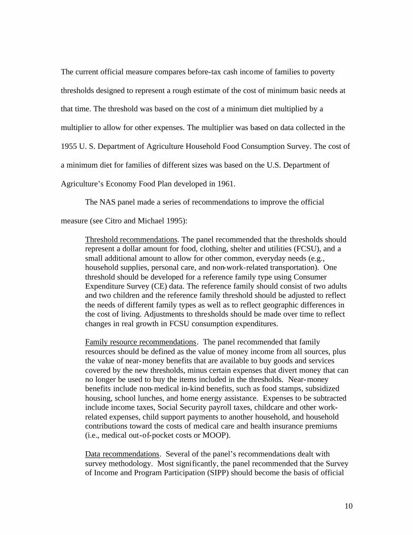
The current official measure compares before-tax cash income of families to poverty

thresholds designed to represent a rough estimate of the cost of minimum basic needs at

that time. The threshold was based on the cost of a minimum diet multiplied by a

multiplier to allow for other expenses. The multiplier was based on data collected in the

1955 U. S. Department of Agriculture Household Food Consumption Survey. The cost of

a minimum diet for families of different sizes was based on the U.S. Department of

Agriculture’s Economy Food Plan developed in 1961.

The NAS panel made a series of recommendations to improve the official

measure (see Citro and Michael 1995):

Threshold recommendations. The panel recommended that the thresholds should represent a dollar amount for food, clothing, shelter and utilities (FCSU), and a small additional amount to allow for other common, everyday needs (e.g., household supplies, personal care, and non-work-related transportation). One threshold should be developed for a reference family type using Consumer Expenditure Survey (CE) data. The reference family should consist of two adults and two children and the reference family threshold should be adjusted to reflect the needs of different family types as well as to reflect geographic differences in the cost of living. Adjustments to thresholds should be made over time to reflect changes in real growth in FCSU consumption expenditures. Family resource recommendations. The panel recommended that family resources should be defined as the value of money income from all sources, plus the value of near-money benefits that are available to buy goods and services covered by the new thresholds, minus certain expenses that divert money that can no longer be used to buy the items included in the thresholds. Near-money benefits include non-medical in-kind benefits, such as food stamps, subsidized housing, school lunches, and home energy assistance. Expenses to be subtracted include income taxes, Social Security payroll taxes, childcare and other work-related expenses, child support payments to another household, and household contributions toward the costs of medical care and health insurance premiums (i.e., medical out-of-pocket costs or MOOP). Data recommendations. Several of the panel’s recommendations dealt with survey methodology. Most significantly, the panel recommended that the Survey of Income and Program Participation (SIPP) should become the basis of official

11

income and poverty statistics, replacing the March income supplement to the Current Population Survey (CPS). In this recommendation, the panel recognized that the SIPP asks more relevant questions than the March CPS and obtains income data of higher quality. The panel also encouraged a review of the CE to improve the quality and usefulness of the data for poverty measurement. Finally, the panel recommended that consideration should be given to the practical problems of implementing fully an improved measure of poverty to be used with other surveys that do not collect the detailed information that is needed.

Since the publication of the NAS recommendations, the Census Bureau has

released two reports presenting alternative, experimental measures that incorporate many

of the panel’s recommendations (Short et al 1999, Short 2001). Consensus has not been

reached on some measurement issues, and so the Census Bureau has presented a series of

different measures in its publications (Proctor and Dalaker, 2002). Nevertheless, the

alternative measures address many of the criticisms of the current official measure

described above and follow the recommendations of the NAS panel.

The purpose of this paper, then, is to examine the relationship between the official

poverty measure, an improved income-based poverty measure, and measures of material

hardship, to see whether or not the revisions to the measure change the relationship of

measured poverty to material hardship. Following work in the U.S., we expect that the

correlation between material hardship and poverty will increase with an improved

measure. Given the European literature on social deprivation and income poverty it is

possible to expect that the relationship may change but not by very much.

Specifically, the two income poverty measures examined in this paper include the

current official measure and an alternative or experimental measure included in Census

Bureau research on poverty measurement10. This alternative measure, following the NAS

10 For those familiar with the Census Bureau reports on experimental poverty measures, the measure examined here is referred to as the MSI measure in Short (2001). MSI represents a measure that subtracts

12

recommendations, uses family resources – after-tax family income minus expenditures on

work and health-related needs plus a value for near-money government transfers. This

resource amount is compared to the poverty thresholds that the NAS panel recommended.

The alternative measure is believed to better represent the amount of ‘current’ income a

family requires to meet its basic needs in a given calendar year. Our interest here is to

compare the populations identified by these two measures of income poverty (referred to

below as ‘poverty’ measures) to groups identified by other indicators of well-being,

described below, and to examine interrelationships among them. The questions we are

asking are – do these measures describe different groups of people? why do they describe

different kinds of people? and what does this tell us about differences in the two

measures of income poverty?

Several measures will be examined in this paper: the official and alternative

poverty measures, an index of material hardship, an indicator of high debt, and responses

to a question about inability to meet expenses. In addition to examining income poverty

and material hardship, a measure of debt is also included in the analysis. Since families

can maintain a level of material comfort with low incomes by incurring debt, this is seen

as a mediating factor between income and hardship. Furthermore, incurring high debt in

and of itself can be seen as a difficult situation leading more and more often to

bankruptcy. Should individuals and families who are bankrupt be considered to be poor?

As families more and more often incur readily accessible debt to get over ‘rough

patches’, some consideration of high debts seems appropriate to this discussion.

medical out-of-pocket expense from income and is only one way of incorporating health care expense into a poverty measure.

13

Finally, a measure of wealth or capital assets should be taken account of. There

have been some attempts to include assets in a measure of income poverty (Ruggles and

Williams (1989)). In such applications, assets are treated like an annuity, a small part of

which is assumed to be available to the family to meet needs over time. While this is not

done here in the alternative poverty measures, a measure of assets is included in the

multivariate analysis described below.

Data

This study uses the 1996 panel of the SIPP. The SIPP allows us to examine all of

these various indicators for the same people. Since there are limitations to our estimates

of taxes and the placement of topical modules in the SIPP we only have experimental

poverty measures for 1996 and material hardship measures for 1998. Thus, the analysis

looks at income poverty in calendar year 1996 as a ‘predictor’ of material hardship two

years later. Since the two are typically not highly correlated with one another, even in the

same year, this disjuncture in time will exacerbate that problem. Nevertheless we can still

compare the predictive power of the two poverty measures one against the other to gauge

whether or not improvements change the relationship to material hardship.

The material hardship measures used here are constructed from a supplemental set

of questions included in the 9th wave of the SIPP. Recall that these questions differ

considerably from those used in the European stud ies, with one difference being that

there is no effort to ascertain whether or not the lack of some item is due to the fact that

the family cannot afford it. In addition, there is no follow-on question to ascertain public

opinion about whether the item should be considered a necessity. In U.S. studies of

14

material hardship, decisions about which items are included in an index are made by the

individual researcher or analyst.

Therefore, a material hardship index is constructed like that used by Mayer and

Jencks (1989). It includes most of the same items, though sometimes differently

measured. Also, every item is given a weight of one. Accordingly, one point was added

to the index for each of the following reported items: experienced difficulty paying rent,

difficulty paying utilities, did not see a doctor or a dentist when needed, did not have

enough food to eat, expressed dissatisfaction with condition of housing, reported at least

two housing-related problems, or reported having no health insurance. Note again that,

while indicators are only included in the European social deprivation measures if the

respondent lacks these items because they cannot afford them, the SIPP questions used

here do not have that follow-up question. So these items may be lacking, but it may not

be ‘enforced’ need. A family is classified as experiencing material hardship if they report

two or more of the above listed items.

Another measure of interest here is a report that the respondent cannot meet

essential expenses. The respondent is asked,

Next are questions about difficulties people sometimes have in meeting their essential household expenses for such things as mortgage or rent payments, utility bills, or important medical care. During the past 12 months, has there been a time when you/your household did not meet all of your essential expenses?”

This item itself is often included in a material hardship measure. However, the report of

inability to meet expenses can occur even in the midst of material plenty. Families can

have high income but also very high expenses, have accumulated material comfort and

still report that they have very high expenses that they cannot meet. This can often

happen if the family has already incurred large debt to obtain material possessions that

15

render them not materially deprived. Since positive responses to this question may occur

along with or without material hardship, with high or low income and with high or low

levels of debt, it is included here as a separate dimension of economic difficulty. This

measure will be referred to as ‘inability to meet expenses’.

The last non- income indicator included here is a high debt-to- income ratio. The

measure of debt used here includes both secured and unsecured debt. Since it includes

mortgage as well as credit card debt, it can be a substantial amount compared with annual

income. In a study of bankruptcy in 1989 Sullivan et al. examined debt-to- income ratios.

From their study of bankruptcy petitioners they estimated a mean debt-to-income ratio of

3.2, in other words, at the mean, a family in bankruptcy owed debts greater than three

years and two months worth of income. For this analysis, we considered a family to have

high debt if its reported debt is greater than twice their current income. As a level of high

debt this represents a family who may be in financial trouble. Further work should be

done examining other levels to indicate ‘high’ indebtedness. Again, we are interested in

examining debt because a family can have low income but no material hardship because

they have borrowed to avoid it (Bauman, 2003), or as Mack and Lansley have stated,

high income and debt, but, due to the demands of debt repayment, deprivation.

Results

Employing two measures of poverty, material hardship, inability to meet

expenses, or high debt may define somewhat different groups of people as economically

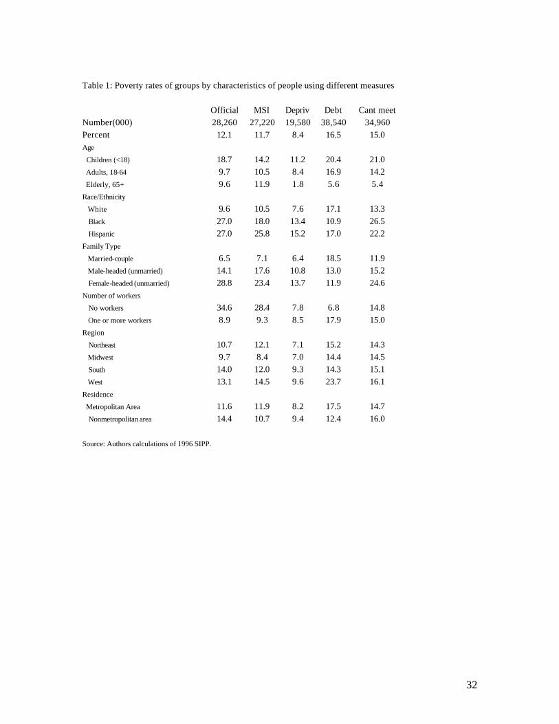
disadvantaged. Table 1 shows the percentage of people who are identified by the different

measures to be poor or experiencing material or financial hardship. Note that this analysis

only includes those in the sample of households who responded to the material well-

16

being module of the SIPP in the 1996 panel. Thus, all results are conditional on

remaining in the SIPP sample, and as such may suffer from attrition bias.

Using an official definition of poverty, for 1996, 12.2 percent of people were

poor, compared with only 11.7 percent poor under the experimental measure while 16.5

percent had high debt-to- income ratios. In 1998, 8.4 percent of these people experienced

two or more items of material hardship and 15.0 percent reported difficulty meeting

expenses. Since the groups vary so much in size across the different measures it is

difficult to understand the implications for subgroups of the population by looking at

these aggregate rates. For this reason, table 2 shows the composition of the various

hardship groups by selected characteristics.

We can examine the characteristics of these different groups to attempt to

understand how each measure identifies different types of families to be ‘in need’ and to

begin to understand which measures are similar to others. If our main purpose for

measuring poverty is to identify groups that are in need, it may be interesting to find

which, if any, measures describe similar groups of people.

Composition of population by age group

0.0

10.0

20.0

30.0

40.0

50.0

60.0

70.0

80.0

90.0

100.0

Children (<18) Adults, 18-64 Elderly, 65+

all

official

exper

hardship

high debt

can't meet

17

The first chart shows the composition of the total population and different disadvantaged

groups by age. For example, the first bar shows the percent of the total population that are

children, about 27 percent. The remaining bars for children are the proportion of each of

the disadvantaged groups using different indicators. The first is the official poverty

measure (41% are children), the second is the alternative poverty measure (32%), and the

third is the measure of material hardship similar to the one used by Mayer and Jencks

(36%). The fourth is a measure of all families with high debt to income (33%). Finally, of

individuals in families who report not being able to make ends meet, 37 percent are

children.

We see from the chart that these measures define groups with a different

composition of ages. For example, the official measure of poverty includes more children

than any of the other measures, though they are a higher percentage of all the

disadvantaged groups than they are in the population as a whole. This is a group with

high poverty, material hardship, and financial difficulties, relative to their representation

in the population as a whole. Of the two poverty measures, the alternative measure looks

more like the material hardship and the inability-to-meet-expenses measure for children.

Non-elderly adults are less disadvantaged by either poverty measure, but do report

material hardship and high debts. This suggests that non-elderly adults can have

relatively high incomes, while incurring debt and still report material and even financial

difficulty. So, this group has low poverty but high material hardship and debt. Reflective

of expenses relating to work, the alternative poverty measure includes a higher proportion

of this group than the official measure.

18

While the elderly show higher representation in the alternative poverty group than

under the official measure, they score low on the other three indicators – suggesting that

the elderly are materially well off despite low income. The alternative measure for this

group is high because this measure subtracts medical costs from income, which are very

high for the elderly. Nevertheless, the elderly do not incur high debts nor do they report a

disproportionate difficulty meeting essent ial expenses. They also do not score high on the

material hardship index that includes, among other things, reports of unmet medical

needs in the form of not being able to see doctors or dentists.

Composition of population by race/ethnicity group

0.0

10.0

20.0

30.0

40.0

50.0

60.0

70.0

80.0

90.0

100.0

White Black Hispanic

allofficialexperhardshiphigh debtcan't meet

The second chart shows the same indicators for racial and ethnic groups. As can be seen,

Whites tend to have disproportionately low poverty and hardship but they also have

relatively high debts. Whites make up a larger proportion of the experimental poor than

the official poor. Their representation in the experimental poor is closer to that of the

other indicators. Of people in families with high debts 86 percent are White, while

Whites comprise 83 percent of the total population.

19

Blacks, on the other hand, are more likely to be both income poor and suffer

material hardship, while they are less likely to incur significant debt. Blacks are also quite

likely to report not being able to make ends meet. It is important also to note that there is

a somewhat different experience of high-debt among the race groups. While this may

reflect differences in tastes, it may also reflect differences in access to credit markets. It is

important to note that differential access to credit markets would also imply a different

relationship between poverty and material hardship for different subgroups of the

population.

Examining the indicators for Latinos shows that both income-based poverty

measures are high for this group. The experimental poverty measures, which are adjusted

for geographic differences in housing costs, reflect the fact that Hispanic families tend to

live where housing costs are higher.

There are striking differences by family type. The third chart shows that married

couples are unlikely to have low incomes, by either poverty measure. However, they are

quite likely to have high debts while female-householder families are extremely likely to

have low incomes and slightly less likely to have incurred debt. Female householders

report material hardships and inability to make ends meet with high frequency as well.

20

Composition of population by family type

0.0

10.0

20.0

30.0

40.0

50.0

60.0

70.0

80.0

90.0

100.0

Married-couple Female-headed (unmarried)

all

official

exper

hardship

high debt

can't meet

Finally, we can look at families by work experience. People in families with no

workers have high poverty but low material and financial hardship. This group is like the

elderly, and probably contains a lot of elderly. Families with at least one worker look like

nonelderly adults, with relatively low poverty but higher material hardship and debt.

Composition of population by work experience

0.0

10.0

20.0

30.0

40.0

50.0

60.0

70.0

80.0

90.0

100.0

No workers One or more workers

all

official

exper

hardship

high debt

can't meet

21

We have seen that different indicators of disadvantage describe sets of people

with differing characteristics. One other thing to notice is that in most cases, the

experimental poverty measure identified a group of people that looked a bit more like the

hardship measures than the official measure. The official measure stood out often from

the other measures, for example, in the case of children, Whites, and Blacks. The elderly

is a group for whom this is not true, since the high medical expenses subtracted from

income in the experimental measure make this measure higher than any of the others. In

the last chart, by work experience, we see that the poverty measures stand apart from the

measures of material and financial hardship, suggesting that income-based poverty reflect

a different experience from the more direct measures of hardship.

Regression analysis

To further examine the interrelationship of the various indicators and to explore

the difference between the official and experimental poverty measures more fully we next

take a multivariate approach. The purpose is to examine the three non- income measures

as a function of the demographic characteristics discussed above and some additional

indicators, such as education of householder and level of assets that should affect any

measure of economic well-being.

Table 3 shows regression results of high debt-to- income ratios, material hardship,

and the inability to meet expenses, each separately, as a function of indicators of age,

region, metro area residence, marital status, family size, presence of children, indicator of

health of family members, race, ethnicity, education of family householder, and level of

assets. All of these refer to calendar year 1996, except assets, which are measured in early

22

1997. Recall that the poverty measures refer to 1996, the debt measures refer to early

1997, and the others to 1998.

Of the three dependent variables, the model best explains the variation in the

indicator of inability to meet expenses in 1998. Debt-to-income ratios show the worst fit.

For each dependent variable there are two versions. One includes the official poverty

measure and one with the experimental poverty measure. All other independent variables

are the same. This gives insight into the relationship of income poverty to the other

indicators of economic disadvantage discussed here, and the difference between the

official and the experimental poverty measures, holding other characteristics constant.

Looking first at the material hardship model, we see that the estimated

coefficients on all of the explanatory variables, except for region, family size, and White

are significant. Examining the individual coefficients shows that material hardship has an

inverted U-shaped relationship with age, lower for children and elderly, higher for adults.

Being in a metropolitan area, married-couple family, being college educated and having

more assets results in lower hardship. Having a family member in less than good health

or being Hispanic results in greater hardship. Oddly, having at least one worker in the

family in 1996 increases the likelihood of reporting material hardship compared with

having no workers. Having children is only significant in the model that includes the

alternative poverty measure.

It is interesting to note that, all else the same, being poor under the alternative

measure is not more highly correlated with material hardship than being classified as

poor under the official measure, the respective coefficients being .7812 and .8629. This

23

result suggests that the relationship between material hardship indicators and poverty

may not be the best way to judge the adequacy of a poverty measure.

As a reminder, though, the material hardship questions in the SIPP do not

represent ‘enforced’ hardship. Since, as has been shown (Bauman, 2003), absence of

material items in the SIPP are reported by high income as well as low income individuals,

and are not conditioned on follow-up questions about ability to afford or obtain an item,

they may, therefore, represent choice as well as hardship.

Next, is an examination of the model explaining the inability to meet expenses.

Unlike material hardship, being White indicates less financial difficulty than another

race. Like material hardship, being married, college-educated, or having more assets

reduces the chance of having difficulty meeting expenses, while having children or poor

health increases the likelihood. The effect of family size on inability to meet expenses is

significant. Reported inability to meet expenses is greater for moderately-sized families

than for singles or large families. The coefficient on having at least one worker in the

family is insignificant using either poverty measure. Also note that the coefficient on the

experimental poverty measure is not more strongly associated with inability to meet

expenses than the official measure, the respective coefficients being .5202 and .6377.

Finally, we examine the model as it explains high debt-to- income ratios. Again,

age is nonlinearly associated with debt. Families living in the West have higher debt than

the South. Unlike the other two indicators, living in a metropolitan area increases the

probability of higher debts. The presence of children, being White, and well-educated

increases the likelihood of having high debt. This differs from the other measures where

24

assets decrease the probability of having material hardship or the inability to meet

expenses. Being Hispanic decreases the probability of having high debt.

Note, however, that in this case, the coefficient on official poverty is .4802

compared with .6999 for experimental poverty. The difference in the estimated

coefficients is small in all of the models and inclusion of one or the other poverty

measures does not change substantially the coefficients of any of the other explanatory

variables. This suggests that the two income poverty measures represent essentially the

same thing, with only slight differences.

However, the result that the size of the respective coefficients is different in this

model may suggest that the experimental measure describes a group more typically

thought of as the ‘working poor’ while the official measure more likely identifies the

‘benefit-recipient poor’. This is consistent with the notion that the working poor may be

more able to use debt to get by and not have to forego material necessities.

One of the main results of this analysis is that the experimental poverty measure,

while including many of the recommendations of earlier studies, fails to improve the

relationship between income poverty and material hardship or financial hardship. The

coefficient on the official poverty measure was not statistically different from that on the

experimental measure as an explanatory variable explaining material hardship, slightly

higher for inability to meet expenses, and only slightly lower for high debt to income

ratios.11 Overall, the estimated models for each hardship indicator using the different

poverty measures were similar no matter which poverty measure was included. While the

11 Only preliminary t-tests with design effects were performed to test the differences, comparing individual coefficients. .

25

models differed across hardship indicators, suggesting that each indicator describes a

different dimension of hardship that falls differentially among the population subgroups.

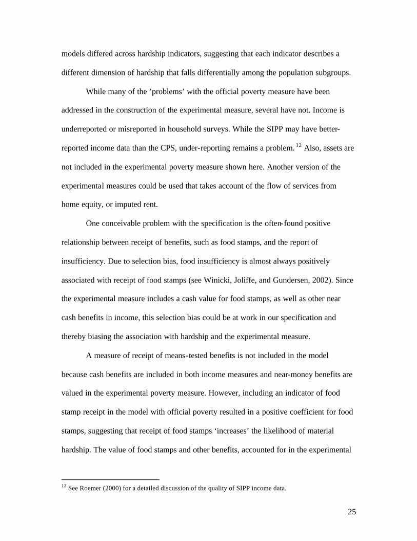
While many of the ’problems’ with the official poverty measure have been

addressed in the construction of the experimental measure, several have not. Income is

underreported or misreported in household surveys. While the SIPP may have better-

reported income data than the CPS, under-reporting remains a problem. 12 Also, assets are

not included in the experimental poverty measure shown here. Another version of the

experimental measures could be used that takes account of the flow of services from

home equity, or imputed rent.

One conceivable problem with the specification is the often-found positive

relationship between receipt of benefits, such as food stamps, and the report of

insufficiency. Due to selection bias, food insufficiency is almost always positively

associated with receipt of food stamps (see Winicki, Joliffe, and Gundersen, 2002). Since

the experimental measure includes a cash value for food stamps, as well as other near

cash benefits in income, this selection bias could be at work in our specification and

thereby biasing the association with hardship and the experimental measure.

A measure of receipt of means-tested benefits is not included in the model

because cash benefits are included in both income measures and near-money benefits are

valued in the experimental poverty measure. However, including an indicator of food

stamp receipt in the model with official poverty resulted in a positive coefficient for food

stamps, suggesting that receipt of food stamps ‘increases’ the likelihood of material

hardship. The value of food stamps and other benefits, accounted for in the experimental

12 See Roemer (2000) for a detailed discussion of the quality of SIPP income data.

26

measure, may have the effect of reducing the statistical association between experimental

poverty and material hardship.

Earlier studies of material hardship have shown that families receiving welfare

benefits are more likely than those classified as officially poor to exhibit material

hardship (Short and Shea, 1995). Since the experimental measure includes near money

benefits as income, families who are receiving benefits from multiple programs may no

longer be classified as in poverty. If these are families who report material hardship, then

this is the expected result.

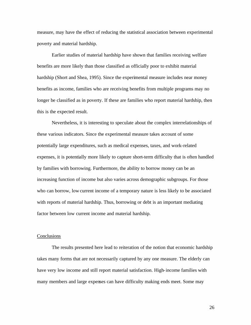
Nevertheless, it is interesting to speculate about the complex interrelationships of

these various indicators. Since the experimental measure takes account of some

potentially large expenditures, such as medical expenses, taxes, and work-related

expenses, it is potentially more likely to capture short-term difficulty that is often handled

by families with borrowing. Furthermore, the ability to borrow money can be an

increasing function of income but also varies across demographic subgroups. For those

who can borrow, low current income of a temporary nature is less likely to be associated

with reports of material hardship. Thus, borrowing or debt is an important mediating

factor between low current income and material hardship.

Conclusions

The results presented here lead to reiteration of the notion that economic hardship

takes many forms that are not necessarily captured by any one measure. The elderly can

have very low income and still report material satisfaction. High- income families with

many members and large expenses can have difficulty making ends meet. Some may

27

borrow excessively to get over difficult times and thus report both high incomes and

difficulty meeting expenses. Others, less able to borrow, are more likely to suffer and

report material hardship when incomes are low. It is clear that all of these dimensions are

important and somewhat independent and contribute to our understanding of economic

well-being as a whole.

The experimental poverty measure appears to describe a population that looks

more like tha t described by material hardship than the official poverty measure. Further,

the experimental poverty measures appear to look more like ‘financial’ difficulty rather

than ‘material’ difficulty. However, the differences are small between the two income

poverty measures when included in a multivariate analysis. While addressing a good

number of the criticisms aimed at the current official measure, it appears that

experimental income poverty, like official income poverty, does not describe the same

group of people in need, as a measure of material hardship does.

There are many additional analyses that should be performed on this topic

including estimating different specifications of the model or constructing different

hardship indexes that include different sets of items. Measuring experimental poverty

contemporaneously with material hardship is an important next step. While assets and

debts clearly play a role in economic well-being and distress, it is not well defined at this

point how that role is best captured in these statistics, or if that is, indeed, yet another

dimension of well-being that deserves its own measure.

This analysis does contribute to the growing understanding that income measures

cannot just be fixed to tell us about material hardship, and that material hardship is

something different and worthy of measurement in its own right. To that end, it might be

28

useful to ensure that the questions on material hardship in the SIPP capture enforced

deprivation rather than just absence of items. Should this be done we could perhaps more

fully explore the relationship between income poverty and material hardship in the U.S.

As has been noted by others, an income poverty measure is a convenient tool to

be used by researchers and policy makers to understand who in a population experiences

difficulties and how to alleviate need. If the difference between material hardship and

income poverty, or financial difficulty and income poverty, is understood more fully,

then measuring income poverty alone becomes a tool that can be interpreted more

appropriately and used more wisely to address the needs of the disadvantaged.

29

Bibliography Atkinson, A.B., B. Cantillon, E. Marlier, and B. Nolan, 2002, Social Indicators, the EU and Social Exclusion, Oxford University Press, Oxford.

Bauman, K., Extended Measures of Well-being: Meeting Basic Needs, Current Population Reports: P70-67. Washington, D.C., U.S. Government Printing Office, 1999.

Bauman, K, “Direct Measures of Poverty as Indicators of Economic Need, Evidence From The Survey of Income and Program Participation”, paper presented at the annual meeting of the Society of Government Economists, January 2003.

Beverly, S.G., “Measure of Material Hardship: Rationale and Recommendations”, Journal of Poverty, 5(1), 23-41 March 2000. Boushey, Heather, Chauna Brocht, Bethney Gundersen, and Jared Bernstein. 2001. Hardships in America: The Real Story of Working Families. Washington, D.C.: Economic Policy Institute. Callan, T., B. Nolan, and C. Whelan, “Resources, Deprivation and the Measurement of Poverty”, Journal of Social Policy, 22,2,141-172. 1993. Citro, C. F. and R.T. Michael, (Eds.), Measuring Poverty: A New Approach, Washington, D.C., National Academy Press, 1995. Edin, K., and Lein, L., Making Ends Meet: How Single Mothers Survive Welfare and Low-wage Work. New York: Russell Sage Foundation. 1997. Federman, Maya, Thesia I. Garner, Kathleen Short, W. Bowman Cutter IV, John Kiely, David Levine, Duane McGough, and Marilyn McMillen. “What Does It Mean to Be Poor in America?” Monthly Labor Review, 119(5) (May 1996), pp. 3-17. Fisher, Gordon, “Enough for a Family to Live On? Questions from members of the American Public and New Perspectives from British Social Scientists,” paper presented at the annual meeting of Association for Public Policy Analysis and Management, November 2001. Layte, R. B. Maitre, B. Nolan, and C. Whelan, “Persistent and Consistent Poverty in the 1994 and 1995 Waves of the European Community Household Panel Survey,” Review of Income and Wealth, Series 47, Number 4, 427-449, December 2001b. Layte, R. B. Maitre, B. Nolan, and C. Whelan, “Explaining Levels of Deprivation in the European Union,” Acta Sociologica, 44(2), 105-22, 2001a. Mack J.H. and S. Lansley, Poor Britain, London: Allen & Unwin, 1985.

30

Mayer, S. E. and C. Jencks, “Poverty and the Distribution of Material Hardship”, Journal of Human Resources, XXIV.1, 88-113, Winter 1989. Nolan, B. and C. Whelan, “Measuring Poverty Using Income and Deprivation Indicators: Alternative Approaches,” Journal of European Social Policy, 1996-6(3) 225-240. Perry, B. 2002 The mismatch between income measures and direct outcome measures of poverty, Social Policy Journal of New Zealand, Issue 19. Proctor, B.D. and J. Dalaker, Poverty in the United States: 2001, U.S. Census Bureau, Current Population Reports, P60-219, U.S. Government Printing Office, Washington, DC, 2002. Rector, Robert E., K. A. Johnson, and S. E. Youssef, “The Extent of Material Hardship and Poverty in the Untied States”, Review of Social Economy, 57(3): 351-358. 1999. Ringen, S., The Possibility of Politics, Clarendon Press, Oxford, 1987. Ringen, S., “Direct and Indirect Measures of Poverty,” Journal of Social Policy, 17(3), 1988. Roemer, Marc I., “Assessing the Quality of the March Current Population Survey and the Survey of Income and Program Participation Income Estimates”, Unpublished paper, U.S. Census Bureau, June 2000. Ruggles P., and R. Williams, “Longitudinal Measures of Poverty: Accounting for Income and Assets over Time,” Review of Income and Wealth, 35:3, 225-244. Saunders P, 2003, The meaning and measurement of poverty: towards an agenda for action, Submission to the Senate Community Affairs Reference Committeed Inquiry into Poverty and Financial Hardship, Social Policy Research Center, University of South Wales Sen, A.K., 1979, “Issues in the Measurement of Poverty,” Scandinavian Journal of Economics, 1979: 285-307. Sen, A.K., 1981, Poverty and Famines, Oxford: Oxford University Press. Short K., and M. Shea, Beyond Poverty, Extended Measures of Wellbeing: 1992, U.S. Census Bureau, Current Population Reports P70-50RV, Washington, D.C.1995. Short K, T. Garner, D. Johnson, and P. Doyle, Experimental Poverty Measures: 1990-1997 , U.S. Census Bureau, Current Population Reports, P60-205, U.S. Government Printing Office, Washington, DC, 1999.

31

Short K., Experimental Poverty Measures: 1999 , U.S. Census Bureau, Current Population Reports, P60-216, U.S. Government Printing Office, Washington, DC, 2001. Sullivan, T.A., E. Warren, and J.L Westbrook, As We Forgive our Debtors; Bankruptcy and Consumer Credit in America, Oxford University Press, New York, 1989. Townsend, P., Poverty in the United Kingdom, (Harmondsworth, Middlesex: Penguin), 1979. Whelan, C.T., Hannan, D.F. and Creighton, S. Unemployment, Poverty and Psychological Distress, General Research Series paper 150, Dublin, The Economic and Social Research Institute. (1991). Winicki, J., D. Jollife, and C. Gundersen, “How do Food Assistance Programs Improve the Well-Being of Low-Income Families?” Food Assistance and Nutrition Research Report, Number 26-9 USDA, Economic Research Service. September 2002.

32

Table 1: Poverty rates of groups by characteristics of people using different measures Official MSI Depriv Debt Cant meet Number(000) 28,260 27,220 19,580 38,540 34,960 Percent 12.1 11.7 8.4 16.5 15.0 Age Children (<18) 18.7 14.2 11.2 20.4 21.0 Adults, 18-64 9.7 10.5 8.4 16.9 14.2 Elderly, 65+ 9.6 11.9 1.8 5.6 5.4 Race/Ethnicity White 9.6 10.5 7.6 17.1 13.3 Black 27.0 18.0 13.4 10.9 26.5 Hispanic 27.0 25.8 15.2 17.0 22.2 Family Type Married-couple 6.5 7.1 6.4 18.5 11.9 Male-headed (unmarried) 14.1 17.6 10.8 13.0 15.2 Female-headed (unmarried) 28.8 23.4 13.7 11.9 24.6 Number of workers No workers 34.6 28.4 7.8 6.8 14.8 One or more workers 8.9 9.3 8.5 17.9 15.0 Region Northeast 10.7 12.1 7.1 15.2 14.3 Midwest 9.7 8.4 7.0 14.4 14.5 South 14.0 12.0 9.3 14.3 15.1 West 13.1 14.5 9.6 23.7 16.1 Residence Metropolitan Area 11.6 11.9 8.2 17.5 14.7 Nonmetropolitan area 14.4 10.7 9.4 12.4 16.0 Source: Authors calculations of 1996 SIPP.

33

Table 2: Composition of groups by characteristics of people using different measures Total Official MSI Depriv Debt Cant meet Number(000) 233,400 28,260 27,220 19,580 38,540 34,960 Percent 100.0 100.0 100.0 100.0 100.0 100.0 Age Children (<18) 26.6 41.2 32.4 35.6 32.8 37.4 Adults, 18-64 61.7 49.6 55.6 61.8 63.2 58.4 Elderly, 65+ 11.7 9.3 12.0 2.5 4.0 4.2 Race/Ethnicity White 83.2 66.2 74.6 75.5 86.2 74.0 Black 12.3 27.4 19.0 19.7 8.1 21.8 Hispanic 11.2 24.9 24.7 20.3 11.5 16.6 Family Type Married-couple 68.5 36.9 41.5 51.8 76.7 54.4 Female-headed (unmarried) 21.7 51.7 43.7 35.6 15.7 35.7 Number of workers No workers 12.6 35.9 30.6 11.7 5.2 12.4 One or more workers 87.4 64.1 69.4 88.3 94.8 87.6 Region Northeast 19.6 17.3 20.3 16.5 18.0 18.7 Midwest 24.4 19.6 17.5 20.4 21.2 23.5 South 34.3 39.6 35.3 38.1 29.7 34.5 West 21.7 23.5 26.9 24.9 31.2 23.4 Residence Metropolitan Area 80.9 77.3 82.6 78.7 85.7 79.6 Nonmetropolitan area 19.1 22.7 17.4 21.3 14.3 20.4 Source: Authors calculations of 1996 SIPP.

34

Table 3: Logistic regression results for various indicators of hardship Material hardship Cannot Meet Expenses High debt-to-income Official Experimental Official Experimental Official Experimental Intercept -2.9872* -2.7162* -2.3128 * -2.0899* -4.2153* -4.3159* Poor 0.8629* 0.7812* 0.6377 * 0.5202* 0.4802* 0.6999* Age 0.0646* 0.0661* 0.0440 * 0.0455* 0.0878* 0.0908*

Age2 -0.0010* -0.0010* -0.0007 * -0.0007* -0.0011* -0.0012* Northeast -0.1135 -0.1331 0.1296 0.1170 -0.0874 -0.0996 Midwest -0.1409 -0.1319 0.1065 0.1112 -0.0927 -0.0861 West 0.0434 0.0187 0.0922 0.0753 0.4805* 0.4682* City -0.2399* -0.2836* -0.1645 * -0.1943* 0.2661* 0.2540* Married -0.6242* -0.6314* -0.6444 * -0.6607* 0.4049* 0.4399* Family size -0.0179 -0.0326 0.1830 * 0.1724* -0.0962 -0.0965

Famsize2 -0.0036 -0.0044 -0.0288 * -0.0291* 0.0001 0.0000 Children 0.0781 0.1445* 0.2357 * 0.2782* 0.1484* 0.1600* Health 0.7832* 0.8034* 0.7995 * 0.8142* -0.0463 -0.0622 Hispanic 0.2779* 0.2666* 0.1205 0.1231 -0.2623* -0.2988* Worker 0.5012* 0.3180* 0.1866 0.0411 0.1714 0.1630 White -0.0695 -0.1291 -0.2648 * -0.3072* 0.2756* 0.2598* Assets -0.3559* -0.3684* -0.3081 * -0.3171* 0.0053 0.0057 College educ -0.3738* -0.4162* -0.2387 * -0.2716* 0.3652* 0.3670* Chi-square 2061 2060 2640 2609 1355 1464 * indicates statistical significance at the .05 level, incorporating a design effect of 2.23. Authors calculations of the 1996 SIPP panel.