Evaluating Alternative Approaches to Poverty Alleviation: Rice Tariffs versus Targeted Transfers in...

WP/08/9

Evaluating Alternative Approaches to Poverty Alleviation:

Rice Tariffs Versus Targeted Transfers in Madagascar

David Coady, Paul Dorosh, and

Bart Minten

© 2008 International Monetary Fund WP/08/9 IMF Working Paper Fiscal Affairs Department

Evaluating Alternative Approaches to Poverty Alleviation: Rice Tariffs versus Targeted Transfers in Madagascar

Prepared by David Coady, Paul Dorosh, and Bart Minten1

Authorized for distribution by Rolando Ossowski

January 2008

Abstract

This Working Paper should not be reported as representing the views of the IMF. The views expressed in this Working Paper are those of the author(s) and do not necessarily represent those of the IMF or IMF policy. Working Papers describe research in progress by the author(s) and are published to elicit comments and to further debate.

This paper uses a partial equilibrium framework to evaluate the relative efficiency, distributional and revenue implications of rice tariffs and targeted transfers in Madagascar, especially in the context of identifying their respective roles for poverty alleviation. Although there are likely to be substantial efficiency gains from tariff reductions, these accrue mainly to higher income households. In addition, poor net rice sellers will lose from lower tariffs. Developing a system of well designed and implemented targeted direct transfers to poor households is thus likely to be a substantially more cost-effective approach to poverty alleviation. Such an approach should be financed by switching revenue raising from rice tariffs to more efficient tax instruments. These policy conclusions are likely to be robust to the incorporation of general equilibrium considerations. JEL Classification Numbers: H2, H5 Keywords: Rice tariffs, targeted transfers, efficiency, distribution, revenue, Madagascar Authors’ E-Mail Addresses: [email protected]; [email protected]; [email protected]

1 David Coady is a Senior Economist in the Fiscal Affairs Department of the IMF. Paul Dorosh is a Senior Rural Development Economist at the World Bank. Bart Minten is Senior Research Fellow at the International Food Policy Research Institute ([email protected]). The authors thank Robin Boadway, Ravi Kanbur, and participants at the Academic Panel Meetings at the IMF in April 2007 for detailed comments and discussion.

2

Contents Page

I. Introduction ............................................................................................................................3

II. A Partial Equilibrium Model.................................................................................................4 A. The Model .................................................................................................................4 B. Rice Tariff Reform....................................................................................................6 C. Targeted Transfers.....................................................................................................7 D. Welfare Weights .......................................................................................................9

III. The Welfare Impact of Tariffs and Transfers ....................................................................10 A. Lowering Rice Tariffs.............................................................................................10 B. Targeted Transfers...................................................................................................19 C. Tariffs, Transfers, or Both? .....................................................................................22

IV. From Partial to General Equilibrium Analysis ..................................................................23

V. Summary and Conclusions..................................................................................................24 Tables 1. Distribution of Welfare Impact from Tariff Increase Across Households ..........................16 2. Marginal Cost of Public Funds for Different Import Elasticities ........................................18 3. Welfare Impact of Lower Rice Tariff ..................................................................................18 4. Welfare Impact of Proxy-Means Targeted Transfers ..........................................................22 Figures 1. Cumulative Densities of Per Capita Consumption ..............................................................10 2a. Net Sellers/Buyers by Welfare Group, Urban....................................................................11 2b. Net Sellers/Buyers by Welfare Group, Rural ....................................................................12 3a. Net Purchases by Welfare Group: Urban...........................................................................13 3b. Net Purchases by Welfare Group: Rural............................................................................13 4a. Welfare Impact of Rice Price Decrease: Urban .................................................................14 4b. Welfare Impact of Rice Price Decrease, Rural ..................................................................15 5. Undercoverage and Leakage, Urban and Rural ...................................................................21 6. Welfare Impact of Tariff Reductions and Targeted Transfers.............................................23 Appendix I. The Madagascar EPM Household Survey............................................................................25 Appendix Table 5. Mean Per Capita Consumption and Welfare Weights .........................................................26 References................................................................................................................................27

3

I. INTRODUCTION

In early 2004, the Madagascar economy suffered a series of adverse shocks resulting in pressure on the government to introduce measures to counteract the negative effects on the real incomes of poor households. In February and March 2004, there was severe cyclone damage to the rice harvest and also to crucial market infrastructure—the rice harvest typically occurs during the months March through June. In addition, the world price of rice increased substantially with a 43 percent increase in the Bangkok dollar price of rice, and the Malagasy franc (FMG) also experienced rapid depreciation of 58 percent relative to the dollar. The import parity price of rice increased by 113 percent between January and August 2004. Such price increases can be expected to have a substantial welfare impact on households since rice is an important staple in Madagascar. These events led to an active policy debate regarding the appropriate policy instrument to use to mitigate their poverty impact, in particular whether the government should decrease the import tax on rice to bring about a decrease in the domestic price of rice or instead rely on direct transfers to poor households. At the time, rice imports were subject both to an import tax of 20 percent and a value-added tax of 21 percent (levied on the import tax-inclusive price), combining for a net tax rate of 45 percent. Those in favor of reducing the rice tariff argued that this would lower the domestic price and quickly have a beneficial effect on the poor for whom rice forms a substantial proportion of their total consumption. Those against argued that lower tariffs would have adverse effects on tax revenues and the balance of payments and may also generate political pressure for wider tariff reductions. It was argued that the government should rely more on direct transfers, although it was recognized that developing a well designed and implemented safety net would take some time. This paper evaluates the relative merits of these two policy responses (i.e., rice tariff reforms versus targeted transfers) from the perspective of their relative distributional, efficiency, and revenue implications.2 The structure of the paper is as follows. Section II sets out a simple partial equilibrium model that provides a framework for integrating the distributional, efficiency, and revenue impacts of both policies into an evaluation of the net welfare impact of the two policy alternatives. Section III uses this framework to evaluate each of the policies in turn and to compare across both. Section IV discusses some caveats related to the use of a partial equilibrium model, identifying potential implications for our policy conclusions. Section V provides a brief summary of the results and their policy implications.

2 The paper abstracts from two tariff-related issues that have been debated in policy circles, namely, the uses of tariffs for infant-industry protection and the use of a variable tariff to smooth volatile world rice prices.

4

II. A PARTIAL EQUILIBRIUM MODEL

In this section we present a partial equilibrium model that provides a useful framework to guide our evaluation of the relative welfare effects of tariff reductions and transfers. Although the model has a clear general equilibrium counterpart, the assumptions we make transform it into a partial equilibrium model.3

A. The Model

The model has two agents: households and the government. Rural agricultural households are incorporated into the household sector so that formally there is no need to distinguish between agricultural producers and non-producers. All other producers in the economy are implicitly assumed to produce using constant returns to scale technology, with producer and factor prices being fixed. Household welfare is captured by a standard indirect utility function V(p, y), where p is a vector of prices facing the household sector (factor prices are included as negative entries) and y is lump-sum income—later, superscript h will be added to denote specific households. Household lump-sum income is given by:

( , ) .y p A mπ= + (1)

where Π(p, A) is a (restricted) profit function giving the imputed rent obtained from land area A given p, and m is lump-sum transfers to or from the government. The profit function in turn is given by:

( , ) . . .p A p q c fπ = − (2)

where q is a vector of agricultural output, c is a vector of input prices, and f is vector of input quantities. The government derives revenue both from rice import tariffs and lump-sum taxation of households, so that revenue R is given by:

3 See Drèze and Stern (1987) and Newbery and Stern (1987) for more detailed discussion of the general model, and Coady and Drèze (2002) for the implications of alternative distributional assumptions for tax rules. See also Braverman, Hammer, and Ahn (1987) and Newbery (1987) for early empirical evaluations of agricultural price reforms for Korea, and Coady (1997) for an application of the model within the context of an evaluation of agricultural pricing policies for Pakistan.

5

( ) .hi i i i i h

R t s T t x q m= + = − −∑ (3)

where subscript i denotes rice, ∑= h

hii xx is aggregate household demand for rice,

∑= hhii qq is aggregate household production of rice, iii qxs −= is imports of rice

calculated as the difference between aggregate consumption and production of rice in the economy, and hm is the lump-sum transfer to each household (if positive) or lump-sum tax from each household (if negative) so that ∑−= h

hmT is net lump-sum taxes and transfers

between the government and households. The import tax per unit of rice is denoted by *iii ppt −= , where the asterisk superscript denotes border import prices—we abstract from

trade and transport margins for convenience. Note that, under this specification, a unit increase in the rice tariff leads to a unit increase in the domestic price. Social welfare in the economy is defined, over H households, by a standard Bergson-Samuelson social welfare function:

1 1[ ( , ),....., ( , ),....., ( , )].h h H HW W V p y V p y V p y= (4)

The effect on social welfare of a (marginal) “reform” of each policy instrument (i.e., tariff it

or transfers hm ) is derived by differentiating the social welfare function with respect to that instrument. Each of these reforms will also have revenue implications that need to be incorporated into the overall welfare analysis. In order to avoid having to explicitly identify the social cost of raising an extra unit of government revenue to finance the resulting expenditures, the approach taken here is to focus on “equal-revenue” expenditure reforms. Specifically, we will identify the welfare effect of a reduction in the tariff that results in a unit decrease in government revenue and compare it to the welfare effect of allocating an extra unit of revenue to a transfer program that delivers transfers to households identified as “poor.” Under such revenue-neutral comparisons, the social cost of raising an extra unit of revenue to finance these unit expenditures can be assumed common across the alternative policy instruments and thus cancels out in any comparison across reforms.4

4 Coady and Harris (2004) present more detailed discussion and examples of the calculation of the marginal cost of funds under alternative tax-transfer schemes within a general equilibrium version of the model.

6

B. Rice Tariff Reform

Differentiating the social welfare function (4) with respect to it , and applying Roy’s Identity to the indirect utility function and Shepard’s lemma to the profit function (2), gives the effect on social welfare of a marginal change, dti, in the rice tariff as:

( )h h

h h h h h h hi i i i i i i i i ih h h hh h h h

i

W W V W Vdt x dt q dt x q dt s dtt V y V y

β β∂ ∂ ∂ ∂ ∂= − + = − − = −

∂ ∂ ∂ ∂ ∂∑ ∑ ∑ ∑

where hβ is the social valuation of an extra unit of income to household h, which is typically referred to as the “welfare weight.” The revenue effect of this reform is given by differentiating the revenue equation (3) with respect to it , which gives:

( ) ( ) (1 )x q si i i ii i i i i i i i i i i i i i i i

i i i i i

x q x qR dt t dt s dt s dt s dt s dtt p p s s

τ η η τ η∂ ∂∂= − + = − + = +

∂ ∂ ∂

where iτ is the tariff rate (i.e., the share of the tariff in the market price), ),,( s

iqi

xi ηηη are the

price elasticities of aggregate rice demand, aggregate rice production, and rice imports

respectively, and ),(i

i

i

i

sq

sx

are the ratios of aggregate demand and production to imports

respectively. The term siiητ can be interpreted as the marginal deadweight loss associated

with a unit increase in the tariff level: the effect on social welfare (ignoring equity concerns so that welfare weights are implicitly unity) is is− , the effect on revenue is )1( s

iiis ητ+ , so

that the net effect on the economy is 0<siiis ητ since 0>is , 0<s

iη and 0>iτ . Dividing the social welfare effect by the revenue effect gives the social welfare cost of an increase in the tariff sufficient to increase revenue by one unit. This can be derived as:

( ) .(1 )

h hh h D Eh

t R t ts hi i

invβ θ

λ β θ η λ λτ η

= = ≡+

∑ ∑ (5)

where h

h h ih

i

ss

θ β=∑ is the share of the burden borne by household h and Rsii ηητ =+ )1( is

the elasticity of revenue with respect to the tariff so that its inverse is the price (or tariff) increase required to increase revenue by one unit. If demand and production do not respond to prices, then 0=s

iη and the welfare effect arises solely from a redistributional effect. Every unit increase in revenue results in a unit decrease in aggregate household income and the

7

numerator captures how this burden is distributed across households. The greater the positive correlation between the burden share and household income (or, equivalently between hβ and

hθ ), the higher the share of the burden borne by low-income households and thus the greater the decrease in social welfare. With 0=s

iη , the revenue elasticity is unity, implying that a 10 percent increase in the tax

will result in a 10 percent increase in revenue. However, if 0<siη , then the revenue elasticity

is less than unity and the tax needs to increase by more than 10 percent to raise an extra 10 percent in revenue. Therefore, the welfare effect of raising a unit of revenue is greater when 0<s

iη , i.e., when the revenue base is elastic. This, of course, is the source of the marginal deadweight loss associated with tariff increases; by fixing the revenue requirement, we are simply returning this extra deadweight loss to households via higher tariffs.

C. Targeted Transfers

The social welfare impact of a transfer program is derived by differentiating the social welfare function with respect to lump-sum transfers from the government, i.e., hm —a transfer program can thus be thought of as a vector, dm, of transfers to households. This gives:

hh h h

h hh h

W W Vdm dm dmm V y

β∂ ∂ ∂= =

∂ ∂ ∂∑ ∑

where hdm is the lump-sum transfer to the household and different transfer programs can be thought of as different vectors of such transfers to households. The revenue effect of the transfer program is made up of the sum of transfers plus an adjustment for the second round revenue effects from the resulting increase in rice consumption:

( )hh hi i i

hh hi

t p xR dm dm dmm p m

∂∂= −

∂ ∂∑ ∑

where ( )hi i

h

p xm

∂∂

is the amount of each extra unit of income to a household that is allocated to

rice consumption, i.e., the “marginal budget share” (MBS) of rice. If we assume that the MBS is constant across households, then this can be rewritten as:

( ) 1 hi ii h

p xR dm dmm m

τ ∂∂ ⎡ ⎤= −⎢ ⎥∂ ∂⎣ ⎦∑

8

The first term in brackets is the “marginal tax propensity” for rice, i.e., the impact on rice tariff revenue of a unit income transfer to households.5 If the tax rate is positive and rice is a normal good, then the marginal tax propensity is positive so that the full term in brackets is less than unity in absolute terms. This captures the fact that each unit of transfer to households generates tax revenues from higher rice consumption so that the net revenue cost of the unit transfer is less than unity.6 Dividing the social welfare effect by the revenue effect gives the social welfare benefit of a program that transfers one unit of revenue across various households, i.e.:

( )1

h hh hh

m hhi i

i h

dmp x dmm

βλ γ β φ

τ= =

∂⎡ ⎤−⎢ ⎥∂⎣ ⎦

∑ ∑∑

where hφ is the share of each household in total transfers and γ is the inverse of

( )1 i ii

p xm

τ ∂⎡ ⎤−⎢ ⎥∂⎣ ⎦. The social welfare impact of the transfer program then depends on how well

it is targeted at low-income households with relatively high welfare weights—the greater the leakage of benefits to high-income households with relatively low welfare weights, the lower the redistributional power of the program and the lower the social welfare impact.7 In practice, a major concern often expressed regarding safety net programs is that too much of program resources are absorbed by operating costs and thus never reach the intended beneficiaries.8 This feature of programs can be incorporated into the above by making the revenue impact also depend on these costs, say, as a fixed proportion of the total program budget. It is then straightforward to show that the social welfare impact of a unit of revenue allocated to the program is simply:

..h h h

h h Dh hm mh h

h

dm dmdm Bβ

λ γ γ β φ ρ λ γρ= = ≡∑ ∑ ∑∑ (6)

5 See Coady and Drèze (2002) for a more detailed discussion of the role of the tax propensity in tax reform and optimum tax rules. 6 Note that the assumption that the MBSs for rice are constant across households biases the welfare impact of transfers downwards for progressive transfers since in reality, one expects that MBSs are negatively correlated with income. 7 See Coady and Skoufias (2004) for more detailed discussion of this statistic. 8 See Grosh (1994) and Caldès, Coady, and Maluccio (2006) for more detailed discussion on the operating costs of transfer programs.

9

where ρ is the share of transfers in total program costs. The inverse of the term ρ can be interpreted as an efficiency cost of transfers, i.e., the budget cost of transferring one unit of revenue to beneficiary households.

D. Welfare Weights

The calculation of tλ and mλ above requires one to specify a set of welfare weights, which capture the relative social valuation of a unit of income to each household. A very useful and common approach to specifying these weights derives from Atkinson’s (1970) constant elasticity of social welfare function where the welfare weight of household h is calculated as:

( / )h k hy y εβ ≡ where k is a reference household (for which 1kβ = ) and ε captures one’s “aversion to inequality,” with this aversion increasing inε . For example, a value of 0ε = implies no aversion to inequality (i.e., a franc is a franc no matter to whom it accrues) so that all welfare weights take on the value unity. A value of 1ε = implies that if household h has twice (half) the income of household k, then its welfare weight is 0.5 (2.0) as opposed to unity for k. A value of 2ε = similarly implies a welfare weight of 0.25 (4.0) for h. As ε approaches infinity, the welfare impact on the poorest household dominates the evaluation, consistent with a Rawlsian maxi-min social welfare perspective where one only cares about the welfare of the poorest household or welfare group. For example, if we divide households into welfare quintiles, assign each household the mean income of its quintile group and set the welfare weight of the lowest quintile equal to unity then, as ε approaches infinity the terms D h h

m hλ β φ≡∑ and D h h

t hλ β θ≡∑ above converge to the share of the total

change in household incomes that accrues to the poorest quintile. More generally, one can interpret these terms as the share of total benefits accruing to the “target population” as defined by the set of welfare weights. In our empirical analysis below, we will evaluate the welfare impact of policy reforms for values 1ε = to 5ε = . Consistent with the literature, we will use household per capita consumption as our measure of household welfare. Figure 1 presents non-parametric cumulative densities of welfare in urban and rural areas separately. The welfare weights used in our analysis are presented in Appendix Table 1; note that if we classify the poorest 30 percent of households as “poor” then the welfare weights for 3ε ≥ mimics very closely the pattern of welfare weights implicit in a “severity of poverty” index with the welfare weights for households at or above the “poverty line: being near zero.” Throughout the paper we use the terms “extreme poor” to refer to households in the bottom welfare decile,

10

“moderate poor” to refer to households in deciles 2–3, “poor” to refer to households in the bottom three welfare deciles, “middle income” to refer to households in deciles 4–7, and “high income” to refer to households in the top three deciles. We also use the terms welfare and income interchangeably. In all figures using non-parametric regressions, we super-impose vertical lines indicating the 10th, 30th, 70th, and 90th percentiles to facilitate interpretation of patterns across the welfare distribution.

Figure 1. Cumulative Densities of Per Capita Consumption

0.2

.4.6

.81

Pro

porti

on o

f Hou

seho

lds

10 20 50 100 300 600Monthly Per Capita Consumption ('000 FMG)

National UrbanRural

III. THE WELFARE IMPACT OF TARIFFS AND TRANSFERS

In this section, we evaluate, in turn, the welfare impact of distributing a unit of revenue to households using rice tariffs and targeted transfers. For each policy instrument, we look separately at the distributional and efficiency implications. We then combine both these dimensions to compare their net welfare impact. For the purposes of analyzing the distributional dimensions, we use data available in the 2001 national household survey (EPM2001)—a brief description of these data is presented in the appendix.

A. Lowering Rice Tariffs

A tariff on rice imports increases the domestic price of rice above world prices and is essentially a subsidy to rice net producers financed by a tax on rice net consumers. The effect on government is similar to that of a net supplier to the market with imported rice being sold at a higher domestic price and the government claiming the difference between domestic and world prices as revenue. In the absence of any demand and supply responses, the government

11

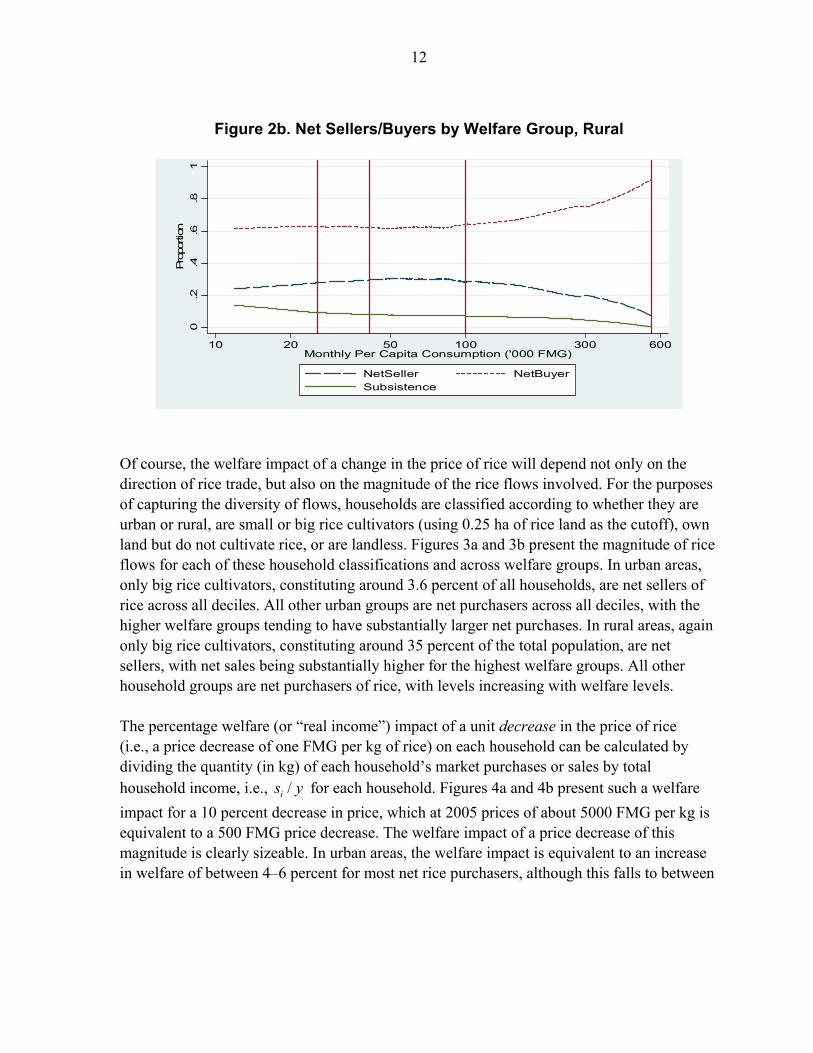
share of the benefit will equal the share of imports in total consumption—the rest goes to net producers. Decreasing the tariff therefore results in a decrease in the domestic price, a redistribution of income from net producers to net consumers, and a decrease in revenue. At the start of 2004, the net tax on rice imports was 45 percent so that, ignoring trade and transport margins, the domestic price faced by producers and consumers was 1.45 times the world price. This net tax reflected a combination of two separate taxes, an import tariff of 20 percent and a value-added tax (VAT) of 21 percent, with the latter levied on the import tax-inclusive price. Rice consumption and production patterns Based to EPM2001, approximately 76 percent of households are classified as rural. Rural households are disproportionately represented among the poor with, for example, around 90 percent of poor households being rural. As expected, the direction of rice trade differs markedly between urban and rural areas. Whereas, in urban areas, 87 percent of households are purchasers of rice, in rural areas, 66 percent are net purchasers. Patterns of trade also vary substantially across welfare groups within both urban and rural areas. Figures 2a and 2b present the classification of urban and rural households according to whether they are net sellers or net buyers or neither (i.e., rice subsistence households). In urban areas, whereas around 65 percent of poor households are net purchasers of rice, over 90 percent of high-income households are net purchasers. Similarly, in rural areas, whereas around 64 percent of poor households are net purchasers, around 70 percent of high-income households are net purchasers.

Figure 2a. Net Sellers/Buyers by Welfare Group, Urban

0.2

.4.6

.81

Prop

ortio

n


NetSeller NetBuyerSubsistence

12

Figure 2b. Net Sellers/Buyers by Welfare Group, Rural

0.2

.4.6

.81

Pro

porti

on


NetSeller NetBuyerSubsistence

Of course, the welfare impact of a change in the price of rice will depend not only on the direction of rice trade, but also on the magnitude of the rice flows involved. For the purposes of capturing the diversity of flows, households are classified according to whether they are urban or rural, are small or big rice cultivators (using 0.25 ha of rice land as the cutoff), own land but do not cultivate rice, or are landless. Figures 3a and 3b present the magnitude of rice flows for each of these household classifications and across welfare groups. In urban areas, only big rice cultivators, constituting around 3.6 percent of all households, are net sellers of rice across all deciles. All other urban groups are net purchasers across all deciles, with the higher welfare groups tending to have substantially larger net purchases. In rural areas, again only big rice cultivators, constituting around 35 percent of the total population, are net sellers, with net sales being substantially higher for the highest welfare groups. All other household groups are net purchasers of rice, with levels increasing with welfare levels. The percentage welfare (or “real income”) impact of a unit decrease in the price of rice (i.e., a price decrease of one FMG per kg of rice) on each household can be calculated by dividing the quantity (in kg) of each household’s market purchases or sales by total household income, i.e., /is y for each household. Figures 4a and 4b present such a welfare impact for a 10 percent decrease in price, which at 2005 prices of about 5000 FMG per kg is equivalent to a 500 FMG price decrease. The welfare impact of a price decrease of this magnitude is clearly sizeable. In urban areas, the welfare impact is equivalent to an increase in welfare of between 4–6 percent for most net rice purchasers, although this falls to between

13

Figure 3a. Net Purchases by Welfare Group, Urban

-.20

.2.4

.6.8

Net

Pur

chas

es ('

000

FMG

)


Landless BigRiceSmallRice OtherLand

Figure 3b. Net Purchases by Welfare Group, Rural

-2-1

.5-1

-.50

.5N

et P

urch

ases

('00

0 FM

G)



14

2–4 percent for high-income households.9 For net sellers (i.e., big rice producers), the impact is a decrease in welfare of greater than 2 percent for moderately poor and middle income households, but this falls towards zero for both extreme poor and high welfare households. For rural households, the impact on net purchasers is clearly progressive with welfare increases between 2.5–7 percent for poor households but falling to less than 3 percent for high-income households. For net sellers, the decrease in welfare is also progressive with poor households experiencing decreases of between 1–3 percent and high-income households experiencing decreases of between 5–15 percent.

Figure 4a. Welfare Impact of Rice Price Decrease, Urban (10% price decrease from 5000 FMG per kg)

-4-2

02

46

Per

cent

age

of C

onsu

mpt

ion



9 The bottom 10 percent of households have monthly per capita consumption less than 25,000 FMG, the bottom 30 percent consumption less than around 40,000 FMG, and the top 30 percent consumption greater than 135,000 FMG.

15

Figure 4b. Welfare Impact of Rice Price Decrease, Rural (10 % price decrease from 5000 FMG per kg)

-1

5-1

0-5

05

10Per

cent

age

of C

onsu

mpt

ion



Distributional impact

The distributional effect of lower rice prices will depend on the relationship between h

h i

i

ss

θ =

and household welfare. Table 1 presents the sum of hθ for each welfare decile and also for each household classification. This shows how the benefit from each unit of revenue lost due to a price (and tariff) decrease is distributed across households. The first column shows the distribution of welfare changes across each welfare decile. The top five deciles all gain from the price decrease—out of every 100 FMG lost from tariff revenue, these households together gain 97.8 FMG. The gains from tariff reduction are thus very badly targeted. But the aggregate gains and losses across deciles hide substantial variation across households within deciles and across household classifications. While landless households in both urban and rural areas together gain 128 FMG, big rice cultivators lose 81 FMG. Non-rice farmers and small rice cultivators also gain 53 FMG. For both gainers and losers, the aggregate impacts on the lower welfare deciles are substantially smaller than for the higher deciles. Therefore, lower rice tariffs essentially involve a redistribution of welfare from higher income net producers to higher income net consumers with little absolute impact on lower income groups reflecting the low absolute rice trading levels of the latter.

16

Ta

ble

1. D

istr

ibut

ion

of W

elfa

re Im

pact

from

Tar

iff In

crea

se A

cros

s H

ouse

hold

s (S

hare

s)

U

rban

Hou

seho

lds

R

ural

Hou

seho

lds

A

ll H

ouse

hold

s La

ndle

ssB

ig R

ice

Cul

tivat

ors

Sm

all R

ice

Cul

tivat

ors

Non

-ric

e Fa

rmer

s

Land

less

B

ig R

ice

Cul

tivat

ors

Sm

all R

ice

Cul

tivat

ors

Non

-ric

e Fa

rmer

s

Bot

tom

0.

018

0.00

0 -0

.000

0.

001

0.00

1

0.00

8 -0

.028

0.

025

0.01

0 2nd

dec

ile

-0.0

02

0.00

4 -0

.005

0.

001

0.00

2

0.00

6 -0

.060

0.

039

0.01

2 3rd

dec

ile

0.02

9 0.

007

-0.0

01

0.00

5 0.

001

0.

017

-0.0

49

0.02

9 0.

020

4th d

ecile

0.

001

0.02

2 -0

.004

0.

002

0.00

3

0.01

5 -0

.100

0.

045

0.01

8 5th

dec

ile

-0.0

24

0.03

9 -0

.003

0.

003

0.00

5

0.02

7 -0

.156

0.

032

0.02

9 6th

dec

ile

0.11

9 0.

061

-0.0

09

0.00

7 0.

008

0.

061

-0.0

68

0.02

4 0.

036

7th d

ecile

0.

116

0.08

1 -0

.000

0.

005

0.00

4

0.08

6 -0

.085

0.

002

0.02

4 8th

dec

ile

0.22

8 0.

162

-0.0

04

0.00

2 0.

008

0.

082

-0.0

65

0.03

0 0.

012

9th d

ecile

0.

301

0.17

5 -0

.003

0.

007

0.00

9

0.09

0 -0

.016

0.

010

0.03

0 To

p 0.

214

0.19

7 -0

.002

0.

003

0.00

3

0.13

7 -0

.148

0.

018

0.00

7

Tota

l 1.

000

0.74

8 -0

.031

0.

036

0.04

4

0.52

9 -0

.775

0.

254

0.19

8

Sha

re o

f Tot

al

Hou

seho

lds

1.00

0 0.

165

0.03

6 0.

024

0.01

2

0.14

1 0.

350

0.18

6 0.

086

Not

e: A

utho

rs’ c

alcu

latio

ns b

ased

on

EPM

2001

.

17

Efficiency impact As well as having a redistributional effect, tariffs have an efficiency effect, which must be incorporated into any analysis. The marginal social cost of raising one unit of revenue by increasing tariffs (or marginal cost of funds, MCF) is calculated as the inverse of the revenue elasticity—see (5). For example, if production is 80 percent of total consumption (imports accounting for the remaining 20 percent), the elasticity of production is 0.2 and the elasticity of consumption is -0.3, then the elasticity of imports is approximately -2.3. This very high elasticity reflects the fact that even small responses in consumption and production translate into very large proportional changes in imports since imports are only a small share of consumption. The tax base is thus extremely elastic. Since the initial tax rate (defined, somewhat differently to earlier, as the share of tax in the domestic price) is 30 percent, the MCF is 3.23 (the inverse of one plus 0.3*-2.3). The deadweight loss associated with an increase in the tariff that raises this one unit of revenue is thus 2.23. The converse of this is that a reduction in the tariff generates an equally large efficiency gain. The marginal efficiency gain from decreasing tariffs can also be expected to decrease as the tariff approaches zero since imports, the tax base, as a proportion of total supply will increase when production falls and consumption increases and the elasticity of imports will also decrease. Table 2 presents the marginal cost of funds for alternative assumptions about the demand and supply elasticities, as well as about the share of imports in total supply. Notice that the MCF is negative when the import share is 10 percent and for higher elasticities of production and consumption. This indicates that the tariff is on the wrong side of the Laffer curve so that a decrease in the tariff is associated with an increase in revenue reflecting a substantial increase in imports. Therefore, in an aggregate sense, a potential Pareto improvement exists since decreasing the tariff will increase both revenue and the aggregate welfare of households since the latter are, in aggregate, net purchasers. Ignoring such Pareto-improving possibilities, the range for the MCF is 1.20–6.25. When combining the distributional and efficiency impacts below, we therefore consider MCF values of 1.20 (LOW), 3.70 (MEDIUM), and 6.25 (HIGH). Distribution and efficiency We now combine the distributional and efficiency implications of tariff decreases using equation (5). Table 3 presents the marginal social benefit from a tariff decrease under alternative assumptions for the MCF and for the level of inequality aversion. The first column presents the pure distributional impact, D

tλ , for alternative levels of inequality aversion, which can be interpreted as the increase in welfare of our “target” population as defined by the underlying welfare weights. This suggests that the benefits from a tariff

18

reduction are not well targeted since Dtλ decreases rapidly with ε . Only 0.019 units of each

revenue unit forgone accrues to the lowest parts of the welfare distribution.

Table 2. Marginal Cost of Public Funds for Different Import Elasticities

Marginal Cost of Funds ( 0.3τ = )

Demand and Production Elasticities

Import Share=10% x/s=100/10=10.0 q/s=90/10=9.0



0.1; 0.1x qη η= − = 2.33 ( 1.90sη = − ) 1.37 ( 0.90sη = − ) 1.20 ( 0.57sη = − )

0.1; 0.2x qη η= − = 6.25 ( 2.80sη = − ) 1.64 ( 1.30sη = − ) 1.32 ( 0.80sη = − )

0.2; 0.1x qη η= − = -7.14 ( 3.80sη = − ) 2.17 ( 1.80sη = − ) 1.51 ( 1.13sη = − )

0.3; 0.2x qη η= − = -2.27 ( 4.80sη = − ) 3.23 ( 2.30sη = − ) 1.78 ( 1.47sη = − )

0.3; 0.3x qη η= − = -1.41 ( 5.70sη = − ) 5.26 ( 2.70sη = − ) 2.04 ( 1.70sη = − )

Note: Authors’ calculations based on EPM2001.

Table 3. Welfare Impact of Lower Rice Tariff

D

tλ tLλ tMλ tHλ

Inequality Aversion

0ε = 1.000 1.200 3.700 6.250

1ε = 0.172 0.207 0.637 1.077

2ε = 0.050 0.059 0.183 0.310

5ε = 0.019 0.023 0.071 0.191

Note: Authors’ calculations based on EPM2001. The final three columns adjust for the efficiency gains from tariff reductions. The first row shows the aggregate welfare benefits for all households for alternative MCFs: the aggregate benefit to households from each unit of revenue forgone from tariff reductions ranges from 1.20 to 6.25 for low to high efficiency gains. For each value of MCF, the column gives the

19

product of the MCF and Dtλ . Looking across the final row, the benefit to the poorest

households from a unit of revenue forgone from a tariff reduction ranges from 0.023 to 0.191.

B. Targeted Transfers

The effectiveness of targeted transfers as a poverty alleviation instrument will depend on how effective the program is at both identifying poor households and ensuring that transfers are delivered to them at low administrative cost. In practice, even the best targeted transfer programs are imperfectly targeted with some of the transfers “leaking” to the non-poor and incomplete “coverage” of the poor. In addition, designing and implementing a transfer program requires that some budget resources be devoted to these activities thus reducing the amount of the budget available for transfers to program beneficiaries. Of course, these two dimensions are interdependent—by allocating more resources to improving the design and implementation of a program, the higher the percentage of the transfer budget that will reach poor households. Existing empirical evidence shows that the performance of transfer programs in these two dimensions varies substantially across and within countries, and also across targeting methods used and program types. A recent review of the targeting performance of transfer programs found that under the median program the “poor” received only 25 percent more than their population share (Coady, Grosh, and Hoddinott, 2004). If 30 percent are classified as poor, then this implies that only 37.5 percent of transfers go to the poor. However, many programs do substantially better than the median program. For example, the median targeting performance for programs using some form of means testing was such that the poor received 1.5 times their population share. Using a 30 percent poverty rate, this implies the poor receive 45 percent of total transfers. Even within means-tested programs, there was substantial variation in performance. The median performance for the top ten performing programs was such that the poor received approximately twice their population share, i.e., the poorest 30 percent would receive 60 percent of transfers. High administrative costs further decrease the effectiveness of transfer programs (conditional on targeting performance). Unfortunately, there is very little evidence on the cost level or structure of transfer programs. But what little evidence exists suggests that there may be great variability, with the share of administrative costs in the total program budget ranging from 10 percent to 40 percent (Grosh, 1994; Caldès, Coady, and Maluccio, 2006). In other words, the fiscal cost of distributing one unit of welfare to all beneficiary households ranges from 1.11–1.67 units.

20

In order to address the issue of the potential effectiveness of targeted transfers in the context of Madagascar, we use information from ECM2001 on the socioeconomic characteristics of households to simulate the targeting performance of a program that employs proxy-means targeting. We start by identifying a range of household characteristics that are typically highly correlated with household welfare.10 Household welfare is then regressed on these characteristics. The estimated coefficients are taken as “weights” that are applied to household characteristics to get a household “score,” in this case, predicted household consumption per capita. Households with a score below some “threshold” are identified as program beneficiaries. Basing program eligibility on the predicted score will of course result in the standard targeting errors. For example, if the poorest 30 percent of households according to the score are deemed “poor” and thus eligible for program benefits, then some poor households based on per capita consumption will be wrongly excluded (“errors of omission”) while some non-poor households will be wrongly included (“errors of inclusion”). Figure 5 presents the distribution of targeting errors for the simulated transfer program.11 The vertical line in Figure 5 is the poverty line, so the curves to the left of it indicate undercoverage of the poor (U) and to the right of it indicate leakage to non-poor households (L). Undercoverage and leakage are highest close to the poverty line, undercoverage is highest in urban areas, and leakage is highest in rural areas. So, on average, the rural non-poor are included at the expense of the urban poor. This, of course could be partly addressed by developing a different proxy-means scoring system for urban and rural areas and allocating program places across urban and rural areas in proportion to their share of the poverty rate.

10 In practice, these characteristics should be easily verified by program officials and not easily manipulated by households in an attempt to gain access to the program. Typically, households will be informed about the existence of such a program and asked to apply at a program office—thus introducing an element of self-selection into the targeting process. At the office, households report these characteristics and are informed if they are potentially eligible. Eligible households will then be visited to verify the reported information. 11 The underlying regression used per capita household consumption as the dependent variable, with independent variables including information on geographic location; gender, age, education and sectoral employment of the head of household; household size and composition; types of housing and materials for walls, floors and ceilings; housing area; source of water and lighting; and possession of various consumer durables. The r-squared for the regression was 0.69 based on 4,857 household observations. More details are available from the authors upon request.

21

Figure 5. Undercoverage and Leakage, Urban and Rural

0.2

.4.6

.8Pr

opor

tion

of H

ouse

hold

s

10 20 50 100 300 600Monthly Per Capita Consumption (Pesos)

U LUU LUUR LR

Table 4 presents the welfare impact of transfers based on (6). The first column presents the share of transfers accruing to the various target populations as specified by the underlying welfare weights. Nearly 30 percent of transfers accrue to the poorest households: every one unit of revenue transferred through the program results in 0.3 going to the bottom of the welfare distribution. The first column essentially abstracts from administrative costs (an efficiency cost) as well as the efficiency benefit associated with the extra rice tariff revenue due to higher rice consumption—these are captured in the final three columns. The first row of these columns gives the share of the budget allocated to transfers (i.e., one minus the share of administrative costs in the budget), reflecting the administrative efficiency of the program, times an adjustment for second-round revenue benefits. This share of the budget allocated to transfers is taken to range from 0.6 for the low-efficiency program (L), to 0.75 for medium-efficiency programs, to 0.9 for the high-efficiency program (H). These are multiplied by 1.057 to capture second-round revenue effects, derived using 0.18 as the marginal budget share for rice based on available empirical estimates.12 Incorporating these into the analysis, the final row shows that the benefit accruing to the lowest welfare households from every one unit of revenue allocated to the program ranges from 0.19 to 0.28.

12 For a discussion of rice demand patterns in Madagascar, see Minten, Randrianarisoa, and Zeller (1998); Ravelosoa, Haggblade, and Rejemison (1999); Lundberg and Rich (2002); and Stifel and Randrianarisoa (2004).

22

Table 4. Welfare Impact of Proxy-Means Targeted Transfers

D

mλ mLλ mMλ mHλ

0ε = 1.000 0.634 0.793 0.951

1ε = 0.608 0.386 0.482 0.579

2ε = 0.442 0.280 0.350 0.420

5ε = 0.297 0.189 0.236 0.283

Note: Authors’ calculations based on EPM2001.

C. Tariffs, Transfers, or Both?

In this section, we compare the net social welfare impact of tariffs and transfers by comparing the welfare impact per unit of revenue absorbed by each policy instrument. As above, for each instrument we consider three scenarios capturing high (H), medium (M), and low (L) efficiency levels. With tariffs, these relate to different assumptions about demand and supply responses, which affect the revenue elasticity and thus the magnitude of the efficiency gain from reducing tariffs. We consider revenue elasticities of 6.25 (tHigh), 3.70 (tMedium), and 1.20 (tLow). With direct transfers, the scenarios relate to the administrative effectiveness in terms of the share of the program budget absorbed by administrative costs: we consider administrative cost shares of 10 percent (mHigh), 25 percent (mMedium), and 40 percent (mLow). Figure 6 presents the high and low efficiency welfare impacts for each policy instrument for 1 5ε≥ ≤ . If the efficiency gains from reducing rice tariffs are on the lower side, then tariff reduction is dominated by even the low-efficiency direct transfer programs. Tariff reductions are only superior if the efficiency gains are on the higher side and at lower values of ε , where sufficient weight is given to welfare gains accruing to higher income groups. With high efficiency gains, tariff reductions clearly dominate at 1ε = where the weight given to welfare gains to higher income households is relatively large. At higher values of ε , the attraction of tariffs as a poverty alleviation mechanism diminishes rapidly, reflecting the almost exclusive focus on gains at the bottom of the welfare distribution. Therefore, a focus on poor households (e.g., taking 2ε > ) would clearly rank direct targeted transfers above tariff reductions a poverty alleviation measure. Reasonably effective transfer programs are clearly a more cost-effective approach to poverty alleviation. This is reinforced when one takes into account that the efficiency gains from tariff reductions are upper-bounds since they refer to marginal changes and thus can be expected to decrease non-linearly with the tariff rate.

23

Figure 6. Welfare Impact of Tariff Reductions and Targeted Transfers

0

0.2

0.4

0.6

0.8

1

1.2

1 2 3 4 5

Inequality Aversion (epsilon)

Wel

fare

Impa

ct/U

nit R

even

ue

tHigh

tLow

mHigh

mLow

It is tempting to interpret the above results as an argument for increasing the rice tariff to finance transfers to the poor. The welfare increase from such a reform package can be calculated as ( )m tλ λ− , which is clearly positive for higher levels of aversion to inequality. However, this ignores the fact that the MCF associated with raising revenue using other tax instruments is probably much lower. In this case, it is clearly preferable to switch from rice tariffs to other taxes and to use any revenue increases to finance a transfer program. In addition, initial tariff reductions will also have a substantial impact on poverty reduction since the efficiency gains are likely to be substantially higher when tariffs are reduced from a high level. The results can also be interpreted as an argument for sequencing policy reforms by initially reducing tariffs, gradually replacing them with other tax revenues (possibly as part of a broader tax reform that improves the efficiency of the tax system), and using some of the extra revenues to develop an effectively targeted transfer program. However, to the extent that it takes time to develop a comprehensive and cost-effective safety net, some ad hoc measures aimed at mitigating the adverse impacts on poor net sellers of rice are warranted. Such measures could take many forms, including measures aimed at increasing land productivity through increasing yields and diversifying into alternative crops. These targeted measures should eventually be integrated into the overall safety net framework.

IV. FROM PARTIAL TO GENERAL EQUILIBRIUM ANALYSIS

An obvious shortcoming of the above discussion is that it is partial equilibrium. A general equilibrium approach that addresses both the indirect revenue effects through changing

24

demand and supply for other taxed or subsidized goods and services, as well as the welfare effects generated through factor markets might change some of the numbers above or even the qualitative nature of the results. For example, in principle, if goods that are very strong substitutes or complements to rice in production or consumption are relatively highly taxed or subsidized, then indirect revenue effects may be substantial. However, in practice, since the other main crops grown in Madagascar (maize and cassava) are not traded internationally and not subject to taxes or subsidies, these indirect revenue effects are not likely to be important. Alternatively, if rice production is relatively unskilled labor-intensive, then lower rice prices may result in lower unskilled wages. If the poorest households rely very heavily on such sources of income and if they cannot find alternative employment, say, in the production of other crops, then in principle, this wage effect may be strong enough to switch these households from being net gainers to net losers. Note that this unskilled wage effect would simply make tariff reductions even less attractive from a distributional perspective and reinforce the dominance of transfers from a poverty alleviation perspective. In this instance, it is still the case that a reform package of lower tariffs combined with increases in other taxes and direct interventions through safety nets is the most effective policy response since the tax reform should generate substantial efficiency gains that can be used to finance a transfer program that benefits the poorest households.

V. SUMMARY AND CONCLUSIONS

The paper is concerned with the relative efficiency, distributional, and revenue implications of tariffs and transfers, especially in the context of identifying their respective roles for poverty alleviation. The results indicate that although there are likely to be substantial efficiency gains from tariff reductions, these accrue mainly to higher income households. In addition, poor net rice sellers lose from price decreases. Developing a system of well designed and implemented targeted direct transfers to poor households is thus likely to be a substantially more cost-effective approach to poverty alleviation. Such an approach can be financed by switching revenue raising from rice tariffs to alternative, more efficient tax instruments. In the short-term the development of a system of direct transfers could focus on poor net rice sellers (i.e., small-holder rice producers) since these households lose from tariff reductions; these transfers could also be conditioned on participation in extension services to promote higher agricultural productivity. Over the longer term, such a program should be integrated into a more comprehensive targeted safety net mechanism that has high coverage of poor households.

25

Appendix I. The Madagascar EPM Household Survey The analysis in the paper uses information from the 2001 Madagascar household survey, “Enquête Permanente auprès des Ménages” (EPM2001), organized by the National Statistical Institute (INSTAT) at the end of 2001. The survey was nationwide and comprehensive, including information on household socioeconomic characteristics, consumption, health, education, income sources, time allocation, and occupation, as well as information on agricultural production. The sample was set up in a stratified manner so as to produce representative statistics at the national and provincial level, as well as along the urban-rural divide. The total sample consists of 5,080 households. About 2,500 households were households that have land in cultivation. Households in rural areas accounted for 2,040 household in the sample. The consumption aggregate was calculated for the year prior to the survey and incorporates food autoconsumption (from agricultural production, from livestock production, and enterprise income), purchased food, food gifts and payments in-kind, education and health care expenditures, imputed and actual housing costs, expenditures on consumer durables, and other non-food expenses. The consumption aggregate is deflated to account for regional price differences using price information available in the survey and the Paasche index method. The definition of poverty used by INSTAT is based on these consumption data. A poor person, as identified by INSTAT, is a person who cannot afford to consume the bundle of food and non-food goods deemed essential to lead an active and social life. The poverty line was evaluated in 2001 at approximately 988.6 FMG per person per year (corresponding to US$0.42 per day). Using this benchmark, it was estimated that almost 70 percent of the Malagasy population was poor. The poverty rate in rural areas was estimated at 77 percent compared to 44 percent in urban areas.

26

Table 5. Mean Per Capita Consumption and Welfare Weights

Welfare Deciles

Mean Per Capita

Consumption

Ratio of

Mean to

Bottom

0.5ε =

1.0ε =

2.0ε =

3.0ε =

4.0ε =

5.0ε =

Bottom 19.86 1.00 1.00 1.00 1.00 1.00 1.00 1.00

2nd 29.60 1.49 0.82 0.67 0.45 0.30 0.20 0.14 3rd 37.61 1.88 0.73 0.53 0.28 0.15 0.08 0.04 4th 46.47 2.33 0.66 0.43 0.18 0.08 0.03 0.01 5th 57.12 2.86 0.59 0.35 0.12 0.04 0.01 0.01 6th 70.80 3.55 0.53 0.28 0.08 0.02 0.01 0.00 7th 89.16 4.47 0.47 0.22 0.05 0.01 0.00 0.00 8th 117.99 5.90 0.41 0.17 0.03 0.00 0.00 0.00 9th 165.44 8.34 0.35 0.12 0.01 0.00 0.00 0.00

Top 299.43 15.41 0.25 0.06 0.00 0.00 0.00 0.00

Note: Based on per capita monthly household consumption (FMG ‘000) adjusted for regional price differences constructed using the 2001 national household survey, EPM2001. Sample used has dropped outliers, identified as households in the bottom and top 1 percent of the national welfare distribution, with the sample decreasing by 125 households, from 5,080 to 4,955 households.

27

References Braverman, A., J. Hammer, and C. Ahn, 1987, “Multimarket Analysis of Agricultural Pricing

Policies in Korea,” in The Theory of Taxation for Developing Countries, ed. by D. Newbery and N. Stern (New York: Oxford University Press).

Caldés, N., D. Coady, and J. A. Maluccio, 2006, “A Comparative Analysis of Program Costs

Across Three Social Safety Net Programs,” World Development, Vol. 34, No. 5, pp. 818–37.

Coady, D., 1997, “Agricultural Pricing Policies in Developing Countries: An Application to

Pakistan,” International Tax and Public Finance, Vol. 4, No. 1, pp. 39–57. ———, and J. Drèze, 2002, “Commodity Taxation and Social Welfare: The Generalized

Ramsey Rule,” International Tax and Public Finance, Vol. 9, No. 3, pp. 295–316. Coady, D., M. Grosh, and J. Hoddinott, 2004, “The Targeting of Transfers in Developing

Countries: Review of Lessons and Experience,” Regional and Sectoral Studies Series (Washington: World Bank).

Coady, D., and R. L. Harris, 2004, “Evaluating Transfer Programmes Within a General

Equilibrium Framework,” Economic Journal, Vol. 114 (October), No. 498, pp. 778–99.

Coady, D., and E. Skoufias, 2004, “On the Targeting and Redistributive Efficiencies of

Alternative Transfer Instruments,” Review of Income and Wealth, Vol. 50 (March), No. 1, pp. 11–27.

Dorosh, P. and B. Minten, eds., 2006, “Rice Policy in Madagascar: The 2004 Crisis, Market

Development and Price Stabilization,” Draft (Washington: World Bank). Drèze, J., and N. Stern, 1987, “The Theory of Cost-Benefit Analysis,” in Handbook of Public

Economics, ed. by A. J. Auerbach and M. Feldstein (Amsterdam and New York: North Holland).

Grosh, M., 1994, “Administering Targeted Social Programs in Latin America,” From

Platitudes to Practice (Washington: World Bank). Lundberg, M., and K. Rich, 2002, “Multimarket Models and Poverty Analysis: An

Application to Madagascar,” Draft (Washington: World Bank).

28

Minten, B., J. C. Randrianarisoa, and M. Zeller, 1998, “Les Déterminants des Dépenses de la Consommation Alimentaires et Non-Alimentaires des Ménages Ruraux,” Cahier de la Recherche sur la Politiques Alimentaires No. 14. (Antananarivo: IFPRI and FOFIFA).

Newbery, D., 1987, “Identifying Desirable Directions of Agricultural Price Reform in

Korea,” in The Theory of Taxation for Developing Countries, ed. by D. Newbery and N. Stern (New York: Oxford University Press).

Ravelosoa, R., S. Haggblade, and H. Rejemison, 1999, “Estimation des Élasticités de

Demande á Madagascar á Partir d'un Modèle AIDS,” CFNPP Working Paper No. 99 (Cornell, NY: Cornell University).

Stifel, D., and J. C. Randrianarisoa, 2004, “Rice Prices, Agricultural Input Subsidies,

Transaction Costs and Seasonality: a Multi-Market Model Poverty and Social Impact Analysis (PSIA) for Madagascar” (Washington: World Bank).

Evaluating Alternative Approaches to Poverty Alleviation: Rice Tariffs versus Targeted Transfers in...

Documents

Transcript of Evaluating Alternative Approaches to Poverty Alleviation: Rice Tariffs versus Targeted Transfers in...