Mapping Forest Growth Stage in the Brigalow Belt Bioregion of Australia through integration of ALOS...
16
Mapping forest growth and degradation stage in the Brigalow Belt Bioregion of Australia through integration of ALOS PALSAR and Landsat-derived foliage projective cover data Richard M. Lucas g, ⁎, Daniel Clewley a,b , Arnon Accad c , Don Butler c , John Armston d , Michiala Bowen e , Peter Bunting a , Joao Carreiras f , John Dwyer e , Teresa Eyre c , Annie Kelly c , Clive McAlpine e , Sandy Pollock c , Leonie Seabrook e a Institute of Geography and Earth Sciences, Aberystwyth University, Aberystwyth, Ceredigion, SY23 2EJ, UK b Ming Hsieh Department of Electrical Engineering, University of Southern California, 3740, McClintock Avenue, EEB 100, Los Angeles, CA 90089-2560, USA c Queensland Herbarium, Department of Science, Information Technology, Innovation and the Arts, Brisbane Botanic Gardens, Mt Coot-tha, Mt Coot-tha Road, Toowong, Queensland, 4066, Australia d Remote Sensing Centre, Department of Science, Information Technology, Innovation and the Arts, Ecosciences Precinct, 41 Boggo Road, Dutton Park, Queensland, 4102, Australia e Centre for Spatial Environmental Research, School of Geography, Planning and Environmental Management, the University of Queensland, Brisbane, Queensland, 4072, Australia f Tropical Research Institute, Travessa do Conde da Ribeira, 9, 1400-142, Lisbon, Portugal g School of Biological, Earth and Environmental Sciences, University of New South Wales, High Street, Kensington, NSW, 2052, Australia abstract article info Article history: Received 18 November 2012 Received in revised form 26 October 2013 Accepted 1 November 2013 Available online xxxx Keywords: Brigalow ALOS PALSAR Landsat Regrowth Degradation Carbon Biodiversity Differentiation of forest growth stages through classification of single date or time-series of Landsat sensor data is limited because of insensitivity to their three-dimensional structure. This study therefore evaluated the benefits of integrating the Advanced Land Observing Satellite (ALOS) Phased Array L-band Synthetic Aperture Radar (PALSAR) L-band HH and HV polarisation response from the woody components of vegetation with Landsat- derived foliage projective cover (FPC). Focus was on 12 regional ecosystems (REs) distributed across the Brigalow Belt Bioregion (BRB) of Queensland, Australia, where different stages of growth dominated by brigalow (Acacia harpophylla) were widespread. From remnant areas of brigalow-dominated forests mapped previously for each RE by the Queensland Herbarium through field visits and interpretations of aerial imagery, frequency distri- butions of all three channels were extracted and compared to those of image segments generated using FPC and PALSAR data. For woody vegetation (with an FPC threshold of ≥9%) outside of the remnant areas, mature (non- remnant) forests were associated with segments where the HH and HV backscatter thresholds were within one standard deviation of the mean extracted for remnant forest. Early-stage regrowth was differentiated using an L- band HH threshold of b−14 dB, common for all REs because of similarities in structure at this stage. The early- stage included forests regrowing over several decades and often occurred in areas recovering from recent clear- ing events. Objects falling between the early and mature stages were considered to be intermediate regrowth and/or degraded forest. All areas with an FPC b 9% were mapped as non-forest. Within the BRB, the Queensland Herbarium established that forests with brigalow as a dominant or subdominant component originally occupied over 7.3 million ha but were reduced to 586,364 ha by 2009, with 460,499 ha (78.5%) having brigalow as the dominant component. Using the Landsat FPC and ALOS PALSAR data, an additional 722,686 ha of brigalow-dominated regrowth forest were identified giving a total forested area (brigalow-domi- nated remnant and secondary forest) of 1,183,185 ha or 17.2% of the area of the 12 REs. Within this area, the greater proportion of regrowth (368,473 ha or 31.1%) was mapped as early stage primarily because of recovery following recent clearance events. 230,551 (19.5%) ha and 123,662 ha (10.5%) were mapped as intermediate and mature (non-remnant) stages respectively and the remainder (38.9%) was remnant forest. Users’ and producers’ accuracies were, respectively, 81% and 69% for early regrowth and 71% and 89% for mature and intermediate stage forests combined. The mapping, which used Queensland Herbarium’s RE data to delineate brigalow extent, provided a structural, rather than age-based classification of growth stage, as is typically retrieved using time- series comparison of optical imagery. The regional estimates of growth/degradation stage generated for the Remote Sensing of Environment xxx (2014) xxx–xxx ⁎ Corresponding author. Tel.: +61 2 99695734. E-mail addresses: [email protected] (R.M. Lucas), [email protected] (D. Clewley), [email protected] (A. Accad), [email protected] (D. Butler), [email protected] (J. Armston), [email protected] (M. Bowen), [email protected] (P. Bunting), [email protected] (J. Carreiras), [email protected] (J. Dwyer), [email protected] (T. Eyre), [email protected] (A. Kelly), [email protected] (C. McAlpine), [email protected] (S. Pollock), [email protected] (L. Seabrook). RSE-09038; No of Pages 16 http://dx.doi.org/10.1016/j.rse.2013.11.025 0034-4257/© 2014 Published by Elsevier Inc. Contents lists available at ScienceDirect Remote Sensing of Environment journal homepage: www.elsevier.com/locate/rse Please cite this article as: Lucas, R.M., et al., Mapping forest growth and degradation stage in the Brigalow Belt Bioregion of Australia through in- tegration of ALOS PALSAR and Lan..., Remote Sensing of Environment (2014), http://dx.doi.org/10.1016/j.rse.2013.11.025
Transcript of Mapping Forest Growth Stage in the Brigalow Belt Bioregion of Australia through integration of ALOS...

Remote Sensing of Environment xxx (2014) xxx–xxx
RSE-09038; No of Pages 16
Contents lists available at ScienceDirect
Remote Sensing of Environment
j ourna l homepage: www.e lsev ie r .com/ locate / rse
Mapping forest growth and degradation stage in the Brigalow BeltBioregion of Australia through integration of ALOS PALSAR andLandsat-derived foliage projective cover data
Richard M. Lucas g,⁎, Daniel Clewley a,b, Arnon Accad c, Don Butler c, John Armston d, Michiala Bowen e,Peter Bunting a, Joao Carreiras f, John Dwyer e, Teresa Eyre c, Annie Kelly c, Clive McAlpine e,Sandy Pollock c, Leonie Seabrook e
a Institute of Geography and Earth Sciences, Aberystwyth University, Aberystwyth, Ceredigion, SY23 2EJ, UKb Ming Hsieh Department of Electrical Engineering, University of Southern California, 3740, McClintock Avenue, EEB 100, Los Angeles, CA 90089-2560, USAc Queensland Herbarium, Department of Science, Information Technology, Innovation and the Arts, Brisbane Botanic Gardens, Mt Coot-tha, Mt Coot-tha Road, Toowong, Queensland, 4066, Australiad Remote Sensing Centre, Department of Science, Information Technology, Innovation and the Arts, Ecosciences Precinct, 41 Boggo Road, Dutton Park, Queensland, 4102, Australiae Centre for Spatial Environmental Research, School of Geography, Planning and Environmental Management, the University of Queensland, Brisbane, Queensland, 4072, Australiaf Tropical Research Institute, Travessa do Conde da Ribeira, 9, 1400-142, Lisbon, Portugalg School of Biological, Earth and Environmental Sciences, University of New South Wales, High Street, Kensington, NSW, 2052, Australia
⁎ Corresponding author. Tel.: +61 2 99695734.E-mail addresses: [email protected] (R.M. Lucas), clewl
[email protected] (J. Armston), mich(J. Dwyer), [email protected] (T. Eyre)(S. Pollock), [email protected] (L. Seabrook).
http://dx.doi.org/10.1016/j.rse.2013.11.0250034-4257/© 2014 Published by Elsevier Inc.
Please cite this article as: Lucas, R.M., et al., Mtegration of ALOS PALSAR and Lan..., Remote
a b s t r a c t
a r t i c l e i n f oArticle history:Received 18 November 2012Received in revised form 26 October 2013Accepted 1 November 2013Available online xxxx
Keywords:BrigalowALOS PALSARLandsatRegrowthDegradationCarbonBiodiversity
Differentiation of forest growth stages through classification of single date or time-series of Landsat sensor data islimited because of insensitivity to their three-dimensional structure. This study therefore evaluated the benefitsof integrating the Advanced Land Observing Satellite (ALOS) Phased Array L-band Synthetic Aperture Radar(PALSAR) L-band HH and HV polarisation response from the woody components of vegetation with Landsat-derived foliage projective cover (FPC). Focuswas on12 regional ecosystems (REs) distributed across theBrigalowBelt Bioregion (BRB) of Queensland, Australia, where different stages of growth dominated by brigalow (Acaciaharpophylla) were widespread. From remnant areas of brigalow-dominated forests mapped previously foreach RE by the Queensland Herbarium through field visits and interpretations of aerial imagery, frequency distri-butions of all three channels were extracted and compared to those of image segments generated using FPC andPALSAR data. For woody vegetation (with an FPC threshold of ≥9%) outside of the remnant areas, mature (non-remnant) forests were associated with segments where the HH and HV backscatter thresholds were within onestandard deviation of themean extracted for remnant forest. Early-stage regrowthwas differentiated using an L-band HH threshold of b−14 dB, common for all REs because of similarities in structure at this stage. The early-stage included forests regrowing over several decades and often occurred in areas recovering from recent clear-ing events. Objects falling between the early and mature stages were considered to be intermediate regrowthand/or degraded forest. All areas with an FPC b9% were mapped as non-forest.Within the BRB, theQueenslandHerbarium established that forestswith brigalow as a dominant or subdominantcomponent originally occupied over 7.3 million ha but were reduced to 586,364 ha by 2009, with 460,499 ha(78.5%) having brigalowas the dominant component. Using the Landsat FPC andALOS PALSARdata, an additional722,686 ha of brigalow-dominated regrowth forest were identified giving a total forested area (brigalow-domi-nated remnant and secondary forest) of 1,183,185 ha or 17.2% of the area of the 12 REs. Within this area, thegreater proportion of regrowth (368,473 ha or 31.1%) was mapped as early stage primarily because of recoveryfollowing recent clearance events. 230,551 (19.5%) ha and 123,662 ha (10.5%)weremapped as intermediate andmature (non-remnant) stages respectively and the remainder (38.9%)was remnant forest. Users’ and producers’accuracies were, respectively, 81% and 69% for early regrowth and 71% and 89% for mature and intermediatestage forests combined. Themapping, which used Queensland Herbarium’s RE data to delineate brigalow extent,provided a structural, rather than age-based classification of growth stage, as is typically retrieved using time-series comparison of optical imagery. The regional estimates of growth/degradation stage generated for the
[email protected] (D. Clewley), [email protected] (A. Accad), [email protected] (D. Butler),[email protected] (M. Bowen), [email protected] (P. Bunting), [email protected] (J. Carreiras), [email protected], [email protected] (A. Kelly), [email protected] (C. McAlpine), [email protected]
apping forest growth and degradation stage in the Brigalow Belt Bioregion of Australia through in-Sensing of Environment (2014), http://dx.doi.org/10.1016/j.rse.2013.11.025

2 R.M. Lucas et al. / Remote Sensing of Environment xxx (2014) xxx–xxx
Please cite this article as: Lucas, R.M., et al., Mtegration of ALOS PALSAR and Lan..., Remote
BRB provide a basis for optimising the use and recovery of these threatened brigalow ecosystems with benefitsfor biodiversity and carbon sequestration.
© 2014 Published by Elsevier Inc.
1. Introduction
The clearance of forests across the world has contributed to signifi-cant declines in both terrestrial carbon stocks and habitat, leading toincreased levels of atmospheric greenhouse gases and losses of biodi-versity (including species extinctions; Dirzo & Raven, 2003; Pan et al.,2011). Nevertheless, in many regions, forests are regenerating on aban-doned and/or previously disturbed land, providing potential for therestoration of ecosystem structure, diversity and function (Bowen,McAlpine, House, & Smith, 2007; 2009; Ramankutty & Foley, 1999). Pri-mary forests that have remained intact (often referred to as remnant)also contain substantial stocks of carbon (Gibbs, Brown, Niles, & Foley,2007) and a high diversity of plant and animal species (Barlow,Gardner, Araujo, et al., 2007). Efforts focusing on conserving forest eco-systems for biodiversity and carbon values therefore rely on knowledgeof the extent of remnant forests (which need to be conserved) and sec-ondary forests at different stages of growth and degradation (whichneed to be protected and managed to facilitate ecosystem restorationand provide additional carbon sequestration). Spatial and quantitativeinformation on forest extent, structural attributes (e.g., cover, height)and biomass, and changes in these is also critical for advising manage-ment strategies that aim to optimise the recovery of forest ecosystemsto retain biodiversity and enhance terrestrial carbon stocks. However,for many regions of the world, such information is lacking. For this rea-son, increasing emphasis is being placed upon using remote sensingobservations to fill these gaps, particularly as these forests are oftenscattered over vast areas and may be experiencing rapid change(Chambers et al., 2007; Goetz et al., 2009).
A common approach to mapping the growth stage of forests hasbeen to use time-series of remote sensing (primarily optical) data to dif-ferentiate forests of differing age (e.g., Helmer, Lefsky, & Roberts, 2009;Prates-Clark, Lucas, & dos Santos, 2009; Yanesse et al., 1997). Thesemethods are data intensive and assume stand age to be an indicatorof the stage of development relative to that of the primary or matureforest, with older forests often considered the most similar in terms ofstructure and species composition (Bowen et al., 2007). However, thesuccession of forests may be influenced by a number of factors, suchas clearing mechanisms, periods and types of use, the history ofburning aswell as physical factors such as soils, climate and topography(Prates-Clark et al., 2009). Degradation of forests within the same land-scape, including those that are regenerating, is also not considered, withmany forests assumed to be developing in one direction. For thesereasons, forests of the same age may differ in their structure, speciescomposition and biomass and rates of change in these attributes overtime (Lucas, Honzak, do Amaral, Curran, & Foody, 2002). Whilst ageinformation is important to retain, remote sensing efforts also need tobe directed towards tracking the structural development or degradationof forests relative to the mature state and ideally quantifying thechanges in biomass (carbon) over time. Such an approach is also advan-tageous as structure often relates to the way that fauna are distributedwithin and utilise a habitat (Bowen et al., 2007; Selwood, MacNally, &Thomson, 2009).
Using areas within the Brigalow Belt Bioregion (BRB) in Queensland,Australia, as an example, Lucas et al. (2006) proposed an approachto identifying regenerating forests at the earliest stage of structuraldevelopment that combined single-date NASA JPL airborne SyntheticAperture Radar (AIRSAR) L-band HH (~25 cmwavelength) polarisationdata and Landsat-derived foliage projective cover (FPC). FPC is thepercentage of an area occupied by the vertical projection of foliage,and is estimated routinely for the state of Queensland using a multiple
apping forest growth and deSensing of Environment (2014
regression relationship established between field measures of woodyFPC and Landsat sensor visible (green and red), near infrared and short-wave infrared data. The FPC ofwoody vegetation is determined by accu-mulating measures of FPC retrieved from time-series of Landsat sensordata, which disaggregates the seasonal contribution from herbaceousvegetation (Armston, Denham, Danaher, Scarth, & Moffiet, 2009).The accuracy of retrieval was increased when vapour pressure deficit(VPD), defined as the difference in vapour pressure from a saturatedatmosphere, was included in the regression because of the known cor-respondence between the evaporative potential of the atmosphereand FPC (Specht & Specht, 1999). Based on cross-validation compari-sons (Armston et al., 2009), the regression model provided an adjustedR2 of 0.80 and RMSE of b10.0% for the estimation of FPC. Lucas et al.(2006) identified the early stage of regeneration as areas supported anFPC associated with forests but an L-band HH backscattering coefficientmore typical to non-forest. Clewley et al. (2012) expanded this ap-proach to differentiate early stage from more intermediate and maturestages by referencing the characteristics of remnant forest, although in-stead used Japanese Aerospace Exploration Agency (JAXA) AdvancedLand Observing Satellite (ALOS) Phased Array L-band SyntheticAperture Radar (PALSAR) HH and HV with Landsat-derived FPCdata to facilitate regional applications. This study therefore sought toevaluate whether the methods of Lucas et al. (2006) and Clewley et al.(2012) could be used in combination to differentiate forests at progres-sive stages of structural development and/or degradation across the BRBgiven the diversity of ecosystems, environments and climates occurring,with focus on ecosystems dominated primarily by brigalow (Acaciaharpophylla). By generating newmaps of forest growth and/or degrada-tion stage for the BRB, significant capacity to quantify biodiversity andcarbon stocks and dynamics would be provided as well as knowledgeon where future restoration activities might be targeted.
In Queensland, regional ecosystems (REs) are defined as vegetationcommunities that are associated with a particular combination ofgeology, landform and soil (Sattler & Williams, 1999). The extent ofthese REs, whether currently forested or otherwise, has been mappedthrough reference to the physical environment and consistent patternsdetectable within time-series of aerial photography and satelliteimagery over thewhole region, with these supported by a limited num-ber of known sample points to provide a description (Neldner, Wilson,Thompson, & Dillewaard, 2012). As few images are available acrossQueensland before the early 1960s and few sample points exist beforethe 1970s (apart from localised explorer and early settle records),what is often referred to as the pre-1750 or pre-European extent ofthe REs (i.e., prior to major impacts from non-indigenous populations)is difficult to ascertain, particularly as ecosystem boundaries mightalso have changed. Hence, the pre-clearing extent is defined, with thisreferring to REs present before known clearing (if occurring) butequating generally to the “pre-1750” or “pre-European” extent (Accad,Neldner, Wilson, & Niehus, 2008; 2012; Neldner, Wilson, Thompson, &Dillewaard, 2005, Neldner et al., 2012). In some cases, old survey re-cords (e.g., from the 1940s and 1950s) have been used to determinethe pre-clearing vegetation in areas already cleared (Fensham &Fairfax, 1997). Remnant forests are considered to be those that haveremained intact before and throughout this period and have neverbeen cleared. In many cases though, the earliest period when these for-ests were observed is the 1940s and 1950s when aerial photographswere first acquired.
This study focused particularly on 12 REs within the BRB wherebrigalow is dominant within the forest community, although withinother REs mapped across the BRB, this species may be subdominant.
gradation stage in the Brigalow Belt Bioregion of Australia through in-), http://dx.doi.org/10.1016/j.rse.2013.11.025
3R.M. Lucas et al. / Remote Sensing of Environment xxx (2014) xxx–xxx
All 12 forest REs considered are endangered following decades ofclearing for agriculture, with ~8% of the original area (where brigalowis either dominant or subdominant) remaining in remnant patches(as of 2009; Accad et al., 2012). Nevertheless, forests regenerated onmany clearances and exist in various stages of regeneration as well asdegradation. Those in the earliest stages of regrowth were, however,often recleared to maintain pastures (Fensham & Guymer, 2009). Allregrowth forests, and particularly those in the earliest stage, haveincreasingly been recognised as providing a potential carbon sink withstrong co-benefits for biodiversity and landscape health (Valbuena,Verburg, Bregt, & Ligtenberg, 2010). Hence, the generation of accuratemaps of growth stage as well as degradation state for these ecosystemswould contribute to efforts supporting restoration of their biodiversityvalues and increasing potential for carbon sequestration.
The paper is structured as follows. Section 2 provides importantbackground information to the BRB relating to the physical environ-ment and land use histories and briefly reviews previous researchthat has focused on mapping forest growth stages from remotesensing data. Section 3 then describes the ALOS PALSAR and LandsatFPC datasets used for classification, the RE mapping (QueenslandHerbarium, 2012c), field data and BioCondition reports (Eyre, Kelly, &Neldner, 2011) for REs with brigalow as a dominant component. Theprocedures developed to map growth (including degradation) stagesare described. In Section 4, the map of these stages and area estimatesfor the BRB of Queensland are provided together with estimates of clas-sification accuracy. Section 5 discusses the approach and conveys theimportance of the study in terms of environmental conservation and
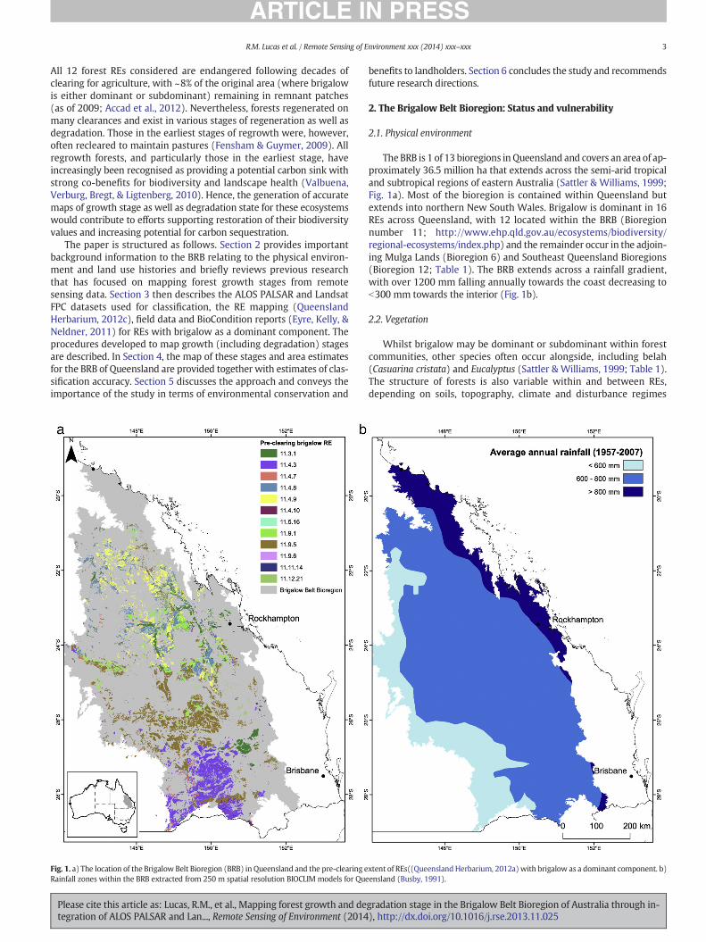
Fig. 1. a) The location of the Brigalow Belt Bioregion (BRB) in Queensland and the pre-clearing eRainfall zones within the BRB extracted from 250 m spatial resolution BIOCLIM models for Que
Please cite this article as: Lucas, R.M., et al., Mapping forest growth and detegration of ALOS PALSAR and Lan..., Remote Sensing of Environment (2014
benefits to landholders. Section 6 concludes the study and recommendsfuture research directions.
2. The Brigalow Belt Bioregion: Status and vulnerability
2.1. Physical environment
TheBRB is 1 of 13 bioregions in Queensland and covers an area of ap-proximately 36.5 million ha that extends across the semi-arid tropicaland subtropical regions of eastern Australia (Sattler & Williams, 1999;Fig. 1a). Most of the bioregion is contained within Queensland butextends into northern New South Wales. Brigalow is dominant in 16REs across Queensland, with 12 located within the BRB (Bioregionnumber 11; http://www.ehp.qld.gov.au/ecosystems/biodiversity/regional-ecosystems/index.php) and the remainder occur in the adjoin-ing Mulga Lands (Bioregion 6) and Southeast Queensland Bioregions(Bioregion 12; Table 1). The BRB extends across a rainfall gradient,with over 1200 mm falling annually towards the coast decreasing tob300 mm towards the interior (Fig. 1b).
2.2. Vegetation
Whilst brigalow may be dominant or subdominant within forestcommunities, other species often occur alongside, including belah(Casuarina cristata) and Eucalyptus (Sattler & Williams, 1999; Table 1).The structure of forests is also variable within and between REs,depending on soils, topography, climate and disturbance regimes
xtent of REs((Queensland Herbarium, 2012a) with brigalow as a dominant component. b)ensland (Busby, 1991).
gradation stage in the Brigalow Belt Bioregion of Australia through in-), http://dx.doi.org/10.1016/j.rse.2013.11.025
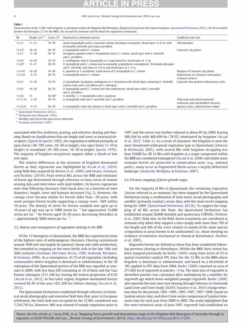
Table 1Characteristics of the 12 REswith brigalow as dominantwithin the Brigalow Belt Bioregion (Regional Ecosystems Description Database; Queensland Herbarium, 2012c). The first numberdenotes the bioregion (11 for the BRB), the second the landzone and the third the vegetation community.
RE Height (m)a,b Cover (%)a Dominant/co-dominant species Landforms and soils
11.3.1 11–15 10–70 Acacia harpophylla and/or Casuarina cristata; Eucalyptus emergents. Shrub layer (2–8 m) withEremophila mitchellii and Geijera parviflora
Alluvial plains
11.4.3c 10–18 30–70 A. harpophylla and/or C. cristata Cainozoic clay plains11.4.7 6–18 30–70 Eucalyptus populneawith A. harpophylla and/or C. cristata; shrub layer with E. mitchellii
and G. parviflora.11.4.8 10–18 10–70 E. cambageana with A. harpophylla or A. argyrodendron; shrub layer of ~2 m.11.4.9c 11–17 30–70 A. harpophyllawith C. cristata and occasionally Lysiphyllumn cunninghamii; Terminalia oblongata
and E. mitchellii; mid story of 2–8 m and shrub layer of 1–2 m.11.4.10 16–26 10–30 E. populnea or E. woollsiana; understorey of A. harpophylla or C. cristata Margins of Cainozoic clay plains11.5.16 9–15 30–70 A. harpophylla and/or C. cristata Depressions on Cainozoic sand plains/
remnant surfaces11.9.1 12–18 10–70 A. harpophylla–Eucalyptus cambageana or E. thozetianawith shrub layer containing E. mitchellii,
Carissa ovate and G. parviflora and T. oblongataCainozoic fine-grained sedimentary rocks
11.9.5 10–20 30–70 A. harpophylla and/or C. cristata and vine understorey; shrub layer with E. mitchelliiand G. parviflora.
11.9.6 15 50–84d A. melvillei ± A. harpophylla with E. populnea.11.11.14 5–10 30–70 A. harpophyllawith low E. mitchellii and G. parviflora Deformed and metamorphosed
sediments and interbedded volcanics11.12.21 9–14 30–70 A. harpophylla;with vine thicket or shrub layer with E. mitchellii and G. parviflora Igneous rocks; colluvial lower slopes
a Queensland Herbarium (2012c).b McDonald and Dilleward (1993).c Shrubby open forest but open forest otherwise.d Fensham and Fairfax (1997).
4 R.M. Lucas et al. / Remote Sensing of Environment xxx (2014) xxx–xxx
associated with fire, herbivory, grazing, and selective clearing and thin-ning. Based on classifications that use height and cover as structural de-scriptors (Specht & Specht, 1999), the vegetation is defined primarily asopen forest (30–70% cover, 10–30 m height), low open forest (5–10 mheight) or woodland (10–30% cover, 10–30 m height; Specht, 1970).The majority of brigalow ecosystems support either a shrub or lowtree layer.
The relative differences in the structure of brigalow-dominatedforests as they regenerate was highlighted by Accad et al. (2010)using field data acquired by Bowen et al. (2009) and Dwyer, Fensham,and Buckley (2010b) from several REs across the BRB and estimatesof forest age determined through reference to time-series of remotesensing data and interviews with land holders. As forests regenerateover time following clearance, their basal area (as a function of stemdiameter), height, cover and biomass increased (Fig. 2). However, thecanopy cover became similar for forests older than ~20 years, withsome younger forests locally supporting a canopy cover N40% within10 years. The density of stems for forests sampled and aged up to10 years of age was up to 7000 stems ha−1 but approached 15,000stems per ha−1 for forests aged 10–20 years, decreasing thereafter tob approximately 3000 stems per ha−1.
2.3. History and consequences of vegetation clearing in the BRB
Of the 13 bioregions in Queensland, the BRB has experienced someof the highest rates of anthropogenic clearance. Clearing commencedaround 1840 and was largely for pastoral (sheep and cattle production)but extended to cropping on the more fertile soils in the late 19th and20th centuries (Fensham, McCosker, & Cox, 1998; Seabrook, McAlpine,& Fensham, 2006). As a consequence, 41.7% of all vegetation (includingcommunities where brigalow is dominant or subdominant) in the 36subregions of the Queensland portion of the BRB was regarded as rem-nant in 2009, with less than 20% remaining in 10 of these and the TaraDowns subregion (511,340 ha) having the lowest proportion of 6.3%(Accad et al., 2012). In this latter region, brigalow-dominated forestscovered 82.4% of the area (421,360 ha) before clearing (Accad et al.,2012).
The Queensland Herbarium established through reference to histor-ical aerial photography and extensive field data that, prior to Europeansettlement, the total land area occupied by the 12 REs considered was7,318,750 ha. However, 90% was cleared of woody vegetation prior to
Please cite this article as: Lucas, R.M., et al., Mapping forest growth and detegration of ALOS PALSAR and Lan..., Remote Sensing of Environment (2014
1997 and the extent was further reduced to about 8% by 2009, leaving586,364 ha with 460,499 ha (78.5%) dominated by brigalow (Accadet al., 2012; Table 2). As a result of clearance, the brigalow is now themost threatened widespread vegetation type in Queensland (Johnson& McDonald, 2005), with several REs with brigalow occupying lessthan 10,000 ha. All 12 REs with brigalow as a major component withinthe BRB are considered endangered (Accad et al., 2008) andwhilst someremnant forests are protected in conservation areas (e.g., nationalparks), many occur as fragmented blocks across a largely deforestedlandscape (Seabrook, McAlpine, & Fensham, 2007).
2.4. Previous mapping of forest growth stages
For the majority of REs in Queensland, the remaining vegetation(herein referred to as remnant) has been mapped by the QueenslandHerbarium using a combination of time-series aerial photography andsatellite (primarily Landsat) sensor data, with themost recent mappingbeing for 2009 (Queensland Herbarium, 2012b). To support the map-ping of all REs across the State, the Queensland Herbarium hasestablished around 20,000 detailed and quaternary CORVEG (Neldneret al., 2005) field sites. In the field, forest ecosystems are considered asremnant only when they support a tree canopy with more than 70% ofthe height and 50% of the cover relative to stands of the same speciescomposition in areas known to be undisturbed (i.e., those showing noevidence of extensive mechanical or chemical disturbance; Neldneret al., 2005).
Regrowth forests are defined as those that have established follow-ing previous clearing or disturbance. Within the BRB, their extent hasbeen mapped previously by Butler (2009) using time-series of 25 mspatial resolution Landsat FPC data. For the 12 REs in the BRB wherebrigalow is dominant or subdominant, and based on a threshold of18% applied to FPC data from 2004, Butler (2009) reported an area of271,902 ha of regrowth in patches N5 ha. The total area of regrowth inidentified patches was calculated after multiplying by a modifier forregrowth age which down-weighted younger regrowth. Butler (2009)also reported the time since last clearing through reference to StatewideLand Cover and Trees Study (SLATS; Danaher et al., 2010) change detec-tion data for the periods 1991–1995, 1995–1997, 1997–1999 (based onLandsat sensor data) anddirect time-series comparison of Landsat time-series data for each year from 2000 to 2005. The study highlighted thatthe more extensive areas of post-1991 regrowth had established on
gradation stage in the Brigalow Belt Bioregion of Australia through in-), http://dx.doi.org/10.1016/j.rse.2013.11.025
110
yrs
1020
yrs
2030
yrs
3040
yrs
4050
yrs
< 1
00 y
rs
Rem
nant
0
10
20
30
40
50
60
a)
basa
l are
a (a
ll st
ems)
110
yrs
1020
yrs
2030
yrs
3040
yrs
4050
yrs
< 1
00 y
rs
Rem
nant
0
50
100
150
200
250
c)
Bio
mas
s (a
ll st
ems)
110
yrs
1020
yrs
2030
yrs
3040
yrs
4050
yrs
< 1
00 y
rs
Rem
nant
0
5
10
15
20
e)
Med
ian
Can
opy
Hei
ght (
all s
tem
s)
110
yrs
1020
yrs
2030
yrs
3040
yrs
4050
yrs
< 1
00 y
rs
Rem
nant
0
5000
10000
15000
20000
b)
Den
sity
(al
l ste
ms)
110
yrs
1020
yrs
2030
yrs
3040
yrs
4050
yrs
< 1
00 y
rs
Rem
nant
0
20
40
60
80
100
d)
Cov
er (
%; a
ll st
ems)
Fig. 2. Variations in a) basal area, b) biomass, c) median canopy height, d) stem density and e) canopy cover as a function of the age of several forest REs dominated by brigalow anddistributed across the BRB (data from Bowen et al., 2009; Dwyer et al., 2010b).
5R.M. Lucas et al. / Remote Sensing of Environment xxx (2014) xxx–xxx
land that had been cleared between 1998 and 2001, a period whendeforestation for agricultural expansion was particularly widespread.The majority of regrowth by percentage and area were found in REs
Table 2Changes in the area of remnant forest with brigalow as a dominant or subdominant componenta percentage of the pre-clearing area for all REs is given in brackets.
RE Pre-clearing 1997 1999 2000 2
11.3.1 786425 96009 (12.2) 88100 (11.2) 84174 (10.7) 811.4.3 1551852 96362 (6.2) 82994 (5.3) 78009 (5.0) 711.4.7 209741 36156 (17.2) 26604 (12.7) 22564 (10.8) 211.4.8 721808 90623 (12.6) 81053 (11.2) 74728 (10.4) 711.4.9 1006131 123917 (12.3) 112936 (11.2) 100877 (10.0) 911.4.10 63123 6811 (10.8) 6675 (10.6) 6515 (10.3) 611.5.16 13357 3491 (26.1) 3357 (25.1) 3336 (25.0) 311.9.1 567885 63304 (11.1) 60359 (10.6) 57273 (10.1) 511.9.5 2270741 197048 (8.7) 180239 (7.9) 172571 (7.6) 111.9.6 15317 389 (2.5) 365 (2.4) 357 (2.3) 311.11.14 39801 5002 (12.6) 4952 (12.4) 4750 (11.9) 411.12.21 72569 7668 (10.6) 7284 (10.0) 6726 (9.3) 6TOTAL 7318750 726780 (9.9) 654918 (8.9) 611880 (8.4) 6
Please cite this article as: Lucas, R.M., et al., Mapping forest growth and detegration of ALOS PALSAR and Lan..., Remote Sensing of Environment (2014
11.3.1, 11.4.3, 11.4.9, 11.4.9, 11.9.1 and 11.9.5. To date, nomaps of forestdegradation states have been produced for the BRB. An FPC threshold of11% is typically used by SLATS to distinguish forest and non-forest,
from pre-clearing to the late 1990s/2000s (Accad et al., 2012). The forest area remaining as
001 2005 2006 2007 2009
2989 (10.6) 81372 (10.3) 81154 (10.3) 81108 (10.3) 80877 (10.4)7477 (5.0) 76095 (4.9) 75996 (4.9) 75779 (4.9) 75712 (4.9)2097 (10.5) 20622 (9.8) 20590 (9.8) 20497 (9.8) 20384 (9.7)3713 (10.2) 71483 (9.9) 71359 (9.9) 71272 (9.9) 71162 (9.9)8817 (9.8) 96383 (9.6) 96145 (9.6) 95981 (9.5) 95498 (9.5)506 (10.3) 6488 (10.3) 6482 (10.3) 6481 (10.3) 6461 (10.2)299 (24.7) 3180 (23.8) 3178 (23.8) 3178 (23.8) 3178 (23.8)6606 (10.0) 55230 (9.7) 55165 (9.7) 55107 (9.7) 55028 (9.7)71020 (7.5) 167239 (7.4) 167005 (7.4) 166815 (7.3) 166571 (7.3)56 (2.3) 350 (2.3) 350 (2.3) 345 (2.3) 345 (2.3)704 (11.8) 4669 (11.7) 4669 (11.7) 4667(11.7) 4667 (11.7)703 (9.2) 6553 (9.0) 6529 (9.0) 6505 (9.0) 6481 (8.9)04287 (8.3) 589664 (8.1) 588622 (8.0) 587735 (8.0) 586364 (8.0)
gradation stage in the Brigalow Belt Bioregion of Australia through in-), http://dx.doi.org/10.1016/j.rse.2013.11.025
6 R.M. Lucas et al. / Remote Sensing of Environment xxx (2014) xxx–xxx
although this does not capture the very early stages of regrowth thattypically support an FPC threshold of ≥9% (Accad et al., 2010).
Whilst the extent of regrowth forests has been mapped, differentia-tion of stages of structural development has remained a significantchallenge. This is particularly the case when using optical data as onlythe upper forest canopy is observed and the three-dimensional distribu-tion of plant material can only be inferred. Lucas et al. (2006) proposedthat the earliest stage of regrowth of stands dominated by brigalowcould be consistently mapped using AIRSAR and hence potentially ALOSPALSAR L-band data in combination with Landsat-derived FPC. Theseearly regrowth forests are particularly widespread and prevalent onland cleared previously for agricultural purposes, and are characterisedby a high density of stems (typically N5000–8000 ha−1) of low stature(b5 m) that support a relatively open canopy (typically b30%) but withhigher cover where clumps occur. Differentiation using AIRSAR datawas achieved as the early stage of regrowth supported an L-band HHbackscattering coefficient similar to non-forest but an FPC equivalent toforest (with a 12% FPC threshold used, equating to ~20% canopy cover).The low response at L-band occurred because individual stems, althoughof high density, were of insufficient size (e.g., in terms of diameter andheight) for strong double-bounce scattering to occur between the trunksand ground. This was established by Lucas et al. (2006) using the SARsimulation model of Durden, van Zyl, and Zebker (1989), who also indi-cated that stems needed to be N~4 cm in diameter (at breast height)and N~2 m in height to generate a scattering response at L-band.
Differentiating more advanced stages of regrowth using thesesame combinations of data is more difficult as the increase in L-bandHH and HV backscattering coefficient and Landsat FPC associated withthe structural development of the forest ultimately results in a greatersimilaritywith remnant forest. Similarly, defining degradation states re-lies on knowledge of the characteristics of the remnant forest. However,Accad et al. (2010) established that forests known to be mature(primarily remnant) collectively supported a greater L-band HH andHV backscatter and Landsat FPC than earlier growth stages, with thisattributed to the amount of plant material in the forest volume(as reflected in their height, basal area, canopy cover and biomass)being generally greater. Hence, by mapping both the remnant andearly regrowth forests using the combination of ALOS PALSAR andLandsat FPC data, all remaining forests could be regarded as being ofan intermediate growth stage or as degraded. On this basis, Clewleyet al. (2012) classified early, intermediate and mature (including rem-nant) stages for a single RE (11.4.3) in the Tara Downs subregionbased on a statistical comparison (z-test) between the L-band HH andHV and Landsat FPC data extracted from image segments of unknownclass with those associated with reference distributions extracted fromareas where field data were available for each growth stage. Classifica-tion accuracies were N70% for all three stages and 90% when onlyearly regrowth and mature (including remnant) stages were consid-ered. The approach provided some flexibility in the mapping of thethree stages given that ecological definitions can vary.
In this study, a combination of the approaches of Lucas et al. (2006)and Clewley et al. (2012) was necessary to differentiate early regrowthand both intermediate and mature growth stages respectively withineach RE, as mapped previously by the Queensland Herbarium. Morespecifically:
a) The earliest stage of regrowth was mapped using an ALOS PALSARL-band HH backscatter threshold (Lucas et al., 2006), with thisjustified by scattering theory, and also thresholds of FPC, as usedby SLATS for producing annual maps of forest/non-forest across theState.
b) The intermediate and mature stages of growth and degradation weredefined andmapped using L-band HH and HV and FPC data extractedfrom previously mapped areas of remnant vegetation for each RE,which could be compared to the same data from non-remnant areas(Clewley et al., 2012).
Please cite this article as: Lucas, R.M., et al., Mapping forest growth and detegration of ALOS PALSAR and Lan..., Remote Sensing of Environment (2014
By referring to existingREmapping (QueenslandHerbarium, 2012b)and rainfall information (Busby, 1991), within-region variations in theL-band HH and HV backscatter and Landsat FPC as a function of soils,land forms and climate were considered.
This modified approach was necessary given the differences in thestructural diversity of brigalow-dominated forests between REs and asa function of environmental conditions. The following sections providemore details of the combined method used to map the different stagesof structural development across the BRB.
3. Materials and methods
3.1. Available data
3.1.1. Remote sensing dataFor the mapping of growth stage across the BRB, ALOS PALSAR
L-band HH and HV Gamma0 (γ0) data tiles, each covering 1° × 1°,were provided through the JAXA Kyoto and Carbon (K&C) Initiative at25 m spatial resolution for 2009. Data were supplied orthorectified,slope-corrected, radiometrically calibrated, and radiometrically bal-anced for seasonal change between adjacent strips (Shimada & Ohtaki,2010). These tiles were combined to generate a seamless mosaic forQueensland, which was masked to the BRB extent. Landsat FPC datamosaics covering the BRB were generated as part of the SLATS programusing standardised procedures outlined by Danaher et al. (2010) andArmston et al. (2009).
3.1.2. Vegetation dataFor the BRB, a reference map of remnant forest extent for 2009 was
provided by the Queensland Herbarium (Queensland Herbarium,2012b). The original baseline map was generated through time-seriescomparison of aerial photography and optical satellite sensors, butrefined in the years following by reallocating areas to a deforestedcategory if clearance was observed within Landsat sensor data acquiredsubsequently under the SLATS program of annual Statewide reporting.In this approach, natural disturbance or degradation of forests(e.g., through fire or as a consequence of drought) was not considered.
3.2. Definition of reference distributions
In the preceding study of Clewley et al. (2012), which focused on theTara Downs subregion, field data collected from 74 plots by Bowen et al.(2009) and Dwyer et al. (2010b) for RE 11.4.3 were assigned to matureforest when they supported N70% of the height and N50% of the covercompared to reference values from known areas of remnant forest inthat RE (following the definition of Neldner et al., 2005). The definitionwas expanded to early-stage regrowth, which was defined as havingless than 30% of the height and cover, relative to reference values. All re-maining plots were assumed to be at an intermediate stage of growth.Using data extracted from plot locations, distributions of L-band HHand HV and FPC for each growth stage were generated and used tosupport an object-based classification of these across the subregion.For this same technique to be extended to all 12 REs,field data providingheight and cover were needed for each and for all growth stagescontained, particularly given the known variability in forest structurebetween REs. Across Queensland, a program of establishing reference(BioCondition) sites is being implemented (Eyre et al., 2011), withdata collected from each serving to capture the natural variation in thestructure and species composition of mature or relatively undisturbedforests as a functionof, for example, soils, topography and climate. How-ever, such data are currently available for only a fewREs andwere insuf-ficient to support the classification across the bioregion.Whilst CORVEGand some other reference datawere available (see Table 1), the descrip-tionswere too broad to allow a quantitative analysis. Hence, themethodof defining distributions for all growth stages, based on plot data(Clewley et al., 2012) could not be applied. Therefore an alternative
gradation stage in the Brigalow Belt Bioregion of Australia through in-), http://dx.doi.org/10.1016/j.rse.2013.11.025

−5
7R.M. Lucas et al. / Remote Sensing of Environment xxx (2014) xxx–xxx
approach was applied, using only reference distributions of L-band HHand HV backscatter and Landsat FPC extracted from areas mapped asremnant by the Queensland Herbarium (2012b).
Using this map, all polygons representing remnant vegetation asso-ciated with each RE were buffered inwards by 200 m (to avoid edgeeffects) and a maximum of five points were located randomly withineach (to avoid the inclusion of marginal areas), with none being closerthan 500 m to another. This provided a total of 2858 points, with thenumber in each RE proportional to its area within the BRB (Table 3).Each point was then buffered by 100 m and L-band HH and HV andLandsat FPC values were extracted. For five of the REs the extent wasb10, 000 ha and hence only a very low number of points (b50) couldbe established.
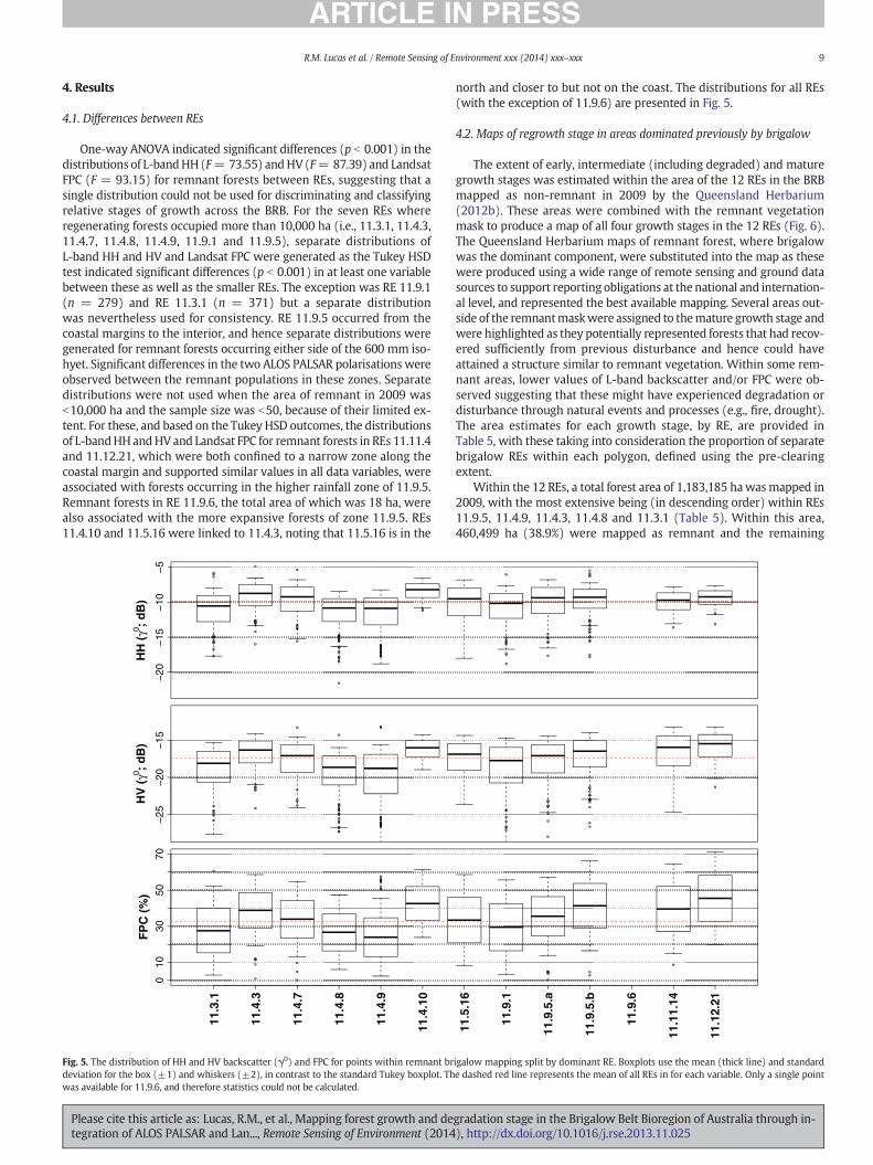
Reference distributions of L-band HH and HV and Landsat FPCextracted for remnant forests for the seven REs with areas N10,000 hawere therefore used as the basis for the subsequent classification. Aone-way analysis of variance (ANOVA)was conducted within the R sta-tistical package (R Core Development Team, 2011) to establishwhetherdifferences in the L-band HH and HV and Landsat FPC were significantbetween these REs because of variability in forest structure anticipatedas a consequence of differences primarily in landform (soils, geologyand topography). A Tukey honesty significant difference (HSD) test(Steel & Torrie, 1980) was then used to determinewhich REs, if any, dif-fered such that these could be grouped or considered separately in thesubsequent mapping of regrowth stage. The tests were also used to es-tablish whether there were differences in values within RE 11.9.5,which spanned an area from the inland to about 100 km from thecoast and where rainfall ranges from b500 mm to N750 mm. For thisanalysis, two rainfall regimes either side of the 600 m isohyet werecompared, with this selected as it approximated the median for the RE.
3.3. Generation of regrowth maps
Remnant forests had been mapped previously by the QueenslandHerbarium and hence such areas were retained within the final growthstage map for the BRB. Within the remaining areas, a segmentationwasundertaken by applying an iterative segmentation algorithm availablewithin RSGISLib (Bunting, Clewley, Lucas, & Gillingham, 2014), to theFPC/PALSAR mosaic to create image objects with a minimum size of1 ha (16 pixels). Following the definition of reference distributions forremnant vegetation for each RE, each object associated with forest(with an FPC ≥ 9%) was assigned to a mature category where the dis-tance of the average HH and HV backscatter and FPC for the objectwas one standard deviation away from themean of the reference distri-bution. This differed from the use of z-scores proposed in Clewley et al.(2012), as reference distributions were only required for a singlegrowth stage and the threshold was consistent, regardless of segment
Table 3REs within the BRB dominated by brigalow and the number of sample points within each.Of the available sample points, 50% were used for generating distributions of L-band HHand HV and Landsat FPC. Note, only areas with brigalow as a dominant component wereconsidered whereas in Table 2, areas with brigalow as a subdominant component werealso included.
RE Area of remnant forest, 2009 (ha) No. of sample points
11.3.1 41763 31711.4.3 69336 38211.4.7 15758 8611.4.8 56324 42811.4.9 70873 48511.4.10 5596 3411.5.16 2832 2811.9.1 40418 27911.9.5 147539 75111.9.6 204 1111.11.14 3794 2511.12.21 6063 42Total 460499 2858
Please cite this article as: Lucas, R.M., et al., Mapping forest growth and detegration of ALOS PALSAR and Lan..., Remote Sensing of Environment (2014
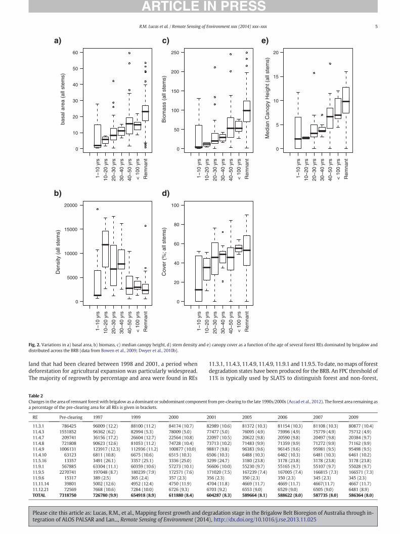
size. As described in Lucas et al. (2006), early regrowth exhibits a back-scatter similar to non-forest as the stems and branches are of insuffi-cient size to generate a strong response at L-band. To determine thisvalue, random points were located within the pre-clearing extent ofBrigalow and distributed across all REs. From these points, over 950 lo-cationswere classified as forest or non-forest, based on interpretation ofvery high resolution satellite imagery (e.g., Quickbird, WorldView)available through Google Maps. From each point, HH backscatter wasextracted for pixels within a 50-m radius. Based on these statistics, avalue of−14 dB was determined to be the upper limit of non-forest re-gardless of the RE considered (Fig. 3),with this explained by the similar-ities in the structure of early regrowth occurring within and betweenREs. This threshold was therefore used to separate early-stage from in-termediate regrowth. Lucas et al. (2006) used this same threshold fordifferentiating early regrowth within RE 11.9.5 using AIRSAR data,which was also identified through backscatter modelling. All remainingforests not classified as remnant, mature or early regrowth were thenassigned to an intermediate stage. This intermediate stage is associatedwith forests that have established on previously cleared land and arehence regenerating. However, these regenerating forests could alsohave degraded during the intervening period and hence this stage canbe associated with a degradation category.
3.4. Assessment of classification accuracy
Aswith the determination of reference distributions, the assessmentof accuracy was problematic because of the lack of field data for each ofthe REs. For this reason, a further 500 randompointswere selected fromthe area associated with each of the REs, with a buffer of 100 m thenplaced around each, which was clipped to the pre-clearing extent ofthe brigalow REs where necessary. These data were then interpretedvisually with reference to very high resolution aerial photographyand satellite imagery available through the Bing Server in ArcMap 10(ESRI, 2012). From the 500 points, 13 were considered invalid becauseof low-quality imagery and were excluded leaving 487 points forassessing accuracy (Table 4).
Examples of the appearance of the three growth stages in true colouraerial photography as well as remnant forest are provided in Fig. 4.Early-stage regrowth was associated with vegetated landscapes withsparse to dense canopies of low stature (indicated by the comparativelack of shadows). Similarly, mature forests were associated with treesthat were visually taller (again, determined through reference to
−20
−15
−10
HH
(γ0
; d
B)
Forest Non Forest
°
°
Fig. 3.Distribution of L-bandHHbackscatter values extracted fromover 950 areas of forestand non-forest located across the 12 REswhere brigalowdominates. Themean (thick line)and standard deviation for the box (±1) and whiskers (±2) are indicated.
gradation stage in the Brigalow Belt Bioregion of Australia through in-), http://dx.doi.org/10.1016/j.rse.2013.11.025

Table 4The number of sample photo points interpreted into different growth stagesand non-forest.
Growth stage Number
Early 144Intermediate (including degraded) 101Mature (excluding remnant) 46Non-forest 196Total 487
8 R.M. Lucas et al. / Remote Sensing of Environment xxx (2014) xxx–xxx
shadow and, to a lesser extent, crown size), with these often occurringin relatively dense stands of high cover. The assignment to a maturestage was undertaken with reference to stands that were known to be
Fig. 4.Aerial photographs showing areas of a) early, b) intermediate (including degraded), c)mare typically lower in stature (as evidenced, in part, by the lack of shadowing). Variability betwein associated species. Sample areas (100 m radius) for the early, intermediate and mature grow
Please cite this article as: Lucas, R.M., et al., Mapping forest growth and detegration of ALOS PALSAR and Lan..., Remote Sensing of Environment (2014
remnant. Whilst structural variation was observed between REsfor remnant forests, most were typically associated with taller treesalthough openness varied depending on whether these were wood-lands, low open forest or forest (Specht, 1970). Photo plots not assignedto an early regrowth ormature categorywere associatedwith the inter-mediate stage of growth (or a degraded state), with this being themostvariable in terms of structure.
The accuracy of the remnant class was not considered as this usedexisting mapping (Queensland Herbarium, 2012b). In each case, andto better explain errors noted in the confusion matrix, the tree coverwas estimated according to categories of b5%, 10%, 25% and 50% andN50%, 75% and 90%. The distribution of trees across the area was alsodescribed as being either evenly distributed (i.e., relatively uniformwithin the 100 m radius circle) or clumped.
ature growth stages and d) remnant forest dominated by brigalow. Areas of early regrowthen REs is a function of these being open forest, low open forest orwoodland and differencesth stages are clipped to the pre-clearing extent of brigalow-dominated REs.
gradation stage in the Brigalow Belt Bioregion of Australia through in-), http://dx.doi.org/10.1016/j.rse.2013.11.025
9R.M. Lucas et al. / Remote Sensing of Environment xxx (2014) xxx–xxx
4. Results
4.1. Differences between REs
One-way ANOVA indicated significant differences (p b 0.001) in thedistributions of L-bandHH (F= 73.55) andHV (F= 87.39) and LandsatFPC (F = 93.15) for remnant forests between REs, suggesting that asingle distribution could not be used for discriminating and classifyingrelative stages of growth across the BRB. For the seven REs whereregenerating forests occupied more than 10,000 ha (i.e., 11.3.1, 11.4.3,11.4.7, 11.4.8, 11.4.9, 11.9.1 and 11.9.5), separate distributions ofL-band HH and HV and Landsat FPC were generated as the Tukey HSDtest indicated significant differences (p b 0.001) in at least one variablebetween these as well as the smaller REs. The exception was RE 11.9.1(n = 279) and RE 11.3.1 (n = 371) but a separate distributionwas nevertheless used for consistency. RE 11.9.5 occurred from thecoastal margins to the interior, and hence separate distributions weregenerated for remnant forests occurring either side of the 600 mm iso-hyet. Significant differences in the two ALOS PALSAR polarisations wereobserved between the remnant populations in these zones. Separatedistributions were not used when the area of remnant in 2009 wasb10,000 ha and the sample size was b50, because of their limited ex-tent. For these, and based on the Tukey HSD outcomes, the distributionsof L-bandHHandHV and Landsat FPC for remnant forests in REs 11.11.4and 11.12.21, which were both confined to a narrow zone along thecoastal margin and supported similar values in all data variables, wereassociated with forests occurring in the higher rainfall zone of 11.9.5.Remnant forests in RE 11.9.6, the total area of which was 18 ha, werealso associated with the more expansive forests of zone 11.9.5. REs11.4.10 and 11.5.16 were linked to 11.4.3, noting that 11.5.16 is in the
−20
−15
−10
−5
HH
(γ0 ;
dB
)
−25
−20
−15
HV
(γ0 ;
dB
)
010
3050
70
FP
C (
%)
11.3
.1
11.4
.3
11.4
.7
11.4
.8
11.4
.9
11.4
.10
Fig. 5. The distribution of HH and HV backscatter (γ0) and FPC for points within remnant brdeviation for the box (±1) and whiskers (±2), in contrast to the standard Tukey boxplot. Thwas available for 11.9.6, and therefore statistics could not be calculated.
Please cite this article as: Lucas, R.M., et al., Mapping forest growth and detegration of ALOS PALSAR and Lan..., Remote Sensing of Environment (2014
north and closer to but not on the coast. The distributions for all REs(with the exception of 11.9.6) are presented in Fig. 5.
4.2. Maps of regrowth stage in areas dominated previously by brigalow
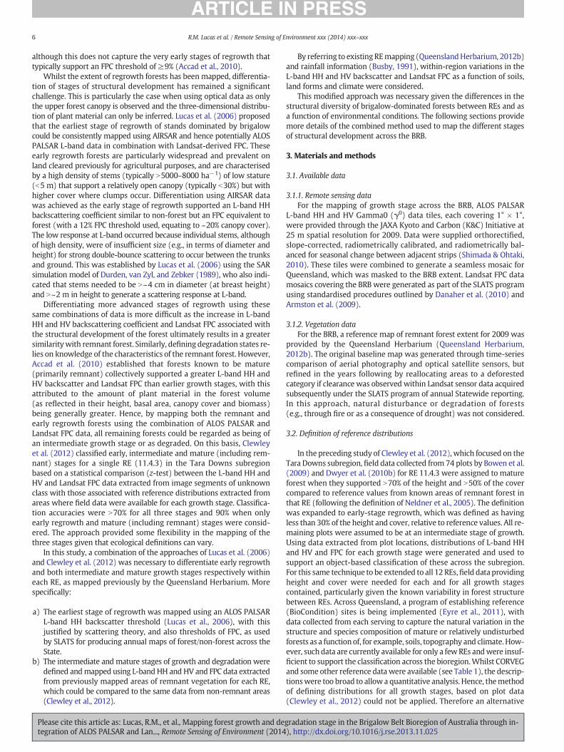
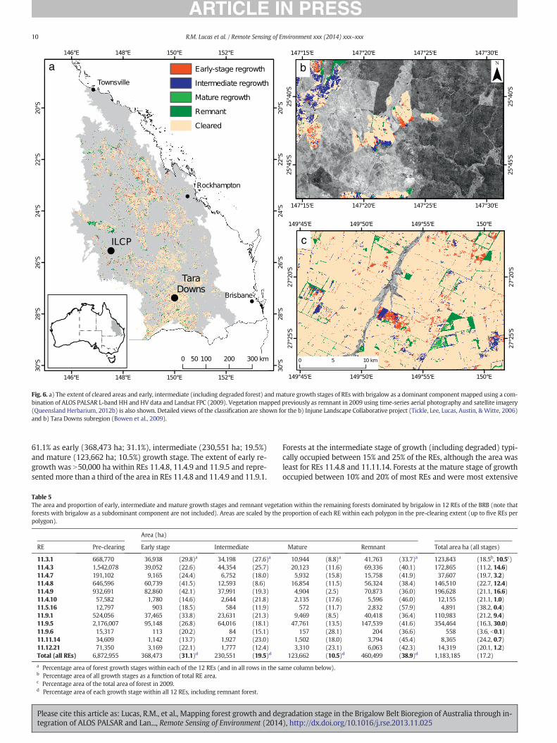
The extent of early, intermediate (including degraded) and maturegrowth stages was estimated within the area of the 12 REs in the BRBmapped as non-remnant in 2009 by the Queensland Herbarium(2012b). These areas were combined with the remnant vegetationmask to produce a map of all four growth stages in the 12 REs (Fig. 6).The Queensland Herbarium maps of remnant forest, where brigalowwas the dominant component, were substituted into the map as thesewere produced using a wide range of remote sensing and ground datasources to support reporting obligations at the national and internation-al level, and represented the best available mapping. Several areas out-side of the remnantmaskwere assigned to themature growth stage andwere highlighted as they potentially represented forests that had recov-ered sufficiently from previous disturbance and hence could haveattained a structure similar to remnant vegetation. Within some rem-nant areas, lower values of L-band backscatter and/or FPC were ob-served suggesting that these might have experienced degradation ordisturbance through natural events and processes (e.g., fire, drought).The area estimates for each growth stage, by RE, are provided inTable 5, with these taking into consideration the proportion of separatebrigalow REs within each polygon, defined using the pre-clearingextent.
Within the 12 REs, a total forest area of 1,183,185 hawasmapped in2009, with the most extensive being (in descending order) within REs11.9.5, 11.4.9, 11.4.3, 11.4.8 and 11.3.1 (Table 5). Within this area,460,499 ha (38.9%) were mapped as remnant and the remaining
11.5
.16
11.9
.1
11.9
.5.a
11.9
.5.b
11.9
.6
11.1
1.14
11.1
2.21
igalow mapping split by dominant RE. Boxplots use the mean (thick line) and standarde dashed red line represents the mean of all REs in for each variable. Only a single point
gradation stage in the Brigalow Belt Bioregion of Australia through in-), http://dx.doi.org/10.1016/j.rse.2013.11.025
a b
c
Fig. 6. a) The extent of cleared areas and early, intermediate (including degraded forest) and mature growth stages of REs with brigalow as a dominant componentmapped using a com-bination of ALOS PALSAR L-band HH and HV data and Landsat FPC (2009). Vegetation mapped previously as remnant in 2009 using time-series aerial photography and satellite imagery(Queensland Herbarium, 2012b) is also shown. Detailed views of the classification are shown for the b) Injune Landscape Collaborative project (Tickle, Lee, Lucas, Austin, & Witte, 2006)and b) Tara Downs subregion (Bowen et al., 2009).
10 R.M. Lucas et al. / Remote Sensing of Environment xxx (2014) xxx–xxx
61.1% as early (368,473 ha; 31.1%), intermediate (230,551 ha; 19.5%)and mature (123,662 ha; 10.5%) growth stage. The extent of early re-growth was N50,000 ha within REs 11.4.8, 11.4.9 and 11.9.5 and repre-sented more than a third of the area in REs 11.4.8 and 11.4.9 and 11.9.1.
Table 5The area and proportion of early, intermediate and mature growth stages and remnant vegetaforests with brigalow as a subdominant component are not included). Areas are scaled by thepolygon).
Area (ha)
RE Pre-clearing Early stage Intermediate
11.3.1 668,770 36,938 (29.8)a 34,198 (27.6)a
11.4.3 1,542,078 39,052 (22.6) 44,354 (25.7)11.4.7 191,102 9,165 (24.4) 6,752 (18.0)11.4.8 646,596 60,739 (41.5) 12,593 (8.6)11.4.9 932,691 82,860 (42.1) 37,991 (19.3)11.4.10 57,582 1,780 (14.6) 2,644 (21.8)11.5.16 12,797 903 (18.5) 584 (11.9)11.9.1 524,056 37,465 (33.8) 23,631 (21.3)11.9.5 2,176,007 95,148 (26.8) 64,016 (18.1)11.9.6 15,317 113 (20.2) 84 (15.1)11.11.14 34,609 1,142 (13.7) 1,927 (23.0)11.12.21 71,350 3,169 (22.1) 1,777 (12.4)Total (all REs) 6,872,955 368,473 (31.1)d 230,551 (19.5)d
a Percentage area of forest growth stages within each of the 12 REs (and in all rows in the sb Percentage area of all growth stages as a function of total RE area.c Percentage area of the total area of forest in 2009.d Percentage area of each growth stage within all 12 REs, including remnant forest.
Please cite this article as: Lucas, R.M., et al., Mapping forest growth and detegration of ALOS PALSAR and Lan..., Remote Sensing of Environment (2014
Forests at the intermediate stage of growth (including degraded) typi-cally occupied between 15% and 25% of the REs, although the area wasleast for REs 11.4.8 and 11.11.14. Forests at the mature stage of growthoccupied between 10% and 20% of most REs and were most extensive
tion within the remaining forests dominated by brigalow in 12 REs of the BRB (note thatproportion of each RE within each polygon in the pre-clearing extent (up to five REs per
Mature Remnant Total area ha (all stages)
10,944 (8.8)a 41,763 (33.7)a 123,843 (18.5b, 10.5c)20,123 (11.6) 69,336 (40.1) 172,865 (11.2, 14.6)5,932 (15.8) 15,758 (41.9) 37,607 (19.7, 3.2)
16,854 (11.5) 56,324 (38.4) 146,510 (22.7, 12.4)4,904 (2.5) 70,873 (36.0) 196,628 (21.1, 16.6)2,135 (17.6) 5,596 (46.0) 12,155 (21.1, 1.0)572 (11.7) 2,832 (57.9) 4,891 (38.2, 0.4)
9,469 (8.5) 40,418 (36.4) 110,983 (21.2, 9.4)47,761 (13.5) 147,539 (41.6) 354,464 (16.3, 30.0)
157 (28.1) 204 (36.6) 558 (3.6, b0.1)1,502 (18.0) 3,794 (45.4) 8,365 (24.2, 0.7)3,310 (23.1) 6,063 (42.3) 14,319 (20.1, 1.2)
123,662 (10.5)d 460,499 (38.9)d 1,183,185 (17.2)
ame column below).
gradation stage in the Brigalow Belt Bioregion of Australia through in-), http://dx.doi.org/10.1016/j.rse.2013.11.025
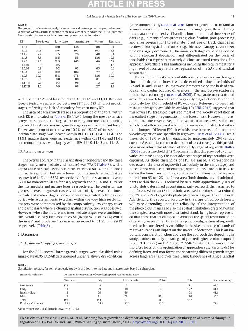
Table 6The proportion of non-forest, early, intermediate andmature growth stages, and remnantvegetation within each RE in relation to the total area of each across the 12 REs (note thatforests with brigalow as a subdominant component are not included).
RE Non-forest Early-stage Intermediate Mature Remnant
11.3.1 9.6 10.0 14.8 8.8 9.111.4.3 24.1 10.6 19.2 16.3 15.111.4.7 2.7 2.5 2.9 4.8 3.411.4.8 8.8 16.5 5.5 13.6 12.211.4.9 12.9 22.5 16.5 4.0 15.411.4.10 0.8 0.5 1.1 1.7 1.211.5.16 0.1 0.2 0.3 0.5 0.611.9.1 7.3 10.2 10.2 7.7 8.811.9.5 32.0 25.8 27.8 38.6 32.011.9.6 0.3 0.0 0.0 0.1 0.011.11.14 0.5 0.3 0.8 1.2 0.811.12.21 1.0 0.9 0.8 2.7 1.3
11R.M. Lucas et al. / Remote Sensing of Environment xxx (2014) xxx–xxx
within RE 11.12.21 and least for REs 11.3.1, 11.4.9 and 11.9.1. Remnantforests typically represented between 33% and 58% of forest growthstages, reflecting the lack of secondary forests in many REs.
The area of each growth stage as a proportion of the total withineach RE is indicated in Table 6. RE 11.9.5, being the most extensiveecosystem supported the largest area of early, intermediate (includingdegraded forest) and mature growth stages as well as remnant forest.The greatest proportion (between 10.2% and 19.2%) of forests in theintermediate stage was located within REs 11.3.1, 11.4.3, 11.4.9 and11.9.1, mature stages were more extensive within REs 11.4.3 and 11.4.8and remnant forests were largely within REs 11.4.9, 11.4.3 and 11.4.8.
4.3. Accuracy assessment
The overall accuracy in the classification of non-forest and the threestages (early, intermediate and mature) was 77.8% (Table 7), with akappa value of 69.0%. Users’ accuracies exceeded 80.0% for non-forestand early regrowth but were lower for intermediate and matureregrowth (61.1% and 55.3% respectively). Producers’ accuracies were87.8% for non-forest, 68.8% for early regrowth and 71.3% and 91.3% forthe intermediate and mature forests respectively. The confusion wasgreatest between regrowth classes and particularly between the inter-mediate and mature stages. Confusion was also greatest between cate-gories where assignments to a class within the very high resolutionimagery were compromised by the comparatively low canopy coverand particularly where a clumped spatial distribution was observed.However, when the mature and intermediate stages were combined,the overall accuracy increased to 85.8% (kappa value of 73.6%) whilstthe users’ and producers’ accuracies increased to 71.2% and 89.1%respectively (Table 8).
5. Discussion
5.1. Defining and mapping growth stages
For the BRB, several forest growth stages were classified usingsingle-date ALOS PALSAR data acquired under relatively dry conditions
Table 7Classification accuracy for non-forest, early regrowth and both intermediate and mature stages
Image classification On screen interpretation of very high spatial resolution
Non-forest Early Inter
Non-forest 172 5 3Early 11 99 10Intermediate 12 29 66Mature 1 11 22Total 196 144 101Producers’ accuracy 87.8 68.8 71.3
Kappa = 69.0 (95% confidence interval = 64–74%).
Please cite this article as: Lucas, R.M., et al., Mapping forest growth and detegration of ALOS PALSAR and Lan..., Remote Sensing of Environment (2014
(as recommended by Lucas et al., 2010) and FPC generated fromLandsatsensor data acquired over the course of a single year. By combiningthese data, the complexity of handling long inter-annual time-series ofdata (e.g., in terms of pre-processing, classification, post-processingand error propagation) to estimate forest age or track changes inretrieved biophysical attributes (e.g., biomass, canopy cover) overtimewas largely overcome. Furthermore, each stage could be associatedwith a structural description and differentiated on the basis ofthresholds that represent relatively distinct structural transitions. Theapproach nevertheless has limitations including the requirement for ahigh level of accuracy in the co-registration of the SAR and Landsatsensor data.
The extent of forest cover and differences between growth stages(including degraded forest) were determined using thresholds ofL-band HH and HV and FPC that were interpretable on the basis of eco-logical knowledge but also differences in the microwave scatteringmechanisms occurring (Lucas et al., 2006). To separate more scatteredareas of regrowth forests in the very early stages of development, arelatively low FPC threshold of 9% was used. Reference to very highresolution imagery available in ArcMap 10 (ESRI, 2012) suggested thatthis lower FPC threshold captured most of the woody vegetation atthe earliest stage of regeneration in the forest mask. However, this re-quired that the cover of vegetation within unit areas was sufficient,which most often occurred when tree crowns were distributed ratherthan clumped. Different FPC thresholds have been used for mappingwoody vegetation and specifically regrowth. Lucas et al. (2006) used athreshold of 12%, with this equating to approximately 20% canopycover in Australia (a common definition of forest cover), as this provid-ed a more robust classification of the early-stage of regrowth. Butler(2009) used a threshold of 18%, recognising that this provided a conser-vative estimate as only the more advanced stages of regeneration werecaptured. As these thresholds of FPC are raised, a correspondingdecrease in the area of regrowth (particularly in the early stage) andhence forest will occur. For example, when the FPC threshold used todefine the forest (including regrowth) and non-forest boundary wasraised from 9% to 12%, the forest area (both dominant and subdomi-nant) within the 12 REs reduced by 8.0%, with approximately 10% ofphoto plots determined as containing early regrowth then assigned tonon-forest. When an 18% threshold was used, the forest area reducedto 32%, and 25% of regrowth photo plots were assigned to non-forest.Additionally, the reported accuracy in the maps of regrowth forestswill vary depending upon the reliability of the interpretation ofthe photo plots images and also the spatial distribution of standswithinthe sampled area, with more distributed stands being better represent-ed than those that are clumped. In addition, the spatial resolution of theobserving sensor in relation to the spatial configuration of regrowthneeds to be considered as variability in the size and shape of stands ofregrowth stands can impact on the success of detection. This is an im-portant consideration when applying the approach developed in thisstudy to other currently operating andplannedhigher resolution optical(e.g., SPOT sensor) and SAR (e.g., PALSAR-2) data. Future work shouldtherefore focus on the optimisation of approaches (e.g., thresholds) fordefining forest and non-forest and separating different growth stagesacross large areas and over time using time-series of single Landsat
based on photoplots.
imagery
mediate Mature Total Users’ Accuracy
1 181 95.02 122 81.11 108 61.1
42 76 55.346 48791.3 77.8
gradation stage in the Brigalow Belt Bioregion of Australia through in-), http://dx.doi.org/10.1016/j.rse.2013.11.025
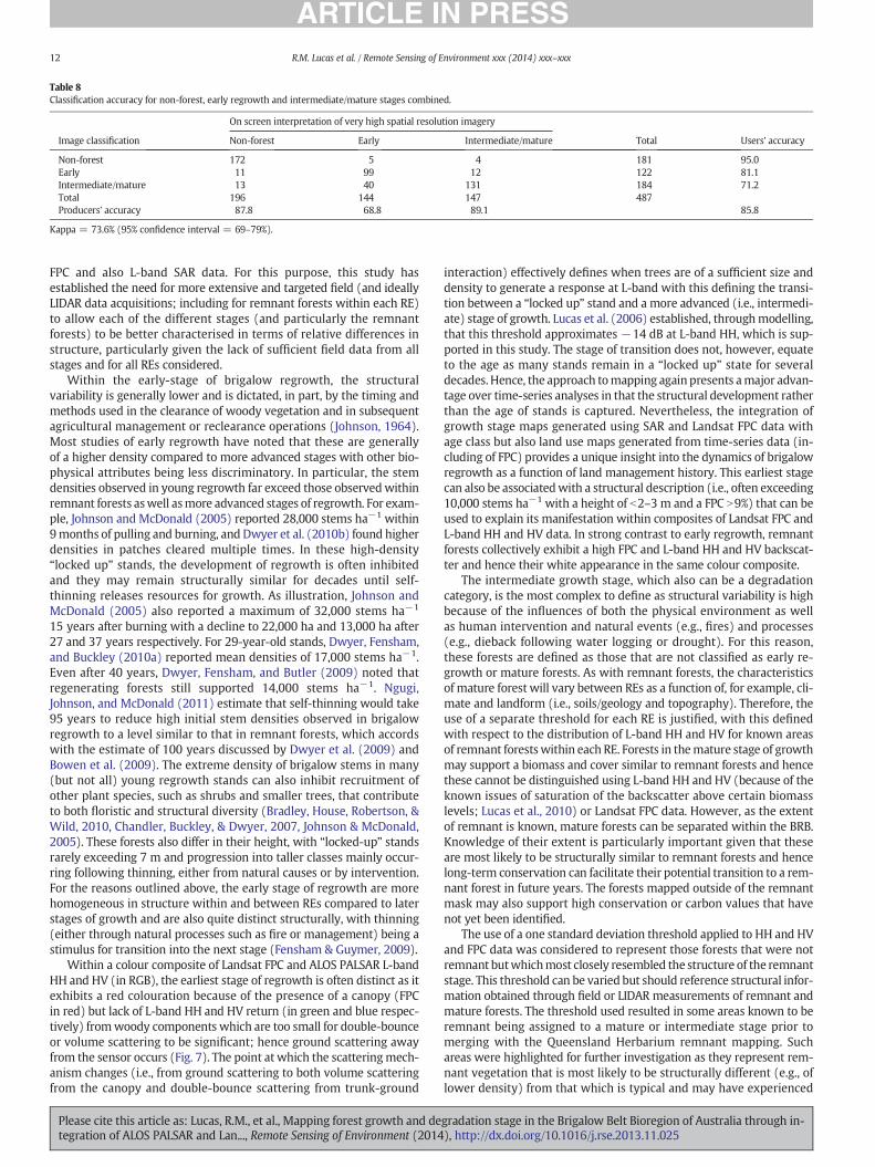
Table 8Classification accuracy for non-forest, early regrowth and intermediate/mature stages combined.
On screen interpretation of very high spatial resolution imagery
Image classification Non-forest Early Intermediate/mature Total Users’ accuracy
Non-forest 172 5 4 181 95.0Early 11 99 12 122 81.1Intermediate/mature 13 40 131 184 71.2Total 196 144 147 487Producers’ accuracy 87.8 68.8 89.1 85.8
Kappa = 73.6% (95% confidence interval = 69–79%).
12 R.M. Lucas et al. / Remote Sensing of Environment xxx (2014) xxx–xxx
FPC and also L-band SAR data. For this purpose, this study hasestablished the need for more extensive and targeted field (and ideallyLIDAR data acquisitions; including for remnant forests within each RE)to allow each of the different stages (and particularly the remnantforests) to be better characterised in terms of relative differences instructure, particularly given the lack of sufficient field data from allstages and for all REs considered.
Within the early-stage of brigalow regrowth, the structuralvariability is generally lower and is dictated, in part, by the timing andmethods used in the clearance of woody vegetation and in subsequentagricultural management or reclearance operations (Johnson, 1964).Most studies of early regrowth have noted that these are generallyof a higher density compared to more advanced stages with other bio-physical attributes being less discriminatory. In particular, the stemdensities observed in young regrowth far exceed those observedwithinremnant forests aswell asmore advanced stages of regrowth. For exam-ple, Johnson and McDonald (2005) reported 28,000 stems ha−1 within9months of pulling and burning, and Dwyer et al. (2010b) found higherdensities in patches cleared multiple times. In these high-density“locked up” stands, the development of regrowth is often inhibitedand they may remain structurally similar for decades until self-thinning releases resources for growth. As illustration, Johnson andMcDonald (2005) also reported a maximum of 32,000 stems ha−1
15 years after burning with a decline to 22,000 ha and 13,000 ha after27 and 37 years respectively. For 29-year-old stands, Dwyer, Fensham,and Buckley (2010a) reported mean densities of 17,000 stems ha−1.Even after 40 years, Dwyer, Fensham, and Butler (2009) noted thatregenerating forests still supported 14,000 stems ha−1. Ngugi,Johnson, and McDonald (2011) estimate that self-thinning would take95 years to reduce high initial stem densities observed in brigalowregrowth to a level similar to that in remnant forests, which accordswith the estimate of 100 years discussed by Dwyer et al. (2009) andBowen et al. (2009). The extreme density of brigalow stems in many(but not all) young regrowth stands can also inhibit recruitment ofother plant species, such as shrubs and smaller trees, that contributeto both floristic and structural diversity (Bradley, House, Robertson, &Wild, 2010, Chandler, Buckley, & Dwyer, 2007, Johnson & McDonald,2005). These forests also differ in their height, with “locked-up” standsrarely exceeding 7 m and progression into taller classes mainly occur-ring following thinning, either from natural causes or by intervention.For the reasons outlined above, the early stage of regrowth are morehomogeneous in structure within and between REs compared to laterstages of growth and are also quite distinct structurally, with thinning(either through natural processes such as fire or management) being astimulus for transition into the next stage (Fensham & Guymer, 2009).
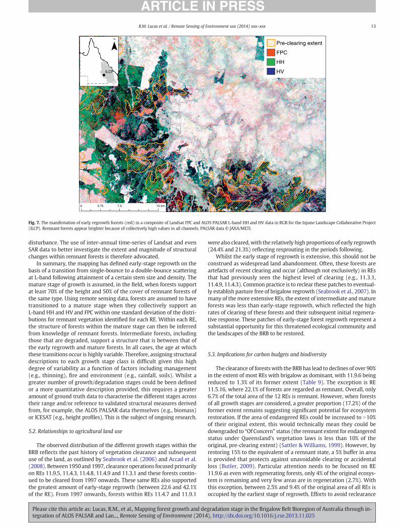
Within a colour composite of Landsat FPC and ALOS PALSAR L-bandHH and HV (in RGB), the earliest stage of regrowth is often distinct as itexhibits a red colouration because of the presence of a canopy (FPCin red) but lack of L-band HH and HV return (in green and blue respec-tively) fromwoody components which are too small for double-bounceor volume scattering to be significant; hence ground scattering awayfrom the sensor occurs (Fig. 7). The point at which the scatteringmech-anism changes (i.e., from ground scattering to both volume scatteringfrom the canopy and double-bounce scattering from trunk-ground
Please cite this article as: Lucas, R.M., et al., Mapping forest growth and detegration of ALOS PALSAR and Lan..., Remote Sensing of Environment (2014
interaction) effectively defines when trees are of a sufficient size anddensity to generate a response at L-band with this defining the transi-tion between a “locked up” stand and a more advanced (i.e., intermedi-ate) stage of growth. Lucas et al. (2006) established, throughmodelling,that this threshold approximates −14 dB at L-band HH, which is sup-ported in this study. The stage of transition does not, however, equateto the age as many stands remain in a “locked up” state for severaldecades. Hence, the approach tomapping again presents amajor advan-tage over time-series analyses in that the structural development ratherthan the age of stands is captured. Nevertheless, the integration ofgrowth stage maps generated using SAR and Landsat FPC data withage class but also land use maps generated from time-series data (in-cluding of FPC) provides a unique insight into the dynamics of brigalowregrowth as a function of land management history. This earliest stagecan also be associatedwith a structural description (i.e., often exceeding10,000 stems ha−1 with a height of b2–3 m and a FPC N9%) that can beused to explain its manifestation within composites of Landsat FPC andL-band HH and HV data. In strong contrast to early regrowth, remnantforests collectively exhibit a high FPC and L-band HH and HV backscat-ter and hence their white appearance in the same colour composite.
The intermediate growth stage, which also can be a degradationcategory, is the most complex to define as structural variability is highbecause of the influences of both the physical environment as wellas human intervention and natural events (e.g., fires) and processes(e.g., dieback following water logging or drought). For this reason,these forests are defined as those that are not classified as early re-growth or mature forests. As with remnant forests, the characteristicsof mature forest will vary between REs as a function of, for example, cli-mate and landform (i.e., soils/geology and topography). Therefore, theuse of a separate threshold for each RE is justified, with this definedwith respect to the distribution of L-band HH and HV for known areasof remnant forestswithin each RE. Forests in themature stage of growthmay support a biomass and cover similar to remnant forests and hencethese cannot be distinguished using L-band HH and HV (because of theknown issues of saturation of the backscatter above certain biomasslevels; Lucas et al., 2010) or Landsat FPC data. However, as the extentof remnant is known, mature forests can be separated within the BRB.Knowledge of their extent is particularly important given that theseare most likely to be structurally similar to remnant forests and hencelong-term conservation can facilitate their potential transition to a rem-nant forest in future years. The forests mapped outside of the remnantmask may also support high conservation or carbon values that havenot yet been identified.
The use of a one standard deviation threshold applied to HH and HVand FPC data was considered to represent those forests that were notremnant butwhichmost closely resembled the structure of the remnantstage. This threshold can be varied but should reference structural infor-mation obtained through field or LIDAR measurements of remnant andmature forests. The threshold used resulted in some areas known to beremnant being assigned to a mature or intermediate stage prior tomerging with the Queensland Herbarium remnant mapping. Suchareas were highlighted for further investigation as they represent rem-nant vegetation that is most likely to be structurally different (e.g., oflower density) from that which is typical and may have experienced
gradation stage in the Brigalow Belt Bioregion of Australia through in-), http://dx.doi.org/10.1016/j.rse.2013.11.025
ILCP
0 7.5 15 km3.75
Pre-clearing extent
FPC
HH
HV
Fig. 7. The manifestation of early regrowth forests (red) in a composite of Landsat FPC and ALOS PALSAR L-band HH and HV data in RGB for the Injune Landscape Collaborative Project(ILCP). Remnant forests appear brighter because of collectively high values in all channels. PALSAR data © JAXA/METI.
13R.M. Lucas et al. / Remote Sensing of Environment xxx (2014) xxx–xxx
disturbance. The use of inter-annual time-series of Landsat and evenSAR data to better investigate the extent and magnitude of structuralchanges within remnant forests is therefore advocated.
In summary, the mapping has defined early-stage regrowth on thebasis of a transition from single-bounce to a double-bounce scatteringat L-band following attainment of a certain stem size and density. Themature stage of growth is assumed, in the field, when forests supportat least 70% of the height and 50% of the cover of remnant forests ofthe same type. Using remote sensing data, forests are assumed to havetransitioned to a mature stage when they collectively support anL-band HH and HV and FPC within one standard deviation of the distri-butions for remnant vegetation identified for each RE. Within each RE,the structure of forests within the mature stage can then be inferredfrom knowledge of remnant forests. Intermediate forests, includingthose that are degraded, support a structure that is between that ofthe early regrowth and mature forests. In all cases, the age at whichthese transitions occur is highly variable. Therefore, assigning structuraldescriptions to each growth stage class is difficult given this highdegree of variability as a function of factors including management(e.g., thinning), fire and environment (e.g., rainfall, soils). Whilst agreater number of growth/degradation stages could be been definedor a more quantitative description provided, this requires a greateramount of ground truth data to characterise the different stages acrosstheir range and/or reference to validated structural measures derivedfrom, for example, the ALOS PALSAR data themselves (e.g., biomass)or ICESAT (e.g., height profiles). This is the subject of ongoing research.
5.2. Relationships to agricultural land use
The observed distribution of the different growth stages within theBRB reflects the past history of vegetation clearance and subsequentuse of the land, as outlined by Seabrook et al. (2006) and Accad et al.(2008). Between1950 and 1997, clearance operations focused primarilyon REs 11.9.5, 11.4.3, 11.4.8, 11.4.9 and 11.3.1 and these forests contin-ued to be cleared from 1997 onwards. These same REs also supportedthe greatest amount of early-stage regrowth (between 22.6 and 42.1%of the RE). From 1997 onwards, forests within REs 11.4.7 and 11.9.1
Please cite this article as: Lucas, R.M., et al., Mapping forest growth and detegration of ALOS PALSAR and Lan..., Remote Sensing of Environment (2014
were also cleared,with the relatively high proportions of early regrowth(24.4% and 21.3%) reflecting resprouting in the periods following.
Whilst the early stage of regrowth is extensive, this should not beconstrued as widespread land abandonment. Often, these forests areartefacts of recent clearing and occur (although not exclusively) in REsthat had previously seen the highest level of clearing (e.g., 11.3.1,11.4.9, 11.4.3). Common practice is to reclear these patches to eventual-ly establish pasture free of brigalow regrowth (Seabrook et al., 2007). Inmany of themore extensive REs, the extent of intermediate andmatureforests was less than early-stage regrowth, which reflected the highrates of clearing of these forests and their subsequent initial regenera-tive response. These patches of early-stage forest regrowth represent asubstantial opportunity for this threatened ecological community andthe landscapes of the BRB to be restored.
5.3. Implications for carbon budgets and biodiversity
The clearance of forestswith the BRB has lead to declines of over 90%in the extent of most REs with brigalow as dominant, with 11.9.6 beingreduced to 1.3% of its former extent (Table 9). The exception is RE11.5.16, where 22.1% of forests are regarded as remnant. Overall, only6.7% of the total area of the 12 REs is remnant. However, when forestsof all growth stages are considered, a greater proportion (17.2%) of theformer extent remains suggesting significant potential for ecosystemrestoration. If the area of endangered REs could be increased to N10%of their original extent, this would technically mean they could bedowngraded to “Of Concern” status (the remnant extent for endangeredstatus under Queensland’s vegetation laws is less than 10% of theoriginal, pre-clearing extent) (Sattler & Williams, 1999). However, byrestoring 15% to the equivalent of a remnant state, a 5% buffer in areais provided that protects against unavoidable clearing or accidentalloss (Butler, 2009). Particular attention needs to be focused on RE11.9.6 as even with regenerating forests, only 4% of the original ecosys-tem is remaining and very few areas are in regeneration (2.7%). Withthis exception, between 2.5% and 9.4% of the original area of all REs isoccupied by the earliest stage of regrowth. Efforts to avoid reclearance
gradation stage in the Brigalow Belt Bioregion of Australia through in-), http://dx.doi.org/10.1016/j.rse.2013.11.025
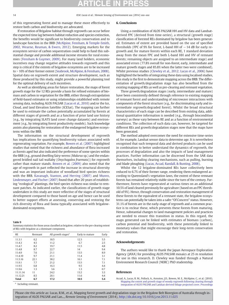
14 R.M. Lucas et al. / Remote Sensing of Environment xxx (2014) xxx–xxx
of this regenerating forest and to manage these more effectively torestore both carbon and biodiversity are advocated.
If restoration of Brigalow habitat through regrowth can occur beforethe expected time lag between habitat reduction and species extinction,the benefits would be significant to biodiversity conservation and tolandscape function in the BRB (McAlpine, Fensham, & Temple-Smith,2002, Wearne, Reuman, & Ewers, 2012). Emerging markets for theecosystem service of carbon sequestration could help to fund this sub-stantial change and provide additional income streams for rural econo-mies (Fensham & Guymer, 2009). For many land holders, economicincentives may change negative attitudes towards regrowth and thisstep is critical if the extents of brigalow ecosystems are to be increasedto N 10% of their former extent (Seabrook, McAlpine, & Fensham, 2008).Spatial data on regrowth extent and structure development, such asthose produced by this study, might provide a powerful planning toolfor the optimal delivery of such incentives.
As well as identifying areas for future restoration, the maps of forestgrowth stage for the 12 REs provide a basis for refined estimates of bio-mass and carbon in vegetation for the BRB, either through extrapolationof field-based estimates or using relationships established with remotesensing data, including ALOS PALSAR (Lucas et al., 2010) and/or the Ice,Cloud, and land Elevation Satellite (ICESat). The mapping can furtherbe used to estimate the carbon potentially accumulated by forests atdifferent stages of growth and as a function of prior land use history(e.g., by integrating SLATS land cover change datasets) and environ-ment (e.g., by integrating forest productivity models). Such knowledgeassists also planning for restoration of the endangered brigalow ecosys-tems within the BRB.
The information on the structural development of regrowthhas implications for quantifying biodiversity values associated withregenerating vegetation. For example, Bowen et al. (2007) highlightedstudies that noted that the richness and abundance of flora increasedas forests aged but also indicated the preference of some species withinthe BRB (e.g., grounddwelling fairy-wrens (Malurus sp.) and the endan-gered bridled nail tail wallaby (Onychagalea fraemata)) for regrowthrather than mature stands. Bowen et al. (2009) also noted that theage of regrowth in part reflected the increase in structural diversityand was an important indicator of woodland bird species richnesswith the BRB. Kavanagh, Stanton, and Herring (2007) and Munro,Lindenmayer, and Fischer (2007) found that after 20 years of establish-ing “ecological” plantings, the bird species richness was similar to rem-nant patches. As indicated earlier, the classifications of growth stageundertaken in this study are more reflective of the stages of structuraldevelopment compared to those based on age and hence can be usedto better support efforts at assessing, conserving and restoring therich diversity of flora and fauna typically associated with brigalow-dominated ecosystems.
Table 9Summary statistics for those areas classified as brigalow, relative to thepre-clearing extentof REs with brigalow as a dominant component.
RE Remnant All growth stagesa Early to mature Early
11.3.1 6.2 18.5 12.3 5.511.4.3 4.5 11.2 6.7 2.511.4.7 8.2 19.7 11.5 4.811.4.8 8.7 22.7 14 9.411.4.9 7.6 21.1 13.5 8.911.4.10 9.7 21.1 11.4 3.111.5.16 22.1 38.2 16.1 7.111.9.1 7.7 21.2 13.5 7.111.9.5 6.8 16.3 9.5 4.411.9.6 1.3 3.6 1.3 0.711.11.14 11 24.2 13.2 3.311.12.21 8.5 20.1 11.6 4.4Total 6.7 17.2 10.5 5.4
a Including remnant.
Please cite this article as: Lucas, R.M., et al., Mapping forest growth and detegration of ALOS PALSAR and Lan..., Remote Sensing of Environment (2014
6. Conclusions
Using a combination of ALOS PALSAR HH and HV data and Landsat-derived FPC (derived from time-series), a structural (growth stage)classification of forested REs dominated by brigalow has been generat-ed. Estimates of extent are provided based on the use of specifiedthresholds (FPC of 9% for forest, L-band HH of −14 dB for early re-growth and, for mature forests within each RE, 1 standard deviationaway from the mean FPC and both L-band HH and HV of remnantforests; remaining objects are assigned to an intermediate stage) andassociated errors (77.8% overall for non-forest, early, intermediate andmature growth stages and 85.8% when the latter two were combined).Whilst previous studies (Clewley et al., 2012; Lucas et al., 2006) havehighlighted the benefits of integrating these data using localised studies,this study is thefirst to demonstratemapping across the BRB. The differ-entiation of growth/degradation stage has also benefited from theexistingmapping of REs aswell as pre-clearing and remnant vegetation.
Three growth/degradation stages (early, intermediate and mature)have been consistently defined through reference to existing mappingof remnant forest and understanding of microwave interactions withcomponents of the forest structure (e.g., for discriminating early and in-termediate regrowth/degraded forest). Whilst the broad structuralcharacteristics of each stage can be described from existing data, addi-tional quantitative information is needed (e.g., through bioconditionsurveys) as these vary between RE and as a function of environmentalconditions. The collection of such data can, however, be targeted fordifferent REs and growth/degradation stages now that the maps havebeen generated.
The method adopted overcomes the need for extensive time-seriesof, for example, Landsat sensor data to determine age. It is neverthelessrecognised that such temporal data and derived products can be usedin combination to better understand the dynamics of regrowth, theprocesses of degradation and also the impacts of land managementpractices. Further information can be discerned from the SAR datathemselves, including clearing mechanisms, such as pulling, burningand blade ploughing (Lucas, Accad, Randall, & Bunting, 2008).
Whilst the 12 brigalow-dominated REs have collectively beenreduced to 6.7% of their former range, rendering them endangered ac-cording to Queensland’s vegetation laws, the extent of these remnantforests has remained relatively stable since the turn of the century. Fur-thermore, forests have regenerated at various times on an additional10.5% of land cleared previously for agriculture (based on an FPC thresh-old of 9%). Hence, through conservation and restorationmanagement ofthese forests to the equivalent of a remnant state, the brigalow ecosys-tems can potentially be taken into a safer “Of Concern” status. However,31.1% of forests are in the early-stage of regrowth and a common prac-tice is to reclear these, which prevents these forests from maturing.Hence, substantial changes to land management policies and practicesare needed to ensure this transition in status. In this regard, themaps generated can be linked with estimates of biomass (carbon),carbon potential and biodiversity, with these potentially linked tomonetary values that might encourage their long-term conservationand restoration.
Acknowledgements
The authors would like to thank the Japan Aerospace ExplorationAgency (JAXA) for providing ALOS PALSAR mosaics at 25 m resolutionfor use in this research. D. Clewley was funded through a NaturalEnvironment Research Council (NERC) PhD studentship.
References
Accad, A., Lucas, R. M., Pollock, A., Armston, J.D., Bowen, M. E., McAlpine, C., et al. (2010).Mapping the extent and growth stage of woody regrowth following clearing throughintegration of ALOS PALSAR and Landsat-derived foliage projected cover. Proceedings
gradation stage in the Brigalow Belt Bioregion of Australia through in-), http://dx.doi.org/10.1016/j.rse.2013.11.025
15R.M. Lucas et al. / Remote Sensing of Environment xxx (2014) xxx–xxx
of 15th Australasian Remote Sensing and Photogrammetry Conference (ARSPC), AliceSprings, Australia, 13–17 September, 2010.
Accad, A., Neldner, V. J., Wilson, B.A., & Niehus, R. E. (2008). Remnant vegetation inQueensland. Analysis of remnant vegetation (1997–1999–2000–2001–2003–2005),including regional ecosystem information. Technical Report, Queensland Herbarium,Brisbane, Queensland (1 pp.).
Accad, A., Neldner, V. J., Wilson, B.A., & Niehus, R. E. (2012). Remnant vegetation in Queens-land. Analysis of remnant vegetation 1997–2009, including regional ecosystem informa-tion. Brisbane Queensland Department of Science, Information Technology,Innovation and the Arts (http://www.ehp.qld.gov.au/ecosystems/remnant-vegetation/index.html (Accessed 01/10/2012)).
Armston, J.D., Denham, R. J., Danaher, T. J., Scarth, P. F., & Moffiet, T. N. (2009). Predictionand validation of foliage projective cover from Landsat-5 TM and Landsat-7 ETM+ imagery. Journal of Applied Remote Sensing, 3, 1–28.
Barlow, J., Gardner, T. A., Araujo, I. S., Ávila-Pires, T. C., Bonaldo, A. B., Costa, J. E., et al.(2007). Quantifying the biodiversity value of tropical primary, secondary and planta-tion forests. Proceedings, National Academy of Sciences of the United States of America(PNAS), 104(47), 18555–18560.
Bowen, M. E., McAlpine, C. A., House, A. P. N., & Smith, G. C. (2007). Regrowth forests onabandoned agricultural land: A review of their habitat values for recovering forestfauna. Biological Conservation, 140, 273–296.
Bowen, M. E., McAlpine, C. A., House, A. P. N., & Smith, G. C. (2009). Agricultural landscapemodification increases the abundance of an important food resource: Mistletoes,birds and brigalow. Biological Conservation, 142, 122–133.
Bradley, M., House, A., Robertson, M., & Wild, C. (2010). Vegetation succession andrecovery of ecological values in the southern Queensland Brigalow Belt. EcologicalManagement and Restoration, 11, 113–118.
Bunting, P., Clewley, D., Lucas, R. M., & Gillingham, S. (2014). The remote sensing and GISSoftware Library (RSGISLib). Computers & Geosciences, 62, 216–226.
Busby, J. R. (1991). BIOCLIM—A bioclimate analysis and prediction system. In C. R.Margules, & M. P. Austin (Eds.), Nature conservation: Cost effective biological surveyand data analysis (pp. 64–68)Melbourne Commonwealth Scientific and Industrial Re-search Organisation.
Butler, D. W. (2009). Planning iterative investment for landscape restoration: Choice ofbiodiversity indicator makes a difference. Biological Conservation, 142, 2202–2216.
Chambers, J., Asner, G., Morton, D., Anderson, L., Saatchi, S., Espirito-Santo, F., et al. (2007).Regional ecosystem structure and function: Ecological insights from remote sensingof tropical forests. Trends in Ecology & Evolution, 22(8), 414–423.
Chandler, T., Buckley, Y., & Dwyer, J. (2007). Restoration potential of Brigalow regrowth:Insights from a cross-sectional study in southern Queensland. Ecological Management& Restoration, 8, 218–221.
Clewley, D., Lucas, R., Accad, A., Armston, J., Bowen, M., Dwyer, J., et al. (2012). An ap-proach tomapping forest growth stages in Queensland, Australia through integrationof ALOS PALSAR and Landsat sensor data. Remote Sensing, 4(8).
Danaher, T., Scarth, P., Armston, J.D., Collett, L., Kitchen, J., & Gillingham, S. (2010). Remotesensing of tree–grass systems: The Eastern Australian woodlands. In M. J. Hill, & N.P.Hanan (Eds.), Ecosystem function in Savannas: Measurement and modelling at land-scape to global scalesBoca Raton CRC Press.
Dirzo, R., & Raven, P. H. (2003). Global state of biodveristy and loss. Annual Review ofEnvironment and Resources, 28, 137–167.
Durden, S. L., van Zyl, J., & Zebker, H. A. (1989). Modeling and observation of the radarpolarisation signature of forested areas. IEEE Transactions on Geoscience and RemoteSensing, 27, 290–301.
Dwyer, J., Fensham, R., & Buckley, Y. M. (2010a). Restoration thinning accelerates struc-tural development and carbon sequestration in an endangered Australian ecosystem.Journal of Applied Ecology, 47(3), 681–691.
Dwyer, J. M., Fensham, R. J., & Buckley, Y. M. (2010b). Agricultural legacy, climate, and soilinfluence the restoration and carbon potential of woody regrowth in Australia.Ecological Applications, 20, 1838–1850.
Dwyer, J., Fensham, R., & Butler, D. (2009). Carbon for conservation: Assessing the poten-tial for win-win investment in an extensive Australian regrowth ecosystem.Agriculture, Ecosystems and Environment, 134, 1–7.
Environmental Systems Research Institute (ESRI) (2012). ArcGIS Desktop 10.1. Geographicinformation systems (GIS) mapping software.
Eyre, T., Kelly, A., & Neldner, V. (2011). Methodology for the establishment and surveyof reference sites for biocondition (Version 2). Technical report, Department ofEnvironment and Resource Management (DERM)Brisbane Biodiversity and EcologicalSciences Unit.
Fensham, R. J., & Fairfax, R. J. (1997). The use of the land survey record to reconstructpre-European vegetation patterns in the Darling Downs, Queensland, Australia.Journal of Biogeography, 24, 827–836.
Fensham, R., & Guymer, G. (2009). Carbon accumulation through ecosystem recovery.Enviromental Science and Policy, 12, 367–372.
Fensham, R. J., McCosker, J. C., & Cox, M. J. (1998). Estimating clearance of Acacia-dominated ecosystems in Central Queensland using land-system mapping data.Australian Journal of Botany, 46, 305–319.
Gibbs, H. K., Brown, S., Niles, J. O., & Foley, J. A. (2007). Monitoring and estimating tropicalforest carbon stocks: Making REDD a reality. Environmental Research Letters, 2(045023, 13 pp.).
Goetz, S. J., Baccini, A., Laporte, N. T., Johns, T., Walker, W., Kellndorfer, J., et al. (2009).Mapping and monitoring carbon stocks with satellite observations: A comparisonof methods. Carbon Balance Management, 4, 2.
Helmer, E. H., Lefsky, M.A., & Roberts, D. A. (2009). Biomass accumulation rates ofAmazonian secondary forest and biomass of old growth forests from Landsat timeseries and the Geoscience Laser Altimeter System. Journal of Applied Remote Sensing,3(1), 033505.
Please cite this article as: Lucas, R.M., et al., Mapping forest growth and detegration of ALOS PALSAR and Lan..., Remote Sensing of Environment (2014
Johnson, R. W. (1964). Ecology and control of brigalow in Queensland. Brisbane,Queensland, Australia Queensland Department of Primary Industries.
Johnson, R. W., & McDonald, W. J. F. (2005). Understanding biological and ecologicalprocesses as a means of managing remnant brigalow communities. In A. Exelby, &A. Melzer (Eds.), Remnant vegetation in the brigalow belt management and conserva-tion. Centre for Environmental Management. (pp. 14–21)Gladstone, Queensland,Australia Central Queensland Uni- versity.
Kavanagh, R. P., Stanton, M.A., & Herring, M. W. (2007). Eucalypt plantings on farmsbenefit woodland birds in south-eastern Australia. Austral Ecology, 32, 635–650.
Lucas, R. M., Accad, A., Randall, L., & Bunting, P. (2008). Assessing human impacts onAustralian forests through integration of airborne/spaceborne remote sensing data.In R. Lafortezza, J. Chen, G. Sanesi, & T. R. Crow (Eds.), Patterns and processes in forestlandscapes: Multiple uses and sustainable management (pp. 213–239)NetherlandsSpringer.
Lucas, R. M., Armston, J.D., Fairfax, R., Fensham, R., Accad, A., Carreiras, J., et al. (2010). Anevaluation of the ALOS PALSAR L-Band backscatter-above ground biomass relation-ship Queensland, Australia: Impacts of surface moisture condition and vegetationstructure. IEEE Journal of Selected Topics in Applied Earth Observations and RemoteSensing, 3, 576–593.
Lucas, R. M., Cronin, N., Moghaddam, M., Lee, A., Armston, J.D., Bunting, P. J., et al. (2006).Integration of radar and Landsat-derived foliage projected cover for woody regrowthmapping, Queensland, Australia. Remote Sensing of Environment, 100, 388–406.
Lucas, R. M., Honzak, M., do Amaral, I., Curran, P. J., & Foody, G. M. (2002). Forestregeneration on abandoned clearances in central Amazonia. International Journal ofRemote Sensing, 23, 965–988.
McAlpine, C. A., Fensham, R. J., & Temple-Smith, D. E. (2002). Biodiversity conservationand vegetation clearing in Queensland: Principles and thresholds. RangelandJournal, 24, 36–55.
McDonald, W. J. F., & Dillewaard, H. A. (1993). CORVEG—user guide for CORVEG Proforma.Brisbane Queensland Herbarium.
Munro, N. T., Lindenmayer, D. B., & Fischer, J. (2007). Faunal response to revegetation inagricultural areas of Australia: A review. Ecological Management & Restoration, 8,199–207.
Neldner, V. J., Wilson, B.A., Thompson, E. J., & Dillewaard, H. A. (2005). Methodology forsurvey and mapping of regional ecosystems and vegetation communities in Queensland.Version 3.1. Brisbane Queensland Herbarium, Environmental Protection Agency(128 pp.).
Neldner, V. J., Wilson, B.A., Thompson, E. J., & Dillewaard, H. A. (2012). Methodology forsurvey and mapping of regional ecosystems and vegetation communities in Queensland.Version 3.2. Updated August 2012. Brisbane Queensland Herbarium, QueenslandDepartment of Science, Information Technology, Innovation and the Arts (124 pp.).
Ngugi, M. R., Johnson, R. W., & McDonald, W. J. F. (2011). Restoration of ecosystemsfor biodiversity and carbon sequestration: Simulating growth dynamics of brigalowvegetation communities in Australia. Ecological Modelling, 222(3), 785–984.
Pan, Y., Birdsey, R., Fang, J., Houghton, R., Kauppi, P., Kurz, W., et al. (2011). A large andpersistent carbon sink in the world's forests. Science, 333(6045), 988–993.
Prates-Clark, C., Lucas, R. M., & dos Santos, J. R. (2009). Implications of land-use history forforest regeneration in the Brazilian Amazon. Canadian Journal of Remote Sensing,35(6), 534–553.
Queensland Herbarium (2012a). Survey and mapping of pre-clearing vegetation communitiesand regional ecosystems of Queensland, Version 7.0. Brisbane Queensland Department ofScience, Information Technology, Innovation and the Arts.
Queensland Herbarium (2012b). Survey and mapping of 2009 vegetation communitiesand regional ecosystems of Queensland, Version 7.0 2012. Brisbane QueenslandDepartment of Science, Information Technology, Innovation and the Arts.
Queensland Herbarium (2012c). Regional Ecosystem Description Database (REDD). A data-base describing regional ecosystems. Brisbane Queensland Department of Science, In-formation Technology, Innovation and the Arts (http://www.ehp.qld.gov.au/redd).
R Core Development Team (2011). R A language and environment for statistical computing.Vienna Austria.
Ramankutty, N., & Foley, J. A. (1999). Estimating historical changes in land-cover: NorthAmerican croplands from 1850 to 1992. Global Ecology and Biogeography, 8, 381–396.
Sattler, P., & Williams, R. (1999). The conservation status of Queensland's bioregional eco-systems, Environmental Protection Agency (EPA). Brisbane, Queensland, AustraliaQueensland Government.
Seabrook, L., McAlpine, C., & Fensham, R. (2006). Cattle, crops and clearing: Regionaldrivers of landscape change in the Brigalow Belt, Queensland, Australia, 1840–2004.Landscape and Urban Planning, 78, 373–385.
Seabrook, L., McAlpine, C., & Fensham, R. (2007). Spatial and temporal analysis ofvegetation change in agricultural landscapes: A case study of two brigalow (Acaciaharpophylla) landscapes in Queensland, Australia. Agriculture, Ecosystems andEnvironment, 120(2–4), 211–228.
Seabrook, L., McAlpine, C., & Fensham, R. (2008). What influences farmers to keep trees?A case study from the Brigalow Belt, Queensland, Australia. Landscape and UrbanPlanning, 84, 266–281.
Selwood, K., MacNally, R., & Thomson, J. R. (2009). Native bird breeding in achronosequence of revegetated sites. Oecologia, 159, 435–446.
Shimada, M., & Ohtaki, T. (2010). Generating large-scale high-quality SAR mosaicdatasets: Application to PALSAR data for global monitoring. IEEE Journal of SelectedTopics in Applied Earth Observations and Remote Sensing, 3(4), 637–656.
Specht, R. (1970). Vegetation. In G. W. Leeper (Ed.), The Australian environment(pp. 44–67) (4th ed.). Melbourne CSIRO-Melbourne Univ. Press.
Specht, R., & Specht, A. (1999). Australian plant communities: Dynamics of structure, growthand biodiversity. Environmental Science, Oxford University Press.
Steel, R. G. D., & Torrie, J. H. (1980). Principles and procedures of statistics: A biometricalapproach. New York McGraw-Hill.
gradation stage in the Brigalow Belt Bioregion of Australia through in-), http://dx.doi.org/10.1016/j.rse.2013.11.025

16 R.M. Lucas et al. / Remote Sensing of Environment xxx (2014) xxx–xxx
Tickle, P. K., Lee, A., Lucas, R. M., Austin, J., &Witte, C. (2006). Quantifying Australian forestand woodland structure and biomass using large-scale photography and small foot-print Lidar. Forest Ecology and Management, 223(1–3), 379–394.
Valbuena, D., Verburg, P. H., Bregt, A. K., & Ligtenberg, A. (2010). An agent-based approachto explore the effect of voluntary mechanisms on land use change: A case in ruralQueensland, Australia. Journal of Environmental Management, 91(12), 2615–2625.
Please cite this article as: Lucas, R.M., et al., Mapping forest growth and detegration of ALOS PALSAR and Lan..., Remote Sensing of Environment (2014
Wearne, O. R., Reuman, D. C., & Ewers, R. M. (2012). Extinction debt and windows ofconservation opportunity in the Brazilian Amazon. Science, 337, 228–232.
Yanesse, C. C. F., Sant'Anna, S. J. S., Frery, A.C., Renno, C. D., Soares, J. V., & Luckman, A. J.(1997). Exploratory study of the relationship between tropical forest regenerationstages and SIR-C L and C data. Remote Sensing of Environment, 59, 180–190.
gradation stage in the Brigalow Belt Bioregion of Australia through in-), http://dx.doi.org/10.1016/j.rse.2013.11.025