ISPRS Journal of Photogrammetry and Remote Sensing 68 (2012) 69–78

Contents lists available at SciVerse ScienceDirect

ISPRS Journal of Photogrammetry and Remote Sensing

journal homepage: www.elsevier .com/ locate/ isprs jprs

Relative radiometric correction of multi-temporal ALOS AVNIR-2 data for theestimation of forest attributes

Qing Xu a,⇑, Zhengyang Hou a,b, Timo Tokola a

a University of Eastern Finland, Faculty of Science and Forestry, School of Forest Sciences, P.O. Box 111, FI-80101 Joensuu, Finlandb European Forest Institute (EFI), Torikatu 34, FI-80100 Joensuu, Finland

a r t i c l e i n f o

Article history:Received 14 March 2011Received in revised form 17 December 2011Accepted 26 December 2011Available online 3 February 2012

Keywords:Multi-temporal imagesPseudo-invariant featuresMultivariate alteration detection (MAD)transformationBi-temporal principle component analysisLocal radiometric correctionEstimation accuracy

0924-2716/$ - see front matter � 2012 Internationaldoi:10.1016/j.isprsjprs.2011.12.008

⇑ Corresponding author. Tel.: +358 132515209; faxE-mail address: qing.xu@uef.fi (Q. Xu).

a b s t r a c t

Relative radiometric correction methods have been widely used to correct ground illumination differencein multi-temporal satellite data. ALOS (Advanced Land Observing Satellite) data starts to play an impor-tant role in forest and carbon assessment, such as the REDD (Reducing Emissions from Deforestation andforest Degradation) program. The objective of the study was to compare three relative radiometric cor-rection methods for five multi-temporal ALOS AVNIR-2 (Advanced Visible and Near Infrared Radiometer)images, and to examine the influence of each correction method on the estimation accuracy of forestattributes with auxiliary field inventory plot data. Both spectral features and textural features wereextracted before and after radiometric correction and used in estimation procedure. All the radiometriccorrection methods used improved the estimation accuracy of forest stem volume at plot level, and theywere MAD (multivariate alteration detection) transformation-based normalization, PCA (principle com-ponent analysis)-based correction and local radiometric correction, among which MAD transformation-based normalization exceeded others by reducing the relative RMSE by 5.75% with the ordinary leastsquare fitting and 6.8% with the K-MSN (K-Most Similar Neighbour) method both after leave-one-outcross-validation. RMSE for only the corrected area is also calculated, in view of the small proportion ofplots in that area. The result can be used to improve the visual effect of mosaics of multi-temporal ALOSscenes, and to retrieve more accurate forest estimates for national forest resources and biomass mapping.� 2012 International Society for Photogrammetry and Remote Sensing, Inc. (ISPRS) Published by Elsevier

B.V. All rights reserved.

1. Introduction

In the global context of Reducing Emissions from Deforestationand forest Degradation (REDD), Asian countries are making effortsto develop remote sensing-aided carbon assessment methodolo-gies. To achieve the accuracy requirements specified by Tier IIand Tier III, as defined by the Intergovernmental Panel on ClimateChange (IPCC, 2006), the approach that integrates a field plotinventory with satellite mapping and carbon modelling can be em-ployed and validated so that the improved ecosystem protectionand increased carbon sequestration can qualify for a correspondingincrease in carbon credits (Gibbs et al., 2007). The ALOS AVNIR-2sensor launched by the Japanese NASDA started to send back earthobservation images from 2006 and soon attracted the attention ofresearchers due to its cost effectiveness and reasonable resolution.Studies on the application of ALOS data to the monitoring of natu-ral resources should not only verify the feasibility of this new data

Society for Photogrammetry and R

: +358 132513634.

source but also offer scientific evidence for the management andprotection of natural resources.

Radiometric correction of multi-temporal satellite images is animportant processing procedure in large-scale forest assessmentsinvolving images acquired on different dates and from severaladjacent swaths (Song et al., 2001; Norjamäki and Tokola, 2007).Forest information which is divided into several images obtainedon different dates cannot be applied directly for the estimation offorest attributes, because the spectral features in the form of digitalnumbers (DNs) obtained for the same ground object are sometimesdramatically different and sometimes only slightly so. One reasonfor the difference in DNs between images acquired on differentdates in the same geographical area may be an actual change inthe ground object concerned, which may have various reflectiveproperties depending on texture and intrinsic colour; while otherreasons may be related to conditions at the time of imageacquisition, such as differences in the geometric properties of thesensor, variations in ground illumination determined by the solarelevation angle and the variations in atmospheric conditions,which can be specified in terms of temperature, humidity, aerosoloptical thickness and cloud (Song et al., 2001; Du et al., 2002; Songand Woodcock, 2003; Hadjimitsis et al., 2009). The target of

emote Sensing, Inc. (ISPRS) Published by Elsevier B.V. All rights reserved.

70 Q. Xu et al. / ISPRS Journal of Photogrammetry and Remote Sensing 68 (2012) 69–78

radiometric correction is to eliminate or reduce the digital numberdifferences caused by effects of the second kind and render theimages acquired on different dates comparable and analysable.

There are basically two streams of thought regarding radiomet-ric correction methods. One is absolute correction that aims at con-verting the digital numbers recorded by satellite sensor to the truesurface reflectance. The theoretical foundation of the method liesin the radiative transfer theory that the electromagnetic signals re-ceived by a satellite sensor are strengthened by path radiance andweakened by the scattering and absorption of gases and aerosols.The large amount of research based on this idea has resulted in anumber of correction models, e.g. the Second Simulation of the Sa-tellite Signal in the Solar Spectrum (6S) and MODerate resolutionatmospheric TRANsmission (MODTRAN). These models estimateefficiently the effects of path radiance, scattering and the absorp-tion of gases and aerosols, and convert at-sensor radiance to sur-face reflectance (Fraser et al., 1992; Song et al., 2001; Norjamäkiand Tokola, 2007). This method corrects digital number differencescaused by atmospheric conditions, but most models except image-based approaches (e.g. Dark Object Subtraction) require in-situground measurements of atmospheric properties at the time of im-age acquisition, which is hard or even impossible to obtain on mostresearch occasions.

The other type of method is relative correction, also referred toas radiometric normalization (Hall et al., 1991), which does not re-quire in-situ ground measurements, and uses only information de-rived from the image itself to correct the difference in digitalnumbers. There are again two categories of method for the relativecorrection of multi-temporal images. One is interior referencemethods, which set up one image as a reference and adjust the dig-ital numbers of other target images to the same DNs scale as thereference image (Tokola et al., 1999; Du et al., 2002; Canty et al.,2004; Canty and Nielsen, 2008; Hadjimitsis et al., 2009). This isbased on the assumptions that the differences in digital numbersbetween multi-temporal images can be explained in terms of a lin-ear relationship, and that pseudo-invariant features (PIFs) can bedetected in image pairs. Thus, radiometric correction is convertedinto a matter of detecting PIFs and exploring their linear relation-ships in image pairs. The other category is exterior reference meth-ods, which select an image from a different data source as thereference image, usually one that has a lower spatial resolutionand covers the whole area of all the target images, and adjust theDNs of the target images to an intermediate scale determined bythe reference image and the algorithm applied (Tuominen andPekkarinen, 2004). The acquisition date for the reference imageshould be as close to those of the target images as possible so asto guarantee that the ground truth recorded by the two datasources is consistent.

The assumption regarding the impact of radiometric correctionon the estimation of forest attributes is that a proper radiometriccorrection method will increase the correlation between the re-mote sensing data and the forest attributes, thereby improvingthe accuracy of the estimated forest attributes. One widely used lo-cal radiometric correction method increased the correlation be-tween the spectral features of aerial photographs and mean plotvolume by 5–17% and improved the relative RMSE of the estimatedmean stand volume by 7.7% at a maximum (Tuominen and Pekk-arinen, 2004). Norjamäki and Tokola (2007) tested three absolutecorrection methods, Dark Object Subtraction (DOS), the SimplifiedMethod for Atmospheric Correction (SMAC), and the Second Simu-lation of Satellite Signal in Solar Spectrum (6S), for the purpose ofcalibrating Landsat TM images. They improved the relative RMSEof the estimated mean stand volume by 6–15%. These studies onlyconcerned alterations in the spectral features of the forest, but didnot take into account how other image features change after cor-rection. Haralick textural features were found by Tuominen and

Pekkarinen (2005) to have a high correlation with forest attributes,and could be used to estimate these. We aim here to add texturalfeatures of the forest to the analysis of the impact of radiometriccorrection in addition to spectral features. And we have selectedtwo recently proposed relative correction methods, those of Duet al. (2002), Canty et al. (2004) and Canty and Nielsen (2008),for comparison with the local radiometric correction method ofTuominen and Pekkarinen (2004). Both spectral and textural fea-tures are calculated before and after radiometric correction and la-ter used to estimate stem volume at the forest plot level.

The objectives of the study are to test three existing relativeradiometric correction methods for ALOS AVNIR-2 data, whichare MAD (multivariate alteration detection) transformation-basednormalization, PCA (principle component analysis)-based correc-tion and local radiometric correction, to verify the feasibility andperformance of ALOS image features in the estimation of forestattributes, and to explore further the influence of radiometric cor-rection on the estimation accuracy of forest attributes. This studyalso develops a methodology for supporting region and even na-tion-wide forest mapping using ALOS data, so that it may becomepart of the monitoring system required for the REDD program.

2. Material

2.1. Study area

The area studied here is the whole administrative area of Qing-dao city (35�350–37�090 N, 119�300–121�000 E) in Shandong Prov-ince, northern China, which borders on the Yellow Sea in thesouth-east. Influenced by a temperate oceanic monsoon climate,the area has a precipitation of about 680 mm annually and a meanannual wind speed of 4.9 m/s. Altitudes vary from 2 m at the sea-shore to 1132 m above sea level on the coastal mountains. Themain features of the terrain are mountains and hills, which occupymore than 40% of the area, while plains occupy 37.7% and the restis low-lying land. The area has 308,400 ha of temperate forests,about 70% of which are even-aged plantations. Most of the planta-tions are pure stands, the rest together with the natural forestsbeing mixed stands. The main tree species are fast-growing aspenspecies, Japanese black pine (Pinus thunbergii) and black locust(Robinia pseudoacacia). Frequently attacked by high winds, thecoastal protection forests grow slowly and suffer easily from dis-eases and the death of trees. The main soil type in the area is abrunisolic soil that covers 60% of the land, while 21.5% is lime con-cretion black soil and 17.55% moisture soil.

2.2. Field measurement data

The field data consisted of 110 randomly sampled relascopeplots, with a relascope factor of 1. These plots were measured insummer 2007 and 2008. Stand characteristics such as diameterat breast height (DBH) and tree species were measured from talliedtrees, and the mean tree height was determined from the diame-ter-median tree of each species on the plot. Total basal area foreach plot was obtained as the sum of the DBH classes, and themean stand volume was calculated adopting the mean experimen-tal form factor approach, M ¼ G� ðH þ 3Þ � f9. The minimum meanvolume was 4.7 m3/ha, the maximum 203.7 m3/ha and the average52.4 m3/ha. The geographical distribution of the sample plots ispresented in Fig. 1.

2.3. Satellite images

The area was covered by five ALOS AVNIR-2 multispectralimages acquired in 2007 and 2008. The AVNIR-2 sensor has four

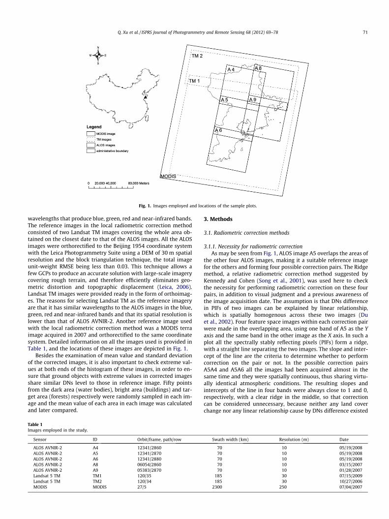
Fig. 1. Images employed and locations of the sample plots.

Q. Xu et al. / ISPRS Journal of Photogrammetry and Remote Sensing 68 (2012) 69–78 71

wavelengths that produce blue, green, red and near-infrared bands.The reference images in the local radiometric correction methodconsisted of two Landsat TM images covering the whole area ob-tained on the closest date to that of the ALOS images. All the ALOSimages were orthorectified to the Beijing 1954 coordinate systemwith the Leica Photogrammetry Suite using a DEM of 30 m spatialresolution and the block triangulation technique, the total imageunit-weight RMSE being less than 0.03. This technique allows afew GCPs to produce an accurate solution with large-scale imagerycovering rough terrain, and therefore efficiently eliminates geo-metric distortion and topographic displacement (Leica, 2006).Landsat TM images were provided ready in the form of orthoimag-es. The reasons for selecting Landsat TM as the reference imageryare that it has similar wavelengths to the ALOS images in the blue,green, red and near-infrared bands and that its spatial resolution islower than that of ALOS AVNIR-2. Another reference image usedwith the local radiometric correction method was a MODIS terraimage acquired in 2007 and orthorectified to the same coordinatesystem. Detailed information on all the images used is provided inTable 1, and the locations of these images are depicted in Fig. 1.

Besides the examination of mean value and standard deviationof the corrected images, it is also important to check extreme val-ues at both ends of the histogram of these images, in order to en-sure that ground objects with extreme values in corrected imagesshare similar DNs level to those in reference image. Fifty pointsfrom the dark area (water bodies), bright area (buildings) and tar-get area (forests) respectively were randomly sampled in each im-age and the mean value of each area in each image was calculatedand later compared.

Table 1Images employed in the study.

Sensor ID Orbit/frame, path/row

ALOS AVNIR-2 A4 12341/2860ALOS AVNIR-2 A5 12341/2870ALOS AVNIR-2 A6 12341/2880ALOS AVNIR-2 A8 06054/2860ALOS AVNIR-2 A9 05383/2870Landsat 5 TM TM1 120/35Landsat 5 TM TM2 120/34MODIS MODIS 27/5

3. Methods

3.1. Radiometric correction methods

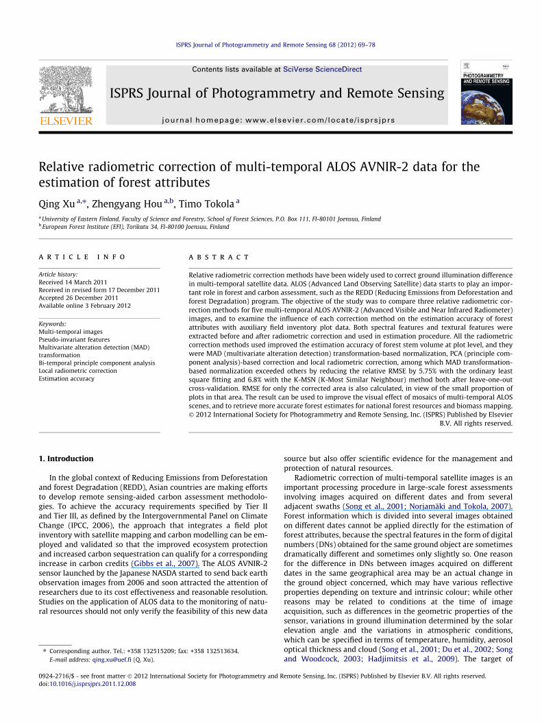
3.1.1. Necessity for radiometric correctionAs may be seen from Fig. 1, ALOS image A5 overlaps the areas of

the other four ALOS images, making it a suitable reference imagefor the others and forming four possible correction pairs. The Ridgemethod, a relative radiometric correction method suggested byKennedy and Cohen (Song et al., 2001), was used here to checkthe necessity for performing radiometric correction on these fourpairs, in addition to visual judgment and a previous awareness ofthe image acquisition date. The assumption is that DNs differencein PIFs of two images can be explained by linear relationship,which is spatially homogenous across these two images (Duet al., 2002). Four feature space images within each correction pairwere made in the overlapping area, using one band of A5 as the Yaxis and the same band in the other image as the X axis. In such aplot all the spectrally stably reflecting pixels (PIFs) form a ridge,with a straight line separating the two images. The slope and inter-cept of the line are the criteria to determine whether to performcorrection on the pair or not. In the possible correction pairsA5A4 and A5A6 all the images had been acquired almost in thesame time and they were spatially continuous, thus sharing virtu-ally identical atmospheric conditions. The resulting slopes andintercepts of the line in four bands were always close to 1 and 0,respectively, with a clear ridge in the middle, so that correctioncan be considered unnecessary, because neither any land coverchange nor any linear relationship cause by DNs difference existed

Swath width (km) Resolution (m) Date

70 10 05/19/200870 10 05/19/200870 10 05/19/200870 10 03/15/200770 10 01/28/2007

185 30 07/15/2009185 30 10/27/2006

2300 250 07/04/2007

72 Q. Xu et al. / ISPRS Journal of Photogrammetry and Remote Sensing 68 (2012) 69–78

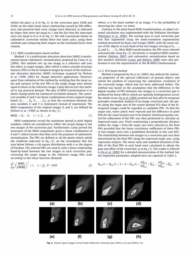
within the pairs (a–d in Fig. 2). In the correction pairs A5A8 andA5A9, on the other hand, linear relationship caused by DNs differ-ence and potential land cover change were detected, as indicatedby slopes that were not equal to 1 and the fact that the interceptswere not equal to 0 (e–h in Fig. 2). We will concentrate below onradiometric correction within these two latter pairs, using threemethods and comparing their impact on the estimated forest stemvolume.

3.1.2. MAD transformation-based methodMethod 1 is a multivariate alteration detection (MAD) transfor-

mation-based radiometric normalization proposed by Canty et al.(2004). This method sets up one image as a reference and usesthe others as target images, after which it selects pseudo-invariantfeatures (PIFs) in the bi-temporal images by means of the multivar-iate alteration detection (MAD) technique proposed by Nielsenet al. (1998, 2002) for change detection applications. However,apart from validation of the method by verifying that the mean va-lue and variance of the test PIFs in the target image were almostequal to those in the reference image, Canty did not test this meth-od in any practical domain. The idea of MAD transformation is todetect change pixels by Canonical Correlation Analysis. The canon-ical variables U and V are linear combinations of two original imagebands (X1, . . ., X4, Y1, . . ., Y4), so that the correlation between thenew variables U and V is minimized instead of maximized. TheMAD components of the original images Xi and Yi are defined byNielsen et al. (1998) as shown in Eq. (1).

MADi ¼ Ui � V i; i ¼ 1;2; . . . ;4 ð1Þ

MAD components record the maximum spread in pixel digitalnumbers, which are considered to reflect the actual change in thetwo images of the correction pair. Furthermore, Canty proved theinvariance of the MAD components given a linear combination ofX and Y, which ensures that they serve the purposes of radiometricnormalization. The PIFs are defined as all the pixels which satisfythe condition indicated in Eq. (2), on the assumption that thesum below follows a chi-square distribution with n as the degreeof freedom. The selected PIFs are used to seek a linear relationshipband-by-band between the two images in each correction pair,correcting the target image to the reference image DNs scaleaccording to the linear function obtained.

Xn

i¼1

MADi

rMADi

� �2

< t; t ¼ v2n; P ¼ 0:01 ð2Þ

Fig. 2. Feature space images of each band within t

where, n is the band number of an image; P is the probability ofobserving the value t or lower.

Contrary to the pixel-based MAD transformation, an object-ori-ented calculation was implemented with the Definiens Developer(Niemeyer et al., 2009). The overlap area in each correction pairwas first segmented using the multi-resolution segmentationmethod presented by Baatz and Schape (2000), with the mean val-ues of the objects in each band of the two images serving as X1, . . .,X4 and Y1, . . ., Y4. After MAD transformation, the PIFs were selectedautomatically using Eq. (2). Iteratively re-weighted MAD transfor-mation (Nielsen, 2007) and radiometric normalization based onthis iterative extension (Canty and Nielsen, 2008) were also per-formed to test the improvement in the IR-MAD transformation.

3.1.3. PCA-based methodMethod 2 proposed by Du et al. (2002) also utilized the statisti-

cal properties of the spectral reflectance of ground objects andsolved the problem of conserving the radiometric resolution ofthe corrected image, which had not been addressed before. Themethod was based on the assumption that the difference in thedigital number of PIFs between two images in a correction pair isproduced by linear effects which are spatially homogeneous acrossthe whole scene. Du et al. (2002) pointed out that after bi-temporalprinciple component analysis of an image correction pair, the pix-els along the major axis of the scatter-plotted PCA data of the bi-temporal images could be regarded as candidate PIFs. To find themajor axis, water pixels were rejected and the difference in pixelDNs for the same location was to be limited. Statistical quality con-trol for refinement of the PIFs was then performed to calculate animproved major axis. Pixels maintaining a perpendicular distancewithin the range ‘ from the major axis were selected as the finalPIFs provided that the linear correlation coefficients of these PIFsin two images were over a predefined threshold, in this case 85%.The relationship between two images in a correction pair was thendetermined by the final PIFs along the improved major axis, usingregression analysis. The mean value and standard deviation of theDNs of the final PIFs in each band were calculated to obtain thegain and offset of the correction, as in Eq. (3). The reader is referredto Du et al. (2002) for a detailed demonstration of the method, butthe important parameters adopted here are reported in Table 2.

Q refðiÞ ¼ Q tarðiÞ � aþ b ¼ Q tarðiÞ �rQ ref

rQ tarþ Q ref �

rQ ref

rQ tar� Q tar ð3Þ

he correction pair A5A4 (a–d) and A5A9 (e–h).

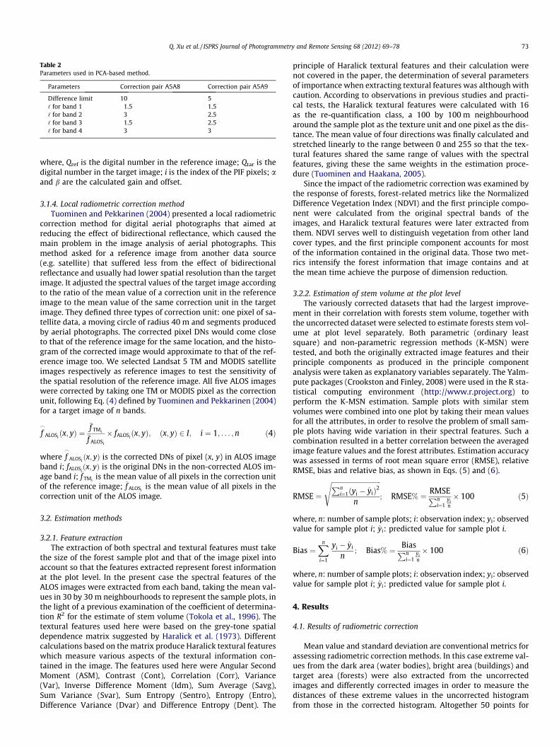
Table 2Parameters used in PCA-based method.

Parameters Correction pair A5A8 Correction pair A5A9

Difference limit 10 5‘ for band 1 1.5 1.5‘ for band 2 3 2.5‘ for band 3 1.5 2.5‘ for band 4 3 3

Q. Xu et al. / ISPRS Journal of Photogrammetry and Remote Sensing 68 (2012) 69–78 73

where, Qref is the digital number in the reference image; Qtar is thedigital number in the target image; i is the index of the PIF pixels; aand b are the calculated gain and offset.

3.1.4. Local radiometric correction methodTuominen and Pekkarinen (2004) presented a local radiometric

correction method for digital aerial photographs that aimed atreducing the effect of bidirectional reflectance, which caused themain problem in the image analysis of aerial photographs. Thismethod asked for a reference image from another data source(e.g. satellite) that suffered less from the effect of bidirectionalreflectance and usually had lower spatial resolution than the targetimage. It adjusted the spectral values of the target image accordingto the ratio of the mean value of a correction unit in the referenceimage to the mean value of the same correction unit in the targetimage. They defined three types of correction unit: one pixel of sa-tellite data, a moving circle of radius 40 m and segments producedby aerial photographs. The corrected pixel DNs would come closeto that of the reference image for the same location, and the histo-gram of the corrected image would approximate to that of the ref-erence image too. We selected Landsat 5 TM and MODIS satelliteimages respectively as reference images to test the sensitivity ofthe spatial resolution of the reference image. All five ALOS imageswere corrected by taking one TM or MODIS pixel as the correctionunit, following Eq. (4) defined by Tuominen and Pekkarinen (2004)for a target image of n bands.

f_

ALOSiðx; yÞ ¼

�f TMi

�f ALOSi

� fALOSiðx; yÞ; ðx; yÞ 2 I; i ¼ 1; . . . ;n ð4Þ

where f_

ALOSi ðx; yÞ is the corrected DNs of pixel (x, y) in ALOS imageband i; fALOSi

ðx; yÞ is the original DNs in the non-corrected ALOS im-age band i; �f TMi is the mean value of all pixels in the correction unitof the reference image; �f ALOSi

is the mean value of all pixels in thecorrection unit of the ALOS image.

3.2. Estimation methods

3.2.1. Feature extractionThe extraction of both spectral and textural features must take

the size of the forest sample plot and that of the image pixel intoaccount so that the features extracted represent forest informationat the plot level. In the present case the spectral features of theALOS images were extracted from each band, taking the mean val-ues in 30 by 30 m neighbourhoods to represent the sample plots, inthe light of a previous examination of the coefficient of determina-tion R2 for the estimate of stem volume (Tokola et al., 1996). Thetextural features used here were based on the grey-tone spatialdependence matrix suggested by Haralick et al. (1973). Differentcalculations based on the matrix produce Haralick textural featureswhich measure various aspects of the textural information con-tained in the image. The features used here were Angular SecondMoment (ASM), Contrast (Cont), Correlation (Corr), Variance(Var), Inverse Difference Moment (Idm), Sum Average (Savg),Sum Variance (Svar), Sum Entropy (Sentro), Entropy (Entro),Difference Variance (Dvar) and Difference Entropy (Dent). The

principle of Haralick textural features and their calculation werenot covered in the paper, the determination of several parametersof importance when extracting textural features was although withcaution. According to observations in previous studies and practi-cal tests, the Haralick textural features were calculated with 16as the re-quantification class, a 100 by 100 m neighbourhoodaround the sample plot as the texture unit and one pixel as the dis-tance. The mean value of four directions was finally calculated andstretched linearly to the range between 0 and 255 so that the tex-tural features shared the same range of values with the spectralfeatures, giving these the same weights in the estimation proce-dure (Tuominen and Haakana, 2005).

Since the impact of the radiometric correction was examined bythe response of forests, forest-related metrics like the NormalizedDifference Vegetation Index (NDVI) and the first principle compo-nent were calculated from the original spectral bands of theimages, and Haralick textural features were later extracted fromthem. NDVI serves well to distinguish vegetation from other landcover types, and the first principle component accounts for mostof the information contained in the original data. Those two met-rics intensify the forest information that image contains and atthe mean time achieve the purpose of dimension reduction.

3.2.2. Estimation of stem volume at the plot levelThe variously corrected datasets that had the largest improve-

ment in their correlation with forests stem volume, together withthe uncorrected dataset were selected to estimate forests stem vol-ume at plot level separately. Both parametric (ordinary leastsquare) and non-parametric regression methods (K-MSN) weretested, and both the originally extracted image features and theirprinciple components as produced in the principle componentanalysis were taken as explanatory variables separately. The YaIm-pute packages (Crookston and Finley, 2008) were used in the R sta-tistical computing environment (http://www.r.project.org) toperform the K-MSN estimation. Sample plots with similar stemvolumes were combined into one plot by taking their mean valuesfor all the attributes, in order to resolve the problem of small sam-ple plots having wide variation in their spectral features. Such acombination resulted in a better correlation between the averagedimage feature values and the forest attributes. Estimation accuracywas assessed in terms of root mean square error (RMSE), relativeRMSE, bias and relative bias, as shown in Eqs. (5) and (6).

RMSE ¼

ffiffiffiffiffiffiffiffiffiffiffiffiffiffiffiffiffiffiffiffiffiffiffiffiffiffiffiffiffiffiPni¼1ðyi � yiÞ2

n

s; RMSE% ¼ RMSEPn

i¼1yin

� 100 ð5Þ

where, n: number of sample plots; i: observation index; yi: observedvalue for sample plot i; yi: predicted value for sample plot i.

Bias ¼Xn

i¼1

yi � yi

n; Bias% ¼ BiasPn

i¼1yin

� 100 ð6Þ

where, n: number of sample plots; i: observation index; yi: observedvalue for sample plot i; yi: predicted value for sample plot i.

4. Results

4.1. Results of radiometric correction

Mean value and standard deviation are conventional metrics forassessing radiometric correction methods. In this case extreme val-ues from the dark area (water bodies), bright area (buildings) andtarget area (forests) were also extracted from the uncorrectedimages and differently corrected images in order to measure thedistances of these extreme values in the uncorrected histogramfrom those in the corrected histogram. Altogether 50 points for

74 Q. Xu et al. / ISPRS Journal of Photogrammetry and Remote Sensing 68 (2012) 69–78

each area in each image were sampled and the mean digital num-ber value for each area was calculated in order to check the trendin the alteration caused by the radiometric corrections.

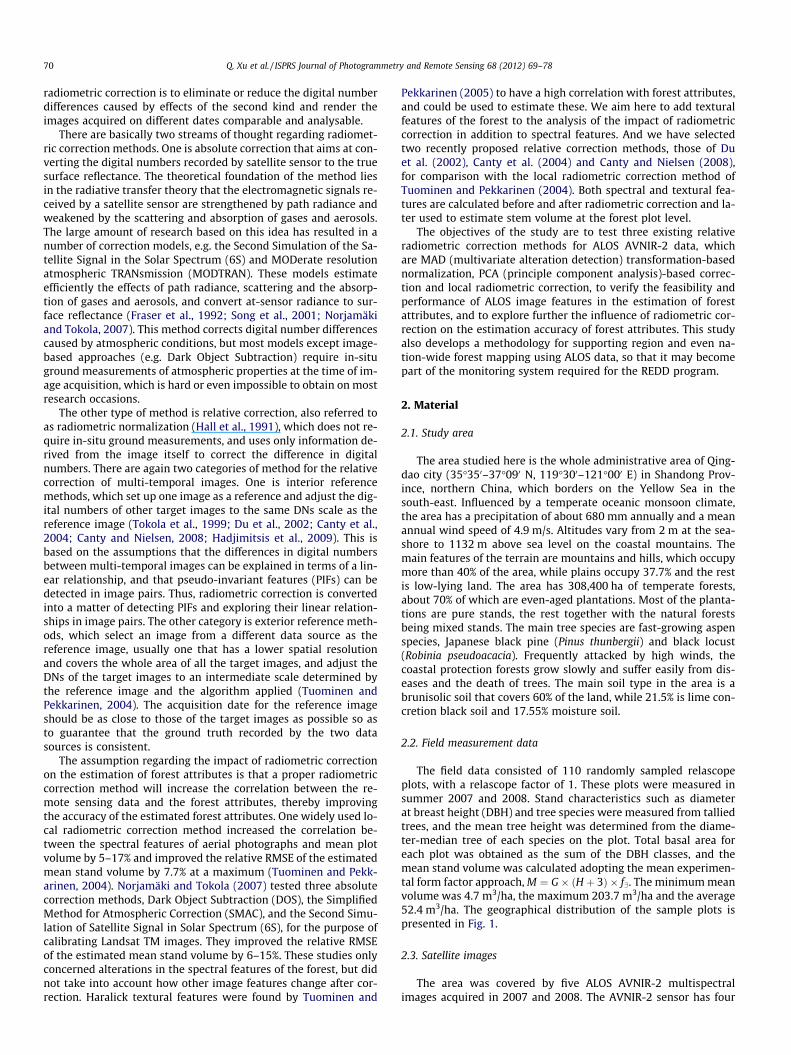
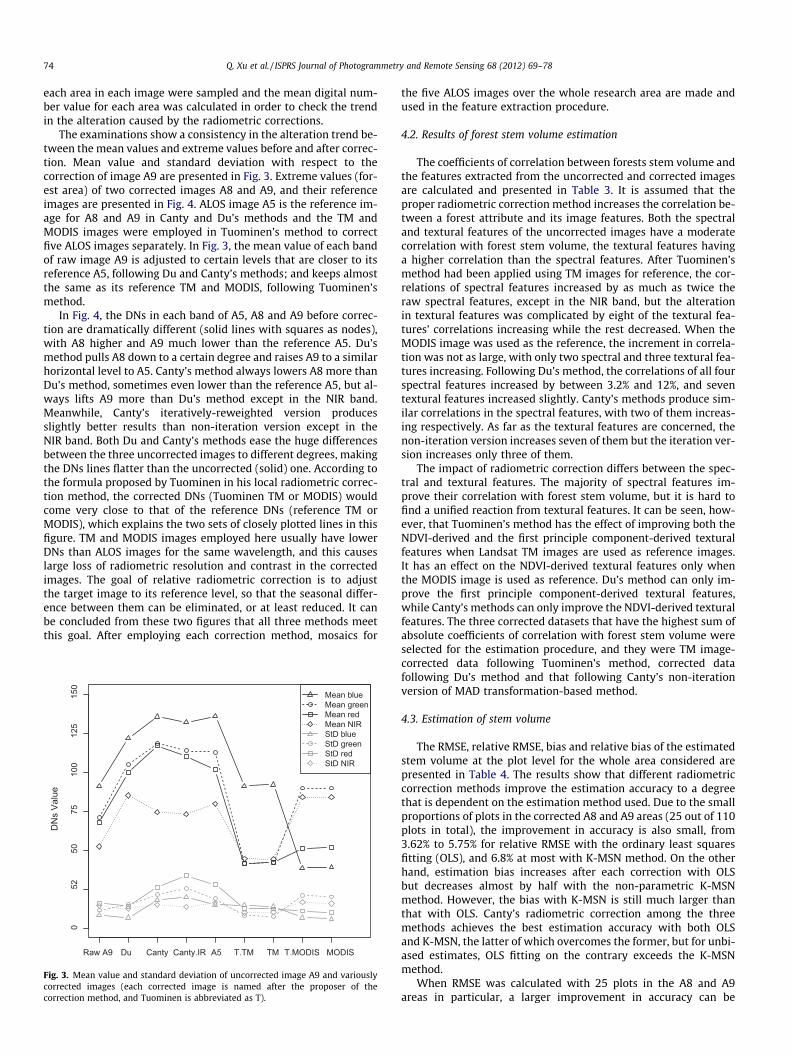
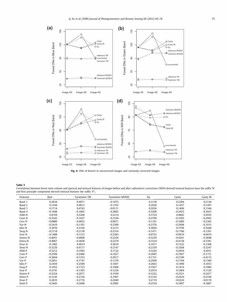
The examinations show a consistency in the alteration trend be-tween the mean values and extreme values before and after correc-tion. Mean value and standard deviation with respect to thecorrection of image A9 are presented in Fig. 3. Extreme values (for-est area) of two corrected images A8 and A9, and their referenceimages are presented in Fig. 4. ALOS image A5 is the reference im-age for A8 and A9 in Canty and Du’s methods and the TM andMODIS images were employed in Tuominen’s method to correctfive ALOS images separately. In Fig. 3, the mean value of each bandof raw image A9 is adjusted to certain levels that are closer to itsreference A5, following Du and Canty’s methods; and keeps almostthe same as its reference TM and MODIS, following Tuominen’smethod.

In Fig. 4, the DNs in each band of A5, A8 and A9 before correc-tion are dramatically different (solid lines with squares as nodes),with A8 higher and A9 much lower than the reference A5. Du’smethod pulls A8 down to a certain degree and raises A9 to a similarhorizontal level to A5. Canty’s method always lowers A8 more thanDu’s method, sometimes even lower than the reference A5, but al-ways lifts A9 more than Du’s method except in the NIR band.Meanwhile, Canty’s iteratively-reweighted version producesslightly better results than non-iteration version except in theNIR band. Both Du and Canty’s methods ease the huge differencesbetween the three uncorrected images to different degrees, makingthe DNs lines flatter than the uncorrected (solid) one. According tothe formula proposed by Tuominen in his local radiometric correc-tion method, the corrected DNs (Tuominen TM or MODIS) wouldcome very close to that of the reference DNs (reference TM orMODIS), which explains the two sets of closely plotted lines in thisfigure. TM and MODIS images employed here usually have lowerDNs than ALOS images for the same wavelength, and this causeslarge loss of radiometric resolution and contrast in the correctedimages. The goal of relative radiometric correction is to adjustthe target image to its reference level, so that the seasonal differ-ence between them can be eliminated, or at least reduced. It canbe concluded from these two figures that all three methods meetthis goal. After employing each correction method, mosaics for

052

5075

100

125

150

DN

s Va

lue

Raw A9 Du Canty Canty.IR A5 T.TM TM T.MODIS MODIS

Mean blueMean greenMean redMean NIRStD blueStD greenStD redStD NIR

Fig. 3. Mean value and standard deviation of uncorrected image A9 and variouslycorrected images (each corrected image is named after the proposer of thecorrection method, and Tuominen is abbreviated as T).

the five ALOS images over the whole research area are made andused in the feature extraction procedure.

4.2. Results of forest stem volume estimation

The coefficients of correlation between forests stem volume andthe features extracted from the uncorrected and corrected imagesare calculated and presented in Table 3. It is assumed that theproper radiometric correction method increases the correlation be-tween a forest attribute and its image features. Both the spectraland textural features of the uncorrected images have a moderatecorrelation with forest stem volume, the textural features havinga higher correlation than the spectral features. After Tuominen’smethod had been applied using TM images for reference, the cor-relations of spectral features increased by as much as twice theraw spectral features, except in the NIR band, but the alterationin textural features was complicated by eight of the textural fea-tures’ correlations increasing while the rest decreased. When theMODIS image was used as the reference, the increment in correla-tion was not as large, with only two spectral and three textural fea-tures increasing. Following Du’s method, the correlations of all fourspectral features increased by between 3.2% and 12%, and seventextural features increased slightly. Canty’s methods produce sim-ilar correlations in the spectral features, with two of them increas-ing respectively. As far as the textural features are concerned, thenon-iteration version increases seven of them but the iteration ver-sion increases only three of them.

The impact of radiometric correction differs between the spec-tral and textural features. The majority of spectral features im-prove their correlation with forest stem volume, but it is hard tofind a unified reaction from textural features. It can be seen, how-ever, that Tuominen’s method has the effect of improving both theNDVI-derived and the first principle component-derived texturalfeatures when Landsat TM images are used as reference images.It has an effect on the NDVI-derived textural features only whenthe MODIS image is used as reference. Du’s method can only im-prove the first principle component-derived textural features,while Canty’s methods can only improve the NDVI-derived texturalfeatures. The three corrected datasets that have the highest sum ofabsolute coefficients of correlation with forest stem volume wereselected for the estimation procedure, and they were TM image-corrected data following Tuominen’s method, corrected datafollowing Du’s method and that following Canty’s non-iterationversion of MAD transformation-based method.

4.3. Estimation of stem volume

The RMSE, relative RMSE, bias and relative bias of the estimatedstem volume at the plot level for the whole area considered arepresented in Table 4. The results show that different radiometriccorrection methods improve the estimation accuracy to a degreethat is dependent on the estimation method used. Due to the smallproportions of plots in the corrected A8 and A9 areas (25 out of 110plots in total), the improvement in accuracy is also small, from3.62% to 5.75% for relative RMSE with the ordinary least squaresfitting (OLS), and 6.8% at most with K-MSN method. On the otherhand, estimation bias increases after each correction with OLSbut decreases almost by half with the non-parametric K-MSNmethod. However, the bias with K-MSN is still much larger thanthat with OLS. Canty’s radiometric correction among the threemethods achieves the best estimation accuracy with both OLSand K-MSN, the latter of which overcomes the former, but for unbi-ased estimates, OLS fitting on the contrary exceeds the K-MSNmethod.

When RMSE was calculated with 25 plots in the A8 and A9areas in particular, a larger improvement in accuracy can be

2055

9012

516

0

Fore

st D

Ns

in B

lue

Band

Image A5 Image A8 Image A9

(a)

uncorrected

Du

CantyCanty.IR

Tuominen TM

reference TM

Tuominen MODISreference MODIS

3055

8010

513

0

Fore

st D

Ns

in G

reen

Ban

d

Image A5 Image A8 Image A9

(b)

uncorrected

Du

CantyCanty.IR

Tuominen TMreference TM

Tuominen MODISreference MODIS

3055

8010

513

0

Fore

st D

Ns

in R

ed B

and

Image A5 Image A8 Image A9

(c)

uncorrected

Du

Canty

Canty.IR

Tuominen TMreference TMTuominen MODISreference MODIS

4055

7085

100

Fore

st D

Ns

in N

IR B

and

Image A5 Image A8 Image A9

(d)

uncorrected

Du

Canty

Canty.IR

Tuominen TM

reference TM

Tuominen MODIS

reference MODIS

Fig. 4. DNs of forests in uncorrected images and variously corrected images.

Table 3Correlations between forest stem volume and spectral and textural features of images before and after radiometric corrections (NDVI-derived textural features have the suffix ‘N’and first principle component-derived textural features the suffix ‘P’).

Features Raw Tuominen TM Tuominen MODIS Du Canty Canty IR

Band 1 0.2034 0.4071 �0.1075 0.3138 0.2284 0.2144Band 2 0.1544 0.4013 �0.1762 0.2028 0.1457 0.1287Band 3 0.1714 0.4743 �0.0111 0.2036 0.1496 0.1344Band 4 �0.1948 �0.1865 �0.2802 �0.3200 �0.2925 �0.2925ASM-N 0.4794 0.5206 0.2214 0.3724 0.4802 0.4593Cont-N �0.3342 �0.1627 �0.2194 �0.2709 �0.3303 �0.2992Corr-N �0.0880 �0.4052 �0.0071 �0.1101 �0.1889 �0.2365Var-N �0.2410 �0.1101 �0.2309 �0.2376 �0.2698 �0.1915Idm-N 0.3970 0.3336 0.2215 0.3026 0.3799 0.3446Savg-N �0.2118 �0.2158 �0.2554 �0.1471 �0.1766 �0.1261Svar-N �0.1488 �0.1315 �0.2283 �0.0752 �0.0910 �0.0419Sentro-N �0.4051 �0.4068 �0.2256 �0.3239 �0.4201 �0.3848Entro-N �0.4067 �0.3838 �0.2279 �0.3234 �0.4158 �0.3781Dvar-N 0.1482 0.4914 0.3810 0.1077 0.1522 0.1368Dent-N �0.3226 �0.4177 �0.2147 �0.2339 �0.3368 �0.3247ASM-P 0.3212 0.1983 0.1722 0.3226 0.2854 0.2931Cont-P �0.2596 �0.2466 �0.1627 �0.2685 �0.1997 �0.1751Corr-P �0.3664 �0.1353 �0.2017 �0.1751 �0.2190 �0.4115Var-P �0.2851 �0.1747 �0.1379 �0.2999 �0.1764 �0.1366Idm-P 0.2459 0.2599 0.1697 0.2663 0.1909 0.1853Savg-P 0.1952 �0.1723 �0.1660 0.1927 0.1474 0.1084Svar-P 0.2741 �0.1365 �0.1226 0.2914 0.1684 0.1126Sentro-P �0.3224 �0.2077 �0.1939 �0.3222 �0.2521 �0.2477Entro-P �0.3145 �0.2156 �0.1907 �0.3143 �0.2416 �0.2338Dvar-P 0.2835 �0.2776 �0.2049 0.2719 �0.0226 �0.0170Dent-P �0.2445 �0.2698 �0.2005 �0.2534 �0.1897 �0.1887

Q. Xu et al. / ISPRS Journal of Photogrammetry and Remote Sensing 68 (2012) 69–78 75

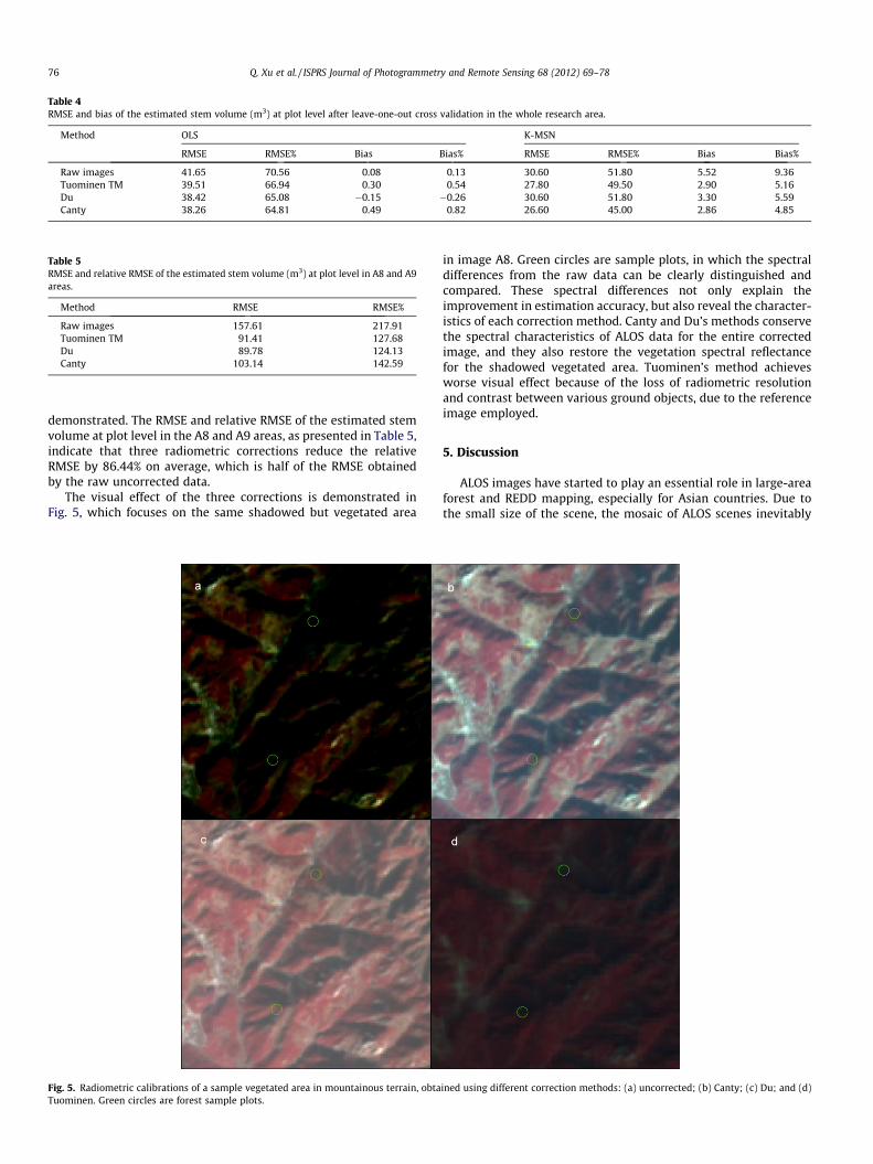
Table 4RMSE and bias of the estimated stem volume (m3) at plot level after leave-one-out cross validation in the whole research area.

Method OLS K-MSN

RMSE RMSE% Bias Bias% RMSE RMSE% Bias Bias%

Raw images 41.65 70.56 0.08 0.13 30.60 51.80 5.52 9.36Tuominen TM 39.51 66.94 0.30 0.54 27.80 49.50 2.90 5.16Du 38.42 65.08 �0.15 �0.26 30.60 51.80 3.30 5.59Canty 38.26 64.81 0.49 0.82 26.60 45.00 2.86 4.85

Table 5RMSE and relative RMSE of the estimated stem volume (m3) at plot level in A8 and A9areas.

Method RMSE RMSE%

Raw images 157.61 217.91Tuominen TM 91.41 127.68Du 89.78 124.13Canty 103.14 142.59

76 Q. Xu et al. / ISPRS Journal of Photogrammetry and Remote Sensing 68 (2012) 69–78

demonstrated. The RMSE and relative RMSE of the estimated stemvolume at plot level in the A8 and A9 areas, as presented in Table 5,indicate that three radiometric corrections reduce the relativeRMSE by 86.44% on average, which is half of the RMSE obtainedby the raw uncorrected data.

The visual effect of the three corrections is demonstrated inFig. 5, which focuses on the same shadowed but vegetated area

Fig. 5. Radiometric calibrations of a sample vegetated area in mountainous terrain, obtaTuominen. Green circles are forest sample plots.

in image A8. Green circles are sample plots, in which the spectraldifferences from the raw data can be clearly distinguished andcompared. These spectral differences not only explain theimprovement in estimation accuracy, but also reveal the character-istics of each correction method. Canty and Du’s methods conservethe spectral characteristics of ALOS data for the entire correctedimage, and they also restore the vegetation spectral reflectancefor the shadowed vegetated area. Tuominen’s method achievesworse visual effect because of the loss of radiometric resolutionand contrast between various ground objects, due to the referenceimage employed.

5. Discussion

ALOS images have started to play an essential role in large-areaforest and REDD mapping, especially for Asian countries. Due tothe small size of the scene, the mosaic of ALOS scenes inevitably

ined using different correction methods: (a) uncorrected; (b) Canty; (c) Du; and (d)

Q. Xu et al. / ISPRS Journal of Photogrammetry and Remote Sensing 68 (2012) 69–78 77

involves the radiometric correction of individual scenes. The keymotivates behind this work were to test the usability of recentlyproposed relative radiometric correction methods with ALOSAVNIR-2 data, and to establish a theoretical base for the generationof regional-scale mosaics consisting of hundreds of ALOS sceneswhich can be used later for deducing the quantities of carbonsequestered in the forest and monitoring forest change.

The radiometric correction methods used here are all automaticand fast and require no auxiliary information other than the actualimage data. The methods of Canty et al. (2004) and Canty and Niel-sen (2008), based on the invariability of MAD components underlinear transformation of original image intensities, select PIFs ofhigh quality. These PIFs then help to extract correct linear relation-ship between two images of different acquisition dates. Accordingto the estimation results and the visual judgement presented in Ta-ble 4 and Fig. 5, ALOS data corrected by this method achieves thehighest estimation accuracy and good enough visual effect. Thismethod appears to be better than other methods because the scaleinvariability guarantees the most suitable PIFs to be detectedautomatically. MAD transformation is highly scene-dependent,however, in that when the difference in intensity between twoacquisition dates exceeds a certain threshold, MAD transformationfails to detect the true PIFs (several clusters in the scatter plot indi-cate no linear relationship between two images) and therefore failsto solve the precise regression equation. This limits the applicationof Canty’s method to the images within the threshold and the mag-nitude of the threshold needs further experiment to be defined.

Principle component analysis, as used by Du et al. (2002), is an-other objective way to select PIFs, and the calculation of correlationcoefficients between the PIFs of two dates provides a form of qual-ity control for this selection. The conservation of radiometric reso-lution, as addressed by Du et al. (2002) is a good point which hasnot attracted much attention in research into radiometric correc-tion. But it can also be achieved in the method of Canty et al.(2004) and Canty and Nielsen (2008) if the criteria for selectingthe reference intensity level are set such that the calculated gainis not less than unity and the offset is not less than zero. This is par-ticularly important for producing visually friendly image mosaics.This method is also based on the statistical property of the images,and the PIFs detected are stable and reliable. Both estimation accu-racy and visual effect following this method have been improvedefficiently. No threshold limit for intensity difference betweentwo images makes Du’s method have broader application extentthan Canty’s MAD transformation-based one, for which Du’s meth-od can be a good substitute in the case that Canty’s method fails todetect true PIFs.

Viewed from the perspective of radiometric correction,Tuominen and Pekkarinen (2004) assign too much weight to thereference image, which causes both the local pixels and the histo-gram of the corrected image to converge with those of the refer-ence image. The spectral characteristics and histogram structureof the ALOS image are not taken into account in the algorithm.Therefore, extreme caution should be paid in the selection of thereference image when using this method. Firstly, the time differ-ence in terms of both year and season between the reference andthe target images should be as small as possible so that land coverchanges will not be introduced into the corrected image. This mayas well reduce the post-processing procedures. Secondly, the em-ployed reference image determines whether the corrected imagesgain or lose radiometric resolution. When it has higher DNs valuethan the target image, the corrected image will gain radiometricresolution and vice versa. Reference image that has similar DNsvalue to the target image is preferred but difficult to obtain in prac-tice. The availability of suitable reference image may hinder theapplication of this method, especially when the output image mo-saic is required for a good visual contrast. Nevertheless, image

classification and object delineation using high resolution datamay benefit from this method because the within-image intensityvariation of one object (e.g. dark pixels in a tree crown) can besolved by using a reference image that has coarser spatial resolu-tion in the same area. Local spectral homogeneity produces lessfragmentation or segments of higher compactness.

Uncertainty in the estimation of forest attributes using opticalremote sensing data stems from the forest type, the positioning ofthe sample plots, the size and shape of the feature extraction unit,the collection of field data, the correlation between image fea-tures and forest attributes and the capability of the estimator.Any of these aspects can contribute to the final estimation error.Compared with previous Scandinavian studies on boreal forestsusing optical remote sensing data (Tokola et al., 1996; Tuominenand Pekkarinen, 2004, 2005; Norjamäki and Tokola, 2007), theestimation accuracy is similar or even better, and although theRMSE achieved here is lower than in other studies of tropical for-ests (Miguel et al., 2010), the relative RMSE is higher, due to thelower average forest stem volume in the area concerned. Our re-sult is also reasonable by comparison with those obtained for thetemperate forests of Jilin Province in China, in which no cross-val-idation was applied (Gu et al., 2006). The forest type is one keyissue to consider before estimation, because various forest typeshave different spectral reflectance characteristics. The temperateforests in the area studied here are dominated by young and mid-dle-aged aspen and Japanese black pine, with the latter growingquite slowly due to the strong winds. More homogeneous foreststands yield better estimation accuracy, at least in theory, andaltitude fluctuation beyond 1000 m, which causes a shift in thesample plots, also contributes to the estimation error, eventhough orthorectification has already been performed. Also, thehand-held GPS device used here has a much larger positioning er-ror than a differential GPS and obviously adds more uncertaintyto the estimation results. The size and shape of the featureextraction unit used in this work have been tested and the fea-tures of different units have been compared in terms of their cor-relations with forest attributes, so that the units which gave thehighest correlations could be selected for the estimation proce-dure. Error in field data collection is inevitable, and it is this thatmakes up a substantial part of the estimation error. The mostimportant source of such error arises from the correlation be-tween the image features and the forest attributes, which deter-mines the feasibility of using remote sensing data to estimateforest attributes. In this case, the features extracted from theimage mosaics using these three methods could increase thesum of the correlation coefficients of all spectral and textural fea-tures. We thus have reason to believe that these three correctedmosaics improve the estimation accuracy in a correspondingmanner.

The limit on the use of optical remote sensing data in forestinventories still accounts for the saturation level of the estimates.The spectral variability in middle-aged and mature forests is verysmall, and a passive optical sensor can hardly distinguish treeswithin this range. The estimation of large trees using data of thiskind would not encounter problems, but the assessment of treesat all development classes will underestimate the attributes ofthe large trees.

Acknowledgements

The authors thank Professor Yuanzhao Hou, Chinese Academyof Forestry for his support in data acquisition, and Dr. Petteri Pack-alén, University of Eastern Finland for good discussions on localradiometric correction. The comments provided by the anonymousreviewers are gratefully acknowledged.

78 Q. Xu et al. / ISPRS Journal of Photogrammetry and Remote Sensing 68 (2012) 69–78

References

Baatz, M., Schape, A., 2000. Multiresolution segmentation – an optimizationapproach for high quality multi-scale image segmentation. In: AngewandteGeographische Informationsverarbeitung XII, Beitrage zum AGIT-SymposiumSalzburg 2000, Karhlsruhe, Herbert Wichmann Verlag, pp. 12–23.

Canty, M.J., Nielsen, A.A., Schmidt, M., 2004. Automatic radiometric normalizationof multitemporal satellite imagery. Remote Sensing of Environment 91 (3–4),441–451.

Canty, M.J., Nielsen, A.A., 2008. Automatic radiometric normalization ofmultitemporal satellite imagery with the iteratively re-weighted madtransformation. Remote Sensing of Environment 112 (3), 1025–1036.

Crookston, N.L., Finley, A.O., 2008. yaImpute: An R package for kNN imputation.Journal of Statistical Software 23 (10), 1–16.

Du, Y., Teillet, P.M., Cihlar, J., 2002. Radiometric normalization of multitemporalhigh-resolution satellite images with quality control for land cover changedetection. Remote Sensing of Environment 82 (1), 123–134.

Fraser, R.S., Ferrare, R.A., Kaufmann, Y.J., 1992. Algorithm for atmospheric correctionof aircraft and satellite imagery. International Journal of Remote Sensing 13 (3),541–557.

Gibbs, H.K., Brown, S., Niles, J.O., Foley, J.A., 2007. Monitoring and estimatingtropical forest carbon stocks: making REDD a reality. Environmental ResearchLetters 2 (4), 1–13.

Gu, H., Dai, L., Wu, G., Xu, D., Wang, S., Wang, H., 2006. Estimation of forest volumesby integrating Landsat TM imagery and forest inventory data. Science in China:Series E Technological Sciences 49 (1), 54–62.

Hadjimitsis, D.G., Clayton, C.R.I., Reralis, A., 2009. The use of selected pseudo-invariant targets for the application of atmospheric correction in multi-temporal studies using satellite remotely sensed imagery. InternationalJournal of Applied Earth Observation and Geoinformation 11 (3), 192–200.

Hall, F.G., Strebel, D.E., Nickeson, J.E., Goetz, S.J., 1991. Radiometric rectification:toward a common radiometric response among multidate, multisensor images.Remote Sensing of Environment 35 (1), 11–27.

Haralick, R.M., Shanmugam, K., Dinsteein, J., 1973. Textural features for imageclassification. IEEE Transactions on Systems, Man, and Cybernetics, SMC-3 (6),610–621.

IPCC, 2006. IPCC Guidelines for National Greenhouse Gas Inventories. Availablefrom: <http://www.ipcc-nggip.iges.or.jp/public/2006gl/index.html> (accessed21.01.12).

Leica, 2006. Leica Photogrammetry Suite Project Manager. Available from: <http://gis.ess.washington.edu/data/erdas_pdfs/LPS_PM.pdf> (accessed 13.09.11).

Miguel, S., Martin, R., Bernardus, J., 2010. Estimation of tropical forest structurefrom SPOT-5 satellite images. International Journal of Remote Sensing 31 (10),2767–2782.

Nielsen, A.A., Conradsen, K., Simpson, J.J., 1998. Multivariate alteration detection(MAD) and MAF post-processing in multispectral bitemporal image data: newapproaches to change detection studies. Remote Sensing of Environment 64 (1),1–19.

Nielsen, A.A., Conradsen, K., Andersen, O.B., 2002. A change oriented extension ofEOF analysis applied to the 1996–1997 AVHRR sea surface temperature data.Physics and Chemistry of the Earth 27 (32–34), 1379–1386.

Nielsen, A.A., 2007. The regularized iteratively reweighted MAD method for changedetection in multi- and hyperspectral data. IEEE Transactions on ImageProcessing 16 (2), 463–478.

Niemeyer, I., Bachmann, F., John, A., Listner, C., Marpu, P.R., 2009. Object-basedChange Detection and Classification. Available from: <http://spiedigitallibrary.org/proceedings/resource/2/psisdg/7477/1/74770S_1?isAuthorized=no> (accessed 17.12.11).

Norjamäki, I., Tokola, T., 2007. Comparison of atmospheric correction methods inmapping timber volume with multitemporal Landsat images in Kainuu, Finland.Photogrammetric Engineering and Remote Sensing 73 (2), 155–163.

Song, C., Woodcock, C.E., Seto, K.C., Lenney, M.P., Macomber, S.A., 2001.Classification and change detection using Landsat TM data: when and how tocorrect atmospheric effects? Remote Sensing of Environment 75 (2), 230–244.

Song, C., Woodcock, C.E., 2003. Monitoring forest succession with multitemporallandsat images: factors of uncertainty. IEEE Transactions on Geoscience andRemote Sensing 41 (11), 2557–2567.

Tokola, T., Pitkänen, J., Partinen, S., Muinonen, E., 1996. Point accuracy of a non-parametric method in estimation of forest characteristics with different satellitematerials. International Journal of Remote Sensing 17 (12), 2333–2351.

Tokola, T., Lögman, S., Erkkilä, A., 1999. Relative calibration of multitemporalLandsat data for forest cover change detection. Remote Sensing of Environment68 (1), 1–11.

Tuominen, S., Pekkarinen, A., 2004. Local radiometric correction of digital aerialphotographs for multi source forest inventory. Remote Sensing of Environment89 (1), 72–78.

Tuominen, S., Haakana, M., 2005. Landsat TM imagery and high altitude aerialphotographs in estimation of forest characteristics. Silva Fennica 39 (4), 573–584.

Tuominen, S., Pekkarinen, A., 2005. Performance of different spectral and texturalaerial photograph features in multi-source forest inventory. Remote Sensing ofEnvironment 94 (2), 256–268.