Data Mining Storm Attributes from Spatial Grids

Data Mining Storm Attributes from Spatial Grids

VALLIAPPA LAKSHMANAN AND TRAVIS SMITH

Cooperative Institute of Mesoscale Meteorological Studies, University of Oklahoma, and National Oceanic

and Atmospheric Administration/National Severe Storms Laboratory, Norman, Oklahoma

(Manuscript received 18 November 2008, in final form 30 April 2009)

ABSTRACT

A technique to identify storms and capture scalar features within the geographic and temporal extent of the

identified storms is described. The identification technique relies on clustering grid points in an observation

field to find self-similar and spatially coherent clusters that meet the traditional understanding of what storms

are. From these storms, geometric, spatial, and temporal features can be extracted. These scalar features can

then be data mined to answer many types of research questions in an objective, data-driven manner. This is

illustrated by using the technique to answer questions of forecaster skill and lightning predictability.

1. Introduction

Hypothesis testing in nowcasting typically involves a

mind-numbing crawl through hours of remotely sensed

data and human identification of features in the dataset.

This is then followed by a quasi-objective association of

human-identified features to observed events. A con-

sequence of such a labor-intensive method is that the

simplest analyses often take years of effort.

For example, Davies (2004) studied the relationship

between environmental sounding parameters and tor-

nado potential in supercell thunderstorms, and 518 en-

vironmental soundings from January 2001 to July 2003

were culled from a numerical model to represent the

near-storm environment in the inflow region of a nearby

supercell. Supercells were identified by examining the

text of associated tornado warning products issued

by the National Weather Service (NWS) or from ana-

lyzing radar reflectivity signatures. From this dataset,

statistics were developed to differentiate between tor-

nadic and nontornadic supercell environments. The

study examined just 10% of tornado events occurring in

the time period. A more complete analysis could have

been performed had there been an automated technique

to extract the environmental parameters in the vicinity

of candidate supercells.

As another example, Trapp et al. (2005) examined

radar reflectivity images associated with 3828 tornadoes

that occurred in 1998–2000 to determine the percentage

of tornadoes that were spawned by quasi-linear con-

vective systems (QLCS). Trapp et al. (2005) describe

the process as ‘‘the labor-intensive categorization of a

large number of events’’ into three broad categories:

cell, QLCS, or other. Their categorizations were largely

subjective in nature and reliant on the interpretation of

the people examining the reflectivity imagery. Such

long-term studies are undertaken less often than they

should, because of the lack of a tool to analyze large

amounts of data in an objective manner.

It would be far better if tasks like storm classification

and attribute extraction in the vicinity of storms could be

accomplished by reliable and accurate automated algo-

rithms. The most straightforward approach to automated

analysis would be to look within a small neighborhood

(say 10 km) of an event of interest (say occurrence of a

lightning flash) and see if certain values of a spatial

gridded field (say the maximum radar reflectivity ob-

served at 6 km or higher) are associated with the event.

This does have the advantage of being able to rapidly

accumulate large amounts of data with which to test a

hypothesis (e.g., if a 45-dBZ echo is observed at 6-km

height, a cloud-to-ground lightning strike will occur

within the next 15 min). However, in reality, the cloud-

to-ground lightning flash could occur anywhere from

within an electrified cloud. The neighborhood would

have to be so large that other, nearby storms would also

get pulled in. It is because pixel-by-pixel verification

Corresponding author address: V. Lakshmanan, 120 David

L. Boren Blvd., Norman, OK 73072.

E-mail: [email protected]

NOVEMBER 2009 L A K S H M A N A N A N D S M I T H 2353

DOI: 10.1175/2009JTECHA1257.1

� 2009 American Meteorological Society

does not work very well that researchers have resorted

to hand creation of testing cases.

The objective of this paper is to describe a technique

that makes it possible to extract features from large

amounts of spatial data (typically remotely observed, al-

though it could also be numerical model assimilated or

forecast fields) and use the features to answer questions in

an automated manner. Such automated analysis based on

large datasets is referred to as data mining. Data mining is

a multidisciplinary field that provides a number of tools

that can be useful in meteorological research.

The rest of this section provides a brief introduction to

data mining and provides the motivation for the tech-

nique described in this paper. The technique itself con-

sists of three major steps, all of which are described in

section 2. Two example uses of features extracted by

using the technique of this paper are described in section 3.

It should be emphasized that the point of this paper is

not the results of the analyses themselves—even though

they are quite interesting—but that analyses of this sort

can be carried out quickly and objectively.

Data mining

Hand et al. (2001) define data mining as the analysis of

often large observational datasets to find relationships

and to summarize data. It comprises methods from ap-

plied statistics, pattern recognition, and computer sci-

ence. The input to data mining techniques, such as

neural networks or decision trees, is a set of ‘‘training

patterns,’’ where each training pattern consists of mul-

tiple associated observations.1

Often, one of the observations is usually unavailable

or hard to collect. The problem, then, is to estimate the

normally unavailable observation using the commonly

available ones. For example, there is a practical limit

imposed by cost on the density of rain gauges. Radar and

satellite observations are routinely available but do not

provide exact measures of rainfall. Thus, data mining

approaches such as neural networks (Hong et al. 2004)

have been used to devise high-density rainfall estimates

starting from remotely sensed measurements.

Another common use of data mining has been in

quality control of datasets. A better, but usually un-

available, source of data can be used to devise models to

determine the quality of routinely collected data using

internal measures on the data itself. These models can

then be applied in real time. Thus, hydrometeor classi-

fication by polarimetric radar was used to create a fuzzy

logic system (Kessinger et al. 2003) operating on the

texture of Weather Surveillance Radar-1988 Doppler

(WSR-88D) reflectivity, velocity, and spectrum width

fields to determine whether the echoes at each range

gate corresponded to precipitation.

A common thread to both the rainfall and quality-

control studies mentioned is that the input features to

the data mining system are statistics in a local neigh-

borhood of every observation point. Such a data mining

approach is limited to estimating spatially smooth fields

such as rainfall. If the grid contains discontinuities (such

as when a satellite image includes both ground and cloud

tops), statistics computed in rectangular subgrids of the

image will be unreliable, because they will include pixels

from both sides of the discontinuity.

If the requirement is to identify characteristics of

storms, the approach of using neighborhood statistics

does not work, because the pattern instances in such a

case should not be geographic points or pixels but the

storms themselves. Correspondingly, the features used

in the data mining technique have to correspond to at-

tributes of the storms, not just the neighborhood of

pixels. For example, to determine whether a given storm

is tornadic, candidate circulations were identified from

radar velocity measurements using the mesocyclone

detection algorithm of Stumpf et al. (1998). Properties of

the circulation were then used to train a neural network

to identify tornadic storms (Marzban and Stumpf 1996).

Similarly, to predict the hail potential of a storm, storms

were identified using the stormcell identification and

tracking algorithm of Johnson et al. (1998). Properties of

the storm such as cell base, height, and near-storm en-

vironmental parameters were used to devise a neural

network to nowcast hail (Marzban and Witt 2001).

The tornado and hail examples illustrate the crux of the

problem. For each problem to be addressed through data

mining, completely separate identification algorithm and

attribute-extraction techniques were required. A general-

purpose method that enables identification of storms

and extraction of features from any suitable spatial field

would be a significant advance. It should be noted that

different applications would have different definitions of

what constitutes a storm (data thresholds, minimum sizes,

and presmoothing) and would require different attributes

to be extracted from different spatial grids, but this does

not imply that a general-purpose algorithm to extract

such attributes cannot be devised. The availability of a

general-purpose method would enable data mining to be

applied routinely on a number of meteorological datasets

and permit objective answers to questions that require

automated analysis of large amounts of data.

Data mining in meteorology, then, often requires, as

inputs, neighborhood features as well as attributes of

1 For example, hourly measurements of temperature and hu-

midity at some location for a decade could form the training da-

taset. Each pattern would consist of the temperature and humidity

measurements at a certain instant in time.

2354 J O U R N A L O F A T M O S P H E R I C A N D O C E A N I C T E C H N O L O G Y VOLUME 26

storms at different scales, corresponding to the phenom-

ena of interest. Neighborhood features are straightfor-

ward to compute. However, a general-purpose technique

to extract storm attributes is needed in order to use

extracted features to answer research questions on large

amounts of data. This paper describes such a general-

purpose technique for extracting storm properties from

spatial grids.

2. Method

The technique consists of three steps: 1) identify

storms from spatial grids; 2) estimate the motion of these

storms; and 3) use the spatial extent of the storms and

their movement to extract geometric, spatial, and tem-

poral properties of the storms. These steps are described

in detail in this section. The extracted properties can be

used to answer different types of research questions.

Two such questions are presented in section 3.

a. Identifying storms

Extracting storm attributes requires a general-purpose

definition of a storm that is amenable to automated

storm identification. Lakshmanan et al. (2009) define a

storm in weather imagery as a region of high intensity

separated from other areas of high intensity. A storm in

their formalism consists of a group of pixels that meet a

size criterion (‘‘saliency’’; Najman and Schmitt 1996),

whose intensity values are greater than a value criterion

(‘‘minimum’’) and whose region of support ‘‘foothills’’ is

determined by the highest intensity within the group.

The ‘‘intensity’’ depends on the weather data in ques-

tion: reflectivity from weather radar, flash density from

cloud-to-ground lightning observations, or infrared

temperature from weather satellites may all be used.

Although the general-purpose definition of a storm

advanced by Lakshmanan et al. (2009) is useful, the

technique of that paper has one critical drawback in that

each group of pixels has to be spatially connected by

intensity values greater than the minimum intensity

threshold. Clustering with spatial constraints, on the

other hand, does not have this limitation and is therefore

better suited to input fields where pixels above a certain

threshold may not be connected. The clustering is set up

as an expectation-minimization problem, with two op-

posing criteria for each pixel so that the cost of assigning

a pixel to the kth cluster is

E(k) 5 ldm

(k) 1 (1� l)dc(k) 0 # l # 1. (1)

The first criterion assigns a cost dm(k) to the difference

in intensity between the pixel intensity Ixy and the mean

intensity of the kth cluster mk, so that pixels tend to

belong to the cluster they are closest to in value space,

dm

(k) 5 kmk� I

xyk. (2)

The second criterion assigns a cost dc(k), which is de-

fined as the number of neighboring pixels that do not

belong to the kth cluster,

dc(k) 5 �

ij�Nxy

[1� d(Sij� k)], (3)

so that the pixel x, y tends to belong to the same cluster as

its neighbors Nxy. Here, Sij is the currently assigned cluster

to the pixel at i, j, and d(Sij 2 k) is a function that is 1 only

if Sij 5 k. Thus, the clustering step balances the dual goals

of self-similarity [dm(k)] and spatial coherence [dc(k)].

The neighbors Nxy of a pixel x, y are the set of pixels

within some spatial distance of that pixel. Through ex-

periment, we found that setting this distance threshold

to be 0.4ffiffiffiffiffiffiffiffiffiffiffiffiffiffiffiffiffi

saliencyp

worked well. Thus, the identification

of a storm is determined by the size criterion starting

from the clusters. These clusters are combined in de-

scending order of intensity to fit larger and larger size

criteria; as the saliency (or minimum size threshold)

increases, farther away pixels are considered in the set of

pixels Nxy. Using multiple size criteria allows for hier-

archical, multiscale storm identification (see Figs. 1b,c).

This technique yields clusters that are nested partitions;

that is, the storms at detailed scales, if they are salient

enough to exist at coarser scales, are wholly contained

within storms at coarser scales. This is useful in order

to extract relationships such as whether a storm cell

(cluster result at a more detailed scale) is contained with

a squall line (cluster result at coarser scale).

This technique of storm identification differs from the

approach presented by Lakshmanan et al. (2009, 2003).

Unlike in Lakshmanan et al. (2009), multiscale seg-

mentation is possible. Also, pixels that are not spatially

connected can belong to the same cluster (see Fig. 1c). In

the multiscale approach of Lakshmanan et al. (2003),

clusters were combined based on intercluster distances

(i.e., clusters a and b would be combined if kma 2 mbkwas below some user-specified threshold). Here, clus-

ters are combined to meet a size threshold. Storms iden-

tified through a size-based saliency definition correspond

better to intuitive understanding of storm structures in

remotely sensed imagery (Lakshmanan et al. 2009).

b. Motion estimation

There are, broadly, two approaches to estimating

movement from spatial grids. A hybrid of the two basic

approaches is followed in this paper.

The optical flow approach estimates movement on

rectangular subgrids of the image by maximizing the

cross correlation between a subgrid at a previous time


FIG

.1.M

ult

isca

leh

iera

rch

ica

lcl

ust

eri

ng

toid

en

tify

sto

rms

an

de

stim

ate

mo

tio

n:(

a)

refl

ect

ivit

yco

mp

osi

tefi

eld

be

ing

clu

ste

red

,wh

ere

the

da

taa

reo

ve

rn

ort

hw

est

Ark

an

sas

on

6Ju

n

20

08

an

dd

ep

ict

an

are

ao

fa

pp

rox

ima

tely

75

km

37

5k

m;

(b)

sto

rms

ide

nti

fied

at

a2

0k

m2

sali

en

cy,

wh

ere

dif

fere

nt

sto

rms

are

shad

ed

dif

fere

ntl

y;

(c)

sto

rms

ide

nti

fie

da

t2

00

km

2

sali

en

cy;(

d)

sto

rms

ide

nti

fie

da

t2

00

km

2u

sin

gth

ea

pp

roa

cho

fL

ak

shm

an

an

et

al.

(20

09);

(e)

mo

tio

ne

stim

ate

at

the

20

0-k

m2

sca

le;a

nd

(f)

usi

ng

the

mo

tio

ne

stim

ate

toa

dv

ect

the

curr

ent

fie

ldfo

rwa

rdb

y3

0m

in.


and a translated version of the subgrid. For example,

Tuttle and Gall (1999) utilized an optical flow approach

to estimate winds in tropical cyclones. Such methods

suffer from two major flaws: the extracted wind fields

tend to be chaotic because of the approach’s reliance on

the maximum, a statistically noisy operation, and be-

cause of the ‘‘aperture’’ problem. The aperture problem

refers to the impossibility of following the movement of

entities in a direction parallel to their length when esti-

mating movement using subgrids that are smaller than

the entity (Barron et al. 1994). The first problem (of

chaotic motion fields) can be ameliorated by smoothing

the image and imposing a maximum deviation from a

global motion vector, as done by Wolfson et al. (1999).

Another way to address the problem of noisy motion

fields without imposing a global direction is to use a

variational optimization approach and to remove echoes

that correspond to unpredictable scales, as in Turner

et al. (2004). The second problem, of aperture, remains

endemic to optical flow approaches.

The second approach to estimating movement from

spatial grids relies on associating storms between frames

to determine the movement of each storm. For example,

Johnson et al. (1998) describe a method of identifying

storms and using heuristics to associate them across time,

whereas Dixon and Wiener (1993) uses a global cost

function to minimize association errors. However, asso-

ciation is fraught with problems, because storms grow,

evolve, decay, merge, and split; each of these is a potential

source of association error. Practical algorithms for as-

sociation involve numerous heuristics. Applying the al-

gorithms unchanged to a variety of remotely sensed fields

can involve difficult choices, so the resulting parameters

often perform better on one type of imagery than others.

Also, in practice, motion estimates from storm associa-

tion may perform poorly in situations such as changes in

storm movement or stormcell splits and merges because

of the technique’s reliance on the position of centroids,

which are greatly affected by storm evolution. However,

operational methods of storm tracking all employ asso-

ciation because of one huge benefit: the ability to track

storm properties. Optical flow approaches are based on

subgrids and therefore do not provide the ability to iden-

tify or track storm attributes over time.

One way to obtain high-quality motion estimates, re-

tain the ability to associate motion with storm entities,

and avoid association error is to employ a hybrid tech-

nique, such as that of Lakshmanan et al. (2003). Storms

are identified in the current frame and associated, not

with storms in the previous frame, but with the image in

the previous frame. Thus, movement is associated not on

rectangular subgrids but on subgrids that have the shape

and size of the current cluster. Even if a storm has merged

or split between the two frames, the motion estimate will

correspond to the parts of image in the previous frame

that the current cluster correspond to. As long as storms

do not grow or evolve too dramatically in the intervening

time period, this cluster-to-image matching side steps

association errors and provides high-quality motion esti-

mates, because the motion estimate corresponds to a

relatively large group of pixels (see Figs. 1e,f). Motion

estimates are estimated over the entire area of interest

by interpolating spatially between the motion estimates

corresponding to each storm. Motion estimates are also

smoothed temporally over time by using a constant-

acceleration Kalman filter. This yields a motion estimate

over the entire domain.

c. Extracting properties

Once clusters have been identified and their motion

have been estimated, geometric, spatial and temporal

properties of the clusters can be extracted.

1) GEOMETRIC PROPERTIES

The number of pixels in each identified cluster is in-

dicative of the size of the cluster. Depending on the map

projection used, that can be converted either exactly or

approximately into a size in square kilometers.

Besides the size, the aspect ratio and orientation of

objects are commonly desired. These can be estimated

by first fitting clusters to an ellipse. If the cluster consists

of pixels x, y, then the best-fit ellipse contains axes of

lengths a and b and orientation f, where (Jain 1989)

a 5 2ffiffiffiffiffiffiffiffiffiffiffiffiffiffiffiffiffiffiffiffiffiffiffiffiffiffiffiffiffiffiffiffiffiffiffiffiffiffiffiffiffiffiffiffiffiffiffiffiffiffiffiffiffiffi

yx

1 yy

1 (yx� y

y)2

1 4y2xy

q

,

b 5 2ffiffiffiffiffiffiffiffiffiffiffiffiffiffiffiffiffiffiffiffiffiffiffiffiffiffiffiffiffiffiffiffiffiffiffiffiffiffiffiffiffiffiffiffiffiffiffiffiffiffiffiffiffiffi

yx

1 yy� (y

x� y

y)2 � 4y2

xy

q

,

f 5 tan�1a2/4� y

xyffiffiffiffiffiffiffiffiffiffiffiffiffiffiffiffiffiffiffiffiffiffiffiffiffiffiffiffiffiffiffiffiffiffi

(a2/4� yx)2

1 y2y

q

yxy

ffiffiffiffiffiffiffiffiffiffiffiffiffiffiffiffiffiffiffiffiffiffiffiffiffiffiffiffiffiffiffiffiffiffiffiffi

(a2/4� y2x)2

1 y2xy

q ,

,

(4)

with yx, yy and yxy given by

yx

5NSx2 � (Sx)2

N2 �N, y

y5

NSy2 � (Sy)2

N2 �N,

yxy

5NSxy� SxSy

N2 �N. (5)

The ratio max(a, b)/min(a, b) can be used as a measure

of the aspect ratio of the cluster, with a ratio near 1 in-

dicative of a circular storm and larger numbers indica-

tive of elongated storms.

2) SPATIAL PROPERTIES

In addition to the properties of the clusters them-

selves (geometric properties), it may be useful to extract


properties of the clusters that correspond to their loca-

tion on the earth. For example, it may be desirable to

obtain the number of people who live in the area cov-

ered by the cluster at a particular point in time. As long

as such information is available as a spatial grid, this

cluster-specific information can be readily extracted.

Spatial grids, such as remotely sensed observations or

population density, should be remapped to the extent of

the clustered grid, so that data are available for each

pixel within a cluster. Geospatial information, such as

watch or warning polygons, can be converted to a spatial

grid where the grid value reflects whether the pixel is

within the polygon. Then, the pixels x, y belonging to

each cluster can be used to estimate spatial properties.

For example, suppose there exists a spatial grid of

maximum expected size of hail (MESH) that is esti-

mated using 3D mosaicked radar data and surface

analysis using a technique such as Witt et al. (1998) and

Lakshmanan et al. (2006). Then, the maximum expected

hail size within the jth cluster could be expressed as

MESHcluster

j5 max

i(MESH

xi,y

ijx

i, y

i� cluster

j) (6)

It is not necessary to use the max operation; other

scalar statistical properties, such as mean, variance,

minimum, median, and 90th percentile, can be similarly

computed. Nonscalar properties, such as probability

distribution functions, can be estimated by accumulating

the frequency of occurrence of values within quantiza-

tion bands.

Derived properties may also be estimated from spatial

grids. For example, the severe hail index (SHI; Witt et al.

1998) may be used to determine if the radar data at a grid

point corresponds to stratiform precipitation or to con-

vection. The fraction of the cluster that is convective can

be estimated by finding the ratio of pixels that have SHI

above a certain threshold to the size of the cluster. The

number of people who live in the area covered by the

cluster at a particular point in time (i.e., the number of

people affected by the storm) can be obtained by nu-

merically integrating the population density associated

with each of the pixels within the cluster.

Thus, spatial properties of the jth cluster can be ex-

tracted by computing scalar statistical properties over all

the pixels xi, yi�clusterj on spatial grids that have been

remapped to the extent and resolution of the clustered

grid.

3) TEMPORAL PROPERTIES

A leading indicator for many phenomena is the rate of

increase or decrease of a spatial property. For example,

cloud-top cooling rates measured from satellite obser-

vations are an important indicator of convection. An

increase in the aspect ratio of an area of high reflectivity

coupled with a decrease in midaltitude rotation may

indicate that a storm is undergoing evolution from an

isolated cell to a linear system. Temporal properties can

be estimated from a time sequence of spatial grids in two

ways: one that relies on cluster association between

frames of the sequence and another that does not.

Suppose that a spatial property MESHclusterjis com-

puted at the current time t0. If this cluster can be asso-

ciated with clusterk at time t21 by using a heuristic, such

as maximum overlap or minimum distance between

centroids, or by using a cost function such as that of

Dixon and Wiener (1993), then the temporal property

dMESH,clusterjat t0 can be obtained from the computed

spatial properties at the two times:

dMESH,cluster

j,t0

5 MESHt0,cluster

j�MESH

t�1,clusterk. (7)

This technique, of course, relies on associating clusters

correctly between frames of a sequence. The larger the

cluster, the more reliable the commonly used heuristics

for cluster association tend to be. However, morpho-

logical changes, such as storm splits and mergers, cause

problems for this approach.

Another way of computing temporal properties is to

side step the association step completely and employ a

cluster-to-image matching method as was done when

computing motion estimates (see section 2b). Assume

that a motion estimate is available over the entire do-

main so that the motion at xi, yi is ui, vi. Then, the tem-

poral property that captures the change in a spatial

property; for example, MESH for the jth cluster can be

obtained by projecting the pixels that belong to the

cluster backward in time and recomputing the spatial

property on the earlier frame of the sequence:

dMESH,cluster

j5 max

i(MESH

t0,xi,y

ijx

i, y

i� cluster

j, t

0)

�maxi(MESH

t�1,xi�ui*(t0�t�1),yi�yi*(t0�t�1)j

xi, y

i� cluster

j, t

0).

(8)

It should be noted that this technique relies only on

the clustering of the current field, not on the clustering of

the previous frame. The assumption, instead, is that the

pixels xi, yi that are part of clusterj will have moved with

the same speed and direction from the previous frame.

Therefore, this technique handles morphological oper-

ations such as splits and mergers well, because it does

not require clustering of the previous frame; instead, just

the corresponding part(s) of the previous grid are used.

However, this technique assumes that there has not

been significant spatial growth or decay of the storm


between the time frames. If, for example, there has been

decay, then dMESH,clusterj

will reflect only the changes

within the core of the storm (because the cluster at t0 will

be smaller than the entity in t21). On the other hand, if

there has been growth, then statistics are computed over

a slightly larger area. Depending on the scalar statistic

and how it is distributed within the storm, this may not

matter. For example, the impact is negligible for the

maximum expected hail size criterion, because the

maximum values tend to be in the core of the storm and

not at the periphery.

The cluster-to-image matching method is more tol-

erant of unstable clustering results (i.e., poor storm

identification or tracking). However, there are three

limitations. First, as noted earlier, sizeable changes

in storm size will cause problems. Second, if different

parts of the cluster move in different directions, then

the motion estimate will be wrong. Third, estimating

changes in geometric properties, such as size or aspect

ratio, has to be performed using the cluster association

technique, because the second technique does not rely

on the clustering result on earlier frames of sequence.

3. Example uses

Section 2 described the technique of identifying

storms from geospatial images and extracting geometric,

spatial, and temporal attributes of those storms in a fully

automated manner. The technique, when applied to

large collections of imagery, yields a pattern (a set of

attributes) for each identified storm. These patterns can

be used as inputs to standard statistical or data mining

techniques. The utility of such an approach to answer a

broad range of questions is illustrated in this section.

a. Forecaster skill

Is it more difficult to issue tornado warnings when the

tornadoes are associated with short-lived pulse storms

compared to tornadoes associated with supercells that

have a much longer life? Intuitively, the answer to the

question seems to be that it should, because pulse storms

ought to be more unpredictable. Yet, the truth of such a

statement would imply that many of the performance

statistics employed by the NWS to evaluate the con-

tinuing improvement of forecast offices are problematic;

year-over-year comparisons of the critical skill index

(CSI; Donaldson et al. 1975) would be heavily influenced

by the type of storms within the county warning area of a

given NWS forecast office during the given time periods.

Similarly, interoffice comparisons and rankings of fore-

cast offices would be questionable practices. Before

making such a charge, though, it is important to prove

that it is indeed the case that tornadoes are systemati-

cally easier or harder to predict, depending on the type

of storms they are associated with.

To show that tornadoes associated with supercells are

easier to predict, it is necessary to compute the CSI

achieved by NWS forecasters on a large number of

supercell storms. One would then compute the CSI on

pulse storms and check whether the difference in CSIs

(if any) was statistically significant. To achieve statistical

significance, it is expected that hundreds of tornado

warnings would have be evaluated. This would mean

that many hundreds of storms would have to be classi-

fied into supercells versus pulse storms. Doing this by

hand would be prohibitively time consuming and ex-

pensive. An automated technique to do this is required

to answer the question of forecaster skill in a practical

manner. At the scale of storm cells, no automated storm-

type algorithm exists.

The data mining approach of this paper was employed

to address this question. The storm attributes were

provided as input to a machine intelligent engine that

would output the type of storm. The engine was trained

based on human classification of a small subset of the

complete collection of data. The first step in training was

to manually associate a storm type with each identified

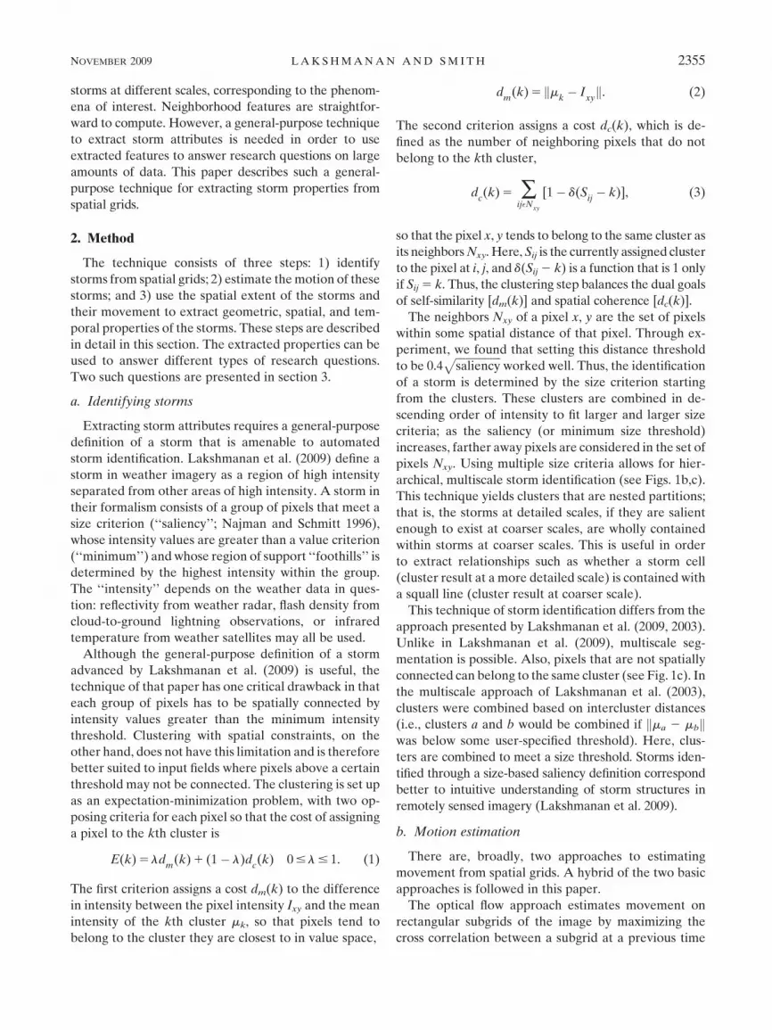
storm by analyzing 72 multiradar images from six days

and drawing polygons (see Fig. 2) representing areas

where all the storms belonged to a certain type (unor-

ganized, pulse storms, quasi-linear convective line, or

supercells).

The polygons were mapped on to a spatial grid of the

same extent and resolution as the multiradar reflectivity

composite used for clustering and storm identification.

Each pixel within the polygon was assigned a category

corresponding to the storm type associated with the

polygon.

In the storm attribute-extraction stage, the storm type

of a cluster was defined as the mode of the storm-type

grid; that is, the storm type of the majority of pixels

within the cluster,

stormtypeclusterj

5 modei(stormtype

xi ,yijx

i, y

i� cluster

j).

(9)

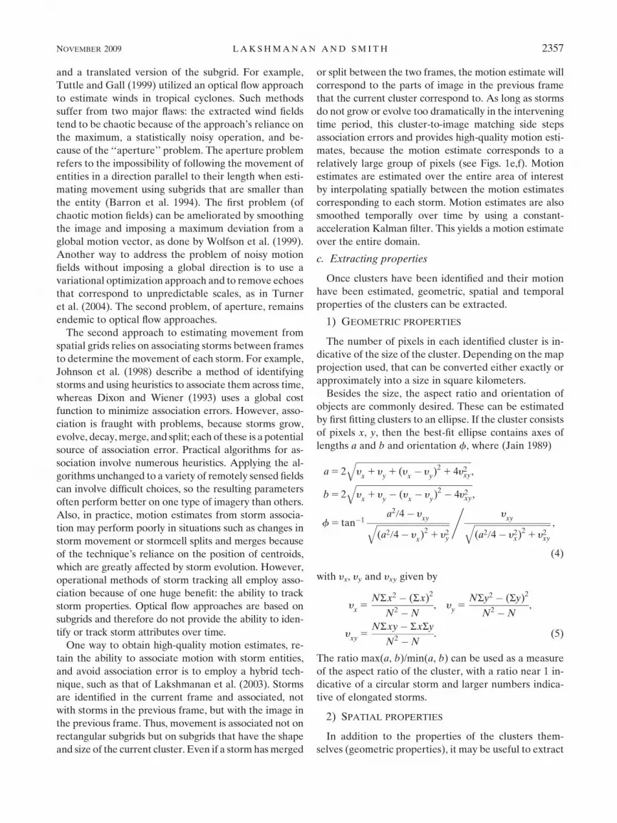
Several other geometric and spatial properties were

extracted for each cluster at a scale of 480 km2 (see

Table 1).

The set of patterns corresponding to all the storms

from the 72 images where storm-type polygons were

manually drawn were then presented to the automated

decision tree algorithm of Quinlan (1993) as im-

plemented by Witten and Frank (2005). It was found

that 30% of the training patterns were reserved for

pruning the created decision tree (to limit overfitting).


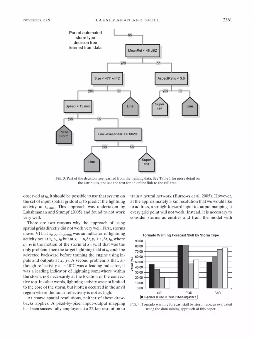
Part of the resulting decision tree is shown in Fig. 3. The

full decision tree (as Java source code) is available on-

line at http://cimms.ou.edu/;lakshman/aicompetition/.

On an independent test set of 72 more images, the de-

cision tree had a multicategory true skill statistic (Wilks

1995) of 0.58. More sophisticated data mining tech-

niques yielded only marginal improvements over the

plain decision tree (Lakshmanan et al. 2008) but lose the

easy understandability of the machine model that a de-

cision tree provides.

The trained decision tree was then used to classify

all identified storms on 12 outbreak days over the en-

tire continental United States. Every tornado warning

issued by the NWS on those days was associated with the

closest storm to the start of the polygon and thus to the

storm type of that storm. Forecast skill was then com-

puted conditioned on the type of storm.

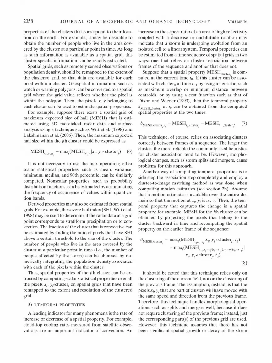
In the case of tornado warnings, there was a significant

(95% confidence) difference in skill between supercells

and pulse storms, as shown in Fig. 4. The significant

difference in skill held for all pairs of storm types except

between convective lines and supercells. A data mining

approach was thus used to show that tornado warning

skill varies by storm type. For more results from this

study, including lead time and the skill associated with

thunderstorm warnings, see Guillot et al. (2008).

b. Lightning prediction

As another illustration of the utility of the attribute-

extraction technique described in this paper, consider

the problem of predicting cloud-to-ground lightning

activity. A data mining approach may involve finding

leading indicators of lightning and then using those to

predict the onset of lightning activity. For example,

Hondl and Eilts (1994) found that radar reflectivity at

2108C was an indicator of lightning. Watson et al. (1995)

suggested the use of vertically integrated liquid (VIL;

Greene and Clark 1972) as a predictor.

One advantage of cloud-to-ground lightning is that it

is a hazard that is observed in real time. There is no

similar real-time source of information on other severe

weather hazards such as hail. Thus, it is possible to

consider creating a data mining approach to predict

cloud-to-ground lightning. If a system can be trained on

input spatial grids of reflectivity and VIL at t230min to

predict the cloud-to-ground lightning activity that is

TABLE 1. Attributes extracted automatically to help answer the question of forecaster skill according to storm type.

Attribute Source (Cluster/Grid) Unit Description

Speed Motion m s21 Movement of cluster

Size Geometric km2 Size of cluster

Orientation Geometric 8 f in ellipse fit

Aspect ratio Geometric none max(a, b)/min(a, b) in ellipse fit

Convective area Severe hail index km2 Count of severe hail index $0.5

Low-level shear Azimuthal shear layer average s21 Max absolute value in cluster

MESH Expected hail size mm Max value in cluster

Max reflectivity Reflectivity composite dBZ Max value in cluster

Mean reflectivity Reflectivity composite dBZ Mean reflectivity in cluster

Max VIL VIL kg m22 Max value in cluster

FIG. 2. (a) An expert drew polygons by hand around storms and labeled each polygon with

the storm type of the storms contained within it. (b) The polygons drawn by the expert were

converted into a spatial grid. The storm-type grid is treated as observed data and a storm type

(supercell or pulse storm for the storms in this image) is associated with every cluster.


observed at t0, it should be possible to use that system on

the set of input spatial grids at t0 to predict the lightning

activity at t30min. This approach was undertaken by

Lakshmanan and Stumpf (2005) and found to not work

very well.

There are two reasons why the approach of using

spatial grids directly did not work very well. First, storms

move. VIL at xi, yi, t230min was an indicator of lightning

activity not at xi, yi, t0 but at xi 1 uidt, yi 1 yidt, t0, where

ui, yi is the motion of the storm at xi, yi. If that was the

only problem, then the target lightning field at t0 could be

advected backward before training the engine using in-

puts and outputs at xi, yi. A second problem is that, al-

though reflectivity at 2108C was a leading indicator, it

was a leading indicator of lightning somewhere within

the storm, not necessarily at the location of the convec-

tive top. In other words, lightning activity was not limited

to the core of the storm, but it often occurred in the anvil

region where the radar reflectivity is not as high.

At coarse spatial resolutions, neither of these draw-

backs applies. A pixel-by-pixel input–output mapping

has been successfully employed at a 22-km resolution to

train a neural network (Burrows et al. 2005). However,

at the approximately 1-km resolution that we would like

to address, a straightforward input to output mapping at

every grid point will not work. Instead, it is necessary to

consider storms as entities and train the model with

FIG. 3. Part of the decision tree learned from the training data. See Table 1 for more detail on

the attributes, and see the text for an online link to the full tree.

FIG. 4. Tornado warning forecast skill by storm type, as evaluated

using the data mining approach of this paper.


storm properties, not just pixel values. This, of course,

is exactly what the attribute-extraction technique de-

scribed in this paper provides.

Cloud-to-ground strike locations from the National

Lightning Detection Network (NLDN) were averaged

in space (3-km radius) and time (15 min) to create a

lightning density grid; that is, the value of the grid at any

point was an exponentially weighted number of strikes

within 15 min and 3 km of the point with farther away

flashes receiving less weight.

The t30min lightning density grid was advected backward

30 min and used as one of the inputs to the attribute-

extraction algorithm. Clustering was performed on a

multiradar reflectivity composite image over the conti-

nental United States (Lakshmanan et al. 2006) at a scale

(minimum size threshold) of 200 km2. Cluster attributes

were extracted using spatial grids of VIL, reflectivity

isotherms, current lightning density (the full list of at-

tributes are listed in Table 2), and the t30min lightning

density that was advected backward 30 min.

A neural network was trained using spatial (1-km

resolution every 5 min) grids over the continental United

States on six days between April and September 2008:

10 April, 14 May, 13 June, 1 July, 20 August, and 11

September.2 The output of the neural network is a

number between 0 and 1 that, because of our choice of

neural network architecture, is the probability of the

storm producing lightning 30 min later. This output was

thresholded to yield a binary outcome: lightning or no

lightning. The variation of the skill of the neural network

and steady-state technique on an independent test set at

different thresholds is shown in Fig. 5. If the output of the

trained neural network is thresholded at 0.41, then the

algorithm has its maximum critical success index (CSI;

Donaldson et al. 1975) of 0.79 when predicting lightning

activity 30 min ahead. By way of contrast, simply ad-

vecting the current lightning density field (and thresh-

olding the forecast field at zero, where the steady-state

technique’s skill is maximum) attains a CSI of 0.69. Other

skill scores at the same thresholds are shown in Table 3.

The difference in the probability of detection (POD)

between the data mining technique of this paper and the

simple steady-state forecast is on the order of 0.2 (0.91

versus 0.71: see Table 3). By definition, the steady-state

forecast consists of already occurring lightning activity.

Therefore, the increase of 0.2 in POD has to be due to

successfully predicted lightning initiation. However,

the price of this increase in POD is a corresponding in-

crease in the false alarm rate (of about 0.1). On balance,

though, the technique demonstrates improvements in

CSI of 0.1 and in Heidke skill score (HSS; Heidke 1926)

of 0.04. Thus, the technique is able to predict the initi-

ation of lightning with skill.

In real time, the neural network is employed to predict

the lightning activity associated with a storm. This

probability is distributed within the extent of the storm

and then advected forward in time to yield the proba-

bility of cloud-to-ground lightning at a particular point

30 min in the future. Example output from the algo-

rithm is shown in Fig. 6. Note that the algorithm is able

to successfully predict initiation of lightning in the storm

in the south-central part of the domain.

TABLE 2. Attributes extracted from clusters for the lightning prediction algorithm. ‘‘Cluster to image’’ refers to the second approach of

estimating temporal properties described in section 2. The units of lightning density are flashes (fl) per square kilometer per second.

Attribute Source (cluster/grid) Unit Description

Speed Motion m s21 Movement of cluster

Size Geometric km2 Size of cluster

Orientation Geometric 8 f in ellipse fit

Aspect ratio Geometric none max(a, b)/min(a, b) in ellipse fit

Max reflectivity Reflectivity composite dBZ Max value in cluster

Reflectivity 2108C Reflectivity 2108C dBZ Max value in cluster

Reflectivity 2108C increase Reflectivity 2108C dBZ d (cluster to image)

Layer average reflectivity Reflectivity 2208 to 08C dBZ Average value in cluster

VIL VIL kg m22 Average value in cluster

VIL increase VIL kg m22 d (cluster to image)

Max VIL VIL kg m22 Max value in cluster

Lightning density Lightning density at t0 fl km22 s21 Max value in cluster

Ideal lightning density Lightning density at t30 fl km22 s21 Max value in cluster

(reverse advected)

2 These days were selected because they had relatively wide-

spread lightning activity and because we did not experience hard-

ware or software problems when collecting the data on these days.

The resulting patterns were randomly divided into three sets of

50%, 25%, and 25%, which were used for training, validation, and

testing, respectively. A neural network with one hidden layer

consisting of eight nodes was trained on the training set, with

the validation set utilized for early stopping to limit overfitting. The

transfer function of the output node was a sigmoid so that the

neural network output is a true probability (Bishop 1995).


4. Discussion

This paper described a technique of automatically

extracting geometric, spatial and temporal attributes

of storms. The technique is comprised of three steps.

The first step is clustering a geospatial grid using an

expectation-minimization criterion that balances the

needs of self-similarity and spatial contiguity within and

between clusters. The clustering can be controlled in a

general-purpose manner through a saliency criterion

based on size. The second step is estimating motion us-

ing a hybrid technique that relies on the best match

between the clusters in one frame and the image itself in

the previous frame. Spatial and temporal smoothness of

the motion estimates are achieved by interpolation and

Kalman filtering. The third step is using the pixels that

belong to the cluster to fit the cluster to an ellipse to

extract geometric properties. Spatial properties can be

extracted by computing scalar statistics on appropriately

remapped spatial grids over the pixels that belong to the

cluster. Temporal properties can be computed in one of

two ways depending on whether association errors or

growth/decay is more likely in the time period of interest.

The technique when applied to large collections of

imagery yields a pattern (i.e., a set of attributes) for each

identified storm. These patterns can be used as inputs

to standard statistical or data mining techniques. The

utility of such an approach was illustrated by considering

two problems: forecaster skill in issuing tornado warn-

ings and the creation of a real-time, high-resolution

lightning prediction algorithm.

Object identification is also now an active area of re-

search in model verification (Marzban and Sandgathe

2006; Davis et al. 2006). However, the challenge in that

area is quite different and cannot be addressed by the

technique of this paper. In object-based model verifi-

cation, objects are identified in both model forecasts

and observed fields and an attempt is made to associate

observed objects with forecast objects (and vice versa)

based on their properties. The method of this paper

deals with objects identified on one spatial field and

properties of that object extracted from other spatial

fields. In doing so, an implicit assumption is made that

the extracted object is aligned in all the fields, an as-

sumption that holds on observed data but emphatically

(given the skill of present-day models) does not hold for

observed data versus model forecasts.

The technique described in this paper allows for the

extraction of properties at different scales. However, it is

not yet known how to select the size parameter that de-

termines the scale. For example, would the lightning pre-

diction have been improved if the size threshold had been

set to 150 km2 instead of 200 km2? Currently, this can be

determined only through experimentation. An objective

scale selection criterion would be an improvement.

The lightning prediction algorithm is ongoing work,

presented to illustrate the utility of being able to rap-

idly build automated algorithms by training on copious

amounts of data. The authors are continuing to collect

data and will retrain the system on a year’s worth of

geospatial grids (the current training set was limited to

the warm season only). At that time, it is expected that

testing will be expanded to a larger dataset. Also, it is

FIG. 5. Skill of steady-state method and trained neural network at predicting lightning ac-

tivity 30 min into the future as the threshold on the output grids is varied to yield a binary yes/no

decision. CSI, HSS, POD, and FAR are shown. The current lightning density field was advected

to create the steady-state forecasts.

TABLE 3. Skill of steady-state method and trained neural net-

work at predicting lightning activity 30 min into the future. The

neural network achieves its peak skill in CSI (see Fig. 5) at a

threshold of 0.41, whereas the steady-state method achieves its

peak skill at a threshold of zero. All the statistics correspond to

those thresholds.

Skill score Steady state Neural network

POD 0.71 0.91

FAR 0.04 0.14

CSI 0.69 0.79

HSS 0.85 0.89


expected that other forecast time periods (besides the

30 min used in this illustration) will be of interest. A

clustering saliency of 200 km2 was arbitrarily chosen

here; it is to be expected that a different clustering sa-

liency may provide superior skill and that different

forecast time periods will require different saliencies.

As another example of the type of data mining work

that this algorithm enables, Bedka et al. (2009) track

cloud-top cooling rates from high-resolution satellite

imagery to predict the onset of convecting initiation,

with the aim of improving the pixel-by-pixel technique

of Mecikalski et al. (2008).

Acknowledgments. Funding for this research was

provided under NOAA–OU Cooperative Agreement

NA17RJ1227, Engineering Research Centers Program

(NSF 0313747). The attribute-extraction algorithm de-

scribed in this paper has been implemented within the

Warning Decision Support System Integrated Information

(WDSSII; Lakshmanan et al. 2007) as the w2segmotionll

process (available online at http://www.wdssii.org).

REFERENCES

Barron, J. L., D. J. Fleet, and S. S. Beauchemin, 1994: Performance

of optical flow techniques. Int. J. Comput. Vis., 12, 43–77.

Bedka, K. M., W. F. Feltz, J. Sieglaff, R. Rabin, M. J. Pavolonis,

and J. C. Brunner, 2009: Toward and end-to-end satellite-

based convective nowcasting system. Preprints, 16th Conf. on

Satellite Meteorology and Oceanography, Phoenix, AZ, Amer.

Meteor. Soc., J15.2.

Bishop, C. M., 1995: Neural Networks for Pattern Recognition.

Oxford University Press, 482 pp.

Burrows, W., C. Price, and L. Wilson, 2005: Warm season lightning

probability prediction for Canada and the northern United

States. Wea. Forecasting, 20, 971–988.

Davies, J., 2004: Estimations of CIN and LFC associated with

tornadic and nontornadic supercells. Wea. Forecasting, 19,714–726.

Davis, C., B. Brown, and R. Bullock, 2006: Object-based verification

of precipitation forecasts. Part I: Methodology and application

to mesoscale rain areas. Mon. Wea. Rev., 134, 1772–1784.

Dixon, M., and G. Wiener, 1993: TITAN: Thunderstorm Identifi-

cation, Tracking, Analysis, and Nowcasting—A radar-based

methodology. J. Atmos. Oceanic Technol., 10, 785–797.

Donaldson, R., R. Dyer, and M. Kraus, 1975: An objective evalu-

ator of techniques for predicting severe weather events. Pre-

prints, Ninth Conf. on Severe Local Storms, Norman, OK,

Amer. Meteor. Soc., 321–326.

Greene, D. R., and R. A. Clark, 1972: Vertically integrated liquid

water—A new analysis tool. Mon. Wea. Rev., 100, 548–552.

Guillot, E., T. Smith, V. Lakshmanan, K. Elmore, D. Burgess, and

G. Stumpf, 2008: Tornado and severe thunderstorm warning

forecast skill and its relationship to storm type. Preprints, 24th

Conf. on IIPS, New Orleans, LA, Amer. Meteor. Soc., 4A.3.

Hand, D., H. Mannila, and P. Smyth, 2001: Principles of Data

Mining. MIT Press, 546 pp.

Heidke, P., 1926: Berechnung des erfolges und der gute der wind-

starkvorhersagen im sturmwarnungsdienst. Geogr. Ann., 8,

301–349.

Hondl, K., and M. Eilts, 1994: Doppler radar signatures of devel-

oping thunderstorms and their potential to indicate the onset

of cloud-to-ground lightning. Mon. Wea. Rev., 122, 1818–1836.

FIG. 6. The lightning prediction algorithm in real time on 28 Apr 2009 over East Texas:

(a) lightning density at 1300 UTC; (b) reflectivity composite, the field on which storm identi-

fication is carried out; (c) identified storms, with different storms shaded differently; (d) re-

flectivity at 2108C, one of the spatial attributes considered; (e) predicted probability of

lightning 30 min later; and (f) actual lightning density at 1330 UTC.


Hong, Y., K. Hsu, S. Sorooshian, and X. Gao, 2004: Precipitation

estimation from remotely sensed imagery using an artificial

neural network cloud classification system. J. Appl. Meteor.,

43, 1834–1853.

Jain, A. K., 1989: Fundamentals of Digital Image Processing.

Prentice Hall, 569 pp.

Johnson, J. T., P. L. MacKeen, A. Witt, E. D. Mitchell,

G. J. Stumpf, M. D. Eilts, and K. W. Thomas, 1998: The storm

cell identification and tracking algorithm: An enhanced WSR-

88D algorithm. Wea. Forecasting, 13, 263–276.

Kessinger, C., S. Ellis, and J. Van Andel, 2003: The radar echo

classifier: A fuzzy logic algorithm for the WSR-88D. Preprints,

Third Conf. on Artificial Applications to the Environmental

Science, Long Beach, CA, Amer. Meteor. Soc., P1.6. [Available

online at http://ams.confex.com/ams/pdfpapers/54946.pdf.]

Lakshmanan, V., and G. Stumpf, 2005: A real-time learning tech-

nique to predict cloud-to-ground lightning. Preprints, Fourth

Conf. on Artificial Intelligence Applications to Environmental

Science, San Diego, CA, Amer. Meteor. Soc., J5.6. [Available

online at http://ams.confex.com/ams/pdfpapers/87206.pdf.]

——, R. Rabin, and V. DeBrunner, 2003: Multiscale storm iden-

tification and forecast. Atmos. Res., 67, 367–380.

——, T. Smith, K. Hondl, G. J. Stumpf, and A. Witt, 2006: A real-

time, three-dimensional, rapidly updating, heterogeneous ra-

dar merger technique for reflectivity, velocity and derived

products. Wea. Forecasting, 21, 802–823.

——, ——, G. J. Stumpf, and K. Hondl, 2007: The Warning Deci-

sion Support System—Integrated Information. Wea. Fore-

casting, 22, 596–612.

——, E. Ebert, and S. Haupt, 2008: The 2008 artificial intelligence

competition. Preprints, Sixth Conf. on Artificial Intelligence

Applications to Environmental Science, New Orleans, LA,

Amer. Meteor. Soc., 2.1. [Available online at http://ams.confex.

com/ams/pdfpapers/132172.pdf.]

——, K. Hondl, and R. Rabin, 2009: An efficient, general-purpose

technique for identifying storm cells in geospatial images.

J. Atmos. Oceanic Technol., 26, 523–537.

Marzban, C., and G. Stumpf, 1996: A neural network for tornado

prediction based on Doppler radar-derived attributes. J. Appl.

Meteor., 35, 617–626.

——, and A. Witt, 2001: A Bayesian neural network for severe-hail

size prediction. Wea. Forecasting, 16, 600–610.

——, and S. Sandgathe, 2006: Cluster analysis for verification of

precipitation fields. Wea. Forecasting, 21, 824–838.

Mecikalski, J., K. Bedka, S. Paech, and L. Litten, 2008: A statistical

evaluation of GOES cloud-top properties for nowcasting

convective initiation. Mon. Wea. Rev., 136, 4899–4914.

Najman, L., and M. Schmitt, 1996: Geodesic saliency of watershed

contours and hierarchical segmentation. IEEE Trans. Pattern

Anal. Mach. Intell., 18, 1163–1173.

Quinlan, J. R., 1993: C4.5: Programs for Machine Learning. Morgan

Kaufmann, 302 pp.

Stumpf, G. J., A. Witt, E. D. Mitchell, P. L. Spencer, J. T. Johnson,

M. D. Eilts, K. W. Thomas, and D. W. Burgess, 1998: The

National Severe Storms Laboratory mesocyclone detection

algorithm for the WSR-88D. Wea. Forecasting, 13, 304–326.

Trapp, J., S. Tessendorf, E. Godfrey, and H. Brooks, 2005: Tor-

nadoes from squall lines and bow echoes. Part I: Climatolog-

ical distribution. Wea. Forecasting, 20, 23–34.

Turner, B. J., I. Zawadzki, and U. Germann, 2004: Predictability

of precipitation from continental radar images. Part III:

Operational nowcasting implementation (MAPLE). J. Appl.

Meteor., 43, 231–248.

Tuttle, J., and R. Gall, 1999: A single-radar technique for esti-

mating the winds in tropical cyclones. Bull. Amer. Meteor.

Soc., 80, 653–668.

Watson, A. I., R. L. Holle, and R. E. Lopez, 1995: Lightning from

two national detection networks related to vertically inte-

grated liquid and echo-top information from WSR-88D radar.

Wea. Forecasting, 10, 592–605.

Wilks, D. S., 1995: Statistical Methods in Atmospheric Sciences:

An Introduction. International Geophysical Series, Vol. 59,

Academic Press, 467 pp.

Witt, A., M. Eilts, G. Stumpf, J. Johnson, E. Mitchell, and

K. Thomas, 1998: An enhanced hail detection algorithm for

the WSR-88D. Wea. Forecasting, 13, 286–303.

Witten, I., and E. Frank, 2005: Data Mining. Elsevier, 524 pp.

Wolfson, M., B. Forman, R. Hallowell, and M. Moore, 1999: The

growth and decay storm tracker. Preprints, Eighth Conf. on

Aviation, Dallas, TX, Amer. Meteor. Soc., 58–62.


Data Mining Storm Attributes from Spatial Grids

Documents

Transcript of Data Mining Storm Attributes from Spatial Grids