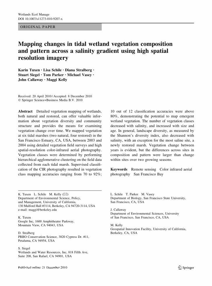
ORIGINAL PAPER

Mapping changes in tidal wetland vegetation compositionand pattern across a salinity gradient using high spatialresolution imagery

Karin Tuxen • Lisa Schile • Diana Stralberg •

Stuart Siegel • Tom Parker • Michael Vasey •

John Callaway • Maggi Kelly

Received: 20 April 2010 / Accepted: 8 December 2010! Springer Science+Business Media B.V. 2010

Abstract Detailed vegetation mapping of wetlands,

both natural and restored, can offer valuable infor-mation about vegetation diversity and community

structure and provides the means for examining

vegetation change over time. We mapped vegetationat six tidal marshes (two natural, four restored) in the

San Francisco Estuary, CA, USA, between 2003 and2004 using detailed vegetation field surveys and high

spatial-resolution color-infrared aerial photography.

Vegetation classes were determined by performinghierarchical agglomerative clustering on the field data

collected from each tidal marsh. Supervised classifi-

cation of the CIR photography resulted in vegetationclass mapping accuracies ranging from 70 to 92%;

10 out of 12 classification accuracies were above

80%, demonstrating the potential to map emergentwetland vegetation. The number of vegetation classes

decreased with salinity, and increased with size and

age. In general, landscape diversity, as measured bythe Shannon’s diversity index, also decreased with

salinity, with an exception for the most saline site, anewly restored marsh. Vegetation change between

years is evident, but the differences across sites in

composition and pattern were larger than changewithin sites over two growing seasons.

Keywords Remote sensing ! Color infrared aerialphotography ! San Francisco Bay

K. Tuxen ! L. Schile ! M. Kelly (&)Department of Environmental Science, Policy,and Management, University of California,130 Mulford Hall #3114, Berkeley, CA 94720-3114, USAe-mail: maggi@berkeley.edu

K. TuxenGoogle Inc, 1600 Amphitheatre Parkway,Mountain View, CA 94043, USA

D. StralbergPRBO Conservation Science, 3820 Cypress Dr. #11,Petaluma, CA 94954, USA

S. SiegelWetlands and Water Resources, Inc, 818 Fifth Ave,Suite 208, San Rafael, CA 94901, USA

L. Schile ! T. Parker ! M. VaseyDepartment of Biology, San Francisco State University,San Francisco, CA, USA

J. CallawayDepartment of Environmental Sciences, Universityof San Francisco, San Francisco, CA, USA

M. KellyGeospatial Innovation Facility, University of California,Berkeley, CA, USA

123

Wetlands Ecol Manage

DOI 10.1007/s11273-010-9207-x

Introduction

Nearly half of the world’s wetlands have been diked,drained, filled, or otherwise lost (Zedler and Kercher

2005), with an 80% loss in developed countries

(Pennings and Bertness 2001). Furthermore, much ofthe remaining wetland area has been degraded by

human activities (Zedler and Kercher 2005).

Recently, there have been significant endeavors torestore wetland habitat throughout the world (Zedler

and Kercher 2005), particularly within major estuar-

ies such as the San Francisco Estuary, where there isthe potential to restore large expanses of tidal marsh

(Williams and Faber 2001). Tidal marshes provide

multiple ecosystem services, habitat for endangeredspecies, flood-control benefits, and, under the right

conditions, can sequester carbon at high rates

(Chmura et al. 2003), providing a potential additionaleconomic incentive for restoration with the emer-

gence of global carbon markets.

Fine-scaled mapping of tidal marsh vegetation isimportant to restoration efforts because it enables

vegetation inventory and change detection, which

informs overall habitat quality for numerous speciesand other important processes like sedimentation.

Wetland vegetation classification using remote-sens-

ing imagery analysis can be challenging, however,because of the high level of spectral confusion with

other land cover classes, among different types of

wetlands (Andresen et al. 2002; Ozesmi and Bauer2002), and among different vegetation species (Oze-

smi and Bauer 2002; Ramsey and Laine 1997; Schmidt

and Skidmore 2003). Floristically-detailed mapping oftidal marsh vegetation is especially challenging in

brackish marshes, which exhibit high levels of patch-

iness in plant species diversity and distribution.The value of remote sensing for wetland monitor-

ing has long been recognized (Hinkle and Mitsch

2005; Phinn et al. 1996), and recent advancementshave made the methods and tools more applicable

and cost-effective. Automated (computer-assisted)

image analysis approaches allow for objective, con-sistent, and repeatable results, making them more

scientifically defensible, especially across large, het-

erogeneous areas. The use of automated imageclassification reduces inconsistencies and error intro-

duced through visual photo-interpretation of imagery.

For this reason, automated image classification acrossmultiple sites and time periods is more consistent and

cost-effective than visual delineation and classifica-tion (Thomson et al. 2003).

Automated pixel-based classification methods are

typically unsupervised, supervised, or a hybrid of bothapproaches. Unsupervised classification performs spec-

tral clustering without a priori input from the analyst.

Supervised classification is informed by ground refer-ence field data as the analyst ‘‘trains’’ the classification

algorithm. Both types have been used successfully in

wetlands but there is no consensus regarding the bestmethod (Belluco et al. 2006; Thomson et al. 1998,

2003). Our study had detailed and abundant field data

collected to informmapping and vegetation analyses, sowe elected to use a supervised classification approach

with high spatial resolution color infrared digital

imagery to map dominant vegetation types.Our overall goal was to characterize the range of

variation invegetationcomposition anddiversity among

sites and years and to demonstrate the accessibility ofremote sensing to restoration ecologists for monitoring

and assessment of marsh vegetation. Our specific

objective was to map tidal marsh vegetation in marshesalong a salinity gradient using high resolution (1-m

pixel) color infrared (CIR) imagery, and to examine

changes in vegetation composition and pattern over twogrowing seasons. First, we separated each site into

vegetation, non-vegetation, and bare areas based on a

simple normalized difference vegetation index (NDVI)threshold. Second, we used detailed, extensive, and

targeted field-based vegetation data to determine the

land cover classification scheme for each site so that itcorresponded to the floristic data at the site, and cross-

walkedwith alliances found in the CaliforniaManual of

Vegetation (Sawyer et al. 2009). We then used the fielddata to train a supervised classification algorithm tomap

the landcover classes at each site across 2 years, and

assessed the accuracy of the resulting maps. Finally, wecalculated landscape metrics at both natural and restor-

ing tidal marshes over two growing periods.

Methods

Study sites

This research was performed as part of the Integrated

Regional Wetland Monitoring (IRWM) Pilot Project

(http://www.irwm.org/), a multi-investigator interdis-ciplinary research project with the goal of evaluating

Wetlands Ecol Manage

123

how wetland restoration efforts throughout the SanFrancisco Estuary, California, USA are affecting

ecosystem processes at different spatial and temporal

scales; and to prepare for subsequent longer-termmonitoring. The IRWM project vegetation compo-

nent focused on data collection between 2003 and

2004.Our study sites were located in the Sacramento-

San Joaquin Delta and San Pablo Bay, within the

greater San Francisco Estuary (Fig. 1; hereaftercalled the Estuary). The Estuary is comprised of

both natural and restored wetlands, as well as

potential restoration sites such as diked baylandareas, former salt ponds, and seasonal and perennial

wetlands. Mean salinities across our study sites

ranged from approximately 15.40% at the western-most study site to 0.17% at the easternmost site

(Table 1). The Estuary is one of the most modified

estuaries in the United States, with history of land andwater development and reclamation, over-fishing, and

waste disposal since 1850 (Nichols et al. 1986).

The six sites that we mapped were (from west toeast): Petaluma River Marsh (PRM) on the Petaluma

River; Pond 2A (P2A), Coon Island (CI), and Bull

Island (BuI) on the Napa River; and Browns Island(BrI) and Sherman Lake (SL) in the western

Sacramento-San Joaquin River Delta (Fig. 1).Browns Island and Sherman Lake are located at the

confluence of the Sacramento and San Joaquin

Rivers, a combined watershed of 257,000 km2, andreceive considerable freshwater input. These two

sites are oligohaline (i.e. characterized by low salinity

(0.5–5 ppt)). under most climate conditions butduring drought years can be subject to higher salinity

levels. Two of the six sites, Coon Island and Browns

Island, are mature marshes (a combination of ancientand centennial marshland); the remaining four sites

were restored within the last 90 years (Table 1).

Study sites were chosen because they were represen-tative of the dominant salinity gradient in the Estuary.

It is widely accepted that in coastal wetlands plant

species richness decreases with salinity due to salinityand inundation-driven osmotic stresses; brackish and

freshwater tidal marshes are characterized by diverse

species mixtures due to reduced osmotic stresses(Engels and Jensen 2009; Sharpe and Baldwin 2009).

These latter marshes usually are composed of several

co-dominant plant species with numerous sub-dom-inant species and configured in a heterogeneous

mosaic of vegetation community types, often with

poorly defined boundaries between patch types. In theEstuary, salt marshes have between 2 and 22 plant

Fig. 1 Study Site Vicinity.The study sites, from westto east, are Petaluma RiverMarsh (PRM) on thePetaluma River; Bull Island(BuI), Coon Island (CI),Pond 2A (P2A) on the NapaRiver; and Browns Island(BrI) and Sherman Lake(SL) in the west Delta

Wetlands Ecol Manage

123

species, brackish marshes contain 27–65 species, and

freshwater marshes have upwards of 117 species

(Parker, unpublished data).Among our study sites, dominant species composi-

tion was variable. Petaluma River Marsh is the most

saline marsh and consisted of four dominant species:California cordgrass (Spartina foliosa Trin.), common

perennial pickleweed (Sarcocornia pacifica (Standl.)

A. J. Scott), annual pickleweed (Salicornia depressaStandl.), and alkali bulrush (Bolboschoenus maritimusPalla). The threeNapaRiver sites are brackishmarshes,

and consisted primarily of the same salt marsh specieswith the addition of more salt-sensitive marsh species:

three-square common bulrush (Schoenoplectus amer-icanus (Persoon) Volkart ex Schinz & R. Keller),common tule (S. acutus var. occidentalis (Muhlenberg

ex Bigelow) A. Love & D. Love), California tule/

bulrush (S. californicus (C. A. Mey.) Sojak), and threecattail species (Typha angustifolia L., T. domengensisPersoon, and T. latifolia L.). Perennial pepperweed

(Lepidium latifolium Linn.) also exists at Coon, Bull,and Browns Island sites. In the freshwater sites,

dominant vegetation consisted of S. americanus,S. acutus, S. californicus, and all Typha species, withthe addition of alkali common reed (Phragmitesaustralis (Cav.) Trin. ex Steud.). Gumplant (Grindeliastricta var. stricta (A.Gray)M.A. Lane) occurred at allthe study sites along channel margins, levees, and

upland areas.

Image acquisition and pre-processing

We used CIR aerial photography that was acquiredfor all of the IRWM project sites in October of 2003

and August of 2004. Imagery was captured with a

Zeiss RMK Top 15 film camera, equipped withforward motion compensation and a Pleogon A3/4

lens with 153 mm focal length. The imagery was

captured at the lowest possible tide in 2003 to aid

vegetation and geomorphic mapping; in 2004, imag-ery was taken at mid-tide to aid channel delineation.

Mid-tide level had the advantage of helping delineate

channels because they had some water in them, butthe level was not high enough to flood the wetland

plane and subcanopy, and thus the vegetation clas-

sification should be comparable between years. Thisimage had three bands: near infrared, red, and green.

All sites were flown at a scale of 1:9,600 and the

hardcopy CIR photography was scanned at a resolu-tion of 1,200 dots per inch (dpi), resulting in a pixel

size of 0.2-m for all sites. The only exception was

that in 2003 only, Petaluma River Marsh was flownfor use with another project and had a slightly

different flight scale (1:7,200). Imagery is available

for download at http://www.irwm.org/. The overallgoal was to achieve the same scale and pixel reso-

lution for all sites, regardless of site size, in order to

achieve uniform data for subsequent analyses. Weused digital photography for this project for two

reasons: first, we could control the time of image

acquisition; and second there is less problems withatmospheric influence with aerial photography.

We utilized at least four Trimble GPS-located (sub-

meter accuracy) geospatial ground control points torectify each photo. These points generally were located

in different corners of each site, in order to maximize

the accuracy of the rectification process (Trimble Inc.2005). The images were orthorectified and digital

elevationmodels (DEMs)were used in the rectification

process to account for the local terrain’s effect onimage distortion, using publicly available USGS 10-m

DEMs. The accuracy standards employed for ortho-

rectification were such that approximately 90% of allcontrol points on the photos were within two meters of

their corresponding ground coordinates.

Table 1 Summary of study site attributes

Study site Location Mean salinity (ppt) Tide range (m) Marsh type Status Year restored Size (ha)

PRM San Pablo Bay 15.40 1.44 Salt Restored 1994 19.4

P2A Napa River 12.28 1.32 Brackish Restored 1995 215.6

CI Napa River 11.88 1.53 Brackish Natural/mature Ancient and centennial 162.2

BuI Napa River 9.40 1.50 Brackish Restored 1950s 43.7

BrI Delta 1.84 0.97 Fresh Natural/mature Ancient 276.4

SL Delta 0.17 0.94 Fresh Restored 1920s 393.3

Wetlands Ecol Manage

123

In preparation for image analysis and metriccalculation, we re-sampled all the imagery from

0.2-m pixel size to 1-m pixel size. The images were

resampled to a coarser pixel size for three reasons.First, the imagery contained high pixel variability that

is common with hyperspatial data, and we wanted to

reduce the amount of spurious pixels in the classifi-cation output. Second, 1-m resolution was considered

appropriate for the development of avian habitat

models (Dechka et al. 2002; Stralberg et al. 2010).Third, we wanted to enable better GIS computing

using the classification output, including the calcula-

tion of landscape pattern metrics.

Field data collection

We collected ground reference data to guide the

classification scheme, train the classification of the

imagery, and to assess the accuracy of the final maps.Ground reference data points were stratified by

vegetation classes. In 2003, the field effort was

carried out in two phases. During the first phase, wecollected ground data for training the image classi-

fication using a supervised approach, in which a

classification algorithm assigns a class to each pixelacross using correlations between ground data and

image spectral properties (Justice and Townshend

1981). We collected data at points that wererandomly-generated in a Geographic Information

System (GIS) prior to field visits, and points were

chosen during the field visit at the discretion of thefield samplers to train the image classification more

effectively, especially for rare or underrepresented

communities. The randomly-generated points werestratified across general vegetation groups that we

created prior to our field visit using a simple

unsupervised classification. We employed this stepto account for the limited prior knowledge of the

vegetation that occurred in the sites. Handheld

Garmin GPS units with an average recorded locationerror of 5 m were used to navigate to each point.

During the second 2003 field phase, we collected dataat randomly-generated points to assess the accuracy

of the 2003 classified vegetation map. In 2004, we

conducted only one field phase that consisted ofaccuracy assessment data collection at randomly-

generated points that were stratified along 2003

vegetation classes and area-weighted.

At all points visited during both years, the field

crew recorded absolute percent cover of all specieswithin a three-meter diameter circular plot. We chose

this plot size in order to accurately represent species

coverage based on observations of the average sizeand distribution of tidal wetland plants in this region

and because these data were collected for purposes

other than vegetation mapping. Percent cover wasestimated using a seven-category modified Dauben-

mire ranking system (Daubenmire 1959). Species

composition and cover data have been used fre-quently as indicators of ecosystem processes and are

a useful component of ecosystem classifications

(Mueller-Dombois and Ellenberg 1974). Between50 and 300 plots were visited at each site in 2003 and

2004 (Table 2). Due to delicate conditions at some of

the sites, including soft sediments and bird nestingterritories, the field crew had the choice to observe

the plot from a few meters away. We used this

practice on less than 10% of the data points.

Image classification

Our classification involved several steps that are

outlined in Fig. 2. We performed all image classifi-

cation work with Leica Geosystem’s Erdas Imaginesoftware (Leica Geosystems Inc. 2006).

Vegetation classification scheme

The most important first step in image classification

is to choose or create a relevant classification schemethat is ecologically meaningful and as unbiased as

possible (Jensen 2000). Many remote sensing map-

ping projects use a pre-defined classification scheme(e.g. USGS Landcover scheme (Anderson et al.

Table 2 Field data summary

Studysite

Training points(random/non-random)

Random pointsused for accuracyassessment, 2003

Random pointsused for accuracyassessment, 2004

PRM 29/7 217 234

P2A 39/47 182 279

CI 27/43 206 236

BuI 24/43 160 296

BrI 24/30 151 272

SL 29/41 101 53

Wetlands Ecol Manage

123

1976)); but such course landcover schemes do not

capture the detailed and complex floristic patterns ofeach site. Instead we matched our field data to the

alliance level listed in the Manual of California

Vegetation (Sawyer and Keeler-Wolf 2004; Sawyeret al. 2009). The concept of the alliance is a

physiognomically uniform plant group with one or

more dominant/diagnostic species. We accomplishedthis by using the field data from all the randomly-

generated points from both years, and performed an

agglomerative hierarchical clustering measure inPC-ORD (McCune and Mefford 1999) for each site.

These kinds of cluster analyses partition

heterogeneous data into more manageable groups—

in our cases, classes that we could use in ourclassification scheme. This algorithm builds a hierar-

chy of similar clusters from individual elements by

progressively merging clusters. The PC-ORD imple-mentation also builds a distance matrix that shows

how different the clusters are from each other using a

user defined distance criteria. Ward’s linkage methodand Euclidean distance were used as a group linkage

method and a distance measure, respectively. The

resulting dendrograms were scaled using Wishart’sobjective function, which measures loss of informa-

tion at each step of cluster formation (McCune and

Fig. 2 Image analysis and classification process. NDVI is Normalized Difference Vegetation Index

Wetlands Ecol Manage

123

Mefford 1999). We used a subjective criterion forpruning the dendrograms so that the resulting classes

chosen matched an alliance in the Manual of

California Vegetation. One species, perennial pepper-weed, was not one of the primary groups from the

hierarchical clustering but was added to the classifi-

cation scheme because it was considered a targetmonitoring species due to its invasiveness in Estuary

marshes (Grossinger et al. 1998). Although we were

primarily concerned with wetland plants, we alsomapped floating aquatic vegetation and upland spe-

cies. We did this to be comprehensive in our mapping,

and to make sure that we could use all the field datacollected.

Separation of vegetated and non-vegetated areas

Vegetated and non-vegetated areas were separated

first using Normalized Difference Vegetation Index(NDVI), which was calculated for each raw 3-band

image using the red and NIR bands. Many studies

have used vegetation indices to aid in wetlandvegetation mapping (Eastwood et al. 1997; Thomson

et al. 2004; Zhang et al. 1997). NDVI is considered

an effective way to indicate presence of vegetation(Tuxen et al. 2008), as it is usually highly correlated

with green leaf biomass and green leaf area index and

is often considered to be a proxy for primaryproduction (Hardisky et al. 1983, 1984; Jensen

2000, Jensen et al. 1998, 2002). The vegetated class

included all the wetland areas, as well as thevegetated upland areas. The non-vegetated areas

were masked out of the dataset to render the raw

imagery for areas with vegetation only (Fig. 2).

Step 3: Supervised classification of individualspecies

All vegetated pixels were then classified into detailed

vegetation classes using a supervised classificationapproach. We first reclassed the plot data according to

the dominant vegetation type in each plot. This wasnecessary in order to simplify and reduce the number

of potential vegetation classifications, since many

field plots had up to 12 species recorded in them. Weconsidered each plot to belong to a certain vegetation

class if that class occupied more than 50% of its area.

These dominance-based plot data were used astraining sets for the maximum likelihood classifier.

Training pixels were created using the ‘‘seed pixel’’

approach, where a pixel chosen at the center of arelatively homogenous feature and whose spectral

properties are compared to its neighboring pixels.

Given enough similarity between neighboring pixels,a training region, or ‘‘signature,’’ expands in the

direction of spectrally similar pixels. The appropriate

vegetation class was then assigned to each signature.We examined the spectral separability for all classes

using a transformed divergence measure, a common

index of signature separability (ERDAS 1999). Theseparability analysis was necessary in order to verify

that the signatures for different classes were not too

spectrally similar so as to produce errors in theclassification output. Transformed divergence ranges

from 0 to 2,000, and is easy to interpret because any

value under 1,700 indicates poor separation betweensignatures (ERDAS 1999). If any confusion existed in

the separability analysis, signatures were added or

removed to allow for better representation of theclasses in the spectral signatures. When adequate

signatures were finalized (i.e. the separation analysis

was satisfactory), each vegetation group image wasclassified using the Maximum Likelihood Classifier

(MLC). Finally, all vegetation groups were combined

together with the non-vegetated areas, to create thevegetation map for each site for each of the 2 years.

Mosaicking images

All but two sites had more than one image tile (i.e.

more than one image to make up the entire site), andfor several sites, the different tiles had varying

airplane tilt, causing brightness gradients from one

side of the tile to the other (Devereux et al. 1990) thatwere impossible to remove completely using standard

radiometric corrections such as illumination correc-

tion. Since images were not color-matched duringmosaicking, some seams were extremely noticeable

and would have caused abrupt spectral changes,causing false vegetation classification. Therefore, for

all sites with more than one image tile, each tile was

classified separately, and then mosaicked beforeaccuracy assessment using the mosaic function in

Erdas Imagine (Leica Geosystems Inc. 2006).

Wetlands Ecol Manage

123

Spatial filtering of spurious pixel effect

The vegetation map was filtered to smooth out thespeckled effect inherent and ubiquitous with all pixel-

based classifications (Blaschke and Strobl 2001). This

is apparent especially in fine-scaled data and caninclude shadows of leaves and plants, patches with

highly mixed species, and differences in reflectance

values on the same species caused by differentreflectance angles off of leaves (Jensen 2000). The

smoothing technique used was an elimination filter, a

function that allows for the specification of aminimum ‘‘clump,’’ or patch of pixels of a certain

number or area, and clumps smaller than the mini-

mum are filled in from their neighboring large clumpsin an iterative fashion until all small patches are

accounted for. The minimum clump size used was

four pixels, resulting in a minimum mapping unit(MMU) of approximately four square-meters, an

adequate size to capture the patchy and heteroge-

neous nature of Pacific coast wetlands (Phinn et al.1996).

Accuracy assessment

We performed an accuracy assessment for each map

by comparing field data to classified data; all fielddata used in accuracy assessment had not been used

for classification training. For each ground point, the

field-based dominant vegetation type was comparedto the mapped dominant vegetation type in order to

assess accuracy. Since each 3-m-diameter plot often

contained a mixture of mapped species, we used thethematic mapped class with the majority of pixels

that fell inside plot as the mapped class for that point.

Standard remote sensing accuracy measures, includ-ing the overall accuracy and errors of omission and

commission for each class at each site for each year

were calculated using the error matrix method(Congalton and Green 1999; Congalton 2009).

Metrics calculation

We calculated site-level diversity metrics as a way to

characterize differences amongst sites and betweenyears. We used FRAGSTATS 3.3 (McGarigal et al.

2002) to calculate the percent of landscape for each

vegetation class, as well as site-wide (landscape)metrics: Shannon’s Diversity Index and Shannon’s

Evenness Index. Shannon’s Diversity measures land-

scape (vegetation class) diversity; it equals zero whenthe landscape contains only one vegetation class, and

increases as the number of different vegetation

classes increases and/or the proportional distributionof area among vegetation classes becomes more

equitable. Shannon’s Evenness measures landscape

evenness; it equals zero when the landscape containsonly one vegetation class and approaches one as the

distribution of area among the different vegetation

classes becomes increasingly uneven (McGarigalet al. 2002).

To understand the similarity of vegetation cover

across sites and between years, we calculated a Bray-Curtis dissimilarity metric (Faith et al. 1987) for each

site/year combination, using the percent cover of each

vegetation type for each site and each year. The BrayCurtis dissimilarity is a statistic used to quantify the

compositional dissimilarity between two different sites.

It is equivalent to the total number of species that areunique to any one of the two sites divided by the total

number of species over the two sites. The metrics were

calculated using the ‘vegan’ package, version 1.3 (J.Oksanen) for R (R_Development_Core_Team 2005).

We did not perform a traditional change detection

in this project for two main reasons. First, conven-tional change detection products, such as a land cover

transition matrix, are usually performed on larger

scale classifications; our fine scale would result inunwieldy transition matrix. In addition, we are mostly

interested in overall changes in land cover class and

particularly in overall pattern changes.

Results

Hierarchical clustering

We used hierarchical clustering of all field data to

develop our classification scheme by site. The hierar-chical dendrogram output for PRM is shown in Fig. 3,

and is a typical output from PC-Ord’s hierarchical

agglomerative clustering routine. The vertical dashedline indicates the pruning point on the tree, which

resulted in five classes in this case. These five classes

were used to train a supervised classification algorithmto map the marsh vegetation. For each additional site,

Wetlands Ecol Manage

123

we repeated this analysis, finding the dominant vege-tation classes to serve as landcover classes in our

remote sensing process. The complete analysis yielded

many additional vegetation classes (Table 4).

Classification results

Map accuracies ranged from 69.8 to 91.5% (Table 3).

The two largest sites, BrI and SL, were the most

problematic to accurately classify. The remainingsites were all classified with over 80% accuracy in

both years. Of the individual vegetation classes, the

most consistently accurately classified was the peren-nial pickleweed, although there was some confusion

with annual pickleweed at some sites; the most

problematic classes were the bulrush, cattail and reedclasses, which had overlap.

Our classification shows some vegetation change

between 2003 and 2004 in each of the six sites. PRMand BuI, for example, shows clear growth in pickle-

weed along channel margins. On the larger sites (BrI

and SL), this change is largely on the marsh plain,

and is likely accounted for by classification confusionbetween some of the more spectrally similar classes

mentioned above (Figs. 4 and 5).

We examined each site’s vegetation compositionand the trends in vegetation composition across site

age, size and salinity, and time. The sites were

increasingly diverse (in terms of number of vegetationclasses) as site salinity decreased, site size increased,

and with age; salinity accounts for the strongest trend

Fig. 3 Cluster analysis dendrogram used for the creation ofthe classification scheme for Petaluma River Marsh. This is oneof six dendrograms created with hierarchical agglomerativeclustering using PC-ORD to create classification schemes for

the vegetation maps for 2003 and 2004. The vertical dashedline indicates the area where tree was pruned to show whichgroups or classes should be used for the classification scheme

Table 3 Summary of accuracy evaluation for each year

Site and year Overall accuracy (%)

2003 2004

PRM 83.9 91.5

P2A 84.3 85.7

CI 85.4 86.8

BuI 91.1 84.7

BrI 77.8 82.0

SL 82.0 69.8

Wetlands Ecol Manage

123

(Table 4). Many of the common brackish marsh

vegetation types were mapped at almost all of the sites(including cattail, common perennial pickleweed, and

bulrush) but no vegetation class was present at all six

sites. Some vegetation types were mapped at only oneor two sites, such as annual pickleweed at the most

saline site (PRM) and alkali common reed, saltgrass,

and floating aquatic vegetation at the two freshest sites(BrI and SL).

The common perennial pickleweed class

increased the most in cover between years at fourof the six sites (BuI, CI, PRM and P2A), with a

corresponding decrease in mudflat at two of these

sites, PRM and P2A—both young, restored sites,

although the difference in tide stage between therespective images needs to be considered. At sites

CI and BuI, the increase in common perennial

pickleweed likely occurred at the expense of alkalibulrush; at PRM this expansion likely was offset by

losses in alkali bulrush and mudflat, reflecting the

colonization of pickleweed onto bare ground fol-lowing restoration (Tuxen et al. 2008). At the

freshest site, SL, there was a change in the cover of

some of the fresh water vegetation classes: adecrease in bulrush and three-square and an increase

in alkali common reed.

Fig. 4 Vegetation maps forPetaluma River Marsh(PRM), Bull Island (BuI),and Coon Island (CI) for2003 (left image) and 2004(right image). Locations ofeach site are found inFig. 1. Petulama RiverMarsh is the most salinesite; Bull Island and Coonare brackish

Wetlands Ecol Manage

123

Diversity metrics

In both years, landscape diversity, as measured byShannon’s Diversity, was slightly greater at fresher,

larger sites, but this was not a strong trend. PRM was

an exception; the smallest, most saline site had asdiverse a landscape as the two large, fresh sites.

Browns Island, a large, old, mature marsh, had the

highest vegetation landscape diversity in both years.These results were the opposite for landscape

Fig. 5 Vegetation maps for Browns Island (BrI), Pond 2A (P2A), and Sherman Lake (SL) for 2003 (left image) and 2004 (rightimage). Locations of each site are found in Fig. 1. Brown Island and Sherman are the largest and freshest sites; Pond 2A is brackish

Wetlands Ecol Manage

123

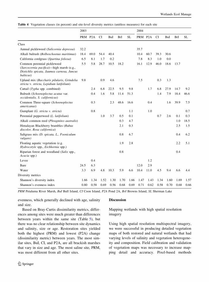
evenness, which generally declined with age, salinity

and size.Based on Bray-Curtis dissimilarity metrics, differ-

ences among sites were much greater than differences

between years within the same site (Table 5), butthere was no clear relationship between site dynamics

and salinity, size or age. Restoration sites yielded

both the highest (PRM) and lowest (P2A) change(dissimilarity metric) between years. The most sim-

ilar sites, BuI, CI, and P2A, are all brackish marshes

that vary in size and age. The most saline site, PRM,was most different from all other sites.

Discussion

Mapping wetlands with high spatial resolution

imagery

Using high spatial resolution multispectral imagery,

we were successful in producing detailed vegetationmaps of both restored and natural wetlands that had

varying levels of salinity and vegetation heterogene-

ity and composition. Field calibration and validationof vegetation maps was necessary to increase map-

ping detail and accuracy. Pixel-based methods

Table 4 Vegetation classes (in percent) and site-level diversity metrics (unitless measures) for each site

2003 2004

PRM P2A CI BuI BrI SL PRM P2A CI BuI BrI SL

Class

Annual pickleweed (Salicornia depressa) 32.2 35.7

Alkali bulrush (Bolboschoenus maritimus) 18.4 69.0 54.4 40.4 10.4 60.7 39.3 30.6

California cordgrass (Spartina foliosa) 6.5 8.1 1.7 0.2 7.8 8.3 1.0 0.0

Common perennial pickleweed(Sarcocornia pacifica)—high marsh (e.g.,Distichlis spicata, Jaumea carnosa, Juncusbalticus)

5.5 5.8 28.7 10.5 18.2 16.1 12.9 46.0 18.6 13.7

Upland mix (Baccharis pilularis, Grindeliastricta v. stricta, Lepidium latifolium)

9.8 0.9 4.6 7.5 0.3 1.3

Cattail (Typha spp. combined) 2.4 6.8 22.5 9.5 9.8 1.7 6.8 27.9 14.7 9.2

Bulrush (Schoenoplectus acutus var.occidentalis, S. californicus)

0.4 1.6 5.8 11.4 51.3 1.4 7.9 18.4 46.6

Common Three-square (Schoenoplectusamericanus)

0.3 2.3 48.6 16.6 0.4 1.6 39.9 7.5

Gumplant (G. stricta v. stricta) 0.8 1.1 1.0 0.7

Perennial pepperweed (L. latifolium) 1.0 3.7 0.5 0.1 0.7 2.6 0.1 0.3

Alkali common reed (Phragmites australis) 0.3 4.7 1.0 18.5

Himalayan Blackberry brambles (Rubusdiscolor, Rosa californica)

2.1 0.3 2.5 1.5

Saltgrass mix (D. spicata, L., Foeniculumvulgare)

0.8 6.7 0.4 6.2

Floating aquatic vegetation (e.g.Hydrocotyle spp., Eichhornia spp.)

1.9 2.8 2.2 5.1

Riparian forest and woodland (Salix spp.,Acacia spp.)

0.8 0.4

Levee 0.4 1.2

Bare 24.5 6.3 12.0 2.9

Water 3.3 6.9 4.8 10.3 5.9 6.6 10.4 11.0 4.5 9.4 6.6 4.4

Diversity metrics

Shannon’s diversity index 1.66 1.34 1.52 1.30 1.70 1.66 1.47 1.43 1.34 1.60 1.69 1.57

Shannon’s evenness index 0.80 0.58 0.69 0.56 0.68 0.69 0.71 0.62 0.58 0.70 0.68 0.66

PRM Petaluma River Marsh, BuI Bull Island, CI Coon Island, P2A Pond 2A, BrI Browns Island, SL Sherman Lake

Wetlands Ecol Manage

123

applied in detailed vegetation type mapping areeffective at measuring large-scale pattern change,

including site-wide richness, diversity, and evenness.

These methods can face challenges when mappingsmall-scale vegetation changes, particularly when the

time interval between measurements is short. This

might suggest that vegetation mapping with this levelof detail should take place less frequently than

annually, and for a longer duration than two time

periods. This limitation is largely due to spectralsimilarity between tidal marsh species assemblages in

the spectral bands available to us. Although high

spatial resolution imagery is necessary for detailedmapping, a per-pixel classification approach is lim-

iting because of high local-scale spectral variability

of the pixels, and the inability of most pixel-basedalgorithms to take spatial and contextual information

into account in the classification. Where only a few

species comprise a relatively homogeneous patchmosaic, CIR imagery is effective and relatively

straightforward. However, for sites with small-scale

diversity, using high spatial resolution CIR imageryrequires different types of classification algorithms

such as object based image analysis, or hyperspectraldata with a high spatial resolution (Blaschke 2010).

These alternate approaches may increase success of

discriminating within-patch species.

Map accuracy

The overall vegetation map accuracy increased from

2003 to 2004 at four out of six sites. Additional

ground reference points and acquiring imagery withbetter spectral separation between vegetation types

could explain this increase (2004 imagery was

acquired at a later date for these two sites than in2003—October rather than August/September). Laba

et al. (2005) found, in contrast, that wetland vegeta-

tion community types could be distinguished bestwith imagery acquired in August for measuring peak

biomass. Our accuracy rates for October 2003

imagery are less than 80% are likely are due to theunderrepresentation of some classes in the field data

due to their small area or habitat conditions that made

field ground-truthing more difficult.

Table 5 Similarity of vegetation type changes between sites and years sites, as measure by the Bray-Curtis Dissimilarity Metric(high values indicate high differences)

2003 2004

PRM2003

P2A2003

CI2003

BuI2003

BrI2003

SL2003

PRM2004

P2A2004

CI2004

BuI2004

BrI2004

SL2004

2003

PRM 2003 0.00 0.60 0.70 0.68 0.91 0.97 0.22

P2A 2003 0.60 0.00 0.31 0.45 0.86 0.90 0.12

CI 2003 0.70 0.31 0.00 0.35 0.68 0.87 0.18

BuI 2003 0.68 0.45 0.35 0.00 0.64 0.75 0.15

BrI 2003 0.91 0.86 0.68 0.64 0.00 0.53 0.15

SL 2003 0.97 0.90 0.87 0.75 0.53 0.00 0.18

2004

PRM 2004 0.22 0.00 0.56 0.68 0.64 0.79 0.96

P2A 2004 0.12 0.56 0.00 0.40 0.45 0.78 0.93

CI 2004 0.18 0.68 0.40 0.00 0.38 0.75 0.90

BuI 2004 0.15 0.64 0.45 0.38 0.00 0.54 0.77

BrI 2004 0.15 0.79 0.78 0.75 0.54 0.00 0.56

SL 2004 0.18 0.96 0.93 0.90 0.77 0.56 0.00

The top half of the table shows the dissimilarity metric between sites in 2003 on the left, and differences between 2003 and 2004 onthe right. The bottom half shows the dissimilarity metric between sites in 2004 on the right, with a repeat of the differences between2003 and 2004 on the left

PRM Petaluma River Marsh, BuI Bull Island, CI Coon Island, P2A Pond 2A, BrI Browns Island, SL Sherman Lake. Within-site,between-year dissimilarity metrics are shown in bold

Wetlands Ecol Manage

123

Though the classification approach used effectivelymappedmarsh vegetation types, each tile was processed

individually, which produced considerable work due to

the idiosyncrasies of each individual image (e.g.,brightness gradients). We recommend acquiring imag-

ery for a site that incorporates as few tiles as possible

(preferably one tile), while still being able to achieve thedesired pixel size for mapping. Modern high resolution

scanners can help achieve this goal by enlarging the

footprint for each photo tile. This practice will reduceprocessing time and image problems due to mosaicking

seams. If a larger spatial extent needed processing,

which requires numerous photograph tiles to capture theentire area, supervised or unsupervised methods may

not be possible, and visual interpretation, albeit time-

consuming, may produce the most accurate results(Zharikov et al. 2005).

Certain vegetation classes were identified with low

accuracy, indicating high commission and omissionerrors. Shrub species, including both gumplant and

coyote brush, usually existed as one or two plants,

creating very small patches that were either too smallfor the one-meter pixel size to detect, or were

eliminated using the filtering technique for smoothing

out the speckled effect. Both of these species oftenexisted on levees and in upland areas, so they were

incorporated into an ‘‘upland’’ class.

Diversity metrics

Vegetation pattern in tidally influenced marshesresponds to the interaction between hydrodynamics

and elevation, and can present clear zonation in

vegetation type, local-scale variations in microtopog-raphy (and hence inundation), which can create more

complex vegetation patterns (Hickey and Bruce 2010,

Pratolongo et al. 2009). But pattern is more difficultto quantify than diversity, thus there are fewer studies

examining pattern and structural differences across

salinity gradients, or across time. Engles and Jensen(2009) looked at wetlands across salinity gradients

along the Elbe (Germany), and the Connecticut(USA) Rivers, and found clear differences in pattern

as expressed by Shannon’s Diversity and Evenness

metrics.We measured overall vegetation similarity

between sites and years with the Bray-Curtis index

(Table 5). In Table 5, we are comparing each site’svegetation with all the other sites’ vegetation in the

same year (e.g. PRM 2003 with P2A 2003), and eachsite’s vegetation in 2003 with its vegetation in 2004

(e.g. PRM 2003 with PRM 2004). The higher Bray-

Curtis score indicates large differences, eitherbetween sites, or across years. In our study, overall

vegetation similarity, showed small differences

between years for any given site, compared to thelarge differences observed between sites in a given

year. Salinity seemed to play a role in this: across

sites, the most similar sites were those that aregeographically close and have similar salinities,

illustrating the effect of position along the estuarine

salinity gradient.Changes in wetland vegetation pattern over time,

especially in restored wetland sites, are also not

straightforward. In many cases, species diversity anddominance patterns do not match those of natural

sites, even decades after restoration (Garbutt and

Wolters 2008). In the long term, disturbance (bothchronic and extreme) will change wetland vegetation

pattern (Byrd and Kelly 2006; Byrd et al. 2004;

Frieswyk and Zedler 2007; Zedler 2009), in manycases shifting toward fewer species and increased

dominance. In our study, site-level diversity metrics

demonstrated several important differences acrosssites and between years that are detailed in the next

sections. Though these metrics may highlight actual

change in vegetation type, it is also possible that anychanges in a two-year study, such as this one, are

depicting annual variability and do not indicate long-

term trends. These metrics are effective at measuringdifferences from year to year and, used over the long

term as a monitoring technique, can allow for land

cover change quantification and ultimately the mea-surement of restoration success.

A recently restored marsh (PRM) ranked as high or

higher than mature marshes in vegetation classdiversity and number of patches in both years

(Shannon’s diversity of 1.66 and 1.47 respectively),

in contrast to the relatively low plant species diversityat this high-salinity site (Callaway et al. 2007). In

other words, the recently restored site had a morecomplex vegetation patch structure than a more

mature marsh. At least at this site, we suggest that

processes of vegetation colonization produce a morecomplex vegetation structure in the early period after

restoration and that over longer time periods this

structure simplifies, due to hydrologic and salinitypatterns, or other factors such as competition.

Wetlands Ecol Manage

123

Bull Island, a restored site, had variable diversityand evenness between years, while other more

recently restored sites (PRM and P2A) were less

variable (Table 5). This finding could reflect anactual true increase in vegetation type diversity at

BuI, or the fact that the earlier image acquisition in

2004 (August 2004 vs. October 2003) allowed forbetter separation of the vegetation types. These

results emphasize the importance of performing these

measures consistently over many years to measurelong-term changes through the marsh’s restoration, in

order to notice long-term changes that could be lost

due to interannual variability.The three oldest sites, two mature marshes (BrI, CI)

and one 83-year old restoration site (SL), exhibited very

small changes in vegetation class diversity, evenness,and patch density. This finding was expected, as these

mature sites should not show as much change (i.e.,

colonization and succession) as the recently restoredsites. For example, at PRM, the large increase of the

perennial pickleweed compared to the smaller increase

in the early-colonizing annual pickleweed reflectsmarsh maturation as more sediment accumulates and

elevation increases at the site.

Conclusions

Based on the findings of this study, we have several

recommendations for applying this kind of vegetation

mapping method. First, images should be collected atthe same time of year when conducting multi-year

evaluations to reduce variability introduced by

growing season spectral variability. Third, except atlocations undergoing very rapid vegetation changes

(newly restored sites), intervals between mapping

should be greater than 1 year in order to captureactual vegetation changes rather than method vari-

ability. Two consecutive years of image acquisition

and analysis might not be sufficient to showsubstantial vegetation change with both natural and

restoring sites. Fourth, avoiding the need for multipleimage tiles through higher altitude image acquisition

and higher resolution scanning improves mapping

results and reduces mapping effort. Sixth, it isbeneficial to have ample field data for use in both

training image processing software and in validating

classification results. With these guidelines, there is

potential value to mapping restored wetlands sitesusing high resolution imagery over the long term.

Acknowledgments This work was supported by the CALFEDCalifornia Bay-Delta Program. The CALFED Science Programsupported most of this work under Grant Number 4600002970.The CALFED Ecosystem Restoration Program supportedmanuscript preparation under Grant Number P0685516. JakeSchweitzer was instrumental in processing and georectifyingaerial imagery from HJW GeoSpatial, Inc.

References

Anderson JR, Hardy EH, Roach JT, Whitmer RE (1976) A landuse and land cover classification system for use withremote sensing data. Washington, DC: U.S. GovernmentPrinting Office. Report: Geological Survey ProfessionalPaper 964

Andresen T, Mott C, Zimmermann S, Schneider T, Melzer A(2002) Object-oriented information extraction for themonitoring of sensitive aquatic environments. IEEE3083–3085

AS ERD (1999) Erdas field guide. Erdas Inc, AtlantaBelluco E, Camuffo M, Ferrari S, Modenese L, Silvestri S,

Marani A, Marani M (2006) Mapping salt-marsh vegeta-tion by multispectral and hyperspectral remote sensing.Remote Sens Environ 105:54–67

Blaschke T (2010) Object based image analysis for remotesensing. ISPRS J Photogramm Remote Sens 65:2–16

Blaschke T, Strobl J (2001) What’s wrong with pixels? Somerecent developments interfacing remote sensing and GIS.GeoBIT/GIS 6:12–17

Byrd K, Kelly M (2006) Salt marsh vegetation response toedaphic and topographic changes from upland sedimen-tation in a Pacific estuary. Wetlands 26:813–829

Byrd KB, Kelly NM, Dyke EV (2004) Decadal changes in aPacific estuary: a multi-source remote sensing approachfor historical ecology. GIScience Remote Sens 41:347–370

Callaway JC, Parker TV, Vasey MC, Schile LM (2007)Emerging issues for the restoration of tidal marsh eco-systems in the context of predicted climate change.Madrono 54:234–248

Chmura GL, Anisfeld SC, Cahoon DR, Lynch JC (2003)Global carbon sequestration in tidal, saline wetland soils.Global Biogeochem Cycles 17:1111

Congalton RG (2009) Accuracy assessment of spatial data sets.In: Madden M (ed) Manual of geographic informationsystems. The American Society of Photogrammetry andRemote Sensing, Bethesda, pp 225–234

Congalton RC, Green K (1999) Assessing the accuracy ofremotely sensed data: principles and practices. CRC Press,Inc, Boca Raton

Daubenmire RF (1959) Canopy coverage method of vegetationanalysis. Northw Sci 33:43–64

Dechka J, Franklin S, Watmough M, Bennett R, Ingstrup D(2002) Classification of wetland habitat and vegetation

Wetlands Ecol Manage

123

communities using multitemporal IKONOS imagery insourthern Saskatchewan. Can J Remote Sens 28:679–685

Devereux BJ, Fuller RM, Carter L, Parsell RJ (1990) Geo-metric correction of airborne scanner imagery by match-ing Delaunay triangles. Int J Remote Sens 11:2237–2251

Eastwood JA, Yates MG, Thomson AG, Fuller RM (1997) Thereliability of vegetation indices for monitoring saltmarshvegetation cover. Int J Remote Sens 18:3901–3907

Engels J, Jensen K (2009) Patterns of wetland plant diversityalong estuarine stress gradients of the Elbe (Germany) andConnecticut (USA) Rivers. Plant Ecol Divers 2:301–311

Faith DP, Minchin PR, Belbin L (1987) Compositional dis-similarity as a robust measure of ecological distance.Vegetatio 69:57–68

Frieswyk C, Zedler J (2007) Vegetation change in Great Lakescoastal wetlands: deviation from the historical cycle.J Great Lakes Res 33:366–380

Garbutt A, Wolters M (2008) The natural regeneration of saltmarsh on formerly reclaimed land. Appl Veg Sci 11:335–344

Grossinger R, Alexander J, Cohen A, Collins JN (1998)Introduced tidal marsh plants in the San Francisco Estu-ary: regional distribution and priorities for control. SanFrancisco Estuary Institute, Richmond, CA

Hardisky MA, Smart RM, Klemas V (1983) Seasonal spectralcharacteristics and aboveground biomass of the tidalmarsh plant, Spartina alterniflora. Photogramm EngRemote Sens 49:85–92

Hardisky MA, Daiber FC, Roman CT, Klemas V (1984)Remote sensing of biomass and annual net aerial primaryproductivity of a salt marsh. Remote Sens Environ 16:91–106

Hickey D, Bruce E (2010) Examining tidal inundation and saltmarsh vegetation distribution patterns using spatial anal-ysis. Botany Bay, Australia

Hinkle RL, Mitsch WJ (2005) Salt marsh vegetation recoveryat salt hay farm wetland restoration sites on DelawareBay. Ecol Eng 25:240–251

Jensen JR (2000) Remote sensing of the environment: anearth resource perspective, 2nd edn. Prentice Hall, UpperSaddle River

Jensen JR, Coombs C, Porter D, Jones B, Schill S, White D(1998) Extraction of smooth cordgrass (Spartina alter-niflora) biomass and leaf area index parameters from highresolution imagery. Geocarto Int 13:25–34

Jensen JR, Olson G, Schill SR, Porter DE, Morris J (2002)Remote sensing of biomass, leaf-area-index, and chloro-phyll a and b content in the ACE Basin National EstuarineResearch Reserve using sub-meter digital camera imag-ery. Geocarto Int 17:25–34

Justice CO, Townshend JRG (1981) Integrating ground datawith remote sensing. In: Townshend JRG (ed) Terrainanalysis and remote sensing. George Allen & Unwin,London, p 232

Laba M, Tsai F, Ogurcak D, Smith S, Richmond ME (2005)Field determination of optimal dates for the discrimina-tion of invasive wetland plant species using derivativespectral analysis. Photogramm Eng Remote Sens71:603–611

Leica Geosystems Inc (2006) (17 January 2007 URL http://gis.leica-geosystems.com/)

McCune B, Mefford MJ (1999) PC-ORD for windows. MjMSoftware Design, Gleneden Beach

McGarigal K, Cushman SA, Neel MC, Ene E (2002) FRAG-STATS: Spatial Pattern Analysis Program for CategoricalMaps. Pages Computer software program produced by theauthors at the University of Massachusetts, Amherst.Available at the following web site: www.umass.edu/landeco/research/fragstats/fragstats.html

Mueller-Dombois D, Ellenberg H (1974) Aims and methods invegetation ecology. Wiley, New York

Nichols FH, Cloern JE, Luoma SN, Peterson DH (1986) Themodification of an estuary. Science 231:567–573

Ozesmi SL, Bauer ME (2002) Satellite remote sensing ofwetlands. Wetl Ecol Manage 10:381–402

Pennings SC, Bertness MD (2001) Salt marsh communities. In:Bertness MD, Gaines SD, Hay ME (eds) Marine com-munity ecology. Sinauer, Sunderland, pp 289–316

Phinn SR, Stow DA, Zedler JB (1996) Monitoring wetlandhabitat restoration in southern California using airbornemultispectral video data. Restor Ecol 4:412–422

Pratolongo PD, Kirby JR, Plater A, Brinson MM (2009)Temperate coastal wetlands: morphology, sediment pro-cesses, and plant communities. In: Perillo GME, WolanskiE, Cahoon DR, Brinson MM (eds) Coastal wetlands: anintegrated ecosystem approach. Elsevier, Amsterdam,pp 89–118

R_Development_Core_Team (2005) R: a language and environ-ment for statistical computing. http://www.r-project.org/

Ramsey EW III, Laine S (1997) Comparison of Landsat The-matic Mapper and high resolution photography to identifychange in complex coastal wetlands. J Coastal Res13:281–292

Sawyer JO, Keeler-Wolf T (2004) A manual of Californiavegetation. California Native Plant Society, Sacramento

Sawyer JO, Keeler Wolf T, Evens JM (2009) A manual ofCalifornia vegetation, 2nd edn. California Native PlantSociety, Sacramento

Schmidt KS, Skidmore AK (2003) Spectral discrimination ofvegetation types in a coastal wetland. Remote SensEnviron 85:92–108

Sharpe P, Baldwin A (2009) Patterns of wetland plant speciesrichness across estuarine gradients of Chesapeake Bay.Wetlands 29:225–235

Stralberg D, Herzog MP, Nur N, Tuxen KA, Kelly M (2010)Predicting avian abundance within and across tidal mar-shes using fine-scale vegetation and geomorphic metrics.Wetlands 30:475–487

Thomson AG, Fuller RM, Sparks TH, Yates MG, Eastwood JA(1998) Ground and airborne radiometry over intertidalsurfaces: waveband selection for cover classification. Int JRemote Sens 19:1189–1205

Thomson AG, Fuller RM, Yates MG, Brown SL, Cox R,Wadsworth RA (2003) The use of airborne remote sensingfor extensive mapping of intertidal sediments and salt-marshes in eastern England. Int J Remote Sens 24:2717–2737

Thomson AG, Huiskes A, Cox R, Wadsworth RA, BoormanLA (2004) Short-term vegetation succession and erosionidentified by airborne remote sensing of Westerscheldesalt marshes, The Netherlends. Int J Remote Sens 25:4151–4176

Wetlands Ecol Manage

123

Trimble Inc (2005) (17 January 2007 URL http://www.trimble.com/)

Tuxen K, Schile L, Kelly M, Siegel S (2008) Vegetation col-onization in a restoring tidal marsh: a remote sensingapproach. Restor Ecol 16:313–323

Williams PB, Faber PM (2001) Salt marsh restoration experi-ence in the San Francisco Bay Estuary. J Coastal Res27:203–211

Zedler J (2009) How frequent storms affect wetland vegetation:a preview of climate-change impacts. Front Ecol Environ8:540–547

Zedler JB, Kercher S (2005) Wetland resources: status, trends,ecosystem services, and restorability. Ann Rev EnvironResour 30:39–74

Zhang M, Ustin SL, Rejmankova E, Sanderson EW (1997)Monitoring Pacific coast saltmarshes using remote sens-ing. Ecol Appl 7:1039–1053

Zharikov Y, Skilleter GA, Loneragan NR, Taranto T, CameronBE (2005) Mapping and characterising subtropical estu-arine landscapes using aerial photography and GIS forpotential application in wildlife conservation and man-agement. Biol Conserv 125:87–100

Wetlands Ecol Manage

123