Wetland Ecological Integrity: An Assessment Approach
171
Wetland Ecological Integrity: An Assessment Approach The Coastal Wetlands Ecosystem Protection Project March 1998 0&=0 Produced by: Massachusetts Coastal Zone Management Through support from: National Oceanic and Atmospheric Administration Coastal Services Center
-
Upload
khangminh22 -
Category
Documents
-
view
1 -
download
0
Transcript of Wetland Ecological Integrity: An Assessment Approach

Wetland Ecological Integrity:An Assessment Approach
The Coastal Wetlands Ecosystem Protection Project
March 1998
0&=0
Produced by:
Massachusetts Coastal Zone Management
Through support from:
National Oceanic and Atmospheric AdministrationCoastal Services Center

Report Title: Wetland Ecological Integrity: An Assessment Approach
Date: 31 March 1998
Principal Author: Bruce K. Carlisle, Massachusetts Coastal Zone Management
Contributing Authors: Jan P. Smith, Massachusetts Coastal Zone ManagementAnna L. Hicks, University of MassachusettsBryan G. Largay, University of California, DavisSamuel R. Garcia, University of California, Santa Cruz
Coordinating Agencies: Waquoit Bay National Estuarine Research Reserve,Massachusetts Department of Environmental Protection
Project: The Coastal Wetlands Ecosystem Protection Project
NOAA# NA57OC0470
Sponsored by: National Oceanic and Atmospheric Administration,Coastal Services Center
Federal Program Officer: Pace Wilber
This report was produced by Massachusetts Coastal Zone Management and is funded by a grant from the CoastalServices Center, National Oceanic and Atmospheric Administration, U.S. Department of Commerce. The viewsexpressed are those of the author(s) and do not necessarily reflect the views of NOAA or any of its sub-agencies. This information is available in alternate formats upon request.

Wetland Ecological Integrity: An Assessment Approach Page i
Acknowledgments
This project was funded by the National Oceanic and Atmospheric Administration’s Coastal ServicesCenter (NOAA Grant Award No. NA57OC0470). We would like to thank Pace Wilber of NOAA’sCoastal Services Center for his interest and assistance with this project. Special thanks are extendedto Anna Hicks of the University of Massachusetts (UMass Extension), to Bryan Largay of theUniversity of California, Davis, and to Samuel Garcia of the University of California Santa Cruz fortheir participation as key members of the project team. Special thanks to all the staff at the WaquoitBay National Estuarine Research Reserve for their hospitality, shared information, and insight to localconditions. Erin Largay, a Connecticut College undergraduate, graciously volunteered her time toassist in data collection. Laura Chaskelson, a University of Massachusetts undergraduate providedcritical assistance in the initial transfer of this Wetlands Ecological Assessment Approach to sites onMassachusetts’ North Shore and aided in final project tasks including the development of a WorldWide Web site. Anne Donovan of Massachusetts Coastal Zone Management and Gary Gonyea ofMassachusetts Department of Environmental Protection provided the important final editorial reviewof this document. Members of the project’s Technical Advisory Group (TAG) should be thanked fortheir critical review of the project from its developmental stages. The TAG is: Ed Eichner, Cape CodCommission; Christine Gault, Rick Crawford, and Maggie Geiss, Waquoit Bay National EstuarineResearch Reserve; Gary Gonyea, MA DEP; Larry Oliver, US Army Corps of Engineers; MarkPatton, Town of Falmouth; Jo Ann Muramoto, Town of Falmouth; Greg Hellyer, US EnvironmentalProtection Agency Region I; Bob Sherman, Town of Mashpee; Marie Studer, Massachusetts BaysProgram (formerly); Ralph Tiner, US Fish and Wildlife Service; Patti Tyler, US EnvironmentalProtection Agency Region I.

Wetland Ecological Integrity: An Assessment Approach Page iii
Table of Contents
Acknowledgments . . . . . . . . . . . . . . . . . . . . . . . . . . . . . . . . . . . . . . . . . . . . . . . . . . . . . . . . . . . iList of Figures . . . . . . . . . . . . . . . . . . . . . . . . . . . . . . . . . . . . . . . . . . . . . . . . . . . . . . . . . . . . . . vList of Tables . . . . . . . . . . . . . . . . . . . . . . . . . . . . . . . . . . . . . . . . . . . . . . . . . . . . . . . . . . . . . . viExecutive Summary . . . . . . . . . . . . . . . . . . . . . . . . . . . . . . . . . . . . . . . . . . . . . . . . . . . . . . . . ix
Part I. Background and Project ScopeSection 1. Introduction . . . . . . . . . . . . . . . . . . . . . . . . . . . . . . . . . . . . . . . . . . . . . . . . . . . . 1-1
The Importance and Diversity of Wetlands . . . . . . . . . . . . . . . . . . . . . . . . . . . . . . . . . 1-1Coastal Tidal Wetlands . . . . . . . . . . . . . . . . . . . . . . . . . . . . . . . . . . . . . . . . . . 1-1Nontidal Wetlands . . . . . . . . . . . . . . . . . . . . . . . . . . . . . . . . . . . . . . . . . . . . . 1-1
Wetland Ecology and Functions . . . . . . . . . . . . . . . . . . . . . . . . . . . . . . . . . . . . . . . . . 1-2Water Quality . . . . . . . . . . . . . . . . . . . . . . . . . . . . . . . . . . . . . . . . . . . . . . . . 1-3Flood Protection . . . . . . . . . . . . . . . . . . . . . . . . . . . . . . . . . . . . . . . . . . . . . . 1-3Shoreline Erosion . . . . . . . . . . . . . . . . . . . . . . . . . . . . . . . . . . . . . . . . . . . . . 1-3Fish and Wildlife Habitat . . . . . . . . . . . . . . . . . . . . . . . . . . . . . . . . . . . . . . . 1-3
Wetland Loss and Degradation . . . . . . . . . . . . . . . . . . . . . . . . . . . . . . . . . . . . . . . . . . 1-4Human Development and Landscape Alteration . . . . . . . . . . . . . . . . . . . . . . . 1-4Impacts to Water Quality: Pollutant Constituents . . . . . . . . . . . . . . . . . . . . . . 1-4Impacts to Hydrology . . . . . . . . . . . . . . . . . . . . . . . . . . . . . . . . . . . . . . . . . . . 1-5
Wetland Assessment . . . . . . . . . . . . . . . . . . . . . . . . . . . . . . . . . . . . . . . . . . . . . . . . . 1-7Section 2. Project Scope . . . . . . . . . . . . . . . . . . . . . . . . . . . . . . . . . . . . . . . . . . . . . . . . . . . 2-1
The Wetland Health Assessment Toolbox . . . . . . . . . . . . . . . . . . . . . . . . . . . . . . . . . 2-2Focus Box: Metrics, Indices and The Reference Condition . . . . . . . . . . . . . . . 2-5
Study Area . . . . . . . . . . . . . . . . . . . . . . . . . . . . . . . . . . . . . . . . . . . . . . . . . . . . . . . . . 2-6Study Sites . . . . . . . . . . . . . . . . . . . . . . . . . . . . . . . . . . . . . . . . . . . . . . . . . . . . . . . . 2-11
Freshwater Sites . . . . . . . . . . . . . . . . . . . . . . . . . . . . . . . . . . . . . . . . . . . . . . 2-11Salt Marsh Sites . . . . . . . . . . . . . . . . . . . . . . . . . . . . . . . . . . . . . . . . . . . . . . 2-17
Part II: Wetland Ecological Assessment:The Wetland Health Assessment Toolbox
Section 3. Rapid Assessment Methodologies . . . . . . . . . . . . . . . . . . . . . . . . . . . . . . . . . . . 3-1Habitat Assessment . . . . . . . . . . . . . . . . . . . . . . . . . . . . . . . . . . . . . . . . . . . . . . . . . . 3-1Nonpoint Source Index . . . . . . . . . . . . . . . . . . . . . . . . . . . . . . . . . . . . . . . . . . . . . . . 3-6
Wetland Ground-Watersheds and Capture Zones . . . . . . . . . . . . . . . . . . . . . . 3-8Geographic Information System Analysis for NPSI . . . . . . . . . . . . . . . . . . . . 3-12
Functional Evaluation . . . . . . . . . . . . . . . . . . . . . . . . . . . . . . . . . . . . . . . . . . . . . . . . 3-18Section 4. Wetland Vegetation . . . . . . . . . . . . . . . . . . . . . . . . . . . . . . . . . . . . . . . . . . . . . . 4-1
Methods . . . . . . . . . . . . . . . . . . . . . . . . . . . . . . . . . . . . . . . . . . . . . . . . . . . . . . . . . . . 4-1Data Analysis . . . . . . . . . . . . . . . . . . . . . . . . . . . . . . . . . . . . . . . . . . . . . . . . . . . . . . . 4-2
Focus Box: Community-Based Method for Vegetation Survey . . . . . . . . . . . . 4-4

Wetland Ecological Integrity: An Assessment ApproachPage iv
Results . . . . . . . . . . . . . . . . . . . . . . . . . . . . . . . . . . . . . . . . . . . . . . . . . . . . . . . . . . . . 4-7Inter-Annual Variation . . . . . . . . . . . . . . . . . . . . . . . . . . . . . . . . . . . . . . . . . . . . . . . . 4-7
Section 5. Aquatic Macro Invertebrates . . . . . . . . . . . . . . . . . . . . . . . . . . . . . . . . . . . . . . 5-1Methods . . . . . . . . . . . . . . . . . . . . . . . . . . . . . . . . . . . . . . . . . . . . . . . . . . . . . . . . . . . 5-1Data Analysis . . . . . . . . . . . . . . . . . . . . . . . . . . . . . . . . . . . . . . . . . . . . . . . . . . . . . . . 5-2Results . . . . . . . . . . . . . . . . . . . . . . . . . . . . . . . . . . . . . . . . . . . . . . . . . . . . . . . . . . . 5-11Seasonal and Inter-Annual Variation . . . . . . . . . . . . . . . . . . . . . . . . . . . . . . . . . . . . 5-21
Section 6. Water Chemistry . . . . . . . . . . . . . . . . . . . . . . . . . . . . . . . . . . . . . . . . . . . . . . . . 6-1Methods . . . . . . . . . . . . . . . . . . . . . . . . . . . . . . . . . . . . . . . . . . . . . . . . . . . . . . . . . . . 6-2Data Analysis . . . . . . . . . . . . . . . . . . . . . . . . . . . . . . . . . . . . . . . . . . . . . . . . . . . . . . . 6-5Results . . . . . . . . . . . . . . . . . . . . . . . . . . . . . . . . . . . . . . . . . . . . . . . . . . . . . . . . . . . . 6-5Stormwater Results . . . . . . . . . . . . . . . . . . . . . . . . . . . . . . . . . . . . . . . . . . . . . . . . . 6-13
Section 7. Wetland Hydroperiod . . . . . . . . . . . . . . . . . . . . . . . . . . . . . . . . . . . . . . . . . . . . 7-1Methods . . . . . . . . . . . . . . . . . . . . . . . . . . . . . . . . . . . . . . . . . . . . . . . . . . . . . . . . . . . 7-1Data Analysis . . . . . . . . . . . . . . . . . . . . . . . . . . . . . . . . . . . . . . . . . . . . . . . . . . . . . . . 7-2Results . . . . . . . . . . . . . . . . . . . . . . . . . . . . . . . . . . . . . . . . . . . . . . . . . . . . . . . . . . . . 7-5The Groundwater Hydrology of an Isolated Depressional Wetland . . . . . . . . . . . . . . . 7-9
Field Methods . . . . . . . . . . . . . . . . . . . . . . . . . . . . . . . . . . . . . . . . . . . . . . . . 7-9Data Analysis . . . . . . . . . . . . . . . . . . . . . . . . . . . . . . . . . . . . . . . . . . . . . . . . 7-10Results . . . . . . . . . . . . . . . . . . . . . . . . . . . . . . . . . . . . . . . . . . . . . . . . . . . . . 7-12Discussion . . . . . . . . . . . . . . . . . . . . . . . . . . . . . . . . . . . . . . . . . . . . . . . . . . 7-13
Section 8. Avifauna . . . . . . . . . . . . . . . . . . . . . . . . . . . . . . . . . . . . . . . . . . . . . . . . . . . . . . 8-1Methods . . . . . . . . . . . . . . . . . . . . . . . . . . . . . . . . . . . . . . . . . . . . . . . . . . . . . . . . . . . 8-1Data Analysis . . . . . . . . . . . . . . . . . . . . . . . . . . . . . . . . . . . . . . . . . . . . . . . . . . . . . . . 8-2Results . . . . . . . . . . . . . . . . . . . . . . . . . . . . . . . . . . . . . . . . . . . . . . . . . . . . . . . . . . . . 8-5
Part III: Discussion and Conclusion:The Wetland Ecological Condition
Section 9. Discussion: Wetland Ecological Condition . . . . . . . . . . . . . . . . . . . . . . . . . . . . 9-1Index Totals: The Wetland Ecological Condition . . . . . . . . . . . . . . . . . . . . . . . . . . . . 9-1Freshwater Wetland Evaluation Areas: Discussion of Results . . . . . . . . . . . . . . . . . . . 9-9Salt Marsh Wetland Evaluation Areas: Discussion of Results . . . . . . . . . . . . . . . . . . 9-15Statistical Examination of Results . . . . . . . . . . . . . . . . . . . . . . . . . . . . . . . . . . . . . . . 9-18
Section 10. Conclusion & Recommendations . . . . . . . . . . . . . . . . . . . . . . . . . . . . . . . . . . 10-1Observations: Patterns of Results . . . . . . . . . . . . . . . . . . . . . . . . . . . . . . . . . . . . . . . 10-2Management Implications and Recommendations . . . . . . . . . . . . . . . . . . . . . . . . . . . 10-3
Section 11. References . . . . . . . . . . . . . . . . . . . . . . . . . . . . . . . . . . . . . . . . . . . . . . . . . . . 11-1Section 12. Appendix . . . . . . . . . . . . . . . . . . . . . . . . . . . . . . . . . . . . . . . . . . . . . . . . . . . . 12-1

Wetland Ecological Integrity: An Assessment Approach Page v
List of Figures
Figure Page2.1. Locus map of Cape Cod and Islands, southeastern Massachusetts . . . . . . . . . . . . . . . . . 2-72.2. Waquoit Bay watershed and contribution areas . . . . . . . . . . . . . . . . . . . . . . . . . . . . . . . 2-92.3. Freshwater wetland study sites . . . . . . . . . . . . . . . . . . . . . . . . . . . . . . . . . . . . . . . . . . . 2-132.4. Salt marsh study sites . . . . . . . . . . . . . . . . . . . . . . . . . . . . . . . . . . . . . . . . . . . . . . . . . . 2-193.1. Watershed delineations (groundwater) for each Wetland Evaluation Area . . . . . . . . . . 3-133.2. Final results of rapid assessment methods: freshwater sites . . . . . . . . . . . . . . . . . . . . . . 3-253.3. Final results of rapid assessment methods: salt marsh sites . . . . . . . . . . . . . . . . . . . . . . 3-274.1. Index of Vegetative Integrity: freshwater sites . . . . . . . . . . . . . . . . . . . . . . . . . . . . . . . 4-114.2. Index of Vegetative Integrity: salt marsh sites . . . . . . . . . . . . . . . . . . . . . . . . . . . . . . . 4-135.1. Invertebrate Community Index scores: freshwater sites . . . . . . . . . . . . . . . . . . . . . . . . 5-135.2. Invertebrate Community Index scores: salt marsh sites . . . . . . . . . . . . . . . . . . . . . . . . . 5-175.3. Graphic of ICI score versus HA score . . . . . . . . . . . . . . . . . . . . . . . . . . . . . . . . . . . . . 5-196.1. Water Chemistry Index: freshwater sites . . . . . . . . . . . . . . . . . . . . . . . . . . . . . . . . . . . . 6-96.2. Water Chemistry Index: salt marsh sites . . . . . . . . . . . . . . . . . . . . . . . . . . . . . . . . . . . . 6-116.3. Average fecal coliform bacteria concentrations in stormwater discharges . . . . . . . . . . . 6-156.4. Average specific conductance stormwater discharges . . . . . . . . . . . . . . . . . . . . . . . . . . 6-156.5. Average phosphorous concentrations in stormwater discharges . . . . . . . . . . . . . . . . . . 6-176.6. Average nitrate/nitrite concentrations in stormwater discharges . . . . . . . . . . . . . . . . . . 6-177.1. Hydroperiod Index: freshwater sites . . . . . . . . . . . . . . . . . . . . . . . . . . . . . . . . . . . . . . . . 7-77.2. Components of the wetland water balance and 4 typical flow regimes at WEA7 . . . . . . 7-158.1. Avifauna Index: freshwater sites . . . . . . . . . . . . . . . . . . . . . . . . . . . . . . . . . . . . . . . . . . 8-78.2. Avifauna Index: salt marsh sites . . . . . . . . . . . . . . . . . . . . . . . . . . . . . . . . . . . . . . . . . . . 8-99.1. Wetland Ecological Condition scores: freshwater sites . . . . . . . . . . . . . . . . . . . . . . . . . . 9-59.2. Wetland Ecological Condition scores: salt marsh sites . . . . . . . . . . . . . . . . . . . . . . . . . . 9-7

Wetland Ecological Integrity: An Assessment ApproachPage vi
List of Tables
Table Page1.1. Major causes of wetland loss and degradation . . . . . . . . . . . . . . . . . . . . . . . . . . . . . . . . 1-61.2. Stormwater constituents and sources . . . . . . . . . . . . . . . . . . . . . . . . . . . . . . . . . . . . . . . 1-62.1. Wetland Health Assessment Toolbox . . . . . . . . . . . . . . . . . . . . . . . . . . . . . . . . . . . . . . . 2-42.2. Wetland Evaluation Areas: Class, cover, and surrounding land use . . . . . . . . . . . . . . . . 2-123.1. Freshwater wetland Habitat Assessment field form . . . . . . . . . . . . . . . . . . . . . . . . . . . . . 3-33.2. Salt marsh Habitat Assessment field form . . . . . . . . . . . . . . . . . . . . . . . . . . . . . . . . . . . . 3-43.3. Habitat Assessment results for freshwater and salt marsh wetlands . . . . . . . . . . . . . . . . . 3-53.4. Nonpoint Source Index method field worksheet . . . . . . . . . . . . . . . . . . . . . . . . . . . . . . . 3-93.5. Land use types and NPSI loading coefficients . . . . . . . . . . . . . . . . . . . . . . . . . . . . . . . 3-163.6. NPSI subtotals and final scores for all study sites . . . . . . . . . . . . . . . . . . . . . . . . . . . . . 3-173.7. New Hampshire method (tidal and nontidal) functional values evaluated . . . . . . . . . . . 3-203.8. Sample page from the NH nontidal wetland evaluation manual . . . . . . . . . . . . . . . . . . . 3-213.9. Functional Evaluation scores for NH method for freshwater sites . . . . . . . . . . . . . . . . . 3-233.10. Functional Evaluation scores for NH method for salt marsh sites . . . . . . . . . . . . . . . . 3-244.1. Wetland vegetation strata . . . . . . . . . . . . . . . . . . . . . . . . . . . . . . . . . . . . . . . . . . . . . . . . 4-24.2. Index of Vegetative Integrity metrics . . . . . . . . . . . . . . . . . . . . . . . . . . . . . . . . . . . . . . . 4-64.3. Index of Vegetative Integrity metrics scoring criteria: freshwater sites . . . . . . . . . . . . . . 4-84.4. Index of Vegetative Integrity metrics scoring criteria: salt marsh sites . . . . . . . . . . . . . . 4-84.5. Final metrics and IVI scores for freshwater study sites . . . . . . . . . . . . . . . . . . . . . . . . . . 4-94.6. Final metrics and IVI scores for salt marsh study sites . . . . . . . . . . . . . . . . . . . . . . . . . . 4-95.1. Freshwater invertebrate community metrics and indices . . . . . . . . . . . . . . . . . . . . . . . . . 5-35.2. Salt marsh invertebrate community metrics and indices . . . . . . . . . . . . . . . . . . . . . . . . . 5-45.3. Freshwater wetland ICI metric calculation . . . . . . . . . . . . . . . . . . . . . . . . . . . . . . . . . . . 5-75.4. Freshwater wetlands ICI metric scoring criteria . . . . . . . . . . . . . . . . . . . . . . . . . . . . . . . 5-85.5. Salt marsh wetlands ICI metric calculation . . . . . . . . . . . . . . . . . . . . . . . . . . . . . . . . . . 5-105.6. Salt marsh wetland ICI metric scoring criteria . . . . . . . . . . . . . . . . . . . . . . . . . . . . . . . 5-105.7. Freshwater wetlands ICI metrics and indices averaged over 3 seasons . . . . . . . . . . . . . 5-125.8. Salt marsh wetlands ICI metrics and indices averaged over 3 seasons . . . . . . . . . . . . . . 5-155.9. Seasonal ICI scores: freshwater sites . . . . . . . . . . . . . . . . . . . . . . . . . . . . . . . . . . . . . . 5-225.10. Seasonal ICI scores: salt marsh sites . . . . . . . . . . . . . . . . . . . . . . . . . . . . . . . . . . . . . 5-226.1. Analysis methods, matrices, references, holding times . . . . . . . . . . . . . . . . . . . . . . . . . . 6-46.2. Metrics for Water Chemistry Index . . . . . . . . . . . . . . . . . . . . . . . . . . . . . . . . . . . . . . . . 6-66.3. Water Chemistry Index metric scoring criteria: freshwater sites . . . . . . . . . . . . . . . . . . . 6-76.4. Water Chemistry Index metric scoring criteria: salt marsh sites . . . . . . . . . . . . . . . . . . . . 6-76.5. Final metric and WCI scores for freshwater sites . . . . . . . . . . . . . . . . . . . . . . . . . . . . . . 6-86.6. Final metric and WCI scores for salt marsh sites . . . . . . . . . . . . . . . . . . . . . . . . . . . . . . . 6-86.7. Pollutant concentrations of stormwater for 3 rain events 1996-1997 . . . . . . . . . . . . . . . 6-147.1. Metrics for Hydroperiod Index . . . . . . . . . . . . . . . . . . . . . . . . . . . . . . . . . . . . . . . . . . . 7-37.2. Hydroperiod Index metric scoring criteria . . . . . . . . . . . . . . . . . . . . . . . . . . . . . . . . . . . 7-4

Wetland Ecological Integrity: An Assessment Approach Page vii
Table Page7.3. Final metric and HPI scores for freshwater sites . . . . . . . . . . . . . . . . . . . . . . . . . . . . . . . 7-67.4. WEA7 site description and results summary . . . . . . . . . . . . . . . . . . . . . . . . . . . . . . . . . 7-147.5. Summary of daily water flow for WEA7 . . . . . . . . . . . . . . . . . . . . . . . . . . . . . . . . . . . 7-148.1. Avifauna Index metrics . . . . . . . . . . . . . . . . . . . . . . . . . . . . . . . . . . . . . . . . . . . . . . . . . 8-38.2. Avifauna Index metric scoring criteria: freshwater sites . . . . . . . . . . . . . . . . . . . . . . . . . 8-48.3. Avifauna Index metric scoring criteria: salt marsh sites . . . . . . . . . . . . . . . . . . . . . . . . . . 8-48.4. Final metric and AVI scores for freshwater sites . . . . . . . . . . . . . . . . . . . . . . . . . . . . . . . 8-68.5. Final metric and AVI scores for salt marsh sites . . . . . . . . . . . . . . . . . . . . . . . . . . . . . . . 8-69.1. Final Wetland Ecological Condition, component indices, and rapid assessment
scores for freshwater sites . . . . . . . . . . . . . . . . . . . . . . . . . . . . . . . . . . . . . . . . . . . . . 9-39.2. Final Wetland Ecological Condition, component indices, and rapid assessment
scores for salt marsh sites . . . . . . . . . . . . . . . . . . . . . . . . . . . . . . . . . . . . . . . . . . . . . . 9-49.3. Correlation matrix for final index and rapid assessment scores: freshwater sites . . . . . . 9-199.4. Correlation matrix for final index and rapid assessment scores: salt marsh sites . . . . . . . 9-20

Wetland Ecological Integrity: An Assessment Approach Page ix
Executive Summary
Since July 1995, Massachusetts Coastal Zone Management has been engaged in a regional researchand demonstration project sponsored by the National Oceanic and Atmospheric Administration’sCoastal Services Center. The goal of the Coastal Wetland Ecosystem Protection Project is todevelop, test, and refine a transferable approach for wetlands evaluation to determine the impacts ofadjacent land uses and nonpoint sources (NPS) of pollution on the ecological integrity of theseaquatic resources. Thirteen wetland study sites were identified in the Waquoit Bay watershed on CapeCod in southeastern Massachusetts. These sites were selected to be representative of the threedominant types in the watershed--salt marshes, bordering riverine wetlands, and isolated depressionalwetland--and of the major land uses types present: residential and commercial development,transportation, agriculture, and recreation. At each site, biological, chemical, and hydrologicalmeasurements were made in order to assess the relative ecological health and functioning of thesewetlands. In addition, several rapid assessment methods and techniques were employed and theresults were examined in light of actual on-site measurements. Through the development andimplementation of this pilot project, project staff were able to evaluate the accuracy and effectivenessof an array of wetland evaluation methods and promote their inclusion in a transferable assessmentapproach.
Based on the analysis of the onsite biological, hydrological, and chemical measurements, there isdiscernable variation between study sites. The data indicate a pattern of ecological degradationassociated with certain land uses and land use practices. Compared to control (or reference) studysites, wetlands with a higher degree and intensity of proximate land uses show a marked shift inbiological species and community composition, dissimilar hydrology, and increased concentrationsof nutrients, sediments, and pathogenic bacteria. Statistical analysis reveals very close correlationsbetween the outputs of the rapid assessment methods and the field-based indicators.
Project results have enabled the authors to identify which wetland sites are exhibiting signs ofecological and functional impairment, to characterize what the adverse effects are, and to infer as tothe potential sources or causes of impairment. This information can be utilized to guide decision-makers as they attempt to address NPS pollution and implement measures to mitigate existingproblems and to prevent future ones. The Wetlands Health Assessment Toolbox (WHAT) approachhas valuable applications for wetlands inventory and assessment in specific geographic areas (suchas towns or watersheds); measuring and evaluating the success of wetland restoration, compensatorymitigation, or banking projects; and for examining and quantifying the impacts of new developmentand other land use activities on wetlands.
Part I of this document provides the introduction, background and scope for the project, setting thefoundation for the detailed description of the assessment methods in Part II which includes theexplanation of methods, data analysis, and results. Part III contributes a site-by-site discussion of theproject results, makes observations on data patterns, and provides some recommendations for furtherdevelopment of the WHAT approach and management actions.

Part I: Background and Project Scope

Section 1. Introduction This section provides an introduction to wetlands ecology, function, and values; briefly reviews the causes and types of wetland degradation, alteration, and impact; and introduces the rationale and impetus behind the Coastal Wetlands Ecosystem Protection Project. Some of the wetland ecology section has been adapted from the US Environmental Protection Agency (USEPA) document, America’s Wetlands: Our Vital Link Between Land and Water. The Importance and Diversity of Wetlands Wetlands are areas where water covers the soil, or is present either at or near the surface of the soil for at least part of the growing season. The occurrence and flow of water (hydrology) largely determine how the soil develops and the types of plant and animal communities living in and on the soil. Wetlands may support both aquatic and terrestrial species. The prolonged presence of water creates conditions that favor the growth of specially adapted plants (hydrophytes) and promote the development of characteristic wetland (hydric) soils. Wetlands vary widely because of regional and local differences in soils, topography, climate, hydrology, water chemistry, vegetation, and other factors, including human disturbance. Indeed, wetlands are found from the tundra to the tropics and on every continent except Antarctica. Two general categories of wetlands are recognized: tidally-influenced wetlands and non-tidal (or inland) wetlands. Coastal Tidal Wetlands Coastal wetlands in the United States, as their name suggests, are found along the Atlantic, Pacific, Alaskan, and Gulf coasts. They are closely linked to estuaries, where sea water mixes with fresh water to form an environment of varying salinities. The salt water and the fluctuating water levels (due to tidal action) combine to create a rather difficult environment for most plants. Consequently, many shallow coastal areas are unvegetated mud flats or sand flats. Some plants, however, have successfully adapted to this environment. Certain grasses and grasslike plants (or graminoids, including sedges and rushes) that adapt to the saline conditions form the tidal salt marshes that are found along the Atlantic, Gulf, and Pacific coasts. Mangrove swamps, with salt-loving shrubs or trees, are common in tropical climates, such as in southern Florida and Puerto Rico. Some tidal freshwater wetlands form beyond the upper edges of tidal salt marshes where the influence of salt water ends. Nontidal Wetlands Inland wetlands are most common on floodplains along rivers and streams (riparian wetlands), in isolated depressions surrounded by dry land (for example, playas, basins, and "potholes"), along the margins of lakes and ponds, and in other low-lying areas where the groundwater intercepts the soil surface or where precipitation sufficiently saturates the soil (vernal pools and bogs). Inland wetlands include marshes and wet meadows dominated by herbaceous plants, swamps dominated by shrubs,
Wetland Ecological Integrity: An Assessment Approach Page 1-1

and wooded swamps dominated by trees. Certain types of inland wetlands are common to particular regions of the country: bogs and fens of the northeastern and north-central states and Alaska; inland saline and alkaline marshes of the arid and semiarid west; prairie potholes of Iowa, Minnesota and the Dakotas; playa lakes of the southwest and Great Plains; and bottomland hardwood swamps of the south. Many of these wetlands are seasonal and, particularly in the arid and semiarid West, may be wet only periodically. The quantity of water present and the timing of its presence in part determine the functions of a wetland and its role in the environment. Even wetlands that appear dry at times for significant parts of the year–such as vernal pools–often provide critical habitat for wildlife adapted to breeding exclusively in these areas. Wetland Ecology and Functions Wetlands are among the most productive ecosystems in the world, comparable to rain forests and coral reefs. An immense variety of species of microbes, plants, insects, amphibians, reptiles, birds, fish, and mammals can be part of a wetland ecosystem. Physical and chemical features such as climate, landscape shape (topology), geology, and the movement and abundance of water help to determine the plants and animals that inhabit each wetland. The complex, dynamic relationships among the organisms inhabiting the wetland environment are referred to as food webs. Wetlands provide great volumes of food that attract many animal species. These animals use wetlands for part of or all of their life-cycle. Dead plant leaves and stems break down in the water to form small particles of organic material called "detritus." This enriched material feeds many small aquatic insects, shellfish, and small fish that are food for larger predatory fish, reptiles, amphibians, birds, and mammals. The biological, chemical, and physical operations and attributes of a wetland are known as wetland functions. Some typical wetland functions include: wildlife habitat and food chain support, surface water retention or detention, groundwater recharge, and nutrient transformation. Distinct from these intrinsic natural functions are human uses of and interaction with wetlands. Society’s utilization and appraisal of wetland resources is referred to as wetland values, which include: support for commercially valuable fish and wildlife, flood control, supply of drinking water, enhancement of water quality, and recreational opportunities. A watershed is a geographic area in which water, sediments, and dissolved materials drain from higher elevations to a common low-lying outlet, basin, or point on a larger stream, lake, underlying aquifer, or estuary. Wetlands play an integral role in the ecology and hydrology of the watershed. The combination of shallow water, high levels of nutrients, and high primary productivity is ideal for the growth of organisms that form the base of the food web and feed many species of fish, amphibians, shellfish, and insects. Many species of birds and mammals rely on wetlands for food, water, and shelter, especially during migration and breeding. Wetlands' microbes, plants, and wildlife are part of global cycles for water, nitrogen, and sulfur. Furthermore, scientists are beginning to realize that atmospheric maintenance may be an additional wetlands function. Wetlands store carbon within their plant communities and soil instead of releasing it to the atmosphere as
Wetland Ecological Integrity: An Assessment Approach Page 1-2

carbon dioxide. Thus wetlands help to moderate global climate conditions. Water Quality Wetlands have important filtering capabilities for intercepting surface water runoff from higher dry land before the runoff reaches open water. As the runoff water passes through, the wetlands retain excess nutrients and some pollutants, and reduce sediment that would clog waterways and affect fish and amphibian egg development. In addition to improving water quality through filtering, some wetlands maintain stream flow during dry periods, and many replenish groundwater. Flood Protection Wetlands function as natural sponges that trap and slowly release surface water, rain, snowmelt, groundwater, and flood waters. Trees, root mats, and other wetland vegetation also slow the speed of flood waters and distribute them more slowly over the floodplain. This combined water storage and braking action lowers downstream flood heights and reduces erosion. Wetlands within and downstream of urban areas are particularly valuable, counteracting the greatly increased rate and volume of surface water runoff from pavement and buildings. The holding capacity of wetlands helps control floods. Preserving and restoring wetlands can often provide the level of flood control otherwise provided by expensive dredge operations and levees. Shoreline Erosion The ability of wetlands to control erosion is so valuable that some states are restoring wetlands in coastal areas to buffer the storm surges from hurricanes and tropical storms. Wetlands at the margins of lakes, rivers, bays, and the ocean protect shorelines and stream banks against erosion. Wetland plants hold the soil in place with their roots, absorb the energy of waves, and slow the flow of stream or river currents along the shore. Fish and Wildlife Habitat More than one-third of the United States' threatened and endangered species live only in wetlands, and nearly half require wetlands at some point in their lives. Many other animals and plants depend on wetlands for survival. Estuarine and marine fish and shellfish, various birds, and certain mammals must have coastal wetlands to survive. Most commercial and game fish breed and raise their young in coastal marshes and estuaries. Menhaden, flounder, sea trout, spot, croaker, and striped bass are among the more familiar fish that depend on coastal wetlands. Shrimp, oysters, clams, and blue and Dungeness crabs likewise need these wetlands for food, shelter, and breeding grounds. For many animals and plants, like wood ducks, muskrat, cattails, and swamp rose, inland wetlands are the only places they can live. Beaver may actually create their own wetlands. For others, such as striped bass, peregrine falcon, otter, black bear, raccoon, and deer, wetlands provide important food, water, or shelter. Many of the U.S. breeding bird populations--including ducks, geese, woodpeckers, hawks, wading birds, and many song-birds--feed, nest, and raise their young in wetlands. Migratory
Wetland Ecological Integrity: An Assessment Approach Page 1-3

waterfowl use coastal and inland wetlands as resting, feeding, breeding, or nesting grounds for at least part of the year. Wetland Loss and Degradation In the 1600s, over 220 million acres of wetlands are thought to have existed in the lower 48 states. Since then, extensive losses have occurred, and over half of our original wetlands have been drained and converted to other uses (Dahl, 1990). The years from the mid-1950s to the mid-1970s were a time of major wetland loss, but since then the rate of loss has decreased. In addition to these losses, many other wetlands have been degraded, although calculating the magnitude of the degradation is difficult. These losses, as well as degradation, have greatly diminished our nation's wetlands resources; as a result, we no longer have the benefits they provided. Recent increases in flood damages, drought damages, and the declining bird populations are, in part, the result of wetlands degradation and destruction. Wetlands have been degraded in ways that are not as obvious as direct physical destruction or degradation (Table 1.1). Other threats have included chemical contamination, increased nutrient inputs and eutrophication (accelerated succession from low to high primary productivity rates), hydrologic modification, and sediment from air and water. Global climate change could affect wetlands through increased air temperature; shifts in precipitation; increased frequency of storms, droughts, and floods; increased atmospheric carbon dioxide concentration; and sea level rise. All of these impacts could affect species composition and wetland functions. Human Development and Landscape Alteration Human alteration to the natural landscape have the potential to exert significant direct and indirect influence on wetland ontogeny and processes. Changes to natural hydrological, chemical, and physical regimes have been documented as affecting the production and succession of a wetland’s ecology, and therefore its functions and values (Mitsch and Gosselink,1993; Booth and Reinelt 1993; Preston and Bedford, 1988.). During urbanization or development, pervious areas–those that permit the infiltration of precipitation through the ground–including vegetated and forested land, are lost. These natural areas are converted to land uses that increase the amount of impervious surfaces, such as roads, parking lots, and buildings. Impervious surfaces transform watershed hydrology by changing the rate and volume of runoff and altering natural drainage features, including groundwater levels. This, in turn, alters wetland hydrology and may adversely affect aquatic and riparian wetland habitat. Increases in population pressures from urbanization results in corresponding increases in pollutant loadings generated from a wide array of human activities. Impacts to Water Quality: Pollutant Constituents Both nationally and in Massachusetts, urban runoff and discharges from stormwater outfalls are
Wetland Ecological Integrity: An Assessment Approach Page 1-4

some of the largest sources responsible for the non-attainment of water quality standards. Table 1.2 shows a breakdown of the individual pollutant constituents typically found in urban stormwater and the principle sources of runoff pollutants. Impacts to Hydrology Urban development of the natural landscape changes both the form and function of the natural downstream drainage system. Data from a host of sources demonstrate that the shift from undeveloped to developed areas results in substantial increases in runoff volume, thereby reducing the amount of rainfall available for groundwater recharge. Increases in peak runoff rates and volumes to stream channels intensifies streambank erosion and alters the natural deposition regimes (USEPA, 1983). Physical, chemical, and biological data from King County, Washington demonstrate that consistent thresholds exist for aquatic ecosystem impacts from urbanization (Booth, 1993). Approximately 10 to 15 percent impervious area in a watershed typically yields demonstrable loss of aquatic system functioning, as measured by changes in channel morphology, fish and amphibian populations, vegetation succession, and water chemistry. Physical changes may result from direct alteration–riparian corridors are cleared, channels are straightened, logs are removed from channels. Indirect alteration results in increased flows from upstream development, increased sediment transport, increase bank erosion, and increased flood durations.
Wetland Ecological Integrity: An Assessment Approach Page 1-5

Wetland Ecological Integrity: An Assessment Approach Page 1-6
Table 1.1. Major causes of wetland loss and degradation Human Actions
Natural Events
- Drainage - Dredging and stream channelization - Deposition of fill material - Diking and damming - Discharge of pollutants - Tilling for crop production - Logging - Mining - Construction - Air and water pollutants - Changing nutrient levels - Grazing by domestic animals
- Erosion - Subsidence - Sea level rise - Droughts - Hurricanes and other storms - Ice scour - Beaver
Table 1.2. Stormwater constituents and sources (Newton, 1989; Horner, 1992)
Stormwater pollutant constituents Sources
- Pathogens/bacteria - Nutrients - Sediments (total suspended solids) - Road salts - Biological and chemical oxygen-demanding substances - Thermal pollution - Metals - Synthetic chemicals - Polyaromatic hydrocarbons (PAHs)
- Construction sites - Street and parking lot pavement - Motor vehicles - Dry atmospheric deposition - Vegetation - Domestic animals, wildlife - Human wastes (failing septic systems, illegal connections) - Spills - Litter - Salt, sand, and de-icing chemicals - Lawn fertilizers - Pesticides, herbicides

Wetland Assessment Methods and techniques for wetland assessment in the United States have evolved rapidly over the last decade, with increased interest not only in the extent of our nation’s wetland resources, but the quality of these resources. The first generation of wetland assessment techniques developed from a need for wetland functional assessment that was applicable to the national wetland regulatory program, or §404 of the Clean Water Act. The most widely used and adopted method was the Wetland Assessment Technique (WET) pioneered by Paul Adamus and the US Army Corps of Engineers in the early 1980s. Another generation of techniques, including the US Fish and Wildlife Service’s Habitat Evaluation Procedures (HEP), the Evaluation for Planned Wetlands (Bartoldus et al., 1994), and several independent efforts from Connecticut (Ammann et al., 1986), New Hampshire (Ammann and Stone, 1991), and Oregon (Roth et al., 1993) furthered the wetland assessment field with improvements and new contributions for wildlife habitat and other functions. The most recent advances in wetland assessment involve specific wetland classification and functional modeling (hydrogeomorphic [HGM] approach) as well as watershed-specific risk ecological risk assessment (US Environmental Protection Agency/Office of Wetlands, Oceans, and Watershed’s Ecological Risk Assessment case studies). Biological, chemical, and physical indicators may be used to assess the ecological health of wetlands through multi-metric or index approaches adapted specifically for wetland ecosystems. An index is an analysis technique utilized to integrate a number of different variables or measurements into a single rank or score (see Focus Box in Section 2). For biological indices, such variables typically include: species diversity, community composition, and abundance of rare or pollution-tolerant species. In addition, the recent development of rapid assessment techniques has enabled the relatively swift evaluation and prediction of wetland functional capacity, biological communities, and susceptibility to degradation.
Wetland Ecological Integrity: An Assessment Approach Page 1-7

Section 2. Project Scope The Coastal Wetlands Ecosystem Protection Project concept was borne by staff at Massachusetts Coastal Zone Management (MCZM) while researching and developing wetland related components of the state's Coastal Nonpoint Source Pollution Control Plan and was reinforced by ongoing efforts at the Waquoit Bay National Estuarine Research Reserve (WBNERR) to identify and quantify nonpoint source (NPS) pollution and its impacts to the Bay and by specific staff interests in the interconnections of wetlands, water quality, and aquatic habitat. Made possible through support from the National Oceanic and Atmospheric Administration’s (NOAA) Coastal Services Center (CSC), the Coastal Wetlands Ecosystem Protection Project was launched with the primary goal of developing and testing an innovative and transferable approach for wetland assessment. To develop the Wetland Health Assessment Toolbox (WHAT) approach, the project relied on a coordinated, inter-disciplinary strategy, utilizing the diverse skills and experience of the project staff, Technical Advisory Group, and other groups and individuals. The project was divided into two phases. This document covers Phase I only–the research for and development of the WHAT approach. The second phase is focused on the development of the methods and means for the transfer of the WHAT approach. The Phase II efforts–including training, technical assistance, and outreach–will be integral to realizing the effective implementation of wetland assessment efforts and NPS control strategies. Phase I of the project scope was comprised of: Objective I: Inventory of wetland resources · Gather and review existing data sources: MA Department of Environmental Protection
interpreted aerial photos, town Conservation Commission delineations, US Fish & Wildlife Service National Wetlands Inventory data.
· Conduct preliminary on-site investigations: confirm inventory, obtain estimates of boundaries, preliminary assessment of wetland types and classifications (hydrogeomorphic factors).
· Select set of reference wetlands: from inventory, determine representative wetland types according to US Army Corps of Engineers’ Hydrogeomorphic Classification framework.
· Map wetland resources: generate Geographical Information System (GIS) overlay of wetland study sites from interpreted aerial photos.
Objective II: Rapid assessments · Evaluate and select methodologies: examine available techniques and indicators for
assessing wetland functions, habitat, and sources of degradation; select appropriate methodologies.
· Conduct rapid assessments: using selected techniques/methodologies, perform assessments on wetland study sites.
· Compile data and analyze results: develop summary of assessment results, compare results between wetland study sites.
Wetland Ecological Integrity: An Assessment Approach Page 2-1

Objective III: Identification of nonpoint sources of pollution · Gather and review data sources: GIS McConnel 1990 land use overlays (MassGIS, 1997),
infrared aerial photos, stormdrain maps, shoreline surveys, and hydrological data. · On-site investigations/confirm sources: develop comprehensive index of nonpoint sources
and confirmed sources from interpreted aerial photos, water quality monitoring, additional shoreline surveys, and site inquiries.
· Data analysis: compile data, analyze results, generate NPS Index maps, examine results of investigation reports and water quality data.
Objective IV: Field-based investigations of ecological indicators · Evaluate and select wetland ecological indicators: examine available indicators for
quantifying/qualifying impairment and select appropriate indicators and methodologies. · Develop appropriate Quality Assurance Plans (QAP): Utilize US Environmental Protection
Agency-approved format, produce QAP, obtain sign-offs from all investigators, field staff, and laboratories.
· Conduct on-site investigations: utilizing selected indicators and methodologies, conduct onsite investigations of project study site wetlands.
· Compile data and analyze results: evaluate data to generate impairment index relative to reference wetlands.
Developing the transferable Wetland Health Assessment Toolbox was the ultimate goal of this pilot research demonstration project. Through the implementation of these Phase I objectives and tasks, the groundwork for the transferable WHAT approach was set. It is important to emphasize that the WHAT approach should be recognized as a collection of assessment methods and a framework for implementing them, rather than a stand-alone product. The Wetland Health Assessment Toolbox The Wetland Health Assessment Toolbox is a multi-component approach to wetland assessment developed by Massachusetts Coastal Zone Management with project partners: the University of Massachusetts/Amherst (The Environmental Institute and UMass Extension) and the Waquoit Bay National Estuarine Research Reserve. The WHAT approach has been designed to be utilized by groups and individuals interested in conducting evaluations of wetland ecological integrity for a host of different purposes. The results of this assessment approach will enable groups or individuals to identify wetland study sites that were exhibiting signs of adverse ecological effects and functional impairments, and, to some extent, to characterize the source(s) or causes(s) of the adverse effects. This information can be utilized to assist decision-makers as they attempt to address NPS pollution and habitat degradation. As discussed in Section 10, the WHAT approach has strong applications for the evaluation of wetland restoration or compensatory mitigation projects and for weighing the impacts of development on a specific site before and after the project has occurred. The WHAT approach combines relatively simple and straight-forward rapid assessment methods with scientifically sound onsite fieldwork to produce a comprehensive evaluation of the ecological health of wetland study site. The WHAT emphasizes a team process, relying on the expertise of professionals from different disciplines. With proper training and guidance, though, each method
Wetland Ecological Integrity: An Assessment Approach Page 2-2

and onsite field investigation can be successfully employed by any group or individual. The rapid assessment methods and onsite field measurements utilized in the WHAT are listed in Table 2.1. For this project, additional detailed investigations of stormwater and groundwater hydrology were conducted at one wetland study site (WEA7). The WHAT approach relies on the use of metrics and indices in data analysis and reporting. The Focus Box below defines and explains the use of metrics, indices and reference sites in a multi-metric assessment approach. A cumulative Wetland Ecological Condition score is the final assessment output, combining all of the above variables into one single quantitative value or rank. Statistical analysis may be employed to examine data patterns, correlations, significance, and use for predictive inquiry. For additional information or to obtain comprehensive guidance information for a specific method, visit the WHAT site (currently under construction) on the world wide web at:
http://www.magnet.state.ma.us/czm/what.htm
or, contact the Project Manager:
Bruce K. Carlisle Wetlands and Water Quality Specialist
Massachusetts Coastal Zone Management 100 Cambridge Street–Room 2006
Boston, MA 02202-0221.
Wetland Ecological Integrity: An Assessment Approach Page 2-3

Wetland Ecological Integrity: An Assessment Approach Page 2-4
Table 2.1. Wetland Health Assessment Toolbox
Rapid Assessment Methods Developed by:
Nonpoint Source Index Habitat Assessment Method for the Evaluation of Nontidal Wetlands Method for the Evaluation of Vegetated Tidal Marshes
Carlisle, B.K. and B.G. Largay Hicks, A.L. Ammann, A.P. and A.L. Stone Cook, R.A., A.L. Stone, and A.P. Ammann
Ecological Indicator: Multi-Metric Approaches
Developed by:
Vegetation Aquatic macro invertebrates Water chemistry Hydroperiod Avifauna
Carlisle, B.K., S.R. Garcia, B.G. Largay, and J.P. Smith Hicks, A.L. Carlisle, B.K., B.G. Largay, and J.P. Smith Carlisle, B.K. and B.G. Largay J.P. Smith and B.K. Carlisle

Focus Box: Metrics, Indices, and The Reference Condition Past studies in the assessment of biological integrity or water chemistry in water bodies have typically focused on a limited number of parameters or attributes that connect to a narrow range of perturbations (Barbour et al., 1994). Recent approaches in biomonitoring and ecological investigations have incorporated methods which examine an array of parameters or variables and incorporate responses from as many ecosystem levels as possible (Adamus, 1992). These methods are referred to as multi-metric approaches. A metric is a parameter or variable which represents some feature, status, or attribute of biotic assemblage, chemical state, or physical condition. In a multi-metric approach, several different metrics are chosen in order to effectively capture and integrate information from individual, population, guild, community, and ecosystem levels and processes. Metrics are selected based on literature reviews, historical data, and professional knowledge. The following are some examples of metric types from the different indicator protocols contained in the Wetland Ecological Health Toolbox: Protocol Metric Type Summary Biological Taxa Richness The diversity of species (taxa) from a population Biological Community Health Proportionate composition of tolerant, sensitive, or invasive species Physical Change in Water Level Measures similarities and differences in hydroperiod Chemical Ortho-Phosphates Measures mean concentration of limiting nutrient in water The quantitative output from each metric is then combined to produce an index. An index is the aggregate of weighted metric scores that serves to summarize the biological, chemical, or physical condition. The use of a control data set, or reference condition, with which to compare other sites in question to is a fundamental tenant of a multi-metric assessment approach. The reference condition establishes the basis for making comparisons and for detecting impairments; it should be applicable to study sites on a regional scale. The reference condition should be representative of sites at which minimal impacts exist (i.e. relatively pristine) or sites with existing conditions that are deemed to be the best attainable for a given region (i.e. heavily urbanized or agricultural). Reference conditions may be established by several means: the collection of in situ data, the use of historical data, employing a simulation model, or from expert or best professional opinion (Barbour et al., 1994). The integration from various ecosystem level attributes is what gives the multi-metric approach its strength. The multi-metric approach is able to pick up perturbations that a more narrowly defined study may not; such an approach is also able to minimize weaknesses or variability of a single metric through the synthesis of the total array of metrics. Over the past decade, multi-metric approaches have been widely utilized for biological surveys of lakes, streams and rivers but have not been adequately explored for their use in wetland ecological assessments. Several recent efforts, such as the Coastal Wetlands Ecosystem Protection Project, have emerged to adapt current methods and develop new techniques. Each new application of these wetland assessment approaches provides an opportunity for testing and refinement.
Wetland Ecological Integrity: An Assessment Approach Page 2-5

Study Area The project study area was the Waquoit Bay watershed in southwestern Cape Cod, and included parts of the towns of Falmouth, Mashpee, and Sandwich (Figure 2.1). Waquoit Bay is a shallow coastal lagoon representative of similar estuaries found in this coastal plain region. The Waquoit Bay watershed is 54 km2 and its geology is characterized by unconsolidated glacial sands and gravel, while the hydrology is predominately driven by groundwater (Figure 2.2). Land cover and use in the watershed is mixed, and is best characterized as dominated by scrub oak/pitch pine forest and moderate to dense residential, with isolated areas of agriculture (cranberry bogs), recreation (golf courses), transportation, and commercial/industrial. Waquoit Bay and the aquatic resources of its watershed are exhibiting symptoms of acute eutrophication, such as fish kills, loss of eelgrass beds, nuisance macro algae blooms, and loss of species diversity. Sources of nutrients in the watershed include septic systems, fertilizers, atmospheric deposition, road runoff, boat waste, domestic animals, and wildlife. Bacterial contamination has led to the closure of shellfish beds. In addition, toxic pollution from the Massachusetts Military Reservation Superfund site has contaminated groundwater in the northwestern part of the Waquoit Bay watershed. A high diversity of wetland hydrogeomorphic types is found within the watershed. Glacial depressions, which reach below the water table, are typically characterized by lacustrine fringe and depressional wetlands and are generally isolated with no, or minor, inlets or outlets. Historical anthropogenic activities have added surface hydrologic connections to enhance conditions for cranberry production or drainage. The lacustrine fringe and depressional wetlands of the Waquoit Bay watershed are hydrologically dominated by groundwater and precipitation and are characterized by vertical hydrodynamic fluctuations. Riverine wetlands, both channel and floodplain, are numerous on each of the two major tributaries to Waquoit Bay: the Childs River and the Quashnet River. Most of these wetlands have been historically altered for cranberry production and many are still in active agricultural use. Groundwater mapping efforts by the Cape Cod Commission indicate that the upper portions of the Quashnet and Childs receive groundwater discharge while the lower portions are mostly recharge areas. These riverine wetlands can be classified as having their hydrology driven by a range of water sources, depending on location within the drainage area, on seasonal water table fluctuation, and precipitation. The riverine hydrodynamics are unidirectional in flow. Fringing and pocket salt marsh wetlands are also located extensively throughout the watershed, with large areas found behind the South Cape barrier beach system in the Sage Lot Pond region. Primary impacts to salt marsh hydrology include filling for commercial or private development, restriction of tidal flow, and historical ditching conducted under the premise of mosquito control. The hydrology of salt marshes is dominated by the inundation by estuarine surface water, limited groundwater discharge, and the evapotranspiration of salt marsh plants. The salt marsh wetlands are driven by diurnal tidal cycles and are classified as exhibiting bidirectional hydrodynamics.
Wetland Ecological Integrity: An Assessment Approach Page 2-6

Wetland Ecological Integrity: An Assessment Approach Page 2-7
Area of Detail
10 0 10 Miles
N
Figure 2.1. Locus map of Cape Cod and Islands, southeastern Massachusetts.

Wetland Ecological Integrity: An Assessment Approach Page 2-9
3 0 3 Miles
N
Figure 2.2. Waquoit Bay watershed and contribution areas.

Study Sites The wetland study sites, or Wetland Evaluation Areas (WEAs), were chosen to be representative of each major hydrogeomorphic type of wetland present in this coastal watershed (isolated depressional, riverine/lacustrine fringe, and tidal salt marsh) and to capture a range of surrounding land use types and intensity (Table 2.2). For both the freshwater wetland study site group and the salt marsh study site group, reference wetlands, or controls, were carefully selected. These reference sites were characterized as having only natural land cover and low impact land use (recreation: walking trails and/or fire roads) within a 1000 meter zone of influence. The three reference sites, WEA2 and WEA3 for freshwater group and WEA10 for the tidal wetland group, were appraised to be wetlands which have been largely unaffected by anthropogenic activities and have little to no invasive land use within their 1000m zone of influence. Impacted study sites had within their 1000m zone of influence various human land uses, including four sites with direct storm drain discharges, seven sites with residential development, three sites with golf courses, and three sites affected by cranberry farming. Study sites ranged in size from less than one acre to approximately forty acres. Figure 2.3 displays the locations and size of the freshwater sites, and Figure 2.4 does the same for the salt marsh sites. During the course of the study, site WEA5, a riparian depressional wetland at the Quashnet Country Club, was removed at the request of the landowner. Freshwater Sites WEA2 One of two freshwater reference sites, WEA2, is an isolated depressional wetland located about 200 meters west of an old fire road and surrounded by several hundred acres of pitch pine and scrub oak forest. This wetland is approximately 6,824 m2 (1.7 acres) and has a diverse plant population. The wetland is comprised of six main vegetative communities, which include a shrub swamp community dominated by Lyonia ligustrina (maleberry), a grassy flooded marsh dominated by Dulichium arundinaceum (three-way sedge) and Glyceria striata (fowl meadow grass), and an area of ponded water dominated by Sagitaria latifolia (big-leaved arrowhead) and Eleocharis ovata (blunt spike rush). The wetland is divided by a line of trees, Pinus rigida (pitch pine) and Acer rubrum (red maple), growing in a strip of elevated topography about five m wide by 20 m long. Water input to this site is dominated by precipitation and groundwater discharge. The wetland has loamy soils with a high content of organic material. An area of open water in this wetland varies considerably in size depending on local water levels and rainfall. The land uses in the 1,000 m zone of influence are conservation and open space, with no apparent sources of NPS pollution. WEA3 Site WEA3, the second freshwater reference site, is a lacustrine fringe wetland located in the northern part of the watershed to the northeast of John’s Pond. The study site is a lacustrine fringe system about 79,865 m2 (19.6 acres) in size and is characterized by fringing emergent marsh, pitch pine, and scrub oak forest. The shoreline is characterized by relatively short, steep banks. The aquatic/emergent community is dominated by Juncus effusis (soft rush) and Decodon verticillatus (swamp loosestrife) and there is ample presence of Nymphaea odorata (white water lily); the shrub community is dominated by Vaccinium corrymbusum (highbush blueberry) and Clethra alnifolia
Wetland Ecological Integrity: An Assessment Approach Page 2-11

Wetland Ecological Integrity: An Assessment Approach Page 2-12
Table 2.2. Wetland Evaluation Areas: Class, cover, and surrounding land use. WEA
Subwatershed
Class
Cover Type
Land Use
WEA1
Quashnet
Riparian depressional
Emergent Shrub
Former cranberry bog, open space, dirt roads
WEA2
Quashnet
Isolated depressional
Emergent Shrub Forest
Open space, dirt road
WEA3
Quashnet
Lacustrine fringe
Emergent Shrub Forest
Military operations, open space, dirt roads
WEA4
Quashnet
Riparian fringe
Cranberry cultivation Emergent Shrub
Agriculture, irrigation, hydromodification
WEA6
Jehu Pond
Lacustrine fringe
Emergent Forest
Golf course, residential, stormwater disposal
WEA7
Flat Pond
Isolated depressional
Forest Shrub Emergent
Golf course, residential, stormwater disposal
WEA8
Quashnet
Lacustrine fringe
Emergent Shrub Forest
Residential, transportation, stormwater disposal
WEA9
Jehu Pond
Isolated depressional
Emergent Shrub Forest
Golf course, residential, stormwater disposal
WEA10
Sage Lot Pond
Tidal salt marsh
Emergent
Open space, dirt road
WEA11
Hamblin Pond
Tidal salt marsh
Emergent
Marina, residential, boating
WEA12
Eel Pond
Tidal salt marsh
Emergent
Residential, boating
WEA13
Eel Pond
Tidal salt marsh
Emergent
Residential, boating
WEA14
Jehu Pond
Tidal salt marsh
Emergent
Public boat ramp, residential, boating

Wetland Ecological Integrity: An Assessment Approach Page 2-13
WEA3
WEA1
WEA4
WEA8
WEA2
WEA7
WEA9
WEA6
N
Figure 2.3. Freshwater wetland study sites.

(sweet pepper bush); and the sapling/forest community is dominated by Acer rubrum (red maple). Soils at WEA3 are predominantly sands. Water input is driven by groundwater discharge and precipitation. The land use in the immediate area consists of open space and recreation, although it is important to note that the Massachusetts Military Reservation (MMR), a national superfund site, located about one kilometer to the north and west of this wetland and that contaminated groundwater plumes have been detected in the area of this site as well as WEA1 and WEA4. The majority of the 1,000 m. zone of influence is characterized by forest and natural vegetation. A dirt road leading to the wetland is gullied and eroding, and this may be a sediment source to a small portion of the wetland. WEA1 WEA1 is a 32,063 m2 (7.8 acre) riverine depressional type wetland, bordering the upper reaches of the Quashnet River. This wetland was utilized for active cranberry production but has been left fallow for at least 12 years (per conversation with local conservation officials). The Quashnet River exits John’s Pond and enters the study site at its northwest edge and fills a network of relict ditches and channels. The surface hydrological connection to John’s Pond is a manmade channel constructed to enhance cranberry irrigation and also resulting in the development of an anadromous herring run to the pond. Groundwater discharge within this marsh appears to constitute 20 percent of total river outflow. This wetland is comprised of five distinct vegetative communities. A community dominated by Typha latifolia(broad-leaved cattail) borders the stream, and an open water community in the slower moving parts of the stream is dominated by Nymphaea odorata (white water lily). Three separate emergent communities are present and are dominated Scirpus cyperinus (wool grass), Spirea tomentosa (steeplebush), and Scirpus americanus (three-square rush). Soils at WEA1 are dominated by sands and the hydrology is both groundwater and riverine flow driven. The land use surrounding WEA1 is primarily town conservation land and town-leased cranberry production (study site WEA4). This cranberry agriculture is downstream of WEA1 and should not contribute significant NPS pollution to this wetland. The most likely NPS source for this site would be the existing reservoirs of particulate-bound nutrients in the wetland soils–remnants of fertilizer usage for this former cranberry bog. As previously mentioned, groundwater plumes from the MMR Superfund site have been detected in the vicinity of this site. WEA4 Study site WEA4 is an active cranberry bog located on the headwaters of the Quashnet River below the outlet of John’s Pond and site WEA1 and occupies 46,841 m2 (11.5 acres). This wetland is dominated by the cultivated Vaccinium macrocarpa (cranberry). Other vegetation species present in this wetland occur in cranberry ditches and in fringing shrub-scrub communities. Plants developing within the manipulated bog are periodically weeded and/or sprayed with herbicide. In addition, bank and ditch maintenance frequently result in physical disturbances, by removing existing vegetation and exposing bare soil. The vegetative community in these areas is very diverse, dominated by colonizing burr reed, sedges, rushes and grasses. Soils at WEA4 are mostly sands and the hydrology measurements indicate that 20-40 percent of the Quashnet flow originates within this site. The surrounding land use is predominantly forested and the main source of NPS pollution is from fertilizer and pesticide applications associated with cranberry production. Because of the presence of the MMR groundwater plume this bog was closed to harvest for the 1997 season.
Wetland Ecological Integrity: An Assessment Approach Page 2-15

WEA5 Study site WEA5 was removed from the research project at the landowners request. WEA6 One of three study sites bordered by golf course land use, WEA6 is a 2,874 m2 (0.7 acre) pond/deep marsh wetland located at the southeast edge of the Waquoit Bay watershed in the New Seabury planned development community. WEA6 is dominated by open water, and its fringing vegetation population is characterized by emergent herbaceous species–Juncus effusis (soft rush), Phragmites australis (common reed), and Scirpus cyperinus (wool grass)–as well as some shrubs and saplings. Soils are mainly sands and water input is groundwater discharge, precipitation, and stormwater discharge. WEA6 is bordered by two golf course fairways and greens with little and no buffer area between the manicured grass and the wetland edge. Bordering wetland and upland plants are frequently mowed, and the pond edge has been conspicuously filled in some areas. In addition, site WEA6 receives direct stormwater discharge from a dense residential subdivision (<1/4 acre lot size) located to the northwest of the site. WEA7 Study site WEA7 is a 2,478 m2 (0.6 acres) isolated depressional wetland located between a golf course and a large, dense residential subdivision. Catch basins along the residential streets in this area collect rainfall and snowmelt and discharge through a 16-inch diameter concrete drain pipe to the wetland. The vegetative survey identified three communities, an emergent section dominated by Typha latifolia (broad-leaved cattail), an herbaceous community dominated by Carex sp. (sedges), and a shrub/forest community dominated by Clethra alnifolia (sweet pepper bush) and Acer rubrum (red maple). Episodic flooding and subsequent dry down in this wetland may be inhibiting the succession into a complete forest cover. This wetland consists primarily of saturated soils of predominantly sands overlain by a fairly thick peat layer (1.0 m). Water inputs to WEA7 include groundwater discharge, precipitation, and stormwater discharge. This site is also connected to a downstream intermittent stream by a culvert that runs under the width of a golfcourse fairway. This stream flows to Flat Pond then onto Sage Lot Pond and into Waquoit Bay. WEA8 Site WEA8 is a lacustrine fringe wetland 28,095 m2 (6.9 acres) in size, located directly to the south of a two lane state highway (Route 151). The wetland consists primarily of open water with fringing emergent and shrub plant communities, and water sources are groundwater, precipitation, and stormwater discharge. A 16-inch diameter culvert empties to the wetland, but the contributing sources to this culvert could not be positively verified. Catch basins along Route 151 collect rainfall runoff, but it is not clear that they are connected to this storm drain. From remote sensing and topographic drainage inspections, the culvert likely serves a long narrow drainage area and a small wetland to the north of Route 151. Site WEA8 is also bordered to the west by a very dense single family residential area (trailer park), served by onsite septic systems. Dominant plant species include Decodon verticillatus (swamp loosestrife), Clethra alnifolia (sweet pepper bush), Lyonia ligustrina (maleberry), and Acer rubrum (red maple). Areal coverage of the open water by Nymphaea odorata (white water lily) is substantial (>90%) in the latter part of the growing season (July to October).
Wetland Ecological Integrity: An Assessment Approach Page 2-16

WEA9 Like WEA7, site WEA9 is an isolated depressional wetland, of similar size–2,671 m2 (0.7 acres)–and is bounded by residential development and golf course land uses. Soils at this site consist of sands with significant peat and muck accumulation. Water inputs include groundwater discharge, precipitation, and stormwater discharge. Similar to site WEA7 also, this wetland receives direct discharge of untreated stormwater runoff from catch basins along the streets in this area. WEA9 is characterized by mixed cover types, with a forest community dominated by Acer rubrum (red maple) and Salix discolor (pussy willow), a shrub community dominated by Clethra alnifolia (sweet pepper bush) and Decodon verticillatus (swamp loosestrife), and an emergent herbaceous community dominated by Scirpus cyperinus (wool grass) and Carex sp.(sedges). Salt Marsh Sites WEA10 Site WEA10, located in a section of protected South Cape Beach State Park, is an excellent example of a healthy New England region salt marsh. Other than low-impact dirt fire roads and walking trails, WEA10 is isolated from immediate sources of NPS pollution, and was selected as the reference site for the salt marsh study group. WEA10 occupies 169,665 m2 (41.6 acres). As typical of this region’s salt marshes, the low marsh communities were dominated by Spartina alterniflora (smooth cordgrass), and several distinct high marsh communities were identified, including one dominated by Juncus gerardii (black grass) and Distichlis spicata (spike grass), one dominated by Iva frutescens (high tide bush), and one dominated by Spartina patens (salt hay grass) and Limonium nashii (sea lavender). Water flow is primarily from by tidal exchange, while groundwater discharge, precipitation, and freshwater surface flow from Flat Pond play lesser roles. WEA11 Study site WEA11 is a very small (376 m2, 0.1 acres) fringing salt marsh on the Little River, one of the fingers of Waquoit Bay. Historic shoreline development and corresponding fill and alterations have divided long fringes of bordering salt marsh into small isolated areas like this and several other of the salt marsh study sites. The Little River Marina occupies much of the zone of influence to this study site and low to medium density residential land use is also present. The vegetative communities at this site are a low marsh, dominated by Spartina alterniflora (smooth cordgrass), a high marsh dominated by Spartina patens (salt hay grass) and Distichlis spicata (spike grass), and an upland bordering community with Iva frutescens (high tide bush) and isolated stems of stunted Phragmites australis (common reed). The site has unrestricted tidal flushing and there was no evidence of channelization or ditching. WEA12 Study site WEA12 is another small fringing salt marsh (1,308 m2, 0.3 acres), located on Eel Pond. Like the other salt marsh study sites, unrestricted tidal exchange dominates the flow regime of WEA12. This site is situated within primarily medium density residential land use, with a public boat landing also present in the zone of influence. A dense stand of Phragmites australis (common reed) and Toxicodendron radicans (poison ivy) dominated the wetland from about the average high tide line up into the upland. Freshwater mounding from septic systems and former disturbance to wetland soils most likely created the conditions for the widespread colonization of Phragmites.
Wetland Ecological Integrity: An Assessment Approach Page 2-17

Other sources of NPS pollution in the zone of influence include erosion, stormwater runoff from the road and boat launch area, and pollutants associated with the septic systems of nearby houses. Also noted at this site, in the edges of the river near the low marsh and at the marsh at the boat ramp, was the widespread presence of thick, decomposing filamentous algal mats. WEA13 Salt marsh study site WEA13, also located on Eel River, is characterized geologically as a pocket marsh rather than a fringing one. WEA13 occupies 4,142 m2 (1.0 acre). Estuarine tidal exchange dominates the water flow. Medium density residential development surrounds this marsh, with several lawns directly abutting the high marsh fringe. For this site, septic system and lawn fertilizer inputs are the NPS pollutants of concern, although a small freshwater drainage, with stormwater runoff inputs, enters the marsh to the north. Similar to site WEA12, late summer visits to WEA13 confirmed the presence of large floating filamentous algal mats. Shorelines just to east and west of this site had been hardened with sea walls and docks. Tidal influence to this site was not observably restricted. WEA14 The final salt marsh study site, WEA14, is a 3,254 m2 (0.8 acres) pocket marsh located on the Great River. Land use in the 1,000m zone of influence includes low to medium density residential, including the 1996-1997 construction of a very large (6+ bedrooms) house immediately to the north (<50 meters) of the study site, and a public boat ramp and paved parking lot. Again, similar to sites WEA12 and WEA13, large floating filamentous algal mats were observed at the edges of this marsh. The vegetation population at this site is dominated by the low marsh Spartina alterniflora (smooth cordgrass), with abundant Iva frutescens (high tide bush) and Distichlis spicata (spike grass) in the high marsh areas.
Wetland Ecological Integrity: An Assessment Approach Page 2-18

Wetland Ecological Integrity: An Assessment Approach Page 2-19
WEA12
WEA13
WEA11
WEA14
WEA10
Figure 2.4. Salt marsh study sites.

Part II: Wetland Ecological AssessmentThe Wetland Health Assessment Toolbox (WHAT)

Wetland Ecological Integrity: An Assessment Approach Page 3-1
Section 3. Rapid Assessment Methodologies
The utilization of the following rapid assessment techniques was an important component of theCoastal Wetland Ecosystem Protection Project. As detailed in the Project Scope (Section 2), one ofthe major objectives of the project was to evaluate, select, and apply several rapid assessmentmethods in order to compare these results with the field-based indicator results. Based on thisinformation, the suitability of these rapid assessment methods as part of an array of available wetlandecological assessment methods would be determined. As explained in each of the followingsubsections, these rapid assessment methods provide valuable information that both enhances the fieldbased data and also serves as an aid to the interpretation of this data. In most cases, the relationshipsbetween the rapid assessment outputs and the individual indices is remarkably close.
Generally, rapid assessment methods are simple models which utilize existing information and basicfield-based wetland and landscape observations to derive a generalized estimate of wetlandconditions. These rapid techniques can be highly useful in that they can be applied very quickly andby most field personnel (given adequate guidance), and they are inexpensive. Currently, several rapidassessment methods are used in lieu of more intensive field-based assessments for state and federalwetland regulatory and restoration programs. In the Wetland Health Assessment Toolbox (WHAT),rapid assessment methods serve to compliment the field-based ecological indicators by aggregatingbasic information on wetland and landscape conditions–a necessary step for the data analysis anddiagnosis of impairment causes. In addition, rapid assessment methods represent options for groupsor individuals who lack sufficient resources to engage in more intensive, field-based wetlandevaluation.
Habitat AssessmentMeasuring impact on wetlands from cumulative nonpoint pollution and hydrological alterations withinthe wetland contribution area, or the zone of influence, requires a landscape approach. Wetlandsneed to be viewed within the context of a larger ecosystem, not just as “black boxes” (Burbridge,1994; Euphrat and Warkentin, 1994). In such an approach, four groups of factors must beconsidered: the source of the impact (the drainage basin and the immediate surrounding landscape),the nature of the wetland as a sink (the characteristics of the wetland and how effectively they canmitigate impact); the logical geographic scale for planning and management (wetland, surroundinglandscape, sub-drainage basin, whole watershed); and finally the biological integrity of the wetland.
The focus of the Habitat Assessment (HA) method is primarily to provide support for the aquaticmacro invertebrate field-based indicator protocol. It provide necessary input on habitat integrity andquality for macro invertebrates, though it certainly has broad implications for other wetland biota.This HA method was adapted by A.L. Hicks (1996) from protocol developed by Plafkin et al. (1989)and Florida DEP (1996).
For the HA method, two groups of criteria are utilized: surrounding landscape characteristics andonsite wetland features. For each site a HA worksheet is completed by trained project staff personnelat least one time during the growing season. The HA field forms are contained below in Table 3.1

Wetland Ecological Integrity: An Assessment ApproachPage 3-2
and Table 3.2. The landscape level characteristics that are evaluated are: the dominant land uses;the amount of impervious cover within the local sub-drainage basin (wetland contribution area); theamount of natural vegetation within the local sub-drainage basin; the ratio between the size of thewetland and the size of the local sub-drainage basin; and finally, the major sources of pollution. Usingthe HA field form, evaluators select from the scoring criteria columns (5-6, 3-4, 1-2, 0) thedescription that best describes the Wetland Evaluation Area (WEA) for each indicator. Evaluatorsuse best professional judgement when examining the WEA in order to assign the scoring criteria atthe higher or lower end of the spectrum (i.e. 5 instead of a 6).
For freshwater wetlands, the onsite descriptors of habitat quality are: degree of water levelfluctuation, nature of any outlet restriction, rate of sedimentation, nature of the wetland substrate,vegetation diversity, degree of buffering from impacts, the intensity of human activities within thewetland, and finally an assessment of the available food sources for aquatic invertebrates. Additionalsalt marsh descriptors include: littoral alterations, plant community types, tidal fluctuation, freshwaterdischarges, channelization, wave action, sediment type, and degree of impact from human activities.The use of Cowardin wetland classes are employed in the HA method. This system was develop byCowardin et al. 1979 to identify wetlands by specific characterizations including vegetation, soils,hydrology, salinity, and others. The Cowardin system has been widely accepted as the currentnational standard for wetland classification (the basis for the National Wetlands Inventory, forexample), though adaptations of the Cowardin system are currently underway to incorporateadditional abiotic features such as landscape position and landform type (Tiner, 1997).
For this project, the HA was completed during May 1996. The results of the HA are displayed inTable 3.3. The output score is a relative ranking of habitat quality on a scale of 100. A score of >80is indicative of healthy wetland habitat conditions. More discussion of the use and output scores ofthe HA method is contained in Section 5 Aquatic Macro Invertebrates. Figure 3.2 and Figure 3.3graphically display the results of each of the three rapid assessment methods applied.

Wetland Ecological Integrity: An Assessment Approach Page 3-3
Table 3.1. Freshwater wetland Habitat Assessment field form.SCORINGCRITERIA:
5-6 3-4 1-2 0 SCORE
LANDSCAPEDominant land use
Forestry and openspace
Low densityresidential or grazing
Medium-high densityresidential
Commercial,industrial,transportation
%Impervious surface < 5 5 - 10 11 - 20 > 20
% Natural vegetation >50 30 - 50 10 - 29 < 10
Ratiowetland/drainagebasin area
> 10% 6 - 10% 2 - 5% < 2%
Possible majorsources of pollution
No discernablesource
Septic sewageeffluent
Fertilizers andpesticides fromgardens, golfcourses,agriculture.Sediments and de-icing salts
Industrialcommercial effluent,urban storm waterrunoff
WETLANDWater levelfluctuation
Due to naturalseasonal fluctuation
Some modification tonatural hydrologythrough artificialcontrol
Controlled bydamming of theoutlet
Fluctuation extremeand unseasonabledue to dam release,or storm water run-off
Outlet restriction No outlet restriction Outlet restriction > 30’
Outlet restriction 5 - 30’
Outlet restriction <5’
Rate ofsedimentation
No evidence ofsedimentation
Evidence ofshallowing processesnear inlets and stormwater drains
Sand accumulationevident with somevegetation growingon bars
Sand accumulationsmotheringvegetation andforming bars
Nature of sediments Composed of equalquantities of gravel,sand, silt/mud andorganic matter
Predominantlysilt/mud with organicmaterial
Predominantlygravel, sand, withsome silt/mud andorganic material
Predominantly rocks,cobbles, gravel andsand with no silt ororganic matter
Vegetation diversity > 4 Cowardin classes 4 Cowardin classes 2 - 3 Cowardinclasses
< 2 Cowardin classes
% Presence of avegetated buffer of100’ width
> 80 50 - 80 20 - 49 < 20
Food sources Abundance ofmacrophytes, algae,periphyton, CPOMand FPOM
Some macrophytes,plus algae,periphyton, CPOMand FPOM
Some algae andperiphyton, CPOMand FPOM
No macrophytes, noalgae or periphyton,only some CPOMand FPOM
Degree of humanactivities in wetland:fishing, swimming,boating, trailsroads, trampling,shorelinemodification, solidwaste
No human impact Low level withminimal impact
Moderate level,erosion noticeable,vegetation degradedin places
High level, wetlandseverely degradedand neglected
TOTAL SCORE:
% (13 indicators, 78 maximum score) n/78 x 100CPOM = Coarse particulate organic matter, FPOM = Fine particulate organic matter

Wetland Ecological Integrity: An Assessment ApproachPage 3-4
Table 3.2. Salt marsh Habitat Assessment field form.SCORINGCRITERIA:
5 - 6 3 - 4 1 - 2 0 SCORE
LANDSCAPEDominant land use
Forestry and openspace
Low densityresidential orgrazing
Medium-highdensity residential
Commercial,industrial,transportation
%Impervious surface < 5 5 - 10 11 - 20 > 20
% Natural vegetation >50 30 - 50 10 - 29 < 10
Ratiowetland/drainagebasin area
> 10% 6 - 10% 2 - 5% < 2%
Possible majorsources of pollution
No discernablesource
Septic sewageeffluent
Fertilizers,pesticides fromgolf courses,agriculture.Sediments and de-icing salts
Industrialcommercialeffluent, urbanstorm water runoff
SALT MARSHTidal fluctuation anddegree of flushing
Natural tidalsurges areunimpeded
Some modificationto naturalfluctuation due toartificial control
Controlled by constriction of theestuary outlet,or shorelinemodification
Salt marsh cut offfrom normal tidalfluctuation
Outlet restriction No outletrestriction
Outlet restriction > 30’
Outlet restriction 5 - 30’
Outlet restriction <5’
Rate of erosion No evidence ofbank erosion
Evidence of bankerosion (musselsdisturbed,grassthinned,slumping)
Bank erodingprocesses wellestablished
Severe bankerosion
Nature of substrate atwater/substrateinterface
Composed of sand,silt/mud, or amixture of both
Predominantlysand, or silt/mudwith organicmaterial
Predominantlyorganic peat withsome sand andsilt/mud
Predominantlyrocks, cobbles, orpeat
Vegetation diversity 4 Cowardin classes 3 Cowardin classes 2 Cowardin classes <2 Cowardinclasses
% Presence of avegetated buffer of100’ width
> 80 50 - 80 20 - 49 < 20
Food sources Abundance ofmacrophytes,algae, periphyton,CPOM and FPOM
Some macrophytes,plus algae,periphyton, CPOMand FPOM
Some algae andperiphyton, CPOMand FPOM
No macrophytes,algae orperiphyton, someCPOM and FPOM
Degree of humanactivities in saltmarsh: fishing,swimming, boating,trampling, shorelinemodification, waste
No human impact Low level withminimal impact
Moderate level,erosion noticeable,vegetationdegraded in places
High level, wetlandseverely degradedand neglected
TOTAL SCORE:
% conversion (13 indicators, 78 is maximum score) n/78 x 100 CPOM = Coarse particulate organic matter, FPOM = Fine particulate organic matter

Wetland Ecological Integrity: An Assessment Approach Page 3-5
Table 3.3. Habitat Assessment results for freshwater and salt marsh wetlands.
Freshwater Site HA Score Salt marsh Site HA Score
WEA2 94 WEA10 94
WEA3 90 WEA11 49
WEA1 80 WEA12 46
WEA4 47 WEA13 45
WEA6 46 WEA14 39
WEA7 46
WEA8 75
WEA9 53
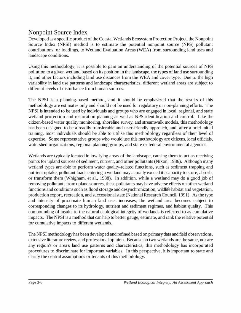
Wetland Ecological Integrity: An Assessment ApproachPage 3-6
Nonpoint Source IndexDeveloped as a specific product of the Coastal Wetlands Ecosystem Protection Project, the NonpointSource Index (NPSI) method is to estimate the potential nonpoint source (NPS) pollutantcontributions, or loadings, to Wetland Evaluation Areas (WEA) from surrounding land uses andlandscape conditions.
Using this methodology, it is possible to gain an understanding of the potential sources of NPSpollution to a given wetland based on its position in the landscape, the types of land use surroundingit, and other factors including land use distances from the WEA and cover type. Due to the highvariability in land use patterns and landscape characteristics, different wetland areas are subject todifferent levels of disturbance from human sources.
The NPSI is a planning-based method, and it should be emphasized that the results of thismethodology are estimates only and should not be used for regulatory or non-planning efforts. TheNPSI is intended to be used by individuals and groups who are engaged in local, regional, and statewetland protection and restoration planning as well as NPS identification and control. Like thecitizen-based water quality monitoring, shoreline survey, and streamwalk models, this methodologyhas been designed to be a readily transferable and user-friendly approach, and, after a brief initialtraining, most individuals should be able to utilize this methodology regardless of their level ofexpertise. Some representative groups who would use this methodology are citizens, local officials,watershed organizations, regional planning groups, and state or federal environmental agencies.
Wetlands are typically located in low-lying areas of the landscape, causing them to act as receivingpoints for upland sources of sediment, nutrient, and other pollutants (Nixon, 1986). Although manywetland types are able to perform water quality-related functions, such as sediment trapping andnutrient uptake, pollutant loads entering a wetland may actually exceed its capacity to store, absorb,or transform them (Whigham, et al., 1988). In addition, while a wetland may do a good job ofremoving pollutants from upland sources, these pollutants may have adverse effects on other wetlandfunctions and conditions such as flood storage and desynchronization, wildlife habitat and vegetation,production export, recreation, and successional state (National Research Council, 1991). As the typeand intensity of proximate human land uses increases, the wetland area becomes subject tocorresponding changes to its hydrology, nutrient and sediment regimes, and habitat quality. Thiscompounding of insults to the natural ecological integrity of wetlands is referred to as cumulativeimpacts. The NPSI is a method that can help to better gauge, estimate, and rank the relative potentialfor cumulative impacts to different wetlands.
The NPSI methodology has been developed and refined based on primary data and field observations,extensive literature review, and professional opinion. Because no two wetlands are the same, nor areany region’s or area’s land use patterns and characteristics, this methodology has incorporatedprocedures to discriminate for important variables. In this perspective, it is important to state andclarify the central assumptions or tenants of this methodology.

Wetland Ecological Integrity: An Assessment Approach Page 3-7
Firstly, one of the primary factors affecting the outcome of this weighted index is the presence, state,and condition of three wetland zones of influence. The first zone of influence is the 30.48 meter (100feet) buffer zone. In Massachusetts, this area is jurisdictional and issuing authorities have discretionregarding activities proposed in this buffer zone. The presence and condition of this upland zone orarea directly adjacent to the wetland has significant influence on the health and functional integrityof the wetland. The second zone of influence is a 100 meter area directly adjacent to the WEA–morethan twice the regulatory buffer zone. Multiple references substantiate the fact that for most wetlandsand riparian areas, in terms of pollutant transport and wildlife habitat, an area larger than 100 feetmust be considered (Desbonnet, et al., 1994; Castelle, et al., 1994; Gilliam, 1994; Groffman, et al.,1990). The final zone of influence is the wetland’s contribution area, or watershed. Watershedmanagement has become widely recognized as an important way to control NPS pollution (U.S.Environmental Protection Agency, 1993). A wetland watershed is the area on the land thatcontributes surface water and groundwater to the wetland. In regions like Cape Cod, Massachusetts,where soils are highly permeable, rainfall infiltrates rapidly and contributes to groundwater flow,while surface water flow occurs only across impervious surfaces such as roads and roofs, or wherethe ground surface intersects the water table to form a river or pond. The second assumption recognizes that the production, transport and fate of NPS pollutants isinfluenced by a number of determinants, including the nature and type of land use, the physicalcharacteristics typical of certain land uses, hydrological patterns of the watershed or contribution areaof the WEA, and intercepting or attenuating conditions. Based on extensive literature and availabledata, generalized assumptions can be made about the relative contributions of NPS pollutants fromspecific land uses. Intensive uses such as commercial areas (malls and urban centers, for example)produce more NPS pollutants than low density residential uses (Horner, 1992). Through thedevelopment of relative land use pollutant loading coefficients, this methodology has attempted toincorporate many of these variables into evaluation procedures. Due to many variables, though, itis important to point out that actual conditions may vary from output results. The pollutant loadingestimate values that have been assigned for each of the different "sources" or land use types must berecognized as educated estimates that are based on a number of different data sets, publishedliterature values, best professional judgement, and loading coefficients currently employed in models,and management and regulatory schemes. It is important to remember that actual pollutant loadsgenerated from the same land use types will vary. Again, it must be emphasized that thismethodology is only intended to be used as a planning and a "broad-brush" identification method.Enforcement, remediation, and mitigation actions should not be undertaken based solely on theoutcome of this methodology but rather on additional follow-up data collection and analysis.
As explained below in detail, the NPSI method examines the land use types in each zone of influencearea, derives estimates of the extent of each land use type, applies land use loading coefficients, andderives an index score to indicate the relative potential for NPS production and transport to a givenwetland. In addition, the NPSI also incorporates a rapid on-site evaluation component, completedwith a field data sheet for each site (Table 3.4).
To derive the Nonpoint Source Index, several steps were necessary. First, the field worksheets foreach WEA were completed, scores were totaled and then adjusted to a scale of 100. For each

Wetland Ecological Integrity: An Assessment ApproachPage 3-8
component of the NPSI method, higher index scores represent lower nonpoint source potential.Next, to complete the land use analysis components, wetland boundary and NPSI zones of influencewere delineated and land use information was compiled. Due to the groundwater dominatedhydrology of the region, the delineation of wetland watersheds was complex. Delineating surfacewater dominated watersheds is considerably simpler%generally accomplished by tracking andbisecting the topographical contour lines of hills surrounding the wetland. Ground-watersheddelineation requires the investigation of groundwater movement and regional water table contours,which are difficult to map.
Wetland Ground-Watersheds and Capture ZonesMuch of Massachusetts wetlands occur on highly permeable soils or are in contact with agroundwater aquifer. Waquoit Bay watershed overlies sandy soils and sediments tens of meters thick.Many of the lakes and wetlands in the watershed are surface water expressions of the water table.
Wetland watershed delineation in a groundwater dominated system involves estimating the degreeto which groundwater flows towards the open water portions of the wetland, or whether flowbypasses the wetland by flowing beneath and/or around it. Groundwater bound for the wetland flowsthrough the capture zone, which is a vertically oriented area that can be conceptualized as the rim ofa funnel which directs water into the wetland. The configuration of the water table determines theorigin of that groundwater which enters the capture zone. The goal of this analysis was to estimatethe depth and width of the capture zone and use this information to delineate the watershed.
The elevation of the water table reflects the potential energy of the groundwater, and this energydissipates as the water flows through sediment. Groundwater will often flow towards an area of openwater because it provides a path of least resistance. Four major factors determine the extent to whichgroundwater is directed into wetlands and thereby the size of the capture zone:
• the size of the open water area in the wetland,• the aquifer permeability and thickness,• the wetland soil permeability and thickness, and • whether streams enter or leave the wetland.
The open water area of the wetland is referred to in this analysis as a “pool”–even though this mayactually be a lake, a river or a small water filled depression. Large pools, thin aquifers, highlypermeable wetland soils and outflowing streams will all increase the wetland capture zone and,therefore, wetland watershed size. The size of the pool determines the energy savings offered by theflow path through the wetland. Aquifer thickness and permeability affect the energy cost of deepgroundwater flowing up from the bottom of the aquifer to pass through the pool.

Wetland Ecological Integrity: An Assessment Approach Page 3-9
Table 3.4. Nonpoint Source Index method field worksheet.
Wetland Evaluation Area: Date:
Nonpoint Source Index Zoneof Influence Includes:
(A) 30.48 meter buffer (100 feet), or (B) 100 meter buffer
Estimated Size of NPSI Zone: Score:
(1) Development Density High ($2 houses/acre) Score = 0
Medium (< 2 houses /acre, > 1 house/2 acres) Score = 2
Low (#1 house/2 acres) Score = 4
No development in NPSI Zone Score = 5
(2) Sewage Disposal If served by sewer Score = 5
If served by septic, score same as (1) Score =
(3) Are the Roads within theNPSI Zone...
mostly unimproved, dirt, gravel Score = 4
mostly 2-lane, paved Score = 2
mostly 4-lane paved Score = 0
(4) Direct Stormdrains towetland?
No Score = 5
Yes Score = 0
(5) Evidence of direct Runoffor Erosion to wetland?
No Score = 5
Yes Score = 2
(6) Are Lawns green and well-managed?
No Score = 5
Yes Score = 2
(7) Agricultural Type in NPSIZone is...
Row crops or nursery plants Score = 2
Orchards Score = 3
Cranberry Score = 1
Turf/Sod Score = 3
(8) Are there signs of runofffrom Dairy/Livestock holdingarea or pasture to WEA?
No Score = 5
Yes Score = 0

Wetland Ecological Integrity: An Assessment ApproachPage 3-10
(9) Do Dairy/Livestockanimals have direct access toWEA?
No Score = 5
Yes Score = 0
(10) Evidence of WaterWithdrawal from WEA?
No Score = 5
Yes Score = 1
(11) Evidence of Pesticideapplication?
No Score = 5
Yes Score = 1
(12) Evidence of recent ForestCutting?
No Score = 5
Yes Score = 1
(13) Marinas present w/inNPSI Zone?
No Score = 5
Yes Score = 1
(14) Slips/Docks/Mooringspresent w/in NPSI Zone?
No Score = 5
Yes Score = 2
(15) Type/intensity of Boatinguse in NPSI Zone is ...
mostly powerboat Score = 0
mixed powerboat/non-motorized craft Score = 2
non-motorized craft only Score = 4
(14) Evidence of recenthydromodification(channelization/fill/flowalteration) or long termimpacts?
No Score = 5
Yes Score = 0
(15) Golf Courses present w/inNPSI Zone?
No Score = 5
Yes Score = 0
(16) Sand/Gravel Extractionpresent in NPSI Zone?
No Score = 5
Yes Score =0

Wetland Ecological Integrity: An Assessment Approach Page 3-11
Wetland soils, such as muck and decomposed peat, can provide considerable resistance to water flow,effectively lengthening the shortcut through the pool. Wetlands with groundwater-fed streams willdraw additional groundwater from the aquifer, while wetlands that detain surface water at levelshigher than the water table may recharge the aquifer beneath, diverting the flow of groundwater awayfrom the wetland.
Methods: Capture zone depth for freshwater wetlandsThe first step in delineating the wetland watersheds was to determine the depth and width of thecapture zones, which describes groundwater flow immediately up gradient from the wetland. Thecapture zone dimensions for the freshwater sites (WEA1 through WEA9) were determined byapplication of a mathematical model developed by the CSIRO Water Resources Branch (Townleyet al., 1993; Nield et al., 1992; Townley and Davidson, 1988). Input parameters include the size ofthe pool, thickness of the aquifer, water table slope, aquifer and wetland soil permeability, surfacewater flows, and recharge rate. Parameters which describe the aquifer, such as its thickness andpermeability, were drawn from local water resources reports (Barlow and Hess, 1993; Masterson etal., 1996; Cambarerri et al., 1992; Sasaki Associates Inc., 1983). Pool size and estimates of wetlandsoil permeability and thickness were determined using aerial photographs, field surveys and theNatural Resource Conservation Service’s Soil Survey of Barnstable County (Fletcher, 1993). It isimportant to note that this model was designed for wetlands with pools that are large compared tothe thickness of the aquifer. Its accuracy is likely to be higher for such wetlands such as WEA3 thanfor wetlands with smaller pools such as WEA7 or WEA2. This model also does not account forchanges in pool size, so an average size was used.
Methods: Capture zone depth for salt marshesGroundwater discharge to salt marshes is affected by the pattern of groundwater discharge to themarine receiving water (Waquoit Bay) and by the differences in density between salt and fresh water.The rate of groundwater discharge is typically maximized at the shore and decreases with distanceinto the bay. Salt marshes at the shore are in a position to receive a large portion of that groundwaterdischarge. This discharge is inhibited by the relatively low permeability of salt marsh peat, but thepresence of springs and seeps indicates that peat is not uniformly impermeable. Capture zone depthwas estimated by assuming that groundwater discharge is diverted neither up nor down by the saltmarsh. The depth of the capture zone was estimated as the depth of the salt marsh peat measurednear the center of the marsh, which ranged between 0.2 and 0.6 meters at the salt marsh study sites(WEA10 through WEA14).
Fresh groundwater floats above saline groundwater with relatively little mixing. In the Waquoit Baysystem, this freshwater lens at the head of the bay tapers away from the shore (Cambarerri et al.,1992). This reduces the freshwater aquifer thickness and forces the groundwater to discharge to theestuary above. At the shore, the thickness of the freshwater lens is the effective thickness of theaquifer. At the head of Waquoit Bay the lens was measured by Cambarerri and others (1992) asapproximately 3.0 meters. This thickness was used for all sites.
The assumption that groundwater discharge occurs at the fringing salt marshes is supported bysalinity measurements of salt marsh porewater at both of the fringing marshes where wells were

Wetland Ecological Integrity: An Assessment ApproachPage 3-12
installed. These measurements indicated that at certain times at least 75 percent of the porewater wasfresh.
Capture zone delineationThe regional water table maps illustrated that groundwater flow diverted towards the larger wetlandstudy sites: WEA1, WEA3, WEA4, WEA8, and WEA10. Capture zone width was determined forthese sites based on the water table maps. For the smaller freshwater sites: WEA2, WEA6, WEA7and WEA9, the CSIRO model was used. This model indicates that capture zone width ranges fromone to two times the width of the pool, depending on wetland soil permeability and the influence ofother wetlands. The fringing salt marshes,WEA11 and WEA12 ,were assigned capture zone widthsequal to the width of the marshes. Pocket marshes, WEA13 and WEA14, were assigned capturezones widths equal to approximately twice the marsh width because groundwater discharge tends tobe focused at embayments.
The up gradient length of the watershed was determined based on the distance from the wetland tothe groundwater divide, which is analogous to the ridge line on a topographic map. The ratio of thedepth of the capture zone to the depth of the aquifer is equal to the ratio of the up gradient length ofthe watershed to the distance to the groundwater divide. Maps of the regional water table byCambarerri et al. (1992) and Sasaki Associates (1983) were used to determine the shape of thewatersheds based on capture zone width and watershed length. The width of the watershed was setequal to the width of the capture zone unless water table contours indicated otherwise. Where thesemaps failed to provide sufficient resolution of the water table (i.e. for WEA11, WEA12, and WEA13)topography and insight from other studies were used to estimate the water table shape.
For all sites, the size of the watershed was primarily a function of pool size, the permeability of thewetland soils, and the distance to the groundwater divide. In regions with highly permeable sedimentsand gentle topography, wetlands with pools generally serve as flow through conduits forgroundwater. Groundwater enters on the up gradient side of the wetland and discharges on the downgradient side. Sites WEA2, WEA3, WEA6, WEA7, WEA8, and WEA9 were found to be flowthough wetlands. Sites WEA1, WEA4, and WEA10 are the source water for outflowing streams.These sites receive groundwater discharge from both sides, and the watersheds for these wetlandsextend up gradient to the water table divide. The fringing salt marshes, WEA11 and WEA12, havesmall watersheds primarily because the wetlands are both small and located close to the localgroundwater divide. The pocket salt marshes WEA13 and WEA14 have relatively larger watershedsbecause of their greater shoreline length, but these sites are also close to the local groundwater dividewhich limits watershed size. Figure 3.1 displays the ground-watersheds for each project WEA.
Geographic Information System Analysis for NPSIFor the purposes of this project, computer software programs were utilized to calculate the NPSIscores. Geographic Information System (GIS) software (ArcView 3.0a) enabled project staff tooverlay wetland and zones of influence polygons over interpreted 1990 land use, query thegeographic information, and to calculate specific areas of intersection. For each WEA, the extentof specific McConnell land use types was computed for each zone of influence: the 30.48 m bufferarea, the 100 m buffer area, and the site wetland watershed. This data was then exported to

Wetland Ecological Integrity: An Assessment Approach Page 3-13
2 0 2 Miles N
Figure 3.1. Watershed delineations (groundwater) for each Wetland Evaluation Area.

Wetland Ecological Integrity: An Assessment Approach Page 3-15
spreadsheet software (Excel 97) for the last analysis steps. For each of the 37 McConnell land usetypes in the GIS land use layer, specific NPSI loading coefficients were developed. Table 3.5contains NPSI coefficients for only those land use types identified in the project area. Next, for eachNPSI zone of influence, the area of each land use type identified was multiplied by the NPSI loadingcoefficient. These products were totaled and divided by the entire area of the specific zone ofinfluence to derive a NPSI subtotal score for each zone. To illustrate, in the watershed zone ofinfluence for site WEA7, four land use types were identified: forest, residential-1 (density is smallerthan 1/4 acre lots), residential-3 (density is larger than ½ acre lots), and golf course, with a total areaof 28,170 m2. First, the forest land use area (1,441 m2) and was multiplied by a NPSI coefficient of1.00. Residential1 area (11,356 m2) was multiplied by 0.36; residential-3 area (2,347 m2) wasmultiplied by 0.75; and golf course area (13,026 m2) was multiplied by 0.55. These four productswere totaled to a sum of 14,454 and then divided by the total watershed area to derive the NPSIwatershed subtotal score of 51.31. This process was repeated for each zone and for each site.
The final step in the NPSI method is to combine each of the scores from the rapid assessment fieldworksheet, the 30.48 m buffer zone, the 100 m buffer zone, and the wetland watershed. Aspreviously explained, one of the major assumptions of this model is that the presence and conditionof upland areas directly adjacent to the wetland have significant influence on the health and functionalintegrity of the wetland. For this reason, the subtotal scores for each NPSI component are weighteddifferently as they are combined to comprise the final NPSI score. The subtotal scores for each NPSIcomponent, their relative weight, and the final NPSI scores are displayed in Table 3.6.
It is important to note that for others interested in implementing the NPSI method, neither GIS norspreadsheet software is necessary–this method can be implemented using information that is easilyobtained from maps and other sources. Once land use and wetland information is acquired, the NPSIanalysis really only involves conducting some area estimates (such as the dot grid method) andperforming some mathematical operations.
The NPSI results serve to provide a robust index of a wetland’s relative potential to receive NPSpollutants from upland land use activities, to rank wetlands for prioritizing management actions, andto aid in the interpretation of other data. For example, sites with high NPSI scores–implying littleNPS contribution potential–but low biological scores are probably exhibiting signs of ecologicalimpairment due to habitat alteration. Section 9 describes the tight statistical correlation between theNPSI scores and other WHAT approach outputs.

Wetland Ecological Integrity: An Assessment ApproachPage 3-16
Table 3.5. Land use types and NPSI loading coefficients.McConnell Land Use 37 Code Land Use Description NPSI Loading Coefficient
1 cropland 0.36
3 forest 1.00
4 wetland 1.00
5 mining, land disturbance 0.30
6 open land 0.96
9 water recreation 0.85
10 residential 0 0.19
11 residential 1 0.36
12 residential 2 0.58
13 residential 3 0.75
14 salt marsh 1.00
15 commercial 0.20
16 industrial 0.36
17 urban open 0.85
18 transportation 0.20
20 water 1.00
21 woody perennial 0.70
23 cranberry bog 0.37
24 power lines 0.96
25 sandy beach 1.00
26 golf 0.55
27 salt marsh 1.00
29 marina 0.64
37 forest wetland 1.00

Wetland Ecological Integrity: An Assessment Approach Page 3-17
Table 3.6. NPSI subtotals and final scores for all study sites.
Site 30.48m Zone(weight x3)
100m Zone(weight x2)
Watershed Zone(weight x1)
Rapid Worksheet(weight x2)
Final NPSIScore
WEA2 100.00 100.00 100.00 98.86 100
WEA3 100.00 97.79 55.53 90.91 92
WEA1 73.90 85.05 59.97 84.09 77
WEA4 56.99 73.12 74.91 76.14 68
WEA6 64.28 58.49 54.02 73.86 64
WEA7 48.65 58.62 51.31 59.09 54
WEA8 93.23 80.61 81.87 76.14 84
WEA9 78.59 71.11 74.85 67.05 73
WEA10 99.77 99.39 98.67 98.86 99
WEA11 61.95 59.69 64.00 73.86 65
WEA12 58.00 58.00 58.00 65.91 60
WEA13 58.00 58.00 58.00 62.50 59
WEA14 91.83 81.05 82.13 59.09 80

Wetland Ecological Integrity: An Assessment ApproachPage 3-18
Functional EvaluationAs discussed in Section 1, wetland functions are the physical, chemical, and biological processes andattributes of a wetland. Wetlands perform these unique functions independent of human society.Human society’s valuation of wetland functions is best described as wetland values. Over the last twodecades, for different purposes, a range of methods or approaches have been developed to determineand assess the relative level of functions that given wetlands perform. Distinct from direct field-basedmeasurements and research of wetland characteristics, indirect or rapid functional assessments relyon relatively simple observations, calculations, and questions to come up with an estimation ofwetland functions and values. Most of these rapid functional assessment methods are based onavailable literature and findings, and, as such, serve as wetland functional models. By inputting certaininformation, it is possible to gain a rough estimate of a wetland’s ability to perform or provide specificfunctions and values.
For the Coastal Wetlands Ecosystem Protection Project, project staff reviewed a host of availablefunctional assessment methodologies to select one that best suited the project needs. For this project,the functional assessment method needed to be current, peer-reviewed, applied in New Englandwetlands, and rapid (i.e. implemented by a trained project team member in a day or less). Thefollowing methods were evaluated for use:
• Method for the Evaluation of NonTidal Wetlands in Connecticut. Ammann, 1986.• Wetland Evaluation Technique (WET), Volume II. Adamus, 1987.• Method for the Comparative Evaluation of NonTidal Wetlands in New Hampshire. Ammann,
1991.• A Hydrogeomorphic Classification for Wetlands. Brinson, 1993.• Method for the Evaluation and Inventory of Vegetated Tidal Marshes in New Hampshire
(Coastal Method). Cook et al., 1993.• The Highway Methodology Workbook: Wetland Functions and Value, A Descriptive
Approach. US Army Corps of Engineers, 1995.• Evaluation for Planned Wetlands. Environmental Concern, Inc., 1996.
After review and evaluation, modified versions of the two New Hampshire methods were selectedas the rapid functional assessment methodologies to be utilized. The following serves as a very briefexplanation for this decision. The Connecticut method is basically an earlier version of the NewHampshire nontidal wetland evaluation, and the more current of these very similar methods wastherefore selected. The WET method was not selected as it was somewhat dated and required threeseparate levels of evaluation: social significance, effectiveness and opportunity, and habitat suitability.The Evaluation for Planned Wetlands is a detailed and effective functional evaluation method but wasexceedingly labor-intensive. Brinson’s HGM method, currently embraced by the US Army Corps ofEngineers as the national standard for functional assessment method, is in its formative stages withregional models for different wetland classes still under development and is not available for use. TheHighway manual had appeal for being quick and straight-forward, but its output is qualitative, ornarrative, and by design does not produce quantitative functional assessments.

Wetland Ecological Integrity: An Assessment Approach Page 3-19
The adaption of New Hampshire tidal and nontidal methods involved selecting the functions, or“functional values,” to be evaluated, changing the scoring approach to exclude wetland size, andmodifying the definition of the wetland evaluation unit. Both New Hampshire methods utilize thesame evaluation format, requiring the evaluator to answer a number of questions both in the field andback in the office for each function. The questions pertain to a range of wetland and landscapephysical, biological, and hydrological characteristics as well as other factors such as surrounding andin-wetland land use. Table 3.7 lists the functions as contained in the New Hampshire manuals andthe functions which were evaluated for the purposes of this project. Table 3.8 contains an exampleof a single page of the New Hampshire method field manual. For each question and answer, thepossible range of scores for the Functional Value Index (right-hand column) is from 0 to 1.0. Toderive the score for each function, the Functional Value Index scores are averaged. According to theNH guidance, the higher the score, the greater degree to which the site exhibits the function inquestion.
The results of the modified New Hampshire method for both the freshwater wetlands are containedin Table 3.9 and the salt marsh functional assessment scores are in Table 3.10. Where a score is “NA”it is because this function is not being performed at the wetland in question and therefore should notbe evaluated. The final NH method scores are the averages of all the individual function evaluations.The results of each of the three rapid assessment methods are graphically represented in Figure 3.2and Figure 3.3.

Wetland Ecological Integrity: An Assessment ApproachPage 3-20
Table 3.7. New Hampshire Method (tidal and nontidal) functional values evaluated.
NonTidal Method Evaluated? Tidal Method Evaluated?
Ecological IntegrityWildlife HabitatFinfish HabitatEducational PotentialVisual/Aesthetic QualityWater-Based RecreationFlood Control PotentialGround Water Use PotentialSediment TrappingNutrient AttenuationShoreline Anchoring andDissipationUrban Quality of LifeHistorical Site PotentialNoteworthiness
YesYesYesYesYesYesYesYesYesYesYesNoNoNo
Ecological IntegrityShoreline AnchoringStorm Surge ProtectionWildlife, Finfish, & ShellfishHabitatWater Quality MaintenanceRecreation PotentialAesthetic QualityEducation PotentialNoteworthiness
YesYesYesYesYesYesYesYesNo
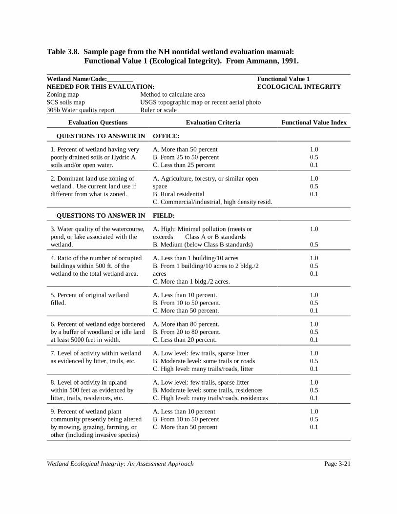
Wetland Ecological Integrity: An Assessment Approach Page 3-21
Table 3.8. Sample page from the NH nontidal wetland evaluation manual: Functional Value 1 (Ecological Integrity). From Ammann, 1991.
Wetland Name/Code:________ Functional Value 1NEEDED FOR THIS EVALUATION: ECOLOGICAL INTEGRITYZoning map Method to calculate area SCS soils map USGS topographic map or recent aerial photo305b Water quality report Ruler or scale
Evaluation Questions Evaluation Criteria Functional Value Index
QUESTIONS TO ANSWER IN OFFICE:
1. Percent of wetland having verypoorly drained soils or Hydric Asoils and/or open water.
A. More than 50 percentB. From 25 to 50 percentC. Less than 25 percent
1.00.50.1
2. Dominant land use zoning ofwetland . Use current land use ifdifferent from what is zoned.
A. Agriculture, forestry, or similar openspaceB. Rural residentialC. Commercial/industrial, high density resid.
1.00.50.1
QUESTIONS TO ANSWER IN FIELD:
3. Water quality of the watercourse,pond, or lake associated with thewetland.
A. High: Minimal pollution (meets orexceeds Class A or B standardsB. Medium (below Class B standards)
1.0
0.5
4. Ratio of the number of occupiedbuildings within 500 ft. of thewetland to the total wetland area.
A. Less than 1 building/10 acresB. From 1 building/10 acres to 2 bldg./2acresC. More than 1 bldg./2 acres.
1.00.50.1
5. Percent of original wetlandfilled.
A. Less than 10 percent.B. From 10 to 50 percent.C. More than 50 percent.
1.00.50.1
6. Percent of wetland edge borderedby a buffer of woodland or idle landat least 5000 feet in width.
A. More than 80 percent.B. From 20 to 80 percent.C. Less than 20 percent.
1.00.50.1
7. Level of activity within wetlandas evidenced by litter, trails, etc.
A. Low level: few trails, sparse litterB. Moderate level: some trails or roadsC. High level: many trails/roads, litter
1.00.50.1
8. Level of activity in uplandwithin 500 feet as evidenced bylitter, trails, residences, etc.
A. Low level: few trails, sparse litterB. Moderate level: some trails, residencesC. High level: many trails/roads, residences
1.00.50.1
9. Percent of wetland plantcommunity presently being alteredby mowing, grazing, farming, orother (including invasive species)
A. Less than 10 percentB. From 10 to 50 percentC. More than 50 percent
1.00.50.1

Evaluation Questions Evaluation Criteria Functional Value Index
Wetland Ecological Integrity: An Assessment ApproachPage 3-22
10. Percent of wetland activelybeing drained for agriculture orother purposes.
A. Less than 10 percent.B. From 10 to 50 percent.C. More than 50 percent.
1.00.50.1
11. Number of public road and/orrailroad crossings per 500 feet ofwetland (measured along long axisof wetland).
A. NoneB. OneC. Two or more
1.00.50.1
12. Long-term stability. A. Wetland appears to be naturally occurring,not impounded by dam or dike.B. Wetland appears to be somewhatdependent on artificial diking by dam, road,fill, etc.
1.0
0.5
Average Functional Value Index for Functional Value 1:
(Average of third column.)

Wetland Ecological Integrity: An Assessment Approach Page 3-23
Table 3.9. Functional Evaluation scores for New Hampshire Method for freshwater sites.
Function WEA2 WEA3 WEA1 WEA4 WEA6 WEA7 WEA8 WEA9
Ecological Integrity 1.00 0.94 0.76 0.58 0.63 0.58 0.65 0.61
Wildlife Habitat 0.81 0.80 0.71 0.56 0.44 0.27 0.51 0.59
Fish Habitat NA 0.83 0.72 0.41 0.37 NA 0.52 0.43
Education Potential 0.6 0.71 0.85 0.60 0.48 0.25 0.23 0.36
Aesthetic Quality 0.84 0.75 0.78 0.62 0.58 0.34 0.42 0.62
Water-Based Recreation NA 0.86 0.59 0.63 0.59 NA 0.27 0.36
Flood Control 1.00 1.00 1.00 1.00 1.00 1.00 1.00 1.00
Ground Water Use 0.88 0.53 0.43 0.43 0.53 0.53 0.56 0.50
Sediment Trapping 0.38 0.49 0.64 0.54 0.61 0.47 0.75 0.82
Nutrient Attenuation 0.40 0.54 0.56 0.70 0.73 0.58 0.78 0.78
Shoreline Anchoring NA 0.67 1.00 0.50 0.37 NA 0.37 0.83
Average All Functions 0.74 0.74 0.73 0.60 0.57 0.50 0.55 0.63
Scale adjusted (x 100) 74 74 73 60 57 50 55 63

Wetland Ecological Integrity: An Assessment ApproachPage 3-24
Table 3.10. Functional Evaluation scores for New Hampshire Method for salt marsh sites.
Function WEA10 WEA11 WEA12 WEA13 WEA14
Ecological Integrity 1.00 0.55 0.48 0.54 0.59
Shoreline Anchoring 0.75 0.75 0.75 1.00 0.75
Storm Surge Protection 0.75 0.10 0.10 0.10 0.10
Wildlife & Fish Habitat 0.66 0.36 0.38 0.40 0.40
Water Quality Maintenance 0.83 0.70 0.70 0.70 0.70
Recreation Potential 0.67 0.57 0.52 0.48 0.64
Aesthetic Quality 0.86 0.43 0.47 0.50 0.63
Education Potential 0.74 0.51 0.51 0.37 0.66
Average All Functions 0.78 0.50 0.49 0.51 0.56
Scale Adjusted (x 100) 78 50 49 51 56

Wetland Ecological Integrity: An Assessment Approach Page 3-25
0.00
10.00
20.00
30.00
40.00
50.00
60.00
70.00
80.00
90.00
100.00
WEA2 WEA3 WEA1 WEA4 WEA6 WEA7 WEA8 WEA9
HANPSIFA
Figure 3.2. Final results of rapid assessment methods: freshwater sites.

Wetland Ecological Integrity: An Assessment Approach Page 3-27
0.00
10.00
20.00
30.00
40.00
50.00
60.00
70.00
80.00
90.00
100.00
WEA10 WEA11 WEA12 WEA13 WEA14
HANPSIFA
Figure 3.3. Final results of rapid assessment methods: salt marsh sites.

Wetland Ecological Integrity: An Assessment Approach Page 4-1
Section 4. Wetland Vegetation
Wetland vegetation, because of its relative stationary properties, may serve as a practical indicatorof ecological stress (Hunsaker and Carpenter, 1990). Changes in wetland vegetative compositionare community-level responses that integrate the effects of a wide range of ecological stressors.Community composition, species abundance, productivity, dynamics, structure, and health willchange as environmental conditions shift (Shindler, 1987). Generally, such responses cannot beattributed to specific stressors without concurrent data on other factors such as hydrology orhydroperiod, water chemistry, and soil conditions. Vegetative indicators were used to assessecological integrity through a multi-metric approach (see Focus Box in Section 2), taking intoconsideration the community assemblage, structure, and function of wetlands to derive an Index ofVegetative Integrity (IVI).
The development of the Index of Vegetative Integrity was based primarily on the existingbiomonitoring index structures established by Karr (1981), Plafkin et al. (1989), and Hicks (1997),which incorporate metrics to address response mechanisms at the individual, population, andcommunity levels. Wetland vegetation will respond to both physical and chemical stressors,including the hydrological alterations and increased nutrient inputs typically associated with humandevelopment of the landscape. In the Waquoit Bay watershed, the main land uses affecting wetlandresources are the drainage and waste practices of medium to high density residential development,the stormwater management conventions of roads and highways, the siting and management ofcranberry agriculture, and golf course construction and management. The Index of VegetativeIntegrity incorporates specific functional attributes and metric scoring in an attempt to quantify theseland use impacts on wetland plant species and communities.
MethodsThe wetland vegetation investigations for this project required species identification and coverabundance assessment at all 13 Wetland Evaluation Areas. Two methods were selected for thevegetative cover analysis. Cover data was collected during the middle of the growing season in1996 (late June to the middle of September). The vegetative cover abundance of 13 study sites wassurveyed using plant community sampling protocols adapted from Tiner (1996) and Jackson (1995):an observation method and a plot sampling method.
The observation method was used only when it was possible to gain a thorough estimate of arealcoverage from vantage points within or next to the wetland. This method was consideredappropriate for use only for very small wetlands (1-2 acres), and only for marsh or shrub wetlandswhere it is possible to observe the entire wetland unit, or for mixed-cover wetlands, where theforested component is predominately open canopy. At least two evaluators walked through thewetland to familiarize themselves with the vegetative communities and species present. Next, a listof the individual species was made. When no new species were found, evaluators estimated theareal coverage of each species on the list. Evaluators then compared coverage values with oneanother and with standardized coverage charts and then revised estimates if necessary. To be asaccurate as possible, areal estimates included the coverage of duff, leaves, bare ground, and open

Wetland Ecological Integrity: An Assessment ApproachPage 4-2
water, collectively designated as other. Areal estimates were adjusted during the analysis stage toaccount for the coverage of this other category.
The plot sampling method was the principal method utilized in this investigation, and wasconsidered appropriate for larger wetlands and for wetlands with dense under and over story. Theplot sampling method produces a comprehensive species list and an accurate assessment of arealcoverage, or abundance. Similar to the general observation method, evaluators first determined thecommunity structure of the study site and the dominant species present. Next the areal coverage foreach community was assessed and then randomized plots were established in each distinct vegetativecommunity. If a random plot siting occurred at the upland border where vegetation patterns weretransitional, the plot was discarded and sited again. Plot size depended on the vegetative strata beingassessed. The four strata groups are defined in Table 4.1.
Table 4.1. Wetland vegetation strata.Strata: Defined As:
Trees Diameter at breast height greater than or equal to 12.7 centimeter (5 in.) and 6.1meter (20 ft.) or taller
Saplings Diameter at breast height less than 12.7 cm and 6.1 m or taller
Shrubs Woody plants less than 6.1 m tall
Herbs Non-woody (herbaceous) plants
A 9.14 m (30 ft.) radius circular plot was utilized for the tree and sapling strata, a 4.57 m (15 ft.)radius plot was used for the shrub stratum, and a 1.52 m (5 ft.) radius plot was used to evaluate theherb stratum. For trees, basal area for each tree was determined. Diameter at breast height wasmeasured with a diameter tape at a height of 1.37 m (4.5 ft.) above the ground surface. Basal areawas calculated using the formula: BA = (3.1416) x (dbh2/4). Every plant present in the samplingplots was identified to species level, if possible. For each species in the sampling plot, arealcoverage was estimated, compared to another evaluators’ estimate and revised if necessary. As withthe observation method, areal estimates took into consideration the coverage of duff, leaves, bareground, open water, and non-target vegetation (i.e., herbaceous species in a shrub plot), and arealestimates were revised accordingly.
Of the thirteen study sites, vegetative cover of nine sites was assessed using the plot samplingmethod (WEA1, WEA2, WEA3, WEA4, WEA7, WEA8, WEA10, WEA12, WEA14) and four siteswere suitable to be evaluated using the observation method (WEA6, WEA9, WEA11, WEA13). Theaverage number of random sample plots per wetland was 7.33.
Data AnalysisThroughout this study, the freshwater and the salt marsh WEAs were evaluated and comparedseparately. Data obtained from each study site were entered into computer spreadsheet files (Excel97), compiled, and metrics were generated as described below. Statistical analysis was completedprimarily by computer statistics software (SPSS 6.0.1). For each plot evaluated, percent coveralways totaled 100, but, as explained above, this cover percentage often included the category called

Wetland Ecological Integrity: An Assessment Approach Page 4-3
other%duff, leaves, bare ground, and open water, and in the case of the plot sampling method, non-target vegetation types. Areal cover percentages, or abundance values, were then adjusted toaccount for the percentage of wetland cover occupied by other. When the other value was removed,the remaining plant species coverage totaled 100.
For this investigation, a community-based assessment approach was employed (see the followingFocus Box). With this assessment method, individual vegetation species abundance values wereadjusted according to the extent of each community in the wetland. This community-basedapproach results in a more accurate estimate of each species’ relative abundance in the wetland, notjust in the plot it was surveyed in.
After the abundance values were adjusted for community-weighting and for other coverage, twototal species lists were compiled, one for the freshwater sites and one for the salt marsh sites. Eachlist includes the total wetland abundance value for each species at each WEA. From the total lists,each species was then assigned specific wetland vegetation attribute scores. Each wetlandvegetation attribute and value is defined below. Section 12 (Appendix) contains the total specieslist and the attribute scores for each species identified in this project.
� Persistent Standing Litter. A species with a positive persistent standing litter attribute hasa significant part of its above-ground biomass that remains standing during the dormantperiod until next growing season. All shrubs and trees are persistent. Examples ofemergent plants with persistent standing litter are: Typha latifolia (broad-leaved cattail),Scirpus cyperinus (wool grass), and Spirea tomentosa (steeple bush). Species with persistentstanding litter were assigned a score of 1; those that die back were assigned a 0. Theattribute scores were based on literature, identification guides, and professional judgement.
� Opportunistic. A species with a positive opportunistic attribute is able to tolerate a widerange of habitat types and conditions and is therefore well adapted to thrive in a variety ofconditions. Opportunistic species will pioneer disturbed areas as well as competeadvantageously in altered sites. Examples of opportunistic species are: Sparganiumeurycarpon (great burreed), Lysimachia terrestris (swamp candle), and Clethra alnifolia(sweet pepper bush). Opportunistic species were assigned a score of 1; others assigned a 0.The attribute scores were based on literature, identification guides, and professionaljudgement.
� Invasive. A species with a positive invasive attribute is defined as an aggressive colonizerof natural and disturbed areas, often forming extensive monocultural stands. Invasivespecies are frequently alien, or non-native. Examples of invasive species are: Phragmitesaustralis (common reed), Decodon verticilattus (swamp loosestrife), and Toxicodentronradicans (poison ivy). Invasive species were assigned a score of 1; others were assigned a0. The attribute scores were based on literature, identification guides, and professionaljudgement.

Wetland Ecological Integrity: An Assessment ApproachPage 4-4
A
B
Focus Box: Community-Based Method for Vegetation Survey
Depending on the method employed, surveying vegetation in the same wetland can actuallyproduce different results. Plot sampling techniques can give very accurate estimates of aspecies dominance in the plot surveyed, but using this information to describe the entirewetland would result in erroneous evaluations. Transect sampling techniques, if utilizedjudiciously, would produce a more accurate picture of species abundance throughout thewetland but can be extremely labor-intensive. In addition, depending on the size of the wetland,an inadequate number or placement of transects would also produce misleading data.
The community-based assessment method used for this investigation relies first on anassessment of the specific communities in a wetland. Next, several vegetation plots are sitedin each community in order to produce an accurate representation of the species present in thecommunity being evaluated. Species abundance values can then be adjusted to reflect thatcommunity’s relative areal coverage of the entire wetland. Consider this simplified examplewithin a hypothetical wetland:
Wetland Plant Community A, in this example,occupies 60 percent of the wetland and can becharacterized as an emergent community with threespecies: Species 1, Species 2, and Species 3. WetlandPlant Community B occupies 40 percent of thewetland and is a shrub sapling community with twospecies, Species 4 and Species 5.
Several plot surveys are conducted in community, andthe abundance values for each species is identified.Consider that for one survey plot in Community A,Species 1 had area cover of 70 percent, Species 2 hadcover of 20 percent and Species 3 had cover of 10percent. For this survey plot, the total speciesabundance totals 100 percent. But Species 1 does notoccupy 70 percent of the wetland. If the plot isrepresentative of Community A (or if enough plotsare surveyed in Community A), though, Species 1 can
be assumed to occupy 70 percent of Community A. Therefore, to determine the abundancevalue of Species 1 for the entire wetland, its community abundance value (70 percent) ismultiplied by Community A’s extent in the wetland (60 percent). As a result of thisadjustment, Species 1 is found to occupy 42 percent of the entire wetland. This sameadjustment is conducted for the rest of the species surveyed in both communities (Species 2through Species 5). The complete community-weighted wetland species list should total 100.

Wetland Ecological Integrity: An Assessment Approach Page 4-5
� Wetness. A ranking of a species relative affinity to hydric (wet) conditions. This attributeis taken directly from the USFWS National List. Attributes range from obligate (wetlanddependent) to upland, based on the median probability of a species occurrence in a wetland.Wetness scores were assigned according to this scale: Obligate = 1.00, FacWet+ = 0.91,FacWet = 0.82, FacWet- = 0.71, Fac+ = 0.60, Fac = 0.50, Fac- = 0.71, FacUp+ = 0.29,FacUp = 0.18, FacUp- = 0.09, Upland = 0.00.
� Flood Tolerance. A ranking of a species tolerance to relative lengths of inundation. Theattribute ranges from intolerant to very high tolerance. Intolerant species are killed by lessthan 3 days of inundation in a growing season, while species with very high tolerance canwithstand a full growing season of inundation. This attribute is used only for freshwaterspecies. Flood tolerance scores were assigned according to this scale: Very High = 1.00,High = 0.80, Medium = 0.60, Low = 0.40, Intolerant = 0.20. The values for this attributewere adapted from the New England Institute for Environmental Studies Plant CommunityIndicator Database (Michner,1990).
� Salinity Tolerance. A ranking of a species’ tolerance to saline conditions. The attributesrange from intolerant to very high tolerance. Intolerant species will not survive salt waterexposure, including occasional ocean spray. Species with very high tolerance will survivein tidal areas with twice daily inundation of salt water. This attribute is used only for saltmarsh wetland species. Salinity tolerance scores were assigned according to this scale: VeryHigh = 1.00, High = 0.80, Medium = 0.60, Low = 0.40, Intolerant = 0.20. The values forthis attribute were adapted the New England Institute for Environmental Studies PlantCommunity Indicator Database (Michner,1990).
� Nutrient Status. A ranking of a species affinity for areas with differing nutrientavailabilities. Attributes range from species generally occurring in areas with low nutrientavailability (as in bogs and isolated wetlands) to those species occurring in areas withdisturbances or enrichment from fertilizer or wastewater. Nutrient status scores wereassigned according to this scale: Bogs, lowest nutrients = 0.12; Sands, low nutrients = 0.23;Acid woods, till, and sandy loam = 0.34; Alluvial acid soils, enriched by flood deposits =0.45; Sweet soils in calcareous areas = 0.56; Alluvial sweet soils = 0.67; Somewhatdisturbed or partly enriched soils = 0.78; Disturbed or enriched soils = 0.89; Very disturbedand heavily enriched = 1.00. The values for this attribute were adapted from the NewEngland Institute for Environmental Studies Plant Community Indicator Database(Michner,1990).
The final data analysis step was to process the species, abundance, and attribute data into a set ofmetrics for each study site. Table 4.2 displays the Index of Vegetative Integrity metrics, therationale for their use, the predicted response to impairment, and the method for metric valuecomputation. Using the reference sites as the bench marks, attributes for each study site werecompared and a relative metric score was computed according to the scoring criteria in Table 4.3and Table 4.4. The metric scores were then totaled and transformed into a final IVI score.

Wetland Ecological Integrity: An Assessment ApproachPage 4-6
Table 4.2. Index of Vegetative Integrity metrics.
Metric Rationale Response toStressors
Metric Computation
Community Similarity Resemblance of communities toreference site will shift asstressors increase
Decline Total percent shared species
Taxa Richness Total number of plant specieswill change as stressorsincrease
Variable Absolute difference of totaltaxa
Persistent StandingLitter
Decomposition of vegetationprovides important food chainsupport and habitat structure
Rise Total abundance of specieswith a positive PSL attribute
Invasive Increased presence of invasivespecies reduces habitat andother wetland functions
Rise Total abundance of specieswith positive invasive attribute
Opportunistic Opportunistic species willcolonize or persist as habitatconditions are altered bystressors
Rise Total abundance of specieswith positive opportunisticattribute
Wetness Species composition will shifttowards upland or obligate dueto hydrologic stressors
Variable Percent similarity of wet valueweighted for abundance
Flood tolerance(freshwater sites only)
Species with higher floodtolerance will colonize orpersist as duration of floodingchanges
Variable Percent similarity of floodtolerance value weighted forabundance
Salinity tolerance(salt marsh sites only)
Species with lower salinitytolerance will colonize orpersist with change in tidalhydrology
Decline Percent similarity of salinitytolerance value weighted forabundance
Nutrient status Species composition will shiftwith nutrient enrichment andelevated eutrophication
Decline Percent similarity of nutrientstatus value weighted forabundance

Wetland Ecological Integrity: An Assessment Approach Page 4-7
ResultsA total of 86 freshwater wetland plant species and 25 saltmarsh plant species were identified in theproject WEAs (see Appendix). Nearly half the freshwater species were found in more than oneWEA. The freshwater species with the greatest total overall abundance values were: Viburnumdentatum (southern arrowwood), Vaccinium macrocarpon (cranberry), Scirpus cyperinus, Nymphaeaodorata (white water lily), and Lysimachia terrestris. The species with the highest frequency ofoccurrence in WEAs were: Acer rubrum (red maple), Sphagnum palustre (sphagnum moss),Vaccinium corrymbusum (Highbush blueberry), Clethra alnifolia, Lysimachia terrestris, andPolygonum punctatum (water smartweed).
For the saltmarsh wetlands, 60 percent of the plant species were found in more than one WEA. Thesaltmarsh species with the greatest total overall abundance values were: Spartina alterniflora(smooth cordgrass), Spartina patens (salt hay grass), Iva frutescens (hightide bush), Distichlisspicata (spike grass), and Phragmites australis. One third of all the saltmarsh species were presentin all of the WEAs. These species were: Distichlis spicata, Iva frutescens, Salicornia europea(common glasswort), Spartina alterniflora, and Spartina patens.
IVI scores for the freshwater wetland study sites ranged from a minimum of 46 to the maximumscore of 100, with a mean of 60.94 and a standard deviation of 17.24. Table 4.5 lists both the metricand IVI scores for the freshwater sites; Figure 4.1 graphically displays the freshwater IVI results.Variability between freshwater sites was greatest for the Community Similarity Metric, theOpportunistic Metric, and the Nutrient Status Metric.
IVI scores for the salt marsh study sites ranged from a minimum of 38 to the maximum of 100, witha mean of 73.33 and a standard deviation of 23.31. Table 4.6 displays the final metric and IVIscores for the saltmarsh study sites; Figure 4.2 graphically displays the salt marsh IVI resultsSaltmarsh study sites displayed the most extreme variability in the Community Similarity Metric,the Decomposition Metric, and the Intrusion Metric. IVI scores for saltmarsh sites WEA12 andWEA13 also fell below the mean.
Inter-Annual VariationTo check the relative variation of the vegetation sampling method, five of the thirteen study siteswere assessed again, following the exact same methodology described above, in June of 1997. Inall five cases, the wetland plant species abundance values varied less than ten percent from the dataobtained in 1996.

Wetland Ecological Integrity: An Assessment ApproachPage 4-8
Table 4.3. Index of Vegetative Integrity metric scoring criteria: freshwater sites.
Score: 0 2 4 6 Standard Deviation
Community Similarity <25 25-49 50-75 >75 25
Taxa Richness >9 7-9 3-6 <3 3
Persistent Standing Litter >89 77-89 65-77 <65 12
Invasive >29 20-29 9-19 <9 10
Opportunistic >75 63-75 50-62 <50 25
Wetness <67 67-77 78-89 >89 11
Flood Tolerance <85 85-89 90-95 >95 5
Nutrient Status <34 34-55 56-78 >78 22
Table 4.4. Index of Vegetative Integrity metric scoring criteria: salt marsh sites.
Score: 0 2 4 6 Standard Deviation
Community Similarity <40 40-59 60-80 >80 20
Taxa Richness >6 5-6 2-4 <2 2
Persistent Standing Litter >90 75-90 58-74 <58 16
Invasive >33 17-33 1-17 <1 16
Opportunistic >72 59-72 44-58 <44 14
Wetness <88 88-91 92-96 >96 4
Salinity Tolerance <70 70-79 80-90 >90 10
Nutrient Status <58 58-71 72-86 >86 14

Wetland Ecological Integrity: An Assessment Approach Page 4-9
Table 4.5. Final metric and IVI scores for freshwater study sites .
Metric WEA2 WEA3 WEA1 WEA4 WEA6 WEA7 WEA8 WEA9
Community 6 6 2 2 2 2 4 2
Taxa Richness 6 6 2 0 2 2 4 6
PersistentStanding Litter
6 4 4 2 2 4 6 0
Invasive 6 4 4 4 6 2 4 4
Opportunistic 6 4 2 6 0 6 6 4
Wetness 6 6 4 4 6 2 4 4
Flood Tolerance 6 6 6 6 6 2 4 6
Nutrient Status 6 6 6 2 4 6 4 6
Raw IVI Score 48 42 32 28 26 30 32 34
Final IVI Score 100 88 67 58 54 63 67 71
Table 4.6. Final metric and IVI scores for salt marsh study sites.
Metric WEA10 WEA11 WEA12 WEA13 WEA14
Community 6 4 2 2 2
Taxa Richness 6 4 4 4 6
Persistent StandingLitter
6 6 2 4 4
Invasive 6 4 0 4 6
Opportunistic 6 4 4 0 4
Wetness 6 4 2 6 6
Salinity Tolerance 6 6 2 6 6
Nutrient Status 6 6 2 6 6
Raw IVI Scores 48 38 18 32 40
Final IVI Scores 100 79 38 67 83

Wetland Ecological Integrity: An Assessment Approach Page 4-11
0.00
10.00
20.00
30.00
40.00
50.00
60.00
70.00
80.00
90.00
100.00
WEA2 WEA3 WEA1 WEA4 WEA6 WEA7 WEA8 WEA9
Figure 4.1. Index of Vegetative Integrity: freshwater sites.

Wetland Ecological Integrity: An Assessment Approach Page 4-13
0.00
10.00
20.00
30.00
40.00
50.00
60.00
70.00
80.00
90.00
100.00
WEA10 WEA11 WEA12 WEA13 WEA14
Figure 4.2. Index of Vegetative Integrity: salt marsh sites.

Wetland Ecological Integrity: An Assessment Approach Page 5-1
Section 5. Aquatic Macro Invertebrates
Aquatic invertebrate biomonitoring has historic roots in stream, river, and lake managementprograms, and is applied nationwide. Within the last five years or so attention has been turned to theapplication of aquatic invertebrate biomonitoring in wetland habitats. There is a growing consensusthat any wetland assessment procedure needs to be based on data that represents a reference, or"minimally impaired" condition against which subject wetland(s) may be compared for degree ofseverity of impact. Normally this reference condition is established from pooled data gathered froma set of reference sites (Brinson and Reinhardt, 1996; Kentula et al., 1993; Yoder and Ranking,1995). Reference sites must be representative of the natural conditions within the same geologicaland climatic setting together with the same hydrological regime as the subject wetlands (Brinson andReinhart, 1996). Due to the high diversity of conditions within wetlands it is also desirable toconsider similarities in vegetation classes.
A habitat assessment that incorporates both surrounding upland and wetland features is an importantcomponent of an invertebrate monitoring program. It is used to interpret the invertebrate samplingresults, indicate the source(s) of impact, and provide a guide to best management practices that canbe implemented to restore ecological integrity to a wetland.
Wetlands present special constraints that challenge the successful design of aquatic invertebratesampling protocols. The constraints include: the complexity of wetland types, seasonality ofhydrological regime, dense and resilient vegetation stands, lack of wetland data on invertebratetolerance ratings, and minimal guidance as to suitable metrics and indices that will be sensitive andaccurate in measuring wetland invertebrate community health.
The objectives of this study were to design aquatic invertebrate biomonitoring protocols for bothfreshwater and salt marsh wetlands, to test their application in the 13 selected wetlands within theWaquoit Bay watershed, and to record the biological condition of the project wetlands.
MethodsSamples of aquatic invertebrates were taken at each Wetland Evaluation Area (WEA) over threeseasons: May 1996, August 1996, and May 1997. This allowed for seasonal variation to bemeasured, and provided an indication of inter-annual variation.
Within the freshwater wetlands, three randomly selected composite (D-Net and Sediment Corer)samples were taken as follows: The D-Net was held fully extended to the right hand side of thebody, and starting at the surface of the water, a 180o sweeping arc was prescribed, incrementallydescending through the vegetation and the water column downwards to complete the sweep on theleft hand side at the sediment interface. The net containing the sample was brought straight up to thesurface for retrieval. The retrieved contents of the net were inverted over a bucket, and using abaster, all debris and invertebrates washed free of the net into the bucket. The net was carefullyexamined for any clinging organisms and vegetation, and removed with forceps to the bucket. Thebucket contents were strained through a standard U.S. No. 30 brass sieve to remove water, and

Wetland Ecological Integrity: An Assessment ApproachPage 5-2
placed into a zip-lock bag, ensuring that no invertebrates were left on the sieve. Sediment sampleswere collected using a Wildco 5.5 cm diameter hand core sediment sampler.
Within the salt marshes, three randomly selected composite (rectangular frame, D-Net, soil auger)samples were taken at the low tide line on the bank and within the water and sediments as follows:a rectangular metal frame, 25 cm x 40 cm, was placed on the surface of the marsh bank, and all visibleliving organisms found within the frame were identified and counted; the water column and vegetationwere sampled using a D-frame aquatic net that was held fully extended to the right hand side of thebody at the water surface, and in an arching sweep pulled slowly downwards through the floating andattached marine vegetation and water column to rest at the sediment interface on the left hand sideof the body. At that point the net was brought sharply to the surface for the retrieval of the contents.Sediment samples were collected using AMS 3 1/4" diameter sand auger.
Samples were bagged, preserved in 70 percent isopropyl alcohol, labeled, and returned to thelaboratory for sorting, identification to family level, and enumeration, without subsampling.
Data AnalysisA multi-metric approach (see Focus Box Section 2) using reference condition was used to analyzethe raw data. The metrics and indices utilized are listed in Tables 5.1 (freshwater) and Table 5.2 (saltmarsh). The values for each metric/index (calculations are shown below) were derived from theaverage of three random samples for each site and scored according to the formulas in Table 5.3(freshwater) and Table 5.5 (salt marsh). By referring to the predetermined Biological ConditionScoring Criteria in Table 5.4 (freshwater) and Table 5.6 (salt marsh), the metric scores wereweighted, summed, and converted to a percentage to derive the final Invertebrate Community Index(ICI).

Wetland Ecological Integrity: An Assessment Approach Page 5-3
Table 5.1. Freshwater invertebrate community metrics and indices.
Metric/Index Category Rationale Response toStressors
Total Number ofOrganisms
Enumeration andcommunity composition
Nutrient enrichment will usuallysupport higher numbers of organisms. Toxicity and habitat degradation willreduce numbers.
Variable
% Contribution of MajorFeeding Groups
Enumeration andcommunity composition
A healthy community will have abalance between the various trophicgroups.
Variable
% Contribution ofDominant Family
Enumeration andcommunity composition
A healthy community will have abalanced composition between taxa,with more than 2 dominant groups.
Rise
Taxa Richness Diversity Diversity is a measure of communitycomplexity, responds adversely tostress intensity.
Decline
EOT Richness(Ephemeroptera,Odonata, Trichoptera)
Diversity Healthy systems have greater numbersof sensitive taxa and predator-guildorganisms.
Decline
EOT/ChironomidaeRatio
Community health Healthy systems have highersensitive/predator to tolerantorganisms ratios.
Decline
OtherOdonata/CoenagrionidaeRatio
Community health Healthy systems have higher sensitiveto tolerant Odonate ratios. Decline
% Tolerant / % IntolerantRatio
Community health Impacted systems have higher tolerantto intolerant organism ratios.
Rise
Family Biotic Index Community health Community’s averaged tolerance valuewill rise with increasing stressors.
Rise
Community TaxaSimilarity Index
Similarity to referencecondition
Resemblance of taxa composition toreference will shift with stressors.
Decline
Community TrophicSimilarity Index
Similarity to referencecondition
Resemblance of trophic pattern toreference will shift with stressors.
Decline
Invertebrate CommunityIndex
Summarizedbioassessment
Overall community condition willdecline with increasing degradation.
Decline
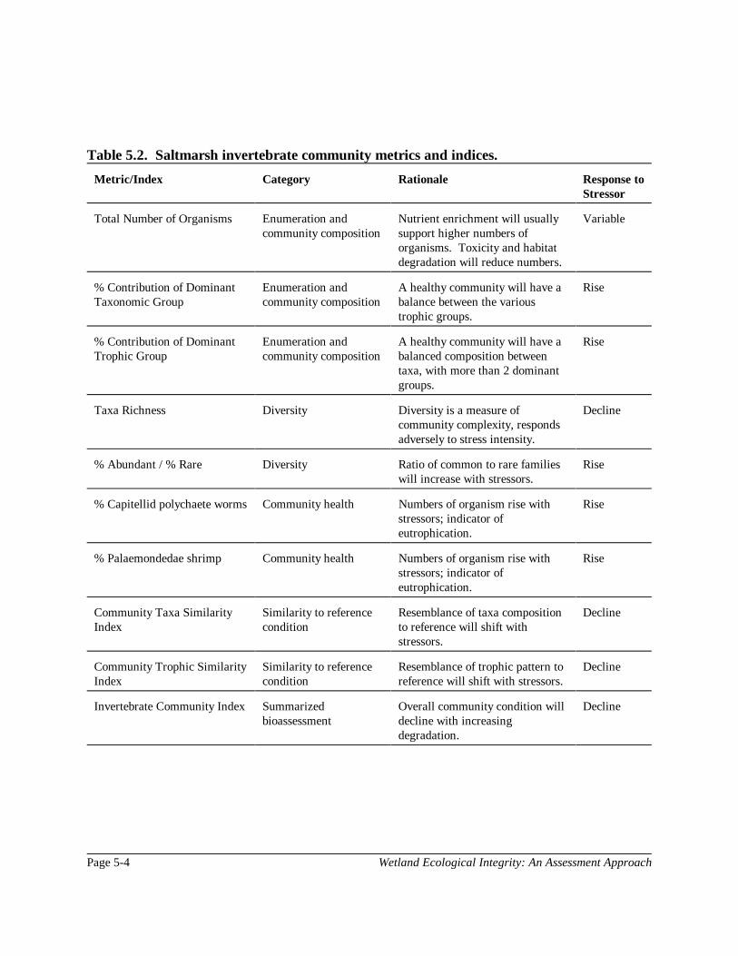
Wetland Ecological Integrity: An Assessment ApproachPage 5-4
Table 5.2. Saltmarsh invertebrate community metrics and indices.
Metric/Index Category Rationale Response toStressor
Total Number of Organisms Enumeration andcommunity composition
Nutrient enrichment will usuallysupport higher numbers oforganisms. Toxicity and habitatdegradation will reduce numbers.
Variable
% Contribution of DominantTaxonomic Group
Enumeration andcommunity composition
A healthy community will have abalance between the varioustrophic groups.
Rise
% Contribution of DominantTrophic Group
Enumeration andcommunity composition
A healthy community will have abalanced composition betweentaxa, with more than 2 dominantgroups.
Rise
Taxa Richness Diversity Diversity is a measure ofcommunity complexity, respondsadversely to stress intensity.
Decline
% Abundant / % Rare Diversity Ratio of common to rare familieswill increase with stressors.
Rise
% Capitellid polychaete worms Community health Numbers of organism rise withstressors; indicator ofeutrophication.
Rise
% Palaemondedae shrimp Community health Numbers of organism rise withstressors; indicator ofeutrophication.
Rise
Community Taxa SimilarityIndex
Similarity to referencecondition
Resemblance of taxa compositionto reference will shift withstressors.
Decline
Community Trophic SimilarityIndex
Similarity to referencecondition
Resemblance of trophic pattern toreference will shift with stressors.
Decline
Invertebrate Community Index Summarizedbioassessment
Overall community condition willdecline with increasingdegradation.
Decline

Wetland Ecological Integrity: An Assessment Approach Page 5-5
The following is an explanation of the freshwater ICI metrics and indices:
• Total Number of Organisms The total number of organisms in each sample, summed, and averaged.
• % Composition of Major Groups(Total average density for each major group/Total average density of the sample) x 100.Groups include: Ephemeroptera, Odonata, Trichoptera, Chironomidae, Other Diptera, Coleoptera,Hemiptera plus Homoptera, Lepidoptera, Amphipoda, Isopoda, Oligochaeta, Hirudinea,Gastropoda, and Pelecypoda.
• % Contribution of Dominant FamilyThe group with the highest percent representation.
• Taxa RichnessThe total number of identified aquatic macro invertebrate families present at each site.
• EOT Richness
The total number of Ephemeroptera, Odonata, and Trichoptera (EOT)families present ateach site.
• EOT/Chironomidae Ratio(Total average density of EOT/Total average density of Chironomidae)
• Other Odonates/Coenagrionidae Ratio(Total average density of other Odonates/Total average density of Coenagrionidae)
• % Tolerant /% Intolerant Ratio Tolerant organisms were those having a tolerance value (Hilsenhoff, 1988) from 7 to 10, andintolerant organisms were those having a tolerance value from 0 to 4.
• Family Biotic IndexThis index averages the various eutrophication tolerances of the families that make up theaquatic invertebrate community (adapted from Hilsenhoff, 1988)
• Community Taxa Similarity IndexThe degree of similarity between the reference condition and study site based on a comparisonof dominant groups. The score is calculated by finding the absolute difference between thereference site and the study site for each family/group, then summing these values. This totalis converted to the index score by dividing in half, and subtracting from 100. [100 - (TotalScore/2)].

Wetland Ecological Integrity: An Assessment ApproachPage 5-6
• Community Trophic Similarity IndexThe degree of similarity between the reference condition and the study site based on acomparison of the trophic groups (scrapers, filter collectors, gathering collectors, predators,shredders, piercers-herbivores, omnivores, mixed). As above, the absolute differences for eachof these trophic groups were summed and converted [100-(Total Score/2)] to derive theCommunity Trophic Similarity Index.
• Invertebrate Community IndexA multiple metric index, combining all the above metrics and indices into a single index valuewithout losing the information from the original measurements (Davis, 1995). Using thereference condition, or model value–the average of the two reference sites WEA2 andWEA3–and project wetland data, the Biological Condition Score (n) was calculated for eachmetric and index as displayed in Table 5.3. The final ICI score was obtained by totaling theBiological Condition Score of the 12 metrics/indices and converting it into a percentage. 72was the maximum possible score for the 12 metrics/indices, and the final ICI was totaled as:n/72 x 100.

Wetland Ecological Integrity: An Assessment Approach Page 5-7
Table 5.3. Freshwater wetlands ICI metric calculation.(Modified from Plafkin, 1989)
Metric Formula
Total Organisms n/Model value x 100
Total Taxa Richness n/Model value x 100
EOT Richness n/Model value x 100
EOT/Chironomidae Ratio n/Model value x 100
Family Biotic Index Model value/n x 100
% Tolerant / % Intolerant Model value/n x 100
% Contribution Dominant Family Model value/n x 100
Other Odonata/Coenagrionidae Ratio n/Model value x 100
% Chironomidae Model value/n x 100
% Oligochaeta Model value/n x 100
Community Taxa Similarity Index n/Model value x 100 (or CTSI n)
Community Trophic Similarity Index n/Model value x 100 (or CTSI n)

Wetland Ecological Integrity: An Assessment ApproachPage 5-8
Table 5.4. Freshwater wetlands ICI metric scoring criteria(Modified from Plafkin, 1989; Ohio EPA, 1991).
Score: 6 4 2 0
Total Organisms >90 70-90 50-69 <50
Total Taxa Richness >90 70-90 50-69 <50
EOT Richness >90 70-90 50-69 <50
EOT/Chironomidae Ratio >80 65-80 26-64 <25
Family Biotic Index >90 70-90 40-69 <40
% Tolerant / % Intolerant >80 65-80 25-64 <25
% Contribution Dominant Family >70 50-70 30-49 <30
Other Odonata/CoenagrionidaeRatio
>80 65-80 25-64 <25
% Chironomidae >90 70-90 50-69 <50
% Oligochaeta >90 70-90 50-69 <50
Community Taxa Similarity Index >64 50-64 35-49 <35
Community Trophic SimilarityIndex
>64 50-64 35-49 <35

Wetland Ecological Integrity: An Assessment Approach Page 5-9
The saltmarsh ICI metrics were calculated using the same methods as for freshwater wetland metricsexcept where noted below: • Total Number of Organisms
• Percent Contribution of Dominant Taxonomic Groups(Nemerta, Capitellida, Cossurida, Ctenodrilla, Eunicida, Orbiniidae, Phyllodocidea,Sabellida, Spionida, Terebelida, Amphipoda, Tanaidacea, Isopoda, Pelecypoda,Gastropoda, Thoracica, Decopoda Shrimps, and other groups).
• Percent Contribution Dominant Trophic Group
• Taxa Richness
• % Abundant/% Rare RatioThis metric was adapted from Roberts et al. 1996. A salt marsh community characterized bya high percentage of rare taxonomic groups but not outbalanced by a high percentage ofabundant groups may be presumed to be "close to pristine" condition. For each site, alltaxonomic groups sampled were listed, and their occurrence was categorized as follows:
Not registered (-); Rare (R) = 0 - 4; Common (C) = 5 - 49; Abundant (A) = >50.The frequency for each of the above categories was noted, and only the proportionalpercentages for R and A were calculated deriving the % Abundant /% Rare Ratio.
• Community Taxa Similarity Index
• Community Trophic Similarity IndexThe trophic categories used for this salt marsh protocol were:Carnivore (C), Deposit Feeder (DF), Grazer (G), Omnivore (O), Suspension Feeder (SF), andMixed (M).
• Invertebrate Community Index
As with the freshwater sites, the Biological Condition Score (n) for the saltmarsh WEAs wascalculated for each metric by the formulas contained in Table 5.5. Using the criteria in Table 5.6, theBiological Condition Score was then derived for each metric. These Biological Condition Scoreswere then summed and converted into a percentage to derive the final ICI score. 54 was themaximum score for 9 metrics/indices, so the final ICI score was: n/54 x 100.

Wetland Ecological Integrity: An Assessment ApproachPage 5-10
Table 5.5. Salt marsh wetlands ICI metric calculation.(Modified from Plafkin et al., 1989; Hicks, 1997)
Metric Formula
Total Organisms n/Model value x 100
Total Taxa Richness n/Model value x 100
% Contribution Dominant Taxonomic Group Model value/n x 100
% Contribution Dominant Trophic Group Model value/n x 100
% Abundant / % Rare Model value/n x 100
% Capitellida polychaete worms Model value/n x 100
% Palaemonedae shrimp Model value/n x 100
Community Taxa Similarity Index n/Model value x 100
Community Trophic Similarity Index n/Model value x 100
Table 5.6. Salt marsh wetland ICI metric scoring criteria.(Modified from Plafkin et al., 1989; Ohio EPA, 1991)
Score: 6 4 2 0
Total Organisms >90 70-90 50-69 <50
Total Taxa Richness >90 70-90 50-69 <50
% Contribution DominantTaxonomic Group
>70 50-70 30-49 <30
% Contribution DominantTrophic Group
>70 50-70 30-49 <30
% Abundant / % Rare >80 65-80 25-64 <25
% Capitellida polychaete worms >90 70-90 50-69 <50
% Palaemonedae shrimp >90 70-90 50-69 <50
Community Taxa Similarity Index >64 50-64 35-49 <35
Community Trophic SimilarityIndex
>64 50-64 35-49 <35

Wetland Ecological Integrity: An Assessment Approach Page 5-11
ResultsSixty-two families were represented throughout the nine freshwater wetlands sampled. The mostcommonly occurring families were: Chironomidae (midges) and Culicidae (mosquitoes) from theorder Diptera; Coenagrionidae (damselflies) from the order Odonata; Lumbricidae from the orderOligochaeta (worms); Sphaeriidae (finger nail clams) from the order Pelecypoda; Gammaridae fromthe order Amphipoda (scuds); Asellidae (sow bugs) from the order Isopoda. In May 1996, therewere higher numbers of individuals in the orders Ephemeroptera (mayflies), Hirudinea (leeches),Coleoptera (beetles), and Trichoptera (caddisflies) than in August 1996. Homoptera (aquatic aphids)were very numerous in several wetlands in August 1996, although this group was not found in spring.No Plecoptera (stoneflies) were collected in either season.
Overall abundance of organisms was higher in August 1996 than in May 1996. Sites with the highestnumber of taxa (families) were WEA1 and WEA6, and those with the lowest were WEA7 andWEA2. In May 1996, there was no single outstanding dominant trophic group, with dominantpercentages shifting from one wetland site to another. In August 1996, however, predatorsfrequently out numbered the other trophic groups in most wetlands. All wetlands had more tolerantindividuals than intolerant, regardless of season.
Seventy-two different taxa were sampled across the five salt marsh sites. The most commoninvertebrates were Mercenaria mercenaria (clams), Modiolus demissus (mussels), Paleamonidae(shrimp), Balanas sp. (barnacles), Amphipoda (mostly Gammaridae), and Nassarius sp. and Littorinasp. (snails). From the Polychaeta class, Nereidae and Spionidae were found in the greatestabundance. Sites with the highest taxa richness were WEA10 and WEA11, and those sites with thelowest were WEA13 and WEA12. Within the taxonomic groups, the seasonal variations that weremost notable were the rise in the number of shrimps and the decline in the number of Polychaeteworms.
Table 5.7 gives the average metrics and indices scores for the three seasons for the freshwaterwetlands. Variability across sites was high for the following: Total Organisms, % Tolerant/%Intolerant Ratio, % Oligochaeta, Community Taxa Similarity Index, Community Trophic SimilarityIndex, and to a lesser degree, % Contribution Dominant Family, % Chironomidae, and InvertebrateCommunity Index. Freshwater sites with ICI scores below the mean (68.4) were, in descendingorder, WEA8, WEA1, WEA4, WEA9, and WEA7. Apart from reference sites WEA2 and WEA3,only WEA6 scored above the mean. Figure 5.1 displays a bar graph of the final freshwater ICIscores, as averaged over the three sampling seasons.
Table 5.8 gives the average metrics and indices scores for the three seasons for the salt marshwetlands. Variability across sites was high for the following: Total Organisms, Community TaxaSimilarity Index, Community Trophic Similarity Index, and to a lesser extent, # of PalaemonedaeShrimps, and Invertebrate Community Index. Apart from the reference site (WEA10) all other sitesscored below the mean ICI score of 71.8. Figure 5.2 displays the ICI scores for the salt marshWEAs, as averaged over 3 seasons.

Wetland Ecological Integrity: An Assessment ApproachPage 5-12
Table 5.7. Freshwater wetlands ICI metrics and indices averaged over 3 seasons.
Metric/Index WEA2 WEA3 WEA1 WEA4 WEA6 WEA7 WEA8 WEA9
Total Organisms 78 203 175 151 85 126 73 71
Total Taxa Richness 11 12 18 18 22 10 12 15
EOT Richness 4 2 2 1 7 0 4 2
EOT/ChironomidaeRatio
2.1 0.3 0 0.1 4.1 0.3 1.2 4.1
Family Biotic Index 6.8 7 6.8 7.3 7.3 7 7.6 7.7
% Tolerant/% Intolerant 15 61 96 32 8 79 27 64
% ContributionDominant Family
55 70 43 39 30 64 59 41
Other Odonata/Coenagronidae Ratio
9.7 1.3 0 0 0.1 0.7 1.6 1.7
% Chironomidae 25 39 37 19 11 1 47 6
% Oligochaeta 0 2 1 0 4 64 8 8
Community TaxaSimilarity Index
100 100 37 28 36 5 54 32
Community TrophicSimilarity Index
100 100 60 34 62 32 68 59
InvertebrateCommunity Index
100 100 57 57 72 42 62 57

Wetland Ecological Integrity: An Assessment Approach Page 5-13
0.00
10.00
20.00
30.00
40.00
50.00
60.00
70.00
80.00
90.00
100.00
WEA2 WEA3 WEA1 WEA4 WEA6 WEA7 WEA8 WEA9
Figure 5.1. Invertebrate Community Index scores: freshwater sites.

Wetland Ecological Integrity: An Assessment Approach Page 5-15
Table 5.8. Salt marsh wetlands ICI metrics and indices averaged over 3 seasons.
Metric/Index WEA10 WEA11 WEA12 WEA13 WEA14
Total Organisms 193 65 119 93 131
Total Taxa Richness 28 23 18 18 20
% Contribution Dominant Taxa Group 50 46 53 52 46
% Contribution Dominant Trophic Group 57 45 54 48 39
% Abundant/% Rare 0.1 0 0.1 0 0.1
% Captellida Polychaeta 1 5 1 2 0
# Palaemonedae Shrimps 1 41 24 36 17
Community Taxa Similarity Index 100 43 65 53 46
Community Trophic Similarity Index 100 58 73 58 58
Invertebrate Community Index 100 61 67 68 63

Wetland Ecological Integrity: An Assessment ApproachPage 5-16
As a summary of the status of each wetland, the ICI was graphed in correlation with the HabitatAssessment (HA) score in Figure 5.3. This allowed for a determination of whether the ICI score wasdue to poor habitat condition, a combination of poor habitat condition and some other stressor, ornot related to poor habitat condition at all, but some other environmental stressor such as poor waterquality. Figure 5.3 correlates the averaged ICI scores with the HA scores for all 13 wetlands. Tointerpret this graphical presentation of the results, the following guidelines are important to consider.The ICI scores are listed on the vertical X axis, and the HA scores are listed horizontally on the Yaxis. On this graph, the shading of the area in which the site number is located serves to indicatewhether the invertebrate community condition is due primarily to poor habitat [red shaded area], tostressors other than habitat (i.e. eutrophication or toxic contamination) [yellow shaded], or acombination of poor habitat and other stressors [green shaded]. For example, if a site receives amoderate ICI score but a low HA score, one can predict that the invertebrate community conditionis most likely impaired due to poor habitat quality (see site WEA14). On the other hand, if a sitescores a low ICI, indicating an impacted invertebrate community, but a high HA score, the conditionis due, most likely, to stressors other than poor habitat, such as chronic nonpoint source pollution (seesite WEA1).

Wetland Ecological Integrity: An Assessment Approach Page 5-17
0.00
10.00
20.00
30.00
40.00
50.00
60.00
70.00
80.00
90.00
100.00
WEA10 WEA11 WEA12 WEA13 WEA14
Figure 5.2. Invertebrate Community Index scores: salt marsh sites.

Wetland Ecological Integrity: An Assessment Approach Page 5-19
0
10
20
30
40
50
60
70
80
90
100
0 10 20 30 40 50 60 70 80 90 100
Poor habitat Poor habitat & other stressors Other stressors
Inve
rteb
rate
Com
mun
ity In
dex
Habitat Assessment
WEA2WEA10WEA3
WEA8
WEA1
WEA6
WEA12WEA13
WEA14 WEA11
WEA4
WEA7
WEA9
Figure 5.3. Graphic of ICI score versus HA score.

Wetland Ecological Integrity: An Assessment Approach Page 5-21
Seasonal and Inter-Annual VariationThe seasonal differences in ICI scores between May 1996, August 1996, and May 1997 are shownin Table 5.9 (freshwater sites) and Table 5.10 (saltmarsh sites). The ICI scores declined between Mayand August 1996 for most of the nine study (non-reference) sites, except WEA1 and WEA8, withthe score unaltered for WEA11. Comparing the inter-annual variation for ICI scores calculated forMay 1996, August 1996, and May 1997 reveals that the standard deviation is generally very lowexcept for sites WEA6, WEA8 and WEA13, indicating that the overall variation (seasonally and inter-annually) was not significant.
It was generally assumed that wetland condition would deteriorate between spring and late summerdue to higher temperatures, lower overnight dissolved oxygen concentrations, higher loads ofnutrients from sewage discharge due to the increase in population over the holiday season, and theimpact of management practices on the cranberry farm and golf courses. Toxicant levels were alsoexpected to rise with increased road usage and applications of pesticides to lawns, golf courses andthe cranberry bog. These impacts would be counter balanced to a marginal degree by the increasedvegetation growth within the wetlands themselves, providing elevated water purification potential toeach wetland, and increasing habitat opportunity for the invertebrates. WEA1’s improved summercondition was due to vegetation growth, and the fact that it was in a protected habitat with minimalhuman impact. WEA8’s condition also improved, possibly due to the difference in vegetation densitybetween the two sampling seasons. All other wetlands’ biological integrity declined over theintervening three months. The biological integrity of all the salt marsh sites declined between Mayand August, due to the same reasons as set out above for freshwater wetlands.

Wetland Ecological Integrity: An Assessment ApproachPage 5-22
Table 5.9. Seasonal ICI scores: freshwater sites
Site ICI May 1996 ICI August 1996 ICI May 1997 StandardDeviation
WEA1 53 61 56 4.04
WEA2 100 100 100 0
WEA3 100 100 100 0
WEA4 61 53 58 4.04
WEA6 72 61 83 11
WEA7 47 39 39 4.62
WEA8 50 72 64 11.14
WEA9 64 53 53 6.35
Table 5.10. Seasonal ICI scores: salt marsh sites
Site ICI May 1996 ICI August 1996 ICI May 1997 StandardDeviation
WEA10 100 100 100 0
WEA11 63 56 63 4.04
WEA12 71 67 63 4
WEA13 67 78 58 10.02
WEA14 67 67 54 7.51
Wetland Ecological Integrity: An Assessment Approach Page 6-1
Section 6. Water Chemistry
As discussed in the introductory section, wetlands provide a multitude of functional roles in thenatural landscape, including critical wildlife habitat and flood control, and water qualityimprovements. The ability of wetlands to serve as improver of water quality has been welldocumented (Mitsch and Gosselink, 1993; Meiorin, 1989; Whigham et al., 1988; Hemmond andBenoit, 1988; Brinson, 1988; Nixon, 1986). Due to their natural landscape positions and depositionalcharacteristics, wetlands are commonly the receivers of anthropogenic sources of pollution. Uniquebiogeochemical conditions in wetlands create strongly reducing environments (low or no oxygen,anaerobic) that allow wetlands to assimilate or transform a wide array of pollutants, includingnutrients, sediments, metals, and biological and chemical oxygen demanding substances. The abilityof a given wetland to retain, absorb, or transform specific pollutants can be compromised, though,when the assimilative capacity of the wetland is surpassed. In addition, while a wetland may beperforming water quality improvements by assimilating anthropogenic pollution, the effects of thesepollutants on the ecology of the wetland and, therefore, on other wetland functions may be severe.Urban and agricultural runoff, sewage disposal practices, sedimentation from construction andforestry activities, and other sources of pollutants have the potential to significantly alter wetlandbiological communities and the subsequent food chains they support, reduce flood storage capacity,and impair drinking water supplies.
While many people become concerned over visible signs of eutrophication in lakes, ponds, streams,and coastal embayments, public recognition of wetland eutrophication is practically non-existent. Infact, public perception towards wetlands and water quality has been strongly towards treating allnaturally occurring wetlands as disposal areas that are best suited for accepting waste and drainage.
The measurement of ambient wetland water chemistry has recently been regarded as one of the mostuseful tools available to wetland managers (Brown et al., 1990; Leibowitz, 1990; Hemond andBenoit, 1988). The comparison of ambient water chemistry of reference wetlands to study sites hasstrong potential to link pollutant concentrations to both surrounding or contributing land use as wellas to biological responses.
The need for comprehensive water quality measurements should not be understated. Due to the highdegree of natural variability found in wetland water chemistry, single samples or limited data sets maylead to inaccurate predictions or analyses. The naturally high spatial and temporal variability can beaddressed by increasing sample size (data points) and by compositing samples. Cost effectivenessis a balancing concern here, though. Samples requiring laboratory analysis have associated costs thatcan quickly add up with number of stations and frequency of collection.
The objectives of this investigation were to sample each reference and study site at a frequencysufficient to obtain a representative perspective of ambient water chemistry, to compare these resultsbetween study sites in order to determine if differences in ambient pollutant concentrations existed,and to use the water chemistry data as an aid to interpret other data sets.

Wetland Ecological Integrity: An Assessment ApproachPage 6-2
Finally, in order to better understand the relative contribution and pollutant concentrations of directstorm drain discharges, a storm event sampling component was added as part of this largerinvestigation. The objectives of the stormwater sampling component were to sample stormwaterdischarge over the course of three storm events, to obtain a representative pollutant concentrationsof storm water discharge over time, and to analyze and present these results.
MethodsWater chemistry measurements were made at one or more stations at each wetland study site on amonthly basis for the 1996 growing season and bi-monthly for the 1996-1997 senescent period.Constituents that were sampled in this investigation include:
• Temperature (degrees C)• pH• Conductivity (uS)• Salinity (ppt)• Dissolved oxygen (mg/l) • Total suspended solids (mg/l)• Nitrate plus nitrite (mg/l)• Ammonia (mg/l)• Ortho-phosphate (mg/l)• Particulate organic carbon and nitrogen (um)• Total fecal coliform bacteria (number/100 ml)
In addition, stormwater sampling was conducted at one of four sites with direct stormwaterdischarges. From this stormwater data, an estimate of pollutant loading on an average storm basis wasobtained.
All samples were collected with standard techniques as outlined in Handbook for Sampling andSample Preservation of Water and Wastewater (EPA-600/4-82-029). All water chemistry samplingwas completed in accordance with an approved Quality Assurance Project Plan (QAPP).
Measurements for temperature, conductivity, pH, and dissolved oxygen were obtained in the fieldwith the use of a YSI 600 probe and data logger. Within one hour of beginning a sampling run, theYSI probe was calibrated in the laboratory using methods described in the YSI 600 Multi-ParameterWater Quality Monitor Instruction Manual.
For all other parameters, sample bottles were all acid-washed or pre-sterilized, with the exception ofthe 250 ml fecal coliform bottles which were autoclaved. Samples were collected by trained ProjectTeam personnel. Sample identification information was completed at the time of sampling. SampleIDs included name, site, date, time, and assay. All samples were maintained on ice and in dark fromcollection in the field through transport directly to the laboratory where the chemical analyses wereperformed.

Wetland Ecological Integrity: An Assessment Approach Page 6-3
Sampling was coordinated so that samples were analyzed within QAPP-specified holding times. Alldissolved nutrient constituents samples were filtered upon collection in the field. Particulate OrganicCarbon and Nitrogen samples were filtered within 24 hours of collection. Bacterial samples wereanalyzed within 12 hours of collection.
Field data sheets were maintained by Project Team personnel to document each sampling event. Thefield data sheets record location, station, date, time of each sample, number of samples by constituent,number of QA samples, weather conditions, physical conditions, and other relevant information.
Samples were collected from pre-selected stations (selected based on representation of a particularwetland type and to encompass the range of environmental variability found within the system). Fieldduplicates (two independent samples from the same sampling site and depth) were collected duringeach sampling round to assess the natural variability of each parameter as well as variabilityintroduced during the sampling and analysis process.
Dissolved nutrient (nitrate-nitrite, ammonium nitrogen, and ortho-phosphate) analyses were extractedfrom a single composite sample. In the field, the sample was extracted at the designated site samplingstation, filtered (0.45 um), and placed on ice. The filtration process went as follows: Utilizing anacid-washed syringe, 60 ml of water was withdrawn from the composite sample. This volume waspassed through the syringe and discarded. Another 60 ml was withdrawn and, utilizing an acid-washed filter housing, 30 ml was passed through the filter and discarded. Another 30 ml was injectedinto the 60 ml sample bottle, the bottle was rinsed, and the volume discarded. Finally, another 60 mlwas withdrawn and passed through the filter into the 60 ml sample bottle.
Particulate nutrient samples remained unfiltered, collected in dark bottles, put immediately on ice andkept dark. These conditions of cold and dark were maintained from field collection through toanalysis at the laboratory. Upon arrival at the laboratory, the POC/PON sample was filtered andrefrigerated until analysis.
Samples for total fecal coliform bacteria were collected in separate, sterilized bottles and transferredto the laboratory the day of sampling for processing within 12 hours.
Samples for organics were collected in separate solvent-rinsed borosilicate glass containers withTeflon-lined caps and transferred to the laboratory the day of sampling for processing within 14 days.
Laboratory analyses methods and holding times are shown in Table 6.1.

Wetland Ecological Integrity: An Assessment ApproachPage 6-4
Table 6.1. Analysis methods, matrices, references, and holding times.
Parameter Matrix Units Method Reference Holding Time
Nitrate + Nitrite water uM Autoanalyzer a 48 hours
Ammonium water uM Indophenol b 24 hours
Total DissolvedNitrogen
water uM Persulfatedigestion
c 24 hours
Ortho-phosphate water uM Molybdenumblue
d 24 hours
ParticulateOrganicCarbon/Nitrogen
particulates uM Elementalanalysis
e 24 hours
Fecal ColiformBacteria
water CFU Membranefiltration
f 12 hours
Total SuspendedSolids
particulates mg/l EPA Method160.2
g 12 hours
Total PetroleumHydrocarbons
water mg/l EPA Method415.1
h 14 days
a Lachat Autoanalysis procedures based upon the following techniques:Wood, E., F. Armstrong, and F. Richards. 1967. Determination of nitrate in sea water by cadmiumcopper reduction to nitrite. J. Mar. Biol. Ass. U.K. 47:23-31.Bendschneider, K. and R. Robinson. 1952. A new spectrophotometric method for the determination of nitrite in sea water. J. Mar. Res. 11: 87-96.
b Scheiner, D. 1976. Determination of ammonia and Kjeldahl nitrogen by indophenol method. Water Resources 10: 31-36.
c D’Elia, C., P. Steudler and N. Corwin. 1977. Limnol. Oceanogr. 22:760-764.d Murphy,J, and J. Riley. 1962. A modified single solution method for the determination of phosphate in
natural waters. Anal. Chim. Acta 27:31-36.e Perkin-Elmer Model 2400 CHN Elemental Analyzer Technical Manual.f Standard Methods for the Examination of Water and Wastewater, 18th Edition, 1992.g Methods for Chemical Analysis of Water and Wastes, US EPA 600/4-79-020, Revised 1983. &
Methods for the Determination of Metals in Environmental samples, June 1991 and Supplement I, May1994.
h Test Methods for Evaluating Solid Waste, US EPA SW846, Third Edition 1986.

Wetland Ecological Integrity: An Assessment Approach Page 6-5
Data AnalysisWater chemistry data was entered into spreadsheet computer software (Excel 97). A multi-metricapproach (see Focus Box, Section 2) using reference conditions was used to analyze the waterchemistry data. Table 6.2 displays the Water Chemistry Index (WCI) metrics for wetlands, therationale for their use, the predicted response to impairment, and the method for metric valuecomputation. For this investigation and analysis, the average pollutant concentrations for eachWetland Evaluation Area (WEA) were utilized to obtain the metric scores. By referring topredetermined scoring criteria, contained in Table 6.3 and Table 6.4, metrics scores were obtainedfor each WEA. The metric scores were summed and then converted to a percentage (scale of 100)to derive the final Water Chemistry Index score.
ResultsTable 6.5 displays the metric scores for each freshwater WEA. The range of WCI scores forfreshwater sites was considerable, with a high of 100 and a low of 17, but the mean freshwater WCIscore was 70.83. The median freshwater WCI score was 72.22, with a standard deviation of 27.98.Figure 6.1 graphically displays the final Water Chemistry Index scores for the freshwater WEAs.
The salt marsh metric scores are displayed in Table 6.6. Saltmarsh WCI scores did not vary as muchas the freshwater sites, with the high salt marsh WCI score being 100 and the low 56. The mean WCIfor saltmarsh WEAs was 74.44, the median 72.22, and the standard deviation was 16.48.
As discussed in Section 9, many of the study sites, both freshwater and salt marsh WEAs,demonstrated high concentrations of nutrients in shallow wetland groundwater. In addition, fecalcoliform levels were consistently found to be significantly over human recreational contact levels atseveral sites, even after extended periods with no precipitation. Uniformly high total suspended solidconcentrations were also detected at several freshwater and salt marsh WEAs.

Wetland Ecological Integrity: An Assessment ApproachPage 6-6
Table 6.2. Metrics for Water Chemistry Index.
Metric Rationale Response toStressors
Metric Computation
Specific Conductivity(Freshwater sites only)
Conductivity levels indicatepresence of dissolvedinorganic compounds
Rise Absolute difference fromreference value
Salinity(Salt marsh sites only)
Salt marsh biologicalcommunities are dependenton specific saline levels
Decline Mean PPT for study site
Fecal Coliform Bacteria Fecal coliform bacteria isharmful to human health
Rise Mean CFU for study site
Total Suspended Solids Reduce quality andavailability of aquatichabitat, reduce clarity andsun penetration, increaserate of sedimentation
Rise Mean concentration (mg/l)for study site
Otho-Phosphates Accelerate primaryproductivity,eutrophication, algalblooms, invasive plantspecies
Rise Mean concentration (mg/l)for study site
Ammonia Accelerate primaryproductivity,eutrophication, algalblooms, invasive plantspecies
Rise Mean concentration (mg/l)for study site
Nitrate/Nitrite Potentially harmful tohuman health; accelerateprimary productivity,eutrophication, algalblooms, invasive plantspecies
Rise Mean concentration (mg/l)for study site

Wetland Ecological Integrity: An Assessment Approach Page 6-7
Table 6.3. Water Chemistry Index metric scoring criteria: freshwater sites.Score: 0 2 4 6 Standard Deviation
Specific Conductivity >157 125-156 93-124 <93 32
Fecal Coliform >200 100-199 50-99 <49 NA
Total Suspended Solids >36 23-35 11-22 <10 13
Phosphorous >0.20 0.11-0.19 0.10-0.03 <0.02 0.09
Ammonia >1.03 0.55-1.02 0.09-0.56 <0.09 0.47
Nitrate + Nitrite >2.28 0.16-2.27 0.04-1.15 <0.04 1.12
Table 6.4. Water Chemistry Index metric scoring criteria: salt marsh sites.Score: 0 2 4 6 Standard Deviation
Salinity <25 25.0-25.9 26.0-27 >27.0 1.3
Fecal Coliform >100 50-100 30-49 <30 NA
Total Suspended Solids >37.0 27.0-37.0 17.0-26.9 <17 10.0
Phosphorous >0.10 0.08-0.10 0.06-0.07 <0.07 0.02
Ammonia >0.12 0.08-0.12 0.04-0.07 <0.04 0.04
Nitrate + Nitrite >0.06 0.05-0.06 0.03-0.04 <0.03 0.02

Wetland Ecological Integrity: An Assessment ApproachPage 6-8
Table 6.5. Final metric and WCI scores for freshwater sites.
Metric WEA2 WEA3 WEA1 WEA4 WEA6 WEA7 WEA8 WEA9
SpecificConductivity
6 6 4 6 2 2 4 4
Fecal Coliform 6 6 6 6 6 0 2 0
TSS 6 6 6 6 6 0 2 6
Phosphorous 6 6 2 4 4 0 4 4
Ammonia 6 6 6 6 6 0 4 6
Nitrate/Nitrite 6 6 0 4 4 4 2 4
Raw WCI Score 36 36 24 32 28 6 18 24
Final WCI Score 100 100 67 89 78 17 50 67
Table 6.6. Final metric and WCI scores for saltmarsh sites.
Metric WEA10 WEA11 WEA12 WEA13 WEA14
Salinity 6 6 4 4 2
Fecal Coliform 6 6 6 6 4
TSS 6 6 2 6 2
Phosphorous 6 4 6 6 6
Ammonia 6 4 4 0 4
Nitrate/Nitrite 6 2 2 4 2
Raw WCI Scores 36 28 24 26 20
Final WCI Scores 100 78 67 72 56

Wetland Ecological Integrity: An Assessment Approach Page 6-9
0
10
20
30
40
50
60
70
80
90
100
WEA2 WEA3 WEA1 WEA4 WEA6 WEA7 WEA8 WEA9
Figure 6.1. Water Chemistry Index: freshwater sites.

Wetland Ecological Integrity: An Assessment Approach Page 6-11
0
10
20
30
40
50
60
70
80
90
100
WEA10 WEA11 WEA12 WEA13 WEA14
Figure 6.2. Water Chemistry Index: salt marsh sites.

Wetland Ecological Integrity: An Assessment Approach Page 6-13
Stormwater ResultsA total of three separate storm events over the course of 1996-1997 were sampled. These eventsoccurred on July 31, 1996; May 6, 1997; and June 22, 1997. Grab samples were taken manuallydirectly from the storm drain discharge point. In all three cases, the first flush from the storm drainwas captured and then samples were taken at regular intervals through the course of the storm event.The first flush refers to the initial discharge of stormwater that collects in the catch basins anddrainage pipes and then overflows from this collection system to release from the outfall structure.Rainfall intensity and volume for these three storm events varied, but for each storm the total rainfallvolume exceeded 0.5"–the minimum volume necessary to qualify as a rain event for this project.Total amounts of precipitation were obtained from a rain gauge at the Waquoit Bay NationalEstuarine Research Reserve and reading were confirmed by rainfall data collected by the MADepartment of Environmental Management at the Long Pond Reservoir in Falmouth, MA.
From the data collected it is clear that pollutant concentrations in stormwater runoff are significantlyhigher than in ambient wetland surface and pore water. In some cases the stormwater runoffpollutant concentrations are several orders of magnitude greater. In addition, from stormwater flowand wetland water level data as well as regular observations, it became evident that sites receivingdirect stormwater discharges were subject to much greater variations in wetland water level thanreference sites and study sites with no direct discharge. Water levels at site WEA7, in particular,exhibited significant variability. Table 6.7 documents the mean, maximum, and minimumconcentration for selected pollutants for the three storm events sampled, as well as the standarddeviation.
Figures 6.3 through 6.6 serve to graphically display the concentrations of specific pollutants instormwater runoff directly discharged to wetland study sites over the course of a rain event. Eachline represents a single storm event at a unique site. Several graphs show only the results from twoevents. This is because nutrient analyses were completed only for two events, and data for anotherevent has a couple TSS and fecal coliform values that were dramatic outliers–perhaps due to samplecontamination (in the field or laboratory). These data were therefore eliminated from the analysis.
As a point of reference, a red line has been placed on each graph showing the ambient concentrationof the pollutant averaged over all of the freshwater sites. This overall average--assimilating even thehigh ambient concentrations of certain study sites–is, in many cases, a fraction of the stormwaterconcentrations. Many of these figures also illustrate the first flush effect of stormwater runoff–thathigher concentration of pollutants are typically contained in the first volumes of stormwaterdischarge.

Wetland Ecological Integrity: An Assessment ApproachPage 6-14
Table 6.7. Pollutant concentrations of stormwater for three rain events 1996-1997.
Mean Maximum Minimum StandardDeviation
Specific Conductivity (uS/cm) 68.25 199.00 7.00 53.49
Total Suspended Solids (mg/l) 86.89 715.00 1.10 170.25
Fecal Coliform (#/100ml) 16,123 60,000 2 21,274.08
PO4 (um/l) 3.95 10.90 2.30 2.48
NH4 (um/l) 19.55 37.10 4.24 16.15
NO3/NO2 (um/l) 56.11 118.44 16.15 29.19

Wetland Ecological Integrity: An Assessment Approach Page 6-15
0
10000
20000
30000
40000
50000
60000
70000
0:00 0:20 0:40 1:00 1:20 1:40 2:00
Storm Time
FC
(#/
100m
l)
Average W EA Concentra tion
0
50
100
150
200
250
0:00 0:20 0:40 1:00 1:20 1:40 2:00
Storm Time
SpC
ond
uS/c
m
Average W EA Concentration
Figure 6.3. Average fecal coliform bacteria concentrations in stormwater discharges.
Figure 6.4. Average specific conductance of stormwater discharges.

Wetland Ecological Integrity: An Assessment Approach Page 6-17
0.00
2.00
4.00
6.00
8.00
10.00
12.00
0:00 0:20 0:40 1:00 1:20 1:40 2:00
Storm Time
PO
4 (u
m/l)
A ve rage W EA Concentration
0 .00
20.00
40.00
60.00
80.00
100.00
120.00
140.00
0:00 0:20 0:40 1:00 1:20 1:40 2:00
Storm Time
NO
3/N
O2
um/l
Average W EA Concentra tion
Figure 6.5. Average phosphorous concentrations in stormwater discharges.
Figure 6.6. Average nitrate/nitrite concentrations in stormwater discharges.

Wetland Ecological Integrity: An Assessment Approach Page 7-1
Section 7. Wetland Hydroperiod
Hydrology is one of the strongest determinants for the establishment and maintenance of wetlandtypes and processes. Anthropogenic impacts may alter wetland hydrologic regimes, and subsequentlyaffect wetland hydroperiod, or the pattern of water level rise and fall over time. Wetland ecosystemresponse to hydrologic changes may be manifested in major habitat changes (through shifts invegetation community abundance, diversity, and invasive/opportunistic species occurrence) as wellas altered flood storage capacity and altered chemical properties (Mitsch and Gosselink, 1993;Taylor, 1993; van der Valk, 1981). The measurement of wetland water levels is important for theinterpretation of most other indicators and data. The goals of the wetland hydroperiod investigationwere to:
• Observe and measure the water level elevations in selected freshwater wetland evaluationstudy sites, approximately monthly over a growing season;
• Generate specific metrics from sample data;
• Compare metrics to other environmental data and assessment method results; and
• Analyze and present results.
The last part of Section 7 contains the summary report of a detailed investigation on wetland andgroundwater hydrology. This component investigation was conducted at a single Wetland EvaluationArea (WEA) in order to accurately quantify the interaction between the wetland site and the watertable aquifer, and thereby estimate the extent and dimensions of its watershed. The delineation ofwetland watersheds, or contribution areas, is a necessary step in the comprehensive assessment ofnonpoint source (NPS) pollution origins, transport, and fate to a wetland.
MethodsAt each freshwater wetland study site, water levels were recorded five times during the 1996growing season (May to September). These measurements generated four separate periods duringwhich the water level changed or remained constant according to the hydrology of the wetland. Forsites with permanent standing water, staff gauges with 0.5 centimeter increments were installed.At sites without permanent standing water, shallow groundwater wells were installed. Wells weremade of 2 meter lengths of 5 cm PVC pipe. The bottom third of the well was drilled with 0.9 cmdiameter holes on three planes around the PVC. Synthetic geotextile filter fabric was then wrappedand secured around the bottom third and the open well bottom. All water levels recorded werestandardized to the surface of the wetland soil substrate.
WEA4 is not included in this analysis, due to repeated vandalization of the staff gauge and resultinglack of data. Water levels from salt marsh study sites were not analyzed as there are no tidalrestrictions present for any site and data indicated normal tidal range and influence.

Wetland Ecological Integrity: An Assessment ApproachPage 7-2
Data AnalysisWater level data were processed into a set of metrics for each study site, using spreadsheet computersoftware (Excel 97). Wetlands were grouped according to two broad hydrogeomorphic classes:small isolated depressional and deep marsh/lacustrine. WEA2 served as the reference site for theisolated depressional class, which included WEA1, WEA7, and WEA9. WEA3 was the control forthe deep marsh/lacustrine fringe class which included WEA6 and WEA8.
Underlying this comparison is the assumption that components of the water budget (i.e. precipitation,groundwater discharge and recharge, surface water input and output, transpiration, evaporation) willbe proportionate for wetlands of similar hydrogeomorphic classes and sizes. This assumption isreasonable given the small size of the Waquoit Bay watershed and the relative uniformity of thewatershed soils. For example, we assumed uniform precipitation over the entire watershed.
The hydroperiod is the sum of the all the water budget components listed above. The hydroperiodshould fluctuate in the same direction by a proportionate amount for wetlands of a given class.Alteration to the wetland or its contribution area may change one or more of the water budgetcomponents–such as adding stormwater inflow through a direct stormwater discharge or paving areasof the wetland contribution area–and, in turn, cause consequential trends in the wetland hydroperiod.
Table 7.1 displays the Hydroperiod Index metrics, the rationale for their use, the predicted responseto impairment, and the method for metric value computation. For each study site, values werecomputed for each metric. By referring to the predetermined scoring criteria in Table 7.2, the metricattributes were scored, summed, and converted to a percentage to derive the final Hydroperiod Index(HPI).

Wetland Ecological Integrity: An Assessment Approach Page 7-3
Table 7.1. Metrics for Hydroperiod Index
Metric Rationale Response toStressors
Metric Computation
Period Rise/FallSimilarity
During a given period, waterlevel change in study sitesshould have the same directionas reference sites
Variable Percent of measurement periodswith same rise/fall direction asreference site
Period of MaximumWater Level
The period with maximumwater level should be the samefor study site as reference site
Variable If maximum level occurs atsame period in both referencesite and study site, score= 1, ifnot score = 0
Period of MinimumWater Level
The period with minimumwater level should be the samefor study site as reference site
Variable If minimum level occurs atsame period in both referencesite and study site, score= 1, ifnot score = 0
Mean Change in WaterLevel
Average change in water levelfor period of measurementshould approximate referencesite
Variable Absolute difference in averagewater level change of study sitefrom reference site over fourperiods during growing season
Total Change in WaterLevel
Total water level change overgrowing season shouldapproximate reference site
Variable Absolute difference in totalwater level change of study sitefrom start to end of growingseason from reference site
Hydroperiod Similarity Hydroperiod of study sitesshould approximate referencesite
Decline Correlation coefficient ofhydroperiod curves (r2)

Wetland Ecological Integrity: An Assessment ApproachPage 7-4
Table 7.2. Hydroperiod Index metric scoring criteria: freshwater sites
Metric 0 2 4 6 SD
Period Rise/Fall Similarity 1 2 3 4 1
Period of Maximum Water Level 0 NA NA 1 NA
Period of Minimum Water Level 0 NA NA 1 NA
Mean Change in Water Level >13 9-13 4-8 <4 4
Total Change in Water Level >60 41-60 20-40 <20 20
Hydroperiod Similarity <.26 .26-.54 .53-.74 >.74 0.53

Wetland Ecological Integrity: An Assessment Approach Page 7-5
ResultsHPI scores for the freshwater wetland study sites ranged from a minimum of 17 to a maximum of100, with a mean of 69.05 and a standard deviation of 34.22. Table 7.3 lists both the metric and HPIscores for the freshwater sites; Figure 7.1 graphically displays the HPI results. Variability betweenfreshwater sites was greatest for the Period of Minimum Water Level Metric, the Period of MaximumWater Level Metric, and the Hydrograph Similarity Metric.
Sites receiving HPI scores below the mean were WEA7 and WEA9. These low scores can beattributed to strong dissimilarity to the reference sites for periods of maximum and minimum waterlevels as well as to exhibiting distinctly different hydroperiod curves. The hydrology of study sitesWEA7 and WEA9 was strongly influenced by the presence of stormwater outfalls, both of whichdrained substantial areas of impervious surfaces. During and after rainfall events, water levels in thesewetlands would increase rapidly. In comparison, water levels in reference and other study sites wouldgradually increase in response to precipitation patterns as rainfall permeated surrounding contributionareas, temporarily raised local water tables, and flowed into the receiving wetlands as shallowsubsurface groundwater.
The hydroperiod of the deep marsh/lacustrine wetlands is closely linked to the regional water tablelevel, while the smaller isolated depressional type wetland are more vulnerable to variations of sitespecific conditions. For the same net input of the budget water, water levels in the deepmarsh/lacustrine class will not shift as dramatically as will the levels in depressional wetlands.

Wetland Ecological Integrity: An Assessment ApproachPage 7-6
Table 7.3. Final metric and HPI scores for freshwater sites.
Metric WEA2(ref.)
WEA1 WEA7 WEA9 WEA3(ref.)
WEA6 WEA8
Period Rise/FallSimilarity
6 4 2 2 6 4 6
Period ofMaximum WaterLevel
6 6 0 0 6 6 6
Period ofMinimum WaterLevel
6 6 0 0 6 0 6
Mean Change inWater Level
6 4 2 4 6 6 6
Total Change inWater Level
6 4 2 4 6 6 6
HydroperiodSimilarity
6 2 0 0 6 4 4
Raw HPI Score 36 26 6 10 36 26 34
Final HPI Score 100 72 17 28 100 72 94

Wetland Ecological Integrity: An Assessment Approach Page 7-7
0.00
10.00
20.00
30.00
40.00
50.00
60.00
70.00
80.00
90.00
100.00
WEA2 WEA3 WEA1 WEA6 WEA7 WEA8 WEA9
Figure 7.1. Hydroperiod Index: freshwater sites.

Wetland Ecological Integrity: An Assessment Approach Page 7-9
The Groundwater Hydrology of an Isolated Depressional WetlandSimilar to the stormwater investigation summarized in Section 6, a groundwater hydrology studywas conducted as a special component of the Coastal Wetlands Ecosystem Protection Project. Thisinvestigation of wetland and groundwater hydrology was implemented in order to accuratelyquantify the interaction between a wetland and the water table aquifer and thereby estimate theextent and dimensions of the watershed to a specific Wetland Evaluation Area (WEA). Thedelineation of wetland watersheds, or contribution areas, is a necessary step in the comprehensiveassessment of nonpoint source (NPS) pollution origins, transport, and fate to a wetland. Theinvestigation consisted primarily of a hydrogeologic analysis, including field measurements ofhydraulic head, hydraulic conductivity, and stratigraphy for the purpose of calculating groundwaterflow using Darcy’s Law.
The study site for this investigation, WEA7, is a small (2478 m2) red maple swamp located 0.7 kmfrom Nantucket Sound in the Great Neck area of Mashpee, Massachusetts. See study sitedescription in Section 2 for more detail. An extensive water table aquifer underlies this WEA. Fieldmeasurements were made of the hydrostatic head and hydraulic conductivity within and beneath thewetland and in the aquifer. These measurements were used to calculated the vertical flow rate ofgroundwater between the aquifer and the wetland.
The area of the wetland watershed was found by comparing the rate of replenishment ofgroundwater at the land surface to the rate of groundwater discharge to the wetland. The land arearequired to supply this groundwater discharge is the groundwater watershed or groundwatercontribution area of the wetland. The rate of groundwater flow between the wetland and aquifer wascompared to measurements of streamflow and estimates of evapotranspiration in order to gaininsight into other hydrologic processes at work in the system and to check the validity of thesemethods and calculations.
Field MethodsWEA7 is essentially a surface water expression of a regional water table aquifer, and is located atthe landward edge of a regional discharge area where groundwater discharges to estuarineembayments. An intermittent creek exits WEA7 and flows to Flat Pond, which connects in turn toSage Lot Pond, Waquoit Bay and Vineyard Sound. The major components of the wetland waterbalance include groundwater flow, evapotranspiration, and intermittent surface water inflow froma stormwater drainpipe and outflow to the channelized drainage creek.
The surface of the swamp is a mosaic of low hummocks and swales; soils consist mostly of peat andmucky fine to medium sands up to 2 m deep. Fine to coarse sands over 100 m deep comprise theglacial outwash and ice contact deposits that underlie the site (Masterson et al., 1996). Theunconfined aquifer extends from the water table at 1 m above sea level to a depth of about 35 mbelow sea level where there exists an interface between salt and fresh groundwater (SasakiAssociates Inc., 1983). The elevation of the aquifer water table tends to change gradually over thecourse of a year and is generally highest in the spring and lowest in mid-fall. For the purpose of thisdocument, groundwater discharge refers to that groundwater which flows from the aquifer to thewetland, the water table refers to the free water surface in either the wetland or the aquifer, and the

Wetland Ecological Integrity: An Assessment ApproachPage 7-10
aquifer head refers to the sum of the elevation and the pressure head of water in the aquifer.
Forty wells and stage staffs were installed in the wetland and surrounding upland. The wells werenested such that one well screen was positioned at the water table while another penetrated 1 m ormore past the peat layer and into the aquifer. The pair of one shallow and one deep well is referredto as a well nest, although certain well nests included multiple deep or shallow wells. Wellsconstruction was PVC pipe, and well screens consisted of prefabricated 10 slot PVC, hack sawedslots, or holes drilled and covered with geotextile fabric. Wells were installed by driving the wellwith either a well hammer or by hand, by auguring a hole with a bucket or screw auger, or by acombination of these methods. The well annulus was backfilled with parent material, fine sand andbentonite clay in order to seal the screened interval from other layers. Well positions and elevationswere surveyed using an autolevel, stadia rod and compass.
Head measurements were taken periodically over the course of 14 months, beginning in July of1996. Heads were measured using a roughened steel tape and chalk. Measurements were repeatedat a given well until successive measurements were within 1.0 mm of each other.
A bucket auger was used to extract sediment cores to depths of up to 3 m at ten points within thewetland. For each distinctive soil layer, the texture, approximate organic material content, color andother qualities were noted in the field. Soil samples were collected from five of the cores forreference purposes. A probe staff, which consisted of a 2 cm diameter pointed metal rod with depthgraduations marked on it, was used to measure the thickness of the peat and mucky sand layers andthe depth to the dense sand underlying the wetland. Probe measurements were made at 30 pointsnear ten well nests within the wetland. A driller’s log from a monitoring well installed for a localwater resource investigation (Sasaki Associates Inc., 1983) was used to describe the aquifersediments to a depth of 6 m. At the end of the field study, wells which had been driven into theground were withdrawn and the type of sediment at the well screen was recorded as an indicationof whether the well penetrated through the organic soils to sand.
Hydraulic conductivity was measured at 17 wells using slug tests conducted and analyzed accordingto the method of Bouwer and Rice (1976). Multiple tests were conducted at each well, and testswhich produced erratic data were discarded. The remaining values for each well were arithmeticallyaveraged. Slug tests were conducted in wells screened at different depths in order to characterizethe hydraulic conductivity of three major types of sediment in this system: wetland peat, aquifersands, and the transitional sediments in between.
Data AnalysisAt each of the nine well nests, Darcy’s Law was used to calculate vertical water velocity betweenthe aquifer and the wetland surface:
q = K*dH/dz
where q is the Darcy Velocity, with units of length/time [L/T],
K is the hydraulic conductivity [L/T], and
Wetland Ecological Integrity: An Assessment Approach Page 7-11
dH/dz is the vertical head gradient [unitless].
Inputs to this calculation included the vertical head gradient measured between the deep and shallowwell and the hydraulic conductivity values assigned to the sediments between the deep well and theground surface. Where head data was unavailable for one of the wells at a specific nest, a value wasassigned based on the heads measured at wells screened in similar sediments and positioned atadjacent well nests.
For each well nest, an average vertical hydraulic conductivity was calculated as the harmonic meanhydraulic conductivity of the sediments between the deep well screen and the ground surface. Thisaveraging calculation is based on the thickness and hydraulic conductivity of each layer and givesmore weight to low conductivity layers. The three major layers of sediment: wetland peat,transitional and aquifer sands, were assigned values for thickness based on bore hole or probe staffdata. Each layer was assigned a hydraulic conductivity value based on slug test measurements. Inthe absence of stratigraphic or slug test data at a specific well nest, values for thickness andhydraulic conductivity were estimated based on measurements made at adjacent well nests.
The Darcy velocity at each nest was transformed into a volumetric flow rate by multiplying theDarcy velocity by the area assigned to that well nest:
Q = q*Awhere
Q is the volumetric flow rate [L3/T],q is the Darcy velocity [L/T], and
A is the area assigned to the well nest [L2].
Areas of the wetland surface were assigned to the well nests based on the proximity of the area tothe nest, and the similarity of the soils and plant cover in the area to those at the nest site.
Groundwater which flowed into the wetland was defined as groundwater discharge, and that whichflowed from the wetland into the aquifer was defined as groundwater recharge. For each date ofmeasurement, the total rate of groundwater discharge and recharge were calculated.
The total watershed area was determined based on the principle of continuity (mass is conserved andwater is incompressible), and the rate of recharge to the aquifer. An annual average groundwaterdischarge rate was calculated based on representative dates.
Provided that there is no change in the amount of water stored in the aquifer or the wetland, thegroundwater which discharges to the wetland is replenished by water recharged to the aquifer overthe area of the watershed. This recharging water, referred to here as aerial recharge, is equal to thedifference between precipitation and losses such as evapotranspiration, runoff, and storage inunsaturated zone. In the Waquoit Bay watershed, the aerial recharge rate is 0.49 m/year (Barlowand Hess, 1993). The effects of mixing in the aquifer were neglected.

Wetland Ecological Integrity: An Assessment ApproachPage 7-12
Dividing the average groundwater discharge rate by the aerial recharge rate gives the area of thewatershed:
W = Qave/R,where
W is the wetland watershed area [L2],Qave is the average groundwater discharge rate [L3/T], and
R is the aerial recharge rate [L/T].
The width of the watershed was estimated based on the horizontal hydraulic gradient between thewetland and well nests positioned on either side of it. The watershed width was assumed to remainconstant along the entire watershed length. The watershed length was obtained by dividing thewatershed area by its width.
The Priestley-Taylor (Dingman, 1994) method was used to estimate daily potentialevapotranspiration. Inputs to this model include daily mean temperature and solar radiation. Allclimate data was obtained from the Long Pond Reservoir, Falmouth Weather Station, located 11 kmfrom the site. The presence of saturated soils and open water permitted the assumption that actualevapotranspiration was equal to potential evapotranspiration. Any influence of the plant communityon evapotranspiration was neglected.
The discharge of the intermittent outflowing stream was determined by measuring the velocity offlow through the channel and multiplying that velocity by the channel area. Across the channelcross section, seven velocity measurements were made at each of four stations, according to themethod of Dunne and Leopold (1978) for measuring discharge without a flow meter.
ResultsTable 7.4 displays the summary results for the groundwater hydrology investigation at site WEA7.Four main groundwater flow regimes were observed: high discharge, low discharge, high recharge,and flow through. The groundwater flow regime was largely determined by the elevation of theaquifer water table, except when the outlet creek was obstructed. The aquifer water table rose whensubstantial aerial recharge occurred, both on a seasonal basis during the winter, and on a short termbasis following extended rainfall. Evapotranspiration and surface water drainage caused the wetlandwater table to generally be lower than the aquifer water table, which directed groundwater dischargeinto the wetland. Groundwater flow rates were highest in the center and near the up gradient edgeof the wetland; these areas were the sites of highest hydraulic conductivity.
The aquifer head beneath the wetland followed the level of the aquifer water table, and at times washigher than the water table in the wetland. On two dates (12/20/96, 11/3/96), artesian pressureswere observed in wells that penetrated the aquifer beneath the wetland. During these timessignificant groundwater discharge occurred across the entire area of the wetland. Table 7.5 showsvalues for groundwater discharge for each of seven dates, groundwater recharge, the number of dayssince the last major rainfall event, the elevation of the water tables and the evapotranspiration rate.
By the end of the summer, after a sustained period of little rain, the water table in both wetland and

Wetland Ecological Integrity: An Assessment Approach Page 7-13
aquifer fell to low levels, and interaction between the wetland and the aquifer was minimal. Afterisolated storm events, however, the wetland filled with stormwater runoff and recharged the aquifer.The rate of recharge following high stormwater runoff events increased considerably when thedrainage creek was blocked with debris, preventing surface water outflow. When the water tablesin both the aquifer and the wetland were at intermediate levels, groundwater discharge occurred onthe up gradient (northeast) side of the wetland and recharge occurred on the down gradient(southwest) side. Figure 7.2 illustrates the basic water budget components and four typical flowregimes observed at WEA7, with the configuration of the water table and the flow of water throughthe wetland.
The annual average groundwater discharge to the wetland was 16 m3/day. This value was calculatedas the average of the daily discharge for three dates. For the purpose of this analysis, the results from12/20/96, 8/20/96 and 9/6/97 were chosen as representative of the periods January through April,May through August, and September through December, respectively. The average watershed area(groundwater contribution area) determined by the recharge method was 11700 m2, based on anaerial recharge rate of 0.49 m/y. The watershed width, as measured by horizontal head gradients,changed over time and was larger on dates with high discharge. The average width was estimatedat 80 m; the up gradient watershed length was calculated to be 146 m. Over this land area, rechargefrom precipitation was sufficient to supply the average groundwater discharge to the wetland.
Daily estimation of evapotranspiration for the years of 1996 and 1997 yielded rates ranging from0.1 to 8.9 mm/day. The average evapotranspiration rate for the period was 3.23 mm/day, while theaverage daily precipitation for that period was 3.29 mm/day. Over the area of the entire wetland,the average daily evapotranspiration flux was 7.9 m3/day and the average daily precipitation fluxwas 8.2 m3/day. Streamflow out of the wetland was difficult to measure because of the small sizeof the channel (under 50 cm wide and 3 to 8 cm deep) and because of the presence of detritus. Adischarge rate of 180 m3/d (0.074 cfs) was measured on 12/21/96, following a period of 3.6 cm ofrain over the course of 4 days. The hydraulic conductivity of wetland peat had a log normaldistribution with a range of 2.7e-3 to 1.5e-1 m/day (n=11); transitional sediments had a range of1.5e-1 to 7.9 e-1 m/day (n=3); aquifer sediments had a range of 4.8 e-1 to 7.1e+0 m/day (n=4).
DiscussionThis field investigation illustrated the importance of groundwater and evapotranspiration in thewater budget of an isolated depressional wetland, and the influence of intermittent surface waterflows on the groundwater regime. During winter and spring months when the aquifer water tablewas high and evapotranspiration small due to low temperatures, groundwater discharge dominatedthe wetland water budget. At these times, groundwater discharged to the wetland and exited throughthe drainage channel. During the summer season, when precipitation was infrequent, groundwater

Wetland Ecological Integrity: An Assessment ApproachPage 7-14
Table 7.4. WEA7 site description and results summary.
Location Mashpee, Massachusetts
Hydrogeomorphic Class Isolated Depressional
Wetland Area 2478 m2, 0.6 acres
Watershed Area 11700 m2, 2.9 acres
Mean Daily Groundwater Discharge (in) 15.9 m3/day, 6.4 mm/day-unit area
Mean Daily Groundwater Recharge (out) 0.3 m3/day, 0.1 mm/day-unit area
Mean Daily Precipitation 8.2 m3/day, 3.29 mm/day-unit area
Mean Daily Evapotranspiration (estimated) 7.9 m3/day, 3.23 mm/day-unit area
Unmeasured Components of Water Budget Stormwater discharge inflow, Surface outflow
Table 7.5. Summary of daily water flow for WEA7.
Date: 9/6/97 12/20/96 11/3/96 9/10/96 9/4/96 8/20/96 8/16/96
Groundwater discharge(m3/day)
-3.3 -41.8 -65.1 0.0 0.0 -2.5 0.0
Groundwater recharge(m3/day)
0.8 0.0 0.0 23.1 38.9 0.0 2.2
Evapotranspiration rate(m3/day)
13.2 3.1 6.0 6.8 11.6 17.8 14.8
Days since last stormevent*
3 1 6 2 2 7 3
Height of wetland watertable (cm)+
90 105 103 132 125 82 88
Height of aquifer watertable (cm)+
93 129 144 119 105 84 87
* A storm event is defined as rain in excess of 1.0 cm.+ Representative elevation of the water table above mean sea level.

Wetland Ecological Integrity: An Assessment Approach Page 7-15
wetland peattransitional sedimentsaquifer sediments
Key
water table elevation
surface water in evapotranspiration
surface water out
groundwater outgroundwater in
regional groundwater flow
precipitation
73 mm/day
0 mm/day17 mm/day
Date: 12/20/96
1.2 mm/day
Figure 7.2. Components of the wetland water balance and four typical flow regimes at WEA7.

Wetland Ecological Integrity: An Assessment ApproachPage 7-16
0.3 mm/day1.3 mm/day
Date: 9/6/96
5.3 mm/day
Blocked
16 mm/day0 mm/day
Date: 9/4/96
4.7 mm/day
Date: 9/6/97

Wetland Ecological Integrity: An Assessment Approach Page 7-17
0 mm/day1.0 mm/day
Date: 8/20/96
7.2 mm/day

Wetland Ecological Integrity: An Assessment ApproachPage 7-18
discharge was insufficient to meet the evapotranspirative demands of the wetland, and the soil beganto dry out. During these dryer months, rain events temporarily reversed the flow of groundwater,refilling soil pores and directing recharge down into the aquifer. The flow of water through theaquifer directly beneath the wetland was approximately 170 m3/d, based on data from previous waterresources investigations in the area (Sasaki Associates Inc., 1983). The average groundwaterdischarge to the wetland was less than ten percent of that value.
The delineation of the watershed based on the recharge method produced a watershed 80 m wide and146 m long that extends up gradient from the wetland according to the regional water table.Precipitation falling and recharging the aquifer over this area was sufficient to account for the averagegroundwater discharge to the wetland. Other sources of recharge such as septic systems andirrigation were neglected in this analysis, but they could impact both the rate of aerial recharge andthe configuration of the aquifer water table.
When calculated on the basis of short term measurements, the watershed area was larger duringperiods of high discharge and smaller during periods of low discharge, but it is important to realizethat the size of the watershed changes more rapidly than water flows through it. For the watershedbased on the average discharge rate, the travel time to the wetland for a parcel of water entering atthe up gradient limit of the watershed is about 2 years. This large travel time is the reason why formanagement purposes it is more appropriate to consider an annual average watershed rather than onebased on more transient hydrologic conditions such as those following a storm event. The travel timeand distance may also be important with respect to the degradation and mixing of pollutants in theaquifer.
Large storm events had the effect of elevating both the aquifer and wetland water tables, howeverthe wetland water table would fall faster because of surface drainage. After these events groundwaterflow was temporarily directed towards the wetland from the upland areas on all sides, and from asfar as 15 m down gradient from the wetland. These local flow systems occurred over relatively shortdistances and involved high horizontal head gradients, and so pollutants and water may have beentransported to the wetland before the flow pattern dissipated. Land uses adjacent to a wetland willpotentially affect influent groundwater chemistry and/or the rate of groundwater discharge even ifthose land uses occur on the down gradient side on the wetland. For management purposes thewetland watershed should encompass these areas.
The watershed generated using these field techniques was 40 percent larger in area than that foundusing the method which incorporates the CSIRO capture zone model (Townley et al., 1993; Nieldet al., 1992; Townley and Davidson, 1988) employed as part of the Nonpoint Source Index rapidassessment method described in Section 3. The watershed delineated through this field investigationwas wider (80 m as opposed to 26.4 m) and shorter (146 m as opposed to 298 m), but the size andgeneral proportions of the two watersheds are somewhat similar. The differences are largely due tothe focus of the CSIRO capture zone model on only the open water portion of the wetland, while atthe study site discharge was also observed in the saturated soil portions of the wetland. The authorsof the CSIRO model (Townley et al., 1993) specifically acknowledged that the model was designedaround wetlands dominated by open water rather than saturated soil. Additionally, the small size of

Wetland Ecological Integrity: An Assessment Approach Page 7-19
the wetland compared to the aquifer thickness is at the bottom of the published range of input valuesfor the CSIRO model, which may have led to some error in its application.
For the purposes of watershed delineation, the impervious surfaces which contributed stormwater tothe wetland must not be neglected. Stormwater runoff discharge into the wetland was not specificallyquantified during this study, but it had an important short term impact on wetland hydrology. Eachlarge storm event raised the water level in the wetland by 5 to 25 cm and increased the inundated areaby over 300 percent. Over the course of three to seven days, this water would exit the wetlandprimarily through the drainage creek and secondarily by groundwater recharge. When the drainagecreek was blocked with debris, storm events resulted in a longer period and higher level of flooding.Adept watershed management must consider both the surface watershed and groundwater watershedof the specific site in question.
The streamflow measured on 12/21/96 illustrated the wetland’s response to stormwater inputs whenthe aquifer water table was high: stormflow passed through the wetland relatively rapidly. Incontrast, when the water table was lower, such as during the summer months, stormwater collectedin the wetland, reversed the flow of groundwater, and infiltrated into the wetland soil. Under thisscenario, there may occur longer stormwater contact times with plant roots and the benthic habitat.In contrast to surface water flows, rates of groundwater discharge changed gradually in time.Wetlands such as WEA7 which have been modified to receive surface water inputs (i.e. stormwater)may be impacted by the increased frequency and level of flooding. Baseline data was unavailable totest that hypothesis in this case. Stormwater delivered sediment into the wetland, and at the sedimentcore site close to the stormwater outfall, deposits of stormwater sediments were 40 cm thick.
It is often desirable to rapidly assess whether groundwater is a significant component of a wetlandwater budget. Field indicators of groundwater discharge include: seeps and springs at the break inslope between the wetland and the upland; reddish-brown (iron oxidizing) bacterial growth in shallowflowing water; temperature anomalies e.g. portions of the wetland surface that remain unfrozen inwinter; areas of flowing water which persist after extended periods of little rain; green vegetation inan otherwise brown landscape; deposits of certain minerals (e.g. carbonates or gypsum); chemicalindicators such as altered pH or specific conductivity; and, in extreme cases, upwelling currents inopen water. Office based indicators of groundwater discharge include the relative elevations of thewetland and the local water table based on water table maps or the levels of water in wells near thesite. In summary, the steps necessary to qualitatively assess the relationship between groundwaterand a wetland include the following:
• A review of hydrogeology of the area permits the identification of the regional groundwatersystem and the depth to the water table.
• Deep and shallow wells permit measurement of the wetland water table and aquifer head inorder to determine the direction of groundwater flow. Relative water levels, as determinedusing a manometer, may suffice for this purpose. Water levels should be observed over thecourse of long term fluctuations of the aquifer water table.

Wetland Ecological Integrity: An Assessment ApproachPage 7-20
• Characterization of the wetland and aquifer sediments, both in texture and thickness, permitsthe estimation of sediment hydraulic conductivity.
• Estimation of the magnitude of the other components of the water budget permits theircomparison with the groundwater flow rate.
These initial steps will allow for the estimation of the rate and direction of groundwater flow, and therelative importance of groundwater to the hydrology of the wetland.

Wetland Ecological Integrity: An Assessment Approach Page 8-1
Section 8. Avifauna
Birds can complement the use of plants, aquatic invertebrates, and other organisms as bioindicatorsof wetland quality, particularly at the landscape scale (Adamus and Brandt, 1990; Adamus, 1992).As longer-lived and generally wide-ranging or migrant indicators, birds may serve to reflect the larger,cumulative landscape-level impacts that may not be as discernable in other biological endpoints, suchas invertebrates or vegetation. Habitat requirements for birds are generally well known. Wetlanddependency in birds varies greatly from species that spend their entire lives in wetlands to those whouse wetlands to feed or nest or for a seasonal duration, such as migration. Since birds are relativelyeasy to census, it is possible to include them as an indicator of wetland health to complement otherindicators. Avifauna operate at a landscape level scale, and by including bird censuses into wetlandecological assessment, the overall evaluation scope broadens to incorporate issues of habitatfragmentation and cumulative impacts.
Disadvantages in or obstacles to the use of avifauna as an indicator of wetland health are several. Thepresence of an avian species in a wetland implies, but does not necessarily establish, specific usageof the wetland in question. Variability–both temporally and spatially–has been documented to be veryhigh for wetland habitats, and data linkage of impaired avian communities to a specific stressor isdifficult. In addition, survey work requires repeated site visits, and some species are more easilydetected than others. For secretive bird species, the use of broadcast vocalizations may be necessary(Gibbs and Melvin, 1993).
MethodsPoint counts were selected as the sample method, using visual and auditory cues. Expert observer(s)sat quietly from a vantage point where all of the wetland could be viewed. All species andindividuals were counted and recorded by the observer, as they were heard or seen demonstrating anyactivity in the wetland or in a 100-foot buffer area. Counts were conducted for a period of 20minutes, broken into four five-minute sample intervals. All individuals were counted, with an effortmade not to duplicate individuals to the extent possible. An additional 10 minutes were allotted toallow the observer to walk slowly along the perimeter of the wetland in order to detect any speciesnot tallied in the 20 minute count. Several sites were visited on the same day, with census beginningat approximately 6:00 AM and ceasing at approximately 8:30 AM in order to capture peak activity.Broadcast vocalizations were not employed for this effort but may be in future work.
Freshwater sites were sampled during the breeding season in May, June, and July in order to capturepeak breeding usage, while saltwater sites were sampled in late August to capture migrating shorebirdusage, since saltmarsh habitats are known to have comparatively fewer breeding species. Mostfreshwater sites were visited several times (average 1.75 census visits or 8.75 sample intervals persite), while salt marsh sites were visited only once.
Because of staff resource issues and time constraints, the sample size and subsequent data set for theavifauna investigation did not meet project targets. As such, it is with reservation that we present thefollowing results. The authors do feel the data analysis methods described below hold regardless of

Wetland Ecological Integrity: An Assessment ApproachPage 8-2
sample size, but emphasize that results may shift with more robust data.
Data AnalysisAvifauna data were entered into spreadsheet computer software (Excel 97). A multi-metric approachusing reference conditions (see Focus Box, Section 2) was used to analyze this data. Table 8.1displays the Avifauna Index metrics for wetlands, the rationale for their use, the predicted responseto impairment, and the method for metric value computation. For this investigation and analysis, rawabundance values were employed for species, not density-weighted values. By referring topredetermined scoring criteria in Table 8.2 and 8.3, the metrics were scored, summed, and convertedto a percentage to derive the final Avifauna Index (AVI).
Observations of neotropical migrants included those seen or heard in the upland buffer zone adjacentto the wetland. Because of their sensitivity to habitat disturbance, the presence alone of neotropicalmigrants is an indicator of habitat quality. Resident species were defined as those that are non- orpartial migrants that can be found at any month of the year. Because wetlands frequently freeze inthe winter, resident species are normally forced to be habitat generalists for the food and shelter theyrequire, and habitat quality is of lower importance. Tolerant species are essentially a subset ofresident species that have adapted to living in disturbed habitats with active human presence. Finally,wetland-dependent species are those that feed and breed exclusively in wetlands.

Wetland Ecological Integrity: An Assessment Approach Page 8-3
Table 8.1. Avifauna Index metrics.
Metric Rationale Response toStressors
Metric Computation
Taxa Richness Feeding and breedingresponse based on habitatquality and food supply
Decline Difference from reference sitetotal taxa
% Neotropical Migrants Migrants are generallysensitive to habitat qualityand are habitat specialists
Decline Percentage of total species
% Resident Species Resident species lesssensitive to habitat qualityand tend to be generalists
Rise Percentage of total species
% Tolerant Species Tolerant species aregeneralists that haveadapted to human-alteredhabitats and landscapes
Rise Percentage of total species
Wetland-DependentSpecies
Species with habitatrequirements that tie themexclusively to aquatichabitats
Decline Number of species

Wetland Ecological Integrity: An Assessment ApproachPage 8-4
Table 8.2. Avifauna Index metric scoring criteria: freshwater sites.Score: 6 4 2 0
Taxa Richness <2 2-5 6-9 >9
% Neotropical Migrants >40 30-40 20-29 <20
% Resident Species <30 30-40 41-50 >50
% Tolerant Species <20 20-30 31-40 >40
Wetland-Dependent Species >5 3-5 1-3 <1
Table 8.3. Avifauna Index metric scoring criteria: salt marsh sites.Score: 6 4 2 0
Taxa Richness <5 5-10 11-15 >15
% Neotropical Migrants >40 30-40 20-29 <20
% Resident Species <30 30-50 51-70 >70
% Tolerant Species <20 20-40 41-60 >60
Wetland-Dependent Species >5 4-5 1-3 <1

Wetland Ecological Integrity: An Assessment Approach Page 8-5
ResultsA total of 51 species were identified in freshwater study sites. Nearly 68 percent of the freshwatersite species were found in more than one study site. The freshwater study site species with thegreatest total overall abundance values were: Agelaius phoeniceus (Red-winged Blackbird). Thespecies with the highest frequency of occurrence in study sites were: Carduelis tristis (AmericanGoldfinch) [100%] and Turdus migratorius (American Robin) [100%].
AVI scores for the freshwater wetland study sites ranged from a minimum of 27 to a maximum of93, with a mean of 64.17 and a standard deviation of 24.93. Table 8.4 lists both the metric and AVIscores for the freshwater sites; Figure 8.1 graphically displays the freshwater AVI results.Variability between freshwater sites was greatest for the % Tolerant Species, % Resident Species,and Wetland Dependent Species metrics. AVI scores for freshwater sites WEA4,WEA6, WEA7and WEA9 fell below the mean.
A total of 42 species were cataloged in the saltmarsh sites. Nearly 53 percent of the bird specieswere found in more than one site. The species with the greatest total overall abundance values insaltmarsh sites were: Larus argentatus (Herring Gull). Hirundo rustica (Barn Swallow) [100%] andCardinalis cardinalis (Northern Cardinal) [100%] species were present in each study site.
AVI scores for the salt marsh study sites ranged from a minimum of 20 to a maximum of 93, witha mean of 46.67 and a standard deviation of 29.06. Table 8.5 displays the final metric and AVIscores for the saltmarsh study sites, and Figure 8.2 graphically displays the AVI scores. Saltmarshstudy sites displayed the most extreme variability in the % Neotropical Migrant Species and %Resident Species metrics. AVI scores for saltmarsh sites WEA11, WEA12, and WEA13 fell belowthe mean.
While the results appear to be generally consistent with the metric analyses for other indicators, thedata are not sufficient to demonstrate differences with a high degree of confidence. Wetland size andhabitat richness strongly affect species richness. Accounting for these factors in the index protocolis difficult. Additional metrics for species and individuals density might be appropriate.

Wetland Ecological Integrity: An Assessment ApproachPage 8-6
Table 8.4. Final metric and AVI scores for freshwater sites.Metric WEA2 WEA3 WEA1 WEA4 WEA6 WEA7 WEA8 WEA9
Taxa Richness 6 4 4 2 6 6 6 6
% Neotropical 6 6 6 6 4 2 6 2
% Residents 6 6 6 2 2 0 4 2
% Tolerants 6 6 6 2 2 0 4 0
Wetland Dependents 2 2 6 4 4 0 4 0
Subtotal 26 24 28 16 18 8 24 10
Final AVI Score 87 80 93 53 60 27 80 33
Table 8.5. Final metric and AVI scores for salt marsh sites.
Metric WEA10 WEA11 WEA12 WEA13 WEA14
Taxa Richness 6 2 4 2 4
% Neotropical 6 0 2 0 2
% Residents 6 0 2 0 2
% Tolerants 4 2 2 2 4
Wetland Dependents 6 4 2 2 4
Subtotal 28 8 12 6 16
Final AVI Score 93 27 40 20 53
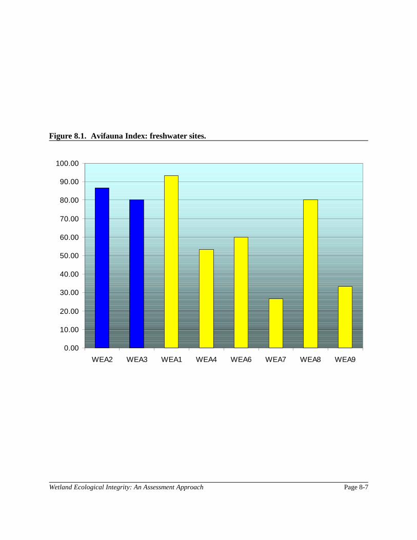
Wetland Ecological Integrity: An Assessment Approach Page 8-7
0.00
10.00
20.00
30.00
40.00
50.00
60.00
70.00
80.00
90.00
100.00
WEA2 WEA3 WEA1 WEA4 WEA6 WEA7 WEA8 WEA9
Figure 8.1. Avifauna Index: freshwater sites.

Wetland Ecological Integrity: An Assessment Approach Page 8-9
0.00
10.00
20.00
30.00
40.00
50.00
60.00
70.00
80.00
90.00
100.00
WEA10 WEA11 WEA12 WEA13 WEA14
Figure 8.2. Avifauna Index: salt marsh sites.

Part III: Discussion and ConclusionThe Wetland Ecological Condition

Wetland Ecological Integrity: An Assessment Approach Page 9-1
Section 9. Discussion: Wetland Ecological Condition
In the attempt to develop a comprehensive approach to evaluate the health–or ecological integrity–ofwetlands it became evident that the use of one single indicator or assessment method would not giveas thorough or holistic a picture of wetland quality as would the application of several diverseindicators, specifically selected to represent distinct components of the ecological web. In addition,while many of the rapid assessment methods available do consider a wide array of wetland functionsand landscape conditions, these summarizing models are only surrogates for actual field-basedinvestigations and data collection. The Wetland Health Assessment Toolbox (WHAT) approach asemployed and described in this project centers on the application of a suite of wetland assessmentmethods so as to yield a comprehensive understanding of the ecological health of the evaluationsite(s) as well as the apparent causes of impairment.
While advocating for as complete an assessment as is realistically possible, the authors do not intendto convey that groups and individuals must replicate the investigation described in this report in orderto engage in meaningful wetland assessment work. Instead, the purpose of this project was toexamine, adapt, and develop wetland diagnostic tools so that groups or individuals could pursuewetland qualitative evaluation through an array of options, and select those that fit their needs,resources, skills, and budgets. For more information on the WHAT approach, visit the world widewebsite (currently under construction) at:
http://www.state.ma.us/magnet/czm/what.htm
The discussion in this section begins with an explanation of how each of the individual assessmentcomponents assemble to produce the summarizing Wetland Ecological Condition. A review of eachwetland site is then presented, demonstrating how the assessment methods function to decipherspecific ecological impairments and potential causes.
Index Totals: The Wetland Ecological ConditionThe Wetland Ecological Condition (WEC) is an integrative score, summarizing the component field-based indices and rapid assessment models. As the final quantitative value, it provides an index orranking of a wetland study site relative to the reference wetland condition. This point must be clearlyemphasized and understood by those employing this and similar assessment approaches that rely onthe use of the reference condition as the baseline for comparison. The output score, or rank, of anysuch index, must be understood as a relative score–relative only to the reference condition to whichit was compared against. This means that one hypothetical study site with its own reference domaincannot be compared to another study site unless the same reference domain was employed for theanalysis. In addition, caution must be exercised when evaluating and discussing the outputs ofreference-based assessments. It may be difficult to make comparisons from one study site to another,outside of the reference context. For example, stating that study site WEAX is more impaired thanWEAY is only valid when qualified. It would be more appropriate to state that WEAX exhibits moreimpairment of its biological or physical components than site WEAY when compared to the referencedomain as established by site WEAZ.

Wetland Ecological Integrity: An Assessment ApproachPage 9-2
While the Wetland Ecological Condition score serves to integrate all of the WHAT ecologicalindicators and rapid assessment methods, its quantitative output should be viewed as a generalranking score, and should be used in the proper context. The final WEC scores should be supportedby descriptive narrative which summarizes the results provided by each of the component assessmentmethods. The site by site discussion in this section, demonstrates how the data and informationgenerated by the Coastal Wetlands Ecosystem Protection Project can be employed to decipherbiological, chemical, or physical impairments and to generate diagnoses as to the potential sourcesand causes for these impairments.
Tables 9.1 and 9.2 display the final Wetland Ecological Condition scores for the freshwater and saltmarsh Wetland Evaluation Areas (WEAs), with all of the component indices and rapid assessmentmethod scores. The Wetland Ecological Condition is simply derived–it is the weighted average ofall the field-based ecological indicator protocols and the rapid assessment methods. To reflect theimportance of obtaining on site field measurements, the ecological indicator indices are weightedtwice the values of the rapid assessment methods. Figures 9.1 and 9.2 graphically display the finalWEC scores.

Wetland Ecological Integrity: An Assessment Approach Page 9-3
Table 9.1. Final Wetland Ecological Condition, component indices, and rapid assessmentscores for freshwater sites.
WEA2 WEA3 WEA1 WEA4 WEA6 WEA7 WEA8 WEA9
Field-based Indicators:
Index of Vegetative Integrity 100 88 67 58 54 63 67 71
Invertebrate CommunityIndex
100 100 57 57 72 42 62 57
Water Chemistry Index 100 100 67 89 78 17 50 67
Hydroperiod Index 100 100 72 NA 72 17 94 28
Avifauna Index 87 80 93 53 60 27 80 33
Average field-based indices 97 94 71 64 67 33 71 51
Rapid Assessments:
Habitat Assessment 94 90 80 47 46 46 75 53
Nonpoint Source Index 100 92 77 68 64 54 84 73
NH Functional Evaluation 74 74 73 60 57 50 55 63
Average rapid assessments 89 85 77 58 56 50 71 63
Wetland EcologicalCondition
95 91 73 62 63 39 71 55

Wetland Ecological Integrity: An Assessment ApproachPage 9-4
Table 9.2. Final Wetland Ecological Condition, component indices, and rapid assessmentscores for salt marsh sites.
WEA10 WEA11 WEA12 WEA13 WEA14
Field-based Investigations:
Index of Vegetative Integrity 100 79 38 67 83
Invertebrate Community Index 100 61 67 68 63
Water Chemistry Index 100 78 67 72 56
Avifauna Index 93 27 40 20 53
Average field-based indices 98 61 53 57 64
Rapid Assessments:
Habitat Assessment 94 49 46 45 39
Nonpoint Source Index 99 65 60 59 80
NH Functional Evaluation 78 50 49 51 56
Average rapid assessments 90 55 52 52 58
Wetland EcologicalCondition
96 59 53 55 62

Wetland Ecological Integrity: An Assessment Approach Page 9-5
0.00
10.00
20.00
30.00
40.00
50.00
60.00
70.00
80.00
90.00
100.00
WEA2 WEA3 WEA1 WEA4 WEA6 WEA7 WEA8 WEA9
Figure 9.1. Wetland Ecological Condition scores: freshwater sites.

Wetland Ecological Integrity: An Assessment Approach Page 9-7
0.00
10.00
20.00
30.00
40.00
50.00
60.00
70.00
80.00
90.00
100.00
WEA10 WEA11 WEA12 WEA13 WEA14
Figure 9.2 Wetland Ecological Condition scores: salt marsh sites.
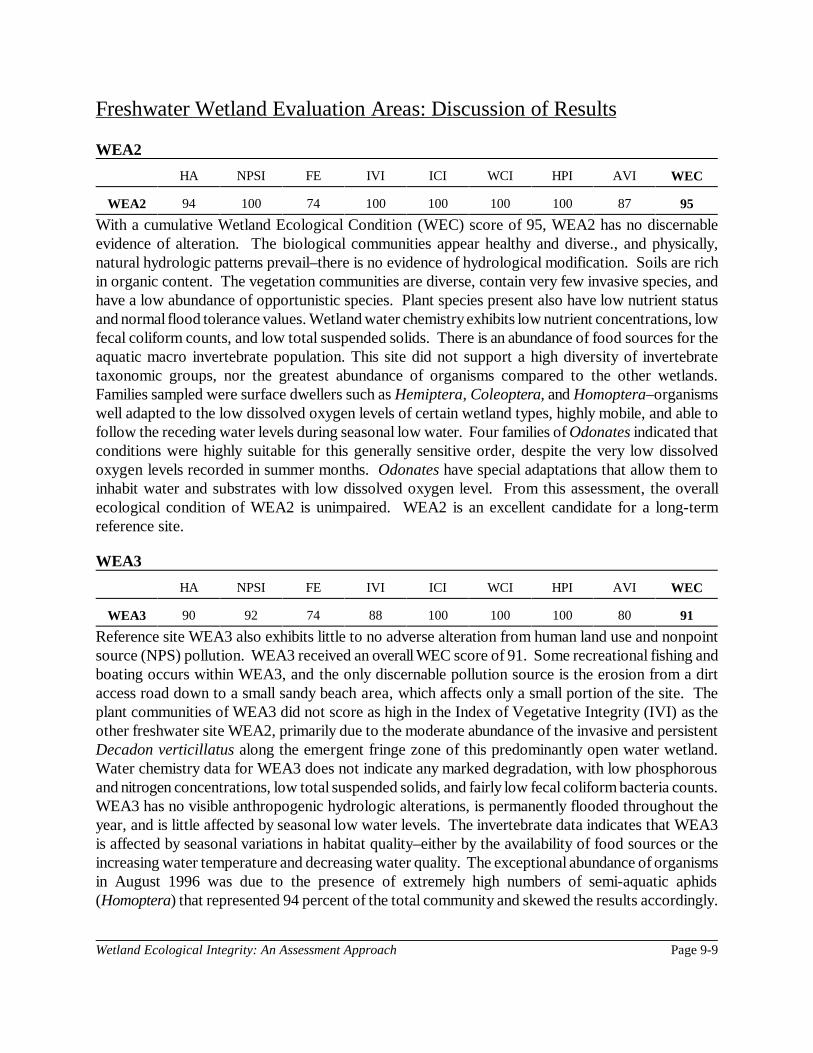
Wetland Ecological Integrity: An Assessment Approach Page 9-9
Freshwater Wetland Evaluation Areas: Discussion of Results
WEA2
HA NPSI FE IVI ICI WCI HPI AVI WEC
WEA2 94 100 74 100 100 100 100 87 95
With a cumulative Wetland Ecological Condition (WEC) score of 95, WEA2 has no discernableevidence of alteration. The biological communities appear healthy and diverse., and physically,natural hydrologic patterns prevail–there is no evidence of hydrological modification. Soils are richin organic content. The vegetation communities are diverse, contain very few invasive species, andhave a low abundance of opportunistic species. Plant species present also have low nutrient statusand normal flood tolerance values. Wetland water chemistry exhibits low nutrient concentrations, lowfecal coliform counts, and low total suspended solids. There is an abundance of food sources for theaquatic macro invertebrate population. This site did not support a high diversity of invertebratetaxonomic groups, nor the greatest abundance of organisms compared to the other wetlands.Families sampled were surface dwellers such as Hemiptera, Coleoptera, and Homoptera–organismswell adapted to the low dissolved oxygen levels of certain wetland types, highly mobile, and able tofollow the receding water levels during seasonal low water. Four families of Odonates indicated thatconditions were highly suitable for this generally sensitive order, despite the very low dissolvedoxygen levels recorded in summer months. Odonates have special adaptations that allow them toinhabit water and substrates with low dissolved oxygen level. From this assessment, the overallecological condition of WEA2 is unimpaired. WEA2 is an excellent candidate for a long-termreference site.
WEA3
HA NPSI FE IVI ICI WCI HPI AVI WEC
WEA3 90 92 74 88 100 100 100 80 91
Reference site WEA3 also exhibits little to no adverse alteration from human land use and nonpointsource (NPS) pollution. WEA3 received an overall WEC score of 91. Some recreational fishing andboating occurs within WEA3, and the only discernable pollution source is the erosion from a dirtaccess road down to a small sandy beach area, which affects only a small portion of the site. Theplant communities of WEA3 did not score as high in the Index of Vegetative Integrity (IVI) as theother freshwater site WEA2, primarily due to the moderate abundance of the invasive and persistentDecadon verticillatus along the emergent fringe zone of this predominantly open water wetland.Water chemistry data for WEA3 does not indicate any marked degradation, with low phosphorousand nitrogen concentrations, low total suspended solids, and fairly low fecal coliform bacteria counts.WEA3 has no visible anthropogenic hydrologic alterations, is permanently flooded throughout theyear, and is little affected by seasonal low water levels. The invertebrate data indicates that WEA3is affected by seasonal variations in habitat quality–either by the availability of food sources or theincreasing water temperature and decreasing water quality. The exceptional abundance of organismsin August 1996 was due to the presence of extremely high numbers of semi-aquatic aphids(Homoptera) that represented 94 percent of the total community and skewed the results accordingly.

Wetland Ecological Integrity: An Assessment ApproachPage 9-10
The most affected metric was % Tolerant/% Intolerant Ratio. These aphids–with a tolerance valueof 8–accumulated in hoards on the water surface in summer, and were therefore able to avoid lowdissolved oxygen and high temperature characterizing the water column in this season. These specieswere completely absent in the spring 1996 and 1997 sampling. Instead, Chironomidae–with atolerance value of 6–were the major taxonomic group, constituting 74 percent of the May communityand more representative of normal wetland conditions. Summer water quality appeared to adverselyaffect diversity of Odonates, only Coenagrionidae were present, and even these in low numbers.Grouped together, these results suggested that seasonality greatly affected the composition of thecommunity at this site. Toxic groundwater plumes from the Massachusetts Military Reservation havebeen documented proximate to this and two other study sites. While microtox water and sedimentand aquatic toxicology tests run by the US Environmental Protection Agency (USEPA) Region ILaboratory for this project failed to pick up any sediment or water column toxicity, it is uncertainwhat, if any, ecological impact this up-gradient hazardous waste site may be having–or will have–onthe ecological integrity of this and sites WEA1 and WEA4.
WEA1
HA NPSI FE IVI ICI WCI HPI AVI WEC
WEA1 80 77 73 67 57 67 72 93 73
WEA1 reflects its history as a formerly active and productive cranberry bog, mostly through thelatent stores of nutrients in its soils. At the outset of the project, study site WEA1 was appraised tobe in relatively healthy condition, apparently recovering from its former agricultural use, asindicated by its diverse vegetation and bird usage. On-site sampling, however, demonstrated notabledifferences from reference conditions primarily in the biological and chemical indices. Site WEA1received a WEC score of 73. While the vegetative communities are diverse with moderateinterspersion of emergent herbaceous and scrub/shrub species, the communities are quite dissimilarfrom either reference site and have a high abundance of opportunistic species, especially Typhalatifolia. Notably high nutrient concentrations were revealed from the pore water chemistry data, andaccording to the invertebrate data, the biological condition of WEA1 was moderately impaired. Someof this site’s Invertebrate Community Index (ICI) metrics (Total Number of Organisms, Total Taxa,Family Biotic Index, % Contribution Dominant Family, % Chironomidae, % Oligochaeta) scoredas well as the reference condition. EOT/Chironomidae Ratio, % Tolerant/% Intolerant Ratio, OtherOdonata/Coenagrionidae Ratio, Community Taxa Similarity Index, and the Community TrophicSimilarity Index all scored well below the reference condition, indicating a very different residentcommunity at WEA1. August 1996 invertebrate samples appeared to be less impaired than eitherMay 1996 or 1997. Overall impairment of the invertebrate community may be due to eutrophicationof the waters rather than due to habitat condition. The previously mentioned MMR plumes cannotbe discounted either, though, again, USEPA toxicity tests could not confirm suspected ecologicalimpact. Site WEA1 receives significant groundwater discharge and has a contribution area with noimpervious area–two factors that would account for relatively stable water levels (with no sharppeaks or troughs), which closely resemble those of the reference sites.

Wetland Ecological Integrity: An Assessment Approach Page 9-11
WEA4
HA NPSI FE IVI ICI WCI HPI AVI WEC
WEA4 47 64 60 58 57 67 NA 53 62
The active cranberry bog is a significantly altered and manipulated wetland system. Project datareveal that the biological communities and the water quality levels are impaired, but not as severelyas initially expected. Study site WEA4 received a WEC score of 62. Though the dominant plantcommunity is the cultivated cranberry (Vaccinium macrocarpon), there are diverse species thrivingin a large unaltered area in the northwest corner of the site and in the banks, ditches, and channels.WEA4 scores poorly in the IVI primarily because of its dissimilarity to reference site plantcommunities, its large abundance of species with high nutrient status, and its high taxa richnessvalue–probably the result of constant disturbance. Water chemistry data indicate nutrientconcentrations higher than reference sites, especially nitrate nitrogen and less so phosphorous, butsimilar suspended solids and fecal coliform measures. The water quality of WEA4 is influencedconsiderably by significant groundwater discharge and by the swiftly flowing Quashnet River mainchannel. WEA4’s Habitat Assessment (HA) score suggested that the invertebrate community shouldbe impacted by poor habitat condition, but the biological condition of this site was consistentlyfound to be moderately impaired. The site metrics that scored as well as the reference conditionwere: Total Organisms, Total Taxa Richness, % Tolerant/ % Intolerant, % Contribution DominantFamily, % Chironomidae, Family Biotic Index, and % Oligochaeta. The remaining metrics andindices (EOT Richness, EOT/Chironomidae Ratio, Family Biotic Index, Other Odonata/Coenagrionidae Ratio, Community Taxa Similarity Index, and Community Trophic Index were wellbelow reference condition. Invertebrate community integrity in both May 1996 and 1997 was betterthan August 1996, and the invertebrate biomonitoring indicated that WEA4 was more impaired thanWEA1, the recovering cranberry bog.
WEA6
HA NPSI FE IVI ICI WCI HPI AVI WEC
WEA6 46 54 57 54 72 78 72 60 63
Study site WEA6 is subject to considerable human alteration from ongoing maintenance of thesurrounding golf course and from stormwater disposal from nearby residential development. WEA6received an overall WEC score of 63. Ambient surface water chemistry reveals slightly elevatednutrient levels, but total suspended solid levels are very low. With adequate water quality as reflectedby the relatively high Water Chemistry Index (WCI) score, the low biological index scores, asdescribed below, must be due, primarily, to poor and altered habitat quality. At the boundaries of siteWEA6, bordering wetland and upland plants are frequently mowed, and the pond edge has beenconspicuously filled in some areas. WEA6 scores poorest for its vegetative integrity as its dominantspecies are ones with either invasive (Phragmites australis), opportunistic (Salix discolor, Scirpuscyperinus, and Juncus effusus), or high nutrient status attributes. For the invertebrate communities,habitat quality is low due to the lack of aquatic vegetation (consisting mostly of a few attachedsubmergent species) in the open water. The HA score indicated the invertebrate community wouldbe affected by relatively poor habitat condition. May 1996 sampling detected slight impairment ofthe invertebrate community as compared to the reference conditions. The biotic condition had

Wetland Ecological Integrity: An Assessment ApproachPage 9-12
deteriorated in August 1996, and the overall summarized assessment of the ICI is somewhatimpaired. ICI metrics and indices that were equal to or better than reference condition were TotalTaxa (Diversity), EOT, EOT/Chironomidae Ratio, % Tolerant/% Intolerant, % ContributionDominant Family, and % Chironomidae. ICI metrics and indices that were far below referencestandard were Total Organisms, Other Odonata/Coenagrionidae, % Oligochaeta, Community Taxaand Community Trophic Similarity Indices. In general it appeared that the minor invertebratecommunity impact at WEA6 is not due to eutrophication, but rather to habitat condition%such as lessbuffer and fringe vegetative growth, sandy substrate, and reduced food sources.
WEA7
HA NPSI FE IVI ICI WCI HPI AVI WEC
WEA7 46 54 50 63 42 17 17 27 33
Sandwiched between dense residential development and an active golf course, site WEA7 is aseverely impaired isolated depressional wetland. WEA7 received some of the lowest index scoresfor each field-based protocol as well as the rapid assessment methods. With a cumulative WEC scoreof 33, WEA7 can be considered as the most ecologically impaired freshwater site in the series.Although heavily vegetated with hydrophytic plants throughout the wetland itself, WEA7 lacks adistinct buffer area to protect it from a wide array of nonpoint sources of pollution present in itscontribution area (in the form of direct stormwater discharges, septic sewage contribution, fertilizers,and pesticides). WEA7 has very poor water quality as indicated by an extremely low WCI score, withelevated nutrient levels. High levels of fecal coliform bacteria were also consistently found in thisstudy site. The wetland vegetation survey identified three primary communities, an emergent/openwater section dominated by Typha latifolia, an herbaceous community dominated by Carex sp., anda shrub/forest community dominated by Clethra alnifolia and Acer rubrum. This wetland has a largediversity of plant species which can be attributed to highly variable water levels (resulting from thecollection and discharge of runoff from a highly impervious catchment area) and the very highconcentrations of nutrients. Episodic flooding and draining in this wetland may be inhibiting thesuccession into a complete forest cover. Though site WEA7 is subject to dramatic water levelfluctuations and has very high ambient nutrient concentrations, its vegetative population, as indicatedby the IVI, does not appear to be reflecting these stresses as strongly as anticipated. Highly variablewater levels observed in WEA7 were exhibited by a low Hydroperiod Index score. In all six of thehydroperiod metrics, WEA7 demonstrated strong dissimilarity to the reference condition. With a lowHA score, it was anticipated that the invertebrate community would reflect impairments due to bothpoor habitat and water quality. Although moderately impaired for both seasons, the InvertebrateCommunity Index of WEA7 was worse in August 1996 than in May 1996 and 1997. Total Taxa(Diversity), Family Biotic Index, % Contribution of Dominant Family, and % Chironomidae wereequal to or better than the reference condition. Total Organisms was somewhat comparable. Theremaining metrics and indices were well below reference. Of the taxa present, Oligochaeta (worms)formed the dominant group. The presence of large numbers of worms suggests that the driving forcesof this wetland’s invertebrate community condition are the low oxygen levels, the soft organicsubstrate, the rapidly fluctuating water table, the lack of sustained open water during the summer, andvery high nutrient levels. Ironically, this wetland has a sign on its upland edge informing the localcommunity that it is a “protected” wetland. Apparently the wetland itself was established in a

Wetland Ecological Integrity: An Assessment Approach Page 9-13
conservation restriction during the development of the surrounding planned residential community.While protected on paper from actual fill and development, the ecological condition of WEA7illustrates the fact that wetlands cannot be truly protected unless the surrounding landscape isprotected and/or managed in accordance with best watershed management practices to reduce NPSpollution and to maintain natural hydrological regimes.
WEA8
HA NPSI FE IVI ICI WCI HPI AVI WEC
WEA8 75 84 55 67 62 50 94 80 71
Characterized predominantly by open water with fringing emergent and shrub vegetation, study siteWEA8 generally has a wide buffer area of natural vegetation between the wetland its surroundingland uses. The direct stormwater discharge to the site, though, was unaffected by the presence ofany buffer zone and, in fact where Route 151 bordered WEA8 to the north, there are areas wherethis vegetated zone was less than several meters. In addition, the impacts of the sewage disposalpractices of the dense trailer park to the northwest of the site are not clearly manifested in itschemical and biological properties. For most of the field-based indices, WEA8 exhibited scores thatwere above the mean and within a standard deviation from the reference scores. With an overallWEC score of 71,WEA8 ranks above all other freshwater WEAs, except WEA1. The vegetationand invertebrate indicators were influenced by the late season dominance of the invasive Decodonverticillatus and abundant Nymphaea odorata, both of which provide poor habitat for the freshwaterinsect species. The abundance of the invasive vegetation species, the poor Community Similaritymetric score, the low Flood Tolerance, and the significant presence of plant species with affinity forenriched sites all contributed to the low final IVI score received by WEA8. According to the WCI,WEA8 did not correspond well with the reference condition. Average nutrient concentrations at thissite were varied with particularly high concentrations of nitrate nitrogen, and suspended solidmeasurements were consistently high at this study site. For the ICI, in both May 1996 and 1997,biological condition was not as high as was recorded in August 1996. Wetlands are able to improvewater quality through the uptake of nutrients and toxicants by vegetation production, and, aspreviously stated, there was abundant floating and emergent growth in August that was not presentin May. Overall the wetland biological condition of study site WEA8 can be viewed as somewhatimpaired. ICI metrics that were equal to or better than the reference condition were Total Taxa(Diversity), EOT Richness, EOT/Chironomidae Ratio, % Tolerant / % Intolerant Ratio. Metrics andindices that were somewhat below reference were % Chironomidae, Community Taxa SimilarityIndex, and Community Trophic Similarity Index. Those that were well below reference were TotalOrganisms, Family Biotic Index, Other Odonata/ Coenagrionidae Ratio, and % Oligochaeta. InMay, Chironomidae made up 85 percent of the community. In August, Diptera other thanChironomidae formed the major group, and another significant part of the population was composedof Coenagrionidae Odonates. This shift in composition is a clear indicator of improved condition.
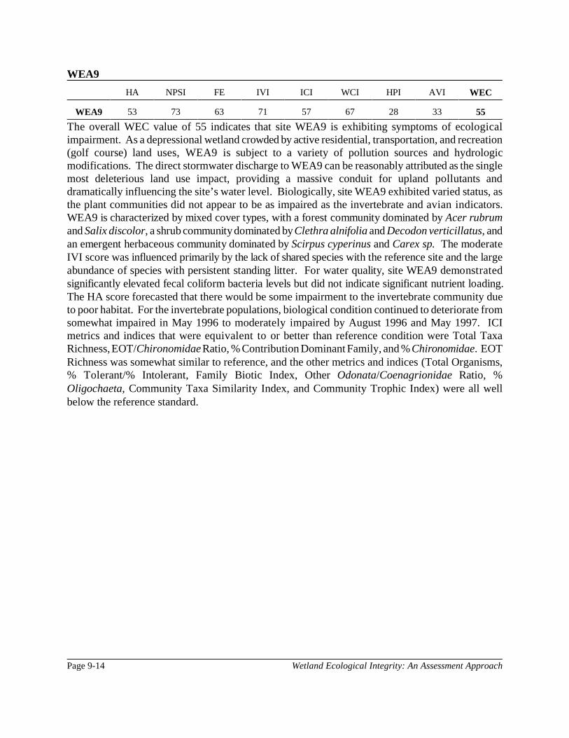
Wetland Ecological Integrity: An Assessment ApproachPage 9-14
WEA9
HA NPSI FE IVI ICI WCI HPI AVI WEC
WEA9 53 73 63 71 57 67 28 33 55
The overall WEC value of 55 indicates that site WEA9 is exhibiting symptoms of ecologicalimpairment. As a depressional wetland crowded by active residential, transportation, and recreation(golf course) land uses, WEA9 is subject to a variety of pollution sources and hydrologicmodifications. The direct stormwater discharge to WEA9 can be reasonably attributed as the singlemost deleterious land use impact, providing a massive conduit for upland pollutants anddramatically influencing the site’s water level. Biologically, site WEA9 exhibited varied status, asthe plant communities did not appear to be as impaired as the invertebrate and avian indicators.WEA9 is characterized by mixed cover types, with a forest community dominated by Acer rubrumand Salix discolor, a shrub community dominated by Clethra alnifolia and Decodon verticillatus, andan emergent herbaceous community dominated by Scirpus cyperinus and Carex sp. The moderateIVI score was influenced primarily by the lack of shared species with the reference site and the largeabundance of species with persistent standing litter. For water quality, site WEA9 demonstratedsignificantly elevated fecal coliform bacteria levels but did not indicate significant nutrient loading.The HA score forecasted that there would be some impairment to the invertebrate community dueto poor habitat. For the invertebrate populations, biological condition continued to deteriorate fromsomewhat impaired in May 1996 to moderately impaired by August 1996 and May 1997. ICImetrics and indices that were equivalent to or better than reference condition were Total TaxaRichness, EOT/Chironomidae Ratio, % Contribution Dominant Family, and % Chironomidae. EOTRichness was somewhat similar to reference, and the other metrics and indices (Total Organisms,% Tolerant/% Intolerant, Family Biotic Index, Other Odonata/Coenagrionidae Ratio, %Oligochaeta, Community Taxa Similarity Index, and Community Trophic Index) were all wellbelow the reference standard.

Wetland Ecological Integrity: An Assessment Approach Page 9-15
Salt Marsh Wetland Evaluation Areas: Discussion of ResultsWEA10
HA NPSI FE IVI ICI WCI AVI WEC
WEA10 94 99 78 100 100 100 93 96
Reference site WEA10, as the basis for which other salt marsh study sites are compared, is a healthyand productive coastal wetland system. WEA10 received an overall WEC value of 96. Aside fromrecreation and some commercial shell fishing, WEA10 has a contribution area with no land useactivity that would contribute to the impairment of its ecological integrity. Tidal influence fromWaquoit Bay into Sage Lot Pond was unrestricted. The only evident factor that would adverselyaffect habitat quality would be the few remnant linear ditches most probably dug under historicalmosquito control work programs. The salt marsh vegetation communities at WEA10 were free frominvasive species. Water chemistry for this site indicates that fecal coliform levels were low with theexception of a single spike which raised the average for the site. TSS levels and nutrientconcentrations were low. As supported by its ICI score, WEA10 had a healthy and diverseinvertebrate population. In sum, because it is the largest salt marsh area in the Waquoit Baywatershed and because it is located in protected conservation land, WEA10 is also an excellentcandidate as a long-term reference site.
WEA11
HA NPSI FE IVI ICI WCI AVI WEC
WEA11 49 65 50 79 61 78 27 59
As with the other salt marsh sites, study site WEA11 has been adversely affected by development andland use patterns that have fragmented a long linear fringing salt marsh into small, isolated remnantpieces. Additionally, the ongoing land use activities in its contribution area, including a large marina,residential development, and heavy boat usage, degrade the ecological condition of WEA11 bygenerating NPS pollution and transforming habitat quality. WEA11’s WEC score is 59. There hasbeen considerable bank erosion and salt marsh slumping at WEA11 from boat handling, and theplacement of large shellfish seeding grates at the toe of the salt marsh bank in the subtidal zone.Despite its small size, the marsh had a diverse vegetation cover, tidal flow was unrestricted, and therewas no channelization or ditching. The near shore sediments were composed of sand and anaerobicmud. There was an abundance of attached algae to provide a food base for the aquatic invertebrates,although the growth suggested eutrophication of the water column. The HA score indicated therewould be considerable impairment to the biological community due to poor habitat condition. Waterchemistry indicates consistently low TSS and fecal coliform concentrations, and only slightly elevatednitrate levels. The final IVI score for WEA11, with relatively high scores for all the IVI metrics. TheICI score indicated a marginally impaired invertebrate community. Seven of the ICI metrics andindices were below reference condition, with three (% Contribution Dominant Taxa Group, %Contribution Dominant Trophic Group, and % Abundant/% Rare Ratio) scoring equal or better thanthe reference. In May 1996 and 1997, Amphipoda were the dominant group, whereas Decapodawere in August 1996. Although this shift indicated decreasing habitat condition during summer, theoverall ICI for both seasons remained the same. Impact was predominantly related to poor habitat

Wetland Ecological Integrity: An Assessment ApproachPage 9-16
condition rather than impaired water quality.
WEA12
HA NPSI FE IVI ICI WCI AVI WEC
WEA12 46 60 49 38 67 67 40 59
Study site WEA12 exhibits significant ecological impairment. Both degraded habitat quality andchronic pollution problems adversely affect this small salt marsh fringe on Eel Pond, the western armof Waquoit Bay. WEA12 received an overall WEC score of 59. The primary land use responsiblefor the degradation of site WEA12 is likely the failing or poorly functioning septic system ofresidential development situated just beyond its upland edge. A dense stand of Phragmites australisand Toxicodendron radicans dominated the wetland vegetation population and strongly influencedthe final IVI. Water chemistry data confirmed suspected high nutrient concentrations, especially inwetland pore water. TSS levels were the highest of all salt marsh study sites. Fecal coliform samplestaken from a shallow ground water well transect at the wetland/upland edge revealed consistentlyhigh populations, giving credence to the assumption that the septic system directly adjacent to thestudy site was poorly functioning. The HA score was poor and indicated that the invertebratecommunity would be adversely affected. Near shore sediments were composed of sand, peat, andmuck. Filamentous algae, as well as marine algae floating mats, provided a rich source of food forinvertebrates. The seasonal ICI score deteriorated between May and August 1996, but the overallassessment of the invertebrate community indicated this site was not severely impacted by residentialland use and boating activities. This situation is likely the partial influence of unrestricted tidalflushing, as the marsh fronts a broad expanse of Eel Pond. WEA12 scored as well as, or better than,the reference condition for these metrics and indices: % Contribution Dominant Family, %Contribution Trophic Group, % Abundant/% Rare Ratio, and % Capitellida. The other metrics andindices were somewhat below (Total Number of Organisms and Community Taxa Similarity Index)or well below (Total Taxa Richness, # Palaemonedae Shrimp) the reference condition.
WEA13
HA NPSI FE IVI ICI WCI AVI WEC
WEA13 45 59 51 67 68 72 20 55
Study site WEA13, with a WEC score of 55, shows indications of degraded ecological qualityattributed to both NPS pollution and habitat alteration. Surrounded on three sides by residentialdevelopment, WEA13 has no functional buffer between the salt marsh and upland land uses. Inaddition, adjoining open water is actively utilized for recreational boating. Several of the waterfrontproperties had constructed rock walls, boat slips, and mooring piers, and these structuralmodifications to the natural shoreline configuration altered tidal flow and decease habitat quality.Nearshore sediments were composed of sand, silt, and muck. By August 1996, a thick mat offilamentous algal growth had covered the open water/sediment interface, suggesting advancedeutrophication, probably as a result of the nearby nutrient loading. Water chemistry data at this siteconfirmed high nutrient concentrations in wetland pore water. WEA13’s relatively low IVI scoreappears to be most influenced by the notable extent of disturbance/colonizer species, such as

Wetland Ecological Integrity: An Assessment Approach Page 9-17
Distichlis spicata and Salicornia sp.. The ICI assessment indicated a moderately impairedinvertebrate population with a seasonal decline from May to August. The ICI metrics and indices thatscored equivalent to or better than reference condition were: % Contribution Dominant Taxa, %Abundant/% Rare Ratio, % Capitellida and % Amphipods. Those somewhat below referencecondition were Total Number of Organisms, Total Taxa Richness, % Contribution Dominant TrophicGroup, and those well below reference condition were # Palaemonedae Shrimp, Community TaxaSimilarity Index, and Community Trophic Similarity Index. A few freshwater insects (chironomidsand several odonate larvae) were observed in samples collected at this site in May 1996. Subsequentsalinity readings confirmed the presence of significant freshwater discharge at the marsh bank andintertidal zone.
WEA14
HA NPSI FE IVI ICI WCI AVI WEC
WEA14 39 80 56 83 63 56 53 62
WEA14 received an overall WEC score of 62. Similar to the other salt marsh study sites, WEA14exhibits symptoms of ecological degradation from both nonpoint sources and direct physicalalteration. Residential development and boating activities dominated the surrounding land uses andthere was little protection afforded by a minimal upland vegetated buffer. Nonpoint sources ofpollution to WEA14 would consist of septic sewage discharge, polluted groundwater discharge,fertilizer and pesticide applications, stormwater runoff from impervious surfaces, and boating fuel andoil leaks. A public boat ramp was located within the western edge of the marsh. Rainfall runoff froma large parking lot was able to travel directly to the study site via this boat ramp. There were severallinear mosquito control ditches in the marsh. Near shore sediments were mostly anaerobic mud withlittle sand, and there was a thick growth of filamentous algae attached to all substrates. Organicfloating mats were abundant in the open water close to the salt marsh bank, suggesting an advancedstage of eutrophication. The vegetation population at this site is significantly dominated by the lowmarsh Spartina alterniflora, with large abundance of Iva frutescens and Distichlis spicata. WEA14’sIVI score indicates that its wetland vegetation population most closely resembles the reference site.WEA14 received high scores for all the IVI metrics but Community Similarity. Nutrient, fecalcoliform, and TSS concentrations at site WEA14 were only slightly more elevated than the referencesite. The HA score indicated significantly impaired habitat condition. The invertebrate communityat WEA14 was somewhat impaired, with the biotic condition deteriorating over the course of thesummer season. ICI metrics and indices that were equal to or better than reference condition were:% Contribution Dominant Family, % Contribution Dominant Trophic Group, % Abundant/% RareRatio, and % Capitellida. Total Taxa Richness was somewhat similar to reference condition, and theremaining metrics and indices were far below.

Wetland Ecological Integrity: An Assessment ApproachPage 9-18
Statistical Examination of ResultsAs described in the project scope, one aspect of the Coastal Ecosystem Protection Project was toevaluate the performance and strength of several rapid assessment methodologies (see Section 2).In certain applications, rapid assessment methods serve two roles. They contribute important–or, insome cases, integral–supplementary information and data to another investigation component of thewetland evaluation. The Habitat Assessment method, for example, provides the means to gather andinput critical habitat characteristic, both of the wetland and of the surrounding landscape, to theInvertebrate Community Index and other multi-metric protocols. Another role of rapid assessmentmethods, though, is to offer an alternative evaluation technique when the option to collect andanalyze on-site, field-based data is unavailable due to resource or time constraints. It is possible forgroups or individuals who are interested in conducting some level of wetland ecological assessmentto use accessible rapid assessment methods not as a substitute for, but as an alternative to, field-basedinvestigations.
For both of these purposes, it is important to confirm that the rapid assessment methods beingemployed function as expected. By implementing the Nonpoint Source Index and New HampshireFunction Evaluation methods, for example, can we arrive at a finding about the relative health of agiven wetland that would approximate a finding derived from field-based measurements and analysis?In order to verify that these methods do perform as anticipated, it is necessary to examine the extentto which the scores or outputs from these rapid assessment methods relate to the scores and outputsof the field-based ecological indicators. What are the relationships between the rapid assessmentmethods and the field-based measurements? What is the interdependence between these twogroups–do they covary–that is, vary together? By computing a measure of association between thesetwo groups, it is possible to examine their relationships.
Correlation coefficient analysis is a statistical technique used to compute the measure of associationbetween two variables. To compute this measure, the Pearson product-moment correlationcoefficient was used. Pearson’s correlation coefficient is a measure of covariation; it measures thelinear relationship between two variables (Sokal, 1995). The equation used to derive Pearson’scorrelation coefficient generates a value between +1.00 and -1.00. The size and sign of thecorrelation indicate the strength and nature of the relationship. A positive relationship indicates adirect association–high scores for one variable connect to high scores for another. A negative, orinverse, relationship results when a high score from one variable relates to a low score for another.Although there is no established principle for what constitutes a strong or weak relationship, we canfollow general guidelines. We know that a correlation coefficient of (+)1.00 indicates a perfectrelationship–that is, every value for one variable covaries identically with the value of anothervariable. Correlation coefficients above 0.75 indicate a very strong relationship between variables,while coefficients from 0.40 to 0.75 imply a moderate relationship. For this analysis, coefficientsbelow 0.40 are considered weak.
In Table 9.3 and 9.4, correlation coefficients matrices are displayed for the freshwater and salt marshWEAs. From these matrices, we can examine the measures of association between variables–in thiscase, each of the rapid assessment methods and field-based indices utilized in the WHAT approach.
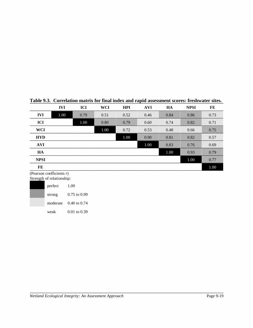
Wetland Ecological Integrity: An Assessment Approach Page 9-19
Table 9.3. Correlation matrix for final index and rapid assessment scores: freshwater sites.IVI ICI WCI HPI AVI HA NPSI FE
IVI 1.00 0.79 0.51 0.52 0.46 0.84 0.86 0.73
ICI 1.00 0.80 0.79 0.60 0.74 0.82 0.71
WCI 1.00 0.72 0.53 0.48 0.66 0.75
HYD 1.00 0.90 0.81 0.82 0.57
AVI 1.00 0.83 0.76 0.69
HA 1.00 0.93 0.79
NPSI 1.00 0.77
FE 1.00
(Pearson coefficients r)Strength of relationship:
perfect 1.00
strong 0.75 to 0.99
moderate 0.40 to 0.74
weak 0.01 to 0.39

Wetland Ecological Integrity: An Assessment ApproachPage 9-20
Table 9.4. Correlation matrix for final index and rapid assessment scores: salt marsh sites.IVI ICI WCI AVI HA NPSI FE
IVI 1.00 0.53 0.52 0.59 0.58 0.80 0.74
ICI 1.00 0.85 0.86 0.97 0.81 0.95
WCI 1.00 0.58 0.93 0.58 0.76
AVI 1.00 0.83 0.95 0.94
HA 1.00 0.80 0.93
NPSI 1.00 0.95
FE 1.00
(Pearson coefficients r)Strength of relationship:
perfect 1.00
strong 0.75 to 0.99
moderate 0.40 to 0.74
weak 0.01 to 0.39

Wetland Ecological Integrity: An Assessment Approach Page 9-21
By examining the correlation coefficient matrix for the freshwater sites, we can develop severalinferences about the evaluation techniques. For one, we can see that none of the relationshipsbetween the evaluation techniques, both rapid assessment methods and field-based measurements,are considered weak. In fact, many of the correlation coefficients are above 0.75–indicating excellentcovariance. We can also see that both the NPSI and the HA methods generally have very strongrelationships with most of the ecological index protocols. The NH Functional Evaluation methoddoes not exhibit as strong association with the ecological index protocols but still demonstrates verygood correlation. The following combination of evaluation techniques utilized for the freshwaterWEAs, in particular, have very strong relationships: • HA : IVI• NPSI : IVI• NPSI : ICI• NPSI : HYD• HA : HYD• HA : AVI
The salt marsh correlation coefficient matrix reveals similar patterns in the association of theseevaluation techniques. Again, none of the relationships between these techniques is considered weak.Even more so than the freshwater WEAs, the salt marsh evaluation techniques exhibit very strongassociations, or covariance. For the salt marsh sites, all of the rapid assessment methods have tightcorrelation to the ecological index protocols. The following combination of evaluation techniquesutilized for the salt marsh WEAs have very strong relationships:
• HA : ICI• HA : WCI• HA : AVI• NPSI : IVI• NPSI : ICI• NPSI : AVI• FE : ICI• FE : AVI
In sum, this statistical correlation analysis verifies the cumulative strength of the WHAT approachand component evaluation techniques. It also demonstrates the rapid assessment methodologies, forthe most part, are able to generally predict patterns of ecological degradation or impairment, asevidenced by the field-based ecological index protocols. With future transfer and implementation ofthe WHAT approach, this type of confirmation analysis will be necessary to ensure that theassessment methods are robust enough to continue to detect trends in wetland ecological andfunctional impairment.

Wetland Ecological Integrity: An Assessment Approach Page 10-1
Section 10. Conclusion & Recommendations
The evaluation of wetland quality is a challenging and complicated task. In many circumstances andfor a host of different reasons, environmental professionals, land use planners, resource managers,and others are faced with the need to assess wetland health. Since the means for engaging inmeaningful wetland assessment are not fully developed, are not accessible, or are not affordable, theevaluation of wetland quality has been widely overlooked and omitted. As a result, land use planningand resource management decisions affecting wetlands are frequently being made with incompleteand inadequate information.
The desire to explore and build on available wetland assessment tools and to develop new techniqueswas borne by the authors and partner organizations through ongoing work in nonpoint source (NPS)pollution control planning, wetlands protection and restoration, biomonitoring, and remote sensing.Through support by the National Oceanic and Atmospheric Administration’s Coastal Services Center,the Coastal Wetlands Ecosystem Protection Project was launched with the primary goal of developingand testing an innovative and transferable approach for wetland assessment.
Nearly three years in the making, the Wetland Health Assessment Toolbox (WHAT) approachpresented and described in this report is the product of a coordinated, multi-disciplinary process tocultivate an innovative approach for wetland evaluation. The WHAT approach is an amalgamationof relatively simple, straight-forward rapid assessment methodologies, with scientifically sound on-sitefieldwork, which are concurrently employed to produce a comprehensive evaluation of the ecologicalcondition of a wetland study site.
To summarize, the rapid assessment tools utilized in the Wetland Ecological Assessment Methodinclude a nonpoint source pollution index, a habitat assessment model, and a wetland functionalassessment protocol. The onsite field-based indicators are comprised of wetland vegetation, aquaticmacro invertebrates, surface and pore water chemistry, hydrology and hydroperiod, and avifauna.Metrics and indices are employed in data analysis and reporting. A cumulative Wetland EcologicalCondition, is the final assessment output, combining all of the above variables into a single score orranking. Statistical analysis is employed to examine data patterns, determine significance, and forpredictive inquiry.
To attempt to recreate the tasks and objectives of the Coastal Wetlands Ecosystem Health Projectwould arguably be an arduous and costly venture. But through the piloting and testing of theseassessment tools, and the subsequent cataloguing and illustration of their implementation, it is hopedthat comprehensive wetland assessment will become more readily accessible to a wider range ofdifferent groups. The focus of this report, therefore, is to describe the project and its results, not toprovide a recipe for the application of the WHAT approach. The outreach and technical assistancetransfer component will be a World Wide Web based site, where potential users and those withvarying degrees of interest in wetland assessment can learn more about the WHAT approach andhow they could employ some or all of the assessment tools described here.

Wetland Ecological Integrity: An Assessment ApproachPage 10-2
The results of this project appear promising. Three reference wetland sites and 10 wetland studysites located throughout the Waquoit Bay watershed in southeastern Cape Cod, Massachusetts wereevaluated using the methods and techniques described in this report. Based on this analysis, it hasbeen demonstrated that nonpoint sources of pollution as well as habitat alterations are causingvarying degrees of biological, physical, and chemical impairments at study sites. Poor stormwatermanagement practices, inadequate siting and/or functioning of onsite septic systems, runoff fromimpervious roads and parking areas, commercial cranberry cultivation, golf course construction andmaintenance, and direct habitat destruction and fragmentation are the most significant causes ofwetland degradation as evidenced by project findings. Statistical correlation indicates that theindividual field-based indices correspond very well with one another and with the rapid assessmentmethodology results.
Data and information generated by this project can be used as baseline information for long-termstudies observing wetland ecological responses to various forms of disturbance over multiple seasons.More applications of this approach method are necessary, though, particularly in other regions andwatersheds with different geology, hydrology, and land use patterns. Work has recently been initiatedto implement the WHAT approach in two watersheds in northeastern Massachusetts. Futureapplications of the WHAT approach are fundamentally necessary to contribute to the expansion ofthe various metric attributes database. Periodic peer review and subsequent edits to this database willbe required in order for it to be as accurate and as current as possible.
Observations: Patterns of ResultsThrough the characterization and evaluation of each of the 13 wetland study sites in the Waquoit Baywatershed, a sufficient estimate of the ecological condition of each of the sites has been obtained.The results of the WHAT approach have identified specific freshwater and saltmarsh wetlands thatare manifesting symptoms of ecological degradation from both nonpoint sources of pollution as wellas habitat alteration from current or historical land uses.
In this investigation, several land use types have emerged as being notably deleterious to wetlandecological integrity. In particular, wetland sites that are subject to direct stormwater discharges fromresidential development and road runoff, exhibit the highest degree of biological, chemical, andphysical impairment (the lowest cumulative Wetland Ecological Condition ranking). In addition, theaggregate nutrient load from residential onsite septic systems and fertilizer use (residential,commercial, and golf courses)–which move relatively liberally through the dominant sandy glacialoutwash soils–are contributing to discernible signs of acute eutrophication. Finally, both active andhistorical (10 years former) agricultural cranberry cultivation–with its associated ditching, sandfilling, water manipulations, fertilizer and pesticide applications%creates both NPS pollutionproblems and severe habitat modifications.
Another important pattern emerging from this project is that small wetlands, especially isolateddepressional types, are more susceptible to land use impacts. With less areal extent, biologicalcommunities have more restricted mobility ranges, pollutant loads become concentrated, andhydrological shifts become very pronounced. Isolated depressional wetlands are most vulnerableas they are not able to export aggregated pollutant loads to downstream systems as readily. The only
Wetland Ecological Integrity: An Assessment Approach Page 10-3
avenue for pollutant export in this class of wetlands, would be through groundwater recharge orthrough the uptake, sequestering, or transformation through biological endpoints. Wetland systemswith surface water hydrological connections, especially riverine systems, will not retain as muchcontributing area pollutant loads, depending on the hydrological patterns of the site.
Another observation is that hydroperiod%or wetland water level%for most of the freshwater sites, wasgenerally strong similarities between sites. This may be due to the underlying geology of thewatershed and its groundwater driven hydrology. It seems that wetland sites would be much moresusceptible to natural variation between sites if the wetlands were not well buffered by groundwater.In surface water dominated systems, the periodicity of flooding depends on many factors: the sizeof the watershed, the slope and roughness of the watershed, and the size and cross-sectional shapeof the wetland. In addition, factors such as the quantity and behavior of inflowing and outflowingsurface water will have a major impact on water levels. Surface water dominated systems alsomagnify variations in precipitation because the runoff is not delayed and buffered by flowingthrough the ground.
Finally, all the salt marsh sites, with the exception of the reference site, were surrounded by similartypes of land uses. Therefore, it was the intensity of the specific land use, not the type, whichappeared to account for discrepancies in biological populations. Tidal influence and the presenceof freshwater seeps from upland sources seemed to affect a study site’s ability to attenuate NPSloads. Fringing saltmarsh sites with a high degree of open water exposure demonstrated lessimpairment to the invertebrate communities, as opposed to pocket-type sites with small drainageditches. Significant size differences between the reference site and the study sites may influencedresults.
Management Implications and RecommendationsThe management implications of this assessment approach are numerous. The Wetland EcologicalAssessment Approach, with its inherent components, has strong potential application for:
• the identification of possible wetland restoration sites,• the measurement of restoration success,• the evaluation of mitigation banking or compensatory mitigation projects, and • the comparison of the impacts of a project (such as a subdivision development) on a specific
site before and after the project has occurred.
For existing wetland sites, the WHAT approach assessment tools can be utilized to identify degradedsites, and the information generated from this evaluation can be utilized by decision-makers as theyprioritize which sites would be candidates for mitigation and restoration efforts. While in most casesit is not possible to relocate or cease existing development and land uses, there are structural and non-structural methods, or Best Management Practices, which, when implemented, can reduce pollutantloading to wetlands and diminish other potential impacts.
For wetlands currently with no or low intensity proximate land uses, the results of this project suggestthat preventative management should be vigorously pursued in order to protect wetlands ecology.

Wetland Ecological Integrity: An Assessment ApproachPage 10-4
Using ecological assessment methods, local, state, and federal planners should be able to identifywetlands with high Wetland Ecological Condition scores (or component index scores)–implying highecological and functional value–and seek to acquire and protect these sites in perpetuity. For wetlandsites currently with, or predictably subject to, new development proposals in their zones of influence,actions must be taken to prevent avoidable impacts. During site planning and project reviewingstages, for example, decision makers should require that development proposals retain sufficientbuffer area of natural vegetation between new development and wetlands, implement aggressivestormwater management practices, reduce impervious areas, decrease or eliminate fertilizer use, andhave acceptable onsite sewage treatment technology.
In sum, the WHAT approach has significant potential for extensive use as wetland analysis tool. TheWHAT approach can be used to measure impairment due to land uses within the watershed,inventory the condition of wetlands within a planning authority’s domain, evaluate the success ofremediation, monitor the progress in created/restored wetlands, conduct before-and-after studies,and perform risk assessment as the basis for watershed management actions. The WHAT approachhas been successfully applied to selected study site wetlands in the Waquoit Bay Watershed and hasbeen able to register their current biological, physical and chemical conditions and indicate whetherimpairment, if present, was due primarily to NPS impacts or poor habitat quality, or due to acombination of both. In addition, it appears that the WHAT approach is sufficiently sensitive todetect the change in environmental conditions between spring and fall and does not appear tofluctuate statistically from one year to another. As anticipated, the results of this project raise difficult environmental management issues but alsopoint to areas of land use planning, wetland resource protection, and NPS control where newassessment tools and corresponding information can help to change ineffective policies and promotenew approaches. In addition, as the Coastal Wetland Ecosystem Protection Project progressed fromthe early planning stages–including study site selection and review of assessment tools–to the moretechnical field based sampling and detailed data analysis steps, many lessons were learned.
Towns, municipalities, regional planning groups, watershed associations, and state resource plannersand land managers should incorporate wetland assessment as an integral part of their ongoing naturalresources inventory efforts. Tracking wetland acreage or quantity has important benefits, but wehave not yet begun to adequately consider wetland health and ecological functioning. By engagingand completing an inventory of wetland in a certain area, information is obtained that enables decisionmakers to prioritize pristine wetlands for aggressive protection, select sites for restoration, andidentify sites to continue to track for future actions.
An ambitious training and technical assistance program should be established to introduce groups andindividuals to the concept of wetland assessment and to train them in the use of rapid assessmenttools and ecological indicators. The WHAT approach is suitable for use by trained wetlandprofessionals with basic experience in aquatic entomology, water chemistry, hydrology, and wetlandecology. Alternatively, a group leader can coordinate individuals with these specific skills to forma joint assessment team. Many of the skills necessary to conduct a comprehensive wetland evaluationcan be acquired through classroom and field based training. Volunteers can gradually acquire specific

Wetland Ecological Integrity: An Assessment Approach Page 10-5
skills and still participate in comprehensive assessment, working as team members.
Effective stormwater management, protective site planning, and specific on-the-ground nonpointsource control “best management practices” must be more widely implemented if the current statusof wetland and water bodies is going to be maintained, at the least, or, ideally, improved. RecentMassachusetts’ and federal efforts to provide policy and technical guidance on stormwatermanagement represent a significant step towards addressing ongoing and cumulative wetland andwater quality degradation. New stormwater policies and standards are subject to fairly steep learningcurve as planners, engineers, and regulators become familiar with new concepts in stormwatermanagement and technologies. Nonetheless, if the implementation of these and other availablemechanisms are not vigorously pursued and enforced, the current trend of ecological degradation willnot cease. Other examples of NPS management measures include sediment and erosion control,limitations on impervious cover, fertilizer and pesticide management, and pollution preventionplanning.
There is little protection given to a wetland by managing activities only in its jurisdictional area ofregulatory programs. Sources and causes of ecological degradation can originate from distance wellbeyond the jurisdictional 100 foot buffer zone. To engage in meaningful wetland protectionstrategies, efforts must be taken to protect or manage its upland watershed, or contribution area. Inaddition to direct land acquisition, there are a host of other land use and site planning tools availableto local, regional, and state planners to manage wetland contribution areas. Wetland bylaws,stormwater management standards, transfer of development rights, cluster zoning, and septicsystems codes are all examples of management tools that can be employed or enforced to achievewetland protection goals.
More attention and emphasis should be placed on localized wetland restoration efforts. State andfederal support and guidance for wetland restoration is at an all time high, and policy makers aresetting optimistic goals for wetland acres restored and backing these goals with new and enhancedsources of funds. It is often at the localized level that the most information about the location,extent, and health of wetland resources exists. In Massachusetts, local Conservation Commissionare the primary implementors of wetland protection regulation. Through the course of their work,Conservation Commissions review numerous permit applications, conduct site visits, and approvemitigation plans. With thorough advance planning, local officials could direct compensatorymitigation efforts toward the restoration of priority degraded wetlands. In addition, local plannerscould also work proactively to propose wetland restoration projects and seek financial and technicalsupport.
As groups and individuals start to implement wetland assessment efforts for inventory purposes, toanalyze restoration projects, and to gauge the effectiveness of NPS and stormwater managementmeasures, the use of wetland reference sites will be necessary as the basis for comparison. Throughcoordination with other groups, and perhaps a lead agency, a robust data set of wetland referencesites could be established. Ideally, this reference data set would include wetlands of different classes,types, and sizes and would eventually contain sites throughout geologic regions or major watershedbasins. In order to be effective and adaptable, care would have to betaken to ensure that

Wetland Ecological Integrity: An Assessment ApproachPage 10-6
methodologies are compatible and strict quality control is implemented. In fact, an excellent projectfor Massachusetts or other states would be to identify and establish reference sites on state orfederally protected lands in a selected number of watersheds, with one or two years worth of datacollection and analysis.
Finally, similar to the establishment of a long-term wetland reference site database, future wetlandassessment projects would contribute to the continued building and refinement of the wetlandbiological attribute database. Metric attributes as described in the sections on wetland vegetation,aquatic macro invertebrates, and avifauna need to be expanded to include species not captured insurveys for this project and attribute values must reflect the most accurate professional judgementas possible. The further development of this biological attribute database would qualify as a highpriority research project with significant applicability and benefits.

Wetland Ecological Integrity: An Assessment Approach Page 11-1
Section 11. References
Adamus, P.R. and L.T. Stockwell. 1983. A Method for Wetland Functional Assessment; Volume1: Critical Review and Evaluation Concepts. Federal Highway Administration, U.S. Department ofTransportation, Washington DC. Report No. FHWA-IP-82-23.
Adamus, P.R., E.J. Clairain Jr., R.D. Smith, and R.E. Young. 1987. Wetlands Evaluation Technique;Volume II: Methodology. US Army Corps of Engineers: Wetlands Research Program.
Adamus, P.R. and K. Brandt. 1990. Impacts on Quality of Inland Wetlands of the United States: ASurvey of Indicators, Techniques, and Applications of Community-Level Biomonitoring Data. USEnvironmental Protection Agency. EPA/600/3-90/073.
Adamus, P.R. 1992. Choices in monitoring wetlands. Pages 571-592 in D.H. McKenzie, D.E.Hyatt, and V.J. McDonald (Eds.). Ecological Indicators. Elsevier Applied Science, New York.
Ammann, A.P., R.W. Franzen, and J.L. Johnson. 1986. Method for the Evaluation of InlandWetlands in Connecticut. Connecticut Department of Environmental Protection. Bulletin No.9.
Ammann, A.P. and A.L. Stone. 1991. Method for the Comparative Evaluation of Nontidal Wetlandsin New Hampshire. NH Department of Environmental Services, Concord, NH. NHDES-WRD-1991-3.
Andreas, B.K. and R.W. Lichvar. 1995. Floristic Index for Establishing Assessment Standards: ACase Study for Northern Ohio. US Army Corps of Engineers: Waterways Experiment Station.WRP-DE-8.
Bannerman,R., D. Owens, R. Dodds, and N. Hornewer. 1993. Sources of pollutants in Wisconsinstormwater. Water Science and Technology. (28):3-5 pp. 241-259.
Barbour, M.T., J.B. Stribling, J. Gerritsen, J.R. Karr, and G.R. Gibson. 1994. Biological Criteria:Technical Guidance for Streams and Small Rivers. US Environmental Protection Agency, Officeof Water. EPA 822-B-94-001.
Barlow, P.M. and K.M. Hess. 1993. Simulated Hydrologic Responses of the Quashnet RiverStream-Aquifer System to Proposed Groundwater Withdrawals, Cape Cod, Massachusetts. WaterResources Investigations Report 93-4064. U.S. Geological Survey.
Bartoldus, C.C., E.W. Garbisch, and M.L. Kraus. 1994. Evaluation for Planned Wetlands: AProcedure for Assessing Wetland Functions and a Guide to Functional Design. EnvironmentalConcerns, Inc. St. Michaels, MD.

Wetland Ecological Integrity: An Assessment ApproachPage 11-2
Bertness, M.D. and A.M. Ellison. 1987. Determinants of pattern in a New England salt marsh plantcommunity. Ecological Monographs 57(2): 129-147.
Booth, DB. 1991. Urbanization and the natural drainage system: Impacts, solutions, and prognoses.Northwest Environmental Journal. 7(1).
Booth, DB. and LE. Reinelt. 1993. Consequences of Urbanization on Aquatic Systems--MeasuredEffects, Degradation Thresholds and Corrective Strategies. Watershed ’93 Conference, March 21-24, 1993, Alexandria, Va.
Boutin C., P.A. Keddy, and L. Twolan-Strutt. 1993. A functional classification of wetland plants.Journal of vegetation science. 4: 591-600.
Bouwer, H. and R.C. Rice. 1976. A slug test for determining hydraulic conductivity of unconfinedaquifers with completely or partially penetrating wells. Water Resources Research 12(3):423-428.
Bouwer, H. 1989. The Bouwer and Rice slug test – an update. Ground Water 27(3):304-309.
Brady, P. and R. Buchsbaum. 1989. Buffer Zones: The Environment’s Last Defense. Wenham,MA: Massachusetts Audubon.
Brinson, M.M., F.R. Hauer, L.C. Lee, W.L. Nutter, R.D. Rheinhardt, R.D. Smith, and D. Whigham.1995. A Guidebook for Application of Hydrogeomorphic Assessments to Riverine Wetlands.Wetlands Research Program Technical Report WRP-DE-11. US Army Corps of Engineers,Washington DC.
Brinson, M.M. 1988. Strategies for assessing the cumulative effects of wetland alteration on waterquality. Environmental Management. 12(5): 655-662.
Brinson, M.M. 1993. A Hydrogeomorphic Classification for Wetlands. US Army Corps ofEngineers: Waterways Experiment Station. WRP-DE-4.
Brinson, M.M. and R. Rheinhardt. 1996. The role of reference wetlands in functional assessmentand mitigation. Ecological Applications 6(1):69-76.
British Columbia Research Corporation. 1992. Urban Runoff Quality Control Guidelines for theProvince of British Columbia. In Horner RR. et al. 1994. Fundamentals of Urban RunoffManagement: Technical and Institutional Issues. Washington, DC: Terrene Institute and USEnvironmental Protection Agency.
Brown, M.T., K. Brandt, and P. Adamus. 1990. Indicator fact sheets for wetlands. In EcologicalIndicators for the Environmental Monitoring and Assessment Program. Hunsaker and Carpenter(Eds.). US EPA, Office of Research and Development. EPA 600/3-90/060.

Wetland Ecological Integrity: An Assessment Approach Page 11-3
Brown, L. 1976. Weeds in Winter. New York, NY: W. W. Norton and Co., Inc.
Burbridge, P.R. 1994. Integrated planning and management of freshwater habitats includingwetlands. Hydrobiologia 285:311-322.
Buzzards Bay Project. 1994. A Buzzards Bay Embayment Subwatershed Evaluation: EstablishingPriorities for Nitrogen Management Action.
Cambareri, T.C., E.M. Eichner, and C.A. Griffeth. 1992. Sub-Marine Groundwater Discharge andNitrate Loading to Shallow Coastal Embayments. Barnstable, MA: Cape Cod Commission.
Carlisle, B.K., and B.G. Largay. 1998. Nonpoint Source Index Methodology. MassachusettsCoastal Zone Management Office, Executive Office of Environmental Affairs.
Carlisle, B.K. 1994. Wetlands and Nonpoint Source Pollution: The Development andImplementation of Massachusetts’ Coastal Nonpoint Pollution Control Program. Medford, MA:Tufts University, Department of Urban and Environmental Policy. Masters Thesis.
Castelle, A., A.W. Johnson and C. Conolly. 1994. Wetland and stream buffer size requirements:a review. Journal of Environmental Quality 23:878-882.
Cook, R.A., A.J. Lindley Stone, and A.P. Ammann. 1993. Method for the Evaluation and Inventoryof Vegetated Tidal Marshes in New Hampshire (Coastal Method): The Audubon Society of NewHampshire.
Cooke, S.S. and A. Azous. 1993. Effects of Urban Stormwater Runoff and Urbanization onPalustrine Wetland Vegetation. Report to U.S. Environmental Protection Agency, Region 10,Center for Urban Water Resources Management, Seattle WA.
Costa, JE. 1995. Managing Anthropogenic Nitrogen Inputs to Coastal Embayments: TechnicalBasis of a Management Strategy Adopted for Buzzards Bay. Massachusetts Coastal ZoneManagement: Buzzard Bay Project.
Cowardin, L.M., V. Carter, F.C. Golet, and E.T. LaRoe. 1979. Classification of Wetlands andDeepwater Habitats of the United States. U.S. Fish and Wildlife Service. Washington, DC.FWS/OBS-79/31.
Dahl, T.E. 1990. Wetland Lossess in the Unites States: 1780’s to 1980’s. U.S. Department of theInterior, Fish and Wildlife Service. Washington, D.C.
Davis, W.S. 1995. Biological Assessment and Criteria: Building on the Past. In BiologicalAssessment and Criteria: Tools for Water Resource Planning and Decision Making. W.S. Davis andT.P. Simon (Eds.). Lewis Publishers, Boca Raton, FL.

Wetland Ecological Integrity: An Assessment ApproachPage 11-4
Department of Environmental Protection, Florida. 1996. Standard Operating Procedures forBiological Assessment. Biological Section, Division of Administration and Technical Services,Department of Environmental Protection, Florida.
Desbonnet, A. et al. 1994. Vegetated Buffers in the Coastal Zone: A Summary Review andBibliography. Kingston, RI: Coastal Resources Center. ISBN 0-938 412-37-x.
DeShon, J.E. 1995. Development and Application of Invertebrate Community Index (ICI). Pages217-244. in, W.S. Davis and T.P. Simon (Eds.) Biological Assessment and Criteria: Tools forWater Resource Planning and Decision Making. Lewis Publishers, Boca Raton, FL.
Dingman S. L. 1994. Physical Hydrology. Englewood Cliffs, NJ: Prentice Hall Inc.
Dunne, T. and L.B. Leopold. 1978. Water in Environmental Planning. New York: W.H. Freemanand Company.
Erman, DC. et al. 1977. Evaluation of Stream Side Buffer Strips for Protecting Aquatic Organisms.Davis, CA: California Water Resource Center, University of California.
Euphrat, F.D. and B.P. Warkentin. 1994. A Watershed Assessment Primer. Oregon WaterResources Research Institute, Oregon State University. U.S. EPA 910/B-94/005, Seattle WA.
Fletcher, P.C. 1993. Soil Survey of Barnstable County, Massachusetts. U.S. Department ofAgriculture, Soil Conservation Service.
Gaudet, C.L. and P.A. Keddy. 1988. A comparative approach to predicting competitive ability fromplant traits. Nature 334: 242-243.
Gibbs, J.T. and S.M. Melvin. 1993. Call-response surveys for monitoring breeding waterbirds.Journal of Wildlife Management. 57(1): 27-34.
Gilliam, JW. 1994. Riparian wetlands and water quality. Journal of Environmental Quality. 23(5):896.
Groffman, PM. et al. 1990. Mechanisms of Pollutant Removal in Vegetated Buffer Strips.Kingston, RI: University of Rhode Island, Department of Natural Resources.
Hemmond, H.F. and J. Benoit. 1988. Cumulative impacts on water quality functions of wetlands.Environmental Management 12(5): 6639-653.
Hicks, A.L. 1997a. New England Freshwater Wetlands Invertebrate Biomonitoring Protocol. TheEnvironmental Institute, University of Massachusetts, Natural Resources and EnvironmentalConservation, UMass Extension, University of Massachusetts, Massachusetts Coastal ZoneManagement, Boston, MA.

Wetland Ecological Integrity: An Assessment Approach Page 11-5
Hicks, a.l. 1997b. New England Salt Marsh Invertebrate Biomonitoring Protocol. NaturalResources and Environmental Conservation, UMass Extension, University of Massachusetts,Massachusetts Coastal Zone Management, Boston, and NOAH. Draft format.
Hicks, A.L. 1997c. Aquatic Invertebrate Monitoring of Fresh and Salt Marsh Wetlands of WaquoitBay, Cape Cod, MA. Amherst, MA: University of Massachusetts, Department of Plant and Soils.
Hicks, A.L. and J.S. Larson. 1997. Aquatic Invertebrates as an Index for Estimating the Impactsof Urbanization on Freshwater Wetlands. Final report and draft document submitted to U.S.Environmental Protection Agency, Corvallis, OR.
Hicks, A.L. and J.S. Larson. 1995. Environmental Indicators of Wetland Attributes in urbanlandscapes: functions, sensitivity to impact, and replacement potential. Final Report submitted toU.S. Environmental Protection Agency, Corvallis, OR.
Hilsenhoff, W.L. Rapid field assessment of organic stream pollution with a family-level bioticindex. Journal of North America Benthological Society 7(1):65-68.
Hornbeck, JW. et al. 1986. Protecting forest streams during whole-tree harvesting. NorthernJournal of Applied Forestry. 3:97-100.
Horner, RR. 1992. Water quality criteria/pollutant loading estimation/treatment effectivenessestimation. In Horner RR. et al. 1994. Fundamentals of Urban Runoff Management: Technical andInstitutional Issues. Washington, DC: Terrene Institute and US Environmental Protection Agency.
Howes, BL. and JM Teal. 1995. Nutrient balance of a Massachusetts cranberry bog andrelationships to coastal eutrophication. Environmental Science and Technology. 29(4).
Hunsaker, C.T. and D.E. Carpenter, eds. 1990. Ecological Indicators for the EnvironmentalMonitoring and Assessment Program. EPA 600/3-90/060. US Environmental Protection Agency,Office of Research and Development, NC.
Jackson, S. 1995. Delineating Bordering Vegetated Wetlands Under the Massachusetts WetlandsProtection Act. Boston: Massachusetts Department of Environmental Protection, Division ofWetlands and Waterways.
Karr, J.R. 1981. Assessment of biological integrity using fish communities. Fisheries, 6(6): 21-27.
Karr, J.R. 1987. Biological monitoring and environmental assessment: a conceptual framework.Environmental Management 11(2):249-356.
Keddy, P.A., L. Twolan-Strutt, and I.C. Wisheu. 1994. Competitive effect and response rankingsin 20 wetland plants: Are they consistent across three environments? Journal of Ecology 82: 635-643.

Wetland Ecological Integrity: An Assessment ApproachPage 11-6
Kenkel, N.C., P. Juhasz-Nagy, and J. Podani. 1989. On sampling procedures in population andcommunity ecology. Vegetatio 83: 195-207.
Kent, D. M., editor. 1994. Applied Wetlands Science and Technology. Boca Raton, FL: LewisPublishers.
Kentula, M.E., R.P. Brooks, S.W. Gwin, C.C. Holland, A.D. Sherman and J.C. Sifnos. 1993.An Approach to Improving Decision Making in Wetland Restoration and Creation. Edited by A.J.Hairston. U.S. Environmental Protection Agency, Environmental Research Laboratory, Corvallis,OR.
Klein, R. 1979. Urbanization and stream quality impairment. Water Resources Bulletin 15(4):948-963.
Knight, RL. 1993. Ancillary benefits and potential problems with the use of wetlands for nonpointsource pollution control. In Created and Natural Wetlands for Controlling Nonpoint SourcePollution. Boca Raton, FL: CK Smoley Inc. for US EPA, Office of Research and Development andOffice of Wetlands, Oceans, and Watersheds.
Knobel, E. 1980. Field Guide to the Grasses, Sedges, and rushes of the United States. New York,NY: Dover Publications, Inc.
Kohlhepp, G.W. and R.A. Hellenthal. 1991. The effects of sediment deposition on insectpopulations and production in a Northern Indiana stream. Pages 73-84 in, T.P. Simon and W.S.Davis (Eds.) Proceedings of the 1991 Midwest Pollution Control Biologists Meeting:Environmental Indicators: Measurement and Assessment Endpoints, Lincolnwood IL.
Leibowitz, N.C. and M.T. Brown. 1990. Indicator strategy for wetlands. In Ecological Indicatorsfor the Environmental Monitoring and Assessment Program. Hunsaker and Carpenter (Eds.). USEPA, Office of Research and Development. EPA 600/3-90/060.
Lenat, D.B. and M.T. Barbour. 1994. Using benthic macro invertebrate community structure forrapid, cost-effective, water quality monitoring: rapid bioassessment. Pages 187-216 in S.L. Loeband A. Spacie (Eds.) Biological Monitoring of Aquatic Systems. Lewis Publishers, Boca Raton, FL.
Ludwa, K.A. 1994. Urbanization Effects on Palustrine Wetlands: Empirical Water Quality Modelsand Development of a Macro Invertebrate Community-Based Biological Index. MS Thesis.Department of Civil Engineering, University of Washington, Seattle WA.
Marsalek, J. 1990. Evaluation of pollutant loads from urban nonpoint sources. Water Science andTechnology. 22(10/11):23-30.
Massachusetts Geographical Information Systems. 1997. MassGIS Datalayer Desriptions and Guideto User Services. Boston: Executive Office of Environmental Affairs, MassGIS.

Wetland Ecological Integrity: An Assessment Approach Page 11-7
Masterson, J.P., D.A. Walter, and J. Savoie. 1996. Use of particle tracking to improve numericalmodel calibration and to analyze ground-water flow and contaminant migration, MassachusettsMilitary Reservation, Western Cape Cod, Massachusetts. U.S. Geological Survey Open-File Report96-214.
McKenny, M., and R.T. Peterson. 1968. A Field Guide to Wildflowers: Northeastern/NorthcentralNorth America. Boston, MA: Houghton Mifflin Co.
Meiorin, E.C. 1989. Urban runoff treatment in a fresh/brackish water marsh in Fremont, CA. InConstructed Wetlands for Wastewater Treatment: Municipal, Industrial, and Agricultural. Chelsea,MI: Lewis Publishers, Inc.
Menzie-Cura & Associates. 1992. Sources and Loadings of Pollutants to the Massachusetts Bays.Report to Massachusetts Bays Program. Chelmsford, MA: Menzie-Cura.
Menzie-Cura & Associates. 1994. Nonpoint Source Runoff PAH Loading Analysis. Report toMassachusetts Bays Program. Chelmsford, MA: Menzie-Cura.
Merritt, R.W. and K.W. Cummins (Editors). 1995. An Introduction to the Aquatic Insects of NorthAmerica. 3rd Edition. Kendall/Hunt Publishing Company, Dubuque, Iowa.
Michner, M. 1990. Plant Community Indicator Database. New England Institute for EnvironmentalStudies, Inc. Version 9004.
Mitsch, W.J. and J. G. Gosselink. 1993. Wetlands. New York: Van Nostrand Reinhold Inc.
Moore, D.R.J., and P.A. Keddy. 1989. The relationship between species richness and standing cropin wetlands: The importance of scale. Vegetatio 79: 99-106.
Municipal Environmental Research Laboratory. 1977. Urban Stormwater Management andTechnology. US Environmental Protection Agency. Office of Research and Development. #600/8-77-014.
National Oceanic and Atmospheric Administration. 1987. National Coastal Pollutant DischargeInventory. Washington, DC: NOAA Strategic Assessment Branch.
National Research Council (U.S.). 1991. Restoration of Aquatic Ecosystems: Science, Technology,and Public Policy. Washington, DC: National Academy of Sciences/National Academy Press.
Newton, RB. 1989. The Effects of Stormwater Surface Runoff on Freshwater Wetlands: a Reviewof the Literature and Annotated Bibliography. Amherst, MA: UMass, Digital Photographic ResearchService and The Environmental Institute.

Wetland Ecological Integrity: An Assessment ApproachPage 11-8
Nield, S.P., L.R. Townley, and A.D. Barr. 1994. A framework for quantitative analysis of surfacewater-groundwater interaction: Flow geometry in vertical section. Water Resources Research, 30(8):2461-2475.
Niering, W.A. 1989. Effects of Stormwater Runoff on Wetland Vegetation. Unpublished.
Niering, W.A. and R.S. Warren. 1980 . Vegetation patterns and processes in New England saltmarshes. BioScience. 30(5): 301-307.
Niering, W.A. 1987. Vegetation dynamics (succession and climax) in relation to plant communitymanagement. Conservation Biology 1(4): 287-295.
Nixon, SW. 1986. Wetlands and Water Quality: a Regional Review of Recent Research in theUnited States on the Role of Freshwater and Saltwater Wetlands as Sources, Sinks, and Transformersof Nitrogen, Phosphorous, and Various Heavy Metals. Vicksburg, MI: US Army Corps of Engineers,Waterways Experiment Station. #Y-86-2.
Northern Virginia Planning District Commission. 1979. Guidebook for Screening Urban NonpointPollution Management Practices. In New York State Department of Environmental Conservation.Watershed Planning Handbook for the Control of NPS Pollution. 1994.
Nutter, WL. and JW Gaskin. 1989. Role of stream side management zones in controllingdischarges to wetlands. In Proceedings of the Symposium: The Forested Wetlands of the SouthernUnited States, July 12-14, 1988. Orlando, FL. USDA Forest Service. SE-50.
Osborne, LL. and MJ. Wiley. 1988. Empirical relationships between land use/cover and streamwater quality in an agricultural watershed. Journal of Environmental Management. 26(4).
Petrides, G.A. 1988. A Field Guide to Eastern Trees: Eastern United States and Canada. NewYork, NY: Houghton Mifflin Co.
Petrides, G.A. 1986. A Field Guide to Trees and Shrubs: Northestern and North-central UnitedStates and Southeastern and South-central Canada. New York, NY: Houghton Mifflin Co.
Pitt, RE. 1991. Nonpoint Source Water Pollution Management. Birmingham, AL: University ofAlabama, Department of Civil Engineering.
Plafkin, J.L., M.T. Barbour, K.D. Porter, S.K. Gross and R.M. Hughes. 1989. Rapid BioassessmentProtocols for Use in Streams and Rivers: Benthic Macro Invertebrates and Fish. EPA/44/4-89-001.U.S. Environmental Protection Agency, Assessment and Watershed Protection Division,Washington DC.
Preston, EM. and BL. Bedford. 1988. Evaluating cumulative effects on wetland functions: Aconceptual overview and generic framework. Environmental Management. 12(5).

Wetland Ecological Integrity: An Assessment Approach Page 11-9
Preston, EM. and BL. Bedford. 1988. Developing the scientific basis for assessing cumulativeeffects on wetland loss and degradation on landscape functions: Status, perspectives, and prospects.Environmental Management. 12(5).
Reddington, C.B. 1994. Plants in Wetlands. Iowa: Kendall Hunt.
Reinelt, L.A. and R.R. Horner. 1991. Urban Stormwater Impacts on the Hydrology and WaterQuality of Palustrine Wetland in the Puget Sound Region. Puget Sound Water Quality Authority,Olympia WA.
Resh, V.H. and J.K. Jackson. 1993. Rapid assessment approaches to biomonitoring using benthicmacro invertebrates. Pages 195-233. In, D.M. Rosenberg and V.H. Resh (Eds.) FreshwaterBiomonitoring and Benthic Macro invertebrates. Chapman & Hall, New York.
Roberts, B.J., J. McClelland and I. Valiela. 1996. Use of Ecosystem Production, Macro BenthicCommunity Variables, Abundance of Taxonomic Groups and Species as Indicators ofEutrophication in Estuaries of Waquoit Bay, Massachusetts. Submitted draft to Marine EcologyProgress Series.
Roth, E., R. Olsen, P. Snow, and R. Sumner. 1993. Oregon Freshwater Assessment Methodology.Oregon Division of State Lands, Wetlands Program. Salem, Oregon.
Sasaki Associates, Inc. 1983. Environmental Impact Study of Proposed Development at NewSeabury on Cape Cod, Support Documentation Volume II-A. Watertown, Massachusetts.
Schueler, T. 1994. The importance of imperviousness. Watershed Protection Techniques 1(3):100-111.
Schueler, TR., PA. Kumble, and MA. Heraty. 1987. A Current Assessment of Urban BestManagement Practices: Techniques for Reducing Nonpoint Source Pollution in the Coastal Zone.Washington, DC: Metropolitan Washington Council of Governments.
Shindler, D.W. 1987. Detecting ecosystem responses to anthropogenic stress. Canadian Journalof Fisheries and Aquatic Sciences. 44: 6-25.
Shipley, B., P.A. Keddy, D.R.J. Moore, and K. Lemky. 1989. Regeneration and establishmentstrategies of emergent macrophytes. Journal of Ecology: 77: 1093-1110.
Smart, R.M. and J.W. Barko. 1978. Influence of sediment salinity and nutrients on the physiologicalecology of selected salt marsh plants. Estuarine and Coastal Marine Science: 7: 487-495.
Smith T., and M. Huston. 1989. A theory of the spatial and temporal dynamics of plant communities.Vegetation 83: 49-69.

Wetland Ecological Integrity: An Assessment ApproachPage 11-10
Sokal, R.R. 1995. Biometry: The Principles and Practice of Statistics in Biological Research. NewYork: W.H. Freeman and Co.
Taylor, B.L. 1993. The Influence of Wetland and Watershed Morphological Characteristics onWetland Hydrology and Relationships to Wetland Vegetation Communities. MS Thesis.Department of Civil Engineering, University of Washington, Seattle WA.
Thompson, CH. and TD. Kyker-Snowman. 1988. Evaluation of Nonpoint Source PollutionProblems from Crossing Streams with Logging Equipment and Off-road Vehicles in Massachusetts.Boston, MA: DEP/DWPC and DEM/DFP Research and Demonstration Project #88-03.
Tiner, R.W. 1996. Wetland Reference Site Data Collection. U.S. Fish and Wildlife Services,Ecological Services, Northeast Region, Hadley, MA.
Tiner, R.W. 1997. Keys to Landscape Position and Landform Desriptors for U.S. Wetlands.Operational Draft. U.S. Fish and Wildlife Service. National Wetlands Inventory Project. Hadley,MA. USFWS Northeast Region.
Tiner, R.W. 1987. Coastal Wetland Plants of the Northeastern United States. Amherst, MA: TheUniversity of Massachusetts Press.
Townley, L.R., J.V. Turner, A.D. Barr, M.G. Trefry, K.D. Wright, V. Gailitis, C.J. Harris, and C.D.Johnson. 1993. Wetlands of the Swan Coastal Plain; Volume 3: Interaction Between Lakes,Wetlands, and Unconfined Aquifers. CSIRO Division of Water Resources: Wembley, WesternAustralia.
Townley, L.R. and M.R. Davidson. 1988. Definition of a capture zone for shallow water table lakes.J. of Hydrology, 104: 53-76.
US Environmental Protection Agency. 1988. America’s Wetlands: Our Vital Link Between Landand Water. Office of Waters Oceans and Wetlands. (OPA 87-016).
US Environmental Protection Agency. 1993. Guidance Specifying Management Measures forSource of Nonpoint Pollution in Coastal Waters. Washington, DC: EPA Office of Water, Oceans,and Wetlands. #840-B-92-002.
US Environmental Protection Agency. 1983. Results of the Nationwide Urban Runoff Program.NTIS PB84-185552. Washington, DC. van der Valk, AG. 1981. Succession in wetlands: A Gleasonian approach. Ecology 62(3): 688-696.
Valiela, I. et al. 1995. Nitrogen Loading from Coastal Watersheds to Receiving Waters: Evaluationof Methods and Calculation of Loading to Waquoit Bay. Waquoit Bay National Estuarine ResearchReserve.

Wetland Ecological Integrity: An Assessment Approach Page 11-11
Valiela, I., J.M. Teal, and N.Y. Person. 1976. Production and dynamics of experimentally enrichedsalt marsh vegetation: Below ground biomass. Limnol. Oceanogr. 21:245-252.
Voss, E.G. 1972. Michigan Flora: a Guide to the Identification and Occurrence of the Native andNaturalized Seed-plants of the State. Part I: Gymnosperms and Monocots. Bloomfield Hills, MG:Cranbrook Press.
Voss, E.G. 1972. Michigan Flora: a Guide to the Identification and Occurrence of the Native andNaturalized Seed-plants of the State. Part II: Dicots. Bloomfield Hills, MG: Cranbrook Press.
Whigham, D.F., C. Chitterling, and B. Palmer. 1988. Impacts of freshwater wetlands on waterquality: a landscape perspective. Environmental Management 12(5): 663:675.
Yoder, C.O. 1995. Policy issues and management applications of biological criteria. Pages 327-343 in W.S. Davis and T.P. Simon (Eds.) Biological Assessment and Criteria: Tools for WaterResource Planning and Decision Making. Lewis Publishers, Boca Raton, FL.
Yoder, C.O. and E.T. Rankin. 1995. Biological response signatures and the area of degradationvalue: new tools for interpreting multi metric data. Pages 263-286 in W.S. Davis and T.P. Simon(Eds.) Biological Assessment and Criteria: Tools for Water Resource Planning and DecisionMaking. Lewis Publishers, Boca Raton, FL.

Appendix: IVI Metric Attribute Values for Plant Species Surveyed
Salt Marsh Species
Genus Species Common PSL Invasive Opportunistic Wet Nutrient SalinityAster subulatus high aster 1 0 0 N/A N/A N/AAster tenuifolius low aster 1 0 0 N/A N/A N/A
Baccharis halimifolia groundsel tree 1 0 0 0.82 0.230 0.80Carex sp sedge N/A N/A N/A N/A N/A N/A
Chamaecyparis thyiodes atlantic white cedar 1 0 0 1.00 0.120 0.20Cuscuta gronovii love vine 1 0 1 0.82 N/A 0.40
Distichlis spicata spike grass 0 0 1 0.91 0.340 1.00Iva frutescens marsh elder 1 0 0 0.91 0.340 0.80
Juncus gerardii black grass 0 0 0 0.91 0.340 1.00Limonium nashii sea lavender 1 0 0 1.00 0.230 1.00
Parthenocissus quinquefolia virginia creeper 1 1 1 0.18 0.340 0.20Phragmites australis common reed 1 1 1 0.82 1.000 0.60Plantago maritima seaside plaintain 1 0 0 0.00 0.340 0.60
Rosa palustris swamp rose 1 0 1 1.00 0.340 0.20Rosa rugosa rugosa rose 1 0 1 0.09 0.230 0.60
Salicornia europaea common glasswort 0 0 1 1.00 N/A 1.00Salicornia virginica woody glasswort 0 0 1 1.00 N/A 1.00
Salsola kali saltwort 0 0 1 0.18 N/A 0.80Solidago sempervirens seaside goldenrod 1 0 1 0.82 0.340 0.80Spartina alterniflora smooth cordgrass 1 0 1 1.00 0.340 1.00Spartina patens salt hay grass 0 0 0 0.91 0.340 1.00Suaeda linearis sea-blite 0 0 0 1.00 N/A 0.80
Toxicodendron radicans poison ivy 1 1 1 0.50 0.340 0.20Triglochin maritimum shore arrowgrass 1 0 1 1.00 0.340 1.00

Freshwater Species
Genus Species Common PSL Invasive Opportunistic Wet Nutrient SalinityAcer rubrum red maple 1 0 0 0.50 0.8 0.340
Agrotis scabra tickle grass 0 0 1 0.50 0.4 0.340Ambrosia* artemisiifolia ragweed 1 1 1 0.18 0.4 0.670
Aronia prunifolia purple chokeberry 1 0 0 0.82 0.4 0.340Aulacomnium* Moss sp. N/A N/A N/A N/A N/A N/A
Barbarea vulgaris wintercress 0 1 1 0.18 0.4 0.340Boehmeria cylindrica false nettle 0 0 0 0.91 0.4 0.340
Calamagrotis canadensis bluejoint grass 0 0 0 0.91 0.6 0.340Carex intumescens swelled sedge 0 0 0 0.91 0.4 0.430Carex lurida lurid sedge 0 0 1 1.00 0.6 0.560Carex scoparia broom sedge 0 0 1 0.82 0.4 0.560Carex sp. sedge N/A N/A N/A N/A N/A N/ACarex stricta tussock sedge 0 0 0 1.00 0.6 0.450
Carex* atlantica sedge 0 0 0 N/A N/A N/ACephalanthus occidentalis buttonbush 1 0 1 1.00 1 0.340
Clethra alnifolia sweet pepperbush 1 0 1 0.60 0.4 0.340Cyperus dentatus flat sedge N/A N/A N/A N/A N/A N/ACyperus strigosus umbrella sedge 0 0 1 0.82 0.4 0.340Decadon verticillatus water willow 1 1 1 1.00 0.6 0.430
Dulichium arundinaceum threeway sedge 0 0 0 1.00 0.6 0.230Eleocharis obtusa blunt spikerush 0 0 1 1.00 0.6 0.340Eleocharis ovata ovate spikerush 0 0 0 1.00 0.6 0.340Epilobium leptophyllum narrowleaf willowweed 0 0 1 1.00 0.4 0.340
Galium tinctorium bedstraw 0 0 0 1.00 0.4 0.340Glyceria striata fowlmeadowgrass 0 0 1 1.00 0.4 0.340
Hypericum gentianoides pineweed 0 0 1 0.00 0.4 0.230Hypericum multilum lg. st.johnswort 0 0 1 0.82 0.4 0.340
Ilex galbra inkberry 1 0 0 0.71 0.4 0.230Ilex verticillata winterberry 1 0 0 0.91 0.6 0.340
Impatiens capensis jewelweed 0 0 1 0.82 0.4 0.450Juncus canadensis canada rush 0 0 1 1.00 0.6 0.230Juncus effusus soft rush 0 0 1 0.91 0.4 0.340

Genus Species Common PSL Invasive Opportunistic Wet Nutrient SalinityJuncus filiformis threadlike rush 0 0 1 0.82 0.6 0.230Juncus marginatus shore rush 0 0 0 0.82 0.4 0.340Kalmia augustifolia sheeplaurel 1 0 1 0.50 0.4 0.230
Leucothoe racemosa fetterbush 1 0 0 0.82 0.6 0.340Lycopus uniflorus water horehound 0 0 1 1.00 0.4 0.340Lyonia ligustrina maleberry 1 0 1 0.82 0.4 0.230
Lysimachia terrestris swamp candles 1 1 1 1.00 0.6 0.340Magnolia virginiana laurel magnolia 1 0 0 0.91 0.4 0.340Nymphaea odorata water lily 0 0 0 1.00 0.6 0.560
Nyssa sylvatica blackgum tupelo 1 0 0 0.50 0.6 0.230Onoclea sensibilis sensitive fern 1 0 1 0.82 0.6 0.340Osmunda cinnamomea cinnamon fern 0 0 0 0.82 0.6 0.340
Phragmites australis common reed 1 1 1 0.82 0.6 1.000Pinus rigida pitch pine 1 0 0 0.18 0.4 0.230Pinus strobus white pine 1 0 1 0.18 0.4 0.340
Poaceae* unknown grass N/A N/A N/A N/A N/A N/APolygonum punctatum water smartweed 0 0 1 1.00 0.6 0.450Polygonum sagittatum arrowleaved tearthumb 0 0 1 1.00 0.6 0.340Pontederia cordata pickerelweed 0 0 1 1.00 0.6 0.560
Populus grandidentata lg.toothed aspen 1 0 0 0.09 0.4 0.340Populus tremula quaking aspen 1 0 0 0.18 0.4 0.340
Puccinellia pallida alkali grass 0 0 0 N/A 0.6 0.340Quercus rubra nrth. red oak 1 0 0 0.09 0.4 0.340
Rhododendron viscosum swamp azelea 1 0 0 1.00 0.4 0.340Rosa palustrus marsh rose 1 0 1 1.00 0.6 0.340
Rubus sp. bramble N/A N/A N/A N/A N/A N/ARumex crispus curled dock 1 1 1 0.18 0.4 0.560
Rhynchospora capitellata beak rush N/A N/A N/A N/A N/A N/ASagittaria latifolia arrowhead 0 0 1 1.00 0.6 0.430
Salix bebbiana bebb’s willow 1 0 1 0.82 0.4 0.340Salix discolor pussy willow 1 0 1 0.82 0.6 0.340
Sassafras albidum sassafras 1 0 1 0.09 0.4 0.340Scirpus americanus three square 0 0 1 1.00 0.6 0.340Scirpus cyperinus woolgrass 1 0 1 0.91 0.6 0.560

Genus Species Common PSL Invasive Opportunistic Wet Nutrient SalinityScirpus validus great bullrush 0 0 0 1.00 0.6 0.340Smilax herbacea carrion flower 1 0 1 0.50 0.4 0.560Smilax rotundifolia greenbrier 1 0 1 0.50 0.4 0.340
Solanum dulcamara bittersweet 1 1 1 0.40 0.4 0.340Solidago hispida goldenrod 1 0 0 0.00 0.4 0.230
Sparganium eurycarpon brd.fruited burreed 0 0 1 1.00 0.6 0.450Sphagnum palustre sphagnum moss 0 0 0 1.00 0.6 0.120
Spirea tomentosa steeplebush 1 0 1 0.82 0.4 0.230Spirodela polyrhiza water flaxseed 0 0 0 1.00 0.8 0.340
Thelyopteris thelyopteroides marsh fern 0 0 0 0.91 0.6 0.340Toxicodendron radicans poison ivy 1 1 1 0.50 0.6 0.340
Triadenum virginicum marsh st.johns wort 0 0 0 1.00 0.6 0.340Typha latifolia brd.leaf cattail 1 1 1 1.00 0.6 0.670
Vaccinium corymbosum highbush blueberry 1 0 0 0.71 0.4 0.340Vaccinium macrocarpon lg.cranberry 1 0 0 1.00 0.6 1.000Viburnum dentatum sthn. arrowwood 1 0 1 0.50 0.6 0.230
Vitis sp grape N/A N/A N/A N/A N/A N/A