Managing the Cost, Energy Consumption, andCarbon Footprint of Internet Services∗

Kien Le†, Ozlem Bilgir‡, Ricardo Bianchini†, Margaret Martonosi‡, and Thu D. Nguyen†

†Rutgers University ‡Princeton University{lekien,ricardob,tdnguyen}@cs.rutgers.edu{obilgir,mrm}@princeton.edu

Technical Report DCS–TR–639, Dept. of Computer Science, Rutgers University, July 2008, Revised December 2009

Abstract

The large amount of energy consumed by Internet services rep-resents significant and fast-growing financial and environmentalcosts. Increasingly, services are exploring dynamic methods tominimize energy costs while respecting their service-level agree-ments (SLAs). Furthermore, it will soon be important for theseservices to manage their usage of “brown energy” (produced viacarbon-intensive means) relative to renewable or “green” energy.This paper introduces a general, optimization-based frameworkfor enabling multi-data-center services to manage their brown en-ergy consumption and leverage green energy, while respectingtheir SLAs and minimizing energy costs. Based on the frame-work, we propose policies for request distribution across the datacenters. Our policies can be used to abide by caps on brownenergy consumption, such as those that might arise from Kyoto-style carbon limits, from corporate pledges on carbon-neutrality,or from limits imposed on services to encourage brown energyconservation. We evaluate our framework and policies exten-sively through simulations and real experiments. Our resultsshow how our policies allow a service to trade off consumptionand cost. For example, using our policies, the service can reducebrown energy consumption by 24% for only a 10% increase incost, while still abiding by SLAs.

1 Introduction

Motivation. Data centers are major energy consumers [16, 2]. In2006, the data centers in the US consumed 61.4 Billion KWhs, anamount of energy that is equivalent to that consumed by the entiretransportation manufacturing industry (the industry thatmakesautomobiles, airplanes, ships, trucks, and other means of trans-portation). Worse, under current efficiency trends, this giganticamount of energy will have nearly doubled by 2011 for an over-all electricity cost of $7.4 Billion per year [2]. These enormouselectricity consumptions translate into large carbon footprints,since most of the electricity produced in the US (and in mostother countries) comes from burning coal, a carbon-intensive ap-proach to energy production [25]. (We refer to energy producedby carbon-intensive means as “brown” energy, in contrast with

∗This research was partially supported by NSF grants #CSR-0916518and #CNS-0448070, and Rutgers grant #CCC-235908.

“green” or renewable energy.)We argue that placing caps on the brown energy consumption

of data centers can help businesses, power utilities, and soci-ety deal with these challenges. The caps may be government-mandated, utility-imposed, or voluntary. Governments mayim-pose Kyoto-stylecap-and-tradeon large brown energy con-sumers to curb carbon emissions, encourage energy conservation,and promote green energy. For example, the UK government willstart a mandatory cap-and-trade scheme for businesses consum-ing more than 6 GWh per year in April 2010 [33]; i.e., a businesswith even a relatively small 700-KW data center will have to par-ticipate. If its brown cap is exhausted, the business will have topurchase offsets from the market. Congress is now discussing afederal cap-and-trade scheme for the US, while regional schemeshave already been created [31].

Power utilities may impose caps on large electricity consumersto encourage energy conservation and manage their own costs.In this scenario, consumers that exceed the cap could pay higherbrown electricity prices, in a scheme we callcap-and-pay.

Finally, businesses may voluntarily set brown energy caps forthemselves in an effort to manage their energy-related costs; inthis scenario, caps translate into explicit targets for energy con-servation. When carbon-neutrality can be used as a marketingtool, businesses may also use caps to predict their expenditureswith neutrality and/or green energy. We refer to these voluntarycaps ascap-as-target.

This paper. Regardless of the capping scheme,the researchquestion is how to create the software support for capping brownenergy consumption1 without excessively increasing costs or de-grading performance. This question has not been addressed be-fore, since we are the first to propose and evaluate approaches tocap brown energy consumption.

In this paper, we seek to answer this question in the contextof Internet services. These services are supported by multipledata centers for high capacity and availability, and low responsetimes. The data centers sit behind front-end devices that inspecteach client request and forward it to one of the data centers thatcan serve it, according to arequest distribution policy. Despitetheir wide-area distribution of requests, services must strive notto violate their service-level agreements (SLAs).

1The energy caps we study should not be confused with power caps,which are used to limit the “instantaneous” power draw of data centers.

1

Specifically, we propose and evaluate a software frameworkfor optimization-based request distribution. The framework en-ables services to manage their energy consumption and costs,while respecting their SLAs. For example, the framework con-siders the energy cost of processing requests before and after thebrown energy cap is exhausted. Under cap-and-trade, this in-volves tracking the market price of carbon offsets and interact-ing with the market after cap exhaustion. At the same time, theframework considers the existing requirements for high through-put and availability. Furthermore, the framework allows servicesto exploit data centers that pay different (and perhaps variable)electricity prices, data centers located in different timezones, anddata centers that can consume green energy (either because theyare located close to green energy plants or because their powerutilities allow them to select a mix of brown and green energy, asmany utilities do today). Importantly, the framework is generalenough to enable energy management in the absence of brownenergy caps, different electricity prices, or green energy.

Based on the framework, we propose request distributionpolicies for cap-and-trade and cap-and-pay. Operationally, anoptimization-based policy defines the fraction of the clients’ re-quests that should be directed to each data center. The front-endsperiodically (e.g., once per hour) solve the optimization prob-lem defined by the policy, using mathematical optimization algo-rithms, time series analysis for load prediction, and statistical per-formance data from data centers. After fractions are computed,the front-ends abide by them until they are recomputed. For com-parison, we also propose a simpler heuristic policy that is greedyand operates quite differently. During each hour, it first exploitsthe data centers with the best power efficiency, and then startsexploiting the data centers with the cheapest electricity.

Using simulation, a request trace from a commercial service,and real network latency, electricity price, and carbon markettraces, we evaluate our optimization and heuristic-based requestdistributions in terms of energy costs and brown energy consump-tions. We also investigate the impact of the capping scheme,thesize of the cap, the performance of the data centers, and serverenergy proportionality. Using a real system distributed over fouruniversities, we validate the simulation with real experiments.

We make several interesting observations from our results.First, our optimization-based distributions achieve lower energycosts than our simpler heuristic. Our best optimization-based dis-tribution achieves 35% lower costs (and similar brown energyconsumption) while meeting the same SLA. Second, we demon-strate that predicting load intensities many hours into thefuturereduces costs significantly. Third, we show that brown energycaps and data centers that exploit green energy can be used tolimit brown energy consumption without significantly increasingenergy costs or violating the SLA. For example, we can reducethe brown energy consumption by 24% for a 10% increase incost. Fourth, we find that our optimization-based distribution canachieve cost reductions of 24% by exploiting different electricityprices at widely distributed data centers, even in the absence ofbrown energy caps and green energy.

Contributions. The vast majority of the previous work on datacenter energy management has focused on a single data center.Furthermore, no previous work has considered the problem ofcapping the brown energy consumption of Internet services,ex-ploiting green energy sources, or interacting with the carbon mar-ket. Thus, this paper makes the following contributions: (1) we

propose a general, optimization-based framework for minimiz-ing the energy cost of services in the presence of brown energycaps, data centers that exploit green energy, data centers that paydifferent electricity prices, data centers located in different timezones, and/or the carbon market; (2) based on the framework,wepropose request distribution policies for minimizing the energycost while abiding by SLAs; (3) we propose a simpler, heuristicpolicy for the same purpose; and (4) we evaluate our frameworkand policies extensively through simulation and experimentation.

2 Background

Current request distribution policies. When multiple data cen-ters are capable of serving a collection of requests, i.e. they aremirrors with respect to the content requested, the service’s front-end devices can intelligently distribute the offered request load.Typically, a request can only be served by 2 or 3 mirrors; furtherreplicating content would increase state-coherence traffic withouta commensurate benefit in availability or performance.

Current request-distribution policies over the wide area typi-cally attempt to balance the load across mirror data centers, min-imize the response time seen by clients, and/or guarantee highavailability, e.g. [5, 30, 34]. For example, round-robin DNS [5]attempts to balance the load by returning the address of a differ-ent front-end for each DNS translation request. More interest-ingly, Ranjanet al. [30] redirect dynamic-content requests froman overloaded data center to a less loaded one, if doing so is likelyto produce a lower response time.

Carbon market dynamics. In cap-and-trade scenarios, our poli-cies make decisions based in part on the market price of carbonoffsets. To illustrate how this market behaves and the feasibilityof basing decisions on it, Figures 1–3 show the price (in Euros)of 1 ton of carbon in the futures market for December 2008 atdifferent time-granularities. Figure 1 depicts how the December2008 futures price fluctuated on a single day: April 3, 2008. Fig-ure 2 depicts the December 2008 futures price as collected duringthe entire week of March 31, 2008. Figure 3 depicts the Decem-ber 2008 futures price as collected during the month of December2007. The data plotted in the figures was obtained from [24].

Although there can be periods of variability, these figures showthat the overall increasing or decreasing price trends remain clear,even at relatively short time scales. In addition, althoughthegraphs span relatively short periods, they show exploitable pricevariations—on the order of 10%. Finally, we can see that it typi-cally takes at least a few hours for prices to change appreciably.

These observations suggest that the market has enough vari-ability to make dynamic decisions worthwhile. Our frameworkand policies enable services to take full advantage of pricevari-ations. Moreover, the market’s stability suggests that market-based decisions will be meaningful; excessive variabilityor theabsence of clear trends could render each of our decisions inade-quate in just a short time. Nevertheless, if a period of instabilityis ever detected, our policies can be tuned to mitigate the impactof the instability on the request distribution.

2

23.35

23.4

23.45

23.5

23.55

23.6

23.65

23.7

23.75

23.8

23.85

03:00 04:00 05:00 06:00 07:00 08:00 09:00 10:00

Eu

ro/T

on

ne

of

CO

2

Hour

Daily Graph

Apr 3 2008

Figure 1:Prices on April 3, 2008. De-creasing trend.

21

21.5

22

22.5

23

23.5

24

24.5

Ma

r/3

1

Ma

r/3

1

Ap

r/0

1

Ap

r/0

1

Ap

r/0

2

Ap

r/0

2

Ap

r/0

3

Ap

r/0

3

Ap

r/0

4

Ap

r/0

4

Ap

r/0

5

Eu

ro/T

on

ne

of

CO

2

Weekly Graph

Week of March 31

Figure 2:Prices on week of March 31,2008. Increasing trend.

21.5

22

22.5

23

23.5

24

12/01/07 12/08/07 12/15/07 12/22/07 12/29/07 01/05/08

Eu

ro/T

on

ne

of

CO

2

Monthly Graph

Dec 2007

Figure 3: Prices in Dec. 2007. De-creasing trend.

3 Request Distribution Policies

Our ultimate goal is to design request-distribution policies thatminimize the energy cost of a multi-data-center Internet service,while meeting its SLA. Next, we discuss the principles and guide-lines behind our policies, and then present each policy in turn.

3.1 Principles and Guidelines

For our policies to be practical, it is not enough to minimizeen-ergy costs; we must also guarantee high performance and avail-ability, and do it all dynamically. Our policies respect these re-quirements by having the front-ends (1) prevent data centerover-loads; and (2) monitor their response times, and adjust the requestdistribution to correct any performance or availability problems.

When data centers can use green energy, we assume that thepower mix for each center is contracted with the correspondingpower utility for an entire year. The information used to deter-mine the mixes comes from the previous year. The brown en-ergy cap is associated with the entire service (i.e., all of its datacenters) and also corresponds to a year, the “energy accountingperiod”. Any leftover brown energy can be used in the follow-ing year. When a service exceeds the cap, it must either purchasecarbon offsets corresponding to its excess consumption (cap-and-trade) or start paying higher electricity prices (cap-and-pay). Theservice has a single SLA with customers, which is enforced ona weekly basis, the “performance accounting period”. The SLAis specified as(L, P ), meaning that at leastP% of the requestsmust complete in less thanL time,as observed by the front-ends.This definition means that any latency added by the front-ends indistributing requests to distant data centers is taken intoaccount.Our SLA can be combined with Internet QoS approaches to ex-tend the guarantees all the way to the users’ sites [35].

Note the SLA definition implies thatthe service does not needto select a front-end device and data center that are closesttoeach client for the lowest response time possible; all it needs isto have respected the SLA at the end of each week. However,some services may not be able to tolerate increases in networklatency. For those services, setL low andP high. Other servicesare more flexible. For example, many services have heavy pro-cessing requirements at the data centers themselves; additionalnetwork latency would represent a small fraction of the overallresponse time. For those services,L can be increased enough to

allow more flexibility in the request distribution and loweren-ergy costs. In Section 4, we investigate the tradeoff between theresponse time requirements (defined by the SLA) and our abilityto minimize costs.

We assume that each data center reconfigures itself by leav-ing only as many servers active as necessary to service the ex-pected load for the next hour (plus an additional 20% slack forunexpected increases in load); other servers can be turned off toconserve energy, as in [6, 7, 8, 14, 23]. Turning servers off doesnot affect the service’s data set, as we assume that servers rely onnetwork-attached storage (and local Flash), like others have doneas well, e.g. [6]. For such servers, the turn-on delay is small andcan be hidden by the slack. In addition, their turn-on/off energyis negligible compared to the overall energy consumed by theser-vice (transitions occur infrequently, as shall be seen in Section 4),so we do not model it explicitly throughout the paper.

3.2 Optimization-Based Distribution

Our framework comprises the parameters listed in Table 1. Us-ing these parameters, we can formulate optimization problemsdefining the behavior of our request distribution policies.Theoptimization seeks to define the power mixesmbrown

i ,mgreen

i

for each data centeri, once per year. At a finer granularity, theoptimization also seeks to define the fractionfy

i (t) of requestsof type y that should be sent by the front-end devices to eachdata centeri, during “epoch”t. During each epoch, the fractionsare fixed. Depending on the solution approach, a set of fractionsis computed for one or more epochs at a time.The computa-tion is performed off the critical path of request distribution. Thefront-ends must recompute the fractions, if the load intensity, theelectricity price, the data center response times, or the marketprices change significantly since the last computation. A solutionis typically computed no more than twice per hour.

After each recomputation and/or every hour, the front-endsin-form the data centers about their expected loads for the nexthour.With this information, the data centers can reconfigure by leavingonly as many servers active as necessary to service the expectedload (plus the 20% slack) [6, 7, 8, 14, 23]. Figure 4 depicts anexample service and the main characteristics of its data centers.

The next subsection describes two specific optimization prob-lems (policies), one for cap-and-trade and one for cap-and-pay.Subsection 3.2.2 describes the instantiation of the parameters.

3

Symbol Meaning

fy

i (t) Percentage of requests of typey to be forwarded to centeri in epochtmbrown

i Percentage of brown electricity in the power mix of centerimgreen

i Percentage of green electricity in the power mix of centeri

Overall Cost Total energy cost (in $) of the serviceBEC Brown energy cap (in KWh) of all centers combinedpy(t) Percentage of requests of typey in the workload in epochtMy

i Equals 1 if data centeri can serve requests of typey. Equals 0 otherwiseReqCosty

i (t) Avg. energy cost (in $) incl. cap-violation charges of serving a request of typey at centeri in epochtBaseCosti(offeredi, t) Base energy cost (in $) incl. cap-violation charges of center i in epocht, underofferedi load

by

i (t) Avg. energy cost (in $) of serving a request of typey using only brown electricity at centerigy

i (t) Avg. energy cost (in $) of serving a request of typey using only green electricity at centeribbasei (offeredi, t) Base energy cost (in $) of centeri in epocht, underofferedi load, using only brown electricity

gbasei (offeredi, t) Base energy cost (in $) of centeri in epocht, underofferedi load, using only green electricity

marketyi (t) Avg. carbon market cost (in $) to offset a request of typey in centeri in epochtmarketBasei(offeredi, t) Market cost (in $) of offsetting the base energy in centeri in epocht, underofferedi load

feeyi (t) Avg. fee for cap violation (in $) for a request of typey in centeri in epochtfeeBasei(offeredi, t) Fee for cap violation (in $) for the base energy in centeri in epocht, underofferedi load

LR(t) Expected peak service load rate (in reqs/sec) for epochtLT(t) Expected total service load (in number of reqs) for epochtLCi Load capacity (in reqs/sec) of centeri

CDFi(L, offeredi) Expected percentage of requests sent to centeri that complete within L time, givenofferedi loadofferedi

∑y

fy

i (t) × My

i × py(t) × LR(t) (in reqs/sec)

Table 1:Framework parameters. Note that we define the “peak” serviceload rate,LR(t), as the 90th percentile of the actual load rateto eliminate outlier load rates. Also, note thatby

i (t), gy

i (t), markety

i (t), andfeey

i (t) exclude the cost of the “base” energy.

Figure 4:Each data centeri consumesmbrowni % brown energy

andmgreen

i % green energy, and has a certain processing capacity(LC) and a history of response times (RTs). Thefi’s are thepercentages of requests that should be sent to the data centers.

Subsection 3.2.3 discusses how to solve the problems.

3.2.1 Problem Formulations

Cap-and-trade policy. Our first optimization problem seeksto optimize the overall energy cost,Overall Cost, in a cap-and-trade scenario. Equation 1 of Figure 5 definesOverall Cost,wherepy(t) is the percentage of requests of typey in the ser-vice’s workload during epocht, LT (t) is the expected total num-ber of requests for the service during epocht, ReqCosty

i (t)is the average energy cost (including cap-violation charges) ofprocessing a request of typey at data centeri during epocht,and BaseCosti(offeredi, t) is the “base” energy cost (includ-ing any cap-violation charges) of data centeri during epocht,under a givenofferedi load. Base energy is the energy that isspent when the active servers are idle; it is zero for a perfectlyenergy-proportional system [3], and non-zero for systems with

idle power dissipation. We defineofferedi as∑

yfy

i (t)×Myi ×

py(t)×LR(t), whereMy

i is set when centeri can serve requestsof typey andLR(t) is the peak request rate during epocht.

The per-request cost,ReqCosty

i (t), is defined in Equation 2,wheregy

i (t) is the average cost of serving a request of typeyat centeri using only green electricity in epocht, by

i (t) is thesame cost when only brown electricity is used,BEC is the brownenergy cap for the service, andmarkety

i (t) is the average costof carbon offsets equivalent to the brown energy consumed bycenteri on a request of typey in epocht.

Essentially, this cost-per-request model says that, before thebrown energy cap is exhausted, the cost of executing an averagerequest of a certain type is the average (weighted by the powermix) of what it would cost using completely green or brown elec-tricity. Beyond the cap exhaustion point, the service needsto ab-sorb the additional cost of purchasing carbon offsets on themar-ket. This cost model also means thatthe optimization problemis non-linear when the power mixes have not yet been computed(since the mixes are multiplied by the fractions inOverall Cost).

The base energy costBaseCosti(offeredi, t) is defined sim-ilarly in Equation 3. In this equation,bbase

i (offeredi, t) is thebase energy cost of centeri in epocht under brown electricityprices,gbase

i (offeredi, t) is the same cost but under green elec-tricity prices, andmarketBasei(offeredi, t) is the market costof offsetting the base energy of centeri in epocht.

Overall Costshould be minimized under the constraints thatfollow the equations above, whereLCi is the processing capacityof centeri, andCDFi(L, offeredi) is the percentage of requeststhat were served by centeri within L time (as observed by thefront-ends) when it most recently receivedofferedi load. Figure5 includes summary descriptions of the constraints.Note that wecould have easily added a constraint to limit the distance betweena front-end and the centers to which it can forward requests.This

4

Overall Cost= (∑

t

∑

i

∑

y

fy

i (t) × My

i × py(t) × LT (t) × ReqCostyi (t)) + (∑

t

∑

i

BaseCosti(offeredi, t)) (1)

ReqCosty

i (t) = mbrowni × by

i (t) + mgreen

i × gy

i (t), if brown energy consumed so far≤ BEC

markety

i (t) + mbrowni × by

i (t) + mgreen

i × gy

i (t), otherwise(2)

BaseCosti(offeredi, t) = mbrowni × bbase

i (offeredi, t) + mgreen

i × gbasei (offeredi, t), if brown energy consumed so far≤ BEC

marketBasei(offeredi, t) + mbrowni × bbase

i (offeredi, t) + mgreen

i × gbasei (offeredi, t), otherwise

(3)1. ∀i mbrown

i andmgreen

i ≥ 0 ⇒ i.e., each part of the mix cannot be negative.2. ∀i mbrown

i + mgreen

i = 1 ⇒ i.e., the mixes need to add up to 1.3. ∀t∀i∀y fy

i (t) ≥ 0 ⇒ i.e., each fraction cannot be negative.4. ∀t∀y

∑i

fy

i (t) × My

i = 1 ⇒ i.e., the fractions for each request type need to add up to 1.5. ∀t∀i offeredi ≤ LCi ⇒ i.e., the offered load to a data center should not overload it.6.

∑t

∑i

∑y(fy

i (t) × My

i × py(t) × LT (t) × CDFi(L, offeredi)) /∑

tLT (t) ≥ P ⇒ i.e., the SLA must be satisfied.

(4)

Figure 5: Cap-and-trade formulation. We solve our formulations to find fy

i (t), mbrowni , andmgreen

i . The goal is to minimize theenergy cost (Overall Cost), under the constraints that no data center should be overloaded and the SLA should be met. The energy costis the sum of dynamic request-processing (ReqCost) and static (BaseCost) costs, including any carbon market costs due to violating thebrown energy cap.

would provide stricter limits on response time than our SLA.

After the optimization problem is solved once to compute thepower mixes for the year and the first set of fractions, the powermix variables can be made constants and the power mix-relatedconstraints can be disregarded. Under these conditions, the prob-lem can be made linear by solving it for one epoch at a time.

Cap-and-pay policy. The formulation just presented assumesthat services may purchase carbon offsets on an open tradingmarket to compensate for having exceeded their brown energycaps. If carbon offsets happen to be cheap, the service does nothave a significant incentive to conserve as much brown energyas possible. If governments or power utilities decide that theywant to promote brown energy conservation (and green energyproduction/consumption), an alternative is to levy high fees onthe service when brown energy caps are exceeded. We also studythis scenario. The only modification required to the formulationabove is to replacemarkety

i (t) andmarketBasei(offeredi, t)with feey

i (t) andfeeBasei(offeredi, t), respectively.

Cap-as-target. A cap-as-target formulation would be similar tothose above. The only difference would be the penalty for violat-ing the self-imposed cap, which would account for the additionalcosts of achieving carbon neutrality (e.g., the cost of plantingtrees). As cap-and-trade and cap-and-pay are enough to explorethe benefits of our framework and policies, we do not considercap-as-target further in this paper.

Applying our formulations to today’s services. It is importantto mention thatthe formulations mentioned above are useful evenfor current Internet services, i.e. those without brown energy capsor green energy consumption.The brown data centers that sup-port these services are spread around the country (and perhapseven around the world) and are exposed to different brown elec-tricity prices. In this scenario, our framework and policies canoptimize costs while abiding by SLAs, by leveraging the differ-ent time zones and electricity prices. To model these services,all we need to do is specify “infinite” energy caps and 100%–0%power mixes for all data centers.

Complete framework and policies. For clarity, the descrip-tion above did not address services with session state (i.e., softstate that only lasts the user’s session with the service) and on-

line writes to persistent state (i.e., writes are assumed tooccurout-of-band). Sessions need not be explicitly considered in theframework or policy formulations, since services ultimately ex-ecute the requests that form the (logical) sessions. (Obviously,sessions must be considered when actually distributing requests,since multiple requests belonging to the same session should beexecuted at the same data center.) Dealing with on-line writesto persistent state mostly requires extensions to account for theenergy consumed in data coherence activities. We present theextended framework and a cap-and-trade formulation includingwrites in Appendix A. In addition, we briefly evaluate the effectof session length and percentage of write requests in Section 4.

3.2.2 Instantiating Parameters

Before we can solve our optimization problems, we must deter-mine input values for their parameters. However, doing so isnotstraightforward in the presence of multiple front-end devices. Forexample, as aforementioned, the response time of the data centersmust be measured at each front-end device. Moreover, no front-end sees the entire load offered to the service. Thus, to selectthe parameters exactly, the front-ends would have to communi-cate and coordinate their decisions. To avoid these overheads, weexplore a simpler approach in which the optimization problem issolved independently by each of the front-ends. If the front-endsguarantee that the constraints are satisfied from their independentpoints of view, the constraints will be satisfied globally.

In this approach, LT (t) and LR(t) (and consequentlyofferedi) are defined for each front-end. In addition, the load ca-pacity of each data center is divided by the number of front-ends.To instantiateCDFi, each front-end collects the recent history ofresponse times of data centeri when the front-end directsofferediload to it. For this purpose, each front-end has a table of these<offered load, percentage of requests served withinL time> en-tries for each data center that is filled over time. Each tablehas4 entries corresponding to different levels of utilization(up to25%, between 25% and 50%, between 50% and 75%, and be-tween 75% and 100%). Similarly, we create a table of<offeredload, base energy consumption> entries for each data center. Theentries are filled by computing the ratio of the peak load and theload capacity of the data center, and assuming that the same ratio

5

of the total set of servers (plus the 20% slack) is left active. Thistable only needs to be re-instantiated when servers are upgradedor added to/removed from the data center.

Because theCDFi and base-energy tables include entries cov-ering the entire range ofofferedi and consequentlyfy

i (t), a solu-tion to our optimization problem will actually consider theeffectof anyfy

i (t) we may select on the performance and energy costof data centeri. This aspect of our formulation contributes heav-ily to the stability of our request distribution approach.

Whenever a solution to the problem needs to be computed, theonly runtime information that the front-ends need from the datacenters is the amount of energy that they have already consumedduring the current energy accounting period. Other information,such as load capacities and electricity costs, can be readily avail-able to all front-ends. In our future work, we will study the trade-off between the overhead of direct front-end communicationinsolving the problem and the quality of the solutions.

3.2.3 Solution Approaches

We study three solution approaches that differ in the extenttowhich they use load-intensity prediction and linear programming(LP) techniques. Next, we discuss each of the approaches in turn.The discussion assumes the carbon-curbing formulation butex-tends trivially to the other formulations as well.

Simulated Annealing (SA): Solving for mixes and fractionsusing week-long predictions. The solution of the optimizationproblem for an entire energy accounting period (one year) pro-vides the best energy cost. However, such a solution is only pos-sible when we can predict future offered load intensities, electric-ity prices, carbon market prices, and data center response times.

Electricity price predictions are trivial when the price iscon-stant or when there are only two prices (on-peak and off-peakprices). Other predictions are harder to make far into the future.Instead, we predict detailed behaviors for the near future (the nextweek, matching the performance accounting period) and use ag-gregate data for the rest of the year. Specifically, our approachdivides the brown energy cap into 52 chunks, i.e. one chunk perweek. The energy associated with each chunk is weighted by theaggregate amount of service load predicted for the correspondingweek. The intuition is that the amount of brown energy requiredis proportional to the offered load. Based on the chunk definedfor the next week, we solve the optimization problem. Thus, weonly need detailed predictions for the next week.

For predicting load intensities during this week, we considerAuto-Regressive Integrated Moving Average (ARIMA) model-ing [4]. We do not attempt to predict carbon market prices orCDFi. Instead, we assume the current market price and the cur-rent CDFi tables as predictions. (As explained below, we re-compute the request distribution, i.e. the fractionsfy

i , when theseassumed values have become inaccurate.)

Unfortunately, in this solution approach we cannot use LPsolvers, which are very fast, even when the power mixes havealready been computed. The reason is that, when we computeresults for many epochs at the same time, we are still left witha few non-linear functions (i.e.,ReqCosty

i , the load intensities,and consequently,BaseCosti and CDFi). Instead of LP, weuse Simulated Annealing [17] and divide the week into 42 4-hourepochs, i.e.t = 1..42. (We could have used a finer granularityat the cost of longer processing time.) For each epoch, the load

Solve the problem to define mixes for the year andfractions for every 4-hour epoch of the first week;

Request mixes from utilities;Every week do

If !first week thenSolve the problem to define fractions for every

4-hour epoch of the week;Start distributing requests according to fractions;Every epoch of the week doRecompute fractions at the end of an epoch if

any electricity price has changed significantlypredictions were inaccurate for the epochthe predicted load for the next epoch is

significantly different than the current load;Recompute fractions immediately if

the brown energy cap expiresa data center becomes unavailable;

After each recomputation and every hourInstall new fractions (if they were recomputed);Inform data centers about their predicted loads

for the next hour;End do;

End do;

Figure 6:Overview of SA solution approach.

intensity is assumed to be the predicted “peak” load intensity (ac-tually, the 90th-percentile of the load intensity to exclude outlierintensities) during the epoch.

We use this approach to determine the power mixes once peryear. After this first solution, we may actually recompute the re-quest distribution in case our predictions become inaccurate overthe course of each week. Specifically, at the end of an epoch, werecompute if any electricity price has changed significantly (thismay only occur when real-time, hourly electricity pricing is used[18, 26, 27]), or the actual peak load intensity was either signif-icantly higher or lower (by more than 10% in our experiments)than the prediction. We do the same for parameters that we donot predict (market price andCDFi); at the end of an epoch, werecompute if any of them has changed significantly with respectto its assumed value. We also recompute at the end of an epochif the predicted load for the next epoch is significantly higheror lower than the current load. In contrast, we recompute im-mediately whenever the brown cap is exhausted or a data centerbecomes unavailable, since these are events that lead to substan-tially different distributions. Given these conditions, recomputa-tions occur at the granularity of many hours in the worst case.

Obviously, we must adjust the brown energy cap every time theproblem is solved to account for the energy that has already beenconsumed. Similarly, we must adjust the SLA percentageP , ac-cording to the requests that have already been serviced within Ltime. Each recomputation produces new results only for the restof the current week. Any leftover energy at the end of a week isadded to the share of the next week.

Finally, after a recomputation occurs and every hour, the front-ends inform the data centers about their predicted loads forthenext hour (i.e., the predicted load intensity at each front-end timesthe fraction of requests to be directed to each data center).Eachdata center collects the predictions from all front-ends and recon-figures its set of active servers accordingly. Figure 6 summarizesthe SA approach to solving our optimization problems.

LP1: Solving for fractions using one-hour predictions. As wementioned above, using week-long predictions means that fast LPsolvers cannot be applied. However, if we assume shorter epochsof only 1 hour and focus solely on the next hour (t = 1), we canconvert the optimization problem into an LP problem and solve itto compute the fractionsfy

i .

6

Characteristic SA LP1 LP0 CA-HeuristicEnergy accounting period 1 year 1 year 1 year 1 yearPower mix computation SA once/year SA once/year SA once/year SA once/year

Performance accounting period 1 week 1 week 1 week 1 weekEpoch length 4 hours 1 hour 1/2 hour 1 hour

Load predictions Per front-end Per front-end None Per front-endfor next week for next epoch for next epoch

Recomputation/reordering decisionEpoch boundary Epoch boundary Epoch boundary Epoch boundaryCommunication with DCs Yes Yes Yes Yes

Table 2:Main characteristics of policies and solution approaches.

The conversion works by transforming non-linear functionsinto constant values. Specifically, we transformReqCosty

i intothe expected per-request costs for the next epoch, since we knowwhether the energy cap has been exceeded. For the load intensity,we predict it to be the expected peak load (as represented by the90th percentile) rate for the next hour, again using ARIMA mod-eling. With the expected load, we transformBaseCosti into theexpected base energy costs for the next epoch. Like we did above,we do not predict carbon market prices orCDFi, instead usingtheir current values as a prediction for the next hour.

We recompute a solution under the same conditions as SA:(1) at the end of an epoch for inaccurate load predictions or as-sumed values; (2) at the end of an epoch, when a prediction forthe next epoch is significantly different than that for the currentepoch; and (3) immediately when the brown energy cap expiresor a data center becomes unavailable. We adjust the cap as be-fore. Given these conditions, recomputations (which are muchfaster than those of SA) occur more frequently than under SA,but typically no more frequently than every hour.

After a recomputation, the front-ends inform the data centersabout their predicted loads for the next hour. The data centersreconfigure accordingly.

LP0: Solving for fractions without using predictions. Finally,we can solve our optimization problem without using any pre-dictions at all. We do so using 30-minute epochs and focusingsolely on the next epoch (t = 1) with an LP solver. Every timethe problem is solved, we use the current values for all problemparameters. For example, the “current” load offered to a datacenter is its average offered load in the last 5 minutes. As inSAand LP1, we check for deviations at the end of each epoch andrecompute a solution if any significant deviations occur. Wealsorecompute immediately, if the cap is exhausted or a center be-comes unavailable. Due to its lack of predictions, we expectthisapproach to cause recomputations nearly every 30 minutes.

After a recomputation, the front-ends inform the data centersabout their expected loads for the next half hour (the current loadoffered to each front-end times the fraction of requests to be di-rected to each center). The data centers reconfigure accordingly.

3.3 Heuristics-Based Request Distribution

We also propose a cost-aware heuristic policy (CA-Heuristic)that is simpler and less computationally intensive than theoptimization-based approaches described above. The policydeals only with dynamic request distribution; the power mixes arestill computed using the optimization-based solution withweek-long predictions (SA).

CA-Heuristic is greedy and uses 1-hour epochs. It tries to for-

ward each request to the best data center that can serve it (basedon a metric described below), without violating two constraints:(1) the load capacity of each data center; and (2) the SLA re-quirement thatP% of the requests complete in less thanL time,as seen by the front-end devices. To avoid the need for coordi-nation between front-ends, they divide the load capacity ofeachdata center by the number of front-ends. In addition, each front-end verifies that the SLA is satisfied from its point of view.

The heuristic works as follows. At each epoch boundary,each front-end computesR = P × E (the number of requeststhat must have lower latency than L), whereE is the numberof requests the front-end expects in the next epoch.E can bepredicted using ARIMA. Each front-end also orders the datacenters that haveCDFi(L, LCi) ≥ P according to the ratioCosti(t)/CDFi(L, LCi), from lowest to highest ratio, whereCosti(t) is the average cost of processing a request (weightedacross all types) at data centeri during epocht. The remainingdata centers are ordered by the same ratio. A final list, calledMainOrder, is created by concatenating the two lists.

Requests are forwarded to the first data center in MainOrderuntil its capacity is met. At that point, new requests are forwardedto the next data center on the list and so on. After the front-endhas served R requests in less than L time, it can disregard Main-Order and start forwarding requests to the cheapest data center(lowestCosti(t)) until its capacity is met. At that point, the nextcheapest data center can be exercised and so on.

If the prediction of the number of requests to be received inan epoch consistently underestimates the offered load, serving Rrequests within L time may not be enough to satisfy the SLA. Toprevent this situation, whenever the prediction is inaccurate, theheuristic adjusts the R value for the next epoch to compensate.

At each epoch boundary, the front-ends inform the centersabout their predicted loads for the next epoch. These predictionsare based on the per-front-end load predictions and their Main-Order lists (the lists may change because of changes toCosti).

Table 2 overviews our policies and solution approaches.

4 Evaluation

4.1 Methodology

To evaluate our framework and policies, we use both simulationand real-system experimentation. Our simulator of a multi-data-center Internet service takes as input a request trace, an electricityprice trace, and a carbon market trace or a fee trace. Using thesetraces, it simulates a request distribution policy, and thedata cen-ter response times and energy consumptions. Our evaluations are

7

50

100

150

200

250

300

350

0 24 48 72 96 120 144 168

Req

s/s

Hour

ActualPredicted

Figure 7:Actual and predicted load intensities.

2.96

2.98

3

3.02

3.04

3.06

3.08

3.1

3.12

3.14

0 24 48 72 96 120 144 168

Cen

ts/K

WH

Hour

Figure 8:Carbon market prices converted to cents/KWh.

based on year-long traces, as well as sensitivity studies varyingour main simulation parameters.

For simplicity, we simulate a single front-end device locatedon the East Coast of the US. The front-end distributes requeststo 3 data centers, each of them located on the West Coast, on theEast Coast, and in Europe.The simulator has been validatedagainst a real prototype implementation, running on serversat four universities located in these same regions(Universityof Washington, Rutgers University, Princeton University,andEPFL). We present our validation results in subsection 4.2.

Request trace, time zones, and response times. Our requesttrace is built from a 1-month-long real trace from a commercialsearch engine, Ask.com. The trace corresponds to a fractionofthe requests Ask.com received during April 2008. Due to com-mercial and privacy concerns, the trace only lists the number ofrequests for each second. (Even though search engines are sen-sitive to increases in response time, this trace is representative ofthe traffic patterns of many real services, including those that cantolerate such increases. In our work, the request traffic, and ourability to predict it and intelligently distribute it are much moreimportant than the actual service being provided.)

To extrapolate the trace to an entire year, we use the searchvolume statistics for Ask.com from Nielsen-online.com. Specifi-cally, we normalize the total number of requests for other monthsin 2008 to those of April. For example, to generate the trace forMay 2008, we multiply the load intensity of every second in Aprilby the normalized load factor for May.

Figure 7 shows the 90th percentile of the actual and ARIMA-predicted request rates during one week of our trace. OurARIMA modeling combines seasonal and non-seasonal compo-nents additively. The non-seasonal component involves 3 auto-regressive parameters and 3 moving average parameters (corre-sponding to the past three hours). The seasonal component in-volves 1 auto-regressive parameter and 1 moving average param-eter (corresponding to the same hour of the previous week). Thefigure shows that the ARIMA predictions are very accurate.

For simplicity, we assume that all requests are of the same typeand can be sent to any of the 3 data centers. A request takes 400ms to process on average and consumes 60 J of dynamic energy(i.e., beyond the base energy), including cooling, conversion, anddelivery overheads. This is equivalent to consuming 150 W ofdynamic power during request processing. By default, we studyservers that are perfectly energy-proportional [3], i.e. they con-sume no base energy (BaseCost = 0, no need to turn machinesoff). Servers today are not energy-proportional, but base energy

Data Center Brown energy cost Green energy costWest Coast 5.23 cents/KWh 7.0 cents/KWhEast Coast 12.42 cents/KWh 18.0 cents/KWh

Europe 11.0 cents/KWh 18.0 cents/KWh

Table 3:Default electricity prices [1, 9, 19, 21, 22].

is expected to decrease considerably in the next few years (bothindustry and academia are seeking energy-proportionality). Nev-ertheless, we also study systems with different amounts of baseenergy (BaseCost 6= 0, some machines are turned off).

The default SLA we simulate requires 90% of the requests tocomplete in 500 ms (i.e., the processing time plus 100 ms) or less.The SLA was satisfied at the end of the performance accountingperiod (one week) in all our simulations.We study other SLAsas well.

To generate a realistic distribution of data center responsetimes, we performed real experiments with servers located inthe 3 regions mentioned above. The requests were issued froma client machine on the East Coast. Each request was made tolast 400 ms on average at a remote server, according to a Poissondistribution. The client exercised the remote servers at 4 utiliza-tion levels in turn to instantiate theCDFi tables. We leave 20%slack in utilizations, so the utilizations that delimit theranges arereally, 20%, 40%, 60%, and 80%. The time between consecutiverequests issued by the client also followed a Poisson distributionwith the appropriate average for the utilization level. Theresultsof these experiments showed that higher utilizations have onlya small impact on the servers’ response time. Overall, we findthat the servers exhibit average response times of 412 ms (EastCoast), 485 ms (West Coast), and 521 ms (Europe) as measuredat the client. With respect to our SLA, only the East Coast servercan produce more than 90% of its replies in 500 ms or less. Theother servers can only reply within 500 ms 76% (West Coast) and16% (Europe) of the time.

The response times collected experimentally for each data cen-ter and utilization level form independent pools for our simula-tions. Every time a request is sent to a simulated data center,the simulator estimates the current offered load to the center andrandomly selects a response time from the corresponding pool.

Electricity prices, carbon prices, and fees. We simulate twoelectricity prices at each data center, one for “on-peak” hours(weekdays from 8am to 8pm) and another for “off-peak” hours(weekdays from 8pm to 8am and weekends) [9]. The on-peakprices are listed in Table 3; by default, the off-peak pricesare 1/3of those on-peak. Note that the West Coast center is located in a

8

state with relatively cheap electricity.We simulate both cap-and-trade (default) and cap-and-pay.For

cap-and-trade, the carbon market trace was collected from Point-Carbon [24] for one month (August 2008). Figure 8 shows thecarbon prices during a week, converted from Euros/ton of carbonto cents/KWh. To extend the trace to an entire year, we used thesame normalization approach described above, again using datafrom [24]. Under cap-and-pay, the default fee for violatingthebrown energy cap is set at the price of brown electricity, meaningthat, above the cap, the price of brown energy doubles. We alsostudy smaller fees.

Other parameters. The default brown energy cap is equivalentto 75% of the dynamic energy required to process the trace, butwe study the effect of this parameter as well. We assume thatgreen energy can be at most 30% of the energy used at eachdata center. The load capacity of all data centers was assumedto be 250 requests/sec. We have scaled down the load capacitytomatch the intensity of our request trace.

Cost-unaware distribution. As the simplest basis for compar-ison, we use a cost-unaware policy (CU-Heuristic) that is sim-ilar to CA-Heuristic but disregards electricity prices andcap-violation penalties. It orders data centers according to perfor-mance, i.e.CDFi(L, LCi), from highest to lowest. Requestsare forwarded to the best-performing data center on the listuntilits capacity is met. At that point, new requests are forwarded tothe next data center on the list and so on. Data center reconfigu-ration happens as in CA-Heuristic.

4.2 Real Implementation and ValidationWe also implemented real prototypes of our request distributionapproaches. To do so, we extended a publicly available HTTPrequest distribution software (called HAProxy [13]) to implementour optimization infrastructure and policies. The optimizationcode was taken verbatim from the simulator. The software wasalso modified to obey the optimized fractions in distributing therequests to the data centers. Overall, we added roughly 3K linesof new code to the roughly 18K lines of HAProxy.

Unfortunately, running the implementation in real time is im-practical; computing the system’s full-year results wouldrequireone full year per parameter setting. Thus, the results in Section4.3 are simulated, but we run the real implementation for 40 hoursto validate the simulator under the same assumptions.

For our validation experiments, we ran our front-end softwareon a machine located on the East Coast. This front-end ma-chine was the same as our client in the response time experimentsabove. The data centers were also represented by the same remoteservers we used in those experiments. The requests were issuedto the front-end from another machine on the East Coast. Thislatter machine replayed a scaled-down version of two 4-hourpe-riods during the first weekday of the Ask.com trace: a low-loadperiod (from midnight to 4am, which includes the lowest loadrate of the day) and a high-load period (from noon to 4pm, whichincludes the highest load rate for the day). We run each of oursolution approaches and heuristics with each of the 4-hour traces.The latencies observed in these runs were fed to the simulator fora proper comparison. The experiments assumed the same defaultparameters as the simulator (including the same power mixes).

Our validation results are very positive. Table 4 summarizesthe differences between the real executions and the simulations

Energy Cost Brown Energy SLA

Low LoadSA 0.03% 0.07% 0.1%LP1 0.01% 0.12% 0.39%LP0 0.03% 0.04% 0.27%CA 0.07% 0.09% 0.24%CU 0.06% 0.06% 0.14%

High LoadSA 0.81% 0.03% 0.31%LP1 1.99% 0.42% 1.06%LP0 2.34% 0.54% 0.96%CA 4.14% 1.68% 0.25%CU 5.99% 1.52% 1.7 %

Table 4:Differences between simulation and prototype.

in terms of energy cost, brown energy consumption, and percent-age of requests completed within 500 ms. The simulator and theprototype produce results that are within 2% of each other. Theonly exceptions are the energy costs of the two heuristics whenthey are exposed to a high request load. However, even in thosecases, the difference is at most 6% only. The reason for the largerdifference is that the simulator and the real system use differ-ent approaches for specifying the capacity of the data centers.Our simulator specifies them in requests per second, whereastheprototype uses a number of concurrent connections. Under lowloads, the request traffic is not high enough for this difference inapproach to noticeably alter the energy costs.

4.3 Results

4.3.1 Comparing Policies and Solution Approaches

We first compare our optimization-based policy for cap-and-trade(under different solution approaches), our cost-aware heuris-tic policy (CA-Heuristic), and the cost-unaware heuristicpolicy(CU-Heuristic). All policies and approaches use the same powermixes for the data centers. The mixes were computed by SA tobe 80/20 (East Coast), 70/30 (West Coast), and 81/19 (Europe),where the first number in each case is the percentage of brownelectricity in the mix. With these mixes, the on-peak electric-ity prices per KWh become 13.54 cents (East Coast), 5.76 cents(West Coast), and 12.33 cents (Europe).

Figure 9 plots the energy cost (bars on the left) and the brownenergy consumption (bars on the right) for the optimization-basedpolicy with SA, LP1, and LP0 solution approaches, CA-Heuristic(labeled “CA”), and CU-Heuristic (“CU”). The cost and con-sumption bars are normalized against the CU-Heuristic results.

The figure shows that both cost-aware policies produce lowercosts than CU-Heuristic, as one would expect. CU-Heuristicsends the vast majority of requests to the most expensive butalsobest performing data center (East Coast). The figure also showsthat the optimization-based policy achieves substantially (up to35%) lower costs than CA-Heuristic, regardless of the solutionapproach. The reason is that CA-Heuristic tries to satisfy the SLAevery hour, greedily sending requests to the most expensivedatacenter until that happens. Comparing the solution approaches tothe optimization problem, we can see that solving it for an en-tire week at a time as in SA leads to the lowest cost. In fact, SAachieves 39% lower costs than CU-Heuristic. Interestingly, thecomparison between LP0 and LP1 shows that accurately predict-

9

0 %

20 %

40 %

60 %

80 %

100 %

120 %

Energy Cost Brown Energy

Nor

mal

ized

Cos

t and

Bro

wn

Ene

rgy

sa

61

95

lp1

76

96

lp0

76

96

ca

94100

cu

100 100

Figure 9: Comparing policies and solution approaches.

Per

cent

requ

ests

ser

ved

with

in 5

00m

s

Hour

sa lp1 ca P80 %

85 %

90 %

95 %

100 %

0 24 48 72 96 120 144 168

Figure 10: Detailed behavior toward meeting the SLA.

ing the load of the next hour is essentially useless, when solvingthe problem for only one hour at a time. Nevertheless, LP0 andLP1 still produce 24% lower costs than CU-Heuristic. The rea-son for SA’s lowest cost is that it exploits the cheapest datacenter(West Coast) more extensively than the other approaches, asitdeduces when it can compensate later for that center’s lowerper-formance (by sending requests to the best-performing data centerduring its off-peak times) and still meet the SLA.

To illustrate these effects, Figure 10 plots the cumulativeper-centage of requests serviced within 500 ms by the policies andsolution approaches (LP0 almost completely overlaps with LP1,so we do not show it), as they progress towards meeting the SLA(L = 500ms,P = 90%) during the first week of the trace. SA’sability to predict future behaviors allows it to exploit lowelec-tricity prices on the West Coast (during on-peak times on theEastCoast), serve slightly less than 90% of the requests within 500 msfor most of the week, and still satisfy the SLA at the end of theweek. Due to their inability to predict behaviors for more than 1hour, the other solution approaches have to be conservativeaboutperformance all the time.

Returning to Figure 9, the optimization-based policy ledto only slightly lower brown energy consumptions than CA-Heuristic and CU-Heuristic. This result is not surprising,sincethe brown energy consumption is determined for the most partby the choice of power mix at each data center. Recall that thischoice is the same for all policies and solution approaches.As weshow in the next subsection, the way to conserve brown energyisto lower the brown energy cap.

Regarding the frequency of recomputations, we find that SAhas to recompute a solution once every 7.6 days on average,whereas LP1 and LP0 do so roughly every 2 hours and every 1.5hour on average, respectively. The average times to solve the op-timization problem once are 392 s for SA and 1.5 ms for the LPapproaches on a 3.0-GHz oct-core machine. These frequenciesand times represent negligible energy overheads for the service.

These results suggest that the optimization-based policy withSA is the most cost-effective approach. The advantage of SA overLP1 and LP0 decreases as we shorten the performance account-ing period. Nevertheless, SA still behaves substantially betterthan its linear counterparts for daily periods. Most services donot require finer granularity enforcement than a day. However,for the few services that require tight hourly SLA guarantees, LP1and LPO are the best choice; although SA could be configured toproduce the same results, it would do so with higher overhead.

Qureshi’s heuristic. Qureshiet al. [27] proposed a greedy

heuristic to distribute requests across data centers basedon elec-tricity prices that vary hourly. The heuristic sends requests to thecheapest data center at each point in time, up to its processingcapacity, before choosing the next cheapest data center andsoon. The heuristic has a very coarse control of response timesbywhich a latency-based radius is defined around each front-end;data centers beyond the radius are not chosen as targets. We im-plemented their heuristic for comparison and found that it eitherleads to very high costs or is unable to meet our SLAs, dependingon the size of the radius around our East Coast front-end. Whenonly the East Coast data center can be reached, the heuristicbe-haves exactly like CU-Heuristic, meeting the SLA but at a veryhigh cost. When the West Coast data center can be reached aswell, the SLA is violated because that data center is cheapermostof the time but does not meet the SLA. In this case, only 80% ofthe requests can be serviced within 500ms. When any data cen-ter can be reached, the situation becomes even worse, since theEuropean data center is sometimes the cheapest but violatestheSLA by a greater amount. In this latter case, the heuristic missesthe SLA by almost 40%. For these reasons, we do not considertheir heuristic further.

4.3.2 Conserving Brown Energy

The results we have discussed so far assume that the brown en-ergy cap is large enough to process 75% of the requests in ourtrace. To understand the impact of the cap, Figure 11 displays theenergy cost and brown energy consumption of SA under brownenergy caps of 100% (effectively no cap), 75%, and 50% of theenergy required to process the requests in the trace. The resultsare normalized to the no-cap scenario.

The figure shows that lowering the brown energy cap from100% to 75% enables a savings of 24% in brown energy con-sumption at only a 10% increase in cost. The cost increase comesfrom having to pick power mixes that use more green energy;consuming brown energy beyond the cap and going to the carbonmarket is actually more expensive under our simulation param-eters. Interestingly, decreasing the cap further to 50% increasesthe brown energy savings to 30% but at a much higher cost in-crease (24%). The reason is that there is not enough green energyto compensate for the 50% cap (the maximum amount of greenenergy in the power mixes is 30%). Thus, the service ends upexceeding the cap and paying the higher market costs.

These results suggest that services can significantly reducetheir brown energy consumption at modest cost increases, aslongas the caps are carefully picked.

10

0 %

20 %

40 %

60 %

80 %

100 %

120 %

140 %

Energy Cost Brown Energy

Nor

mal

ized

Cos

t and

Bro

wn

Ene

rgy

50%

123

70

75%

110

76

100%

100 100

Figure 11: Effect of cap on brown energy consumption.

0 %

20 %

40 %

60 %

80 %

100 %

50 Percent Cap 75 Percent Cap

Nor

mal

ized

Bro

wn

Ene

rgy

CATrade

7076

CAPay-low

87 87

CAPay-high

7076

Figure 12: Comparing cap-and-trade and cap-and-pay.

4.3.3 Comparing Cap-and-Trade and Cap-and-Pay

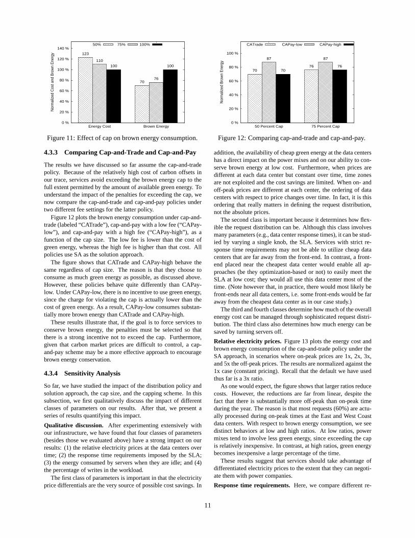
The results we have discussed so far assume the cap-and-tradepolicy. Because of the relatively high cost of carbon offsets inour trace, services avoid exceeding the brown energy cap to thefull extent permitted by the amount of available green energy. Tounderstand the impact of the penalties for exceeding the cap, wenow compare the cap-and-trade and cap-and-pay policies undertwo different fee settings for the latter policy.

Figure 12 plots the brown energy consumption under cap-and-trade (labeled “CATrade”), cap-and-pay with a low fee (“CAPay-low”), and cap-and-pay with a high fee (“CAPay-high”), as afunction of the cap size. The low fee is lower than the cost ofgreen energy, whereas the high fee is higher than that cost. Allpolicies use SA as the solution approach.

The figure shows that CATrade and CAPay-high behave thesame regardless of cap size. The reason is that they choose toconsume as much green energy as possible, as discussed above.However, these policies behave quite differently than CAPay-low. Under CAPay-low, there is no incentive to use green energy,since the charge for violating the cap is actually lower thanthecost of green energy. As a result, CAPay-low consumes substan-tially more brown energy than CATrade and CAPay-high.

These results illustrate that, if the goal is to force services toconserve brown energy, the penalties must be selected so thatthere is a strong incentive not to exceed the cap. Furthermore,given that carbon market prices are difficult to control, a cap-and-pay scheme may be a more effective approach to encouragebrown energy conservation.

4.3.4 Sensitivity Analysis

So far, we have studied the impact of the distribution policyandsolution approach, the cap size, and the capping scheme. In thissubsection, we first qualitatively discuss the impact of differentclasses of parameters on our results. After that, we presentaseries of results quantifying this impact.

Qualitative discussion. After experimenting extensively withour infrastructure, we have found that four classes of parameters(besides those we evaluated above) have a strong impact on ourresults: (1) the relative electricity prices at the data centers overtime; (2) the response time requirements imposed by the SLA;(3) the energy consumed by servers when they are idle; and (4)the percentage of writes in the workload.

The first class of parameters is important in that the electricityprice differentials are the very source of possible cost savings. In

addition, the availability of cheap green energy at the datacentershas a direct impact on the power mixes and on our ability to con-serve brown energy at low cost. Furthermore, when prices aredifferent at each data center but constant over time, time zonesare not exploited and the cost savings are limited. When on- andoff-peak prices are different at each center, the ordering of datacenters with respect to price changes over time. In fact, it is thisordering that really matters in defining the request distribution,not the absolute prices.

The second class is important because it determines how flex-ible the request distribution can be. Although this class involvesmany parameters (e.g., data center response times), it can be stud-ied by varying a single knob, the SLA. Services with strict re-sponse time requirements may not be able to utilize cheap datacenters that are far away from the front-end. In contrast, a front-end placed near the cheapest data center would enable all ap-proaches (be they optimization-based or not) to easily meettheSLA at low cost; they would all use this data center most of thetime. (Note however that, in practice, there would most likely befront-ends near all data centers, i.e. some front-ends would be faraway from the cheapest data center as in our case study.)

The third and fourth classes determine how much of the overallenergy cost can be managed through sophisticated request distri-bution. The third class also determines how much energy can besaved by turning servers off.

Relative electricity prices. Figure 13 plots the energy cost andbrown energy consumption of the cap-and-trade policy undertheSA approach, in scenarios where on-peak prices are 1x, 2x, 3x,and 5x the off-peak prices. The results are normalized against the1x case (constant pricing). Recall that the default we have usedthus far is a 3x ratio.

As one would expect, the figure shows that larger ratios reducecosts. However, the reductions are far from linear, despitethefact that there is substantially more off-peak than on-peaktimeduring the year. The reason is that most requests (60%) are actu-ally processed during on-peak times at the East and West Coastdata centers. With respect to brown energy consumption, we seedistinct behaviors at low and high ratios. At low ratios, powermixes tend to involve less green energy, since exceeding thecapis relatively inexpensive. In contrast, at high ratios, green energybecomes inexpensive a large percentage of the time.

These results suggest that services should take advantage ofdifferentiated electricity prices to the extent that they can negoti-ate them with power companies.

Response time requirements. Here, we compare different re-

11

0 %

20 %

40 %

60 %

80 %

100 %

120 %

Energy Cost Brown Energy

Nor

mal

ized

Cos

t and

Bro

wn

Ene

rgy

1x

100 100

2x

67

99

3x

57

87

5x

48

87

Figure 13: Effect of ratio of electricity prices.

0 %

20 %

40 %

60 %

80 %

100 %

120 %

Energy Cost

Nor

mal

ized

Ene

rgy

Cos

t

475 ms

100

500 ms

72

525 ms

51

550 ms

50

575 ms

50

600 ms

50

Figure 14: Effect of latency requirement (L).

0 %

20 %

40 %

60 %

80 %

100 %

120 %

0 Watts 75 Watts 150 Watts

Nor

mal

ized

Ene

rgy

Cos

t

sa

61

77 80

lp1

76

85 88

lp0

7684 87

ca

94 97 98

cu

100 100 100

Figure 15: Effect of base energy.

0 %

20 %

40 %

60 %

80 %

100 %

120 %

0 Percent 10 Percent 20 Percent 30 Percent

Nor

mal

ized

Ene

rgy

Cos

t

sa

61

7179

87

ca

94 96 97 98

cu

100 100 100 100

Figure 16: Effect of write percentage.

sponse time requirements (SLAs) and the cost savings that canbe achieved when they allow flexibility in request distribution.Figure 14 shows the energy costs of SA forP = 90%, as we varyL from 475 to 600ms. Recall that our results so far have assumedL = 500ms. The response times have a negligible impact on thebrown energy consumption.

The figure demonstrates that having less strict SLAs enablessignificant cost savings, e.g. 28% and 49% forL = 500ms and525ms, respectively. The reason is that the West Coast data cen-ter can be used more frequently in those cases. As the latencyrequirement is relaxed further, no more cost savings can be ac-crued since at that point all data centers can meet the SLA inde-pendently. We also conducted an experiment where a very strictP = 99% is enforced withL = 550ms (this is the first responsetime for whichP = 99% can actually be satisfied). We observedthat the cost compared toP = 90% increases by 16%.

These results illustrate the fundamental tradeoff betweenSLArequirements and our ability to lower costs. When SLAs arestrict, we can meet them but at a high cost. When these require-ments can be relaxed, significant cost savings can be achieved.

Base energy. Figure 15 plots the energy costs of the policies andsolution approaches, as a function of the amount of power serversconsume when idle. (Since we assume a dynamic power range of150W, a base power of 150W roughly represents today’s servers.)The costs are normalized to those of CU-Heuristic. Recall that allresults we discussed thus far assumed no base energy.

The figure shows exactly the same trends across base powers.In fact, even under the most pessimistic assumptions, SA canstillproduce 20% energy cost reductions.

This result suggests that the benefits of our optimization-based

framework and policies will increase with time, as servers be-come more energy-proportional.

Request types and on-line writes to persistent state. To as-sess the impact of these workload characteristics, we modifiedthe Ask.com trace to include 3 different request types, suchthatone type involves writes. Our systems handle each write requestat a data center by propagating coherence messages to its mirrordata centers. All simulation parameters were kept at their defaultvalues, but writes were assumed to consume 60 J at each datacenter because of coherence activity.

Figure 16 depicts the energy costs of SA, CA-Heuristic, andCU-Heuristic, as a function of the percentage of write requests.The figure shows that SA produces costs that are 19% and 21%lower than those of CA-Heuristic and CU-Heuristic, respectively,when 20% of the requests are writes. These cost savings aresmaller than those from Section 4.3.1, but are still quite signif-icant. Write percentages that are substantially higher than 20%are not as likely in practice. Nevertheless, the SA cost savingsare still 11-13% when as many as 30% of the requests are writes.

Session length. Our results so far have assumed that each sessioncontained a single request. For completeness, we also studytheimpact of longer sessions. To evaluate this impact, we createdtwo variations of the Ask.com trace that assigned each request toa specific user session. In the first variation, we created sessionswith an average of 3 requests, whereas the second variation hassessions with an average of 10 requests. Recall that our systemsdistribute entire sessions (rather than individual requests), suchthat all requests belonging to a session are forwarded to thesamecenter as the first request of the session.

Our results show that the session length has only a negligible

12

(≤ 1%) impact on energy cost and brown energy consumption.The reason is that, for any sufficiently large number of sessions,the percentage of requests of each type forwarded to a particulardata center is roughly the same across all session lengths.

4.3.5 Optimizing Costs For Current Services

The results presented above considered that brown energy capswere in effect and data centers can use green energy to abide bythem. However, current services do not need to cap their brownenergy consumption or use green energy. This section demon-strates how our framework and policies can be used to optimizeenergy costs even for today’s services.

Our framework enables services to take advantage of two as-pects of electricity prices that they currently may not benefitfrom: (1) the fact that off-peak and on-peak times can have dif-ferent prices; and (2) the fact that data centers at different timezones are exposed to different prices at each point in time. Toisolate the benefit of these aspects, we compare our default SAresults for with those of two other versions of our service. In oneversion, all data centers are on the East Coast with the same on-and off-peak electricity prices. To avoid changing two parame-ters at once, we keep the response times of the data centers thesame as in the default version. This version is called EC. In theother version, the data centers are distributed like in our defaultconfiguration but each pays a fixed (but different) price for theirelectricity. The fixed price is the average price weighted bythehourly load intensity of the trace. This version is called FP.

Comparing our default version against EC shows that takingadvantage of time zones reduces energy costs by 5%. Comparingour default version against FP shows that taking advantage ofon/off prices reduces energy costs by 24%.

5 Related WorkThis paper is the first to propose capping the brown energy con-sumption of large computer systems. It is also the first to considercarbon market interactions.Nevertheless, there have been relatedefforts on four topics, as we discuss next.

Conserving energy in data centers. Many works have beendone on this topic, e.g. [6, 7, 8, 10, 14, 15, 20, 23, 28, 32]. Mostof these works extend Load Concentration (LC) proposed in [23].In LC, the system dynamically determines how many servers arerequired to serve the offered load, directs the load to this manyservers, and turns the others off. Our evaluation assumed LCwasperformed within each data center.

Our work differs from these efforts in many ways: (1) noneof the previous works considered multi-mirror services andtheirrequest distribution; (2) none of them considered the goal of cap-ping energy consumption; and (3) none of them considered greenenergy or carbon market interactions.

Capping power consumption in data centers. [12, 29, 11] con-sidered power capping of data centers. Our work differs signif-icantly from these efforts, since capping energy is qualitativelydifferent than capping power. In particular, capping poweren-ables cheaper cooling and packaging, and adding more hardwareto a system without harming it. However, it may not conserve en-ergy, if obeying the cap causes a significant increase in runningtime. In contrast, capping brown energy can conserve brown en-ergy and promote green energy.

Optimization-based request distribution in Internet services.As far as we know, the only previous work on this topic is ourown [18], which is a short workshop paper that introduced aninitial, simplified framework for cost-aware request distribution.The framework did not consider brown energy caps, market inter-actions, request types, or power mixes. Moreover, the paperdidnot address LP-based solution approaches and did not include areal implementation.

Importantly, note that optimization has been used in a few pre-vious energy management works, e.g. [8, 14].However, none ofthose works considered multiple data centers or used optimiza-tion to define the load distribution.For example, [8] optimizedthe number of active nodes and their CPU frequencies in a singledata center. Independently of the optimization, their within-data-center distribution trivially attempts to evenly balance the loadacross the active nodes dedicated to a service. Our optimizationcomputes what percentage of requests of each type should be sentto each data center.

Furthermore, our work (1) demonstrates that optimization,which is rarely used when systems must make online dynamicdecisions, easily outperforms heuristicsfor a completely new andtimely problem, real workloads, real network latencies;and (2)compares three solution approaches thatcombine prediction andrecomputation in novel ways.

Leveraging variability in electricity prices in Internet ser-vices. Qureshi’s work [26] considered variable electricity pricesfor each data center (the price varies in an hourly basis) andpro-posed to shut down entire data centers when their electricity costsare relatively high. Recently, Qureshiet al. [27] studied dynamicrequest distribution based on hourly electricity prices.

This paper makes many major contributions with respect toQureshi’s work: (1) we built a real distributed implementationfor experimentation and simulator validation, whereas Qureshirelied solely on simulations; (2) we introduce brown energycaps(and carbon market interaction), whereas Qureshi did not con-sider caps or attempt to conserve energy; (3) we minimize costsbased on caps, green energy, electricity prices, and carbonmar-kets, whereas Qureshi focused solely on hourly electricityprices;(4) we use statistical response time information from data centersto abide by SLAs, whereas Qureshi used a simple radius metricthat is unable to meet our SLAs at low cost (Section 4.3.1); and(5) we demonstrate that optimization easily outperforms heuris-tics such as those used by Qureshi. Contributions (2), (3), and (4)mandate significant changes in the request distribution approachand also amplify the benefits of optimization-based techniquesover heuristics.In summary, our work is critical in enabling ser-vices to manage the likely emergence of brown energy caps mosteffectively; a problem that Qureshi did not address at all.

6 Conclusions

In this paper, we proposed an optimization-based frameworkfor enabling multi-data-center Internet services to manage theirbrown energy consumption and leverage green energy, while re-specting their SLAs and minimizing costs. Moreover, our frame-work enables services to exploit different electricity prices anddata centers located at different time zones to minimize costs,even in the absence of brown energy caps, different electricityprices, or green energy. We also proposed a simple heuristic

13

for achieving the same goals. We evaluated our proposals ex-tensively, using simulations, real experiments, and real traces.

Our work demonstrates the value of formal optimization tech-niques, workload prediction, and electricity price diversity for en-ergy management in Internet services. Given current skyrocket-ing energy costs, as well as likely future caps on carbon emis-sions and/or brown energy consumption, frameworks such asours should become extremely useful in practice.

Acknowledgements

We would like to thank Fred Chong and Luiz Barroso for com-ments that helped improve this paper. We would also like to thankFrank Felder and Robert Patrick for helping us understand thecarbon and electricity markets. Last but not least, we wouldliketo thank Ask.com for giving us a real request trace, and DejanKostic and John Zahorjan for lending us machines at EPFL andthe University of Washington, respectively.

References[1] Energy Information Administration. Average Retail Price of

Electricity to Ultimate Customers by End-Use Sector, by State.http://www.eia.doe.gov/cneaf/electricity/epm/table56 b.html.

[2] US Environmental Protection Agency. EPA Report on Server andData Center Energy Efficiency. August 2007.

[3] L. A. Barroso and U. Holzle. The Case for Energy-ProportionalComputing.IEEE Computer, 40(12), December 2007.

[4] G. Box and G. Jenkins.Time Series Analysis, Forecasting and Con-trol. Holden-Day, Incorporated, 1990.

[5] V. Cardellini, M. Colajanni, and P. Yu. Dynamic Load Balancing onWeb-Server Systems.IEEE Internet Computing, 3(3), May 1999.

[6] J. Chase et al. Managing Energy and Server Resources in HostingCenters. InSOSP, October 2001.

[7] G. Chen et al. Energy-Aware Server Provisioning and LoadDis-patching for Connection-Intensive Internet Services. InNSDI, April2008.

[8] Y. Chen et al. Managing Server Energy and Operational Costs inHosting Centers. InSIGMETRICS, June 2005.

[9] K. Coughlin et al. The Tariff Analysis Project: ADatabase and Analysis Platform for Electricity Tariffs.http://repositories.cdlib.org/lbnl/LBNL-55680.

[10] E. N. Elnozahy, M. Kistler, and R. Rajamony. Energy ConservationPolicies for Web Servers. InUSITS, March 2003.

[11] X. Fan, W.-D. Weber, and L. A. Barroso. Power Provisioning for aWarehouse-sized Computer. InISCA, June 2007.

[12] M. Femal and V. Freeh. Boosting Data Center PerformanceThrough Non-Uniform Power Allocation. InICAC, June 2005.

[13] HAProxy. The Reliable, High Performance TCP/HTTP LoadBal-ancer. http://haproxy.1wt.eu/.

[14] T. Heath et al. Energy Conservation in Heterogeneous Server Clus-ters. InPPoPP, June 2005.

[15] T. Horvath et al. Dynamic Voltage Scaling in Multi-tierWeb Serverswith End-to-End Delay Control.IEEE Transactions on Computers,56(4), April 2007.

[16] Uptime Institute and McKinsey & Company. Revolutionizing DataCenter Energy Efficiency Key Analyses. 2008.

[17] S. Kirkpatrick, C. D. Gelatt, and M. P. Vecchi. Optimization bysimulated annealing.Science, 220(4598), May 1983.

[18] K. Le et al. Cost- And Energy-Aware Load Distribution AcrossData Centers. InHotPower, October 2009.

[19] Green Electricity Marketplace. Green Electricity Marketplace.http://www.greenelectricity.org/.

[20] D. Meisner, B. T. Gold, and T. F. Wenisch. PowerNap: EliminatingServer Idle Power. InASPLOS, March 2009.

[21] The Green Power Network. Buy Green Power.http://apps3.eere.energy.gov/greenpower/buying/buying power.shtml.

[22] Department of Energy and Climate Change. Quarterly EnergyPrices. http://stats.berr.gov.uk/uksa/energy/sa20090625b.htm.

[23] E. Pinheiro et al. Dynamic Cluster Reconfiguration for Power andPerformance. In L. Benini, M. Kandemir, and J. Ramanujam, ed-itors, Compilers and Operating Systems for Low Power. KluwerAcademic Publishers, August 2003. Earlier version published inCOLP, September 2001.

[24] PointCarbon, Retrieved in March 2008.http://www.pointcarbon.com.

[25] Power Scorecard. Electricity from Coal, Retrieved in April 2008.http://www.powerscorecard.org/techdetail.cfm?resourceid=2.

[26] A. Qureshi. Plugging Into Energy Market Diversity. InHotNets,October 2008.

[27] A. Qureshi et al. Cutting the Electric Bill for Internet-Scale Sys-tems. InSIGCOMM, August 2009.

[28] K. Rajamani and C. Lefurgy. On Evaluating Request-DistributionSchemes for Saving Energy in Server Clusters. InISPASS, March2003.

[29] P. Ranganathan et al. Ensemble-Level Power ManagementforDense Blade Servers. InISCA, June 2006.

[30] S. Ranjan, R. Karrer, and E. Knightly. Wide Area Redirection ofDynamic Content by Internet Data Centers. InINFOCOMM, March2004.

[31] Regional Greenhouse Gas Initiative. Regional Greenhouse Gas Ini-tiative: An Initiative of the Northeast and Mid-Atlantic States of theUS, Retrieved in April 2008. http://www.rggi.org/.

[32] C. Rusu et al. Energy-Efficient Real-Time Heterogeneous ServerClusters. InRTAS, April 2006.

[33] UK Government. Carbon Reduction Commitment, Retrieved inJuly 2009. http://www.carbonreductioncommitment.info/.

[34] L. Wang, V. Pai, and L. Peterson. The Effectiveness of RequestRedirection on CDN Robustness. InOSDI, December 2002.

[35] W. Zhao, D. Olshefski, and H. Schulzrinne. Internet Quality of Ser-vice: An Overview. Technical Report CUCS-003-00, Departmentof Computer Science, Columbia University, February 2000.

14

Appendix A: Extended framework and cap-and-trade formulation including sessions and writes

Symbol Meaning

fy

i (t) Percentage of requests of typey to be forwarded to centeri in epocht

mbrowni Percentage of brown electricity in the power mix of centeri

mgreen

i Percentage of green electricity in the power mix of centeri

Overall Cost Total energy cost (in $) of the serviceBEC Brown energy cap (in KWh) of all centers combinedpy(t) Percentage of requests of typey in the workload in epochtwy(t) Percentage of requests of typey in epocht that involve writes to persistent stateMy

i Equals 1 if data centeri can serve requests of typey. Equals 0 otherwiseReqCosty

i (t) Avg. energy cost (in $) incl. cap-violation charges of serving a request of typey at centeri in epochtCohCosty

i (t) Avg. energy cost (in $) incl. cap-violation charges of serving a coherence request of typey at centeri in epochtBaseCosti(offeredi, t) Base energy cost (in $) incl. cap-violation charges of center i in epocht, underofferedi load

bry

i (t) Avg. energy cost (in $) of serving a request of typey using only brown electricity at centerigry

i (t) Avg. energy cost (in $) of serving a request of typey using only green electricity at centeribcy

i (t) Avg. energy cost (in $) of serving a coherence request of typey using only brown electricity at centerigcy

i (t) Avg. energy cost (in $) of serving a coherence request of typey using only green electricity at centeribbi(offeredi, t) Base energy cost (in $) of centeri in epocht, underofferedi load, using only brown electricitygbi(offeredi, t) Base energy cost (in $) of centeri in epocht, underofferedi load, using only green electricitymarketReqyi (t) Avg. market cost (in $) to offset the brown energy used by a request of typey in centeri in epochtmarketCohyi (t) Avg. market cost (in $) to offset the brown energy used by a coherence request of typey in centeri in epocht

marketBasei(offeredi, t) Market cost (in $) of offsetting the base brown energy in center i in epocht, underofferedi loadfeeReqyi (t) Avg. fee for cap violation (in $) for the brown energy used by arequest of typey in centeri in epochtfeeCohyi (t) Avg. fee for cap violation (in $) for the brown energy used by acoherence request of typey in centeri in epocht

feeBasei(offeredi, t) Fee for cap violation (in $) for the base brown energy in center i in epocht, underofferedi loadLR(t) Expected peak service load rate (in reqs/sec) for epochtLT(t) Expected total service load (in number of reqs) for epochtLCi Load capacity (in reqs/sec) of centeri

CDFi(L, offeredi) Expected percentage of requests sent to centeri that complete within L time, givenofferedi load

Table 5:Extended framework. Note that this table extends Table 1 with the parameters associated with write requests and the coherenceactivity that they trigger:wy(t), CohCosty

i (t), bcy

i (t), gcy

i (t), marketCohyi (t), andfeeCohyi (t).

offeredi = (∑

yfy

i (t) × My

i × py(t) × LR(t)) + (∑

y(1 − fy

i (t)) × wy(t) × My

i × py(t) × LR(t)) =∑y(fy

i (t) + ((1 − fy

i (t)) × wy(t))) × My

i × py(t) × LR(t)(5)

Overall Cost= (∑

t

∑i

∑y

fy

i (t) × My

i × py(t) × LT (t) × ReqCostyi (t))+

(∑

t

∑i

∑y(1 − fy

i (t)) × wy(t) × My

i × py(t) × LT (t) × CohCostyi (t))+

(∑

t

∑iBaseCosti(offeredi, t))

(6)

ReqCosty

i (t) = mbrowni × bry

i (t) + mgreen

i × gry

i (t), if brown energy consumed so far≤ BEC

marketReqy

i (t) + mbrowni × bry

i (t) + mgreen

i × gry

i (t), otherwise(7)

CohCosty

i (t) = mbrowni × bcy

i (t) + mgreen

i × gcy

i (t), if brown energy consumed so far≤ BEC

marketCohy

i (t) + mbrowni × bcy

i (t) + mgreen

i × gcy

i (t), otherwise(8)

BaseCosti(offeredi, t) = mbrowni × bbi(offeredi, t) + mgreen

i × gbi(offeredi, t), if brown energy consumed so far≤ BEC

marketBasei(offeredi, t) + mbrowni × bbi(offeredi, t) + mgreen

i × gbi(offeredi, t), otherwise(9)

1. ∀i mbrowni andmgreen

i ≥ 0 ⇒ i.e., each part of the mix cannot be negative.2. ∀i mbrown

i + mgreen

i = 1 ⇒ i.e., the mixes need to add up to 1.3. ∀t∀i∀y fy

i (t) ≥ 0 ⇒ i.e., each fraction cannot be negative.4. ∀t∀y

∑i

fy

i (t) × My

i = 1 ⇒ i.e., the fractions for each request type need to add up to 1.5. ∀t∀i offeredi ≤ LCi ⇒ i.e., the offered load to a data center should not overload it.6.

∑t

∑i

∑y(fy

i (t) × My

i × py(t) × LT (t) × CDFi(L, offeredi)) /∑

tLT (t) ≥ P ⇒ i.e., the SLA must be satisfied.

(10)

Figure 17: Extended cap-and-trade formulation. These equations extend those from Figure 5 by (1) accounting for data coher-ence activity when definingOverall Cost; and (2) defining the average energy cost of the coherence activity at a mirror data center(CohCosty

i (t)), as a result of a write processed at another data center. Theequations also re-define the offered load to a data center(offeredi). The constraints are unchanged from their definition in Figure 5.

15