Management Decision Modeling - StudyDaddy
61
Dr. Jose Garcia‐Rubia Management Decision Modeling Chapter 9. Transportation, Assignment, and Network Models
-
Upload
khangminh22 -
Category
Documents
-
view
5 -
download
0
Transcript of Management Decision Modeling - StudyDaddy
Dr. Jose Garcia‐Rubia
Management Decision ModelingChapter 9. Transportation, Assignment, and Network Models
Management Decision ModelingChapter 9. Transportation, Assignment, and Network Models
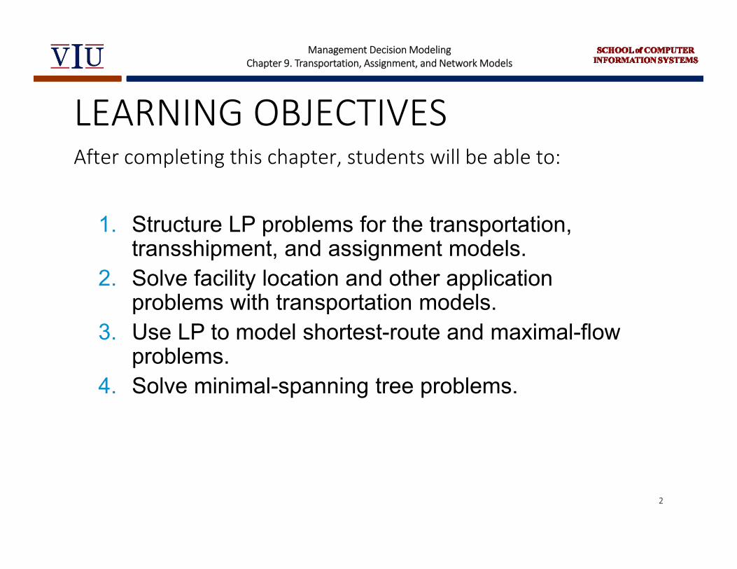
LEARNING OBJECTIVESAfter completing this chapter, students will be able to:
1. Structure LP problems for the transportation, transshipment, and assignment models.
2. Solve facility location and other application problems with transportation models.
3. Use LP to model shortest-route and maximal-flow problems.
4. Solve minimal-spanning tree problems.
2
Management Decision ModelingChapter 9. Transportation, Assignment, and Network Models
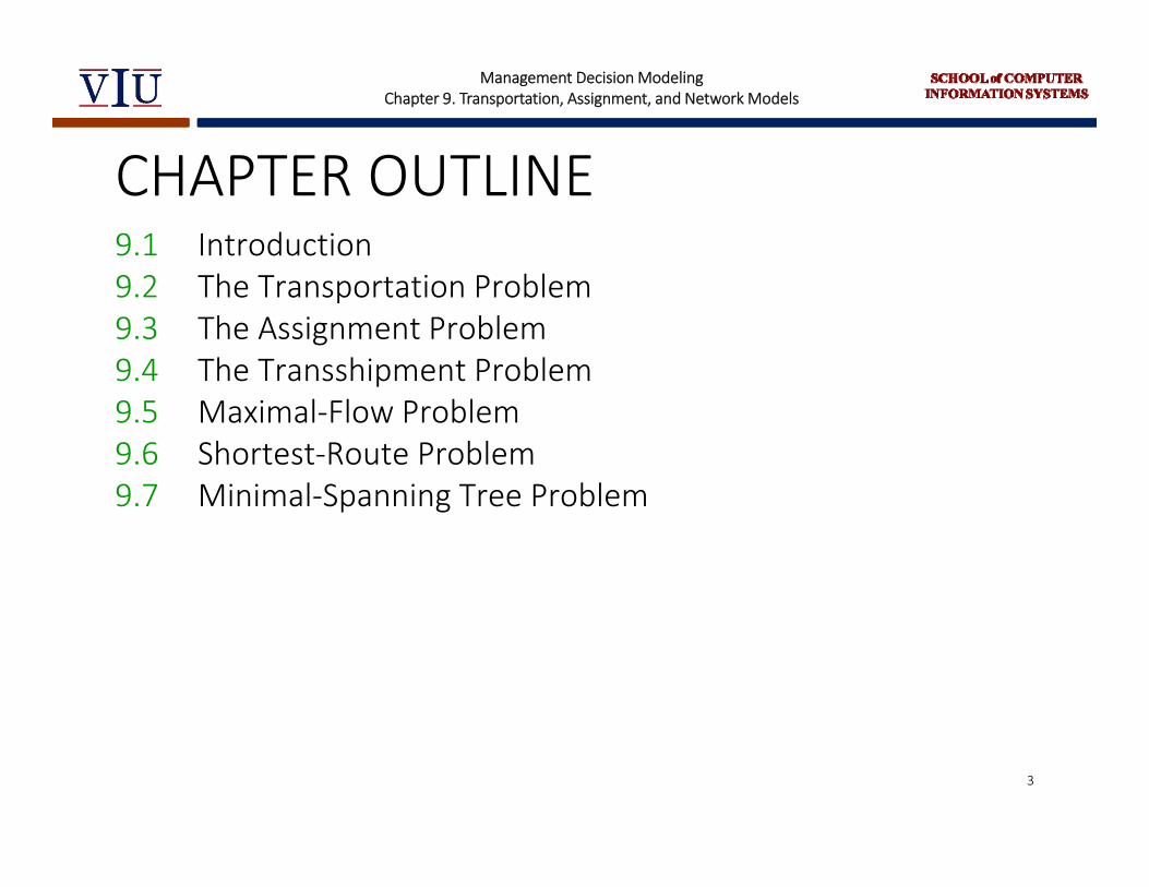
CHAPTER OUTLINE9.1 Introduction9.2 The Transportation Problem9.3 The Assignment Problem9.4 The Transshipment Problem9.5 Maximal‐Flow Problem 9.6 Shortest‐Route Problem 9.7 Minimal‐Spanning Tree Problem
3
Management Decision ModelingChapter 9. Transportation, Assignment, and Network Models
Introduction LP problems modeled as networksHelps visualize and understand problems
Transportation problem Transshipment problem Assignment problem Maximal-flow problem Shortest-route problem Minimal-spanning tree problem
Specialized algorithms available
4
Management Decision ModelingChapter 9. Transportation, Assignment, and Network Models
Introduction Common terminology for network
modelsPoints on the network are referred to as
nodes Typically circles
Lines on the network that connect nodes are called arcs
5

Management Decision ModelingChapter 9. Transportation, Assignment, and Network Models
The Transportation Problem Deals with the distribution of goods from
several points of supply (sources) to a number of points of demand (destinations)Usually given the capacity of goods at each
source and the requirements at each destination
Typically objective is to minimize total transportation and production costs
6

Management Decision ModelingChapter 9. Transportation, Assignment, and Network Models
Activity 9.1 Linear Program for Transportation Executive Furniture Corporation
transportation problemMinimize transportation costMeet demandNot exceed supply
7
Management Decision ModelingChapter 9. Transportation, Assignment, and Network Models
Linear Program for Transportation
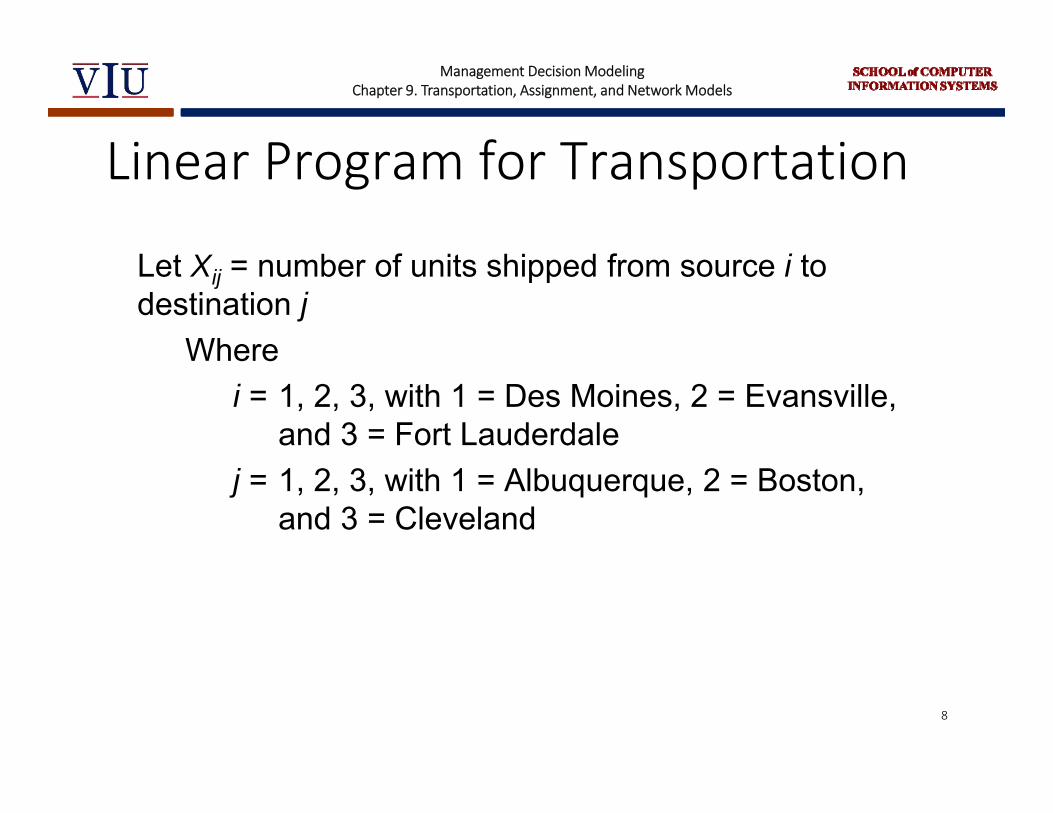
Let Xij = number of units shipped from source i to destination j
Wherei = 1, 2, 3, with 1 = Des Moines, 2 = Evansville,
and 3 = Fort Lauderdalej = 1, 2, 3, with 1 = Albuquerque, 2 = Boston,
and 3 = Cleveland
8
Management Decision ModelingChapter 9. Transportation, Assignment, and Network Models
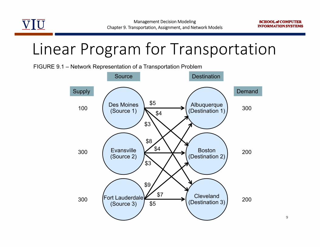
Linear Program for TransportationFIGURE 9.1 – Network Representation of a Transportation Problem
100
300
300
Supply
$5
$4
$3
$8$4
$3
$9
$7$5
Demand
200
200
300
Source
Des Moines(Source 1)
Evansville(Source 2)
Fort Lauderdale(Source 3)
Albuquerque(Destination 1)
Boston(Destination 2)
Cleveland(Destination 3)
Destination
9
Management Decision ModelingChapter 9. Transportation, Assignment, and Network Models
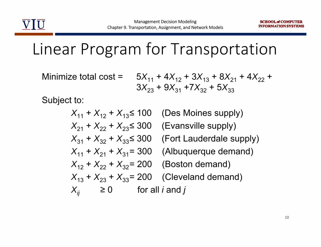
Linear Program for TransportationMinimize total cost = 5X11 + 4X12 + 3X13 + 8X21 + 4X22 +
3X23 + 9X31 +7X32 + 5X33
Subject to:X11 + X12 + X13≤ 100 (Des Moines supply)X21 + X22 + X23≤ 300 (Evansville supply)X31 + X32 + X33≤ 300 (Fort Lauderdale supply)X11 + X21 + X31= 300 (Albuquerque demand)X12 + X22 + X32= 200 (Boston demand)X13 + X23 + X33= 200 (Cleveland demand)Xij ≥ 0 for all i and j
10

Management Decision ModelingChapter 9. Transportation, Assignment, and Network Models
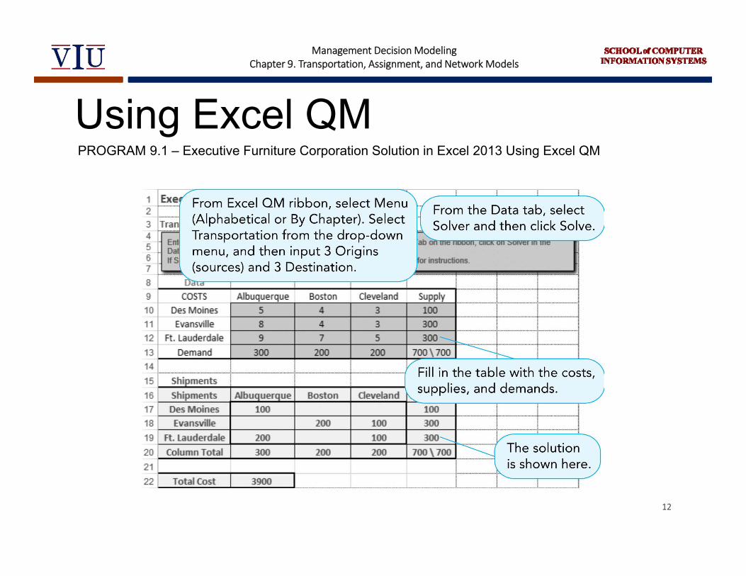
Linear Program for Transportation
Optimal solution
100 units from Des Moines to Albuquerque 200 units from Evansville to Boston100 units from Evansville to Cleveland 200 units from Ft. Lauderdale to
Albuquerque 100 units from Ft. Lauderdale to ClevelandTotal cost = $3,900
11
Management Decision ModelingChapter 9. Transportation, Assignment, and Network Models
Using Excel QMPROGRAM 9.1 – Executive Furniture Corporation Solution in Excel 2013 Using Excel QM
12
Management Decision ModelingChapter 9. Transportation, Assignment, and Network Models
A General LP Model for Transportation Problems
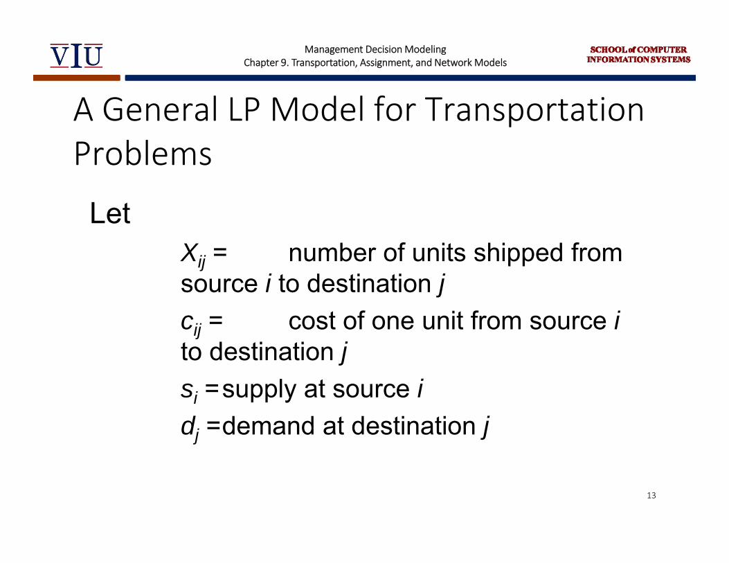
LetXij = number of units shipped from source i to destination jcij = cost of one unit from source ito destination jsi =supply at source idj =demand at destination j
13

Management Decision ModelingChapter 9. Transportation, Assignment, and Network Models
Minimize cost cij xiji1
m
j1
n
A General LP Model for Transportation Problems
Subject to:
xij si i 1,2,...,mj1
n
xiji1
m
dj j 1,2...,n
xij 0 for all i and j14

Management Decision ModelingChapter 9. Transportation, Assignment, and Network Models
Activity 9.2 Facility Location Analysis Transportation method especially useful New location is major financial importance Several alternative locations evaluated Subjective factors are considered Final decision also involves minimizing total
shipping and production costs Alternative facility locations analyzed within
the framework of one overall distribution system 15

Management Decision ModelingChapter 9. Transportation, Assignment, and Network Models
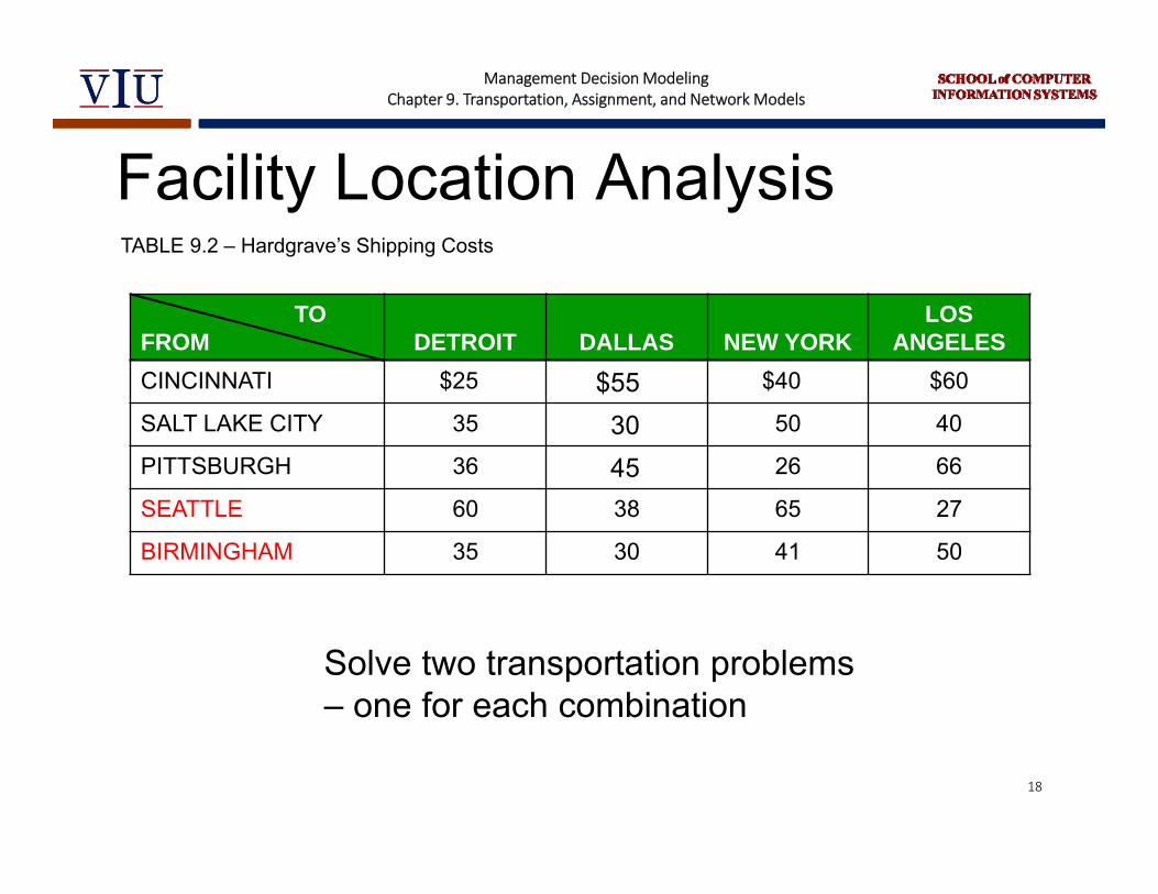
Facility Location Analysis Hardgrave Machine Company produces
computer components in Cincinnati, Salt Lake City, and Pittsburgh
Four warehouses in Detroit, Dallas, New York, and Los Angeles
Two new plant sites being considered –Seattle and Birmingham
Which of the new locations will yield the lowest cost for the firm in combination with the existing plants and warehouses?
16
Management Decision ModelingChapter 9. Transportation, Assignment, and Network Models
Facility Location Analysis
WAREHOUSE
MONTHLY DEMAND (UNITS)
PRODUCTION PLANT
MONTHLY SUPPLY
COST TO PRODUCE
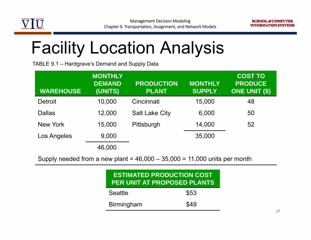
ONE UNIT ($)Detroit 10,000 Cincinnati 15,000 48
Dallas 12,000 Salt Lake City 6,000 50
New York 15,000 Pittsburgh 14,000 52
Los Angeles 9,000 35,000
46,000
Supply needed from a new plant = 46,000 – 35,000 = 11,000 units per month
TABLE 9.1 – Hardgrave’s Demand and Supply Data
ESTIMATED PRODUCTION COSTPER UNIT AT PROPOSED PLANTS
Seattle $53
Birmingham $4917
Management Decision ModelingChapter 9. Transportation, Assignment, and Network Models
Facility Location Analysis
TOFROM DETROIT DALLAS NEW YORK
LOS ANGELES
CINCINNATI $25 $55 $40 $60
SALT LAKE CITY 35 30 50 40
PITTSBURGH 36 45 26 66
SEATTLE 60 38 65 27
BIRMINGHAM 35 30 41 50
TABLE 9.2 – Hardgrave’s Shipping Costs
Solve two transportation problems – one for each combination
18
Management Decision ModelingChapter 9. Transportation, Assignment, and Network Models
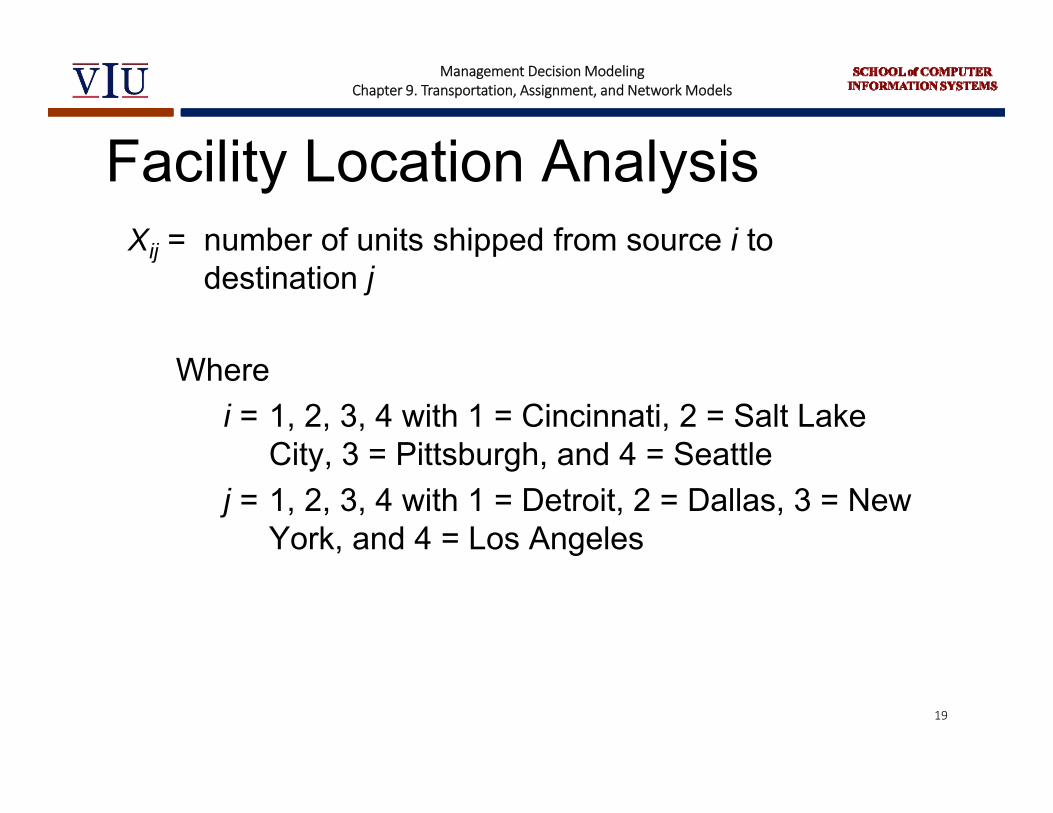
Facility Location AnalysisXij = number of units shipped from source i to
destination j
Wherei = 1, 2, 3, 4 with 1 = Cincinnati, 2 = Salt Lake
City, 3 = Pittsburgh, and 4 = Seattlej = 1, 2, 3, 4 with 1 = Detroit, 2 = Dallas, 3 = New
York, and 4 = Los Angeles
19
Management Decision ModelingChapter 9. Transportation, Assignment, and Network Models
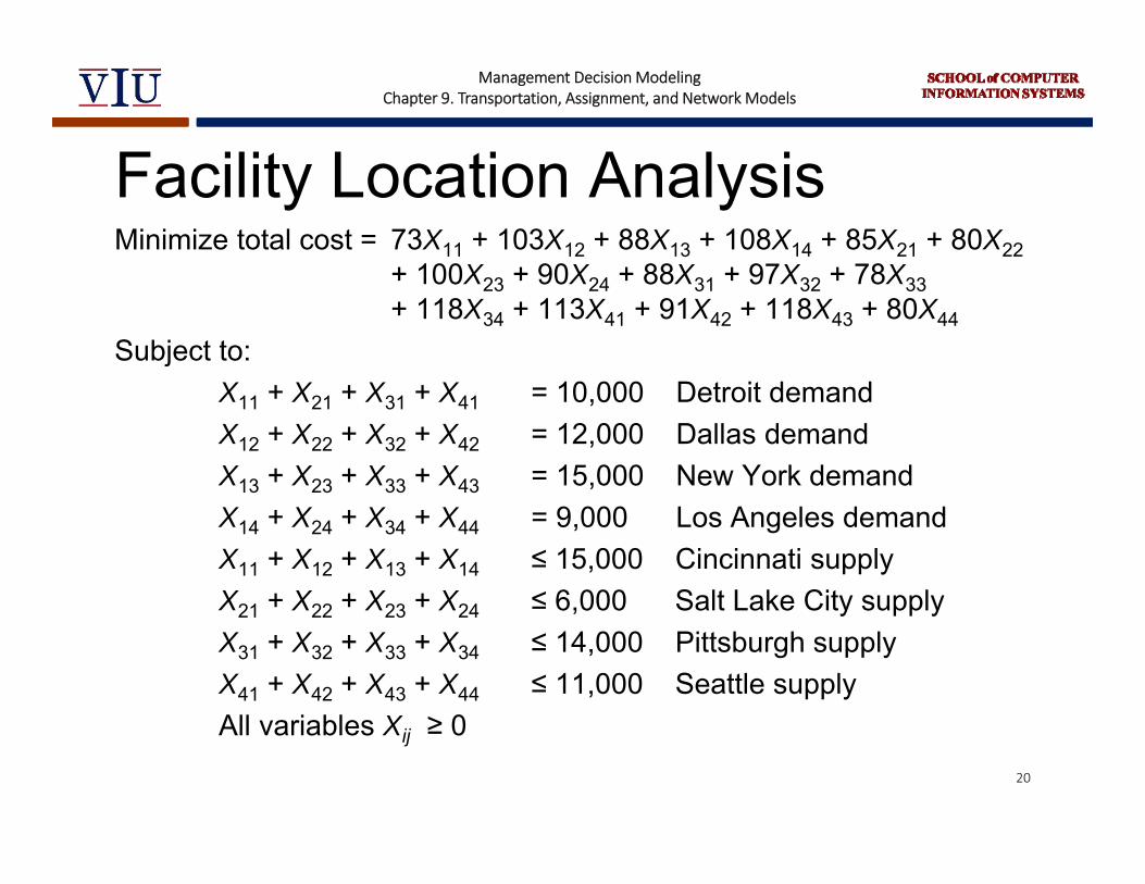
Facility Location AnalysisMinimize total cost = 73X11 + 103X12 + 88X13 + 108X14 + 85X21 + 80X22
+ 100X23 + 90X24 + 88X31 + 97X32 + 78X33+ 118X34 + 113X41 + 91X42 + 118X43 + 80X44
Subject to:X11 + X21 + X31 + X41 = 10,000 Detroit demandX12 + X22 + X32 + X42 = 12,000 Dallas demandX13 + X23 + X33 + X43 = 15,000 New York demandX14 + X24 + X34 + X44 = 9,000 Los Angeles demandX11 + X12 + X13 + X14 ≤ 15,000 Cincinnati supplyX21 + X22 + X23 + X24 ≤ 6,000 Salt Lake City supplyX31 + X32 + X33 + X34 ≤ 14,000 Pittsburgh supplyX41 + X42 + X43 + X44 ≤ 11,000 Seattle supplyAll variables Xij ≥ 0
20

Management Decision ModelingChapter 9. Transportation, Assignment, and Network Models
Minimize total cost = 73X11 + 103X12 + 88X13 + 108X14 + 85X21 + 80X22+ 100X23 + 90X24 + 88X31 + 97X32 + 78X33+ 118X34 + 113X41 + 91X42 + 118X43 + 80X44
Subject to:X11 + X21 + X31 + X41 = 10,000 Detroit demandX12 + X22 + X32 + X42 = 12,000 Dallas demandX13 + X23 + X33 + X43 = 15,000 New York demandX14 + X24 + X34 + X44 = 9,000 Los Angeles demandX11 + X12 + X13 + X14 ≤ 15,000 Cincinnati supplyX21 + X22 + X23 + X24 ≤ 6,000 Salt Lake City supplyX31 + X32 + X33 + X34 ≤ 14,000 Pittsburgh supplyX41 + X42 + X43 + X44 ≤ 11,000 Seattle supplyAll variables Xij ≥ 0
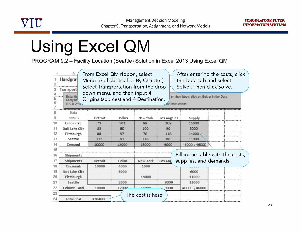
Facility Location AnalysisThe total cost for the Seattle alternative = $3,704,000
21

Management Decision ModelingChapter 9. Transportation, Assignment, and Network Models
Minimize total cost = 73X11 + 103X12 + 88X13 + 108X14 + 85X21 + 80X22+ 100X23 + 90X24 + 88X31 + 97X32 + 78X33+ 118X34 + 113X41 + 91X42 + 118X43 + 80X44
Subject to:X11 + X21 + X31 + X41 = 10,000 Detroit demandX12 + X22 + X32 + X42 = 12,000 Dallas demandX13 + X23 + X33 + X43 = 15,000 New York demandX14 + X24 + X34 + X44 = 9,000 Los Angeles demandX11 + X12 + X13 + X14 ≤ 15,000 Cincinnati supplyX21 + X22 + X23 + X24 ≤ 6,000 Salt Lake City supplyX31 + X32 + X33 + X34 ≤ 14,000 Pittsburgh supplyX41 + X42 + X43 + X44 ≤ 11,000 Seattle supplyAll variables Xij ≥ 0
Facility Location AnalysisThe total cost for the Seattle alternative = $3,704,000
Reformulating the problem for the Birmingham alternative and solving, the total cost = $3,741,000
22
Management Decision ModelingChapter 9. Transportation, Assignment, and Network Models
Using Excel QMPROGRAM 9.2 – Facility Location (Seattle) Solution in Excel 2013 Using Excel QM
23

Management Decision ModelingChapter 9. Transportation, Assignment, and Network Models
Using Excel QMPROGRAM 9.3 – Facility Location (Birmingham) Solution in Excel 2013 Using Excel QM
24
Management Decision ModelingChapter 9. Transportation, Assignment, and Network Models
The Assignment Problem This class of problem determines the most
efficient assignment of people or equipment to particular tasks
Objective is typically to minimize total cost or total task time
25
Management Decision ModelingChapter 9. Transportation, Assignment, and Network Models
Activity 9.2 Linear Program for Assignment The Fix-it Shop has just received three new
repair projects that must be repaired quickly1. A radio2. A toaster oven3. A coffee table
Three workers with different talents are able to do the jobs
Owner estimates wage cost for workers on projects
Objective – minimize total cost 26
Management Decision ModelingChapter 9. Transportation, Assignment, and Network Models
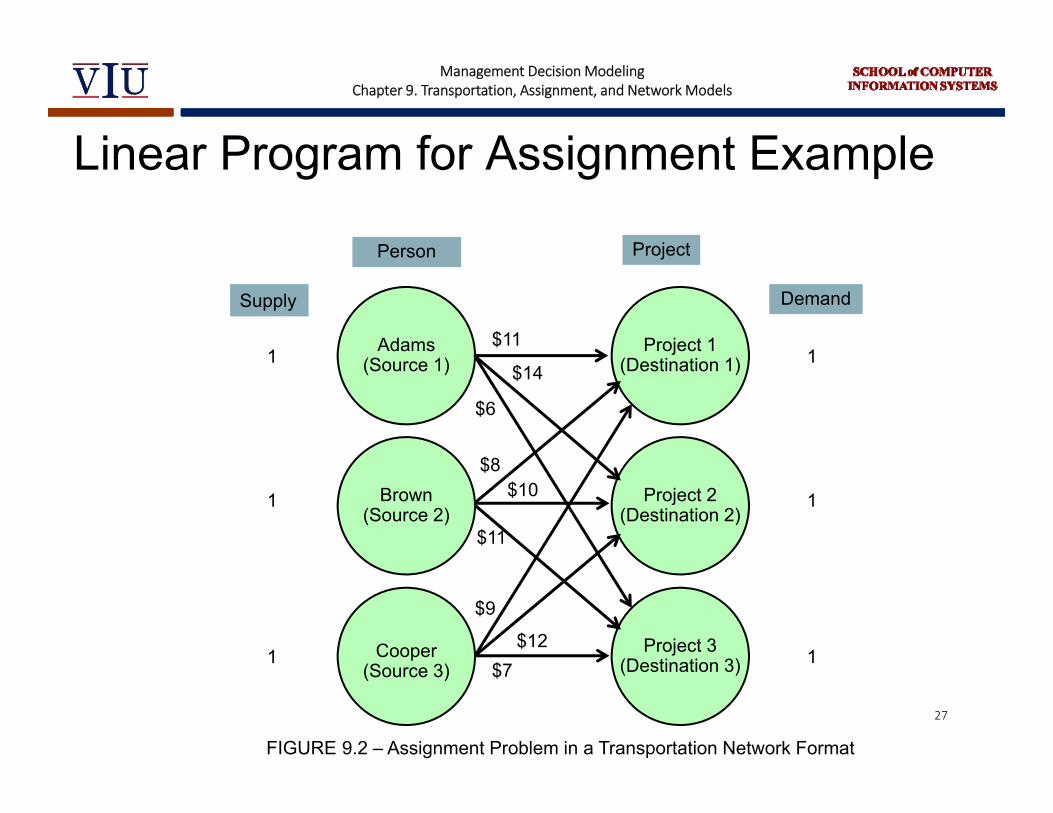
Linear Program for Assignment Example
FIGURE 9.2 – Assignment Problem in a Transportation Network Format
1
1
1
Supply
$11
$14
$6
$8$10
$11
$9
$12$7
1
1
1
Demand
Person
Adams(Source 1)
Brown(Source 2)
Cooper(Source 3)
Project 1(Destination 1)
Project 2(Destination 2)
Project 3(Destination 3)
Project
27
Management Decision ModelingChapter 9. Transportation, Assignment, and Network Models
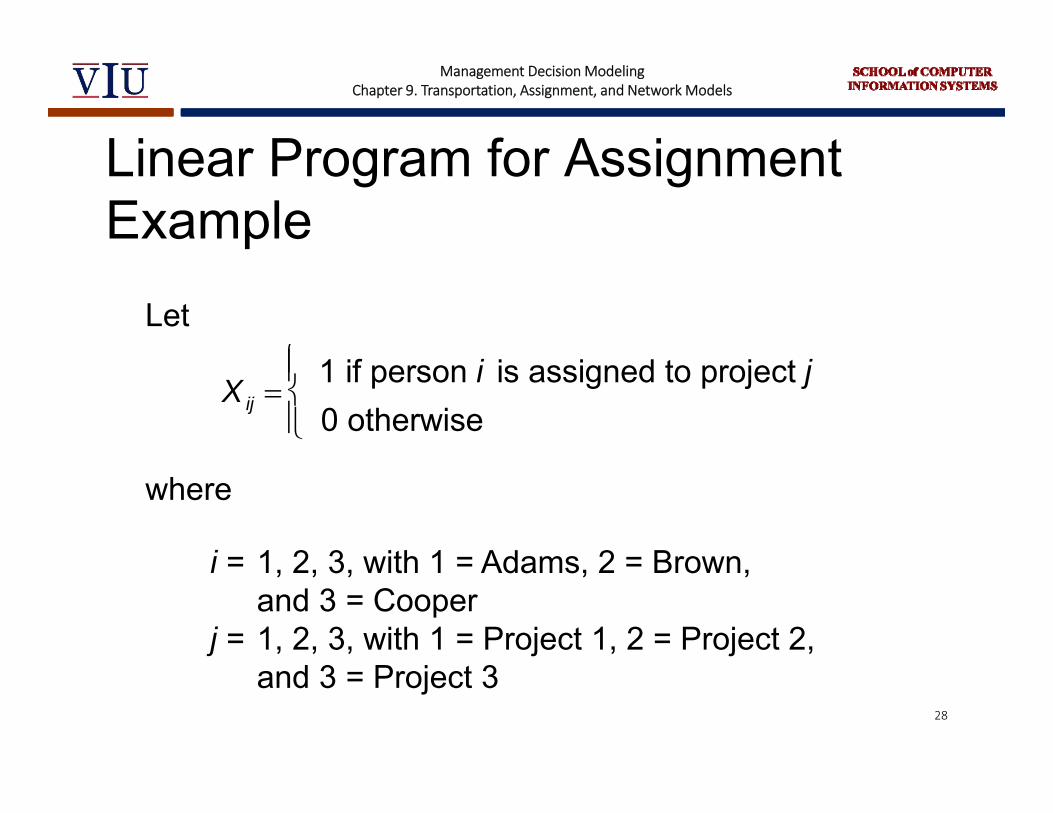
Linear Program for Assignment Example
Xij 1 if person i is assigned to project j0 otherwise
Let
where
i = 1, 2, 3, with 1 = Adams, 2 = Brown, and 3 = Cooper
j = 1, 2, 3, with 1 = Project 1, 2 = Project 2, and 3 = Project 3
28

Management Decision ModelingChapter 9. Transportation, Assignment, and Network Models
Linear Program for Assignment Example
Minimize total cost = 11X11 + 14X12 + 6X13 + 8X21+ 10X22 + 11X23 + 9X31 + 12X32 + 7X33
subject toX11 + X12 + X13 = 1X21 + X22 + X23 = 1X31 + X32 + X33 = 1X11 + X21 + X31 = 1X12 + X22 + X32 = 1X13 + X23 + X33 = 1
Xij = 0 or 1 for all i and j29

Management Decision ModelingChapter 9. Transportation, Assignment, and Network Models
Linear Program for Assignment Example
Minimize total cost = 11X11 + 14X12 + 6X13 + 8X21+ 10X22 + 11X23 + 9X31 + 12X32 + 7X33
subject toX11 + X12 + X13 ≤ 1X21 + X22 + X23 ≤ 1X31 + X32 + X33 ≤ 1X11 + X21 + X31 = 1X12 + X22 + X32 = 1X13 + X23 + X33 = 1Xij = 0 or 1 for all i and j
Solution
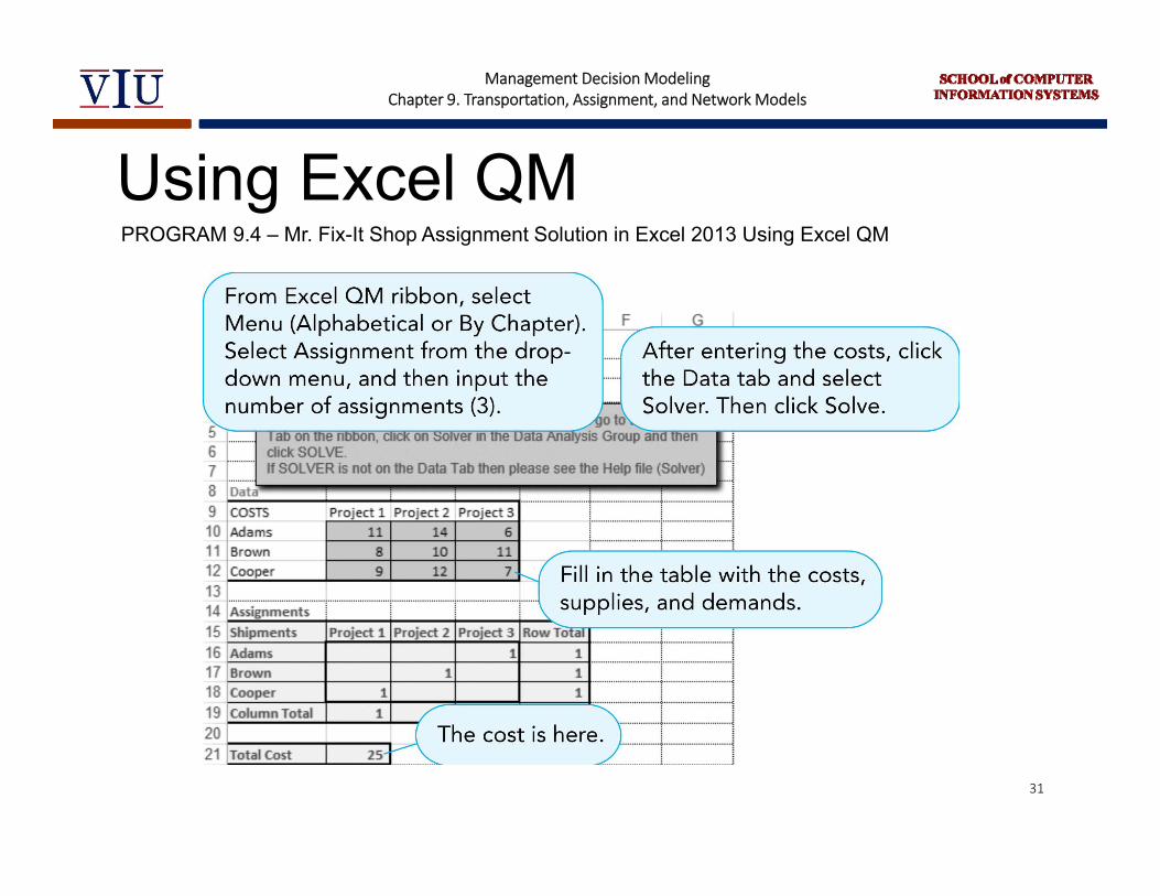
X13 = 1, Adams assigned to Project 3X22 = 1, Brown assigned to Project 2X31 = 1, Cooper is assigned to Project 1
Total cost = $25
30
Management Decision ModelingChapter 9. Transportation, Assignment, and Network Models
Using Excel QMPROGRAM 9.4 – Mr. Fix-It Shop Assignment Solution in Excel 2013 Using Excel QM
31

Management Decision ModelingChapter 9. Transportation, Assignment, and Network Models
The Transshipment Problem Items are being moved from a source to a
destination through an intermediate point (a transshipment point)
Transshipment problem
32

Management Decision ModelingChapter 9. Transportation, Assignment, and Network Models
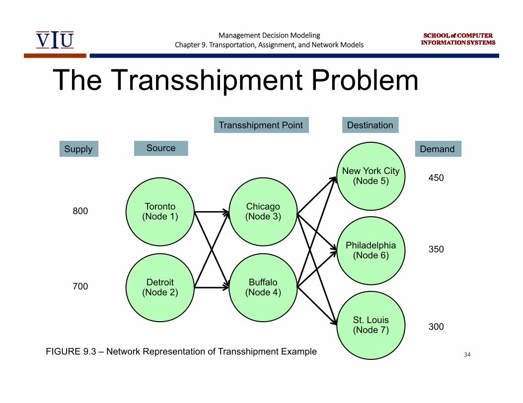
Activity 9.4 The Transshipment Problem Frosty Machines manufactures snow blowers in
Toronto and Detroit Shipped to regional distribution centers in
Chicago and Buffalo Then shipped to supply houses in New York,
Philadelphia, and St. Louis Shipping costs vary by location and destination Snow blowers cannot be shipped directly from
the factories to the supply houses33
Management Decision ModelingChapter 9. Transportation, Assignment, and Network Models
The Transshipment Problem
FIGURE 9.3 – Network Representation of Transshipment Example
800
700
Supply
300
350
450
DemandSource
Toronto(Node 1)
Detroit(Node 2)
New York City(Node 5)
Philadelphia(Node 6)
St. Louis(Node 7)
Destination
Chicago(Node 3)
Transshipment Point
Buffalo(Node 4)
34

Management Decision ModelingChapter 9. Transportation, Assignment, and Network Models
The Transshipment ProblemTABLE 9.3 – Frosty Machine Transshipment Data
TO
FROM CHICAGO BUFFALONEW YORK
CITY PHILADELPHIAST.
LOUIS SUPPLY
Toronto $4 $7 — — — 800
Detroit $5 $7 — — — 700
Chicago — — $6 $4 $5 —
Buffalo — — $2 $3 $4 —
Demand — — 450 350 300
Minimize transportation costs associated with shipping snow blowers subject to demands and supplies
35
Management Decision ModelingChapter 9. Transportation, Assignment, and Network Models
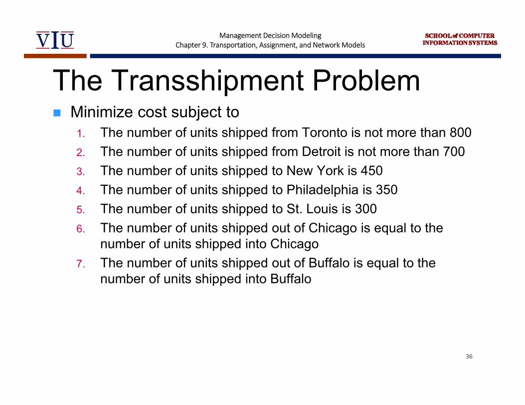
The Transshipment Problem Minimize cost subject to
1. The number of units shipped from Toronto is not more than 8002. The number of units shipped from Detroit is not more than 7003. The number of units shipped to New York is 4504. The number of units shipped to Philadelphia is 3505. The number of units shipped to St. Louis is 3006. The number of units shipped out of Chicago is equal to the
number of units shipped into Chicago7. The number of units shipped out of Buffalo is equal to the
number of units shipped into Buffalo
36

Management Decision ModelingChapter 9. Transportation, Assignment, and Network Models
The Transshipment ProblemDecision variables
Xij = number of units shipped from location (node) i to location (node) j
where
i = 1, 2, 3, 4j = 3, 4, 5, 6, 7
37
Management Decision ModelingChapter 9. Transportation, Assignment, and Network Models
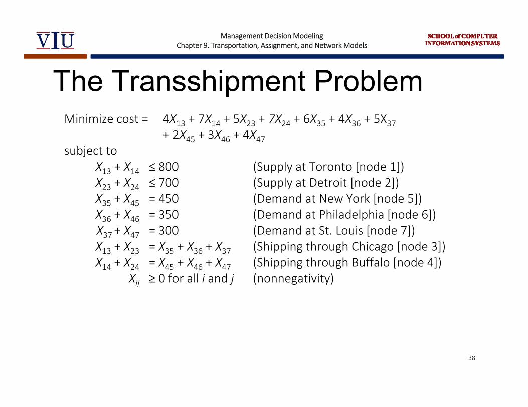
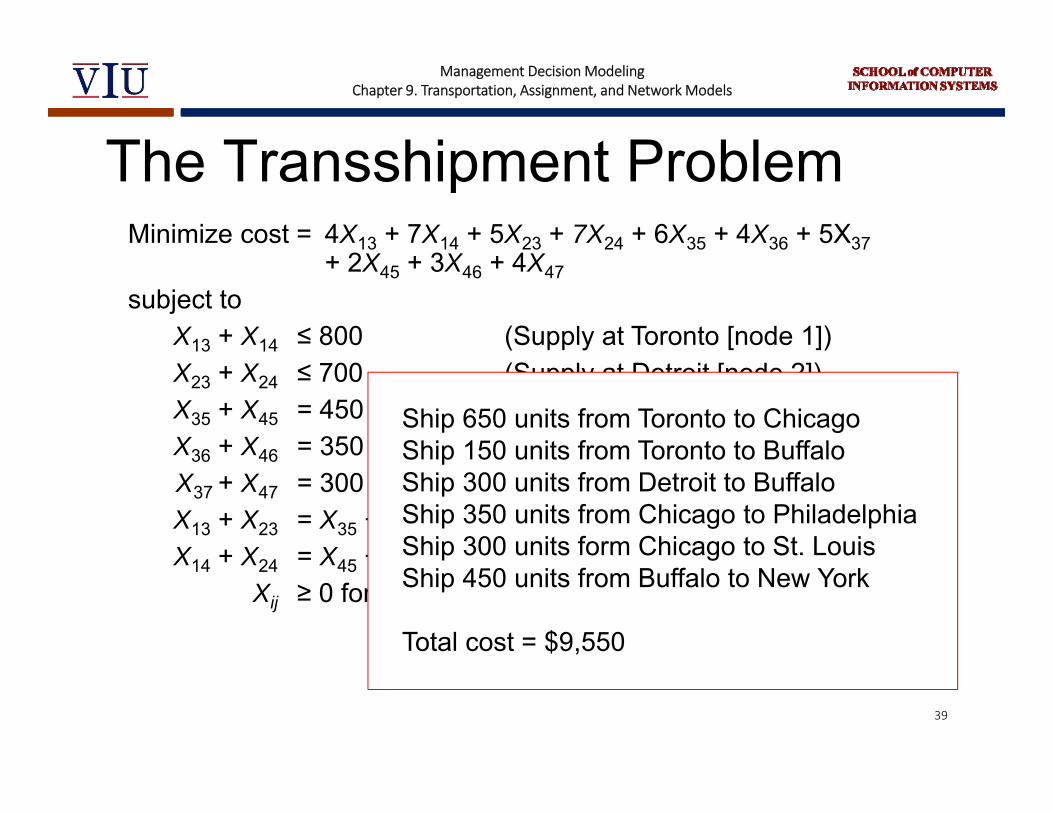
The Transshipment ProblemMinimize cost = 4X13 + 7X14 + 5X23 + 7X24 + 6X35 + 4X36 + 5X37
+ 2X45 + 3X46 + 4X47subject to
X13 + X14 ≤ 800 (Supply at Toronto [node 1])X23 + X24 ≤ 700 (Supply at Detroit [node 2])X35 + X45 = 450 (Demand at New York [node 5])X36 + X46 = 350 (Demand at Philadelphia [node 6])X37 + X47 = 300 (Demand at St. Louis [node 7])X13 + X23 = X35 + X36 + X37 (Shipping through Chicago [node 3])X14 + X24 = X45 + X46 + X47 (Shipping through Buffalo [node 4])
Xij ≥ 0 for all i and j (nonnegativity)
38
Management Decision ModelingChapter 9. Transportation, Assignment, and Network Models
Minimize cost = 4X13 + 7X14 + 5X23 + 7X24 + 6X35 + 4X36 + 5X37+ 2X45 + 3X46 + 4X47
subject toX13 + X14 ≤ 800 (Supply at Toronto [node 1])X23 + X24 ≤ 700 (Supply at Detroit [node 2])X35 + X45 = 450 (Demand at New York [node 5])X36 + X46 = 350 (Demand at Philadelphia [node 6])X37 + X47 = 300 (Demand at St. Louis [node 7])X13 + X23 = X35 + X36 + X37 (Shipping through Chicago [node 3])X14 + X24 = X45 + X46 + X47 (Shipping through Buffalo [node 4])
Xij ≥ 0 for all i and j (nonnegativity)
The Transshipment Problem
Ship 650 units from Toronto to ChicagoShip 150 units from Toronto to BuffaloShip 300 units from Detroit to BuffaloShip 350 units from Chicago to PhiladelphiaShip 300 units form Chicago to St. LouisShip 450 units from Buffalo to New York
Total cost = $9,550
39

Management Decision ModelingChapter 9. Transportation, Assignment, and Network Models
Using Excel QMPROGRAM 9.5 – Excel QM Solution to Frosty Machine Transshipment Problem
40

Management Decision ModelingChapter 9. Transportation, Assignment, and Network Models
Maximal-Flow Problem Determining the maximum amount of
material that can flow from one point (the source) to another (the sink) in a network
Two common methodsLinear programmingMaximal-flow technique
41
Management Decision ModelingChapter 9. Transportation, Assignment, and Network Models
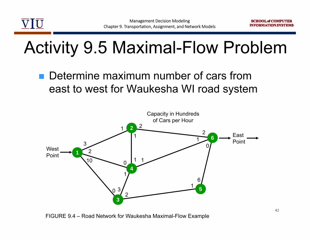
Activity 9.5 Maximal-Flow Problem Determine maximum number of cars from
east to west for Waukesha WI road system
1
2
3
4
5
6
West Point
East Point
Capacity in Hundreds of Cars per Hour
32
10
1 2
1
0 1 1
0 32
21
0
16
1
FIGURE 9.4 – Road Network for Waukesha Maximal-Flow Example 42
Management Decision ModelingChapter 9. Transportation, Assignment, and Network Models
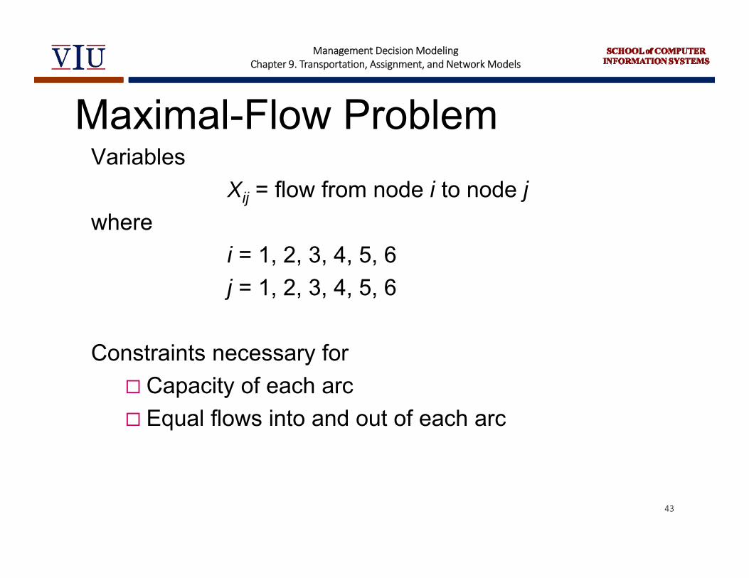
Maximal-Flow ProblemVariables
Xij = flow from node i to node jwhere
i = 1, 2, 3, 4, 5, 6j = 1, 2, 3, 4, 5, 6
Constraints necessary for Capacity of each arc Equal flows into and out of each arc
43
Management Decision ModelingChapter 9. Transportation, Assignment, and Network Models
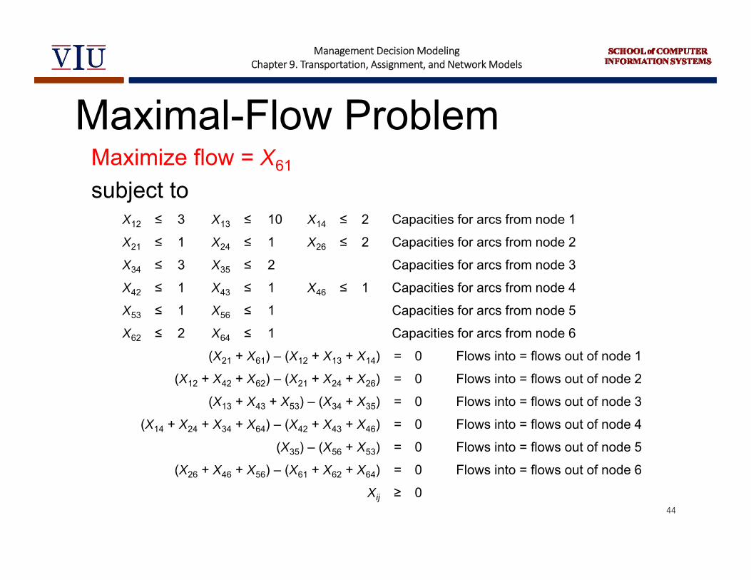
Maximal-Flow ProblemMaximize flow = X61
subject to
(X21 + X61) – (X12 + X13 + X14) = 0 Flows into = flows out of node 1
(X12 + X42 + X62) – (X21 + X24 + X26) = 0 Flows into = flows out of node 2
(X13 + X43 + X53) – (X34 + X35) = 0 Flows into = flows out of node 3
(X14 + X24 + X34 + X64) – (X42 + X43 + X46) = 0 Flows into = flows out of node 4
(X35) – (X56 + X53) = 0 Flows into = flows out of node 5
(X26 + X46 + X56) – (X61 + X62 + X64) = 0 Flows into = flows out of node 6
Xij ≥ 0
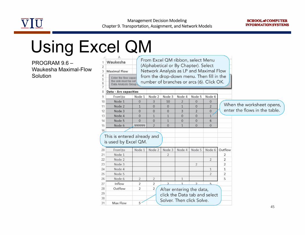
X12 ≤ 3 X13 ≤ 10 X14 ≤ 2 Capacities for arcs from node 1
X21 ≤ 1 X24 ≤ 1 X26 ≤ 2 Capacities for arcs from node 2
X34 ≤ 3 X35 ≤ 2 Capacities for arcs from node 3
X42 ≤ 1 X43 ≤ 1 X46 ≤ 1 Capacities for arcs from node 4
X53 ≤ 1 X56 ≤ 1 Capacities for arcs from node 5
X62 ≤ 2 X64 ≤ 1 Capacities for arcs from node 6
44
Management Decision ModelingChapter 9. Transportation, Assignment, and Network Models
Using Excel QMPROGRAM 9.6 –Waukesha Maximal-Flow Solution
45
Management Decision ModelingChapter 9. Transportation, Assignment, and Network Models
Shortest-Route Problem Find the shortest distance from one
location to another Can be modeled asA linear programming problem with 0-1
variables A special type of transshipment problem
Using specialized algorithm
46
Management Decision ModelingChapter 9. Transportation, Assignment, and Network Models
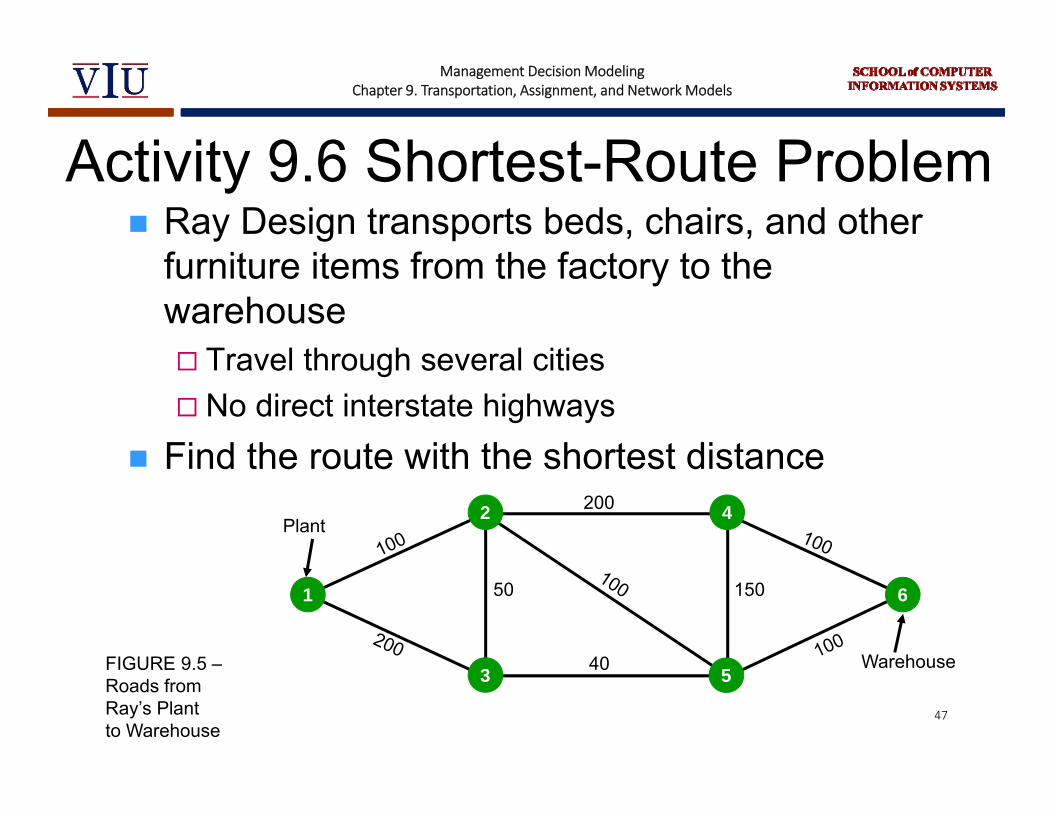
Activity 9.6 Shortest-Route Problem Ray Design transports beds, chairs, and other
furniture items from the factory to the warehouse Travel through several cities No direct interstate highways
Find the route with the shortest distance
Plant
Warehouse
1
2
3
4
5
650
40
150
200
FIGURE 9.5 –Roads from Ray’s Plant to Warehouse
47
Management Decision ModelingChapter 9. Transportation, Assignment, and Network Models
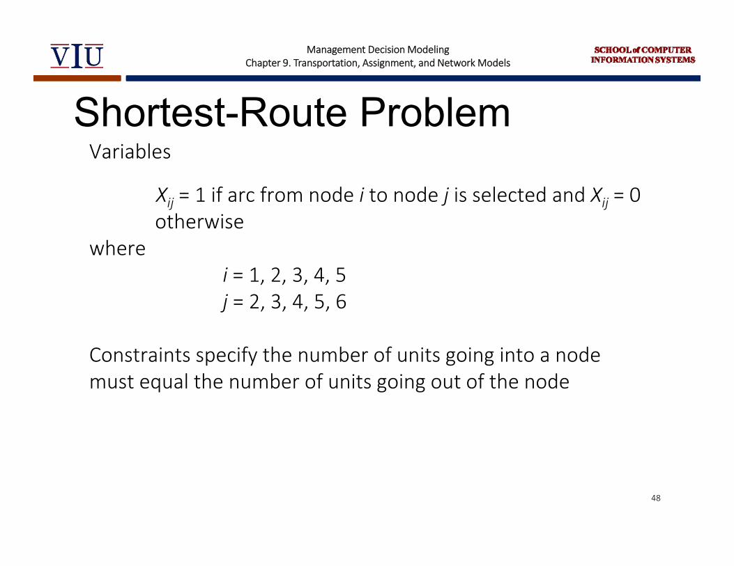
Shortest-Route ProblemVariables
Xij = 1 if arc from node i to node j is selected and Xij = 0 otherwise
wherei = 1, 2, 3, 4, 5j = 2, 3, 4, 5, 6
Constraints specify the number of units going into a node must equal the number of units going out of the node
48
Management Decision ModelingChapter 9. Transportation, Assignment, and Network Models
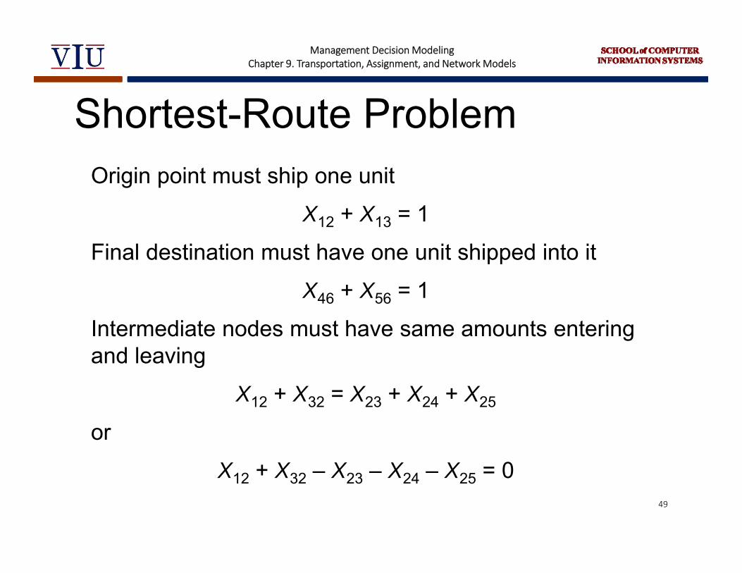
Shortest-Route ProblemOrigin point must ship one unit
X12 + X13 = 1
Final destination must have one unit shipped into it
X46 + X56 = 1
Intermediate nodes must have same amounts entering and leaving
X12 + X32 = X23 + X24 + X25
or
X12 + X32 – X23 – X24 – X25 = 049
Management Decision ModelingChapter 9. Transportation, Assignment, and Network Models
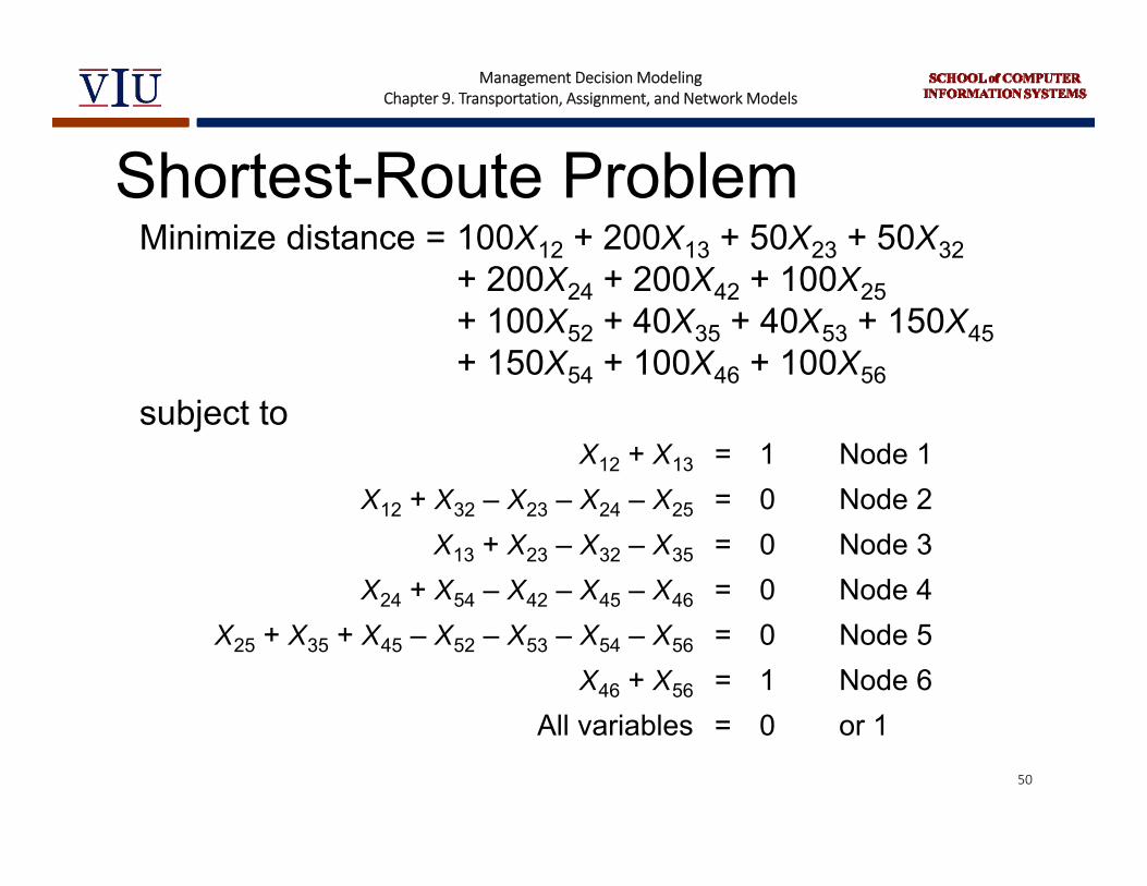
Shortest-Route ProblemMinimize distance = 100X12 + 200X13 + 50X23 + 50X32
+ 200X24 + 200X42 + 100X25+ 100X52 + 40X35 + 40X53 + 150X45+ 150X54 + 100X46 + 100X56
subject toX12 + X13 = 1 Node 1
X12 + X32 – X23 – X24 – X25 = 0 Node 2X13 + X23 – X32 – X35 = 0 Node 3
X24 + X54 – X42 – X45 – X46 = 0 Node 4X25 + X35 + X45 – X52 – X53 – X54 – X56 = 0 Node 5
X46 + X56 = 1 Node 6All variables = 0 or 1
50

Management Decision ModelingChapter 9. Transportation, Assignment, and Network Models
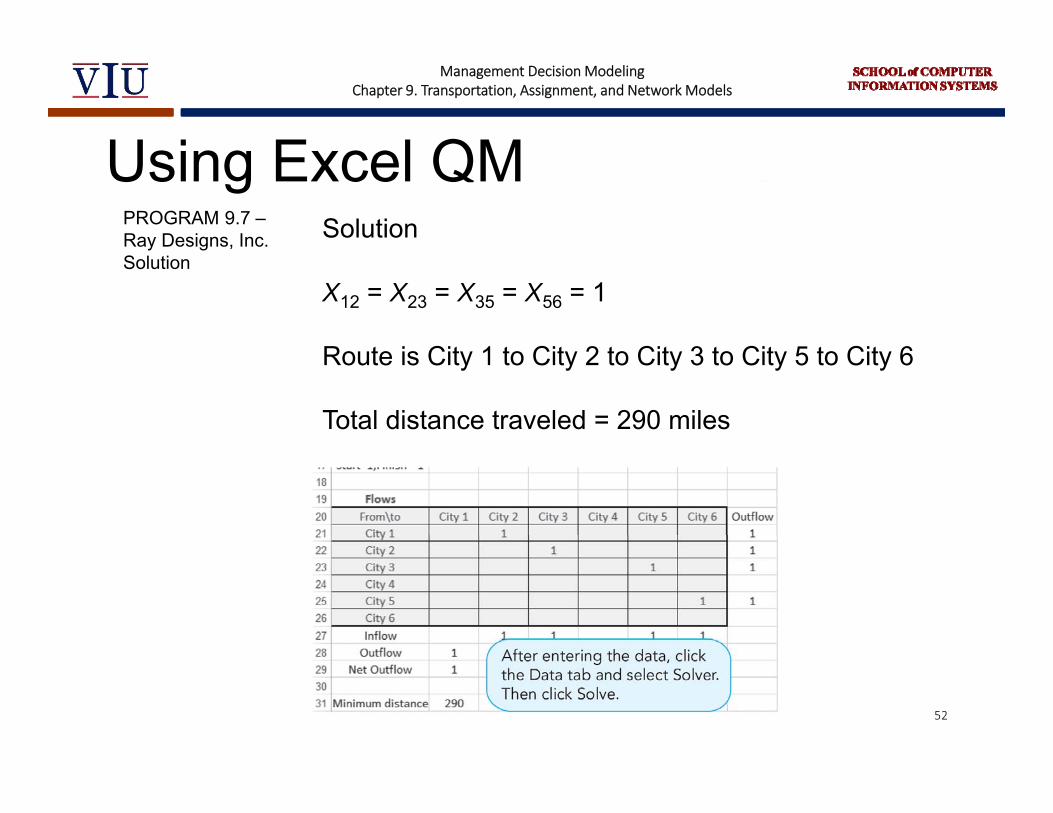
Using Excel QMPROGRAM 9.7 –Ray Designs, Inc.Solution
51
Management Decision ModelingChapter 9. Transportation, Assignment, and Network Models
Using Excel QMPROGRAM 9.7 –Ray Designs, Inc.Solution
Solution
X12 = X23 = X35 = X56 = 1
Route is City 1 to City 2 to City 3 to City 5 to City 6
Total distance traveled = 290 miles
52

Management Decision ModelingChapter 9. Transportation, Assignment, and Network Models
Minimal‐Spanning Tree Problem Connecting all points of a network together
while minimizing the total distance of the connections
Linear programming can be used but is complex
Minimal-spanning tree technique is quite easy
53

Management Decision ModelingChapter 9. Transportation, Assignment, and Network Models
Minimal‐Spanning Tree ProblemSteps for the Minimal-Spanning Tree Technique
1. Select any node in the network.2. Connect this node to the nearest node that
minimizes the total distance.3. Considering all of the nodes that are now connected,
find and connect the nearest node that is not connected. If there is a tie for the nearest node, select one arbitrarily. A tie suggests there may be more than one optimal solution.
4. Repeat the third step until all nodes are connected.
54
Management Decision ModelingChapter 9. Transportation, Assignment, and Network Models
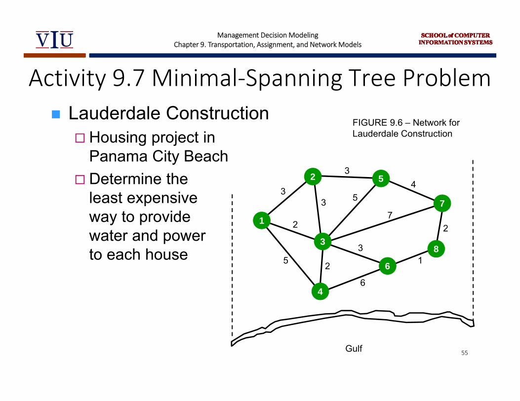
Activity 9.7 Minimal‐Spanning Tree Problem Lauderdale Construction
Housing project in Panama City Beach
Determine the least expensive way to provide water and power to each house
1
2
4
6
Gulf
3
5
7
8
3
27
5
6
1
43
3
3
2
2
5
FIGURE 9.6 – Network for Lauderdale Construction
55

Management Decision ModelingChapter 9. Transportation, Assignment, and Network Models
Minimal‐Spanning Tree ProblemStep 1 – Arbitrarily select
node 1Step 2 – Connect node 1
to node 3 (nearest)
1
2
4
6
Gulf
3
5
7
8
3
27
5
6
1
43
3
3
2
2
5
FIGURE 9.7 – First Iteration
56

Management Decision ModelingChapter 9. Transportation, Assignment, and Network Models
Minimal‐Spanning Tree ProblemStep 3 – Connect next nearest unconnected
node, node 4Continue for other unconnected nodes
1
2
4
6
3
5
7
8
3
27
5
6
1
43
3
3
2
2
5
FIGURE 9.8 – Second and Third Iterations
1
2
4
6
3
5
7
8
3
27
5
6
1
43
3
3
2
2
5
(a) Second Iteration (b) Third Iteration57
Management Decision ModelingChapter 9. Transportation, Assignment, and Network Models
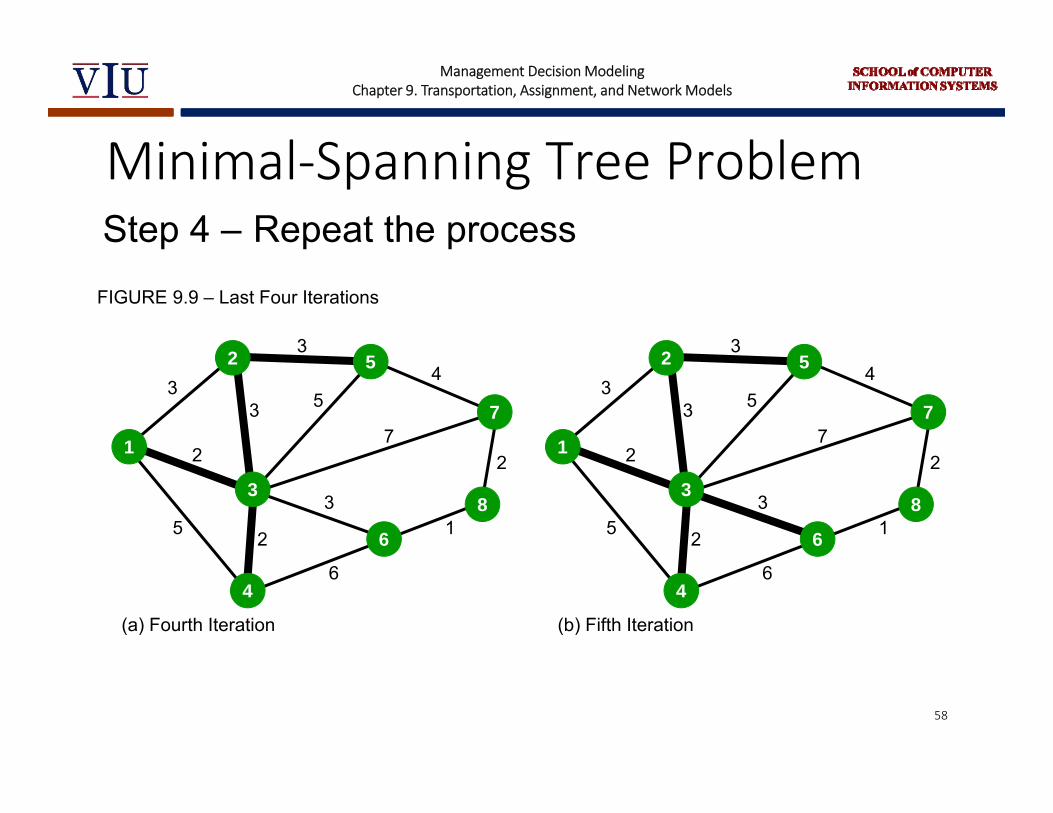
Minimal‐Spanning Tree ProblemStep 4 – Repeat the process
1
2
4
6
3
5
7
8
3
27
5
6
1
43
3
3
2
2
5
FIGURE 9.9 – Last Four Iterations
1
2
4
6
3
5
7
8
3
27
5
6
1
43
3
3
2
2
5
(a) Fourth Iteration (b) Fifth Iteration
58
Management Decision ModelingChapter 9. Transportation, Assignment, and Network Models
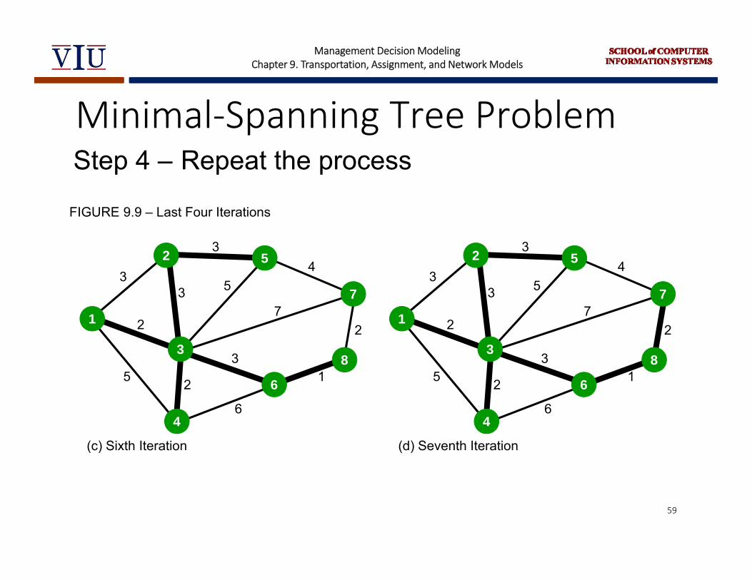
Step 4 – Repeat the processMinimal‐Spanning Tree Problem
1
2
4
6
3
5
7
8
3
27
5
6
1
43
3
3
2
2
5
FIGURE 9.9 – Last Four Iterations
1
2
4
6
3
5
7
8
3
27
5
6
1
43
3
3
2
2
5
(c) Sixth Iteration (d) Seventh Iteration
59
Management Decision ModelingChapter 9. Transportation, Assignment, and Network Models
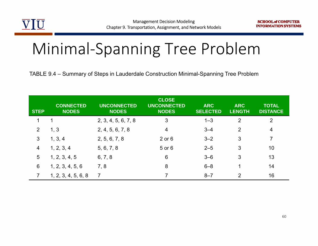
Minimal‐Spanning Tree ProblemTABLE 9.4 – Summary of Steps in Lauderdale Construction Minimal-Spanning Tree Problem
STEPCONNECTED
NODESUNCONNECTED
NODES
CLOSE UNCONNECTED
NODESARC
SELECTEDARC
LENGTHTOTAL
DISTANCE
1 1 2, 3, 4, 5, 6, 7, 8 3 1–3 2 2
2 1, 3 2, 4, 5, 6, 7, 8 4 3–4 2 4
3 1, 3, 4 2, 5, 6, 7, 8 2 or 6 3–2 3 7
4 1, 2, 3, 4 5, 6, 7, 8 5 or 6 2–5 3 10
5 1, 2, 3, 4, 5 6, 7, 8 6 3–6 3 13
6 1, 2, 3, 4, 5, 6 7, 8 8 6–8 1 14
7 1, 2, 3, 4, 5, 6, 8 7 7 8–7 2 16
60
Management Decision ModelingChapter 9. Transportation, Assignment, and Network Models
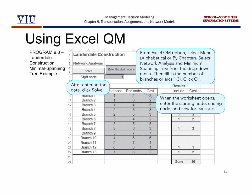
Using Excel QMPROGRAM 9.8 –Lauderdale Construction Minimal-Spanning Tree Example
61