Machine Learning for Microcontroller-Class Hardware - arXiv
29
LOGO-jsen-web.eps IEEE SENSORS JOURNAL, VOL. XX, NO. XX, XXXX 2022 1 Machine Learning for Microcontroller-Class Hardware - A Review Swapnil Sayan Saha, Student Member, IEEE , Sandeep Singh Sandha and Mani Srivastava, Fellow, IEEE Abstract — The advancements in machine learning opened a new opportunity to bring intelligence to the low-end Internet-of-Things nodes such as microcontrollers. Conventional machine learning deployment has high memory and compute footprint hindering their direct deployment on ultra resource-constrained microcontrollers. This paper highlights the unique requirements of enabling onboard machine learning for microcontroller class devices. Researchers use a specialized model development workflow for resource-limited applications to ensure the compute and latency budget is within the device limits while still maintaining the desired performance. We characterize a closed-loop widely applicable workflow of machine learning model development for microcontroller class devices and show that several classes of applications adopt a specific instance of it. We present both qualitative and numerical insights into differ- ent stages of model development by showcasing several use cases. Finally, we identify the open research challenges and unsolved questions demanding careful considerations moving forward. Index Terms— Feature projection, internet-of-things, machine learn- ing, microcontrollers, model compression, neural architecture search, neural networks, optimization, sensors, TinyML. I. I NTRODUCTION Low-end Internet-of-Things (IoT) nodes such as microcon- trollers are widely adopted in resource-limited applications such as wildlife monitoring, oceanic health tracking, search and rescue, activity tracking, industrial machinery debug- ging, onboard navigation, and aerial robotics [1] [2]. These applications limit the compute device payload capabilities, and necessitate the deployment of lightweight hardware and inference pipelines. Traditionally, microcontrollers operated on low-dimensional structured sensor data (e.g., temperature and humidity) using classical methods, making simple inferences at the edge. Recently, with the advent of machine learning, considerable endeavors are underway to bring machine learn- ing (ML) to the edge [3] [4]. Manuscript received: January 15, 2022; revised: June 5, 2022; ac- cepted: July 17, 2022; date of publication: XXXX XX 2022; date of current version: XXXX XX 2022. This work was supported in part by the CONIX Research Center, one of six centers in JUMP, a Semicon- ductor Research Corporation (SRC) program sponsored by DARPA; by the IoBT REIGN Collaborative Research Alliance funded by the Army Research Laboratory (ARL) under Cooperative Agreement W911NF-17- 2-0196; and by the NIH mHealth Center for Discovery, Optimization and Translation of Temporally-Precise Interventions (mDOT) under award 1P41EB028242. Swapnil Sayan Saha, Sandeep Singh Sandha, and Mani Srivastava are with the Dept. of Electrical and Computer Engineering and the Dept. of Computer Science, University of California - Los Angeles, CA 90095, USA (e-mail: [email protected], [email protected], [email protected]). Digital Object Identifier: However, directly porting ML models designed for high-end edge devices such as mobile phones or single-board computers are not suitable for microcontrollers. A typical microcontroller has 128 KB RAM and 1 MB of flash, while a mobile phone can have 4 GB of RAM and 64 GB of storage [5]. The ultra resource limitations of microcontroller class IoT nodes demand the design of a systematic workflow and tools to guide onboard deployment of ML pipelines. This paper presents the unique requirements, challenges, and opportunities presented when developing ML models do- ing sensor information processing on microcontrollers. While prior surveys [3] [4] [6] [7] present a qualitative review of the model development cycle for microcontrollers, they fail to provide quantitative comparisons across alternative workflow choices and insights from application-specific case studies. In contrast, we illustrate a closed-loop workflow of ML model development and deployment for microcontroller class IoT nodes with quantitative evaluation, numerical analy- sis, and benchmarks showing different instances of proposed workflow across various applications. Specifically, we discuss in detail workflow components while making performance comparisons and tradeoffs of the workflow adoptions in the existing literature. Finally, we also identify bottlenecks in the current model development cycle and propose open research challenges going forward. Our contributions are as follows: • We illustrate a coherent and closed-loop ML model devel- arXiv:2205.14550v3 [cs.LG] 18 Jul 2022
-
Upload
khangminh22 -
Category
Documents
-
view
1 -
download
0
Transcript of Machine Learning for Microcontroller-Class Hardware - arXiv

LOGO-jsen-web.epsIEEE SENSORS JOURNAL, VOL. XX, NO. XX, XXXX 2022 1
Machine Learning for Microcontroller-ClassHardware - A Review
Swapnil Sayan Saha, Student Member, IEEE , Sandeep Singh Sandha and Mani Srivastava, Fellow, IEEE
Abstract— The advancements in machine learning opened a newopportunity to bring intelligence to the low-end Internet-of-Thingsnodes such as microcontrollers. Conventional machine learningdeployment has high memory and compute footprint hindering theirdirect deployment on ultra resource-constrained microcontrollers.This paper highlights the unique requirements of enabling onboardmachine learning for microcontroller class devices. Researchersuse a specialized model development workflow for resource-limitedapplications to ensure the compute and latency budget is within thedevice limits while still maintaining the desired performance. Wecharacterize a closed-loop widely applicable workflow of machinelearning model development for microcontroller class devices andshow that several classes of applications adopt a specific instanceof it. We present both qualitative and numerical insights into differ-ent stages of model development by showcasing several use cases.Finally, we identify the open research challenges and unsolvedquestions demanding careful considerations moving forward.
Index Terms— Feature projection, internet-of-things, machine learn-ing, microcontrollers, model compression, neural architecturesearch, neural networks, optimization, sensors, TinyML.
I. INTRODUCTION
Low-end Internet-of-Things (IoT) nodes such as microcon-trollers are widely adopted in resource-limited applicationssuch as wildlife monitoring, oceanic health tracking, searchand rescue, activity tracking, industrial machinery debug-ging, onboard navigation, and aerial robotics [1] [2]. Theseapplications limit the compute device payload capabilities,and necessitate the deployment of lightweight hardware andinference pipelines. Traditionally, microcontrollers operated onlow-dimensional structured sensor data (e.g., temperature andhumidity) using classical methods, making simple inferencesat the edge. Recently, with the advent of machine learning,considerable endeavors are underway to bring machine learn-ing (ML) to the edge [3] [4].
Manuscript received: January 15, 2022; revised: June 5, 2022; ac-cepted: July 17, 2022; date of publication: XXXX XX 2022; date ofcurrent version: XXXX XX 2022. This work was supported in part bythe CONIX Research Center, one of six centers in JUMP, a Semicon-ductor Research Corporation (SRC) program sponsored by DARPA; bythe IoBT REIGN Collaborative Research Alliance funded by the ArmyResearch Laboratory (ARL) under Cooperative Agreement W911NF-17-2-0196; and by the NIH mHealth Center for Discovery, Optimization andTranslation of Temporally-Precise Interventions (mDOT) under award1P41EB028242.
Swapnil Sayan Saha, Sandeep Singh Sandha, and Mani Srivastavaare with the Dept. of Electrical and Computer Engineering and theDept. of Computer Science, University of California - Los Angeles, CA90095, USA (e-mail: [email protected], [email protected],[email protected]).
Digital Object Identifier:
However, directly porting ML models designed for high-endedge devices such as mobile phones or single-board computersare not suitable for microcontrollers. A typical microcontrollerhas 128 KB RAM and 1 MB of flash, while a mobile phonecan have 4 GB of RAM and 64 GB of storage [5]. Theultra resource limitations of microcontroller class IoT nodesdemand the design of a systematic workflow and tools to guideonboard deployment of ML pipelines.
This paper presents the unique requirements, challenges,and opportunities presented when developing ML models do-ing sensor information processing on microcontrollers. Whileprior surveys [3] [4] [6] [7] present a qualitative reviewof the model development cycle for microcontrollers, theyfail to provide quantitative comparisons across alternativeworkflow choices and insights from application-specific casestudies. In contrast, we illustrate a closed-loop workflow ofML model development and deployment for microcontrollerclass IoT nodes with quantitative evaluation, numerical analy-sis, and benchmarks showing different instances of proposedworkflow across various applications. Specifically, we discussin detail workflow components while making performancecomparisons and tradeoffs of the workflow adoptions in theexisting literature. Finally, we also identify bottlenecks in thecurrent model development cycle and propose open researchchallenges going forward. Our contributions are as follows:
• We illustrate a coherent and closed-loop ML model devel-
arX
iv:2
205.
1455
0v3
[cs
.LG
] 1
8 Ju
l 202
2
2 IEEE SENSORS JOURNAL, VOL. XX, NO. XX, XXXX 2022
Fig. 1. Closed-loop workflow of porting machine learning modelsonto microcontrollers. Step (3) to Step (8) are repeated until desiredperformance is achieved. (1) Data engineering performs acquisition,analytics and storage of raw sensor streams (Section III). (2) Optionalfeature projection directly reduces dimensionality of input data (Sec-tion IV). (3) Models are chosen from a lightweight ML zoo based onthe application and hardware specifications (Section VI and Section X).(4) Neural architecture search strategy builds candidate models fromthe search space for training and evaluates the model based on costfunction (Section VII). (5) Trained candidate model is ported to a TinyMLsoftware suite. (6) The TinyML software suite performs inference engineoptimizations, deep compression and code generation. It also providesapproximate hardware metrics (e.g., SRAM, Flash and latency) (Sec-tion V, Section VII, and Section VIII). (7) The embedded C file systemis ported onto the microcontroller via command line interface. (8) Themicrocontroller optionally reports real runtime hardware metrics backto the neural architecture search strategy (Section VII). (9) On-devicetraining or federated learning are used occasionally to account for shiftsin incoming data distribution (Section IX).
opment and deployment workflow for microcontrollers.We delineate each block in the workflow, providing bothqualitative and numerical insights.
• We provide application-dependent quantitative evaluationand comparison of proposed workflow adaptations.
• We discuss several tradeoffs in the existing model-development process for microcontrollers and showcaseopportunities and ideas in this workspace.
The rest of the paper is organized as follows: Section IIoutlines the TinyML workflow of model development anddeployment for microcontrollers. Section III explores dataengineering frameworks. Section IV shows feature projectiontechniques. Section V discusses model compression methods.Section VI describes lightweight ML blocks suitable for mi-crocontrollers. Section VII discusses neural architecture search(NAS) frameworks for microcontrollers. Section VIII outlinesseveral software suites available for porting developed modelsonto microcontrollers. Section IX showcases TinyML onlinelearning frameworks. Section X provides quantitative andqualitative comparison of workflow variations depending onapplication. Section XI presents inter-relative and quantitativeanalysis of individual portions of the workflow through casestudies. Section XII illustrates open challenges and ideas forfuture research. Section XIII provides concluding remarks.
II. TINYML WORKFLOW
We use the term ”TinyML” to refer to model compression,machine-learning blocks, AutoML frameworks, and hardware
TABLE ICOMPARISON OF HARDWARE FOR DOING MACHINE LEARNING ON
CLOUD SERVERS, MOBILE PHONES, AND MICROCONTROLLERS [8]
Platform Memory Storage PowerCloud GPU 16 GB HBM TB/PB 250WMobile CPU 4 GB DRAM 64 GB Flash 8WMicrocontroller 2-1024 kB SRAM 32-2048 kB eFlash 0.1-0.3W
and software suites designed to perform ultra-low-power (≤1 mW), always-on, and on-board sensor data analytics [4][6] [7] on resource-constrained platforms. Typical TinyMLplatforms such as microcontrollers have SRAM in the orderof 100 − 102 kB and flash in the order of 103 kB [6]. Table Iprovides characteristics of these devices compared to cloudservers and mobile phones. Given the widespread penetrationof microcontroller-based IoT platforms in our daily lives forpervasive perception-processing-feedback applications, thereis a growing push towards embedding intelligence into thesefrugal smart objects [3]. Embedded AI on microcontrollersis motivated by applicability, independence from networkinfrastructure, security and privacy, and low deployment cost:
(i) Applicability: Neural networks have been shown toprovide rich and complex inferences over the first-principleapproaches for sensor data analytics without domain expertise.With the emergence of real-time ML for microcontrollers, itis possible to turn IoT nodes from simple data harvesters orfirst-principles data processors to learning-enabled inferencegenerators. TinyML combines the lightweightness of first-principle approaches with the accuracy of large neuralnetworks.
(ii) Independence from Network Infrastructure via RemoteDeployment: Traditionally, sensor data is offloaded ontomodels running on mobile devices or cloud servers [19] [20].This is not suitable for time-critical sense-compute-actuationapplications such as autonomous driving [21] [22], robotcontrol [4] [23], and industrial control system. Moreover,reliable network bandwidth or power may not be availablefor communicating with online models, such as in wildlifemonitoring [1] or energy-harvesting intermittent systems [24][25] [26]. TinyML allows offline and on-board inferencewithout requiring data offloading or cloud-based inference.
(iii) Security and Privacy: Streaming private data onto third-party cloud servers yields privacy concerns from end-users,while cybercriminals can exploit weakly protected datastreams. Federated learning [27], secure aggregation [28],and homomorphic encryption [29] allow privacy-preservingand secure inference, but suffer from expensive networkand compute requirement. On-board inference constrains thesource and destination of private data within the IoT nodeitself, reducing the probability of privacy leaks and attacksurfaces.
(iv) Low Deployment Cost: While graphics processing units(GPUs) have revolutionized deep-learning [30], GPUs areenergy-hungry and expensive to maintain continually for

SAHA et al.: MACHINE LEARNING FOR MICROCONTROLLER-CLASS HARDWARE - A REVIEW (JUNE 2022) 3
TABLE IIMLPERF TINY V0.5 INFERENCE BENCHMARKS [9]
Application Dataset (Input Size) Model Type (TFLM model size) Quality Target (Metric)Keyword Spotting Speech Commands [10] (49×10) DS-CNN [11] [12] [13] (52.5 kB) 90% (Top-1)Visual Wake Words VWW Dataset [14] (96×96) MobileNetV1 [12] (325 kB) 80% (Top-1)Image Recognition CIFAR-10 [15] (32×32) ResNetV1 [16] (96 kB) 85% (Top-1)Anomaly Detection ToyADMOS [17], MIMII [18] (5×128) FC-Autoencoder [9] (270 kB) 0.85 AUC
inference using small models, leading to long term financialand environmental degeneration [5]. A Cortex M4 classmicrocontroller costs around 5-10 USD and can run on acoin-cell battery for months, if not years [7]. TinyML allowsthese microcontrollers to be exploited for ultra-low-powerand low-cost AI inference.
Achieving low deployment cost without sacrificingperformance gains requires an unique workflow to portmachine learning models onto microcontrollers comparedto traditional model design. Fig. 1 illustrates the general”closed-loop” workflow for TinyML model developmentand deployment. For various parts of this workflow, specifictechnologies and variations have emerged [6] [8] [31], whichwe discuss in upcoming sections. The workflow can bedivided into two phases:
(i) Model Development Phase: The phase begins bypreparing a dataset from raw sensor streams using dataengineering techniques (Section III). Data engineeringframeworks are used to collect, analyze, label, and cleansensory streams to produce a dataset. Optionally, featureprojection (Section IV) is also performed at this stage.Feature projection reduces the dimensionality of the inputdata through linear methods, non-linear methods, or domain-specific feature extraction. Next, several models are chosenfrom a pool of established lightweight model zoo basedon the application and hardware constraints (Section VIand Section X). The zoo contains optimized blocks forwell-known machine-learning primitives (e.g., convolutionalneural networks, recurrent neural networks, decision trees,k-nearest neighbors, convolutional-recurrent architectures,and attention mechanisms). To achieve maximal accuracywithin microcontroller SRAM, flash, and latency targets,neural architecture search or hyperparameter tuning isperformed on candidate models from the zoo (Section VII).The hardware metrics are either obtained through proxies(approximations) or real measurements.
(ii) Model Deployment Phase: The deployment phase beginsby porting the best performing model to a TinyML softwaresuite (Section VIII). These suites perform inference engineoptimizations, operator optimizations, and model compres-sion (Section V), along with embedded code generation. Theembedded C file system is then flashed onto the microcon-troller for inference. The model can be periodically fine-tunedto account for data distribution shifts using online learning(on-device training and federated learning) frameworks (Sec-tion IX).
To measure and compare the performance of the tinyMLworkflow for specific applications, Banbury et al. [9] proposedthe widely-used MLPerf Tiny Benchmark Suite, illustrated inTable II. The benchmark contains four tasks representing awider array of applications expected from microcontroller-class models. These include multiclass image recognition,binary image recognition, keyword spotting, and outlier detec-tion. The benchmark suite also embraces the usage of standarddatasets for each task and provides quality target metricsand model size that new workflows should aim to achieve.Hardware metrics include the working memory requirements(SRAM), model size (flash), number of multiply and add op-erations (MACs), and latency. From Section III to Section IX,we discuss each block in the TinyML workflow, while inSection X, we provide quantitative evaluation of the entireworkflow based on applications in light of the benchmarks.In Section XI, we break down the end-to-end workflow andprovide analysis of individual aspects.
III. DATA ENGINEERING
Data engineering is the practice of building systems foracquisition, analytics, and storage of data at scale [37]. Dataengineering is well explored in production-scale big datasystems, where robust and scalable analytics engines (e.g.,Apache Spark, Apache Hadoop, Apache Hive, Apache H2O,Apache Flink, and DataBricks LakeHouse) ingest real-timesensory data via publish-subscribe paradigms (e.g., MQTTand Apache Kafka) [38]. Data streaming systems providereal-time data acquisition protocols for requirement defini-tions and data gathering, while analytics engines providesupport for data provenance, refinement, and sustainment.Popular general-purpose exploratory data analysis tools usedin TinyML data analytics include MATLAB [39], Giotto-TDA [40], OpenCV [41], ImgAug [42], Pillow [43], Scikit-learn [44], and SciPy [45]. To suit the specific needs and goalsof data engineering for TinyML systems, several specializedframeworks have emerged, illustrated in Table III.
A major challenge for enabling applications that use ma-chine learning on microcontrollers is preparing the data andlearning techniques that can automatically generalize wellon unseen scenarios [33]. Thereby, most of these frame-works provide common data augmentation and data cleaningtechniques such as geometric transforms, spectral transforms,oversampling, class balancing, and noise addition. MSWC [33]and Plumerai Data [36] go one step further, providing unit testsand anomaly detectors to identify problematic samples andevaluate the quality of labeled data. Plumerai Data can alsoautomatically identify samples in the training set that are likelyto be edge cases or problematic based on model performance
4 IEEE SENSORS JOURNAL, VOL. XX, NO. XX, XXXX 2022
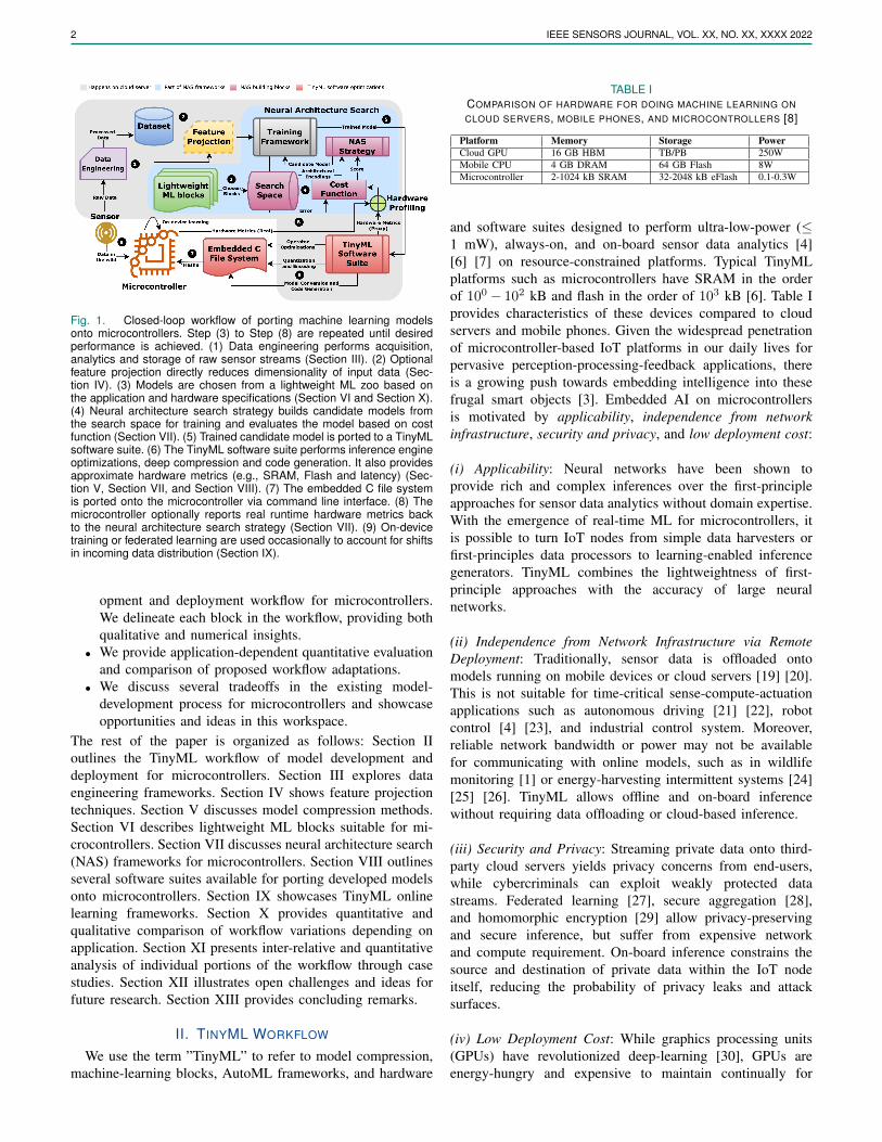
TABLE IIIFEATURES OF NOTABLE TINYML DATA ENGINEERING FRAMEWORKS
Framework Data Type Collection Labeling Alignment Augmentation Visualization Cleaning Open-source
EdgeImpulse [32]
Audio, images,time-series
Real-time (WebUSB, serialdaemon, Linux SDK),offline
AI-assisted,DSP-assisted,manual
7 Geometric imagetransforms, noise, audiospectrogram transforms,color depth
Images, plots: raw, spectrogram,statistical, DSP, MFE, MFCC,syntiant, feature explorer
Class balancing,crop, scale, split
7
MSWC [33] Audio withtranscription
Offline speech datasets Heuristic-based auto
Montrealforced
Synthetic noise, environ-mental noise
Plots: raw, spectrogram, featureembeddings
Gender balance,speaker diversity,self-supervisedquality estimation
3
SensiMLDCL [34]
Time-series,audio
Real-time (WiFi, BLE, Se-rial daemon), offline
Plot-assisted,Threshold-based auto
Video-assisted
Noise, pool, convolve,drift, dropout, quantize,reverse, time warp
Plots: raw, spectrogram, statisti-cal, DSP, MFCC
Class balancing,crop, scale, split
7
QeexoAutoML [35]
Time-series,audio
Real-time (Serial daemon,BLE), offline
Plot-assisted 7 7 Plots: raw, spectrogram, statisti-cal, DSP, MFCC, feature embed-dings
Segment 7
PlumeraiData [36]
Images Offline AI-assisted,manual
7 Targetted image trans-forms, oversampling
Images (AI-assisted visual simi-larity)
Unit tests, failurecase identification
7
on detected problematic samples. Such test-driven develop-ment can help users discover edge cases and outliers duringmodel validation stages, and allow users to apply targetedaugmentation, oversampling, and label correction. To reducedata collection bias, labeling errors and manual labeling effort,Edge Impulse [32], MSWC [33], SensiML DCL [34] andPlumerai Data [36] provide AI, DSP and heuristic-assistedautomated labeling tools. In particular, for large-scale key-word spotting dataset generation, MSWC can automaticallyestimate word boundaries from audio with transcription usingforced alignment and extract keywords based on user-definedheuristics in 50 languages. MSWC also automatically ensuresthat the generated dataset is balanced by gender and speakerdiversity. Edge Impulse provides automated labeling of ob-ject detection data using YOLOv5 and extraction of wordboundaries from keyword spotting audio samples using DSPtechniques. SensiML DCL allows video-assisted threshold-based semi-automated labeling of sensor data. Overall, theseframeworks ensure that the data being used for training arerelevant in context, free from bias, class-balanced, correctlylabeled, contains edge cases, free from shortcuts, and encom-pass sufficient diversity [36].
IV. FEATURE PROJECTION
An optional step in the TinyML workflow is to directlyreduce the dimensionality of the data. Models operating onintrinsic dimensions of the data are computationally tractableand mitigate the curse of dimensionality. Feature projectioncan be divided into three types:
Linear Methods: Linear methods for dimensionalityreduction commonly used in large-scale data-mining includematrix factorization and principal component analysis (PCA)techniques such as singular value decomposition (SVD) [61],flattened convolutions [61], non-negative matrix factorization(NMF) [62], independent component analysis (ICA) [63], andlinear discriminant analysis [64]. PCA is used to maximizethe preservation of variance of the data in the low-dimensionalmanifold [65]. Among the popular linear methods, NMFis suitable for finding sparse, parts-based, and interpretablerepresentations of non-negative data [62]. SVD is useful for
finding a holistic yet deterministic representation of inputdata, with a hierarchical and geometric basis ordered bycorrelation among the most relevant variables. SVD providesa deeper factorization with lower information loss than NMF.ICA is suitable for finding independent features (blind sourceseparation) from non-Gaussian input data [63]. ICA doesnot maximize variance or mutual orthogonality among theselected features. Nevertheless, linear methods are unableto model non-linearities or preserve the global relationshipamong features, and struggle in presence of outliers, skeweddata distribution, and one-hot encoded variables.
Non-linear Methods: Non-linear methods minimize adistance metric (e.g., fuzzy embedding topology [66],Kullback-Leibler divergence [67], local neighbourhoods [68],and Euclidean norm [69]) between the high-dimensionaldata and a low-dimensional latent representation. Non-linearmethods to handle non-linear sampling of low-dimensionalmanifolds by high-dimensional vectors include locallylinear embedding (LLE) [68], kernel PCA [69], t-distributedstochastic neighbor embedding (t-SNE) [70], uniformmanifold approximation and projection (UMAP) [66], andautoencoders [71]. Kernel PCA couples k-NN, Dijkstra’salgorithm, and partial eigenvalue decomposition to maintaingeodesic distance in a low-dimensional space [69]. Similarly,LLE can be thought of as a PCA ensemble maintaininglocal neighborhoods in the embedding space, decomposingthe latent space into several small linear functions [68].However, both LLE and kernel PCA do not perform well withlarge and complex datasets. t-SNE optimizes KL-divergencebetween student’s T distribution in the manifold-spaceand Gaussian joint probabilities in the higher-dimensionalspace [70]. t-SNE is able to reveal data structures at multiplescales, manifolds, and clusters. Unfortunately, t-SNE iscomputationally expensive, lacks explicit global structurepreservation, and relies on random seeds. UMAP optimizesa low-dimensional fuzzy embedding to be as topologicallysimilar as the Cech complex embedding [66]. Compared tot-SNE, UMAP provides a more accurate global structurerepresentation, while also being faster due to the use of graphapproximations. Nonetheless, while linear methods have been

SAHA et al.: MACHINE LEARNING FOR MICROCONTROLLER-CLASS HARDWARE - A REVIEW (JUNE 2022) 5
TABLE IVFEATURES OF NOTABLE TINYML MODEL COMPRESSION FRAMEWORKS
Framework Compression Type Parameters Size or Latency Change* Open-Source
TensorFlow Lite [46]
Post-training quantization Bit-width (float16, int16, int8), scheme (full-integer, dy-namic, float16)
4× smaller, 2-3× speedup [47]
3Quantization-aware training Bit-width (arbitrary) Depends on bit-width (upto 8× smaller)Weight pruning Sparsity distribution (constant, polynomial decay), pruning
policy5-10× smaller [48], 4× speedup [49]
Weight clustering Number of clusters, initial distribution (random, density-based, linear)
3-6× smaller
QKeras [50] Quantization-aware training Bit-width (arbitrary), symmetry, quantized layer definitions,quantized activation functions
Depends on bit-width (upto 8× smaller) 3
Qualcomm AIMET [51]
Post-training quantization Bit-width (arbitrary), rounding mode (nearest, stochastic),scheme (data-free, adaptive rounding) Depends on bit-width (upto 8× smaller)
3Quantization-aware training Bit-width (arbitrary), scheme (vanilla, range-learning)Channel pruning Compression ratio, layers to ignore, compression ratio can-
didates, reconstruction samples, cost metric 2× smaller
Matrix factorization Factorization algorithm (weight SVD, spatial SVD), com-pression ratio, fine-tuning (per layer, rank rounding)
Plumerai LARQ [52] Binarized network training Bit-width (int1), quantized activation functions, quantizedlayer definitions (convolution primitives and dense), bina-rized model backbones
8× smaller, 8.5-19× speedup (withLARQ compute engine) [53]
3
Microsoft NNI [54]
Post-training quantization Scheme (naive, observer), bit-width (8-bit, arbitrary), type(dynamic, integer), operator type Depends on bit-width (upto 8× smaller)
3Quantization-aware training Scheme (Vanilla, LARQ, learned step size, DoReFa), bit-width (8-bit, arbitrary), type (dynamic, integer), operatortype, optimizer
Basic pruners Sparsity distribution, mode (normal, dependency-aware), op-erator type, training scheme, pruning algorithm (level, L1,L2, FPGM, slim, ADMM, activation APOZ rank, activationmean rank, Taylor FO)
1.4-20× smaller, 1.6-5× speedup
Scheduled pruners All parameters of basic pruners, basic pruning algorithm,scheduled pruning algorithm (linear, AGP, lottery ticket,simulated annealing, auto compress, AMC)
1.1-120× smaller, 1.81-4× speedup
CMix-NN [55] Quantization-aware training(mixed precision)
Bit-width (int2, int4, int8), weight quantization type (per-channel, per-layer), batch normalization folding type anddelay, memory constraints, quantized convolution primitives
7× smaller 3
Microsoft SeeDot [56] Post-training quantization(with autotuned andoptimized operators)
Bit-width (8-bit), model (Bonsai [57], ProtoNN [58], Fast-GRNN [59], RNNPool [60]), error metric, scale parameter
2.4-82.2× speedup [56] 3
Genesis@ [24] Tucker decomposition andweight pruning
Rank decomposition, network configuration, sparsity dis-tribution, pruning policy, sensing energy, communicationenergy
2-109x smaller 7
*for ∼1-4% drop in accuracy over uncompressed models.@ compression framework for intermittent computing systems.
ported to microcontrollers [32] [72], non-linear methods arenot suitable for real-time execution on microcontrollers andare usually used for visualizing high-dimensional handcraftedfeatures.
Feature Engineering: Feature engineering uses domain exper-tise to extract tractable features from the raw data [73]. Typicalfeatures include spectral and statistical features. Domain-specific feature extraction is generally more suited for micro-controllers over linear and non-linear dimensionality reductiontechniques due to their relative lightweightness, as well asthe availability of dedicated signal processors in commoditymicrocontrollers for spectral processing. However, featureengineering requires human knowledge to design statisticallysignificant features. Feature selection can reduce the numberof redundant features further during model development [74].Feature selection methods include statistical tests, correlationmodeling, information-theoretic techniques, tree ensembles,and metaheuristic methods (e.g., wrappers, filters, and embed-ded techniques) [75].
V. PRUNING, QUANTIZATION AND ENCODING
Model compression aims to reduce the bitwidth and exploitthe redundancy and sparsity inherent in neural networks to
reduce memory and latency. Han et al. [49] first showedthe concept of pruning, quantization, and Huffman codingjointly in the context of pre-trained deep neural networks(DNN). Pruning [76] refers to masking redundant weights(i.e., weights lying within a certain activation interval) andrepresenting them in a row form. The network is then retrainedto update the weights for other connections. Quantization [77]accelerates DNN inference latency by rounding off weightsto reduce bit width while clustering similar ones for weightsharing. Encoding (e.g., Huffman encoding) representscommon weights with fewer bits, either through conversionof dense matrices to sparse matrices [49] or smaller densematrices through parameter redundancies [78]. Combiningthe three techniques can drastically reduce the size of state-of-the-art DNNs such as AlexNet (35×, 6.9 MB), LeNet-5(39×, 44 kB), LeNet-300- 100 (40×, 27 kB), and VGG-16(49×, 11.3 MB) without losing accuracy [49].
Common Model Compression Techniques: Table IVshowcases and compares several frameworks for modelcompression for microcontrollers. Among the differentframeworks, TensorFlow Lite [46] is available as part ofthe TensorFlow training framework [79], while others arestandalone libraries that can be integrated with TensorFlow or

6 IEEE SENSORS JOURNAL, VOL. XX, NO. XX, XXXX 2022
PyTorch. 88% of the frameworks provide various quantizationprimitives, while 50% of the frameworks support severalpruning algorithms. Most of these techniques result inunstructured or random sparse patterns.
(i) Quantization Schemes: From Table IV, we can observethat the most widely-used quantization technique formicrocontrollers is the fixed-precision uniform affine post-training quantizer, where a real number is mapped to afixed-point representation via a scale factor and zero-point(offset) after training [80] [47]. Variations include quantizationof weights, weights, and activations, and weights, activations,and inputs [81]. While post-training quantization (with 4, 8,and 16 bits) has been shown to reduce the model size by4× and speed up inference by 2-3×, quantization-awaretraining is recommended for microcontroller-class models tomitigate layer-wise quantization error due to a large range ofweights across channels [80] [47]. This is achieved throughthe injection of simulated quantization operations, weightclamping, and fusion of special layers [51], allowing upto 8× model size reduction for same or lower accuracydrop. However, care must be taken to ensure that thetarget hardware supports the used bitwidth. To account fordistinct compute and memory requirements of differentlayers, mixed-precision quantization assigns differentbit-widths for weights and activation for each layer [82].For microcontrollers, the network subgraph is represented asa quantized convolutional layer with vectorized MAC unit,while special layers are folded into the activation functionvia integer channel normalization [83] [55]. Mixed-precisionquantization provides 7× memory reduction [55] but issupported by limited models of microcontrollers. Recently,binarized neural networks [84] have been ported ontomicrocontroller-class hardware [52], where the weights andactivations are quantized to a single bit (-1 or +1). Binarizedquantization can provide 8.5-19× speedup and 8× memoryreduction [53].
(ii) Pruning Algorithms: Among the different pruningalgorithms, weight pruning is the most common, providing4× speedup and 5-10× memory reduction [49] [48]. Weightpruning follows a schedule that specifies the type of layers toconsider, the sparsity distribution to follow during training orfine-tuning, and the metric to follow when pruning (pruningpolicy). Common weight pruning evaluation metrics includethe level and norm of weights [79] [54]. For intermittentcomputing systems with extremely limited power budgets,the pruning policy usually includes the energy and memorybudget to maximize the collection of interesting eventsper unit of energy [24]. Pruning policies for intermittentcomputing treat pruning as a hyperparameter tuning problem,sweeping through the memory, energy, and accuracy spacesto build a Pareto frontier. Some frameworks [51] [54] providesupport for structured pruning, allowing policies for channeland filter pruning rather than pruning weights in an irregularfashion.
Structured Sparsity: Although model compression improves
speedup, eliminates ineffective computations, and reduces stor-age and memory access costs, unstructured sparsity can induceirregular processing and waste execution time. The benefits ofefficient acceleration through sparsity require special hardwareand software support for storage, extraction, communication,computation, and load-balance of nonzero and trivial elementsand inputs [85]. Several techniques for exploiting structuredsparsity for microcontrollers have emerged. Bayesian com-pression [86] [87] assumes hierarchical, sparsity-promotingpriors on channels (output activations for convolutional layersand input features for fully-connected layers) via variationalinference, approximating the weight posterior by a certaindistribution. For the same accuracy, Bayesian compressioncan reduce parameter count by 80× over unpruned models.Layer-wise SIMD-aware weight pruning [88] divides theweights into groups equal to the SIMD width of the mi-crocontroller for maximal SIMD unit utilization and columnindex sharing. Trivial weight groups are pruned based onthe root mean square of each group. SIMD-aware pruningprovides 3.54× speedup and 88% reduction in model size,compared to 1.90× speedup and 80% reduction in model sizeprovided by traditional weight pruning over unpruned models.Differentiable network pruning [89] performs structuredchannel pruning during training by applying channel-wisebinary masks depending on channel salience. The size of eachlayer is learned through bi-level continuous gradient descentrelaxation through pruning feedback and resource feedbacklosses without additional training overhead. Compared totraditional pruning methods, differentiable pruning provides upto 1.7× speedup, while compressing unpruned models by 80×.Doping [90] [91] improves the accuracy and compressionfactor of networks compressed using structured matrices (e.g.Kronecker products (KP)) by adding an extremely sparsematrix, using co-matrix regularization to reduce co-matrixadaptation during training. Doped KP matrices achieve a 2.5-5.5× speedup and 1.3-2.4× higher compression factor overtraditional compression techniques, beating weight pruningand low-rank methods with 8% higher accuracy.
VI. LIGHTWEIGHT MACHINE LEARNING BLOCKS
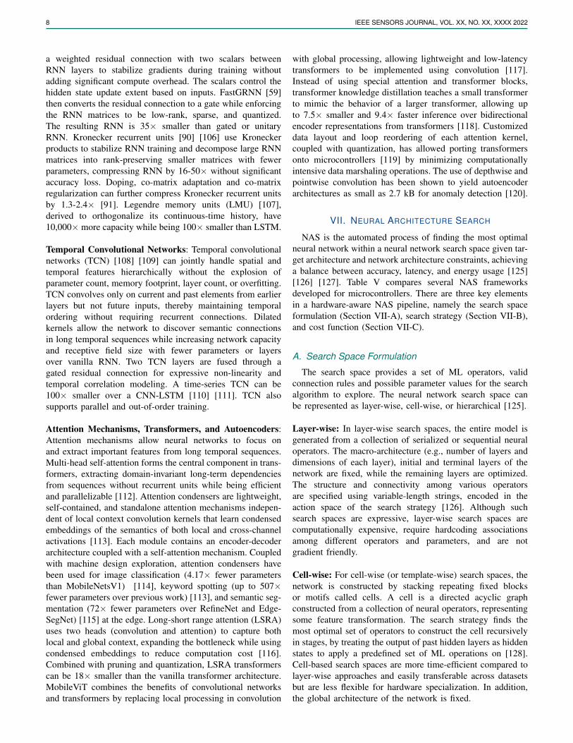
To reduce the memory footprint and latency while retainingthe performance of ML models running on microcontrollers,several ultra-lightweight machine learning blocks have beenproposed, illustrated in Fig. 2. We describe some of theseblocks in this section.
Sparse Projection: When the input feature space is high-dimensional, sparsely projecting input features onto alow-dimensional linear manifold, called prototypes, canreduce the parameter count and improve compute efficiencyof models. The projection matrix can be learned as part ofthe model training process using stochastic gradient descentand iterative hard thresholding to mitigate accuracy loss.Bonsai [57] is a non-linear, shallow, and sparse decisiontree (DT) that can make inferences on prototypes. Similarly,ProtoNN [58] is a lightweight k-nearest neighbor (kNN)classifier that operates on prototypes.

SAHA et al.: MACHINE LEARNING FOR MICROCONTROLLER-CLASS HARDWARE - A REVIEW (JUNE 2022) 7
Fig. 2. Example of lightweight machine learning blocks. (a) Sparse projection onto low-dimensional linear manifold yields lightweight decision treesand k-nearest neighbor classifiers. (b) Fire module containing bottleneck (pointwise) and excitation (pointwise and depthwise) convolutional layers.(c) The inverted residual connection between squeeze layers instead of excitation layers reduces memory and compute. (d) Group convolution withchannel shuffle improves cross-channel relations. (e) Adding a gated residual connection and enforcing RNN matrices to be low rank, sparse, andquantized yields stable and lightweight RNN. (f) Temporal convolutional networks extract spatio-temporal representations using causal and dilatedconvolution kernels. (g) Depthwise separable convolution yields 7-9× memory savings over vanilla convolution kernel (figure adapted from [2]).
Lightweight Spatial Convolution: SqueezeNet [92] broughton several micro-architectural enhancements to AlexNet [93].These include replacing 3×3 kernels with point-wise filters,decreasing input channel count using point-wise filters asa linear bottleneck, and late downsampling to enhancefeature maps. The resulting network consists of stacked”fire modules”, with each module containing a bottlenecklayer (layer with point-wise filters) and an excitationlayer (mix of point-wise and 3×3 filters). Using pruning,quantization, and encoding, SqueezeNet reduced the sizeof AlexNet by 510× (< 0.5 MB). MobileNetsV1 [12]introduced depthwise separable convolution [11] (channel-wise convolution followed by bottleneck layer), and widthand resolution multipliers to control layer width and inputresolution of AlexNet. Depth-wise separable convolution is9× cheaper and induces 7-9× memory savings over 3×3kernels. MobileNetV2 [94] introduced the concepts of invertedresiduals and linear bottleneck, where a residual connectionexists between bottleneck layers rather than excitation layers,and a linear output is enforced at the last convolution ofa residual block. To reduce channel count, the depthwiseseparable convolution layer can be enclosed between thepointwise group convolution layer with channel shuffle,thereby improving the semantic relation between input andoutput channels across all the groups through the use of wideactivation maps [95]. Instead of having residual connectionsacross two layers, the gradient highway can act as a mediumto feed each layer activation maps of all preceding layers.This is known as channel-wise feature concatenation [96] and
encourages reuse and stronger propagation of low-complexitydiversified feature maps and gradients while drasticallyreducing network parameter count.
Lightweight Multiscale Spatial Convolution: For scalable,efficient, and real-time object detection across scales,EfficientDet [97] introduced a bidirectional feature pyramidnetwork (FPN) to aggregate features at different resolutionswith two-way information flow. The feature network topologyis optimized through NAS via heuristic compound scaling ofweight, depth, and resolution. EfficientDet is 4–9× smaller,uses 13-42× fewer FLOPS, and outperforms (in terms oflatency and mean average precision) YOLOv3, RetinaNet,AmoebaNet, Resnet, and DeepLabV3. Scaled-YOLOv4 [98]converts portions of FPN of YOLOv4 [99] to cross-stagepartial networks [100], which saves up-to 50% computationalbudget over vanilla CNN backbones. Removal or fusion ofbatch normalization layers and downscaling input resolutioncan speed up multi-resolution inference by 3.6-8.8× [101]over vanilla YOLO [102] or MobileNetsV1 [12]
Low-Rank, Stabilized, and Quantized Recurrent Models:Although recurrent neural networks (RNN) are lightweightby design, they suffer from exploding and vanishing gradientproblem (EVGP) for long time-series sequences. Widely-used solutions to EVGP, namely long short-term memory(LSTM) [103], gated recurrent units [104], and unitaryRNN [105] either cause loss in accuracy, or increase memoryand compute overhead. FastRNN [59] solves EVGP by adding
8 IEEE SENSORS JOURNAL, VOL. XX, NO. XX, XXXX 2022
a weighted residual connection with two scalars betweenRNN layers to stabilize gradients during training withoutadding significant compute overhead. The scalars control thehidden state update extent based on inputs. FastGRNN [59]then converts the residual connection to a gate while enforcingthe RNN matrices to be low-rank, sparse, and quantized.The resulting RNN is 35× smaller than gated or unitaryRNN. Kronecker recurrent units [90] [106] use Kroneckerproducts to stabilize RNN training and decompose large RNNmatrices into rank-preserving smaller matrices with fewerparameters, compressing RNN by 16-50× without significantaccuracy loss. Doping, co-matrix adaptation and co-matrixregularization can further compress Kronecker recurrent unitsby 1.3-2.4× [91]. Legendre memory units (LMU) [107],derived to orthogonalize its continuous-time history, have10,000× more capacity while being 100× smaller than LSTM.
Temporal Convolutional Networks: Temporal convolutionalnetworks (TCN) [108] [109] can jointly handle spatial andtemporal features hierarchically without the explosion ofparameter count, memory footprint, layer count, or overfitting.TCN convolves only on current and past elements from earlierlayers but not future inputs, thereby maintaining temporalordering without requiring recurrent connections. Dilatedkernels allow the network to discover semantic connectionsin long temporal sequences while increasing network capacityand receptive field size with fewer parameters or layersover vanilla RNN. Two TCN layers are fused through agated residual connection for expressive non-linearity andtemporal correlation modeling. A time-series TCN can be100× smaller over a CNN-LSTM [110] [111]. TCN alsosupports parallel and out-of-order training.
Attention Mechanisms, Transformers, and Autoencoders:Attention mechanisms allow neural networks to focus onand extract important features from long temporal sequences.Multi-head self-attention forms the central component in trans-formers, extracting domain-invariant long-term dependenciesfrom sequences without recurrent units while being efficientand parallelizable [112]. Attention condensers are lightweight,self-contained, and standalone attention mechanisms indepen-dent of local context convolution kernels that learn condensedembeddings of the semantics of both local and cross-channelactivations [113]. Each module contains an encoder-decoderarchitecture coupled with a self-attention mechanism. Coupledwith machine design exploration, attention condensers havebeen used for image classification (4.17× fewer parametersthan MobileNetsV1) [114], keyword spotting (up to 507×fewer parameters over previous work) [113], and semantic seg-mentation (72× fewer parameters over RefineNet and Edge-SegNet) [115] at the edge. Long-short range attention (LSRA)uses two heads (convolution and attention) to capture bothlocal and global context, expanding the bottleneck while usingcondensed embeddings to reduce computation cost [116].Combined with pruning and quantization, LSRA transformerscan be 18× smaller than the vanilla transformer architecture.MobileViT combines the benefits of convolutional networksand transformers by replacing local processing in convolution
with global processing, allowing lightweight and low-latencytransformers to be implemented using convolution [117].Instead of using special attention and transformer blocks,transformer knowledge distillation teaches a small transformerto mimic the behavior of a larger transformer, allowing upto 7.5× smaller and 9.4× faster inference over bidirectionalencoder representations from transformers [118]. Customizeddata layout and loop reordering of each attention kernel,coupled with quantization, has allowed porting transformersonto microcontrollers [119] by minimizing computationallyintensive data marshaling operations. The use of depthwise andpointwise convolution has been shown to yield autoencoderarchitectures as small as 2.7 kB for anomaly detection [120].
VII. NEURAL ARCHITECTURE SEARCH
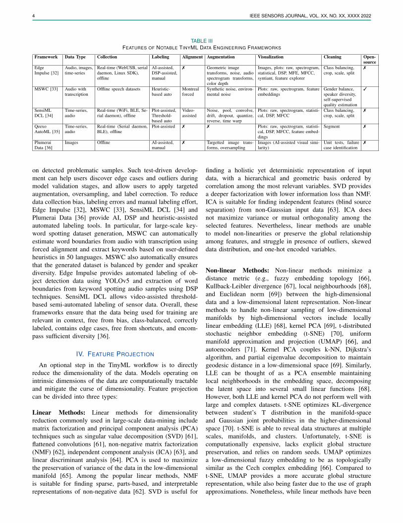
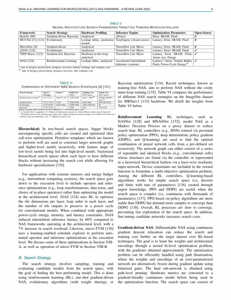
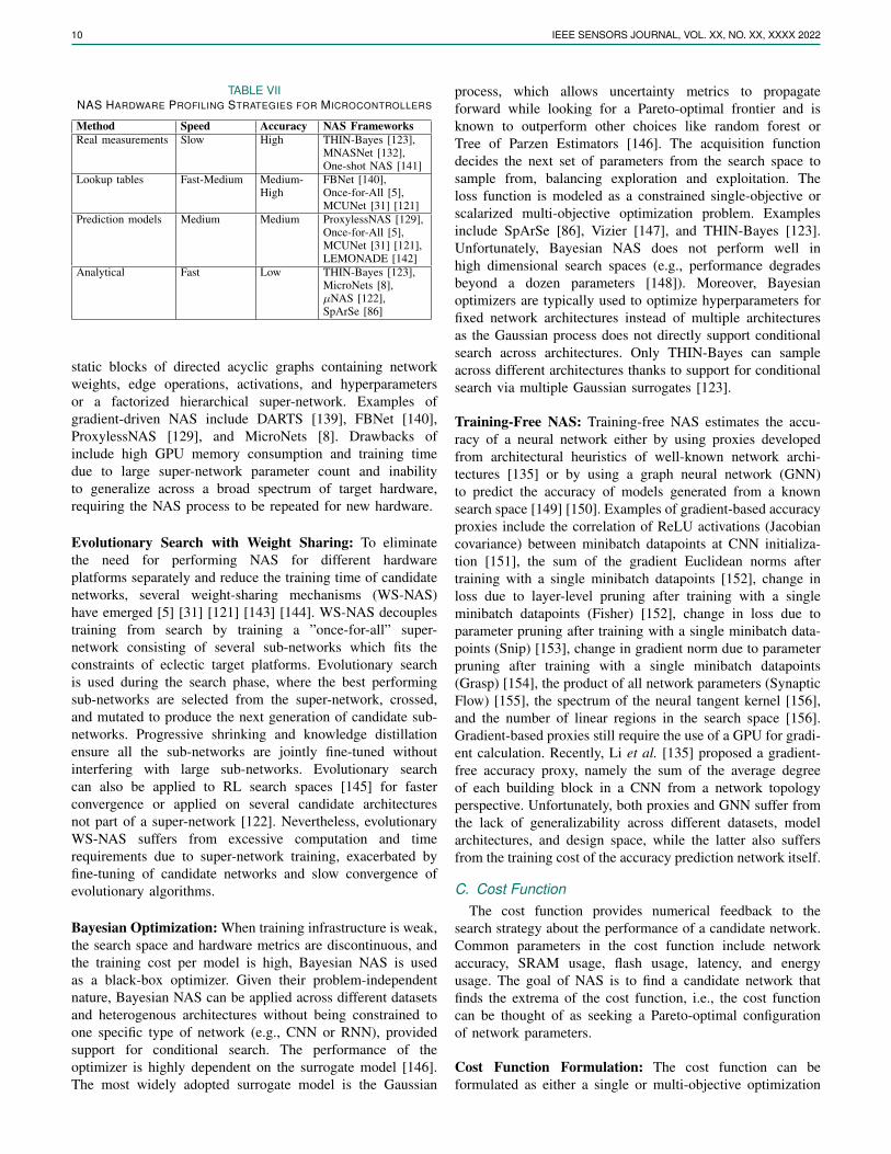
NAS is the automated process of finding the most optimalneural network within a neural network search space given tar-get architecture and network architecture constraints, achievinga balance between accuracy, latency, and energy usage [125][126] [127]. Table V compares several NAS frameworksdeveloped for microcontrollers. There are three key elementsin a hardware-aware NAS pipeline, namely the search spaceformulation (Section VII-A), search strategy (Section VII-B),and cost function (Section VII-C).
A. Search Space Formulation
The search space provides a set of ML operators, validconnection rules and possible parameter values for the searchalgorithm to explore. The neural network search space canbe represented as layer-wise, cell-wise, or hierarchical [125].
Layer-wise: In layer-wise search spaces, the entire model isgenerated from a collection of serialized or sequential neuraloperators. The macro-architecture (e.g., number of layers anddimensions of each layer), initial and terminal layers of thenetwork are fixed, while the remaining layers are optimized.The structure and connectivity among various operatorsare specified using variable-length strings, encoded in theaction space of the search strategy [126]. Although suchsearch spaces are expressive, layer-wise search spaces arecomputationally expensive, require hardcoding associationsamong different operators and parameters, and are notgradient friendly.
Cell-wise: For cell-wise (or template-wise) search spaces, thenetwork is constructed by stacking repeating fixed blocksor motifs called cells. A cell is a directed acyclic graphconstructed from a collection of neural operators, representingsome feature transformation. The search strategy finds themost optimal set of operators to construct the cell recursivelyin stages, by treating the output of past hidden layers as hiddenstates to apply a predefined set of ML operations on [128].Cell-based search spaces are more time-efficient compared tolayer-wise approaches and easily transferable across datasetsbut are less flexible for hardware specialization. In addition,the global architecture of the network is fixed.
SAHA et al.: MACHINE LEARNING FOR MICROCONTROLLER-CLASS HARDWARE - A REVIEW (JUNE 2022) 9
TABLE VNEURAL ARCHITECTURE SEARCH FRAMEWORKS TARGETTED TOWARDS MICROCONTROLLERS
Framework Search Strategy Hardware Profiling Inference Engine Optimization Parameters Open-SourceSpArSe [86] Gradient-driven Bayesian Analytical uTensor Error, SRAM, Flash 7MCUNet [31] [121] Evolutionary Lookup tables, prediction
modelsTinyEngine (closed-source) Latency, Error, SRAM, Flash 7
MicroNets [8] Gradient-driven Analytical Tensorflow Lite Micro Latency, Error, SRAM, Flash 7µNAS [122] Evolutionary Analytical Tensorflow Lite Micro Latency, Error, SRAM, Flash 3THIN-Bayes [123] Gradient-free Bayesian Hardware-in-the-loop,
analyticalTensorflow Lite Micro Latency, Error, SRAM, Flash,
Arena size, Energy3
iNAS [124] Reinforcement Learning Lookup tables, analytical Accelerated IntermittentInference (custom)
Latency*, Error, Volatile Buffer,Flash, Power-Cycle Energy@
3
* sum of progres preservation, progress recovery, battery recharge and compute cost@ sum of progres preservation, progress recovery, and compute cost
TABLE VICOMPARISON OF DIFFERENT NAS SEARCH STRATEGIES [5] [131]
Search Strategy Top-1%Accuracy
Latency∧ Model Size(MAC)
Training Cost(GPU hours)
Search Cost(GPU hours)
Reinforcement Learning∨ 74%-75.2% 58mS-70 mS 219M-564M None*, 180N@ 40000N-48000N*,None@
Gradient-driven 73.1%-74.9% 71mS 320M-595M 250N-384N 96N-(288+24N)Evolutionary 72.4%-80.0% 58mS-59mS 230M-595M 1200-(1200+kN) 40Bayesian∨ 73.4%-75.8% - 225M None 23N-552N
dataset: ImageNet-1000, backbone network: MBNetV3, k = fine-tuning epoch count∧ on Google Pixel1 smartphone, N = Number of deployment scenarios for which different models must be found [5]∨ Techniques based on RL and Bayesian usually have coupled training and search (training cost included with search cost)* NASNet [128] and MNASNet [132], @ MBNetV3 Search [133]
Hierarchical: In tree-based search spaces, bigger blocksencompassing specific cells are created and optimized aftercell-wise optimization. Primitive templates which are knownto perform well are used to construct larger network graphsand higher-level motifs recursively, with feature maps oflow-level motifs being fed into high-level motifs. Factorizedhierarchical search spaces allow each layer to have differentblocks without increasing the search cost while allowing forhardware specialization [129].
For applications with extreme memory and energy budget(e.g., intermittent computing systems), the search space goesdown to the execution level to include operator and infer-ence optimizations (e.g., loop transformations, data reuse, andchoice of in-place operators) rather than optimizing the modelat the architectural level. iNAS [124] uses RL to optimizethe tile dimensions per layer, loop order in each layer, andthe number of tile outputs to preserve in a power cyclefor convolutional models. When combined with appropriatepower-cycle energy, memory, and latency constraints, iNASreduced intermittent inference latency by 60% compared toNAS frameworks operating at the architectural level, with a7% increase in search overhead. Likewise, micro-TVM [130]uses a learning-enabled schedule explorer to perform auto-mated operator and inference optimizations at the executionlevel. We discuss some of these optimizations in Section VIII-A, as well as operation of micro-TVM in Section VIII-B.
B. Search Strategy
The search strategy involves sampling, training andevaluating candidate models from the search space, withthe goal of finding the best performing model. This is doneusing reinforcement learning (RL), one-shot gradient-drivenNAS, evolutionary algorithms (with weight sharing), or
Bayesian optimization [134]. Recent techniques, known astraining-free NAS, aim to perform NAS without the costlyinner-loop training [135]. Table VI compares the performanceof different NAS search strategies on the ImageNet datasetfor MBNetv3 [133] backbone. We distill the insights fromTable VI below.
Reinforcement Learning: RL techniques, such asNASNet [128] and MNASNet [132], model NAS as aMarkov Decision Process on a proxy dataset to reducesearch time. RL controllers (e.g., RNNs trained via proximalpolicy optimization (PPO), deep deterministic policy gradient(DDPG), and Q-learning) are used to find the optimalcombination of neural network cells from a pre-defined setrecursively. The network graph can either consist of a seriesof repeatable and identical blocks (e.g., convolutional cells)whose structures are found via the controller or representedin a factorized hierarchical fashion via a layer-wise stochasticsuper-network. Device constraints are included in the rewardfunction to formulate a multi-objective optimization problem.Among the different RL controllers, Q-learning-basedalgorithms works for simple search space (i.e, discreteand finite with tens of parameters) [136] created throughexpert knowledge. PPO and DDPG are useful when thesearch space is complex (i.e, continuous with thousands ofparameters) [137]. PPO-based on-policy algorithms are morestable than DDPG but demand more samples to converge thanDDPG [138]. Overall, RL processes are slow to converge,preventing fast exploration of the search space. In addition,fine-tuning candidate networks increases search costs.
Gradient-driven NAS: Differentiable NAS using continuousgradient descent relaxation can reduce the search andtraining cost further on the target dataset over RL-basedtechniques. The goal is to learn the weights and architecturalencodings through a nested bi-level optimization problem,with the gradients obtained approximately. The optimizationproblem can be efficiently handled using path binarization,where the weights and encodings of an over-parametrizednetwork are alternatively frozen during gradient update usingbinarized gates. The final sub-network is obtained usingpath-level pruning. Hardware metrics are converted to agradient-friendly continuous model before being used inthe optimization function. The search space can consist of
10 IEEE SENSORS JOURNAL, VOL. XX, NO. XX, XXXX 2022
TABLE VIINAS HARDWARE PROFILING STRATEGIES FOR MICROCONTROLLERS
Method Speed Accuracy NAS FrameworksReal measurements Slow High THIN-Bayes [123],
MNASNet [132],One-shot NAS [141]
Lookup tables Fast-Medium Medium-High
FBNet [140],Once-for-All [5],MCUNet [31] [121]
Prediction models Medium Medium ProxylessNAS [129],Once-for-All [5],MCUNet [31] [121],LEMONADE [142]
Analytical Fast Low THIN-Bayes [123],MicroNets [8],µNAS [122],SpArSe [86]
static blocks of directed acyclic graphs containing networkweights, edge operations, activations, and hyperparametersor a factorized hierarchical super-network. Examples ofgradient-driven NAS include DARTS [139], FBNet [140],ProxylessNAS [129], and MicroNets [8]. Drawbacks ofinclude high GPU memory consumption and training timedue to large super-network parameter count and inabilityto generalize across a broad spectrum of target hardware,requiring the NAS process to be repeated for new hardware.
Evolutionary Search with Weight Sharing: To eliminatethe need for performing NAS for different hardwareplatforms separately and reduce the training time of candidatenetworks, several weight-sharing mechanisms (WS-NAS)have emerged [5] [31] [121] [143] [144]. WS-NAS decouplestraining from search by training a ”once-for-all” super-network consisting of several sub-networks which fits theconstraints of eclectic target platforms. Evolutionary searchis used during the search phase, where the best performingsub-networks are selected from the super-network, crossed,and mutated to produce the next generation of candidate sub-networks. Progressive shrinking and knowledge distillationensure all the sub-networks are jointly fine-tuned withoutinterfering with large sub-networks. Evolutionary searchcan also be applied to RL search spaces [145] for fasterconvergence or applied on several candidate architecturesnot part of a super-network [122]. Nevertheless, evolutionaryWS-NAS suffers from excessive computation and timerequirements due to super-network training, exacerbated byfine-tuning of candidate networks and slow convergence ofevolutionary algorithms.
Bayesian Optimization: When training infrastructure is weak,the search space and hardware metrics are discontinuous, andthe training cost per model is high, Bayesian NAS is usedas a black-box optimizer. Given their problem-independentnature, Bayesian NAS can be applied across different datasetsand heterogenous architectures without being constrained toone specific type of network (e.g., CNN or RNN), providedsupport for conditional search. The performance of theoptimizer is highly dependent on the surrogate model [146].The most widely adopted surrogate model is the Gaussian
process, which allows uncertainty metrics to propagateforward while looking for a Pareto-optimal frontier and isknown to outperform other choices like random forest orTree of Parzen Estimators [146]. The acquisition functiondecides the next set of parameters from the search space tosample from, balancing exploration and exploitation. Theloss function is modeled as a constrained single-objective orscalarized multi-objective optimization problem. Examplesinclude SpArSe [86], Vizier [147], and THIN-Bayes [123].Unfortunately, Bayesian NAS does not perform well inhigh dimensional search spaces (e.g., performance degradesbeyond a dozen parameters [148]). Moreover, Bayesianoptimizers are typically used to optimize hyperparameters forfixed network architectures instead of multiple architecturesas the Gaussian process does not directly support conditionalsearch across architectures. Only THIN-Bayes can sampleacross different architectures thanks to support for conditionalsearch via multiple Gaussian surrogates [123].
Training-Free NAS: Training-free NAS estimates the accu-racy of a neural network either by using proxies developedfrom architectural heuristics of well-known network archi-tectures [135] or by using a graph neural network (GNN)to predict the accuracy of models generated from a knownsearch space [149] [150]. Examples of gradient-based accuracyproxies include the correlation of ReLU activations (Jacobiancovariance) between minibatch datapoints at CNN initializa-tion [151], the sum of the gradient Euclidean norms aftertraining with a single minibatch datapoints [152], change inloss due to layer-level pruning after training with a singleminibatch datapoints (Fisher) [152], change in loss due toparameter pruning after training with a single minibatch data-points (Snip) [153], change in gradient norm due to parameterpruning after training with a single minibatch datapoints(Grasp) [154], the product of all network parameters (SynapticFlow) [155], the spectrum of the neural tangent kernel [156],and the number of linear regions in the search space [156].Gradient-based proxies still require the use of a GPU for gradi-ent calculation. Recently, Li et al. [135] proposed a gradient-free accuracy proxy, namely the sum of the average degreeof each building block in a CNN from a network topologyperspective. Unfortunately, both proxies and GNN suffer fromthe lack of generalizability across different datasets, modelarchitectures, and design space, while the latter also suffersfrom the training cost of the accuracy prediction network itself.
C. Cost FunctionThe cost function provides numerical feedback to the
search strategy about the performance of a candidate network.Common parameters in the cost function include networkaccuracy, SRAM usage, flash usage, latency, and energyusage. The goal of NAS is to find a candidate network thatfinds the extrema of the cost function, i.e., the cost functioncan be thought of as seeking a Pareto-optimal configurationof network parameters.
Cost Function Formulation: The cost function can beformulated as either a single or multi-objective optimization

SAHA et al.: MACHINE LEARNING FOR MICROCONTROLLER-CLASS HARDWARE - A REVIEW (JUNE 2022) 11
problem. Single objective optimization problems onlyoptimize for model accuracy. To take hardware constraintsinto account, single-objective optimization problems areusually treated as constrained optimization problems withhardware costs acting as regularizers [123]. Multi-objectivecost functions are usually transformed into a single objectiveoptimization problem via weighted-sum or scalarizationtechniques [86] or solved using genetic algorithms.
Hardware Profiling: Hardware-aware NAS employshardware-specific cost functions or search heuristics viahardware profiling. The target hardware can be profiled inreal-time by running sampled models on the actual targetdevice (hardware-in-the-loop), estimated using lookup tables,prediction models, and silicon-accurate emulators [157] oranalytically estimated using architectural heuristics. Commonhardware profiling techniques are shown in Table VII.Hardware-in-the-loop is slowest but most accurate duringNAS runtime, while analytical estimation is fastest butleast accurate [125] [134]. Examples of analytical modelsfor microcontrollers include using FLOPS as a proxy forlatency [8] [122], and standard RAM usage model [86] forworking memory estimation. Recently, latency predictionmodels have been made more accurate through kernel(execution unit) detection and adaptive sampling [158].For intermittent computing systems, the latency is the timerequired for progress preservation (writing progress indicatorsand computed tile outputs to flash at the end of a powercycle), progress recovery (system reboot, loading progressindicators, and tiled outputs into SRAM), battery recharge,and running inference (cost of computing multiple tiles perenergy cycle) [124]. The SRAM usage in such systems isthe sum of memory consumed by the input feature map,weights, and output feature map, dependent upon the tiledimensions, loop order, and preservation batch size in thesearch space [124].
VIII. TINYML SOFTWARE SUITES
After the best model is constructed from lightweight MLblocks through NAS, the model needs to be prepared for de-ployment onto microcontrollers. This is performed by TinyMLsoftware suites, which generate embedded code and performoperator and inference engine optimizations, some of whichare shown in Fig. 3 and discussed in Section VIII-A. Inaddition, some of these frameworks also provide inferenceengines for resource management and model execution duringdeployment. We discuss features of notable TinyML softwaresuites in Section VIII-B.
A. Operator and Inference OptimizationsAll TinyML software suites perform several operator and
inference engine optimizations to improve data locality,memory usage, and spatiotemporal execution [162]. Commontechniques include the use of fused or in-place operators [130],loop transformations [161], and data reuse (output sharing orvalue sharing) [163].
Fig. 3. Example operator optimizations performed by TinyML softwaresuites. (a) Use of fused and in-place activated operators reduce memoryaccess cost and improves inference speed [158] [159]. (b) Convertingdepthwise convolution to in-place depthwise convolution reduces peakmemory usage by 1.6×, by allowing first channel output activation(stored in a buffer) to overwrite the previous channel’s inpur activationuntil written back to the last channel’s input activation [31]. (c) Loopunrolling eliminates branch instruction overhead [31]. (d) Loop tilingencourages resuse of array elements within each tile by partitioningthe loop’s iterative space into blocks [160], while loop reordering (withtiling) improves spatiotemporal execution and locality of reference withindevice memory constraints [161] [162].
In-Place and Fused Operators: Operator fusion or foldingcombines several ML operators into a specialized kernelwithout saving the intermediate feature representations inmemory (known as in-place activation) [130]. The softwaresuites follow user-defined rules for operator fusion dependingon graph operator type (e.g., injective, reduction, complex-outfusable, and opaque) [130]. Use of fused and in-placeoperators have been shown to reduce memory usage by1.6× [31] and improve speedup by 1.2-2× [130].
Loop Transformations: Loop transformations aim to improvespatiotemporal execution and inference speed by reducingloop overheads [161]. Common loop transformations includeloop reordering, loop reversal, loop fusion, loop distribution,loop unrolling, and loop tiling [161] [162] [161] [160].Loop reordering (and reversal) finds the loop permutationthat maximizes data reuse and spatiotemporal locality. Loopfusion combines different loop nests into one, therebyimproving temporal locality, and increasing data locality andreuse by creating perfect loop nests from imperfect loopnests. To enable loop permutation for loop nests that arenot permutable, loop distribution breaks a single loop intomultiple loops [161]. Loop unrolling helps eliminate branchpenalties and helps hide memory access latencies [130].Loop tiling improves data reuse by diving the loops intoblocks while considering the size of each level of memoryhierarchy [160].
Data Reuse: Data reuse aims to improve data locality andreduce memory access costs. While data reuse is mostly

12 IEEE SENSORS JOURNAL, VOL. XX, NO. XX, XXXX 2022
TABLE VIIIFEATURES OF NOTABLE TINYML SOFTWARE SUITES FOR MICROCONTROLLERS
Framework Supported Platforms Supported Models Supported Training Libraries Open-Source FreeTensorFlow Lite Micro(Google) [167] [46]
ARM Cortex-M, Espressif ESP32,Himax WE-I Plus
NN TensorFlow 3 3
uTensor (ARM) [168] ARM Cortex-M (Mbed-enabled) NN TensorFlow 3 3uTVM (Apache) [130] ARM Cortex-M NN PyTorch, TensorFlow, Keras 3 3EdgeML (Microsoft)[57] [58] [59] [60], [169]–[171]
ARM Cortex-M, AVR RISC NN, DT, kNN, unary classifier PyTorch, TensorFlow 3 3
CMSIS-NN (ARM) [164] ARM Cortex-M NN PyTorch, TensorFlow, Caffe 3 3EON Compiler (EdgeImpulse) [32]
ARM Cortex-M, TI CC1352P,ARM Cortex-A, Espressif ESP32,Himax WE-I Plus, TENSAI SoC
NN, k-means, regressors (supportsfeature extraction)
TensorFlow, Scikit-Learn 7 3
STM32Cube.AI (STMi-croelectronics) [172]
ARM Cortex-M (STM32 series) NN, k-means, SVM, RF, kNN, DT,NB, regressors
PyTorch, Scikit-Learn, Tensor-Flow, Keras, Caffe, MATLAB,Microsoft Cognitive Toolkit,Lasagne, ConvnetJS
7 3
NanoEdge AI Studio(STMicroelectronics) [173]
ARM Cortex-M (STM32 series) Unsupervised learning - 7 7
EloquentML [72] ARM Cortex-M, Espressif ESP32,Espressif ESP8266, AVR RISC
NN, DT, SVM, RF, XGBoost, NB,RVM, SEFR (feature extractionthrough PCA)
TensorFlow, Scikit-Learn 3 3
Sklearn Porter [174] - NN (MLP), DT, SVM, RF,AdaBoost, NB
Scikit-Learn 3 3
EmbML [175] ARM Cortex-M, AVR RISC NN (MLP), DT, SVM, regressors Scikit-Learn, Weka 3 3FANN-on-MCU [176] ARM Cortex-M, PULP NN FANN 3 3
SONIC, TAILS@ [24] TI MSP430 NN TensorFlow 3 3@ inference framework for intermittent computing systems.
achieved through loop transformations, several other tech-niques have also been proposed. CMSIS-NN provides spe-cial pooling and multiplication operations to promote datareuse [164]. TF-Net [163] proposed the use of direct bufferconvolution on Cortex-M microcontrollers to reduce input un-packing overhead, which reuses inputs in the current windowunpacked in a buffer space for all weight filters. Input reusereduces SRAM usage by 2.57× and provides 2× speedup.Similarly, for GAP8 processors, the PULP-NN library providesa reusable im2col buffer (height-width-channel data layout)to reduce im2col creation overhead [165] [166], providingpartial spatial data reuse. PULP-NN also features register-leveldata reuse, achieving 20% speedup over CMSIS-NN and 1.9×improvement over native GAP8-NN libraries.
B. Notable TinyML Software Suites
Notable open-source TinyML frameworks and inferenceengines include TensorFlow Lite Micro [167] [46],uTensor [168], uTVM [130], Microsoft EdgeML [57] [58][59] [60], [169]–[171], CMSIS-NN [164], EloquentML [72],Sklearn Porter [174], EmbML [175], and FANN-on-MCU [176]. Closed-source TinyML frameworks andinference engines include STM32Cube.AI [172], NanoEdgeAI Studio [173], Edge Impulse EON Compiler [32],TinyEngine [31] [121], Qeexo AutoML [35], DeepliteNeutrino [177], Imagimob AI [178], Neuton TinyML [179],Reality AI [180], and SensiML Analytics Studio andKnowledge Pack [34]. Table VIII compares the features ofsome of these frameworks.
TensorFlow Lite Micro: TensorFlow Lite Micro (TFLM) [46][167] is a specialized version of TFLite aimed towards
optimizing TF models for Cortex-M and ESP32 MCU.TFLite Micro embraces several embedded runtime designphilosophies. TFLM drops uncommon features, data types,and operations for portability. It also avoids specializedlibraries, operating systems, or build-system dependenciesfor heterogeneous hardware support and memory efficiency.TFLM avoids dynamic memory allocation to mitigatememory fragmentation. TFLM interprets the neural networkgraph at runtime rather than generating C++ code tosupport easy pathways for upgradability, multi-tenancy,multi-threading, and model replacement while sacrificingfinite savings in memory. Fig 4 summarizes the operationof TFLM. TFLM consists of three primary components.First, the operator resolver links only essential operationsto the model binary file. Second, TFLM pre-allocates acontiguous memory stack called the arena for initializationand storing runtime variables. TFLM uses a two-stackallocation strategy to discard initialization variables aftertheir lifetime, thereby minimizing memory consumption.The space between the two stacks is used for temporaryallocations during memory planning, where TFLM usesbin-packing to encourage memory reuse and yield optimalcompacted memory layouts during runtime. Lastly, TFLMuses an interpreter to resolve the network graph at runtime,allocate the arena, and perform runtime calculations. TFLMwas shown to provide 2.2× speedup and 1.08× memoryand flash savings over CMSIS-NN for image recognition [31].
uTensor: uTensor [168] generates C++ files from TF modelsfor Mbed-enabled boards, aiming to generate models of < 2kB in size. It is subdivided into two parts. The uTensorcore provides a set of optimized runtime data structuresand interfaces under computing constraints. The uTensor

SAHA et al.: MACHINE LEARNING FOR MICROCONTROLLER-CLASS HARDWARE - A REVIEW (JUNE 2022) 13
Fig. 4. Operation of TensorFlow Lite Micro, an interpreter-based infer-ence engine. (a) The training graph is frozen, optimized and convertedto a flatbuffer serialized model schema, suitable for deployment inembedded devices. (b) The TFLM runtime API preallocates a portionof memory in the SRAM (called arena) and performs bin-packing duringruntime to optimize memory usage (figure adapted from [167]).
library provides default error handlers, allocators, contexts,ML operations, and tensors built on the core. Basic datatypes include integral type, uTensor strings, tensor shape,and quantization primitives borrowed from TFLite. Interfacesinclude the memory allocator interface, tensor interface, tensormaps, and operator interface. For memory allocation, uTensoruses the concept of arena borrowed from TFLM. In addition,uTensor boasts a series of optimized (built to run CMSIS-NN under the hood), legacy, and quantized ML operatorsconsisting of activation functions, convolution operators, fully-connected layers, and pooling.
uTVM: micro-TVM [130] extends the TVM compiler stackto run models on bare-metal IoT devices without the need foroperating systems, virtual memory, or advanced programminglanguages. micro-TVM first generates a high-level andquantized computational graph (with support for complexdata structures) from the model using the relay module.The functional representation is then fed into the TVMintermediate representation module, which generatesC-code by performing operator and loop optimizations viaAutoTVM and Metascheduler, procedural optimizations, andgraph-level modeling for whole program memory planning.AutoTVM consists of an automatic schedule explorerto generate promising and valid operator and inferenceoptimization configurations for a specific microcontroller,and an XGBoost model to predict the performance of eachconfiguration based on features of the lowered loop program.The developer can either specify the configuration parametersto explore using a schedule template specification API, orpossible parameters can be extracted from the hardwarecomputation description written in the tensor expressionlanguage. AutoTVM has lower data and exploration costs
than black-box optimizers (e.g., ATLAS [181]), and providesmore accurate modeling than polyhedral methods [182]without needing a hardware-dependent cost model. Thegenerated code is integrated alongside the TVM C runtime,built, and flashed onto the device. Inference is made onthe device using a graph extractor. AutoTVM was shownto generate code that is only 1.2× slower compared tohandcrafted CMSIS-NN-based code for image recognition.
Microsoft EdgeML: EdgeML provides a collection oflightweight ML algorithms, operators, and tools aimed towardsdeployment on Class 0 devices, written in PyTorch and TF.Included algorithms include Bonsai [57], ProtoNN [58],FastRNN [59], FastGRNN [59], ShallowRNN [169], EMI-RNN [170], RNNPool [60], and DROCC [171]. EMI-RNNexploits the fact that only a small, tight portion of atime-series plot for a certain class contributes to the finalclassification while other portions are common among allclasses. Shallow-RNN is a hierarchical RNN architecturethat divides the time-series signal into various blocks andfeeds them in parallel to several RNNs with shared weightsand activation maps. RNNPool is a non-linear poolingoperator that can perform ”pooling” on intermediate layersof a CNN by a downsampling factor much larger than 2(4-8×) without losing accuracy while reducing memory usageand decreasing compute. Deep robust one-class classifier(DROCC) is an OCC under limited negatives and anomalydetector without requiring domain heuristics or handcraftedfeatures. The framework also includes a quantization toolcalled SeeDot [56].
CMSIS-NN: Cortex Microcontroller Software InterfaceStandard-NN [164] was designed to transform TF, PyTorch,and Caffe models for Cortex-M series MCU. It generatesC++ files from the model, which can be included in themain program file and compiled. It consists of a collectionof optimized neural network functions with fixed-point quan-tization, including fully connected layers, depth-wise separableconvolution, partial image-to-column convolution, in-situ splitx-y pooling, and activation functions (ReLU, sigmoid, andtanh, with the latter two implemented via lookup tables). Italso features a collection of support functions including datatype conversion and activation function tables (for sigmoid andtanh). CMSIS-NN provides 4.6× speedup and 4.9× energysavings over non-optimized convolutional models.
Edge Impulse EON Compiler: Edge Impulse [32] provides acomplete end-to-end model deployment solution for TinyMLdevices, starting with data collection using IoT devices,extracting features, training the models, and then deploymentand optimization of models for TinyML devices. It uses theinterpreter-less Edge Optimized Neural (EON) compilerfor model deployment, while also supporting TFLM. EONcompiler directly compiles the network to C++ source code,eliminating the need to store ML operators that are not inuse (at the cost of portability). EON compiler was shown torun the same network with 25-55% less SRAM and 35% lessflash than TFLM.

14 IEEE SENSORS JOURNAL, VOL. XX, NO. XX, XXXX 2022
TABLE IXFEATURES OF NOTABLE TINYML ON-DEVICE LEARNING FRAMEWORKS
Framework Working Principle SupportedHardware
Tested Application Network Type Open-source
Learning in theWild [183]
W: Per-output feature distribution divergence.H: Transfer learning on last-layer; sample importanceweighing to maximize learning effect.T: Gradient norm for sample selection via uncertainty anddiversity.
TI MSP430 Image recognition (MNIST, CIFAR-10, GT-SRB)
CNN 7
TinyOL [184] W: Running mean and variance of streaming inputH: Transfer learning on additional layer at the output of thefrozen network using stochastic gradient descent (SGD).
ARM Cortex-M Anomaly detection Autoencoder 7
ML-MCU [185] H: Optimized SGD (inherits stability of GD and efficiencyof SGD); optimized one-versus-one (OVO) binary classifiersfor multiclass classification
ARM Cortex-M,Espressif ESP32
Image recognition (MNIST), mHealth (HeartDisease, Breast Cancer), Other (Iris)
Optimized OVObinary classifiers
3
Train++ [186] W: Confidence score of prediction.H: Incremental training via constrained optimization classi-fier update
ARM Cortex-M,ARM Cortex-A,Espressif ESP32,Xtensa LX
Image recognition (MNIST, Banknote Au-thentication), mHealth (Heart Disease, BreastCancer, Haberman’s Survival), Other (Iris,Titanic Survival)
Binary classifiers 3
TinyTL [19] H: Update bias instead of weights and use lite residuallearning modules to recoup accuracy loss
ARM Cortex-A Face recognition (CelebA), Image recogni-tion (Cars, Flowers, Aircraft, CUB, Pets,Food, CIFAR-10, CIFAR-100)
CNN(ProxylessNAS-MB, MBNetV2)
3
Imbal-OL [187] T: Weighted replay and oversampling for minority classes ARM Cortex-A Image recognition (CIFAR-10, CIFAR-100) CNN (ResNet-18) 7QLR-CL [188] H: Continual learning with quantized latent replays (store
activation maps at latent replay layer instead of samples),slow-learning below the latent replay layer.
PULP Image recognition (Core50) CNN (MBNetV1) 7
W: When to learn, H: How to learn, T: What to learn (sample selection)
STM32Cube.AI and NanoEdge AI Studio: X-Cube-AIfrom STMicroelectronics [172] generates STM32 compatibleC code from a wide variety of deep-learning frameworks(e.g., PyTorch, TensorFlow, Keras, Caffe, MATLAB,Microsoft Cognitive Toolkit, Lasagne and ConvnetJS). Itallows quantization (min-max), operator fusion, and theuse of external flash or SRAM to store activation maps orweights. The tool also features functions to measure systemperformance and deployment accuracy and suggests a list ofcompatible STM32 platforms based on model complexity.X-Cube-AI was shown to provide 1.3× memory reductionand 2.2× speedup over TFLM for gesture recognition andkeyword spotting [189]. NanoEdge AI Studio [173] is anotherAutoML framework from STMicroelectronics for prototypinganomaly detection, outlier detection, classification, andregression problems for STM32 platforms, including anembedded emulator.
Eloquent MicroML and TinyML: MicroMLgen portsdecision trees, support vector machines (linear, polynomial,radial kernels or one-class), random forests, XGboost, NaiveBayes, relevant vector machines, and SEFR (a variant ofSVM) from SciKit-Learn to Arduino-style C code, with themodel entities stored on flash. It also supports onboard featureprojection through PCA. TinyMLgen ports TFLite models tooptimized C code using TFLite’s code generator [72].
Sklearn Porter: Sklearn Porter [174], generates C, Java, PHP,Ruby, GO, and Javascript code from Scikit-Learn models. Itsupports the conversion of support vector machines, decisiontrees, random forests, AdaBoost, k-nearest neighbors, NaiveBayes, and multi-layer perceptrons.
EmbML: Embedded ML [175] converts logistic regressors,decision trees, multi-layer perceptrons, and support vector
machines (linear, polynomial, or radial kernels) modelsgenerated by Weka or Scikit-Learn to C++ code native toembedded hardware. It generates initialization variables,structures, and functions for classification, storing theclassifier data on flash to avoid high memory usage, andsupports the quantization of floating-point entities. EmbMLwas shown to reduce memory usage by 31% and latency by92% over Sklearn Porter.
FANN-on-MCU: FANN-on-MCU [176] ports multi-layerperceptrons generated by fast artificial neural networks(FANN) library to Cortex-M series processors. It allowsmodel quantization and produces an independent callable Cfunction based on the specific instruction set of the MCU. Ittakes the memory of the target architecture into account andstores network parameters in either RAM or flash dependingupon whichever does not overflow and closer to the processor(e.g., RAM is closer than flash).
SONIC, TAILS: Software-only neural intermittent computing(SONIC) and tile-accelerated intermittent low energy accel-erator (LEA) support (TAILS) [24] are inference enginesfor intermittent computing systems. SONIC eliminates redo-logging, task transitions, and wasted work associated withmoving data between SRAM and flash by introducing loopcontinuation, which allows loop index modification directlyon the flash without expensive saving and restoring. To ensureidempotence, SONIC uses loop ordered buffering (loop re-ordering and double buffering partial feature maps to eliminatecommits in a loop iterations) and sparse undo-logging (bufferreuse to ensure idempotence for sparse ML operators). SONICintroduces a latency overhead of only 25-75% over non-intermittent neural network execution (compared to 10× over-head from baseline intermittent model execution frameworks),reducing inference energy by 6.9× over competing baselines.TAILS exploits LEA in MSP430 microcontrollers to maximize
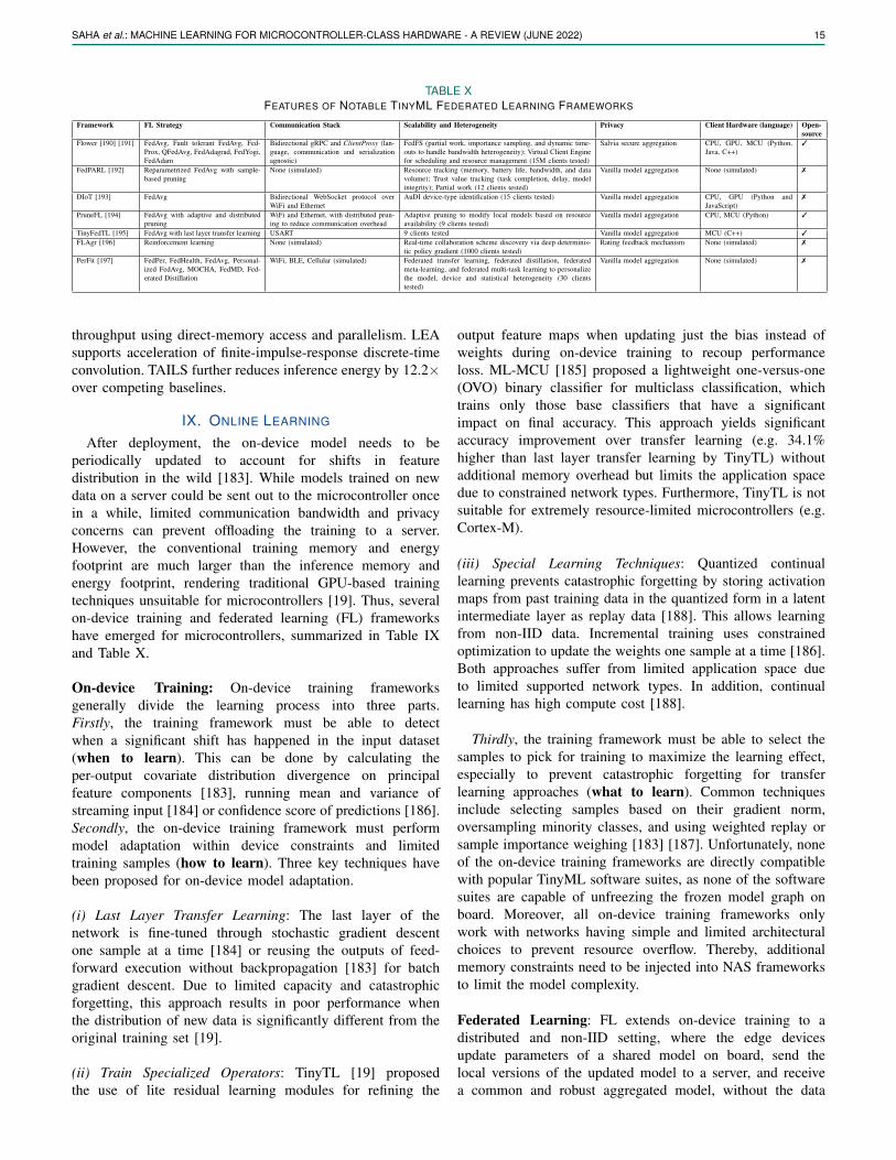
SAHA et al.: MACHINE LEARNING FOR MICROCONTROLLER-CLASS HARDWARE - A REVIEW (JUNE 2022) 15
TABLE XFEATURES OF NOTABLE TINYML FEDERATED LEARNING FRAMEWORKS
Framework FL Strategy Communication Stack Scalability and Heterogeneity Privacy Client Hardware (language) Open-source
Flower [190] [191] FedAvg, Fault tolerant FedAvg, Fed-Prox, QFedAvg, FedAdagrad, FedYogi,FedAdam
Bidirectional gRPC and ClientProxy (lan-guage, communication and serializationagnostic)
FedFS (partial work, importance sampling, and dynamic time-outs to handle bandwidth heterogeneity); Virtual Client Enginefor scheduling and resource management (15M clients tested)
Salvia secure aggregation CPU, GPU, MCU (Python,Java, C++)
3
FedPARL [192] Reparametrized FedAvg with sample-based pruning
None (simulated) Resource tracking (memory, battery life, bandwidth, and datavolume); Trust value tracking (task completion, delay, modelintegrity); Partial work (12 clients tested)
Vanilla model aggregation None (simulated) 7
DIoT [193] FedAvg Bidirectional WebSocket protocol overWiFi and Ethernet
AuDI device-type identification (15 clients tested) Vanilla model aggregation CPU, GPU (Python andJavaScript)
7
PruneFL [194] FedAvg with adaptive and distributedpruning
WiFi and Ethernet, with distributed prun-ing to reduce communication overhead
Adaptive pruning to modify local models based on resourceavailability (9 clients tested)
Vanilla model aggregation CPU, MCU (Python) 3
TinyFedTL [195] FedAvg with last layer transfer learning USART 9 clients tested Vanilla model aggregation MCU (C++) 3
FLAgr [196] Reinforcement learning None (simulated) Real-time collaboration scheme discovery via deep determinis-tic policy gradient (1000 clients tested)
Rating feedback mechanism None (simulated) 7
PerFit [197] FedPer, FedHealth, FedAvg, Personal-ized FedAvg, MOCHA, FedMD, Fed-erated Distillation
WiFi, BLE, Cellular (simulated) Federated transfer learning, federated distillation, federatedmeta-learning, and federated multi-task learning to personalizethe model, device and statistical heterogeneity (30 clientstested)
Vanilla model aggregation None (simulated) 7
throughput using direct-memory access and parallelism. LEAsupports acceleration of finite-impulse-response discrete-timeconvolution. TAILS further reduces inference energy by 12.2×over competing baselines.
IX. ONLINE LEARNING
After deployment, the on-device model needs to beperiodically updated to account for shifts in featuredistribution in the wild [183]. While models trained on newdata on a server could be sent out to the microcontroller oncein a while, limited communication bandwidth and privacyconcerns can prevent offloading the training to a server.However, the conventional training memory and energyfootprint are much larger than the inference memory andenergy footprint, rendering traditional GPU-based trainingtechniques unsuitable for microcontrollers [19]. Thus, severalon-device training and federated learning (FL) frameworkshave emerged for microcontrollers, summarized in Table IXand Table X.
On-device Training: On-device training frameworksgenerally divide the learning process into three parts.Firstly, the training framework must be able to detectwhen a significant shift has happened in the input dataset(when to learn). This can be done by calculating theper-output covariate distribution divergence on principalfeature components [183], running mean and variance ofstreaming input [184] or confidence score of predictions [186].Secondly, the on-device training framework must performmodel adaptation within device constraints and limitedtraining samples (how to learn). Three key techniques havebeen proposed for on-device model adaptation.
(i) Last Layer Transfer Learning: The last layer of thenetwork is fine-tuned through stochastic gradient descentone sample at a time [184] or reusing the outputs of feed-forward execution without backpropagation [183] for batchgradient descent. Due to limited capacity and catastrophicforgetting, this approach results in poor performance whenthe distribution of new data is significantly different from theoriginal training set [19].
(ii) Train Specialized Operators: TinyTL [19] proposedthe use of lite residual learning modules for refining the
output feature maps when updating just the bias instead ofweights during on-device training to recoup performanceloss. ML-MCU [185] proposed a lightweight one-versus-one(OVO) binary classifier for multiclass classification, whichtrains only those base classifiers that have a significantimpact on final accuracy. This approach yields significantaccuracy improvement over transfer learning (e.g. 34.1%higher than last layer transfer learning by TinyTL) withoutadditional memory overhead but limits the application spacedue to constrained network types. Furthermore, TinyTL is notsuitable for extremely resource-limited microcontrollers (e.g.Cortex-M).
(iii) Special Learning Techniques: Quantized continuallearning prevents catastrophic forgetting by storing activationmaps from past training data in the quantized form in a latentintermediate layer as replay data [188]. This allows learningfrom non-IID data. Incremental training uses constrainedoptimization to update the weights one sample at a time [186].Both approaches suffer from limited application space dueto limited supported network types. In addition, continuallearning has high compute cost [188].
Thirdly, the training framework must be able to select thesamples to pick for training to maximize the learning effect,especially to prevent catastrophic forgetting for transferlearning approaches (what to learn). Common techniquesinclude selecting samples based on their gradient norm,oversampling minority classes, and using weighted replay orsample importance weighing [183] [187]. Unfortunately, noneof the on-device training frameworks are directly compatiblewith popular TinyML software suites, as none of the softwaresuites are capable of unfreezing the frozen model graph onboard. Moreover, all on-device training frameworks onlywork with networks having simple and limited architecturalchoices to prevent resource overflow. Thereby, additionalmemory constraints need to be injected into NAS frameworksto limit the model complexity.
Federated Learning: FL extends on-device training to adistributed and non-IID setting, where the edge devicesupdate parameters of a shared model on board, send thelocal versions of the updated model to a server, and receivea common and robust aggregated model, without the data
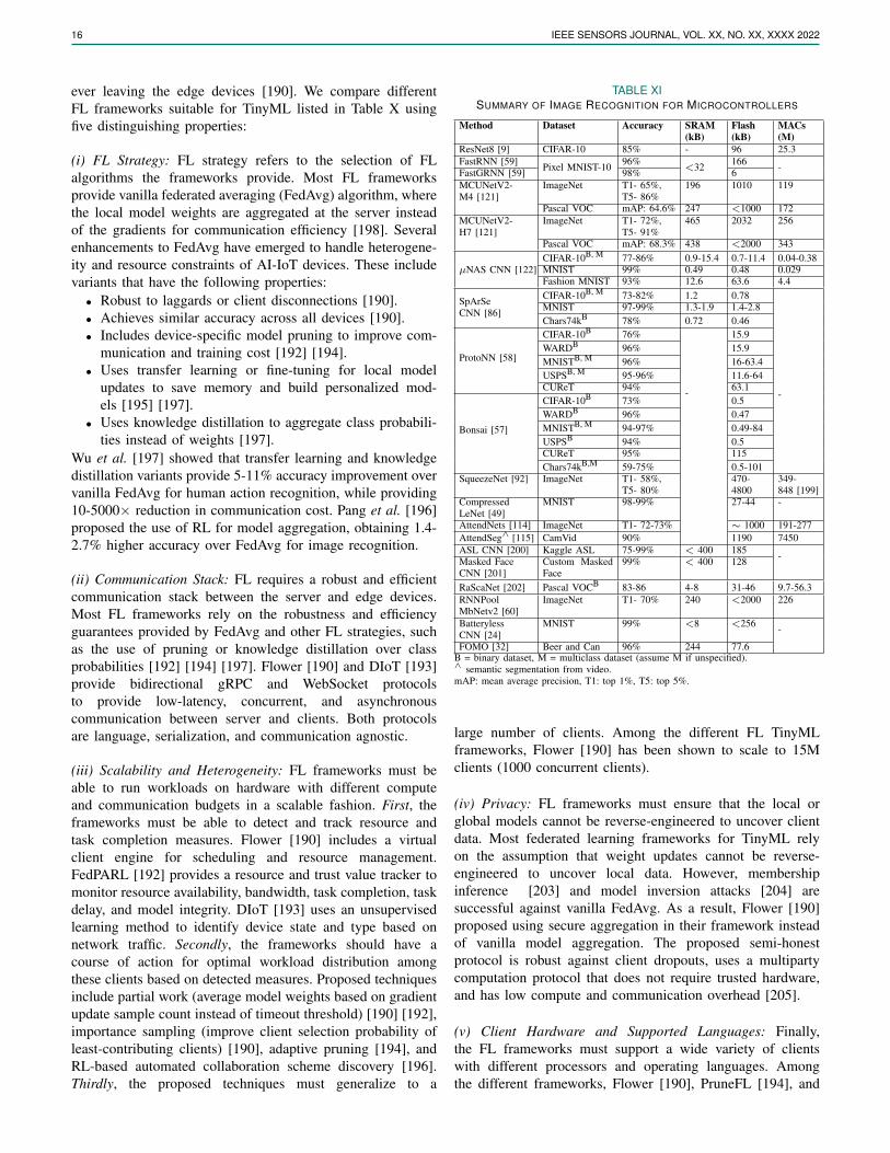
16 IEEE SENSORS JOURNAL, VOL. XX, NO. XX, XXXX 2022
ever leaving the edge devices [190]. We compare differentFL frameworks suitable for TinyML listed in Table X usingfive distinguishing properties:
(i) FL Strategy: FL strategy refers to the selection of FLalgorithms the frameworks provide. Most FL frameworksprovide vanilla federated averaging (FedAvg) algorithm, wherethe local model weights are aggregated at the server insteadof the gradients for communication efficiency [198]. Severalenhancements to FedAvg have emerged to handle heterogene-ity and resource constraints of AI-IoT devices. These includevariants that have the following properties:
• Robust to laggards or client disconnections [190].• Achieves similar accuracy across all devices [190].• Includes device-specific model pruning to improve com-
munication and training cost [192] [194].• Uses transfer learning or fine-tuning for local model
updates to save memory and build personalized mod-els [195] [197].
• Uses knowledge distillation to aggregate class probabili-ties instead of weights [197].
Wu et al. [197] showed that transfer learning and knowledgedistillation variants provide 5-11% accuracy improvement overvanilla FedAvg for human action recognition, while providing10-5000× reduction in communication cost. Pang et al. [196]proposed the use of RL for model aggregation, obtaining 1.4-2.7% higher accuracy over FedAvg for image recognition.
(ii) Communication Stack: FL requires a robust and efficientcommunication stack between the server and edge devices.Most FL frameworks rely on the robustness and efficiencyguarantees provided by FedAvg and other FL strategies, suchas the use of pruning or knowledge distillation over classprobabilities [192] [194] [197]. Flower [190] and DIoT [193]provide bidirectional gRPC and WebSocket protocolsto provide low-latency, concurrent, and asynchronouscommunication between server and clients. Both protocolsare language, serialization, and communication agnostic.
(iii) Scalability and Heterogeneity: FL frameworks must beable to run workloads on hardware with different computeand communication budgets in a scalable fashion. First, theframeworks must be able to detect and track resource andtask completion measures. Flower [190] includes a virtualclient engine for scheduling and resource management.FedPARL [192] provides a resource and trust value tracker tomonitor resource availability, bandwidth, task completion, taskdelay, and model integrity. DIoT [193] uses an unsupervisedlearning method to identify device state and type based onnetwork traffic. Secondly, the frameworks should have acourse of action for optimal workload distribution amongthese clients based on detected measures. Proposed techniquesinclude partial work (average model weights based on gradientupdate sample count instead of timeout threshold) [190] [192],importance sampling (improve client selection probability ofleast-contributing clients) [190], adaptive pruning [194], andRL-based automated collaboration scheme discovery [196].Thirdly, the proposed techniques must generalize to a
TABLE XISUMMARY OF IMAGE RECOGNITION FOR MICROCONTROLLERS
Method Dataset Accuracy SRAM(kB)
Flash(kB)
MACs(M)
ResNet8 [9] CIFAR-10 85% - 96 25.3FastRNN [59] Pixel MNIST-10 96%
<32 166 -FastGRNN [59] 98% 6MCUNetV2-M4 [121]
ImageNet T1- 65%,T5- 86%
196 1010 119
Pascal VOC mAP: 64.6% 247 <1000 172MCUNetV2-H7 [121]
ImageNet T1- 72%,T5- 91%
465 2032 256
Pascal VOC mAP: 68.3% 438 <2000 343
µNAS CNN [122]CIFAR-10B, M 77-86% 0.9-15.4 0.7-11.4 0.04-0.38MNIST 99% 0.49 0.48 0.029Fashion MNIST 93% 12.6 63.6 4.4
SpArSeCNN [86]
CIFAR-10B, M 73-82% 1.2 0.78
-
MNIST 97-99% 1.3-1.9 1.4-2.8Chars74kB 78% 0.72 0.46
ProtoNN [58]
CIFAR-10B 76%
-
15.9WARDB 96% 15.9MNISTB, M 96% 16-63.4USPSB, M 95-96% 11.6-64CUReT 94% 63.1
Bonsai [57]
CIFAR-10B 73% 0.5WARDB 96% 0.47MNISTB, M 94-97% 0.49-84USPSB 94% 0.5CUReT 95% 115Chars74kB,M 59-75% 0.5-101
SqueezeNet [92] ImageNet T1- 58%,T5- 80%
470-4800
349-848 [199]
CompressedLeNet [49]
MNIST 98-99% 27-44 -
AttendNets [114] ImageNet T1- 72-73% ∼ 1000 191-277AttendSeg∧ [115] CamVid 90% 1190 7450ASL CNN [200] Kaggle ASL 75-99% < 400 185 -Masked FaceCNN [201]
Custom MaskedFace
99% < 400 128
RaScaNet [202] Pascal VOCB 83-86 4-8 31-46 9.7-56.3RNNPoolMbNetv2 [60]
ImageNet T1- 70% 240 <2000 226
BatterylessCNN [24]
MNIST 99% <8 <256 -
FOMO [32] Beer and Can 96% 244 77.6B = binary dataset, M = multiclass dataset (assume M if unspecified).∧ semantic segmentation from video.mAP: mean average precision, T1: top 1%, T5: top 5%.
large number of clients. Among the different FL TinyMLframeworks, Flower [190] has been shown to scale to 15Mclients (1000 concurrent clients).
(iv) Privacy: FL frameworks must ensure that the local orglobal models cannot be reverse-engineered to uncover clientdata. Most federated learning frameworks for TinyML relyon the assumption that weight updates cannot be reverse-engineered to uncover local data. However, membershipinference [203] and model inversion attacks [204] aresuccessful against vanilla FedAvg. As a result, Flower [190]proposed using secure aggregation in their framework insteadof vanilla model aggregation. The proposed semi-honestprotocol is robust against client dropouts, uses a multipartycomputation protocol that does not require trusted hardware,and has low compute and communication overhead [205].
(v) Client Hardware and Supported Languages: Finally,the FL frameworks must support a wide variety of clientswith different processors and operating languages. Amongthe different frameworks, Flower [190], PruneFL [194], and
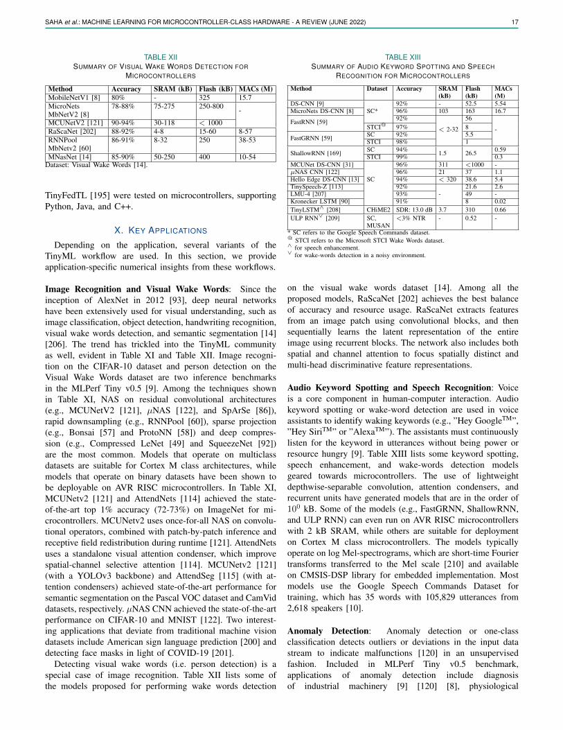
SAHA et al.: MACHINE LEARNING FOR MICROCONTROLLER-CLASS HARDWARE - A REVIEW (JUNE 2022) 17
TABLE XIISUMMARY OF VISUAL WAKE WORDS DETECTION FOR
MICROCONTROLLERS
Method Accuracy SRAM (kB) Flash (kB) MACs (M)MobileNetV1 [8] 80% - 325 15.7MicroNetsMbNetV2 [8]
78-88% 75-275 250-800 -
MCUNetV2 [121] 90-94% 30-118 < 1000RaScaNet [202] 88-92% 4-8 15-60 8-57RNNPoolMbNetv2 [60]
86-91% 8-32 250 38-53
MNasNet [14] 85-90% 50-250 400 10-54Dataset: Visual Wake Words [14].
TinyFedTL [195] were tested on microcontrollers, supportingPython, Java, and C++.
X. KEY APPLICATIONS
Depending on the application, several variants of theTinyML workflow are used. In this section, we provideapplication-specific numerical insights from these workflows.
Image Recognition and Visual Wake Words: Since theinception of AlexNet in 2012 [93], deep neural networkshave been extensively used for visual understanding, such asimage classification, object detection, handwriting recognition,visual wake words detection, and semantic segmentation [14][206]. The trend has trickled into the TinyML communityas well, evident in Table XI and Table XII. Image recogni-tion on the CIFAR-10 dataset and person detection on theVisual Wake Words dataset are two inference benchmarksin the MLPerf Tiny v0.5 [9]. Among the techniques shownin Table XI, NAS on residual convolutional architectures(e.g., MCUNetV2 [121], µNAS [122], and SpArSe [86]),rapid downsampling (e.g., RNNPool [60]), sparse projection(e.g., Bonsai [57] and ProtoNN [58]) and deep compres-sion (e.g., Compressed LeNet [49] and SqueezeNet [92])are the most common. Models that operate on multiclassdatasets are suitable for Cortex M class architectures, whilemodels that operate on binary datasets have been shown tobe deployable on AVR RISC microcontrollers. In Table XI,MCUNetv2 [121] and AttendNets [114] achieved the state-of-the-art top 1% accuracy (72-73%) on ImageNet for mi-crocontrollers. MCUNetv2 uses once-for-all NAS on convolu-tional operators, combined with patch-by-patch inference andreceptive field redistribution during runtime [121]. AttendNetsuses a standalone visual attention condenser, which improvespatial-channel selective attention [114]. MCUNetv2 [121](with a YOLOv3 backbone) and AttendSeg [115] (with at-tention condensers) achieved state-of-the-art performance forsemantic segmentation on the Pascal VOC dataset and CamViddatasets, respectively. µNAS CNN achieved the state-of-the-artperformance on CIFAR-10 and MNIST [122]. Two interest-ing applications that deviate from traditional machine visiondatasets include American sign language prediction [200] anddetecting face masks in light of COVID-19 [201].
Detecting visual wake words (i.e. person detection) is aspecial case of image recognition. Table XII lists some ofthe models proposed for performing wake words detection
TABLE XIIISUMMARY OF AUDIO KEYWORD SPOTTING AND SPEECH
RECOGNITION FOR MICROCONTROLLERS
Method Dataset Accuracy SRAM(kB)
Flash(kB)
MACs(M)
DS-CNN [9]SC*
92% - 52.5 5.54MicroNets DS-CNN [8] 96% 103 163 16.7
FastRNN [59] 92%
< 2-32
56
-STCI@ 97% 8
FastGRNN [59] SC 92% 5.5STCI 98% 1
ShallowRNN [169] SC 94% 1.5 26.5 0.59STCI 99% 0.3
MCUNet DS-CNN [31]
SC
96% 311 <1000 -µNAS CNN [122] 96% 21 37 1.1Hello Edge DS-CNN [13] 94% < 320 38.6 5.4TinySpeech-Z [113] 92%
-21.6 2.6
LMU-4 [207] 93% 49 -Kronecker LSTM [90] 91% 8 0.02TinyLSTM∧ [208] CHiME2 SDR: 13.0 dB 3.7 310 0.66ULP RNN∨ [209] SC,
MUSAN<3% NTR - 0.52 -
* SC refers to the Google Speech Commands dataset.@ STCI refers to the Microsoft STCI Wake Words dataset.∧ for speech enhancement.∨ for wake-words detection in a noisy environment.
on the visual wake words dataset [14]. Among all theproposed models, RaScaNet [202] achieves the best balanceof accuracy and resource usage. RaScaNet extracts featuresfrom an image patch using convolutional blocks, and thensequentially learns the latent representation of the entireimage using recurrent blocks. The network also includes bothspatial and channel attention to focus spatially distinct andmulti-head discriminative feature representations.
Audio Keyword Spotting and Speech Recognition: Voiceis a core component in human-computer interaction. Audiokeyword spotting or wake-word detection are used in voiceassistants to identify waking keywords (e.g., ”Hey GoogleTM”,”Hey SiriTM” or ”AlexaTM”). The assistants must continuouslylisten for the keyword in utterances without being power orresource hungry [9]. Table XIII lists some keyword spotting,speech enhancement, and wake-words detection modelsgeared towards microcontrollers. The use of lightweightdepthwise-separable convolution, attention condensers, andrecurrent units have generated models that are in the order of100 kB. Some of the models (e.g., FastGRNN, ShallowRNN,and ULP RNN) can even run on AVR RISC microcontrollerswith 2 kB SRAM, while others are suitable for deploymenton Cortex M class microcontrollers. The models typicallyoperate on log Mel-spectrograms, which are short-time Fouriertransforms transferred to the Mel scale [210] and availableon CMSIS-DSP library for embedded implementation. Mostmodels use the Google Speech Commands Dataset fortraining, which has 35 words with 105,829 utterances from2,618 speakers [10].
Anomaly Detection: Anomaly detection or one-classclassification detects outliers or deviations in the input datastream to indicate malfunctions [120] in an unsupervisedfashion. Included in MLPerf Tiny v0.5 benchmark,applications of anomaly detection include diagnosisof industrial machinery [9] [120] [8], physiological
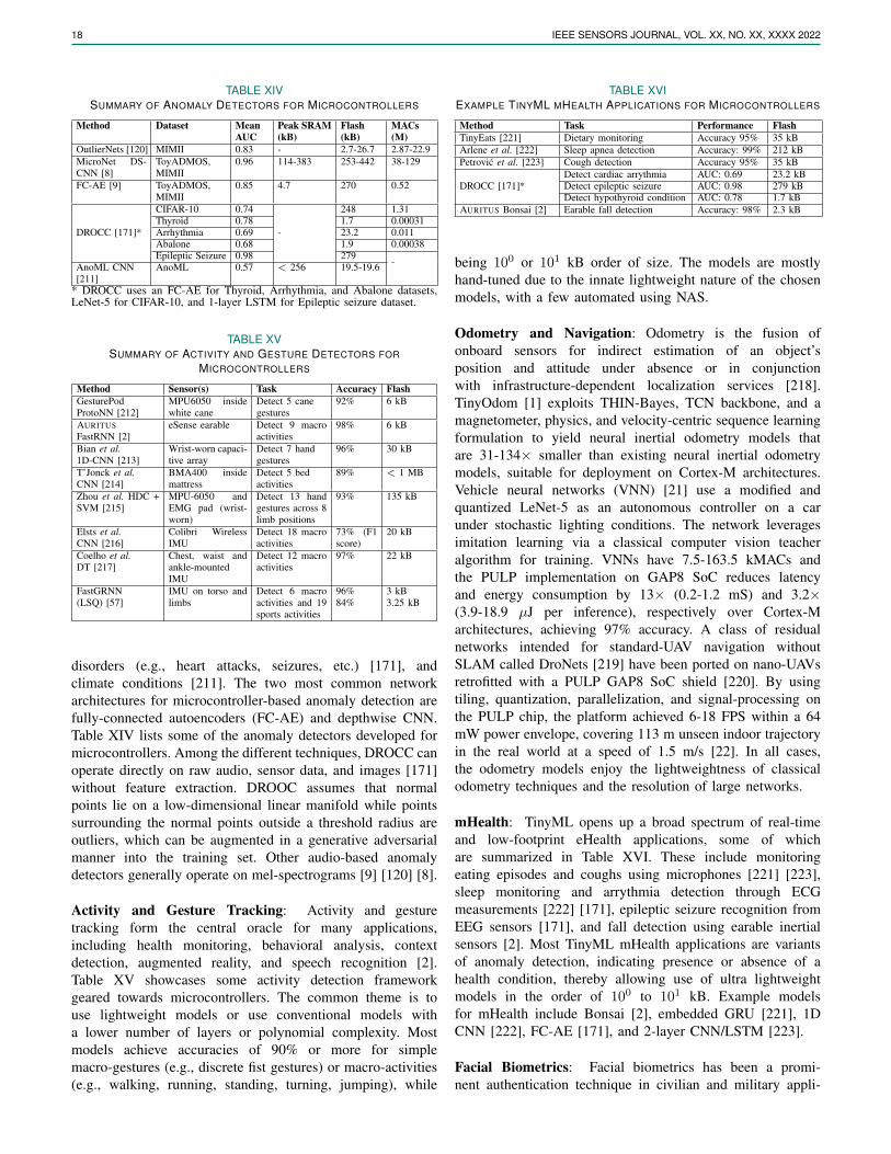
18 IEEE SENSORS JOURNAL, VOL. XX, NO. XX, XXXX 2022
TABLE XIVSUMMARY OF ANOMALY DETECTORS FOR MICROCONTROLLERS
Method Dataset MeanAUC
Peak SRAM(kB)
Flash(kB)
MACs(M)
OutlierNets [120] MIMII 0.83 - 2.7-26.7 2.87-22.9MicroNet DS-CNN [8]
ToyADMOS,MIMII
0.96 114-383 253-442 38-129
FC-AE [9] ToyADMOS,MIMII
0.85 4.7 270 0.52
DROCC [171]*
CIFAR-10 0.74
-
248 1.31Thyroid 0.78 1.7 0.00031Arrhythmia 0.69 23.2 0.011Abalone 0.68 1.9 0.00038Epileptic Seizure 0.98 279 -AnoML CNN
[211]AnoML 0.57 < 256 19.5-19.6
* DROCC uses an FC-AE for Thyroid, Arrhythmia, and Abalone datasets,LeNet-5 for CIFAR-10, and 1-layer LSTM for Epileptic seizure dataset.
TABLE XVSUMMARY OF ACTIVITY AND GESTURE DETECTORS FOR
MICROCONTROLLERS
Method Sensor(s) Task Accuracy FlashGesturePodProtoNN [212]
MPU6050 insidewhite cane
Detect 5 canegestures
92% 6 kB
AURITUSFastRNN [2]
eSense earable Detect 9 macroactivities
98% 6 kB
Bian et al.1D-CNN [213]
Wrist-worn capaci-tive array
Detect 7 handgestures
96% 30 kB
T’Jonck et al.CNN [214]
BMA400 insidemattress
Detect 5 bedactivities
89% < 1 MB
Zhou et al. HDC +SVM [215]
MPU-6050 andEMG pad (wrist-worn)
Detect 13 handgestures across 8limb positions
93% 135 kB
Elsts et al.CNN [216]
Colibri WirelessIMU
Detect 18 macroactivities
73% (F1score)
20 kB
Coelho et al.DT [217]
Chest, waist andankle-mountedIMU
Detect 12 macroactivities
97% 22 kB
FastGRNN(LSQ) [57]
IMU on torso andlimbs
Detect 6 macroactivities and 19sports activities
96%84%
3 kB3.25 kB
disorders (e.g., heart attacks, seizures, etc.) [171], andclimate conditions [211]. The two most common networkarchitectures for microcontroller-based anomaly detection arefully-connected autoencoders (FC-AE) and depthwise CNN.Table XIV lists some of the anomaly detectors developed formicrocontrollers. Among the different techniques, DROCC canoperate directly on raw audio, sensor data, and images [171]without feature extraction. DROOC assumes that normalpoints lie on a low-dimensional linear manifold while pointssurrounding the normal points outside a threshold radius areoutliers, which can be augmented in a generative adversarialmanner into the training set. Other audio-based anomalydetectors generally operate on mel-spectrograms [9] [120] [8].
Activity and Gesture Tracking: Activity and gesturetracking form the central oracle for many applications,including health monitoring, behavioral analysis, contextdetection, augmented reality, and speech recognition [2].Table XV showcases some activity detection frameworkgeared towards microcontrollers. The common theme is touse lightweight models or use conventional models witha lower number of layers or polynomial complexity. Mostmodels achieve accuracies of 90% or more for simplemacro-gestures (e.g., discrete fist gestures) or macro-activities(e.g., walking, running, standing, turning, jumping), while
TABLE XVIEXAMPLE TINYML MHEALTH APPLICATIONS FOR MICROCONTROLLERS
Method Task Performance FlashTinyEats [221] Dietary monitoring Accuracy 95% 35 kBArlene et al. [222] Sleep apnea detection Accuracy: 99% 212 kBPetrovic et al. [223] Cough detection Accuracy 95% 35 kB
DROCC [171]*Detect cardiac arrythmia AUC: 0.69 23.2 kBDetect epileptic seizure AUC: 0.98 279 kBDetect hypothyroid condition AUC: 0.78 1.7 kB
AURITUS Bonsai [2] Earable fall detection Accuracy: 98% 2.3 kB
being 100 or 101 kB order of size. The models are mostlyhand-tuned due to the innate lightweight nature of the chosenmodels, with a few automated using NAS.
Odometry and Navigation: Odometry is the fusion ofonboard sensors for indirect estimation of an object’sposition and attitude under absence or in conjunctionwith infrastructure-dependent localization services [218].TinyOdom [1] exploits THIN-Bayes, TCN backbone, and amagnetometer, physics, and velocity-centric sequence learningformulation to yield neural inertial odometry models thatare 31-134× smaller than existing neural inertial odometrymodels, suitable for deployment on Cortex-M architectures.Vehicle neural networks (VNN) [21] use a modified andquantized LeNet-5 as an autonomous controller on a carunder stochastic lighting conditions. The network leveragesimitation learning via a classical computer vision teacheralgorithm for training. VNNs have 7.5-163.5 kMACs andthe PULP implementation on GAP8 SoC reduces latencyand energy consumption by 13× (0.2-1.2 mS) and 3.2×(3.9-18.9 µJ per inference), respectively over Cortex-Marchitectures, achieving 97% accuracy. A class of residualnetworks intended for standard-UAV navigation withoutSLAM called DroNets [219] have been ported on nano-UAVsretrofitted with a PULP GAP8 SoC shield [220]. By usingtiling, quantization, parallelization, and signal-processing onthe PULP chip, the platform achieved 6-18 FPS within a 64mW power envelope, covering 113 m unseen indoor trajectoryin the real world at a speed of 1.5 m/s [22]. In all cases,the odometry models enjoy the lightweightness of classicalodometry techniques and the resolution of large networks.
mHealth: TinyML opens up a broad spectrum of real-timeand low-footprint eHealth applications, some of whichare summarized in Table XVI. These include monitoringeating episodes and coughs using microphones [221] [223],sleep monitoring and arrythmia detection through ECGmeasurements [222] [171], epileptic seizure recognition fromEEG sensors [171], and fall detection using earable inertialsensors [2]. Most TinyML mHealth applications are variantsof anomaly detection, indicating presence or absence of ahealth condition, thereby allowing use of ultra lightweightmodels in the order of 100 to 101 kB. Example modelsfor mHealth include Bonsai [2], embedded GRU [221], 1DCNN [222], FC-AE [171], and 2-layer CNN/LSTM [223].
Facial Biometrics: Facial biometrics has been a promi-nent authentication technique in civilian and military appli-

SAHA et al.: MACHINE LEARNING FOR MICROCONTROLLER-CLASS HARDWARE - A REVIEW (JUNE 2022) 19
TABLE XVIISUMMARY OF FACE DETECTORS FOR MICROCONTROLLERS
Method Dataset Performance Peak SRAM MACsFaceReID [224] VGGFace2 Accuracy: 0.97 352 kB 85MBatteryless FaceDetection [25]
CelebA Accuracy: 0.97 384 kB -
EagleEye [225] WIDER FACE mAP∗: 0.77 1170 kB 80MRNNPoolS3FD [60]
WIDER FACE mAP∗: 0.83 225 kB 120M
MCUNetv2S3FD [121]
WIDER FACE mAP∗: 0.89 672 kB 110M
* mean average precision for ≤3 faces
cations [226]. Existing face detectors use deep-learning toautomate the feature representation pipeline while approachinghuman performance [226]. Table XVII illustrates some facedetectors for microcontrollers. A common recipe for portingdeep face detectors onto microcontrollers includes the useof lightweight spatial convolution coupled with NAS, quan-tization, and inference engine optimizations. Typical neuralblocks include squeeze and excitation modules [224], cou-pling depthwise with pointwise convolution [225], and non-linear pooling between convolutional layers [60]. Successiveand rapid downsampling helps cut out redundant networklayers further [60] [225] while ensuring scale-equitable facedetection. Inference engine optimizations include patch-basedinference scheduling [121], receptive field redistribution [121],and dual memory management [224]. Patch-by-patch inferenceallows operation on only a tiny region of the activation map,while receptive field redistribution shifts receptive field andFLOPS to later stages to mitigate peak memory usage andoverlapping patches [121]. Dual memory management swapsvariables between flash and RAM whenever required [224].
XI. DISCUSSION AND CASE STUDIES
In this section, we break down the end-to-end workflowand provide quantitative analysis of individual aspects ofthe workflow based on select examples from Section IV toSection X. We discuss how individual aspects contribute tothe overall execution, and also describe qualitatively howindividual techniques for one aspect impact the choices forother aspects.
Feature Projection vs. No Feature Projection: Featureprojection allows a domain expert to retain data variance whilereducing data dimensionality [2]. Intuitively, this reducesthe model complexity needed to capture the variations ininput data, i.e., feature projection is useful for simplifyingthe architecture of non-TinyML models. Consider thegesture recognition example in Table XVIII. Both CNNand the MLP achieve the same accuracy. However, theMLP pipeline, operating on spectral features, requires 2.5×less flash, runs 2.2× faster, and requires 18× less SRAMthan the CNN pipeline, which operates on raw data. Byleveraging domain knowledge, simpler models can achievethe same accuracy, yet save memory and inference costsover complex models. Well-designed features (e.g., audioMFCC, spectrograms, and signal power) are also able toexploit DSP functions (e.g. CMSIS-DSP) and accelerators
TABLE XVIIIIMPACT OF FEATURE PROJECTION VS. RAW DATA INFERENCE
Application Method Accuracy Latency/MAC
Flash
Gesture Recognition∨CNN [32] 100% 11 mS 45.3 kBMLP [32] 100% 5 mS 17.8 kB
Human ActivityRecognition@
TCN [2] 94.6% 7.52M 52.8kBFastGRNN [2] 97.6% - 13.1 kBBonsai [2] 80.3% 0.0136M 14.8 kB
Anomaly Detection* DROCC [171] F1 - 68% 0.00038M 1.9kBOC-SVM [171] F1 - 48% - 2.99 MB
∨: Device: Cortex M7* Dataset: Abalone, @ Dataset: AURITUS
Models operating on features
embedded in most microcontrollers [6]. However, if theextracted features are not sufficiently discriminatory due to alack of domain knowledge, then the performance of modelswill degrade [227]. Consider the human activity recognitionexample in Table XVIII. Bonsai operates on five statisticalfeatures surrounding the signal amplitude, which are unableto sufficiently distinguish among activity primitives thatare statistically similar (e.g., sitting and sleeping). Thus,Bonsai suffers a 17% accuracy drop while being similar insize to FastGRNN. To achieve the performance of complexmodels that do not operate on features while having thecomputational efficiency of simple models operating onhandcrafted features, ultra-lightweight ML blocks are used.These blocks can often be much more efficient and accuratethan models tied to a feature extraction pipeline, as poorlydesigned features can yield significant compute overhead [2].For example, in Table XVIII, DROCC outperforms one-classSVM for anomaly detection not only in accuracy (+20% gain)but also in model size (1600× reduction). Unfortunately, theproblem with lightweight models is two-fold. Firstly, mostof these models do not have enough parameters to modelglobally significant features, failing to generalize to new datadistributions in the field [2]. Secondly, most NAS frameworks,TinyML software suites, intermittent computing tools, andonline learning frameworks lack support for deploying someof these models on commodity microcontrollers. Therefore,adopting feature extraction requires careful understanding ofthe application constraints, striking a balance between theavailability of domain knowledge, feasible model architecturesets, feature acceleration support, and support from modeloptimization and architecture search tools.
Compression vs. No Compression: Exploiting sparsity andreducing bitwidth of models depends on three key factors:
(i) Large-Sparse vs. Small-Dense: Large-sparse models(compressed and vanilla models) are known to outperformsmall-dense models (uncompressed and lightweight models)for a broad range of network architectures [48] in termsof compression ratio for comparable accuracy. This isevident from the speech commands and MNIST-10 examplesin Table XIX. LSTM-Prune and LSTM-KP outperformFastGRNN and Bonsai, providing on average 12× modelsize reduction with only 2.3% accuracy loss. Moreover,on average, all uncompressed and vanilla models provided
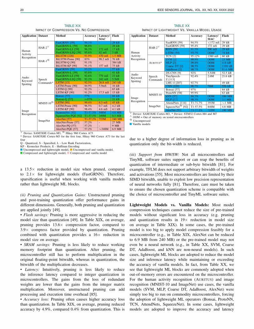
20 IEEE SENSORS JOURNAL, VOL. XX, NO. XX, XXXX 2022
TABLE XIXIMPACT OF COMPRESSION VS. NO COMPRESSION
Application Dataset Method Accuracy Latency/MAC
Flash
HumanActivityRecognition
HAR-2∨FastGRNN [59] 94.5% - 29 kBFastGRNN-L [59] 96.8% - 28 kBFastGRNN-LS [59] 96.3% 172 mS 17 kBFastGRNN-LSQ [59] 95.6% 62 mS 3 kB
HAR-1@BiLSTM [228] 91.9% 470 mS 1.5 MBBiLSTM-Prune [90] 83% 98.2 mS 76 kBBiLSTM-Q [90] 91.1% - 384 kBBiLSTM-KP [90] 91.1% 157 mS 75 kB
AudioKeywordSpotting
SpeechCommands*
FastGRNN [59] 93.2% - 57 kBFastGRNN-L [59] 93.8% - 41 kBFastGRNN-LS [59] 92.6% 779 mS 22 kBFastGRNN-LSQ [59] 92.2% 242 mS 5.5kBLSTM [13] 92.5% 26.8 mS 243 kBLSTM-Prune [90] 84.9% 5.9mS 16 kBLSTM-Q [90] 92.2% - 65 kBLSTM-KP [90] 91.2% 17.5 mS 15 kB
ImageRecognition
MNIST-10@
Bonsai [57] 97% - 84 kBBonsai-Q [57] ∼97% - 21 kBLSTM [90] 99.4% 6.3 mS 45 kBLSTM-Prune [90] 96.5% 0.7 mS 4.2 kBLSTM-KP [90] 98.4% 4.6 mS 4.1 kB
ImageNet
SqueezeNet [92] T1-57.5% 848M 4.8 MBSqueezeNet-PQE [92] T1-57.5% 349M 0.5 MBAlexNet [57] T1-57.2% 723M 240 MBAlexNet-Prune [57] 57.2% - 27 MBAlexNet-PQ [57] 57.2% - 9 MBAlexNet-PQE [57] 57.2% ∼348M 6.9 MB
∨ Device: SAM3X8E Cortex-M3, @ Hikey 960 Cortex A73* Device: SAM3X8E Cortex-M3 for the first four, Hikey 960 Cortex A73 for the lastfourQ - Quantized, S - Sparsified, L - Low Rank Factorization,KP - Kronecker Products, E - Huffman Encoding
Uncompressed and lightweight model, Uncompressed and vanilla model,Compressed and lightweight model, Compressed and vanilla model
a 13.5× reduction in model size when pruned, comparedto 2.1× for lightweight models (FastGRNN). Therefore,sparsification is useful when working with vanilla modelsrather than lightweight ML blocks.
(ii) Pruning and Quantization Gains: Unstructured pruningand post-training quantization offer performance gains indifferent dimensions. Generally, both pruning and quantizationare applied jointly [49].• Flash savings: Pruning is more aggressive in reducing themodel size than quantization [49]. In Table XIX, on average,pruning provides 13.6× compression factor, compared to3.9× compress factor provided by quantization. Pruningcombined with quantization provides a 16× reduction inmodel size on average.• SRAM savings: Pruning is less likely to reduce workingmemory footprint than quantization. After pruning, themicrocontroller still has to perform multiplication in theoriginal floating-point bitwidth, whereas in quantization, thebitwidth of the multiplication decreases.• Latency: Intuitively, pruning is less likely to reducethe inference latency compared to integer quantization inmicrocontrollers. The gains from the loss of redundantweights are lower than the gains from the integer matrixmultiplication. Moreover, unstructured pruning can addprocessing and execution time overhead [85].• Accuracy loss: Pruning often causes higher accuracy lossthan quantization. In Table XIX, on average, pruning reducedaccuracy by 4.9%, compared 0.4% from quantization. This is
TABLE XXIMPACT OF LIGHTWEIGHT VS. VANILLA MODEL USAGE
Application Dataset Method Accuracy Latency/MAC
Flash
HumanActivityRecognition
HAR-2∨FastRNN [59] 94.5% <172 mS 29 kBFastGRNN [59] 95.4% 172 mS 29 kBRNN [59] 91.3% 590 mS 29 kBLSTM [59] 93.7% OOM∧ 74 kB
AURITUS*
TCN [2] 95.12% 1380 mS 60 kBSVM [2] 99.9% OOM 23 MBMLP [2] 99.8% OOM 418 kBCoarse DT [2] 98.5% OOM 1100 kBAdaBoost [2] 98.7% OOM 81.6 MB
AudioKeywordSpotting
SpeechCommands
DS-CNN [9] 92% 5.54M 52.5 kBTinySpeech-Z [113]
92.4% 2.6M 21.6 kB
LMU-4 [207] 92.7% - 49 kBCNN [229] 90.7% 76M 556 kB
ImageRecognition
MNIST-10
Bonsai [57] 97% - 84 kBProtoNN [58] 95.9% 63 kBkNN [57] 94.3% OOM 184 MBMLP [57] 98.3% OOM 3.1 MB
ImageNetAttendNets [114] T1-71.7% 191M ∼1 MBSqueezeNet@ [92] T1-57.5% 848M 4.8 MBAlexNet [93] T1-57.2% 723M 240 MB
∨ Device: SAM3X8E Cortex-M3, * Device: STM32 Cortex-M4 and M7∧ OOM = Out of memory on tested microcontrollers@ Uncompressed
Vanilla models
due to a higher degree of information loss in pruning as inquantization only the bit-width is reduced.
(iii) Support from HW/SW: Not all microcontrollers andTinyML software suites support or can reap the benefits ofquantization of intermediate or sub-byte bitwidth [81]. Forexample, TFLM does not support arbitrary bitwidth of weightsand activations [55]. Most microcontrollers are limited by theirSIMD bitwidth, unable to exploit low precision representationof neural networks fully [81]. Therefore, care must be takento ensure the chosen quantization scheme is compatible withthe choice of microcontroller and TinyML software suites.
Lightweight Models vs. Vanilla Models: Most modelcompression techniques cannot reduce the size of pre-trainedmodels without significant loss in accuracy (e.g. pruningand quantization results in 19× reduction in model sizeon average in Table XIX). In some cases, the pre-trainedmodel is too big to apply model compression feasibly for amicrocontroller (e.g., in Table XIX, AlexNet can be reducedto 6.9 MB from 240 MB) or the pre-trained model may noteven be a neural network (e.g., in Table XX, SVM, CoarseDT, AdaBoost, and kNN are non-neural models). In suchcases, lightweight ML blocks are adopted to reduce the modelsize and inference latency while maintaining or exceedingthe accuracy of vanilla models. In fact, from Table XX, wesee that lightweight ML blocks are commonly adopted whenout-of-memory errors are encountered on the microcontroller.For the human activity recognition (AURITUS) and imagerecognition (MNIST-10 and ImageNet) use cases, the vanillamodels (SVM, MLP, Coarse DT, AdaBoost, AlexNet) weresimply too big to run on commodity microcontrollers, forcingthe adoption of lightweight ML operators (Bonsai, ProtoNN,TCN, AttendNets, SqueezeNet). In some cases, lightweightmodels are adopted to improve the accuracy and latency
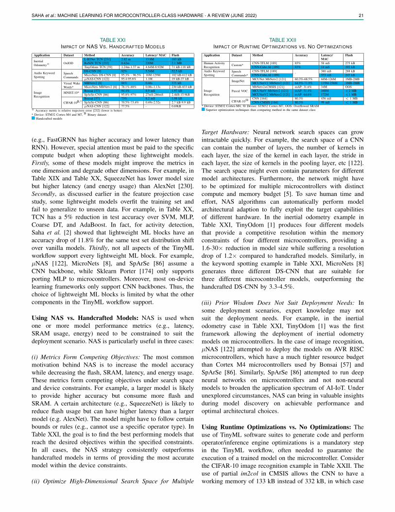
SAHA et al.: MACHINE LEARNING FOR MICROCONTROLLER-CLASS HARDWARE - A REVIEW (JUNE 2022) 21
TABLE XXIIMPACT OF NAS VS. HANDCRAFTED MODELS
Application Dataset Method Accuracy Latency/ MAC Flash
InertialOdometry◦ OxIOD
L-IONet TCN [231] 2.82 m 13.9M 183 kBRoNiN TCN [232] 0.42m 220M 2.1 MBTinyOdom TCN [59] 1.24m-1.37 m 4.64M-8.92M 71 kB-118 kB
Audio KeywordSpotting
SpeechCommands
DS-CNN [9] 92% 5.54M 52.5 kBMicroNets DS-CNN [8] 95.3% - 96.5% 16M-129M 102 kB-612 kBµNAS-CNN [122] 95.4-95.6% 1.1M 19 kB-37 kB
ImageRecognition
Visual WakeWords*
MBNetv2 [8] 86% 0.46s 375 kBMicroNets MBNetv2 [8] 78.1%-88% 0.08s-1.13s 230 kB-833 kB
MNIST-10* Bonsai [57] 94.4% 8.9 mS 1.97 kBSpArSe-CNN [86] 95.8%-97% 27mS-286mS 2.4kB-15.9kB
CIFAR-10B,*Bonsai [57] 73% 8.2 mS 1.98 kBSpArSe-CNN [86] 70.5%-73.4% 0.49s-2.52s 2.7 kB-9.9 kBµNAS-CNN [122] 77.5% - 0.69kB
◦ Accuracy metric is relative trajectory error [232] (lower is better)* Device: STM32 Cortex-M4 and M7, B Binary dataset
Handcrafted models
(e.g., FastGRNN has higher accuracy and lower latency thanRNN). However, special attention must be paid to the specificcompute budget when adopting these lightweight models.Firstly, some of these models might improve the metrics inone dimension and degrade other dimensions. For example, inTable XIX and Table XX, SqueezeNet has lower model sizebut higher latency (and energy usage) than AlexNet [230].Secondly, as discussed earlier in the feature projection casestudy, some lightweight models overfit the training set andfail to generalize to unseen data. For example, in Table XX,TCN has a 5% reduction in test accuracy over SVM, MLP,Coarse DT, and AdaBoost. In fact, for activity detection,Saha et al. [2] showed that lightweight ML blocks have anaccuracy drop of 11.8% for the same test set distribution shiftover vanilla models. Thirdly, not all aspects of the TinyMLworkflow support every lightweight ML block. For example,µNAS [122], MicroNets [8], and SpArSe [86] assume aCNN backbone, while Sklearn Porter [174] only supportsporting MLP to microcontrollers. Moreover, most on-devicelearning frameworks only support CNN backbones. Thus, thechoice of lightweight ML blocks is limited by what the othercomponents in the TinyML workflow support.
Using NAS vs. Handcrafted Models: NAS is used whenone or more model performance metrics (e.g., latency,SRAM usage, energy) need to be constrained to suit thedeployment scenario. NAS is particularly useful in three cases:
(i) Metrics Form Competing Objectives: The most commonmotivation behind NAS is to increase the model accuracywhile decreasing the flash, SRAM, latency, and energy usage.These metrics form competing objectives under search spaceand device constraints. For example, a larger model is likelyto provide higher accuracy but consume more flash andSRAM. A certain architecture (e.g., SqueezeNet) is likely toreduce flash usage but can have higher latency than a largermodel (e.g. AlexNet). The model might have to follow certainbounds or rules (e.g., cannot use a specific operator type). InTable XXI, the goal is to find the best performing models thatreach the desired objectives within the specified constraints.In all cases, the NAS strategy consistently outperformshandcrafted models in terms of providing the most accuratemodel within the device constraints.
(ii) Optimize High-Dimensional Search Space for Multiple
TABLE XXIIIMPACT OF RUNTIME OPTIMIZATIONS VS. NO OPTIMIZATIONS
Application Dataset Method Accuracy Latency/MAC
Flash
Human ActivityRecognition Custom* CNN-TFLM [189] 85% 58 mS 275 kB
CNN-Cube.AI [189] 85% 14 mS 192 kBAudio KeywordSpotting
SpeechCommands*
CNN-TFLM [189] - 380 mS 288 kBCNN-Cube.AI [189] 373 mS 247 kB
ImageRecognition
ImageNet MCUNet MbNetv2 [121] 60.3%-68.5% 68M-126M 1MB-2MBMCUNetV2 MbNetv2 [121] 64.9%-71.8% 119M-256M 1MB-2MB
Pascal VOCMbNetv2+CMSIS [121] mAP: 31.6% 34M OOSMCUNetV MbNetv2 [121] mAP: 51.4% 168M <2 MBMCUNetV2 MbNetv2 [121] mAP: 64.6% 172M <1 MB
CIFAR-10@CNN [164] 80.3% 456 mS < 1 MBCNN-CMSIS [164] 80.3% 99 mS < 1 MB
* Device: STM32 Cortex-M4, @ Device: STM32 Cortex-M7, OOS: Overflowed SRAMSuperior optimization techniques than comparing method in the same dataset class
Target Hardware: Neural network search spaces can growintractable quickly. For example, the search space of a CNNcan contain the number of layers, the number of kernels ineach layer, the size of the kernel in each layer, the stride ineach layer, the size of kernels in the pooling layer, etc [122].The search space might even contain parameters for differentmodel architectures. Furthermore, the network might haveto be optimized for multiple microcontrollers with distinctcompute and memory budget [5]. To save human time andeffort, NAS algorithms can automatically perform modelarchitectural adaption to fully exploit the target capabilitiesof different hardware. In the inertial odometry example inTable XXI, TinyOdom [1] produces four different modelsthat provide a competitive resolution within the memoryconstraints of four different microcontrollers, providing a1.6-30× reduction in model size while suffering a resolutiondrop of 1.2× compared to handcrafted models. Similarly, inthe keyword spotting example in Table XXI, MicroNets [8]generates three different DS-CNN that are suitable forthree different microcontroller models, outperforming thehandcrafted DS-CNN by 3.3-4.5%.
(iii) Prior Wisdom Does Not Suit Deployment Needs: Insome deployment scenarios, expert knowledge may notsuit the deployment needs. For example, in the inertialodometry case in Table XXI, TinyOdom [1] was the firstframework allowing the deployment of inertial odometrymodels on microcontrollers. In the case of image recognition,µNAS [122] attempted to deploy the models on AVR RISCmicrocontrollers, which have a much tighter resource budgetthan Cortex M4 microcontrollers used by Bonsai [57] andSpArSe [86]. Similarly, SpArSe [86] attempted to run deepneural networks on microcontrollers and not non-neuralmodels to broaden the application spectrum of AI-IoT. Underunexplored circumstances, NAS can bring in valuable insightsduring model discovery on achievable performance andoptimal architectural choices.
Using Runtime Optimizations vs. No Optimizations: Theuse of TinyML software suites to generate code and performoperator/inference engine optimizations is a mandatory stepin the TinyML workflow, often needed to guarantee theexecution of a trained model on the microcontroller. Considerthe CIFAR-10 image recognition example in Table XXII. Theuse of partial im2col in CMSIS allows the CNN to have aworking memory of 133 kB instead of 332 kB, in which case

22 IEEE SENSORS JOURNAL, VOL. XX, NO. XX, XXXX 2022
TABLE XXIIIIMPACT OF ONLINE LEARNING VS. STATIC MODELS
Application Dataset Method Accuracy Latency
ImageRecognition*
MNIST-10 CNN [183] 10%-82%
-CNN (LW) [183] 65%-98%
CIFAR-10 CNN [183] 12%-38%CNN (LW) [183] 55%-68%
AnomalyDetection @ Custom Autoencoder [184] 75% 1.75 mS
Autoencoder(TinyOL) [184]
100% 1.92 mS
* Device: TI MSP430@ Signal reconstruction error, Device: nRF52840 Cortex-M
No online learning
the CNN would overflow the Cortex-M7 SRAM [164]. Theoptimized operator set also reduces the inference latency by4.6× and decreases energy usage by 4.9× [164]. Similarly,MCUNetv2 [121] achieved record ImageNet and Pascal VOCaccuracy on microcontrollers by optimizing a large MBNetv2that normally overflows the SRAM using patch-by-patch in-ference and receptive field redistribution. However, to pick theappropriate software suite, other questions must be asked.
1) Which microcontrollers are suitable for my application?2) What are the memory, latency, and energy requirements?3) Which ML blocks are suitable for my application?4) Which training frameworks can I use?5) Do I need support for intermittent computing?6) Do I need support for online learning?7) Do I need an automated schedule explorer?8) Is dynamic memory management necessary?9) How many models need to run on the same platform?
10) Do I need to share the same model across platforms?11) Do I need to sparsify or quantize any model?
Consider the human activity recognition and keyword spottinguse case in Table XXII. TFLM uses an interpreter-basedapproach to realize the model graph during runtime [167].TFLM supports dynamic memory management {7)},multitenancy {8)}, and updating the model binaries ratherthan the entire codebase for fast prototyping and portabilityacross platforms {9)}. However, {7)}, {8)} and {9)} comeat 1.3× increase in flash usage and 2.6× increase in latency(lagging on {2)}) compared to STM32Cube.AI, whichembeds operator function calls into native C code [172].STM32Cube.AI, on the other hand, only supports STM32series of Cortex-M microcontrollers (lagging on {1)}),while TFLM provides much broader platform support.However, STM32Cube.AI also supports non-neural modeldeployment (e.g., k-means, SVM, RF, kNN, DT, etc.), whileTFLM only supports neural network deployment (lagging on{3)}). Likewise, {5)} can only be realized through SONIC,TAILS [24], and {7)} is provided by only micro-TVM [130].Both quantitative and qualitative tradeoffs similar to thecase study here must be performed to pick the appropriatesoftware suite.
Using Online Learning vs. Static Models: Online learningimproves the performance of the model by adapting the modelon board without sensitive data leaving the device. Considerthe case studies on online learning shown in Table XXIII. The
performance of models improves by 34% when on-devicetraining is used to adapt to dataset shifts. For TinyOL, thelatency overhead to include online learning is 10%. Whilethe performance gains are somewhat transparent, the majorbarrier in on-device learning is the lack of support from otheraspects of the workflow. For example, most on-device learningframeworks assume the use of CNN or binary classifiers andalso use a custom code generator for the model due to a lackof online learning support from existing TinyML softwaresuites. Moreover, it is not clear how NAS should accountfor the training memory and inference overheads whenon-device learning is used. The lack of comprehensive studiesof on-device learning also limits the adoption of federatedlearning in TinyML. Particularly, while the TinyML workflowwas designed for a single non-collaborative model, federatedlearning requires the distribution of a global model to beenhanced via local model updates. While existing federatedlearning frameworks have tools to distribute resourcesheterogeneously, it is unclear how NAS, model compression,or lightweight ML blocks affect the real-world setting, asnone of the federated learning frameworks have studiedthese effects. Thereby, online learning constrains the userto a very specific choice of models and custom software suites.
XII. CHALLENGES AND OPPORTUNITIES
The first-generation efforts in TinyML focused on theengineering and mechanics of squeezing ML models withinthe limited memory, compute, and power bounds of amicrocontroller. Both academia and industry have establishedseveral TinyML software frameworks to streamline thedeployment of ML models for microcontrollers. Many of theissues raised by prior surveys [3] [4] [6] have been addressed.However, the following new challenges are emerging thatrequire further research.
Application Specific Safety and Heuristic Requirements:Real-world IoT applications operate within certain bounds,correlations, and heuristic rules set forth by the operatingdomain and system physics. For example, a UAV cannotexceed a certain bank angle without compromisingstability [233]. In complex event processing, specificgranular action primitives (e.g., cooking a dish) must alwaysprecede other primitives (e.g., chopping vegetables) [234].Neural networks cannot assure that the learned distributionsobey all the laws [235]. As a result. recent neural networkpipelines are being injected with trainable neuro-symbolicreasoning [236] [237], signal temporal logic [235], andphysics-aware embeddings [238] [239] [240] [241] for robustcomplex event processing within the laws and bounds ofphysics. For making rich and complex inferences beyondbinary classification, the TinyML workflow requires researchto combine data and human knowledge by including logicalreasoning modules within the microcontroller’s compute andmemory bounds.
Data Quality and Uncertainty Awareness: Sensor datain the wild suffers from missing data, cross-channel

SAHA et al.: MACHINE LEARNING FOR MICROCONTROLLER-CLASS HARDWARE - A REVIEW (JUNE 2022) 23
timestamp misalignment, and window jitter [227] [242].These uncertainties may stem from scheduling and timingstack delays, system clock imperfections, sensor malfunction,memory overflow, or power constraints [243] [244]. Sensinguncertainty can reduce the performance of ML modelswhen training for complex event processing [227]. TinyMLmodels need to be injected with uncertainty awarenessby incorporating appropriate training frameworks [227][242] in the workflow or use onboard clocks and hardwareenhancements for precise time-synchronization [245].
On-Device Fine-Tuning: Models in the wild need to be fine-tuned periodically to ensure robustness across domain shiftsin incoming data distribution [183]. Firstly, while severalon-device learning frameworks have been proposed for edgedevices [246], they either work on high-end edge devices(e.g., Raspberry Pi) [19] [247] or can update weights of a fewlayers on microcontrollers [183]. Software-centric resourceconstraints, constrained learning theories, and static resourcebudget prevent on-device learning from being a viablealternative to cloud-based training for microcontrollers [246].Secondly, an alternate line of work suggests low-latencycompressive offloading onto the cloud [20] but has non-deterministic compression ratios and offloading points.Lastly, the models themselves can be made more robustto domain shifts through representation learning [248] ordomain-adversarial training [249], but the resulting modelsdo not fit on microcontrollers. More work needs to be donein striking an optimal balance between on-device fine-tuningand over-the-air model updates, and whether unsupervisedembeddings can be ported onto microcontrollers.
Backward Compatibility: The changes in behavior whendeploying an upstream model (e.g., a model on the cloud)to microcontrollers through the TinyML workflow cannot bemeasured in isolation using only the aggregate performancemeasures (such as accuracy) [250] Even when a TinyMLmodel (downstream model) and the upstream model havethe same accuracy, they may not be functionally equivalentand may have sample-wise inconsistencies [251] resultingin new failures impacting high stake domains such ashealthcare. This notion of functional equivalence between anupstream and a downstream model is known as backwardcompatibility. When previously unseen errors are observed inthe downstream model, the downstream model is said to bebackward incompatible [252] and has low fidelity [253] andhigh perceived regression [251] with respect to the upstreammodel. As a result, to have robust inference, the TinyMLmodel must have both high accuracy and high fidelitywith its upstream counterpart. Proposed solutions, such aspositive congruent training [251] and backward compatiblelearning [254], are yet to be integrated and optimized for theTinyML workflow.
New Security and Privacy Threats: While constrainingprivate data within the IoT node reduce the chance of privacyand security leaks associated with cloud-based inference, theattack surface on TinyML platforms is wide open. Compressed
models are prone to adversarial attacks and false data injectionwith a higher success rate than larger models [255] [256][257]. At the sensing layer, microarchitectural and physicalside channels can leak information from microcontroller chipsthrough cache leaks, power analysis, and electromagneticanalysis [258]. Direct attacks on IoT devices include malwareinjection, model extraction, access control, man-in-the-middle,flooding, and routing [258]. Therefore, the NAS optimizationfunction in the TinyML workflow should include adversarialrobustness goals to provide not only the smallest modelsbut also the models most robust to adversarial attacks [256][257] [259]. The workflow should also include attack surfaceanalysis and tools to defend the inference pipeline againstattacks.
Hardware/Software Co-Exploration: Much of the develop-ment in TinyML has been software-driven, with the hardwareplatform being static. While IoT platforms hosting micro-controllers are shrinking due to Moore’s Law, the workloadand the complexity of neural networks have skyrocketed [7][260]. Proposed hardware innovations include the use of asystolic array, stochastic computing, in-memory computing,near-data processing, spiking neural hardware, and non-vonNeumann architectures [7] [260] [261]. However, such ar-chitecture innovations are largely disjoint from the TinyMLsoftware communities. Developments in TinyML softwareneed to be performed hand-in-hand with attention-directedhardware design, with the platform and model being optimizedjointly [262] [263].
XIII. CONCLUSION
It is desirable to enable onboard ML on microcontrollers,turning them from simple data harvesters to learning-enabledinference generators. To that end, we introduced a widelyapplicable workflow of ML model development and deploy-ment on microcontroller class devices. Several applicationsare showcased to highlight the tradeoffs in different instancesof this workflow adoption. Although the current efforts cantransition the state-of-the-art ML models to ultra resource-constrained environments, we consider them as the first gen-eration of TinyML and present new opportunities. Throughthis review, we envision a need for the next generation ofTinyML frameworks to address the discussed challenges thathave received limited explorations.
REFERENCES
[1] S. S. Saha, S. S. Sandha, L. Garcia, and M. Srivastava, “Tinyodom:Hardware-aware efficient neural inertial navigation,” in Proceedings ofthe ACM on Interactive, Mobile, Wearable and Ubiquitous Technolo-gies. ACM New York, NY, USA, 2022.
[2] S. S. Saha, S. S. Sandha, S. Pei, V. Jain, Z. Wang, Y. Li, A. Sarker,and M. Srivastava, “Auritus: An open-source optimization toolkit fortraining and development of human movement models and filters usingearables,” in Proceedings of the ACM on Interactive, Mobile, Wearableand Ubiquitous Technologies. ACM New York, NY, USA, 2022.
[3] R. Sanchez-Iborra and A. F. Skarmeta, “Tinyml-enabled frugal smartobjects: Challenges and opportunities,” IEEE Circuits and SystemsMagazine, vol. 20, no. 3, pp. 4–18, 2020.
[4] L. Dutta and S. Bharali, “Tinyml meets iot: A comprehensive survey,”Internet of Things, vol. 16, p. 100461, 2021.
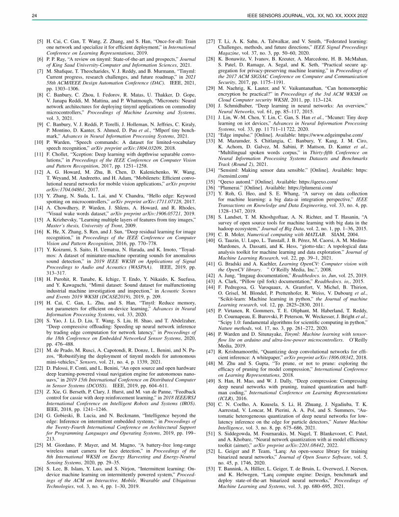
24 IEEE SENSORS JOURNAL, VOL. XX, NO. XX, XXXX 2022
[5] H. Cai, C. Gan, T. Wang, Z. Zhang, and S. Han, “Once-for-all: Trainone network and specialize it for efficient deployment,” in InternationalConference on Learning Representations, 2019.
[6] P. P. Ray, “A review on tinyml: State-of-the-art and prospects,” Journalof King Saud University-Computer and Information Sciences, 2021.
[7] M. Shafique, T. Theocharides, V. J. Reddy, and B. Murmann, “Tinyml:Current progress, research challenges, and future roadmap,” in 202158th ACM/IEEE Design Automation Conference (DAC). IEEE, 2021,pp. 1303–1306.
[8] C. Banbury, C. Zhou, I. Fedorov, R. Matas, U. Thakker, D. Gope,V. Janapa Reddi, M. Mattina, and P. Whatmough, “Micronets: Neuralnetwork architectures for deploying tinyml applications on commoditymicrocontrollers,” Proceedings of Machine Learning and Systems,vol. 3, 2021.
[9] C. Banbury, V. J. Reddi, P. Torelli, J. Holleman, N. Jeffries, C. Kiraly,P. Montino, D. Kanter, S. Ahmed, D. Pau et al., “Mlperf tiny bench-mark,” Advances in Neural Information Processing Systems, 2021.
[10] P. Warden, “Speech commands: A dataset for limited-vocabularyspeech recognition,” arXiv preprint arXiv:1804.03209, 2018.
[11] F. Chollet, “Xception: Deep learning with depthwise separable convo-lutions,” in Proceedings of the IEEE Conference on Computer Visionand Pattern Recognition, 2017, pp. 1251–1258.
[12] A. G. Howard, M. Zhu, B. Chen, D. Kalenichenko, W. Wang,T. Weyand, M. Andreetto, and H. Adam, “Mobilenets: Efficient convo-lutional neural networks for mobile vision applications,” arXiv preprintarXiv:1704.04861, 2017.
[13] Y. Zhang, N. Suda, L. Lai, and V. Chandra, “Hello edge: Keywordspotting on microcontrollers,” arXiv preprint arXiv:1711.07128, 2017.
[14] A. Chowdhery, P. Warden, J. Shlens, A. Howard, and R. Rhodes,“Visual wake words dataset,” arXiv preprint arXiv:1906.05721, 2019.
[15] A. Krizhevsky, “Learning multiple layers of features from tiny images,”Master’s thesis, University of Tront, 2009.
[16] K. He, X. Zhang, S. Ren, and J. Sun, “Deep residual learning for imagerecognition,” in Proceedings of the IEEE Conference on ComputerVision and Pattern Recognition, 2016, pp. 770–778.
[17] Y. Koizumi, S. Saito, H. Uematsu, N. Harada, and K. Imoto, “Toyad-mos: A dataset of miniature-machine operating sounds for anomaloussound detection,” in 2019 IEEE WKSH on Applications of SignalProceedings to Audio and Acoustics (WASPAA). IEEE, 2019, pp.313–317.
[18] H. Purohit, R. Tanabe, K. Ichige, T. Endo, Y. Nikaido, K. Suefusa,and Y. Kawaguchi, “Mimii dataset: Sound dataset for malfunctioningindustrial machine investigation and inspection,” in Acoustic Scenesand Events 2019 WKSH (DCASE2019), 2019, p. 209.
[19] H. Cai, C. Gan, L. Zhu, and S. Han, “Tinytl: Reduce memory,not parameters for efficient on-device learning,” Advances in NeuralInformation Processing Systems, vol. 33, 2020.
[20] S. Yao, J. Li, D. Liu, T. Wang, S. Liu, H. Shao, and T. Abdelzaher,“Deep compressive offloading: Speeding up neural network inferenceby trading edge computation for network latency,” in Proceedings ofthe 18th Conference on Embedded Networked Sensor Systems, 2020,pp. 476–488.
[21] M. de Prado, M. Rusci, A. Capotondi, R. Donze, L. Benini, and N. Pa-zos, “Robustifying the deployment of tinyml models for autonomousmini-vehicles,” Sensors, vol. 21, no. 4, p. 1339, 2021.
[22] D. Palossi, F. Conti, and L. Benini, “An open source and open hardwaredeep learning-powered visual navigation engine for autonomous nano-uavs,” in 2019 15th International Conference on Distributed Computerin Sensor Systems (DCOSS). IEEE, 2019, pp. 604–611.
[23] Z. Xie, G. Berseth, P. Clary, J. Hurst, and M. van de Panne, “Feedbackcontrol for cassie with deep reinforcement learning,” in 2018 IEEE/RSJInternational Conference on Intelligent Robots and Systems (IROS).IEEE, 2018, pp. 1241–1246.
[24] G. Gobieski, B. Lucia, and N. Beckmann, “Intelligence beyond theedge: Inference on intermittent embedded systems,” in Proceedings ofthe Twenty-Fourth International Conference on Architectural Supportfor Programming Languages and Operating Systems, 2019, pp. 199–213.
[25] M. Giordano, P. Mayer, and M. Magno, “A battery-free long-rangewireless smart camera for face detection,” in Proceedings of the8th International WKSH on Energy Harvesting and Energy-NeutralSensing Systems, 2020, pp. 29–35.
[26] S. Lee, B. Islam, Y. Luo, and S. Nirjon, “Intermittent learning: On-device machine learning on intermittently powered system,” Proceed-ings of the ACM on Interactive, Mobile, Wearable and UbiquitousTechnologies, vol. 3, no. 4, pp. 1–30, 2019.
[27] T. Li, A. K. Sahu, A. Talwalkar, and V. Smith, “Federated learning:Challenges, methods, and future directions,” IEEE Signal ProceedingsMagazine, vol. 37, no. 3, pp. 50–60, 2020.
[28] K. Bonawitz, V. Ivanov, B. Kreuter, A. Marcedone, H. B. McMahan,S. Patel, D. Ramage, A. Segal, and K. Seth, “Practical secure ag-gregation for privacy-preserving machine learning,” in Proceedings ofthe 2017 ACM SIGSAC Conference on Computer and CommunicationSecurity, 2017, pp. 1175–1191.
[29] M. Naehrig, K. Lauter, and V. Vaikuntanathan, “Can homomorphicencryption be practical?” in Proceedings of the 3rd ACM WKSH onCloud Computer security WKSH, 2011, pp. 113–124.
[30] J. Schmidhuber, “Deep learning in neural networks: An overview,”Neural Networks, vol. 61, pp. 85–117, 2015.
[31] J. Lin, W.-M. Chen, Y. Lin, C. Gan, S. Han et al., “Mcunet: Tiny deeplearning on iot devices,” Advances in Neural Information ProcessingSystems, vol. 33, pp. 11 711–11 722, 2020.
[32] “Edge impulse.” [Online]. Available: https://www.edgeimpulse.com/[33] M. Mazumder, S. Chitlangia, C. Banbury, Y. Kang, J. M. Ciro,
K. Achorn, D. Galvez, M. Sabini, P. Mattson, D. Kanter et al.,“Multilingual spoken words corpus,” in Thirty-fifth Conference onNeural Information Processing Systems Datasets and BenchmarksTrack (Round 2), 2021.
[34] “Sensiml: Making sensor data sensible.” [Online]. Available: https://sensiml.com/
[35] “Qeexo automl.” [Online]. Available: https://qeexo.com/[36] “Plumerai.” [Online]. Available: https://plumerai.com/[37] Y. Roh, G. Heo, and S. E. Whang, “A survey on data collection
for machine learning: a big data-ai integration perspective,” IEEETransactions on Knowledge and Data Engineering, vol. 33, no. 4, pp.1328–1347, 2019.
[38] S. Landset, T. M. Khoshgoftaar, A. N. Richter, and T. Hasanin, “Asurvey of open source tools for machine learning with big data in thehadoop ecosystem,” Journal of Big Data, vol. 2, no. 1, pp. 1–36, 2015.
[39] C. B. Moler, Numerical computing with MATLAB. SIAM, 2004.[40] G. Tauzin, U. Lupo, L. Tunstall, J. B. Perez, M. Caorsi, A. M. Medina-
Mardones, A. Dassatti, and K. Hess, “giotto-tda:: A topological dataanalysis toolkit for machine learning and data exploration.” Journal ofMachine Learning Research, vol. 22, pp. 39–1, 2021.
[41] G. Bradski and A. Kaehler, Learning OpenCV: Computer vision withthe OpenCV library. ” O’Reilly Media, Inc.”, 2008.
[42] A. Jung, “Imgaug documentation,” Readthedocs. io, Jun, vol. 25, 2019.[43] A. Clark, “Pillow (pil fork) documentation,” Readthedocs. io,, 2015.[44] F. Pedregosa, G. Varoquaux, A. Gramfort, V. Michel, B. Thirion,
O. Grisel, M. Blondel, P. Prettenhofer, R. Weiss, V. Dubourg et al.,“Scikit-learn: Machine learning in python,” the Journal of machineLearning research, vol. 12, pp. 2825–2830, 2011.
[45] P. Virtanen, R. Gommers, T. E. Oliphant, M. Haberland, T. Reddy,D. Cournapeau, E. Burovski, P. Peterson, W. Weckesser, J. Bright et al.,“Scipy 1.0: fundamental algorithms for scientific computing in python,”Nature methods, vol. 17, no. 3, pp. 261–272, 2020.
[46] P. Warden and D. Situnayake, Tinyml: Machine learning with tensor-flow lite on arduino and ultra-low-power microcontrollers. O’ReillyMedia, 2019.
[47] R. Krishnamoorthi, “Quantizing deep convolutional networks for effi-cient inference: A whitepaper,” arXiv preprint arXiv:1806.08342, 2018.
[48] M. Zhu and S. Gupta, “To prune, or not to prune: exploring theefficacy of pruning for model compression,” International Conferenceon Learning Representations, 2018.
[49] S. Han, H. Mao, and W. J. Dally, “Deep compression: Compressingdeep neural networks with pruning, trained quantization and huff-man coding,” International Conference on Learning Representations(ICLR), 2016.
[50] C. N. Coelho, A. Kuusela, S. Li, H. Zhuang, J. Ngadiuba, T. K.Aarrestad, V. Loncar, M. Pierini, A. A. Pol, and S. Summers, “Au-tomatic heterogeneous quantization of deep neural networks for low-latency inference on the edge for particle detectors,” Nature MachineIntelligence, vol. 3, no. 8, pp. 675–686, 2021.
[51] S. Siddegowda, M. Fournarakis, M. Nagel, T. Blankevoort, C. Patel,and A. Khobare, “Neural network quantization with ai model efficiencytoolkit (aimet),” arXiv preprint arXiv:2201.08442, 2022.
[52] L. Geiger and P. Team, “Larq: An open-source library for trainingbinarized neural networks,” Journal of Open Source Software, vol. 5,no. 45, p. 1746, 2020.
[53] T. Bannink, A. Hillier, L. Geiger, T. de Bruin, L. Overweel, J. Neeven,and K. Helwegen, “Larq compute engine: Design, benchmark anddeploy state-of-the-art binarized neural networks,” Proceedings ofMachine Learning and Systems, vol. 3, pp. 680–695, 2021.

SAHA et al.: MACHINE LEARNING FOR MICROCONTROLLER-CLASS HARDWARE - A REVIEW (JUNE 2022) 25
[54] Microsoft, “microsoft/nni: An open source automl toolkit for automatemachine learning lifecycle, including feature engineering, neuralarchitecture search, model compression and hyper-parameter tuning.”[Online]. Available: https://github.com/microsoft/nni
[55] A. Capotondi, M. Rusci, M. Fariselli, and L. Benini, “Cmix-nn: Mixedlow-precision cnn library for memory-constrained edge devices,” IEEETransactions on Circuits and Systems II: Express Briefs, vol. 67, no. 5,pp. 871–875, 2020.
[56] S. Gopinath, N. Ghanathe, V. Seshadri, and R. Sharma, “Compilingkb-sized machine learning models to tiny iot devices,” in Proceedingsof the 40th ACM SIGPLAN Conference on Programming LanguageDesign and Implementation, 2019, pp. 79–95.
[57] A. Kumar, S. Goyal, and M. Varma, “Resource-efficient machinelearning in 2 kb ram for the internet of things,” in InternationalConference on Machine Learning. PMLR, 2017, pp. 1935–1944.
[58] C. Gupta, A. S. Suggala, A. Goyal, H. V. Simhadri, B. Paranjape,A. Kumar, S. Goyal, R. Udupa, M. Varma, and P. Jain, “Protonn: Com-pressed and accurate knn for resource-scarce devices,” in InternationalConference on Machine Learning. PMLR, 2017, pp. 1331–1340.
[59] A. Kusupati, M. Singh, K. Bhatia, A. Kumar, P. Jain, and M. Varma,“Fastgrnn: a fast, accurate, stable and tiny kilobyte sized gated recurrentneural network,” in Proceedings of the 32nd International Conferenceon Neural Information Processing Systems, 2018, pp. 9031–9042.
[60] O. Saha, A. Kusupati, H. V. Simhadri, M. Varma, and P. Jain, “Rnnpool:Efficient non-linear pooling for ram constrained inference,” Advancesin Neural Information Processing Systems, vol. 33, 2020.
[61] E. L. Denton, W. Zaremba, J. Bruna, Y. LeCun, and R. Fergus,“Exploiting linear structure within convolutional networks for efficientevaluation,” in Advances in Neural Information Processing Systems,2014, pp. 1269–1277.
[62] D. D. Lee and H. S. Seung, “Learning the parts of objects by non-negative matrix factorization,” Nature, vol. 401, no. 6755, pp. 788–791,1999.
[63] P. Comon, “Independent component analysis, a new concept?” SignalProceedings, vol. 36, no. 3, pp. 287–314, 1994.
[64] S. Balakrishnama and A. Ganapathiraju, “Linear discriminant analysis-a brief tutorial,” Institute for Signal and Information Processing,vol. 18, no. 1998, pp. 1–8, 1998.
[65] M. Espadoto, R. M. Martins, A. Kerren, N. S. Hirata, and A. C. Telea,“Toward a quantitative survey of dimension reduction techniques,”IEEE Transactions on visualization and Computer graphics, vol. 27,no. 3, pp. 2153–2173, 2019.
[66] L. McInnes, J. Healy, N. Saul, and L. Großberger, “Umap: Uniformmanifold approximation and projection,” Journal of Open SourceSoftware, vol. 3, no. 29, 2018.
[67] S. Kullback and R. A. Leibler, “On information and sufficiency,” TheAnnals of Mathematical Statistics, vol. 22, no. 1, pp. 79–86, 1951.
[68] S. T. Roweis and L. K. Saul, “Nonlinear dimensionality reduction bylocally linear embedding,” Science, vol. 290, no. 5500, pp. 2323–2326,2000.
[69] B. Scholkopf, A. Smola, and K.-R. Muller, “Kernel principal com-ponent analysis,” in International Conference on Artificial NeuralNetworks. Springer, 1997, pp. 583–588.
[70] L. Van der Maaten and G. Hinton, “Visualizing data using t-sne.”Journal of Machine Learning Research, vol. 9, no. 11, 2008.
[71] D. E. Rumelhart, G. E. Hinton, and R. J. Williams, “Learning internalrepresentations by error propagation,” California Univ San Diego LaJolla Inst for Cognitive Science, Tech. Rep., 1985.
[72] “eloquentarduino.” [Online]. Available: https://github.com/eloquentarduino
[73] I. Guyon, S. Gunn, M. Nikravesh, and L. A. Zadeh, Feature extraction:foundations and applications. Springer, 2008, vol. 207.
[74] I. Guyon and A. Elisseeff, “An introduction to variable and featureselection,” Journal of Machine Learning Research, vol. 3, no. Mar, pp.1157–1182, 2003.
[75] G. Chandrashekar and F. Sahin, “A survey on feature selection meth-ods,” Computer & Electrical Engineering, vol. 40, no. 1, pp. 16–28,2014.
[76] S. Han, J. Pool, J. Tran, and W. Dally, “Learning both weightsand connections for efficient neural network,” Advances in NeuralInformation Processing Systems, vol. 28, 2015.
[77] S. Gupta, A. Agrawal, K. Gopalakrishnan, and P. Narayanan, “Deeplearning with limited numerical precision,” in International Conferenceon Machine Learning. PMLR, 2015, pp. 1737–1746.
[78] S. Yao, Y. Zhao, A. Zhang, L. Su, and T. Abdelzaher, “Deepiot:Compressing deep neural network structures for sensing systems with
a compressor-critic framework,” in Proceedings of the 15th ACMConference on Embedded Network Sensor Systems, 2017, pp. 1–14.
[79] M. Abadi, P. Barham, J. Chen, Z. Chen, A. Davis, J. Dean, M. Devin,S. Ghemawat, G. Irving, M. Isard et al., “{TensorFlow}: A systemfor {Large-Scale} machine learning,” in 12th USENIX symposium onoperating systems design and implementation (OSDI 16), 2016, pp.265–283.
[80] B. Jacob, S. Kligys, B. Chen, M. Zhu, M. Tang, A. Howard, H. Adam,and D. Kalenichenko, “Quantization and training of neural networksfor efficient integer-arithmetic-only inference,” in Proceedings of theIEEE Conference on Computer Vision and Pattern Recognition, 2018,pp. 2704–2713.
[81] P.-E. Novac, G. B. Hacene, A. Pegatoquet, B. Miramond, andV. Gripon, “Quantization and deployment of deep neural networks onmicrocontrollers,” Sensors, vol. 21, no. 9, p. 2984, 2021.
[82] K. Wang, Z. Liu, Y. Lin, J. Lin, and S. Han, “Haq: Hardware-awareautomated quantization with mixed precision,” in Proceedings of theIEEE/CVF Conference on Computer Vision and Pattern Recognition,2019, pp. 8612–8620.
[83] M. Rusci, A. Capotondi, and L. Benini, “Memory-driven mixed lowprecision quantization for enabling deep network inference on micro-controllers,” Proceedings of Machine Learning and Systems, vol. 2,2020.
[84] I. Hubara, M. Courbariaux, D. Soudry, R. El-Yaniv, and Y. Bengio, “Bi-narized neural networks,” Advances in Neural Information ProcessingSystems, vol. 29, 2016.
[85] S. Dave, R. Baghdadi, T. Nowatzki, S. Avancha, A. Shrivastava,and B. Li, “Hardware acceleration of sparse and irregular tensorcomputations of ml models: A survey and insights,” Proceedings ofthe IEEE, vol. 109, no. 10, pp. 1706–1752, 2021.
[86] I. Fedorov, R. P. Adams, M. Mattina, and P. N. Whatmough, “Sparse:Sparse architecture search for cnns on resource-constrained microcon-trollers,” Advances in Neural Information Processing Systems, vol. 32,2019.
[87] Z. Liu, M. Sun, T. Zhou, G. Huang, and T. Darrell, “Rethinking thevalue of network pruning,” in International Conference on LearningRepresentations, 2018.
[88] J. Yu, A. Lukefahr, D. Palframan, G. Dasika, R. Das, and S. Mahlke,“Scalpel: Customizing dnn pruning to the underlying hardware paral-lelism,” in 2017 ACM/IEEE 44th Annual International Symposium onComputer Architecture (ISCA). IEEE Computer Society, 2017, pp.548–560.
[89] E. Liberis and N. D. Lane, “Differentiable network pruning for micro-controllers,” arXiv preprint arXiv:2110.08350, 2021.
[90] U. Thakker, I. Fedorov, C. Zhou, D. Gope, M. Mattina, G. Dasika,and J. Beu, “Compressing rnns to kilobyte budget for iot devicesusing kronecker products,” ACM Journal on Emerging Technologiesin Computing Systems (JETC), vol. 17, no. 4, pp. 1–18, 2021.
[91] U. Thakker, P. Whatmough, Z. Liu, M. Mattina, and J. Beu, “Doping:A technique for extreme compression of lstm models using sparsestructured additive matrices,” Proceedings of Machine Learning andSystems, vol. 3, 2021.
[92] F. N. Iandola, S. Han, M. W. Moskewicz, K. Ashraf, W. J. Dally,and K. Keutzer, “Squeezenet: Alexnet-level accuracy with 50x fewerparameters and¡ 0.5 mb model size,” arXiv preprint arXiv:1602.07360,2016.
[93] A. Krizhevsky, I. Sutskever, and G. E. Hinton, “Imagenet classificationwith deep convolutional neural networks,” Advances in Neural Infor-mation Processing Systems, vol. 25, pp. 1097–1105, 2012.
[94] M. Sandler, A. Howard, M. Zhu, A. Zhmoginov, and L.-C. Chen, “Mo-bilenetv2: Inverted residuals and linear bottlenecks,” in Proceedings ofthe IEEE Conference on Computer Vision and Pattern Recognition,2018, pp. 4510–4520.
[95] X. Zhang, X. Zhou, M. Lin, and J. Sun, “Shufflenet: An extremely effi-cient convolutional neural network for mobile devices,” in Proceedingsof the IEEE Conference on Computer Vision and Pattern Recognition,2018, pp. 6848–6856.
[96] G. Huang, Z. Liu, L. Van Der Maaten, and K. Q. Weinberger,“Densely connected convolutional networks,” in Proceedings of theIEEE Conference on Computer Vision and Pattern Recognition, 2017,pp. 4700–4708.
[97] M. Tan, R. Pang, and Q. V. Le, “Efficientdet: Scalable and efficientobject detection,” in Proceedings of the IEEE Conference on ComputerVision and Pattern Recognition, 2020, pp. 10 781–10 790.
[98] C.-Y. Wang, A. Bochkovskiy, and H.-Y. M. Liao, “Scaled-yolov4:Scaling cross stage partial network,” in Proceedings of the IEEE/CVF
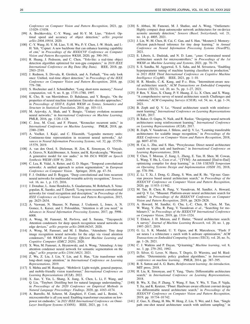
26 IEEE SENSORS JOURNAL, VOL. XX, NO. XX, XXXX 2022
Conference on Computer Vision and Pattern Recognition, 2021, pp.13 029–13 038.
[99] A. Bochkovskiy, C.-Y. Wang, and H.-Y. M. Liao, “Yolov4: Op-timal speed and accuracy of object detection,” arXiv preprintarXiv:2004.10934, 2020.
[100] C.-Y. Wang, H.-Y. M. Liao, Y.-H. Wu, P.-Y. Chen, J.-W. Hsieh, and I.-H. Yeh, “Cspnet: A new backbone that can enhance learning capabilityof cnn,” in Proceedings of the IEEE/CVF Conference on ComputerVision and Pattern Recognition WKSH, 2020, pp. 390–391.
[101] R. Huang, J. Pedoeem, and C. Chen, “Yolo-lite: a real-time objectdetection algorithm optimized for non-gpu computers,” in 2018 IEEEInternational Conference on Big Data (Big Data). IEEE, 2018, pp.2503–2510.
[102] J. Redmon, S. Divvala, R. Girshick, and A. Farhadi, “You only lookonce: Unified, real-time object detection,” in Proceedings of the IEEEConference on Computer Vision and Pattern Recognition, 2016, pp.779–788.
[103] S. Hochreiter and J. Schmidhuber, “Long short-term memory,” Neuralcomputation, vol. 9, no. 8, pp. 1735–1780, 1997.
[104] K. Cho, B. van Merrienboer, D. Bahdanau, and Y. Bengio, “On theproperties of neural machine translation: Encoder–decoder approaches,”in Proceedings of SSST-8, Eighth WKSH on Syntax, Semantics andStructure in Statistical Translation, 2014, pp. 103–111.
[105] M. Arjovsky, A. Shah, and Y. Bengio, “Unitary evolution recurrentneural networks,” in International Conference on Machine Learning.PMLR, 2016, pp. 1120–1128.
[106] C. Jose, M. Cisse, and F. Fleuret, “Kronecker recurrent units,” inInternational Conference on Machine Learning. PMLR, 2018, pp.2380–2389.
[107] A. Voelker, I. Kajic, and C. Eliasmith, “Legendre memory units:Continuous-time representation in recurrent neural networks,” Ad-vances in Neural Information Processing Systems, vol. 32, pp. 15 570–15 579, 2019.
[108] A. van den Oord, S. Dieleman, H. Zen, K. Simonyan, O. Vinyals,A. Graves, N. Kalchbrenner, A. Senior, and K. Kavukcuoglu, “Wavenet:A generative model for raw audio,” in 9th ISCA WKSH on SpeechSynthesis WKSH (SSW 9), 2016.
[109] C. Lea, R. Vidal, A. Reiter, and G. D. Hager, “Temporal convolutionalnetworks: A unified approach to action segmentation,” in EuropeanConference on Computer Vision. Springer, 2016, pp. 47–54.
[110] F. J. Ordonez and D. Roggen, “Deep convolutional and lstm recurrentneural networks for multimodal wearable activity recognition,” Sensors,vol. 16, no. 1, p. 115, 2016.
[111] J. Donahue, L. Anne Hendricks, S. Guadarrama, M. Rohrbach, S. Venu-gopalan, K. Saenko, and T. Darrell, “Long-term recurrent convolutionalnetworks for visual recognition and description,” in Proceedings of theIEEE Conference on Computer Vision and Pattern Recognition, 2015,pp. 2625–2634.
[112] A. Vaswani, N. Shazeer, N. Parmar, J. Uszkoreit, L. Jones, A. N.Gomez, Ł. Kaiser, and I. Polosukhin, “Attention is all you need,” inAdvances in Neural Information Processing Systems, 2017, pp. 5998–6008.
[113] A. Wong, M. Famouri, M. Pavlova, and S. Surana, “Tinyspeech:Attention condensers for deep speech recognition neural networks onedge devices,” arXiv preprint arXiv:2008.04245, 2020.
[114] A. Wong, M. Famouri, and M. J. Shafiee, “Attendnets: Tiny deepimage recognition neural networks for the edge via visual attentioncondensers,” 6th WKSH on Energy Efficient Machine Learning andCognitive Computer (EMC2 2020), 2020.
[115] X. Wen, M. Famouri, A. Hryniowski, and A. Wong, “Attendseg: A tinyattention condenser neural network for semantic segmentation on theedge,” arXiv preprint arXiv:2104.14623, 2021.
[116] Z. Wu, Z. Liu, J. Lin, Y. Lin, and S. Han, “Lite transformer withlong-short range attention,” in International Conference on LearningRepresentations, 2019.
[117] S. Mehta and M. Rastegari, “Mobilevit: Light-weight, general-purpose,and mobile-friendly vision transformer,” International Conference onLearning Representations (ICLR), 2022.
[118] X. Jiao, Y. Yin, L. Shang, X. Jiang, X. Chen, L. Li, F. Wang, andQ. Liu, “Tinybert: Distilling bert for natural language understanding,”in Proceedings of the 2020 Conference on Empirical Methods inNatural Language Proceedings: Findings, 2020, pp. 4163–4174.
[119] A. Burrello, M. Scherer, M. Zanghieri, F. Conti, and L. Benini, “Amicrocontroller is all you need: Enabling transformer execution on low-power iot endnodes,” in 2021 IEEE International Conference on Omni-Layer Intelligent Systems (COINS). IEEE, 2021, pp. 1–6.
[120] S. Abbasi, M. Famouri, M. J. Shafiee, and A. Wong, “Outliernets:Highly compact deep autoencoder network architectures for on-deviceacoustic anomaly detection,” Sensors (Basel, Switzerland), vol. 21,no. 14, p. 4805, 2021.
[121] J. Lin, W.-M. Chen, H. Cai, C. Gan, and S. Han, “Mcunetv2: Memory-efficient patch-based inference for tiny deep learning,” in AnnualConference on Neural Information Processing Systems (NeurIPS),2021.
[122] E. Liberis, Ł. Dudziak, and N. D. Lane, “µnas: Constrained neuralarchitecture search for microcontrollers,” in Proceedings of the 1stWKSH on Machine Learning and Systems, 2021, pp. 70–79.
[123] S. S. Sandha, M. Aggarwal, S. S. Saha, and M. Srivastava, “Enablinghyperparameter tuning of machine learning classifiers in production,”in 2021 IEEE Third International Conference on Cognitive MachineIntelligence (CogMI). IEEE, 2021, pp. 1–10.
[124] H. R. Mendis, C.-K. Kang, and P.-c. Hsiu, “Intermittent-aware neu-ral architecture search,” ACM Transactions on Embedded ComputingSystems (TECS), vol. 20, no. 5s, pp. 1–27, 2021.
[125] P. Ren, Y. Xiao, X. Chang, P.-Y. Huang, Z. Li, X. Chen, and X. Wang,“A comprehensive survey of neural architecture search: Challenges andsolutions,” ACM Computing Surveys (CSUR), vol. 54, no. 4, pp. 1–34,2021.
[126] B. Zoph and Q. V. Le, “Neural architecture search with reinforce-ment learning,” International Conference on Learning Representations(ICLR), 2017.
[127] B. Baker, O. Gupta, N. Naik, and R. Raskar, “Designing neural networkarchitectures using reinforcement learning,” International Conferenceon Learning Representations (ICLR), 2017.
[128] B. Zoph, V. Vasudevan, J. Shlens, and Q. V. Le, “Learning transferablearchitectures for scalable image recognition,” in Proceedings of theIEEE Conference on Computer Vision and Pattern Recognition, 2018,pp. 8697–8710.
[129] H. Cai, L. Zhu, and S. Han, “Proxylessnas: Direct neural architecturesearch on target task and hardware,” in International Conference onLearning Representations, 2018.
[130] T. Chen, T. Moreau, Z. Jiang, L. Zheng, E. Yan, H. Shen, M. Cowan,L. Wang, Y. Hu, L. Ceze et al., “{TVM}: An automated {End-to-End}optimizing compiler for deep learning,” in 13th USENIX Symposiumon Operating Systems Design and Implementation (OSDI 18), 2018,pp. 578–594.
[131] Z. Li, T. Xi, J. Deng, G. Zhang, S. Wen, and R. He, “Gp-nas: Gaus-sian process based neural architecture search,” in Proceedings of theIEEE/CVF Conference on Computer Vision and Pattern Recognition,2020, pp. 11 933–11 942.
[132] M. Tan, B. Chen, R. Pang, V. Vasudevan, M. Sandler, A. Howard,and Q. V. Le, “Mnasnet: Platform-aware neural architecture search formobile,” in Proceedings of the IEEE/CVF Conference on ComputerVision and Pattern Recognition, 2019, pp. 2820–2828.
[133] A. Howard, M. Sandler, G. Chu, L.-C. Chen, B. Chen, M. Tan,W. Wang, Y. Zhu, R. Pang, V. Vasudevan et al., “Searching for mo-bilenetv3,” in Proceedings of the IEEE/CVF International Conferenceon Computer Vision, 2019, pp. 1314–1324.
[134] T. Elsken, J. H. Metzen, and F. Hutter, “Neural architecture search:A survey,” Journal of Machine Learning Research, vol. 20, no. 1, pp.1997–2017, 2019.
[135] G. Li, S. K. Mandal, U. Y. Ogras, and R. Marculescu, “Flash: Fast neura l a rchitecture s earch with h ardware optimization,” ACMTransactions on Embedded Computing Systems (TECS), vol. 20, no. 5s,pp. 1–26, 2021.
[136] C. J. Watkins and P. Dayan, “Q-learning,” Machine learning, vol. 8,no. 3, pp. 279–292, 1992.
[137] D. Silver, G. Lever, N. Heess, T. Degris, D. Wierstra, and M. Ried-miller, “Deterministic policy gradient algorithms,” in Internationalconference on machine learning. PMLR, 2014, pp. 387–395.
[138] R. S. Sutton and A. G. Barto, Reinforcement learning: An introduction.MIT press, 2018.
[139] H. Liu, K. Simonyan, and Y. Yang, “Darts: Differentiable architecturesearch,” in International Conference on Learning Representations,2018.
[140] B. Wu, X. Dai, P. Zhang, Y. Wang, F. Sun, Y. Wu, Y. Tian, P. Vajda,Y. Jia, and K. Keutzer, “Fbnet: Hardware-aware efficient convnet designvia differentiable neural architecture search,” in Proceedings of theIEEE/CVF Conference on Computer Vision and Pattern Recognition,2019, pp. 10 734–10 742.
[141] Z. Guo, X. Zhang, H. Mu, W. Heng, Z. Liu, Y. Wei, and J. Sun, “Singlepath one-shot neural architecture search with uniform sampling,” in

SAHA et al.: MACHINE LEARNING FOR MICROCONTROLLER-CLASS HARDWARE - A REVIEW (JUNE 2022) 27
European Conference on Computer Vision. Springer, 2020, pp. 544–560.
[142] T. Elsken, J. H. Metzen, and F. Hutter, “Efficient multi-objectiveneural architecture search via lamarckian evolution,” in InternationalConference on Learning Representations, 2018.
[143] H. Pham, M. Guan, B. Zoph, Q. Le, and J. Dean, “Efficient neuralarchitecture search via parameters sharing,” in International conferenceon machine learning. PMLR, 2018, pp. 4095–4104.
[144] D. Stamoulis, R. Ding, D. Wang, D. Lymberopoulos, B. Priyantha,J. Liu, and D. Marculescu, “Single-path nas: Designing hardware-efficient convnets in less than 4 hours,” in Joint European Confer-ence on Machine Learning and Knowledge Discovery in Databases.Springer, 2019, pp. 481–497.
[145] E. Real, A. Aggarwal, Y. Huang, and Q. V. Le, “Regularized evolutionfor image classifier architecture search,” in Proceedings of the AAAIConference on Artificial Intelligence, vol. 33, no. 01, 2019, pp. 4780–4789.
[146] S. S. Sandha, M. Aggarwal, I. Fedorov, and M. Srivastava, “Mango: Apython library for parallel hyperparameter tuning,” in ICASSP 2020-2020 IEEE International Conference on Acoustics, Speech and SignalProcessing (ICASSP). IEEE, 2020, pp. 3987–3991.
[147] D. Golovin, B. Solnik, S. Moitra, G. Kochanski, J. Karro, andD. Sculley, “Google vizier: A service for black-box optimization,” inProceedings of the 23rd ACM SIGKDD International Conference onknowledge discovery and data mining, 2017, pp. 1487–1495.
[148] S. Daulton, D. Eriksson, M. Balandat, and E. Bakshy, “Multi-objectivebayesian optimization over high-dimensional search spaces,” in The38th Conference on Uncertainty in Artificial Intelligence, 2022.
[149] L. Dudziak, T. Chau, M. Abdelfattah, R. Lee, H. Kim, and N. Lane,“Brp-nas: Prediction-based nas using gcns,” Advances in Neural Infor-mation Processing Systems, vol. 33, pp. 10 480–10 490, 2020.
[150] W. Wen, H. Liu, Y. Chen, H. Li, G. Bender, and P.-J. Kindermans,“Neural predictor for neural architecture search,” in European Confer-ence on Computer Vision. Springer, 2020, pp. 660–676.
[151] J. Mellor, J. Turner, A. Storkey, and E. J. Crowley, “Neural architecturesearch without training,” in International Conference on MachineLearning. PMLR, 2021, pp. 7588–7598.
[152] M. S. Abdelfattah, A. Mehrotra, Ł. Dudziak, and N. D. Lane, “Zero-cost proxies for lightweight nas,” in International Conference onLearning Representations, 2020.
[153] N. Lee, T. Ajanthan, and P. Torr, “Snip: Single-shot network prun-ing based on connection sensitivity,” in International Conference onLearning Representations, 2018.
[154] C. Wang, G. Zhang, and R. Grosse, “Picking winning tickets beforetraining by preserving gradient flow,” in International Conference onLearning Representations, 2019.
[155] H. Tanaka, D. Kunin, D. L. Yamins, and S. Ganguli, “Pruning neuralnetworks without any data by iteratively conserving synaptic flow,”Advances in Neural Information Processing Systems, vol. 33, pp. 6377–6389, 2020.
[156] W. Chen, X. Gong, and Z. Wang, “Neural architecture search onimagenet in four gpu hours: A theoretically inspired perspective,” inInternational Conference on Learning Representations, 2020.
[157] M. Gielda, “Renode: a flexible, open-source simulation framework forbuilding scalable, well-tested risc-v systems,” 7th RISC-V WorkshopProceedings, 2017.
[158] L. L. Zhang, S. Han, J. Wei, N. Zheng, T. Cao, Y. Yang, andY. Liu, “nn-meter: towards accurate latency prediction of deep-learningmodel inference on diverse edge devices,” in Proceedings of the 19thAnnual International Conference on Mobile Systems, Applications, andServices, 2021, pp. 81–93.
[159] S. R. Bulo, L. Porzi, and P. Kontschieder, “In-place activated batchnormfor memory-optimized training of dnns,” in Proceedings of the IEEEConference on Computer Vision and Pattern Recognition, 2018, pp.5639–5647.
[160] J. Xue, Loop tiling for parallelism. Springer Science & BusinessMedia, 2000, vol. 575.
[161] S. Carr, K. S. McKinley, and C.-W. Tseng, “Compiler optimizationsfor improving data locality,” ACM SIGPLAN Notices, vol. 29, no. 11,pp. 252–262, 1994.
[162] S. Dave, Y. Kim, S. Avancha, K. Lee, and A. Shrivastava, “Dmazerun-ner: Executing perfectly nested loops on dataflow accelerators,” ACMTransactions on Embedded Computing Systems (TECS), vol. 18, no. 5s,pp. 1–27, 2019.
[163] J. Yu, A. Lukefahr, R. Das, and S. Mahlke, “Tf-net: Deploying sub-byte deep neural networks on microcontrollers,” ACM Transactions onEmbedded Computing Systems (TECS), vol. 18, no. 5s, pp. 1–21, 2019.
[164] L. Lai, N. Suda, and V. Chandra, “Cmsis-nn: Efficient neural networkkernels for arm cortex-m cpus,” arXiv preprint arXiv:1801.06601,2018.
[165] A. Burrello, A. Garofalo, N. Bruschi, G. Tagliavini, D. Rossi, andF. Conti, “Dory: Automatic end-to-end deployment of real-world dnnson low-cost iot mcus,” IEEE Transactions on Computers, vol. 70, no. 8,pp. 1253–1268, 2021.
[166] A. Garofalo, M. Rusci, F. Conti, D. Rossi, and L. Benini, “Pulp-nn:accelerating quantized neural networks on parallel ultra-low-power risc-v processors,” Philosophical Transactions of the Royal Society A, vol.378, no. 2164, p. 20190155, 2020.
[167] R. David, J. Duke, A. Jain, V. Janapa Reddi, N. Jeffries, J. Li,N. Kreeger, I. Nappier, M. Natraj, T. Wang et al., “Tensorflow litemicro: Embedded machine learning for tinyml systems,” Proceedingsof Machine Learning and Systems, vol. 3, 2021.
[168] N. Tan, “utensor/utensor: Tinyml ai inference library.” [Online].Available: https://github.com/uTensor/uTensor
[169] D. K. Dennis, D. A. E. Acar, V. Mandikal, V. S. Sadasivan,V. Saligrama, H. V. Simhadri, and P. Jain, “Shallow rnn: Accurate time-series classification on resource constrained devices,” in Advances inNeural Information Processing Systems, vol. 32, 2019.
[170] D. K. Dennis, C. Pabbaraju, H. V. Simhadri, and P. Jain, “Multipleinstance learning for efficient sequential data classification on resource-constrained devices,” in Proceedings of the 32nd International Confer-ence on Neural Information Processing Systems, 2018, pp. 10 976–10 987.
[171] S. Goyal, A. Raghunathan, M. Jain, H. V. Simhadri, and P. Jain, “Drocc:Deep robust one-class classification,” in International Conference onMachine Learning. PMLR, 2020, pp. 3711–3721.
[172] “X-cube-ai - ai expansion pack for stm32cubemx -stmicroelectronics.” [Online]. Available: https://www.st.com/en/embedded-software/x-cube-ai.html
[173] “Cartesiam, nanoedge ai library,” Dec 2021. [Online]. Available:https://cartesiam.ai/
[174] D. Morawiec, “sklearn-porter.” [Online]. Available: https://github.com/nok/sklearn-porter
[175] L. T. da Silva, V. M. Souza, and G. E. Batista, “Embml tool: Support-ing the use of supervised learning algorithms in low-cost embeddedsystems,” in 2019 IEEE 31st International Conference on Tools withArtificial Intelligence (ICTAI). IEEE, 2019, pp. 1633–1637.
[176] X. Wang, M. Magno, L. Cavigelli, and L. Benini, “Fann-on-mcu: Anopen-source toolkit for energy-efficient neural network inference at theedge of the internet of things,” IEEE Internet of Things Journal, vol. 7,no. 5, pp. 4403–4417, 2020.
[177] “Ai-driven deep neural network optimizer.” [Online]. Available:https://www.deeplite.ai/
[178] “Edge ai / tinyml: Saas: Deep learning.” [Online]. Available:https://www.imagimob.com/
[179] “Neuton.ai - no-code artificial intelligence for all.” [Online]. Available:https://neuton.ai/
[180] “Reality ai.” [Online]. Available: https://reality.ai/[181] R. C. Whaley and J. J. Dongarra, “Automatically tuned linear algebra
software,” in SC’98: Proceedings of the 1998 ACM/IEEE conferenceon Supercomputing. IEEE, 1998, pp. 38–38.
[182] U. Bondhugula, A. Hartono, J. Ramanujam, and P. Sadayappan, “Apractical automatic polyhedral parallelizer and locality optimizer,” inProceedings of the 29th ACM SIGPLAN Conference on ProgrammingLanguage Design and Implementation, 2008, pp. 101–113.
[183] S. Lee and S. Nirjon, “Learning in the wild: When, how, and whatto learn for on-device dataset adaptation,” in Proceedings of the2nd International WKSH on Challenges in Artificial Intelligence andMachine Learning for Internet of Things, 2020, pp. 34–40.
[184] H. Ren, D. Anicic, and T. A. Runkler, “Tinyol: Tinyml with online-learning on microcontrollers,” in 2021 International Joint Conferenceon Neural Networks (IJCNN). IEEE, 2021, pp. 1–8.
[185] B. Sudharsan, J. G. Breslin, and M. I. Ali, “Ml-mcu: A framework totrain ml classifiers on mcu-based iot edge devices,” IEEE Internet ofThings Journal, 2021.
[186] B. Sudharsan, P. Yadav, J. G. Breslin, and M. I. Ali, “Train++:An incremental ml model training algorithm to create self-learningiot devices,” in 2021 IEEE SmartWorld, Ubiquitous Intelligence &Computing, Advanced & Trusted Computing, Scalable Computing& Communications, Internet of People and Smart City Innovation(SmartWorld/SCALCOM/UIC/ATC/IOP/SCI). IEEE, 2021, pp. 97–106.
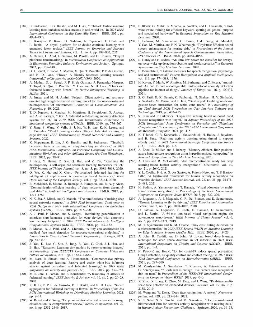
28 IEEE SENSORS JOURNAL, VOL. XX, NO. XX, XXXX 2022
[187] B. Sudharsan, J. G. Breslin, and M. I. Ali, “Imbal-ol: Online machinelearning from imbalanced data streams in real-world iot,” in 2021 IEEEInternational Conference on Big Data (Big Data). IEEE, 2021, pp.4974–4978.
[188] L. Ravaglia, M. Rusci, D. Nadalini, A. Capotondi, F. Conti, andL. Benini, “A tinyml platform for on-device continual learning withquantized latent replays,” IEEE Journal on Emerging and SelectedTopics in Circuits and Systems, vol. 11, no. 4, pp. 789–802, 2021.
[189] A. Osman, U. Abid, L. Gemma, M. Perotto, and D. Brunelli, “Tinymlplatforms benchmarking,” in International Conference on Applicationsin Electronics Pervading Industry, Environment and Society. Springer,2022, pp. 139–148.
[190] D. J. Beutel, T. Topal, A. Mathur, X. Qiu, T. Parcollet, P. P. de Gusmao,and N. D. Lane, “Flower: A friendly federated learning researchframework,” arXiv preprint arXiv:2007.14390, 2020.
[191] A. Mathur, D. J. Beutel, P. P. B. de Gusmao, J. Fernandez-Marques,T. Topal, X. Qiu, T. Parcollet, Y. Gao, and N. D. Lane, “On-devicefederated learning with flower,” On-Device Intelligence Workshop atMLSys, 2021.
[192] A. Imteaj and M. H. Amini, “Fedparl: Client activity and resource-oriented lightweight federated learning model for resource-constrainedheterogeneous iot environment,” Frontiers in Communications andNetworks, p. 10, 2021.
[193] T. D. Nguyen, S. Marchal, M. Miettinen, H. Fereidooni, N. Asokan,and A.-R. Sadeghi, “Dıot: A federated self-learning anomaly detectionsystem for iot,” in 2019 IEEE 39th International conference ondistributed computing systems (ICDCS). IEEE, 2019, pp. 756–767.
[194] Y. Jiang, S. Wang, V. Valls, B. J. Ko, W.-H. Lee, K. K. Leung, andL. Tassiulas, “Model pruning enables efficient federated learning onedge devices,” IEEE Transactions on Neural Networks and LearningSystems, 2022.
[195] K. Kopparapu, E. Lin, J. G. Breslin, and B. Sudharsan, “Tinyfedtl:Federated transfer learning on ubiquitous tiny iot devices,” in 2022IEEE International Conference on Pervasive Computing and Commu-nications Workshops and other Affiliated Events (PerCom Workshops).IEEE, 2022, pp. 79–81.
[196] J. Pang, Y. Huang, Z. Xie, Q. Han, and Z. Cai, “Realizing theheterogeneity: a self-organized federated learning framework for iot,”IEEE Internet of Things Journal, vol. 8, no. 5, pp. 3088–3098, 2020.
[197] Q. Wu, K. He, and X. Chen, “Personalized federated learning forintelligent iot applications: A cloud-edge based framework,” IEEEOpen Journal of the Computer Society, vol. 1, pp. 35–44, 2020.
[198] B. McMahan, E. Moore, D. Ramage, S. Hampson, and B. A. y Arcas,“Communication-efficient learning of deep networks from decentral-ized data,” in Artificial intelligence and statistics. PMLR, 2017, pp.1273–1282.
[199] N. K. Jha, S. Mittal, and G. Mattela, “The ramifications of making deepneural networks compact,” in 2019 32nd International Conference onVLSI Design and 2019 18th International Conference on EmbeddedSystems (VLSID). IEEE, 2019, pp. 215–220.
[200] A. J. Paul, P. Mohan, and S. Sehgal, “Rethinking generalization inamerican sign language prediction for edge devices with extremelylow memory footprint,” in 2020 IEEE Recent Advances in IntelligentComputational Systems (RAICS). IEEE, 2020, pp. 147–152.
[201] P. Mohan, A. J. Paul, and A. Chirania, “A tiny cnn architecture formedical face mask detection for resource-constrained endpoints,” inInnovations in Electrical and Electronic Engineering. Springer, 2021,pp. 657–670.
[202] J. Yoo, D. Lee, C. Son, S. Jung, B. Yoo, C. Choi, J.-J. Han, andB. Han, “Rascanet: Learning tiny models by raster-scanning images,”in Proceedings of the IEEE/CVF Conference on Computer Vision andPattern Recognition, 2021, pp. 13 673–13 682.
[203] M. Nasr, R. Shokri, and A. Houmansadr, “Comprehensive privacyanalysis of deep learning: Passive and active white-box inferenceattacks against centralized and federated learning,” in 2019 IEEEsymposium on security and privacy (SP). IEEE, 2019, pp. 739–753.
[204] M. S. Jere, T. Farnan, and F. Koushanfar, “A taxonomy of attacks onfederated learning,” IEEE Security & Privacy, vol. 19, no. 2, pp. 20–28,2020.
[205] K. H. Li, P. P. B. de Gusmao, D. J. Beutel, and N. D. Lane, “Secureaggregation for federated learning in flower,” in Proceedings of the 2ndACM International Workshop on Distributed Machine Learning, 2021,pp. 8–14.
[206] W. Rawat and Z. Wang, “Deep convolutional neural networks for imageclassification: A comprehensive review,” Neural computation, vol. 29,no. 9, pp. 2352–2449, 2017.
[207] P. Blouw, G. Malik, B. Morcos, A. Voelker, and C. Eliasmith, “Hard-ware aware training for efficient keyword spotting on general purposeand specialized hardware,” in Research Symposium on Tiny MachineLearning, 2020.
[208] I. Fedorov, M. Stamenovic, C. Jensen, L.-C. Yang, A. Mandell,Y. Gan, M. Mattina, and P. N. Whatmough, “Tinylstms: Efficient neuralspeech enhancement for hearing aids,” in Proceedings of the AnnualConference of the International Speech Communication Association,INTERSPEECH. ISCA, 2020, pp. 4054–4058.
[209] E. Hardy and F. Badets, “An ultra-low power rnn classifier for always-on voice wake-up detection robust to real-world scenarios,” in ResearchSymposium on Tiny Machine Learning, 2020.
[210] P. Mermelstein, “Distance measures for speech recognition, psycholog-ical and instrumental,” Pattern Recognition and artificial intelligence,vol. 116, pp. 374–388, 1976.
[211] H. Kayan, Y. Majib, W. Alsafery, M. Barhamgi, and C. Perera, “Anoml-iot: An end to end re-configurable multi-protocol anomaly detectionpipeline for internet of things,” Internet of Things, vol. 16, p. 100437,2021.
[212] S. G. Patil, D. K. Dennis, C. Pabbaraju, N. Shaheer, H. V. Simhadri,V. Seshadri, M. Varma, and P. Jain, “Gesturepod: Enabling on-devicegesture-based interaction for white cane users,” in Proceedings ofthe 32nd Annual ACM Symposium on User Interface Software andTechnology, 2019, pp. 403–415.
[213] S. Bian and P. Lukowicz, “Capacitive sensing based on-board handgesture recognition with tinyml,” in Adjunct Proceedings of the 2021ACM International Joint Conference on Pervasive and UbiquitousComputer and Proceedings of the 2021 ACM International Symposiumon Wearable Computer, 2021, pp. 4–5.
[214] K. T’Jonck, C. R. Kancharla, J. Vankeirsbilck, H. Hallez, J. Boydens,and B. Pang, “Real-time activity tracking using tinyml to supportelderly care,” in 2021 International Scientific Conference Electronics(ET). IEEE, 2021, pp. 1–6.
[215] A. Zhou, R. Muller, and J. Rabaey, “Memory-efficient, limb position-aware hand gesture recognition using hyperdimensional computing,” inResearch Symposium on Tiny Machine Learning, 2020.
[216] A. Elsts and R. McConville, “Are microcontrollers ready for deeplearning-based human activity recognition?” Electronics, vol. 10,no. 21, p. 2640, 2021.
[217] Y. L. Coelho, F. d. A. S. dos Santos, A. Frizera-Neto, and T. F. Bastos-Filho, “A lightweight framework for human activity recognition onwearable devices,” IEEE Sensors Journal, vol. 21, no. 21, pp. 24 471–24 481, 2021.
[218] H. Badino, A. Yamamoto, and T. Kanade, “Visual odometry by multi-frame feature integration,” in Proceedings of the IEEE InternationalConference on Computer Vision WKSH, 2013, pp. 222–229.
[219] A. Loquercio, A. I. Maqueda, C. R. Del-Blanco, and D. Scaramuzza,“Dronet: Learning to fly by driving,” IEEE Robotics and AutomationLetters, vol. 3, no. 2, pp. 1088–1095, 2018.
[220] D. Palossi, A. Loquercio, F. Conti, E. Flamand, D. Scaramuzza,and L. Benini, “A 64-mw dnn-based visual navigation engine forautonomous nano-drones,” IEEE Internet of Things Journal, vol. 6,no. 5, pp. 8357–8371, 2019.
[221] M. T. Nyamukuru and K. M. Odame, “Tiny eats: Eating detection ona microcontroller,” in 2020 IEEE Second WKSH on Machine Learningon Edge in Sensor Systems (SenSys-ML). IEEE, 2020, pp. 19–23.
[222] A. John, B. Cardiff, and D. John, “A 1d-cnn based deep learningtechnique for sleep apnea detection in iot sensors,” in 2021 IEEEInternational Symposium on Circuits and Systems (ISCAS). IEEE,2021, pp. 1–5.
[223] N. Petrovic and Kocic, “Iot for covid-19 indoor spread prevention:Cough detection, air quality control and contact tracing,” in 2021 IEEE32nd International Conference on Microelectronics (MIEL). IEEE,2021, pp. 297–300.
[224] M. Zemlyanikin, A. Smorkalov, T. Khanova, A. Petrovicheva, andG. Serebryakov, “512kib ram is enough! live camera face recognitiondnn on mcu,” in Proceedings of the IEEE/CVF International Confer-ence on Computer Vision WKSH, 2019, pp. 0–0.
[225] X. Zhao, X. Liang, C. Zhao, M. Tang, and J. Wang, “Real-time multi-scale face detector on embedded devices,” Sensors, vol. 19, no. 9, p.2158, 2019.
[226] M. Wang and W. Deng, “Deep face recognition: A survey,” Neurocom-puting, vol. 429, pp. 215–244, 2021.
[227] S. S. Saha, S. S. Sandha, and M. Srivastava, “Deep convolutionalbidirectional lstm for complex activity recognition with missing data,”in Human Activity Recognition Challenge. Springer, 2020, pp. 39–53.
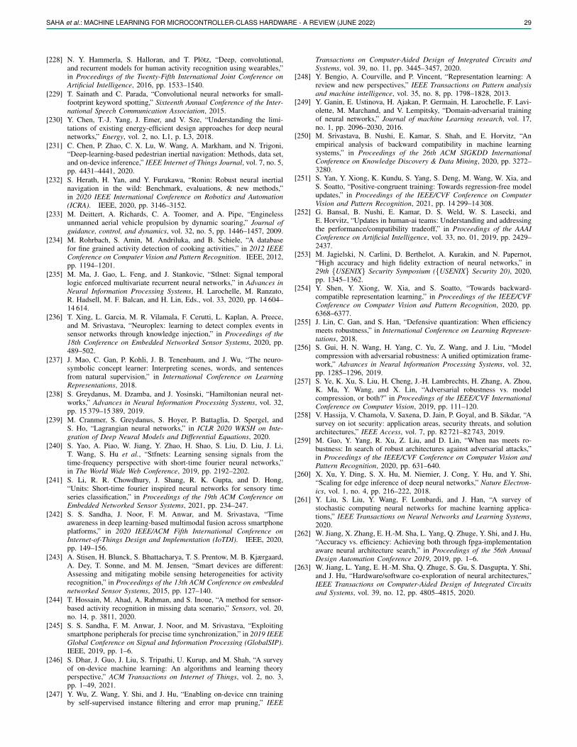
SAHA et al.: MACHINE LEARNING FOR MICROCONTROLLER-CLASS HARDWARE - A REVIEW (JUNE 2022) 29
[228] N. Y. Hammerla, S. Halloran, and T. Plotz, “Deep, convolutional,and recurrent models for human activity recognition using wearables,”in Proceedings of the Twenty-Fifth International Joint Conference onArtificial Intelligence, 2016, pp. 1533–1540.
[229] T. Sainath and C. Parada, “Convolutional neural networks for small-footprint keyword spotting,” Sixteenth Annual Conference of the Inter-national Speech Communication Association, 2015.
[230] Y. Chen, T.-J. Yang, J. Emer, and V. Sze, “Understanding the limi-tations of existing energy-efficient design approaches for deep neuralnetworks,” Energy, vol. 2, no. L1, p. L3, 2018.
[231] C. Chen, P. Zhao, C. X. Lu, W. Wang, A. Markham, and N. Trigoni,“Deep-learning-based pedestrian inertial navigation: Methods, data set,and on-device inference,” IEEE Internet of Things Journal, vol. 7, no. 5,pp. 4431–4441, 2020.
[232] S. Herath, H. Yan, and Y. Furukawa, “Ronin: Robust neural inertialnavigation in the wild: Benchmark, evaluations, & new methods,”in 2020 IEEE International Conference on Robotics and Automation(ICRA). IEEE, 2020, pp. 3146–3152.
[233] M. Deittert, A. Richards, C. A. Toomer, and A. Pipe, “Enginelessunmanned aerial vehicle propulsion by dynamic soaring,” Journal ofguidance, control, and dynamics, vol. 32, no. 5, pp. 1446–1457, 2009.
[234] M. Rohrbach, S. Amin, M. Andriluka, and B. Schiele, “A databasefor fine grained activity detection of cooking activities,” in 2012 IEEEConference on Computer Vision and Pattern Recognition. IEEE, 2012,pp. 1194–1201.
[235] M. Ma, J. Gao, L. Feng, and J. Stankovic, “Stlnet: Signal temporallogic enforced multivariate recurrent neural networks,” in Advances inNeural Information Processing Systems, H. Larochelle, M. Ranzato,R. Hadsell, M. F. Balcan, and H. Lin, Eds., vol. 33, 2020, pp. 14 604–14 614.
[236] T. Xing, L. Garcia, M. R. Vilamala, F. Cerutti, L. Kaplan, A. Preece,and M. Srivastava, “Neuroplex: learning to detect complex events insensor networks through knowledge injection,” in Proceedings of the18th Conference on Embedded Networked Sensor Systems, 2020, pp.489–502.
[237] J. Mao, C. Gan, P. Kohli, J. B. Tenenbaum, and J. Wu, “The neuro-symbolic concept learner: Interpreting scenes, words, and sentencesfrom natural supervision,” in International Conference on LearningRepresentations, 2018.
[238] S. Greydanus, M. Dzamba, and J. Yosinski, “Hamiltonian neural net-works,” Advances in Neural Information Processing Systems, vol. 32,pp. 15 379–15 389, 2019.
[239] M. Cranmer, S. Greydanus, S. Hoyer, P. Battaglia, D. Spergel, andS. Ho, “Lagrangian neural networks,” in ICLR 2020 WKSH on Inte-gration of Deep Neural Models and Differential Equations, 2020.
[240] S. Yao, A. Piao, W. Jiang, Y. Zhao, H. Shao, S. Liu, D. Liu, J. Li,T. Wang, S. Hu et al., “Stfnets: Learning sensing signals from thetime-frequency perspective with short-time fourier neural networks,”in The World Wide Web Conference, 2019, pp. 2192–2202.
[241] S. Li, R. R. Chowdhury, J. Shang, R. K. Gupta, and D. Hong,“Units: Short-time fourier inspired neural networks for sensory timeseries classification,” in Proceedings of the 19th ACM Conference onEmbedded Networked Sensor Systems, 2021, pp. 234–247.
[242] S. S. Sandha, J. Noor, F. M. Anwar, and M. Srivastava, “Timeawareness in deep learning-based multimodal fusion across smartphoneplatforms,” in 2020 IEEE/ACM Fifth International Conference onInternet-of-Things Design and Implementation (IoTDI). IEEE, 2020,pp. 149–156.
[243] A. Stisen, H. Blunck, S. Bhattacharya, T. S. Prentow, M. B. Kjærgaard,A. Dey, T. Sonne, and M. M. Jensen, “Smart devices are different:Assessing and mitigating mobile sensing heterogeneities for activityrecognition,” in Proceedings of the 13th ACM Conference on embeddednetworked Sensor Systems, 2015, pp. 127–140.
[244] T. Hossain, M. Ahad, A. Rahman, and S. Inoue, “A method for sensor-based activity recognition in missing data scenario,” Sensors, vol. 20,no. 14, p. 3811, 2020.
[245] S. S. Sandha, F. M. Anwar, J. Noor, and M. Srivastava, “Exploitingsmartphone peripherals for precise time synchronization,” in 2019 IEEEGlobal Conference on Signal and Information Processing (GlobalSIP).IEEE, 2019, pp. 1–6.
[246] S. Dhar, J. Guo, J. Liu, S. Tripathi, U. Kurup, and M. Shah, “A surveyof on-device machine learning: An algorithms and learning theoryperspective,” ACM Transactions on Internet of Things, vol. 2, no. 3,pp. 1–49, 2021.
[247] Y. Wu, Z. Wang, Y. Shi, and J. Hu, “Enabling on-device cnn trainingby self-supervised instance filtering and error map pruning,” IEEE
Transactions on Computer-Aided Design of Integrated Circuits andSystems, vol. 39, no. 11, pp. 3445–3457, 2020.
[248] Y. Bengio, A. Courville, and P. Vincent, “Representation learning: Areview and new perspectives,” IEEE Transactions on Pattern analysisand machine intelligence, vol. 35, no. 8, pp. 1798–1828, 2013.
[249] Y. Ganin, E. Ustinova, H. Ajakan, P. Germain, H. Larochelle, F. Lavi-olette, M. Marchand, and V. Lempitsky, “Domain-adversarial trainingof neural networks,” Journal of machine Learning research, vol. 17,no. 1, pp. 2096–2030, 2016.
[250] M. Srivastava, B. Nushi, E. Kamar, S. Shah, and E. Horvitz, “Anempirical analysis of backward compatibility in machine learningsystems,” in Proceedings of the 26th ACM SIGKDD InternationalConference on Knowledge Discovery & Data Mining, 2020, pp. 3272–3280.
[251] S. Yan, Y. Xiong, K. Kundu, S. Yang, S. Deng, M. Wang, W. Xia, andS. Soatto, “Positive-congruent training: Towards regression-free modelupdates,” in Proceedings of the IEEE/CVF Conference on ComputerVision and Pattern Recognition, 2021, pp. 14 299–14 308.
[252] G. Bansal, B. Nushi, E. Kamar, D. S. Weld, W. S. Lasecki, andE. Horvitz, “Updates in human-ai teams: Understanding and addressingthe performance/compatibility tradeoff,” in Proceedings of the AAAIConference on Artificial Intelligence, vol. 33, no. 01, 2019, pp. 2429–2437.
[253] M. Jagielski, N. Carlini, D. Berthelot, A. Kurakin, and N. Papernot,“High accuracy and high fidelity extraction of neural networks,” in29th {USENIX} Security Symposium ({USENIX} Security 20), 2020,pp. 1345–1362.
[254] Y. Shen, Y. Xiong, W. Xia, and S. Soatto, “Towards backward-compatible representation learning,” in Proceedings of the IEEE/CVFConference on Computer Vision and Pattern Recognition, 2020, pp.6368–6377.
[255] J. Lin, C. Gan, and S. Han, “Defensive quantization: When efficiencymeets robustness,” in International Conference on Learning Represen-tations, 2018.
[256] S. Gui, H. N. Wang, H. Yang, C. Yu, Z. Wang, and J. Liu, “Modelcompression with adversarial robustness: A unified optimization frame-work,” Advances in Neural Information Processing Systems, vol. 32,pp. 1285–1296, 2019.
[257] S. Ye, K. Xu, S. Liu, H. Cheng, J.-H. Lambrechts, H. Zhang, A. Zhou,K. Ma, Y. Wang, and X. Lin, “Adversarial robustness vs. modelcompression, or both?” in Proceedings of the IEEE/CVF InternationalConference on Computer Vision, 2019, pp. 111–120.
[258] V. Hassija, V. Chamola, V. Saxena, D. Jain, P. Goyal, and B. Sikdar, “Asurvey on iot security: application areas, security threats, and solutionarchitectures,” IEEE Access, vol. 7, pp. 82 721–82 743, 2019.
[259] M. Guo, Y. Yang, R. Xu, Z. Liu, and D. Lin, “When nas meets ro-bustness: In search of robust architectures against adversarial attacks,”in Proceedings of the IEEE/CVF Conference on Computer Vision andPattern Recognition, 2020, pp. 631–640.
[260] X. Xu, Y. Ding, S. X. Hu, M. Niemier, J. Cong, Y. Hu, and Y. Shi,“Scaling for edge inference of deep neural networks,” Nature Electron-ics, vol. 1, no. 4, pp. 216–222, 2018.
[261] Y. Liu, S. Liu, Y. Wang, F. Lombardi, and J. Han, “A survey ofstochastic computing neural networks for machine learning applica-tions,” IEEE Transactions on Neural Networks and Learning Systems,2020.
[262] W. Jiang, X. Zhang, E. H.-M. Sha, L. Yang, Q. Zhuge, Y. Shi, and J. Hu,“Accuracy vs. efficiency: Achieving both through fpga-implementationaware neural architecture search,” in Proceedings of the 56th AnnualDesign Automation Conference 2019, 2019, pp. 1–6.
[263] W. Jiang, L. Yang, E. H.-M. Sha, Q. Zhuge, S. Gu, S. Dasgupta, Y. Shi,and J. Hu, “Hardware/software co-exploration of neural architectures,”IEEE Transactions on Computer-Aided Design of Integrated Circuitsand Systems, vol. 39, no. 12, pp. 4805–4815, 2020.