machine learning based spectrum decision in cognitive radio

MACHINE LEARNING BASED SPECTRUM DECISION IN COGNITIVE RADIO

NETWORKS

by

KOUSHIK ARASEETHOTA MANJUNATHA

FEI HU, COMMITTEE CHAIRSUNIL KUMAR, COMMITTEE CO-CHAIR

AIJUN SONGSHUHUI LIMIN SUN

A DISSERTATION

Submitted in partial fulfillment of the requirementsfor the degree of Doctor of Philosophy

in the Department of Electrical and Computer Engineeringin the Graduate School of

The University of Alabama

TUSCALOOSA, ALABAMA

2018

Copyright Koushik Araseethota Manjunatha 2018ALL RIGHTS RESERVED

ABSTRACT

The cognitive radio network (CRN) is considered as one of the promising solutions to

address the issue of spectrum scarcity and effective spectrum utilization. In a CRN the Secondary

User (SU) is allowed to occupy the spectrum which is temporarily not used by the Primary User

(PU). Frequent interruptions from the PUs is the fundamental issue in CRN. The interruption

forces SU to perform handoff to another idle channel. On the other hand, spectrum handoff can

occur due to the mobility of the node. Hence, CRNs needs a smart spectrum decision scheme to

timely switch the channels. An important issue in spectrum decision is spectrum handoff. Since

the SU’s spectrum usage is constrained by the PU’s traffic pattern, it should carefully choose the

right handoff time. To increase the overall performance of the SU in the long term we use several

machine learning algorithms in spectrum decision and compare it with the myopic decision which

tries to achieve maximum performance in the short run.

ii

DEDICATION

This dissertation is dedicated to my lovely Parents who sacrificed everything in their life

for me as well as to all my Gurus(Teachers) from my schooling to doctorate study.

iii

ACKNOWLEDGMENTS

Firstly, I would like to express my sincere gratitude to my advisor Dr. Fei Hu for the

continuous support of my Ph.D study and allowing me to think freely on the research, for his

patience, concerns over students, motivation, and immense knowledge. His guidance helped me

in all the time of research and writing of this thesis. I could not have imagined having a better

advisor and mentor for my Ph.D study.

Secondly, I would like to express my sincere gratitude to my co-advisor Dr. Sunil Kumar

for his support and guidance throughout my PhD study for the better research work, for his

patience, motivation, and immense knowledge. His guidance on conducting research work and

more importantly presenting those work through journals and articles helped me to improve my

research skills, and make this thesis look outstanding.

Besides, I would like to thank the rest of my thesis committee: Dr.Aijun Song, Dr. Shuhui

Li, and Prof. Min Sun, for their insightful comments and encouragement, but also for the hard

question which incented me to widen my research from various perspectives.

My sincere thanks also goes to Mr. John D. Matyjas, U.S Air Force Research Lab(AFRL)

who provided me an opportunity to do the research for them and present the work at their lab.

Without they precious support it would not be possible to conduct this research.

I thank my fellow labmates in for the stimulating discussions, fun we have had in the last

four years. In addition, I would like to thank all my friends and undergrad and graduate professors

for their support and motivation to pursue PhD study.

Last but not the least, I would like to thank my family: my parents, cousins and all family

friends for supporting me spiritually throughout writing this thesis and my life in general.

iv

CONTENTS

ABSTRACT . . . . . . . . . . . . . . . . . . . . . . . . . . . . . . . . . . . . . . . . . . ii

DEDICATION . . . . . . . . . . . . . . . . . . . . . . . . . . . . . . . . . . . . . . . . . iii

ACKNOWLEDGMENTS . . . . . . . . . . . . . . . . . . . . . . . . . . . . . . . . . . . iv

LIST OF TABLES . . . . . . . . . . . . . . . . . . . . . . . . . . . . . . . . . . . . . . . viii

LIST OF FIGURES . . . . . . . . . . . . . . . . . . . . . . . . . . . . . . . . . . . . . . ix

CHAPTER 1 INTRODUCTION . . . . . . . . . . . . . . . . . . . . . . . . . . . . . . 1

CHAPTER 2 INTELLIGENT SPECTRUM MANAGEMENT BASED ON TRANSFERACTOR-CRITIC LEARNING . . . . . . . . . . . . . . . . . . . . . . . . . . . . . . . 3

2.1 Introduction . . . . . . . . . . . . . . . . . . . . . . . . . . . . . . . . . . . . . . 3

2.2 Related Work . . . . . . . . . . . . . . . . . . . . . . . . . . . . . . . . . . . . . 6

2.3 Channel Selection Metric . . . . . . . . . . . . . . . . . . . . . . . . . . . . . . . 7

2.3.1 Channel Utilization Factor (CUF) . . . . . . . . . . . . . . . . . . . . . . 7

2.3.2 Non-Preemptive M/G/1 Priority Queueing Model . . . . . . . . . . . . . . 8

2.3.3 Throughput Determination in Decoding-CDF based Rateless Transmission 9

2.4 Overview of Q-Learning based intelligent Spectrum Management(iSM) . . . . . . 12

2.5 TACT based intelligent Spectrum Management(iSM) . . . . . . . . . . . . . . . . 14

2.6 Performance Evaluation . . . . . . . . . . . . . . . . . . . . . . . . . . . . . . . . 20

2.6.1 Channel Selection: . . . . . . . . . . . . . . . . . . . . . . . . . . . . . . 20

2.6.2 Average Queueing Delay: . . . . . . . . . . . . . . . . . . . . . . . . . . . 21

2.6.3 Decoding CDF Learning: . . . . . . . . . . . . . . . . . . . . . . . . . . . 22

2.6.4 TACT Enhanced Spectrum Management Scheme: . . . . . . . . . . . . . . 23

2.7 Discussion . . . . . . . . . . . . . . . . . . . . . . . . . . . . . . . . . . . . . . . 26

v

CHAPTER 3 CHANNEL/BEAM HANDOFF CONTROL IN MULTI-BEAM ANTENNABASED COGNITIVE RADIO NETWORKS . . . . . . . . . . . . . . . . . . . . . . . 27

3.1 Introduction . . . . . . . . . . . . . . . . . . . . . . . . . . . . . . . . . . . . . . 27

3.2 Related Work . . . . . . . . . . . . . . . . . . . . . . . . . . . . . . . . . . . . . 30

3.2.1 Parallel and Independent Queueing Model for MBSA based Networks . . . 30

3.2.2 Packet Detouring in CRNs: . . . . . . . . . . . . . . . . . . . . . . . . . . 31

3.2.3 Spectrum Handoff: . . . . . . . . . . . . . . . . . . . . . . . . . . . . . . 31

3.3 Network Model . . . . . . . . . . . . . . . . . . . . . . . . . . . . . . . . . . . . 32

3.4 Queueing Model with Discretion Rule . . . . . . . . . . . . . . . . . . . . . . . . 32

3.5 Beam Handoff via Packet Detouring . . . . . . . . . . . . . . . . . . . . . . . . . 34

3.6 FEAST-based CBH Scheme . . . . . . . . . . . . . . . . . . . . . . . . . . . . . 38

3.6.1 SVM-based Learning Model . . . . . . . . . . . . . . . . . . . . . . . . . 39

3.6.2 FEAST Learning Model . . . . . . . . . . . . . . . . . . . . . . . . . . . 40

3.7 Performance Analysis . . . . . . . . . . . . . . . . . . . . . . . . . . . . . . . . . 44

3.7.1 Average Queueing Delay . . . . . . . . . . . . . . . . . . . . . . . . . . . 45

3.7.2 Beam Handoff Performance . . . . . . . . . . . . . . . . . . . . . . . . . 47

3.7.3 FEAST-based Spectrum Decision Performance . . . . . . . . . . . . . . . 49

CHAPTER 4 A HARDWARE TESTBED ON LEARNING BASED SPECTRUM HAND-OFF IN COGNITIVE RADIO NETWORKS . . . . . . . . . . . . . . . . . . . . . . . 54

4.1 Introduction . . . . . . . . . . . . . . . . . . . . . . . . . . . . . . . . . . . . . . 54

4.2 Related work . . . . . . . . . . . . . . . . . . . . . . . . . . . . . . . . . . . . . 56

4.3 Reinforcement Learning for Spectrum Handoff . . . . . . . . . . . . . . . . . . . 57

4.4 Transfer Learning for Spectrum Handoff . . . . . . . . . . . . . . . . . . . . . . . 59

4.5 Testbed Implementation . . . . . . . . . . . . . . . . . . . . . . . . . . . . . . . . 62

4.5.1 Testbed environment . . . . . . . . . . . . . . . . . . . . . . . . . . . . . 62

4.5.2 Network Setup . . . . . . . . . . . . . . . . . . . . . . . . . . . . . . . . 63

4.5.3 Implementation of Reinforcement Learning Scheme . . . . . . . . . . . . . 64

4.5.4 Implementation of Transfer Learning Algorithm . . . . . . . . . . . . . . . 66

vi

4.5.5 Design Challenges . . . . . . . . . . . . . . . . . . . . . . . . . . . . . . 66

4.6 Expertimental Results . . . . . . . . . . . . . . . . . . . . . . . . . . . . . . . . . 68

4.6.1 Channel Sensing . . . . . . . . . . . . . . . . . . . . . . . . . . . . . . . 68

4.6.2 Reinforcement Learning Performance . . . . . . . . . . . . . . . . . . . . 68

4.6.3 Transfer Learning Performance . . . . . . . . . . . . . . . . . . . . . . . . 71

4.6.4 Video Transmission Performance . . . . . . . . . . . . . . . . . . . . . . . 73

4.6.5 Comparision between Reinforcement learning and Transfer learning . . . . 73

CHAPTER 5 MULTI-HOP QUEUEING MODEL FOR UAV SWARMING NETWORK 75

5.1 Introduction . . . . . . . . . . . . . . . . . . . . . . . . . . . . . . . . . . . . . . 75

5.2 Related Work . . . . . . . . . . . . . . . . . . . . . . . . . . . . . . . . . . . . . 77

5.3 Network Model . . . . . . . . . . . . . . . . . . . . . . . . . . . . . . . . . . . . 78

5.4 Mixed PRP-NPRP M/G/1 priority repeat Queueing model . . . . . . . . . . . . . . 80

5.4.1 Packet Arrival rate . . . . . . . . . . . . . . . . . . . . . . . . . . . . . . 82

5.4.2 Service time and rate for Queues . . . . . . . . . . . . . . . . . . . . . . . 82

5.4.3 Average Queueing Delay and Packet Dropping Rate . . . . . . . . . . . . . 83

5.5 Performance Analysis . . . . . . . . . . . . . . . . . . . . . . . . . . . . . . . . . 84

5.5.1 Average Multihop Queueing Delay . . . . . . . . . . . . . . . . . . . . . . 84

CHAPTER 6 FUTURE RESEARCH . . . . . . . . . . . . . . . . . . . . . . . . . . . . 87

6.0.1 UAV deployment parameters . . . . . . . . . . . . . . . . . . . . . . . . . 89

6.0.2 Jamming condition . . . . . . . . . . . . . . . . . . . . . . . . . . . . . . 89

6.1 DQN based UAV track management . . . . . . . . . . . . . . . . . . . . . . . . . 90

CHAPTER 7 CONCLUSION . . . . . . . . . . . . . . . . . . . . . . . . . . . . . . . . 95

REFERENCES . . . . . . . . . . . . . . . . . . . . . . . . . . . . . . . . . . . . . . . . . 97

vii

LIST OF TABLES

2.1 Simulation Parameters . . . . . . . . . . . . . . . . . . . . . . . . . . . . . . . . 20

3.1 Confusion matrix comparison between the FEAST and No-FEAST models. . . . . 52

4.1 Network Parameters for CRN testbed . . . . . . . . . . . . . . . . . . . . . . . . . 63

4.2 Q-table description and reward for best and wrong actions for each state-action pair. 65

4.3 Comparison between self-learning and Transfer Learning. . . . . . . . . . . . . . . 74

5.1 Network Parameters List . . . . . . . . . . . . . . . . . . . . . . . . . . . . . . . 80

5.2 Average end-to-end queueing delay for each source data of hop 1 . . . . . . . . . . 86

viii

LIST OF FIGURES

2.1 The big picture of iSM concept. . . . . . . . . . . . . . . . . . . . . . . . . . . . . 5

2.2 The Q-learning based iSM. . . . . . . . . . . . . . . . . . . . . . . . . . . . . . . 14

2.3 Gephi-simulated expert SU search. . . . . . . . . . . . . . . . . . . . . . . . . . . 16

2.4 TACT based SU-to-SU teaching. . . . . . . . . . . . . . . . . . . . . . . . . . . . 18

2.5 The channel selection parameters. . . . . . . . . . . . . . . . . . . . . . . . . . . 20

2.6 Comparison of the proposed and random channel selection schemes. Here, FDrepresents the frame duration. . . . . . . . . . . . . . . . . . . . . . . . . . . . . . 21

2.7 Comparison of the proposed channel selection scheme with [11] and [17]. . . . . . 21

2.8 Average delay for the non-preemptive M/G/1 priority queueing model and non-prioritized model. . . . . . . . . . . . . . . . . . . . . . . . . . . . . . . . . . . . 21

2.9 Estimated CDF for different SNR levels. . . . . . . . . . . . . . . . . . . . . . . 22

2.10 Channel throughput estimation for Raptor codes for Rayleigh fading channel. . . . 23

2.11 Zoomed-in section of Figure 10 (for time 61-73 ms). . . . . . . . . . . . . . . . . 23

2.12 The MOS performance for slow moving node. . . . . . . . . . . . . . . . . . . . . 24

2.13 The MOS performance for fast moving node. . . . . . . . . . . . . . . . . . . . . 24

2.14 The MOS performance comparison without the decoding-CDF. . . . . . . . . . . . 24

2.15 The MOS performance with the use of decoding-CDF . . . . . . . . . . . . . . . . 24

2.16 The effect of transfer rate, ω on learning performance. . . . . . . . . . . . . . . . . 24

2.17 The comparison of our TACT model with RL [75] and AL [74]. . . . . . . . . . . 24

3.1 FEAST “Channel + Beam” spectrum handoff model in MBSA-based CRNs. . . . . 30

3.2 Multi-beam sector antenna model (left), and multi-beam antenna lobes (right). . . . 32

3.3 Queueing model in CRNs with MBSAs. . . . . . . . . . . . . . . . . . . . . . . . 33

ix

3.4 Using detour path: distribution of packets among different beams in a 2-hop relaycase. . . . . . . . . . . . . . . . . . . . . . . . . . . . . . . . . . . . . . . . . . . 35

3.5 Data classification achieved by the support vector machine (SVM). . . . . . . . . . 40

3.6 FEAST-based CBH scheme, which mainly consists of SVM, LTRE, and RRE mod-ules to take the long-term and short-term decisions. . . . . . . . . . . . . . . . . . 43

3.7 The comparison of (a) mixed PRP/NPRP vs. NPRP, and (b) mixed PRP/NPRP vs.PRP queueing models, with λp = 0.05, E[Xp] = 6 slots, and E[Xs] = 5 slots. . . . . 46

3.8 Effect of the discretion threshold (φ) on the average queueing delay for differentpriorities of SUs. . . . . . . . . . . . . . . . . . . . . . . . . . . . . . . . . . . . 46

3.9 (Ideal case) Percentage of packet detour vs. achieved source data rate. Here, everybeam has the same percentage of packet detouring and latency requirements. . . . . 47

3.10 MOS performance for different source rate rb when each detour beam has a channelcapacity of Ci=4.5Mbps and it’s own data rate Ri=3Mbps. . . . . . . . . . . . . . 47

3.11 MOS performance for different source rates and different numbers of detour beams.Each detour beam has a channel capacity of Ci=4.5Mbps and its own data rateRi=3Mbps. . . . . . . . . . . . . . . . . . . . . . . . . . . . . . . . . . . . . . . 48

3.12 MOS performance for different source rates, rb and detour beam’s own data rates, Ri 49

3.13 Performance comparison of our previous learning schemes, RL, AL, and MAL. . . 50

3.14 Performance analysis of the FEAST-based spectrum handoff scheme. . . . . . . . 50

3.15 Performance comparison of FEAST-based spectrum handoff scheme with MAL-based scheme for 100 iterations (packet transmission). . . . . . . . . . . . . . . . . 51

3.16 The FEAST model performance for the linear SVM and RBF SVM kernels. . . . . 52

3.17 Number of support vectors generated in the FEAST model. . . . . . . . . . . . . . 53

4.1 Q-learning based spectrum handoff in Cognitive Radio Network. . . . . . . . . . . 59

4.2 Transfer learning based handoff in cognitive radio environment. . . . . . . . . . . . 60

4.3 GNU Radio Architecture. . . . . . . . . . . . . . . . . . . . . . . . . . . . . . . . 62

4.4 Architecture of the USRP module [21]. . . . . . . . . . . . . . . . . . . . . . . . . 63

4.5 The Network Setup. . . . . . . . . . . . . . . . . . . . . . . . . . . . . . . . . . . 64

4.6 The reinforcement learning setup for CRN testbed. . . . . . . . . . . . . . . . . . 64

4.7 Transfer Learning setup for CRN testbed. . . . . . . . . . . . . . . . . . . . . . . 66

x

4.8 Channel sensing result at center frequency 2.45GHz. . . . . . . . . . . . . . . . . 68

4.9 The performance of RL scheme in terms of the expected reward for the number ofpackets sent. . . . . . . . . . . . . . . . . . . . . . . . . . . . . . . . . . . . . . 69

4.10 Performance variation when there is an arrival of PU (after around 20000 packets)and when there is an interruption from another node (after around 40,000 packets). 69

4.11 Q-table variation during transmission. X-axis defines the state-action pair as ex-plained in the table Q- table (Table 4.2). H-F : Handoff, Tx- Transmission. ChannelStates: Occupied, idle, Bad, Good. . . . . . . . . . . . . . . . . . . . . . . . . . . 70

4.12 ’Hello’ message received by the expert node. . . . . . . . . . . . . . . . . . . . . . 71

4.13 (Left) "Q-table received" message at the learner node after Q-table is received fromthe expert node; (Right) Message shown at the learner node when no expert nodeis found. . . . . . . . . . . . . . . . . . . . . . . . . . . . . . . . . . . . . . . . . 71

4.14 The transfer learning performance in terms of the expected reward for the numberof packets sent. . . . . . . . . . . . . . . . . . . . . . . . . . . . . . . . . . . . . 72

4.15 Performance variations in transfer learning scheme due to the arrival of PU (ataround 20,000 packets) and interruption from another SU (at around 180,000 pack-ets). . . . . . . . . . . . . . . . . . . . . . . . . . . . . . . . . . . . . . . . . . . 72

4.16 Q-table variation during transmission at the learner node. . . . . . . . . . . . . . . 73

4.17 The impact of interference and spectrum handoff on video quality . . . . . . . . . 73

4.18 Comparison between the performance of RL, TL, and greedy algorithms for first30 packets transmissions. . . . . . . . . . . . . . . . . . . . . . . . . . . . . . . . 74

5.1 UAV swarming pattern. . . . . . . . . . . . . . . . . . . . . . . . . . . . . . . . . 78

5.2 UAV Network Model. . . . . . . . . . . . . . . . . . . . . . . . . . . . . . . . . . 78

5.3 Mixed Pre-emptive Repeat M/G/1 queueing model in a multi-hop network. . . . . . 81

5.4 Elementary network structure for the simulation . . . . . . . . . . . . . . . . . . . 84

5.5 Average Waiting delay at each hop for the source data as well as relay data com-pared with FIFO queuing method . . . . . . . . . . . . . . . . . . . . . . . . . . . 85

5.6 Locally zoomed version of the figure 5.5 . . . . . . . . . . . . . . . . . . . . . . . 85

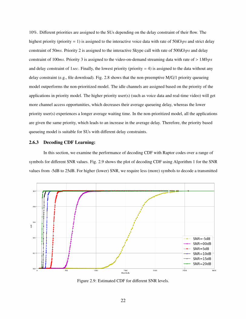
5.7 Average Waiting delay for all the source data for the given elementary networkstructure [hop1: Video, hop2: Skype, hop3: HD Video, hop4: Voice] . . . . . . . . 86

6.1 Gray scale image of UAV swarming. . . . . . . . . . . . . . . . . . . . . . . . . . 90

xi

6.2 Gray scale image of link quality between a gateway node and the tail end node[Black line indicates the link connecting different nodes] . . . . . . . . . . . . . . 90

6.3 DQN based UAV deployment. . . . . . . . . . . . . . . . . . . . . . . . . . . . . 92

xii

CHAPTER 1

INTRODUCTION

Firstly, in our work, we combined network models of a cognitive radio network (CRN)

with the models of machine learning algorithms. Spectrum decision based on Transfer

Actor-Critic Learning (TACT) is formulated by considering the idle duration of an idle channel,

packet dropping rate (PDR), and throughput of the channel in a distributed network. CUF is

estimated by a spectrum quality modeling scheme, which includes parameters spectrum sensing

accuracy and channel holding time. PDR is calculated from non-preemptive (NPRP) M/G/1

queueing model for CRN by considering SU contention with different latency requirements to

occupy the channel. Using NPRP M/G/1 queueing model, highest priority is given to low latency

data (ex. Real-time voice transmission) and low priority is given to high latency data (ex. file

download). And the flow throughput is estimated the statistics of history of symbol transmission

called as decoding-CDF along with rateless codes. TACT learning can adapt to the varying

conditions on its own and outperforms myopic based spectrum decisions. This research answered

the problem of tackling myopic decisions, delay induced in learning the spectrum strategies on its

own from the scratch.

Secondly, we analyzed the "channel+beam handoff" in Multibeam Smart

Antennas(MBSAs) based CRN. Here I formulated preemptive (PRP)/NPRP M/G/1 queueing

model with discretion rule, independently for each beam. In the proposed queueing model, the

high priority user with low latency requirement can interrupt the service of a low priority user if

the remaining service time of the low priority user is above a threshold. Here the high priority

user will not suffer large queueing delay and low priority user doesn’t undergo multiple

interruptions during their service. In addition, for the interruption duration, we detour the

interrupted packets (beam handoff) through neighbor beams over 2-hop relay. We formulated the

1

packet detouring as an optimization problem and determine the best way of selecting the

detouring paths using channel capacity and buffer level at each beam. This work answers the

problem of receiver keeping idle for long time when its sender node is being interrupted.

Moreover, using beam handoff, the interrupted user can finish its task just by detouring its data

during the interruption period.

Thirdly, we investigate how the transfer learning algorithms can improve the performance

of the network as compared to self-learning algorithms like Q-learning. Here, I developed a CRN

testbed for spectrum decision using machine learning algorithms with GNU Radio and USRP

modules. Practically implemented and tested transfer learning algorithm with simple 4 node

network. Here also we verified that using Transfer learning algorithm the node can quickly learn

the spectrum decision strategies and can outperform self-learning algorithm based on

reinforcement learning, and myopic decisions. To determine the performance of the testbed under

different learning algorithms, we used real-time video transmission. This work was presented to

US Air Force Lab (AFRL) as part of our research work.

Lastly, we extended our proposed Queueing models to multi-hop scenario, where each

node has its own data to transmit to central controller and it takes the help from its next hop to

forward its data to central node. Hence, each node will have its own data along with the relay data

to forward to the next node until it reaches the destination. We analyzed such multi-hop network

using preemptive M/G/1 Repeat queueing model where the priorty is assigned to each packet

based on the remaining time to live(TTL) of each. Any packet can be preempted by other packet

if it has very strict delay deadline than the earlier one. We analyzed the performance of such

queueing model by considering different data applications such as real-time voice, real-time

video(Skype), HD preencoded video(Youtube), and a File download(email). It was proved that

the proposed model outperforms the traditional First In First Out(FIFO) queueing model in such

mutlihop networks.

2

CHAPTER 2INTELLIGENT SPECTRUM MANAGEMENT BASED ON TRANSFER

ACTOR-CRITIC LEARNING

Chapter summary: In Chapter 2 we mentioned about the TACT-based spectrum handoff scheme.

In this chapter we discuss an intelligent spectrum mobility in cognitive radio networks (CRNs). Spectrum

mobility could be real spectrum handoff (i.e., the user jumps to a new channel) or wait-and-stay (i.e., the

user pauses the transmission for a while until the channel quality becomes good again. An optimal

spectrum mobility strategy needs to consider its long-term impact on the network performance, such as

flow throughput and packet dropping rate, instead of adopting a myopic scheme that optimizes only the

short-term throughput. We thus propose to use a promising machine learning scheme, called Transfer

Actor-Critic Learning (TACT), for the spectrum mobility strategies. Such a TACT-based scheme shortens a

user’s spectrum handoff delay, due to the use of a comprehensive reward function that considers the channel

utilization factor (CUF), packet error rate (PER), packet dropping rate (PDR), and flow throughput. Here,

the CUF is estimated by a spectrum quality modeling scheme, which considers spectrum sensing accuracy

and channel holding time. The PDR is calculated from NPRP M/G/1 queueing model, and the flow

throughput is estimated from a link-adaptive transmission scheme, which utilizes the rateless codes. Our

simulation results show that the TACT algorithm along with the decoding-CDF model achieves optimal

reward value in terms of Mean Opinion Score (MOS), compared to the myopic spectrum decision scheme.

2.1 Introduction

The spectrum mobility management is very important in cognitive radio networks (CRNs) [14].

Although a secondary user (SU) does not know exactly when the primary user (PU) will take the channel

back, it wants to achieve a reliable spectrum usage to support its quality of service (QoS) requirements. If

the quality of the current channel degrades, the SU can take one of the following three decisions: (i) Stay in

the same channel waiting for it to become idle again (called stay-and-wait); (ii) Stay in the same channel

and adjust to the varying channel conditions (called stay-and-adjust); (iii) Switch to another channel that

3

meets its QoS requirement (called spectrum handoff). Generally, if the waiting time is longer than the

channel switching delay plus traffic queueing delay, the SU should switch to another channel [75].

In this paper, we design an intelligent spectrum mobility management (iSM) scheme. To

accurately measure the channel quality for spectrum mobility management, we define a channel selection

metric (CSM) based on the following three important factors: (i) Channel Utilization Factor (CUF)

determined based on the spectrum sensing accuracy, false alarm rate, and channel holding time (CHT) [78];

(ii) Packet Dropping Rate (PDR) determined by evaluating the expected waiting delay for a SU in the

queue associated with the channel; (iii) Flow throughput which uses the decoding-CDF [34], along with

the prioritized Raptor codes (PRC) [77].

The spectrum management should maximize the performance for the entire session instead of

maximizing only the short-term performance. Motivated by this, we design an iSM scheme by integrating

the CSM with machine learning algorithms. The spectrum handoff scheme based on the long-term

optimization model, such as Q-learning used in our previous work [75], can determine the proper spectrum

decision actions based on the SU state estimation (including PER, queueing delay, etc.). However, the SU

does not have any prior knowledge of the CRN environment in the beginning. It starts with a trial-and-error

process by exploring each action in every state. Therefore, the Q-learning could take considerable time to

converge to an optimal, stable solution. To enhance the spectrum decision learning process, we use the

transfer learning schemes in which a newly joined SU learns from existing SUs which have similar QoS

requirements [74]. Unlike the Q-learning model that asks a SU to recognize and adapt to its own radio

environment, the transfer learning models pass over the initial phase of building all the handoff control

policies [25, 74].

The transfer actor-critic learning (TACT) method used in this paper is a combination of actor-only

and critic-only models [44]. While the actor performs the actions without the need of optimized value

function, the critic criticizes the actions taken by the actor and keeps updating the value function. By using

TACT, a new SU need not perform iterative optimization algorithms from scratch. To form a complete

TACT-based transfer learning framework, we solve the following two important issues: Selection of an

expert SU and transfer of policy from the expert to the learner node. We enhance the original TACT

algorithm by exploiting the temporal and spatial correlations in the SU’s traffic profile, and update the

value and policy functions separately for easy knowledge transfer. A SU learns from an expert SU in the

4

beginning; Thereafter, it gradually updates its model on its own. The preliminary results of this scheme

appeared in [41].

The CSM concept as well as the big picture of our iSM model is shown in Fig. 1. After the CSM is

determined, the TACT model will generate CRN states and actions, which consist of three iSM options

(spectrum handoff, stay-and-wait, or stay-and-adjust).

Goal: Intelligent

Spectrum Mobility

Spectrum Handoff

Stay and Adjust

Stay and Wait

State

Action

CSM

Transfer Actor-Critic Learning

(TACT )CUF: Channel

Utilization Factor

PDR: Packet

Dropping Rate

Link Throughput

Spectrum Sensing

Accuracy

NPRP M/G/1

Queueing Model

Rateless codes with

decoding-CDF

Figure 2.1: The big picture of iSM concept.

The main contributions of this paper are:

1) Teaching based spectrum management is proposed to enhance the spectrum decision process.

Previously, we proposed an apprenticeship learning based transfer learning scheme for CRN [74], which

can be further improved in some areas. For example, the exact imitation of the expert node’s policy should

be avoided since each node in the network may experience different channel conditions. Therefore, it is

helpful to consider a TACT-based transfer learning algorithm which uses the learned policy from the expert

SU to build its own optimized learning model by fine tuning the expert policy according to the channel

conditions it experiences. More importantly, we connect the Q-learning with TACT to receive the learned

policy from the expert node, which greatly enhances the teaching process without introducing much

overhead to the expert node.

2) Decoding-CDF with prioritized Raptor codes (PRC) are used to perform the high-throughput

spectrum adaptation. Due to mobility, the SU may experience fading and poor channel conditions. In order

to improve the QoS performance, we introduce spectrum adaptation by using the decoding-CDF along with

machine learning. Initially, the decoding-CDF was proposed for use with the Spinal codes [53], whereas

we use the decoding-CDF along with our prioritized Raptor codes (PRC) [77]. Our PRC model considers

the prioritized packets and allocates better channels to high-priority traffic.

5

The rest of this paper is organized as follows. The related work is discussed in Section II. The

channel selection metric is described in Section III, followed by an overview of the Q-learning based iSM

scheme in Section IV. Our TACT-based iSM scheme is described in Section V. The performance evaluation

and simulation results are provided in Section VI, followed by a discussion in Section VII. Finally, the

conclusions are given in Section VIII.

2.2 Related Work

In this section, we review the literature related to our work, which includes the three aspects:

a. Learning-based Wireless Adaptation: The strategy of learning from expert SUs was proposed in

our previous work, called the apprenticeship learning based spectrum handoff [74], which was further

extended in [76] as the multi teacher apprenticeship learning where the node learns spectrum handoff

strategy from multiple nodes in the network. Other related work in this direction includes the concept of

docitive learning (DL) [10, 25], reinforced learning (RL) used in CRNs [57], RL-based cooperative

spectrum sensing [47], and Q-learning based channel allocation [11, 32, 74]. DL was successfully used for

interference management in femtocell [25]. However, it did not consider the concrete channel selection

parameters. Also, it does not have clear definitions of expert selection process and node-to-node similarity

calculation functions. A channel selection scheme was implemented on GNU radio in [34]. But the CHT

and PDR were not used for channel selection. The same drawback exists in [32] and [11]. The TACT

learning scheme is superior to RL since it can use both node-to-node teaching and self-learning to adapt to

the complex CRN spectrum conditions.

b. Channel Selection Metric: The concept of channel selection metric in CRN was proposed

in [17,74]. A SU selects an idle channel based on the channel conditions and queueing delay. A QoS-based

channel selection scheme was proposed in [79], but the channel sensing accuracy and CHT were not

considered. Note that the CHT determines the period over which a SU can occupy the channel without

interruption from the PU. Further, authors in [70] proposed OFDM based MAC protocol for spectrum

sensing and sharing which reduces the sharing overhead, but they did not consider the kind of channel that

should be selected by the SU for transmission. Our spectrum evaluation scheme considers the channel

dynamics with respect to the interference, fading loss, and other channel variations.

c. Decoding-CDF based Spectrum Adaptation: The rateless codes have been used in wireless

6

communications due to its property of recovering the original data with low error rate. The popular rateless

codes include the Spinal codes [53,54], Raptor codes [61] and Strider codes [20,24,27]. The rateless codes

for CRNs were proposed in [10, 85]. Authors in [10] proposed a feedback technique for rateless codes

using multi-user MIMO to improve the QoS and to provide delay guarantee. Authors in [34] used

decoding-CDF with the Spinal codes. In this paper, we use decoding-CDF along with our prioritized

Raptor codes (PRC) [77] to perform spectrum adaptation.

2.3 Channel Selection Metric

In order to select a suitable channel for spectrum handoff, the SU should consider the time varying

and spatial channel characteristics. The time-varying channel characteristics comprise of CHT and PDR,

which are mainly observed due to PU interruption and SU contentions, and the spatial characteristics

comprise of achievable throughput and PER observed due to the SU mobility. As mentioned in Section I,

the CSM comprises of CUF, PDR and flow throughput which are described below.

2.3.1 Channel Utilization Factor (CUF)

If a busy channel is detected as idle, this misinterpretation is called as false alarm, which is a key

parameter of spectrum sensing accuracy. We use the spectrum sensing accuracy and CHT for evaluating the

effective channel utilization. From [78], we know that a higher detection probability, Pd, has a low false

alarm probability, P f . Hence we express the spectrum sensing accuracy as

MA = Pd(1−P f ) (2.1)

If T denotes the total frame length and τ is the channel sensing time, the transmission period is T -

τ. We assume that the PU arrival rate λph follows the Poisson distribution and the CHT with duration t has

the following probability distribution,

f (t) = λphe−(λph)t (2.2)

Since PU’s arrival time is unpredictable, it can interfere with the SU’s transmission. Hence, the

7

predictable interruption duration can be determined as [66],

y(t) =

T −τ− t, 0 ≤ t ≤ (T −τ)

0, t ≥ (T −τ)(2.3)

The SU transmits the data with an average collision duration [66] as,

y(T ) = 1−∫ T−τ

0(T −τ− t) f (t)d(t) = (T − t)− t(1− e(− (T−τ)

t )) (2.4)

Hence, the probability that a SU experiences the interference from a PU within its frame transmission

duration is given by

Pps =

y(T )(T −τ)

= 1−t

(T −τ)

(1− e

(−

(T−τ)t

))(2.5)

The total channel utilization (CUF) is determined by using CHT and probability of interference from PU as,

CUF = MA(T −τ)

T(1−Pp

s) (2.6)

Substituting the results from (6) in (7), the CUF can be defined as follows,

CUF = MA.tT

(1− e

(−

(T−τ)t

))(2.7)

The CUF can be used to represent the spectrum evaluation results for the selection of an optimal channel.

According to IEEE 802.22 recommendations, the probability of correct detection, Pd = [0.9,0.99] and the

probability of false alarm, P f = [0.01,0.1]. Therefore, the probability of spectrum sensing accuracy is

Pd(1−P f ) = [0.81,0.99].

2.3.2 Non-Preemptive M/G/1 Priority Queueing Model

We use a non-preemptive M/G/1 priority queueing model where a lower priority SU accesses

channel without interruption from higher priority SUs. We denote j=1 (or N) as the highest (or lowest)

priority SU. However, any SU transmissions can be interrupted by a PU. When the channel becomes idle, a

higher priority SU will be served. When a SU is interrupted by a PU, it can either stay-and-wait in the same

8

channel until it becomes idle again, or handoff to another suitable channel.

Let Delay j,i be the delay of a S U j connection due to the first (i−1) interruptions. A S U j packet

will be dropped if its delay exceeds the delay deadline d j. In our previous work [75], we deduced the

PDR(k)j,i as the probability of packet being dropped during the ith interruption for channnel k with packet

arrival rate, λ, and mean service rate, µ. It equals to the probability of handoff delay E[Dkj,i] being larger

than d j−Delay j,i [75].

PDR(k)j,i = ρ(k)

j,i .exp(−ρ(k)

j,i × (d j−Delay j,i)

E[D(k)j,i ]

) (2.8)

Here, ρ(k)j,i is the normalized load of channel k caused by type j SU. It is defined as follows,

ρ(k)j,i =

λi

µk≤ 1 (2.9)

2.3.3 Throughput Determination in Decoding-CDF based Rateless Transmission

After we identify a high-CUF channel, the next step is to transmit the SU’s packets in this channel.

Even a channel with high CUF can experience the time varying link quality due to the mobility of SU.

Therefore, link adaptation is important to avoid frequent spectrum handoffs. Generally, the sender needs to

adjust its data rate depending on the channel conditions since a poor link (lower channel SNR) can result in

a higher packet loss rate. For example, in IEEE 802.11, the sender uses the channel SNR to select a

suitable modulation constellation and forward error correcting (FEC) code rate from a set of discrete

values. Such a channel adaptation cannot achieve a smooth rate adjustment since only a limited number of

adaptation rates are available. Because channel condition variations can occur on very short time scales

(even at the sub-packet level), it is challenging to adapt to the dynamic channel conditions in CRNs.

Rateless codes have shown promising performance improvement in multimedia transmission over

CRNs [77]. At the sender side, each group of packets is decomposed into symbols with certain redundancy

such that the receiver can reconstruct the original packets as long as enough number of symbols are

received. The sender does not need to change the modulation and encoding schemes. It simply keeps

9

sending symbols until an ACK is received from the receiver, signaling that enough symbols have been

received to reconstruct the original packets. The sender then sends out the next group of symbols. For a

well-designed rateless code, the number of symbols for packets closely tracks the changes in the channel

conditions.

In this paper, we employ our unequal error protection (UEP) based prioritized Raptor codes

(PRC) [77]. In PRC, more symbols are generated for the higher priority packets than the lower priority

packets. As a result, PRC can support higher reliability requirements of more important packets. We

describe below how we can achieve cognitive link adaptation through a self-learning of ACK feedback

statistics (such as inter-arrival time gaps between two feedbacks). We also show how a SU can build a

decoding-CDF by using the previously transmitted symbols and how it can be used for channel selection

and link adaptation.

CDF-Enhanced Raptor Codes

In rateless codes, after sending certain number of symbols, the sender pauses the transmission and

waits for a feedback (ACK) from the receiver. No ACK is sent if the receiver cannot reconstruct the

packets, and the sender needs to send extra symbols. Each pause for ACK introduces overhead in terms of

the total time spent on symbol transmission plus ACK feedback [34]. The decoding-CDF defines the

probability of decoding a packet successfully from the received symbols. In the CDF-enhanced rateless

codes, the sender can use the statistical distribution to determine the number of symbols it should send

before each pause. The CDF distribution is sensitive to the code parameters, channel conditions, and code

block length. Surprisingly, only a small number of records on the relationship between n (number of

symbols sent between two consecutive pauses) and τ (ACK feedback delay) are needed to obtain the CDF

curve [34].

In order to speed up the CDF learning process, the Gaussian approximation can be used which

provides a reasonable approximation at low channel SNR, and its maximum likelihood (ML) requires only

mean (µ) and variance (σ2). In addition, we introduce the parameter α, which ranges from 0 (means no

memory) to 1 (unlimited memory), to represent the importance of past symbols in the calculation. This

process has two advantages: the start-up transition dies out quickly, and the ML estimator is well behaved

for α = 1. The Algorithm 1 defines the Gaussian CDF learning process.

10

Algorithm 1 : Decoding CDF Estimation by Gaussian Approximation1: Input: alpha, % learning rate [0,1]2: Step-1: Initialization3: NS =1 % encoded samples4: sum = 05: sumsq = sum2 + 06: Step-2: Update % updating sum and samples7: NS = NS*alpha +18: sum = sum*alpha + NS9: sumsq=sumsq*alpha + NS2

10: Step-3: Get CDF: % estimating CDF by mean & variance11: mean = sum/NS12: variance= sumsq/NS - mean2

13: estimate CDF

Using Algorithm 1, the decoding-CDF can be estimated by using the following standard equation,

F(x) =

∫ NS

0

1

σ√

2πe−

(NS−µ)2

2σ2 dx (2.10)

Here, NS, µ and σ are the number of symbols, mean and variance, respectively.

For the observed link SNR, we can determine the number of symbols that need to be transmitted in

order to decode the packet successfully. When the channel condition degrades in-terms of PER but

PDR ≤ PDRth, the additional symbols are transmitted to adapt to the current channel conditions, which

avoids unnecessary spectrum handoff. After the number of transmitted symbols reaches the maximum

value, (NS )max, the SU should perform spectrum handoff to a new channel. This is called as link adaptation

using decoding-CDF.

After determining the number of symbols per packet (NS), which are required to successfully

decode a packet, we can calculate the rateless throughput (TH) of channel k in a Rayleigh fading channel

as [34],

T Hk =2× fs× (NS )

tsymbols/s/Hz (2.11)

Where fs and t are the sampling frequency and transmission time, respectively. The value of NS

varies over time due to the Rayleigh fading channel and number of symbols per packet estimated using the

decoding-CDF curve. Since each node observes either time spreading of digital pulses or time-varying

11

behavior of the channel due to mobility, Rayleigh fading channel is appropriate due to its ability to capture

both variations (time spreading and time varying).

The normalized throughput is:

(T Hk)norm =T Hk

(T Hk)ideal(2.12)

Here, (T Hk)ideal is the ideal throughput calculated via Shannon capacity theorem.

Now we can integrate the above three models together into a weighted channel selection metric for

ith interruption in kth channel for the S U with priority j [32],

U(k)i j = w1?CUF + w2? (1−PDR(k)

i j ) + w2? (T Hk)norm (2.13)

Where w1,w2 and w3 are weights representing the relative importance of the channel quality, PDR and

throughput, respectively. Here w1 + w2 + w3 = 1. Their setup depends on application QoS requirements. For

real-time applications, the throughput is more important than PDR. On the other hand, PDR is the most

important factor for the FTP applications. For video applications, CHT (part of CUF model) is more

important.

2.4 Overview of Q-Learning based intelligent Spectrum Management(iSM)

In this paper, the Q-learning scheme is used to compare the performance of our proposed

TACT-based learning scheme for intelligent spectrum mobility management. More details about Q-learning

based spectrum decisions are available in [75]. The Q-learning uses special Markov Decision Process

(MDP), which can be stated as a tuple (S ,A,T,R) [57]. Here, S depicts the set of system states; A is the set

of system actions at each state; T represents the transition probability, where T = {P(s,a, s′)}, and P(.) the

probability of transition from state s to s′ when action a is taken; and R : S ×A 7→ R is the reward or cost

function for taking an action a ∈ A in state s ∈ S . In MDP, we intend to find the optimal policy π∗(s) ∈ A,

i.e., a series of actions {a1,a2,a3, ...} for state s, in order to maximize the total discount reward function.

States: For S Ui, the network state before ( j + 1)th channel assignment is depicted as

si j = {χ(k)i j , ξ

(k)i j ,ρ

(k)i j ,φ

(k)i j }. Here k is the channel being used; χ(k)

i j depicts the channel status (idle or busy); ξ(k)i j

12

is the channel quality (CSM); ρ(k)i j indicates the traffic load of channel; and φ(k)

i j represents the QoS priority

level of S Ui.

Actions: Three actions are considered for iSM scheme - stay-and-wait, stay-and-adjust and

spectrum handoff. We denote ai j = {β(k)i j } ∈ A as the candidate of actions for S Ui on state si j after the

assignment of ( j + 1)th channel, and β(k)i j represents the probability of choosing action ai j.

The Q-learning algorithm aims to find an optimal action which minimizes the expected cost of the

current policy π∗(si, j,ai, j) for ( j + 1)th channel assignment to S Ui. It is based on the value function Vπ(s)

that determines how good it is for a given agent to perform a certain action under a given state. Similarly,

we use the action value function, Qπ(s,a); It defines which action has low cost in the long term. Bellman

optimality equation gives the high and discounted long-term rewards [56]. For the sake of simplicity, in

further sections we consider si, j as s, action ai, j as a, and state si, j+1 as s′.

Rewards: The reward R of an action is defined as the predicted reward function for data

transmission, for a certain channel assignment. For multimedia data, we use the mean opinion score (MOS)

metric. Based on our previous work [75], the MOS can be calculated as follows,

R = MOS =a1 + a2FR + a3ln(S BR)

1 + a4T PER + a5(T PER)2 (2.14)

where FR, SBR and TPER are the frame rate, sending bit rate, total packet error rate, respectively. The

parameter ai, i ∈ {1,2,3,4,5} is estimated using the linear regression process. MOS varies from 1 (lowest)

to 5 (highest). When the channel status is idle, ’transmission’ is an ideal action to take, which would

achieve MOS close to 5. On the other hand, when PDR (State: traffic load) or PER (State: channel quality)

is high, low MOS would be achieved which reflects poor performance in the acquired channel.

The estimation of expected discounted reinforcement of taking action a in state s, Q∗(s,a) can be

written as [75],

Q∗(s,a) = E(Ri, j+1) +γ∑

s′

Ps,s′(a)maxa′∈A

Q∗(s,a) (2.15)

We adopt softmax policy for long-term optimization. π(s,a), which determines the probability of taking

13

action a, can be determined by utilizing Boltzmann distribution as [75]

π(s,a) =exp( Q(s,a)

τ )∑a′∈A exp( Q(s,a′)

τ )(2.16)

Here, Q(s,a) defines the affinity to select action a at state s; it is updated after every iteration. τ is the

temperature. The Boltzman distribution is chosen to avoid jumping into exploitation phase before testing

each action in every state. The high temperature indicates the exploration of the unknown state-action

values, whereas the low temperature indicates the exploitation of known state-action pairs. If τ is close to

infinity, the probability of selecting an action follows the uniform distribution, i.e., the probability of

selecting any action is equal. On the other hand, when τ is close to zero, the probability of choosing an

action associated with the highest Q-value in a particular state is one.

Fig. 2.2 shows the procedure of using Q-learning for iSM. Here the dynamic spectrum conditions

are captured by the states, which are used for policy search in order to maximize the reward function. The

optimal policy determines the corresponding spectrum management action in the current round.

Cognitive Radio

EnvironmentTransmission Rate,

SINR,

PU s signal

StatesStates

Q-table

Q(s,a)

Q-table

Q(s,a)

1. Throughput

2. Channel status

3. PDR

Information Update

1. Throughput

2. Channel status

3. PDR

Information UpdateReward

MOS

Spectrum

Decision

Action

Spectrum

Decision

ActionCognitive Radio


SINR,

PU s signal

States

Q-table

Q(s,a)

1. Throughput

2. Channel status

3. PDR


MOS

Spectrum

Decision

Action

Q-learning machine

Cognitive Radio


SINR,

PU s signal

States

Q-table

Q(s,a)

1. Throughput

2. Channel status

3. PDR


MOS

Spectrum

Decision

Action

Q-learning machine

𝒂𝒊𝒋

𝒂𝒊𝒋

Sta

tes

𝝅(𝒔

,𝒂)

𝝆𝒊𝒋(𝒌)

(𝜺𝒊𝒋(𝒌)

)

Figure 2.2: The Q-learning based iSM.

2.5 TACT based intelligent Spectrum Management(iSM)

The Q-learning based MDP algorithm could be very slow due to two reasons: (1) It requires the

selection of suitable initial state/parameters in the Markov chain; (2) It also needs proper settings of

Markov transition matrix based on different traffic, QoS and CRN conditions.

Let us consider a new SU which has just joined the network, and needs to build a MDP model.

14

Instead of using trial-and-error to find the appropriate MDP settings, it may find a neighboring SU with

similar traffic and QoS demands, and request it to serve as "expert" (or teacher) and transfer its optimal

policies. Such teaching or transfer based scheme can considerably shorten the learning (or convergence)

time.

We use the TACT model for the knowledge transfer between SUs, which consists of three

components: actor, critic and environment [44] [41]. For a given state, the actor selects and executes an

action in a stochastic manner. This causes the system to transition from one state to another with a reward

as feedback to the actor. Then the critic evaluates the action taken by the actor in terms of time difference

(TD) error, and updates the value function. After receiving the feedback from the critic, the actor updates

the policy. The algorithm repeats until it converges.

To apply TACT in our spectrum management scheme, we solve the following two issues:

(1) Selection of the Expert SU: We consider a distributed network without a central coordinator.

When a new SU joins the network, it performs the localized search broadcasting the Expert-Seek messages.

The nearby nodes may be located in the area covered by the same PU(s), and thus have similar spectrum

availability. The SU should select a critic SU based on its relevance to the application, level of expertise,

and influence of an action on the environment. To find the expert SU, the SUs share the following three

types of information among them, i.e., channel statistics (such as CUF), node statistics (node mobility,

modulation modes, etc.), and application statistics (QoS, QoE, etc.). The similarity of the SUs can be

evaluated in an actor SU by using the manifold learning [74], which uses the Bregman Ball concept to

compare the complex objects. The Bregman ball comprises of a center (µ(k)) and a radius (R(k)). The data

point Xp which lies inside the ball possesses strong similarity with µ(k). We define their distance as [74],

B(µk,Rk) = {Xt ∈ X : Dφ(Xt,µk) ≤ Rk} (2.17)

Here D(p,q) is known as the Bregman Divergence, which is the manifold distance between two

signal points (the expert SU and learning SU). If the distance is less than a specified threshold, we conclude

that p and q are similar to each other. All distances are visualized in Gephi (a network analysis and

visualization software) [4], as shown in Fig. 2.3. The similarity calculation between any two SUs includes

three metrics: (1) The application statistics, which mainly refer to the QoS parameters such as the data

15

rates, delay, etc.; (2) The node statistics, which include the node modulation modes, location, mobility

pattern, etc.; (3) The channel statistics, which include the channel parameters such as bandwidth, SNR, etc.

The SU with the highest similarity value with the learning SU is chosen as the expert SU. In Fig. 2.3, SU3

is selected as the expert SU (i.e., the critic) since it has stronger similarity to the learning SU (SU1)

compared to the rest of the SUs.

Figure 2.3: Gephi-simulated expert SU search.

(2) The Knowledge Transfer via TACT Model: The actor-critic learning updates the value function

and policy function separately, which makes it easier to transfer the policy knowledge compared to the

other critic-only schemes, such as Q-learning and greedy algorithm. We implement the TACT-based iSM

as follows:

(i) Action Selection: When a new SU joins the network, the initial state is si j in channel k. In order

to optimize the performance, the SU chooses suitable actions to balance two explicit functions: a)

searching for the new channel if the current channel condition degrades (exploration), and b) finding an

optimal policy by sticking to the current channel (exploitation). This also enables the SU to not only

explore a new channel but also to find the optimal policy based on its past experience. The probability of

taking an action a in state s is determined, as mentioned in equation (2.16).

(ii) Reward: The MOS from equation (16) is evaluated as the reward resulting out of an action

a ∈ {A} taken in state s ∈ {S }.

(iii) State-Value Function Update: Once the SU chooses an action in channel k , the system

changes the state from s to s′ with a transition probability,

P(s′|s,a) =

1, s′ ∈ S

0, otherwise(2.18)

16

The total reward for the taken action would be Rs.a. The time difference (TD) error can be calculated from

the difference between (i) the state-value function, V(s) estimated in the previous state, and (ii) Rs,a + V(s′)

at the critic [38],

δ(s,a) = Rs,a +γ∑s′∈S

P(s′|s,a)V(s′)−V(s)

= Rs,a +γV(s′)−V(s) (2.19)

Subsequently, the TD error is sent back to the actor. By using TD error, the actor updates its state-value

function as

V(s′) = V(s) +α(ν1(s,m))δ(s,a) (2.20)

Where ν1(s,m) indicates the occurrence time of state s in these m stages. α(.) is a positive step-size

parameter that affects the convergence rate. V(s′) remains as V(s) in case of s , s′.

(iv) Policy Update: The critic would employ the TD error to evaluate the selected action by the

actor, and the policy can be updated as [28],

p(s,a) = p(s,a)−β(ν2(s,a,m))δ(s,a) (2.21)

Here ν2(s,a,m) denotes the occurrence time of action a at state s in these m stages. β(.) denotes the positive

step size parameter defined by (m∗ logm)−1 [44]. Equations (2.16) and (2.21) ensure that an action in a

specific state can be selected with a higher probability, if we reach the highest minimum reward, i.e.,

δ(s,a) < 0.

If each action is executed for infinite times in each state and the learning algorithm follows a

greedy exploration, the value function V(s) and the policy function π(s,a) will ultimately converge to V∗(s)

and π∗, respectively, with a probability of 1.

(v) Formulation of Transfer Actor-Critic Learning: Initially, the expert SU shares its optimal policy

with the new SU. Let p(s,a) denote the likelihood of taking action a in state s. When the process

eventually converges, the likelihood of choosing a particular action a in a particular state s is relatively

higher than that of other actions. In other words, if the spectrum handoff is performed based on a learned

17

strategy by S Ui, the reward will be high in the long term. However, in spite of the similarities between the

two SUs, they might have some differences, such as in the QoS parameters. This may make an actor SU

take more aggressive action(s). To avoid these problems, the transferred policy should have a decreasing

impact on the choice of certain actions, especially after the SU has taken its action and learned an updated

policy. This is the basic idea of TACT-based knowledge transfer and self-learning.

ActionAction

Figure 2.4: TACT based SU-to-SU teaching.

The new policy update follows TACT principle (see Fig. 2.4), in which the overall policy of

selecting an action is divided into a native policy, pn and an exotic policy, pe. Assume at stage m, the state

is s and the chosen action is a. The overall policy can be updated as [8]:

p(m+1)o (s,a) = [(1−ω(ν2(s,a,m))p(m+1)

n (s,a)

+ω(ν2(s,a,m))p(m+1)e (s,a)]pt

−pt(2.22)

Where [x]ba with b > a, indicates the Euclidean distance of interval [a,b], i.e., [x]b

a = a if x < a;

[x]ba = b if x > b and [x]b

a = x if a≤ x ≤ b. In this scenario, a = −pt and b = pt. In addition,

p(m+1)0 (s,a) = p(m)

0 (s,a), ∀a ∈ A but a , ai j. And pn(s,a) updates itself according to equation (2.21).

During the initial learning process, the exotic policy pe(s,a) is dominant. Therefore, when the SU

enters a state s, the presence of pe(s,a) forces it to choose the action, which might be optimal based on the

expert SU. Subsequently, the proposed policy update strategy can improve the performance. We define

ω ∈ (0,1) as the transfer rate, and ω 7→ 0 as the number of iterations goes to∞. Thus the impact of exotic

policy pe(s,a) is decreased. Algorithm 2 describes our proposed TACT-based iSM scheme.

18

Algorithm 2 : TACT-based Spectrum Decision SchemeInput: Channel, Node and Application statisticsOutput: best policy π(s,a) of S UiPart-I

1: Initialization2: if node is new then3: if there is expert then4: Perform TACT algorithm from Part-II5: else6: Determine the channel k status and CUF from (8).7: Find PDR from (9) and (T H)norm from (13).8: Calculate U(k)

i j using (14) and select the best channel9: Perform Q-learning itself

10: end if11: else12: Perform TACT algorithm from Part-II13: if channel condition is below the threshold then14: Perform one of the three actions: stay-and-wait, stay-and-adjust, or Handoff

15: end if16: end if

- - - - - - - - - - - - - - - - - - - - - - - - - - - - - - - - - - - - -Part-IIInput: Channel, Node and Application statisticsOutput: best policy π(s,a) of S Ui

1: Initialize Vπ(s) arbitrarily.2: Exchange node information among node i and its neighbors.3: Using manifold learning to find the expert.4: Get the expert policy, i.e., exotic policy Pe(s,a), from expert SU.5: Initialize native policy, pn(s,a) .6: Repeat:7: Choose an action based on the initial policy π(0).8: Calculate MOS, update TD error using (20), state-value function (21), and native and overall

policy using (22) and (23), respectively.9: Update the strategy function using (17).

10: end

19

2.6 Performance Evaluation

In this section, we evaluate the performance of our proposed scheme, including the channel

selection, decoding CDF and enchanced TACT learning model.

2.6.1 Channel Selection:

We first examine our channel selection scheme (described in Section III), including the effect of

spectrum sensing accuracy (MA) and CHT. We setup the parameters as shown in Table I.

Parameters ValuesNumber of time slots, (T) 100

False Alarm Probability,P f [0.01,0.1]Detection probability, Pd [0.9,0.99]

Exponential distribution rate λpi, i = 0,1 [0.02,1]Temperature, τ 1000

Discount factor, γ 0.001Transfer rate, ω 0.7

The number of channels 10Learning rate, α (decoding CDF) [0.9,0.8,0.99]

Packet aggregation cost, n f 10

Table 2.1: Simulation Parameters

We consider N=10 PUs, each of them possessing one primary channel, and randomly select the

probability parameters given in Table I. Fig. 2.5a and 2.5b represent MA and CHT, respectively. By

considering both MA and CHT, the SU determines the CUF for each channel and ranks them in the

decreasing order as shown in Fig. 2.5c.

CH1CH2

CH3CH4

CH5CH6

CH7CH8

CH9CH10

Channels

0.0

0.2

0.4

0.6

0.8

1.0

Accu

racy

(a) Spectrum sensing accuracy

CH1CH2

CH3CH4

CH5CH6

CH7CH8

CH9CH10

Channels

0

10

20

30

40

50

time

(ms)

(b) PU idle duration (CHT)

CH2CH9

CH4CH8

CH3CH10 CH5

CH7CH1

CH6

Channels

0.0

0.1

0.2

0.3

0.4

0.5

Chan

nel u

tiliz

atio

n fa

ctor

(c) Channel utilization factor

Figure 2.5: The channel selection parameters.

Fig. 2.6 shows the normalized throughput of the system that can be achieved by our channel

selection scheme (BIGS) for different frame rates and PU idle durations (CHT). Here, BIGS refers to the

20

Figure 2.6: Comparison of theproposed and random channel se-lection schemes. Here, FD repre-sents the frame duration.

Figure 2.7: Comparison ofthe proposed channel selectionscheme with [11] and [17].

500 1000 1500 2000 2500Traffic intensity per node (Kbps)

0

1000

2000

3000

4000

5000

6000

7000

Aver

age

dela

y (m

s)

priority=1priority=2priority=3priority=4average (without Priority)

Figure 2.8: Average delay forthe non-preemptive M/G/1 pri-ority queueing model and non-prioritized model.

channel sensing using Bayesian Inference with Gibbs Sampling [78]. For comparison, we also show the

normalized throughput achieved by a random channel selection (RCS) scheme. Our scheme achieves better

throughput than RCS because it selects the channel with high sensing accuracy as well as high CHT,

whereas RCS does not consider the CHT and is also prone to channel miss detection and false alarm.

In Fig. 2.7, we compare the normalized throughput of our channel selection model with [11]

and [17]. In our scheme, the SU senses the channel and ranks them based on the channel sensing accuracy

and CHT. Similarly, authors in [17] performed the channel sensing based on the energy detection, and

categorized the channels based on their CHT. In addition, they considered the directional antenna whereas

we use the omni-directional antenna. Therefore, [17] has higher channel sensing accuracy than our scheme

as the interference level is much lower in directional communication as compared to the omni

communication. As a result, the throughput of [17] is higher than ours. To compare our schemne with [11],

we consider that the channel can use one band at a time and also assume that the Q-learning has achieved

the optimal condition. Alongside we also consider that SU communicates in its current channel until it is

occupied by other users. Since the channel selection is random in [11], the SU may select a channel with

small CHT even when a channel with longer CHT is available. Therefore, though its sensing accuracy is

close to ours, the throughput is lower. Channel selection based on the channel ranking is very important to

achieve smooth communication and to avoid frequent spectrum handoffs.

2.6.2 Average Queueing Delay:

We assume that the service time of SUs follows the exponential distribution, and the number of

channels is 10. The maximum transmission rate of each channel is 3Mbps, and the PER varies from 2% to

21

10%. Different priorities are assigned to the SUs depending on the delay constraint of their flow. The

highest priority (priority = 1) is assigned to the interactive voice data with rate of 50Kbps and strict delay

constraint of 50ms. Priority 2 is assigned to the interactive Skype call with rate of 500Kbps and delay

constraint of 100ms. Priority 3 is assigned to the video-on-demand streaming data with rate of > 1Mbps

and delay constraint of 1sec. Finally, the lowest priority (priority = 4) is assigned to the data without any

delay constraint (e.g., file download). Fig. 2.8 shows that the non-preemptive M/G/1 priority queueing

model outperforms the non-prioritized model. The idle channels are assigned based on the priority of the

applications in priority model. The higher priority user(s) (such as voice data and real-time video) will get

more channel access opportunities, which decreases their average queueing delay, whereas the lower

priority user(s) experiences a longer average waiting time. In the non-prioritized model, all the applications

are given the same priority, which leads to an increase in the average delay. Therefore, the priority based

queueing model is suitable for SUs with different delay constraints.

2.6.3 Decoding CDF Learning:

In this section, we examine the performance of decoding CDF with Raptor codes over a range of

symbols for different SNR values. Fig. 2.9 shows the plot of decoding CDF using Algorithm 1 for the SNR

values from -5dB to 25dB. For higher (lower) SNR, we require less (more) symbols to decode a transmitted

Figure 2.9: Estimated CDF for different SNR levels.

22

packet. The Rayleigh fading channel is used.

Using the decoding CDF, we examine the throughput for Raptor codes in Fig. 2.10. For better

visualization, Fig. 2.11 zooms in a section of Fig. 2.10. As mentioned before, the decoding CDF enables

us to find the optimal feedback strategy, i.e., when to pause for feedback and how many symbols should be

transmitted before the next pause. The throughput is examined for a SU moving at a speed of 10 m/s over

Rayleigh fading channel at 2.4GHz (channel S NR = 15dB) within a time range of 100 ms with a packet

aggregation cost n f = 10, which decides the number of packets to be aggregated to send an ACK. The

throughput is estimated offline using Algorithm 1 with learning rate parameter, α, set to 0.9. It can be seen

from Fig. 2.10 and 2.11 that α need not to be close to 1 to obtain a good performance. The throughput

achieved by the Raptor codes is almost half of the Shannon capacity [34]. The decoding CDF performance

is close to that of the ideal learning which is determined based on receiving ACKs from the receiver.

0 20 40 60 80 100Time (ms)

0

20

40

60

80

100

Thr

ough

put (

Mbp

s)

Channel capacity Raptor codes: Ideal Learning α=0.90 α=0.80 α=0.99

Figure 2.10: Channel throughput estimation for Raptor codes for Rayleigh fading channel.

62 64 66 68 70 72Time (ms)

0

20

40

60

80

100

Thr

ough

put (

Mbp

s)

Channel capacity Raptor codes: Ideal Learning α=0.90 α=0.80 α=0.99

Figure 2.11: Zoomed-in section of Figure 10 (for time 61-73 ms).

2.6.4 TACT Enhanced Spectrum Management Scheme:

In this section, we study the performance of our TACT-based spectrum mobility scheme. For 10

available channels with capacity of 3Mbps each, we assume there are 10 different PUs with different data

rates for transmission which can interrupt the SU transmission. Different SUs contending for the channel

23

0 1 2 3 4 5 6 7 8 9 10

x 104

0

0.5

1

1.5

2

2.5

3

3.5

4

4.5

5

Time slot

Exp

ecte

d M

ean

opin

ion

scor

e

MyopicQ−learningTACT

Figure 2.12: The MOS performance for slow movingnode.

0 1 2 3 4 5 6 7 8 9 10

x 104

0

0.5

1

1.5

2

2.5

3

3.5

4

4.5

5

Time slot

Exp

ecte

d M

ean

opin

ion

scor

e

MyopicQ−learningTACT

Figure 2.13: The MOS performance for fast movingnode.

4 5 6 7 8 9 10 11 12 13 14 15

x 104

3

3.2

3.4

3.6

3.8

4

4.2

4.4

4.6

4.8

5

Time slot

Exp

ecte

d M

ean

opin

ion

scor

e

Q−learningTACT

Figure 2.14: The MOS performance comparisonwithout the decoding-CDF.

4 5 6 7 8 9 10 11 12 13 14 15

x 104

3

3.2

3.4

3.6

3.8

4

4.2

4.4

4.6

4.8

5

Time Slot

Exp

ecte

d M

ean

Opi

nion

Sco

re

Q−learningTACT

Figure 2.15: The MOS performance with the use ofdecoding-CDF

0 1 2 3 4 5

Time slot 104

2

2.5

3

3.5

4

4.5

5

Exp

ecte

d M

ean

opin

ion

scor

e

TACT- = 0.2TACT- = 0.5TACT- = 0.8

Figure 2.16: The effect of transfer rate, ω on learningperformance.

0 1 2 3 4 5

Time slot 104

2

2.5

3

3.5

4

4.5

5

Exp

ecte

d M

ean

opin

ion

scor

e

[2]- Reinforcement Learning[6]- Apprenticeship LearningTACT- = 0.7

Figure 2.17: The comparison of our TACT modelwith RL [75] and AL [74].

24

access also have different data rates. We study the performance of a SU which is supporting a Skype video

call at 500 Kbps and has a priority of 2. All SUs use the Raptor codes, and the expert SU teaches a new SU

about its transmission strategy based on the decoding-CDF profile. We consider the following four cases.

Case 1: The newly joined SU moves very slowly at <5mph; Case 2: The SU moves fast (>50mph) and

experiences different channel conditions; Case 3: The SU moves fast but does not use the decoding CDF

and pause control for transmission. Instead, it manually changes the symbol sending rate based on the

current channel conditions; Case 4: The SU moves fast and uses the decoding CDF. We use the

low-complexity MOS metric to estimate the received quality.

In Fig. 2.12 (for Case 1), the Q-learning based spectrum decision scheme outperforms the myopic

approach, because the former takes spectrum decisions to maximize the long-terms reward (i.e., MOS)

whereas the latter considers only the immediate reward. Further, our proposed TACT-based scheme

outperforms the Q-learning scheme since the newly joined SU can learn from the expert SU, and thus

spends less time in estimating the channel dynamics. Without the expert node, the node in Q-learning

scheme learns everything by itself, and thus needs more time to converge to a stable solution. Fig. 2.13

shows the result for fast moving SU for Case 2, which experiences channel condition variations with time.

Our proposed TACT scheme still performs better than the Q-learning scheme.

Fig. 2.14 depicts the Case 3 where the SU moves fast but does not use the decoding-CDF concept

for Raptor codes. Since the SU is moving fast, it experiences different channel conditions. Once the SU

attains the convergent state it achieves a high MOS value. But this does not guarantee that it will stay in the

optimal state during the entire communication due to variations in channel conditions. Without the use of

decoding-CDF, the SU is unable to adapt to the channel variations which results in the lower MOS value of

around 4. In Fig. 2.15 (Case 4), the SU uses the CDF curve to learn the strategy of transmitting more

symbols with lower overhead, and achieves a higher MOS of around 4.4. In both cases we can see that the

MOS drops due to the change in channel condition at time slot 7. But CDF helps to quickly improve the

MOS value to around 4.4.

Figure 2.16 shows the effect of transfer rate, ω on learning performance. We observe that the

transfer rate has impact only at the beginning. Higher the transfer rate (ω = 0.8), faster the adaptation to the

network with less MOS variations. Whereas lower the transfer rate (ω = 0.2), slower is the adaptation to

the network and more are fluctuations in the MOS value. The performance converges after some iterations

25

as the SU gradually builds up its own policy using the expert node.

Figure 2.17 shows that our TACT based spectrum decision scheme outperforms the Q (or RL)

scheme [75] and the apprenticeship based transfer learning scheme [74]. In AL scheme, the student node

uses the expert node’s policy for its own spectrum decision. This model works well if both the student and

expert nodes experience the same channel and traffic conditions. Our TACT based model, on the other

hand, can tune the expert policy according to its own channel conditions in a few iterations.

2.7 Discussion

Main concern in transfer learning approach is the overhead introduced by the expert search and the

transfer of its knowledge (optimal policy) to the learner node. The proposed TACT learning-based spectrum

decision requires a ’learner node’ to communicate only with the closest neighbors, since only these nearby

nodes are likely to have similar PU traffic distribution and channel conditions. This communication with

neighbors can be easily achieved by the MAC (medium access control) protocols. It is also possible to

piggyback this information exchange in the node discovery messages. Similarly, route discovery messages

could also be used for this purpose. In this process, the learner node has more involvement and does not put

much burden of transfer of the expert strategies on most other nodes in the network.

In fact, a node which is new to the network needs to exchange the control messages with its

neighbors to find an expert node only in the beginning. If there is a new transmission task for an existing

node, it might be able to use the policy it has learned over the previous transmissions without the need of

triggering a new round of expert search. More importantly, the policy π(s,a) is just an array of size 4

(≈ 20bytes), which does not add much overhead to the packet size.

26

CHAPTER 3CHANNEL/BEAM HANDOFF CONTROL IN MULTI-BEAM ANTENNA BASED COGNITIVE

RADIO NETWORKS

Chapter summary: In Chapter 3, a novel spectrum handoff scheme, called Feature Stacking

(FEAST), is proposed to achieve the optimal “channel + beam” handoff (CBH) control in cognitive radio

networks (CRNs) with multi-beam smart antennas (MBSAs). FEAST uses the online supervised learning

based on the support vector machine (SVM) to maximize the long-term quality of experience (QoE) of user

data. The spectrum handoff uses the mixed preemptive/non-preemptive M/G/1 queueing model with a

discretion rule in each beam, to overcome the interruptions from the primary users (PU) and to resolve the

channel contentions among different classes of secondary users (SUs). A real-time CBH scheme is

designed to allow the packets in an interrupted beam of a SU to be detoured through its neighboring beams,

depending their available capacity and queue sizes. The proposed scheme adapts to the dynamic channel

conditions and performs spectrum decision in time- and space-varying CRN conditions. The simulation

results demonstrate the effectiveness of our CBH-based packet detouring scheme, and show that the

proposed FEAST-based spectrum decision can adapt to the complex channel conditions and improves the

quality of real-time data transmissions compared to the conventional spectrum handoff schemes.

3.1 Introduction

In this paper, we study the spectrum handoff issues in cognitive radio networks (CRN) where the

wireless nodes are equipped with multi-beam smart antennas (MBSAs). In CRN, the secondary users

(SUs) use the spectrum opportunistically whenever the licensed user (i.e., a primary user (PU)) is not

active. Hence, CRNs need a smart spectrum handoff scheme to switch the channels in a timely

manner [75]. At the same time, the user mobility introduces the time- and space-varying channel

conditions, which make the spectrum handoff challenging.

Unlike the omnidirectional antennas that can cause interference to all the neighboring nodes, a

directional antenna can transmit data towards a specific receiver over a long range without causing interfere

27

to its neighboring nodes. This also enables the spatial reuse that brings higher network throughput. In a

CRN consisting of the nodes equipped with MBSAs, each beam may occupy a different channel (i.e.,

frequency band) at the same time to reduce the interference with the PUs [84]. For the beams occupying

the same channel, those beams should either be in all-Tx (transmission) or all-Rx (reception) mode at any

given time [84].

If the channel being used by a beam of the SU is occupied by a PU, the beam can either switch to

another channel, or its traffic can be sent via other beam(s) of the node. We call the former as the “channel

handoff”, and the latter as the “beam handoff”. Together they are called as the "channel + beam" handoff

(CBH). In [39], we briefly discussed the following three issues related to CBH: 1) Multi-class handoff to

handle PU or SU interruptions, based on a mixed PRP/NPRP M/G/1 queueing model with a discretion

rule [12]. 2) Multiple handoff decisions: When a beam of SU is interrupted by a PU or a higher priority SU,

three handoff options are available: (a) stay-and-wait, (b) channel switching, and (c) beam handoff. 3)

Throughput-efficient beam handoff to select the detour paths by considering the channel capacity and

queue size of each beam. In this paper, the beam handoff process of forwarding the data of an interrupted

beam via other beam(s) of the node is also known as the packet detouring, and the paths taken by those

packets are known as the detour paths.

This paper significantly extends our preliminary study in [39] to a comprehensive CBH model, as

discussed below.

First, we study the beam handoff and solve the packet detouring issue through an optimal rate

allocation scheme among the available beams. When a beam is interrupted, its buffered data is detoured

through the neighboring beams depending on their channel capacity and queue sizes. The nodes which are

one-hop away from both the sender and receiver are used for packet detouring. We formulate the packet

detouring as an optimization problem to achieve the desired QoS level. Our optimization model considers

detouring beam’s traffic, channel capacity, and queue level.

Second, we then build a complete spectrum handoff model based on the analysis of beam queueing

delay. We also consider the space-varying characteristics of the SUs, such as the mobility-caused

multi-path fading, which introduces significant variations in the packet error rates (PERs) and thus

seriously affects the QoS. The SU collects the network parameters (e.g., handoff delay, channel status,

PER, etc.) to make the spectrum handoff decision during the interruption. The spectrum decision

28

performance is measured by the Mean Opinion Score (MOS).

Third, we propose a supervised learning-based scheme to achieve CBH in dynamic channel

conditions. Existing intelligent spectrum decision schemes in CRNs use the unsupervised learning to

improve the long-term performance. For example, the reinforcement learning (RL)-based unsupervised

learning scheme uses the Markov Decision Process (MDP) to build the optimal spectrum decision model

over the long term [75]. Since the CRN conditions are dynamic due to the user mobility, multipath fading,

and channel condition changes, a learning model will be built to learn the radio environment on the fly.

However, because the arrival time of a PU or a high-priority SU is uncertain, the SU node cannot spend too

much time in learning the spectrum handoff strategies. Therefore, we propose a no-regret online learning

model, called FEAST (Feature Stacking), which performs the appropriate spectrum handoff on the fly by

mapping the observed CRN features to one of the optimal classifiers in support vector machine (SVM)

model. Specifically, the Rapid Response Engine (RRE) takes the fast decisions as a short-term handoff

control policy based on the previously built learning model. When the observed spectrum handoff

performance falls below a threshold, the node invokes the Long Term Response Engine (LTRE), which

collects the current CRN features, combines them with the previous feature set, and updates the model as a

long-term handoff control policy, which is then transferred to RRE. Thus FEAST can learn and adapt to the

dynamic CRN channel conditions on the fly by adding the newly observed radio characteristics to the

dataset in order to improve the spectrum decision accuracy in each iteration. Figure 3.1 illustrates the

FEAST-based spectrum handoff model.

The rest of this paper is organized as follows: The related work is discussed in Section II. The

assumed network model is described in Section III, followed by the queueing model descriptions in Section

IV. The beam handoff principle via beam detouring is discussed in Section V, followed by the

FEAST-based CBH scheme in Section VI. Section VII provides the performance analysis of the proposed

handoff schemes, followed by the conclusions in Section VIII.

29

MBSA based Cognitive Radio Network

Time varying

characteristics

Channel-kChannel-kChannel-k

Mixed PRP/NPRP M/G/1

Queueing Model

𝝁𝒌

PU interruption, Priority SUs arrival

𝝀𝒃

Time varying

characteristics

Channel-k


Queueing Model

𝝁𝒌


𝝀𝒃

Time varying

characteristics

Channel-k


Queueing Model

𝝁𝒌


𝝀𝒃

Space varying

characteristics

Mobility, Fading, Signal Attenuation

Space varying

characteristics

Mobility, Fading, Signal Attenuation

Average Waiting Delay Channel Capacity

FEAST

PDR PERDetour Beams PrioriyChannel Status PDR PERDetour Beams PrioriyChannel Status PDR PERDetour Beams PrioriyChannel Status𝐷′

𝐷′ Feature

vector

𝑫 ← 𝑫 ∪𝑫′ CRN

FeaturesSVM(D A)

Spectrum Decision

Stay-and-Wait

Channel Handoff

Beam Handoff

Stay-and-Wait

Channel Handoff

Beam Handoff

Spectrum Decision

Stay-and-Wait

Channel Handoff

Beam Handoff

Y-A

xis

X-Axis

Y-A

xis

X-Axis

Y-A

xis

X-Axis

SINR

Figure 3.1: FEAST “Channel + Beam” spectrum handoff model in MBSA-based CRNs.

3.2 Related Work

3.2.1 Parallel and Independent Queueing Model for MBSA based Networks

Only a few studies have addressed the scheduling issues in directional communication systems. A

distributed scheduling algorithm based on queue length changes was presented in [9]. The algorithm

stability was analyzed through a mean drift analysis. In [8], an optimal scheduling scheme was proposed

for a multi-antenna UAV central node, which collects channel state information from multiple distributed

UAVs, and the beam scheduling problem is solved via beamforming models.

The above-mentioned schemes considered only general directional antennas, and are thus not

suitable to the MBSA-based CRNs. In our previous work on MBSA-based CRNs, we proposed a

non-preemptive resume priority (NPRP) M/G/1 queueing model [74], where the high priority node cannot

interrupt low priority nodes being served. The drawback of this model is that high priority users with low

latency traffic may suffer from long queueing delay, which eventually degrades the user’s

quality-of-experience (QoE). A preemptive resume priority (PRP) M/G/1 queueing model was proposed

for CRNs with multi-priority SU connections in [69]. This model gives ample spectrum access

opportunities to high priority users, but the low priority SUs can experience multiple interruptions.

Recently, we have proposed a mixed PRP-NPRP M/G/1 queueing model in [76]. If the remaining service

time of an SU is above a predefined threshold, it operates in the PRP mode; otherwise, it operates in the

30

NPRP mode. In this paper, we use the mixed PRP/NPRP M/G/1 queuing model, and consider the

multi-beam queuing service time as a part of the discretion rule and formulate a parallel and independent

queueing model for the SU with MBSA.

3.2.2 Packet Detouring in CRNs:

A packet detouring scheme based on the link quality observations in a diamond-like network

topology was presented in [39]. It considered the multi-hop communications in a Rayleigh fading channel

for omni-directional communication. A QoE-oriented data relay scheduling problem in CRNs was studied

in [73] to achieve the optimized performance in terms of high capacity and low packet loss rate. It detours

the packets through multiple neighboring nodes when there is an interruption from the PU. Similar work

was done in [35], where beamforming was used among the relay nodes, PUs, and other SUs, to determine

the channel state information (CSI) to detour the packets upon interruption from PUs. However, these

schemes on packet detouring in CRNs considered the interruptions from the PU only, without considering

the multi-SU contention case. In this paper, the packet detouring is used whenever there is an interruption

from a PU or high priority SU, and the packets are detoured only during the interruption time interval,

which is determined by using the mixed PRP/NPRP M/G/1 queuing model with a discretion threshold.

3.2.3 Spectrum Handoff:

In our previous works [41, 74–76], we designed the RL-based spectrum handoff schemes by

considering the channel status (measured by packet drop rate (PDR)), channel quality (measured by packer

error rate (PER)), and the SU priorities. The main drawback of the Markov decision based RL model is that

it needs many iterations to converge to an optimal solution, which is not affordable in the network where

the channel access time is very limited. Another limitation of these approaches is that they cannot adapt to

the channel variations on the fly. Our proposed FEAST-based spectrum decision model learns and acts

according to the complex channel conditions on the fly, through the SVM-based learning model. A few

other schemes have also used the SVM for spectrum handoff. A SVM-based spectrum handoff scheme was

presented in [28], where the nodes can predict the handoff time proactively before the channel is occupied

by the PUs. However, the scheme did not consider different channel characteristics (PDR, PER, etc.)

before switching the channel. In [71], the proposed spectrum mobility prediction was used by considering

the time-varying channel characteristics. However, such a learning scheme cannot be performed on the fly.

31

3.3 Network Model

We assume a CRN consisting of n SUs equipped with MBSAs. The MBSA can form beams in M

sectors (see Fig 3.2) with each sector having a beamwidth of 360M degrees. The sectorization provides higher

interference suppression and efficient frequency reuse.

Beam-1

Bea

m-

M-1

Beam-5

Bea

m-3

SU

𝜃𝑎𝑟𝑐 =𝑀

360°

SU-1 SU-2

Side lobe

Main lobe

Figure 3.2: Multi-beam sector antenna model (left), and multi-beam antenna lobes (right).

All the beams can select the same or different channels since the interference between the adjacent

beams is assumed to be negligible in a MBSA. In each beam, the SU communicates with a different SU in

the network. Without the loss of generality, we consider that the sender SU can reach out to the receiving

SU through direct transmission or over a 2-hop detour path through relay node(s). Each relay node also has

its own data to transmit to other nodes in the network.

3.4 Queueing Model with Discretion Rule

We consider an MBSA with M beams that can handle independent flows. Figure 3.3 shows the

schematic diagram of a queueing model for a MBSA-equipped node. Each beam maintains a queue with

packet arrival rate λb (arrivals/slot) and mean service rate Xb (slots/arrival), b ∈ {1,2, ..M}. These queues are

analyzed individually through the mixed PRP/NPRP M/G/1 queueing model [76]. We assume that K flows

(K ≤ M) are sent to different SUs at time instance t, where the associated signal vector can be represented

as s(t) = [s1(t), s2(t), ...., sK(t)]T .

In addition, we assume that there are N randomly located neighbors around the SU. Each beam of

the SU selects an appropriate channel with long channel holding time (CHT) and high

signal-to-interference-and-noise ratio (SINR). These beams can transmit different types of traffic with

various priority levels. The beam with the packets with the smallest delay deadline is assigned with the

highest priority ( j = 2) (note that j = 1 is reserved for PU), whereas the beam serving the packets with the

longest delay deadline is assigned with the lowest priority ( j = C). Note that the channel selected by a

32

SUs with Priority and PU-(k+1)

Channel-(k+1)


Channel-(k+1)

𝝁(𝒌+𝟏)′

Ch

an

nel

uti

liza

tio

n b

y P

Us

an

d S

Us

wit

h d

iffe

ren

t p

rio

rit

y

SUs with Priority and PU-(k-1)

Channel-k-1Channel-k-1

Ch

an

nel

uti

liza

tio

n b

y P

Us

an

d S

Us

wit

h d

iffe

ren

t p

rio

rit

y

SUs with Priority and PU-k

𝝁𝒌

Channel-k


Channel-k+1


Channel-(k-1)


Channel-(k-1)


Channel-k

𝝁𝒌′

𝝁(𝒌+𝟏)

𝝁(𝒌−𝟏)′ 𝝁(𝒌−𝟏)

𝝀(𝒃−𝟏)

Beam Handoff

Beam Handoff

Stay and wait Switch over to channel k q𝒓𝒃

p𝒓𝒃

𝝀𝒃

𝝀(𝒃+𝟏)

SU-i bth beam

𝑹𝒃−𝟏

𝑹𝒃+𝟏

𝒓𝒃


Channel-(k+1)

𝝁(𝒌+𝟏)′

Ch

an

nel

uti

liza

tio

n b

y P

Us

an

d S

Us

wit

h d

iffe

ren

t p

rio

rit

y


Channel-k-1

Ch

an

nel

uti

liza

tio

n b

y P

Us

an

d S

Us

wit

h d

iffe

ren

t p

rio

rit

y


𝝁𝒌

Channel-k


Channel-k+1


Channel-(k-1)


Channel-k

𝝁𝒌′

𝝁(𝒌+𝟏)

𝝁(𝒌−𝟏)′ 𝝁(𝒌−𝟏)

𝝀(𝒃−𝟏)

Beam Handoff

Beam Handoff


p𝒓𝒃

𝝀𝒃

𝝀(𝒃+𝟏)

SU-i bth beam

𝑹𝒃−𝟏

𝑹𝒃+𝟏

𝒓𝒃

FIFO Queue

FIFO Queue


Channel-(k+1)

𝝁(𝒌+𝟏)′

Ch

an

nel

uti

liza

tio

n b

y P

Us

an

d S

Us

wit

h d

iffe

ren

t p

rio

rit

y


Channel-k-1

Ch

an

nel

uti

liza

tio

n b

y P

Us

an

d S

Us

wit

h d

iffe

ren

t p

rio

rit

y


𝝁𝒌

Channel-k


Channel-k+1


Channel-(k-1)


Channel-k

𝝁𝒌′

𝝁(𝒌+𝟏)

𝝁(𝒌−𝟏)′ 𝝁(𝒌−𝟏)

𝝀(𝒃−𝟏)

Beam Handoff

Beam Handoff


p𝒓𝒃

𝝀𝒃

𝝀(𝒃+𝟏)

SU-i bth beam

𝑹𝒃−𝟏

𝑹𝒃+𝟏

𝒓𝒃

FIFO Queue

FIFO Queue

Figure 3.3: Queueing model in CRNs with MBSAs.

beam may be interrupted due to the arrival of a PU or higher-priority SU’ traffic.

In the PRP queueing scheme, the lower priority SU’s service can be interrupted at any time by a

PU or a higher priority SU. But the service of the low-priority SU cannot be interrupted by a higher priority

SU in the NPRP model. Our queueing scheme uses the mixed PRP/NPRP model with a discretion rule,

based on the remaining service time of the low priority SU [76]. We assume that the interrupted SU can

resume its transmission from the point where it was interrupted as soon as a channel becomes available.

Figure 3.3 depicts the mixed PRP/NPRP M/G/1 queueing model for a SU with MBSA.

We classify the CRN nodes using a given channel into three classes [83]: type α, j and β. Type α

refers to any PU or higher priority SUs, 1 ≤ α ≤ j−1. Type j refers to the SUs with priority j. A Type β SU

has a priority β, j + 1 ≤ β ≤C. Type β users can be in protection mode based on their remaining service

time. Hence, a new type j SU using a particular channel (or a SU that has been handed off to this channel),

has to wait in the queue if there is any higher priority user (or a user in the non-preemptive mode) ahead of

it in the queue; otherwise, it can immediately take over the channel.

Discretion Rule: To reduce the queueing delay (which is a major part of the entire handoff delay)

of a low-priority SU, we adopt a discretion rule that does not allow its transmission to be interrupted if its

remaining service time is below a threshold (i.e., on the verge of completing its service) [76]. The total

service time of an SU, S j, is determined by the preemptive duration S A j and the non-preemptive duration

S B j [76], as follows:

33

S j = S A j + S B j (3.1)

For a threshold τ j, the discretion rule can be defined as

S A j = max[0,S j−τ j] and S B j = min[S j, τ j] (3.2)

For a PU, we have S B1 = 0 and S A1 = S 1 since it is allowed to interrupt any SU.

Spectrum Handoff Delay: We define the type j connection as the secondary connection that has

experienced i interruptions, 0 ≤ i ≤ nmax, where nmax is the maximum allowable number of interruptions.

When the beam b j of an SU that is using channel k, is interrupted by a high-priority user, it may either stay

in the same channel and wait for it to become available again (i.e., stay-and-wait case), or move to another

channel k′ (i.e., the channel switching case), depending upon the channel switching time and channel

holding time.

The handoff delay E[W′j,i(k)], starting from the instance of ith interruption to the instance when the

interrupted service is resumed in channel k, can be determined as [76],

E[W′j,i(k,b)] =

E[W′j

(k)], if stay-and-wait in channel k

E[W(k)j ] + Ts, if switches from channel k to k’

Here, E[W′(k)j ] (or E[W (k)

j ]) is the average delay of the ith interruption, if the interrupted beam of

SU chooses to stay at the same channel k (or switch over to another channel k′). Ts is the channel switching

time (a constant value determined by the hardware properties). The detailed process of computing the

handoff delay for both cases is described in [76]. For simplicity, the average queueing delay of the

interrupted beam, E[W′j,i(k,b)], is denoted as E[W] in the rest of this paper.

3.5 Beam Handoff via Packet Detouring

During the spectrum handoff, the interrupted beam of an SU may stay idle when it is either in the

stay-and-wait mode or its packets are waiting in the queue during the channel handoff. The proposed beam

34

handoff scheme can eliminate or reduce this waiting/queueing delay by allowing the data packets of the

interrupted beam to be detoured to the destination through the neighboring beams of the node. Let N

represent the number of available detour beams that form a parallel queueing system.

Figure 3.4 shows a typical packet detouring scenario among N neighboring beams of SU. In

addition to detouring the packets from other beams, each detour beam also has its own data packets to be

sent to the next-hop node or destination. The packets in the queue of a beam are served using the

first-in-first-out (FIFO) order. Recall that all the beams of an SU should be synchronized, i.e., all the beams

should either send or receive the packets at a given time. Without the loss of generality, we assume in Fig.

3.4 that the traffic of the interrupted beam of the source node S (which was connected to the destination

node D via a one-hop link before interruption) is detoured by using its other beams which are connected to

the destination D through the 2-hop links via relay nodes. In practice, the detour beams can also use more

than two hops.

𝑹𝑰Ñ𝑫 + 𝒑Ñ

𝑹𝑰𝟏𝑫 + 𝒑𝟏

S

2

Ñ

D

𝑹𝑺𝑰Ñ + 𝒑Ñ

𝑹𝑺𝑰𝟐 + 𝒑𝟐

𝑹𝑰𝟐𝑫 + 𝒑

𝟐

𝑹𝑺𝑰𝟏 + 𝒑𝟏

I_1

Ñ-1

𝑹𝑺𝑰Ñ−𝟏 + 𝒑

Ñ−𝟏 𝑹𝑰Ñ−𝟏𝑫 +

𝒑Ñ−𝟏

Figure 3.4: Using detour path: distribution of packets among different beams in a 2-hop relay case.

For a 2-hop detour path (e.g., S − Ii−D) in Fig. 3.4, the source SU S is in the transmission mode

(Tx) and the relay SU Ii is in the reception mode (Rx) in the first phase. In the second phase, Ii is in Tx

mode and D is in the Rx mode. Here, additional delay is introduced due to the use of 2-hop paths through

the relay nodes. Therefore, the aggregate data rate at the relay node Ii is:

Ragg,S Ii = RS Ii + pi bits/sec f or i ∈ {1,2, ..., N} (3.3)

The aggregate data rate at D from the relay node Ii is:

35

Ragg,IiD = RIiD + pi bits/sec f or i ∈ {1,2, ..., N} (3.4)

where, RS Ii is the data rate of the source S to the relay node Ii, and RIiD is the own data rate of the

relay node Ii to the destination D, on beam i. We assume that rb is the source data rate in the interrupted

beam b that will be sent to the destination D through the detour beams. pi is the fraction of rb that can be

detoured through beam i and i , b, i ∈ {1,2, ..., N}. Hence, (3.3) and (3.4) represent the traffic loads in each

link.

Our goal is to compute the value of pi that can be transmitted over the detour path i. Since the

channel conditions of a link are instantaneous and its corresponding transmission rate may not meet the

current application requirements, each link can have outage and all the packets to/from the relay SU may

not be detoured successfully.

The SINR observed at beam b for the channel k can be written as [41],

S INRk,b =(1/nk)|hkub|

2

σ2 +∑nk

i,b(1/nk)|hkui|2

(3.5)

where nk denotes the number of neighboring beams, hk denotes the gain in channel k, and ub (or ui)

denotes the unit power assigned to beam b (or i where i , b). The link capacity associated with the detour

beam i, for the S INRk′,i and bandwidth B in channel k′, is defined as

Ci = B∗ log2(1 + S INRk′,i) bits/sec f or i ∈ {1,2, ..., N} (3.6)

Thus the maximum available link capacity in the detour link i is

Ci = min(CS Ii ,CIiD) bits/sec f or i ∈ {1,2, ..., N} (3.7)

Since it is assumed that each detour beam also has its own data to send, the minimum capacity

36

required for the successful transmission of detour beam’s own data in link i is

Ri = max(RS Ii ,RIiD) bits/sec f or i ∈ {1,2, ..., N} (3.8)

where RS Ii (RIiD) is the detour beam’s own data rate on detour path i.

On a 2-hop path, an SU has to switch from Tx to Rx mode, and vice versa, during the available

transmission period (E[W]). Since the MBSA beams are synchronized, we assume that each detour path

has equal Tx and Rx durations. Therefore, the fraction of the maximum data that can be detoured on path i

over two hops is

pCi =12

[1−

Ri

Ci

]f or i ∈ {1,2, ..., N} (3.9)

In (3.9), the control packet overhead and the transmission mode switching delay are ignored. Each

detour beam has an independent queue to serve the data packets. Since the detoured packets, together with

the original packets, will increase the packet accumulation level in the queue, the number of packets that

can be detoured on a beam should be selected such that the queue does not overflow. We assume that the

maximum queue size of a beam is L packets. The queue level at beam i due to its own data at any instance,

t, can be computed as

Li =Ri

Lp×E[Wi]×Lt, i ∈ {1,2, ..., N} (3.10)

where Ri is from (3.8), Lp is the packet size, Lt is the length of the time slot, and E[Wi] is the

average queueing delay in path i (from the FIFO queue of beam i). To avoid the packet drops due to queue

overflow, Li should be less than L. Let PDRi be the total packet drop rate observed at the detour path i, then

the fraction of data rate of beam b that can be detoured on link i is

pi = (1−PDRi)∗ pCi ∗ rb bits/sec, f or i ∈ {1,2, ..., N} (3.11)

For successful packet detouring, an optimization procedure to determine the detour path with the maximum

37

achievable average throughput can be defined as

max1

E[W]

∫ E[W]

t=0MOS t

bdt

s.t : i.N∑

i=1

pit ≤ rb,

ii. Cti −Rt

i − pit ≥ 0,

iii. (L−Li)Lp ≥ (Ci−Ri)Lt,

iv. min(CHT ti1,CHT t

i2) ≥ E[W], f or i ∈ {1,2, ..., N} (3.12)

Here rb is the source data rate of the interrupted beam, b, which is supposed to be detoured; Rti is the detour

beam’s own data rate at instance t, either from the source node to the relay node, or from the relay node to

the destination node. The MOS [59] is used to measure the quality of audio and video data transmissions.

Constraint (iv) in the above equation defines the condition of checking the detour path’s interruption time.

CHT ti1 is the channel holding time (CHT ) in the first hop of the detour path, and CHT t

i2 is the CHT in the

second hop of the detour path which reaches the destination node. Here, the minimum CHT of the detour

path should be greater than or equal to the total waiting time (detour duration, E[W]) of the interrupted

beam. This ensures that the interrupted data can be successfully transmitted over the available 2-hop detour

path without the detoured packets getting stuck in a loop without reaching the destination.

3.6 FEAST-based CBH Scheme

In this section, we address the intelligent spectrum handoff using FEAST, an SVM-based learning

model that considers the multi-channel, multi-beam, and multi-SU (3M) scenario. When a new SU joins

the network, it can make a spectrum handoff decision by using the available time and spatial characteristics

of the channel in beam b. Since the channel is time-varying, the previously learnt CBH model may not fit

well at a new time instant, which would introduce the spectrum decision errors over time. Therefore, we

propose a learning model which can make the optimal CBH decisions on the fly.

38

3.6.1 SVM-based Learning Model

The SVM is a supervised learning approach that has been applied to the data classification

problems and regression analysis [71]. SVM is popular in statistical learning that adopts structural risk

minimization algorithms, and has been shown to outperform the traditional neural network based

classification [7, 71]. The SVM is very effective in high-dimensional spaces. Different kernel functions can

be used in SVM, including the customized kernels. The training dataset consists of N f pairs of input and

output labels that can be represented as

(xi,yi), i = 1,2, .......,N f ; xi ∈ Rd,yi ∈ R. (3.13)

Here, xi is the input vector containing multiple features, and yi ∈ [−1,+1] is the output data or class

indicator. For the training samples xit at time instant t with t = 1,2, ..T , the SVM maps the inputs to outputs,

and predicts an output [-1,+1] (for a 2-class problem) by finding a hyperplane which has the maximum

separation from the support vectors:

w · x + c = 0 (3.14)

The largest margin satisfies the following conditions:

w · xit + c ≥ 1 f or yit = 1

w · xit + c ≤ −1 f or yit = −1 (3.15)

Here, w is a vector perpendicular to the hyperplane which represents the hyperplane orientation,

and c = w0 represents the hyperplane position (also called as offset argument), which describes the

perpendicular distance between the origin and hyperplane, as shown in Fig. 3.5. The main objective is to

maximize the difference between the hyperplane and the support vectors of the two data classes, which is

given by 2||w|| . To avoid the overfitting problem and reduce the misclassification errors, we introduce a slack

variable ξit [3, 71] to produce a classifier as follows,

39

yit (w · xit + c) ≥ 1− ξit ; ξit ≥ 0 (3.16)

Here, ξit = 0 indicates that the dataset is correctly classified, and those data points are either on the

margin or on the correct side of classification margin; 0 < ξit ≤ 1 means the dataset is inside the margin and

correctly classified. To avoid the misclassifications (i.e.,∑

it ξit > 1), we can impose an upper bound on the

number of training errors. Therefore, to achieve the minimum classification error, the distance between the

support vectors (SVs) and the hyperplane should be maxmized.

𝑥1

𝑥2 2

| 𝑤 |

1

2

3

4

Margin

Y = +1

Y = -1

• 1,2,3, and 4 are support vectors

𝝃

Figure 3.5: Data classification achieved by the support vector machine (SVM).

3.6.2 FEAST Learning Model

Machine learning techniques have been used in CRNs to build a cognitive system that can adapt to

the dynamic RF environment. Such a cognitive system relies on the accurate dynamic models that can

predict the long-term consequences of various spectrum decisions (actions) and suitable reward functions.

But modeling an uncontrollable network environment is challenging. In addition, the previous

models [41, 74–76] built for spectrum decision are mostly based on the assumption that the inputs (or

observations) used in prediction follow the same underlying distribution during both training and testing

phases. However, this assumption may not hold in dynamic RF environment, and can lead to poor QoS

performance due to inaccurate spectrum decision in the long run.

To overcome this issue, we propose the FEAST, which uses an online learning model. We

represent each beam of the SU in the CRN as a tuple denoted by < D′,A,R >, where:

a) States, D′: The states S ∈ Rd are called as the observations of CRN. In our model, the states in

40

bth beam of a SU consist of the following five aspects: (1) ρ(k)b , which represents the SU priority in bth beam

in channel k; (2) Channel status χ(k)b , i.e., whether the channel is occupied or idle; (3) Channel condition

υ(k)b , which determines the channel quality in terms of PER; (4) Traffic load on the channel, δ(k)

b , which is

already determined in Section V in terms of PDR; and (5) The number of neighboring beams (Nb) for

packet detouring in case of interruption. Collectively all the states can be represented as

D′ = {ρ(k)b ,χ(k)

b ,υ(k)b , δ(k)

b , N(k)b }.

b) Actions, A: The actions are used to change the behavior of SU in response to the states. They

are executed sequentially. If the states do not change significantly, the SU continues its operation in the

current beam and channel. When the transmission of an SU is interrupted, the action set consists of the

stay-and-wait at the current channel k, the spectrum handoff to another channel k′, and the beam handoff to

detour the packets through the neighboring beams.

c) Policy Set, π: We denote the class of learned policies for a beam b by π. At any time t, the

distribution of states for an executed policy π from time 0 to t−1 is represented by dtπ. Furthermore, the

average distribution of the states over a period T is

dπ =1T

T∑t=1

dtπ (3.17)

d) Reward, R: The reward determines how well an SU is performing CBH in its beam b under the

current network conditions. We measure the reward in terms of MOS, which represents the quality of

experience (QoE). MOS value ranges from 0 to 5, where the value close to 5 (0) indicates that the SU is

performing very well (very poor). The MOS can be represented as follows [59],

R = MOS =a1 + a2FR + a3ln(S BR)

1 + a4T PER + a5(T PER)2 (3.18)

where FR, SBR and TPER are the frame rate, sending bit rate, and total packet error rate (calculated as

T PER = PER2 + PDR2−PER∗PDR), respectively. The parameter ai, i ∈ {1,2,3,4,5} is estimated by using

the linear regression.

Main Components of FEAST: FEAST mainly consists of two parts: (1) Rapid Response Engine

41

Algorithm 3 : FEAST-based CBH schemeInitialization, D← ∅ and RepeatPart-I: LTREInput: D′: RF State vector, {ρ(k)

b ,χ(k)b ,υ(k)

b , δ(k)b , N(k)

b }

Output: SVM: Decision model for RRE.1: if |D| > MAXIMUMINS T ANCES then2: Remove oldest Instance, D from D3: end if4: D← D∪D′ % Append current instance to D5: MOS = S V M(L,D) = <w ·x> + c % Retrain the model6: TRANSFER updated SVM to RRE- - - - - - - - - - - - - - - - - - - - - - - - - - - - - - - - - - - - -Part-II: RREInput: D′: RF State vector, {ρ(k)

b ,χ(k)b ,υ(k)

b , δ(k)b , N(k)

b }

Input: τ: Error threshold on MOSInput: Updated SVM model, newS V MOutput: Optimal policy, π∗

1: S V M← newS V M % Receive newSVM from LTRE2: Obtain new state observation, D′

3: if |MOS t−1−MOS t| > τ then4: Trigger LTRE to Retrain5: end if6: for a ∈ A do7: πa = S V M(D′,a) % prediction on each action8: end for9: π∗ = argmax(a,πa) % Optimal Policy

10: End

42

Multibeam Cognitive

Radio Network Priority

Channel Status

PER

PDR

Detour Beam-Ñ

Priority

Channel Status

PER

PDR

Detour Beam-Ñ

Priority

Channel Status

PER

PDR

Detour Beam-Ñ

CRN States

Priority

Channel Status

PER

PDR

Detour Beam-Ñ

CRN States

LTRESVM

RRESpectrum Decision

Mixed PRP/NPRP Queueing Model

Priority,Queue LengthChannel Status

Reward, RMOS

𝑹 ≥ 𝑹𝒕𝒉

𝑹 < 𝑹𝒕𝒉

𝑹 < 𝑹𝒕𝒉 SINR,

Secondary User Contention,

Primary Users

𝜋

𝐷′ 𝑫 ← 𝑫∪ 𝑫′

𝜋* 𝐷′

(PER,PDR)

Figure 3.6: FEAST-based CBH scheme, which mainly consists of SVM, LTRE, and RRE modules to takethe long-term and short-term decisions.

(RRE), and (2) Long-Term Response Engine (LTRE) [29].

Real-Time Decision Engine, RRE

It performs the spectrum decision rapidly in real-time based on the best action that is chosen from

the SVM-based prediction scheme managed by LTRE module. If the observed reward (viz MOS) at

instance t, is below the threshold value (Rth), the RRE instructs LTRE to retrain the SVM model, based on

the collected feature vectors. Then RRE compares the new action with the current model, and selects a

suitable action with the best model.

Long-Term Decision Engine, LTRE

Long-term response model updates the learning model by collecting the network parameters as

mentioned before. This model collects the newly observed network parameters (such as PDR, PER etc.)

into its database and updates the SVM model. This model mainly performs two functions: (1) Collect and

add the new network conditions (i.e., feature vector, D′) to its old dataset D← D∪D′, and (2) Calculate

the new kernel values (i.e., compute the hyperplane), and update the SVM model using (3.19), which is

then used by the RRE to perform the spectrum decisions. To avoid the dataset overflow, the old dataset is

overwritten with feature vectors circularly after the data acquisition bound is reached.

Figure 3.6 illustrates our FEAST-based CBH model in CRN. Each beam observes both

time-varying and space-varying channel variations in CRNs. Based on the observed channel variations,

each beam collects CRN states and uses them as feature vectors D′. In the beginning, the feature vectors

43

are fed to LTRE as D← D∪D′ to build the decision model, πa. This model is used by RRE to perform

handoff decision. If the MOS falls below the threshold, Rth, the observed state vector D′ is added to the

feature stack, D, and the model is retrained and updated at LTRE. The performance of the updated policy is

compared with the old policy, and the optimal policy π∗ is used as the best policy for each state-action pair,

and the process continues.

Algorithm 1 illustrates the process of FEAST model. At time instance t, a SU in beam b chooses an

action a ∈ A for an observation, D′, to maximize the performance of the spectrum decision (in terms of

MOS) by using the learned model as follows:

πa = S V M(D′,a) =

Nsv∑sv=1

(αsv−α∗sv)φ(xsv, x) + c (3.19)

Here, αsv and α∗sv are the Lagrange multipliers, Nsv is the number of support vectors, and φ(xsv, x)

is the kernel, a non-linear mapping function that transforms RF features to a high-dimensional space and

produces a linear separation to obtain a perfect hyperplane if the feature vector observed at instance t is

non-linear. xsv is an instance in the training data, selected as a support vector to define the hyperplane, and

x is the instance that we attempt to predict via the learned model.

When the drop in MOS value is above τ, the RRE selects the best policy that can achieve the

highest MOS, as follows:

π∗ = argmax(a,πa), a ∈ A (3.20)

3.7 Performance Analysis

In this section, we evaluate the performance of: (i) the mixed PRP/NPRP M/G/1 queueing model

in terms of the average queueing delay, which specifies how long a beam waits when it is interrupted by the

high priority users, (ii) the beam handoff in terms of packet detouring, and (iii) the proposed FEAST model

that achieves integrated “channel+beam” handoff. The performance of our FEAST model is also compared

with our previous learning-based spectrum handoff schemes, i.e., the reinforcement learning (RL) [75],

apprenticeship learning (AL) [74], and multi-teacher apprenticeship learning (MAL) [76].

In our simulations, we consider 3 PUs and 8 SUs, which communicate over 3 channels. Each SU is

44

equipped with an MBSA with 8 beams, where each beam has a beamwidth of 45◦, whereas PUs are

equipped with omni-directional antennas. As the Rician fading channel model covers both multipath and

line-of-sight (LOS) effects, we assume that each node is experiencing Rician fading conditions [50], with at

least one LOS signal component, and the channel capacity is determined as in (3.6) and (3.7). To determine

the PDR due to queueing delay, we use the equation (19) from [75], and the PER varies from 2%−10%

with the packet size of Lp = 1500 bytes. The slot duration is Lt = 50ms. When the interference takes place,

the sender SU uses other beams or channels to forward the interrupted data to the destination SU through

the relay node(s).

3.7.1 Average Queueing Delay

We evaluate the performance in terms of the average queueing delay (during handoff) upon

interruption from a PU or high priority SUs. Different priorities are assigned to the SUs depending on the

delay constraint of their flow. The highest priority (priority = 1) is assigned to the interactive voice data

with a rate of 50Kbps and strict delay constraint of 50ms. Priority 2 is assigned to the interactive Skype

call with a rate of 500Kbps and delay constraint of 100ms. Priority 3 is assigned to the video-on-demand

(VoD) streaming data with a rate of > 1Mbps and delay constraint of 1sec. Finally, the lowest priority

(priority = 4) is assigned to the data without any delay constraint (e.g., file downloading service). Since the

SU priorities depend on the delay requirements of their data, we describe the channel access as a

priority-based queueing model.

Figures 3.7a and 3.7b compare the average delay of the mixed PRP/NPRP queueing model with the

NPRP and PRP models, respectively, for different traffic classes (priorities). Here, the PU arrival rate is set

to λp = 0.05 arrival/slot, its service rate is set to E[Xp] = 6 slots/arrival, and E[Xs] = 5 slots/arrival

is set as the service rate for SU. We observe that the mixed PRP/NPRP queueing model can serve as a fair

scheduling model, because it gives more spectrum access to the higher priority SUs by interrupting only

those low priority SUs whose remaining service time is above a threshold. As a result, the low priority SUs

which are close to completing their service are not interrupted. On the other hand, the NPRP queueing

model does not allow the higher priority SUs to interrupt the lower priority SUs at all. As a result, the

higher priority SUs experience slightly higher delay and lower priority SUs experience lower average

delay, compared to the mixed PRP/NPRP queueing model. In the PRP model, on the other hand, the lower

priority SUs suffer from higher queueing delay due to frequent interruptions from higher priority SUs.

45

500 1000 1500 2000 2500SU bitrate, Kbps

5

10

15

20

25

Averag

e Qu

eueing

Delay

(tim

e slo

ts)

Average Queueing Delay for Different Priorities of SUMixed,Class-1Mixed,Class-2Mixed,Class-3Mixed,Class-4NPRP,Class-1NPRP,Class-2NPRP,Class-3NPRP,Class-4

(a) NPRP v/s Mixed PRP-NPRP model

500 1000 1500 2000 2500SU bitrate, Kbps

5

10

15

20

25

Aver

age

Queu

eing

Del

ay (t

ime

slots

)

Average Queueing Delay for Different Priorities of SUMixed,Class-1Mixed,Class-2Mixed,Class-3Mixed,Class-4PRP,Class-1PRP,Class-2PRP,Class-3PRP,Class-4

(b) PRP v/s Mixed PRP-NPRP model

Figure 3.7: The comparison of (a) mixed PRP/NPRP vs. NPRP, and (b) mixed PRP/NPRP vs. PRP queueingmodels, with λp = 0.05, E[Xp] = 6 slots, and E[Xs] = 5 slots.

Figure 3.8 demonstrates the effect of the discretion threshold, φ, on average queueing delay, when

φ changes from 0 to 1. Here, φ = 0 and 1 represent the NPRP and PRP modes, respectively, and 0 > φ > 1

represents the mixed PRP/NPRP model. The queueing delay of the lowest priority SU (Priority 4) becomes

longer when the discretion threshold increases, because a higher-priority SU can easily interrupt it. Based

on the traffic delay constraint, the parameter φ can be tuned to meet the QoS requirements of SUs.

0.0 0.1 0.2 0.3 0.4 0.5 0.6 0.7 0.8 0.9Discretion threshold, φ

0

5

10

15

20

25

30

35

Averag

e Qu

eueing

Delay

(tim

e slo

ts)

PRP-mode

NPRP-mode

NPRP-mode

PRP-mode

Class-1Class-2Class-3Class-4

Figure 3.8: Effect of the discretion threshold (φ) on the average queueing delay for different priorities ofSUs.

46

0% 5% 10% 15% 20% 25% 30% 35% 40%Percentage of Packet Distribution in each path

0.0

0.5

1.0

1.5

2.0

2.5

3.0

3.5

Total d

ata rate achieve

d, r b

Mbp

s

1-Detour Path2-Detour Path3-Detour Path4-Detour Path

Figure 3.9: (Ideal case) Percentage of packet detour vs. achieved source data rate. Here, every beam has thesame percentage of packet detouring and latency requirements.

3.7.2 Beam Handoff Performance

Figure 3.9 shows an ideal case where all the detour beams have the same available channel

capacity for transmitting the detour packets. Here, the source data rate (rb) is 3Mbps. The plot shows the

total data rate that can be achieved with different number of detour paths when each beam carries the same

percentage of detoured source data. A higher data rate is obtained by either increasing the number of

detour beams or the data carried on each beam, until 100% detour data is transmitted.

50 500 1000 1500 2000 2500 3000Source data rate, rb, Kbps

0.0

0.5

1.0

1.5

2.0

2.5

3.0

3.5

4.0

Mea

n Op

inion Sc

ore (M

OS)

3.93.38

2.72 2.77 2.8 2.8 2.8

Figure 3.10: MOS performance for different source rate rb when each detour beam has a channel capacityof Ci=4.5Mbps and it’s own data rate Ri=3Mbps.

Figure 3.10 shows the variations in MOS for different types of source data, when each detour beam

has a channel capacity of Ci = 4.5Mbps and its own data rate is Ri = 3Mbps. In this case, four detour

beams are available for forwarding the interrupted beam’s data. The Priority 1 data of the interrupted beam

47

(with source rate, rb = 50Kbps, and delay deadline = 50ms) is detoured with a high MOS score of 4, since

it requires less channel capacity but with stringent delay constraint. Also note that each packet on the

detour beam travels through two hops, which increases the delay and leads to the packet drops. The

Priority 2 traffic in the interrupted beam (with source rate, rb = 500Kbps, and delay deadline = 100ms) is

detoured with a slightly lower MOS. The Priority 3 traffic in the interrupted beam (with source rate, rb ≥

1000Kbps, and delay deadline = 1sec) achieves MOS < 3, because it requires more channel resources and

does not have a priority higher than the detour beam’s own data (which also has priority 3). An interesting

trend is observed for the Priority 3 traffic: as the data rate increases, the MOS also slightly increases. This

is because MOS is logarithmically proportional to the source bit rate.

In Figure 3.11, the number of available detour beams as well as the source data rate are changed.

Using more detour beams improves MOS score when the source data rate of the interrupted beam is

>500Kbps. When the data rate is higher and more packets are detoured through a beam, packet drop rate

increases due to the packet expiry in the queue over two hops. As the packets are distributed among more

detour beams, the load on each beam is reduced, and thus leads to a lower PDR that provides a higher

MOS.

50 500 1000 1500 2000 2500 3000bth Source data rate, rb Kbps

0.0

0.5

1.0

1.5

2.0

2.5

3.0

3.5

4.0

4.5

Mea

n Op

inion Sc

ore (M

OS)

1-detour path2-detour paths3-detour paths4-detour paths

Figure 3.11: MOS performance for different source rates and different numbers of detour beams. Eachdetour beam has a channel capacity of Ci=4.5Mbps and its own data rate Ri=3Mbps.

Figure 3.12 shows the MOS score when both the source data rate, rb, and each detour beam’s own

data rate, Ri, vary over the range of 50Kbps to 3Mbps. Here, four detour paths are available. No variation

in the performance is observed for the higher priority data (Priority 1 data @50Kbps and Priority 2 data

@500Kbps), when the detour beam’s own data rate (Ri) is varied from 50Kbps to 3Mbps. Similar trend is

observed for the source rate of 1Mbps and 1.5Mbps, but the MOS score is lower because the source data

48

Ri, Kbps

5050010001500200025003000

rb , Kbps

5050010001500200025003000

Mean Opinion Score (M

OS)

0.0

0.5

1.0

1.5

2.0

2.5

3.0

3.5

4.0

Figure 3.12: MOS performance for different source rates, rb and detour beam’s own data rates, Ri

priority is 3, which is the same as the detour beam’s own data. Whereas, for the source rate rb ≥ 2Mbps

(which also corresponds to priority 3) and Ri ≥ 2Mbps, we observe a further drop in the MOS score

because the load on each beam increases and the packets experience a higher delay (i.e., higher PDR).

3.7.3 FEAST-based Spectrum Decision Performance

We then study performance of the cognitive spectrum handoff by using our FEAST based CBH

model. We generate one feature vector at a time to train the FEAST model. A feature vector consists of

PER, PDR, detour-status, channel-status, and flow priority. An observed feature vector can belong to one

of the three classes: stay-and-wait, channel handoff, and beam handoff. In our simulations, the PER varies

from 2% to 10%, and PDR is calculated using the queueing model. The arrival rate and the service time of

the SU and PU connections are set as λp = 0.05 arrivals/slot, E[Xp] = 6 slots/arrival,

λs = 0.05 arrivals/slot, and E[Xs] = 8 slots/arrival. In addition, we consider the availability of three

channels and four detour beams, and the number of traffic priority classes is 4. Based on the training

model, the node takes the spectrum decisions with respect to the observed RF conditions. When there is a

continuous degradation in the performance, the observed feature vector is added to the feature set and the

model is retrained.

Our main goal is to show that the proposed supervised learning algorithm, FEAST, can outperform

the unsupervised learning based schemes (e.g., RL, AL, and MAL), in terms of the number of iterations

needed to achieve the optimal condition. Here, we consider an iteration as the packet transmission attempt

and analyze the performance of our model by considering two scenarios: slow-moving and fast-moving

nodes.

49

To compare different learning-based schemes, we use the soft-max policy with a temperature rate

(1/K), where K is the number of iterations and discount rate γ = 0.6. The temperature value decreases with

the number of iterations to ensure that the learning model goes through the exploration and exploitation

phases for each state-action pair.

0 200 400 600 800 1000Number of packets

1.5

2.0

2.5

3.0

3.5

4.0

4.5

5.0

Expe

cted

Mea

n Opinion

Sco

re, E

[MOS]

RL-1AL-1

MAL-1

RL-2AL-2

MAL-2

RL-3AL-3

MAL-3

RL-4AL-4

MAL-4

Slow Moving node

RL:priority-1AL:priority-1MAL:priority-1




(a) Slow Moving Node


1.5

2.0

2.5

3.0

3.5

4.0

4.5

5.0

Expe

cted

Mea

n Opinion

Sco

re, E

[MOS]

RL-1

AL-1

MAL-1

RL-2AL-2

MAL-2

RL-3AL-3

MAL-3

RL-4AL-4

MAL-4

Fast Moving node





(b) Fast Moving Node

Figure 3.13: Performance comparison of our previous learning schemes, RL, AL, and MAL.


1.5

2.0

2.5

3.0

3.5

4.0

4.5

5.0

Expected Mean Opinion Score, E[MOS]

FEAST: Slow Moving node

FEAST -1No FEAST-1

FEAST -2No FEAST-2

FEAST -3No FEAST-3

FEAST -4No FEAST-4



1.5

2.0

2.5

3.0

3.5

4.0

4.5

5.0

Expe

cted

Mea

n Opinion

Score, E

[MOS]

FEAST: Fast Moving node

FEAST -1No FEAST-1

FEAST -2No FEAST-2

FEAST -3No FEAST-3

FEAST -4No FEAST-4


Figure 3.14: Performance analysis of the FEAST-based spectrum handoff scheme.

Figures 3.13a and 3.13b show the number of iterations needed for achieving the optimal

performance (measured by MOS) for the traffic of four priorities for the slow-moving and fast-moving

scenarios, respectively. For both scenarios, the reinforcement learning (RL)-based spectrum decision [75]

needs more than 200 iterations to converge. For the apprenticeship learning (AL)-based spectrum

decision [74], the performance is slightly better (the node achieves optimal performance within 200

50


1.5

2.0

2.5

3.0

3.5

4.0

4.5

5.0

Expe

cted

Mea

n Opinion

Score, E

[MOS]

Slow Moving node

FEAST:priority-1MAL:priority-1






1.5

2.0

2.5

3.0

3.5

4.0

4.5

5.0

Expe

cted

Mea

n Opinion

Score, E

[MOS]

Fast Moving node






Figure 3.15: Performance comparison of FEAST-based spectrum handoff scheme with MAL-based schemefor 100 iterations (packet transmission).

iterations). The multi-teacher apprenticeship learning (MAL)-based spectrum decision [76] needs only

about 50 iterations to reach the optimal performance. Further, the slow-moving SU needs less number of

iterations to achieve the optimal performance, compared to the fast-moving SU.

The performance of the proposed FEAST model-based spectrum decision scheme is shown in Fig.

3.14a (for slow-moving SU) and 3.14b (for fast-moving SU). The FEAST-based spectrum decision scheme

needs only about 15 iterations to achieve the optimal MOS value for the traffic of all the four priorities. Fig.

3.15b shows the zoomed version for FEAST and MAL [76] schemes for the first 100 iterations. We can

easily see that the FEAST model achieves a significant improvement compared to the MAL-based model.

In addition, the FEAST model also outperforms the No-FEAST model which does not use online learning

( [71]), shown in Fig. 3.14a and 3.14b.

Note that the number of iterations taken by the spectrum decision scheme to converge to the

optimal performance is very important for the SUs with delay-sensitive traffic. Requiring more iterations

for deciding the handoff would also degrade the performance (such as throughput) for dynamic channel

conditions. More importantly, a CR node does not have much time for handoff operations since the

availability of channel also varies with time. Although the AL and MAL do not require the exploration

phase for each state-action pair, they need more time to search and receive the optimal strategy from

multiple nodes, which affects the utilization of the available spectrum. The proposed FEAST model takes

only a few iterations without the need for other nodes’ information, unlike the MAL model.

51


1.5

2.0

2.5

3.0

3.5

4.0

4.5

5.0

Expe

cted

Mea

n Opinion

Score, E

[MOS]

Slow Moving node

FEAST-linear:priority-1FEAST-RBF:priority-1




Figure 3.16: The FEAST model performance for the linear SVM and RBF SVM kernels.

Finally, we compare our spectrum handoff results for the linear SVM and the SVM with RBF

kernel, and found no difference in their performance (i.e., both curves overlap in Fig. 3.16) since the data

are linearly separable. We observed that our handoff application is a linear SVM problem as the use of

other kernels did not improve the performance. In addition, the linear SVM has lower implementation

complexity.

ALPL

Stay-and-WaitChannelHandoff

BeamHandoff

Stay-and-WaitFEAST 246 2 1

No-FEAST 142 97 76

ChannelHandoff

FEAST 2 211 3

No-FEAST 108 135 81

BeamHandoff

FEAST 3 5 527

No-FEAST 103 73 185

Table 3.1: Confusion matrix comparison between the FEAST and No-FEAST models.

Table I shows the confusion matrix for the spectrum handoff schemes based on the FEAST and

No-FEAST models, determined by using the actual labels (AL) and predicted labels (PL) for 1000

iterations. The true positive (TP) values are along the diagonal direction and the off-diagonal elements

represent the false positive (FP) and false negative (FN) values. To compute the confusion matrix, the

predicted labels from all three folds are combined into one vector, and are compared to the actual labels of

the dataset. In the FEAST model, 984 out of 1000 predictions are TP for all the three classes. In the

No-FEAST model [71], the total number of TPs are only 491, which is less than 50% of the actual

52

predictions, exemplifying the need for online learning. When adding a new feature D′ to the feature stack,

D← D∪D′, if the number of feature vectors belonging to one class dominates the feature vectors of other

classes, the model will be biased towards the dominant class. Therefore, maintaining an equal proportion

of feature vectors for each class during data aggregation reduces the risk of bias towards a particular class.

Finally, Fig. 3.17 demonstrates the number of support vectors (SVs) used during spectrum handoff

process for the traffic of four priority classes. The number of SVs increases almost monotonically with the

number of training vectors (counted in terms of the number of packet transmissions), strengthening the

decision boundary for each class.


0

5

10

15

20

25

30

35

# of Sup

port Vectors

FEAST-1FEAST-2

FEAST-3FEAST-4

Figure 3.17: Number of support vectors generated in the FEAST model.

53

CHAPTER 4A HARDWARE TESTBED ON LEARNING BASED SPECTRUM HANDOFF IN COGNITIVE

RADIO NETWORKS

Chapter summary: In Chapter 4, We present a real-time Cognitive Radio Network (CRN)

platform by using USRP GNU radio to demonstrate the use of both self-learning and transfer learning in

the implementation of spectrum handoff scheme, which can switch channels to adapt to the various QoS

requirements of the multimedia applications. By considering channel status (idle or occupied) and channel

condition (in terms of packet error rate), the sender node performs the learning-based spectrum handoff. In

our implementation, we use reinforcement learning as a self-learning strategy to learn the complex CRN

conditions. However, the number of network observations it takes to achieve the optimal solution to a

handoff task is often prohibitively high in real-time applications. Every time when the node experiences

new channel conditions, the learning process is restarted from scratch even though the similar channel

condition has been experienced before. In this regard, we implement transfer learning based spectrum

handoff that enables a node to acquire knowledge from different neighboring nodes to improve its own

spectrum handoff performance. In transfer learning, at the beginning the node searches for the expert node

in the network. If there is no expert node in the network the node learns the spectrum handoff strategy on

its own by using Reinforcement learning. When there is already an expert node in the network then the new

node requests the Q-table from the expert node and uses that in its spectrum handoff. Our hardware

experiment results show that machine learning based spectrum handoff performs better in the long term and

effectively utilizes the available spectrum. In addition, our hardware testbed shows that transfer learning

requires less number of packet transmissions to achieve optimal condition as compared to self-learning that

takes considerably more packet transmissions to achieve the optimal condition.

4.1 Introduction

The cognitive radio network (CRN) is considered as a promising solution to address the issue of

spectrum scarcity and effective spectrum utilization. In CRN, the secondary users (SU) are allowed to

54

occupy the spectrum when it is not used by the primary users (PU), which is known as the dynamic

spectrum access (DSA) [16]. However, the frequent interruptions from PUs in CRN force the SUs to

perform handoff to other idle channels. The spectrum handoff can also occur due to node

mobility [68] [62] [43]. Thus, it is very important for SUs to keep monitoring the link status (due to

temporal mobility) and link quality (spatial mobility).

In this paper, we implement the spectrum handoff process in a CRN testbed using the universal

software radio peripheral (USRP) boards and GNU Radio. Our main goal is to enable each SU node to

learn the spectrum handoff based on its past observations. Since CRN is able to learn and reason the radio

environment through a cognitive engine, the use of machine learning algorithms can enhance the learning

and reasoning of the spectrum handoff process. Here, a learning model represents the process of acquiring

the knowledge by interacting with the environment, to improve the future decisions. In recent years, the

machine learning algorithms have been widely used in CRN [33] [5].

In this paper, we implement the reinforcement learning (RL) and transfer learning (TL) based

spectrum handoff schemes in CRN, by using the GNU Radio programming environment [37] for

multimedia transmissions (such as real-time video). Note that a myopic spectrum handoff scheme may not

achieve the best performance in the long-term, since it tends to select the channels which maximize the

short-term reward. When an SU learns about the spectrum handoff decisions on its own by using the RL

algorithm [75], it typically needs more time to converge to the optimal solution, which is undesirable for

real-time data transmission. Instead, a new node can seek help from other nodes in the network, which are

termed as the ’expert nodes’ [18, 23, 26]. Specifically, when a new (or learning) node joins the network, it

searches for an expert node in the network by using the control channel. If an expert node is found, it

shares its optimal strategy with the new node to help with the spectrum handoff decisions. This is termed as

the ’transfer learning’ (TL). When the communication tasks are similar between the learning and expert

nodes, the knowledge transferred from the expert node enables the learning node to start communications

from the optimal condition without taking much time to acquire knowledge about the RF environment,

which significantly enhances its performance. If there is no expert node in the network, the new node

learns about the environment on its own and builds the optimal strategy by using RL.

We address the following issues in building a hardware testbed for intelligent spectrum handoff. (i)

How often should the node sense the channel? (ii) How often should the learning algorithm be updated?

55

(iii) How long should the learning node wait for the response from the expert node? Since the GNU Radio

software does not have any pre-defined machine learning functions, all the modules need to be built from

the scratch. The main contributions of this paper are twofold:

Real-time CRN Testbed

The USRP and GNU Radio based testbed, which uses the directional antennas, is built for

multimedia data transmissions. Using USRP 210 series we have implemented spectrum sensing, spectrum

handoff and other CRN functions. All the communication modules are built using Python and C ++ in the

GNU Radio environment. In addition, we have implemented the machine learning modules using Python

on the host level of GNU Radio. Thus our CRN testbed serves as a platform for implementing the

advanced CRN protocols and machine learning algorithms.

TL-based spectrum handoff

RL is used when the node is new to the network and cannot find an expert node. In our testbed, we

use the Q-learning as the RL scheme to perform spectrum handoff due to its ability to explore and exploit

the best actions for each state. To enhance the process of adaptation to the radio environment and to

achieve optimal condition faster, we have implemented TL algorithm. There are several TL approaches,

such as the inverse RL, apprenticeship learning, etc. We have used a typical Docitive learning model,

where the optimal Q-table is transferred from the expert node to the learning node.

The rest of this paper is organized as follows: The related work is summarized in Section II. The

RL and TL based spectrum handoff schemes are explained in Sections III and IV, respectively. The CRN

testbed set up and design challenges are described in Section V. The experimental results are presented in

Section VI, followed by the conclusions in Section VII.

4.2 Related work

Several CRN testbeds using USRP and GNU Radio, with spectrum sensing, dynamic spectrum

access and interference management functions, have been discussed in [1, 16, 67]. A CRN testbed with

spectrum sensing function was implemented in [37]. The authors also extended their work to observe the

56

burst errors in OFDM using Markov traffic models, and implemented a 4-node CRN network to observe the

effect of interference on the delay performance. A comparative study of different spectrum sensing

techniques using the USRP and GNU Radio was performed in [23]. Researchers at UC Berkeley [48]

designed a CRN testbed by using BEE2 and a multi-FPGA emulation engine, to verify different sensing

processes at the physical layer in real-time system. They developed two CRN testbeds with 8 WARP nodes

and 11 USRP nodes. A large-scale CRN testbed with distributed spectrum sensing was developed in [55].

The researchers at Virginia Tech [51] developed the VT-CORNET testbed, for the development, testing and

evaluation of several cognitive radio applications.

However, only a few testbeds have used the machine learning algorithms in CRN. Authors in [2]

developed machine learning plugins (i.e., linear logistic regression classifiers), by using the GNU Radio

companion and Python coding. A Q-learning based interference management in cognitive femtocell

networks was developed in [19] using the USRP and GNU Radio. A practical signal detection and

classification scheme in GNU Radio was developed in [19] by using the artificial neural networks (ANN).

The fusion of signal detection and classification algorithms. A Q-learning based channel allocation

platform was proposed in [52] for a 4-node CRN, where each node acts individually without collaborating

with other nodes, to avoid the overhead introduced in cooperative spectrum access. In [31, 58], a

Q-learning based spectrum management system for a Markovian modeled, large-scale multi-agent network

was implemented, and the success rate of packet transmission was improved.

Most of the existing testbeds have used the RL based models. Ours is the first testbed to implement

a transfer learning algorithm to enhance the learning speed of the network, which can tune its strategy to

the dynamic variations of the channel.

4.3 Reinforcement Learning for Spectrum Handoff

The RL [64] is a prominent unsupervised learning schemes, which can enable a node to learn

autonomously in CRN environment [5, 63]. The RL is a special case of the Markov decision process

(MDP), which can be stated as a tuple (S, A, T, R). Here S corresponds to the finite set of states for the

node. A is the finite set of actions available for a node in each state. T defines the transition probability,

(s j|si,a) , from state, si ∈ S to state, s j ∈ S , after the action a ∈ A is being taken. R denotes the Reward,

57

R(s,a) , observed when action, a ∈ A is performed while in state, s ∈ S . After a series of actions, a ∈ A for

state, s ∈ S , the system reaches an optimal condition by building an optimal policy π(s,a), which defines

the probability of taking an action a in state s.

In our cognitive radio testbed, for spectrum handoff, the tuple (S, A, T, R) are defined as follows:

States, S: for the node, when occupying a channel at iteration t, the node observes the state as ξt,φt.

Where, ξt denotes the condition of the channel in terms of packet error rate (PER). φt denotes the status of

the channel (idle or busy).

Action, A: The following actions are considered for the spectrum handoff: (1) a1: stay and transmit

in the same channel. (2) a2: perform spectrum handoff to another vacant channel upon interruption from

PU or if channel condition becomes worse.

Reward, R: the reward is defined as the immediate reward incurred for the multimedia

transmission. In our testbed, when the channel condition is good and the action taken is transmission (a1),

then we assign the reward of 10. When channel condition is bad and the action taken is spectrum handoff

(a2), the reward is 5. For any other combination of state and action the reward is set to -5. Reward -5 is

assumed because that action may not be desired in the observed state at that instance.

In our cognitive radio testbed, we adopt Q-learning based handoff for a node that cannot find any

expert node to transfer the knowledge to it. The Q-learning algorithm estimates Q-values, Q(s,a) of the

joint state-action pairs (s,a). Q-table determines how good it is for a given agent to perform a certain action

under a given state. The one-step Q-table update equation is defined as:

Q(st,at)← Q(st,at) +α[Rt+1 +γmaxa

Qst+1,a−Q(st,at] (4.1)

Where Rt, st and at are, reward, state and action at tth iteration of the learning process. And

γ ∈ [0,1) is the discount factor that maximizes the total expected rewards by controlling the influence of the

previous reward on current action. And α ,0 ≤ ≤ 1, is the learning rate defining how much of the newly

acquired information can be used to strengthen Q− value, and it keeps updating and eventually attains the

optimal value, Q∗. However, it is required that all the state-action pairs need to be updated continuously to

attain the correct optimal condition. This can be ensured either by using ε−greedy algorithm or so f t−max

58

policy to update all state-action pairs to lead to the optimal policy, π∗.

Figure 4.1 shows the typical diagram of Q-learning based RL in spectrum handoff control of CRN

testbed.

Cognitive Radio

Environment

1. Channel Status

2. Channel Condition,

PER

States

1. Channel Status


PER

States Q-table

Q(s,a)

Q-table

Q(s,a)

1. Channel status

2. PER

Observations

1. Channel status

2. PER

ObservationsReward, R(t)

(10,5,-5)

1. Transmit

2. Handoff

Action

1. Transmit

2. Handoff

Action

Cognitive Radio

Environment

1. Channel Status


PER

States Q-table

Q(s,a)

1. Channel status

2. PER


(10,5,-5)

1. Transmit

2. Handoff

Action

Figure 4.1: Q-learning based spectrum handoff in Cognitive Radio Network.

4.4 Transfer Learning for Spectrum Handoff

The TL [18, 23, 26] is analogous to multi-agent learning where an existing node in the network

serves as a teacher to the newly joined nodes. Initially, RL is used which needs no knowledge about its

environment. Thus, the node learns about its environment by itself and builds the acquired knowledge. To

achieve this, the node experiments with each available action,a ∈ A, in every encountered state, and records

the reward, R(t). This phase is called "exploration". After exploring all the state-action pairs, the node

starts to strengthen the set of state-action pairs which are given the highest reward compared to other

state-action pairs. This is called the "exploitation" phase.

In CRN, an SU uses the available idle spectrum and cannot afford to spend lot of time in

understanding the radio environment. So the node should curb the exploration phase to effectively utilize

the available idle duration of the channel. Therefore, we implement the TL in our testbed, where a new

node in the network (called learning node) learns the spectrum handoff strategy from an existing node

(called the expert node).

Figure 4.2 shows the typical structure of TL, where the node first learns the optimal policy through

its experience and actions (by using RL), and in the second stage it shares its handoff strategy with the new

59

node in the network. To accept the handoff knowledge transferred from the expert node, the new node must

have similar requirements (such as QoS) and face similar RF environment as the expert node. However, in

dynamic channel conditions, the expert node cannot match exactly with the learning node. In order to keep

track of the dynamic channel conditions, the learning model, therefore, needs to be updated, either by the

node itself or by taking help of expert nodes, to increase the spectrum efficiency. More importantly, the

learning node should be able to fine tune the expert knowledge according to its own channel conditions.

The red dashed line in Fig. 4.2 represents the process where the expert node continuously helps the new

node to solve new tasks.

Cognitive Radio

Environment

1. Channel Status


PER

States

1. Channel Status


PER

States Q-table

Q(s,a)

Q-table

Q(s,a)

1. Channel status

2. PER

Observations

1. Channel status

2. PER


(10,5,-5)

1. Transmit

2. Handoff

Action

1. Transmit

2. Handoff

Action

Cognitive Radio

Environment

1. Channel Status


PER

States Q-table

Q(s,a)

1. Channel status

2. PER


(10,5,-5)

1. Transmit

2. Handoff

Action

Expert Node

Optimal Strategy. Π* or Q*

Cognitive Radio

Environment

1. Channel Status


PER

States

1. Channel Status


PER

States Q-table

Q(s,a)

Q-table

Q(s,a)

1. Channel status

2. PER

Observations

1. Channel status

2. PER


(10,5,-5)

1. Transmit

2. Handoff

Action

1. Transmit

2. Handoff

Action

Cognitive Radio

Environment

1. Channel Status


PER

States Q-table

Q(s,a)

1. Channel status

2. PER


(10,5,-5)

1. Transmit

2. Handoff

Action

Expert Node


Learning Node

Cognitive Radio

Environment

1. Channel Status


PER

States

1. Channel Status


PER

States Q-table

Q(s,a)

Q-table

Q(s,a)

1. Channel status

2. PER

Observations

1. Channel status

2. PER


(10,5,-5)

1. Transmit

2. Handoff

Action

1. Transmit

2. Handoff

Action

Cognitive Radio

Environment

1. Channel Status


PER

States Q-table

Q(s,a)

1. Channel status

2. PER


(10,5,-5)

1. Transmit

2. Handoff

Action

Expert Node


Learning Node

Knowledge Transfer

Cognitive Radio

Environment

1. Channel Status


PER

States

1. Channel Status


PER

States Q-table

Q(s,a)

Q-table

Q(s,a)

1. Channel status

2. PER

Observations

1. Channel status

2. PER


(10,5,-5)

1. Transmit

2. Handoff

Action

1. Transmit

2. Handoff

Action

Cognitive Radio

Environment

1. Channel Status


PER

States Q-table

Q(s,a)

1. Channel status

2. PER


(10,5,-5)

1. Transmit

2. Handoff

Action

Expert Node


Learning Node

Knowledge Transfer

Figure 4.2: Transfer learning based handoff in cognitive radio environment.

We consider spectrum handoff as a Markov decision process (MDP) with tuple (S, A, T, R) and

share the same action space S ×R. KLs represents the knowledge collected from the L node’s spectrum

handoff schemes and Kt represents the knowledge which the expert node may acquire (if any) when

continuously helping the learning node. Hence the transfer phase is defined as [23],

S Htrans f er : KLs ×Kt→ Ktrans f er (4.2)

60

Where, Ktrans f er is the final knowledge acquired by the expert node, and Kt is zero in our case

since the expert’s knowledge is received only once and no further updates are given based on future RF

conditions that the new node encounters. The learning algorithm of the new node can be defined as:

S Hlearner : Ktrans f er ×Kt→ Klearner (4.3)

Typically, every expert node was a learning node in the beginning. The node becomes expert node

either by learning on its own or from another expert node in the network. During learning the node visits

each state-action pair. For all s ∈ S and a ∈ A, the learning rate {α(st,at)} is defined such that [23]

∑t

α(st,at) =∞ and,∑

t

α(st,at)2 <∞ (4.4)

The node eventually becomes an expert node when Q-learning algorithm converges with

probability 1. Taking the finite advice from the expert, the learning node adopts the Q-learning algorithm,

and each state-action pair is visited for some time.

The expert node shares the optimal strategy with the learner node by means of ’Q-table’ exchange.

The learner node adds the optimal Q-table to its initialized Q-table as follows,

Qlearner(s,a) = Qinitialized(s,a) + Qexpert(s,a) (4.5)

Above method is also called "early advising" [23] since the expert node shares its knowledge with

the learning node at the beginning of the connection and stops guiding it down the course of its connection.

In our testbed implementation, when the new node joins the network, it broadcasts a "Hello

message" to all the nodes in the network to search the expert node, and requests for optimized Q-value, Q∗.

The expert node in the network, upon receiving the "Hello message", shares its currently updated and

optimized Q-value with the new node. The new node can directly use the received Q-value in its

transmission and update its Q-values according to the channel conditions it experiences. Eventually the

61

new node changes its role from a learning node to an expert node and can share its learned Q-values with

another new node(s).

4.5 Testbed Implementation

4.5.1 Testbed environment

GNU radio [6] is an open source programming platform for implementing the communication and

signal processing applications in software defined radio (SDR). The GNU radio applications are mainly

written and developed in Python, which is an object-oriented high-level language. It provides a

user-friendly front end platform. The core applications are written in C++ and Python from the backend by

using simplified wrapper and interface grabber (SWIG). The advantage of using Python at the front end is

that it need not be compiled every time it executes the code, thereby reducing the delay introduced due to

compilation. In addition, Python can easily run the C codes as the natively compiled codes by using SWIG.

In the USRP board, very high speed hardware description language (VHDL) is used, in the front end of the

field programmable array (FPGA). The basic GNU radio architecture is shown in Fig. 4.3.

Python

(Rapid changes)

C++

(Long compilation)

SWIG

Signal Processing and

Communication Blocks

Verilog/VHDL

FPGA

PC USRP

USRP

frontend

antenna

Python

(Rapid changes)

C++

(Long compilation)

SWIG

Signal Processing and

Communication Blocks

Verilog/VHDL

FPGA

PC USRP

USRP

frontend

antenna

Figure 4.3: GNU Radio Architecture.

The USRP [21] has a small motherboard containing up to four 14-bit 128M sample/sec DACs and

12-bit 64M sample/sec ADCs.The motherboard supports four daughter boards, two for transmission and

two for reception, as shown in Fig. 4.4.

62

Antenna

RF front endRF front end

Antenna

Receive Daughterboard

Transmit Daughterboard



AD

CD

AC

AD

CD

AC

FPGA

USB 2 Controller

Antenna

RF front endRF front end

Antenna





AD

CD

AC

AD

CD

AC

FPGA

USB 2 Controller

Figure 4.4: Architecture of the USRP module [21].

4.5.2 Network Setup

Our network setup is shown in Fig. 4.5. It can be easily extended to a larger network. We have

used 3 channels, CH-C, CH1 and, CH2, and a real-time video transmission with a data rate of 720kbps

encoded by H.264 AVC encoder. Out of 3 channels, one channel is control channel and the remaining 2

channels are data channels. Control channel, CH-C is used by (1) the receiver node to send ACK to the

sender node, (2) the learning node to request the optimal strategy from the expert node using ’Hello

Message’, and (3) the expert node to share its optimal strategy with the learning node. The data channel is

used to transmit the multimedia video. Table 1 shows the network parameters used in our cognitive radio

testbed. They can be adjusted based on the user’s network conditions.

Parameters ValuesNumber of secondary users 4

Number of PUs 1Common Control Channel 2.4 GHzAvailable Data Channels 2.425 GHz, 2.475 GHz

Modulation GMSKData Rate 720 KbpsPacket size 1500 bytes

ACK 1NACK 0 or ’P’

Hello-Message ’Q’Type of data H.264 encoded real time video

Table 4.1: Network Parameters for CRN testbed

63

Receiver-2

Receiver-1

Expert node /

Primary User

(only during interruption)

Learner node /

Primary User


Receiver-2

Receiver-1

Expert node /

Primary User


Learner node /

Primary User


Transmitter node Receiver node Interfering node

Warning message

InterferenceData

Figure 4.5: The Network Setup.

4.5.3 Implementation of Reinforcement Learning Scheme

Our self-learning scheme is based on Q-learning based RL algorithm. Figure 4.6 shows the

experimental setup for implementing self-learning.

Python Coding

1.Spectrum Handoff

2.Transmit,

Actions

1.Channel Status

2.Channel Condition,

States

GNU Radio(Reinforcement

learning)

[Q-table]

USRP CRN channel

Python Coding

1.Spectrum Handoff

2.Transmit,

Actions

1.Channel Status


States

GNU Radio(Reinforcement

learning)

[Q-table]

USRP CRN channel

Figure 4.6: The reinforcement learning setup for CRN testbed.

Figure 6 shows the experimental setup for implementing RL, which is based on Q learning

algorithm. We define and set up the following parameters - State (S) is defined based on two parameters

explained in Section IV: (1) Channel condition (s0) is based on the PER value of the link sent by the

receiver during the communications. A value of 0 (1) represents poor (good) channel, where a poor channel

condition implies a possible interruption from other SUs; (2) Channel status (s1) is based on PU traffic

patterns, with a value of 0 (channel is busy), or 1 (channel is idle). The action set (A) represents one of two

actions: (1) Spectrum handoff (a0): When the channel is busy or experiencing strong interruption from

other nodes, the node changes the channel from channel CH1 to channel CH2; (2) Transmit (a1): When the

64

channel is idle, the node transmits data. For all the state-action pairs, the Q-table is shown in Table 4.2.

States,[s0, s1]Channel

ConditionR

Best ActionR

Wrong Action

[0,0]–>1 Very Poor (5)Spectrum Handoff 1(Action: Transmit)

[0,1]–>2 Poor (5)Spectrum Handoff 1(Action: Transmit)

[1,0]–>3 Poor (5)Spectrum Handoff 1(Action: Transmit)

[1,0]–>4 Very Good (10)Transmit -5(Action: Handoff)

Table 4.2: Q-table description and reward for best and wrong actions for each state-action pair.

In addition to the above parameters, a few more parameters need to be set up: discount factor γ,

learning rate α, and temperature τ. The discount factor exemplifies how much the future reward has an

impact on achieving the optimal solution. Typically, a smaller value (close to 0) of γ does not help to

achieve an optimal value in a good channel condition because it considers only the current rewards.

Authors in [31] have demonstrated that for γ ≥ 0.5 the network achieves a similar performance and makes

only little difference in the number of iterations that the node would take to reach the optimal condition. As

far as the learning rate α is concerned, no matter what initial value is chosen, as long as there is a robust

selection of γ [31], the node achieves the optimal condition. Finally, the temperature τ is set to ( 1000k ),

where k is the number of iterations of the learning algorithm. As the number of iteration progresses, τ

decreases by increasing the probability of choosing the action which can cause the highest reward.

Initially, the new node selects the channel CH1 and senses the status of the channel. If the channel

is idle, the node starts transmitting; if the channel is busy, it switches over to a new channel CH2. If there is

no expert node in the network, the new node should learn the channel characteristics on its own. In the

beginning, the Q-table matrix is set zero. In our implementation, until the node reaches the optimal

condition, in each iteration the node transmits one packet; after the optimal condition, the node transmits

multiple packets per iteration. For every iteration, the sending node senses the channel and determines the

channel status. In addition, for every 500 packets, the receiver node sends the feedback to the sender

indicating the condition of the channel. In each iteration, the node encounters a state, s ∈ S , and takes

action a ∈ A, and immediately gets a reward, R. In each iterations the Q-table is updated with new reward

value, and it strengthens an action for a particular state. If there is a primary user in the network, the sender

65

node detects it by sensing the channel. If there is an interruption from other secondary nodes and there is a

high packet error rate, then receiver node sends NACK with a sequence of 0s indicating that there is an

interruption. Once the sender node receives NACK or detects the presence of a primary user, it performs

spectrum handoff to another idle channel. If the receiver node sends ACK with a sequence of 1s, it

continues its transmission.

4.5.4 Implementation of Transfer Learning Algorithm

In TL-based scheme, an expert node in the network shares its optimal Q-table with the new node.

In the beginning, a new node uses a control channel to send the ’Hello’ message containing a sequence of

character ’Q’, and waits for 5 seconds. If an expert node receives the ’Hello’ message, it sends the Q-table

to the new node, with the packet header containing the character ’Q’ that indicates it is different from every

other packet (data packet, ACK, or NACK). If the Q-table is not received within 5 seconds, the new node

assumes that no expert node is available and shifts to the RL mode. Upon receiving the Q-table from the

expert node, the new node selects the channel, CH1 and senses its status. If CH1 is occupied, it takes action

a0 to perform spectrum handoff to CH2. Eventually, the new node builds up its own Q-table. Figure 4.7

shows the CRN testbed setup with TL scheme.

Python Coding

1.Spectrum Handoff

2.Transmit,

Actions

1.Channel Status


States

GNU Radio(Reinforcement learning)

[Q-table]

USRP CRN channel

Python Coding

1.Spectrum Handoff

2.Transmit,

Actions

1.Channel Status


States


[Q-table]

USRP CRN channel

Expert Node(Reinforcement learning)

[Q-table]

Learner Node

Q-table Transfer

Python Coding

1.Spectrum Handoff

2.Transmit,

Actions

1.Channel Status


States


[Q-table]

USRP CRN channel

Expert Node(Reinforcement learning)

[Q-table]

Learner Node

Q-table Transfer

Figure 4.7: Transfer Learning setup for CRN testbed.

4.5.5 Design Challenges

Our implementation has addressed the following issues:

(1) How often the node should sense the channel: This is a crucial part of our testbed

implementation. If the channel is sensed too frequently, the packet dropping rate (PDR) is increased and

the network performance goes down. On the other hand, if the channel sensing interval is too long, the

66

node will not be able to detect the interference or the presence of the PU in the network, which can reduce

the performance and also cause interference to other nodes. Therefore, in our testbed implementation, the

node changes from transmit mode to receive mode and senses the channel to determine the presence of PU

after transmitting 500 packets. In addition, the node changes its frequency to the common control channel

(CCC) to receive the value of current PER from the receiver node.

Upon detecting a PU, the node immediately performs handoff; Otherwise, it waits for the feedback

from the receiver node about the channel condition. If there is no response or the feedback is 1, the node

continues its transmission; Otherwise, if the feedback is 0 which indicates the presence of an interruption,

it performs spectrum handoff to an idle channel.

(2) How often the learning algorithm should be updated: Updating the learning algorithm

frequently helps the algorithm to converge quickly at the cost of decreased performance as each packet

experiences more delay. On the other hand, a larger update interval prevents the learning algorithm from

converging quickly, and the performance of the node keeps varying until the node converges to a stable

status. To achieve a tradeoff between these two cases, we update the learning algorithm for each packet

transmission until it converges. Once it converges, the update interval is increased to 500 packets so that

the packets do not suffer more delay and, at the same time, the node does not take wrong actions. When the

algorithm is being updated per packet transmission, a few packets may be dropped until the node reaches a

stable status.

(3) How long the learning node should wait for the response from the expert node: Waiting for too

long can keep the packet waiting in the queue beyond its time to live (TTL) duration, whereas waiting for a

short period of time may result in missing the expert’s response. Thus, we choose almost half of the RL

time as the waiting time to receive the expert’s response.

Note that the USRP 210 boards have limited processing capacity to support high speed

calculations. Also, they do not support the modification of the modules at the FPGA level. Therefore, the

complex and advanced machine learning function modules have been implemented at the host level of

GNU Radio so that it is easy to modify them according to the application requirements.

67

4.6 Expertimental Results

4.6.1 Channel Sensing

Figure 4.8 shows the result of channel sensing at around 2.45 GHz. A high peak (of amplitude 18)

is observed which indicates the presence of a PU or SU node. Since our channel selection is based on the

energy detection scheme, we consider the channel as idle when the noise amplitude is below 5.

Figure 4.8: Channel sensing result at center frequency 2.45GHz.

4.6.2 Reinforcement Learning Performance

In the beginning, we set {S tate,Action} = {0,0} to initiate the process of occupying a new idle

channel. The sender senses the channel for each packet transmission to enhance the speed of learning in the

beginning. After the optimal condition is achieved, the sender senses the channel after every 500 packet

transmissions and waits for the feedback from receiver. The PER value received as part of the feedback

helps in determining the channel condition. Based on the channel sensing result and the receiver feedback,

the node performs spectrum handoff.

Figure 4.9 shows the achieved average reward for the number of packets sent. On average, the RL

algorithm takes about 15-packet transmission time to achieve the optimal condition. Fig.4.9a shows some

variations in the reward during the transmission of first 15 packets, indicating that the node has not found

the best action for the state of the channel, although the channel was found to be idle. After achieving the

optimal reward, the node chooses the action, a1-Transmit, which gives the highest reward to the node (see

Fig. 4.14b).

68

(a) Performance for the first 15 packets transmission (b) Long term Performance

Figure 4.9: The performance of RL scheme in terms of the expected reward for the number of packets sent.

Figure 4.10 shows the performance of RL scheme when there is an interruption from a PU or other

SUs. When PU is present (at 20,000 packets) or an interruption from other SUs is encountered (around

40,000 packets), the spectrum handoff is performed, and the performance drops as a reward of 5 is assigned

for spectrum handoff. The figure also illustrates that the right action (viz. spectrum handoff) is being

performed during the interruption, otherwise the performance would have reached zero at the interruption

points. The node quickly recovers from the dip in the performance and achieves optimal transmission.

Figure 4.10: Performance variation when there is an arrival of PU (after around 20000 packets) and whenthere is an interruption from another node (after around 40,000 packets).

Figure 4.11 shows the Q-value bar graph for each state-action pair. When the channel is good and

69

idle, the best action is ’transmit’ and the higher Q-value is achieved as more packets are transmitted. The

yellow bar has negative values because a wrong action (i.e., handoff (H-F)) was taken when the channel

was good and received a reward of -5, during the early stages of learning process when the node was in the

exploration phase. On the other hand, the blue bar shows the positive value for spectrum handoff when the

channel is not good, due to which the node received reward of +5. The blue bar is much smaller compared

to the rest of the bars because we did not introduce frequent interruptions during our transmissions, and

therefore the machine learning algorithm didn’t encounter that state more than once. Importantly, multiple

black lines on each bar line (e.g., below 0 value in the red bar) indicate that during the course of

transmission the node went through the exploration phase and learnt the strategy on its own.

Figure 4.11 shows the bar graph of each state-action pair of the Q-table. It can be seen that, when

the channel is good and idle, the best action is transmitting, and it achieves the higher Q-value as the more

number of packets are transmitted.

Figure 4.11: Q-table variation during transmission. X-axis defines the state-action pair as explained in thetable Q- table (Table 4.2). H-F : Handoff, Tx- Transmission. Channel States: Occupied, idle, Bad, Good.

We observe that the node immediately performs spectrum handoff when it senses a bad channel as

seen from the drop in rewards and quick improvement in it (shown in Fig 10). The spectrum handoff would

take at the most 500 packet transmission time if channel condition is bad because the channel is sensed

after 500 packet transmissions.

70

4.6.3 Transfer Learning Performance

As shown in Fig. 4.12, when the expert node receives the ’Hello’ message from a new (learner)

node, a window pops up at the expert node showing that a learner node is searching for the expert node and

requesting the Q-table. Upon receiving the ’Hello’ message, the expert node shares its Q-table with the

learner node. If the learner node receives the Q-table within its waiting time, it displays a window message

as shown in Fig. 4.13 (left). If no expert node is found or if the Q-table is not received, a window message

pops up at the learner node indicating that no expert is found as shown in Fig. 4.13(right).

Figure 4.12: ’Hello’ message received by the expert node.

Figure 4.13: (Left) "Q-table received" message at the learner node after Q-table is received from the expertnode; (Right) Message shown at the learner node when no expert node is found.

Figure 4.14 illustrates the learning performance of TL algorithm. Figure 4.14a shows that TL,

unlike RL, requires only 3 packet transmissions to reach the optimal (stable) condition because the new

node need not go through the exploration phase. In Fig.??, the node is continuously choosing action,

a1-transmit, which is giving the highest reward.

Figure 4.15 shows the performance of the TL-based handoff during the interruptions from PU or

71

(a) Performance for the first 10 packet transmissions (b) Long term performance

Figure 4.14: The transfer learning performance in terms of the expected reward for the number of packetssent.

other SUs. When a PU arrives (at 20,000 packets) or an interruption occurs from another SU, the spectrum

handoff is performed, resulting in the performance drop, since the spectrum handoff is assigned a reward of

5. In addition, the figure also illustrates that the right action (viz. spectrum handoff) is performed during

the interruption, otherwise the performance would have reached zero at the interruption points.

Figure 4.15: Performance variations in transfer learning scheme due to the arrival of PU (at around 20,000packets) and interruption from another SU (at around 180,000 packets).

In Fig.4.16, Q-table values are shown in bar graphs. It is evident that, the TL continues to

strengthen the Q-table after it was received from the expert node. Notably, there are no multiple black lines

(unlike in Fig. 4.11) on each bar line (below 0 value in red bar), which indicates that the node did not go

72

through the exploration phase.

Figure 4.16: Q-table variation during transmission at the learner node.

4.6.4 Video Transmission Performance

The performance of our spectrum handoff scheme using the RL scheme is shown in Fig.4.17. It

clearly shows that when an interference signal is detected, the video quality becomes unacceptable. After

performing the spectrum handoff, the video quality recovers with zero error rate. The same performance is

observed for the arrival of PU.

(a) Video quality before the interfer-ence

(b) Video quality after interference (c) Video transmission after spectrumhandoff

Figure 4.17: The impact of interference and spectrum handoff on video quality

4.6.5 Comparision between Reinforcement learning and Transfer learning

Since we consider each packet transmission as an iteration until the node achieves the optimal

condition, approximately 1.5 seconds are required to transmit a packet in each iteration since the device

must sense the channel for a second and change its mode of operations (transmit and receive). An

additional duration of 5 seconds is needed to receive the Q-table from expert node in TL since the machine

learning algorithm is written at the host level, which makes the system slow to respond to the commands.

In RL scheme, an average of 20-packet transmission time is required to achieve the optimal condition,

73

whereas only 3-packet transmission is required to achieve the optimal condition in TL scheme. Based on

these observations, the total time required to achieve the optimal condition in both the learning schemes is

shown in Table 4.3. It is observed that RL takes approximately twice the time taken by TL to achieve the

optimal condition.

Algorithms# of packet transmission

to achieve optimality Q-table receive durationTotal time to achieve

optimal condition

Self-learning20 packet transmission

so, 20*1.5 = 30 sec 0 30 sec

Transfer-learning3 packet transmission

so, 3*1.5 ≈ 4 sec ≈ 12 sec 16 sec

Table 4.3: Comparison between self-learning and Transfer Learning.

In Fig.4.18, we compare the performance of the RL and TL schemes with greedy learning. When a

node experiences a new CRN environment, the RL takes long time to adjust its learning parameters to

achieve the optimal condition. TL outperforms both the RL and greedy learning schemes as it receives the

knowledge of the channel conditions (in terms of Q-table) from an expert node. The greedy algorithm takes

fewer iterations than RL to achieve optimal solution since we have used simple channel conditions. In [75],

we showed that the RL based spectrum decision outperforms the greedy learning for the complex channel

condition and network set up.

Figure 4.18: Comparison between the performance of RL, TL, and greedy algorithms for first 30 packetstransmissions.

74

CHAPTER 5

MULTI-HOP QUEUEING MODEL FOR UAV SWARMING NETWORK

5.1 Introduction

As the definition of swarming defines [13], UAV swarming is collection of autonomous individuals

relying on a local sensing and the global behaviors emerge from the reactive interactions among those

individuals. UAV swarming is inherently resilient,versatile, and are highly scalable meaning that in the

swarming, more nodes can be added to the swarming network and the redundant nodes can be removed to

achieve the effective communication and energy cost. Unmanned air vehicles are increasingly playing a

prominent role in defense, strategic and surveillance purposes. In these applications, many UAVs are

deployed in a certain region of interest an the UAVs are allowed to swarm in a particular pattern. Most

widely used UAV swarming patterns are spiral and semi circular where the UAVs are equally spaced with a

certain distance. Increasing the distance between the UAVs results in high transmission cost whereas

decreased distance brings increased UAV deployment cost.

Communication and networking among UAVs are essential to establish team behavior,

co-ordination and achieve the desired task out of UAV swarming [30]. Maintaining a stable communication

link as well as the stable swarming pattern is crucial under dynamic channel conditions. In our case, we

consider UAV swarming region as a low layer where the nodes (say manned air vehicles (MANs)) in the

upper layer are communicating with the lower layer nodes by selecting multiple gateway nodes among the

swarming UAVs and each gateway node. So, UAV swarming nodes selects the best gateway node of either

one hop or several hops away to send its data to the higher layer. The upper layer nodes are connected to

the powerful control station through a satellite connection.

But when the UAV nodes are in swarming, maintaining their optimal position under adversarial

network conditions is crucial. Since, 2 UAVs should be separated at a certain distance, that distance would

not be optimal under the fading and multipath effects of the channel conditions. Hence, to compensate for

the improvement of the link quality, the distance between the UAV node and its next communicating node

75

should be optimized. Similarly, under jamming scenario, the UAV node should be moved away from the

jamming area re-establish communication between the UAV and the gateway node.

We model the problem of UAV position management under adversarial network conditions by a

Markov Decision Process(MDP) based algorithm, Reinforcement learning. Specifically, we use Deep

Q-learning network (DQN) to perform the positioning of the UAV positioning actions. Motivated by the

Deep minds [49] work on Atari game, where the DQN is a combination of Deep convolutional network and

Q-learning with images being the input to the convolutional network. Similarly, we consider the images of

the UAV swarming and network condition as the input to the DQN network to determine the optimal

Q-function for the UAV positioning action.

To determine the UAV swarming pattern, we assume the each UAVs are GPS enabled and the

central control station is able to draw the UAV swarming graph with accurate position mapping. On the

other hand, to determine link quality we consider link quality in terms of Signal to Interference Noise

Ratio(SINR) level assuming the UAVs are equipped with a directional antenna and face Rayleigh fading

channel. Furthermore, to determine the jamming conditions over communication link, we not only just

consider the observed SINR level, we also consider the MAC layer level information in terms of Packet

Dropping Rate(PDR) over a multihop link by analyzing the problem of sending data packets to gateway

node interms of M/G/1 Preemptive(PRP) Repeat priority Queueing model. Here priority is assigned to data

packets based on the latency requirement of the data packets. Why multihop Queuing model? the reason

being, the UAV node has to reach out to the gateway node which is few hops away, multihop queueing

model helps the UAV to choose the best gateway node which satisfies its QoS requirements, and in

addition, multihop queueing model helps to assess which all the links are affected by the jamming.

Finally, we convert the link information interms of SINR and jamming information from the

Queuing model into a gray scale image w.r.t the UAV swarming pattern image and we feed those 2 graphs

as an input to DQN. Moreover, traditional Q-learning [36] algorithms are not able to keep track of the

different pattern of the UAV swarming and channel condition graphs. Even the algorithms we proposed in

our previous works [40, 76] cannot learn the changes to the network graph pattern. Hence, we adopt

memory replay mechanism where the control station maintains the memory of the different patterns of the

UAV swarming and channel conditions and uses it retrain the convolutional layer when the UAV is unable

to choose an optimal action. Replay buffer [45] is maintained at the central controller level and the optimal

76

Q-function values are sent to UAV nodes to perform an optimal action. By doing so, the burden of finding

the optimal Q-function with large data set of network graph is no more on the power limited UAVs.

The main contributions of our work are:

M/G/1 Preemptive Repeat Priority Queueing model

To deliver the sensed data, UAVs have to select a particular gateway node which are several hops

away from it. Similarly, the intermediate nodes acts as source + relay nodes including gateway node. The

data that needs to be delivered through gateway node are classified into different priority levels based on

their latency requirements. At each relay node, the packets are forwarded to the next hop based on their

priority. This queueing model not only considers the physical layer parameters in terms of channel capacity

but also considers the MAC layer information about the number of retransmission available for each packet

under the interruption from high priority packets.This queueing model not only helps the UAVs to choose

their best gateway node based on the Traffic density, latency requirement, but also helps the central

controller to determine the jamming level at different hops which is one of the input parameters for our

learning algorithm.

5.2 Related Work

M/G/1 Preemptive Repeat Priority Queueing model

There are several works that have modeled multihop Queueuing model. Author in [60] have

proposed the Prp M/G/1 repeat priority queueing model for the multihop network for the video

transmission. The video packets are prioritized based on their importance parameters in a multi-source and

multi-receiver wireless networks. Where as in our case we extended the priorities out to different level of

data including voice, reat-time video and pre-encoded video and latency free data transmissions by

considering the waiting time induced in channel access as well. Delay and Rate based priority scheme for

multihop network is proposed in the work [65]. This work doesn’t consider the packet level retransmission

in the network to meet the desirable QoS. On the other hand, authors in [46] proposed a location based

multi-hop queueing model where packets are forwarded to the next hop based on the closeness of the

source node to the gateway node but the packet priorities are not considered in this work.

77

5.3 Network Model

We assume a UAV swarming network consists of M nodes arranged in a circular pattern with

radius r in a spiral fashion of S spirals as shown in figure 5.1.The distance between a node ni,s and its

immediate neighbors ui−1,s′ and ui+1,s′ have the minimum separation Di j ≥ Dmin, where Dmin is the

minimum separation that the two nodes should maintain. Where i ∈ {M},s, s′ ∈ {S }, s ∈ {s′}, and s′ ⊂ {S }.

Out of S nodes, the central controller chooses L nodes as the gateway nodes where the sensed data from the

individual node is delivered to the central controller over a multihop link of maximum 5 hops with each

swarming node acting either as just source node or source and relay node. In addition, we assume the exact

location of each swarming node is known to the central controller using GPS service. The ability of

tracking each UAV location helps the controller to build the swarming graph which becomes the basic

input parameter for our deep reinforcement learning based UAV position and pattern maintenance in the

case of poor channel condition and jamming events.

Leader node

Follower

node

𝑫𝒊𝒋

𝑫𝒊𝒋

i j

(𝒙𝒊,𝒚𝒊)

(𝒙𝒋,𝒚𝒋)

Leader node

Follower

node

𝑫𝒊𝒋

𝑫𝒊𝒋

i j

(𝒙𝒊,𝒚𝒊)

(𝒙𝒋,𝒚𝒋)

Figure 5.1: UAV swarming pattern.

Upper Layer (UL)

Inter layer

communication

Ground Control Station

Satellite

Gateway

node

Gateway

node

UAV swarming

Manned Air Vehicles

Lower Layer (LL)

Upper Layer (UL)

Inter layer

communication

Ground Control Station

Satellite

Gateway

node

Gateway

node

UAV swarming

Manned Air Vehicles

Lower Layer (LL)

Figure 5.2: UAV Network Model.

78

At the UAV, we assume each UAV is equipped with a directional antenna and every node in the

network is assigned a transmission bandwidth of B and communication between UAVs are dominated by

Line-of-sight(LoS) links. Furthermore, the Doppler effect due to the mobility of UAVs is assumed to be

perfectly compensated. Every swarming node can move with a constant speed of V and positioned at

(xi,yi) of 2D plane A. For ease of exposition, we assume the total time is divided in to discrete time slots of

length NT with T = NT ∗δt, where δt is the length of a time slot chosen sufficiently small to make sure that

the UAV location is constant within each time slot. We also assume that

|(xi,yi)n+1− (xi,yi)n| ≤ Vδt ≈ V,n = 1,2, ...,NT −1 [81].

As far as the channel modeling is considered, we assume the link between the two nodes located at

(xi,yi) and (x j,y j) has the fast Rayleigh fading,hi j, a Gaussian distribution N(0,1). The associated channel

response at time slot n,n = 1,2, ....,NT is given by

Gi j[n] =Ci j[n]|hi j[n]|2

(Di j[n])α(5.1)

The associated Signal to interference ratio (SINR) level observed between the two nodes (xi,yi)

and (x j,y j) at time slot n can be defined as

γi j[n] =P j[n]Gi j[n]∑M

j′=1 j′, j P j′[n]Gi j′[n] +σ2i

, n = 1,2, ....,NT (5.2)

Where P j is the transmit power of the node j and P′j is the transmit power of node P j′ causing interference

to the node i. Thus, the achievable average rate observed at the node i over the interval T is given by

Ri =1N

NT∑n=1

Ri[n] =1N

NT∑n=1

Blog2(1 +γi j[n]

)(5.3)

79

Parameters List

Parameters Description

H Maximum number of hops, H is also the gateway node

di Delay deadline of the packet with priority i, i ∈ {1,2,3,4}

λi,s,h Source packets at hth hop, h ∈ {1,2,3, ..,H} with priority i

λi,r,h Relay packets at hth hop with priority i

Li Packet length with priority i, i ∈ {1,2,3,4}

Ri Bit rate of packet with priority i

Wa,h Channel access delay at node h

Wi,h Queueing delay due to packet priority,i at node h

ρi,h,h+1 PER for priority i between nodes h and h + 1

Ch,h+1 Channel capacity between nodes h and h + 1

γi,h,h+1 Maximum number of re-transmission for priority i between nodes h and h + 1

Table 5.1: Network Parameters List

5.4 Mixed PRP-NPRP M/G/1 priority repeat Queueing model

There are four priority classes of the packets: 1. Real time Voice data 2. Real time Video data

(Skype) 3. Non-Real time video packets 4. Normal data. Let, di, i ∈ {1,2, ..,4} is the delay deadline of the

each priority packets, where, d1 < d2 < d3 < d4.

To make our queueing model more general, we do not consider any special MAC layer protocol

but we assume channel access is granted based on one of our queueing model proposed in our previous

work [76]. Each node in the network associated with two queues, one is for its own data with arrival

rate,λs,h and another for relay packets with arrival rate λr,h to the gateway node. Node,h=H is considered as

the gateway node,G talking to the top layer network. The gateway node takes the responsibility of

delivering the relay plus source data to the higher layer.

To meet the delay constraints of each packets while transmitting over multi-hop network, we

further study queueing model for a multi-hop network based on the packet priority defined earlier in the

section.

We assume each node is equipped with a directional antenna, hence each node transmit in only one

direction. The depiction of our queueing model is shown in figure 5.3.

To analyze the queueing effects in the multi-hop environment, the parameters from the different

80

Hop h Hop h+k

Ch

an

nel co

nte

ntio

n

fro

m o

ther

use

rs

𝝁𝒉

Ch

an

nel co

nte

ntio

n

fro

m o

ther

use

rs

𝝁𝒉+𝒌

Hop 1

Application(User Priority, Packet

deadline)

Network(Relay selecting

parameter)

MAC-PHY(#Retransmission,

SINR, PER)

PRP/NPRP

Preemptive Repeat

M/G/1 Queueing

Service-time

analysis


deadline)


parameter)


SINR, PER)

PRP/NPRP

Preemptive Repeat

M/G/1 Queueing

Service-time

analysis

Priority Users

Packets𝝀𝒊,𝒋

𝝁𝒊,𝒋

𝑳𝒊,𝒋,𝒅𝒊,𝒋

𝑻𝒊,𝒋,𝝆𝒊,𝒋

𝜷𝒊,𝒋

𝝋𝒊,𝒋 Application

(User Priority, Packet

deadline)


parameter)


SINR, PER)

PRP/NPRP

Preemptive Repeat

M/G/1 Queueing

Service-time

analysis

Priority Users


𝝁𝒊,𝒋



𝜷𝒊,𝒋



deadline)


parameter)


SINR, PER)

PRP/NPRP

Preemptive Repeat

M/G/1 Queueing

Service-time

analysis

Priority Users


𝝁𝒊,𝒋



𝜷𝒊,𝒋

𝝋𝒊,𝒋

𝝀𝒉

𝝀𝒉+𝒌

𝝀𝑹𝒉

Ch

an

nel co

nte

ntio

n

fro

m o

ther

use

rs

𝝁𝟏

Leader Node

𝝀𝟏

Ch

an

nel co

nte

ntio

n

fro

m o

ther

use

rs

𝝁𝟏

Leader Node

𝝀𝟏

Ch

an

nel co

nte

ntio

n

fro

m o

ther

use

rs

𝝁𝟏

Leader Node

𝝀𝟏

𝝀𝑹𝟏

Relay Node

Follower Node

Hop h Hop h+k

Ch

an

nel co

nte

ntio

n

fro

m o

ther

use

rs

𝝁𝒉

Ch

an

nel co

nte

ntio

n

fro

m o

ther

use

rs

𝝁𝒉+𝒌

Hop 1


deadline)


parameter)


SINR, PER)

PRP/NPRP

Preemptive Repeat

M/G/1 Queueing

Service-time

analysis


deadline)


parameter)


SINR, PER)

PRP/NPRP

Preemptive Repeat

M/G/1 Queueing

Service-time

analysis

Priority Users


𝝁𝒊,𝒋



𝜷𝒊,𝒋



deadline)


parameter)


SINR, PER)

PRP/NPRP

Preemptive Repeat

M/G/1 Queueing

Service-time

analysis

Priority Users


𝝁𝒊,𝒋



𝜷𝒊,𝒋

𝝋𝒊,𝒋

𝝀𝒉

𝝀𝒉+𝒌

𝝀𝑹𝒉

Ch

an

nel co

nte

ntio

n

fro

m o

ther

use

rs

𝝁𝟏

Leader Node

𝝀𝟏

Ch

an

nel co

nte

ntio

n

fro

m o

ther

use

rs

𝝁𝟏

Leader Node

𝝀𝟏

𝝀𝑹𝟏

Relay Node

Follower Node

Figure 5.3: Mixed Pre-emptive Repeat M/G/1 queueing model in a multi-hop network.

layers need to taken into consideration.

Application layer

In this layer, the packet priority is determined by the relay node before it is being relayed to the

next hop.

Network Layer

The routing scheme considered in our scheme is shortest path routing with an assumption that each

node can find atleast one path to the gateway node. The ratio of total nodes which are h hops away in the

network is represented as X(h) =N(h)

N . Where N(h) defines the number of nodes which are h hop away from

gateway node,H. In addition, while picking any relay node, the node should consider the following

parameters: 1) long channel idle duration, 2) minimum contention from the neighboring nodes for the

channel access and, 3)Minimum transmission power required to reach the relay node.

MAC Layer

In our work we do not consider any specific MAC protocol. Instead, we consider p(h) as the

probability of successfull channel access probability for the h−hop node. p(h) should be determined based

on considerng the channel interference, channel contention, number of available channels and the MAC

protocol.Hence, in this case we assume the MAC protocol has been designed based on the scheduling

algorithms [76]. More importantly, the node which is close to the gateway or the gateway node,H itself

needs be given more channel access opportunities due to its large amount of relayed traffic. Besides,We

81

consider γi,h,h+1 as the maximum number of re-transmission allowed for the priority i packet between link h

and h + 1. The optimal number of re-transmission is decided based on the delay deadline associated with

the priority packets.

Physical layer

In link h, the available transmission capacity and packet error rate is defined by Ch,h+1 and ρi,h,h+1.

Hence, over H-hops, the end-to-end packet dropping rate for priority i packet is given by

Ψi = 1−(1−Ψi,0

) H∏h=1

1−Ψi,h

(5.4)

where,Ψi,h is the packet loss probability incurred due to delay expiration during a specific hop h,

given the packet was relayed from the previous hop without being dropped. Parameter Ψi,0 is the initial

packet dropping rate observed at the source node while accessing the channel (this waiting delay

determined using our previous work [76]).

5.4.1 Packet Arrival rate

Let any packet with priority i arrives at hop h having PDR Ψh,i,recursively, expected packet arrival

rate is given by

(1−Ψi,h)λi,r,h =

h∏h=1

(1−Ψi,h)λi,s,h (5.5)

5.4.2 Service time and rate for Queues

Estimation of the service time distribution at the each hop is dependent on the following

parameters:

1. Available channel idle duration due to channel contention from neighboring nodes denoted

E[Wh]. In other words, we approximated the interarrival time as E[Wh] determined using our previous

work [42, 76] as an exponential random variable with mean 1µs(h) . Thus, the arrival rate of transmission

opportunities for node h is given by

µs(h) =1tc

ln(

11− p(h)

)(5.6)

82

Gateway node, H and nodes close to it should be given higher chance so that E[Wh] is small.

2. Service time associated each packet with priority i in h hop node. Assuming the geometric

distribution of the service time, the first moment of the packet service time at hop h can be expressed

E[Xi,h] =Li(1−ρ

γi,h,h+1i,h,h+1)

Ti,h,h+1(1−ρi,h,h+1)(5.7)

Assuming (1−ργi,h,h+1i,h,h+1) ≈ 1, we have

E[Xi,h] =Li

Ti,h,h+1(1−ρi,h,h+1)(5.8)

The second moment of the service time for priority-i user is given by,

E[X2i,h] =

L2i (1−ρi,h,h+1)

T 2i,h,h+1(1−ρi,h,h+1)2

(5.9)

Hence, average service time of the priority packet at hop-h is given by

E[S i,h] = E[Wh] + E[Xi,h] (5.10)

5.4.3 Average Queueing Delay and Packet Dropping Rate

Let E[Wi,h] is the average Queueing delay of priority i packet seen at hop h. Based on the priority

queueing analysis for the preemptive priority M/G/1 queueing model [15], we get

E[Wi,h] =

4∑i=1λi,hE[S 2

i,h]

2(1−

4−1∑i=1λi,hE[S 2

i,h])(

1−4∑

i=1λi,hE[S 2

i,h]) (5.11)

Hence, end to end packet dropping rate seen from source node to the gateway node is determined as

83

Ψi,h = Prob(Wi,h > di−

h−1∑j=0

E[Wi, j])

=

( 4∑i=1

λi,hE[S i,h])exp

−(di−

h∑j=1

E[Wi, j])(

4∑i=1λi,hE[S i,h]

)E[Wi,h]

(5.12)

5.5 Performance Analysis

5.5.1 Average Multihop Queueing Delay

In this section, we analyze the performance of our proposed multihop queueing model for UAV

swarming. We considered four types of data transmission such as 1) Voice data with bitrate 50 Kbps and

latency constraint of 50 ms, 2) Real-time Video(ex: Skype) with bitrate 500 Kbps and latency constraint of

100 ms, 3) Pre-encoded video (HD Video) with bitrate 3 Mbps and playback delay deadline 1 sec, 4) Data

without any delay constraint (Ex: File download: 2 Mbps). In the simulation, total packet length Lk is upto

1000 bytes. In addition, link capacity at each hop varies from 5 Mbps to 10 Mbps with PER=1%.

We analyze the performance of multihop Queueing model in terms of end-to-end average waiting

time based on the link quality, PER and channel capacity,T and we compare the result with FIFO queueing

model [46] where the packet priority based on the latency requirement is not considered at each. For the

sake of simplicity, we consider average waiting delay in channel access for each node h is E[Wh] = 0 .

𝝁𝟏 𝝁𝟏 𝝁𝟏 𝝁𝟏 𝝁𝟏 𝝁𝟏 𝝁𝟏 𝝁𝟏

Hop 1: Voice data Hop 2: Skype Video Hop 3: HD Video Hop 4: Voice data

To the control node

Relay data Relay data Relay data

Figure 5.4: Elementary network structure for the simulation

We consider an elementary network structure as shown in Fig. 5.4 with each hop has its own

source data and relays the data forwarded from the previous hop node with a link capacity of 5 Mbps. In

the elementary structure, the source data at each hop are real-time voice, Skype video, HD video and

real-time voice respectively over a 4-hop link. The analytical expected end-to-end queueing delay for

priority k, E[Wk] are shown in figure 5.5. Since, the hop-1 source data is a voice data with a very narrow

latency requirement, it is given a higher priority at all hops hence it experienced almost zero queueing

delay at all hops. Similary, Skype video has given the second priority since its latency requirement is bit

84

hop-1 hop-2 hop-3 hop-4Hop

0

500

1000

1500

2000

Averaging Qu

eueing

Delay

(ms)

VoiceRT-VideoHD VideoVoiceAverage:FIFO

Figure 5.5: Average Waiting delay at each hop for the source data as well as relay data compared with FIFOqueuing method

higher than the voice. But, as we observe from figure 5.5, at hop-4, the source data is a voice data has given

a priority less than Skype video as Skype video experiencing more queueing delay. Besides, hop-3 source

data is a HD video with a high play-back time thus it is given least priority due to which it experiences

higher queueing delay than any other data, which is acceptable. Moreover, the proposed model performs

better than the FIFO model [46] for the higher priority packets to meet the delay requirements. Fig. 5.6 is

zoomed version of 5.5. Finally, figure 5.7 depicts the expected end-to-end Queueing delay experienced by

the source data of each hop. As stated earlier, HD video at hop-3 experiences highest delay as whereas the

voice data at hop-1 experiences least delay. Table-II shows the end-to-end delay experienced by each

source data at each hop when source data at hop-1 are varied for the elementary network defined in figure

5.4.

hop-1 hop-2 hop-3 hop-4Hop

0

500

1000

1500

2000

Averaging Qu

eueing

Delay

(ms)

VoiceRT-VideoHD VideoVoiceAverage:FIFO

Figure 5.6: Locally zoomed version of the figure 5.5

85

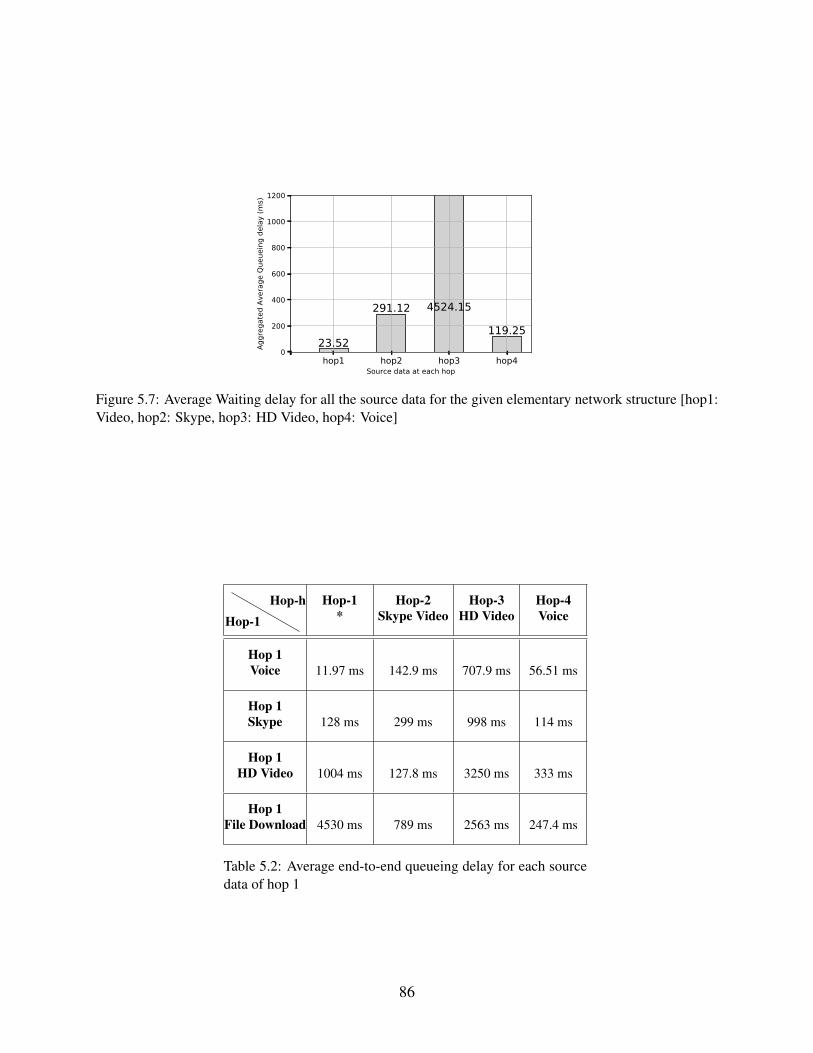
hop1 hop2 hop3 hop4Source data at each hop

0

200

400

600

800

1000

1200

Aggreg

ated

Ave

rage

Que

ueing de

lay (m

s)

23.52

291.12 4524.15

119.25

Figure 5.7: Average Waiting delay for all the source data for the given elementary network structure [hop1:Video, hop2: Skype, hop3: HD Video, hop4: Voice]

Hop-hHop-1

Hop-1*

Hop-2Skype Video

Hop-3HD Video

Hop-4Voice

Hop 1Voice 11.97 ms 142.9 ms 707.9 ms 56.51 ms

Hop 1Skype 128 ms 299 ms 998 ms 114 ms

Hop 1HD Video 1004 ms 127.8 ms 3250 ms 333 ms

Hop 1File Download 4530 ms 789 ms 2563 ms 247.4 ms

Table 5.2: Average end-to-end queueing delay for each sourcedata of hop 1

86

CHAPTER 6

FUTURE RESEARCH

Deep Q-learning Network based UAV position management

We model the problem of UAV position management under adversarial network conditions by a

Markov Decision Process(MDP) based algorithm, Reinforcement learning. Specifically, we use Deep

Q-learning network (DQN) to perform the positioning of the UAV positioning actions. Motivated by the

Deep minds [49] work on Atari game, where the DQN is a combination of Deep convolutional network and

Q-learning with images being the input to the convolutional network. Similarly, we consider the images of

the UAV swarming and network condition as the input to the DQN network to determine the optimal

Q-function for the UAV positioning action.

To determine the UAV swarming pattern, we assume the each UAVs are GPS enabled and the

central control station is able to draw the UAV swarming graph with accurate position mapping. On the

other hand, to determine link quality we consider link quality in terms of Signal to Interference Noise

Ratio(SINR) level assuming the UAVs are equipped with a directional antenna and face Rayleigh fading

channel. Furthermore, to determine the jamming conditions over communication link, we not only just

consider the observed SINR level, we also consider the MAC layer level information in terms of Packet

Dropping Rate(PDR) over a multihop link by analyzing the problem of sending data packets to gateway

node interms of M/G/1 Preemptive(PRP) Repeat priority Queueing model. Here priority is assigned to data

packets based on the latency requirement of the data packets. Why multihop Queuing model? the reason

being, the UAV node has to reach out to the gateway node which is few hops away, multihop queueing

model helps the UAV to choose the best gateway node which satisfies its QoS requirements, and in

addition, multihop queueing model helps to assess which all the links are affected by the jamming.

Finally, we convert the link information interms of SINR and jamming information from the

Queuing model into a gray scale image w.r.t the UAV swarming pattern image and we feed those 2 graphs

as an input to DQN. Moreover, traditional Q-learning [36] algorithms are not able to keep track of the

87

different pattern of the UAV swarming and channel condition graphs. Even the algorithms we proposed in

our previous works [40, 76] cannot learn the changes to the network graph pattern. Hence, we adopt

memory replay mechanism where the control station maintains the memory of the different patterns of the

UAV swarming and channel conditions and uses it retrain the convolutional layer when the UAV is unable

to choose an optimal action. Replay buffer [45] is maintained at the central controller level and the optimal

Q-function values are sent to UAV nodes to perform an optimal action. By doing so, the burden of finding

the optimal Q-function with large data set of network graph is no more on the power limited UAVs.

We use a different approach which is influenced by google’s deep mind work [49] to optimize the

UAV position in the swarming. Based on the UAVs location determined using GPS, information on link

quality and jamming condition are converted into a gray scale image. In addition, the UAV swarming graph

is also taken in a gray scale image and fed as an input along with the link quality + jamming image to the

DQN. The DQN selects an optimal positioning action by improving the Q-function estimation accuracy.

More importantly, the replay buffer helps to improve the decision accuracy under decreased performance.

This method not only reduces the intense calculations at the UAV side and leaves the whole training burden

to the central controller. To the best of our knowledge, we are the first to approach UAV position

management similar to playing an Atari game demonstrated by google deep mind [49].

Authors in [80, 81] proposed optimization theory for UAV position optimization by considering

both energy and communication throughput considering a single UAV which acts a relay node between

source and destination nodes. Similar work was seen in [82] where the UAV is considered as a relay node

its performance optimization formulation was proposed for uplink and downlink rate optimization. These

works consider the problem of single UAV deployment and its trajectory optimization. On the other hand,

the UAV swarming with routing optimization is proposed in [72] with a hueristic approach to solve

improve the information control plane(ICP) ensures the high quality routes between static nodes and then

physical control plane guides the nodes to reconfigure the position according to ICP. In our case, we

assume the routing path has been already established for the for the current swarming setup and we

optimize the position of the nodes based on the information flow. Interestingly, a time varying formation

tracking protocol with Riccati equation is proposed using neighboring UAVs information in a follower

UAVs following a leader UAV strategy. Interestingly,authors in [22] proposed path planning of the mobile

robots with target using the prediction of the wireless links built using a supervised learning approach

88

together with information collected from the neighbor robots. All of the above works are done in a

distributed manner where the each UAV has to perform complex operations to be inline with the swarming

pattern as well as maintain a good link quality to communicate effectively.

6.0.1 UAV deployment parameters

UAV swarming requires the UAV nodes are placed in such a way that the swarming pattern is

preserved. Hence, the UAV deployment and its position optimization while swarming under different

network condition is crucial. Our main parameters to maintain the UAV swarming pattern are

Channel Condition

Channel condition should be assessed in terms of path loss and multipath fading models as both

these characteristics depend on the fact that the signal is obstructed, reflected and scattered by the presence

of obstacles in the region of interest. Hence, we consider the Rayleigh fading channel model to assess the

channel condition in the specific area around the access point regions. The quality of the channel can be

decided based on the minimum SINR, γ required to maintain a minimum link quality. The probability of

successful transmission on link-ij can be defined using 5.3 and 5.3 as

P(γi j > γ

)= exp

σ2i Dα

i j

1

(6.1)

6.0.2 Jamming condition

Since we assume UAV swarming network is built upon a shared medium which is prone to

adversarial nodes launch jamming-style attacks, dodging these areas to increase the performance of the

network and establish communication among the UAVs and ground based nodes is important. Hence, we

determine the presence of a jamming environment from the perspective of UAV deployment and the UAVs

should be re-positioned to avoid the jammed areas. To determine the presence of the jamming effect we use

the result from multi-hop queueing model which we modelled in section IV. Since, Received Signal

Strength(RSSI) alone cannot be used as a metric to conclude the presence of the jamming, we use total

packet error ratio (TPER), TPER = PDR+ PER-PDR*PER which captures the MAC layer information in

89

terms of number of successful attempts made to in packet transmission. More importantly, we collect the

information of TPER at each node for the high priority packets because high priority packets are given

higher chance to access the channel. Hence the presence of jamming attack is decided based on the

presence of high TPER and low RSSI. The estimated TPER for priority 1 packets determined for N

retransmission in Ts time slots at hop-h.

6.1 DQN based UAV track management

Figure 6.1: Gray scale image of UAV swarming.

Figure 6.2: Gray scale image of link quality between a gateway node and the tail end node [Black lineindicates the link connecting different nodes]

In this section, we model the task of positioning the UAV node under different dynamics of the

channel condition. Motivated by the work done by deep mind group in [49], we model the whole network

dynamics into 2 graphs. Each graph is a grey scale image in which the first graph depicts the UAV

swarming pattern where all the nodes are mapped into a connected graph as shown in Fig. 6.1. Whereas,

the second graph defines dynamics of the UAV network in terms of low signal noise ratio and high queueing

90

delay in the case of high fading effect and jamming conditions. To map UAV swarming pattern we denote

the nodes and whole nodes in a white color as shown in 6.1. For the second graph, we use the TPER

determined using our multihop queueing model and the determined SINR level and denote those multihop

links by a white space where there is jamming condition and the positions will be marked with a grey color

to determine those areas as the high fading regions as shown in figure [add figure]. Finally, we give the

input images into our DQN network to optimally place the UAV node to achieve maximum throughput.

We represent the whole swarming condition with respect to UAV−i as a tuple denoted as {s, x,R},

where,

State,s

In the dynamic optimal UAV positioning game, the UAV can apply Q-learning to derive the

optimal policy to determine the optimal positioning pattern under the case of low channel quality and

jamming scenarios. The action of the SU is selected based on the current system state at time slot n denoted

by sn, which represents the UAV swarming graph, Network condition graph determined in terms of TPER

and SINR. More specifically, at time slot n, the system state sk consists of the information regarding

swarming graph and network condition for the time slot [n−1], i.e., sn = {Networkgrahs,S INR}(n−1).

Action,x

The actions are used to change the behavior of the UAV in response to the states seen at time slot n.

They are executed sequentially. To optimally deploy the UAVs, we consider the basic moves as the action

of the UAV under different network states defined earlier. The action set in UAV consists of the following

moves a) North, b)South, c) East, d) West, and e) Stay.

Reward,R

The reward defines how well the positioning of the UAV in the current state s for the action x in

time slot [n]. Hence, when the DQN optimizes the position of the UAV by maximizing SINR. In our model

we use total SINR as a parameter to quantify the optimal positioning of the UAV which is defined as

follows,

91

R = γi j[n] =P j[n]Gi j[n]

P jam f (T PER) +∑M

j′=1 j′, j P j′[n]Gi j′[n] +σ2j

,

n = 1,2, ....,NT (6.2)

where f (T PER) is an indicator function defining the presence of jamming condition.

UAV network: Gateways, Ground nodes, and Relays

UAV network states

Network Load

Traffic load

Link Quality

Jamming condition

UAV network states

Network Load

Traffic load

Link Quality

Jamming condition

𝑠𝑘 = {𝜉𝑟 , 𝜈𝑟}

𝜑𝑘 = (𝑠𝑘−𝑤 ,𝑥𝑘−𝑤 ,…… . 𝑥𝑘−1, 𝑠𝑘)

Replay memoryReplay memory

(𝜑1 ,𝑥1 ,𝑢1 ,𝜑2)

(𝜑𝑘 ,𝑥𝑘 ,𝑢𝑘 ,𝜑𝑘+1) Minibatch

CNN

Conv_1: 4x4x20Conv_2: 3x3x20

FC_1 : 180 FC_2 : N+1

DQN loss and gradient

Action xk with ϵ − greedy Q-function

UAV position

optimizationUAV sector

Rew

ard

𝐔𝐩𝐝𝐚𝐭𝐞 𝛉

(𝑥𝑑 ,𝑢𝑑 ,𝜑𝑑+1)

𝜑𝑘

𝜑𝑑

UAV network: Gateways, Ground nodes, and Relays

UAV network states

Network Load

Traffic load

Link Quality

Jamming condition

𝑠𝑘 = {𝜉𝑟 , 𝜈𝑟}

𝜑𝑘 = (𝑠𝑘−𝑤 ,𝑥𝑘−𝑤 ,…… . 𝑥𝑘−1, 𝑠𝑘)

Replay memory

(𝜑1 ,𝑥1 ,𝑢1 ,𝜑2)

(𝜑𝑘 ,𝑥𝑘 ,𝑢𝑘 ,𝜑𝑘+1) Minibatch

CNN

Conv_1: 4x4x20Conv_2: 3x3x20

FC_1 : 180 FC_2 : N+1

DQN loss and gradient

Action xk with ϵ − greedy Q-function

UAV position

optimizationUAV sector

Rew

ard

𝐔𝐩𝐝𝐚𝐭𝐞 𝛉

(𝑥𝑑 ,𝑢𝑑 ,𝜑𝑑+1)

𝜑𝑘

𝜑𝑑

Figure 6.3: DQN based UAV deployment.

There are mainly 2 components in DQN: (1) Convolutional Neural Network,(CNN) (2) Q-learning

based decision model. As depicted in the figure 6.3, the system uses the CCN to enhance the learning

speed of Q-learning as the UAV swarming network and network dynamics keep changing over time.

Similar to Q-learning, DQN updates Q-function for each state-action pair, which is the expected discounted

long term reward for state s and action x at time slot n which is given by

Q(s, x) = Es′

[Rs +γmax

x′Q(s′, x)|s, x

](6.3)

Where Rs is the reward received at the state s for action x which resulted in the next state s′ with a

discount factor γ, defining the uncertainty of the SU about the future reward.

As a matter of fact, Q-function can be approximated using Deep-CNN by tuning weight

92

parameters, a non-linear approximator for each action. However due to the dynamics of the network, the

CNN model needs to be retrained to adapt to the instabilities in the UAV swarming. Hence, a replay buffer

is used with the collection of past experienced state-action pairs and their respective rewards. The CNN

consists of 2 convolutional layers and 2 fully connected (FC) layers. For the first convolutional layer, it

consists of 20 filters each with size of 3×3 and stride 1, and the second convolutional layer consists of 40

filters with size 2×2 and no change to stride value. Rectified linear units (ReLU) is used as an activation

function in each layers including FC layers. In addition, first FC layer consists of 180 ReLU units and the

second FC has 5 ReLU units. At time slot [n], the weight of the filter in each layer is denoted by θn.

Further more, at time slot [n], the observed state sequence for the current state andW system

state-action pairs is denoted as ϕn = {sn−W, xn−W, ..., xn−1, sn}. Input to the CCN is given from the replay

buffer by reshaping the state sequence into 6×6 matrix to estimate the Q(ϕn, x|θn),

x ∈ {North,S outh,East,West,S tay}. The state sequence in replay buffer is chosen randomly from the

experience memory pool, D = {e1, .....,en}, where en = (ϕn, xn,Rns ,ϕ

n+1). Basically, experience replay

chooses an experience ed randomly, with 1 ≤ d < n to update weight parameter θn according to Stochastic

Gradient Descent (SGD) method. Updating θn results in minimized mean-squared error of the target

optimal Q-function with the minibatch updates, and the following loss function can be denoted as

L(θn) = Eϕn,x,Rs,ϕn+1

[(QTarget −Q(ϕn, x : θn+1)

)2]

(6.4)

Where QTarget is the target optimal Q-fucntion, which is given by

QTarget = Rs +γmaxx′

Q(ϕn+1,x′;θn−1) (6.5)

The weights θn are updated by using the gradient of the loss function L w.r.t to the weights θn. The

loss gradient ∇θnL(θn) can be expressed as

∇θnL(θn) = Eϕn,x,Rs,ϕn+1[QT∇θn Q(ϕn, x : θn)

]−Eϕn,x,Rs,ϕn+1

[Q(ϕn, x : θn)∇θn Q(ϕn, x : θn)

](6.6)

The weight parameter θn is updated for every time slot which repeats B times by randomly

93

selecting the experiences from the experience pool. Finally, with the updated Q-function, the action xn is

chosen in state sn according to the ε-greedy algorithm. The optimal action is chosen from the set of

Q-functions with the probability 1− ε as x∗ = argmaxx′ Q(ϕn, x′). When the UAV takes any move, the UAV

observes the SINR as a reward information from the environment and according to the next state

determined in terms of UAV swarming graph and network graph, the UAV stores the new experience

{ϕn, xn,Rns ,ϕ

n+1} in the memory pool D as shown in Fig. 6.3.

94

CHAPTER 7

CONCLUSION

In chapter 2, we have comprehensively implemented an iSM scheme through machine learning methods.

Our target is to achieve an intelligent spectrum handoff decision during rateless multimedia transmissions

in dynamic CRN links. The handoff operation needs to have a good knowledge of channel quality such that

it knows which channel to switch to. For accurate channel quality evaluation, we calculate the CUF that

can comprehensively measure the link quality. To adapt to the dynamic CRN channel conditions, we have

used CDF-enhanced, UEP-based Fountain Codes to achieve intelligent link adaptation. A good link

adaptation strategy can significantly reduce the spectrum handoff events.

Our final goal is make a correct iSM decision, which could be a spectrum handoff or wait-and-stay.

The iSM decision is based on a teaching-and-learning based cognitive method, called TACT, to make

optimal spectrum handoff in different SU states. The proposed cognitive learning methods can achieve real

"cognitive" radio networks, not only in spectrum mobility tasks, but also in many other CRN topics, such

as multimedia streaming over CRN, dynamic routing establishment, and others.

Our next-step research topic in this direction is to further enhance our TACT-based model, by

using budget-limited teaching process, in order to efficiently transfer important parameters from an expert

SU to a learning SU within time constraint. The expert searching model will be based on Manifold learning

and NMF (non-negative matrix factorization) pattern extraction/recognition schemes. Thus a better expert

SU can be found in the neighborhood of a learning SU.

In chapter 3, we have studied FEAST-based CBH in MBSA-based CRNs. By considering

independent and parallel preemptive PRP/NPRP M/G/1 queueing model with discretion rule, the average

waiting delay during the interruption of beam-b can be determined. During the waiting time, the

interrupted beam’s data is detoured through the neighboring beams over 2-hop relay. The packet detouring

performance has been analyzed using MOS by varying source data rate as well as the detouring beam’s

own data rate. Performance analysis has showed that more detouring paths with enough detouring rate can

help to achieve the optimal performance. The extension of spectrum decision to online learning model

95

using FEAST could enhance the performance of spectrum decision. Our model achieves better

performance in terms of expected MOS and also takes less iterations to achieve optimal condition. In

addition, the node adapts to the changes of the network parameters, and tunes its handoff policy

accordingly to maximize the handoff performance. This is very important in dynamic CRN environments.

In chapter 4, we have implemented the CRN testbed with intelligent spectrum handoff by using

GNU Radio and USRP. We have implemented Reinforcement learning based spectrum handoff as a

self-learning method, by considering Transmit and Spectrum Handoff as the actions and Channel

condition/status as the parameters of the states of the learning method. It is shown that self-learning

method takes a long time to achieve optimal condition. Hence, to enhance the learning process we have

adopted Transfer Learning where the learning node receives optimal strategy (Q-table) from the expert

node and uses it to perform spectrum handoff. From the results, it is evident that Transfer Learning takes

less time to achieve optimal condition. As a future work, we will build a large-scale (>50 nodes) CRN

testbed and test the performance of our handoff schemes. We will consider dynamic channel conditions and

test the performance of both self-learning and Transfer Learning in such a large network testbed.

Finally, in chapter 5 we formulated multihop queueing model for UAV swarming management

using Preemptive Repeat M/G/1 queueing model at each relay node. The single path multihop network

delivers its data to a central controller through a gateway node. The performance analysis shows that the

packets are relayed based on their remaining delay deadline to meet the QoS requirement of the user.

96

REFERENCES

[1] Adnan Aftab and Muhammad Nabeel Mufti. Spectrum sensing through implementation of usrp2,2011.

[2] R Anil, R Danymol, Harsha Gawande, and R Gandhiraj. Machine learning plug-ins for gnu radiocompanion. In Green Computing Communication and Electrical Engineering (ICGCCEE), 2014International Conference on, pages 1–5. IEEE, 2014.

[3] Olusegun Peter Awe, Ziming Zhu, and Sangarapillai Lambotharan. Eigenvalue and support vectormachine techniques for spectrum sensing in cognitive radio networks. In Conf. Technologies andApplications of Artificial Intelligence (TAAI), pages 223–227, 2013.

[4] Mathieu Bastian, Sebastien Heymann, and Mathieu Jacomy. Gephi: An open source software forexploring and manipulating networks, 2009.

[5] Mario Bkassiny, Yang Li, and Sudharman K Jayaweera. A survey on machine-learning techniques incognitive radios. IEEE Communications Surveys & Tutorials, 15(3):1136–1159, 2013.

[6] Eric Blossom. Gnu radio: tools for exploring the radio frequency spectrum. Linux journal,2004(122):4, 2004.

[7] Evgeny Byvatov, Uli Fechner, Jens Sadowski, and Gisbert Schneider. Comparison of support vectormachine and artificial neural network systems for drug/nondrug classification. J. ChemicalInformation and Computer Sciences, 43(6):1882–1889, 2003.

[8] Batu K Chalise, Yimin D Zhang, and Moeness G Amin. Multi-beam scheduling for unmanned aerialvehicle networks. In IEEE/CIC Intl. Conf. Comm. in China (ICCC), pages 442–447, 2013.

[9] Arpan Chattopadhyay and A Chockalingam. Past queue length based low-overhead link scheduling inmulti-beam wireless mesh networks. In Intl. Conf. Signal Processing and Comm. (SPCOM), pages1–5, 2010.

[10] Xiaoming Chen and Chau Yuen. Efficient resource allocation in a rateless-coded MU-MIMOcognitive radio network with QoS provisioning and limited feedback. IEEE Trans. VehicularTechnology, 62(1):395–399, 2013.

[11] Zhe Chen and Robert C Qiu. Q-learning based Bidding Algorithm for Spectrum Auction in CognitiveRadio. In IEEE Southeastcon, pages 409–412, 2011.

[12] You Ze Cho and Chong K Un. Analysis of the M/G/1 queue under a combinedpreemptive/nonpreemptive priority discipline. IEEE Trans. Comm., 41(1):132–141, 1993.

[13] Bruce T Clough. Uav swarming? so what are those swarms, what are the implications, and how dowe handle them? Technical report, AIR FORCE RESEARCH LAB WRIGHT-PATTERSON AFBOH AIR VEHICLES DIRECTORATE, 2002.

97

[14] Federal Communications Commission. Spectrum Policy Task Force Report, Nov. 2002.

[15] R Walter Conway, William L Maxwell, and Louis W Miller. Theory of scheduling. eading.Massachussets: Addison-Wesley, 1967.

[16] Alice Crohas. Practical implementation of a cognitive radio system for dynamic spectrum access.PhD thesis, University of Notre Dame, 2008.

[17] Ying Dai and Jie Wu. Sense in Order: Channel Selection for Sensing in Cognitive Radio Networks.In 8th IEEE Intl. Conf. Cognitive Radio Oriented Wireless Networks (CROWNCOM), pages 74–79,2013.

[18] Mischa Dohler, Lorenza Giupponi, Ana Galindo-Serrano, and Pol Blasco. Docitive networks: Anovel framework beyond cognition. IEEE Communications Society, Multimdia Communications TC,E-Letter, 5(1):1–3, 2010.

[19] Medhat HM Elsayed and Amr Mohamed. Distributed interference management using q-learning incognitive femtocell networks: new usrp-based implementation. In New Technologies, Mobility andSecurity (NTMS), 2015 7th International Conference on, pages 1–5. IEEE, 2015.

[20] Uri Erez, Mitchell D Trott, and Gregory W Wornell. Rateless Coding for Gaussian Channels. IEEETrans. Information Theory, 58(2):530–547, 2012.

[21] M Ettus. Universal software radio peripheral (usrp), ettus research llc, 2008.

[22] Eduardo Feo Flushing, Michal Kudelski, Luca M Gambardella, and Gianni A Di Caro. Spatialprediction of wireless links and its application to the path control of mobile robots. In IndustrialEmbedded Systems (SIES), 2014 9th IEEE International Symposium on, pages 218–227. IEEE, 2014.

[23] Ana Galindo-Serrano, Lorenza Giupponi, Pol Blasco, and Mischa Dohler. Learning from experts incognitive radio networks: The docitive paradigm. In Cognitive Radio Oriented Wireless Networks &

Communications (CROWNCOM), 2010 Proceedings of the Fifth International Conference on, pages1–6. IEEE, 2010.

[24] Robert G Gallager. Low-density parity-check codes. IEEE Trans. Information Theory, 8(1):21–28,1962.

[25] Lorenza Giupponi, Ana Galindo-Serrano, Pol Blasco, and Mischa Dohler. Docitive networks: Anemerging paradigm for dynamic spectrum management. IEEE Trans. Wireless Communication,17(4):47–54, 2010.

[26] Lorenza Giupponi, Ana Galindo-Serrano, Pol Blasco, and Mischa Dohler. Docitive networks: anemerging paradigm for dynamic spectrum management [dynamic spectrum management]. IEEEWireless Communications, 17(4), 2010.

[27] Aditya Gudipati and Sachin Katti. Strider: Automatic Rate Adaptation and Collision Handling. InACM SIGCOMM Computer Communication Review, volume 41, pages 158–169, 2011.

[28] Jinghua Guo, Hong Ji, Yi Li, and Xi Li. A novel spectrum handoff management scheme based onSVM in cognitive radio networks. In 6th Intl. ICST Conf. Comm. and Networking in China(CHINACOM), pages 645–649, 2011.

[29] Karen Zita Haigh, Allan M Mackay, Michael R Cook, and Li L Lin. Parallel Learning and DecisionMaking for a Smart Embedded Communications Platform, 2015. Accessed on April 10, 2017.

98

[30] Zhu Han, A Lee Swindlehurst, and KJ Ray Liu. Optimization of manet connectivity via smartdeployment/movement of unmanned air vehicles. IEEE Transactions on Vehicular Technology,58(7):3533–3546, 2009.

[31] Neil Hosey, Susan Bergin, Irene Macaluso, and Diarmuid P O’Donoghue. Q-learning for cognitiveradios. In Proceedings of the China-Ireland Information and Communications TechnologyConference (CIICT 2009). ISBN 9780901519672. National University of Ireland Maynooth, 2009.

[32] Neil Hosey, Susan Bergin, Irene Macaluso, and Diarmuid O’Donohue. Q-Learning for CognitiveRadios. In Proc. China-Ireland Information and Communications Technology Conf., ISBN9780901519672, 2009.

[33] Peter Hossain, Adaulfo Komisarczuk, Garin Pawetczak, Sarah Van Dijk, and Isabella Axelsen.Machine learning techniques in cognitive radio networks. arXiv preprint arXiv:1410.3145, 2014.

[34] Peter Anthony Iannucci, Jonathan Perry, Hari Balakrishnan, and Devavrat Shah. No symbol leftbehind: A link-layer protocol for rateless codes. In 18th ACM Annual Intl. Conf. Mobile Computingand Networking, pages 17–28, 2012.

[35] Kommate Jitvanichphaibool, Ying-Chang Liang, and Rui Zhang. Beamforming and power control formulti-antenna cognitive two-way relaying. In IEEE Wireless Comm. and Networking Conf., pages1–6, 2009.

[36] Leslie Pack Kaelbling, Michael L Littman, and Andrew W Moore. Reinforcement learning: A survey.Journal of artificial intelligence research, 4:237–285, 1996.

[37] Chen Ke-Yu and Zhi-Feng Chen. Gnu radio. Department of Electrical Computer Engineering,University of Florida, Gainesville, Florida, 2006.

[38] Vijaymohan R Konda and Vivek S Borkar. Actor-Critic–Type Learning Algorithms for MarkovDecision Processes. SIAM J. Control and Optimization, 38(1):94–123, 1999.

[39] AM Koushik, Fei Hu, and Sunil Kumar. Multi-Class "Channel+ Beam" Handoff in Cognitive RadioNetworks with Multi-Beam Smart Antennas. In IEEE Global Comm. Conf. (GLOBECOM), pages1–6, 2016.

[40] AM Koushik, Fei Hu, and Sunil Kumar. Intelligent Spectrum Management based on TransferActor-Critic Learning for Rateless Transmissions in Cognitive Radio Networks. IEEE Trans. onMobile Computing, 2017.

[41] AM Koushik, Fei Hu, Ji Qi, and Sunil Kumar. Cognitive Spectrum Decision via Machine Learning inCRN. In Conf. Information Technology: New Generations, pages 13–23. Springer, 2016.

[42] AM Koushik, John D Matyjas, Fei Hu, and Sunil Kumar. Channel/beam handoff control inmulti-beam antenna based cognitive radio networks. IEEE Transactions on CognitiveCommunications and Networking, 2017.

[43] Krishan Kumar, Arun Prakash, and Rajeev Tripathi. Spectrum handoff in cognitive radio networks: Aclassification and comprehensive survey. Journal of Network and Computer Applications,61:161–188, 2016.

[44] Rongpeng Li, Zhifeng Zhao, Xianfu Chen, Jacques Palicot, and Honggang Zhang. TACT: A TransferActor-Critic Learning Framework for Energy Saving in Cellular Radio Access Networks. IEEETrans. Wireless Communications, 13(4):2000–2011, 2014.

99

[45] Ruishan Liu and James Zou. The effects of memory replay in reinforcement learning. arXiv preprintarXiv:1710.06574, 2017.

[46] Tehuang Liu and Wanjiun Liao. Location-dependent throughput and delay in wireless meshnetworks. IEEE Transactions on Vehicular Technology, 57(2):1188–1198, 2008.

[47] Brandon F Lo and Ian F Akyildiz. Reinforcement Learning based Cooperative Sensing in CognitiveRadio Ad Hoc Networks. In 21st IEEE PIMRC, pages 2244–2249, 2010.

[48] Shridhar Mubaraq Mishra, Danijela Cabric, Chen Chang, Daniel Willkomm, Barbara Van Schewick,Adam Wolisz, and Robert W Brodersen. A real time cognitive radio testbed for physical and linklayer experiments. In New Frontiers in Dynamic Spectrum Access Networks, 2005. DySPAN 2005.2005 First IEEE International Symposium on, pages 562–567. IEEE, 2005.

[49] Volodymyr Mnih, Koray Kavukcuoglu, David Silver, Andrei A Rusu, Joel Veness, Marc GBellemare, Alex Graves, Martin Riedmiller, Andreas K Fidjeland, Georg Ostrovski, et al.Human-level control through deep reinforcement learning. Nature, 518(7540):529–533, 2015.

[50] Michael L Moher and John H Lodge. TCMP-A modulation and coding strategy for Rician fadingchannels. IEEE J. Selected Areas in Communications, 7(9):1347–1355, 1989.

[51] Timothy R Newman, An He, Joseph Gaeddert, Ben Hilburn, Tamal Bose, and Jeffrey H Reed.Virginia tech cognitive radio network testbed and open source cognitive radio framework. In Testbedsand Research Infrastructures for the Development of Networks & Communities and Workshops, 2009.TridentCom 2009. 5th International Conference on, pages 1–3. IEEE, 2009.

[52] Timothy J O’shea, T Charles Clancy, and Hani J Ebeid. Practical signal detection and classification ingnu radio. In Sdr forum technical conference, page 143, 2007.

[53] Jonathan Perry, Hari Balakrishnan, and Devavrat Shah. Rateless Spinal Codes. In 10th ACMWorkshop on Hot Topics in Networks, page 6, 2011.

[54] Jonathan Perry, Peter A Iannucci, Kermin E Fleming, Hari Balakrishnan, and Devavrat Shah. SpinalCodes. In ACM SIGCOMM Conf. Applications, Technologies, Architectures, and Protocols forComputer Communication, pages 49–60, 2012.

[55] Robert C Qiu, Changchun Zhang, Zhen Hu, and Michael C Wicks. Towards a large-scale cognitiveradio network testbed: spectrum sensing, system architecture, and distributed sensing. J. Commun,7(7):552–566, 2012.

[56] A David Redish, Steve Jensen, Adam Johnson, and Zeb Kurth-Nelson. Reconciling ReinforcementLearning Models with Behavioral Extinction and Renewal: Implications for Addiction, Relapse, andProblem Gambling. Psychological Review, 114(3):784, 2007.

[57] Yu Ren, Pawel Dmochowski, and Peter Komisarczuk. Analysis and implementation of reinforcementlearning on a GNU radio cognitive radio platform. In 5th Intl. Conf. Cognitive Radio OrientedWireless Networks and Communications, Cannes, France, 2010.

[58] Yu Ren, Pawel Dmochowski, and Peter Komisarczuk. Analysis and implementation of reinforcementlearning on a gnu radio cognitive radio platform. In Cognitive Radio Oriented Wireless Networks &

Communications (CROWNCOM), 2010 Proceedings of the Fifth International Conference on, pages1–6. IEEE, 2010.

100

[59] Flávio Ribeiro, Dinei Florêncio, Cha Zhang, and Michael Seltzer. Crowdmos: An approach forcrowdsourcing mean opinion score studies. In IEEE Intl. Conf. Acoustics, Speech and SignalProcessing (ICASSP), pages 2416–2419, 2011.

[60] Hsien-Po Shiang and Mihaela Van Der Schaar. Multi-user video streaming over multi-hop wirelessnetworks: a distributed, cross-layer approach based on priority queuing. IEEE Journal on SelectedAreas in Communications, 25(4), 2007.

[61] Amin Shokrollahi. Raptor Codes. IEEE Trans. Information Theory, 52(6):2551–2567, 2006.

[62] Yi Song and Jiang Xie. On the spectrum handoff for cognitive radio ad hoc networks withoutcommon control channel. In Cognitive Radio Mobile Ad Hoc Networks, pages 37–74. Springer, 2011.

[63] Matthew D Sunderland. Software-defined radio interoperability with frequency hopping waveforms.2010.

[64] Richard S Sutton and Andrew G Barto. Reinforcement learning: An introduction, volume 1. MITpress Cambridge, 1998.

[65] S Tamilarasan and P Kumar. Dynamic resource allocation using priority queue scheduling inmulti-hop cognitive radio networks. In Computational Intelligence and Computing Research(ICCIC), 2016 IEEE International Conference on, pages 1–5. IEEE, 2016.

[66] Wuchen Tang, Muhammad Zeeshan Shakir, Muhammad Ali Imran, Rahim Tafazolli, and M-SAlouini. Throughput Analysis for Cognitive Radio Networks with Multiple Primary Users andImperfect Spectrum Sensing. IET Communications, 6(17):2787–2795, 2012.

[67] Venkat vinod Patcha. Experimental study of cognitive radio test-bed using usrp. 2011.

[68] Li-Chun Wang and Chung-Wei Wang. Spectrum handoff for cognitive radio networks:Reactive-sensing or proactive-sensins? In Performance, Computing and CommunicationsConference, 2008. IPCCC 2008. IEEE International, pages 343–348. IEEE, 2008.

[69] Li-Chun Wang, Chung-Wei Wang, and Chung-Ju Chang. Modeling and analysis for spectrumhandoffs in cognitive radio networks. IEEE Trans. Mobile Computing, 11(9):1499–1513, 2012.

[70] Lu Wang, Kaishun Wu, Jiang Xiao, and Mounir Hamdi. Harnessing frequency domain forcooperative sensing and multi-channel contention in CRAHNs. IEEE Trans. WirelessCommunications, 13(1):440–449, 2014.

[71] Yao Wang, Zhongzhao Zhang, Lin Ma, and Jiamei Chen. SVM-based spectrum mobility predictionscheme in mobile cognitive radio networks. The Scientific World J., 2014.

[72] Ryan K Williams, Andrea Gasparri, and Bhaskar Krishnamachari. Route swarm: Wireless networkoptimization through mobility. In Intelligent Robots and Systems (IROS 2014), 2014 IEEE/RSJInternational Conference on, pages 3775–3781. IEEE, 2014.

[73] Kun Wu, Li Guo, Hua Chen, Yonghua Li, and Jiaru Lin. Queuing based optimal schedulingmechanism for QoE provisioning in cognitive radio relaying network. In 16th Intl. Symp. WirelessPersonal Multimedia Comm. (WPMC), pages 1–5, 2013.

[74] Yeqing Wu, Fei Hu, Sunil Kumar, John Matyjas, Qingquan Sun, and Yingying Zhu. Apprenticeshiplearning based spectrum decision in multi-channel wireless mesh networks with multi-beamantennas. IEEE Trans. Mobile Computing, 16(2):314–325, 2017.

101

[75] Yeqing Wu, Fei Hu, Sunil Kumar, Yingying Zhu, Ali Talari, Nazanin Rahnavard, and John DMatyjas. A learning-based QoE-driven spectrum handoff scheme for multimedia transmissions overcognitive radio networks. IEEE J. Selected Areas in Comm., 32(11):2134–2148, 2014.

[76] Yeqing Wu, Fei Hu, Yingying Zhu, and Sunil Kumar. Optimal spectrum handoff control for CRNbased on hybrid priority queuing and multi-teacher apprentice learning. IEEE Trans. VehicularTechnology, 66(3):2630–2642, 2017.

[77] Yeqing Wu, Sunil Kumar, Fei Hu, Yingying Zhu, and John D Matyjas. Cross-layer Forward ErrorCorrection Scheme Using Raptor and RCPC Codes for Prioritized Video Transmission over WirelessChannels. IEEE Trans. on Circuits and Systems for Video Technology, 24(6):1047–1060, 2014.

[78] Xiaoshuang Xing, Tao Jing, Yan Huo, Hongjuan Li, and Xiuzhen Cheng. Channel quality predictionbased on Bayesian inference in cognitive radio networks. In IEEE INFOCOM, pages 1465–1473,2013.

[79] Luca Zappaterra. QoS-Driven Channel Selection for Heterogeneous Cognitive Radio Networks. InACM Conf. CoNEXT Student Workshop, pages 7–8, 2012.

[80] Yong Zeng and Rui Zhang. Energy-efficient uav communication with trajectory optimization. IEEETransactions on Wireless Communications, 16(6):3747–3760, 2017.

[81] Yong Zeng, Rui Zhang, and Teng Joon Lim. Throughput maximization for mobile relaying systems.In Globecom Workshops (GC Wkshps), 2016 IEEE, pages 1–6. IEEE, 2016.

[82] Pengcheng Zhan, Kai Yu, and A Lee Swindlehurst. Wireless relay communications with unmannedaerial vehicles: Performance and optimization. IEEE Transactions on Aerospace and ElectronicSystems, 47(3):2068–2085, 2011.

[83] Caoxie Zhang, Xinbing Wang, and Jun Li. Cooperative cognitive radio with priority queueinganalysis. In IEEE Intl. Conf. Comm., pages 1–5, 2009.

[84] Yimin Zhang, Xin Li, and Moeness G Amin. Multi-channel smart antennas in wireless networks. In40th IEEE Asilomar Conf. on Signals, Systems and Computers, pages 305–309, 2006.

[85] Xi-Yun Zhi, Zhi-Qiang He, and Wei-Ling Wu. A Novel Cooperation Strategy based on RatelessCoding in Cognitive Radio Network. Intl. J. Advancements in Computing Technology, 4(8):333–347,2012.

102

machine learning based spectrum decision in cognitive radio

Documents

Transcript of machine learning based spectrum decision in cognitive radio