Efficient blind spectrum sensing for cognitive radio networks based on compressed sensing
Upload
khangminh22Category
view
2download
0
HAL Id: tel-03635895https://tel.archives-ouvertes.fr/tel-03635895v2
Submitted on 8 Apr 2022
HAL is a multi-disciplinary open accessarchive for the deposit and dissemination of sci-entific research documents, whether they are pub-lished or not. The documents may come fromteaching and research institutions in France orabroad, or from public or private research centers.
L’archive ouverte pluridisciplinaire HAL, estdestinée au dépôt et à la diffusion de documentsscientifiques de niveau recherche, publiés ou non,émanant des établissements d’enseignement et derecherche français ou étrangers, des laboratoirespublics ou privés.
Enhancement of spectrum sensing in cognitive radio :providing reliable spectral opportunities
Azza Moawad
To cite this version:Azza Moawad. Enhancement of spectrum sensing in cognitive radio : providing reliable spectralopportunities. Networking and Internet Architecture [cs.NI]. Université de Bretagne occidentale -Brest, 2020. English. �NNT : 2020BRES0074�. �tel-03635895v2�
THESE DE DOCTORAT DE
L'UNIVERSITE
DE BRETAGNE OCCIDENTALE
ECOLE DOCTORALE N° 601
Mathématiques et Sciences et Technologies
de l'Information et de la Communication
Spécialité : Télécommunications
Enhancement of Spectrum Sensing in Cognitive Radio : Providing Reliable Spectral Opportunities. Thèse présentée et soutenue à Brest, le 10 décembre 2020 Unité de recherche : Lab-STICC
Par
Azza MOAWAD
Rapporteurs avant soutenance : Denis HAMMAD Professeur des universités, Université du Littoral, Calais, France Cornel IOANA Maître de conférences, HDR, INP Grenoble, France
Composition du Jury : Président du Jury : Christian JUTTEN Professeur émérite des université, INP Grenoble,France Examinateurs : Emanuel RADOI Professeur des universités, UBO Brest, France Marwa EL-BOUZ Enseignant-Chercheuse, HDR, ISEN Brest, France Denis HAMMAD Professeur des universités, Université du Littoral, Calais, France Cornel IOANA Maître de conférences, HDR, INP Grenoble, France Dir. de thèse : Roland GAUTIER Maître de conférences, Hors-Classe, HDR, UBO Brest, France Co-dir. de thèse : Koffi-Clément YAO Maître de conférences, HDR, UBO, Brest, France
Invité(s) : Ali MANSOUR Professeur, ENSTA Bretagne, Brest, France Mohamed ABAZA Associate Professor, AASTMT, Cairo, Egypt

ACKNOWLEDGEMENT
I am very grateful to ALLAH for all his blessings. I would also like to thank my
parents, husband and daughters for what they have contributed towards my educa-
tion. Their unconditional love, constant support, great advice and prayers over the
past years are something that I cannot thank them for enough. Additionally, knowing
that my success in completing my Ph.D would be a source of happiness for them, I was
further motivated to work hard.
I am sincerely grateful for my thesis directors, Dr. Roland Gautier, for his support
and encouragement and for giving me the opportunity to learn and develop, and Dr.
Koffi-Clément Yao for the time he took to evaluate my contributions, the problems
he noticed, and the discussions we had, which helped me to progress in my work
and results. I am deeply indebted to my thesis supervisor, Prof. Ali Mansour, for his
valuable comments, discussions, and encouragement. I thank him for always being
available and helpful.
I want to thank Prof. Christian Jutten from the University of Grenoble for being
the president of my Ph.D. committee. I also would like to thank the rapporteurs Prof.
Denis Hamad from the University of Littoral Côte d’Opale and Dr. Ioana Cornel from
the University of INP Grenoble for their valuable comments and corrections. I also
thank Prof. Emanuel Radio from Université de Bretagne Occidentale and Dr. Marwa
El-Bouz from ISEN Brest, for accepting to be the examiners of my dissertation.
Moreover, I would like to express my hearty thanks to Prof. Mohamed El Ma-
hallawy, the head of the department of Electronics and Communications Engineering
from Arab Academy for Science and Technology and Maritime Transport (AASTMT),
Egypt, for his continuous support along my Ph.D work and his eagerness to give me
the time to accomplish my research work. Also, I am deeply thankful for my friends
especially Eng. Nihal Sameh and Eng. Mai AbdelMoniem. They always encouraged
me in this challenge.
Finally, I would like to thank my colleagues with whom I had fruitful discussions
during the preparation of my thesis: Dr. Mohamed Abaza from Arab Academy for
Science and Technology and Maritime Transport (AASTMT), Egypt, Dr. Ahmed Ali
i

from Carlton University, Canada, Dr. El Nasser Salah El deen from McGill University,
Canada, and last but not least, Dr. Karim Seddik from the American University in Cairo
(AUC), Egypt.
ii

RÉSUMÉ
Le partage dynamique du spectre (Dynamic Spectrum Sharing DSS) vise à améliorer
l’efficacité d’accesssion aux bandes de fréquences sous-utilisées. Dans le mode en-
trelacé d’accès au spectre, la Radio Cognitive permet à un utilisateur sans licence (util-
isateur secondaire SU) d’accéder de manière opportuniste aux bandes de spectre sous
licence lorsque l’utilisateur sous licence (utilisateur principal PU) est absent. Dès lors,
la détection du signal émis par le PU constitue l’étape primordiale pour l’accès au spec-
tre en Radio Cognitive. L’objectif principal de la thèse est de concevoir un système de
détection fiable, capable de détecter un signal assimilable au bruit, dans un contexte
non-coopératif. Nous exploitons la puissance de l’analyse cepstrale pour développer
un système capable de détecter les signaux à spectre étalé. Nous avons proposé un
détecteur PassBand-AutoCesptrum (PB-ACD), qui réalise la detection par rapport au
pic dominant de l’auto-cepstre dans certains cas ou par rapport à la valeur moyenne
des pics dans d’autres cas. Les techniques proposées ont montré une grande fiabilité
pour la détection des signaux à spectre étalé et des signaux ultra large bande (UWB).
En outre, nous avons proposé la technique PB-ACD améliorée pour lisser les fluctua-
tions des estimateurs d’autocorrélation en utilisant l’algorithme TVD (Total Variation
Denoising ) pour la réduction du bruit. Nous avons étendu nos travaux au cas du
spectre à très large bande composé de plusieurs sous-bandes de fréquences. La pre-
mière phase de la procédure consiste en la détection des frontières entre les différentes
sous-bandes de fréquences avant d’effectuer par la suite la detection du signal du PU.
À cet effet, nous avons introduit l’algorithme DLSD (Differential Log Spectral Density)
pour identifier les limites spectrales du spectre large bande cible. Ensuite, pour la de-
tection du signal du PU, nous avons développé le détecteur BaseBand-AutoCepstrum
(BB-ACD) qui extrait les informations du signal en bande de base avant d’appliquer
la technique de detection basée sur l’auto-cepstre. La technique BB-ACD permet de
prendre en compte l’incertitude sur les fréquences qui peut résulter de la mauvaise
detection des limites spectrales. Enfin, la méthode du cepstre de puissance améliorée
est introduite par le détecteur de covariance Cepstrale (CCD) pour détecter les signaux
modulés numériquement.
iii


TABLE OF CONTENTS
Acknowledgement i
Résumé iii
List of Figures ix
List of Tables xiv
Abbreviations xiv
List of Symbols xix
Mathematical Notations xxvii
1 Introduction 1
1.1 Background . . . . . . . . . . . . . . . . . . . . . . . . . . . . . . . . . . . 1
1.2 Thesis Contributions . . . . . . . . . . . . . . . . . . . . . . . . . . . . . . 4
1.3 Thesis Organization . . . . . . . . . . . . . . . . . . . . . . . . . . . . . . . 8
2 State-of-The-Art 11
2.1 Introduction . . . . . . . . . . . . . . . . . . . . . . . . . . . . . . . . . . . 11
2.2 Overview On Cognitive Radios . . . . . . . . . . . . . . . . . . . . . . . . 12
2.2.1 Cognitive Capability of Cognitive Radio Networks . . . . . . . . 14
2.2.2 Tasks of Cognitive Radio Systems . . . . . . . . . . . . . . . . . . 15
2.2.3 Cognitive Radio Paradigms . . . . . . . . . . . . . . . . . . . . . . 17
2.2.4 Cognitive Radio Bands . . . . . . . . . . . . . . . . . . . . . . . . . 18
2.3 Literature Review on Spectrum Sensing Techniques . . . . . . . . . . . . 19
2.3.1 NarrowBand Spectrum Sensing . . . . . . . . . . . . . . . . . . . . 23
2.3.2 WideBand Spectrum Sensing . . . . . . . . . . . . . . . . . . . . . 37
2.4 Spectrum Sensing By Scattering Operators . . . . . . . . . . . . . . . . . 39
2.4.1 Overview on Scattering Transform . . . . . . . . . . . . . . . . . . 39
v
TABLE OF CONTENTS
2.4.2 Reprocessing of Received Signals by The Scattering Operators . . 42
2.4.3 Numerical Results and Insights . . . . . . . . . . . . . . . . . . . . 43
2.5 Enhancement of Primary User Detection Through Channel Estimation . 46
2.5.1 Channel Impairments: Overview . . . . . . . . . . . . . . . . . . . 46
2.5.2 System Model . . . . . . . . . . . . . . . . . . . . . . . . . . . . . . 48
2.5.3 Problem Formulation and Proposed Solution . . . . . . . . . . . . 50
2.5.4 Numerical Results and Insights . . . . . . . . . . . . . . . . . . . . 55
2.6 Summary . . . . . . . . . . . . . . . . . . . . . . . . . . . . . . . . . . . . . 58
3 Cepstral Analysis Approaches for Spectrum Sensing in Cognitive Radio 59
3.1 Introduction . . . . . . . . . . . . . . . . . . . . . . . . . . . . . . . . . . . 59
3.2 Related Work . . . . . . . . . . . . . . . . . . . . . . . . . . . . . . . . . . 60
3.2.1 Overview on Cepstral Analysis . . . . . . . . . . . . . . . . . . . . 61
3.2.2 Application of Cepstral Analysis in Communications . . . . . . . 65
3.3 System Description and Channel Model . . . . . . . . . . . . . . . . . . . 66
3.3.1 System Model . . . . . . . . . . . . . . . . . . . . . . . . . . . . . . 66
3.3.2 Signal and Channel Model . . . . . . . . . . . . . . . . . . . . . . 67
3.4 Spectrum Sensing Technique By The Autocepstrum Approach . . . . . . 68
3.4.1 Detection of Direct Sequence-Spread Spectrum Signals By The
PB-ACD Technique . . . . . . . . . . . . . . . . . . . . . . . . . . . 69
3.4.2 Application of The PB-ACD Technique to Detecting Frequency-
Hopping and Chirp Spread Spectrum Signals . . . . . . . . . . . 96
3.5 Spectrum Sensing by The Smoothed PB-ACD Technique . . . . . . . . . 107
3.5.1 Fluctuations Smoothing by The Total Variation Denoising Based
on The Majorization-Minimization Algorithm: . . . . . . . . . . . 110
3.5.2 Application of the Proposed Smoothing Process to the Case of
Detecting a DS-SS Signal: . . . . . . . . . . . . . . . . . . . . . . . 112
3.6 Numerical Results and Discussions . . . . . . . . . . . . . . . . . . . . . . 117
3.7 Summary . . . . . . . . . . . . . . . . . . . . . . . . . . . . . . . . . . . . . 125
4 Wideband Spectrum Sensing Technique By Cepstral Analysis Approaches 127
4.1 Introduction . . . . . . . . . . . . . . . . . . . . . . . . . . . . . . . . . . . 127
4.2 Related Work . . . . . . . . . . . . . . . . . . . . . . . . . . . . . . . . . . 130
4.3 Problem Formulation of Wideband Spectrum Sensing . . . . . . . . . . . 133
4.3.1 Phase I: Identification of Spectral Boundaries . . . . . . . . . . . 134
vi

TABLE OF CONTENTS
4.3.2 Phase II: Primary User Detection . . . . . . . . . . . . . . . . . . . 137
4.4 The Proposed Wideband Spectrum Sensing Approach . . . . . . . . . . . 137
4.4.1 Identification of Spectral Boundaries By Cepstral Analysis . . . . 138
4.5 PU Detection Under Frequency Uncertainty by The BB-ACD Technique: 149
4.6 Numerical Results and Discussions . . . . . . . . . . . . . . . . . . . . . . 153
4.6.1 Performance Evaluation of The Proposed Edge Detection Ap-
proach: . . . . . . . . . . . . . . . . . . . . . . . . . . . . . . . . . . 154
4.6.2 Detection of Noise-Like Signals Under Carrier Frequency Uncer-
tainty By The BB-ACD Technique: . . . . . . . . . . . . . . . . . . 159
4.7 Summary . . . . . . . . . . . . . . . . . . . . . . . . . . . . . . . . . . . . . 164
5 Spectrum Sensing By Cepstral Covariance Detection in Cognitive Radio 166
5.1 Introduction . . . . . . . . . . . . . . . . . . . . . . . . . . . . . . . . . . . 166
5.2 Signal Model and System Description . . . . . . . . . . . . . . . . . . . . 167
5.3 Detection By The Cepstral Covariance Technique . . . . . . . . . . . . . . 167
5.4 Design Characteristics of The Cepstral Covariance Detector . . . . . . . . 169
5.5 Numerical Results and Discussions . . . . . . . . . . . . . . . . . . . . . . 171
5.5.1 Detection Performance of The CCD Algorithm . . . . . . . . . . . 171
5.5.2 Complexity Analysis . . . . . . . . . . . . . . . . . . . . . . . . . . 174
5.6 Summary . . . . . . . . . . . . . . . . . . . . . . . . . . . . . . . . . . . . . 176
6 Conclusion and Future Work 177
Conclusion 177
6.1 Conclusions . . . . . . . . . . . . . . . . . . . . . . . . . . . . . . . . . . . 177
6.2 Recommendations for Future Work . . . . . . . . . . . . . . . . . . . . . . 179
Appendix A 182
A.1 Derivation of The Generalized Expression of The log�χ2ν for ν Degrees
of Freedom . . . . . . . . . . . . . . . . . . . . . . . . . . . . . . . . . . . . 182
A.2 Expression for The False-alarm Probability . . . . . . . . . . . . . . . . . 184
Appendix B 186
B.1 Maximum-to-Minimum Eigenvalue Detection Algorithm . . . . . . . . . 186
B.2 Energy with Minimum Eigenvalue Detection Algorithm . . . . . . . . . 186
vii

TABLE OF CONTENTS
Appendix C 187
C.1 Validation of a Chosen Majorizer Equation . . . . . . . . . . . . . . . . . 187
Appendix D 188
D.1 The Statistical Distribution of A Random Variable follows Modulus Log
Chi-Squared Distribution . . . . . . . . . . . . . . . . . . . . . . . . . . . 188
Appendix E 189
E.1 Review on General Expressions of The PSD of Basic Digitally Modulated
Signals . . . . . . . . . . . . . . . . . . . . . . . . . . . . . . . . . . . . . . 189
List of Publications 192
Bibliography 195
viii
LIST OF FIGURES
1.1 The interplay among the system complexity, the detection accuracy, and
the processing time . . . . . . . . . . . . . . . . . . . . . . . . . . . . . . . 3
1.2 A summary of the research pillars and contributions . . . . . . . . . . . . 6
2.1 The global estimation of the growth rate in subscriptions of mobile com-
munications and electronic elements technologies (Source: Cisco) . . . . 12
2.2 A logical diagram that illustrates the differences among conventional
radio, SDR, and CR . . . . . . . . . . . . . . . . . . . . . . . . . . . . . . . 14
2.3 An illustration of the opportunistic and the fixed spectrum sharing mod-
els in CRs . . . . . . . . . . . . . . . . . . . . . . . . . . . . . . . . . . . . . 15
2.4 Different tasks of a cognitive radio system . . . . . . . . . . . . . . . . . . 16
2.5 The hierarchy of spectrum sensing techniques as classified based on the
type of the accessed spectrum model . . . . . . . . . . . . . . . . . . . . . 23
2.6 A demonstration of a typical operation of an interweave CR system . . . 24
2.7 The block diagram of a conventional energy detector . . . . . . . . . . . 26
2.8 The interplay between the false-alarm probability and the detection thresh-
old of a conventional ED for different sample sizes . . . . . . . . . . . . . 27
2.9 The detection probability of a conventional ED for detecting for detect-
ing Independent and Identically Distributed (IID) signals . . . . . . . . . 28
2.10 The receiver operating characteristics of an energy detector in case of a
Gaussian PU signal . . . . . . . . . . . . . . . . . . . . . . . . . . . . . . . 29
2.11 The block diagram of a matched filter detector; TMFD denotes the test
statistic of the detector and ηMFD is the detection threshold . . . . . . . . 30
2.12 The detection probability of a MFD based on a static threshold . . . . . . 31
2.13 The block diagram of the EigenValue-based Detection (EVD); TEVD de-
notes the test statistic of the detector and ηEVD is the detection threshold 31
2.14 A comparison of the detection probabilities of the ED and EVD for dif-
ferent false-alarm probabilities . . . . . . . . . . . . . . . . . . . . . . . . 32
ix
LIST OF FIGURES
2.15 The block diagram of a cyclostationary feature detector; TCFD denotes
the test statistic of the detector and ηCFD is the detection threshold . . . 35
2.16 The spectral correlation of a real BPSK signal . . . . . . . . . . . . . . . . 35
2.17 The block diagram of a conventional wavelet-based edge detector; Sy( f )
denotes the power spectral density of the received signal and WTS( f ) is
the wavelet transform of the signal’s PSD . . . . . . . . . . . . . . . . . . 38
2.18 The block diagram of a multi-band joint detector . . . . . . . . . . . . . . 38
2.19 A hierarchal representation of a typical scattering network . . . . . . . . 41
2.20 A functional block diagram of signals detection by the proposed ST-
based detector . . . . . . . . . . . . . . . . . . . . . . . . . . . . . . . . . . 43
2.21 A comparison of the detection probabilities for detecting a DS-SS signal
by using the ED and the STD techniques . . . . . . . . . . . . . . . . . . . 45
2.22 A comparison of the detection probabilities for detecting a chirp signal
by using the ED and the STD techniques . . . . . . . . . . . . . . . . . . . 45
2.23 A demonstration of the different multipath propagation mechanisms . . 47
2.24 A block diagram represents the proposed method; y(n) is the received
PU signal, yeq(n) stands for the equalized received signal, h represents
the estimated channel impulse response, and ψMD(n) denotes the Morlet-
Derivative Wavelet (MDW) function . . . . . . . . . . . . . . . . . . . . . 49
2.25 An illustration of the frequency localization of the real Morlet and the
MDW functions . . . . . . . . . . . . . . . . . . . . . . . . . . . . . . . . . 52
2.26 The distribution of noise and faded Primary User (PU) signals with a
10-taps Channel . . . . . . . . . . . . . . . . . . . . . . . . . . . . . . . . . 56
2.27 The misdetection probability of the Principal Component Analysis (PCA)-
based Energy Detection (ED) with a 5-taps channel . . . . . . . . . . . . 57
2.28 The misdetection probability for different false-alarm values for a 5-taps
channel after employing the proposed channel estimation technique fol-
lowed by the equalization process . . . . . . . . . . . . . . . . . . . . . . 57
3.1 A general description a communication scenario between Secondary User
(SU) and PU networks . . . . . . . . . . . . . . . . . . . . . . . . . . . . . 66
3.2 An illustration of various autocepstrum analysis of Direct Sequence-
Spread Spectrum (DS-SS) signal and the Additive White Gaussian Noise
(AWGN); Td= 10 msec and fc = 10 MHz . . . . . . . . . . . . . . . . . . . 71
3.3 Comparing the cepstrum and the autocepstrum of a DS-SS signal . . . . 72
x
LIST OF FIGURES
3.4 The simulated and theoretical Receiver Operating Characteristics (ROC)
curves of the PassBand-AutoCesptrum Detection (PB-ACD) technique . 80
3.5 The ROC curves of the PB-ACD simulated for different Signal-to-Noise-
Ratio (SNR) values for real-valued Gaussian signals . . . . . . . . . . . . 81
3.6 Comparison of the ROC curves for the PB-ACD and ED techniques for
different SNR values for real-valued Gaussian signals . . . . . . . . . . . 82
3.7 Comparison of the ROC curves for the PB-ACD and ED techniques sim-
ulated for different signal sizes at -5 dB for real-valued Gaussian signals 83
3.8 The frame structure for periodic sensing . . . . . . . . . . . . . . . . . . . 90
3.9 The achievable SU’s throughput for the ED technique . . . . . . . . . . . 93
3.10 SU’s achievable throughput for the PB-ACD technique . . . . . . . . . . 94
3.11 A comparison of the achievable SU’s throughput between the ED and
the PB-ACD techniques . . . . . . . . . . . . . . . . . . . . . . . . . . . . 94
3.12 A comparison of the achievable SU’s throughput between the ED and
the PB-ACD techniques based on the CLT assumption . . . . . . . . . . . 95
3.13 An example of a SFH-SS/FSK signal . . . . . . . . . . . . . . . . . . . . . 99
3.14 The spectrum of the hopping subcarriers . . . . . . . . . . . . . . . . . . 100
3.15 The power spectral density of the SFH-SS/FSK signal . . . . . . . . . . . 101
3.16 The autocepstral peaks of the SFH-SS/FSK signal . . . . . . . . . . . . . 102
3.17 An example of the chirp/FSK signal that sweeps within 1 msec . . . . . 106
3.18 A demonstration of the autocesptrum and the autocepstrogram of a chirp/FSK
signal . . . . . . . . . . . . . . . . . . . . . . . . . . . . . . . . . . . . . . . 107
3.19 The proposed smoothing process; Ry(τ) is the autocorrelation estimate
of the received signal; ρo(τ) is the ACE fluctuations; ρo(τ) is the smoothed
ACE fluctuations; Ry(τ) represents the smoothed autocorrelation estimate108
3.20 The effect of applying the smoothing process on the estimated Power
Spectral Density (PSD) . . . . . . . . . . . . . . . . . . . . . . . . . . . . . 115
3.21 The estimated PSD after applying the Total Variation Denoising-Mazjorization-
Minimization (TVD-MM) algorithm to the fluctuations of the AutoCor-
relation Estimators (ACEs) of the received signal; the signal is sampled
at Nyquist’s rate . . . . . . . . . . . . . . . . . . . . . . . . . . . . . . . . . 116
3.22 Performance evaluation of the PB-ACD as compared to ED for fixed PFA 117
3.23 Detection probability of the PB-ACD as compared to ED for 64-QAM PU
signal . . . . . . . . . . . . . . . . . . . . . . . . . . . . . . . . . . . . . . . 119
xi

LIST OF FIGURES
3.24 Detection probability of the PB-ACD as compared to ED for an OFDM
PU signal in AWGN channel . . . . . . . . . . . . . . . . . . . . . . . . . . 120
3.25 The detection probability of the PB-ACD as compared to the smoothed
PB-ACD and different state-of-the-art techniques for detection a DS-SS
signal; PB-ACDs denotes the smoothed PB-ACD technique . . . . . . . . 121
3.26 The detection probability of the PB-ACD as compared to the smoothed
PB-ACD and different state-of-the-art techniques for detection an Im-
pulse Radio-Ultra WideBand (IR-UWB) signal; PB-ACDs denotes the
smoothed PB-ACD technique . . . . . . . . . . . . . . . . . . . . . . . . . 122
3.27 The detection probability of the Averaged Passband-AutoCesptrum De-
tection (APB-ACD) as compared to ED and EVD techniques to detect
Slow Frequency Hopping-Spread Spectrum (SFH-SS) PU signal . . . . . 123
3.28 The detection probability of the APB-ACD as compared to ED and EVD
techniques to detect a chirp/FSK PU signal . . . . . . . . . . . . . . . . . 124
4.1 A general description of the wideband spectrum sensing problem . . . . 135
4.2 The sequence of operations of the proposed WBSS approach . . . . . . . 138
4.3 Illustration of the effect of applying the DLSD to the AWGN spectrum . 140
4.4 An example of a wideband spectrum that consists of consecutive subbands141
4.5 The spectral edges when applying the proposed DLSD algorithm for the
high SNR case (the average SNR is 5.9 dB for σ2w = 14.7 dB) . . . . . . . 142
4.6 The spectral edges when applying the proposed DLSD algorithm for the
medium SNR case (the average SNR is 0.6 dB for σ2w = 20 dB) . . . . . . 143
4.7 The spectral edges when applying the proposed DLSD algorithm for the
low SNR case (the average SNR is -3.4 dB for σ2w = 24 dB) . . . . . . . . . 144
4.8 The spectral edges when applying the proposed DLSD algorithm with
denoising for the low SNR case (the average SNR is -3.4 dB for σ2w = 24
dB) . . . . . . . . . . . . . . . . . . . . . . . . . . . . . . . . . . . . . . . . 145
4.9 The spectral edges when applying the proposed DLSD algorithm if im-
pulsive noise is imposed at average SNR of 5.7 dB . . . . . . . . . . . . . 146
4.10 The spectral edges when applying the proposed DLSD algorithm with
denoising if impulsive noise is imposed at average SNR of 5.7 dB . . . . 147
4.11 The system architecture of the proposed baseband autocepstrum tech-
nique; CLT denotes the circular topological filter . . . . . . . . . . . . . . 150
xii
LIST OF FIGURES
4.12 The autocepstrum of the passband DS-SS signal; a large peak is located
at a quefrency value that is equivalent to the reciprocal of the signal’s
operating frequency of 1 GHz . . . . . . . . . . . . . . . . . . . . . . . . . 151
4.13 The frequency domain version of the autocepstrum of the baseband DS-
SS signal which reveals periodicity at multiples of 1 MHz . . . . . . . . 152
4.14 An example of a noisy spectral model . . . . . . . . . . . . . . . . . . . . 156
4.15 A comparison of the probability of false detection of an original edge by
the DLSD technique evaluated as opposed to wavelet-based techniques 157
4.16 A comparison of the probability of misdetecting an original spectral
boundary by the DLSD technique evaluated as opposed to wavelet-
based techniques . . . . . . . . . . . . . . . . . . . . . . . . . . . . . . . . 158
4.17 A comparison of the average detection error probability of the DLSD
technique evaluated as opposed to wavelet-based techniques . . . . . . . 159
4.18 The detection probability of the BB-ACD technique for different modu-
lation schemes . . . . . . . . . . . . . . . . . . . . . . . . . . . . . . . . . . 160
4.19 The detection probability of the BB-ACD as compared to the PB-ACD
under carrier frequency uncertainty for detecting a DS-SS signal; PB-
ACDFE refers to the applying the PB-ACD in case of frequency errors . . 161
4.20 The detection performance of the BB-ACD technique as compared to
the PB-ACD technique in Rayleigh fading channel; PB-ACDRay refers to
employing the PB-ACD technique in Rayleigh fading channel . . . . . . 161
4.21 The detection performance of the BB-ACD technique as compared to the
PB-ACD technique in a frequency selective fading channel . . . . . . . . 163
5.1 A functional block diagram of the proposed System; T [Kcc] denotes the
test statistic of the proposed detector . . . . . . . . . . . . . . . . . . . . 168
5.2 The detection probability of the CCD technique for different modulation
schemes . . . . . . . . . . . . . . . . . . . . . . . . . . . . . . . . . . . . . 171
5.3 The detection probability of the CCD technique in case of a wireless mi-
crophone signal . . . . . . . . . . . . . . . . . . . . . . . . . . . . . . . . . 172
5.4 The detection probability of the Cepstral Covariance Detection (CCD)
technique for detecting IID Gaussian signals . . . . . . . . . . . . . . . . 174
5.5 The time complexity analysis of the proposed CCD algorithm as com-
pared to ED, EVD, CAVD, and logDet-CAVD algorithms . . . . . . . . . 175
xiii
LIST OF TABLES
2.1 Comparison between the cognitive radio paradigms . . . . . . . . . . . . 17
2.2 Comparison of the different spectrum sensing techniques . . . . . . . . . 36
2.3 Simulation parameters for the scattering-based energy detection . . . . . 44
2.4 Simulation Setup . . . . . . . . . . . . . . . . . . . . . . . . . . . . . . . . 56
3.1 Variants of the cepstral analysis terms . . . . . . . . . . . . . . . . . . . . 65
4.1 The SNR specifications per subband of an example of a wideband spec-
trum . . . . . . . . . . . . . . . . . . . . . . . . . . . . . . . . . . . . . . . . 141
4.2 Simulation parameters of the edge-detection phase . . . . . . . . . . . . 155
4.3 Spectral Specifications of one randomly generated spectral model; the
noise variance σ2w = 20 dB . . . . . . . . . . . . . . . . . . . . . . . . . . . 155
4.4 Comparing wavelet analysis to cepstral analysis for edge detection in
wideband spectrum sensing . . . . . . . . . . . . . . . . . . . . . . . . . . 162
4.5 Summary of the computational complexity of the DLSD algorithm as
compared to the WTMP algorithm . . . . . . . . . . . . . . . . . . . . . . 164
xiv
ABBREVIATIONS
ACEs AutoCorrelation Estimators. xi, 6, 61, 107–109, 111, 112, 114–116, 125, 126, 131
APB-ACD Averaged Passband-AutoCesptrum Detection. xii, 6, 8, 96, 98, 105, 121–123
AWGN Additive White Gaussian Noise. x, 6, 7, 43, 67, 70–72, 99, 114, 118, 121, 122,
125, 126, 136, 138, 140, 143, 144, 150, 152, 154
BB-ACD BaseBand AutoCesptrum Detection. 7–9, 131, 149, 151, 153, 154, 163, 165
C-SS Chirp-Spread Spectrum. 6, 8, 96, 101, 104, 125
CA Cepstral Analysis. 5, 9, 61, 62, 65, 96, 130, 132, 133, 137, 138, 181
CAVD Covariance Absolute Value Detection. 172–174, 176
CCD Cepstral Covariance Detection. xiii, 7–9, 167, 170, 171, 173–176
CFD Cyclostationary Feature Detection. 19, 20, 33, 34
CLT Central Limit Theorem. 26, 48, 77, 79, 93, 100, 118, 149, 171
CR Cognitive Radio. 1, 2, 4, 5, 8, 12–15, 17–19, 21, 23, 29, 46, 48, 50, 55, 56, 58, 65, 66,
69, 90, 91, 97, 108, 109, 118, 126, 132, 134, 136, 137, 146, 170, 176, 181
CSS Compressive Spectrum Sensing. 21, 22, 38, 39
DLSD Differential Log Spectral Density. 7, 8, 131, 138–140, 142–146, 148, 153–158, 164,
165
DS-SS Direct Sequence-Spread Spectrum. x, 42–44, 58, 60, 67–73, 96, 98, 112, 114, 117,
118, 120, 131, 149
ED Energy Detection. x–xii, 19, 20, 27, 28, 32, 35, 42–44, 49, 55, 57, 58, 79, 82, 83, 92, 93,
118, 119, 122, 123, 163, 173, 175, 176
EME Energy with Minimum Eigenvalue. 32, 119, 123
EVD EigenValue-based Detection. ix, xii, 20, 31, 32, 118, 119, 122, 123, 171, 173, 176
FFT Fast Fourier Transform. 20, 25, 29, 34, 118, 124, 163, 175
xv
Abbreviations
FH-SS Frequency Hopping-Spread Spectrum. 6, 8, 96–98, 105, 121, 123, 125
IID Independent and Identically Distributed. 27, 28, 32, 77, 79, 82, 170, 173, 174
IR-UWB Impulse Radio-Ultra WideBand. xii, 8, 17, 118, 120–122
MBSA Multi-Band Spectrum Access. 5, 7, 8, 165
MDW Morlet-Derivative Wavelet. x, 49, 52, 54
ME Maximum Eigenvalue. 32, 33, 119, 122, 123, 171
MFD Matched Filter Detection. 19, 20, 29–31, 118, 120
MLBS Machine Learning Based Sensing. 19, 21, 36
MM Majorization-Minimization. 111, 125, 142
MME Maximum-to-Minimum Eigenvalue. 32, 119, 122, 123
NBSS NarrowBand Spectrum Sensing. 19, 23, 37
NPL Neyman-Pearson Lemma. 6, 24, 73, 167, 173
OFDM Orthogonal Frequency Division Multiplexing. 65, 118, 130, 161, 172
PB-ACD PassBand-AutoCesptrum Detection. xi, 5–8, 72, 73, 80–83, 90, 92, 93, 95, 96,
107, 114, 118–121, 125, 131, 149, 153, 165
PC Power Cepstrum. 7, 9, 64, 168–170, 173
PCA Principal Component Analysis. x, 55, 57, 58, 173, 176
PDF Probability Density Function. 75, 152, 153
PN Pseudo Noise. 102, 104, 105, 117
PSD Power Spectral Density. xi, 64, 69, 70, 73, 76, 82, 96–98, 102–105, 107, 114–116,
135–140, 145, 150, 151, 154, 164, 170, 173, 175
PU Primary User. x, 2, 4–7, 9, 16–18, 20, 21, 23, 24, 27, 28, 30, 32, 37, 42, 44, 48, 50, 54–56,
58, 65–69, 71, 72, 90, 91, 98, 116–120, 131, 134, 136, 138, 170, 173, 174
ROC Receiver Operating Characteristics. xi, 25, 27, 30, 79–83
SBSA Single-Band Spectrum Access. 5, 8, 118, 125, 165
SDR Software Defined Radios. 12, 13, 19
xvi

Abbreviations
SFH-SS Slow Frequency Hopping-Spread Spectrum. xii, 98, 121–123
SNR Signal-to-Noise-Ratio. xi, 7, 9, 20, 27, 28, 39, 44, 55, 58, 61, 79, 81, 82, 91, 93, 114,
118–123, 125, 133, 138–140, 142, 144, 154, 160, 165, 173, 176
SS Spread Spectrum. 4, 6, 61, 66, 96, 109
ST Scattering Transform. 8, 12, 39, 40, 42, 44, 49, 53, 54, 58
STD Scattering Transform-based Detection. 42–44, 58
SU Secondary User. x, 2, 16–18, 20, 28, 42, 66, 67, 90, 91, 133, 134, 136
TVD Total Variation Denoising. 110, 111, 116, 125
TVD-MM Total Variation Denoising-Mazjorization-Minimization. xi, 6, 9, 114–116, 125,
126, 142, 156–158
WBSS WideBand Spectrum Sensing. 7, 19, 22, 37, 131–134, 137, 138
WTMM Wavelet Transform Modulus Maxima. 132, 142, 143, 154, 156–158
WTMP Wavelet Transform Multiscale Product. 132, 163
WTMS Wavelet Transform Multiscale Sum. 132, 154, 156–158
xvii


LIST OF SYMBOLS
H0 Null hypothesis
H1 Alternative hypothesis
y(t) The received signal at the CR receiver
w(t) The imposed noise on the received PU signal
σ2w The noise variance
s(t) The transmitted PU signal
hs(t;τ) The impulse response of a time-varying fading channel
τ A time lag
L(y) The likelihood ratio
p(y; H0) The probability density function of the received signal
under the null hypothesis
p(y; H1) The probability density function of the received signal
under the alternative hypothesis
PD The probability of detection
p(H1|H1) The conditional probability of deciding
an occupied spectral hole while it is actually busy
PFA The false-alarm probability
p(H1|H0) The conditional probability of deciding on the presence of a PU
while it is actually idle
PMD The probability of miss-detection
PCN The probability of correct no-detection
Y(k) The FFT of the received signal
TED[Y ] The test statistic of the conventional energy detector
y(n) The discrete time-domain signal
ηED The detection threshold of the conventional energy detector
N The sequence length
xix
List of Symbols
γ Signal-to-noise ratio
TMFD[Y ] The test statistic of the matched filter detector
ηMFD The detection threshold of the conventional MFD
x⇤MF(n) The complex conjugate of the allocated pilot samples
Es The energy of the PU signal
ηEVD The approximated detection threshold of the eigenvalue-based detector
F�1app(.) The approximated distribution function of the eigenvalue ratio
Ry(t, τ) The cyclic correlation function
αc The cyclic frequency parameter
Sy(αc, f ) The spectral correlation function
TCFD[Y ] The detection test statistic of the CFD
Y( f ) The spectrum of the received signal
Dh A diagonal N ⇥ N channel gain matrix
Xns( f ) The spectrum of the nths signal
W( f ) The spectrum of the additive noise
S The set of subbands in a wideband spectrum
r f The M ⇥ 1 measurement vector
M An arbitrary integer describing a number of measurements or segments
Φ The M ⇥ N sensing matrix
y f The projection of the received signal in the frequency domain
x0(t) An arbitrary time-domain signal
φ(t) A low-pass filter of a time support T
ψ(t)λs2ΛsThe wavelet function describing a band-pass filter
λs The center frequency of the wavelet filter
ψλs(t) A mother wavelet function
ψλs(ω) The Fourier Transform of a mother wavelet function
Wx0 The wavelet transform of a given signal x0(t)
Smscx0(t) The average of the signal x0(t) obtained by the low-pass filter φ(t)
Ux The scattering operator
msc The decomposition order of the scattering network
TSTD(Y) The test statistic fo the STD technique
xx

List of Symbols
yST(is) The iths scattering coefficient
Is Represents the number of the scattering coefficients
σ2r The variance of the Rayleigh random process
σ2ST The variance of the scattered signal under H0
aT(t) The attenuation function describing the total channel impairments
aP(t) The attenuation function due to the path-loss
aS(t) The attenuation function due to shadowing
aF(t) The attenuation function due to multipath fading
H( f , t) The complex channel attenuation function due to fading
ip The multipath index
lipA signal fading transmission path
τipThe arrival time of a copy of the transmitted signal along the path ip
c The speed of light
aipThe attenuation factor of the path ip
θ A Boolean parameter indicating the absence or the presence of PU
n The discrete time index
nc The discrete time-shift
x(n) An arbitrary discrete-time domain signal
xc(n) The analyzed complex discrete time-domain signal
k The discrete frequency variable
yeq(n) The equalized received signal
h The estimated channel impulse response
ψMD(n) The Morlet-Derivative function
h(n;nc) The discrete channel impulse response
Ab(n) The baseband signal with phase of φs(n)
s(n) The discrete time-domain signal
sa(n) The analytic version of the discrete time-domain signal s(n)
sar The real part of the analytic signal sa(n)
saIThe imaginary parts of the analytic signal sa(n)
anc The discrete time-domain representation of the path attenuation
τnc The discrete time-domain representation of the path delay of the propagation channel
xxi
List of Symbols
Nl The number of propagation paths in the transmission medium
ψM(t) The complex analytic Morlet function
f0 An arbitrary sinusoidal frequency parameter
σG Time spread of a Gaussian pulse
ΨM( f ) The spectrum of the Morlet wavelet function
ψMD(t) Time-domain representation of the Morlet-Derivative wavelet function
ψMD( f ) Frequency-domain representation of the Morlet-Derivative wavelet function
∆ f Frequency resolution of the Morlet function
A(n) Complex envelope of the analytical signal sa(n)
a An arbitrary constant
b An arbitrary constant
k The discrete frequency-domain parameter
Y(k) The spectrum of the noisy received in the discrete frequency-domain
kc The discrete frequency parameter of the carrier signal
ωsh The angular frequency shift of the Morlet-Derivative wavelet function
kch The frequency location of the discrete channel impulse response
mch An integer multiple of kch
kψ The maximum wavelet frequency
DW(k) The discrete spectrum of the filtered faded PU signal with the wavelet function W(k)
N0 Power spectral density of an AWGN signal
GE( f ) Transfer function of the equalization filter
H(k) The channel transfer function
H⇤(k) The conjugate of the channel transfer function
n The discrete quefrency variable
Rx(nc) The discrete autocorrelation function of the signal x(n)
X0(k) The first derivative of X(k)
cc(n) The complex cepstrum
log The natural logarithm
Xc(ω) The DTFT of the signal xc(n)
Zc A complex quantity
Nc The number of samples used to evaluate the complex cepstrum
xxii

List of Symbols
cr(n) The real cepstrum
Nr The number of employed samples to evaluate the real cepstrum
cp(n) The phase cepstrum
cpc(n) The power cepstrum
ca(n) The autocepstrum
cd(n) The differential cepstrum
s(t) The transmitted PU signal
As The carrier amplitude
fc The carrier frequency
θ The carrier signal phase at t = 0
Td Duration of a rectangular pulse
d(t) The data modulating signal; a non-overlapping sequence
of rectangular pulses of duration Td
p(t) The spreading waveform
pi one spreading pulse or chip
Tc The chip duration
Rs(τ) The autocorrelation function of s(t)
Rd(τ) The autocorrelations of the data
Rp(τ) The autocorrelations of the spreading waveforms
Ns The length of the m-sequence pseudo random spreading code
ms The degree of a chosen primitive polynomial
Tcarr The reciprocal of the carrier frequency
xP(t) The faded PU signal
Ncarr The number of samples corresponding to Tcarr
T1[ca] The detection test statistic of the autocepstrum detector
η1 The detection threshold of the autocepstrum detector
K(m) The cumulant generating function
MX(t) The moment generating function
Γ(.) The upper incomplete gamma function
Km The cumulant of order m
ψd(.) The digamma function
xxiii
List of Symbols
ψ(1)p (x) The polygamma function
log�χ2ν The log-Chi squared distribution with
ν degrees of freedom
σ2z The variance of a random variable Z
Z(k) The natural logarithm of the PSD of a PU signal
fCa(ca; H1) The probability density function of the random variable Ca
Sy( f ) The PSD of the received signal
FR(r) The Cumulative Distribution Function (CDF) of the random variable R
αE The scale parameter of the Exponential distribution
τs The sensing duration
Tf The frame durations
C0 The channel capacity of the SU signal under H0
C1 The channel capacity of the SU signal under H1
Bs The bandwidth of the SU signal
SNRs The SNR of the secondary link assuming point-to-point
transmission in the secondary network
Ps The received power of the SU signal
Pw The noise power
Pp The interference power measured at the CR receiver
Ravg(τs, η1) The average throughput for the secondary network
Nsub The number of subbands in a wideband spectrum
hhop(t) The hopping signal
φhiThe phase of a local oscillator
sFH The frequency-hopped transmit signal
Sd( f ) The PSD of the data signal before hopping
Hhop( f ) The PSD of the hopping waveform
SFH( f ) The PSD of the transmitted FH-SS signal
T2[ca] The detection test statistic of the averaged autocepstral detector
Np The number of autocepstral peaks
η2 The detection threshold of the averaged autocepstral detector
based on the maximum ratio combing
xxiv
List of Symbols
sc�ss(t) A chirp waveform
aE(t) The envelope of the chirp signal
φc�ss(t) The chirp angle
Π(t) A rectangular pulse shape
Tp The duration of a rectangular pulse
hg(t) A complex Gaussian signal
sPN�C(t) A pseudo noise chirp signal
c(t) The waveform of the PN-sequence
ρRy(τ) The fluctuations of the autocorrelation estimators
F(.) A representation of a functional
αr The regularization parameter of the TVD-MM algorithm
fsNThe Nyquist’s rate
B The bandwidth of a wideband spectrum
r(t) The received wideband signal by the CR receiver
sns(t) The nths signal occupying the nth
s subband, Bns
Sr( f ) The PSD of the observed signal r(t) at the CR front-end
a2ns
The PSD level in the nths subband
γ0( f ) The relative PSD variations of the transmitted wideband signal to the noise
fns The location of nths spectral boundary
D( f ) The differential log spectral density function
T [A] The test statistic of the DLSD peak detector
A[i] The ith peak value within the set of peaks
of length Lp points defined in the quefrency domain
ηp The detection threshold of the edge detector
B(t) A baseband signal
O(t) The output of the CTF after applying Hilbert filtering
Kcc(τe) The test statistic of the cepstral covariance detector
τe The time between two consecutive peaks in the power cesptrum of a digital signal
T [Kcc] The test statistic of the cepstral covariance detector
Ncc The number of cepstral covariance peaks
ηcc The detection threshold of the CCD technique
xxv

List of Symbols
F( f ) The enhanced power cepstrum
h( f ) A sinusoid shaping function
xxvi

MATHEMATICAL NOTATIONS
(·)�1 The inverse of a matrix
8 For all
2 An element of
⇤ Convolution operator
E[.] The ensemble average
erf(.) Error function
erfc(.) Complementary error function
|.| The absolute value
F{.} Fourier transform operator
F�1{.} Inverse Fourier transform operator
arg[.] The argument operator
R The set of real numbers
< . > The averaging operator
(.)H The Hilbert transform
Q(.) Gaussian-Q function
QM(.) Marcum-Q function
||.||1 `1 norm of a vector
||.||2 `2 norm of a vector
erfc(jz) Complex complementary error function of the quantity z
w(.) The Faddeeva function
erfi(.) Imaginary error function
Q(., .) The regularized gamma function
xxvii

CHAPTER 1
INTRODUCTION
1.1 Background
The spectral bandwidth is a valuable resource that needs to be sufficiently available
in order to meet the growing demands for wireless services. The increased popularity
of Internet-based data applications and the growth of the mobile data traffic have led
to the problem of spectrum congestion. Indeed, a paradoxical situation has been in-
troduced due to setting licensed frequency bands to specific cellular networks, where
on one side, there is a spectrum scarcity due to the demand density, on the other side,
there is an inefficient spectrum utilization. The evolution of the wireless technologies
aims to fulfill the needs for higher data rates and the increased number of users. As a
result, a major rethinking in the resource allocation policies led to a massive research
activity in the concept of Cognitive Radio (CR). The CR technology, which is endowed
with spectrum awareness, thrusts itself as a suitable candidate to solve the problem
of the scarce radio resources. Such technology can be integrated with the next cellular
wireless standards.
In 1999, Mitola et al. have proposed the concept of CR as a path breaking transfor-
mation in the radio technology [1]. They have provided the conceptual possibilities for
improving the utilization of the heavily congested radio spectrum. Moreover, Haykin
in [2] has defined a CR system as an intelligent wireless communication system that
is aware of the surroundings, able to learn from them, and accordingly adapts its pa-
rameters to meet the users’ needs. Also, he has discussed the emergent behavior of
cognitive radios as well as the interference temperature as a new metric for interfer-
ence quantification and management. Recently, the research is directed towards pro-
viding cellular wireless systems integrated with CRs. For instance, one of the primary
goals of the Fifth Generation (5G) technology is to bring and interconnect wireless and
wired systems with a large variety of services, which requires the cognitive capability
of communication networks. While a little has been achieved so far for having a fully
1
Partie , Chapter 1 – Introduction
CR system, and the practical deployment of a 5G-CR based system poses challenges in
the network infrastructure which limits the integration between both technologies, the
5G New Radio (NR) standard allows for some basic spectrum sharing technologies [3],
[4].
Despite the fact that the commercial 5G networks are currently hardly operational
in some countries, this has not stopped engineers to think towards the Sixth Gener-
ation (6G) technology that is concerned with adaptivity, cognition, and resiliency of
communication. This makes the CR approaches and concepts are good candidates to
be realized in the next mobile communication standards. For this purpose, the first
global summit on the 6G wireless standards was held in the beginning of 2019 to dis-
cuss some academic speculations about the possible potentials of 6G technology [5].
Further, the USA Federal Communication Commission has announced the opening
of the terahertz wave spectrum, ranging from 95 GHz to 3 Tera-Hertz (THz), for ex-
periments on next standards, as well as a full of a 21.5 GHz spectrum for testing of
unlicensed devices [6]. Nevertheless, a possible 6G-CR based system could provide
self-regulating mobile radios and also facilitate a seamless mobile convergence across
different networks.
The CR networks encompass the opportunistic use of spectrum and the rights of
users to transmit over such spectrum. Based on the ownership (license) of spectrum
users, the users with the CRs desirous of opportunistic use of the spectrum are usually
referred to as the SUs. On the other hand, the incumbent (licensed) users occupying
the spectrum are referred to as the PUs. For example, this hierarchy is obvious in the
operation of the SUs in the TV band while the PU is the television broadcasting com-
panies in the licensed TV frequency bands. A secondary user could sense the spectrum
and use a white band of frequencies in the television channel if it is idle. Another class
of the users hierarchy may occur due to differences in the technology capability of the
radio devices. Capable users are those who may have access to side information re-
garding the transmission of non-capable users. They exploit the side information to
avoid interfering with the less capable users.
A key technology applying the CR concept is the Dynamic Spectrum Access (DSA)
technology [7]. This technology uses the understanding-by-building methodology to
learn from the environment, and hence corresponds to statistical variations by adapt-
ing its internal states in real-time to access the spectral resources dynamically. To ap-
ply DSA to a radio spectrum, a CR system must perform three main functions: spec-
2
1.1. Background
trum sensing, spectrum analysis (e.g., channel estimation), and spectrum management.
Through spectrum sensing, a CR system detects spectrum holes to decide on the pres-
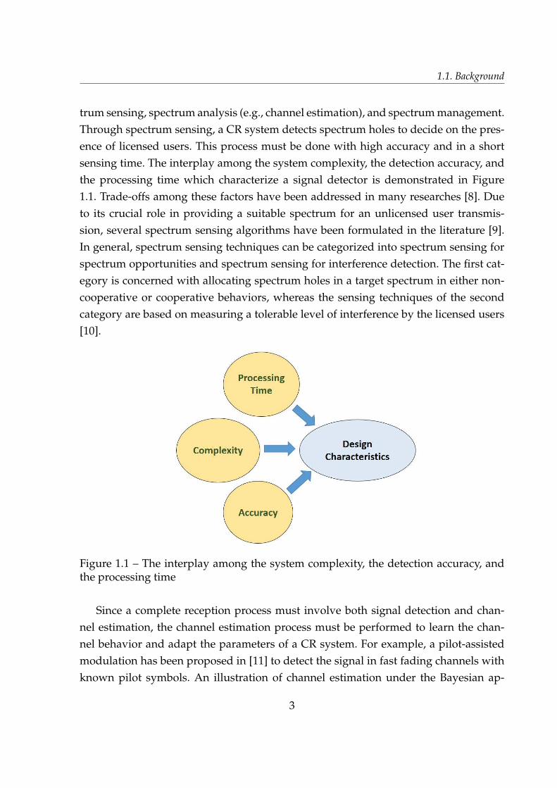
ence of licensed users. This process must be done with high accuracy and in a short
sensing time. The interplay among the system complexity, the detection accuracy, and
the processing time which characterize a signal detector is demonstrated in Figure
1.1. Trade-offs among these factors have been addressed in many researches [8]. Due
to its crucial role in providing a suitable spectrum for an unlicensed user transmis-
sion, several spectrum sensing algorithms have been formulated in the literature [9].
In general, spectrum sensing techniques can be categorized into spectrum sensing for
spectrum opportunities and spectrum sensing for interference detection. The first cat-
egory is concerned with allocating spectrum holes in a target spectrum in either non-
cooperative or cooperative behaviors, whereas the sensing techniques of the second
category are based on measuring a tolerable level of interference by the licensed users
[10].
Figure 1.1 – The interplay among the system complexity, the detection accuracy, andthe processing time
Since a complete reception process must involve both signal detection and chan-
nel estimation, the channel estimation process must be performed to learn the chan-
nel behavior and adapt the parameters of a CR system. For example, a pilot-assisted
modulation has been proposed in [11] to detect the signal in fast fading channels with
known pilot symbols. An illustration of channel estimation under the Bayesian ap-
3

Partie , Chapter 1 – Introduction
proach in CRs is shown [12]. In the literature, challenges associated with spectrum
sensing are addressed with suggested solutions on how sensing errors may affect the
channel estimation decisions and vice versa. Basically, the research studies in [13] and
[14] have considered the joint problem of the spectrum sensing and the channel esti-
mation processes and illustrated the interrelation between them. They have also made
some investigations on the dependence of different channel estimation schemes on the
obtained sensing decisions. Essentially, this dependence reflects the importance of de-
veloping efficient spectrum sensing algorithms.
In fact, there are different factors that impose challenges on the spectrum sensing
performance. These factors include the hardware complexity, the hidden PU problem,
and the sensing duration and frequency [10]. For instance, in wireless applications,
terminals are required to perform spectrum sensing with a high sampling rate, high
resolution analog-to-digital converters with a large dynamic range, and high speed
signal processors. This entails the increased hardware complexity and the longer time
for processing. Also, the hidden PU problem occurs when a weak signal occupies a
desired frequency band but it is undetectable by the CR receiver. This is either due to
an obstacle, the transmission channel effects, such as multipath fading, or due to the
noise-like nature of PU signals such as Spread Spectrum (SS) signals. This problem can
be partially avoided if the hopping pattern is known and a perfect synchronization
to the signal can be achieved. Nevertheless, licensed users can claim their frequency
bands anytime while a CR is operating on their bands. So, in order to prevent any
interference to/from licensed owners, a CR should be able to identify their activity as
quickly as possible and should vacate the band immediately. This requirement poses a
limit on the performance of sensing algorithms and creates a challenge for the design
of a CR system.
1.2 Thesis Contributions
The main objective of the thesis is to develop means of enhancing the process of
spectrum sensing in CR so as to provide more spectral opportunities, and hence in-
crease the throughput of a secondary network. Among the previously mentioned chal-
lenges, we choose to tackle the detection problem of a hidden Primary User (PU). Our
choice is motivated by the following reasons:
— Due to the noisy variations at the CR receiver, the detection errors may occur
4

1.2. Thesis Contributions
due to falsely detecting the presence of a possible PU signal. False-alarms lead
to the loss of potential spectral resources.
— A licensed user’s signal may appear hidden at the CR receiver’s side, if it nat-
urally behaves like noise. For example, a SS signal with the Low-Probability-
of-Intercept (LPI) property may cause the misdetection of the PU signal. This
results in mistakenly declaring a vacant channel. In this case, the transmission
of the CR user’s signal will cause interference to the licensed user which will
affect its Quality of Service (QoS).
— The detection of a hidden PU is a difficult task when detection is performed by a
non-cooperative system. On the other hand, prior knowledge of the PU signal’s
features must be provided to facilitate the detection process, which is performed
by a cooperative system.
Based on the aforementioned reasons, our target is to devise a robust spectrum sens-
ing algorithm while operating in a non-cooperative detection scenario. Therefore, the
important characteristic of the detection algorithm is to be able to exploit the distin-
guished features in a signal. The identification of hidden features of a targel signal
helps to differentiate between the signal of a significant user signal and the noise,
which helps in mitigating the misdetection and false-alarm problems.
Remarkably, the concept of Cepstral Analysis (CA) has a strong impact on several
applications comprising audio and speech processing, as well as mechanical systems
[15], [16], [17]. In the literature, it has been employed in the fields of signal classifica-
tion or features detection [18], [19]. Thus, the CA approach is used to identify certain
features hidden in a signal that can be revealed in the cepstral domain. According to
the variants of the CA approach, a certain CA variant is chosen in order to fit a specific
application. That is why a researcher must be aware of the problem under analysis,
and whether employing the CA approach will unleash significant details about the
signal in the logarithmic domain. In our proposed work, we employed the CA ap-
proach to tackle the misdetection and false-alarm problems in the context of CR in the
Single-Band Spectrum Access (SBSA) and the Multi-Band Spectrum Access (MBSA)
approaches.
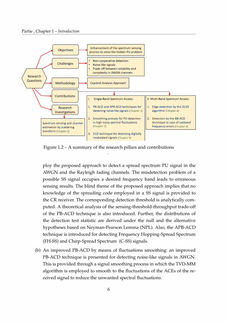
A summary of the research pillars by which we constructed our presented study is
shown in Figure 1.2. Specifically, our main contributions are listed as follows:
1. Spectrum sensing algorithm for SBSA:
(a) A PB-ACD technique for detecting spread spectrum signals and its: we em-
5
Partie , Chapter 1 – Introduction
Figure 1.2 – A summary of the research pillars and contributions.
ploy the proposed approach to detect a spread spectrum PU signal in the
AWGN and the Rayleigh fading channels. The misdetection problem of a
possible SS signal occupies a desired frequency band leads to erroneous
sensing results. The blind theme of the proposed approach implies that no
knowledge of the spreading code employed in a SS signal is provided to
the CR receiver. The corresponding detection threshold is analytically com-
puted. A theoretical analysis of the sensing-threshold-throughput trade-off
of the PB-ACD technique is also introduced. Further, the distributions of
the detection test statistic are derived under the null and the alternative
hypotheses based on Neyman-Pearson Lemma (NPL). Also, the APB-ACD
technique is introduced for detecting Frequency Hopping-Spread Spectrum
(FH-SS) and Chirp-Spread Spectrum (C-SS) signals.
(b) An improved PB-ACD by means of fluctuations smoothing: an improved
PB-ACD technique is presented for detecting noise-like signals in AWGN.
This is provided through a signal smoothing process in which the TVD-MM
algorithm is employed to smooth to the fluctuations of the ACEs of the re-
ceived signal to reduce the unwanted spectral fluctuations.
6
1.2. Thesis Contributions
(c) A generalized spectrum sensing approach for detecting digitally modulated
signals by the CCD technique: the proposed CCD exploits the periodicity in-
herited in the Power Cepstrum (PC) of digitally modulated signals to detect
their presence in a specific frequency band. By correlating the signals’ PC to
a sinusoidal signal having the fundamental frequency equal to the PC’s pe-
riodic frequency, the signal component will be enhanced and the detector
will simultaneously reject the noisy spectral variations that lead to possible
false-alarms.
2. Spectrum sensing algorithm for MBSA:
(a) Edge-detection technique by the Differential Log Spectral Density (DLSD)
algorithm for WideBand Spectrum Sensing (WBSS): we propose the DLSD
algorithm for the edge detection phase in order to detect the spectral bound-
aries within the wideband of interest. Also, we present a mathematical frame-
work of the proposed algorithm under AWGN channels. An expression for
the detection threshold of the proposed detector is derived according to its
statistical properties. The simulation results have shown a superior perfor-
mance of the proposed edge detection algorithm to different wavelet-based
techniques at relatively low-to-medium noise power levels (i.e., at an aver-
age SNR over the range [0,6] dB). Used in conjunction with denoising, the
proposed edge detector shows good detection results at high noise power
levels (i.e., below an average SNR of 0 dB). The performance of the proposed
algorithm is tested when impulsive noise is imposed.
(b) Detection of a PU signal under the uncertainty of the subbands’ center fre-
quencies by the BaseBand AutoCesptrum Detection (BB-ACD) technique:
the BB-ACD technique is formulated for detecting noise-like signals when
there may be possible errors in the identified center frequencies of the in-
tended subbands. The proposed BB-ACD consists of a circular topological
filter followed by the autocepstrum detection. The circular topological filter
utilizes the circular topology of a typical sinusoidal signal to separate the
baseband signal or its squared version. The detection of a noise-like PU sig-
nal, or a conventional digitally modulated signal, by the PB-ACD technique
depends on the presence of a strong peak appearing at a quefrency 1 value
1. Quefrency: It defines the inverse of the distance between successive log-spectral lines in a signal’scepstrum [20].
7

Partie , Chapter 1 – Introduction
equivalent to the reciprocal of the center frequency of a certain subband. Due
to the possible frequency estimation errors from the edge detection phase,
the PB-ACD gives a poor performance. A mathematical analysis of the de-
tection threshold is presented according to the statistical distribution of the
devised detection test statistic. Through simulations, we provided compar-
isons of the BB-ACD technique with the PB-ACD technique to show the effi-
cacy of the proposed technique when the problem of center frequency errors
is encountered in frequency selective fading channels.
1.3 Thesis Organization
This thesis includes the presented research work in six chapters. First, the state-
of-the-art techniques and a literature review are covered in chapter 2. Chapters 3 and
4 introduce the proposed detection techniques for the SBSA and the MBSA cases, re-
spectively. The CCD techniques is discussed in chapter 5 and the conclusions with the
future work are drawn in chapter 6. In particular, this thesis is organized as follows:
Chapter 2 reviews the state-of-the-art of the spectrum sensing techniques in CR sys-
tems. It covers the advantages and the disadvantages of these techniques and also it
discusses the challenges facing the spectrum sensing process. Further, this chapter in-
troduces the suggested spectrum sensing and channel estimation techniques through
Scattering Transform (ST), and gives some insights about the obtained results, as well
as highlighting the strengths and limitations of the proposed techniques.
Chapter 3 presents the proposed PB-ACD algorithm for detecting noise-like signals
such as spread spectrum and IR-UWB signals. The proposed technique is considered
for the SBSA scenario in which a specific CR receiver tests the availability of a narrow
frequency band. A mathematical analysis of the proposed detector is formulated and
its performance is compared with different state-of-the-art techniques. Moreover, The
APB-ACD technique is presented for detecting FH-SS and C-SS signals and the math-
ematical demonstration of the proposed detection technique is introduced.
Chapter 4 discusses the two phases of wideband spectrum sensing, namely: the edge
detection and the PU detection. In this chapter, we introduce the DLSD algorithm for
8
1.3. Thesis Organization
detecting the spectral boundaries of the intended subbands. The devised algorithm is
compared to different wavelet-based edge detection techniques showing high detec-
tion performance at medium-to-high SNR values. Used in conjunction with denoising
by TVD-MM algorithm, the edge detection is improved at a low SNR level. Moreover,
we tackled the problem of detecting PU signal occupying a specific narrow frequency
band when uncertainty of the subband’s center frequency is encountered. For this pur-
pose, we formulated the BB-ACD technique in which the periodicity inherited in the
signal’s PC in baseband.
Chapter 5 proposes the CCD technique to detect digitally modulated signals by evalu-
ating the PC of the received signal and correlating it to a shaping function, which has
a fundamental frequency equals to the PC’s periodic frequency. The aim of employing
a shaping function is to enhance the peaks that occur in the PC while simultaneously
rejecting the noisy spectral variations.
Chapter 6 provides the conclusions of the presented research work and gives some
prospects for further investigations related to the scope of the thesis, in which a dual
spectrum sensing and channel estimation technique is suggested based on CA ap-
proaches, and also the role of employing Artificial Intelligence (AI) algorithms in co-
operative sensing is discussed.
9

CHAPTER 2
STATE-OF-THE-ART
2.1 Introduction
In the last two decades, the world has witnessed a great growth in the global mobile
traffic. This growth is expected to increase more in data volume by 2021 as compared
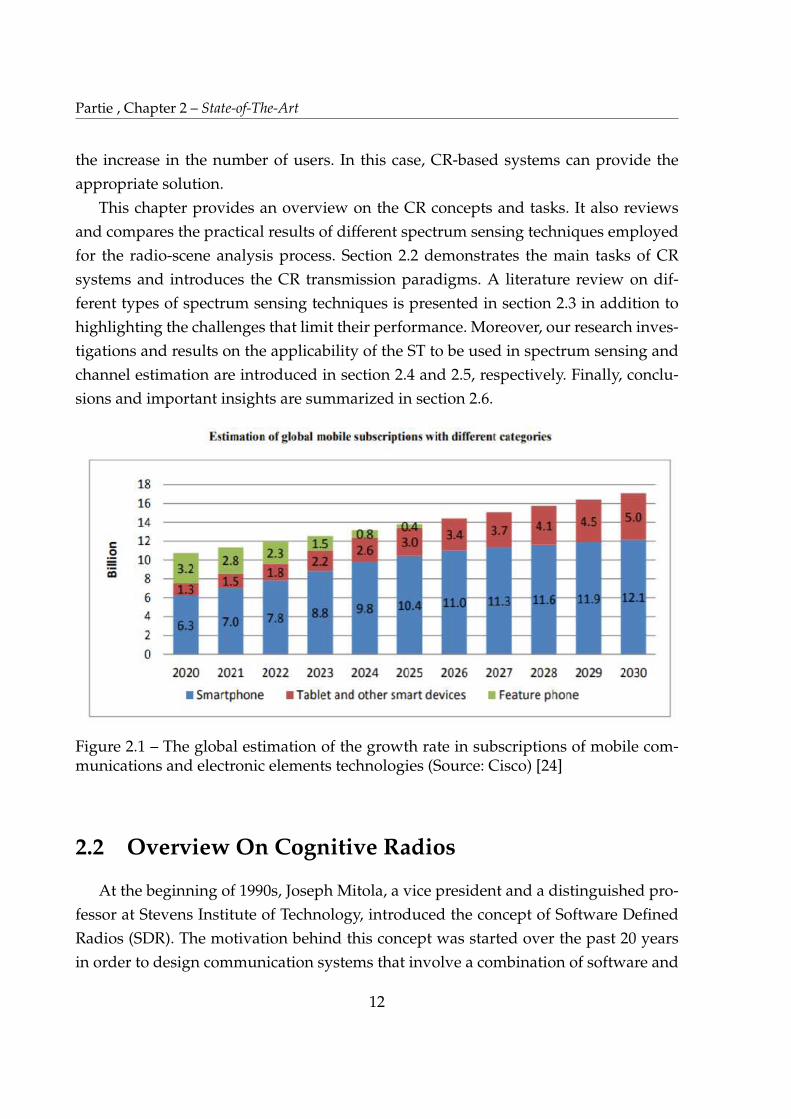
to 2005 [21]. The trend of this exponential growth, as shown in Figure 2.1, is expected
to even continue to 2030,as predicted by the International Telecommunication (ITU)
[22]. Therefore, without making use of the unoccupied spectrum bands, the radio fre-
quency becomes under-utilized. Indeed, as many academic research studies about the
6G technology is gradually taking momentum, scientific speculations claim that after
30 years of effort, 6G will eventually see the full potential of a Cognitive Radio (CR)
system [23], [24].
In fact, the design of any wireless system must consider the transmission data rates,
the geographical coverage area, the suitable transmission power, and the mobility of
users. Generally, various communication systems can be classified into:
— High-power wide area systems (cellular systems), which support mobile users
roaming over wide coverage areas.
— Low-power local area systems, such as cordless telephone systems.
— Low-power wide area systems, which are designed to support low data rate
services such as paging systems.
— High-speed local area systems, which are designed to allow for high data rate
services, such as wireless Local Area Networks (LANs).
Obviously, the first two classes are designed for voice applications, whereas the last
two classes are designed for data applications. In the design and implementation of
these systems, some challenges occur. Such challenges include radio resource alloca-
tion, management of the Medium Access Control (MAC) layer, the mobility manage-
ment, Quality of Service (QoS), and security. A very important challenge is the radio
resource allocation as well as the need for spectrum management in order to handle
11
Partie , Chapter 2 – State-of-The-Art
the increase in the number of users. In this case, CR-based systems can provide the
appropriate solution.
This chapter provides an overview on the CR concepts and tasks. It also reviews
and compares the practical results of different spectrum sensing techniques employed
for the radio-scene analysis process. Section 2.2 demonstrates the main tasks of CR
systems and introduces the CR transmission paradigms. A literature review on dif-
ferent types of spectrum sensing techniques is presented in section 2.3 in addition to
highlighting the challenges that limit their performance. Moreover, our research inves-
tigations and results on the applicability of the ST to be used in spectrum sensing and
channel estimation are introduced in section 2.4 and 2.5, respectively. Finally, conclu-
sions and important insights are summarized in section 2.6.
Figure 2.1 – The global estimation of the growth rate in subscriptions of mobile com-munications and electronic elements technologies (Source: Cisco) [24]
2.2 Overview On Cognitive Radios
At the beginning of 1990s, Joseph Mitola, a vice president and a distinguished pro-
fessor at Stevens Institute of Technology, introduced the concept of Software Defined
Radios (SDR). The motivation behind this concept was started over the past 20 years
in order to design communication systems that involve a combination of software and
12
2.2. Overview On Cognitive Radios
hardware systems away from pure hardware-based systems. SDR have a radio fre-
quency with a software-controlled tuner. Signals are being processed using a recon-
figurable device such as a Field-Programmable Gate Array (FPGA) or a digital signal
processor. Therefore, their ability to reconfigure the modulation scheme makes them
SDR. In his dissertation [25], Mitola introduced CRs as SDR with Artificial Intelligence
(AI). These radios are capable of sensing and reacting according to changes in the sur-
roundings. Simon Haykin also suggested another definition for a CR system in 2005.
He defined it as "an intelligent wireless communications system that is aware of its
surrounding environment and uses the methodology of understanding-by-building to
learn from the environment and adapt its internal states to statistical variations in the
incoming RF stimuli by making corresponding changes in certain operating parame-
ters in real-time".
Figure 2.2 shows the internal structure of the conventional radios, the SDR, and the
CRs. The spectrum licensing scheme set by the USA Federal Communications Com-
mission (FCC) leads to an inefficient usage of the radio spectrum. When the radio
spectrum allocated to licensed users is not used, it cannot be occupied by unlicensed
users. Therefore, legacy systems have to operate only on a dedicated spectrum band
and cannot adapt the transmission band according to the change in the environment.
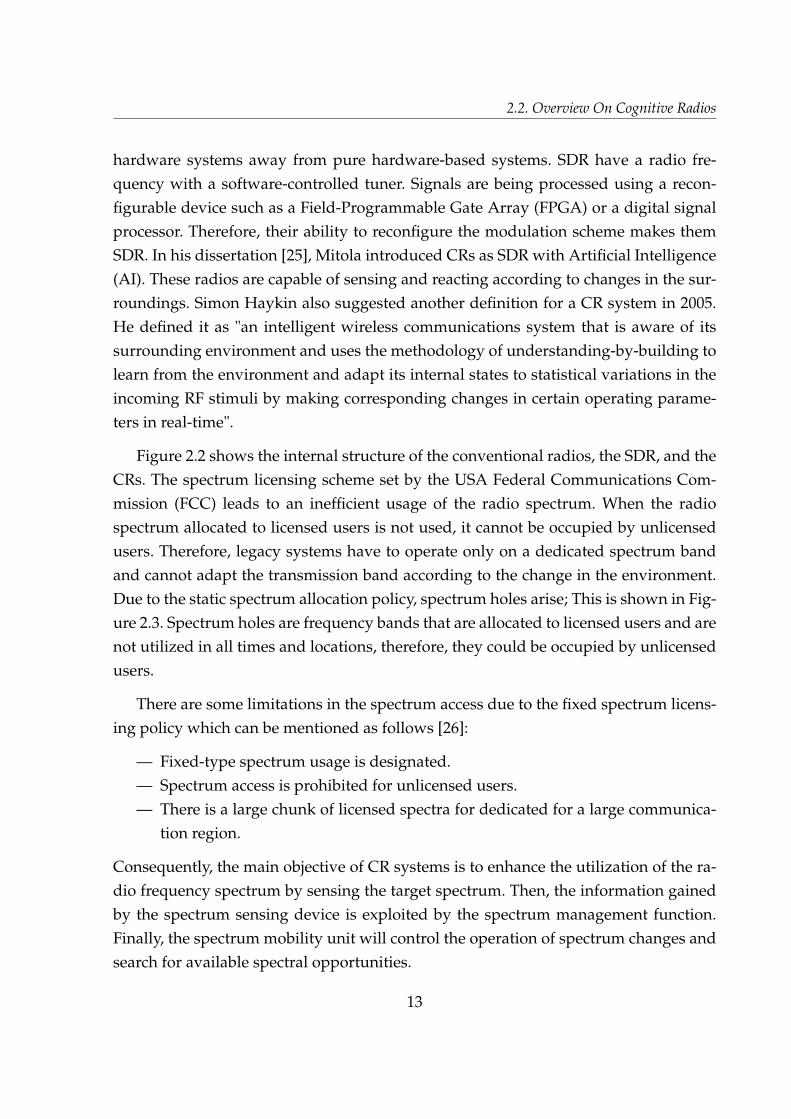
Due to the static spectrum allocation policy, spectrum holes arise; This is shown in Fig-
ure 2.3. Spectrum holes are frequency bands that are allocated to licensed users and are
not utilized in all times and locations, therefore, they could be occupied by unlicensed
users.
There are some limitations in the spectrum access due to the fixed spectrum licens-
ing policy which can be mentioned as follows [26]:
— Fixed-type spectrum usage is designated.
— Spectrum access is prohibited for unlicensed users.
— There is a large chunk of licensed spectra for dedicated for a large communica-
tion region.
Consequently, the main objective of CR systems is to enhance the utilization of the ra-
dio frequency spectrum by sensing the target spectrum. Then, the information gained
by the spectrum sensing device is exploited by the spectrum management function.
Finally, the spectrum mobility unit will control the operation of spectrum changes and
search for available spectral opportunities.
13

Partie , Chapter 2 – State-of-The-Art
Figure 2.2 – A logical diagram that illustrates the differences among conventional ra-dio, SDR, and CR [26]
2.2.1 Cognitive Capability of Cognitive Radio Networks
Multiple domains such as knowledge, model-based reasoning and negotiation can
remark the cognitive capability of a CR system. Conceptually, any radio etiquette with
different aspects, including RF bands and air interfaces, can be equipped with knowl-
edge and reasoning tools. Remarkably, CRs are characterized by their agility that dif-
ferentiates them from conventional radios. This agility is described by [27]:
— Frequency agility: it refers to the followed strategies to find the available spec-
trum which requires the design of good algorithms and protocols for appropri-
ately selecting the transmission frequencies.
— Technology agility: it refers to operating a single radio device over various ac-
cess technologies. It includes seamless interoperability which can be enabled by
multiplatform radios that are realized as system-on-a-chip platforms and can
operate as Bluetooth, WiFi, and GPS transceivers.
14
2.2. Overview On Cognitive Radios
Figure 2.3 – An illustration of the opportunistic and the fixed spectrum sharing modelsin CRs
— Protocol agility: depending on the devices they connect with, CR devices con-
tain a reconfigurable protocol stack so that they can preactively an reactively
adapt their protocol.
Such cognitive behavior could extend to networks of radios so that they mimic
human behavior in a civilized society. Eventually, this implies a framework that senses
the surrounding conditions to identify opportunistic spectra.
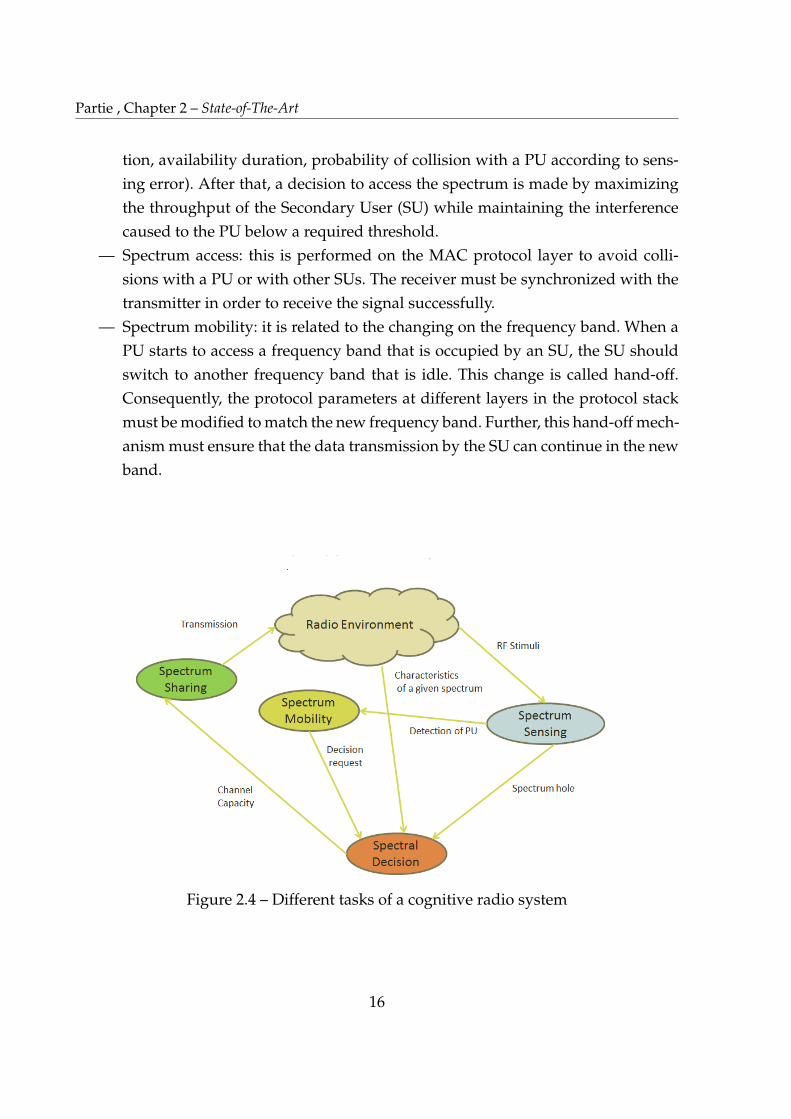
2.2.2 Tasks of Cognitive Radio Systems
A typical cognitive radio system performs different tasks through a cognitive cycle
by which it obtains the required information to reuse a specific frequency band. The
distribution of these tasks and their interconnection to each other, illustrated in Figure
2.4, are summarized as follows:
— Spectrum sensing: the main objective of the spectrum sensing process is to mea-
sure the status of a target spectrum and the activity of a Primary User (PU).
This is accomplished by a CR transceiver that detects a spectrum hole and the
appropriate method of accessing it (i.e. duration, transmission power) without
interfering with the PU signal.
— Spectrum analysis: information gained from the spectrum sensing process is
then analyzed to get knowledge about spectrum holes (e.g. interference estima-
15
Partie , Chapter 2 – State-of-The-Art
tion, availability duration, probability of collision with a PU according to sens-
ing error). After that, a decision to access the spectrum is made by maximizing
the throughput of the Secondary User (SU) while maintaining the interference
caused to the PU below a required threshold.
— Spectrum access: this is performed on the MAC protocol layer to avoid colli-
sions with a PU or with other SUs. The receiver must be synchronized with the
transmitter in order to receive the signal successfully.
— Spectrum mobility: it is related to the changing on the frequency band. When a
PU starts to access a frequency band that is occupied by an SU, the SU should
switch to another frequency band that is idle. This change is called hand-off.
Consequently, the protocol parameters at different layers in the protocol stack
must be modified to match the new frequency band. Further, this hand-off mech-
anism must ensure that the data transmission by the SU can continue in the new
band.
Figure 2.4 – Different tasks of a cognitive radio system
16
2.2. Overview On Cognitive Radios
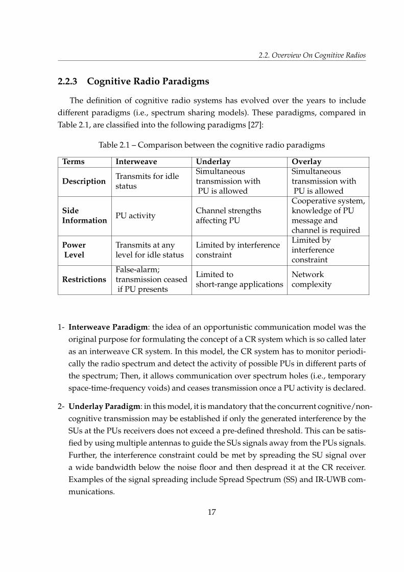
2.2.3 Cognitive Radio Paradigms
The definition of cognitive radio systems has evolved over the years to include
different paradigms (i.e., spectrum sharing models). These paradigms, compared in
Table 2.1, are classified into the following paradigms [27]:
Table 2.1 – Comparison between the cognitive radio paradigms
Terms Interweave Underlay Overlay
DescriptionTransmits for idlestatus
Simultaneoustransmission withPU is allowed
Simultaneoustransmission withPU is allowed
SideInformation
PU activityChannel strengthsaffecting PU
Cooperative system,knowledge of PUmessage andchannel is required
PowerLevel
Transmits at anylevel for idle status
Limited by interferenceconstraint
Limited byinterferenceconstraint
RestrictionsFalse-alarm;transmission ceasedif PU presents
Limited toshort-range applications
Networkcomplexity
1- Interweave Paradigm: the idea of an opportunistic communication model was the
original purpose for formulating the concept of a CR system which is so called later
as an interweave CR system. In this model, the CR system has to monitor periodi-
cally the radio spectrum and detect the activity of possible PUs in different parts of
the spectrum; Then, it allows communication over spectrum holes (i.e., temporary
space-time-frequency voids) and ceases transmission once a PU activity is declared.
2- Underlay Paradigm: in this model, it is mandatory that the concurrent cognitive/non-
cognitive transmission may be established if only the generated interference by the
SUs at the PUs receivers does not exceed a pre-defined threshold. This can be satis-
fied by using multiple antennas to guide the SUs signals away from the PUs signals.
Further, the interference constraint could be met by spreading the SU signal over
a wide bandwidth below the noise floor and then despread it at the CR receiver.
Examples of the signal spreading include Spread Spectrum (SS) and IR-UWB com-
munications.
17

Partie , Chapter 2 – State-of-The-Art
2- Overlay Paradigm: in overlay-enabled systems, knowledge of the PUs’ codebooks
and their messages must be provided at the CR receiver. For example, if the non-
cognitive users follow a uniform communication standards based on a publicized
codebook, this information could be easily obtained and hence could be utilized in
different ways. On the one hand, this information can be exploited to cancel the
interference caused by the PUs at the SUs receivers. On the other hand, the CR
users can assign part of their transmission power for their communication and the
remainder is to assist (i.e., relay) the PUs transmission.
2.2.4 Cognitive Radio Bands
The propagation environment of CR networks must be well understood in order
to design these networks efficiently. The knowledge of the propagation characteris-
tics will help in the design, implementation, and analysis of different transmission
strategies. The amount of interference that may be imposed on the PU signal must
be kept in mind as an important feature affecting the CR system design. The interfer-
ence level depends on the transmission power of the CR as well as the characteristics
of the wireless propagation channel. Cognitive radios may operate over a wide range
of the frequency spectrum. The bands below about 3.5 GHz have a lower propagation
loss and are sought after by all services. Therefore, these bands are ideal candidates for
the deployment of cognitive radio networks but not necessarily exclusive. They have
different primary systems, each with its service type, architecture, bandwidth, and tol-
erance to interference. Some candidate frequency bands for CR systems are mentioned
below [28]:
— UHF bands: these bands are currently used by the broadcast television. Terres-
trial broadcasting transmitters tend to have high antennas (hundreds of meters)
and large powers (kilowatt range). In this service, the transmission is one-way,
the transmitting antenna may be outside the area containing the cognitive radios
and the TV customers are generally fixed. In 2010, the US FCC adopted rules to
allow unlicensed radio transmitters to operate in the broadcast television spec-
trum at locations where the spectrum is not being used by the licensed services.
We find that the IEEE 802.11af, IEEE 802.22 and IEEE 802.19.1 are operating over
TV white spaces (54 to 60 MHz, TV channel 2; 76 to 88 MHz, TV channels 5 and
6; 174 to 216 MHz, TV channels 7 to 13; 470 to 608 MHz, TV channels 14 to 36;
18
2.3. Literature Review on Spectrum Sensing Techniques
and 614 to 698 MHz, TV channels 38 to 51). The unused TV spectrum can be
used as white spaces.
— Cellular bands: typical cellular bands are centered near 800/900 MHz, 1.8/1.9
GHz, 2.1 GHz, 2.3 GHz, and 2.5 GHz. Cellular networks have wide coverage,
with cell site antennas mounted at rooftops of buildings. This is a two-way ser-
vice, with the cell sites generally in the same region as the cognitive radios, and
the cellular customers can be mobile.
— Fixed wireless access bands: these bands provide two-way broadband service. They
are centered near 2.5 and 3.5 GHz. Fixed wireless systems are similar to cellu-
lar networks in layout, with the customers located at fixed locations, such as
companies and homes.
2.3 Literature Review on Spectrum Sensing Techniques
The broad definition of a vacant opportunity comes in terms of an idle frequency
band, a time slot, a geographical area, a code dimension, or the angle-of-arrival of a
signal. Many investigations on spectrum sensing techniques have focused in exploring
vacant frequency bands.
Different spectrum sensing techniques have been introduced over the last decade.
Based on the scanned bandwidth of the target frequency range, these techniques can
be classified into NarrowBand Spectrum Sensing (NBSS) and WBSS techniques. In the
NBSS approaches, a CR system scans only one frequency band, whereas in the WBSS
approaches a number of sub-channels are scanned, either simultaneously or sequen-
tially. In the literature, several NBSS algorithms and techniques have been formulated.
These techniques include ED, Matched Filter Detection (MFD), covariance-based de-
tection, Cyclostationary Feature Detection (CFD), and Machine Learning Based Sens-
ing (MLBS) [9].
Due to its calculation and implementation simplicity, ED has been used extensively
in the literature. In the design of an energy detector, there must be an accurate mod-
eling of the detection test statistic, and also a prior knowledge of the noise power is
required at the CR receiver. Regarding the estimation of the noise power, an experi-
mental study is covered in [29] in which a practical realization of energy detectors by
SDR is introduced. In the proposed study, it has been shown that an inaccurate model-
ing of the detectors test statistic leads to a deterioration in the detection performance.
19
Partie , Chapter 2 – State-of-The-Art
For this purpose, the authors of [30] have proposed a histogram-based method to de-
termine the detection threshold when a large sample size is sufficiently collected. From
the observed samples, two histograms are obtained to indicate the presence or absence
of a possible PU signal. This detection threshold is chosen to fit certain false-alarm
and misdetection probabilities. However, in noisy and fading environments, the de-
tection of PUs becomes a difficult task [31]. This gives the existence of the SNR wall
phenomenon, which is the SNR value below which all the detectors will fail to detect
the presence of a signal even for large channel observations [32]. This phenomenon
has been mathematically validated through mathematical modeling in [33]. In order
to provide an accurate prediction of the SNR wall constraints, the authors in [34] have
introduced a prediction method to estimate the noisy variations as well as the Rayleigh
fading coefficients. Moreover, theoretical analysis of energy detection that is based on
a dynamic selection of the detection threshold is given in [35].
A suitable alternative approach to the energy detector is the matched filter detector
which is described to be the optimum detector that maximizes the SNR in Additive
White Gaussian Noise (AWGN) channel [36]. Since the MFD technique requires prior
knowledge of the PU’s signal parameters, which is not feasible practically, a blind es-
timation technique is proposed in [37] to extract the signals parameters. However, the
pre-processing offered by the blind parameter estimator increases the detector com-
plexity and the sensing time as well. Another approach is presented in [38] to increase
the sensing efficiency of the MFD by introducing a dynamic selection of the detection
threshold. On the other hand, the covariance-based detection techniques offer a blind
approach for the PU detection that is based on calculating the covariance matrix of the
received signal. By exploiting the correlation of the signals samples, the detector uses
this characteristic to distinguish between the noise and the signal. Different techniques
have been developed based on the covariance-based detection such as the EVD [39].
A superior sensing technique than ED, MFD, and the covariance-based detection
is offered by the CFD approach, in which the inherited cyclostationary features in a
PU signal is revealed and utilized for the signal detection. In [40], the authors have
evaluated the performance of the cyclostationary detector for different modulation
schemes. Also, the authors in [41] have shown the employment of the cyclostation-
ary Fast Fourier Transform (FFT) Accumulation Method (FAM) to tackle the problem
of hidden SUs signals and in order to improve more users recognition. To improve the
detection performance of the CFD, the authors in [42] have shown the effect of employ-
20
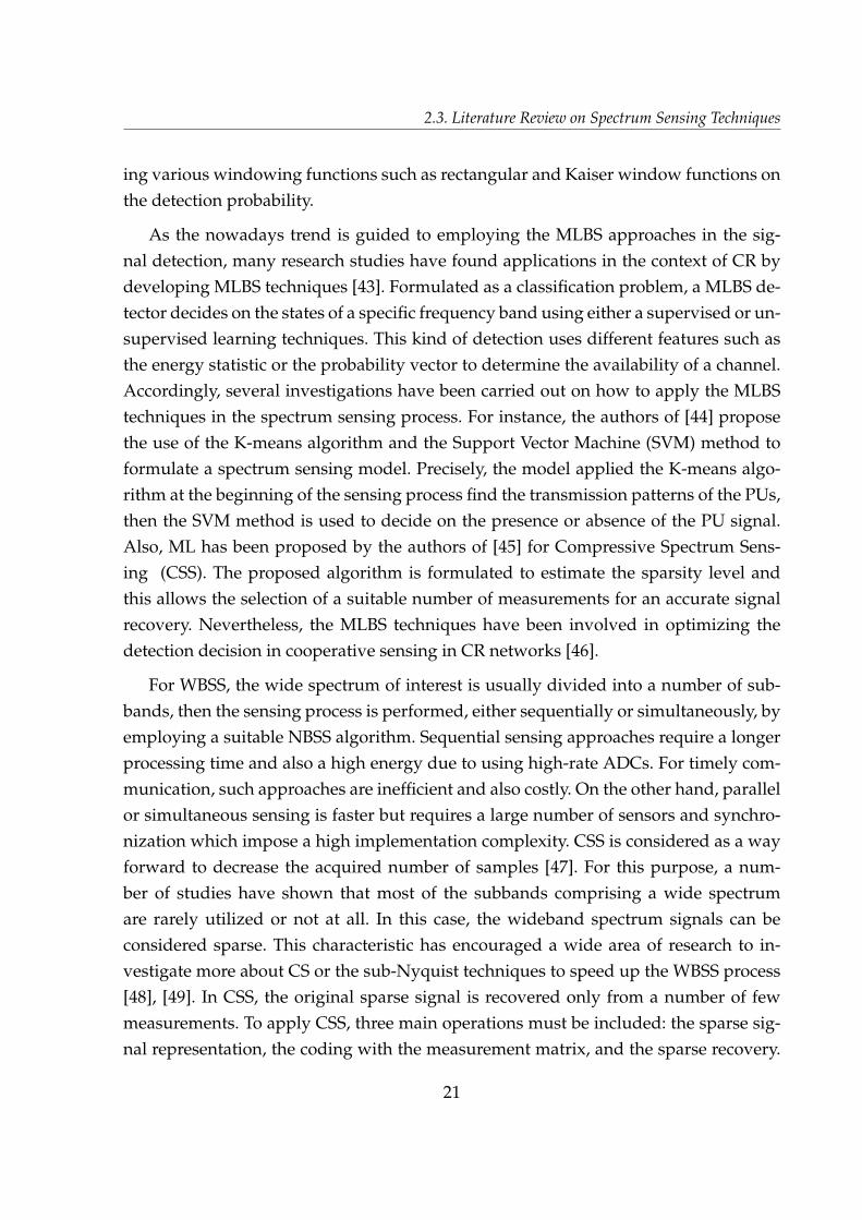
2.3. Literature Review on Spectrum Sensing Techniques
ing various windowing functions such as rectangular and Kaiser window functions on
the detection probability.
As the nowadays trend is guided to employing the MLBS approaches in the sig-
nal detection, many research studies have found applications in the context of CR by
developing MLBS techniques [43]. Formulated as a classification problem, a MLBS de-
tector decides on the states of a specific frequency band using either a supervised or un-
supervised learning techniques. This kind of detection uses different features such as
the energy statistic or the probability vector to determine the availability of a channel.
Accordingly, several investigations have been carried out on how to apply the MLBS
techniques in the spectrum sensing process. For instance, the authors of [44] propose
the use of the K-means algorithm and the Support Vector Machine (SVM) method to
formulate a spectrum sensing model. Precisely, the model applied the K-means algo-
rithm at the beginning of the sensing process find the transmission patterns of the PUs,
then the SVM method is used to decide on the presence or absence of the PU signal.
Also, ML has been proposed by the authors of [45] for Compressive Spectrum Sens-
ing (CSS). The proposed algorithm is formulated to estimate the sparsity level and
this allows the selection of a suitable number of measurements for an accurate signal
recovery. Nevertheless, the MLBS techniques have been involved in optimizing the
detection decision in cooperative sensing in CR networks [46].
For WBSS, the wide spectrum of interest is usually divided into a number of sub-
bands, then the sensing process is performed, either sequentially or simultaneously, by
employing a suitable NBSS algorithm. Sequential sensing approaches require a longer
processing time and also a high energy due to using high-rate ADCs. For timely com-
munication, such approaches are inefficient and also costly. On the other hand, parallel
or simultaneous sensing is faster but requires a large number of sensors and synchro-
nization which impose a high implementation complexity. CSS is considered as a way
forward to decrease the acquired number of samples [47]. For this purpose, a num-
ber of studies have shown that most of the subbands comprising a wide spectrum
are rarely utilized or not at all. In this case, the wideband spectrum signals can be
considered sparse. This characteristic has encouraged a wide area of research to in-
vestigate more about CS or the sub-Nyquist techniques to speed up the WBSS process
[48], [49]. In CSS, the original sparse signal is recovered only from a number of few
measurements. To apply CSS, three main operations must be included: the sparse sig-
nal representation, the coding with the measurement matrix, and the sparse recovery.
21
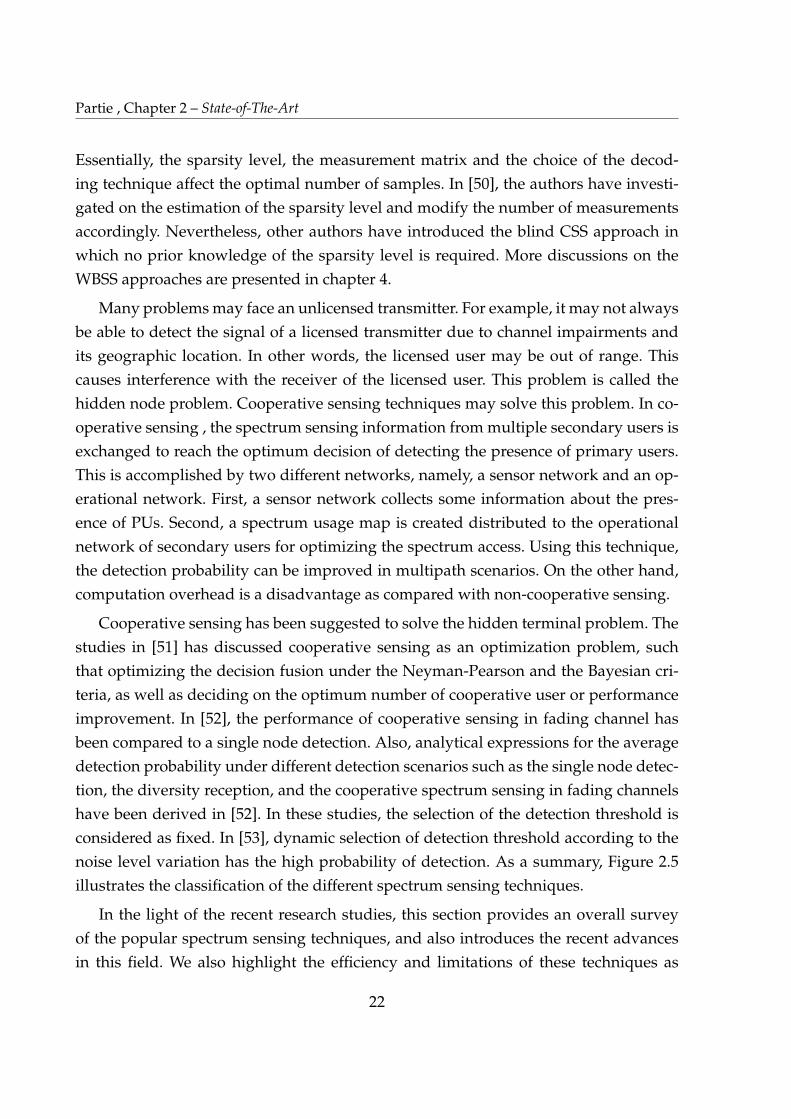
Partie , Chapter 2 – State-of-The-Art
Essentially, the sparsity level, the measurement matrix and the choice of the decod-
ing technique affect the optimal number of samples. In [50], the authors have investi-
gated on the estimation of the sparsity level and modify the number of measurements
accordingly. Nevertheless, other authors have introduced the blind CSS approach in
which no prior knowledge of the sparsity level is required. More discussions on the
WBSS approaches are presented in chapter 4.
Many problems may face an unlicensed transmitter. For example, it may not always
be able to detect the signal of a licensed transmitter due to channel impairments and
its geographic location. In other words, the licensed user may be out of range. This
causes interference with the receiver of the licensed user. This problem is called the
hidden node problem. Cooperative sensing techniques may solve this problem. In co-
operative sensing , the spectrum sensing information from multiple secondary users is
exchanged to reach the optimum decision of detecting the presence of primary users.
This is accomplished by two different networks, namely, a sensor network and an op-
erational network. First, a sensor network collects some information about the pres-
ence of PUs. Second, a spectrum usage map is created distributed to the operational
network of secondary users for optimizing the spectrum access. Using this technique,
the detection probability can be improved in multipath scenarios. On the other hand,
computation overhead is a disadvantage as compared with non-cooperative sensing.
Cooperative sensing has been suggested to solve the hidden terminal problem. The
studies in [51] has discussed cooperative sensing as an optimization problem, such
that optimizing the decision fusion under the Neyman-Pearson and the Bayesian cri-
teria, as well as deciding on the optimum number of cooperative user or performance
improvement. In [52], the performance of cooperative sensing in fading channel has
been compared to a single node detection. Also, analytical expressions for the average
detection probability under different detection scenarios such as the single node detec-
tion, the diversity reception, and the cooperative spectrum sensing in fading channels
have been derived in [52]. In these studies, the selection of the detection threshold is
considered as fixed. In [53], dynamic selection of detection threshold according to the
noise level variation has the high probability of detection. As a summary, Figure 2.5
illustrates the classification of the different spectrum sensing techniques.
In the light of the recent research studies, this section provides an overall survey
of the popular spectrum sensing techniques, and also introduces the recent advances
in this field. We also highlight the efficiency and limitations of these techniques as
22
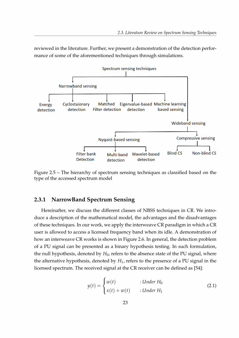
2.3. Literature Review on Spectrum Sensing Techniques
reviewed in the literature. Further, we present a demonstration of the detection perfor-
mance of some of the aforementioned techniques through simulations.
Figure 2.5 – The hierarchy of spectrum sensing techniques as classified based on thetype of the accessed spectrum model
2.3.1 NarrowBand Spectrum Sensing
Hereinafter, we discuss the different classes of NBSS techniques in CR. We intro-
duce a description of the mathematical model, the advantages and the disadvantages
of these techniques. In our work, we apply the interweave CR paradigm in which a CR
user is allowed to access a licensed frequency band when its idle. A demonstration of
how an interweave CR works is shown in Figure 2.6. In general, the detection problem
of a PU signal can be presented as a binary hypothesis testing. In such formulation,
the null hypothesis, denoted by H0, refers to the absence state of the PU signal, where
the alternative hypothesis, denoted by H1, refers to the presence of a PU signal in the
licensed spectrum. The received signal at the CR receiver can be defined as [54]:
y(t) =
8
<
:
w(t) : Under H0
x(t) + w(t) : Under H1
(2.1)
23

Partie , Chapter 2 – State-of-The-Art
where w(t) is the thermal noise imposed on the received PU signal that can be modeled
as a Gaussian distributed process with a variance σ2w. The faded PU signal is given by:
x(t) = s(t) ⇤ hs(t;τ) (2.2)
where s(t) is the PU transmitted signal, ⇤ denotes the convolution operator, and hs(t;τ)
is the sensing channel that is generally described as a time-varying fading channel with
a time lag, denoted by τ.
Figure 2.6 – A demonstration of a typical operation of an interweave CR system.
In a spectrum sensing process, the sensing threshold is an important design param-
eter of any signal detector. Indeed, a detector with a non properly adjusted threshold
leads to a degraded sensing performance. Based on an appropriate selection of a detec-
tion threshold, the sensing decision is made. It means that the choice of the detection
threshold reflects the offered accuracy of any spectrum sensing algorithm. Based on
the NPL, a detector decides H1 if the likelihood ratio L(y) is greater than a threshold η.
The likelihood ratio is given by [54]:
L(y) =p(y; H1)
p(y; H0)(2.3)
24

2.3. Literature Review on Spectrum Sensing Techniques
where p(y; H1) and p(y; H0) denote the probability density function of the received
signal under the alternative and the null hypotheses, respectively. To evaluate the de-
tection performance of the spectrum sensing techniques, an important metric is con-
sidered which is the ROC curve. It evaluates the detector performance in terms of the
following metrics:
— The probability of detection, PD: it describes the probability of the SU to declare
the presence of a PU signal. It is given in terms the conditional probability PD =
p(H1|H1) of deciding an occupied spectral hole while it is actually busy.
— The false-alarm probability, PFA: it describes the probability of deciding on the
presence of a PU in a spectral hole while it is actually idle. It is given in terms of
the conditional probability PFA = p(H1|H0).
— The probability of miss-detection, PMD: it describes the probability of a miss-
detected target while the detector declares a spectral hole. It is given in terms of
the detection probability as PMD = 1 � PD.
— The probability of correct no-detection, PCN: it describes the correct probability
of having a spectral hole, which is given by PCN = 1 � PFA.
Energy Detection
The detector computes the energy of the received signal by the CR user and com-
pares it to a threshold. If the computed energy exceeds the decision threshold, the PU
is considered present; otherwise, the channel is considered idle. Figure 2.7 shows the
block diagram of the conventional energy detector that calculates the energy as the
squared magnitude of the FFT averaged over the number of samples of the received
signal. The test statistic of the ED is given by:
TED[Y ] =1N
N
∑k=1
[Y(k)]2H1?H0
ηED (2.4)
where Y(k) denotes the FFT of the received signal represented in the discrete time
domain as y(n), and ηED denotes the detection threshold of the Energy Detection (ED)
technique. The value of the detection threshold depends on the noise variance. Thus,
the detection performance is affected by the appropriate selection of ηED.
Despite its simplicity, the ED technique cannot distinguish between the noise and
the PU signal. That is why the detection decision is subjected to a high uncertainty
25

Partie , Chapter 2 – State-of-The-Art
and results in a low detection performance in low SNR values, as shown in [31]. The
two performance metrics (PD, PFA) can be evaluated using the Central Limit Theorem
(CLT) 1 when the sample size N of the observed signal is large enough to approximate
the test statistics as Gaussian random variables [55]. For the conventional ED, these
two probabilities are given by [54]:
PD = Q
ηED � N(1 + γ)p
2N(1 + γ)2)
!
(2.5)
PFA = Q
ηED � Nσ2w
p
2Nσ4w
!
(2.6)
where γ is the SNR, and Q(.) is the Gaussian Q-function that describes the tail prob-
ability of the normal distribution with zero mean and unit variance which is given by
[54]:
Q(x) =1p2π
Z ∞
xexp
✓
� t2
2
◆
dt. (2.7)
consequently, the detection threshold is expressed in terms of a target PFA as follows:
ηED = σ2w
⇣
Q�1(PFA
p2N + N)
⌘
(2.8)
Based on equation (2.8), the sensing threshold of the energy detector depends on
the noise power, thus it is sensitive to the noise uncertainty. Figure 2.8 demonstrates
the relation between the false-alarm probability and the detection threshold as a func-
tion of the number of samples of the observed signal as indicated in equation (2.6). At
a specific detection threshold, as the number of samples increases, the probability of
1. CLT states that when a large number of independent random variables are added, their normal-ized sum tends toward a normal distribution even if the original variables themselves are not normallydistributed.
Figure 2.7 – The block diagram of a conventional energy detector.
26
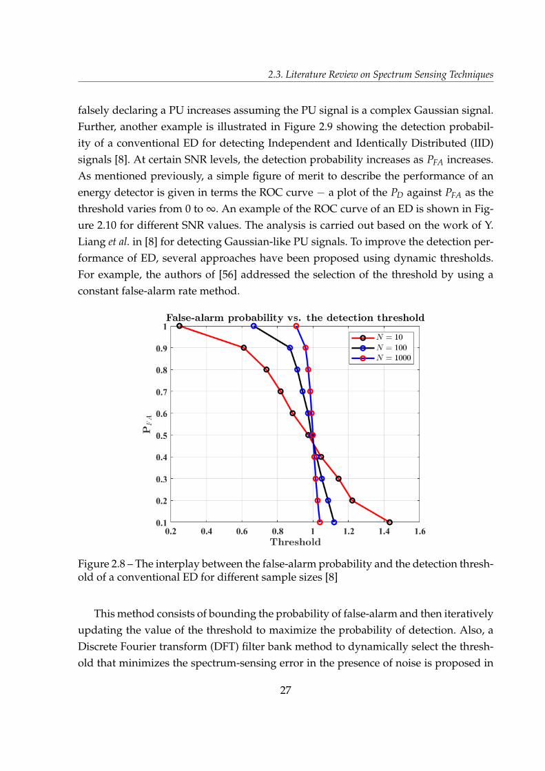
2.3. Literature Review on Spectrum Sensing Techniques
falsely declaring a PU increases assuming the PU signal is a complex Gaussian signal.
Further, another example is illustrated in Figure 2.9 showing the detection probabil-
ity of a conventional ED for detecting Independent and Identically Distributed (IID)
signals [8]. At certain SNR levels, the detection probability increases as PFA increases.
As mentioned previously, a simple figure of merit to describe the performance of an
energy detector is given in terms the ROC curve � a plot of the PD against PFA as the
threshold varies from 0 to ∞. An example of the ROC curve of an ED is shown in Fig-
ure 2.10 for different SNR values. The analysis is carried out based on the work of Y.
Liang et al. in [8] for detecting Gaussian-like PU signals. To improve the detection per-
formance of ED, several approaches have been proposed using dynamic thresholds.
For example, the authors of [56] addressed the selection of the threshold by using a
constant false-alarm rate method.
Figure 2.8 – The interplay between the false-alarm probability and the detection thresh-old of a conventional ED for different sample sizes [8]
This method consists of bounding the probability of false-alarm and then iteratively
updating the value of the threshold to maximize the probability of detection. Also, a
Discrete Fourier transform (DFT) filter bank method to dynamically select the thresh-
old that minimizes the spectrum-sensing error in the presence of noise is proposed in
27

Partie , Chapter 2 – State-of-The-Art
Figure 2.9 – The detection probability of a conventional ED for for detecting IID signals[8]
.
[57]. The double-threshold technique is introduced in [58] to deal with the noise un-
certainty. Although this double-threshold algorithm decreases the collision between
the PU and the SU signals, its detection performance is not guaranteed for low SNR
values, and its sensitivity to noise uncertainty is very high.
Matched Filter Detection
Matched filtering is known as the optimal method for the detection of PUs when
the transmitted signal is known. It is a linear filter designed to maximize the output
SNR for a given input signal. It is obtained by correlating a known signal, with an un-
known signal to detect the presence of the known signal in the unknown one. This is
equivalent to convolving the unknown signal with a time-reversed version of the sig-
nal. Convolution is at the heart of matched filters. Convolution does essentially with
two functions that it places one function over another function and outputs a single
value suggesting a level of similarity, and then it moves the first function an infinites-
imally small distance and finds another value. The end result comes in the form of
28
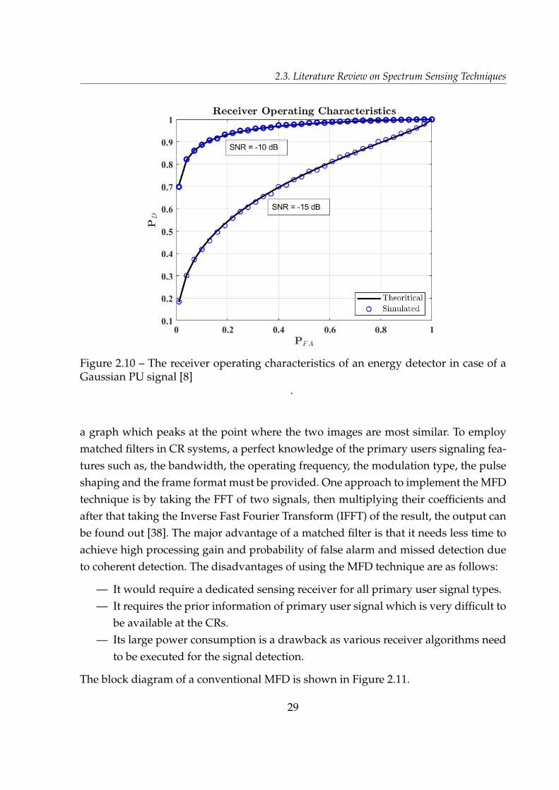
2.3. Literature Review on Spectrum Sensing Techniques
Figure 2.10 – The receiver operating characteristics of an energy detector in case of aGaussian PU signal [8]
.
a graph which peaks at the point where the two images are most similar. To employ
matched filters in CR systems, a perfect knowledge of the primary users signaling fea-
tures such as, the bandwidth, the operating frequency, the modulation type, the pulse
shaping and the frame format must be provided. One approach to implement the MFD
technique is by taking the FFT of two signals, then multiplying their coefficients and
after that taking the Inverse Fast Fourier Transform (IFFT) of the result, the output can
be found out [38]. The major advantage of a matched filter is that it needs less time to
achieve high processing gain and probability of false alarm and missed detection due
to coherent detection. The disadvantages of using the MFD technique are as follows:
— It would require a dedicated sensing receiver for all primary user signal types.
— It requires the prior information of primary user signal which is very difficult to
be available at the CRs.
— Its large power consumption is a drawback as various receiver algorithms need
to be executed for the signal detection.
The block diagram of a conventional MFD is shown in Figure 2.11.
29
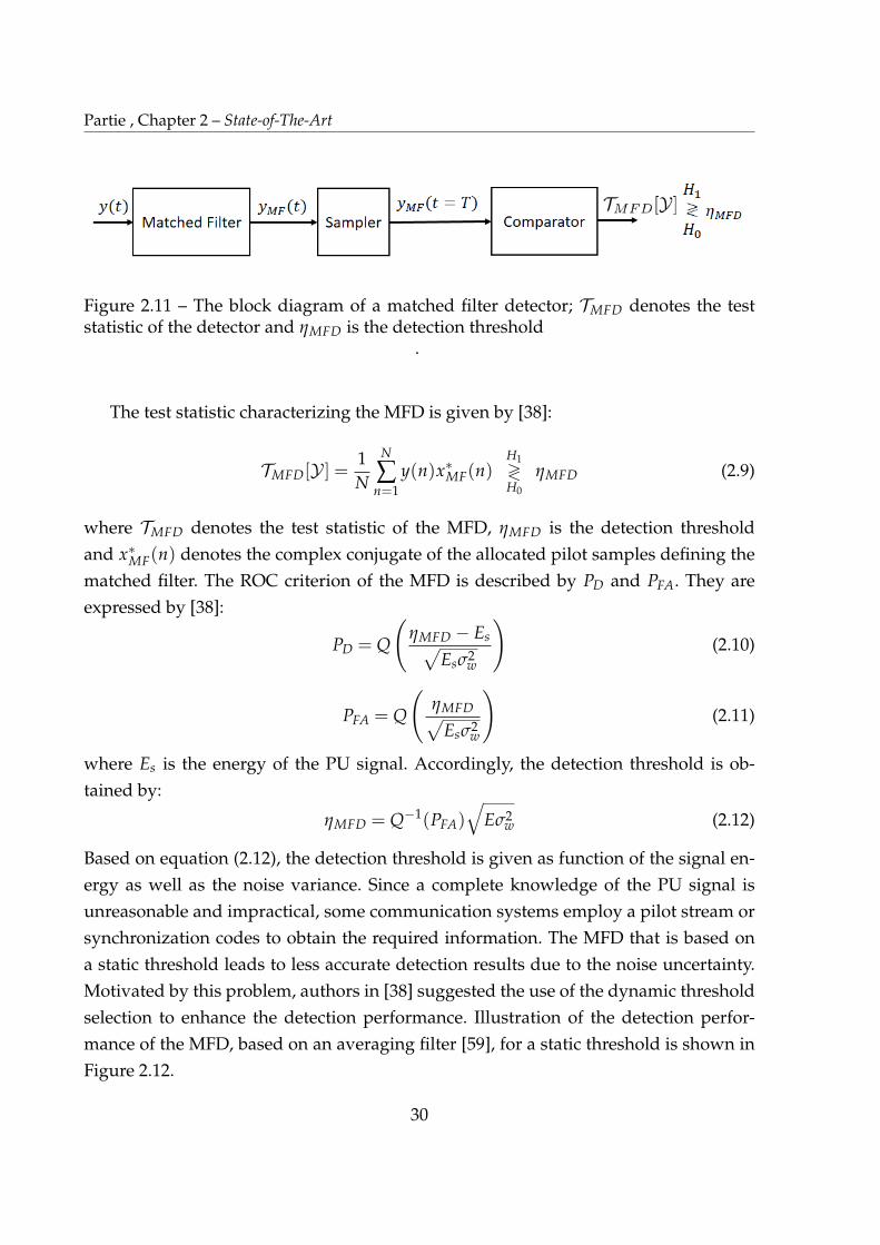
Partie , Chapter 2 – State-of-The-Art
Figure 2.11 – The block diagram of a matched filter detector; TMFD denotes the teststatistic of the detector and ηMFD is the detection threshold
.
The test statistic characterizing the MFD is given by [38]:
TMFD[Y ] =1N
N
∑n=1
y(n)x⇤MF(n)H1?H0
ηMFD (2.9)
where TMFD denotes the test statistic of the MFD, ηMFD is the detection threshold
and x⇤MF(n) denotes the complex conjugate of the allocated pilot samples defining the
matched filter. The ROC criterion of the MFD is described by PD and PFA. They are
expressed by [38]:
PD = Q
ηMFD � Esp
Esσ2w
!
(2.10)
PFA = Q
ηMFDp
Esσ2w
!
(2.11)
where Es is the energy of the PU signal. Accordingly, the detection threshold is ob-
tained by:
ηMFD = Q�1(PFA)q
Eσ2w (2.12)
Based on equation (2.12), the detection threshold is given as function of the signal en-
ergy as well as the noise variance. Since a complete knowledge of the PU signal is
unreasonable and impractical, some communication systems employ a pilot stream or
synchronization codes to obtain the required information. The MFD that is based on
a static threshold leads to less accurate detection results due to the noise uncertainty.
Motivated by this problem, authors in [38] suggested the use of the dynamic threshold
selection to enhance the detection performance. Illustration of the detection perfor-
mance of the MFD, based on an averaging filter [59], for a static threshold is shown in
Figure 2.12.
30
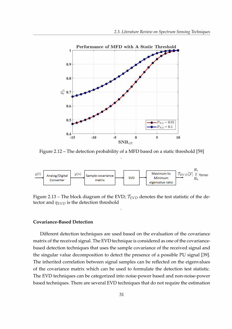
2.3. Literature Review on Spectrum Sensing Techniques
Figure 2.12 – The detection probability of a MFD based on a static threshold [59].
Figure 2.13 – The block diagram of the EVD; TEVD denotes the test statistic of the de-tector and ηEVD is the detection threshold
.
Covariance-Based Detection
Different detection techniques are used based on the evaluation of the covariance
matrix of the received signal. The EVD technique is considered as one of the covariance-
based detection techniques that uses the sample covariance of the received signal and
the singular value decomposition to detect the presence of a possible PU signal [39].
The inherited correlation between signal samples can be reflected on the eigenvalues
of the covariance matrix which can be used to formulate the detection test statistic.
The EVD techniques can be categorized into noise-power based and non-noise-power
based techniques. There are several EVD techniques that do not require the estimation
31
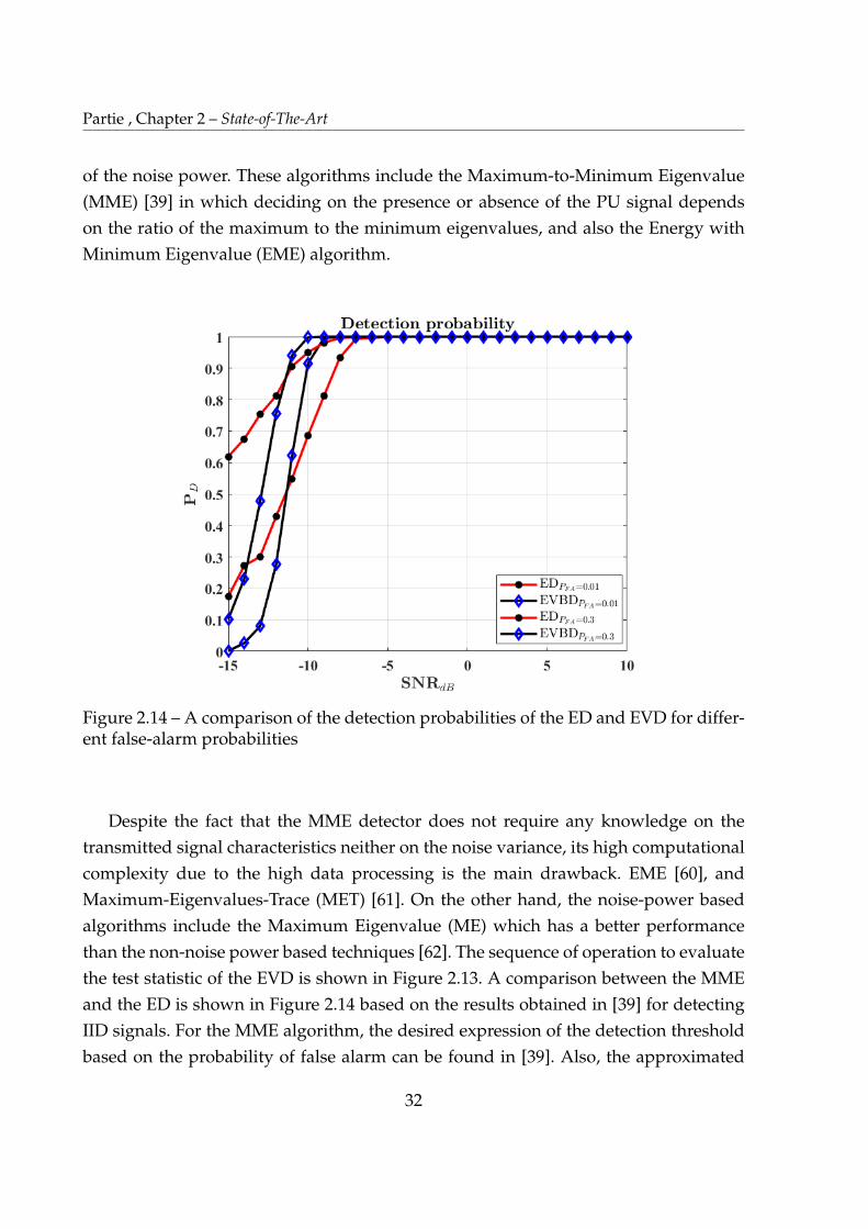
Partie , Chapter 2 – State-of-The-Art
of the noise power. These algorithms include the Maximum-to-Minimum Eigenvalue
(MME) [39] in which deciding on the presence or absence of the PU signal depends
on the ratio of the maximum to the minimum eigenvalues, and also the Energy with
Minimum Eigenvalue (EME) algorithm.
Figure 2.14 – A comparison of the detection probabilities of the ED and EVD for differ-ent false-alarm probabilities
Despite the fact that the MME detector does not require any knowledge on the
transmitted signal characteristics neither on the noise variance, its high computational
complexity due to the high data processing is the main drawback. EME [60], and
Maximum-Eigenvalues-Trace (MET) [61]. On the other hand, the noise-power based
algorithms include the Maximum Eigenvalue (ME) which has a better performance
than the non-noise power based techniques [62]. The sequence of operation to evaluate
the test statistic of the EVD is shown in Figure 2.13. A comparison between the MME
and the ED is shown in Figure 2.14 based on the results obtained in [39] for detecting
IID signals. For the MME algorithm, the desired expression of the detection threshold
based on the probability of false alarm can be found in [39]. Also, the approximated
32
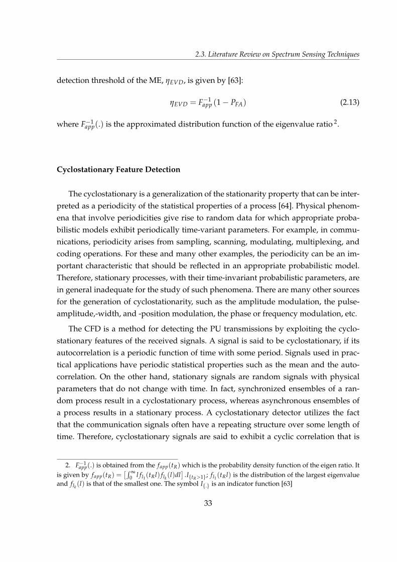
2.3. Literature Review on Spectrum Sensing Techniques
detection threshold of the ME, ηEVD, is given by [63]:
ηEVD = F�1app (1 � PFA) (2.13)
where F�1app(.) is the approximated distribution function of the eigenvalue ratio 2.
Cyclostationary Feature Detection
The cyclostationary is a generalization of the stationarity property that can be inter-
preted as a periodicity of the statistical properties of a process [64]. Physical phenom-
ena that involve periodicities give rise to random data for which appropriate proba-
bilistic models exhibit periodically time-variant parameters. For example, in commu-
nications, periodicity arises from sampling, scanning, modulating, multiplexing, and
coding operations. For these and many other examples, the periodicity can be an im-
portant characteristic that should be reflected in an appropriate probabilistic model.
Therefore, stationary processes, with their time-invariant probabilistic parameters, are
in general inadequate for the study of such phenomena. There are many other sources
for the generation of cyclostationarity, such as the amplitude modulation, the pulse-
amplitude,-width, and -position modulation, the phase or frequency modulation, etc.
The CFD is a method for detecting the PU transmissions by exploiting the cyclo-
stationary features of the received signals. A signal is said to be cyclostationary, if its
autocorrelation is a periodic function of time with some period. Signals used in prac-
tical applications have periodic statistical properties such as the mean and the auto-
correlation. On the other hand, stationary signals are random signals with physical
parameters that do not change with time. In fact, synchronized ensembles of a ran-
dom process result in a cyclostationary process, whereas asynchronous ensembles of
a process results in a stationary process. A cyclostationary detector utilizes the fact
that the communication signals often have a repeating structure over some length of
time. Therefore, cyclostationary signals are said to exhibit a cyclic correlation that is
2. F�1app(.) is obtained from the fapp(tR) which is the probability density function of the eigen ratio. It
is given by fapp(tR) =⇥R ∞
0 l fl1(tRl) flk(l)dl
⇤
.I{tR>1}; fl1(tRl) is the distribution of the largest eigenvalueand flk
(l) is that of the smallest one. The symbol I{.} is an indicator function [63]
33
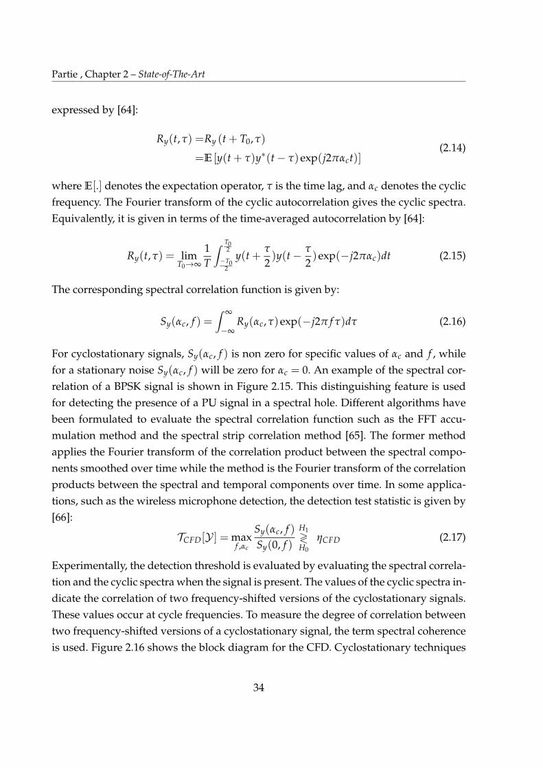
Partie , Chapter 2 – State-of-The-Art
expressed by [64]:
Ry(t, τ) =Ry (t + T0, τ)
=E [y(t + τ)y⇤(t � τ)exp(j2παct)](2.14)
where E[.] denotes the expectation operator, τ is the time lag, and αc denotes the cyclic
frequency. The Fourier transform of the cyclic autocorrelation gives the cyclic spectra.
Equivalently, it is given in terms of the time-averaged autocorrelation by [64]:
Ry(t, τ) = limT0!∞
1T
Z
T02
�T02
y(t +τ
2)y(t � τ
2)exp(�j2παc)dt (2.15)
The corresponding spectral correlation function is given by:
Sy(αc, f ) =Z ∞
�∞Ry(αc, τ)exp(�j2π f τ)dτ (2.16)
For cyclostationary signals, Sy(αc, f ) is non zero for specific values of αc and f , while
for a stationary noise Sy(αc, f ) will be zero for αc = 0. An example of the spectral cor-
relation of a BPSK signal is shown in Figure 2.15. This distinguishing feature is used
for detecting the presence of a PU signal in a spectral hole. Different algorithms have
been formulated to evaluate the spectral correlation function such as the FFT accu-
mulation method and the spectral strip correlation method [65]. The former method
applies the Fourier transform of the correlation product between the spectral compo-
nents smoothed over time while the method is the Fourier transform of the correlation
products between the spectral and temporal components over time. In some applica-
tions, such as the wireless microphone detection, the detection test statistic is given by
[66]:
TCFD[Y ] = maxf ,αc
Sy(αc, f )
Sy(0, f )
H1?H0
ηCFD (2.17)
Experimentally, the detection threshold is evaluated by evaluating the spectral correla-
tion and the cyclic spectra when the signal is present. The values of the cyclic spectra in-
dicate the correlation of two frequency-shifted versions of the cyclostationary signals.
These values occur at cycle frequencies. To measure the degree of correlation between
two frequency-shifted versions of a cyclostationary signal, the term spectral coherence
is used. Figure 2.16 shows the block diagram for the CFD. Cyclostationary techniques
34

2.3. Literature Review on Spectrum Sensing Techniques
provide a better detection performance than ED techniques [66].
Figure 2.15 – The block diagram of a cyclostationary feature detector; TCFD denotes thetest statistic of the detector and ηCFD is the detection threshold
.
Figure 2.16 – The spectral correlation of a real BPSK signal [64].
Further, their ability to differentiate between signals and noise allows these tech-
niques to be less susceptible to noise uncertainty and hence have a lesser probability
of false-alarm compared to energy detection-based techniques. The performance of the
cyclostationary detection can be further enhanced by increasing the number of sam-
ples. However, this can result in an increase in the sensing time and the complexity
as the length of the received signal increases. A balance between the sensing time and
the performance detection must be found to reduce this complexity while achieving an
35
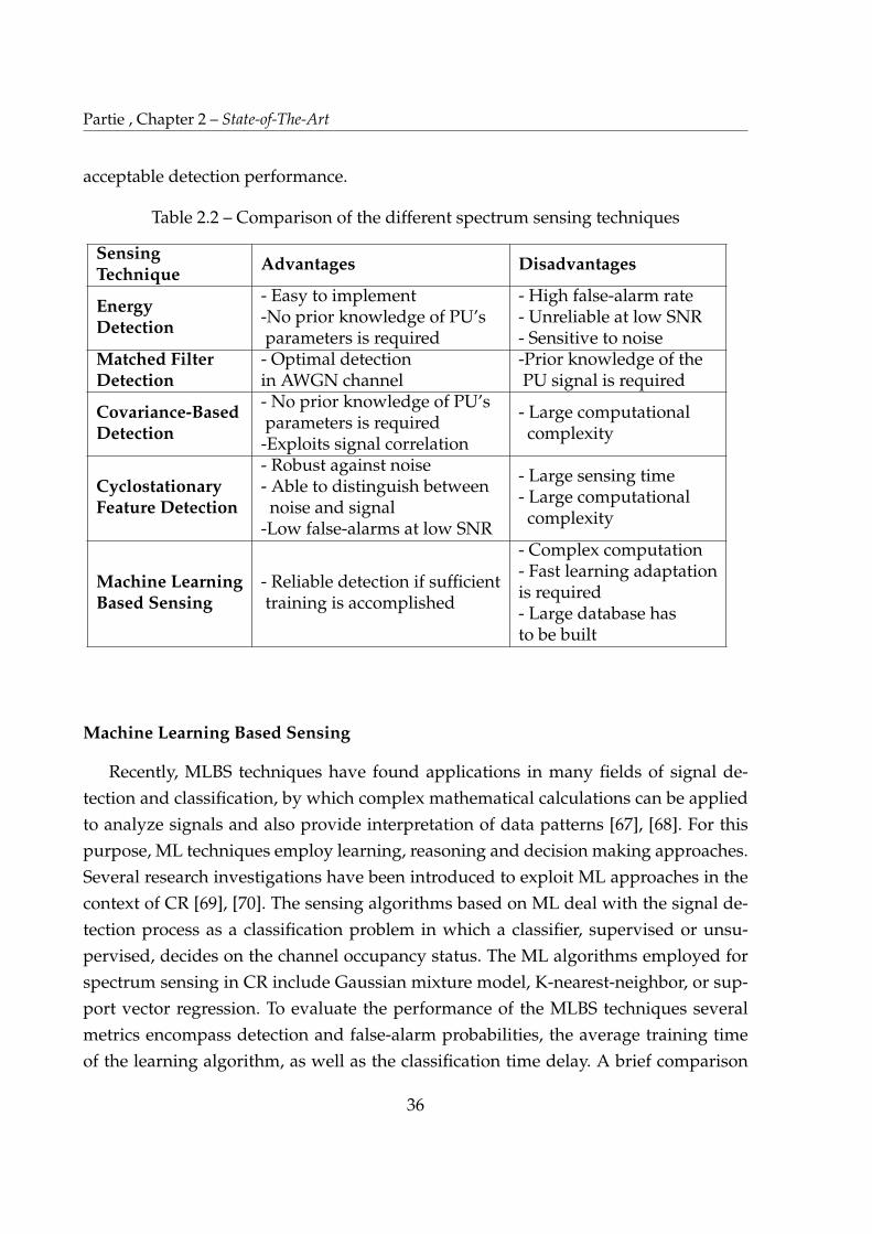
Partie , Chapter 2 – State-of-The-Art
acceptable detection performance.
Table 2.2 – Comparison of the different spectrum sensing techniques
SensingTechnique
Advantages Disadvantages
EnergyDetection
- Easy to implement-No prior knowledge of PU’sparameters is required
- High false-alarm rate- Unreliable at low SNR- Sensitive to noise
Matched FilterDetection
- Optimal detectionin AWGN channel
-Prior knowledge of thePU signal is required
Covariance-BasedDetection
- No prior knowledge of PU’sparameters is required
-Exploits signal correlation
- Large computationalcomplexity
CyclostationaryFeature Detection
- Robust against noise- Able to distinguish betweennoise and signal
-Low false-alarms at low SNR
- Large sensing time- Large computationalcomplexity
Machine LearningBased Sensing
- Reliable detection if sufficienttraining is accomplished
- Complex computation- Fast learning adaptationis required- Large database hasto be built
Machine Learning Based Sensing
Recently, MLBS techniques have found applications in many fields of signal de-
tection and classification, by which complex mathematical calculations can be applied
to analyze signals and also provide interpretation of data patterns [67], [68]. For this
purpose, ML techniques employ learning, reasoning and decision making approaches.
Several research investigations have been introduced to exploit ML approaches in the
context of CR [69], [70]. The sensing algorithms based on ML deal with the signal de-
tection process as a classification problem in which a classifier, supervised or unsu-
pervised, decides on the channel occupancy status. The ML algorithms employed for
spectrum sensing in CR include Gaussian mixture model, K-nearest-neighbor, or sup-
port vector regression. To evaluate the performance of the MLBS techniques several
metrics encompass detection and false-alarm probabilities, the average training time
of the learning algorithm, as well as the classification time delay. A brief comparison
36

2.3. Literature Review on Spectrum Sensing Techniques
between the different NBSS techniques is given in Table 2.2. Nevertheless, there are
other NBSS techniques, which involve waveform detection [71], detection based on
principal component analysis [72], and cumulative power spectral density detection
[73]. Also, the spectrum sensing for full-duplex cognitive radio systems is discussed
in [74], and the recurrence quantification analysis approach is employed for spectrum
sensing in [75].
2.3.2 WideBand Spectrum Sensing
High data rates characterize the design objectives of the next generation of commu-
nication systems, thus a larger bandwidth is required to accommodate the evolution
of the communication standards. Accordingly, the CR systems need to scan a wide
spectrum to find the best available subbands. Thus, several approaches of multiband
and WBSS techniques have been investigated in the literature [76]. In the following,
we review the most relevant WBSS techniques and also discuss their advantages and
disadvantages.
Nyquist Wideband Spectrum Sensing
Standards analog-to-digital converter are employed in the conventional WBSS tech-
niques to sample a wideband signal at the Nyquist’s rate. These techniques include the
wavelet-based detection, the multi-band detection, and the filter bank detection.
1- Wavelet-Based Detection
Different wavelet-based detection approaches have been considered for spectrum sens-
ing in CR by performing edge detection of the spectral boundaries of a wide spectrum.
This is inspired by the capabilities of the wavelet transform to characterize irregular
shapes in a signal. The general structure of the wavelet-based detector is shown in
Figure 2.17.
2- Multi-Band Joint Detection
This detection approach senses the presence or absence of a PU signal over multiple
frequency bands at once using a one of the narrowband spectrum sensing techniques.
The objective of this approach is to find an optimum threshold vector to increase the
detection probability for all bands jointly by solving an optimization problem. Figure
2.18 shows the structure of the multi-band joint detector.
37
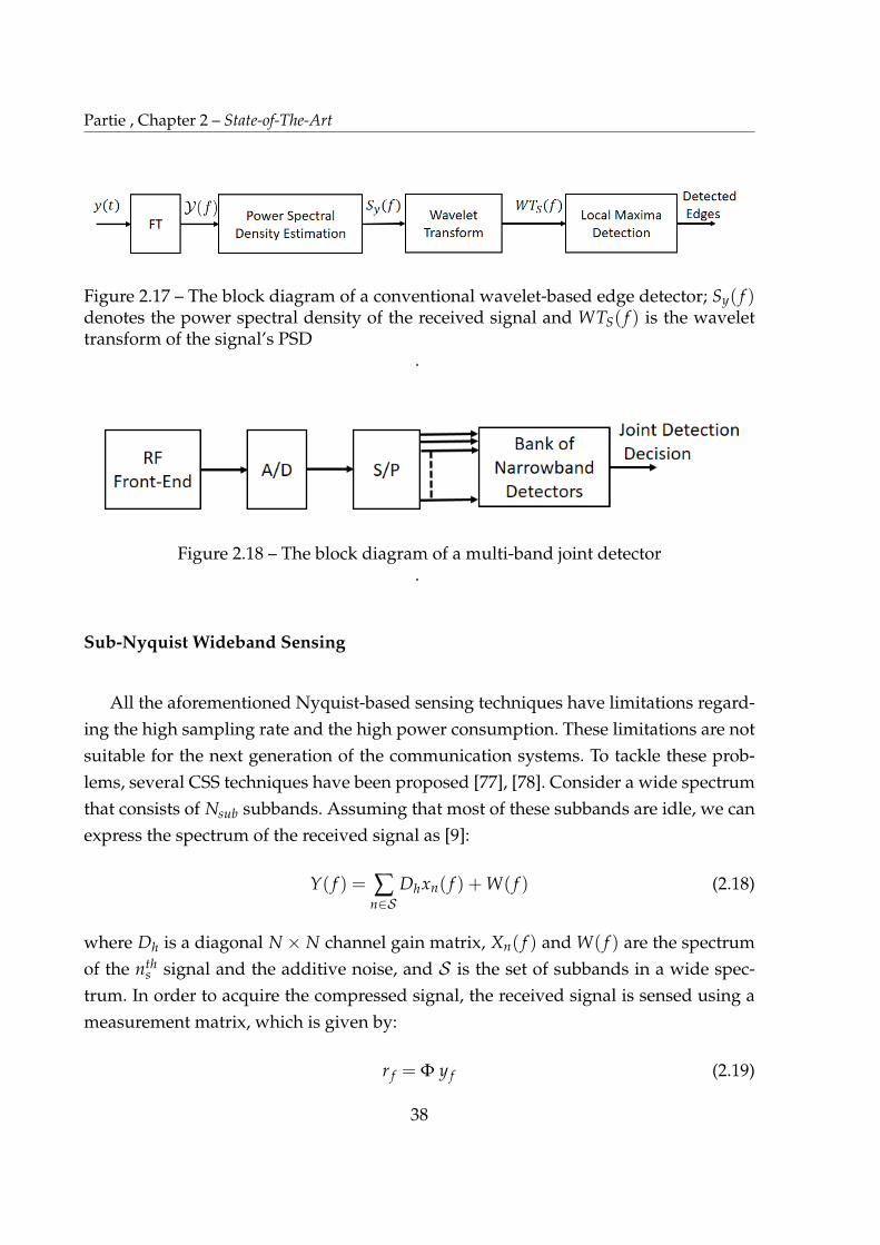
Partie , Chapter 2 – State-of-The-Art
Figure 2.17 – The block diagram of a conventional wavelet-based edge detector; Sy( f )denotes the power spectral density of the received signal and WTS( f ) is the wavelettransform of the signal’s PSD
.
Figure 2.18 – The block diagram of a multi-band joint detector.
Sub-Nyquist Wideband Sensing
All the aforementioned Nyquist-based sensing techniques have limitations regard-
ing the high sampling rate and the high power consumption. These limitations are not
suitable for the next generation of the communication systems. To tackle these prob-
lems, several CSS techniques have been proposed [77], [78]. Consider a wide spectrum
that consists of Nsub subbands. Assuming that most of these subbands are idle, we can
express the spectrum of the received signal as [9]:
Y( f ) = ∑n2S
Dhxn( f ) + W( f ) (2.18)
where Dh is a diagonal N ⇥ N channel gain matrix, Xn( f ) and W( f ) are the spectrum
of the nths signal and the additive noise, and S is the set of subbands in a wide spec-
trum. In order to acquire the compressed signal, the received signal is sensed using a
measurement matrix, which is given by:
r f = Φ y f (2.19)
38
2.4. Spectrum Sensing By Scattering Operators
where r f is the M ⇥ 1 measurement vector, M is the number of measurements which
depends on the sparsity level, Φ denotes the M ⇥ N sensing matrix, and y f is the pro-
jection of the received signal in the frequency domain. The sensing decision is obtained
after reconstructing the signal using a sparse recovery technique. By allocating the zero
and non-zero components of the signal, these location are employed to obtain the de-
tection status. The basic concept of compressive wideband spectrum sensing was first
introduced by Tian et al. in [79]. In their proposed work, the received signal is trans-
formed into a digital signal by an analog-to-information converter. Their approach
have some drawbacks such as the complexity of the computational burden as well as
the design imperfections of the converter could affect the sensing results. There are two
types of CSS: the blind and non-blind CSS techniques. Several researches concerning
both types can be found in [80].
2.4 Spectrum Sensing By Scattering Operators
The reduction of the false-alarm probability for a target detection probability is one
of the main objectives when designing a reliable spectrum sensing. Among different
spectrum sensing techniques, the Energy Detection (ED) technique is widely used due
to its implementation simplicity. However, since it cannot differentiate between useful
signals and noise, it gives a poor performance in a low SNR environment [31]. In the
following proposed work, we employ the ST, which provides a method for a hierarchal
signal representation based on deep Convolutional Networks (ConvNets), as a pre-
processing step before applying the ED technique. The multi-stage architecture of a
scattering network analyses the signal of interest into its significant features through
every stage. Our main objective is to take advantage of the sparsity provided through
the wavelet filtering,the nonlinearity and the pooling processes to detect the presence
of a signal. Due to the cascaded theme of the ConvNets, the noise effect can be revealed
and reduced at every stage.
2.4.1 Overview on Scattering Transform
Scattering transform is originally developed based on wavelet filtering to provide
an informative and a stable presentation for the classification of signals. The idea was
initially motivated by developing deep ConvNets which can describe the internal struc-
39
Partie , Chapter 2 – State-of-The-Art
ture of signals due to their hierarchal nature [81]. Following the developed work on
ConvNets by LeCun, J. Bruna and S. Mallat have suggested the use of ST via ConvNets
to find a time-invariant signal representation the is suitable for signals classification
[82]. Moreover, S. Mallat et al. have found applications of scattering networks in au-
dio and image processing as a solution for the averaging offered by the Mel-frequency
spectrogram [83].
To describe the operation of ST, which is based on the wavelet analysis, we begin
with describing the wavelet transform of a signal x0(t), which is a convolution with
a low-pass filter φ(t) of a time support T, followed by another convolution of x0(t)
with the wavelet function ψ(t)λs2Λswhich denotes a band-pass filter. With λs being
the center frequency of the filter, a dilated mother wavelet can be defined by:
ψλs(t) = λsψλs
(λst), ψλs(ω) = ψλs
(ω
λs) (2.20)
where ψλs(ω) is the Fourier transform of ψλs
(t). The wavelet transform of x0(t), de-
fined by Wx0, can be described by:
Wx0 = (x0 ⇤ φ(t), x0 ⇤ ψλs(t))t2R,λs2Λs
(2.21)
The hierarchal description of a scattering network can be described as follows [83]:
— At the root of the network, we obtain an average signal description according
to:
S0x0(t) = x0 ⇤ φ(t) (2.22)
— To gain the high frequency information, we apply the scattering operator Ux
(i.e., wavelet transform modulus operator), which is given by:
U1x0(t, λs1) = |x0 ⇤ ψλs1(t)| (2.23)
— To regain stabilization, the operator is averaged out by:
S1x0(t, λs1) = U1x0(t, λs1) ⇤ φ(t) (2.24)
S1x0(t, λs1) is defined as the first order scattering coefficients. These are com-
puted with wavelets ψλs1(t).
— Next, the output of the first order scattering operator is convolved with second
40
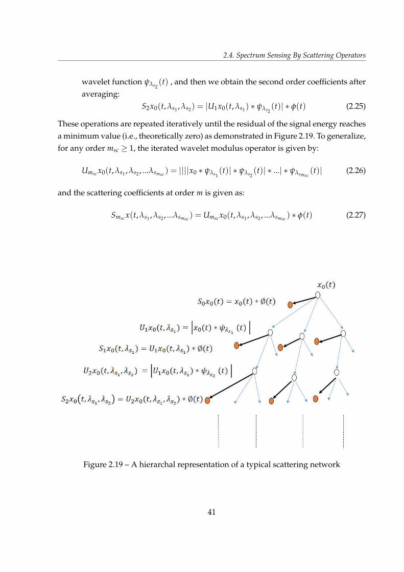
2.4. Spectrum Sensing By Scattering Operators
wavelet function ψλs2(t) , and then we obtain the second order coefficients after
averaging:
S2x0(t, λs1 , λs2) = |U1x0(t, λs1) ⇤ ψλs2(t)| ⇤ φ(t) (2.25)
These operations are repeated iteratively until the residual of the signal energy reaches
a minimum value (i.e., theoretically zero) as demonstrated in Figure 2.19. To generalize,
for any order msc � 1, the iterated wavelet modulus operator is given by:
Umsc x0(t, λs1 , λs2 , ...λsmsc) = ||||x0 ⇤ ψλs1
(t)| ⇤ ψλs2(t)| ⇤ ...| ⇤ ψλsmsc
(t)| (2.26)
and the scattering coefficients at order m is given as:
Smsc x(t, λs1 , λs2 , ...λsmsc) = Umsc x0(t, λs1 , λs2 , ...λsmsc
) ⇤ φ(t) (2.27)
Figure 2.19 – A hierarchal representation of a typical scattering network
41
Partie , Chapter 2 – State-of-The-Art
2.4.2 Reprocessing of Received Signals by The Scattering Operators
A binary hypothesis test can simply describe the received signal y(t) by [54]:
y(t) = s(t) + w(t), under H1 (2.28)
where H1 indicates the occupancy of a channel. On the other hand, when noise only
presents, y(t) becomes:
y(t) = w(t), under H0 (2.29)
where H0 indicates an idle status, w(t) is the noise imposed at the receiver input, and
s(t) the PU received signal by the SU receiver. In [82], it has been shown that the first
order scattering coefficients measures the time variation of signal amplitude within
frequency bands covered by wavelet filter banks. For further analysis, co-occurrence
coefficients reflecting the noise and the interference can be provided through deeper
decomposition. In wavelet theory, filtering with wavelets is a measure of projection of a
signal into the wavelet basis. So, by a proper choice of the wavelet function, significant
signal measurements can be obtained while reducing the noise effect. A block diagram
to demonstrate the idea of processing the received signal in the scattering domain is
shown in Figure 2.20.
Our work proposed in [84] has investigated the effects of using the ST before ap-
plying ED on detecting a DS-SS PU signal. When compared with the conventional
ED, although the results have shown that both techniques yield the same detection
performance, the simplicity of implementation and low computational burden remark
energy detectors. As an alternative approach, we exploited the average first order scat-
tering coefficients to form the detection test statistic of the Scattering Transform-based
Detection (STD). The steps of this processing before applying spectrum sensing are
summarized as follows:
— The received signal is processed for the signal decomposition. The resultant first
order scattering coefficients are used for the signal detection process.
— The first order scattering coefficients are used to form a test statistic TSTD which
is compared to a detection threshold ηSTD. The test statistic is given by:
TSTD(Y) =1Is
Is
∑is=1
yST(is) (2.30)
42

2.4. Spectrum Sensing By Scattering Operators
where yST(is) denotes the iths scattering coefficient and Is represents the number
of scattering coefficients.
— The noise variance is assumed to be known. This information can be provided
off-line through experimental measurements. If the noise is assumed to be a zero
mean AWGN with a unit variance σ2w, the processed noise through the complex
modulus wavelet decomposition and averaging result in a Rayleigh distributed
process. Since the variance of a Rayleigh process σ2r is defined by [84]:
σ2r = σ2
w.(2 � π/2) (2.31)
In this case, variance of the scattered signal under H0 is given by:
σ2ST = σ2
w.(2 � π/2)||ψλ||2 (2.32)
For sufficiently large number of scattering coefficients, the distribution of the
test statistic follows a Gaussian distribution with a variance denoted by σ2ST.
Based on the NP’s Lemma, the detection threshold is found according to equa-
tion (2.3).
Figure 2.20 – A functional block diagram of signals detection by the proposed ST-baseddetector
2.4.3 Numerical Results and Insights
In the following, we aim to evaluate the detection performance of the STD as com-
pared to the conventional ED by using the first order scattering coefficients. This eval-
uation is performed in AWGN channel. The performance evaluation is formulated in
terms of calculating the detection probability, PD, at a pre-defined false-alarm prob-
ability. The simulation parameters are summarized in Table 2.3. The simulations are
conducted for DS-SS and chirp signals. We choose to detect a DS-SS signal without
43
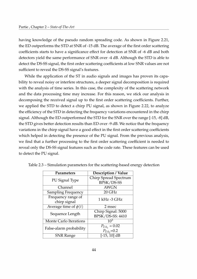
Partie , Chapter 2 – State-of-The-Art
having knowledge of the pseudo random spreading code. As shown in Figure 2.21,
the ED outperforms the STD at SNR of -15 dB. The average of the first order scattering
coefficients starts to have a significance effect for detection at SNR of -6 dB and both
detectors yield the same performance of SNR over -4 dB. Although the STD is able to
detect the DS-SS signal, the first order scattering coefficients at low SNR values are not
sufficient to reveal the DS-SS signal’s features.
While the application of the ST in audio signals and images has proven its capa-
bility to reveal noisy or interfere structures, a deeper signal decomposition is required
with the analysis of time series. In this case, the complexity of the scattering network
and the data processing time may increase. For this reason, we stick our analysis in
decomposing the received signal up to the first order scattering coefficients. Further,
we applied the STD to detect a chirp PU signal, as shown in Figure 2.22, to analyze
the efficiency of the STD in detecting the frequency variations encountered in the chirp
signal. Although the ED outperformed the STD for the SNR over the range [-15, -8] dB,
the STD gives better detection results than ED over -9 dB. We notice that the frequency
variations in the chirp signal have a good effect in the first order scattering coefficients
which helped in detecting the presence of the PU signal. From the previous analysis,
we find that a further processing to the first order scattering coefficient is needed to
reveal only the DS-SS signal features such as the code rate. These features can be used
to detect the PU signal.
Table 2.3 – Simulation parameters for the scattering-based energy detection
Parameters Description / Value
PU Signal TypeChirp Spread Spectrum
BPSK/DS-SSChannel AWGN
Sampling Frequency 20 GHzFrequency range of
chirp signal1 kHz -3 GHz
Average time of φ(t) 2 msec
Sequence LengthChirp Signal: 5000BPSK/DS-SS: 4410
Monte Carlo Iterations 103
False-alarm probabilityPFA1 = 0.02PFA2=0.2
SNR Range [-15, 10] dB
44

2.4. Spectrum Sensing By Scattering Operators
Figure 2.21 – A comparison of the detection probabilities for detecting a DS-SS signalby using the ED and the STD techniques
Figure 2.22 – A comparison of the detection probabilities for detecting a chirp signalby using the ED and the STD techniques
45

Partie , Chapter 2 – State-of-The-Art
2.5 Enhancement of Primary User Detection Through Chan-
nel Estimation
There are many challenges affecting the signal detection for the spectrum sensing
process in CR. One of these challenges is the detection of a received signal transmitted
through a multipath environment. The detection process becomes difficult and makes
it hard for an occupied band to be correctly detected. In such cases, the incumbent
users may be miss-detected, which consequently increases the sensing errors. In this
section, we present our proposed solution to mitigate this problem. We introduce the
use of a blind channel estimation technique based on the ST to acquire the required
channel state information and henceforth, apply channel equalization to remove its ef-
fect. Before illustrating the proposed technique, we give a quick overview over possible
channel impairments that affect signals detection.
2.5.1 Channel Impairments: Overview
The performance of a communication system is determined by the behavior of the
transmission medium. In wireless channels, the characterization of the channel state
variation over a short time span is a difficult task. However, this information must
be obtained to provide a reliable communication. There are different types of wireless
channels, such as: urban, suburban, indoor, and underwater. Accordingly, the trans-
mission path between the transmitter and the receiver can be altered from simple line-
of-sight to a drastically obstructed one. Hence, different propagating environments
mechanisms are used in modeling the wireless channel.
Broadly speaking, these mechanisms can be generally attributed to reflection, diffrac-
tion, and scattering. Reflections appear when the plane waves are incident upon a sur-
face with dimensions that are very large compared to the wavelength. Diffraction oc-
curs if an obstruction blocks the transmitted signal, so secondary waves are generated
behind it. As for scattering, it arises when the incident wavelength is in the order of
or larger than the dimension of the irregular-shaped blocking object. Figure 2.23 indi-
cates the different multipath propagation mechanisms [85], [86]. Due to these mecha-
nisms, the effect of the propagation medium on the transmitted signal can be described
roughly by three independent phenomena:
— Path-loss
46

2.5. Enhancement of Primary User Detection Through Channel Estimation
— Shadowing
— Multipath Fading
While path-loss is a deterministic effect that depends on the distance between the trans-
mitter and the receiver, shadowing and multipath fading have a stochastic nature.
Figure 2.23 – A demonstration of the different multipath propagation mechanisms [86]
Multipath fading leads to significant attenuation changes within small-time scales.
For generality, the attenuation due to the aforementioned channel impairments is given
by [86]:
aT(t) = aP(t) aS(t) aF(t) (2.33)
where aP(t), aS(t), aF(t) are the attenuation due to the path-loss, shadowing, and mul-
tipath fading, receptively. The fading problem caused by multipath propagation in
wireless communication is modeled by the Rayleigh distribution. The Rayleigh fading
process is characterized by its power spectral density and its autocorrelation function.
The autocorrelation function depends on the Doppler frequency which corresponds to
the relative motion of the receiver and the transmitter. The fading channel might have
a time-varying or a frequency varying attenuating impact on the transmitted signal.
Due to the time and frequency variations, we denote the complex attenuation due to
fading by |H( f , t)|, so the magnitude is given by
aF(t) = |H( f , t)| (2.34)
In multipath fading, many copies of the transmitted signal each have followed a dif-
ferent path ip which has a different length lipdepending on the propagation channel.
Because of this difference, each signal copy traveling along a path arrives with a differ-
47
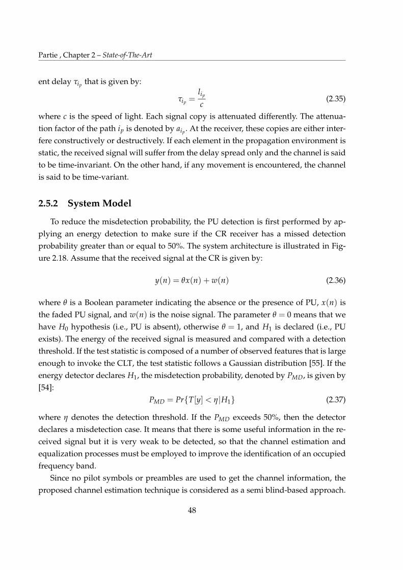
Partie , Chapter 2 – State-of-The-Art
ent delay τipthat is given by:
τip=
lip
c(2.35)
where c is the speed of light. Each signal copy is attenuated differently. The attenua-
tion factor of the path ip is denoted by aip. At the receiver, these copies are either inter-
fere constructively or destructively. If each element in the propagation environment is
static, the received signal will suffer from the delay spread only and the channel is said
to be time-invariant. On the other hand, if any movement is encountered, the channel
is said to be time-variant.
2.5.2 System Model
To reduce the misdetection probability, the PU detection is first performed by ap-
plying an energy detection to make sure if the CR receiver has a missed detection
probability greater than or equal to 50%. The system architecture is illustrated in Fig-
ure 2.18. Assume that the received signal at the CR is given by:
y(n) = θx(n) + w(n) (2.36)
where θ is a Boolean parameter indicating the absence or the presence of PU, x(n) is
the faded PU signal, and w(n) is the noise signal. The parameter θ = 0 means that we
have H0 hypothesis (i.e., PU is absent), otherwise θ = 1, and H1 is declared (i.e., PU
exists). The energy of the received signal is measured and compared with a detection
threshold. If the test statistic is composed of a number of observed features that is large
enough to invoke the CLT, the test statistic follows a Gaussian distribution [55]. If the
energy detector declares H1, the misdetection probability, denoted by PMD, is given by
[54]:
PMD = Pr{T[y] < η|H1} (2.37)
where η denotes the detection threshold. If the PMD exceeds 50%, then the detector
declares a misdetection case. It means that there is some useful information in the re-
ceived signal but it is very weak to be detected, so that the channel estimation and
equalization processes must be employed to improve the identification of an occupied
frequency band.
Since no pilot symbols or preambles are used to get the channel information, the
proposed channel estimation technique is considered as a semi blind-based approach.
48
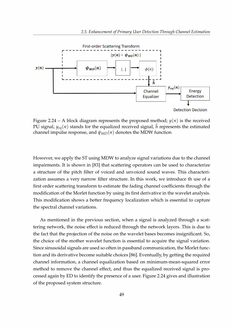
2.5. Enhancement of Primary User Detection Through Channel Estimation
Figure 2.24 – A block diagram represents the proposed method; y(n) is the receivedPU signal, yeq(n) stands for the equalized received signal, h represents the estimatedchannel impulse response, and ψMD(n) denotes the MDW function
However, we apply the ST using MDW to analyze signal variations due to the channel
impairments. It is shown in [83] that scattering operators can be used to characterize
a structure of the pitch filter of voiced and unvoiced sound waves. This characteri-
zation assumes a very narrow filter structure. In this work, we introduce th use of a
first order scattering transform to estimate the fading channel coefficients through the
modification of the Morlet function by using its first derivative in the wavelet analysis.
This modification shows a better frequency localization which is essential to capture
the spectral channel variations.
As mentioned in the previous section, when a signal is analyzed through a scat-
tering network, the noise effect is reduced through the network layers. This is due to
the fact that the projection of the noise on the wavelet bases becomes insignificant. So,
the choice of the mother wavelet function is essential to acquire the signal variation.
Since sinusoidal signals are used so often in passband communication, the Morlet func-
tion and its derivative become suitable choices [86]. Eventually, by getting the required
channel information, a channel equalization based on minimum-mean-squared error
method to remove the channel effect, and thus the equalized received signal is pro-
cessed again by ED to identify the presence of a user. Figure 2.24 gives and illustration
of the proposed system structure.
49

Partie , Chapter 2 – State-of-The-Art
2.5.3 Problem Formulation and Proposed Solution
We consider that both the PU signal and the wavelet function to be analytic signals.
Also, we assume that the multipath propagation channel is discrete, time-invariant,
and frequency selective Rayleigh fading channel. An example of such channel can be
given by the two-ray Rayleigh channel model or the three-ray Rician channel model
if a strong line-of-sight component exists. Accordingly, we can represent the general
model of the received signal in discrete-time domain as [86]:
y(n) = ∑kc
h(n;nc)s(n � nc) + w(n) (2.38)
where h(n;nc) is the discrete channel impulse response given as a function of the dis-
crete time index n = 0,1, ...N � 1, with N being the sequence length, and the time-shift
nc. The signal s(n) is the digital modulated transmitted PU signal and w(n) is the noise
samples at the CR receiver. For time-invariant, linear, and frequency-selective channel,
h(n;nc) is reduced to h(0;nc) = h(nc). It means that, although the channel behavior
does not vary with respect to time, each propagation path had different channel at-
tenuation and path delay. So, h(nc) is defined as the time-invariant impulse response
of the transmission channel to a unit impulse transmitted at time 0. To define s(n) and
h(nc), consider the passband representation of the transmitted PU signal s(n) such that
the real valued signal is expressed by:
s(n) = Ab(n)cos(2π fcn + φs(n)) (2.39)
where Ab(n) is the baseband version of the PU signal with phase of φs(n) and fc is
the carrier frequency. Since the analytic representation of signals is more appropriate
in practical signal processing, we define sa(n) as the analytic version of the signal s(n)
that is given by:
sa(n) = sar(n) + jsaI(n) (2.40)
where sar and saIare its the real and imaginary parts, respectively. The real part sar
is the original real-valued signal s(n), whereas the imaginary part saIis the Hilbert
transform of s(n). Accordingly, we can rewrite sa(n) as:
sa(n) = Ab(n)[cos(2π fcn + φs(n)) + j sin(2π fcn + φ(n))] (2.41)
50

2.5. Enhancement of Primary User Detection Through Channel Estimation
equivalently, we obtain:
sa(n) = Ab(n)exp(jφs(n))exp(j2π fcn) (2.42)
Then, we define the complex envelope of the analytic signal sa(n) by:
A(n) = Ab(n)exp(jφs(n)) (2.43)
and the time-invariant channel can be define by:
h(nc) =Nl
∑nc=1
anc δ(nc � τnc) (2.44)
where anc and τnc are the nthc path attenuation and the path delay of the propagation
channel, respectively, and Nl denotes the number of propagation paths in the trans-
mission medium. Therefore, the received signal can be expressed by:
y(n) = ∑nc
h(nc)A(n � nc)exp(j2π fc(n � nc)) + w(n) (2.45)
eventually, the received signal, y(n), is processed to extract the necessary channel in-
formation.
Channel Estimation
Let us consider the complex analytic Morlet function ψM(t) which is defined in time
domain by [87], [88]:
ψM(t) = [exp(�j2π f0t)� exp(�2π2 f 20 σ2
G)]exp(�t2
2σ2G
) (2.46)
where f0 is the sinusoidal frequency, and σG represents the spread of the Gaussian
function. The Fourier transform of ψM(t) is given by [88]:
ΨM( f ) =p
2πσG[exp(�2π2σ2G( f � f0)
2)
� exp(�2π2σ2G f 2)exp(�2π2σ2
G f 20 )]
(2.47)
51
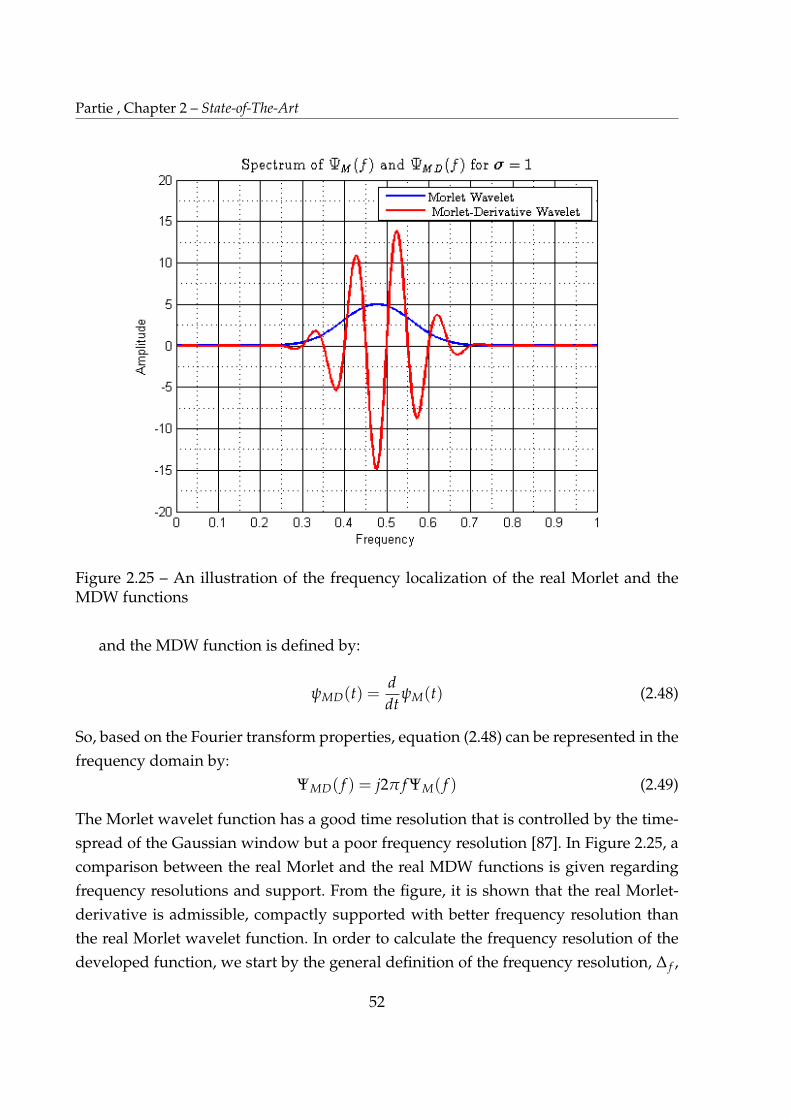
Partie , Chapter 2 – State-of-The-Art
Figure 2.25 – An illustration of the frequency localization of the real Morlet and theMDW functions
and the MDW function is defined by:
ψMD(t) =d
dtψM(t) (2.48)
So, based on the Fourier transform properties, equation (2.48) can be represented in the
frequency domain by:
ΨMD( f ) = j2π f ΨM( f ) (2.49)
The Morlet wavelet function has a good time resolution that is controlled by the time-
spread of the Gaussian window but a poor frequency resolution [87]. In Figure 2.25, a
comparison between the real Morlet and the real MDW functions is given regarding
frequency resolutions and support. From the figure, it is shown that the real Morlet-
derivative is admissible, compactly supported with better frequency resolution than
the real Morlet wavelet function. In order to calculate the frequency resolution of the
developed function, we start by the general definition of the frequency resolution, ∆ f ,
52
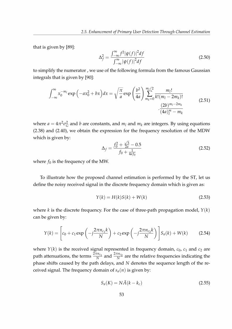
2.5. Enhancement of Primary User Detection Through Channel Estimation
that is given by [89]:
∆2f =
R ∞
�∞f 2|ψ( f )|2d f
R ∞
�∞|ψ( f )|2d f
(2.50)
to simplify the numerator , we use of the following formula from the famous Gaussian
integrals that is given by [90]:
Z ∞
�∞x�ml0 exp
⇣
�ax20 + bx
⌘
dx =
r
π
aexp
b2
4a
!
ml/2
∑mk=0
ml !k!(ml � 2mk)!
.(2b)ml�2mk
(4a)ml � mk
(2.51)
where a = 4π2σ2G and b are constants, and ml and mk are integers. By using equations
(2.38) and (2.40), we obtain the expression for the frequency resolution of the MDW
which is given by:
∆ f =f 20 +
p3
2a � 0.5
f0 +1
4a f0
(2.52)
where f0 is the frequency of the MW.
To illustrate how the proposed channel estimation is performed by the ST, let us
define the noisy received signal in the discrete frequency domain which is given as:
Y(k) = H(k)S(k) + W(k) (2.53)
where k is the discrete frequency. For the case of three-path propagation model, Y(k)
can be given by:
Y(k) =
"
c0 + c1 exp✓
�j2πnc1k
N
◆
+ c2 exp✓
�j2πnc2k
N
◆
#
Sa(k) + W(k) (2.54)
where Y(k) is the received signal represented in frequency domain, c0, c1 and c2 are
path attenuations, the terms2πnc1
N and2πnc2
N are the relative frequencies indicating the
phase shifts caused by the path delays, and N denotes the sequence length of the re-
ceived signal. The frequency domain of sa(n) is given by:
Sa(K) = NA(k � kc) (2.55)
53
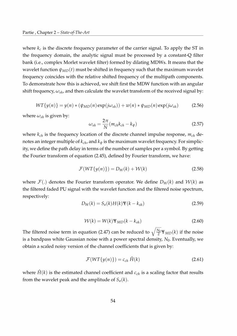
Partie , Chapter 2 – State-of-The-Art
where kc is the discrete frequency parameter of the carrier signal. To apply the ST in
the frequency domain, the analytic signal must be processed by a constant-Q filter
bank (i.e., complex Morlet wavelet filter) formed by dilating MDWs. It means that the
wavelet function ψMD(t) must be shifted in frequency such that the maximum wavelet
frequency coincides with the relative shifted frequency of the multipath components.
To demonstrate how this is achieved, we shift first the MDW function with an angular
shift frequency, ωsh, and then calculate the wavelet transform of the received signal by:
WT{y(n)} = y(n) ⇤ (ψMD(n)exp(jωsh)) + w(n) ⇤ ψMD(n)exp(jωsh) (2.56)
where ωsh is given by:
ωsh =2π
N(mchkch � kψ) (2.57)
where kch is the frequency location of the discrete channel impulse response, mch de-
notes an integer multiple of kch, and kψ is the maximum wavelet frequency. For simplic-
ity, we define the path delay in terms of the number of samples per a symbol. By getting
the Fourier transform of equation (2.45), defined by Fourier transform, we have:
F (WT{y(n)}) = DW(k) +W(k) (2.58)
where F (.) denotes the Fourier transform operator. We define DW(k) and W(k) as
the filtered faded PU signal with the wavelet function and the filtered noise spectrum,
respectively:
DW(k) = Sa(k)H(k)Ψ(k � ksh) (2.59)
W(k) = W(k)ΨMD(k � ksh) (2.60)
The filtered noise term in equation (2.47) can be reduced toq
N02 ΨMD(k) if the noise
is a bandpass white Gaussian noise with a power spectral density, N0. Eventually, we
obtain a scaled noisy version of the channel coefficients that is given by:
F (WT{y(n)}) = cch H(k) (2.61)
where H(k) is the estimated channel coefficient and cch is a scaling factor that results
from the wavelet peak and the amplitude of Sa(k).
54

2.5. Enhancement of Primary User Detection Through Channel Estimation
Channel Equalization
To reverse the effect of distortion of the transmitted signals due to channel impair-
ments, a perfect equalization process must be employed. Different types of channel
equalizers were developed in literature among which zero-forcing and the Minimum
Mean Squared Error (MMSE)-based equalizers are popular. The former is the simplest
but has the disadvantage of boosting up the noise level at the equalizer output. On the
other hand, the latter is robust against noise. In this work, we applied the MMSE-based
equalizer. In this equalization process, we need to find the transfer function GE( f ) such
that the Mean Squared Error (MSE) is minimized. The error is given by [91]:
MSE = E|GE(k)Y(k)� Sa(k)|2 (2.62)
accordingly, the required function is expressed by [91]:
GE(k) =H⇤(k)
|H(k)|2 + 1γ
(2.63)
where H⇤(k) is the conjugate of the original channel transfer function H(k) and γ is
the SNR.
2.5.4 Numerical Results and Insights
In order to evaluate the misdetection performance after applying the proposed
channel estimation method, simulations are conducted and the misdetection results
are compared with ED based on the PCA. The PCA technique has been applied as a
multi-antenna CR system, such that it yields a filtered copy of the PU signal and results
in an improved SNR [72]. Table 2.4 shows the employed simulation parameters.
First, to apply the ED technique, we need to estimate the distribution of the test
statistic through a histogram and then deduce the noise variance. In case of 5-taps and
10-taps channels, the test statistic follows the Gaussian distribution. This is shown in
Figure 2.26. To evaluate the ED-PCA as proposed in [92], the misdetection probability
is calculated in the case of 5-taps channel; This is shown in Figure 2.27.
In Figure 2.28, we find a reduction of the misdetection probability when the pro-
posed channel estimation technique is employed as compared to the ED-PCA tech-
nique. Precisely, the misdetection probability is reduced by around 44% and 30% for
55

Partie , Chapter 2 – State-of-The-Art
Table 2.4 – Simulation Setup
Parameters Description / ValuePU Signal Type BPSK
ChannelFrequency selective, time
invariant Rayleigh ChannelSampling Frequency 1 kHz
Carrier Frequeny 20 kHzSequence Length 106
NoiseCircularly Symmetric
Complex Gaussian (CSCG)No. of MonteCarlo Iterations 106
False Alarm ProbabilityPFA1 = 0.02PFA2=0.6
SNR Range -20 dB to 20 dB
Figure 2.26 – The distribution of noise and faded PU signals with a 10-taps Channel
PFA of 0.01 and 0.2, respectively, after applying the proposed channel estimation ap-
proach.
However, it is worth mentioning that as the number of channel taps increases, then
the number of wavelet filter increases as well as the complexity of the CR system. Also,
the improved performance obtained through the proposed technique depends on our
56
2.5. Enhancement of Primary User Detection Through Channel Estimation
Figure 2.27 – The misdetection probability of the PCA-based ED with a 5-taps channel
Figure 2.28 – The misdetection probability for different false-alarm values for a 5-tapschannel after employing the proposed channel estimation technique followed by theequalization process
57

Partie , Chapter 2 – State-of-The-Art
strong assumption on having a very narrowband filter which could face challenges in
the practical implementation. We deduce that the efficacy of employing the scattering
transform approach to detect time series lies in devising a method to extract the hidden
details of a target signal.
2.6 Summary
In this chapter, an overview on the basic concepts of CRs has been introduced. We
have discussed the different types of spectrum sensing techniques for the cases of nar-
rowband and wideband spectrum access. The scope of our research thesis focuses on
the non-cooperative spectrum sensing techniques. Further, our investigations on ap-
plying the scattering operators for spectrum sensing have been presented for detecting
the DS-SS and chirp PU signals. The carried out analysis has shown the capability of
the STD to detect the presence of PU signals at medium-to-high SNRs, but its detec-
tion performance deteriorates at low SNR values. This infers that more processing to
the scattering coefficients is recommended to reveal some distinguishing patterns for
detection. On the other hand, the STD performs better in detecting the chirp PU signal
which means that the detector is able to utilize the frequency variations in the chirp
signal to improve the detection process.
Moreover, we have introduced the application of the ST before ED in the frequency
domain for estimating the fading coefficients for the Rayleigh channel to reduce the
probability of misdetection. The effect of applying the proposed technique in reducing
the PMD is tested as compared to applying only the ED-PCA based technique. De-
spite the increased complexity of the proposed channel estimation technique due to
the number of filters, it reduces the chances of miss-detecting a PU signal. In accor-
dance with our investigations on the ST in CR, our aim is to provide a reliable non-
cooperative PU detector in a low SNR environment. Obviously, such detector must be
low in the computational and the implementation complexities in order to add a prac-
tical advantage in CR systems. It also needs to be able to reveal specific features that
can differentiate between different signals. These motives have established our con-
cern towards exploiting the different variants of cepstral analysis in CR for spectrum
sensing, which is discussed in chapter 3.
58
CHAPTER 3
CEPSTRAL ANALYSIS APPROACHES FOR
SPECTRUM SENSING IN COGNITIVE
RADIO
3.1 Introduction
The problem of detecting Spread Spectrum (SS) Primary User (PU) signals becomes
harder than the PU detection of classic signals. This is due to the fact that their power
is distributed over a wide frequency band, which can reduce the SNR at the Cognitive
Radio (CR) receiver. Consequently, the misdetection of a possible SS signal may cause
harmful interference to the licensed receivers. In this chapter, we propose a solution
for the misdetection problem of SS PU signals by employing Cepstral Analysis (CA)
approaches. The incitement of our choice of the CA techniques is highly motivated
by its ability to reveal some characteristics hidden in a signal in the cepstral domain.
These characteristics include induced periodicities due to delays, echoes, harmonics,
or multipath channel effects [93].
We introduce semi-blind spectrum sensing techniques based on CA approaches for
interweave CR systems. The main scope of this chapter is to mitigate the problem of
weak signal detection to allow for an interference-free spectrum sharing model. The
misdetection problem of a legitimate user occupies a desired frequency band leads to
erroneous sensing results. Based on the periodicity revealing property of some cep-
stral variants, we formulate a spectrum sensing technique based on the PassBand-
AutoCepstrum Detection (PB-ACD) approach. In section 3.2, we review the related
work to the detection of SS signals and we provide an overview on basic cepstral vari-
ants and their applications in signal detection. The system and signal models of the
carried out analysis are described in section 3.3. In section 3.4, we introduce the PB-
ACD technique to detect Direct Sequence-Spread Spectrum (DS-SS) signals in Additive
59

Partie , Chapter 3 – Cepstral Analysis Approaches for Spectrum Sensing in Cognitive Radio
White Gaussian Noise (AWGN) channels. We extend our analysis to the detection of
Frequency Hoping-Spread Spectrum (FH-SS), and Chirp-Spread Spectrum (C-SS) PU
signals. The blind theme of the proposed approach implies that no knowledge of the
spreading code employed in the SS signal is provided at the CR receiver. For the case
of the DS-SS PU signal, a mathematical formulation of the detection problem is formu-
lated. Further, the statistical distribution of the detection test statistic is derived under
the null and the alternative hypotheses based on the Neyman-Pearson Lemma (NPL)
for the case of a real-valued Gaussian noise. Also, the Receiver Operating Characteris-
tics (ROC) metrics are derived in terms of the false-alarm and detection probabilities
for the case of a Circularly Symmetric Complex Gaussian (CSCG) noise. The corre-
sponding detection threshold is analytically computed. To provide a broader analysis
of the PB-ACD technique for detecting SS signals, a mathematical formulation of the
Averaged PassBand-AutoCepstrum Detection (APB-ACD) technique is carried out for
the cases of the FH-SS and C-SS signals. Also, a theoretical analysis of the sensing-
threshold-throughput trade-off of the PB-ACD technique is presented to highlight the
impact of choosing a suitable detection threshold on the achievable throughput of the
CR system.
Since in the PB-ACD techniques the PU detection depends on monitoring the pres-
ence of a large cepstral peak at the reciprocal of the carrier frequency, this peak may
suffer from high noisy fluctuations. These spectral fluctuations may affect the detection
performance. In order to enhance the detection results, we introduce the smoothed PB-
ACD technique in section 3.5. The proposed smoothing process is performed before
employing the PB-ACD technique to reduce the fluctuations experienced in the Auto-
Correlation Estimators (ACEs) before evaluating the Power Spectral Density (PSD) of
the received signal. The smoothing process includes applying the Total Variation De-
noising (TVD) technique based on the Majorization-Minimization (MM) algorithm to
reduce the unwanted spectral fluctuations. The performance of the proposed spectrum
sensing algorithms is compared with different state-of-the-art techniques in terms of
the detection probability in section 3.6. The chapter summary is given in section 3.7.
3.2 Related Work
In the literature, there are some employed methods to detect DS-SS signals. For
example, the author of [94] has proposed a method for detecting DS-SS signals by
60

3.2. Related Work
evaluating the fluctuations of the autocorrelation estimators. The proposed method
utilizes the fact that the fluctuations of the ACEs of a significant signal and the back-
ground noise are distinguishable. Also, the authors of [95] have proposed an auto-
correlation estimation based detection methods to detect SS signals. In particular, the
detector searches for the autocorrelation peaks that may occur at integer times of the
chip duration of a pseudo-random sequence. Then, the detection decision is made by
the cumulative peak-to-average criteria. Although the proposed method in [95] has
shown a good detection performance at low SNR values, it requires the prior knowl-
edge of the chip duration.
Moreover, a robust spectrum sensing scheme based on the generalized order statis-
tics has been proposed in [96] than can be employed for detecting SS signals. The
proposed detector provides a protection against the background noise and analyzes
the false-alarm and detection probabilities under noise uncertainty. However, the de-
tection accuracy of the order statistics detector depends on increasing the size of the
analyzed samples, which may increase the processing time.
Cepstral Analysis (CA) is a logarithmic based approach for detecting signal fea-
tures. Analyzing a given signal in the cepstral domain has gained much interest in
different fields such as speech and image processing [16]. Also, we can find applica-
tions of the CA techniques in mechanical and communication applications [97]. The
cepstral signal processing concept was applied for echoes detection in seismic waves
[18]. Based on the homomorphic capabilities of cepstral analysis, it is also used to esti-
mate the frequency response of multipath fading channels. Hereinafter, we review the
basic definitions of different cepstral variants to remark their significant applications
in the filed of signal detection.
3.2.1 Overview on Cepstral Analysis
The concept of cepstrum was firstly introduced by Bogert, Healy, and Tukey to ana-
lyze time series in the logarithmic frequency domain [20]. Their investigations revealed
that the logarithmic spectrum of a signal containing echoes has an additive component
reflecting the size and the delay of the echo. Moreover, they introduced new terminolo-
gies such as: the cepstrum and the quefrency. In the literature, the cepstrum is generally
defined as the inverse Fourier transform of the logarithmic magnitude spectrum of a
signal. Cepstral analysis has been widely used in audio and image processing for its
61
Partie , Chapter 3 – Cepstral Analysis Approaches for Spectrum Sensing in Cognitive Radio
ability to reveal hidden features about signals. According to the variants of the CA
approach, a certain CA variant is chosen to fit a specific application. That is why a
researcher must be aware of the problem under analysis, and whether employing the
CA approach will unleash significant details about the signal in the logarithmic do-
main. For example, the cepstrum of a pure sinusoidal signal does not show significant
peaks, however, an echoed version added to it could show such significance. Before
describing the different cepstral variants, let us define the following variables:
— n: The discrete-time domain
— x(n): An arbitrary discrete-time domain signal
— xc(n): The analyzed complex discrete time domain signal.
— k: The discrete frequency variable
— X(k): The Fourier Transform of x(n).
— F{.}, and F�1{.}: The Fourier and inverse Fourier transform operators, respec-
tively
— n:The discrete quefrency variable, which is a measure of alternative time in the
cesptral domain
— Rx(nc): The discrete autocorrelation function of the signal x(n) at a time lag of
nc
— X0(k): The first derivative of X(k)
Generally, there exist different variants of CA terms such as:
1- Complex cepstrum: it describes the logarithmic operation applied on the
complex spectrum of a signal. Given a complex discrete-time signal xc(n),
the exact definition of the complex cepstrum is given by [98]:
cc(n) =1
2π
Z π
�πlog [Xc(ω)]exp(jωn)dω (3.1)
where log stands for the natural logarithm and Xc(ω) is the Discrete-Time
Fourier Transform (DTFT) of xc(n), which is given by:
Xc(ω) =∞
∑n=�∞
xc(n)exp(�jωn) (3.2)
where ω denotes the angular frequency (-π < ω π). Generally, the complex
62

3.2. Related Work
logarithm log [Zc] of a complex quantity Zc is defined as:
log [Zc] = log |Zc|+ j arg [Zc] (3.3)
where arg[.] denotes the argument operator. In practice, the complex cep-
strum is computed using the Discrete Fourier Transform (DFT), which is a
sampled version of of the DTFT. The signal DFT X(k) defined by [98]:
Xc(k) =Nc
∑n=0
xc(n)exp✓
�j2πkn
Nc
◆
(3.4)
where Nc is the number of data points used in evaluating the complex cep-
strum. Thus, the complex cepstrum is given by:
cc(n) =1pNc
Nc�1
∑k=0
(log|Xc(k)|+ j arg [Xc(k)])exp✓
j2πkn
Nc
◆
(3.5)
The main challenge in computing the complex cepstrum is the implementa-
tion of the complex logarithm and computation of the angle arg [Xc(k)] due
to the problem of unwrapping the phase function. The accurate implementa-
tion of the unwrapping is a practical challenge [99]. However, the invertible
advantage of the complex cepstrum makes it applicable in signals process-
ing that involves homomorphic filtering such as speech, image, or seismic
data processing.
2- Real cepstrum: due to the implementation difficulties of the complex cep-
strum, the real cepstrum is usually used in practice [98]. It defines the loga-
rithmic operation on the real spectrum of a signal. The real cepstrum is given
by [98]:
cr(n) =1pNr
Nr�1
∑k=0
log |Xc(k)|exp✓
j2πkn
Nr
◆
(3.6)
where Nr is the number of employed samples to evaluate the real cepstrum.
Since the phase is discarded in the real signals, the real cepstrum is symmet-
ric across the zero-point. In fact, the real cepstrum sequence is equivalent to
63
Partie , Chapter 3 – Cepstral Analysis Approaches for Spectrum Sensing in Cognitive Radio
the even part of the complex cepstrum [98]:
cr(n) =cc(n) + cc(�n)
2(3.7)
An added advantage of the real cepstrum over the real cepstrum is that only
the first half of the the cesptrum sequence is taken into account in calcula-
tions. For simplicity, the real cepstrum is referred as the cepstrum and cr(n)
is equivalent to c(n) for convenience.
3- Phase cepstrum: the inverse DFT of the phase of the complex logarithm de-
fines the phase cepstrum. It is given by:
cp(n) =1pNr
Nr�1
∑k=0
arg [Xc(k)]exp✓
j2πkn
Nr
◆
(3.8)
Due to the difficulties in implementation and computation, the usage of the
phase cepstrum is minimal in practical applications.
4- Power cepstrum: the basic foundation of cepstral analysis is based on the evaluation
of the Power Cepstrum (PC) as described by Bogert et al. [20]. The PC is defined as
the squared magnitude of the inverse Fourier transform of the logarithmic square
magnitude of the signal spectrum or simply the logarithmic power spectrum of a
signal [20], [100]. The expression of the power cepstrum is given by:
cpc(n) =
�
�
�
�
1Nr
Nr�1
∑k=0
log�
�X(k)�
�
2 exp✓
j2πkn
Nr
◆�
�
�
�
2
The PC finds applications in mechanical systems such as analyzing the periodic
effects caused by a vibrating machine for fault detection in a turbine blade or a
gearbox [101].
In the literature, there are other cepstral variants that include the differential cep-
strum, which is the inverse Fourier transform of the first derivative of the signal’s log-
spectrum, and the autocepstrum that is defined by the inverse Fourier transform of the
signal’s log-PSD. A summary of the different cepstral variants is given in Table 3.1.
64
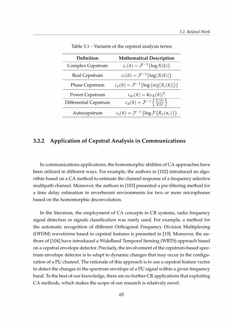
3.2. Related Work
Table 3.1 – Variants of the cepstral analysis terms
Definition Mathematical Description
Complex Cepstrum cc(n) = F�1{log X(k)}
Real Cepstrum cr(n) = F�1{log |X(k)|}
Phase Cepstrum cp(n) = F�1{log�
arg[Xc(k)]�
}
Power Cepstrum cpc(n) = 4|cR(n)|2
Differential Cepstrum cd(n) = F�1n
X0(k)X(k)
o
Autocepstrum ca(n) = F�1 {logF{Rx(nc)}}
3.2.2 Application of Cepstral Analysis in Communications
In communications applications, the homomorphic abilities of CA approaches have
been utilized in different ways. For example, the authors in [102] introduced an algo-
rithm based on a CA method to estimate the channel response of a frequency selective
multipath channel. Moreover, the authors in [103] presented a pre-filtering method for
a time delay estimation in reverberant environments for two or more microphones
based on the homomorphic deconvolution.
In the literature, the employment of CA concepts in CR systems, radio frequency
signal detection or signals classification was rarely used. For example, a method for
the automatic recognition of different Orthogonal Frequency Division Multiplexing
(OFDM) waveforms based in cepstral features is presented in [19]. Moreover, the au-
thors of [104] have introduced a WideBand Temporal Sensing (WBTS) approach based
on a cepstral envelope detector. Precisely, the involvement of the cepstrum-based spec-
trum envelope detector is to adapt to dynamic changes that may occur in the configu-
ration of a PU channel. The rationale of this approach is to use a cepstral feature vector
to detect the changes in the spectrum envelope of a PU signal within a given frequency
band. To the best of our knowledge, there are no further CR applications that exploiting
CA methods, which makes the scope of our research is relatively novel.
65
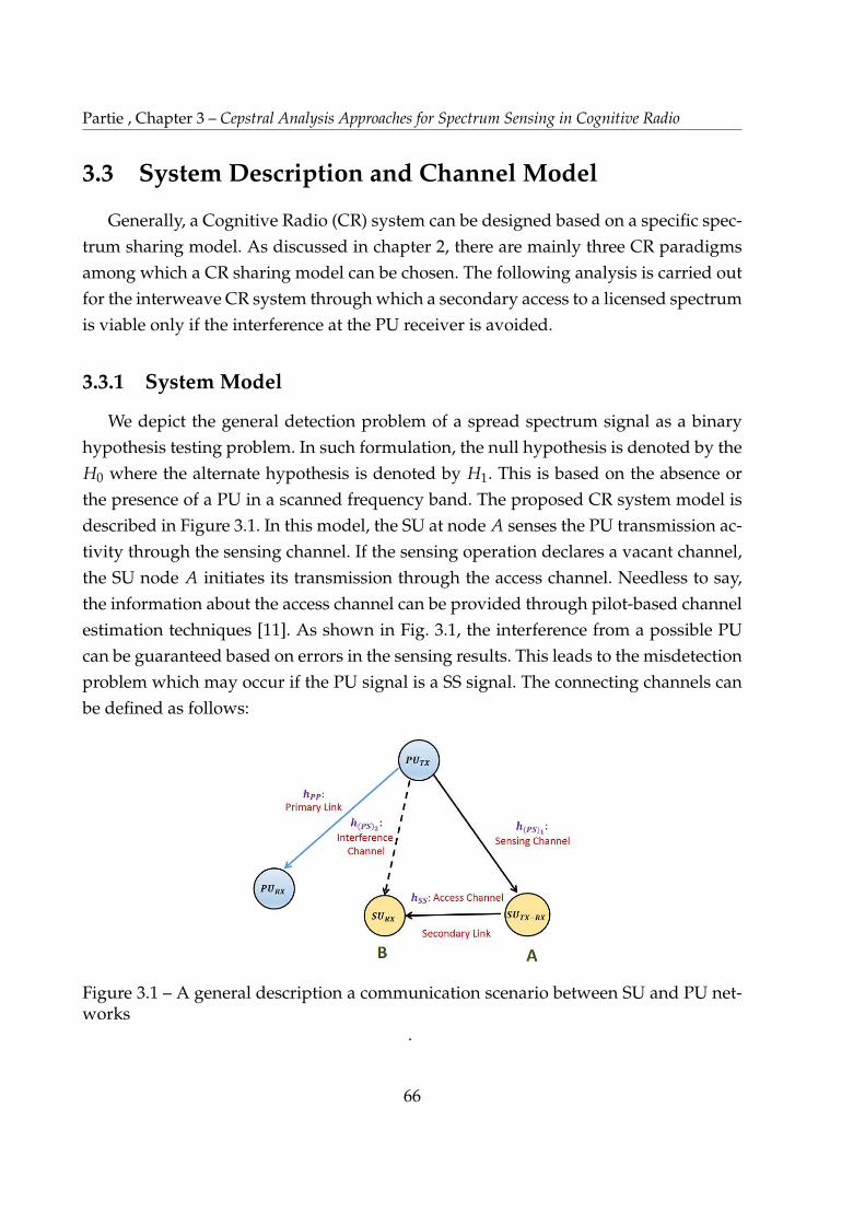
Partie , Chapter 3 – Cepstral Analysis Approaches for Spectrum Sensing in Cognitive Radio
3.3 System Description and Channel Model
Generally, a Cognitive Radio (CR) system can be designed based on a specific spec-
trum sharing model. As discussed in chapter 2, there are mainly three CR paradigms
among which a CR sharing model can be chosen. The following analysis is carried out
for the interweave CR system through which a secondary access to a licensed spectrum
is viable only if the interference at the PU receiver is avoided.
3.3.1 System Model
We depict the general detection problem of a spread spectrum signal as a binary
hypothesis testing problem. In such formulation, the null hypothesis is denoted by the
H0 where the alternate hypothesis is denoted by H1. This is based on the absence or
the presence of a PU in a scanned frequency band. The proposed CR system model is
described in Figure 3.1. In this model, the SU at node A senses the PU transmission ac-
tivity through the sensing channel. If the sensing operation declares a vacant channel,
the SU node A initiates its transmission through the access channel. Needless to say,
the information about the access channel can be provided through pilot-based channel
estimation techniques [11]. As shown in Fig. 3.1, the interference from a possible PU
can be guaranteed based on errors in the sensing results. This leads to the misdetection
problem which may occur if the PU signal is a SS signal. The connecting channels can
be defined as follows:
Figure 3.1 – A general description a communication scenario between SU and PU net-works
.
66

3.3. System Description and Channel Model
— The downlink between the PU transmitter and the detector installed at the SU
transmitter at node A, denoted by the channel h(PS)1. The received signal yA(t),
at node A, can de defined as:
yA(t) =
8
<
:
wST(t) : Under Ho
sPU(t) ⇤ h(PS)1(t;τ) + wST(t) : Under H1
(3.9)
where sPU(t) is the PU transmitted signal, ⇤ denotes the convolution product,
h(PS)1(t;τ) is the sensing channel generally described as time varying fading
channel with a delay defined by τ, and wST(t) is the thermal noise presented,
modeled as AWGN, at the detector of A.
— The uplink between SU transmitter and receiver denoted by the channel hSS.
— The downlink between the PU transmitter and the SU receiver is h(PS)2.
— The uplink between PU transmitter and receiver is h(PP). In the following, we
will refer to sPU(t) as s(t) since we are considering only the PU signal in our
analysis.
The misdetection of PU at SU receiver is evaluated as 1 � PD, where PD denotes
the detection probability. Also, the Correct-No-Detection probability, PCN, is evaluated
by 1 � PFA where PFA denotes the false-alarm probability. Accordingly, The received
signal yB(t), at node B, can be defined as:
yB(t) =
8
>
>
>
<
>
>
>
:
sPU(t) ⇤ h(PS)2(t;τ)
+sSU(t) ⇤ h(SS)(t;τ) + wSR(t) : 1 � PD
sSU(t) ⇤ h(SS)(t;τ) + wSR(t) : 1 � PFA
(3.10)
where sSU(t) stands for the SU transmitted signal, h(PS)2(t;τ) is the interference chan-
nel generally described as time-varying fading channel with delay defined by τ, and
wSR(t) is the thermal noise presented, modeled as AWGN, at the SU receiver of B.
3.3.2 Signal and Channel Model
As mentioned earlier, our focus is on detecting low-probability of intercept signals.
Specifically, we propose an algorithm to detect a DS-SS signal that is denoted by sPU(t)
defined in equation (3.9). Since we are concerned with detecting the PU signal, we
will refer to sPU(t) as s(t) for simplicity in the following analysis. In designing the
67

Partie , Chapter 3 – Cepstral Analysis Approaches for Spectrum Sensing in Cognitive Radio
algorithm, we assume all channels information is provided at the CR system so that
we are concerned with the spectrum sensing only. Accordingly, we consider the sum
of faded PU signal, which is given by:
xP(t) = s(t) ⇤ h(PS)1(t;τ) (3.11)
In order to build up the algorithm based on the autocepstrum of the received PU signal.
Let us define the signal s(t) by [105]:
s(t) = As d(t) p(t) cos(2π fct + θc) (3.12)
where s(t) is the passband representation of DS-SS, As is the carrier amplitude, d(t) is
the data signal, p(t) is the spreading waveform, fc is the carrier frequency, and θc is
the carrier signal phase at t = 0. The data modulating signal d(t) is a non-overlapping
sequence of rectangular pulses of duration Td, each of which has an amplitude of +1
or -1 if the data bit is ’1’ or ’0’, respectively. Moreover, the spreading waveform p(t) is
given by [105]:
p(t) =∞
∑i=�∞
pi P(t � iTc) (3.13)
where each pi represents one spreading pulse or chip which equals +1 or -1, and Tc is
the chip duration. The chip waveform P(t) is designed ideally to avoid inter-chip in-
terference [105]. In the following analysis, we employ the maximal-length-shift-register
sequence (i.e., m-sequence) to generate the DS-SS signal [105].
3.4 Spectrum Sensing Technique By The Autocepstrum
Approach
The autocepstrum of a time-domain signal can be defined by the inverse Fourier
transform of the natural logarithm of the signal’s PSD. The steps to calculate the auto-
cepstrum can be summarized as follows:
1- Estimate the autocorrelation of the received signal.
2- Evaluate the Fourier transform and its magnitude.
3- Compute the natural logarithm.
68
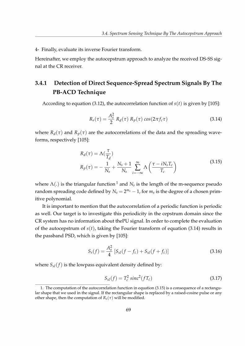
3.4. Spectrum Sensing Technique By The Autocepstrum Approach
4- Finally, evaluate its inverse Fourier transform.
Hereinafter, we employ the autocepstrum approach to analyze the received DS-SS sig-
nal at the CR receiver.
3.4.1 Detection of Direct Sequence-Spread Spectrum Signals By The
PB-ACD Technique
According to equation (3.12), the autocorrelation function of s(t) is given by [105]:
Rs(τ) =A2
s
2Rd(τ) Rp(τ) cos(2π fcτ) (3.14)
where Rd(τ) and Rp(τ) are the autocorrelations of the data and the spreading wave-
forms, respectively [105]:
Rd(τ) = Λ(τ
Td)
Rp(τ) =� 1Ns
+Ns + 1
Ns
∞
∑i=�∞
Λ
✓
τ � iNsTc
Tc
◆ (3.15)
where Λ(.) is the triangular function 1 and Ns is the length of the m-sequence pseudo
random spreading code defined by Ns = 2ms � 1, for ms is the degree of a chosen prim-
itive polynomial.
It is important to mention that the autocorrelation of a periodic function is periodic
as well. Our target is to investigate this periodicity in the cepstrum domain since the
CR system has no information about thePU signal. In order to complete the evaluation
of the autocepstrum of s(t), taking the Fourier transform of equation (3.14) results in
the passband PSD, which is given by [105]:
Ss( f ) =A2
s
4[Ssl( f � fc) + Ssl( f + fc)] (3.16)
where Ssl( f ) is the lowpass equivalent density defined by:
Ssl( f ) = T2c sinc2( f Tc) (3.17)
1. The computation of the autocorrelation function in equation (3.15) is a consequence of a rectangu-lar shape that we used in the signal. If the rectangular shape is replaced by a raised-cosine pulse or anyother shape, then the computation of Rs(τ) will be modified.
69

Partie , Chapter 3 – Cepstral Analysis Approaches for Spectrum Sensing in Cognitive Radio
To investigate the periodicity of (3.17) in the cepstrum domain, we define:
Zsl( f ) = log[Ssl( f )]
= 2 log[Tc] + 2 log[sin(πTc f )]� 2 log[πTc f ](3.18)
It is shown in equation (3.18) that the natural logarithm of the lowpass PSD of a DS-SS
signal is periodic because of the term log[sin(πTc f )] with an inclination and shift along
the y-axis due to the other terms. Moreover, referring to equation (3.16), the natural
logarithm of the passband PSD is a shift at the carrier frequency fc. By getting the
inverse Fourier transform of equation (3.17), the periodic behavior of the signal gives
spectral lines, and their peaks are employed to formulate our detection techniques.
To design a detector based on periodic features appearing in the cesptral domain,
we need to investigate different types of periodicities that may occur based on Rs(τ).
According to equation (3.15), we have three sources of possible periodicities that arise
from the data waveform, the pseudo-random spreading code, and the carrier signal. In
Figure 3.2, we illustrate the evaluation of the autocepstrum of the AWGN, the spread-
ing waveform, and the baseband and passband versions of the DS-SS signal. In fact,
Figure 3.2 shows the autocepstrum analysis of each autocorrelation term appearing in
equation (3.15). Also, Figure 3.3 shows a comparison of evaluating the cepstrum and
the autocepstrum of a DS-SS signal. Consequently, we observe the following proper-
ties:
— The autocepstrum of the pseudo-random spreading code has few peaks repeat-
ing at multiple of Ns Tc. This resembles the autoceptsrum peaks of the AWGN,
that has a peak at zero quefrency at almost zero elsewhere.
— The autocepstrum of the baseband s(t) gives spectral lines at integer multiples
of Td with one major peak and Td and other negative peaks.
— The passband version of s(t) gives spectral lines in the autocepstrum occurring
at integer multiple of the carrier period Tcarr =1fc
with one major peak at Tcarr
and the rest are negatives.
— The cepstrum of the DS-SS shown in Figure 3.3 shows no significant peaks along
the quefrency values.
The result in Figure 3.3 is due to the fact that a peak occurring in the cepstral domain
reflects harmonics that are multiple of periodicities in the spectrum. In other words,
the cepstrum of a pure sinusoidal signal does not show significant peaks, however, an
echoed version added to it could show such significance.
70
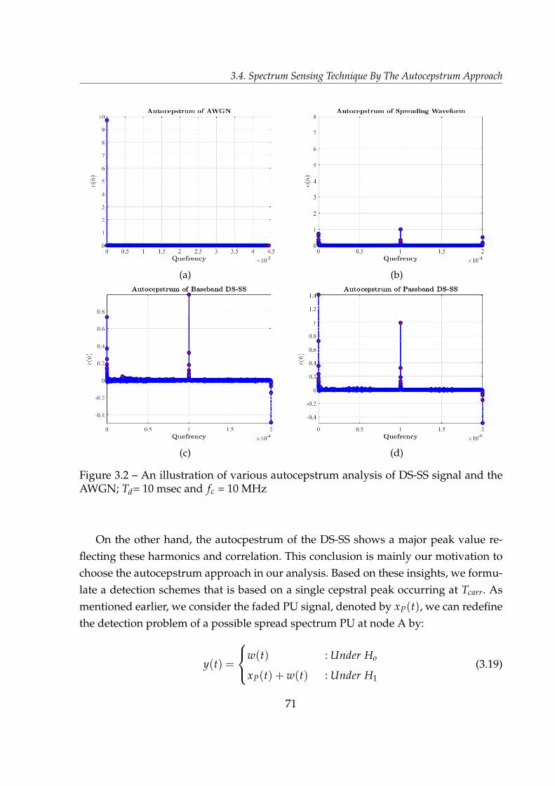
3.4. Spectrum Sensing Technique By The Autocepstrum Approach
(a) (b)
(c) (d)
Figure 3.2 – An illustration of various autocepstrum analysis of DS-SS signal and theAWGN; Td= 10 msec and fc = 10 MHz
On the other hand, the autocpestrum of the DS-SS shows a major peak value re-
flecting these harmonics and correlation. This conclusion is mainly our motivation to
choose the autocepstrum approach in our analysis. Based on these insights, we formu-
late a detection schemes that is based on a single cepstral peak occurring at Tcarr. As
mentioned earlier, we consider the faded PU signal, denoted by xP(t), we can redefine
the detection problem of a possible spread spectrum PU at node A by:
y(t) =
8
<
:
w(t) : Under Ho
xP(t) + w(t) : Under H1
(3.19)
71
Partie , Chapter 3 – Cepstral Analysis Approaches for Spectrum Sensing in Cognitive Radio
Figure 3.3 – Comparing the cepstrum and the autocepstrum of a DS-SS signal.
The proposed detection approach is based on the distinguished features illustrated
in Figure 3.3. In other words, by applying the autocepstrum approach under the null
hypothesis, we obtain approximately only one peak at the zero quefrency. Thus, the
significance of this approach to mitigate the misdetection problem due to the unde-
fined nature of a PU signal is measurable in terms of the occurrence of spectral line
peaks at non-zero quefrencies.
Proposed Detectors Based on The Autocepstrum Approach
The proposed PB-ACD scheme is formulated based on the detection of a single cep-
stral peak occurring at Tcarr. According to the fact that the autocepstrum of the AWGN
is zero for all nonzero quefrencies values, the detection problem can be formulated as:
8
<
:
H0 : |ca(n)||n=Ncarr = 0
H1 : |ca(n)||n=Ncarr 6= 0(3.20)
72
3.4. Spectrum Sensing Technique By The Autocepstrum Approach
where Ncarr is the number of samples corresponding to Tcarr. To apply the proposed
spectrum sensing algorithm, we have to estimate the autocorrelation of the received
signal, evaluate the PSD, and get the inverse Fourier transform of its natural logarithm.
To evaluate the detection results, we employ the detection test statistic given by:
T1[ca] = |ca(n)||n=Ncarr
H1?H0
η1 (3.21)
where the detection threshold η1 can be evaluated based on the choice of a specific
communication scenario,taking into consideration the transmission paths.
Another way to formulate the autocepstrum detector is to picture the detection
problem as detecting a random peak value [54]. A reasonable approach might be to
average the autocesptrum of the received samples and use this averaged value as a
test statistic, T 0[ca], and compare it to a detection threshold, η0. In this case, the test
statistic of the autocepstrum detector becomes:
T 0[ca] =1
Np
Np
∑i=1
|ca(i)|H1?H0
η0 (3.22)
where Np denotes the number of the autocepstral peaks. In order not to confuse the
reader, in our study we refer by the autocepstrum detector to all the types of detectors
that are based on calculating the autocepstrum of the received signal. These detectors
include the PB-ACD technique and also the Averaged PassBand-AutoCepstrum Detec-
tion (APB-ACD) technique which will be discussed in subsection 3.4.2. It is important
to mention that in the case of the DS-SS signal T1 and T 0 are the same, since we are
considering only one autocepstral peak. Throughput our analysis, we find it more con-
venient to employ T 0 for detecting Frequency Hopping and Chirp spread spectrum
techniques, which will be discussed in subsection 3.4.2.
Distribution of Log-Chi-Squared Random Variable
In order to derive the statistics of the proposed detector based on the NPL, we first
discuss the statistics of the log-Chi-squared distribution. Let A be a random variable
with the Gaussian distribution of zero mean and unit variance denoted by N (0,1). If
X = A2, then X is said to follow the Chi-squared distribution denoted by χ2ν. If Z =
log X, and by employing one-to-one transformation, we obtain an expression for the
73
Partie , Chapter 3 – Cepstral Analysis Approaches for Spectrum Sensing in Cognitive Radio
Log-Chi-squared distribution with one degree of freedom, log�χ21, as follows:
fZ(z) =1p2π
q
exp (z) exp✓
�exp (z)
2
◆
, z > 0 (3.23)
we can make use of the cumulant generating function to find the first and second mo-
ments [64]. The cumulant generating function is given by:
K(m) = log�
E[exp (z)m]�
= log ( E[Xm]) (3.24)
where m is an integer, E[Xm] is the mth moment of X and the moment generating
function of the random variable X is defined by MX(t) = E[exp(tX)] [106]. Thus, the
moment generating function of χ21 distribution is given by [107]:
µm =2m Γ(1
2 + m)
Γ(12)
(3.25)
where Γ(.) is the upper incomplete gamma function 2. By applying equation (3.24) into
equation (3.23), we get:
K(m) = m log(2) + log
Γ
✓
12+ m
◆�
� log
Γ
✓
12
◆�
(3.26)
Thus, we can compute the required moments by applying the following formula relat-
ing cumulants and moments [107]:
µm = Km +m�1
∑i=1
✓
m � 1i � 1
◆
Ki µi�m (3.27)
where Km is the cumulant of order m obtained through the derivative of the CGF eval-
uated at the required moment order. Hence, we obtain the first and second cumulants
by:
K1 = log 2 + ψd
✓
12
◆
,K2 = ψ(1)p
✓
12
◆
(3.28)
2. For complex numbers with a positive real part, the gamma function is defined by the integral:Γ(z0) =
R ∞
0 xz0�10 exp(�x0), R > 0. For any positive integer m, the gamma function is represented by
Γ(m) = (m � 1)!.
74
3.4. Spectrum Sensing Technique By The Autocepstrum Approach
where ψd(.) is the digamma function 3, which can be defined using Stirling’s approxi-
mation for x > 0 by [108]:
ψd(x) =Γ0(x)
Γ(x)⇡ log(x) +
12x
(3.29)
and the first derivative of ψd(.) is called the polygamma function which is denoted by
ψ(1)p (x) [108]. Definition of the polygamma function can be given as:
ψ(1)p (x) ⇡ 1
x� 1
2x2 (3.30)
We deduce from equations (3.22) and (3.25) that the mean of the log�χ21 is the first
cumulant such that:
E[Z] = µZ = k1 (3.31)
Similarly, by employing equation (3.25), we can evaluate the second moment E[Z2(k)]
as well as the variance σ2Z, where k denotes the corresponding discrete frequency pa-
rameter in the cepstral domain.
For the log�χ2ν with ν degrees of freedom, the derived Probability Density Function
(PDF) derived in equation (3.23), can be expressed by:
fZ(z) =1
2ν2 Γ�
ν2
� [exp (z)]ν/2 exp✓
�exp (z)
2
◆
, z > 0 (3.32)
where Γ(.) denotes the upper incomplete gamma function 4. To find the first moment, µZ,
we compute the ensemble average of the log�χ2ν PDF by:
E[Z] =Z x0
0
z
2ν2 Γ�
ν2
� [exp (z)]ν/2 exp✓
�exp (z)
2
◆
dz , 0 < x0 < ∞ (3.33)
If we substitute R = exp(z) and employ the integration by parts method, we obtain:
E[Z] = log (exp(x0))ΓL
�
ν2 , 1�
Γ�
ν2
�
1
2ν2� 1
2
�
(3.34)
3. The digamma function is a special function which is given by the logarithmic derivative of thegamma function.
4. For a positive integer s, the upper incomplete gamma function is generally expressed by:Γ(s, x0) =R ∞
x0ts�1 exp(�t)dt .
75

Partie , Chapter 3 – Cepstral Analysis Approaches for Spectrum Sensing in Cognitive Radio
where ΓL(., .) denotes the lower incomplete gamma function 5.
Similarly, we obtain the second moment of Z by:
E[Z2] =
"
ΓL
�
ν2 , exp(x0)
�
2ν2 Γ�
ν2
�
#
h
(log [exp(x0)])2 � 2 log (exp(x0))
i
(3.35)
To simplify the expressions obtained in equations (3.34) and (3.35), we express the ra-
tional function ΓL(.,.)Γ(.) by the P(., .) which represents the regularized gamma function 6.
Thus, the first moment can be simplified to:
E[Z] = log (exp(x0)) P
⇣ν
2,1⌘
1
2ν2� 1
2
�
(3.36)
also, the second moment of Z can be reduced to:
E[Z2] = P
⇣ν
2,1⌘ h
(log [exp(x0)])2 � 2 log (exp(x0))
i
(3.37)
Consequently, to evaluate σ2Z = E[Z2] � (E[Z])2, we can use the obtained results in
equations (3.36) and (3.37). Further, the detailed derivation of the log�χ2ν distribution
and the corresponding false-alarm probability of an autocepstrum detector are given
in Appendix A.
Derivation of The Receiver Operating Characteristic for The Case of Central log�χ2ν
Real-Valued Signals
Generally, we can define the autocepstrum of a signal in the discrete quefrency
domain by:
ca(n) =1pN
N�1
∑k=0
Z(k) exp
j2πkn
N
!
(3.38)
where N is the sequence length and Z(k) is the natural logarithm of the signal’s PSD.
Since the distribution of the noise at the CR receiver is assumed to be Gaussian, the PSD
of the noise follows a Chi-squared distribution with one degree of freedom. Hence,
the distribution of the natural logarithm of the noise PSD follows log�χ2ν distribu-
5. The lower incomplete gamma function is given by: ΓL(s, x0) =R x0
0 ts�1 exp(�t)dt .6. P(s, x0) represents the regularized gamma function which is the cumulative distribution function
for the Gamma random variables with the shape parameter s .
76

3.4. Spectrum Sensing Technique By The Autocepstrum Approach
tion. Being a unitary transform, the inverse Fourier transform defined in equation
(3.38) maintains the same distribution for the autocepstrum coefficient ca(n). More-
over, since the set of coefficients of {ca(n)} is a sum of rotated IID log�χ2ν random
variable Z(k)exp⇣
j2πknN
⌘
, the distribution of this sum can be analyzed according to
two assumptions:
1. If N is sufficiently large: in this case, we can invoke the CLT. Hence, the test
statistic is assumed to follow Gaussian distribution [54]. Based on the test statis-
tic defined in equation (3.22), we find that T 0[ca] follows normal distribution,
N (µc0 , σ2c0), where σ2
c0denotes the variance of the autocepstrum coefficients un-
der H0. In this case, we must obtain the right-tail probability of the proposed test
statistic under H0 for a fixed value of PFA. This is generally can be expressed by
[54]:
PFA =Z
{Ca :T 0>η0}fCa
(ca; H0) dr = αFA (3.39)
where η0 is the detection threshold, αFA is the PFA value, and fCa(ca; H0) is the
probability density function of a random process Ca under H0. In particular, the
false-alarm probability, for µc0 = 0, is given by:
PFA = Q
0
@
η0q
σ2c0N
1
A (3.40)
where Q(.) denotes the Gaussian Q-function 7. Similarly, T 0[ca] under H1 follows
normal distribution, N (µc1 , σ2c1), where σ2
c1denotes the variance of the autocep-
strum coefficients under H1. Thus, the detection probability can be expressed by
[54]:
PD = Q
0
@
η0 � µc1q
σc1N
1
A (3.41)
Thus, the detection threshold can be expressed by:
η0 =
s
σ2c0
NQ�1(PFA) (3.42)
7. The Q-function represents the tail distribution function of the normal distribution and µc0 is the
mean of the test statistic under H0. It is given by: Q(x) = 1p2π
R ∞
x exp⇣
� u2
2
⌘
du.
77
Partie , Chapter 3 – Cepstral Analysis Approaches for Spectrum Sensing in Cognitive Radio
To obtain an expression for the proposed detection threshold, η1, we have to eval-
uate µ and σ. The mean of ca(n) is found from equation (3.31) by:
E[ca(n)] =1pN
N�1
∑k=0
E[Z(k)] exp
j2πkn
N
!
(3.43)
where E[Z(k)] is denoted by µZ. The term ∑N�1k=0
exp⇣
j2πknNr
⌘
yields the following:
N�1
∑k=0
exp
j2πkn
Nr
!
=
8
<
:
N : i f n = 01�(�1)n
1�exp(jπnNr): elsewhere
(3.44)
However, for large value of Nr, this sum yields approximately zero for n 6= 0.
Hence, this leads to:
E[ca(n)|n=0] = µca = µZ
pN (3.45)
Then, the variance is found by:
Var[c(n)] = E[c2a(n)]� µ
2ca
(3.46)
thus, we need to find the second moment of ca(n) to get the variance. The second
moment is given by:
E[c2a(n)] =
1N
E
"
N�1
∑k=0
Z(k) exp
j2πkn
N
!!2#
=1N ∑
k,k0E
h
Z(k)Z(k0)i
exp
j2π(k + k0)nN
! (3.47)
for different values of k and k0, and assuming Z(k) and Z(k0) are uncorrelated,
we get:
E[c2a(n)] =
8
>
>
>
<
>
>
>
:
1N σ2
z : k, k0 = 01N E
h
Z2(k)i
∑N�1k=0
exp⇣
j4πknN
⌘
: k = k0 6= 0
0 : k 6= k0
(3.48)
where σ2Z =Var[Z(k)]. Since the proposed detection scheme is based on the choice
78
3.4. Spectrum Sensing Technique By The Autocepstrum Approach
of the autocesptral coefficients for n 6= 0, and from equation (3.48), the exponential
sum yields zero at n 6= 0 as well, then we finally get:
Var[ca(n)] ⇡1N
σ2Z (3.49)
Basically, each pair of (PD, PFA) identifies the ROC curve which represents the
reliability of a specific detector by describing. This pair is associated with a par-
ticular threshold to make the sensing decision at a specific Signal-to-Noise (SNR)
value. As the threshold value increases, the PFA and PD decrease. A reliable de-
tection decision can be remarked if the ROC curve is above the 45� line [54]. A 45�
ROC curve can be attained if the detector decision ignores all the processed data
and bases its decision on flipping a coin. Based on the CLT assumption men-
tioned, we employed the obtained results in equations (3.40) and (3.41) to plot
the ROC curves of the proposed autocepstrum detector and compare them with
the conventional energy detector. Figure 3.4 shows the simulated and theoretical
ROC curve for the case of detecting real valued IID Gaussian signals at -5 dB. We
started by employing a few number of samples (i.e., N = 10) to show the effect
of increasing the sequence length on the detection performance. The simulation
were carried on 10000 Monte Carlo iterations. We also compared the ROC metrics
of the autocepstrum detector with the ED technique for N = 100 at SNR of 0 dB
and -5 dB as shown in Figure 3.5. We notice that with a few samples at SNR of
-5 dB the proposed technique outperforms the ED technique as shown in Figure
3.6. In particular, for 100 samples, the proposed technique is superior to the ED
technique at -5 dB.
Although the detection performance of an energy detector increases as the signal
size increases, the noise suppression effect through the calculation of the auto-
cepstrum of the received signal makes the performance of the proposed detector
better than the ED technique as illustrated in Figure 3.7. We also note that as the
number of samples increases (N=1000), both techniques behaves similarly.
2. If N represents a few number of samples: this is a situation where the number of
communication paths is limited. Thus, the autocepstral coefficients ca(n) follows
log�χ21. Hence, the right-tail probability of log�χ2
1 distribution is obtained by:
PFA =Z ∞
η1
1p2π
q
exp (z) exp✓
�exp (z)
2
◆
dz (3.50)
79

Partie , Chapter 3 – Cepstral Analysis Approaches for Spectrum Sensing in Cognitive Radio
Figure 3.4 – The simulated and theoretical ROC curves of the PB-ACD technique
The integral in equation (3.50) can be simplified by methods of substitution.
If we define x0 = exp(z) and the noise variance is given by σ2w, it yields:
PFA =Z ∞
exp(η1)
σwp2πx0
exp⇣
�x0σw
2
⌘
dx0 (3.51)
then, if we let u =q
x0σ2w
2 , we obtain:
PFA =2pπ
Z ∞
σ2wp2
pexp(η1)
exp(�u2) du (3.52)
hence, the integral in equation (3.52) can be expressed by:
PFA = 2 Q
✓
σwp2
q
exp(η1)
◆
(3.53)
The detection threshold for a fixed value of PFA and unit noise variance is found
80
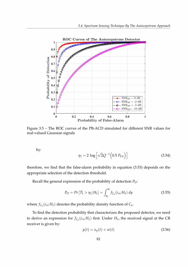
3.4. Spectrum Sensing Technique By The Autocepstrum Approach
Figure 3.5 – The ROC curves of the PB-ACD simulated for different SNR values forreal-valued Gaussian signals
by:
η1 = 2 loghp
2Q�1⇣
0.5 PFA
⌘i
(3.54)
therefore, we find that the false-alarm probability in equation (3.53) depends on the
appropriate selection of the detection threshold.
Recall the general expression of the probability of detection PD:
PD = Pr [T1 > η1|H1] =Z ∞
η1
fCa(ca; H1) dy (3.55)
where fCa(ca; H1) denotes the probability density function of Ca.
To find the detection probability that characterizes the proposed detector, we need
to derive an expression for fCa(ca; H1) first. Under H1, the received signal at the CR
receiver is given by:
y(t) = xp(t) + w(t) (3.56)
81
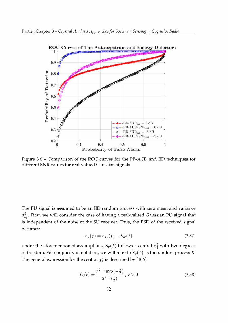
Partie , Chapter 3 – Cepstral Analysis Approaches for Spectrum Sensing in Cognitive Radio
Figure 3.6 – Comparison of the ROC curves for the PB-ACD and ED techniques fordifferent SNR values for real-valued Gaussian signals
The PU signal is assumed to be an IID random process with zero mean and variance
σ2xp
. First, we will consider the case of having a real-valued Gaussian PU signal that
is independent of the noise at the SU receiver. Thus, the PSD of the received signal
becomes:
Sy( f ) = Sxp( f ) + Sw( f ) (3.57)
under the aforementioned assumptions, Sy( f ) follows a central χ22 with two degrees
of freedom. For simplicity in notation, we will refer to Sy( f ) as the random process R.
The general expression for the central χ2ν is described by [106]:
fR(r) =r
ν2�1 exp(� r
2)
2ν2 Γ( ν
2 ), r > 0 (3.58)
82

3.4. Spectrum Sensing Technique By The Autocepstrum Approach
Figure 3.7 – Comparison of the ROC curves for the PB-ACD and ED techniques simu-lated for different signal sizes at -5 dB for real-valued Gaussian signals
where ν denotes the number of degrees of freedom, and Γ(.) is the upper incomplete gamma
function, which is expressed by:
Γ(m) = (m � 1)! (3.59)
defined for any positive integer m. For ν = 2, equation (3.58) becomes:
fR(r) =exp(� r
2)
2, r > 0 (3.60)
which reduces to an Exponential distribution with the decay rate of 2. If Z = log[R],
then the test statistic under H1 follows log�exponential distribution. The cumulative
distribution function of R is described by:
FR(r) =Z r
0fR(r)dr = 1 � exp
⇣
� r
2
⌘
(3.61)
83
Partie , Chapter 3 – Cepstral Analysis Approaches for Spectrum Sensing in Cognitive Radio
then the cumulative distribution function of Z is given by:
FZ(z) =Pr [Z z]
=Pr [logr z] = Pr [r exp(z)]
=1 � exp✓
�exp(z)2
◆
(3.62)
then, by differentiating equation (3.62) we obtain:
fZ(z) =d
dzFZ(z) =
12
exp✓
�exp(z)2
◆
exp(z), z > 1 (3.63)
To find the detection probability, we solve the given integral:
PD =12
Z ∞
η1
exp✓
�exp(z)2
◆
exp(z) dz (3.64)
by using the method of substitution, and by letting x0 = exp(z), PD is obtained as:
PD = exp✓
�σ2x
2exp(η1)
◆
(3.65)
where σ2x denotes the variance of the signal xp(t). By substituting η1 from equation
(3.65) into PFA found in equation (3.53) and for σ2s = 1, the mathematical relation joining
PFA and PD is given by:
PFA = Q⇣
jp
2log PD
⌘
(3.66)
Since the Gaussian Q-function is usually defined for real non-negative arguments, ex-
pressions involving the Q-function are usually applicable only for a limited range of
values of the physical parameters involved [109]. Therefore, the extension of the Q-
function to the complex plane results in more powerful representations that are inde-
pendent on the physical parameters. The equivalent to the complex Q-function is the
complex complementary error function which is used more often in detection prob-
lems that involves complex arguments [109], [110]. Given in terms of the Faddeeva
84
3.4. Spectrum Sensing Technique By The Autocepstrum Approach
function 8[109], the complex complementary error function is given by:
er f c(jz) = w(z)exp(z2) (3.67)
where w(z) is the Faddeeva function which is given in terms of the Fresnel integral
[109]. Since Q(z) = 0.5 er f c⇣
zp2
⌘
where er f c(.) is the complementary error function 9.
The false-alarm probability, defined in equation (3.66), can be expressed by:
PFA = 0.5 er f c⇣
jp
2log PD
⌘
(3.68)
Derivation of The Receiver Operating Characteristic for The Case of Non-Central
log�χ2ν Real-Valued Signals
Under H0, the distribution of Sy( f ), denoted by R for simplicity, for real Gaussian
noise with mean µw is the non-central χ21. The non-centrality parameter is given by:
λ =k
∑i
µ2i (3.69)
thus, the non-central χ21 of one degree of freedom is given by [106]:
fR(r) = χ2(1, λ) =r�1/2 exp(� r+λ
2 )p2 Γ(1
2)
"
exp(�p
rλ) + exp(p
rλ)
2
#
(3.70)
Similarly, the distribution of the test static in this case for Z = log[R] is described by:
fZ(z) =1p2π
exp⇣ z
2
⌘
exp✓
�exp(z) + λ
2
◆
"
exp(�p
exp(zλ)) + exp(p
exp(zλ))
2
#
(3.71)
8. The Faddeeva function, or Kramp function, is a scaled complex complementary error functionwhich is related to the Fresnel integral, to Dawson’s integral, and to the Voigt function. It arises invarious physical problems in describing electromagnetic response in complicated media. It is given by
the integral: w(z) = exp(�z2)⇣
1 + j 2pπ
R z0 exp(t2)dt
⌘
.
9. The complementary error function is given by er f c(x) = 2pπ
R ∞
x exp (�t2)dt
85

Partie , Chapter 3 – Cepstral Analysis Approaches for Spectrum Sensing in Cognitive Radio
hence, the false-alarm probability is obtained by:
PFA =Z ∞
ηfZ(z)dz
= C
Z ∞
exp(η)x�1/2
0 exp(�x0(12+ λ)) dx0 +
Z ∞
exp(η)x�1/2
0 exp(x0(�12
+ λ)) dx0
�
(3.72)
where C =exp(�λ/2)p
2 πand x0 = exp(z). The two integrals given by equation (3.72) can
be solved using integration by methods of substitution. Let II and II I denote the two
integrals representing PFA such that:
II =Z ∞
exp(η)x�1/2
0 exp(�a x0) dx0
II I =Z ∞
exp(η)x�1/2
0 exp(b x0) dx0
(3.73)
where a = λ + 12 and b = λ � 1
2 . To solve for II , let u =p
a x0, hence:
II =2p
aZ ∞
pa exp(η1)
exp(�u2)du =p
aπ er f c(q
a exp(η1))
=
s
✓
λ +12
◆
π er f c
s
✓
λ +12
◆
exp(η1)
! (3.74)
Likewise, by employing the imaginary error function that is given by [110]:
er f i(z) =2pπ
Z z
0exp(t2)dt (3.75)
the second integral, II I , is obtained as:
II I =p
bπ
✓
1 � er f i(q
a exp(η1))
◆
=
s
✓
λ � 12
◆
π
1 � er f i(
s
✓
λ � 12
◆
exp(η1)
! (3.76)
86

3.4. Spectrum Sensing Technique By The Autocepstrum Approach
thus, by combining the two integrals we get:
PFA =exp(�λ/2)p
2
"s
✓
λ +12
◆
π er f c
r
(λ +12) exp(η1)
!
+
s
✓
λ � 12
◆
π
1 � er f i(
s
✓
λ � 12
◆
exp(η1)
!#(3.77)
Based on equation (3.77), the false-alarm probability is a function of the non-centrality
parameter and the detection threshold.
Under H1, the distribution of Sr( f ) follows a non-central χ22 of two degrees of free-
dom with λ = ∑2i=1 µ2
i , which is given by:
fR(r) =12
exp(�r + λ
2) I0(
pλr) (3.78)
where I0 denotes the modified Bessel function of the first kind. Consequently, the dis-
tribution of Z is given by the Rice density function:
fZ(z) =12
exp(� exp(z) + λ
2) I0(
q
λexp(z))exp(z) (3.79)
In order to find PD, let us define x0 =p
exp(z) and d2 = λ, hence we need to solve the
following integral such that:
PD =Z ∞
pexp(η1)
x0 I0(dx0)exp
�x20 + d2
2
!
dx0 (3.80)
Recall the expression of the Marcum Q-function QM(.), which is given by [111]:
QM(a, b) =Z ∞
bx0
hx0
a
iM�1exp
"
�x20 + d2
2
#
IM�1(bx0)dx0 (3.81)
where M denotes the order of the QM. By comparing the integral in equation (3.79) to
equation (3.80), PD can be expressed by:
PD = Q1(p
λ,q
exp(η1)) (3.82)
The Marcum Q-function is a monotonic and log-concave function which is a general-
87

Partie , Chapter 3 – Cepstral Analysis Approaches for Spectrum Sensing in Cognitive Radio
ized form of the Gaussian Q-function. One possible approximation of equation (3.81)
is given for a large value of η1 using the asymptotic form of the zero-order modified
Bessel function of the first kind [111]. This approximation comes in the form of:
Q1(a, b) =
r
b
aQ(b � a) (3.83)
by applying equation (3.83) to equation (3.82), we obtain:
Qh
exp⇣η1
2
⌘
� λ1/2i
= PDλ1/4
exp(η1/4)(3.84)
The Chernoff bound of the Gaussian Q-function is given by [112]:
Q(x) exp(�x2
2) , x > 0 (3.85)
by employing Equation (3.85) in equation (3.84) we obtain:
hη1
2� exp
⇣η1
2
⌘i
= 2logh
PDλ1/4i
�p
λ (3.86)
By referring to the left-hand side of equation (3.86) as the ηlog, equation (3.86) can be
rewritten as:
ηlog = 2logh
PDλ1/4i
�p
λ (3.87)
which is a function of the detection threshold as well as the non-centrality parameter
λ.
Derivation of The Receiver Operating Characteristic for The Case of Circularly Sym-
metric Complex Gaussian Signals
Generally, if a random variable is said to be a Circularly Symmetric Complex Gaus-
sian (CSCG), its real and imaginary parts are independent and have equal variance.
Basically, if y(t) = w(t) under H0, and the noise is said to be CSCG signal, thus |W( f )|
follows Rayleigh distribution. Therefore, the distribution of Sy( f ) = Sw( f ) is given by
the Exponential distribution [107]:
fR(r) =1
αEexp(
�r
αE) , αE > 0, r > 0 (3.88)
88
3.4. Spectrum Sensing Technique By The Autocepstrum Approach
where αE is the scale parameter of the distribution. Then, the distribution of the log
PSD of the received noise is given in terms of the log-Exponential distribution by:
fZ(z) =1
αEexp
✓
�exp(z)αE
+ z
◆
, αE > 0, z > 1 (3.89)
the false-alarm probability is given by:
PFA =Z ∞
η1
fZ(z)dz = exp(� η
αE) (3.90)
Under H1, the received signal’s PSD Sy( f ) = Sx p( f ) + Sw( f ) indicates a sum of
squares of two Rayleigh distributed signals that are independent to each other. Equiv-
alently, we have Sx p( f ) and Sw( f ) follows Exponential distribution. Their joint CDF is
given by:
FR(r) = 1 � exp(� r
αE)� r
αEexp(� r
αE) (3.91)
By differentiating the CDF, we obtain:
fR(r) =r
α2E
exp✓
r
αE
◆
(3.92)
where fR(r) is the log�Erlang(mE, αE) distribution 10 which is a special case of the
Gamma distribution [107] and mE is the number of random variables. The difference
between the Erlang and the Gamma distribution is that in the Gamma distribution mE
can be non-integer [107]. Consequently, the statistical distribution that describes the
characteristics of the test statistic under H1 is given by:
fZ(z) =r
α2E
exp(2z) exp✓
exp(z)αE
◆
(3.93)
which represents the log�Erlang(mE, αE) distribution for m = 2. Thus the detection
probability is described by:
PD = exp✓
�exp(η1)
αE
◆
"
exp(η1)
αE+
1α2
E
#
(3.94)
10. The Erlang distribution with the shape parameter, mE 2 N, and the scale parameter, αE > 0, cor-responds to a sum of mE independent exponential distributions with the exponential rate αE.
89
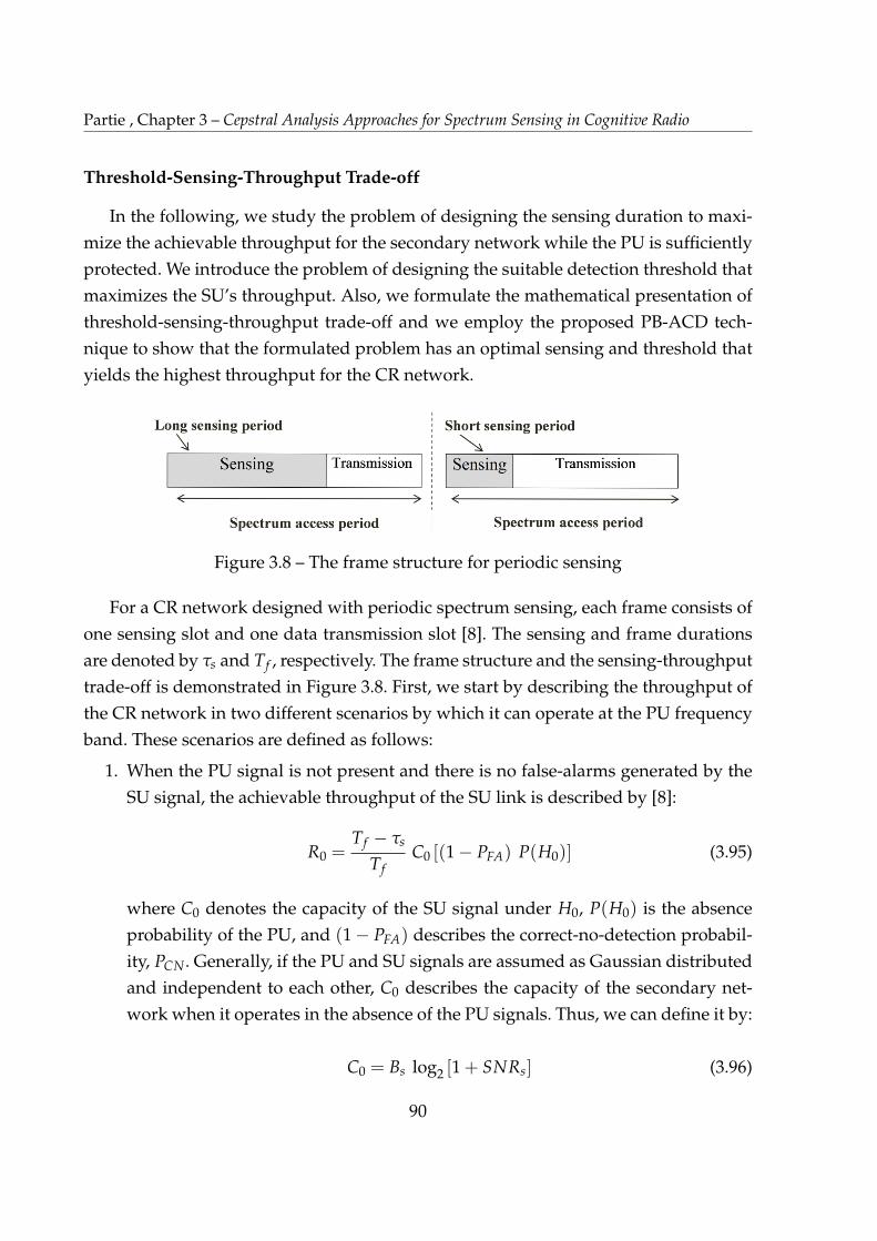
Partie , Chapter 3 – Cepstral Analysis Approaches for Spectrum Sensing in Cognitive Radio
Threshold-Sensing-Throughput Trade-off
In the following, we study the problem of designing the sensing duration to maxi-
mize the achievable throughput for the secondary network while the PU is sufficiently
protected. We introduce the problem of designing the suitable detection threshold that
maximizes the SU’s throughput. Also, we formulate the mathematical presentation of
threshold-sensing-throughput trade-off and we employ the proposed PB-ACD tech-
nique to show that the formulated problem has an optimal sensing and threshold that
yields the highest throughput for the CR network.
Figure 3.8 – The frame structure for periodic sensing
For a CR network designed with periodic spectrum sensing, each frame consists of
one sensing slot and one data transmission slot [8]. The sensing and frame durations
are denoted by τs and Tf , respectively. The frame structure and the sensing-throughput
trade-off is demonstrated in Figure 3.8. First, we start by describing the throughput of
the CR network in two different scenarios by which it can operate at the PU frequency
band. These scenarios are defined as follows:
1. When the PU signal is not present and there is no false-alarms generated by the
SU signal, the achievable throughput of the SU link is described by [8]:
R0 =Tf � τs
TfC0 [(1 � PFA) P(H0)] (3.95)
where C0 denotes the capacity of the SU signal under H0, P(H0) is the absence
probability of the PU, and (1 � PFA) describes the correct-no-detection probabil-
ity, PCN. Generally, if the PU and SU signals are assumed as Gaussian distributed
and independent to each other, C0 describes the capacity of the secondary net-
work when it operates in the absence of the PU signals. Thus, we can define it by:
C0 = Bs log2 [1 + SNRs] (3.96)
90
3.4. Spectrum Sensing Technique By The Autocepstrum Approach
where Bs is the bandwidth of the SU signal, SNRs =PsPw
denotes the SNR of the
secondary link assuming point-to-point transmission in the secondary network,
Ps is the received power of the SU signal and Pw is the noise power.
2. When the PU is active but miss-detected by the CR receiver, then the achievable
SU throughput is given by:
R1 =Tf � τs
TfC1 [(1 � PD) P(H1)] (3.97)
where C1 is the capacity of the SU signal under H1, P(H1) is the active probability
of the PU, and (1 � PD) refers to the misdetection probability PMD. The capacity
of the SU under H1 is given by:
C1 = Bs log2
1 +SNRs
SNRp + 1
�
(3.98)
where SNRs =PsPw
denotes the SNR of the primary link and Pp is the interference
power measured at the CR receiver.
Thus, the average throughput for the secondary network is given by:
Ravg(τs, η1) = R0(τs, η1) + R1(τs, η1) (3.99)
Since C0 > C1, the equation (3.99) can be approximated by:
Ravg(τs, η1) ⇡ R0(τs, η1) (3.100)
From the literature, the sensing-throughput trade-off is formulated as an optimization
problem which is stated as:
maxτs
Ravg(τs, η1) = R0(τs, η1)
s.t PD � PD
(3.101)
where PD denotes the target detection probability which is set to be close but not equal
to 1 in order to allow the protection of the PU while the SU is allowed to access the
frequency band when it is idle. For this reason, the activity probability of the PU is con-
sidered small such that it is economically advisable to explore the SU for the intended
91
Partie , Chapter 3 – Cepstral Analysis Approaches for Spectrum Sensing in Cognitive Radio
frequency band. An example of the achievable SU’s throughput for ED based on equa-
tion (3.99) is shown in Figure 3.8 where Ravg(τs, η1) denotes the average throughput.
When the PB-ACD technique is applied while choosing PD = PD, we employ the ex-
pressions of PFA and PD derived in equations (3.90) and (3.84) for the case of CSCG
signal and noise in equation (3.100). By differentiating equation (3.100) with respect to
τs, it can be verified that:
R0avg
C0 P(H0)= � 1
Tf+
1Tf
exp✓
� η1
αE
◆
(3.102)
where R0avg denotes the first derivative of the approximated average throughput of the
SU network. By using the fact that the function exp⇣
� η1αE
⌘
is upper bounded by 0 for
large values of η1, thus:
limτ!Tf
R0avg < C0 P(H0)
� 1Tf
+1Tf
exp✓
� η1
αE
◆
!
< 0 (3.103)
also,
limτs!0
R0avg = +∞ (3.104)
From equations (3.103) and (3.104), we note that there is a maximum point of Ravg
within the frame interval Tf . Moreover, by differentiating equation (3.100) with respect
to η1, we find that:
R0avg
C0 P(H0)= αE exp
✓
� η1
αE
◆
� αEτ
Tfexp
✓
� η1
αE
◆
(3.105)
thus, we obtain:
limη1!+∞
R0avg < C0 P(H0)
✓
1 � 1τs
◆
exp✓
� η1
αE
◆
< 0 (3.106)
also,
limη1!0
R0avg = αE C0 P(H0)
✓
1 � 1τs
◆
(3.107)
We find that as η1 increases, PFA decreases hence the throughput increases. Thus, there
is a unique point of η1 at which the maximum throughput of the SU link is achieved
at certain sensing interval τs. For the case of the PB-ACD detector, the achievable SU’s
92
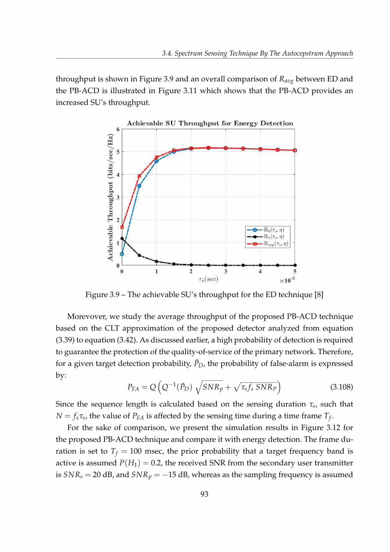
3.4. Spectrum Sensing Technique By The Autocepstrum Approach
throughput is shown in Figure 3.9 and an overall comparison of Ravg between ED and
the PB-ACD is illustrated in Figure 3.11 which shows that the PB-ACD provides an
increased SU’s throughput.
Figure 3.9 – The achievable SU’s throughput for the ED technique [8]
Morevover, we study the average throughput of the proposed PB-ACD technique
based on the CLT approximation of the proposed detector analyzed from equation
(3.39) to equation (3.42). As discussed earlier, a high probability of detection is required
to guarantee the protection of the quality-of-service of the primary network. Therefore,
for a given target detection probability, PD, the probability of false-alarm is expressed
by:
PFA = Q⇣
Q�1(PD)q
SNRp +p
τs fs SNRP
⌘
(3.108)
Since the sequence length is calculated based on the sensing duration τs, such that
N = fsτs, the value of PFA is affected by the sensing time during a time frame Tf .
For the sake of comparison, we present the simulation results in Figure 3.12 for
the proposed PB-ACD technique and compare it with energy detection. The frame du-
ration is set to Tf = 100 msec, the prior probability that a target frequency band is
active is assumed P(H1) = 0.2, the received SNR from the secondary user transmitter
is SNRs = 20 dB, and SNRp =�15 dB, whereas as the sampling frequency is assumed
93

Partie , Chapter 3 – Cepstral Analysis Approaches for Spectrum Sensing in Cognitive Radio
Figure 3.10 – SU’s achievable throughput for the PB-ACD technique
Figure 3.11 – A comparison of the achievable SU’s throughput between the ED and thePB-ACD techniques
94

3.4. Spectrum Sensing Technique By The Autocepstrum Approach
to be 6 MHz. The target probability is set to 90%, whereas the sensing time is ranging
from 0 to 5 msec. As shown in Figure 3.12, the achievable throughput of the proposed
sensing technique is higher compared to the respective throughput to the conventional
energy detector. Analytically, we see that the probability of false-alarm given in equa-
tion (3.108) is lower than that of the energy detection technique, such that [8]:
PFAED= Q
⇣
Q�1(PD)q
2 SNRp + 1 +p
τs fs SNRp
⌘
(3.109)
Thus, by referring to equation (3.95), the term 1 � PFA, which represents the probabil-
ity of correct no detection, increases for the proposed PB-ACD technique that conse-
quently increases the average throughput of the SU. One can clearly see that the av-
erage achievable throughput of the proposed PB-ACD technique is much higher than
energy detection for short sensing durations. As the sensing time increases, both tech-
niques achieve the same throughput at τs =Tf
2 . As the sensing time increases within
the frame duration, the average throughput decreases.
Figure 3.12 – A comparison of the achievable SU’s throughput between the ED and thePB-ACD techniques based on the CLT assumption
95

Partie , Chapter 3 – Cepstral Analysis Approaches for Spectrum Sensing in Cognitive Radio
3.4.2 Application of The PB-ACD Technique to Detecting Frequency-
Hopping and Chirp Spread Spectrum Signals
The increased dimensionality of the signals by SS techniques has the goal of making
eavesdropping and/or jamming more difficult. In particular, if there are more dimen-
sions in the signal to consider, its probability-of-intercept will be low. In the SS tech-
niques, the main method of increasing the dimensionality of the signals is to increase
their spectral occupancy. In section 3.4, we started to discuss the impact of applying the
PB-ACD technique for detecting DS-SS signals. In the following, we broaden our in-
vestigations on the capability of the CA approaches to detect other SS techniques such
as, FH-SS and C-SS. We introduce the APB-ACD technique which exploits the average
of the autocepstral peaks inherited in the FH-SS and C-SS signals.
Detection of FH-SS Signals by The APB-ACD Technique
In FH-SS, the carrier frequency of the sinusoidal signal modulated by the data is
changed periodically over a predetermined bandwidth. This is achieved by hopping
the center frequency of the carrier signal among Nsub contiguous but non-overlapping
frequency bands in a pseudo random manner. In this case, the overall spectrum oc-
cupancy is increased by the factor Nsub. Mathematically, the hopping signal can be
represented by [113]:
hhop(t) =∞
∑i=�∞
p(t � iTc) cos(2π fit + φi) (3.110)
where p(t) denotes the pulse shape used for the hopping waveform which is typically
represented as a square pulse. Also, fi 2 { f1, f2, . . . fNsub} are the Nsub hop frequencies,
and φhiare the phases of each oscillator. The Frequency-Hopped (FH) transmitted sig-
nal is given by [113]:
sFH = [sd(t) hhop(t)]BPF (3.111)
where sd(t) is the bandpass data signal that depends on the employed modulation
scheme, and the bandpass filter, applied to the quantity within [.]BPF, is designed to
transmit the sum frequencies part of the signal. The FH signal occupies a separate
frequency band that is determined by the hopping sequence as the time advances.
Thus, the PSD of the transmitted signal is seems to spread on the average over the
96
3.4. Spectrum Sensing Technique By The Autocepstrum Approach
entire band. If each frequency band is utilized 1Nsub
of the time, the overall spectrum
will be similar to that seen in DS-SS systems when averaged over a sufficiently long
time period [113].
Normally, the reception of a FH-SS signal can be accomplished through coherent
detection in which the despread signal y(t) is obtained by multiplying the incoming
signal and filtering out the images or by non-coherent detection. In the coherent detec-
tion, the knowledge of the hopping pattern is required. For the interweave CR system,
the identification of the PU signal is not a main task for spectrum sensing, however,
only detecting the signal presence is the target. Thus, without knowing the hopping
pattern, detection of a possible PU FH-SS signal becomes a challenge. Our objective is
to utilize the periodicity inherited in the FH-SSsignal in the cepstral domain to detect
its presence. The PSD of a FH-SS signal can be expressed by [113]:
SFH( f ) = Sd( f ) ⇤ Hhop( f ) (3.112)
where Sd( f ) is the PSD of the data signal before hopping and Hhop( f ) denotes the PSD
of the hopping waveform. As an example, let us consider the PSD when BPSK with
coherent frequency hopping is used. From previous developments, the passband PSD
of the BPSK is given by [36]:
Sd( f ) =AsTb
4[sinc2(Tb( f � fc)) + sinc2(Tb( f + fc))] (3.113)
Assuming that all the hop frequencies are equally likely and the frequency spacing
between the hop frequencies to be an integer multiple of the hop rate, then Hhop( f )
can be expressed by [113]:
Hhop( f ) ⇡ 1N2
sub
Nsub
∑i=1
[δ( f � fi) + δ( f + fi)]
+Tc
Nsub
✓
1 � 1Nsub
◆Nsub
∑i=1
[sinc2(Tb( f � fi)) + sinc2(Tb( f + fi))]
(3.114)
By applying equation (3.111), the PSD of the transmitted FH-SS signal is given by [113]:
SFH( f ) =PTb
2Nsub
Nsub
∑i=1
[sinc2(Tb( f � fi � fc)) + sinc2(Tb( f + fi + fc))] (3.115)
97
Partie , Chapter 3 – Cepstral Analysis Approaches for Spectrum Sensing in Cognitive Radio
where the constant P = A2s Tc2 . Referring to Equation (3.105), the PSD of the FH-SS signal
is the sum of Nsub replicas of the PSD of the information signal each located at certain
hopping frequency. If i = 1 and fi + fc = f0, equation (3.115) can be rewritten as:
SFHi=1( f ) =PTb
2Nsub
h
sinc2(Tb( f � f0)) + sinc2(Tb( f + f0))i
(3.116)
We find that the result obtained in equation (3.116) is similar to the analysis car-
ried on in equations (3.16) and (3.17). Consequently, we find that for k = 1, the natu-
ral logarithm of SFH( f ) experiences periodicities since the natural logarithm of sinc(.)
function gives negative periodicity. Since the spectrum of a FH-SS signal includes Nsub
terms each located at different f0, thus the inverse Fourier transform of SFH( f ) will
include not only one major autocepstral peak like the case of the DS-SS signal. In this
case, the detection of a FH-SS PU signal can be formulated based on averaging these
autocepstral peaks.
In Figure 3.13, we give an example of a SFH-SS signal. The SFH-SS scheme is char-
acterized by having one or multiple symbols transmitted per hop. It is used to reduce
the effects of radio signal fading and to minimize the effects of interference from radio
channels that are operating on the same radio frequency. In the given example in Fig-
ure 3.13, we employ 4-ary Frequency Shift Keying (4-FSK) modulation where the FSK
frequency tones are f1 = 2 MHz, and f2 = 8 MHz. The length of the data sequence is
10000 samples and the pseudo-number sequence generator consists of 4 flip-flops. The
length of the PN segment per hop is 3 such that every segment corresponds to a specific
hoping carrier frequency among 8 possible values. Since we assume that a carrier hops
to a new frequency after transmitting two FSK symbols or equivalently, 4 information
bits. The considered data rate is 1 Mbps and the range of the scanned bandwidth is
over about [10,34] MHz. The spectrum of the 8 subcarriers is shown in Figure 3.14 and
the PSD of the frequency-hopped signal is shown in Figure 3.15. By computing the au-
tocepstrum of given SFH-SS/FSK signal, the autocepstral coefficients are manifested
as significant peaks as shown in Figure 3.16. These peaks reflect the presence of the
subcarrier signals in the analyzed signal.
By averaging the autocepstral peaks we can identify the presence of FH-SS signal
in a target frequency band. In particular, the proposed technique for detecting FH-SS
signals is designed to combine the autocepstral peaks to formulate the APB-ACD tech-
nique. By combing these peaks which occur at integer multiple of 1fi+ fc
, the detection
98

3.4. Spectrum Sensing Technique By The Autocepstrum Approach
test statistic can be expressed as:
T2[ca] =1
Np
Np
∑i=1
[|ca(i)|]H1?H0
η2 (3.117)
where Np denotes the number of autocepstral peaks and η2 denotes the detection
threshold. To find an expression for the detection threshold, we need to find the suit-
able statistical distribution of T2[ca]. Obviously, the statistical distribution of the detec-
tor test statistic is influenced by Np and the distribution of ca(i). Under H0 and in the
case of real-valued AWGN signal, Sy( f ) follows a Chi-squared distribution.
Figure 3.13 – An example of a SFH-SS/FSK signal
99
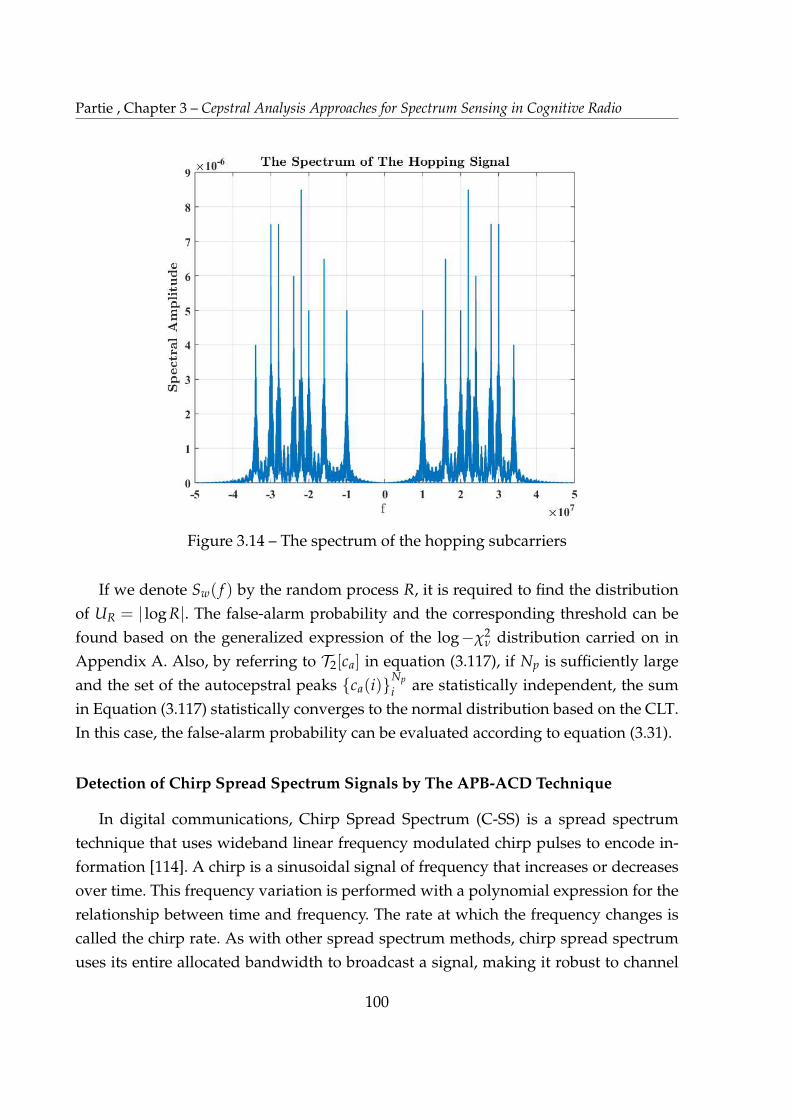
Partie , Chapter 3 – Cepstral Analysis Approaches for Spectrum Sensing in Cognitive Radio
Figure 3.14 – The spectrum of the hopping subcarriers
If we denote Sw( f ) by the random process R, it is required to find the distribution
of UR = | log R|. The false-alarm probability and the corresponding threshold can be
found based on the generalized expression of the log�χ2ν distribution carried on in
Appendix A. Also, by referring to T2[ca] in equation (3.117), if Np is sufficiently large
and the set of the autocepstral peaks {ca(i)}Np
i are statistically independent, the sum
in Equation (3.117) statistically converges to the normal distribution based on the CLT.
In this case, the false-alarm probability can be evaluated according to equation (3.31).
Detection of Chirp Spread Spectrum Signals by The APB-ACD Technique
In digital communications, Chirp Spread Spectrum (C-SS) is a spread spectrum
technique that uses wideband linear frequency modulated chirp pulses to encode in-
formation [114]. A chirp is a sinusoidal signal of frequency that increases or decreases
over time. This frequency variation is performed with a polynomial expression for the
relationship between time and frequency. The rate at which the frequency changes is
called the chirp rate. As with other spread spectrum methods, chirp spread spectrum
uses its entire allocated bandwidth to broadcast a signal, making it robust to channel
100
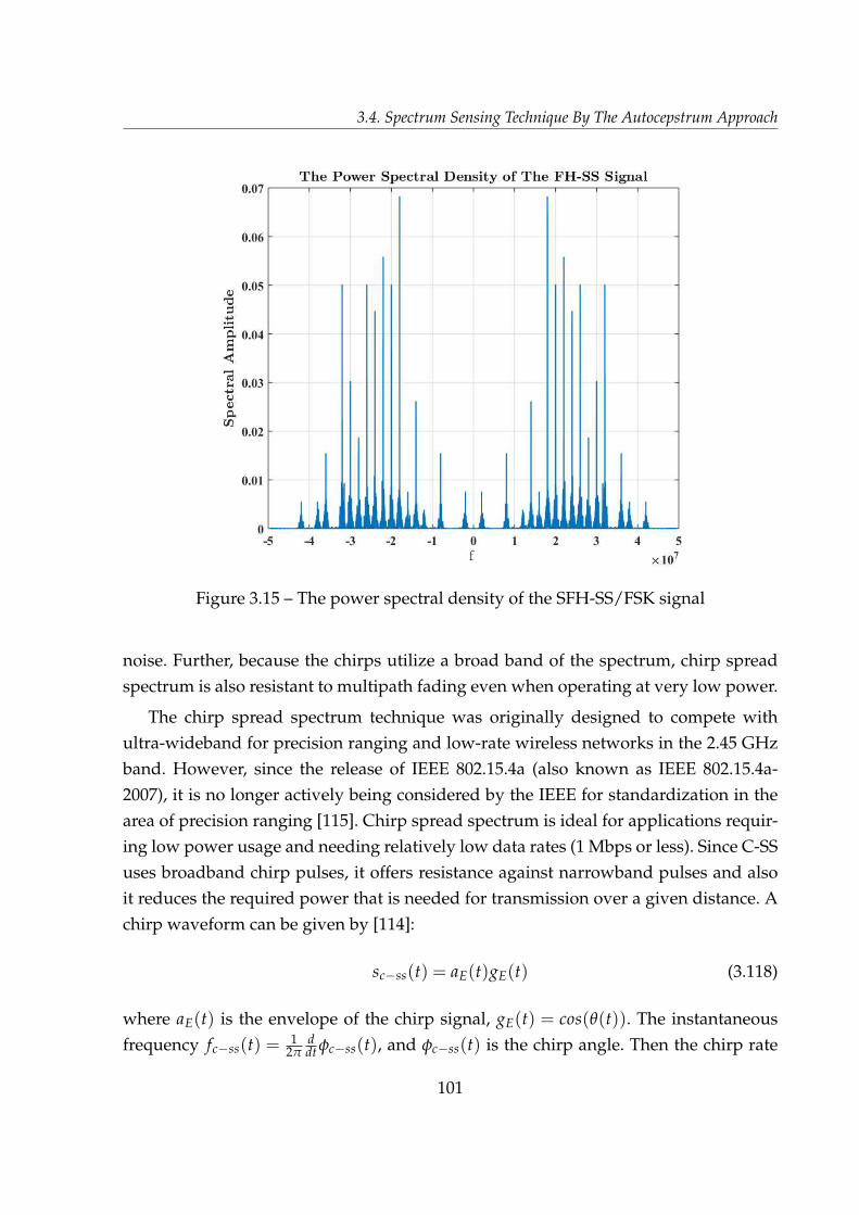
3.4. Spectrum Sensing Technique By The Autocepstrum Approach
Figure 3.15 – The power spectral density of the SFH-SS/FSK signal
noise. Further, because the chirps utilize a broad band of the spectrum, chirp spread
spectrum is also resistant to multipath fading even when operating at very low power.
The chirp spread spectrum technique was originally designed to compete with
ultra-wideband for precision ranging and low-rate wireless networks in the 2.45 GHz
band. However, since the release of IEEE 802.15.4a (also known as IEEE 802.15.4a-
2007), it is no longer actively being considered by the IEEE for standardization in the
area of precision ranging [115]. Chirp spread spectrum is ideal for applications requir-
ing low power usage and needing relatively low data rates (1 Mbps or less). Since C-SS
uses broadband chirp pulses, it offers resistance against narrowband pulses and also
it reduces the required power that is needed for transmission over a given distance. A
chirp waveform can be given by [114]:
sc�ss(t) = aE(t)gE(t) (3.118)
where aE(t) is the envelope of the chirp signal, gE(t) = cos(θ(t)). The instantaneous
frequency fc�ss(t) =1
2πddt φc�ss(t), and φc�ss(t) is the chirp angle. Then the chirp rate
101
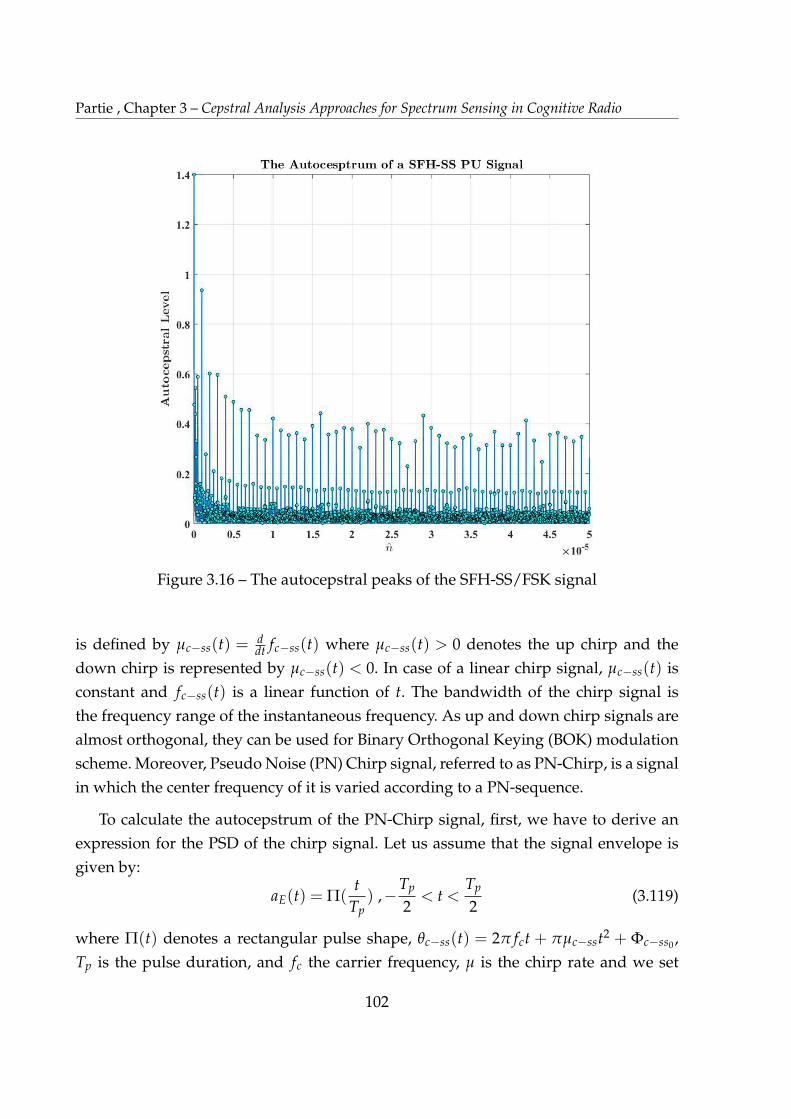
Partie , Chapter 3 – Cepstral Analysis Approaches for Spectrum Sensing in Cognitive Radio
Figure 3.16 – The autocepstral peaks of the SFH-SS/FSK signal
is defined by µc�ss(t) =ddt fc�ss(t) where µc�ss(t) > 0 denotes the up chirp and the
down chirp is represented by µc�ss(t) < 0. In case of a linear chirp signal, µc�ss(t) is
constant and fc�ss(t) is a linear function of t. The bandwidth of the chirp signal is
the frequency range of the instantaneous frequency. As up and down chirp signals are
almost orthogonal, they can be used for Binary Orthogonal Keying (BOK) modulation
scheme. Moreover, Pseudo Noise (PN) Chirp signal, referred to as PN-Chirp, is a signal
in which the center frequency of it is varied according to a PN-sequence.
To calculate the autocepstrum of the PN-Chirp signal, first, we have to derive an
expression for the PSD of the chirp signal. Let us assume that the signal envelope is
given by:
aE(t) = Π(t
Tp) ,�
Tp
2< t <
Tp
2(3.119)
where Π(t) denotes a rectangular pulse shape, θc�ss(t) = 2π fct + πµc�sst2 + Φc�ss0 ,
Tp is the pulse duration, and fc the carrier frequency, µ is the chirp rate and we set
102

3.4. Spectrum Sensing Technique By The Autocepstrum Approach
θc�ss0 = 0 for simplicity. Based on equation (3.118), the PSD of sc�ss0(t) is given by:
Ssc�ss( f ) = SaE( f ) ⇤ Sgc�ss( f ) (3.120)
where Sgc�ss( f ) = |F{gc�ss(t)}|2 = |G( f )|2 and SaE( f ) = |F{aE(t)}|
2 = |AE( f )|2 where
⇤ denotes the convolution operator and AE( f ) denotes the Fourier transform of the
pulse shaping function which is given by:
SaE( f ) = T2
psinc2(Tp f ) (3.121)
To obtain the PSD of g(t):
gc�ss(t) =12
h
exp(j2π fct)exp(jµc�sst2) + exp(�j2π fct)exp(�jµc�sst
2)i
(3.122)
let us assume that:
gc�ss1(t) =12
h
exp(�j2π fct)exp(�jµc�sst2)i
(3.123)
The spectrum of a complex Gaussian function of the form hg(t) = exp(�jσgt2) is given
by [116]:
Hg( f ) =
s
π
σgexp
j
✓
π2
σgf 2 � π
4
◆�
, σg > 0 (3.124)
and for σg < 0 we have:
Hg( f ) =
s
π
|σg|exp
�j
✓
π2
|σg|f 2 � π
4
◆�
(3.125)
then based on equations (3.123) and (3.124), we obtain:
Gc�ss1( f ) =1
2p
µc�ssexp
✓
j
π
µc�ss( f + fc)
2 � π
4
�◆
(3.126)
similarly, if gc�ss2(t) =12
⇥
exp(j2π fct)exp(jµc�sst2)⇤
, we get:
G1( f ) =1
2p
µc�ssexp
✓
�j
π
µc�ss( f � fc)
2 � π
4
�◆
(3.127)
103

Partie , Chapter 3 – Cepstral Analysis Approaches for Spectrum Sensing in Cognitive Radio
if Φc�ss( f ) = πµc�ss
( f 2 + f 2c )� π
4 and by further mathematical simplification, we obtain:
Gc�ss( f ) =1pµ
cos(Φc�ss( f ))exp✓
jwc f
µc�ss
◆
(3.128)
consequently, the PSD is given by:
Sgc�ss( f ) =1
µc�sscos2(Φ( f )) (3.129)
accordingly, Ss( f ) of the chirp signal can by expressed as:
Ss( f ) =T2
p
2µc�sssinc2(Tp f ) +
"
T2p
2µc�sssinc2(Tp f ) ⇤ cos(2Φc�ss( f ))
#
(3.130)
If we assumed that Ss1( f ) =T2
p
2µc�sssinc2(Tp f ) and Ss2( f ) =
T2p
2µc�sssinc2(Tp f ) ⇤ cos(2Φc�s( f ))
and Tp is the envelope duration in msec, we note that term sinc2(Tp f ) varies slower
than cos(2Φc�ss( f )). Thus, we can approximate the convolution of cos(2Φc�ss( f )) with
sinc(Tp f ) as if convolving cos(2Φc�ss( f )) with a constant within the main lobe of
sinc2(Tp f ), � 1Tp
< f < 1Tp
. Accordingly, an approximated expression for the linear C-SS
signal can be obtained as:
Ss( f ) ⇡T2
p
2µc�sssinc2(Tp f ) +
T2p
2µc�sscos(2Φc�ss( f )) (3.131)
A Pseudo Noise (PN) chirp signal, referred to as PN-Chirp, is a signal in which the
center frequency of it is varied according to a PN-sequence. This signal is given by:
sPN�C(t) = c(t)sc�ss(t) (3.132)
where c(t) is the waveform of the PN-sequence and sc�ss(t) is the chirp signal. We
assume that both c(t) and sc�cc(t) are independent. The PSD of the sc�ss(t) is given by:
SPN�C( f ) = Sc( f ) ⇤ Sc�ss( f ) (3.133)
From the literature, a generated pseudo random sequence by a maximal length shift
104
3.4. Spectrum Sensing Technique By The Autocepstrum Approach
register has the following PSD [113]:
Sc( f ) =Ns + 1
N2s
∞
∑i=�∞,i 6=0
sinc2✓
i
Ns
◆
δ
✓
f � i
NsTc
◆
+1
N2s
δ( f ) (3.134)
where Ns = 2ms � 1 denotes the PN sequence length, ms is the degree of the employed
primitive polynomial, and Tc is the chirp duration. If we apply the representation
SPN�C( f ) = SPN�C1( f ) + SPN�C2( f ), where SPN�C1( f ) and SPN�C2( f ) are defined by:
SPN�C1( f ) =Ns + 1
N2s
T2c
2µ
h ∞
∑i=�∞,i 6=0
sinc2⇣ i
Ns
⌘⇣
sinc2⇣
Tc
⇣
f � i
NsTc
⌘⌘
+
cos⇣
2Φ⇣
f � i
NsTc
⌘⌘⌘i
SPN�C2( f ) =T2
c
2µN2s
sinc2(Tc f ) +T2
c
2µc�sscos(2Φc�ss( f ))
�
(3.135)
and if we assume that A= Ns+1N2
s
T2c
2µc�ssand B(i) = sinc2
⇣
iNs
⌘
, we can rewrite SPN�C1( f )
as:
SPN�C1( f ) = A
"
∞
∑i=�∞,i 6=0
B(i)
✓
sinc2✓
T
✓
f � i
NsTc
◆◆
+ cos
✓
2Φ
✓
f � i
NsTc
◆◆◆
#
(3.136)
where for i = m Ns2 , B(i) = 0 where m is an integer number. As explained previously, the
natural logarithm of sinc(.) function gives rise to spectral lines and its inverse Fourier
transform reveals a cepstral peak for i = 1, thus, the same concept applies for sinc2(.)
as well as the chirp signal term in equation (3.135) for different values of i. Therefore,
we the APB-ACD as applied in the case of the FH-SS signal.
To demonstrate the concept, we give an example of a linear chirp/FSK spread spec-
trum signal in Figure 3.17. The time duration to sweep from the starting frequency to
the final frequency using up-chirp is 100 msec. The swept bandwidth of the chirp sig-
nal is 10 MHz. The binary FSK signaling modulates 10000 binary samples by switching
between f1 = 1 kHz and f2 = 10 kHz for a sampling frequency of 1 MHz. The evalu-
ation of the autocepstrum of the given signal with the illustration of the autocepstro-
gram is shown in Figure. 3.18. The autocepstrum of the chirp signal shows a group of
105
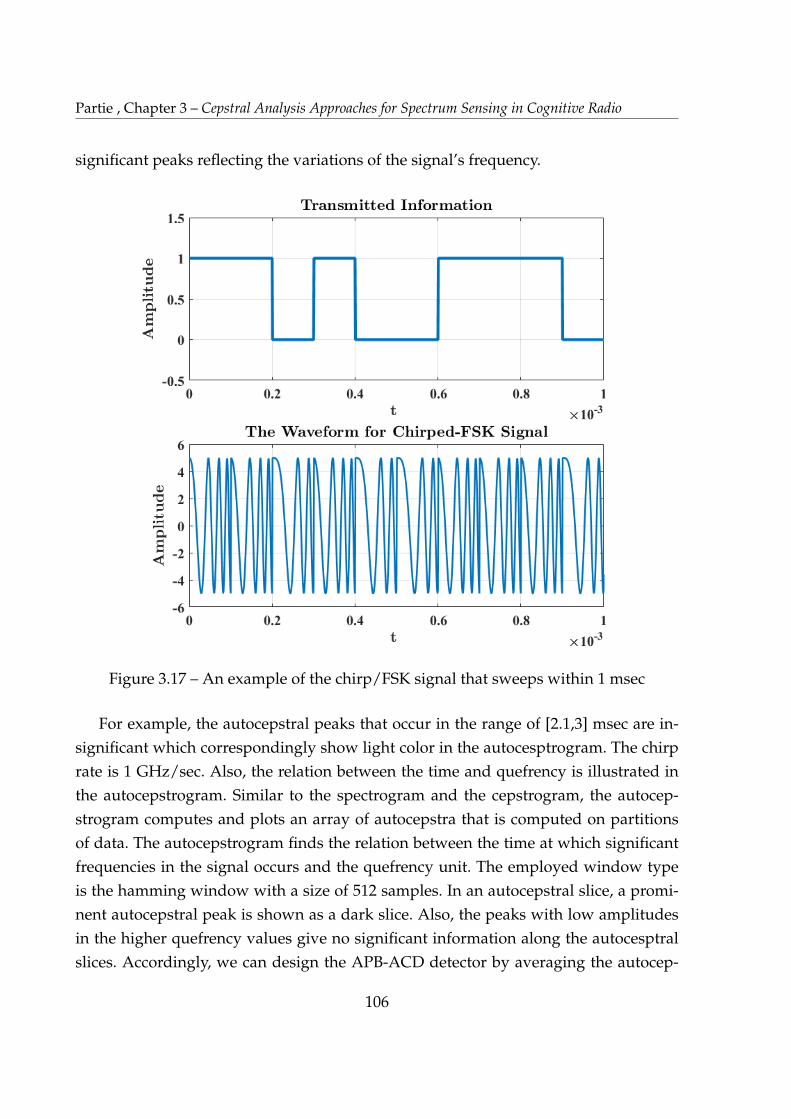
Partie , Chapter 3 – Cepstral Analysis Approaches for Spectrum Sensing in Cognitive Radio
significant peaks reflecting the variations of the signal’s frequency.
Figure 3.17 – An example of the chirp/FSK signal that sweeps within 1 msec
For example, the autocepstral peaks that occur in the range of [2.1,3] msec are in-
significant which correspondingly show light color in the autocesptrogram. The chirp
rate is 1 GHz/sec. Also, the relation between the time and quefrency is illustrated in
the autocepstrogram. Similar to the spectrogram and the cepstrogram, the autocep-
strogram computes and plots an array of autocepstra that is computed on partitions
of data. The autocepstrogram finds the relation between the time at which significant
frequencies in the signal occurs and the quefrency unit. The employed window type
is the hamming window with a size of 512 samples. In an autocepstral slice, a promi-
nent autocepstral peak is shown as a dark slice. Also, the peaks with low amplitudes
in the higher quefrency values give no significant information along the autocesptral
slices. Accordingly, we can design the APB-ACD detector by averaging the autocep-
106
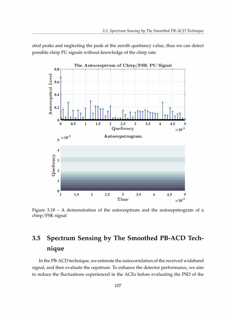
3.5. Spectrum Sensing by The Smoothed PB-ACD Technique
stral peaks and neglecting the peak at the zeroth quefrency value, thus we can detect
possible chirp PU signals without knowledge of the chirp rate.
Figure 3.18 – A demonstration of the autocesptrum and the autocepstrogram of achirp/FSK signal
3.5 Spectrum Sensing by The Smoothed PB-ACD Tech-
nique
In the PB-ACD technique, we estimate the autocorrelation of the received wideband
signal, and then evaluate the cepstrum. To enhance the detector performance, we aim
to reduce the fluctuations experienced in the ACEs before evaluating the PSD of the
107
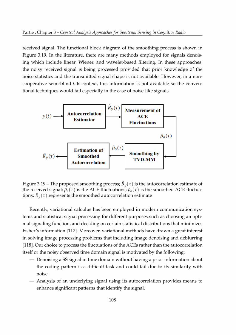
Partie , Chapter 3 – Cepstral Analysis Approaches for Spectrum Sensing in Cognitive Radio
received signal. The functional block diagram of the smoothing process is shown in
Figure 3.19. In the literature, there are many methods employed for signals denois-
ing which include linear, Wiener, and wavelet-based filtering. In these approaches,
the noisy received signal is being processed provided that prior knowledge of the
noise statistics and the transmitted signal shape is not available. However, in a non-
cooperative semi-blind CR context, this information is not available so the conven-
tional techniques would fail especially in the case of noise-like signals.
Figure 3.19 – The proposed smoothing process; Ry(τ) is the autocorrelation estimate ofthe received signal; ρo(τ) is the ACE fluctuations; ρo(τ) is the smoothed ACE fluctua-tions; Ry(τ) represents the smoothed autocorrelation estimate
Recently, variational calculus has been employed in modern communication sys-
tems and statistical signal processing for different purposes such as choosing an opti-
mal signaling function, and deciding on certain statistical distributions that minimizes
Fisher’s information [117]. Moreover, variational methods have drawn a great interest
in solving image processing problems that including image denoising and deblurring
[118]. Our choice to process the fluctuations of the ACEs rather than the autocorrelation
itself or the noisy observed time domain signal is motivated by the following:
— Denoising a SS signal in time domain without having a prior information about
the coding pattern is a difficult task and could fail due to its similarity with
noise.
— Analysis of an underlying signal using its autocorrelation provides means to
enhance significant patterns that identify the signal.
108

3.5. Spectrum Sensing by The Smoothed PB-ACD Technique
— It has been shown in the work of Burel in [94] that the fluctuations of ACEs
of noise differs from that of a spread spectrum signal. This distinguishing fea-
ture can be applied to eliminate the noisy variation in the autocorrelation of the
received SS signal.
In order to compute the autocorrelation estimator, we can divide the received time
domain signal into M segments over a time rectangular window of a duration Tp. Then,
we can evaluate the ACE for the mth segment by [94]:
Rmy (τ) =
1Tp
Z Tp
0y(t) y⇤(t � τ) dt (3.137)
where y⇤(t) denotes the complex conjugate of the received signal, and τ is the time lag.
In the statistical description of random processes, the second order moment describes
the random fluctuations of a signal. Since the variance may characterize the random
fluctuations around the mean value, the fluctuations of the ACEs are identified by their
mean and variance as mentioned in [94]. The measure of the fluctuations in terms of
the second order moment of the ACE is given by:
ρRy(τ) =⌦
|Ry(τ)|2↵ (3.138)
or approximately,
ρRy(τ) =1M
M�1
∑m=0
|Rmy (τ)|
2 (3.139)
where < . > in Equation (3.139) represents the averaging operator. If the signal and
noise are considered uncorrelated then we get:
Ry(τ) ⇡ Rs(τ) + Rw(τ) (3.140)
where Rs(τ) and Rw(τ) are the autocorrelation of the noise-free signal and the noise at
the CR receiver, respectively. In this case, we can define the underlying fluctuations of
the ACEs of the received signal according to equation (3.140) by:
ρRy(τ) = ρs(τ) + ρw(τ) (3.141)
109

Partie , Chapter 3 – Cepstral Analysis Approaches for Spectrum Sensing in Cognitive Radio
3.5.1 Fluctuations Smoothing by The Total Variation Denoising Based
on The Majorization-Minimization Algorithm:
In general, the variational calculus is employed to find local extrema in a functional
by solving differential equations. Signal denoising is one of its essential applications.
An important aspect of signal denoising is to preserve signal features, and also identify
signal trends. An approach for the signal denoising by variational calculus is the Total
Variation Denoising (TVD), through which the output is obtained by minimizing a
particular cost function [119]. Unlike conventional filtering, the TVD is defined in terms
of an optimization problem. To formulate our smoothing problem, we should illustrate
first the following notations:
— The L�point signal ρs is represented by the vector:
ρs = [ρs(0), · · · , ρs(L � 1)]T (3.142)
— The `1 norm of the vector d, which represents the discrete notations of the con-
tinuous variable t, is given by:
||d||1 = ∑`
|d(l)| (3.143)
— The `2 norm of the vector d is given by:
||d||2 =
v
u
u
t
"
∑`
|d(l)|2
#
(3.144)
— The diagonal matrix D is given by:
D =
2
6
6
6
6
4
1 0 0 0
�1 1 0 0
0 . . . 1 0
0 0 �1 1
3
7
7
7
7
5
by which the first-order difference of a L�point signal ρs is denoted by: Dρs
110
3.5. Spectrum Sensing by The Smoothed PB-ACD Technique
— The measurement of the total variation of a L�point signal ρs is given by [120]:
TV(ρs) =L�1
∑l=1
|ρs(l)� ρs(l � 1)| = ||Dρs||1 (3.145)
— The optimization problem, defining the smoothing of the ACEs fluctuations, is
given by:ρs(l) = arg min
ρs(l){F(ρs(l))} (3.146)
where F(.) is the functional to be minimized in order to find the desired estimate.
This functional can be defined in terms of mean squared error, such as [120]:
F(ρs(l)) =12
L�1
∑l=0
|ρo(l)� ρs(l)|2 + αrTV(ρs) (3.147)
where L is the maximum time lag at which the ACEs fluctuations function is
evaluated, ρo(l) denotes the observed fluctuations, for the case of uncorrelated
signal and noise, that is given by:
ρo(τ) = ρs(τ) + ρw(τ) (3.148)
and αr > 0 represents the regularization parameter that controls the smoothing
degree. An appropriate value of αr can be found heuristically.
In order to solve the minimization problem defined in equation (3.146), various al-
gorithms can be employed, such as the TVD clipping algorithm [121]. However, the
appropriate choice of an algorithm depends on the desired accuracy level and the con-
vergence rate. For example, the Majorization-Minimization (MM) algorithm is applied
to solve the TVD problem, which provides a significant accuracy on the expenses of
the convergence time. The MM algorithm solves the minimization problem using a se-
quence of functions, called majorizer functions, that are easier to solve than the original
cost function. To use the MM algorithm and reduce the computation burden, one must
choose carefully an optimization function denoted by G(ρs) to approximate F(ρs). To
choose G(.), the MM approach requires that:
1. G(ρs) is a majorizer of F(ρs):
G(ρs) � F(ρs),8ρs(l).
2. The majorizer coincides with the F(.) at each iteration, i: Gi(ρs(l)) = F(ρs(l)).
111

Partie , Chapter 3 – Cepstral Analysis Approaches for Spectrum Sensing in Cognitive Radio
3. G(ρs) must be a convex function, so that the MM algorithm obtains the solution
at each ith iteration by minimizing the majorizer function.
3.5.2 Application of the Proposed Smoothing Process to the Case of
Detecting a DS-SS Signal:
To anticipate a constructive example for showing the applicability of the proposed
smoothing process to our detection problem, consider the case of a passband DS-SS
signal, s(t), occupying a wideband of interest with the autocorrelation function given
by [105]:
Rs(τ) =A2
2Rd(τ)Rp(τ)cos(2π fcτ) (3.149)
where Rd(τ) and Rp(τ) are the autocorrelation of the data and spreading waveform,
respectively, and they are given by [105]:
Rd(τ) = Λ(τ
Td) =
1 � |τ|
Td
Rp(τ) =� 1Ns
+Ns + 1
Ns
∞
∑i=�∞
Λ
✓
τ � iNsTc
Tc
◆ (3.150)
where Td is the symbol duration, Tc is the chip duration and Λ(.) is the triangular
function; Ns = 2ms � 1 is the length of the m-sequence pseudo random spreading code;
ms is the degree of a chosen primitive polynomial. Based on the baseband version of
equation (3.149), we can express the ACEs fluctuation function of s(t) by:
ρs(τ) ⇡ ρp
∞
∑i=�∞
Λ
✓
τ � iNsTc
Tc
◆
(3.151)
in which ρs(τ) viewed as a periodic triangular wave form with peak values ρp. Accord-
ing to equation (3.151), a convenient majorizer function, Gi(ρs(τ)) = gMM(t), at the ith
iteration for one period of ρ(τ) is given by:
gMM(t) = cMM � bMMt2 (3.152)
From the MM algorithm, gMM(t) must satisfy:
g(t)MM � fMM(t), 8t (3.153)
112

3.5. Spectrum Sensing by The Smoothed PB-ACD Technique
where fMM(t) is the original cost function. Equivalently, if we set ρp = 1, then we
should have:
cMM � bMMt2 � 1 � t
Tc,8 t > 0 (3.154)
In this case, we need to evaluate the constants cMM and bMM to validate that the chosen
function in equation (3.152) is a majorizer. The mathematical analysis to find cMM and
bMM yields the following:
bMM =1
2Tc|ti|, cMM =
1 � 2|ti|
2Tc(3.155)
(See Appendix B for the proof). Clearly, an upper bound of one period of fMM(t) is
given by gMM(t), then by substituting cMM and bMM in equation (3.154), we get:
1 � 2ti
2Tc� t2
2Tcti� 1 � |t|
Tc, 8t 2 R (3.156)
To obtain the required cost function, we use d(l) for the discrete notation instead of t,
and then by summing over l, we obtain:
L
∑l=1
✓
1 � 2|di(l)|
2Tc� d2(l)
2Tc|di(l)|
◆
�L
∑l=1
1 � |d(l)|
Tc(3.157)
By using vector notations, we can rewrite equation (3.157) in a compact form as:
✓
�Ns
2� ||di(l)||1 �
12
dT∆�1
i d
◆
� � ||d||1 (3.158)
where ∆i = diag (|di(l)|) denotes a diagonal matrix. Recalling the definition of the TVD
in equation (3.145), then by replacing d with Dρs in equation (3.158), multiplying it by
the regularity parameter αr, and adding the error data term er(l) =12 ||ρo(l)� ρ(l)||22 to
its both sides, then we get:
er(l)�αrNs
2� αr||Dρsi
(l)||1 �αr
2ρT
s DT∆�1
i Dρs � er(l)� αr||Dρs||1 (3.159)
Clearly, the majorizer of the cost function is given by:
Gi(ρs) = er(l)�αrNs
2� αr||Dρsi
(l)||1 �αr
2ρT
s DT∆�1
i Dρs (3.160)
113

Partie , Chapter 3 – Cepstral Analysis Approaches for Spectrum Sensing in Cognitive Radio
Using equation (3.160), we seek to obtain the update equation (ρs)i+1 as follows:
— Set the iteration index i to 0 and initialize (ρs)0.
— Set (ρs)i+1 as a minimizer of Gi(ρs) such that:
(ρs)i+1 = arg minρs
Gi(ρs) (3.161)
— Set i = i + 1 and go to step 2.
Accordingly, by differentiating equation (3.160) and equating the results to zero, it
yields:
(ρs)i+1 = (I + U)�1ρ(l) (3.162)
where I is the identity matrix, and U is defined by:
U = αrDT∆�1
iD (3.163)
In Figure 3.20, we illustrate the effect of applying the smoothing process for the case of
a DS-SS signal at SNR of -10 dB.
The operating specifications are based on the IEEE802.11a standards that uses DS-
SS signal with 5 GHz as the operating frequency and 54 Mbps for the data rate [105].
It is important to clarify that despite the effective results provided by the proposed
smoothing process on the estimated PSDs, there is an 8% estimation error in the oper-
ating frequency. For this reason, it is essential that the PU detector operates indepen-
dently on the operating frequency value. Taking into account that random ACEs fluc-
tuations of the DS-SS signal and that of the AWGN are distinguishable, the smoothed
PB-ACD exploits the advantage of denoising the fluctuations of the ACEs by the TVD-
MM algorithm. The calculation of the ACEs fluctuations involves dividing the time
domain signal into M segments. By respecting Nyquist’s rate fsN, the estimated PSD
maintains the exact frequency information as shown in Figure 3.21. However, in case
of oversampling the signal, the estimated PSD experiences a minor loss of frequency
localization [122].
As the number of samples increases within each signal segment, in case of oversam-
pling, the summation of the segmented autocorrelation will smooth out the signals de-
tails. Therefore, the maxima presented in the sum will be more smoothed resulting in
minor frequency shift in the estimated PSD. Also, as the oversampling increases above
double the Nyquist’s rate, a substantial loss of frequency localization occurs.
114

3.5. Spectrum Sensing by The Smoothed PB-ACD Technique
(a) The original PSD of a DS-SS signal (b) The received signal PSD at SNR of -10 dB
(c) The estimated PSD Sr( f ) in decibels after applying the TVD-MM algorithm to the fluctua-tions of the ACEs of the received signal in case of oversampling
Figure 3.20 – The effect of applying the smoothing process on the estimated PSD
115
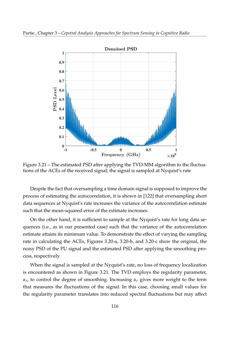
Partie , Chapter 3 – Cepstral Analysis Approaches for Spectrum Sensing in Cognitive Radio
Figure 3.21 – The estimated PSD after applying the TVD-MM algorithm to the fluctua-tions of the ACEs of the received signal; the signal is sampled at Nyquist’s rate
Despite the fact that oversampling a time domain signal is supposed to improve the
process of estimating the autocorrelation, it is shown in [122] that oversampling short
data sequences at Nyquist’s rate increases the variance of the autocorrelation estimate
such that the mean-squared error of the estimate increases.
On the other hand, it is sufficient to sample at the Nyquist’s rate for long data se-
quences (i.e., as in our presented case) such that the variance of the autocorrelation
estimate attains its minimum value. To demonstrate the effect of varying the sampling
rate in calculating the ACEs, Figures 3.20-a, 3.20-b, and 3.20-c show the original, the
noisy PSD of the PU signal and the estimated PSD after applying the smoothing pro-
cess, respectively.
When the signal is sampled at the Nyquist’s rate, no loss of frequency localization
is encountered as shown in Figure 3.21. The TVD employs the regularity parameter,
αr, to control the degree of smoothing. Increasing αr gives more weight to the term
that measures the fluctuations of the signal. In this case, choosing small values for
the regularity parameter translates into reduced spectral fluctuations but may affect
116

3.6. Numerical Results and Discussions
the level of the exact spectral boundaries. Therefore, before choosing the regularity
parameter, we have to be aware of the required detection accuracy level to avoid over-
smoothing the analyzed signal and hence increasing the misdetection probability.
3.6 Numerical Results and Discussions
In order to prove the efficacy of the autocepstrum detector, we evaluate the detec-
tion performance as compared to different state-of-the-art techniques. The simulations
are averaged over 3000 realizations with an observation interval of 0.7 sec and the chip
duration is 1.54 µsec. In the simulations, we employed a Boolean parameter Θ, which
is uniformly distributed and takes randomly a value of 0 or 1 in order to include the
presence or absence of a DS-SS PU signal. The used spreading code is based on a prim-
itive polynomial defining the m-sequence code in the form of x6 + x + 1 [113]. The
length of the spreading code is 63 sample to generate a long PN sequence, and the
PN sequence length of the analyzed signal is 4410 sample. The modulation type is the
passband BPSK modulation scheme with a carrier frequency of 5 GHz, and a sampling
frequency fs of 30 GHz.
Figure 3.22 – Performance evaluation of the PB-ACD as compared to ED for fixed PFA
.
117

Partie , Chapter 3 – Cepstral Analysis Approaches for Spectrum Sensing in Cognitive Radio
The performance of the proposed autocepstrum detector is measured in terms of
the detection probability which is evaluated from -15 dB to 10 dB. The required noise
statistics are evaluated through histogram estimation. All simulations are carried on
under the CLT assumption. It can be seen from Figure 3.22 that the proposed detector
outperforms energy detection at low SNR although there is no noise uncertainty that
is assumed. It means that the PB-ACD can detect a signal hidden in noise by -15 dB
with probability of approximately 0.1 for PFA = 0.01. Further, at the same SNR and for
PFA = 0.05, PB-ACD gives 0.5 detection probability which is approximately double the
ED’s detection performance.
Also, to elaborate more on higher-order and advanced modulations, Figure 3.23
shows a comparison of the detection performance of the PB-ACD technique with ED
for detecting 16-QAM and 64-QAM PU signals. In wireless communication, the 64-
QAM modulation scheme is used in 4G systems in the uplink and provides the most
benefit in small cell environments under good uplink conditions. Moreover, we simu-
lated the PB-ACD technique, as shown in Figure 3.24, to test its detection performance
for detecting OFDM PU signals and compare them with ED and the EVD. The simula-
tions are conducted for 2000 Monte Carlo iterations. In simulating OFDM modulated
signals, we considered the parameters defined in the IEEE802.11 specifications [85].
The number of total subcarriers (i.e., FFT size) is 64, for 48 data subcarriers and 4 pi-
lot subcarriers. The FFT duration is 3.2 µsec, the number of symbols is 104, and the
OFDM bandwidth is 20 MHz. In Figure 3.24, the OFDM PU signal can be detected
by the PB-ACD technique by over about 40% than ED and EVD at -15 dB. In section
3.5, we proposed a solution for improving the detection performance of the PB-ACD
technique for detecting noise-like signals through a smoothing process. Indeed, the de-
tection of low-power signals in CR is a spectrum sensing challenge, especially when
the CR receiver has no knowledge of the specifications of the noise-like signal. Further,
we have discussed the capability of the PB-ACD technique for detecting a DS-SS sig-
nal under the AWGN channel in case of the SBSA. Hereinafter, we aim to evaluate the
performance of the smoothed PB-ACD in terms of the detection probability for DS-SS
and an IR-UWB signals.
To provide more improvement over the ED technique, we applied the proposed
smoothed PB-ACD technique and compare it with different state-of-the-art spectrum
sensing techniques, such as the EVD, and the MFD. The detection probability is evalu-
ated as shown in Figure 3.25.
118
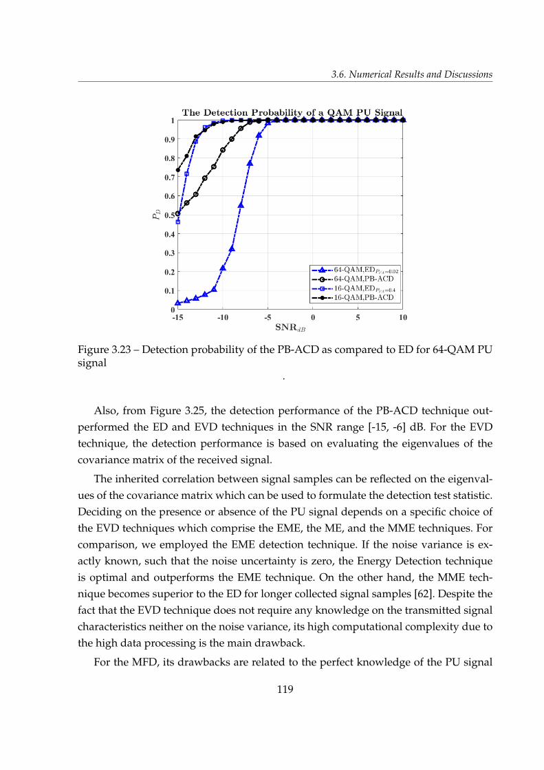
3.6. Numerical Results and Discussions
Figure 3.23 – Detection probability of the PB-ACD as compared to ED for 64-QAM PUsignal
.
Also, from Figure 3.25, the detection performance of the PB-ACD technique out-
performed the ED and EVD techniques in the SNR range [-15, -6] dB. For the EVD
technique, the detection performance is based on evaluating the eigenvalues of the
covariance matrix of the received signal.
The inherited correlation between signal samples can be reflected on the eigenval-
ues of the covariance matrix which can be used to formulate the detection test statistic.
Deciding on the presence or absence of the PU signal depends on a specific choice of
the EVD techniques which comprise the EME, the ME, and the MME techniques. For
comparison, we employed the EME detection technique. If the noise variance is ex-
actly known, such that the noise uncertainty is zero, the Energy Detection technique
is optimal and outperforms the EME technique. On the other hand, the MME tech-
nique becomes superior to the ED for longer collected signal samples [62]. Despite the
fact that the EVD technique does not require any knowledge on the transmitted signal
characteristics neither on the noise variance, its high computational complexity due to
the high data processing is the main drawback.
For the MFD, its drawbacks are related to the perfect knowledge of the PU signal
119

Partie , Chapter 3 – Cepstral Analysis Approaches for Spectrum Sensing in Cognitive Radio
Figure 3.24 – Detection probability of the PB-ACD as compared to ED for an OFDMPU signal in AWGN channel
.
and the noise variance. In [123], the detection threshold of the suggested MFD is given
as a function of SNR so at low SNR, the value of the detection threshold becomes
higher such that the detection performance deteriorates. In Figure 3.25, the matched
filter detector has the highest detection probability among the energy Detector and the
eigenvalue-based detector at SNR of -15 dB, whereas the PB-ACD technique is higher
in detection probability by 30% than the matched filter detector. However, as the SNR
slightly increases to -12 dB, the PB-ACD and the MFD techniques performs similarly.
By applying the smoothing process to the PB-ACD, the detection results increased by
40%.
The detection results illustrate the efficacy of the PB-ACD technique to be the less
likely to miss-detect the presence of a DS-SS PU signal among the considered state-of-
the-art techniques. For the IR-UWB signal, we used a Gaussian monocycle waveform
to generate the transmitted pulses along with the passband BPSK modulation scheme.
The impulse duration is 0.5 nsec, and the carrier frequency is 6 GHz. Our choice of the
IR-UWB signal is due to its very low power level.
The number of segments used to calculate the autocorrelation estimates in 630 seg-
120
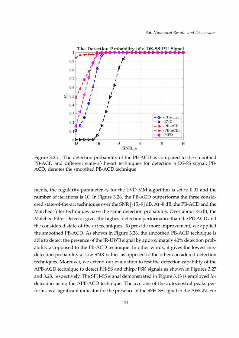
3.6. Numerical Results and Discussions
Figure 3.25 – The detection probability of the PB-ACD as compared to the smoothedPB-ACD and different state-of-the-art techniques for detection a DS-SS signal; PB-ACDs denotes the smoothed PB-ACD technique
ments, the regularity parameter αr for the TVD-MM algorithm is set to 0.01 and the
number of iterations is 10. In Figure 3.26, the PB-ACD outperforms the three consid-
ered state-of-the-art techniques over the SNR [-15,-9] dB. At -8 dB, the PB-ACD and the
Matched filter techniques have the same detection probability. Over about -8 dB, the
Matched Filter Detector gives the highest detection performance than the PB-ACD and
the considered state-of-the-art techniques. To provide more improvement, we applied
the smoothed PB-ACD. As shown in Figure 3.26, the smoothed PB-ACD technique is
able to detect the presence of the IR-UWB signal by approximately 40% detection prob-
ability as opposed to the PB-ACD technique. In other words, it gives the lowest mis-
detection probability at low SNR values as opposed to the other considered detection
techniques. Moreover, we extend our evaluation to test the detection capability of the
APB-ACD technique to detect FH-SS and chirp/FSK signals as shown in Figures 3.27
and 3.28, respectively. The SFH-SS signal demonstrated in Figure 3.13 is employed for
detection using the APB-ACD technique. The average of the autocepstral peaks per-
forms as a significant indicator for the presence of the SFH-SS signal in the AWGN. For
121
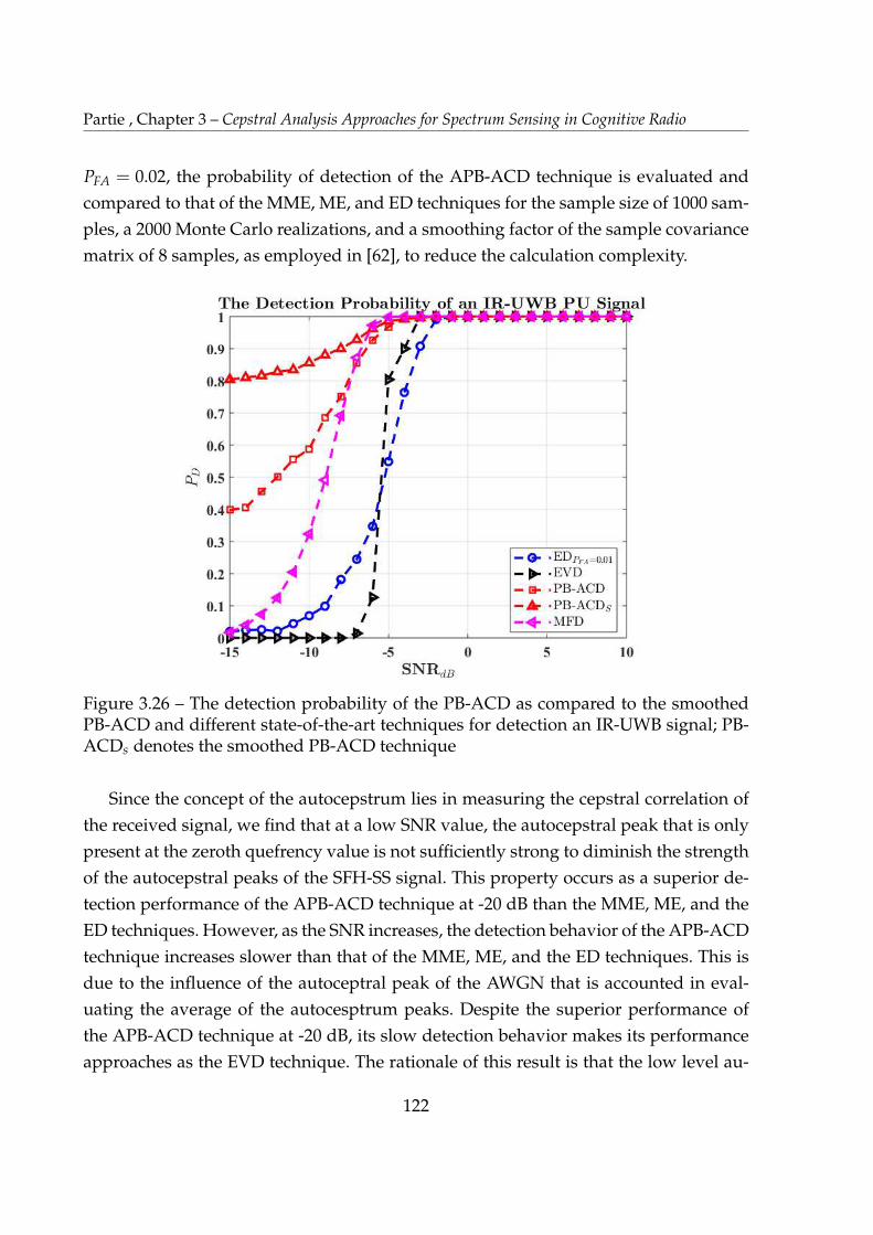
Partie , Chapter 3 – Cepstral Analysis Approaches for Spectrum Sensing in Cognitive Radio
PFA = 0.02, the probability of detection of the APB-ACD technique is evaluated and
compared to that of the MME, ME, and ED techniques for the sample size of 1000 sam-
ples, a 2000 Monte Carlo realizations, and a smoothing factor of the sample covariance
matrix of 8 samples, as employed in [62], to reduce the calculation complexity.
Figure 3.26 – The detection probability of the PB-ACD as compared to the smoothedPB-ACD and different state-of-the-art techniques for detection an IR-UWB signal; PB-ACDs denotes the smoothed PB-ACD technique
Since the concept of the autocepstrum lies in measuring the cepstral correlation of
the received signal, we find that at a low SNR value, the autocepstral peak that is only
present at the zeroth quefrency value is not sufficiently strong to diminish the strength
of the autocepstral peaks of the SFH-SS signal. This property occurs as a superior de-
tection performance of the APB-ACD technique at -20 dB than the MME, ME, and the
ED techniques. However, as the SNR increases, the detection behavior of the APB-ACD
technique increases slower than that of the MME, ME, and the ED techniques. This is
due to the influence of the autoceptral peak of the AWGN that is accounted in eval-
uating the average of the autocesptrum peaks. Despite the superior performance of
the APB-ACD technique at -20 dB, its slow detection behavior makes its performance
approaches as the EVD technique. The rationale of this result is that the low level au-
122
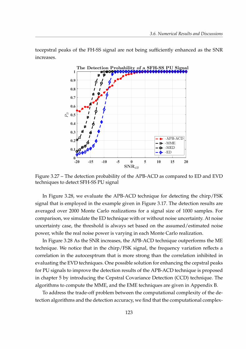
3.6. Numerical Results and Discussions
tocepstral peaks of the FH-SS signal are not being sufficiently enhanced as the SNR
increases.
Figure 3.27 – The detection probability of the APB-ACD as compared to ED and EVDtechniques to detect SFH-SS PU signal
In Figure 3.28, we evaluate the APB-ACD technique for detecting the chirp/FSK
signal that is employed in the example given in Figure 3.17. The detection results are
averaged over 2000 Monte Carlo realizations for a signal size of 1000 samples. For
comparison, we simulate the ED technique with or without noise uncertainty. At noise
uncertainty case, the threshold is always set based on the assumed/estimated noise
power, while the real noise power is varying in each Monte Carlo realization.
In Figure 3.28 As the SNR increases, the APB-ACD technique outperforms the ME
technique. We notice that in the chirp/FSK signal, the frequency variation reflects a
correlation in the autocesptrum that is more strong than the correlation inhibited in
evaluating the EVD techniques. One possible solution for enhancing the cepstral peaks
for PU signals to improve the detection results of the APB-ACD technique is proposed
in chapter 5 by introducing the Cepstral Covariance Detection (CCD) technique. The
algorithms to compute the MME, and the EME techniques are given in Appendix B.
To address the trade-off problem between the computational complexity of the de-
tection algorithms and the detection accuracy, we find that the computational complex-
123
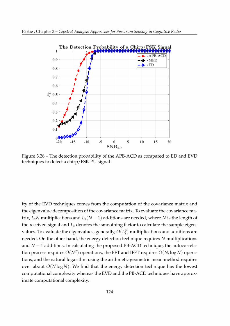
Partie , Chapter 3 – Cepstral Analysis Approaches for Spectrum Sensing in Cognitive Radio
Figure 3.28 – The detection probability of the APB-ACD as compared to ED and EVDtechniques to detect a chirp/FSK PU signal
ity of the EVD techniques comes from the computation of the covariance matrix and
the eigenvalue decomposition of the covariance matrix. To evaluate the covariance ma-
trix, LsN multiplications and Ls(N � 1) additions are needed, where N is the length of
the received signal and Ls denotes the smoothing factor to calculate the sample eigen-
values. To evaluate the eigenvalues, generally, O(L3s ) multiplications and additions are
needed. On the other hand, the energy detection technique requires N multiplications
and N � 1 additions. In calculating the proposed PB-ACD technique, the autocorrela-
tion process requires O(N2) operations, the FFT and IFFT requires O(Nr log N) opera-
tions, and the natural logarithm using the arithmetic geometric mean method requires
over about O(N log N). We find that the energy detection technique has the lowest
computational complexity whereas the EVD and the PB-ACD techniques have approx-
imate computational complexity.
124
3.7. Summary
3.7 Summary
In this chapter, we show that cepstral signal processing can be significant in CR
for detecting DS-SS PU signal by employing the autocepstrum concept for the SBSA
model. We offer a solution for the hidden spread spectrum PU problem that causes
misdetection due to the nature of the PU signal. We formulate a spectrum sensing al-
gorithm that is based on an autocepstral peak appearing at a quefrency value equals
to the carrier signal duration. On the other hand, the fact that zero autocepstral peaks
appearing at the same quefrency value for the AWGN case enables a CR receiver to
differentiate between noise-like PU signal and thermal noise. Further, we derive ex-
pression for the probability distribution of the autocepstrum of the received signal un-
der the null hypothesis. Also, we present an analytical framework for evaluating the
mean and variance of the detection test statistic, and we formulate an expression for
the detection threshold in case of having cepstral coefficients that follow log�χ2ν dis-
tribution. For performance evaluation, the proposed detector is compared to different
state-of-the-art techniques and shows better performance than ED in low SNR envi-
ronment. A mathematical analysis for the autocepstrum approach for the FH-SS and
C-SS signals is carried out. The sensing-throughput-threshold trade-off of the PB-ACD
technique is analytically discussed.
Through the PB-ACD technique, the detection process merely depends on identi-
fying a significant peak in the cepstral domain at the reciprocal of center frequency of
the target spectral band. However, in a low SNR environment (e.g., -15 dB) in which
high noisy fluctuations are experienced, identifying this major peak will be a difficult
task. For this purpose, we introduce an improved version of the PB-ACD technique
by providing a smoothing process. We formulate a novel signal smoothing technique
that involves the use of the TVD approach through the MM algorithm. We start by
evaluating the fluctuations of the ACEs of the received noise-like signal (i.e., spread
spectrum signal) to which we apply the TVD-MM algorithm, and then estimating the
smoothed spectrum before applying the PB-ACD approach. Since we assume working
in a non-cooperative detection environment, and knowing that most of the denoising
techniques depend on some knowledge provided of the received signal, noise statis-
tics, and channel information, we apply the TVD-MM algorithm in semi-blind theme
without a prior knowledge of the nature of the noise-like signal. Precisely, we utilize
the fact that the fluctuations of the autocorrelation estimators of the received SS signal
125

Partie , Chapter 3 – Cepstral Analysis Approaches for Spectrum Sensing in Cognitive Radio
and that of the AWGN are distinguishable [94], the TVD-MM algorithm is applied on
the ACEs of the received CR signal utilizing this discriminating feature. The purpose
of applying the smoothing process is to reduce possible false alarms. For the case of
multiband spectrum access model, we introduce in chapter 4 a wideband spectrum
sensing technique by employing CR approaches.
126
CHAPTER 4
WIDEBAND SPECTRUM SENSING
TECHNIQUE BY CEPSTRAL ANALYSIS
APPROACHES
4.1 Introduction
The process of sensing a wide radio spectrum is performed through two phases,
namely: the edge detection phase, and the PU detection phase. Through the edge de-
tection phase, the wideband of interest is analyzed to identify the subbands spectral
boundaries, which are characterized by irregularities appearing in the spectrum. For
instance, The Wavelet-Based Detection (WBD) approaches employ Wavelet Transform
(WT) as a powerful mathematical tool for singularities detection [124]. These singu-
larities, which represent irregular signal structures, define the subband edges (i.e.,
boundaries). As for the PU detection phase, one of the conventional NarrowBand
Spectrum Sensing (NBSS) techniques can be utilized, such as Energy Detection (ED),
Matched-Filter Detection (MFD), Cyclostationary feature detection (CFD), and Com-
pressive Spectrum Sensing (CSS) [9]. In general, there are two main methods to apply
NBSS: sequentially, or through parallel sensing. In the sequential sensing method, a
narrowband detector senses multiple bands in a serial manner. The major disadvan-
tage of employing sequential sensing is the slow processing time, and also the require-
ment of retuning the used filters and oscillators. While the theme of the parallel sensing
method assures a better processing time, the increased complexity of the CR receiver
architecture becomes a drawback. This increased complexity is due to the integrated
multiple narrowband detectors at the CR receiver.
Since possible errors in the edge detection results consequently affect the perfor-
mance of the PU detection phase, the crucial challenge in applying the WideBand
Spectrum Sensing (WBSS) techniques is the devised edge detection algorithm. In other
127
Partie , Chapter 4 – Wideband Spectrum Sensing Technique By Cepstral Analysis Approaches
words, false alarms can be generated due to the presence of spurious edges caused by
noisy spectral variations. Moreover, errors in estimating the location of an exact spec-
tral boundary may lead to the misdetection problem. Thus, the promising accuracy of
the chosen edge detection approach is vital to assure the overall efficiency of the WBSS
process. Clearly, further advancements in wideband sensing are required to provide a
high detection robustness against noisy spectral variations with offered low complex-
ity. Therefore, we should highlight the trade-off between the detection accuracy, and
the computational burden or the offered hardware complexity. For example, despite
the fact that the wavelet-based detector provides a reliable detection accuracy in an
Additive White Gaussian Noise (AWGN) channel on the one hand, but on the other
hand its hardware and computational complexities are significant. This is because a
wavelet-based detector is basically implemented as a bank of multiresolution filters; So
for better detection results, the signal analysis is carried out through all dyadic scales
which increases the computational cost.
Moreover, the CS exploits the signal sparsity in the frequency domain knowing that
a scarce or underutilized spectrum is sparse. This sparsity invokes a few number of
measurements to be used, hence a performance degradation is expected due to the re-
duced Signal-to-Noise Ratio (SNR) despite the hardware simplicity of the CS detector.
Motivated by these insights, in this chapter, we present a novel WBSS technique that is
based on the Cepstral Analysis (CA) in the context of CR. We introduce an edge detec-
tion algorithm based on calculating the Differential Log-Spectral Density (DLSD) of the
received wideband signal. This is to identify the spectral boundaries and characterize
the number of occupied subbands. In order not to confuse the readers, evaluating the
DLSD is slightly different than the conventional differential cepstrum. For a given sig-
nal, the DLSD evaluates the derivative of the natural logarithm of the signal’s Power
Spectral Density (PSD), whereas the differential cepstrum calculates the derivative of
a signal’s Fourier Transform (FT). A mathematical framework of the proposed edge
detection algorithm is analytically illustrated to show the effect of the noisy spectral
fluctuations on the resultant spectral boundaries. The proposed algorithm is compared
to different wavelet-based edge detection algorithms at different noise power levels to
validate its efficacy.
In the literature, the CA has a strong impact on several applications comprising au-
dio and speech processing, as well as mechanical systems. It is also employed in the
fields of signal classification or feature detection. Thus, the CA approach is used to
128

4.1. Introduction
identify certain features hidden in a signal that can be revealed in the cepstral domain.
According to the variants of the CA approach, a certain CA variant is chosen in order
to fit a specific application. That is why a researcher must be aware of the problem un-
der analysis, and whether employing the CA approach will unleash significant details
about the signal in the logarithmic domain.
By completing the edge detection phase, we eventually obtain the required infor-
mation about the spectral boundaries of the sensed wide spectrum. Afterwards, we
proceed to identify the presence of possible PUs in the sensed frequency bands. The ED
technique is a versatile NBSS technique that does not require a prior information about
the PU signal. However, its susceptibility to noise variations results in a poor perfor-
mance in low SNR environments [31]. Employing the ED technique for detecting a PU
signal assumes that the frequency band of interest is exactly defined and recognized
by its spectral boundaries. However, in WBSS, the performance of ED deteriorates.
Since the PSD level within a certain subband is evaluated by the integration of the PSD
over certain frequency bands, it should take into account the PSD level within the es-
timated frequency boundaries which are subjected to possible errors. Also, in the case
of practical blunt spectrum shapes, the PSD leakage related to the PU signal outside
the spectral boundaries will not be considered in the energy calculation [125]. Thus,
this may cause the misdetection of a PU. To overcome these drawbacks, the Broadened
Energy Detection (BED) and the Weighted Energy Detection (WED) are suggested in
[125]. However, the increased resulting complexity is pushing ED to lose its simplicity
property amongst different semi-blind NBSS techniques.
Although the PB-ACD technique has shown its efficacy in detecting a DS-SS PU
signal in [126], with an exact knowledge of the subbands center frequencies, its per-
formance deteriorates when applied in the MBSA scenario due to the potential errors
in estimating the subbands center frequencies. These errors may result in the misde-
tection and false-alarm problems. As a solution, we introduce the BaseBand AutoCep-
strum Detector (BB-ACD) that exploits the periodicity feature that can be revealed of
the baseband digital signals in the cepstral domain. Accordingly, we propose a non-
coherent detection of the received signal via a circular topological filter, which consists
of Hilbert Filtering (HF) and a Square-Law Device (SLD). This is to extract the base-
band version of a signal before evaluating the power cepstrum of the received signal,
so that the detection process does not depend on the exact knowledge of the center
frequency of a specific subband. In this chapter, A novel edge detection algorithm is
129
Partie , Chapter 4 – Wideband Spectrum Sensing Technique By Cepstral Analysis Approaches
introduced by the DLSD approach to identify the spectral boundaries of the subbands
comprising the target wideband spectrum. A mathematical framework of the DLSD
approach is illustrated in low, medium, and high SNR environments. An analytical
expression of the detection threshold characterizing the proposed DLSD detector is
derived under AWGN channels. The BB-ACD technique is formulated for detecting
noise-like signals under the subband center frequency uncertainty problem. A math-
ematical analysis of the detection threshold is presented according to the statistical
distribution of the devised detection test statistic. Through simulations, we provided
comparisons of the BB-ACD technique with the PB-ACD technique to show the efficacy
of the proposed technique when the problem of center frequency errors is encountered.
This chapter is organized as follows: section 4.2 gives a brief state-of-the-art on
edge detection, and also summarizes the advantages and critics of the wavelet-based
edge detection techniques. Section 4.3 states the mathematical foundation of the prob-
lem under investigation and describes the overall proposed system architecture. The
proposed edge detection and the CA-based PU detection techniques are introduced
in section 4.4, with the mathematical analysis of both techniques. In section 4.5, the
numerical results are illustrated, and the chapter summary is given in section 4.6.
4.2 Related Work
As it was previously mentioned, CA has been utilized differently in the field of sig-
nal detection. For example, it has been applied for echoes detection in seismic waves
[18]. Further, it has been used to estimate the multipath time delay as introduced in
[93], or for detecting audio watermarks [15]. In the contexts of spectrum sensing and
signal detection in CR, CA approaches have been rarely utilized. For instance, the au-
thors in [19] have employed CA techniques in waveform classification and for detect-
ing OFDM signals and also for estimating their parameters. Moreover, the authors of
[104] have introduced a WideBand Temporal Sensing (WBTS) approach based on a
cepstral envelope detector. Precisely, the involvement of the cepstrum-based spectrum
envelope detector is to adapt to dynamic changes that may occur in the configuration
of a PU channel. The rationale of this approach is to use a cepstral feature vector to
detect the changes in the spectrum envelope of a PU signal within a given frequency
band. Based on the recursive temporal spectrum sensing algorithm proposed in [127],
[128], the authors in [104] have proposed the use of cepstral analysis to monitor the
130

4.2. Related Work
change of the PU’s configuration instead of the conventional ED front end.
In the WBTS approach, a given frequency band is divided into narrowband chan-
nels of equal bandwidths. Every narrowband channel is then sensed individually using
a Hidden Markov Model (HMM)-based approach [129]. The employed HMM model
is trained by an observation sequence that consists of average received signal pow-
ers. The parameters of the trained HMM model is estimated by the Baum algorithm 1
[130]. According to a modified correlation metric, the adjacent channels are aggregated
to form larger channels. After being conducted in a recursive manner, this process
eventually results in the identification of a set of PU channels with their HMM esti-
mated parameters. At the same time, a cepstrum-based envelope detector is applied
to monitor the transition of the PU channel to a different configuration. The spectrum
envelope detector is designed based on the HMM model in which the employed ob-
servation vector corresponds to the signal’s cepstrum. Our proposed cepstrum-based
WBSS approach differs from the WBTS approach such that it introduces the following:
— Identification of the number of occupied subbands in a target wide spectrum.
This is formulated as an edge detection problem and accomplished by develop-
ing the DLSD algorithm.
— Detection of noise-like PU signals such as spread spectrum signals. For this pur-
pose, we reviewed our proposed PB-ACD technique in chapter 3 which detects
the presence of a DS-SS signal by monitoring a major autocepstral peak. The
improved PB-ACD technique is proposed for improving the detection process
by providing a smoothing to the fluctuation so the ACEs.
— Detection of noise-like signals under the uncertainty problem of the subbands
center frequencies is accomplished by introducing the BB-ACD technique.
— To the best of our knowledge, the proposed WBSS approach is the first to con-
sider the use of the DLSD algorithm for edge detection in CR and also improved
PB-ACD technique for detecting noise-like PU signals. Also, exploiting the cep-
stral features of the baseband signals for PU detection when the uncertainty
problem of the subbands center frequencies is relatively novel.
In some approaches, the process of wideband spectrum sensing starts with detect-
ing the edges of the spectral boundaries. Many researches have presented the process
of edge detection as a peak detection problem. The notion of a peak depends on the
1. The Baum algorithm is a special case of the Expectation-Maximization (EM) algorithm that is usedto find the unknown parameters of an HMM.
131
Partie , Chapter 4 – Wideband Spectrum Sensing Technique By Cepstral Analysis Approaches
function representing the required set of peaks in a signal. A peak function is one that
characterizes a peak detector. It captures the spikiness of a significant feature in a sig-
nal, or generally, in a given time-series. Generally, there are some standard approaches
to detect peaks, such as:
i Fitting a smoothed time series to a known function (e.g., wavelet analysis).
ii Matching a known peak shape to a given time series.
iii Detection of zero-crossings in the differences between a specific points and its
neighbors (e.g., Hilbert Filtering) [131].
Amongst many peak detection approaches, the wavelet analysis approach is significant
in determining sharp variations appeared in a signal. So, in this section, we present a
brief overview of the wavelet-based detection techniques. Further, we illustrate the
applications of CA in CR and the importance of applying CA in the WBSS problem as
compared to the wavelet-based detection techniques.
Wavelet analysis is considered as an efficient mathematical tool to describe the ir-
regular structure in a signal by defining its singularities. Based on this concept, it has
been adopted to identify the boundaries of non-overlapping subbands in a wide spec-
trum so as to classify them into white, gray, or black spectral holes. In [132], Tian and
Giannakis introduced the use of Wavelet Transform Modulus Maxima (WTMM) ap-
proach to allocate wideband edges, and hence simultaneously identify all piece-wise
flat frequency bands. One major limitation of this approach is its sensitivity to noisy
fluctuations. Even by thresholding, all spurious components cannot be eliminated. Fur-
ther, the authors suggested the use of Wavelet Transform Multiscale Product (WTMP)
[133], to enhance the multiscale modulus coefficients while suppressing noise. How-
ever, this results in misdetecting an exact edge that is heavily corrupted with noise. On
the other hand, WTMP exploits the correlation provided to improve the detection per-
formance. The disadvantages of this approach are the loss of signals details, and losing
the property of the multiresolutional analysis to distinguish between narrowband and
wideband signals. To reduce this effect, the authors of [134] suggested the analysis of
small and large scales separately. As an alternative approach, Wavelet Transform Mul-
tiscale Sum (WTMS) was discussed in [134] for an information preservation as well as
avoiding attenuation that possibly occurs because of multiplication operations.
Despite the offered advantage of the WTMS over the WTMP, the dramatic increase
of the scales throughout the analysis causes edges localization loss. A solution of this
problem has been addressed in [135] by employing a non-orthogonal class of wavelet
132
4.3. Problem Formulation of Wideband Spectrum Sensing
functions such as the Gaussian wavelet function. Moreover, Sahil et al. in [136] has
tested the work of Tian and Giannakis in a multipath fading channel, and they found
that a good performance is achievable in moderate fading, but it is dropped signifi-
cantly in deep fading channels. In [136], the authors suggested applying a logarithmic
scaling preceded by thresholding in order to enhance the small modulus maxima val-
ues at the exact edges. However, the computation burden becomes a consequence of
applying their proposed technique. Also, this enhancement affects negatively the spu-
rious edges by magnifying them. This increases false alarms at high noise variance. In
this sense, discrete wavelet transform based algorithm is suggested in [137] to alleviate
this problem. The discrete wavelet transform algorithm can perform edge detection
and denoising simultaneously providing reliable performance in high SNR scenarios.
In the case of low SNR scenarios, a moving averaging filtering strategy is adopted. As
a result, a better performance is achieved at lower scales, thus the computation time is
reduced on the expenses of the increased hardware complexity.
At the best of our knowledge, a WBSS approach based on CA been introduced
rarely in the literature. Since our goal is to identify the frequency locations of non-
overlapping spectrum bands and detect the presence of spectral holes, the adaptation
of CA for WBSS as opposed to the wavelet based approach is motivated by the follow-
ing insights:
— Using wavelet analysis to the intended spectrum depends on the applied wavelet
function, so the accuracy and the performance will also depend on the appro-
priate choice of the mother wavelet.
— The complexity of the wavelet approach offered, due to the consecutive scaling
and shifting operations, affects the sensing time.
— CA has the property of revealing hidden harmonics and periodic features of
analyzed signals.
— CA is lower in the implementation complexity as opposed to wavelet analysis.
4.3 Problem Formulation of Wideband Spectrum Sens-
ing
The main target of employing wideband sensing is to provide more spectral oppor-
tunities. It means that the SU must recognize precisely the number of subbands in the
133
Partie , Chapter 4 – Wideband Spectrum Sensing Technique By Cepstral Analysis Approaches
wide sensed spectrum before testing the occupancy of each one of them. To design the
wideband detector, we should take into account the problem of edge detection and the
identification of spectral holes. Further, there are some challenges, facing the design of
the wideband detector, that must be clarified. They are summarized as follows:
— The inspected subband may be licensed to certain wireless devices, such that
they consume small portion of the reserved bandwidth, yet the total bandwidth
might be considered occupied. In this case, the SU must be aware of the percent-
age of the spectral occupancy accurately to avoid interfering with the licensed
user, and to be able to configure properly its transmission to exploit the non-
utilized portion. This is illustrated in Figure 4.1.
— Subbands are assumed to be non-overlapping and have identical bandwidths;
and the occupied channels are uncorrelated, in contrast to systems such as WiLAN
and Broadcast TV in which subchannels are correlated.
— The detection of a PU, transmitting a wideband signal in a deep fading chan-
nel is challenging because without providing the CR systems with subchannels
correlation information, the SU may interfere with the PU when resuming its
transmission.
4.3.1 Phase I: Identification of Spectral Boundaries
In a cognitive communication network in which heterogeneous wireless devices are
supported, a CR user must be able to sense the wireless environment at a specific time
and place within a wide spectrum. In particular, the SU must acquire the knowledge of
the subchannel edges characterizing the spectral boundaries. Once the boundaries are
estimated, we can define their center frequencies, and eventually the PU occupancy
can be examined. In this context, we can formulate the problem statement for the edge
detection in WBSS as follows:
In order to detect a specific spectral hole in a predefined wide frequency band by a cog-
nitive radio receiver, we need to identify the parameters characterizing the wideband spectral
environment which are: the number of subbands Nsub, their corresponding center frequencies
{ fcns}Nsub�1
ns=1 , and the spectral boundaries { fns}Nsub�1ns=1 .
Before representing our proposed solution to this problem, some basic assumptions
are drawn:
— The entire wide band under scrutiny is modeled as a train of consecutive fre-
134

4.3. Problem Formulation of Wideband Spectrum Sensing
Figure 4.1 – A general description of the wideband spectrum sensing problem
quency subbands, where the power spectral characteristic is analyzed under
two conditions:
i Piece-wise flat spectrum that exhibits a discontinuous change between adja-
cent subbands.
ii Blunt-shaped spectrum generated by a raised-cosine pulse shaping filter as
a practical example.
These changes are irregularities in the PSD. They carry key information on sub-
band locations.
— The wide spectrum of interest denoted by B is defined in the frequency range
[ f0, fNsub] provided that the spectral boundaries f0 and fNsub
are known by the
CR system.
— The nths subband within B is defined by Bns such that: f 2 Bns : fns�1 f < fns ,
and the frequency boundaries of the consecutive bands are denoted by f0 · · · fNsub,
where Nsub is the number of frequency bands within B.
135
Partie , Chapter 4 – Wideband Spectrum Sensing Technique By Cepstral Analysis Approaches
— The number of frequency bands is unknown to the CR as well as the frequency
boundaries.
— The ambient noise is assumed to be an additive white Gaussian noise, with zero
mean and two-sided PSD:
Sw( f ) =N0
2, 8 f (4.1)
— We consider the case of a slotted medium access in the interweave CR system,
by which the SU performs a periodic sensing on segmented time frames.
— The effect of adjacent channel interference is neglected by assuming the nth sub-
band PSD Sns( f ) = 0,8 f /2 [ fns�1, fns ].
Signal and Channel Models
Let us define the received wideband signal by the CR receiver by:
r(t) = s(t) + w(t)
=Nsub
∑ns=1
sns(t) + w(t)(4.2)
where s(t) is the transmitted PU signal, w(t) is the AWGN signal, and sns(t) is the nths
signal occupying the nths subband, Bns , which is given by:
sns(t) = xns(t) ⇤ hns(t) (4.3)
where xn(t) is the transmitted signal that is represented by a sequence of a digitally
modulated pulses in the nth band. The channel impulse response between the PU and
the SU at the nth subband is denoted by hn, whereas the symbol ⇤ denotes the convo-
lution product. In the case of a narrowband channel, we can rewrite equation (4.3) as:
sns(t) = ans
∞
∑k=�∞
bk p(t � kTs) exp(j2π fcnst) (4.4)
where an represents the attenuation suffered by the transmitted signal in the nth sub-
band. Also, {bk} are the set of digital symbols, p(t) is the pulse shaping function,
fcns=
fns+ fns�12 is the subband center frequency, and fns is the ns
th frequency bound-
136
4.4. The Proposed Wideband Spectrum Sensing Approach
ary. The PSD of the observed signal r(t) at the CR front-end can be written as:
Sr( f ) =Nsub
∑ns=1
a2ns
Sx( f ) + Sw( f ), f 2 [ f0, fNsub] (4.5)
where a2ns
is the PSD level in the nsth band due to the channel attenuation, Sx( f ) is the
PSD of transmitted digital signal, and Sw( f ) is the noise PSD.
4.3.2 Phase II: Primary User Detection
Following the edge detection phase, the WBSS problem requires the CR receiver to
solve Nsub binary hypothesis testing problems. For an independent subchannel occu-
pancy, the WBSS problem definition can be defined as:
r =
8
<
:
w : Under Hons
x + w : Under H1ns
(4.6)
where r = [r1, r2, r3, · · · rNsub] denotes the received signal matrix, w is the noise vector
at each subband, and H0ns , H1
ns represents the nsth null and alternative hypothesis,
respectively. As seen from equation (4.6), the complexity of the detection problem in-
creases as the number of subchannels increases. The decision rule, represented by the
test statistic T [rns ] and the detection threshold ζns , can be given by:
T [rns ]H1
ns
?H0
nsζns (4.7)
It is important to indicate that the definition of the test statistic depends on the type
of the applied narrowband detector. Also, The formulation of the detection threshold
depends on the statistical distribution of the noise in the detector test statistic. In the
following sections, we illustrate the proposed approach in both phases.
4.4 The Proposed Wideband Spectrum Sensing Approach
In this work, we develop a complete framework of the WBSS approach based on the
CA of the received signal. In our investigation, we seek a reduced system complexity
137
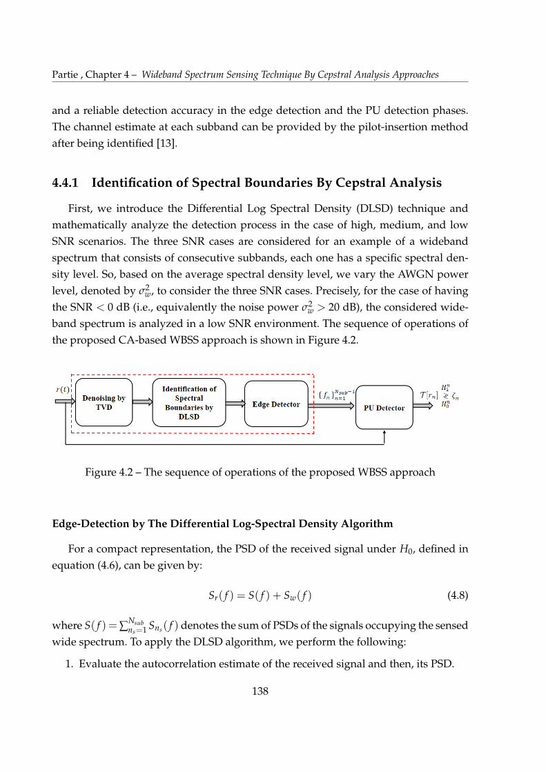
Partie , Chapter 4 – Wideband Spectrum Sensing Technique By Cepstral Analysis Approaches
and a reliable detection accuracy in the edge detection and the PU detection phases.
The channel estimate at each subband can be provided by the pilot-insertion method
after being identified [13].
4.4.1 Identification of Spectral Boundaries By Cepstral Analysis
First, we introduce the Differential Log Spectral Density (DLSD) technique and
mathematically analyze the detection process in the case of high, medium, and low
SNR scenarios. The three SNR cases are considered for an example of a wideband
spectrum that consists of consecutive subbands, each one has a specific spectral den-
sity level. So, based on the average spectral density level, we vary the AWGN power
level, denoted by σ2w, to consider the three SNR cases. Precisely, for the case of having
the SNR < 0 dB (i.e., equivalently the noise power σ2w > 20 dB), the considered wide-
band spectrum is analyzed in a low SNR environment. The sequence of operations of
the proposed CA-based WBSS approach is shown in Figure 4.2.
Figure 4.2 – The sequence of operations of the proposed WBSS approach
Edge-Detection by The Differential Log-Spectral Density Algorithm
For a compact representation, the PSD of the received signal under H0, defined in
equation (4.6), can be given by:
Sr( f ) = S( f ) + Sw( f ) (4.8)
where S( f ) = ∑Nsubns=1 Sns( f ) denotes the sum of PSDs of the signals occupying the sensed
wide spectrum. To apply the DLSD algorithm, we perform the following:
1. Evaluate the autocorrelation estimate of the received signal and then, its PSD.
138
4.4. The Proposed Wideband Spectrum Sensing Approach
2. Evaluate the first derivative of the autocepstrum of the received signal in the
frequency domain.
For convenience, by applying the natural logarithm to equation (4.8), we obtain:
Zr( f ) = log Sr( f )
= log[Sw( f )] + log [γ0( f ) + 1](4.9)
where γ0( f ) = S( f )Sw( f )
defines the relative PSD variations of the transmitted wideband
signal to the noise. The nsth spectral peak identifying the ns
th subband boundary is
located at:
fns = arg {| D( f )|} , fns 2 [ f1, fNsub�1] (4.10)
where arg(.) defines the argument of a function within the round parenthesis, and
D( f ) = dd f Zr( f ) represents the DLSD function. Accordingly, we need to analyze Zr( f )
in case of a medium-to-high SNR environment as well as a low SNR environment.
Since the PSD level of the noise is assumed to be constant, getting its natural log-
arithm decreases the PSD value. Therefore, the value Zw( f ) = log [Sw( f )] is much
lower than log [γ0( f ) + 1]. By taking the derivative of Zr( f ), we can consider that
Dw( f ) = dd f log [Sw( f )] ⇡ 0, then we obtain:
D( f ) =d
d flog[γ0( f ) + 1] =
11 + γ0( f )
d
d fγ0( f ) (4.11)
substituting equation (4.8) in equation (4.11), we get:
D( f ) =1
S( f ) + Sw( f )
Nsub
∑n=1
d
d fSn( f ) (4.12)
According to equation (4.12), and for the case of a medium-to-high SNR, the relative
PSD variations is assumed γ0( f ) >> 1, then equation (4.12) can be reduced to:
D( f ) ⇡ 1S( f )
d
d fS( f ) (4.13)
whereas for the low SNR case, γ0( f ) << 1, then we obtain:
D( f ) ⇡ 2N0
d
d fS( f ) (4.14)
139

Partie , Chapter 4 – Wideband Spectrum Sensing Technique By Cepstral Analysis Approaches
To clarify the concept, Figure 4.3 shows the low PSD level of the AWGN after apply-
ing the DLSD technique and justifies the approximation applied in equation (4.11). Fig-
ure 4.4 gives another example of the wideband spectrum scenario that consists a group
of consecutive flat piece-wise subbchannels. In that example, the wideband spectrum
is ranging from 50 to 250 GHz, such that each subband has a specific spectral density
level within its corresponding bandwidth. Also, in Table 4.1 indicates the SNR values
for each subband with respect to the noise variance.
Figure 4.3 – Illustration of the effect of applying the DLSD to the AWGN spectrum.
The effect of applying the proposed DLSD technique for the case of low, medium or
high noise power with respect to the average PSD level of the consecutive subbands is
illustrated in Figure 4.5, 4.6, and 4.7. For the case of low and medium noise variances
(precisely, σ2w = 14.7 dB and σ2
w = 20 dB), the spectral boundaries are clearly distin-
guishable from the noisy edges. When the noisy spectral variations are high, as shown
in Figure 4.7, the actual spectral boundaries are hardly being differentiated from the
spurious edges and may result in detection errors.
140
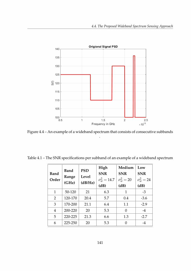
4.4. The Proposed Wideband Spectrum Sensing Approach
Figure 4.4 – An example of a wideband spectrum that consists of consecutive subbands.
Table 4.1 – The SNR specifications per subband of an example of a wideband spectrum
Band
Order
Band
Range
(GHz)
PSD
Level
(dB/Hz)
High
SNR
σ2w = 14.7
(dB)
Medium
SNR
σ2w = 20
(dB)
Low
SNR
σ2w = 24
(dB)
1 50-120 21 6.3 1 -3
2 120-170 20.4 5.7 0.4 -3.6
3 170-200 21.1 6.4 1.1 -2.9
4 200-220 20 5.3 0 -4
5 220-225 21.3 6.6 1.3 -2.7
6 225-250 20 5.3 0 -4
141
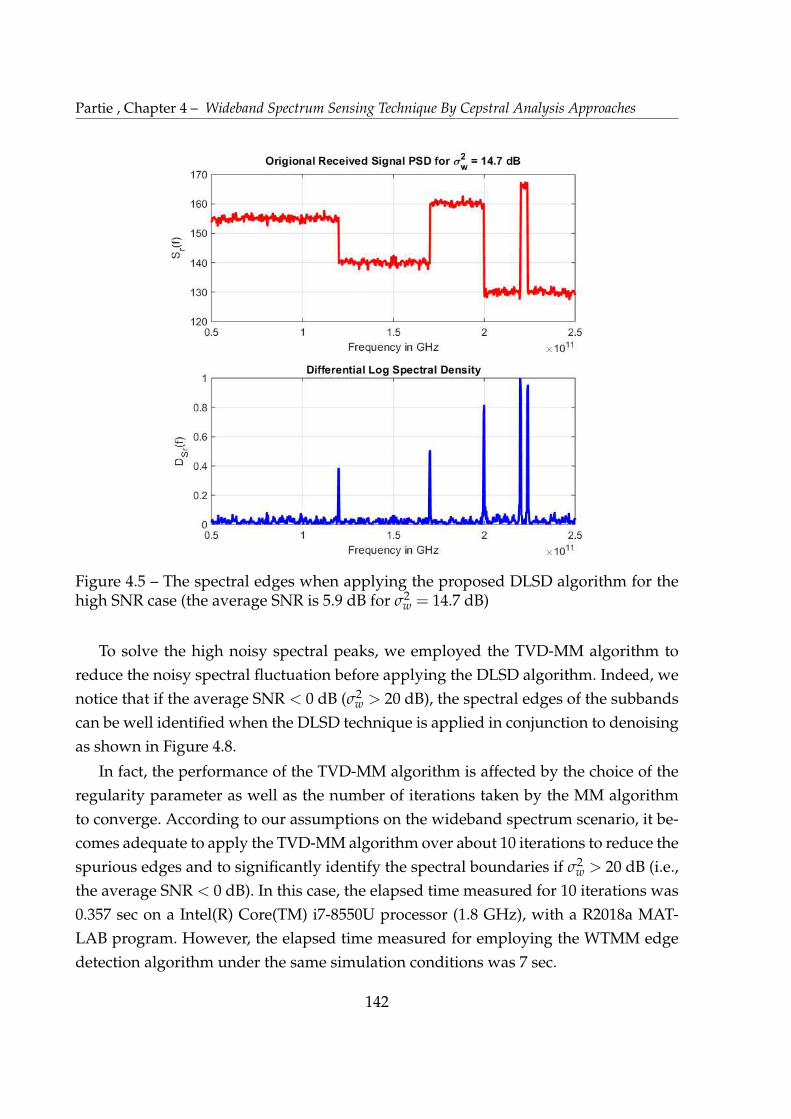
Partie , Chapter 4 – Wideband Spectrum Sensing Technique By Cepstral Analysis Approaches
Figure 4.5 – The spectral edges when applying the proposed DLSD algorithm for thehigh SNR case (the average SNR is 5.9 dB for σ2
w = 14.7 dB)
To solve the high noisy spectral peaks, we employed the TVD-MM algorithm to
reduce the noisy spectral fluctuation before applying the DLSD algorithm. Indeed, we
notice that if the average SNR < 0 dB (σ2w > 20 dB), the spectral edges of the subbands
can be well identified when the DLSD technique is applied in conjunction to denoising
as shown in Figure 4.8.
In fact, the performance of the TVD-MM algorithm is affected by the choice of the
regularity parameter as well as the number of iterations taken by the MM algorithm
to converge. According to our assumptions on the wideband spectrum scenario, it be-
comes adequate to apply the TVD-MM algorithm over about 10 iterations to reduce the
spurious edges and to significantly identify the spectral boundaries if σ2w > 20 dB (i.e.,
the average SNR < 0 dB). In this case, the elapsed time measured for 10 iterations was
0.357 sec on a Intel(R) Core(TM) i7-8550U processor (1.8 GHz), with a R2018a MAT-
LAB program. However, the elapsed time measured for employing the WTMM edge
detection algorithm under the same simulation conditions was 7 sec.
142
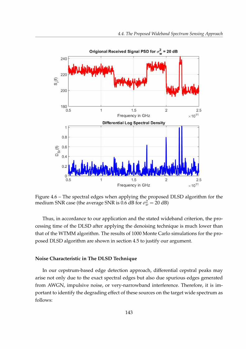
4.4. The Proposed Wideband Spectrum Sensing Approach
Figure 4.6 – The spectral edges when applying the proposed DLSD algorithm for themedium SNR case (the average SNR is 0.6 dB for σ2
w = 20 dB)
Thus, in accordance to our application and the stated wideband criterion, the pro-
cessing time of the DLSD after applying the denoising technique is much lower than
that of the WTMM algorithm. The results of 1000 Monte Carlo simulations for the pro-
posed DLSD algorithm are shown in section 4.5 to justify our argument.
Noise Characteristic in The DLSD Technique
In our cepstrum-based edge detection approach, differential cepstral peaks may
arise not only due to the exact spectral edges but also due spurious edges generated
from AWGN, impulsive noise, or very-narrowband interference. Therefore, it is im-
portant to identify the degrading effect of these sources on the target wide spectrum as
follows:
143
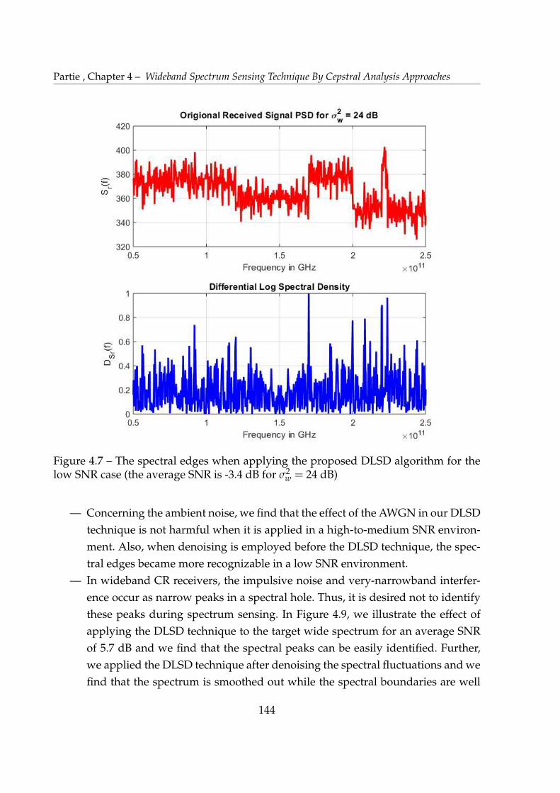
Partie , Chapter 4 – Wideband Spectrum Sensing Technique By Cepstral Analysis Approaches
Figure 4.7 – The spectral edges when applying the proposed DLSD algorithm for thelow SNR case (the average SNR is -3.4 dB for σ2
w = 24 dB)
— Concerning the ambient noise, we find that the effect of the AWGN in our DLSD
technique is not harmful when it is applied in a high-to-medium SNR environ-
ment. Also, when denoising is employed before the DLSD technique, the spec-
tral edges became more recognizable in a low SNR environment.
— In wideband CR receivers, the impulsive noise and very-narrowband interfer-
ence occur as narrow peaks in a spectral hole. Thus, it is desired not to identify
these peaks during spectrum sensing. In Figure 4.9, we illustrate the effect of
applying the DLSD technique to the target wide spectrum for an average SNR
of 5.7 dB and we find that the spectral peaks can be easily identified. Further,
we applied the DLSD technique after denoising the spectral fluctuations and we
find that the spectrum is smoothed out while the spectral boundaries are well
144
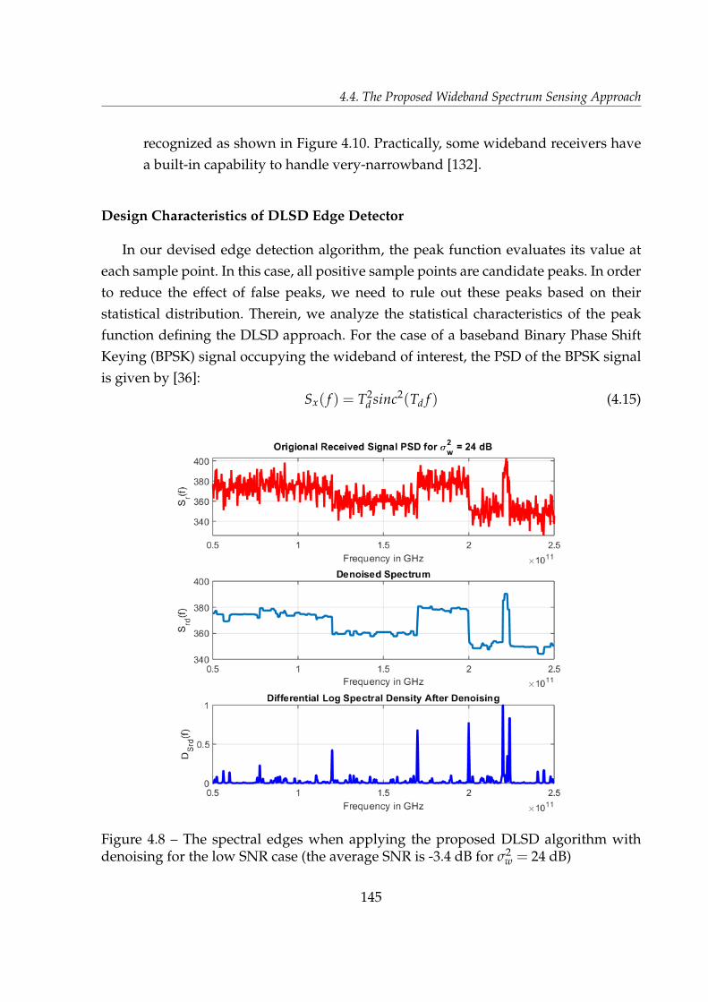
4.4. The Proposed Wideband Spectrum Sensing Approach
recognized as shown in Figure 4.10. Practically, some wideband receivers have
a built-in capability to handle very-narrowband [132].
Design Characteristics of DLSD Edge Detector
In our devised edge detection algorithm, the peak function evaluates its value at
each sample point. In this case, all positive sample points are candidate peaks. In order
to reduce the effect of false peaks, we need to rule out these peaks based on their
statistical distribution. Therein, we analyze the statistical characteristics of the peak
function defining the DLSD approach. For the case of a baseband Binary Phase Shift
Keying (BPSK) signal occupying the wideband of interest, the PSD of the BPSK signal
is given by [36]:
Sx( f ) = T2d sinc2(Td f ) (4.15)
Figure 4.8 – The spectral edges when applying the proposed DLSD algorithm withdenoising for the low SNR case (the average SNR is -3.4 dB for σ2
w = 24 dB)
145

Partie , Chapter 4 – Wideband Spectrum Sensing Technique By Cepstral Analysis Approaches
Figure 4.9 – The spectral edges when applying the proposed DLSD algorithm if impul-sive noise is imposed at average SNR of 5.7 dB
where Td denotes the symbol duration. The peak function, based on the DLSD ap-
proach described in Equation (4.12), is given by:
P( f ) = |D( f )| =�
�
�
dd f Sr( f )
S( f ) + Sw( f )
�
�
� (4.16)
in this case, if the noise at the CR receiver is assumed to be real Gaussian and based
on equation (4.1), the estimate of Sw( f ) follows a Chi-squared distribution, χ21, with
one degree of freedom. Accordingly, the edge detection problem can be formulated as
a binary hypothesis test by:
P( f ) =
8
>
<
>
:
P0( f ) = |d
d f Sr( f )
Sw( f )| : Under Ho
P1( f ) = |d
d f Sr( f )
S( f )+Sw( f )| : Under H1
(4.17)
146
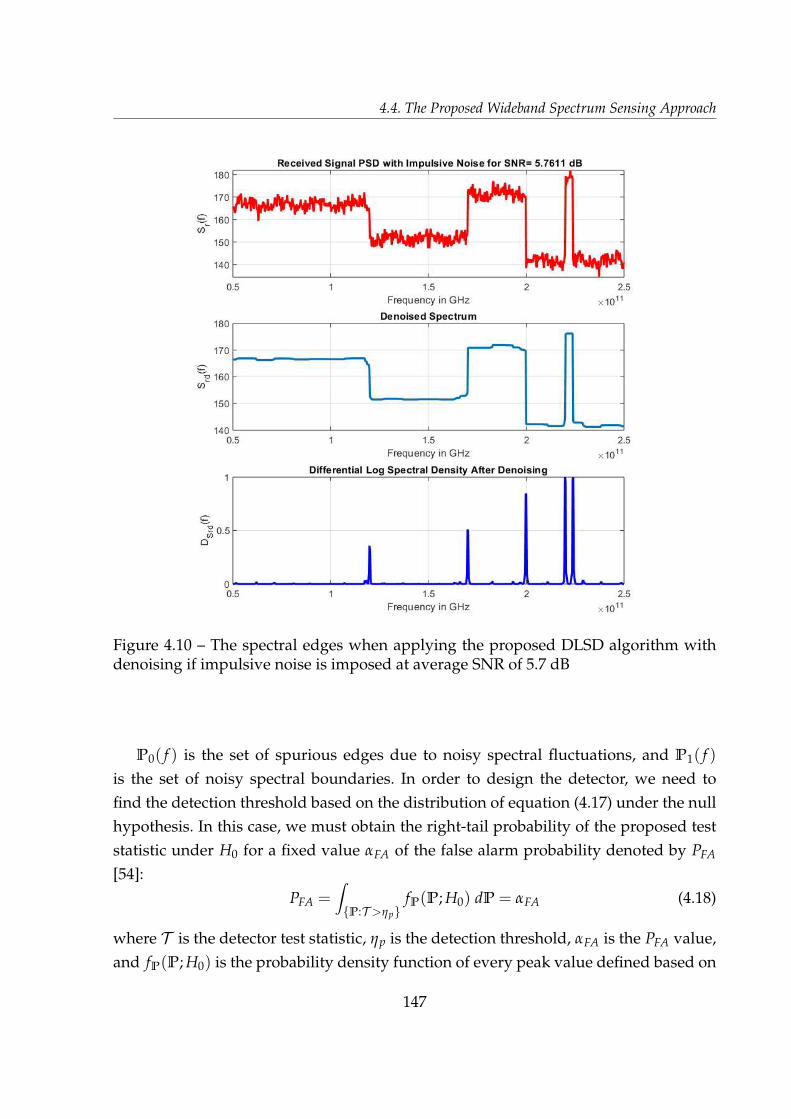
4.4. The Proposed Wideband Spectrum Sensing Approach
Figure 4.10 – The spectral edges when applying the proposed DLSD algorithm withdenoising if impulsive noise is imposed at average SNR of 5.7 dB
P0( f ) is the set of spurious edges due to noisy spectral fluctuations, and P1( f )
is the set of noisy spectral boundaries. In order to design the detector, we need to
find the detection threshold based on the distribution of equation (4.17) under the null
hypothesis. In this case, we must obtain the right-tail probability of the proposed test
statistic under H0 for a fixed value αFA of the false alarm probability denoted by PFA
[54]:
PFA =Z
{P:T >ηp}fP(P; H0) dP = αFA (4.18)
where T is the detector test statistic, ηp is the detection threshold, αFA is the PFA value,
and fP(P; H0) is the probability density function of every peak value defined based on
147
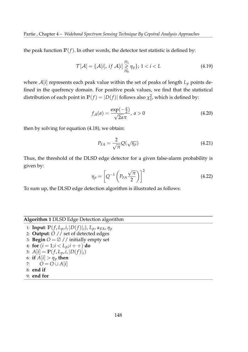
Partie , Chapter 4 – Wideband Spectrum Sensing Technique By Cepstral Analysis Approaches
the peak function P( f ). In other words, the detector test statistic is defined by:
T [A] = {A[i], i f A[i]H1?H0
ηp}; 1 < i < L (4.19)
where A[i] represents each peak value within the set of peaks of length Lp points de-
fined in the quefrency domain. For positive peak values, we find that the statistical
distribution of each point in P( f ) = |D( f )| follows also χ21, which is defined by:
fA(a) =exp(� a
2)p2aπ
, a > 0 (4.20)
then by solving for equation (4.18), we obtain:
PFA =2pπ
Q(p
ηp) (4.21)
Thus, the threshold of the DLSD edge detector for a given false-alarm probability is
given by:
ηp =
Q�1✓
PFA
pπ
2
◆�2
(4.22)
To sum up, the DLSD edge detection algorithm is illustrated as follows:
Algorithm 1 DLSD Edge Detection algorithm
1: Input: P( f , Lp, i, |D( f )|i), Lp, αFA, ηp
2: Output: O // set of detected edges3: Begin O = ∅ // initially empty set4: for (i = 1; i < Lp; i ++) do5: A[i] = P( f , Lp, i, |D( f )|i)6: if A[i] > ηp then7: O = O [ A[i]8: end if9: end for
148
4.5. PU Detection Under Frequency Uncertainty by The BB-ACD Technique:
4.5 PU Detection Under Frequency Uncertainty by The
BB-ACD Technique:
The proposed BaseBand-AutoCepstrum Detection (BB-ACD) Technique consists of
a circular topological filter followed by the PB-ACD. The circular topological filter uti-
lizes the circular topology of a typical sinusoidal signal to separate the baseband sig-
nal or its squared version. The detection of a noise-like PU signal, or a conventional
digitally modulated signal, by the PB-ACD technique depends on the presence of a
strong peak appearing at a quefrency value equivalent to the reciprocal of the center
frequency of a certain subband. Due to the possible frequency estimation errors from
the edge detection phase, the PB-ACD gives a poor performance. Thus, our objective is
to utilize the baseband features of the target signal appearing in the power cepstrum of
the received signal. Specifically, we exploit the peaks reflecting the periodicity appears
in the power cepstrum of the nsth baseband signal. These peaks interpret the presence
of digitally modulated symbols of a possible PU signal. By using the combination of the
Hilbert Filtering (HF) and the Square Law Device (SLD), we can obtain the required
term representing the baseband signal. A functional block diagram of the proposed
BB-ACD is shown in Figure 4.11. To illustrate the concept, we notice in Figure 4.12 that
the autocepstrum of a passband DS-SS signal reveals a major peak that appears at the
reciprocal of the carrier frequency after getting the inverse Fourier Transform of the au-
tocepstrum, whereas a periodicity is revealed in the baseband version of the frequency
domain version of the autocepstrum in Figure 4.13. This is shown at multiples of the
reciprocal of the bit duration of the DS-SS signal.
To illustrate the calculus, consider a digitally modulated carrier signal, Bd(t), which
is defined by:
Bd(t) = B(t) cos(2π fcn t) (4.23)
where B(t) is the baseband signal, and fcn is the carrier frequency (i.e., the center fre-
quency of the nsth subband). Assuming that B(t) is narrow band as compared to fcn ,
the output O(t) of theCLT after applying Hilbert filtering to equation (4.23), is given
by:
O(t) = B2d(t) + [BH
d (t)]2 = B2(t) (4.24)
where (.)H denotes the Hilbert version. Practically, the carrier frequency will be re-
placed with fe = fcn ± δ f , where fe indicates the estimated center frequency.
149

Partie , Chapter 4 – Wideband Spectrum Sensing Technique By Cepstral Analysis Approaches
Figure 4.11 – The system architecture of the proposed baseband autocepstrum tech-nique; CLT denotes the circular topological filter
Also, δ f is the frequency deviation from the actual carrier frequency that causes the
estimation error. The noise effect at the CR receiver is considered for the AWGN noise
w(t), hence, the output O(t) becomes:
O(t) =[Bd(t) + w(t)]2 + [BHd (t) + wH(t)]2
=Bs(t) + Es(t) + 2B(t) [w(t)cos(2π fcn t) + wH(t)sin(2π fcn t)](4.25)
In equation (4.25), the squared baseband version of the signal, B2(t), is denoted by
Bs(t), and Es(t) = w2(t) + (wH(t))2 denotes the squared envelope of the noise signal.
However, it is required to eliminate the high frequency terms before defining the de-
tector test statistic. A possible solution is to apply the autocepstrum approach. To do
this, first, we determine the autocorrelation of O(t) such that:
RO(τ) ⇡ RBs(τ) + REs(τ) (4.26)
then, by getting the Fourier Transform of RO(τ), we obtain the corresponding PSD
terms by:
SO( f ) ⇡ SBs( f ) + SEs( f ) (4.27)
By taking the natural logarithm of SO( f ), we get the autocepstrum by:
ZO( f ) = log[SBs( f ) + SEs( f )] (4.28)
150
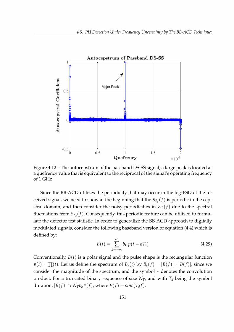
4.5. PU Detection Under Frequency Uncertainty by The BB-ACD Technique:
Figure 4.12 – The autocepstrum of the passband DS-SS signal; a large peak is located ata quefrency value that is equivalent to the reciprocal of the signal’s operating frequencyof 1 GHz
Since the BB-ACD utilizes the periodicity that may occur in the log-PSD of the re-
ceived signal, we need to show at the beginning that the SBs( f ) is periodic in the cep-
stral domain, and then consider the noisy periodicities in ZO( f ) due to the spectral
fluctuations from SEs( f ). Consequently, this periodic feature can be utilized to formu-
late the detector test statistic. In order to generalize the BB-ACD approach to digitally
modulated signals, consider the following baseband version of equation (4.4) which is
defined by:
B(t) =∞
∑k=�∞
bk p(t � kTs) (4.29)
Conventionally, B(t) is a polar signal and the pulse shape is the rectangular function
p(t) = ∏(t). Let us define the spectrum of Bs(t) by Bs( f ) = |B( f )| ⇤ |B( f )|, since we
consider the magnitude of the spectrum, and the symbol ⇤ denotes the convolution
product. For a truncated binary sequence of size NT, and with Td being the symbol
duration, |B( f )| ⇡ NTbkP( f ), where P( f ) = sinc(Td f ).
151
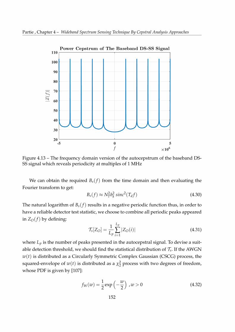
Partie , Chapter 4 – Wideband Spectrum Sensing Technique By Cepstral Analysis Approaches
Figure 4.13 – The frequency domain version of the autocepstrum of the baseband DS-SS signal which reveals periodicity at multiples of 1 MHz
We can obtain the required Bs( f ) from the time domain and then evaluating the
Fourier transform to get:
Bs( f ) ⇡ N2Tb2
k sinc2(Td f ) (4.30)
The natural logarithm of Bs( f ) results in a negative periodic function thus, in order to
have a reliable detector test statistic, we choose to combine all periodic peaks appeared
in ZO( f ) by defining:
Ts[ZO] =1
Lp
Lp
∑i=1
|ZO(i)| (4.31)
where Lp is the number of peaks presented in the autocepstral signal. To devise a suit-
able detection threshold, we should find the statistical distribution of Ts. If the AWGN
w(t) is distributed as a Circularly Symmetric Complex Gaussian (CSCG) process, the
squared-envelope of w(t) is distributed as a χ22 process with two degrees of freedom,
whose PDF is given by [107]:
fW(w) =12
exp⇣
�w
2
⌘
, w > 0 (4.32)
152
4.6. Numerical Results and Discussions
Thus, the statistical distribution of T follows a Modulus Log Chi-Squared (MLCS) (i.e.,
Modulus-log�χ2(2)) distribution. By using the PDF approach of the transformation of
random variables, the MLCS distribution is given by:
fTs(ts) =
12
exp✓
ts �12
exp(ts)
◆
+12
exp✓
�ts �12
exp(�ts)
◆
(4.33)
as demonstrated in Appendix C.
In order to get an expression for the detector threshold ζ, we follow the same con-
cept indicated in equation (4.18) for a fixed false-alarm probability PFA. By employing
the method of substitution, we obtain:
PFA = exp
� exp(ζ)2
!
� exp
� exp(�ζ)
2
!
+ 1 (4.34)
also, we can simplify equation (4.34) by decomposing the exponential terms and sub-
stitute for sinh(ζ) = 0.5[exp(ζ) + exp(�ζ)], then we obtain:
PFA = exp
� exp(ζ)2
!
+ 2exp
� exp(�ζ)
4
!
sinh
exp(�ζ)
4
!
(4.35)
The approximation of the hyperbolic function can be given by Taylor expansion. How-
ever, the Taylor series diverges to infinity, so a closed form expression for ζ cannot be
found analytically, and equation (4.35) can be solved numerically by different methods
such as the Newton Raphson Method [138].
4.6 Numerical Results and Discussions
In order to validate the efficacy of the proposed wideband spectrum sensing ap-
proach, we begin with evaluating the performance of the proposed DLSD technique
as opposed to different wavelet-based edge detection techniques. This evaluation in-
cludes calculating the average detection error probability Pe as mentioned in [135],
which is given in terms of the probability of misdetecting an actual spectral bound-
ary, PMD, and the probability of falsely detecting a spurious edge PFD. Then, we show
the applicability of the proposed BB-ACD technique to different digitally modulated
signals. We also address the problem of detecting noise-like signals by the PB-ACD
153

Partie , Chapter 4 – Wideband Spectrum Sensing Technique By Cepstral Analysis Approaches
technique under the carrier frequency uncertainty, and we show the advantage of ap-
plying the proposed BB-ACD instead.
4.6.1 Performance Evaluation of The Proposed Edge Detection Ap-
proach:
The frequency of the wideband spectrum under consideration extends from 30 GHz
to 300 GHz. The proposed algorithm is simulated through randomly generated spec-
trum models for generalization. The average PSD level within each occupied subband
is maintained to 6 W/Hz assuming 60% of spectrum occupancy rate. Although the
assumed average PSD level is large as opposed to normal radiation levels in practical
settings, it is chosen to match the chosen specifications in [132] for the sake of compari-
son. The characteristics of each spectrum model are generated randomly. They include
the number of subchannels within the wideband of interest, the exact spectral bound-
aries, and the signal power specified in each subband. These subbands are assumed
to have different bandwidths to match up with the diversity of the transmission tech-
nologies.
Further, depending on the distance between the CR receiver and the transmission
station in the occupied subband, as well as the status of the spectrum occupancy, the
SNR level is assumed to differ from one subband to another. The performance of the
proposed technique is tested by adding white Gaussian noise with the same power to
the received RF stimuli corresponding to the whole sensed spectrum while maintain-
ing the same average PSD level in all spectrum models. A summary of the simulation
parameters are listed in Table 4.2. For clarification, Table 4.3 shows the detailed infor-
mation of an example of a randomly generated PSD model shown in Figure 4.14. The
Simulations are done with R2018a MATLAB, and the obtained results are based on
1000 Monte Carlo trials.
First, we discuss the effects of applying the DLSD algorithm on spurious edges
generated by the noisy spectral variations in PFD. In Figure 4.15, at considerably low-
to-medium noise power (i.e., over the range [10,22] dB), we notice that the proposed
DLSD algorithm outperforms the WTMM, the WTMS, or the improved WTMM al-
gorithms. Thanks to the ability of the cepstral analysis approach to reduce the noisy
spectral variations. In fact, the white Gaussian noise’s cepstrum becomes a Dirac im-
pulse at the zeroth quefrency value. Clearly, this characterization of the AWGN in the
154
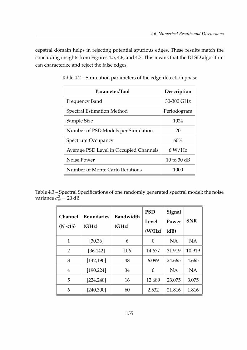
4.6. Numerical Results and Discussions
cepstral domain helps in rejecting potential spurious edges. These results match the
concluding insights from Figures 4.5, 4.6, and 4.7. This means that the DLSD algorithm
can characterize and reject the false edges.
Table 4.2 – Simulation parameters of the edge-detection phase
Parameter/Tool Description
Frequency Band 30-300 GHz
Spectral Estimation Method Periodogram
Sample Size 1024
Number of PSD Models per Simulation 20
Spectrum Occupancy 60%
Average PSD Level in Occupied Channels 6 W/Hz
Noise Power 10 to 30 dB
Number of Monte Carlo Iterations 1000
Table 4.3 – Spectral Specifications of one randomly generated spectral model; the noisevariance σ2
w = 20 dB
Channel
(N <15)
Boundaries
(GHz)
Bandwidth
(GHz)
PSD
Level
(W/Hz)
Signal
Power
(dB)
SNR
1 [30,36] 6 0 NA NA
2 [36,142] 106 14.677 31.919 10.919
3 [142,190] 48 6.099 24.665 4.665
4 [190,224] 34 0 NA NA
5 [224,240] 16 12.689 23.075 3.075
6 [240,300] 60 2.532 21.816 1.816
155

Partie , Chapter 4 – Wideband Spectrum Sensing Technique By Cepstral Analysis Approaches
Figure 4.14 – An example of a noisy spectral model
From literature, the major drawback of the WTMM algorithm is the increased num-
ber of spurious edges which cannot be eliminated even with a threshold-based detec-
tion [11]. The superior performance of the WTMS technique over the WTMM tech-
nique is due to the averaging effect of the WTMS algorithm over the noisy spectral
edges. However, as shown in Figure 4.7, if the noise power increases (i.e., above 22
dB), the performance of the DLSD algorithm decreases due to the increased number of
spurious edges. To improve the DLSD performance, we employed the TVD-MM algo-
rithm in order to reduce the noisy fluctuations before applying the DLSD technique.
We employed the TVD-MM algorithm on about 10 iterations with two different reg-
ularity parameters: α = 0.9 and 1.2 respectively. As seen in Figures 4.8 and 4.15, the
employment of denoising before applying the DLSD algorithm helped in reducing the
spurious edges and hence reducing the PFD.
Precisely, for a noise power value over the range [10,22] dB, the DLSD algorithm
with denoising outperforms the four considered algorithm, and performs similar to
the improved WTMM algorithm for σ2w > 22 dB. Considering the probability of misde-
156
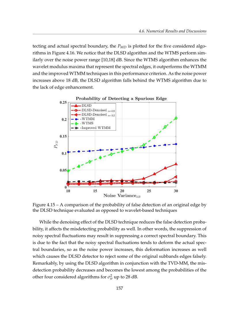
4.6. Numerical Results and Discussions
tecting and actual spectral boundary, the PMD is plotted for the five considered algo-
rithms in Figure 4.16. We notice that the DLSD algorithm and the WTMS perform sim-
ilarly over the noise power range [10,18] dB. Since the WTMS algorithm enhances the
wavelet modulus maxima that represent the spectral edges, it outperforms the WTMM
and the improved WTMM techniques in this performance criterion. As the noise power
increases above 18 dB, the DLSD algorithm falls behind the WTMS algorithm due to
the lack of edge enhancement.
Figure 4.15 – A comparison of the probability of false detection of an original edge bythe DLSD technique evaluated as opposed to wavelet-based techniques
While the denoising effect of the DLSD technique reduces the false detection proba-
bility, it affects the misdetecting probability as well. In other words, the suppression of
noisy spectral fluctuations may result in suppressing a correct spectral boundary. This
is due to the fact that the noisy spectral fluctuations tends to deform the actual spec-
tral boundaries, so as the noise power increases, this deformation increases as well
which causes the DLSD detector to reject some of the original subbands edges falsely.
Remarkably, by using the DLSD algorithm in conjunction with the TVD-MM, the mis-
detection probability decreases and becomes the lowest among the probabilities of the
other four considered algorithms for σ2w up to 28 dB.
157
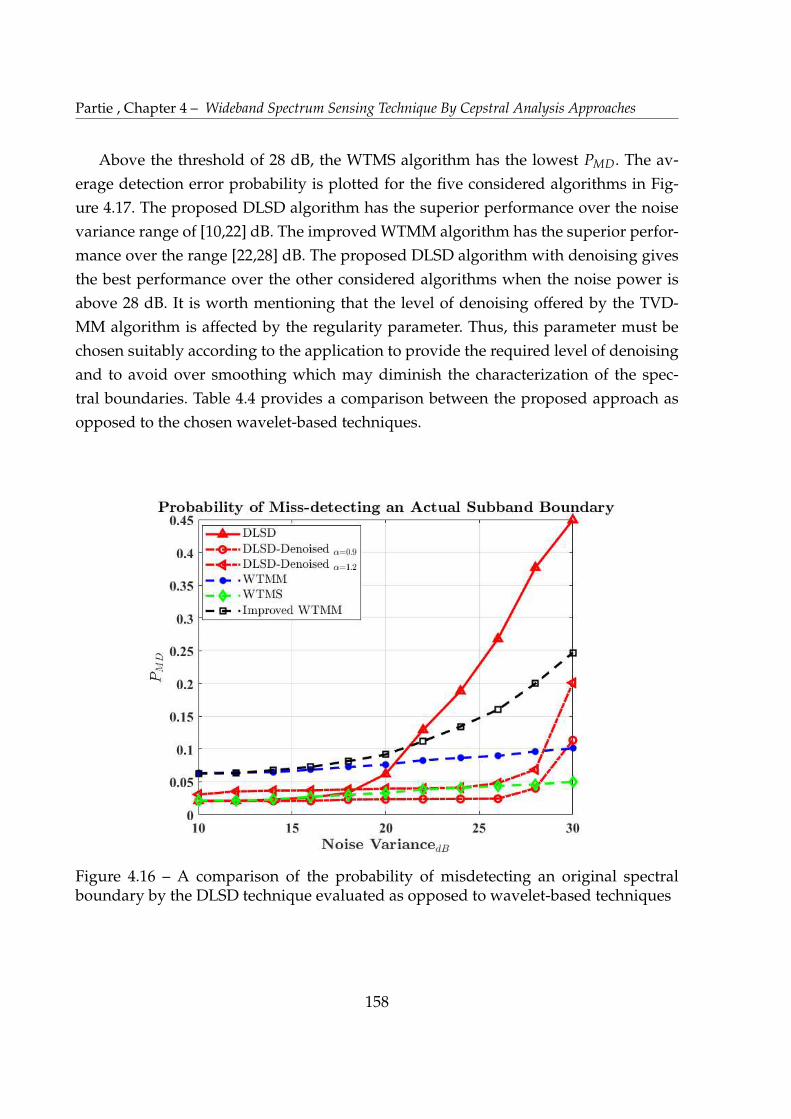
Partie , Chapter 4 – Wideband Spectrum Sensing Technique By Cepstral Analysis Approaches
Above the threshold of 28 dB, the WTMS algorithm has the lowest PMD. The av-
erage detection error probability is plotted for the five considered algorithms in Fig-
ure 4.17. The proposed DLSD algorithm has the superior performance over the noise
variance range of [10,22] dB. The improved WTMM algorithm has the superior perfor-
mance over the range [22,28] dB. The proposed DLSD algorithm with denoising gives
the best performance over the other considered algorithms when the noise power is
above 28 dB. It is worth mentioning that the level of denoising offered by the TVD-
MM algorithm is affected by the regularity parameter. Thus, this parameter must be
chosen suitably according to the application to provide the required level of denoising
and to avoid over smoothing which may diminish the characterization of the spec-
tral boundaries. Table 4.4 provides a comparison between the proposed approach as
opposed to the chosen wavelet-based techniques.
Figure 4.16 – A comparison of the probability of misdetecting an original spectralboundary by the DLSD technique evaluated as opposed to wavelet-based techniques
158
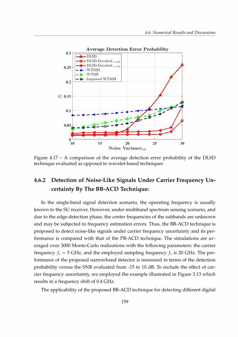
4.6. Numerical Results and Discussions
Figure 4.17 – A comparison of the average detection error probability of the DLSDtechnique evaluated as opposed to wavelet-based techniques
4.6.2 Detection of Noise-Like Signals Under Carrier Frequency Un-
certainty By The BB-ACD Technique:
In the single-band signal detection scenario, the operating frequency is usually
known to the SU receiver. However, under multiband spectrum sensing scenario, and
due to the edge-detection phase, the center frequencies of the subbands are unknown
and may be subjected to frequency estimation errors. Thus, the BB-ACD technique is
proposed to detect noise-like signals under carrier frequency uncertainty and its per-
formance is compared with that of the PB-ACD technique. The simulations are av-
eraged over 3000 Monte-Carlo realizations with the following parameters: the carrier
frequency fc = 5 GHz, and the employed sampling frequency fs is 20 GHz. The per-
formance of the proposed narrowband detector is measured in terms of the detection
probability versus the SNR evaluated from -15 to 10 dB. To include the effect of car-
rier frequency uncertainty, we employed the example illustrated in Figure 3.13 which
results in a frequency shift of 0.4 GHz.
The applicability of the proposed BB-ACD technique for detecting different digital
159
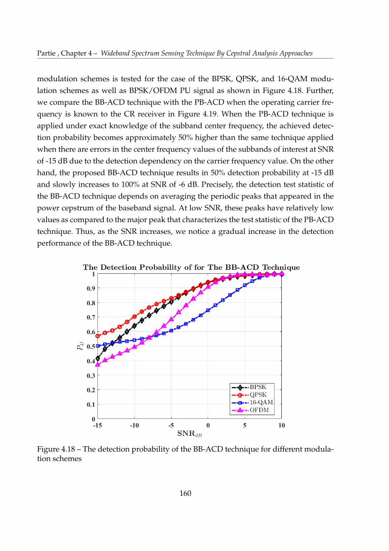
Partie , Chapter 4 – Wideband Spectrum Sensing Technique By Cepstral Analysis Approaches
modulation schemes is tested for the case of the BPSK, QPSK, and 16-QAM modu-
lation schemes as well as BPSK/OFDM PU signal as shown in Figure 4.18. Further,
we compare the BB-ACD technique with the PB-ACD when the operating carrier fre-
quency is known to the CR receiver in Figure 4.19. When the PB-ACD technique is
applied under exact knowledge of the subband center frequency, the achieved detec-
tion probability becomes approximately 50% higher than the same technique applied
when there are errors in the center frequency values of the subbands of interest at SNR
of -15 dB due to the detection dependency on the carrier frequency value. On the other
hand, the proposed BB-ACD technique results in 50% detection probability at -15 dB
and slowly increases to 100% at SNR of -6 dB. Precisely, the detection test statistic of
the BB-ACD technique depends on averaging the periodic peaks that appeared in the
power cepstrum of the baseband signal. At low SNR, these peaks have relatively low
values as compared to the major peak that characterizes the test statistic of the PB-ACD
technique. Thus, as the SNR increases, we notice a gradual increase in the detection
performance of the BB-ACD technique.
Figure 4.18 – The detection probability of the BB-ACD technique for different modula-tion schemes
160
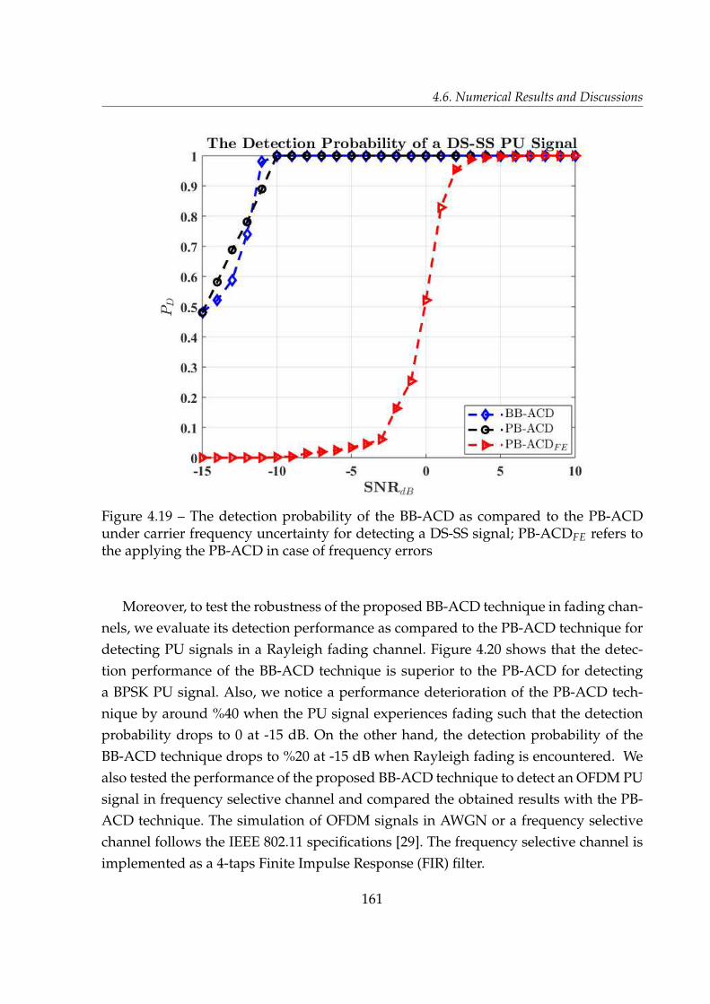
4.6. Numerical Results and Discussions
Figure 4.19 – The detection probability of the BB-ACD as compared to the PB-ACDunder carrier frequency uncertainty for detecting a DS-SS signal; PB-ACDFE refers tothe applying the PB-ACD in case of frequency errors
Moreover, to test the robustness of the proposed BB-ACD technique in fading chan-
nels, we evaluate its detection performance as compared to the PB-ACD technique for
detecting PU signals in a Rayleigh fading channel. Figure 4.20 shows that the detec-
tion performance of the BB-ACD technique is superior to the PB-ACD for detecting
a BPSK PU signal. Also, we notice a performance deterioration of the PB-ACD tech-
nique by around %40 when the PU signal experiences fading such that the detection
probability drops to 0 at -15 dB. On the other hand, the detection probability of the
BB-ACD technique drops to %20 at -15 dB when Rayleigh fading is encountered. We
also tested the performance of the proposed BB-ACD technique to detect an OFDM PU
signal in frequency selective channel and compared the obtained results with the PB-
ACD technique. The simulation of OFDM signals in AWGN or a frequency selective
channel follows the IEEE 802.11 specifications [29]. The frequency selective channel is
implemented as a 4-taps Finite Impulse Response (FIR) filter.
161

Partie , Chapter 4 – Wideband Spectrum Sensing Technique By Cepstral Analysis Approaches
Table 4.4 – Comparing wavelet analysis to cepstral analysis for edge detection in wide-band spectrum sensing
Approach Wavelet Analysis Cepstral Analysis
PostProcessing
Local maxima are foundthrough differentiatingthe filtered PSD.
Local maxima are foundthrough differentiatingthe natural logarithmof a signal’s PSD.
White NoiseCharacteristics
WTMM: calculates the waveletmodulus maxima in the frequencydomain. However, the noise impactaffects detection ofspectral boundaries.
Improved WTMM: exploits thesingularity characteristics ofthe wavelet multiscale toidentify spurious edgesand reject them.Its performance is degraded in lowSNR environment.
WTMP: The product of thefirst derivative of WT isdeveloped for noisesuppression and edgesharpening, but it results inattenuating the edges due tothe multiplication operation.
WTMS: It preserves the edgesinformation and avoids edgesattenuation. Increasing the scalesleads to a better detection performancebut at higher complexity.
Cesptrum:AWGN fluctuations aresuppressed at all thequefrencies values exceptfor a major peak atthe zeroth quefrency.
DLSD: It reduces the noisyspectral variations.
ApplicationVersatility
The detection performancedepends on the analyzed signal andthe used mother wavelet function.
The CA approach dependson the type of thecepstral algorithm usedthat is suitable for theproblem under analysis
ImplementationComplexity
WT is implemented as a bankof filters. Reducing spurious edgescan be accomplished by processingthe signal of interest through allscales which substantially increasesthe computational burden.
Relatively lowerthan the WBD
162

4.6. Numerical Results and Discussions
Figure 4.20 – The detection performance of the BB-ACD technique as compared to thePB-ACD technique in Rayleigh fading channel; PB-ACDRay refers to employing thePB-ACD technique in Rayleigh fading channel
The path delays vector is given as τp = [0,100,35,120] µsec, and the average path
gains vector is given by PG = [0,�1,�1,�3] dB. For a sample period Ts = 1µsec, the
maximum Doppler frequency equals 100 kHz. The detection performance of the BB-
ACD as compared to the PB-ACD under the Doppler frequency shift due to the fre-
quency selective fading channel is shown in Figure 4.21.
According to our simulations, we find that the proposed BB-ACD technique gives
better detection results than the PB-ACD technique at -15 dB, whereas the PB-ACD
starts to significantly detect the PU presence above -4 dB. This means that the effect of
the Doppler frequency shift deteriorates the PB-ACD performance, especially at low
SNR values, while the BB-ACD technique can detect the OFDM PU signal successfully.
Another important performance metric to evaluate the efficacy of the proposed
techniques is computational complexity. In this regard, we analyze the computational
complexity of the DLSD edge detection algorithm followed by the BB-ACD technique
and compare it with the WTMP edge detection technique followed by ED. For a 1D
signal of size N, the edge detection algorithm given by the WTMP technique involves
evaluating the autocorrelation of the received signal followed by the FFT operation to
163

Partie , Chapter 4 – Wideband Spectrum Sensing Technique By Cepstral Analysis Approaches
Figure 4.21 – The detection performance of the BB-ACD technique as compared to thePB-ACD technique in a frequency selective fading channel
obtain the PSD. To identify the spectral boundaries, the received signal’s PSD is fil-
tered by the Fourier Transform of the smoothing wavelet function through a convolu-
tion operation. On the other hand, the proposed DLSD algorithm involves getting the
autocorrelation, the PSD of the received signal followed by the gradient of the natural
logarithm of the signal’s PSD. Table 4.5 summarizes the complexity of the arithmetic
operations involved in evaluating both algorithms.
To perform energy detection, the computational complexity requires O(N) mul-
tiplications and O(N � 1) for the averaging. For the BB-ACD technique, it requires
O(NK) for convolving the received signal with the Hilbert filter of size K, O(N) for the
square-law device, and for the power cepstrum the complexity is similar to the DLSD
algorithm except for that of the differentiation step. Based on Table 4.5, we find that
the complexity of the WTMP is higher than the DLSD algorithm since the complex-
ity of evaluating linear convolution is greater than that of the natural logarithm [139].
However, under the problem of frequency uncertainty, the BB-ACD has a higher com-
plexity than ED or the BED despite its high detection accuracy. A trade-off analysis
between the computational complexity and the maximum detection accuracy can be
164

4.7. Summary
further investigated to highlight the competence of the proposed approach.
Table 4.5 – Summary of the computational complexity of the DLSD algorithm as com-pared to the WTMP algorithm
WTMP DLSD
Arithmetic Operations Complexity
Autocorrelation O(N2)FFT O(N log N)Linear Convolution bya kernel of size K O(NK)Product of ModulusMaxima O(N)
Arithmetic Operations Complexity
Autocorrelation O(N2)FFT O(N log N)Natural Logarithm usingArithmetic-Geometric Mean O(N log N)Automatic or numericalDifferentiation O(N)
4.7 Summary
In this chapter, we proposed a wideband spectrum sensing approach based on the
cepstral analysis of the received signal. It is shown that the spectral boundaries of the
subbands comprising the target wide band can be well identified, in medium-to-high
SNR environment, by employing the proposed DLSD algorithm. Although the detec-
tion of the spectral edges becomes difficult in low SNR environment, the performance
of the proposed DLSD algorithm provides good detection results as compared to dif-
ferent wavelet-based approaches when further denoising is applied. For the PU detec-
tion phase, we tackled the problem of detecting noise-like signals in the SBSA and the
MBSA scenarios. Further, we addressed the problem of the carrier frequency uncer-
tainty in the MBSA and presented the BB-ACD technique to provide better detection
of possible noise-like signals in a low SNR environment. The applicability of the pro-
posed BB-ACD algorithm to different digitally modulated signals is evaluated, and
also its reliability is validated as opposed to the PB-ACD technique for detecting PU
signals in frequency selective fading channels. The periodicity of the baseband digitally
modulated signals that is revealed in the cepstral domain can be effectively utilized for
signal detection. Based on this observation, the Cepstral Covariance Detection (CCD)
is introduced in chapter 5.
165
CHAPTER 5
SPECTRUM SENSING BY CEPSTRAL
COVARIANCE DETECTION IN COGNITIVE
RADIO
5.1 Introduction
Hereinafter, we aim to enhance the Power Cepstrum (PC) of digitally modulated
signals to formulate a generalized spectrum sensing approach. We propose the Cep-
stral Covariance Detection (CCD) technique is to exploit the inherited periodicity of the
digitally modulated baseband signals that is presented in their Power Cepstrum (PC).
In this Chapter, our objective is to utilize the CCD technique to detect the presence
of a possible PU signal in the background noise. Despite being simple and reliable in
high SNR communication environment, the conventional ED has a poor detection per-
formance when the spectral noisy variations exceed the Power Spectral Density (PSD)
level of a PU signal. This is due to the fact that the calculation of the test statistic of the
Energy Detection (ED) technique includes the noise effect. So in a low SNR scenario,
the detector may give false decision about the PU presence which causes false-alarms.
In this case, the CR receiver will initiate the transmission of the SU signal which will
cause harmful interference to the PU signals.
In fact, the concept of the pseudo-autocovaraince technique was first applied to
estimate the time delay between a signal arrival and the arrival of an echo [20]. Pre-
cisely, the presence of digitally modulated signals (i.e., phase or amplitude modulation
schemes) in noise manifests itself as periodic peaks in the PC. In order to take advan-
tage of this property, we introduce the CCD technique for spectrum sensing in CR
systems to improve the process of signal detection in a noisy environment. By correlat-
ing the signals’ PC to a sinusoidal signal having a fundamental frequency equals to the
PC’s periodic frequency, the signal component will be enhanced and the detector will
166
5.2. Signal Model and System Description
simultaneously reject the noisy spectral variations that lead to possible false-alarms.
The rest of the chapter is organized as follows: section 5.2 describes the proposed
system and the signal model. Section 5.3 represents the analytical framework of the
proposed detection technique based on NPL. In section 5.4, the expression of the dis-
tribution of the detection test statistic under the null hypothesis is derived, and the
detection threshold is evaluated. The numerical results are discussed in section 5.5 and
the summary is given in section 5.6.
5.2 Signal Model and System Description
In the following, we apply the signal model we employed in chapter 2. Recall the
formulation of the detection problem, which is given by;
y(t) =
8
<
:
wS(t) : Under Ho
s(t) ⇤ hsens(t;τ) + w(t) : Under H1
(5.1)
where s(t) is the transmitted PU signal, hsens(t;τ) is the sensing channel which is gen-
erally described as a time varying fading channel with delay defined by τ, the convolu-
tion product is denoted by ⇤, and w(t) is the thermal noise presented at the SU receiver
which is modeled as an Additive White Gaussian Noise (AWGN). We assume the chan-
nel information is provided at the CR system, so that we only focus on the spectrum
sensing problem. Accordingly, we consider the sum of faded PU signal xP(t), which is
given by:
xP(t) = s(t) ⇤ hsens(t;τ) (5.2)
5.3 Detection By The Cepstral Covariance Technique
In chapter 3 and chapter 4, we have discussed the employment of the autocepstral
technique for detecting noise-like signals. Based on the proposed BaseBand AutoCep-
strum Detection (BB-ACD) technique, which is introduced in chapter 4, our aim is to
enhance the periodic peaks reflecting the data rate of a given digital signal by employ-
ing the CCD technique. For example, in case of medium-to-high SNR, we can easily
identify the peaks in the BB-ACD technique of the signal reflecting the repetition of the
pseudo random code at the reciprocal of the chip duration Tc for a Direct Sequence-
167
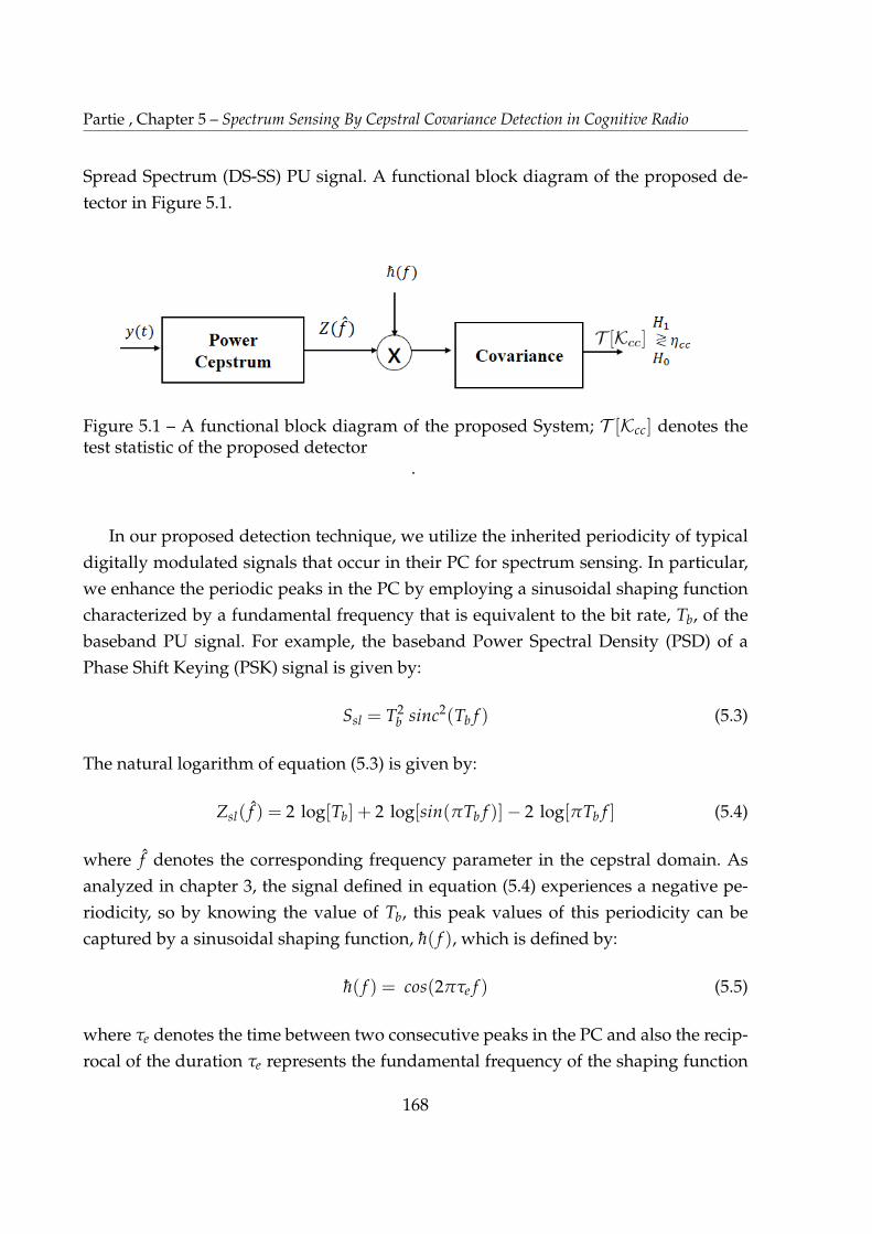
Partie , Chapter 5 – Spectrum Sensing By Cepstral Covariance Detection in Cognitive Radio
Spread Spectrum (DS-SS) PU signal. A functional block diagram of the proposed de-
tector in Figure 5.1.
Figure 5.1 – A functional block diagram of the proposed System; T [Kcc] denotes thetest statistic of the proposed detector
.
In our proposed detection technique, we utilize the inherited periodicity of typical
digitally modulated signals that occur in their PC for spectrum sensing. In particular,
we enhance the periodic peaks in the PC by employing a sinusoidal shaping function
characterized by a fundamental frequency that is equivalent to the bit rate, Tb, of the
baseband PU signal. For example, the baseband Power Spectral Density (PSD) of a
Phase Shift Keying (PSK) signal is given by:
Ssl = T2b sinc2(Tb f ) (5.3)
The natural logarithm of equation (5.3) is given by:
Zsl( f ) = 2 log[Tb] + 2 log[sin(πTb f )]� 2 log[πTb f ] (5.4)
where f denotes the corresponding frequency parameter in the cepstral domain. As
analyzed in chapter 3, the signal defined in equation (5.4) experiences a negative pe-
riodicity, so by knowing the value of Tb, this peak values of this periodicity can be
captured by a sinusoidal shaping function, h( f ), which is defined by:
h( f ) = cos(2πτe f ) (5.5)
where τe denotes the time between two consecutive peaks in the PC and also the recip-
rocal of the duration τe represents the fundamental frequency of the shaping function
168
5.4. Design Characteristics of The Cepstral Covariance Detector
h( f ). Consequently, the cepstral covariance of enhanced PC can be evaluated by:
Kcc(τe) =Z f2
f1
Zsl( f ) h( f ) d f (5.6)
where the frequency range f2 � f1 is the bandwidth of the received signal within the
observation interval T. Therefore, we can define the detection test statistic by:
T [Kcc] = |Kcc(τe)|H1?H0
ηcc (5.7)
where ηcc denotes the detection threshold of the proposed detector.
5.4 Design Characteristics of The Cepstral Covariance De-
tector
To evaluate the detection threshold of the proposed detector, we need to find the
statistical distribution of the detection test statistic, which is given in equation (5.7).
First, we can apply further simplifications to the cepstral covariance function, Kcc, by
representing the integral in equation (5.6) using Riemann sums [140]. For example, Let
F(x) represents a function of which we wish to find a particular definite integral. The
Riemann sums equivalent to an arbitrary integral can be given by [140]:
Z b
aF(x)dx = lim
N!∞
N
∑i=1
∆x F(xi) (5.8)
where a and b are arbitrary constants defining the integral limits, the small segments
of the function F(x) are denoted by ∆x = b�aN , xi = a + i ∆x, and N is the size of the
target function. Similarly, if we define:
F( f ) = Z( f ) h( f ) (5.9)
thus, the Riemann sums equivalent to the integral, defined in equation (5.6), can be
rewritten as:
Kcc(τe) =Z f 2
f 1F( f )d f = lim
N!∞
N
∑i=1
∆ f F( fi) (5.10)
169
Partie , Chapter 5 – Spectrum Sensing By Cepstral Covariance Detection in Cognitive Radio
where the frequency segments are given by ∆ f = f2� f1N , and fi = f1 + i∆ f .
Assume that the received PSD of the PU signal at the CR receiver is given by:
Sy = Ss( f ) + Sw( f ) (5.11)
where Ss( f ) and Sw( f ) denote the PSDs of the PU signal and the background noise,
respectively.Therefore, the enhanced PC can be evaluated by:
F( f ) = log[Ss( f ) + Sw( f )](cos(2π f τe))
= log[Ss( f )](cos(2π f τe)) + log [1 + L( f )] (cos(2π f τe))(5.12)
where L( f ) = Sw( f )Ss( f )
. Clearly, the statistical characterization of the enhanced PC, F( f ),
depends on the statistical distribution of L( f ). If we consider the case of having a good
PSD estimate of the transmitted PU signal, such that L( f ) << 1, thus we can approx-
imate log[1 + L( f )] ⇡ L( f ) [20]. In this case, if w(t) is a real-valued Gaussian noise,
then Sw( f ) follows Chi-squared distribution, χ2. Also, if we only consider a group of
peaks, Np, among the noisy PC, we can redefine the cepstral covariance by:
Kavg(τe) ⇡1
Np
Np
∑i=1
|F( fi)| (5.13)
where fi denotes the location of the ith peak within Np. If Np is sufficiently large and the
enhanced power cepstral peaks are IID, then Kavg(τe) follows a Gaussian distribution
denoted by N (µF, σ2F
Np), where µF and σ2
F are the mean and the variance of the enhanced
PC. Consequently, the false-alarm probability can be given by:
PFA = Q
0
B
B
@
ηcc � µFr
σ2F
Np
1
C
C
A
(5.14)
and the detection threshold of the CCD technique is given by:
ηcc = Q�1(PFA)σFp
Np+ µF (5.15)
Further, if L( f )>> 1, we find that equation (5.12) holds and the statistical distribution
170
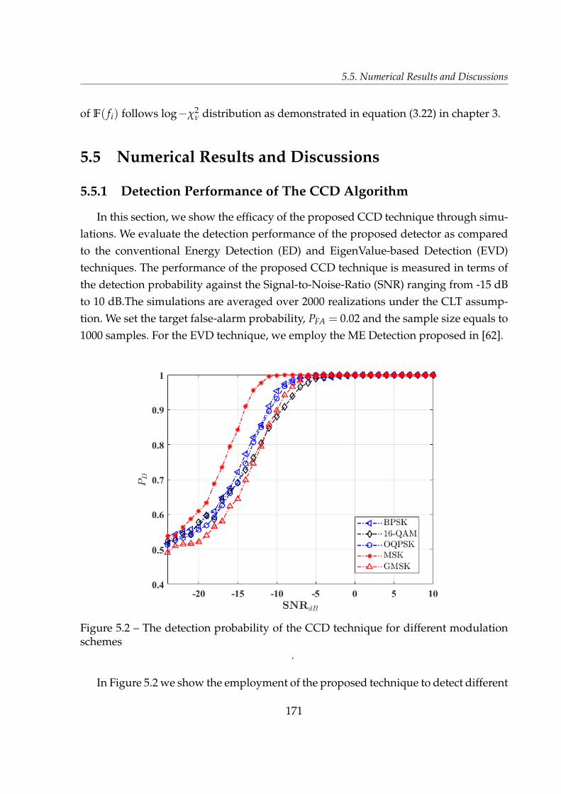
5.5. Numerical Results and Discussions
of F( fi) follows log�χ2ν distribution as demonstrated in equation (3.22) in chapter 3.
5.5 Numerical Results and Discussions
5.5.1 Detection Performance of The CCD Algorithm
In this section, we show the efficacy of the proposed CCD technique through simu-
lations. We evaluate the detection performance of the proposed detector as compared
to the conventional Energy Detection (ED) and EigenValue-based Detection (EVD)
techniques. The performance of the proposed CCD technique is measured in terms of
the detection probability against the Signal-to-Noise-Ratio (SNR) ranging from -15 dB
to 10 dB.The simulations are averaged over 2000 realizations under the CLT assump-
tion. We set the target false-alarm probability, PFA = 0.02 and the sample size equals to
1000 samples. For the EVD technique, we employ the ME Detection proposed in [62].
Figure 5.2 – The detection probability of the CCD technique for different modulationschemes
.
In Figure 5.2 we show the employment of the proposed technique to detect different
171
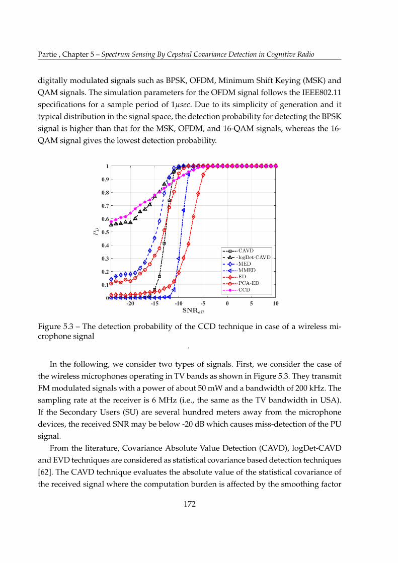
Partie , Chapter 5 – Spectrum Sensing By Cepstral Covariance Detection in Cognitive Radio
digitally modulated signals such as BPSK, OFDM, Minimum Shift Keying (MSK) and
QAM signals. The simulation parameters for the OFDM signal follows the IEEE802.11
specifications for a sample period of 1µsec. Due to its simplicity of generation and it
typical distribution in the signal space, the detection probability for detecting the BPSK
signal is higher than that for the MSK, OFDM, and 16-QAM signals, whereas the 16-
QAM signal gives the lowest detection probability.
Figure 5.3 – The detection probability of the CCD technique in case of a wireless mi-crophone signal
.
In the following, we consider two types of signals. First, we consider the case of
the wireless microphones operating in TV bands as shown in Figure 5.3. They transmit
FM modulated signals with a power of about 50 mW and a bandwidth of 200 kHz. The
sampling rate at the receiver is 6 MHz (i.e., the same as the TV bandwidth in USA).
If the Secondary Users (SU) are several hundred meters away from the microphone
devices, the received SNR may be below -20 dB which causes miss-detection of the PU
signal.
From the literature, Covariance Absolute Value Detection (CAVD), logDet-CAVD
and EVD techniques are considered as statistical covariance based detection techniques
[62]. The CAVD technique evaluates the absolute value of the statistical covariance of
the received signal where the computation burden is affected by the smoothing factor
172

5.5. Numerical Results and Discussions
when calculating the sample covariance matrix. Particularly, it evaluates the ratio be-
tween the off-diagonal to the diagonal elements of the sample covariance matrix and
compare it to a detection threshold. A major limitation of the CAVD algorithm is that
its performance is highly affected by the correlation of the received signals. Therefore,
its performance deteriorates for detecting uncorrelated signals. To test the detectability
of the proposed CCD algorithm to FM-WM signals, we consider a soft peaker audio
signal operating in an indoor environment for a frequency deviation of 32.6 kHz and a
carrier frequency of 3.26 MHz, which is chosen from a 6 MHz band from 2.38 MHz to
8.38 MHz. In Figure 5.3, the CCD algorithm achieves high detection probability, thanks
to strength of the cepstral covariance that reflects the presence of the power cepstral
peaks of the FM-WM signal with respect to the power cepstrum of the background
noise. The logDet-CAVD technique shows a similar behavior but on the expenses of
increased complexity which will be discussed next. Also, the EVD-based techniques
shows a superior performance to the ED techniques due to their ability to utilize the
correlation of the WM signal.
However, we notice in Figure 5.3 the slow increase of the detection probability of
the CCD technique as compared to the ED and the EVD techniques as the SNR in-
creases gradually. This is because the average of the cepstral peaks may include some
spurious peaks occur at the fundamental frequency of the sinusoidal shaping function.
The next type of signals to consider for detection is the IID signals. These types of sig-
nals model a sum of received signals from different antennas. From the literature, it is
well-known that energy detection is optimal for detecting white IID noise. Based on
NPL, the likelihood ratio test is maximized for IID received PU signals under H1 [13].
In Figure 5.4, the detection probability is evaluated for the proposed CCD algo-
rithm as opposed to different state-of-the-art techniques. We find that the detection
performance of the CCD algorithm is superior to ED, PCA-based ED, EVD and CAVD
techniques. Precisely, based on the calculations of the PC of the received PU signal un-
der H1, provided that the PU signal and the background noise are uncorrelated, we
obtain:
Z( f ) = log[Ss( f ) + Sw( f )]
= log
Ss( f )
Sw( f )+ 1�
+ log[Sw( f )](5.16)
If the average signal’s PSD is higher than the average noise PSD, the power cepstrum of
173

Partie , Chapter 5 – Spectrum Sensing By Cepstral Covariance Detection in Cognitive Radio
the IID signal dominates over the power cepstrum of the noise, so that the evaluated
cepstral covariance represents the signal presence over the noise. Nevertheless, the
CAVD technique fails to detect the presence of the IID PU signal since it requires the
existence of correlated samples of the received PU signal to be able to differentiate
between a PU signal and the noise. Although the detection probability of the logDet-
CAVD technique is higher than the proposed CCD technique by about 10% at -24 dB,
its high computation complexity makes its implementation difficult.
Figure 5.4 – The detection probability of the CCD technique for detecting IID Gaussiansignals
.
5.5.2 Complexity Analysis
The computation complexity of an algorithm is related to the number of arithmetic
operations that are needed to execute it. For example, the energy detection technique
needs about N multiplications and additions. For the CAVD algorithm, the computa-
tion of the autocorrelation of the received signal requires about LsN multiplications
and additions, where Ls denotes the size of the sample covariance matrix and N is
the number of samples in the received signal. Also, the ratio of the average of the off-
174

5.5. Numerical Results and Discussions
diagonal elements to the diagonal elements of the sample covariance matrix requires L2s
additions. Thus, the total number of multiplications and additions is about LsN + L2s .
For the EVD techniques, the computation of the sample autocorrelation requires
LsN multiplications and additions, whereas the computation of the extreme eigenval-
ues needs about O(L3s ) operations. Therefore, the overall computation complexity is
about LsN +O(L3s ). Since the N > Ls, hence the first term in the computation complex-
ity is dominant.
The complexity of the proposed CCD algorithm includes the evaluation of the au-
tocorrelation of the received signal, the calculation of the FFT to get the PSD, obtaining
the natural logarithm of the PSD to get the power cepstrum, and finally getting the
cepstral covariance. Thus, the total computation complexity of the CCD algorithm is
about LsN + N log N.
Figure 5.5 – The time complexity analysis of the proposed CCD algorithm as comparedto ED, EVD, CAVD, and logDet-CAVD algorithms
.
To show the time complexity for executing the aforementioned algorithms, we mea-
sure the time complexity of each algorithm as compared to the number of samples of
the received signal. In Figure 5.5, the ED algorithm has the fastest convergence time
175

Partie , Chapter 5 – Spectrum Sensing By Cepstral Covariance Detection in Cognitive Radio
due to its low computation complexity. Following the ED algorithm, the CCD tech-
nique and the EVD based techniques have similar behavior as the number of samples
increases. Despite the reliable detection performance of the logDet-CAVD algorithm, it
has the longest convergence time amongst the considered algorithms.
5.6 Summary
In this chapter, the CCD algorithm is proposed for spectrum sensing in CR systems.
The purpose of the proposed technique is to formulate a versatile approach that is able
to sense the activity of digitally modulated PU signals at low SNR levels. The CCD
algorithm is based on exploiting the inherited periodicity in the power cepstrum of
digitally modulated signals for the spectrum sensing and it aims to mitigate the false-
alarm problem that may be caused by the spectral fluctuation of the background noise.
To reduce the false-alarms, the power cepstrum of the PU signal is enhanced through
evaluating the cepstral covariance of its power cepstrum with a sinusoidal shaping
function. By knowing the data rate of the PU signal, the shaping function is able to
capture the cepstral peaks and reject the spurious peaks caused by the background
noise. The CCD technique is tested with different digital modulation schemes and it
has shown its applicability and reliability at low SNR values over EVD, ED, PCA-
based ED, and CAVD techniques. Although the logDet-CAVD technique is slightly
superior to the CCD technique, its computation complexity limits its application. For
future perspectives, further analysis of the CCD algorithm can be studied with the
involvement of multipath fading communication channels.
176
CHAPTER 6
CONCLUSION AND FUTURE WORK
6.1 Conclusions
Over the last several years, the data transmission of wireless technologies has tremen-
dously grown [141]. This growth is driven largely by people employing different ap-
plications such as video streaming and scrolling through social media. To meet this de-
mand, an efficient spectrum allocation must be managed, such that different wireless
technologies cannot have exclusive frequencies, but must share their available spectral
resources. The concept of Cognitive Radio (CR) has provided conceptual possibilities
for improving the utilization of the heavily congested radio spectrum.
As the name implies, a CR system is a communication system that is aware of its
surrounding and it is able to adapt its parameter according to the collected informa-
tion. Monitoring the spectrum resource is referred to as spectrum sensing. The ob-
tained sensing results are used to optimize spectrum sharing amongst different net-
works, thus integrating the CR concept with wireless communication systems adds
cognitive intelligence. This motivates the importance of providing reliable spectrum
sensing techniques.
In the literature, there are different spectrum sensing techniques to allow for a sec-
ondary user (SU), which is a lower-priority user than a primary user (PU), to occupy
a licensed frequency band. These techniques are classified into non-cooperative and co-
operative methods. The non-cooperative methods include semi-blind techniques which
imply no prior information about PU signal is provided at the SU receiver. These
approaches encompass energy detection (ED), and the Eigenvalue-based Detection
(EVD). In the cooperative techniques, some information about PU must be provided
for detection. These techniques include waveform based detection (WBD), and matched
filter detection (MFD). The ED technique is very simple to apply and implement but
it is sensitive to noise. Although the EVD does not require prior information about
the noise power, the increased processing burden is a drawback. Moreover, the MFD
177

requires knowledge of the pulse shape of the transmitted signal which impractical to
provide.
The spectrum sensing process in a CR system confronts many challenges that affect
its performance. Some of these challenges include hardware complexity, the hidden
PU problem, achieving the optimum sensing duration, and signal detection in a low
SNR communication environment. Beside these challenges, there two factors mainly
affect the detection performance of a spectrum sensing technique, namely: false-alarm
and misdetection. The former occurs due to noise uncertainty presents at CR receiver
which may lead to false detection of a spectral occupancy and this lost spectral oppor-
tunity affects SU transmission. On the other hand, the misdetection problem occurs
when a weak signal occupies a desired frequency band but it is undetectable by the
CR receiver. This problem is either due to the transmission channel effects, such as
multipath fading, or the nature of the signal itself.
Although the filed of Cepstral Analysis (CA) is not novel, it has proven its effi-
cacy in the filed of signal detection and classification. The advantage of the CA-base
techniques lies in their ability to reveal some features characterizing the signal of in-
terest. In our thesis, we formulated different spectrum sensing techniques by taking
advantage of the strength of the Cepstral Analysis approaches. We introduced reliable
cepstrum-based detectors that are suitable for narrowband and wideband spectrum
sensing processes in Cognitive Radio (CR) systems. We aimed to combat the misdetec-
tion problem of detecting possible Spread Spectrum (SS) Primary Users (PUs) without
knowledge of the spreading pseudo random code. A non-cooperative detection pro-
cess is considered a challenge for detecting SS signals. For this reason, we presented
the PassBand AutoCesptrum Detection (PB-ACD) technique that employs an autocep-
stral peak detector for spectrum sensing. The proposed detectors was sufficiently able
to distinguish between noise and noise-like signals, such as SS and Ultra-WideBand
(UWB) signals.
To improve the performance of the PB-ACD technique, we employed a smooth-
ing process as a preceding stage before the PB-ACD process. The role of the improved
PB-ACD technique is to smooth out the fluctuations of the autocorrelation estimators.
The proposed smoothing process is performed by using the Total Variation Denois-
ing (TVD) algorithm to improve the detection of a potential PU signal by the PB-ACD
technique when the transmission medium experiences high noisy spectral fluctuations.
Also, we analyzed the autocepstral behavior of the Frequency Hopping-Spread Spec-
178
trum (SS) and Chirp-Spread Spectrum (C-SS) schemes and we utilized the periodic
autocepstral peaks to formulate the Averaged PassBand-AutoCepstral Detection (APB-
ACD) technique.
Moreover, we broadened our study to wideband spectrum sensing. We developed
a cepstrum-based WideBand Spectrum Sensing (WBSS) approach that includes two
processes: edge detection and PU signal detection. At the best of our knowledge, our
proposed WBSS approach is the first to formulate the Differential Log Spectral Density
(DLSD) algorithm to identify the spectral boundaries of the target wideband spectrum.
The proposed DLSD technique showed a high detection accuracy and a low process-
ing time required to identify the wideband spectral edges as compared to different
wavelet-based edge detection techniques.
Furthermore, we addressed the problem of erroneous spectral boundaries that may
be encountered in WBSS. For this purpose, introduced the BaseBand AutoCepstrum
Detection (BB-ACD) technique to process the received signal in its baseband version,
to reduce the dependency factor of the PU detection process on the carrier frequency
value. The proposed technique showed high detection efficacy in detecting PU sig-
nals in frequency fading channels that experiences Doppler frequency shifts. Based on
our investigations of the periodicity of the power cesptrum, inherited in basic digitally
modulated signals, we introduced the Cepstral Covariance Detection (CCD) technique.
The job of the CCD technique is to capture the periodic peaks of the digital signals
and evaluate the cepstral covariance of its enhanced power cepstrum. Through simu-
lations, the presented detector showed a high detection accuracy for different digital
modulation schemes.
6.2 Recommendations for Future Work
The results of this dissertation point to several intriguing paths, which can be pur-
sued in future work. For example:
— A tradeoff study between the complexity and detection accuracy of the pro-
posed techniques with that of the wideband sensing technique of similar kind
can be considered to provide a broader competence view.
— The involvement of a reliable channel estimation process is essential to include
its effect on the spectrum sensing results. In this regards, A dual spectrum sens-
179

ing and channel estimation by the autocepstrum approach can be investigated.
Originally, the purpose of the Power Cepstrum (PC) was to determine the echo
arrival times in a composite signal as discussed in [18], since delayed echoes
appear as ripples in the logarithmic spectrum of the input data sequence x(n)
[100]. Conventionally, the PC of a signal can be defined as the sequence of
the inverse Z-transform of the logarithm of the magnitude squared of the Z-
transform of the data sequence. This is can be written by:
xPC(n) = Z�1{log |X(Z)|2}2 (6.1)
where X(z) represents the Z transform of the data sequence x(n). If the data
sequence consists of two convolved sequences, such as a modulated signal y(n)
and the impulse response of the communication channel h(n), we obtain:
x(n) = y(n) ⇤ h(n) (6.2)
this equation can be rewritten as the multiplication of the Fourier transform of
the two sequences:
|X(z)|2 = |Y(z)|2.|V(z)|2 (6.3)
by taking the logarithm of both sides of the equation (6.3), we obtain:
log |X(z)|2 = log |Y(z)|+ log |V(z)|2 (6.4)
To further elaborate on the power spectrum analysis, let us assume that the time-
invariant multipath channel impulse response is given as:
h(n) = δ(n) + γ f δ(n � no) (6.5)
where δ(n) denotes the unit impulse response function and γ f denotes the fad-
ing coefficient. On the basis of this equation, we can further write:
|X(z)|2 = |Y(z)|2 |1 + γ f Z�no |2 (6.6)
by taking the logarithm of both sides and substituting by Z = exp(jω), we ex-
180
pand equation (6.6) as:
log |X(exp(jω))|2 = log |Y(exp(jω))|+ log�
1 + γ2f
�
+ log
1 +2γ f
1 + γ2f
cos(ωno)
!
(6.7)
In equation (6.7), we can observe that the PC of the data sequence contains si-
nusoidal components (ripples). The amplitude and frequencies of these ripples
correspond to the amplitude of every impulsive component and the time de-
lay corresponds to the delayed multipath component. By taking the inverse Z-
transform of (6.7), we obtain:
xPC(n) = yPC(n) + hPC(n) (6.8)
In the literature, the CA of a multipath signal is carried out for the purpose
of estimating the communication channel coefficients provided that prior infor-
mation about the transmitted signal are available at the receiver. However, in a
non-cooperative transmission reception scenario, such as in CR system, knowl-
edge of the PU signal characteristics is not provided. This makes a dual channel
estimation and spectrum sensing an important argument to be addressed in fur-
ther studies.
— Cooperative sensing could be the target of our next area of research for the
performance enhancement of CR systems when combined with artificial intel-
ligence. In this regard, the employment of artificial intelligence algorithms can
be considered to dynamically sense the target spectrum and consequently make
a decision to share the spectrum based on reasoning [141]. In particular, some
research advances in artificial intelligence-based 5G studies discussed the ap-
plication of artificial intelligence algorithms in the radio networks [142]. These
networks would be permitted to utilize a specific frequency band after an opti-
mized decision of an artificial intelligence algorithm.
181
APPENDIX A
A.1 Derivation of The Generalized Expression of The log�χ2ν
for ν Degrees of Freedom
Recall the computation of the autocesptrum of an underlying signal X(n), which is
given by:
ca(n) =1pNr
Nr�1
∑k=0
Z(k) exp
j2πkn
Nr
!
(A.1)
where Z(k) is the natural logarithm of the signal’s PSD which can be given by:
Z(k) =
8
<
:
log[σ2wSw(k)] : H0
log[σ2s Ss(k) + σ2
wSw(k)] : H1
(A.2)
where the variances, σ2w and σ2
s , represents also the PSD levels of the spectra of the
noise and the PU signal. Precisely, we can re-define equation (A.1) under H0 by:
pNrca(n) =
Nr�1
∑k=0
⇣
log[σ2w] + log[Sw(k)]
⌘
exp
j2πkn
Nr
!
=(log[σ2w])δ(n) + caw(n)
(A.3)
where δ(n) denote the delta Dirac function and caw(n represents the autocepstrum of
the noise signal. By dividing both sides of equation (A.3) by σ2wlog
= log[σ2w], we obtain:
pNrca(n)
σ2wlog
= δ(n) + caw(n) (A.4)
182
where caw(n) denotes the normalized noise autocepstrum. Likewise, the autocepstrum
of the received signal under H1 is given by:
pNrca(n) =
Nr�1
∑k=0
h
log[σ2wSw(k)][γγ0(k) + 1]
i
exp
j2πkn
Nr
!
(A.5)
where γ denotes the SNR level and γ0(k) =Ss(k)
Sw(k)denotes the spectral variation be-
tween the signal and the noise. To simplify equation (A.5), we approximate the term
log[γγ0(k) + 1] ⇡ log[γγ0(k)] for γγ0(k) >> 1, thus we obtain:
pNrca(n) = (log[σ2
w])δ(n) + caw(n) + log[γ]δ(n) +Nr�1
∑k=0
log
"
γ0(k)exp
j2πkn
Nr
!#
(A.6)
thus, equation (A.6) can be reduced to:
pNrca(n) = log[σ2
s ]δ(n) +Nr�1
∑k=0
log[Ss(k)]exp
j2πkn
Nr
!
(A.7)
equivalently, it can be expressed by:
pNrca(n)
σ2slog
= δ(n) + cas(n) (A.8)
where σ2slog
= log[σ2s ] and cas(n) =
cas (n)
σ2slog
denotes the normalized cepstrum of the target
signal.Thus, we can describe the statistical distribution of ca(n) under the null and the
alternative hypotheses by:
fCa(ca) =
8
>
>
<
>
>
:
σ2wlogp
Nrflog�χ2
✓
σ2wlog
ν ca, ν
◆
: H0
σ2slogpNr
flog�χ2
✓
σ2slog
ν ca, ν
◆
: H1
(A.9)
where flog�χ2 denotes the probability density function of the log�χ2ν with ν degrees
of freedom. By using the method of transformation of random variables, flog�χ2 under
183

H0 is given by:
fCa(ca; H0) =
σ2wlog
ν
exp(ca)
Γ( ν2 ) 2
M2
exp(ca)σ2wlog
ν
!
ν2�1
exp
�exp(ca)σ2
wlog
ν
!
(A.10)
A.2 Expression for The False-alarm Probability
To find expression for the false-alarm probability, we evaluate the following inte-
gral:
PFA =Z ∞
η1
fCa(ca; H0)dca
=
σ2wlog
ν
!
ν2
1
Γ( ν2 )2
ν2
Z ∞
η1
exp(ca))ν2 exp
�exp(ca)σ2
wlog
ν
! (A.11)
where η1 denotes the detection threshold of an autocepstrum detector. Using the meth-
ods of substitution by assuming x0 = exp(ca), we obtain:
PFA = A
Z ∞
exp(η)(x0)
ν2 exp
�x0σ2
wlog
ν
!
dx0 (A.12)
where A =
✓
σ2wlogν
◆
ν2
1Γ( ν
2 )2ν2
. If we assume that s = ν2 and t =
x0σ2wlog
ν , then we can rewrite
equation (A.12) as:
PFA =
"
ν
σ2wlog
#2
A
Z ∞
σ2wlog
ν exp(η1)ts�1 exp(�t)dt (A.13)
where the integral resembles that defined by the upper incomplete gamma function, which
is given by:
Γ(s, x) =Z ∞
xts�1 exp(�t)dt (A.14)
By applying equation (A.14), the false-alarm probability becomes:
PFA =
σ2wlog
ν
!
ν2�2
Q(s, x) (A.15)
184

where Q(s, x) represents the regularized gamma function, which is expressed by:
Q(s, x) =
Γ
✓
ν2 ,
σ2wlog
ν exp(η1
◆
Γ�
ν2
�
2ν2
(A.16)
185

APPENDIX B
B.1 Maximum-to-Minimum Eigenvalue Detection Algo-
rithm
1. Compute the sample covariance matrix of the received signal of size N.
2. Obtain the maximum and the minimum eigenvalues of the covariance matrix for
a smoothing factor of size Ls.
3. The detection decision is obtained by comparing the ratio of the maximum-to-
minimum eigenvalues to the detection threshold, which is given by [62]:
ηMME =(p
N +p
Ls)2
(p
N �p
L)2
1 +(p
N +p
Ls)�2/3
(NLs)1/6 F�11 (1 � PFA)
!
(B.1)
where F1 denotes the cumulative distribution function of he Tracy-Widom distri-
bution of order 1 [62].
B.2 Energy with Minimum Eigenvalue Detection Algo-
rithm
1. Compute the sample covariance matrix of the received signal.
2. Compute the average power of the received signal and obtain the minimum
eigenvalue of the covariance matrix.
3. The detection decision is obtained by comparing the ratio of the average power
of the received signal-to-minimum eigenvalue to the detection threshold, which
is given by [62]:
ηEME =
r
2N
Q�1(PFA + 1)
!
N
(p
N �p
Ls)2(B.2)
186
APPENDIX C
C.1 Validation of a Chosen Majorizer Equation
We need to get the constants cMM and bMM in order to verify that the chosen func-
tion gMM(t) is a valid majorizer for fMM(t), so based on the second condition of MM
algorithm, we have:
gMM(t = tk) = fMM(t = tk) (C.1)
accordingly, we get:
cMM =1Tc
� tk(1Tc
� bMMtk) (C.2)
referring to the inequality in equation (3.153), we have:
bMMt2 � t
Tc+ (
1Tc
� cMM) < 0 (C.3)
then for bMM > 0:
4b (1Tc
� cMM) =1
T2c
(C.4)
substitute equation (C.2) in equation (C.4), for uMM = bMMTctk we have:
u2MM � uMM +
14� 0 (C.5)
thus, for a general expression:
bMM =1
2Tc|tk|, cMM =
1 � 2|tk|
2Tc(C.6)
187

APPENDIX D
D.1 The Statistical Distribution of A Random Variable
follows Modulus Log Chi-Squared Distribution
Consider a random process J = | log[V]|, and we seek the distribution of J if V fol-
lows χ2(2). Thus, J follows MLCS distribution. Based on the probability density function
approach, we find the required distribution by:
f J(j) =fV(v)
|dJ/dV|
�
�
�
V=±J(D.1)
then, by substituting for dJdV = V
|V| |, we get:
f J(j) =12
exp✓
j � 12
exp(j)
◆
+ exp✓
�j � 12
exp(�j)
◆�
(D.2)
188
APPENDIX E
E.1 Review on General Expressions of The PSD of Basic
Digitally Modulated Signals
The signal’s PSD can be evaluated by using either a deterministic or a stochastic ap-
proach. To evaluate the PSD by the deterministic approach, a particular data sequence
is assumed to be known, whereas the data sequence is assumed to be randomly gener-
ated in the stochastic approach. The general expression for a digitally modulated signal
is given by:
Ss( f ) =|P( f )|2
Ts
∞
∑k=�∞
R(k)exp (j2π f Ts) (E.1)
where P( f ) is the FT of the pulse shaping function p(t) and R(k) is the autocorrelation
of the random data sequence which is given by:
R(k) =I
∑i=1
(anan+k)Pi (E.2)
where an and an+k are the voltage levels of the data pulses at the nth and (n + k)th
symbol positions, respectively, and Pi is the probability of having the ith anan+k prod-
uct. From equation (E.1), we note that the signal’s PSD depends on the pulse shaping
function and the statistical properties of the data. By few mathematical manipulation,
the PSD of some basic digital signals with data modulation of rectangular bit shape are
given as follows [36]:
— The PSD of the baseband Amplitude Shift Keying (ASK) signals:
Ss( f ) =A2
c Tb
4sinc2( f Tb)
1 +1
Tbδ( f )
�
(E.3)
where Ac is the carrier amplitude
189
— The PSD for the complex envelope of MPSK or QAM signals:
Ss( f ) = CσlTbsinc2( f lTb) (E.4)
where l denotes the number of bits per symbol and Cσ is a positive number
denoting the variance of the complex valued random variable representing the
multilevel value during the nth symbol pulse.
— The PSD for the complex envelope of Minimum Shift Keying (MSK) signals:
Ss( f ) =16A2
c T2b
π2
cos2(2πTb f )
(1 � (4Tb f )2)2
�
(E.5)
where the normalized power of the MSK signal is A2c /2.
— The PSD of OFDM signals: The PSD of an OFDM signal can be obtained rela-
tively easily, since an OFDM signal consists of orthogonal carriers modulated by
data with rectangular pulses of duration of Ts. Consequently, the PSD of each
carrier is of the form sinc2(Ts( f � fn)) hence, the overall PSD of the complex
envelope of the OFDM signal is given by:
Ss( f ) = A2c Pwn
N�1
∑n=0
|sinc(Ts( f � fn))|2 (E.6)
where Pwn is the normalized power of the nth element of the N-element parallel
data vector in the OFDM signal.
190

LIST OF PUBLICATIONS
International Journals
1- A. Moawad, K. Yao, A. Mansour, R. Gautier, "A Wideband Spectrum Sensing Ap-
proach in Cognitive Radio Based on Cepstral Analysis", IEEE open journal of the
communications society, vol. 1, no. 20, pp. 863–888, 2020.
2- A. Moawad, K. Yao, A. Mansour, R. Gautier, "Spectrum Sensing By Cepstral Co-
variance Detection in Cognitive Radio”, submitted to the journal of IEEE Commu-
nication Letters.
Conferences
1- S E. El Khamy, Amr M. El Helw, and A. Moawad, "Classification of Multi-rate
CDMA Signals Using Compressed Cyclostationary Features," Proceedings of the
Progress In Electromagnetics Research Symposium (PIERS), pp. 1361-1365, Kuala
Lumpur, Malaysia, Mar 2012.
2- S. E. El Khamy, A. M. El Helw, and A. Moawad, "Digital Signal Classification by
Compressed Cyclostationary Features," The 29th National Radio Science Confer-
ence (NRSC), Cairo, Egypt, Apr 2012
3- S. E. El Khamy, A. M. El Helw, and A. Moawad,"Spectral Separation of Com-
pressed Cyclostationary Signals Using Adaptive FRESH Filtering," Proceedings of
the Progress In Electromagnetics Research Symposium (PIERS), Stockholm, Swe-
den, Aug 2013
4- A. Moawad, K. Yao, A. Mansour, R. Gautier, “Spectrum Sensing by Scattering Op-
erators in Cognitive Radio,” in Proceedings of the 2nd International Conference on
Advanced Technology and Applied Science, pp. 388-395, Alex, Egypt, Sept 2017.
192
5- A. Moawad, K. Yao, A. Mansour, R. Gautier, “Enhancement of Primary User Detec-
tion in Cognitive Radio by Scattering Transform,” in Proceedings of the 19th Inter-
national Conference on Electronics and Wireless Communications, pp. 2384-2390,
Istanbul, Turkey, Oct 2017.
6- A. Moawad, K. Yao, A. Mansour, R. Gautier, “Autocepstrum Approach for Spec-
trum Sensing in Cognitive Radio,” in Proceedings of the 15th International Sympo-
sium on Wireless Communication Systems (ISWCS), Lisbon, Portugal, Aug 2018.
193

BIBLIOGRAPHY
[1] J. Mitola and G. Q. Maguire, “Cognitive radio: making software radios more
personal,” IEEE Personal Communications, vol. 6, no. 4, pp. 13–18, 1999.
[2] S. Haykin, “Cognitive radio: brain-empowered wireless communications,” IEEE
Journal on Selected Areas in Communications, vol. 23, no. 2, pp. 201–220, 2005.
[3] S. Sasipriya and R. Vigneshram, “An overview of cognitive radio in 5g wireless
communications,” in IEEE International Conference on Computational Intelligence
and Computing Research (ICCIC), pp. 1–5, New Tehri, India, Dec 2016.
[4] F. W. Vook, A. Ghosh, E. Diarte, and M. Murphy, “5g new radio: Overview and
performance,” in 52nd IEEE Asilomar Conference on Signals, Systems, and Comput-
ers, pp. 1247–1251, CA, USA, Oct 2018.
[5] E. Yaacoub and M.-S. Alouini, “A key 6g challenge and opportunity–connecting
the remaining 4 billions: A survey on rural connectivity,” arXiv preprint
arXiv:1906.11541, 2019.
[6] I. Abdo, T. Fujimura, T. Miura, A. Shirane, and K. Okada, “A 300ghz dielec-
tric lens antenna,” in 12th IEEE Global Symposium on Millimeter Waves (GSMM),
pp. 17–19, Sendai, Japan, May 2019.
[7] A. Garhwal and P. P. Bhattacharya, “Dynamic spectrum access in cognitive ra-
dio: a brief review,” International Journal of Computer Application in Engineering
Sciences, Special Issue on Computer Networks & Security, vol. 1, pp. 149–153, 2011.
[8] Y.-C. Liang, Y. Zeng, E. C. Peh, and A. T. Hoang, “Sensing-throughput trade-
off for cognitive radio networks,” IEEE Transactions on Wireless Communications,
vol. 7, no. 4, pp. 1326–1337, 2008.
[9] Y. Arjoune and N. Kaabouch, “A comprehensive survey on spectrum sensing in
cognitive radio networks: Recent advances, new challenges, and future research
directions,” Sensors, vol. 19, no. 1, p. 126, 2019.
[10] T. Yucek and H. Arslan, “A survey of spectrum sensing algorithms for cogni-
tive radio applications,” IEEE Communications Surveys & Tutorials, vol. 11, no. 1,
pp. 116–130, 2009.
195

[11] M. K. Tsatsanis and Z. Xu, “Pilot symbol assisted modulation in frequency se-
lective fading wireless channels,” IEEE Transactions on Signal Processing, vol. 48,
no. 8, pp. 2353–2365, 2000.
[12] Z. Fan, Z. Lu, and Y. Hu, “Reliable channel estimation based on bayesian com-
pressive sensing for tds-ofdm systems,” in IEEE International Conference on Com-
munication Systems, pp. 620–624, IEEE, Macau, China, Nov 2014.
[13] M. C. Gursoy and S. Gezici, “On the interplay between channel sensing and esti-
mation in cognitive radio systems,” in IEEE Global Telecommunications Conference-
GLOBECOM 2011, pp. 1–5, IEEE, Texas, USA, Dec 2011.
[14] Y. Yilmaz, Z. Guo, and X. Wang, “Sequential joint spectrum sensing and chan-
nel estimation for dynamic spectrum access,” IEEE Journal on Selected Areas in
Communications, vol. 32, no. 11, pp. 2000–2012, 2014.
[15] G. Hua, J. Goh, and V. L. Thing, “Cepstral analysis for the application of echo-
based audio watermark detection,” IEEE Transactions on Information Forensics and
Security, vol. 10, no. 9, pp. 1850–1861, 2015.
[16] J. K. Lee, M. Kabrisky, M. E. Oxley, S. K. Rogers, and D. W. Ruck, “The com-
plex cepstrum applied to two-dimensional images,” Pattern Recognition, vol. 26,
no. 10, pp. 1579–1592, 1993.
[17] P. Borghesani, P. Pennacchi, R. Randall, N. Sawalhi, and R. Ricci, “Application of
cepstrum pre-whitening for the diagnosis of bearing faults under variable speed
conditions,” Mechanical Systems and Signal Processing, vol. 36, no. 2, pp. 370–384,
2013.
[18] E. Flinn, T. Cohen, and D. McCowan, “Detection and analysis of multiple seismic
events,” Bulletin of the Seismological Society of America, vol. 63, no. 6-1, pp. 1921–
1935, 1973.
[19] J. Jäntti, S. Chaudhari, and V. Koivunen, “Detection and classification of ofdm
waveforms using cepstral analysis,” IEEE Transactions on Signal Processing,
vol. 63, no. 16, pp. 4284–4299, 2015.
[20] B. P. Bogert, M. J. R. Healy, and J. W. Tukey, “The quefrency alanysis of time
series for echoes; cepstrum, pseudo-autocovariance, cross-cepstrum and saphe
cracking,” in Proceedings of Time series analysis, pp. 209–243, M. Rosenblatt, Ed.,
New York, Wiley ,1963, ch. 15.
196

[21] T. S. Rappaport, Y. Xing, O. Kanhere, S. Ju, A. Madanayake, S. Mandal, A. Alkha-
teeb, and G. C. Trichopoulos, “Wireless communications and applications above
100 ghz: Opportunities and challenges for 6g and beyond,” IEEE Access, vol. 7,
pp. 78729–78757, 2019.
[22] S. Dang, O. Amin, B. Shihada, and M.-S. Alouini, “What should 6g be?,” Nature
Electronics, vol. 3, no. 1, pp. 20–29, 2020.
[23] F. Tariq, M. Khandaker, K.-K. Wong, M. Imran, M. Bennis, and M. Debbah, “A
speculative study on 6g,” arXiv preprint arXiv:1902.06700, 2019.
[24] I. Union, “Imt traffic estimates for the years 2020 to 2030,” Report ITU, pp. 1–51,
2015.
[25] J. Mitola, Cognitive radio. PhD thesis, Institutionen för teleinformatik, 2000.
[26] E. Hossain, D. Niyato, and Z. Han, Dynamic spectrum access and management in
cognitive radio networks. Cambridge university press, 1st Ed., New York, USA,
2009.
[27] E. Biglieri, A. J. Goldsmith, L. J. Greenstein, N. B. Mandayam, and H. V. Poor,
Principles of cognitive radio. Cambridge University Press, 1st Ed., New York, USA,
2013.
[28] A. Khattab and M. A. Bayoumi, “Standardization of cognitive radio networking:
a comprehensive survey,” Annals of Telecommunications-annales des téléCommuni-
cations, vol. 70, no. 11-12, pp. 465–477, 2015.
[29] K. Kim, Y. Xin, and S. Rangarajan, “Energy detection based spectrum sensing
for cognitive radio: An experimental study,” in IEEE Global Telecommunications
Conference GLOBECOM, pp. 1–5, Florida, USA, Dec 2010.
[30] D. Bao, L. De Vito, and S. Rapuano, “A histogram-based segmentation method
for wideband spectrum sensing in cognitive radios,” IEEE Transactions on Instru-
mentation and Measurement, vol. 62, no. 7, pp. 1900–1908, 2013.
[31] B. Shent, L. Huang, C. Zhao, Z. Zhou, and K. Kwak, “Energy detection based
spectrum sensing for cognitive radios in noise of uncertain power,” in Inter-
national Symposium on Communications and Information Technologies, pp. 628–633,
IEEE, 2008.
[32] R. Tandra and A. Sahai, “Snr walls for signal detection,” IEEE Journal of Selected
Topics in Signal Processing, vol. 2, no. 1, pp. 4–17, 2008.
197
[33] R. Tandra and A. Sahai, “Noise calibration, delay coherence and snr walls for
signal detection,” in 3rd IEEE Symposium on New Frontiers in Dynamic Spectrum
Access Networks, pp. 1–11, IEEE, 2008.
[34] I. E. Atawi, O. S. Badarneh, M. S. Aloqlah, and R. Mesleh, “Energy-detection
based spectrum-sensing in cognitive radio networks over multipath/shadowed
fading channels,” in Wireless Telecommunications Symposium (WTS), pp. 1–6, IEEE,
New York, USA, Apr 2015.
[35] D. M. M. Plata and Á. G. A. Reátiga, “Evaluation of energy detection for spec-
trum sensing based on the dynamic selection of detection-threshold,” Procedia
Engineering, vol. 35, pp. 135–143, 2012.
[36] L. W. Couch, Digital & Analog Communication Systems. Prentice Hall, 6th Ed.,
New Jersey, USA, 2011.
[37] S. Upadhyay and S. Deshmukh, “Blind parameter estimation based matched fil-
ter detection for cognitive radio networks,” in International Conference on Com-
munications and Signal Processing (ICCSP), pp. 0904–0908, IEEE, Chengdu, China,
Oct 2015.
[38] F. Salahdine, H. El Ghazi, N. Kaabouch, and W. F. Fihri, “Matched filter detection
with dynamic threshold for cognitive radio networks,” in International Conference
On Wireless Networks and Mobile communications (WINCOM), pp. 1–6, IEEE, Mar-
rakech, Morocco, Oct 2015.
[39] Y. Zeng and Y.-C. Liang, “Eigenvalue-based spectrum sensing algorithms for
cognitive radio,” IEEE Transactions on Communications, vol. 57, no. 6, pp. 1784–
1793, 2009.
[40] P. Aparna and M. Jayasheela, “Cyclostationary feature detection in cognitive ra-
dio using different modulation schemes,” International Journal of Computer Appli-
cations, vol. 47, no. 21, 2012.
[41] A. Al-Dulaimi, N. Radhi, and H. Al-Raweshidy, “Cyclostationary detection of
undefined secondary users,” in Third International Conference on Next Generation
Mobile Applications, Services and Technologies, pp. 230–233, IEEE, Wales, United
Kingdom, Sept 2009.
[42] A. H. Ansari and S. Gulhane, “Cyclostationary method based spectrum sensing
and analysis using different windowing method,” in International Conference on
Energy Systems and Applications, pp. 684–688, IEEE, Pune, India, Nov 2015.
198
[43] O. P. Awe, Machine learning algorithms for cognitive radio wireless networks. PhD
thesis, Loughborough University, 2015.
[44] Y. Yao, Y. Liu, Y. Yu, H. Xu, W. Lv, Z. Li, and X. Chen, “K-svm: An effective
svm algorithm based on k-means clustering.,” Journal of Computers, vol. 8, no. 10,
pp. 2632–2639, 2013.
[45] B. Khalfi, A. Zaid, and B. Hamdaoui, “When machine learning meets compres-
sive sampling for wideband spectrum sensing,” in 13th International Wireless
Communications and Mobile Computing Conference (IWCMC), pp. 1120–1125, IEEE,
Valencia, Spain, Jun 2017.
[46] Z. Li, W. Wu, X. Liu, and P. Qi, “Improved cooperative spectrum sensing model
based on machine learning for cognitive radio networks,” IET Communications,
vol. 12, no. 19, pp. 2485–2492, 2018.
[47] D. L. Donoho, “Compressed sensing,” IEEE Transactions on information theory,
vol. 52, no. 4, pp. 1289–1306, 2006.
[48] Y. L. Polo, Y. Wang, A. Pandharipande, and G. Leus, “Compressive wide-band
spectrum sensing,” in IEEE International Conference on Acoustics, Speech and Signal
Processing, pp. 2337–2340, IEEE, Taipei, Taiwan, Apr 2009.
[49] Y. Arjoune and N. Kaabouch, “Wideband spectrum sensing: A bayesian com-
pressive sensing approach,” Sensors, vol. 18, no. 6, p. 1839, 2018.
[50] M. Lopes, “Estimating unknown sparsity in compressed sensing,” in Interna-
tional Conference on Machine Learning, pp. 217–225, Atlanta, USA, Jun 2013.
[51] S. Kyperountas, N. Correal, Q. Shi, and Z. Ye, “Performance analysis of coopera-
tive spectrum sensing in suzuki fading channels,” in 2nd International Conference
on Cognitive Radio Oriented Wireless Networks and Communications, pp. 428–432,
IEEE, Florida, USA, Aug 2007.
[52] S. Nallagonda, S. D. Roy, and S. Kumdu, “Performance of cooperative spectrum
sensing in fading channels,” in 1st International Conference on Recent Advances in
Information Technology (RAIT), pp. 202–207, IEEE, Dhanbad, India, Mar 2012.
[53] R. Wan, L. Ding, N. Xiong, W. Shu, and L. Yang, “Dynamic dual threshold co-
operative spectrum sensing for cognitive radio under noise power uncertainty,”
Human-centric Computing and Information Sciences, vol. 9, no. 1, p. 22, 2019.
[54] S. M. Kay, Fundamentals of statistical signal processing, Vol. II: Detection Theory.
Prentice Hall, 1st Ed., New Jersey, USA, 1993.
199
[55] L. Koralov and Y. G. Sinai, Theory of probability and random processes. Springer
Science & Business Media, 2nd Ed., Heidelberg, Germany, 2010.
[56] D. M. M. Plata and Á. G. A. Reátiga, “Evaluation of energy detection for spec-
trum sensing based on the dynamic selection of detection-threshold,” Procedia
Engineering, vol. 35, pp. 135–143, 2012.
[57] D. R. Joshi, D. C. Popescu, and O. A. Dobre, “Adaptive spectrum sensing with
noise variance estimation for dynamic cognitive radio systems,” in 44th Annual
Conference on Information Sciences and Systems (CISS), pp. 1–5, IEEE, New Jersey,
USA, Mar 2010.
[58] A. Bagwari and G. S. Tomar, “Adaptive double-threshold based energy detector
for spectrum sensing in cognitive radio networks,” International Journal of Elec-
tronics Letters, vol. 1, no. 1, pp. 24–32, 2013.
[59] B. A. Odhavjibhai and S. Rana, “Analysis of matched filter based spectrum sens-
ing in cognitive radio,” International Research Journal of Engineering and Technology,
vol. 4, no. 4, pp. 578–581, 2017.
[60] P. Alvarez, N. Pratas, A. Rodrigues, N. R. Prasad, and R. Prasad, “Energy detec-
tion and eigenvalue based detection: An experimental study using gnu radio,”
in 14th International Symposium on Wireless Personal Multimedia Communications
(WPMC), pp. 1–5, IEEE, Brest, France, Oct 2011.
[61] L. Du, M. Laghate, C. Liu, D. Cabric, and Y. Chen, “Improved eigenvalue-based
spectrum sensing via sensor signal overlapping,” in 8th IEEE International Confer-
ence on Communication Software and Networks (ICCSN), pp. 122–126, IEEE, Beijing,
China, Jun 2016.
[62] Y. Zeng, C. L. Koh, and Y.-C. Liang, “Maximum eigenvalue detection: Theory
and application,” in IEEE International Conference on Communications, pp. 4160–
4164, IEEE, Beijing, China, May 2008.
[63] S. K. Sharma, S. Chatzinotas, and B. Ottersten, “Maximum eigenvalue detection
for spectrum sensing under correlated noise,” in IEEE International Conference on
Acoustics, Speech and Signal Processing (ICASSP), pp. 7268–7272, IEEE, Florence,
Italy, May 2014.
[64] W. A. Gardner, “Introduction to random processes with applications to signals
and systems((book)),” 2nd Ed., New York, MacMillan, 1986.
200

[65] D. C. Simic and J. Simic, “The strip spectral correlation algorithm for spectral
correlation estimation of digitally modulated signals,” in 4th International Con-
ference on Telecommunications in Modern Satellite, Cable and Broadcasting Services.
TELSIKS’99 (Cat. No. 99EX365), vol. 1, pp. 277–280, IEEE, 1999.
[66] J.-M. Kadjo, K. C. Yao, and A. Mansour, “Blind detection of cyclostationary fea-
tures in the context of cognitive radio,” in IEEE International Symposium on Sig-
nal Processing and Information Technology (ISSPIT), pp. 150–155, Limassol, Cyprus,
Dec 2016.
[67] S. Rajendran, W. Meert, D. Giustiniano, V. Lenders, and S. Pollin, “Deep learning
models for wireless signal classification with distributed low-cost spectrum sen-
sors,” IEEE Transactions on Cognitive Communications and Networking, vol. 4, no. 3,
pp. 433–445, 2018.
[68] U. Côté-Allard, C. L. Fall, A. Drouin, A. Campeau-Lecours, C. Gosselin, K. Glette,
F. Laviolette, and B. Gosselin, “Deep learning for electromyographic hand ges-
ture signal classification using transfer learning,” IEEE Transactions on Neural Sys-
tems and Rehabilitation Engineering, vol. 27, no. 4, pp. 760–771, 2019.
[69] P. Hossain, A. Komisarczuk, G. Pawetczak, S. Van Dijk, and I. Axelsen, “Machine
learning techniques in cognitive radio networks,” arXiv preprint arXiv:1410.3145,
2014.
[70] H. Anandakumar and K. Umamaheswari, “Supervised machine learning tech-
niques in cognitive radio networks during cooperative spectrum handovers,”
Cluster Computing, vol. 20, no. 2, pp. 1505–1515, 2017.
[71] A. Nasser, A. Mansour, K. C. Yao, H. Charara, and M. Chaitou, “Efficient spec-
trum sensing approaches based on waveform detection,” in 3rd International Con-
ference on e-Technologies and Networks for Development (ICeND2014), pp. 13–17,
IEEE, Beirut, Lebanon, May 2014.
[72] A. Nasser, A. Mansour, K.-C. Yao, H. Abdallah, M. Chaitou, and H. Charara,
“Spectrum sensing enhancement using principal component analysis,” in IEEE
International Symposium on Signal Processing and Information Technology (ISSPIT),
pp. 263–267, IEEE, Limassol, Cyprus, Dec 2016.
[73] A. Nasser, A. Mansour, K. C. Yao, H. Abdallah, and H. Charara, “Spectrum sens-
ing based on cumulative power spectral density,” EURASIP Journal on Advances
in Signal Processing, vol. 2017, no. 1, p. 38, 2017.
201
[74] A. Nasser, A. Mansour, K.-C. Yao, H. Charara, and M. Chaitou, “Spectrum sens-
ing for full-duplex cognitive radio systems,” in International Conference on Cogni-
tive Radio Oriented Wireless Networks, pp. 363–374, Springer, May 2016, Grenoble,
France.
[75] J.-M. Kadjo, K. C. Yao, and A. Mansour, “Blind spectrum sensing based on recur-
rence quantification analysis in the context of cognitive radio,” in 26th European
Signal Processing Conference (EUSIPCO), pp. 1835–1839, IEEE, Rome, Italy, Sept
2018.
[76] G. Hattab and M. Ibnkahla, “Multiband spectrum access: Great promises for fu-
ture cognitive radio networks,” Proceedings of the IEEE, vol. 102, no. 3, pp. 282–
306, 2014.
[77] X. Yanwei, Z. Jianhua, and Z. Ping, “Compressed sensing based multi-rate sub-
nyquist sampling system,” The Journal of China Universities of Posts and Telecom-
munications, vol. 22, no. 2, pp. 89–95, 2015.
[78] Z. Dai, Y. Chen, W. Wen, and Y. Zheng, “Compressed sensing based sub-nyquist
sampling of multiple sinusoids with dual rate channels,” Review of Scientific In-
struments, vol. 89, no. 12, p. 125113, 2018.
[79] Z. Tian and G. B. Giannakis, “Compressed sensing for wideband cognitive ra-
dios,” in IEEE International Conference on Acoustics, Speech and Signal Processing
(ICASSP), vol. 4, pp. IV–1357, IEEE, Hawaii, USA, Apr 2007.
[80] H. Sun, A. Nallanathan, C.-X. Wang, and Y. Chen, “Wideband spectrum sensing
for cognitive radio networks: a survey,” IEEE Wireless Communications, vol. 20,
no. 2, pp. 74–81, 2013.
[81] Y. LeCun, K. Kavukcuoglu, and C. Farabet, “Convolutional networks and ap-
plications in vision,” in IEEE International Symposium on Circuits and Systems,
pp. 253–256, IEEE, Paris, France, May 2010.
[82] J. Bruna and S. Mallat, “Invariant scattering convolution networks,” IEEE Trans-
actions on Pattern Analysis and Machine Intelligence, vol. 35, no. 8, pp. 1872–1886,
2013.
[83] J. Andén and S. Mallat, “Deep scattering spectrum,” IEEE Transactions on Signal
Processing, vol. 62, no. 16, pp. 4114–4128, 2014.
202
[84] A. Moawad, K.-C. Yao, A. Mansour, and R. Gautier, “Spectrum sensing by scat-
tering operators in cognitive radio,” in 2nd International Conference on Advanced
Technology and Applied Science (ICATAS), pp. 1–6, Alex, Egypt, Sept 2017.
[85] A. Goldsmith, Wireless communications. Cambridge university press, 2nd Ed.,
USA, 2005.
[86] G. Matz and F. Hlawatsch, “Fundamentals of time-varying communication chan-
nels,” in Wireless Communications Over Rapidly Time-Varying Channels, pp. 1–63,
Acdemic Press, Amsterdam, 2011.
[87] M. Stephane, “A wavelet tour of signal processing,” The Sparse Way, 1st Ed., Mas-
sachusetts, 1999.
[88] D. T. Lee and A. Yamamoto, “Wavelet analysis: theory and applications,” Hewlett
Packard journal, vol. 45, pp. 44–44, 1994.
[89] R. X. Gao and R. Yan, “From fourier transform to wavelet transform: A historical
perspective,” in Wavelets, pp. 17–32, Springer Science+Business Media, Heidel-
berg, 2011.
[90] I. S. Gradshteyn and I. M. Ryzhik, Table of integrals, series, and products. Academic
press, 6th Ed., Massachusetts, 2014.
[91] A. R. Bahai, B. R. Saltzberg, and M. Ergen, “Channel estimation and equaliza-
tion,” Multi-Carrier Digital Communications: Theory and Applications of OFDM,
pp. 117–165, Boston, 2004.
[92] A. Moawad, K.-C. Yao, A. Mansour, and R. Gautier, “Enhancement of primary
user detection in cognitive radio by scattering transform,” in 19th International
Conference on Electronics and Wireless Communication (ICEWC), pp. 1–6, Istanbul,
Turkey, Sept 2017.
[93] E. L. Ferguson, S. B. Williams, and C. T. Jin, “Improved multipath time delay esti-
mation using cepstrum subtraction,” in IEEE International Conference on Acoustics,
Speech and Signal Processing (ICASSP), pp. 551–555, Brighton, UK, May 2019.
[94] G. Burel, “Detection of spread spectrum transmissions using fluctuations of cor-
relation estimators,” in IEEE International Symposium on Intelligent Signal Process-
ing and Communication Systems (ISPACS), vol. 11, p. B8, Hawaii, USA, Nov 2000.
[95] Z. Deng, L. Shen, N. Bao, B. Su, J. Lin, and D. Wang, “Autocorrelation based
detection of dsss signal for cognitive radio system,” in International Conference
203
on Wireless Communications and Signal Processing (WCSP), pp. 1–5, IEEE, Kerala,
India, Feb 2011.
[96] S. Rostami, K. Arshad, and K. Moessner, “Order-statistic based spectrum sens-
ing for cognitive radio,” IEEE Communications Letters, vol. 16, no. 5, pp. 592–595,
2012.
[97] R. B. Randall, “A history of cepstrum analysis and its application to mechanical
problems,” Mechanical Systems and Signal Processing, vol. 97, pp. 3–19, 2017.
[98] D. G. Childers, D. P. Skinner, and R. C. Kemerait, “The cepstrum: A guide to
processing,” Proceedings of the IEEE, vol. 65, no. 10, pp. 1428–1443, 1977.
[99] Z. N. Karam and A. V. Oppenheim, “Computation of the one-dimensional un-
wrapped phase,” in 15th International Conference on Digital Signal Processing,
pp. 304–307, IEEE, Wales, UK, Jul 2007.
[100] A. V. Oppenheim and R. W. Schafer, “From frequency to quefrency: A history
of the cepstrum,” IEEE signal processing Magazine, vol. 21, no. 5, pp. 95–106, Oct
2004.
[101] C. Peeters, P. Guillaume, and J. Helsen, “Vibration-based bearing fault detection
on experimental wind turbine gearbox data,” in 3rd European Conference of the
Prognostics and Health Management Society, pp. 1–10, Bilbao, Spain, Jul 2016.
[102] W.-J. Zeng, X. Jiang, X.-L. Li, and X.-D. Zhang, “Deconvolution of sparse under-
water acoustic multipath channel with a large time-delay spread,” The Journal of
the Acoustical Society of America, vol. 127, no. 2, pp. 909–919, 2010.
[103] A. Stéphenne and B. Champagne, “Cepstral prefiltering for time delay estima-
tion in reverberant environments,” in International Conference on Acoustics, Speech,
and Signal Processing, vol. 5, pp. 3055–3058, IEEE, 1995.
[104] H. Cheng, B. L. Mark, and Y. Ephraim, “Wideband temporal spectrum sensing
using cepstral features,” in IEEE 20th International Symposium on" A World of Wire-
less, Mobile and Multimedia Networks"(WoWMoM), pp. 1–6, IEEE, Washington DC,
USA, June 2019.
[105] T. S. Rappaport et al., Wireless communications: principles and practice, vol. 2. Pren-
tice Hall, 2nd Ed., New Jersey, 1996.
[106] S. E. Pav, “Moments of the log non-central chi-square distribution,” arXiv preprint
arXiv:1503.06266, 2015.
204
[107] K. Krishnamoorthy, Handbook of statistical distributions with applications. Chapman
and Hall/CRC, 1st Ed., 2006, Florida.
[108] N. Batir, “On some properties of digamma and polygamma functions,” Journal of
Mathematical Analysis and Applications, vol. 328, no. 1, pp. 452–465, 2007.
[109] G. Navas-Palencia, “Extending error function and related functions to complex
arguments,” 2016.
[110] S. Abrarov and B. Quine, “Accurate approximations for the complex error func-
tion with small imaginary argument,” arXiv preprint arXiv:1411.1024, 2014.
[111] G. Di Blasio and A. Neri, “Modified q-functions and their use in detection anal-
ysis,” IEEE transactions on information theory, vol. 37, no. 4, pp. 1123–1142, 1991.
[112] G. K. Karagiannidis and A. S. Lioumpas, “An improved approximation for the
gaussian q-function,” IEEE Communications Letters, vol. 11, no. 8, pp. 644–646,
2007.
[113] R. L. Peterson, R. E. Ziemer, and D. E. Borth, Introduction to spread-spectrum com-
munications, vol. 995. Prentice hall, 1st Ed., 1995, New Jersey.
[114] M. Kowatsch and J. Lafferl, “A spread-spectrum concept combining chirp mod-
ulation and pseudonoise coding,” IEEE Transactions on Communications, vol. 31,
no. 10, pp. 1133–1142, 1983.
[115] E. Karapistoli, F.-N. Pavlidou, I. Gragopoulos, and I. Tsetsinas, “An overview
of the ieee 802.15. 4a standard,” IEEE Communications Magazine, vol. 48, no. 1,
pp. 47–53, 2010.
[116] T. Rebane and P. Vitushinskii, “Complex gaussian functions for four-particle sys-
tems,” Optics and Spectroscopy, vol. 92, no. 1, pp. 17–19, 2002.
[117] J.-F. Bercher and C. Vignat, “On minimum fisher information distributions with
restricted support and fixed variance,” Information Sciences, vol. 179, no. 22,
pp. 3832–3842, 2009.
[118] M. N. Kohan and H. Behnam, “Denoising medical images using calculus of vari-
ations,” Journal of medical signals and sensors, vol. 1, no. 3, p. 184, 2011.
[119] L. Chato, S. Latifi, and P. Kachroo, “Total variation denoising method to improve
the detection process in ir images,” in IEEE 8th Annual Ubiquitous Computing,
Electronics and Mobile Communication Conference (UEMCON), pp. 441–447, IEEE,
New York City, NY, USA, Oct. 2017.
205

[120] I. Selesnick, “Total variation denoising (an mm algorithm),” NYU Polytechnic
School of Engineering Lecture Notes, 2012.
[121] A. Chopra and H. Lian, “Total variation, adaptive total variation and noncon-
vex smoothly clipped absolute deviation penalty for denoising blocky images,”
Pattern Recognition, vol. 43, no. 8, pp. 2609–2619, 2010.
[122] S. Kay, “The effect of sampling rate on autocorrelation estimation,” IEEE Trans-
actions on Acoustics, Speech, and Signal Processing, vol. 29, no. 4, pp. 859–867, Aug
1981.
[123] F. Salahdine, H. El Ghazi, N. Kaabouch, and W. F. Fihri, “Matched filter detec-
tion with dynamic threshold for cognitive radio networks,” in the International
Conference on Wireless Networks and Mobile Communications (WINCOM), pp. 1–6,
Marrakech, Morocco, Oct 2015.
[124] S. Mallat and W. L. Hwang, “Singularity detection and processing with
wavelets,” IEEE Transactions on Information Theory, vol. 38, no. 2, pp. 617–643,
1992.
[125] E.-N. S. E.-D. Youssef, “Advanced wavelet-based approach to spectrum sensing
for cognitive radio networks,” Master’s thesis, Arab Academy for Science and
Technology and Maritime Transport, Cairo, Egypt, 2013.
[126] A. Moawad, K.-C. Yao, A. Mansour, and R. Gautier, “Autocepstrum approach for
spectrum sensing in cognitive radio,” in 15th International Symposium on Wireless
Communication Systems (ISWCS), pp. 1–6, Lisbon, Portugal, Aug 2018.
[127] Y. Sun, B. L. Mark, and Y. Ephraim, “Online parameter estimation for temporal
spectrum sensing,” IEEE Transactions on Wireless Communications, vol. 14, no. 8,
pp. 4105–4114, 2015.
[128] J. M. Bruno and B. L. Mark, “A recursive algorithm for wideband temporal spec-
trum sensing,” IEEE Transactions on Communications, vol. 66, no. 1, pp. 26–38,
2017.
[129] T. Nguyen, B. L. Mark, and Y. Ephraim, “Spectrum sensing using a hidden bi-
variate markov model,” IEEE Transactions on Wireless Communications, vol. 12,
no. 9, pp. 4582–4591, 2013.
[130] P. Gopalakrishnan, D. Kanevsky, A. Nadas, and D. Nahamoo, “A generalization
of the baum algorithm to rational objective functions,” in International Conference
on Acoustics, Speech, and Signal Processing,, pp. 631–634, IEEE, 1989.
206

[131] S. Rezk, C. Join, and S. El Asmi, “An algebraic derivative-based method for r
wave detection,” in 19th European Signal Processing Conference, pp. 1578–1582,
Barcelona, Spain, Aug 2011.
[132] Z. Tian and G. B. Giannakis, “A wavelet approach to wideband spectrum sens-
ing for cognitive radios,” in 1st international conference on cognitive radio oriented
wireless networks and communications, pp. 1–5, Mykonos Island, Greece, Jun 2006.
[133] Z. Xiaoli, “Edge detection algorithm based on multiscale product with gaussian
function,” Procedia Engineering, vol. 15, pp. 2650–2654, 2011.
[134] K. Divakaran, N. Manikandan, S. Hari, et al., “Wavelet based spectrum sensing
techniques for cognitive radio—a survey,” International Journal of Computer Sci-
ence and Information Technology, vol. 3, no. 2, pp. 123–137, 2011.
[135] S. E. El-Khamy, M. S. El-Mahallawy, and E.-N. S. Youssef, “Improved wideband
spectrum sensing techniques using wavelet-based edge detection for cognitive
radio,” in International Conference on Computing, Networking and Communications
(ICNC), pp. 418–423, San Diego, USA, Jan 2013.
[136] S. Jindal, D. Dass, and R. Gangopadhyay, “Wavelet based spectrum sensing in
a multipath rayleigh fading channel,” in 20th National Conference on Communica-
tions (NCC), pp. 1–6, Kanpur, India, Feb 2014.
[137] A. Kumar, S. Saha, and R. Bhattacharya, “Wavelet transform based novel edge
detection algorithms for wideband spectrum sensing in crns,” AEU-International
Journal of Electronics and Communications, vol. 84, pp. 100–110, 2018.
[138] S. C. Chapra, R. P. Canale, et al., Numerical methods for engineers. Boston: McGraw-
Hill Higher Education„ 2010.
[139] R. E. Blahut, Fast algorithms for signal processing. Cambridge University Press, 1st
Ed., 2010, Cambridge.
[140] V. Sealey, “Definite integrals, riemann sums, and area under a curve: What is
necessary and sufficient,” in Proceedings of the 28th annual meeting of the North
American Chapter of the International Group for the Psychology of Mathematics Educa-
tion, vol. 2, pp. 46–53, Yucatan, Mexico, 2006.
[141] P. Tilghman, “Ai will rule the airwaves: A darpa grand challenge seeks au-
tonomous radios to manage the wireless spectrum,” IEEE Spectrum, vol. 56, no. 6,
pp. 28–33, 2019.
207

[142] D. Wang, B. Song, D. Chen, and X. Du, “Intelligent cognitive radio in 5g: Ai-
based hierarchical cognitive cellular networks,” IEEE Wireless Communications,
vol. 26, no. 3, pp. 54–61, 2019.
208
Titre : Amélioration de la détection du spectre dans la radio cognitive : offrir des opportunités
spectrales fiables
Mot clés : Radio Cognitive, des signaux à spectre étalé, l’analyse cepstrale
Résumé : L’objectif principal de la thèseest de concevoir un système de détectionfiable, capable de détecter un signal as-similable au bruit, dans un contexte non-coopératif. Nous avons proposé l’approcheautocepstrum pour détecter les signaux detype bruit. Les techniques proposées ont mon-tré une grande fiabilité pour la détection dessignaux à spectre étalé et des signaux ultralarge bande (UWB). Pour améliorer le pro-cessus de détection, nous lissons les fluctua-tions des estimateurs d’autocorrélation en uti-lisant l’algorithme TVD (Total Variation Denoi-sing). Nous avons étendu nos travaux au casdu spectre à très large bande composé de
plusieurs sous-bandes de fréquences. À ceteffet, nous avons introduit l’algorithme DLSD(Differential Log Spectral Density) pour iden-tifier les limites spectrales du spectre largebande cible. Ensuite, pour la detection du si-gnal du PU, nous avons développé le détec-teur BaseBand-AutoCepstrum (BB-ACD) quiextrait les informations du signal en bande debase pour tenir compte des erreurs possiblesdans les limites spectrales. Enfin, la méthodedu cepstre de puissance améliorée est intro-duite par le détecteur de covariance Cepstrale(CCD) pour détecter les signaux modulés nu-mériquement.
Title: Enhancement of Spectrum Sensing in Cognitive Radio: Providing Reliable Spectral Op-
portunities
Keywords: Cognitive radio, spread spectrum, cesptrum analysis
Abstract: The main objective of the thesis isto devise a reliable non-cooperative spectrumsensing system that is able to detect noise-like signals. We harness the strength of cep-stral analysis to develop a system able to de-tect spread spectrum signals. We have pro-posed the autocepstrum approach to detectnoise-like signals. The proposed techniquesshowed reliability for detecting spread spec-trum and Ultra-Wide Band (UWB) signals. Forimproved detection process, we smoothen thefluctuations of the autocorrelation estimatorsby using the Total Variation Denoising (TVD)algorithm. We formulate a wideband spectrumsensing problem which based on detecting the
spectral boundaries followed by the PU de-tection phase. In this regard, we introducedthe Differential Log Spectral Density (DLSD)algorithm to identify the spectral boundariesof the target wideband spectrum. For thePU detection, we introduced the BaseBand-AutoCepstrum Detection (BB-ACD) which ex-tracts the baseband information before apply-ing the auto-cepstrum detection technique totake into account the frequency uncertaintythat may result from falsely detected spectralboundaries. Finally, an enhanced power cep-strum is introduced by the Cepstral Covari-ance Detection (CCD) for detecting digitallymodulated signals.
Copyright © 2022 FDOKUMEN