Blind Spectrum Sensing Algorithms for Cognitive Radio Networks

2834 IEEE TRANSACTIONS ON VEHICULAR TECHNOLOGY, VOL. 57, NO. 5, SEPTEMBER 2008

Blind Spectrum Sensing Algorithmsfor Cognitive Radio Networks

Parthapratim De and Ying-Chang Liang, Senior Member, IEEE

Abstract—In a cognitive radio network, the spectrum that isallocated to primary users can be used by secondary users if thespectrum is not being used by the primary user at the current timeand location. The only consideration is that the secondary usershave to vacate the channel within a certain amount of time when-ever the primary user becomes active. Thus, the cognitive radiofaces the difficult challenge of detecting (sensing) the presence ofthe primary user, particularly in a low signal-to-noise ratio region,since the signal of the primary user might be severely attenuateddue to multipath and shadowing before reaching the secondaryuser. In this paper, a blind sensing algorithm is derived, whichis based on oversampling the received signal or by employingmultiple receive antennas. The proposed method combines linearprediction and QR decomposition of the received signal matrix.Then, two signal statistics are computed from the oversampledreceived signal. The ratio of these two statistics is an indicator ofthe presence/absence of the primary signal in the received signal.Our algorithm does not require the knowledge of the signal or ofthe noise power. Moreover, the proposed detection algorithm inthis paper is blind in the sense that it does not require informationabout the multipath channel distortions the primary signal hasundergone on its way to reaching the secondary user. Simulationshave shown that our algorithm performs much better than thecommonly used energy detector, which usually suffers from thenoise uncertainty problem.

Index Terms—Blind detection algorithm, cognitive radio,QR decomposition, spectrum sensing.

I. INTRODUCTION

IN A COGNITIVE radio network, the spectrum that is allo-cated to the primary users can be used by secondary users if

the spectrum is not being used by the primary user at the currenttime and location [1], [6], [8]. This is inspired by the actualmeasurement, which shows that most of the allocated spectrumis underutilized, and by allowing secondary users to obtain anaccess to the unused frequency bands, the spectrum utilizationefficiency can be greatly increased. The only consideration isthat the secondary users should vacate the channel within acertain amount of time whenever the primary users becomeactive [9], [10].

To ensure that there will be no harmful interference to theprimary user, the secondary users need to periodically detect(sense) the presence of the primary user. To do so, each mediumaccess control frame consists of two subframes—a channel

Manuscript received August 3, 2006; revised July 17, 2007 and October 24,2007. The review of this paper was coordinated by Prof. X.-G. Xia.

The authors are with the Institute for Infocomm Research, Singapore 119613(e-mail: [email protected]; [email protected]).

Color versions of one or more of the figures in this paper are available onlineat http://ieeexplore.ieee.org.

Digital Object Identifier 10.1109/TVT.2008.915520

sensing subframe and a data transmission subframe. There areseveral factors that prevent the spectrum sensing from operatingin a reliable manner. One factor is that the strength of theprimary users’ signals could be very weak when they reach thesecondary users. This is due to the fact that wireless propagationsuffers from multipath fading and shadowing loss. Therefore,the signal-to-noise ratio (SNR) of the primary users’ signalcould be very low. If the secondary user makes an erroneousdecision in detection and starts transmitting when the primaryusers are active, its own signal will interfere with the primaryusers’ signals.

Energy detector is one of the most commonly used signaldetection schemes, as it does not require prior knowledgeabout the correlation structure of the primary signal. How-ever, the energy detector requires perfect information for thenoise variance to properly perform the detection. In practice,the noise variance may change with time, which yields noiseuncertainty. Because of that, in practice, it is very difficult toobtain the accurate noise variance, which makes the energydetector quite unreliable. In fact, it has been shown in [1]and [7] that, in the presence of noise uncertainty, the energydetector cannot detect a signal that is below a certain SNRvalue.

In this paper, we propose a blind sensing algorithm by over-sampling the received signal or by employing multiple receiveantennas. The proposed method is based on a combinationof linear prediction and QR decomposition of the receivedsignal matrix. Then, two signal statistics are computed from theoversampled received signal. The ratio of these two statistics isan indicator of the presence/absence of the primary signal in thereceived signal. Our algorithm does not require the knowledgeof the channel and the noise power. The input signal to thesensing algorithm will be cyclostationary in nature. Whereasthe oversampled received signal consists of signal and noiseparts, the correlation between signal components in differentoversampled channels is high. The correlation between thenoise components in different oversampled branches is verylow. It is this distinguishing property between the signal andnoise components (in the received signal) that makes it possibleto detect the signal at a very low SNR. When the primary signalis present, the signal statistics that are computed in this paperwill differ much more in value from each other than when noprimary signal is present. This discrimination will improve thedetection process.

This paper is organized as follows. Section II gives the sys-tem model. Section III provides a description of the novel blindsensing algorithm that is introduced in this paper. Section IVextends the algorithm to the case when there are multiple

0018-9545/$25.00 © 2008 IEEE

DE AND LIANG: BLIND SENSING ALGORITHMS FOR COGNITIVE RADIO NETWORKS 2835

primary users. Section V gives the simulation results and theperformance advantages of our algorithm. Section VI providesthe conclusions to this paper.

Notations: Bold uppercase symbols, e.g., A, are used todenote matrices. Bold lowercase symbols, e.g., b, are used todenote vectors. Ia is an identity matrix of size a × a, and 0a,b

is a zero matrix of size a × b.

II. SYSTEM MODEL

The algorithms developed in this paper are obtained byoversampling the received signal. The oversampling factor isdenoted L. The system from the primary user’s signal tothe channel outputs is modeled as a single-input, multiple-output system. Such a system is referred to as a fractionallyspaced system. The transmitted data s(n) are fed into a setof L filters. The signal s(n) passes through the ith channel{hi(k)} to produce the ith oversampled branch output. For eachsymbol interval k, the L length channel vector hk is defined ashk = [h0(k), h1(k), . . . , hL−1(k)]T . Let the multipath channelextend over L1 symbols. Then, the total channel vector isgiven by h = [hT

0 ,hT1 , . . . ,hT

L1]T . The received signal at the

ith oversampled branch is given by

yi(n) =L1∑

k=0

hi(k)s(n − k) + wi(n), (i = 0, 1, . . . , L − 1)

(1)

where wi(n) is the noise in the ith oversampled branch atsymbol interval n. The oversampled received signal y(n) andthe oversampled noise vector w(n) are given at time n byL-dimensional vectors, i.e.,

y(n) =

⎡⎢⎢⎣

y0(n)y1(n)

...yL−1(n)

⎤⎥⎥⎦ w(n) =

⎡⎢⎢⎣

w0(n)w1(n)

...wL−1(n)

⎤⎥⎥⎦ . (2)

Then, the received signal at time n (which includes a noiseterm) is given by

y(n) =L1∑

k=0

hks(n − k) + w(n) (3)

where s(n) is the transmitted signal in symbol interval n.The received signal y(n) is observed over successive symbolintervals. Stacking N successive symbols on top of each other,the NL × 1 received signal vector can be written as

yN (n) =

⎡⎢⎢⎣

y(n)y(n − 1)

...y(n − N + 1)

⎤⎥⎥⎦ . (4)

Similarly, stacking (N + L1) successive symbols of the trans-mitted signal and N successive symbols of noise, we obtain the

transmitted signal and noise vectors as

s(n) =

⎡⎢⎢⎣

s(n)s(n − 1)

...s(n − N − L1 + 1)

⎤⎥⎥⎦

wN (n) =

⎡⎢⎢⎣

w(n)w(n − 1)

...w(n − N + 1)

⎤⎥⎥⎦ . (5)

Then, the received signal model is given by

yN (n) = HNs(n) + wN (n) (6)

where s(n) is of size (N + L1) × 1, wN (n) is of size NL × 1,and HN is the channel matrix of size NL × (N + L1), i.e.,

HN =

⎡⎢⎢⎣

h0 · · · hL1 0 00 h0 · · · hL1 0

. . .. . .

0 0 h0 · · · hL1

⎤⎥⎥⎦ . (7)

We make the following assumptions in this paper.

AS1) We assume that the transfer functions of subchannelshi(n)’s (i = 0, 1, . . . , L − 1) have no common zeros.This implies that the channel matrix is of full columnrank, provided that N > L1.

AS2) The input sequence s(k) is stationary with zero meanand variance σ2

s . The input sequence is uncorrelated.AS3) The noise is stationary white with zero mean and

variance σ2.AS4) The input sequence s(k) is uncorrelated with the noise

sequence w(k).The received signal vectors at time {n, n − 1, . . . , n −

M + 1} are collected to form the columns of the received datamatrix YN (n), i.e.,

YN (n) = [yN (n),yN (n − 1), . . . ,yN (n − M + 1)]

=

⎡⎢⎢⎢⎢⎣

y(n) · · · y(n − M + 1)y(n − 1) · · · y(n − M)

......

y(n − N + 2) · · · y(n − M − N + 3)y(n − N + 1) · · · y(n − M − N + 2)

⎤⎥⎥⎥⎥⎦ .

(8)

The received data matrix YN (n), which is of size NL × M ,can be partitioned as

YN (n) =

⎡⎢⎢⎢⎣

y(n) . . . y(n − M + 1)...

...y(n − N + 2) . . . y(n − M − N + 3)y(n − N + 1) . . . y(n − M − N + 2)

⎤⎥⎥⎥⎦

=[

Y(n)y(n − N + 1) . . . y(n − M − N + 2)

]

(9)


where Y(n) is a matrix of size ((N − 1)L) × M and isgiven by

Y(n) =HN (1 : (N − 1)L, 1 : N + L1 − 1)S(n) + W(n)

= HNS(n) + W(n) (10)

where S(n) and W(n) are the transmitted data and the noisematrices, respectively, which are given by

S(n)=

⎡⎢⎢⎣

s(n) · · · s(n−M+1)s(n−1) · · · s(n−M)

......

s(n−N−L1+2) · · · s(n−N−L1−M+3)

⎤⎥⎥⎦

(11)

W(n)=

⎡⎢⎢⎣

w(n) · · · w(n−M + 1)w(n−1) · · · w(n−M)

......

w(n−N + 2) · · · w(n−M−N + 3)

⎤⎥⎥⎦ . (12)

A. Problem Formulation

Our goal in this paper is to detect the presence of the primarysignal based on the received signals. In terms of (6), s(n)is the signal of the primary user, and yN (n) is the receivedsignal at the secondary user. From the received measurementsyN (n), the secondary user must decide if the primary user istransmitting at the moment [in which case, s(n) is nonzero] orif the primary user is not transmitting at the moment [in whichcase, s(n) is zero]. However, the primary user’s signal may bevery weak and distorted when it is received by the secondaryuser. Thus, the secondary user has to solve the signal detectionproblem under the constraint that the signal is buried in noise.

III. DETECTION ALGORITHM

To understand the ability of the proposed sensing method tosense a primary signal at a low SNR, let us consider an example.For the received signal model in (6), let L = 2, L1 = 0, andN = 1. Then, we have

[y0(n)y1(n)

]=

[h0(0)h1(0)

]s(n) +

[w0(n)w1(n)

](13)

=[

d0(n)d1(n)

]+

[w0(n)w1(n)

]. (14)

The signal components in the two oversampled branches ared0(n) and d1(n), whereas the noise components in the twooversampled branches are w0(n) and w1(n). The correlationbetween the signal components d0(n) and d1(n) is high be-cause of the presence of the common term s(n) in both d0(n)and d1(n). We have

E [d0(n)d∗1(n)] = h0(0)h∗1(0)σ2

s (15)

where E is the expectation operator. On the other hand, thecorrelation between the noise components w0(n) and w1(n)

is very low, i.e., E[w0(n)w∗1(n)] ≈ 0. It is this distinguishing

property between the signal and noise components (in thereceived signal) that makes it possible to detect the signal ata very low SNR.

The sensing algorithm in this paper is based on linearprediction, which involves predicting a future value of a sta-tionary discrete-time stochastic process, given a set of pastsamples of the process. Consider the time series of receivedsignal vectors {y(n),y(n − 1), . . . ,y(n − N + 1)}. In back-ward linear prediction, samples {y(n),y(n − 1), . . . ,y(n −N + 2)} are used to predict the past sample y(n − N + 1).In this paper, backward linear prediction will be used. Thebackward prediction error at time n is denoted by e(n) and isgiven by

e(n) = [−PN−1 | IL]yN (n). (16)

The prediction error vector e(n) is a column vector of sizeL × 1. The L × (N − 1)L matrix PN−1 contains the linearbackward prediction coefficients. IL is an L × L identity ma-trix. The ensemble averaged mean squared error J(n) is thendefined as

J(n) = E{e(n)eH(n)

}. (17)

This can be written as

J(n) = E

{[−PN−1 | IL]yN (n)yH

N (n)[−PH

N−1

IL

]}.

(18)

In practice, when working with real data, the expectation op-eration is replaced by time averaging over a large number ofsymbols. Let us define the backward error matrix as containingthe backward prediction error vector over M symbols, i.e.,

E(n) = [e(n), e(n − 1), . . . , e(n − M + 1)] (19)

which can be written as

E(n) = [−PN−1 | IL]YN (n). (20)

In practice, the ensemble-averaged mean squared error iscomputed by time averaging the squared error over M sym-bols. The number of symbols M required is very large. Theensemble-averaged mean squared error J(n) can then be ap-proximated by

J(n) ≈ 1M

M−1∑i=0

{e(n − i)eH(n − i)

}

=1M

{E(n)EH(n)}. (21)

To obtain the optimal prediction parameters, we minimize themean squared error with respect to PN−1, i.e.,

minPN−1

tr{E(n)EH(n)

}

= minPN−1

tr{

[−PN−1|IL]YN (n)YHN (n)

[−PH

N−1

IL

]}. (22)


The blind sensing algorithm in this paper combines linearprediction with the QR decomposition of the received data ma-trix. QR decomposition is a widely used technique in numericalanalysis and linear algebra [4]. Based on this approach, somesignal statistics will be defined, which reveal distinctive featuresonly in the presence of primary signals. This discrimination willimprove the probability of detection.

In the noiseless case, as the number of data symbols Mbecomes very large, we have

Y(n)YH(n) = HNS(n)SH(n)HHN = HNHH

N . (23)

The last equation follows because S(n)SH(n) = I due to theuncorrelatedness of the transmitted data sequence and due tosensing algorithms at a low SNR that are typically operatingwith a large number of data symbols. From (23), Y(n) is of thesame rank as the channel matrix HN , i.e., the rank of Y(n) isr = (N + L1 − 1). From [4], the QR decomposition of YH(n)is given by

YH(n)∏

= Q[

R1 R2

0M−r,r 0M−r,(N−1)L−r

]. (24)

In (24), R1 is an upper triangular matrix of size (N + L1 −1) × (N + L1 − 1), and R2 is of size (N + L1 − 1) × ((N −1)L − (N + L1 − 1)). Q is a unitary matrix of size M × M .∏

is a permutation matrix that permutes the different columnsof YH(n) so that the absolute values of the diagonal elementsof R1 are in descending order.

We minimize tr{E(n)EH(n)} in (22). By using the orthog-onality principle of mean squares estimation, we obtain

(PN−1Y(n) − [y(n − N + 1), . . . ,y(n − M − N + 2)]

)

YH(n) = 0L,(N−1)L. (25)

The resulting linear prediction error from (25) is now com-bined with the QR decomposition of YH(n) given in (24). Indoing so, some signal statistics based on the linear predictionerror matrix will be obtained below. These signal statistics forman essential part of the blind sensing of the primary signal at lowSNR values. It can be shown from (25) that

[−PN−1 | IL]YN (n)Q[

R1 R2

0M−r,r 0M−r,(N−1)L−r

]

= 0L,(N−1)L. (26)

Let Q(i : j) refer to columns i to j of the Q matrix. Then

[−PN−1 | IL]YN (n)Q(1 : r)[R1R2] + [−PN−1 | IL]

× YN (n)Q(r + 1 : M) · [0M−r,r0M−r,(N−1)L−r]

= 0L,(N−1)L. (27)

Since [R1R2] is of full row rank = r, we have

[−PN−1 | IL]YN (n)Q(1 : r) = 0L,r. (28)

To determine [−PN−1 | IL]YN (n)Q(r + 1 : M), wesee that

[−PN−1 | IL]YN (n)Q = −PN−1Y(n)Q

+ [y(n − N + 1), . . . ,y(n − M − N + 2)]Q. (29)

Substituting the value of YH(n)Q from (24) in (29), we have

[−PN−1 | IL]YN (n)Q

= −PN−1

∏[RH

1 0r,M−r

RH2 0(N−1)L−r,M−r

]QHQ

+ [y(n − N + 1), . . . ,y(n − M − N + 2)]Q. (30)

Since Q is a unitary matrix, it follows that

[−PN−1 | IL]YN (n)Q

= −PN−1

∏[RH

1 0r,M−r

RH2 0(N−1)L−r,M−r

]

+ [y(n − N + 1), . . . ,y(n − M − N + 2)]Q. (31)

Then, we have

[−PN−1 | IL]YN (n)Q(r+1 : M)=0L,M−r

+ [y(n−N+1),. . . ,y(n−M−N+2)] · Q(r+1 : M). (32)

Last, we obtain

[−PN−1 | IL]YN (n)Q = [0L,r|X] (33)

where

X=[y(n−N+1), . . . ,y(n−M−N+2)] [qN+L1 , . . . ,qM ](34)

where qi is the ith column of Q.Note that [−PN−1|I]YN (n) is the prediction error matrix.

Thus, (33) provides useful information about the product ofthe prediction error matrix and orthogonal matrix Q [associatedwith the data matrix YH(n)]. It shows that the first r = (N +L1 − 1) columns of the product of the prediction error matrixand orthogonal matrix Q will be zero (or low valued in thepresence of noise). This implies that the prediction error matrixis orthogonal to a matrix that is composed of the first r columnsof the Q matrix. Thus, the product of the prediction error matrixand the first r columns of the Q matrix will be used as a statisticin the novel blind sensing algorithm in this paper.

A. Physical Interpretation

A closer look at (33) provides a physical interpretation of theequation. This physical interpretation will enable us to developthe sensing algorithm. First, we see that the Q matrix can bewritten as

Q = [Q1 | Q2] (35)

where Q1 consists of the first r columns, and Q2 consists ofthe last (M − r) columns of the Q matrix. Then, Q1 is in the


signal space of YH(n), and the right partition of the Q matrix,i.e., Q2, is in the null space of YH(n). This is because

QH2

(YH(n)

∏)=

(QH

2 Q1

)[R1 R2] = 0M,NL (36)

since the matrices Q1 and Q2 are orthogonal to each other.Now, the prediction error [−PN−1|IL]YN (n) provides an

estimate of the transmitted data {s(n − N), . . . , s(n − N −M + 1)}. Equation (33) then indicates that the estimate of theprediction error matrix [or the transmitted data s(n − N)] isuncorrelated with the signal space of YH(n) [which is one-to-one with the data that are transmitted after time (n − N)];however, it is correlated with the null space of YH(n), with thecorrelation being given by X.

Until now, we have considered the case when the receivedsignal at a secondary user does not contain any noise. We nowextend the results to the case when the received signal containsthe primary signal and noise, as well as to the case when (inthe absence of the primary signal) the received signal containsnoise only.

For these two cases, the product of the prediction er-ror matrix and the orthogonal Q matrix, i.e., the statistic[−PN−1 | I ]YN (n)Q, is evaluated.

B. Noisy Case

We consider the case when the received signal at a secondaryuser is corrupted by the additive white Gaussian noise. Afterminimizing tr{E(n)EH(n)}, we obtain(PN−1Y(n) − [y(n − N + 1), . . . ,y(n − M − N + 2)]

)

YH(n) = 0L,(N−1)L. (37)

When the received signal at a secondary user consists of boththe primary signal and the noise, the QR decomposition ofYH(n) is no longer given by (24). The QR decomposition ofYH(n) will now be given by

YH(n)∏

= Q[

R1 R2

0M−r,r R3

](38)

where the matrix R3 will be nonzero when there is an additivenoise component in the received signal.

Then, in (37), which is obtained from the minimization ofthe mean squared error, we substitute the QR decomposition ofYH(n) to obtain

[−PN−1 | IL]YN (n)Q(1 : N + L1 − 1)[R1R2]

= −[−PN−1 | IL]YN (n)Q ((N + L1) : M)

· [0M−r,rR3]. (39)

Equation (39) then gives us

[−PN−1 | IL]YN (n)Q(1 : N + L1 − 1)

= −[−PN−1 | IL]YN (n)Q ((N + L1) : M)

· [0M−r,rR3][R1R2]†. (40)

Since R3 is no longer 0M−r,(N−1)L−r [as was the case in (27)],(39) and (40) show that

[−PN−1 | IL]YN (n)Q(1 : N + L1 − 1) �= 0L,r. (41)

The quantity on the left-hand side of the above equation would,thus, have a nonzero value.

Now, for the noiseless signal part (in the received signal), thequantity

[−PN−1 | IL]YN (n)Q(1 : N + L1 − 1) = 0L,r

as given by (28). However, for the noisy received signal,the quantity {[−PN−1 | IL]YN (n)Q(1 : N + L1 − 1)} in(41) is nonzero. Thus, for the noisy received signal, theaforementioned quantity {[−PN−1 | IL]YN (n)Q(1 : N +L1 − 1)} provides an estimate of the noise variance. This istrue even if the received signal contains both the primary signaland noise. It is desirable for a sensing algorithm to operatewithout requiring the knowledge of the noise variance. A sta-tistic S2 based on the quantity {[−PN−1 | IL]YN (n)Q(1 :N + L1 − 1)}, which is solely calculated from the receivedsignal, will be defined later and provides an estimate of thenoise.

C. No Signal Case

Suppose that no primary signal has been transmitted andthat the received signal at the secondary user y(n) consistsonly of noise w(n). The noise is assumed to be additive whiteGaussian noise. Since the noise is uncorrelated, the matrixcontaining the linear backward prediction coefficients is givenby PN−1 = 0L,(N−1)L. Then

[−PN−1|IL]YN (n)Q = [y(n − N + 1) , . . .

y(n − M − N + 2)] [q1, . . . ,qM ]. (42)

Now, the received signal at the secondary user y(n) corre-sponds only to noise at time n, and because of the uncorre-latedness of noise, the quantities on the right-hand side of theequation above will be low valued.

D. Detection Algorithm Steps

In the proposed detection scheme, we compute two differentsignal statistics.

1) S1 =[y(n − N+ 1),y(n −N), . . . ,y(n − M− N+ 2)][q1, . . . ,qr].

2) S2 = [−PN−1 | IL]YN (n)[q1, . . . ,qr].When the primary signal is present, signal statistic S1 will

have a large value since the received signal at a secondary userwill have components along the signal space of Y(n).

When the primary signal is present, signal statistic S2 willhave a small value, as given by (33). This is because theprediction error matrix is shown to be uncorrelated with thesignal space of YH(n). This holds even when the signal thatis received at a secondary user contains the primary signal.

When no primary signal is present, and the received signalconsists of noise only, from (42), we see that both signalstatistics S1 and S2 will approximately be the same and havea small value.


Thus, we see that signal statistic S1 provides an estimateof the primary signal that is present in the received data.Signal statistic S2 provides an estimate of the noise, even ifthe received signal contains both the signal and noise. This isuseful since it is desirable for a sensing algorithm to operatewithout requiring the knowledge of the noise variance. Theratio norm(S1)/norm(S2) is, thus, an indicator of the presence/absence of the primary signal in the signal that is received bythe secondary user.

The steps of the detection algorithm are listed below.1) First, solve for the backward prediction parameters PN−1

by the normal equations

PN−1 =([y(n−N+1), . . . ,y(n−M−N+2)] · YH(n)

)

×(Y(n)YH(n)

)†(43)

where † refers to the pseudoinverse operation. The aboveequation directly follows from (25). Equation (43) is aleast-squares solution to (25). The exact solution existswhen the inverse exists. The backward prediction pa-rameters can also be recursively computed by using arecursive least-squares-type algorithm [5] to reduce thecomputational complexity.

2) Next, compute the QR decomposition of YH(n) by (24).3) Compute signal statistic S1.

Compute signal statistic S2.We compute the Frobenius norm of signal statistics S1

and S2.4) If norm(S1) ≥ γ norm(S2), then the primary signal is

present.In the simulations presented in this paper, the threshold γ is

chosen in such a way that the probability of the false alarm isbelow 0.15.

IV. EXTENSION TO THE MULTIPLE PRIMARY USERS CASE

So far, we have considered the case when the cognitive radiohas to detect only one primary user. However, circumstancesmight arise when there are two or more primary users that arepresent in the system. The cognitive radio then has to detectthe presence of multiple users to determine whether it can starttransmitting. This is necessary to avoid interference with any ofthe primary users.

The algorithm derived in the earlier section is now extendedto the multiple-users case. For simplicity, we consider the caseof two primary users. However, the extension to the case ofmore primary users is straightforward. Let the channel vectorsfrom the two primary users to the cognitive radio be hk and hk

at symbol interval k. Let s1(n) and s2(n) be the transmittedsignals of the two users at symbol interval n. The channelmatrix HN is now given by

HN

=

⎡⎢⎢⎣

[h0h0] · · · [hL1 hL1 ] 0 00 [h0h0] · · · [hL1 hL1 ] 0

. . .. . .

0 0 [h0h0] · · · [hL1 hL1 ]

⎤⎥⎥⎦ . (44)

The transmitted signal vector is now given by

⎡⎢⎢⎢⎢⎢⎢⎢⎢⎣

[s1(n)s2(n)

][

s1(n − 1)s2(n − 1)

]

...[s1(n − N − L1 + 1)s2(n − N − L1 + 1)

]

⎤⎥⎥⎥⎥⎥⎥⎥⎥⎦

. (45)

The received data matrix YN (n) has the same structure as forthe single primary user case. Similar to (33), we have

[−PN−1 | IL]YN (n)Q = [0L,r′ |X] (46)

where

X=[y(n−N+1), . . . ,y(n−M−N+2)] [qr′+1, . . . ,qM ].(47)

For the case of two primary users, we have r′ = 2(N +L1 − 1). This is because the channel matrix is assumed to beof full column rank = 2(N + L1 − 1). If there are K primaryusers, then r′ = K(N + L1 − 1).

A cognitive radio might need to detect the presence of one ormultiple primary users. However, the cognitive radio might notknow the number of primary users that are transmitting at thatparticular time, although the number of nonzero columns in thequantity {[−PN−1 | IL]YN (n)Q} in (46) is r′, which de-pends on K, which is the number of primary users. To developa detection algorithm that does not require the knowledge ofthe number of primary users that might be currently active, wenote that the first r = (N + L1 − 1) columns of the quantity{[−PN−1 | IL]YN (n)Q} will always be zero, i.e., 0L,r.This will hold true, irrespective of the number of primary users’signals that are present in the overall received signal. Thus, sig-nal statistic S2 will be defined by using only the first r = (N +L1 − 1) columns of the quantity [−PN−1 | IL]YN (n)Q.The two signal statistics are then still given by S1 = [y(n −N + 1),y(n − N), . . . ,y(n − M − N + 2)][q1, . . . ,qr], andS2 = [−PN−1|IL]YN (n)[q1, . . . ,qr].

V. COMPUTER SIMULATIONS

Simulation results are presented to evaluate the performanceof the proposed blind sensing algorithm. The simulations havebeen carried out under different channel conditions. The novelsensing algorithm is obtained by oversampling the receiveddata. For all simulations, the SNR is defined as the input to thesensing algorithm, i.e.,

SNR =E

(|y(k)|2

)

E(|w(k)|2

) (48)

where y(k) are the received data after passing the transmitteddata through the channel, and w(k) is the noise. For each ex-periment, an independent identically distributed input sequencethat is drawn from a binary source is used. The noise is drawnfrom a white Gaussian distribution at varying SNRs.


Fig. 1. Probability of detection in the cognitive radio (a fixed channel).

Simulation Parameters: All simulations are performed over150 computer experiments. Five thousand symbols were usedin each experiment. The oversampling factor is L = 4. Thechannel length is L1 = 4. The prediction order N is taken as 15.

Example 1—Single Primary User (a Fixed Channel): Sim-ulation results are provided for the novel sensing algorithm inFig. 1. The channel considered here is a fixed channel, as in [2].The channel is given by h0 =[−0.5825 −0.3257 0.20460.7161]T , h1 =[0.0414 0.0216 −0.0196 −0.0604]T , h2 =[−0.0703 −0.0241 0.0843 0.2351]T , h3 =[0.3874 0.49310.5167 0.4497]T, and h4=[0.8825 0.4283 0.0389 −0.1902]T .The results are compared with that of the energy detector.Since it is difficult to accurately estimate the noise variance,the performance of the energy detector (with 2-dB uncertaintyin the noise variance) is analyzed. The comparative results inFig. 1 show that the proposed algorithm performs much betterthan the energy detector. The estimate of the noise variance(given as input to the energy detector) is 2 dB different from thetrue value of the noise variance. Fig. 1 shows the comparativeplots for the probability of detection for the proposed algorithmand the energy detector. It also shows the plot for the probabilityof a false alarm for the proposed algorithm. For the energydetector (with 2-dB uncertainty in the noise variance), theprobability of a false alarm is 0.478. The probability of a falsealarm for the proposed algorithm is found to be less than 0.15.

Example 2—Single Primary User (a Random Channel):Simulation results in Fig. 2 consider a channel with five taps.The channel taps are of equal power and are randomly gener-ated in each computer experiment. The simulation results areshown in Fig. 2.

Example 3—Real DTV Data: For a cognitive radio-basedIEEE 802.22 system, real-world digital television (DTV) datahave been collected and made available in [11]. Our algorithmhas been tested on these real-world DTV data. In this paper, weshow the results for the DTV signal set WAS-003/27/01 in [11].This corresponds to the data that were collected at Washington,DC, on 27 March 2006. The receiver is outside: 48.41 mi fromthe DTV station. The results are shown in Fig. 3. It can be seenthat the proposed sensing algorithm is about 9.5 dB better thanthe energy detector at a detection probability of 0.9.

Fig. 2. Probability of detection in the cognitive radio (a random channel).

Fig. 3. Probability of detection in the cognitive radio for real DTV data.

Example 4—Two Primary Users: In this simulation exam-ple, the receiver of the secondary user has to detect the presenceof two primary users. The oversampling factor is taken tobe 6. Simulation results are shown in Fig. 4. Again, the pro-posed sensing algorithm in this paper performs very well. Theperformance of the energy detector is very inferior.

Example 5—Choice of a Threshold Value: The next issueconcerns the choice of the value of the threshold γ. Fromthe discussion in Section III, it is seen that when no primarysignal is present, and the received signal consists of noise only,both signal statistics S1 and S2 will approximately be thesame. Then, γ = norm(S1)/norm(S2) will be approximatelyaround 1. However, this holds when the number of symbols Mis very large. In fact, simulations show that as M increases,norm(S1)/norm(S2) gets closer to 1.

In the simulations presented in this paper, the threshold γis chosen in such a way that the probability of the false alarmis below 0.15, and γ is found to be around 1.45. To study theimpact of the different γ values, we present Figs. 5 and 6. First,we reduce the threshold value to 1.35. The probability of thefalse alarm increases to around 0.35, which is far above 0.15.


Fig. 4. Probability of detection in the cognitive radio (two primary users).

Fig. 5. Probability of detection in the cognitive radio (a lower threshold).

Fig. 6. Probability of detection in the cognitive radio (a higher threshold).

Although, in Fig. 5, the probability of detection increases suchthat even at an SNR of −15 dB, the probability of detection isaround 0.68, the high false alarm probability is not acceptable.

Fig. 7. Probability of detection in the cognitive radio (a reduced number ofdata symbols).

Next, the threshold value is increased to 1.55, and the simu-lation results are plotted in Fig. 6. In this case, the probabilityof false alarm has decreased to 0.04 and below. However, theprobability of detection has decreased, and the probability ofdetection at −15 dB is very low (at 0.1385).

Example 6—Simulations With a Reduced Number of DataSamples: In the simulations up to now, the performance ofthe proposed detection algorithm has been observed by using5000 data symbols. Detection algorithms at a low SNR typi-cally require a large number of data symbols. If the number ofdata symbols is not enough, the performance of the proposedmethod will degrade. The estimate of the probability of detec-tion will no longer be as accurate. Fig. 7 shows the probabilityof detection and the probability of false alarm curves when2500 data symbols, instead of 5000 data symbols, are used.The probability of the detection curve is shifted downward,as compared to Fig. 1, where 5000 data symbols were used.In Fig. 1, probabilities of detection at SNRs of −12 and−10 dB are 0.8846 and 1, respectively. In Fig. 7, the corre-sponding probabilities of detection are 0.6308 and 0.9769.

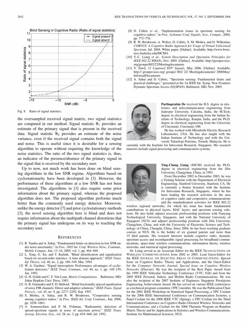
Example 7—Ratio of Signal Statistics: In this simulationexample, the ratio of signal statistics norm(S1)/norm(S2) isplotted versus the SNR (in decibels). As mentioned earlier,signal statistic S1 provides an estimate of the primary signalthat is present in the received data, whereas signal statistic S2

provides an estimate of the noise. Our detection method seesif this ratio is above a threshold. Fig. 8 shows that when thesignal is present, the ratio is always higher than when it is notpresent, even at −15 dB. As the SNR increases, the ratio (withthe signal present) increases much faster than when no signalis present. In the absence of the signal in the received data, theratio norm(S1)/norm(S2) remains almost constant.

VI. CONCLUSION

This paper has introduced a blind sensing algorithm forthe cognitive radio. The method is based on oversampling thereceived data or employing multiple receive antennas. By usinga combination of linear prediction and QR decomposition of


Fig. 8. Ratio of signal statistics.

the oversampled received signal matrix, two signal statisticsare computed in our method. Signal statistic S1 provides anestimate of the primary signal that is present in the receiveddata. Signal statistic S2 provides an estimate of the noisevariance, even if the received signal contains both the signaland noise. This is useful since it is desirable for a sensingalgorithm to operate without requiring the knowledge of thenoise statistics. The ratio of the two signal statistics is, thus,an indicator of the presence/absence of the primary signal inthe signal that is received by the secondary user.

Up to now, not much work has been done on blind sens-ing algorithms in the low SNR regime. Algorithms based oncyclostationarity have been developed in [3]. However, theperformance of these algorithms at a low SNR has not beeninvestigated. The algorithms in [3] also require some priorinformation about the primary signal, whereas the proposedalgorithm does not. The proposed algorithm performs muchbetter than the commonly used energy detector. Moreover,unlike the energy detector [7] and prior cyclostationary methods[3], the novel sensing algorithm here is blind and does notrequire information about the multipath channel distortions thatthe primary signal has undergone on its way to reaching thesecondary user.

REFERENCES

[1] R. Tandra and A. Sahai, “Fundamental limits on detection in low SNR un-der noise uncertainty,” in Proc. 2005 Int. Conf. Wireless Netw., Commun.,Mobile Comput., Jun. 13–16, 2005, vol. 1, pp. 464–469.

[2] L. Tong, G. Xu, and T. Kailath, “Blind identification and equalizationbased on second-order statistics: A time domain approach,” IEEE Trans.Inf. Theory, vol. 40, no. 2, pp. 340–349, Mar. 1994.

[3] W. A. Gardner, “Signal interception: Performance advantages of cyclic-feature detectors,” IEEE Trans. Commun., vol. 40, no. 1, pp. 149–159,Jan. 1992.

[4] G. H. Golub and C. F. Van Loan, Matrix Computations. Baltimore, MD:Johns Hopkins Univ. Press, 1983.

[5] G. B. Giannakis and S. D. Halford, “Blind fractionally spaced equalizationof noisy FIR channels: Direct and adaptive solutions,” IEEE Trans. SignalProcess., vol. 45, no. 9, pp. 2277–2292, Sep. 1997.

[6] S. Mishra, A. Sahai, and R. W. Brodersen, “Cooperative sensingamong cognitive radios,” in Proc. IEEE Int. Conf. Commun., Jun. 2006,pp. 1658–1663.

[7] A. Sonnenschien and P. M. Fishman, “Radiometric detection ofspread-spectrum signals in noise of uncertain power,” IEEE Trans.Aerosp. Electron. Syst., vol. 28, no. 3, pp. 654–660, Jul. 1992.

[8] D. Cabric et al., “Implementation issues in spectrum sensing forcognitive radios,” in Proc. Asilomar Conf. Signals, Syst., Comput., 2004,pp. 772–776.

[9] R. W. Broderson, A. Wolisz, D. Cabric, S. M. Mishra, and D. Wilkomm,CORVUS: A Cognitive Radio Approach for Usage of Virtual UnlicensedSpectrum, Jul. 2004. White paper. [Online]. Available: http://www.bwrc.eecs.berkeley.edu/MCMA

[10] Y.-C. Liang et al., System Description and Operation Principles forIEEE 802.22 WRANs, Nov. 2005. [Online]. Available: http://grouper.ieee.org/groups/802/22/Meetingdocuments

[11] V. Tawil, 51 Captured DTV Signals, May 2006. [Online]. Available:http:// grouper.ieee.org/ groups/ 802/ 22/ Meetingdocuments/ 2006May/InformalDocuments

[12] A. Sahai and D. Cabric, “Spectrum sensing: Fundamental limits andpractical challenges,” presented at the 1st IEEE Int. Symp. New FrontiersDynamic Spectrum Access (DySPAN), Baltimore, MD, Nov. 2005.

Parthapratim De received the B.S. degree in elec-tronics and telecommunication engineering fromJadavpur University, Calcutta, India, the M.Tech.degree in electrical engineering from the Indian In-stitute of Technology, Kanpur, India, and the Ph.D.degree in electrical engineering from the Universityof Cincinnati, Cincinnati, OH.

He has worked with Mitsubishi Electric ResearchLaboratories, USA. He has also taught with theIndian Institute of Technology and with the Uni-versiti Teknologi Petronas, Tronoh, Malaysia. He is

currently with the Institute for Infocomm Research, Singapore. His researchinterests include signal processing and communication systems.

Ying-Chang Liang (SM’00) received the Ph.D.degree in electrical engineering from the JilinUniversity, Changchun, China, in 1993.

From December 2002 to December 2003, he wasa Visiting Scholar with the Department of ElectricalEngineering, Stanford University, Stanford, CA. Heis currently a Senior Scientist with the Institutefor Infocomm Research, Singapore, where he hasbeen leading the research activities in the areaof cognitive radio and cooperative communicationsand the standardization activities for IEEE 802.22

wireless regional networks, for which his team has made fundamentalcontributions in physical layers, MAC layers, and spectrum sensing solu-tions. He also holds adjunct associate professorship positions with NanyangTechnological University, Singapore, and with the National University ofSingapore (NUS) and adjunct professorship positions with Jilin University,Changchun, China, and with the University of Electronic Science and Tech-nology of China, Chengdu, China. Since 2004, he has been teaching graduatecourses at NUS. He is the holder of six granted patents and more than15 filed patents. His research interests include cognitive radio, dynamicspectrum access and reconfigurable signal processing for broadband commu-nications, space-time wireless communications, information theory, wirelessnetworks, and statistical signal processing.

Dr. Liang served as an Associate Editor for the IEEE TRANSACTIONS ON

WIRELESS COMMUNICATIONS from 2002 to 2005, Lead Guest-Editor forthe IEEE JOURNAL ON SELECTED AREAS IN COMMUNICATIONS, SpecialIssue on Cognitive Radio: Theory and Applications, and the Guest-Editorfor the Computer Networks Journal, Special Issue on Cognitive WirelessNetworks (Elsevier). He was the recipient of the Best Paper Award fromthe 1999 IEEE Vehicular Technology Conference (VTC, Fall) and from the2005 IEEE Personal, Indoor, and Mobile Radio Communications. He wasalso the recipient of the 2007 Institute of Engineers Singapore PrestigiousEngineering Achievement Award. He has served on various IEEE conferencesas a technical program committee (TPC) member. He was the Publication Chairfor the 2001 IEEE Workshop on Statistical Signal Processing, a TPC Cochairfor the 2006 IEEE International Conference on Communication Systems, aPanel Cochair for the 2008 IEEE VTC (Spring), a TPC Cochair for the ThirdInternational Conference on Cognitive Radio Oriented Wireless Networks andCommunications, and a Cochair for the 2006 Thematic Program on RandomMatrix Theory and Its Applications in Statistics and Wireless Communications,Institute for Mathematical Sciences, NUS.

Blind Spectrum Sensing Algorithms for Cognitive Radio Networks

Documents

Transcript of Blind Spectrum Sensing Algorithms for Cognitive Radio Networks