Machine Learning Algorithms: An Experimental Evaluation for ...

��

Citation: Silva, H.; Bernardino, J.

Machine Learning Algorithms: An

Experimental Evaluation for Decision

Support Systems. Algorithms 2022, 15,

130. https://doi.org/10.3390/

a15040130

Academic Editor: Roberto

Montemanni

Received: 9 March 2022

Accepted: 12 April 2022

Published: 15 April 2022

Publisher’s Note: MDPI stays neutral

with regard to jurisdictional claims in

published maps and institutional affil-

iations.

Copyright: © 2022 by the authors.

Licensee MDPI, Basel, Switzerland.

This article is an open access article

distributed under the terms and

conditions of the Creative Commons

Attribution (CC BY) license (https://

creativecommons.org/licenses/by/

4.0/).

algorithms

Article

Machine Learning Algorithms: An Experimental Evaluation forDecision Support SystemsHugo Silva 1 and Jorge Bernardino 1,2,*

1 Polytechnic of Coimbra, Institute of Engineering of Coimbra—ISEC, Rua Pedro Nunes,3030-199 Coimbra, Portugal; [email protected]

2 Centre for Informatics and Systems, University of Coimbra (CISUC), Pólo II, Pinhal de Marrocos,3030-290 Coimbra, Portugal

* Correspondence: [email protected]

Abstract: Decision support systems with machine learning can help organizations improve operationsand lower costs with more precision and efficiency. This work presents a review of state-of-the-artmachine learning algorithms for binary classification and makes a comparison of the related metricsbetween them with their application to a public diabetes and human resource datasets. The twomainly used categories that allow the learning process without requiring explicit programming aresupervised and unsupervised learning. For that, we use Scikit-learn, the free software machinelearning library for Python language. The best-performing algorithm was Random Forest for su-pervised learning, while in unsupervised clustering techniques, Balanced Iterative Reducing andClustering Using Hierarchies and Spectral Clustering algorithms presented the best results. Theexperimental evaluation shows that the application of unsupervised clustering algorithms does nottranslate into better results than with supervised algorithms. However, the application of unsuper-vised clustering algorithms, as the preprocessing of the supervised techniques, can translate into aboost of performance.

Keywords: machine learning; decision support systems; big data; clustering; healthcare; humanresources; preprocessing

1. Introduction

Decision support systems (DSSs) are well-established types of information systemswith the primary purpose of improving decision making based on data and analysis. Theyanalyze massive amounts of data through the comprehensive compilation of information tosolve problems and support decision making. With this information, the system producesreports that may project revenue, sales, or manage inventory. These systems are veryimportant for many different industries, from healthcare to agriculture. A medical clinicianusing a computerized decision support system which combines the clinician inputs andprevious electronic health records can assist in diagnosing and prescribing the patient.

Healthcare is one of the fastest growing sectors and is currently in the middle of aglobal overhaul and transformation. Global healthcare costs, currently estimated betweenUSD 6 trillion and USD 7 trillion, are projected to reach more than USD 12 trillion in 2024 [1].Regarding this rapid growth in costs, measures need to be taken in order to ensure thathealthcare costs do not further spin out of control. Machine learning has been identifiedas having major technological applications in the healthcare realm, where it will probablynever completely replace physicians but will certainly transform the healthcare sector,benefiting both patients and providers.

Machine learning is a subfield of artificial intelligence that gives computers the abilityto learn. It focuses on the use of data and algorithms to imitate the way in which humanslearn [2]. The process of learning starts with data observation with examples, directexperience or instruction, so it can look for patterns in the provided data to support

Algorithms 2022, 15, 130. https://doi.org/10.3390/a15040130 https://www.mdpi.com/journal/algorithms

https://doi.org/10.3390/a15040130

https://doi.org/10.3390/a15040130

https://creativecommons.org/

https://creativecommons.org/licenses/by/4.0/

https://creativecommons.org/licenses/by/4.0/

https://www.mdpi.com/journal/algorithms

https://www.mdpi.com

https://orcid.org/0000-0003-1184-2433

https://orcid.org/0000-0001-9660-2011

https://doi.org/10.3390/a15040130

https://www.mdpi.com/journal/algorithms

https://www.mdpi.com/article/10.3390/a15040130?type=check_update&version=1

Algorithms 2022, 15, 130 2 of 24

decisions in the future. The goal is to allow computers to learn automatically withouthuman intervention and automatically adjust actions accordingly [3].

Machine learning algorithms are often categorized as either supervised and unsu-pervised. Supervised machine learning algorithms learn from labeled examples so newdata can be predicted. The learning algorithm compares the output with the correct result,finding errors in order to modify the model accordingly. Unsupervised machine learningalgorithms are characterized as systems that do not know the right output but explore thedata and draw inferences from datasets to describe hidden structures from unlabeled data.

Clustering is considered to be the most important technique of unsupervised learn-ing [4]. The definition of a cluster might be seen as a collection of data objects whichare similar to one another within the same group and are different from the objects inother clusters. Clustering can work as a standalone tool to derive insights about the datadistribution or as a preprocessing step in other algorithms.

Most works in the industry apply supervised machine learning techniques as they aremore prone to using such techniques and can be clearly compared with unsupervised learn-ing whilst supervised learning provides more relevant results; hence, artificial applicationsin the industry most often use supervised learning [5].

A recent study [6] showed that the most frequently used algorithms for predictionwere Support Vector Machine followed by Naïve Bayes. However, the Random Forestalgorithm presented superior accuracy. All of them are supervised machine learningtechniques [6]. Another study [7], for cancer diagnosis, used supervised machine learningtechniques, where the Support Vector Machine achieved maximum accuracy. Anotherstudy [8] on postpartum depression used six supervised machine learning algorithms,namely Logistic Regression, Support Vector Machine, Decision Tree, Naïve Bayes, ExtremeGradient Boosting (XGBoost) and Random Forest. As a result, the Support Vector Machinemodel was the best-performing model.

In this paper, we applied several machine learning techniques, both supervised andunsupervised, namely Logistic Regression, Support Vector Machine, Decision Tree, K-Nearest Neighbors (KNN), Naïve Bayes and Random Forest as supervised techniques andK-Means, Spectral Clustering, Mean Shift, Density-Based Spatial Clustering of Applicationswith Noise (DBSCAN) and Balanced Iterative Reducing and Clustering Using Hierarchies(BIRCH) as unsupervised clustering techniques to a diabetes and human resource datasets.We also applied unsupervised clustering algorithms such as K-Means and BIRCH forpreprocessing supervised techniques, namely Logistic Regression, Decision Tree and NaïveBayes. For the implementation of these algorithms, we used the Scikit-learn library, the freesoftware machine learning library for the Python programming language.

Our results showed the best performance for supervised techniques against unsuper-vised techniques. The best-performing algorithms were Random Forest, as the supervisedtechnique, and BIRCH and Spectral Clustering, as the unsupervised techniques. The use ofclustering unsupervised techniques, such as K-Means and BIRCH, for the preprocessing ofsupervised techniques, namely Logistic Regression, Decision Tree and Naïve Bayes, mayresult in a boost of performance.

The main contributions of this paper are the following:

1. A succinct survey of supervised and unsupervised clustering machine learning techniques;2. The presentation of the best-performing supervised and unsupervised clustering

machine learning techniques applied to healthcare and human resource datasets forbinary classification;

3. The application of unsupervised clustering algorithms for preprocessing the super-vised techniques.

The rest of this paper is organized as follows. Section 2 describes the related work onsupervised and preprocessing clustering techniques and Section 3 surveys the machinelearning algorithms and techniques used in the experiments. Section 4 presents the method-ology, detailing the characteristics of the datasets and the evaluation metrics that wereused for the performance assessment. Section 5 presents the experimental evaluation and

Algorithms 2022, 15, 130 3 of 24

Section 6 discusses the main findings. Finally, Section 7 presents the main conclusions andfuture work.

2. Related Work

This section is divided into two parts. The first part presents related research paperson decision support systems (DSSs) using supervised techniques. The second part presentsrelated research papers using preprocessing clustering techniques.

2.1. Supervised Techniques

Regarding DSSs using supervised techniques, in [9], the authors presented a work thatshowed a compilation of machine learning algorithms used in the healthcare sector andtheir accuracy for different diseases. The contribution of these authors is that for a specificdisease, there was a study conducted in the available literature that took the best algorithmswith the top performance, and a survey which was made to allow saving research timewhile gathering all this information in one single paper. The best-performing algorithmsfor different datasets varied from Logistic Regression, Decision Tree, Support Vector Ma-chine, Random Forest, Naïve Bayes, Artificial Neural Network and K-Nearest Neighbor.Nevertheless, the work compares supervised algorithms but for different datasets whichmay impact the conclusions, because the best algorithm may depend on the characteristicsof the dataset, the size and its features, among other particularities.

The work in [6] presents a study that provides a wide overview of the relative per-formance of different variants of supervised machine learning algorithms for diseaseprediction. The authors remarked that the information of the relative performance canbe used to aid researchers in the selection of an appropriate supervised machine learningalgorithm for their studies. It was found that the Support Vector Machine algorithm is themost frequently applied, followed by Naïve Bayes. However, the Random Forest algorithmshowed a superior accuracy followed by the Support Vector Machine. The research study,in addition to comparing different supervised machine learning models, does not considervariants from each algorithm, and only a comparison between the different algorithms ismade but it does not consider the hyperparameters or their tuning, which obviously has animpact on the performance results.

In [7], the authors studied three supervised machine learning techniques for cancerdiagnosis using the descriptions from breast masses. The work explored the use of av-eraging and voting ensembles to improve predictive performance. The study aimed todemonstrate that the principals can be readily applied to other complex tasks includingnatural language processing and image recognition. Maximum accuracy and the area underthe curve (AUC) were achieved using the Support Vector Machine algorithm, wherein theprediction performance increased marginally when the algorithms were arranged into avoting ensemble. The authors used a dataset which has a low number of instances andfeatures which show a lack of sparsity and high dimensionality, which are computationallyless demanding, but in another way, could lead to overfitting and do not generalize to othertest instances.

The work in [10] presents a case study related to mechanical ventilation, a life-savingintervention which, when improperly delivered, can affect and injure the patient. Thedecision support system presented promises to reduce risks by performing the per-breathclassification of five of the most widely used ventilation modes in the United States ofAmerica using the high-performance supervised machine learning model Random Forest,while having to restrict the size of the training set and maintain model generalization.The authors used almost the same size training and test datasets, which normally is notrecommended for creating a machine learning model. Additionally, as the ventilationmodes are so heterogeneous and can be difficult to identify, the dataset classification usedfor training was captured by two clinicians by mere visualization, which can be erroneousin its labeling. To conclude, the gathering of data was also confined to a single academic

Algorithms 2022, 15, 130 4 of 24

medical center and single ventilator type, which can be a limitation for a robust and reliablemachine learning model.

In [11], the authors presented a case study of people experiencing low back painevolving into a chronic condition, unless the patient receives the right interventions at theright moment. The research was initiated with the design of the decision support systemusing supervised machine learning with three classification models: Decision Tree, RandomForest and Boosted Tree. This study showed promising results with the Boosted Tree modeland Decision Tree but must still be improved with the new collection of cases, classifiedas self-care cases. One limitation of this study was that the cases in the training datasetwere fictitious cases on lower back pain collected during a vignette study with primaryhealthcare professionals which can impact the performance of the model. Additionally, weconsidered that the test dataset was excessively small, with only 38 real-life cases.

The work in [12] presented a case study for the diagnosis of periodontal disease,which is a common infectious disease in humans that may cause cardiovascular diseaseand complications of coronary heart disease. With the high prevalence of periodontaldisease, the prevention, identification and early treatment of periodontal disease havebecome extremely important. This study, using the records of 300 patients, was performedusing the Support Vector Machine supervised algorithm and based on different kernelfunctions using the cross-validation method, showing that the radial kernel function has thebest performance. Other similar studies regarding the same disease were conducted. Forexample, one study of 150 periodontal patients showed that the Support Vector Machineand Decision Tree have higher accuracy, while the Artificial Neural Network presentedthe worst results. Another study of 30 patients described the use of the Artificial NeuralNetwork with a top precision rating. One constraint of this study was that a limited datasetsize was used, where more accurate results can be obtained if more data can be used.

In [13], the authors presented a case study of coronavirus disease 2019 (COVID-19),the acute respiratory disease that has been classified as a pandemic by the World HealthOrganization. It is crucial to identify the key factors for mortality prediction to optimize thepatient treatment strategy. The dataset, after preprocessing, consisted of 1766 datapointscorresponding to 370 patients suspected of having COVID-19 from a Hospital in Wuhan.The study proposed supervised machine learning methods, namely Neural Networks,Logistic Regression, XGBoost, Random Forest, Support Vector Machine and Decision Tree,based on blood tests to predict COVID-19, using a strong combination of five features.The results showed that for feature importance and classification, XGBoost and NeuralNetwork, respectively, demonstrated the top performances. Other machine learning modelsinvolving trees and regression algorithms performed the next best performance results.

The work in [14] presented a study to support clinicians and researchers in machinelearning approaches in the field of infection management. Supervised machine learningtechniques were used, including Logistic Regression in 18 studies, followed by RandomForest, Support Vector Machine and Artificial Neural Networks in 18, 12 and 7 studies,respectively. The best-performing techniques were Long Short-Term Memory Networks,Artificial Neural Network, Logistic Regression, Support Vector Machine, Regression Treeand Stochastic Gradient Boosting. Some limitations of this study included the fact thatthe comparability of the different approaches per research area was limited and should beinterpreted with great caution. There is large heterogeneity between the identified studies,namely in terms of predicted outcomes, the features used and the study size. Knowing thatthe operations of cleaning and transforming, normally represents the majority percentageof the entire work of applying a machine learning model to data, in 39% of the previouscarried studies there was no mention to this kind of operations.

In [8], the authors presented a study of postpartum depression, which is a depressiveepisode that begins within one year from childbirth, interfering with the mother’s emotionalwell-being but also associated with infant morbidity and poorer cognitive and behavioralskills in children later in life. Electronic health records were obtained from two Hospitalsbetween 2015–2017 with 9980 episodes of pregnancy identified. Six supervised machine

Algorithms 2022, 15, 130 5 of 24

learning algorithms were used, including Logistic Regression, Support Vector Machine,Decision Tree, Naïve Bayes, XGBoost and Random Forest. The Support Vector Machinemodel was the best-performing model. Nevertheless, the use of multiple features fromthe dataset can lead to a complex system wherein the most correlated features should bechosen among the total set. Additionally, the method used for oversampling to handle animbalanced dataset may contribute to overfitting and impacting the model performance.

The work in [15] presented a study of the early prediction of asthma exacerbations,which is the most common and costly chronic disease in United States. For the detection ofthis disease, a prediction model was built using the Bayesian Classifier, Adaptative BayesianNetwork and Support Vector Machine supervised algorithms. The dataset consisted of7001 records collected using a previously prescribed remote management from homemethod, wherein patients used a laptop computer at home to fill in their asthma diary on adaily basis. It was found that the dataset distribution is highly skewed, where the problemwas addressed by rearranging the dataset for three experiments: the first one with all thedata used for training and testing; the second one with stratified samples for both trainingand testing; and the last one with a stratified sample for training all the remaining datafor testing. Then, the three predictive models were used, wherein predictive models weretrained on stratified samples, which yielded better results. Nevertheless, this study hassome limitations, namely the relatively small data sample, containing limited numbers ofcases of asthma exacerbations.

2.2. Preprocessing Clustering Techniques

Regarding research papers using preprocessing clustering techniques, the authorsin [16] proposed an evaluation method while using unsupervised clustering algorithms bymeasuring the usefulness of the task under consideration. For that, they used two examplescenarios, among which one included the use of clustering as an automated pre-processingstep in a whole data-processing chain. The purpose of this was to improve the overallperformance of the system, which can be quantified by some problem-dependent score.The clustering algorithm was just one more “parameter” that has to be tuned and thistuning can be achieved in the same way as for all other parameters. What matters is notthe evaluation of the quality of the clustering and which meaningful groups it discovers,but the usefulness of the clustering for achieving the final goal.

The work in [17] presented a study using stochastic gradient Markov Chain MonteCarlo (SG-MCMC) and proposed a subsampling strategy to reduce the variance of apply-ing naïve subsampling. For that, the authors partitioned the dataset with the K-MeansClustering algorithm in a preprocessing step and used fixed clustering throughout theentire MCMC simulation. In particular, the clustering procedure was performed on thedata samples only once before simulation, and during the sampling procedure, it was easierto compute the new gradient estimator without having extra overhead.

In [18], the authors presented a study of an unsupervised clustering approach toresolve the frequent data imbalance problem in supervised learning problems in functionalgenomics. The study proposed preprocessing majority instances by partitioning them intoclusters using class purity maximization clustering, which greatly reduced the ambiguitybetween minority instances and the instances in each cluster. For a moderately or highlyimbalanced ratio and low in-class complexity, this technique has a better prediction accuracythan the under sampling method. For an extremely unbalanced ratio, this techniquedemonstrates an almost perfect recall that reduces the amount of imbalance with significantimprovements over previous predictors.

The work in [19] presents a study on hydrological models wherein the dynamic char-acteristics, such as seasonal dynamics, are revealed to be a model structural deficiency. Theauthors proposed a clustering preprocessing framework for the calibration of hydrologicalmodels to simulate seasonal dynamic behaviors. Two clustering operations were performedbased on the preprocessed climatic index and land-surface index systems. The obtainedresults show that the performance of the model with a clustering preprocessing framework

Algorithms 2022, 15, 130 6 of 24

in the middle and low-flow conditions is significantly improved without reducing thesimulation accuracy for high flows.

From previous research papers, the application of the clustering preprocessing tech-nique is used for subsampling, data imbalance, or model calibration. The specific appli-cation to supervised algorithms is still uncommon to the best of our knowledge. Thiswork intends to highlight the importance of these unsupervised techniques. Mainly, theuse of clustering for preprocessing supervised algorithms may translate into a boost intheir performance.

3. Machine Learning Algorithms and Techniques

In this section, we survey the algorithms and techniques used for the diabetes andhuman resource datasets. A brief conceptual explanation of both supervised and clusteringunsupervised techniques is presented.

3.1. Logistic Regression

Logistic Regression is a supervised algorithm that is often used for predictive analyticsand modeling to understand the relationship between a dependent variable and one ormore independent variables, wherein probabilities are estimated using a logistic regressionequation [20]. The dependent variable is finite or categorical, whereas for binary regression,we have A or B options, and for multinomial regression, we have a range of finite options,for example A, B, C or D. Examples that use this technique can be found in [8,9,13,14].

3.2. Support Vector Machine

Support Vector Machine is a supervised algorithm whose the purpose is to find ahyperplane in an N-dimensional space with N as the number of features which distinctlyclassifies the data points [21]. There are many possible hyperplanes that can separate thetwo classes of data points, however, we want to maximize the distance between the datapoints of the classes while having a plane that has a maximum margin. With this, futuredata points can be classified with more confidence. Among related works, [6–9,13–15] areexamples that use this technique.

3.3. Decision Tree

Decision Tree is a supervised algorithm to categorize or make predictions on how aprevious set of questions were answered [22]. As the name says, it resembles a tree whereinthe base of the tree is the root node, from which we obtain a series of decision nodes thatdepict the decisions to be made. From the decision nodes representing the question orsplit point, we have leaf nodes which represent the consequences of those decisions or theanswers. Examples that use this technique can be found in [8,9,11–13].

3.4. Naïve Bayes

Naïve Bayes is a supervised algorithm based on the Bayes theorem as in Equation (1),where we can find the probability of A happening, given that B has occurred [23].

Precision =P(B|A)P(A)

P(B)(1)

The assumption made is that the predictors or features are independent, meaning thatthe presence of one particular feature does not affect the other. Even if there is dependency,all these features still independently contribute to the probability; hence, it is called naïve.Among related works, [6,8,9] are examples that use this technique.

3.5. Random Forest

Random Forest is a supervised algorithm which combines the output of multipledecision trees to reach a single result [24]. It generates a random subset of features, whichensures low correlation among decision trees. This is a key difference between decision

Algorithms 2022, 15, 130 7 of 24

trees and random forest. While decision trees consider all possible features splits, randomforest only select a subset of those features. Examples that use this technique can be foundin [6,8–11,13,14].

3.6. K-Nearest Neighbors (KNN)

KNN is a supervised algorithm which estimates the likelihood that a data point willbecome a member of one group or another based on what group the data points nearestto it belong to [25]. It is called a lazy learning algorithm because it does not perform anytraining when we supply the training data, but simply stores them during the training timeand no calculations are made. KNN tries to determine what group a data point belongsto by looking at the data points around it. In related work, [9] is an example that usesthis technique.

The algorithm performs a voting mechanism to determine the class of an unseenobservation where the class with the majority vote will become the class of the data point.If the value of K is equal to one, then it will use only the nearest neighbor to determine theclass, and if the value of K is equal to ten, it will use the ten nearest neighbors.

3.7. K-Means

K-Means is a clustering unsupervised algorithm where the purpose is to group similardata points together and discover underlying patterns whilst looking for a fixed number(k) of clusters in the dataset [26]. A cluster is nothing more than a collection of data pointsaggregated together because of certain similarities. We started to define a target number kwhich is the number of centroids. A centroid is the imaginary or real location representingthe center of the cluster, and every data point is allocated to each of the clusters by reducingthe in-cluster sum of squares. In other words, it tries to keep the centroids as small aspossible. An example from the related work that uses this technique can be found in [17].

3.8. Spectral Clustering

Spectral Clustering is a clustering unsupervised algorithm which reduces complexmultidimensional datasets into clusters of similar data in rarer dimensions [27]. It makesno assumptions about the form of the clusters. In contrast to the K-Means technique, whichassumes that the points assigned to a cluster are spherical about the cluster center, SpectralClustering helps to create more accurate clusters and can correctly cluster observations thatactually belong to the same cluster. However, these are farther off than observations inother clusters due to the dimension reduction.

3.9. Mean Shift

Mean Shift is a clustering unsupervised algorithm whose purpose is to discover blobsin a smooth density of samples [28]. It is a centroid-based algorithm that works by updatingcandidates for centroids to be the mean of the points within a given region, also calledbandwidth. These candidates are then filtered in a post-processing stage to eliminatenear-duplicates to form the final set of centroids. In contrast to K-Means, there is no needto choose the number of clusters.

3.10. DBSCAN

DBSCAN is a clustering unsupervised algorithm that groups together data pointsthat are close to each other based on a distance measurement and a minimum numberof points [29]. It also marks the data points that are in low-density regions as outliers.Basically, this requires two parameters: the first one specifies how close data points shouldbe to each other to be considered part of the cluster; and the second parameter is to definethe minimum number of data points to form a dense region.

Algorithms 2022, 15, 130 8 of 24

3.11. BIRCH

BIRCH is a clustering unsupervised algorithm that uses hierarchical methods tocluster and reduce data [30]. The algorithm only needs to scan the dataset in a single pass toperform clustering and uses a tree structure to create a cluster which is generally called theClustering Feature Tree. Each node of the tree is composed of several clustering features.

BIRCH is often used to complement other clustering algorithms by creating a summaryof the dataset that the other clustering algorithm can now use [31]. It can only process themetric attributes represented in Euclidean space, i.e., no categorical attributes should bepresent. Categorical refers to attributes that generally take a limited number of possiblevalues that do not necessarily need to be numerical but can be textual in nature.

4. Materials and Methods

This section aims to provide the methodology, specifying the characteristics of thedatasets, the applied preprocessing steps and the evaluation metrics that were used for theperformance assessment.

4.1. Dataset and Preprocessing

We describe the diabetes and human resource datasets along with the preprocessingoperations before submitting to the algorithms. Note that the unsupervised clusteringalgorithms applied for preprocessing the supervised algorithms were executed after thefollowing preprocessing operations for the datasets.

4.1.1. Diabetes Dataset

The type II diabetes disease dataset was originally from the National Institute ofDiabetes and Digestive and Kidney Diseases, and was obtained from [32]. In particular, allthe data refer to female patients that were at least 21 years old and of Pima heritage, whichare Native Americans who traditionally lived along the Gila and Salt rivers in Arizona inthe United States of America [33].

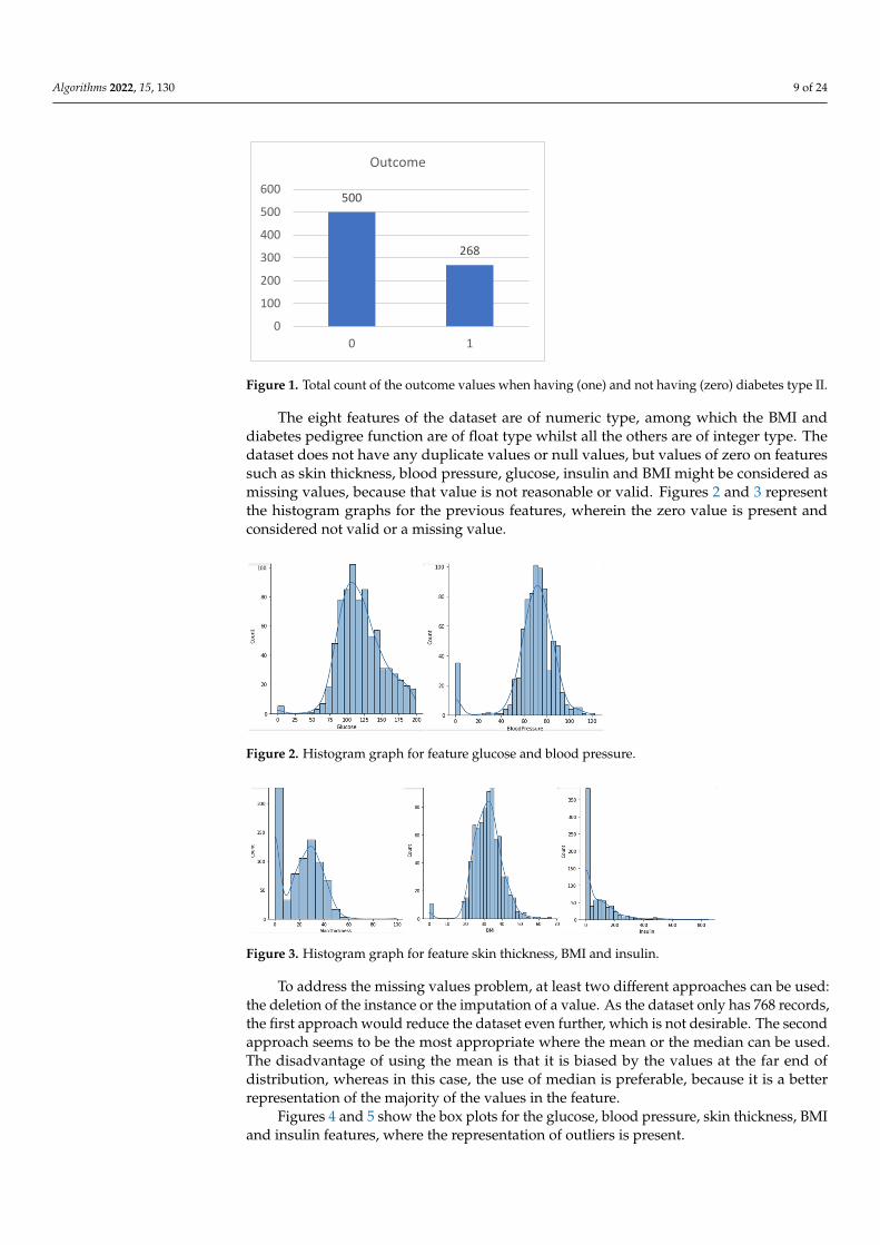
The dataset has 768 records, each one of which are for a single person with eightfeatures and a target label. The first feature, pregnancies, is the number of times that theperson was pregnant. The second feature, glucose, is the plasma glucose concentration intheir blood and the main indicator of diabetes. Diabetes is characterized by the difficulty orinability of the pancreas to produce insulin, a hormone that transforms glucose from food.The third feature, blood pressure, measured in units of millimeters of mercury (mmHg),is the pressure in which blood circulates within the arteries which varies throughoutthe day along normal values. The fourth feature, skin thickness, measured in mm, isprimarily determined by collagen content and is increased when having diabetes. The fifthfeature, insulin, measured in µIU/mL, is a hormone responsible for lowering blood glucoseby promoting the entry of glucose into cells. The sixth feature, body mass index (BMI),measured in kg/m2, is used to know whether the weight matches the person’s height,namely if the person is underweight, normal weight or above what would be expected fortheir weight. The seventh feature, diabetes pedigree function, is a function that determinesthe risk of type II diabetes based on family history. A bigger function indicates a greaterrisk of type II diabetes. The eighth feature, age, is the age of the person. The outcometarget label is our target or class attribute, which is one or zero depending on whether theperson has been diagnosed with type II diabetes or not, respectively. The dataset contains268 records of persons with diabetes type II and 500 records of persons who do not, asshown in Figure 1.

Algorithms 2022, 15, 130 9 of 24

Algorithms 2022, 14, x FOR PEER REVIEW 9 of 24

height, namely if the person is underweight, normal weight or above what would be ex-pected for their weight. The seventh feature, diabetes pedigree function, is a function that determines the risk of type II diabetes based on family history. A bigger function indicates a greater risk of type II diabetes. The eighth feature, age, is the age of the person. The outcome target label is our target or class attribute, which is one or zero depending on whether the person has been diagnosed with type II diabetes or not, respectively. The dataset contains 268 records of persons with diabetes type II and 500 records of persons who do not, as shown in Figure 1.

Figure 1. Total count of the outcome values when having (one) and not having (zero) diabetes type II.

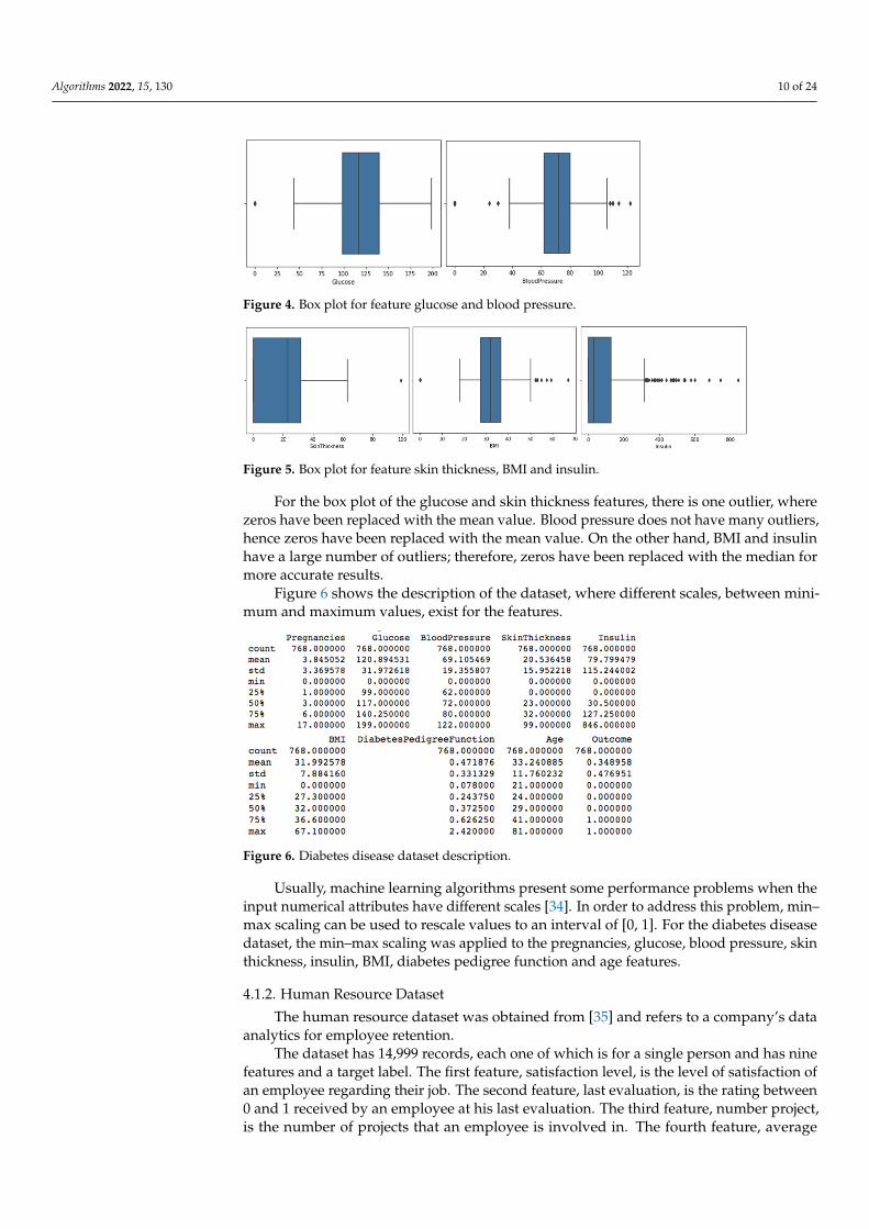
The eight features of the dataset are of numeric type, among which the BMI and dia-betes pedigree function are of float type whilst all the others are of integer type. The da-taset does not have any duplicate values or null values, but values of zero on features such as skin thickness, blood pressure, glucose, insulin and BMI might be considered as miss-ing values, because that value is not reasonable or valid. Figures 2 and 3 represent the histogram graphs for the previous features, wherein the zero value is present and consid-ered not valid or a missing value.

Figure 2. Histogram graph for feature glucose and blood pressure.

Figure 3. Histogram graph for feature skin thickness, BMI and insulin.

500

268

0

100

200

300

400

500

600

0 1

Outcome


The eight features of the dataset are of numeric type, among which the BMI anddiabetes pedigree function are of float type whilst all the others are of integer type. Thedataset does not have any duplicate values or null values, but values of zero on featuressuch as skin thickness, blood pressure, glucose, insulin and BMI might be considered asmissing values, because that value is not reasonable or valid. Figures 2 and 3 representthe histogram graphs for the previous features, wherein the zero value is present andconsidered not valid or a missing value.







500

268

0

100

200

300

400

500

600

0 1

Outcome








500

268

0

100

200

300

400

500

600

0 1

Outcome


To address the missing values problem, at least two different approaches can be used:the deletion of the instance or the imputation of a value. As the dataset only has 768 records,the first approach would reduce the dataset even further, which is not desirable. The secondapproach seems to be the most appropriate where the mean or the median can be used.The disadvantage of using the mean is that it is biased by the values at the far end ofdistribution, whereas in this case, the use of median is preferable, because it is a betterrepresentation of the majority of the values in the feature.

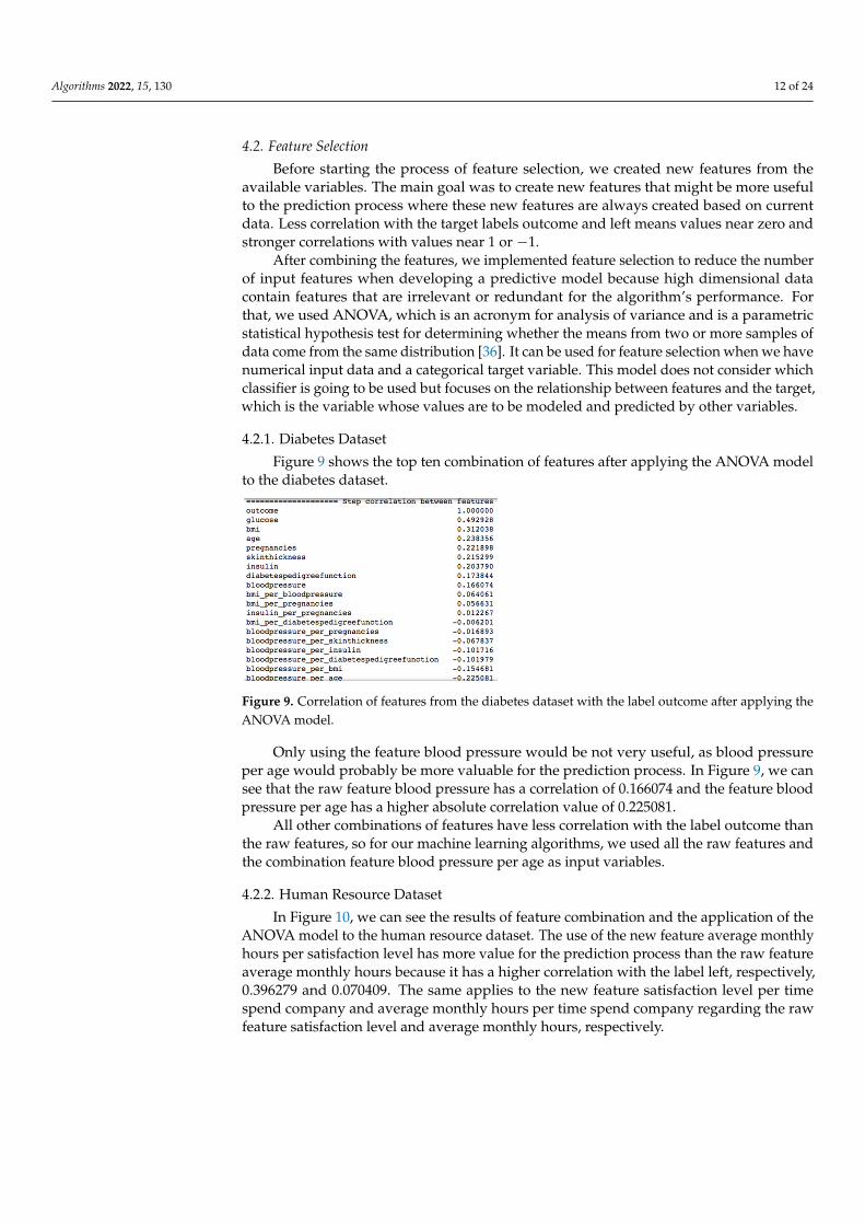
Figures 4 and 5 show the box plots for the glucose, blood pressure, skin thickness, BMIand insulin features, where the representation of outliers is present.

Algorithms 2022, 15, 130 10 of 24


To address the missing values problem, at least two different approaches can be used: the deletion of the instance or the imputation of a value. As the dataset only has 768 rec-ords, the first approach would reduce the dataset even further, which is not desirable. The second approach seems to be the most appropriate where the mean or the median can be used. The disadvantage of using the mean is that it is biased by the values at the far end of distribution, whereas in this case, the use of median is preferable, because it is a better representation of the majority of the values in the feature.

Figures 4 and 5 show the box plots for the glucose, blood pressure, skin thickness, BMI and insulin features, where the representation of outliers is present.

Figure 4. Box plot for feature glucose and blood pressure.

Figure 5. Box plot for feature skin thickness, BMI and insulin.

For the box plot of the glucose and skin thickness features, there is one outlier, where zeros have been replaced with the mean value. Blood pressure does not have many outli-ers, hence zeros have been replaced with the mean value. On the other hand, BMI and insulin have a large number of outliers; therefore, zeros have been replaced with the me-dian for more accurate results.

Figure 6 shows the description of the dataset, where different scales, between mini-mum and maximum values, exist for the features.

Figure 6. Diabetes disease dataset description.

Usually, machine learning algorithms present some performance problems when the input numerical attributes have different scales [34]. In order to address this problem, min–max scaling can be used to rescale values to an interval of [0, 1]. For the diabetes












For the box plot of the glucose and skin thickness features, there is one outlier, wherezeros have been replaced with the mean value. Blood pressure does not have many outliers,hence zeros have been replaced with the mean value. On the other hand, BMI and insulinhave a large number of outliers; therefore, zeros have been replaced with the median formore accurate results.












Usually, machine learning algorithms present some performance problems when theinput numerical attributes have different scales [34]. In order to address this problem, min–max scaling can be used to rescale values to an interval of [0, 1]. For the diabetes diseasedataset, the min–max scaling was applied to the pregnancies, glucose, blood pressure, skinthickness, insulin, BMI, diabetes pedigree function and age features.

4.1.2. Human Resource Dataset

The human resource dataset was obtained from [35] and refers to a company’s dataanalytics for employee retention.

The dataset has 14,999 records, each one of which is for a single person and has ninefeatures and a target label. The first feature, satisfaction level, is the level of satisfaction ofan employee regarding their job. The second feature, last evaluation, is the rating between0 and 1 received by an employee at his last evaluation. The third feature, number project,is the number of projects that an employee is involved in. The fourth feature, average

Algorithms 2022, 15, 130 11 of 24

monthly hours, is the average number of hours in a month spent by an employee at theoffice. The fifth feature, time spend company, is the number of years that an employee hasspent in the company. The sixth feature, work accident, is a binary value where zero meansthat the employee had no accident during their stay and one means that the employee hadaccident during their stay. The seventh feature, promotion last 5 years, is the number ofpromotions during an employee’s stay. The eighth feature, department, is the departmentthat an employee belongs to. The ninth feature, salary, is the level of salary an employeehas, namely low, medium or high. The target label, left, is a binary value, wherein zeroindicates that the employee remains in the company and one indicates that the employeeleft the company.

The dataset does not contain missing or null values but contains duplicate records.The duplicates were eliminated, resulting in 10,000 records of employees remaining in thecompany and 1991 records of employees leaving, as shown in Figure 7.


disease dataset, the min–max scaling was applied to the pregnancies, glucose, blood pres-sure, skin thickness, insulin, BMI, diabetes pedigree function and age features.

4.1.2. Human Resource Dataset The human resource dataset was obtained from [35] and refers to a company’s data

analytics for employee retention. The dataset has 14,999 records, each one of which is for a single person and has nine

features and a target label. The first feature, satisfaction level, is the level of satisfaction of an employee regarding their job. The second feature, last evaluation, is the rating between 0 and 1 received by an employee at his last evaluation. The third feature, number project, is the number of projects that an employee is involved in. The fourth feature, average monthly hours, is the average number of hours in a month spent by an employee at the office. The fifth feature, time spend company, is the number of years that an employee has spent in the company. The sixth feature, work accident, is a binary value where zero means that the employee had no accident during their stay and one means that the em-ployee had accident during their stay. The seventh feature, promotion last 5 years, is the number of promotions during an employee’s stay. The eighth feature, department, is the department that an employee belongs to. The ninth feature, salary, is the level of salary an employee has, namely low, medium or high. The target label, left, is a binary value, wherein zero indicates that the employee remains in the company and one indicates that the employee left the company.

The dataset does not contain missing or null values but contains duplicate records. The duplicates were eliminated, resulting in 10,000 records of employees remaining in the company and 1991 records of employees leaving, as shown in Figure 7.

Figure 7. Total count of left values when employees have left (one) or not left (zero) the company.

The features satisfaction level and last evaluation of the dataset are of float continu-ous numeric type. The features number project, average monthly hours and time spend company are of integer numeric type, while the features work accident and promotion last are of categorical numeric type and the department of the categorical type. The last feature salary is of ordinal type.

In order to have inputs as numeric type for the algorithms, a conversion to numeric was made for the feature department and salary. Figure 8 shows the description of the dataset, wherein only the feature average monthly hours has a different scale from the remaining feature, and min–max scaling was applied to this feature.

Figure 7. Total count of left values when employees have left (one) or not left (zero) the company.

The features satisfaction level and last evaluation of the dataset are of float continuousnumeric type. The features number project, average monthly hours and time spendcompany are of integer numeric type, while the features work accident and promotion lastare of categorical numeric type and the department of the categorical type. The last featuresalary is of ordinal type.

In order to have inputs as numeric type for the algorithms, a conversion to numericwas made for the feature department and salary. Figure 8 shows the description of thedataset, wherein only the feature average monthly hours has a different scale from theremaining feature, and min–max scaling was applied to this feature.


Figure 8. Human resource dataset description.

4.2. Feature Selection Before starting the process of feature selection, we created new features from the

available variables. The main goal was to create new features that might be more useful to the prediction process where these new features are always created based on current data. Less correlation with the target labels outcome and left means values near zero and stronger correlations with values near 1 or −1.

After combining the features, we implemented feature selection to reduce the num-ber of input features when developing a predictive model because high dimensional data contain features that are irrelevant or redundant for the algorithm’s performance. For that, we used ANOVA, which is an acronym for analysis of variance and is a parametric statis-tical hypothesis test for determining whether the means from two or more samples of data come from the same distribution [36]. It can be used for feature selection when we have numerical input data and a categorical target variable. This model does not consider which classifier is going to be used but focuses on the relationship between features and the target, which is the variable whose values are to be modeled and predicted by other variables.

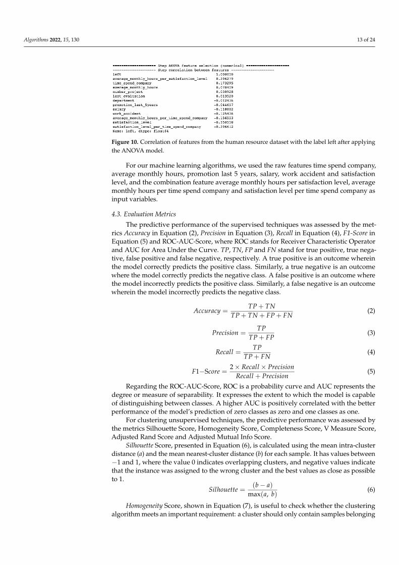
4.2.1. Diabetes Dataset Figure 9 shows the top ten combination of features after applying the ANOVA model

to the diabetes dataset.

Figure 9. Correlation of features from the diabetes dataset with the label outcome after applying the ANOVA model.

Only using the feature blood pressure would be not very useful, as blood pressure per age would probably be more valuable for the prediction process. In Figure 9, we can


Algorithms 2022, 15, 130 12 of 24

4.2. Feature Selection

Before starting the process of feature selection, we created new features from theavailable variables. The main goal was to create new features that might be more usefulto the prediction process where these new features are always created based on currentdata. Less correlation with the target labels outcome and left means values near zero andstronger correlations with values near 1 or −1.

After combining the features, we implemented feature selection to reduce the numberof input features when developing a predictive model because high dimensional datacontain features that are irrelevant or redundant for the algorithm’s performance. Forthat, we used ANOVA, which is an acronym for analysis of variance and is a parametricstatistical hypothesis test for determining whether the means from two or more samples ofdata come from the same distribution [36]. It can be used for feature selection when we havenumerical input data and a categorical target variable. This model does not consider whichclassifier is going to be used but focuses on the relationship between features and the target,which is the variable whose values are to be modeled and predicted by other variables.

4.2.1. Diabetes Dataset

Figure 9 shows the top ten combination of features after applying the ANOVA modelto the diabetes dataset.



4.2. Feature Selection Before starting the process of feature selection, we created new features from the

available variables. The main goal was to create new features that might be more useful to the prediction process where these new features are always created based on current data. Less correlation with the target labels outcome and left means values near zero and stronger correlations with values near 1 or −1.

After combining the features, we implemented feature selection to reduce the num-ber of input features when developing a predictive model because high dimensional data contain features that are irrelevant or redundant for the algorithm’s performance. For that, we used ANOVA, which is an acronym for analysis of variance and is a parametric statis-tical hypothesis test for determining whether the means from two or more samples of data come from the same distribution [36]. It can be used for feature selection when we have numerical input data and a categorical target variable. This model does not consider which classifier is going to be used but focuses on the relationship between features and the target, which is the variable whose values are to be modeled and predicted by other variables.

4.2.1. Diabetes Dataset Figure 9 shows the top ten combination of features after applying the ANOVA model

to the diabetes dataset.

Figure 9. Correlation of features from the diabetes dataset with the label outcome after applying the ANOVA model.

Only using the feature blood pressure would be not very useful, as blood pressure per age would probably be more valuable for the prediction process. In Figure 9, we can

Figure 9. Correlation of features from the diabetes dataset with the label outcome after applying theANOVA model.

Only using the feature blood pressure would be not very useful, as blood pressureper age would probably be more valuable for the prediction process. In Figure 9, we cansee that the raw feature blood pressure has a correlation of 0.166074 and the feature bloodpressure per age has a higher absolute correlation value of 0.225081.

All other combinations of features have less correlation with the label outcome thanthe raw features, so for our machine learning algorithms, we used all the raw features andthe combination feature blood pressure per age as input variables.

4.2.2. Human Resource Dataset

In Figure 10, we can see the results of feature combination and the application of theANOVA model to the human resource dataset. The use of the new feature average monthlyhours per satisfaction level has more value for the prediction process than the raw featureaverage monthly hours because it has a higher correlation with the label left, respectively,0.396279 and 0.070409. The same applies to the new feature satisfaction level per timespend company and average monthly hours per time spend company regarding the rawfeature satisfaction level and average monthly hours, respectively.

Algorithms 2022, 15, 130 13 of 24


see that the raw feature blood pressure has a correlation of 0.166074 and the feature blood pressure per age has a higher absolute correlation value of 0.225081.

All other combinations of features have less correlation with the label outcome than the raw features, so for our machine learning algorithms, we used all the raw features and the combination feature blood pressure per age as input variables.

4.2.2. Human Resource Dataset In Figure 10, we can see the results of feature combination and the application of the

ANOVA model to the human resource dataset. The use of the new feature average monthly hours per satisfaction level has more value for the prediction process than the raw feature average monthly hours because it has a higher correlation with the label left, respectively, 0.396279 and 0.070409. The same applies to the new feature satisfaction level per time spend company and average monthly hours per time spend company regarding the raw feature satisfaction level and average monthly hours, respectively.

Figure 10. Correlation of features from the human resource dataset with the label left after applying the ANOVA model.

For our machine learning algorithms, we used the raw features time spend company, average monthly hours, promotion last 5 years, salary, work accident and satisfaction level, and the combination feature average monthly hours per satisfaction level, average monthly hours per time spend company and satisfaction level per time spend company as input variables.

4.3. Evaluation Metrics The predictive performance of the supervised techniques was assessed by the metrics

Accuracy in Equation (2), Precision in Equation (3), Recall in Equation (4), F1-Score in Equa-tion (5) and ROC-AUC-Score, where ROC stands for Receiver Characteristic Operator and AUC for Area Under the Curve. TP, TN, FP and FN stand for true positive, true negative, false positive and false negative, respectively. A true positive is an outcome wherein the model correctly predicts the positive class. Similarly, a true negative is an outcome where the model correctly predicts the negative class. A false positive is an outcome where the model incorrectly predicts the positive class. Similarly, a false negative is an outcome wherein the model incorrectly predicts the negative class. 𝐴𝑐𝑐𝑢𝑟𝑎𝑐𝑦 = 𝑇𝑃 + 𝑇𝑁𝑇𝑃 + 𝑇𝑁 + 𝐹𝑃 + 𝐹𝑁 (2)

𝑃𝑟𝑒𝑐𝑖𝑠𝑖𝑜𝑛 = 𝑇𝑃𝑇𝑃 + 𝐹𝑃 (3)

𝑅𝑒𝑐𝑎𝑙𝑙 = 𝑇𝑃𝑇𝑃 + 𝐹𝑁 (4)

𝐹1-S𝑐𝑜𝑟𝑒 = 2 𝑅𝑒𝑐𝑎𝑙𝑙 𝑃𝑟𝑒𝑐𝑖𝑠𝑖𝑜𝑛𝑅𝑒𝑐𝑎𝑙𝑙 + 𝑃𝑟𝑒𝑐𝑖𝑠𝑖𝑜𝑛 (5)

Regarding the ROC-AUC-Score, ROC is a probability curve and AUC represents the degree or measure of separability. It expresses the extent to which the model is capable of

Figure 10. Correlation of features from the human resource dataset with the label left after applyingthe ANOVA model.

For our machine learning algorithms, we used the raw features time spend company,average monthly hours, promotion last 5 years, salary, work accident and satisfactionlevel, and the combination feature average monthly hours per satisfaction level, averagemonthly hours per time spend company and satisfaction level per time spend company asinput variables.

4.3. Evaluation Metrics

The predictive performance of the supervised techniques was assessed by the met-rics Accuracy in Equation (2), Precision in Equation (3), Recall in Equation (4), F1-Score inEquation (5) and ROC-AUC-Score, where ROC stands for Receiver Characteristic Operatorand AUC for Area Under the Curve. TP, TN, FP and FN stand for true positive, true nega-tive, false positive and false negative, respectively. A true positive is an outcome whereinthe model correctly predicts the positive class. Similarly, a true negative is an outcomewhere the model correctly predicts the negative class. A false positive is an outcome wherethe model incorrectly predicts the positive class. Similarly, a false negative is an outcomewherein the model incorrectly predicts the negative class.

Accuracy =TP + TN

TP + TN + FP + FN(2)

Precision =TP

TP + FP(3)

Recall =TP

TP + FN(4)

F1−Score =2× Recall × Precision

Recall + Precision(5)

Regarding the ROC-AUC-Score, ROC is a probability curve and AUC represents thedegree or measure of separability. It expresses the extent to which the model is capableof distinguishing between classes. A higher AUC is positively correlated with the betterperformance of the model’s prediction of zero classes as zero and one classes as one.

For clustering unsupervised techniques, the predictive performance was assessed bythe metrics Silhouette Score, Homogeneity Score, Completeness Score, V Measure Score,Adjusted Rand Score and Adjusted Mutual Info Score.

Silhouette Score, presented in Equation (6), is calculated using the mean intra-clusterdistance (a) and the mean nearest-cluster distance (b) for each sample. It has values between−1 and 1, where the value 0 indicates overlapping clusters, and negative values indicatethat the instance was assigned to the wrong cluster and the best values as close as possibleto 1.

Silhouette =(b− a)

max(a, b)(6)

Homogeneity Score, shown in Equation (7), is useful to check whether the clusteringalgorithm meets an important requirement: a cluster should only contain samples belonging

Algorithms 2022, 15, 130 14 of 24

to a single class. It has values between 0 and 1, where 1 means that there is a perfecthomogeneous classification.

Homogeneity = 1−H(

Ytrue

∣∣∣Ypred)

H(Ytrue)(7)

Completeness Score, shown in Equation (8), has the purpose of checking whether all thedata points that are members of a given class are elements of the same cluster. This variesbetween 0 and 1, where 1 means that all members of a class belong to the same cluster.

Completeness = 1−H(

Ypred

∣∣∣Ytrue)

H(

Ypred

) (8)

V Measure Score, shown in Equation (9), is the harmonic mean between homogeneityand completeness, varying between 0 and 1, with values of 1 meaning that there is aperfect homogeneous and complete classification. Beta is the ratio of weight attributed tohomogeneity versus completeness.

V Measure =(1 + beta) × homogeneity × completness

beta × homogeneity × completeness(9)

Adjusted Rand Score, shown in Equation (10), is used to determine whether two clusterresults are similar to each other. In formula (10), RI stands for the Rand index, whichcalculates the similarity between two cluster results by taking all the points identifiedwithin the same cluster. It can have values between −1 and 1, where values close to 0 meana random classification and values closer to 1 mean the best classification.

Adjusted Rand Score =RI − Expected_RI

max(RI)− Expected_RI(10)

Adjusted Mutual Info Score, shown in Equation (11), is an adjustment of the MutualInformation (MI) score to account for chance. It accounts for the fact that MI is generallyhigher for two clusterings with a larger number of clusters regardless of whether there isactually more information shared. U denotes label true and V denotes label pred. It variesbetween −1 and 1, returning 1 when two partitions are identical or perfectly classified,while random partitions correspond to values close to 0.

Adjusted Mutual In f o Score =MI(U, V)− E(MI(U, V))

avg(H(U), H(V))− E(MI(U, V))(11)

4.4. Training and Testing

We tested 12 different algorithms to compare the predictive performance of variousmachine learning algorithms, as described in the following subsections. From the Scikit-learn library in Python, between supervised and unsupervised clustering techniques, alongwith the application of two unsupervised clustering algorithms (K-Means and BIRCH)for preprocessing three supervised techniques (Decision Tree, Logistic Regression andNaïve Bayes).

For all algorithms, three groups of the dataset were defined with training and testingpercentages of 80% and 20%, 75% and 25%, and 70% and 30%, respectively.

4.4.1. Logistic Regression, Decision Tree, Naïve Bayes

We used all the default parameters values of the supervised Logistic Regression,Decision Tree and Naïve Bayes algorithms from the Scikit-learn library.

Algorithms 2022, 15, 130 15 of 24

4.4.2. Support Vector Machine

There are two variants of the supervised Support Vector Machine algorithm, linear andnon-linear, where the difference between them is the fact that the first can easily separatedata with a linear line, and the second cannot.

For the linear variant, default values from the Scikit-learn library were used exceptfor parameter C, which is a regularization parameter [37]. For large values of C, theoptimization will choose a smaller-margin hyperplane to obtain all of the correctly classifiedtraining points. Conversely, a very small value of C will cause the optimizer to look for alarger-margin separating hyperplane, even if that hyperplane misclassifies more points. Cparameter values of 0.1, 1 and 10 were defined.

For the non-linear variant, default values were used, except for parameters C, gammaand kernel. The gamma parameter is used for non-linear hyperplanes, where higher valuesmean that the algorithm will try to exactly fit the training data [37]. The kernel parameter isa method used to take data as input and transform into the required form of processing data.C and gamma parameter values of 0.1, 1 and 10 were defined, and the kernel parametervalues of ‘linear’ and radial basis function (‘rbf’).

4.4.3. Random Forest

We used default values of the supervised random forest algorithm from the Scikit-learn library, except for the n_estimators, criterion and class_weight parameters. TheN_estimators parameter is the number of trees needed in the algorithm that depends on thenumber of rows in the dataset. More rows means that more trees are needed [38]. The crite-rion parameter is a function that measures the quality of a split in a tree. The class_weightparameter allows to specify the weights of each class in the case of an imbalanced dataset.

In the experiments, the n_estimators parameter assumes values of 10, 40, 70 and100. The criterion parameter has the values of ‘gini’ and ‘entropy’, and the class_weightparameter values of ‘balanced’ and ‘balanced_subsample’.

4.4.4. K-Nearest Neighbors

We used the default values of the supervised clustering KNN algorithm from theScikit-learn library, except for the n_neighbors parameter. The n_neighbors value indicatesthe count of nearest neighbors we want to select to predict the class of a given item [39].

The n_neighbors parameter was defined with integer values from 1 to 9.

4.4.5. K-Means

We used the default values for the K-Means unsupervised clustering algorithm fromthe Scikit-learn library except for the n_clusters and n_init parameters. The n_clustersparameter is the number of clusters to form as well as the number of centroids to generate,while the n_init parameter is the number of times that the algorithm will be run withdifferent centroid seeds [40].

The n_clusters parameter was defined with integer values from to 2 to 5, and the n_initparameter was defined with integer values from 1 to 4.

4.4.6. Spectral Clustering

We used the default values of the unsupervised clustering Spectral Clustering al-gorithm from the Scikit-learn library, except for the n_clusters, n_init, gamma and as-sign_labels parameters. The n_clusters and n_init parameters have the same definitionas from the K-Means algorithm, while the gamma parameter is the kernel coefficient andassign_labels is the strategy for assigning labels in the embedding space. The assign_labelsparameter can take the values of ‘kmeans’ and ‘discretize’, where the first can be sensitiveto initialization and the second is less sensitive to random initialization [41].

The n_clusters parameter was defined with values of 2 and 3, n_init parameter wasdefined with values of 1 and 2, gamma parameter was defined with values of 0.01, 0.1 and1, and assign_labels parameter was defined with values of ‘kmeans’ and ‘discretize’.

Algorithms 2022, 15, 130 16 of 24

4.4.7. Mean Shift

For the unsupervised clustering Mean Shift algorithm, we used the default valuesfrom the Scikit-learn library, except for the bandwidth parameter which makes the KernelDensity Estimation (KDE) differ across different sizes. A small kernel bandwidth makesthe KDE surface hold the peak for every data point, stating that each point has its cluster;on the other hand, a large kernel bandwidth results in fewer kernels of fewer clusters [42].

The bandwidth parameter was defined with integer values from 2 to 5.

4.4.8. DBSCAN

For the unsupervised clustering DBSCAN algorithm, we used the default valuesfrom the Scikit-learn library except for the eps and min_samples parameters. The epsparameter is the maximum distance between two samples for one to be considered as inthe neighborhood of the other, while the min_samples parameter is the number of samplesin a neighborhood for a point to be considered as a core point [43].

The eps parameter was defined with real values from 0.5 to 4 and min_samplesparameter integer was defined with real values from 1 to 4.

4.4.9. BIRCH

For the unsupervised clustering BIRCH algorithm, we used the default values from theScikit-learn library, except for the threshold, branching_factor and n_clusters parameters.For the threshold parameter, the radius of the subcluster obtained by merging a newsample and the closest subcluster should be lesser that the threshold, otherwise, a newsubcluster is started. For the branching_factor parameter, if a new sample enters such thatthe number of subclusters exceeds the branching factor, then that node is removed and twonew subclusters are added as the parents of the two split nodes. The n_clusters parameteris the number of clusters after the final clustering step which handles the subclusters fromthe leaves as new samples [44].

The threshold parameter was defined with values of 0.1, 2 and 5, branching_factorparameter was defined with values of 20, 40 and 60 and n_clusters parameter was definedwith values from 1 to 3.

5. Experimental Evaluation

In this section, we present the results obtained by applying the machine learningalgorithms to the two datasets, following the approach described in the previous section.The Python source code used in the experiments is freely available at: https://github.com/hfilipesilva/ml-algorithms (accessed on 7 April 2022).

5.1. Diabetes Dataset

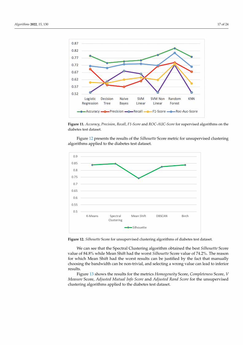
Figure 11 shows the best results of supervised algorithms for Accuracy, Precision, Recall,F1-Score and ROC-AUC-Score metrics, applied to diabetes test dataset.

The Random Forest algorithm obtained the best performance results in all metrics,with Accuracy of 83.8%, Precision of 73.9%, Recall of 72.3%, F1-Score of 73.1% and ROC-AUC-Score of 80.6%. On the other hand, the Decision Tree algorithm presented the worst resultsfor the metrics Accuracy of 73.6%, F1-Score of 59.6% and ROC-AUC-Score of 70.2%. TheNaïve Bayes algorithm presented the worst result for Precision of 57.1%, while the LogisticRegression and KNN had the worst result for Recall with a value of 53.2%.

https://github.com/hfilipesilva/ml-algorithms


Algorithms 2022, 15, 130 17 of 24


The Python source code used in the experiments is freely available at: https://github.com/hfilipesilva/ml-algorithms (accessed on 7 April 2022).

5.1. Diabetes Dataset Figure 11 shows the best results of supervised algorithms for Accuracy, Precision, Re-

call, F1-Score and ROC-AUC-Score metrics, applied to diabetes test dataset.

Figure 11. Accuracy, Precision, Recall, F1-Score and ROC-AUC-Score for supervised algorithms on the diabetes test dataset.

The Random Forest algorithm obtained the best performance results in all metrics, with Accuracy of 83.8%, Precision of 73.9%, Recall of 72.3%, F1-Score of 73.1% and ROC-AUC-Score of 80.6%. On the other hand, the Decision Tree algorithm presented the worst results for the metrics Accuracy of 73.6%, F1-Score of 59.6% and ROC-AUC-Score of 70.2%. The Naïve Bayes algorithm presented the worst result for Precision of 57.1%, while the Logistic Regression and KNN had the worst result for Recall with a value of 53.2%.

Figure 12 presents the results of the Silhouette Score metric for unsupervised cluster-ing algorithms applied to the diabetes test dataset.

Figure 12. Silhouette Score for unsupervised clustering algorithms of diabetes test dataset.

Figure 11. Accuracy, Precision, Recall, F1-Score and ROC-AUC-Score for supervised algorithms on thediabetes test dataset.

Figure 12 presents the results of the Silhouette Score metric for unsupervised clusteringalgorithms applied to the diabetes test dataset.


The Python source code used in the experiments is freely available at: https://github.com/hfilipesilva/ml-algorithms (accessed on 7 April 2022).

5.1. Diabetes Dataset Figure 11 shows the best results of supervised algorithms for Accuracy, Precision, Re-

call, F1-Score and ROC-AUC-Score metrics, applied to diabetes test dataset.

Figure 11. Accuracy, Precision, Recall, F1-Score and ROC-AUC-Score for supervised algorithms on the diabetes test dataset.

The Random Forest algorithm obtained the best performance results in all metrics, with Accuracy of 83.8%, Precision of 73.9%, Recall of 72.3%, F1-Score of 73.1% and ROC-AUC-Score of 80.6%. On the other hand, the Decision Tree algorithm presented the worst results for the metrics Accuracy of 73.6%, F1-Score of 59.6% and ROC-AUC-Score of 70.2%. The Naïve Bayes algorithm presented the worst result for Precision of 57.1%, while the Logistic Regression and KNN had the worst result for Recall with a value of 53.2%.

Figure 12 presents the results of the Silhouette Score metric for unsupervised cluster-ing algorithms applied to the diabetes test dataset.

Figure 12. Silhouette Score for unsupervised clustering algorithms of diabetes test dataset. Figure 12. Silhouette Score for unsupervised clustering algorithms of diabetes test dataset.

We can see that the Spectral Clustering algorithm obtained the best Silhouette Scorevalue of 84.8% while Mean Shift had the worst Silhouette Score value of 74.2%. The reasonfor which Mean Shift had the worst results can be justified by the fact that manuallychoosing the bandwidth can be non-trivial, and selecting a wrong value can lead to inferiorresults.

Figure 13 shows the results for the metrics Homogeneity Score, Completeness Score, VMeasure Score, Adjusted Mutual Info Score and Adjusted Rand Score for the unsupervisedclustering algorithms applied to the diabetes test dataset.

Algorithms 2022, 15, 130 18 of 24


We can see that the Spectral Clustering algorithm obtained the best Silhouette Score value of 84.8% while Mean Shift had the worst Silhouette Score value of 74.2%. The reason for which Mean Shift had the worst results can be justified by the fact that manually choos-ing the bandwidth can be non-trivial, and selecting a wrong value can lead to inferior results.

Figure 13 shows the results for the metrics Homogeneity Score, Completeness Score, V Measure Score, Adjusted Mutual Info Score and Adjusted Rand Score for the unsupervised clustering algorithms applied to the diabetes test dataset.

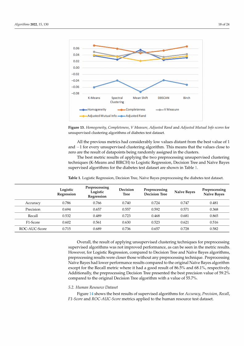
Figure 13. Homogeneity, Completeness, V Measure, Adjusted Rand and Adjusted Mutual Info scores for unsupervised clustering algorithms of diabetes test dataset.

All the previous metrics had considerably low values distant from the best value of 1 and −1 for every unsupervised clustering algorithm. This means that the values close to zero are the result of datapoints being randomly assigned in the clusters.

The best metric results of applying the two preprocessing unsupervised clustering techniques (K-Means and BIRCH) to Logistic Regression, Decision Tree and Naïve Bayes supervised algorithms for the diabetes test dataset are shown in Table 1.

Table 1. Logistic Regression, Decision Tree, Naïve Bayes preprocessing the diabetes test dataset.

Logistic Re-gression

Preprocessing Logistic Regression

Decision Tree Preprocessing Decision Tree

Naïve Bayes Preprocessing Naïve Bayes

Accuracy 0.786 0.766 0.740 0.724 0.747 0.481 Precision 0.694 0.657 0.557 0.592 0.571 0.368

Recall 0.532 0.489 0.723 0.468 0.681 0.865 F1-Score 0.602 0.561 0.630 0.523 0.621 0.516

ROC-AUC-Score 0.715 0.689 0.736 0.657 0.728 0.582

Overall, the result of applying unsupervised clustering techniques for preprocessing supervised algorithms was not improved performance, as can be seen in the metric results. However, for Logistic Regression, compared to Decision Tree and Naïve Bayes algo-rithms, preprocessing results were closer those without any preprocessing technique. Pre-processing Naïve Bayes had lower performance results compared to the original Naïve Bayes algorithm except for the Recall metric where it had a good result of 86.5% and 68.1%, respectively. Additionally, the preprocessing Decision Tree presented the best pre-cision value of 59.2% compared to the original Decision Tree algorithm with a value of 55.7%.

Figure 13. Homogeneity, Completeness, V Measure, Adjusted Rand and Adjusted Mutual Info scores forunsupervised clustering algorithms of diabetes test dataset.

All the previous metrics had considerably low values distant from the best value of 1and −1 for every unsupervised clustering algorithm. This means that the values close tozero are the result of datapoints being randomly assigned in the clusters.

The best metric results of applying the two preprocessing unsupervised clusteringtechniques (K-Means and BIRCH) to Logistic Regression, Decision Tree and Naïve Bayessupervised algorithms for the diabetes test dataset are shown in Table 1.

Table 1. Logistic Regression, Decision Tree, Naïve Bayes preprocessing the diabetes test dataset.

LogisticRegression

PreprocessingLogistic

Regression

DecisionTree

PreprocessingDecision Tree Naïve Bayes Preprocessing

Naïve Bayes

Accuracy 0.786 0.766 0.740 0.724 0.747 0.481

Precision 0.694 0.657 0.557 0.592 0.571 0.368

Recall 0.532 0.489 0.723 0.468 0.681 0.865

F1-Score 0.602 0.561 0.630 0.523 0.621 0.516

ROC-AUC-Score 0.715 0.689 0.736 0.657 0.728 0.582

Overall, the result of applying unsupervised clustering techniques for preprocessingsupervised algorithms was not improved performance, as can be seen in the metric results.However, for Logistic Regression, compared to Decision Tree and Naïve Bayes algorithms,preprocessing results were closer those without any preprocessing technique. PreprocessingNaïve Bayes had lower performance results compared to the original Naïve Bayes algorithmexcept for the Recall metric where it had a good result of 86.5% and 68.1%, respectively.Additionally, the preprocessing Decision Tree presented the best precision value of 59.2%compared to the original Decision Tree algorithm with a value of 55.7%.

5.2. Human Resource Dataset

Figure 14 shows the best results of supervised algorithms for Accuracy, Precision, Recall,F1-Score and ROC-AUC-Score metrics applied to the human resource test dataset.

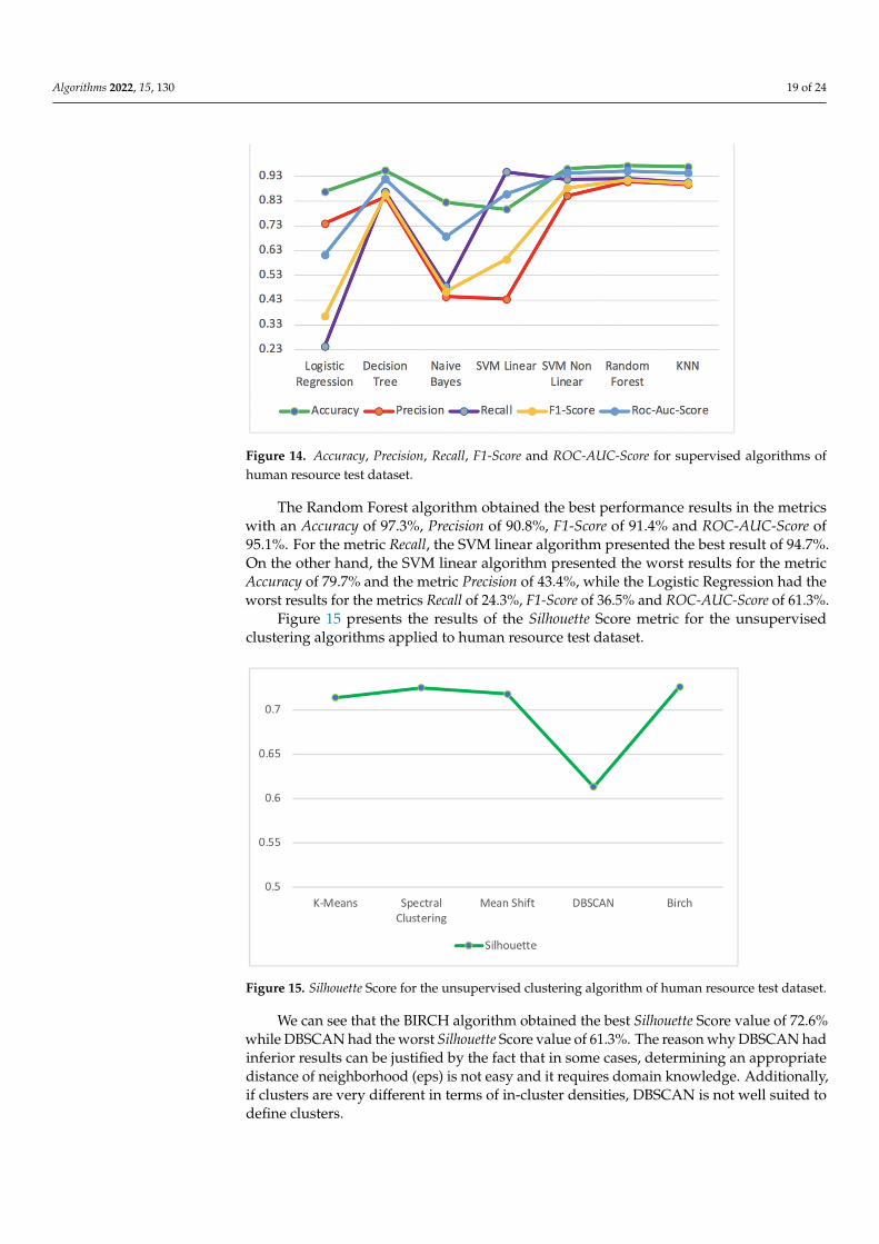
Algorithms 2022, 15, 130 19 of 24


5.2. Human Resource Dataset Figure 14 shows the best results of supervised algorithms for Accuracy, Precision, Re-

call, F1-Score and ROC-AUC-Score metrics applied to the human resource test dataset.

Figure 14. Accuracy, Precision, Recall, F1-Score and ROC-AUC-Score for supervised algorithms of hu-man resource test dataset.

The Random Forest algorithm obtained the best performance results in the metrics with an Accuracy of 97.3%, Precision of 90.8%, F1-Score of 91.4% and ROC-AUC-Score of 95.1%. For the metric Recall, the SVM linear algorithm presented the best result of 94.7%. On the other hand, the SVM linear algorithm presented the worst results for the metric Accuracy of 79.7% and the metric Precision of 43.4%, while the Logistic Regression had the worst results for the metrics Recall of 24.3%, F1-Score of 36.5% and ROC-AUC-Score of 61.3%.

Figure 15 presents the results of the Silhouette Score metric for the unsupervised clus-tering algorithms applied to human resource test dataset.

Figure 15. Silhouette Score for the unsupervised clustering algorithm of human resource test da-taset.

We can see that the BIRCH algorithm obtained the best Silhouette Score value of 72.6% while DBSCAN had the worst Silhouette Score value of 61.3%. The reason why DBSCAN

Figure 14. Accuracy, Precision, Recall, F1-Score and ROC-AUC-Score for supervised algorithms ofhuman resource test dataset.

The Random Forest algorithm obtained the best performance results in the metricswith an Accuracy of 97.3%, Precision of 90.8%, F1-Score of 91.4% and ROC-AUC-Score of95.1%. For the metric Recall, the SVM linear algorithm presented the best result of 94.7%.On the other hand, the SVM linear algorithm presented the worst results for the metricAccuracy of 79.7% and the metric Precision of 43.4%, while the Logistic Regression had theworst results for the metrics Recall of 24.3%, F1-Score of 36.5% and ROC-AUC-Score of 61.3%.

Figure 15 presents the results of the Silhouette Score metric for the unsupervisedclustering algorithms applied to human resource test dataset.


5.2. Human Resource Dataset Figure 14 shows the best results of supervised algorithms for Accuracy, Precision, Re-

call, F1-Score and ROC-AUC-Score metrics applied to the human resource test dataset.

Figure 14. Accuracy, Precision, Recall, F1-Score and ROC-AUC-Score for supervised algorithms of hu-man resource test dataset.

The Random Forest algorithm obtained the best performance results in the metrics with an Accuracy of 97.3%, Precision of 90.8%, F1-Score of 91.4% and ROC-AUC-Score of 95.1%. For the metric Recall, the SVM linear algorithm presented the best result of 94.7%. On the other hand, the SVM linear algorithm presented the worst results for the metric Accuracy of 79.7% and the metric Precision of 43.4%, while the Logistic Regression had the worst results for the metrics Recall of 24.3%, F1-Score of 36.5% and ROC-AUC-Score of 61.3%.

Figure 15 presents the results of the Silhouette Score metric for the unsupervised clus-tering algorithms applied to human resource test dataset.

Figure 15. Silhouette Score for the unsupervised clustering algorithm of human resource test da-taset.

We can see that the BIRCH algorithm obtained the best Silhouette Score value of 72.6% while DBSCAN had the worst Silhouette Score value of 61.3%. The reason why DBSCAN

Figure 15. Silhouette Score for the unsupervised clustering algorithm of human resource test dataset.

We can see that the BIRCH algorithm obtained the best Silhouette Score value of 72.6%while DBSCAN had the worst Silhouette Score value of 61.3%. The reason why DBSCAN hadinferior results can be justified by the fact that in some cases, determining an appropriatedistance of neighborhood (eps) is not easy and it requires domain knowledge. Additionally,if clusters are very different in terms of in-cluster densities, DBSCAN is not well suited todefine clusters.

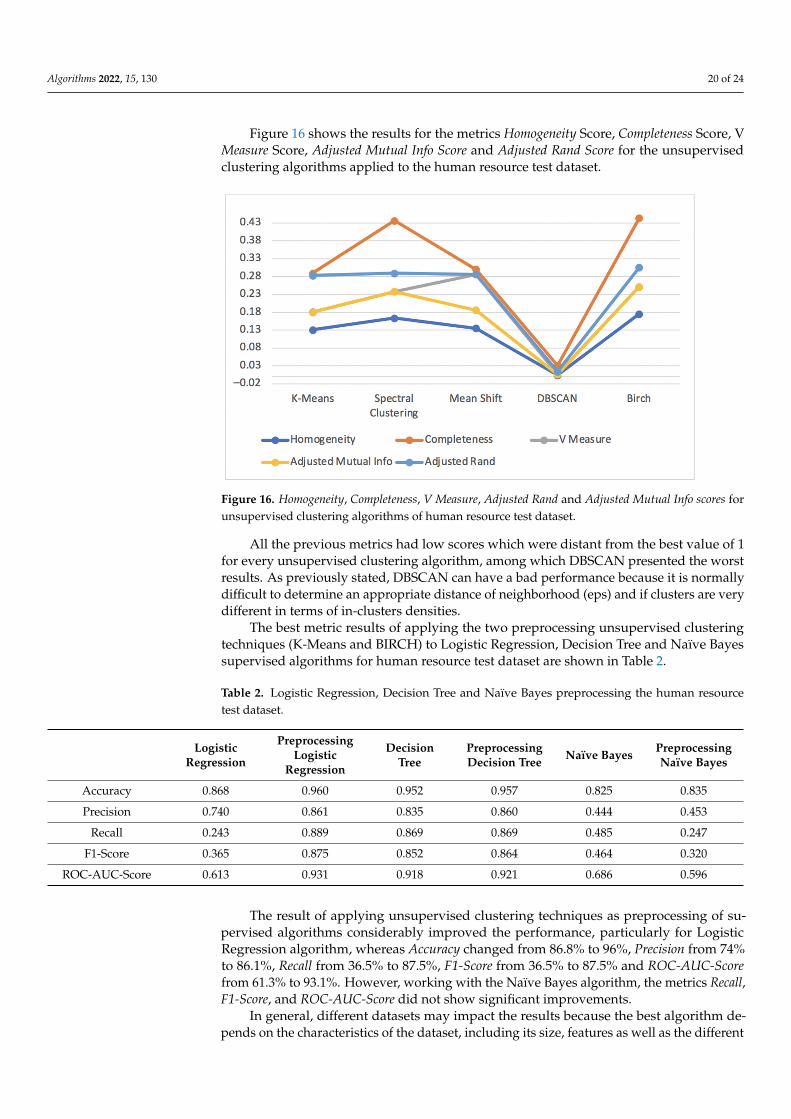
Algorithms 2022, 15, 130 20 of 24

Figure 16 shows the results for the metrics Homogeneity Score, Completeness Score, VMeasure Score, Adjusted Mutual Info Score and Adjusted Rand Score for the unsupervisedclustering algorithms applied to the human resource test dataset.


had inferior results can be justified by the fact that in some cases, determining an appro-priate distance of neighborhood (eps) is not easy and it requires domain knowledge. Ad-ditionally, if clusters are very different in terms of in-cluster densities, DBSCAN is not well suited to define clusters.

Figure 16 shows the results for the metrics Homogeneity Score, Completeness Score, V Measure Score, Adjusted Mutual Info Score and Adjusted Rand Score for the unsupervised clustering algorithms applied to the human resource test dataset.

Figure 16. Homogeneity, Completeness, V Measure, Adjusted Rand and Adjusted Mutual Info scores for unsupervised clustering algorithms of human resource test dataset.

All the previous metrics had low scores which were distant from the best value of 1 for every unsupervised clustering algorithm, among which DBSCAN presented the worst results. As previously stated, DBSCAN can have a bad performance because it is normally difficult to determine an appropriate distance of neighborhood (eps) and if clusters are very different in terms of in-clusters densities.

The best metric results of applying the two preprocessing unsupervised clustering techniques (K-Means and BIRCH) to Logistic Regression, Decision Tree and Naïve Bayes supervised algorithms for human resource test dataset are shown in Table 2.

Table 2. Logistic Regression, Decision Tree and Naïve Bayes preprocessing the human resource test dataset.

Logistic Re-gression

Preprocessing Logistic Regression

Decision Tree Preprocessing Decision Tree

Naïve Bayes Preprocessing Naïve Bayes

Accuracy 0.868 0.960 0.952 0.957 0.825 0.835 Precision 0.740 0.861 0.835 0.860 0.444 0.453

Recall 0.243 0.889 0.869 0.869 0.485 0.247 F1-Score 0.365 0.875 0.852 0.864 0.464 0.320

ROC-AUC-Score 0.613 0.931 0.918 0.921 0.686 0.596

The result of applying unsupervised clustering techniques as preprocessing of super-vised algorithms considerably improved the performance, particularly for Logistic Re-gression algorithm, whereas Accuracy changed from 86.8% to 96%, Precision from 74% to 86.1%, Recall from 36.5% to 87.5%, F1-Score from 36.5% to 87.5% and ROC-AUC-Score from 61.3% to 93.1%. However, working with the Naïve Bayes algorithm, the metrics Recall, F1-Score, and ROC-AUC-Score did not show significant improvements.

Figure 16. Homogeneity, Completeness, V Measure, Adjusted Rand and Adjusted Mutual Info scores forunsupervised clustering algorithms of human resource test dataset.

All the previous metrics had low scores which were distant from the best value of 1for every unsupervised clustering algorithm, among which DBSCAN presented the worstresults. As previously stated, DBSCAN can have a bad performance because it is normallydifficult to determine an appropriate distance of neighborhood (eps) and if clusters are verydifferent in terms of in-clusters densities.

The best metric results of applying the two preprocessing unsupervised clusteringtechniques (K-Means and BIRCH) to Logistic Regression, Decision Tree and Naïve Bayessupervised algorithms for human resource test dataset are shown in Table 2.

Table 2. Logistic Regression, Decision Tree and Naïve Bayes preprocessing the human resourcetest dataset.

LogisticRegression

PreprocessingLogistic

Regression

DecisionTree

PreprocessingDecision Tree Naïve Bayes Preprocessing

Naïve Bayes

Accuracy 0.868 0.960 0.952 0.957 0.825 0.835

Precision 0.740 0.861 0.835 0.860 0.444 0.453

Recall 0.243 0.889 0.869 0.869 0.485 0.247

F1-Score 0.365 0.875 0.852 0.864 0.464 0.320

ROC-AUC-Score 0.613 0.931 0.918 0.921 0.686 0.596

The result of applying unsupervised clustering techniques as preprocessing of su-pervised algorithms considerably improved the performance, particularly for LogisticRegression algorithm, whereas Accuracy changed from 86.8% to 96%, Precision from 74%to 86.1%, Recall from 36.5% to 87.5%, F1-Score from 36.5% to 87.5% and ROC-AUC-Scorefrom 61.3% to 93.1%. However, working with the Naïve Bayes algorithm, the metrics Recall,F1-Score, and ROC-AUC-Score did not show significant improvements.

In general, different datasets may impact the results because the best algorithm de-pends on the characteristics of the dataset, including its size, features as well as the different

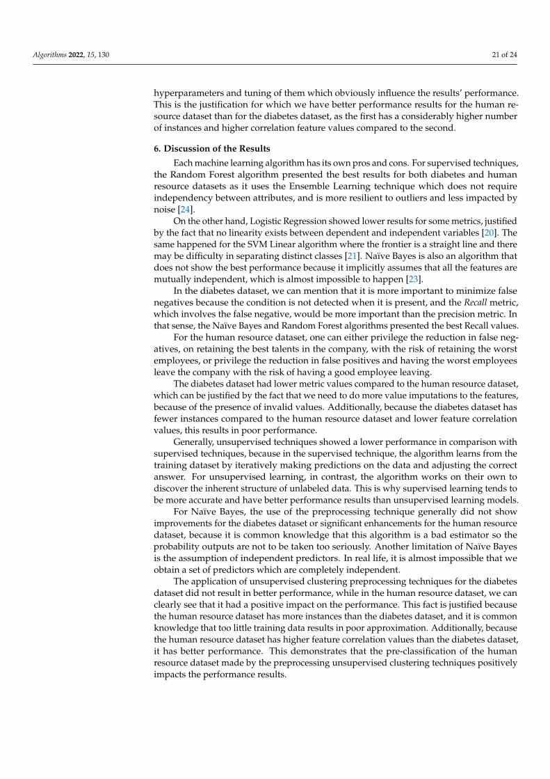
Algorithms 2022, 15, 130 21 of 24

hyperparameters and tuning of them which obviously influence the results’ performance.This is the justification for which we have better performance results for the human re-source dataset than for the diabetes dataset, as the first has a considerably higher numberof instances and higher correlation feature values compared to the second.

6. Discussion of the Results

Each machine learning algorithm has its own pros and cons. For supervised techniques,the Random Forest algorithm presented the best results for both diabetes and humanresource datasets as it uses the Ensemble Learning technique which does not requireindependency between attributes, and is more resilient to outliers and less impacted bynoise [24].

On the other hand, Logistic Regression showed lower results for some metrics, justifiedby the fact that no linearity exists between dependent and independent variables [20]. Thesame happened for the SVM Linear algorithm where the frontier is a straight line and theremay be difficulty in separating distinct classes [21]. Naïve Bayes is also an algorithm thatdoes not show the best performance because it implicitly assumes that all the features aremutually independent, which is almost impossible to happen [23].

In the diabetes dataset, we can mention that it is more important to minimize falsenegatives because the condition is not detected when it is present, and the Recall metric,which involves the false negative, would be more important than the precision metric. Inthat sense, the Naïve Bayes and Random Forest algorithms presented the best Recall values.

For the human resource dataset, one can either privilege the reduction in false neg-atives, on retaining the best talents in the company, with the risk of retaining the worstemployees, or privilege the reduction in false positives and having the worst employeesleave the company with the risk of having a good employee leaving.

The diabetes dataset had lower metric values compared to the human resource dataset,which can be justified by the fact that we need to do more value imputations to the features,because of the presence of invalid values. Additionally, because the diabetes dataset hasfewer instances compared to the human resource dataset and lower feature correlationvalues, this results in poor performance.

Generally, unsupervised techniques showed a lower performance in comparison withsupervised techniques, because in the supervised technique, the algorithm learns from thetraining dataset by iteratively making predictions on the data and adjusting the correctanswer. For unsupervised learning, in contrast, the algorithm works on their own todiscover the inherent structure of unlabeled data. This is why supervised learning tends tobe more accurate and have better performance results than unsupervised learning models.

For Naïve Bayes, the use of the preprocessing technique generally did not showimprovements for the diabetes dataset or significant enhancements for the human resourcedataset, because it is common knowledge that this algorithm is a bad estimator so theprobability outputs are not to be taken too seriously. Another limitation of Naïve Bayesis the assumption of independent predictors. In real life, it is almost impossible that weobtain a set of predictors which are completely independent.

The application of unsupervised clustering preprocessing techniques for the diabetesdataset did not result in better performance, while in the human resource dataset, we canclearly see that it had a positive impact on the performance. This fact is justified becausethe human resource dataset has more instances than the diabetes dataset, and it is commonknowledge that too little training data results in poor approximation. Additionally, becausethe human resource dataset has higher feature correlation values than the diabetes dataset,it has better performance. This demonstrates that the pre-classification of the humanresource dataset made by the preprocessing unsupervised clustering techniques positivelyimpacts the performance results.

Algorithms 2022, 15, 130 22 of 24

7. Conclusions and Future Work

In this work, we used 12 algorithms among supervised and unsupervised clusteringtechniques applied to diabetes and human resource datasets for binary classification. Wealso applied the preprocessing technique to supervised algorithms, using unsupervisedclustering techniques as this topic was little explored.

The knowledge generated by this work, namely the use of preprocessing supervisedand unsupervised clustering algorithms, can contribute to the wider use and explorationof this technique so that the performance results of the application of supervised machinelearning algorithms can be improved.

As future work, we intend to apply this technique to larger datasets to consolidate thepromising benefits of using it. Additionally, we intend to use not only clustering also otherunsupervised techniques as preprocessing to compare their impact on performance results.Finally, we also intend to use the cross-validation technique to test the model’s ability topredict new data that were not used in the estimation in order to flag problems such asoverfitting or selection bias and to give insight into how the model will generalize into anindependent dataset.

Author Contributions: Conceptualization, H.S. and J.B.; Methodology, H.S. and J.B.; Software, H.S.;Validation, H.S. and J.B.; Formal analysis, H.S. and J.B.; Investigation, H.S.; Resources, H.S.; Datacuration, H.S.; Writing—original draft preparation, H.S.; Writing—review and editing, H.S. and J.B.;Supervision, J.B.; Project administration, J.B.; Funding acquisition, J.B. All authors have read andagreed to the published version of the manuscript.

Funding: This research received no external funding.

Institutional Review Board Statement: Not applicable.

Informed Consent Statement: Not applicable.

Data Availability Statement: The Python source code used in the experiments is publicly availableat: https://github.com/hfilipesilva/ml-algorithms (accessed on 5 February 2022).

Conflicts of Interest: The authors declare no conflict of interest.

References1. Bhardwaj, R.; Nambiar, A.R.; Dutta, D. A Study of Machine Learning in Healthcare. In Proceedings of the 2017 IEEE 41st Annual

Computer Software and Applications Conference (COMPSAC), Turin, Italy, 4–8 July 2017; Volume 2, pp. 236–241. [CrossRef]2. IBM. What is Machine Learning? Available online: https://www.ibm.com/cloud/learn/machine-learning (accessed on 14

November 2021).3. Expert.ai. What is the Definition of Machine Learning? Available online: https://www.expert.ai/blog/machine-learning-

definition/ (accessed on 14 November 2021).4. Seema Singh. An Introduction to Clustering. Clustering is Considered to be the Most . . . Data Driven Investor. Available online:

https://medium.datadriveninvestor.com/an-introduction-to-clustering-61f6930e3e0b (accessed on 14 November 2021).5. Jiang, F.; Jiang, Y.; Zhi, H.; Dong, Y.; Li, H.; Ma, S.; Wang, Y.; Dong, Q.; Shen, H.; Wang, Y. Artificial intelligence in healthcare: Past,

present and future. Stroke Vasc. Neurol. 2017, 2, 230–243. [CrossRef] [PubMed]6. Uddin, S.; Khan, A.; Hossain, E.; Moni, M.A. Comparing different supervised machine learning algorithms for disease prediction.

BMC Med. Inform. Decis. Mak. 2019, 19, 281. [CrossRef] [PubMed]7. Sidey-Gibbons, J.A.M.; Sidey-Gibbons, C.J. Machine learning in medicine: A practical introduction. BMC Med. Res. Methodol.

2019, 19, 64. [CrossRef] [PubMed]8. Wang, S.; Pathak, J.; Zhang, Y. Using Electronic Health Records and Machine Learning to Predict Postpartum Depression. Stud.

Health Technol. Inform. 2019, 264, 888–892. [CrossRef] [PubMed]9. Ferdous, M.; Debnath, J.; Chakraborty, N.R. Machine Learning Algorithms in Healthcare: A Literature Survey. In Proceedings of

the 2020 11th International Conference on Computing, Communication and Networking Technologies (ICCCNT), Kharagpur,India, 1–3 July 2020.

10. Rehm, G.B.; Kuhn, B.T.; Nguyen, J.; Anderson, N.R.; Chuah, C.-N.; Adams, J.Y. Improving Mechanical Ventilator Clinical DecisionSupport Systems with a Machine Learning Classifier for Determining Ventilator Mode. Stud. Health Technol. Inform. 2019, 264,318–322. [PubMed]

11. Nijeweme-D’Hollosy, W.O.; van Velsen, L.; Poel, M.; Groothuis-Oudshoorn, C.G.; Soer, R.; Hermens, H. Evaluation of threemachine learning models for self-referral decision support on low back pain in primary care. Int. J. Med. Inform. 2018, 110, 31–41.[CrossRef] [PubMed]


http://doi.org/10.1109/COMPSAC.2017.164

https://www.ibm.com/cloud/learn/machine-learning

https://www.expert.ai/blog/machine-learning-definition/

https://www.expert.ai/blog/machine-learning-definition/

https://medium.datadriveninvestor.com/an-introduction-to-clustering-61f6930e3e0b

http://doi.org/10.1136/svn-2017-000101

http://www.ncbi.nlm.nih.gov/pubmed/29507784

http://doi.org/10.1186/s12911-019-1004-8


http://doi.org/10.1186/s12874-019-0681-4


http://doi.org/10.3233/SHTI190351



http://doi.org/10.1016/j.ijmedinf.2017.11.010


Algorithms 2022, 15, 130 23 of 24

12. Farhadian, M.; Shokouhi, P.; Torkzaban, P. A decision support system based on support vector machine for diagnosis ofperiodontal disease. BMC Res. Notes 2020, 13, 337. [CrossRef] [PubMed]

13. Karthikeyan, A.; Garg, A.; Vinod, P.K.; Priyakumar, U.D. Machine Learning Based Clinical Decision Support System for EarlyCOVID-19 Mortality Prediction. Front. Public Health 2021, 9, 626697. [CrossRef] [PubMed]

14. Luz, C.; Vollmer, M.; Decruyenaere, J.; Nijsten, M.; Glasner, C.; Sinha, B. Machine learning in infection management using routineelectronic health records: Tools, techniques, and reporting of future technologies. Clin. Microbiol. Infect. 2020, 26, 1291–1299.[CrossRef] [PubMed]

15. Finkelstein, J.; Jeong, I.C. Machine learning approaches to personalize early prediction of asthma exacerbations. Ann. N. Y. Acad.Sci. 2017, 1387, 153–165. [CrossRef] [PubMed]

16. von Luxburg, U.; Williamson, R.C.; Guyon, I. Clustering: Science or Art? In Proceedings of the ICML Workshop on Unsupervisedand Transfer Learning, Bellevue, WA, USA, 2 July 2012; Volume 27, pp. 65–79.

17. Fu, T.; Zhang, Z. CPSG-MCMC: Clustering-Based Preprocessing method for Stochastic Gradient MCMC. In Proceedings of the20th International Conference on Artificial Intelligence and Statistics, Fort Lauderdale, FL, USA, 9–11 May 2017; pp. 841–850.

18. Yoon, K.; Kwek, S. An unsupervised learning approach to resolving the data imbalanced issue in supervised learning problems infunctional genomics. In Proceedings of the Fifth International Conference on Hybrid Intelligent Systems (HIS’05), Rio de Janeiro,Brazil, 6–9 November 2005; p. 6.

19. Lan, T.; Lin, K.R.; Liu, Z.Y.; He, Y.H.; Xu, C.Y.; Zhang, H.B.; Chen, X.H. A clustering preprocessing framework for the subannualcalibration of a hydrological model considering climate-land surface variations–Enhanced Reader. Water Resour. Res. 2018, 54,10–34. [CrossRef]

20. IBM. What is Logistic Regression? Available online: https://www.ibm.com/se-en/topics/logistic-regression (accessed on 26December 2021).

21. Gandhi, R.; Towards Data Science. Support Vector Machine—Introduction to Machine Learning Algorithms. Available online:https://towardsdatascience.com/support-vector-machine-introduction-to-machine-learning-algorithms-934a444fca47 (accessedon 26 December 2021).

22. What Is a Decision Tree? Available online: https://www.mastersindatascience.org/learning/introduction-to-machine-learning-algorithms/decision-tree/ (accessed on 26 December 2021).

23. Gandhi, R.; Towards Data Science. Naive Bayes Classifier. What is a Classifier? Available online: https://towardsdatascience.com/naive-bayes-classifier-81d512f50a7c (accessed on 26 December 2021).

24. IBM. What is Random Forest? Available online: https://www.ibm.com/cloud/learn/random-forest (accessed on 26December 2021).

25. What Is K-Nearest Neighbor? An ML Algorithm to Classify Data. Available online: https://learn.g2.com/k-nearest-neighbor(accessed on 26 December 2021).

26. Garbade, M.J.; Towards Data Science. Understanding K-means Clustering in Machine Learning. Available online:https://towardsdatascience.com/understanding-k-means-clustering-in-machine-learning-6a6e67336aa1 (accessed on 26December 2021).

27. What is Spectral Clustering and How its Work? Available online: https://www.mygreatlearning.com/blog/introduction-to-spectral-clustering/ (accessed on 26 December 2021).

28. Mean Shift. Available online: https://ml-explained.com/blog/mean-shift-explained (accessed on 26 December 2021).29. do Prado, K.S.; Towards Data Science. How DBSCAN Works and Why Should We Use it? Available online: https://

towardsdatascience.com/how-dbscan-works-and-why-should-i-use-it-443b4a191c80 (accessed on 26 December 2021).30. BIRCH Clustering Clearly Explained. Available online: https://morioh.com/p/c23e0d680669 (accessed on 26 December 2021).31. Gupta, A.; Geek Culture|Medium. Balanced Iterative Reducing and Clustering Using Hierarchies (BIRCH) Algorithm in Machine

Learning. Available online: https://medium.com/geekculture/balanced-iterative-reducing-and-clustering-using-hierarchies-birch-1428bb06bb38 (accessed on 26 December 2021).

32. Kaggle. Pima Indians Diabetes Database. Available online: https://www.kaggle.com/uciml/pima-indians-diabetes-database(accessed on 27 December 2021).

33. Britannica. Pima|People. Available online: https://www.britannica.com/topic/Pima-people (accessed on 27 December 2021).34. Borkin, D.; Némethová, A.; Michal’conok, G.; Maiorov, K. Impact of Data Normalization on Classification Model Accuracy. Res.

Pap. Fac. Mater. Sci. Technol. Slovak Univ. Technol. 2019, 27, 79–84. [CrossRef]35. Hr-Comma-Sep. Kaggle. Available online: https://www.kaggle.com/pankeshpatel/hrcommasep (accessed on 7 February 2022).36. Popovic-Stijacic, M.; Mihic, L.; Ðurdevic, D.F. Analyzing data from memory tasks-comparison of ANOVA, logistic regression and

mixed logit model. Psihologija 2018, 51, 469–488. [CrossRef]37. Sklearn.Svm.SVC—Scikit-Learn 1.0.2 Documentation. Available online: https://scikit-learn.org/stable/modules/generated/

sklearn.svm.SVC.html (accessed on 5 February 2022).38. Sklearn.Ensemble.RandomForestClassifier—Scikit-Learn 1.0.2 Documentation. Available online: https://scikit-learn.org/stable/

modules/generated/sklearn.ensemble.RandomForestClassifier.html (accessed on 5 February 2022).39. Sklearn.Neighbors.KNeighborsClassifier—Scikit-Learn 1.0.2 Documentation. Available online: https://scikit-learn.org/stable/

modules/generated/sklearn.neighbors.KNeighborsClassifier.html (accessed on 5 February 2022).

http://doi.org/10.1186/s13104-020-05180-5


http://doi.org/10.3389/fpubh.2021.626697


http://doi.org/10.1016/j.cmi.2020.02.003


http://doi.org/10.1111/nyas.13218


http://doi.org/10.1029/2018WR023160

https://www.ibm.com/se-en/topics/logistic-regression

https://towardsdatascience.com/support-vector-machine-introduction-to-machine-learning-algorithms-934a444fca47

https://www.mastersindatascience.org/learning/introduction-to-machine-learning-algorithms/decision-tree/

https://www.mastersindatascience.org/learning/introduction-to-machine-learning-algorithms/decision-tree/

https://towardsdatascience.com/naive-bayes-classifier-81d512f50a7c

https://towardsdatascience.com/naive-bayes-classifier-81d512f50a7c

https://www.ibm.com/cloud/learn/random-forest

https://learn.g2.com/k-nearest-neighbor

https://towardsdatascience.com/understanding-k-means-clustering-in-machine-learning-6a6e67336aa1

https://www.mygreatlearning.com/blog/introduction-to-spectral-clustering/

https://www.mygreatlearning.com/blog/introduction-to-spectral-clustering/

https://ml-explained.com/blog/mean-shift-explained

https://towardsdatascience.com/how-dbscan-works-and-why-should-i-use-it-443b4a191c80

https://towardsdatascience.com/how-dbscan-works-and-why-should-i-use-it-443b4a191c80

https://morioh.com/p/c23e0d680669

https://medium.com/geekculture/balanced-iterative-reducing-and-clustering-using-hierarchies-birch-1428bb06bb38

https://medium.com/geekculture/balanced-iterative-reducing-and-clustering-using-hierarchies-birch-1428bb06bb38

https://www.kaggle.com/uciml/pima-indians-diabetes-database

https://www.britannica.com/topic/Pima-people

http://doi.org/10.2478/rput-2019-0029

https://www.kaggle.com/pankeshpatel/hrcommasep

http://doi.org/10.2298/PSI170615023P

https://scikit-learn.org/stable/modules/generated/sklearn.svm.SVC.html

https://scikit-learn.org/stable/modules/generated/sklearn.svm.SVC.html

https://scikit-learn.org/stable/modules/generated/sklearn.ensemble.RandomForestClassifier.html

https://scikit-learn.org/stable/modules/generated/sklearn.ensemble.RandomForestClassifier.html

https://scikit-learn.org/stable/modules/generated/sklearn.neighbors.KNeighborsClassifier.html

https://scikit-learn.org/stable/modules/generated/sklearn.neighbors.KNeighborsClassifier.html

Algorithms 2022, 15, 130 24 of 24

40. Sklearn.Cluster.KMeans—Scikit-Learn 1.0.2 Documentation. Available online: https://scikit-learn.org/stable/modules/generated/sklearn.cluster.KMeans.html (accessed on 5 February 2022).

41. Sklearn.Cluster.SpectralClustering—Scikit-Learn 1.0.2 Documentation. Available online: https://scikit-learn.org/stable/modules/generated/sklearn.cluster.SpectralClustering.html (accessed on 5 February 2022).

42. Sklearn.Cluster.MeanShift—Scikit-Learn 1.0.2 Documentation. Available online: https://scikit-learn.org/stable/modules/generated/sklearn.cluster.MeanShift.html (accessed on 5 February 2022).

43. Sklearn.Cluster.DBSCAN—Scikit-Learn 1.0.2 Documentation. Available online: https://scikit-learn.org/stable/modules/generated/sklearn.cluster.DBSCAN.html (accessed on 5 February 2022).

44. Sklearn.Cluster.Birch—Scikit-Learn 1.0.2 Documentation. Available online: https://scikit-learn.org/stable/modules/generated/sklearn.cluster.Birch.html (accessed on 5 February 2022).

https://scikit-learn.org/stable/modules/generated/sklearn.cluster.KMeans.html

https://scikit-learn.org/stable/modules/generated/sklearn.cluster.KMeans.html

https://scikit-learn.org/stable/modules/generated/sklearn.cluster.SpectralClustering.html

https://scikit-learn.org/stable/modules/generated/sklearn.cluster.SpectralClustering.html

https://scikit-learn.org/stable/modules/generated/sklearn.cluster.MeanShift.html

https://scikit-learn.org/stable/modules/generated/sklearn.cluster.MeanShift.html

https://scikit-learn.org/stable/modules/generated/sklearn.cluster.DBSCAN.html

https://scikit-learn.org/stable/modules/generated/sklearn.cluster.DBSCAN.html

https://scikit-learn.org/stable/modules/generated/sklearn.cluster.Birch.html

https://scikit-learn.org/stable/modules/generated/sklearn.cluster.Birch.html

Machine Learning Algorithms: An Experimental Evaluation for ...

Documents

Transcript of Machine Learning Algorithms: An Experimental Evaluation for ...