Elicitation Strategies for Soft ConstraintProblems with Missing Preferences: Properties,

Algorithms and Experimental Studies

Mirco Gelain1, Maria Silvia Pini1, Francesca Rossi1, K. Brent Venable1,and Toby Walsh2

1 Dipartimento di Matematica Pura ed Applicata,Universita di Padova, Italy

E-mail: {mgelain,mpini,frossi,kvenable}@math.unipd.it2 NICTA and UNSW Sydney, Australia,

Email: Toby.Walsh@nicta.com.au

Abstract

We consider soft constraint problems where some of the preferences may beunspecified. This models, for example, settings where agents are distributed andhave privacy issues, or where there is an ongoing preferenceelicitation process.In this context, we study how to find an optimal solution without having to waitfor all the preferences. In particular, we define algorithms, that interleave searchand preference elicitation, to find a solution which is necessarily optimal, that is,optimal no matter what the missing data will be, with the aim to ask the user to re-veal as few preferences as possible. We define a combined solving and preferenceelicitation scheme with a large number of different instantiations, each correspond-ing to a concrete algorithm, which we compare experimentally. We compute boththe number of elicited preferences and the user effort, which may be larger, as itcontains all the preference values the user has to compute tobe able to respondto the elicitation requests. While the number of elicited preferences is importantwhen the concern is to communicate as little information as possible, the user ef-fort measures also the hidden work the user has to do to be ableto communicatethe elicited preferences. Our experimental results on classical, fuzzy, weightedand temporal incomplete CSPs show that some of our algorithms are very good atfinding a necessarily optimal solution while asking the userfor only a very smallfraction of the missing preferences. The user effort is alsovery small for the bestalgorithms.

Keywords: preferences, soft constraints, incompleteness, elicitation

1

1 Introduction

Traditionally, tasks such as scheduling, planning, and resource allocation have beentackled using several techniques, among which constraint reasoning is one of the mostpromising. The task is represented by a set of variables, their domains, and a set ofconstraints, and a solution of the problem is an assignment to all the variables in theirdomains such that all constraints are satisfied. Preferences or objective functions havebeen used to extend this formalism and allow for the modelling of constraint optimiza-tion, rather than satisfaction, problems. In all these approaches, the data (variables, do-mains, constraints) are completely known before the solving process starts. However,the increasing use of web services and in general of multi-agent applications demandsfor the formalization and handling of data that is only partially known when the solvingprocess works, and that can be added later, for example via elicitation [23, 24]. In manyweb applications, data may come from different sources, which may provide their pieceof information at different times. Also, in multi-agent settings, data provided by someagents may be voluntarily hidden due to privacy reasons, andonly released if neededto find a solution to the problem.

Here we consider these issues focusing on constraint optimization problems wherewe look for an optimal solution. In particular, we consider problems where constraintsare replaced by soft constraints, in which each assignment to the variables of the con-straint has an associated preference coming from a preference set [1]. We assume thatvariables, domains, and constraint topology are given at the beginning, while the pref-erences are partially specified and are elicited during the solving process.

There are several application domains where this might be useful. One regards thefact that quantitative preferences, needed in soft constraints, may be difficult and te-dious to provide for a user. Another one concerns multi-agent settings, where agentsagree on the structures of the problem but they may provide their preferences on dif-ferent parts of the problem at different times. Finally, some preferences can be initiallyhidden because of privacy reasons.

Formally, we take the soft constraint formalism and we allowfor some preferencesto be left unspecified. In our setting, users may know all the preferences but are willingto reveal only some of them at the beginning. Although some ofthe preferences can bemissing, it could still be feasible to find an optimal solution. If not, we ask the user toprovide some of the missing preferences and we start again from the new problem. Weconsider two notions of optimal solution:possibly optimalsolutions are assignments toall the variables that are optimal inat least one wayin which the currently unspecifiedpreferences can be revealed, whilenecessarily optimalsolutions are assignments to allthe variables that are optimal inall waysin which the currently unspecified preferencescan be revealed. This notation comes from multi-agent preference aggregation [17, 20,21], where, in the context of voting theory, some preferences are missing but still onewould like to declare a winner.

Given an incomplete soft constraint problem (ISCSP), its set of possibly optimalsolutions is never empty, while the set of necessarily optimal solutions can be empty.Of course what we would like to find is a necessarily optimal solution, to be on thesafe side: such solutions are optimal regardless of how the missing preferences arespecified. Unfortunately, such a set may be empty. In this case there are two choices:

2

either we may be satisfied with a possibly optimal solution, or we can elicit some of themissing preferences from the user and see if the new ISCSP hasa necessarily optimalsolution.

In this paper we follow this second approach and we repeat theprocess until thecurrent ISCSP has at least one necessarily optimal solution. In order to do that, weexploit a modified version of the classical branch and bound scheme and we considerdifferent elicitation strategies. In particular, we definea general algorithm scheme thatis based on three parameters:whento elicit,whatto elicit, andwhochooses the value tobe assigned to the next variable. For example, we may only elicit missing preferencesafter running branch and bound to exhaustion, or at the end ofevery complete branch,or even at every node in the search tree. Also, we may elicit all missing preferencesrelated to the candidate solution, or we might just ask the user for the worst preferenceamong some missing ones. Finally, when choosing the value toassign to a variable, wemight ask the user, who knows or can compute (all or some of) the missing preferences,for help.

We test all possible instances of the scheme, obtained by selecting different elicita-tion strategies, on randomly generated soft constraint problems (fuzzy and weighted).By varying the number of variables, the tightness and density of constraints as well asthe percentage of missing preferences, we produce a diversified and meaningful testset. The experiments demonstrate that some of the algorithms are very good at findingnecessarily optimal solutions without eliciting too many preferences. We also test someof the algorithms on problems with hard constraints and on fuzzy temporal constraints.Our experimental study on randomly generated problems permits us to filter out algo-rithms with a poor performance and, thus, to identify those that are more promising forfuture testing on real-life scenarios.

In our experiments, we compute the elicited preferences, that is, the missing valuesthat the user has to provide to the system because they are requested by the algorithm.Providing these values usually has a cost, either in terms ofthe computational effort, orin terms of a decrease in privacy, or in terms of the communication bandwidth. Whilstknowinghow many preferences are elicitedis important, we also compute a measureof theuser’s effort. This may be much larger than the number of elicited preferences,as it contains all the preference values the user may have to compute to be able torespond to the elicitation requests. For example, suppose we ask the user for the worstpreference value amongk missing ones. The user will communicate only one value,but he may have to compute and consider allk of them. Knowing the number of elicitedpreferences is important when the concern is to communicateas little information aspossible. The user effort, on the other hand, measures the hidden work the user has todo to be able to communicate the elicited preferences. This user’s effort is thereforealso an important measure.

As a motivating example, recommender systems give suggestions based on partialknowledge of the user’s preferences. Our approach could improve performance byidentifying some key questions to ask before giving recommendations. Privacy con-cerns regarding the percentage of elicited preferences aremotivated by eavesdropping.User’s effort is instead related to the burden on the user. Our results show that thechoice of the preference elicitation strategy is crucial for the performance of the solver.While the best algorithms need to elicit as little as 10% of the missing preferences, the

3

worst ones need much more. The user’s effort is also very small for the best algorithms.The performance of the best algorithms also shows that we only need to ask the userfor a very small amount of additional information to be able to solve problems withmissing data.

The paper is structured as follows. In Section 2 we define softconstraint problems,known in literature, where all the preferences are given. InSection 3 we introduce softconstraint problems where some preferences are missing (i.e., ISCSPs), we give newnotions of optimal solutions, i.e., the possibly and the necessarily optimal solutions,and we characterize them in Section 4. In Section 5 we presenta general algorithmicscheme for ISCSPs with all its possible instances. In Section 6 we describe the problemgenerator used in the experimental studies and we indicate what we measure in the ex-periments. Next, in Section 7 we summarize and discuss our experimental comparisonof all the algorithms. Finally, in Section 8 we compare our approach to other existingapproaches to deal with incompletely specified constraint optimization problems, andin Section 9 we summarize the results contained in this paper, and we give some hintsfor future work.

Preliminary versions of parts of this paper have appeared in[12, 13].

2 Soft constraints

A soft constraint [1] is just a classical constraint [5] where each instantiation of itsvariables has an associated value from a (totally or partially ordered) set. This set hastwo operations, which makes it similar to a semiring, and is called a c-semiring. Moreprecisely, a c-semiring is a tuple〈A, +,×,0,1〉 whereA is a set, called the carrier ofthe c-semiring, and0,1 ∈ A; + is commutative, associative, idempotent,0 is its unitelement, and1 is its absorbing element;× is associative, commutative, distributes over+, 1 is its unit element and0 is its absorbing element. Consider the relation≤S overA such thata ≤S b iff a + b = b. Then:≤S is a partial order;+ and× are monotoneon≤S ; 0 is its minimum and1 its maximum;〈A,≤S〉 is a lattice and, for alla, b ∈ A,a + b = lub(a, b). Moreover, if× is idempotent, then〈A,≤S〉 is a distributive latticeand× is its glb. Informally, the relation≤S gives us a way to compare (some of the)tuples of values and constraints. In fact, when we havea ≤S b, we will say thatb isbetter than a. Thus,0 is the worst value and1 is the best one.

Given a c-semiringS = 〈A, +,×,0,1〉, a finite setD (the domain of the variables),and an ordered set of variablesV , a constraint is a pair〈def, con〉 wherecon ⊆ V isthe scope of the constraint anddef : D|con| → A is the preference function of theconstraint. Therefore, a constraint specifies a set of variables (the ones incon), andassigns to each tuple of values ofD of these variables an element of the semiring setA. A soft constraint satisfaction problem (SCSP) is just a setof soft constraints over aset of variables.

Many classes of satisfaction or optimization problem can bedefined in this for-malism. A classical CSP is just an SCSP where the chosen c-semiring is: SCSP =〈{false, true}, ∨,∧, false, true〉. On the other hand, fuzzy CSPs [22, 11] can bemodelled in the SCSP framework by choosing the c-semiring:SFCSP = 〈[0, 1],max, min, 0, 1〉. For weighted CSPs, the semiring isSWCSP = 〈ℜ+, min, +,

4

+∞, 0〉. Here preferences are interpreted as costs from0 to +∞, which are com-bined with the sum and compared withmin. Thus the optimization criterion is tominimize the sum of costs. For probabilistic CSPs [10], the semiring isSPCSP =〈[0, 1], max,×, 0, 1〉. Here preferences are interpreted as probabilities ranging from0to 1, which are combined using the product and compared usingmax. Thus the aim isto maximize the joint probability.

Given an assignments to all the variables of an SCSPP , i.e., a solution ofP , wecan compute its preference valuepref(P, s) by combining the preferences associatedby each constraint to the sub-tuples of the assignments referring to the variables of theconstraint. More precisely,pref(P, s) = Π〈def,con〉∈Cdef(s↓con), whereΠ refers tothe× operation of the semiring ands↓con is the projection of tuples on the variablesin con. For example, in fuzzy CSPs, the preference of a complete assignment is theminimum preference given by the constraints. In weighted constraints, it is instead thesum of the costs given by the constraints.

Definition 1 (optimal solution) An optimal solution of an SCSPP is a complete as-signments such that there is no other complete assignments′ with pref(P, s) <S

pref(P, s′). The set of optimal solutions of an SCSPP will be written asOpt(P ).

Notice that Opt(P) is always well-defined, since the domain Dis finite, so there canonly be finitely many preference values for an SCSP.

3 Incomplete Soft Constraint Problems (ISCSPs)

Informally, an incomplete SCSP, written ISCSP, is an SCSP where the preferencesof some tuples in the constraints, and/or of some of the values in the domains, are notspecified. In detail, given a set of variablesV with finite domainD, and c-semiringS =〈A, +,×, 0, 1〉, we extend the SCSP framework to incompleteness by the followingdefinitions.

Definition 2 (incomplete soft constraint) Given a set of variablesV with finite do-mainD, and a c-semiring〈A, +,×, 0, 1〉, an incomplete soft constraint is a pair〈idef,con〉 wherecon ⊆ V is the scope of the constraint andidef : D|con| −→ A ∪ {?} isthe preference function of the constraint. All tuples mapped into ? by idef are calledincomplete tuples.

In an incomplete soft constraint, the preference function can either specify thepreference value of a tuple by assigning a specific element from the carrier of thec-semiring, or leave such preference unspecified. Formally, in the latter case the asso-ciated value is?. A soft constraint is a special case of an incomplete soft constraintwhere all the tuples have a specified preference.

Definition 3 (incomplete soft constraint problem (ISCSP))An incomplete soft con-straint problem is a pair〈C, V, D〉 whereC is a set of incomplete soft constraints overthe variables inV with domainD. Given an ISCSPP , we will denote withIT (P ) theset of all incomplete tuples inP .

5

Definition 4 (completion) Given an ISCSPP , a completion ofP is an SCSPP ′ ob-tained fromP by associating to each incomplete tuple in every constraintan elementof the carrier of the c-semiring. A completion is partial if some preference remainsunspecified. We will denote withC(P ) the set of all possible completions ofP andwith PC(P ) the set of all its partial completions.

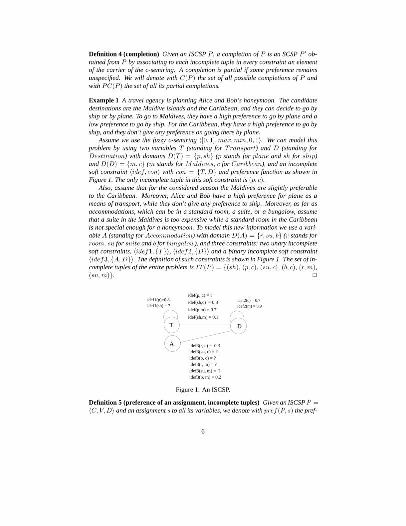
Example 1 A travel agency is planning Alice and Bob’s honeymoon. The candidatedestinations are the Maldive islands and the Caribbean, andthey can decide to go byship or by plane. To go to Maldives, they have a high preference to go by plane and alow preference to go by ship. For the Caribbean, they have a high preference to go byship, and they don’t give any preference on going there by plane.

Assume we use the fuzzy c-semiring〈[0, 1], max, min, 0, 1〉. We can model thisproblem by using two variablesT (standing forTransport) and D (standing forDestination) with domainsD(T ) = {p, sh} (p stands forplane and sh for ship)andD(D) = {m, c} (m stands forMaldives, c for Caribbean), and an incompletesoft constraint〈idef, con〉 with con = {T, D} and preference function as shown inFigure 1. The only incomplete tuple in this soft constraint is (p, c).

Also, assume that for the considered season the Maldives areslightly preferableto the Caribbean. Moreover, Alice and Bob have a high preference for plane as ameans of transport, while they don’t give any preference to ship. Moreover, as far asaccommodations, which can be in a standard room, a suite, or abungalow, assumethat a suite in the Maldives is too expensive while a standardroom in the Caribbeanis not special enough for a honeymoon. To model this new information we use a vari-ableA (standing forAccommodation) with domainD(A) = {r, su, b} (r stands forroom, su for suite andb for bungalow), and three constraints: two unary incompletesoft constraints,〈idef1, {T }〉, 〈idef2, {D}〉 and a binary incomplete soft constraint〈idef3, {A, D}〉. The definition of such constraints is shown in Figure 1. The set of in-complete tuples of the entire problem isIT (P ) = {(sh), (p, c), (su, c), (b, c), (r, m),(su, m)}. 2

idef2(c) = 0.7idef2(m) = 0.9

idef1(p)=0.8idef1(sh) = ?

D

idef3(r, c) = 0.3idef3(su, c) = ?idef3(b, c) = ?idef3(r, m) = ?

idef3(b, m) = 0.2idef3(su, m) = ?

idef(p,m) = 0.7

idef(sh,c) = 0.8

idef(sh,m) = 0.1

idef(p, c) = ?

T

A

Figure 1: An ISCSP.

Definition 5 (preference of an assignment, incomplete tuples) Given an ISCSPP =〈C, V, D〉 and an assignments to all its variables, we denote withpref(P, s) the pref-

6

erence ofs in P and with DEF(P,s) the set of soft constraints with no s-related miss-ing preferences, that is,DEF (P, s) = < idef, con >∈ C|idef(s↓con) 6=?. In detail,pref(P, s) = Π<idef,con>∈DEF (P,s)idef(s↓con). Moreover, we denote byit(s) theset of all the projections ofs over constraints ofP which have an unspecified prefer-ence.

The preference of an assignments in an incomplete problem is thus obtained bycombining the known preferences associated with the projections of the assignment,that is, of the appropriated sub-tuples in the constraints.The projections which haveunspecified preferences, that is, those init(s), are simply ignored.

Example 2 Consider the two assignmentss1 = (p, m, b) ands2 = (p, m, su) for theproblem in Figure 1. We have thatpref(P, s1) = min (0.8, 0.7, 0.9, 0.2) = 0.2, whilepref(P, s2) = min (0.8, 0.7, 0.9) = 0.7. However, while the preference ofs1 is fixed,since none of its projections is incomplete, the preferenceof s2 may become lower than0.7 depending on the preference of the incomplete tuple(su, m). 2

As shown by the example, the presence of incompleteness partitions the set ofassignments into two sets: those which have a certain preference which is independentof how incompleteness is resolved, and those whose preference is only an upper bound,in the sense that it can be lowered in some completions. Givenan ISCSPP , we willdenote the first set of assignments asFixed(P ) and the second withUnfixed(P ). InExample 2,Fixed(P ) = {s1}, while all other assignments belong toUnfixed(P ).

In SCSPs, an assignment is an optimal solution if its global preference is undom-inated. This notion can be generalized to the incomplete setting. In particular, whensome preferences are unknown, we will speak of necessarily and possibly optimal so-lutions, that is, assignments which are undominated in all (resp., some) completions.

Definition 6 (necessarily and possibly optimal solution)Given an ISCSPP = 〈C, V,D〉, an assignments ∈ D|V | is a necessarily (resp, possibly) optimal solution iff∀Q ∈ C(P ) (resp.,∃Q ∈ C(P )) ∀s′ ∈ D|V |, pref(Q, s′) 6> pref(Q, s).

Given an ISCSPP , we will denote withNOS(P ) (resp.,POS(P )) the set of nec-essarily (resp., possibly) optimal solutions ofP . Notice that, whilePOS(P ) is neverempty, in generalNOS(P ) may be empty. In particular,NOS(P ) is empty when-ever the available preferences are not sufficient to establish the relationship between anassignment and all others.

Example 3 In the ISCSPP of Figure 1, we can easily see thatNOS(P ) = ∅ since,given any assignment, it is possible to construct a completion ofP in which it is not anoptimal solution. On the other hand,POS(P ) contains all assignments not includingtuple(sh, m). 2

4 Characterizing POS(P) and NOS(P)

In this section we characterize the set of necessarily and possibly optimal solutionsof an ISCSP given the preferences of the optimal solutions oftwo of the completions

7

of P . All the results are given for ISCSPs defined on totally ordered c-semirings. Inparticular, given an ISCSPP defined on the c-semiring〈A, +,×,0,1〉, we consider:

• the SCSPP0 ∈ C(P ), called the0-completion ofP , obtained fromP by asso-ciating preference0 to each tuple ofIT (P ).

• the SCSPP1 ∈ C(P ), called the1-completion ofP , obtained fromP by asso-ciating preference1 to each tuple ofIT (P ).

Let us indicate respectively withpref0 andpref1 the preference of an optimalsolution ofP0 andP1. Due to the monotonicity of×, and since0 ≤ 1, we have thatpref0 ≤ pref1.

Example 4 Consider the problem shown in Figure 1. We have thatpref0 = 0.2 andpref1 = 0.7. 2

We will now give some lemmas that will be useful to show the following theorems.

Lemma 1 Given an ISCSPP and the completionP1 ∈ C(P ) as defined above, wehave thatpref(P, s) = pref(P1, s).

Proof: Follows immediately from the definition ofpref(P, s) and from the fact thatin a c-semiring1 is the unit element. 2

Lemma 2 Given an ISCSPP and the completionP1 ∈ C(P ) as defined above, therealways exists an assignments such thatpref(P, s) = pref1.

Proof: Follows from Lemma 1 and choosing anys ∈ Opt(P1). 2

Lemma 3 Given an ISCSPP , the completionsP0, P1 ∈ C(P ) as defined above, andanother completionP ′ ∈ C(P ), then,∀s ∈ Opt(P ′), pref0 ≤ pref(P ′, s) ≤ pref1.

Proof: Due to monotonicity, for any solutions we have thatpref(P ′, s) ≤ pref(P1,s) ≤ pref1, sincepref1 is the optimal preference ofP1. Assume there is a solutions ∈ Opt(P ′) such thatpref(P ′, s) < pref0. Then, for any solutions0 ∈ Opt(P0), wehave, by monotonicity,pref(P ′, s) < pref0 = pref(P0, s0) ≤ pref(P ′, s0). Thus,we have a contradiction, sinces is an optimal solution ofP ′. 2

Lemma 4 Given an ISCSPP and the completionP1 ∈ C(P ) as defined above, ifpref1 > pref0, thenOpt(P1) ⊆ Unfixed(P ).

Proof: Assume there is a fixed solutions such thats ∈ Opt(P1). Then we wouldhave thatpref(P0, s) = Pref(P1, s) = pref1 and thuspref(P0, s) > pref0 whichis a contradiction, sincepref0 is the optimal preference inP0. 2

Lemma 5 Given an ISCSPP , we have thatNOS(P ) = ∩P ′∈C(P )Opt(P ′).

8

Proof: Any solutions ∈ ∩P ′∈C(P )Opt(P ′) satisfies the definition of necessarily opti-mal. Consider nows ∈ NOS(P ) and a completionP ′ of P . Then, by Definition 6,scannot be dominated by another solutions′, and thuss ∈ Opt(P ′). 2

In the following theorem we will show that, ifpref0 > 0, there is a necessarilyoptimal solution ofP iff pref0 = pref1, and in this caseNOS(P ) coincides with theset of optimal solutions ofP0.

Theorem 1 Given an ISCSPP and the two completionsP0, P1 ∈ C(P ) as definedabove, ifpref0 > 0 we have thatNOS(P ) 6= ∅ iff pref1 = pref0. Moreover, ifNOS(P ) 6= ∅, thenNOS(P ) = Opt(P0).

Proof: Since we know thatpref0 ≤ pref1, if pref0 6= pref1 thenpref1 > pref0.We prove that, ifpref1 > pref0, thenNOS(P ) = ∅. Let us consider any assignments of P . Due to the monotonicity of×, for all P ′ ∈ C(P ), we havepref(P ′, s) ≤pref(P1, s) ≤ pref1.

• If pref(P1, s) < pref1, thens is not inNOS(P ) sinceP1 is a completion ofPwheres is not optimal.

• If insteadpref(P1, s) = pref1, then,s ∈ Opt(P1) and, by Lemma 4 we havethats ∈ Unfixed(P ). Thus we can consider completionP ′

1 obtained fromP1

by associating preference0 to the incomplete tuples ofs. In P ′1 the preference of

s is 0 and the preference of an optimal solution ofP ′1 is, due to the monotonicity

of ×, at least that of an optimal solution ofP0, that ispref0 > 0 Thuss 6∈NOS(P ).

Next we consider whenpref0 = pref1. ¿From Lemma 5 follows thatNOS(P ) ⊆Opt(P0). We will show thatNOS(P ) 6= ∅ by showing that anys ∈ Opt(P0) isin NOS(P ). Let us assume, on the contrary, that there iss ∈ Opt(P0) such thats 6∈ NOS(P ). Thus there is a completionP ′ of P with an assignments′ withpref(P ′, s′) > pref(P ′, s). By construction ofP0, any assignments ∈ Opt(P0) mustbe inFixed(P ). In fact, if it had some incomplete tuple, its preference inP0 wouldbe 0, since0 is the absorbing element of×. Sinces ∈ Fixed(P ), pref(P ′, s) =pref(P0, s) = pref0. By construction ofP1 and monotonicity of×, we havepref(P1,s′) ≥ pref(P ′, s′). Thus the contradictionpref1 ≥ pref(P1, s′) ≥ pref(P ′, s′) >pref(P ′, s) = pref0. This allows us to conclude thats ∈ NOS(P ) = Opt(P0). 2

In the theorem above we have assumed thatpref0 > 0. The case in whichpref0 =0 needs to be treated separately. We consider it in the following theorem.

Theorem 2 Given ISCSPP = 〈C, V, D〉 and the two completionsP0, P1 ∈ C(P )as defined above, assumepref0 = 0. Then, ifpref1 = 0, NOS(P ) = D|V |. Ifpref1 > 0, NOS(P ) = {s ∈ Opt(P1)|∀s′ ∈ D|V | with pref(P1, s

′) > 0 we haveit(s) ⊆ it(s′)}.

Proof: We prove the two items separately.

9

• If pref0 = pref1 = 0, then, from Lemma 3 follows that the preference levelof the optimal solution of SCSPP ′ is 0. Thus all assignments have always thesame preference equal to0. Thus they are all necessarily optimal solutions.

• Let us now assume that0 = pref0 < pref1. From Lemma 5, only assignmentsin Opt(P1) can be inNOS(P ) since all other assignments are not optimal inP1. Let us now considers ∈ Opt(P1). By Lemma 4 we have thatit(s) 6= ∅.If there existss′ ∈ D|V |, with pref(P1, s

′) > 0, such thatit(s) 6⊆ it(s′)then we can construct a completion ofP , sayP ′ wheres is not optimal. Itis sufficient to set the preference of the tuples init(s′) to 1 and the tuples init(s)\it(s′) to0. We have thatpref(P ′, s) = 0, since0 is the absorbing elementof ×, andpref(P ′, s′) = pref(P1, s

′). Thus, inP ′ we havepref(P ′, s′) =pref(P1, s

′) > pref(P ′, s) = 0.

We will now show that, if givens ∈ Opt(P1) there is nos′ ∈ D|V | withpref(P1, s

′) > 0 such thatit(s) 6⊆ it(s′), thens ∈ NOS(P ).

First notice that, since1 is the unit element of×, ∀P ′ ∈ C(P ) pref(P ′, s) =pref(P1, s)×it-pref(P ′, s) andpref(P ′, s′) = pref(P1, s

′)×it-pref(P ′, s′)whereit-pref(P ′, s) (resp. it-pref(P ′, s′)) is the combination of the prefer-ences associated inP ′ to the incomplete tuples init(s) (resp.it(s′)).

Since for everys′ ∈ D|V | with pref(P1, s′) > 0 we are assuming thatit(s) ⊆

it(s′), then∀P ′ ∈ C(P ), it-pref(P ′, s) ≥ it-pref(P ′, s′), due to the inten-sive property of×. Moreover, sinces ∈ Opt(P1), pref(P1, s) = pref1 >pref(P1, s

′). Thus, for everyP ′ ∈ C(P ), ∀s′ ∈ D|V | (trivially for those withpref(P1, s

′) = 0) we have thatpref(P ′, s) ≥ pref(P ′, s′). This allows us toconclude thats ∈ NOS(P ). 2

Intuitively, if the tuples ofs are not a subset of the incomplete tuples of someassignments′, then we can makes′ dominates in a completion by setting all theincomplete tuples ofs′ to 1 and all the remaining incomplete tuples ofs to 0. In sucha completions is not optimal. Thuss is not a necessarily optimal solution. However, ifthe tuples ofs are a subset of the incomplete tuples of all other assignments, then it isnot possible to lowers without lowering all other tuples even further. This means thats is a necessarily optimal solution.

We now turn our attention to possible optimal solutions. Given a c-semiring〈A, +,×, 0,1〉, it has been shown in [2] that idempotency and strict monotonicity of the×operator are incompatible, that is, at most one of these two properties can hold. Inthe following two theorems we show that the presence of one orthe other of such twoproperties plays a key role in the characterization ofPOS(P ) whereP is an ISCSP. Inparticular, if× is idempotent, then the possibly optimal solutions are the assignmentswith preference inP betweenpref0 andpref1. If, instead,× is strictly monotonic,then the possibly optimal solutions have preference inP betweenpref0 andpref1 anddominate all the assignments which have as set of incompletetuples a subset of theirincomplete tuples.

Theorem 3 Given an ISCSPP defined on a c-semiring with idempotent× and the twocompletionsP0, P1 ∈ C(P ) as defined above, ifpref0 > 0 we have that:POS(P ) ={s ∈ D|V ||pref0 ≤ pref(P, s) ≤ pref1}.

10

Proof: First we show that anys such thatpref0 ≤ pref(P, s) ≤ pref1 is inPOS(P ). Let us consider the completion ofP , P ′, obtained by associating prefer-encepref(P, s) to all the incomplete tuples ofs and0 to all other incomplete tuplesof P . For any other assignments′ we can show that it never dominatess:

• s′ ∈ Fixed(P ) and thuspref(P ′, s′) = pref(P0, s′) ≤ pref0 ≤ pref(P, s);

• s′ ∈ Unfixed(P ) and

– it(s′) 6⊆ it(s), thenpref(P ′, s′) = 0 since inP ′ the incomplete tuples init(s′) which are not init(s) have been associated with preference0;

– it(s′) ⊆ it(s). By construction ofP ′ and since× is idempotent and asso-ciative we have that:pref(P ′, s) = (pref(P, s)×(Π|it(s)|pref(P, s))) =pref(P, s) andpref(P ′, s′) = (pref(P, s′) × (Π|it(s′)|pref(P, s))) =pref(P, s′) × pref(P, s). Since× is intensive,pref(P ′, s′) = (pref(P,s′) ×pref(P, s)) ≤ pref(P, s) = pref(P ′, s).

Thus inP ′ no assignment dominatess. This means thats ∈ POS(P ).We will now show that ifs ∈ POS(P ), pref0 ≤ pref(P, s) ≤ pref1. If

s ∈ POS(P ), thens ∈ Opt(Q) form someQ ∈ C(P ). Thus we can concludeby Lemma 3. 2

Informally, given a solutions such thatpref0 ≤ pref(P, s) ≤ pref1, it can be shownthat it is an optimal solution of the completion ofP obtained by associating preferencepref(P, s) to all the incomplete tuples ofs, and0 to all other incomplete tuples ofP .On the other hand, by construction ofP0 and due to the monotonicity of×, any assign-ment which is not optimal inP0 cannot be optimal in any other completion. Also, byconstruction ofP1, there is no assignments with pref(P, s) > pref1.

Theorem 4 Given an ISCSPP defined on a c-semiring with a strictly monotonic×and the two completionsP0, P1 ∈ C(P ) as defined above, ifpref0 > 0 we have that:s ∈ POS(P ) iff pref0 ≤ pref(P, s) ≤ pref1 andpref(P, s) = max{ pref(P, s′)|it(s′) ⊆ it(s)}.

Proof: Let us first show that if assignments is such thatpref0 ≤ pref(P, s) ≤ pref1

andpref(P, s) = max{pref(P, s′)|it(s′) ⊆ it(s)} it is in POS(P ). We must showthere is a completion ofP wheres is undominated. Let us consider completionP ′

obtained by associating preference1 to all the tuples init(s) and0 to all the tuplesin IT (P ) \ it(s). First we notice thatpref(P ′, s) = pref(P, s), since1 is the unitelement of×. Let us consider any other assignments′. Then we have one of thefollowing:

• it(s′) = ∅, which means thats′ ∈ Fixed(P ) and thuspref(P ′, s′) = pref(P0,s′) ≤ pref0 ≤ pref(P, s) = pref(P ′, s);

• it(s′) 6⊆ it(s), which means that there is at least one incomplete tuple ofit(s′)which is associated with0. Since0 is the absorbing element of×, pref(P ′, s′) =0 and thuspref(P ′, s′) < pref0 ≤ pref(P ′, s);

11

• it(s′) ⊆ it(s), in this casepref(P ′, s′) = pref(P, s′) since all tuples init(s′)are associated with1 in P ′. However sincepref(P, s) = max{pref(P, s′)|it(s′)⊆ it(s)}, pref(P ′, s′) ≤ pref(P ′, s).

We can thus conclude thats is not dominated by any assignment inP ′. Hences ∈POS(P ).

Let us now prove the other direction by contradiction. Ifpref(P, s) < pref0 thenwe can conclude by Lemma 2. We must prove that ifpref0 ≤ pref(P, s) ≤ pref1

andpref(P, s) < max{pref(P, s′)|it(s′) ⊆ it(s)} thens is not in POS(P ). Inany completionP ′ of P we have thatpref(P ′, s) = pref(P, s) × it-pref(P ′, s)and pref(P ′, s′) = pref(P, s′) × it-pref(P ′, s′) where it-pref(P ′, s) (resp. it-pref(P ′, s′)) is the combination of the preferences associated to the incomplete tu-ples in it(s) (resp. it(s′)). Sinceit(s′) ⊆ it(s), for any completionP ′ we havethat it-pref(P ′, s) ≤ it-pref(P ′, s′). Moreover, lets′′ be such thatpref(P, s′′) =max{pref(P, s′)|it(s′) ⊆ it(s)}. Then we have that for any completionP ′, pref(P ′, s′′) >pref(P ′, s) sincepref(P, s′′) > pref(P, s) and it-pref(P ′, s′′) ≥ it-pref(P ′, s)and× is strictly monotonic. Thus, ifpref0 ≤ pref(P, s) ≤ pref1 andpref(P, s) <max{pref(P, s′)| it(s′) ⊆ it(s)}, thens is not inPOS(P ). 2

The intuition behind the statement of this theorem is that, if assignments is such thatpref0 ≤ pref(P, s) ≤ pref1 andpref(P, s) = max{pref(P, s′)|it(s′) ⊆ it(s)},then it is optimal in the completion obtained associating preference1 to all the tuplesin it(s) and0 to all the tuples inIT (P ) \ it(s). On the contrary, ifpref(P, s) <max{pref(P, s′)|it(s′) ⊆ it(s)}, there must be another assignments′′ such thatpref(P, s′′) = max{pref(P, s′)|it(s′) ⊆ it(s)}. It can then be shown that, in allcompletions ofP , s is dominated bys′′.

In constrast toNOS(P ), whenpref0 = 0 we can immediately conclude thatPOS(P ) = D|V |, independently of the nature of×, since all assignments are optimalin P0.

Corollary 4.1 Given an ISCSPP = 〈C, V, D〉, if pref0 = 0, thenPOS(P ) = D|V |.

For ease of clarity, the results shown in this section can be summarized as follows:

• whenpref0 = pref1 = 0

– NOS(P ) = D|V | (by Theorem 2);

– POS(P ) = D|V | (by Corollary 4.1) ;

• when0 = pref0 < pref1

– NOS(P ) = {s ∈ Opt(P1)|∀s′ ∈ D|V | with pref(P1, s′) > 0 we have

it(s) ⊆ it(s′)} (by Theorem 2);

– POS(P ) = D|V | (by Corollary 4.1);

• when0 < pref0 = pref1

– NOS(P ) = Opt(P0) (by Theorem 1);

12

– if × is idempotent:POS(P ) = {s ∈ D|V ||pref0 ≤ pref(P, s) ≤ pref1}(by Theorem 3);

– if × is strictly monotonic:POS(P ) = {s ∈ D|V ||pref0 ≤ pref(P, s) ≤pref1, pref(P, s) = max{ pref(P, s′)|it(s′) ⊆ it(s)}} (by Theorem 4);

• when0 < pref0 < pref1

– NOS(P ) = ∅ (by Theorem 1);

– POS(P ) as for the case when0 < pref0 = pref1.

5 Solving ISCSPs

In this section we first describe a general schema for solvingISCSPs based on interleav-ing a branch and bound search with elicitation. Such a general schema is instantiatedto different elicitation strategies generating several concrete algorithms. A computa-tional analysis of the algorithms is provided both in terms of the number of elicitedpreferences and of the user effort for revealing some of the missing preferences.

5.1 The solver schema and its instances

The solving strategy which we propose for ISCSPs is based on the idea of combininga branch and bound search (B&B) with elicitation steps in which the user is asked toprovide some type of missing information. In general, B&B proceeds by consideringthe variables in some order, by choosing a value for each variable in the order, andby computing, using some heuristics, an upper bound on the global preference of anycompletion of the current partial assignment. B&B also stores the highest preference(assuming the goal is to maximize) of a complete assignment found so far. If at anystep the upper bound is lower than the preference of the current best solution, the searchbacktracks.

When some of the preferences are missing, as in ISCSPs, the agent may be askedfor some preferences or other information regarding the preferences in order to knowthe true preference of a partial or complete assignment or inorder to choose the nextvalue for some variable. Preferences can be elicited after each run of B&B (as in [12])or during a B&B run while preserving the correctness of the approach. For example, wecan elicit preferences at the end of every complete branch (that is, regarding preferencesof every complete assignment considered in the branch and bound algorithm), or atevery node in the search tree (thus considering every partial assignment). Moreover,when choosing the value for the next variable to be assigned,we can ask the user (whoknows the missing preferences) for help. Finally, rather than eliciting all the missingpreferences in the possibly optimal solution, or the complete or partial assignmentunder consideration, we can elicit just some of the missing preferences.

For example, with incomplete fuzzy constraint problems (IFCSPs), eliciting justthe worst preference among the missing ones is sufficient, since only the worst value isimportant to the computation of the overall preference value. Instead, with incompleteweighted constraint problems (IWCSPs), we need to elicit asmany preference values

13

as needed to decide whether the current assignment is betterthan the best one found sofar.

More precisely, the algorithm schema we propose is based on the following param-eters:

1. WHO chooses the value of a variable:

(a) the algorithm, using one of the following heuristics:

i. values are picked in decreasing order w.r.t. their preference values inthe 1-completion. The order is maintained dynamically. We denotethis heuristic withdp;

ii. values are picked in decreasing order w.r.t. the preferences in the0-completion of the initial ISCSP. The order is thus static. Wedenotethis heuristic withdpi.

(b) The user, revealing the value that he prefers according to one of the follow-ing criteria:

i. the value is the most preferred among those in the domain whichhaven’t been considered yet (lazy user, lu for short);

ii. the value is the most preferred among those which haven’tbeen con-sidered yet given the constraints involving the current variable and thepast variables in the search order (smart user, su for short);

2. WHAT must be elicited:

(a) the preferences of all the incomplete tuples of the current assignment (de-noted withall);

(b) for IFCSPs, only the preference of the worst tuple of the current assign-ment, if it is worse than the known ones (denoted withworst);

(c) for IWCSPs:

• the worst missing cost (that is, the highest) until either all the costs areelicited or the current global cost of the (possibly partial) assignmentis higher than the optimum found so far. This strategy is denoted byWW.

• the best (i.e. the minimum) cost until either all the costs are elicitedor the current global cost of the (possibly partial) assignment is higherthan t he optimum found so far. This strategy is denoted by BB.

• the best and the worst cost in turn. This strategy is denoted by BW.

3. WHEN elicitation should take place:

(a) at the end of the branch and bound search (attree level).

(b) during the search, when we have a complete assignment to all the variables(i.e., when we have reached a leaf of the search tree, and thuswhen we areat the end of abranch). We will refer to such a heuristics, by saying “atbranchlevel”.

14

(c) during search, whenever a new value is assigned to a variable. We will referto such a heuristics, by saying “at thenodelevel”.

Summarizing, we have three features which we callwho, whatandwhen. Thereare four possible choices forwho: dp, dpi, lu, andsu. If we work with IFCSPs, thereare two possibilities forwhat: all andworst. Instead, with IWCSPs, there are fouroptions:all, WW, BB, and BW.

It should be noticed that while theworst option is meaningful only for the fuzzy c-semiring. In fact, in the fuzzy semiring the preference of a possibly partial assignmentcorresponds to the worst one associated with one of its subtuples. Finally, there arethree options forwhen: tree, branch, andnode. If when = tree, elicitation takesplace only when the search is completed. This means that the B&B search can beperformed more than once. In contrast, ifwhen = branch or when = node, the B&Bsearch is performed only once and the elicitation is done either at every node of thesearch tree or at every leaf.

By choosing a value for each of the three parameters above in aconsistent way, weobtain, for IFCSPs, a total of 16 different algorithms, as summarized in Figure 2.

Figure 2: The algorithms for IFCSPs.

If instead we work with IWCSPs, we have a total of 32 algorithms, as can be seenin Figure 3.

The pseudocode of our general solver, which we call ISCSP-SCHEME, is shownin Algorithms 1 and 2. Every point in Figure 2 represents an instantiation of ISCSP-SCHEME to specific values for parameterswho, what andwhen.

ISCSP-SCHEME takes in input an ISCSPP and the values for the three param-eters:who, what, andwhen. It returns an ISCSPQ, a complete assignments anda preferencep. In Theorems 5 and 7 we will show thatQ is a partial completionof P ands is a necessarily optimal solution ofQ with preferencep. As a first step,ISCSP-SCHEME computes the0-completion ofP , calledP0, and finds one of its op-timal solutions, saysmax, and its preference, sayprefmax, by applying a standardbranch and bound procedure (denoted byB&B). Next, procedureBBE is called. IfBBE succeeds, it returns a partial completion ofP , one of its necessarily optimalsolutions, and its associated preference. Otherwise, it returns a solution equal tonil.

15

Figure 3: The algorithms for IWCSPs.

Algorithm 1 : ISCSP-SCHEMEInput : an ISCSPP , a parameterwho indicating the method of valuesinstantiation, a parameterwhat indicating the elicitation policy, a parameterwhen indicating the level at which the elicitation must be doneOutput : an ISCSPQ, an assignment s, a preference pcomputeP0

Q← P0

smax, prefmax ← B&B(P0,−)Q′,s1,pref1 ← BBE(P, 0, who, what, when, smax, prefmax)if s1 6= nil then

smax ← s1

prefmax ← pref1

Q← Q′

return Q, smax, prefmax

In the first case the output of ISCSP-SCHEME coincides with that of BBE, otherwiseISCSP-SCHEME returnsP0 and one of its optimal solutions with the correspondingpreference.

Procedure BBE takes as input the same values as ISCSP-SCHEMEand, in addition,a solutionsol and a preferencelb representing the current lower bound of the optimalpreference level. Solutionsol′ and preferencepref ′ are initialized to such values at thebeginning of BBE. ProcedurenexV ariable applied to the1-completion of the ISCSPin input (denoted byP [?/1]) allows to assign tocurrentV ariable the next variableto be assigned. The algorithm then assigns a value to this variable. If the BooleanfunctionnextV alue returns true (if there is a value in the domain), we select a valuefor currentV ariable according to the value of parameterwho.

The computation of the upper bound for the preference that can be obtained by anycompletion of the current partial assignment is performed by procedureUpperBound.In general, any kind of upper bound can be used. However, we have chosen to estimate

16

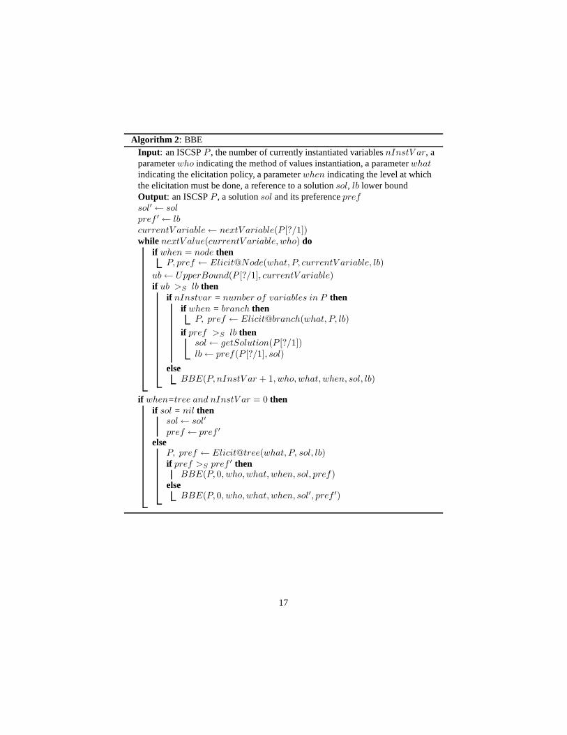
Algorithm 2 : BBEInput : an ISCSPP , the number of currently instantiated variablesnInstV ar, aparameterwho indicating the method of values instantiation, a parameterwhatindicating the elicitation policy, a parameterwhen indicating the level at whichthe elicitation must be done, a reference to a solutionsol, lb lower boundOutput : an ISCSPP , a solutionsol and its preferenceprefsol′← solpref ′← lbcurrentV ariable← nextV ariable(P [?/1])while nextV alue(currentV ariable, who) do

if when = node thenP, pref ← Elicit@Node(what, P, currentV ariable, lb)

ub← UpperBound(P [?/1], currentV ariable)if ub >S lb then

if nInstvar = number of variables in P thenif when = branch then

P, pref ← Elicit@branch(what, P, lb)

if pref >S lb thensol← getSolution(P [?/1])lb← pref(P [?/1], sol)

elseBBE(P, nInstV ar + 1, who, what, when, sol, lb)

if when=tree and nInstV ar = 0 thenif sol = nil then

sol← sol′

pref ← pref ′

elseP, pref ← Elicit@tree(what, P, sol, lb)if pref >S pref ′ then

BBE(P, 0, who, what, when, sol, pref)else

BBE(P, 0, who, what, when, sol′, pref ′)

17

it by combining the preferences of the constraints involving only variables that havealready been instantiated. Formally, lett be the current partial assignment to variablesin {v1, . . . , vk} ⊆ V , and letci = 〈defi, coni〉 be a constraint, such thatconi ⊆{v1, . . . , vk}. Then, the valueub returned byUpperBound is:

ub =k∏

i=1

defi(t ↓coni),

where∏

is the combination operator of the semiring.We will now describe procedure BBE by considering the various values for param-

eterwhen. This corresponds to consider the algorithms in Figures 2 and 3 divided intothe three horizontal planes obtained fixing the value on thewhen-axis.

• If when = tree, elicitation is handled by procedureElicit@tree and takes placeonly at the end of the search over the1-completion. The user is not involved inthe value assignment steps within the search and thus there are only two possiblevalues for variablewho, i.e. dp anddpi. At the end of the search, if a solutionis found, the user may be asked to reveal all the preferences of the incompletetuples in the solution (ifwhat = all). If we work with IFCSPs, we could alsoask for just the worst one among the missing preferences if itis worst than theknown ones (ifwhat = worst). If instead we work with IWCSPs, preferencescan be asked in decreasing (what = BB), increasing (what = WW), or alternatingorder (what = BW) until we have enough information. If the preference of thissolution is better than the best found so far, BBE is called recursively with thenew best solution and preference, otherwise the recursive call is done with theold solution and preference.

• If when = branch, B&B is performed only once and not several times as in theprevious case. The user may be asked to choose the next value for the currentvariable being instantiated. Preference elicitation, which is handled by functionElicit@branch, takes place during search, whenever all variables have beeninstantiated. As above, the user can be asked either to reveal the preferences ofall or some of the incomplete tuples depending on the value ofwhat. In all casesthe information gathered is sufficient to compare the preference of the currentassignment against the current lower bound.

• If when = node, preferences are elicited every time a new value is assignedto a variable, and it is handled by procedureElicit@node. The tuples to beconsidered for elicitation are those involving the value which has just been as-signed and belonging to constraints between the current variable and alreadyinstantiated variables. The value ofwhat determines whether one or all or somepreference values involving the new assignment are asked tothe user. With theinformation given by the user, the preference of the currentpartial assignmentis updated in order to determine if the subtree rooted at the current node can bepruned.

18

5.2 Termination and correctness

We will now prove that algorithm ISCSP-SCHEME, when given anISCSP in input,always terminates generating a completion of the ISCSP and one of its necessarilyoptimal solution.

Theorem 5 Given an ISCSPP andwhen = tree, if

• what = all, or

• what = worst andP is an IFCSP, or

• (what = WW orwhat = BB or what = BW) andP is an IWCSP,

algorithmISCSP-SCHEMEalways terminates and returns an ISCSPQ such thatQ ∈PC(P ), an assignments ∈ NOS(Q), and its preference inQ.

Proof: Clearly ISCSP-SCHEME terminates if and only if BBE terminates. If weconsider the pseudo-code of procedure BBE shown in Algorithm 2, we see that ifwhen = tree, BBE terminates whensol = nil. This happens only when the searchfails to find a solution of the current problem with a preference strictly greater thanthe current lower bound, i.e., when the conditionpref >S lb is never satisfied. Letus denote withQi andQi+1 respectively the ISCSPs given in input to thei-th and(i + 1)-th recursive call of BBE. First we notice that only procedure Elicit@treemodifies the ISCSP in input by possibly adding new elicited preferences. Moreover,whatever the value of parameterwhat is, the returned ISCSP is either the same asthe one in input or it is a (possibly partial) completion of the one in input. Thus wehaveQi+1 ∈ PC(Qi) and Qi ∈ PC(P ). Since the search is always performedon the1-completion of the current ISCSP, we can conclude that for every solutions, pref(Qi+1, s) ≤S pref(Qi, s). Let us now denote withlbi and lbi+1 the lowerbounds given in input respectively to thei-th and (i + 1)-th recursive call of BBE. It iseasy to see thatlbi+1 ≥S lbi. Thus, since at every iteration the preferences of solutionscannot increase and the bound cannot decrease, and since we have a finite number ofsolutions, we can conclude that BBE always terminates.

The reasoning that follows relies on the fact that valuepref returned by functionElicit@tree is the final preference after elicitation of assignmentsol given in input.This is true since eitherwhat = all and thus all preferences have been elicited andthe overall preference ofsol can be computed, or only theworst preference has beenelicited but in a fuzzy context where the overall preferencecoincide with the worstone, or we are in a IWCSP and we have elicited enough preferences to discover thatthe current solution is worst then the optimum found so far orwe have elicited all itscosts.

If called withwhen = tree ISCSP-SCHEME exits when the last branch and boundsearch has ended returningsol = nil. In such a casesol andpref are updated tocontain the best solution and associated preference found so far, i.e. sol′ andpref ′.Then, the algorithm returns the current ISCSP, sayQ, andsol andpref . Following thesame reasoning as above done forQi, we can conclude thatQ ∈ PC(P ).

At the end of a while loop execution of the first call of BBE (thebottom of the callstack), assignmentsol either contains an optimal solutionsol of the1-completion of

19

the current ISCSP orsol = nil. sol = nil iff there is no assignment with preferencehigher thanlb in the 1-completion of the current ISCSP. In this situation,sol′ andpref ′ are an optimal solution and preference of the1-completion of the current ISCSP.However, since the preference ofsol′, pref ′ is fixed and since, due to monotonicity, theoptimal preference value of the1-completion is always better than or equal to that ofthe0-completion, we have thatsol′ andpref ′ are an optimal solution and preferenceof the0-completion of the current ISCSP as well.

By Theorems 1 and 2, we can conclude thatNOS(Q) is not empty. Ifpref = 0,thenNOS(Q) contains all the assignments and thus alsosol. The algorithm correctlyreturns the same ISCSP given in input, assignmentsol and its preferencepref . Ifinstead0 < pref , again the algorithm is correct, since by Theorem 1 we know thatNOS(Q) = Opt(Q[?/0]), and we have shown thatsol ∈ Opt(Q[?/0]). 2

Moreover, if parameterwhen = tree, then no useless work is done to elicit prefer-ences related to solutions which cannot be necessarily optimal for any partial comple-tion of the given problem.

Theorem 6 If ISCSP-SCHEMEis given in inputwhen = tree, then only preferencesof tuples of solutions inPOS(P ) are elicited.

Proof: If when = tree then, during the execution of ISCSP-SCHEME, prefer-ences are elicited only by procedureElicit@tree. A call to such a procedure, suchasElicit@tree (what, P, sol, lb), depending on the value of parameterwhat, elicitsall or a subset of the preferences of the incomplete tuples ofassignmentsol, return-ing the (eventually) new global preference ofsol, pref and the completion ofP ob-tained adding the new elicited preferences. During the execution of ISCSP-SCHEME,Elicit@tree is called on the current partial completion of the ISCSP given in input,Pand on an optimal solution of its1-completion,sol. By Theorems 3 and 4, any optimalsolution of the1-completion of the current partial completion ofP is a possibly opti-mal solution of such a partial completion. 2

We will now consider other values for parameterwhen.

Theorem 7 Given a fuzzy or weighted ISCSPP and (when = branch or when =node), AlgorithmISCSP-SCHEMEalways terminates, and it returns an ISCSPQ suchthatQ ∈ PC(P ), an assignments ∈ NOS(Q), and its preference inQ.

Proof: In order to prove that the algorithm terminates, it is sufficient to show thatBBE terminates. Since the domains are finite, the labelling phase produces a numberof finite choices at every level of the search tree. Moreover,since the number of vari-ables is limited, then, we have also a finite number of levels in the tree. Hence,BBEconsiders at most all the possible assignments, that are a finite number. At the endof the execution of ISCSP-SCHEME,sol, with preferencepref is one of the optimalsolutions of the currentP [?/1]. Thus, for every assignments′, pref(P [?/1], s′) ≤S

pref(P [?/1], sol). Moreover, for every completionQ′ ∈ C(P ) and for every as-signments′, pref(Q′, s′) ≤S pref(P [?/1], s′). Hence, for every assignments′ andfor everyQ′ ∈ C(P ), we have thatpref(Q′, s′) ≤S pref(P [?/1], sol). In order to

20

prove thatsol ∈ NOS(P ), now it is sufficient to prove that for everyQ′ ∈ C(P ),pref(P [?/1], sol) = pref(Q′, sol). This is true, sincesol ∈ Fixed(P ) both wheneliciting all the missing preferences, and when eliciting only the worst one for fuzzyISCSPs, and when eliciting via BB, BW, or WW in weighted ISCSPs. In fact, in bothcases, the preference ofsol is the same in every completion. To show that the finalproblemQ returned by BBE is inPC(P ), it is sufficient to note that only the proce-duresElicit@node andElicit@branch modify the ISCSP in input by possibly addingsome missing preferences. Thus, the returned ISCSP is inPC(P ). 2

6 Problem generator and experimental design

To test the performance of these different algorithms, we created Fuzzy ISCSPs (alsodenoted by IFCSPs) using a generator which is a simple extension of the standardrandom model for hard constraints to soft and incomplete constraints. The generatorhas the following parameters:

• n: number of variables;

• m: cardinality of the variable domains;

• d: density, that is, the percentage of binary constraints present in the problemw.r.t. the total number of possible binary constraints thatcan be defined onnvariables;

• t: tightness, that is, the percentage of tuples with preference0 in each constraintand in each domain w.r.t. the total number of tuples (m2 for the constraints, sincewe have only binary constraints, andm in the domains);

• i: incompleteness, that is, the percentage of incomplete tuples (that is, tupleswith preference?) in each constraint and in each domain.

Given values for these parameters, we generate IFCSPs as follows. We first generatenvariables and thend% of then(n− 1)/2 possible constraints. Then, for every domainand for every constraint, we generate a random preference value in (0, 1] for each ofthe tuples (that arem for the domains, andm2 for the constraints); we randomly sett%of these preferences to0; and we randomly seti% of the preferences as incomplete.

For example, if the generator is given in inputn = 10, m = 5, d = 50, t = 10,andi = 30, it generates a binary IFCSP with10 variables, each with5 elements in thedomain,22 constraints (that is50% of 45 = 10(10− 1)/2), 2 tuples with preference0(that is,10% of 25 = 5 × 5) and7 incomplete tuples (that is,30% of 25 = 5 × 5) ineach constraint, and1 missing preference (that is,30% of 5) in each domain. Noticethat we use a model B generator: density and tightness are interpreted as percentages,and not as probabilities [14].

We also generate random IWSCSPs using the same parameters asfor IFCSPs, withcosts in[0, 10] ∪ {+∞}.

Our experiments measure thepercentage of elicited preferences(over all the miss-ing preferences) as the generation parameters vary. Since some of the algorithm in-stances require the user to suggest the value for the next variable, or ask for the worst

21

value among several, we also show theuser’s effortin the various solvers, formallydefined as the percentage of missing preferences the user hasto consider to give therequired help.

Besides the 16 instances of the scheme for IFCSPs described above, we also con-sidered a ”baseline” algorithm that elicits preferences ofrandomly chosen tuples everytime branch and bound ends. All algorithms are named by meansof the three param-eters. For example, algorithm DPI.WORST.BRANCH has parameterswho = dpi,what = worst, andwhen = branch. For the baseline algorithm, we use the nameDPI.RANDOM.TREE.

For every choice of parameter values, 100 problem instancesare generated. Theresults shown are the average over the 100 instances. Also, when it is not specifiedotherwise, we setn = 10 andm = 5. However, we have similar results forn = 5, 8,11, 14, 17, and 20. All our experiments have been performed onan AMD Athlon 64x22800+, with 1 Gb RAM, Linux operating system, and using JVM 6.0.1.

7 Results

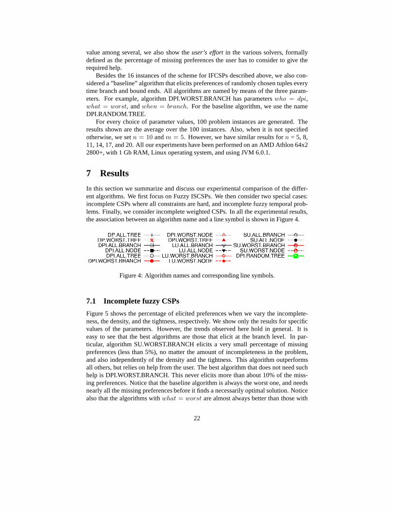
In this section we summarize and discuss our experimental comparison of the differ-ent algorithms. We first focus on Fuzzy ISCSPs. We then consider two special cases:incomplete CSPs where all constraints are hard, and incomplete fuzzy temporal prob-lems. Finally, we consider incomplete weighted CSPs. In allthe experimental results,the association between an algorithm name and a line symbol is shown in Figure 4.

Figure 4: Algorithm names and corresponding line symbols.

7.1 Incomplete fuzzy CSPs

Figure 5 shows the percentage of elicited preferences when we vary the incomplete-ness, the density, and the tightness, respectively. We showonly the results for specificvalues of the parameters. However, the trends observed herehold in general. It iseasy to see that the best algorithms are those that elicit at the branch level. In par-ticular, algorithm SU.WORST.BRANCH elicits a very small percentage of missingpreferences (less than 5%), no matter the amount of incompleteness in the problem,and also independently of the density and the tightness. This algorithm outperformsall others, but relies on help from the user. The best algorithm that does not need suchhelp is DPI.WORST.BRANCH. This never elicits more than about 10% of the miss-ing preferences. Notice that the baseline algorithm is always the worst one, and needsnearly all the missing preferences before it finds a necessarily optimal solution. Noticealso that the algorithms withwhat = worst are almost always better than those with

22

what = all, and thatwhen = branch is almost always better thanwhen = node orwhen = tree.

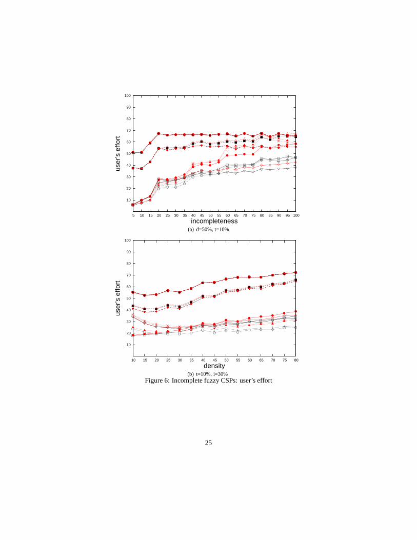
Figure 6 (a) shows the user’s effort as incompleteness varies. As could be pre-dicted, the effort grows slightly with the incompleteness level, and it is equal to thepercentage of elicited preferences only whenwhat = all andwho = dp or dpi. Forexample, whenwhat = worst, even if who = dp or dpi, the user has to considermore preferences than those elicited, since to identify theworst preference value theuser needs to check all of them (that is, those involved in a partial or complete as-signment). DPI.WORST.BRANCH requires the user to look at 60% of the missingpreferences at most, even when incompleteness is 100%.

Figure 6 (b) shows the user’s effort as density varies. Also in this case, as expected,the effort grows slightly with the density level. In this case DPI.WORST.BRANCHrequires the user to look at most 40% of the missing preferences, even when the densityis 80%.

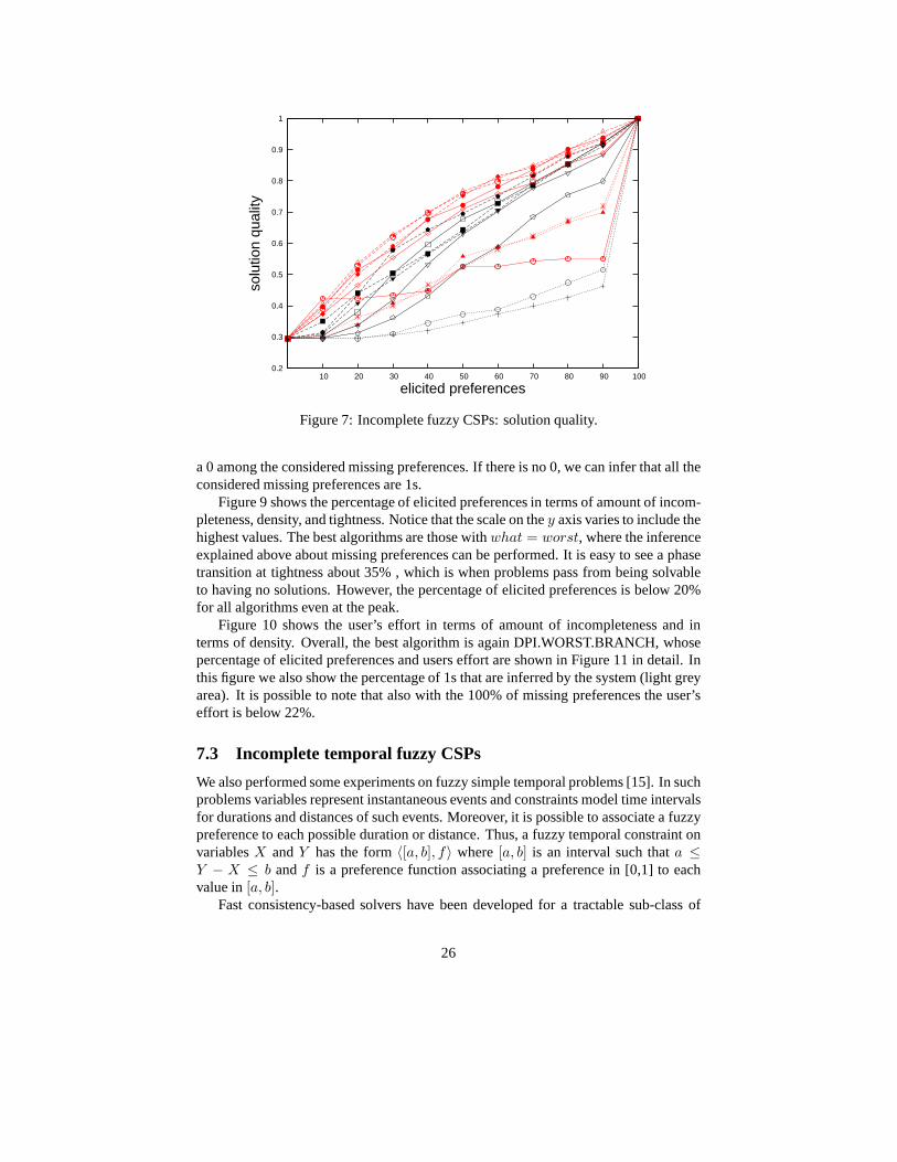
All these algorithms have a useful anytime property, since they can be stopped evenbefore their end obtaining a possibly optimal solution withpreference value higher thanthe solutions considered up to that moment. Figure 7 shows how fast the various al-gorithms reach optimality. They axis represents the solution quality during execution,normalized to allow for comparison among different problems. The algorithms thatperform best in terms of elicited preferences, such as DPI.WORST.BRANCH, are alsothose that approach optimality fastest. We can therefore stop such algorithms early andstill obtain a solution of good quality in all completions.

Figure 8 (a) shows the percentage of elicited preferences (white part of the bar)over all the preferences (white + grey part), as well as the user’s effort (black part)for DPI.WORST.BRANCH. Even with high levels of incompleteness, this algorithmelicits only a very small fraction of the preferences, whileasking the user to considerat most half of the missing preferences. For example, with incompleteness at60%, theuser effort is at less than30% and the elicited preferences are at less than10%

Figure 8 (b) shows results for LU.WORST.BRANCH, where the user is involvedin the choice of the value for the next variable. Compared to DPI.WORST.BRANCH,this algorithm is better both in terms of elicited preferences and user’s effort (whileSU.WORST.BRANCH is better only for the elicited preferences). We conjecture thatthe help the user gives in choosing the next value guides the search towards bettersolutions, thus resulting in an overall decrease of the number of elicited preferences.

Although we are mainly interested in the amount of elicitation, we also computedthe time to run the 16 algorithms. Ignoring the time taken to ask the user for missingpreferences, the best algorithms need about 200 ms to find thenecessarily optimalsolution for problems with 10 variables and 5 elements in thedomains, no matter theamount of incompleteness. Most of the algorithms need less than 500 ms.

7.2 Incomplete CSPs

We also tested these algorithms on incomplete hard CSPs. In this case, preferencesare only 0 and 1, and necessarily optimal solutions are complete assignments whichare feasible in all completions. The problem generator is adapted accordingly. Theparameterwhat now has a specific meaning:what = worst means asking if there is

23

0

10

20

30

40

50

60

70

80

90

100

5 10 15 20 25 30 35 40 45 50 55 60 65 70 75 80 85 90 95 100

elic

ited

pref

eren

ces

(%)

incompleteness

(a) d=50%, t=10%

10

20

30

40

50

60

70

80

90

100

10 15 20 25 30 35 40 45 50 55 60 65 70 75 80

elic

ited

pref

eren

ces

(%)

density

(b) t=35%, i=30%

10

20

30

40

50

60

70

80

90

100

5 10 15 20 25 30 35 40 45 50 55 60 65 70 75 80

elic

ited

pref

eren

ces

(%)

tightness

(c) d=50%, i=30%Figure 5: Percentage of elicited preferences in incompletefuzzy CSPs.

24

10

20

30

40

50

60

70

80

90

100

5 10 15 20 25 30 35 40 45 50 55 60 65 70 75 80 85 90 95 100

user

’s e

ffort

incompleteness(a) d=50%, t=10%

10

20

30

40

50

60

70

80

90

100

10 15 20 25 30 35 40 45 50 55 60 65 70 75 80

user

’s e

ffort

density(b) t=10%, i=30%

Figure 6: Incomplete fuzzy CSPs: user’s effort

25

0.2

0.3

0.4

0.5

0.6

0.7

0.8

0.9

1

10 20 30 40 50 60 70 80 90 100

solu

tion

qual

ity

elicited preferences

Figure 7: Incomplete fuzzy CSPs: solution quality.

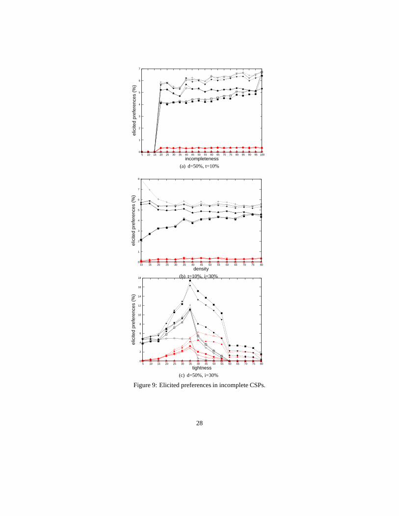
a 0 among the considered missing preferences. If there is no 0, we can infer that all theconsidered missing preferences are 1s.

Figure 9 shows the percentage of elicited preferences in terms of amount of incom-pleteness, density, and tightness. Notice that the scale onthey axis varies to include thehighest values. The best algorithms are those withwhat = worst, where the inferenceexplained above about missing preferences can be performed. It is easy to see a phasetransition at tightness about 35% , which is when problems pass from being solvableto having no solutions. However, the percentage of elicitedpreferences is below 20%for all algorithms even at the peak.

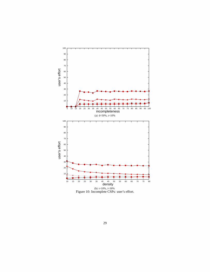
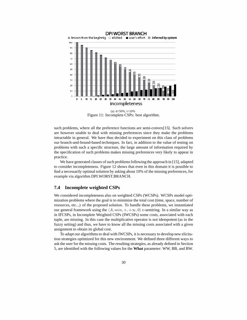
Figure 10 shows the user’s effort in terms of amount of incompleteness and interms of density. Overall, the best algorithm is again DPI.WORST.BRANCH, whosepercentage of elicited preferences and users effort are shown in Figure 11 in detail. Inthis figure we also show the percentage of 1s that are inferredby the system (light greyarea). It is possible to note that also with the 100% of missing preferences the user’seffort is below 22%.

7.3 Incomplete temporal fuzzy CSPs

We also performed some experiments on fuzzy simple temporalproblems [15]. In suchproblems variables represent instantaneous events and constraints model time intervalsfor durations and distances of such events. Moreover, it is possible to associate a fuzzypreference to each possible duration or distance. Thus, a fuzzy temporal constraint onvariablesX andY has the form〈[a, b], f〉 where[a, b] is an interval such thata ≤Y − X ≤ b andf is a preference function associating a preference in [0,1] to eachvalue in[a, b].

Fast consistency-based solvers have been developed for a tractable sub-class of

26

(a) d=50%, t=10%

(b) d=50%, t=10%Figure 8: Incomplete fuzzy CSPs: best algorithms.

27

0

1

2

3

4

5

6

7

5 10 15 20 25 30 35 40 45 50 55 60 65 70 75 80 85 90 95 100

elic

ited

pref

eren

ces

(%)

incompleteness

(a) d=50%, t=10%

0

1

2

3

4

5

6

7

8

10 15 20 25 30 35 40 45 50 55 60 65 70 75 80

elic

ited

pref

eren

ces

(%)

density

(b) t=10%, i=30%

0

2

4

6

8

10

12

14

16

18

5 10 15 20 25 30 35 40 45 50 55 60 65 70 75 80

elic

ited

pref

eren

ces

(%)

tightness

(c) d=50%, i=30%

Figure 9: Elicited preferences in incomplete CSPs.

28

10

20

30

40

50

60

70

80

90

100

5 10 15 20 25 30 35 40 45 50 55 60 65 70 75 80 85 90 95 100

user

’s e

ffort

incompleteness(a) d=50%, t=10%

10

20

30

40

50

60

70

80

90

100

10 15 20 25 30 35 40 45 50 55 60 65 70 75 80

user

’s e

ffort

density(b) t=10%, i=30%

Figure 10: Incomplete CSPs: user’s effort.

29

(a) d=50%, t=10%Figure 11: Incomplete CSPs: best algorithm.

such problems, where all the preference functions are semi-convex[15]. Such solversare however unable to deal with missing preferences since they make the problemsintractable in general. We have thus decided to experiment on this class of problemsour branch-and-bound-based techniques. In fact, in addition to the value of testing onproblems with such a specific structure, the large amount of information required bythe specification of such problems makes missing preferences very likely to appear inpractice.

We have generated classes of such problems following the approach in [15], adaptedto consider incompleteness. Figure 12 shows that even in this domain it is possible tofind a necessarily optimal solution by asking about 10% of themissing preferences, forexample via algorithm DPI.WORST.BRANCH.

7.4 Incomplete weighted CSPs

We considered incompleteness also on weighted CSPs (WCSPs). WCSPs model opti-mization problems where the goal is to minimize the total cost (time, space, number ofresources, etc...) of the proposed solution. To handle these problems, we instantiatedour general framework using the〈A, min, +, +∞, 0〉 c-semiring. In a similar way asin IFCSPs, in Incomplete Weighted CSPs (IWCSPs) some costs,associated with eachtuple, are missing. In this case the multiplicative operator is not idempotent (as in thefuzzy setting) and thus, we have to know all the missing costsassociated with a givenassignment to obtain its global cost.

To adapt our algorithms to deal with IWCSPs, it is necessary to develop new elicita-tion strategies optimized for this new environment. We defined three different ways toask the user for the missing costs. The resulting strategies, as already defined in Section5, are identified with the following values for theWhat parameter: WW, BB, and BW.

30

10

20

30

40

50

60

70

80

90

100

10 20 30 40 50 60 70 80 90 100

elic

ited

pref

eren

ces

incompleteness

Figure 12: Percentage of elicited preferences in incomplete fuzzy temporal CSPs.

Figure 13: Algorithms for IWCSPs.

Notice that, with WW, we elicit the worst missing cost (that is, the highest) until eitherall the costs are elicited or the current global cost of the (possibly partial) assignment ishigher than the optimum found so far. By doing this, we know ifthe global cost exceedsthe optimum as early as possible. With BB, we elicit the best (i.e. the minimum) costuntil either all the costs are elicited or the current globalcost of the (possibly partial)assignment is higher than the optimum found so far. Knowing the best cost of a givenassignment allows the system to infer that all the other missing costs are at least as highas the last one elicited. This inference allows us to update the1-completion during thesearch by lowering the upper bound of the missing costs. In this way, we overesti-mate the real value of the unknown costs. LetP 1

∗ the1-completion updated with theinferred costs. Given an assignments, pref(P1, s) ≥S pref(P 1

∗, s) ≥S pref(P ′, s)whereP ′ is P in which all the incomplete tuples ofs are elicited. With BW, we elicitin turn the best and the worst cost. In this case we want to testempirically if thecombination of the previous two strategies is better in practice.

In all the experimental results, the association between analgorithm name and aline symbol is shown in Figure 13.

We tested our algorithms on randomly generated IWCSPs, and we used theWhat =ALL method as a baseline because it is the most general elicitation strategy that canbe applied in every possible setting: Hard CSPs, Fuzzy ISCSPs, etc.

The randomly generated IWCSPs have the same default parameter values as in theIFCSPs experiments, except for the tightness that has a default value of 25%. We

31

choose this value because it is near the middle from 0 and 40%,where we will see aphase transition in the percentage of elicited tuples (Figure 14(c)). We recall that eachcost has a value in[0, 10] ∪ {+∞}.

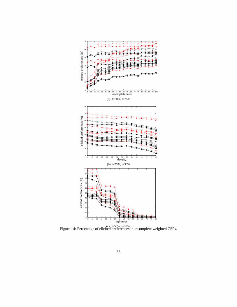
Figure 14 shows the percentage of elicited preferences as wevary density, incom-pleteness and tightness. As expected, the number of elicited tuples increases with theincompleteness of the problem (see Figure 14(a)). As we varythe tightness (Figure14(c)), we can observe a phase transition at t=40%. At that point, most of the prob-lems have an optimal solution with infinite cost, thus the algorithms do not need moreinformation to find that extreme solution.

When the density increases (Figure 14(b)), the percentage of elicited costs tendsto decrease slightly. This may be surprising, since, increasing the number of con-straints, the number of incomplete tuples increases, thus the percentage of elicited costsshould increase. However, the number of infinite costs increases together with the in-completeness. In this particular case, using t=25% and i=30%, the number of infinitecost values increases enough to make the problem easier to solve, thus it requires lesselicitation. We performed other experiments decreasing the default tightness value tot=10%. In this case the percentage of elicited values increases slightly, because thereare not enough infinite costs to make the problem easier to solve. On the other hand,the number of incomplete tuples increases with density, making the problem harderto solve (thus requiring more elicitation). Summarizing, increasing density, both in-completeness and tightness increase. When t=25% the contribution of the tightness ismore important than incompleteness and the problems becomeeasier to solve. On thecontrary, when t=10%, the contribution of the incompleteness is greater and thus theproblems becomes harder.

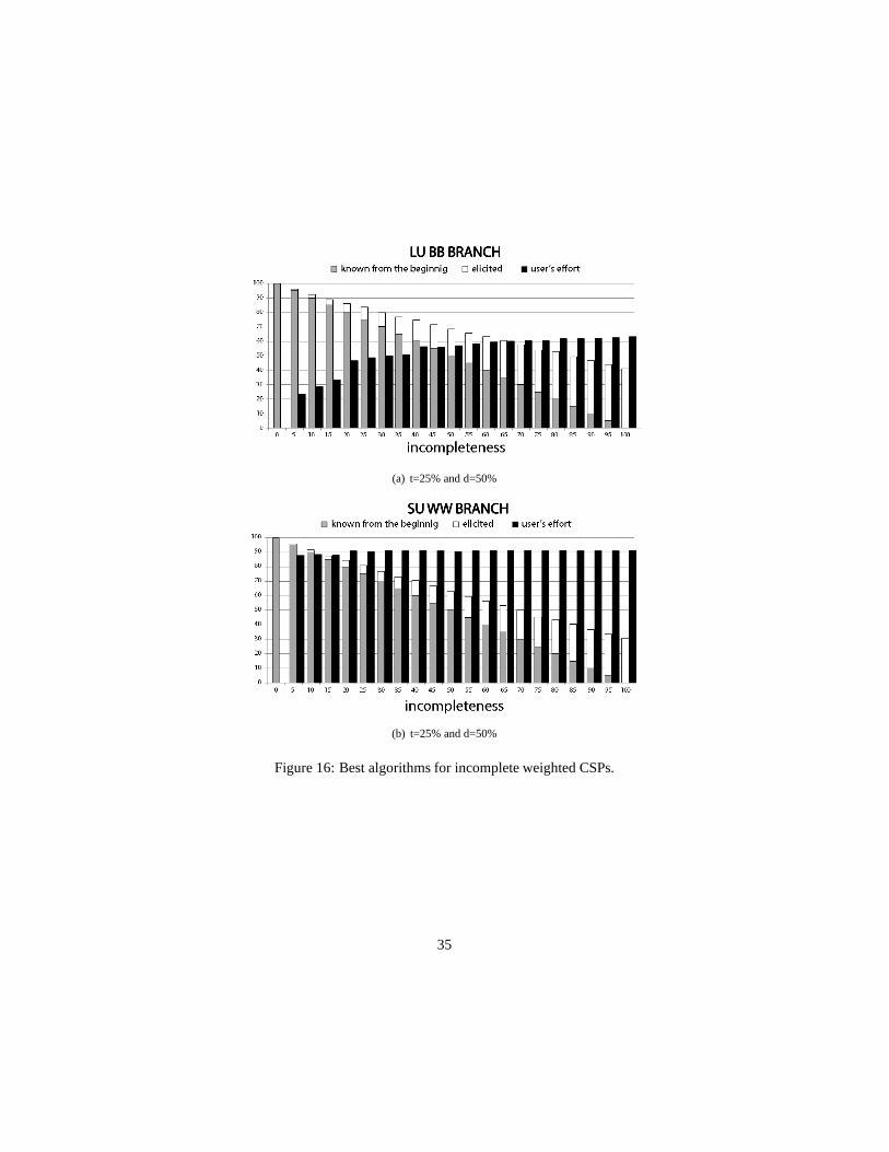
It easy to see that the best algorithms are those withwhen = branch andwho =su. These algorithms ask for only around 30% of the costs neededto solve a totallyincomplete problem. The parameterwho = su forces the user to select the value toinstantiate, which implies an additional effort by the user. This behavior is depicted inFigure 16(b) where the algorithm elicits a very small numberof tuples but the user hasto check almost all the incomplete tuples every time.

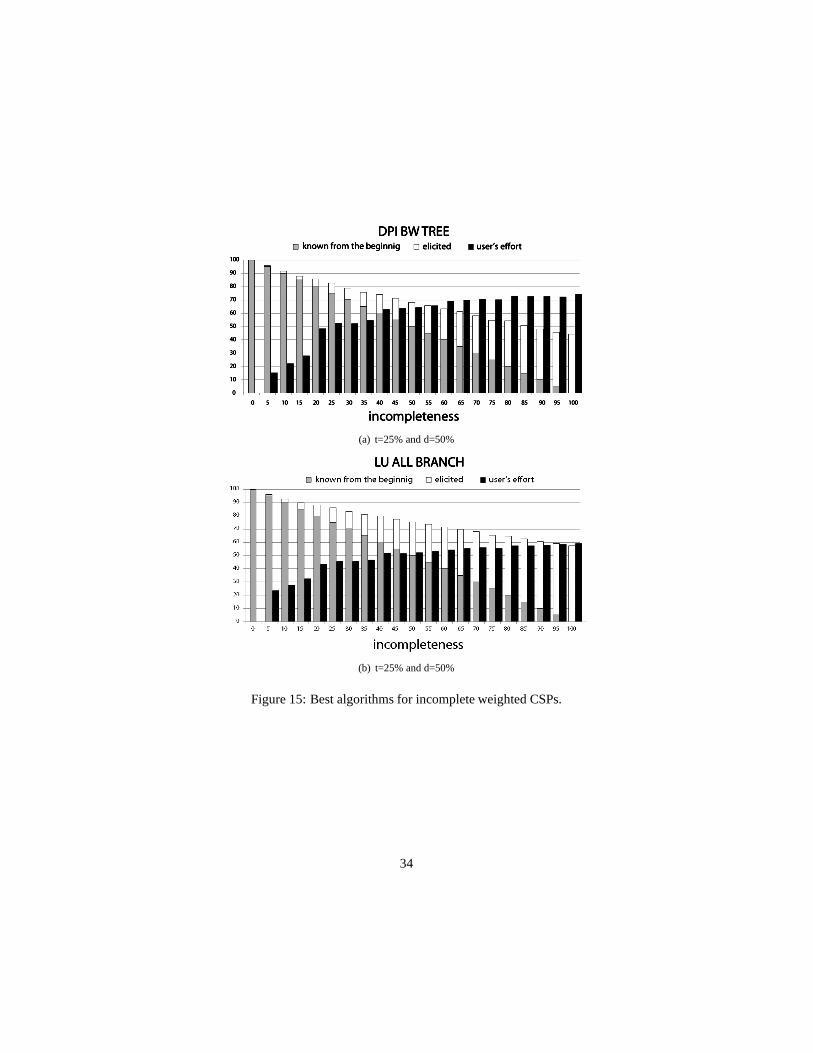
Among the algorithms where the user does not help the system in the value instan-tiation, the algorithm that elicits less values is DPI.BW.TREE (see Figure 15(a)).

DPI.BW.TREE elicits less that half of the unknown costs on 100% of incomplete-ness, requiring the user to look at 70% of incomplete tuples to answer the system’squery. All our experiments shown that, iteratively asking the user for the best and theworst preference of a given assignment is the best compromise when the value instan-tiation is totally done by the system. On the other hand, it forces the user to considermore than 70% of the incomplete tuples.

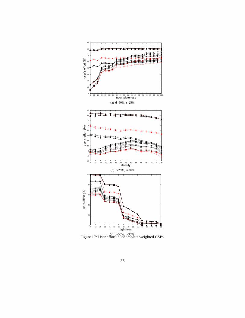
If we want to minimize the user effort, the best choice is the LU.ALL.BRANCHalgorithm (see Figure 15(b)). As shown in Figure 17(a), the user does less work withLU.ALL.BRANCH than with the other algorithms when the incompleteness is vary-ing. We obtain the same result when the density or the tightness is varying (see Fig-ures 17(b), 17(c)). If we want a balance between the percentage of elicited costs andthe user effort, the best compromise is LU.BB.BRANCH. Figure 16(a) shows that,on IWCSPs with no initial costs, it elicits 40% of incompletetuples with a user ef-fort of about 60%. Summarizing, SU.WW.BRANCH (Figure 16(b)) is the algorithm

32

10

20

30

40

50

60

70

5 10 15 20 25 30 35 40 45 50 55 60 65 70 75 80 85 90 95 100

elic

ited

pref

eren

ces

(%)

incompleteness

(a) d=50%, t=25%

10

20

30

40

50

60

70

80

10 15 20 25 30 35 40 45 50 55 60 65 70 75 80

elic

ited

pref

eren

ces

(%)

density

(b) t=25%, i=30%

0

10

20

30

40

50

60

70

80

90

100

5 10 15 20 25 30 35 40 45 50 55 60 65 70 75 80

elic

ited

pref

eren

ces

(%)

tightness

(c) d=50%, i=30%Figure 14: Percentage of elicited preferences in incomplete weighted CSPs.

33

(a) t=25% and d=50%

(b) t=25% and d=50%

Figure 15: Best algorithms for incomplete weighted CSPs.

34

(a) t=25% and d=50%

(b) t=25% and d=50%

Figure 16: Best algorithms for incomplete weighted CSPs.

35

10

20

30

40

50

60

70

80

90

5 10 15 20 25 30 35 40 45 50 55 60 65 70 75 80 85 90 95 100

user

’s e

ffort

(%

)

incompleteness

(a) d=50%, t=25%

35

40

45

50

55

60

65

70

75

80

85

10 15 20 25 30 35 40 45 50 55 60 65 70 75 80

user

’s e

ffort

(%

)

density

(b) t=25%, i=30%

0

20

40

60

80

100

5 10 15 20 25 30 35 40 45 50 55 60 65 70 75 80

user

’s e

ffort

(%

)

tightness

(c) d=50%, i=30%Figure 17: User effort in incomplete weighted CSPs.

36

which elicits less tuples but, if we want the user to just answer the elicitation queries,the best is DPI.BW.TREE. The algorithm that minimizes the user effort is insteadLU.ALL.BRANCH, whereas the best compromise between user effort and elicitationis LU.BB.BRANCH.

8 Related work

Recently, some lines of work have addressed issues similar to those considered in thispaper by allowing for open settings in CSPs: both open CSPs [7, 9] and interactiveCSPs [16] work with domains that can be partially specified, and in dynamic CSPs [6]variables, domains, and constraints may change over time. It has been shown that theseapproaches are closely related. In fact, interactive CSPs can be seen as a special caseof both dynamic and open CSPs [18].

While the main goal of the work on interactive CSPs is to minimize the run time ofthe solver, we emphasize the minimization of the number of queries to the user and/orof the user effort. The work closest to ours is the one on open CSPs. An open CSPis a possibly unbounded, partially ordered set{CSP (0), CSP (1), ...} of constraintsatisfaction problems, each of which contains at least one more domain values than itspredecessor. Thus, in [9] the approach is to solve larger andlarger problems until asolution is found, while minimizing the number of variable values asked to the user.To compare it to our setting, we assume all the variable values are known from thebeginning, while some of the preferences may be missing, andour algorithms work ondifferent completions of the given problem. Also, open CSPsexploit aMonotonicityAssumptionthat each agent provides variable values in strictly non-decreasing order ofpreference. Even when there are no preferences, each agent gives only variable valuesthat are feasible. Working under this assumption means thatthe agent that providesnew values/costs for a variable must know the bounds on the remaining possible costs,since they are provided best value first. If the bound computation is expensive or timeconsuming, then this is not desirable. This is not needed in our setting, where singlepreferences are elicited.

¿From the algorithmic point of view, in [7, 9, 8] the authors develop specific al-gorithms for open CSPs, and then generalize it to fuzzy and weighted open CSPs.Our approach instead went from the general to the specific level: we defined a gen-eral framework for incomplete soft constraint problems, and then we instantiated it tospecific classes, such as classical CSPs, fuzzy CSPs, and weighted CSPs. Thus, thegeneral framework is maintained in all these classes, and itcan be augmented by thedefinition of specific optimized elicitation strategies, which may exploit the propertiesof the c-semiring used.

Besides the theoretical differences between our approach and the one in [9], wealso made an experimental comparison on the same classes of problems considered in[9]. We randomly generated coloring problems with 5-14 variables and 3-11 valuesper variable, and inequality constraints between randomlychosen variable pairs so thatthe constraint graph is at least connected and at most complete. We used algorithmLU.WORST.BRANCH on a test set generated in the following way: we randomlygenerated 1000 coloring problems each with 5-14 variables with 11 values per vari-

37

Figure 18: Average number of values used in incomplete coloring problems with 11values per variable.

able. Then we set the cost of 0 to 8 values per variable to+∞ (in order to have 3-11feasible values). We also ensured that the constraint graphwas at least connected and atmost complete. To simulate the totally unknown domains in [9] at the beginning of thesearch process, we generated variables with no known costs.Finally, we grouped theseproblems in classes with the same average number of values per domain. In [9] the au-thors measure the average number of queries per variable. Tocompare their algorithmwith LU.WORST.BRANCH, we measured the average number of different values pervariable our algorithm needs to solve the problem (counting1 every time a value isinstantiated for the first time). In Figure 18 we can see that our algorithm needs about2 values per variable to solve problems with 4 to 9 values per domain. This is the sameresult as the best algorithm in [9], which is pleasing as our algorithm is general purposeand not specifically designed for this purpose.

An example of another approach to explicit elicitation in incomplete CSPs is theone presented in [4], where the user provides a classical CSPand a partially unknownutility function over its solutions. The system then performs elicitation queries to se-lect a specific utility function by a regret-based technique, where the elicitation is usedto ease the computation of the minimax regret function. In particular, the elicitationconcerns bounds on the parameters of the utility function. Moreover, quasi-optimaldecisions may be obtained, since often they require much less effort than finding op-timal ones. This approach is very interesting but rather farfrom ours. In particular,our approach does not work with bounds, since we ask for specific preference values.Moreover, our preference functions are based on the preferences in the constraints, andnot on the variable values. Also, we want to obtain an optimalsolution, although weexperimentally analyzed all our algorithms to see whether agood solution is obtainedearly (see Figure 7).

38

9 Conclusion and future work

We have considered incomplete soft constraint problems where some preferences aremissing. We have defined a formalism, that extends the soft constraint one, to modelsuch an incompleteness. Two new notions of optimal solutions have been considered:the possibly optimal solutions, that are optimal in at leastone way of revealing miss-ing preferences, and the necessarily optimal solutions, that are optimal in all ways ofrevealing missing preferences, and we have given characterizations of these two setsof optimal solutions. To find necessarily optimal solutionsof these problems, we havedefined a general solver schema, that interleaves branch andbound (B&B) search withelicitation steps. This solver schema can be instantiated in 16 ways, that depend onwhen to elicit (at the end of the B&B search, at a branch, or at anode of a B&Bsearch), what to elicit (all the missing preferences or onlythe worst one), and who elic-its (the algorithm or the user). We have tested and compared these 16 instances of thegeneral solver on randomly generated Fuzzy ISCSPs, by measuring the percentage ofthe elicited preferences and the user’s effort, that is, thenumber of missing preferencesthat the user has to consider in order to give his elicitationanswers. Experimental re-sults have shown that the best algorithms are those that elicit at the branch level and,among those, the ones that perform better are those that elicit only the worst preferenceif it is necessary. Such algorithms are also very helpful since they reach optimalityvery quickly. This fact allows one to stop elicitation anytime, being sure to have apossibly optimal solution with a higher level of preference. The percentage of elicitedpreferences for these best algorithms is below10% and the user’s effort does not ex-ceed30%. In addition, we have considered incomplete CSPs where the soft constraintshave been replaced by hard constraints. Experimental results have shown a trend whichis similar to the one registered for Fuzzy ISCSPs. We have also considered problemswith a precise structure. These are, the fuzzy simple temporal problems where the con-straints allow constraints time intervals for durations and distances of events, and fuzzypreferences associated with each element of an interval. Also in this context, to find anecessarily optimal solution with the best algorithm, thatelicits at the branch level onlythe worst preference if it is necessary, it is sufficient to ask about 10% of the missingpreferences.

In the problems considered in this paper, we have no information about the missingpreferences. We are currently considering settings in which each missing preference isassociated with a range of possible values, that may be smaller than the whole rangeof preference values. For such problems, we intend to define several notions of opti-mality, among which necessarily and possibly optimal solutions are just two examples,and to develop specific elicitation strategies for each of them. We are also studying softconstraint problems where no preference is missing, but some preferences are unstable,and are associated with a perturbation range of possible alternative values. Moreover,we will consider other approaches to preference elicitation and measures of the in-formation elicited from the user, such as those in [3, 4, 19].We also intend to buildsolvers based on local search or variable elimination methods. Finally, we want to addelicitation costs and to use them also to guide the search, asdone in [25] for hard CSPs.

39

Acknowledgments

This work has been partially supported by Italian MIUR PRIN project “Constraintsand Preferences” (n.2005015491). The last author is funded by the Department ofBroadband, Communications and the Digital Economy, and theAustralian ResearchCouncil.

References

[1] S. Bistarelli, U. Montanari, and F. Rossi. Semiring-based constraint solving andoptimization.JACM, 44(2):201–236, 1997.

[2] S. Bistarelli, U. Montanari, F. Rossi, T. Schiex, G. Verfaillie, and H. Fargier.Semiring-based CSPs and valued CSPs: Frameworks, properties, and compari-son.Constraints, 4(3):199–240, 1999.

[3] C. Boutilier. A POMDP Formulation of Preference Elicitation Problems. In Proc.AAAI 2002, pages 239–246, 2002.

[4] C. Boutilier, R. Patrascu, P. Prosser, P. Poupart, and D.Schuurmans. Constraint-based Optimization and Utility Elicitation using the Minimax Decision Criterion.In Artificial Intelligence, Volume 170, Number 8, pages 686–713. Elsevier, 2006.

[5] R. Dechter.Constraint processing. Morgan Kaufmann, 2003.

[6] R. Dechter and A. Dechter. Belief maintenance in dynamicconstraint networks.In Proc.AAAI 1998, pages 37–42, 1988.

[7] B. Faltings and S. Macho-Gonzalez. Open constraint satisfaction. In Proc.CP2002, volume 2470 ofLNCS, pages 356–370. Springer, 2002.

[8] B. Faltings and S. Macho-Gonzalez. Open constraint optimization. In Proc.CP2003, volume 2833 ofLNCS, pages 303–317. Springer, 2003.

[9] B. Faltings and S. Macho-Gonzalez. Open constraint programming.AI Journal,161(1-2):181–208, 2005.

[10] H. Fargier and J. Lang. Uncertainty in constraint satisfaction problems: a proba-bilistic approach. In Proc.ECSQARU 1993, volume 747 ofLNCS, pages 97–104.Springer, 1993.

[11] H. Fargier, T. Schiex, and G. Verfaille. Valued Constraint Satisfaction Problems:Hard and Easy Problems. In Proc.IJCAI 1995, pages 631–637. Morgan Kauf-mann, 1995.

[12] M. Gelain, M. S. Pini, F. Rossi, and K. B. Venable. Dealing with incompletepreferences in soft constraint problems. In Proc.CP 2007, volume 4741 ofLNCS,pages 286–300. Springer, 2007.

40

[13] M. Gelain, M. S. Pini, F. Rossi, K. B. Venable, and Toby Walsh. Elicitationstrategies for fuzzy constraint problems with missing preferences: properties, al-gorithms and experimental studies. In Proc.CP 2008, volume 5202 ofLNCS,pages 402–417. Springer, 2008.

[14] I.P. Gent, E. Macintyre, P. Prosser, B.M. Smith, and T. Walsh. Random ConstraintSatisfaction: Flaws and Structure. InConstraints, Volume 6, Number 4, pages345–372. Springer, 2001.

[15] L. Khatib, P. Morris, R. Morris, F. Rossi, A. Sperduti, and K. Brent Venable.Solving and learning a tractable class of soft temporal problems: theoretical andexperimental results.AI Communications, 20(3):181–209, 2007.

[16] E. Lamma, P. Mello, M. Milano, R. Cucchiara, M. Gavanelli, and M. Piccardi.Constraint propagation and value acquisition: Why we should do it interactively.In Proc.IJCAI 1999, pages 468–477, 1999.

[17] J. Lang, M. S. Pini, F. Rossi, K. B. Venable, and T. Walsh.Winner determinationin sequential majority voting. In Proc.IJCAI 2007, pages 1372–1377, 2007.

[18] S. Macho Gonzalez, C. Ansotegui, and P. Meseguer. On the relation among open,interactive and dynamic CSP. In Proc.Fifth Workshop on Modelling and SolvingProblems with Constraints (IJCAI), 2005.

[19] R. T. Maheswaran, J. P. Pearce, E. Bowring, P. Varakantham, M. Tambe. PrivacyLoss in Distributed Constraint Reasoning: A Quantitative Framework for Analy-sis and its Applications.Journal of Autonomous Agents and Multiagent Systems(JAAMAS), 2006.

[20] M. S. Pini, F. Rossi, K. B. Venable and T. Walsh. Incompleteness and Incompa-rability in Preference Aggregation. In Proc.IJCAI 2007, pages 1464-1469, 2007.

[21] M. S. Pini, F. Rossi, K. B. Venable and T. Walsh. Computing possible and neces-sary winners from incomplete partially-ordered preferences. In Proc.ECAI 2006,pages 767-768, 2006.

[22] Z. Ruttkay. Fuzzy constraint satisfaction. InProc. 1st IEEE Conference on Evo-lutionary Computing, pages 542–547, Orlando, 1994.

[23] Toby Walsh. Uncertainty in preference elicitation andaggregation. In Proc.AAAI2007, pages 3-8, 2007.

[24] T. Walsh. Complexity of Terminating Preference Elicitation. In Proc.AAMAS2008, 2008.

[25] N. Wilson, D. Grimes, and E. C. Freuder. A cost-based model and algorithms forinterleaving solving and elicitation of csps. In Proc.CP 2007, volume 4741 ofLNCS, pages 666–680. Springer, 2007.

41