Cyber Attack Detectionthanks to Machine Learning Algorithms

COMS7507: Advanced Security

Antoine Delplacea.delplace@uq.net.au

University of Queensland

Sheryl Hermosos.hermoso@uq.net.au

University of Queensland

Kristofer Ananditak.anandita@uq.net.au

University of Queensland

May 17, 2019

Abstract

Cybersecurity attacks are growing both in frequency and sophistication over the years. This increas-ing sophistication and complexity call for more advancement and continuous innovation in defensivestrategies. Traditional methods of intrusion detection and deep packet inspection, while still largely usedand recommended, are no longer sufficient to meet the demands of growing security threats.

As computing power increases and cost drops, Machine Learning is seen as an alternative method oran additional mechanism to defend against malwares, botnets, and other attacks. This paper exploresMachine Learning as a viable solution by examining its capabilities to classify malicious traffic in a net-work.

First, a strong data analysis is performed resulting in 22 extracted features from the initial Netflowdatasets. All these features are then compared with one another through a feature selection process.

Then, our approach analyzes five different machine learning algorithms against NetFlow dataset con-taining common botnets. The Random Forest Classifier succeeds in detecting more than 95% of thebotnets in 8 out of 13 scenarios and more than 55% in the most difficult datasets.

Finally, insight is given to improve and generalize the results, especially through a bootstrappingtechnique.

Useful keywords: Botnet, Malware Detection, Cyber Attack Detection, NetFlow, Machine Learning

GitHub repository: https://github.com/antoinedelplace/Cyberattack-Detection

Lecturer: Marius Portmann

1

arX

iv:2

001.

0630

9v1

[cs

.LG

] 1

7 Ja

n 20

20

Contents1 Introduction and Context 4

2 Review of background and related work 42.1 NetFlow . . . . . . . . . . . . . . . . . . . . . . . . . . . . . . . . . . . . . . . . . . . . . . . . 4

2.1.1 Traffic Flow data . . . . . . . . . . . . . . . . . . . . . . . . . . . . . . . . . . . . . . . 52.1.2 NetFlow for Anomaly Detection . . . . . . . . . . . . . . . . . . . . . . . . . . . . . . 6

2.2 Machine Learning . . . . . . . . . . . . . . . . . . . . . . . . . . . . . . . . . . . . . . . . . . . 62.2.1 Machine Learning for Botnet Detection . . . . . . . . . . . . . . . . . . . . . . . . . . 6

2.3 Machine Learning Methods . . . . . . . . . . . . . . . . . . . . . . . . . . . . . . . . . . . . . 62.3.1 Extreme Learning Machine . . . . . . . . . . . . . . . . . . . . . . . . . . . . . . . . . 72.3.2 Random Forest . . . . . . . . . . . . . . . . . . . . . . . . . . . . . . . . . . . . . . . . 72.3.3 Gradient Boosting . . . . . . . . . . . . . . . . . . . . . . . . . . . . . . . . . . . . . . 82.3.4 Support Vector Machine . . . . . . . . . . . . . . . . . . . . . . . . . . . . . . . . . . . 82.3.5 Logistic Regression . . . . . . . . . . . . . . . . . . . . . . . . . . . . . . . . . . . . . . 9

2.4 Anomaly Detection Methods . . . . . . . . . . . . . . . . . . . . . . . . . . . . . . . . . . . . 92.4.1 CAMNEP . . . . . . . . . . . . . . . . . . . . . . . . . . . . . . . . . . . . . . . . . . . 102.4.2 MINDS . . . . . . . . . . . . . . . . . . . . . . . . . . . . . . . . . . . . . . . . . . . . 102.4.3 Xu . . . . . . . . . . . . . . . . . . . . . . . . . . . . . . . . . . . . . . . . . . . . . . . 10

2.5 Clustering Methods based on Botnet behavior . . . . . . . . . . . . . . . . . . . . . . . . . . . 102.5.1 BClus . . . . . . . . . . . . . . . . . . . . . . . . . . . . . . . . . . . . . . . . . . . . . 102.5.2 K-Means Algorithm . . . . . . . . . . . . . . . . . . . . . . . . . . . . . . . . . . . . . 10

2.6 Malware Infection Process Stage Detection . . . . . . . . . . . . . . . . . . . . . . . . . . . . 102.6.1 BotHunter . . . . . . . . . . . . . . . . . . . . . . . . . . . . . . . . . . . . . . . . . . . 102.6.2 B-ELLA . . . . . . . . . . . . . . . . . . . . . . . . . . . . . . . . . . . . . . . . . . . . 11

3 Aim of the Project 113.1 Objectives . . . . . . . . . . . . . . . . . . . . . . . . . . . . . . . . . . . . . . . . . . . . . . . 113.2 Methodology . . . . . . . . . . . . . . . . . . . . . . . . . . . . . . . . . . . . . . . . . . . . . 113.3 Main issue with Network Security Data . . . . . . . . . . . . . . . . . . . . . . . . . . . . . . 12

4 Data analysis 134.1 CTU-13 Dataset . . . . . . . . . . . . . . . . . . . . . . . . . . . . . . . . . . . . . . . . . . . 134.2 Feature extraction . . . . . . . . . . . . . . . . . . . . . . . . . . . . . . . . . . . . . . . . . . 20

4.2.1 Motivation . . . . . . . . . . . . . . . . . . . . . . . . . . . . . . . . . . . . . . . . . . 204.2.2 Use of time windows . . . . . . . . . . . . . . . . . . . . . . . . . . . . . . . . . . . . . 204.2.3 Extracted features . . . . . . . . . . . . . . . . . . . . . . . . . . . . . . . . . . . . . . 20

4.3 Feature selection . . . . . . . . . . . . . . . . . . . . . . . . . . . . . . . . . . . . . . . . . . . 214.3.1 Filter and Wrapper methods . . . . . . . . . . . . . . . . . . . . . . . . . . . . . . . . 214.3.2 Embedded methods . . . . . . . . . . . . . . . . . . . . . . . . . . . . . . . . . . . . . 244.3.3 Dimensionality reduction . . . . . . . . . . . . . . . . . . . . . . . . . . . . . . . . . . 31

5 Results 325.1 Metrics . . . . . . . . . . . . . . . . . . . . . . . . . . . . . . . . . . . . . . . . . . . . . . . . 325.2 Algorithms . . . . . . . . . . . . . . . . . . . . . . . . . . . . . . . . . . . . . . . . . . . . . . 33

5.2.1 Logistic Regression . . . . . . . . . . . . . . . . . . . . . . . . . . . . . . . . . . . . . . 335.2.2 Support Vector Machine . . . . . . . . . . . . . . . . . . . . . . . . . . . . . . . . . . . 335.2.3 Random Forest . . . . . . . . . . . . . . . . . . . . . . . . . . . . . . . . . . . . . . . . 355.2.4 Gradient Boosting . . . . . . . . . . . . . . . . . . . . . . . . . . . . . . . . . . . . . . 355.2.5 Dense Neural Network . . . . . . . . . . . . . . . . . . . . . . . . . . . . . . . . . . . . 36

5.3 Comparison of algorithms . . . . . . . . . . . . . . . . . . . . . . . . . . . . . . . . . . . . . . 37

2

5.4 Detection of different Botnets . . . . . . . . . . . . . . . . . . . . . . . . . . . . . . . . . . . . 385.4.1 Main Results . . . . . . . . . . . . . . . . . . . . . . . . . . . . . . . . . . . . . . . . . 385.4.2 Statistic analysis . . . . . . . . . . . . . . . . . . . . . . . . . . . . . . . . . . . . . . . 385.4.3 Generalization . . . . . . . . . . . . . . . . . . . . . . . . . . . . . . . . . . . . . . . . 395.4.4 Data augmentation . . . . . . . . . . . . . . . . . . . . . . . . . . . . . . . . . . . . . . 405.4.5 Other algorithms . . . . . . . . . . . . . . . . . . . . . . . . . . . . . . . . . . . . . . . 41

6 Conclusion 43

References 44

3

1 Introduction and ContextCybersecurity is evolving and the rate of cybercrime is constantly increasing. Sophisticated attacks areconsidered as the new normal as they are becoming more frequent and widespread. This constant evolutionalso calls for innovation in the cybersecurity defense.

There are existing solutions and a combination of these methods are still widely used. Network IntrusionDetection and Prevention Systems (IDS/IPS) monitor for malicious activity or policy violations. Signature-based IDS relies on known signatures and is effective at detecting malwares that match these signatures.Behaviour-based IDS, on the other hand, learns what is normal for a system and reports on any triggerthat deviates from it. Both types, though effective, have some weaknesses. Signature-based systems rely onsignatures of known threats and thus ineffective for zero-day attacks or new malware samples. Traditionalbehaviour-based systems rely on a standard profile which is hard to define with the growing complexity ofnetworks and applications, and thus may be ineffective for anomaly detection. Full data packet analysis isanother option, however, it is both computationally expensive and risks exposure of sensitive user informa-tion.

Machine Learning (ML) has gained a wide interest on many applications and fields of study, particularlyin Cybersecurity. With hardware and computing power becoming more accessible, machine learning methodscan be used to analyze and classify bad actors from a huge set of available data. There are hundreds of Ma-chine Learning algorithms and approaches, broadly categorized into supervised and unsupervised learning.Supervised learning approaches are done in the context of Classification where input matches to an output,or Regression where input is mapped to a continuous output. Unsupervised learning is mostly accomplishedthrough Clustering and has been applied to exploratory analysis and dimension reduction. Both of theseapproaches can be applied in Cybersecurity for analysing malware in near real-time, thus eliminating theweaknesses of traditional detection methods.

Our approach uses NetFlow data for analysis. NetFlow records provide enough information to uniquelyidentify traffic using attributes such as 5-tuples and other fields, but do not expose private or personally-identifiable information (PII). NetFlow, along with its open standard version IPFIX, is already widely usedfor network monitoring and management. Availability of NetFlow data along with the privacy features makesit an efficient choice.

This paper is structured as follows: In Section 2, we review and present some Related Work where wediscuss relevant topics on NetFlow, Machine Learning, Detection and Clustering Methods. Section 3 clarifiesthe objective of the project and the methodology used. In Section 4, we present the detail of our DataAnalysis, explaining the chosen dataset and the steps involved in feature extraction and feature selection.We then present the Results in Section 5, including the metrics and algorithms used. And finally, we presentour Conclusions in Section 6.

2 Review of background and related work

2.1 NetFlowNetFlow is a feature developed by Cisco that characterizes network operations (Benoit Claise 2004). Networkdevices (routers and switches) can be used to collect IP traffic information on any of its interfaces whereNetFlow is enabled. This information, known as Traffic Flows, is then collected and analyzed by a centralcollector.

NetFlow has since become an industry standard (Claise 2013) for capturing session data. NetFlow dataprovides information that can be used to (1) identify network traffic usage and status of resources, and (2)

4

detect network anomalies and potential attacks. It can assist in identifying devices that are hogging band-width, finding bottlenecks, and improving network efficiency. Tools such as NfSen/NfDump1 can analyzeNetFlow data and track traffic patterns, which is useful for network monitoring and management. There isalso an increasing number of threat analytics and anomaly detection tools that use NetFlow traffic. Thispaper focuses on extracting NetFlow information for forensics purposes.

NetFlow v5, NetFlow v9, and the open standard IPFIX are widely used. NetFlow v5 records include theIP 5-tuple data, documenting the source and destination IP addresses, source and destination ports, andthe transport protocol involved in each IP flow. NetFlow v9 and IPFIX are extensible, which allow them toinclude other fields such as usernames, MAC addresses, and URLs.

2.1.1 Traffic Flow data

Flows are defined as unidirectional sequence of packets with some common properties passing through anetwork device (Benoit Claise et al. 2004). Flow records include information such as IP addresses, packetand byte counts, timestamp, Type of Service (ToS), application ports, input and output interfaces, amongothers. The 5-tuple consisting of client IP, client port number, server IP, server port number, and protocolincluded in the flow data is important for identifying connection. By investigating the correlation betweenflows, we can find meaningful traffic patterns and node behaviours.

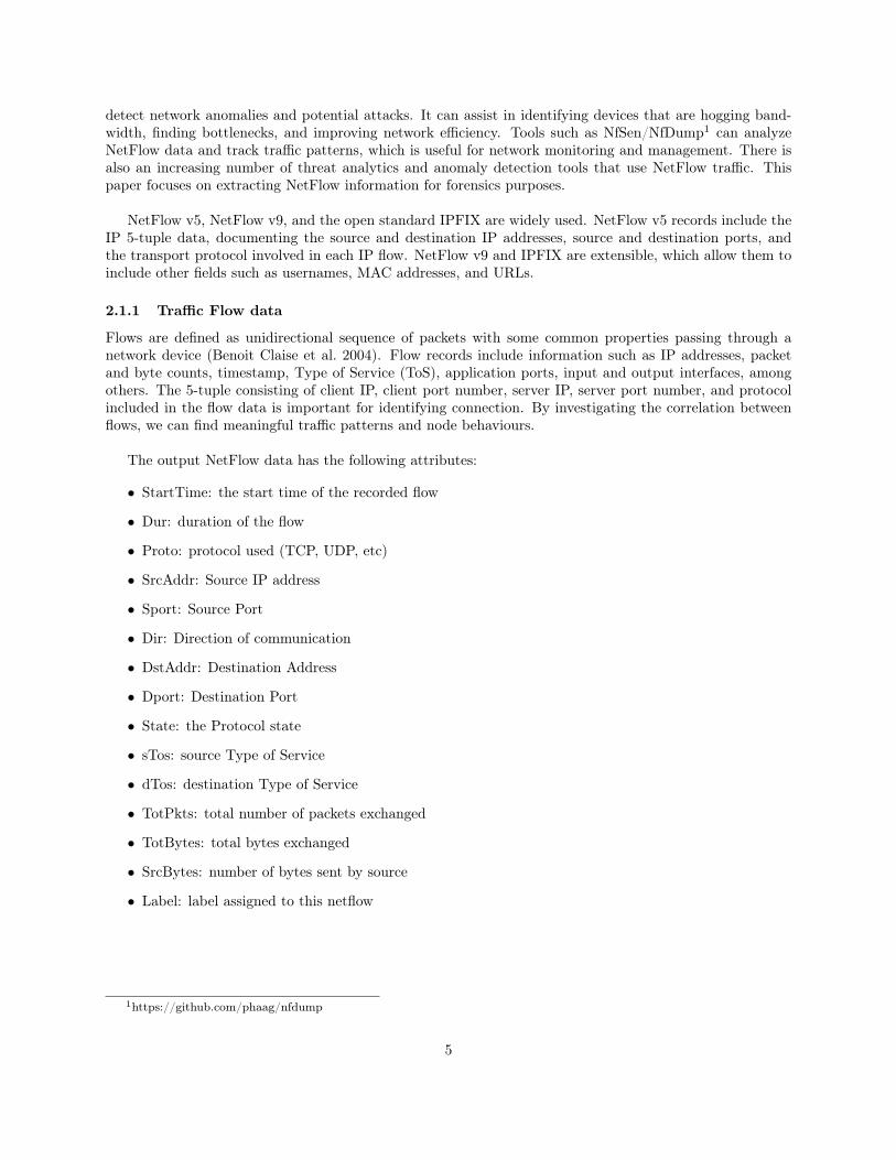
The output NetFlow data has the following attributes:

• StartTime: the start time of the recorded flow

• Dur: duration of the flow

• Proto: protocol used (TCP, UDP, etc)

• SrcAddr: Source IP address

• Sport: Source Port

• Dir: Direction of communication

• DstAddr: Destination Address

• Dport: Destination Port

• State: the Protocol state

• sTos: source Type of Service

• dTos: destination Type of Service

• TotPkts: total number of packets exchanged

• TotBytes: total bytes exchanged

• SrcBytes: number of bytes sent by source

• Label: label assigned to this netflow

1https://github.com/phaag/nfdump

5

2.1.2 NetFlow for Anomaly Detection

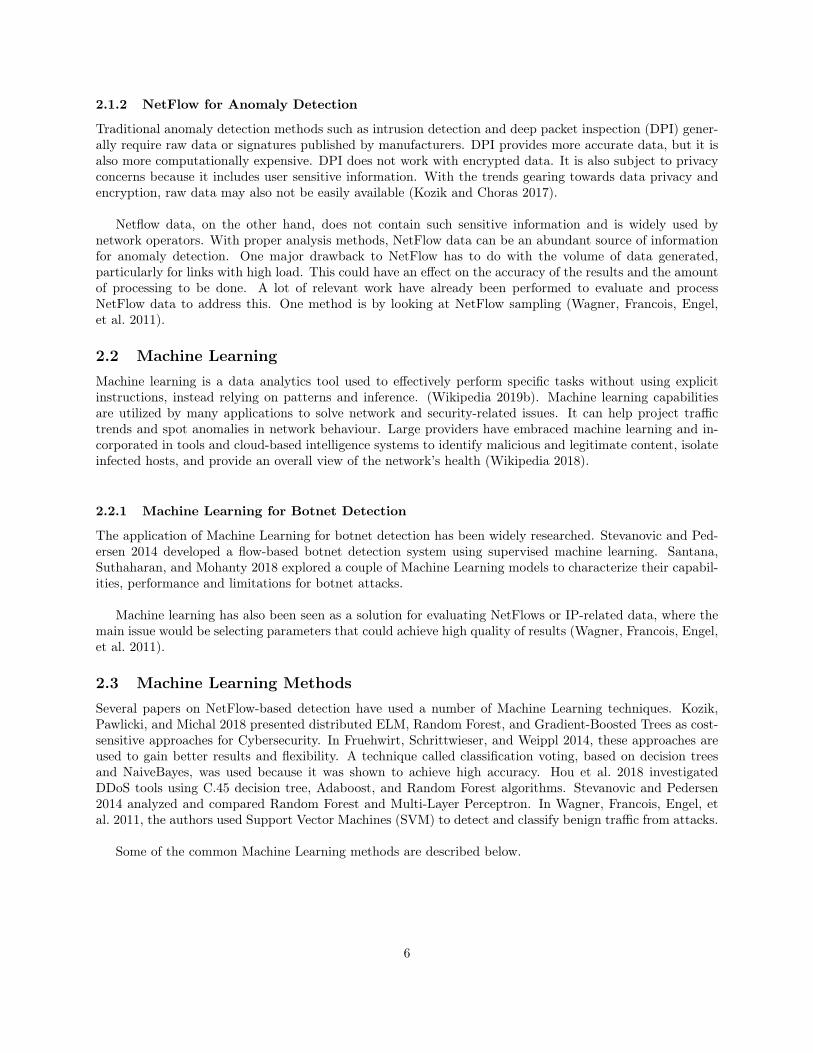
Traditional anomaly detection methods such as intrusion detection and deep packet inspection (DPI) gener-ally require raw data or signatures published by manufacturers. DPI provides more accurate data, but it isalso more computationally expensive. DPI does not work with encrypted data. It is also subject to privacyconcerns because it includes user sensitive information. With the trends gearing towards data privacy andencryption, raw data may also not be easily available (Kozik and Choras 2017).

Netflow data, on the other hand, does not contain such sensitive information and is widely used bynetwork operators. With proper analysis methods, NetFlow data can be an abundant source of informationfor anomaly detection. One major drawback to NetFlow has to do with the volume of data generated,particularly for links with high load. This could have an effect on the accuracy of the results and the amountof processing to be done. A lot of relevant work have already been performed to evaluate and processNetFlow data to address this. One method is by looking at NetFlow sampling (Wagner, Francois, Engel,et al. 2011).

2.2 Machine LearningMachine learning is a data analytics tool used to effectively perform specific tasks without using explicitinstructions, instead relying on patterns and inference. (Wikipedia 2019b). Machine learning capabilitiesare utilized by many applications to solve network and security-related issues. It can help project traffictrends and spot anomalies in network behaviour. Large providers have embraced machine learning and in-corporated in tools and cloud-based intelligence systems to identify malicious and legitimate content, isolateinfected hosts, and provide an overall view of the network’s health (Wikipedia 2018).

2.2.1 Machine Learning for Botnet Detection

The application of Machine Learning for botnet detection has been widely researched. Stevanovic and Ped-ersen 2014 developed a flow-based botnet detection system using supervised machine learning. Santana,Suthaharan, and Mohanty 2018 explored a couple of Machine Learning models to characterize their capabil-ities, performance and limitations for botnet attacks.

Machine learning has also been seen as a solution for evaluating NetFlows or IP-related data, where themain issue would be selecting parameters that could achieve high quality of results (Wagner, Francois, Engel,et al. 2011).

2.3 Machine Learning MethodsSeveral papers on NetFlow-based detection have used a number of Machine Learning techniques. Kozik,Pawlicki, and Michal 2018 presented distributed ELM, Random Forest, and Gradient-Boosted Trees as cost-sensitive approaches for Cybersecurity. In Fruehwirt, Schrittwieser, and Weippl 2014, these approaches areused to gain better results and flexibility. A technique called classification voting, based on decision treesand NaiveBayes, was used because it was shown to achieve high accuracy. Hou et al. 2018 investigatedDDoS tools using C.45 decision tree, Adaboost, and Random Forest algorithms. Stevanovic and Pedersen2014 analyzed and compared Random Forest and Multi-Layer Perceptron. In Wagner, Francois, Engel, etal. 2011, the authors used Support Vector Machines (SVM) to detect and classify benign traffic from attacks.

Some of the common Machine Learning methods are described below.

6

2.3.1 Extreme Learning Machine

Extreme Learning Machine (ELM) is a learning algorithm that utilizes feedforward neural networks witha single layer or multiple layers of hidden nodes. These hidden nodes are tuned at random and theircorresponding output weights are analytically determined by the algorithm. According to the creators, thislearning algorithm can produce good generalization performance and can learn a thousand times faster thanconventional learning algorithms for feedforward neural networks (Huang, Zhu, and Siew 2006).

Figure 1: Simplified illustration of ELM Algorithm(Huang 2015)

2.3.2 Random Forest

Random Forest (RF) is a supervised machine learning algorithm that involves the use of multiple decisiontrees in order to perform classification and regression tasks (Ho 1995). The Random Forest algorithm isconsidered to be an ensemble machine learning algorithm as it involves the concept of majority voting ofmultiple trees. The algorithm’s output, represented as a class prediction, is determined from the aggregateresult of all the classes predicted by the individual trees. Recent studies have explored the capabilities ofRandom Forest in security attacks, specifically in injection attacks, spam filtering, malware detection andmore (Kapoor, Gupta, and Kumar 2018 and Khorshidpour, Hashemi, and Hamzeh 2017).

Figure 2: Simplified illustration of the Random Forest Algorithm(Khorshidpour, Hashemi, and Hamzeh 2017)

7

2.3.3 Gradient Boosting

Gradient boosting is a machine learning technique for regression and classification problems, which producesa prediction model in the form of an ensemble of weak prediction models, typically decision trees (Wikipedia2019b). It combines the elements of a loss function, weak learner, and an additive model. The model addsweak learners to minimize the loss function. The basic assumption with gradient boosting is to repetitivelyleverage the patterns in residuals and strengthen a model with weak predictions and make it better (Grover2017). When it reaches a stage wherein the residuals do not have any pattern that could be modeled, thenmodeling of residuals will be stopped (otherwise it might lead to overfitting). Mathematically, this meansminimizing the loss function such that test loss reaches its minima.

Figure 3: Simplified illustration of the Gradient Boosting Algorithm(Grover 2017)

2.3.4 Support Vector Machine

Support Vector Machine (SVM) is a supervised learning model used for regression and classification analysis(Wikipedia 2019d). It is highly preferred for its high accuracy with less computation power and complexity.SVM is also used in computer security, where they are used for intrusion detection. For example, One classSVM was used for analyzing records based on a new kernel function (Wagner, Francois, Engel, et al. 2011)and accurate Internet traffic classification (Yuan et al. 2010).

8

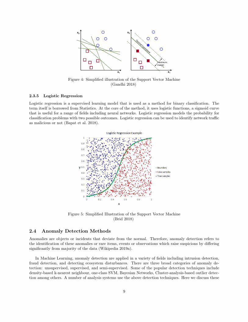
Figure 4: Simplified illustration of the Support Vector Machine(Gandhi 2018)

2.3.5 Logistic Regression

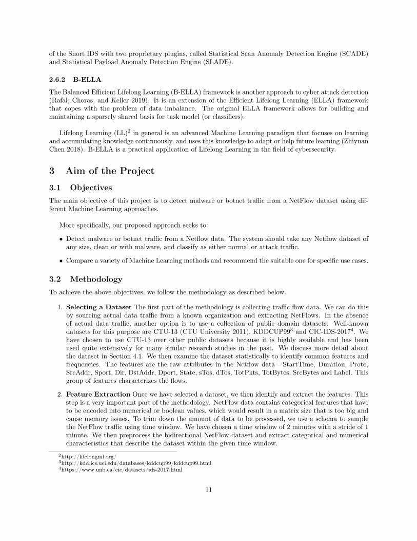
Logistic regression is a supervised learning model that is used as a method for binary classification. Theterm itself is borrowed from Statistics. At the core of the method, it uses logistic functions, a sigmoid curvethat is useful for a range of fields including neural networks. Logistic regression models the probability forclassification problems with two possible outcomes. Logistic regression can be used to identify network trafficas malicious or not (Bapat et al. 2018).

Figure 5: Simplified Illustration of the Support Vector Machine(Brid 2018)

2.4 Anomaly Detection MethodsAnomalies are objects or incidents that deviate from the normal. Therefore, anomaly detection refers tothe identification of these anomalies or rare items, events or observations which raise suspicions by differingsignificantly from majority of the data (Wikipedia 2019a).

In Machine Learning, anomaly detection are applied in a variety of fields including intrusion detection,fraud detection, and detecting ecosystem disturbances. There are three broad categories of anomaly de-tection: unsupervised, supervised, and semi-supervised. Some of the popular detection techniques includedensity-based k-nearest neighbour, one-class SVM, Bayesian Networks, Cluster-analysis-based outlier detec-tion among others. A number of analysis systems use the above detection techniques. Here we discuss these

9

three systems - CAMNEP, MINDS and Xu - which was compared in detail in Garcia et al. 2014.

2.4.1 CAMNEP

The Cooperative Adaptive Mechanism for Network Protection (CAMNEP) is a network intrusion detection(Rehak et al. 2008) system. The CAMNEP system uses a set of anomaly detection model that maintain amodel of expected traffic on the network and compare it with real traffic to identify the discrepancies thatare identified as possible attacks. It has three principal layers that evaluate the traffic: anomaly detectors,trust models, and anomaly aggregators. The anomaly detector layer analyzes the NetFlows using variousanomaly detection algorithms, each of which uses a different set of features. The output are aggregated intoevents and sent into the trust models. The trust model maps the NetFlows into traffic clusters. NetFlowswith similar behavioural patterns are clustered together. The aggregator layer creates the composite outputthat integrates the individual opinion of several anomaly detectors.

2.4.2 MINDS

The Minnesota Intrusion Detection System (MINDS) uses a suite of data mining techniques to automaticallydetect attacks (Ertoz et al. 2004). It builds a context information for each evaluated NetFlow using thefollowing features: the number of NetFlows from the same source IP address as the evaluated NetFlow, thenumber of NetFlows toward the same destination host, the number of NetFlows towards the same destinationhost from the same source port, and the number of NetFlows from the same source host towards the samedestination port. The anomaly value for a NetFlow is based on its distance to the normal sample (Rehaket al. 2008).

2.4.3 Xu

This algorithm was proposed by Xu et al. The context of each NetFlow to be evaluated is created with allthe NetFlows coming from the same source IP address. The anomalies are detected by some classificationrules that divide the traffic into normal and anomalous flows.

2.5 Clustering Methods based on Botnet behavior2.5.1 BClus

The BClus Method is a an approach that uses behavioural-based botnet detection. BClus creates a model ofknown botnet behaviours and uses them to detect similar traffic on the network. The purpose of the methodis to cluster the traffic sent by each IP address and to recognize which clusters have a behaviour similar tothe botnet traffic. (Rehak et al. 2008).

2.5.2 K-Means Algorithm

K-means algorithm is an unsupervised machine learning algorithm popular for clustering and data mining.It works by storing k centroids that is used to define a cluster. In D. S. Terzi, R. Terzi, and Sagiroglu 2017,the aggregated NetFlows are clustered based on the K-means algorithm, and clusters are expected to occurbased on traffic behaviour.

2.6 Malware Infection Process Stage Detection2.6.1 BotHunter

The BotHunter method is useful for detection of infections and for coordination dialog of botnets. It isdone by matching state-based infection sequence models. It consists of a correlation engine that aims atdetecting specific stages of the malware infection process (Rehak et al. 2008). It uses an adaptive version

10

of the Snort IDS with two proprietary plugins, called Statistical Scan Anomaly Detection Engine (SCADE)and Statistical Payload Anomaly Detection Engine (SLADE).

2.6.2 B-ELLA

The Balanced Efficient Lifelong Learning (B-ELLA) framework is another approach to cyber attack detection(Rafal, Choras, and Keller 2019). It is an extension of the Efficient Lifelong Learning (ELLA) frameworkthat copes with the problem of data imbalance. The original ELLA framework allows for building andmaintaining a sparsely shared basis for task model (or classifiers).

Lifelong Learning (LL)2 in general is an advanced Machine Learning paradigm that focuses on learningand accumulating knowledge continuously, and uses this knowledge to adapt or help future learning (ZhiyuanChen 2018). B-ELLA is a practical application of Lifelong Learning in the field of cybersecurity.

3 Aim of the Project

3.1 ObjectivesThe main objective of this project is to detect malware or botnet traffic from a NetFlow dataset using dif-ferent Machine Learning approaches.

More specifically, our proposed approach seeks to:

• Detect malware or botnet traffic from a Netflow data. The system should take any Netflow dataset ofany size, clean or with malware, and classify as either normal or attack traffic.

• Compare a variety of Machine Learning methods and recommend the suitable one for specific use cases.

3.2 MethodologyTo achieve the above objectives, we follow the methodology as described below.

1. Selecting a Dataset The first part of the methodology is collecting traffic flow data. We can do thisby sourcing actual data traffic from a known organization and extracting NetFlows. In the absenceof actual data traffic, another option is to use a collection of public domain datasets. Well-knowndatasets for this purpose are CTU-13 (CTU University 2011), KDDCUP993 and CIC-IDS-20174. Wehave chosen to use CTU-13 over other public datasets because it is highly available and has beenused quite extensively for many similar research studies in the past. We discuss more detail aboutthe dataset in Section 4.1. We then examine the dataset statistically to identify common features andfrequencies. The features are the raw attributes in the Netflow data - StartTime, Duration, Proto,SrcAddr, Sport, Dir, DstAddr, Dport, State, sTos, dTos, TotPkts, TotBytes, SrcBytes and Label. Thisgroup of features characterizes the flows.

2. Feature Extraction Once we have selected a dataset, we then identify and extract the features. Thisstep is a very important part of the methodology. NetFlow data contains categorical features that haveto be encoded into numerical or boolean values, which would result in a matrix size that is too big andcause memory issues. To trim down the amount of data to be processed, we use a schema to samplethe NetFlow traffic using time window. We have chosen a time window of 2 minutes with a stride of 1minute. We then preprocess the bidirectional NetFlow dataset and extract categorical and numericalcharacteristics that describe the dataset within the given time window.

2http://lifelongml.org/3http://kdd.ics.uci.edu/databases/kddcup99/kddcup99.html4https://www.unb.ca/cic/datasets/ids-2017.html

11

3. Feature Selection This step is required to select features from the extracted ones. It involves the useof feature selection techniques to reduce the dimension of the input training matrix. Filtering featuresthrough Pearson Correlation, wrapper methods using Backward Feature Elimination, embedded meth-ods within the Random Forest Classifier, Principal Component Analysis (PCA), and the t-distributedStochastic Neighbour Embedding (t-SNE) are the different techniques used for this purpose.

4. Comparison of Algorithms We wanted to compare five chosen algorithms. The various MachineLearning Models to be trained in this step are: Logistic Regression, Support Vector Machine (SVM),Random Forest Classifier, Gradient Boosting, and Dense Neural Network.

5. Botnet Detection The last step in our methodology involves testing our model to see if it cansuccessfully detect botnet traffic from the CTU-13 dataset. The overall performance of botnet detectionis determined from the f1 score of the aforementioned models.

3.3 Main issue with Network Security DataWorking with Network Security Data brings lots of challenges. First, the data are very imbalance becausemost of the traffic is harmless and only a tiny part of it is malicious. That causes the model to difficultly learnwhat is harmful. Moreover, the risk of overfitting during the training process is high because the structureof the network influences the way the model learns while a network-independent algorithm is wanted.

Furthermore, traffic analysis deals with a network which is a dynamic structure: communications aretime dependent and links between servers may appear and disappear with new requests and new users inthe network. That is why detecting new unknown botnets is a real challenge in network security.

To cope with all these challenges, an accurate data analysis is needed and mechanisms to prevent over-fitting like cross-validation are necessary.

12

4 Data analysis

4.1 CTU-13 DatasetThe CTU-13 Dataset is a labeled dataset used in the literature to train botnet detection algorithms (see forexample Garcia et al. 2014 and Rafal, Choras, and Keller 2019). It was created by the CTU University 2011and captures real botnet traffic mixed with normal traffic and background traffic. In this section, we willdescribe the dataset in order to find relevant features to extract, and train our models.

The CTU-13 Dataset is made of 13 captures of different botnet samples summarized in 13 bidirectionalNetFlow5 files (see Figure 6).

Figure 6: Scenarios of the CTU-13 Dataset (CTU University 2011)

We focus here our presentation on the first scenario, which uses a malware called Neris. The capturelasted 6.15 hours during which the botnet used HTTP based C&C channels6 to send SPAM and performClick-Fraud. The NetFlow file weights 368 Mo and is made of 2 824 636 bidirectional communicationsdescribed by 15 features:

1. StartTime: Date of the flow start (from 2011/08/10 09:46:53 to 2011/08/10 15:54:07)

5“NetFlow is a feature that was introduced on Cisco routers around 1996 that provides the ability to collect IP networktraffic as it enters or exits an interface.” Wikipedia 2019c

6“A Command-and-Control [C&C] server is a computer controlled by an attacker or cybercriminal which is used to sendcommands to systems compromised by malware and receive stolen data from a target network.” Trend Micro 2019

13

10:00 11:00 12:00 13:00 14:00 15:00 16:00Date

0

20000

40000

60000

80000

100000

Freq

uenc

y

Figure 7: Frequency of NetFlows wrt Time

As shown in Figure 7, the start times of NetFlows seem uniformly distributed during the experimentwith an exception at around 10:20 with a pic of starting NetFlows.

2. Dur: Duration of the communication in seconds(min: 0 s.; max: 3 600 s.; mean: 432 s.; std: 996 s.; median: 0.001 s.; 3rd quantile: 9 s.)

0 500 1000 1500 2000 2500 3000 3500Duration (in seconds)

104

105

106

Freq

uenc

y

Figure 8: Duration of the communications

Figure 8 shows that the majority of the communications last for a very short time (less than 1 ms. for

14

half of them). One can also notice frequency peaks each time a minute is reached.

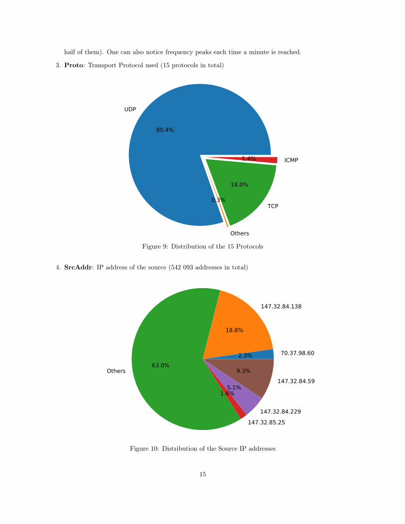
3. Proto: Transport Protocol used (15 protocols in total)

UDP

80.4%

Others

0.3%TCP

18.0%

ICMP1.4%

Figure 9: Distribution of the 15 Protocols

4. SrcAddr: IP address of the source (542 093 addresses in total)

70.37.98.602.3%

147.32.84.138

18.8%

Others63.0%

147.32.85.25

1.6%

147.32.84.229

5.1%147.32.84.59

9.3%

Figure 10: Distribution of the Source IP addresses

15

The huge number of different IP addresses prevents the categorization of the data from SrcAddr becauseof memory concerns. Another way needs to be found to represent the huge amount of data.

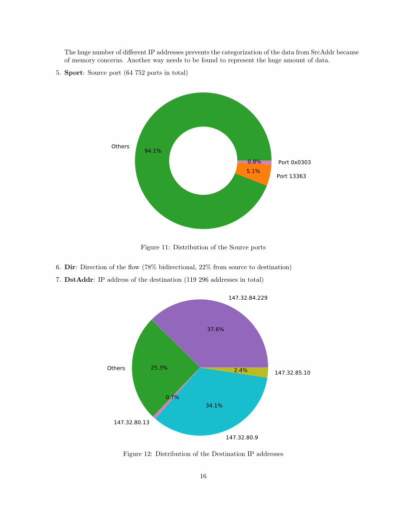
5. Sport: Source port (64 752 ports in total)

Others 94.1%

Port 133635.1%

Port 0x03030.8%

Figure 11: Distribution of the Source ports

6. Dir: Direction of the flow (78% bidirectional, 22% from source to destination)

7. DstAddr: IP address of the destination (119 296 addresses in total)

147.32.84.229

37.6%

Others 25.3%

147.32.80.13

0.7%

147.32.80.9

34.1%

147.32.85.1002.4%

Figure 12: Distribution of the Destination IP addresses

16

8. Dport: Destination port7 (73 786 ports in total)

Port 4432.5%

Port 13363

36.1%

Others16.2%

Port 68810.8%

Port 80

9.1%

Port 53

35.2%

Figure 13: Distribution of the Destination ports

9. State: Transaction state8 (230 states in total)

FSA_FSA0.9%SRPA_FSPA1.3%S_RA2.2%

S_2.4%CON

77.6%

Others

4.1%URP

0.8%INT

3.0%

FSPA_FSPA7.7%

Figure 14: Distribution of Transaction states

7Port 53: Domain Name System (DNS); Port 80: Hypertext Transfer Protocol (HTTP); Port 443: Hypertext TransferProtocol over TLS/SSL (HTTPS); Port 6881: BitTorrent (Unofficial)

8The state is protocol dependent and _ is a separator for one end of the connection. Examples of states: CON = Connected(UDP); INT = Initial (UDP); URP = Urgent Pointer (UDP); F = FIN (TCP); S = SYN = Synchronization (TCP); P = Push(TCP); A = ACK = Acknowledgement (TCP); R = Reset (TCP); FSPA = All flags - FIN, SYN, PUSH, ACK (TCP)

17

10. sTos: Source TOS9 byte value (0 for 99.9% of the communications)

11. dTos: Destination TOS byte value (0 for 99.99% of the communications)

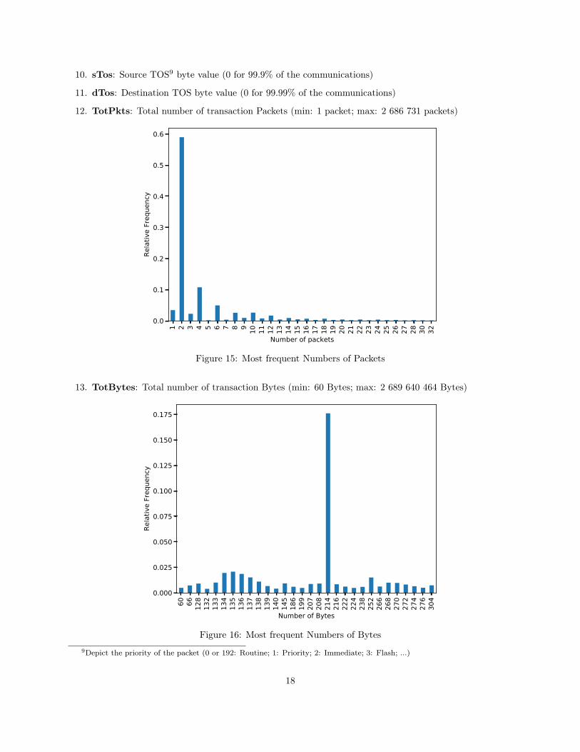
12. TotPkts: Total number of transaction Packets (min: 1 packet; max: 2 686 731 packets)

1 2 3 4 5 6 7 8 9 10 11 12 13 14 15 16 17 18 19 20 21 22 23 24 25 26 27 28 30 32

Number of packets

0.0

0.1

0.2

0.3

0.4

0.5

0.6Re

lativ

e Fr

eque

ncy

Figure 15: Most frequent Numbers of Packets

13. TotBytes: Total number of transaction Bytes (min: 60 Bytes; max: 2 689 640 464 Bytes)

60 66 128

132

133

134

135

136

137

138

139

140

145

186

199

207

208

214

216

222

224

238

252

266

268

270

272

274

276

304

Number of Bytes

0.000

0.025

0.050

0.075

0.100

0.125

0.150

0.175

Rela

tive

Freq

uenc

y

Figure 16: Most frequent Numbers of Bytes9Depict the priority of the packet (0 or 192: Routine; 1: Priority; 2: Immediate; 3: Flash; ...)

18

14. SrcBytes: Total number of transaction Bytes from the Source (min: 0 Byte; max: 2 635 366 235 Bytes)

60 66 70 71 72 73 74 75 76 77 78 79 80 81 82 83 84 85 86 87 132

145

146

148

150

152

154

156

186

222

Number of Bytes from Source

0.000

0.025

0.050

0.075

0.100

0.125

0.150

0.175

Rela

tive

Freq

uenc

y

Figure 17: Most frequent Numbers of Bytes

15. Label: Label made of “flow=” followed by a short description (Source/Destination-Malware/Application)

Back

grou

nd

To-B

ackg

roun

d

From

-Bot

net

From

-Nor

mal

From

-Bac

kgro

und

To-N

orm

al

Norm

al

0.0

0.1

0.2

0.3

0.4

0.5

0.6

Rela

tive

Freq

uenc

y

63.29%

34.17%

1.45% 1.07% 0.02% 0.00% 0.00%

Figure 18: Distribution of the 113 Labels

19

4.2 Feature extraction4.2.1 Motivation

The main issue with NetFlow data is that most of the information is in the form of categorical features.Trying to transform the categories into boolean columns results in a boom of the matrix size causing memoryerrors (even after using compressed sparse matrix representation).

This major problem encouraged us to extract new features, based on the reviewed literature of networktraffic analysis.

4.2.2 Use of time windows

A popular idea is to summarize data inside a time window. This is justified by the fact that botnets “tendto have a temporal locality behavior” (Garcia et al. 2014). Moreover, it enables us to reduce the amount ofdata and to deliver a botnet detector which gives live results after each time window (in exchange for inputdata details).

The main issue is to determine the width and the stride of the time window. The reviewed literaturesuggests different options (2 minutes in the BClus detection method in Garcia et al. 2014, 3 seconds in theMINDS algorithm in Ertoz et al. 2004, 5 minutes in the Xu algorithm in Xu, Zhang, and Bhattacharyya2015) but these suggestions are often empirical. In our case, we have chosen a time window width of 2minutes and a stride of 1 minute.

Another problem we encountered is that the time window gathers NetFlow communications according tothe start time of the connection. Using the communication status (active or finished) resulted in a boom inthe data size so we used the duration of the communication as extra features.

4.2.3 Extracted features

The extracted features try to represent the NetFlow communications inside a time window. To do so, thetime window data are gathered by source addresses.

There are 2 features extracted from each categorical NetFlow characteristics (in our case: the sourceports, the destination addresses and the destination ports):

• the number of unique occurrences in the subgroup

• the normalized subgroup entropy defined as

E = −∑xi∈X

p(xi) log p(xi) with p(xi) =#xi#X

and X, the subgroup of the source address (1)

As for the numerical NetFlow characteristics (in our case: the duration of the communication, the totalnumber of exchanged bytes, the number of bytes sent by the source), 5 features are extracted:

• the sum

• the mean

• the standard deviation

• the maximum

• the median

All these extracted features will enable us to train different models. However, they may be redundant orirrelevant to detect botnets so a feature selection is needed.

20

4.3 Feature selection4.3.1 Filter and Wrapper methods

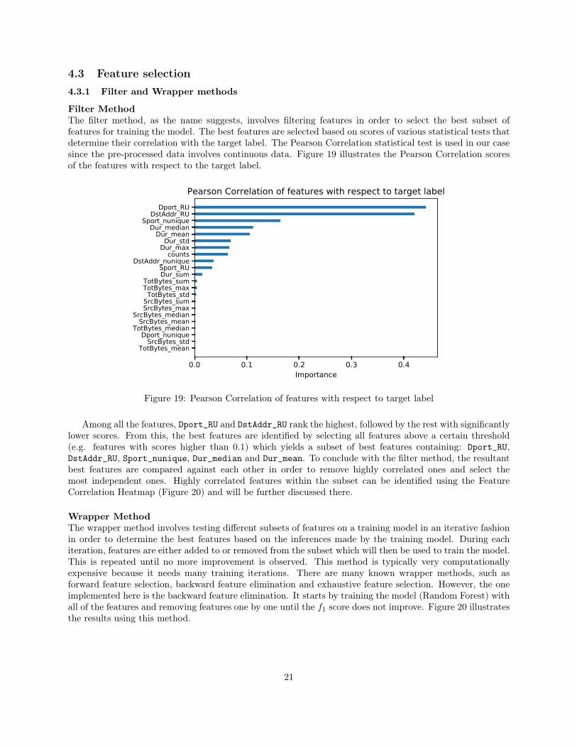
Filter MethodThe filter method, as the name suggests, involves filtering features in order to select the best subset offeatures for training the model. The best features are selected based on scores of various statistical tests thatdetermine their correlation with the target label. The Pearson Correlation statistical test is used in our casesince the pre-processed data involves continuous data. Figure 19 illustrates the Pearson Correlation scoresof the features with respect to the target label.

0.0 0.1 0.2 0.3 0.4Importance

TotBytes_meanSrcBytes_std

Dport_nuniqueTotBytes_median

SrcBytes_meanSrcBytes_median

SrcBytes_maxSrcBytes_sumTotBytes_std

TotBytes_maxTotBytes_sum

Dur_sumSport_RU

DstAddr_nuniquecounts

Dur_maxDur_std

Dur_meanDur_median

Sport_nuniqueDstAddr_RU

Dport_RU

Pearson Correlation of features with respect to target label

Figure 19: Pearson Correlation of features with respect to target label

Among all the features, Dport_RU and DstAddr_RU rank the highest, followed by the rest with significantlylower scores. From this, the best features are identified by selecting all features above a certain threshold(e.g. features with scores higher than 0.1) which yields a subset of best features containing: Dport_RU,DstAddr_RU, Sport_nunique, Dur_median and Dur_mean. To conclude with the filter method, the resultantbest features are compared against each other in order to remove highly correlated ones and select themost independent ones. Highly correlated features within the subset can be identified using the FeatureCorrelation Heatmap (Figure 20) and will be further discussed there.

Wrapper MethodThe wrapper method involves testing different subsets of features on a training model in an iterative fashionin order to determine the best features based on the inferences made by the training model. During eachiteration, features are either added to or removed from the subset which will then be used to train the model.This is repeated until no more improvement is observed. This method is typically very computationallyexpensive because it needs many training iterations. There are many known wrapper methods, such asforward feature selection, backward feature elimination and exhaustive feature selection. However, the oneimplemented here is the backward feature elimination. It starts by training the model (Random Forest) withall of the features and removing features one by one until the f1 score does not improve. Figure 20 illustratesthe results using this method.

21

subs

et1

subs

et2

subs

et3

subs

et4

subs

et5

subs

et6

subs

et7

subs

et8

subs

et9

subs

et10

subs

et11

subs

et12

subs

et13

subs

et14

subs

et15

subs

et16

subs

et17

subs

et18

subs

et19

subs

et20

subs

et21

subs

et22

subs

et23

0.96

0.97

0.98

0.99

1.00

recallprecisionf1-score

Figure 20: Backward Feature Elimination Results

Features removed in each subset:

• subset 1: No features removed

• subset 2: counts removed

• subset 3: Sport_nunique removed

• subset 4: DstAddr_nunique removed

• subset 5: Dport_nunique removed

• subset 6: Dur_sum removed

• subset 7: Dur_mean removed

• subset 8: Dur_std removed

• subset 9: Dur_max removed

• subset 10: Dur_median removed

• subset 11: TotBytes_sum removed

• subset 12: TotBytes_mean removed

• subset 13: TotBytes_std removed

• subset 14: TotBytes_max removed

• subset 15: TotBytes_median removed

• subset 16: SrcBytes_sum removed

• subset 17: SrcBytes_mean removed

• subset 18: SrcBytes_std removed

• subset 19: SrcBytes_max removed

• subset 20: SrcBytes_median removed

• subset 21: Sport_RU removed

• subset 22: DstAddr_RU removed

• subset 23: Dport_RU removed

We begin by training the Random Forest model with subset 1 containing all 22 features to establishan initial control output. From there, we re-train the model for each feature removed in order to find thebest subset. This is repeated until there is no improvement in the f1 score or until the features are allexhausted. From Figure 20, we can see that there are 7 subsets that have achieved the highest possible f1score (f1 score = 1.0). Because of this, we stop at 21 features instead of removing more as we cannot achieve

22

a higher f1 score. Therefore, the best subsets are: subset 5, subset 7, subset 11, subset 12, subset 13, subset17 and subset 22.

CorrelationFeature Correlation is useful to identify how each feature relates to one another. Correlation can either bepositive or negative. A positive correlation indicates that an increase in one value of a feature increases thevalue of the other feature, while the latter indicates the opposite. Both positive and negative correlationcan indicate highly correlated features. The closer the score is to the value 1 indicates a high positivecorrelation, and the closer the score is to the value -1 indicates a high negative correlation. Below is aheatmap to illustrate the correlation among all our features.

coun

ts

Spor

t_nu

niqu

e

DstA

ddr_

nuni

que

Dpor

t_nu

niqu

e

Dur_

sum

Dur_

mea

n

Dur_

std

Dur_

max

Dur_

med

ian

TotB

ytes

_sum

TotB

ytes

_mea

n

TotB

ytes

_std

TotB

ytes

_max

TotB

ytes

_med

ian

SrcB

ytes

_sum

SrcB

ytes

_mea

n

SrcB

ytes

_std

SrcB

ytes

_max

SrcB

ytes

_med

ian

Spor

t_RU

DstA

ddr_

RU

Dpor

t_RU

Labe

l_<la

mbd

a>

counts

Sport_nunique

DstAddr_nunique

Dport_nunique

Dur_sum

Dur_mean

Dur_std

Dur_max

Dur_median

TotBytes_sum

TotBytes_mean

TotBytes_std

TotBytes_max

TotBytes_median

SrcBytes_sum

SrcBytes_mean

SrcBytes_std

SrcBytes_max

SrcBytes_median

Sport_RU

DstAddr_RU

Dport_RU

Label_<lambda>

1 0.87 0.11 0.95 0.083 -0.014 0.01 -0.0024 -0.014 0.022 -0.000150.00079 0.0069 -0.00022 0.0061 -0.000120.00019 0.0018 -0.00016 -0.014 -0.063 -0.063 0.064

0.87 1 0.1 0.71 0.093 -0.032 0.0077 -0.012 -0.032 0.043 -0.00029 0.0018 0.014 -0.00046 0.0096 -0.000250.00044 0.0035 -0.00035 0.0063 -0.15 -0.16 0.16

0.11 0.1 1 0.041 0.57 -0.011 0.11 0.045 -0.021 0.049 -0.0002 0.0031 0.026 -0.00042 0.016 -0.000120.00099 0.0083 -0.00027 -0.16 -0.015 -0.062 0.036

0.95 0.71 0.041 1 0.046 -0.0016 0.0069 0.002 -0.0024 0.0048 -2.2e-050.00017 0.0014 -4e-05 0.0029 -5.4e-06 9e-05 0.00053-2.6e-05 -0.01 -0.0077 0.000180.00024

0.083 0.093 0.57 0.046 1 0.25 0.23 0.32 0.23 0.083 0.0031 0.0055 0.027 0.0027 0.023 0.0025 0.002 0.011 0.0024 -0.16 0.023 -0.0095 -0.015

-0.014 -0.032 -0.011 -0.0016 0.25 1 0.078 0.97 1 0.0036 0.011 0.0017 0.0059 0.011 0.0039 0.0092 0.00063 0.0041 0.011 0.019 0.17 0.14 -0.11

0.01 0.0077 0.11 0.0069 0.23 0.078 1 0.29 0.046 0.022 0.0095 0.028 0.022 0.0054 0.016 0.01 0.017 0.016 0.0069 -0.29 -0.13 -0.19 0.069

-0.0024 -0.012 0.045 0.002 0.32 0.97 0.29 1 0.95 0.014 0.012 0.0081 0.014 0.011 0.0092 0.011 0.0043 0.0087 0.011 -0.049 0.12 0.077 -0.067

-0.014 -0.032 -0.021 -0.0024 0.23 1 0.046 0.95 1 0.0023 0.01 0.00048 0.0047 0.011 0.003 0.0088 -0.0001 0.0032 0.011 0.027 0.17 0.14 -0.11

0.022 0.043 0.049 0.0048 0.083 0.0036 0.022 0.014 0.0023 1 0.67 0.65 0.92 0.54 0.67 0.49 0.53 0.63 0.3 0.00031 -0.019 -0.02 0.0046

-0.00015-0.00029-0.0002 -2.2e-05 0.0031 0.011 0.0095 0.012 0.01 0.67 1 0.37 0.79 0.96 0.43 0.56 0.31 0.44 0.5 0.0019 -0.0049 -0.0042 -0.0001

0.00079 0.0018 0.0031 0.00017 0.0055 0.0017 0.028 0.0081 0.00048 0.65 0.37 1 0.75 0.15 0.75 0.5 0.85 0.76 0.16 0.0013 -0.019 -0.017 0.003

0.0069 0.014 0.026 0.0014 0.027 0.0059 0.022 0.014 0.0047 0.92 0.79 0.75 1 0.64 0.73 0.58 0.62 0.72 0.35 0.0012 -0.016 -0.015 0.0045

-0.00022-0.00046-0.00042 -4e-05 0.0027 0.011 0.0054 0.011 0.011 0.54 0.96 0.15 0.64 1 0.24 0.45 0.088 0.24 0.52 0.0018 -0.0016 -0.0015-0.00099

0.0061 0.0096 0.016 0.0029 0.023 0.0039 0.016 0.0092 0.003 0.67 0.43 0.75 0.73 0.24 1 0.79 0.88 0.99 0.46 0.00028 -0.0072 -0.0054 0.0016

-0.00012-0.00025-0.00012-5.4e-06 0.0025 0.0092 0.01 0.011 0.0088 0.49 0.56 0.5 0.58 0.45 0.79 1 0.59 0.8 0.87 0.0012 -0.002 -0.0012 -0.0011

0.000190.000440.00099 9e-05 0.002 0.00063 0.017 0.0043 -0.0001 0.53 0.31 0.85 0.62 0.088 0.88 0.59 1 0.89 0.18 0.00046 -0.0065 -0.0047 0.00014

0.0018 0.0035 0.0083 0.00053 0.011 0.0041 0.016 0.0087 0.0032 0.63 0.44 0.76 0.72 0.24 0.99 0.8 0.89 1 0.47 0.00064 -0.0066 -0.0045 0.0013

-0.00016-0.00035-0.00027-2.6e-05 0.0024 0.011 0.0069 0.011 0.011 0.3 0.5 0.16 0.35 0.52 0.46 0.87 0.18 0.47 1 0.0012 0.000450.00046 -0.0013

-0.014 0.0063 -0.16 -0.01 -0.16 0.019 -0.29 -0.049 0.027 0.00031 0.0019 0.0013 0.0012 0.0018 0.00028 0.0012 0.000460.00064 0.0012 1 0.15 0.22 -0.034

-0.063 -0.15 -0.015 -0.0077 0.023 0.17 -0.13 0.12 0.17 -0.019 -0.0049 -0.019 -0.016 -0.0016 -0.0072 -0.002 -0.0065 -0.0066 0.00045 0.15 1 0.86 -0.42

-0.063 -0.16 -0.062 0.00018 -0.0095 0.14 -0.19 0.077 0.14 -0.02 -0.0042 -0.017 -0.015 -0.0015 -0.0054 -0.0012 -0.0047 -0.0045 0.00046 0.22 0.86 1 -0.44

0.064 0.16 0.036 0.00024 -0.015 -0.11 0.069 -0.067 -0.11 0.0046 -0.0001 0.003 0.0045 -0.00099 0.0016 -0.0011 0.00014 0.0013 -0.0013 -0.034 -0.42 -0.44 1

0.25

0.00

0.25

0.50

0.75

1.00

Figure 21: Feature Correlation Heatmap

From Figure 21, we can deduce which of the features have the highest correlation among each other.

23

The green colored tiles indicate the highest positive correlations, whereas the red ones indicate the highestnegative correlations. High correlation is observed in all of the Duration, TotBytes, SrcBytes and entropyfeatures, but this is not surprising as they are derived from statistical measures of the same column in theraw dataset.

Relating back to the filter method, we can now use the heatmap to identify highly correlated featureswithin the subset containing the best features and select the best ones that represent it. From the heatmap,it is seen that features Dport_RU and DstAddr_RU, as well as features Dur_mean and Dur_median, are highlycorrelated. As a result, we select the features with the higher correlation score with respect to the targetlabel. The end result of the filter method then yields the final subset of best features which contains:Dport_RU, Sport_nunique and Dur_median.

4.3.2 Embedded methods

Embedded methods can also be used to select features according to the score of the classifier (ie using labels).

Lasso and Ridge logistic regressionIn order to use Logistic Regression, we need to find a way to cope with the data imbalance. Thus, crossvalidation is used to find the best weight to balance the dataset.

0.0 0.1 0.2 0.3 0.4 0.5Botnet class weight

0.0

0.2

0.4

0.6

0.8

1.0 test_precisiontest_recalltest_f1

Figure 22: Scores wrt Botnet class weight

24

0.00 0.02 0.04 0.06 0.08 0.10Botnet class weight

0.0

0.2

0.4

0.6

0.8

1.0 test_precisiontest_recalltest_f1

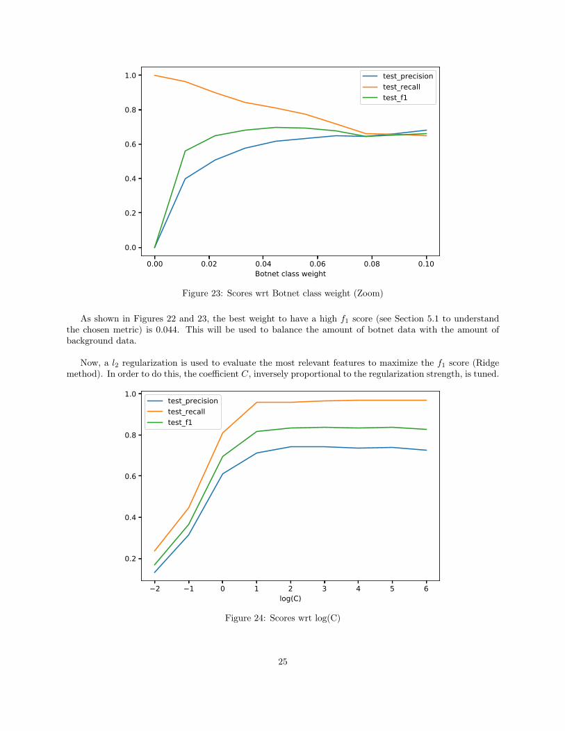
Figure 23: Scores wrt Botnet class weight (Zoom)

As shown in Figures 22 and 23, the best weight to have a high f1 score (see Section 5.1 to understandthe chosen metric) is 0.044. This will be used to balance the amount of botnet data with the amount ofbackground data.

Now, a l2 regularization is used to evaluate the most relevant features to maximize the f1 score (Ridgemethod). In order to do this, the coefficient C, inversely proportional to the regularization strength, is tuned.

2 1 0 1 2 3 4 5 6log(C)

0.2

0.4

0.6

0.8

1.0test_precisiontest_recalltest_f1

Figure 24: Scores wrt log(C)

25

200 400 600 800 1000C

0.75

0.80

0.85

0.90

0.95test_precisiontest_recalltest_f1

Figure 25: Scores wrt C (Zoom)

Figures 24 and 25 show the evolution of the different scores with respect to the regularization parameterC. The best f1 score is obtained for C = 550 so the feature coefficients must be analyzed with this parameter.

As we are interested in the feature coefficients, here is the detailed list of the features:

0. The number of communications in the subgroup

1. The number of unique source ports

2. The number of unique destination addresses

3. The number of unique destination ports

4. The sum of the communication durations

5. The mean of the communication durations

6. The standard deviation of the communication dura-tions

7. The maximum of the communication durations

8. The median of the communication durations

9. The sum of the total number of exchanged bytes

10. The mean of the total number of exchanged bytes

11. The standard deviation of the total number of ex-changed bytes

12. The maximum of the total number of exchangedbytes

13. The median of the total number of exchanged bytes

14. The sum of the number of bytes sent by the source

15. The mean of the number of bytes sent by the source

16. The standard deviation of the number of bytes sentby the source

17. The maximum of the number of bytes sent by thesource

18. The median of the number of bytes sent by thesource

19. The normalized entropy of the source ports

20. The normalized entropy of the destination addresses

21. The normalized entropy of the destination ports

26

2 1 0 1 2 3 4 5 6log(C)

40

20

0

20

40

60

0123456789101112131415161718192021

Figure 26: Feature coefficients wrt log(C)

200 400 600 800 1000C

20

10

0

10

0123456789101112131415161718192021

Figure 27: Feature coefficients wrt C (Zoom)

Figures 26 and 27 represent the importance of each feature with respect to C. We can see that thefeatures 3 and 9 have the most impact on the results. Then, the features 4, 5 and 11 seem to contribute to

27

the score as well as the features 12 and 16 for C = 550. On the other hand, the features 1, 6, 10, 19, 20, 21do not have a strong impact on the results and can easily be forgotten.

Now, the same thing is done with a l1 regularization (Lasso method). This technique is more computa-tional expensive because there is no analytic solution, so the score tolerance has to be reduced. Nevertheless,using the solver SAGA (Stochastic Average Gradient Augmented), the algorithm did not succeed to converge,giving thus very poor results. Consequently, despite being slower, the solver Liblinear (A Library for LargeLinear Classification) is used. However, this technique has not succeeded to give relevant results since itcannot perform cross-validation over the parameter C (very slow to converge).

Support Vector Machine (SVM) method with Recursive Feature Elimination (RFE)Another technique to select features is to recursively remove the less relevant feature and train the model toanalyze the scores. For this, we used the Support Vector Machine Classification algorithm with the Stochas-tic Gradient Descent (SGD) learning method.

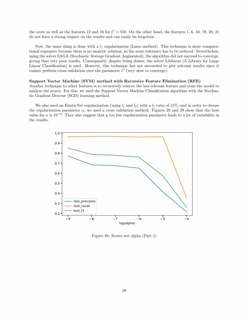
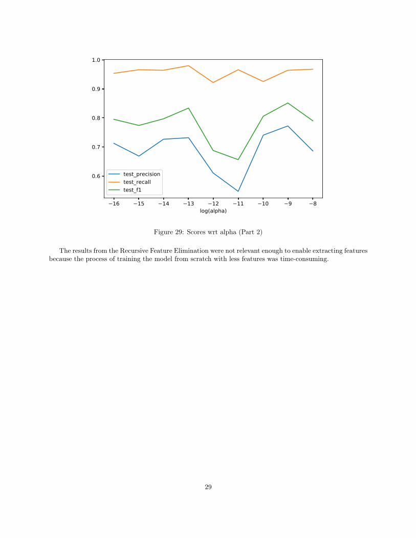
We also used an ElasticNet regularization (using l1 and l2) with a l1 ratio of 15%, and in order to choosethe regularization parameter α, we used a cross validation method. Figures 28 and 29 show that the bestvalue for α is 10−9. They also suggest that a too low regularization parameter leads to a lot of variability inthe results.

9 8 7 6 5 4log(alpha)

0.2

0.3

0.4

0.5

0.6

0.7

0.8

0.9

1.0

test_precisiontest_recalltest_f1

Figure 28: Scores wrt alpha (Part 1)

28

16 15 14 13 12 11 10 9 8log(alpha)

0.6

0.7

0.8

0.9

1.0

test_precisiontest_recalltest_f1

Figure 29: Scores wrt alpha (Part 2)

The results from the Recursive Feature Elimination were not relevant enough to enable extracting featuresbecause the process of training the model from scratch with less features was time-consuming.

29

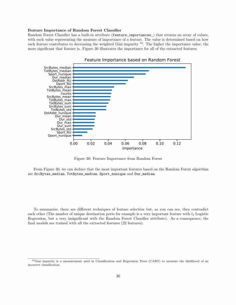
Feature Importance of Random Forest ClassifierRandom Forest Classifier has a built-in attribute (feature_importances_) that returns an array of values,with each value representing the measure of importance of a feature. The value is determined based on howeach feature contributes to decreasing the weighted Gini impurity 10. The higher the importance value, themore significant that feature is. Figure 30 illustrates the importance for all of the extracted features.

0.00 0.02 0.04 0.06 0.08 0.10 0.12Importance

Dport_nuniqueSport_RU

SrcBytes_stdDur_sumDur_maxDur_std

Dur_meanDstAddr_nunique

TotBytes_stdSrcBytes_sumTotBytes_sumTotBytes_max

SrcBytes_meancounts

TotBytes_meanSrcBytes_max

Dport_RUDstAddr_RUDur_median

Sport_nuniqueTotBytes_medianSrcBytes_median

Feature Importance based on Random Forest

Figure 30: Feature Importance from Random Forest

From Figure 30, we can deduce that the most important features based on the Random Forest algorithmare SrcBytes_median, TotBytes_median, Sport_nunique and Dur_median.

To summarize, there are different techniques of feature selection but, as you can see, they contradicteach other (The number of unique destination ports for example is a very important feature with l2 LogisticRegression, but a very insignificant with the Random Forest Classifier attribute). As a consequence, thefinal models are trained with all the extracted features (22 features).

10Gini impurity is a measurement used in Classification and Regression Trees (CART) to measure the likelihood of anincorrect classification.

30

4.3.3 Dimensionality reduction

Another idea to reduce the number of features is to use dimensionality reduction techniques. It is also veryuseful to visualize the dataset.

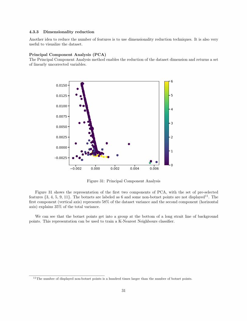
Principal Component Analysis (PCA)The Principal Component Analysis method enables the reduction of the dataset dimension and returns a setof linearly uncorrected variables.

0.002 0.000 0.002 0.004 0.006

0.0025

0.0000

0.0025

0.0050

0.0075

0.0100

0.0125

0.0150

0

1

2

3

4

5

6

Figure 31: Principal Component Analysis

Figure 31 shows the representation of the first two components of PCA, with the set of pre-selectedfeatures {3, 4, 5, 9, 11}. The botnets are labeled as 6 and some non-botnet points are not displayed11. Thefirst component (vertical axis) represents 58% of the dataset variance and the second component (horizontalaxis) explains 35% of the total variance.

We can see that the botnet points get into a group at the bottom of a long strait line of backgroundpoints. This representation can be used to train a K-Nearest Neighbours classifier.

11The number of displayed non-botnet points is a hundred times larger than the number of botnet points.

31

t-SNE (t-distributed Stochastic Neighbour Embedding)T-SNE is another method to reduce the dimension of the dataset to 2 or 3 features.

80 60 40 20 0 20 40 60 80

80

60

40

20

0

20

40

60

80

0

1

2

3

4

5

6

Figure 32: t-SNE

Figure 32 shows the result of the dimensionality reduction (the botnets are labeled as 6). We can seethat the botnet points are not gathered in one place that could differentiate them from the regular traffic.Moreover, the algorithm is very time and memory consuming. Consequently, the use of the K-nearestneighbours method is no longer taken into consideration to detect botnet activities in this paper.

5 Results

5.1 MetricsIn order to compare the results of different algorithms, some metrics need to be chosen to evaluate theperformance of the methods. The usual way is to look at the number of false positives (ie the number ofbackground communications labeled as botnets) and false negatives (ie the number of botnets labeled asbackground communications).

To do this, three scores can be used12:

• the Recall: R =tp

tp+ fn

• the Precision: P =tp

tp+ fp

12tp: true positives; fp: false positives; fn: false negatives

32

• the f1 Score: f1 =

(R−1 + P−1

2

)−1= 2× R× P

R+ P

One needs to remember that, for our project of detecting malicious software, having a low recall is worstthan having a low precision because it means that most detected communications are botnets (precision)but most botnet communications remain undetected (recall).

Of course, having a good recall is easy because all you have to do is label every communication as botnet.So the chosen compromise is to maximize the f1 score while checking that the recall is not too low.

Remark: The accuracy score, defined as the normalized number of well predicted labels, is not relevantto our case because of the imbalance of the dataset. Only a weighted accuracy can be relevant (using theweight found in Section 4.3.2 with the f1 score).

5.2 Algorithms5.2.1 Logistic Regression

The Logistic Regression method is an algorithm that uses a linear combination of the features to classify theflows. As presented in Section 4.3.2, cross-validation is necessary to tune the parameters of the model. Thefinal chosen parameters are C = 550 and Weightnon-botnet = 0.044.

5.2.2 Support Vector Machine

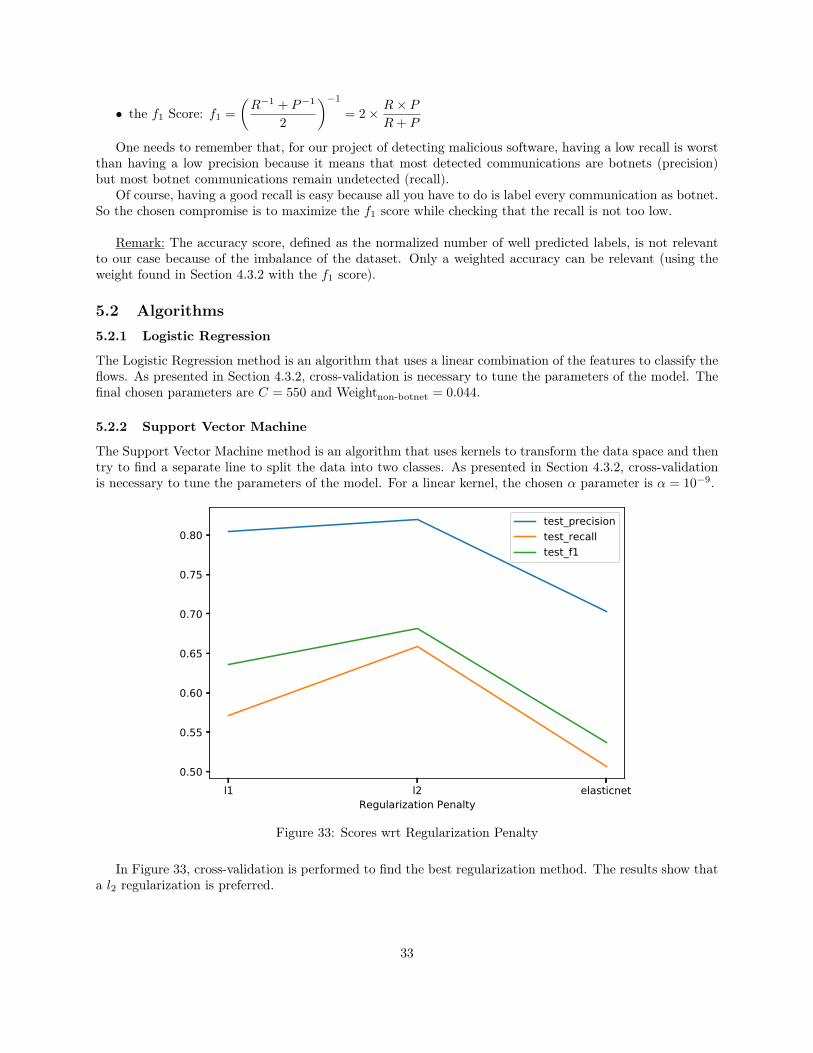
The Support Vector Machine method is an algorithm that uses kernels to transform the data space and thentry to find a separate line to split the data into two classes. As presented in Section 4.3.2, cross-validationis necessary to tune the parameters of the model. For a linear kernel, the chosen α parameter is α = 10−9.

l1 l2 elasticnetRegularization Penalty

0.50

0.55

0.60

0.65

0.70

0.75

0.80test_precisiontest_recalltest_f1

Figure 33: Scores wrt Regularization Penalty

In Figure 33, cross-validation is performed to find the best regularization method. The results show thata l2 regularization is preferred.

33

0.00 0.01 0.02 0.03 0.04Gamma

0.5

0.6

0.7

0.8

0.9

test_precisiontest_recalltest_f1

Figure 34: Scores wrt Gamma

For a Radial Basis Function (RBF) kernel, Figure 34 shows that the best γ parameter is γ = 0.03567.

2.00 2.25 2.50 2.75 3.00 3.25 3.50 3.75 4.00Degree

0.65

0.70

0.75

0.80

0.85 test_precisiontest_recalltest_f1

Figure 35: Scores wrt Polynomial Degree

Finally, for a polynomial kernel, Figure 35 shows that the best degree for the polynomial function is 2.

To conclude, the best SVM parameters for the botnet detection in the first scenario of CTU-13 are apolynomial kernel with a degree of 2.

34

5.2.3 Random Forest

Random Forest is an algorithm that uses several decision tree classifiers to predict the class of each inputflows. The chosen number of trees in the forest is 100.

5.2.4 Gradient Boosting

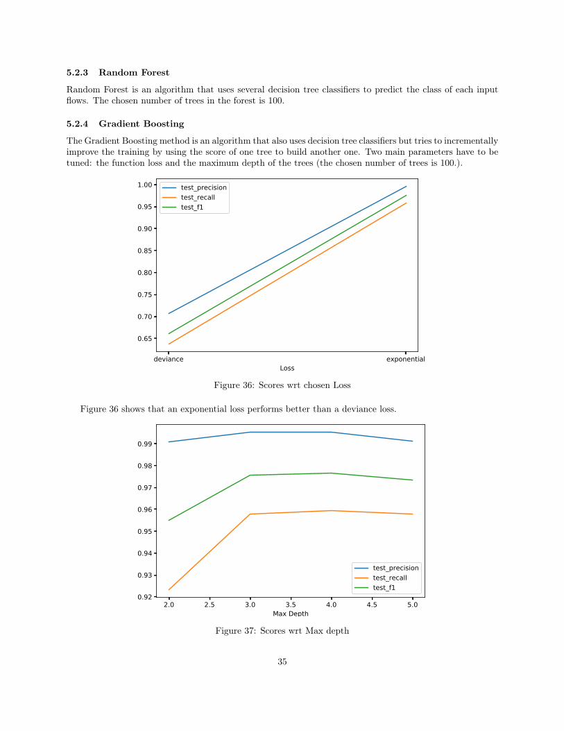
The Gradient Boosting method is an algorithm that also uses decision tree classifiers but tries to incrementallyimprove the training by using the score of one tree to build another one. Two main parameters have to betuned: the function loss and the maximum depth of the trees (the chosen number of trees is 100.).

deviance exponentialLoss

0.65

0.70

0.75

0.80

0.85

0.90

0.95

1.00 test_precisiontest_recalltest_f1

Figure 36: Scores wrt chosen Loss

Figure 36 shows that an exponential loss performs better than a deviance loss.

2.0 2.5 3.0 3.5 4.0 4.5 5.0Max Depth

0.92

0.93

0.94

0.95

0.96

0.97

0.98

0.99

test_precisiontest_recalltest_f1

Figure 37: Scores wrt Max depth

35

Figure 37 shows that the most relevant maximum depth for the classifier is 4.

5.2.5 Dense Neural Network

Recently, neural networks have gained popularity since they perform very well when a lot of data is available.We test here a simple dense (or fully connected) neural network with 2 hidden layers: the first one has 256neurons and the second one has 128.

The parameters of the neural network are composed of a batch-normalization, no dropout, a ReLU ac-tivation function (except for the output layer where a sigmoid function is used). The model has 39 681trainable parameters and 768 non-trainable parameters.

Figure 38 shows the binary cross-entropy loss for the training set and the validation set (15% of the wholeset) along the 10 epochs (a batch of 32 is used).

0 2 4 6 8Epochs

0.0002

0.0004

0.0006

0.0008

0.0010

Loss

Learning curvelossval_lossbest model

Figure 38: Learning curve of the Neural Network

36

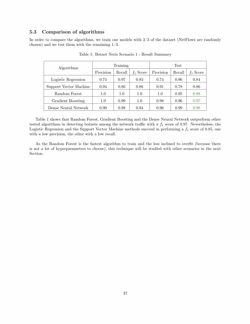
5.3 Comparison of algorithmsIn order to compare the algorithms, we train our models with 2/3 of the dataset (NetFlows are randomlychosen) and we test them with the remaining 1/3.

Table 1: Botnet Neris Scenario 1 - Result Summary

Algorithms Training Test

Precision Recall f1 Score Precision Recall f1 Score

Logistic Regression 0.74 0.97 0.83 0.74 0.96 0.84

Support Vector Machine 0.94 0.80 0.86 0.91 0.78 0.86

Random Forest 1.0 1.0 1.0 1.0 0.95 0.98

Gradient Boosting 1.0 0.99 1.0 0.98 0.96 0.97

Dense Neural Network 0.90 0.98 0.94 0.96 0.99 0.98

Table 1 shows that Random Forest, Gradient Boosting and the Dense Neural Network outperform othertested algorithms in detecting botnets among the network traffic with a f1 score of 0.97. Nevertheless, theLogistic Regression and the Support Vector Machine methods succeed in performing a f1 score of 0.85, onewith a low precision, the other with a low recall.

As the Random Forest is the fastest algorithm to train and the less inclined to overfit (because thereis not a lot of hyperparameters to choose), this technique will be studied with other scenarios in the nextSection.

37

5.4 Detection of different Botnets5.4.1 Main Results

In order to see if the results of the Random Forest Classifier on the Scenario 1 of the CTU-13 dataset canbe generalized, we test it on all the other scenarios.

Table 2: Result Summary using Random Forest Classifier

Botnet Dataset Training Test

Size Botnets Precision Recall f1 Score Precision Recall f1 Score

Neris - Scenario 1 2 226 720 1.28 %�� 1.0 1.0 1.0 1.0 0.95 0.975

Neris - Scenario 2 1 431 539 1.45 %�� 1.0 1.0 1.0 1.0 0.98 0.99

Rbot - Scenario 3 2 024 053 4.99 %�� 1.0 0.99 0.99 1.0 0.96 0.98

Rbot - Scenario 4 470 663 2.36 %�� 1.0 0.90 0.95 1.0 0.69 0.82

Virut - Scenario 5 63 643 3.46 %�� 1.0 1.0 1.0 1.0 0.25 0.4

DonBot - Scenario 6 220 863 5.57 %�� 1.0 1.0 1.0 1.0 0.9 0.95

Sogou - Scenario 7 50 629 1.38 %�� 1.0 1.0 1.0 1.0 0.25 0.4

Murlo - Scenario 8 1 643 574 6.80 %�� 1.0 1.0 1.0 1.0 0.94 0.97

Neris - Scenario 9 1 168 424 12.51 %�� 1.0 0.99 1.0 1.0 0.94 0.97

Rbot - Scenario 10 559 194 9.67 %�� 1.0 0.98 0.99 1.0 0.90 0.95

Rbot - Scenario 11 61 551 2.76 %�� 1.0 1.0 1.0 0.5 0.33 0.4

NSIS.ay - Scenario 12 156 790 10.20 %�� 1.0 0.82 0.90 0.92 0.41 0.56

Virut - Scenario 13 1 294 025 7.57 %�� 1.0 1.0 1.0 1.0 0.96 0.98

Table 2 shows that the Random Forest Classifier succeeds in detecting most of the botnets for 8 scenariosout of 13. The poor scores of the 5 other scenarios seem to be related to the size of the dataset.

5.4.2 Statistic analysis

The main problem with the results of Table 2 is that they are only based on one test dataset. Thus, if thesize of the dataset is too small, statistical error may be significant. Therefore, a statistic analysis is made onthe scenarios which have small datasets.

38

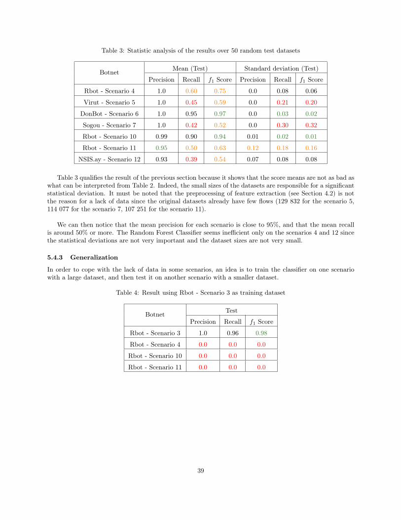
Table 3: Statistic analysis of the results over 50 random test datasets

Botnet Mean (Test) Standard deviation (Test)

Precision Recall f1 Score Precision Recall f1 Score

Rbot - Scenario 4 1.0 0.60 0.75 0.0 0.08 0.06

Virut - Scenario 5 1.0 0.45 0.59 0.0 0.21 0.20

DonBot - Scenario 6 1.0 0.95 0.97 0.0 0.03 0.02

Sogou - Scenario 7 1.0 0.42 0.52 0.0 0.30 0.32

Rbot - Scenario 10 0.99 0.90 0.94 0.01 0.02 0.01

Rbot - Scenario 11 0.95 0.50 0.63 0.12 0.18 0.16

NSIS.ay - Scenario 12 0.93 0.39 0.54 0.07 0.08 0.08

Table 3 qualifies the result of the previous section because it shows that the score means are not as bad aswhat can be interpreted from Table 2. Indeed, the small sizes of the datasets are responsible for a significantstatistical deviation. It must be noted that the preprocessing of feature extraction (see Section 4.2) is notthe reason for a lack of data since the original datasets already have few flows (129 832 for the scenario 5,114 077 for the scenario 7, 107 251 for the scenario 11).

We can then notice that the mean precision for each scenario is close to 95%, and that the mean recallis around 50% or more. The Random Forest Classifier seems inefficient only on the scenarios 4 and 12 sincethe statistical deviations are not very important and the dataset sizes are not very small.

5.4.3 Generalization

In order to cope with the lack of data in some scenarios, an idea is to train the classifier on one scenariowith a large dataset, and then test it on another scenario with a smaller dataset.

Table 4: Result using Rbot - Scenario 3 as training dataset

Botnet Test

Precision Recall f1 Score

Rbot - Scenario 3 1.0 0.96 0.98

Rbot - Scenario 4 0.0 0.0 0.0

Rbot - Scenario 10 0.0 0.0 0.0

Rbot - Scenario 11 0.0 0.0 0.0

39

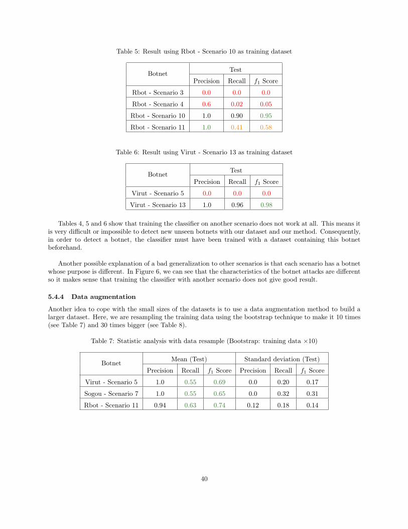
Table 5: Result using Rbot - Scenario 10 as training dataset

Botnet Test

Precision Recall f1 Score

Rbot - Scenario 3 0.0 0.0 0.0

Rbot - Scenario 4 0.6 0.02 0.05

Rbot - Scenario 10 1.0 0.90 0.95

Rbot - Scenario 11 1.0 0.41 0.58

Table 6: Result using Virut - Scenario 13 as training dataset

Botnet Test

Precision Recall f1 Score

Virut - Scenario 5 0.0 0.0 0.0

Virut - Scenario 13 1.0 0.96 0.98

Tables 4, 5 and 6 show that training the classifier on another scenario does not work at all. This means itis very difficult or impossible to detect new unseen botnets with our dataset and our method. Consequently,in order to detect a botnet, the classifier must have been trained with a dataset containing this botnetbeforehand.

Another possible explanation of a bad generalization to other scenarios is that each scenario has a botnetwhose purpose is different. In Figure 6, we can see that the characteristics of the botnet attacks are differentso it makes sense that training the classifier with another scenario does not give good result.

5.4.4 Data augmentation

Another idea to cope with the small sizes of the datasets is to use a data augmentation method to build alarger dataset. Here, we are resampling the training data using the bootstrap technique to make it 10 times(see Table 7) and 30 times bigger (see Table 8).

Table 7: Statistic analysis with data resample (Bootstrap: training data ×10)

Botnet Mean (Test) Standard deviation (Test)

Precision Recall f1 Score Precision Recall f1 Score

Virut - Scenario 5 1.0 0.55 0.69 0.0 0.20 0.17

Sogou - Scenario 7 1.0 0.55 0.65 0.0 0.32 0.31

Rbot - Scenario 11 0.94 0.63 0.74 0.12 0.18 0.14

40

Table 8: Statistic analysis with data resample (Bootstrap: training data ×30)

Botnet Mean (Test) Standard deviation (Test)

Precision Recall f1 Score Precision Recall f1 Score

Virut - Scenario 5 1.0 0.57 0.70 0.0 0.20 0.17

Sogou - Scenario 7 1.0 0.55 0.65 0.0 0.33 0.32

Rbot - Scenario 11 0.94 0.64 0.74 0.12 0.19 0.15

Tables 7 and 8 show the statistic analysis of the scenarios 5, 7 and 11 using the bootstrap method asresampling. We can see in Table 7 that the recall and f1 score are increased by around 10 points eachfor all of the scenarios. This means that the size of the dataset is the real problem for detecting botnets.However, Table 8 shows that this resampling trick cannot be used as much as we want since the scores reacha saturation point, even if the training dataset increases in size with the bootstrap method.

Remark: The standard deviations remain unchanged because the bootstrap method is only used with thetraining dataset and not with the test dataset.

5.4.5 Other algorithms

In this section, we compare the results of different algorithms on the scenarios where the Random ForestClassifier performs poorly (ie scenarios 4, 5, 7, 11 and 12).

Logistic RegressionA Logistic Regression classification is run to detect botnets in the scenarios 4, 5, 7, 11, and 12. The chosenparameters (C and Weightnon-botnet) are the same as the ones used for the scenarios 1.

Table 9: Result using Logistic Regression

Botnet Training Test

Precision Recall f1 Score Precision Recall f1 Score

Rbot - Scenario 4 0.07 0.07 0.07 0.05 0.05 0.05

Virut - Scenario 5 0.45 0.91 0.60 0.32 0.72 0.43

Sogou - Scenario 7 0.15 0.25 0.18 0.02 0.05 0.03

Rbot - Scenario 11 0.27 0.54 0.35 0.20 0.36 0.22

NSIS.ay - Scenario 12 0.09 0.38 0.14 0.08 0.35 0.13

Table 9 shows that the Logistic Regression cannot detect botnets in complicated scenarios where dataare scarce or not representative of malware behaviours.

Gradient BoostingThe same scenarios are tested with the Gradient Boosting method with the same parameters as scenario 1.

41

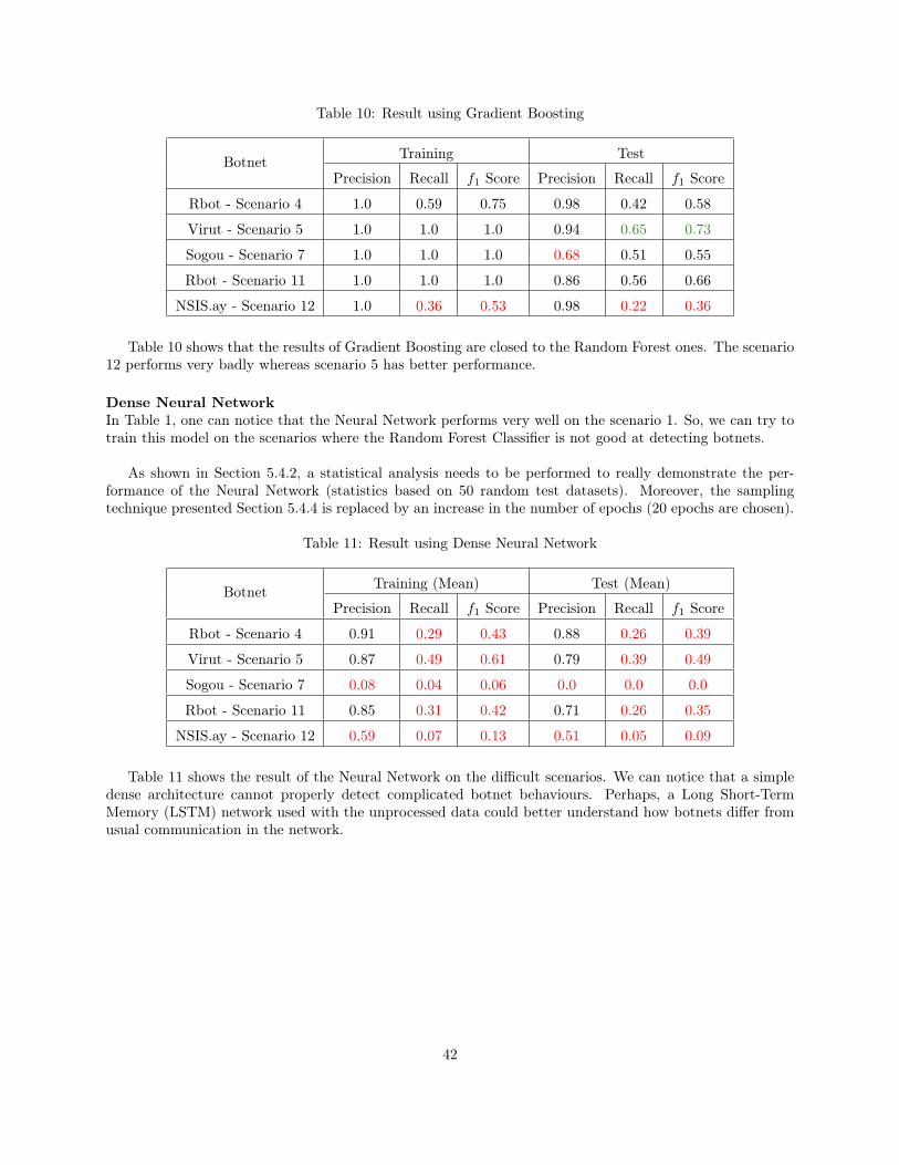
Table 10: Result using Gradient Boosting

Botnet Training Test

Precision Recall f1 Score Precision Recall f1 Score

Rbot - Scenario 4 1.0 0.59 0.75 0.98 0.42 0.58

Virut - Scenario 5 1.0 1.0 1.0 0.94 0.65 0.73

Sogou - Scenario 7 1.0 1.0 1.0 0.68 0.51 0.55

Rbot - Scenario 11 1.0 1.0 1.0 0.86 0.56 0.66

NSIS.ay - Scenario 12 1.0 0.36 0.53 0.98 0.22 0.36

Table 10 shows that the results of Gradient Boosting are closed to the Random Forest ones. The scenario12 performs very badly whereas scenario 5 has better performance.

Dense Neural NetworkIn Table 1, one can notice that the Neural Network performs very well on the scenario 1. So, we can try totrain this model on the scenarios where the Random Forest Classifier is not good at detecting botnets.

As shown in Section 5.4.2, a statistical analysis needs to be performed to really demonstrate the per-formance of the Neural Network (statistics based on 50 random test datasets). Moreover, the samplingtechnique presented Section 5.4.4 is replaced by an increase in the number of epochs (20 epochs are chosen).

Table 11: Result using Dense Neural Network

Botnet Training (Mean) Test (Mean)

Precision Recall f1 Score Precision Recall f1 Score

Rbot - Scenario 4 0.91 0.29 0.43 0.88 0.26 0.39

Virut - Scenario 5 0.87 0.49 0.61 0.79 0.39 0.49

Sogou - Scenario 7 0.08 0.04 0.06 0.0 0.0 0.0

Rbot - Scenario 11 0.85 0.31 0.42 0.71 0.26 0.35

NSIS.ay - Scenario 12 0.59 0.07 0.13 0.51 0.05 0.09

Table 11 shows the result of the Neural Network on the difficult scenarios. We can notice that a simpledense architecture cannot properly detect complicated botnet behaviours. Perhaps, a Long Short-TermMemory (LSTM) network used with the unprocessed data could better understand how botnets differ fromusual communication in the network.

42

6 ConclusionTo conclude, our project aimed at building and comparing models that are able to detect botnets in a realnetwork traffic represented by Netflow datasets.

After a strong analysis of the data and a lot of reviews of network security papers, relevant features wereextracted. Their influence were then studied through a selection process but no feature was poor enough tobe left aside for the training part.

Then, different algorithms were tested among which a Logistic Regression, Support Vector Machine,Random Forest, Gradient Boosting and a Dense Neural Network. The Random Forest Classifier was chosento detect botnets in all the other scenarios, resulting in an detection accuracy of more than 95% of thebotnets for 8 out of 13 scenarios.

After that, our group focused on increasing the accuracy for the 5 most difficult scenarios. The useof a bootstrap method to increase the amount of data has resulted in detecting more than 55% of thescenarios 5, 7 and 11. Only the scores of the scenarios 4 and 12 were difficult to improve (f1 score of 0.75 forscenario 4 and 0.54 for scenario 12). This is perhaps due to a bad representation of the botnet behaviourswith the extracted features or more complex algorithms need to be used (like recursive deep neural networks).

The possible improvement of the work presented here would be to try to modify the extracted featureswith different widths and strides for the time window and explore more hyperparameters for the difficultscenarios. Another idea would be to try to train and test several scenarios at the same time. Finally,unsupervised learning can be tested to detect the behaviour of botnets without using the labels of the data.

43

References[Bap+18] Rohan Bapat et al. “Identifying malicious botnet traffic using logistic regression”. In: 2018 Sys-

tems and Information Engineering Design Symposium (SIEDS). IEEE. 2018, pp. 266–271.

[Bri18] Rajesh Brid. Regression Analysis. 2018. url: https://medium.com/greyatom/logistic-regression-89e496433063 (visited on 05/11/2019).

[Cla+04] Benoit Claise et al. “RFC 3954: Cisco systems NetFlow services export version 9”. In: InternetEngineering Task Force (2004).

[Cla04] Benoit Claise. Cisco systems netflow services export version 9. Tech. rep. 2004.

[Cla13] B Claise. Trammell, B., Ed., and P. Aitken," Specification of the IP Flow Information Export(IPFIX) Protocol for the Exchange of Flow Information. Tech. rep. STD 77, RFC 7011, Septem-ber, 2013.

[CTU11] CTU University. The CTU-13 Dataset. A Labeled Dataset with Botnet, Normal and Back-ground traffic. 2011. url: https://www.stratosphereips.org/datasets- ctu13 (visitedon 03/29/2019).

[CV95] Corinna Cortes and Vladimir Vapnik. “Support-vector networks”. In: Machine learning 20.3(1995), pp. 273–297.

[Dso18] Melisha Dsouza. Build botnet detectors using machine learning algorithms in Python [Tuto-rial]. 2018. url: https://hub.packtpub.com/build-botnet-detectors-using-machine-learning-algorithms-in-python-tutorial/ (visited on 04/10/2019).

[Ert+04] Levent Ertoz et al. The MINDS - Minnesota Intrusion Detection System. Ed. by Data Mining-Next Generation. 2004. Chap. 3.

[FSW14] P Fruehwirt, S Schrittwieser, and ER Weippl. “Using machine learning techniques for trafficclassification and preliminary surveying of an attackers profile”. In: Proc. of Int. Conf. on Privacy,Security, Risk and Trust. 2014.

[Gan18] Rohith Gandhi. Support Vector Machines - Introduction to Machine Learning Algorithms. 2018.url: https://towardsdatascience.com/support- vector- machine- introduction- to-machine-learning-algorithms-934a444fca47 (visited on 05/11/2019).

[Gar+14] S. Garcia et al. “An empirical comparison of botnet detection methods”. In: ScienceDirect Com-puters & Security 45 (2014), pp. 100–123.

[Gro17] P Grover. “Gradient Boosting from scratch”. In: Retrieved from Medium (2017).

[Ho95] Tin Kam Ho. “Random Decision Forests”. In: Proceedings of the 3rd International Conference onDocument Analysis and Recognition (1995), pp. 278–282.

[Hou+18] Jiangpan Hou et al. “Machine Learning Based DDos Detection Through NetFlow Analysis”.In: MILCOM 2018-2018 IEEE Military Communications Conference (MILCOM). IEEE. 2018,pp. 1–6.

[Hua15] Guang-Bin Huang. “What are extreme learning machines? Filling the gap between Frank Rosen-blatt’s dream and John von Neumann’s puzzle”. In: Cognitive Computation 7.3 (2015), pp. 263–278.

[HZS06] Guang-Bin Huang, Qin-Yu Zhu, and Chee-Kheong Siew. “Extreme learning machine: Theoryand applications”. In: Neurocomputing 70 (2006), pp. 489–501.

[KC17] Rafal Kozik and Michal Choras. “Pattern Extraction Algorithm for NetFlow-Based Botnet Ac-tivities Detection”. In: Security and Communication Networks 2017 (2017).

[KGK18] Saakshi Kapoor, Vishal Gupta, and Rohit Kumar. “An Obfuscated Attack Detection Approachfor Collaborative Recommender Systems”. In: Journal of Computing and Information Technology26 (2018), pp. 45–56.

44

[KHH17] Zeinab Khorshidpour, Sattar Hashemi, and Ali Hamzeh. “Evaluation of random forest classifierin security domain”. In: Applied Intelligence 47 (2017), pp. 558–569.

[KPM18] Rafal Kozik, Marek Pawlicki, and Choras Michal. “Cost-Sensitive Distributed Machine Learningfor NetFlow-Based Botnet Activity Detection”. In: Security and Communication Networks 2018(2018).

[Par15] Paranet. Tip of the Week: A TCP flags and handshakes walk-through. 2015. url: https://www.paranet.com/blog/bid/147655/Tip-of-the-Week-A-TCP-flags-and-handshakes-walk-through (visited on 03/31/2019).

[Pet18] Ted Petrou. From Pandas to Scikit-Learn - A new exciting workflow. 2018. url: https://medium.com/dunder-data/from-pandas-to-scikit-learn-a-new-exciting-workflow-e88e2271ef62 (visited on 04/16/2019).

[QoS14] QoSient. Read Argus (ra) Documentation. 2014. url: https://qosient.com/argus/man/man1/ra.1.pdf (visited on 04/11/2019).

[RC14] Kozik Rafal and Michal Choras. “Machine Learning Techniques for Cyber Attacks Detection”.In: Image Processing and Communications Challenges 5 233 (2014), pp. 391–398.

[RCK19] Kozik Rafal, Michal Choras, and Jorg Keller. “Balanced Efficient Lifelong Learning (B-ELLA)for Cyber Attack Detection”. In: Journal of Universal Computer Science 25 (2019), pp. 2–15.

[Reh+08] Martin Rehak et al. “CAMNEP: agent-based network intrusion detection system”. In: Proceedingsof the 7th international joint conference on Autonomous agents and multiagent systems: indus-trial track. International Foundation for Autonomous Agents and Multiagent Systems. 2008,pp. 133–136.

[SP14] Matija Stevanovic and Jens Myrup Pedersen. “An efficient flow-based botnet detection usingsupervised machine learning”. In: 2014 international conference on computing, networking andcommunications (ICNC). IEEE. 2014, pp. 797–801.

[SSM18] David Santana, Shan Suthaharan, and Somya Mohanty. “What we learn from learning-Understandingcapabilities and limitations of machine learning in botnet attacks”. In: arXiv preprint arXiv:1805.01333(2018).

[Tre19] Trend Micro. Command and Control [C&C] Server. 2019. url: https://www.trendmicro.com/vinfo/us/security/definition/command-and-control-server (visited on 04/11/2019).

[TTS17] Duygu Sinanc Terzi, Ramazan Terzi, and Seref Sagiroglu. “Big data analytics for network anomalydetection from netflow data”. In: 2017 International Conference on Computer Science and En-gineering (UBMK). IEEE. 2017, pp. 592–597.

[W+11] Cynthia Wagner, Jerome Francois, Thomas Engel, et al. “Machine learning approach for ip-flowrecord anomaly detection”. In: International Conference on Research in Networking. Springer.2011, pp. 28–39.

[Wik18] Wikipedia. Cisco: How AI and Machine Learning are going to change your network. 2018. url:https://www.networkworld.com/article/3305327/cisco-how-ai-and-machine-learning-are-going-to-change-your-network.html (visited on 05/11/2019).

[Wik19a] Wikipedia. Anomaly Detection. 2019. url: https : / / en . wikipedia . org / wiki / Anomaly _detection (visited on 04/11/2019).

[Wik19b] Wikipedia. Machine Learning. 2019. url: https : / / en . wikipedia . org / wiki / Machine _learning (visited on 05/07/2019).

[Wik19c] Wikipedia. NetFlow. 2019. url: https : / / en . wikipedia . org / wiki / NetFlow (visited on04/11/2019).

[Wik19d] Wikipedia. Support-vector Machine. 2019. url: https://en.wikipedia.org/wiki/Support-vector_machine (visited on 05/11/2019).

45

[Wik19e] Wikipedia. Type of Service. 2019. url: https://en.wikipedia.org/wiki/Type_of_service(visited on 04/11/2019).

[XZB15] Kuai Xu, Zhi-Li Zhang, and Supratik Bhattacharyya. “Reducing Unwanted Traffic in a BackboneNetwork”. In: SRUTI (2015).

[Yua+10] Ruixi Yuan et al. “An SVM-based machine learning method for accurate internet traffic classifi-cation”. In: Information Systems Frontiers 12.2 (2010), pp. 149–156.

[Zhi18] Bing Liu Zhiyuan Chen. Lifelong Machine Learning. 2018. url: https://www.cs.uic.edu/~liub/lifelong-machine-learning.html (visited on 05/11/2019).

46