Low Complex System for Levitating Ferromagnetic Materials

Dahiru Sani Shu’aibu et. al. / International Journal of Engineering Science and Technology Vol. 2(6), 2010, 1844-1859

Low Complex System for Levitating Ferromagnetic Materials

*3Dahiru Sani Shu’aibu*1, Sharifah Kamilah Syed-Yusof *1, Norsheila Fisal*1 and Sanusi Sani Adamu*2 *1 Universiti Tecknologi Malaysia Skudai 81310 Johor Bahru Malaysia. *2 Bayero University Kano Nigeria PMB 3011 Kano Nigeria. *3 Corresponding author e-mail [email protected], [email protected] phone no;- +60177994950

ABSTRACT This paper primarily presents detailed design and implementation of a low complex magnetic levitation system which can be used in laboratory for levitation experiments. The system transfer function was derived from the co-energy and the mathematical model of the state space representation was obtained. The mathematical model showed that, the system is highly non-linear and inherently unstable. Based on simulation, a low complex circuit was designed and implemented to stabilize the system, using MATLAB control tool-box. The developed controller was simple, cheap and effective, capable of controlling weights of different masses at various distances as compared to some controllers in literature.

Key words: electromagnet, magnetic field, force actuator, levitation, controller, root locus 1.0 INTRODUCTION

The advance technology in transport system brought out the idea of levitation, which can be described as a process by which an object is suspended by physical force against gravity. An object or a body in space is normally pulled towards the centre of the earth by the gravitational force. When the object or body is made up of ferromagnetic materials, it can be suspend in space by the use of electromagnetic force generated by the magnet which balances the gravitational force. This can be achieved by controlling current flowing in an electromagnet that controls the generated magnetic force which lifts the ferromagnetic material. This phenomenon of magnetic levitation is typically accomplished by using actively controlled electromagnets. Magnetic actuation has the potential for numerous applications. The present maglev train is an example of levitation, In addition to supporting loads, it can damp vibration, apply precision force and move objects to precise distances without contact surfaces [1]. Such actuation can be used in harsh environments (corrosive, vacuum,etc), where traditional mechanical or hydraulic actuators might not survive. A magnetic levitation can operate in ultra clean environment without the hazard of producing contaminants from its use. The main hindrance to widespread application of magnetic levitation and other magnetically actuated system is the complexity of the involved physics [2]. We organized the rest of the report as follows; Section 2 focuses on literature review, Section 3 deals with the derivation of mathematical model of magnetic levitation system, Section 4 presents controller design and simulation results, section 5 is on system realization, experimental results were presented in section 6 and conclusions were drawn in section 7.

2.0 RELATED WORKS

A lot of researches were conducted in the field of magnetic levitation [3]-[9]. Most of the current researches on maglev make use of an electromagnet, because the strength of an electromagnet can be varied by simply controlling the current through the magnet [3], [9] . In some research paper a combination of permanent magnet and electromagnets were used for levitating the object [8]. In most of the research, the sensors performed a vital role in stabilizing the system. The sensor feedbacks the actual position of the levitated object to the controller that adjusts

ISSN: 0975-5462 1844


the current through the magnet accordingly. In [3] two phototransistors and photodiode were used as a sensing element, one photo transistor is used as a reference the other transistor detect the actual ball or object position when suspended. The controller received the two signals and act accordingly, the controller in this, is made up of complex electronics circuit. In [4] and [5] a similar approach as in [3] with less complexity was presented, a hall effect sensor at the base of solenoid was used to sense the actual position of the object and damping is provided by the washer attached to the levitated object. In [6] and [7] four hybrid-excited magnets were used for levitating object, the magnets were carefully controlled in synchronism, DSP (TMS320F2407) was used in [7] to control the magnets. In [8] and [9] a bio-inspired methods of control was implemented, in [8] an adaptive neuron was used to regulated the PID parameters whereas in the parameters were controlled by genetic algorithm. In this paper we will present a low complex circuit then [4] and [5] cheaper and very effective.

3.0 MATHEMATICAL DERIVATION OF THE SYSTEM MODEL

The dynamics and control aspects of the magnetic levitation system block diagram can be model as in figure 1, this comprises controller, force actuator, plant, and the sensor in a closed loop control system.

Figure 1 Block diagram for Closed Loop Control System

The block diagram in Figure 1 represents the complete closed loop system. The plant is the ferromagnetic material to be suspended, the force actuator is the electromagnet and controller is the circuit that controls the suspended object. The sensor feeds back the actual position of the suspended object.

3.1 FORCE ACTUATOR

An electromagnet was used as the force actuator, it produces the force to attract the object (a steel ball), upward against gravitational force. The forces acting on the object are the gravitational force (Gf), electromagnetic force (Mf) and of course, the difference between these two forces gives the object an acceleration which moves down ward or upward depending on the strength of individual force. There are also some disturbances such as wind, fluctuation in the line voltage and the ambient light. The effect of disturbances is assumed to be negligible compared to the two forces acting on the Object. To balance these two forces at a certain position known as the desired position (Yo), there is need to have a controller Figure 2 shows the schematic diagram of the system.

ISSN: 0975-5462 1845


Figure 2. Schematic diagram of the system

The basic set up of this system is shown in figure 2 The electromagnet is made up of steel rod as the core with a former covering the rod and a wire wound round the former. The conducting wire which is wound round the magnet has a certain resistance that can be negligibleted and an inductance which may not be negligible in this case. The definitions of the parameters are given below.

Figure 3 Assumed variation of the inductance of the coil with position The electromagnetic inductance of the coil is assumed to have the form of Figure 3 [10]. The following parameters define the meaning of the terms used for obtaining the system equations. Current through is i, the perturbation current is I and the steady state position current is Io. Vertical displacement of the Object from the pole of magnet is y, perturbation displacement is Y and steady state position is Yo. Total inductance of the magnet is L(y), additional inductance due the suspended object is Lo the inductance when there is no suspended object is L1. 3.1.1 FORCE ACTUATOR MODEL

The electromagnetic force on the levitated object is found using the concept of co-energy [11]. The co-energy (W1) is defined as [10];-

)(2

1),( 21 yLiyiW (1)

ISSN: 0975-5462 1846


o

o

Y

yL

LyL

1

)( 1 (2)

If we assumed that y/Yo >>1, then L(y) [10] becomes:- y

YLLyL oo 1)( (3)

where L(y) is the total inductance of the coil. Substituting the value of L(y) into equation (1) gives,

)(2

1),( 1

21

y

YLLiyiW oo (4)

Differentiating equation (4) with respect to y the results gives the force of the Electromagnet Fe

2

21

2

),(

y

iYL

y

yiWFe oo

(5)

If we let 2o oL Y

C (Nm2A-2) , where C is the Electromagnetic constant or Electromagnetic Strength then equation

(5) becomes

2

y

iCFe (6)

The negative sign of equation (6) indicates the direction of the force is upward. Now the equation of motion of the levitated object is given by the summation of all the forces acting on the suspended body.

Femgym (7)

Substituting equation (6) into (7) gives the equation 2

y

iCmgym (8)

At static equilibrium, the magnetic force on the object equals to gravitational force , therefore the left hand side of the equation (8) is zero hence:-

2

0

o

o

Y

ICmg Therefore we have

2

o

o

Y

ICmg (9)

Experimentally the value of C was computed using equation (9) The non-linear equation of force Fe in equation (6) can be linearize using Taylor Series Expansion by simply taking the first few terms of the series [11].

ii

YiFey

y

yiFeYIFeyiFe oo

ˆ),(ˆ

),(),()ˆ,ˆ(

(10)

Note that the perturbed quantities are defined as Yyy ˆ , & Iii ˆ

Substituting the value of Fe from equation (6) and its derivatives into equation (10) gives

iY

ICy

Y

IC

Y

ICyiFe

o

o

o

o

o

o ˆ2ˆ2)ˆ,ˆ(23

22

(11)

Hence the basic linearized equation is given by )ˆ,ˆ( yiFemgym Substituting equations (9) and (11) into

basic linear equation we have

iY

ICy

Y

IC

Y

IC

Y

ICyiFe

o

o

o

o

o

o

o

o ˆ2ˆ2)ˆ,ˆ(23

222

(12)

ISSN: 0975-5462 1847


From equation (12) the first two terms will simply cancel. The remaining in terms of perturbations quantities, gives

iY

ICy

Y

ICymFe

o

o

o

o ˆ2ˆ2ˆ23

2

(13)

Equation (13) is in form of a linear relationship iKyKym ˆˆˆ21 where K1 is in N/m while K2 is in N/A and they

can be obtained experimentally when the value of Io, Yo and C are known. For the electrical equation, it is assumed that the electromagnet coil is adequately modeled by a series resistor-inductor combination. The inductor includes that of the object when suspended as described. The circuit is shown in figure 4.

Figure 4 Coil of the magnet The electrical equation is given by;

t

iyLRiV

)( (14)

Equation (14) is highly non-linear because the inductance L(y) depends on the object position. The analysis can be simplify by assuming that the system is properly designed, such that the ball (object) remains closed to its equilibrium position, that is Y0 = y. This means that L(y) = L1+L0. From equation (3), by assuming that the inherent inductance of the coil, L1 is much larger than the inductive contribution of the object to be suspended, Lo, gives the final equation 14 as:-

t

iLRiV

1 (15)

3.2 PLANT MODEL

The plant consist of the object to be levitated only Therefore, Using Newton’s Law of motion

ymF (16)

Where m is the mass of the object, y is the displacement of the steel ball below the magnet

3.3 SENSOR MODEL

A light depending resistor was used as a sensor; the position sensor should be tested and calibrated according to the degree of sensing or blocking. This calibration is achieved by incrementing a light or rays such that it corresponds to the object’s size in the y direction and then recording the sensor output voltage. The data is given as a displacement from the bottom of the electromagnet coil down to the top of the ball (positive is down). In this configuration, the sensor is placed so as to detect the bottom edge of the levitated object. The sensor is to be used in its linear region

such that i kx b [11]

The sensor should not be allowed to operate in its saturation region. Sensors like phototransistor, photodiodes or an array of photocells and a light source could also be used. A light depending resistor or photoconductive cell is simply modeled as a gain element. The relationship is given in equation (17)

ISSN: 0975-5462 1848


yV (17)

Where α is the gain of the sensor its unit is V/m, y is the vertical distance in m, V is the voltage across the sensor in Volts. Equations (13), (15), (16) and (17) are the equations describing the system. A Laplace transform or state space techniques can be used for analyzing the system in linearized form.

3.4 System Transfer function

The transfer function of the system is the ratio of the position of steel ball below the magnet Y(s) to the current through the magnet I(s).

Hence G(s) = Y(s) / I(s) (18) However it can be express in term of voltage across the sensor and the magnet. G(s) = Vs(s) / Vm(s) (19) This is because the input voltage to the magnet is proportional to its current at constant reactance, and the output voltage across the sensor is directly proportional to the position of steel below the electromagnet. The four equations that described the system are given by equation 13, 15,16 and 17. Taking the Laplace transform of these equations we obtained the following in s-domain;

2 2 (20)

(21)

(22)

Vs=αY(s) (23) By combining equation (20) – (23), the transfer function of the system is given by,

⁄ (24)

Figure 5 Transfer function Block Diagram

3.5 DETERMINATION OF SYSTEM PARAMETERS

The parameters of the maglev system in an open loop condition is obtained as follows. The coil resistance (R) and inductance (L1) were measured with ohms meter and inductance meter respectively. The mass of the object (m) is measured, it is placed under the electromagnetic pole on a known distance (Yo) and current through the electromagnet (Io) is gradually increase up the time when it picks the object, the gain of the sensor α, is obtained by knowing the equilibrium position distance the shadow of a given mass of object it cast on the sensor, and the

ISSN: 0975-5462 1849


corresponding voltage the sensor produce, using equation 17, the sensor gain α is obtained. The parameters obtained are given in table 1

Table 1 Parameters for magnetic levitation system

PARAMETERS VALUE Equilibrium distance Yo 0.01m Equilibrium Current Io 0.5A Mass of the object m 0.02312Kg Force Constant C 9.07*10-5Nm2A-2 Coil Resistance R 3Ω Coil Inductance L1 0.0425H Sensor Gain α 511.4V/m

Substituting parameters of table 1 in equation (24) the system poles were evaluated to be at 44.289, -70.588, and -44.289 this means that the system is highly unstable to stabilized it we need a controller that will shift the unstable pole to the left hand side of the plane.

4.0 CONTROLLER DESIGN AND SIMULATION RESULTS

Phase-lead compensation was design by the method of root locus in order stabilizing the system . The root locus of an open-loop transfer function H(s) is a plot of the locations (locus) of all possible closed loop poles with proportional gain K and unity feedback [11]. If a plant dynamics are of such a nature that a satisfactory design cannot be achieved by adjusting of feedback gain alone, then some modification or compensation must be made in the feedback to achieve the desired specifications [12]. Typically, it takes the form;-

( )s z

D s Ks p

(26)

Where D(s) is called lead compensator if z < p otherwise lag compensator and K is the gain. Lead compensator approximate the addition of a derivatives control term and tends to increase the bandwidth and the speed of the response while decreasing the overshoot [12]. Lead compensation provides an increased magnitude slope and an increased phase in the interval between these two break points; the maximum being half-way between the two break points on a logarithmic scale. The maximum phase increase is [12]

sin , where

Generally a lead compensation with gain can be represented by the equation below [11];-

cs

csKsD

1000

100)(

(27)

The constant c and K are chosen to match the desired performance requirements. The system root locus can be used iteratively to aid in the determination of these constants. Settling time can be represented on the s-plane as a vertical line on the negative real axis. The position is approximately given by [12] as

.

(28)

Any roots to the left of this line satisfy the maximum settling time requirement. The percent overshoot is represented on the s-plane as an angle from the origin. The angle is measured as positive moving clockwise from the negative real axis. The angle magnitude is the arccosine of the damping ratio ζ, which is related to the percent overshoot through [12]

ISSN: 0975-5462 1850


21. 100p o e

(29)

Any roots that fall within an angle smaller than the critical angle will have a lower percent overshoot. The uncompensated root-locus is shown in figure 6;-

Figure 6 Root loci for Maglev

The uncompensated root locus in figure 6 showed that the system is unstable and can not be stabilized by just changing the system gain. It can be seen that, one of the pole will always be in the right hand side of the s-plane irrespective of the value of the system gain. To pull the root locus into the left hand plane pole, there is need to add a compensator’s zero in the left –hand plane between the first left hand pole and the origin. The first left hand pole is -44.289 so compensator’s zero should be place between this location and the origin. The necessary pole required is then placed deeper than the deepest pole of the system, so that it can pull it into the left hand plane, this will minimize the impact of the compensator pole on the root locus [11]. By chosen one of the constant c, using roots locus the other constant can be selected to give the desired specification. Let c be 0.3 rad/sec so that the controller equation 27 now changes to;-

30( )

300

sD s K

s

(30)

The value of c is carefully selected so that the zero of the controller is between the origin and the first pole of the system and the pole of the controller is deeper than the deepest system pole [11]. The gain k can be selected by

-400 -300 -200 -100 0 100 200-300

-200

-100

0

100

200

300Root Locus

Real Axis

Imag

inar

y Axi

s

ISSN: 0975-5462 1851


rlocfind with unity feedback and value of K to range from 0 to 7. Then we have figure 7

Figure 7 Compensated root locus

The plot above shows all possible closed loop pole locations after adding the lead compensator. Obviously not all those closed-loop poles will satisfy the design criteria. The specification is to have a damping ratio of 0.7, and undamped natural frequency of 3.2 rad/sec. The gain K can be selected from the plot so that the specifications can be achieved. After specifying the damping ratio zeta ( ζ ) and undamped natural frequency Wn, the value of k obtained was 3.9991which satisfied the specification. The selected point, gives a stable closed loop poles, with a rise time of 0.033sec settling time of 0.279 sec with percent overshot of <37% the damping ratio is 0.304 at a natural frequency of 54.189rad/sec. Figure 8 gives the step response of the system it shows that the reference input need to be scaled down in order to catch up with step response.

Figure 8 Step Response with gain K

-350 -300 -250 -200 -150 -100 -50 0 50 100-100

-80

-60

-40

-20

0

20

40

60

80

100

Root Locus

Real Axis

Imag

inar

y Axi

s

0 0.05 0.1 0.15 0.2 0.25 0.3 0.350

0.5

1

1.5

2

2.5

3

3.5

4Step Response

Time (sec)

Amplitu

de

ISSN: 0975-5462 1852


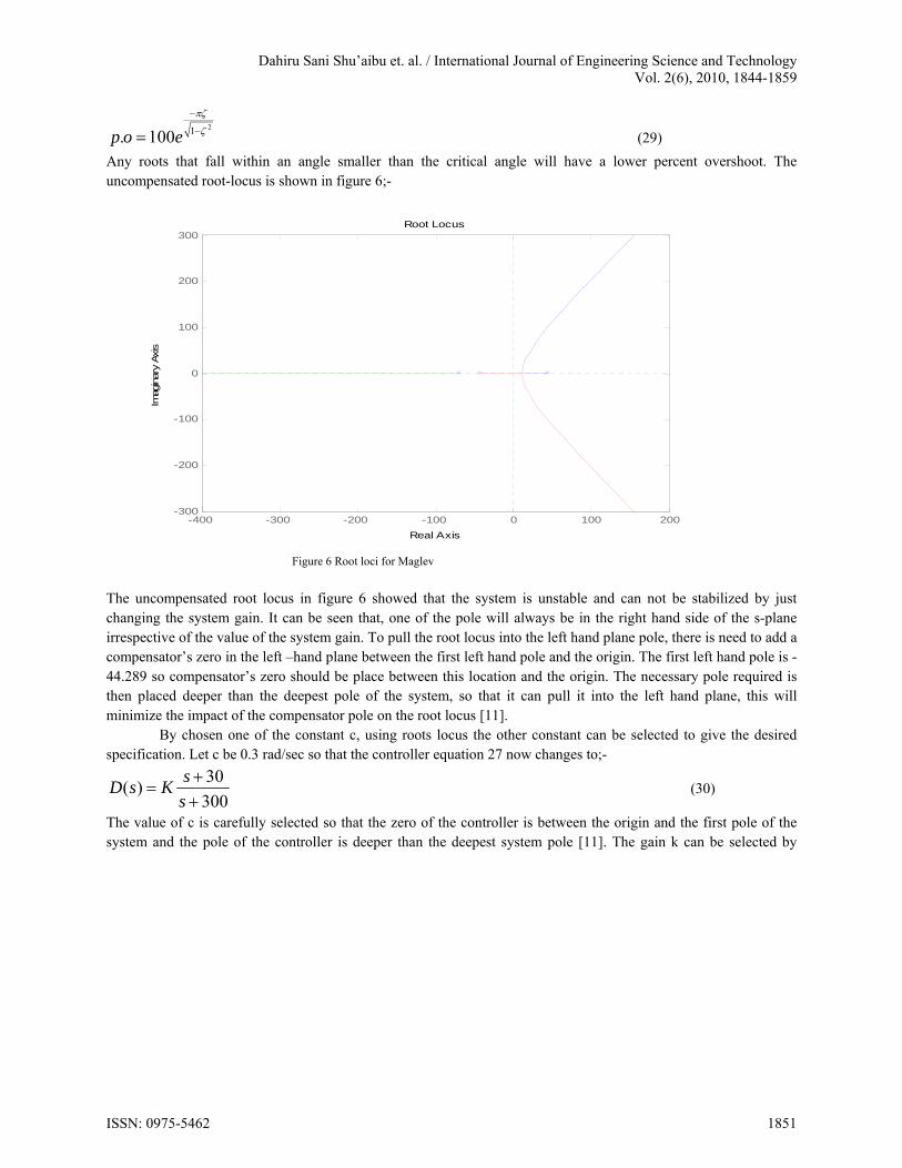
5.0 SYSTEM REALIZATION The controller can be realized using passive and active components consisting of resistors, capacitors, transistors, diodes and op-amps. The transfer function of the controller is given by;-

300

309991.3)(

s

ssD (31)

From the circuit diagram shown in figure 9 R1, R2 and C form the compensator network where as Ro and Rf forms the compensator gain (K) [11]. The transfer function between R1 R2 and C is ratio of the input voltage to the controller V1 to the output voltage V2

2 2 1

1 2 1 1

( 1)

( 1)

V R R sC

V R R sC R

(32)

2

2 1 2

1 21

1 2

Rs

V R R CR RV sR R C

(33)

By carefully selecting R1=330KΩ and C = 0.1μF, R2 is calculated to be 37KΩ. While carry out this calculation it is important to avoid cancellation between numerator and denominator because some of the terms will disappear.

Figure 9 Compensator circuit

Therefore the compensator above will be used in providing the gain; this is given by [12]-

1 3.9991, 2.9991 , select 10 , 29.991

5.1 COIL DRIVER DESIGN

This circuit controls the current through the electromagnets, which is one of the state variables. The system is shown in figure 10.

Figure 10 Electromagnetic driver

ISSN: 0975-5462 1853


The load, which is the electromagnet, has a resistance of about 3Ω and an inductance of about 0.0425H. The transistor collector current supplies the driving current to the magnetic coil. The collector current is β times the base current, which is found by dividing the Op-Amp output voltage, by the potentiometer resistance (Rs). The magnetic coil driving current is therefore;-

(34)

This relationship provides the final gain in the system. A diode is connected in the circuit to prevent the coil back emf from destroying the transistor; the electromagnet being an inductive load. A medium power transistor is used in driving the magnet.

5.2 REFERENCE SETTING AND SENSING ELEMENT (FEEDBACK)

The reference setting provides the desire object position, and it can be designed based on the sensitivity of the feedback element which is the sensor in this case. Previously the equation of the sensor is given by y = αx, where α is computed to be 511.4V/m. A potentiometer is used to set the reference or desired ball position and is chosen to vary the ball position from 0.1mm to 20.00mm below the electromagnet. The circuit arrangement is shown in figure 11

Figure 11 Feedback element A photoconductive cell (photo resistor) is used as a sensing element where it detects the vertical position of the ball (object) and sends back an analogue signal (voltage) which corresponds to the actual position of that object. The overall circuit arrangement is shown in figure 12 and figure 13 shows the pictorial view of the whole system in action, it lifts a medium size hollow steel ball of mass 27g.

Figure 12 Overall circuit diagram

ISSN: 0975-5462 1854


6. EXPERIMENTAL RESULTS

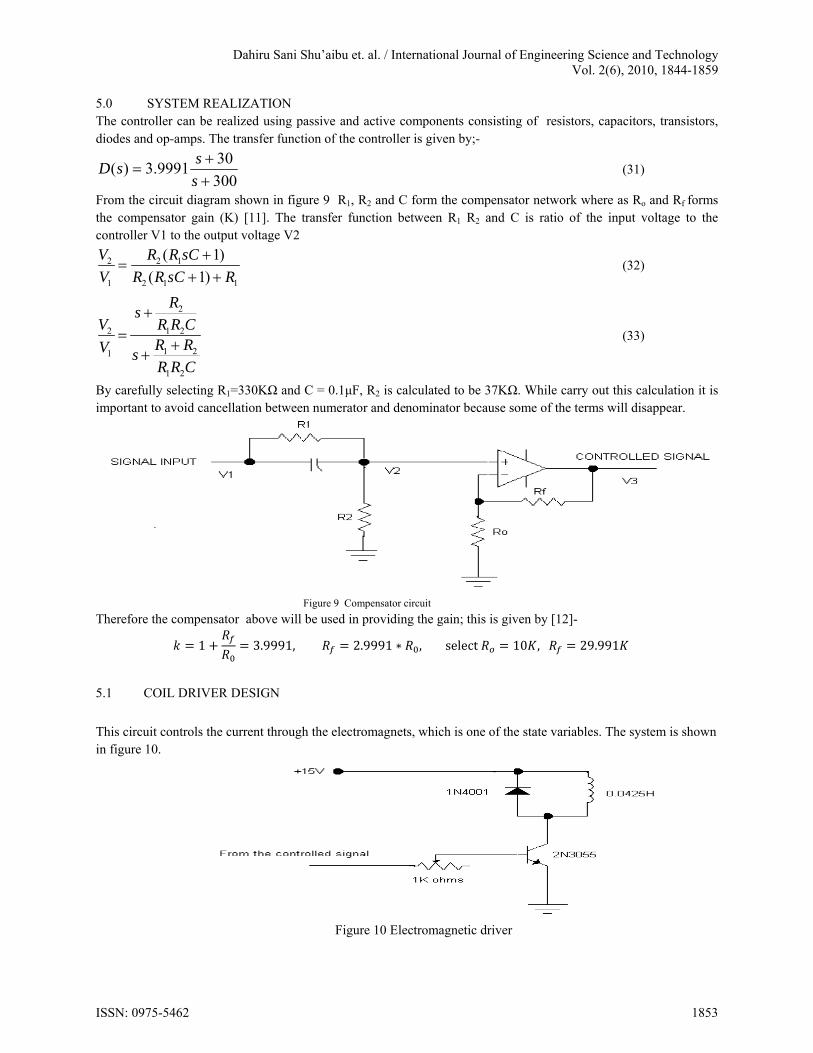
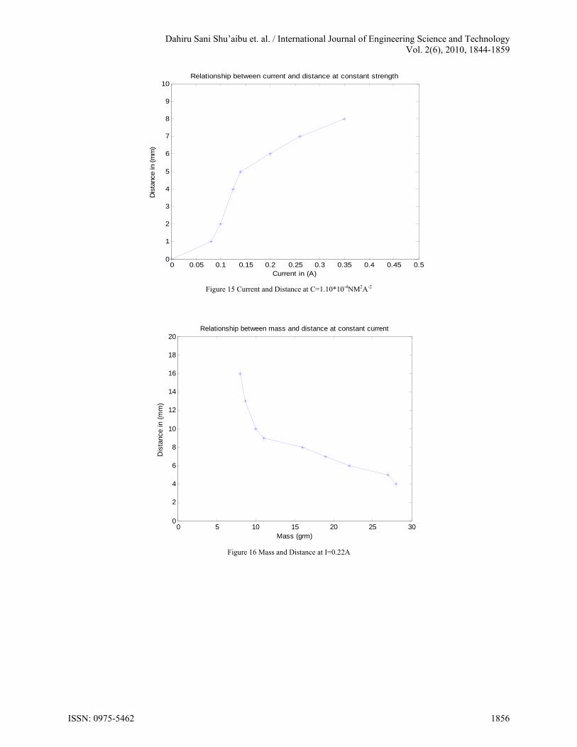
A series of experiment were conducted, in order to analysis the performance of the system. In each experiment, mass of object, current and distance were recorded and the corresponding strength of magnet was computed. Based on this, readings obtained were classified into two. Those readings with constant strength and those readings obtained at constant current. Figure 13, 14 and 15 showed the relationship at constant reading of the electromagnetic strength (1.0e-4 NM2A-2) when the ferromagnetic materials of different masses were suspended by the maglev system the graph showed that the relation obey the linear approximation given by equation (13). Figure 16, 17 and 18 showed similar relationship at constant current (0.22A) the graph obey the linear approximation given by equation (13). The pictorial view of the whole system while suspending 27g is shown in Figure 19.

Figure 13 Mass and Distance at C=1.10*10-4NM2A-2

Figure 14 Mass and Current at C=1.10*10-4NM2A-2

0 5 10 15 20 25 300

1

2

3

4

5

6

7

8

9

10Relationship between mass and distance at constant strength

Mass (grm)

Dis

tanc

e in

(m

m)

0 5 10 15 20 25 300

0.05

0.1

0.15

0.2

0.25

0.3

0.35

0.4

0.45

0.5Relationship between mass and current at constant strength

Mass (grm)

Cur

rent

in A

mpe

re (

A)

ISSN: 0975-5462 1855


Figure 15 Current and Distance at C=1.10*10-4NM2A-2

Figure 16 Mass and Distance at I=0.22A

0 0.05 0.1 0.15 0.2 0.25 0.3 0.35 0.4 0.45 0.50

1

2

3

4

5

6

7

8

9

10Relationship between current and distance at constant strength

Current in (A)

Dis

tanc

e in

(m

m)

0 5 10 15 20 25 300

2

4

6

8

10

12

14

16

18

20Relationship between mass and distance at constant current

Mass (grm)

Dis

tanc

e in

(m

m)

ISSN: 0975-5462 1856


Figure 17 Mass and Strength at I=0.22A

Figure 18 Distance and Strength at I=0.22A

0 5 10 15 20 25 300

0.5

1

1.5

2

2.5

3

3.5

4

4.5

5x 10

-4 Mass and strength of the Electromagnet at constant current

Mass in (grm)

Stren

gth

in (N

M2 A

-2 )

0 5 10 150

0.5

1

1.5

2

2.5

3

3.5

4

4.5

5x 10

-4 Distance and strength of Electromagnet at constant current

Distance in (mm)

Stren

gth

in (N

M2 A

-2 )

ISSN: 0975-5462 1857


Figure 19 pictorial view of the system.

7.0 Conclusion

In this paper, we presented a low complex circuit system for magnetic levitation control experiments, the system has a less complexity in term of number of components involved, this makes the implementation very cheap and easy to developed, the non-linear system was approximated with linear equations and experimental results obey the approximation of the system.

Acknowledgment

The authors would like to thank all those who contributed toward making this research successful. Also, we would like to thank to all the reviewers for their insightful comment. This work was sponsored by the research management unit, Universiti Teknologi Malaysia.

REFERENCES:

[1] Europe’s Network of patent Databases. Online available. http://gb.espacenet.com. “Transportation Network” [2] United States of America Patents and Trademark Office. Online Available. http://www.uspto.gov “Transportation Network” [3] Barry’s website http://www.oz.net “Barry’s Magnetic Levitation” [4] Katie A. Lilienkamp and Kent Lundberg “Low-cost magnetic Levitation project kits for teaching feedback system design, Proc, of the 2004

American control Conference” pg 1308-1313 [5] Kent H. Lundberg, Katie A. Lilienkamp and Guy Marsden “Low-cost Magnetic Levitation project kits, IEEE Control System Magazine

October, 2004” pg 65 - 69 [6] Liming Shi, Zhengguo Xu, etc “Decoupled Control for Hybrid-Magnets Used In Maglev system with large air gap” Proc, of 4th

International symposium on linear Drives for Industry application pg 267-270, 2003. [7] Z.G. Xu, N.Q. Jin, L.M. Shi and S.H. Xu, “Magnetic System with Hybrid-Excited Magnets and Air-gap Length control”, MAAGLEV 02,pg

1019-1023, 2004. [8] Shaohui Xu, Zhengguo Xu, Nengqiang Jin and Liming Shi “Levitation control scheme for hybrid Maglev system Based on Neuron-PID

control”, Proceeding 8th international conference on Electric machines and system ICEMS vol. 2, 2005, pg 1865-1868. [9] Hung-cheng Chen and sheng-hsiung Chang “genetic Algorithms based on Optimization design of a PID Controller for an active magnetic

bearing”, International journal of Computer Science and Network Security, Vol. 6, No. 12 , December 2006 pg 95-99. [10] H. H. Woodson and J.R. Melcher “Elactromechanical Dynamics” John Wiley & Sons, Inc., 1968. [11] Benjamin C. K “Automatic Control System” fifth edition. Prentice hall of Indian Private ltd, New Delhi, 1989. [12] Gene F. Franklin, J David Powell and Michael Workman. “Digital Control Of Dynamic Systems” Third Edition Addison Wesley Longman,

inc. 2725 Sand Hill Road Menlo Park, USA. 1998.

ISSN: 0975-5462 1858

Low Complex System for Levitating Ferromagnetic Materials

Documents

Transcript of Low Complex System for Levitating Ferromagnetic Materials