Loudness Control by Intelligent Audio Content Analysis - DiVA ...
68
Loudness Control by Intelligent Audio Content Analysis Hossein Sabri This thesis is presented as part of Degree of Master of Science in Electrical Engi neering Blekinge Institute of Technology September 2012 Blekinge Institute of Technology School of Engineering Department of Applied Signal Processing Supervisors: Dr. Nedelko Grbic Dr.-Ing. Wolfgang Hess Dr.-Ing. Christian Uhle Advisor/Supervisor: Dr. Ingvar Claesson Examiner: Dr. Sven Johansson
-
Upload
khangminh22 -
Category
Documents
-
view
0 -
download
0
Transcript of Loudness Control by Intelligent Audio Content Analysis - DiVA ...
Loudness Control by Intelligent
Audio Content Analysis
Hossein Sabri
This thesis is presented as part of Degree of
Master of Science in Electrical Engineering
Blekinge Institute of Technology
September 2012
Blekinge Institute of Technology
School of Engineering
Department of Applied Signal Processing
Supervisors: Dr. Nedelko Grbic
Dr.-Ing. Wolfgang Hess
Dr.-Ing. Christian Uhle
Advisor/Supervisor: Dr. Ingvar Claesson
Examiner: Dr. Sven Johansson

Abstract
Automatic audio segmentation aims at extracting information of audio signals. In the
case of music tracks, detecting segment boundaries, labeling segments, and detecting
repeated segments could be performed. These information can be used in different ap-
plications such as creating song summaries and facilitating browsing in music collections.
This thesis studies the Foote method which is one of the automatic audio segmentation
algorithms. Numerous experiments are carried out to improve the performance of this
method. The most suitable parameter settings of the Foote method, which have the best
performance in detection of segment boundaries as correct as possible in real time audio
segmentation, have been selected. Finally, real time audio segmentation results were
applied to automatically control loudness level of a streaming audio input signal. Our
experiments show that this application results in better dynamic structure preserving
and faster loudness level adjustment.


Acknowledgements
First of all, I would like to thank my supervisor at Blekinge Institute of Technology, Dr.
Nedelko Grbic, who taught me the basic knowledge in audio processing. It was him who
made me interested in this research area and also introduced Fraunhofer IIS to me as
one of the most intellectual research institutes.
I would like to express my greatest gratitude to my supervisor at Fraunhofer IIS, Dr.
Wolfgang Hess, whom offered me this interesting topic and gave me the opportunity
to do this research under his supervision. He always helped me with all the coming
problems, and I could never finish this thesis without his enlightening instructions and
support.
I would also like to gratefully thank Dr. Christian Uhle who always guided me patiently
through all the steps of this research. He never withheld his beneficial supports, even
when he was pretty busy. I really appreciate all the things he taught me in audio filed
and also in MATLAB.
Last but not least, my special thanks to my wife who was always right by my side and
supported me in all the steps of this work.
Finally, I could never thank my parents enough for their support and encouragement
during my whole life.
v


Contents
Abstract iii
Acknowledgements v
List of Figures ix
1 Introduction 1
1.1 Motivation . . . . . . . . . . . . . . . . . . . . . . . . . . . . . . . . . . . 1
1.2 Audio content analysis . . . . . . . . . . . . . . . . . . . . . . . . . . . . . 2
1.3 Contributions . . . . . . . . . . . . . . . . . . . . . . . . . . . . . . . . . . 3
1.4 Thesis organization . . . . . . . . . . . . . . . . . . . . . . . . . . . . . . . 3
2 State of the art 5
2.1 Foote method . . . . . . . . . . . . . . . . . . . . . . . . . . . . . . . . . . 5
2.1.1 Technical details . . . . . . . . . . . . . . . . . . . . . . . . . . . . 6
2.2 Techniques for the automatic audio segmentation . . . . . . . . . . . . . . 12
2.3 Audio feature extraction . . . . . . . . . . . . . . . . . . . . . . . . . . . . 13
2.3.1 Chroma features . . . . . . . . . . . . . . . . . . . . . . . . . . . . 13
2.3.2 Mel-Frequency Cepstral Coefficients (MFCC) . . . . . . . . . . . . 15
2.3.3 Spectral features . . . . . . . . . . . . . . . . . . . . . . . . . . . . 19
2.3.4 Combination of spectral features . . . . . . . . . . . . . . . . . . . 21
2.4 Loudness level measurement (Recommendation ITU-R BS.1770-2) . . . . 21
3 Audio segmentation 25
3.1 Parameter settings in the Foote method . . . . . . . . . . . . . . . . . . . 26
3.1.1 Kernel time . . . . . . . . . . . . . . . . . . . . . . . . . . . . . . . 26
3.1.2 Frame size . . . . . . . . . . . . . . . . . . . . . . . . . . . . . . . . 27
3.1.3 Distance measure . . . . . . . . . . . . . . . . . . . . . . . . . . . . 29
3.1.4 Feature vectors . . . . . . . . . . . . . . . . . . . . . . . . . . . . . 30
3.1.5 Summary . . . . . . . . . . . . . . . . . . . . . . . . . . . . . . . . 32
3.2 Proposed methods to improve the Foote method . . . . . . . . . . . . . . 33
3.2.1 Feature vectors manipulation . . . . . . . . . . . . . . . . . . . . . 33
3.2.2 Relative silent detection . . . . . . . . . . . . . . . . . . . . . . . . 37
3.2.3 Summary . . . . . . . . . . . . . . . . . . . . . . . . . . . . . . . . 41
vii

Contents viii
4 Evaluation setup and results 43
4.1 Evaluation setup . . . . . . . . . . . . . . . . . . . . . . . . . . . . . . . . 43
4.1.1 Block diagram . . . . . . . . . . . . . . . . . . . . . . . . . . . . . 43
4.2 Results . . . . . . . . . . . . . . . . . . . . . . . . . . . . . . . . . . . . . . 44
4.2.1 Loudness level control . . . . . . . . . . . . . . . . . . . . . . . . . 50
5 Conclusion 53
List of Figures
2.1 Block diagram of segmentation process . . . . . . . . . . . . . . . . . . . . 6
2.2 Distance matrix calculation . . . . . . . . . . . . . . . . . . . . . . . . . . 7
2.3 Similarity visualization of Bach’s Prelude No.1 . . . . . . . . . . . . . . . 9
2.4 90 x 90 kernel with Gaussian taper . . . . . . . . . . . . . . . . . . . . . . 10
2.5 Novelty score for Gloud performance and two different kernel size . . . . . 12
2.6 Shepard’s helix of pitch perception . . . . . . . . . . . . . . . . . . . . . . 14
2.7 Block digram of chroma feature extraction . . . . . . . . . . . . . . . . . . 16
2.8 Visualization of a chromogram . . . . . . . . . . . . . . . . . . . . . . . . 16
2.9 Block digram of MFCC feature extraction . . . . . . . . . . . . . . . . . . 17
2.10 The mel frequency scale . . . . . . . . . . . . . . . . . . . . . . . . . . . . 18
2.11 Visualization of an MFCC feature extraction . . . . . . . . . . . . . . . . 19
2.12 Feature vector visualization using combined spectral features . . . . . . . 21
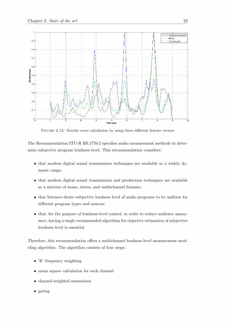
2.13 Novelty score calculation by using three different feature vectors . . . . . 22
2.14 Block diagram of multichannel loudness level measurement algorithm . . . 23
3.1 Impact of kernel time on novelty score . . . . . . . . . . . . . . . . . . . . 27
3.2 Impact of frame size on novelty score I . . . . . . . . . . . . . . . . . . . . 28
3.3 Impact of frame size on novelty score II . . . . . . . . . . . . . . . . . . . 28
3.4 Impact of distance measure on novelty score I . . . . . . . . . . . . . . . . 29
3.5 Impact of distance measure on novelty score II . . . . . . . . . . . . . . . 30
3.6 Impact of extracted feature vectors on novelty score I . . . . . . . . . . . 31
3.7 Impact of extracted feature vectors on novelty score II . . . . . . . . . . . 32
3.8 Smoothed Spectrogram . . . . . . . . . . . . . . . . . . . . . . . . . . . . 34
3.9 Impact of smoothing spectrogram on the novelty score . . . . . . . . . . . 35
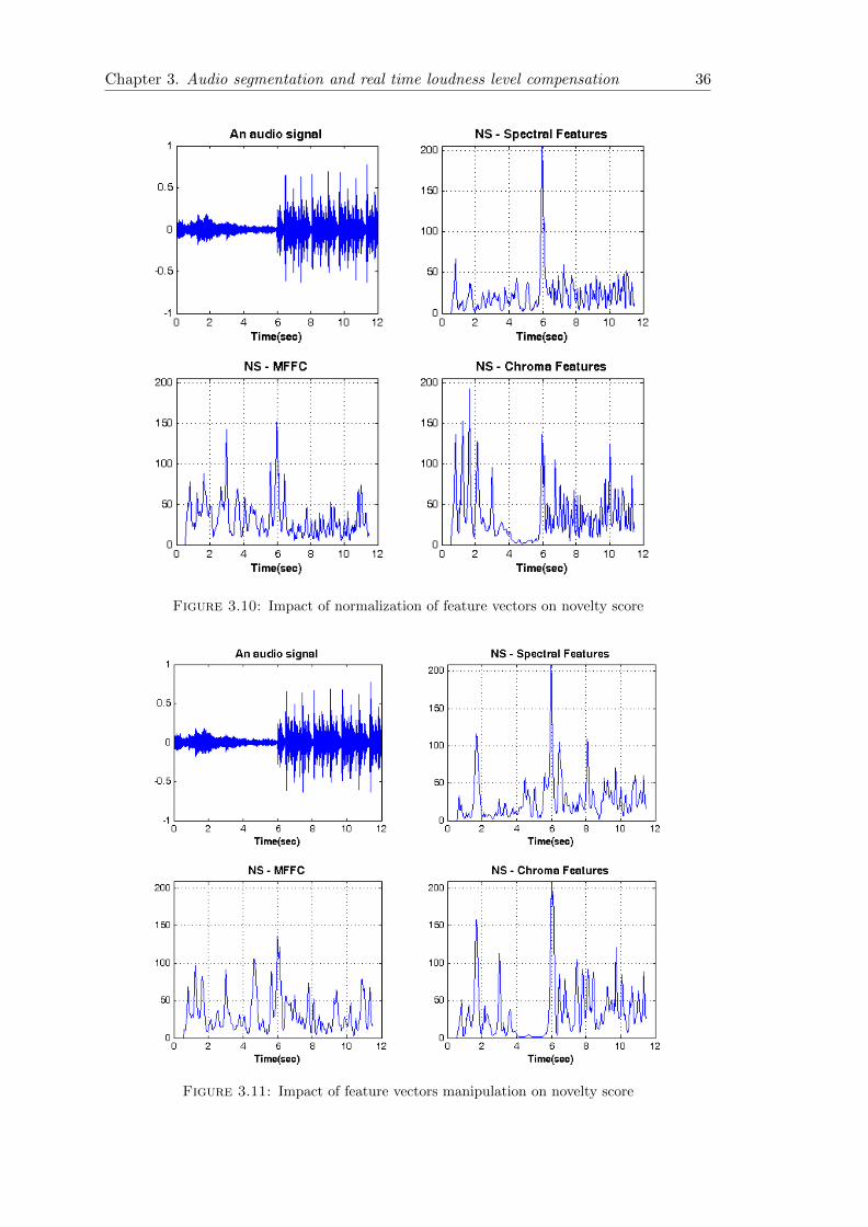
3.10 Impact of normalization of feature vectors on novelty score . . . . . . . . 36
3.11 Impact of feature vectors manipulation on novelty score . . . . . . . . . . 36
3.12 Fixed threshold for silent relative detection . . . . . . . . . . . . . . . . . 38
3.13 Adaptive threshold for silent relative detection I . . . . . . . . . . . . . . 39
3.14 Adaptive threshold for silent relative detection II . . . . . . . . . . . . . . 40
3.15 Distance normalization by loudness level . . . . . . . . . . . . . . . . . . . 41
4.1 Block diagram of evaluation setup . . . . . . . . . . . . . . . . . . . . . . 44
4.2 Effect of the frame size in the evaluation I . . . . . . . . . . . . . . . . . . 45
4.3 Effect of kernel time in the evaluation I . . . . . . . . . . . . . . . . . . . 46
4.4 Effect of kernel time in the evaluation II . . . . . . . . . . . . . . . . . . . 47
4.5 Effect of STFT smoothing in the evaluation . . . . . . . . . . . . . . . . . 47
4.6 Effect of the relative silence detection . . . . . . . . . . . . . . . . . . . . 48
4.7 Effect of the data set and the train set on each other . . . . . . . . . . . . 49
ix

List of Figures x
4.8 Fixed threshold for the novelty score . . . . . . . . . . . . . . . . . . . . . 50
4.9 Loudness level control . . . . . . . . . . . . . . . . . . . . . . . . . . . . . 50

To my wife who is my everything. . .
xi

Chapter 1
Introduction
1.1 Motivation
Listeners prefer to experience a uniform subjective loudness level of audio signals of
different input signals. As an example, they do not want to get annoyed by loudness
level differences when switching between broadcast channels or music tracks. Manually
adjusting playback levels is still a common solution to this problem. Therefore, the
aim of the automatic loudness control is to compensate loudness differences between
different inputs by adaptive adjustment of the playback level. The accomplishment of
this procedure depends on a method of modifying the loudness level and a loudness model
which is computationally capable of estimating the loudness level before and after the
modification. The preservation of the dynamic structure of original input audio signals is
the vital issue in this task, i.e. any loudness level modification algorithm should preserve
loudness level fluctuations and should not introduce any artefacts within one track.
Therefore, the exact segment boundary detection which discriminates different audio
signal types is needed for automatic loudness level control. A common problem occurs
when the audio segmentation algorithm mistakenly detects segment boundaries within
an audio signal source, e.g. within a music track because of the appearance of verse and
chorus or within a single speaker’s speech because of the silent/noisy sections during
speech. This problem may causes unwanted change in the dynamic structure of audio
signal sources. Thus, the accuracy of the audio segmentation algorithm has a direct
influence on preservation of the dynamic structure of audio signals. In cases which
whole audio signal is previously available, the automatic loudness level control can be
done effectively. A challenge occurs when we encounter audio streaming and both, the
automatic audio segmentation and the automatic loudness control, must be done in
real-time. Although streaming audio cannot automatically leveled to equal loudness
1
Chapter 1. Introduction 2
level without affecting its dynamic structure, an intelligent strategy could result in an
improved subjective experience if the level adjustment is neither to slow nor to abrupt.
This control level method can be guided by audio segmentation which identifies segment
boundaries between different tracks and indicates switching between broadcast channels.
1.2 Audio content analysis
Automatic audio content analysis aims to extract information from audio signals. In
digital signal processing, audio signals are presented as discrete values which correspond
to amplitude levels of sounds. These digital signals contain all information of the sound in
the time domain and they should be interpreted in order to obtain meaningful properties
in the frequency domain. Presentation of a short interval of an audio signal in the time
domain or frequency domain may consist of a large vector. As an example, 20ms of an
audio signal that has a frequency sampling rate equal to 16kHz will be presented by a
vector containing 320 elements in the time domain. A more powerful way of presentation
audio intervals with small number of elements is needed. Feature extraction must be
done to present each audio interval in a compact and informative form.This process is
called audio content analysis.
Automatic audio segmentation could be considered as a subset of the automatic audio
content analysis which aims at extracting information about the structure of audio
signals. These information could be useful for detecting segment boundaries and labeling
each segment. Human listeners can easily detect where the segments such as choruses
occur since the chorus sections are the most repeated and memorable sections within
a music track. Computers need to be programmed by sophisticated algorithms to be
capable of detecting novelty in audio signals.
The framework of the audio segmentation aims to have digital processors classify parts
of audio signals similar to the way that human understand them. The automatic audio
segmentation could be useful in various practical applications as follows:
• Audio thumbnails / Audio gisting: Music track review can be available at online
music stores by representing a short excerpt of each music track which is somehow
representative of the whole music track. If we use an analogy to image thumbnails,
where easily convey the ”gist” of an image, these short excerpts can be called
”audio thumbnails” [1]. This could be done by extracting the segment which has a
maximum similarity to the whole track. However, detection of exact boundaries of
choruses is hard but this is much more better than a random segment extraction
by a human being in terms of time saving.
Chapter 1. Introduction 3
• Audio summarization: Detected segments within a music track can be clustered.
Then, only the most important novel segments will be included. The segments
which are too similar to each other can be ignored without losing too much infor-
mation. Automatic audio summarization enable quick overview of audio contents.
• Audio classification and retrieval: This procedure will work more effectively on
shorter audio segments than long data [2]. This application would be useful for
locating a known music or audio in a longer file. The audio segmentation will be
implemented in longer files and the similarity between the detected segments and
the target segments will be measured in order to find similar segments.
1.3 Contributions
In this thesis, a well-known audio segmentation method, the Foote method, has been
investigated [2]. A real time segmentation algorithm which is based on this method is
evolved. In this algorithm, different kinds of features extractions from audio signals can
be used. The best set of the extracted features which works well for various combinations
of audio signals such as combinations of different types of music, speech, and different
broadcasting channels have been selected.Furthermore, a relative silence detection is
introduced which decreases false detections of segment boundaries within a music track
or speech. This method aims to locate intervals with loudness levels below an adaptive
threshold value and labels these intervals as relatively silent in comparison with adjacent
intervals. This algorithm restricts continuous applications of automatic loudness level
control by introducing a threshold value for novelty of audio signals. This restriction
improves the preservation of the dynamic structure of incoming audio signals.
1.4 Thesis organization
The remainder of this thesis is organized as follows.
• Chapter two: State of the art. In this chapter, the well-known Foote method,
which is based on self-similarity between audio frames, is described for audio
segmentation. Moreover, various methods of feature extraction and a loudness
level measurement algorithm according to recommendation ITU-R BS.1770-2 is
explained as well.
• Chapter three: Audio segmentation. In this chapter, some proposed manipula-
tions in feature extraction and self-similarity matrix calculation are represented.

Chapter 1. Introduction 4
Moreover, the effect of them on novelty score measurements in the Foote method
is examined.
• Chapter four: Results. In this chapter, the result of our audio segmentation eval-
uation is presented and the most powerful one has been selected from the best
results. Moreover, the power of this best set of configuration in audio segmenta-
tion is demonstrated in an automatic loudness level control.
• Chapter five: Conclusion. In this chapter, the important conclusions are presented
and some methods are stated which might be beneficial for improvement.
Chapter 2
State of the art
In this chapter, the Foote method that is one of the well-known audio segmentation
algorithms is described at length. Afterwards, some useful audio segmentation methods
introduced briefly. Furthermore, various methods of audio feature extractions are out-
lined. In the final section, a loudness level measurement algorithm is stated based on
recommendation ITU-R BS.1770-2 summarily.
2.1 Foote method
This method tries to locate the points of significant changes in audio signals automati-
cally. It can be done by analysing self-similarity within a audio/music track which can
find segment boundaries in different types of audio signals such as verse/chorus detec-
tion in a music or speech/music transitions. Furthermore, this approach does not need
training nor depend on specific acoustic cues. Instead, this method uses the signal to
model itself. This feature has a wide range of benefits in different applications such as
indexing, segmenting, and beat tracking of music [2].
The main idea of Foote method is based on frame-to-frame similarities which can be used
for the automatic segmentation. The term frame or block corresponds to a sequence of
limited number of audio samples. Using approaches like measuring spectral differences
between frames, increases the risk of having errors due to false alarms as typical spectra
for speech and music is in constant flux[2].
By considering the self-similarity of an audio signal, Foote method tries to find the
points of maximum novelties in it. For each frame of the audio, the self-similarity for
past and future intervals is computed.Then, a point in the audio signal calls a signif-
icant novel point when the past and the future intervals have high self-similarity and
low cross-similarity. It should be noted that past and future intervals’ lengths indicate
5
Chapter 2. State of the art 6
the purpose of our segmentation. If we are interested in finding individual notes short
intervals can be used; while for finding longer events, such as musical themes, longer
intervals can be exploited. The result of this approach shows how novel the audio signal
is at any point. Note that in determining a novelty score of an instant, future frames
are not available at the same time. Thus, a delay occurs corresponding to this waiting
time.
2.1.1 Technical details
The Foote method produces time series values which correspond to acoustic novelty of
an audio signal at any time. Large audio changes occur at peaks and high values of this
time series values, which are called novelty scores in the Foote method. These novelty
scores can be used to find segment boundaries of an audio by assigning a threshold value.
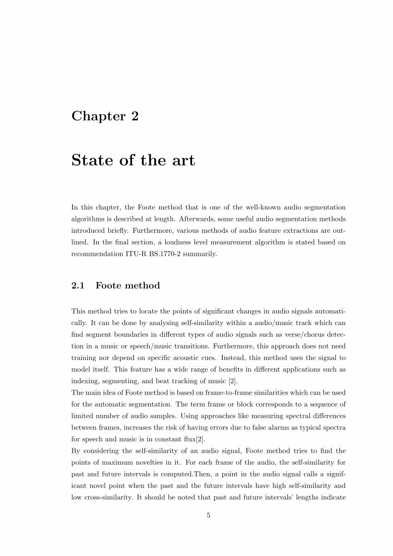
Figure 2.1 shows a block diagram of computing the novelty score.
The first step in computing the novelty score is feature extraction. This can be im-
plemented by windowing the audio waveform as an initial phase. It should be noted
that any windows’ width and overlaps can be used in windowing procedure. Each
frame/block is then utilized for an audio feature extraction. Different methods of audio
feature extraction will be presented in section 2.3.
Figure 2.1: Block diagram of segmentation process

Chapter 2. State of the art 7
Distance matrix calculation
Once the audio features have been extracted, they can be used in a two dimensional
representation [3]. Figure 2.2 shows two dimensional representation of a similarity ma-
trix. The measure D in Figure 2.2 shows how similar two feature vectors vi and vj are.
These vi and vj correspond to audio frames i and j. Different distance measurements
can be used to identify the distances between the frames. The simplest one could be the
Euclidean distance which is the square root of the sum of squared differences of feature
vector pairs:
DE(i, j) ≡√∑
p
(vi(p)− vj(p))2 (2.1)
Another distance measure is the dot product of the feature vectors. This value will be
Figure 2.2: Distance matrix calculation [2]
large if the feature vectors are both large and oriented in similar direction. On the other
hand, it will be small if the feature vectors are small or in different directions.
Dd(i, j) ≡ vi • vj (2.2)
The previous measurement, the scalar product of the feature vectors, is dependent on
magnitude of the feature vectors. In order to remove this dependence, the product
can be normalized by multiplication of the magnitudes of two feature vectors. This is
equivalent to the cosine of the angle between the feature vectors.
DC(i, j) ≡ vi • vj
‖ vi ‖‖ vj ‖(2.3)
Chapter 2. State of the art 8
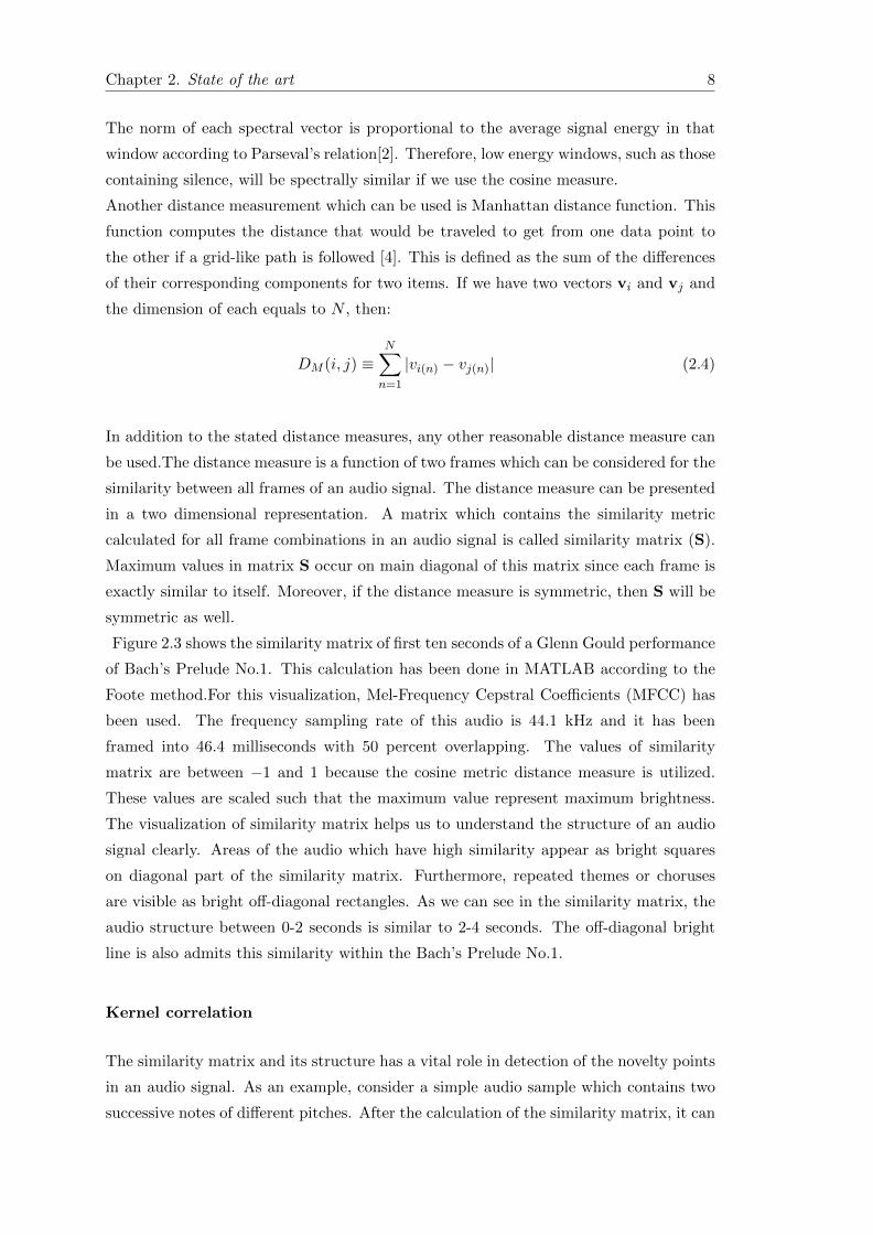
The norm of each spectral vector is proportional to the average signal energy in that
window according to Parseval’s relation[2]. Therefore, low energy windows, such as those
containing silence, will be spectrally similar if we use the cosine measure.
Another distance measurement which can be used is Manhattan distance function. This
function computes the distance that would be traveled to get from one data point to
the other if a grid-like path is followed [4]. This is defined as the sum of the differences
of their corresponding components for two items. If we have two vectors vi and vj and
the dimension of each equals to N , then:
DM (i, j) ≡N∑
n=1
|vi(n) − vj(n)| (2.4)
In addition to the stated distance measures, any other reasonable distance measure can
be used.The distance measure is a function of two frames which can be considered for the
similarity between all frames of an audio signal. The distance measure can be presented
in a two dimensional representation. A matrix which contains the similarity metric
calculated for all frame combinations in an audio signal is called similarity matrix (S).
Maximum values in matrix S occur on main diagonal of this matrix since each frame is
exactly similar to itself. Moreover, if the distance measure is symmetric, then S will be
symmetric as well.
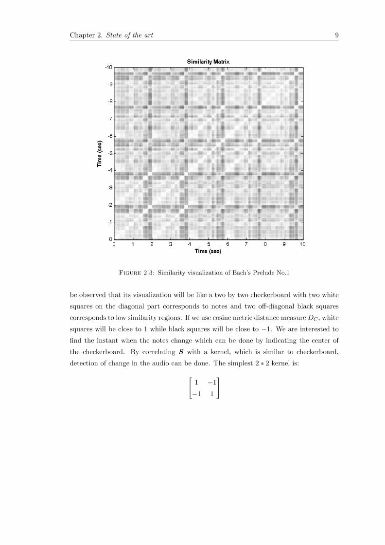
Figure 2.3 shows the similarity matrix of first ten seconds of a Glenn Gould performance
of Bach’s Prelude No.1. This calculation has been done in MATLAB according to the
Foote method.For this visualization, Mel-Frequency Cepstral Coefficients (MFCC) has
been used. The frequency sampling rate of this audio is 44.1 kHz and it has been
framed into 46.4 milliseconds with 50 percent overlapping. The values of similarity
matrix are between −1 and 1 because the cosine metric distance measure is utilized.
These values are scaled such that the maximum value represent maximum brightness.
The visualization of similarity matrix helps us to understand the structure of an audio
signal clearly. Areas of the audio which have high similarity appear as bright squares
on diagonal part of the similarity matrix. Furthermore, repeated themes or choruses
are visible as bright off-diagonal rectangles. As we can see in the similarity matrix, the
audio structure between 0-2 seconds is similar to 2-4 seconds. The off-diagonal bright
line is also admits this similarity within the Bach’s Prelude No.1.
Kernel correlation
The similarity matrix and its structure has a vital role in detection of the novelty points
in an audio signal. As an example, consider a simple audio sample which contains two
successive notes of different pitches. After the calculation of the similarity matrix, it can
Chapter 2. State of the art 9
Figure 2.3: Similarity visualization of Bach’s Prelude No.1
be observed that its visualization will be like a two by two checkerboard with two white
squares on the diagonal part corresponds to notes and two off-diagonal black squares
corresponds to low similarity regions. If we use cosine metric distance measure DC , white
squares will be close to 1 while black squares will be close to −1. We are interested to
find the instant when the notes change which can be done by indicating the center of
the checkerboard. By correlating S with a kernel, which is similar to checkerboard,
detection of change in the audio can be done. The simplest 2 ∗ 2 kernel is:[1 −1
−1 1
]
Chapter 2. State of the art 10
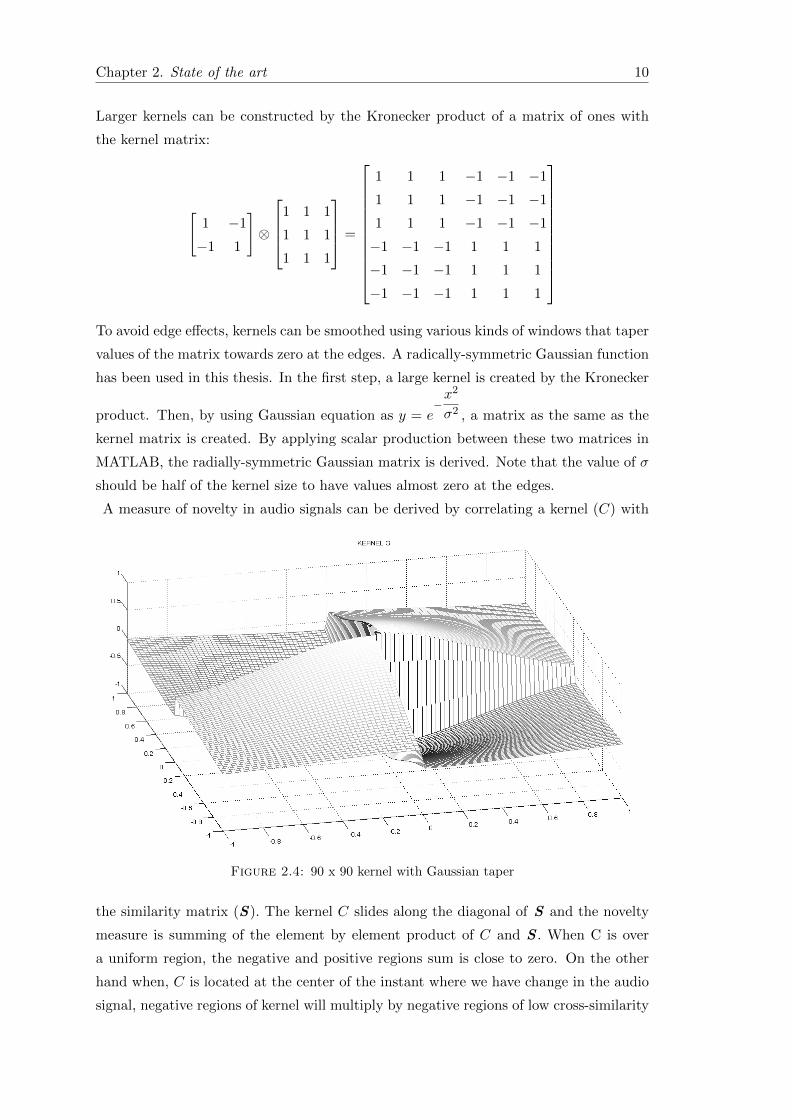
Larger kernels can be constructed by the Kronecker product of a matrix of ones with
the kernel matrix:
[1 −1
−1 1
]⊗
1 1 1
1 1 1
1 1 1
=
1 1 1 −1 −1 −1
1 1 1 −1 −1 −1
1 1 1 −1 −1 −1
−1 −1 −1 1 1 1
−1 −1 −1 1 1 1
−1 −1 −1 1 1 1
To avoid edge effects, kernels can be smoothed using various kinds of windows that taper
values of the matrix towards zero at the edges. A radically-symmetric Gaussian function
has been used in this thesis. In the first step, a large kernel is created by the Kronecker
product. Then, by using Gaussian equation as y = e−x2
σ2 , a matrix as the same as the
kernel matrix is created. By applying scalar production between these two matrices in
MATLAB, the radially-symmetric Gaussian matrix is derived. Note that the value of σ
should be half of the kernel size to have values almost zero at the edges.
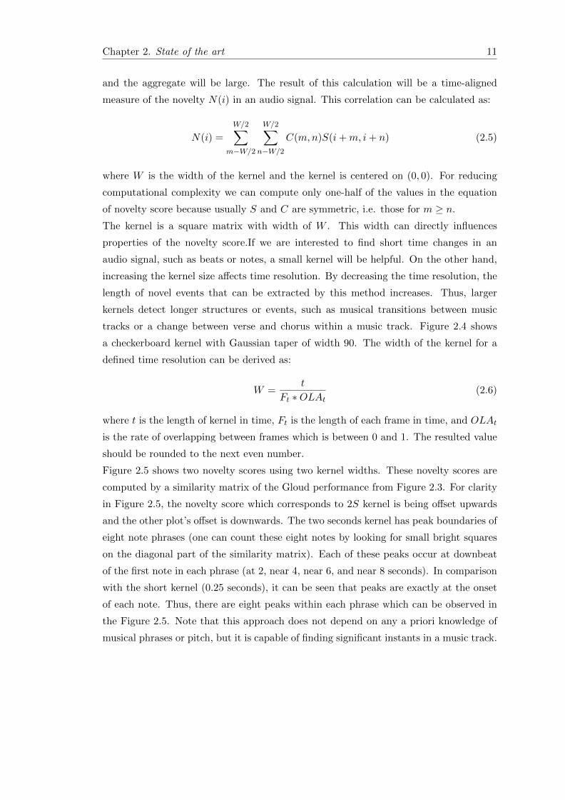
A measure of novelty in audio signals can be derived by correlating a kernel (C) with
Figure 2.4: 90 x 90 kernel with Gaussian taper
the similarity matrix (S). The kernel C slides along the diagonal of S and the novelty
measure is summing of the element by element product of C and S . When C is over
a uniform region, the negative and positive regions sum is close to zero. On the other
hand when, C is located at the center of the instant where we have change in the audio
signal, negative regions of kernel will multiply by negative regions of low cross-similarity
Chapter 2. State of the art 11
and the aggregate will be large. The result of this calculation will be a time-aligned
measure of the novelty N(i) in an audio signal. This correlation can be calculated as:
N(i) =
W/2∑m−W/2
W/2∑n−W/2
C(m,n)S(i+m, i+ n) (2.5)
where W is the width of the kernel and the kernel is centered on (0, 0). For reducing
computational complexity we can compute only one-half of the values in the equation
of novelty score because usually S and C are symmetric, i.e. those for m ≥ n.
The kernel is a square matrix with width of W . This width can directly influences
properties of the novelty score.If we are interested to find short time changes in an
audio signal, such as beats or notes, a small kernel will be helpful. On the other hand,
increasing the kernel size affects time resolution. By decreasing the time resolution, the
length of novel events that can be extracted by this method increases. Thus, larger
kernels detect longer structures or events, such as musical transitions between music
tracks or a change between verse and chorus within a music track. Figure 2.4 shows
a checkerboard kernel with Gaussian taper of width 90. The width of the kernel for a
defined time resolution can be derived as:
W =t
Ft ∗OLAt(2.6)
where t is the length of kernel in time, Ft is the length of each frame in time, and OLAt
is the rate of overlapping between frames which is between 0 and 1. The resulted value
should be rounded to the next even number.
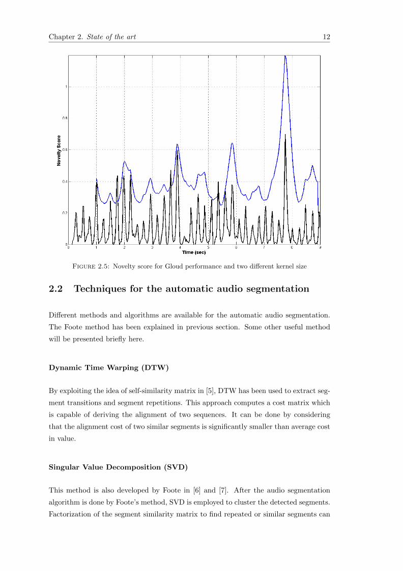
Figure 2.5 shows two novelty scores using two kernel widths. These novelty scores are
computed by a similarity matrix of the Gloud performance from Figure 2.3. For clarity
in Figure 2.5, the novelty score which corresponds to 2S kernel is being offset upwards
and the other plot’s offset is downwards. The two seconds kernel has peak boundaries of
eight note phrases (one can count these eight notes by looking for small bright squares
on the diagonal part of the similarity matrix). Each of these peaks occur at downbeat
of the first note in each phrase (at 2, near 4, near 6, and near 8 seconds). In comparison
with the short kernel (0.25 seconds), it can be seen that peaks are exactly at the onset
of each note. Thus, there are eight peaks within each phrase which can be observed in
the Figure 2.5. Note that this approach does not depend on any a priori knowledge of
musical phrases or pitch, but it is capable of finding significant instants in a music track.
Chapter 2. State of the art 12
Figure 2.5: Novelty score for Gloud performance and two different kernel size
2.2 Techniques for the automatic audio segmentation
Different methods and algorithms are available for the automatic audio segmentation.
The Foote method has been explained in previous section. Some other useful method
will be presented briefly here.
Dynamic Time Warping (DTW)
By exploiting the idea of self-similarity matrix in [5], DTW has been used to extract seg-
ment transitions and segment repetitions. This approach computes a cost matrix which
is capable of deriving the alignment of two sequences. It can be done by considering
that the alignment cost of two similar segments is significantly smaller than average cost
in value.
Singular Value Decomposition (SVD)
This method is also developed by Foote in [6] and [7]. After the audio segmentation
algorithm is done by Foote’s method, SVD is employed to cluster the detected segments.
Factorization of the segment similarity matrix to find repeated or similar segments can
Chapter 2. State of the art 13
be done by applying the SVD to the full sample-indexed similarity matrix. More details
can be found in [6].
Hidden Markov Models (HMM)
This method has been exploited by many researchers [8], [9], [10], and [11]. A Markov
model’s states cannot be observed directly. They can only be estimated by the out-
put products calls HMM. In this approach, audio feature vectors are extracted and
parametrization is applied using Gaussian Mixture Models (GMM). The GMMs are one
of the most statistically mature methods for clustering. These parameters can be used
as the HMM’s output values. In the first step, the emission and the transition proba-
bility matrices are estimated. Then, state sequences with high probabilities are Viterbi
decoded. Finally, the HMM states can be used as segment types.
2.3 Audio feature extraction
For many applications of audio processing such as audio classification and audio seg-
mentation, audio feature extraction is one of the most important steps. An audio signal
which is represented over time is not so informative. Moreover, according to the fre-
quency sampling rate of an audio signal, even a short block in time could contain many
samples (e,g more than 100). Thus, a wise solution can be interpretation an audio frame
into smaller frames which reflect the most important information of the original frame.
This can be done by converting the signal over time into the frequency domain and
extracting desirable information from that. In this section, some of the most common
methods of audio feature extraction which have been used in this thesis are described.
2.3.1 Chroma features
One of the techniques introduced for extracting the harmonic contents of a music signal
is chroma feature extraction.Chroma feature is a common representation of tonal infor-
mation contained in audio signals.
In 1964, Shepard reported an important idea about the representation of the perceptual
structure of pitch. In [12], he reported that two dimensions are necessary to represent
the perceptual structure of pitch rather than one dimension.He described that the hu-
man auditory system’s perception of pitch can be represented as a helix and coined
the terms tone height and chroma to characterize the vertical and angular dimensions,
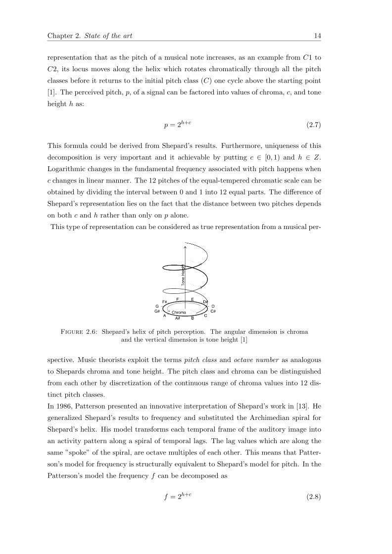
respectively. Figure 2.6 shows an illustration of this helix. It can be observed in this
Chapter 2. State of the art 14
representation that as the pitch of a musical note increases, as an example from C1 to
C2, its locus moves along the helix which rotates chromatically through all the pitch
classes before it returns to the initial pitch class (C) one cycle above the starting point
[1]. The perceived pitch, p, of a signal can be factored into values of chroma, c, and tone
height h as:
p = 2h+c (2.7)
This formula could be derived from Shepard’s results. Furthermore, uniqueness of this
decomposition is very important and it achievable by putting c ∈ [0, 1) and h ∈ Z.
Logarithmic changes in the fundamental frequency associated with pitch happens when
c changes in linear manner. The 12 pitches of the equal-tempered chromatic scale can be
obtained by dividing the interval between 0 and 1 into 12 equal parts. The difference of
Shepard’s representation lies on the fact that the distance between two pitches depends
on both c and h rather than only on p alone.
This type of representation can be considered as true representation from a musical per-
Figure 2.6: Shepard’s helix of pitch perception. The angular dimension is chromaand the vertical dimension is tone height [1]
spective. Music theorists exploit the terms pitch class and octave number as analogous
to Shepards chroma and tone height. The pitch class and chroma can be distinguished
from each other by discretization of the continuous range of chroma values into 12 dis-
tinct pitch classes.
In 1986, Patterson presented an innovative interpretation of Shepard’s work in [13]. He
generalized Shepard’s results to frequency and substituted the Archimedian spiral for
Shepard’s helix. His model transforms each temporal frame of the auditory image into
an activity pattern along a spiral of temporal lags. The lag values which are along the
same ”spoke” of the spiral, are octave multiples of each other. This means that Patter-
son’s model for frequency is structurally equivalent to Shepard’s model for pitch. In the
Patterson’s model the frequency f can be decomposed as
f = 2h+c (2.8)
Chapter 2. State of the art 15
where the restrictions for c and h are the same as Shepard’s model. In another way,
chroma from a given frequency can be calculated as
c = log2 f − blog2 fc (2.9)
where b.c denotes the greatest integer function. Therefore, chroma is the fractional part
of the base-2 logarithm of frequency. Some frequencies in this system share the same
chroma class if and only if they are mapped into the same value of c. This is similar to
the idea of pitch. Consequently, 220, 440 and 880 Hz all share the same chroma class as
110 Hz, but 330 Hz does not.
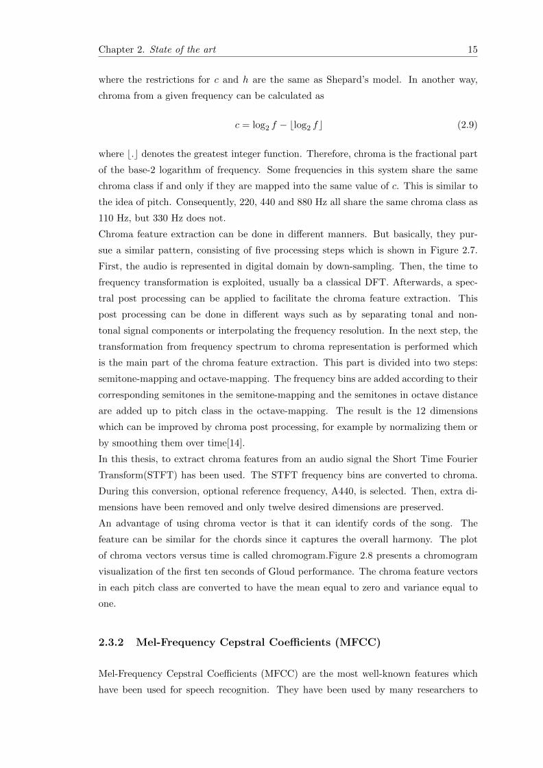
Chroma feature extraction can be done in different manners. But basically, they pur-
sue a similar pattern, consisting of five processing steps which is shown in Figure 2.7.
First, the audio is represented in digital domain by down-sampling. Then, the time to
frequency transformation is exploited, usually ba a classical DFT. Afterwards, a spec-
tral post processing can be applied to facilitate the chroma feature extraction. This
post processing can be done in different ways such as by separating tonal and non-
tonal signal components or interpolating the frequency resolution. In the next step, the
transformation from frequency spectrum to chroma representation is performed which
is the main part of the chroma feature extraction. This part is divided into two steps:
semitone-mapping and octave-mapping. The frequency bins are added according to their
corresponding semitones in the semitone-mapping and the semitones in octave distance
are added up to pitch class in the octave-mapping. The result is the 12 dimensions
which can be improved by chroma post processing, for example by normalizing them or
by smoothing them over time[14].
In this thesis, to extract chroma features from an audio signal the Short Time Fourier
Transform(STFT) has been used. The STFT frequency bins are converted to chroma.
During this conversion, optional reference frequency, A440, is selected. Then, extra di-
mensions have been removed and only twelve desired dimensions are preserved.
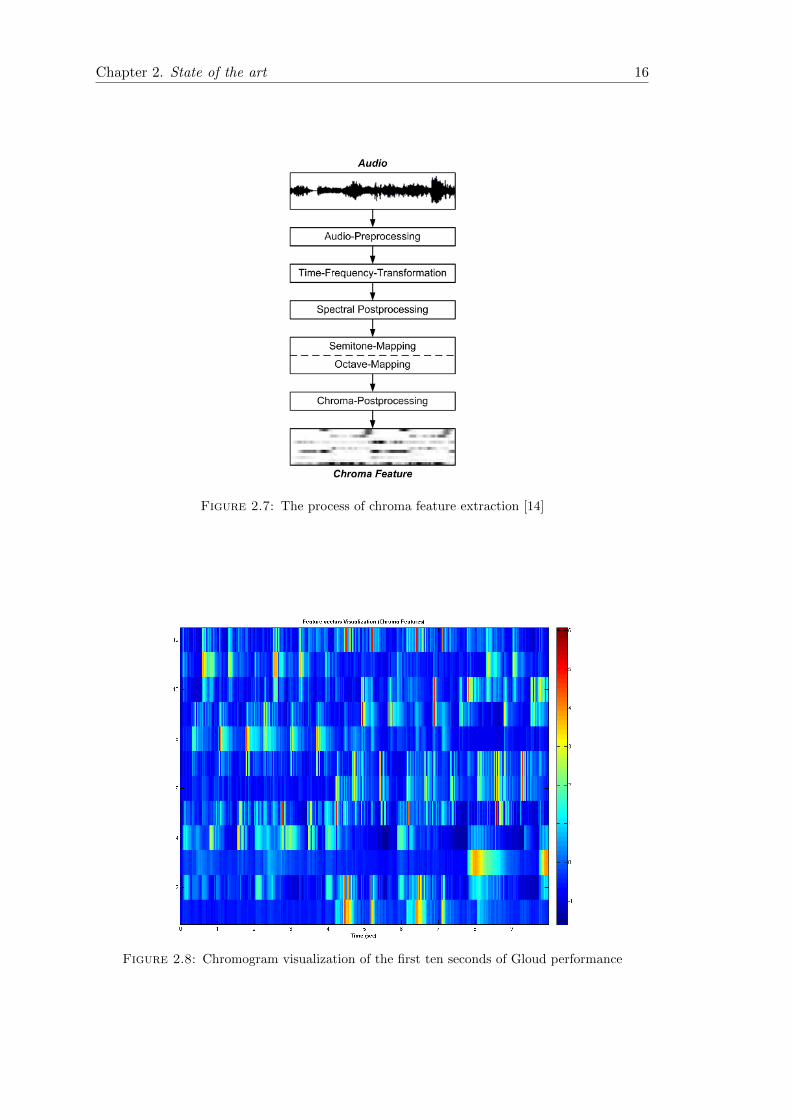
An advantage of using chroma vector is that it can identify cords of the song. The
feature can be similar for the chords since it captures the overall harmony. The plot
of chroma vectors versus time is called chromogram.Figure 2.8 presents a chromogram
visualization of the first ten seconds of Gloud performance. The chroma feature vectors
in each pitch class are converted to have the mean equal to zero and variance equal to
one.
2.3.2 Mel-Frequency Cepstral Coefficients (MFCC)
Mel-Frequency Cepstral Coefficients (MFCC) are the most well-known features which
have been used for speech recognition. They have been used by many researchers to
Chapter 2. State of the art 16
Figure 2.7: The process of chroma feature extraction [14]
Figure 2.8: Chromogram visualization of the first ten seconds of Gloud performance
Chapter 2. State of the art 17
model music and audio signals. Foote in [15] represented a retrieval system which is
built based on cepstral representation of audio signals. Logan and Chu in [16], pre-
sented a music summarization system based on cepstral features. Also, Blum in [17],
listed MFCCs as one of the features in his retrieval system.
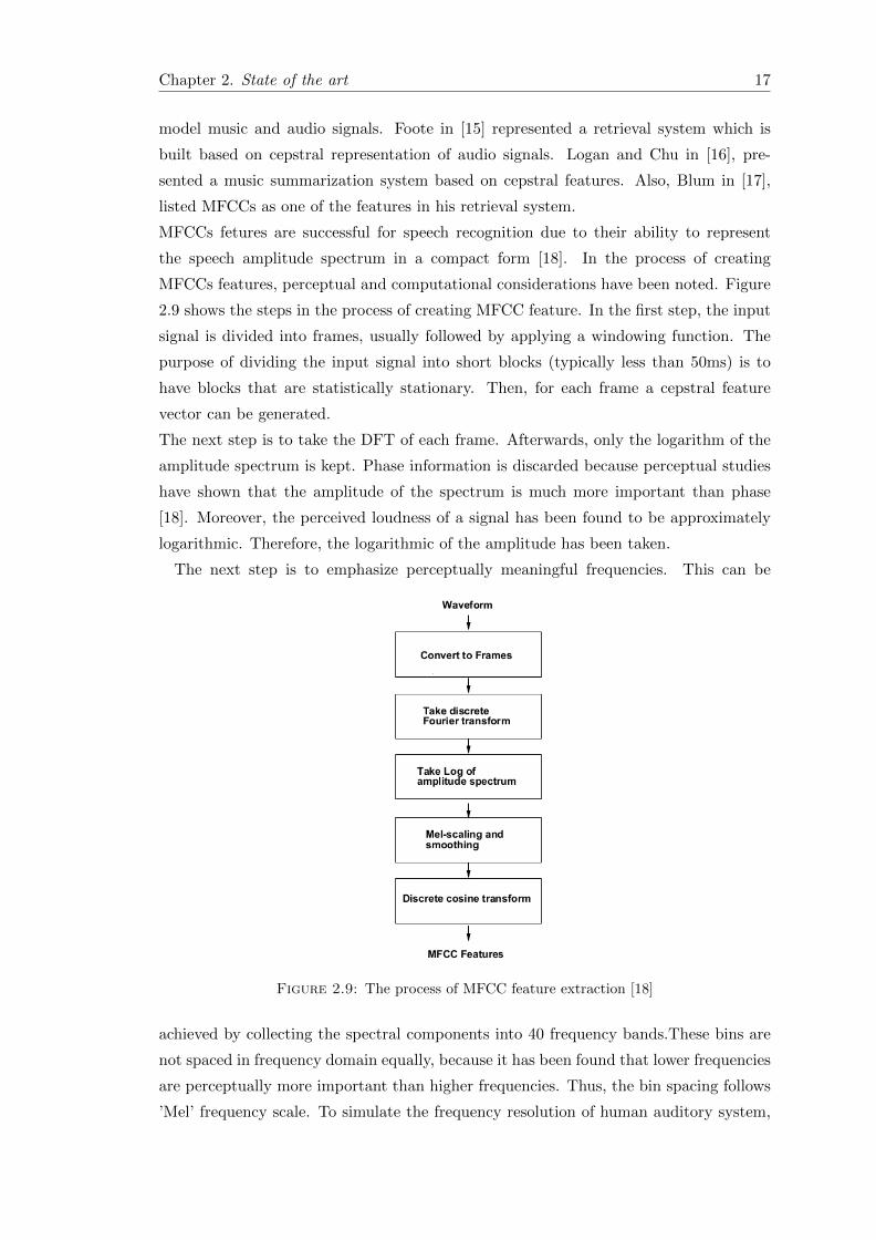
MFCCs fetures are successful for speech recognition due to their ability to represent
the speech amplitude spectrum in a compact form [18]. In the process of creating
MFCCs features, perceptual and computational considerations have been noted. Figure
2.9 shows the steps in the process of creating MFCC feature. In the first step, the input
signal is divided into frames, usually followed by applying a windowing function. The
purpose of dividing the input signal into short blocks (typically less than 50ms) is to
have blocks that are statistically stationary. Then, for each frame a cepstral feature
vector can be generated.
The next step is to take the DFT of each frame. Afterwards, only the logarithm of the
amplitude spectrum is kept. Phase information is discarded because perceptual studies
have shown that the amplitude of the spectrum is much more important than phase
[18]. Moreover, the perceived loudness of a signal has been found to be approximately
logarithmic. Therefore, the logarithmic of the amplitude has been taken.
The next step is to emphasize perceptually meaningful frequencies. This can be
Figure 2.9: The process of MFCC feature extraction [18]
achieved by collecting the spectral components into 40 frequency bands.These bins are
not spaced in frequency domain equally, because it has been found that lower frequencies
are perceptually more important than higher frequencies. Thus, the bin spacing follows
’Mel’ frequency scale. To simulate the frequency resolution of human auditory system,
Chapter 2. State of the art 18
which has high resolution in low-frequency and low resolution in high frequency of the
spectrum of any sound, we can use the mel frequency scale. This transformation can be
done by:
fmel(f) = 2595 log(1 +f
700Hz) (2.10)
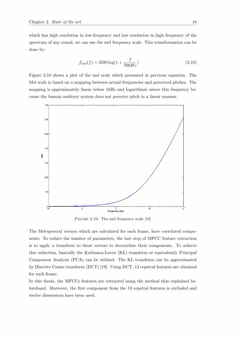
Figure 2.10 shows a plot of the mel scale which presented in previous equation. The
Mel scale is based on a mapping between actual frequencies and perceived pitches. The
mapping is approximately linear below 1kHz and logarithmic above this frequency be-
cause the human auditory system does not perceive pitch in a linear manner.
Figure 2.10: The mel frequency scale [18]
The Mel-spectral vectors which are calculated for each frame, have correlated compo-
nents. To reduce the number of parameters, the last step of MFCC feature extraction
is to apply a transform to these vectors to decorrelate their components. To achieve
this reduction, basically the Karhunen-Loeve (KL) transform or equivalently Principal
Component Analysis (PCA) can be utilized. The KL transform can be approximated
by Discrete Cosine transform (DCT) [19]. Using DCT, 13 cepstral features are obtained
for each frame.
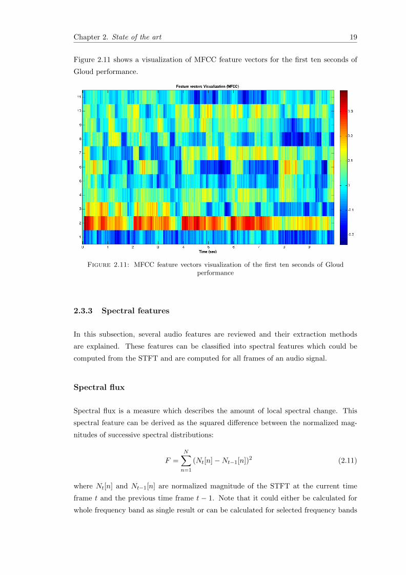
In this thesis, the MFCCs features are extracted using the method that explained be-
forehand. Moreover, the first component from the 13 cepstral features is excluded and
twelve dimensions have been used.
Chapter 2. State of the art 19
Figure 2.11 shows a visualization of MFCC feature vectors for the first ten seconds of
Gloud performance.
Figure 2.11: MFCC feature vectors visualization of the first ten seconds of Gloudperformance
2.3.3 Spectral features
In this subsection, several audio features are reviewed and their extraction methods
are explained. These features can be classified into spectral features which could be
computed from the STFT and are computed for all frames of an audio signal.
Spectral flux
Spectral flux is a measure which describes the amount of local spectral change. This
spectral feature can be derived as the squared difference between the normalized mag-
nitudes of successive spectral distributions:
F =
N∑n=1
(Nt[n]−Nt−1[n])2 (2.11)
where Nt[n] and Nt−1[n] are normalized magnitude of the STFT at the current time
frame t and the previous time frame t − 1. Note that it could either be calculated for
whole frequency band as single result or can be calculated for selected frequency bands
Chapter 2. State of the art 20
individually. In this thesis, three bands have been selected. Therefore, the result for
each frame is a dimensional vector.
Spectral Centroid
Spectral centroid is a measure which is defined as center of gravity of the magnitude
spectrum of the STFT:
F =
∑Nn=1 n|Mt[n]|2∑Nn=1 |Mt[n]|2
(2.12)
where Mt[n] is the magnitude of the STFT at frame t and frequency bin n. The centroid
is a measure of spectral shape. This spectral feature could also be represented in three
dimensions.
Spectral spread
Spectral spread is a measure of bandwidth of a spectrum and can be derived as:
F =
∑Nn=1 (n− Fsc)
2|Mt[n]|∑Nn=1 |Mt[n]|
(2.13)
where Fsc is feature extracted from spectral centroid. In this thesis, three sub-bands
have been used for calculation of this measure.
Spectral flatness
Spectral flatness is also called the tonality coefficient. It shows how much a sound
frame is similar to a tone or similar to a noise. Here, the tone can be defined as the
amount of peaks or resonant structure in a power spectrum. On the other hand, the
noise corresponds to flat spectrum of a white noise. A high value of spectral flatness
shows that the spectrum has a similar amount of power in all spectral bands i.e. this
frame could be considered as noise. The spectral flatness is calculated by dividing the
geometric mean of the power spectrum by the arithmetic mean of the power spectrum:
F =
3
√∏Nn=1Mt[n]∑Nn=1 Mt[n]
N
(2.14)
This measurement can be represented in different sub-bands instead of the whole band.
Chapter 2. State of the art 21
2.3.4 Combination of spectral features
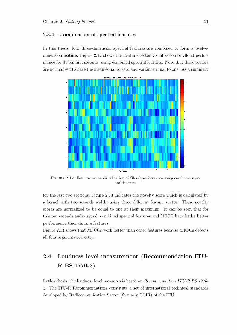
In this thesis, four three-dimension spectral features are combined to form a twelve-
dimension feature. Figure 2.12 shows the Feature vector visualization of Gloud perfor-
mance for its ten first seconds, using combined spectral features. Note that these vectors
are normalized to have the mean equal to zero and variance equal to one. As a summary
Figure 2.12: Feature vector visualization of Gloud performance using combined spec-tral features
for the last two sections, Figure 2.13 indicates the novelty score which is calculated by
a kernel with two seconds width, using three different feature vector. These novelty
scores are normalized to be equal to one at their maximum. It can be seen that for
this ten seconds audio signal, combined spectral features and MFCC have had a better
performance than chroma features.
Figure 2.13 shows that MFCCs work better than other features because MFFCs detects
all four segments correctly.
2.4 Loudness level measurement (Recommendation ITU-
R BS.1770-2)
In this thesis, the loudness level measures is based on Recommendation ITU-R BS.1770-
2. The ITU-R Recommendations constitute a set of international technical standards
developed by Radiocomunication Sector (formerly CCIR) of the ITU.
Chapter 2. State of the art 22
Figure 2.13: Novelty score calculation by using three different feature vectors
The Recommendation ITU-R BS.1770-2 specifies audio measurement methods to deter-
mine subjective program loudness level. This recommendation considers:
• that modern digital sound transmission techniques are available in a widely dy-
namic range;
• that modern digital sound transmission and production techniques are available
as a mixture of mono, stereo, and multichannel formats;
• that listeners desire subjective loudness level of audio programs to be uniform for
different program types and sources;
• that, for the purpose of loudness level control, in order to reduce audience annoy-
ance, having a single recommended algorithm for objective estimation of subjective
loudness level is essential.
Therefore, this recommendation offers a multichannel loudness level measurement mod-
eling algorithm. The algorithm consists of four steps:
• ’K’ frequency weighting
• mean square calculation for each channel
• channel-weighted summation
• gating
Chapter 2. State of the art 23
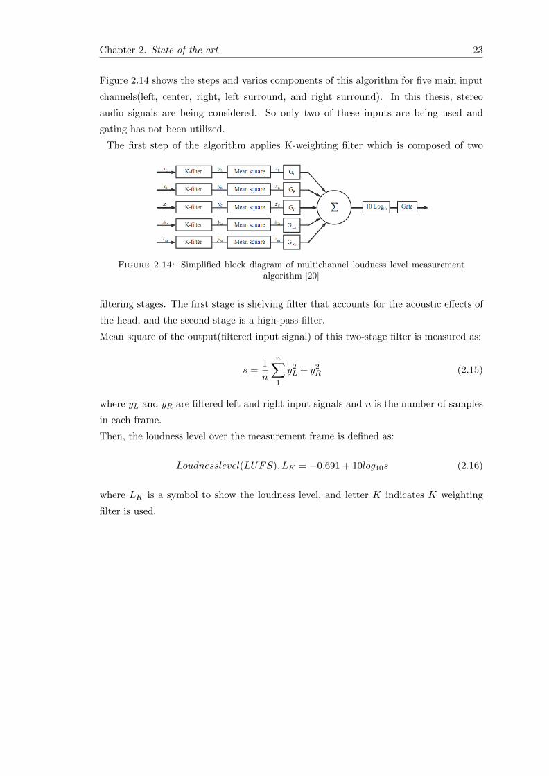
Figure 2.14 shows the steps and varios components of this algorithm for five main input
channels(left, center, right, left surround, and right surround). In this thesis, stereo
audio signals are being considered. So only two of these inputs are being used and
gating has not been utilized.
The first step of the algorithm applies K-weighting filter which is composed of two
Figure 2.14: Simplified block diagram of multichannel loudness level measurementalgorithm [20]
filtering stages. The first stage is shelving filter that accounts for the acoustic effects of
the head, and the second stage is a high-pass filter.
Mean square of the output(filtered input signal) of this two-stage filter is measured as:
s =1
n
n∑1
y2L + y2R (2.15)
where yL and yR are filtered left and right input signals and n is the number of samples
in each frame.
Then, the loudness level over the measurement frame is defined as:
Loudnesslevel(LUFS), LK = −0.691 + 10log10s (2.16)
where LK is a symbol to show the loudness level, and letter K indicates K weighting
filter is used.

Chapter 3
Audio segmentation
In this chapter, different characteristics of the Foote method have been studied. Various
parameters which could affect the Foote method’s performance have been considered.
Moreover, some modifications have been proposed in order to improve the results of
the Foote method. In each section, the reason behind proposed method and proposed
parameter variation in addition to the expected results are stated. Then, the obtained
results are presented and they are compared with the expected results.
In this thesis, three main types of items and their combination with each other have
been utilized. These three types of items are speeches, musics, and recorded audio from
broadcast radio channels. The combined items have 12s length and consist of two 6s
length parts. These 6s parts have been selected from the three mentioned main types
of items. Table 3.1 shows these different combination of items and the abbreviation of
that have been used in this thesis.
We are interested to find the segment boundary correctly and also want to reduce
the number of false segment boundaries which are detected in the audio segmentation
procedure.
Combination Abbreviation
Music-Music MM
Speech-Speech SS
Broadcast-Broadcast BB
Music-Speech MS
Music-Broadcast MB
Speech-Music SM
Speech-Broadcast SB
Broadcast-Music BM
Broadcast-Speech BS
Table 3.1: Different kinds of audio combinations
25
Chapter 3. Audio segmentation and real time loudness level compensation 26
3.1 Parameter settings in the Foote method
In this section, the impact of four different parameters on the Foote method are pre-
sented. The kernel time is one of these parameters. According to the Foote method,
one could expect larger kernel times tend to detect longer novel events while the smaller
kernel time detects novelty on a short time scale. Secondly, the size of each frame have
an effect on the time resolution. It can be anticipated that the smaller frames have more
time resolution and increase the accuracy of short novel events. On the other hand, the
larger frames tend to ignore changes in short intervals and perform better in detection
of long novel events.
Distance measure could be considered as a third parameter in the Foote method stud-
ies. One could expect that cosine metric distance which does not depend on the vectors
magnitude may have a better performance. Finally, the kind of feature vectors that use
in the Foote method have a great impact on the final segmentation results. The MFCCs
could work better on items containing speech parts while chroma vectors could have a
better performance on items containing music parts.
3.1.1 Kernel time
For calculation of a novelty at an instant in an audio signal, the Foote method needs
to use the information equal to half of the kernel time before the instant and after the
instant. Thus, in order to measure the novelty of an instant in an audio signal, we would
have a delay which is equal to the half of the kernel time in an ideal situation (if we
ignore the computation time).
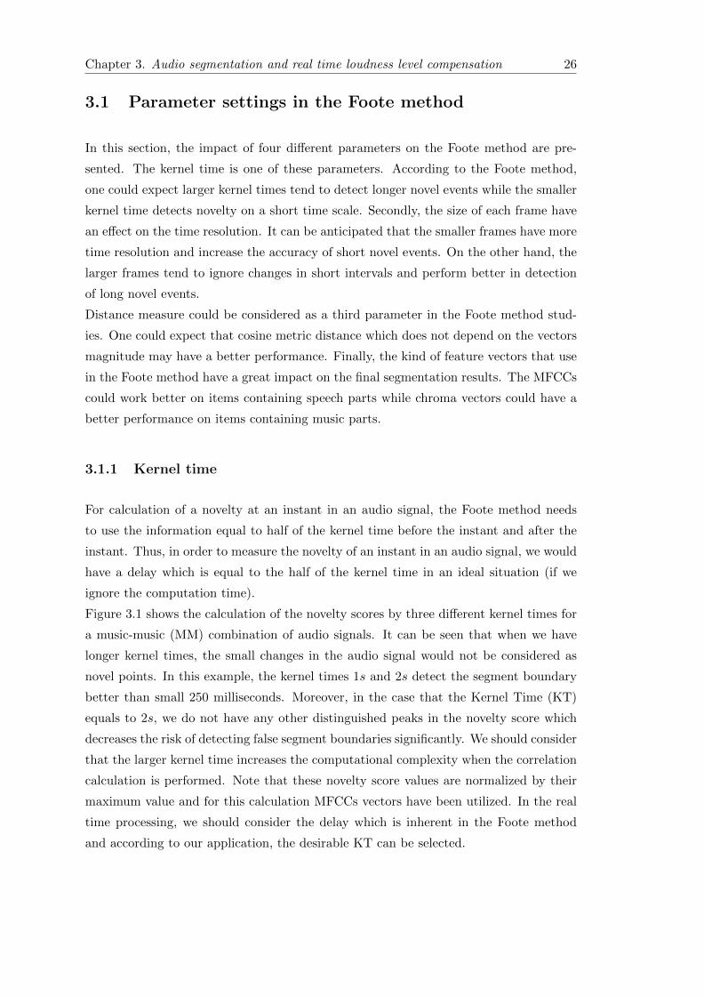
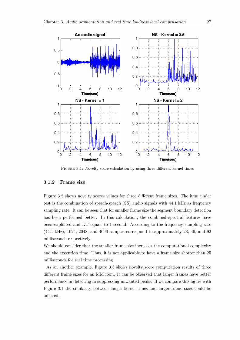
Figure 3.1 shows the calculation of the novelty scores by three different kernel times for
a music-music (MM) combination of audio signals. It can be seen that when we have
longer kernel times, the small changes in the audio signal would not be considered as
novel points. In this example, the kernel times 1s and 2s detect the segment boundary
better than small 250 milliseconds. Moreover, in the case that the Kernel Time (KT)
equals to 2s, we do not have any other distinguished peaks in the novelty score which
decreases the risk of detecting false segment boundaries significantly. We should consider
that the larger kernel time increases the computational complexity when the correlation
calculation is performed. Note that these novelty score values are normalized by their
maximum value and for this calculation MFCCs vectors have been utilized. In the real
time processing, we should consider the delay which is inherent in the Foote method
and according to our application, the desirable KT can be selected.
Chapter 3. Audio segmentation and real time loudness level compensation 27
Figure 3.1: Novelty score calculation by using three different kernel times
3.1.2 Frame size
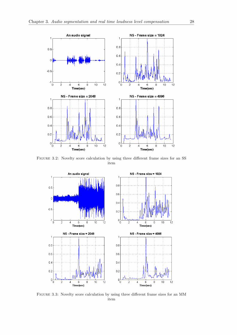
Figure 3.2 shows novelty scores values for three different frame sizes. The item under
test is the combination of speech-speech (SS) audio signals with 44.1 kHz as frequency
sampling rate. It can be seen that for smaller frame size the segment boundary detection
has been performed better. In this calculation, the combined spectral features have
been exploited and KT equals to 1 second. According to the frequency sampling rate
(44.1 kHz), 1024, 2048, and 4096 samples correspond to approximately 23, 46, and 92
milliseconds respectively.
We should consider that the smaller frame size increases the computational complexity
and the execution time. Thus, it is not applicable to have a frame size shorter than 25
milliseconds for real time processing.
As an another example, Figure 3.3 shows novelty score computation results of three
different frame sizes for an MM item. It can be observed that larger frames have better
performance in detecting in suppressing unwanted peaks. If we compare this figure with
Figure 3.1 the similarity between longer kernel times and larger frame sizes could be
inferred.
Chapter 3. Audio segmentation and real time loudness level compensation 28
Figure 3.2: Novelty score calculation by using three different frame sizes for an SSitem
Figure 3.3: Novelty score calculation by using three different frame sizes for an MMitem

Chapter 3. Audio segmentation and real time loudness level compensation 29
3.1.3 Distance measure
Figure 3.4 shows three calculated novelty scores for an MM(music-music combination)
audio signal. It can be observed that the novelty values for the case Manhattan distance
measure are relatively large. This occurs because the range of distance measures using
Manhattan distance measure are larger than Ecludian and cosine metric distance mea-
sure and these larger values result in larger novelty scores. Moreover, it can be seen for
this item the cosine metric distance measure performed better because the real segment
boundary’s novelty score for this case is relatively larger than the second important
peak.
Figure 3.4: Novelty score calculation by using three different distance measures
One way to normalize these distance measures is to transform them to the range of
between 0 and 1. The cosine metric which is originally between −1 and 1 can be trans-
formed as:
DCnew ≡ eDC−1 (3.1)
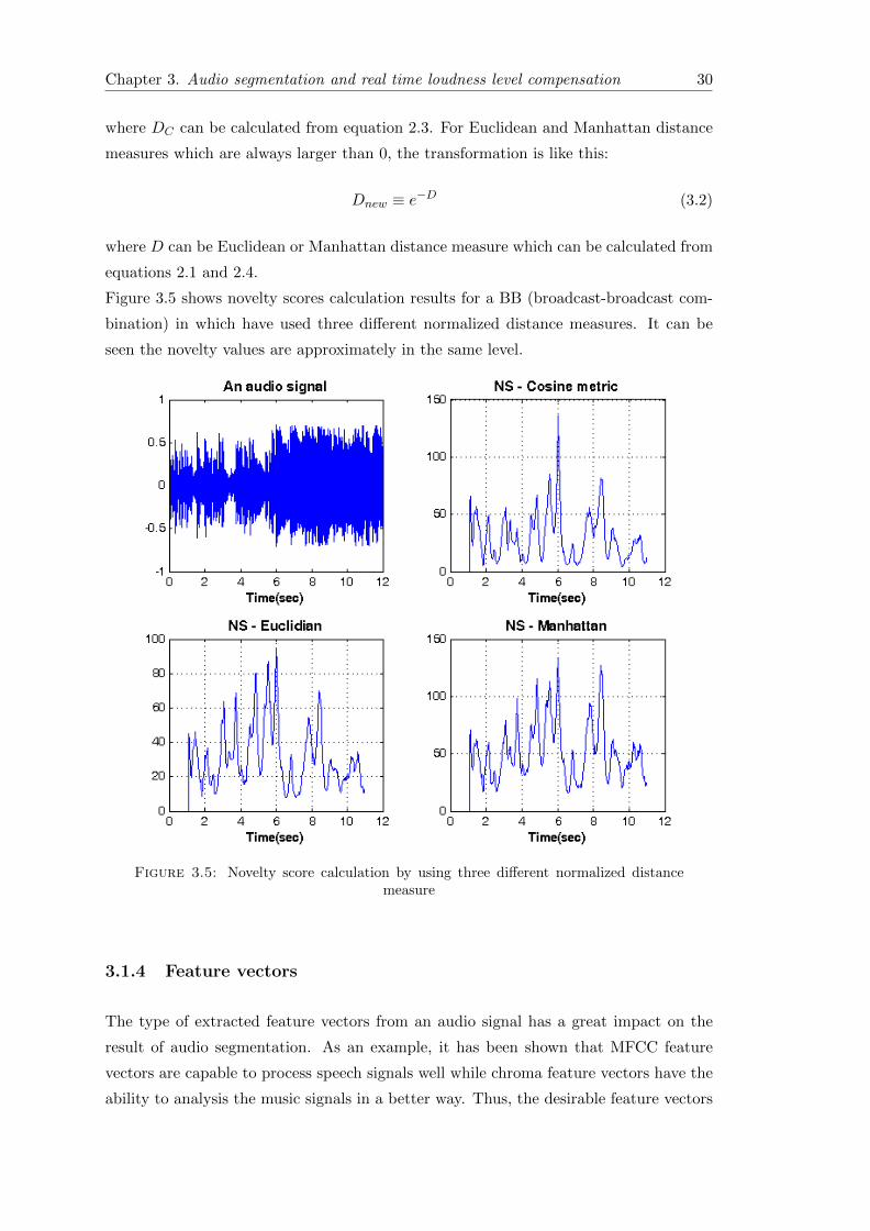
Chapter 3. Audio segmentation and real time loudness level compensation 30
where DC can be calculated from equation 2.3. For Euclidean and Manhattan distance
measures which are always larger than 0, the transformation is like this:
Dnew ≡ e−D (3.2)
where D can be Euclidean or Manhattan distance measure which can be calculated from
equations 2.1 and 2.4.
Figure 3.5 shows novelty scores calculation results for a BB (broadcast-broadcast com-
bination) in which have used three different normalized distance measures. It can be
seen the novelty values are approximately in the same level.
Figure 3.5: Novelty score calculation by using three different normalized distancemeasure
3.1.4 Feature vectors
The type of extracted feature vectors from an audio signal has a great impact on the
result of audio segmentation. As an example, it has been shown that MFCC feature
vectors are capable to process speech signals well while chroma feature vectors have the
ability to analysis the music signals in a better way. Thus, the desirable feature vectors
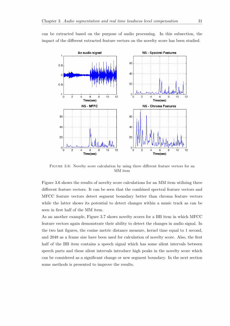
Chapter 3. Audio segmentation and real time loudness level compensation 31
can be extracted based on the purpose of audio processing. In this subsection, the
impact of the different extracted feature vectors on the novelty score has been studied.
Figure 3.6: Novelty score calculation by using three different feature vectors for anMM item
Figure 3.6 shows the results of novelty score calculations for an MM item utilizing three
different feature vectors. It can be seen that the combined spectral feature vectors and
MFCC feature vectors detect segment boundary better than chroma feature vectors
while the latter shows its potential to detect changes within a music track as can be
seen in first half of the MM item.
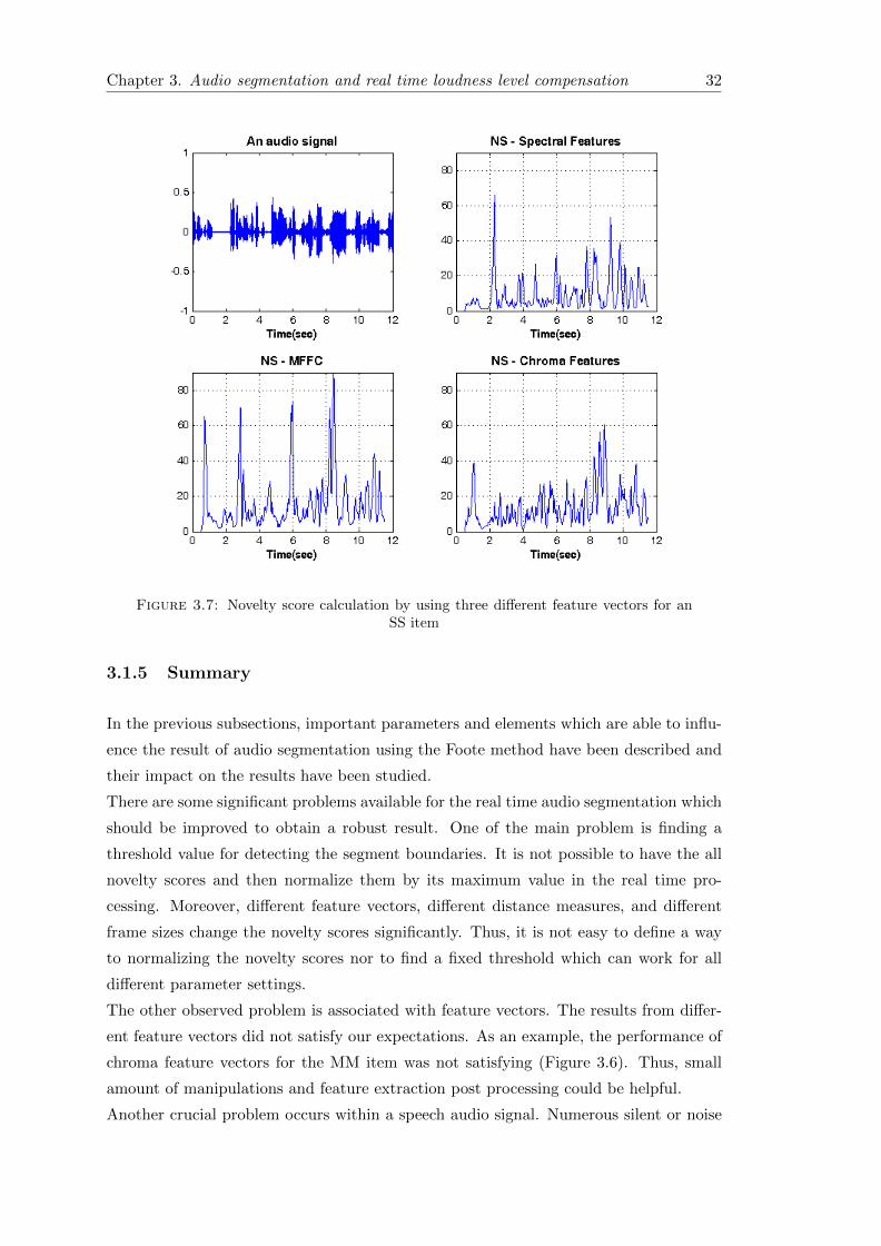
As an another example, Figure 3.7 shows novelty scores for a BB item in which MFCC
feature vectors again demonstrate their ability to detect the changes in audio signal. In
the two last figures, the cosine metric distance measure, kernel time equal to 1 second,
and 2048 as a frame size have been used for calculation of novelty score. Also, the first
half of the BB item contains a speech signal which has some silent intervals between
speech parts and these silent intervals introduce high peaks in the novelty score which
can be considered as a significant change or new segment boundary. In the next section
some methods is presented to improve the results.
Chapter 3. Audio segmentation and real time loudness level compensation 32
Figure 3.7: Novelty score calculation by using three different feature vectors for anSS item
3.1.5 Summary
In the previous subsections, important parameters and elements which are able to influ-
ence the result of audio segmentation using the Foote method have been described and
their impact on the results have been studied.
There are some significant problems available for the real time audio segmentation which
should be improved to obtain a robust result. One of the main problem is finding a
threshold value for detecting the segment boundaries. It is not possible to have the all
novelty scores and then normalize them by its maximum value in the real time pro-
cessing. Moreover, different feature vectors, different distance measures, and different
frame sizes change the novelty scores significantly. Thus, it is not easy to define a way
to normalizing the novelty scores nor to find a fixed threshold which can work for all
different parameter settings.
The other observed problem is associated with feature vectors. The results from differ-
ent feature vectors did not satisfy our expectations. As an example, the performance of
chroma feature vectors for the MM item was not satisfying (Figure 3.6). Thus, small
amount of manipulations and feature extraction post processing could be helpful.
Another crucial problem occurs within a speech audio signal. Numerous silent or noise
Chapter 3. Audio segmentation and real time loudness level compensation 33
intervals occurs during a speech signal and these combination of silent intervals and
speech intervals introduce high peaks in the novelty score. Thus, the false detection
increases and the real segment boundary detection gets hard.
Finally, it can be mentioned that our expectations about the impacts of kernel time,
frame size, and distance measure correspond to the obtained result. Note that it is not
a wise manner to look into the obtained results item by item. Therefore, an evaluation
which could measures the performance of segmentation for large set of data is needed.
This evaluation is presented in chapter four.
3.2 Proposed methods to improve the Foote method
In the last part of previous section, it has been stated some problems of the segmentation
procedure in the Foote method. In this section some ideas proposed to solve these
problems. One idea could be smoothing the STFT that is used in extracting feature
vectors. This smoothing could make the adjacent frames similar to each other that
may reduce unwanted high peaks within an audio track. The second modification could
be an application of model-based normalization technique on each dimension of feature
vectors. Mean and variance are two statistical properties that can be considered in this
normalization.
Furthermore, in this section two ideas are presented to reduce the unwanted segment
boundaries detection within a music or speech track. The first one is based on detection
of abrupt decrease of loudness level within an audio track and set the novelty score
corresponding to this instant as minimum. These instants are potential to be detected
as segment boundaries. The second one, could be normalizing the distance between
frames by their loudness levels. This modification may help considering the distance of
silent or noise frames as zero or near to zero. Thus, the distance of silent intervals to
any frames would be considered as minimum, i.e. these frames could be ignored during
the segmentation procedure.
3.2.1 Feature vectors manipulation
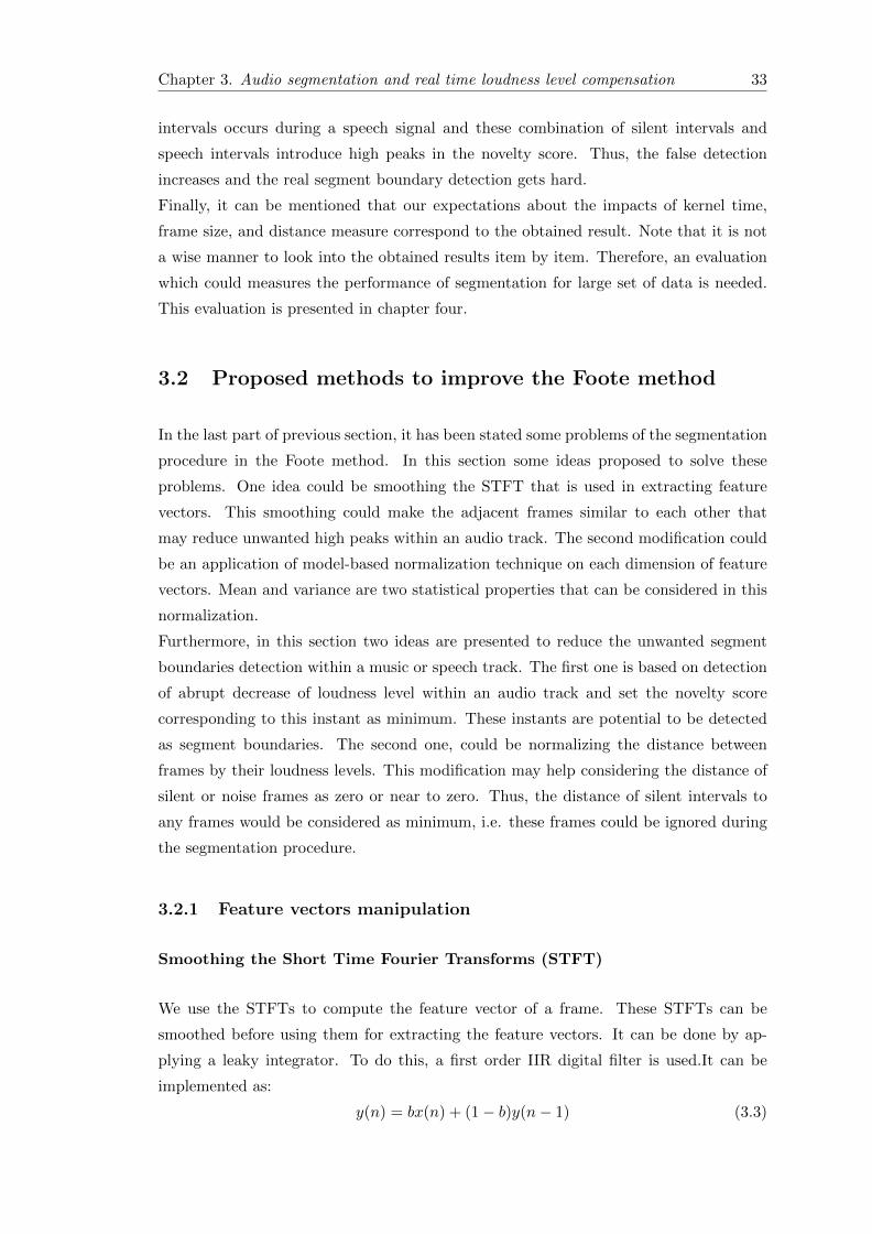
Smoothing the Short Time Fourier Transforms (STFT)
We use the STFTs to compute the feature vector of a frame. These STFTs can be
smoothed before using them for extracting the feature vectors. It can be done by ap-
plying a leaky integrator. To do this, a first order IIR digital filter is used.It can be
implemented as:
y(n) = bx(n) + (1− b)y(n− 1) (3.3)
Chapter 3. Audio segmentation and real time loudness level compensation 34
where y(n− 1) is the previous feature vector and b is the leaky coefficient.
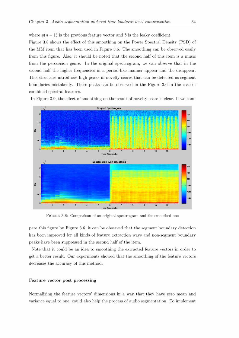
Figure 3.8 shows the effect of this smoothing on the Power Spectral Density (PSD) of
the MM item that has been used in Figure 3.6. The smoothing can be observed easily
from this figure. Also, it should be noted that the second half of this item is a music
from the percussion genre. In the original spectrogram, we can observe that in the
second half the higher frequencies in a period-like manner appear and the disappear.
This structure introduces high peaks in novelty scores that can be detected as segment
boundaries mistakenly. These peaks can be observed in the Figure 3.6 in the case of
combined spectral features.
In Figure 3.9, the effect of smoothing on the result of novelty score is clear. If we com-
Figure 3.8: Comparison of an original spectrogram and the smoothed one
pare this figure by Figure 3.6, it can be observed that the segment boundary detection
has been improved for all kinds of feature extraction ways and non-segment boundary
peaks have been suppressed in the second half of the item.
Note that it could be an idea to smoothing the extracted feature vectors in order to
get a better result. Our experiments showed that the smoothing of the feature vectors
decreases the accuracy of this method.
Feature vector post processing
Normalizing the feature vectors’ dimensions in a way that they have zero mean and
variance equal to one, could also help the process of audio segmentation. To implement
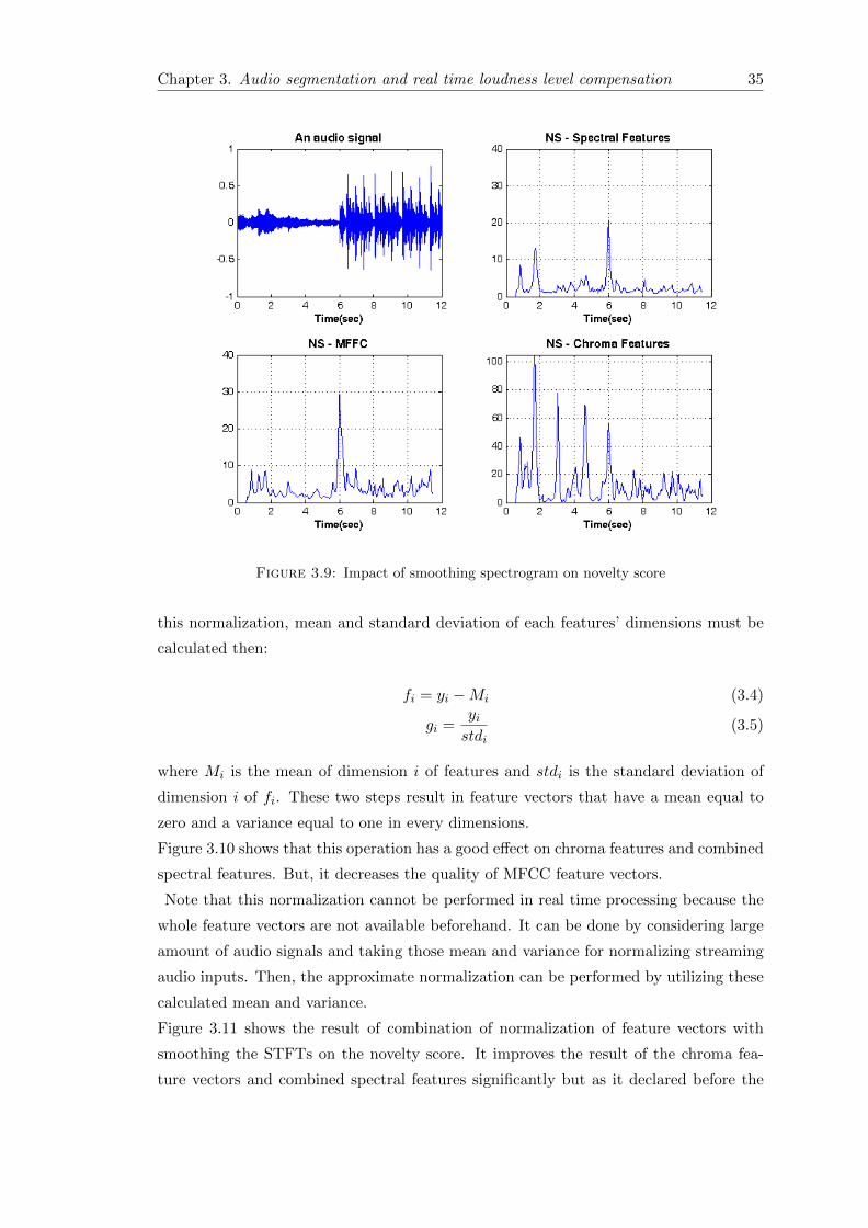
Chapter 3. Audio segmentation and real time loudness level compensation 35
Figure 3.9: Impact of smoothing spectrogram on novelty score
this normalization, mean and standard deviation of each features’ dimensions must be
calculated then:
fi = yi −Mi (3.4)
gi =yistdi
(3.5)
where Mi is the mean of dimension i of features and stdi is the standard deviation of
dimension i of fi. These two steps result in feature vectors that have a mean equal to
zero and a variance equal to one in every dimensions.
Figure 3.10 shows that this operation has a good effect on chroma features and combined
spectral features. But, it decreases the quality of MFCC feature vectors.
Note that this normalization cannot be performed in real time processing because the
whole feature vectors are not available beforehand. It can be done by considering large
amount of audio signals and taking those mean and variance for normalizing streaming
audio inputs. Then, the approximate normalization can be performed by utilizing these
calculated mean and variance.
Figure 3.11 shows the result of combination of normalization of feature vectors with
smoothing the STFTs on the novelty score. It improves the result of the chroma fea-
ture vectors and combined spectral features significantly but as it declared before the
Chapter 3. Audio segmentation and real time loudness level compensation 36
Figure 3.10: Impact of normalization of feature vectors on novelty score
Figure 3.11: Impact of feature vectors manipulation on novelty score
Chapter 3. Audio segmentation and real time loudness level compensation 37
normalization does not have good effect on MFCC feature vectors. The same result oc-
curred for other different types of items. Thus, in the following sections in this chapter
the novelty scores are calculated using chroma vectors and combined spectral features
which are normalized and the STFTs are smoothed before features extraction. But,
when MFCC feature vectors are used only the STFTs are filtered before extraction of
the feature vectors.
3.2.2 Relative silent detection
We may encounter many silent intervals during a single speaker speech signal or during
a conversation between two or more people. In these cases the loudness level decreases
abruptly and increases to the previous level again. These abrupt changes in the audio
signal could introduce unwanted high peaks in the novelty score which increases the
number of false segment boundaries detection. Thus, we are interested to find a simple
way which could help us to detect these silent intervals and remove the corresponding
high peaks from novelty score. Note that the procedure of silent detection is not a simple
task and it is beyond of the scope of this thesis. In the next subsections we introduce
some simple ways to overcome this problem.
Fixed threshold for loudness level
In addition to feature vector extraction, the loudness level of the each frame of an audio
signal can be computed. Then, a fixed threshold can be defined to simply decide that
if a frame is silent or not. Then, the novelty scores computation performs based on this
decision. If a frame detected as a non-silent frame, the novelty score will be computed
normally. In the case of silent frame, a zero value will be assigned to the novelty score
of this instant.
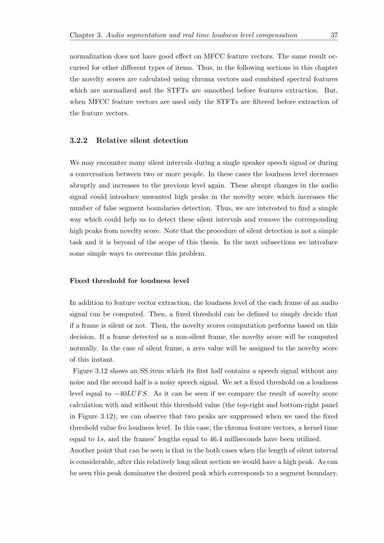
Figure 3.12 shows an SS item which its first half contains a speech signal without any
noise and the second half is a noisy speech signal. We set a fixed threshold on a loudness
level equal to −40LUFS. As it can be seen if we compare the result of novelty score
calculation with and without this threshold value (the top-right and bottom-right panel
in Figure 3.12), we can observe that two peaks are suppressed when we used the fixed
threshold value fro loudness level. In this case, the chroma feature vectors, a kernel time
equal to 1s, and the frames’ lengths equal to 46.4 milliseconds have been utilized.
Another point that can be seen is that in the both cases when the length of silent interval
is considerable, after this relatively long silent section we would have a high peak. As can
be seen this peak dominates the desired peak which corresponds to a segment boundary.
Chapter 3. Audio segmentation and real time loudness level compensation 38
Figure 3.12: Impact of fixed threshold silent detection on novelty score
Adaptive threshold for loudness level
In the previous subsection, we presented a simple way that could remove some false
boundary detections. One way to improve the previous manner is that to have an
adaptive threshold for loudness level based on average of the loudness level over a limited
period of time. Thus, if the loudness level of a frame is less than the average of previous
loudness levels (say 1 second) then this frame will be considered as silent frame and its
corresponding novelty score will be considered as 0.
Furthermore, the decided silent frames would not contribute in the computation of
novelty score. It means that when a frame considered as a silent frame the algorithm
will ignore this frame and assumes that no new frame arrives at this instant. As an
example, if we encounter twenty subsequent silent frames, the algorithm would go into
an standby mode an wait for a non-silent frame to update the self-similarity matrix and
to compute a new novelty score.
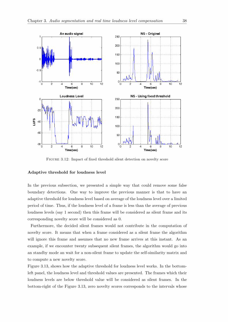
Figure 3.13, shows how the adaptive threshold for loudness level works. In the bottom-
left panel, the loudness level and threshold values are presented. The frames which their
loudness levels are below threshold value will be considered as silent frames. In the
bottom-right of the Figure 3.13, zero novelty scores corresponds to the intervals whose
Chapter 3. Audio segmentation and real time loudness level compensation 39
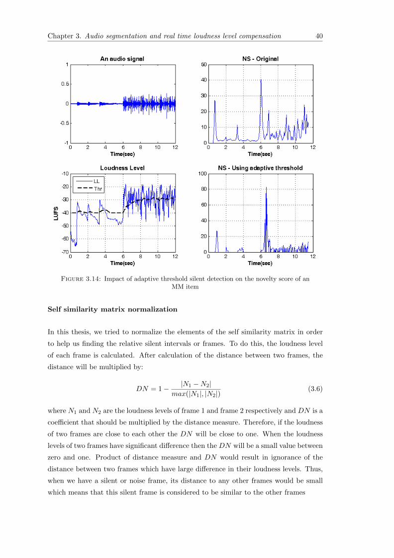
Figure 3.13: Impact of adaptive threshold silent detection on the novelty score of aSS item
loudness levels below the threshold curve. As can be seen, this modification has better
result than the fixed threshold for loudness level. In the latter case, local maximum
point in the novelty score which corresponds to real segment boundary at 6th second
is dominated by a high peak value. But, when adaptive threshold for loudness level is
used the boundary is distinguishable. Note that in the second half of this item, some
unwanted peaks are increased in value.
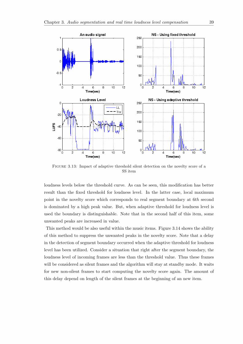
This method would be also useful within the music items. Figure 3.14 shows the ability
of this method to suppress the unwanted peaks in the novelty score. Note that a delay
in the detection of segment boundary occurred when the adaptive threshold for loudness
level has been utilized. Consider a situation that right after the segment boundary, the
loudness level of incoming frames are less than the threshold value. Thus these frames
will be considered as silent frames and the algorithm will stay at standby mode. It waits
for new non-silent frames to start computing the novelty score again. The amount of
this delay depend on length of the silent frames at the beginning of an new item.
Chapter 3. Audio segmentation and real time loudness level compensation 40
Figure 3.14: Impact of adaptive threshold silent detection on the novelty score of anMM item
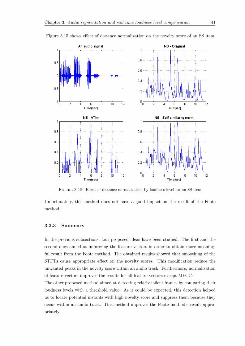
Self similarity matrix normalization
In this thesis, we tried to normalize the elements of the self similarity matrix in order
to help us finding the relative silent intervals or frames. To do this, the loudness level
of each frame is calculated. After calculation of the distance between two frames, the
distance will be multiplied by:
DN = 1− |N1 −N2|max(|N1|, |N2|)
(3.6)
where N1 and N2 are the loudness levels of frame 1 and frame 2 respectively and DN is a
coefficient that should be multiplied by the distance measure. Therefore, if the loudness
of two frames are close to each other the DN will be close to one. When the loudness
levels of two frames have significant difference then the DN will be a small value between
zero and one. Product of distance measure and DN would result in ignorance of the
distance between two frames which have large difference in their loudness levels. Thus,
when we have a silent or noise frame, its distance to any other frames would be small
which means that this silent frame is considered to be similar to the other frames
Chapter 3. Audio segmentation and real time loudness level compensation 41
Figure 3.15 shows effect of distance normalization on the novelty score of an SS item.
Figure 3.15: Effect of distance normalization by loudness level for an SS item
Unfortunately, this method does not have a good impact on the result of the Foote
method.
3.2.3 Summary
In the previous subsections, four proposed ideas have been studied. The first and the
second ones aimed at improving the feature vectors in order to obtain more meaning-
ful result from the Foote method. The obtained results showed that smoothing of the
STFTs cause appropriate effect on the novelty scores. This modification reduce the
unwanted peaks in the novelty score within an audio track. Furthermore, normalization
of feature vectors improves the results for all feature vectors except MFCCs.
The other proposed method aimed at detecting relative silent frames by comparing their
loudness levels with a threshold value. As it could be expected, this detection helped
us to locate potential instants with high novelty score and suppress them because they
occur within an audio track. This method improves the Foote method’s result appro-
priately.

Chapter 3. Audio segmentation and real time loudness level compensation 42
Finally, the idea of normalizing the distance between frames by their loudness level’s dif-
ferences has been proposed. The obtained results showed that this modification change
the result of novelty score slightly and does not improve it.
Chapter 4
Evaluation setup and results
4.1 Evaluation setup
The concatenated items that have been used in this chapter are selected according to
table 3.1 in chapter 3. These items are uncompressed audio files in PCM format, mono
channel, and with 44100Hz frequency sampling rate. Our experiments show that results
of mono channel audio files and stereo files are almost the same. Thus, one channel of
these items are used for reducing the processing time.
4.1.1 Block diagram
Figure 4.1 shows steps of the process of evaluation. First, it can be divided into two
processing parts: the process of the train set and the process of test set. The train
set items are selected from the same type as the test data but different items. The
same feature vectors will be extracted for these processes. Once features are available,
the novelty score of train set data can be calculated. Then, the average of maxima
that occur around the segment boundaries (half of a second before and after segment
boundary) will be computed. It can be used different ideas to set a threshold value for
test procedures. One way could be taking the average of these maxima and the other
way may be select a value which at least give us 50 percent success in detecting the
segment boundary points if the train set would be under the test. In this evaluation,
the later method has been exploited and the obtained threshold value has been used to
mark maximum points in the test procedure as segment boundaries or not. In the last
step, if one consider N as a number of segment boundaries, FN as the number of false
negatives (number of missed segment boundaries in the test procedure), and FP the
number of false positive (number of predicted non-segment boundary points), it can be
43

Chapter 4. Evaluation setup and results 44
written:
TP = N − FN (4.1)
Sensitivity(S) =TP
N(4.2)
Precision(P ) =TP
TP + FP(4.3)
F − Score(F ) =2 ∗ S ∗ PS + P
(4.4)
where TP is true positive (number of segment boundaries that are detected correctly).
Therefore, a sensitivity value close to one show the ability of the process to detect
segment boundaries correctly. In a similar way, a precision value close to one shows that
almost all the detected points are occurred at segment boundaries.
Figure 4.1: Block diagram of evaluation setup
4.2 Results
In the following parts, each parameter is studied under test in order to find a set of
parameter settings which give the best result. In these sections, four type of extracted
Chapter 4. Evaluation setup and results 45
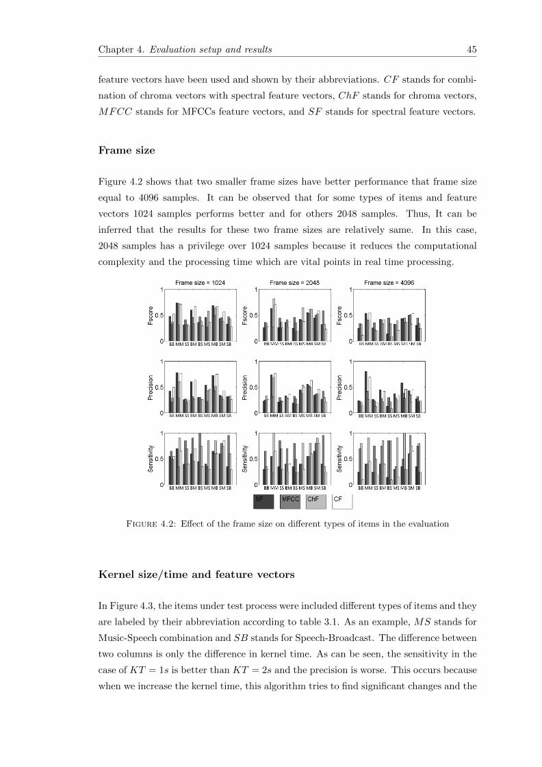
feature vectors have been used and shown by their abbreviations. CF stands for combi-
nation of chroma vectors with spectral feature vectors, ChF stands for chroma vectors,
MFCC stands for MFCCs feature vectors, and SF stands for spectral feature vectors.
Frame size
Figure 4.2 shows that two smaller frame sizes have better performance that frame size
equal to 4096 samples. It can be observed that for some types of items and feature
vectors 1024 samples performs better and for others 2048 samples. Thus, It can be
inferred that the results for these two frame sizes are relatively same. In this case,
2048 samples has a privilege over 1024 samples because it reduces the computational
complexity and the processing time which are vital points in real time processing.
Figure 4.2: Effect of the frame size on different types of items in the evaluation
Kernel size/time and feature vectors
In Figure 4.3, the items under test process were included different types of items and they
are labeled by their abbreviation according to table 3.1. As an example, MS stands for
Music-Speech combination and SB stands for Speech-Broadcast. The difference between
two columns is only the difference in kernel time. As can be seen, the sensitivity in the
case of KT = 1s is better than KT = 2s and the precision is worse. This occurs because
when we increase the kernel time, this algorithm tries to find significant changes and the
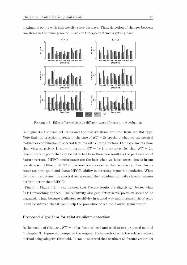
Chapter 4. Evaluation setup and results 46
maximums points with high novelty score decrease. Thus, detection of changes between
two items in the same genre of musics or two speech items is getting hard.
Figure 4.3: Effect of kernel time on different types of items in the evaluation
In Figure 4.4 the train set items and the test set items are both from the BM type.
Note that the precision increase in the case of KT = 2s specially when we use spectral
features or combination of spectral features with chorma vectors. Our experiments show
that when sensitivity is more important, KT = 1s is a better choice than KT = 2s.
One important point that can be extracted form these two results is the performance of
feature vectors. MFFCs performance are the best when we have speech signals in our
test data set. Although MFFCs’ precision is not as well as their sensitivity, their F-score
result are quite good and shows MFCCs ability in detecting segment boundaries. When
we have music items, the spectral features and their combination with chroma features
perform better than MFCCs.
Finaly in Figure 4.5, it can be seen that F-score results are slightly got better when
STFT smoothing applied. The sensitivity also gets better while precision seems to be
degraded. Thus, because it affected sensitivity in a good way and increased the F-score
it can be inferred that it could help the procedure of real time audio segmentation.
Proposed algorithm for relative silent detection
In the results of this part, KT = 1s has been utilized and tried to test proposed method
in chapter 3. Figure 4.6 compares the original Foote method with the relative silence
method using adaptive threshold. It can be observed that results of all feature vectors set
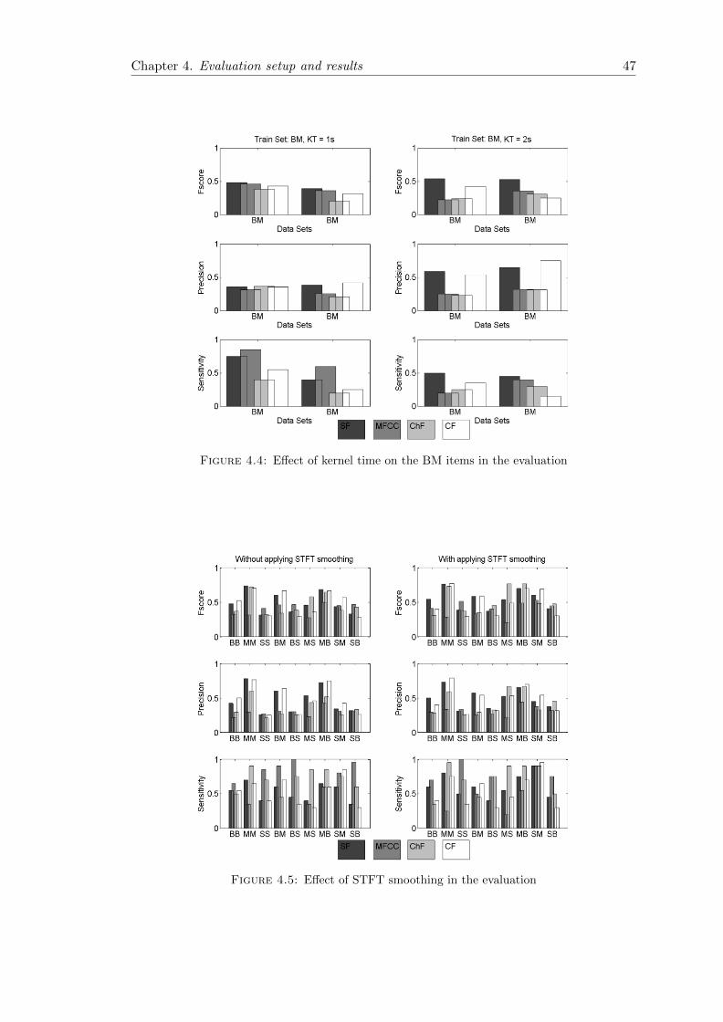
Chapter 4. Evaluation setup and results 47
Figure 4.4: Effect of kernel time on the BM items in the evaluation
Figure 4.5: Effect of STFT smoothing in the evaluation
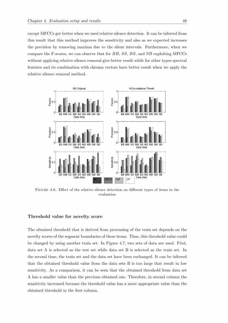
Chapter 4. Evaluation setup and results 48
except MFCCs get better when we used relative silence detection. It can be inferred from
this result that this method improves the sensitivity and also as we expected increases
the precision by removing maxima due to the silent intervals. Furthermore, when we
compare the F-scores, we can observe that for BB, SS, BS, and SB exploiting MFCCs
without applying relative silence removal give better result while for other types spectral
features and its combination with chroma vectors have better result when we apply the
relative silence removal method.
Figure 4.6: Effect of the relative silence detection on different types of items in theevaluation
Threshold value for novelty score
The obtained threshold that is derived from processing of the train set depends on the
novelty scores of the segment boundaries of these items. Thus, this threshold value could
be changed by using another train set. In Figure 4.7, two sets of data are used. First,
data set A is selected as the test set while data set B is selected as the train set. In
the second time, the train set and the data set have been exchanged. It can be inferred
that the obtained threshold value from the data sets B is too large that result in low
sensitivity. As a comparison, it can be seen that the obtained threshold from data set
A has a smaller value than the previous obtained one. Therefore, in second column the
sensitivity increased because the threshold value has a more appropriate value than the
obtained threshold in the first column.
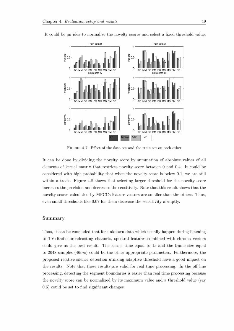
Chapter 4. Evaluation setup and results 49
It could be an idea to normalize the novelty scores and select a fixed threshold value.
Figure 4.7: Effect of the data set and the train set on each other
It can be done by dividing the novelty score by summation of absolute values of all
elements of kernel matrix that restricts novelty score between 0 and 0.4. It could be
considered with high probability that when the novelty score is below 0.1, we are still
within a track. Figure 4.8 shows that selecting larger threshold for the novelty score
increases the precision and decreases the sensitivity. Note that this result shows that the
novelty scores calculated by MFCCs feature vectors are smaller than the others. Thus,
even small thresholds like 0.07 for them decrease the sensitivity abruptly.
Summary
Thus, it can be concluded that for unknown data which usually happen during listening
to TV/Radio broadcasting channels, spectral features combined with chroma vectors
could give us the best result. The kernel time equal to 1s and the frame size equal
to 2048 samples (46ms) could be the other appropriate parameters. Furthermore, the
proposed relative silence detection utilizing adaptive threshold have a good impact on
the results. Note that these results are valid for real time processing. In the off line
processing, detecting the segment boundaries is easier than real time processing because
the novelty score can be normalized by its maximum value and a threshold value (say
0.6) could be set to find significant changes.
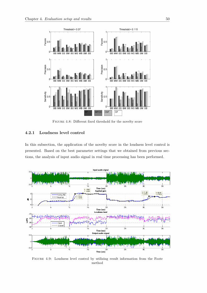
Chapter 4. Evaluation setup and results 50
Figure 4.8: Different fixed threshold for the novelty score
4.2.1 Loudness level control
In this subsection, the application of the novelty score in the loudness level control is
presented. Based on the best parameter settings that we obtained from previous sec-
tions, the analysis of input audio signal in real time processing has been performed.
Figure 4.9: Loudness level control by utilizing result information from the Footemethod
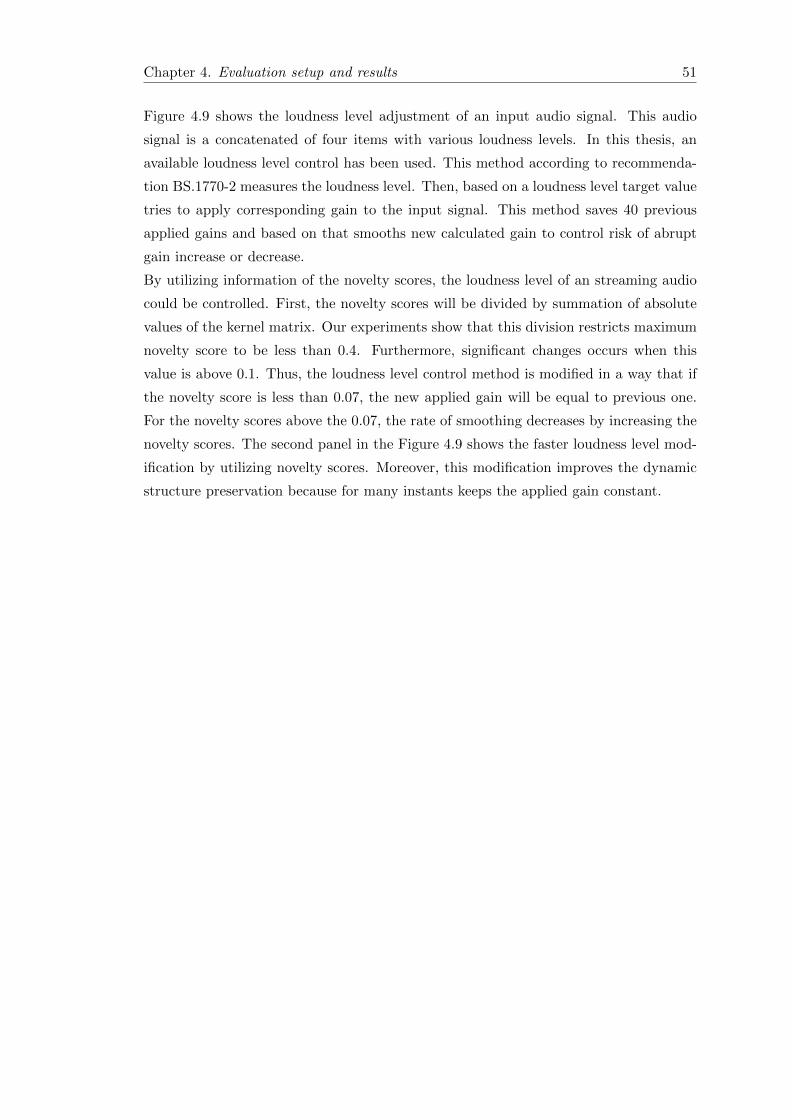
Chapter 4. Evaluation setup and results 51
Figure 4.9 shows the loudness level adjustment of an input audio signal. This audio
signal is a concatenated of four items with various loudness levels. In this thesis, an
available loudness level control has been used. This method according to recommenda-
tion BS.1770-2 measures the loudness level. Then, based on a loudness level target value
tries to apply corresponding gain to the input signal. This method saves 40 previous
applied gains and based on that smooths new calculated gain to control risk of abrupt
gain increase or decrease.
By utilizing information of the novelty scores, the loudness level of an streaming audio
could be controlled. First, the novelty scores will be divided by summation of absolute
values of the kernel matrix. Our experiments show that this division restricts maximum
novelty score to be less than 0.4. Furthermore, significant changes occurs when this
value is above 0.1. Thus, the loudness level control method is modified in a way that if
the novelty score is less than 0.07, the new applied gain will be equal to previous one.
For the novelty scores above the 0.07, the rate of smoothing decreases by increasing the
novelty scores. The second panel in the Figure 4.9 shows the faster loudness level mod-
ification by utilizing novelty scores. Moreover, this modification improves the dynamic
structure preservation because for many instants keeps the applied gain constant.

Chapter 5
Conclusion
This thesis could be separated into two parts. In the first part, it has been studied the
Foote method which is a robust algorithm for the automatic audio segmentation. Then,
it has been tried to improve this method and to use it in real time audio processing.
The feature vectors that have been utilized in the Foote method have great impact on
the final results. Thus, the most suitable feature vectors, which can be used in audio
segmentation, for different types of audio signals are introduced. Our experiment data
set consisted from combination of speech, music, and radio broadcast audio signals.
In the second part, the application of real time audio segmentation in automatic loudness
level control has been studied. It showed that real time change detection in an audio
signal could increase pace of loudness level modification. Also, it improves the dynamic
structure preservation of an input audio signal by keeping the applied gain constant
while no novelty occurs in the input signal.
Therefore, our main contributions can be summarized as follows:
• Feature vectors selection for audio segmentation for different types of audio signals.
If speech signal is available MFFCs feature vectors and if music tracks are available
chroma vectors and spectral features would have the best results. For unknown
audio types, the later features have a better performance.
• Introducing a parameter setting that has the best result in real time audio segmen-
tation when we exploit the Foote method (KT = 1s, framesize = 46ms, applying
STFT smoothing, and feature vector normalization)
• Proposing an algorithm which helps to increase the precision of the Foote method
in real time processing.
• Utilizing previous results to improve the automatic loudness level control. This
result in better dynamic structure preserving and faster loudness level adjustment.
53

Chapter 5. Conclusion 54
As a future work, one could improve the accuracy of the audio segmentation by com-
bination of these set of configuration in a probability estimation model. This could
improve detecting of content changes in an audio signal and could improve removal un-
wanted detected changes within the audio signal. This could result in more accurate
and approximately online automatic loudness level control with almost full preservation
of dynamic structure of an input audio signal.
References
[1] Bartsch, M.A.; Wakefield, G.H.; , ”Audio thumbnailing of popular music using
chroma-based representations,” Multimedia, IEEE Transactions on , vol.7, no.1,
pp. 96- 104, Feb. 2005
[2] J. Foote, ”Methods for the automatic analysis of music and audio”, FXPAL
Technical Report FXPAL-TR-99-038.
[3] J. Foote, ”Visualizing Music and Audio using Self-Similarity.” In Proc. ACM Mul-
timedia 99, Orlando, FL.
[4] www.improvedoutcomes.com/docs/WebSiteDocs/Clustering/Clustering_
Parameters/Manhattan_Distance_Metric.htm.
[5] W. Chai. Automated analysis of musical structure. PhD thesis, Massachusetts
Institute of Technology, MA, USA, September 2005.
[6] J. Foote and M. Cooper. Media segmentation using self-similarity decomposition.
In Proceedings of the SPIE Storage and Retrieval for Media Databases, volume
5021, pages 167175, Santa Clara, California, USA, 2003.
[7] M. Cooper and J. Foote. Summarizing popular music via structural similarity anal-
ysis. In Proceedings of the IEEE Workshop on Applications of Signal Processing
to Audio and Acoustics (WASPAA 2003), pages 127130, New Paltz, New York,
USA, 2003.
[8] S. Abdallah, K. Noland, M. Sandler, M. Casey, and C. Rhodes. Theory and eval-
uation of a Bayesian music structure extractor. In Proceedings of the 6th Interna-
tional Conference on Music Information Retrieval (ISMIR 2005), pages 420425,
London, UK, 2005.
[9] J.J. Aucouturier and M. Sandler. Segmentation of musical signals using Hidden
Markov Models. In Proceedings of the 110th Audio Engineering Society Convention
(AES), Amsterdam, The Netherlands, 2001. Preprint Number: 5379.
55
Chapter 5. Conclusion 56
[10] M. Levy and M. Sandler. New methods in structural segmentation of musical
audio. In Proceedings of European Signal Processing Conference (EUSIPCO 2006),
Florence, Italy, 2006.
[11] M. Levy, M. Sandler, and M. Casey. Extraction of high-level musical structure
from audio data and its application to thumbnail generation. In Proceedings of
the IEEE International Conference on Acoustics, Speech and Signal Processing
(ICASSP 2006), Toulouse, France, 2006.
[12] R. N. Shepard, Circularity in judgements of relative pitch, J. Acoust. Soc. Amer.,
vol. 36, pp. 23462353, 1964.
[13] R. D. Patterson, Spiral detection of periodicity and the spiral form of musical
scales, Psychol. Music, vol. 14, pp. 4461, 1986.
[14] M. Stein, B. Schubert, M. Gruhne, G. Gatzsche, and M. Mehnert. Evaluation
and Comparison of Audio Chroma Feature Extraction Methods. In Proceedings of
the 126th Audio Engineering Society Convention (AES), Munich, Germany, 2009.
Preprint Number: 7814.
[15] J. T. Foote, ”Content-based retrieval of music and audio,” in SPIE, pp. 138-147.
[16] B. T. Logan and S. Chu, ”Music summarization using key phrases,” in proceedings
IEEE International Conference on Acoustics, Speech, and Signal Processing, 2000.
[17] T. L. Blum, D. F. Keislar, J. A. Wheaton, and E. H. Wold, ”Method and article
of manufacture for content-based analysis, storage, retrieval, and segmentation of
audio information,” U.S. Patent 5, 918,223.
[18] B. Logan, ”Mel frequency cepstral coefficients for music modelling”, Proc. of IS-
MIR, 2000.
[19] N. Marhav and C.-H. Lee, ”On the asymptotic statistical behavior of empirical
cepstral coefficients,” IEEE Transactions on Signal Processing 41, 1990-1993.
[20] ITU-R Recommendation BS.1770-2 (2011): ”Algorithms to measure audio pro-
gramme loudness and true-peak audio level”, International Telecommunications
Union, Geneva.
[21] J.X. Zhang, J. Whalley, and S. Brooks. A two phase method for general audio
segmentation. Proceedings 2009 IEEE International Conference on Multimedia and
Expo (ICME), p 626-9, 2009
[22] F. Kaiser, M.G. Arvanitidou, and T. Sikora. Audio similarity matrices enhance-
ment in an image processing framework. 2011 9th International Workshop on
Content-Based Multimedia Indexing (CBMI), p 67-72, 2011